Document downloaded from:

This paper must be cited as:

The final publication is available at

Copyright

Additional Information

https://doi.org/10.1016/j.ijpe.2012.06.032

http://hdl.handle.net/10251/99055

Elsevier

Araujo, FF.; Costa, AM.; Miralles Insa, CJ. (2012). Two extensions for the ALWABP: Parallelstations and collaborative approach. International Journal of Production Economics.140(1):483-495. doi:10.1016/j.ijpe.2012.06.032

Two extensions for the assembly line worker assignment

and balancing problem: parallel stations and collaborative approach.

Felipe F. B. Araújo Instituto de Ciências Matemáticas e de Computação

Universidade de São Paulo

felipe@icmc.usp.br

Alysson M. Costa

Instituto de Ciências Matemáticas e de Computação

Universidade de São Paulo

alysson@icmc.usp.br

Cristóbal Miralles

ROGLE - Dpto. Organización de Empresas

Universitat Politècnica de València

cmiralles@omp.upv.es

Abstract

In this article, we introduce two new variants of the assembly line worker assignment and

balancing problem that allow parallelization of and collaboration between heterogeneous

workers. These new line balancing approaches introduce an additional level of flexibility in the

assignment and planning process, which may be particularly useful in practical situations

where the aim is to progressively integrate slow or limited workers in conventional assembly

lines. We present linear models and heuristic procedures for these two new problems.

Computational results show the efficiency of the proposed approaches and the efficacy of the

studied layouts in different situations.

Keywords: assembly line balancing, disabled workers.

1. Introduction According to the International Labour Organization (ILO), people with disabilities represent an

estimated 10 per cent of the world’s population, or some 650 million people worldwide.

Approximately 470 million are of working age. Many have demonstrated that with the right

opportunities along with adaptations and support, if needed, they can make a major

contribution at all levels of the economy and society. Yet, they are often excluded and

marginalized, and are particularly vulnerable in times of crisis (ILO, 2009).

Like everyone else, people with disabilities have a right to a full life in every sense, and one of

those fundamental rights is the right to work. Employment is, in itself, the key to integration

and autonomy. In fact, the allocation of roles that employment gives becomes the most

effective form of rehabilitation (Wolfensberger, 1983). Work provides structure, friends outside

of one's domestic circle, something to look forward to each day in short and long terms, and

valuable socialization as well as the need to develop new skills and to enhance existing skills.

Consequently, working in the competitive workforce has been a goal of the movement towards

social inclusion (Stephens et al., 2005).

But the disabled do not form a homogeneous group. They may be affected by a congenital

disability, or one acquired during infancy or adolescence, or equally later, during higher

education or active life. The disability may not practically influence the person’s capacity to

work and participate in society, or, on the contrary, may have a serious repercussion, meaning a

need for considerable help and support, with multiple variations between these two extremes.

The social context is also important and thus, while in some societies the disabled they are

considered valuable members of the active population, in others they are not considered

suitable for employment; being apparent that in all countries the unemployment rates of the

disabled are much higher than the average. Thus, in the United States, only 3 in 10 disabled

people aged 16 to 64 work part- or full-time. In the European Union in 2003, 40 per cent of

disabled people of working age were employed compared to 64.2 per cent of persons without a

disability; whereas in Paraguay, 18.5 per cent of people with disabilities participate in the

labour force compared to 59.8 per cent of their non-disabled counterparts (ILO, 2009).

To improve this situation, the legal frameworks and regulations have been significantly

modified over the last three decades and many governments have implemented policies aimed

at promoting the right of the disabled to be integrated as fully as possible into society. One of

the references has been the Declaration of the fundamental workplace principles and rights of

the International Labour Organization (ILO, 2007), that proposes active policies to combat the

discrimination against these workers in three ways: (1) Via the formulation of policies and

regulations against discrimination in the workplace; (2) Via an increase in the opportunities for

people liable of being discriminated to find a job; (3) Via an improvement of the hiring

procedures in public and private sectors (Miralles et al., 2010).

In this framework, one of the strategies most commonly adopted in many countries to facilitate

the integration of disabled workers into the labor market has been the creation of sheltered

work centers for Disabled (henceforth SWDs). This model of socio-labor integration tries to

move away from the traditional stereotype that considers disabled people as unable to develop

continuous professional work. Just as in any other firm, a SWD competes in real markets and

must be flexible and efficient enough to adapt to market fluctuations and changes, the only

difference being that the SWD is a Not-For-Profit organization and most of its workers

(normally around 70%) must be disabled. Thus, the potential benefits that may be obtained

from increased efficiency are usually invested into the growth of the SWD. This results in more

jobs for the Disabled and the gradual integration of people with higher levels of disability,

which are in fact the primary aims of every SWD.

In countries such as Spain, this labour integration formula has been really successful in

decreasing the former high unemployment rates, and one of the most usual strategies used by

SWDs to facilitate this integration has been the adoption of assembly lines. In this sense

Miralles et al. (2007) have shown how the integration of disabled workers in the productive

systems can be done without losing, even gaining, productive efficiency through the use of

assembly lines. In particular, the traditional division of work into single tasks seems to be a

useful tool for making certain worker disabilities invisible; even becoming a good method for

therapeutic rehabilitation of certain disabilities if appropriate task assignments and job rotation

mechanisms are applied (Costa and Miralles, 2009).

1.1. Real integration formulas But, despite the great legislative efforts made by multiple national and international institutions,

total social-employment integration of people with disabilities still seems far away. This fact

confirms the perception that the solution has to come not only by special work formulas like

SWDs, but also by overcoming the prejudices about the capabilities of the disabled, and by the

genuine commitment of ordinary companies to include integration programs in their strategies

and models. In this context the Corporate Social Responsibility policies of companies should

include those people with disabilities as a priority within the stakeholder group of employees;

empowering voluntarily their integration in the production systems, and seeing this as an

opportunity, and not as an imposition.

The incorporation of disabled people to many productive activities generates added value to a

company, as well as to society as a whole, which is particularly timely given the current

pensions crisis and ageing population. Moreover, to integrate disabled workers into normal

companies would doubly contribute to the normalization: on one hand those that are integrated

as work colleagues into the staff of ordinary companies, with the consequent benefit for them;

and on the other hand, the fact that the other workers without a disability begin to perceive as

normal an heterogeneous working environment where all workers, with or without some form

of disability, undertake the most appropriate tasks according to their abilities and capacities.

With this, it is not intended to play down the great contribution that SWDs have made towards

diminishing the high levels of unemployment in this difficult sector, but it is also certain that, if

the efforts to provide work to these people are only focused on these centers, the separation

between ordinary workers and those with a disability is made more critical, relegating the latter

to work centers away from the rest.

This is especially true for the case of developmental disabilities, where employment not only

provides economic benefits to the individuals and the community, but it also contributes to the

development of various adaptive skills such as physical abilities, cognitive abilities, and social

skills. In this sense, the longitudinal study of Stephens et al. (2005) also confirms that

beneficial skills appear to be learned within integrative work settings and lost within segregated

work settings.

1.2. Contribution of this work As introduced earlier, some previous studies have highlighted the importance of assembly lines

as a means to integrate as many disabled workers as possible into the workforce of SWDs

(Miralles et al. (2007, 2008), Costa and Miralles (2009); Chaves et al. (2009); Blum and

Miralles (2011)). These references provide different approaches to face the so-called Assembly

Line Worker Assignment and Balancing Problem (ALWABP); which aims to model the

heterogeneous scenario of SWDs assembly lines, where different task times are considered

depending on the worker assigned.

Although these pioneer references have had a great importance in giving visibility to this social

problem throughout our academic area, they may be too centered in the specific scenario of

SWDs; where most workers are supposed to be disabled. In the classical ALWABP framework

each task has a worker-dependent processing time, which allows taking into account the

limitations of each worker depending on his/her disability. Therefore the input data are

normally expressed by a time matrix where for every task, several possible times are available

depending on the worker; and where task times in the matrix normally have a very high

variability.

As it has been introduced, the desirable fact in this scenario would be to integrate the disabled

not only in SWDs but also in ordinary companies. Therefore we should face the ALWABP

with more open hypothesis of diversity, where for example these two situations are likely to

occur:

- Ordinary companies should be able to integrate efficiently one only disabled worker

into an assembly line; normally being this worker much slower than the rest. In these

cases the parallelization of workstations is a very interesting extension for ALWABP,

which can easily integrate disabled workers without losing much efficiency.

- In other cases the disabled workers to be integrated may have incompatible

assignments that permit few possible solutions to ALWABP. In these cases, an

efficient way to widen the chances of possible assignments is the “Collaborative

ALWABP” approach; where different workers can complement their capabilities

collaborating in the same product within certain workstation.

The aim of this paper is to present new models and approaches for these two extensions of

ALWABP which, even attending specific requirements that would normally arise in ordinary

companies (with few disabled workers), can perfectly be adopted generally by SWDs. The

same way around, the classical approaches of ALWABP are completely valid for an

environment with less diversity simply by modifying the input data. In this sense, this paper

will use data with more or less diversity independently.

The general aim is keep providing the production managers with practical tools that ease the

integration of disabled in different scenarios since, obviously, the source of inspiration of a

problem is not its only application field.

1.3. Paper outline In Section 2, we statea formal codification of the two extensions proposed for ALWABP;

analysing their practical implications and reviewing those references of the literature with

useful related approaches. Section 3 then presents the corresponding IP models for both the

parallel and the collaborative approach of ALWABP; while Section 4 proposes resolution

procedures for each extension. Finally, Section 5 summarizes the computational results, and in

Section 6 we discuss the main findings and offer some conclusions and further research lines.

2. Assembly line Worker Assignment and Balancing Problem The so-called Simple Assembly Line Balancing Problem (SALBP) was initially defined by

Baybars (1986) through several well-known simplifying hypotheses. This classical single-

model problem, which consists of finding the best feasible assignment of tasks to stations so

that certain precedence constraints are fulfilled, has been the reference problem in the literature

in its two basic versions: when the cycle time C is given, and the aim is to optimize the number

of necessary work stations, the problem version is called SALBP-1. Whereas when there is a

given number m of work stations, and the goal is to minimize the cycle time C the literature

knows this second version as SALBP-2 (Scholl, 2006).

SALBP is based on a set of limiting assumptions which reduce the complex problem of

assembly line configuration to the ‘‘core’’ problem of assigning tasks to stations. The balancing

of real-world assembly lines will, however, require the observation of a large variety of

additional technical or organizational aspects, which will heavily affect the structure of the

problem. Among the extensions considered in the literature are parallel work stations and tasks,

cost synergies, processing alternatives, zoning restrictions, stochastic and sequence-dependent

processing times as well as U-shaped assembly lines (Boysen et al. 2008).

We focus on the Assembly Line Worker Assignment and Balancing Problem (ALWABP), a

generalization of SALBP where, in addition to the assignment of tasks to stations, a set of

heterogeneous workers that execute the tasks also has to be assigned to stations (Miralles et al.

2008). In this scenario each task has a worker-dependent processing time, which allows taking

into account the limitations of each worker depending on his/her disability. Thus, in ALWABP

the input data are normally expressed by a precedence network and a time matrix like the one in

Table 1, where for every task (columns) several operation times (rows) are possible depending

on the worker. Even when the time to execute a task for certain worker is very high, this

assignment is considered infeasible and the incompatibility is represented by a dash in the

corresponding cell of the input data matrix:

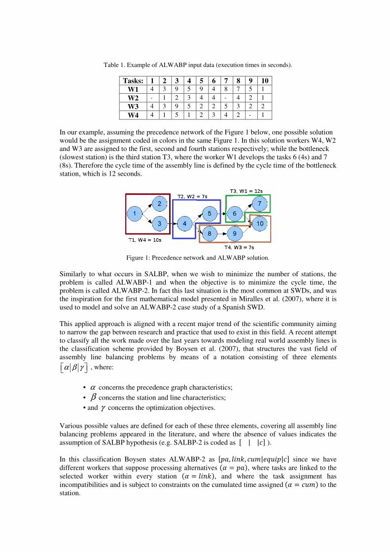
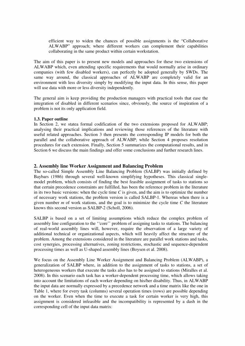
Table 1. Example of ALWABP input data (execution times in seconds).

Tasks: 1 2 3 4 5 6 7 8 9 10

W1 4 3 9 5 9 4 8 7 5 1

W2 - 1 2 3 4 4 - 4 2 1

W3 4 3 9 5 2 2 5 3 2 2

W4 4 1 5 1 2 3 4 2 - 1

In our example, assuming the precedence network of the Figure 1 below, one possible solution

would be the assignment coded in colors in the same Figure 1. In this solution workers W4, W2

and W3 are assigned to the first, second and fourth stations respectively; while the bottleneck

(slowest station) is the third station T3, where the worker W1 develops the tasks 6 (4s) and 7

(8s). Therefore the cycle time of the assembly line is defined by the cycle time of the bottleneck

station, which is 12 seconds.

Figure 1: Precedence network and ALWABP solution.

Similarly to what occurs in SALBP, when we wish to minimize the number of stations, the

problem is called ALWABP-1 and when the objective is to minimize the cycle time, the

problem is called ALWABP-2. In fact this last situation is the most common at SWDs, and was

the inspiration for the first mathematical model presented in Miralles et al. (2007), where it is

used to model and solve an ALWABP-2 case study of a Spanish SWD.

This applied approach is aligned with a recent major trend of the scientific community aiming

to narrow the gap between research and practice that used to exist in this field. A recent attempt

to classify all the work made over the last years towards modeling real world assembly lines is

the classification scheme provided by Boysen et al. (2007), that structures the vast field of

assembly line balancing problems by means of a notation consisting of three elements

α β γ , where:

• α concerns the precedence graph characteristics;

• β concerns the station and line characteristics;

• and γ concerns the optimization objectives.

Various possible values are defined for each of these three elements, covering all assembly line

balancing problems appeared in the literature, and where the absence of values indicates the

assumption of SALBP hypothesis (e.g. SALBP-2 is coded as � | |�� ).

In this classification Boysen states ALWABP-2 as ���, ��, � �|�� �|�� since we have

different workers that suppose processing alternatives �� � ���, where tasks are linked to the

selected worker within every station �� � ���, and where the task assignment has

incompatibilities and is subject to constraints on the cumulated time assigned�� � � �� to the

station.

Note that the fundamental difference of ALWABP-2 with respect to other equipment selection

problems �� � �� �� is the fact that resources are constrained: each unique worker can only

be assigned to exactly one work station. In some cases workers with similar characteristics are

considered, but even in these cases there is not an infinite number of resources available, as

assumed in most robotic or automated lines, or in general in the so called assembly system

design problems (Pinto et al. (1983), Rubinovitz and Bukchin (1993), Pinnoi and Wilhelm

(1997, 1998), Bukchin and Rubinovitz (1997), Wilhelm (1999), Dolgui et al. (1999, 2006),

Nicosia et al. (2002), Bukchin and Tzur (2000), Nicosia et al. (2002), Rekiek et al. (2002)).

Moreover, in contrast to the ALWABP-2 none of these references has the objective of

minimizing the cycle time (γ = c) given certain resources, as ALWABP-2 does. Instead they

all aim to minimize the cost (γ =Co) or the resources implied (γ =m); objectives that here

would seem contradictory, since the objective of integrating disabled workers means to assign

them, and not to minimize their number or try to avoid their participation.

Thus, as it has been introduced, two new extensions of ALWABP will be presented in this

paper:

- One extension allowing the parallelization of workstations, what can be coded as ���, ��, � �|�����, �� �|��.

- And a second extension considering the possible collaboration of various workers

mounting the same product within one station ���, ��, � �|�����, �� �|��.

In the next two sections these extensions will be described through simple examples, analysing

their specific implications and reviewing those references of the literature that use similar

approaches. Once the main features of each extension are clarified, a formal definition of their

corresponding mathematical models will be presented (Section 3).

2.1. Extension 1: ALWABP with parallel stations In this first extension the constraint of one worker per station is relaxed, so that the same subset

of tasks can be assigned in parallel to two (or more) workers within the same station. To

facilitate presentation, we will say that each worker is assigned to a station in the same stage of

the line. Using the same example of last section, the following assignment could be a solution

using this extension:

Figure 2: ALWABP with parallel stations.

In this solution we have worker W4 in the first stage developing tasks 1 (4s), 2 (1s) and 3 (5s);

and worker W1 in the third stage developing tasks 7 (8s) and 10 (1s). However, the second

stage is composed by two stations in parallel with worker W2 and worker W3. They both

develop the same tasks (4, 5, 6, 8 and 9), but with their own operation times according to the

time matrix of Table 1. This fact makes it difficult to calculate the overall cycle time of the

second stage, which is not as obvious as in Bard (1989), Sarker and Shanthikumar, (1983), or

Pinto et al. (1981). Indeed, in order to compute this parameter, it is easier to express the

productive parameters in terms of throughput rates (parts produced per unit of time); as will be

exposed in the following example:

E.g. Let us define a productive system A working at a cycle time of CA=1 min/part, then we can

assume that its throughput rate is TRA=60 parts/hour. Let us define another productive system B

in parallel with A producing the same parts but with a cycle time of CB=2 min/part, which is

TRB=30 parts/hour. What is very intuitive is that the overall Throughput Rate of both systems

working in parallel is the sum: TRAB = TRA + TRB = 60 + 30 = 90 parts/hour; and therefore the

overall cycle time is given by �

��� ���� +

��� �

��+

� → CAB=0.67 min/part

Then, in our case the cycle time calculated will be: ��"# �

��$#

+ ��$%

� ��& +

��' → CT2=7.6 s

Whenever we have two productive systems in parallel we can assume this way of calculating

the cycle time. Thus, applying parallelization to ALWABP has implications in the model

linearity, that can be solved through the mechanisms that will be exposed in section 3.

Apart from these mathematical implications in the model, the parallelization has also some

practical implications that can be summarized as follows:

- As there are two (or more) workers in parallel in the same stage developing the same

tasks, they need two different products. Therefore, a sufficient buffer of work in

progress products must be set so that no lack of material appears for any of the

workers. As soon as the cycle time of the parallelized stage is balanced with respect to

the rest of stages, this quantity will be limited by an additional unit in most cases.

- The parallelization of stations suppose the duplication of facilities and tools that may

be necessary for every worker in the stage. This practical implication has to be taken

into account specially when there are physical constraints or high installation costs.

- In case of workers with very slow operation times, it is much easier to integrate them if

we allow parallel stations. This is especially important in ordinary companies, since we

can combine slow and fast workers for integrating disabled workers with the minimum

loss of efficiency (as will be demonstrated in section 5).

- As it happens with SALBP, when we allow parallelization the cycle time can be lower

than the largest operation time. In the case of ALWABP lower than the slowest task to

execute (obtained with a max-min operation over all execution times).

Despite the fact that most assembly lines addressed in the literature are quite different from

ALWABP, it is important to review the most important references that face somehow

parallelization. The research on the inclusion of parallel workstation within assembly lines is

limited and of relatively recent origin (see pioneer studies Pinto et al. (1981), Sarker and

Shanthikumar, (1983) or Bard (1989). Askin and Zhou (1997) consider mixed-model assembly

lines with task dependent equipment costs and arbitrary number of parallel workstations. They

propose a heuristic procedure that uses a threshold value for the equipment utilization. Süer

(1998) propose a simple resolution method in three phases, while McMullen and Frazier (1997,

1998) propose first a heuristic and later a simulated annealing technique for a problem with

parallel stations and stochastic times. In both, they measure the line performance by the total

cost and the extent to which cycle time is met. Vilarinho and Simaria (2002) introduce a two-

stage heuristic method for mixed-model assembly lines, where their primary goal is to

minimize the number of workstations for a given cycle time, and the secondary goal is to

balance the workload between workstations. Bukchin and Rubinovitz (2003) study the

equipment selection problem on parallel workstations, investigating the influence of assembly

sequence flexibility and cycle time on the balancing improvement due to the station paralleling.

Simaria and Vilarinho (2004) propose a model and a genetic algorithm for a mixed model

assembly line with parallel stations. Two years later the same authors propose in (Vilarinho and

Simaria, 2006) an ant colony optimization algorithm for balancing the mixed-model assembly

lines with zoning restrictions and parallel workstations. Boysen and Fliedner (2006) present a

versatile graphic algorithm that can be adapted for parallel stations, and Ege (2009) consider

parallel workstations and propose a branch and bound algorithm to minimize total equipment

and workstation opening costs. Finally, Scholl and Boysen (2009) consider a problem first

introduced by Gökçen et al. (2006) and named as parallel assembly line balancing problem

(PALBP) where multiple products have to be assigned to parallel lines that have to be balanced.

To our knowledge, no reference has used parallel stations in ALWABP. From section 3 on, this

paper will contribute to model and propose resolution procedures for this extension.

2.2. Extension 2: Collaborative ALWABP Another way of enlarging the potential of assembly lines for integrating the disabled in the

workforce is the “collaborative ALWABP” approach we propose here. In this variant, different

workers can be assigned to the same station, where they collaborate mounting the same

product. This doesn’t mean to set parallel workplaces like in the previous extension: in the

collaborative ALWABP framework, even if workers share the same stage, they are assigned

different tasks.

In general, many products manufactured on assembly lines are large enough to be worked at by

several workers simultaneously. As a major example, we can cite the final assembly of cars in

the automobile industry, where up to five workplaces are installed within a single station on a

paced assembly line (Becker and Scholl, 2009). But the characteristic of the collaborative

approach that makes it particularly interesting in this scenario is the allowance of many more

feasible combinations than the conventional ALWABP, what is especially useful in those cases

where certain incompatibilities may difficult the worker integration.

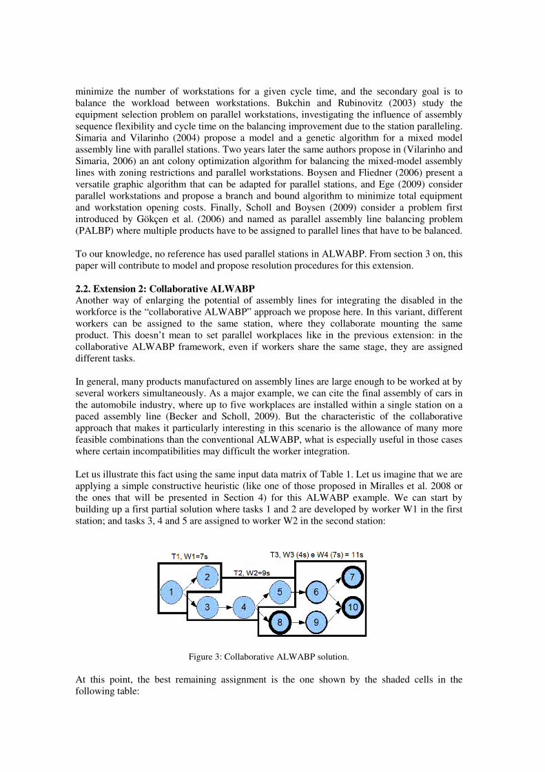
Let us illustrate this fact using the same input data matrix of Table 1. Let us imagine that we are

applying a simple constructive heuristic (like one of those proposed in Miralles et al. 2008 or

the ones that will be presented in Section 4) for this ALWABP example. We can start by

building up a first partial solution where tasks 1 and 2 are developed by worker W1 in the first

station; and tasks 3, 4 and 5 are assigned to worker W2 in the second station:

Figure 3: Collaborative ALWABP solution.

At this point, the best remaining assignment is the one shown by the shaded cells in the

following table:

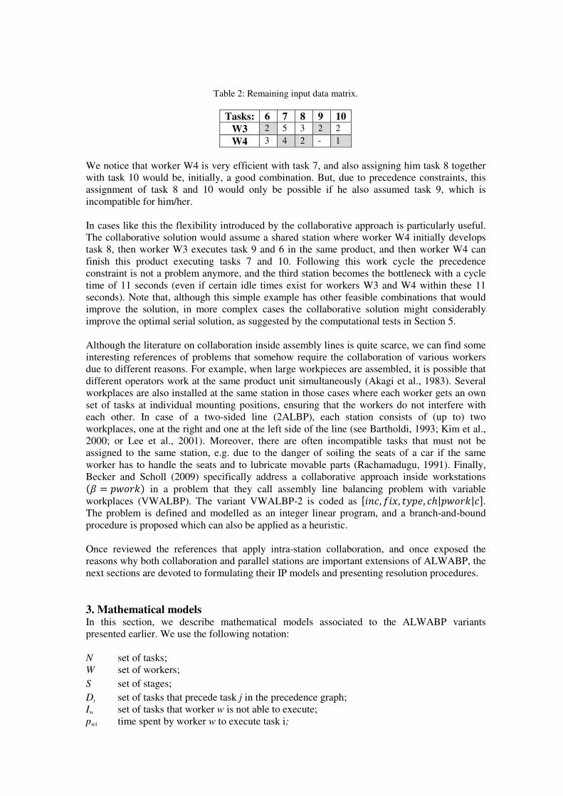
Table 2: Remaining input data matrix.

Tasks: 6 7 8 9 10

W3 2 5 3 2 2

W4 3 4 2 - 1

We notice that worker W4 is very efficient with task 7, and also assigning him task 8 together

with task 10 would be, initially, a good combination. But, due to precedence constraints, this

assignment of task 8 and 10 would only be possible if he also assumed task 9, which is

incompatible for him/her.

In cases like this the flexibility introduced by the collaborative approach is particularly useful.

The collaborative solution would assume a shared station where worker W4 initially develops

task 8, then worker W3 executes task 9 and 6 in the same product, and then worker W4 can

finish this product executing tasks 7 and 10. Following this work cycle the precedence

constraint is not a problem anymore, and the third station becomes the bottleneck with a cycle

time of 11 seconds (even if certain idle times exist for workers W3 and W4 within these 11

seconds). Note that, although this simple example has other feasible combinations that would

improve the solution, in more complex cases the collaborative solution might considerably

improve the optimal serial solution, as suggested by the computational tests in Section 5.

Although the literature on collaboration inside assembly lines is quite scarce, we can find some

interesting references of problems that somehow require the collaboration of various workers

due to different reasons. For example, when large workpieces are assembled, it is possible that

different operators work at the same product unit simultaneously (Akagi et al., 1983). Several

workplaces are also installed at the same station in those cases where each worker gets an own

set of tasks at individual mounting positions, ensuring that the workers do not interfere with

each other. In case of a two-sided line (2ALBP), each station consists of (up to) two

workplaces, one at the right and one at the left side of the line (see Bartholdi, 1993; Kim et al.,

2000; or Lee et al., 2001). Moreover, there are often incompatible tasks that must not be

assigned to the same station, e.g. due to the danger of soiling the seats of a car if the same

worker has to handle the seats and to lubricate movable parts (Rachamadugu, 1991). Finally,

Becker and Scholl (2009) specifically address a collaborative approach inside workstations

�� � ������ in a problem that they call assembly line balancing problem with variable

workplaces (VWALBP). The variant VWALBP-2 is coded as ���, (), �*��, �ℎ|�����|��. The problem is defined and modelled as an integer linear program, and a branch-and-bound

procedure is proposed which can also be applied as a heuristic.

Once reviewed the references that apply intra-station collaboration, and once exposed the

reasons why both collaboration and parallel stations are important extensions of ALWABP, the

next sections are devoted to formulating their IP models and presenting resolution procedures.

3. Mathematical models In this section, we describe mathematical models associated to the ALWABP variants

presented earlier. We use the following notation:

N set of tasks;

W set of workers;

S set of stages;

Dj set of tasks that precede task j in the precedence graph;

Iw set of tasks that worker w is not able to execute;

pwi time spent by worker w to execute task i;

The original formulation for the ALWABP was proposed by Miralles et al (2007) and contains

a continuous variable indicating the cycle time and two sets of binary variables, as indicated

below:

C cycle time of the line,

),-. binary variables equal to one if worker w executes task i in station s and to zero,

otherwise, ∈ 0,� ∈ 1, � ∈ 2.

*,- binary variables equal to one if worker w is designated to station s, � ∈ 1, � ∈2.

With these variables, the authors were able to write the following linear model for the

ALWABP:

3�4

(1)

Subject to 5 5),-. � 1,∀ ∈ 0,,∈8-∈9

(2)

5*,- � 1,∀� ∈ 1,,∈8

(3)

5 *,- � 1,∀� ∈ 2-∈9

, (4)

5 5�),-. ≤ 5 5�),-.,∀, ; ∈ 0| ∈ <=,∈8-∈9,∈8-∈9

, (5)

∑ ∑ �-.),-. ≤ 4.∈?-∈9 , ∀� ∈ 2, (6)

5),-. ≤ |0|*,- ,∀� ∈ 1,∀� ∈ 2.∈?

, (7)

),-. � 0,∀� ∈ 1,∀� ∈ 2, ∀ ∈ A-. (8)

The objective function (1) minimizes the cycle time. Constraints (2) guarantee the execution of

each task in one station by a single worker, while constraints (3) and (4) create a biunivocal

relationship between workers and stations. Constraints (5) handle the precedence relationships

between tasks, ensuring that a task i that must preced a task j is only assigned to the same

station to which j has been assigned or to an earlier station. Constraints (6) define the cycle

time as the total execution time of the bottleneck station, while constraints (7) guarantee

coherence between the binary variables: a task can only be executed by a worker in a station if

that worker is assigned to that station. Finally, constraints (8) handle a-priori assignment

infeasibilities.

In this article, we propose extensions to formulation (1)-(8) in order to model the two new

problem variants described in Section 2. The first new model, presented below, deals with the

parallel ALWABP. In this model, the definition of the set S described earlier is changed, and

each element of S represents no longer a station but a stage (which might contain at most Kmax

stations). The definitions of variables xswi and ysw are modified accordingly. Moreover, in order

to describe this model, the following additional variables are defined:

tis binary variables equal to one if task i is executed in stage s and to zero, otherwise,

∈ 0, � ∈ 2. zsk binary variables indicating the level of parallelism of a stage, equal to one if stage s

contains k stations in parallel and to zero, otherwise. (� ∈ 2, k=1…Kmax).

With these new variables, the parallel ALWABP model can be written as:

3�4

(9)

Subject to: 5��., ≤,∈8

5��=,,∈8

,∀, ; ∈ 0| ∈ <=, (10)

5 ),-. ≥ ���., + D,E − 1�,-∈9

∀� ∈ 2, ∀� ∈ �0, GHIJ�, ∀ ∈ 0, (11)

),-. ≤ �.,,∀� ∈ 2, ∀� ∈ 1,∀ ∈ 0, (12)

5 D,E � 1,∀� ∈ 2KLMN

EOP, (13)

5 *,- �-∈9

5 �D,E ,∀� ∈ 2KLMN

EOP, (14)

5*,- � 1,∀� ∈ 1,∈8

, (15)

∑ �.,,∈8 � 1,∀ ∈ 0, (16)

),-. � *,- ,∀� ∈ 2, ∀� ∈ 1,∀ ∈ 0, (17)

),-. � 0,∀� ∈ 1,∀� ∈ 2, ∀ ∈ A- , (18)

5 1∑ �-.),-..∈?

≥ 14-∈9|QRSO�,∀� ∈ 2|D,P � 0. (19)

As before, the objective function (9) minimizes the cycle time. Constraints (10) represent the

precedence relationships between tasks and are similar to constraints (5). Constraints (11) force

that in a stage with k stations, each task be executed by k different workers. Constraints (12)

state that a worker can execute a task in a stage only if that task is assigned to that stage, while

constraints (13) indicate that each stage has only one level of parallelism. Notice that the

number of stations in a stage can be zero, that is, a stage can be empty (this only indicates the

fact that the number of workers is fixed and, by assigning more than a worker to a stage, the

final number of stages must be reduced). Constraints (14) force the assignment of k workers to

a stage with k stations. Constraints (15) and (16) are concerned with the fact that each worker

and each task must be assigned to a single stage, while constraints (17) guarantee that a worker

only executes tasks in a stage if that worker is assigned to that stage. Constraints (18) handle

the a-priori infeasibility assignments. Finally, constraints (19) calculate the cycle time as the

inverse of the throughput rate of the assembly line, which is limited by the lowest throughput

rate among non-empty stages. The throughput rate of a stage is the sum of the throughput rates

of each worker assigned to that stage, which can be computed as the inverse of the task

execution times for each worker (see example in Section 2.1). Due to constraints (19), model

(9)-(19) becomes non-linear.

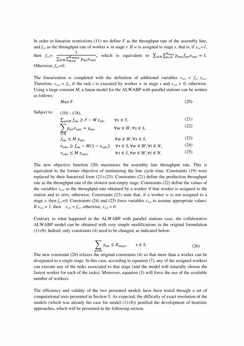
In order to linearize restrictions (11) we define F as the throughput rate of the assembly line,

and fsw as the throughput rate of worker w in stage s. If w is assigned to stage s, that is, if ysw=1,

then fsw=

�∑ ∑ TSUJRSUVLMN

WXYU∈Z, which is equivalent to

∑ ∑ �,-.(,-),-.KLMNEOP � 1.∈? .

Otherwise, fsw=0.

The linearization is completed with the definition of additional variables vswi = fsw xswi.

Therefore, vswi = fsw if the task i is executed by worker w in stage s and vswi = 0, otherwise.

Using a large constant M, a linear model for the ALWABP with parallel stations can be written

as follows:

3�)[

(20)

Subject to: (10) – (18),

∑ (,--∈9 ≥ [ −3D,P,∀� ∈ 2, (21)

5�-.\,-..∈?

� *,- ,∀� ∈ 1,∀� ∈ 2, (22)

(,- ≤ 3*,- ,∀� ∈ 1, ∀� ∈ 2, (23)

\,-. ≥ (,- −3�1 − ),-.�,∀� ∈ 2, ∀� ∈ 1,∀ ∈ 0, (24)

\,-. ≤ 3),-.,∀� ∈ 2, ∀� ∈ 1,∀ ∈ 0. (25)

The new objective function (20) maximizes the assembly line throughput rate. This is

equivalent to the former objective of minimizing the line cycle time. Constraints (19) were

replaced by their linearized form (21)-(25). Constraints (21) define the production throughput

rate as the throughput rate of the slowest non-empty stage. Constraints (22) define the values of

the variables vswi as the throughput rate obtained by a worker if that worker is assigned to the

station and to zero, otherwise. Constraints (23) state that, if a worker w is not assigned to a

stage s, then fsw=0. Constraints (24) and (25) force variables vswi to assume appropriate values:

If xswi = 1, then vswi = fsw, otherwise, vswi = 0.

Contrary to what happened in the ALWABP with parallel stations case, the collaborative

ALWABP model can be obtained with very simple modifications in the original formulation

(1)-(8). Indeed, only constraints (4) need to be changed, as indicated below:

5 *,- ≤ GHIJ,� ∈ 2.-∈9

(26)

The new constraint (26) relaxes the original constraints (4) so that more than a worker can be

designated to a single stage. In this case, according to equation (7), any of the assigned workers

can execute any of the tasks associated to that stage (and the model will naturally choose the

fastest worker for each of the tasks). Moreover, equation (3) will force the use of the available

number of workers.

The efficiency and validity of the two presented models have been tested through a set of

computational tests presented in Section 5. As expected, the difficulty of exact resolution of the

models (which was already the case for model (1)-(8)) justified the development of heuristic

approaches, which will be presented in the following section.

4. Heuristic solution method In this section we describe a heuristic procedure that can be used to solve the two new proposed

extensions. This procedure relies on the construction of a solution that designates workers and

tasks to the stages in a sequential manner and is adapted from the SALBP and ALWABP

literatures.

In the following we first present a description of the general algorithmic scheme in which the

heuristic is used. Then, we describe the task and worker selection priority rules, stating in both

cases the particularities for parallel and collaborative scenarios. These particularities are

illustrated through the example exposed in section 4.2. Finally, two further variants of the

heuristic developed are described in section 4.3.

4.1. Algorithmic scheme The core characteristic of the proposed method is the sequential resolution of version-1

assembly line balancing problems (minization of the number of stations given a maximum

allowed cycle time) in order to solve the version-2 problem. Algorithm 1 below presents a

pseudo-code of this idea.

Algorithm 1: Station oriented procedure for version-2 assembly line balancing problems

Requires: Lower and upper bounds on cycle time, LC and UC, respectively

1. �]=LC;

2. while �̅ < `4, do

3. Solve version-1 problem;

4. if version-1 problem finds a solution with cycle time less or equal to �̅ 5. END; 6. Else 7. increase �̅; 8. end if 9. end while

10. Return “no solution found”; END.

The strategy of the algorithm is quite straightforward. For each possible cycle time, a version-1

assembly line balancing problem is solved. If a solution containing at most the desired number

of stations is found, then there is a solution with the current cycle time for the version-2

problem and the algorithm ends (lines 5 and 6). Otherwise, the algorithm restarts with a larger

cycle time value (line 7).

Scholl and Voβ (1996) and Moreira et al. (2011) have proposed algorithms for the SALBP-1

and ALWABP-1, respectively. Both algorithms rely on a constructive resolution method, which

sequentially assign tasks (SALBP-1) or task and workers (ALWABP-1) to the stations,

respecting the cycle time. This assignment is done according to a criterion that might give

priority, for example, to tasks with a large number of successors. In the case of ALWABP, the

worker selection criterion might, for example, give priority to workers that assign the larger

number of tasks at that point of the assembly line.

We propose a version-2 problem to be used in the cases of the parallel and collaborative

ALWABP. We also define appropriate priority criteria for this situation and discuss the main

particularities of the method in this context. Algorithm 2 presents a pseudo code of the method.

In the algorithm, t(Sk) represents the load of stage k.

Algorithm 2: Station oriented procedure for the Parallel and collaborative ALWABP-1

Requires: Kmax, desired cycle time, �̅. 1. n =0, t(2E�= 0;

2. `- � 1, ` � 0;

3. 1ab,c � ∅; f9ab,c � ∅; cr(1ab,c, f9ab,c� � 0; 4. for each � � 1…GHIJ do

5. for each 1′ ⊂ 1, |1′| � GHIJ do

6. compute set of assignable tasks (respecting the task priority criterion and �̅), f9j; 7. compute worker priority criterion associated with the solution, cr(1′, f9j�; 8. if cr(1′, f9j� > cr(1ab,c , f9ab,c� 9. cr(1ab,c, f9ab,c� = cr(1′, f9j�; 1ab,c � 1′;f9ab,c � f9j 10. end if; 11. end for; 12. end for;

13. assign �1ab,c , f9ab,c� to stage n; `- � `-\1ab,c ; ` � `\f9ab,c; 14. if `- ≠ ∅

goto step 3;

else

if ` ≠ ∅ 16. a solution has been found; END;

17. Else

18. no solution has been found for �̅; END;

19. end if;

20. end if.

A few comments are in order. Algorithm 2 computes, for each possible subset of workers

respecting the maximum parallelization (lines 4 and 5), the set of tasks that would be assigned

to the current stage, f9j, and the associated worker assignment criterion (lines 6 and 7). The set

with best criterion is chosen and the workers and tasks are assigned to the stage (line 13). This

continues until no more workers are available. At this point, if all tasks have been assigned, a

solution with cycle time of at most � ̅has been found (line 16). Otherwise, the algorithm returns

a message indicating that it was not able to find a feasible solution for the desired cycle time.

Several details must be defined in order to have a functional version of Algorithm 2, including

the priority criteria associated with the selection of tasks (line 6) and workers (line7), and the

computation of the cycle time associated with a given solution (see example in section 4.2).

4.1.1. Task selection (line 6) In what concerns the task priority criteria, we adapted some of the task priority rules used by

Scholl and Voβ (1996). Since some of these rules calculate the priority of the tasks based on

their execution times, in ALWABP they need to be modified in order to use the appropriate

parameters available, i.e., the task execution times depending on the selected worker(s)

(Moreira et al. 2011).

In the specific case of the parallel and collaborative ALWABP, a new problem arises since task

times are not well defined for sets of more than one worker. Indeed, consider the parallel

ALWABP: the increase in the current stage load depends not only on the selected workers and

on the current task, but also on the tasks that are already assigned to the stage (due to the non-

linear characteristics associated with the cycle time computation). The solution found was to

define the execution time of task i in a dynamic fashion:

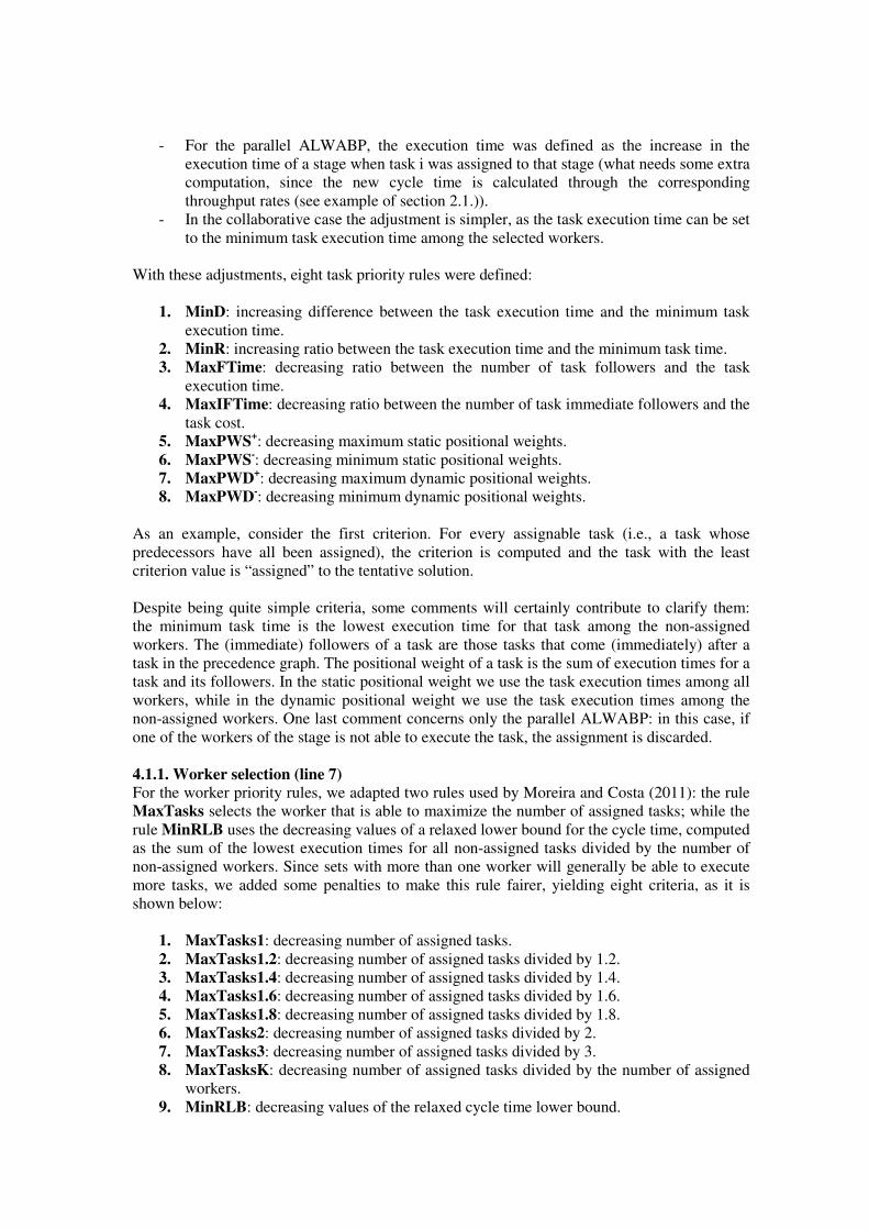
- For the parallel ALWABP, the execution time was defined as the increase in the

execution time of a stage when task i was assigned to that stage (what needs some extra

computation, since the new cycle time is calculated through the corresponding

throughput rates (see example of section 2.1.)).

- In the collaborative case the adjustment is simpler, as the task execution time can be set

to the minimum task execution time among the selected workers.

With these adjustments, eight task priority rules were defined:

1. MinD: increasing difference between the task execution time and the minimum task

execution time. 2. MinR: increasing ratio between the task execution time and the minimum task time. 3. MaxFTime: decreasing ratio between the number of task followers and the task

execution time. 4. MaxIFTime: decreasing ratio between the number of task immediate followers and the

task cost. 5. MaxPWS+

: decreasing maximum static positional weights.

6. MaxPWS-: decreasing minimum static positional weights.

7. MaxPWD+: decreasing maximum dynamic positional weights.

8. MaxPWD-: decreasing minimum dynamic positional weights.

As an example, consider the first criterion. For every assignable task (i.e., a task whose

predecessors have all been assigned), the criterion is computed and the task with the least

criterion value is “assigned” to the tentative solution.

Despite being quite simple criteria, some comments will certainly contribute to clarify them:

the minimum task time is the lowest execution time for that task among the non-assigned

workers. The (immediate) followers of a task are those tasks that come (immediately) after a

task in the precedence graph. The positional weight of a task is the sum of execution times for a

task and its followers. In the static positional weight we use the task execution times among all

workers, while in the dynamic positional weight we use the task execution times among the

non-assigned workers. One last comment concerns only the parallel ALWABP: in this case, if

one of the workers of the stage is not able to execute the task, the assignment is discarded.

4.1.1. Worker selection (line 7) For the worker priority rules, we adapted two rules used by Moreira and Costa (2011): the rule

MaxTasks selects the worker that is able to maximize the number of assigned tasks; while the

rule MinRLB uses the decreasing values of a relaxed lower bound for the cycle time, computed

as the sum of the lowest execution times for all non-assigned tasks divided by the number of

non-assigned workers. Since sets with more than one worker will generally be able to execute

more tasks, we added some penalties to make this rule fairer, yielding eight criteria, as it is

shown below:

1. MaxTasks1: decreasing number of assigned tasks.

2. MaxTasks1.2: decreasing number of assigned tasks divided by 1.2. 3. MaxTasks1.4: decreasing number of assigned tasks divided by 1.4. 4. MaxTasks1.6: decreasing number of assigned tasks divided by 1.6.

5. MaxTasks1.8: decreasing number of assigned tasks divided by 1.8. 6. MaxTasks2: decreasing number of assigned tasks divided by 2.

7. MaxTasks3: decreasing number of assigned tasks divided by 3. 8. MaxTasksK: decreasing number of assigned tasks divided by the number of assigned

workers.

9. MinRLB: decreasing values of the relaxed cycle time lower bound.

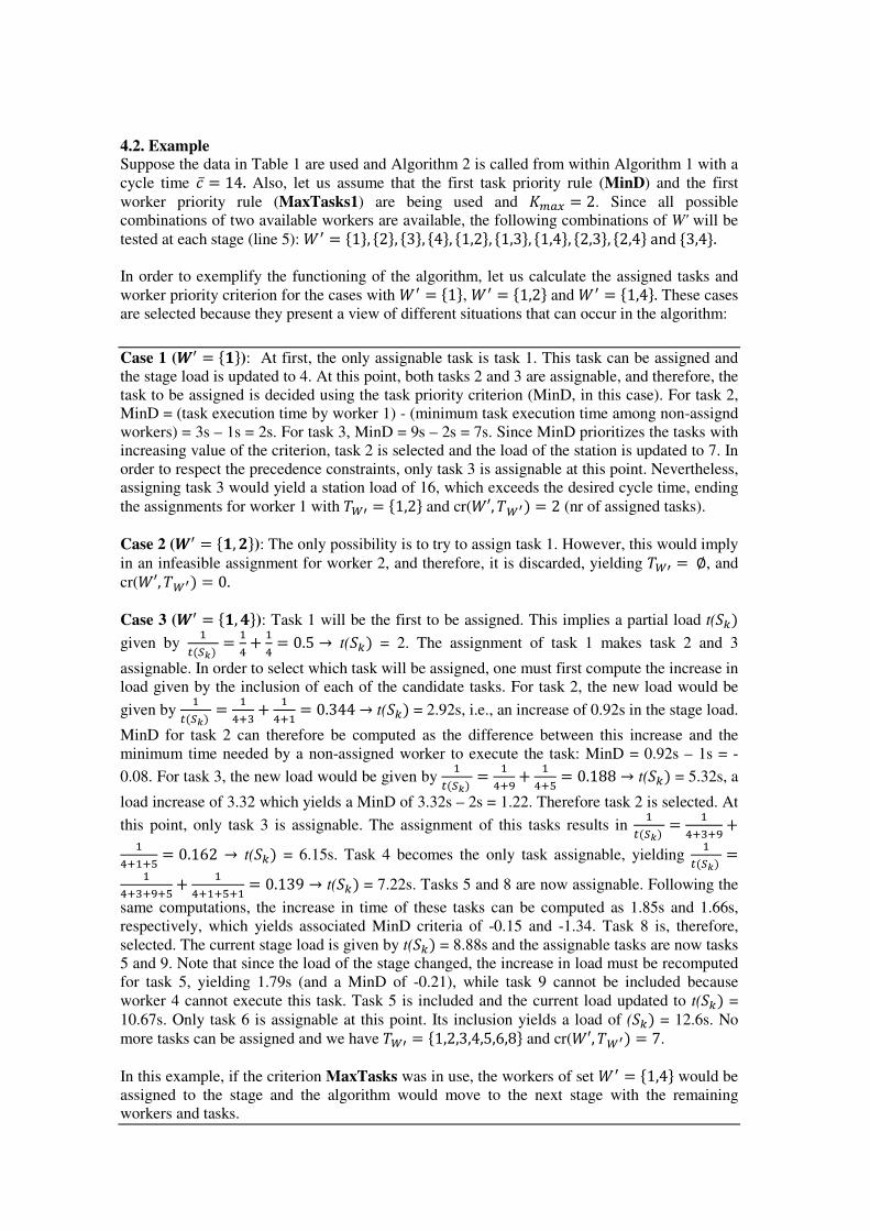
4.2. Example Suppose the data in Table 1 are used and Algorithm 2 is called from within Algorithm 1 with a

cycle time �̅ � 14. Also, let us assume that the first task priority rule (MinD) and the first

worker priority rule (MaxTasks1) are being used and GHIJ � 2. Since all possible

combinations of two available workers are available, the following combinations of W' will be

tested at each stage (line 5): 1j � o1p, o2p, o3p, o4p, o1,2p, o1,3p, o1,4p, o2,3p, o2,4pando3,4p.

In order to exemplify the functioning of the algorithm, let us calculate the assigned tasks and

worker priority criterion for the cases with 1j � o1p, 1j � o1,2p and 1j � o1,4p. These cases

are selected because they present a view of different situations that can occur in the algorithm:

Case 1 (uj � ovp): At first, the only assignable task is task 1. This task can be assigned and

the stage load is updated to 4. At this point, both tasks 2 and 3 are assignable, and therefore, the

task to be assigned is decided using the task priority criterion (MinD, in this case). For task 2,

MinD = (task execution time by worker 1) - (minimum task execution time among non-assignd

workers) = 3s – 1s = 2s. For task 3, MinD = 9s – 2s = 7s. Since MinD prioritizes the tasks with

increasing value of the criterion, task 2 is selected and the load of the station is updated to 7. In

order to respect the precedence constraints, only task 3 is assignable at this point. Nevertheless,

assigning task 3 would yield a station load of 16, which exceeds the desired cycle time, ending

the assignments for worker 1 with f9j � o1,2p and cr(1′, f9w� � 2 (nr of assigned tasks).

Case 2 (uj � ov, xp): The only possibility is to try to assign task 1. However, this would imply

in an infeasible assignment for worker 2, and therefore, it is discarded, yielding f9j � ∅, and

cr(1′, f9w� � 0.

Case 3 (uj � ov, yp): Task 1 will be the first to be assigned. This implies a partial load t(2E� given by

�c�8W� �

�'+

�' � 0.5 → t(2E� = 2. The assignment of task 1 makes task 2 and 3

assignable. In order to select which task will be assigned, one must first compute the increase in

load given by the inclusion of each of the candidate tasks. For task 2, the new load would be

given by �

c�8W� ��

'{|+�

'{� � 0.344 → t(2E� = 2.92s, i.e., an increase of 0.92s in the stage load.

MinD for task 2 can therefore be computed as the difference between this increase and the

minimum time needed by a non-assigned worker to execute the task: MinD = 0.92s – 1s = -

0.08. For task 3, the new load would be given by �

c�8W� ��

'{}+�

'{~ � 0.188 → t(2E� = 5.32s, a

load increase of 3.32 which yields a MinD of 3.32s – 2s = 1.22. Therefore task 2 is selected. At

this point, only task 3 is assignable. The assignment of this tasks results in �

c�8W� ��

'{|{}+�

'{�{~ � 0.162 → t(2E� = 6.15s. Task 4 becomes the only task assignable, yielding �

c�8W� ��'{|{}{~+

�'{�{~{� � 0.139 → t(2E� = 7.22s. Tasks 5 and 8 are now assignable. Following the

same computations, the increase in time of these tasks can be computed as 1.85s and 1.66s,

respectively, which yields associated MinD criteria of -0.15 and -1.34. Task 8 is, therefore,

selected. The current stage load is given by t(2E� = 8.88s and the assignable tasks are now tasks

5 and 9. Note that since the load of the stage changed, the increase in load must be recomputed

for task 5, yielding 1.79s (and a MinD of -0.21), while task 9 cannot be included because

worker 4 cannot execute this task. Task 5 is included and the current load updated to t(2E� =

10.67s. Only task 6 is assignable at this point. Its inclusion yields a load of (2E� = 12.6s. No

more tasks can be assigned and we have f9j � o1,2,3,4,5,6,8p and cr(1′, f9w� � 7.

In this example, if the criterion MaxTasks was in use, the workers of set 1j � o1,4p would be

assigned to the stage and the algorithm would move to the next stage with the remaining

workers and tasks.

4.3. Heuristic variants Even though sets of workers are considered in line 5 of Algorithm 2, it might happen that the

final solution obtained by the algorithm is still serial. Therefore, we also tested versions of the

proposed heuristics including simple modifications in order to promote the finding of solutions

containing at least one stage with more than a worker.

Two modifications were introduced:

Mod 1: In this version, the algorithm is run iteratively (|S|-1) times. At each run, a stage is

selected and at least two workers are assigned to this stage. This is done by ignoring sets

containing a single worker in line 5 of Algorithm 2, when the selected stage is being

considered.

Mod 2: In this version, the algorithm is run iteratively |W| times. At each run, a worker is

selected and this worker is only considered for assignment in conjunction with other workers.

In the following section, we test the proposed models and heuristics in a set of instances

adapted from the literature; analyzing the results and extracting valuable conclusions.

5. Computational results In this section, we present a set of computational experiments used to evaluate the efficiency of

the proposed models and algorithms. We used the four families of instances proposed by

Chaves et al. (2007). This benchmark was generated from four instances specifically selected

from the well-known classical SALBP collection of Hoffmann (1990) so that problems with

low and high order strength (which measures the structural properties of the precedence graph),

and with low and high number of tasks were represented.

From each instance the benchmark includes 80 different problems that were generated

attending high/low variability of task times, high/low number of tasks per worker, and high/low

percentage of incompatibilities; resulting in a robust benchmark of 320 ALWABP-2 instances

of varying characteristics.

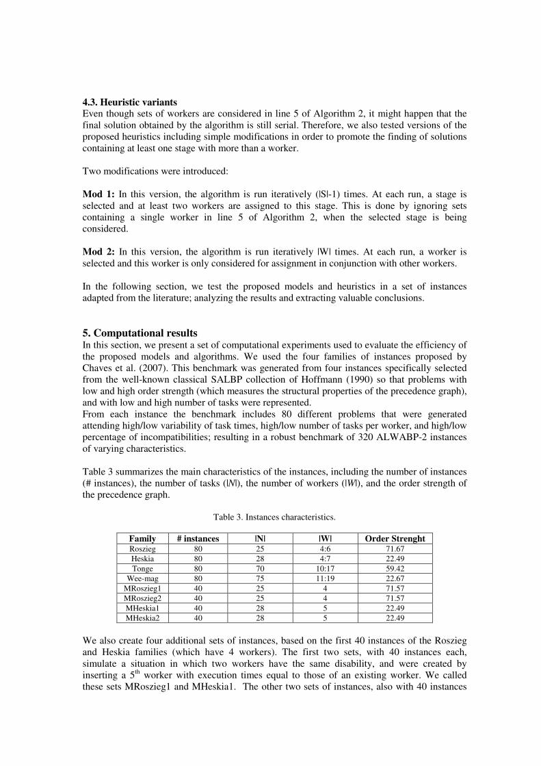
Table 3 summarizes the main characteristics of the instances, including the number of instances

(# instances), the number of tasks (|N|), the number of workers (|W|), and the order strength of

the precedence graph.

Table 3. Instances characteristics.

Family # instances |N| |W| Order Strenght Roszieg 80 25 4:6 71.67

Heskia 80 28 4:7 22.49

Tonge 80 70 10:17 59.42

Wee-mag 80 75 11:19 22.67

MRoszieg1 40 25 4 71.57

MRoszieg2 40 25 4 71.57

MHeskia1 40 28 5 22.49

MHeskia2 40 28 5 22.49

We also create four additional sets of instances, based on the first 40 instances of the Roszieg

and Heskia families (which have 4 workers). The first two sets, with 40 instances each,

simulate a situation in which two workers have the same disability, and were created by

inserting a 5th worker with execution times equal to those of an existing worker. We called

these sets MRoszieg1 and MHeskia1. The other two sets of instances, also with 40 instances

each, simulate a situation in which one of the workers is very slow in comparison to the others.

These sets were created by adding to each instance a 5th worker with execution times

corresponding to three times the largest execution time for each task. We named these sets of

tasks MRoszieg2 and MHeskia2.

In the following we present three different sets of experiments with their corresponding

discussions: first, we evaluate the behavior of the exact models and discuss the improvement on

certain parameters; then we present the results of the heuristic procedure using the different

criteria for task and worker selection; and finally we present some interesting results on the

heuristic variants.

In all experiments, the results obtained are compared with those obtained by serial layouts

using the same set of workers. This allows for a fair comparison, since we want to verify if

better results can be obtained by the parallel and collaborative ALWABP using the same

resources that were available for the serial problem.

5.1. Serial vs parallel and collaborative approaches The instances with 4 and 5 workers were solved using the commercial package IBM ILOG

CPLEX 12.1 in a Intel Core 2 Duo T5450 processor, with 1.66 GHz and 3 GB of RAM. 4

presents the results obtained when solving the models for groups Heskia (first 40 instances),

Roszieg (first 40 instances), MRoszieg1 and MHeskia1. The table shows the number of

parallel and colaborative solutions that improved the best serial solution, the average

improvement obtained for these cases, the best improvement obtained in each family and the

average computational time needed to solve the model.

Table 4. Results for the exact resolution of the parallel and collaborative models.

(Instances Roszieg, Heskia, MRoszieg1 and MHeskia1).

Parallel ALWABP Colaborative ALWABP Number

of

improved

solutions

Average

improvement

(%)

Best

improvement

(%)

Time

(s)

Number

of

improved

solutions

Average

improvement

(%)

Best

improvement

(%)

Time

(s)

Roszieg 2 3.25% 4.90% 62.63 4 24.63% 43.42% 9.18

Heskia 0 0.00% 0.00% 143.45 0 0.00% 0.00% 1.24

MRoszieg1 7 3.44% 5.88% 29.91 4 7.03% 9.52% 8.49

MHeskia1 5 1.56% 3.17% 152.16 0 0.00% 0.00% 5.56

The number of workers in the instances of these families is only four. Even though,

improvements could be obtained with the flexibility introduced by the new problems. For the

parallel ALWABP, better configurations were found in 14 of the 160 instances (only the first

40 instances of the families Roszieg and Heskia were considered) while 8 improved solutions

were found for the collaborative ALWABP. Due to the small number of workers, the

interesting fact is not the number of instances that could be improved but the existence of

instances that could strongly benefit from the new layouts. Indeed, an instance of the Roszieg

family presented an improvement of 43.42% in efficiency (compared to the best serial solution)

when the workers were allowed to work collaboratively. The parallel ALWABP, in turn,

seemed to be useful for the modified instances (where 12 out of the 14 improvements were

found). In these cases, the solution usually assigned the slowest worker in parallel with a faster

worker. The figures in the table show that, in some cases, the use of collaborative strategies

may significantly increase the throughput of the line.

Tables 5 and 6 show the results obtained by the methods for the second class of modified

instances (MRoszieg2 and MHeskia2). The computational time was limited to 3600s for the

resolution of each instance in this case.

Table 5. Results for the exact resolution of the parallel ALWABP, with Kmax limited to 2 and 3.

(Instances MRoszieg2 and MHeskia2).

Parallel ALWABP

Kmax=2 Kmax=3 Number

of

improved

solutions

Average

improvement

(%)

Best

improvement

(%)

Time

(s)

Number

of

improved

solutions

Average

improvement

(%)

Best

improvement

(%)

Time

(s)

MRoszieg2 11 3.18% 10.53% 1730.26 11 3.18% 10.53% 1838.15

MHeskia2 20 4.45% 13.39% 2894.76 18 4.15% 13.39% 3077.08

Table 6. Results for the exact resolution of the collaborative ALWABP.

(Instances MHeskia2 and MRoszieg2).

Collaborative ALWABP Number of

improved

solutions

Average

improvement

(%)

Best

improvement

(%)

Time

(s)

Number of

improved solutions

(respect to parallel)

MRoszieg2 7 25.53% 50% 64.78 7

MHeskia2 0 0% 0% 24.67 0

These instances were much harder to solve and to reduce the computational times in the case of

the parallel ALWABP, Kmax was limited to 2 and 3. The results indicate that for these instances,

the parallel ALWABP could again be useful, yielding improvements in 31 out of the 80

instances. The fact that the average improvements were higher for the case with Kmax = 2 is due

to the fact that optimal solutions could not always be found in these simulations within the time

limit of 3600s. When such situation happened, the best incumbent solution was used.

The collaborative ALWABP improved a smaller number of solutions but, when improved

solutions were found the gains were important, up to 50% in one of the cases.

5.2. Evaluation of heuristics

For larger instances, exact methods were not able to obtain feasible solutions and we therefore

tested the solutions yielded by the constructive heuristic approach. In tables 7 and 8, we present

the results obtained by the heuristic method for Kmax = 2 and 3, respectively. In the tables, we

present the gap (with respect to the best known serial solution), the percentage of parallel

solutions found, the best improvement found and the computational time needed to solve the

method. Each row of the tables presents the results for one of the worker priority criteria

(associated with the best task priority criterion).

Table 7. Results for the heuristic resolution of the parallel ALWABP with Kmax = 2.

(Averaged over all instances).

Gap % of

parallel

solutions

Best improvement

Time (s)

MaxTasks1 +

MaxPWD- 50.85% 90.21% 8.47% 6.78

MaxTasks1.2 +

MinD 38.67% 81.88% 13.96% 0.30

MaxTasks1.4 +

MinR 27,92% 70.21% 15.08% 0.27

MaxTasks1.6 +

MaxPWD- 23.12% 59.79% 14.29% 0.58

MaxTasks1.8 +

MinPWD- 21.10% 41.25% 14.29% 0.57

MaxTasks2 +

MaxPWD- 19.93% 18.54% 14.29% 5.75

MaxTasks3 +

MaxPWD- 19.24% 4.79% 13.49% 5.81

MaxTasksK +

MaxPWD- 19.52% 10.00% 13.49% 5.81

MinRLB +

MaxPWD- 14.92% 28.54% 14.29% 6.37

Table 8. Results for the heuristic resolution of the parallel ALWABP with Kmax = 3.

(Averaged over all instances).

Gap

% of

parallel solutions

Best improvement

Time (s)

MaxTasks1 +

MaxPWD- 68.02% 90.21% 4.76% 28.78

MaxTasks1.2 +

MinD 57.59% 75.04% 10.41% 1.51

MaxTasks1.4 +

MinD 41.23% 52.96% 11.70% 1.34

MaxTasks1.6 +

MinR 31.88% 39.74% 12.05% 1.25

MaxTasks1.8 +

MinR 26.83% 31.59% 12.05% 1.19

MaxTasks2 +

MaxPWD- 24.75% 29.17% 0.00% 23.68

MaxTasks3 +

MaxPWD- 20.17% 7.29% 0.00% 22.71

MaxTasksK +

MaxPWD- 21.02% 10.21% 0.00% 22.68

MinRLB +

MaxPWD- 14.91% 28.75% 2.65% 24.60

For most of the worker priority criteria, the most effective task priority criterion was the

decreasing minimum dynamic positional weights (MaxPWD-). Among the worker priority

criteria, MinRLB presented the best results, yielding a gap of 14.92% and 14.91% with respect

to the best known serial solutions when Kmax was set to 2 and 3, respectively. A considerable

number of parallel solutions was obtained by the method and some important improvements in

the line efficiency could be verified for some instances. The algorithm was efficient in

computational terms, solving the instances in less than one minute in average.

As we can see below, Tables 9 and 10 present the analogous results for the collaborative

ALWABP.

Table 9. Results for the heuristic resolution of the collaborative ALWABP with Kmax = 2.

(Averaged over all instances).

Gap

% of

collaborative solutions

Best

improvement Time (s)

MaxTasks1 +

MinD 53.80% 96.04% 46.77% 0.29

MaxTasks1.2

+ MinD 41.84% 81.88% 50.00% 0.27

MaxTasks1.4

+ MinD 29.79% 63.54% 46.77% 0.25

MaxTasks1.6

+ MinR 23.18% 47.92% 50.00% 0.25

MaxTasks1.8

+ MinR 21.31% 36.88% 50.00% 0.25

MaxTasks2 +

MinR 19.96% 23.13% 50.00% 0.25

MaxTasks3 +

MinR 20.78% 7.29% 50.00% 0.26

MaxTasksK +

MinR 19.83% 16.04% 50.00% 0.25

MinRLB +

MinR 16.79% 39.79% 46.77% 0.40

Table 10. Results for the heuristic resolution of the collaborative ALWABP with Kmax = 3.

(Averaged over all instances).

Gap % of

collaborative solutions

Best improvement

Time (s)

MaxTasks1 +

MinD 74.12% 97.71% 46.77% 1.42

MaxTasks1.2

+ MinD 64.81% 87.29% 50.00% 1.39

MaxTasks1.4

+ MinD 49.36% 68.33% 46.77% 1.27

MaxTasks1.6

+ MinD 40.19% 55.83% 45.45% 1.24

MaxTasks1.8

+ MinR 32.81% 47.08% 45.45% 1.20

MaxTasks2 +

MinR 26.09% 32.29% 50.00% 1.16

MaxTasks3 +

MinR 21.62% 9.79% 50.00% 1.18

MaxTasksK +

MinR 19.87% 16.04% 50.00% 1.13

MinRLB +

MinR 16.68% 39.79% 46.77% 1.81

As for the parallel ALWABP, the criterion MinRLB presented the best results, yielding

solutions with a gap of less than 17% with respect to the best known solutions. Solutions with

efficiency improved in up to 50% were found by the method in very small computational times

(around 1s).

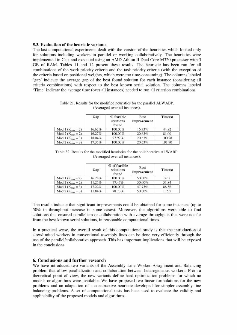
5.3. Evaluation of the heuristic variants The last computational experiments dealt with the version of the heuristics which looked only

for solutions including workers in parallel or working collaboratively. The heuristics were

implemented in C++ and executed using an AMD Athlon II Dual Core M320 processor with 3

GB of RAM. Tables 11 and 12 present these results. The heuristic has been run for all

combinations of the work priority criteria and the task priority criteria (with the exception of

the criteria based on positional weights, which were too time-consuming). The columns labeled

‘gap’ indicate the average gap of the best found solution for each instance (considering all

criteria combinations) with respect to the best known serial solution. The columns labeled

‘Time’ indicate the average time (over all instances) needed to run all criterion combinations.

Table 21. Results for the modified heuristics for the parallel ALWABP.

(Averaged over all instances).

Gap % feasible

solutions found

Best improvement

Time(s)

Mod 1 (Kmax = 2) 16.62% 100.00% 16.73% 44.82

Mod 2 (Kmax = 2) 16.27% 100.00% 20.63% 81.00

Mod 1 (Kmax = 3) 18.04% 97.97% 20.63% 100.98

Mod 2 (Kmax = 3) 17.35% 100.00% 20.63% 191.70

Table 32. Results for the modified heuristics for the collaborative ALWABP.

(Averaged over all instances).

Gap % of feasible

solutions

found

Best

improvement Time(s)

Mod 1 (Kmax = 2) 16.28% 100.00% 50.00% 37.8

Mod 2 (Kmax = 2) 11.25% 77.47% 50.00% 51.84

Mod 1 (Kmax = 3) 17.22% 100.00% 47.73% 88.56

Mod 2 (Kmax = 3) 11.84% 78.73% 50.00% 175.5

The results indicate that significant improvements could be obtained for some instances (up to

50% in throughput increase in some cases). Moreover, the algorithms were able to find

solutions that ensured parallelism or collaboration with average throughputs that were not far

from the best-known serial solutions, in reasonable computational times.

In a practical sense, the overall result of this computational study is that the introduction of

slow/limited workers in conventional assembly lines can be done very efficiently through the

use of the parallel/collaborative approach. This has important implications that will be exposed

in the conclusions.

6. Conclusions and further research We have introduced two variants of the Assembly Line Worker Assignment and Balancing

problem that allow parallelization and collaboration between heterogeneous workers. From a

theoretical point of view, the new variants define hard optimization problems for which no

models or algorithms were available. We have proposed two linear formulations for the new

problems and an adaptation of a constructive heuristic developed for simpler assembly line

balancing problems. A set of computational tests has been used to evaluate the validity and

applicability of the proposed models and algorithms.

The results have indicated that the flexibility introduced by these new extensions may

significantly improve the efficiency of the line. Therefore, even if there is no particular reason

for favouring parallel or collaborative layouts, they can be useful from the point of view of line

efficiency. The results also showed that the proposed approaches can be especially beneficial

when workers have very different task execution times, as it could be the case when one tries to

integrate disabled workers in conventional assembly lines. In these cases, combining the

parallel/collaborative approaches, they can be easily integrated in work teams together with

experienced ordinary workers; so that they can feel more confident and progressively improve

their performance with their advice. Therefore, our main conclusion is that companies can

contribute to an important social aim, the socio-labour integration of people with disabilities,

without important losses in productivity. This is even more important if we have in mind the

global scenario where Corporate Social Responsibility implies the consideration of different

stakeholders simultaneously.

About further research, several work lines may emerge from the studies discussed in this paper.

For example, it would be interesting to consider how the different assignments obtained by the

new approaches may help in obtaining effective job rotation schedules in assembly lines with

heterogeneous workers. From an optimization point of view, the study of more elaborate

metaheuristics such as grasp and random-key genetic algorithms may be of interest. These

heuristics can clearly make use of the constructive approaches developed in this paper.

Acknowledgments This research was supported by CAPES, CNPq and FAPESP. This support is gratefully

acknowledged.

References Akagi, F., Osaki, H., Kikuchi, S., 1983. A method for assembly line balancing with more than

one worker in each station. International Journal of Production Research 21, 755-770.

Askin R.G., Zhou M., 1997. A parallel station heuristic for the mixed model production line

balancing problem, International Journal of Production Research 35 (1997), pp. 3095-3105.

Bard J.F., 1989. Assembly line balancing with parallel workstations and dead time.

International Journal of Production Research 27, 1005-1018.

Bartholdi, J., 1993. Balancing two-sided assembly lines: A case study. International Journal of

Production Research 31, 2447-2461.

Baybars, I., 1986. A survey of exact algorithms for the simple assembly line balancing

problem. Management Science 32, 909-932.

Becker C., Scholl A., 2009. Balancing assembly lines with variable parallel workplaces:

Problem definition and effective solution procedure. European Journal of Operational Research

199, 359-374.

Blum C., Miralles C., 2011. On solving the assembly line worker assignment and balancing

problem via beam search. Computers &Operationsresearch 38, 328-339.

Boysen N., Fliedner M., Scholl A., 2007. A classification of assembly line balancing problems.

European Journal of Operational Research 183, 674-693

Boysen, N., Fliedner, M., 2006. A versatile algorithm for assembly line balancing, European

Journal of Operational Research, 184, 39-56.

Boysen N., Fliedner M., Scholl A.,2008. Assembly line balancing: which model to use when?

International Journal of Production Economics 111, 509-528.

Bukchin J., Rubinovitz, J., 2003. A weighted approach for assembly line design with station

paralleling and equipment selection, IIE Transactions 35, pp. 73-85.

Bukchin, J., Dar-El, E.M., Rubinovitz, J., 1997. Team oriented assembly system design: a new

approach. International Journal of Production Economics 51, 47-57.

Bukchin, J., Tzur, M., 2000. Design of flexible assembly line to minimize equipment cost. IIE

Transactions 32, 585-598.

Chaves A.A.; Lorena L.A.N., Miralles C. 2007. Clustering search approach for the Assembly

Line Worker Assignment and Balancing Problem. In Elwany MH, Eltawil AB, editors.

Proceedings of ICC&IE2007—37th International conference on computers and industrial

engineering, 1469-1478.

Chaves A.A.; Lorena L.A.N., Miralles C. 2009. Hybrid Metaheuristic for the Assembly Line

Worker Assignment and Balancing Problem. Lecture notes in Computer Science 5818, 1-14

Costa A.M.; Miralles C. 2009. Job rotation in assembly lines employing disabled workers.

International Journal of Production Economics 120, 625-632.

Dolgui, A., Guschinski, N., Levin, G., 1999. On problem of optimal design of transfer lines

with parallel and sequential operations. In: Fuertes, J.M. (Ed.), Proceedings of the Seventh

IEEE International Conference on Emerging Technologies and Factory Automation, Barcelona,

Spain, vol. 1, 1999, pp. 329-334.

Dolgui, A., Guschinsky, N., Levin, G., 2006. A special case of transfer lines balancing by

graph approach. European Journal of Operational Research 168, 732-746.

Ege, Y., Azizoglu, M., Ozdemirel, N. E., 2009. Assembly line balancing with station

paralleling, Computers & Industrial Engineering, 57, 1218-1225.

Gökçen H., Agpak K., Benzer R., 2006. Balancing of parallel assembly lines. International

Journal of Production Economics 103, 600-609.

Hoffmann, T.R., 1990. Assembly line balancing: A set of challenging problems. International

Journal of Production Research 28, 1807-1815.

ILO – International Labour Office, 2007. Equality at work: Tackling the challenges.

International Labour Conference 96th Session 2007 Report I (B)

ILO – International Labour Office, 2009. Facts on Disability and Decent Work.

http://www.ilo.org/disability

Lee, T.O., Kim, Y., Kim, Y.K., 2001. Two-sided assembly line balancing to maximize work

relatedness and slackness. Computers and Industrial Engineering 40, 273-2927.

McMullen P.R., Frazier G.U., 1998. Using simulated annealing to solve a multiobjective

assembly line balancing problem with parallel workstations, International Journal of Production

Research 36, pp. 2717-2741.

McMullen, P.R., Frazier, G.V., 1997. Heuristic for solving mixed-model line balancing

problems with stochastic task durations and parallel stations. International Journal of

Production Economics 51 (3), 177-190

Miralles C., Marin-Garcia J.A., Ferrus G., Costa A. M. 2010. OR/MS tools for integrating

people with disabilities into employment. A study on Valencia’s Sheltered Work centres for

Disabled. International Transactions In Operational Research 17, 457-473.

Moreira, M. C. O., Costa, A. M., Chaves, A. A., Ritt, M. (2011). Simple heuristics for the

Assembly Line and Worker Assignment Balancing Problem. Working paper.

Nicosia, G., D. Pacciarelli and A.Pacifici, 2002. Optimally balancing assembly lines with

different workstations, Discrete Applied Mathematics 118, 99-113.

Pinnoi, A. and W.E. Wilhelm, 1997. A family of hierarchical models for assembly system

design, International Journal of Production Research 35, 253-280.

Pinnoi, A., Wilhelm, W.E., 1998. Assembly system design: A branch and cut approach,

Management Science 44,103-118.

Pinto, P.A., D.G. Dannenbring and B.M. Khumawala, 1983. Assembly line balancing with

processing alternatives: an application, Management Science 29, 817-830.

Pinto, P.A., Dannenbring, D.G., Khumawala, B.M., 1981. Branch and bound and heuristic

procedures for assembly line balancing with paralleling of stations. International Journal of

Production Research 19, 565-576.

Rachamadugu, R., 1991. Assembly line design with incompatible task assignments. Journal of

Operations Management 10, 469-487.

Rekiek, B., de Lit, P., Delchambre, A. 2002. Hybrid assembly line design and user’s

preferences, International Journal of Production Research 40, 1095-1111.

Rubinovitz, J., Bukchin, J., 1993. RALB — a heuristic algorithm for design and balancing of

robotic assembly lines. Annals of the CIRP 42, 497-500.

Sarker, B.R., Shanthikumar, J.G., 1983. A generalized approach for serial or parallel line

balancing. International Journal of Production Research 21, 109-133.

Scholl, A., Voβ , S. (1996). Simple assembly line balancing - Heuristic approaches. Journal of

Heuristics, 2, 217-244.

Scholl A., Boysen N., 2009. Designing parallel assembly lines with split workplaces: Model

and optimization procedure. International Journal of Production Economics 119, 90-100.

Scholl, A. Becker, C. 2006. State-of-the-art exact and heuristic solution procedures for simple

assembly line balancing, European Journal of Operational Research 168, 666-693.

Simaria, A. S., Vilarinho, P. M., 2004. A genetic algorithm based approach to the mixed-model

assembly line balancing problem of type II, Computers & Industrial Engineering 47, 391-407.

Stephens D.A., Collins M.D., Dodder, R.A., 2005. A longitudinal study of employment and

skill acquisition among individuals with developmental disabilities. Research in Developmental

Disabilities 26 (2005) 469-486.

Süer, G. A., 1998. Designing parallel assembly lines, Computers & industrial engineering,

1998, 35, 467-470.

Vilarinho P.M., Simaria, A.S., 2002. A two-stage heuristic method for balancing mixed-model

assembly lines with parallel workstations, International Journal of Production Research 40, pp.

1405-1420.

Vilarinho P.M., Simaria, A.S., 2006. ANTBAL: An ant colony optimization algorithm for

balancing mixed-model assembly lines with parallel workstations, International Journal of

Production Research 44, pp. 291-303

Wilhelm, W.E., 1999. A column-generation approach for the assembly system design problem

with tool changes. International Journal of Flexible Manufacturing Systems 11, 177-205.

Wolfensberger, W. 1983. Social Role Valorization: a proposed new term for the principle of

normalization, Mental Retardation 21, pp. 234-239.