do teachers matter? measuring the variation in teacher effectiveness in england*
TRANSCRIPT

THE CENTRE FOR MARKET AND PUBLIC ORGANISATION
Centre for Market and Public Organisation Bristol Institute of Public Affairs
University of Bristol 2 Priory Road
Bristol BS8 1TX http://www.bristol.ac.uk/cmpo/
Tel: (0117) 33 10799 Fax: (0117) 33 10705
E-mail: [email protected] The Centre for Market and Public Organisation (CMPO) is a leading research centre, combining expertise in economics, geography and law. Our objective is to study the intersection between the public and private sectors of the economy, and in particular to understand the right way to organise and deliver public services. The Centre aims to develop research, contribute to the public debate and inform policy-making. CMPO, now an ESRC Research Centre was established in 1998 with two large grants from The Leverhulme Trust. In 2004 we were awarded ESRC Research Centre status, and CMPO now combines core funding from both the ESRC and the Trust.
ISSN 1473-625X
Do teachers matter? Measuring the variation in teacher effectiveness in England
Helen Slater, Neil Davies and Simon Burgess
January 2009
Working Paper No. 09/212

CMPO Working Paper Series No. 09/212
CMPO is jointly funded by the Leverhulme Trust and the ESRC
Do teachers matter? Measuring the variation in teacher effectiveness in England
Helen Slater1, Neil Davies2,3
and Simon Burgess3
1HM Treasury
2 Department of Social Medicine, University of Bristol 3 CMPO, University of Bristol
January 2009
Abstract Using a unique primary dataset for the UK, we estimate the effect of individual teachers on student outcomes, and the variability in teacher quality. This links over 7000 pupils to the individual teachers who taught them, in each of their compulsory subjects in the high-stakes exams at age 16. We use point-in-time fixed effects and prior attainment to control for pupil heterogeneity. We find considerable variability in teacher effectiveness, a little higher than the estimates found in the few US studies. We also corroborate recent findings that observed teachers’ characteristics explain very little of the differences in estimated effectiveness. Keywords: education, test scores, teacher effectiveness JEL Classification: I20
Electronic version: www.bristol.ac.uk/cmpo/publications/papers/2009/wp212.pdf Acknowledgements The team that originally collected and managed the data were: Adele Atkinson, Simon Burgess, Bronwyn Croxson, Paul Gregg, Carol Propper, Helen Slater, and Deborah Wilson; clearly, this project could not have happened without that data and we are very grateful for their roles in securing that. Address for Correspondence CMPO, Bristol Institute of Public Affairs University of Bristol 2 Priory Road Bristol BS8 1TX [email protected] www.bris tol.ac.uk/cmpo/

1. Introduction It seems common sense that teachers matter, and that pupils will achieve more with an
inspirational teacher than with an average or poor teacher. Anecdotes abound of the
transformational effect of excellent teaching. Yet trying to quantify this is difficult,
principally because of the data requirements. To a degree, social science research has
emphasised family and home rather than teachers and school in the production of
human capital1. Disentangling the separate contributions of schools, teachers, classes,
peers and pupils themselves needs extremely rich and full disaggregate data. Whilst a
small number of papers have been able to make progress here, we do not yet have a
settled view on the importance of teachers.
Using a unique primary dataset for the UK, we estimate the effect of individual
teachers on student outcomes, and the variability in teacher quality2. We show that
teachers matter a great deal: being taught by a high quality (75th percentile) rather than
low quality (25th percentile) teacher adds 0.425 of a GCSE point per subject to a given
student, or 25% of the standard deviation of GCSE points. This shows the strong
potential for improving educational standards by improving average teacher quality.
However, implementing such a policy would not be straightforward, as we also
corroborate recent US findings that good teachers are difficult to identify ex ante.
As Rockoff (2004) notes, most of the issues in this field relate to data quality. We use
a unique primary dataset that matches a short panel of pupils to a short panel of
teachers. We link over 7000 pupils, their exam results and prior attainment to the
individual teachers who taught them, in each of their compulsory subjects in the
crucial high-stakes exams at age 16. These exams provide access to higher education
and are highly valued in the job market.
Our dataset complements and in some ways extends the current leading datasets in
this field used by Aaronson, Barrow and Sander (2007) (ABS), Kane, Rockoff and
Staiger (2007) (KRS), Rivkin, Hanushek and Kain (2005) RHK and Rockoff (2004)
(R). Like ABS and R, but unlike RHK and KRS, we can match a student to her/his
actual teacher, rather than to the school-grade average teacher. Unlike ABS, KRS,
1 Particularly since the Coleman report (1966). 2 Throughout this paper we use teacher “quality” as shorthand for the impact on test scores, and we are clear that it says nothing about a teacher’s wider contributions to the school.

1
RHK and R, our context is one of students taking exams that are very important to
them and to the school. Unlike ABS, KRS, RHK and R, we exploit the fact that we
observe students taking three exams at the same date, allowing us to use a point-in-
time student fixed effect, in addition to subject-specific prior attainment. We believe
that this allows us to control well for variations in student ability that might otherwise
corrupt our measures of teacher effectiveness if students are not randomly assigned to
teachers (see Rothstein, 2008). Finally, and also unlike ABS, KRS and RHK, our
student-teacher data are matched in and by the school, thus ensuring a high-quality
match. Nevertheless, while our data have these advantages relative to existing
datasets, there are other issues with our data, and we detail below these short-comings
and what we can and cannot estimate.
We show that the standard deviation of teacher effectiveness is 32.6% of a GCSE
point, or 18.9% of a standard deviation (1.722 GCSE points), from Table 5 column 1.
The lowest bound estimate we have is 28.8% of a GCSE point or 16.7% of the
standard deviation. These estimates are in line with those found in the US, which tend
to be around a 10% impact on test scores of a unit standard deviation change in
teacher quality. Using another metric, teacher effectiveness is about a quarter as
variable as pupil effectiveness. However, a teacher’s effectiveness influences the
GCSE outcomes of the entire class, and so the teacher’s effectiveness has greater
leverage.
The next section reviews the current datasets used and highlights the advantages and
disadvantages of ours; we also summarise the results from these studies. Section 3
discusses our own dataset, and section 4 the econometric approach. Section 5 presents
the results. In the Conclusion, we discuss the implications of these results for policy
on teacher effectiveness, teacher selection, and for the incentivisation of teachers.
2. Evidence
As we have noted, the data required to estimate the effectiveness of teachers are
complex. Early studies, surveyed by Hanushek (2002), had to work with data that did
not allow complete controls for the characteristics of students and the allocation of
students to teachers. Recent analysis has been hugely helped by the use of
administrative data, and a small set of recent papers have pushed the field forward a

2
great deal. Rothstein (2008), however, sounds a cautionary note, arguing that there is
strong non-random sorting within schools, and that in some cases the estimated
teacher effects do not have persistent effects on attainment. Recent research includes
notably Aaronson, Barrow and Sander (2007) (ABS), Kane, Rockoff and Staiger
(2007) (KRS), Rivkin, Hanushek and Kain (2005) RHK and Rockoff (2004). Whilst
Clotfelter et al (2006, 2007) follow a different methodology, they also use state-wide
administrative data from North Carolina. The analysis presented here builds on these
foundations and provides new evidence from a dataset that in some ways offers better
features than those currently available.
Rockoff (2004) estimates teacher effectiveness using data from two school districts in
New Jersey over the years 1989/90 to 2000/01 covering grades 2 to 6. The data allow
individual teachers to be matched with their pupils for each year of the study. A
drawback of using elementary (primary) school data is that typically students are only
taught by one teacher. This means that it is not possible to estimate the effects of
multiple teachers on the same student in different subjects at the same time. Rockoff
finds that a one standard deviation increase in teacher quality results in a 0.11
standard deviation increase in reading and writing test results. Teacher experience is
found to a have a significant positive effect on maths and reading exam results, but no
other observable teacher characteristics are found to have significant effects.
RHK use a large dataset that spans grades 3 to 7, for three cohorts of a total of half a
million students across 3000 schools in Texas. Their data does not match individual
students to individual teachers, only to a set of teachers in a grade within a school.
This is likely to attenuate estimated teacher effects. Their lower bound estimate
implies a one standard deviation increase in teacher quality is associated with 0.11
and 0.095 standard deviation increases annual growth in achievement in maths and
English respectively in grade 4. They find a significant negative effect of inexperience
in maths teachers, and a smaller negative effect for English teachers. However the
qualifications of teachers were found to have no significant effect.
The context studied by Aaronson et al (2007) is ninth-grade maths scores in one
school district in Chicago over a three year period. Key advantages of their data are
the ability to link students with the actual teacher that taught them, and the availability
of prior attainment data, which they assume absorbs student heterogeneity. They find
that an increase in teacher quality of one standard deviation above the mean is
associated with 0.15 standard deviation increase in the maths test score.
3
Clotfelter et al (2006, 2007) take a different approach and directly regress student
outcomes on teacher characteristics including teacher credentials, following the
educational production function approach. They have longitudinal data across grades
3 to 5 from North Carolina data and use student fixed effects to deal with potential
non-random matching of students and teachers. They find that teacher certification
matters and has an important effect on test scores.
In comparison to RHK, we can match students to actual teachers. In comparison to
ABS: our data matches students and their actual teachers like theirs, relates to high
school education like theirs, and also contains prior attainment data, and, like theirs, is
not nationally representative. There are three important differences. First, they make
it clear that their ninth-grade maths scores are not high stakes tests, whereas the exams
that we study matter a great deal, both for student and school. This makes it more
relevant for policy discussions. While in principle it also raises the worry of cheating,
the exams are nationally set and marked outside the school by national bodies, leaving
little scope for systematic manipulation. Second, we observe the same student taking
exams in three different subjects contemporaneously. We therefore do not need to rely
on over-time student “fixed effects” being actually fixed over a period of time when
student abilities can change rapidly. Relative to R, in our data the multiple subjects
are taught by different teachers, so allowing us to compare the same student paired
with different teachers. As mentioned, we use subject-specific prior attainment as
well, so we believe that this approach deals quite thoroughly with variations in student
ability and non-random allocation. On the other hand, we do have to make
assumptions about the correlation of student abilities in different subjects. We detail
the approaches we take to this below. Third, ABS carry out their own teacher-student
matching, and achieve a 75% match. For us, the match was done in the school, and by
the school, typically by the school secretary or administrative computing team.
3. Data
The data contains the exam results for 7,305 pupils and 740 teachers across 33 schools
in England.3 These are state secondary schools in England over 1999 to 2002.
Schools were asked to provide the GCSE and Keystage 3 (KS3) results in Maths, 3 This bespoke dataset was collected by CMPO for a project evaluating the introduction of performance pay (the “Performance Threshold”) for teachers. This project is described in Atkinson et al (2009).
4
Science and English. The GCSE exams (also known as Keystage 4) are taken at age
16 in a number of different subjects. They are the key gateway exams into higher
education as well as being important in the labour market. It is compulsory to take
GCSEs in English, Maths and Science. Keystage 3 exams are taken at age 14 just
prior to the start of the GCSE programme and are also compulsorily taken in English,
maths and science. The Keystage 3 test scores are widely used as a measure of prior
attainment when studying GCSE scores, and we follow that practice here. These are
all nationally set and marked exams.
We requested two tranches of this data. First, test scores of pupils who took their
GCSEs in 1999, along with the pupil’s date of birth, gender and postcode (zip code).
The schools were asked again in 2002/3 for the same information on the tranche of
pupils who took their GCSEs in 2002. Schools were also asked to provide details of
students’ classes, including a teacher id, the teacher’s age, gender, length of tenure,
salary, and spine point (a point on a nationwide teacher pay scale). Given the
demanding data requirements, only a small sample of schools responded and provided
full data. Whilst not very different to the overall set of schools, there are some
differences and there is no presumption that the sample is representative of all English
secondary schools.4
The data linking pupils to teachers are class lists, provided by schools. Classes
typically differ by subject – that is, a pupil will have different peers and different
teachers for each subject. Each pupil may have more than one teacher per subject over
the two years of the course. The mean number of teachers per pupil is 4.13 over these
three subjects, and the modal number is 5. Essentially, an observation is a pupil-
teacher match, or equivalently a pupil-subject-teacher match as each teacher only
teaches one subject. But there is some variety of practice across schools in terms of
the number of teachers a pupil has, particularly in science. Because of this, the
individual pupil-teacher observations are weighted so that each exam result has equal
weight regardless of the number of teachers that contributed. That is, if a student has n
teachers, each pupil-teacher observation is weighted by 1/n. Each of a student’s
teachers for a single subject is assumed to contribute equally. In summary, the data
used in the initial regression contain 25,770 unique exam results, 30,149 pupil-teacher
matches and 52,613 unweighted observations. The mean number of observations per
pupil is 7.20, with 95% of pupils having at least 6 observations. In the subsequent 4 Atkinson et al (2004) compares the achieved sample to all state secondary schools.

5
tables we calculate the sum of the regression weights for each teacher and use this
total to calculate the weighted variance.
The pupil and teacher data were matched at teacher level by and in the school. We
also match in school level variables from the National Pupil Database (NPD). Finally,
data from the Database of Teacher Records were later matched in to provide
information on teachers’ education.
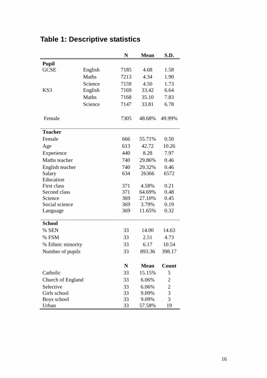
Some brief descriptive statistics are given for the key variables in Table 1. Note the
different metrics that GCSE points and KS3 exams are measured in. There are a
number of missing values, most importantly for some of the teacher characteristics.
Teacher characteristics are generally well measured, other than salary and education
history for which we have a large number of missing values. We deal with these by
retaining the observation in the analysis, replacing the missing by an appropriate value
and including an indicator for each missing variable. At pupil level, we omit pupils
with missing KS3 or GCSE score; there are no missing school variables.
4. Method
a. Measuring the variation in teacher effectiveness
We start from a simple and standard assumption about the factors involved in
generating a particular test score outcome for each pupil in each subject. This follows
Aaronson et al (2007), and is standard if rather complex in terms of the number of
levels of variation in the data. Let itzjsG denote the GCSE score of pupil i in cohort t in
subject z, taught by teacher j, in school s; let Kitzs denote the corresponding prior
attainment (KS3) score of that pupil in that cohort in that subject and school5. We
assume that test scores are generated as follows:
itzjssjiitzsitzjs tZKG εβδψφαλ ++++++= (1)
There are a number of issues and assumptions involved here. We include dummy
variables to allow for differences in mean scores by subject, δZ, and over the two
5 We could write K as G from the prior grade level as that is what it is, but adding a further subscript seems unnecessary.

6
cohort/time periods, βt. As the residual error term, itzjsε is likely to be correlated
across each pupils’ three exam results, we cluster standard deviations at individual
level.
The inclusion of prior attainment means that we are focussing here on the impact of
the teacher on pupil progress or value-added. Prior attainment captures some of the
school effect, the effect of previous teachers’ inputs and also the pupil’s own ability
and prior effort.
We can identify pupil fixed effects, α , as we observe each pupil across three subjects
at the same point in time. This subsumes the influence on progress of unobserved
pupil ability and effort, and family background. The issue here is whether it is
appropriate to assume that this has the same impact across all three subjects; whether,
in other words, able pupils are good at everything, and less able ones score low at
everything. We can use national data from the pupil census (PLASC/NPD) data to get
a view of the appropriateness of these two approaches. Pairwise correlations between
GCSE points on these three subjects are as follows: English and Maths, 0.768,
English and Science 0.793, and Maths and Science 0.848. These high values suggest
that there is a high level of commonality in achievement in GCSEs and that therefore
the way we use the pupil fixed effects may not be unreasonable. Any common subject
level differences are swept up into the teacher effects and purged in the second stage
regression.
An alternative is to not include pupil fixed effects, but to include our two observed
pupil characteristics, gender and within-year age. It means that we do not control for
unobserved pupil differences (for example, effort) and therefore implicitly assumes
that these are conditionally randomly distributed across teachers, conditional on KS3,
gender and age. Denoting the vector of pupil observables as X, this involves
estimating:
izjstsjiitzsizjst tZKG εβδψφλ ++++++= aX (2)
The focus of our analysis is on the role of teacher fixed effects,φ , and school fixed
effects, ψ . The former captures in a very general way the influence of a specific
teacher on pupil progress, relative to other teachers in the sample. Note that this
formulation assumes that a given teacher is equally effective for all pupils, which may

7
or may not be the case. We provide some indirect evidence on this potential
heterogeneity below. The latter captures factors common across the school that might
influence progress. For example, the school ethos, resources and facilities,
disciplinary policy and selection policy may all influence student outcomes.
We observe teachers linked to multiple pupils. For a subset of teachers, we also
observe them in both cohorts, three years apart. However, by construction in our
sample, all teachers remain in the same school over the two periods. This means that it
is impossible to separately identify a pure teacher effect and a school effect. This
problem is also faced in different ways by some of the other papers mentioned above.
What we observe is the sum of the two: ( ))( jsjj ψφτ += . We pursue two strategies to
isolate the variation in true teacher effectiveness. First, we report the within-school
variation in the estimated values of τj, that is, the variance of ( ))( jsj ττ − . This nets out
all school level factors, and provides a lower bound to the degree of variation. For
example, if schools hired teachers randomly then this measure would reflect the true
overall variation in teacher effectiveness. But if, as seems more likely, good teachers
cluster together and less able teachers cluster together, then the within-school variance
will be lower than the true overall variation.
Second, we use a subsidiary regression to purge observable school effects from the
measure. That is, we regress τj on Ws, a set of school level variables, take the residual
as the estimate of teacher effectiveness, )( jsjj bW−=τυ , and examine the variation in
that.
These two approaches give us two estimates of the variability in teacher effectiveness.
Comparing them, the within-school measure will be lower than the residual variance,
both because we do not observe all relevant school factors (so some are left in the
error term), and because there is likely to be between-school variation as well.
b. Explaining the variation in teacher effectiveness One of the interesting results emerging in this literature is that teacher effectiveness is
not closely related to observable teacher characteristics such as teaching
qualifications. Our data include information on age, experience and gender, whether
8
the teacher has a degree, and what class and subject that degree was taken in. We will
test whether these variables have any explanatory power of teacher effectiveness.
5. Results
a. Estimating Teacher Effects We present the results of the initial estimation in Table 2; these are the empirical
counterparts of equations (1) and (2). Column (1) includes pupil fixed effects and the
subject-specific prior attainment, whereas column (2) has observable pupil
characteristics (gender and within-year age) rather than the fixed effect. The results
are as expected – subject-specific prior attainment matters very significantly, the role
of prior attainment is reduced with the inclusion of pupil fixed effects, and female
pupils and older pupils score more highly.
In terms of variability, the standard deviation of GCSE scores is 1.722 GCSE points6,
and the standard deviation of the residuals is 0.493 points in the pupil fixed effects
estimation and 0.934 points with the observable characteristics. We also present the
inter-quartile range (IQR) as a measure of variability. The IQR is 2 GCSE points for
the dependent variable and 0.570 points and 1.113 points for the residuals
respectively.
b. Variability in Teacher Effects, 1
Table 3 focusses on the estimated teacher effects from these regressions. Note that
these are in fact estimates of ( ))( jsjj ψφτ += ; that is, they also include school factors
which we deal with shortly and we postpone the detailed interpretation of our
estimates of teacher effectiveness variability until after that. This brief discussion
deals with the results from specification (1), the pupil fixed effects regression, but
most of the comments apply equally to both pupil-level models.
In column (1) of the Table, the standard deviation of teacher effects is 0.534 GCSE
points, and the IQR is 0.710 points. We argued above that a lower bound on
variability is the variation within schools of teacher effectiveness. Table 3 shows that
6 In all the results presented, the metric is GCSE points: an increase from one grade to the next, say a B to an A, is one point.

9
this is 0.354 GCSE points, in column (1), 0.541 in column (2). This estimate is one of
our key findings. We can also express this relative to the variation in pupil effects. In
fact, within-school teacher effectiveness is about a third as variable as pupil
effectiveness, 0.354 relative to 1.088.
We also present an adjusted standard deviation. As Kane and Staiger (2002), Rockoff
(2004) and Aaronson et al (2007) all argue, the variance of the estimated teacher
effects includes sampling variation as well as the true variation in teacher
effectiveness. This can be particularly the case for teacher effects estimated from
small numbers of pupils. In our case, most teachers are estimated from reasonably
large numbers: 572 teachers with at least 40 observations, and only 30 teachers with
fewer than 20.
Nevertheless, we follow the approach used by Aaronson et al (2007, p. 111) to deal
with the issue. We assume that the estimated teacher effect is the sum of the true
underlying effectiveness and a sampling error, uncorrelated with the true value. The
variance of the true effectiveness is then simply the estimated variance minus the
average sampling variance. Again following ABS, we use the mean of the square of
the standard error estimates of the teacher fixed effects as the estimate of the average
sampling error variance and subtract this from the observed variance to yield the
adjusted variance, and then present the adjusted standard deviation.
We see from Table 3, column (1) that the adjusted variance is 0.395, a reduction of
26% from the unadjusted value. In column (2), the adjusted variance is 0.730, a fall of
12%. The teacher effects are more precisely estimated in column (2) as we are not
estimating the 7305 pupil fixed effects, so correcting for sampling error has less
effect.
There is no obvious way of separately adjusting the within-school variance. It is
useful to have an estimate of the adjusted within-school variance to compare below.
To generate a rough estimate, we simply split the adjustment factor of 0.139
proportionately between the within and between variances, and subtract these. This
gives a value of 0.288 in column (1) (0.354 – 0.139*(0.354/(0.354+0.388)) and 0.496
in column (2).

10
c. Removing School Factors
Our second strategy to isolate teacher effectiveness from τj is to remove the effects of
observable school factors through regression. The regression results in Table 4 are
largely as one would expect, and we do not dwell on them here. In order to deal with
the sampling variability problem, we adjust the estimated teacher effects prior to this
regression. We multiplied each estimated teacher effect by the ratio of the estimated
overall variance and the adjusted variance as described in section 5b above. We then
used that as the dependent variable in the regression, and analyse the residual standard
deviation below. It is important to note that the individual effect of, say, being a pupil
eligible for free school meals is already captured by the pupil fixed effect, and the
coefficient on the school percentage of FSM pupils is therefore picking up more
general factors correlated with the school’s location, intake and teacher mix. Second,
the standard errors reported here for the estimated coefficients have not been
corrected for the fact that the dependent variable is estimated. Thus, inference using
these will not be secure, but this is not our main purpose here.
d. Variability in Teacher Effects, 2
We now present our main results in Table 5. These are corrected for sampling
variability and purged of observable school factors. The standard deviation of teacher
effectiveness is 0.326 GCSE points in column (1), 0.514 in column (2). These can be
compared to the adjusted within-school variation estimated in section b above at 0.288
(column 1), and 0.496 (column 2). We would expect the within-school calculation to
be lower for two reasons: it eliminates all school factors, whereas the regression
approach deals with the measured factors in our data; and there is very likely to be
between-school variation reflecting clustering of teachers in schools by ability.
Nevertheless, it is reassuring that the different ways of dealing with pupil ability and
the different methods of removing school factors lead to estimates that are roughly
similar.
We can interpret the size of these in a number of different ways. First, take the IQR as
a measure of the gain per pupil per subject from having a ‘good’ teacher (defined as
being at the 75th percentile) relative to a ‘poor’ teacher (defined as being at the 25th

11
percentile). This is 0.425 GCSE points in column 1 and 0.649 in column 2. These are
not trivial numbers: a pupil taking 8 GCSEs and taught by 8 ‘good’ teachers will score
3.4 more GCSE points than the same pupil in the same school taught by 8 ‘poor’
teachers. The IQR is 24.7% of the standard deviation of GCSE scores. Obviously, the
gain per pupil per subject is greater still looking at the extreme range: comparing a
teacher at the 95th percentile with one at the 5th percentile, this is 1.070 or 1.766.
Second, we can view the variation in teacher effectiveness relative to the variation in
pupil ‘effectiveness’, the latter measured as the pupil fixed effect. The Table shows
that this is 0.254 comparing the standard deviations and 0.262 comparing the IQRs.
Teacher effectiveness is one quarter as variable as pupil effectiveness. This seems
reasonable and is in line with other findings that the single most important influence
on the test outcome is the pupil’s own characteristics. However, a teacher’s
effectiveness influences the GCSE outcomes of more pupils – around 30 per class.
Hence there is greater leverage for the teacher’s effectiveness to matter.
Third, we can compare the within-school and between-school variability in
effectiveness. As we would expect, the within-school variation having purged school-
level effects is essentially the same as in the raw teacher effects, 0.249. We can also
express this as a proportion of the within-school variation in pupil effectiveness,
1.088. So again, variability in teacher effectiveness is a quarter of the variability in
pupil effectiveness. Equally as we would expect, while the between-school variation
is considerably reduced from 0.315 in table 37 to 0.213 in Table 5, the purging of a
wide range of observable school factors has not reduced the between-school
variability to zero. It is not possible to identify in this data whether this is because
there are important remaining differences between schools, or that average teacher
effectiveness differs between the schools in our sample. Both are likely to be true, but
we cannot say in what proportion.
We have also explored a number of dimensions of heterogeneity. Tables are not
reported here but are available from the authors. First, we split the pupils into thirds of
initial ability, and re-run the analysis separately for these groups, including both the
first stage regression on pupils and the analysis of teacher effectiveness variability.
The results show that teachers are marginally more important for the top third and the
lowest third of the ability distribution, though the differences are not large. The key
7 The value in the table of 0.388 has been adjusted for sampling variation as described in section 5b.

12
numbers for Table 5, column 1 are standard deviations of 0.423 for the highest ability
third, 0.327 for the middle and 0.475 for the lowest third. Note that Aaronson et al
also find variations in teacher quality to be more important for low ability students.
e. Explaining Teacher Effectiveness
We now finally explore whether any of the few observable teacher characteristics that
we have are correlated with estimated teaching effectiveness: gender, age, experience,
and education. We include these variables alongside the school factors in a regression
on the estimated teacher effects from table 2. The results are in Table 6. In fact, none
of these variables play any statistically significant role in explaining teacher
effectiveness, other than very low levels of experience showing a negative effect.
Finally, for the sub-sample of teachers that we see in both cohorts, we can test directly
for the influence of class composition on outcomes and on our estimates of teacher
effectiveness. Our use of prior attainment in the pupil-level regression means that we
are estimating teacher impact on pupil progress, and this removes the first-order effect
of class ‘quality’ on the outcome. Also, by controlling for pupil fixed effects, we are
taking out pupil heterogeneity completely. Nevertheless, it could be that there are
class-level effects on progress. In tables available from the authors, we include class
mean prior attainment in the analysis of Table 4 and Table 5. In the regressions in
Table 4, mean prior attainment is significant but small. Consequently, the impact on
measured teacher effectiveness is also minor, changing the estimated variability in the
specification of column 1, Table 5 from 0.326 to 0.315.
6. Conclusion
Do schools matter? Do teachers matter? Or are education outcomes largely driven by
family and home? We have focussed on the second question here, on the impact on
test scores of being taught by high or low quality8 teachers. We have shown that
teachers matter a great deal: having a one-standard deviation better teacher raises the
test score by (at least) 25% of a standard deviation. Having a good teacher as opposed
8 Throughout, we use teacher “quality” to mean the impact on test scores, and we are clear that it says nothing about a wider contribution to the school.

13
to a mediocre or poor teacher makes a big difference. Raising average teacher quality
does seem a promising direction for public policy. Of course, it does not necessarily
follow that schools matter. If teacher quality is randomly distributed across schools9,
then school assignment is unimportant, and teacher assignment within school is
crucial. But this seems most unlikely: it seems much more likely that teachers will
tend to cluster by quality to some degree. This might arise through schools’ hiring
policies or through teacher job acceptance decisions. We cannot answer this question
definitively in this dataset as we cannot distinguish mean teacher effects within a
school from unmeasured school factors10.
Nevertheless, showing the importance of teacher quality for the high-stakes GCSE
outcomes means that family background is not everything. The same student, bringing
to bear the skills derived from her home and family, can systematically score
significantly different marks in different subjects given different teacher quality.
Rivkin et al (2005) relate the teacher quality measure to the socioeconomic gap in
outcomes, and that comparison is informative here too. The gap in GCSE points
between a poor and non-poor student is 6.08 GCSE points. Suppose this gap arises
over 8 subjects that they both take. If the poor student had good (75th percentile
teachers) for all 8 subjects and the non-poor student had poor (25th percentile
teachers) for all 8, this would make up 3.4 points. This is a powerful effect, and not
one typically addressed in explanations of the socioeconomic education gap. School
and teacher assignment could in principle have a strong role to play in alleviating
unequal outcomes.
By the same token, the assignment of pupils to teachers of varying quality may be an
important part in generating the socio-economic attainment gaps in the first place. We
can test this idea, correlating within-school differences in teacher quality with within-
school differences in class mean prior attainment (we do not have pupil level poverty
status). Taking out school means of both teacher quality and class mean initial score,
we find a correlation of +0.23 between the average ability of the class that a teacher is
assigned and that teacher’s quality11. This will map quite closely on to a correlation
between teacher quality and the pupil’s socio-economic status. Schools face quite
complex incentives for teacher allocation, with the key public quality measure being
9 And if schools add little on top of teacher quality. 10 The fact that we show the between-school variance is larger than the within-school is driven by both unmeasured school-level factors and differences in the average quality of teachers across schools. 11 Using the pupil fixed-effects specification; it is 0.49 in the alternative specification.
14
the fraction of pupils getting at least 5 C grades. It would therefore be valuable to
allocate the best teachers to those pupils close to the C/D borderline. The implication
of this for the allocation of teacher quality and the evolution of the socio-economic
test score gap is an issue for future research.
We have shown that the observed characteristics of teachers in our data do not predict
our measure of their quality well. Whilst we have relatively few characteristics, some
other authors with much richer datasets in that regard confirm this finding (see in
particular Kane, Rockoff and Staiger, 2007). By contrast, Clotfelter et al (2006, 2007)
find that teacher qualifications do have a significant effect. In the 2007 paper, they
argue that teacher credentials exhibit a large effect compared to the effect of changing
class size or of parental education, particularly in maths. This debate has important
implications for improving average teacher quality that previous authors have also
drawn out. The findings show that it may be hard to identify good teachers ex ante,
but that administrative data can be used to identify them ex post. This suggests a
greater role for performance management and personnel policies in schools. This
might include a stronger role for pupil progress analysis in probationary periods,
mentoring, more stringent hiring procedures or sharper performance pay using such
data. However, the cautions of Kane and Staiger (2002) on the folly of basing
important decisions on the small samples of such data in a single school need always
to be borne in mind.
Clearly, further research with richer data may well uncover some important elements
of a teacher’s training or personality that do help to predict quality better. The data
required to carry out the present study were very extensive, complex and difficult to
obtain. Nevertheless, repeating or extending the exercise would appear to be of great
value.

15
References Aaronson, D., Barrow, L. and Sander, W. (2007) “Teachers and Student Achievement
in the Chicago Public High Schools” Journal of Labor Economics, vol. 25(1), pages 95-136.
Atkinson, A., Burgess, S., Croxson, B., Gregg, P., Propper, C., Slater, H., and Wilson, D. (2009) Evaluating the Impact of Performance-related Pay for Teachers in England. Forthcoming Labour Economics. CMPO DP 04/113, University of Bristol.
Clotfelter, C. T., Ladd, H. F. and Vigdor, J. L. (2006) Teacher-Student Matching and the Assessment of Teacher Effectiveness. NBER Working Paper 11936, NBER, Cambridge.
Clotfelter, C. T., Ladd, H. F. and Vigdor, J. L. (2007) How and why do Teacher Credentials matter for Student Achievement? NBER Working Paper 12828, NBER, Cambridge.
Coleman, J. S. et al (1966) Equality of Educational Opportunity. Washington DC . US Government Printing Office.
Hanushek, E. A. (2002) Publicly Provided Education. In Handbook of public finance vol. 4 ed. Auerbach, A. and Feldstein, M. Amsterdam North Holland Press.
Kane, T. J. and Staiger, D. O. (2002) The promises and pitfalls of using imprecise school accountability measures. Journal of Economic Perspectives vol. 16 no 4: pp 91 – 114.
Kane, T. J., Rockoff, J. E. And Staiger, D. O. (2007) What does certification tell us about teacher effectiveness? Evidence from New York City. Economics of Education Review
Rivkin, S.G., Hanushek, E.A., and Kain, J.F. (2005) “Teachers, schools, and academic achievement” Econometrica, Vol. 73, No. 2, 417–458
Rockoff, J. E. (2004) “The impact of individual teachers on student achievement: Evidence from panel data”. American Economic Review. Vol. 94, no. 2.pp. 247 – 252.
Rothstein, J. (2008) Teacher Quality in Educational Production: Tracking, Decay and Student Achievement. NBER Working Paper 14442, NBER, Cambridge.
16
Table 1: Descriptive statistics N Mean S.D.
Pupil GCSE English 7185 4.68 1.58 Maths 7213 4.34 1.90 Science 7159 4.50 1.73 KS3 English 7169 33.42 6.64 Maths 7168 35.10 7.83 Science 7147 33.81 6.78 Female 7305 48.68% 49.99% Teacher Female 666 55.71% 0.50 Age 613 42.72 10.26 Experience 440 8.28 7.97 Maths teacher 740 29.86% 0.46 English teacher 740 29.32% 0.46 Salary 634 26366 6572 Education First class 371 4.58% 0.21 Second class 371 64.69% 0.48 Science 369 27.10% 0.45 Social science 369 3.79% 0.19 Language 369 11.65% 0.32 School % SEN 33 14.00 14.63 % FSM 33 2.51 4.73 % Ethnic minority 33 6.17 10.54 Number of pupils 33 893.36 398.17 N Mean Count Catholic 33 15.15% 5 Church of England 33 6.06% 2 Selective 33 6.06% 2 Girls school 33 9.09% 3 Boys school 33 9.09% 3 Urban 33 57.58% 19

17
Table 2 – Pupil-level regression Dep. Var: GCSE Points score Pupil Fixed Pupil effects Characteristics (1) (2) Prior attainment (subject 0.07*** 0.16*** specific) (34.8) (83.9) Female 0.12*** (5.9) Month of birth dummies? No Yes Pupil effects? Yes No Subject effects? Yes Yes Teacher effects? Yes Yes School effects? No Yes Year effects? No Yes Observations 52,613 52,613 R2 0.918 0.706 Number of pupils 7,305 7,305 Number of teachers 740 740 Std. dev. GCSE points 1.722 1.722 IQR GCSE points 2.000 2.000 Std. dev. Residuals 0.493 0.934 IQR residuals 0.570 1.113 Chi2 H0: all Teacher effects=0 9.916 7.789 Notes:
1) Robust t-statistics clustered at individual pupil level in parentheses. 2) p < 0.05, ** p < 0.01, *** p < 0.001 3) Each observation is weighted by gk/Nk, where Nk is the number of observations for grade in
subject k, and gk is the number of exam results for that subject. (1 for Maths and English, 1-3 for science.)

18
Table 3: Variability in teacher effectiveness, 1
Units: GCSE points (1) (2) Pupil fixed
effects Pupil
characteristics Teacher plus school effects: Standard deviation 0.534 0.825 Adjusted standard deviation 0.395 0.730 Interquartile range (P75 – P25) 0.710 1.248 Extreme range (P95 – P5) 1.707 2.792 Relative variation: Std dev of teacher effects relative to std dev of residuals from Table 2 regression 1.083 0.883 IQR of teacher effects relative to IQR of residuals from Table 2 regression 1.247 1.121 Std dev of teacher effects relative to std dev of pupil effects from Table 2 regression 0.416 IQR of teacher effects relative to IQR of pupil effects from Table 2 regression 0.438 Within- and between-school variation Within school std dev 0.354 0.541 Between school std dev 0.388 0.610 Pupil within school std dev 1.088 Pupil between school std dev 0.698 Notes:
1) Unadjusted for sampling variation, other than the specified row. 2) Weighted by the teacher specific sum of weights from table 2. 3) Based on the estimated teacher effects from Table 2.

19
Table 4: Removing school factors
Dep. Var.: Adjusted teacher Pupil Pupil effects from Table 2 fixed effects Characteristics (1) (2) Catholic school -0.264*** 0.271*** (0.040) (0.062) Church of England school -0.082 -0.352** (0.045) (0.127) Selective school -0.266** -0.280* (0.082) (0.116) Girls school -0.128 0.058 (0.109) (0.156) Urban school 0.122** 0.494*** (0.041) (0.068) % Pupils with special -0.006* 0.014*** educational needs (0.003) (0.004) % Pupils eligible for free -0.014** 0.023* school meals (0.005) (0.010) % Chinese pupils -0.120 -0.084 (0.065) (0.101) % Bangladeshi pupils -0.158 -0.143 (0.112) (0.182) % Pakistani pupils 0.010 -0.159** (0.054) (0.061) % Indian pupils 0.002 0.039* (0.009) (0.016) % Black African pupils 0.049 -0.305*** (0.038) (0.052) % Black Caribbean pupils -0.054*** -0.023 (0.013) (0.019) % Other Black pupils 0.104* 0.184** (0.047) (0.064) % Other ethnicity pupils 0.049 0.021 (0.034) (0.054) First tranche 0.085 0.084 (0.065) (0.112) Subject = English 0.233*** -0.600*** (0.032) (0.050) Subject = Maths 0.006 0.131* (0.033) (0.053) Size of school/10 0.000 -0.003*** (0.000) (0.000) Observations 740 740 R-Squared 0.318 0.504
Notes: 1) Robust standard errors in parentheses 2) * p < 0.05, ** p < 0.01, *** p < 0.001 3) Regression weighted by the sum of the weights from the regression in table 2. 4) Ex ante adjustment, [teacher effect * (adjusted variance/unadjusted variance)]

20
Table 5: Variability in teacher effectiveness, 2 Units: GCSE points Pupil fixed
effects Pupil
characteristics Teacher effects: (1) (2) Standard deviation 0.326 0.514 Interquartile range (P75 – P25) 0.425 0.649 Extreme range (P95 – P5) 1.070 1.766 Relative variation: Std dev of teacher effects relative to std dev of residuals from Table 2 regression 0.662 0.550 IQR of teacher effects relative to IQR of residuals from Table 2 regression 0.746 0.583 Std dev of teacher effects relative to std dev of pupil effects from Table 2 regression 0.254 IQR of teacher effects relative to IQR of pupil effects from Table 2 regression 0.262 Within- and between-school variation Within school std dev 0.249 0.379 Between school std dev 0.213 0.351 Notes:
1) Ex ante variance adjustment, [teacher effect * (adjusted variance/unadjusted variance)] 2) Weighted by the sum of the weights from the regression in table 2. 3) Conditional on school characteristics, ie. based on the residuals from Table 4, columns 1, 2.

21
Table 6: Explaining teacher fixed effects
Dependent Variable: adjusted teacher fixed effects from Table 2 Pupil fixed
effects (1)
Pupil characteristics
(2) Teacher female 0.019 0.031 (0.031) (0.051) Age 0.001 -0.006 (0.007) (0.011) Age squared -0.000 -0.000 (0.000) (0.000) One years experience -0.190*** -0.014 (0.050) (0.090) 2-4 years experience -0.038 -0.013 (0.045) (0.081) 5-10 years experience 0.023 0.019 (0.060) (0.079) 10-15 years experience 0.014 0.075 (0.070) (0.102) Experience squared -0.000 -0.000 (0.000) (0.001) Experience cubed 0.000 0.000 (0.000) (0.000) Subject = Maths 0.091 0.053 (0.083) (0.132) Subject = English 0.073 0.150 (0.091) (0.137) Degree class: First class 0.185* 0.250 (0.089) (0.149) Second class 0.030 0.054 (0.037) (0.062) Science Degree 0.026 0.053 (0.050) (0.078) Social Sci Degree 0.001 -0.025 (0.103) (0.131) Language Degree 0.073 -0.188 (0.059) (0.102) Salary band 0.000 0.000 (0.000) (0.000) School factors Yes Yes Observations 740 740 R-Squared 0.368 0.539
Notes: 1) Robust standard errors in parentheses 2) * p < 0.05, ** p < 0.01, *** p < 0.001 3) School factors also included as in Table 4 4) Regression weighted by the sum of the weights from the regression in table 2. 5) Ex ante variance adjustment, [teacher effect * (adjusted variance/unadjusted variance)]

22
Appendix Table 1: Data Requested Information Level Class lists for year 10 in 1997/8 and year 11 in 1998/9, with pupil identifiers and teacher identifiers
pupil
Class lists for year 10 in 2000/1 and year 11 in 2001/2, with pupil identifiers and teacher identifiers
pupil
Pupil test/exam scores for Key Stage 3 in 1996/7 and GCSE 1998/9, for all English, maths and science subjects, with pupil identifiers
pupil
Pupil test/exam scores for Key Stage 3 in 1999/00 and GCSE 2001/02, for all English, maths and science subjects, with pupil identifiers
pupil
Supplementary information for each pupil: date of birth, gender, postcode. With pupil identifier
pupil
Teachers characteristics at 1 September 1999: age, gender, salary, experience, spine point, whether applied for Performance Threshold. With teacher identifier
teacher