www.elsevier.com/locate/gca

Geochimica et Cosmochimica Acta 70 (2006) 5169–5182

Dissociation constants and speciation in aqueousLi2SO4 and K2SO4 from measurements of electrical

conductance to 673 K and 29 MPa

Andrei V. Sharygin a, Brian K. Grafton b, Caibin Xiao c, Robert H. Wood e,*,Victor N. Balashov d

a General Electric Company, GE Plastics, Specialty Film and Sheet, 1 Lexan Lane, Mount Vernon, IN 47620, USAb Exxon Mobil, Research and Engineering Company, Fairfax, VA, USA

c GE Water and Process Technologies 4636 Somerton Road, Trevose, PA 19053, USAd The Energy Institute, Pennsylvania State University, University Park, PA 16802, USA

e Department of Chemistry and Biochemistry, University of Delaware, Newark, DE 19716, USA

Received 4 January 2006; accepted in revised form 25 July 2006

Abstract

The electrical conductivities of aqueous solutions of Li2SO4 and K2SO4 have been measured at 523–673 K at 20–29 MPa in dilutesolutions for molalities up to 2 · 10�2 mol kg�1. These conductivities have been fitted to the conductance equation of Turq, Blum,Bernard, and Kunz with a consensus mixing rule and mean spherical approximation activity coefficients. In the temperature interval523–653 K, where the dielectric constant, e, is greater than 14, the electrical conductance data can be fitted by a solution model whichincludes ion association to form MSO4

�, M2SO40, and HSO4

�, where M is Li or K. The adjustable parameters of this model are the firstand second dissociation constants of the M2SO4. For the 673 K and 300 kg m�3 state point where the Coulomb interactions are thestrongest (dielectric constant, e = 5), models with more extensive association give good fits to the data. In the case of the Li2SO4 model,including the multi-ion associate, Li16ðSO4Þ80, gave an extremely good fit to the conductance data.� 2006 Elsevier Inc. All rights reserved.

1. Introduction

A knowledge of the activity coefficients and associa-tion constants of alkali sulfates, in particular Li2SO4(aq)and K2SO4(aq), are important in a variety of geochemi-cal and industrial processes. Sulfates represent an impor-tant component of the mineral economy and of pollutionproblems in air and water. There is considerable scientificinterest in the mineralogy and geochemistry of sulfateminerals in both high-temperature (igneous and hydro-thermal) and low-temperature (weathering and evaporite)

0016-7037/$ - see front matter � 2006 Elsevier Inc. All rights reserved.

doi:10.1016/j.gca.2006.07.034

* Corresponding author. Fax: +1 302 831 6335.E-mail addresses: andrei.sharygin@ge.com (A.V. Sharygin), rwood@

udel.edu (R.H. Wood), vnb1@psu.edu (V.N. Balashov).

environments. The physical scale of processes affected byaqueous sulfate spans from submicroscopic reactions atmineral–water interfaces to global oceanic cycling andmass balance, and to extraterrestrial applications in theexploration of other planets and their satellites (Alperset al., 2001). The association of alkali metal sulfates inaqueous solutions at elevated temperatures is also ofgreat importance in many industrial processes such asmaterial transport, solid deposition, and corrosion inelectric power plants. Sulfates are common products ofhydrothermal waste destruction by supercritical wateroxidation.

The data on limiting equivalent sulfate conductance arenecessary to predict the diffusion transport of sulfate com-ponents in geochemical processes involving fluid–rockinteraction (Balashov, 1995).

5170 A.V. Sharygin et al. 70 (2006) 5169–5182

One of the most accurate and comprehensive sets ofconductivity measurements of aqueous K2SO4 from 18up to 306 �C was reported by Arthur Noyes and ArthurMelcher one century ago (Noyes and Melcher, 1907). Theinitial and final dates of their K2SO4 experiments areMarch 14, 1904, and September 29, 1905, respectively.These investigations were continued at ambient tempera-tures by different authors (Clews, 1935; Jenkins and Monk,1950; Broadwater and Evans, 1974; Valyashko and Ivanov,1974; Fedoroff, 1989; Indelli, 1989) and at elevated temper-atures (Quist and Marshall, 1966) using conductance mea-surements, and (Matsushima and Okuwaki, 1988) usinge.m.f. measurements. These efforts resulted in the determi-nation of the ion-pair KSO4

� dissociation constant andlimiting equivalent conductance of SO4

2�. However,KSO4

� has not been studied at temperatures near thecritical point of water.

The conductivity of aqueous Li2SO4 was also studied byseveral authors (Austin and Mair, 1962; Postler, 1970;Valyashko and Ivanov, 1974; Indelli, 1989) but the resultsare limited to T 6 200 �C. There are no previous measure-ments of association to form the uncharged ion aggregatesK2SO4

0(aq) and Li2SO40(aq).

The conductivities of aqueous K2SO4 and Li2SO4 atmolalities from 0.05 up to 0.5 mol kg�1 and up to 200 �Cwere measured by Mil’chev and Gorbachev (1958) but theirmolalities are two high for our method of analysis.

Recently, a new quantitative approach to the analysis ofelectrical conductivity of aqueous electrolyte solutions wasdeveloped by R.H. Wood et al. (Sharygin et al., 2001, 2002;Hnedkovsky et al., 2005). Here, we report new conductivitymeasurements for Li2SO4(aq) and K2SO4(aq) in an appara-tus with solution flow (Sharygin et al., 2000). Associationconstants and limiting equivalent conductances are derivedfor Li2SO4(aq) and K2SO4(aq) at temperatures from 18 to400 �C, pressures up to 29 MPa, and water densities from1000 kg m�3 to 300 kg m�3.

We found that the model that reproduces most of theexperimental data is a model with association to formMSO4

�(aq) and M2SO40(aq), where M is Li or K, and with

ion activities calculated with the Mean Spherical Approxi-mation (MSA). In the case of aqueous Li2SO4 for theregion where the dielectric constant is very low, (water den-sity 300 kg m�3), a model with further association to formaggregates Lim(SO4)s with m + s > 3 fits the data at thehighest molality 2.6 · 10�3.

2. Experimental

The flow-type, high-temperature, high-pressure con-ductance apparatus and the associated operating proce-dures have been previously described in detail(Zimmerman et al., 1995; Gruszkiewicz and Wood,1997; Sharygin et al., 2001, 2002) and will not be repeat-ed here. The conductance apparatus with platinum–rho-dium tubing in the hot zone was used to measureaqueous solutions of Li2SO4 and K2SO4 at a given

temperature and pressure. The conductance cell consistedof a platinum–rhodium cup which served as an outerelectrode and a sapphire insulator with a hole in the cen-ter through which the inner electrode passed into thecenter of the cup. Resistances were measured at frequen-cies of 1 and 10 kHz using a RCL meter (Fluke Co.;Model PM6304c) with manufacturer’s stated accuracyof 0.05% at 1 kHz and 0.1% at 10 kHz. All measuredresistances were corrected for the lead resistance. Leadresistances were always less than 0.5% of the solutionresistance. The temperature was measured by a platinumresistance thermometer (Hart Scientific; Model 5612)with a stated calibration accuracy of ±0.007 K at273 K, ±0.024 K at 473 K, and ±0.033 K at 673 K.The solution was introduced inside of the conductanceapparatus using an HPLC pump (Waters, Division ofMillipore, Inc.; Model 590) which was operated at a con-stant flow rate of 8.3 · 10�3 cm3 s�1. The pressure wasmeasured using a Digiquartz pressure transducer (Paro-Scientific, Inc.; Model 760-6K) with an accuracy of±0.01 MPa. The temperature and pressure were recordedimmediately after a stable reading of resistance wasachieved, corresponding to a sample plateau.

The cell constant was first determined before all report-ed measurements by a series of four measurements on di-lute aqueous solutions of KCl (with molarities from 10�4

to 10�2 mol dm�3) at T = 298.15. The solutions of KClused in the calibration of the cell were prepared by massfrom certified A.C.S. grade KCl (Fisher Scientific Co.;maximum impurity was mass fraction 10�4 of Br�) and dis-tilled and deionized water. The salt was dried for 24 h atT = 573 K, cooled in a desicator under vacuum, and dilut-ed by mass with conductivity water to the initial molality.All apparent masses were corrected for buoyancy. Usingequations given by (Justice, 1983) and (Barthel et al.,1980) for KCl (aq) the cell constant was calculated to be(0.2025 ± 0.0004) cm�1 at 298 K. Calculated cell constantsagreed within 0.2% over the complete range of concentra-tions. The cell constant at elevated temperatures was calcu-lated from the known thermal expansion of the platinumcup, inner electrode, and sapphire insulator. The correc-tions are small.

Stock solutions of K2SO4 were prepared from A.C.S.reagent-grade granular potassium sulfate, which wasdried overnight in a vacuum oven at T = 473 K, cooledunder vacuum, and diluted with conductivity water.The solutions were prepared by mass, and all weightswere corrected to air buoyancy. Stock solutions ofLi2SO4 were prepared from A.C.S. reagent-grade lithiumsulfate monohydrate using the same procedure as de-scribed for K2SO4. The conductivities of all stock solu-tions were measured at room temperature immediatelyafter all experiments were completed. This showed thatthe solutions had not changed during the course of themeasurement (±0.1%). A glass cell with the cell constantequal to 23.705 cm�1 was used to measure conductivitiesof concentrated stock solutions and these conductivities

Dissociation constants of Li2SO4(aq) and K2SO4(aq) 5171

agreed with literature values to 0.2%. The conductivitywater used was first treated using a reverse osmosis sys-tem, then passed through one carbon adsorbent and twodeionization tanks (Hydro Service and Supplies, Inc.;Picosystem, Model 18). The resulting specific conduc-tance of water was about 2 · 10�5 S m�1 at T = 298 K.The solvent conductance was measured at each tempera-ture and pressure.

The experimental conductivities of Li2SO4(aq) andK2SO4(aq) were corrected for the specific conductivity ofimpurities in the solvent (water) according to the equation

jcrra ¼ jobs

a � jobssolvent þ jw; ð1Þ

where a is Li2SO4 or K2SO4; jw, S cm�1, is conductivity ofpure H2O calculated from jw and the equivalent conduc-tances of H+ and OH�. This correction is based on theassumption that the solvent conductance above that dueto H+ and OH� is due to impurities also present in thesolutions [see (Sharygin et al., 2001) for details].

The apparent equivalent conductances of Li and K sul-fates were defined by expression

Ka ¼1000jcrr

a

2ca; ð2Þ

where ca, the molar concentration in mol dm�3, is

ca ¼ma

V �: ð3Þ

The volume of solution per 1 kg of water in dm3 kg�1, V*,was calculated from the thermodynamic model of electro-lyte solutions [see Section 3]. The Li2SO4(aq) andK2SO4(aq) experimental data at each temperature andpressure are listed in Tables 1 and 2, respectively.

3. Theory

3.1. Fitting conductance data

Aqueous solutions of Li2SO4 and K2SO4 must be treat-ed as mixed electrolytes, since association of sulfate ionwith Li+ and K+ ion occurs. Our equation for the conduc-tance of a reacting mixture of electrolytes has three compo-nents: (1) a model for the activity coefficients of the ions, sothat the equilibrium concentrations of free ions in a mix-ture of species at a given salt concentration can be calculat-ed from the mass balance relations and the equilibriumconstants for the reactions; (2) an equation for the equiva-lent conductivity of a single strong electrolyte as a functionof concentration; (3) a mixing rule that predicts theconductance of a mixture of strong electrolytes from theconductance of the single electrolytes. Recently, Sharyginet al. (2001) have tested this model and shown that it allowsthe calculation of association constants from conductancemeasurements containing a mixture of ions. The completedetails of the equations used in our model have been pub-lished (Sharygin et al., 2001, 2002). Below we will give onlya brief discussion of the model.

3.2. Multiple ion association

In general, for a 1:2 electrolyte, M2SO4, we assume theexistence of MmHh(SO4)s ion aggregates with charge(m + h � 2s). We characterize the ion equilibria in solutionby overall dissociation reactions:

MmHhðSO4Þmþn�2ss ¼ mMþ þ hHþ þ sSO4

2�: ð4Þ

The thermodynamic expression of mass action law ofReaction (4) has the form

KMm;h;s ¼

amMþah

HþasSO4

2�

aMmHhðSO4Þmþh�2ss

; ð5Þ

with aMþ ¼ cMþmMþ etc., are the molal activities of speciesin solution, KM

m;h;s is the overall dissociation constant of anion cluster with cluster index, m,h,s; mMþ is the molalityand cMþ is the molal activity coefficient. The conversionof this constant to the constant with a 1 mol dm�3 standardstate is given by expression

KcMm;h;s ¼ KM

m;h;sðV 0Þ1�m�h�s; ð6Þ

where V 0 is the volume of 1 kg of pure solvent (water).

3.3. Activity coefficient models

We have used the mean spherical approximation (Blumand Høye, 1977) (MSA) to calculate activity coefficients.The MSA equation is much more accurate than theDebye–Huckel equation for the activity coefficients of hardspheres in a continuous dielectric medium and it is still ananalytic equation. It is more accurate because it conformsto both the Debye–Huckel limiting law at low concentra-tions and the correct hard sphere repulsion in very concen-trated solutions. Both equations apply to a hard sphere ionin a continuous dielectric medium and both equations arerigorously applicable only to the McMillan–Mayer stan-dard state (Friedman and Dale, 1977). In our calculations,we ignored the corrections to the McMillan–Mayer stan-dard state but we did account for the difference in standardstates [1 mol dm�3 for MSA; see Eq. (6)] and this appearsto reduce corrections to the McMillan–Mayer standardstate (Sedlbauer and Wood, 2004) so the corrections areprobably less than the corrections predicted by Myerset al. (2003) at the highest molality of the two highesttemperatures. Other corrections are small. When the usualDebye–Huckel equations are used, the large densitychanges with concentration are not taken into accountand it performs badly near the critical point (Sedlbauerand Wood, 2004).

The activity coefficient at c = 1 mol dm�3 standard statein the MSA approximation can be expressed in the form ofelectrostatic (el) and hard sphere (hs) contributions:

ln yMSAi ¼ ln yel

i þ ln yhsi : ð7Þ

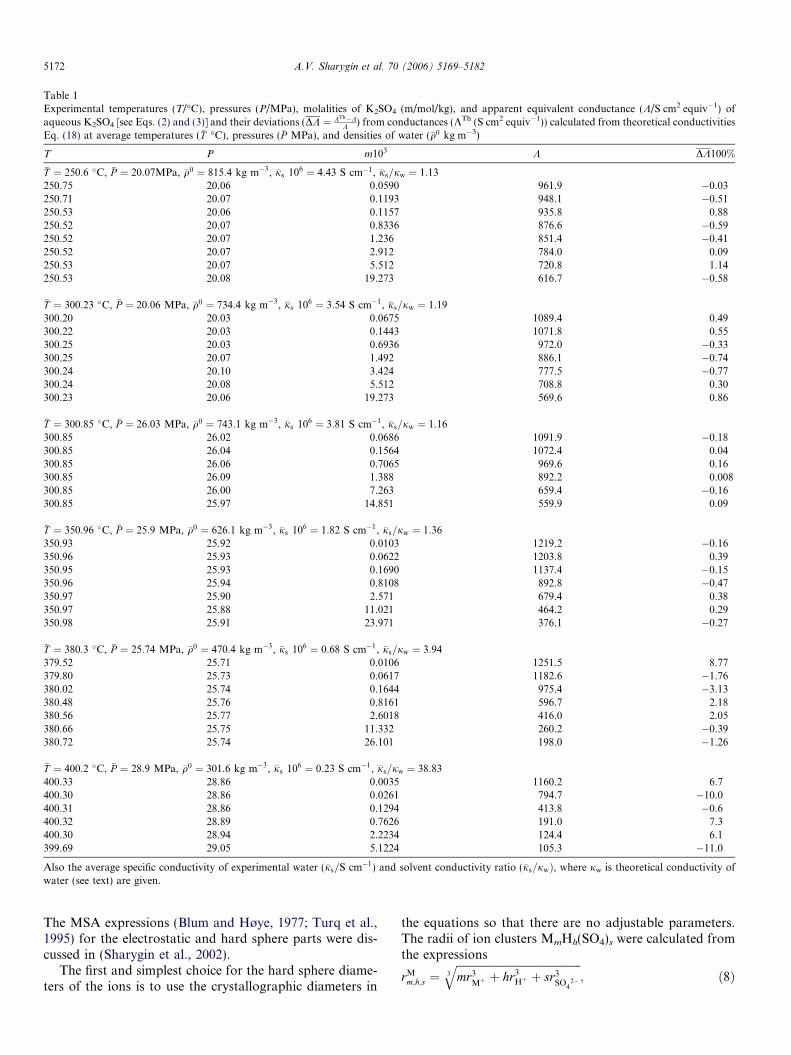
Table 1Experimental temperatures (T/�C), pressures (P/MPa), molalities of K2SO4 (m/mol/kg), and apparent equivalent conductance (K/S cm2 equiv�1) ofaqueous K2SO4 [see Eqs. (2) and (3)] and their deviations (DK ¼ KTh�K

K ) from conductances (KTh (S cm2 equiv�1)) calculated from theoretical conductivitiesEq. (18) at average temperatures (�T �C), pressures (�P MPa), and densities of water (�q0 kg m�3)

T P m103 K DK100%

�T ¼ 250:6 �C, �P ¼ 20:07MPa, �q0 ¼ 815:4 kg m�3, �js 106 ¼ 4:43 S cm�1, �js=jw ¼ 1:13250.75 20.06 0.0590 961.9 �0.03250.71 20.07 0.1193 948.1 �0.51250.53 20.06 0.1157 935.8 0.88250.52 20.07 0.8336 876.6 �0.59250.52 20.07 1.236 851.4 �0.41250.52 20.07 2.912 784.0 0.09250.53 20.07 5.512 720.8 1.14250.53 20.08 19.273 616.7 �0.58

�T ¼ 300:23 �C, �P ¼ 20:06 MPa, �q0 ¼ 734:4 kg m�3, �js 106 ¼ 3:54 S cm�1, �js=jw ¼ 1:19300.20 20.03 0.0675 1089.4 0.49300.22 20.03 0.1443 1071.8 0.55300.25 20.03 0.6936 972.0 �0.33300.25 20.07 1.492 886.1 �0.74300.24 20.10 3.424 777.5 �0.77300.24 20.08 5.512 708.8 0.30300.23 20.06 19.273 569.6 0.86

�T ¼ 300:85 �C, �P ¼ 26:03 MPa, �q0 ¼ 743:1 kg m�3, �js 106 ¼ 3:81 S cm�1, �js=jw ¼ 1:16300.85 26.02 0.0686 1091.9 �0.18300.85 26.04 0.1564 1072.4 0.04300.85 26.06 0.7065 969.6 0.16300.85 26.09 1.388 892.2 0.008300.85 26.00 7.263 659.4 �0.16300.85 25.97 14.851 559.9 0.09

�T ¼ 350:96 �C, �P ¼ 25:9 MPa, �q0 ¼ 626:1 kg m�3, �js 106 ¼ 1:82 S cm�1, �js=jw ¼ 1:36350.93 25.92 0.0103 1219.2 �0.16350.96 25.93 0.0622 1203.8 0.39350.95 25.93 0.1690 1137.4 �0.15350.96 25.94 0.8108 892.8 �0.47350.97 25.90 2.571 679.4 0.38350.97 25.88 11.021 464.2 0.29350.98 25.91 23.971 376.1 �0.27

�T ¼ 380:3 �C, �P ¼ 25:74 MPa, �q0 ¼ 470:4 kg m�3, �js 106 ¼ 0:68 S cm�1, �js=jw ¼ 3:94379.52 25.71 0.0106 1251.5 8.77379.80 25.73 0.0617 1182.6 �1.76380.02 25.74 0.1644 975.4 �3.13380.48 25.76 0.8161 596.7 2.18380.56 25.77 2.6018 416.0 2.05380.66 25.75 11.332 260.2 �0.39380.72 25.74 26.101 198.0 �1.26

�T ¼ 400:2 �C, �P ¼ 28:9 MPa, �q0 ¼ 301:6 kg m�3, �js 106 ¼ 0:23 S cm�1, �js=jw ¼ 38:83400.33 28.86 0.0035 1160.2 6.7400.30 28.86 0.0261 794.7 �10.0400.31 28.86 0.1294 413.8 �0.6400.32 28.89 0.7626 191.0 7.3400.30 28.94 2.2234 124.4 6.1399.69 29.05 5.1224 105.3 �11.0

Also the average specific conductivity of experimental water (�js=S cm�1) and solvent conductivity ratio (�js=jwÞ, where jw is theoretical conductivity ofwater (see text) are given.

5172 A.V. Sharygin et al. 70 (2006) 5169–5182

The MSA expressions (Blum and Høye, 1977; Turq et al.,1995) for the electrostatic and hard sphere parts were dis-cussed in (Sharygin et al., 2002).

The first and simplest choice for the hard sphere diame-ters of the ions is to use the crystallographic diameters in

the equations so that there are no adjustable parameters.The radii of ion clusters MmHh(SO4)s were calculated fromthe expressions

rMm;h;s ¼

ffiffiffiffiffiffiffiffiffiffiffiffiffiffiffiffiffiffiffiffiffiffiffiffiffiffiffiffiffiffiffiffiffiffiffiffiffiffiffiffiffiffiffiffiffimr3

Mþþ hr3

Hþ þ sr3SO4

2�3

q; ð8Þ

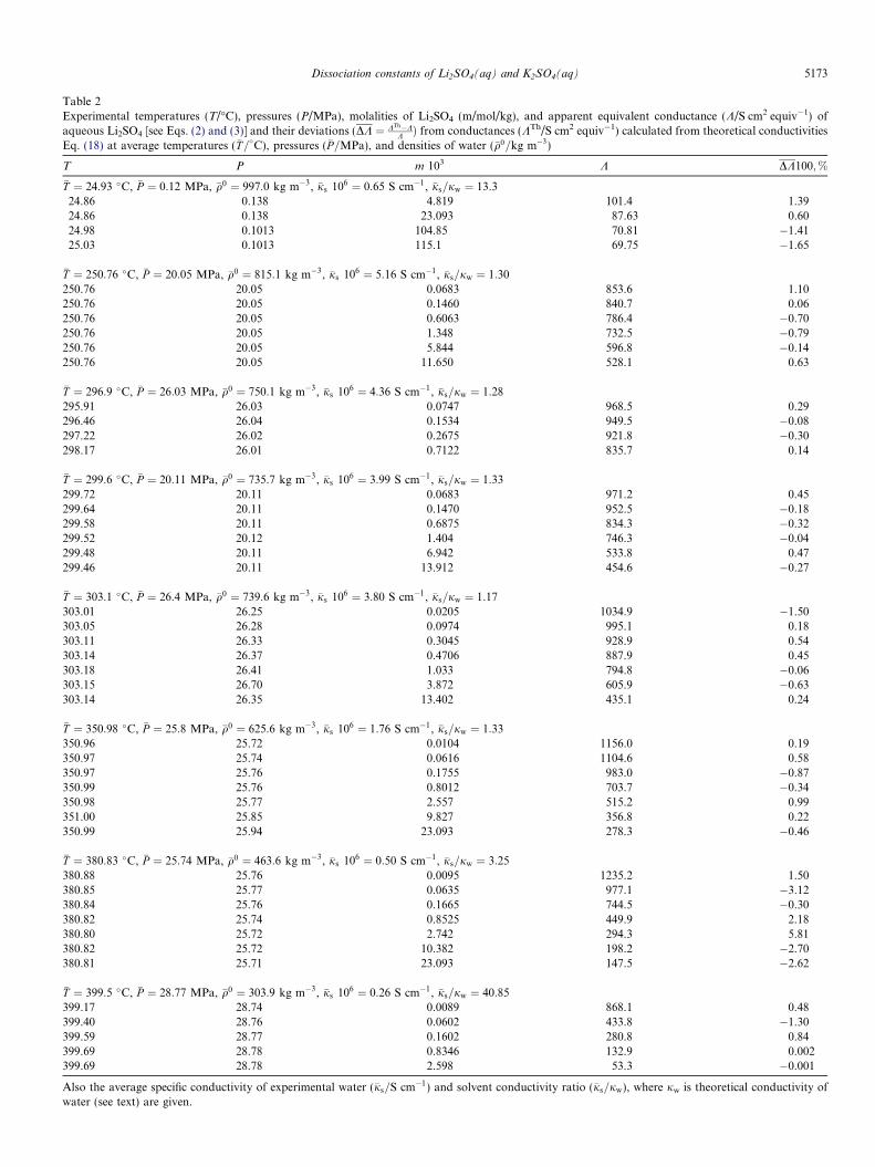
Table 2Experimental temperatures (T/�C), pressures (P/MPa), molalities of Li2SO4 (m/mol/kg), and apparent equivalent conductance (K/S cm2 equiv�1) ofaqueous Li2SO4 [see Eqs. (2) and (3)] and their deviations (DK ¼ KTh�K

K Þ from conductances (KTh/S cm2 equiv�1) calculated from theoretical conductivitiesEq. (18) at average temperatures (�T=�C), pressures (�P=MPa), and densities of water (�q0=kg m�3)

T P m 103 K DK100;%

�T ¼ 24:93 �C, �P ¼ 0:12 MPa, �q0 ¼ 997:0 kg m�3, �js 106 ¼ 0:65 S cm�1, �js=jw ¼ 13:324.86 0.138 4.819 101.4 1.3924.86 0.138 23.093 87.63 0.6024.98 0.1013 104.85 70.81 �1.4125.03 0.1013 115.1 69.75 �1.65

�T ¼ 250:76 �C, �P ¼ 20:05 MPa, �q0 ¼ 815:1 kg m�3, �js 106 ¼ 5:16 S cm�1, �js=jw ¼ 1:30250.76 20.05 0.0683 853.6 1.10250.76 20.05 0.1460 840.7 0.06250.76 20.05 0.6063 786.4 �0.70250.76 20.05 1.348 732.5 �0.79250.76 20.05 5.844 596.8 �0.14250.76 20.05 11.650 528.1 0.63

�T ¼ 296:9 �C, �P ¼ 26:03 MPa, �q0 ¼ 750:1 kg m�3, �js 106 ¼ 4:36 S cm�1, �js=jw ¼ 1:28295.91 26.03 0.0747 968.5 0.29296.46 26.04 0.1534 949.5 �0.08297.22 26.02 0.2675 921.8 �0.30298.17 26.01 0.7122 835.7 0.14

�T ¼ 299:6 �C, �P ¼ 20:11 MPa, �q0 ¼ 735:7 kg m�3, �js 106 ¼ 3:99 S cm�1, �js=jw ¼ 1:33299.72 20.11 0.0683 971.2 0.45299.64 20.11 0.1470 952.5 �0.18299.58 20.11 0.6875 834.3 �0.32299.52 20.12 1.404 746.3 �0.04299.48 20.11 6.942 533.8 0.47299.46 20.11 13.912 454.6 �0.27

�T ¼ 303:1 �C, �P ¼ 26:4 MPa, �q0 ¼ 739:6 kg m�3, �js 106 ¼ 3:80 S cm�1, �js=jw ¼ 1:17303.01 26.25 0.0205 1034.9 �1.50303.05 26.28 0.0974 995.1 0.18303.11 26.33 0.3045 928.9 0.54303.14 26.37 0.4706 887.9 0.45303.18 26.41 1.033 794.8 �0.06303.15 26.70 3.872 605.9 �0.63303.14 26.35 13.402 435.1 0.24

�T ¼ 350:98 �C, �P ¼ 25:8 MPa, �q0 ¼ 625:6 kg m�3, �js 106 ¼ 1:76 S cm�1, �js=jw ¼ 1:33350.96 25.72 0.0104 1156.0 0.19350.97 25.74 0.0616 1104.6 0.58350.97 25.76 0.1755 983.0 �0.87350.99 25.76 0.8012 703.7 �0.34350.98 25.77 2.557 515.2 0.99351.00 25.85 9.827 356.8 0.22350.99 25.94 23.093 278.3 �0.46

�T ¼ 380:83 �C, �P ¼ 25:74 MPa, �q0 ¼ 463:6 kg m�3, �js 106 ¼ 0:50 S cm�1, �js=jw ¼ 3:25380.88 25.76 0.0095 1235.2 1.50380.85 25.77 0.0635 977.1 �3.12380.84 25.76 0.1665 744.5 �0.30380.82 25.74 0.8525 449.9 2.18380.80 25.72 2.742 294.3 5.81380.82 25.72 10.382 198.2 �2.70380.81 25.71 23.093 147.5 �2.62

�T ¼ 399:5 �C, �P ¼ 28:77 MPa, �q0 ¼ 303:9 kg m�3, �js 106 ¼ 0:26 S cm�1, �js=jw ¼ 40:85399.17 28.74 0.0089 868.1 0.48399.40 28.76 0.0602 433.8 �1.30399.59 28.77 0.1602 280.8 0.84399.69 28.78 0.8346 132.9 0.002399.69 28.78 2.598 53.3 �0.001

Also the average specific conductivity of experimental water (�js=S cm�1) and solvent conductivity ratio (�js=jw), where jw is theoretical conductivity ofwater (see text) are given.

Dissociation constants of Li2SO4(aq) and K2SO4(aq) 5173

5174 A.V. Sharygin et al. 70 (2006) 5169–5182

where ra are the crystallographic radii of correspondingions (0.6, 1.33, 1.4, and 2.3 A for Li+, K+, H3O+, andSO4

2�, respectively) (Marcus, 1985).

3.4. Determination of solution volume

The volume of solution per 1 kg of solvent (water),dm3 kg�1, was calculated according to (Pitzer, 1991;Sedlbauer et al., 1998)

V � ¼ 1000

q0þX

i

miV 0i þ 1000Av

I lnð1þ bffiffiIpÞ

b; ð9Þ

where q0 is the water density (kg m�3), V 0i is standard par-

tial molar volume of ith solute at infinite dilution(dm3 mol�1), I is ionic strength of solution, I ¼ 1

2

Pmiz2

i ,b = 1.2 (kg1/2 mol�1/2). Coefficient Av (m3 mol�1) is definedby equation

Av ¼ 2A/RT 3o ln eoP T

� jH2O

� �; ð10Þ

where A/ (kg1/2 mol�1/2) is the Debye–Huckel slope(Pitzer, 1991) in the formulation,

A/ ¼ 13ð2pNAq0Þ1=2 e2

4pe0ekBT

� �3=2

: ð11Þ

At the highest temperatures, the standard partial molarvolumes of the ions in solution were approximated by theformula

V 0i ¼ z2

i

V 0Naþ þ V 0

Cl�

2; z2

i P 1; ð12Þ

For neutral aggregates of ions the approximation,

V 0i ¼ V 0

NaCl; z2i ¼ 0: ð13Þ

was used. The calculations of the standard volumes forV 0

Naþ , V 0Cl� , and V 0

NaCl were based on the results of Sed-lbauer et al. (1998). This approximation relies on electro-striction effects dominating the partial molar volumesnear the critical point. At the experimental molalities, set-ting the salt volume correction in Eq. (9) to zero made neg-ligible changes at 373–573 K (less than 0.02%) and smallchanges of 0.1%, 0.2%, and 1.8% at 623, 663, and 673 K,respectively. The approximations in Eqs. (12) and (13)are needed at 673 K. However, at this temperature themaximum changes are still less than the average absolutedeviation of the fit (6.9%).

3.5. Chemical equilibrium computation

The nonlinear system of mass balance equations andmass action law equations corresponding to the set of inde-pendent chemical reactions in aqueous solution was solvedby a modified Newton method (Stoer and Bulirsch, 1980).To take into account the activity coefficients and volumecorrections the solution of the non-linear chemical systemwas repeated until the desirable convergence was achieved.

3.6. Turq–Blum–Bernard–Kunz conductance model

In the TBBK model (Turq et al., 1995), the Fuoss–Onsager continuity equations were solved directly by aGreen’s function technique with the MSA pair distributionfunctions for the unrestricted primitive model (differentionic sizes). The single electrolyte solution consists of twotypes of free ions—cation (1) and anion (2)—with totalconductance given by

KF ¼ kF1 þ kF

2 ; ð14Þwhere

kFi ¼ k0

i 1þ dveli

v0i

� �1þ dX

X

� �; ð15Þ

is the i th ion conductance. In the last expression, k0i is

the limiting equivalent conductance at infinite dilution,dvel

i =v0i is the free ion electrophoretic velocity effect and

dX/X is the free ion relaxation force correction. Theion velocity at infinite dilution in electric field E isdefined by

v0i ¼ eiE

D0i

kBT; ð16Þ

where ei = zie is the electric charge of the i th ion, E is theelectric field, and D0

i is the diffusion coefficient of the ithion,

D0i ¼

k0i RT

jzijF 2; ð17Þ

where F is the Faraday number.

3.7. Mixture model

In this work, we use the same mixing rules which wereused by Sharygin and coworkers (Sharygin et al., 2001,2002) to define the theoretical conductivity, j. The consen-sus equation is for a solution with a molar ionic strength,Ic, and MSA shielding parameter, Cc, is

j½Ic;Cc� ¼ NXN c

M¼1

XNa

X¼1

xcM xa

X KMX ½Ic;Cc�; ð18Þ

where N ¼P

ccM zc

M ¼P

caX jza

X j is the equivalent concen-tration, the equivalent fractions of species in solutionare given by xc

M ¼ ccM zc

M=N and xaX ¼ ca

X jzaX j=N , the sums

are over all cations M and all anions X. The equiva-lent conductance of the pure electrolyte, KMX [Ic, Cc],is calculated by the TBBK equation at the molar ionicstrength of the Ic ¼ ð

PcM z2

M þP

cxz2xÞ=2 mixture with

the shielding parameter Cc set equal to the shieldingparameter of the mixture. Using this shielding parame-ter may be more accurate than using the shieldingparameter of the pure electrolyte as done previously(Sharygin et al., 2001). This speeds up the calculation,and the difference between the two methods is quitesmall.

Dissociation constants of Li2SO4(aq) and K2SO4(aq) 5175

4. Ion-association model and its auxiliary parameters

4.1. Ion-reaction model and constants

Basically, we investigated the following set of indepen-dent reactions between ions and ion aggregates:

H2O ¼ Hþ þOH� KW

HSO4� ¼ Hþ þ SO4

2� KH

H2SO4 ¼ Hþ þHSO4� KHH ð19Þ

MSO4� ¼ Hþ þ SO4

2� KM

M2SO4 ¼Mþ þMSO4� KMM

MHSO4 ¼Mþ þHSO4� KMH

where KW, KH, . . .,KMH are the dissociation constantsin molal concentration scale, M stands for Li or K.The dissociation constant of water Kw was calculatedaccording to Marshall and Franck (Marshall andFranck, 1981). On the basis of present conductancedata we can calculate the KMM and KM but the seconddissociation constant of sulfuric acid (KH) must beknown from other work. The KH is important becauseit determines the degree of hydrolysis of sulfate ion inaqueous solution. The hydrolysis can be written as lin-ear combination of first two independent reactions in(19)

SO42� þH2O ¼ HSO4

� þOH�: ð20Þ

In this work, we have used the new values for KH and KHH

from conductances of aqueous electrolyte mixtures ofNa2SO4 and H2SO4 at temperatures 373–673 K (Hnedkov-sky et al., 2005). It was shown that logKH at densities740–1000 kg/m3 (373–573 K) can be described by a lineardensity function

log KH ¼ �18:5þ 16q; ð21Þand logKH at densities 360–730 kg/m3 (573–673 K) is givenby a linear density function

log KH ¼ �12:1þ 7:6q: ð22ÞThe parameter q stands for the dimensionless reducedwater density and is equal qH2O=1000 kg m�3.

4.2. Limiting equivalent conductances of Li+, K+, OH�, H+,HSO4

�, LiSO4� and KSO4

�

The experimental data and theoretical calculations(Xiao and Wood, 2000) show for T < 773 K andP < 200 MPa that within experimental errors the tempera-ture dependence at constant water density of the relativelimiting equivalent conductances of different ions areapproximately the same. Thus, for two ions X and Y wecan write

1

k0½X �ok0½X �

oT

� �q

� 1

k0½Y �ok0½Y �

oT

� �q

; ð23Þ

where k0 [X] is a limiting equivalent conductance of X ion.Eq. (23) implies that the ratio of limiting equivalent con-ductances is a function of water density only. Particularlywe must find

k0½Y � � k0½X �k0½X �

� f ðqÞ: ð24Þ

This rule is reasonably accurate at high temperatures whereWaldens rule fails. However, Waldens rule predicts thatEq. (24) is also true. We choose X = NaCl because it isthe best data set of aqueous conductances. We will referto (k0 [Y] � k0 [NaCl])/k0[NaCl] as the reduced limitingequivalent conductance of ion (electrolyte) Y. In thisway, since we have a full data set for limiting equivalentconductance of NaCl (aq) as function of water densityand temperature, we can describe the conductances ofother ions (electrolytes) through Eq. (24).

Two different equations are used to represent the limit-ing equivalent conductance for sodium chloride, K0 [NaCl](cm2 S equiv�1), (Wright et al., 1961; Quist and Marshall,1968; Zimmerman et al., 1995; Gruszkiewicz and Wood,1997) which is needed to obtain k0 [Li+] and k0[K+] byEq. (24). In the temperature range 290–520 K and in thewater density (qH2O) range 800–1000 kg/m3, K0 [NaCl] canbe described with an absolute average deviation (AAD)of 0.25% by the following polynomial dependence of thelogarithm of Walden product on the reduced inverse tem-perature, t = 1000 K/T, and the logarithm of water density,d ¼ lnðqH2O=1000 kg m�3Þ, with water viscosity, g (Pa s),taken from (Sengers and Watson, 1986),

lnðK0½NaCl�gÞLT ¼ � 2:03� 1:61d � 2:13d2

� ð0:22� 0:92dÞt þ 0:054t2: ð25Þ

In the temperature range 520–700 K and in the water den-sity (qH2O) range 200–800 kg/m3 or at temperatures 700–800 K and at water densities 500–800 kg/m3, the sodiumchloride data of limiting equivalent conductance (Quistand Marshall, 1968; Zimmerman et al., 1995; Gruszkiewiczand Wood, 1997), can be described by the following poly-nomial dependence of logarithm of Walden product

lnðK0½NaCl�gÞHT ¼ �13:4þ 605d2 � 0:2jþ 0:04j2

þ ð12:8� 159d � 2010d2 � 269d3 � 109d4Þtþ ð277d þ 2261d2 þ 350d3 þ 142d4Þt2 ð26Þ� ð4þ 160d þ 1058d2 þ 114d3 þ 47d4Þt3

þ ð1þ 31d þ 176d2Þt4;

where j ¼ � o ln V H2O

oP (Pa�1) is the compressibility of water.The average absolute deviation from experimental datafor this equation is 0.35%.

Then we define

k0½Naþ� ¼ K0½NaCl�t0Naþ ½NaCl�; ð27Þ

with K0[NaCl] calculated from Eqs. (25) or (26), and theNa+ transference number, t0

Naþ ½NaCl�, from Marshall(Marshall, 1987). The relative difference between experi-

5176 A.V. Sharygin et al. 70 (2006) 5169–5182

mental data (Zimmerman et al., 1995; Gruszkiewicz andWood, 1997) for K0[LiCl] and K0[NaCl], defined by Eq.(26), fits the polynomial function from dimensionless re-duced water density (q = qH2O/1000) in the temperaturerange 600–670 K

K0½LiCl� � K0½NaCl�K0½NaCl� ¼ Dk0½Liþ �Naþ�

K0½NaCl� ¼ �0:095q2: ð28Þ

A similar relation was found for KCl data (Wright et al.,1961; Hwang et al., 1970; Ho and Palmer, 1997; Sharyginet al., 2002) in the temperature range 550–670 K,

K0½KCl� � K0½NaCl�K0½NaCl� ¼ Dk0½Kþ �Naþ�

K0½NaCl�¼ 0:28� 0:86qþ 0:72q2: ð29Þ

The value of k0[M+], where M+ is Li+ or K+, for temper-ature range 520–670 K was calculated by

k0½Mþ� ¼ k0½Naþ� þ Dk0½Mþ �Naþ�; ð30Þwhere k0[Na+] was calculated according to Eq. (27) andDk0[M+–Na+] was calculated from Eqs. (26), (28), and(29).

The limiting equivalent conductance of OH�, k0[OH�],was calculated from an interpolation of the results of(Wright et al., 1961; Bianchi et al., 1994; Ho and Palmer,1996; Ho and Palmer, 1997) using Marshall’s equation.

The limiting equivalent conductances of H+, HSO4�,

were calculated from the data of (Hnedkovsky et al.,2005). From this work we have for k0½HSO4

��

k0½HSO4�� � K0½NaCl�

K0½NaCl� ¼ �0:47� 0:15q; ð31Þ

which is valid for density H2O: 300–960 kg m�3 (373–673 K). The limiting equivalent conductances of MSO4

�

ion were approximated by the scaling relation

k0½MSO4�� ¼ k0½HSO4

�� r0;1;1

rM1;0;1

; ð32Þ

where the crystallographic radii are calculated using Eq.(8).

5. Conductance data and their analysis

5.1. Aqueous K2SO4

The pioneering electrical conductivity data of ArthurNoyes and his coworkers are very accurate and the pub-lished presentation of these data is complete and suitablefor further analysis (Noyes, 1907). The data for aqueousK2SO4 are for six temperatures from 18 up to 306 �C; start-ing from 100 �C the pressures are close to the saturationpressures of vapor–water equilibrium (Noyes and Melcher,1907). The temperatures were 18 �C, and about 100, 156,218, 281, and 306 �C. The temperatures above the 100 �Cwere dictated by use of vapor baths for the conductivityapparatus. Bromobenzene was used as a boiling substance

for 156�C, and naphthalene for 218 �C. Bromonaphthaleneand benzophenone were used as boiling substances for thetemperatures of 281 and 306 �C.

For each state-point, they measured electrical conduc-tivities of four K2SO4 aqueous solutions with concentra-tions (at 4 �C) in miliequivalents per liter: 2, 12.5, 50, and100. The total number of measured data points forK2SO4 equals 110; 42 measurements at 18 �C, 16—at eachtemperature in the range 100–218 �C, and 10—at each oflast temperatures: 281 and 306 �C.

The published (Noyes and Melcher, 1907) quantitativeanalysis of their electrical conductivity data correspondsto the state of electrolyte solutions theory in the beginningof the 20th century and it is very poor compared to con-temporary theoretical standards. We fit the Noyes datato the present conductance model with extremely goodresults (see Table 3). For all state points, we can determinelogKK and k0½SO4

2�� with excellent accuracy, and for twolast state points we can determine logKKK.

In the following we will discuss the auxiliary parametersof these fits. In the case of Noyes state points 1–4 thek0 [K+] was calculated by Marshall polynomial function(Marshall, 1987), for the 5th and 6th state points it was cal-culated through Eqs. (30) and (29). At 18 and 100 �C, thecalculated k0 [K+] exactly correspond to the published val-ues in (Robinson and Stokes, 1959). For 18 �C we usedk0 [H+] = 315 S cm2 equiv�1 from (Robinson and Stokes,1959). For all other temperatures the k0[H+] was takenfrom (Hnedkovsky et al., 2005). The k0½HSO4

�� andk0½KSO4

�� were always calculated through Eqs. (31) and(32). logKH and logKHH were taken from (Hnedkovskyet al., 2005). Our calculations were done in the regionwhere the influence of the reaction governed by KMH wasnegligible [see Eq. (19)], so logKKH was given the value 0.

The values of pressure were chosen to agree with thespecific volumes of aqueous K2SO4 solutions reported by(Noyes and Melcher, 1907).

To retrieve the k0½SO42�� and logKK at 25 �C we com-

bined the excellent electrical conductivity data set of (Jenkinsand Monk, 1950) and (Broadwater and Evans, 1974). Thecombined data set has 27 data points which belong to inter-val of K2SO4 equivalent concentrations 10�4 to 10�3. The re-sults of this fit are presented in Table 3. In this fit we usedk0 [H+] = 349.8 S cm2 equiv�1 from (Robinson and Stokes,1959). All other auxiliary parameters were calculated in thesame manner as it was in the case of Noyes data. The valuefound for k0½SO4

2�� ¼ 79:94ð4Þ is very close to the value of80.02(5) from (Robinson and Stokes, 1959).

The results of the fits of the present electrical conduc-tivity measurements of aqueous K2SO4 (Table 1) to theconductance model are presented in the last part ofTable 3. In this case the limiting equivalent conductancesof K+ were always calculated through Eqs. (29) and (30).All other necessary auxiliary parameters were calculatedon the basis of the data of (Hnedkovsky et al., 2005) inthe same way as it was done for the first two parts ofTable 3.

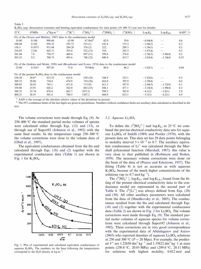
Table 3K2SO4 (aq): dissociation constants and limiting equivalent conductances for state points (18–400 �C) (see text for details)

T/�C P/MPa q0/kg m�3 k0 [K+] k0½SO42�� k0½HSO4

�� k0½KSO4�� LogKK LogKKK AADa, %

Fit of the (Noyes and Melcher, 1907) data to the conductance model18.00 0.100 998.60 63.90 67.9(6)b 42.0 39.6 �0.84(4) — 0.6

100.04 0.102 958.32 195.72 233.(1) 141.4 133.3 �1.06(2) — 0.2156.3 0.5675 911.04 284.28 376.(2) 222. 209.3 �1.36(1) — 0.2218.05 2.241 842.71 393.4 522.(13) 310. 292.3 �1.87(4) — 0.5281.04 7.8 750.57 460.4 697.(11) 399.6 376.8 �2.36(3) �1.06(4) 0.2305.35 9.2 700.75 495.6 748.(22) 440.9 415.7 �2.65(4) �1.34(4) 0.25

Fit of the (Jenkins and Monk, 1950) and (Broadwater and Evans, 1974) data to the conductance model25.00 0.1013 997.05 73.4 79.94(4) 49.0 46.2 �1.02(1) — 0.04

Fit of the present K2SO4 data to the conductance model250.58 20.07 815.35 415.6 558.(10) 344.9 325.1 �1.82(6) — 0.5300.23 20.06 734.4 474.9 710.(20) 416.8 392.9 �2.50(4) — 0.6300.85 26.03 743.1 471.0 713.(9) 411.5 387.9 �2.44(3) �1.32(9) 0.1350.96 25.91 626.2 562.0 865.(33) 506.1 477.1 �3.18(4) �1.90(4) 0.3380.25 25.74 470.4 665.7 1071.0 599.3 565.0 �4.1(2) �2.8(1) 2.8400.21 28.91 301.6 780.5 1207.2 660.9 623.1 �5.5(5) �4.2(1) 6.9

a AAD is the average of the absolute relative values of the deviations in percent.b The 95% confidence limits of the last digits are given in parentheses. Numbers without confidence limits are auxiliary data calculated as described in the

text.

Dissociation constants of Li2SO4(aq) and K2SO4(aq) 5177

The volume corrections were made through Eq. (9). At250–400 �C the standard partial molar volumes of specieswere calculated either through Eqs. (12) and (13), orthrough use of Supcrt92 (Johnson et al., 1992) with thesame final results. In the temperature range 250–300 �Cthe volume corrections were close to the volume data of(Obsil et al., 1997).

The equivalent conductances obtained from the fits andcalculated through Eqs. (18) and (2) together with theexperimental conductance data (Table 1) are shown inFig. 1 for K2SO4.

Fig. 1. Plot of experimental and calculated equivalent conductances ofaqueous K2SO4. The numbers on the lines following the temperaturescorrespond to the H2O density in kg m�3.

5.2. Aqueous Li2SO4

To define the k0½SO42�� and logKLi at 25 �C we com-

bined the previus electrical conductivity data sets for aque-ous Li2SO4 of Indelli (1989) and Postler (1970), with thepresent data set. This data set has 29 data points belongingto molality interval 5 · 10�3 to 0.7. The auxiliary equiva-lent conductance of Li+ was calculated through the Mar-shall polynomial function (Marshall, 1987); this value isvery close to that published in (Robinson and Stokes,1959). The necessary volume corrections were done onthe basis of the data of (Pearce and Eckstrom, 1937). Thefitting (Table 4) is not as accurate as with aqueousK2SO4, because of the much higher concentrations of thesolutions (up to 0.7 mol kg�1).

The k0½SO42��, logKLi, and logKLiLi found from the fit-

ting of the present electrical conductivity data to the con-ductance model are represented in the second part ofTable 4. The k0 [Li+] was always defined from Eqs. (28)and (30). All other auxiliary parameters were calculatedfrom the data of (Hnedkovsky et al., 2005). The conduc-tances resulted from the fits and calculated through Eqs.(18) and (2) together with the experimental conductancedata (Table 2) are shown in Fig. 2 for Li2SO4. The volumecorrections were made through Eq. (9). The standard par-tial molar volumes of aqueous species for volume correc-tions were calculated through Supcrt92 (Johnson et al.,1992). These corrections are in very good correspondencewith the experimental data of Abdulagatov and Azizov(2003) who reported densities of aqueous Li2SO4 solutionsat 250 and 300 �C (P = 20 Mpa). For example, the predict-ed V* are 1.22650 dm3 kg�1 and 1.35822 dm3 kg�1 at statepoints (250.8 �C, 20.05 MPa) and (299.6 �C, 20.11 MPa)for solutions with highest molality, 0.012 mol and

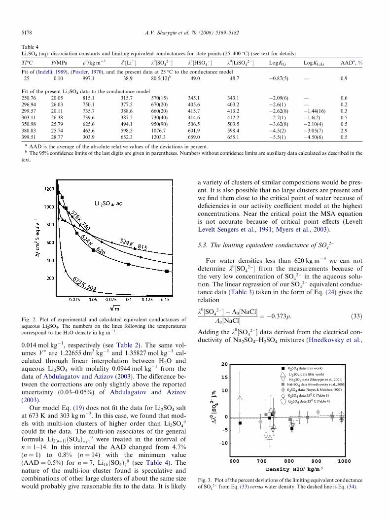
Table 4Li2SO4 (aq): dissociation constants and limiting equivalent conductances for state points (25–400 �C) (see text for details)

T/�C P/MPa q0/kg m�3 k0[Li+] k0½SO42�� k0½HSO4

�� k0½LiSO42�� LogKLi LogKLiLi AADa, %

Fit of (Indelli, 1989), (Postler, 1970), and the present data at 25 �C to the conductance model25 0.10 997.1 38.9 80.5(12)b 49.0 48.7 �0.87(5) — 0.9

Fit of the present Li2SO4 data to the conductance model250.76 20.05 815.1 315.7 570(15) 345.1 343.1 �2.09(6) — 0.6296.94 26.03 750.1 377.5 670(20) 405.6 403.2 �2.6(1) — 0.2299.57 20.11 735.7 388.6 660(20) 415.7 413.2 �2.62(8) �1.44(16) 0.3303.11 26.38 739.6 387.5 730(40) 414.6 412.2 �2.7(1) �1.6(2) 0.5350.98 25.79 625.6 494.1 950(90) 506.5 503.5 �3.62(8) �2.10(4) 0.5380.83 25.74 463.6 598.5 1076.7 601.9 598.4 �4.5(2) �3.05(7) 2.9399.51 28.77 303.9 652.3 1203.3 659.0 655.1 �5.5(1) �4.50(6) 0.5

a AAD is the average of the absolute relative values of the deviations in percent.b The 95% confidence limits of the last digits are given in parentheses. Numbers without confidence limits are auxiliary data calculated as described in the

text.

Fig. 2. Plot of experimental and calculated equivalent conductances ofaqueous Li2SO4. The numbers on the lines following the temperaturescorrespond to the H2O density in kg m�3.

Fig. 3. Plot of the percent deviations of the limiting equivalent conductanceof SO4

2� from Eq. (33) versus water density. The dashed line is Eq. (34).

5178 A.V. Sharygin et al. 70 (2006) 5169–5182

0.014 mol kg�1, respectively (see Table 2). The same vol-umes V* are 1.22655 dm3 kg�1 and 1.35827 mol kg�1 cal-culated through linear interpolation between H2O andaqueous Li2SO4 with molality 0.0944 mol kg�1 from thedata of Abdulagatov and Azizov (2003). The difference be-tween the corrections are only slightly above the reporteduncertainty (0.03–0.05%) of Abdulagatov and Azizov(2003).

Our model Eq. (19) does not fit the data for Li2SO4 saltat 673 K and 303 kg m�3. In this case, we found that mod-els with multi-ion clusters of higher order than Li2SO4

0

could fit the data. The multi-ion associates of the generalformula Li2ðnþ1ÞðSO4Þnþ1

0 were treated in the interval ofn = 1–14. In this interval the AAD changed from 4.7%(n = 1) to 0.8% (n = 14) with the minimum value(AAD = 0.5%) for n = 7, Li16ðSO4Þ80 (see Table 4). Thenature of the multi-ion cluster found is speculative andcombinations of other large clusters of about the same sizewould probably give reasonable fits to the data. It is likely

a variety of clusters of similar compositions would be pres-ent. It is also possible that no large clusters are present andwe find them close to the critical point of water because ofdeficiencies in our activity coefficient model at the highestconcentrations. Near the critical point the MSA equationis not accurate because of critical point effects (LeveltLevelt Sengers et al., 1991; Myers et al., 2003).

5.3. The limiting equivalent conductance of SO42�

For water densities less than 620 kg m�3 we can notdetermine k0½SO4

2�� from the measurements because ofthe very low concentration of SO4

2� in the aqueous solu-tion. The linear regression of our SO4

2� equivalent conduc-tance data (Table 3) taken in the form of Eq. (24) gives therelation

k0½SO42�� � K0½NaCl�K0½NaCl� ¼ �0:373q: ð33Þ

Adding the k0½SO42�� data derived from the electrical con-

ductivity of Na2SO4–H2SO4 mixtures (Hnedkovsky et al.,

Dissociation constants of Li2SO4(aq) and K2SO4(aq) 5179

2005) and aqueous Na2SO4 solutions (Sharygin et al., 2001)to the fit does not change the coefficient of linear regression(33). The percent deviations of different experimental limit-ing equivalent conductances SO4

2� are represented inFig. 3.

The linear dependence of k0½SO42�� on water density

reported in (Hnedkovsky et al., 2005) is

k0½SO42�� � K0½NaCl�K0½NaCl� ¼ �0:018� 0:35q: ð34Þ

The differences between Eqs. (33) and (34), are very small,see Fig. 3. Eq. (33) was used in this work to calculate thenecessary k0½SO4

2�� in the region of low H2O densities.The k0½SO4

2�� values derived from the electrical conduc-tivity of aqueous Li2SO4 are scattered to a greater degreethan those derived from either Na2SO4–H2SO4 or K2SO4

data (see Fig. 3).

6. Discussion

The logarithms of equilibrium constants and the limitingequivalent conductances can be described by functions oftwo independent variables: inverse temperature and densityof solvent–water (Quist and Marshall, 1968; Marshall andFranck, 1981; Marshall, 1987). The simplest equation hasfollowing form

log K ¼ Aþ BTþ C log q; ð35Þ

the more important term being C logq. The logK’srepresented in this work are in the temperature range18–400 �C (290–673 K) with a narrow pressures interval0.1–28 MPa; see Tables 3 and 4. Because of the highcorrelation between the experimental density and tempera-ture, we cannot accurately determine both B and C fromour data. As a consequence, Eq. (35) should not be usedoutside the range of our experimental data.

300 400 500 600 700 800 900 1000

Density H2O/kg/m3

-6

-5

-4

-3

-2

-1

logKK (this work)

logKKK (this work)

logKLi (this work)

logKLiLi (this work)

logKK (Noyes & Melcher, 1907)

logKKK (Noyes & Melcher, 1907)

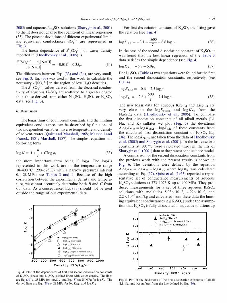
Fig. 4. Plot of the dependences of first and second dissociation constantsof K2SO4 (lines) and Li2SO4 (dashed lines) with water density. The linesare Eq. (36) at 28 MPa for logKKK and Eq. (37) at 28 MPa for logKK. Thedashed lines are Eq. (38) at 28 MPa for logKLiLi and logKLi.

For first dissociation constant of K2SO4 the fitting gavethe relation (see Fig. 4)

log KKK ¼ �3:1þ 1600

Tþ 6:6 log q: ð36Þ

In the case of the second dissociation constant of K2SO4 itwas found that the best linear regression of the Table 3data satisfies the simple dependence (see Fig. 4)

log KK ¼ �6:8þ 5:9q: ð37ÞFor Li2SO4 (Table 4) two equations were found for the firstand the second dissociation constants, respectively, (seeFig. 4)

log KLiLi ¼ �0:6þ 7:5 log q;

log KLi ¼ �2:6þ 500

Tþ 7:4 log q: ð38Þ

The new logK data for aqueous K2SO4 and Li2SO4 arevery close to the logKNaNa and logKNa from theNa2SO4 data (Hnedkovsky et al., 2005). To comparethe first dissociation constants of all alkali metals (Li,Na, and K) sulfates we plot (Fig. 5) the deviationsDlogKMM = logKMM � logKKK of these constants fromthe calculated first dissociation constant of K2SO4 Eq.(36). The logKNaNa are taken from the data of Hnedkovskyet al. (2005) and Sharygin et al. (2001). In the last case twoconstants at 300 �C were calculated through the fits ofSharygin et al. (2001) data to the present conductance model.

A comparison of the second dissociation constants fromthe previous work with the present results is shown inFig. 6. The deviations were defined by the equationDlogKM = logKM � logKK, where logKK was calculatedaccording to Eq. (37). Quist et al. (1963) reported a repre-sentative set of conductance measurements of aqueousK2SO4 solutions at 373–1073 K up to 400 MPa. They pro-duced measurements for a set of three aqueous K2SO4

solutions with molalities 5.03 · 10�4, 4.99 · 10�3, and2.2 · 10�3 mol/kg and calculated from these data the limit-ing equivalent conductances K0 [K2SO4] under the assump-tion that K2SO4 is fully dissociated in aqueous solutions up

Fig. 5. Plot of the deviations of the first dissociation constants of alkali(Li, Na, and K) sulfates from the line defined by Eq. (36).

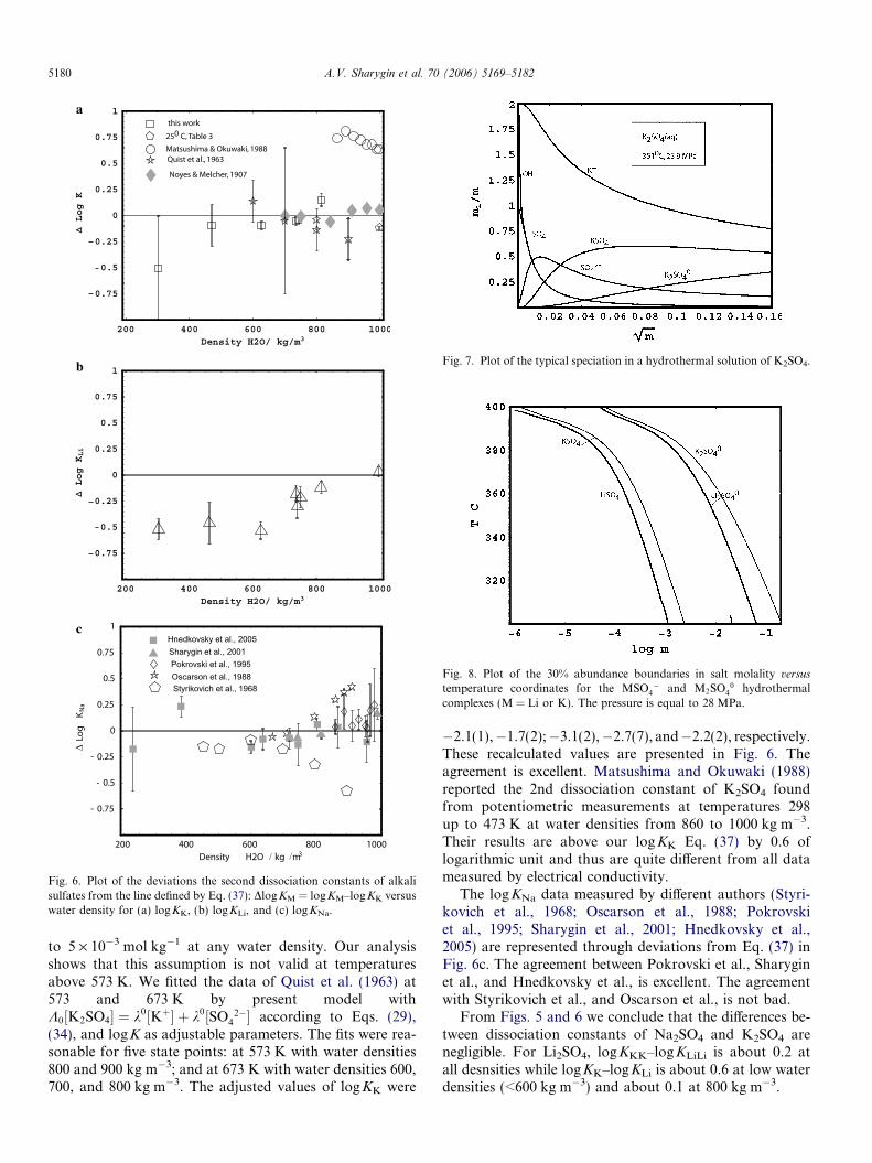
a

b

c

Fig. 6. Plot of the deviations the second dissociation constants of alkalisulfates from the line defined by Eq. (37): DlogKM = logKM–logKK versuswater density for (a) logKK, (b) logKLi, and (c) logKNa.

Fig. 7. Plot of the typical speciation in a hydrothermal solution of K2SO4.

Fig. 8. Plot of the 30% abundance boundaries in salt molality versus

temperature coordinates for the MSO4� and M2SO4

0 hydrothermalcomplexes (M = Li or K). The pressure is equal to 28 MPa.

5180 A.V. Sharygin et al. 70 (2006) 5169–5182

to 5 · 10�3 mol kg�1 at any water density. Our analysisshows that this assumption is not valid at temperaturesabove 573 K. We fitted the data of Quist et al. (1963) at573 and 673 K by present model withK0½K2SO4� ¼ k0½Kþ� þ k0½SO4

2�� according to Eqs. (29),(34), and logK as adjustable parameters. The fits were rea-sonable for five state points: at 573 K with water densities800 and 900 kg m�3; and at 673 K with water densities 600,700, and 800 kg m�3. The adjusted values of logKK were

�2.1(1),�1.7(2);�3.1(2),�2.7(7), and�2.2(2), respectively.These recalculated values are presented in Fig. 6. Theagreement is excellent. Matsushima and Okuwaki (1988)reported the 2nd dissociation constant of K2SO4 foundfrom potentiometric measurements at temperatures 298up to 473 K at water densities from 860 to 1000 kg m�3.Their results are above our logKK Eq. (37) by 0.6 oflogarithmic unit and thus are quite different from all datameasured by electrical conductivity.

The logKNa data measured by different authors (Styri-kovich et al., 1968; Oscarson et al., 1988; Pokrovskiet al., 1995; Sharygin et al., 2001; Hnedkovsky et al.,2005) are represented through deviations from Eq. (37) inFig. 6c. The agreement between Pokrovski et al., Sharyginet al., and Hnedkovsky et al., is excellent. The agreementwith Styrikovich et al., and Oscarson et al., is not bad.

From Figs. 5 and 6 we conclude that the differences be-tween dissociation constants of Na2SO4 and K2SO4 arenegligible. For Li2SO4, logKKK–logKLiLi is about 0.2 atall desnsities while logKK–logKLi is about 0.6 at low waterdensities (<600 kg m�3) and about 0.1 at 800 kg m�3.

Dissociation constants of Li2SO4(aq) and K2SO4(aq) 5181

The main result of this study is the measurement ofKLi, KLiLi, KK, and KKK in the temperature interval18–400 �C with water densities from 300 to 1000 kg m�3

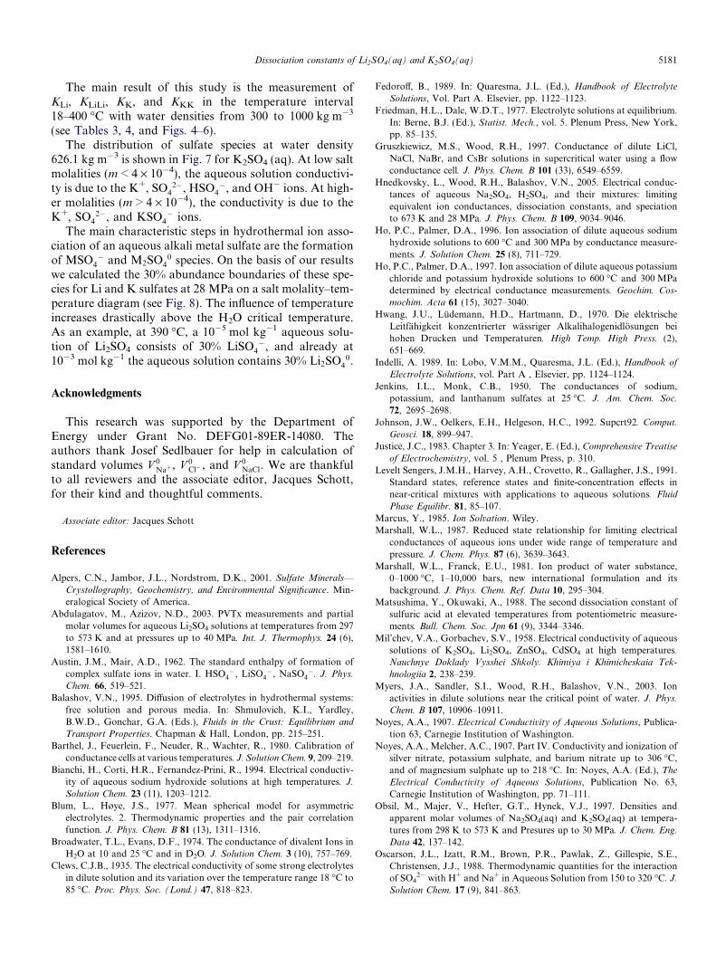
(see Tables 3, 4, and Figs. 4–6).The distribution of sulfate species at water density

626.1 kg m�3 is shown in Fig. 7 for K2SO4 (aq). At low saltmolalities (m < 4 · 10�4), the aqueous solution conductivi-ty is due to the K+, SO4

2�, HSO4�, and OH� ions. At high-

er molalities (m > 4 · 10�4), the conductivity is due to theK+, SO4

2�, and KSO4� ions.

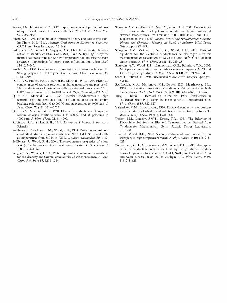
The main characteristic steps in hydrothermal ion asso-ciation of an aqueous alkali metal sulfate are the formationof MSO4

� and M2SO40 species. On the basis of our results

we calculated the 30% abundance boundaries of these spe-cies for Li and K sulfates at 28 MPa on a salt molality–tem-perature diagram (see Fig. 8). The influence of temperatureincreases drastically above the H2O critical temperature.As an example, at 390 �C, a 10�5 mol kg�1 aqueous solu-tion of Li2SO4 consists of 30% LiSO4

�, and already at10�3 mol kg�1 the aqueous solution contains 30% Li2SO4

0.

Acknowledgments

This research was supported by the Department ofEnergy under Grant No. DEFG01-89ER-14080. Theauthors thank Josef Sedlbauer for help in calculation ofstandard volumes V 0

Naþ , V 0Cl� , and V 0

NaCl. We are thankfulto all reviewers and the associate editor, Jacques Schott,for their kind and thoughtful comments.

Associate editor: Jacques Schott

References

Alpers, C.N., Jambor, J.L., Nordstrom, D.K., 2001. Sulfate Minerals—

Crystollography, Geochemistry, and Environmental Significance. Min-eralogical Society of America.

Abdulagatov, M., Azizov, N.D., 2003. PVTx measurements and partialmolar volumes for aqueous Li2SO4 solutions at temperatures from 297to 573 K and at pressures up to 40 MPa. Int. J. Thermophys. 24 (6),1581–1610.

Austin, J.M., Mair, A.D., 1962. The standard enthalpy of formation ofcomplex sulfate ions in water. I. HSO4

�, LiSO4�, NaSO4

�. J. Phys.

Chem. 66, 519–521.Balashov, V.N., 1995. Diffusion of electrolytes in hydrothermal systems:

free solution and porous media. In: Shmulovich, K.I., Yardley,B.W.D., Gonchar, G.A. (Eds.), Fluids in the Crust: Equilibrium and

Transport Properties. Chapman & Hall, London, pp. 215–251.Barthel, J., Feuerlein, F., Neuder, R., Wachter, R., 1980. Calibration of

conductance cells at various temperatures. J. Solution Chem. 9, 209–219.Bianchi, H., Corti, H.R., Fernandez-Prini, R., 1994. Electrical conductiv-

ity of aqueous sodium hydroxide solutions at high temperatures. J.

Solution Chem. 23 (11), 1203–1212.Blum, L., Høye, J.S., 1977. Mean spherical model for asymmetric

electrolytes. 2. Thermodynamic properties and the pair correlationfunction. J. Phys. Chem. B 81 (13), 1311–1316.

Broadwater, T.L., Evans, D.F., 1974. The conductance of divalent Ions inH2O at 10 and 25 �C and in D2O. J. Solution Chem. 3 (10), 757–769.

Clews, C.J.B., 1935. The electrical conductivity of some strong electrolytesin dilute solution and its variation over the temperature range 18 �C to85 �C. Proc. Phys. Soc. (Lond.) 47, 818–823.

Fedoroff, B., 1989. In: Quaresma, J.L. (Ed.), Handbook of Electrolyte

Solutions, Vol. Part A. Elsevier, pp. 1122–1123.Friedman, H.L., Dale, W.D.T., 1977. Electrolyte solutions at equilibrium.

In: Berne, B.J. (Ed.), Statist. Mech., vol. 5. Plenum Press, New York,pp. 85–135.

Gruszkiewicz, M.S., Wood, R.H., 1997. Conductance of dilute LiCl,NaCl, NaBr, and CsBr solutions in supercritical water using a flowconductance cell. J. Phys. Chem. B 101 (33), 6549–6559.

Hnedkovsky, L., Wood, R.H., Balashov, V.N., 2005. Electrical conduc-tances of aqueous Na2SO4, H2SO4, and their mixtures: limitingequivalent ion conductances, dissociation constants, and speciationto 673 K and 28 MPa. J. Phys. Chem. B 109, 9034–9046.

Ho, P.C., Palmer, D.A., 1996. Ion association of dilute aqueous sodiumhydroxide solutions to 600 �C and 300 MPa by conductance measure-ments. J. Solution Chem. 25 (8), 711–729.

Ho, P.C., Palmer, D.A., 1997. Ion association of dilute aqueous potassiumchloride and potassium hydroxide solutions to 600 �C and 300 MPadetermined by electrical conductance measurements. Geochim. Cos-

mochim. Acta 61 (15), 3027–3040.Hwang, J.U., Ludemann, H.D., Hartmann, D., 1970. Die elektrische

Leitfahigkeit konzentrierter wassriger Alkalihalogenidlosungen beihohen Drucken und Temperaturen. High Temp. High Press. (2),651–669.

Indelli, A. 1989. In: Lobo, V.M.M., Quaresma, J.L. (Ed.), Handbook of

Electrolyte Solutions, vol. Part A , Elsevier, pp. 1124–1124.Jenkins, I.L., Monk, C.B., 1950. The conductances of sodium,

potassium, and lanthanum sulfates at 25 �C. J. Am. Chem. Soc.

72, 2695–2698.Johnson, J.W., Oelkers, E.H., Helgeson, H.C., 1992. Supcrt92. Comput.

Geosci. 18, 899–947.Justice, J.C., 1983. Chapter 3. In: Yeager, E. (Ed.), Comprehensive Treatise

of Electrochemistry, vol. 5 , Plenum Press, p. 310.Levelt Sengers, J.M.H., Harvey, A.H., Crovetto, R., Gallagher, J.S., 1991.

Standard states, reference states and finite-concentration effects innear-critical mixtures with applications to aqueous solutions. Fluid

Phase Equilibr. 81, 85–107.Marcus, Y., 1985. Ion Solvation. Wiley.Marshall, W.L., 1987. Reduced state relationship for limiting electrical

conductances of aqueous ions under wide range of temperature andpressure. J. Chem. Phys. 87 (6), 3639–3643.

Marshall, W.L., Franck, E.U., 1981. Ion product of water substance,0–1000 �C, 1–10,000 bars, new international formulation and itsbackground. J. Phys. Chem. Ref. Data 10, 295–304.

Matsushima, Y., Okuwaki, A., 1988. The second dissociation constant ofsulfuric acid at elevated temperatures from potentiometric measure-ments. Bull. Chem. Soc. Jpn 61 (9), 3344–3346.

Mil’chev, V.A., Gorbachev, S.V., 1958. Electrical conductivity of aqueoussolutions of K2SO4, Li2SO4, ZnSO4, CdSO4 at high temperatures.

Nauchnye Doklady Vysshei Shkoly. Khimiya i Khimicheskaia Tek-

hnologiia 2, 238–239.Myers, J.A., Sandler, S.I., Wood, R.H., Balashov, V.N., 2003. Ion

activities in dilute solutions near the critical point of water. J. Phys.

Chem. B 107, 10906–10911.Noyes, A.A., 1907. Electrical Conductivity of Aqueous Solutions, Publica-

tion 63, Carnegie Institution of Washington.Noyes, A.A., Melcher, A.C., 1907. Part IV. Conductivity and ionization of

silver nitrate, potassium sulphate, and barium nitrate up to 306 �C,and of magnesium sulphate up to 218 �C. In: Noyes, A.A. (Ed.), The

Electrical Conductivity of Aqueous Solutions, Publication No. 63,Carnegie Institution of Washington, pp. 71–111.

Obsil, M., Majer, V., Hefter, G.T., Hynek, V.J., 1997. Densities andapparent molar volumes of Na2SO4(aq) and K2SO4(aq) at tempera-tures from 298 K to 573 K and Presures up to 30 MPa. J. Chem. Eng.

Data 42, 137–142.Oscarson, J.L., Izatt, R.M., Brown, P.R., Pawlak, Z., Gillespie, S.E.,

Christensen, J.J., 1988. Thermodynamic quantities for the interactionof SO4

2� with H+ and Na+ in Aqueous Solution from 150 to 320 �C. J.

Solution Chem. 17 (9), 841–863.

5182 A.V. Sharygin et al. 70 (2006) 5169–5182

Pearce, J.N., Eckstrom, H.C., 1937. Vapor pressures and partial volumesof aqueous solutions of the alkali sulfates at 25 �C. J. Am. Chem. Soc.

59, 2689–2691.Pitzer, K.S., 1991. Ion interaction approach: Theory and data correlation.

In: Pitzer, K.S. (Ed.), Activity Coefficients in Electrolyte Solutions.CRC Press, Boca Raton, pp. 76–148.

Pokrovski, G.S., Schott, J., Sergeyev, A.S., 1995. Experimental determi-nation of stability constants of NaSO4

� and NaBðOHÞ40 in hydro-thermal solutions using a new high-temperature sodium-selective glasselectrode—implications for boron isotopic fractionation. Chem. Geol.

124, 253–265.Postler, M., 1970. Conductance of concentrated aqueous solutions. II.

Strong polyvalent electrolytes. Coll. Czech. Chem. Commun. 35,2244–2249.

Quist, A.S., Franck, E.U., Jolley, H.R., Marshall, W.L., 1963. Electricalconductances of aqueous solutions at high temperature and pressure. I.The conductances of potassium sulfate–water solutions from 25 to800 �C and at pressures up to 4000 bars. J. Phys. Chem. 67, 2453–2459.

Quist, A.S., Marshall, W.L., 1966. Electrical conductances at hightemperatures and pressures. III. The conductances of potassiumbisulfate solutions from 0 to 700 �C and at pressures to 4000 bars. J.

Phys. Chem. 70 (11), 3714–3725.Quist, A.S., Marshall, W.L., 1968. Electrical conductances of aqueous

sodium chloride solutions from 0 to 800 �C and at pressures to4000 bars. J. Phys. Chem. 72, 684–703.

Robinson, R.A., Stokes, R.H., 1959. Electrolyte Solutions. ButterworthScientific.

Sedlbauer, J., Yezdimer, E.M., Wood, R.H., 1998. Partial molal volumesat infinite dilution in aqueous solutions of NaCl, LiCl, NaBr, and CsBrat temperatures from 550 K to 725 K. J. Chem. Thermodyn. 30, 3–12.

Sedlbauer, J., Wood, R.H., 2004. Thermodynamic properties of diluteNaCl(aq) solutions near the critical point of water. J. Phys. Chem. B

108, 11838–11849.Sengers, J.V., Watson, J.T.R., 1986. Improved international formulations

for the viscosity and thermal conductivity of water substance. J. Phys.

Chem. Ref. Data 15, 1291–1314.

Sharygin, A.V., Grafton, B.K., Xiao, C., Wood, R.H., 2000. Conductanceof aqueous solutions of potassium sulfate and lithium sulfate atelevated temperatures. In: Tremaine, P.R., Hill, P.G., Irish, D.E.,Balakrishnan, P.V. (Eds.), Steam, Water, and Hydrothermal Systems:

Physics and Chemistry Meeting the Needs of Industry. NRC Press,Ottawa, pp. 488–493.

Sharygin, A.V., Mokbel, I., Xiao, C., Wood, R.H., 2001. Tests ofequations for the electrical conductances of electrolyte mixtures:measurements of association of NaCl (aq) and Na2SO4 (aq) at hightemperatures. J. Phys. Chem. B 105 (1), 229–237.

Sharygin, A.V., Wood, R.H., Zimmerman, G.H., Balashov, V.N., 2002.Multiple ion association versus redissociation in aqueous NaCl andKCl at high temperatures. J. Phys. Chem. B 106 (28), 7121–7134.

Stoer, J., Bulirsch, R., 1980. Introduction to Numerical Analysis. Springer–Verlag.

Styrikovich, M.A., Martynova, O.I., Belova, Z.C., Menshikova, B.L.,1968. Electrolytical properties of sodium sulfate at water in hightemperatures. Dokl. Akad. Nauk U.S.S.R. 182, 644–646 (in Russian).

Turq, P., Blum, L., Bernard, O., Kunz, W., 1995. Conductance inassociated electrolytes using the mean spherical approximation. J.

Phys. Chem. B 99, 822–827.Valyashko, V.M., Ivanov, A.A., 1974. Electrical conductivity of concen-

trated solutions of alkali metal sulfates at temperatures up to 75 �C.

Russ. J. Inorg. Chem. 19 (11), 1628–1632.Wright, J.M., Lindsay, J.W.T., Druga, T.R., 1961. The Behavior of

Electrolytic Solutions at Elevated Temperatures as Derived fromConductance Measurement, Bettis Atomic Power Laboratory,pp. 1–31.

Xiao, C., Wood, R.H., 2000. A compressible continuum model for iontransport in high-temperature water. J. Phys. Chem. B 104 (5), 918–925.

Zimmerman, G.H., Gruszkiewicz, M.S., Wood, R.H., 1995. New appa-ratus for conductance measurements at high temperaturers: conduc-tance of aqueous solutions of LiCl, NaCl, NaBr, and CsBr at 28 MPaand water densities from 700 to 260 kg m�3. J. Phys. Chem. B 99,11612–11625.