discrepancy between i/b/e/s actual eps and analysts' inferred eps

Discrepancy between I/B/E/S Actual EPS and Analysts’ Inferred EPS

Lawrence D. Brown

Georgia State University

School of Accountancy

P. O. Box 4050 Atlanta, GA 30302-4050

404-413-7205

[email protected]

Stephannie Larocque

University of Notre Dame

398 Mendoza College of Business

Notre Dame, IN 46556

574-631-6136

[email protected]

November 22, 2011

We thank Brad Badertscher, Jeff Burks, William Buslepp, Gus De Franco, Peter Easton, Tom

Frecka, Yu Gao, Leo Guo, Mo Khan, Jevons Lee, Greg McPhee, Jeff Miller, Jom Ruangprapun,

Pervin Shroff, and Ling Zhou as well as seminar participants at the 2011 AAA Annual

Meeting (Denver), Tulane University, University of Minnesota, University of Notre Dame,

and Washington University (St. Louis) for their helpful comments and suggestions. We

gratefully acknowledge Thomson Reuters for providing I/B/E/S analyst earnings forecast

data. Any errors remain our responsibility.


Abstract

I/B/E/S includes actual earnings realizations to accompany the earnings-per-share (EPS) forecasts provided by its analyst contributors. These actuals are available at the firm-year (or firm-quarter) level—they do not vary by analyst. Not all analysts provide EPS forecasts to I/B/E/S on the same basis (e.g., some include special items; others exclude them). We investigate the potential discrepancy between the actual Q1 EPS reported by I/B/E/S and the inferred analyst’s Q1 EPS, which we define as the difference between the analyst’s earnings forecast for the fiscal year after the Q1 earnings announcement and her contemporaneous forecast for the remainder of the fiscal year. We find that the analyst’s inferred Q1 EPS differs from the I/B/E/S actual Q1 EPS 36.5 percent of the time, even when only one analyst follows the firm. We show that this data discrepancy varies systematically at the analyst, firm, industry, and year levels. More specifically it is more evident: (1) for analysts who forecast less frequently, who follow more firms, and who are employed by small brokerage houses; (2) for firms followed by more analysts and firms reporting non-operating or extraordinary items; (3) for the transportation and energy industries; and (4) in more recent years. We illustrate four adverse consequences of this data discrepancy: less accurate earnings forecasts, smaller earnings revision coefficients, greater analyst forecast dispersion, and smaller market reactions to I/B/E/S earnings surprises. We provide two ways for researchers to mitigate the problems we highlight: (1) use an indicator variable approach to control for the measurement error, and (2) incorporate a proxy for the magnitude of the measurement error into their models. We provide an illustration of how a research study may be impacted by the data discrepancy. Keywords: I/B/E/S actual EPS, analyst inferred actual EPS, discrepancy, accuracy, revisions, dispersion, surprises.

1


1. Introduction

Many studies use actual EPS reported by I/B/E/S when they examine analyst

forecast accuracy, analyst forecast revision, analyst forecast dispersion, and the market

reaction to analyst-based earnings surprises.1 Researchers conducting these studies

implicitly assume that individual analysts submitting their forecasts to I/B/E/S incorporate

these I/B/E/S actuals into their own earnings forecasts. However, no study to date has

examined the validity of this assumption or the adverse effects to the results of studies

when this assumption is violated. We refer to violation of this assumption as data

discrepancy, and we examine: (1) how often it occurs, (2) when it is likely to occur, (3) its

adverse consequences, (4) how to mitigate problems arising from the data discrepancy, and

(5) how an extant study may have reached different conclusions had it confined its sample

to cases where the data discrepancy is absent.

We show that the data discrepancy occurs nearly 40 percent of the time in our

sample; it varies systematically at the analyst, firm, industry, and year levels; it reduces

earnings forecast accuracy, earnings revision coefficients, and the market reaction to

earnings surprises; and it increases analyst forecast dispersion.2 In order to elaborate on

what we mean by a data discrepancy between the I/B/E/S actual EPS and the analyst

inferred EPS, we offer the following example. Firm j reports its first quarter EPS at 10am on

1 See Ramnath, Rock, and Shane (2008) for summaries of studies published after 1990, and Brown (2007)

for abstracts of articles using analyst earnings data. For a recent article in each area, see Ertimur, Sunder,

and Sunder (2007) for accuracy, Feng and McVay (2010) for revision, Barron, Byard, and Kim (2002) for dispersion, and Hugon and Muslu (2010) for market reaction to I/B/E/S earnings surprise. 2 While we focus on cases where the data discrepancy impacts the primary variables of interest, the data

discrepancy results in unreliable coefficient estimates for the primary variables of studies whose primary

variable of interest is not I/B/E/S actuals but which use I/B/E/S actuals as a control variable if measurement

error in the control variable is correlated with the primary variable of interest (Greene 2003).

2

April 12th. I/B/E/S reports the actual first quarter EPS for firm j as $0.25 at 11am on April

12th. Analysts A and B make forecasts of firm j’s second, third, and fourth quarter earnings,

and its annual earnings at noon on April 14th. More specifically,

(1) Both analysts forecast EPS of $0.25 for Q2, $0.25 for Q3, $0.25 for Q4.

(2) Analyst A forecasts $1.00 for the full fiscal year.

(3) Analyst B forecasts EPS of $1.05 for the full fiscal year.

To determine whether a data discrepancy exists between the I/B/E/S Q1 actual EPS and

analyst A’s (B’s) inferred Q1 EPS, we compare analyst A’s (B’s) forecast for the fiscal year

with the sum of analyst A’s (B’s) forecast for the remainder of the year and the I/B/E/S Q1

actual EPS. In the case of analyst A, the numbers do add up (i.e., the $1.00 forecast for the

full fiscal year equals the sum of analyst A’s forecast of $0.75 for the remainder of the year

and the I/B/E/S Q1 actual EPS of $0.25). In the case of analyst B, the numbers do not add up

(i.e., analyst B’s $1.05 forecast for the full fiscal year is five cents greater than the sum of his

forecast of $0.75 for the remainder of the year and the I/B/E/S Q1 actual EPS of $0.25). We

measure analyst A’s inferred Q1 EPS as $0.25, and analyst B’s inferred Q1 EPS as $0.30. We

say that a data discrepancy does not exist for analyst A but that it does exist for analyst B.3 4

We show that this data discrepancy, defined in our primary analysis as cases where

the I/B/E/S actual Q1 EPS differs from the analyst’s inferred Q1 EPS by at least one penny,

occurs 39% of the time. We document that this data discrepancy has analyst, firm, industry,

3 It is beyond the scope of our study to determine how much of the data discrepancy is due to analysts, how

much to I/B/E/S, how much is intentional, and how much is unintentional. Our goals are more modest. We

seek to introduce the problem of the data discrepancy, to determine its prevalence, to identify factors

associated with it, to ascertain its adverse consequences to studies that ignore it, and to provide ways to mitigate its effects. 4 According to an I/B/E/S official, I/B/E/S applies a 4¢ leverage policy, such that it would not exclude a

broker’s annual estimates when the sum of that broker’s quarterly EPS estimates are within $0.04 of the

broker’s annual EPS estimate. In our sample, we find that 88% of analysts’ fiscal-year estimates differ from

the I/B/E/S Q1 actual plus their forecast for the remainder of the year by less than |$0.04|.

3

and year effects, and that it occurs more often for analysts who forecast less frequently,

who forecast many firms, and who are employed by smaller brokerage.5 It occurs more

often for firms with non-operating or extraordinary items on their income statements and

for firms followed by more analysts. It is more evident in the transportation and energy

industries, and it has increased substantially over the time period of our study. We

document four statistically and economically significant adverse consequences of this data

discrepancy, two pertaining to analysts (reduced forecast accuracy and smaller earnings

revision coefficients) and two pertaining to firms (greater analyst forecast dispersion and

smaller market reactions to I/B/E/S earnings surprises). We provide two ways for

researchers to mitigate the problems caused by the data discrepancy. Finally, we provide an

example of how an extant study may have reached different conclusions had it focused on

observations where the data discrepancy does not exist.

We proceed as follows. We present our research questions in section 2. We discuss

our sample selection procedures and show the prevalence of the data discrepancy in section

3. We examine factors associated with the data discrepancy in sections 4 and 5,

respectively. We provide a replication of prior research in section 6, robustness tests in

section 7, and conclusions in section 8. Appendix 1 contains definitions of variables used in

our study. Appendix 2 provies additional insight on how we determine the presence or

absence of data discrepancy in our primary analysis.

5 The brokerage house effect is consistent with the contention of Ljungqvist et al. (2009).that I/B/E/S pays

more attention to large brokerage houses.

4

2. Research questions

Because we are the first to identify the aforementioned data discrepancy, it is

important to examine the extent to which researchers should be concerned about it. We

first examine its prevalence. If it occurs rarely, it is of little concern to researchers. We show

that it occurs often. Second, we examine if its occurrence is random or systematic. If it is

systematic, it is more likely to impact studies whose samples are heavily weighted in the

systematic factors. We show that it is systematic. Third, we examine the magnitude of the

adverse consequences to the results of studies that ignore it. If the magnitudes of the

coefficients of studies that ignore it are not materially affected, failure of researchers to

consider it is of little consequence. We show that the coefficients of studies that ignore it

are materially affected, both statistically and economically. Finally, we examine whether

there are ways to mitigate the adverse effects of the data discrepancy. If it is not possible to

mitigate the adverse effects of the data discrepancy, researchers have little choice but to

ignore it. We identify two ways to mitigate the problem, enabling researchers to conduct

studies whose coefficient estimates are more precise than if they continue to ignore the

data discrepancy.

In order to determine whether a discrepancy exists between the Q1 I/B/E/S actual

EPS and the analyst’s inferred Q1 EPS, we compare the Q1 I/B/E/S actual EPS with the

inferred Q1 analyst EPS for all analysts in the I/B/E/S database possessing the requisite

information. Prior to the Q1 earnings announcement, an analyst forecasts earnings of Q1

and FY (the fiscal year).6 After Q1 earnings are announced, the same analyst forecasts Q2,

Q3, Q4, and FY. We refer to the analyst’s forecasts prior to (after) the Q1 earnings

6 Of course the analyst may forecast other earnings numbers but we don’t require forecasts other than Q1

and FY.

5

announcement as her first (second) forecast, and we measure her inferred Q1 EPS by

subtracting the summation of her second forecast of Q2, Q3, and Q4 from her second

forecast of FY.7 Our first task is to determine how often the data discrepancy occurs since

the frequency of its occurrence is positively related to its potential impact on studies that do

not attempt to mitigate its effects. Our first research question (RQ1) is:

RQ1: How often does the I/B/E/S Q1 actual EPS differ from the analyst’s Q1 inferred

EPS?

After providing evidence that this data discrepancy is pervasive in our sample, we

investigate whether it is random or systematic. If it is systematic, it is likely to have a larger

potential impact on studies whose data possess the systematic factors that we document.

We consider four possible factors that may be related to this data discrepancy: analyst

effects, firm effects, industry effects, and year effects. Our second research question is:

RQ2: Is the data discrepancy we document systematically related to analyst effects,

firm effects, industry effects, and/or year effects?

After finding evidence that the data discrepancy we introduce is related to all four of

these fixed effects, we examine the adverse consequences of the data discrepancy for four

common types of studies using I/B/E/S actual EPS data.8 The importance to researchers of

7 In accordance with the preceding note, the analyst need not make a first forecast of Q2, Q3, and Q4. 8 We do not query whether any effects exist because the measurement error caused by data discrepancy guarantees that the effects exist for earnings forecast accuracy (i.e., adding measurement error reduces

unsigned earnings forecast accuracy), earnings forecast revisions and the market reaction to earnings

surprises (i.e., adding measurement error to an independent variable mitigates the magnitude of the

variable’s coefficient estimate). Our task is to determine the economic significance of the measurement

error caused by the discrepancy.

6

the data discrepancy is positively related to the magnitude of its effects on the coefficients

that researchers seek to determine.9 Our third research question is:

RQ3: What are the consequences to researchers of not controlling for the data

discrepancy we document for studies of earnings forecast accuracy, earnings forecast

revisions, earnings forecast dispersion, and the market reaction to earnings surprises?

We find that the consequences of failing to control for the data discrepancy are both

statistically significant and economically relevant in that it has a material effect on the

magnitudes of coefficients of studies of earnings forecast accuracy, earnings forecast

revisions, earnings forecast dispersion, and the market reaction to earnings surprises. After

showing that the data discrepancy is pervasive and systematic, and that it has significant

adverse consequences to studies that fail to control for it, we examine if it is possible to

mitigate the effects of the data discrepancy. Our final research question is:

RQ4: Can researchers mitigate the data discrepancy we document to provide more

reliable estimates of their variables of interest for studies of earnings forecast

accuracy, earnings forecast revisions, earnings forecast dispersion, and the market

reaction to earnings surprises?

We provide two ways for researchers to mitigate the effects of the data discrepancy.

We also provide an illustration of how an extant study may have obtained different results if

it confined its data to cases where the data discrepancy we introduce did not exist,

suggesting that researchers should conduct sensitivity analyses to determine if the results of

their studies are robust after addressing the data discrepancy problem we introduce.

9 For simplicity, we only consider the direct effects of the data discrepancy. We do not consider its effects

on studies whose focus is on variables that do not incorporate I/B/E/S actual EPS but which include these

data in their control variables. Thus, our findings probably understate the potential problems to researchers

who do not address the data discrepancy we introduce.

7

3. Sample selection procedures and evidence regarding prevalence of data

discrepancy

We extract from the I/B/E/S earnings detail files 74,009 U.S. firm-years with

available reporting dates for fiscal year t-1 (FYt-1) and the first and second quarters of fiscal

year t (Q1t and Q2t) for the 13 years, 1996 to 2008.10 We require reporting dates for FYt-1,

Q1t, and Q2t because we examine analyst forecasts made: (1) after the year t-1 report but

before the first quarter of year t report; and (2) after the first quarter of year t report but

before the second quarter of year t report. We delete 7,858 firm-years for which we cannot

obtain actual earnings (EPSt) from I/B/E/S for FYt and Q1t, leaving us with 66,151 firm-

years.11 We also delete 5,470 firm-years without share prices as of the end of year t-1

available from CRSP, resulting in 60,681 firm-years.

For these 60,681 firm-years, we search the I/B/E/S detail file for analysts who, after

the release of Q1t earnings, issued EPS forecasts for Q2t, Q3t, Q4t, and FYt on the same day.

We limit the sample to the 32,019 analyst-firm-years who issued a Q1t forecast after the

release of FYt-1 earnings but before the release of Q1t earnings. We use these 32,019

analyst-firm-years to examine the impact of data discrepancy on analyst forecast accuracy

of Q1t.12 36% (64%) of analyst-firm-years are followed by only (more than) one analyst. We

require that multiple analysts follow a firm when we examine the association of data

discrepancy with analyst effects and analyst earnings forecast dispersion.

10 We use the unadjusted I/B/E/S files, following Payne and Thomas (2003). Inferences throughout are unchanged when we use the I/B/E/S adjusted files. 11 While we require the reporting dates for year t-1and the second quarter of year t, we do not require their

actual earnings numbers. 12 These data are used in panels A and D of Table 2 shown in Section 4. The other panels of that table and

subsequent tables use smaller sample sizes as the tests have additional data restrictions.

8

We form four sub-samples of the 32,019 analyst-firm-years. We use: (1) 24,427

analyst-firm-years with FYt forecasts made after the release of FYt-1 earnings but before the

release of Q1t earnings to examine the impact of data discrepancy on analyst forecast

accuracy of FYt; (2) 21,192 analyst-firm-years with Q2t, Q3t, and Q4t forecasts made after

release of FYt-1 earnings but before release of Q1t earnings to examine the impact of data

discrepancy on analyst earnings forecast revisions; (3) 7,152 (5,169) firm-years with multiple

analyst following to examine the impact of data discrepancy on analyst forecast dispersion

in Q1t (FYt) earnings forecasts; and (4) 18,533 firm-years with non-missing CRSP stock return

data to examine the impact of data discrepancy on the capital market reaction to I/B/E/S

earnings surprises. Table 1 outlines our sample selection method.

We examine the analyst’s annual earnings forecast made after Q1 earnings is

known. We measure the absence or presence of data discrepancy based on whether or not

the I/B/E/S actual and the inferred analyst actual are within one penny of each other. More

specifically, if the analyst’s annual earnings forecast made after Q1 earnings is (not) within a

penny of the sum of the I/B/E/S Q1 actual and the analyst’s forecast for the remainder of

the year, we set DISCREP (discrepancy) equal to 0 (1).13 Appendix 2 illustrates how we

compute DISCREP.

In untabulated results, we find that DISCREP equals 0 for 19,489 observations or

61% of the analyst-firm-years and 1 for 12,530 or 39% of the analyst-firm-years. Figure 1

presents the distribution of the difference between the analysts’ inferred Q1 EPS and the

I/B/E/S Q1 actual. The median difference of 0.000 and the mean difference of -0.006 are

insignificantly different from zero. The standard deviation of the distribution is 0.244,

13 The term DISCREPijt in our accuracy and revision analyses refers to analyst-firm-years. The term

DISCREPjt in our dispersion and market reaction to earnings surprise analyses refers to firm-years.

9

revealing that 95% of the time the data discrepancy is between -0.494 and 0.483 (two

standard deviations on either side of the mean). Skewness is +78.669, indicating that the

distribution of the difference the analysts’ inferred Q1 EPS and the I/B/E/S Q1 actual is

skewed right, and kurtosis is +10,539, indicating that the distribution is leptokurtic (i.e., it

has fat tails).

4. Factors associated with data discrepancy

In order to determine if the data discrepancy is systematic or random, we estimate

the following fixed effects model using the logistic regression:

DISCREPijkt = μi + δj + λk + γt + εijkt (1)

We consider four factors, namely: (1) analyst effects (μi), (2) firm effects (δj), (3) industry

effects (λk), and (4) year (γt) effects. The dependent variable, DISCREPijkt equals 1 when

analyst i following firm j in I/B/E/S industry k in year t has an annual forecast for year t made

following the release of Q1 EPS that is not within one penny of the sum of t and 0

otherwise. The model residual is represented by εijkt. Following O’Brien (1990), we estimate

four separate fixed effects models where each model estimates only one of the four fixed

effects. Following Hamilton (1992), we evaluate the log-likelihood of each logistic model to

determine if the fixed effect helps to explain the probability that the data discrepancy

occurs.

Our estimations require multiple observations of: (1) analysts for the analyst model;

(2) firms for the firm model; (3) industries for the industry model; and (4) years for the year

model. Table 2 presents the results. When we include only analyst fixed effects, panel A of

10

Table 2 indicates that the log-likelihood ratio is -7,723.314. When we include only firm fixed

effects, the log-likelihood ratio is -10,335.4. When we include only industry fixed effects, the

log-likelihood ratio is -19,025.0. When we include only year fixed effects, the log-likelihood

ratio is -19,097.2. When we include all four fixed effects, the log-likelihood ratio is -2,835.7.

In sum, it is evident that the data discrepancy is systematically associated with analyst, firm,

industry, and year.

To learn more about these four fixed effects, we investigate each one separately.

Panel A of Table 3 presents the association of DISCREP with five analyst-level variables

commonly used in the literature (Mikhail, Walther, and Willis 1997; Clement 1999; Jacob,

Lys, and Neale 1999; Clement and Tse 2005): (1) firm experience (FEXP), (2) forecast

frequency (FREQ), (3) number of firms covered (NFIRMS), (4) brokerage size (BSIZE), and (5)

forecast horizon (HORIZON). Our results reveal that the data discrepancy is less prevalent

for analysts who forecast frequently and for analysts who work for large brokerage houses;

it is more prevalent for analysts who follow more firms. The extant literature has shown

that analysts who forecast more frequently and who work for large brokerage houses make

more accurate forecasts, whereas analysts who follow more firms make less accurate

forecasts (Clement and Tse 2005). Thus our results suggest that lower quality analysts are

relatively more likely to be subject to the data discrepancy we introduce.

Panel B examines the first firm effect, the number of analysts following the firm. The

frequency of data discrepancy increases monotonically as the number of analysts following

the firm increases, but it still occurs 36.5 percent of the time when only one follows a firm.

14

The χ2 for each model is significant at the 0.00 level.

11

Thus, the frequency of measurement errors we document is substantial, and it is not solely

attributable to the fact that I/B/E/S actuals represent the majority opinion of analysts.15

We examine a second firm effect in untabulated analysis: the presence or absence

of non-operating or extraordinary items. We test the correlation between DISCREP and

NONOP, which equals 1 when the absolute value of the difference between Q1 Compustat

operating earnings and Q1 Compustat earnings after extraordinary items exceeds one

penny. The correlation is positive and significant (0.056, p < 0.001), which suggests that

firms reporting Q1 EPS containing non-operating or extraordinary items are more likely to

display this data discrepancy.

Panel C provides pooled descriptive statistics on the percent of data discrepancy for

each of the 11 industries: Basic Industries (Basic), Capital Goods (Capital), Consumer

Durables (ConsDur), Consumer Non-Durables (ConsNonDur), Consumer Services (ConsSvc),

Energy (Energy), Finance (Finance), Health Care (Health), Technology (Technol),

Transportation (Transp), and Public Utilities (Utility). Data discrepancy ranges from around

32 percent for the capital goods industry to 45 percent or more for the utility,

transportation and energy industries.

Panel D examines year effects by estimating the following specification for the full

sample of 32,019 observations:

Pr(DISCREPijt =1) = a + b * Yearijt + eijt (2)

To facilitate interpretation of our results, we set the first year of our sample (1996) equal to

one, the second year equal to two, and so on. In addition to showing the regression result,

15 According to I/B/E/S, “when a company reports their earnings, the data is evaluated by a Market

Specialist to determine if any Extraordinary or Non-Extraordinary Items (charges or gains) have been

recorded by the company during the period… If one or more items have been recorded during the period,

actuals will be entered based upon the estimates majority basis at the time of reporting.”

12

we show the percent of the data discrepancy for each year of our sample. Our results reveal

that data discrepancy in the I/B/E/S earnings data base has significantly increased over time.

Un-tabulated results reveal that discrepancy between I/B/E/S actual EPS and analyst EPS

equals 50% in the last three years of our sample (2006-2008).

In sum, the likelihood of data discrepancy is higher for: (1) analysts who seldom

forecast, who follow more firms, and who are employed by small brokerage houses; (2)

firms with non-operating or extraordinary items and firms with greater analyst following; (3)

the energy, transportation and utility industries; and (4) in more recent years.

5. Adverse consequences of the data discrepancy

We provide univariate results for the full sample, the DISCREP = 0 and DISCREP = 1

sub-samples, and the difference between the two sub-samples. In multivariate analyses, we

document the severity of the consequences of the data discrepancy for studies of forecast

accuracy, forecast revision, forecast dispersion, and market reaction to I/B/E/S-derived

earnings surprise. To mitigate the impact of outliers, we winsorize the distributions of

accuracy, revisions, and earnings forecasts in the dispersion analysis, and the distribution of

I/B/E/S-derived earnings surprises in the top and bottom 1% of observations.

5.1 Earnings forecast accuracy

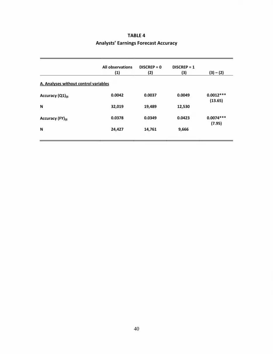
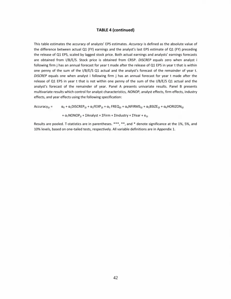
Table 4 presents separate results for modeling the accuracy of analysts’ forecasts of

both first-quarter EPS and annual EPS. For brevity, we only discuss first-quarter results in

the text, but results for annual forecasts are qualitatively similar. Accuracy is defined as the

absolute value of the difference between I/B/E/S actual earnings and the analyst’s last EPS

estimate before the release of Q1 EPS, scaled by lagged stock price (i.e., stock price as of the

13

end of fiscal year t-1) so that a smaller value indicates greater accuracy. We expect analysts

whose inferred Q1 EPS differs from the I/B/E/S Q1 actual to make less accurate earnings

forecasts because accuracy is based on the I/B/E/S actual EPS rather than the analyst’s

inferred EPS. Thus, the analyst is evaluated against a different target than she was aiming at.

Panel A presents pooled accuracy results for the full sample. Earnings forecast accuracy

averages 0.0042 across all analyst-firm-years, and it is 0.0037 and 0.0049 for DISCREP = 0

and DISCREP = 1 analyst-firm-years, respectively. The order of magnitude of unsigned error

for DISCREP = 1 is nearly one-third larger than that for DISCREP = 0, an amount which is both

economically and statistically significant (t-statistic = 13.65).

Panel B provides results of a multivariate analysis to examine the relation between

forecast accuracy and data discrepancy. We estimate the following model:

Accuracyijt = α0 + α1DISCREPijt + α2FEXPijt + α3FREQijt + α4NFIRMSijt + α5BSIZEijt

+ α6HORIZONijt + α7NONOPjt + ΣAnalyst + ΣFirm + ΣIndustry + ΣYear + eijt

(3)

We control for five analyst-firm-year effects: firm experience (FEXP), forecast

frequency (FREQ), number of firms followed (NFIRMS), brokerage size (BSIZE), and forecast

horizon (HORIZON). We also control for instances where firms have non-operating or

extraordinary items on their income statements (NONOP) along with analyst, firm, industry,

and year fixed effects. Based on prior research (Mikhail et al. 1997; Clement 1999; Jacob et

al. 1999; Clement and Tse 1995), we expect analysts who are more experienced, forecast

more often, and work for larger brokerage houses to be more accurate. We expect analysts

who follow more firms, make forecasts over longer time horizons, and forecast firms

reporting non-operating or extraordinary items to be less accurate. With the exception of

14

firm experience, the coefficients on the control variables have their expected signs.16

Analysts are less accurate if they make forecasts over longer horizons, follow more firms, or

forecast earnings with non-operating or extraordinary items.17 Analysts who forecast more

often and who are employed at large brokerage houses are more accurate, but these effects

are not significant.

As in the univariate analyses, we find that data discrepancy leads to significantly less

accurate forecasts. To assess the economic significance of our results, we compare the

coefficient on DISCREP (α1) with the intercept (α0), which represents the accuracy of

analysts whose inferred Q1 EPS are within one penny of the I/B/E/S Q1 actual EPS (after

controlling for the other factors in the model). Analysts’ one-quarter-ahead forecasts are

100% less accurate (0.0004/0.0008) when DISCREP = 1 rather than 0.18 As evidence of the

economic importance of our evidence, DISCREP’s coefficient of 0.0004 is identical to that of

NONOP, the other indicator variable.

5.2 Earnings forecast revisions

Table 5 presents results relating to the revision of analysts’ EPS forecasts for the last

nine months of the fiscal year. Panel A estimates the following equation:

REV_9Mijt = a + b * SURPijt + eijt (4)

The dependent variable (REV_9M) represents the revision of analyst i’s EPS estimate for

firm j for Q2 through Q4 of year t, defined as the difference between the analyst’s first

forecast of Q2 through Q4 issued after the release of Q1 earnings and before the release of

16 Jacob et al. (1999) also do not find more experienced analysts to be more accurate. 17 The coefficients on NFIRMS and NONOP are insignificant in the multivariate analysis of annual

forecasts. 18 Analysts’ annual earnings forecasts are 82% less accurate (0.0022/0.0121) when analysts’ actuals are

inconsistent with I/B/E/S actuals.

15

Q2 earnings and the same analyst’s last forecast of Q2 through Q4 earnings issued after the

release of year t-1 earnings and before the release of Q1 earnings, scaled by lagged stock

price. SURP is defined as the difference between the I/B/E/S actual Q1 earnings and the last

Q1 forecast issued by analyst i before the release of Q1 earnings, scaled by lagged stock

price. We expect the beta coefficient for the sub-sample without the data discrepancy to be

higher than the beta coefficient for the sub-sample with the data discrepancy because

measurement error in SURP drives the beta coefficient towards zero.

Table 5 Panel A presents pooled revision results for the sub-sample of 21,192

analyst-firm-years with the same analyst’s earnings forecasts of Q1, Q2, Q3, and Q4 EPS

made on the same day before the release of Q1 earnings. The revision slope coefficient of

1.03 for all analyst-firm-years reveals that for every $1.00 of SURP for Q1, on average,

analysts revise their EPS forecasts of the remainder of the year in the same direction of the

surprise by $1.03 (t-statistic = 53.67). As in Table 4, we partition our sample into DISCREP =

0 and DISCREP = 1. The forecast revision coefficient for the first sub-sample is significantly

larger than the forecast revision coefficient for the latter sub-sample (1.24 versus 0.85, t-

statistic of the difference = 10.01). In other words, when the inferred analyst Q1 EPS is equal

to the I/B/E/S Q1 actual EPS, for every $1.00 of SURP, on average, they revise their EPS

forecast for the remainder of the year in the same direction of the surprise by $1.24 (t-

statistic = 48.45). In contrast, when the inferred analyst Q1 EPS differs from the I/B/E/S Q1

actual EPS, for every $1.00 of SURP, on average, analysts revise their EPS forecast for the

remainder of the year in the same direction of the surprise by only $0.85 (t-statistic =

28.76). The order of magnitude of the revision coefficient for DISCREP = 0 is more than 45%

16

higher than that for DISCREP = 1, a difference which is both economically and statistically

significant (t-statistic = 10.01).

Panel B provides results which control for NONOP along with analyst, firm, industry,

and year fixed effects. More specifically, it estimates the following model:

REV_9Mijt = α0 + α1DISCREPijt + α2SURPijt + α3DISCREPijt * SURPijt + α4NONOPjt

+ ΣAnalyst + ΣFirm + ΣIndustry + ΣYear + eijt

(5)

We have no priors regarding DISCREP’s main effect (α1). Given that analysts revise

their forecasts of future quarters in the direction of their most recent forecast error (Brown

and Rozeff 1979), we expect analysts’ revisions (α2) to be positively related to SURP.

Because SURP measures the analyst’s SURP with error when the analyst’s inferred Q1 EPS

differs from the I/B/E/S Q1 actual, we expect the revision coefficient on SURP to be smaller

when DISCREP = 1 (α3). As non-operating and extraordinary items are more transitory than

operating earnings (Elliott and Hanna 1996), we expect analysts to revise their forecasts of

future earnings to a lesser extent conditional on SURP when it contains a non-operating or

extraordinary item component (α4).

The main effect of DISCREP is small in magnitude and statistically insignificant

(coefficient = -0.0002, t-value = -0.84). As expected, the coefficient on SURP is positive and

significant (1.0240, t-value = 31.91). Most importantly for our purposes, the coefficient on

DISCREP*SURP is negative and significant (-0.3939, t-value = -8.68). Thus, analysts whose

inferred Q1 EPS equals the I/B/E/S Q1 actual EPS revise their earnings forecasts for the

remainder of the year in the direction of the Q1 error 63% more than do those analysts

17

whose inferred Q1 EPS does not equal the I/B/E/S Q1 actual EPS.19 Our results are both

economically and statistically significant.20

5.3 Earnings forecast dispersion

Table 6 presents results for the dispersion of analysts’ first-quarter and annual EPS

estimates. For brevity, we only discuss the first-quarter results in the text but the annual

results are qualitatively similar. We expect mean dispersion to be smaller when all analysts

are shooting at the same target than when different analysts are shooting at a different

targets. Panel A presents estimates of dispersion as a pooled average of the standard

deviation of analysts’ EPS estimates for each firm-quarter for firms with multiple analysts

following them in a given firm-quarter. Mean dispersion (STD (Q1)) for these 7,152 firm-

years is 0.046. Mean dispersion is 0.045 for firm-years with DISCREP = 0 (all analysts are

shooting at the same target), and 0.057 for firm-years with DISCREP = 1 (different analysts

are shooting at different targets). Thus, mean dispersion for firm-years with data

discrepancy is 28% greater than for firm-years without data discrepancy. 21

Panel B presents results which control for firms’ earnings stability (STABLE), NONOP,

and fixed effects for firm, industry and year. More specifically, we estimate the model:

STD (Q1)jt = α0 + α1DISCREPjt + α2STABLEjt + α3NONOPjt + ΣFirm + ΣIndustry

+ ΣYear + ejt

(6)

19 63 percent equals 1.0240/ (1.0240-0.3939). 20 As expected, NONOP has a negative coefficient but it is not significantly different from zero. 21 Researchers who use analyst dispersion as a proxy for difference of opinion should be aware that

dispersion may reflect both differences of opinion regarding an earnings number defined a certain way (e.g., all analysts’ forecasts include restructuring charges) and differences of opinion regarding an earnings

number defined in different ways (e.g., some analysts’ forecasts exclude restructuring charges while other

analysts’ forecasts include restructuring charges). Thus, the researcher’s proxy variable includes both

differences of opinion regarding an earnings number(s) and definitional differences of what earnings

number analysts are thinking about.

18

There is likely to be less agreement among analysts when DISCREP = 1 than when

DISCREP = 0 so we expect the coefficient on DISCREP (α1) to be positive. As there is likely to

be more agreement among analysts when earnings are more stable, we expect the

coefficient on STABLE (α2) to be negative. Because there is likely to be less agreement

among analysts when firms report non-operating or extraordinary items, we expect NONOP

to have a positive coefficient (α3).

The coefficients on the two control variables are insignificant.22 More importantly,

dispersion is greater for when DISCREP = 1 than when DISCREP = 0 (α2 = 0.0037, t-value =

3.41). To determine the economic significance of our results, we compare the α1 coefficient

with the intercept (α0) which represents dispersion for firms followed by analysts who all

agree with the I/B/E/S Q1 actual. Analyst dispersion is 25% greater (.0037/.0151) when

DISCREP = 1 for at least one analyst following the firm. Our results are both economically

and statistically significant.

5.4 Market reaction coefficients

Table 7 provides results from estimating the market reaction to the first quarter

I/B/E/S earnings surprise. Panel A presents results based on the following specification:

CARjt = a + b * SURPjt + ejt (7)

CAR is the two-day (-1, 0) cumulative return minus the cumulative value-weighted market

return related to the announcement of Q1 earnings for firm j in year t. SURP is defined as

the I/B/E/S actual Q1 EPS minus the last Q1 estimate issued by an analyst following firm j

before the release of Q1 earnings, scaled by lagged stock price.23 24 We expect the beta

22 They are both significant for the analysis of annual forecasts but they have the “wrong” sign. 23 We use the last forecast in lieu of the consensus because it more closely represents market expectations

(Brown and Kim 1991).

19

coefficient for the sub-sample without the data discrepancy to be higher than the beta

coefficient for the sub-sample with the data discrepancy because measurement error in

SURP drives the beta coefficient towards zero. Using the entire sample for which we can

calculate CAR, b in equation (7) is estimated to be 1.435 (t-statistic = 19.78) conforming to

the well-documented evidence that abnormal returns are positively and significantly related

to quarterly earnings surprises (Brown and Kennelly 1972; Foster 1977). As in Tables 4 to 6,

we partition our sample into DISCREP = 0 and DISCREP = 1 sub-samples. Columns 2 and 3

respectively include firm-years for which DISCREP = 0 and DISCREP = 1 for at least one

analyst following the firm. The b coefficient for the market reaction coefficient for the

DISCREP = 0 sub-sample has nearly twice the magnitude of the DISCREP = 1 sub-sample

(1.987/1.036). This difference is also statistically significant (t-statistic = -6.48).

Panel B provides results which control for STABLE, NONOP, and fixed effects for firm,

industry, and year. More specifically, we estimate the following model:

CARjt = α0 + α1DISCREPjt + α2SURPjt + α3DISCREPjt * SURPjt + α4STABLEjt

+ α5NONOPjt + ΣFirm + ΣIndustry + ΣYear + ejt

(8)

Firms with stable earnings should have higher valuation multipliers (Beaver 1998) so

we expect α4 to be positive. The market should react less to firms’ earnings with non-

operating or extraordinary items because their earnings are more transitory (Elliott and

Hanna 1996) so we expect α5 to be negative. Scores of studies have shown that earnings

surprises are value-relevant (Ball and Brown 1968; Foster 1977; Beaver et al. 1979) so we

expect α2 to be positive. We have no priors for the main effect of DISCREP which is

24 The analyst in this regression may be an analyst for which DISCREP = 1 or DISCREP = 0. Thus, our

results probably understate the effects that we document.

20

measured by the sign of α1, but we do have a prior for the coefficient on our primary

variable of interest: the interaction of DISCREP with SURP (α3). The positive relation

between market reaction and earnings surprise should be attenuated when DISCREP = 1 so

we expect α3 to be negative.

As expected, there is a positive market reaction to I/B/E/S earnings surprises for

firm-years when DISCREP = 0 (α2 = 2.1867, t-value = 13.11). The coefficients on the control

variables STABLE and NONOP are insignificant. Most importantly for our purposes, the

positive reaction to earnings surprises is substantially mitigated for firm-years when

DISCREP = 1 (α3 = -0.6026, t-value = -2.74). To determine the economic significance of these

results we take the ratio of the coefficient of DISCREP*SURP to that of SURP. The market

reaction to the earnings surprise is 38 percent greater when DISCREP = 0 than when

DISCREP = 1. Thus, the results for our key variable of interest are both economically and

statistically significant.

6. Replication of prior research Impact of non-GAAP disclosure regulations on the probability disclosed earnings meet or beat forecasted earnings

Heflin and Hsu (2008) investigate the Impact of non-GAAP disclosure regulations on

the probability that disclosed earnings meet or beat forecasted earnings. They find that

non-GAAP disclosure regulations made effective in early 2003 are associated with a

reduction in the probability that firms disclosed earnings that meet or beat analysts’

earnings forecasts. Because the discrepancy between I/B/E/S reported actual earnings and

analysts’ inferred EPS increased over time (see Table 3, Panel D), it is possible that Heflin

21

and Hsu’s results would change if they had confined their analysis to cases where the data

discrepancy does not exist.

To investigate the possible impact of the data discrepancy between I/B/E/S reported

actual earnings and analysts’ inferred EPS on the results reported by Heflin and Hsu (2008),

we construct a data set similar to theirs for the same March 2000 to February 2005 time

period. The first column of Table 8 is our replication of Table 5 in Heflin and Hsu (2008)

using a sample of 35,142 firm-quarters.25 We use variable definitions similar to those in

Heflin and Hsu (2008), including:

NGREGq, which equals 1 if quarter q is the first quarter of 2003 or later and zero otherwise;

POST_01q, which equals one if quarter q is the first quarter of 2002 or later and zero

otherwise;

SOXq, which equals one if quarter q is the third quarter of 2002 or later and zero otherwise;

SPECiq, which equals one if firm I reports a special item in quarter q and zero otherwise;

LOSSiq, which equals one if firm I’s GAAP earnings in quarter q are less than zero, and zero

otherwise;

UPEARNiq, which equals one if firm I’s GAAP earnings in quarter q are greater than or equal

to earnings in the same quarter from the previous year, and zero otherwise;

GROWTHiq, firm I’s quarter q sales growth over the previous year’s same quarter sales;

BTMiq, the ratio of book value of equity over market value of equity for firm I in quarter q;

LEViq, total liabilities divided by book value of shareholders’ equity;

N_ANLSTiq, the number of analysts following firm I in quarter q;

FCSTDiq, the standard deviation of the most recent analysts’ forecasts for firm I in quarter q;

25Our sample is qualitatively similar to Heflin and Hsu (2008)’s sample of 38,886 firm-quarters.

22

TECHi, which equals one if firm I is in a high-tech industry and zero otherwise;

RETiq, firm I’s raw return over quarter q;

INDPRDq, the percentage change in the quarterly seasonal adjusted industrial production;

and QTR4q, which equals one if quarter q is a fourth quarter and zero otherwise .

We present results of our replication of Table 5 in Heflin and Hsu (2008) in the first

column of Table 8. Similar to Heflin and Hsu (2008), we obtain positive coefficients on

POST_01, SPEC, UPEARN, GROWTH, TECH, and RET, negative coefficients on SOX and

FCSTD., and, most importantly, a negative coefficient for Heflin and Hsu’s primary variable

of interest NGREG.26 The second column of Table 8 limits the sample to those 3,820 firm-

quarters used in Column 1 which we identify as DISCREP = 1. In this sub-sample, we again

find a negative and significant coefficient on NGREG. The third column limits the sample to

those 11,931 firm-quarters used in Column 1 which we identify as DISCREP = 0. In this sub-

sample, we do not obtain a significant coefficient on NGREG. Moreover, the magnitude of

the coefficient on NGREG in column three is 94.2% smaller than that in column two. Overall,

the analysis reported by Heflin and Hsu (2008) appears to be affected by the discrepancy

between I/B/E/S reported actual earnings and analysts’ inferred EPS.

7. Robustness tests using a continuous measure of data discrepancy

To this point we have measured DISCREP as a zero-one indicator variable based on

whether there is at least a penny difference between the analyst’s inferred EPS and the

I/B/E/S actual EPS. This approach has two disadvantages: (1) it ignores the magnitude of the

data discrepancy; and (2) the penny cutoff is arbitrary. We repeat our multivariate analyses

26 With the exception of SOX, all the variables are significant.

23

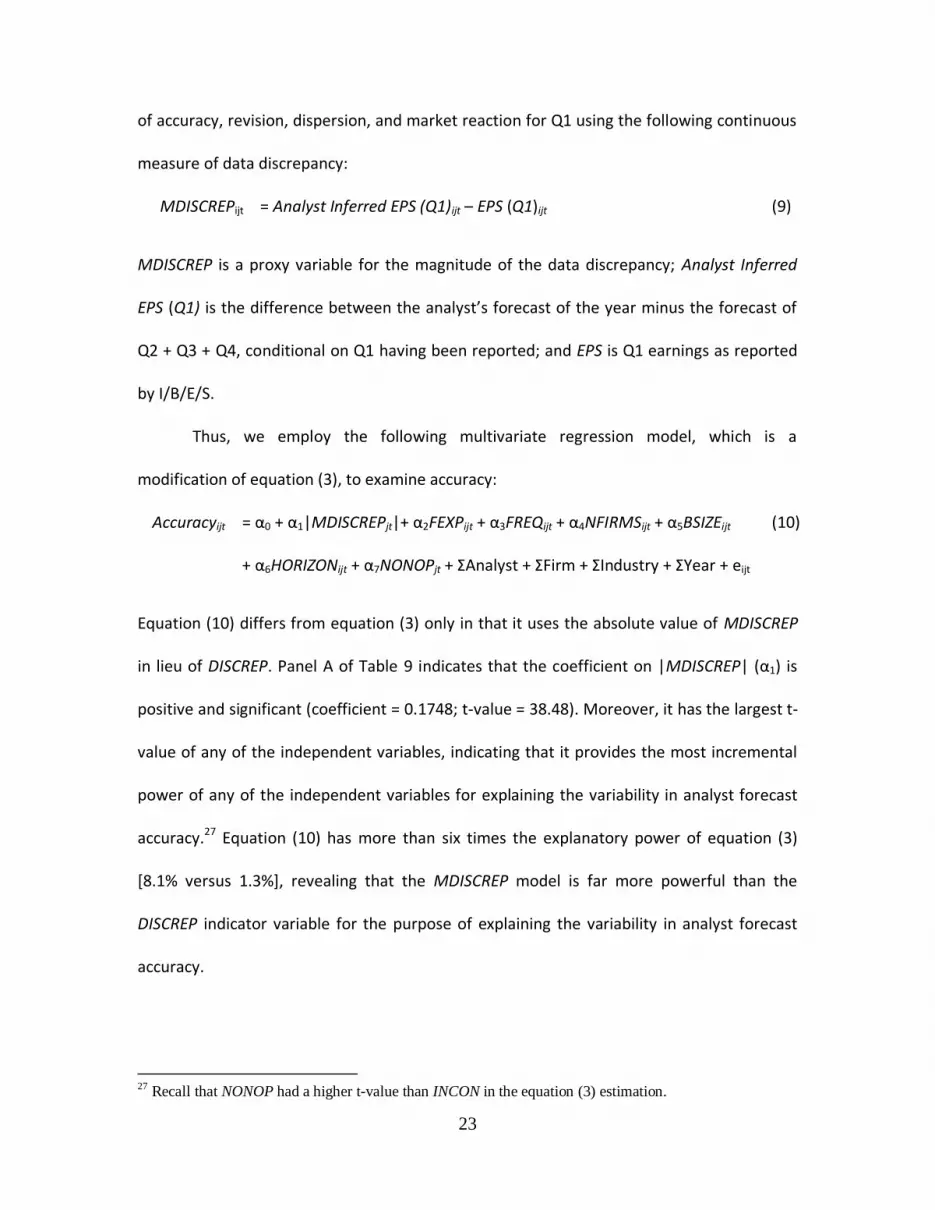
of accuracy, revision, dispersion, and market reaction for Q1 using the following continuous

measure of data discrepancy:

MDISCREPijt = Analyst Inferred EPS (Q1)ijt – EPS (Q1)ijt (9)

MDISCREP is a proxy variable for the magnitude of the data discrepancy; Analyst Inferred

EPS (Q1) is the difference between the analyst’s forecast of the year minus the forecast of

Q2 + Q3 + Q4, conditional on Q1 having been reported; and EPS is Q1 earnings as reported

by I/B/E/S.

Thus, we employ the following multivariate regression model, which is a

modification of equation (3), to examine accuracy:

Accuracyijt = α0 + α1|MDISCREPjt|+ α2FEXPijt + α3FREQijt + α4NFIRMSijt + α5BSIZEijt

+ α6HORIZONijt + α7NONOPjt + ΣAnalyst + ΣFirm + ΣIndustry + ΣYear + eijt

(10)

Equation (10) differs from equation (3) only in that it uses the absolute value of MDISCREP

in lieu of DISCREP. Panel A of Table 9 indicates that the coefficient on |MDISCREP| (α1) is

positive and significant (coefficient = 0.1748; t-value = 38.48). Moreover, it has the largest t-

value of any of the independent variables, indicating that it provides the most incremental

power of any of the independent variables for explaining the variability in analyst forecast

accuracy.27 Equation (10) has more than six times the explanatory power of equation (3)

[8.1% versus 1.3%], revealing that the MDISCREP model is far more powerful than the

DISCREP indicator variable for the purpose of explaining the variability in analyst forecast

accuracy.

27 Recall that NONOP had a higher t-value than INCON in the equation (3) estimation.

24

We run the following multivariate regression which is a modification of equation (6),

to examine analyst forecast dispersion:

STD (Q1)jt = α0 + α1|MDISCREPjt|+ α2STABLEjt + α3NONOPjt + ΣFirm + ΣIndustry

+ ΣYear + ejt

(11)

Equation (11) differs from equation (6) in only one way; it uses the absolute value of the

magnitude of DISCREP in lieu of DISCREP. Panel A of Table 9 indicates that the coefficient on

|MDISCREP| (α1) is positive and significant (coefficient = 0.1985, t-value = 3.58), and it has

the largest t-value of any of the independent variables, indicating it provides the greatest

incremental power for explaining the variability in earnings forecast dispersion. Equation

(12) has similar explanatory power to equation (6) [2.3% versus 2.3%], revealing that the

MDISCREP model is as powerful as the DISCREP model in spite of the fact that the latter

model has one fewer explanatory variable.

We employ the following multivariate regression which is a modification of equation

(5), to examine analyst forecast revisions:

REV_9Mijt = α1QN1ijt + α2QN2ijt + α3QN3ijt + α4QN4ijt + α5QN5ijt + α6SURP * QN1ijt

+ α7SURP * QN2ijt + α8SURP * QN3ijt + α9SURP * QN4ijt + α10SURP * QN5ijt

+ α11NONOPjt + ΣAnalyst + ΣFirm + ΣIndustry + ΣYear + eijt

(12)

Equation (12) differs from equation (5) insomuch as it interacts SURP with the quintile

ranking of the absolute value of MDISCREP.28 While the focal point of equation (5) is on the

interaction term between DISCREP and SURP, in equation (12) we are interested in how the

coefficient on SURP changes as we move from the lowest (QN1) to the highest (QN5)

28 Unlike accuracy and dispersion, the results of revisions and market reaction cannot easily be compared

using MDISCEP versus DISCREP since the MDISCREP formulations have more explanatory variables

than their DISCREP counterparts.

25

quintile of the absolute value of MDISCREP. We expect the analyst to revise his earnings

forecast of the remainder of the year in the direction of SURP. Thus, we expect the

coefficient on SURP to be positive. We also expect the coefficient on SURP to decrease as

we move to higher levels of MDISCREP because increased measurement error drives the

coefficient estimate to zero. Consistent with our expectations, panel B of Table 9 reveals

that the coefficient of SURP decreases nearly monotonically as the quintile rank of

MDISCREP increases.29

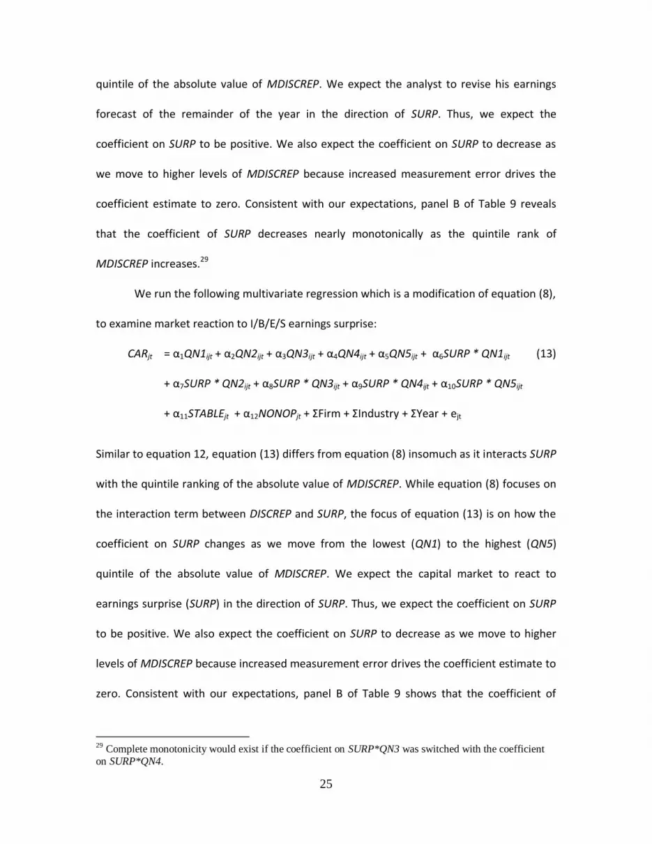
We run the following multivariate regression which is a modification of equation (8),

to examine market reaction to I/B/E/S earnings surprise:

CARjt = α1QN1ijt + α2QN2ijt + α3QN3ijt + α4QN4ijt + α5QN5ijt + α6SURP * QN1ijt

+ α7SURP * QN2ijt + α8SURP * QN3ijt + α9SURP * QN4ijt + α10SURP * QN5ijt

+ α11STABLEjt + α12NONOPjt + ΣFirm + ΣIndustry + ΣYear + ejt

(13)

Similar to equation 12, equation (13) differs from equation (8) insomuch as it interacts SURP

with the quintile ranking of the absolute value of MDISCREP. While equation (8) focuses on

the interaction term between DISCREP and SURP, the focus of equation (13) is on how the

coefficient on SURP changes as we move from the lowest (QN1) to the highest (QN5)

quintile of the absolute value of MDISCREP. We expect the capital market to react to

earnings surprise (SURP) in the direction of SURP. Thus, we expect the coefficient on SURP

to be positive. We also expect the coefficient on SURP to decrease as we move to higher

levels of MDISCREP because increased measurement error drives the coefficient estimate to

zero. Consistent with our expectations, panel B of Table 9 shows that the coefficient of

29 Complete monotonicity would exist if the coefficient on SURP*QN3 was switched with the coefficient

on SURP*QN4.

26

SURP decreases monotonically as the amount of the measurement error in SURP (as proxied

by the quintile of the absolute value of MDISCREP) increases.

8. Conclusion

We examine the prevalence of, factors associated with, and consequences of data

discrepancy between I/B/E/S actual EPS and analysts’ inferred EPS. We find that the I/B/E/S

actual EPS differs from the analyst’s inferred actual EPS 39% of the time. Thus, the data

discrepancy we discover is prevalent in the I/B/E/S earnings database. The data discrepancy

we discover is systematic, being associated with analyst, firm, industry, and year. It is more

likely to pertain to analysts who forecast infrequently, follow many firms and work for small

brokerage houses. It is more prevalent for firms reporting non-operating or extraordinary

items and firms followed by more analysts. It occurs more often in the energy,

transportation and utility industries. We show four adverse consequences of this data

discrepancy: (1) less accurate earnings forecasts by analysts; (2) smaller forecast revision

coefficients by analysts; (3) more disperse earnings forecasts among analysts following a

firm; (4) and lower market reactions to firms’ I/B/E/S-based earnings surprises. Our results

are both statistically and economically significant. The order of magnitude that we identify

is large, as is evident by our univariate results for Q1 when I/B/E/S actuals differ from the

analysts’ inferred actuals: (1) Absolute forecast error is nearly 100% larger; (2) Forecast

revision coefficients are 38% smaller; (3) Dispersion of analyst forecasts is more than 25%

larger; and (4) Capital markets react nearly 28% less to I/B/E/S-derived earnings surprises.

We provide two methods for users of I/B/E/S actual EPS data to increase the power

of their tests when they examine forecast accuracy, forecast revisions, forecast dispersion,

27

or market reaction to I/B/E/S earnings surprises. One method is to use an indicator variable

for the data discrepancy, setting DISCREP equal to one if the I/B/E/S actual differs from the

analyst’s inferred actual by at least a penny. The other approach is to use a continuous

variable, which is our proxy for the magnitude of the data discrepancy, measured as the

analyst’s inferred actual minus the I/B/E/S actual.

We investigate whether our data discrepancy findings might affect prior published

results. We replicate findings in Heflin and Hsu (2008), who investigate the Impact of non-

GAAP disclosure regulations on the probability that disclosed earnings meet or beat

forecasted earnings. While we obtain similar results to Heflin and Hsu using both a similar

sample to theirs, and using a sub-sample of firm-quarters for which we can identify DISCREP

= 1, we fail to find that their result in a sub-sample of firm-quarters for which DISCREP = 0.

We thus conclude that the analysis reported by Heflin and Hsu appears to be affected by the

discrepancy between I/B/E/S reported actual earnings and analysts’ inferred EPS.

Our study is related to the recent study by Ljungqvist, Malloy, and Marston (2009).

Both studies document that I/B/E/S data are inconsistent but the two studies differ in three

major respects. First, Ljungqvist et al. find inconsistencies in the I/B/E/S recommendations

data base while we demonstrate discrepancies in I/B/E/S actual earnings and analyst

earnings. Second, Ljungqvist et al. assert that inconsistencies in the recommendations data

base have been mitigated in recent years while we find that discrepancies in the earnings

data base have become more pervasive in recent years. Third, Ljungqvist et al. maintain that

researchers cannot address most of the problems they identify while we offer researchers

two methods for addressing all the problems we identify.

28

We recommend that researchers conduct sensitivity analyses to determine if their

results are impacted by the data discrepancy we introduce. We also recommend that

researchers determine whether the data discrepancy exists in other data sources (Zacks,

First Call) and in international data. We predict that it is pervasive in other data sources and

that it is not confined to U.S. data.

29

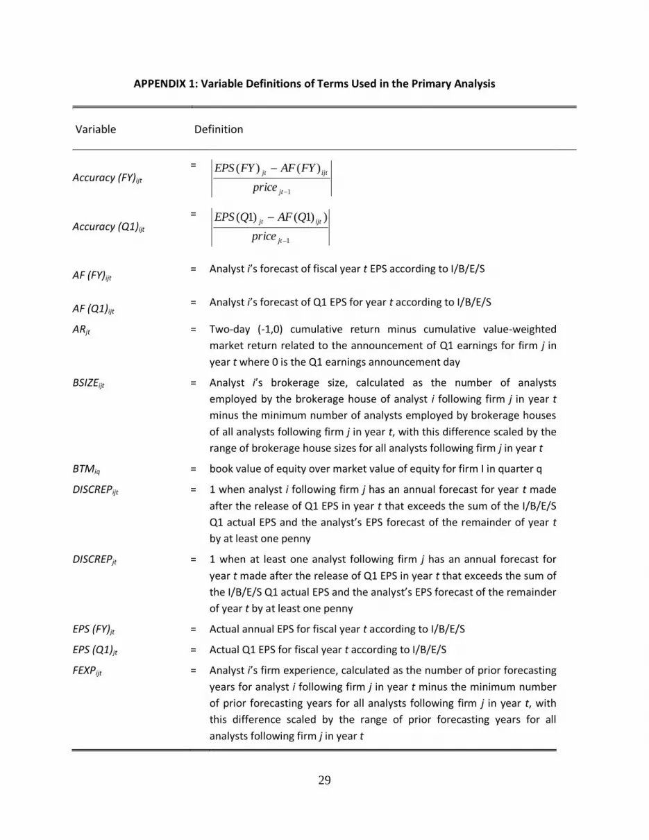
APPENDIX 1: Variable Definitions of Terms Used in the Primary Analysis

\

Variable Definition

Accuracy (FY)ijt =

1

)()(

jt

ijtjt

price

FYAFFYEPS

Accuracy (Q1)ijt =

1

))1()1(

jt

ijtjt

price

QAFQEPS

AF (FY)ijt = Analyst i’s forecast of fiscal year t EPS according to I/B/E/S

AF (Q1)ijt = Analyst i’s forecast of Q1 EPS for year t according to I/B/E/S

ARjt = Two-day (-1,0) cumulative return minus cumulative value-weighted

market return related to the announcement of Q1 earnings for firm j in

year t where 0 is the Q1 earnings announcement day

BSIZEijt = Analyst i’s brokerage size, calculated as the number of analysts

employed by the brokerage house of analyst i following firm j in year t

minus the minimum number of analysts employed by brokerage houses

of all analysts following firm j in year t, with this difference scaled by the

range of brokerage house sizes for all analysts following firm j in year t

BTMiq = book value of equity over market value of equity for firm I in quarter q

DISCREPijt = 1 when analyst i following firm j has an annual forecast for year t made

after the release of Q1 EPS in year t that exceeds the sum of the I/B/E/S

Q1 actual EPS and the analyst’s EPS forecast of the remainder of year t

by at least one penny

DISCREPjt = 1 when at least one analyst following firm j has an annual forecast for

year t made after the release of Q1 EPS in year t that exceeds the sum of

the I/B/E/S Q1 actual EPS and the analyst’s EPS forecast of the remainder

of year t by at least one penny

EPS (FY)jt = Actual annual EPS for fiscal year t according to I/B/E/S

EPS (Q1)jt = Actual Q1 EPS for fiscal year t according to I/B/E/S

FEXPijt = Analyst i’s firm experience, calculated as the number of prior forecasting

years for analyst i following firm j in year t minus the minimum number

of prior forecasting years for all analysts following firm j in year t, with

this difference scaled by the range of prior forecasting years for all

analysts following firm j in year t

30

FREQijt = Analyst i’s forecast frequency, calculated as the number of firm j

forecasts made by analyst i following firm j in year t minus the minimum

number of firm j forecasts for all analysts following firm j in year t, with

this difference scaled by the range of number of firm j forecasts issued

by all analysts following firm j in year t

GROWTHiq = firm i’s quarter q sales growth over the previous year’s same quarter

sales

HORIZONijt = Analyst i’s horizon, calculated as the number of days from the year t

forecast date (following the release of Q1 earnings) to the earnings

announcement date for analyst following firm j in year t minus the

minimum forecast horizon for all analysts who follow firm j in year t,

with this difference scaled by the range of forecast horizons for all

analysts following firm j in year t

INDPRDq = percentage change in the quarterly seasonal adjusted industrial

production

LOSSiq = 1 if firm i’s GAAP earnings in quarter q are less than zero

MDISCREPijt = Analyst inferred actual – IBES actual, scaled by pricet-1, where the analyst

inferred actual is the difference between analyst i’s forecast for the fiscal

year and the sum of the analyst’s forecasts for Q2, Q3, and Q4 of the

same year

N_ANLSTiq = number of analysts following firm i in quarter q

NFIRMSijt = The number of firms followed, calculated as the total number of firms

followed by analyst i following firm j in year t minus the minimum

number of firms followed by all analysts covering firm j in year t, with

this difference scaled by the range of the number of firms followed by all

analysts covering firm j in year t

NGREGq = 1 if quarter q is the first quarter of 2003 or later

NONOPjt = 1 when the absolute value of the difference between Q1 EPS Compustat

operating earnings and Compustat earnings after extraordinary items for

year t exceeds one penny for firm j in year t

POST_01q = 1 if quarter q is the first quarter of 2002 or later

Pricejt-1 = Stock price as of the end of fiscal year t-1 according to CRSP

QN1 … QN5 = Indicator variables that = 1 if the absolute value of MDISCREP is in the

first … fifth quintile

QTR4q = 1 if quarter q is a fourth quarter

RETiq =

firm i’s raw return over quarter q

31

REV_9Mijt = The difference between analyst i’s first estimate of Q2 through Q4 issued

after the release of Q1 earnings and the same analyst’s last estimate of

Q2 through Q4 issued before the release of Q1 earnings, scaled by stock

price as of the end of fiscal year t-1 according to CRSP

SOXq = 1 if quarter q is the third quarter of 2002 or later

SPECiq = 1 if firm i reports a special item in quarter q

STABLEjt = I/B/E/S stability measure, defined by I/B/E/S as a gauge of annual EPS

growth consistency over the past 5 years

STDjt = Standard deviation of analysts’ EPS estimates for firm j, for a given

quarter or year t, for those firms with >1 analyst following in our sample

SURPjt =

1

)1()1(

jt

jtjt

price

QAFQEPS

UPEARNiq = 1 if firm i’s GAAP earnings in quarter q are greater than or equal to

earnings in the same quarter from the previous year

32

APPENDIX 2: Calculation of the DISCREP variable

Assume: EPS (Q1) = Actual Q1 EPS according to I/B/E/S AF (FY/Q1) = Analyst’s forecast of annual EPS according to I/B/E/S issued after the quarter 1 earnings announcement AF(Q2-Q4/Q1)= Analyst’s forecast of EPS for the remainder of the fiscal year issued after the quarter 1 earnings announcement We define the Analyst’s Inferred EPS (Q1) = AF(FY/Q1) – AF(Q2-Q4/Q1)

DISCREP = 1 if: |Analyst Inferred EPS (Q1) – EPS (Q1)| > 0.01 and DISCREP = 0 if: |Analyst Inferred EPS (Q1) – EPS(Q1)| ≤ 0.01

33

References

Ball, R. and P. Brown. 1968. An empirical evaluation of accounting income numbers.

Journal of Accounting Research 6 (2): 159-178.

Barron, O., D. Byard, and O. Kim. 2002. Changes in analysts’ information around earnings announcements. The Accounting Review 77 (4): 821-846. Beaver, W. 1998. Financial Reporting: An Accounting Revolution, Third Edition, Prentice Hall, Englewood Cliffs, New Jersey.

Beaver, W., R. Clarke, and W. Wright. 1979. The association between unsystematic

security returns and the magnitude of earnings forecast errors. Journal of Accounting

Research 17 (2): 316-340.

Bhattacharya, N., E. Black, T. Christensen, and C. Larson. 2003. Assessing the relative informativeness and permanence of pro forma earnings and GAAP operating earnings. Journal of Accounting and Economics 36 (1-3): 285-319.

Bradshaw, M. 2003. A discussion of ‘Assessing the relative informativeness and permanence of pro forma earnings and GAAP operating earnings.’ Journal of Accounting and Economics 36 (1-3): 321-335.

Bradshaw, M. and R. Sloan. 2002. GAAP versus the street: An empirical assessment of two alternative definitions of earnings. Journal of Accounting Research 40 (1): 41-66.

Brown, L. (editor). 2007. Thomson Financial Research Bibliography. First Edition. Thomson. New York.

Brown, L. and K. Kim. 1991. Timely aggregate analyst forecasts as better proxies for market earnings expectations. Journal of Accounting Research 29 (2): 382-385.

Brown, L. and K. Sivakumar. 2003. Comparing the value relevance of two operating income measures. Review of Accounting Studies 8 (4): 561-572.

Brown, L. and M. Rozeff. 1979. Adaptive expectations, time-series models, and analyst forecast revision. Journal of Accounting Research 17 (2): 341-351.

Brown, P. and J. Kennelly. 1972. The informational content of quarterly earnings: An extension and some further evidence. Journal of Business 45 (3): 403-415.

Clement, M. 1999. Analyst forecast accuracy: Do ability, resources and portfolio complexity matter? Journal of Accounting and Economics 27 (3): 285-303.

Clement, M. and S. Tse. 2005. Financial analyst characteristics and herding behavior in forecasting. Journal of Finance 60 (1): 307-341.

Doyle, J., R. Lundholm, and M. Soliman. 2003. The predictive value of expenses excluded from pro forma earnings. Review of Accounting Studies 8 (2-3): 145-174.

Elliott, J. and J. Hanna. 1996. Repeated accounting write-offs and the information

content of earnings. Journal of Accounting Research 34 (Supplement): 135-155.

Ertimur, Y., J. Sunder, and S. Sunder. 2007. Measure for measure: The relation between forecast accuracy and recommendation profitability of analysts. Journal of Accounting Research 45 (3): 567-606.

Feng, M. and S. McVay. 2010. Analysts’ incentives to overweight management guidance when revising their short-term earnings forecasts. The Accounting Review 85 (5): 1617-1646.

Foster, G. 1977. Quarterly accounting data: Time series properties and predictive-ability results. The Accounting Review 52 (1): 1-21.

34

Greene, W. 2003. Econometric Analysis, Fifth Edition. Pearson Education, Upper Saddle River, New Jersey.

Hamilton, L. 1992. Regression with Graphics. Wadsworth, Inc. Heflin, F., and C. Hsu. 2008. The impact of the SEC’s regulation of non-GAAP disclosures. Journal of Accounting and Economics 46 (2-3): 349-365. Hugon, A. and V. Muslu. 2010. Market demand for conservative analysts. Journal of Accounting and Economics 50 (1): 42-57. Jacob, J., T. Lys, and M. Neale. 1999. Expertise in forecasting performance of security analysts. Journal of Accounting and Economics 28 (1): 51-82. Ljungqvist, A., C. Malloy, and F. Marston. 2009. Rewriting history. Journal of Finance 64 (4): 1935-1960. Mikhail, M., B. Walther, and R. Willis. 1997. Do security analysts improve their performance with experience? Journal of Accounting Research 35 (Supplement): 131-157. O’Brien, P. 1990. Forecast accuracy of individual analysts in nine industries. Journal of Accounting Research 28 (2): 286-304. Payne, J., and W. Thomas. 2003. The implications of using stock-split adjusted I/B/E/S data in empirical research. The Accounting Review 78: 1049-1067. Ramnath, S., S. Rock, and P. Shane. 2008. The financial analyst forecasting literature: taxonomy with suggestions for future research. International Journal of Forecasting 24 (1): 34-75.

35

FIGURE 1 Distribution of Differences between I/B/E/S Q1 Actual EPS and Analysts’ Inferred Q1

EPS

This Figure presents the distribution of the difference between the analysts’ inferred Q1 EPS and the

I/B/E/S Q1 actual for the analyst-firm-years in our sample. Variable definitions are in the Appendix.

36

TABLE 1 Sample Selection Procedure for the Main Analysis

Criteria Analyst-

firm-years

Firm-years

Firm-years:

U.S. firm-years with FYt-1, Q1t, and Q2t reporting dates available from I/B/E/S for

1996 to 2008

74,009

Keep: Firm-years with I/B/E/S actual Q1t and FYt earnings 66,151

Keep: Firm-years with year t-1 prices available from CRSP 60,681

Analyst-firm-years:

Analyst-firm-years with Q2t, Q3t, Q4t, and FYt EPS forecasts issued on the same

day after the release of Q1t earnings

83,789 33,650

Keep: Analyst-firm-years with Q1t EPS forecasts issued on any day after the

release of FYt-1 earnings but prior to the release of Q1t earnings (Table 4)

32,019 18,533

Analyst-firm-years with 1 analyst following in our sample 11,381 11,381

Analyst firm-years with >1 analyst following in our sample 20,638 7,152

Sub-samples:

Analyst-firm-years with FYt EPS forecasts issued after the release of FYt-1

earnings but prior to the release of Q1t earnings (Table 4)

24,427 15,060

Analyst-firm-years with Q2t, Q3t, and Q4t EPS forecasts issued after the release

of FYt-1 earnings but prior to the release of Q1t earnings (Table 5)

21,192 14,052

Analyst-firm-years with FYt EPS forecasts issued after the release of FYt-1

earnings but prior to the release of Q1t earnings, with > 1 analyst following

(Table 6)

14,537 5,169

Firm-years with non-missing CARt (Table 7) 18,533

This table summarizes the procedure used to select the sample for Tables 4-7. Variable definitions are in

Appendix 1.

37

TABLE 2 Estimation of Model with Analyst, Firm, Industry, and Year Fixed Effects

Panel A Analysts Firms I/B/E/S Industries Years Full Model1 Logit Model (1) (2) (3) (4) (5)

N 3,710 4,327 11 13 28,584

Log-likelihood -7,723.5 -10,335.4 -19,025.0 -19,097.2 -2,835.7

Prob > χ2 0.00 0.00 0.00 0.00 0.00 1 Sample sizes and full-model log-likelihood are reported.

This table estimates the following equation using a logit specification:

DISCREPijkt = μi + δj + λk + γt + εijkt

Observations in which the analyst or firm appears only once in the full sample are deleted in order to

estimate the fixed effects models. Variable definitions are in Appendix 1.

38

TABLE 3 Investigation of Analyst, Firm, Industry, and Year Effects

Panel A

Analyst Effects Intercept

(1)

FEXPijt

(2)

FREQijt

(3)

NFIRMSijt

(4)

BSIZEijt

(5)

HORIZONijt

(6)

% Concordant

Number of analyst-firm-

years

Pr(DISCREPijt)=1 0.5059 (<0.0001)

0.0500 (0.1269)

-0.1138 (0.0051)

0.0880 (0.0189)

-0.1257 (0.0005)

0.0509 (0.2956)

49.9 28,526

Panel B

Firm Effects ANF=1 ANF=2 ANF=3 ANF=4 ANF≥5

(1) (2) (3) (4) (5)

# analyst-firm-years 11,381 8,324 4,527 2,772 5,015

% DISCREPijt 0.365 0.382 0.391 0.424 0.448

Panel C

Industry Effects Basic Capital ConsDur ConsNonDur ConsSvc Energy Finance Health Technol Transp Utility Total

(1) (2) (3) (4) (5) (6) (7) (8) (9) (10) (11)

# analyst-firm-years 2,848 2,072 1,365 1,045 4,538 4,668 5,268 2,535 5,078 1,363 1,219 32,019

% DISCREPijt 36.8 32.0 37.1 33.8 40.3 47.6 36.5 36.7 37.1 45.6 45.0 39.1

39

TABLE 3 (continued)

Panel D

Year Effects Total

a -0.586***

b 0.018***

% Concordant 48.1

# analyst-firm-years 31,999

This table investigates the effects of analysts, firms, industries, and years on the DISCREP indicator

variable.

Panel A presents results based on estimating the following equation using a logit specification for the sub-

sample of analyst-firm-years for which the analyst variables could be estimated (p-values are in

parentheses):

Pr(DISCREPijt=1) = α0 + α1FEXPijt + α2FREQijt + α3NFIRMSijt + α4BSIZEijt + α5HORIZONijt + eijt

Panel B provides the number and percent of analyst-firm-years for DISCREP for one, two, three, four, and

five or more analysts following the firm.

Panel C presents the correlation of DISCREP with NONOP for analyst-firm-years that could be matched

with Compustat for 11 I/B/E/S industries: Basic Industries (Basic), Capital Goods (Capital), Consumer

Durables (ConsDur), Consumer Non-Durables (ConsNonDur), Consumer Services (ConsSvc), Energy

(Energy), Finance (Finance), Health Care (Health), Technology (Technol), Transportation (Transp), and

Public Utilities (Utility). Standard errors are in parentheses.

Panel D provides the number and percent of analyst-firm-years for DISCREP for each I/B/E/S industry and

for the full sample.

Panel E presents results of estimating the following specification for each I/B/E/S industry and for the full

sample:

Pr(DISCREPijt=1) = a + b*Yeart + eijt

Results are pooled. ***, **, and * denote significance at the 1%, 5%, and 10% levels, based on one-tailed

tests, respectively. Variable definitions are in the Appendix.

40

TABLE 4

Analysts’ Earnings Forecast Accuracy

All observations DISCREP = 0 DISCREP = 1 (1) (2) (3) (3) – (2)

A. Analyses without control variables

Accuracy (Q1)ijt 0.0042

0.0037

0.0049

0.0012*** (13.65)

N 32,019 19,489 12,530

Accuracy (FY)ijt 0.0378

0.0349

0.0423

0.0074*** (7.95)

N 24,427 14,761 9,666

41

TABLE 4 (continued)

B. Analyses with control variables

Dependent variable is: Accuracy(Q1)ijt Accuracy(FY)ijt

Intercept ? 0.0004*

(1.76) 0.0099***

(4.34)

DISCREPijt + 0.0004*** (4.62)

0.0022*** (2.92)

FEXPijt - 0.0005*** (3.42)

0.0058*** (3.91)

FREQijt - -0.0002 (-1.13)

0.0019 (1.16)

NFIRMSijt + 0.0006*** (3.43)

0.0008 (0.42)

BSIZEijt - -0.0002 (-0.73)

-0.0045* (-1.79)

HORIZONijt + 0.0013*** (6.49)

0.0037* (1.88)

NONOPjt + 0.0004*** (5.34)

0.0018** (2.43)

Analyst Effects Yes Yes

Firm Effects Yes Yes

Industry Effects Yes Yes

Year Effects Yes Yes

Adj. R2 0.013 0.021

Number of Analyst-firm-years 19,765 15,444

42

TABLE 4 (continued)

This table estimates the accuracy of analysts’ EPS estimates. Accuracy is defined as the absolute value of

the difference between actual Q1 (FY) earnings and the analyst’s last EPS estimate of Q1 (FY) preceding

the release of Q1 EPS, scaled by lagged stock price. Both actual earnings and analysts’ earnings forecasts

are obtained from I/B/E/S. Stock price is obtained from CRSP. DISCREP equals zero when analyst i

following firm j has an annual forecast for year t made after the release of Q1 EPS in year t that is within

one penny of the sum of the I/B/E/S Q1 actual and the analyst’s forecast of the remainder of year t.

DISCREP equals one when analyst i following firm j has an annual forecast for year t made after the

release of Q1 EPS in year t that is not within one penny of the sum of the I/B/E/S Q1 actual and the

analyst’s forecast of the remainder of year. Panel A presents univariate results. Panel B presents

multivariate results which control for analyst characteristics, NONOP, analyst effects, firm effects, industry

effects, and year effects using the following specification:

Accuracyijt = α0 + α1DISCREPijt + α2FEXPijt + α3 FREQijt + α4NFIRMSijt + α5BSIZEijt + α6HORIZONijt

+ α7NONOPjt + ΣAnalyst + ΣFirm + ΣIndustry + ΣYear + eijt

Results are pooled. T-statistics are in parentheses. ***, **, and * denote significance at the 1%, 5%, and

10% levels, based on one-tailed tests, respectively. All variable definitions are in Appendix 1.

43

TABLE 5 Analysts’ Earnings Forecast Revisions



b 1.0343*** (53.67)

1.2384*** (48.45)

0.8527*** (28.76)

-0.3857*** (-10.01)

Adj. R2 0.120 0.155 0.090

N 21,192 12,827 8,365


Dependent variable is: REV_9Mijt

Intercept ? -0.0001

(-0.15)

DISCREPijt ? -0.0002 (-0.84)

SURPijt + 1.0240*** (31.91)

DISCREPijt * SURPijt - -0.3939*** (-8.68)

NONOPjt - -0.0002 (-0.65)

Analyst Effects Yes

Firm Effects Yes

Industry Effects Yes

Year Effects Yes

Adj. R2 0.101

Number of Analyst-firm-years 14,459

44

TABLE 5 (continued)

This table estimates the revision of analysts’ EPS forecasts. The revision of the analyst’s EPS estimate for

Q2 through Q4 (REV_9M) is defined as the difference between the analyst’s first 9M estimate after the

release of Q1 earnings and the same analyst’s last 9M estimate before the release of Q1 earnings, scaled

by lagged stock price, where the 9M estimate is the summation of the estimates of Q2, Q3, and Q4. The

I/B/E/S earnings surprise (SURP) is defined as the difference between the I/B/E/S Q1 actual earnings and

the same analyst’s last Q1 estimate before the release of Q1 earnings, scaled by lagged stock price

DISCREP equals zero when analyst i following firm j has an annual forecast for year t made after the

release of Q1 EPS in year t that is within one penny of the sum of the I/B/E/S Q1 actual and the analyst’s

forecast of the remainder of year t. DISCREP equals one when analyst i following firm j has an annual

forecast for year t made after the release of Q1 EPS in year t that is not within one penny of the sum of

the I/B/E/S Q1 actual and the analyst’s forecast of the remainder of year.Panel A uses the following

specification:

REV_9Mijt = a + b*SURPijt + eijt

Results for the intercepts are excluded for simplicity. The final column compares the slope coefficients in

columns 2 and 3.

Panel B presents results which control for NONOP, and analyst, firm, industry, and year effects:

REV_9Mijt = α0 + α1DISCREPijt + α2SURPijt + α3 DISCREPijt * SURPij + α4NONOPjt

+ ΣAnalyst + ΣFirm + ΣIndustry + ΣYear + eijt



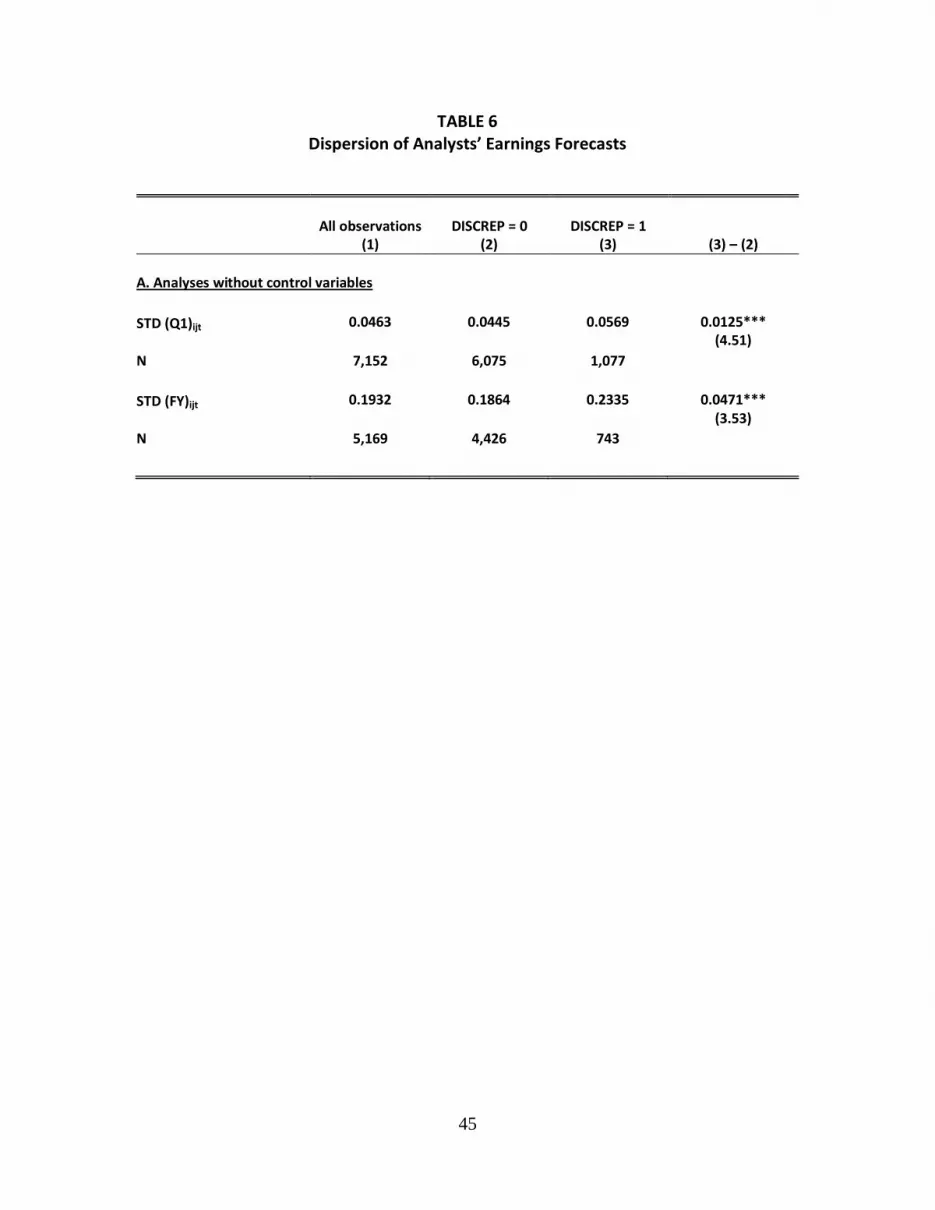
45

TABLE 6 Dispersion of Analysts’ Earnings Forecasts



STD (Q1)ijt 0.0463 0.0445 0.0569 0.0125*** (4.51)

N 7,152 6,075 1,077

STD (FY)ijt 0.1932 0.1864 0.2335 0.0471*** (3.53)

N 5,169 4,426 743

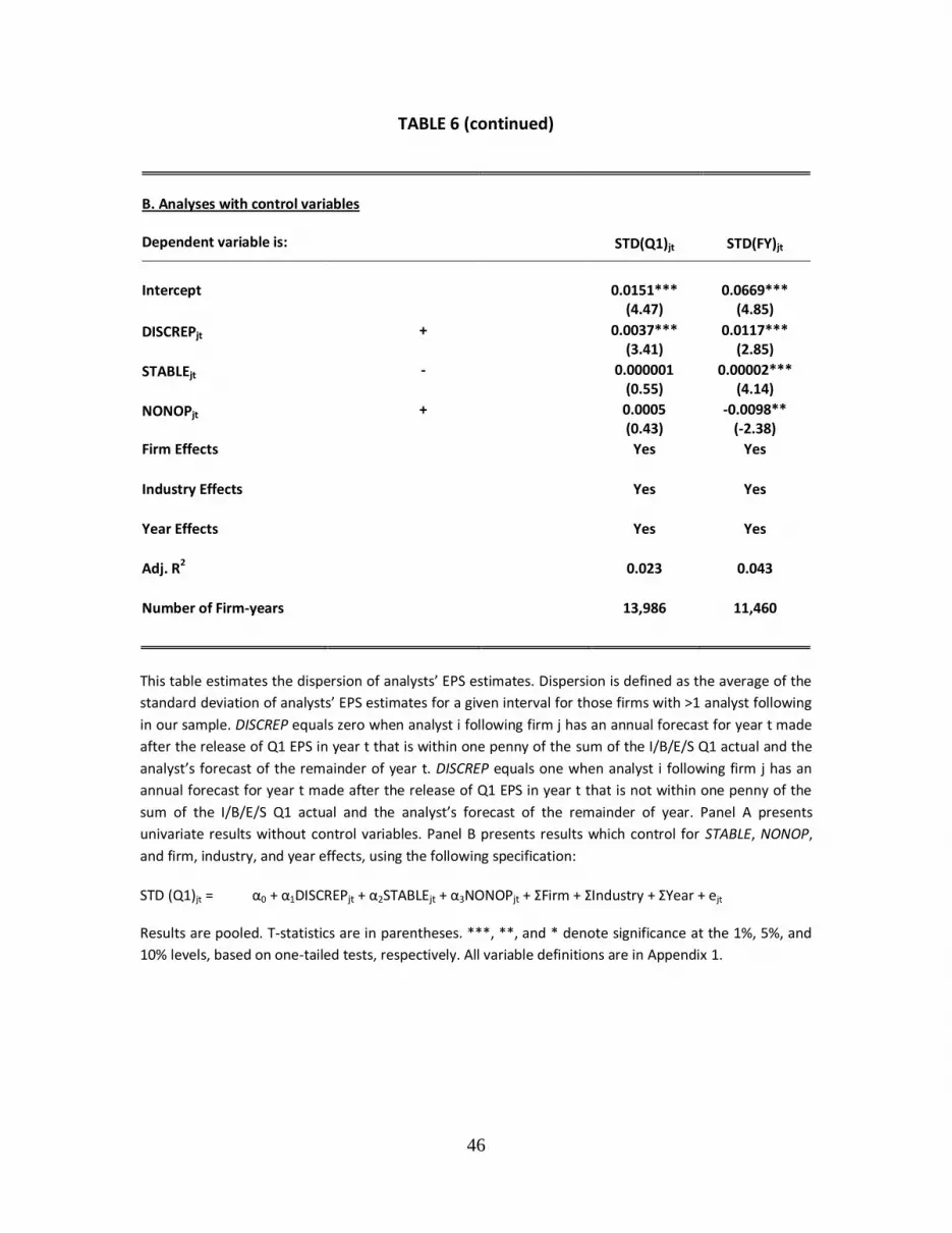
46

TABLE 6 (continued)


Dependent variable is: STD(Q1)jt STD(FY)jt

Intercept 0.0151***

(4.47) 0.0669***

(4.85)

DISCREPjt + 0.0037*** (3.41)

0.0117*** (2.85)

STABLEjt - 0.000001 (0.55)

0.00002*** (4.14)

NONOPjt + 0.0005 (0.43)

-0.0098** (-2.38)




Adj. R2 0.023 0.043

Number of Firm-years 13,986 11,460

This table estimates the dispersion of analysts’ EPS estimates. Dispersion is defined as the average of the

standard deviation of analysts’ EPS estimates for a given interval for those firms with >1 analyst following

in our sample. DISCREP equals zero when analyst i following firm j has an annual forecast for year t made

after the release of Q1 EPS in year t that is within one penny of the sum of the I/B/E/S Q1 actual and the

analyst’s forecast of the remainder of year t. DISCREP equals one when analyst i following firm j has an

annual forecast for year t made after the release of Q1 EPS in year t that is not within one penny of the

sum of the I/B/E/S Q1 actual and the analyst’s forecast of the remainder of year. Panel A presents

univariate results without control variables. Panel B presents results which control for STABLE, NONOP,

and firm, industry, and year effects, using the following specification:

STD (Q1)jt = α0 + α1DISCREPjt + α2STABLEjt + α3NONOPjt + ΣFirm + ΣIndustry + ΣYear + ejt



47

TABLE 7

Market Reaction to I/B/E/S Earnings Surprises



B 1.4348*** (19.78)

1.9868*** (17.62)

1.0357*** (10.99)

-0.9511*** (-6.48)

Adj. R2 0.021 0.031 0.013

N 18,533 9,617 8,908


Dependent variable is: CARjt

Intercept ? 0.0013

(0.39)

DISCREPjt ? -0.0002 (-0.14)

SURPjt + 2.1867*** (13.11)

DISCREPjt * SURPjt - -0.6026*** (-2.74)

STABLEjt + -0.00002 (-0.13)

NONOPjt - 0.0009 (0.73)

Firm Effects Yes

Industry Effects Yes

Year Effects Yes

Adj. R2 0.027

Number of Firm-years 10,264

48

TABLE 7 (continued)

This table estimates the stock market reaction to first quarter I/B/E/S earnings surprise. CAR represents

two-day (-1, 0) abnormal returns where day 0 is the release of Q1 earnings. DISCREP equals zero when

analyst i following firm j has an annual forecast for year t made after the release of Q1 EPS in year t that is

within one penny of the sum of the I/B/E/S Q1 actual and the analyst’s forecast of the remainder of year t.

DISCREP equals one when analyst i following firm j has an annual forecast for year t made after the

release of Q1 EPS in year t that is not within one penny of the sum of the I/B/E/S Q1 actual and the

analyst’s forecast of the remainder of year. Panel A uses the following specification:

CARjt = a + b*SURPjt + ejt

Results for intercepts are excluded for simplicity. The final column compares the slope coefficients in

columns 2 and 3.

Panel B presents results which control for STABLE, NONOP, and firm, industry, and year effects, using the

following specification:

CARjt = α0 + α1DISCREPjt + α2SURPjt + α3 DISCREPjt * DISCREPjt*SURPjt + α4STABLEjt + α5NONOPjt

+ ΣFirm + ΣIndustry + ΣYear + ej



49

TABLE 8 Impact of non-GAAP disclosure regulations on the probability disclosed earnings

meets or beats forecasted earnings

2000-2005 2000-2005 2000-2005

All Firms (1)

DISCREP=1 (2)

DISCREP=0 (3)

Intercept -0.275*** -0.542*** -0.390***

NGREG -0.068** -0.294** -0.017

POST_01 0.231*** 0.456*** 0.314***

SOX -0.074 0.004 -0.133

SPEC 0.047* 0.146** 0.032

LOSS -0.411*** -0.447*** -0.350***

UPEARN 0.833*** 1.017*** 0.879***

GROWTH 0.091*** 0.220*** 0.243***

BTM 0.002 -0.014 0.002

LEV -0.0004 0.002 0.0001

N_ANLST 0.002 0.012** -0.005

FCSTD -2.171*** -1.567*** -1.902***

TECH 0.276*** 0.184** 0.326***

RET 0.676*** 0.753*** 0.777***

INDPRD -1.206*** -1.455** -1.212***

QTR4 -0.054**

Max-rescaled R2 0.103 0.151 0.117

Number of firm-quarters 35,142 3,820 11,931

50

TABLE 8 (continued)

This table replicates Table 5 of Heflin and Hsu (2008) using a similar sample to theirs in Column 1, the sub-

sample of firm-quarters for which we can identify DISCREP = 1 in Column 2, and the sub-sample of firm-

quarters for which we can identify DISCREP = 0 in Column 3. ***, **, and * denote significance at the 1%,

5%, and 10% levels, based on one-tailed tests, respectively. All variable definitions are in Appendix 1.

51

TABLE 9

Analyses Using a Continuous Measure of Data Discrepancy

Panel A: Dependent variable is: Accuracy(Q1)ijt STD (Q1)jt

Intercept ? 0.0005**

(2.27) 0.0167***

(5.01)

|MDISCREPijt| + 0.1748*** (38.48)

0.1985*** (3.58)

FEXPijt - 0.0005*** (3.36)

FREQijt - -0.0003* (-1.80)

NFIRMSijt + 0.0006*** (3.09)

BSIZEijt - -0.0002 (-0.65)

HORIZONijt + 0.0014*** (7.01)

STABLEjt - 0.00001 (0.50)

NONOPjt + 0.0004*** (4.78)

0.0005 (0.50)

Analyst Effects Yes No




Adj. R2 0.081 0.023

Number of observations 19,765 13,986

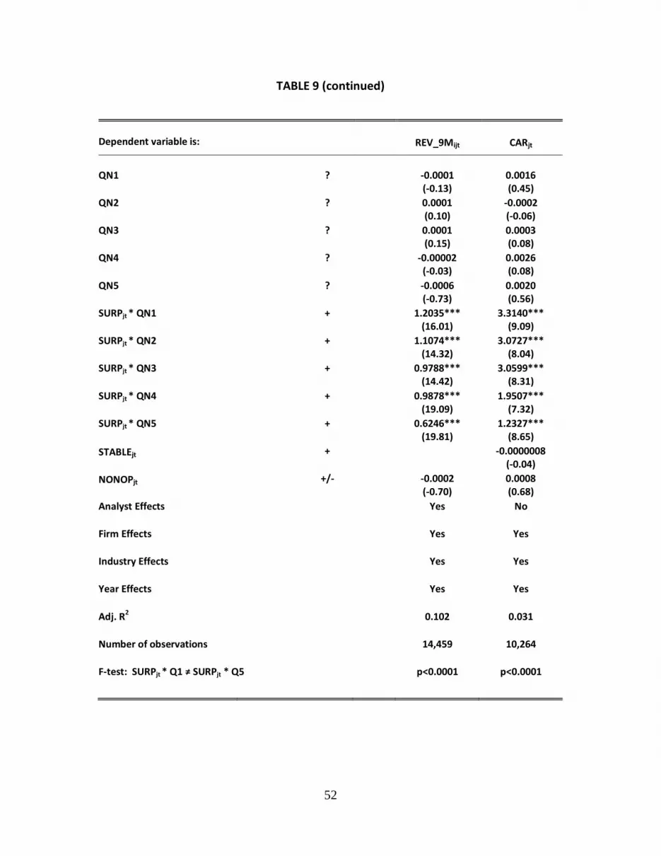
52

TABLE 9 (continued)

Dependent variable is: REV_9Mijt CARjt

QN1 ? -0.0001

(-0.13) 0.0016 (0.45)

QN2 ? 0.0001 (0.10)

-0.0002 (-0.06)

QN3 ? 0.0001 (0.15)

0.0003 (0.08)

QN4 ? -0.00002 (-0.03)

0.0026 (0.08)

QN5 ? -0.0006 (-0.73)

0.0020 (0.56)

SURPjt * QN1 + 1.2035*** (16.01)

3.3140*** (9.09)

SURPjt * QN2 + 1.1074*** (14.32)

3.0727*** (8.04)

SURPjt * QN3 + 0.9788*** (14.42)

3.0599*** (8.31)

SURPjt * QN4 + 0.9878*** (19.09)

1.9507*** (7.32)

SURPjt * QN5 + 0.6246*** (19.81)

1.2327*** (8.65)

STABLEjt + -0.0000008 (-0.04)

NONOPjt +/- -0.0002 (-0.70)

0.0008 (0.68)

Analyst Effects Yes No




Adj. R2 0.102 0.031

Number of observations 14,459 10,264

F-test: SURPjt * Q1 ≠ SURPjt * Q5 p<0.0001 p<0.0001

53

TABLE 9 (continued)

This table repeats the panel B analyses in Tables 4 to 7 using a continuous measure of data discrepancy,

the difference between the analyst’s inferred Q1 actual and the I/B/E/S Q1 actual. This continuous

measure is denoted as MDISCREP to designate the magnitude of the discrepancy. Panel A investigates

accuracy and dispersion. It uses the absolute value of MDISCREP. Panel B investigates revisions and

market reactions to I/B/E/S earnings surprises. It uses the five quintiles of the absolute value of MDISCREP

ordered from smallest to largest. Results are pooled. T-statistics are in parentheses. ***, **, and * denote

significance at the 1%, 5%, and 10% levels, based on one-tailed tests, respectively. All variable definitions

are in Appendix 1.

discrepancy between i/b/e/s actual eps and analysts' inferred eps

Documents