direct and inverse problems of electromagnetoelasticity

Pergamon Phys. Chem. Earth, Vol. 23, No. 9-10, pp. 883-893, 1998

© 1998 Published by Elsevier Science Ltd All rights reserved

0079-1946/98IS--see front matter

PII: S0079-1946(98)00115-3

Direct and Inverse Problems of Electromagnetoelasticity

V. G. R o m a n o v and S. I. Kabanikhin

S. L. Sobolev Insti tute of Mathematics Universtetski i prosp., 4 Novosibirsk, 630090, Russia

Received 25 April 1997; revised 25 April 1998; accepted 27 April 1998

Abstract. We give a review which summa- rizes the literature about coupled electromagnetic and elastic phenomena, theory and numerics of the reconstruction of material parameters for the electromagnetoelasticity equations. Theorem of uniqueness and conditional stability of the inverse problems solution are presented. We describe the scheme of conjugate gradient method for the reconstruction media parameters and unknown sources.

© 1998 Published by Elsevier Science Ltd. All rights reserved.

1 Introduction

During the last 25 years a lot of papers have been published describing the connection and conversion of seismic into electromagnetic energy and waves in geological environments and the detection of the electric or magnetic signals as a method of geophys- ical exploration. However, the phenomena involved in the conversion of seismic energy and waves to electromagnetic energy and waves are not fully understood. This problem needs both experimental and theoretical investigations. For example, if an elastic electroconductive mediun is imbedded in an electromagnetic field, then the elastic oscillations propagating through the medium will exite oscillations of the electromagnetic field and themselves will change under the influence of the latter. The waves has arising as a result of such an interaction are usually referred to as magnetoelastic. We describe the theoretical analysis of the joint inversion of the coupled system of electrodynamics and elasticity, the structure of the Cauchy problem solution in the case of point sources.

It is of common knowledge that when elastic waves are propagated through an electroconductive medium within the magnetic field, an interaction between EM and elastic oscillations appears. The resulting waves are called the magneto-elastic (ME) waves. In the case of electroconductive fluids, similar waves arise which have been studied properly enough (see, for example, Landau and Lif~chitz, [1]). Elastic wave propagation in the magnetic field of the Earth was investigated in Knopoif [2] as well as some boundary value problems for a layer and for a half space adjacent to elastic non-conducting media. We refer readers also to Novatskii [3], Keilis- Borok and Monin [49, Dunkin and Eringen [5], Rakhmatulin and Shkenev [6], Balakirev and Gilin- skii [7] where similar questions are studied.

In all the mentioned papers the influence of the EM field on the deformation field is considered as a result of the Lorentz forces arising in the equations of movements. To reflect an increase of the electric field density, an additional term should be included into the equation describing Ohm's law. This term is dependent on the velocity of particles which move in the magnetic field. In this case, the influence of the magneto-elastic field on the elastic waves propagation can be shown (see Landau and Lifschitz, [I]) to be negligible. At the same time, as follows from experimental researches (see Alers and Fleury, [8]), if the original magnetic field is strong enough, the influence of the ME forces may be significant.

The ME models are of our interest due to their applications in geophysics and acoustics.

An inverse problem of simultaneous determination of electromagnetic (EM) and elastic parameters was considered in Lavrent'ev (jr) and Priimenko [9]. More precisely, they study the Maxwell and

883

884 V. G. Romanov and S. I. Kabanikhin: Direct and Inverse Problems of Electromagnctoelasticity

the Lamd systems in the case when the EM field is generated by elastic oscillations. At the same time, they neglect the reverse influence of the electromagnetic field on the elastic oscillations. For a model system of two equations with piecewise constant coefficients an approximate algorithm for solving the inverse problem was described.

2 T h e s t r u c t u r e o f t h e C a u c h y p r o b l e m s o l u t i o n for a c o u p - l ed s y s t e m o f e q u a t i o n s o f e l e c t r o d y n a m i c s a n d e las - t i c i t y in t h e c a s e o f p o i n t s o u r c e s

2.1 Statement of the direct problem

Let us consider the linear interaction of an electromagnetic field with an isotropic nonhomogeneous medium which is described by the set of equations (see, e.g. [11, 3})

curl H - [~(E + qut x h°)t

+ a(E+/~ut x h°)] = j , (x,t) E R 3 x R (2.1)

curl E +pHt = O, (x, t) e R 3 x R (2.2)

putt - (A + 2,¢) V div u + a curl curl u - VA div u

a 0a 0u V,~x c u r l u - 2 ~ 0xl ax~

l----1

-alJ(E+I~u~ x h °) x h ° = f, (x, t) E R 3 x R. (2.3)

Here H, E, u are the vectors of magnetic intensity, electric field, and displacement respectively. Ma- terial parameters of the medium characterizing its magnetic properties are denoted by e, a,/J; and p, A, ~ denote the density and elastic moduli of the medium. The coefficient q is defined by the formula q = (e~u - gf~)/z where g, 12 are the values of the parameters e, /~ in vacuum and h ° is the vector of magnetic intensity characterizing the strong constant magnetic field in the resting medium. The magnetic properties of the medium are usually assumed to be constant. In view of this we take from here on that p is a positive constant and h ° is a constant vector, h ° ~ 0. Material parameters of the medium are assumed to be smooth bounded functions of x E R a (to be more precise, functions of

class Cm(R 3) with a sufficiently large m), e, p, A, being strictly positive and cr > O. Vectors j , f char- acterize the current from external sources and the external force acting on the medium. It is assumed here that j , f are generalized finite functions (distributions). We will consider the solutions to Eqs. (2.1) - (2.3) with the initial data

(H, E, u) = 0, (x, t) e R 3 x R _ (2.4)

R_ = {t E Rlt < 0}

as generalized functions over the space of infinitely differentiable finite functions.

Under the assumption of the weak conductivity of the medium a system of equations is presented in [12] obtained by linearizing the problem (2.1)- (2.4) on a. The inverse problem treated below is connected exactly with this system which can be written as

curl H - [e (E +qut x h°)t + a(E ° + Du o × h°)] J (2.5)

(z, t) ~ R 3 x R

c u r l E + # H t = 0 , (x,t) e R 3 x R (2.6)

putt - (A + 2s)Vdiv u + ~ curl curl u - VAdiv u

3

- 2 Z O~ Ou V s x cu r lu ~=1 Ox~ Ox~

-a#(E°+#u°txh°)×h° = f , (x,t) e R a x R (2.7)

(H, E, u) = 0, (z, t) e R 3 x R_ (2.8) where (H° ,E° ,u °) is the solution to the Cauchy problem (2.1)-(2.4) subject to the condition a ~ 0.

The structure of the solution of the problem (2.5)-(2.9) has been studied in [12] on condition that j , f are given by the formulae

j = j°6(x - x °, t), f = f°6(x - x °, t) (2.9)

where j0, f0 are constant vectors and x ° E R 3 is some fixed point. Let us present the formulation of th result obtained.

Let cl, c2, c3 be the propagation velocities of electromagnetic, longitudinal and transversal elastic waves respectively

1 e , - - c2-- V - - Z - - , Cs-- (2.10)

V. G. Romanov and S. I. Kabanikhin: Direct and Inverse Problems of Electromagnetoelasticity

We introduce for each of them the l~iemannian N > 5 belong to Cm(Ra), m > 3(N + 10) + 10. metric in which the length element d ~ is defined Then the solution to the problem (2.5)-(2.9) can by the equality be represented as

885

drk = c~(z)ds, k = l ,2 ,3 (2.11)

where ds is the length element in the Euclidian metric. Let F~(z°,~) denote the geodesic of the metric (2.11) connecting the points x °, z; and let rk(x °, z) denote its length. It is well-known that r~(~ °, z) as a function of point • satisfies the relations

Iw 'k(~ °, x)l ~ = c~ "2

~'k(~ °, x) = 0 ( 1 ~ ° - xl) as ,~ --, ~o. (2.12)

Hereafter, we always suppose that each of the metrics (2.11) is simple; i.e., each pair of points z °, x is connected by one geodesic 7~(z °, x). It is assumed as well that ck(z), k = 1,2,3, satisfy the conditions

N v'(.. ,) : +

+7'n(:~)On(Ss)~. + V~v(x,t), i = 1,2,3 (2.16)

where V/~(x,t)h @ CN(R3 x R ) and coef~cients sin, ~n(z), 7 / (z) have the following properties

i) s3_2(~) = ~_2(x) = 7s_~(x) = o; ii) sin(z), ~n(z), 7~(z) are analytic real func-

tions in the region Do \ {z ° } and smooth functions outside Do (to put it more precisely, functions of class Cm-~"-S(R a \ Do)); besides there exists a constant C > 0 depending only on the values of the coefficients ~, p, a, p, A, x in the region Do and on IJ°l, If°l, Ih°l such that

0 < 1T~ a < C3(Z ) < C2(X) < Cl(X) ___< M1 < (2.13)

where m3, M1 are some fixed numbers. Let Oo(t) denote the Heaviside function: Oo(t) =

1 for t > 0 and Oo(t) = 0 for t < 0. Let us define the functions

t n o . ( t ) = ~Oo( t )

d" O_,(t) = --~-ffOo(t), n = 1,2 . . . . (2.14)

Sk = Sk(x, t ,x °) = t - r k ( x ° , x ) , k = 1,2,3. (2.15)

Differentiation in (2.14) is understood in the sense of distributions. Therefore 0-1(0 = 6(0, O-(n+l ) = 6(n)(t), n _> 1. Note that O~n(t) = On-l(t) for all integer n. Equalities Sk = 0, k = 1,2,3, define characteristic cones corresponding to the velocities ok, k = 1,2,3. l~anctions On(S~), n _< -1 , are convenient for characterizing the singular part of the solution to the problem (2.5)-(2.9), and functions On(Sk), n > O, are convenient for characterizing the discontinuities of the solution and its derivatives on the characteristic cone Sk = 0.

Let us define the functions V i, i = 1,2,3, through the equalities V 1 = H, V 2 = E, V z = u. From [12] we have the following theorem.

T h e o r e m 1.1 . Let there be 6o > 0 such that the t o e , cleats ~, a, p, )t, s¢ are constant in a region Do = {z e RZl Ix°-xl < 60} and for some integer

i i ~ I x ° - z l - (a+")' i = 1,2 ( I s , I, ID~,I, I t , I) <_ C

L [z ° - z[ -(2+"), i = 3 (2 .1r)

iii) in the region {(z,t)l Sa > 0, x 6 Do} the functions

N = i 0 ~ ( ~ , t )

n = - 2

satisfy the estimates

IY~l < c l ~ ° - ~t -~

If'~l _< Clx ° - ~1-3 (2.18)

1931 _< c l ~ ° - xl -~

with the same constant C as m formula (2.17).

R e m a r k 1.1. For a homogeneous medium the solution to the problem (2.5)-(2.9) is of the form (2.16) with N = 5, V~ - 0.

The result formulated forms the basis for the statement of the inverse problem for weakly conductive media.

886 V. G. Romanov and S. I. Kabanikhin: Direct and

2.2 P r o b l e m s s t a t e m e n t a n d m a i n r e s u l t s

Let the coefficients of the set of equations (2.5)- (2.7) be constant and known outside some finite region D (and the parameter ~ is constant everywhere in R s) and unknown functions of x E D in the region D. For the sake of simplicity we assume that they are functions of class Cm(R 3) with sufficiently large m and therefore continuous for derivatives of order up to m on the boundary of the region D. Let S be some closed convex smooth surface containing the region D inside. Suppose that the function V = (H, E, u) - the solution to the problem (2.5)- (2.9) - is known on the set S x [0,T] where T > 0 is sufficiently large and the point x ° E S is arbitrary; i.e.

V = F ix , t, x°), (x, t, x °) E S x [0, T] x S = G. (2.19)

Inverse p rob l em: Given the function F(x, t ,x°) , find ~, a, p, A, ~ in the region D.

Hereafter, we always suppose that T > d/ms, where d is the diameter of the region restricted by S, and ma is the constant from formula (2.13). In this case it follows from the representation (2.16) that specifying the function F(x, t, x °) on G permits us to find uniquely

1) "rk(x°,x),(x°,x) E S x S, k = 1,2,3; 2) o~',,(:~°,~), ~(xo,:, , ) , ,.y~(xo,~), (xo,x) e s x

S , i -- 1,2,3, n _> - 2 . Thus the original inverse problem is reduced to sue- cessive solving the inverse kinematical problem of determining the velocities ck (x) inside D from the functions rk(x°,x), (x°,x) E S x S, k = 1,2,3, and determining the yet unknown combinations of required functions, given the functions i 0 ~.(~ ,~), ~ ( x ° , x ) , ~f~(x°,x) on S x S. The theory of the inverse kinematical problem for isotropic media is fairly well developed (see, e.g. [19, 20, 21, 14]). In particular, it has been established that, in the case of simple metrics, specifying r~(x °, x) on S x S defines c~(x) inside D uniquely. Therefore, let us suppose that the velocities ck(x), k = 1, 2, 3, have already been determined in D as a result of solving the inverse kinematic problems corresponding to them. Specifying ck(x), k = 1, 2, 3, determinates, as is obvious from formulae (2.10), three nonlin- ear relations between the media parameters sought for. Since the coefficient # is assumed to be known and constant everywhere, therefore, the coefficient e is determined uniquely from these relations, and

Inverse Problems of Eicctromagnetoelasticity

the moduli of elasticity can be expressed in terms of the medium density p and known velocities c2, c3, only. Thus the parameters remaining unknown are the medium conductivity a and its density p. To find them one can make use of the functions ~ ( x °, x ) , / ~ ( x °, x), 7~(x °, x). Of particular interest are by far the coefficients at the main singu- larities; i.e., the functions ot~2(x°,x), ~2 (x° , x ) , 7~_2(x°,x), i = 1,2,3, since they are in the most simple relation with the medium parameters sought for. Nonetheless the coefficients corresponding to the values n _> - 1 can also be used successfully to solve the inverse problem.

It should be noted that the above stated method of reducing the inverse problem to successive solving the inverse kinematical problem and then em- ploying the radial amplitudes for determining the remaining relations between the desired coefficients was earlier employed by the author [13 - 15] and by V. G. Yakhno [16 - 18] for studying the simpler inverse problems for equations of the second order and for equations arising in the theory of elasticity.

Below, one of the possible statements of the problem of determining the parameters a, p is considered; namely when the function a12(x °, x) is used for this purpose. In the treatment that follows it is assumed that f0 = 0, a(x) - a0 > 0, x E R s \ D; q # 0, x E D. Then the problem concerned can be reduced to the following problem of integral geometry (tomography): given the integrals

(aWl 4-b) (x °,x), (x °,x) S S Pl E X l(zo,x)

(2.20)

f r a n d s =p2(x°,x) , (x°,x) S x S E (2.21) ,(~o,z)

from functions a, b with the known weight functions 71, ~ , find a, b inside D if they are known outside D. Here, a, b are connected with the medium parameters a, p and determined by the relations a = aq/2p(~ -c~)cle, b = -a/2c1~; and weight functions 71, 72 are defined by the equalities

i71 = (h ° . ~°)21w°1-2 4- ~(h °. v) 2

72 = (h °" co°)(h O" ( v x w°))lw°l-2 (2.22)

where~ = ( ~ - c ~ ) / ( ~ - ~ ) , 0 < ~ < 1, y i s t h e unit vector of the tangent to Fl(x °, x) at the point x, and w ° is the solution to the Cauchy problem (3.15), (3.17) and is completely defined given jo and cdx).

V. G, Romanov and S. I. Kabanikhin: Direct and Inverse Problems of Electromagnetoelasticity 887

Note that the functions a, b define uniquely only a and the ratio a/p. Therefore, the density p can be determined only in those points of the ratio D where a ~ 0. This circumstance is a characteristic feature of the problem concerned, based on using the information on the coefficient a12. It could be shown that the density p can be determined uniquely in D, if the coefficient a03(x °, x), (x °, x) e S × S, is used (under the condition f0 ~ 0). The proof of this fact s yet out of the scope of the present paper.

The presence of the weight functions ~1, ~ in equalities (2.20), (2.21) comlicates considerably the problem of integral geometry. Unfortunately, the author has not yet obtained final results. Let us mention just three special results.

1) Let c, = const = c,0, jo = (1, 0, 0)41r~0 ' h ° = (1, 0,1). Let S(z) and D(z) denote the cross- sections of the surface S and the region D, respectively by the plane x3 = z. In this case the problem of integral geometry decomposes into a one- parameter family of planar problems for each cross- section of the region D by the plane xz = z. Vector v, corresponding to the straight line Fl(x °, x), x ° 6 S(z), x 6 S(z), can be characterized in this case by the angular coordinate ~o: v = (cos ~o, sin ~o, 0) which is constant along F,(x °, z) and therefore de- pends only on endpoints x °, x, belonging to S(z). In these circumstances ~/2 = sin ~, ~h = 1 + ~ cos 2 ~. Therefore, the weight function z/2 is constant along r l (x° ,x ) , and equality (2.21) can be written as

f ads =p~(x°,x), (x°,x) e S x S (2.23)

rl(zO,x)

1 f - Ol Ol' dldl' (2.24) s(z) S(z) S(z)

D(z) S(z) S(z)

+ Ol 0l' J dldl' (2.25)

where d£" = dXl dx2, and symbo/s O/Ol, O/Ol' denote the derivatives in the direction of the tangents to S(z) in points x °, x, respectively, and Ol, Ol ~ denote the elements of the arc length calculated at these very points.

2) Let us modify slightly the statement of the problem and consider its two-dimensional variant. Namely, let D be an infinite cylindrical region with the ruling parallel to the axis x3: D = Do × R where Do is the cross-section of the region D by the plane xa --- 0; and let the medium parameters be independent of the variable x3. Let then S be a convex closed smooth curve containing the region Do inside, and let vectors j0, h 0 have the same values as in the previous case. Geodesics Fl(x°,x), (x°,x) E S × S, are plane ones in this case. Denot- ing the unit vector of the tangent to Fl(Z°,x) at the point x as v = (cos ~, sin ~o, 0) we obtain that in this case also ~ = sin ~o, Th = 1 + ~ cos 2 ~. There is a substantial difference between this case and the previous one, lying in the fact that the weight function ~ is not constant along the geodesic. Equation (2.21) in this case can be written as

where p~ = P2/sin ~o. The problem of determining the function a from equality (2.23) is a standard problem of tomography. After a has been found, the integral from the product a~h along Fl(X°,x) can be calculated, and a similar problem of tomography arises for the function b. Uniqueness of its solution is obvious. Less obvious is the stability estimate since the weight function ~h in general is not constant along Fl(x °, z). Let us present the corresponding result.

T h e o r e m 1.2. Let (a, b), (~, b) be the solutions to Eqs. (2.20), (2.23) corresponding to the data (Pl,f2), (Pl,16~), respectively, and coinciding outside D. Then the following estimates hold for differences ~ = a --fi, b = b-b, Pl = Pl --Pl, P2 = P2 --P2:

f adx2=p2(xO,x), (x°,x) E S x S .

rl (x°,z) (2.2o)

Thus P2 is an integral along Fl(X°,x) of the sim- plest form of the first degree. The problems defin- ing a form of the first degree by its integrals along a family of geodesics of the Riemannian metric have been considered in [13, 14, 22, 23].

Suppose that there are two solutions a, a to Eq. (2.26) coinciding outside Do. Then their difference fi = a - 5 satisfies the homogenous equation. From [23] it follows that OS/Oxl = 0, x E Do. Since ~ = 0 outside Do, we arrive at the conclusion that 5 = 0, x E De; i.e., a = a. It has a consequence to the uniqueness theorem for the whole problem.

888 V. G. Romanov and S. I. Kabanikhin: Direct and Inverse Problems of Electromagnetoelasticity

T h e o r e m 1.3. Specifying the functions Pl, 192 for (x° ,x) E S x S defines the functions a, b in the region Do uniquely.

It should be noted that some of the stability estimates for the solution to the problem (2.20), (2.26) follow from the estimates obtained in [22].

3) Now we return to the former formulation of the problem. Let the velocity el(X) depend essentially on all three variables xl, x2, x3. Let jo be a fixed non-zero vector; and let us assume that the vector h ° can take on two different values h °k, k = 1,2, where h °2 = rh °1, r 2 ~ 1, and for each vector h °k the function a~2(x °, x) and, consequently, the functions Pl (x °, x), P2 (x ° , x), (x °, x) E S x S, are known. Let Plk, k = 1, 2, denote the function Pl corresponding to h °k. From equality (2.20) where h ° = h °k, k = 1, 2, one can easily obtain the relations

ds (~o (~o S × S

rl (z°,x) (2.2z)

(x °, x) 6 S x S (2.28) f bds=~2(xO,x) '

rl (x °,x) where ~/o = (h 01 " •0)2[•01-2 + ~(h 01 " v) 2, i61 = (]911 -- PI2)/(I -- r2),/~2 = (PI2 -- Pllr2)/( 1 -- r2) •

Thus, making use of two observations corresponding to different values of the vector h ° allows one to split the original problem into two problems independent of each other. An the problem of determining the function b(x) from Eq. (2.28) is a thor- oughly studied problem of integral geometry (see, e.g. [14, 19]). The following stability theorem (an analog of the estimate (3.54) from [14]) is valid for this problem.

T h e o r e m 1.4. Let b, b' be the solution of Eq. (2.28) corresponding to the righthand sides P2, Pt2 respectively, and let b = b' outs/de D. Then the following inequality holds for the differences b = b - b ' , ~ = ~ - ~

D S

X I k , j ~ l ( ~2T1 ~2~ I/2 dgx dSxo

(2.29)

where n(x) is a unit normal vector to S at the point X.

The question of the properties of Eq. (2.27) re- quires further consideration.

3 Optimizat ion m e t h o d in the inverse electromagnetoelasticity problem in quasista- t ionary approximation.

3.1 Setting of the direct and inverse problems

Here we consider the formulation of the inverse problem for electromagnetoelasticity in its quasistationary approximation. The motion of an elastic conductive medium in an electromagnetic field is described by two systems. First is the system of differential equations of elasticity theory. The second system is the Maxwell equations system. These equations are correlated due to additional terms which describe the effects connected with the motion of elastic conductive medium in electromagnetic field. If we assume that the displacement current are small compared with the conductive current, we obtain the setting of the problem in the quasistationary approximation. We shall consider the fields of small perturbations which allow us to consider the linearized setting of the problem.

The setting of the direct problem is as follows. We consider the Cartesian coordinate system z = (xl, x2, xs). Suppose that x3 = 0 is the earth (x3 > O) - air (x3 < 0) interface.

The process of propagation of elastic waves is described by the system of the equations of elasticity

P-~= ax# 'i=1'2'3 (3.1) jr1

\Ox# + Ox~] + 6°d ivu ' i , j = 1,2,3

(3.2) where T~j(u) is the stress tensor; p is the medium density; A, k are the Lamd coefficients; 6q is the Kronecker delta.

The process of electromagnetic wave propagation in an elastic conductive medium in its quasistationary approximation is described by the system

a E = curl H - a#ut x H ° (3.3)


# ( H ° + H) t = - curl E. (3.4)

Here e, # are the electric and magnetic permeabili- ties; a is the medium conductivity; u = (ul, u2, u3), E = (E1,E2,E3); H = (H1,H2,H3) are the displacement vectors corresponding to small perturbations of elastic and electromagnetic fields. H ° is a constant vector which is related to a nonperturbed medium.

We suppose that elastic vibrations arise due to a force source concentrated in the origin

Tk,a(u) xs---° = tSk,zf(t)tS(xl, X3), k = 1,2, 3 (3.5)

where ~ is the Dirac function. We assume that the electromagnetic field is ab-

sent till the moment t = 0

(f , u, E, H) t<° = 0. (3.6)

We also assume that the radiation condition holds in infinity,

lim ( E , H ) = 0. (3.7) Izl-.oo

In the planes of coefficient discontinuities we pose the jump condition

= Ig l = [u l = = 0 (3.8)

k = 1 , 2 ; m = 1 , 2 , 3 .

The setting of the inverse problem is as follows: the elastic and electromagnetic characteristics of medium are known; H ° is known; to find the function vectors u, E , H from relations (3.1) - (3.8).

In [27], elastic and electromagnetic characteristics of a medium and the function f ( t ) from system (3.1) - (3.8) were determined in a special case. The additional information was given by the components of vectors u and E. In [27] the authors have constructed an algorithm for the successive determination of the propagation rate of elastic waves and the form of probing signal. Then, the diffu- sion process of electromagnetic waves on the basis of the optimizational approach was determined. The essence of such an approach is minimizing the residual functional of observed and calculated test direct problems in the given frequency domain w.

The main goal of our paper is to apply the opti- mization method [7] to the simultaneous determination of elastic and electromagnetic characteristics of a medium and a shape of a probing signal. The minimization of the residual functional is done during

all the time interval of observation of the medium response .

We shall formulate the setting of the inverse problem similar to those that was done in [5].

Suppose that v(z) is the speed of longitudinal waves and c(z) is the speed of diffusional process of electromagnetic waves. It is known that they have the following form

A~2k 1

V - - 7 ' --

Let F~Ix~(. ) be the Fourier transformation with respect to the variables Xl, z2, and Vl, v2 be the dual variables. Then, for the functions

u(z , t ) = ReFzlx2(u3) va=v2=o

E ( z , t ) = ReF~,x2(E1) ]vl=v2=0

problem (3.1) - (3.8) will be as follows

Utt = p(Z)Uzz, (t, Z) e R x f/ ' (3.9)

u t<0 = 0 (3.10)

u z z = ° = j . y ( t ) , u z== O (3.11)

Et = q(z)Ezz - #Hurt , (t, z) 6 R x ~ (3.12)

E t<° = 0, z-~lim E = 0 (3.13)

Ez z=° = 0, u Iz=t= 0. (3.14)

Here, for convenience, we introduce the notations

( j = A(0) +2k(0 , z = x3

pCz) = v2(z ) , q(z) = c2(z)

I is a sufficiently large number. We suppose that relative to the direct problem

(3.9) - (3.14), we know the additional information

u z=° = so(t) (3.15)

E z=° = Eo(t), t e [0, + ~ ) . (3.16)

Then, the inverse problem may be posed as follows: find the functions p(z), f(t), q(z) and the numbers #, H from relations (3.9) - -(3.14) by information (3.15), (3.16).

889


Further, we shall suppose that # = #0, where #0 is the magnetic permeability of the vacuum.

Note that in general inverse problem (3.9) - -(3.16) may have many solutions. The uniqueness theorem can be proved only when two functions are unknown. Nevertheless, we introduce the general algorithm which easily can be specified to the problem of finding p(z) or q(z), or f(t) only; or some combinations of 2 functions.

Note that if we know f(t), then the inverse problem (3.9) - -(3.11), (3.15) is independent and can be solved separately. But if, for instance, we know only Eo(t) from (3.16), and want to find p(z), then we should consider all equations (3.9) - -(3.16).

Therefore, the following algorithm can be used for very many inverse problems. It 's up to the theorem of uniqueness. If you have the uniqueness theorem, then you can find the unknown coefficients minimizing J(p, f , g) in which some arguments are supposed to be given.

3 . 2 A n o p t i m i z a t i o n m e t h o d f o r t h e i n v e r s e p r o b l e m s o l u t i o n

Now we shall formulate the inverse problem setting as it is done in optimal control theory.

To find the control V = (p(z), f(t), q(z)) which % /

gives the minimum for the functional

T

0

[ l') + E(O, t ;q)-Eo( t ) dt (3.17)

Here, as it is done in optimal control theory, the de- pendence of the direct problem solution on the desired functions is denoted as u(0, t,p, f), E(0, t; q).

For minimization of the functional, we apply the conjugate gradient method as follows.

The initial control V ° = (p(0), f(o), q(0)) is given. Suppose that the control V (n) = (p(n), f(n), q(n)) is obtained. Then the components of the control V n+t may be found by the formulae

p(n+l)(z) = p(n)(z) - a'~R'~, n = 1,2,3, . . . (3.18)

Ro = j~(p(O)), R~ = J~(p(n)(z)) -~R'~- ' . (3.19)

Here, the coefficient a~ is determined from the conditions

j~ (p(n) _ apR'~ ) = min J~ (p(n) (z) - c~pP~ ) c~1, >0 r k

and

= j~CpC-)) 2 / g~(p(.-1)) 2. (3.20)

The component f(n+l) of V (n+l) is calculated as follows

f("+l)(t) = f(") - a ~ R ~ , n = 1,2,3, . . . (3.21)

R~ = J r ( i ( 0 ) ) , _ ~ = j f ( f ( n ) ) ~ n D n - 1 (3.22) - - i J f ~ ¢ f •

The component a~ is as follows

and . 2 . 2

~7 = Js ( f (=)) / JA/(~-~)) • (3.23)

Finally, the component q(n+l) may be found from the relations

q(n+l)(z) = q(n)(z) - C~qR~, n = 1,2,3, . . . (3.24)

R ° = J~(q(°)), R~ = j ; (q ( . -1 ) ) _ ~ R ~ - I

and the coefficients a~, f~ satisfy the relations

Jq(q(n)(z) - aqRq ) = min Jq(q(n)(z) - aqRq ) aq>O \

f~ = jq(q(n)) 2/ j~(q(,~-l)) 2 (3.25)

where

is the gradient of the functional (3.17). Now we shall calculate the formula for the func-

tional gradient. The obtain formula similar to that which was obtained in [7].

For this purpose we consider the differences

(0, t; p + ~p; s + 68) - ~(0, t; p; s) 5u

6E = E(O, t ;q+6q) -E(O, t ;q ) .

It is easy to show that 6u solves the problem

~fuu - p(z)6Uzz = ~fpUzz, 0 < z < 1, 0 < t < T (3.26)

6u trio = 0, 0 < z < l (3.27)

6ut t f° = 0, 0 < z < l (3.28)

V. G. Romanov and S. I. Kabanikhin: Direct and Inverse Problems of Electromagnctoelasticity

5Uz Iz=0 = j6 f , 0 < t < T (3.29)

6u ]/=l= 0, 0 < t < T (3.30)

and the function 6E satisfies the following relations

6Et - q(z)6Ezz + #H6uu = 6qEzz (3.31)

0 < z < / , 0 < t < T

,~E L=o = O, 0 < z < l (3.32)

6Et ]z=0 = 0, 0 < t < T (3.33)

6E Izfl = 0, 0 < t < T. (3.34)

The increment of the functional (3.17) may be written as follows

T

AJ(p, f ,q) ~- / 26u[u(O,t;p; f ) - uo(t)]2 dt o

T +/26E[E(O, t ;q ) -Eo( t ) ] dt (3.35)

o

where terms of order (116 , + are glected.

We introduce now the auxiliary problems, which further we shall call conjugate relative to the function ~(z, t)

~tt - (P~P)zz + #Hef t = 2 [U(0, t;p; f ) - u0(t)]

x 6 ( z ) , 0 < t < T , 0 < z < / (3.36)

It=T = 0, 0 < Z < I (3.37)

~Ot ItffiT = 0, 0 <_ Z <_ I ( 3 . 3 8 )

~Oz I~ffi0 = 0, 0 < t < T ( 3 . 3 9 )

~o Iz= = O, 0 < t < T (3.40)

and conjugate relative to the function ¢(z, t)

- ¢ t - (q¢)zz = 2[E(O,t;q) - EoCt)]6(z) (3.41)

0 < t < T , 0 < z < /

Ct It=T = O, 0 < Z < I (3.42)

~z Iz=o = 0, 0 < t < T (3.43)

¢ z=l= 0, 0 < t < T. (3.44)

Taking into account relations (3.36) and (3.41), we may write the increment of the functional (3.35) in another way

T l

o o

T l

= 11+I .

o o (3.45/

In formula (3.45) we have denoted the first integral as I1 and the second as/2.

Now we transform these integrals integrating term-by-term

I T

o o l

+ / [~ot( z, T)~u(z, T) - ~ot ( z, O )6u( z, O ) ] dz o l

- f [ ~ ( z , T)6ut(z, T) - cp( z, O)6ut(z, 0)]dz 0 T

0

T

0

l

+ / , H [¢t( z, T) $u( z, T) - ¢t ( z, O )~Su(z, o ) ] dz o

1 - / l~H[ ¢( z, T)6ut ( z, T) - ¢ ( z, O )~Sut ( z, o) l dz

o I T

+ / / # H ¢ 6 u u d t d z . o o

Taking into account relations (3.26) - (3.30) and (3.37) - (3.40), we obtain

T l T I

0 0 0 0

891


T

-- f j6f(pqo)(0, t) dt. 0

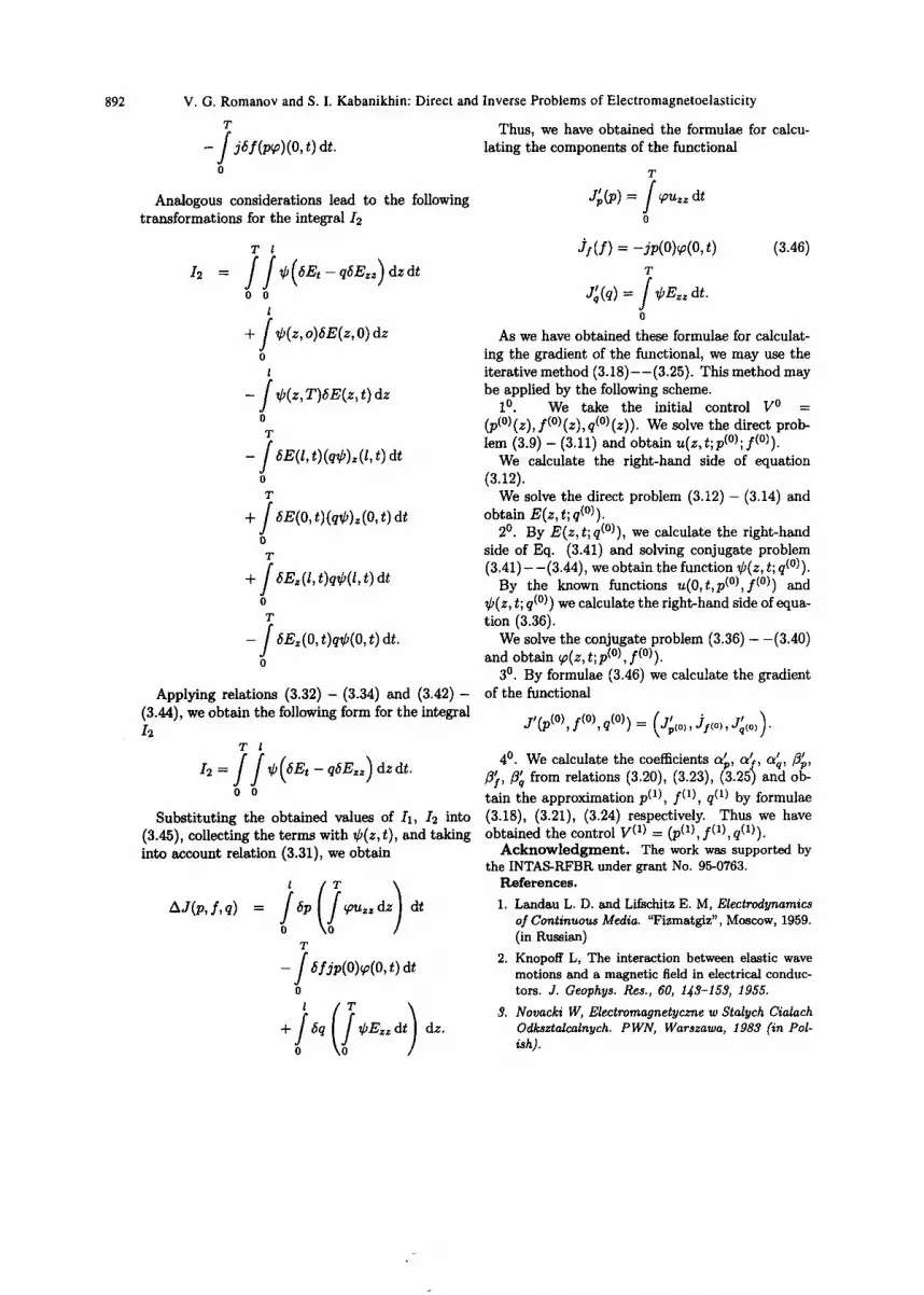
Analogous considerations lead to the following transformations for the integral/2

/2

T l

0 0

l

+ f ¢(Z, o)6E(z, O) dz 0

l

- f ¢(z, T)6E(z, t) dz 0

T

- / 6E(l, t)(qO)z(l, t) dt 0

T

+ f 6E(0, t)(q¢), (0, t) dt 0

T

÷ / 6Ez(l, t)q¢(l, t) dt 0

T

- f 6E~(0, t)q¢(0, t) dr.

Applying relations (3.32) - (3.34) and (3.42) - (3.44), we obtain the following form for the integral I2

T l

0 0

Thus, we have obtained the formulae for calcu- lating the components of the functional

T

(p) = / qouzz dt 4 0

J:(/) = -jp(O)~(o,t) (3.46) T

= / CE~z dr. g(q) ,J

0

As we have obtained these formulae for calculat- ing the gradient of the functional, we may use the iterative method (3.18)--(3.25). This method may be applied by the following scheme.

10 . We take the initial control V ° = (p(°)(z), f(°)(z), q(°)(z)). We solve the direct problem (3.9) - (3.11) and obtain u(z, t;p(°); f(o)).

We calculate the right-hand side of equation (3.12).

We solve the direct problem (3.12) - (3.14) and obtain E( z, t; q(O)).

2 °. By E(z, t; q(O)), we calculate the right-hand side of Eq. (3.41) and solving conjugate problem (3.41) - -(3.44), we obtain the function ¢(z, t; q(0)). By the known functions u(O,t,p(°),f (°)) and

¢(z, t; q(0)) we calculate the right-hand side of equation (3.36).

We solve the conjugate problem (3.36) - -(3.40) and obtain qo(z, t ;p (°), f(o)).

3 °. By formulae (3.46) we calculate the gradient of the functional

.,:,f,o, :)__ (.;,o,, 0 l l / / 4 . We calculate the coefficients ap, c~l, C~q, fl~,

/~,/~ from relations (3.20), (3.23), (3.25) and obtain the approximation p(1) f(1), q(1) by formulae

Substituting the obtained values of I1, /2 into (3.18), (3.21), (3.24) respectively. Thus we have (3.45), collecting the terms with ¢(z, t), and taking obtained the control V (1) = (p(1), f(1), q(1)). into account relation (3.31), we obtain A c k n o w l e d g m e n t . The work was supported by

As(p, f, q) 6p dz dt 0

T - / ~fjp(O)qo(O, t) dt

0

( : ) + / lfq CEzz dt dz. 0

the INTAS-RFBR under grant No. 95-0763. References.

1. Landau L. D. and Lifschitz E. M, Electrodynamics of Continuous Media. "Fizmatgiz", Moscow, 1959. (in Russian)

2. Knopoff L, The interaction between elastic wave motions and a magnetic field in electrical conduc- tors. J. Geophys. Res., 60, 143-153, 1955.

3. Novacki W, Electromagnetyezne w Stalych Cialach Odksztalcalnych. PWN, Warszawa, 1983 (in Pol- ish).


4. Keilis-Borok V. L and Monin A. S, Magnetoelastic waves on the boundary of the Earth core. Izvestiya Akademii Nauk SSSR, set. 9eofizika, (11), 1529- 1541, 1959 (in Russian).

5. Dunkin J. W. and Eringen A. C, On the propagation of waves in an electromagnetic elastic solid. J.Engn. SCI., 1, (4), 461, 1963.

6. Rakhmatulin Kh. A. and Shkenev Yu. S, The In- teraction Between Media and Waves. "FAN", Tashkent, (I 985) (in Russian).

7. Balakirev M. K. and Gilinskii L A, Waves in the "Piezo" Crystals. "Nauka", Novosibirsk, 1982 (in Russian).

8. Ale, s G. A. and Fleury P. A, Modification of the velocity of found m metals by magnetic field. Phys. Rev., 129, (6), 2435, (1963).

9. M.M. Lavrent'ev (jr.), V.LPriimenko, Simultane- ous determination of elastic and electromagnetic medium parameters. Computerized Tomography. Proc. of the Fourth Intern. Syrup., Novosibirsk, August 10-14 (1998) Bd. by M.M. Lavrent'ev.- Utrecht: VSP 302-808, 1995.

10. V.G. Romanov, On an inverse problem for a coupled system of equations of electrodynamics and elasticity. J. of Inverse and RI-Posed Problems 3(4), 321-SSe, 1995.

11. Eringen A.C. and Maugin G.A, Electrodynamics of Continua, 1, IL Springer-Verla9, 1990.

12. V.G. Romanov, Structure of a solution to the Cauchy problem for the system of the equations of electrodynamics and elasticity in the case of paint sources. Siberian Math. J. 36(3), 541-561, 1995.

13. V.G. Romanov, Integral geometry and Inverse Problems for Hyperbolic Equations. Springer Ver- lag, Berlin, 1974.

14. V.G. Romanov, Inverse Problems of Mathematical Physics. Utrecht, VNU SCI. Press, 1987.

15. V.G. Romanov, Uniqueness theorems in inverse problems for some second-order equations. Soviet Math. Dold. 44(3), 678-682, 1992.

16. V. G. Yakhno, Multidimensional inverse d~namical problem of isotropic elasticity. Soviet Phys. Dokl. Za(1), 35-36, 1989.

17. V.G. Yakhno, Two-dimensional inverse problem

for a system of dynamic Lame equations. Soviet Phys. Dokl. 34(7), 616-617, 1989.

18. V.G. Yakhno, Inverse Problems for Differential Equations of Elasticity. Nauka, Novosibirsk, 1990 (in Russian).

19. LN. Bernstein and M.L. Gerver, A problem of integral geometry for a family of geodesics and an inverse kinematic problem of seismology, Soviet Dokl. Earth Sci. Section 243($), 302-305, 1978 (in Russian).

$0. R.G. Mukhometov, Problem of recovering two- dimensional Riemannian metric and integral geometry. Soviet Math. Dokl. 18(1), 27-31, 1977.

21. R.G. Mukhometov and V.G. Romanov, On the problem of detervnining an isotropic Riemannian metric n-dimensional space. Soviet Math. Dold. 19(6), 1330-1333, 1978.

22. V.A. Sharafutdinov, Integral Geometry of Tensor Fields. Utrecht, VSP, 1994.

23. Yu.E. Anikonov, Some methods for Studying Mul- tidimensional Inverse Problem for Differential Equations. Nauka, Novosibirsk, 1978 (in Rus- sian).

24. A.Lorenzi, V.G. Romanov. Identification of the electromagnetic coefficient connected with deformation currents. Inverse Problems 9, 301-319, 1993.

~5. V.G. Yakhno. Inverse Problems for the Differen- tial Equations of Elasticity. Nauka, Novosibirsk (in Russian).

26. M.M. Lavrent'ev, An inverse problem for a wave equation. Calcolo, 28, (8-4), 249-~65, 1991.

27. A.V. Avdeev, E.V. Goruynov, V.I. Priimenko. An inverse problem of electromagnetoelasticity with unknown source of elastic oscillations. Preprint of Inst. of Math. Sibirsk Otdel. Ros. Akad. Nauk (1074), 24, 1996.

28. F.P. Vasil'ev. Methods for solving e~remal problems. Nauka, Moscow, 400, 1981 (in Russian).

~9. K.T. lskakov, S.L Kabanikhin. The solution of one-dimensional inverse problem of geoelectries by the method of conjugate gradients. Russian Jour- nal of Theoretical and Applied Mechanics, New York. (3), 78-88, 1991.

893

direct and inverse problems of electromagnetoelasticity

Documents