diffraction analysis of rough reflective surfaces

$: Diffraction analysis of rough reflective surfaces$
Diffraction analysis of rough reflective surfaces

Karen J. Allardyce and Nicholas George

For ground metallic samples illuminated at various angles of incidence, optical transform patterns aredetermined theoretically and then verified both experimentally and using computer simulations. Surfaceroughness in the range from 0.025 to 3.2 jam is studied and means for categorizing surface roughnessautomatically are established. A noncontact optical method which provides a real-time display of Fouriertransforms is compared to a computer-aided technique that models the optical system using profilometerdata as an input. Also, the Fourier transforms for a periodic phase-reflection surface are presented at threeangles of illumination to illustrate the effective increase in grating frequency and apparent decrease inroughness as the illumination angle is increased. Excellent results are obtained in accurately measuringroughened flat metallic surfaces remotely.

1. Introduction

The measurement of surface characteristics hasbeen a subject of considerable interest in recent years.Numerous methods have been developed to measuresurface roughness.1-'8 However, most techniqueshave restrictions or limitations as to the measurablerange of roughness, type of test surfaces, and operatingenvironment. Thus, despite the wealth of informa-tion on surface roughness measurement now availableto the scientific community, the need to expand onpresent theory and practical systems continues. Themeasurement of surface roughness and the determina-tion of surface characteristics are important for manyapplications. Before giving a brief overview of theseapplications, however, surface roughness should bedefined and distinctions should be made between thecommon terms used to describe various surface char-acteristics.

Surface roughness as small as a few tens of ang-stroms in height, with lateral separations less than amillimeter, causes scattered light in optical systems.'Surface roughness is usually described quantitativelyby the root mean square (or rms) height calculated inthe equation below:

arms = Cy, -)] '(1)

where arms is the standard deviation of the heights, N isthe number of height data points, yi is the height, and yis the mean of the height distribution. A surface is alsooften characterized by its distribution of correlationlengths (i.e., the separation between similar topo-graphic features). Hence, both roughness in heightand correlation length along a surface are importantcharacterizations.

In addition to the different types of height variation,a distinction is made between smooth and rough sur-faces. Smooth and rough are relative terms whichdepend on the angle of illumination and the wave-length of illumination compared to the height fluctua-tions on the surface. The Rayleigh criterion, Eq. (2), isoften used to specify the conditions in which a surfacemay be considered smooth. According to this criteri-on, a surface is considered smooth for

8 cosO(2a)

or when

'Yrms _ 0 orO - 27 '

When this work was done both authors were with University ofRochester, Institute of Optics, Rochester, New York 14627; K. J.Allardyce is now with TRW, 1 Space Park, Redondo Beach, Califor-nia 90278.

Received 2 December 1986.0003-6935/87/122364-12$02.00/0.© 1987 Optical Society of America.

(2b)

where X is the wavelength and 0 is the angle of illumina-tion with respect to the surface normal.2

Surface roughness measurement techniques may beseparated into two basic categories-contact and non-contact. The most common contact technique of sur-face roughness measurement employs the use of a sty-lus profilometer. A narrow diamond stylus is tracedlightly across the surface contour to produce a timevarying voltage output whose magnitude is directly

2364 APPLIED OPTICS / Vol. 26, No. 12 / 15 June 1987

F //

/ x

h (x', y')

Xx'~~~~~~~~~~~~Y, J~~~~~~~~~

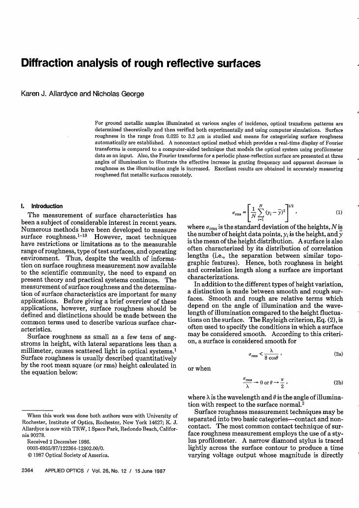
Y ~~ ~~~~b Fig. 1. Optical transform configuration for rough reflective surface(S) illuminated by a monochromatic plane wave at an angle 0.Incident plane wave W at I is perturbed to W' at II and then Fourier

transformed by a canonical processor.

proportional to the height of the surface contour.6

The width of the stylus tip must be small compared tothe lateral separation of the irregularities to give anaccurate contour of the surface profile. Unfortunate-ly, the stylus may damage the test surface. Also, thestylus profilometer gives only 1-D information aboutsurface roughness of the object and is inefficient for acomplete scan of a 2-D rough surface. Thus, substan-tial effort has been made in recent years to replace theprofilometer with some noncontacting optical tech-nique. Noncontacting optical methods can begrouped into two types: imaging system or transformsystem. In this paper we limit our consideration to thelatter type, i.e., the optical transform system.

Analysis of rough surfaces and their correspondingoptical transform patterns is of primary interest in thispaper. Because each rough object has its own uniquetransform, it is clear that a number of important char-acteristics of surfaces (e.g., roughness, correlationlength, slope distribution) are related to the opticaltransform of the surface roughness.

As an example of diffraction calculations for phasereflection-type surfaces, the theoretical and experi-mental analyses of a phase grating of known frequencyare presented. We consider the phase reflection grat-ing as an ideal one-dimensionally grooved surfacewhose transform may be described theoretically forvarious angles of incidence with excellent accuracy.Through this study, some insight is gained as to thebehavior of the transforms of the metallic samplesground from flat stock under various angles of illumi-nation. The object function for the phase grating issimilar to that derived for the metallic phase reflectionsurfaces.

The relationship between the intensity distributionin the diffraction pattern and certain characteristics ofrough surfaces is noted. Specifically, the diffractioncaused by one-dimensionally grooved metallic surfacesis analyzed for roughnesses between 0.025- and 3.2 -,umrms height.

Two methods of analysis are presented and com-pared. The first is a noncontact optical method which

provides a real-time display of optical transform pat-terns for each of the sample surfaces. This noncontactoptical system consists primarily of a transform lensproviding convergent illumination of the sampleswhich is then reflected by the samples. The transformpattern is detected by a linear photodiode array placedat the focal length of the transform lens. The experi-mental system and measurement techniques are de-scribed in detail.

The second method is a computer-aided analysistechnique that models the noncontact optical systemmentioned above. To model this system, the phaseperturbation to a wavefront reflected by the roughsurfaces is derived, surface height profiles are obtainedby a stylus profilometer, and a fast Fourier transformroutine is implemented. The similarities and differ-ences between the optical system transforms and thetheoretical computer model transforms are discussed.

II. Optical Transform Theory for Surfaces in Reflection

The development of a noncontact optical system toexamine surfaces in reflection and a computer-aidedtechnique which models this system are presented.After first discussing the general optical configurationfor taking an optical Fourier transform, we present ananalysis based on diffraction theory. The transformdepends in an interesting way on the angle of illumina-tion. To place this in evidence we calculate the specialcase of a phase reflection grating for later comparisonwith experiment.

A. Optical Transform Theory for Oblique Angles of

Illumination

Consider the optical transform setup shown in Fig. 1.The rough surface S is illuminated by a monochromat-ic plane wave incident at an angle 0 with respect to thenormal n. The incident plane wavefront (Wat plane I)is perturbed by roughness heights h(x',y') measuredalong n. The perturbed wavefront (W at plane II) isFourier transformed between planes II (xy) and III(Q,,) by the lens of focal length F. This configuration ischosen for analytical simplicity, since the transforma-tion between planes II and III is well known19 and thatbetween planes I and II can be readily determined by acalculation of the effective phase retardations. 2 Theoptical axis for the system is taken along the ray inci-dent at the origin (0,0) at 0 and that reflected at 0, bothshown dashed in Fig. 1.

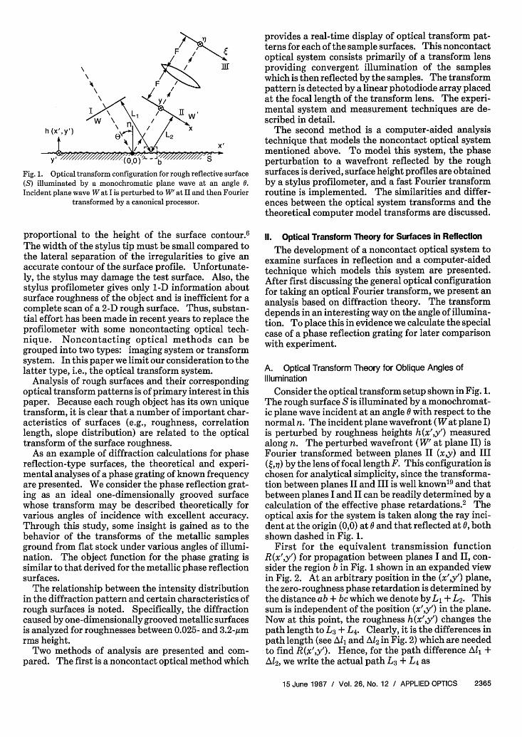
First for the equivalent transmission functionR(x',y') for propagation between planes I and II, con-sider the region b in Fig. 1 shown in an expanded viewin Fig. 2. At an arbitrary position in the (x',y') plane,the zero-roughness phase retardation is determined bythe distance ab + bc which we denote by L, + L2. Thissum is independent of the position (x',y') in the plane.Now at this point, the roughness h(x',y') changes thepath length to L3 + L4. Clearly, it is the differences inpath length (see All and A12 in Fig. 2) which are neededto find R(W',y'). Hence, for the path difference All +Al2, we write the actual path L 3 + L 4 as

15 June 1987 / Vol. 26, No. 12 / APPLIED OPTICS 2365

function is implicit in the reflectance R(x',y'). Thisfunction is established by the size of the illuminationspot on the rough surface S.

For the reduced but important practical case of nor-mal illumination, 0 = 0, and Eqs. (7) and (8) can becombined to give a simpler form for the output denot-ed by Vo(fxfy). The result is

Vo(fxfy) = B j dxdy expI-i27rVfx + fyy- 2h(x,y)/X]I. (11)

Fig. 2. Insert b from Fig. 1 showing an expanded view of roughsurface h(x',y') and path differences All and Al2. Segment ab is Ll

and bc is L2 in Fig. 1.

L3 + L4 = (L1 + L2) - (All + Al2), (3)

in which

All + A12 = 2h(x',y') cos@.

Consider an approximate form for Eq. (8) that isobtained by transforming the integration to the plane(x',y'). For the differential dx, we use Eq. (5) assum-ing that h(x',y') sin0 is small enough so that we arejustified to write

cosOdx' dx,

dy' = dy. (12)

Using Eqs. (7), (9), and (10), we can rewrite Eq. (8) as(4) follows:

It is convenient to summarize the coordinate transfor-mation between (x',y') and (x,y) for the surface S.From a straightforward trigonometric consideration,one can show that

x' cos0 - h(x',y') sin0 = x, (5)

y'= y. (6)

Now, for a suppressed harmonic time dependenceexp(iwt) using Eqs. (3) and (4) and dropping unessen-tial constant phase delays, we define the reflectancefunction R(x',y') by

R(x',y') = exp[+i2kh(x',y') cos0], (7)

in which the wavenumber k = c/c = 27r/X, where X isthe wavelength of the illumination. In Eq. (7) for thewavefront perturbation, we calculate the phase differ-ences along the optic axis (which is taken along theincident and reflected rays at an angle 0), ignoring thelocal slope. Hence, the calculation is essentially par-axial, but with respect to the optic axis. Ray offset,however, is included in Eq. (7) by virtue of the coordi-nate transformation in Eqs. (5) and (6), as will be clearin the later analyses.

Since Eq. (7) for R(x',y') gives us an expression forthe perturbed phase front W at II, we can immediatelywrite the output scalar component V3 (,) at the out-put plane III. The paraxial form is given by

V3(Q,,1 ) = B J J dxdyR(x',y') exp[i2ir(#x + ,qy)/(FX)], (8)

in which B = [i/(XF)] exp(-i47rF/X) and R(x',y') isgiven in Eq. (7) with coordinate transformations inEqs. (5) and (6).

One often prefers to express V3 (Q,-) in Eq. (8) interms of spatial frequencies (ffy) defined by

fx= -/(FX), (9)

Iyc=c-oq(F). (10)

In calculations using Eq. (8) we assume that a blocking

V3(,77) = B cosO LJ dx'dy' exp[i2rh(x',y')

X (2 cos0/X + fx sinG)] exp[-i2r(f. cos0x' + fyy')]. (13)

A fairly direct physical interpretation can be made ofEq. (13). First, we emphasize that the equation isvalid for general 2-D roughness, h(x,y). The phaseperturbations in wavefront W, in effect, include allangles of arrival into the Fourier transform lens sys-tem. The tendency for a rough surface to appearsmoother as the angle 0 is increased is readily seen inthe term in the exponent, 47rh(x',y') cos0/X, as was firstpointed out by Rayleigh. Another point to note in Eq.(13) is that the spatial frequency content correspond-ing to x' detail is angle dependent while that for y' isnot. To understand this consider some detail in theoptical transform that appears at a spatial frequencyfxo in the 0 = 0 case; then by Eq. (13) we see that, forincidence at 0, this detail will shift to a new spatialfrequency f given by

f = 0xcoso (14)

Hence, we expect the optical transform pattern tospread out due to the higher spatial frequencies whichappear as the angle of incidence 0 is increased. Theexponential term 27rh(x',y')fx sin0 has been ignored inthis discussion. One can verify that this factor isnegligible for fairly smooth surfaces at low angles ofincidence and at small spatial frequencies. However,in general it can have a noticeable effect and thereforeit is retained.

B. Sinusoidal Phase Grating Illuminated in Reflection

The results of the previous section are applied to thecase of a sinusoidal grating of period w and relief heightho. This illustration will give us a better understand-ing of the dependence of the output spectrum in the(Q,1) plane on the angle of incidence. It will also serveto illustrate an approximate calculation using Eq. (8)


transformed to the (xy) plane as an alternate to theapproach in Eq. (13).

We rewrite Eq. (8) using Eq. (7) and Eqs. (5), (6), (9),and (10) to obtain the following form for the outputtransform V3(Q,7):

V3(,n) = B J o dxdy exp[i4irh(x/cosO,y) cosO/X

- i2r(fx + fyy)]. (15)

This equation is also approximate since we have usedx- x/cos0 in the argument of h(x',y') as an approxi-mation to the transformation in Eq. (5).

For the reflection grating, let h(x',y') be given by

h(x',y') = ho sin(2irx'/w), (16)

where w is the spatial period and ho is the amplitude.Moreover, if we use a circular spot of illumination witha radius a, Eq. (16) can be substituted into Eq. (15) andintegrated using standard Fourier transform relations.The result of this calculation for V3 (Q,7) is summarizedas follows:

V3 (Q,n1) = a2 B E Jn(A)J 1(2-7rav)/(av), (17)

have a formula which relates the intensity atfx = y = 0to the roughness.

Consider a 1-D rough surface h(x') as in Fig. 1, withnormally incident illumination and readout. For sim-plicity we will take the aperture function to be rectan-gular, D1 by D2 , i.e., given by

D(x',y') = rect ( ) rect Y- ' (22)

in which D1 and D2 are large compared to the trans-verse correlation length, 40, along the x' direction.Equation (15) is rewritten for this case, setting 0 = 0and using V(fxfy) to represent V3 (,r), so the outputscalar amplitude in plane III is given by

V(f.,fy) = B dx'dy'D(x',y')

X expt-i2ir[?7h(x') + fxx' + fyy]} (23)

in which X = 2 cos0/X and the blocking function D(x',y')is defined by Eq. (22).

Since the roughness is assumed to be 1-D, one canintegrate Eq. (23) with respect to y'; the result is

V(fxfy) = BD2 sinc(D2 fy) f dx' rect(x'/D 1 )

where J is a Bessel function of the first kind and inwhich the symbols are defined by

A = 47rho cosO/X, (18)

B = [i/(XF;')] exp(-i4irF/X), (19)

v= [x - n/(w cosY)]2 + f . (20)

Spatial frequency variablesf, andfy are defined in Eqs.(9) and (10). By Eq. (17) we see that the spectrumV3Q(,n) is a 1-D series of narrow Airy disks centered atfy = 0 and distributed along

f.= ' n0,+1,+2 ....W coso

(21)

Both of the general observations made in the discus-sion of Eq. (13) are seen in the result for this illustra-tive calculation. The amplitudes of the Airy disks aregiven by Jn(A) and the Rayleigh height dependence hocos0 is seen in the argument A in Eq. (18). Moreover,the spectral peaks in Eq. (21) are seen to shift to higherfrequencies as the angle of incidence 0 is increased. Asinusoidal relief grating was fabricated both to verifythese calculations and to serve as a calibration stan-dard. These experiments are described in a later sec-tion of this paper.

C. Statistical Theory for the Specular Peak

In reflection from a smooth surface, there is a brightspecular peak. As the roughness is increased, less andless energy is observed in the central Airy disk. Thisenergy decrease in the specular peak would appear tobe a good basis for remotely sensing object roughness,particularly if one notes that this phenomenon doesnot exhibit pronounced saturation at a roughness ofthe order of a wavelength. Hence, we would like to

X exp(-i2ir[nh(x') + fxx']I. (24)

For the statistical calculation, we need to compute theexpected value of the intensity, U(fxfy) = IV(fXfy)12,where the expectation is taken over an ensemble of therough surfaces. Related calculations are found in theliterature.2 ' 13' 2 0

For the expected value of the intensity, we write

(U(fxfy)) = (V(fxsty)V*(fxxty))1

and by Eq. (24), it follows that

(U(f~fY)) = U0 J J dx'dx" rect(x'/D) rect(x"/D 2 )

X exp[i2irf(x" - x')]

X (exp[-i27rinh(x') + i27rflh(x")]),

(25)

(26)

where we define U0 = [IBID2 sinc(D2 fy)]2. The expect-ed value for the bracketed term in the integrand of Eq.(26) is the 2-D characteristic function corresponding tothe joint probability density for the random process ofheights, h(x') and h(x"), but with a sign alteration toaccount for the complex conjugation.

Here for the sake of definiteness, we assert that therandom process of roughness is stationary and more-over that the probability density of heights is jointlynormal and can be written as follows:

f(h1,h 2;r12 ) = expl-(h2 - 2rl 2hlh2 + h2)/[2U2 (1 - r 2)] (

where the correlation coefficient r12 is formally foundas the following expectation:

<hlh2 >/U2 = r12. (28)

We have taken the mean value of h(x) to be zero, i.e.,the origin of coordinates (0,0) in Figs. 1 and 2 is at the


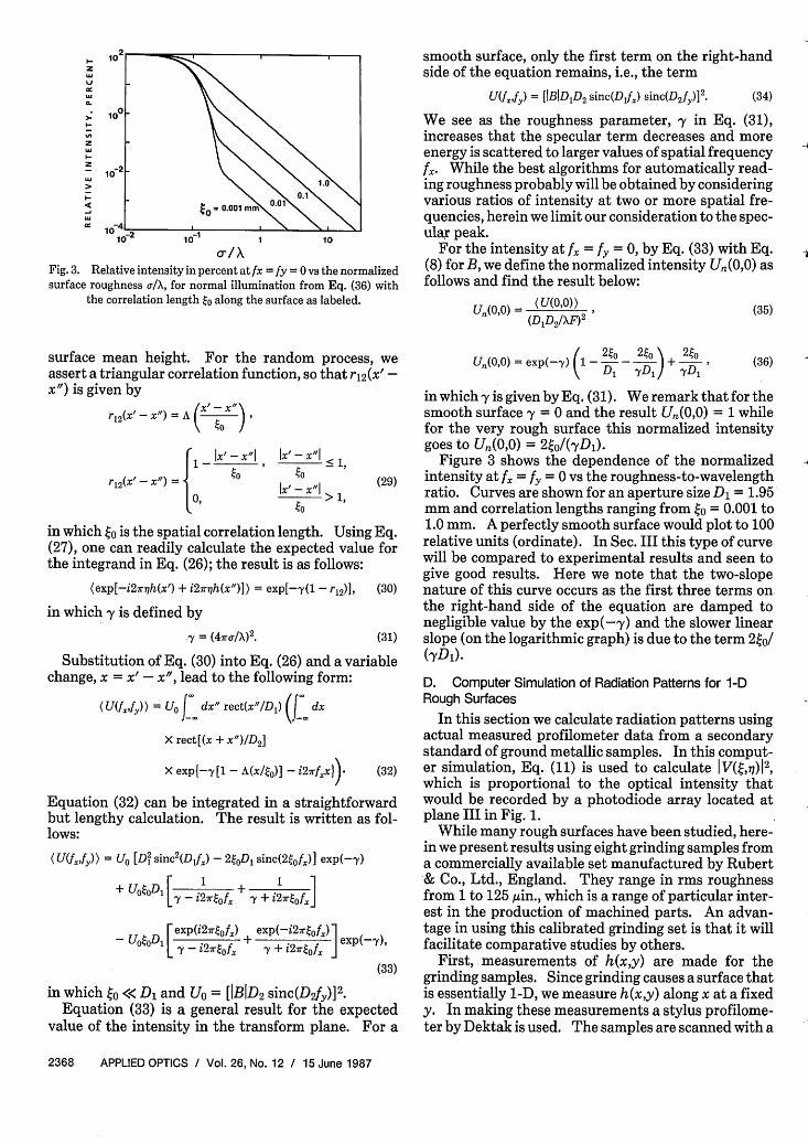
- 2010

~~~~~to 10 01 10

102 10

v/AFig. 3. Relative intensity in percent atfx = fy = vs the normalizedsurface roughness a/X, for normal illumination from Eq. (36) with

the correlation length 40 along the surface as labeled.

surface mean height. For the random process, weassert a triangular correlation function, so that r12 (x' -x") is given by

rl2(X - X") = A (x ) ,

- x I")-xI/

rl2(X' - X) = 4 t

LO,

< 1,I1

~~> 1,to

in which 40 is the spatial correlation length. Using Eq.(27), one can readily calculate the expected value forthe integrand in Eq. (26); the result is as follows:

(exp[-i2ir77h(x') + i2ir77h(x")]) = exp[-(1 - r12 )], (30)

in which y is defined byy = (47ra/X)2. (31)

Substitution of Eq. (30) into Eq. (26) and a variablechange, x = x'- x", lead to the following form:

(U(fxfy)) = U0J dx" rect(x'/D1) (f dx

X rect[(x + x")/D 2 ]

X expl-y[1 - A(x/0 )] - i2rfxxl). (32)

Equation (32) can be integrated in a straightforwardbut lengthy calculation. The result is written as fol-lows:

(U(fxfy)) = U0 [D2 sinc2(D1f) - 2D 1 sinc(20f,)] exp(--y)

+ UotoD, [a - irtofx + My + irtoix]

exp(i2-~of,) exp(-i2r-of.)1- UOtODl L -y - i27r of. + y + i2 - f ] exp(-y),

(33)

in which 0 << D, and U0 = [IBID2 sinc(D2fy)] 2.Equation (33) is a general result for the expected

value of the intensity in the transform plane. For a

smooth surface, only the first term on the right-handside of the equation remains, i.e., the term

U(fxfy) = [IBID1D2 sinc(D1 fx) inc(D2 fy)12. (34)

We see as the roughness parameter, y in Eq. (31),increases that the specular term decreases and moreenergy is scattered to larger values of spatial frequencyfx. While the best algorithms for automatically read-ing roughness probably will be obtained by consideringvarious ratios of intensity at two or more spatial fre-quencies, herein we limit our consideration to the spec-ular peak.

For the intensity at fx = fy = 0, by Eq. (33) with Eq.(8) for B, we define the normalized intensity UA(O,0) asfollows and find the result below:

U(,0) - D(U(0,0))(DD 2/XF)2

(0, _ 2p- 2(0U,,(0,0) = exp(--y) 1 - - y- + D1

(35)

(36)

in which y is given by Eq. (31). We remark that for thesmooth surface -y = 0 and the result Un(O,O) = 1 whilefor the very rough surface this normalized intensitygoes to Un(0,0) = 2o/(-yDj).

Figure 3 shows the dependence of the normalizedintensity at f,, = fy = 0 vs the roughness-to-wavelengthratio. Curves are shown for an aperture size D1 = 1.95mm and correlation lengths ranging from 4o = 0.001 to1.0 mm. A perfectly smooth surface would plot to 100relative units (ordinate). In Sec. III this type of curvewill be compared to experimental results and seen togive good results. Here we note that the two-slopenature of this curve occurs as the first three terms onthe right-hand side of the equation are damped tonegligible value by the exp(-y) and the slower linearslope (on the logarithmic graph) is due to the term 2to/(yD).

D. Computer Simulation of Radiation Patterns for 1-DRough Surfaces

In this section we calculate radiation patterns usingactual measured profilometer data from a secondarystandard of ground metallic samples. In this comput-er simulation, Eq. (11) is used to calculate IV(n)12,which is proportional to the optical intensity thatwould be recorded by a photodiode array located atplane III in Fig. 1.

While many rough surfaces have been studied, here-in we present results using eight grinding samples froma commercially available set manufactured by Rubert& Co., Ltd., England. They range in rms roughnessfrom 1 to 125 yin., which is a range of particular inter-est in the production of machined parts. An advan-tage in using this calibrated grinding set is that it willfacilitate comparative studies by others.

First, measurements of h(x,y) are made for thegrinding samples. Since grinding causes a surface thatis essentially 1-D, we measure h(x,y) along x at a fixedy. In making these measurements a stylus profilome-ter by Dektak is used. The samples are scanned with a


1.0

0.0

I

I

-1.0O.c

10.0

0.0

-10.00.0 1400.0

SURFACE LENGTH (m)

Fig. 4. Profilometer height measurements for ground metallic sam-ples. Note that the scale of (b) rough covers ten times the range of

(a) smooth.

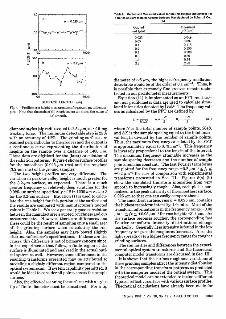
diamond stylus (tip radius equal to 2.54,Mm) at -15-mgtracking force. The minimum detectable step is 25 Awith an accuracy of 2%. The grinding surfaces arescanned perpendicular to the grooves and the output isa continuous curve representing the distribution ofheights on the sample over a distance of 1400 m.These data are digitized for the (later) calculation ofthe radiation patterns. Figure 4 shows surface profilesfor the smoothest (0.025-,Mm rms) and the roughest(3.2-Am rms) of the ground samples.

The two height profiles are very different. Thevariation in peak-to-valley height is much greater forthe 3.2 -Am surface, as expected. There is a muchgreater frequency of relatively deep scratches for the0.02 5-Mum surface, specifically -12 in 1200 Mm vs 2 or 3for the 3.2-,gm surface. Equation (1) is used to calcu-late the rms height for this portion of the surface andthe results are compared with manufacturer's quotedvalues in Table I. We see a generally good correlationbetween the manufacturer's quoted roughness and ourmeasurements. However, there are differences andthese could be the result of sampling only a small areaof the grinding surface when calculating the rmsheight. Also, the samples may have bowed slightlyafter manufacturer's specifications. If these are thecauses, this difference is not of primary concern since,in the experiments that follow, a finite region of thesurface is illuminated and analyzed in the actual opti-cal system as well. However, some differences in theresulting transforms presented may be attributed tomodeling a slightly different region compared to theoptical system scan. If system capability permitted, itwould be ideal to consider all points across the samplesurface.

Also, the effect of scanning the surfaces with a stylustip of finite diameter must be considered. For a tip

Table 1. Quoted and Measured Values for the rms Heights (Roughness) ofa Series of Eight Metallic Ground Surfaces Manufactured by Rubert & Co.,

Ltd.

Quoted MeasuredaM (um) aC (um)

0.025 0.0490.05 0.0870.1 0.1150.2 0.1500.4 0.2830.8 0.601.6 0.743.2 2.23

diameter of -5 Am, the highest frequency oscillationdetectable would be of the order of 0.1,gm-1. Thus, itis possible that extremely fine grooves remain unde-tected in our profilometer measurements.

Equation (11) is implemented as an FFT routine, 2 1

and our profilometer data are used to calculate simu-lated intensities denoted by | Vs1.2 The frequency val-ues as calculated by the FFT are defined by

n -N 0+NI NAX 2 2 (37)

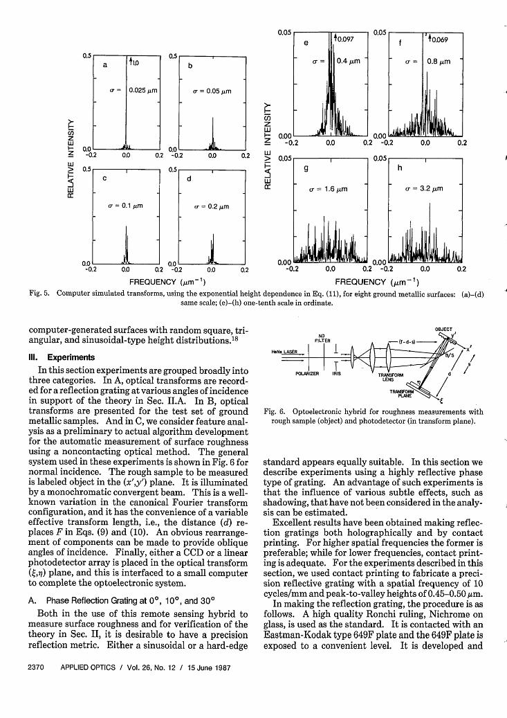
where N is the total number of sample points, 2048,and AX is the sample spacing equal to the total inter-val length divided by the number of sample points.Thus, the maximum frequency calculated by the FFTis approximately equal to 0.73,4m-m. This frequencyis inversely proportional to the length of the interval.The maximum frequency attainable increases as thesample spacing decreases and the number of samplepoints remains constant. The fast Fourier transformsare plotted for the frequency range -0.2 gm-1 _ f, -+0.2 ,m-1 for ease of comparison with experimentaltransforms presented in Sec. III. Figures 5(a)-(h)show the simulated transform intensities from verysmooth to increasingly rough. Also, each plot is nor-malized to the peak intensity of the smoothest surface,0.025jum so that one can easily compare them.

The smoothest surface, rms h = 0.025,Mm, containsthe highest transform intensity, 1.0 units. Most of thetransform information is in the frequency range -0.05pm-' ' fx _ +0.05 /m-m for rms heights <0.4 Mm. Asthe surface becomes rougher, the corresponding fastFourier transform intensity distributions changemarkedly. Generally, less intensity is found in the lowfrequency range as the roughness increases. Also, thelight spreads over a higher frequency range for roughergrinding surfaces.

The similarities and differences between the experi-mental optical system transforms and the theoreticalcomputer model transforms are discussed in Sec. III.

It is shown that the surface roughness variations ofthese grinding samples affect the intensty distributionin the corresponding transform patterns as predictedwith the computer model of the optical system. Thistheoretical model can be extended to include differenttypes of reflective surface with various surface profiles.Theoretical calculations have already been made for


= 0.025 m

- b o = 3.2Am

I . . I I . I . ,

1400.0I . I . . . . . .

,0

0.05

0.5

0.0 L_-0.2 0.0 0.2

).O '= I 0.0 --0.2 0.0 0.2 -0.2

b

(7= 0.05 gm

0.0-0.2 0.0 0.;

o _ - -

,zwz

1=wr

2

0.0 0.2

0.00 _-0.2

0.05

0.00 -0.2

0.05

0 I 02I'WUUL I 0.00 20.0 0.2 -0.2

0.05

0.0 0.2 -0.2

FREQUENCY (Am- 1) FREQUENCY (m- 1 )Fig. 5. Computer simulated transforms, using the exponential height dependence in Eq. (11), for eight ground metallic surfaces: (a)-(d)

same scale; (e)-(h) one-tenth scale in ordinate.

computer-generated surfaces with random square, tri-angular, and sinusoidal-type height distributions.' 8

Ill. Experiments

In this section experiments are grouped broadly intothree categories. In A, optical transforms are record-ed for a reflection grating at various angles of incidencein support of the theory in Sec. II.A. In B, opticaltransforms are presented for the test set of groundmetallic samples. And in C, we consider feature anal-ysis as a preliminary to actual algorithm developmentfor the automatic measurement of surface roughnessusing a noncontacting optical method. The generalsystem used in these experiments is shown in Fig. 6 fornormal incidence. The rough sample to be measuredis labeled object in the (x',y') plane. It is illuminatedby a monochromatic convergent beam. This is a well-known variation in the canonical Fourier transformconfiguration, and it has the convenience of a variableeffective transform length, i.e., the distance (d) re-places F in Eqs. (9) and (10). An obvious rearrange-ment of components can be made to provide obliqueangles of incidence. Finally, either a CCD or a linearphotodetector array is placed in the optical transform(Q,-) plane, and this is interfaced to a small computerto complete the optoelectronic system.

A. Phase Reflection Grating at 0, 100, and 300

Both in the use of this remote sensing hybrid tomeasure surface roughness and for verification of thetheory in Sec. II, it is desirable to have a precisionreflection metric. Either a sinusoidal or a hard-edge

OBJECT

FILTER Y-d-s

POLARIZER IRISTRNFM d /

Fig. 6. Optoelectronic hybrid for roughness measurements withrough sample (object) and photodetector (in transform plane).

standard appears equally suitable. In this section wedescribe experiments using a highly reflective phasetype of grating. An advantage of such experiments isthat the influence of various subtle effects, such asshadowing, that have not been considered in the analy-sis can be estimated.

Excellent results have been obtained making reflec-tion gratings both holographically and by contactprinting. For higher spatial frequencies the former ispreferable; while for lower frequencies, contact print-ing is adequate. For the experiments described in thissection, we used contact printing to fabricate a preci-sion reflective grating with a spatial frequency of 10cycles/mm and peak-to-valley heights of 0.45-0.50 gm.

In making the reflection grating, the procedure is asfollows. A high quality Ronchi ruling, Nichrome onglass, is used as the standard. It is contacted with anEastman-Kodak type 649F plate and the 649F plate isexposed to a convenient level. It is developed and


a f ID

( = 0.025 Am

f Tuvoy

(r = 0.8 Arm

.X~I

e

a = 0.4 m

I 11.C"zzw

w

d

Cr = 0.2 grm

'7

0.0 0.2

0.0 0.2

_.'.1 '' T a r . I - I ' r R ' ' w _

9_kn n7

sac~

fixed. Finally it is overcoated with aluminum. Thefixing causes a relief height in the emulsion, as desired;and the aluminum overcoating provides high reflectiv-ity. The resulting metric provided a 0.5-tim peak-to-valley height and a period w = 0.10 mm.

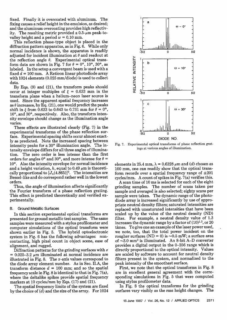
This reflection phase-type object is placed in thediffraction pattern apparatus, as in Fig. 6. While onlynormal incidence is shown, the apparatus is readilyadjusted for incident illumination at 0 and readout atthe reflection angle 0. Experimental optical trans-form data are shown in Fig. 7 for 0 = 0°, 10°, 300, aslabeled. In the setup a convergent beam is used with afixed d = 100 mm. A Reticon linear photodiode arraywith 1024 elements (0.025 mm/diode) is used to collectdata.

By Eqs. (9) and (21), the transform peaks shouldoccur at integer multiples of = 0.633 mm in thetransform plane when a helium-neon laser source isused. Since the apparent spatial frequency increasesas 0 increases, by Eq. (21), one would predict the peaksshift in t from 0.633 to 0.643 to 0.731 mm for 0 = 0°,100, and 300, respectively. Also, the transform inten-sity envelope should change as the illumination anglevaries.

These effects are illustrated clearly (Fig. 7) in theexperimental transforms of the phase reflection sur-face. Experimental spacing shifts occur almost exact-ly as predicted. Note the increased spacing betweenintensity peaks for a 300 illumination angle. The in-tensity envelope differs for all three angles of illumina-tion. The zero order is less intense than the firstorders for angles 0° and 300, and more intense for 0 =100. Also the intensity envelope for normal incidenceand a height variation, h, equal to 0.49 gm is theoreti-cally proportional to [J,(4.865)]2. The intensities areBessel-like and do correspond rather well in the lowestorders.

Thus, the angle of illumination affects significantlythe Fourier transform of a phase reflection grating.This effect is predicted theoretically and verified ex-perimentally.

B. Ground Metallic Surfaces

In this section experimental optical transforms arepresented for ground metallic test samples. The samesamples were measured with a stylus profilometer andcomputer simulations of the optical transform wereshown earlier in Fig. 5. The hybrid optoelectronicsystem in Fig. 6 has the following advantages: non-contacting, high pixel count in object scene, ease ofalignment, and rugged.

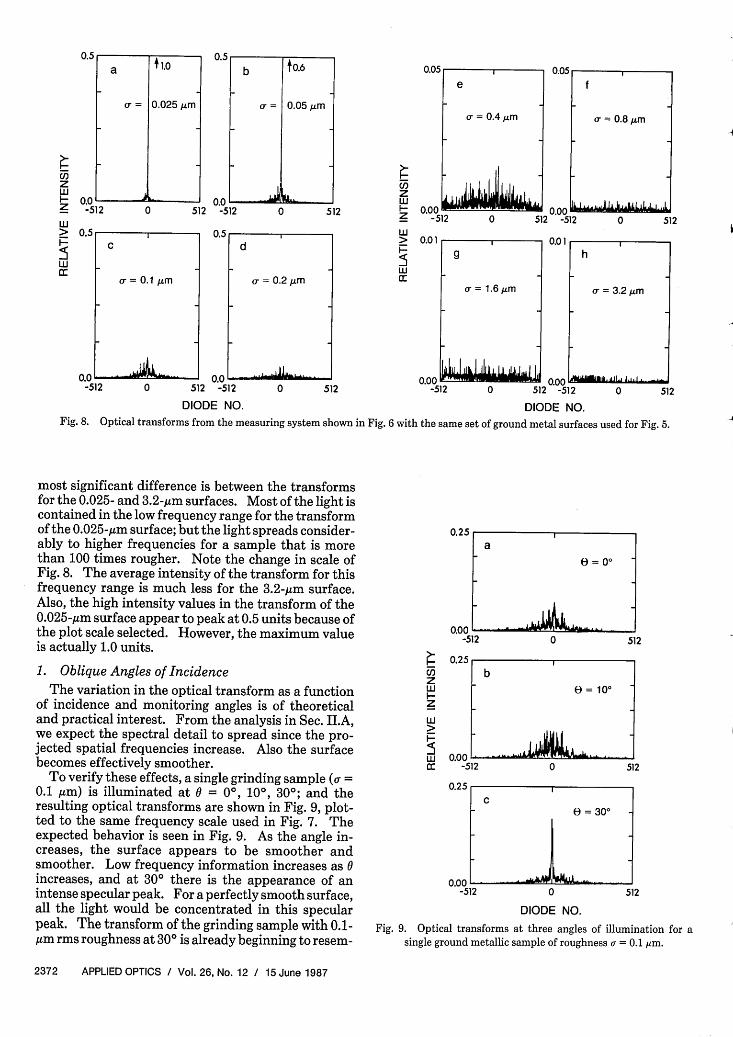
Diffraction patterns for the grinding surfaces with a= 0.025-3.2 ,um illuminated at normal incidence areillustrated in Fig. 8. The x-axis values correspond tothe diode array element number. As in Sec. II.A, thetransform distance d = 100 mm; and so the spatialfrequency scale in Fig. 8 is identical to that in Fig. 7(a),where the deltalike spikes provide spatial frequencymarkers at 10 cycles/mm by Eqs. (17) and (21).

The spatial frequency limits of the system are fixedby the choice of (d) and the size of the array. For 1024

0-5

U,

wHz

wr

0-5

0

- a

= 0

512 0 5

- b 0- 0 ~~~e= 10°

, .. . . .11 1 12 0 51

- ,

= 300

L.-IL I 1 -LLL,-512 0

12

2

512

DIODE NO.

Fig. 7. Experimental optical transforms of phase reflection grat-ings at various angles of illumination.

elements in 25.4 mm, X = 0.6328 Am and (d) chosen as100 mm, one can readily show that the optical trans-form records over a spatial frequency range of ±201cycles/mm. A count of spikes in Fig. 7(a) verifies this.

A scan time of 10 ms is selected for each of the eightgrinding samples. The number of scans taken persample and averaged is also selected; eighty scans persample were taken. The dynamic range of the photo-diode array is increased significantly by use of appro-priate neutral density filters; saturated intensities arereplaced with unsaturated intensities that have beenscaled up by the value of the neutral density (ND)filter. For example, a neutral density value of 1.3increases the dynamic range by a factor of (10)1.3, or 20times. To give one an example of the laser power used,we note, too, that the total power incident on therougher surfaces (ND = 0) is -0.5 mW; a surface areaof -3.0 mm 2 is illuminated. An 8-bit A-D converterprovides a digital output in the 0-256 range which isdirectly proportional to the optical intensity. Valuesare scaled by software to account for neutral densityfilters present in the system, and normalized to thepeak intensity of the smoothest surface.

First, we note that the optical transforms in Fig. 8are in excellent general agreement with the corre-sponding simulations in Fig. 5 that were computedusing stylus profilometer data.

In Fig. 8 the optical transforms for the grindingsurfaces vary visibly as the rms height changes. The


1

1

a

( = 0.025 m

0.0 - --512 0 512

A .

0.0'--512 0

0.5 -

0.0 -512

512 -512

DIODE NO.

0.05

Uzw

F

Erc:

0 512

512

0.00'-51

0.01

12

0.00 K2-512

0 5120 512 -512

0.0Ir

0 512 -51 2

DIODE NO.

0 512

Fig. 8. Optical transforms from the measuring system shown in Fig. 6 with the same set of ground metal surfaces used for Fig. 5.

most significant difference is between the transformsfor the 0.025- and 3.2-gm surfaces. Most of the light iscontained in the low frequency range for the transformof the 0.025-Am surface; but the light spreads consider-ably to higher frequencies for a sample that is morethan 100 times rougher. Note the change in scale ofFig. 8. The average intensity of the transform for thisfrequency range is much less for the 3.2-gtm surface.Also, the high intensity values in the transform of the0.025-,um surface appear to peak at 0.5 units because ofthe plot scale selected. However, the maximum valueis actually 1.0 units.

1. Oblique Angles of IncidenceThe variation in the optical transform as a function

of incidence and monitoring angles is of theoreticaland practical interest. From the analysis in Sec. II.A,we expect the spectral detail to spread since the pro-jected spatial frequencies increase. Also the surfacebecomes effectively smoother.

To verify these effects, a single grinding sample (a =0.1 gim) is illuminated at 0 = 0, 100, 300; and theresulting optical transforms are shown in Fig. 9, plot-ted to the same frequency scale used in Fig. 7. Theexpected behavior is seen in Fig. 9. As the angle in-creases, the surface appears to be smoother andsmoother. Low frequency information increases as 0increases, and at 300 there is the appearance of anintense specular peak. For a perfectly smooth surface,all the light would be concentrated in this specularpeak. The transform of the grinding sample with 0.1-gum rms roughness at 300 is already beginning to resem-

0.25

0.00-51

0.25U,zlL

zw

HwU

cc0.00

V.L I

0.00'-51 0

512

512

512

DIODE NO.

Fig. 9. Optical transforms at three angles of illumination for asingle ground metallic sample of roughness a = 0.1 ,um.


b tO.6

a = 0.05 Aum

AL�1� �

e

= 0.4 A'm

U,zw

zw

c

0.05

(7= 0.8 Am

0.00

c

a= 0.1 Mm

h

(7= 3.2 Mm

0.00 .AiAhLLmhil, J

a=0

2 0A

b9) = 100 -

, b e1oo -51 0, i

c0 = 30

~ ... A

I

. _ __ A_

120

-512 0

21:

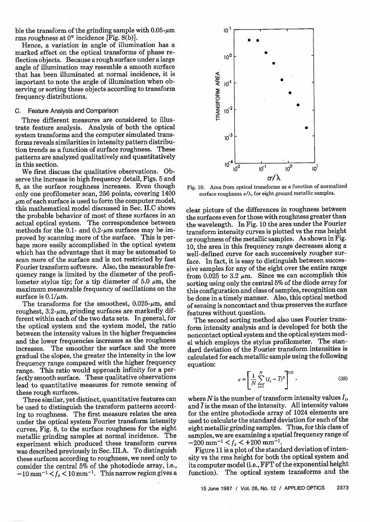
ble the transform of the grinding sample with 0.05-gmrms roughness at 00 incidence [Fig. 8(b)].

Hence, a variation in angle of illumination has amarked effect on the optical transforms of phase re-flection objects. Because a rough surface under a largeangle of illumination may resemble a smooth surfacethat has been illuminated at normal incidence, it isimportant to note the angle of illumination when ob-serving or sorting these objects according to transformfrequency distributions.

C. Feature Analysis and Comparison

Three different measures are considered to illus-trate feature analysis. Analysis of both the opticalsystem transforms and the computer simulated trans-forms reveals similarities in intensity pattern distribu-tion trends as a function of surface roughness. Thesepatterns are analyzed qualitatively and quantitativelyin this section.

We first discuss the qualitative observations. Ob-serve the increase in high frequency detail, Figs. 5 and8, as the surface roughness increases. Even thoughonly one profilometer scan, 256 points, covering 1400,gm of each surface is used to form the computer model,this mathematical model discussed in Sec. II.C showsthe probable behavior of most of these surfaces in anactual optical system. The correspondence betweenmethods for the 0.1- and 0.2-,gm surfaces may be im-proved by scanning more of the surface. This is per-haps more easily accomplished in the optical systemwhich has the advantage that it may be automated toscan more of the surface and is not restricted by fastFourier transform software. Also, the measurable fre-quency range is limited by the diameter of the profi-lometer stylus tip; for a tip diameter of 5.0 im, themaximum measurable frequency of oscillations on thesurface is 0.1/,gm.

The transforms for the smoothest, 0.025-gim, androughest, 3.2-gim, grinding surfaces are markedly dif-ferent within each of the two data sets. In general, forthe optical system and the system model, the ratiobetween the intensity values in the higher frequenciesand the lower frequencies increases as the roughnessincreases. The smoother the surface and the moregradual the slopes, the greater the intensity in the lowfrequency range compared with the higher frequencyrange. This ratio would approach infinity for a per-fectly smooth surface. These qualitative observationslead to quantitative measures for remote sensing ofthese rough surfaces.

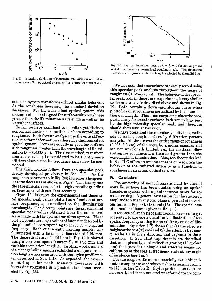
Three similar, yet distinct, quantitative features canbe used to distinguish the transform patterns accord-ing to roughness. The first measure relates the areaunder the optical system Fourier transform intensitycurves, Fig. 8, to the surface roughness for the eightmetallic grinding samples at normal incidence. Theexperiment which produced these transform curveswas described previously in Sec. III.A. To distinguishthese surfaces according to roughness, we need only toconsider the central 5% of the photodiode array, i.e.,-10 mm- 1 <f < 10 mm-1. This narrow region gives a

101

100

LU

a:

0OLLU,zCC

-1

-2

lo-3

10I

0o/XFig. 10. Area from optical transforms as a function of normalized

surface roughness a/X, for eight ground metallic samples.

clear picture of the differences in roughness betweenthe surfaces even for those with roughness greater thanthe wavelength. In Fig. 10 the area under the Fouriertransform intensity curves is plotted vs the rms heightor roughness of the metallic samples. As shown in Fig.10, the area in this frequency range decreases along awell-defined curve for each successively rougher sur-face. In fact, it is easy to distinguish between succes-sive samples for any of the eight over the entire rangefrom 0.025 to 3.2 im. Since we can accomplish thissorting using only the central 5% of the diode array forthis configuration and class of samples, recognition canbe done in a timely manner. Also, this optical methodof sensing is noncontact and thus preserves the surfacefeatures without question.

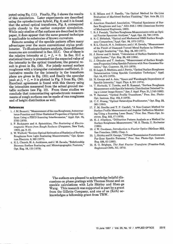
The second sorting method also uses Fourier trans-form intensity analysis and is developed for both thenoncontact optical system and the optical system mod-el which employs the stylus profilometer. The stan-dard deviation of the Fourier transform intensities iscalculated for each metallic sample using the followingequation:

- N - 1/2a = 7 (Ii - )2, (38)

where N is the number of transform intensity values Ii,and I is the mean of the intensity. All intensity valuesfor the entire photodiode array of 1024 elements areused to calculate the standard deviation for each of theeight metallic grinding samples. Thus, for this class ofsamples, we are examining a spatial frequency range of-200 mm-1 < f7, < +200 mm-1.

Figure 11 is a plot of the standard deviation of inten-sity vs the rms height for both the optical system andits computer model (i.e., FFT of the exponential heightfunction). The optical system transforms and the


U,zzU-0

LL

z

00

0

0zH1

l-1

162 [

3O5 I

)2

* I

0A

* AA A

0

0-1 0 0

10 10° 101

0/AFig. 11. Standard deviation of transform intensities vs normalized

roughness a/X: , optical system and A, computer simulation.

modeled system transforms exhibit similar behavior.As the roughness increases, the standard deviationdecreases. For the noncontact optical system, thissorting method is also good for surfaces with roughnessgreater than the illumination wavelength as well as thesmoother surfaces.

So far, we have examined two similar, yet distinct,noncontact methods of sorting surfaces according toroughness. Both feature analyses use the optical Fou-rier transform information gathered by the noncontactoptical system. Both are equally as good for surfaceswith roughness greater than the wavelength of illumi-nation (X = 0.6328 gm). The first method, transformarea analysis, may be considered to be slightly moreefficient since a smaller frequency range may be con-sidered.

The third feature follows from the specular peaktheory developed previously in Sec. II.C. As theroughness parametery in Eq. (36) increases, the specu-lar term decreases as shown in Fig. 3. This theory andthe experimental results for the eight metallic grindingsurfaces agree with excellent accuracy.

Figure 12 illustrates the experimental and theoreti-cal specular peak values plotted as a function of sur-face roughness, a, normalized to the illuminationwavelength. The discrete points are the experimentalspecular peak values obtained from the noncontactscans made with the optical transform system. Theseplotted points are single values of intensity detected bythe photodiode corresponding to the f, fy = 0 spatialfrequency. Each of the eight grinding samples wasilluminated with a laser spot diameter of 1.95 mm.The theoretical curve (solid line) in Fig. 12 is plottedusing a constant spot diameter D = 1.95 mm andvariable correlation length 40. In other words, each ofthe eight grinding samples exhibited a unique correla-tion length when measured with the stylus profilome-ter described in Sec. II.D. As expected, the experi-mental specular peak intensity decreases withincreasing roughness in a predictable manner, mod-eled by Eq. (36).

102

Z 1

I-z

-4

101o- 10- 1 +1

01 X

Fig. 12. Optical transform data at f = = 0 for actual groundmetallic surfaces vs normalized roughness a/X. The theoretical

curve with varying correlation length is plotted by the solid line.

We also note that the surfaces are easily sorted usingthis specular peak analysis throughout the range ofroughness (0.025-3.2 gm). The behavior of the specu-lar peak, both in theory and experiment, is very similarto the area analysis described above and shown in Fig.10. Both contain a downward sloping curve whenplotted against roughness normalized by the illumina-tion wavelength. This is not surprising, since the area,particularly for smooth surfaces, is driven in large partby the high intensity specular peak, and thereforeshould show similar behavior.

We have presented three similar, yet distinct, meth-ods of sorting rough surfaces by diffraction patternanalysis. All three cover the entire range of roughness(0.025-3.2 gm) of the metallic grinding samples andare not wavelength limited; i.e., the methods allowsorting for roughness less than and greater than thewavelength of illumination. Also, the theory derivedin Sec. II.C offers an accurate means of predicting thebehavior of the radiated intensity as a function ofroughness in an actual optical system.

IV. Conclusions

The scattering of monochromatic light by groundmetallic surfaces has been studied using an opticaltransform system with a photodetector array for re-mote sensing. A general expression for the scatteredamplitude in the transform plane is presented in vari-ous forms in Eqs. (8), (13), and (15). The special caseof normal incidence is given in Eq. (11).

A theoretical analysis of a sinusoidal phase grating ispresented to provide a quantitative illustration of thespatial frequency scaling for an arbitrary angle of illu-mination. Equation (17) shows that (1) the effectiveheight varies as h(x') cos0 and (2) the effective frequen-cy scales 1:1 in the y direction and as f/cos0 in the xdirection. In Sec. III.A experiments are describedthat use a phase type of reflective grating (10 cycles/mm) that provides a simple and effective means forcalibration of the spatial frequency scale at any angleof incidence (see Fig. 7).

For the rough surfaces, commercially available cali-brated samples are used with roughness ranging from 1to 125 gin. (see Table I). Stylus profilometer data aremeasured, and then simulated transform data are com-


0

0

1~~~~~~

- I~~~~~~~~~~

I

1

1(54 I

puted using Eq. (11). Finally, Fig. 5 shows the resultsof this simulation. Later experiments are describedusing the optoelectronic hybrid, Fig. 6; and it is foundthat the actual optical transforms, Fig. 8, correspondquite closely to the earlier computer simulation.While only studies of flat surfaces are described in thispaper, it does appear that the same general techniqueis applicable to substrates of known curvature.

Remote sensing of the speckle pattern offers manyadvantages over the more conventional stylus profi-lometer. To illustrate feature analysis, three differentmeasures are considered in Sec. III.C. One of these isthe relative intensity at fA = fy = 0. In Sec. II.C astatistical theory is presented for the expected value ofthe intensity in the optical transform; the general re-sult is given in Eq. (26). For jointly normal surfaceroughness with a triangular correlation coefficient, il-lustrative results for the intensity in the transformplane are given in Eq. (33); and finally the specularpeak at fA = fy = 0 is plotted in Fig. 3 from Eq. (36).Excellent agreement is found with this theory usingthe intensities measured from the actual ground me-tallic surfaces (see Fig. 10). From these studies weconclude that noncontacting optoelectronic measure-ments of rough surfaces can be made of rms roughnessand of height distribution as well.

References

1. J. M. Bennett, "Measurement of the rms Roughness, Autocovar-

iance Function and Other Statistical Properties of Optical Sur-

faces Using a FECO Scanning Interferometer," Appl. Opt. 15,

2705 (1976).2. P. Beckmann and A. Spizzichino, The Scattering of Electro-

magnetic Waves from Rough Surfaces (Pergamon, New York,1963), pp. 9-10.

3. W. Welford, "Review-Optical Estimation of Statistics of Surface

Roughness from Light Scattering Measurements," Opt. Quan-tum Electron. 9, 269 (1977).

4. E. L. Church, H. A. Jenkinson, and J. M. Zavada, "RelationshipBetween Surface Scattering and Microtopographic Features,"

Opt. Eng. 18, 125 (1979).

5. E. Milana and F. Rasello, "An Optical Method for On-Line

Evaluation of Machined Surface Finishing," Opt. Acta 28, 111

(1981).6. American Standard Association, "Physical Specimens of Sur-

face Roughness and Lay," ASA-B46.1-1962 (American Society

of Mechanical Engineers, 1962).7. B. J. Pernick, "Surface Roughness Measurements with an Opti-

cal Fourier Spectrum Analyzer," Appl. Opt. 18, 796 (1979).

8. R. C. Birkebak, "Optical and Mechanical RMS Surface Rough-ness Comparison,"Appl. Opt. 10, 1970 (1971).

9. E. L. Church, H. A. Jenkinson, and J. M. Zavada, "Measurement

of the Finish of Diamond-Turned Metal Surfaces by Differen-

tial Light Scattering," Opt. Eng. 16, 360 (1977).10. J. Stover and S. Serati, "Calculation of Surface Statistics from

Light Scatter," Opt. Eng. 23, 406 (1984).11. J. Ohtsubo and T. Asakura, "Measurement of Surface Rough-

ness Properties Using Speckle Patterns with Non-Gaussian Sta-tistics," Opt. Commun. 25, 315 (1978).

12. D. Leger, E. Mathieu, and J. Perrin, "Optical Surface Roughness

Determination Using Speckle Correlation Technique," Appl.Opt. 14, 872 (1975).

13. N. George and A. Jain, "Space and Wavelength Dependence of

Speckle Intensity," Appl. Phys. 4, 201 (1974).14. T. Horiuchi, Y. Tomita, and R. Kammel, "Surface Roughness

Measurement with Speckle Intensity Distribution Detected Us-ing a Linear Image Sensor," Jpn. J. Appl. Phys. 21, L743 (1982).

15. T. Sawatari, "Optical Profile Transducer," Proc. Soc. Photo-Opt. Instrum. Eng. 153, 8 (1978).

16. C. C. Huang, "Optical Heterodyne Profilometer," Opt. Eng. 23,365 (1984).

17. F. M. Smolka and T. P. Caudell, "A Non-Contact Method for

Surface Profile Measurement and Angular Deflection Monitor-ing Using a Scanning Laser Beam," Proc. Soc. Photo-Opt. In-

strum. Eng. 153, 17 (1978).18. K. J. Allardyce, "Diffraction Pattern Analysis as a Method for

Surface Roughness Measurement," M. S. Thesis, U. Rochester

(1985).19. J. W. Goodman, Introduction to Fourier Optics (McGraw-Hill,

San Francisco, 1968), Chap. 5.20. L. Shirley and N. George, "Diffuser Transmission Functions and

Far-Zone Speckle Patterns," Proc. Soc. Photo-Opt. Instrum.Eng. 556, 63 (1985).

21. E. 0. Brigham, The Fast Fourier Transform (Prentice-Hall,Englewood Cliffs, NJ, 1974).

The authors are pleased to acknowledge helpful dis-cussions on phase gratings with Thomas Stone and onspeckle calculations with Lyle Shirley and Shen-geWang. This research was supported in part by a grantfrom the Gillette Company, and one of us (KJA) ac-knowledges a fellowship grant from TRW.


diffraction analysis of rough reflective surfaces

Documents