diagnosing examinees' attributes-mastery using the
TRANSCRIPT

DIAGNOSING EXAMINEES’ ATTRIBUTES-MASTERY USING THE
BAYESIAN INFERENCE FOR BINOMIAL PROPORTION: A NEW METHOD
FOR COGNITIVE DIAGNOSTIC ASSESSMENT
A Dissertation
Presented to
The Academic Faculty
By
Hyun Seok Kim (John)
In Partial Fulfillment
of the Requirements for the Degree
Doctor of Philosophy in the
School of Psychology
Georgia Institute of Technology
August 2011

DIAGNOSING EXAMINEES’ ATTRIBUTES-MASTERY USING THE
BAYESIAN INFERENCE FOR BINOMIAL PROPORTION: A NEW METHOD
FOR COGNITIVE DIAGNOSTIC ASSESSMENT
Approved by:
Dr. Susan E. Embretson, Advisor
School of Psychology
Georgia Institute of Technology
Dr. Rustin Meyer
School of Psychology
Georgia Institute of Technology
Dr. Lawrence R. James
School of Psychology
Georgia Institute of Technology
Dr. Charles Parsons
College of Management
Georgia Institute of Technology
Dr. Daniel Spieler
School of Psychology
Georgia Institute of Technology
Date Approved: June 15, 2011

DEDICATION
I dedicate this paper to the true author, the Lamb of God, who provided a bit of His
wisdom from the beginning to the end of this study.
“Truly my soul silently waits for God; From Him comes my salvation. He only is my
rock and my salvation; He is my defense; I shall not be greatly moved.” (Psalms 62:1-2)

iv
ACKNOWLEDGEMENTS
First, I wish to thank my advisor, Susan Embretson. Her profound knowledge has
inspired and guided my study at Georgia Tech, and I especially appreciate her patience
and consideration for the study. I also thank my committee members, Larry James, Dan
Spieler, Rustin Meyer, and Charles Parsons, for their feedback and all the help I got from
them. I can‟t forget Greg Corso, Jan Westbrook, Sereath Hopkins, and Renee Simpkins
for their help and kindness. I am indebted to Megan Lutz in my lab for her generous help
and I thank all the quantitative psychology faculties and students. My Wieuca Road
Baptist Church members also deserve a special acknowledgement: Thanks for all your
prayers, Dixie, Jack, and Anne Gee, Sam Hayes, Sharon Smith, Jan Bell, Bill Givens,
Pam Cravy and so many others. My deep gratitude goes to my lovely family, my wife
(Mia), and the two precious daughters (Uni and Minji). Their prayers and support made
me keep studying. Finally, to my father and mother who have supported me hoping and
enduring everything, thanks for your waiting for the past nine years. However, all the
praise and glory should go to God who made everything beautiful in His time. I thank
Him for changing me through the time! Now, I am yours. Take my life and lead our
family wherever you have planned.

v
TABLE OF CONTENTS
ACKNOWLEDGEMENTS………………………………………………………………iv
LIST OF TABLES……………………………………………………………………..ix
LIST OF FIGURES…………………………………………………………………….xi
SUMMARY………………………………………………………………..…………xii
CHAPTER 1: INTRODUCTION…………………………………………………………….1
1.1 What is Cognitive Diagnostic Assessment (CDA)?…………....…………….1
1.2 Current Issues in CDA………………………………………………………..4
1.3 Purpose of the Study …………………………………………………………5
CHAPTER 2: COGNITIVE DIAGNOSIS MODELS…………………….…...................7
2.1 Overview……………………………………………………………………...7
2.2 Rule Space Method…………………………………………………………..11
2.3 Fusion Model………………………………………………………………...18
2.4 DINA, NIDA, and DINO Model…………………………………………….22
2.5 LLTM………………………..……….………………………………………26
2.6 MLTM…………………………………..…………………………………....28
2.7 GLTM………………………………………..………………………………30
2.8 LCDM……………………………………………………………………….32
CHAPTER 3: BAYESIAN STATISTICAL INFERENCE……………………………...35
3.1 Introduction…………………………………………………………………..35
3.2 Bayes‟ Theorem.……………………………………………………………..36
3.3 Bayesian Inference for Binomial Proportion (BIBP)…...……………………39

vi
3.4 Estimators for Proportion (π)………………………………………………...42
3.5 Bayesian Inference for Normal Mean……………………………………..…44
CHAPTER 4: THE CURRENT STUDIES ………………….………………………….49
4.1 Study Design/Purpose……………….……...…………….....................49
4.2 Assumptions………………………………………………………………50
4.3 Defining “Mastery”………………………………………………………51
CHAPTER 5: REAL DATA STUDY 1: FOUR-ATTRIBUTE DATA…………….….53
5.1 Method……………………...……………........................................53
5.1.1 Subjects and Instruments………………………………………………53
5.1.2 Estimating Single-Attribute Parameters (Step 1)………………………54
5.1.3 Estimating Multiple-Attribute Parameters (Step 2)……………………55
5.1.4 Updating the Single-Attribute Parameters (Step 3)……………………57
5.2 Results…………………….……………………...…………….....................61
5.2.1 Descriptive Statistics ………………………..…………………….…...61
5.2.2 Individual Diagnosis Result …………………………………….…….62
5.3 Discussion…………………...……………………………….........................66
CHAPTER 6: REAL DATA STUDY 2: TEN-ATTRIBUTE DATA………………….68
6.1 Method…………………………………..………..………….....................68
6.1.1 Subjects and Instruments………………………………………………
6.1.2 Estimating the Parameters Directly Measured by the Items(Step1)......69
6.1.3 Inference about the Unmeasured Single-Attribute Parameters(Step2)...71
6.2 Results……………………...……………………………….....................73
6.2.1 Descriptive Statistics ………………………..…………………….…...73
6.2.2 Individual Diagnosis Result …………………………………….…….76
6.3 Discussion…………………...………………………………........................80
CHAPTER 7: REAL DATA STUDY 3: COMPARING BIBP TO DINA
AND LCDM………………..……………………………………………………………81
7.1 Method…………..……………………...…………….............................82
7.1.1 Subjects and Instruments………………………………………………82
7.1.2 Procedure…………………………………………………………..82

vii
7.2 Results……………………...……………...............................................83
7.2.1 Descriptive Statistics ………………………..………………….…...83
7.2.2 Individual diagnosis result …………………………………...…….85
7.3 Discussion………………...…………………………………………….....87
CHAPTER 8: SIMULATION STUDY 1: GENERAL ACCURACY AND
EFFECTIVENESS OF THE PARAMETER ESTIMATION.................................89
8.1 Method…………………………………………………................................89
8.1.1 Item Design…………………………………………………………89
8.1.2 Examinee Attribute Mastery Probability and
Mastery Pattern.......................................................................9 0
8.1.3 Item Response Data Generation……………………………………….92
8.1.4 Estimation of and ………………………………………....92
8.2 Results…………………………………………………...............................93
8.2.1 Descriptive Statistics of True πk and the Estimates ( )……………..93
8.2.2 Correct Classification Rate for Attribute Mastery …………………….93
8.2.3 Accuracy of the Attribute-Mastery Probability Recovery......................95
8.3 Discussion ………………...…………………………………………….....96
CHAPTER 9: SIMULATION STUDY 2: ACCURACY OF THE PARAMETER
ESTIMATION UNDER VARIOUS CONDITIONS.......................................................97
9.1 Method…………………………………………………...............................97
9.1.1 Attribute Correlation and Attribute Difficulty……………………97
9.1.2 Sample Size……………………….…………………………………99
9.1.3 Item Response Data Generation………………………………….100
9.1.4 Comparison with the DINA Estimation…………………………….100
9.2 Results………………………………………………………………….101
9.2.1 Attribute Correlation …………………………………………….101
9.2.2 Attribute Difficulty…………………………………………………101
9.2.3 Sample Size………………….………………………………………103
9.2.4 Interactions of the Simulation Variables……………………………..104
9.2.5 Comparison with the DINA Estimation…………………………….106
9.3 Discussion………………………………………………………………….110
CHAPTER 10: CONCLUSION………………………………………………………112
APPENDIX A: Four Standards and their Benchmarks………………………………..117

viii
APPENDIX B: FOUR-ATTRIBUTE DATA ESTIMATION RESULTS
(REAL DATA STUDY 1)………………………………………………………..……..118
APPENDIX C: SIMULATED (TRUE) ATTRIBUTE MASTERY PROBABILITIES,
ATTRIBUTE MASTERY PATTERNS, AND RAW SCORES (FROM THE RESPONSE
DATA) IN SIMULATION STUDY 1…………………………………………………..123
APPENDIX D: AVERAGE CCR, RMSE, AND ASB OF THE 36 SIMULATED
CONDITIONS FOR BIBP……………………………………………………………....124
APPENDIX E: AVERAGE CCR, RMSE, AND ASB OF THE 36 SIMULATED
CONDITIONS FOR DINA……………………………………………………………125
REFERENCES…………………………………………………………………………126

ix
LIST OF TABLES
Table 2.1 List of the CDMs in Two Categories.........................................................8
Table 2.2 Attributes and Q-matrix for Fraction Addition Problems..........................13
Table 2.3 The 11 Most Common Knowledge States for Fraction
Addition Problems……………………….………………………………14
Table 5.1 Item Design for the Four Attributes................................ ..................54
Table 5.2 Descriptive Statistics of the Raw Score and Estimated Attribute
Probability ( ) Mastery in Step 1 & 2 and Step 3 (N=2993)…………60
Table 5.3 Attribute Difficulty (pk) in Step 1 & 2 and Step 3 (N=2993)………....61
Table 5.4 Inter-Attribute Correlations (Step 1& 2)………………………………..62
Table 5.5 Inter-Attribute Correlations (Step 3)…………………………………….62
Table 5.6 Diagnosis Results for the Three Examinees (Raw Score: 64/86)
by Step 1&2 and Step 3 …………………………..……………………..63
Table 6.1 Item Design for the Ten Attributes……………………………………69
Table 6.2 Descriptive Statistics of the Raw Score and from Step 1
and Step 2………….…………………………………………………74
Table 6.3 Attribute Difficulty……………………………………………..….74
Table 6.4 Inter-Attribute Correlations of the Single Attributes…………………75
Table 6.5 Inter-Attribute Correlations between Single Attributes
and Multiple Attributes……………………………………………….75
Table 6.6 Diagnosis Results for the Three Examinees (Raw Score: 64/86)……….77
Table 7.1 Descriptive Statistics of the Raw Score and of the Four Attributes
for DINA, LCDM, and BIBP…………………………………….….84
Table 7.2 Inter-Attribute Correlations and pk …………………………………..85
Table 7.3 Proportion of Same Classifications for Examinee Attribute Mastery
Pattern (αk) of the Three Models ………………………………………..86

x
Table 7.4 Diagnosis Results ( , αk) for the Three Examinees (Raw Score: 64/86)
by the Three Models…………………………………………………86
Table 8.1 Simulated Item Design………………………………………………90
Table 8.2 Descriptive Statistics of True πk, raw score, and the Estimate ( )……..94
Table 8.3 Correct Classification Rate (CCR) for Attribute Mastery Patterns ……94
Table 8.4 Average Signed Bias (ASB) and Root Mean Square Error (RMSE) …...95
Table 9.1 Three Simulation Variables and their Levels…………………………...99
Table 9.2 CCR, ASB, and RMSE for Attribute Correlation …………………...101
Table 9.3 CCR, ASB, and RMSE for Attribute Difficulty………………………102
Table 9.4 CCR, ASB, and RMSE for Sample Size…………………………….103
Table 9.5 Marginal Means and Standard Deviations of CCR, RMSE, and ASB
for the DINA and BIBP Estimations ………………………………….107
Table 9.6 Unidimensional IRT Model (3PLM) Fit of the Four Correlations……..108
Table B.1 Examinee Attribute Mastery Probability Estimates (Step 1&2)….…119
Table B.2 Examinee Attribute Mastery Patterns (Step 1&2)…………………….120
Table B.3 Examinee Attribute Mastery Probability Estimates (Step 3)…………...121
Table B.4 Examinee Attribute Mastery Patterns (Step 3)……………………..…122

xi
LIST OF FIGURES
Figure 2.1 Sample rule space of four knowledge states.............................................16
Figure 2.2 Graphical Representation of the LLTM (Wilson & De Boeck, 2004).....27
Figure 2.3 Four different hierarchical structures (Leighton et al., 2004)...................29
Figure 3.1 Samples of Beta Distribution (adapted from Bolstad, 2007)....................41
Figure 3.2 Prior, Data, Posterior Distributions...........................................................48
Figure 4.1 Bloom‟s Taxonomy of Cognitive Domain...............................................51
Figure 5.1 Estimating the Posteriors of the Attribute Mastery Probabilities
in Study 1…………………………………………………………..…..57
Figure 5.2 Estimated Posteriors of , , , and for Examinee #11…………64
Figure 5.3 Estimated Posteriors of , , , and for Examinee #130…………65
Figure 6.1 Estimating the Posteriors of the thirteen Parameters…………………….70
Figure 6.2 Estimated Posteriors of , , and for Examinee #116……….….78
Figure 6.3 Estimated Posteriors of , , and for Examinee #130……….……79
Figure 6.4 Estimated Posteriors of , , , , , and for Examinee #2706..80
Figure 9.1 Effect of Attribute Difficulty on CCR, ASB, and MRSE………….102
Figure 9.2 Effect of Sample Size on CCR, ASB, and MRSE………….………104
Figure 9.3 Two-Way Interactions of Attribute Difficulty × Sample Size and
of Attribute Correlation × Sample Size in CCR…………………..104
Figure 9.4 Attribute Difficulty × Sample Size for Attribute Difficulties
(3-Way Interaction) in CCR……………………………………………105
Figure 9.5 Effect of Attribute Correlation on CCR, ASB, and MRSE in DINA….108
Figure 9.6 Effect of Attribute Difficulty on CCR, ASB, and MRSE in DINA…..109
Figure 9.7 Effect of Sample Size on CCR, ASB, and MRSE in DINA…...……….109

xii
SUMMARY
Cognitive diagnostic assessment (CDA) is a new theoretical framework for
psychological and educational testing that is designed to provide detailed information
about examinees‟ strengths and weaknesses in specific knowledge structures and
processing skills. During the last three decades, more than a dozen psychometric models
have been developed for CDA, which are also called cognitive diagnosis models (CDM).
Although they have successfully provided useful diagnostic information about the
examinee, most CDMs are complex due to a large number of parameters in proportion to
the number of skills (attributes) to be measured in an item. The large number of
parameters causes heavy computational demands for the estimation. Also, a variety of
specific software applications is needed depending on the chosen models.
Purpose of this study was to propose a simple and effective method for CDA
without heavy computational demand using a user-friendly software application.
Bayesian inference for binomial proportion (BIBP) was applied to CDA because of the
following fact: When we have binomial observations such as item responses
(right/wrong), using a beta distribution as a prior of a parameter to estimate (i.e.,
attribute-mastery probability) makes it very simple to find the beta posterior of the
parameter without any integration. The application of BIBP to CDA can be flexible
depending on the test item-attribute design and examinees‟ attribute-mastery patterns. In
this study, effective ways of applying the BIBP method was explored using real data
studies and simulation studies. Also, other preexisting diagnosis models such as DINA
and LCDM were compared to the BIBP method in their diagnosis results.

xiii
In real data studies, the BIBP method was applied to a test data using two
different item designs: four and ten attributes. Also, the BIBP method was compared with
DINA and LCDM in their diagnosis result using the same four-attribute data set. There
were slight differences in the attribute mastery probability estimate ( ) among the three
model (DINA, LCDM, BIBP), which could result in different diagnosis results for
attribute mastery pattern (αk). Simulation studies were conducted to (1) evaluate general
accuracy of the BIBP parameter estimation, (2) examinee the impact of various factors
such as attribute correlation (no, low, medium, and high), attribute difficulty (easy,
medium, and hard) and sample size (100, 300, and 500) on the consistency of the
parameter estimation of BIBP, and (3) compare the BIBP method with the DINA model
in the accuracy of recovering true parameters. It was found that the general accuracy of
the BIBP method in the true parameter estimation was relatively high. The DINA
estimation showed slightly higher overall correct classification rate but the bigger overall
biases and estimation errors than the BIBP estimation. The three simulation variables
(Attribute Correlation, Attribute Difficulty, and Sample Size) showed significant impacts
on the parameter estimations of both models. However, they affected differently the two
models: Harder attributes showed the higher accuracy of attribute mastery classification
in the BIBP estimation whereas easier attributes were associated with the higher accuracy
of the DINA estimation. In conclusion, BIBP appears an effective method for CDA with
the advantage of easy and fast computation and a relatively high accuracy of parameter
estimation.

1
CHAPTER 1
INTRODUCTION
1.1 What is Cognitive Diagnostic Assessment (CDA)?
Cognitive diagnostic assessment (CDA) is a new theoretical framework for
psychological and educational tests designed to diagnose examinees‟ skill profiles rather
than just rank the examinees based on test scores. Although traditional tests have served
to grade and rank examinees‟ test performance successively, they do not typically
provide useful diagnostic information about each examinee (Chipman, Nichols, &
Brennan, 1995). CDA does provide detailed information about examinees‟ strengths and
weaknesses in specific knowledge structure and processing skills so that examinees can
understand why they pass or fail in a specific item and improve their future performance.
The history of CDA can be traced to the late 1960s and early 1970s when
cognitive psychology (which examines internal mental processes including how people
think, perceive, remember and learn) and psychometrics (which is concerned with the
theories, models and statistical techniques applied to develop psychological and
educational tests) met (Bejar, 2008; Chipman et al., 1995; Leighton & Gierl, 2007).
During that time, Item Response Theory (IRT: Lord & Novick, 1968; Rasch, 1960) and
its psychometric models (i.e., Rasch, 2PL, 3PL IRT models) emerged and IRT became
the mainstream of modern psychometric theory.
Cognitive psychology has provided a much improved understanding of the
component processing skills, strategies, and knowledge structures underlying the test
performance that is a key part of CDA (Snow & Lohman, 1989). Specifically,

2
information-processing analysis of problem solving which began in the 1970s (e.g.,
Carroll, 1976; Hogaboam & Pellegrino, 1978; Hunt, Frost, & Lunneborg, 1973;
Sternberg, 1977) has greatly influenced important developments in CDA. According to
Mislevy (2006), the focus of the information-processing analysis is on “what‟s happening
within people‟s heads” (p. 262) while they are responding to items. As Bejar (2008)
noted, many studies about cognitive ability such as analogical reasoning (Sternberg,
1977), spatial reasoning (Egan, 1979; Pellegrino & Kail, 1982), inductive reasoning
(Pellegrino & Kail, 1982), and verbal ability (Hunt, 1978; Hunt, Lunnenborg, & Lewis,
1975) help psychometricians understand a wide variety of cognitive skills underlying test
performance. Thus, the interpretation of test performance reflects a complex combination
of component processing skills, strategies, and knowledge structures (Snow& Lohman,
1993).
The synergy between cognitive psychology and psychometrics also led to
cognitively based item generation in the 1980‟s (e.g., Bejar, 1985; Butterfield, Nielsen,
Tangen, & Richardson, 1985; Bejar & Yocom, 1986; Hornke, 1986). As noted by Bejar
(2008), Embretson‟s publications (1983, 1985) “created momentum for the idea of
cognitively based item generation” (p. 11). Cognitively based item generation implies
that a well-developed cognitive theory can provide a framework for guiding item
selection and design. Snow and Lohman (1989) and Messick (1989) were inspired by
several precedent research studies (e.g., Cronbach, 1970; Embretson, 1983; Pellegrino &
Glaser, 1979) and escalated interest in and emphasized the need for cognitive diagnostic
assessment in their book chapters in 1989. Since then, the term, CDA, has been widely

3
used and has grown into one of the major issues in development of ability and
achievement tests (Leighton & Gierl, 2007).
For the last two or three decades, researchers have proposed several psychometric
models and test design approaches to implement CDA. Of the psychometric models, the
linear logistic test model (LLTM; Fischer, 1973) is considered to be the first
psychometric model which effectively bridged cognitive psychology and psychometrics.
In the 1980s, the multidimensional latent trait model (MLTM; Whitely, 1980; Embretson,
1991) and the general component latent trait model (GLTM; Embretson, 1984) were
developed as multidimensional and noncompensatory extensions of the Rasch model and
the linear logistic test model, respectively. At that time, the rule space methodology (K. K.
Tatsuoka, 1983, 1990; K. K. Tatsuoka & M. M. Tatsuoka, 1987) was also proposed and
became a cornerstone of many diagnostic models in educational measurement (e.g.,
unified model, fusion model, DINA, AHM). In the 1990‟s, several influential studies
about test design approach and psychometric models for CDA were introduced such as
the cognitive design system (Embretson, 1992, 1994), Evidence-Centered Design
(Mislevy, 1994), unified model (DiBello, Stout, & Roussos, 1993), fusion model (Hartz,
2002; Roussos et al., 2007), Deterministic Inputs, Noisy “And” gate (DINA) model
(Haertel, 1989), Noisy Inputs, Deterministic “And” gate (NIDA) model (Junker &
Sijtsma, 2001), Deterministic Inputs, Noisy “Or” gate (DINO) model (Templin & Henson,
2006), HYBRID model (Yamamoto, 1989), 2PL-Constrained model (Embretson, 1999),
and log-linear cognitive diagnostic model (LCDM; Henson, Templin, & Willse, 2009).

4
1.2 Current Issues in CDA
Although the psychometric models for CDA, which are also called cognitive
diagnosis models (CDM) or diagnostic classification models (DCM), have own strengths
and weaknesses, they successfully provided useful diagnostic information about the
examinee, as well as about each test item. However, most CDMs are complex due to a
large number of parameters in proportion to the number of skills to be measured in an
item. For example, fusion model has k+2 parameters (k = number of skills to be measured
in an item) and the DINO model includes 2k parameters to be estimated. The large
number of parameters in the models cause heavy computational demands for the
parameter estimation. In some models such as fusion model, Markov chain Monte Carlo
(MCMC) method is used for the parameter estimation since it is easier to extend to
parametrically complex models than Expectation Maximization (EM) algorithms.
However, the MCMC causes even heavier computational demand than the marginal
maximum likelihood estimation (MMLE) with the EM algorithm. It takes several hours
even for a single estimation and a day or more for more complex models or large
amounts of data. Also, the MCMC can be misused easily because of the complexity of its
algorithms, thus, it is uncommon for users to take the result of the MCMC analysis with
confidence (Kim & Bolt, 2007).
A variety of software applications is needed depending on the chosen models for
the parameter estimation. Some examples of typical software applications for the CDMs
include (Rupp & Templin, 2008):
Rule space method: BUGLIB (Research License, [email protected])
Fusion model: Arppegio (Commercial, www.assess.com)

5
DINA, NIDA, and DINO: DCM (Free ware but requires the commercial
version of Mplus, [email protected])
DINA and DINO: DCM in R (Free ware requiring the freeware R,
LLTM: ConQuest (Commercial, www.assess.com), LPCM-WIN
(Commercial, www.assess.com), SAS (Commercial, www.sas.com)
LPCM: LPCM-WIN (Commercial, www.assess.com)
2PL-Constrained model, MLTM, & GLTM: SAS (Commercial, www.sas.com)
It is still challenging for general users to run most of these software packages with
confidence because they are complex to operate and uncertainty exists about the analysis
results, especially for a complex model with heavy computational demands.
1.3 Purpose of the Study
Purpose of this study was to propose a simple and effective method for CDA
without heavy computational demand and using an user-friendly software application.
Bayesian inference for binomial proportion (BIBP) was applied to CDA because of the
following fact: When we have binomial observations such as item responses
(right/wrong), using a beta distribution as a prior of a parameter to estimate (i.e.,
attribute-mastery probability) makes it very simple to find the beta posterior of the
parameter without any integration in the Bayesian framework (Bolstad, 2007). Therefore,
first, how to effectively apply BIBP to CDA was explored using a real test data with
different item designs. The diagnosis results (e.g., examinees‟ attribute mastery
probability and the patterns) of the BIBP method were also compared to the results of

6
other diagnosis models. Second, using simulated data, the accuracy of the parameter
estimation of the BIBP method was evaluated and how various conditions on examinee
and item design can affect the estimation accuracy was also explored.

7
CHAPTER 2
Cognitive Diagnosis Model (CDM)
2.1 Overview
Although several different ways of classifying cognitive diagnosis models may
exist, they were divided into two categories in this study: (1) latent class model and (2)
latent trait model. A latent class model denotes the model which classifies examinees into
categories on a set of skills (e.g., mastery or nonmastery of the skill), thus providing a
mastery pattern (or mastery probabilities) as the examinee‟s skill profile. Fusion model,
DINA, NIDA, and DINO models are in this category (Roussos et al., 2008). Whereas, a
latent trait model is an extension or a generalization of unidimensional IRT models (e.g.,
Rasch, 2PLM) that place estimate examinee‟s ability on a continuous scale for each skill;
LLTM, MLTM, GLTM, and 2PL-constrained model belong to this category. The list of
the CDMs for the two categories is presented in Table 2.1.
In the latent class model-category, the rule space method was a pioneering and
successful method of diagnosing examinees‟ knowledge levels as an attempt to overcome
the limitation of the traditional test scoring system where valuable information from the
examinee‟s item response pattern is thrown away for the sake of simplicity. It has greatly
influenced the development of all the subsequent models in this category (e.g., DINA,
Unified, Fusion). The rule space method is not a single psychometric model, but rather a
system which guides both how to diagnose an examinee‟s skill profile and how to
improve the examinee‟s knowledge level. However, the rule space method has a
limitation in treating a variety of sources of response variation which caused mismatches

8
between observed and Q-predicted response patterns. The contribution of the unified
model was to find a way of identifying and treating different sources of response
variation such as Strategy Selection, Completeness, Positivity, and Slips. Then, the
Fusion model was developed to overcome the limited identifiability of the unified model
while maintaining its flexibility and interpretability.
Table 2.1 List of the CDMs in Two Categories
Years Latent Class Models Latent Trait Models
1970 LLTM (Fischer, 1973)
1980 Rule space (K. K. Tatsuoka, 1983)
DINA (Haertel, 1989)
HYBRID model (Yamamoto,
1989)
MLTM (Embretson, 1980)
MIRT-C (McKinley & Reckase, 1982)
GLTM (Embretson, 1984)
1990 Unified model
(DiBello, Stout, & Roussos, 1993)
LPCM (Fischer & Ponocny, 1994)
2PL-Constrained model
(Embretson, 1999)
2000 NIDA (Junker & Sijtsma, 2001)
Fusion (Hartz, 2002)
AHM (Leighton, Gierl, & Hunka,
2004)
DINO (Templin & Henson, 2006)
MLTM-D (Embretson & Yang, 2008)
LCDM (Henson, Templin, & Willse, 2009)
The Fusion model is mathematically equivalent to the original unified model but
has reduced the number of item parameters from 2k + 3 to k+2 (k = number of skills) by
setting the strategy selection parameter to 1. Therefore, the Fusion model traded the
flexibility of handling multiple strategies for the identifiability of all item parameters. Yet,
Fusion keeps good flexibility to deal with incomplete Q-matrix and positivity of
attributes, which provides information about how effective an item is in measuring the

9
attributes. However, there exist some drawbacks due to the parameter estimation method
(MCMC) used in Fusion, which causes heavy computational demand and uncertainty
about the analysis result, especially when the number of skills or attributes (k) to be
measured in an item increases.
An important feature of DINA model and its followers (NIDA, DINO) is the
dealing with false positive and false negative errors of examinees, which correspond to
positivity in the unified model and fusion model. Although they share the same
mathematical concept, there are some differences with each other. On one hand, DINA
and NIDA are non-compensatory models, thus appropriate for the skill diagnosis where
consecutive skills should be successfully performed in order to arrive at a correct answer
(e.g., a mathematical test). On the other hand, DINO is a compensatory model which is
increasingly applied to the settings like medical and psychological disorder diagnoses.
Furthermore, DINA is a more complex model than NIDA because DINA was designed in
the item-level perspective while NIDA was constructed in the skill-level perspective and
the number of items is always bigger than the number of skills to be measured in a test.
The HYBRID model has an interesting characteristic. It was developed to handle
response variation caused by the two strategies used by examinees (Q-based strategy and
non-Q-based strategy), which correspond to strategy selection in the unified model.
Based on examinee response patterns, HYBRID model adopts a non-compensatory latent
class model (e.g., DINA) for the Q-based strategy and a unidimensional IRT model for
the non-Q-based strategy. The log-linear cognitive diagnostic model (LCDM; Henson et
al., 2009) is a generalized model to express both compensatory and non-compensatory
models.

10
Although most of those latent class models are very practical and useful to
diagnose examinee skill profiles, they cannot estimate direct effects of the skills or item
stimulus features on cognitive requirements to solve an item. Thus, they are not useful for
a cognitive model-based test design in which cognitive theories are incorporated into item
generation. AHM is an exception in this category. It incorporates a cognitive model of
structured attributes into the test design, following the approach of information-
processing analysis of problem solving. AHM classifies examinee‟s test performance into
a set of structured attribute patterns by the product of probabilities of positive and
negative slips (corresponding to false positive and false negative probabilities in DINA)
using an unidimensional IRT model. However, if examinees make several slips, then,
very low likelihood estimates usually happen, which makes it very hard to classify the
examinees into the structured attribute patterns.
In the latent trait model-category, LLTM, 2PL-Constrained model, LPCM, and
GLTM allow test developers to incorporate item stimulus features based on cognitive
theories and to estimate direct effects of the stimulus features on cognitive requirements
for success in the item. Therefore, they met the need of psychometric models for
cognitive model-based test design. Latent trait models can be divided into two
subcategories which are unidimensional and multidimensional models. Although
multidimensional models, such as compensatory multidimensional IRT model (MIRT-C;
McKinley & Reckase, 1982), MLTM, GLTM, are appropriate for diagnosing multiple-
skill profiles, unidimensional models, such as LLTM, 2PL-Constrained model, linear
partial credit model (LPCM; Fischer & Ponocny, 1994), are also very useful for CDA
because most achievement tests typically fit unidimensional IRT models fairly well and

11
these models are simple and easy to apply for the test design. In the multidimensional
model-subcategory, MLTM and GLTM are appropriate for most ability and achievement
tests because typical skills (attributes) and processing stages in the test items are
sequentially dependent, whereas, MIRT-C seems more appropriate for medical and
psychological disorder diagnoses like DINO. One drawback of MLTM and GLTM is that
these models typically need both subtask and full task data for the same item, which
makes the data collecting process complex. Recently, Embretson and Yang (2008)
proposed multicomponent latent trait model for cognitive diagnosis (MLTM-D) which
was specifically designed for CDA.
In this chapter, some of the popular CDMs were reviewed in more detail. They
are Rule space method, Fusion model, DINA, NIDA, DINO, LLTM, MLTM, GLTM,
and LCDM.
2.2 Rule Space Method
Tatsuoka and her associates (K. K. Tatsuoka, 1983, 1990; K. K. Tatsuoka & M.
M. Tatsuoka, 1987) developed a pioneering method to diagnose examinees‟ knowledge
levels. This method was named Rule Space Methodology. Development of the Rule Space
Methodology was motivated by the issue that traditional test scores have the limitation of
providing detailed information about examinees‟ knowledge structure that underlies test
performance. In other words, the same total scores do not necessarily reflect the same
level of knowledge or understanding of the examinees. Valuable information from the
examinees‟ item response patterns is thrown away for the sake of simplicity in traditional
test scoring. Tatsuoka (1983) believed that analysis of student‟s misconceptions

12
throughout a test could provide “specific prescriptions for planning remediation for a
student as well as useful information in evaluating instruction or instructional material”
(p. 345). The rule space methodology includes two parts: (1) Q-matrix theory and (2) rule
space.
First, the Q-matrix is a [kn] matrix of ones and zeros, in which k represents the
number of attributes to be measured and n represents the number of items on the test. For
example, there are 12 fraction addition problems in Table 2.2, and nine attributes or
cognitive tasks (A1 through A9) required to answer the problems (Tatsuoka, 1997). In the
bottom of the table, Q-matrix for this test are provided. Because there are twelve items,
the dimension of the Q-matrix became [912]; nine attributes and 12 items. In the Q-
matrix, a one indicates that the item measures the attribute, and a zero indicates that it
does not. Therefore, item 1 measures all attributes but 3 and 9. Item 3 measures attributes
4, 6, and 7. All attributes that an item measures should be mastered by an examinee in
order to answer the item correctly. If an examinee answered the item 1 correctly, then,
theoretically, it means that he/she mastered all attributes but 3 and 9. Furthermore, if an
examinee‟s response pattern for the 12 items was like [0 0 1 0 1 0 1 1 0 1 1 1] (i.e.,
responding correctly to items 3, 5, 7, 8, 10, 11, and 12 and incorrectly to the rest of items),
then, we can infer that the examinee mastered attributes 3, 4, 6 and 7 based on the Q-
matrix in the table.
The attribute mastery patterns, which consist of various combinations of the nine
attributes (see Table 2.2), are referred to as knowledge states. K.K. Tatsuoka and M. M.
Tatsuoka (1992) identified 33 knowledge states based on the frequency of the rules that
examinees used in solving the fraction addition problems in Table 2.2. Of the 33

13
knowledge states, 11 of the most common knowledge states are described in Table 2.3.
Knowledge state #10 is the mastery state that indicates all answers are correct. On the
other hand, knowledge state #21 designates the non-mastery state with all the answers
wrong.
Table 2.2 Attributes and Q-matrix for Fraction Addition Problems
Fraction addition problems, )()(f
ed
c
ba
I1. )6
10(3)
6
8(2 I2.
8
12
5
2 I3.
5
6
5
8 I4. )
4
2(4)
2
1(2
I5. )7
10(1
2
1 I6. )
7
6(4)
7
5(3 I7.
5
7
5
3 I8.
2
1
3
1
I9. )7
12(1)
7
4(1 I10.
5
1
5
3 I11.
2
1
4
3 I12. )
9
1(1)
9
5(2
Attributes
A1. Separate the whole number part from the fraction part when a≠ 0 or d≠ 0.
A2. Separate the whole number part from the fraction part when a≠ 0 and d≠ 0.
A3. Get the common denominator (CD) when c≠ f.
A4. Convert the fraction part before getting the CD.
A5. Reduce the fraction part before getting the CD.
A6. Answer to be simplified.
A7. Add two numerators.
A8. Adjust a whole number part.
A9. Combination of A2 and A3 Mixed numbers with c≠ f.
Q-matrix [912]
Items (12)
Attributes (9)
0001100000
1001110010
1111111111
1111111010
1101000000
1110101010
0101100100
1001110010
1001010010

14
Next, an ideal response pattern for each knowledge state needs to be established
in order to compare it with observed item response patterns so that the observed response
pattern can be classified into one of the 33 knowledge states. Notice that the word “ideal”
does not mean a perfect response pattern, but rather perfect fit with a knowledge state.
For example, the ideal response pattern of the knowledge state #4 is [1 0 1 0 0 1 1 0 1 1 0
1] because all but attribute 3 are mastered in knowledge state #4 and items #2, 4, 5, 8, and
11 measure attribute 3.
Table 2.3 The 11 Most Common Knowledge States for Fraction Addition Problems
Knowledge states
#4 Cannot get the common denominator (CD) but can do simple fraction addition
problems (A1, A2, A4, A5, A6, A7, A8, and A9 mastered).
#6 Cannot get CDs for the problems involving mixed number(s)
(A1, A2, A3, A4, A5, A6, A7, and A8 mastered).
#9 Has problems in simplifying answers to the simplest form
(A1, A2, A3, A5, A7, A8, and A9 mastered).
#10 Mastery state: All attributes are answered correctly
(A1, A2, A3, A4, A5, A6, A7, A8, and A9 mastered).
#11 Can do addition only of two simple fractions (F) when they have the same
denominators (A4, A6, A7, A8, and A9 mastered).
#16 Cannot get CDs and cannot add two reducible mixed numbers (M). Also has
problems with simplification of answers (A1, A2, A7, and A9 mastered).
#21 Non-mastery state: All attributes are answered incorrectly (no attribute
mastered).
#24 Cannot add a mixed number and a fraction. Cannot get CDs. Cannot reduce
fraction parts correctly before getting the CDs (A1, A2, A4, A6, A7, A8, and A9
mastered).
#25 Cannot add the combinations of M and F. Also, cannot get CDs
(A2, A4, A5, A6, A7, and A9 mastered).
#26 Does not realize that adding zero to a nonzero number a yields a itself. That is,
does not grasp the Identity Principle, a + 0 = a
(A2, A3, A4, A5, A6, A7, A8, and A9 mastered).
#33 When adding mixed numbers, adds the fractions correctly but omits the whole
number part or gets it wrong due to incorrect simplification of the fraction part.
(A1, A6, A7, A8, and A9 mastered).

15
An examinee in state #4 cannot answer correctly those five items but should answer
correctly the rest of the 12 items. However, it is very rare to have the observed response
patterns perfectly match with the theoretically expected response patterns (ideal response
patterns) because examinees most likely do not apply the same erroneous rules
consistently over the entire test (Birenbaum & Tatsuoka, 1993; Tatsuoka, 1990).
Moreover, various random errors such as careless errors, uncertainty, or distraction
(referred to as slips, hereafter) cause even more deviations of observed response patterns.
Therefore, the rule space concept was introduced to handle the problem caused by slips.
Second, as mentioned earlier, after establishing ideal response patterns for the
knowledge states, the next step is to compare them with observed examinee‟s item
response pattern, thereby classifying the examinee into one of the knowledge state
categories. However, because the observed response patterns are not identical to the ideal
response patterns, in general, a method called “rule space” is used to deal with this
problem.
Rule space is a graphical representation of the knowledge states for each of the
ideal response patterns and observed response patterns (Tatsuoka, 1990). In rule space,
the distances between ideal and observed response patterns are measured in order to
determine which knowledge state is closest to an observed response pattern as shown in
Figure 2.1. The figure illustrates a sample rule space in which four knowledge states (#6,
9, 10, and 16 in Table 2.3) and some hypothetical observed response patterns (marked by
“x”) are represented. Although knowledge states are unobservable traits and cannot be
represented in such a space directly, Tatsuoka (1984) utilized item response theory ability

16
parameter ( ) and the “atypicality parameter ( )” to present them in two-dimensional
space.
Figure 2.1 Sample rule space of four knowledge states
The value of the atypicality parameter, on the y-axis, indicates how unusual a response
pattern is (similar to a person-fit index) and is calculated as the standardized product
of two residual matrices between observed and expected values (see Tatsuoka, 1996 for
more detail). , on the x-axis, represents an examinee‟s trait or ability estimated by an
unidimensional IRT model (e.g., 1PL, 2PL, or 3PL model).
For example, in Figure 2.1, knowledge state #10 (mastery state) requires a higher
level of ability than any other states, thereby being the farthest to the right on the -axis.
State #9 and #6 seem to have same value, but different values; state #6 is closer to
-axis than state #9. This means that state #6 occurs more frequently in the population.
Finally, state #16 has a mastery pattern of only four attributes (A1, A2, A7, and A9) and
requires a lower level of ability than other knowledge states in Figure 2.1, thus being
located at the farthest left on the -axis. The distances between the knowledge states
10
6
9
16 Ability level ( )
Atypicality ( )

17
(ideal response patterns) and the observed response patterns can be approximated by the
Mahalanobis distance between the centroids of the two points (Tatsuok, 1995). The
closest knowledge state to an observed response pattern will be considered the
individual‟s attribute mastery pattern. Bayes‟ decision rules can also be used to minimize
misclassifications because it provides the probability level which attributes a given
examinee is likely to have mastered (Birenbaum, Kelly, & Tatsuok, 1993).
The rule space methodology has many advantages over traditional way of
assessment. In a traditional test scoring system, individuals within both knowledge state #
6 and #9 could receive the same score. However, the rule space methodology provides
more specific information about how their abilities are actually different. Furthermore,
rule space illustrates the relationships between the knowledge states by showing how far
apart they are using the Mahalanobis distance. Once an examinee is classified into one of
the knowledge states, the next knowledge state that the examinee needs to go to will be
the closest one to his/her current state. The rule space methodology also provides the way
of achieving the next knowledge states. In an adaptive test setting, K. K. Tatsuoka and M.
M. Tatsuoka (1997) showed how to provide immediate feedback and remedial instruction
to each examinee after diagnosing his/her knowledge state.
In general, the rule space methodology has been considered a practical method of
classifying response patterns into knowledge states by simple statistics. Moreover, the Q-
matrix theory in this methodology became a foundation for the development of many
following diagnostic models (e.g., RUM, Fusion, DINO), especially in educational
assessment. However, the rule space methodology has some limitations. There is still
uncertainty about how accurately an examinee‟s knowledge state can be identified given

18
the variability of possible item response patterns. Also, the rule space methodology is not
an approach of a cognitive model-based test design to incorporate cognitive theories into
item generation but just a methodology to diagnose students‟ misconceptions and
knowledge states especially in achievement testing.
2.3 Fusion Model (Reparameterized Unified Model)
The unified model (DiBello, Stout, & Roussos, 1993, 1995) has a critical
limitation, that is, not all of the parameters in the model can be statistically identifiable.
To overcome the limited identifiability while maintaining the advantages of flexibility
and interpretability of the unified model, Hartz (2002) reduced the number of parameters
from 2k + 3 to k+2 (k = number of skills to be measured in an item). The reduced model
is referred to as the reparameterized unified model (RUM), of which all k+2 parameters
are identifiable. RUM is also called the fusion model. Roussos et al. (2007) defined the
fusion model system as a CDA system which includes skills diagnosis, the parameter
estimation method (i.e., MCMC), model checking procedures and skills-level score
statistics. RUM is the item response function model within the fusion model system.
RUM is mathematically equivalent to the original unified model (Roussos et al.,
2007). However, there was a trade-off between reducing the number of parameters and a
source of flexibility in the original unified model. That is, Strategy Selection ( id )
parameter was omitted in the RUM. Therefore, the probability that an examinee selects a
Q-strategy is set to 1 ( id = 1) in the RUM. In other words, there is no possibility that
examinees may use other strategies than the Q-strategy to solve the item. If id parameter

19
in the unified model is set to 1, the unified model can be converted into RUM as follows
(Roussos et al., 2007):
),|1( jjijXP = )(1
)1(
jc
K
k
q
ik
q
ik i
ikjkikjk pr
=
K
k
jc
q
iki i
ikjk Pr1
)1()( . (2.1)
),|1( jjijXP is the probability of answering item i correctly given that examinee j
has a skill mastery vector of j and a residual (supplemental) ability parameter of
j ,
just as in the unified model. i( =
K
k
q
ikik
1
) is the probability that an examinee having
mastered ALL the skills required for solving item i will correctly apply ALL those skills
to answer the item.
ikr is expressed as )1|1(
)0|1(
jkijk
jkijk
YP
YP=
ik
ikr
, where ik is the
probability of applying successfully skill k to item i given that the examinee has mastered
the skill, and ikr is the probability of applying successfully skill k to item i given that the
examinee has NOT mastered the skill.
The
ikr parameter plays an important role in evaluating the diagnostic ability of an
assessment. It distinguishes which item is more effectively discriminating between
examinees who have mastered or not mastered skill k. For example, if an item more
strongly depends on mastery of skill k, then the probability of passing the item ( ikr ) is
getting lower for a nonmaster of the skill k, thus
ikr will be close to zero. When the
ikr
parameters are closer to zero for most items of a test, the test will be considered to be
well designed for diagnosing mastery on skill k (Roussos et al., 2007). This is very
similar to the positivity index in the unified model.

20
The residual ability parameter (j ) in the )( jci
P component was retained from
the unified model to deal with the issue that the Q-matrix may not include all necessary
skills or attributes for solving an item (incomplete Q-matrix). As in the unified model,
)( jciP is the Rasch model with a difficulty parameter of negative ic (- ic ), which can be
expressed as
)( jciP =
)](exp[1
)](exp[
is
is
c
c
. (2.2)
It should be noted that if the value of ic is bigger (meaning an easier item in the Rasch
model), then )( jciP will also be higher. In RUM, ic plays an important role for
diagnosing the influence of the missing multiple skills (residual ability) on the whole
item response function, ),|1( jjijXP . For example, if ic is 3 (meaning very easy in
the Rasch model), then )( jciP will be almost 1 for most examinees. In such a case, the
residual ability (j ) has almost no impact on ),|1( jjijXP . On the other hand, if ic is
-3, then )( jciP will be close to 0 for most examinees. In such a case,
j will make
),|1( jjijXP almost zero regardless of the rest of the parts of ),|1( jjijXP ,
which indicates that )( jciP has a great impact on ),|1( jjijXP and that the Q-
matrix is incomplete, thus needing to include more skills to be measured.
To estimate item parameters ( i,
ikr , ic ) and examinee skills parameters (j ) in
Equation 2.2, the Markov chain Monte Carlo (MCMC) method, which is firmly rooted in
the Bayesian inference, has been employed. The MCMC method has several advantages
over other parameter estimation methods. First, MCMC algorithms are easier to extend to
parametrically complex models such as RUM than Expectation Maximization (EM)

21
algorithms. Secondly, MCMC provides a joint estimated posterior distribution of both the
item parameters and the examinee skills parameters, which provides better understanding
of the true standard errors involved (Patz & Junker, 1999). Also, MCMC provides a
potentially richer description of the parameters (i.e., a full posterior distribution) than
Maximum Likelihood (ML) method which provides an estimate and its standard error
because MCMC is based on Bayesian inference on estimating model parameters, (Kim &
Bolt, 2007; Roussos, DiBello, Henson, Jang, & Templin, 2008). Finally, a free software
is available for MCMC, such as the WINBURGS program (Spiegelhalter, Thomas, Best,
& Lunn, 2003), although the Arpeggio program (Hartz, Roussos, & Stout, 2002) is
mainly used for parameter estimation of RUM.
MCMC has some disadvantages. The primary drawback of MCMC is the
complexity of its algorithms, which causes heavy computational demand and uncertainty
about the analysis result in some cases. MCMC algorithms require a large number of
iterations until a reliable parameter estimation, thus taking several hours even for a single
estimation and a day or more for more complex models or large amounts of data (Kim &
Bolt, 2007). Also, MCMC can be misused easily because of the complexity of its
algorithms. It is uncommon for users to take the result of the MCMC analysis with
confidence, especially with complex models requiring more parameters to estimate (Kim
& Bolt, 2007).
The RUM provides useful pieces of information about item properties and
examinees‟ skill profiles while its parameters are identifiable. It estimates each
examinee‟s skill mastery vector j and a residual (supplemental) ability (
j ). It
estimates the item parameter (
ikr ) which evaluates how effectively the item discriminates

22
between masters and nonmasters of skill k. Also, ic parameter indicates if Q-matrix is
incomplete, thus if more skills need to be added in the Q-matrix. These item parameters
can be also used to evaluate and support the construct validity of the test. However, the
evaluation of convergence for each parameter is difficult because there has yet been no
reliable statistic for MCMC convergence check (Roussos et al., 2007) and the RUM is a
still complex model having many parameters to estimate.
2.4 DINA, NIDA, and DINO Model
The Deterministic Inputs, Noisy “And” gate (DINA; Haertel, 1989) model and
the Noisy Input, Deterministic “And” gate (NIDA; Junker & Sijtsma, 2001) models are
conjunctive (non-compensatory) models for skills diagnosis. The HYBRID model
(Yamamoto, 1989) is also a conjunctive model, but, interestingly, is flexible to choose a
latent class model such as DINA or an IRT model (1PL, 2PL, or 3PL model) based on
examinees‟ observations. These conjunctive models are appropriate for skill diagnosis
where the solution of a task is broken down into a series of steps with conjunctive
interaction rather than with compensatory interaction (Roussos et al., 2008). Typical
examples of the conjunctive interaction can be found in the skills required to solve
mathematical items where the consecutive skills should be successfully performed in
order to arrive at a correct answer.
However, the Deterministic Input; Noisy “Or” gate (DINO; Templin & Henson,
2006) model is a disjunctive (compensatory) model. The compensatory models have been
increasingly applied to a variety of settings, such as medical and psychological disorder
diagnosis, where the presence of other symptoms can compensate the absence of certain

23
symptoms (Rousoss et al., 2008). Those four models (DINA, NIDA, HYBRID, & DINO)
are closely related to each other in their item response functions.
2.4.1 DINA Model
The item response function for a single task of the DINA model is
),,|1( gsXP ij = ijij
jj gs
1
)1( , (2.3)
where ij =
K
k
Q
ikjk
1
indicates if examinee i has all the skills to solve item j (ij =1,
otherwise ij = 0). ),,|1( gsXP ij is the probability of answering item j correctly given
that examinee i has a skill mastery vector of and error probabilities of s and g . The
parameterjs , denoting )1|0( ijijXP , is the probability of answering incorrectly item
j even though examinee i has all the attributes (skills) for the item (ij = 1). On the
contrary, the parameter, jg , representing )0|1( ijijXP , is the probability of
answering correctly item j even though examinee i has NOT mastered all the attributes
for the item j (ij = 0). The false negative (
js ) and false positive (jg ) probabilities
correspond to the positivity treated as a source of response variation in the unified model
and the RUM, andjg corresponds to ikr in those two models.
js and jg can reflect on
“examinees‟ slips and guesses, poor wording of the task description, inadequate
specification of the Q matrix, use of an alternative solution strategy by the examinee, and
general lack of model fit” (Junker & Sijtsma, 2001, p. 263).
The vector of ij = ( 1i 2i ,…,
ij ) represents ideal response patterns in the rule
space methodology‟s terms and is regarded as a Deterministic Input from each

24
examinee‟s skills mastery patterns (Junker & Sijtsma, 2001). Eachij plays as an “And”
gate in Equation 2.3 because selecting between the probabilities (1-js ) and
jg depends
on the binary value of ij (0 or 1). 1-
js = )1|1( ijijXP is the probability of getting a
correct answer for item j, given examinee i has all the attributes (skills) for the item,
which corresponds to ik in the unified model and the RUM. 1-js will be selected only if
ij is 1, otherwise, jg will be chosen in the item response function. Then, because each
ijX is considered a Noisy observation of each ij , this model was referred to as
Deterministic Inputs, Noisy “And” gate model.
2.4.2 NIDA Model
The item response function of the NIDA model is shown as
),,|1( gsXP ij =
K
k
jkikijk QP1
),|1( . (2.4)
In the NIDA model, the latent variable ijk is newly introduced and indicates whether
examinee i‟s performance in the context of item j is consistent with possessing skill k (1
= consistent, 0 = inconsistent). The observed item response ijX can be defined as
ijX =
K
k
ijk
1
.The two error probabilities were retained from the DINA model in the view point
of skill level rather than in the item level. The false negative probability is expressed as
ks = )1,1|0( jkikijk QP , (2.5)
which represents the probability that the examinee does NOT show consistent
performance with having skill k required to solve item j. The false positive probability is
expressed as

25
kg = )1,0|1( jkikijk QP , (2.6)
which denotes the probability that the examinee‟s performance in the context of item j is
consistent WITHOUT possessing skill k required to solve item j. Also, for the skills
irrelevant to item j, the probability of getting 1ijk is fixed to 1 regardless of the value
a (1 or 0) of ik in order not to influence the whole model,
)0,|1( jkikijk QaP 1. (2.7)
Finally, Equation 2.4 can be converted as follows:
),,|1( gsXP ij =
K
k
jkikijk QP1
),|1( =
K
k
Q
kkjkikik gs
1
1])1[(
=
K
k
K
k
Q
k
k
k jkjkQik
gg
s
1 1
)1
( . (2.8)
The NIDA model is so named because “Noisy Inputs ijk , reflecting attributes ik in
examinees, are combined in a Deterministic And gate ijX ” (Junker & Sijtsma, 2001, p.
265).
2.4.3 DINO Model
The item response function of DINO model is same as the one of DINA, as shown
in Equation 2.3, except it is compensatory (the “Or” in DINO) instead of being
conjunctive (the “And” in DINA).
),,|1( gsXP ij = ijij
jj gs
1
)1( , (2.9)
where ij =
K
k
Qjk
ik
1
)1(1 , indicating if examinee i has satisfied at least one criterion
(e.g., symptom) that Q-matrix includes for item j (ij =1) or if examinee i has NOT
satisfied any criteria that Q-matrix includes for item j (ij =0). As in the DINA model,

26
js and jg denote false negative and false negative probabilities, respectively. As
mentioned above, DINO is a compensatory model which can be applied for medical and
psychological disorder diagnosis. With the DINO model, it does not matter how many or
which particular criteria have been satisfied if an examinee has satisfied one or more in
the item (DiBello et al., 2007).
2.5 LLTM
Although a variety of latent class models successfully diagnosed an examinee‟s
skill profile, they did not seem to incorporate cognitive models into test design except
AHM. However, most latent trait models can link a cognitive theory to the test design
and, in turn, can test the cognitive theory by the significance of the estimated item
parameters in the model. Q-matrix is also applicable to latent trait models. The linear
logistic test model (LLTM) was the first psychometric model that could effectively
bridge cognitive psychology and item design. That is, the model can incorporate item
stimulus features into the prediction of item success. LLTM is a generalization of the
Rasch model which is given as
)exp(1
)exp()1(
is
isisXP
, (2.10)
where )1( isXP is the probability that person s passes item i, s is the trait level of
person s, and i is the difficulty parameter of item i. Because i does not include the
cognitive variables (item stimulus features) involved in the item, it is replaced with a
linear function of cognitive variables in LLTM as follows:

27
ikkiii
K
k
ikki qqqqq
...221100
0
, (2.11)
where k represents the effect of stimulus feature k, ikq is the score (e.g., 0 = absence,
1 = presence) of stimulus feature k of item i, and 00q is the intercept of the equation.
The full LLTM combines Equation 2.10 with Equation 2.11;
K
k ikks
K
k ikks
is
q
qXP
0
0
)exp(1
)exp()1( . (2.12)
The Q matrix which consists of ikq (the indicators of k stimulus features of i items) is
usually structured as a (I, K) matrix with rank K, where K < I. The method of coding the
indicators, ikq , can be dummy coding or scores for the item on cognitive model variables,
depending on the purpose of the application. LLTM can be graphically represented as in
Figure 2.2.
Figure 2.2 Graphical Representation of the LLTM (Wilson & De Boeck, 2004).
i
k ,...,1
0
0iq
iki qq ,...,1
s
0sZ
K
k ikks q0
)1( isXP
Logit link
Random variable
Fixed variable
Linear components
Linear effect of the predictors
Person predictor

28
In Figure 2.2, dotted circles or ellipses represent random variables and regular circles or
ellipses symbolize fixed variables. The figure shows ikq , k , all the constants and their
predicted value ( i ) as fixed variables and explains s as a random variable. Logit link
indicates that )1( isXP is the function of
K
k ikks q0
. The contribution of each item
is explained by the linear components of item stimulus features ( ikq ) and their fixed
effects ( k ) and the person predictor ( s ).
2.6 MLTM
Many ability and achievement test items require multiple skills or competencies
to obtain a correct response. As shown in Figure 2.2, the SAT Algebra item required
multiple skills (attributes) to arrive at a correct response such as comprehension of text,
algebraic manipulation, linear functions, and simultaneous equations. Although MIRT-C
models can be applied to identify multiple dimensions of an item, they are only
appropriate for items in which the multiple skills are compensatory. One important aspect
of multidimensionality is that the skills or processing stages in the items often are
sequentially dependent. Typical cognitive models for tasks postulate a flow of
information from one stage to another. Thus, the assumptions underlying the MIRT-C
models that low trait levels on one skill or stage can be compensated for by high trait
levels on other skills or stages do not fit well with the cognitive psychology views of task
performance.
Leighton et al. (2004) identified four possible forms of the hierarchical structures
of attributes, as shown in Figure 2.3. In all the structures, attribute 1 is considered

29
prerequisite to the other attributes that follow. Except in Figure 2.3 (D), the unstructured
hierarchy, there are orderings among attributes and there are unique relationships
between the total score and the expected examinee response pattern (Leighton, et al.,
2004). The four possible hierarchical structures in Figure 2.3 can be expanded and
combined to apply to more complex hierarchies, where the complexity varies with the
cognitive problem-solving task. Therefore, a model that can reflect the sequential
dependency among the processing stages is necessary to assess properly the source of
multidimensionality in the item domain, which better explains why an examinee fails a
specific item.
Figure 2.3 Four different hierarchical structures (Leighton et al., 2004).
The multidimensional latent trait model (MLTM; Whitely, 1980; Embretson,
1991; Embretson & Yang, 2006) is based on a continued product of processing outcome
1
2
3
4
5
6
A. Linear
1 1
1
2 3 4 5 6
2 2
3 3 4
4
5
5
6
6
B. Convergent
C. Divergent
D. Unstructured

30
probabilities to reflect the sequentially dependent stages (called component, here), as
follows:
)exp(1
)exp()()1(
iksk
ikskkiskkis XPXP
, (2.13)
where )1( isXP is the probability of success for person s on item i and )( iskk XP is
the product of success on each processing component k, given the correct outcome of the
preceding component. The right side of the equation contains Rasch models for the
probability of success on each component, where sk is the trait level of person s on
component k and ik is the difficulty of item i on component k.
2.7 GLTM
The general component latent trait model (GLTM; Embretson, 1984) is the
generalization of the MLTM that incorporates a mathematical model to relate the
difficulty of each component ( ik ) to stimulus features in the item. For example,
paragraph comprehension items, in which a short paragraph is followed by a question
based on the paragraph, have two major components, text representation and decision.
The difficulty of each component is related to stimulus features in the item. That is, text
representation depends on vocabulary level and syntactic complexity while decision
depends on the inference level and the amount of relevant text for the question (Gorin &
Embretson, 2006). Therefore, ik is predicted by the weighted sum of underlying
stimulus features as follows:
ikm
m
m
kmik q
0
, (2.14)

31
where ikmq is the score of stimulus feature m on component k for item i, ikm is the
weight of stimulus feature m on component k, and 00 ikk q is an intercept. The full GLTM
combines Equation 2.13 with Equation 2.14.
)exp(1
)exp()1(
0
0
ikm
m
m kmsk
ikm
m
m kmsk
kisT
q
qXP . (2.15)
The GLTM enables an examination of how the underlying stimulus features will
impact the difficulty of each component ( ik ) based on pre-established cognitive theories.
Since GLTM is an extension of the MLTM, it also estimates individual ability on each
component (also called cognitive attribute) as a continuous variable, thus giving detailed
information about an examinee‟s skill profile.
GLTM may be contrasted to the latent class model (e.g., RUM, DINA, NIDA,
AHM). Both types of models require a Q-matrix that specifies the sources of complexity
in the items. In the latent class models, each combination of attributes potentially can
define a mastery class or state. However, the number of classes can become quite large,
even when just a few attributes are scored on items. The large number of classes may
result in too fine distinctions since most achievement tests typically fit unidimensional
IRT models fairly well. GLTM, in contrast, provides estimates of a few major component
trait levels for examinees. Component trait levels also have diagnostic potential because
they have implications for the likelihood that a person solves items with specific
combinations of attributes.
Like MLTM, GLTM can be estimated readily when both subtask and full task
data are available for the same item. The GLTM can be estimated with full task data if
the stimulus factors adequately describe the components (e.g., Embretson & McCollam,

32
2000). For example, in the Embretson (1995) study, a working memory capacity
component was separated from control processes in performance on spatial ability items
because a highly predictive model for the difficulty of working memory load was
available. Other circumstances in which GLTM can be estimated include setting
constraints, data augmentation, and component structures that vary between items.
Finally, a generalized version of MLTM (Embretson & Yang, 2006, 2007) is
especially applicable to cognitive diagnosis. The model is appropriate for items in which
the mixture of components required for solution is varied. For example, in mathematics
items, such as those found on the GRE, some items require only procedural skills (i.e.,
problems that contain only equations), while others require integration but no
computation. Embretson and Yang (2006, 2007) show how the generalized version of
MLTM is estimated with no requirement of special item subtasks. A similar
generalization of GLTM readily follows from Embretson and Yang (2006, 2007).
2.8 LCDM
Math tests are typical examples where mastery of attributes cannot make up for
nonmastery of the other attributes which are required to solve an item (non-
compensatory). Thus, non-compensatory models, more specifically conjunctive models
such as fusion, DINA, MLTM, and GLTM, are especially useful for diagnosing
mathematical skills. In contrast, disjunctive models, such as DINO, are useful for the skill
diagnosis where mastery of a subset of the attributes is sufficient to get a high probability
of solving the item (Henson, Templin, & Willse, 2009). The log-linear cognitive
diagnostic model (LCDM; Henson et al., 2009) is a generalized model to express both

33
conjunctive and disjunctive models. In LCDM, a non-compensatory model is expressed
as a model where the relationship between any attribute (e.g., A1) required in an item and
the item response (x) depend on mastery or nonmastery of the remaining required
attribute (e.g., A2) while a compensatory model is expressed as a model where the
conditional relationship of A1, A2 and x does not exist (Henson et al., 2009). The general
form of the LCDM is as follows:
(2.16)
where is the probability that respondent r with the attribute-mastery
profile correctly responds to the ith
item. can be rewritten as:
(2.17)
where,
is a vector of weights (k = # of attributes) for the i
th item.
For example, represents a simple main effect of attribute 1, refers to
a simple main effect of attribute 2, and represents a two-way interaction
of attributes 1 and 2. is an intercept.
is the Q-matrix entries of attributes to be measured in the ith
item ( vector).
represents the attribute mastery profile of respondent r (1 vector).
is a set of linear combinations of and .
Therefore, the probability of a correct response for an item which requires two attributes
(A1 and A2) can be defined as:
. (2.18)

34
In this equation, if attribute 1 (A1) is mastered ( =1), then the probability of a correct
response increases by a factor of given that other attribute (attribute 2) has not
been mastered. represents the extent to which the conditional relationship of A1
and the item response depends on attribute 2 (A2). Thus, if A2 is mastered ( =1), the
probability of a correct response increases by a factor of . Such a model in
Equation 2.17 can be extended to include all possible main effects and interactions of
attributes.
One of the contributions of LCDM is that this model can provide empirical
information regarding the relationship between attribute mastery and the item response
without having to specify a type of model such as compensatory or non-compensatory
(Henson et al., 2009). In other words, LCDM can show what type of model could have
better fit for some test items. However, as one attribute is added in the model, the number
of item parameters of LCDM will be doubled. For example, there are two item
parameters (including the intercept) for one attribute, four item parameters for two
attributes, eight parameters for three attributes, sixteen parameters for four attributes, and
thirty two parameters for five attributes. Such large number of item parameters (2k) is a
drawback in LCDM because it causes even heavier computational demand than those of
fusion model (k + 2) and the DINO model (2k) as well as large standard errors for the
parameter estimation.

35
CHAPTER 3
BAYESIAN STATISTICAL INFERENCE
3.1 Introduction
There are two main approaches to statistical inference. The first is classical
approach (also called frequentist approach) which has been a mainstream of statistical
inference so far. The second approach is named Bayesian approach. Although both
approaches are based on probability, Gillies (2000) defined the frequentist view of
probability as limiting frequency of an outcome in a long series of similar events and the
Bayesian (also called subjective) view of probability as degree of belief of the event. In
the classical approach, parameters- the numerical characteristics of the population- are
considered fixed but unknown constants, thus confidence statements such as 95% or 99%
confidence interval are used to make inference about the parameters. The confidence is
determined by the average behavior of the procedure over all possible random samples.
However, in the Bayesian approach, the unknown parameters are considered random
variables, thus direct probability statements about the parameters can be made. This is
more straightforward and useful for making inferences than the confidence statements in
the classical approach (Bolstad, 2007). In a variety of fields of science including IRT
parameter estimation (e.g., EAP, MMLE), Bayesian statistical inference has been a
solution to overcome the limitation of the classical statistics. Currently, there is an
upsurge in using Bayesian statistical methods for applied statistical analysis (Bolstad,
2007).

36
3.2 Bayes’ Theorem
An English Presbyterian minister, the reverend Thomas Bayes (1702-1761),
discovered Bayes‟ theorem, a single tool that Bayesian statistics relies on. His friend
Richard Price found his paper about the theorem, An Towards Solving a Problem in the
Doctrine of Chances, after his death and had it published in 1763 in Philosophical
Transactions of the Royal Society. From the late 18th
century, Bayesian approach to
statistics had been extensively developed until the frequentist approach to statistics was
developed in the 19th
century and eventually came to dominate the field of statistics.
Then, Bayesian approach had fallen from favor by the early 20th
century, but it revived
from the mid 20th
century by De Finetti, Jeffreys, Savage, and Lindley, among others
who completed current methods of Bayesian statistical inference (Bolstad, 2007).
In Bayes‟ theorem, inverse probability is used to find the predictive distribution of
future observations based on prior knowledge and the information contained in the
current observation. The mathematical statement of Bayes‟ theorem is given by
(3.1)
where is an unobservable event (parameter),
D is an observable event (data),
P( ) is the prior probability of event ,
P(D| ) is the likelihood (conditional probability) of D given ,
is the marginal probability of D, and
P( |D) is the posterior probability of given D.
For example, suppose we have an educational process and we desire to estimate the
probability that the process is either in Good Condition (G) or Bad Condition (B). If we

37
observed a success in the first trial period, then, the probability of G given the
observation of success, P(G|success), and the probability of B given the observation of
success, P(B|success), are as follows, respectively:
If priors and likelihoods are available from the historical data as follows, the posterior
probabilities can be computed as
where P(G) = .90, P(success | G ) = .95, P(success | B) =.70,
P(B) = .10, P(failure | G) = .05, and P(failure | B ) = .30.
Consecutively, suppose we observed failure in the second trial period. Then, the
probability of G given the observation of failure, P(G|failure), can be computed as
Note that the priors, P(G) and P(B), are now .924 and .076, respectively, which were the
posteriors in the previous stage, P(G|success) and P(B|success), respectively. That is, the
posterior after the previous step is used as the prior for the next step in Bayes‟ theorem.
Likewise, the probability of B given the observation of failure, P(B|failure), can be
obtained by

38
Notice that our belief about parameter (prior) is revised by the sample data which
depends on the parameter in the Bayesian inference. Therefore, Bayesian approach offers
following advantages over the classical approach to statistics:
First, it allows direct probability statements about the parameters based on the
actual occurring data. This contrasts with the classical approach where inference
probabilities about the unknown parameters are based on all possible data sets that may
or may not occur. In other words, the Bayesian approach provides a way to estimate the
probability of a hypothesis given data, P(H0 |data), while the classical approach is to
estimates the probability of data given a hypothesis, P(data|H0). This is a very compelling
reason to use Bayesian statistics because the direct probability statements about the
parameters are more useful for statistical inferences (Bolstad, 2007).
Second, in the classical approach to statistics, any prior knowledge about the
parameters is disregarded for the purpose of “objectivity” (p. xxi, Bolstad, 2007).
However, it would be the waste of information if we just throw away prior knowledge
about the parameters which can be obtained from previous study results or researcher‟s
belief. Bayesian approach uses both sources of information (the prior information and the
data) to find a posterior distribution of the parameter. Additionally, the posterior
distribution obtained in the previous stage is used as a prior distribution in the subsequent
statistical procedure. In other words, posterior distribution gives the relative weights to

39
each parameter value after analyzing the data, thus the Bayesian estimator has often
smaller estimation error than the unbiased estimator in the classical approach.
Third, Bayesian statistics has a single tool, Bayes‟ theorem, which is easy to
understand and can be used for all situations. On the contrary, classical statistics has
many different tools and methods which are generally complex to understand and should
be applied to different situations (Bolstad, 2007).
3.3 Bayesian Inference for Binomial Proportion (BIBP)
If a random experiment has the outcome of one of two mutually exclusive and
exhaustive ways (e.g., success/failure), it is called Bernoulli experiment. If a Bernoulli
experiment occurs several independent times so that the probability of success remains
the same over the times, it is called Bernoulli trials (Hogg & Craig, 1995). The Binomial
(n, π) distribution models the data from n Bernoulli trials with the probability of “success”
of π. The possible observed number of “successes” (=y) will be 0, 1, 2,…,n in the data. If
we hold y fixed at a certain number and let π vary over its possible values, the conditional
probability (likelihood) of observation y given the parameter π is as follows:
yny
y
nyf
)1()|( for .10 (3.2)
Binary item responses (i.e., correct/incorrect) can be a good example of binomial
data. If we apply the binomial likelihood function to the binary item responses, then y
will be the total number of corrects out of independent responses to n items. The
unknown parameter π can be interpreted as the probability that an examinee possesses
and correctly applies the attributes required to solve the items, assuming the items are
measuring the same attribute(s). In other words, π can be regarded as the degree of belief
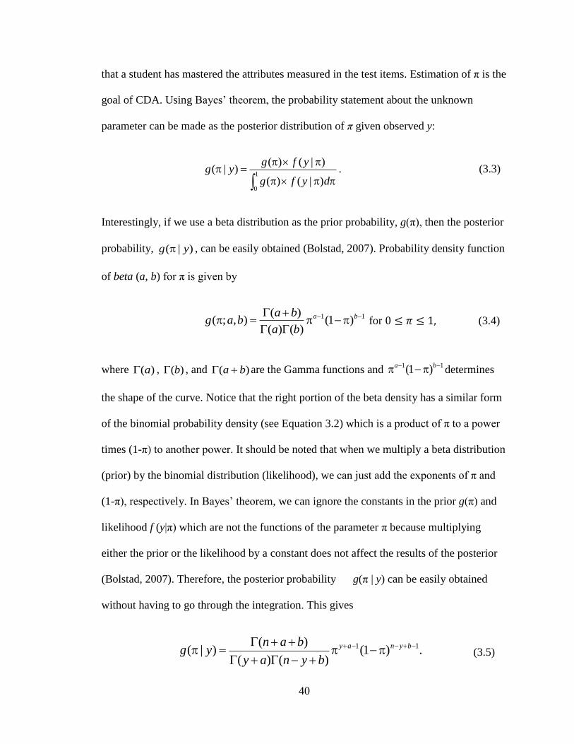
40
that a student has mastered the attributes measured in the test items. Estimation of π is the
goal of CDA. Using Bayes‟ theorem, the probability statement about the unknown
parameter can be made as the posterior distribution of π given observed y:
1
0)|()(
)|()()|(
dyfg
yfgyg . (3.3)
Interestingly, if we use a beta distribution as the prior probability, g(π), then the posterior
probability, )|( yg , can be easily obtained (Bolstad, 2007). Probability density function
of beta (a, b) for π is given by
11 )1()()(
)(),;(
ba
ba
babag for (3.4)
where )(a , )(b , and )( ba are the Gamma functions and 11 )1( badetermines
the shape of the curve. Notice that the right portion of the beta density has a similar form
of the binomial probability density (see Equation 3.2) which is a product of π to a power
times (1-π) to another power. It should be noted that when we multiply a beta distribution
(prior) by the binomial distribution (likelihood), we can just add the exponents of π and
(1-π), respectively. In Bayes‟ theorem, we can ignore the constants in the prior g(π) and
likelihood f (y|π) which are not the functions of the parameter π because multiplying
either the prior or the likelihood by a constant does not affect the results of the posterior
(Bolstad, 2007). Therefore, the posterior probability g(π | y) can be easily obtained
without having to go through the integration. This gives
.)1()()(
)()|( 11
bynay
bynay
banyg (3.5)

41
Notice that the posterior is also a function of the beta (a’, b’) distribution with a‟= a + y
and b‟ = b + n - y. In other words, the number of success (y) was added to a and the
number of failure (n-y) was added to b. Using a beta prior allows getting a beta posterior
by the simple updating rule “add successes to a, add failures to b”. Therefore, when we
have binomial observation, using a beta prior makes it particularly easy to get a posterior.
Therefore Beta distribution is called the conjugate family for the binomial observation
distribution (Bolstad, 2007).
The shapes of the beta (a, b) family are different depending on the values a and b.
Some examples of beta distributions are shown in Figure 3.1.
Figure 3.1 Samples of Beta Distribution (adapted from Bolstad, 2007)

42
The uniform (0,1) distribution is a special case of the beta distribution, beta (1, 1).
When we have no knowledge or belief about a parameter before looking at the data, we
often use the uniform prior which gives equal weight to all possible values of the
parameter. Suppose we use the uniform prior, beta (1, 1), for the unknown π and
observed one success from one trial (y = 1, n=1), then the posterior will be beta (2, 1) by
adding y to a (=1). As shown in Figure 3.1, if a > b, the density has more weight in the
upper half (> 0.5). In other words, the posterior mean of beta (2, 1) should be bigger than
that of beta (1, 1) prior. The mean and variance of beta (a, b) distribution can be
computed as follows:
Mean:
(3.6)
Variance:
(3.7)
respectively. Therefore, the means of uniform prior, beta (1, 1), and the posterior, beta (2,
1), will be 0.5 and 0.67, respectively.
3.4 Estimators for Proportion (π)
The posterior mean is considered the best estimate for a beta distribution, which
has the smallest posterior mean square. In other words, it is closer to the parameter π on

43
average than any other estimates such as posterior mode and posterior median. Because π
ranges between 0 and 1, the beta distribution does not have long tails (or large skewness),
which makes the posterior mean a good measure of location for the beta distribution
(Bolstad, 2007). However, the posterior mean is a biased estimator of π like the most
other Bayesian estimators because, in Bayesian inference, parameters are considered
unknown and random variables, thus unbiasedness is not emphasized by Bayesian
statisticians (Bolstad, 2007). An estimator is unbiased if and only if
(3.8)
where is the sampling distribution of the estimator given the parameter . Bias
is given by
(3.9)
Therefore, unbiased estimators which classical statistics emphasizes have zero bias while
biased estimators have non-zero values for Equation 3.9. However, mean squared error
(MSE) or root mean squared error (RMSE) is a more widely used criterion for judging
estimators than the bias because MSE considers both the bias and the variance of the
estimators. MSE is defined as (Bolstad, 2007)
(3.10)
Interestingly enough, Bolstad (2007) maintains that Bayesian‟s biased estimators often
have smaller MSE values than the unbiased estimator in classical statistic. For example,
suppose the parameter is known to be 0.4 for ten binomial observations (n = 10). First,
the unbiased estimator for ( ) and its variance are given by = y/n and
, respectively, where y = the number of successes.

44
Then, MSE can be calculated as
=
= 0.024.
Second, as the unbiased estimator for (= ), the posterior mean will be as follows if
we use a uniform prior, beta (1,1):
, for y = .
The variance of is given by
.
Then, MSE can be computed as
= +
=
= 0.017.
MSE of the biased estimator is smaller (= 0.017) than that of the unbiased estimator
(= 0.024), which indicates that is closer to the true value than on average.
3.5 Bayesian Inference for Normal Mean
If we use a normal distribution as a prior in Bayes‟ theorem, it is also particularly
easy to obtain a posterior given data without any numerical integration as in the beta
distribution update. The posterior will also be a normal distribution where the parameters
can be updated by a simple rule (Bolstad, 2007).
Normal distributions are symmetric, single-peaked, and bell-shaped, which are
good descriptions for many distributions of real data. Also, many statistical inference

45
procedures based on normal distributions perform well for other roughly symmetric
distributions. In the Bayesian framework, it is appropriate to consider normal
distributions as likelihoods in many cases (Spiegelhalter, Abrams, & Myles, 2004).
Suppose we have a random sample y1, y2, …, yn taken from a normal distribution with
mean µ and variance σ2, where σ
2 is assumed to be known. The conditional probability
(likelihood) of observation y given the parameter µ is
(3.11)
Then, the conditional probability of the unknown parameter µ given y (=posterior)
can be expressed by Bayes‟ theorem as follows:
dyfg
yfg
)|()(
)|()(. (3.12)
where g(µ) is a normal prior distribution with mean m and variance s2.
The shape of the likelihood is proportional to
,
,
because the left portion of Equation 3.11 (i.e.,
) is independent of the parameter µ
and multiplying the likelihood by any constant will cancel out in the posterior. Likewise,
the shape of the prior will be as follows:
.
Then, the shape of prior likelihood will be given by (Bolstad, 2007):
.

46
In Bayes‟ theorem, it is always true that the posterior is proportional to the prior
likelihood because the denominator (the integration part) of Equation 3.12 is a constant:
(3.13)
Therefore, the posterior is a normal [m’, (s’ )2] distribution having mean and variance
given by
(3.14)
respectively. To sum up, using a normal (m, s2) prior, we can obtain a normal [m’, (s’ )
2]
posterior by the parameter updating rule in Equation 3.14 without having to go through
the integration. Therefore, the normal distribution is called the conjugate family for the
normal observation distribution (Bolstad, 2007).
The precision of a distribution (reciprocal of the variance) is given by
(3.15)
Notice that it is the prior precision (1/s2 ) plus the observation (data) precision (1/σ
2 ).
Then, the posterior mean in Equation 3.14 can be rewritten as
.
This is the weighted prior mean (m) by its precision (1/s2) and the weighted observation
(y) by its precision (1/σ2). If we use a sample mean ( ) instead of a single observation
value (y) and σ2/n instead of σ
2 as the variance, then the posterior mean and variance will
be given by

47
, (3.16)
, (3.17)
where m and s2 are the prior mean and variance, and
, σ2/n, and n are the data (sample) mean, variance, and size.
This updating rule is also applicable for the flat priors such as uniform and Jeffreys‟
(Bolstad, 2007). Spiegelhalter et al. (2004) introduced simpler but equivalent formulae to
those in Equation 3.16 and 3.17. They used the same variance σ2 for both the prior and
the data, but a sample size n0 for the prior as follows:
(3.18)
(3.19)
where , σ2/n0, n0 are the prior mean, variance, and „implicit‟ sample size, and
, σ2/n, and n are the data mean, variance, and size.
For example, suppose we have the prior mean (m) of 20 and the variance (s2) of 6
2 and
the data mean ( ) of 25 from 10 samples given σ2
= 12. Then, the posterior mean (m’) and
the variance will be obtained using the updating rule in Equation 3.16 and 3.17 as
follows:

48
If we apply Equation 3.18 and 3.19 to this example, m’ and will be computed as
where the implicit sample size of prior n0 = 1/36 since
= 6
2.
The example above shows that the two different versions of normal distribution updating
formulae (Equation 3.16 ~3.17 and Equation 3.18 ~ 3.19) are equivalent. The prior, data,
and the posterior distributions of the example are shown in Figure 3.2. As shown in the
figure, the posterior distribution has the smallest variance, thus providing more accurate
measure of the parameter. This is why the Bayesian estimators have often smaller MSEs
than the unbiased estimators of classical statistics.
Figure 3.2 Prior, Data, Posterior Distributions
0 5 10 15 20 25 30 35 40
prior
data
posterior

49
CHAPTER 4
THE CURRENT STUDIES
4.1 Study Design/Purpose
Test items are developed for measuring specific attributes; number of the
attributes that each item involves is various. Items with a simple item-attribute structure
measure one or two attributes only while complex items measure several attributes
together. Similarly, some attributes can be measured individually but some should be
jointly measured with others due to the dependency of the attributes. In general, the total
number of attributes to be measured in a test affects the complexity of the item-attribute
structure. The most effective way of applying BIBP to diagnostic assessment may differ
depending on the test item-attribute design as well as the attribute-mastery patterns of
examinees. In the current studies, effective ways of applying the BIBP method were
explored using real data studies and simulation studies. Also, the diagnosis results of
other preexisting diagnosis models were compared to the result of BIBP for the validity
check.
Three studies were conducted using a middle school mathematical achievement
data. In Real Data Study 1 and Study 2, the BIBP method was applied to a data which
involved different total number of attributes based on the mathematical standards or
benchmarks; four attributes (based on four mathematical standards) or ten attributes
(based on ten benchmarks of the four standards), respectively. In Real Data Study 3, the
BIBP method was compared to other two existing popular diagnosis models, DINA and
LCDM, in diagnosing examinees‟ attribute mastery using the same data. For the

50
simulation study, two studies were conducted. In Simulation Study 1, the general
accuracy of the BIBP method in the parameter estimation was evaluated. In Simulation
Study 2, the impact of various conditions regarding attribute characteristics (e.g.,
correlation, difficulty) was examined for the accuracy of parameter estimation. Using
same simulation data, the BIBP method was compared with DINA model in the
parameter estimation accuracy on the various conditions.
4.2 Assumptions
There are three assumptions for BIBP method for CDA. First, it is assumed that
the combined attributes are not necessarily same as simply adding the individual
attributes. For example,
A12 ≠ A1 + A2,
A124 ≠ A12 + A4 ≠ A1 + A2 + A4,
where A1 = attribute 1, A2= attribute 2, A4= attribute 4, A12= combined attribute
of A1 & A2 (jointly measured in an item), A124= combined attribute of A1, A2 & A4
Bloom (1956) defined the synthesis- cognitive level (see Figure 4.1) as putting parts
together to form a new whole. Forming a new whole does not mean simply adding two or
more parts but creating a new meaning or structure. Therefore, the mastery probabilities
of the combined attributes (e.g., π12, π34, π123, π1234) were separately estimated in this
study in addition to the mastery probabilities of the single attributes (e.g., π1, π2, π3, π4).
This is one of the unique features of the BIBP method unlike the other diagnostic models
that estimate the mastery probabilities of only single attributes. Second, all the responses
to n items which measure same attribute are independent (local independence for each

51
attribute). It other words, if there are three items (item #1, item #2, and item #3) which
measure a same attribute (A1), then the probability of answering correctly item #1 does
not affect the probabilities of correct answer for item #2 or #3.
Figure 4.1 Bloom‟s Taxonomy of Cognitive Domain
Third, the examinee mastery probability (πk) for attribute k is constant over all the
responses to n items measuring attribute k. The last two assumptions are the fundamental
assumptions of binomial likelihood function. Since BIBP method uses the binomial
probability function as the likelihood, these two assumptions should be met.
4.3 Defining “Mastery”
In order to decide examinees‟ attribute mastery patterns, the state of “Mastery”
should be defined first in terms of the attribute mastery probability (π). Mastery can be
defined as the state “when students demonstrate a thorough understanding of content as
evidenced by doing something substantive with the content beyond merely echoing it.”
(p.12, Wormeli, 2006). Mastery should include not only possessing the attribute but also

52
correctly applying it to the related problems. Although pure declaration of mastery may
not be possible, the letter grades combined with 100-point scale, A (90-100), B (80-90),
C (70-80), D (60-70), and F (< 60), are often used for most instructional decisions. The
letter grades are typically interpreted as follows (Wormeli, 2006):
Proximal mastery: A (Excellent), B (Good), and C(Fair)
Limited proficiency: D
No proficiency : F
Empirically, if an examinee answers three out of four questions correctly, the beta
posterior mean of π will be also 70% when using Jeffreys‟ prior; since a (# of corrects) =
3 and b (# of incorrect) = 1, the posterior distribution will be beta (3 + 0.5, 1+ 0.5), thus
E(π) = a’/(a’+b’) = 3.5/(3.5+1.5) = 0.7 by Equation 3.6. Given the posterior mean of π =
0.7, the probability of nonmastery will be 0.3 (= 1 – π). Then, the binomial probability of
getting three or four correct answers although the examinee actually does not mastered
the attribute (i.e., false positive probability) will be as follows:
0837.0081.0756.)3.01(3.04
4)3.01(3.0
3
4)3( 444343
yf
Therefore, we can assume with more than 90% confidence that the examinee masters the
attribute if he/she answers three out of four items correctly. In the current studies, the
cutoff π-value for deciding the mastery or nonmastery was set to 0.7. Thus, if the
estimated posterior mean of π for an attribute was equal to or bigger than 0.7, then it was
considered as the evidence of „Mastery‟ of the attribute, otherwise „Nonmastery.‟

53
CHAPTER 5
REAL DATA STUDY 1: FOUR-ATTRIBUTE DATA
The goal of this study was to find the way to estimate examinees‟ mastery
probabilities and to diagnose their attribute mastery patterns using the BIBP method
when a test involves four attributes. As mentioned above, the posteriors of single-
attribute parameters (e.g., π1, π2) as well as multiple-attributes parameters (e.g., π12) were
obtained. The Excel program was used for the parameter estimation in the BIBP method.
5.1 Method
5.1.1 Subjects and Instruments
A mathematical achievement test of 86 items was administered to 8th
grade
students in a Midwestern state at the end of each school year. Binary item responses
(correct/incorrect) from a random sample of 2,993 students were obtained. All items in
the test were multiple-choice items with four options. The mathematical test items were
developed by the blueprint which represents four mathematical standards areas: (1)
Number and Computation, (2) Algebra, (3) Geometry, and (4) Data. There are several
benchmarks within the standards (see Appendix A for detailed information about the
benchmarks). Each of the mathematical items was originally designed to involve a single
standard (e.g., A1) based on the blueprint, but it was found that some items required the
mastery of multiple standards (e.g., A12 or A124). Thus, a Q matrix, a incidence matrix of
the attributes involved in each item, was developed by a mathematician who was

54
experienced in state assessment. Table 5.1 presents the item design based on the Q matrix
in which each of the 86 items measure a single or multiple attributes.
Table 5.1 Item Design for the Four Attributes
Block
Attribute
Item #
Total number
of items
Parameter 1 2 3 4
1 1 0 0 0 6, 8~12, 53, 71~74 11 π1
2 0 1 0 0 24~35, 83~86 16 π2
3 0 0 1 0 19~23, 43~46, 75~82 17 π3
4 0 0 0 1 36~42, 54~57 11 π4
5 1 1 0 0 1, 2~5, 7, 48~52, 65~70, 17 π12
6 0 1 1 0 47 1 π23
7 1 0 0 1 14 1 π14
8 1 1 0 1 13, 15~18 5 π124
9 1 1 1 1 58~64 7 π1234
Note: 1=measuring, 0 = not measuring
As shown in the table, 65 out of 86 items (76%) involved a single attribute
(Blocks 1 through 4) while 21 items (23%) involved more than two attributes (Block 5
through 9). More than five items belong to each block except Blocks 6 and 7 that include
only one item each. Only a single test item should not be good enough to measure any
attribute effectively and this issue will be discussed later (in Step 2). In Table 5.1, π1
refers to the mastery probability of A1, π12 refers to the mastery probability of the
combined attribute of A1 and A2 and so on. The four standards were used as four
attributes to measure in this study.
5.1.2 Estimating Single-Attribute Parameters (Step 1)
The single-attribute parameters, π1, π2, π3, and π4, were estimated as the first step.
In order to obtain the posterior of each of the four parameters, Jeffrey‟s prior, beta (0.5,
0.5), and the responses to the items of blocks 1, 2, 3, and 4 were used. When we do not

55
have any prior knowledge about a parameter, generally the uniform prior is widely used,
which gives equal weight to all possible values of the parameter. However, for
diagnosing the attribute mastery pattern (mastery/nonmastery), Jeffrey‟s prior may be
more appropriate to apply to the data because it puts more weight on the two extreme
sides (0 and 1). In reality, the distribution of the attribute mastery probability is usually
bimodal (mastery or nonmastery rather than the middle). Therefore, Jeffrey‟s prior was
adopted as the priors of π1, π2, π3, and π4. Then, the posterior of each parameter was
obtained by the simple updating rule “add successes to a, add failures to b” as elaborated
in Chapter 3. For example, because block 1 includes eleven items which involves A1 (see
Table 5.1), the posterior of π1 can be computed as beta (0.5 + y, 0.5 + 11 - y), where y =
number of corrects in the eleven items. The same rule was applied to the posterior of π2,
π3, and π4, respectively. The posterior mean of each parameter was used as the parameter
estimate (= ) as mentioned earlier (see Chapter 3.4)
5.1.3 Estimating Multiple-Attribute Parameters (Step 2)
The posteriors of the five multiple-attribute parameters (π12, π23, π14, π124, and
π1234) were estimated, as the second step, using the response data of block 5, 6, 7, 8, and 9,
respectively. In this step, it should be noted that the posteriors of the single-attribute
parameters estimated in Step 1 were used as the priors of the multiple-attribute
parameters. For example, for the prior of π12, the posterior of either π1 or π2 was used
depending on the examinee‟s ability. That is, if an examinee‟s is smaller than , then,
the posterior of π1 was used as the prior of π12 of the examinee because should be
equal to or lower than . For example, suppose that the obtained posteriors of π1 and π2
of an examinee were a beta (9.5, 2.5) with M = 0.79 and beta (15.5, 1.5) with M = 0.91,

56
respectively. Then, the posterior of π1, beta (9.5, 2.5), would be used as the prior of π12 of
the examinee because (= 0.79) is smaller than (= 0.91). Then, the posterior of π12
would be computed as beta (9.5 + y, 2.5 + 17 – y) based on the responses to the 17 items
that involve A12 (block 5 in Table 5.1).
The same rule was applied to π23 and π14. It should be noted that although each of
π23 and π14 was involved by only one item as shown in Table 5.1, since its prior was
obtained from the posterior of π1, π2, or π3 which were involved by at least eleven items,
the estimation error due to a single item was greatly reduced. This is one of the important
advantages of using the Bayesian approach. As mentioned in Chapter 3.2, Bayesian
approach uses both sources of information, the prior information and the data, to find a
posterior distribution of the parameter, thus often resulting in smaller estimation error
than the unbiased estimator in the classical approach. For π124, the posterior of either π12
or π4 was used as its prior although the posterior of π14 or π2 could be also used for the
prior of π124. It is because the number of items involving π12 and π4 is bigger than the
number of items involving π14 and π2, thus π12 and π4 can give better prior information for
π124 than π14 and π2. Finally, for the mastery probability of all attributes combined
(=π1234), the posterior of either π124 or π3 were selected as the prior of π1234. Although
other parameters‟ posteriors, such as single-attribute parameters or π12, could be used as
the prior, the combination of π124 and π3 was chosen because especially the posterior of
π124 was updated by many other parameters such as π1, π2, π12, and π4, thus providing a
better source of prior information for π1234. The procedure of estimating the posteriors of
these nine parameters (π1, π2, π3, π4, π12, π23, π14, π124, and π1234) is graphically displayed
in Figure 5.1.

57
Figure 5.1 Estimating the Posteriors of the Attribute Mastery Probabilities in Study 1
5.1.4 Updating the Single-Attribute Parameters (Step 3)
In Step 1, the posteriors of the single-attribute parameters (π1, π2, π3, & π4) were
estimated using the data of Blocks 1 through 4 only which directly measured the single
attributes, thus the rest of data (from Blocks 5 through 9 in Table 5.1) which measured
multiple attributes were not used. Based on the current item design in Table 4, it may not
necessary to update the four single-attribute parameter estimates further because each of
the single attributes was measured by a large enough number of items (at least eleven).
However, this step was conducted as an effort to find a way to update the single-attribute
parameter estimates using the response data to the multiple-attribute items.
In this step, the single-attribute parameter estimates were updated differently
depending on examinees‟ ability levels on the attributes. For example, if an examinee
showed the mastery of A1 ( ≥ 0.7) but nonmastery of A2 ( < 0.7), then the responses

58
to items involving A12 (Block 5) depended on the mastery probability of A2 (= π2). In
such case, the block 5-data was used to update the posterior of π2 of the examinee using
the beta updating rule: a‟= a + y and b‟ = b + n – y, where n = 17 since Block 5 includes
17 items. However, if both A1 and A2 were mastered ( ≥ 0.7 and ≥ 0.7), the
posteriors of both π1 and π2 were updated by the Block 5-data. Otherwise (if neither A1
nor A2 were mastered), no posterior of π1 and π2 could be updated because it was
uncertain whether incorrect answers to block 5-items were due to the nonmastery of A1 or
nonmastery of A2. Following is a proposed system of updating the posteriors of π1, π2, π3,
and π4 using the response data from blocks 5 through 9.
Using the Block 5-data (involving A12)
o If < 0.7 (nonmastery) and ≥ 0.7 (mastery), the posterior of π1 will be
updated
o Else if ≥ 0.7 (mastery) and < 0.7 (nonmastery), the posterior of π2
will be updated
o Else if both and ≥ 0.7 (mastery), the posteriors of both π1 and π2 will
be updated.
o Otherwise, no updating for the posteriors of π1 and π2.
Using the Block 6-data (involving A23)
o Same rule as in block 5 will be applied to update the posterior of π2 or
(and) π3.
Using the Block 7-data (involving A14)
o Same rule as in block 5 will be applied to update the posterior of π1 or (and)
π4.

59
Using the Block 8-data (involving A124)
o If only one of , , and < 0.7, then its posterior will be updated
o Else if all , , and ≥ 0.7, the posteriors of all π1, π2, and π4 will be
updated.
o Otherwise, no updating for the posteriors of π1, π2 and π4.
Using the Block 9-data (involving A1234)
o If only one of , , and < 0.7, then its posterior will be updated by
the data
o If all of , , and ≥ 0.7, then its posterior will be updated.
o Otherwise, no updating for any of the posteriors of π1, π2, π3, and π4.
It was also evaluated whether this step would actually improve the accuracy of the
parameter estimation using a simulation study in Chapter 8.
5.2 Result
5.2.1 Descriptive Statistics
The descriptive statistics of the raw score and attribute mastery probability
estimate ( ) were provided in Table 5.2. Each descriptive statistic was reported for Step
1 & 2 and for Step 3, separately. Note that the raw scores and the multiple-attribute
parameter estimates (e.g., , ) remained same on both sides since Step 3 was
conducted to update only the single-attribute parameters (e.g., , ). The raw scores
ranged from 22 to 86 (out of 86) with the mean of 60.68 (70.6%) and SD of 15.12. As
shown in the table, the mean of was highest (≈ .72) and the mean of was lowest
(≈ .60) in both Step 1& 2 and Step 3, which means that the examinees were more likely

60
to master A3 (Geometry) and less likely to master A14 (combined attribute of „Number
and Computation‟ and „Data‟) than any other attributes.
Table 5.2 Descriptive Statistics of the Raw Score and Estimated Attribute Mastery
Probability ( ) in Step 1 & 2 and Step 3 (N=2993)
Step 1 & 2 Step 3
Min. Max. M SD Min. Max. M SD
Raw
score
22 86 60.68
(71%)
15.12 22 86 60.68
(71%)
15.12
0.0417 0.9583 0.6394 0.2124 0.0385 0.9881 0.6669 0.2125
0.0882 0.9706 0.6702 0.1976 0.0882 0.9894 0.6817 0.1986
0.0833 0.9722 0.7242 0.2142 0.0833 0.9808 0.7218 0.2116
0.0417 0.9583 0.6394 0.1968 0.0417 0.9800 0.6633 0.2027
0.1897 0.9828 0.6619 0.1761 0.1897 0.9828 0.6619 0.1761
0.0833 0.9722 0.6305 0.2091 0.0833 0.9722 0.6305 0.2091
0.0385 0.9615 0.5973 0.1925 0.0385 0.9615 0.5973 0.1925
0.0294 0.9706 0.6003 0.1940 0.0294 0.9706 0.6003 0.1940
0.1000 0.9737 0.6209 0.1807 0.1000 0.9737 0.6209 0.1807
Table 5.3 presented the attribute difficulty, pk (= proportion of all the examinees
who have mastered attribute k). pk of the nine attributes ranged from .32 to .57 in Step 1
and from .32 to .58 in Step 2. Note that the average pk (= .43 in Step 1) was lower than
the average percentage of the raw scores (71%). It was because the mastery of an
attribute was defined as ≥ 0.7 (see Chapter 4.3) in this study, thus examinees should
answer at least three out of four items correctly in order to be classified as a mastery.
Like , pk was highest for A3 (.57 in Step 1&2 and .58 in Step 3) and lowest for
A14 (= .32). In other words, about 60% of the examinees mastered A3 while only 32% of
the examinees mastered A14. It should be also noted that and pk of the single-attributes
(A1, A2, A3, A4) were slightly increased in Step 3 after updating them by the multiple-
attribute item response data.

61
Table 5.3 Attribute Difficulty (pk) in Step 1 & 2 and Step 3 (N=2993)
Attribute
Step 1 & 2 Step 3
# of examinees
who mastered
pk # of examinees
who mastered
pk
A1 1419 0.47 1561 0.52
A2 1477 0.49 1568 0.52
A3 1694 0.57 1742 0.58
A4 1314 0.44 1499 0.50
A12 1369 0.46 1369 0.46
A23 1230 0.41 1230 0.41
A14 964 0.32 964 0.32
A124 1000 0.33 1000 0.33
A1234 1132 0.38 1132 0.38
Inter-attribute correlations were also presented in Table 5.4 and Table 5.5 for Step
1 & 2 and Step 3, respectively. The Pearson correlation of with each other was
considered an inter-attribute correlation. As shown in Table 5.4, the four single-attributes
had medium inter-attribute correlations ranging from .614 to .722 while the multiple-
attributes showed high inter-attribute correlations ranging from .703 to .925. Inter-
correlations of the multiple attributes had relatively higher than those of the single
attributes. It was observed that the inter-attribute correlations became higher in general
when the two attributes shared more common attributes. For example, r ( , ) =.874
was bigger than r ( , ) = .709 and r ( , ) =.917 was even bigger than r ( ,
) since and had a common attribute A1 and A14 and A124 shared more attributes
(A1 and A4). As shown in Table 5.5, it was also an interesting finding that the inter-
attribute correlations in Step 3 were generally higher than those in Step 1&2, which
implied that updating the single-attribute parameter estimates in Step 3 increased their
inter-attribute correlations.

62
Table 5.4 Inter-Attribute Correlations (Step 1& 2)
.672* .687
* .614
* .833
* .709
* .874
* .832
* .806
*
1 .722* .632
* .857
* .925
* .703
* .819
* .821
*
1 .637* .785
* .872
* .710
* .757
* .807
*
1 .705* .668
* .849
* .788
* .778
*
1 .868* .834
* .888
* .891
*
1 .740* .833
* .869
*
1 .917* .887
*
1 .914*
1
* significant at the 0.001 level.
Table 5.5. Inter-Attribute Correlations (Step 3)
.817* .746* .751* .884* .782* .873* .863* .842*
1 .759* .741* .893* .917* .752* .847* .849*
1 .701* .789* .873* .713* .760* .814*
1 .776* .736* .863* .835* .823*
* significant at the 0.001 level.
5.2.2 Individual diagnosis result
The BIBP method estimated the mastery probabilities ( ) and the mastery
pattern (αk) of each examinee for a total of nine attributes (A1, A2, A3, A4, A12, A23, A14,
A124, and A1234). Appendix B provided the parameter estimates for the first twenty and
the last ten examinees in the Excel program view. Since examinees who have the same
raw score may have a variety of different attribute-mastery patterns, the purpose of CDA
is to provide the detailed attribute-mastery profile for each individual rather than just test
score. Table 5.6 presents the diagnosis results for three examinees whose raw scores were
64 out of 86: and αk of the nine attributes estimated in Step 1&2 and Step 3.

63
Table 5.6 Diagnosis Results for the Three Examinees (Raw Score: 64/86) by Step 1&2
and Step 3
Examinee
ID
Ste
p 1
& 2
#116
αk 0.458 0.912 0.806 0.375 0.603 0.816 0.423 0.559 0.605
0 1 1 0 0 1 0 0 0
#130
αk
0.208 0.794 0.806 0.958 0.603 0.806 0.269 0.265 0.395
0 1 1 1 0 1 0 0 0
#2706
αk
0.875 0.500 0.861 0.542 0.721 0.472 0.577 0.523 0.563
1 0 1 0 1 0 0 0 0
Ste
p 3
#116
αk 0.603 0.917 0.816 0.375 0.603 0.816 0.423 0.559 0.605
0 1 1 0 0 1 0 0 0
#130
αk 0.607 0.806 0.816 0.958 0.603 0.806 0.269 0.265 0.395
0 1 1 1 0 1 0 0 0
#2706
αk
0.875 0.700 0.861 0.577 0.721 0.472 0.577 0.523 0.563
1 1 1 0 1 0 0 0 0
Examinee #116 was diagnosed to have mastered A2 and A3 but not mastered A1
and A4 (αk= 0110) for the four single attributes, while examinee #130 was diagnosed to
have the mastery pattern of „0110‟ (αk= 1, if ) in both Step 1& 2 and Step 3. Note
that was substantially increased for these two examinees in Step 3 as shown in Table
5.6. By examining their item response data, it was found that the two examinees
performed poor on the 11 items involving A1 (five and two corrects, respectively), but
they did relatively well on the 17 items involving A12 (11 and 14 corrects, respectively).
It was speculated that their improved their by the updating procedure in Step 3.
The change between Step 1 & 2 and Step 3 was graphically represented in Figure 5.2
(examinee #116) and 5.3 (examinee #130), respectively.

64
Figure 5.2 Estimated Posteriors of , , , and for Examinee #116

65
Figure 5.3 Estimated Posteriors of , , , and for Examinee #130

66
Figure 5.4 Estimated Posteriors of , , , and for Examinee #2706
It was an interesting finding that Examinee #2706 showed the mastery pattern of
„1010‟ in Step 1 & 2 (mastery of A1, A3) but „1110‟ in Step 3 (mastery of A1, A2, A3). As

67
shown in Table 5.6, the value of was changed from .50 to .70 in Step 3, thus this
examinee was diagnosed to have mastered A2 according to the decision rule of mastery
(αk= 1, if ). Similarly to examinees #116 and #130, extremely good performance
on the items involving A12 (16 corrects out of 17) resulted in such a different diagnosis
result on A2 for this examinee. The changes of the parameter estimates for this examinee
were graphically represented in Figure 5.4.
5.2.3 Discussion
The aberrant item response patterns on between the single-attribute (lower level)
and the multiple-attribute (higher level) such as poor performance on A1 or A2, but better
performance on A12 in the three examinees above may be due to several reasons.
Negative slips on the single-attribute items or positive slips (guessing) on the
multiple-attribute items could result in the aberrant result. To detect the aberrant item
response patterns of examinees, a variety of person-fit indices have been developed and
applied. However, it is still unclear to decide whether the unusual response pattern is due
to the negative slip or positive slip by the person-fit index only. Also, the aberrant
response pattern may suggest that there is a compensatory nature between the attributes
(e.g., A1 or A2) in a combined multiple attribute (e.g., A12). Step 3 (updating the single-
attribute by multiple-attribute data) can be helpful for case of the negative-slips on
single-attribute items but it will decrease the parameter estimation accuracy for the case
of positive-slips on multiple-attributes items. It was examined whether the updating step
generally improves the accuracy of parameter estimation in Simulation Study 1. Step
1&2 and Step 3 was compared in the accuracy of recovering true parameters.

68
CHAPTER 6
REAL DATA STUDY 2: TEN-ATTRIBUTE DATA
In this, BIBP method was applied to a more complex item design involving a total
of ten attributes in a test, especially where every single attribute could not be measured
directly by the test items. Therefore, it was explored how to infer of such unmeasured
single attributes from the parameter estimates of the attributes directly measured by the
test items. The Excel program was used for all the parameter estimation.
6.1 Method
6.1.1 Subjects and Instruments
Subjects and instruments are the same as in Real Data Study 1. However, the ten
benchmarks (see Appendix A) of the four mathematical standards were used as the ten
attributes to be measured in this study. The first three benchmarks (1.Number Sense,
2.Number System and their Properties, 3.Computation) are the benchmarks of Standard 1
(Number and Computation). The next three benchmarks (4.Variabel, Equations, and
Inequalities, 5. Functions, 6.Models) are of Standard 2 (Algebra). Then, Benchmark 7
(Geometric Figures and their Properties) and 8 (Geometry from an Algebraic Perspective)
belong to Standard 3 (Geometry). Finally, Benchmark 9 (Probability) and 10 (Statistics)
belong to Standard 4 (Data). The Q-matrix was also developed based on the ten
benchmarks (attributes) and Table 6.1 presents the item design according to the ten-
benchmark Q-matrix.

69
For the ten attributes, 33 out of 86 items (38%) involved single attribute, A2, A3,
A7, A8, and A9 (blocks 1 to 5) while the rest of 53 items (62%) measured multiple
attributes (blocks 6 to 21). Note that the five attributes, A1, A4, A5, A6, and A10 (=tenth
Attribute) are not measured directly by the test items but jointly with other attributes (e.g.,
A124, A456, A23610). There are a total of 21 blocks in this item design but no block exists
for π1, π4, π5, π6, and π10.
6.1.2 Estimating the Parameters Directly Measured by the Items (Step 1)
Table 6.1 Item Design for the Ten Attributes
Block
Attribute
Item #
Number
of items
Parameter 1 2 3 4 5 6 7 8 9 10
1 0 1 0 0 0 0 0 0 0 0 71~74 4 π2
2 0 0 1 0 0 0 0 0 0 0 53 1 π3
3 0 0 0 0 0 0 1 0 0 0 19~23, 43~46 9 π7
4 0 0 0 0 0 0 0 1 0 0 75~82 8 π8
5 0 0 0 0 0 0 0 0 1 0 36~42, 54~57 11 π9
6 0 1 1 0 0 0 0 0 0 0 6, 12 2 π23
7 0 0 1 1 0 0 0 0 0 0 65~70 6 π34
8 0 0 0 1 1 0 0 0 0 0 24 1 π45
9 0 0 0 1 0 1 0 0 0 0 31, 32, 34, 35,
83~86
8 π46
10 0 0 0 1 0 0 1 0 0 0 47 1 π47
11 0 0 1 0 0 1 0 0 0 0 52 1 π36
12 1 1 1 0 0 0 0 0 0 0 8~11 4 π123
13 0 1 1 1 0 0 0 0 0 0 2~5 4 π234
14 1 1 0 1 0 0 0 0 0 0 1 1 π124
15 0 1 1 0 0 0 0 0 0 1 14 1 π2310
16 0 0 0 1 1 1 0 0 0 0 25~30, 33 7 π456
17 1 1 1 1 0 0 0 0 0 0 7 1 π1234
18 0 1 1 0 0 1 0 0 0 1 13 1 π23610
19 0 1 1 0 1 0 0 0 0 1 15~18 4 π23510
20 0 1 1 1 0 1 0 0 0 0 48~51 4 π2346
21 0 0 1 1 0 1 1 0 1 0 58~64 7 π34679
Note: 1 = measuring, 0 = not measuring

70
As the first step, the four single-attribute parameters (π2, π 7, π8, & π9) and the nine
multiple-attribute parameters (π23, π34, π46, π123, π234, π456, π23510, π2346, & π34679) were
estimated (see Table 6.1). They could be estimated directly by the item responses in the
same way used in Step 1 and Step 2 in the previous study 1. The procedure of estimating
the posteriors of these thirteen parameters is graphically presented in Figure 6.1. It should
be noted that the eight blocks (2, 8, 10, 11, 14, 15, 17, & 18) which are shaded in Table
6.1 include only one item each. Thus, the items of these eight blocks were excluded in
this step because using only one item for the parameter estimation could be misleading
and no prior information of the parameter was available.
Firgure 6.1. Estimating the Posteriors of the thirteen Parameters.

71
As in Real Data Study 1, Jeffreys‟ prior, beta(.5,.5), was used as the priors of π2,
π 7, π8, π9, π23, π34, π46, π123, π456, π23510, and π34679 because no prior knowledge about
these eleven parameters was available from the data. However, for π234, since the
posteriors of π2 and π34 could provide the prior knowledge, the posterior of either π2 or
π34 which had the smaller mean was used as the prior of π234 in the same way used in Step
2 of Real Data Study 1. Likewise, the posterior of either π23 or π46 with the smaller mean
was used as the prior for the parameter π2346 estimation.
6.1.3 Inference about the Unmeasured Single-Attribute Parameters (Step 2)
In the previous step, the four single-attribute parameters (π2, π 7, π8, & π9) were
estimated along with the nine multiple-attribute parameters. Six parameters out of the ten
single-attribute parameters (π1 through π10) were still not estimated; of the six, five
parameters (π1, π4, π5, π6, & π10) had no test item that directly measured them and π3 was
involved by only one item. Therefore, the purpose of this step was to find a way to infer
the unmeasured single-attribute parameters from the thirteen parameters estimated in Step
1. Some single-attribute parameters could be inferred by a simple and obvious way, but
some of the parameters should be inferred by a complex or many alternate ways due to
the item design of this mathematical test. For example, π5 could be inferred by the
posteriors of π46 and π456 as follows: If an examinee showed an evidence of mastery of
A46 ( ≥ .7) but A5 was not measured for the examinee in Step 1, then it would be
obvious that the mastery (or non-mastery) of A456 depends on whether the examinee
mastered or not A5. Thus, it was inferred that the posterior of π456 would be very close to
the unknown posterior of π5. In such a case, was used as the approximation of .
However, if an examinee did not master A46, then A456 should not be mastered. In such

72
case, would not be used as because it was uncertain whether the non-mastery of
A456 was due to the non-mastery of A46 only or both A46 and the unknown A5. Since π5
was still unknown in this case, Jeffreys‟ prior remained as the posterior of π5 without any
inference about it. It should be noted that such logical processes for the inference can be
more complex for the parameters of some attributes depending on the test item design.
Also, there would be a variety ways of the inference for some attributes such as A3, A4
that are jointly measured with many other attributes (e.g., A23, A34, A46, A234, A2346).
Therefore, this step was performed as an effort to find a way to infer the unmeasured
parameters in Step 1 (π1, π3, π4, π5, π6, & π10). Followings are the inference processes of
the six parameters:
To infer π1, if ≥ 0.7 (mastery) or ≥ 0.7 (mastery), then was used as
( = ). Otherwise = 0.5 (the mean of Jeffreys‟ prior).
To infer π4, if ≥ 0.7 or ≥ 0.7 (mastery), then = . Else if ≥ 0.7),
then = . Otherwise = 0.5.
To infer π5, if ≥ 0.7, then = . Otherwise = 0.5.
To infer π6, if ≥ 0.7, then = . Else if all of , , and ≥ 0.7,
then = . Otherwise = 0.5.
To infer π10, if either or ≥ 0.7 and ≥ 0.7, then = .
Otherwise = 0.5.
To update the posterior of π3, if ≥ 0.7, then use the response data of A23. Else if
≥ 0.7 or ≥ 0.7, then use the response data of A34.
For π1, if the examinee mastered A23 ( ≥ 0.7) or A234 ( ≥ 0.7), then was used
as the π1 estimate (= ). Otherwise, the mean of Jeffreys‟ prior was used as (= 0.5).

73
For the rest of parameters except π3, similar rules were applied as shown above. The
posterior of π3 could be estimated by the Jeffreys‟ prior and its item response data as in
Step 1. However, since a single item involved A3, the posterior of π3 should be updated
by the response data to the relevant multiple-attribute items as in Step 3 of Study 1.
Therefore, item response data of A34 was used for updating the posterior of π3 if an
examinee was diagnosed to master A46 or A4.
6.2 Results
6.2.1 Descriptive Statistics
The descriptive statistics of the raw score (same as in Real Data Study 1) and the
thirteen ‟s estimated in Step 1 and the six ‟s obtained in Step 2 were provided in
Table 6.2. Note that the six parameters ( , , , , , & ) could not be directly
measured by the test items, thus they were inferred from the parameter estimates in Step
1. In Real Data Study 1, Standard 3 (Geometry) showed highest mean while Standard
1 (Number and Computation) and Standard 4 (Data) had lowest of the four single
attributes. In this study, A7 (Geometric Figures and their Properties) and A8 (Geometry
from an Algebraic Perspective) which are the benchmarks of Standard 3 (see Appendix A)
also showed the highest mean ‟s (.69 and .73, respectively) of the ten single attributes.
On the other hand, A1 (Number Sense), A2 (Number System and their Properties), and A3
(Computation) which are the benchmarks of Standard 1 showed low mean ‟s; .48. .66,
and .63, respectively.

74
Table 6.2 Descriptive Statistics of the Raw Score and from Step 1 and Step 2 (N=2993)
Min. Max. M SD
Ste
p 1
Raw score 22 86 60.68 15.12
0.1000 0.9000 0.6572 0.2431
0.0500 0.9500 0.6948 0.2449
0.0556 0.9444 0.7319 0.2043
0.0417 0.9583 0.6394 0.1968
0.1667 0.8333 0.5043 0.2480
0.0714 0.9286 0.6796 0.2139
0.1000 0.9000 0.7662 0.1889
0.1000 0.9000 0.6706 0.2110
0.0455 0.9444 0.6322 0.1840
0.0625 0.9375 0.6142 0.2456
0.1000 0.9000 0.7267 0.2137
0.0556 0.9286 0.5802 0.2083
0.0625 0.9375 0.7451 0.1675
Ste
p 2
0.1000 0.9000 0.6301 0.1771
0.2500 0.7500 0.4795 0.1083
0.0556 0.9444 0.6606 0.1750
0.0625 0.9375 0.6313 0.2172
0.0714 0.9375 0.5964 0.1583
0.1000 0.9000 0.6162 0.1739
pk was also presented for each attribute in Table 6.3. A8 showed the highest pk
(=.66) and A6 had the lowest value (.24) of the single attributes. Unexpectedly, some of
the multiple attributes (e.g., A46, A23510) showed higher values than single attributes. It
may suggest that the single-attribute parameters, especially the inferred attributes were
underestimated due to the lack of information for the inference.
Table 6.3 Attribute Difficulty
Attribute A1 A2 A3 A4 A5 A6 A7 A8 A9 A10
pk .41 .63 .43 .48 .36 .24 .56 .66 .44 .33
Attribute A23 A34 A46 A123 A234 A456 A235(10) A2346 A34679
pk .28 .51 .83 .65 .40 .38 .78 .29 .58

75
Inter-attribute correlations were also provided in Table 6.4 (the ten single-
attributes) and in Table 6.5 (between the single and the multiple attributes).
Table 6.4 Inter-Attribute Correlations of the Single Attributes
Standard 1
Standard 2
Standard 3
Standard 4
1 .470 .286 .521 .490 .600 .509 .466 .528 .530
1 .317 .607 .360 .372 .441 .434 .425 .362
1 .338 .280 .267 .418 .385 .361 .266
1 .375 .460 .460 .451 .473 .391
1 .502 .542 .487 .500 .705
1 .526 .449 .574 .520
1 .609 .602 .475
1 .535 .441
1 .480
* All correlations are significant at the 0.001 level.
Table 6.5 Inter-Attribute Correlations between Single Attributes and Multiple Attributes
.539 .520 .358 .698 .606 .509 .398 .612 .430
.309 .401 .320 .355 .720 .404 .349 .442 .381
.243 .361 .430 .324 .367 .380 .342 .369 .336
.189 .598 .471 .301 .840 .442 .375 .414 .429
.382 .455 .365 .453 .473 .927 .393 .549 .454
.556 .536 .346 .451 .525 .496 .342 .747 .438
.413 .556 .486 .525 .571 .596 .497 .626 .532
.370 .531 .464 .484 .549 .545 .480 .549 .523
.428 .535 .455 .506 .566 .548 .453 .615 .496
.383 .438 .321 .465 .477 .700 .468 .525 .402
* All correlations are significant at the 0.001 level.
Overall, the inter-attribute correlations (M = .469) were lower than those of the four-
attribute data in Real Data Study 1 (M = .792). It was speculated that the ten benchmarks
are more specific (unique) contents than the four standards, thus they were less inter-

76
correlated. The intercorrelations of the ten single attributes (A1 through A10) showed low
to medium correlations ranging from .280 to .705 (M = .460).
The correlations between the single attributes and the nine multiple-attributes (A23
through A34679) showed a wide range of correlations from .189 to .927 (M = .473). In
Table 6.4, it was observed that the inter-benchmark correlations within standards were
not higher than those between standards. For example, the three benchmarks (A1, A2, A3)
of Standard 1 showed lower intercorrelations (r = .286 to .470, M = .358) than the
correlations with A7 (r = .508, .441, and .418, respectively) that is one of the benchmarks
of Standard 3. Therefore, it was speculated that the specific benchmarks of each standard
were unique, thus generally they were less related with each other than the benchmarks
outside of the standard. It may suggest that the higher inter-benchmark correlations
between standards reflected the relatively high inter-standard correlations as shown in
Real Data Study 1 (see Table 6.4 & 6.5).
6.2.2 Individual diagnosis result
The BIBP method estimated and αk of a total of nineteen attributes (A1, A2, A3,
A4,…, A34679) for each examinee. Table 6.6 shows the diagnosis results for the same three
examinees with the raw score of 64 who were presented in Real Data Study 1 (see Table
5.6); and αk of the ten single attributes (ten benchmarks).
Examinee #116 who was diagnosed to have mastered only Standards 2 and 3 (αk
= 0110) in Study 1 showed the mastery pattern of the ten benchmarks of αk =
0000101101 (=mastery of Benchmarks 5, 7, 8, & 10). Consistently with the diagnosis
result of the standards in Study 1, this examinee showed no mastery of A1, A2, and A3 (=

77
the three benchmarks of Standard1) and A10 (= one of the benchmarks of Standard 4) but
mastery of both A7 and A8 (the two benchmarks of Standard 3).
Table 6.6 Diagnosis Results for the Three Examinees (Raw Score: 64/86)
Standard 1 Standard 2 Standard 3 Standard 4
Examinee
#116
sd
0.50 0.30 0.56 0.61 0.94 0.50 0.75 0.83 0.38 0.90
0.35 0.19 0.17 0.15 0.08 0.35 0.13 0.12 0.13 0.12
#130
sd
0.50 0.10 0.69 0.90 0.69 0.69 0.75 0.83 0.96 0.50
0.35 0.12 0.15 0.12 0.15 0.15 0.13 0.12 0.06 0.35
#2706
sd
0.90 0.90 0.94 0.83 0.50 0.72 0.95 0.72 0.54 0.50
0.12 0.12 0.08 0.12 0.35 0.14 0.07 0.14 0.14 0.35
αk #116 0 0 0 0 1 0 1 1 0 1
#130 0 0 0 1 0 0 1 1 1 0
#2706 1 1 1 1 0 1 1 1 0 0
sd = posterior standard deviation
However, for Standard 2 that this examinee was diagnosed to have mastered showed
mastery of only A5 (one of the three benchmarks of Standard 2) as shown in Table 6.6
( = .94). For the other two benchmarks (A4 and A6) of Standard 2, was lower
than .70 with relatively large posterior sd (.15 and .35, respectively). It should be noted
that these three parameters (π4, π5, & π6) were inferred using the posteriors of the
parameters estimated in Step 1 since there was no test item to directly measure them. The
inconsistency between the diagnosis results regarding Standard 2 and Benchmarks 4 and
6 may be due to the lack of information for the inference in Step 2. The estimated
posteriors of the three benchmarks of Standard 2 for examinee #116 were shown in
Figure 6.2.

78
Figure 6.2 Estimated Posteriors of , , and for Examinee #116
Examinee #130 who was diagnosed to have mastered Standards 2, 3, and 4 (αk =
0111) in Real Data Study 1 showed the mastery pattern of the ten benchmarks as αk =
0001001110 (= mastery of Benchmarks 4, 7, 8, & 9). The diagnosis result regarding the
seven attributes (A1, A2, A3, A4, A7, A8, and A9) was consistent with the diagnosis result
of the four standards in Real Data Study 1. Although Benchmarks 5, 6, and 10 should be
mastered based on the Study 1 result, this examinee nearly mastered Benchamrks 5 and 6
(πk =.69) and did not show the mastery of Benchmark 10 due to the lack of information
for the inference (πk =.50). The estimated posteriors of , , and for the for
examinee #130 were shown in Figure 6.3.

79
Figure 6.3 Estimated Posteriors of , , and for Examinee #130
In Real Data Study 1, examinee #2706 showed the four-standard mastery pattern
of αk = 1010 in Step 1&2 and αk = 1110 in Step 3. In this study, this examinee showed
the mastery of all the benchmarks (A1 through A8) of Standards 1, 2, and 3, except A1, A5;
no inference was made about π5 for this examinee due to the lack of information (
= .50, sd = .35). The estimated posteriors of Standards 1 and 2 are presented in Figure 6.4.

80
Figure 6.4 Estimated Posteriors of , , , , , and for Examinee #2706
6.3 Discussion
In this study, the BIBP method was applied to a more complex test data which
involved ten attributes. In this item design, every attribute was not directly measured by
the test items. Therefore, it was explored how to infer of such unmeasured single
attributes from the parameter estimates of the attributes directly measured by the test
items. There will be different ways of the inference because some attributes were jointly
measured with many other attributes (e.g., A234, A2346, A456, A23510, and A34679). Logical
processes for the inference were introduced and applied to six unmeasured attributes (A1,
A3, A4, A5, A6, and A10). It seemed that some of the attributes were underestimated due to
the lack of information for the inference. The inference processes need to be revised in
the future study.

81
CHAPTER 7
REAL DATA STUDY 3: COMPARING BIBP TO DINA AND LCDM
In Real Data Study 1 and 2, the BIBP method was applied to a mathematical test
data to estimate examinees‟ attribute-mastery probability ( ) and the pattern (αk) of each
examinee. In this study, the estimated parameters by the BIBP method were compared to
the parameters estimated by existing diagnosis models, DINA and LCDM. As elaborated
in Chapter 2, DINA is a noncompensatory model which is appropriate to diagnose
mathematical skills where mastery of the skills cannot compensate for nonmastery of the
other skills. In DINA, examinees are classified into two classes for each item; those who
have mastered all the skills required to solve the item (ij =1 in Equation 2.3) and those
who do not (ij =0). Although it is one of the most widely accepted noncompensatory
models, one criticism of DINA is that this model may not be very practical because
missing one of the required attributes is considered to be equivalent to missing all the
attributes (Henson & Douglas, 2005). LCDM is a generalized model which can be
applied to any type of data, whether compensatory or non-compensatory. It provides
information about whether conditional relationships exist between required attributes and
the item response, thus it can give the insight as to what type of model (compensatory or
non-compensatory) could be more appropriate for the items (Henson et al., 2009).

82
7.1 Method
7.1.1 Subjects and Instruments
The same subjects and instruments as in Real Data Study 1 and Study 2 were used
for the comparison purpose in this study. The item design involving four attributes (see
Table 5.1) was adopted for this study since the estimated item parameters of LCDM was
expected to have large standard errors especially for large number (e.g., ten) of attributes
involved in the test items (Henson et al., 2009).
7.1.2 Procedure
For the parameter estimation of the both models, the LCDM program (Burke &
Henson, 2008) was used. The program allows user specified constraints for LCDM to fit
the DINA model. For the DINA model, only the highest order interaction parameter and
the intercept will be included under the LCDM framework (see Equation 2.17) since it is
the non-compensational model, thus no main effect needs to be estimated. For example,
the logit, , of the LCDM and DINA for item #1 which involves A1 and A2 are
as follows:
LCDM: =
DINA: =
Followings are the logits of both models for item #15 involving A1, A2, and A4:
LCDM: =
+ ,
DINA: =
For this item, DINA includes only three-way interaction of A1, A2, and A4 and the
intercept without any main effect nor two-way interactions. Therefore, DINA has two

83
parameters per item regardless of the number of attributes involved in the item. However,
in LCDM, the number of parameters per item became doubled as one attribute is added
(e.g., two parameters for one attribute, four parameters for two attributes, eight for three
attributes, and sixteen for four attributes).
After estimating attribute difficulty attribute mastery probability (πk) and the
attribute mastery pattern (αk) of each examinee, the estimation results of the three models,
DINA, LCDM, and BIBP, were compared. Also, the proportion of examinees who have
mastered attribute k (= pk) and inter-attribute correlations were obtained based on the
parameter estimates of the three models and compared.
7.2 Results
7.2.1 Descriptive Statistics
The descriptive statistics of the raw score and of the four attributes were
provided in Table 7.1. Each descriptive statistic was reported separately for the DINA,
LCDM, and BIBP estimations for the comparison purpose. However, the raw score
statistics are same for the three models. As shown in Table 7.1, the estimated attribute-
mastery probability of the four attributes (A1, A2, A3, A4) were slightly different among
the three models; = .56, = .62, =.84, and = .95 for DINA, ; = .48, = .59,
=.54, and = .51for LCDM, and ; = .64, = .67, =.72, and = .64 for BIBP
(Step 1&2 result). The average -value was the highest (.746) for DINA and was the
lowest (.531) for CDM while it was in the middle (.668) for BIBP of the three estimation
results.

84
Table 7.1 Descriptive Statistics of the Raw Score and of the Four Attributes for DINA,
LCDM, and BIBP (N=2993)
DINA LCDM BIBP
Min Max M Min Max M Min Max M
Raw
score
22 86 60.68
(15.12)
22 86 60.68
(15.12)
22 86 60.68
(15.12)
0.00
1.00
0.564
(0.47)
0.00
1.00
0.481
(0.47)
0.042 0.958 0.639
(0.21)
0.00
1.00
0.623
(0.46)
0.00
1.00
0.588
(0.46)
0.088 0.971 0.670
(0.20)
0.00
1.00
0.843
(0.36)
0.00
1.00
0.539
(0.48)
0.083 0.972 0.724
(0.21)
0.00
1.00
0.952
(0.21)
0.00
1.00
0.514
(0.45)
0.042 0.958 0.639
(0.20)
Note. ( ) =standard deviation
Note that the standard deviation of was smallest in the BIBP estimation. In the
DINA estimation, (=.84) and (=.95) appeared to be overestimated, considering that
average raw scores for the items involving A3 and A4 were 12.5/17 (74%) and 7.2/11
(65%), respectively. Inter-attribute correlations and the proportion of examinees who
have mastered attribute k (pk) were presented in Table 7.2 for the three models. It should
be noted that the calculation of inter-attribute correlations in DINA and LCDM is
different from that in BIBP. In the DINA and LCDM calculation, each attribute was
assumed to load on a general factor and the correlation between any two attributes was
the product of the loadings of the two respective attributes on the general factor (Burke &
Henson, 2008). However, in BIBP, the Pearson correlation between any two was used
as the inter-attribute correlation The inter-attribute correlations of DINA were high,
ranging from .751 to .996 (M = .869) while the inter-attribute correlations of LCDM and
BIBP had medium sizes, ranging from .617 to .755 (M = .685) for LCDM and from .614
to .722 (M = .661) for BIBP.

85
Table 7.2 Inter-Attribute Correlations and pk
Model Attribute A1 A2 A3 A4
DINA A1 1 0.751 0.8 0.798
A2 1 0.936 0.934
A3 1 0.996
pk 0.64 0.72 0.95 0.99
LCDM A1 1 0.617 0.745 0.675
A2 1 0.69 0.626
A3 1 0.755
pk 0.52 0.60 0.57 0.55
BIBP A1 1 0.672 0.687 0.614
A2 1 0.722 0.632
A3 1 0.637
pk 0.47 0.49 0.57 0.44
The pk results were consistent with the estimation results in Table 7.1. In
DINA, A3 (Geometry) and A4 (Data) showed very high proportions of the attribute
mastery, p3 = .95 and p4 = .99, respectively ( = .84, and = .99). For both LCDM and
BIBP, A2 (Algebra) and A3 (Geometry) showed higher pk‟s than A1 (Number and
Computation) and A4 (Data). Also, p3 was same (=.57) between the two models. As
discussed in Chapter 5, in DINA and LCDM, 0.5 was used as the cutoff -value for
deciding the mastery or nonmastery of attribute k while 0.7 was used in the BIBP method.
7.2.2 Individual Diagnosis Result
Table 7.3 presents the comparison of the three models in estimating the examinee
attribute mastery pattern (αk) for each attribute and for whole pattern. For α1 and α2, the
proportion of same classifications was high among the three models, ranging .86 to .94.
However, for α3 and α4, same classification proportion was high only between LCDM
and BIBP (.95 and .87, respectively). The proportion of whole pattern was .67 between
LCDM and BIBP.

86
Table 7.3 Proportion of Same Classifications for Examinee Attribute Mastery Pattern (αk)
of the Three Models (N=2993)
Comparison α1 α2 α3 α4 Whole pattern
(α1 α2 α3 α4)
DINA vs. LCDM 0.90 0.94 0.70 0.56 0.47
DINA vs. BIBP 0.87 0.86 0.72 0.49 0.34
LCDM vs. BIBP 0.90 0.89 0.95 0.87 0.67
For the three examinees (raw score: 64 out of 86) who were examined as sample
subjects in Study 1 and 2, their attribute mastery probabilities and the mastery patterns
were compared among the DINA, LCDM, and BIBP estimations in Table 7.4.
Table 7.4 Diagnosis Results ( , αk) for the Three Examinees (Raw Score: 64/86) by the
Three Models
Model Examinee
ID
αk
(A1 A2 A3 A4)
DINA
#116 0.920 1 1 1 1 1 1 1
#130 0 1 1 1 0 1 1 1
#2706 1 1 1 1 1 1 1 1
LCDM
#116 0 1 0.727 0 0 1 1 0
#130 0 1 1 1 0 1 1 1
#2706 1 0.290 1 0.263 1 0 1 0
BIBP
#116 0.458 0.912 0.806 0.375 0 1 1 0
#130 0.208 0.794 0.806 0.958 0 1 1 1
#2706 0.875 0.500 0.861 0.542 1 0 1 0
Examinee #116 was diagnosed to have mastered all the four standards by the
DINA model but diagnosed to have mastered only two standards (A2, A3) by the LCDM
and BIBP method. However, the αk -diagnosis result of examinee #130 for the three
models were same: mastery of three standards (A2, A3, A4) but no mastery of A1.

87
Examinee #2706 was diagnosed to have mastered all the standards by DINA but to have
mastered A1 and A3 only by LCDM and BIBP. Overall, the αk -diagnosis results were
same between the LCDM and BIBP estimation although -values (in Table 5.10) were
not identical. However, the diagnosis result of DINA was quite different from those of
the other two models except examinee #130.
7.3 Discussion
In this study, it was found that there were differences in the attribute mastery
probability estimates ( ) among the three model (DINA, LCDM, BIBP), which could
result in different attribute mastery pattern (αk)- diagnosis results. However, it remains
uncertain which model provides more accurate diagnosis information about examinees
before conducting a simulation study using true examinee parameters known.
As expected, one big advantage of the BIBP method over DINA and LCDM was
easy and quick parameter estimation. For this four-attribute data, it took less than a
second to estimate and αk for all the 2993 examinees by the BIBP method while it
took about 30 minutes by DINA and about one and a half hours by LCDM using the
Pentium(R) dual-core CPU (1.50 GHz). It was because the BIBP estimation needs no
iteration procedure such as MMLE-EM or MCMC. However, the LCDM program used
the MCMC algorithm for the DINA and LCDM parameter estimations. Especially for
LCDM, although the number of parameters per item is 16 for the current four-attribute
data, it will become doubled as one attribute is added. Therefore, for ten-attribute data, it
will become 16 x 26
(= 1024) parameters per item, which will greatly increase the
computational demand and time.

88
Another advantage of the BIBP method is to provide the estimates of both single-
attribute parameters (e.g., π1, π 2, π3) and multiple- (or combined) attribute parameters
(e.g., π12, π23, π123) based on the assumption that the combined attributes are not
necessarily same as simply adding the single attributes (see Chpater 4). The separate
parameter estimations would be helpful in diagnosing examinees‟ ability, especially
when the attributes within a test items are compensatory. As discussed in Chapter 5,
aberrant item response patterns on between single-attributes and the multiple-attributes
can be often found in practice (e.g., poor performance on A1 but better performance on
A12). Such an aberrant response pattern can be explained not only by positive or negative
slip possibility but also by the compensation of A1 by A2 within the test item involving
A12. Therefore, providing parameter estimates of both single-and multiple attributes
would be helpful for diagnosing test items as well as examinees‟ ability.

89
CHAPTER 8
SIMULATION STUDY 1: GENERAL ACCURACY AND EFFECTIVENESS OF
THE PARAMETER ESTIMATION
Accurate diagnosis is the final goal of every test. To evaluate the general accuracy
of BIBP for CDA, Monte Carlo simulation methods was used to generate item response
data assuming that the true attribute mastery pattern (αk) and attribute mastery probability
(πk) for each examinee were known. Following measures were used to check the accuracy
of the diagnostic classification and the parameter estimation ( ): Correct Classification
Rate (CCR), Average Signed Biase (ASB), and Root Mean Square Error (RMSE). CCR
was computed for examinees‟ attribute mastery patterns as well as for each attribute
marginally (Henson & Douglas, 2005; Templin, Henson, Templin, & Roussos, 2008).
ASB and RMSE were used to measure the discrepancy between the true and estimated πk.
Additionally, the parameter estimation was obtained in two ways: with and without
updating the posteriors of the single-attribute parameters by the multiple-attribute data
(Step 3 of Real Data Study 1). In order to find out whether the updating step actually
improved the accuracy of the parameter estimation, CCRs, ASB‟s, and RMSEs were
compared for both estimation results. Excel programming including Visual Basic (VBA)
macro was used for this simulation.
8.1 Method
8.1.1 Item Design
To simulate realistic patterns of attributes involved in a test, the four-attribute
item design of the real data study 1(Table 5.1) was used. However, the number of items

90
in each block was balanced unlike the real data in which some attributes were measured
by a single item. Table 8.1 presents the number of items and the parameter to be
simulated for each of the nine blocks. Blocks six, seven, and eight include six items per
each and the rest of the blocks have seven items per each, thus a total of 60 items were
generated in this study.
Table 8.1 Simulated Item Design
Block
Attribute Number
of items
Parameter 1 2 3 4
1 1 0 0 0 7 π1
2 0 1 0 0 7 π2
3 0 0 1 0 7 π3
4 0 0 0 1 7 π4
5 1 1 0 0 7 π12
6 0 1 1 0 6 π23
7 1 0 0 1 6 π14
8 1 1 0 1 6 π124
9 1 1 1 1 7 π1234
Total 60
1=measuring, 0 = not measuring
8.1.2 Examinee Attribute Mastery Probability and Mastery Pattern
10,000 hypothetical examinees who had different attribute mastery probabilities
( ) and attribute mastery patterns ( ) for the four attributes were generated. When
generating , two criteria are generally considered to be important for an appropriate
simulation (Henson & Douglas, 2005): (1) Attribute difficulty (pk) and (2) Attribute
correlation. First, the actual pk –values of the four attributes in Real Data Study 1 were
used: p1 = .47, p2 = .49, p3= .57, and p4 = .44, respectively (from step 1&2). Theses actual
four attributes seemed to have medium difficulties. Second, attributes have typically non-

91
zero correlations with each other in practice. Attribute correlations vary depending on the
degree of multidimensionality of the test. Low attribute correlations indicate a high
degree of multidimensionality of the test and vice versa (Templin et al., 2008). In this
study, to imitate the actual relations of the four attributes, the correlation matrix [4×4]
of the four attributes of Real Data Study 1 (from step 1&2) were used:
R=
164.63.61.
64.172.70.
63.72.167.
61.70.67.1
.
As the first step of this simulation, a random score (for examinee j and
attribute k) was drawn from a multivariate normal (MVN) distribution with a mean vector
of zeros (O) and the correlation matrix shown above. As the second step, was
generated using the score as follows:
where p1 = .47, p2 = .49, p3= .57, and p4 = .44.
Notice that INVNORM (pk) is a z-score value corresponding to the cumulative probability
of pk under standard normal distribution. For example, INVNORM (p1 = .47) is -0.075,
thus is .47. If zjk was smaller than or equal to INVNORM (pk), examinee j
was considered to have mastered attribute k. Then, πk of the examinee was randomly
drawn from the uniform (U) distribution (.70, .99). Otherwise, πk was randomly drawn
from a U (.01, .69) distribution, considering that the examinee have not mastered the
attribute. The four attribute mastery probabilities (π1, π2, π3, & π4) of each examinee was
generated using the different pk-values for the four attributes as described above. It

92
should be noted that could be neither 0 nor 1 due to the non-zero positive or (i.e.,
correct guessing) negative slip possibility. As a result, attribute mastery probability
matrix [j ×k] was generated, where j = 10,000 (examinees) and k = 4 (attributes). Also,
attribute mastery pattern matrix [j ×k] was generated based on πjk (mastery if πjk ≥ 0.7;
non-mastery otherwise).
8.1.3 Item Response Data Generation
Given πk generated above, binary response (xij) to item i was generated for
examinee j using a Uniform distribution, U (0,1) as follows:
where = for single attribute-items (block 1 to 4 in Table 8.1), or
the smallest of all involved s for multiple-attributes items (block 5 to 15).
For example, if examinee j had = .90, = .80, = .30, and = .70, then was
equal to for the items involving only A1 (block 1) while was equal to for the
items measuring all four attributes (block 15) because (=.30) was the smallest of the
four s involved for this item. As a result, item response matrix [j ×i] was generated,
where j = 10,000 (examinees) and i = 60 (items).
8.1.4 Estimation of the Examinee Attribute Mastery Pattern and
Given item response data generated above, examinee attribute mastery pattern and
the mastery probability for each attribute were estimated using the same way used in Real
Data Study 1 (step 1, 2, and 3). CCR and RMSE were used to check the general accuracy
of the diagnostic classification and the parameter estimation ( ), respectively.
Additionally, it was examined whether the step 3 of Real Data Study 1 (= updating the

93
posteriors of the single-attribute parameters by the multiple-attribute item response data)
improved the accuracy of the parameter estimation. Therefore, the estimation was
conducted in two ways: (1) Using steps 1 and 2 and (2) using all steps 1, 2, and 3. Then,
CCR, ASB, and RMSE were compared for both estimation results. RMSE and ASB can
be defined respectively as:
RMSE=N
N
j
jkjk
1
2)ˆ(
and ASB=N
N
j
jkjk
1
)ˆ(
,
where N is the total number of examinees.
8.2 Results
8.2.1 Descriptive Statistics of True πk and the Estimates ( )
The descriptive statistics of the simulated (true) πk –parameter, raw scores from
the simulated item response data, and the parameter estimates ( ) for the four single
attributes (A1, A2, A3, A4) were presented in Table 8.2. (for the first 20 and the last 10
examinees, the true πjk and -parameters, and the raw scores were provided in
Appendix C). In the table, was reported separately for Step 1 & 2 (without updating
single-attribute by multiple-attribute data) and for Step 3 (with the updating).
The average true πk of the four attributes ranged from .57 to 0.64 (M = .60) and
the average ranged from 0.56 to 0.62 (M = .58) in Step 1 & 2 and from 0.54 to 0.61
(M = .56) in Step 3. It was found that the average in Step 1 & 2 was closer to the
average true πk and was slightly bigger than in Step 3.
8.2.2 Correct Classification Rate for Attribute Mastery

94
To evaluate the general accuracy of the attribute-mastery classification in BIBP,
three measures of correct classification rate (CCR) were reported in Table 8.3: Marginal
CCR for each attribute, CCR for the whole mastery pattern of individuals (all four
attributes correct), and proportion of examinees having three or more attributes correctly
classified. Also, the three measures were examined separately for Step 1 & 2 and Step 3
as shown in the table in order to find whether or not the updating procedure actually
improved the accuracy of the parameter estimation.
Table 8.2 Descriptive Statistics of True πk , raw score, and the Estimate ( ) (N = 10000)
Parameter Min. Max. M SD
True π1 0.0100 0.9899 0.5830 0.2922
π2 0.0101 0.9900 0.5948 0.2900
π3 0.0101 0.9900 0.6367 0.2806
π4 0.0102 0.9899 0.5687 0.2915
Raw score 1 60 30.09 (50%) 13.89
Estimated in
Step 1 & 2 0.0625 0.9375 0.5751 0.2877
0.0625 0.9375 0.5834 0.2875
0.0625 0.9375 0.6155 0.2787
0.0625 0.9375 0.5629 0.2882
Estimated in
Step 3 0.0455 0.9545 0.5387 0.2500
0.0455 0.9545 0.5529 0.2531
0.0455 0.9545 0.6071 0.2682
0.0455 0.9545 0.5460 0.2693
Table 8.3 Correct Classification Rate (CCR) for Attribute Mastery Patterns
Marginal CCR CCR for
the whole
pattern
CCR for three
or more
attributes A1 A2 A3 A4 M
Step 1 & 2 .825 .822 .798 .834 .820 .481 .834
Step 3 .770 .766 .820 .830 .796 .442 .794

95
As shown in Table 8.3, on average, 82% of the attributes were correctly classified
in Step 1 & 2, which was 2.4% higher than in Step 3 (average marginal CCR = .796).
Individually, proportion of the CCR for the whole four-attributes pattern was 48.1% and
for the three or more attributes was 83.4% in Step 1 & 2, which were higher than in Step
3 by 1.9% and 4%, respectively. The result suggested that Step 3 was not effective in
improving the accuracy of attribute-mastery classification. With respect to the marginal
CCR for each attribute, A4 showed the highest CCR (83.4%), A1 and A2 had 82.5% and
82.2%, respectively, and A3 showed the lowest value (79.8%). It was an interesting
finding that the order of CCR was equal to the order of attribute difficulty (pk). That is,
the harder attribute showed the better CCR; p4 = .44, p1 = .47, p2 = .49, and p3 = .57.
8.2.3 Accuracy of the Attribute-Mastery Probability Recovery
As a check of the estimation accuracy of the attribute-mastery probability (πk),
ASB and RMSE were obtained for each attribute in Table 8.4. Again, these measures
were provided separately for Step 1&2 and Step 3 for the comparison purpose.
Table 8.4 Average Signed Bias (ASB) and Root Mean Square Error (RMSE)
π1 π2 π3 π4 M
Step 1 & 2 ASB .0112 .0126 .0152 .0079 .0117
RMSE .1382 .1354 .1337 .1397 .1368
Step 3 ASB .0436 .0431 .0253 .0227 .0337
RMSE .1504 .1451 .1312 .1403 .1417
Mean ASB and RMSE of Step 1 & 2 were .0117 and .1368, respectively and they
were smaller than those of Step 3 by .022 and .0049, respectively. The result suggested
that the Step 3 (updating the single attribute parameters) did not improve the accuracy of

96
the πk- parameter estimation. With respect to ASB for each attribute, interestingly, the
order of its size was equal to the order of attribute difficulty as in the CCR result above.
That is, the harder attribute showed the smaller ASB; .0079 for A4, .0112 for A1, 0126 for
A2, and .0152 for A3.
8.3 Discussion
It was found that the marginal correct classification rate of the BIBP estimation
was relatively high (about 80%) and the true πk -parameter recovery error was small
(ASB < .05, RMSE < .15). The BIBP parameter estimation was more accurate when no
update was made for the single-attribute by multiple-attribute data (Step 1&2). The
finding suggests that the updating step (Step 3) does not actually improve the accuracy of
the BIBP parameter estimation. In real data Study 1, it was discussed that the aberrant
item response patterns (e.g., poor performance on either A1 or A2, but good performance
on A12) may be due to negative slips on A1 (or A2) or positive slips (successful guessing)
on A12. However, the updating step may not be helpful because it will increase the
parameter-estimation accuracy in the negative-slip case but decrease the accuracy in the
positive-slip case.
Another interesting finding was that more accurate true parameter recovery was
found for harder attributes. The finding suggests that the attribute difficulty may affect
the parameter estimation in BIBP. Therefore, the effect of attribute difficulty on the
parameter estimation was evaluated in the next simulation study.

97
CHAPTER 9
SIMULATION STUDY 2: ACCURACY OF THE PARAMETER ESTIMATION
UNDER VARIOUS CONDITIONS
In this study, the impact of the three variables on the BIBP parameter estimation
was examined: (1) Attribute Correlation (2) Attribute Difficulty and (3) Sample Size.
First, the correlations among the attributes in a test may vary depending on the
characteristics of the attributes involved in the test. In this study, examinee attribute
mastery patterns were generated to have various degrees of inter-attribute correlations: (a)
zero, (b) low, (c) medium, and (d) high. Second, in Simulation Study 1, it was found that
the BIBP parameter estimation was more accurate (i.e., higher CCR, lower ASB) for the
harder attributes. Therefore, in this study, different levels of attribute difficulty were
simulated in the item design; easy (pk = .7 to .9), medium (pk = .4 to .6), and hard (pk = .1
to .3). Third, three different sample sizes (100, 300, and 500) were used to examine if
sample size affects the accuracy of parameter estimation and if the sample size also
interacts with the other two factors (attribute correlation, attribute difficulty). For the
simulation, Excel VBA (macro) and the R program were used. It was elaborated how to
simulate the various attribute correlations and the difficulties below.
9.1 Method
9.1.1 Attribute Correlation and Attribute Difficulty
The same simulated item design as in Study 1 was used in which 60 items
measured four attributes (see Table 8.1). In order to simulate different types of relations
of four attributes, a multivariate normal distribution with a mean vector of zeros and one

98
of the following correlation matrices was used to generate : R1 (no
correlations), R2 (low correlations), R3 (medium correlations), and R4 (high correlations),
R1 =
0000
0000
0000
0000
, R2 =
130.20.10.
30.120.20.
20.20.130.
10.20.30.1
, R3
160.50.40.
60.150.50.
50.50.160.
40.50.60.1
, and
R4 =
109.08.07.
09.108.08.
08.08.109.
07.08.09.1
.
As in Simulation Study 1 (see Chapter 8.1.2), (for examinee j and attribute k) was
generated by comparing the score generated above with INVNORM ( ):
where
To simulate different levels of attribute difficulties, (= probability that attribute k is
mastered in all examinees) was randomly drawn from U (.10, .30) for hard, U (.40, .60)
for medium, and U (.70, .90) for easy attributes, respectively. As mentioned in
Simulation Study 1, INVNORM (pk) is a z-score corresponding to the cumulative
probability of pk under standard normal distribution. If zjk is smaller than or equal to
INVNORM (pk), then, examinee j is considered to have mastered the attribute, otherwise,
the examinee does not. For hard attributes [ ~U (.10, .30)], examinees are less likely to
show the mastery than for easy attributes [ ~U (.70, .90)]. was also generated based
on πjk (mastery if πjk ≥ 0.7; non-mastery otherwise) as in Simulation Study 1.

99
In addition, the unidimensionality was checked for the four different attribute
correlations. It was hypothesized that the data with higher inter-attribute correlations
would fit better the unidimensional IRT model. 3PLM was adopted for the
unidimensionality check. IRTPRO (item response theory for patient-reported outcomes;
Thissen, 2010) program was used for the IRT analysis.
9.1.2 Sample Size
Henson et al. (2006) observed that higher attribute correlations were associated
with slightly higher CCR‟s in their simulation study. However, no simulation study that
links sample size with attribute correlation or attribute difficulty was found for the CDA
parameter estimation. Therefore, sample size was added to this simulation study as the
third conditional variable to see whether it interacts with attribute correlation and
difficulty in the parameter estimation.
Table 9.1 Three Simulation Variables and their Levels
Attribute Correlation
(4)
Attribute Difficulty
(3)
Sample Size
(3)
Simulated
Conditions
(36)
R1 (no correlation)
R2 (low correlations)
R3 (medium correlations)
R4 (high correlations)
Easy
Medium-difficulty
Hard
100
300
500
4×3×3=36
(replication=100)
In this study, the effect of three different sample sizes on parameter estimation
was examined for each level of the attribute correlation and attribute difficulty: 100

100
subjects (small sample size), 300 subjects (medium sample size), and 500 subjects
(relatively large sample size). Therefore, there were a total of 36 simulated conditions (4
attribute correlations × 3 attribute difficulties × 3 sample sizes) as presented in Table 9.1.
Every simulated condition was replicated 100 times.
9.1.3 Item Response Data Generation
As in Simulation Study 1, binary response (xij) to item i was generated for
examinee j using a Uniform distribution, U (0,1) based on πjk generated above:
where = for single attribute-items, or the smallest of all involved s for
multiple-attributes items.
In each of the 36 conditions as presented in Table 9.1, item response vector to 60 items
was generated. For each condition, the data generation was replicated 100 times. Then,
the parameters, and αjk, were estimated assuming they were unknown in the same
way as in Real Data Study 1. CCR, ASB, and RMSE were used to check the parameter-
recovery accuracy for and .
9.1.4 Comparison with the DINA estimation
The BIBP estimation was compared with the DINA estimation in the parameter-
recovery accuracy. For the comparison, the item response data was regenerated for each
of the 36 simulation conditions (replication = 20), and the CCR, ASB, and RMSE were
compared between the DINA and BIBP estimations using the same data. The impact of
the three variables (Attribute Correlation, Attribute Difficulty and Sample Size) for the
BIBP parameter estimation was also examined and compared with the BIBP estimation.

101
9.2 Results
9.2.1 Attribute Correlation
Marginal means of CCR, ASB, and RMSE were presented for each level of the
simulated attribute correlation in Table 9.2. Low and medium correlations showed
slightly higher CCR‟s than no and high correlations. However, ANOVA test indicated
that there was no significant difference for the different levels of attribute correlations in
all the three measures; CCR [F(3,3596) = 2.19, p = .087, ηp2 = .002], ASB[F(3,3596) =
2.04, p = .106, ηp2 = .002], and RMSE[F(3,3596) = 1.31, p = .271, ηp
2 = .001].
Table 9.2 CCR, ASB, and RMSE for Attribute Correlation
Simulation Variable Levels CCR ASB RMSE
Attribute
Correlation
No correlation .808 0.015 0.135
Low .814 0.014 0.136
Medium .815 0.013 0.136
High .811 0.015 0.135
Total 0.812 0.014 0.136
9.2.2 Attribute Difficulty
Attribute difficulty showed a significant effect on the BIBP parameter estimation.
For all the three measures, CCR, ASB, and RMSE, significant differences were found
among the three difficulty levels; CCR [F(2,3597) = 22103.94, p = .000, ηp2 = .93],
ASB[F(2,3597) = 13332.99, p = .000, ηp2 = .88], and RMSE[F(2,3597) = 3498.99, p
= .000, ηp2 = .66]. The large ηp
2 indicated that most of the total variances in CCR (93%),
ASB (88%), and RMSE (66%) were explained by attribute difficulty. As shown in Table
9.3, and Figure 9.1, the harder attribute resulted in higher CCR but larger RMSE on
average. It was speculated that the observation was due to the following reason: In

102
general, more false negative classifications (classifying mastery as non-mastery) were
observed than false positive classifications (classifying a non-mastery as a mastery)
because of the range difference between mastery and non-mastery. In other words, the
range of for mastery (.70 to .99) is smaller than the -range for non-mastery (.01
to .69) based on the definition in the current study. Therefore, the probability of false
negative classification is higher than that of false positive classification. Note that if the
attribute difficulty increased (=harder), then the number of examinees who mastered the
attribute decreased, thus making a smaller number of false negative classifications, which
resulted in higher CCR and larger RMSE for harder attributes.
Table 9.3 CCR, ASB, and RMSE for Attribute Difficulty
Simulation Variable pk-range CCR ASB RMSE
Attribute
Difficulty
.68 ~ .88 (easy) .734 0.033 0.129
.44 ~ .55 (medium) .813 0.014 0.135
.11~ .30 (hard) .890 -0.005 0.142
Total 0.812 0.014 0.136
Figure 9.1 Effect of Attribute Difficulty on CCR, ASB, and MRSE
0.5
0.6
0.7
0.8
0.9
1
easy medium hard
CCR
-0.02
0.03
0.08
0.13
easy medium hard
ASB, RMSE
ASB
RMSE

103
Post-hoc tests (Tukey, Scheffe, Bonferroni) indicated that the three levels of
difficulties (easy, medium, hard) was significantly different from each other in all the
three measures (CCR, ASB, and RMSE).
9.2.3 Sample Size
A significant effect of sample size was also found for the three measures; CCR
[F(2,3597) = 11.44, p = .000, ηp2 = .006], ASB[F(2,3597) = 12.38, p = .000, ηp
2 = .007],
and RMSE[F(2,3597) = 8.14, p = .000, ηp2 = .005]. However, effect sizes (ηp
2) for the
three measures were very small (less than .01), which suggested that sample size was not
a strong factor as attribute difficulty on the BIBP parameter estimation. Post-hoc tests
(Tukey, Scheffe, Bonferroni) indicated that the significant difference existed between the
sample size of 500 and the other sample sizes (100 and 300) and no significant difference
existed between the sample sizes of 100 and 300 for all the three measures (CCR, ASB,
and RMSE). Table 9.4 and Figure 9.2 presented the different marginal means of CCR,
ASB, and RMSE for each sample size.
Table 9.4 CCR, ASB, and RMSE for Sample Size
Simulation Variable Levels CCR ASB RMSE
Sample Size 100 .808 0.015 0.135
300 .809 0.015 0.135
500 .820 0.012 0.136
Total 0.812 0.014 0.136

104
Figure 9.2 Effect of Sample Size on CCR, ASB, and MRSE
9.2.4 Interactions of the Simulation Variables
To check the interactions and the main effects (unique effect) of the three
simulation variables after controlling for the all the other effects, a three-way ANOVA
(Attribute Correlation × Attribute Difficulty × Sample Size) was conducted. For the 36
simulation conditions (4 Attribute Correlations × 3 Attribute Difficulties × 3 Sample
Sizes), average CCR, ASB, and RMSE were also provided in Appendix D.
Figure 9.3 Two-Way Interactions of Attribute Difficulty × Sample Size and
of Attribute Correlation × Sample Size in CCR
0.8
0.805
0.81
0.815
0.82
0.825
100 300 500
CCR
0
0.005
0.01
0.015
0.02
100 300 500
ASB
0.134
0.1345
0.135
0.1355
0.136
0.1365
100 300 500
RMSE
0.7
0.75
0.8
0.85
0.9
0.95
100 300 500
Attribute Difficulty × Sample Size
Easy
Medium
Hard
0.79
0.8
0.81
0.82
0.83
100 300 500
Attribute Correlation × Sample Size
no corr
low corr
medium corr
high corr

105
For CCR, significant 2-way interactions between Attribute Difficulty and Sample
Size [F (2,3564) = 6.44, p = .000, ηp2 = .007] and between Attribute Correlation and
Sample Size [F (2,3564) = 3.68, p = .001, ηp2 = .006] and a significant 3-way interaction
[F (2,3564) = 4.85, p = .000, ηp2 = .016] were found. However, their effect sizes were
very small for the 2-way interactions (ηp2 <.01) and small for the 3-way interaction.
Figure 9.4 Attribute Difficulty × Sample Size for Attribute Difficulties
(3-Way Interaction) in CCR
As presented in Figure 9.3, the Sample Size‟s effect was slightly different for easy
attributes (smaller CCR for 500 sample-size than 300) compared with medium difficulty
attributes. Figure 9.3 and 9.4 showed that Sample Size‟s effect on CCR was different for
high attribute correlations compared to the other levels of correlations and the overall
pattern of the Sample Size effect varied for different Attribute Difficulties (hard attributes
showed more linear patterns of Sample Size effect). The main effect of Attribute
Correlation (unique effect) after controlling for all the other effects was found significant,
F (2,3564) = 33.43, p = .000, ηp2 = .027, while the other two main effects (Attribute
Difficulty, Sample Size) became more significant.
0.71
0.72
0.73
0.74
0.75
100 300 500
Easy
0.79
0.8
0.81
0.82
0.83
100 300 500
Medium
0.86
0.87
0.88
0.89
0.9
0.91
100 300 500
Hard
no corr
low corr
medium corr
high corr

106
For ASB, only the 2-way interaction between Attribute Difficulty and Sample
Size and the 3-way interaction were significant, F (2,3564) = 6.15, p = .000, ηp2 = .007
and F (2,3564) = 4.29, p = .000, ηp2 = .014, respectively. However, for RMSE, no
significant interaction was found. On both ASB and RMSE, the unique effect of Attribute
Correlation was found significant, F (2,3564) = 18.81, p = .000, ηp2 = .016 and F (2,3564)
= 3.92, p = .008, ηp2 = .003l while the main effects of the other two factors remained
significant after holding all the other effects.
9.2.5 Comparison with the DINA Estimation
To compare with the DINA estimation, the item response data was regenerated
for each of the 36 simulation conditions (replication = 20), and the average CCR, ASB,
and RMSE were compared between the DINA and BIBP estimations using the same data.
Marginal means and standard deviations of CCR, ASB, and RMSE of each level of the
three simulation variables were provided for the two models in Table 9.5.
For the 36 simulation conditions (4 Attribute Correlations × 3 Attribute Difficulties × 3
Sample Sizes), average CCR, ASB, and RMSE for the DINA estimation were also
provided in Appendix E.
The overall CCR of DINA (=.867) was higher than that of BIBP (=.786) while the
overall ASB and RMSE of BIBP (.015 and .140, respectively) were smaller than those of
DINA (-.051 and .271, respectively). The standard deviations of the three estimation-
accuracy measures were larger in the DINA estimation than in the BIBP estimation.
Generally, the less accurate estimation (lower CCR, bigger ASB/RMSE) showed the
larger standard deviation of the measure.

107
Table 9.5 Marginal Means and Standard Deviations of CCR, RMSE, and ASB for the
DINA and BIBP Estimations
Simulation
Variables
Levels
DINA BIBP
CCR ASB RMSE CCR ASB RMSE
Attribute
Correlation
No corr. M 0.853 -0.066 0.269 0.772 0.018 0.139
SD 0.118 0.073 0.048 0.091 0.018 0.008
Low Corr. M 0.829 -0.075 0.284 0.788 0.014 0.140
SD 0.133 0.088 0.066 0.084 0.017 0.009
Med Corr. M 0.872 -0.046 0.268 0.794 0.014 0.140
SD 0.102 0.086 0.044 0.085 0.016 0.008
High Corr. M 0.913 -0.017 0.264 0.789 0.014 0.140
SD 0.054 0.092 0.034 0.080 0.016 0.007
Attribute
Difficulty
pk =.74~.92 M 0.946 -0.127 0.232 0.694 0.032 0.133
(easy) SD 0.043 0.023 0.033 0.023 0.006 0.005
pk =.54~.67 M 0.888 -0.022 0.270 0.774 0.017 0.138
(medium) SD 0.059 0.040 0.035 0.040 0.009 0.006
pk =.14~.34 M 0.765 -0.003 0.313 0.889 -0.004 0.147
(hard) SD 0.118 0.110 0.043 0.021 0.007 0.006
Sample
Size
100 M 0.833 -0.081 0.293 0.781 0.016 0.139
SD 0.145 0.099 0.062 0.088 0.018 0.009
300 M 0.887 -0.035 0.260 0.783 0.015 0.139
SD 0.077 0.079 0.035 0.085 0.016 0.007
500 M 0.880 -0.037 0.262 0.793 0.014 0.140
SD 0.088 0.076 0.041 0.082 0.016 0.007
Total M 0.867 -0.051 0.271 0.786 0.015 0.140
SD 0.110 0.088 0.050 0.085 0.017 0.008
In the DINA estimation, all the main effects of the three variables (Attribute
Correlation, Attribute Difficulty, and Sample Size) were significant at α = .01 on the
three measures (CCR, ASB, RMSE). For Attribute Correlation, more accurate parameter
estimation (i.e., higher CCR, smaller ASB/RMSE) was observed in the higher
correlations except in low correlation which showed the least accuracy in parameter
estimation (see Figure 9.5). In addition, for the different correlations, the data-model fit
for a unidimensional IRT model (3PLM) was compared using -2loglikelihood which
indicates the degree of departure of the data from the model. To get the simple effect of

108
the correlation, a random data with only medium-difficulty and 300-sample size was
chosen for each of the four correlations. As expected, the higher correlation-data showed
the better fit as presented in Table 9.6, which suggested that the higher inter-attribute
correlations, the stronger unidimensioanlity the data had.
Figure 9.5 Effect of Attribute Correlation on CCR, ASB, and MRSE in DINA
Table 9.6 Unidimensional IRT Model (3PLM) Fit for the Four Correlations
Model fit No Corr. Low Corr. Medium Corr. High Corr.
-2loglikelihood 22859.27 22465.44 21961.14 20984.72
For Attribute Difficulty, the easier attributes were estimated more accurately than
the harder attributes, which was opposite to the BIBP estimation where the harder, the
better estimations were observed (see Figure 9.6). Note that the larger standard deviations
were observed in the DINA estimation of hard attributes. Post-hoc tests (Tukey, Scheffe,
Bonferroni) indicated that every difficulty level was significantly different from each
other in the three measures.
0.75
0.8
0.85
0.9
0.95
CCR
-0.08
-0.06
-0.04
-0.02
0
ASB
0.25
0.26
0.27
0.28
0.29
RMSE

109
Figure 9.6 Effect of Attribute Difficulty on CCR, ASB, and MRSE in DINA
For Sample Size, more accurate estimation was observed in the sample size of
300 or 500 than the sample size of 100 (see Figure 9.7). The post-hoc tests showed a
significant difference between the sample sizes of 100 and 300 (or 500) but no significant
difference between the sample sizes of 300 and 500. In addition, all the interactions of the
three simulation variables (Attribute Correlation, Attribute Difficulty, Sample Size) were
found significant at the .05 level on CCR, ASB, and RMSE.
Figure 9.7 Effect of Sample Size on CCR, ASB, and MRSE in DINA
0.50.60.70.80.9
1
CCR
-0.15
-0.1
-0.05
0
ASB
00.10.20.30.4
RMSE
0.8
0.85
0.9
100 300 500
CCR
-0.1
-0.05
0
100 300 500
ASB
0.24
0.26
0.28
0.3
100 300 500
RMSE

110
9.3 Discussion
The overall accuracy of the BIBP parameter estimation of this study (CCR = .812,
ASB = .014, RMSE = .136) was similar to the general accuracy result of Study 1 (CCR
= .820, ASB = .012, RMSE = .137). The DINA estimation showed higher overall CCR
(= .867) but the bigger overall biases and estimation errors (ASB = -.051, RMSE = .271)
than the BIBP estimation. The three simulation variables (Attribute Correlation, Attribute
Difficulty, and Sample Size) showed significant impacts on the parameter estimations of
both models. However, they affected differently the two models.
In the BIBP estimation, Attribute Difficulty was the strongest factor and
explained most variance in the correct classification (ηp2 = .934) although the other
factors (Attribute Correlation and Sample size) were significant. The harder the attribute
was, the more accurate its parameter estimation was and the low and medium attribute
correlation resulted in higher accuracy in the parameter estimation. Also, 500-sample size
showed the higher estimation accuracy than 100-or 300-sample size. Therefore, the
condition of hard attribute difficulty, low attribute correlation, and sample size of 500
showed the highest CCR (= .902) while the condition of easy attribute difficulty, no
attribute correlation, and sample size of 100 had the lowest CCR ( = .727).
In the DINA estimation, Attribute Correlation showed a strong effect size on the
correct classification (ηp2 = .211) although Attribute Difficulty remained as the strongest
factor (ηp2 = .618). However, unlike the BIBP estimation, the highly correlated and easy
attributes showed the highest accuracy of the parameter estimation. Therefore, the
condition of easy attribute difficulty, high attribute correlation, and sample size of 500

111
showed the highest CCR (= .968) while the condition of hard attribute difficulty, low
attribute correlation, and sample size of 100 had the lowest CCR ( = .582).

112
CHAPTER 10
CONCLUSION
Cognitive diagnostic assessment (CDA) is a new theoretical framework for
psychological and educational testing that is designed to diagnose detailed information
about examinees‟ mastery of attributes in a test (specific knowledge structures and
processing skills). Cognitive psychology plays a key role in CDA since it provides the
basis to identify and understand the component processing skills or attributes underlying
the test performance. Also, a well-developed cognitive theory can provide a framework
for guiding item selection and design (i.e., cognitively based item generation).
During the last three decades, more than a dozen psychometric models have been
developed for CDA. Although they have successfully provided useful diagnostic
information about the examinee, most CDMs are complex due to a large number of
parameters in proportion to the number of attributes (= k) to be measured in an item. For
example, fusion model has k+2 parameters, the DINO model includes 2k parameters, and
LCDM has even 2k parameters. The large number of parameters causes heavy
computational demands for the estimation. For some CDM‟s (e.g., Fusion, LCDM),
MCMC algorithm is used for the parameter estimation because it is easier to extend to
parametrically complex models than Expectation Maximization (EM) algorithms.
However, the MCMC causes even heavier computational demand than the marginal
maximum likelihood estimation (MMLE) with the EM algorithm. It takes several hours
even for a single estimation and a day or more for more complex models or large
amounts of data. Also, the MCMC can be misused easily because of the complexity of its

113
algorithms. Another issue in CDA is that a variety of specific software applications were
developed for the chosen CDMs and most of them are not user-friendly.
Therefore, purpose of this study was to propose a simple and effective method
for CDA without heavy computational demand and using a user-friendly software
application. Bayesian inference for binomial proportion was applied to CDA because of
the following reason: When we have binomial observations such as item responses
(right/wrong), using a beta distribution as a prior of a parameter to estimate (i.e.,
attribute-mastery probability) makes it very simple to find the beta posterior of the
parameter without any integration. However, the application of BIBP to CDA can be
flexible depending on the test item-attribute design and examinees‟ attribute-mastery
patterns. In this study, effective ways of applying the BIBP method was explored using
real data studies and simulation studies. Also, other preexisting diagnosis models such as
DINA and LCDM were compared to the BIBP method in their diagnosis results.
In the real data studies, the BIBP method was applied to a mathematical test data
which involved different total number of attributes based on Q-matrics: four attributes
(based on four mathematical standards) or ten attributes (based on ten benchmarks of the
four standards). Also, the BIBP method was compared with DINA and LCDM in
diagnosing examinees‟ attributes- mastery using the same data set (four attributes). There
were slight differences in the attribute mastery probability estimate ( ) among the three
model (DINA, LCDM, BIBP), which could result in different attribute mastery pattern
(αk)- diagnosis results. Interestingly, the diagnosis results of BIBP and LCDM were very
similar while the DINA result was quite different from them. In both four-attribute and
ten-attribute data studies, aberrant item response patterns such as poor performance on

114
single-attribute items (e.g., A1, A2) and better performance on multiple attribute items
(A12) was found. It was speculated that negative slips on the single-attribute items or
positive slips (guessing) on the multiple-attribute items could result in the aberrant result.
Also, the aberrant response pattern may suggest that there was a compensatory nature
between the attributes (e.g., A1 or A2) in a combined multiple attribute (e.g., A12).
Simulation studies were conducted to (1) evaluate general accuracy of the BIBP
parameter estimation and the effectiveness of updating of single attributes by of
multiple attributes , (2) examinee the impact of various factors such as attribute
correlation (no, low, medium, and high), attribute difficulty (easy, medium, and hard) and
sample size (100, 300, and 500) on the consistency of the parameter estimation of BIBP,
and (3) compare the BIBP method with the DINA model in the accuracy of recovering
true parameters. It was found that the general accuracy of the BIBP method in the true
parameter estimation was relatively high and the DINA estimation showed higher overall
CCR but the bigger overall biases and estimation errors than the BIBP estimation. It was
also found that the BIBP parameter estimation was more accurate when no update was
made for the single-attribute by multiple-attribute data. Therefore, it appears that the
updating step does not actually improve the accuracy of the BIBP parameter estimation.
The updating step can be helpful for the case of negative-slips on single-attribute items
but it will decrease the parameter estimation accuracy for the case of positive-slips on
multiple-attributes items.
The three simulation variables (Attribute Correlation, Attribute Difficulty, and
Sample Size) showed significant impacts on the parameter estimations of both models.
However, they affected differently the two models. In the BIBP estimation, Attribute

115
Difficulty was the strongest factor and explained most variance (93.4%) in the correct
classification and the harder attributes showed the more accurate classification. In the
DINA estimation, although Attribute Difficulty still accounted for majority of the
variance in the correct classification (62%), the effect of Attribute Correlation became
stronger, explaining 21% of variance of the correct classification. However, unlike the
BIBP estimation, the highly correlated and easy attributes showed the highest accuracy of
the parameter estimation. In addition, for the different correlations, the data-model fit for
a unidimensional IRT model (3PLM) was compared. As expected, the higher correlation-
data showed the stronger unidimensioanlity.
One big advantage of the BIBP method over other CDM‟s was the fast parameter
estimation. For the four-attribute data, it took about a second to estimate and αk for all
the 2993 examinees while it took about 30 minutes by DINA and about one and a half
hours by LCDM using the Pentium(R) dual-core CPU (1.50 GHz). It was because the
BIBP estimation needed no iteration procedure such as MMLE-EM or MCMC unlike the
DINA and LCDM estimation. Especially for LCDM, although the number of parameters
per item is 16 for the current four-attribute data, it will be doubled as one attribute is
added. Therefore, for ten-attribute data, it will become 16 x 26
(=1024) parameters per
item, which will greatly increase the computational demand and the estimation time. Also,
the BIBP parameter estimation is available for a user-friendly program such as Excel.
Therefore, the BIBP method may benefit general users such as school teachers who
administer classroom tests on a daily base. Another advantage of the BIBP method was to
provide the estimates of both single-attribute parameters (e.g., π1, π 2, π3) and multiple-
(or combined) attribute parameters (e.g., π12, π23, π123), which would be helpful in

116
diagnosing examinees‟ ability, especially when the attributes within a test items are
compensatory.
In conclusion, the application of BIBP appears an effective method for CDA with
a relatively high accuracy of diagnosing examinees‟ attribute mastery. However, in the
future, it needs to be further explored how to infer the parameters of the unmeasured
attributes directly by test items as in Real Data Study 2. Also, R-programming can be
used for the BIBP parameter estimation in the future study. An increased interest in the
research about the combination of CDA and computerized testing (e.g., Tatsuoka &
Tatsuoka, 1997; McGlohen, 2004) has already occurred. However, few studies dealing
with response time within the CDA framework have been found. Therefore, the potential
benefits which response time data can give for the CDA application need to be explored
in future research.

117
APPENDIX A: FOUR STANDARDS AND THEIR BENCHMARKS
Standard Benchmark
1. Number and
Computation
1) Number Sense: The student demonstrates number sense for
real numbers and simple algebraic expressions in a variety of
situations.
2) Number System and Their Properties: The student
demonstrates an understanding of the real number system;
recognizes, applies, and explains their properties; and extends
these properties to algebraic expressions.
3) Computation: The student models, performs, and explains
computation with rational numbers, the irrational number pi, and
algebraic expressions in a variety of situations.
2. Algebra 4) Variable, Equations, and Inequalities: The student uses
variables, symbols, real numbers, and algebraic expressions to
solve equations and inequalities in a variety of situations.
5) Functions: The student recognizes, describes, and analyzes
constant, linear, and nonlinear relationships in a variety of
situations.
6) Models: The student generates and uses mathematical models
to represent and justify mathematical relationships found in a
variety of situations.
3. Geometry 7) Geometric Figures and Their Properties: The student
recognizes geometric figures and compares their properties in a
variety of situations.
8) Geometry from an Algebraic Perspective: The student uses
an algebraic perspective to examine the geometry of two
dimensional figures in a variety of situations.
4. Data 9) Probability: The student applies the concepts of probability to
draw conclusions, generate convincing arguments, and make
predictions and decisions including the use of concrete objects in
a variety of situations.
10) Statistics: The student collects, organizes, displays, explains,
and interprets numerical (rational) and non-numerical data sets
in a variety of situations.

118
APPENDIX B
FOUR-ATTRIBUTE DATA ESTIMATION RESULTS
(REAL DATA STUDY 1)

119
Table B.1 Examinee Attribute Mastery Probability Estimates (Step 1&2)
ID
Raw
score
1 77 0.88 0.85 0.81 0.96 0.90 0.82 0.88 0.84 0.82
2 79 0.88 0.91 0.97 0.88 0.84 0.92 0.88 0.91 0.87
3 79 0.88 0.85 0.81 0.96 0.90 0.82 0.88 0.89 0.86
4 53 0.71 0.68 0.58 0.29 0.66 0.61 0.35 0.38 0.45
5 68 0.88 0.44 0.92 0.54 0.69 0.47 0.58 0.52 0.60
6 77 0.79 0.91 0.92 0.71 0.84 0.92 0.73 0.79 0.82
7 67 0.54 0.85 0.97 0.63 0.64 0.81 0.58 0.56 0.71
8 37 0.38 0.26 0.36 0.38 0.46 0.25 0.42 0.30 0.40
9 75 0.88 0.85 0.92 0.79 0.81 0.86 0.81 0.85 0.82
10 41 0.54 0.44 0.47 0.46 0.46 0.42 0.50 0.48 0.44
11 68 0.54 0.79 0.86 0.63 0.71 0.81 0.58 0.68 0.66
12 36 0.54 0.26 0.47 0.46 0.31 0.25 0.5 0.3 0.35
13 63 0.79 0.5 0.75 0.88 0.63 0.47 0.73 0.61 0.56
14 61 0.54 0.79 0.58 0.54 0.74 0.61 0.58 0.62 0.61
15 69 0.63 0.62 0.86 0.96 0.72 0.64 0.65 0.66 0.69
16 42 0.38 0.62 0.31 0.54 0.47 0.34 0.42 0.38 0.38
17 66 0.96 0.62 0.64 0.63 0.75 0.64 0.65 0.7 0.65
18 62 0.71 0.62 0.58 0.63 0.72 0.61 0.65 0.7 0.66
19 77 0.88 0.79 0.92 0.79 0.84 0.81 0.81 0.85 0.87
20 63 0.63 0.79 0.81 0.54 0.67 0.75 0.58 0.68 0.61
: : : : : : : : : : :
2984 27 0.21 0.21 0.47 0.38 0.25 0.19 0.27 0.25 0.23
2985 73 0.79 0.74 0.86 0.96 0.78 0.75 0.81 0.75 0.77
2986 46 0.46 0.62 0.69 0.46 0.43 0.58 0.42 0.38 0.61
2987 50 0.63 0.62 0.47 0.54 0.63 0.45 0.58 0.56 0.50
2988 43 0.29 0.56 0.47 0.46 0.50 0.45 0.35 0.26 0.45
2989 70 0.71 0.85 0.97 0.54 0.74 0.86 0.58 0.62 0.66
2990 71 0.88 0.79 0.92 0.54 0.84 0.81 0.58 0.62 0.61
2991 52 0.63 0.50 0.69 0.71 0.43 0.53 0.65 0.57 0.56
2992 82 0.71 0.91 0.97 0.96 0.88 0.92 0.73 0.79 0.82
2993 67 0.71 0.68 0.86 0.71 0.78 0.64 0.73 0.70 0.69

120
Table B.2 Examinee Attribute Mastery Patterns (Step 1&2)
ID Raw score
1 77 1 1 1 1 1 1 1 1 1
2 79 1 1 1 1 1 1 1 1 1
3 79 1 1 1 1 1 1 1 1 1
4 53 1 0 0 0 0 0 0 0 0
5 68 1 0 1 0 0 0 0 0 0
6 77 1 1 1 1 1 1 1 1 1
7 67 0 1 1 0 0 1 0 0 1
8 37 0 0 0 0 0 0 0 0 0
9 75 1 1 1 1 1 1 1 1 1
10 41 0 0 0 0 0 0 0 0 0
11 68 0 1 1 0 1 1 0 0 0
12 36 0 0 0 0 0 0 0 0 0
13 63 1 0 1 1 0 0 1 0 0
14 61 0 1 0 0 1 0 0 0 0
15 69 0 0 1 1 1 0 0 0 0
16 42 0 0 0 0 0 0 0 0 0
17 66 1 0 0 0 1 0 0 1 0
18 62 1 0 0 0 1 0 0 1 0
19 77 1 1 1 1 1 1 1 1 1
20 63 0 1 1 0 0 1 0 0 0
: : : : : : : : : : :
2984 27 0 0 0 0 0 0 0 0 0
2985 73 1 1 1 1 1 1 1 1 1
2986 46 0 0 0 0 0 0 0 0 0
2987 50 0 0 0 0 0 0 0 0 0
2988 43 0 0 0 0 0 0 0 0 0
2989 70 1 1 1 0 1 1 0 0 0
2990 71 1 1 1 0 1 1 0 0 0
2991 52 0 0 0 1 0 0 0 0 0
2992 82 1 1 1 1 1 1 1 1 1
2993 67 1 0 1 1 1 0 1 1 0

121
Table B.3 Examinee Attribute Mastery Probability Estimates (Step 3)
ID
Raw
score
1 77 0.88 0.85 0.81 0.96 0.9 0.82 0.88 0.84 0.82
2 79 0.88 0.91 0.97 0.88 0.84 0.92 0.88 0.91 0.868
3 79 0.88 0.85 0.81 0.96 0.9 0.82 0.88 0.89 0.86
4 53 0.71 0.68 0.58 0.29 0.66 0.61 0.35 0.38 0.447
5 68 0.88 0.44 0.92 0.54 0.69 0.47 0.58 0.52 0.604
6 77 0.79 0.91 0.92 0.71 0.84 0.92 0.73 0.79 0.816
7 67 0.54 0.85 0.97 0.63 0.64 0.81 0.58 0.56 0.711
8 37 0.38 0.26 0.36 0.38 0.46 0.25 0.42 0.3 0.396
9 75 0.88 0.85 0.92 0.79 0.81 0.86 0.81 0.85 0.816
10 41 0.54 0.44 0.47 0.46 0.46 0.42 0.5 0.48 0.438
11 68 0.54 0.79 0.86 0.63 0.71 0.81 0.58 0.68 0.658
12 36 0.54 0.26 0.47 0.46 0.31 0.25 0.5 0.3 0.354
13 63 0.79 0.5 0.75 0.88 0.63 0.47 0.73 0.61 0.563
14 61 0.54 0.79 0.58 0.54 0.74 0.61 0.58 0.62 0.605
15 69 0.63 0.62 0.86 0.96 0.72 0.64 0.65 0.66 0.688
16 42 0.38 0.62 0.31 0.54 0.47 0.34 0.42 0.38 0.38
17 66 0.96 0.62 0.64 0.63 0.75 0.64 0.65 0.7 0.646
18 62 0.71 0.62 0.58 0.63 0.72 0.61 0.65 0.7 0.66
19 77 0.88 0.79 0.92 0.79 0.84 0.81 0.81 0.85 0.868
20 63 0.63 0.79 0.81 0.54 0.67 0.75 0.58 0.68 0.605
: : : : : : : : : : :
2984 27 0.21 0.21 0.47 0.38 0.25 0.19 0.27 0.25 0.229
2985 73 0.79 0.74 0.86 0.96 0.78 0.75 0.81 0.75 0.771
2986 46 0.46 0.62 0.69 0.46 0.43 0.58 0.42 0.38 0.605
2987 50 0.63 0.62 0.47 0.54 0.63 0.45 0.58 0.56 0.5
2988 43 0.29 0.56 0.47 0.46 0.5 0.45 0.35 0.26 0.447
2989 70 0.71 0.85 0.97 0.54 0.74 0.86 0.58 0.62 0.658
2990 71 0.88 0.79 0.92 0.54 0.84 0.81 0.58 0.62 0.605
2991 52 0.63 0.5 0.69 0.71 0.43 0.53 0.65 0.57 0.563
2992 82 0.71 0.91 0.97 0.96 0.88 0.92 0.73 0.79 0.816
2993 67 0.71 0.68 0.86 0.71 0.78 0.64 0.73 0.7 0.688

122
Table B.4 Examinee Attribute Mastery Patterns (Step 3)
ID Raw score
1 77 1 1 1 1 1 1 1 1 1
2 79 1 1 1 1 1 1 1 1 1
3 79 1 1 1 1 1 1 1 1 1
4 53 1 0 0 0 0 0 0 0 0
5 68 1 1 1 0 0 0 0 0 0
6 77 1 1 1 1 1 1 1 1 1
7 67 0 1 1 0 0 1 0 0 1
8 37 0 0 0 0 0 0 0 0 0
9 75 1 1 1 1 1 1 1 1 1
10 41 0 0 0 0 0 0 0 0 0
11 68 1 1 1 0 1 1 0 0 0
12 36 0 0 0 0 0 0 0 0 0
13 63 1 0 1 1 0 0 1 0 0
14 61 1 1 0 0 1 0 0 0 0
15 69 0 0 1 1 1 0 0 0 0
16 42 0 0 0 0 0 0 0 0 0
17 66 1 1 0 0 1 0 0 1 0
18 62 1 1 0 0 1 0 0 1 0
19 77 1 1 1 1 1 1 1 1 1
20 63 0 1 1 0 0 1 0 0 0
: : : : : : : : : : :
2984 27 0 0 0 0 0 0 0 0 0
2985 73 1 1 1 1 1 1 1 1 1
2986 46 0 0 0 0 0 0 0 0 0
2987 50 0 0 0 0 0 0 0 0 0
2988 43 0 0 0 0 0 0 0 0 0
2989 70 1 1 1 1 1 1 0 0 0
2990 71 1 1 1 0 1 1 0 0 0
2991 52 0 0 0 1 0 0 0 0 0
2992 82 1 1 1 1 1 1 1 1 1
2993 67 1 1 1 1 1 0 1 1 0

123
APPENDIX C: SIMULATED (TRUE) ATTRIBUTE MASTERY PROBABILITIES,
ATTRIBUTE MASTERY PATTERNS, AND RAW SCORES (FROM THE
RESPONSE DATA) IN SIMULATION STUDY 1
Attribute Mastery Probability Attribute Mastery Pattern Raw Score
id A1 A2 A3 A4 A1 A2 A3 A4 (total:60)
1 0.0307 0.79772 0.6672 0.57368 0 1 0 0 22
2 0.725 0.97883 0.8832 0.79704 1 1 1 1 49
3 0.1926 0.12169 0.4687 0.23862 0 0 0 0 38
4 0.8355 0.80928 0.9519 0.78479 1 1 1 1 54
5 0.5994 0.73506 0.6598 0.77782 0 1 0 1 25
6 0.6174 0.49628 0.8571 0.66599 0 0 1 0 18
7 0.9133 0.84693 0.8007 0.80086 1 1 1 1 54
8 0.4447 0.92651 0.9205 0.19596 0 1 1 0 23
9 0.4657 0.44651 0.4082 0.43002 0 0 0 0 15
10 0.1316 0.18762 0.749 0.80472 0 0 1 1 27
11 0.8359 0.97984 0.7792 0.3121 1 1 1 0 45
12 0.8286 0.81866 0.7268 0.80168 1 1 1 1 58
13 0.5329 0.56335 0.301 0.25158 0 0 0 0 28
14 0.2048 0.93531 0.283 0.03471 0 1 0 0 22
15 0.6616 0.35837 0.8089 0.55035 0 0 1 0 19
16 0.9405 0.84085 0.7292 0.8469 1 1 1 1 52
17 0.3142 0.89857 0.8003 0.89466 0 1 1 1 28
18 0.7792 0.78615 0.6599 0.79013 1 1 0 1 45
19 0.0748 0.92525 0.8084 0.89115 0 1 1 1 21
20 0.7803 0.75835 0.853 0.8032 1 1 1 1 43
: : : : : : : : : :
9991 0.3589 0.32564 0.435 0.13236 0 0 0 0 24
9992 0.9014 0.74277 0.8672 0.7997 1 1 1 1 48
9993 0.5908 0.30147 0.8858 0.13064 0 0 1 0 14
9994 0.6726 0.48113 0.2849 0.12537 0 0 0 0 19
9995 0.7036 0.02131 0.1052 0.62664 1 0 0 0 27
9996 0.5504 0.75655 0.9692 0.88003 0 1 1 1 36
9997 0.0896 0.5118 0.1627 0.10205 0 0 0 0 18
9998 0.7915 0.30302 0.5641 0.40766 1 0 0 0 16
9999 0.2931 0.97558 0.0114 0.24813 0 1 0 0 20
10000 0.8659 0.76826 0.3418 0.92896 1 1 0 1 45

124
APPENDIX D: AVERAGE CCR, RMSE, AND ASB OF THE 36 SIMULATED
CONDITIONS FOR BIBP
Condit
ion
Sample Size Attribute
Correlation
Attribute
Difficulty
CCR RMSE ASB
1 100 R1 (no correlation)
Easy 0.727 0.128 0.034
2 Medium 0.803 0.135 0.016
3 Hard 0.877 0.141 -0.002
4 R2 (low)
Easy 0.729 0.129 0.034
5 Medium 0.815 0.135 0.014
6 Hard 0.885 0.142 -0.004
7 R3 (medium)
Easy 0.736 0.128 0.032
8 Medium 0.812 0.135 0.015
9 Hard 0.887 0.142 -0.005
10 R4 (high)
Easy 0.728 0.128 0.034
11 Medium 0.811 0.135 0.015
12 Hard 0.884 0.141 -0.001
13 300 R1 (no correlation)
Easy 0.729 0.128 0.034
14 Medium 0.805 0.135 0.016
15 Hard 0.888 0.141 -0.004
16 R2 (low)
Easy 0.732 0.128 0.033
17 Medium 0.812 0.135 0.014
18 Hard 0.884 0.142 -0.003
19 R3 (medium)
Easy 0.733 0.128 0.034
20 Medium 0.811 0.135 0.014
21 Hard 0.891 0.143 -0.005
22 R4 (high)
Easy 0.735 0.128 0.033
23 Medium 0.809 0.135 0.015
24 Hard 0.885 0.142 -0.003
25 500 R1 (no correlation)
Easy 0.746 0.128 0.034
26 Medium 0.821 0.136 0.012
27 Hard 0.894 0.142 -0.005
28 R2 (low)
Easy 0.746 0.130 0.030
29 Medium 0.823 0.136 0.011
30 Hard 0.902 0.143 -0.007
31 R3 (medium)
Easy 0.746 0.129 0.030
32 Medium 0.824 0.136 0.011
33 Hard 0.900 0.143 -0.008
34 R4 (high)
Easy 0.734 0.128 0.034
35 Medium 0.815 0.136 0.013
36 Hard 0.901 0.143 -0.008
Total 0.812 0.136 0.014

125
APPENDIX E: AVERAGE CCR, RMSE, AND ASB OF THE 36 SIMULATED
CONDITIONS FOR DINA
Condit
ion
Sample
Size
Attribute
Correlation
Attribute
Difficulty
CCR RMSE ASB
1 100 R1 (no correlation)
Easy 0.941 0.237 -0.121
2 Medium 0.882 0.271 -0.027
3 Hard 0.646 0.363 -0.112
4 R2 (low)
Easy 0.863 0.303 -0.156
5 Medium 0.862 0.287 -0.020
6 Hard 0.582 0.380 -0.189
7 R3 (medium)
Easy 0.946 0.231 -0.138
8 Medium 0.894 0.279 -0.023
9 Hard 0.674 0.351 -0.078
10 R4 (high)
Easy 0.954 0.237 -0.131
11 Medium 0.914 0.259 -0.045
12 Hard 0.843 0.316 0.069
13 300 R1 (no correlation)
Easy 0.963 0.218 -0.128
14 Medium 0.884 0.262 -0.026
15 Hard 0.764 0.296 -0.012
16 R2 (low)
Easy 0.952 0.221 -0.124
17 Medium 0.872 0.271 -0.039
18 Hard 0.787 0.291 0.015
19 R3 (medium)
Easy 0.956 0.219 -0.125
20 Medium 0.889 0.264 -0.014
21 Hard 0.828 0.289 0.057
22 R4 (high)
Easy 0.964 0.223 -0.114
23 Medium 0.921 0.265 -0.002
24 Hard 0.862 0.296 0.090
25 500 R1 (no correlation)
Easy 0.961 0.219 -0.126
26 Medium 0.883 0.262 -0.025
27 Hard 0.748 0.295 -0.019
28 R2 (low)
Easy 0.933 0.229 -0.127
29 Medium 0.843 0.287 -0.045
30 Hard 0.770 0.290 0.005
31 R3 (medium)
Easy 0.957 0.222 -0.123
32 Medium 0.894 0.263 -0.011
33 Hard 0.808 0.290 0.043
34 R4 (high)
Easy 0.968 0.219 -0.116
35 Medium 0.919 0.268 0.007
36 Hard 0.872 0.294 0.091
Total 0.867 0.271 -0.051

126
REFERENCES:
Almond, R. G., Steinberg, L. S., & Mislevy, R. J. (2003). A framework for reusing
assessement components. In H. Yanai, A. Okada, K. Shigemasu, Y. Kano, & J. J.
Meulman. (Eds.), New Development in Psychometrics. Tokyo, Japan: Springer.
Berger, M. (1982). The scientific approach to intelligence: An overview of its history
with special reference to mental speed. In H. J. Eysenck (Ed.), A Model for
Intelligence (pp. 13-43). Berlin, New York: Springer-Verlag.
Bejar, I. I. (1985). Speculations on the future of test design. In S. E. Embretson (Ed.),
Test design: Contribution from education and psychometrics (pp 279-294). New
York Academic Press.
Bejar, I. I. (2008). Model based item generation: A review of recent research. In
Embretson, S. E. (ed.) New directions in measuring psychological constructs with
model-base approaches. Washington, D.C.: American Psychological Association
Books.
Bejar, I. I., Lawless, R. R., Morley, M. E., Wagner, M. E., Bennett, R. E. and Revuelta,
J. (2003). A feasibility study of on-the-fly item generation in adaptive testing.
Journal of Technology, Learning, and Assessment 2, Available from
http://www.jtla.org.
Bejar, I. I., & Yocom, P. (1986). A generative approach to the development of hidden-
figure items (Research Report No. RR-86-20-ONR). Princeton, NJ: Educational
Testing Service.
Bergstrom, B., Gershon, R., & Lunz, M. E. (1994). Computerized Adaptive Testing
Exploring Examinee Response Time Using Hierarchical Linear Modeling. Paper
presented at the annual meeting National Council on Measurement in Education
New Orleans, LA: April.
Birenbaum, M., Kelly, A. E., & Tatsuoka, K. K. (1993). Diagnosing knowledge states in
algebra using the rule-space model. Journal for Research in Mathematics
Education, 24, 442–459.
Bloom, B. (1956). Taxonomy of Educational Objectives, Handbook 1: Cognitive Domain.
New York: Longman.
Bolt, D. M. & Lall, V. F. (2003). Estimation of Compensatory and Noncompensatory
Multidimensional Item Response Models Using Markov Chain Monte Carlo.
Applied Psychological Measurement, 27, 395–414.

127
Brown, J. S., & Burton, R. R. (1978). Diagnostic models for procedural bugs in basic
mathematics skills. Cognitive Science, 2, 155-192.
Burke, M. J., & Henson, R. (2008). LCDM user’s manual. Greensboro: University of
North Carolina at Greensboro.
Chipman, S. F., Nichols, P. D., & Brennan, R. L. (1995). Introduction. In P. D. Nichols,
S. F. Chipman & R. L. Brennan (Eds.) Cognitively diagnostic assessment (pp. 1-
18). Hillsdale, NJ: Erlbaum.
DiBello, L. V., Stout, W. F., & Roussos, L. A. (1993). Unified cognitive/psychometric
Diagnosis foundation. Manuscript submitted for publication.
DiBello, L. V., Stout, W. F., & Roussos, L. A. (1995). Unified cognitive/psychometric
diagnostic assessment likelihood-based classification techniques. In P. D. Nichols,
S. F. Chipman & R. L. Brennan (Eds.), Cognitively diagnostic assessment (pp.
361-389). Hillsdale, NJ: Erlbaum.
DiBello, L. V., Roussos, L. A., & Stout, W. F. (2007). Review of cognitive diagnostic
assessment and a summary of psychometric models. In C. R. Rao & S. Sinharay
(Eds.), Handbook of statistics: Volume 26, psychometrics (pp. 979-1030).
Amsterdam: Elsevier.
Embretson, S. E. (1983). Construct validity: Construct representation versus nomothetic
span. Psychological Bulletin, 93, 179-197.
Embretson, S. E. (1984). A general multicomponent latent trait model for response
processes. Psychometrika 49, 175-186
Embretson, S. E. (1985a). Test design: Developments in psychology and psychometrics.
New York: Academic Press.
Embretson, S. E. (1985b). Studying intelligence with test theory models. Current Topics
in Human Intelligence, 1, 98-140.
Embretson, S. E. (1990). Diagnostic testing by measuring learning processes:
Psychometric considerations for dynamic testing. In N. Frederiksen, R. Glaser, A.
Lesgold, & M. Shafto (Eds.), Diagnostic monitoring of skill and knowledge
acquisition. (pp. 407-432). Hillsdale, NJ, England: Lawrence Erlbaum Associates,
Inc.
Embretson, S. E. (1991). A multidimensional latent trait model for measuring learning
and change. Psychometrika, 56(3), 495-516.

128
Embretson, S. E. (1993). Psychometric models for learning and cognitive processes. In N.
Frederiksen, R. J. Mislevy & I. I. Bejar (Eds.), Test theory for a new generation of
tests (pp. 125-150). Hillsdale, NJ: Erlbaum.
Embretson, S. E. (1994). Application of cognitive design systems to test development. In
C. R. Reynolds (Ed.), Cognitive assessment: A multidisciplinary perspective (pp.
107-135). New York: Plenum Press.
Embretson, S. E. (1998). A cognitive design system approach to generating valid tests:
Application to abstract reasoning. Psychological Methods 3, 300-396.
Embretson, S. E. (1999). Generating items during testing: Psychometric issues and
models. Psychometrika 64, 407-433.
Embretson, S. E. (1995a). Developments toward a cognitive design system for
psychological tests. In D. J. Lupinsky & R. V. Dawis (Eds.), Assessing individual
differences in human behavior (pp. 17-48). Palo Alto, CA: Davies-Black
Publishing.
Embretson, S. E. (1995b). The role of working memory capacity and general control
processes in intelligence. Intelligence, 20, 169-189.
Embretson, S. E. (1995c). A measurement model for linking individual change to
processes and knowledge: Application to mathematical reasoning. Journal of
Educational Measurement, 32, 277-294.
Embretson, S. E. (1998a). A cognitive design system approach to generating valid tests:
Application to abstract reasoning. Psychological Methods, 3, 300-396.
Embretson, S. E. (1998b, August). Modifiability in lifespan development:
Multidimensioal Rasch model for learning and change. Paper presented at the
meeting of the American Psychological Association, San Francisco, CA.
Embretson, S. E. (1999). Generating items during testing: Psychometric issues and
models. Psychometrika, 64, 407-433.
Embretson, S. E. (2000). Multidimensional measurement from dynamic tests: Abstract
reasoning under stress. Multivariate Bahavioral research, 35 (4), 505-542.
Embretson, S.E. (2002). Generating abstract reasoning items with cognitive theory. In
Irvine, S, & Kyllonen, P. (Eds.) Generating items for cognitive tests: Theory and
Practice. Mahwah, NJ:Erlbaum.
Embretson, S. E. (2003). Cognitive models for psychometric properties of GRE
quantitative items. ETS Progress Report for Research Project.

129
Embretson, S. E. (2004a). The second century of ability testing:some predictions and
speculations. Measurement: Interdisciplinary research and perspectives, 2 (1), 1-
32.
Embretson, S. E. (2004b). A cognitive model of mathematical reasoning. Paper
presented at the annual meeting of the Society for Multivariate Experimental
Psychology. Naples, FL: October.
Embretson, S. E. (2005). Measuring human intelligence with artificial intelligence:
Adaptive item generation. In R. J. Sternberg, & J. E. Pretz (Eds.), Cognition and
Intelligence: Identifying the mechanisms of the mind. New York, NY: Cambridge
University Press.
Embretson, S. E. (2006). Item Difficulty. Georgia Institute of Technology: Lectures in
Psychology 7303, Psychometric Theory.
Embretson, S. E. (2007). Construct Validity: A Universal Validity System or Just
Another Test Evaluation Procedure? Educational Researcher, 36, 449 - 455.
Embretson, S. E. & Daniel, R. C. (2008). Understanding and quantifying cognitive
complexity level in mathematical problem solving Items. Psychology Science.
Embretson, S. E., Fultz, J., & Dayl, N. (1989). The influence of paragraph
comprehension components on test validity. In R. F. Dillon, F. Ronna, J.
Pellegrino, & W. James (Eds.), Testing: Theoretical and applied perspectives. (pp.
36-65). New York, NY, England: Praeger Publishers.
Embretson, S. E., & Gorin, J. (2001). Improving construct validity with cognitive
psychology principles. Journal of Educational Measurement, 38 (4), 343-368.
Embretson, S. E. & McCollam, K. M. (2000). A multicomponent Rasch model for
covert processes. In M. Wilson & G. Engelhard (Eds.), Objective Measurement V.
Norwood, NJ: Ablex.
Embretson, S. E., & Prenovost, L. K. (2000). Dynamic cognitive testing: What kind of
information is gained by measuring response time and modifiability? Educational
and Psychological Measurement, 60 (6), 837-863.
Embretson, S.E., & Reise, S.P., (2000). Item Response Theory for Psychologists.
Mahwah, New Jersey: Lawrence Erlbaum Associates, publishers.
Embretson, S. E., Schneider, L. M., & Roth, D. L. (1986). Multiple processing strategies
and the construct validity of verbal reasoning tests. Journal of Educational
Measurement, 23 (1), 13-32.
Embretson, S. E., & Yang, X. (2006a). Multicomponent latent trait models for complex
tasks. Journal of Applied Measurement, 7 (3), 540-557.

130
Embretson, S. E. & Yang, X. (2007) Automatic item generation and cognitive
psychology. In C. R. Rao & S. Sinharay (Eds.), Handbook of statistics: Volume
26, psychometrics (pp. 747-767). Amsterdam: Elsevier.
Embretson, S. E. & Yang, X. (2008). Multicomponent latent trait model for cognitive
diagnosis. Paper presented at annual meeting of Psychometric Society, University
of New Hampsire, NH.
Fischer, G. H. (1973). The linear logistic test model as an instrument in educational
research. Acta Psychologica 37, 359-374.
Fischer, G. H. and Ponocny, I. (1994). An extension of the partial credit model with an
application to the measurement of change. Psychometrika 59, 177-192.
Gierl, M. J., & Leighton, J. P. (2007). Directions for future research in cognitive
diagnostic assessment. In J. Leighton., & M. Gierl (Eds.), Cognitive Diagnostic
Assessment for Education. New York, NY: Cambridge University Press.
Gierl, M .J., Leighton, J. P., & Tan, X. (2006). Evaluating DETECT classification
accuracy and consistency when data display complex structure. Journal of
Educational Measurement. 43. 265-289.
Gierl, M. J., Leighton, J. P., & Hunka, S. (2007). Using the Attribute Hierarchy Method
to make diagnostic inferences about examinees‟ cognitive skills. In J. Leighton., &
M. Gierl (Eds.), Cognitive Diagnostic Assessment for Education. New York, NY:
Cambridge University Press.
Gitomer, D. H., & Yamamoto, K. (1991). Performance modeling that integrates latent
trait and class theory. Journal of Educational Measurement, 28, 173-189.
Gorin, J. S. (2007). Test construction and diagnostic testing. In J. Leighton., & M. Gierl
(Eds.), Cognitive Diagnostic Assessment for Education. New York, NY:
Cambridge University Press.
Gorin, J. S. (2007). Reconsidering Issues in Validity Theory. Educational Researcher, 36,
456 - 462.
Gorin, J. S. & Embretson, S. E. (2006). Item difficulty modeling of paragraph
comprehension items. Applied Psychological Measurement, 30 (5), 394-411.
Hartz, S. (2002). A Bayesian framework for the Unified Model for assessing cognitive
abilities: Blending theory with practice. Unpublished doctoral dissertation,
University of Illinois at Urbana-Champaign.
131
Hartz, S., Roussos, L., & Stout, W. (2002). Skills diagnosis: Theory and practice. User
Manual for Arpeggio software. ETS.
Henson, R. & Douglas, J. (2005). Test construction for cognitive diagnosis. Applied
Psychological Measurement, 29, 262-277.
Henson, R., Stout, W., Douglas, J., He, X., & Roussos, L. (2006). Cognitive Diagnostic
Attribute Level Discrimination Indices. Unpublished ETS Project Report.
Jiang, H. (1996). Applications of Computational Statistics in Cognitive Diagnosis and IRT
Modeling. Doctoral thesis, The University of Illinois at Urbana-Champaign.
Junker, B. W. & Sijtsma, K. (2001). Cognitive assessment models with few assumptions,
and connects with non-parametric IRT. Applied Psychological Measurement, 25,
258-272.
Kim, J., & Bolt, D. M. (2007). An NCME instructional module on estimating item
response theory models using Markov chain Monte Carlo methods. Educational
Measurement: Issues and Practice, Winter 2007, 38-51.
Leighton, J. P., Gierl, M. J., & Hunka, S. (2004). The Attribute Hierarchy Method for
Cognitive Assessment: A Variation on Tatsuoka‟s Rule-Space Approach. Journal
of Educational Measurement, 41, 205-236.
Leighton, J. P.& Gierl, M. J.(2007). Verbal Reports as Data for Cognitive Diagnostic
Assessment. In J. Leighton., & M. Gierl (Eds.), Cognitive Diagnostic Assessment
for Education. New York, NY: Cambridge University Press.
Leighton, J. P., & Gierl, M. J. (2007). Defining and evaluating models of cognition used
in educational measurement to make inferences about examinees‟ thinking
processes. Educational Measurement: Issues and Practice, 26(2), 3–16.
McGlohen, M. K. (2004). The application of a cognitive diagnosis model via an analysis
of a large-scale assessment and a computerized adaptive testing administration,
Unpublished doctoral dissertation, University of Texas at Austin.
McGlohen, M. K., Chang, H. H., & Wills, J. T. (2004). Combining Computer Adaptive
Testing Technology with Cognitively Diagnostic Assessment, Paper presented at
the annual meeting of the National Council on Measurement in Education, San
Diego, CA.
McKinley, R. L., & Reckase, M. D. (1982). The use of the general Rasch model with
multidimensional item response data (Research Rep. ONR 82-1). Iowa City IA:
American College Testing.

132
Messick, S. (1989). Validity. In R. L. Linn (Ed.), Educational measurement (3rd
ed., pp.
1-103). New York: American Council on Education/Macmillan.
Messick, S. (1995). Validity of psychological assessment: Validation of inferences from
persons' responses and performances as scientific inquiry into score meaning. The
American Psychologist, 50, 741 -749.
Mislevy, R. J. (1994). Evidence and inference in educational assessment. Psychometrika,
59, 439-483.
Mislevy, R. J. (1995). Probability-Based Inference in Cognitive Diagnosis. In P. D.
Nichols, S. F. Chipman & R. L. Brennan (Eds.) Cognitively diagnostic
assessment (pp. 43-72). Hillsdale, NJ: Erlbaum.
Mislevy, R. J. (2006). Cognitive psychology and educational assessment. In R. L.
Brennan (Ed.), Educational measurement (4th ed., pp. 257–305). Westport, CT:
American Council on Education/Praeger
Mislevy, R. J. (2007). Validity by Design, Educational Researcher, 36, 463 - 469.
Mislevy, R. J., Steinberg, L. S., & Almond, R. G. (2002). Design and analysis in task-
based language assessment. Language Testing. Special Issue: Interpretations,
intended uses, and designs in task-based language, 19(4), 477-496.
Mislevy, R. J., Steinberg, L. S., & Almond, R. G. (2003). On the structure of educational
assessments. Measurement: Interdisciplinary Research and Perspectives, 1, 3-67.
Mislevy, R. J., Almond, R. G., & Lukas, J. F. (2004). A brief introduction to Evidence-
Centered Design. CSE Technical Report 632, The National Center for research on
Evaluation, Standard, and Student Testing (CRESST), Center for the Study of
Evaluation (SCE), UCLA, Los Angeles, CA.
Muthen, L.K., & Muthen, B.O. (1998). Mplus User's Guide. Los Angeles: Muthen &
Muthen.
Newstead, S. E., Bradon, P., Handley, S. J., Dennis, I., & Evans, J. S. B. T. (2006).
Predicting the difficulty of complex logical reasoning problems. Thinking &
Reasoning, 12(1), 62-90.
Newstead, S. E., Pollard, P., Evans, J. S. T., & Allen, J. L. (1992). The source of belief
bias effects in syllogistic reasoning. Cognition, 45(3), 257-284.
Patz, R. J., & Junker, B. (1999). A straightforward approach to Markov chain Monte
Carlo methods for item response models. Journal of Educational and Behavioral
Statistics, 24, 146-178.
Rasch, G. (1960). Probabilistic models for some intelligence and attainment tests.

133
Chicago: University of Chicago Press
Rijmen, F., & De Boeck, P. (2001). Propositional reasoning: The differential contribution
of "rules" to the difficulty of complex reasoning problems. Memory & Cognition,
29(1), 165-175.
Reckase, M. D. (1985). The difficulty of test items that measure more than one ability.
Applied Psychological Measurement. 9. 401-412.
Reckase, M. D. (1997). The past and future of multidimensional item response theory.
Applied Psychological Measurement, 21, 25-36.
Reckase, M. D., & McKinley, R. L. (1991). The discriminating power of items that
measure more than one dimension. Applied Psychological Measurement, 15. 361-
373.
Roskam, E. E. (1987). Toward a psychometric theory of intelligence. In E. E. Roskam and
R. Suck (Eds.), Progress in Mathematical Psychology (pp. 151-174). Amsterdam:
North-Holland.
Rupp, A.A., & Mislevy, R. J. (2007). Cognitive Foundations of Structured Item Response
Models. In J. Leighton., & M. Gierl (Eds.), Cognitive Diagnostic Assessment for
Education. New York, NY: Cambridge University Press.
Rupp, A. A., & Templin, J. T. (2008). Unique Characteristics of Diagnostic Classification
Models: A Comprehensive Review of the Current State-of-the-Art. Measurement:
Interdisciplinary Research & Perspective, 6(4), 219-262.
Roussos, L. A., DiBello, L. V., Stout, W., Hartz, S. M., Henson, R. A., & Templin, J. L.
(2007). The fusion model skills diagnosis system. In J. Leighton., & M. Gierl
(Eds.), Cognitive Diagnostic Assessment for Education. New York, NY:
Cambridge University Press.
Roussos, L. A., DiBello, L. V., Henson, R. A., Jang, E. E., & Templin, J. L. (2008).
Skills diagnosis for education and psychology with IRT-based parametric latent
class models. In S. Embretson & J. Roberts (Eds.), New directions in
psychological measurement with model-based approaches. Washington, DC:
American Psychological Association.
Snow, R. E., & Lohman, D. F. (1989). Implication of cognitive psychology for
educational measurement. In R. L. Linn (Ed.), Educational measurement (3rd
ed.,
pp. 263-331). New York: American Council on Education/Macmillan.

134
Snow, R. E., & Lohman, D. F. (1993). Cognitive psychology, new test design, and new
test theory: An introduction. In N. Frederiksen, R. J. Mislevy & I. I. Bejar (Eds.),
Test theory for a new generation of tests (pp. 1-18). Hillsdale, NJ: Erlbaum.
Spiegelhalter, D. J., Abrams, K. R., & Myles, J. P. (2004). Bayesian Approaches to
Clinical Trials and Health-Care Evaluation. England: John Wiley & Sons, Ltd.
Spiegelhalter, D. J., Thomas, A., Best, N., & Lunn, D. (2003). WINBUGS Version 1.4
User’s manual [Computer software manual]. Cambridge, UK: MRC Biostatistics
Unit.
Tatsuoka, K. K. (1983). Rule space: An approach for dealing with misconceptions based
on item response theory. Journal of Educational Measurement, 20, 34-38.
Tatsuoka, K. K. (1984). Caution indices based on item response theory. Psychometrika,
49, 94-110.
Tatsuoka, K. K. (1985). A probabilistic model for diagnosing misconceptions in the
pattern classification approach. Journal of Educational Statistics, 12, 55-73.
Tatsuoka, K. K. (1990). Toward an integration of item-response theory and cognitive
error diagnoses. In N. Frederiksen, R. L. Glaser, A. M. Lesgold, & M. G. Shafto
(Eds.), Diagnostic monitoring of skill and knowledge acquisition (pp. 453-486).
Hillsdale, NJ: Lawrence Erlbaum Associates.
Tatsuoka, K. K. (1995). Architecture of knowledge structures and cognitive diagnosis:
A statistical pattern recognition and classification approach. In P. D. Nichols, S.
F. Chipman & R. L. Brennan (Eds.) Cognitively diagnostic assessment (pp. 327-
359). Hillsdale, NJ: Erlbaum.
Tatsuoka, K. K. (1996). Use of generalized person-fit indexes, Zetas for statistical
pattern classification. Applied Measurement in Education, 9, 65-75.
Tatsuoka, K. K., & Tatsuoka, M. M. (1987). Bug distribution and pattern classification.
Psychometrika, 52(2), 193-206.
Tatsuoka, K. K., & Tatsuoka, M. M. (1992). A psychometrically sound cognitive
diagnostic model: Effect of remediation as empirical validity (research report).
Princeton, NJ: Educational Testing Service.
Tatsuoka, K. K., & Tatsuoka, M. M. (1997). Computerized cognitive diagnostic adaptive
testing: Effect on remedial instruction as empirical validation. Journal of
Educational Measurement, 34, 3-20.
Tatsuoka, K. K., Corter, J. E., & Tatsuoka, C. (2004). Patterns of diagnosed

135
mathematical content and process skills in TIMSS-R across a sample of 20
countries. American Educational Research Journal, 41, pp. 901- 926.
Templin, J. L., & Henson, R. A. (2006). Measurement of psychological disorders using
cognitive diagnosis models. Psychological Methods, 11(3), 287-305.
Templin, J. L., Henson, R. A., & Douglas, J. (2006). General theory and estimation of
cognitive diagnosis models: Using Mplus to derive model estimates. 2007
National Council on Measurement in Education training session, Chicago, Illinois.
Templin, J. L., Henson, R. A., Templin, S. E., & Roussos, L. (2008). Robustness of
Hierarchical Modeling of Skill Association in Cognitive Diagnosis Models.
Applied Psychological Measurement, 32, 559-574.
Thissen, D. (2010). IRTPRO Beta Features and Operation [Computer software manual],
IL: Scientific Software International.
Tippins, N. T., Beaty, J., Drasgow, F., Gibson, W. M., Pearlman, K., Segall, D. O., &
Shepherd, W. (2006). Unproctored internet testing in employment settings.
Personnel Psychology, 59, 189-225.
Wilson, M., & De Boeck, P. (2004). Descriptive and explanatory item response
models. In P. De Boeck, & M. Wilson (Eds.), Explanatory Item Response Models:
A generalized linear and nonlinear approach. New York: Springer.
Whitely, S. E. (1980). Multicomponent latent trait models for ability tests. Psychometrika,
45, 479-494.
Yamamoto, K. (1989). HYBRID model of IRT and latent class models (ETS Research
Report RR-89-41). Princeton, NJ: Educational Testing Service (ERIC Document
Reproduction Service No. ED 310161).
Yamamoto, K. (1995). Estimating the effects of test length and test time on parameter
estimation using the HYBRID model (ETS Research Report RR-95-2). Princeton,
NJ: Educational Testing Service (ERIC Document Reproduction Service No. ED
395035).
Yamamoto, K., & Everson, H.T. (1995). Modeling the mixture of IRT and pattern
responses by a modified HYBRID model (ETS Research Report RR-95-16).
Princeton, NJ: Educational Testing Service (ERIC Document Reproduction
Service No. ED 395036).
Yang, X., & Embretson, S. E. (2007). Construct validity and cognitive diagnostic
assessment. In J. Leighton., & M. Gierl (Eds.), Cognitive Diagnostic Assessment
for Education. New York, NY: Cambridge University Press.