ABSTRACT

Title of dissertation: DYNAMICS OF VAPOR COMPRESSIONCYCLE WITH THERMAL INERTIA

Rohit DhumaneDoctor of Philosophy2018

Dissertation directed by: Professor Reinhard RadermacherDepartment of Mechanical Engineering

The use of heating, ventilation, air conditioning, and refrigeration (HVACR)

systems is always increasing. Reducing energy consumption has become necessary

in modern times for environmental, economic and legislative reasons. Thus, there

is ongoing research to improve the performance and reduce the negative environ-

mental impact of these systems. HVACR systems are normally sized for peak load

conditions. As a result, these systems operate under off-peak conditions most of

the time by on-off cycling. The efficiency of the system during cycling is lower than

continuous operation due to transient losses caused by refrigerant migration and

redistribution. This motivates a detailed understanding of the dynamics of vapor

compression systems (VCS) for their improved design and performance.

The dissertation contributes towards reducing energy consumption from HVACR

by exploring both sides: improving the performance of current systems and devel-

oping highly energy efficient personal conditioning systems (PCS) which reduce the

load of HVACR systems altogether. PCS reduce the energy consumption of building

HVACR by up to 30%. Multi-physics modeling including thermo-fluid, electricity

and mechanical domains is conducted to compare performance of four PCS employ-

ing different thermal storage options. The dissertation then focuses on vapor com-

pression system based version of PCS called Roving Comforter, operating cyclically

between its cooling and recharge mode. Exhaustive study of design space including

optimization of thermal storage, operation with a natural refrigerant and alternate

recharge modes is conducted to improve its overall coefficient of performance.

The dissertation then presents comprehensive dynamic validated modeling of

air-conditioning systems operating in cyclic operations to characterize cyclic losses.

Parametric study with different operating conditions is carried out to provide guide-

lines for reduction of these cyclic losses. Secondly, a physically based model of the

test setup for quantifying the cyclic losses of HVACR systems is developed and used

to understand its influence on the cyclic losses. A new term called Thermal Iner-

tia Factor is defined to enable more uniform rating of equipment from various test

centers and help selection of actual energy efficient HVACR.

DYNAMICS OF VAPOR COMPRESSION CYCLE WITHTHERMAL INERTIA

by

Rohit Dhumane

Dissertation submitted to the Faculty of the Graduate School of theUniversity of Maryland, College Park in partial fulfillment

of the requirements for the degree ofDoctor of Philosophy

2018

Advisory Committee:Dr. Reinhard Radermacher, Chair/AdvisorDr. Raymond Adomaitis, Dean’s RepresentativeDr. Jelena SrebricDr. Amir RiazDr. Bao YangDr. Jiazhen Ling

© Copyright byRohit Dhumane

2018

Dedication

Dedicated to my parents for their support and sacrifice to encourage me to

pursue my studies in a different country.

ii

Acknowledgments

I would first of all like to extend sincere thanks to my advisor, Prof Reinhard

Radermacher, for providing me several exciting opportunities to work with world-

class scholars during my past four years and also funding my graduate school. His

timely guidance has benefited me not only in technical aspects, where he is one

of the foremost scholars, but also in matters of professional etiquette and ethics.

CEEE is a highly successful research group due to his excellent work practices and

learning these first hand from him will help me immensely in my career. I also

thank members of my committee with whom I share good relations. They have

been kind enough to share their valuable time and expertise to provide direction to

the dissertation; Prof Jelena Srebric for her constant encouragement and motivation

during RoCo meetings and towards my Ph.D. proposal, Prof Raymond Adomaitis

for his always always-smiling and encouraging support during Solar Decathlon, Prof

Bao Yang for encouragement during his courses in my initial stages of graduate

school and Prof Amir Riaz during several friendly interactions on the office floor.

Next I would like to thank Dr Vikrant Aute for providing me two extremely

high-quality research projects, both of them being unique in their own aspects. His

outstanding knowledge in a variety of mathematical domains and guidance towards

approaching problem has benefited me enormously. This Ph.D. work could not have

been possible without Dr Jiazhen Ling, who taught me how to navigate through

graduate school successfully. He is a superman who provided me guidance on a

variety of aspects from teaching me Modelica, on managing time for multiple tasks,

iii

writing publications and to several aspects on personal side as well. I also thank

Dr Yunho Hwang with whom I got to work during my PhD projects and Solar

Decathlon. Finally, I thank Jan Muehlbauer for providing me several crash courses

on experimental design: be it installing thermocouples, refrigerant tubes, water

pumps, controls in Arduino and so on. I feel really privileged to have gotten an

opportunity to collaborate with all the CEEE faculty, who have been kind, patient

and very approachable.

I would also like to thank sponsors of both my projects, ARPA-E and Carrier

Center of Excellence. I am grateful to Jack Esformes and Allen Chad Kirkwood for

providing their technical insights, encouragement and professional opportunities in

the past two years. I would also especially thank Dr Anne Mallow for teaching me

best practices on publication over numerous telephone interactions. It has really

been a pleasure to have her as a senior student and mentor. Among office col-

leagues, I feel lucky to have Zhenning Li for entirety of my graduate school life and

being part of several wonderful memories over the past four years. His kindness and

helpfulness is unbelievable. Other colleagues who have brought positive influence

on my graduate life are Ransisi Huang (lunch mate), Ryan Kenneth, Sarah Troch,

Andrew Riveira (previous 3 for introducing me to American culture), Viren Bhanot

(the only person to whom I talked Hindi in office), Daniel Bacellar (brainstorming

research directions and guidance on graduate school life), James Tancabel (thanks

for numerous edits!) and Arne Speerforck (teaching German publication best prac-

tices). Finally, I also extent my gratitude to my flatmates Shayandev Sinha and

Parth Desai, who are my family here in College Park.

iv

Table of Contents

List of Tables viii

List of Figures ix

1 Introduction 11.1 Motivation . . . . . . . . . . . . . . . . . . . . . . . . . . . . . . . . . 11.2 Literature Review . . . . . . . . . . . . . . . . . . . . . . . . . . . . . 5

1.2.1 Vapor Compression System Modeling with Modelica . . . . . 61.2.1.1 Modeling Thermo-Fluid Systems with Modelica . . . 71.2.1.2 Stream Connectors . . . . . . . . . . . . . . . . . . . 101.2.1.3 Current State of Art of Modeling VCC . . . . . . . . 131.2.1.4 Mass Conservation in Dynamic VCC Models . . . . . 151.2.1.5 Non-homogeneous two-phase flow . . . . . . . . . . . 17

1.2.2 Thermosiphon Modeling . . . . . . . . . . . . . . . . . . . . . 191.2.3 Phase Change Materials . . . . . . . . . . . . . . . . . . . . . 21

1.2.3.1 Numerical Modeling . . . . . . . . . . . . . . . . . . 221.2.3.2 3-D analysis . . . . . . . . . . . . . . . . . . . . . . . 231.2.3.3 System simulation . . . . . . . . . . . . . . . . . . . 24

1.2.4 Personal Conditioning Systems . . . . . . . . . . . . . . . . . 251.2.5 Refrigerant Migration . . . . . . . . . . . . . . . . . . . . . . . 281.2.6 Current methods for estimating HVAC cyclic performance . . 31

1.3 Objectives . . . . . . . . . . . . . . . . . . . . . . . . . . . . . . . . . 381.4 Thesis Outline . . . . . . . . . . . . . . . . . . . . . . . . . . . . . . . 39

2 Portable Personal Conditioning Devices 402.1 Multi-physics Modeling of PPCS . . . . . . . . . . . . . . . . . . . . 41

2.1.1 PCM Heat Exchanger . . . . . . . . . . . . . . . . . . . . . . 452.1.2 Air-to-Water Heat Exchanger . . . . . . . . . . . . . . . . . . 492.1.3 Water Tank . . . . . . . . . . . . . . . . . . . . . . . . . . . . 502.1.4 Ice Tank . . . . . . . . . . . . . . . . . . . . . . . . . . . . . . 512.1.5 Battery . . . . . . . . . . . . . . . . . . . . . . . . . . . . . . 522.1.6 Robotic Platform . . . . . . . . . . . . . . . . . . . . . . . . . 55

v

2.2 Results and Discussion . . . . . . . . . . . . . . . . . . . . . . . . . . 572.2.1 System Comparison . . . . . . . . . . . . . . . . . . . . . . . . 602.2.2 Air Flow Rate . . . . . . . . . . . . . . . . . . . . . . . . . . . 632.2.3 Phase Change Material . . . . . . . . . . . . . . . . . . . . . . 652.2.4 Price Considerations . . . . . . . . . . . . . . . . . . . . . . . 66

3 Development of Vapor Compression Cycle based Personal Conditioning Sys-tem 723.1 Introduction . . . . . . . . . . . . . . . . . . . . . . . . . . . . . . . . 723.2 Component Modeling . . . . . . . . . . . . . . . . . . . . . . . . . . . 76

3.2.1 Downcomer and Riser . . . . . . . . . . . . . . . . . . . . . . 773.2.2 Phase Change Material Control Volume . . . . . . . . . . . . 78

3.2.2.1 PCM Heat Storage . . . . . . . . . . . . . . . . . . . 793.2.2.2 PCM Heat Transfer . . . . . . . . . . . . . . . . . . 803.2.2.3 Empirical heat transfer coefficient function . . . . . . 81

3.2.3 Thermosiphon Evaporator Control Volume . . . . . . . . . . . 843.3 System Modeling . . . . . . . . . . . . . . . . . . . . . . . . . . . . . 883.4 Evaluating Performance of Graphite Enhanced PCM . . . . . . . . . 93

4 Performance Improvements of Personal Conditioning Systems 1004.1 Introduction . . . . . . . . . . . . . . . . . . . . . . . . . . . . . . . . 1004.2 Performance with a natural refrigerant . . . . . . . . . . . . . . . . . 100

4.2.1 Empirical PCM heat transfer coefficient . . . . . . . . . . . . 1014.2.2 Simulation of Cooling Operation of Roving Comforter . . . . . 1054.2.3 Comparison of RoCo performance with R134a and R290 . . . 109

4.3 Analysis of heat pump based recharge . . . . . . . . . . . . . . . . . . 1134.3.1 Heat Pump System Description . . . . . . . . . . . . . . . . . 1134.3.2 Modeling graphite enhanced PCM storage . . . . . . . . . . . 1154.3.3 Validation of graphite enhanced PCM model . . . . . . . . . . 1184.3.4 Heat Pump based recharge . . . . . . . . . . . . . . . . . . . . 122

5 Cyclic Losses in Vapor Compression System 1275.1 Introduction . . . . . . . . . . . . . . . . . . . . . . . . . . . . . . . . 1275.2 Modeling Vapor Compression System . . . . . . . . . . . . . . . . . . 127

5.2.1 Heat Exchangers . . . . . . . . . . . . . . . . . . . . . . . . . 1285.2.1.1 Refrigerant Control Volume . . . . . . . . . . . . . . 1315.2.1.2 Air side Control Volume . . . . . . . . . . . . . . . . 1355.2.1.3 Tube Walls and Fins Control Volume . . . . . . . . . 136

5.2.2 Compressor . . . . . . . . . . . . . . . . . . . . . . . . . . . . 1375.2.3 Thermostatic Expansion Valve . . . . . . . . . . . . . . . . . . 1385.2.4 Refrigerant Lines . . . . . . . . . . . . . . . . . . . . . . . . . 140

5.3 Code Tester . . . . . . . . . . . . . . . . . . . . . . . . . . . . . . . . 1415.3.1 Background . . . . . . . . . . . . . . . . . . . . . . . . . . . . 1415.3.2 Model development . . . . . . . . . . . . . . . . . . . . . . . . 143

5.4 Results and Discussion . . . . . . . . . . . . . . . . . . . . . . . . . . 145

vi

5.4.1 Validation of cyclic test performance . . . . . . . . . . . . . . 1465.4.2 Refrigerant Migration . . . . . . . . . . . . . . . . . . . . . . . 149

6 Analysis of evaluation of Cyclic Degradation Coefficient 1566.1 Introduction . . . . . . . . . . . . . . . . . . . . . . . . . . . . . . . . 1566.2 Influence of thermal inertia from Code Tester . . . . . . . . . . . . . 1576.3 New Correction Method to reduce Code Tester influence . . . . . . . 1626.4 Measurement uncertainty . . . . . . . . . . . . . . . . . . . . . . . . . 166

7 Summary 1767.1 Conclusions . . . . . . . . . . . . . . . . . . . . . . . . . . . . . . . . 1767.2 Contributions . . . . . . . . . . . . . . . . . . . . . . . . . . . . . . . 178

Bibliography 181

vii

List of Tables

1.1 Cyclic Losses from Refrigerant Migration . . . . . . . . . . . . . . . . 281.2 Refrigerant Charge Distribution in HVAC Systems . . . . . . . . . . . 29

2.1 Thermophysical properties of PCM . . . . . . . . . . . . . . . . . . . 482.2 Dimensions for the Air to Water Heat Exchanger . . . . . . . . . . . 512.3 Total HVAC energy savings when varying cooling setpoints [109] . . . 67

3.1 Evaluation of Ideal Cd for CT-A and CT-B . . . . . . . . . . . . . . 823.2 Geometric parameters of PCMHX . . . . . . . . . . . . . . . . . . . . 863.3 Properties of PCM and PCM composites . . . . . . . . . . . . . . . . 943.4 CENG thermal storage geometry . . . . . . . . . . . . . . . . . . . . 96

5.1 Evaporator geometry parameters . . . . . . . . . . . . . . . . . . . . 1295.2 Condenser geometry parameters . . . . . . . . . . . . . . . . . . . . . 130

6.1 Evaluation of Ideal Cd for CT-A and CT-B . . . . . . . . . . . . . . 1656.2 Uncertainties for evaluation of Cd . . . . . . . . . . . . . . . . . . . . 1696.3 Uncertainties for evaluation of Cd . . . . . . . . . . . . . . . . . . . . 175

viii

List of Figures

1.1 Sequence of Operation in a Typical Refrigerant Control Volume . . . 91.2 The FluidPort connector in Modelica Standard Library . . . . . . . . 111.3 Connectors connecting three thermo-fluid components . . . . . . . . . 121.4 Object diagram of heat exchanger . . . . . . . . . . . . . . . . . . . . 141.5 Refrigerant density of R410a as the static quality varies from a sub-

cooled liquid to a superheated vapor at a pressure of 2850 kPa . . . . 161.6 Schematic of Environment Chamber showing Code Tester . . . . . . . 321.7 Schematic of a Code Tester . . . . . . . . . . . . . . . . . . . . . . . 33

2.1 Portable Personal Conditioning System in Operation . . . . . . . . . 412.2 Schematics of the four cooling systems compared . . . . . . . . . . . 422.3 Model of Ice Tank System . . . . . . . . . . . . . . . . . . . . . . . . 432.4 Model of Vapor Compression System . . . . . . . . . . . . . . . . . . 442.5 Discretization of PCM Control Volume . . . . . . . . . . . . . . . . . 462.6 Discretization of Waterside Control Volume . . . . . . . . . . . . . . 492.7 Modeling of Battery Pack by Scaling a Single Cell Modeled as an RC

Circuit . . . . . . . . . . . . . . . . . . . . . . . . . . . . . . . . . . . 532.8 Validation of Battery Model . . . . . . . . . . . . . . . . . . . . . . . 542.9 Free Body Diagram for Robotic Platform . . . . . . . . . . . . . . . . 562.10 Input Set for the Robotic Platform . . . . . . . . . . . . . . . . . . . 562.11 Temperatures at various locations in WTS . . . . . . . . . . . . . . . 572.12 Temperatures at various locations in ITS . . . . . . . . . . . . . . . . 582.13 Temperatures at various locations in PCMS . . . . . . . . . . . . . . 592.14 Temperatures at various locations in VCS . . . . . . . . . . . . . . . 602.15 Breakdown of Power Consumption in VCS . . . . . . . . . . . . . . . 612.16 Comparison of Weight . . . . . . . . . . . . . . . . . . . . . . . . . . 612.17 Comparison of Price . . . . . . . . . . . . . . . . . . . . . . . . . . . 622.18 Comparison of Battery . . . . . . . . . . . . . . . . . . . . . . . . . . 622.19 Cooling Capacity Required to Obtain the Same Supply Air Temper-

ature at Different Ambient Conditions . . . . . . . . . . . . . . . . . 642.20 Power Consumption by the Four PPCS . . . . . . . . . . . . . . . . . 682.21 Mean Yearly Savings from PPCS Operation . . . . . . . . . . . . . . 68

ix

2.22 Maximum Yearly Savings from PPCS Operation . . . . . . . . . . . . 692.23 Payback Evaluation from Mean Savings for VCS . . . . . . . . . . . . 702.24 Payback Evaluation from Maximum Savings for VCS . . . . . . . . . 70

3.1 Schematic of two modes of operation of RoCo . . . . . . . . . . . . . 733.2 Control volume for downcomer . . . . . . . . . . . . . . . . . . . . . . 773.3 Schematic of the setup for evaluating heat transfer coefficient on the

shell side of PCM storage and the helical coil used for the experiment 823.4 Temperatures measured by RTDs (resistance temperature detector)

located on the water-side at inlet and outlet of PCM-HX . . . . . . . 833.5 Temperatures averaged from the three thermocouples for wall, and

ten thermocouples located inside PCM . . . . . . . . . . . . . . . . . 843.6 Melt fraction as a function of temperature . . . . . . . . . . . . . . . 853.7 Heat transfer coefficient as a function of melt fraction . . . . . . . . . 853.8 PCM-HX used in RoCo and the control volume used for modeling . . 873.9 Model diagram for solidification experiment with water . . . . . . . . 893.10 Water temperatures at the inlet and outlet of PCM-HX . . . . . . . . 903.11 Modelica model used for the thermosiphon simulation with pure PCM 913.12 PCM temperature comparison between experimental data and simu-

lation . . . . . . . . . . . . . . . . . . . . . . . . . . . . . . . . . . . . 923.13 Condenser airside temperature comparison between experimental data

and simulation . . . . . . . . . . . . . . . . . . . . . . . . . . . . . . 933.14 Average heat transfer coefficient as a function of CENG volume fraction 953.15 Relative performance of various CENG composites capable of a two-

hour operation time . . . . . . . . . . . . . . . . . . . . . . . . . . . . 963.16 Temperature profile during thermosiphon operation with enhanced

graphite thermal storage . . . . . . . . . . . . . . . . . . . . . . . . . 973.17 Heat removal rate during thermosiphon operation with enhanced graphite

thermal storage . . . . . . . . . . . . . . . . . . . . . . . . . . . . . . 983.18 COP of RoCo for the different thermal storage options . . . . . . . . 99

4.1 Temperatures at the inlet and outlet of PCM-HX . . . . . . . . . . . 1024.2 Mass flow rate of water flowing through PCM-HX . . . . . . . . . . . 1034.3 Temperatures of the thermocouple on PCM-HX tube . . . . . . . . . 1034.4 Enthalpy temperature function obtained from DSC data . . . . . . . 1044.5 Lumped PCM Temperature obtained from Enthalpy . . . . . . . . . . 1044.6 Melting HTC as a function of melt fraction . . . . . . . . . . . . . . . 1054.7 Model diagram for cooling cycle of Roving Comforter . . . . . . . . . 1064.8 Validation of Suction and Discharge Pressure of RoCo . . . . . . . . . 1084.9 Validation of Mass Flow Rate of RoCo . . . . . . . . . . . . . . . . . 1094.10 Validation of Compressor Power of RoCo . . . . . . . . . . . . . . . . 1104.11 Validation of Measured Cooling Capacity . . . . . . . . . . . . . . . . 1104.12 Comparison of cooling capacity . . . . . . . . . . . . . . . . . . . . . 1104.13 Comparison of operating pressures . . . . . . . . . . . . . . . . . . . 1114.14 Comparison of mass flow rate . . . . . . . . . . . . . . . . . . . . . . 111

x

4.15 Comparison of compressor power . . . . . . . . . . . . . . . . . . . . 1124.16 Schematic showing both thermosiphon and heat pump mode of recharge1144.17 Cross section for modeling PCM . . . . . . . . . . . . . . . . . . . . . 1164.18 Model diagram for discretized PCM control volume . . . . . . . . . . 1174.19 Model diagram for thermosiphon . . . . . . . . . . . . . . . . . . . . 1184.20 Comparison of airside temperature across condenser . . . . . . . . . . 1194.21 Refrigerant pressure inside PCM-HX . . . . . . . . . . . . . . . . . . 1204.22 Refrigerant temperature inside PCM-HX . . . . . . . . . . . . . . . . 1214.23 Temperature of PCM . . . . . . . . . . . . . . . . . . . . . . . . . . . 1214.24 Model diagram for heat pump recharge . . . . . . . . . . . . . . . . . 1234.25 Power consumption of PCM at different RPM with heat pump recharge1244.26 Melt fraction of PCM at different RPM with heat pump recharge . . 1254.27 Recharge performance by heat pump operation at different compres-

sor RPM . . . . . . . . . . . . . . . . . . . . . . . . . . . . . . . . . . 1264.28 Comparison of various recharge options for RoCo . . . . . . . . . . . 126

5.1 Model diagram for cyclic D-Test of air conditioner in a Code Tester . 1285.2 Calculations inside refrigerant control volume of heat exchangers . . . 1325.3 Void fraction from various correlations at flow conditions of system

under investigation . . . . . . . . . . . . . . . . . . . . . . . . . . . . 1335.4 Pressure Drop Regularization . . . . . . . . . . . . . . . . . . . . . . 1345.5 Interpolation of heat transfer coefficient between phases . . . . . . . . 1345.6 Schematic of heat transfer interactions in compressor model . . . . . 1385.7 Tunnel Air Enthalpy Method Arrangement . . . . . . . . . . . . . . 1425.8 Modeling various components of code tester . . . . . . . . . . . . . . 1445.9 Component Model of Duct and Mixer . . . . . . . . . . . . . . . . . . 1445.10 Comparison of suction and discharge pressure . . . . . . . . . . . . . 1465.11 Comparison of refrigerant mass flow rate . . . . . . . . . . . . . . . . 1475.12 Comparison of compressor power . . . . . . . . . . . . . . . . . . . . 1485.13 Comparison of code tester outlet thermocouple grid . . . . . . . . . . 1485.14 Comparison of temperatures at suction and discharge . . . . . . . . . 1495.15 Comparison of temperatures at suction and discharge . . . . . . . . . 1505.16 Refrigerant distribution in three locations during C-Test . . . . . . . 1515.17 Refrigerant distribution in three locations during D-Test . . . . . . . 1525.18 Case 01 for Refrigerant distribution in three locations during D-Test . 1535.19 Case 02 for Refrigerant distribution in three locations during D-Test . 1545.20 Case 03 for Refrigerant distribution in three locations during D-Test . 154

6.1 Distribution of thermal inertia of CT-A . . . . . . . . . . . . . . . . . 1586.2 Model diagram for heater test with CT-A . . . . . . . . . . . . . . . 1596.3 Temperature Validation of Model at Outlet TC grid . . . . . . . . . . 1606.4 Temperature Validation of Model at Mixer TC grid . . . . . . . . . . 1606.5 Net heat stored in code tester during cycling with heater . . . . . . . 1616.6 Parametric study with code tester airflow variables . . . . . . . . . . 1666.7 TLDB for multiple five cyclic D-Tests . . . . . . . . . . . . . . . . . . 172

xi

6.8 Plotting TLDB for all on-cycles from the five cyclic D-Tests . . . . . 1736.9 Standard deviation for TLDB array . . . . . . . . . . . . . . . . . . . 173

xii

Nomenclature

Abbreviations

m Mass Flow Rate [kg s−1]

Q Heat Exchanger Capacity [W]

V Voltage [V]

A Area [m2]

a Acceleration [m s−2]

C Capacity of cell [C]

c Specific Heat Capacity [J kg−1 K−1]

Cd Cyclic degradation coefficient [−]

COP Coefficient of Performance [−]

E Energy density [J m−3]

EERB Energy efficiency ratio from B-Test [Btu/hr−W]

F Force [N]

f Fanning Friction Factor [−]

G Thermal Conductance [W K−1]

g Acceleration due to gravity [m s−2]

h Specific Enthalpy [J kg−1]

I Current [A]

K Thermal Degradation Parameter [−]

k Thermal Conductivity [W m−2 K−1]

kC Degradation coefficient[C]

L Latent Heat of Melting [J kg−1]

xiii

Lt Length [m]

m Mass [kg]

n Number of items

P Power [W]

p Pressure [Pa]

PLF Part Load Factor [−]

q′′ Heat flux [W m−2]

q Integrated cooling capacity [J]

Qabs Absolute value of charge transferred to and from cell [C]

R Electric Resistance [Ω]

r Radius [m]

S Perimeter [m]

S Surface area [m2]

SEER Seasonal energy efficiency ratio [−]

SOC State of charge [−]

T Temperature [K]

t Time [s]

tc Complete cycle time (On+Off) during D-Test [s]

to On time during cyclic D-Test [s]

TIF Thermal Inertia Factor [−]

u Kirchoff Temperature [K]

V Volume [m3]

v Velocity [m s−1]

Greek

α Heat Transfer Coefficient [W m−2 K−1]

ηv Volumetric Efficiency [−]

λ Melt Fraction [−]

xiv

ρ Density [kg m−3]

θ Inclination Angle [°]

Subscript

a acceleration

air Air side

b TXV bulb

bat battery

c cross section

cell cell

cv Control Volume

cyc cyclic test D-Test

d TXV diaphragm

d drag

dis Discharge side of Compressor

dry dry condition of coil, i.e. no condensation

e Evaporator

eff Effective

ext external

f friction

fc Forced Convection

fin Heat Exchanger Airside Fins

flow Refrigerant Flow Direction during On-cycle

g gravity

i Inner

ice ice

in inlet

j Grid point in the discretized control volume

xv

L Liquid

leak Refrigerant Leakage during Off-cycle

m Melting Temperature

nc Natural Convection

o Outer

out outlet

p parallel arrangement of cells

pcm Phase Change Material

ref Refrigerant Side

S Solid

s series arrangement of cells

sat Saturation Temperature Correction

sen Sensible Heat

sl Solid to Liquid Phase Change

ss steady state test, C-Test

suc Suction side of Compressor

t total

ts Thermosiphon

tube Refrigerant Tube

tube refrigerant tubing

V Vapor

vcc Vapor Compression Cycle

w water

xvi

Chapter 1: Introduction

Human beings are sophisticated creatures and have been modifying their sur-

roundings to make their existence more comfortable. With development of languages

and written communication, it has become possible to connect with generations from

the past and use their knowledge and wisdom. Human creativity over the years has

enabled the use of discoveries like fire from basic uses like cooking and protection,

to several modern ones like automobile combustion and fireworks. With the amount

of natural resources being limited and the human population ever increasing, it is

prudent to adapt a sustainable lifestyle. This requires reduction of our dependence

on natural resources.

1.1 Motivation

With the goal of promoting sustainability, this thesis looks at the generic

question of “What are more efficient ways of using energy?” from the point of view

of space heating and cooling in buildings.

Heating, ventilating and air conditioning (HVAC) systems consume 14% of US

primary energy consumption [1]. Since this is a sizable portion of the total energy

consumption, there are many ongoing efforts to achieve improved building heating

1

and cooling efficiency. Over 15 billion dollars are spent on energy for residential

air-conditioning alone each year, and air-conditioning remains the largest source of

peak electrical demand [2]. Reduction of energy consumption and refrigerant charge

in HVAC systems is becoming increasingly important for environmental, legislative

and economic reasons.

Current approaches can generally be categorized as novel configurations of

HVAC components, improved designs of components and more strategic use of ex-

isting system through different control and optimization strategies [3]. Technolo-

gies being developed to reduce energy consumption in building HVAC include, but

are not limited to thermoelectric systems [4, 5], shifting peak demand with phase

change materials [6–8], variable refrigerant flow systems [9], use of new refrigerant

mixtures [10], ground-source heat pump systems [11, 12], desiccant cooling [13, 14],

ejector systems, use of thermally activated building systems [15], novel heat ex-

changers [16], controllers based on optimization of energy consumption [17], and

energy efficient design of building envelope [18–20].

However, even though these new approaches for enhanced HVAC performance

tend to save operational costs, capital investment is greater compared to con-

ventional air conditioning systems [21–23]. Furthermore, most of them require

retrofitting, which is not cost-effective because of much longer service life of the

building components (e.g, residential HVAC systems are designed for 10 to 25

years) [24]. The average life span of residential buildings is about 30 to 40 years [25],

during which building owners are not motivated to invest on retrofitting due to

longer payback periods (typically greater than 5 years [26]). By retrofitting existing

2

roof-top units with advanced controls, Wang et al. (2015) [27] observed average 57%

energy consumption savings. Thus, there is a great scope in saving building energy

consumption and it is essential to develop technologies that can be implemented in

existing buildings in a cost-effective manner.

Secondly, much of building HVAC energy consumption goes into maintaining

narrow indoor temperature ranges that building operators consider necessary for

comfort, however, this is not actually true [28]. Current practice persists because

there is a substantial reluctance in the building and real estate industry to try new

measures for indoor comfort control [29]. In a broad overview of best practices for the

design of offices, Aronoff and Kaplan [30] argue that because the thermal conditions

that individuals find comfortable are so variable, the ideal solution would be to allow

everyone to set the conditions that they find comfortable. However, improved spatial

control requires a reconfiguration of the building interior or complete replacement

of the building HVAC units. It is highly unlikely that spatial control with current

building HVAC technologies will reach the resolution of the individual occupant [29].

Vapor compression cycle (VCC) have been at the heart of HVAC systems for

several years now. Through research efforts spanning several decades and regulatory

control, their energy efficiency has been constantly rising. However, thermodynamics

and heat transfer put a limit on the extent to which the efficiency of these systems

can be improved. Use of local thermal management systems reduces the load on

the building HVAC and permits them to operate at elevated set-points temperature

without compromising personal comfort. Development of a low-cost, low-energy

consuming local thermal management system is expected to provide 10 to 30% of

3

reducing in the HVAC energy consumption of buildings.

Building HVAC systems are sized for peak capacity and operate cyclically

most of the time. Refrigerant migration and redistribution have been identified as

factors affecting the dynamic cyclic performance of all refrigeration and AC equip-

ment. When the compressor is turned off, the condenser gradually cools down,

while the evaporator heats up, depending on the surrounding temperature. The

refrigerant migrating from condenser to evaporator carries energy and disturbs the

steady state operating parameters of the system. This refrigerant and heat redis-

tribution presents itself as a load during the startup as the thermal mass of the

system and so the system has to be reconditioned to steady state conditions. This

reconditioning represents a loss in capacity of the system during the startup until

the steady operating conditions are achieved. Transient losses of about 18.5% have

been reported by Kapadia et al. [31]. The increased understanding of the process

of refrigerant migration is expected to enable improved design of HVAC systems for

cyclic performance.

The measurements of the cooling capacity are performed as per the AHRI

210/240 [32] standard. However, the standard is not sufficiently uniform and leads

to variations in the measured cyclic performance and seasonal energy efficiency

ratio of the unit, which provide guidance for selecting the most energy efficient

air conditioner. The present study represents a first attempt at understanding

and reducing the variations in the measured cyclic performance of the same HVAC

system with different measurement setup.

To summarize, there are several inefficiencies existing in the use of energy

4

by the current HVAC systems. The physics involved in the operation of these

technologies is complex and development of dynamic modeling tools to understand

their operation has potential towards their improvement. Modeling and simulation

are indispensable when dealing with complex engineering systems. Dynamic sim-

ulations can be used to design and evaluate systems, controllers and understand

system trends for improved design. Several dynamic models are developed in the

thesis capable of answering design questions related to dynamic operation of a va-

riety of two-phase thermo-fluid systems. The models are validated with experiment

data and then exercised to suggest improvements in the existing technology towards

reduced energy consumption in building space heating and cooling.

1.2 Literature Review

Modelica is used as the primary tool for the current research. So, a liter-

ature review of the state of the art is presented to familiarize the reader to the

basic terminology and unique approaches of this language. The existing technology

for personal conditioning system is reviewed to understand current state-of-art and

identify challenges for widespread implementation. Studies to improve cyclic opera-

tion of VCC are reviewed to understand the dynamics of cyclic operation of HVAC

and standards for its quantification.

5

1.2.1 Vapor Compression System Modeling with Modelica

Modeling in Modelica is much different from the standard procedural coding

platforms. It has several unique features which makes it very challenging to adjust to

the new way of thinking. The next subsection attempts to provide an appreciation

of the advantages and limitations of the framework as well as familiarize the reader

to the terminology used throughout this thesis.

Modelica is a language for modeling of physical systems, designed to support

effective library development and model exchange. It is specifically designed to

facilitate model reuse [33]. It is intended for modeling within many application do-

mains such as electrical circuits, multi-body systems, hydraulics, thermodynamics,

etc. and is intended to serve as a standard format so that models arising in different

domains can be exchanged between tools and users [34].

Modelica is particularly appropriate for the development of system models, due

to its object-oriented, declarative and acausal modeling approach [35]. The Modelica

view on object orientation is different than traditional object oriented programming

languages like Simula, C++, Java, etc., as well as procedural languages such as

Fortran or C. It emphasizes structured mathematical modeling and views object

orientation as a structuring concept that is used to handle the complexity of large

system description to further simplify analysis [36]. Thus, the system models can

have multiple levels and it is possible to create models which can have many sub-

models, which have sub-models themselves.

The concept of declarative programming is inspired by mathematics, where it

6

is common to state or declare what holds, rather than giving a detailed stepwise

algorithm on how to achieve the desired goal, as required when using procedural

languages. This relieves the programmer from the burden of keeping track of trans-

port of data between objects through assignment statements, makes the code more

concise and easier to change without introducing error [36].

Acausal modeling is a declarative modeling style, meaning modeling based on

equations instead of assignment statements. Equations do not specify which vari-

ables are inputs and which are outputs, whereas in assignment statements variables

on the left hand side are always outputs and variables on the right hand side are

always inputs. Thus, the causality of equation based models is unspecified and be-

comes fixed only when the corresponding equation systems are solved. Equations

are more flexible than assignments since they do not prescribe a certain data flow

direction or execution order. This is the key to the physical modeling capabilities

and increased reuse potential of Modelica classes [36]. However, thinking in terms of

equations is a bit unusual for a programmer. This makes development in Modelica

quite challenging since it requires a novel outlook towards programming. Strategies

unique to the domain of modeling are developed and distributed as part of Modelica

Standard Library to aid designers. The following section describes thermo-fluid system

modeling with Modelica and a brief discussion on the current state of the art.

1.2.1.1 Modeling Thermo-Fluid Systems with Modelica

The modeling of thermo-fluid systems started with the efforts of Tummescheit and

Eborn [37–41] which provided strong groundwork with sufficiently generic components and

framework to enable extensive detailed component development. Consequently, several

7

libraries developed by expanding their work in the past decade e.g. Thermal-Flow Library

[39,40], ThermoTwoPhase Library [42], Air Conditioning Library [43,44], Modelica Fluid

Library [45], TIL [46] and CEEE Modelica Library [47].

One of the important simplifications in modeling of dynamical systems are time

scale abstractions. Three of these time scale abstractions are very common [39]:

1. Features of the system that change much slower than the current time scale of

interest are treated as constants.

2. Dynamics which settle on a timescale faster than those of main interest in the model

are treated as always being in steady state.

3. Changes in conserved quantities which happen in much shorter times than those of

interest are treated as jumps.

Thermo-fluid systems use two types of abstractions, which work well for a large

class of real process equipment. Large equipment is modeled by storage of mass and

energy in a control volume. Equipment with small volumes but high power densities

like pumps, turbines, valves and orifices have a negligible mass and energy storage but

often large changes in pressure and sometimes kinetic energy. Large volume equipment

will be refered to as control volume, while the small volume equipment as flow model.

This separates the basic conservation equations into two model types: the dynamic mass

and energy balances are modeled in control volume models and the quasi steady state or

dynamic momentum balance is modeled in flow models [39].

The control volume can be either lumped or discretized. The models are designed

for system level simulation and are thus discretized in one dimension or even lumped

parameter approximations [38]. Combining two control volume models without a flow

8

Flow Model

Equations

Flow Model

Equations

Control Volume

State Variables

,p h

Medium Model

Mass & Energy Balances

,dM dU

dt dt

State Transformations

,dp dh

dt dt

, , , ,pT c U

, , , ,

, ,p

p h T

c U

, convm q

, , , ,

, ,p

p h T

c U

, convm q

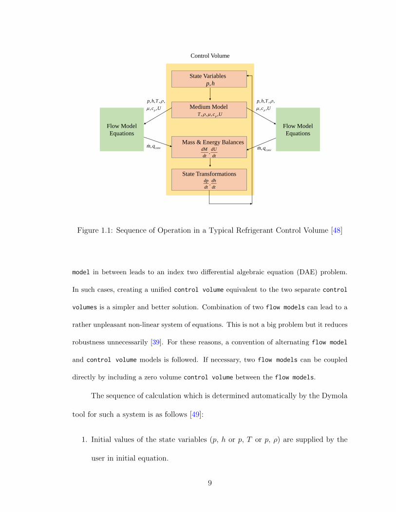
Figure 1.1: Sequence of Operation in a Typical Refrigerant Control Volume [48]

model in between leads to an index two differential algebraic equation (DAE) problem.

In such cases, creating a unified control volume equivalent to the two separate control

volumes is a simpler and better solution. Combination of two flow models can lead to a

rather unpleasant non-linear system of equations. This is not a big problem but it reduces

robustness unnecessarily [39]. For these reasons, a convention of alternating flow model

and control volume models is followed. If necessary, two flow models can be coupled

directly by including a zero volume control volume between the flow models.

The sequence of calculation which is determined automatically by the Dymola

tool for such a system is as follows [49]:

1. Initial values of the state variables (p, h or p, T or p, ρ) are supplied by the

user in initial equation.

9

2. Other thermodynamic properties are calculated using the medium model from

the state variables.

3. The flow models use the value of these variables for evaluating the mass and

energy flows. It accesses these variables through the connectors.

4. Mass and energy flows from the flow models are used to calculate the mass

balances (dM) and energy balances (dU) in the control volumes.

5. State transformation is carried out to transform the time derivatives of total

mass and internal energy (dM and dU) to time derivatives of state variables

(p,h) using functions like ddph and ddhp.

6. The time derivatives of pressure and temperature are used for evaluating the

new values of the states.

1.2.1.2 Stream Connectors

Modelica offers a very powerful software component model that is on par

with hardware component systems in flexibility and reusability. Components have

well-defined interfaces consisting of ports (refered to as connectors in Modelica ter-

minology) to the external world. A component should be defined independently of the

environment where it is used, which is essential for its reusability. This means that in the

definition of the component, only local variables and connector variables can be used. No

means of communication between a component and the rest of the system, apart from the

connector is recommended [36].

10

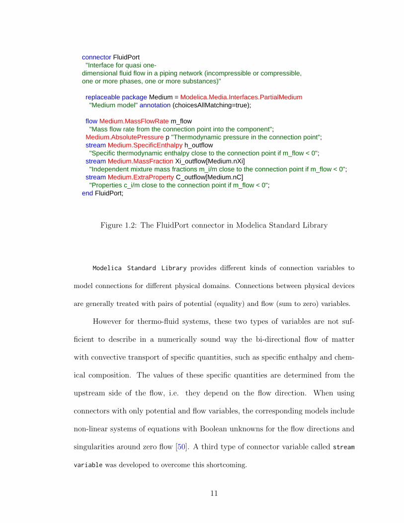
connector FluidPort

"Interface for quasi one-

dimensional fluid flow in a piping network (incompressible or compressible,

one or more phases, one or more substances)"

replaceable package Medium = Modelica.Media.Interfaces.PartialMedium

"Medium model" annotation (choicesAllMatching=true);

flow Medium.MassFlowRate m_flow

"Mass flow rate from the connection point into the component";

Medium.AbsolutePressure p "Thermodynamic pressure in the connection point";

stream Medium.SpecificEnthalpy h_outflow

"Specific thermodynamic enthalpy close to the connection point if m_flow < 0";

stream Medium.MassFraction Xi_outflow[Medium.nXi]

"Independent mixture mass fractions m_i/m close to the connection point if m_flow < 0";

stream Medium.ExtraProperty C_outflow[Medium.nC]

"Properties c_i/m close to the connection point if m_flow < 0";

end FluidPort;

Figure 1.2: The FluidPort connector in Modelica Standard Library

Modelica Standard Library provides different kinds of connection variables to

model connections for different physical domains. Connections between physical devices

are generally treated with pairs of potential (equality) and flow (sum to zero) variables.

However for thermo-fluid systems, these two types of variables are not suf-

ficient to describe in a numerically sound way the bi-directional flow of matter

with convective transport of specific quantities, such as specific enthalpy and chem-

ical composition. The values of these specific quantities are determined from the

upstream side of the flow, i.e. they depend on the flow direction. When using

connectors with only potential and flow variables, the corresponding models include

non-linear systems of equations with Boolean unknowns for the flow directions and

singularities around zero flow [50]. A third type of connector variable called stream

variable was developed to overcome this shortcoming.

11

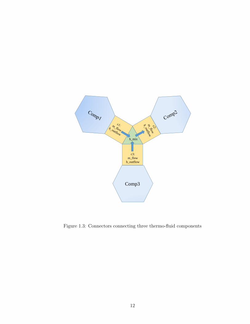
c3:

m_flow

h_outflow

Comp3

h_mix

Figure 1.3: Connectors connecting three thermo-fluid components

12

A built-in operator inStream, which when applied to a stream variable in a stream

connector returns its value close to the connection point provided that the associated mass

flow rate is positive in the direction into the component. A built-in operator actualStream,

which when applied to a stream variable returns its value close to the connection point

regardless of the direction of the associated mass flow.

1.2.1.3 Current State of Art of Modeling VCC

The ThermoFluid library [37–41] provides base library for dynamic simulation of

thermo-hydraulic processes. Pfafferott [43,44] used the models of the ThermoFluid library

as a starting point for the development of additional component models to simulate mo-

bile air conditioning system. This Modelica library called ACLib [51] was used to simulate

mobile R134a and CO2 air conditioning systems. This was later used to in the design

process of the AirConditioning library developed by Modelon AB and presented in [52].

The AirConditioning library is the currently most widely used Modelica library to simu-

late air-conditioning systems. The structure of components, however, is very complex in

AirConditioning library due to extensive hierarchy from multiple inheritance and TIL li-

brary was developed with a structure that is simple to understand for students, developers

and simulation specialists [46].

The AirConditioning Library is capable of handling both steady state and transient

simulations. However, it was mainly developed for automotive air conditioning systems.

For detailed modeling of building HVAC systems CEEE Modelica Library [47] has been

developed. The library includes detailed finite volume based as well as moving boundary

based heat exchanger models with capability to model frosting and defrosting.

In all these libraries, there are two commonly used heat exchanger modeling meth-

13

air

wall

refrigeranth

eat

tran

spo

rt

medium transport

medium transport

n = number of passes * discretization/pass

1 2 3 n

Fluidport

Heatport

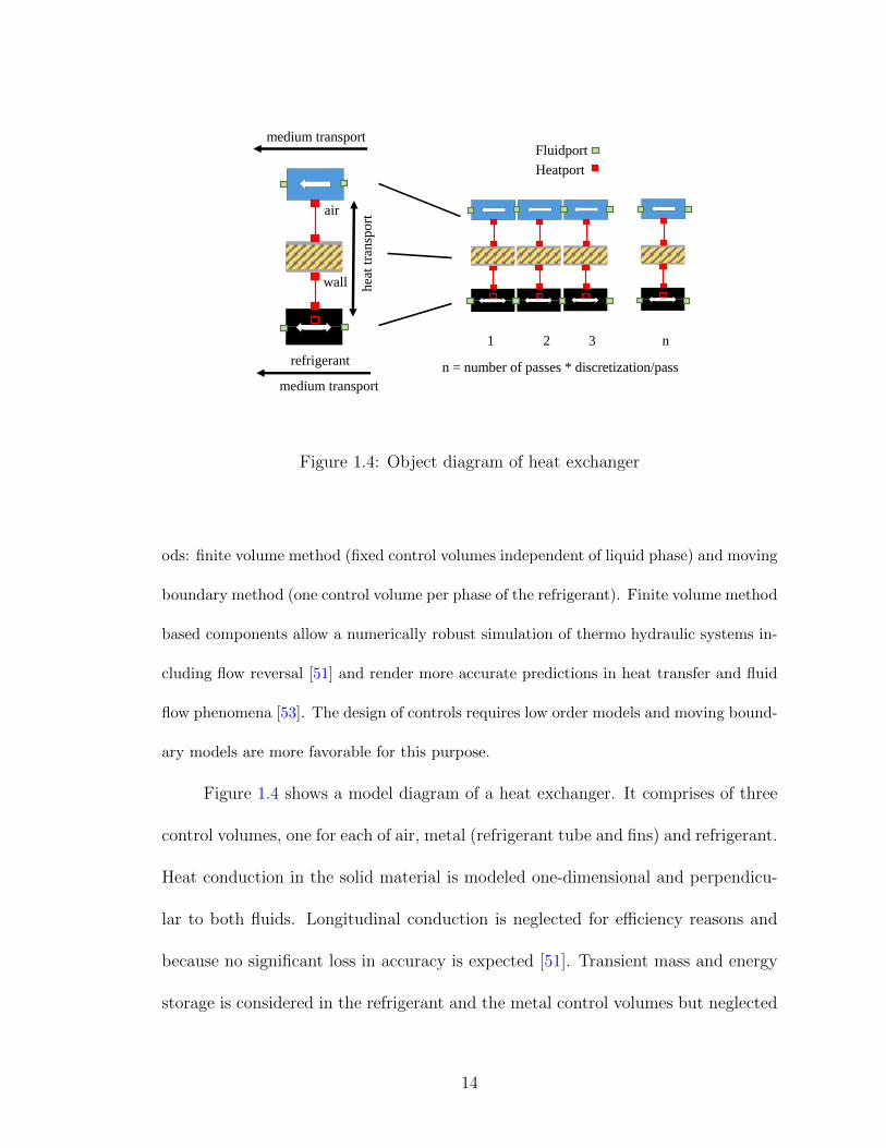
Figure 1.4: Object diagram of heat exchanger

ods: finite volume method (fixed control volumes independent of liquid phase) and moving

boundary method (one control volume per phase of the refrigerant). Finite volume method

based components allow a numerically robust simulation of thermo hydraulic systems in-

cluding flow reversal [51] and render more accurate predictions in heat transfer and fluid

flow phenomena [53]. The design of controls requires low order models and moving bound-

ary models are more favorable for this purpose.

Figure 1.4 shows a model diagram of a heat exchanger. It comprises of three

control volumes, one for each of air, metal (refrigerant tube and fins) and refrigerant.

Heat conduction in the solid material is modeled one-dimensional and perpendicu-

lar to both fluids. Longitudinal conduction is neglected for efficiency reasons and

because no significant loss in accuracy is expected [51]. Transient mass and energy

storage is considered in the refrigerant and the metal control volumes but neglected

14

at the airside. The mass and specific heat capacity of the air are much smaller than

that of the metal or the refrigerant. So, the airside control volume is modeled as

quasi-steady.

1.2.1.4 Mass Conservation in Dynamic VCC Models

Many dynamic vapor compression system models demonstrate significant vari-

ations in the total system charge which does not correspond to observed behavior in

experimental systems [54]. This is significant because the dynamics associated with

variations in the cycle charge will be coupled to the other system dynamics and

introduce aberrant behavior that would not be observed in experimental system.

These mass variations are caused by interactions between the numerical behavior of

the DAE solver and the thermodynamic properties of the refrigerant in the neighbor-

hood of the saturated liquid line for the conventional choice of pressure and specific

enthalpy as state variables [55].

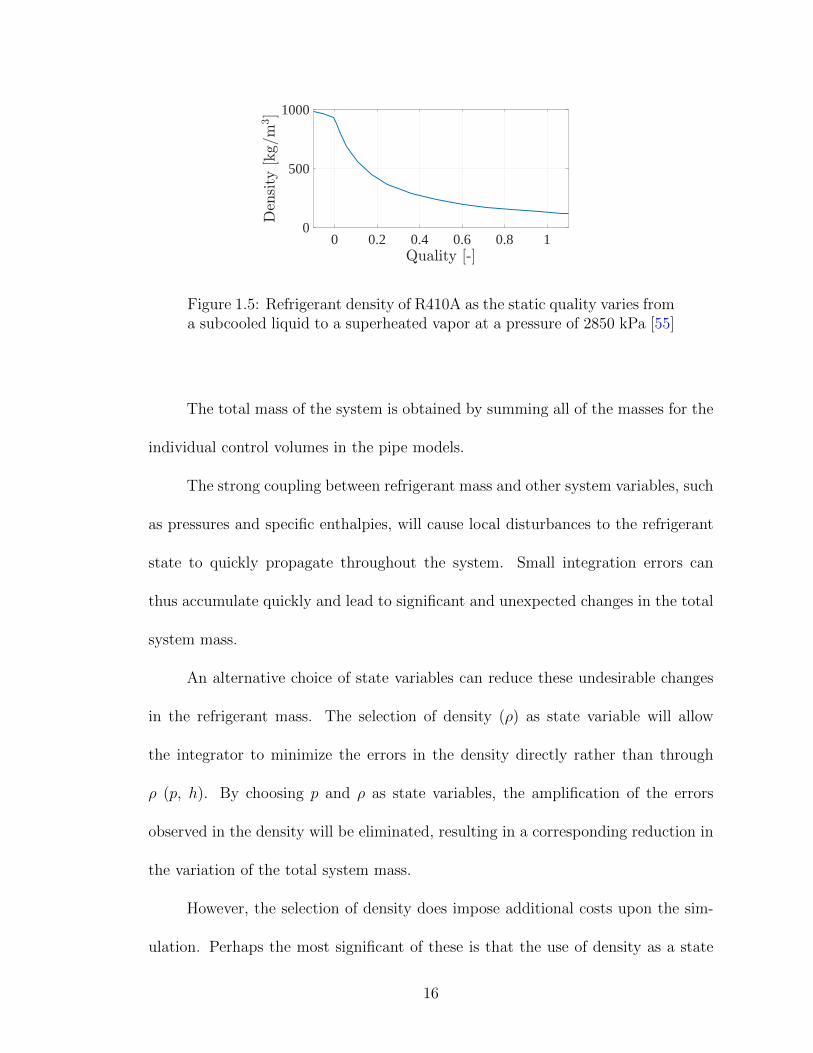
Two-phase refrigerant flows experience large changes in density as the fluid

passes from the liquid region into the two-phase region. These large changes in

density can be seen in Figure 1.5. At the static quality of zero for the given pressure,

it is evident that there is a discontinuous change in the derivative of density with

respect to the static quality, and hence with respect to the mixture specific enthalpy.

Integration errors that are added to the state variables located barely on the single

phase side of the saturated liquid line can therefore cause the resulting refrigerant

density to be calculated on the two-phase side of the saturated line [55].

15

0 0.2 0.4 0.6 0.8 1Quality [-]

0

500

1000

Den

sity

[kg=m

3]

Figure 1.5: Refrigerant density of R410A as the static quality varies froma subcooled liquid to a superheated vapor at a pressure of 2850 kPa [55]

The total mass of the system is obtained by summing all of the masses for the

individual control volumes in the pipe models.

The strong coupling between refrigerant mass and other system variables, such

as pressures and specific enthalpies, will cause local disturbances to the refrigerant

state to quickly propagate throughout the system. Small integration errors can

thus accumulate quickly and lead to significant and unexpected changes in the total

system mass.

An alternative choice of state variables can reduce these undesirable changes

in the refrigerant mass. The selection of density (ρ) as state variable will allow

the integrator to minimize the errors in the density directly rather than through

ρ (p, h). By choosing p and ρ as state variables, the amplification of the errors

observed in the density will be eliminated, resulting in a corresponding reduction in

the variation of the total system mass.

However, the selection of density does impose additional costs upon the sim-

ulation. Perhaps the most significant of these is that the use of density as a state

16

variable will cause the solver to take smaller time steps because of large values of

derivatives. Also the set of equations that needs to be solved now is non-linear [55].

Another alternative method for describing the dynamics of the differential

control volume involves expanding the number of state variables to include pressure,

specific enthalpy and density. While this approach does result in a larger number of

state variables, it has the advantage of simultaneously minimizing the variations in

system charge while enabling the use of pressure and specific enthalpy for calculating

other refrigerant properties.

The problems associated with total charge estimation with pressure and en-

thalpy as state variables can also be minimized by increasing the solver tolerance

from 1e-4 to 1e-6. The system simulation is the fastest with pressure and enthalpy

as state variables and if the total system charge does not change appreciably with

a high tolerance value, this selection should be preferred.

1.2.1.5 Non-homogeneous two-phase flow

The choice of flow model used to describe a vapor compression system is impor-

tant because some of the systems equilibrium characteristics, such as its total mass

inventory, are strongly related to the flow regime. One particularly common type

of heterogeneous flow model is known as a slip-flow model, in which it is assumed

that mass transfer across the phasic interface takes place without an accompanying

momentum transfer. This model can be formulated as a set of equations describing

the two-phase mixture with an extra set of closure relations to relate the different

17

phasic properties to each other and, consequently, is much simpler than a complete

multi fluid model [56].

Bauer (1999) [57] developed two different slip-flow models for the dynamics of

a evaporator, one of these models used a static relation to describe the interactions

between the phases, while the second incorporated an innovative description of the

mass, momentum, and energy transfer between the phases without developing a

complete two-fluid model. The results from this work demonstrated that the homo-

geneous flow modeling approach was inadequate to describe the evaporators mass

inventory and that the performances of the momentum balance with and without a

momentum transfer across the two phase interface were comparable.

The slip-flow cycles simulated by Laughman et al.(2015) [56] had a total evap-

orator inventory that is 75-85% higher than the homogeneous flow cycle, although

the cycles were all initialized at the same operating point. These differences in

charge are part to the fact that the liquid phase velocity is much lower than the

vapor phase velocity, causing the total residence time of the liquid in the heat ex-

changers to be much longer for the slip flow cycles than for the homogenous flow

cycle.

The differences in charge between the cycles with the different flow assump-

tions are only relevant to the components with two-phase flows. The components

in the cycle that have a single phase flow will have the same charge inventory. The

mass inventory in the condenser is also similar, because much of the mass is con-

tained in the sub-cooled section of the condenser and because the length of the two

phase region in the condenser is shorter than it is in evaporator.

18

It is also interesting to note that the different slip-flow correlations correspond

to different transient responses. Laughman et al.(2015) [56] found that the transient

corresponding to the homogeneous flow assumption is much faster than both the

experimental data and the comparable slip flow transients.

1.2.2 Thermosiphon Modeling

Two-phase thermosiphon is also a fairly commonly used thermo-fluid system.

A brief review of the modeling effort is presented in this subsection.

The thermosiphon mechanism has been studied by researchers for the past

100 years, starting notably with Lord Rayleigh [58]. Dobran [59] provided the first

comprehensive control volume (CV) based model to analyze the steady-state char-

acteristics of a two-phase thermosiphon. Reed and Tien [60] advanced this work by

including transient behaviors, analyzing dry-out and flooding. These models [59,60]

were created for counter-current two-phase closed thermosiphons, which are essen-

tially wick-less heat pipes. Examples of counter-current thermosiphon analysis can

be found in several review articles [61–63]. The development of predictive tools for

heat pipe technologies, such as a thermosiphon, remains an active field of research.

Industrial applications typically involve co-current two-phase loop thermosiphons

(TPTL) due to their capability of transporting large heat quantities and less liquid-

vapor interaction [64]. Several steady-state models are available in literature for

TPTL [65–69]. The first model for such a thermosiphon based on the control volume

approach for overall performance in transient operation was developed by Vincent

19

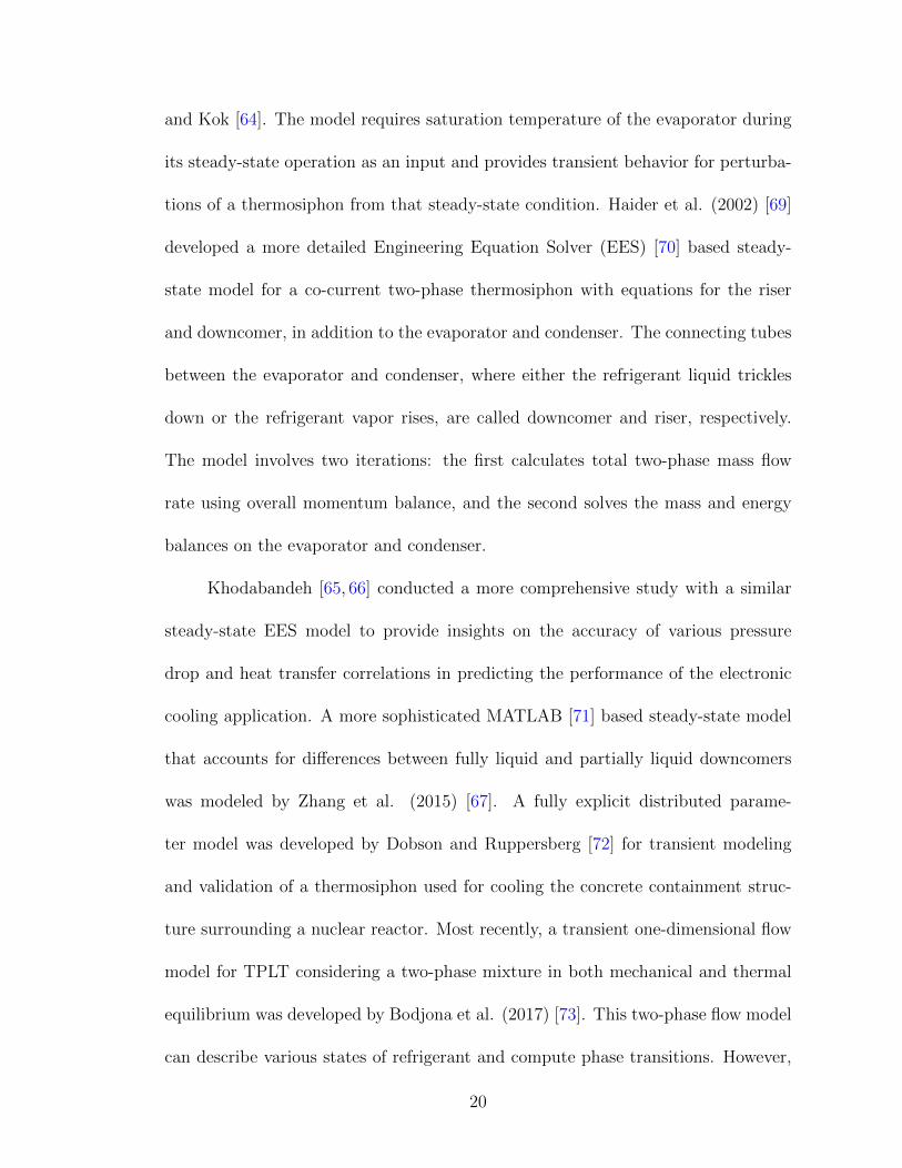
and Kok [64]. The model requires saturation temperature of the evaporator during

its steady-state operation as an input and provides transient behavior for perturba-

tions of a thermosiphon from that steady-state condition. Haider et al. (2002) [69]

developed a more detailed Engineering Equation Solver (EES) [70] based steady-

state model for a co-current two-phase thermosiphon with equations for the riser

and downcomer, in addition to the evaporator and condenser. The connecting tubes

between the evaporator and condenser, where either the refrigerant liquid trickles

down or the refrigerant vapor rises, are called downcomer and riser, respectively.

The model involves two iterations: the first calculates total two-phase mass flow

rate using overall momentum balance, and the second solves the mass and energy

balances on the evaporator and condenser.

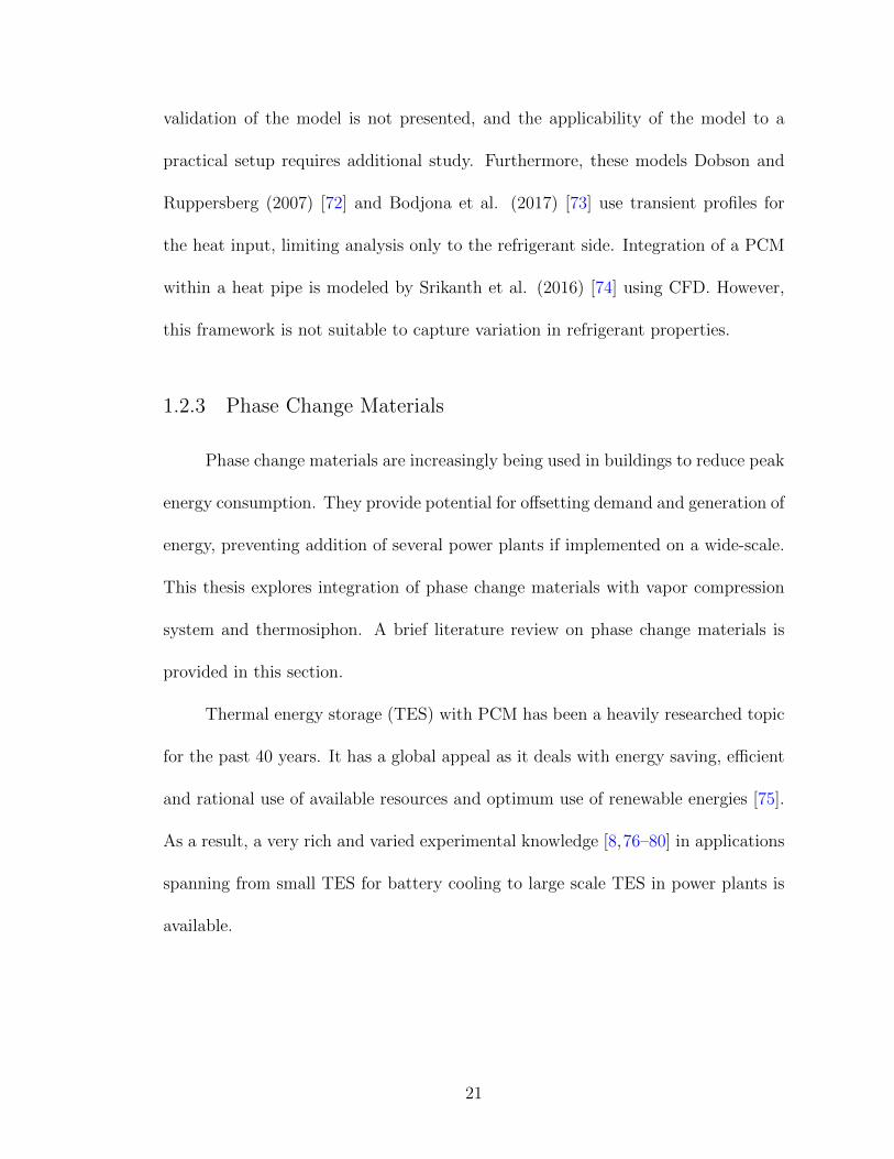
Khodabandeh [65, 66] conducted a more comprehensive study with a similar

steady-state EES model to provide insights on the accuracy of various pressure

drop and heat transfer correlations in predicting the performance of the electronic

cooling application. A more sophisticated MATLAB [71] based steady-state model

that accounts for differences between fully liquid and partially liquid downcomers

was modeled by Zhang et al. (2015) [67]. A fully explicit distributed parame-

ter model was developed by Dobson and Ruppersberg [72] for transient modeling

and validation of a thermosiphon used for cooling the concrete containment struc-

ture surrounding a nuclear reactor. Most recently, a transient one-dimensional flow

model for TPLT considering a two-phase mixture in both mechanical and thermal

equilibrium was developed by Bodjona et al. (2017) [73]. This two-phase flow model

can describe various states of refrigerant and compute phase transitions. However,

20

validation of the model is not presented, and the applicability of the model to a

practical setup requires additional study. Furthermore, these models Dobson and

Ruppersberg (2007) [72] and Bodjona et al. (2017) [73] use transient profiles for

the heat input, limiting analysis only to the refrigerant side. Integration of a PCM

within a heat pipe is modeled by Srikanth et al. (2016) [74] using CFD. However,

this framework is not suitable to capture variation in refrigerant properties.

1.2.3 Phase Change Materials

Phase change materials are increasingly being used in buildings to reduce peak

energy consumption. They provide potential for offsetting demand and generation of

energy, preventing addition of several power plants if implemented on a wide-scale.

This thesis explores integration of phase change materials with vapor compression

system and thermosiphon. A brief literature review on phase change materials is

provided in this section.

Thermal energy storage (TES) with PCM has been a heavily researched topic

for the past 40 years. It has a global appeal as it deals with energy saving, efficient

and rational use of available resources and optimum use of renewable energies [75].

As a result, a very rich and varied experimental knowledge [8,76–80] in applications

spanning from small TES for battery cooling to large scale TES in power plants is

available.

21

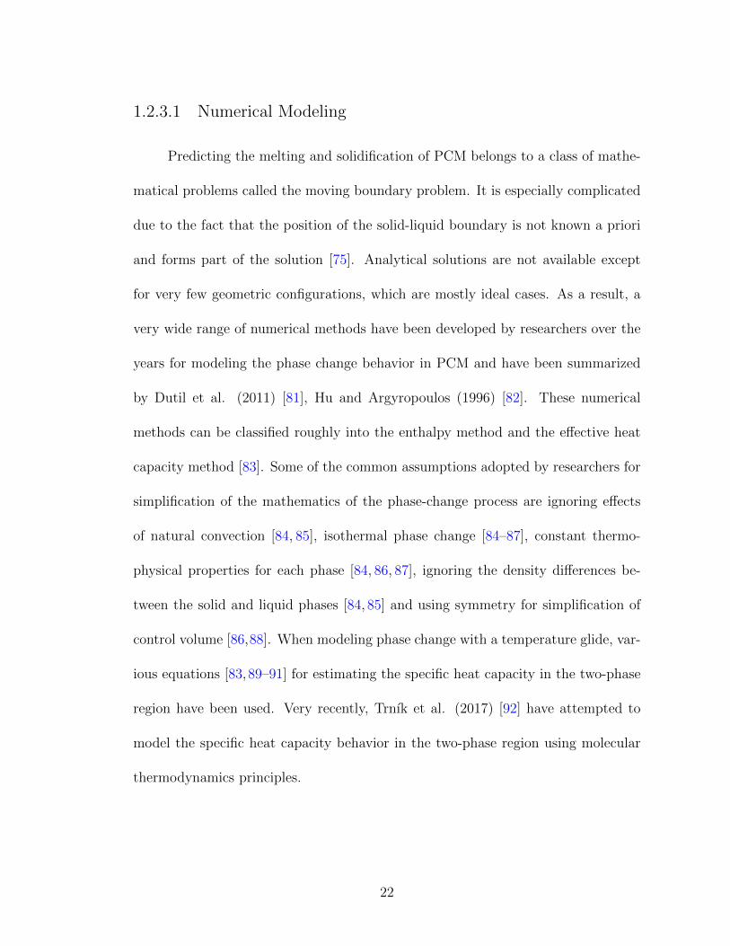
1.2.3.1 Numerical Modeling

Predicting the melting and solidification of PCM belongs to a class of mathe-

matical problems called the moving boundary problem. It is especially complicated

due to the fact that the position of the solid-liquid boundary is not known a priori

and forms part of the solution [75]. Analytical solutions are not available except

for very few geometric configurations, which are mostly ideal cases. As a result, a

very wide range of numerical methods have been developed by researchers over the

years for modeling the phase change behavior in PCM and have been summarized

by Dutil et al. (2011) [81], Hu and Argyropoulos (1996) [82]. These numerical

methods can be classified roughly into the enthalpy method and the effective heat

capacity method [83]. Some of the common assumptions adopted by researchers for

simplification of the mathematics of the phase-change process are ignoring effects

of natural convection [84, 85], isothermal phase change [84–87], constant thermo-

physical properties for each phase [84, 86, 87], ignoring the density differences be-

tween the solid and liquid phases [84, 85] and using symmetry for simplification of

control volume [86,88]. When modeling phase change with a temperature glide, var-

ious equations [83,89–91] for estimating the specific heat capacity in the two-phase

region have been used. Very recently, Trnık et al. (2017) [92] have attempted to

model the specific heat capacity behavior in the two-phase region using molecular

thermodynamics principles.

22

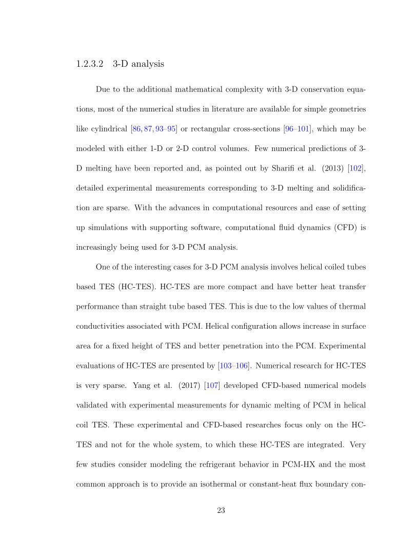
1.2.3.2 3-D analysis

Due to the additional mathematical complexity with 3-D conservation equa-

tions, most of the numerical studies in literature are available for simple geometries

like cylindrical [86, 87, 93–95] or rectangular cross-sections [96–101], which may be

modeled with either 1-D or 2-D control volumes. Few numerical predictions of 3-

D melting have been reported and, as pointed out by Sharifi et al. (2013) [102],

detailed experimental measurements corresponding to 3-D melting and solidifica-

tion are sparse. With the advances in computational resources and ease of setting

up simulations with supporting software, computational fluid dynamics (CFD) is

increasingly being used for 3-D PCM analysis.

One of the interesting cases for 3-D PCM analysis involves helical coiled tubes

based TES (HC-TES). HC-TES are more compact and have better heat transfer

performance than straight tube based TES. This is due to the low values of thermal

conductivities associated with PCM. Helical configuration allows increase in surface

area for a fixed height of TES and better penetration into the PCM. Experimental

evaluations of HC-TES are presented by [103–106]. Numerical research for HC-TES

is very sparse. Yang et al. (2017) [107] developed CFD-based numerical models

validated with experimental measurements for dynamic melting of PCM in helical

coil TES. These experimental and CFD-based researches focus only on the HC-

TES and not for the whole system, to which these HC-TES are integrated. Very

few studies consider modeling the refrigerant behavior in PCM-HX and the most

common approach is to provide an isothermal or constant-heat flux boundary con-

23

dition to the PCM control volume. The refrigerant side of the PCM-HX used by El

Qarnia (2009) [86] and Bakhshipour et al. (2017) [87] is liquid, thus enabling the

assumption of incompressible flow and a relatively simple model. It is necessary to

point out that the geometries modeled by El Qarnia (2009) [86] and Bakhshipour

et al. (2017) [87] are cylindrical enabling them to develop a 2D model for the PCM

cross-section.

1.2.3.3 System simulation

Modeling or testing of TES at a component level leads to its improved sub-

system performance. However, a dynamic model of the entire system (of which

TES is a sub-system) provides several additional benefits like optimization of the

entire operation, development of controls, understanding the safety of operation,

replacement of time and cost intensive experiments for parametric study. System

models magnify human intuition by enabling development of hitherto unseen system

behavior patterns, and thus reduce development time and production costs with

increased product quality and a more reliable system operation. Sub-system models

are modeled using a very high level of detail. Using the same sub-system model to

develop a system model will lead to very large complexity, which may not be solved

by numerical solvers and significant computational effort [108]. So it is necessary to

find a balance between accuracy and level of detail in a system simulation.

The system-level models involving TES in literature are used only for qualita-

tive study and lack detailed validation. Azzouz et al. (2008) [85] modeled a dynamic

24

model of VCC with a PCM integrated with its evaporator in a domestic refrigerator.

The model uses a simplified dynamic model with a rectangular slab PCM, which is

validated by comparison with experimental measurements obtained for a refrigera-

tor without PCM and then used to obtain qualitative trends after including PCM.

Leonhardt and Muller [90] describe modeling and simulation of a TES integrated in

a heat pump system. The PCM model ignores effects of natural convection and is

used only for qualitative analysis of system performance. The heat pump model is

implemented as a black box model. Another system level model with PCM is de-

veloped by Buschle et al. (2006) [91] for qualitative analysis of steam accumulator

in power plant application .

1.2.4 Personal Conditioning Systems

Hoyt et al. (2015) [109] demonstrated the energy savings potential from ex-

tending building thermostat set-points. They concluded that if it were possible to

relax the temperature set-point in either the hot or cold direction, total HVAC en-

ergy is reduced at a rate of 10% per °C. To enable expansion of building set-point

temperatures without affecting occupant thermal comfort, one option is to provide

supplementary Personal Conditioning System (PCS), which consumes significantly

lower energy. PCS offers dual benefits of energy saving and increased comfort [110].

Energy is used to modify the local thermal envelope around the human body rather

than the building, thus allowing the thermostat to be relaxed without compromising

the occupant comfort. This was confirmed in the experimental studies carried out

25

by several researchers with human subjects using their respective PCS [111–113].

By offering personalized comfort, PCS are able to deliver comfort to every individual

rather than the conventional HVAC systems which cater to the average population.

Percentage satisfaction as high as 100% has been reported in the literature with well-

designed PCS [114]. Some additional benefits of PCS are lower capital installation

costs and ease of implementation when compared to novel HVAC solutions.

Due to these benefits, a large number of PCS exist which are summarized in

the review articles by Zhang et al. (2015) [110], Vesely and Zeiler (2014) [115].

Task ambient conditioning systems [114, 116–118] are typically space condi-

tioning systems, typically installed in office buildings. The occupants can control

the thermal conditions in the small regions surrounding them. Recently, the appli-

cation of these systems is being explored in bedrooms to increase thermal comfort in

sleeping environment and at the same time reduce energy use [116,119]. There is a

lot of variation in design of these systems, but usually they consist of air nozzles to

supply air to the upper body and a radiant panel for heating the legs. They provide

conditioning only to the limited space surrounding the office desk towards which

the air nozzles and radiant panel are directed. Air nozzles pull air from underfloor

plenum or ceiling vertical ducts leading to retrofitting costs.

In an evaporative cooling system for air conditioning [120, 121], the air has

a direct contact with water. The evaporation of water causes cooling and humid-

ification simultaneously. However, these technologies increase the indoor humidity

leading to additional loads on the building HVAC. However, these technologies are

excellent for hot and dry climates.

26

Cooled chairs [122–124] is another type of PCS, capable of providing improved

comfort. They may include fans to provide ventilation [123] or thermo-electric

devices providing heating and cooling in the surface of the chair [122]. The chairs

demonstrated ability to provide thermal comfort at ambient temperatures as high

as 29-30°C [122,123]. However, the occupant needs to be seated in the chair to feel

comfortable.

Personal cooling garments [125–127] have been effective in providing comfort

in hot environments and have been used in special fields like military training,

firefighting, medical operations and sports. They may use liquid cooling [128, 129],

air cooling [130], phase change material [127] or a combination of the above methods

[125]. For formal office wear, however, they are inappropriate because they are bulky,

heavy and have poor ergonomics. The liquid cooled and air cooled vests have other

drawbacks like high cost, complexity and non-portability due to the refrigeration

system [125].

Thus, despite great energy savings potential the current PCS, they do not

have much market value due to factors such as high cost, limited range of comfort,

poor thermal performance, low energy efficiency and poor aesthetics. Consequently,

except for common desk and ceiling fans, most of these are not commercially avail-

able [110]. Except for the cooling jacket, the other PCS, target the occupants’

workstations and may not cover all the spaces an occupant might visit or pass

through during the day. If the occupant divides his/her time between two locations,

there is a need to install two PCS.

27

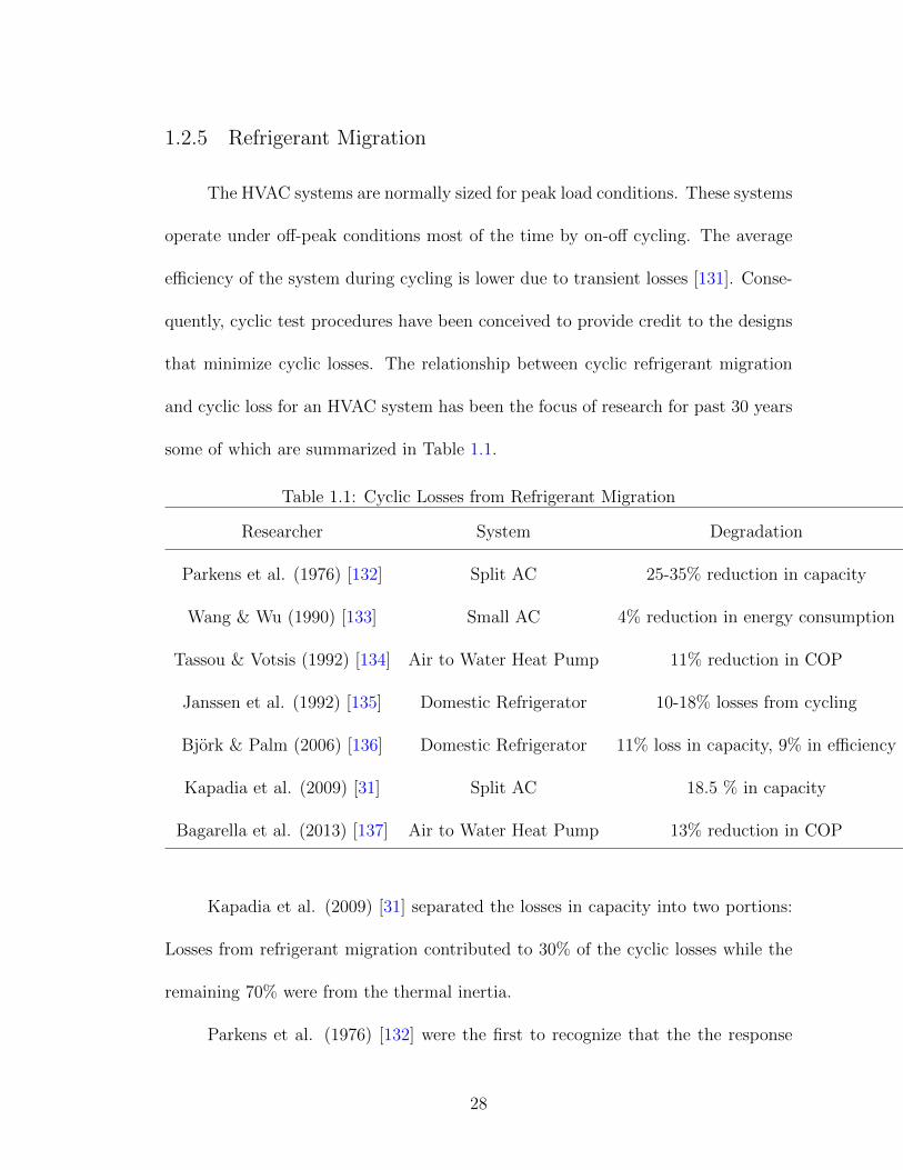
1.2.5 Refrigerant Migration

The HVAC systems are normally sized for peak load conditions. These systems

operate under off-peak conditions most of the time by on-off cycling. The average

efficiency of the system during cycling is lower due to transient losses [131]. Conse-

quently, cyclic test procedures have been conceived to provide credit to the designs

that minimize cyclic losses. The relationship between cyclic refrigerant migration

and cyclic loss for an HVAC system has been the focus of research for past 30 years

some of which are summarized in Table 1.1.

Table 1.1: Cyclic Losses from Refrigerant Migration

Researcher System Degradation

Parkens et al. (1976) [132] Split AC 25-35% reduction in capacity

Wang & Wu (1990) [133] Small AC 4% reduction in energy consumption

Tassou & Votsis (1992) [134] Air to Water Heat Pump 11% reduction in COP

Janssen et al. (1992) [135] Domestic Refrigerator 10-18% losses from cycling

Bjork & Palm (2006) [136] Domestic Refrigerator 11% loss in capacity, 9% in efficiency

Kapadia et al. (2009) [31] Split AC 18.5 % in capacity

Bagarella et al. (2013) [137] Air to Water Heat Pump 13% reduction in COP

Kapadia et al. (2009) [31] separated the losses in capacity into two portions:

Losses from refrigerant migration contributed to 30% of the cyclic losses while the

remaining 70% were from the thermal inertia.

Parkens et al. (1976) [132] were the first to recognize that the the response

28

of the system at startup and the cycling rate of the equipment could be combined

to form a part load correlation. They used this concept to develop the degradation

coefficient (Cd) used in the SEER rating procedure to predict the part load effects.

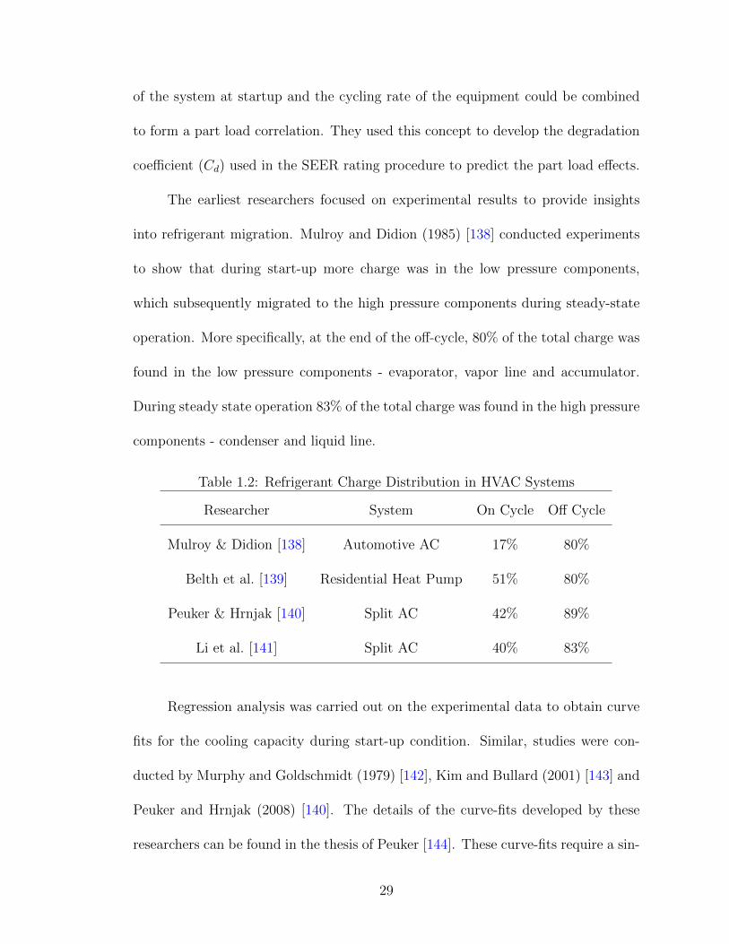
The earliest researchers focused on experimental results to provide insights

into refrigerant migration. Mulroy and Didion (1985) [138] conducted experiments

to show that during start-up more charge was in the low pressure components,

which subsequently migrated to the high pressure components during steady-state

operation. More specifically, at the end of the off-cycle, 80% of the total charge was

found in the low pressure components - evaporator, vapor line and accumulator.

During steady state operation 83% of the total charge was found in the high pressure

components - condenser and liquid line.

Table 1.2: Refrigerant Charge Distribution in HVAC Systems

Researcher System On Cycle Off Cycle

Mulroy & Didion [138] Automotive AC 17% 80%

Belth et al. [139] Residential Heat Pump 51% 80%

Peuker & Hrnjak [140] Split AC 42% 89%

Li et al. [141] Split AC 40% 83%

Regression analysis was carried out on the experimental data to obtain curve

fits for the cooling capacity during start-up condition. Similar, studies were con-

ducted by Murphy and Goldschmidt (1979) [142], Kim and Bullard (2001) [143] and

Peuker and Hrnjak (2008) [140]. The details of the curve-fits developed by these

researchers can be found in the thesis of Peuker [144]. These curve-fits require a sin-

29

gle or multiple experimentally derived time-constants are parameters to match their

respective data. As pointed out in Mulroy and Didion (1985) [138], even though

the time constant value is the best representative of the state of the art, it is not

possible to determine the range and median values without conducting further ex-

periments. Since, the curve-fits are very much model specific, they do not reduce

any experimental burden.

Due to the advancement of computing facilities, it has become possible to

model complex systems. There are several publications on transient modeling of

vapor compression cycles, but few results are available concerning the modeling of

refrigerant migration behavior.

Murphy and Goldschmidt (1985,1986) [145,146] present simulated refrigerant

migration results in some partial system components during start-up and shut-down

transients. Ozyurt and Egrican (2010) [147] steady state refrigerant mass distribu-

tion of the system model with the experimental data.

Li et al (2011) [148] presented the first refrigerant mass migration predic-

tion in a validated dynamic system model. However, the focus of their research

was on development of controls and hence they employed moving boundary models

[MBM]. MBM utilize lumped characteristics for each of the control volumes such

as single void fraction for the entire two phase section, which could lead to lower

accuracy [149]. It is necessary to identify beforehand what possible phase region

combinations can exist logically in the heat exchanger and the manner of their tran-

sition. As pointed out it Qiao (2014) [47], they employ huge look-up tables for

correlating mean void fraction, the refrigerant pressure and the outlet vapor qual-

30

ity before conducting the simulation. This makes the simulation very application

specific. Another disadvantage of moving boundary models is that the mode tran-

sitions are such that phase boundaries enter or leave the heat exchanger only from

the refrigerant outlet end. The model cannot handle a situation where the phase

boundary enters or leaves from the refrigerant inlet end [149]. Thus, phenomena

like refrigerant leakage through compressor cannot be modeled using the approach.

It is also not possible to model complex refrigerant circuitry on the air-side using

MBM with accuracy.

Distributed parameter model permit modeling of space-time variation in prop-

erties. It is capable of accounting for the complex tube circuitry of the heat ex-

changer. A first principles based model for the refrigerant migration dynamics will

enable accurate modeling of the complex phenomena associated with the transient

behavior of vapor compression cycles in cyclic operation. The insights are expected

to aid the improvement of HVAC equipment leading to better cyclic performance.

1.2.6 Current methods for estimating HVAC cyclic performance

The DOE and ASHRAE standards for evaluation of part load performance are

based on the experimental work [150] conducted at National Institute of Standards

and Technology (then called National Bureau of Standards). The methodology to

estimate cyclic degradation is given in standards ANSI/AHRI Standard 210/240-

2008 [32] & ASHRAE 116-2010 [151]. The indoor and outdoor ambient conditions

are, for a large fraction of the time in regions throughout US, such that an air condi-

31

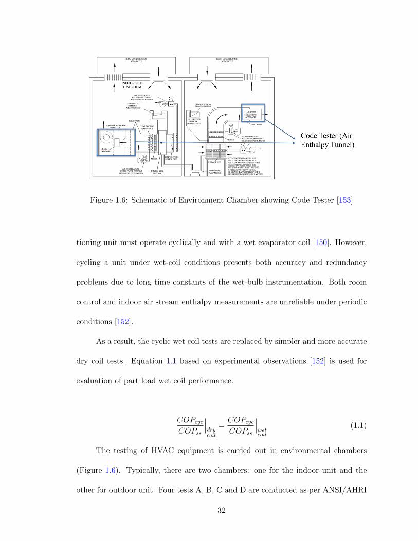
Figure 1.6: Schematic of Environment Chamber showing Code Tester [153]

tioning unit must operate cyclically and with a wet evaporator coil [150]. However,

cycling a unit under wet-coil conditions presents both accuracy and redundancy

problems due to long time constants of the wet-bulb instrumentation. Both room

control and indoor air stream enthalpy measurements are unreliable under periodic

conditions [152].

As a result, the cyclic wet coil tests are replaced by simpler and more accurate

dry coil tests. Equation 1.1 based on experimental observations [152] is used for

evaluation of part load wet coil performance.

COPcycCOPss

∣∣∣drycoil

=COPcycCOPss

∣∣∣wetcoil

(1.1)

The testing of HVAC equipment is carried out in environmental chambers

(Figure 1.6). Typically, there are two chambers: one for the indoor unit and the

other for outdoor unit. Four tests A, B, C and D are conducted as per ANSI/AHRI

32

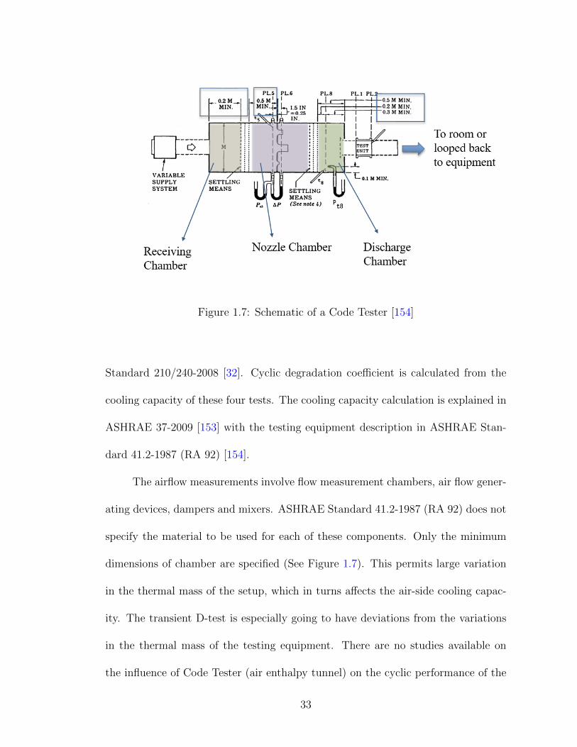
Figure 1.7: Schematic of a Code Tester [154]

Standard 210/240-2008 [32]. Cyclic degradation coefficient is calculated from the

cooling capacity of these four tests. The cooling capacity calculation is explained in

ASHRAE 37-2009 [153] with the testing equipment description in ASHRAE Stan-

dard 41.2-1987 (RA 92) [154].

The airflow measurements involve flow measurement chambers, air flow gener-

ating devices, dampers and mixers. ASHRAE Standard 41.2-1987 (RA 92) does not

specify the material to be used for each of these components. Only the minimum

dimensions of chamber are specified (See Figure 1.7). This permits large variation

in the thermal mass of the setup, which in turns affects the air-side cooling capac-

ity. The transient D-test is especially going to have deviations from the variations

in the thermal mass of the testing equipment. There are no studies available on

the influence of Code Tester (air enthalpy tunnel) on the cyclic performance of the

33

HVAC unit being tested.

Parken et al. (1976) [132] introduced the non-dimensional forms of efficiency

(called part load factor, PLF) and cyclic cooling capacity (called cooling load factor,

CLF) as per Equations (1.2) and (1.3).

PLF =COPcyc,dryCOPss,dry

(1.2)

CLF =

∫ to0Qcyc,drydt

Qss,drytc(1.3)

The PLF and CLF were related by a linear fit even though there were vari-

ations in the PLF data due to the cycling rate, which led to the development of

the degradation coefficient, Cd, defined by Equation(1.4). The part load factor in

Equation (1.5) [PLF (0.5)] is evaluated for a CLF of 0.5 to estimate the SEER.

Cd =1− PLF1− CLF

(1.4)

This SEER evaluation procedure is based on experimental data available at

that time without any significant theoretical research. Starting from Murphy &

Goldschmidt [142], Goldschmidt et al. [155] to ONeal & Katipamula [156], in efforts

spanning well over a decade, several researchers conducted extensive experimental

34

and theoretical investigations to understand the validity of the assumptions made

in the development of the procedure.

SEER = PLF (0.5) ∗ EERB (1.5)

Single time constant models, in which the start-up cooling capacity of the

air conditioning system is modeled using an exponential function with the time

constant, were used by Katipamula & ONeal (1991) [157], ONeal & Katipamula

(1993) [156] to show that the relationship between PLF and CLF is not linear.

Henderson et al. [158] realized that use of Cd to evaluate PLF (by substitution in

Equation (1.4)) is not accurate and implemented alternate empirical equation in

DOE-2, which is a building energy simulation program. Experiments conducted

by Bettanini et al. (2003) [159] to evaluate the use of Cd to evaluate PLF from

Equation (1.4), show that this approximation is not acceptable. They propose a

new parameter Z, which is the ratio of the electric power consumption at part load

working condition to the one at full capacity to evaluate PLF. Italian standard UNI

10963 also identifies the shortcoming of Cd and uses the Z-parameter method to

evaluate PLF Bettanini et al. (2003) [159]. However, the ISO Standard 16358-

1 [160] still uses Cd and defines 0.25 as default value.

The single-time-constant model assumes that the shutdown transients have

no direct impact on the startup characteristics. The startup losses can be better

predicted by two-time-constant models Mulroy & Didion (1985) [138], with one time

35

constant capturing the capacity delay due to the mass of the heat exchanger, while

the second time constant capturing the delay in reaching steady state refrigerant

distribution from the off-cycle refrigerant distribution. Sigmoid and polynomial

functions for startup have been used by Fuentes et al.(2016) [161]. However, the

behavior of PLF and CLF obtained by integrating these functions has not been

investigated.

The heat losses to the test setup have not been considered by any of these

researchers. AHRI Standard 210/240 (2017) [162] as well as ASHRAE Standard

116 (2010) [151] recognize the contribution of the code tester in the measured cyclic

cooling capacity by introducing a correction procedure. For the discussion of the

chapter, since the focus is on air-conditioners, we will focus only on the indoor room

apparatus in laboratory testing of split air conditioners. The method is described

in the operation manual of AHRI Standard 210/240 (2017) and is summarized here.

An electric heater is used as the source for integrated measured capacity and is

cycled every 6 minutes with alternating on and off cycles. Ten on-off cycles are

carried out over two-hour duration with a fixed airflow of 1200 cfm (0.566 m3 s−1).

The temperature at the location of highest thermal mass (typically, the mixer) is

measured at the start and end of the off cycle. For the discussion in this section, it

will be assumed that this assumption is valid.

The average value of integrated airside capacity (qts,avg) evaluated as per

ASHRAE Standard 116 (2010) [151] from last 6 to 8 cycles is calculated using

Equation (1.6).

36

qts,avg = mc

((∆T1)offtoff

)(1.6)

The integrated capacity (q′) is corrected using the thermal inertia term calcu-

lated from Equation (1.6) as shown in Equation (1.7).

q = qts,avgmc(∆T1)off (1.7)

The temperature difference at the beginning and end of either the off cycle

is used in Equation (1.6) while that during the on time during the cyclic D-Test

(Equation (1.8)) for the mixer.

qts =

∫off

Qdt =n∑n=1

mc(∆Ti)off (1.8)

The dampers that circulate air into the code tester may have a different cycling

time than the compressor and in such cases, the integration time should be taken

from damper cycling. However, this is much closer to the on-cycle time in D-Test

and so it is assumed equal in Equation (1.8).

mc = m1c1 +n∑n=1

mici

((∆Ti)off(∆T1)off

)(1.9)

In the real case, the qts term should involve heat transfer from all the regions

of the code tester. If mixer has the higher thermal mass for a code tester with

37

n regions arranged in descending order of thermal mass, the thermal inertia term

evaluated in Equation (1.6) is given by Equation (1.9). The standard, thus, ignores

the second term on the right-hand side of Equation (1.9). It has been observed

that this assumption leads to under prediction of thermal inertia effects from a code

tester (by as much as 70% as will be shown later), and is one of the reasons for the

differences in measured values of Cd for the same system when tested with different

code testers.

1.3 Objectives

The thesis discusses modeling strategies for system simulation of complex two-

phase refrigerant systems integrated with different thermal masses. This generic

modeling framework is applied to improve cyclic performance of such systems. The

insights from the thesis are expected to reduce energy consumption for space heating

and cooling of buildings.

1. Investigate the influence of PCM on different thermo-fluid systems

Water systems, vapor compression systems

PCM-heat driven two-phase thermosiphon

2. Model dynamic vapor compression system with thermal inertia of code tester

Develop modeling framework to simulate cyclic test

Simulate refrigerant migration dynamics

3. Quantify code tester thermal inertia effect on cycling of air conditioner

38

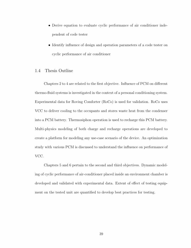
Derive equation to evaluate cyclic performance of air conditioner inde-

pendent of code tester

Identify influence of design and operation parameters of a code tester on

cyclic performance of air conditioner

1.4 Thesis Outline

Chapters 2 to 4 are related to the first objective. Influence of PCM on different

thermo-fluid systems is investigated in the context of a personal conditioning system.

Experimental data for Roving Comforter (RoCo) is used for validation. RoCo uses

VCC to deliver cooling to the occupants and stores waste heat from the condenser

into a PCM battery. Thermosiphon operation is used to recharge this PCM battery.

Multi-physics modeling of both charge and recharge operations are developed to

create a platform for modeling any use-case scenario of the device. An optimization

study with various PCM is discussed to understand the influence on performance of

VCC.

Chapters 5 and 6 pertain to the second and third objectives. Dynamic model-

ing of cyclic performance of air-conditioner placed inside an environment chamber is

developed and validated with experimental data. Extent of effect of testing equip-

ment on the tested unit are quantified to develop best practices for testing.

39

Chapter 2: Portable Personal Conditioning Devices

As discussed in Chapter 1, despite the great energy saving potential, the cur-

rent Personal Conditioning Systems (PCS) do not have much market value due to

a combination of factors such as high cost, limited range of comfort, poor thermal

performance, low energy efficiency and poor aesthetics. Consequently, except for

common desk and ceiling fans, most of these are not commercially available [110].

Except for the cooling jacket, the other PCS, target the occupants’ workstations

and may not cover all the spaces an occupant might visit or pass through during

the day. If the occupant divides his/her time between two locations, there is a need

to install two PCS.

A Portable PCS (PPCS) is a personal attendant for thermal comfort and can

deliver cooling through robotically-controlled air nozzles. A conceptual PPCS in

operation is shown in Figure 2.1. It enables buildings to relax their thermostat by

up to 4°F (2.2°C) and provides similar, if not better, thermal comfort with these

new temperature settings in a cost-effective and energy efficient manner, leading to

energy savings in the range of 10 to 30% depending on climate conditions. Thus, it

addresses the issues of current PCS in that it does not require any retrofit, comfort

range is not limited to any particular spot and thermal loads on the building do not

40

Figure 2.1: Portable Personal Conditioning System in Operation

increase.

This chapter presents four cooling systems (see Figure 2.2), which can be

integrated on a robotic platform to function as a portable cooling device and com-

pares their performance through multi-physics modeling. Modelica [163] is used for

developing the models due to its ability to model equations from different physi-

cal domains, object-oriented programming and acausal modeling capabilities with

well-supported libraries permitting re-usability of components.

2.1 Multi-physics Modeling of PPCS

A portable cooling device needs to be both affordable and energy efficient.

The four cooling systems considered are modeled for their thermodynamic behav-

ior, weight and battery consumption to understand the trade-offs involved therein.

Vapor compression cycle is the predominant cooling technology used currently and

a PPCS based on it is shown in the top left schematic of Figure 2.2 (labeled as

VCS). In the United States, buildings are typically conditioned using chillers, and

41

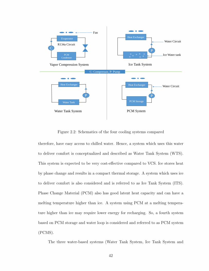
Water Tank

P

Heat Exchanger

Water Circuit

Ice Water tank

P

Heat Exchanger

Fan

R134a Circuit

Evaporator

C

PCM

Condenser

Vapor Compression System

PCM Storage

Heat Exchanger Water Circuit

P

Ice Tank System

Water Tank System PCM System

C: Compressor, P: Pump

Figure 2.2: Schematics of the four cooling systems compared

therefore, have easy access to chilled water. Hence, a system which uses this water

to deliver comfort is conceptualized and described as Water Tank System (WTS).

This system is expected to be very cost-effective compared to VCS. Ice stores heat

by phase change and results in a compact thermal storage. A system which uses ice

to deliver comfort is also considered and is referred to as Ice Tank System (ITS).

Phase Change Material (PCM) also has good latent heat capacity and can have a

melting temperature higher than ice. A system using PCM at a melting tempera-

ture higher than ice may require lower energy for recharging. So, a fourth system

based on PCM storage and water loop is considered and referred to as PCM system

(PCMS).

The three water-based systems (Water Tank System, Ice Tank System and

42

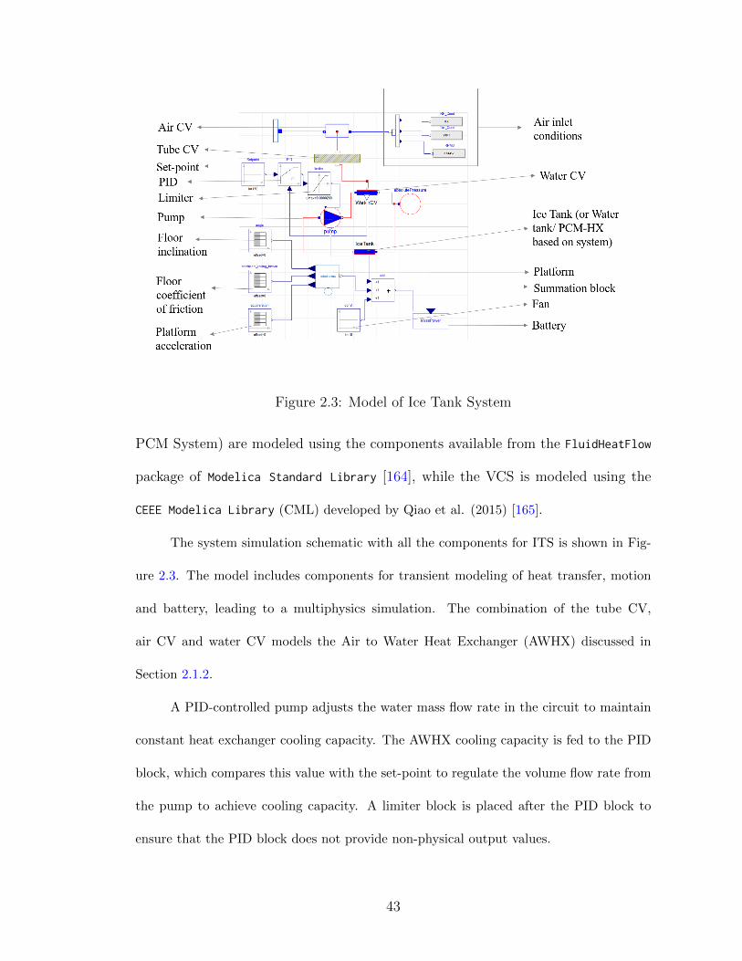
Figure 2.3: Model of Ice Tank System

PCM System) are modeled using the components available from the FluidHeatFlow

package of Modelica Standard Library [164], while the VCS is modeled using the

CEEE Modelica Library (CML) developed by Qiao et al. (2015) [165].

The system simulation schematic with all the components for ITS is shown in Fig-

ure 2.3. The model includes components for transient modeling of heat transfer, motion

and battery, leading to a multiphysics simulation. The combination of the tube CV,

air CV and water CV models the Air to Water Heat Exchanger (AWHX) discussed in

Section 2.1.2.

A PID-controlled pump adjusts the water mass flow rate in the circuit to maintain

constant heat exchanger cooling capacity. The AWHX cooling capacity is fed to the PID

block, which compares this value with the set-point to regulate the volume flow rate from

the pump to achieve cooling capacity. A limiter block is placed after the PID block to

ensure that the PID block does not provide non-physical output values.

43

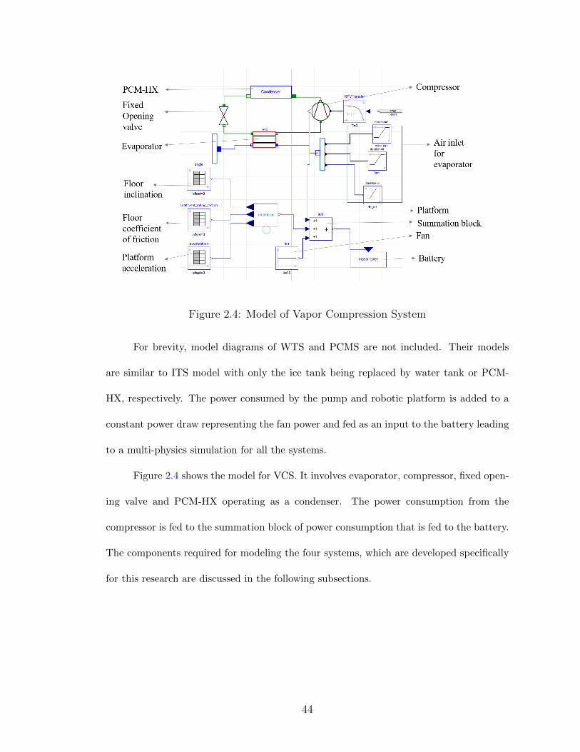
Figure 2.4: Model of Vapor Compression System

For brevity, model diagrams of WTS and PCMS are not included. Their models

are similar to ITS model with only the ice tank being replaced by water tank or PCM-

HX, respectively. The power consumed by the pump and robotic platform is added to a

constant power draw representing the fan power and fed as an input to the battery leading

to a multi-physics simulation for all the systems.

Figure 2.4 shows the model for VCS. It involves evaporator, compressor, fixed open-

ing valve and PCM-HX operating as a condenser. The power consumption from the

compressor is fed to the summation block of power consumption that is fed to the battery.

The components required for modeling the four systems, which are developed specifically

for this research are discussed in the following subsections.

44

2.1.1 PCM Heat Exchanger

The PCM heat exchanger (PCM-HX) is used in two systems: VCS and PCMS. A

different PCM is used in each system.

PCM-HX is modeled with three control volumes (CV): PCM, refrigerant tubing,

and refrigerant. These control volumes are connected by a HeatPort interface, which

is the standard connector for heat transfer in the Modelica Standard Library. Contact

resistance between the refrigerant tube and PCM is neglected. For the VCS, the refrigerant

control volume is two-phase control volume and for the PCMS it is single-phase water

control volume. The PCM and refrigerant tubing CV are the same for the two heat

exchangers. This is a good example of the model re-usability aspect that makes Modelica

very convenient for system modeling.

The melting and solidification processes are especially complicated due to the fact

that the solid-liquid boundary moves depending on the rate at which latent heat is ab-

sorbed or lost at the boundary. So, the position of the boundary is not known a priori and

forms part of the solution [75]. The heat transfer during PCM phase change is affected

by varying effects of conduction and natural convection, which depend on the amount

of PCM that has melted [96, 166]. Modeling of these effects requires three-dimensional

modeling of the separate velocity flows of both phases, which heavily depends upon the

geometry of PCM-HX.

For the conceptual nature of the present chapter, the model assumes that the domi-

nant mode of heat transfer is conduction in the radial direction. The PCM-HX is modeled

as a straight refrigerant tube surrounded by PCM (See Figure 2.5). Cylindrical co-ordinate

system with finite volume discretization along the radial direction is used with a fixed grid.

45

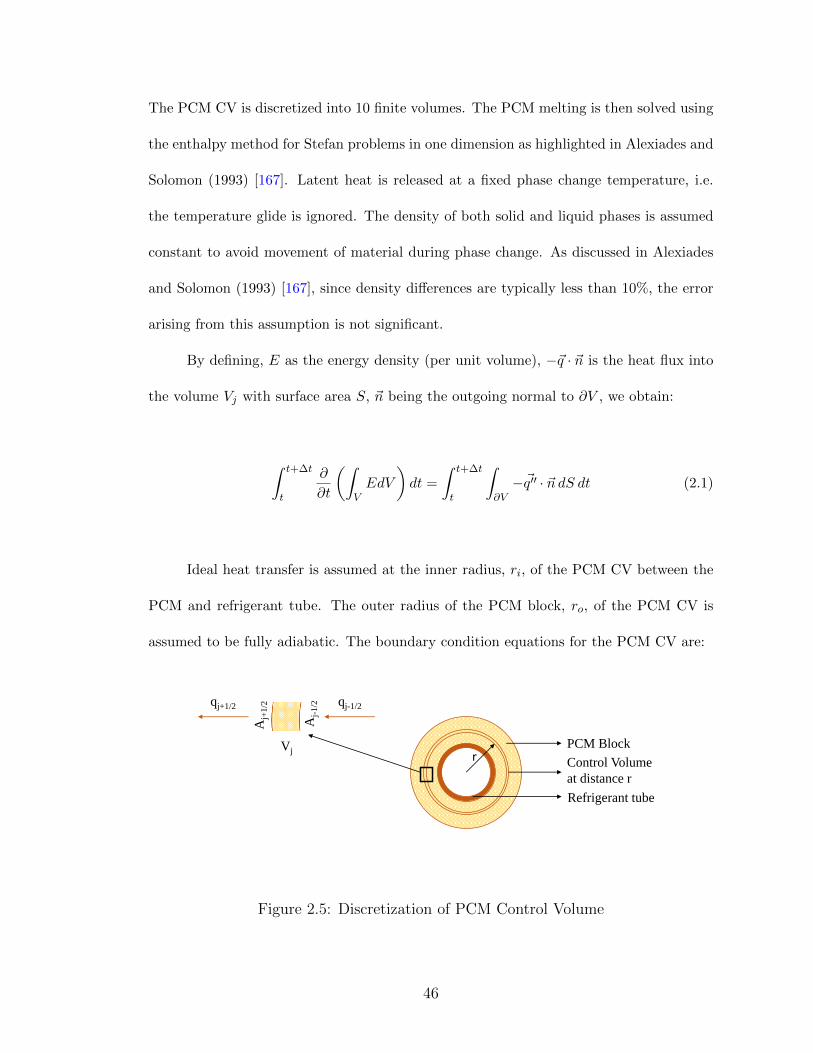
The PCM CV is discretized into 10 finite volumes. The PCM melting is then solved using

the enthalpy method for Stefan problems in one dimension as highlighted in Alexiades and

Solomon (1993) [167]. Latent heat is released at a fixed phase change temperature, i.e.

the temperature glide is ignored. The density of both solid and liquid phases is assumed

constant to avoid movement of material during phase change. As discussed in Alexiades

and Solomon (1993) [167], since density differences are typically less than 10%, the error

arising from this assumption is not significant.

By defining, E as the energy density (per unit volume), −~q · ~n is the heat flux into

the volume Vj with surface area S, ~n being the outgoing normal to ∂V , we obtain:

∫ t+∆t

t

∂

∂t

(∫VEdV

)dt =

∫ t+∆t

t

∫∂V−~q′′ · ~n dS dt (2.1)

Ideal heat transfer is assumed at the inner radius, ri, of the PCM CV between the

PCM and refrigerant tube. The outer radius of the PCM block, ro, of the PCM CV is

assumed to be fully adiabatic. The boundary condition equations for the PCM CV are:

rPCM Block

Control Volume

at distance r

Refrigerant tube

qj-1/2qj+1/2

Vj

Aj-

1/2

Aj+

1/2

Figure 2.5: Discretization of PCM Control Volume

46

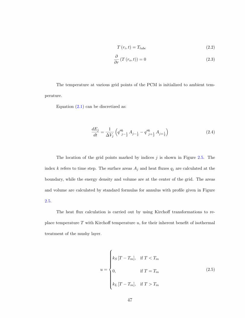
T (ri, t) = Ttube (2.2)

∂

∂r(T (ro, t)) = 0 (2.3)

The temperature at various grid points of the PCM is initialized to ambient tem-

perature.

Equation (2.1) can be discretized as:

dEjdt

=1

∆Vj

(q′′kj− 1

2

Aj− 12− q′′k

j+ 12

Aj+ 12

)(2.4)

The location of the grid points marked by indices j is shown in Figure 2.5. The

index k refers to time step. The surface areas Aj and heat fluxes qj are calculated at the

boundary, while the energy density and volume are at the center of the grid. The areas

and volume are calculated by standard formulas for annulus with profile given in Figure

2.5.

The heat flux calculation is carried out by using Kirchoff transformations to re-

place temperature T with Kirchoff temperature u, for their inherent benefit of isothermal

treatment of the mushy layer.

u =

kS [T − Tm], if T < Tm

0, if T = Tm

kL [T − Tm], if T > Tm

(2.5)

47

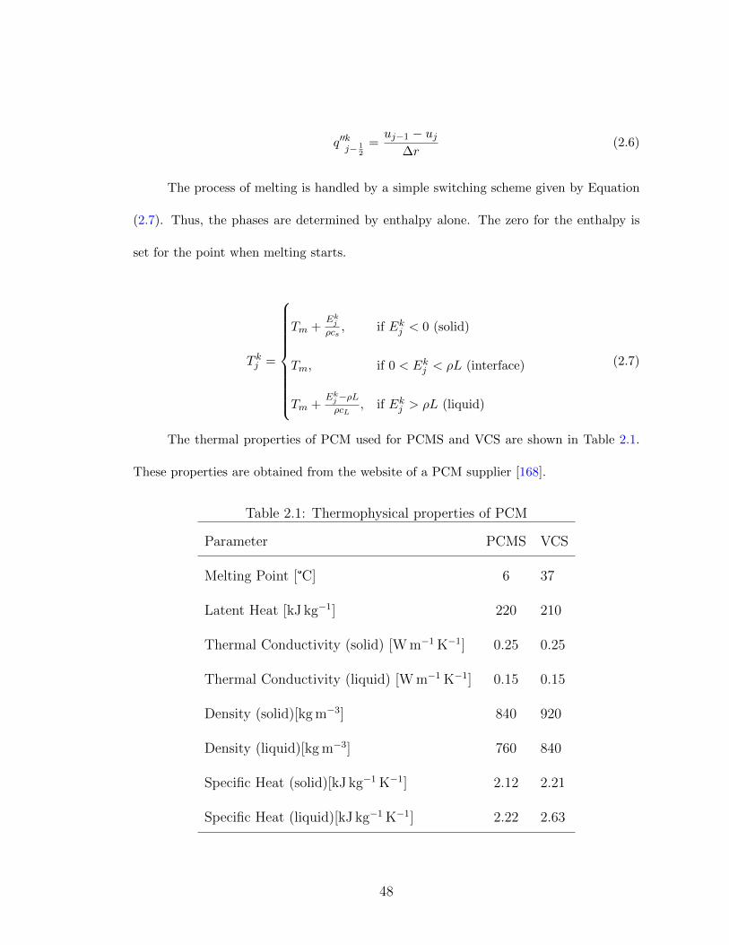
q′′kj− 1

2

=uj−1 − uj

∆r(2.6)

The process of melting is handled by a simple switching scheme given by Equation

(2.7). Thus, the phases are determined by enthalpy alone. The zero for the enthalpy is

set for the point when melting starts.

T kj =

Tm +Ekjρcs, if Ekj < 0 (solid)

Tm, if 0 < Ekj < ρL (interface)

Tm +Ekj−ρLρcL

, if Ekj > ρL (liquid)

(2.7)

The thermal properties of PCM used for PCMS and VCS are shown in Table 2.1.

These properties are obtained from the website of a PCM supplier [168].

Table 2.1: Thermophysical properties of PCM

Parameter PCMS VCS

Melting Point [°C] 6 37

Latent Heat [kJ kg−1] 220 210

Thermal Conductivity (solid) [W m−1 K−1] 0.25 0.25

Thermal Conductivity (liquid) [W m−1 K−1] 0.15 0.15

Density (solid)[kg m−3] 840 920

Density (liquid)[kg m−3] 760 840

Specific Heat (solid)[kJ kg−1 K−1] 2.12 2.21

Specific Heat (liquid)[kJ kg−1 K−1] 2.22 2.63

48

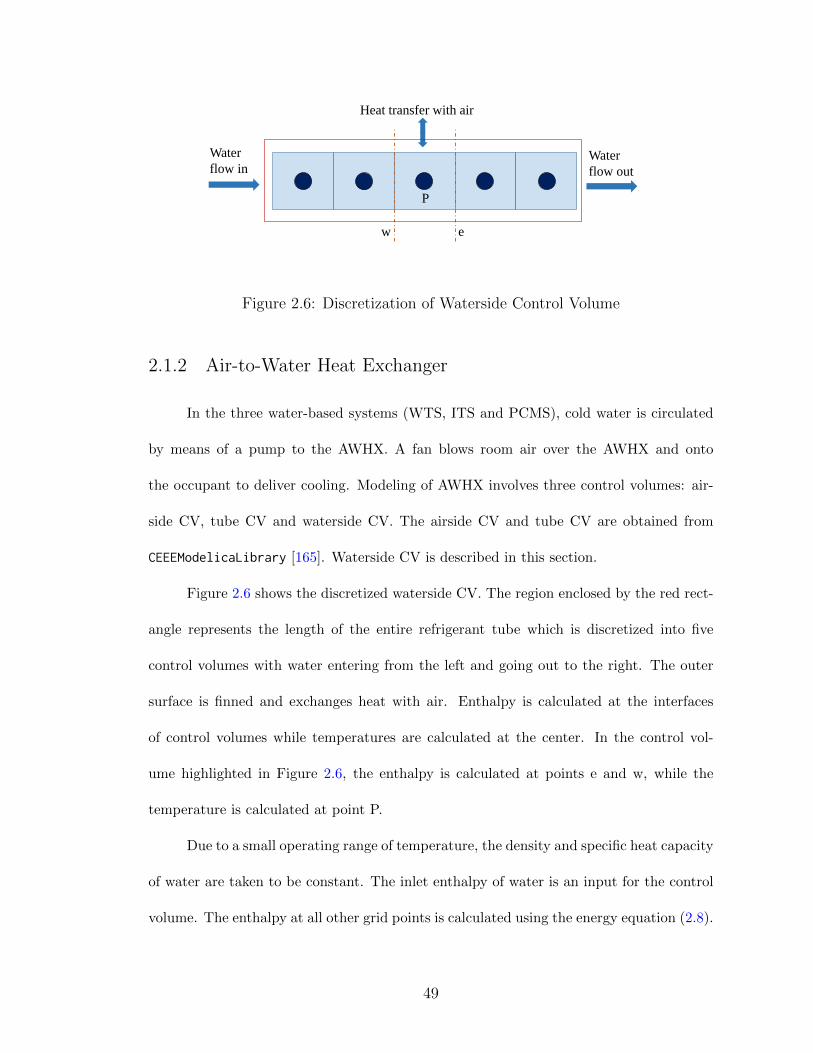
ew

P

Water

flow inWater

flow out

Heat transfer with air

Figure 2.6: Discretization of Waterside Control Volume

2.1.2 Air-to-Water Heat Exchanger

In the three water-based systems (WTS, ITS and PCMS), cold water is circulated

by means of a pump to the AWHX. A fan blows room air over the AWHX and onto

the occupant to deliver cooling. Modeling of AWHX involves three control volumes: air-

side CV, tube CV and waterside CV. The airside CV and tube CV are obtained from

CEEEModelicaLibrary [165]. Waterside CV is described in this section.

Figure 2.6 shows the discretized waterside CV. The region enclosed by the red rect-

angle represents the length of the entire refrigerant tube which is discretized into five

control volumes with water entering from the left and going out to the right. The outer

surface is finned and exchanges heat with air. Enthalpy is calculated at the interfaces

of control volumes while temperatures are calculated at the center. In the control vol-

ume highlighted in Figure 2.6, the enthalpy is calculated at points e and w, while the

temperature is calculated at point P.

Due to a small operating range of temperature, the density and specific heat capacity

of water are taken to be constant. The inlet enthalpy of water is an input for the control

volume. The enthalpy at all other grid points is calculated using the energy equation (2.8).

49

mcdT

dt+ mouthout − minhin = αA (Ttube − Tw) (2.8)

The heat transfer coefficient is calculated using Churchill's correlation [169] for the

transition and turbulent regions of flow. For the laminar region, the constant Nusselt

number for constant heat flux condition is used, since the system is modeled to deliver

a constant cooling load. The discontinuity in the correlation at the transition region is

smoothened out by using a splice function as described in Li et al. (2010) [170].

The friction factor used for the heat transfer correlation is obtained from Churchill

and Usagi (1972) [171] as it covers the entire flow regime. The dynamic viscosity and

thermal conductivity of water used in calculations of Reynolds number and Prandtl num-

ber are calculated at ambient pressure and the temperature of control volume using the

WaterIF97 [172] property calls from Modelica.Media.Water.

The dimensions for the AWHX are given in Table 2.2. These parameters are chosen

by optimization using genetic algorithms in CoilDesigner [173] for maximum capacity and

least cost as objective functions.

2.1.3 Water Tank

Recall that the WTS circulates chilled water through its water circuit. The chilled

water is stored in a water tank. The water tank is modeled as a stratified tank with

discretization along its height. The tank is assumed to be adiabatic.

The tank has discretized into five finite volumes. Each volume is modeled using

the heated pipe component (Modelica.Thermal.FluidHeatFlow.Components.HeatedPipe)

from Modelica Standard Library. This component provides a HeatPort interface, which is

50

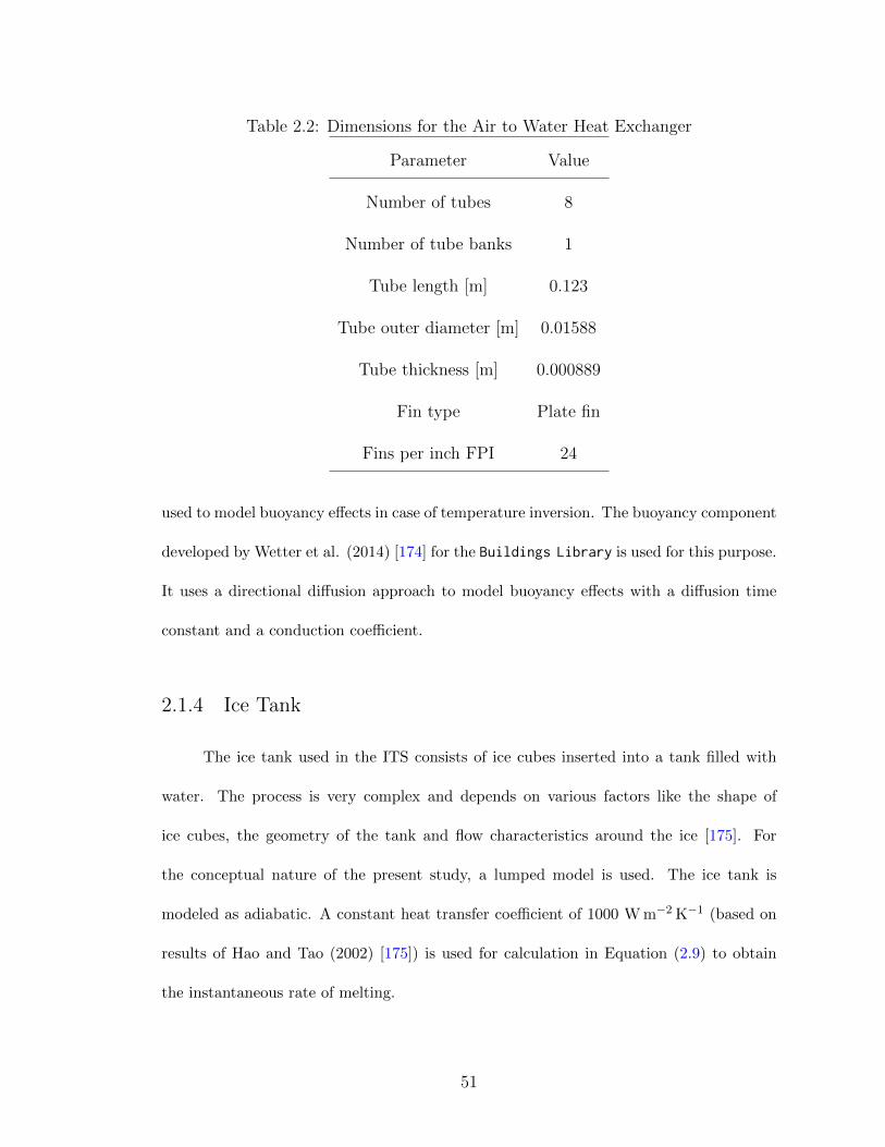
Table 2.2: Dimensions for the Air to Water Heat Exchanger

Parameter Value

Number of tubes 8

Number of tube banks 1

Tube length [m] 0.123

Tube outer diameter [m] 0.01588

Tube thickness [m] 0.000889

Fin type Plate fin

Fins per inch FPI 24

used to model buoyancy effects in case of temperature inversion. The buoyancy component

developed by Wetter et al. (2014) [174] for the Buildings Library is used for this purpose.

It uses a directional diffusion approach to model buoyancy effects with a diffusion time

constant and a conduction coefficient.

2.1.4 Ice Tank

The ice tank used in the ITS consists of ice cubes inserted into a tank filled with

water. The process is very complex and depends on various factors like the shape of

ice cubes, the geometry of the tank and flow characteristics around the ice [175]. For

the conceptual nature of the present study, a lumped model is used. The ice tank is

modeled as adiabatic. A constant heat transfer coefficient of 1000 W m−2 K−1 (based on

results of Hao and Tao (2002) [175]) is used for calculation in Equation (2.9) to obtain

the instantaneous rate of melting.

51

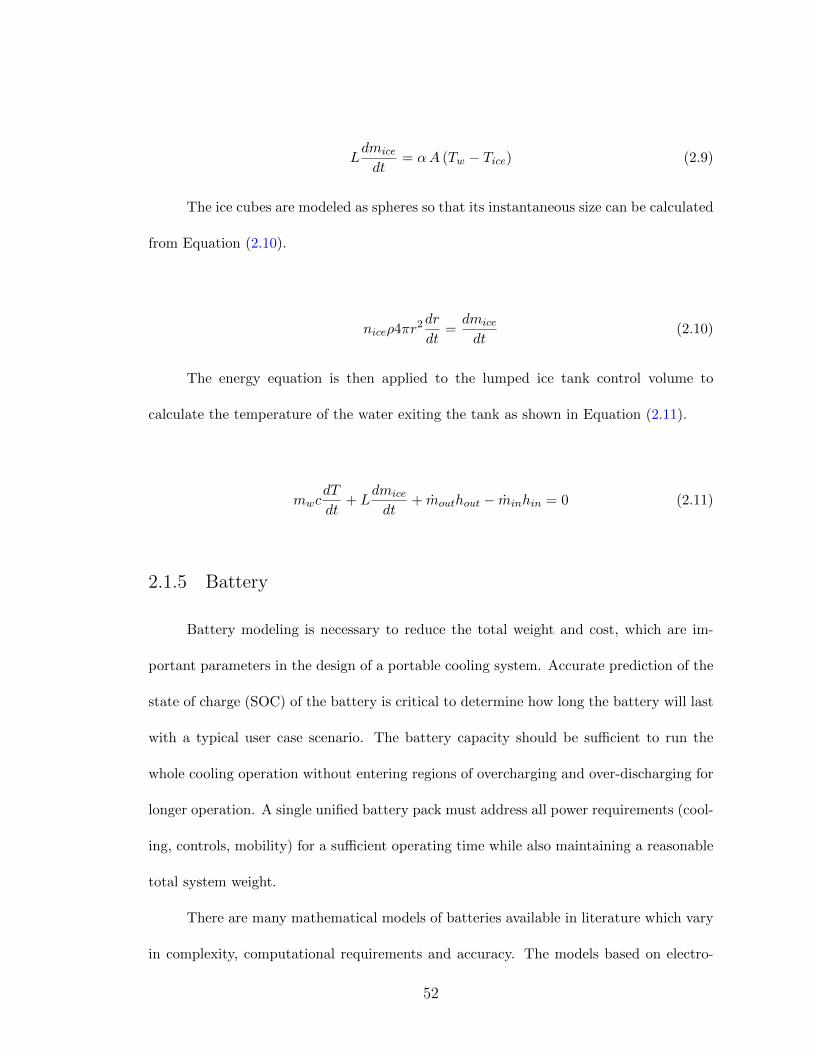
Ldmice

dt= αA (Tw − Tice) (2.9)

The ice cubes are modeled as spheres so that its instantaneous size can be calculated

from Equation (2.10).

niceρ4πr2dr

dt=dmice

dt(2.10)

The energy equation is then applied to the lumped ice tank control volume to

calculate the temperature of the water exiting the tank as shown in Equation (2.11).

mwcdT

dt+ L

dmice

dt+ mouthout − minhin = 0 (2.11)

2.1.5 Battery

Battery modeling is necessary to reduce the total weight and cost, which are im-

portant parameters in the design of a portable cooling system. Accurate prediction of the

state of charge (SOC) of the battery is critical to determine how long the battery will last

with a typical user case scenario. The battery capacity should be sufficient to run the

whole cooling operation without entering regions of overcharging and over-discharging for

longer operation. A single unified battery pack must address all power requirements (cool-

ing, controls, mobility) for a sufficient operating time while also maintaining a reasonable

total system weight.

There are many mathematical models of batteries available in literature which vary

in complexity, computational requirements and accuracy. The models based on electro-

52

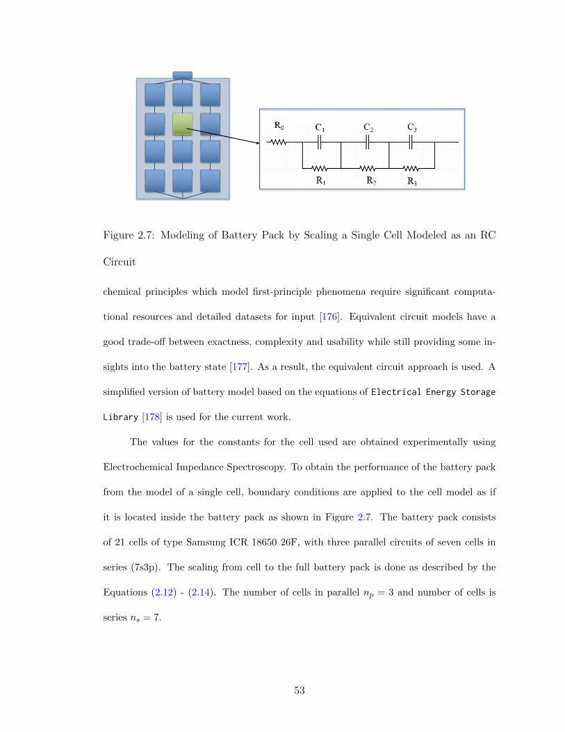
Figure 2.7: Modeling of Battery Pack by Scaling a Single Cell Modeled as an RC

Circuit

chemical principles which model first-principle phenomena require significant computa-

tional resources and detailed datasets for input [176]. Equivalent circuit models have a

good trade-off between exactness, complexity and usability while still providing some in-

sights into the battery state [177]. As a result, the equivalent circuit approach is used. A

simplified version of battery model based on the equations of Electrical Energy Storage

Library [178] is used for the current work.

The values for the constants for the cell used are obtained experimentally using

Electrochemical Impedance Spectroscopy. To obtain the performance of the battery pack

from the model of a single cell, boundary conditions are applied to the cell model as if

it is located inside the battery pack as shown in Figure 2.7. The battery pack consists

of 21 cells of type Samsung ICR 18650 26F, with three parallel circuits of seven cells in

series (7s3p). The scaling from cell to the full battery pack is done as described by the

Equations (2.12) - (2.14). The number of cells in parallel np = 3 and number of cells is

series ns = 7.

53

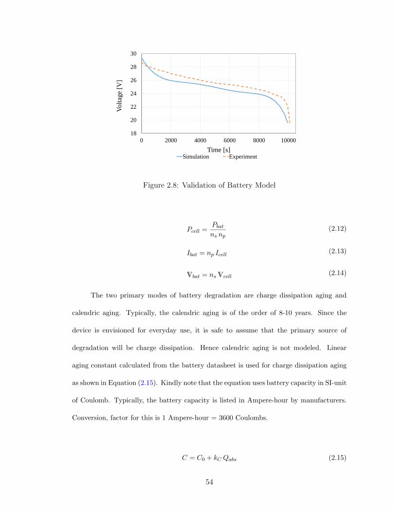
18

20

22

24

26

28

30

0 2000 4000 6000 8000 10000

Vo

ltag

e [V

]

Time [s]Simulation Experiment

Figure 2.8: Validation of Battery Model

Pcell =Pbatns np

(2.12)

Ibat = np Icell (2.13)

Vbat = nsVcell (2.14)

The two primary modes of battery degradation are charge dissipation aging and

calendric aging. Typically, the calendric aging is of the order of 8-10 years. Since the

device is envisioned for everyday use, it is safe to assume that the primary source of

degradation will be charge dissipation. Hence calendric aging is not modeled. Linear

aging constant calculated from the battery datasheet is used for charge dissipation aging

as shown in Equation (2.15). Kindly note that the equation uses battery capacity in SI-unit

of Coulomb. Typically, the battery capacity is listed in Ampere-hour by manufacturers.

Conversion, factor for this is 1 Ampere-hour = 3600 Coulombs.

C = C0 + kC Qabs (2.15)

54

During continuous battery operation, the chemical energy is converted to electricity

with some energy lost as heat. This energy loss to heat leads to faster dissipation of

battery and is calculated using a proportional constant as shown in Equation (2.16).

SOC = SOC0 −KQabs −Q0

C(2.16)

Icell =Vcell −V1 −V2 −V3

Rext +R0

(2.17)

The voltage across the battery is a function of its state of charge; a correlation

connecting voltage and state of charge can be developed from discharge curves found

in the battery datasheet. Finally, the current across the equivalent R-C circuit from

Figure 2.7, is calculated using Equation (2.17). The model is validated by comparing its

results to a 70 W constant power draw circuit. The results of the validation are shown in

Figure 2.8 .

2.1.6 Robotic Platform

The power consumption from the motion of robotic platform is estimated from first-

principles based approach used by Gonullu [179]. The free body diagram of the platform is

shown in Figure 2.9. The total force required for motion (Ft) is the sum of the gravitational

force acting along the incline (Fg), the drag force by the air (Fd), the force to overcome

friction (Ff ) and the force required to produce acceleration (Fa).

Ft = Fg + Fd + Ff + Fa (2.18)

Since the platform operates at speeds around 1 m s−2 , drag force can be neglected.

If m is the total mass of the portable cooling system, g the acceleration due to gravity,

55

α

Fa

Fd

Fg

Ff

Figure 2.9: Free Body Diagram for Robotic Platform

Figure 2.10: Input Set for the Robotic Platform

the remaining forces can be calculated as:

Fg = mg sin(θ) (2.19)

Ff = frmg cos(θ) (2.20)

Fa = ma (2.21)

Finally, the net power for the motion of the platform (P ) is obtained as:

P = Ft v (2.22)

where v is the velocity of the platform.

Typical variations in motion are changes in velocity, motion over different surfaces

and changes in surface inclination. One TimeTable block is assigned to each of acceleration

56

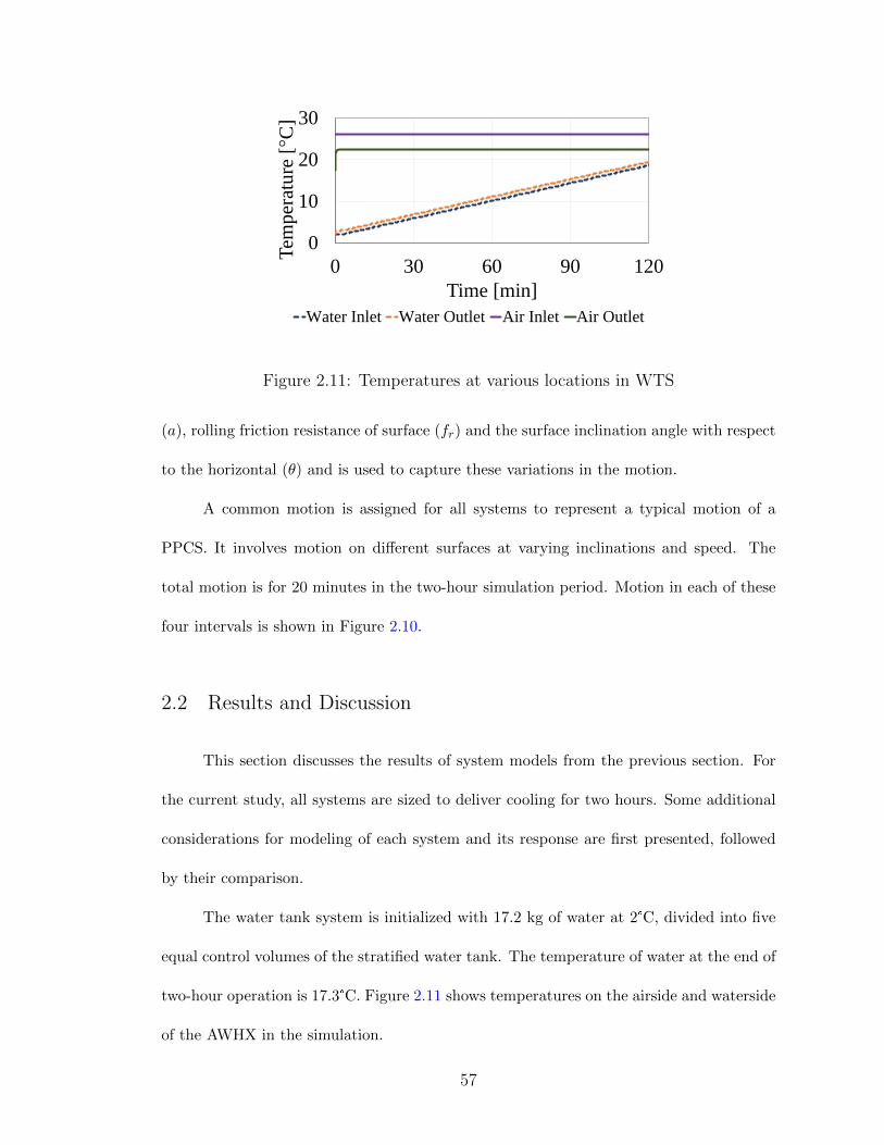
0

10

20

30

0 30 60 90 120T

emper

ature

[°C

]Time [min]

Water Inlet Water Outlet Air Inlet Air Outlet

Figure 2.11: Temperatures at various locations in WTS

(a), rolling friction resistance of surface (fr) and the surface inclination angle with respect

to the horizontal (θ) and is used to capture these variations in the motion.

A common motion is assigned for all systems to represent a typical motion of a

PPCS. It involves motion on different surfaces at varying inclinations and speed. The

total motion is for 20 minutes in the two-hour simulation period. Motion in each of these

four intervals is shown in Figure 2.10.

2.2 Results and Discussion

This section discusses the results of system models from the previous section. For

the current study, all systems are sized to deliver cooling for two hours. Some additional

considerations for modeling of each system and its response are first presented, followed

by their comparison.

The water tank system is initialized with 17.2 kg of water at 2°C, divided into five

equal control volumes of the stratified water tank. The temperature of water at the end of

two-hour operation is 17.3°C. Figure 2.11 shows temperatures on the airside and waterside

of the AWHX in the simulation.

57

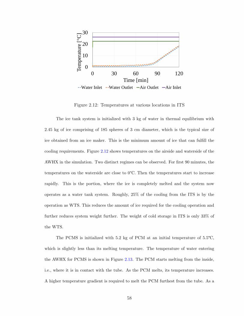
0

10

20

30

0 30 60 90 120T

emper

ature

[°C

]Time [min]

Water Inlet Water Outlet Air Outlet Air Inlet

Figure 2.12: Temperatures at various locations in ITS

The ice tank system is initialized with 3 kg of water in thermal equilibrium with

2.45 kg of ice comprising of 185 spheres of 3 cm diameter, which is the typical size of

ice obtained from an ice maker. This is the minimum amount of ice that can fulfill the

cooling requirements. Figure 2.12 shows temperatures on the airside and waterside of the

AWHX in the simulation. Two distinct regimes can be observed. For first 90 minutes, the

temperatures on the waterside are close to 0°C. Then the temperatures start to increase

rapidly. This is the portion, where the ice is completely melted and the system now

operates as a water tank system. Roughly, 25% of the cooling from the ITS is by the

operation as WTS. This reduces the amount of ice required for the cooling operation and

further reduces system weight further. The weight of cold storage in ITS is only 33% of

the WTS.

The PCMS is initialized with 5.2 kg of PCM at an initial temperature of 5.5°C,

which is slightly less than its melting temperature. The temperature of water entering

the AWHX for PCMS is shown in Figure 2.13. The PCM starts melting from the inside,

i.e., where it is in contact with the tube. As the PCM melts, its temperature increases.

A higher temperature gradient is required to melt the PCM furthest from the tube. As a

58

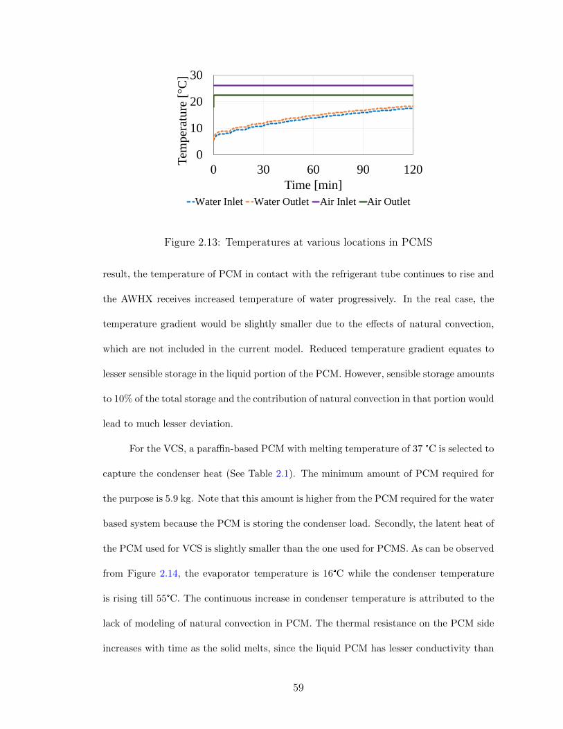
0

10

20

30

0 30 60 90 120T

emper

ature

[°C

]Time [min]

Water Inlet Water Outlet Air Inlet Air Outlet

Figure 2.13: Temperatures at various locations in PCMS

result, the temperature of PCM in contact with the refrigerant tube continues to rise and

the AWHX receives increased temperature of water progressively. In the real case, the

temperature gradient would be slightly smaller due to the effects of natural convection,

which are not included in the current model. Reduced temperature gradient equates to

lesser sensible storage in the liquid portion of the PCM. However, sensible storage amounts

to 10% of the total storage and the contribution of natural convection in that portion would

lead to much lesser deviation.

For the VCS, a paraffin-based PCM with melting temperature of 37 °C is selected to

capture the condenser heat (See Table 2.1). The minimum amount of PCM required for

the purpose is 5.9 kg. Note that this amount is higher from the PCM required for the water

based system because the PCM is storing the condenser load. Secondly, the latent heat of

the PCM used for VCS is slightly smaller than the one used for PCMS. As can be observed

from Figure 2.14, the evaporator temperature is 16°C while the condenser temperature

is rising till 55°C. The continuous increase in condenser temperature is attributed to the

lack of modeling of natural convection in PCM. The thermal resistance on the PCM side

increases with time as the solid melts, since the liquid PCM has lesser conductivity than

59

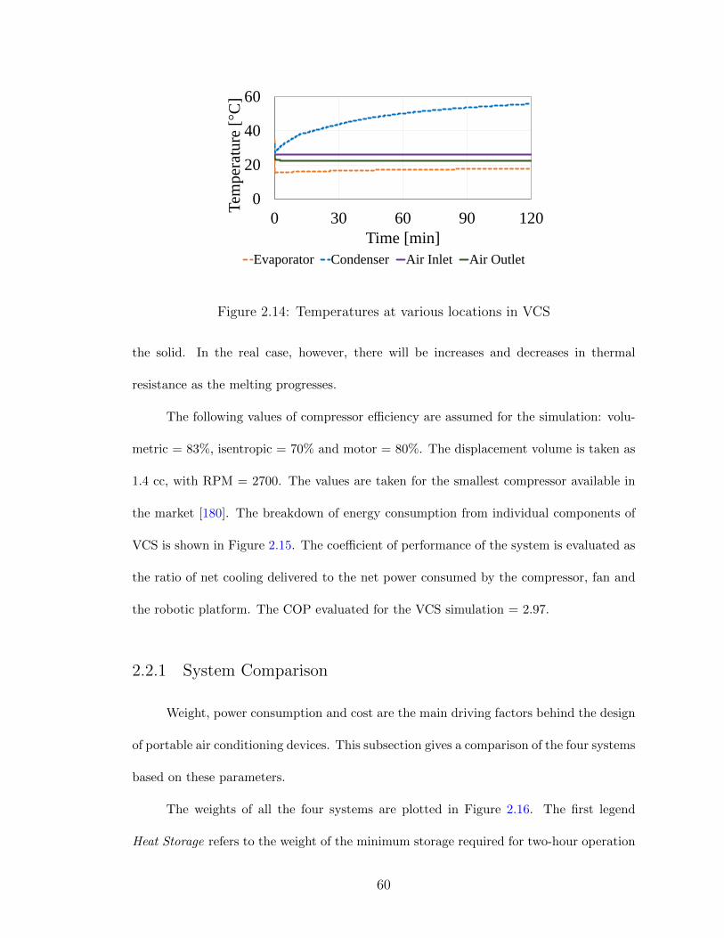
0

20

40

60

0 30 60 90 120T

emper

ature

[°C

]Time [min]

Evaporator Condenser Air Inlet Air Outlet

Figure 2.14: Temperatures at various locations in VCS

the solid. In the real case, however, there will be increases and decreases in thermal

resistance as the melting progresses.

The following values of compressor efficiency are assumed for the simulation: volu-

metric = 83%, isentropic = 70% and motor = 80%. The displacement volume is taken as

1.4 cc, with RPM = 2700. The values are taken for the smallest compressor available in

the market [180]. The breakdown of energy consumption from individual components of

VCS is shown in Figure 2.15. The coefficient of performance of the system is evaluated as

the ratio of net cooling delivered to the net power consumed by the compressor, fan and

the robotic platform. The COP evaluated for the VCS simulation = 2.97.

2.2.1 System Comparison

Weight, power consumption and cost are the main driving factors behind the design

of portable air conditioning devices. This subsection gives a comparison of the four systems

based on these parameters.

The weights of all the four systems are plotted in Figure 2.16. The first legend

Heat Storage refers to the weight of the minimum storage required for two-hour operation

60

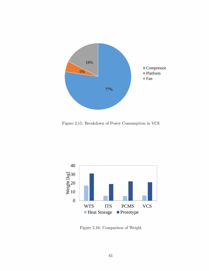
77%

5%

18%

Compressor

Platform

Fan

Figure 2.15: Breakdown of Power Consumption in VCS

0

10

20

30

40

WTS ITS PCMS VCS

Wei

ght

[kg]

Heat Storage Prototype

Figure 2.16: Comparison of Weight

61

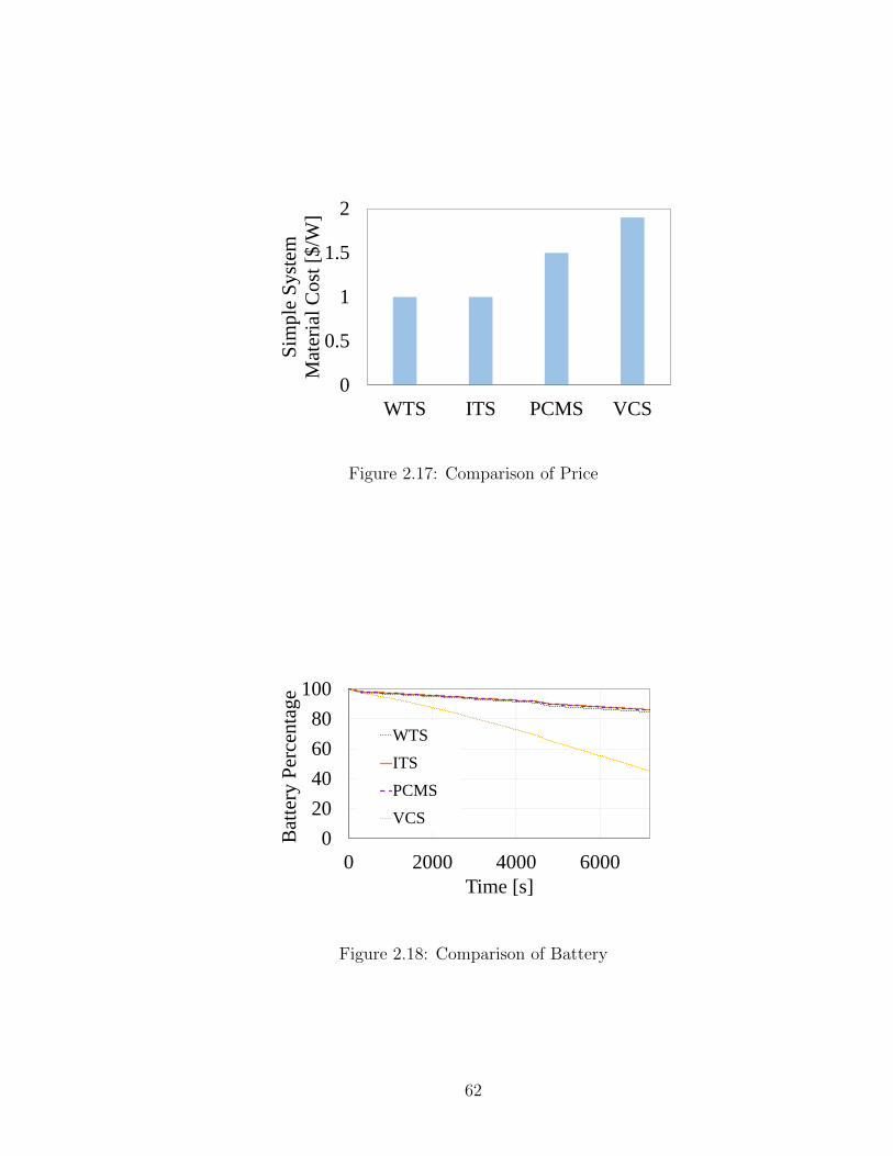
0

0.5

1

1.5

2

WTS ITS PCMS VCS

Sim

ple

Syst

em

Mat

eria

l C

ost

[$

/W]

Figure 2.17: Comparison of Price

0

20

40

60

80

100

0 2000 4000 6000

Bat

tery

Per

centa

ge

Time [s]

WTS

ITS

PCMS

VCS

Figure 2.18: Comparison of Battery

62

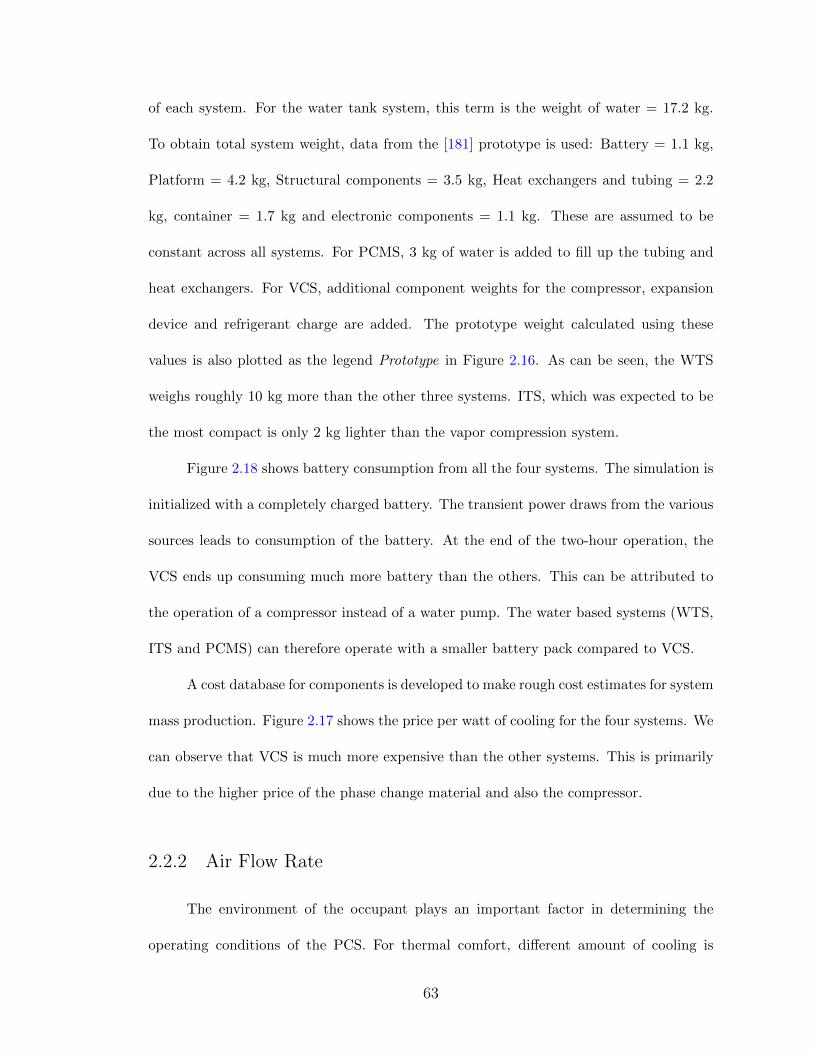
of each system. For the water tank system, this term is the weight of water = 17.2 kg.

To obtain total system weight, data from the [181] prototype is used: Battery = 1.1 kg,

Platform = 4.2 kg, Structural components = 3.5 kg, Heat exchangers and tubing = 2.2

kg, container = 1.7 kg and electronic components = 1.1 kg. These are assumed to be

constant across all systems. For PCMS, 3 kg of water is added to fill up the tubing and

heat exchangers. For VCS, additional component weights for the compressor, expansion

device and refrigerant charge are added. The prototype weight calculated using these

values is also plotted as the legend Prototype in Figure 2.16. As can be seen, the WTS

weighs roughly 10 kg more than the other three systems. ITS, which was expected to be

the most compact is only 2 kg lighter than the vapor compression system.

Figure 2.18 shows battery consumption from all the four systems. The simulation is

initialized with a completely charged battery. The transient power draws from the various

sources leads to consumption of the battery. At the end of the two-hour operation, the

VCS ends up consuming much more battery than the others. This can be attributed to

the operation of a compressor instead of a water pump. The water based systems (WTS,

ITS and PCMS) can therefore operate with a smaller battery pack compared to VCS.

A cost database for components is developed to make rough cost estimates for system

mass production. Figure 2.17 shows the price per watt of cooling for the four systems. We

can observe that VCS is much more expensive than the other systems. This is primarily

due to the higher price of the phase change material and also the compressor.

2.2.2 Air Flow Rate

The environment of the occupant plays an important factor in determining the

operating conditions of the PCS. For thermal comfort, different amount of cooling is

63

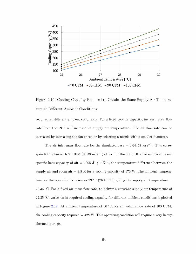
100

150

200

250

300

350

400

450

25 26 27 28 29 30

Co

oli

ng C

apac

ity [

W]

Ambient Temperature [°C]

70 CFM 80 CFM 90 CFM 100 CFM

Figure 2.19: Cooling Capacity Required to Obtain the Same Supply Air Tempera-

ture at Different Ambient Conditions

required at different ambient conditions. For a fixed cooling capacity, increasing air flow

rate from the PCS will increase its supply air temperature. The air flow rate can be

increased by increasing the fan speed or by selecting a nozzle with a smaller diameter.

The air inlet mass flow rate for the simulated case = 0.04452 kg s−1. This corre-

sponds to a fan with 80 CFM (0.038 m3 s−1) of volume flow rate. If we assume a constant

specific heat capacity of air = 1005 J kg−1 K−1, the temperature difference between the

supply air and room air = 3.8 K for a cooling capacity of 170 W. The ambient tempera-

ture for the operation is taken as 79 °F (26.15 °C), giving the supply air temperature =

22.35 °C. For a fixed air mass flow rate, to deliver a constant supply air temperature of

22.35 °C, variation in required cooling capacity for different ambient conditions is plotted

in Figure 2.19. At ambient temperature of 30 °C, for air volume flow rate of 100 CFM,

the cooling capacity required = 428 W. This operating condition will require a very heavy

thermal storage.

64

The supply temperature of the PCS, however, may not be the correct design pa-

rameter for sizing the air flow rates. Zhu et al. [182] carried out a CFD-based analysis to

investigate the cooling efficiency of a PCS (ratio of the sensible heat removal to the cooling

capacity). Their study involved a 100 W cooling capacity PCS placed at a distance of 1 m

from the occupant, in a room with 3 ACH (Air Changes per Hour Ventilation Rate) and

air temperature of 26°C. They found a positive linear correlation between sensible heat

loss and air flow rate, indicating that the personalized airflow with higher airflow rates

could effectively remove additional heat from human body. Additionally, at the same air

flow rate, a smaller nozzle could remove more sensible heat from the human body. Thus,

the effect of local forced convection overcame the opposing effect of temperature increase

for their set of operating conditions. So it may be possible to keep occupants in higher

ambient conditions comfortable at higher supply air temperatures (and thus a much lower

cooling capacity). The correct design conditions for operation at all these variations of

ambient conditions will require experimental thermal comfort study and is part of future

research.

2.2.3 Phase Change Material

The selection of PCM is an important design criteria for PCS. The PCM has to go

through both melting and solidification in a reasonable amount of time. Secondly, PCM

manufacturer may not have a good resolution of melting temperature range. In the VCS,

the PCM is used to capture the condenser heat. This is done to prevent additional heat

loads to the building. PCM with following melting temperatures are available at one of

the manufacturers [168](29°C, 37°C, 42°C and 48°C). For vapor compression cycle, a lower

PCM melting temperature would result in a higher COP. If the melting temperature

65

is very close to the ambient temperature, the solidification of PCM after the cooling

operation will take a very long time due to a low temperature gradient available for heat

exchange. Among the range of temperatures available, 37°C is selected from both COP

and solidification time point of view.

The PCMS uses water to extract cooling from the frozen PCM. The melting tem-

perature of PCM selected for this application is 6°C. PCM with following melting temper-

atures are alternate options for this application [168](4°C, 7°C, 8°C and 15°C). The latent

heat of the PCM melting at 6°C is 220 kJ kg−1 is much higher than the latent heat of the

other candidates available in its neighborhood (178 to 187 kJ kg−1). To make the thermal

storage lightest, the current choice is the best option.

2.2.4 Price Considerations

Hoyt et al. (2015) [109] simulated HVAC energy savings by varying cooling setpoints

in 7 different climates and 5 different HVAC model types. The averaged results from their

work is listed in Table 2.3. In 2011, total primary energy consumption per person in

the United States was about 310 million Btu [1]. Building sector accounts for 41% of

the primary energy consumption, with 11.8% of that fraction taken up by space cooling.

Hence, energy spent on cooling per person =(0.118*0.41*310 million Btu)= 15 million

Btu = 15.8× 1010 J. Assuming symmetrical heating and cooling seasons, time duration

for cooling = 0.5 year = 0.5*365*24*60*60 sec = 15.768× 1010 sec. Thus, average cooling

power per person = (cooling energy per person)/(cooling time duration) = 1002 W.

The average price of electricity in the United States is approximately 12 cents per

kWh [183]. For a setpoint of 25.6 °C, mean saving = 31%. Thus, cost saving for each hour

= $ 0.12*0.31*1002/1000 = $ 0.037. For the cooling duration of half year, net saving for

66

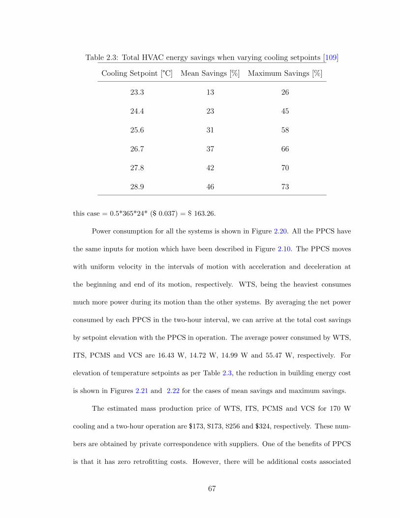
Table 2.3: Total HVAC energy savings when varying cooling setpoints [109]

Cooling Setpoint [°C] Mean Savings [%] Maximum Savings [%]

23.3 13 26

24.4 23 45

25.6 31 58

26.7 37 66

27.8 42 70

28.9 46 73

this case = 0.5*365*24* ($ 0.037) = $ 163.26.

Power consumption for all the systems is shown in Figure 2.20. All the PPCS have

the same inputs for motion which have been described in Figure 2.10. The PPCS moves

with uniform velocity in the intervals of motion with acceleration and deceleration at

the beginning and end of its motion, respectively. WTS, being the heaviest consumes

much more power during its motion than the other systems. By averaging the net power

consumed by each PPCS in the two-hour interval, we can arrive at the total cost savings

by setpoint elevation with the PPCS in operation. The average power consumed by WTS,

ITS, PCMS and VCS are 16.43 W, 14.72 W, 14.99 W and 55.47 W, respectively. For

elevation of temperature setpoints as per Table 2.3, the reduction in building energy cost

is shown in Figures 2.21 and 2.22 for the cases of mean savings and maximum savings.

The estimated mass production price of WTS, ITS, PCMS and VCS for 170 W

cooling and a two-hour operation are $173, $173, $256 and $324, respectively. These num-

bers are obtained by private correspondence with suppliers. One of the benefits of PPCS

is that it has zero retrofitting costs. However, there will be additional costs associated

67

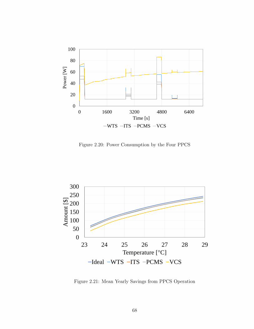
0

20

40

60

80

100

0 1600 3200 4800 6400

Pow

er [

W]

Time [s]

WTS ITS PCMS VCS

Figure 2.20: Power Consumption by the Four PPCS

0

50

100

150

200

250

300

23 24 25 26 27 28 29

Am

ou

nt

[$]

Temperature [°C]

Ideal WTS ITS PCMS VCS

Figure 2.21: Mean Yearly Savings from PPCS Operation

68

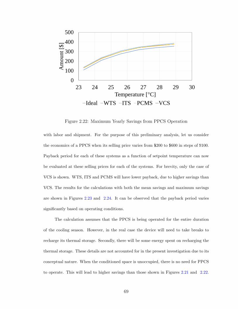
0

100

200

300

400

500

23 24 25 26 27 28 29 30

Am

ou

nt

[$]

Temperature [°C]

Ideal WTS ITS PCMS VCS

Figure 2.22: Maximum Yearly Savings from PPCS Operation

with labor and shipment. For the purpose of this preliminary analysis, let us consider

the economics of a PPCS when its selling price varies from $200 to $600 in steps of $100.

Payback period for each of these systems as a function of setpoint temperature can now

be evaluated at these selling prices for each of the systems. For brevity, only the case of

VCS is shown. WTS, ITS and PCMS will have lower payback, due to higher savings than

VCS. The results for the calculations with both the mean savings and maximum savings

are shown in Figures 2.23 and 2.24. It can be observed that the payback period varies

significantly based on operating conditions.

The calculation assumes that the PPCS is being operated for the entire duration

of the cooling season. However, in the real case the device will need to take breaks to

recharge its thermal storage. Secondly, there will be some energy spent on recharging the

thermal storage. These details are not accounted for in the present investigation due to its

conceptual nature. When the conditioned space is unoccupied, there is no need for PPCS

to operate. This will lead to higher savings than those shown in Figures 2.21 and 2.22.

69

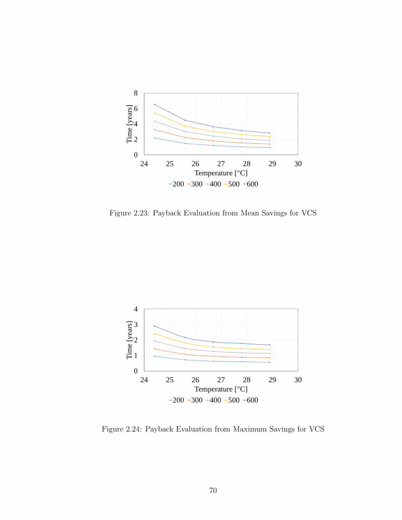
0

2

4

6

8

24 25 26 27 28 29 30

Tim

e [y

ears

]

Temperature [°C]

200 300 400 500 600

Figure 2.23: Payback Evaluation from Mean Savings for VCS

0

1

2

3

4

24 25 26 27 28 29 30

Tim

e [y

ears

]

Temperature [°C]

200 300 400 500 600

Figure 2.24: Payback Evaluation from Maximum Savings for VCS

70

These details will become clearer with development and testing of real devices and is part

of future research. A more realistic payback period may be in the range of 5-10 years.

The price of PPCS is being around $500 for the consumer makes this a very attractive

option for saving building cooling energy. Personalized conditioning also provides better

cooling than the conventional systems.

71

Chapter 3: Development of Vapor Compression Cycle based Per-

sonal Conditioning System

3.1 Introduction

The previous chapter highlighted benefits of using personal conditioning systems.

Water based PCS require more user attention for continuous usage like refill chilled water

or ice, re-solidify PCM. From user’s convenience perspective, the vapor compression system

based PCS is the most desired and so, a prototype based on this idea called the Roving

Comforter (RoCo) has been developed [181]. The present chapter briefly discusses its

operation and then discusses development of a dynamic model for its thermal storage

recharge, which was identified as an important factor for improvement.

RoCo uses a compact R134a based vapor compression system for cooling. Following

its cooling operation, during which waste heat from the condensing refrigerant is stored in

a phase change material (PCM), a two-phase loop thermosiphon is used to discharge (so-

lidify) the PCM to enable its next operation. The transient operation of this thermosiphon

is the focus of the present chapter.

Use of a PCM as the storage medium provides high energy density due to the ability

to store thermal energy as latent heat during the phase transition; however, the discharge

rate is limited by the low thermal conductivity of the PCM. Insertion of a graphite foam

72

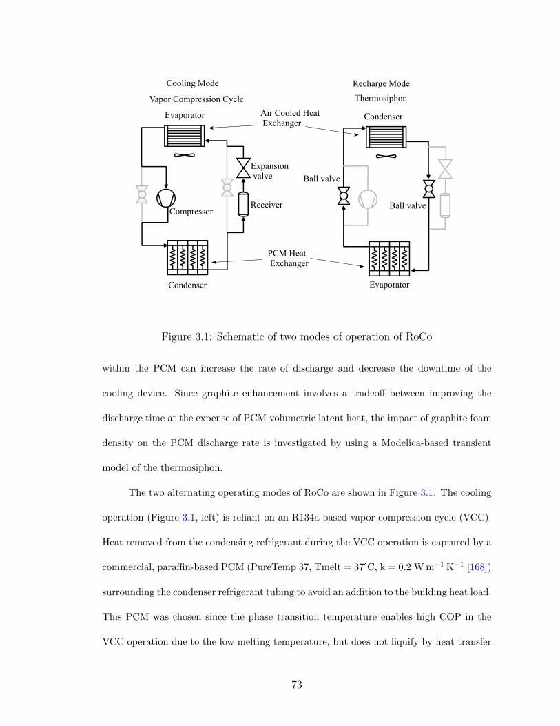
Figure 3.1: Schematic of two modes of operation of RoCo

within the PCM can increase the rate of discharge and decrease the downtime of the

cooling device. Since graphite enhancement involves a tradeoff between improving the

discharge time at the expense of PCM volumetric latent heat, the impact of graphite foam

density on the PCM discharge rate is investigated by using a Modelica-based transient

model of the thermosiphon.

The two alternating operating modes of RoCo are shown in Figure 3.1. The cooling

operation (Figure 3.1, left) is reliant on an R134a based vapor compression cycle (VCC).

Heat removed from the condensing refrigerant during the VCC operation is captured by a

commercial, paraffin-based PCM (PureTemp 37, Tmelt = 37°C, k = 0.2 W m−1 K−1 [168])

surrounding the condenser refrigerant tubing to avoid an addition to the building heat load.

This PCM was chosen since the phase transition temperature enables high COP in the

VCC operation due to the low melting temperature, but does not liquify by heat transfer

73

with the surroundings since the transition temperature is 9°C higher than the weighted

mean of the US summer dry bulb temperature [152]. Stability of this material has been

demonstrated over 65,000 thermal cycles [168].

The cooling operation terminates when the PCM is completely melted since the

condenser can no longer store rejected heat from the refrigerant as latent energy, leading

to elevated condenser temperatures and decreased cycle efficiency. Thus, there is a need

for re-solidification of the PCM (PCM discharge) before the next cooling operation. Since

the PCM is insulated from the ambient to minimize heat loss to the conditioned space

during cooling, a thermosiphon operation in the same refrigerant circuitry is employed to

enable a controlled discharge process.

In the thermosiphon operation, liquid refrigerant in the PCM-HX absorbs heat

from the PCM and vaporizes. The thermosiphon operation is used to discharge the heat

stored during the cooling operation. Typically, the cooling is required during the day

time and thermosiphon is at night time. This also facilitates peak load shifting from

the electricity grid as the discharge is done during the off-peak hours and provides cost

savings to customers. There are two methods to reject the heat during night time: (1)

reject heat to the internal spaces during the night when the building is unoccupied and

the building load is insignificant (2) reject heat outside the conditioned space by moving

the RoCo [184]. The vapor rises and condenses in the air-cooled heat exchanger (AC-

HX). The condensed liquid flows back by gravity to the PCM-HX. A receiver is included

in the circuit to ensure that the PCM-HX is filled with liquid refrigerant to prevent dry

out during the thermosiphon operation. The initial PCM-HX prototype provided 2 hours

of cooling operation and required 8 hours for discharge [181], limiting RoCo to a single

cooling operation per day. The long discharge time can be attributed to the low thermal

74

conductivity of the PCM.

The present chapter focuses on modeling a thermosiphon used to recharge the PCM

battery of an innovative personal air conditioning device called the Roving Comforter

(RoCo), which is described in detail in Du et al.(2016) [181]. Figure 3.1 shows the

schematic for the two alternating operating modes of RoCo. During the cooling oper-

ation shown in the left image of Figure 3.1, the heat released by the condenser is captured

by the surrounding PCM to avoid addition to building heat loads. The cooling operation

is terminated when the PCM surrounding the condenser is completely melted. Before the

next cooling operation, there is a need for re-solidification of the PCM (PCM recharge).

The right image in Figure 3.1 shows RoCo operating in thermosiphon mode. The com-

pressor and the expansion valve are bypassed by operating a pair of ball valves to reduce

pressure drops in the refrigerant circuit. A receiver is included in the circuit to ensure that

the PCM based heat exchanger (PCM-HX) is always completely filled with liquid refrig-

erant during the thermosiphon operation to prevent dryout. The system provides more

than two hours of cooling operation with 8 hours for recharge [181]. This essentially limits

RoCo to a single cooling operation per day, which is not desirable. The long recharge time

can be attributed to the low thermal conductivity of the PCM.

One method to increase the thermal conductivity of PCM is to create a composite of

pure PCM and a highly conductive porous compressed expanded natural graphite (CENG)

foam [185–187]. The amount of CENG in the composite PCM is measured as graphite

bulk density, or mass of graphite in the sample volume. As the graphite bulk density

increases, the thermal conductivity increases, but the composite latent heat decreases. The

saturation of CENG foams with PCM has been shown to increase the thermal conductivity

by more than an order of magnitude; however, this reduces the latent heat storage of the

75

PCM up to 35% due to the displacement of PCM by graphite as well as air contained within

closed pores formed during the fabrication process [185–187]. The reduced latent heat of

the PCM composite leads to increased weight and volume of the thermal battery, which

is not desireable for a portable device like RoCo. Thus, there is a tradeoff between the

reduced recharge time and increased volume in the material selection. A transient analysis

of the thermosiphon mechanism is carried out to evaluate the most suitable material among

the CENG developed by Mallow et al. [188].

This chapter presents a semi-empirical model for a thermosiphon with transient

equations not only for the refrigerant side but also the thermal storage. The state of the

PCM is part of the solution, adding further to the complexity of the model. Modelica [33]

is used for modeling because of the object-oriented, declarative, and acausal modeling

approach, reusable libraries for two-phase flow, refrigerant media property packages [189]

based on REFPROP 9.0 database and differential algebraic equation solvers. This enables

development of the model with similar detailing on the refrigerant side as Bodjona et

al. [190], without the need to write equations for refrigerant properties and solvers.

3.2 Component Modeling

This section discusses equations and assumptions used in the component models

for the thermosiphon system model. The component models will be combined to form

the system model, which will be first validated with experimental data and then used to

evaluate the thermal storage performance of graphite enhanced PCM.

76

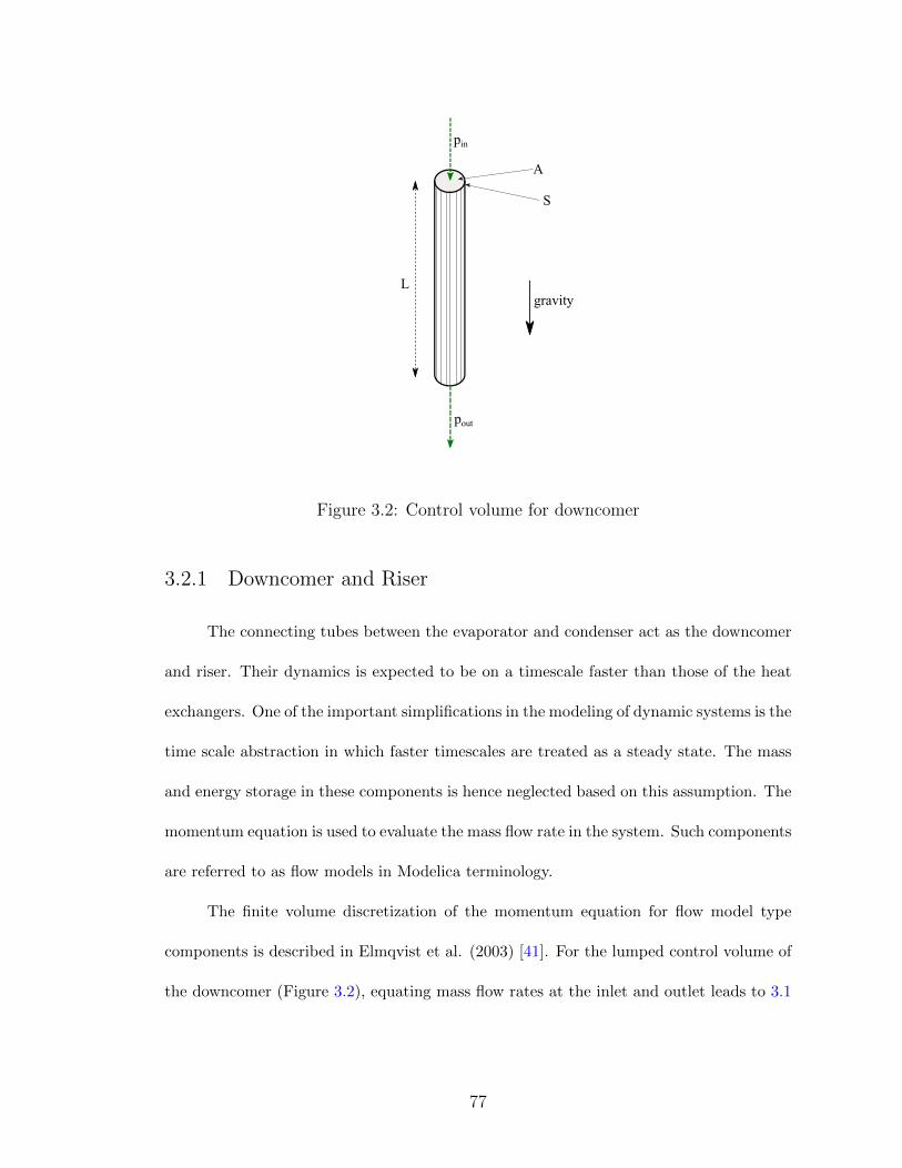
Figure 3.2: Control volume for downcomer

3.2.1 Downcomer and Riser

The connecting tubes between the evaporator and condenser act as the downcomer

and riser. Their dynamics is expected to be on a timescale faster than those of the heat

exchangers. One of the important simplifications in the modeling of dynamic systems is the

time scale abstraction in which faster timescales are treated as a steady state. The mass

and energy storage in these components is hence neglected based on this assumption. The

momentum equation is used to evaluate the mass flow rate in the system. Such components

are referred to as flow models in Modelica terminology.

The finite volume discretization of the momentum equation for flow model type

components is described in Elmqvist et al. (2003) [41]. For the lumped control volume of

the downcomer (Figure 3.2), equating mass flow rates at the inlet and outlet leads to 3.1

77

Ltdm

dt= Ac(pin − pout)−

1

2

m2

ρA2fSLt −AcρgLt (3.1)

For the downcomer, the outlet is below the inlet in height and this leads to 3.2.

Ltdm

dt= A(pin − pout)−

1

2

m2

ρA2fSLt +AρgLt (3.2)

Since the the model assumes single phase refrigerant flow in the riser and downcomer,

the Fanning friction factor is calculated using a function developed by combining Hagen-

Poiseulle and Blasius [191] equations to account for both laminar and turbulent flows for

single phase refrigerant. The objective of the current investigation is the heat transfer

characteristics of the thermosiphon for which the assumption is valid (the sensible heat of

R134a is very small compared to its latent heat). However, for an investigation focused

on fluid flow characteristics, it may be necessary to develop a more detailed model for the

downcomer and riser. Interpolation is necessary to avoid chattering issues encountered in

transient simulations with equations that are not continuous and differentiable.

3.2.2 Phase Change Material Control Volume

Several models exist in the literature for modeling the melting and solidification

of PCM [192–194]. The enthalpy method [195] is used in the current study due to the

advantage of carrying out calculations on a fixed grid with an implicit treatment of the

phase change boundary.

The energy equation applied to the PCM control volume gives rise to Equation (3.3).

The PCM-HX involves helical tubes surrounded by PCM, which results in very compli-

cated 3D mathematical equations involving phase change and refrigerant flow. For the

78

purpose of current research, two primary assumptions are made to obtain equations for

system level simulation. First, the PCM control volume is modeled as a lumped system.

This eliminates the need for 3D momentum equations for natural convection flow within

the molten PCM. Secondly, since the density difference between the solid and liquid phase

of PCM is less than 10%, the average value of densities of both the phases is used in

the calculations. These two assumptions enable modeling a simpler form of the energy

equation shown in Equation (3.4).

ρ∂h

∂t+∇(ρvh) = ∇k(∇T ) (3.3)

mpcmdh

dt= Q (3.4)

The PCM modeling consists of two components: one to model its heat storage and

a second to model its rate of heat transfer.

3.2.2.1 PCM Heat Storage

The PCM heat storage is modeled using a component named PCM Capacitor. It

models the left-hand side of Equation (3.4). The only unknown variable in the enthalpy

method formulation is the enthalpy-temperature dependency of the PCM which is calcu-

lated using Equation (3.5). The PCM solidifies over the temperature range from TL to

TS. DSC measurements were taken using a TA Instruments Q2000 with a heating and

cooling speed of 5°C min−1 to obtain the variations of the effective specific heat capacity,

79

c(T), in the interface region. The point where the PCM just starts to melt is taken as the

zero reference for the enthalpy function.

h(T ) =

∫ TAT csdT, solid

∫ TATB

c(T )dT, two phase

hsl +∫ TBT cLdT, liquid

(3.5)

3.2.2.2 PCM Heat Transfer

The heat transfer from the PCM is modeled using the PCM Conductor block. To en-

able modeling of any heat exchanger geometry, either with a helical or straight refrigerant

tube, the heat transfer coefficient as a function of melt fraction, λ, is set as an input and

evaluated by experimental or numerical methods. This enables modeling varying effects of

conduction and natural convection, which occurs in the case of a non-enhanced PCM with

helical refrigerant tubes. The conduction dominant heat transfer in a graphite enhanced

PCM with straight refrigerant tubes can also be captured using the same component.

The melt fraction is calculated from PCM enthalpy by using Equation (3.6) in the

PCM Capacitor block. It is then provided as an input to the PCM Conductor block. The

use of the heat transfer coefficient, pcm, simplifies the right-hand side of Equation (3.4)

as shown in Equation (3.6). Calculation of αpcm will be discussed in the subsection 3.2.2.3

for the case of pure PCM and in Section (3.4) for the graphite enhanced PCM. The net

value of net heat transfer is calculated using the temperature difference between PCM

Conductor and lumped refrigerant CV (Equation (3.8)).

80

λ = max(0,min(1,h

hl)) (3.6)

Qpcm = αpcmA (Ttube − Tpcm) (3.7)

3.2.2.3 Empirical heat transfer coefficient function

The empirical heat transfer coefficient as a function of melt fraction, which is an

input for the PCM Conductor (Equation (3.8)), is not available in the literature and is,

hence, obtained by an experiment. The heat transfer coefficient evaluation procedure is

similar to the one adopted by Merlin et al. [196] and is only briefly explained for the sake

of brevity. The experimental setup (see Figure 3.3, left image) includes a single helical coil

(see Figure 3.3, right image) placed inside a cylinder filled with PCM. It is representative

of one quarter of the PCM-HX. A peristaltic pump is used to circulate water through a

PID-controlled heater to melt the PCM at a constant water inlet temperature. During

solidification, the heater is turned off. The pump continues to circulate water through the

circuit during solidification. An air to water heat exchanger cools the water temperature

at the inlet to a constant value. This value can be adjusted by changing the temperature

of the environmental chamber where the setup is placed. The entire PCM-HX is insulated

with foam to minimize heat losses to the surroundings.

The instrumentation used for the evaluation of the heat transfer coefficient is sum-

marized in the Table 3.1. The experiment is repeated three times to ensure repeatability

of the data. The standard deviation in the RTD measurements is 0.04°C. The uncertainty

associated with the heat transfer coefficient is estimated to be 13%, when the temperature

81

Figure 3.3: Schematic of the setup for evaluating heat transfer coefficient on the

shell side of PCM storage and the helical coil used for the experiment

difference between the RTD values is 1.2°C. Three thermocouples are soldered to the

helical coil to measure the helical coil temperature, while ten thermocouples are evenly

distributed inside the PCM. The average values of these thermocouples provide the tube

temperature and lumped PCM temperature used in the determination of the heat transfer

coefficient.

Table 3.1: Evaluation of Ideal Cd for CT-A and CT-B

Manufacturer Device Accuracy Range Accuracy Specification

Omega RTD 0 to 100°C (0.03)°C

Omega T-type -200 to 350°C 0.5°C

Emerson Coriolis flow meter 0-100 g s−1 0.2% of flow rate

The results of temperatures measured in the experiment are shown in the Figure 3.4

and 3.5. The flow rate of water is constant during the experiment. Mean value of this

82

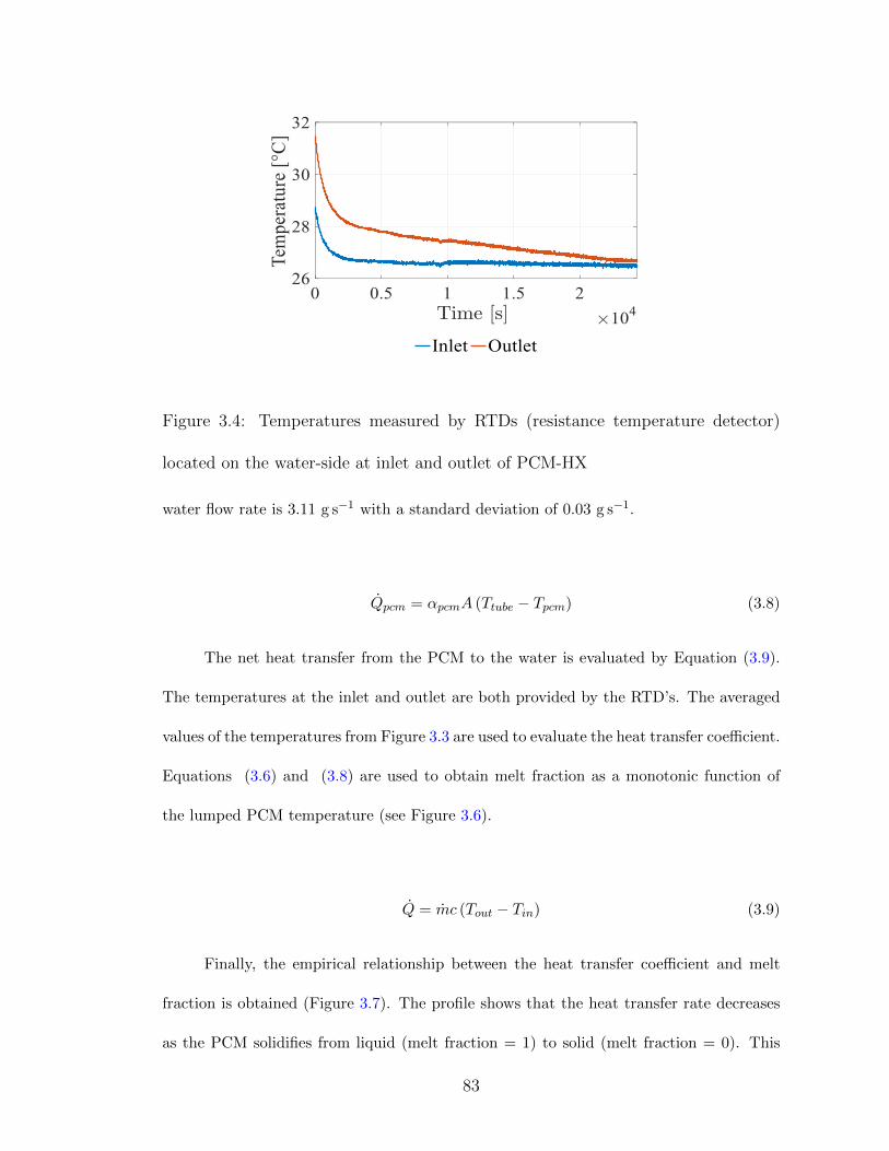
Figure 3.4: Temperatures measured by RTDs (resistance temperature detector)

located on the water-side at inlet and outlet of PCM-HX

water flow rate is 3.11 g s−1 with a standard deviation of 0.03 g s−1.

Qpcm = αpcmA (Ttube − Tpcm) (3.8)

The net heat transfer from the PCM to the water is evaluated by Equation (3.9).

The temperatures at the inlet and outlet are both provided by the RTD’s. The averaged

values of the temperatures from Figure 3.3 are used to evaluate the heat transfer coefficient.

Equations (3.6) and (3.8) are used to obtain melt fraction as a monotonic function of

the lumped PCM temperature (see Figure 3.6).

Q = mc (Tout − Tin) (3.9)

Finally, the empirical relationship between the heat transfer coefficient and melt

fraction is obtained (Figure 3.7). The profile shows that the heat transfer rate decreases

as the PCM solidifies from liquid (melt fraction = 1) to solid (melt fraction = 0). This

83

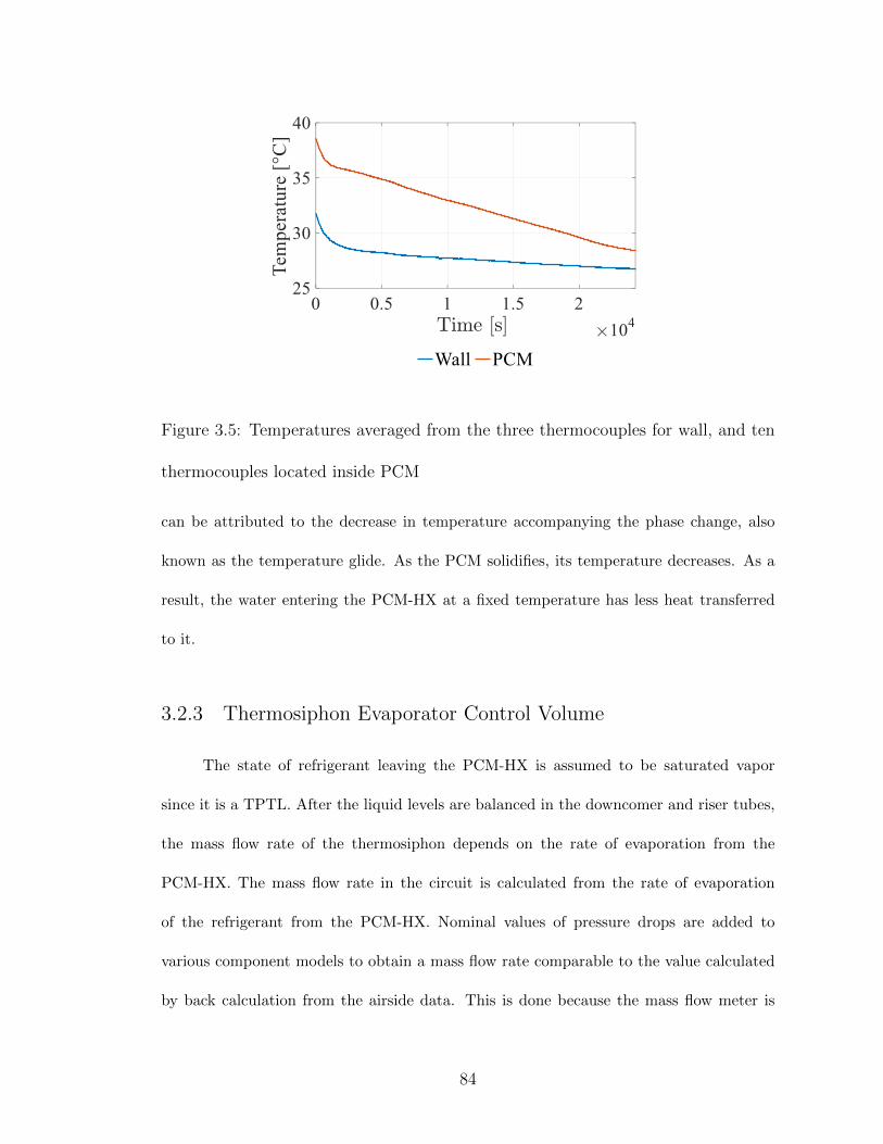
Figure 3.5: Temperatures averaged from the three thermocouples for wall, and ten

thermocouples located inside PCM

can be attributed to the decrease in temperature accompanying the phase change, also

known as the temperature glide. As the PCM solidifies, its temperature decreases. As a

result, the water entering the PCM-HX at a fixed temperature has less heat transferred

to it.

3.2.3 Thermosiphon Evaporator Control Volume

The state of refrigerant leaving the PCM-HX is assumed to be saturated vapor

since it is a TPTL. After the liquid levels are balanced in the downcomer and riser tubes,

the mass flow rate of the thermosiphon depends on the rate of evaporation from the

PCM-HX. The mass flow rate in the circuit is calculated from the rate of evaporation

of the refrigerant from the PCM-HX. Nominal values of pressure drops are added to

various component models to obtain a mass flow rate comparable to the value calculated

by back calculation from the airside data. This is done because the mass flow meter is

84

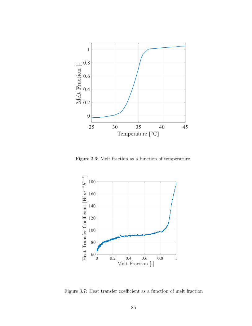
Figure 3.6: Melt fraction as a function of temperature

Figure 3.7: Heat transfer coefficient as a function of melt fraction

85

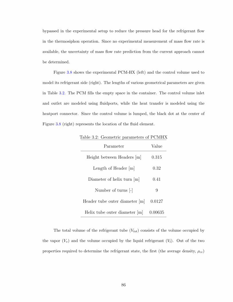
bypassed in the experimental setup to reduce the pressure head for the refrigerant flow

in the thermosiphon operation. Since no experimental measurement of mass flow rate is

available, the uncertainty of mass flow rate prediction from the current approach cannot

be determined.

Figure 3.8 shows the experimental PCM-HX (left) and the control volume used to

model its refrigerant side (right). The lengths of various geometrical parameters are given

in Table 3.2. The PCM fills the empty space in the container. The control volume inlet

and outlet are modeled using fluidports, while the heat transfer is modeled using the

heatport connector. Since the control volume is lumped, the black dot at the center of

Figure 3.8 (right) represents the location of the fluid element.

Table 3.2: Geometric parameters of PCMHX

Parameter Value

Height between Headers [m] 0.315

Length of Header [m] 0.32

Diameter of helix turn [m] 0.41

Number of turns [-] 9

Header tube outer diameter [m] 0.0127

Helix tube outer diameter [m] 0.00635

The total volume of the refrigerant tube (Vtot) consists of the volume occupied by

the vapor (Vv) and the volume occupied by the liquid refrigerant (Vl). Out of the two

properties required to determine the refrigerant state, the first (the average density, ρcv)

86

Refrigerant Outlet

(Port B)

Refrigerant Inlet

(Port A)

Heat In

(Heatport)

Figure 3.8: PCM-HX used in RoCo and the control volume used for modeling

can be calculated as follows:

Vt = VV + VL (3.10)

m = ρV VV + ρLVL (3.11)

dm

dt= min − mout (3.12)

ρcv =m

Vt(3.13)

The second property (pressure, pcv), can be obtained by averaging the pressure at

the inlet and outlet as shown in Equation (3.14).

pcv =pin + pout

2(3.14)

These two properties are sufficient to determine the state of refrigerant, and all the

remaining properties are calculated. Functions are available from the in-house REFPROP

9.0 based library [189] for refrigerant media.

87

The energy conservation equation (Equation (3.15)) and chain rule of derivatives

applied to the partial derivative of density with state variables (Equation (3.16)) are

used to update pressure and specific enthalpy, which are the state variables. The par-

tial derivatives of density are also functions of state variables [165] and evaluated using

property functions [189].

Vtdhcvdt

+ h(mout − min) + (mouthout − minhin) = Qr + Vtdpcvdt

(3.15)

∂ρcv∂t

=∂ρcv∂pcv

∣∣∣∣hcv

dpcvdt

+∂ρcv∂hcv

∣∣∣∣pcv

dhcvdt

(3.16)

The heat transfer coefficient for heat transfer from the heatport, αr,e in Equa-

tion (3.17), is calculated from Shah’s correlation [197] with Schmidt correlation [198]

for helical coils used for calculating liquid-only heat transfer coefficient. Since enthalpy

in the FluidPort is defined as a stream variable [199], outflow enthalpies need to be set

for both the inlet and outlet. The outflow enthalpy at the outlet, hout, is set as saturated

vapor enthalpy, hv,cv in Equation (3.18), while the outflow enthalpy at the inlet port is

set as saturated liquid enthalpy, hin in Equation (3.19).

Qr,e = αr,eA (Ttube − Tcv) (3.17)

hout = hV,cv (3.18)

hin = hL,cv (3.19)

3.3 System Modeling

The nature of PCM-HX model used in the study is relatively simple to reduce the

complexity of dynamics of thermosiphon assisted solidification for a system level sim-

88

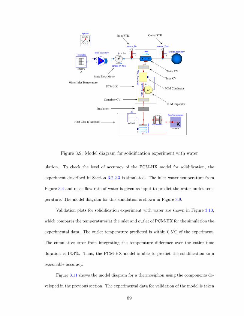
Figure 3.9: Model diagram for solidification experiment with water

ulation. To check the level of accuracy of the PCM-HX model for solidification, the

experiment described in Section 3.2.2.3 is simulated. The inlet water temperature from

Figure 3.4 and mass flow rate of water is given as input to predict the water outlet tem-

perature. The model diagram for this simulation is shown in Figure 3.9.

Validation plots for solidification experiment with water are shown in Figure 3.10,

which compares the temperatures at the inlet and outlet of PCM-HX for the simulation the

experimental data. The outlet temperature predicted is within 0.5°C of the experiment.

The cumulative error from integrating the temperature difference over the entire time

duration is 13.4%. Thus, the PCM-HX model is able to predict the solidification to a

reasonable accuracy.

Figure 3.11 shows the model diagram for a thermosiphon using the components de-

veloped in the previous section. The experimental data for validation of the model is taken

89

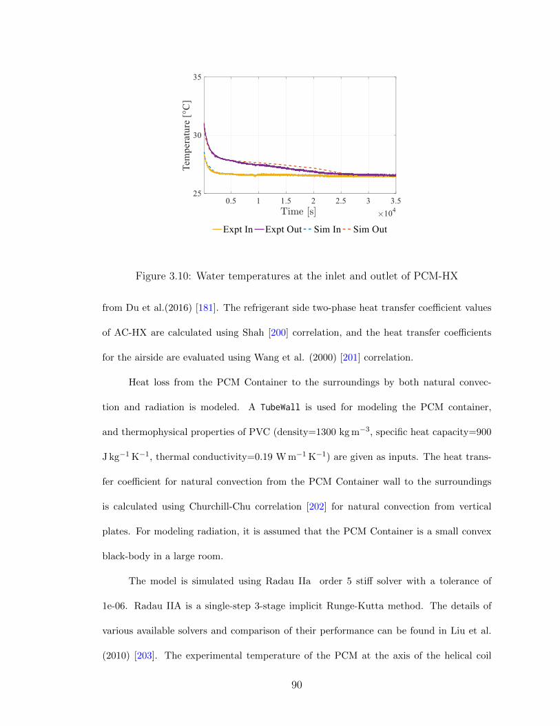
Figure 3.10: Water temperatures at the inlet and outlet of PCM-HX

from Du et al.(2016) [181]. The refrigerant side two-phase heat transfer coefficient values

of AC-HX are calculated using Shah [200] correlation, and the heat transfer coefficients

for the airside are evaluated using Wang et al. (2000) [201] correlation.

Heat loss from the PCM Container to the surroundings by both natural convec-

tion and radiation is modeled. A TubeWall is used for modeling the PCM container,

and thermophysical properties of PVC (density=1300 kg m−3, specific heat capacity=900

J kg−1 K−1, thermal conductivity=0.19 W m−1 K−1) are given as inputs. The heat trans-

fer coefficient for natural convection from the PCM Container wall to the surroundings

is calculated using Churchill-Chu correlation [202] for natural convection from vertical

plates. For modeling radiation, it is assumed that the PCM Container is a small convex

black-body in a large room.

The model is simulated using Radau IIa order 5 stiff solver with a tolerance of

1e-06. Radau IIA is a single-step 3-stage implicit Runge-Kutta method. The details of

various available solvers and comparison of their performance can be found in Liu et al.

(2010) [203]. The experimental temperature of the PCM at the axis of the helical coil

90

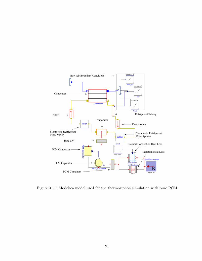
Figure 3.11: Modelica model used for the thermosiphon simulation with pure PCM

91

Figure 3.12: PCM temperature comparison between experimental data and simula-

tion

and at the wall (Figure 3.8, left) is compared with the lumped CV temperature from the

model in Figure 3.12.

T-Type thermocouples were used for the temperature measurement with the un-

certainty of temperature measure of 0.5°C. The thermocouples were calibrated between

0-80°C with 10°C increments. The PCM wall temperature refers to the temperature mea-

sured by the thermocouples between the PCM container wall and outside the helical coil.

This is lower than the temperature in the axis region of the helical coils because the axis

region gets heated from all sides, while the region outside the helical coil dissipates heat to

the ambient. The thermocouple temperature falls faster than the simulation temperature

because the thermocouples are located close to the helical coil, and they may not be exact

representation of volume averaged temperature of the entire lump of PCM.

Figure 3.13 shows the comparison of the condenser airside temperatures to the ex-

perimental data. Though there is a slight mismatch in the initial part of the cycle, which

can be attributed to lack of a receiver model in the simulation model, the model can

92

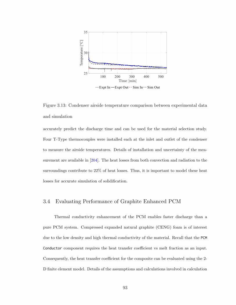
Figure 3.13: Condenser airside temperature comparison between experimental data

and simulation

accurately predict the discharge time and can be used for the material selection study.

Four T-Type thermocouples were installed each at the inlet and outlet of the condenser

to measure the airside temperatures. Details of installation and uncertainty of the mea-

surement are available in [204]. The heat losses from both convection and radiation to the

surroundings contribute to 22% of heat losses. Thus, it is important to model these heat

losses for accurate simulation of solidification.

3.4 Evaluating Performance of Graphite Enhanced PCM

Thermal conductivity enhancement of the PCM enables faster discharge than a

pure PCM system. Compressed expanded natural graphite (CENG) foam is of interest

due to the low density and high thermal conductivity of the material. Recall that the PCM

Conductor component requires the heat transfer coefficient vs melt fraction as an input.

Consequently, the heat transfer coefficient for the composite can be evaluated using the 2-

D finite element model. Details of the assumptions and calculations involved in calculation

93

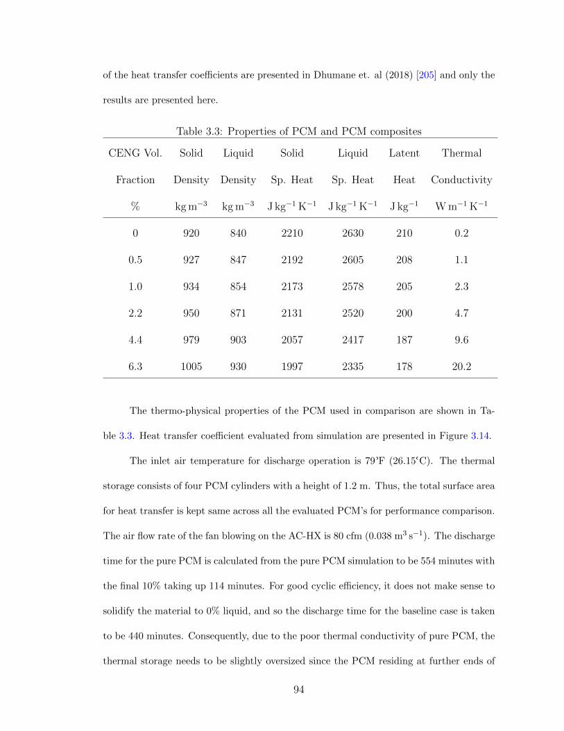
of the heat transfer coefficients are presented in Dhumane et. al (2018) [205] and only the

results are presented here.

Table 3.3: Properties of PCM and PCM composites

CENG Vol. Solid Liquid Solid Liquid Latent Thermal

Fraction Density Density Sp. Heat Sp. Heat Heat Conductivity

% kg m−3 kg m−3 J kg−1 K−1 J kg−1 K−1 J kg−1 W m−1 K−1

0 920 840 2210 2630 210 0.2

0.5 927 847 2192 2605 208 1.1

1.0 934 854 2173 2578 205 2.3

2.2 950 871 2131 2520 200 4.7

4.4 979 903 2057 2417 187 9.6

6.3 1005 930 1997 2335 178 20.2

The thermo-physical properties of the PCM used in comparison are shown in Ta-

ble 3.3. Heat transfer coefficient evaluated from simulation are presented in Figure 3.14.

The inlet air temperature for discharge operation is 79°F (26.15°C). The thermal

storage consists of four PCM cylinders with a height of 1.2 m. Thus, the total surface area

for heat transfer is kept same across all the evaluated PCM’s for performance comparison.

The air flow rate of the fan blowing on the AC-HX is 80 cfm (0.038 m3 s−1). The discharge

time for the pure PCM is calculated from the pure PCM simulation to be 554 minutes with

the final 10% taking up 114 minutes. For good cyclic efficiency, it does not make sense to

solidify the material to 0% liquid, and so the discharge time for the baseline case is taken

to be 440 minutes. Consequently, due to the poor thermal conductivity of pure PCM, the

thermal storage needs to be slightly oversized since the PCM residing at further ends of

94

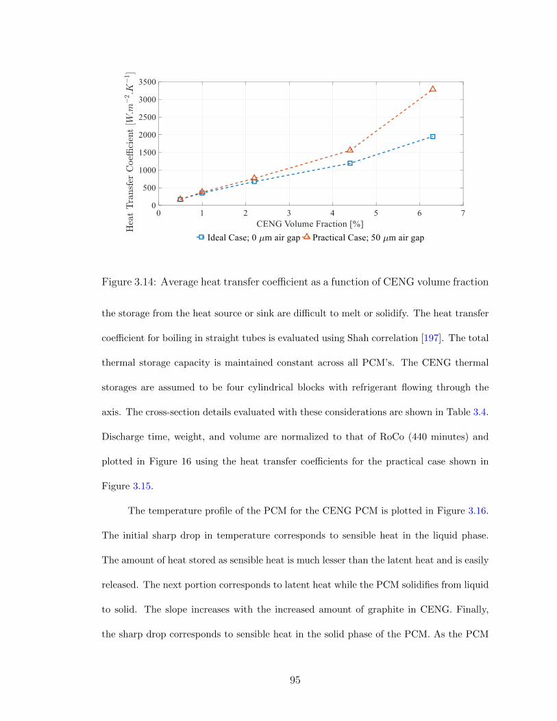
Figure 3.14: Average heat transfer coefficient as a function of CENG volume fraction

the storage from the heat source or sink are difficult to melt or solidify. The heat transfer

coefficient for boiling in straight tubes is evaluated using Shah correlation [197]. The total

thermal storage capacity is maintained constant across all PCM’s. The CENG thermal

storages are assumed to be four cylindrical blocks with refrigerant flowing through the

axis. The cross-section details evaluated with these considerations are shown in Table 3.4.

Discharge time, weight, and volume are normalized to that of RoCo (440 minutes) and

plotted in Figure 16 using the heat transfer coefficients for the practical case shown in

Figure 3.15.

The temperature profile of the PCM for the CENG PCM is plotted in Figure 3.16.

The initial sharp drop in temperature corresponds to sensible heat in the liquid phase.

The amount of heat stored as sensible heat is much lesser than the latent heat and is easily

released. The next portion corresponds to latent heat while the PCM solidifies from liquid

to solid. The slope increases with the increased amount of graphite in CENG. Finally,

the sharp drop corresponds to sensible heat in the solid phase of the PCM. As the PCM

95

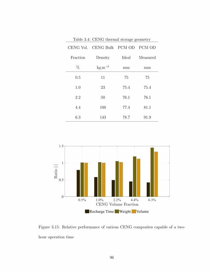
Table 3.4: CENG thermal storage geometry

CENG Vol. CENG Bulk PCM OD PCM OD

Fraction Density Ideal Measured

% kg m−3 mm mm

0.5 11 75 75

1.0 23 75.4 75.4

2.2 50 76.1 76.1

4.4 100 77.4 81.1

6.3 143 78.7 91.9

Figure 3.15: Relative performance of various CENG composites capable of a two-

hour operation time

96

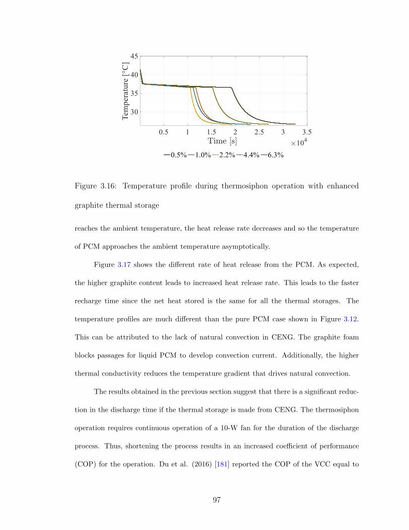
Figure 3.16: Temperature profile during thermosiphon operation with enhanced

graphite thermal storage

reaches the ambient temperature, the heat release rate decreases and so the temperature

of PCM approaches the ambient temperature asymptotically.

Figure 3.17 shows the different rate of heat release from the PCM. As expected,

the higher graphite content leads to increased heat release rate. This leads to the faster

recharge time since the net heat stored is the same for all the thermal storages. The

temperature profiles are much different than the pure PCM case shown in Figure 3.12.

This can be attributed to the lack of natural convection in CENG. The graphite foam

blocks passages for liquid PCM to develop convection current. Additionally, the higher

thermal conductivity reduces the temperature gradient that drives natural convection.

The results obtained in the previous section suggest that there is a significant reduc-

tion in the discharge time if the thermal storage is made from CENG. The thermosiphon

operation requires continuous operation of a 10-W fan for the duration of the discharge

process. Thus, shortening the process results in an increased coefficient of performance

(COP) for the operation. Du et al. (2016) [181] reported the COP of the VCC equal to

97

Figure 3.17: Heat removal rate during thermosiphon operation with enhanced

graphite thermal storage

2.85. The system COP for RoCo should incorporate the power consumed during both the

cooling as well as the recharge process.

For the present analysis, the COP for the VCC will be assumed constant for all

the variations of thermal storage. In reality, the CENG thermal storage will have lower

condenser temperature due to improved thermal conductivity and will further enhance the

COP. The evaporator capacity reported by Du et al.(2016) [181] is 165.6 W for a period

of two hours. This value is averaged value over the two hour period. Average power

consumption for the two-hour interval can be calculated from Equation (3.20) = 58.1 W.

COPvcc =¯Q¯W vcc

(3.20)

COPtot =¯Q∆tvcc

¯Wvcc∆tvcc + ¯Wts∆tts(3.21)

Equation (3.21) can be used to evaluate the overall COP for RoCo. This incorporates

the energy consumed during both recharge and discharge processes. The results for all

the cases are presented in Figure 3.18. It can be observed that the COP is in the range

98

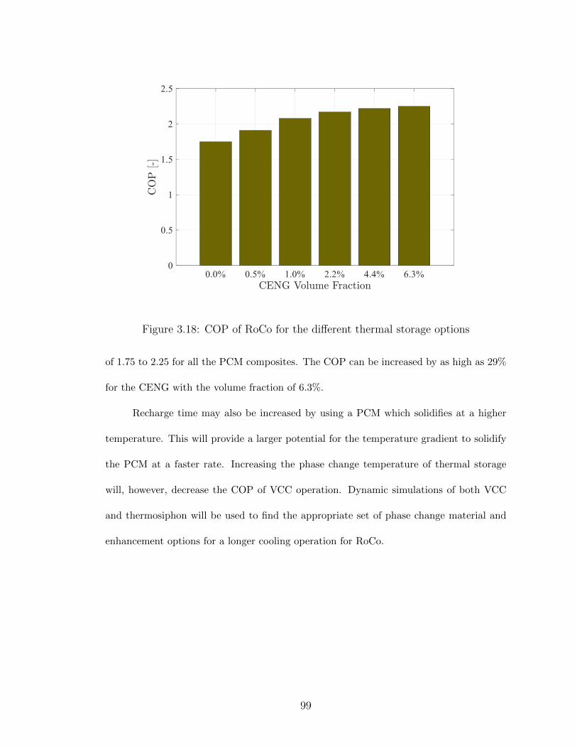
Figure 3.18: COP of RoCo for the different thermal storage options

of 1.75 to 2.25 for all the PCM composites. The COP can be increased by as high as 29%

for the CENG with the volume fraction of 6.3%.

Recharge time may also be increased by using a PCM which solidifies at a higher

temperature. This will provide a larger potential for the temperature gradient to solidify

the PCM at a faster rate. Increasing the phase change temperature of thermal storage

will, however, decrease the COP of VCC operation. Dynamic simulations of both VCC

and thermosiphon will be used to find the appropriate set of phase change material and

enhancement options for a longer cooling operation for RoCo.

99

Chapter 4: Performance Improvements of Personal Conditioning Sys-

tems

4.1 Introduction

The present chapter seeks to provide design insights for increased overall coefficient

of performance of Roving Comforter. Dynamic model for modeling the thermosiphon

based recharge was developed in the previous chapter and used to understand performance

improvement from graphite enhancement to phase change material. Two other ideas for

improvement of the performance are discussed: one is switching to a natural refrigerant

R290 and second is using a heat pump based recharge.

4.2 Performance with a natural refrigerant

The current RoCo prototype uses R134a as the refrigerant, primarily due to lesser

safety concerns related to the flammability, enabling development in a university labora-

tory. Secondly, the wider experience of development of systems with R134a enables the

researchers to focus on improving the novelty aspects of the prototype and fewer design

challenges. R134a is a hydrofluorocarbon (HFC) and has zero ozone depletion potential,

however, its global warming potential (GWP) is 1300 [206]. Thus, it is a potent green-

house gas and is thousands of times more potent than carbon dioxide in contributing to

100

climate change. If HFC growth continues on the current trajectory, the increase in HFC

emissions is projected to offset much of the climate benefit achieved by phasing out the

ozone-depleting substances which were replaced by the HFCs [207].

As R134a is affected by the Kigali Agreement under the Montreal Protocol [208],

it should be gradually phased out and replaced by low-GWP alternatives. The minia-

ture hermetic rotary compressor [180] used in the Roving Comforter is compatible with

R134a, R404A, R600a and R290. Hydrocarbon (HC) refrigerants have equal or better heat

transfer performance and lower pressure drop compared to R134a [209]. Other expected

benefits from switching an HFC to HC are higher efficiency, lower charge quantity and

lower compressor discharge temperature [210].

The cooling operation of RoCo is modeled using CEEEModelicaLibrary [165]. The

model is validated with experiment data for RoCo working with R134a and then used for

comparing system level performance of the Roving Comforter with propane (R290) as a

refrigerant in comparison with the current R134a.

4.2.1 Empirical PCM heat transfer coefficient

Experiment is conducted to obtain the heat transfer coefficient of PCM for melting

in helical coils. Unlike the solidification, melting of PCM involves heat transfer by both

conduction and natural convection.

The schematic of the experiment for evaluating the heat transfer coefficient for

melting is the same which was used for solidification (see Figure 3.3). The equations and

procedure for calculation of heat transfer coefficient is presented in 3.2.2.3 and skipped

here for brevity.

The thermal conductance on the water-side is calculated using water flow conditions.

101

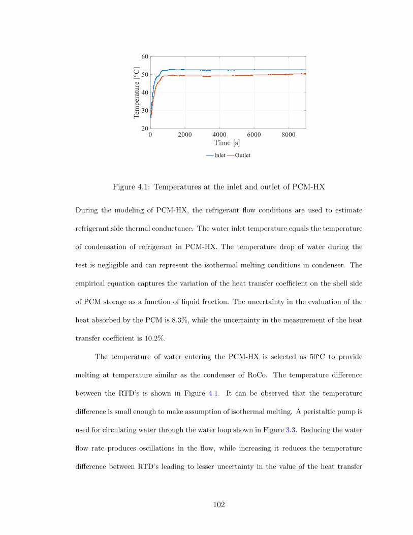
Figure 4.1: Temperatures at the inlet and outlet of PCM-HX

During the modeling of PCM-HX, the refrigerant flow conditions are used to estimate

refrigerant side thermal conductance. The water inlet temperature equals the temperature

of condensation of refrigerant in PCM-HX. The temperature drop of water during the

test is negligible and can represent the isothermal melting conditions in condenser. The

empirical equation captures the variation of the heat transfer coefficient on the shell side

of PCM storage as a function of liquid fraction. The uncertainty in the evaluation of the

heat absorbed by the PCM is 8.3%, while the uncertainty in the measurement of the heat

transfer coefficient is 10.2%.

The temperature of water entering the PCM-HX is selected as 50°C to provide

melting at temperature similar as the condenser of RoCo. The temperature difference

between the RTD’s is shown in Figure 4.1. It can be observed that the temperature

difference is small enough to make assumption of isothermal melting. A peristaltic pump is

used for circulating water through the water loop shown in Figure 3.3. Reducing the water

flow rate produces oscillations in the flow, while increasing it reduces the temperature

difference between RTD’s leading to lesser uncertainty in the value of the heat transfer

102

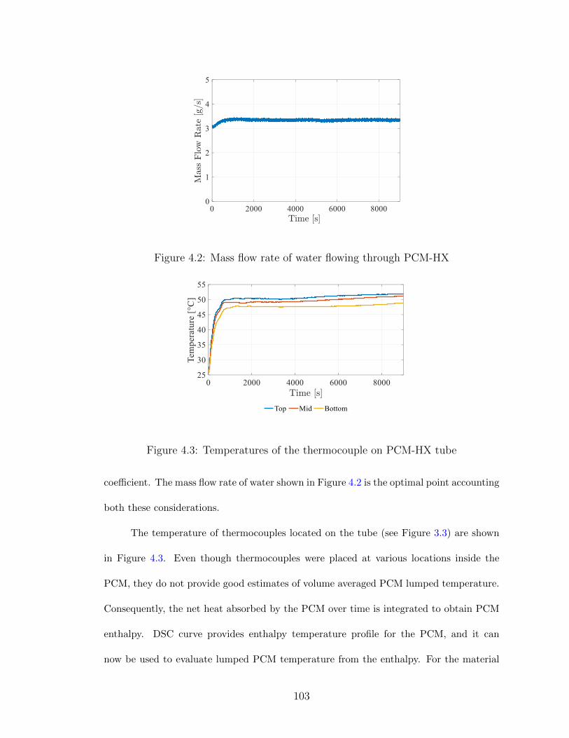
Figure 4.2: Mass flow rate of water flowing through PCM-HX

Figure 4.3: Temperatures of the thermocouple on PCM-HX tube

coefficient. The mass flow rate of water shown in Figure 4.2 is the optimal point accounting

both these considerations.

The temperature of thermocouples located on the tube (see Figure 3.3) are shown

in Figure 4.3. Even though thermocouples were placed at various locations inside the

PCM, they do not provide good estimates of volume averaged PCM lumped temperature.

Consequently, the net heat absorbed by the PCM over time is integrated to obtain PCM

enthalpy. DSC curve provides enthalpy temperature profile for the PCM, and it can

now be used to evaluate lumped PCM temperature from the enthalpy. For the material

103

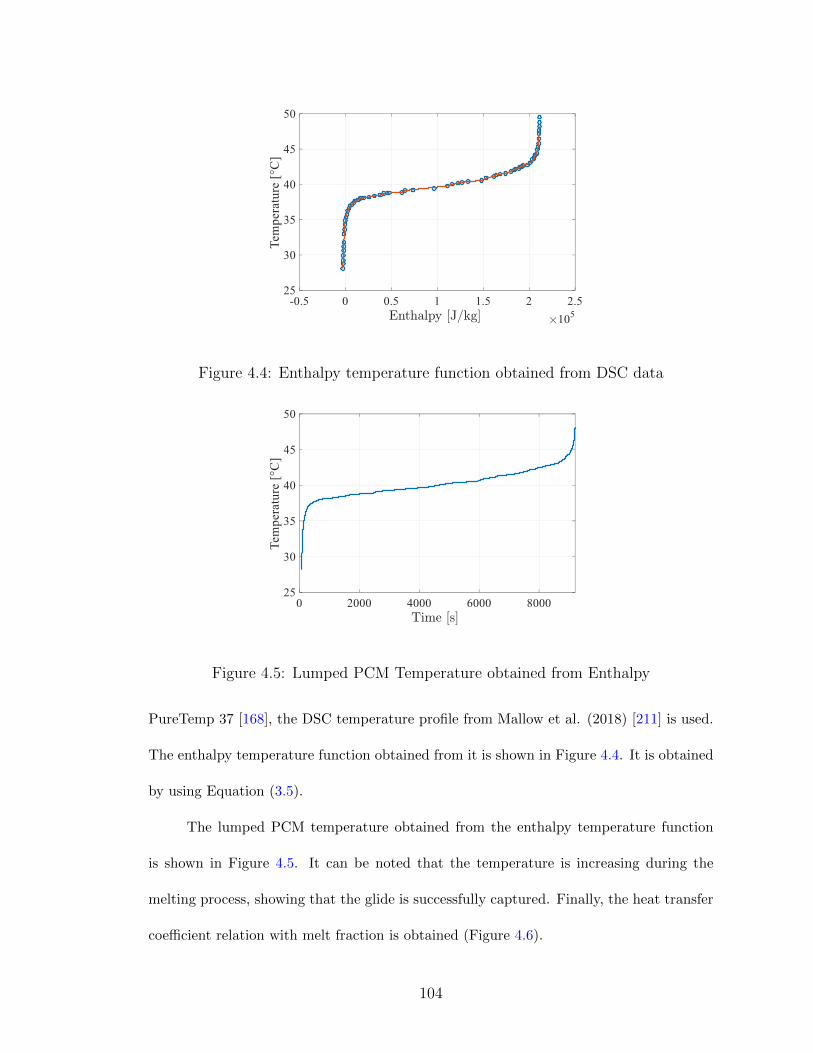
Figure 4.4: Enthalpy temperature function obtained from DSC data

Figure 4.5: Lumped PCM Temperature obtained from Enthalpy

PureTemp 37 [168], the DSC temperature profile from Mallow et al. (2018) [211] is used.

The enthalpy temperature function obtained from it is shown in Figure 4.4. It is obtained

by using Equation (3.5).

The lumped PCM temperature obtained from the enthalpy temperature function

is shown in Figure 4.5. It can be noted that the temperature is increasing during the

melting process, showing that the glide is successfully captured. Finally, the heat transfer

coefficient relation with melt fraction is obtained (Figure 4.6).

104

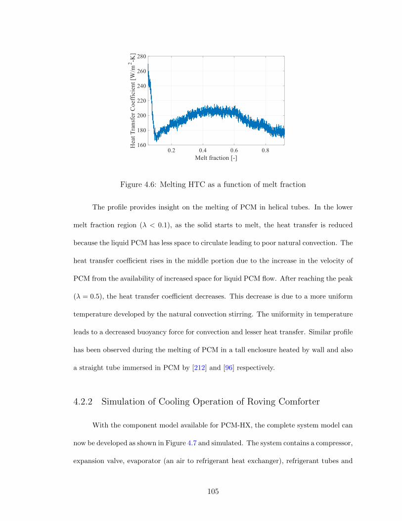
Figure 4.6: Melting HTC as a function of melt fraction

The profile provides insight on the melting of PCM in helical tubes. In the lower

melt fraction region (λ < 0.1), as the solid starts to melt, the heat transfer is reduced

because the liquid PCM has less space to circulate leading to poor natural convection. The

heat transfer coefficient rises in the middle portion due to the increase in the velocity of

PCM from the availability of increased space for liquid PCM flow. After reaching the peak

(λ = 0.5), the heat transfer coefficient decreases. This decrease is due to a more uniform

temperature developed by the natural convection stirring. The uniformity in temperature

leads to a decreased buoyancy force for convection and lesser heat transfer. Similar profile

has been observed during the melting of PCM in a tall enclosure heated by wall and also

a straight tube immersed in PCM by [212] and [96] respectively.

4.2.2 Simulation of Cooling Operation of Roving Comforter

With the component model available for PCM-HX, the complete system model can

now be developed as shown in Figure 4.7 and simulated. The system contains a compressor,

expansion valve, evaporator (an air to refrigerant heat exchanger), refrigerant tubes and

105

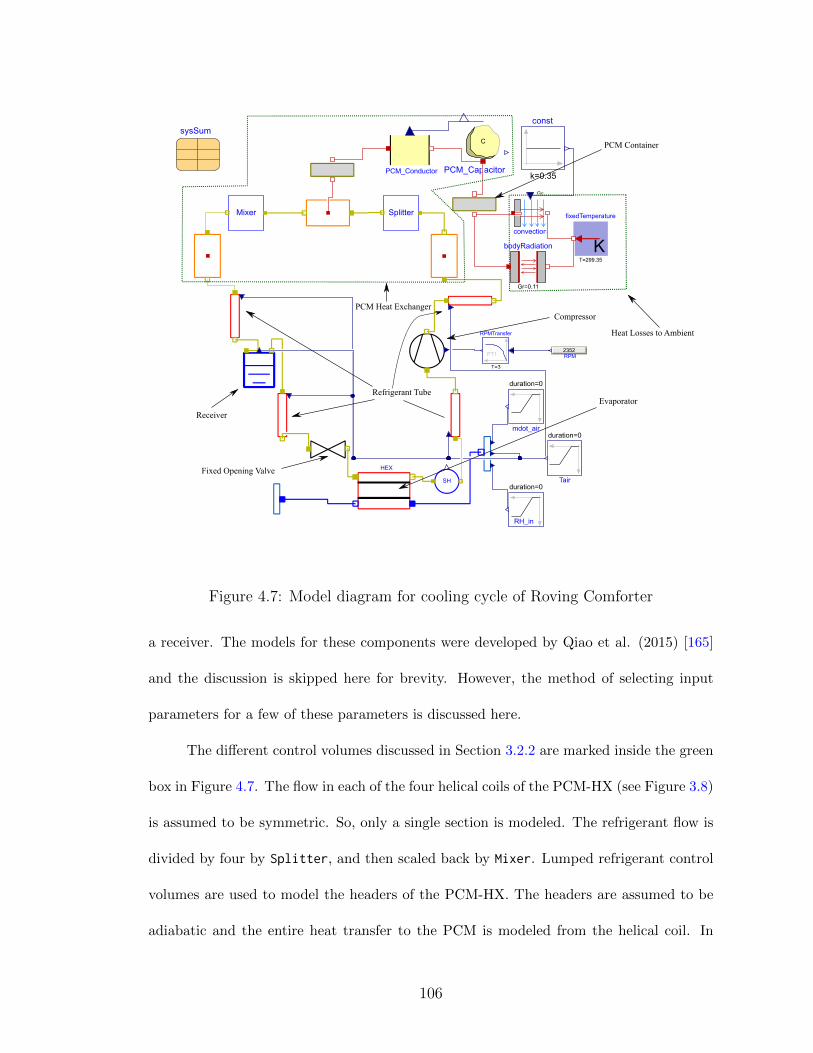
Figure 4.7: Model diagram for cooling cycle of Roving Comforter

a receiver. The models for these components were developed by Qiao et al. (2015) [165]

and the discussion is skipped here for brevity. However, the method of selecting input

parameters for a few of these parameters is discussed here.

The different control volumes discussed in Section 3.2.2 are marked inside the green

box in Figure 4.7. The flow in each of the four helical coils of the PCM-HX (see Figure 3.8)

is assumed to be symmetric. So, only a single section is modeled. The refrigerant flow is

divided by four by Splitter, and then scaled back by Mixer. Lumped refrigerant control

volumes are used to model the headers of the PCM-HX. The headers are assumed to be

adiabatic and the entire heat transfer to the PCM is modeled from the helical coil. In

106

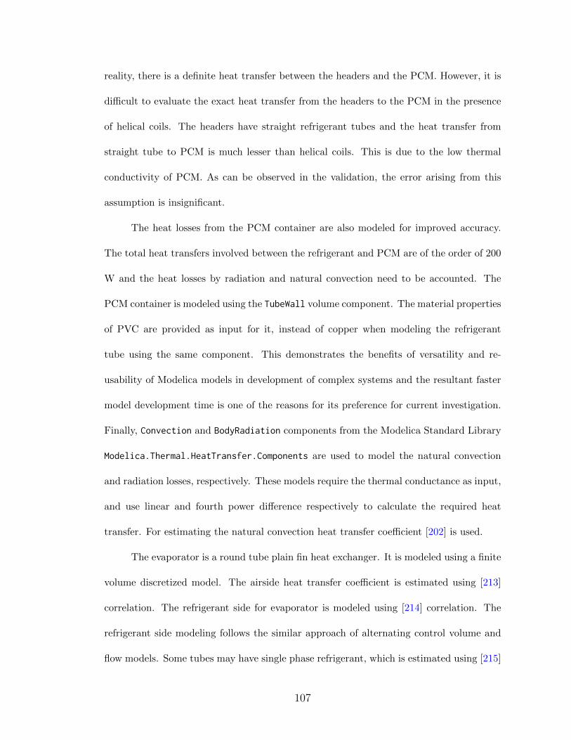
reality, there is a definite heat transfer between the headers and the PCM. However, it is

difficult to evaluate the exact heat transfer from the headers to the PCM in the presence

of helical coils. The headers have straight refrigerant tubes and the heat transfer from

straight tube to PCM is much lesser than helical coils. This is due to the low thermal

conductivity of PCM. As can be observed in the validation, the error arising from this

assumption is insignificant.

The heat losses from the PCM container are also modeled for improved accuracy.

The total heat transfers involved between the refrigerant and PCM are of the order of 200

W and the heat losses by radiation and natural convection need to be accounted. The

PCM container is modeled using the TubeWall volume component. The material properties

of PVC are provided as input for it, instead of copper when modeling the refrigerant

tube using the same component. This demonstrates the benefits of versatility and re-

usability of Modelica models in development of complex systems and the resultant faster

model development time is one of the reasons for its preference for current investigation.

Finally, Convection and BodyRadiation components from the Modelica Standard Library

Modelica.Thermal.HeatTransfer.Components are used to model the natural convection

and radiation losses, respectively. These models require the thermal conductance as input,

and use linear and fourth power difference respectively to calculate the required heat

transfer. For estimating the natural convection heat transfer coefficient [202] is used.

The evaporator is a round tube plain fin heat exchanger. It is modeled using a finite

volume discretized model. The airside heat transfer coefficient is estimated using [213]

correlation. The refrigerant side for evaporator is modeled using [214] correlation. The

refrigerant side modeling follows the similar approach of alternating control volume and

flow models. Some tubes may have single phase refrigerant, which is estimated using [215]

107

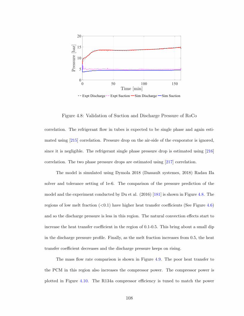
Figure 4.8: Validation of Suction and Discharge Pressure of RoCo

correlation. The refrigerant flow in tubes is expected to be single phase and again esti-

mated using [215] correlation. Pressure drop on the air-side of the evaporator is ignored,

since it is negligible. The refrigerant single phase pressure drop is estimated using [216]

correlation. The two phase pressure drops are estimated using [217] correlation.

The model is simulated using Dymola 2018 (Dassault systemes, 2018) Radau IIa

solver and tolerance setting of 1e-6. The comparison of the pressure prediction of the

model and the experiment conducted by Du et al. (2016) [181] is shown in Figure 4.8. The

regions of low melt fraction (<0.1) have higher heat transfer coefficients (See Figure 4.6)

and so the discharge pressure is less in this region. The natural convection effects start to

increase the heat transfer coefficient in the region of 0.1-0.5. This bring about a small dip

in the discharge pressure profile. Finally, as the melt fraction increases from 0.5, the heat

transfer coefficient decreases and the discharge pressure keeps on rising.

The mass flow rate comparison is shown in Figure 4.9. The poor heat transfer to

the PCM in this region also increases the compressor power. The compressor power is

plotted in Figure 4.10. The R134a compressor efficiency is tuned to match the power

108

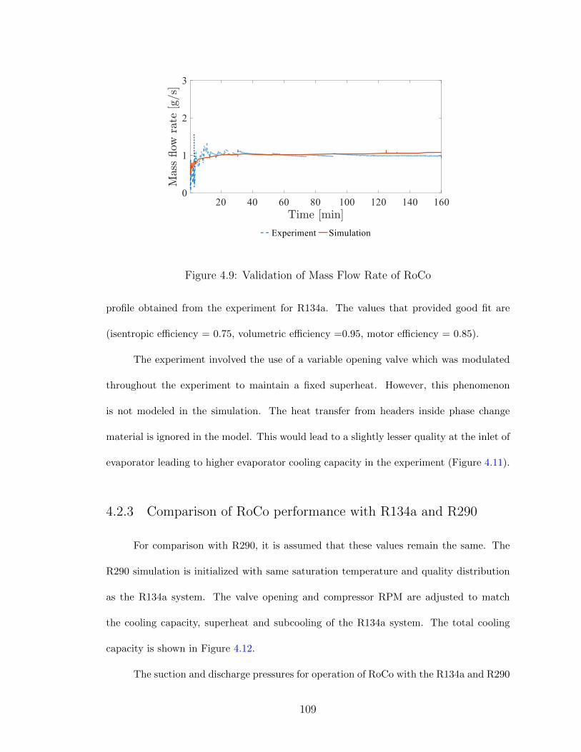
Figure 4.9: Validation of Mass Flow Rate of RoCo

profile obtained from the experiment for R134a. The values that provided good fit are

(isentropic efficiency = 0.75, volumetric efficiency =0.95, motor efficiency = 0.85).

The experiment involved the use of a variable opening valve which was modulated

throughout the experiment to maintain a fixed superheat. However, this phenomenon

is not modeled in the simulation. The heat transfer from headers inside phase change

material is ignored in the model. This would lead to a slightly lesser quality at the inlet of

evaporator leading to higher evaporator cooling capacity in the experiment (Figure 4.11).

4.2.3 Comparison of RoCo performance with R134a and R290

For comparison with R290, it is assumed that these values remain the same. The

R290 simulation is initialized with same saturation temperature and quality distribution

as the R134a system. The valve opening and compressor RPM are adjusted to match

the cooling capacity, superheat and subcooling of the R134a system. The total cooling

capacity is shown in Figure 4.12.

The suction and discharge pressures for operation of RoCo with the R134a and R290

109

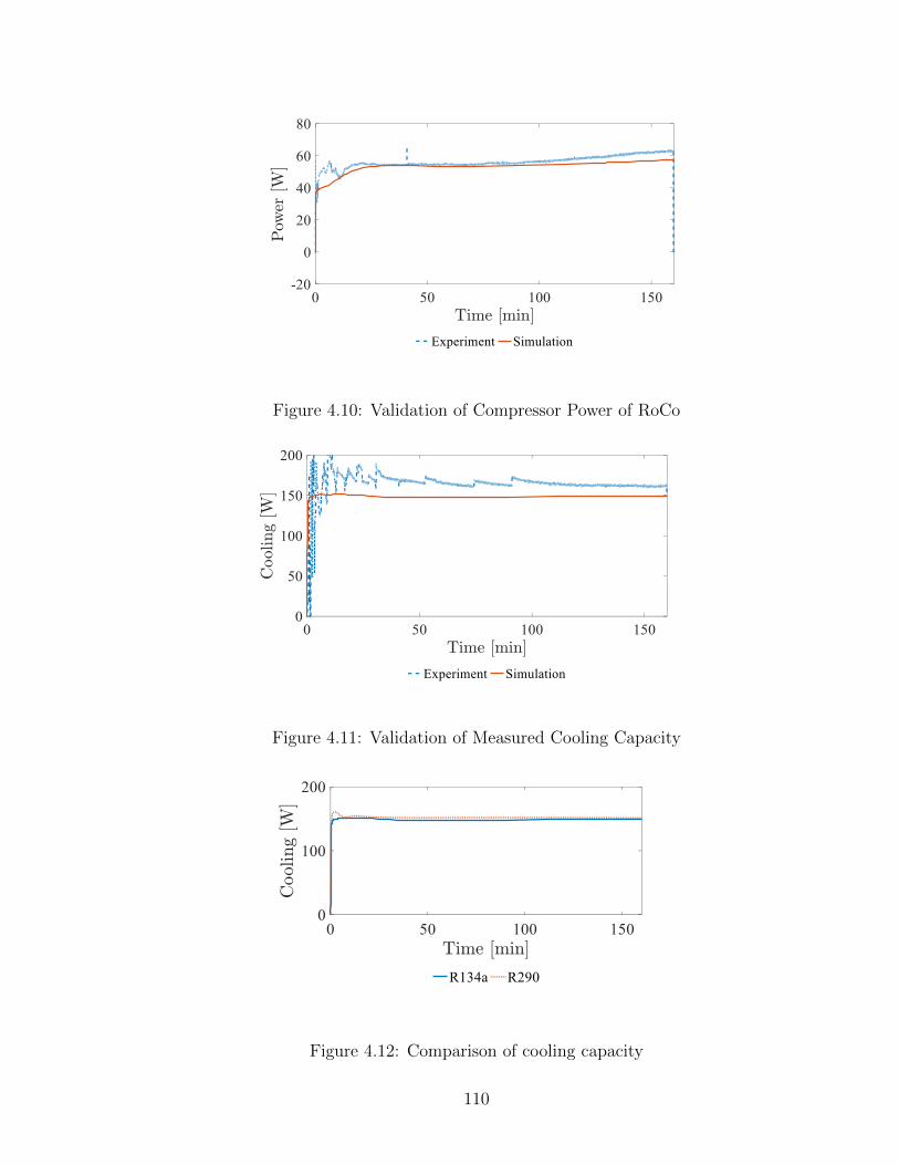
Figure 4.10: Validation of Compressor Power of RoCo

Figure 4.11: Validation of Measured Cooling Capacity

Figure 4.12: Comparison of cooling capacity

110

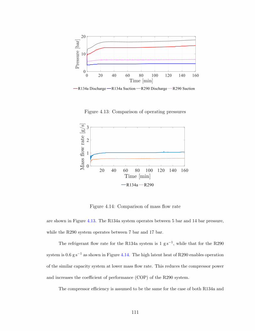
Figure 4.13: Comparison of operating pressures

Figure 4.14: Comparison of mass flow rate

are shown in Figure 4.13. The R134a system operates between 5 bar and 14 bar pressure,

while the R290 system operates between 7 bar and 17 bar.

The refrigerant flow rate for the R134a system is 1 g s−1, while that for the R290

system is 0.6 g s−1 as shown in Figure 4.14. The high latent heat of R290 enables operation

of the similar capacity system at lower mass flow rate. This reduces the compressor power

and increases the coefficient of performance (COP) of the R290 system.

The compressor efficiency is assumed to be the same for the case of both R134a and

111

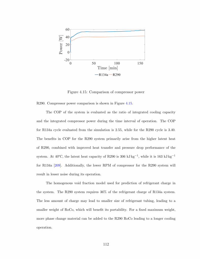
Figure 4.15: Comparison of compressor power

R290. Compressor power comparison is shown in Figure 4.15.

The COP of the system is evaluated as the ratio of integrated cooling capacity

and the integrated compressor power during the time interval of operation. The COP

for R134a cycle evaluated from the simulation is 2.55, while for the R290 cycle is 3.40.

The benefits in COP for the R290 system primarily arise from the higher latent heat

of R290, combined with improved heat transfer and pressure drop performance of the

system. At 40°C, the latent heat capacity of R290 is 306 kJ kg−1, while it is 163 kJ kg−1

for R134a [209]. Additionally, the lower RPM of compressor for the R290 system will

result in lesser noise during its operation.

The homogenous void fraction model used for prediction of refrigerant charge in

the system. The R290 system requires 36% of the refrigerant charge of R134a system.

The less amount of charge may lead to smaller size of refrigerant tubing, leading to a

smaller weight of RoCo, which will benefit its portability. For a fixed maximum weight,

more phase change material can be added to the R290 RoCo leading to a longer cooling

operation.

112

4.3 Analysis of heat pump based recharge

The thermosiphon operation period may be reduced significantly by enhancing the

thermal conductivity of PCM using graphite. To achieve more savings from the use of

RoCo, the cooling operation period needs to be increased and the recharge time decreased.

With this objective, the PCM storage in newer versions of RoCo are developed using the

graphite enhanced PCM. The amount of PCM is increased to support four hour cooling

operation. Another option for solidification is to reverse the refrigerant flow in circuit and

solidify the PCM by making the PCM-HX as an evaporator. This mode of operation will be

referred to as heat-pump mode for recharge. The air-cooled heat exchanger now operates

as a condenser and rejects heat to the ambient. Heat pump mode utilizes the compressor

for its operation resulting in higher power consumption, but is expected to solidify the

PCM much faster. The focus of the present section is to explore the advantages and

disadvantages of thermosiphon and heat pump operation for solidification of PCM.

4.3.1 Heat Pump System Description

The schematic of the two operations for recharge of RoCo is shown in Figure 4.16.

Recall that the refrigerant circuit of RoCo using thermosiphon for recharge involves two

ball valves, which by-pass the compressor and expansion device from the refrigerant cir-

cuit for cooling cycle. Details of this thermosiphon operation is available in Chapter 3

and omitted here for brevity. As discussed in the Section 3.4 the recharge time of the

thermosiphon can be significantly enhanced by addition of graphite to the phase change

material (PCM). The systems discussed in the current research use these graphite en-

hanced PCM. For further value addition from RoCo, the cooling operation duration for

113

Figure 4.16: Schematic showing both thermosiphon and heat pump mode of recharge

the system is twice than those considered in the first prototype (discussed in Chapter 3)

and this is achieved by increasing the weight of the PCM used in the thermal storage.

The higher weight of PCM leads to addition of recharge time.

Consequently, a second mode of recharge called the heat pump mode is considered.

A reversible four-way valve can be used to change the refrigerant flow direction from the

compressor and recharge the PCM by operating the PCM storage as an evaporator. The

compressor used in RoCo is of the variable-speed type and the recharge time may be

controlled by adjusting its RPM. There are two TXV in the circuit for heat pump, each

protected by a check valve. The bulbs of the TXV are connected to outlet of either the air

to refrigerant heat exchanger or the PCM-HX. During the cooling operation, the outlet of

air to refrigerant heat exchanger (marked as condenser in Figure 4.16) is connected to the

bulb of TXV, while the outlet of PCM-HX is connected to the bulb of the second TXV.

This second TXV is operational during the heat pump operation.

114

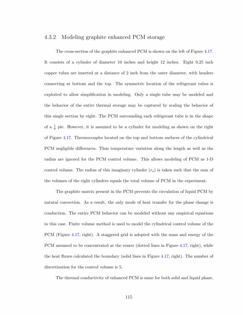
4.3.2 Modeling graphite enhanced PCM storage

The cross-section of the graphite enhanced PCM is shown on the left of Figure 4.17.

It consists of a cylinder of diameter 10 inches and height 12 inches. Eight 0.25 inch

copper tubes are inserted at a distance of 2 inch from the outer diameter, with headers

connecting at bottom and the top. The symmetric location of the refrigerant tubes is

exploited to allow simplification in modeling. Only a single tube may be modeled and

the behavior of the entire thermal storage may be captured by scaling the behavior of

this single section by eight. The PCM surrounding each refrigerant tube is in the shape

of a 18 pie. However, it is assumed to be a cylinder for modeling as shown on the right

of Figure 4.17. Thermocouples located on the top and bottom surfaces of the cylindrical

PCM negligible differences. Thus temperature variation along the length as well as the

radius are ignored for the PCM control volume. This allows modeling of PCM as 1-D

control volume. The radius of this imaginary cylinder (ro) is taken such that the sum of

the volumes of the eight cylinders equals the total volume of PCM in the experiment.

The graphite matrix present in the PCM prevents the circulation of liquid PCM by

natural convection. As a result, the only mode of heat transfer for the phase change is

conduction. The entire PCM behavior can be modeled without any empirical equations

in this case. Finite volume method is used to model the cylindrical control volume of the

PCM (Figure 4.17, right). A staggered grid is adopted with the mass and energy of the

PCM assumed to be concentrated at the center (dotted lines in Figure 4.17, right), while

the heat fluxes calculated the boundary (solid lines in Figure 4.17, right). The number of

discretization for the control volume is 5.

The thermal conductivity of enhanced PCM is same for both solid and liquid phase,

115

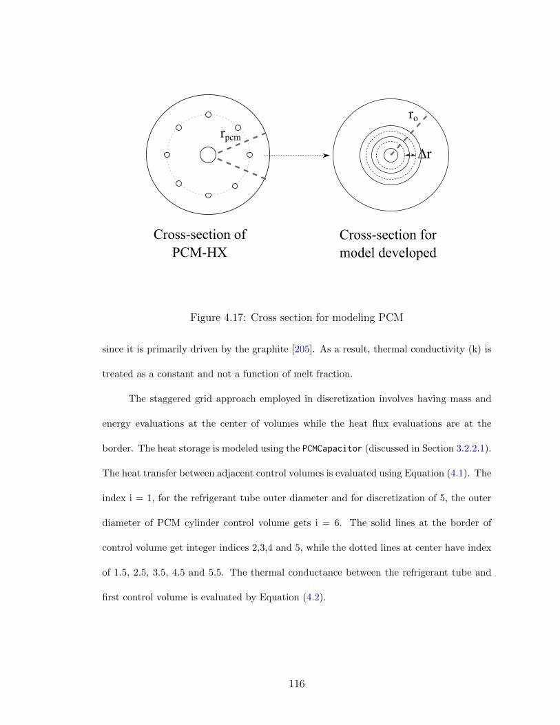
Figure 4.17: Cross section for modeling PCM

since it is primarily driven by the graphite [205]. As a result, thermal conductivity (k) is

treated as a constant and not a function of melt fraction.

The staggered grid approach employed in discretization involves having mass and

energy evaluations at the center of volumes while the heat flux evaluations are at the

border. The heat storage is modeled using the PCMCapacitor (discussed in Section 3.2.2.1).

The heat transfer between adjacent control volumes is evaluated using Equation (4.1). The

index i = 1, for the refrigerant tube outer diameter and for discretization of 5, the outer

diameter of PCM cylinder control volume gets i = 6. The solid lines at the border of

control volume get integer indices 2,3,4 and 5, while the dotted lines at center have index

of 1.5, 2.5, 3.5, 4.5 and 5.5. The thermal conductance between the refrigerant tube and

first control volume is evaluated by Equation (4.2).

116

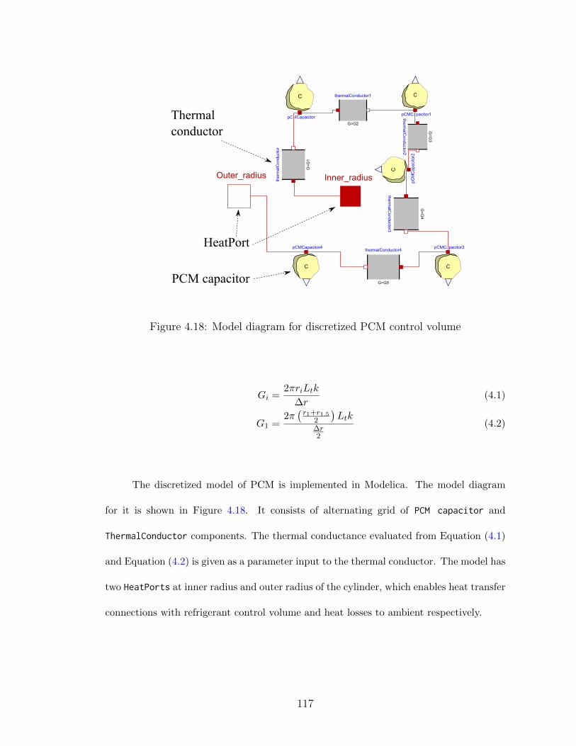
Figure 4.18: Model diagram for discretized PCM control volume

Gi =2πriLtk

∆r(4.1)

G1 =2π(r1+r1.5

2

)Ltk

∆r2

(4.2)

The discretized model of PCM is implemented in Modelica. The model diagram

for it is shown in Figure 4.18. It consists of alternating grid of PCM capacitor and

ThermalConductor components. The thermal conductance evaluated from Equation (4.1)

and Equation (4.2) is given as a parameter input to the thermal conductor. The model has

two HeatPorts at inner radius and outer radius of the cylinder, which enables heat transfer

connections with refrigerant control volume and heat losses to ambient respectively.

117

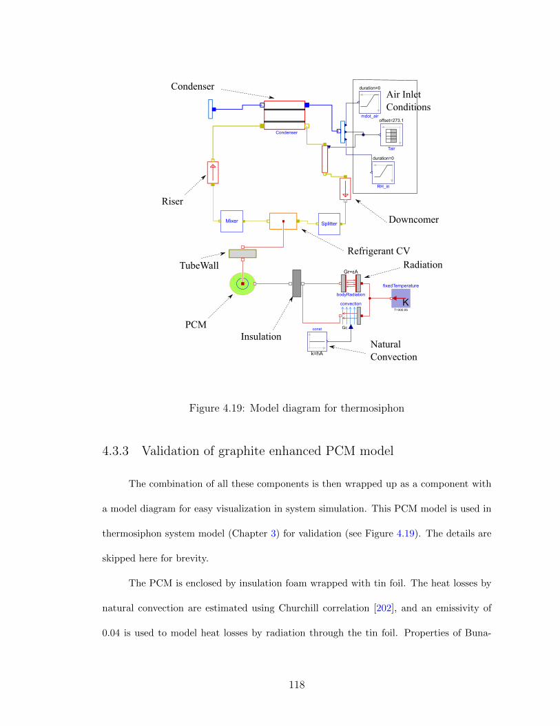
Figure 4.19: Model diagram for thermosiphon

4.3.3 Validation of graphite enhanced PCM model

The combination of all these components is then wrapped up as a component with

a model diagram for easy visualization in system simulation. This PCM model is used in

thermosiphon system model (Chapter 3) for validation (see Figure 4.19). The details are

skipped here for brevity.

The PCM is enclosed by insulation foam wrapped with tin foil. The heat losses by

natural convection are estimated using Churchill correlation [202], and an emissivity of

0.04 is used to model heat losses by radiation through the tin foil. Properties of Buna-

118

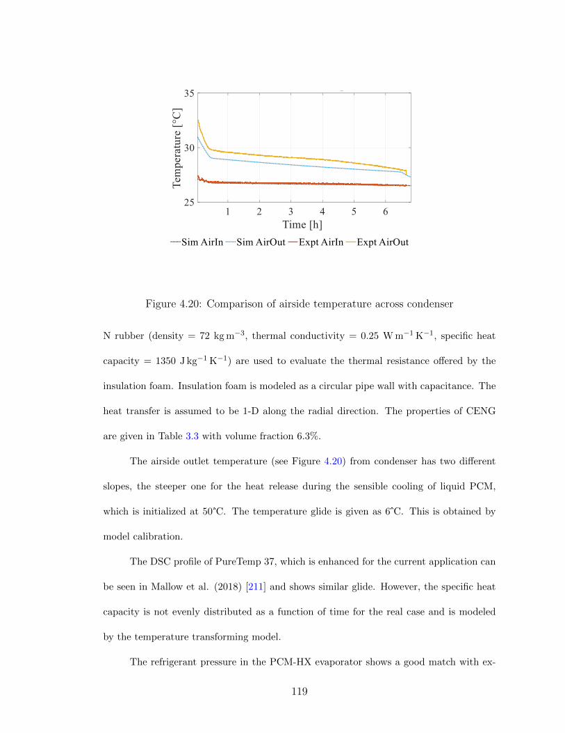
Figure 4.20: Comparison of airside temperature across condenser

N rubber (density = 72 kg m−3, thermal conductivity = 0.25 W m−1 K−1, specific heat

capacity = 1350 J kg−1 K−1) are used to evaluate the thermal resistance offered by the

insulation foam. Insulation foam is modeled as a circular pipe wall with capacitance. The

heat transfer is assumed to be 1-D along the radial direction. The properties of CENG

are given in Table 3.3 with volume fraction 6.3%.

The airside outlet temperature (see Figure 4.20) from condenser has two different

slopes, the steeper one for the heat release during the sensible cooling of liquid PCM,

which is initialized at 50°C. The temperature glide is given as 6°C. This is obtained by

model calibration.

The DSC profile of PureTemp 37, which is enhanced for the current application can

be seen in Mallow et al. (2018) [211] and shows similar glide. However, the specific heat

capacity is not evenly distributed as a function of time for the real case and is modeled

by the temperature transforming model.

The refrigerant pressure in the PCM-HX evaporator shows a good match with ex-

119

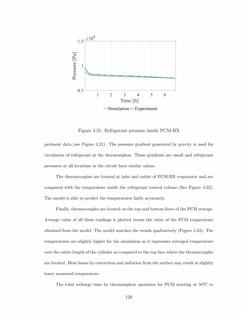
Figure 4.21: Refrigerant pressure inside PCM-HX

periment data (see Figure 4.21). The pressure gradient generated by gravity is used for

circulation of refrigerant in the thermosiphon. These gradients are small and refrigerant

pressures at all locations in the circuit have similar values.

The thermocouples are located at inlet and outlet of PCM-HX evaporator and are

compared with the temperature inside the refrigerant control volume (See Figure 4.22).

The model is able to predict the temperatures fairly accurately.

Finally, thermocouples are located on the top and bottom faces of the PCM storage.

Average value of all these readings is plotted versus the value of the PCM temperature

obtained from the model. The model matches the trends qualitatively (Figure 4.23). The

temperatures are slightly higher for the simulation as it represents averaged temperature

over the entire length of the cylinder as compared to the top face where the thermocouples

are located. Heat losses by convection and radiation from the surface may result in slightly

lower measured temperature.

The total recharge time by thermosiphon operation for PCM starting at 50°C to

120

Figure 4.22: Refrigerant temperature inside PCM-HX

Figure 4.23: Temperature of PCM

121

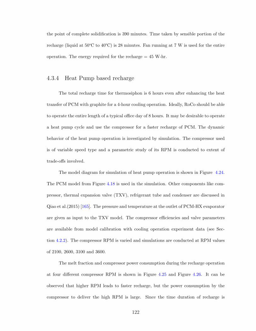
the point of complete solidification is 390 minutes. Time taken by sensible portion of the

recharge (liquid at 50°C to 40°C) is 28 minutes. Fan running at 7 W is used for the entire

operation. The energy required for the recharge = 45 W-hr.

4.3.4 Heat Pump based recharge

The total recharge time for thermosiphon is 6 hours even after enhancing the heat

transfer of PCM with graphite for a 4-hour cooling operation. Ideally, RoCo should be able

to operate the entire length of a typical office day of 8 hours. It may be desirable to operate

a heat pump cycle and use the compressor for a faster recharge of PCM. The dynamic

behavior of the heat pump operation is investigated by simulation. The compressor used

is of variable speed type and a parametric study of its RPM is conducted to extent of

trade-offs involved.

The model diagram for simulation of heat pump operation is shown in Figure 4.24.

The PCM model from Figure 4.18 is used in the simulation. Other components like com-

pressor, thermal expansion valve (TXV), refrigerant tube and condenser are discussed in

Qiao et al.(2015) [165]. The pressure and temperature at the outlet of PCM-HX evaporator

are given as input to the TXV model. The compressor efficiencies and valve parameters

are available from model calibration with cooling operation experiment data (see Sec-

tion 4.2.2). The compressor RPM is varied and simulations are conducted at RPM values

of 2100, 2600, 3100 and 3600.

The melt fraction and compressor power consumption during the recharge operation

at four different compressor RPM is shown in Figure 4.25 and Figure 4.26. It can be

observed that higher RPM leads to faster recharge, but the power consumption by the

compressor to deliver the high RPM is large. Since the time duration of recharge is

122

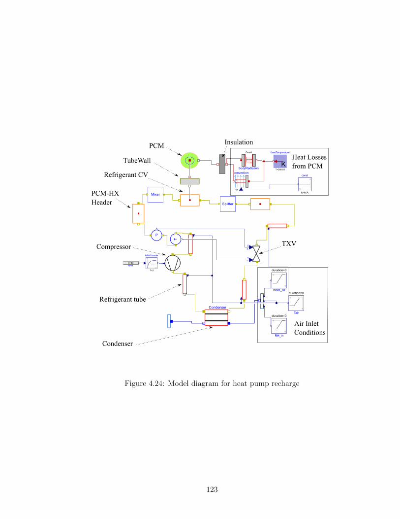
Figure 4.24: Model diagram for heat pump recharge

123

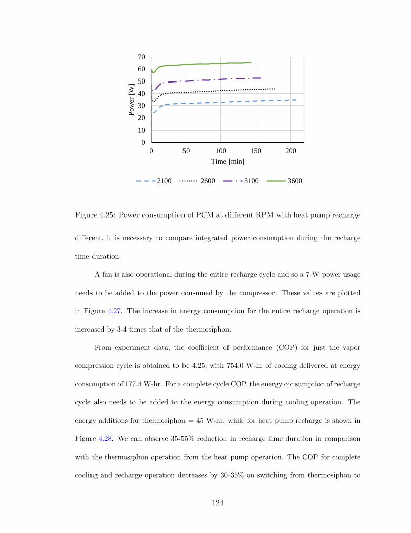
0

10

20

30

40

50

60

70

0 50 100 150 200

Po

wer

[W

]

Time [min]

2100 2600 3100 3600

Figure 4.25: Power consumption of PCM at different RPM with heat pump recharge

different, it is necessary to compare integrated power consumption during the recharge

time duration.

A fan is also operational during the entire recharge cycle and so a 7-W power usage

needs to be added to the power consumed by the compressor. These values are plotted

in Figure 4.27. The increase in energy consumption for the entire recharge operation is

increased by 3-4 times that of the thermosiphon.

From experiment data, the coefficient of performance (COP) for just the vapor

compression cycle is obtained to be 4.25, with 754.0 W-hr of cooling delivered at energy

consumption of 177.4 W-hr. For a complete cycle COP, the energy consumption of recharge

cycle also needs to be added to the energy consumption during cooling operation. The

energy additions for thermosiphon = 45 W-hr, while for heat pump recharge is shown in

Figure 4.28. We can observe 35-55% reduction in recharge time duration in comparison

with the thermosiphon operation from the heat pump operation. The COP for complete

cooling and recharge operation decreases by 30-35% on switching from thermosiphon to

124

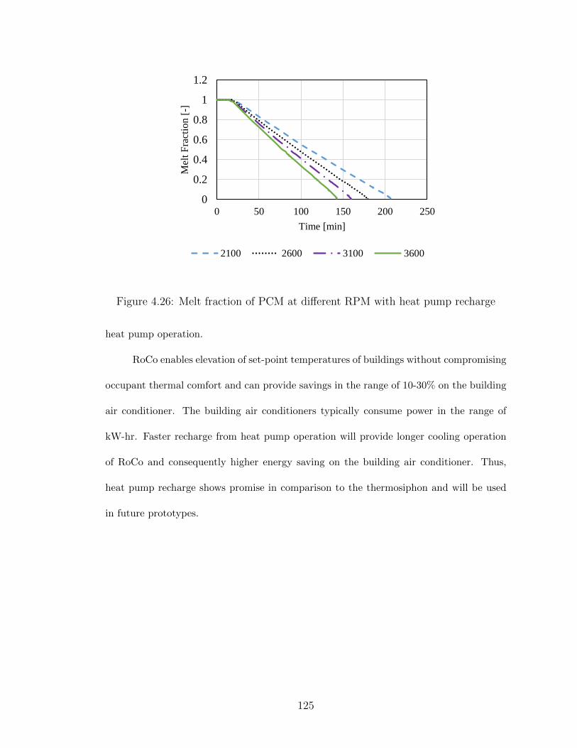
0

0.2

0.4

0.6

0.8

1

1.2

0 50 100 150 200 250

Mel

t F

ract

ion [

-]

Time [min]

2100 2600 3100 3600

Figure 4.26: Melt fraction of PCM at different RPM with heat pump recharge

heat pump operation.

RoCo enables elevation of set-point temperatures of buildings without compromising

occupant thermal comfort and can provide savings in the range of 10-30% on the building

air conditioner. The building air conditioners typically consume power in the range of

kW-hr. Faster recharge from heat pump operation will provide longer cooling operation

of RoCo and consequently higher energy saving on the building air conditioner. Thus,

heat pump recharge shows promise in comparison to the thermosiphon and will be used

in future prototypes.

125

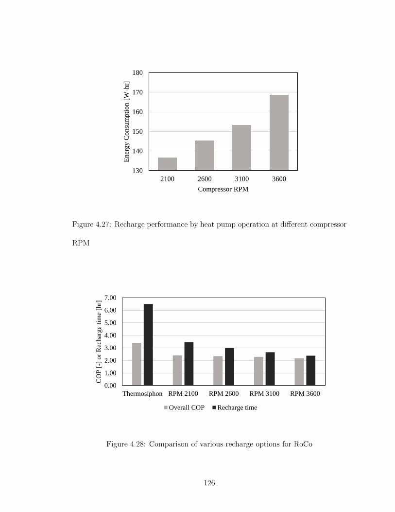
130

140

150

160

170

180

2100 2600 3100 3600

Ener

gy C

onsu

mp

tio

n [

W-h

r]

Compressor RPM

Figure 4.27: Recharge performance by heat pump operation at different compressor

RPM

0.00

1.00

2.00

3.00

4.00

5.00

6.00

7.00

Thermosiphon RPM 2100 RPM 2600 RPM 3100 RPM 3600

CO

P [

-] o

r R

echar

ge

tim

e [h

r]

Overall COP Recharge time

Figure 4.28: Comparison of various recharge options for RoCo

126

Chapter 5: Cyclic Losses in Vapor Compression System

5.1 Introduction

Previous chapters describe development of personal conditioning systems which have

the potential to reduce 10-30% of energy consumption by building HVAC. Further reduc-

tion in energy consumption can be achieved by improving the performance of the building

HVAC itself. Typically, building HVAC consists of a vapor compression system, which

operates cyclically. This cyclic behavior leads to losses in performance, which will be the

focus of the present chapter. A dynamic model of a conventional split-type air condi-

tioner is developed and validated with experiment data. Special attention is given to the

refrigerant migration occurring during the cyclic operation. The ANSI/AHRI Standard

210/240-2008 [32] specifies a cyclic D-Test, which is carried out with the air conditioner

for validation.

5.2 Modeling Vapor Compression System

The model diagram for the system simulation is shown in Figure 5.1. The basic

control volume equations are obtained from the CEEE Modelica Library developed by Qiao

(2014) [47]. To enable stable simulation for reversible and zero flows which are expected

during the cyclic operation, the components are updated to the Stream Connector on

127

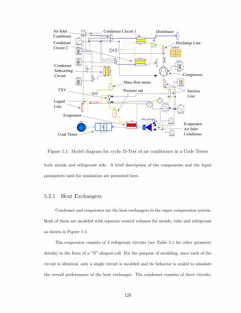
Figure 5.1: Model diagram for cyclic D-Test of air conditioner in a Code Tester

both airside and refrigerant side. A brief description of the components and the input

parameters used for simulation are presented here.

5.2.1 Heat Exchangers

Condenser and evaporator are the heat exchangers in the vapor compression system.

Both of them are modeled with separate control volumes for airside, tube and refrigerant

as shown in Figure 1.4.

The evaporator consists of 3 refrigerant circuits (see Table 5.1 for other geometry

details) in the form of a ”N”-shaped coil. For the purpose of modeling, since each of the

circuit is identical, only a single circuit is modeled and its behavior is scaled to simulate

the overall performance of the heat exchanger. The condenser consists of three circuits,

128

two with identical number of tubes and a third circuit with a different number of tubes (see

Table 5.2). Only one of the identical circuits is modeled and its performance parameters

are scaled by two to model the identical circuits. For the third circuit, a separate heat

exchanger model is used. The airside mass flow rate is distributed in the ratio of the

number of tubes in each circuit. A distributor model is used to divide the refrigerant

flow into these components as per their flow resistances. Finally, the refrigerant from

these three circuits, flows through a sub-cooling circuit, which is modeled by a separate

component. The detailed accounting of internal volume of the heat exchanger is required

to capture the refrigerant migration accurately. Geometry details of them are found in

Table 5.1 and 5.2.

Table 5.1: Evaporator geometry parameters

Parameter Unit Value

Tubes Per Row (Normal to Air Flow) - 36

Number Tube Rows (In the direction of Air Flow) - 2

Number of refrigerant circuits - 3

Total number of tubes - 72

Number of tubes per circuit - 24

Tube Length m 0.408

Tube Inner Diameter m 0.0083566

Tube Outer Diameter m 0.0100076

Fins per inch (FPI) in−1 16

Tube Material - Aluminum

Fin Material - Aluminum

129

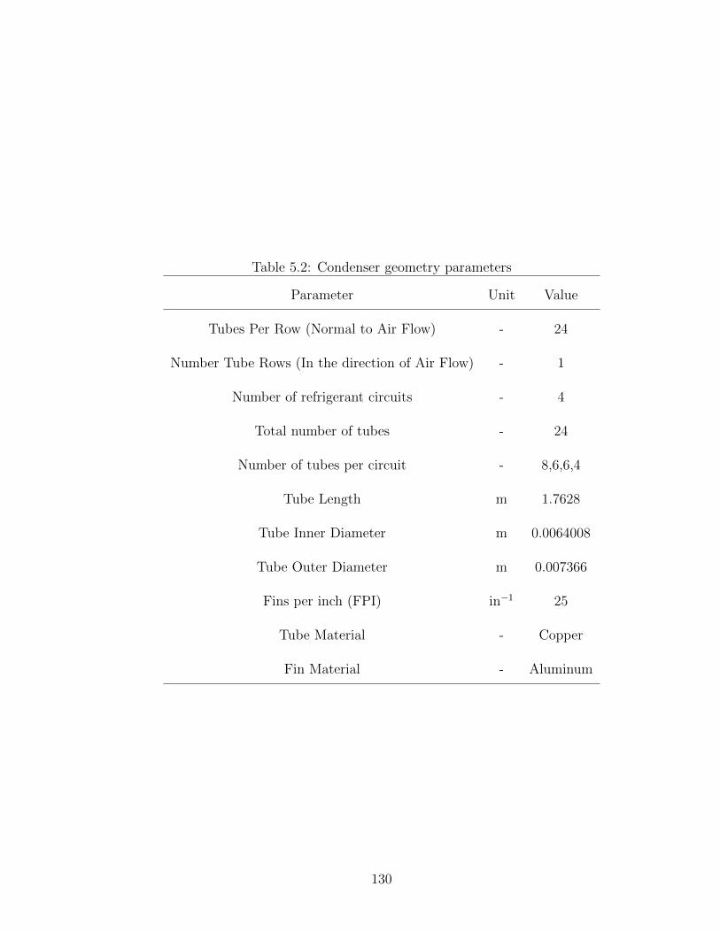
Table 5.2: Condenser geometry parameters

Parameter Unit Value

Tubes Per Row (Normal to Air Flow) - 24

Number Tube Rows (In the direction of Air Flow) - 1

Number of refrigerant circuits - 4

Total number of tubes - 24

Number of tubes per circuit - 8,6,6,4

Tube Length m 1.7628

Tube Inner Diameter m 0.0064008

Tube Outer Diameter m 0.007366

Fins per inch (FPI) in−1 25

Tube Material - Copper

Fin Material - Aluminum

130

5.2.1.1 Refrigerant Control Volume

A flow chart representing the calculations for the refrigerant side are shown in Fig-

ure 5.2. Pressure and density weighted enthalpy are used as state variables. Void fraction

based enthalpy correction is implemented to differentiate flow enthalpy from static en-

thalpy. Details of the calculations are presented in Laughman et al. (2015) [56]. Finally,

using state transformations (partial derivatives of density with respect to the state vari-

ables), the transient mass and energy storage terms are converted to partial derivatives

of state variables. These derivatives are used to calculate the values of the state variables

at the next time step. The process continues until the stop time of dynamic simulation is

reached.

Prediction of refrigerant charge in various portions of heat exchanger is best pre-

dicted by the Rouhani Axelsson correlation [218] with Steiner modification [219] as per

the observations from optical void fraction measurement by Wojtan et al. (2004) [220].

However, it is a drift-flux based model, depending of refrigerant mass flow rate. At zero

flow conditions, the model may produce division-by-zero errors. Slip-flow based void frac-

tion models are also plotted at the flow conditions, alongside homogeneous and Rouhani-

Axelsson with Steiner modification as shown in Figure 5.3. It can be observed that ho-

mogeneous void fraction model over-predicts void fraction significantly. Smith [221] and

Chisholm [222] correlations provide similar results as the Rouhani-Axelsson correlation.

Zivi correlation [223] has small under-prediction in regions of small flow quality, but it in-

volves much less thermo-physical property evaluations. This leads to a faster computation

time and is preferred for the present investigation.

Simulating vapor compression cycles at or near zero flow is challenging, due to the

131

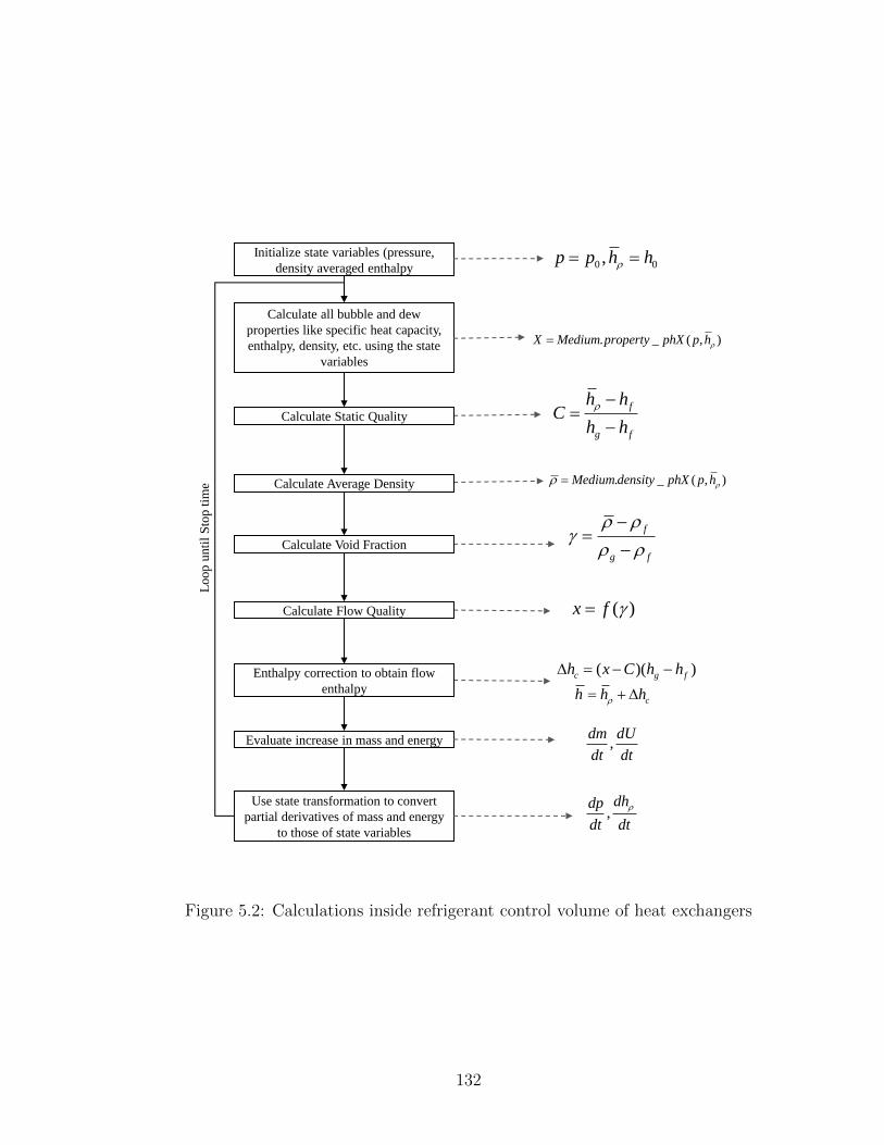
0 0,p p h h

f

g f

h hC

h h

( )x f

f

g f

. _ ( , )Medium density phX p h

( )( )c g fh x C h h

ch h h

Initialize state variables (pressure,

density averaged enthalpy

Calculate all bubble and dew

properties like specific heat capacity,

enthalpy, density, etc. using the state

variables

Calculate Static Quality

Calculate Average Density

Calculate Void Fraction

Calculate Flow Quality

Enthalpy correction to obtain flow

enthalpy

Evaluate increase in mass and energy

Use state transformation to convert

partial derivatives of mass and energy

to those of state variables

,dm dU

dt dt

,dhdp

dt dt

Lo

op

un

til

Sto

p t

ime

. _ ( , )X Medium property phX p h

Figure 5.2: Calculations inside refrigerant control volume of heat exchangers

132

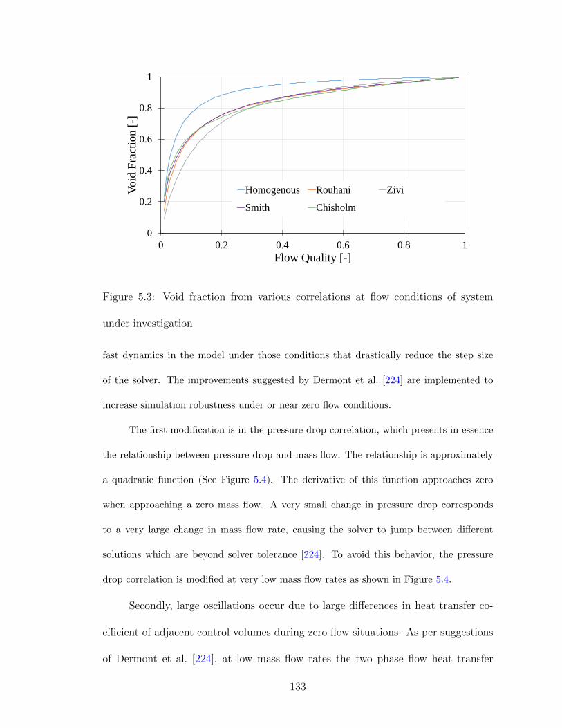
0

0.2

0.4

0.6

0.8

1

0 0.2 0.4 0.6 0.8 1

Void

Fra

ctio

n [

-]

Flow Quality [-]

Homogenous Rouhani Zivi

Smith Chisholm

Figure 5.3: Void fraction from various correlations at flow conditions of system

under investigation

fast dynamics in the model under those conditions that drastically reduce the step size

of the solver. The improvements suggested by Dermont et al. [224] are implemented to

increase simulation robustness under or near zero flow conditions.

The first modification is in the pressure drop correlation, which presents in essence

the relationship between pressure drop and mass flow. The relationship is approximately

a quadratic function (See Figure 5.4). The derivative of this function approaches zero

when approaching a zero mass flow. A very small change in pressure drop corresponds

to a very large change in mass flow rate, causing the solver to jump between different

solutions which are beyond solver tolerance [224]. To avoid this behavior, the pressure

drop correlation is modified at very low mass flow rates as shown in Figure 5.4.

Secondly, large oscillations occur due to large differences in heat transfer co-

efficient of adjacent control volumes during zero flow situations. As per suggestions

of Dermont et al. [224], at low mass flow rates the two phase flow heat transfer

133

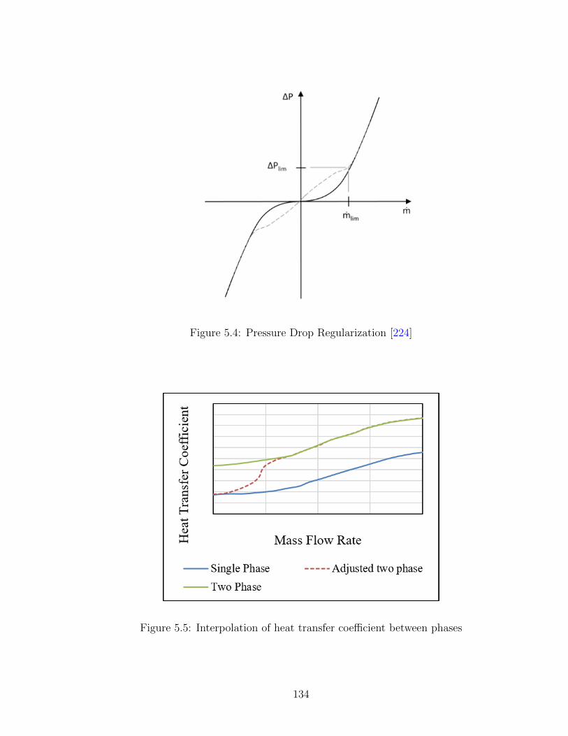
Figure 5.4: Pressure Drop Regularization [224]

Figure 5.5: Interpolation of heat transfer coefficient between phases

134

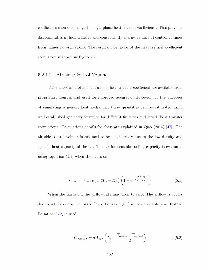
coefficients should converge to single phase heat transfer coefficients. This prevents

discontinuities in heat transfer and consequently energy balance of control volumes

from numerical oscillations. The resultant behavior of the heat transfer coefficient

correlation is shown in Figure 5.5.

5.2.1.2 Air side Control Volume

The surface area of fins and airside heat transfer coefficient are available from

proprietary sources and used for improved accuracy. However, for the purposes

of simulating a generic heat exchanger, these quantities can be estimated using

well established geometry formulae for different fin types and airside heat transfer

correlations. Calculations details for these are explained in Qiao (2014) [47]. The

air side control volume is assumed to be quasi-steady due to the low density and

specific heat capacity of the air. The airside sensible cooling capacity is evaluated

using Equation (5.1) when the fan is on.

Qsen,o = ˙maircp,air (Tw − Tair)(

1− e−αAeff˙maircp,air

)(5.1)

When the fan is off, the airflow rate may drop to zero. The airflow is occurs

due to natural convection based flows. Equation (5.1) is not applicable here. Instead

Equation (5.2) is used.

Qsen,off = αAeff

(Tw −

Tair,in − Tair,out2

)(5.2)

135

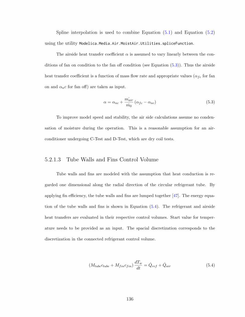
Spline interpolation is used to combine Equation (5.1) and Equation (5.2)

using the utility Modelica.Media.Air.MoistAir.Utilities.spliceFunction.

The airside heat transfer coefficient α is assumed to vary linearly between the con-

ditions of fan on condition to the fan off condition (see Equation (5.3)). Thus the airside

heat transfer coefficient is a function of mass flow rate and appropriate values (αfc for fan

on and αnc for fan off) are taken as input.

α = αnc +˙mair

m0(αfc − αnc) (5.3)

To improve model speed and stability, the air side calculations assume no conden-

sation of moisture during the operation. This is a reasonable assumption for an air-

conditioner undergoing C-Test and D-Test, which are dry coil tests.

5.2.1.3 Tube Walls and Fins Control Volume

Tube walls and fins are modeled with the assumption that heat conduction is re-

garded one dimensional along the radial direction of the circular refrigerant tube. By

applying fin efficiency, the tube walls and fins are lumped together [47]. The energy equa-

tion of the tube walls and fins is shown in Equation (5.4). The refrigerant and airside

heat transfers are evaluated in their respective control volumes. Start value for temper-

ature needs to be provided as an input. The spacial discretization corresponds to the

discretization in the connected refrigerant control volume.

(Mtubectube +Mfincfin)dTwdt

= Qref + Qair (5.4)

136

5.2.2 Compressor

Detailed geometry based compressor model is not a viable methodology for system

level simulation due to short timescale and relatively long simulation run time [225]. So

only the most important dynamics contributing to heat losses are modeled (see Figure 5.6).

Lumped control volumes for refrigerant flow in both suction and discharge are mod-

eled. TubeWall model is used to model the metal portion of the compressor. Motor

efficiency is provided as an input parameter and the heat generated by the losses in mo-

tor is transferred to the suction control volume. Heat losses by radiation and natural

convection from both top and lower shell of compressor are estimated. Conduction axial

conduction along the shell is not modeled. Motor is also assumed to transfer heat entirely

to the suction control volume and thus, heat losses from motor to ambient are neglected.

The refrigerant side heat transfer coefficient inside compression can be evaluated using

Dittus-Boelter correlation [215] as per suggestion by Bell et al.(2008) [226].

The refrigerant flow through the compressor as a function of its RPM is calculated

using Equation (5.5). During the off-cycle of the compressor, there may be a leakage

of refrigerant from the high-side to the low-side. At low mass flow rates, this flow is

expected to be laminar. A linear leakage model is implemented to be correctly able to

predict refrigerant migration through compressor during the off cycle using nominal values

of refrigerant flow for a nominal pressure drop (Equation 5.6). The total refrigerant flow

through the compressor is evaluated using Equation (5.7).

137

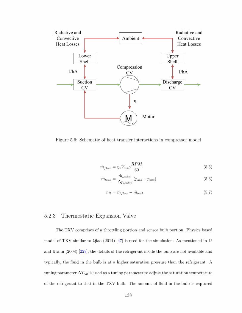
SuctionCV

LowerShell

DischargeCV

UpperShell

M

Ambient

CompressionCV

Motor

η

Radiative andConvectiveHeat Losses

Radiative andConvectiveHeat Losses

1/hA1/hA

Figure 5.6: Schematic of heat transfer interactions in compressor model

mflow = ηvVdisρRPM

60(5.5)

mleak =mleak,0

∆pleak,0(pdis − psuc) (5.6)

mt = mflow − mleak (5.7)

5.2.3 Thermostatic Expansion Valve

The TXV comprises of a throttling portion and sensor bulb portion. Physics based

model of TXV similar to Qiao (2014) [47] is used for the simulation. As mentioned in Li

and Braun (2008) [227], the details of the refrigerant inside the bulb are not available and

typically, the fluid in the bulb is at a higher saturation pressure than the refrigerant. A

tuning parameter ∆Tsat is used as a tuning parameter to adjust the saturation temperature

of the refrigerant to that in the TXV bulb. The amount of fluid in the bulb is captured

138

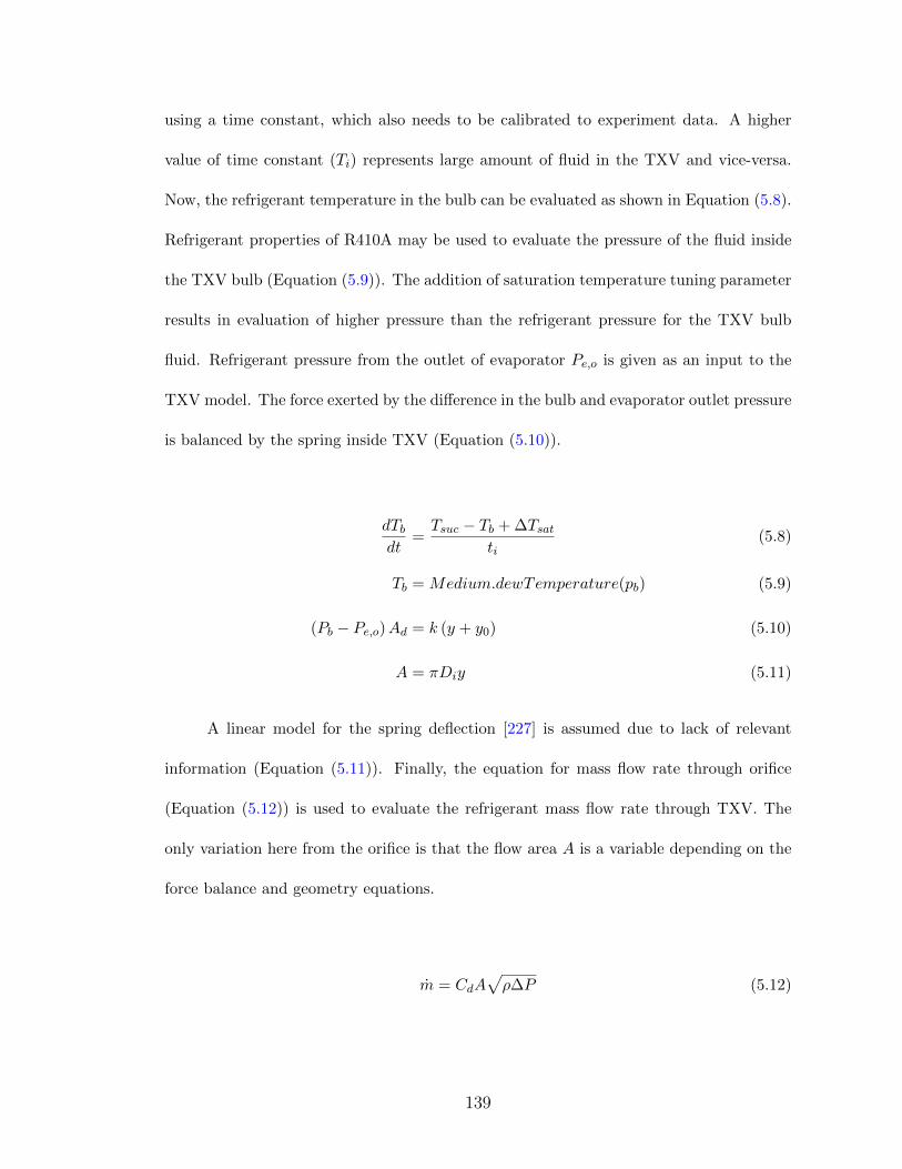
using a time constant, which also needs to be calibrated to experiment data. A higher

value of time constant (Ti) represents large amount of fluid in the TXV and vice-versa.

Now, the refrigerant temperature in the bulb can be evaluated as shown in Equation (5.8).

Refrigerant properties of R410A may be used to evaluate the pressure of the fluid inside

the TXV bulb (Equation (5.9)). The addition of saturation temperature tuning parameter

results in evaluation of higher pressure than the refrigerant pressure for the TXV bulb

fluid. Refrigerant pressure from the outlet of evaporator Pe,o is given as an input to the

TXV model. The force exerted by the difference in the bulb and evaporator outlet pressure

is balanced by the spring inside TXV (Equation (5.10)).

dTbdt

=Tsuc − Tb + ∆Tsat

ti(5.8)

Tb = Medium.dewTemperature(pb) (5.9)

(Pb − Pe,o)Ad = k (y + y0) (5.10)

A = πDiy (5.11)

A linear model for the spring deflection [227] is assumed due to lack of relevant

information (Equation (5.11)). Finally, the equation for mass flow rate through orifice

(Equation (5.12)) is used to evaluate the refrigerant mass flow rate through TXV. The

only variation here from the orifice is that the flow area A is a variable depending on the

force balance and geometry equations.

m = CdA√ρ∆P (5.12)

139

5.2.4 Refrigerant Lines

The refrigerant lines are important from the point of view of correctly predicting

the charge migration. The suction line is insulated, while the liquid line is not. Mod-

els accounting for both insulated and uninsulated refrigerant lines are modeled. The

non-insulated refrigerant line is modeled with similar control volume structure as the

heat exchanger (see Figure 1.4). However, the airside control volume is much sim-

plified and models just the heat transfer to ambient by natural convection using the

Modelica.Thermal.HeatTransfer.Components.Convection component. The airside heat

transfer coefficient is estimated through Churchill-Chu correlation for natural convection

from horizontal tube [228]. The insulated refrigerant line model consists of an additional

TubeWall model described in Section 5.2.1.3 for insulated foam alongside another for re-

frigerant tube.

Heat transfer coefficient is given as a fixed input parameter for the models. The

airside temperature for heat transfer needs to be provided as an input for these models.

For the refrigerant lines, present inside the indoor unit environment chamber, the airside

temperature of evaporator is given as the input temperature. Similarly, for the refrigerant

lines present inside the outdoor unit environment chamber, the outdoor unit temperature

is given as input. Portions of suction line and liquid line are present in both the rooms as

they connect the two heat exchangers. As a result, these refrigerant lines are divided to

account for accurate heat losses. The temperature at the inlet of compressor is measured

by using a surface thermocouple. A small portion of the refrigerant line is uninsulated

near the location of this thermocouple. As a result, this small portion is modeled using

the uninsulated refrigerant line model.

140

5.3 Code Tester

5.3.1 Background

Code tester is described in ASHRAE Standard 41.2 [154], which provides recom-

mended practices for airflow measurements. The test chamber is a generic name applied

to these devices, but code tester has also been used for many years. The code tester

(see Figure 5.7) consists of ducts for airflow passage from the test unit with pressure and

temperature being measured at various locations along the passage. Flow settling devices

(mixers) are placed in portions of the air duct to reduce the temperature gradient in the

airflow. Nozzles alongside calibrated correlations are used to determine the volume flow

rate of the air. A few dimensional constraints are applicable to their geometry. However,

due to a wide variety of possibilities from these constraints, the design of code testers at

different facilities are very different. There are also no guidelines on materials selected for

fabricating the code testers. These aspects lead to significant variations in the thermal

inertia effects for a tested unit in different code testers.

Split air conditioners (SPAC) are tested using separate environmental cham-

bers for both indoor unit (IDU) and outdoor unit (ODU) as shown in Figure 5.7.

The method used for calculating the cooling capacity is called the tunnel air en-

thalpy test. The code tester (labeled as airflow measuring apparatus in Figure 5.7

needs to be connected to only the IDU for the case of SPAC. A room conditioning

apparatus maintains the IDU chamber to a fixed temperature, which is measured by

the incoming thermocouple grid. The air flows over the IDU, where it gets cooled

if the SPAC is ON. The code tester includes a mixer, an outlet thermocouple grid,

141

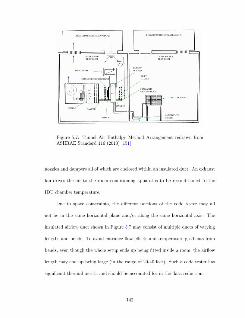
ROOM CONDITIONING APPARATUS ROOM CONDITIONING APPARATUS

INDOOR SIDE

TEST ROOM

OUTDOOR SIDE

TEST ROOM

MANOMETER

INLET

TC GRID

OUTLET

TC GRID

DAMPER

MIXER

INSULATED AIRFLOW DUCT

NOZZLE

OUTDOOR UNIT

LIQUID FLOW

METER

INSULATED

AIRFLOW DUCT

DAMPER

Figure 5.7: Tunnel Air Enthalpy Method Arrangement redrawn fromASHRAE Standard 116 (2010) [151]

nozzles and dampers all of which are enclosed within an insulated duct. An exhaust

fan drives the air to the room conditioning apparatus to be reconditioned to the

IDU chamber temperature.

Due to space constraints, the different portions of the code tester may all

not be in the same horizontal plane and/or along the same horizontal axis. The

insulated airflow duct shown in Figure 5.7 may consist of multiple ducts of varying

lengths and bends. To avoid entrance flow effects and temperature gradients from

bends, even though the whole setup ends up being fitted inside a room, the airflow

length may end up being large (in the range of 20-40 feet). Such a code tester has

significant thermal inertia and should be accounted for in the data reduction.

142

5.3.2 Model development

To correctly evaluate the outlet thermocouple grid temperature, the model

for code tester is also developed and connected to the model of evaporator. The

components for Code Tester are developed using the control volumes of Modelica

Buildings Library [229].

The code tester used for measuring the cyclic performance of the tested unit is

shown in Figure 5.8. Only a small portion of duct exists between the indoor unit and

the outlet thermocouple grid to reduce the influence of code tester thermal inertia

effects. An alternate proprietary code tester design, which is also used for in the

current investigation consists of much longer air flow passage between the indoor

unit and the outlet thermocouple grid.

This section describes the variety of components required for modeling the

Code Tester. The two types of components used for modeling any generic code

tester are Duct and Mixer. The object oriented nature of Modelica enables modeling

any generic code tester by providing appropriate input parameters to these components.

Typically, multiple duct components and a single mixer component will be required to

model the complete code tester. As shown in Figure 5.8, pipe1 and pipe2 are the regions

modeled using Duct. Details of the code tester shown in Figure 5.8 can be found in Qiu

(2018) [230].

Figure 5.9 shows the component model for Duct (on Left) and Mixer (on Right). The

ControlVolume and PressureDrop models are obtained from Buildings.Fluid.MixingVolumes.

MixingVolume and Buildings.Fluid.FixedResistances.PressureDrop, respectively.

ControlVolume represents an instantaneously mixed volume. Potential and kinetic

143

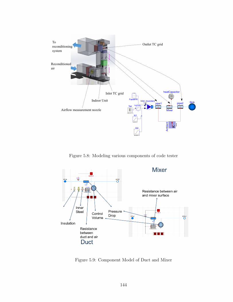
Figure 5.8: Modeling various components of code tester

Figure 5.9: Component Model of Duct and Mixer

144

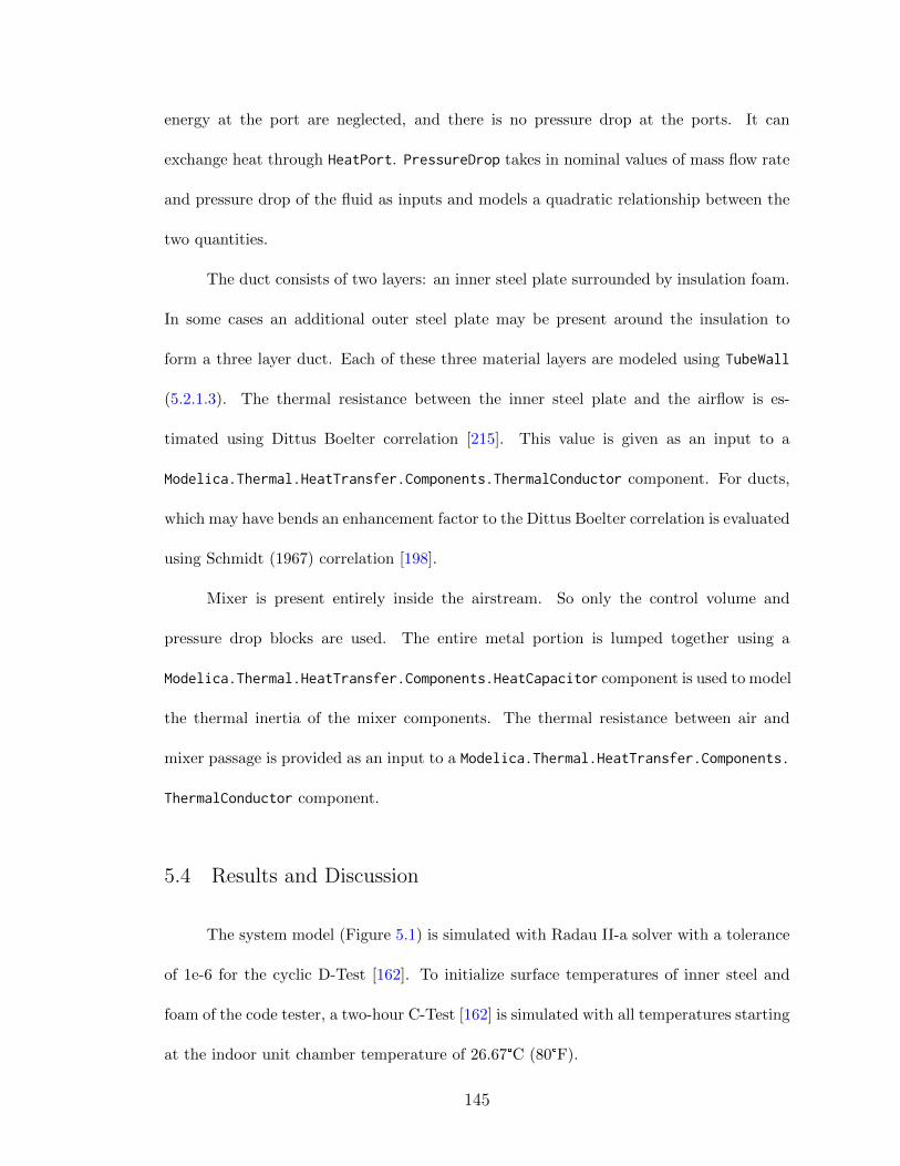
energy at the port are neglected, and there is no pressure drop at the ports. It can

exchange heat through HeatPort. PressureDrop takes in nominal values of mass flow rate

and pressure drop of the fluid as inputs and models a quadratic relationship between the

two quantities.

The duct consists of two layers: an inner steel plate surrounded by insulation foam.

In some cases an additional outer steel plate may be present around the insulation to

form a three layer duct. Each of these three material layers are modeled using TubeWall

(5.2.1.3). The thermal resistance between the inner steel plate and the airflow is es-

timated using Dittus Boelter correlation [215]. This value is given as an input to a

Modelica.Thermal.HeatTransfer.Components.ThermalConductor component. For ducts,

which may have bends an enhancement factor to the Dittus Boelter correlation is evaluated

using Schmidt (1967) correlation [198].

Mixer is present entirely inside the airstream. So only the control volume and

pressure drop blocks are used. The entire metal portion is lumped together using a

Modelica.Thermal.HeatTransfer.Components.HeatCapacitor component is used to model

the thermal inertia of the mixer components. The thermal resistance between air and

mixer passage is provided as an input to a Modelica.Thermal.HeatTransfer.Components.

ThermalConductor component.

5.4 Results and Discussion

The system model (Figure 5.1) is simulated with Radau II-a solver with a tolerance

of 1e-6 for the cyclic D-Test [162]. To initialize surface temperatures of inner steel and

foam of the code tester, a two-hour C-Test [162] is simulated with all temperatures starting

at the indoor unit chamber temperature of 26.67°C (80°F).

145

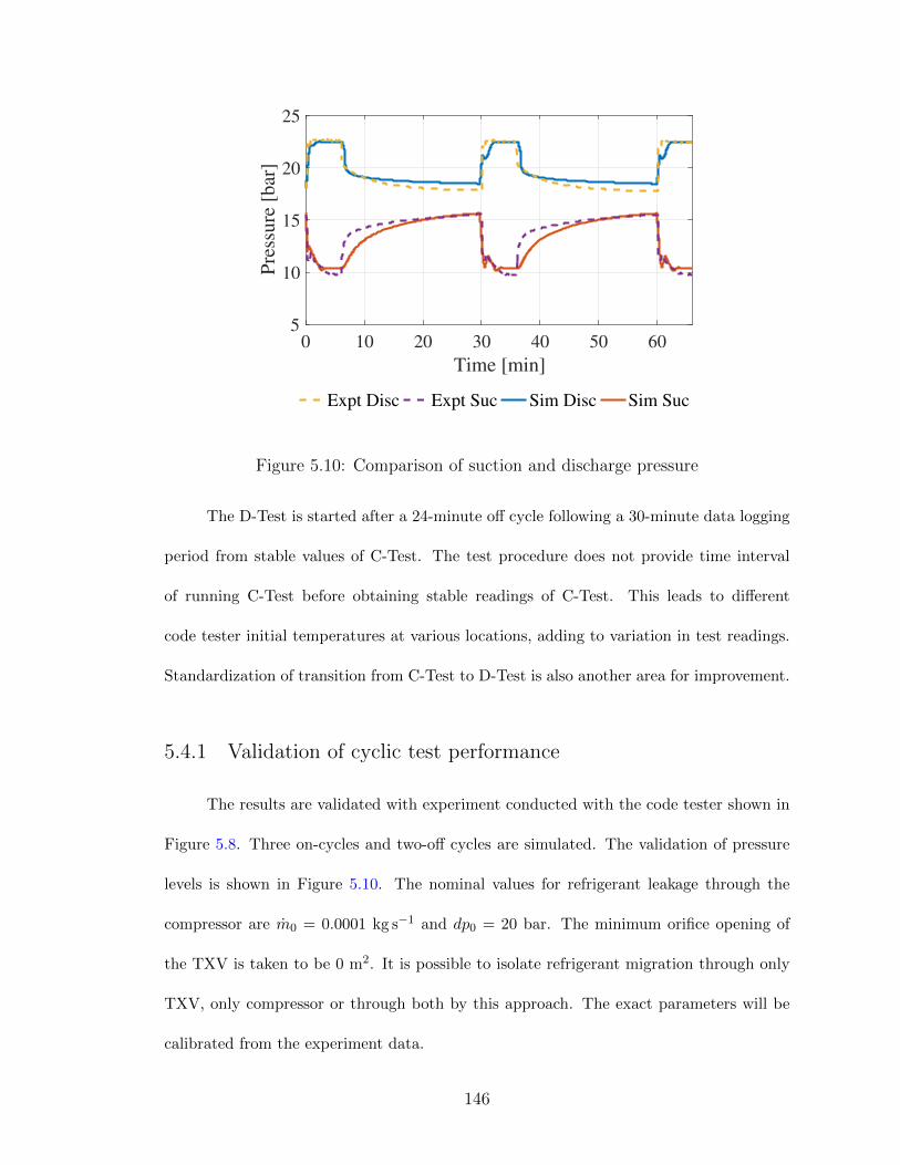
0 10 20 30 40 50 60

Time [min]

5

10

15

20

25

Pre

ssure

[bar

]

Expt Disc Expt Suc Sim Disc Sim Suc

Figure 5.10: Comparison of suction and discharge pressure

The D-Test is started after a 24-minute off cycle following a 30-minute data logging

period from stable values of C-Test. The test procedure does not provide time interval

of running C-Test before obtaining stable readings of C-Test. This leads to different

code tester initial temperatures at various locations, adding to variation in test readings.

Standardization of transition from C-Test to D-Test is also another area for improvement.

5.4.1 Validation of cyclic test performance

The results are validated with experiment conducted with the code tester shown in

Figure 5.8. Three on-cycles and two-off cycles are simulated. The validation of pressure

levels is shown in Figure 5.10. The nominal values for refrigerant leakage through the

compressor are m0 = 0.0001 kg s−1 and dp0 = 20 bar. The minimum orifice opening of

the TXV is taken to be 0 m2. It is possible to isolate refrigerant migration through only

TXV, only compressor or through both by this approach. The exact parameters will be

calibrated from the experiment data.

146

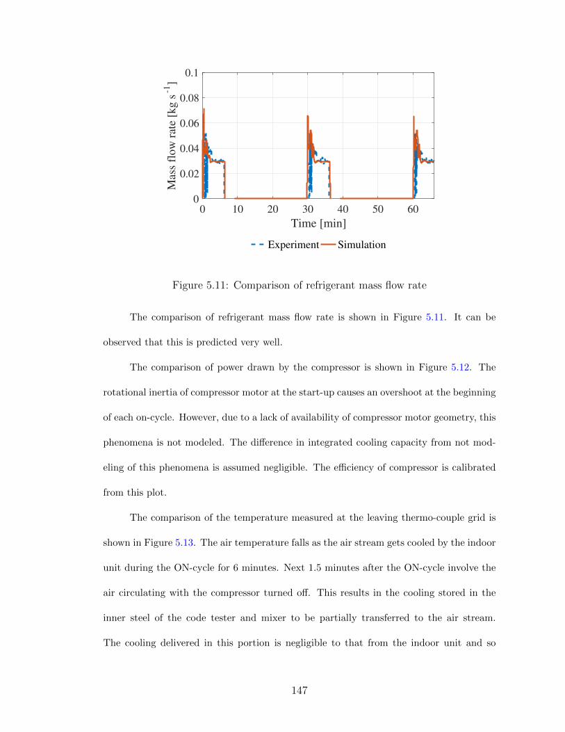
0 10 20 30 40 50 60

Time [min]

0

0.02

0.04

0.06

0.08

0.1

Mas

s fl

ow

rat

e [k

g s

-1]

Experiment Simulation

Figure 5.11: Comparison of refrigerant mass flow rate

The comparison of refrigerant mass flow rate is shown in Figure 5.11. It can be

observed that this is predicted very well.

The comparison of power drawn by the compressor is shown in Figure 5.12. The

rotational inertia of compressor motor at the start-up causes an overshoot at the beginning

of each on-cycle. However, due to a lack of availability of compressor motor geometry, this

phenomena is not modeled. The difference in integrated cooling capacity from not mod-

eling of this phenomena is assumed negligible. The efficiency of compressor is calibrated

from this plot.

The comparison of the temperature measured at the leaving thermo-couple grid is

shown in Figure 5.13. The air temperature falls as the air stream gets cooled by the indoor

unit during the ON-cycle for 6 minutes. Next 1.5 minutes after the ON-cycle involve the

air circulating with the compressor turned off. This results in the cooling stored in the

inner steel of the code tester and mixer to be partially transferred to the air stream.

The cooling delivered in this portion is negligible to that from the indoor unit and so

147

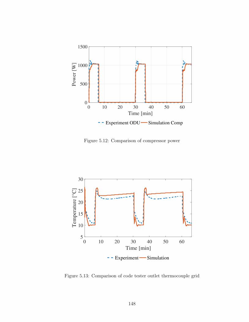
0 10 20 30 40 50 60

Time [min]

0

500

1000

1500

Po

wer

[W

]

Experiment ODU Simulation Comp

Figure 5.12: Comparison of compressor power

0 10 20 30 40 50 60

Time [min]

5

10

15

20

25

30

Tem

per

ature

[°C

]

Experiment Simulation

Figure 5.13: Comparison of code tester outlet thermocouple grid

148

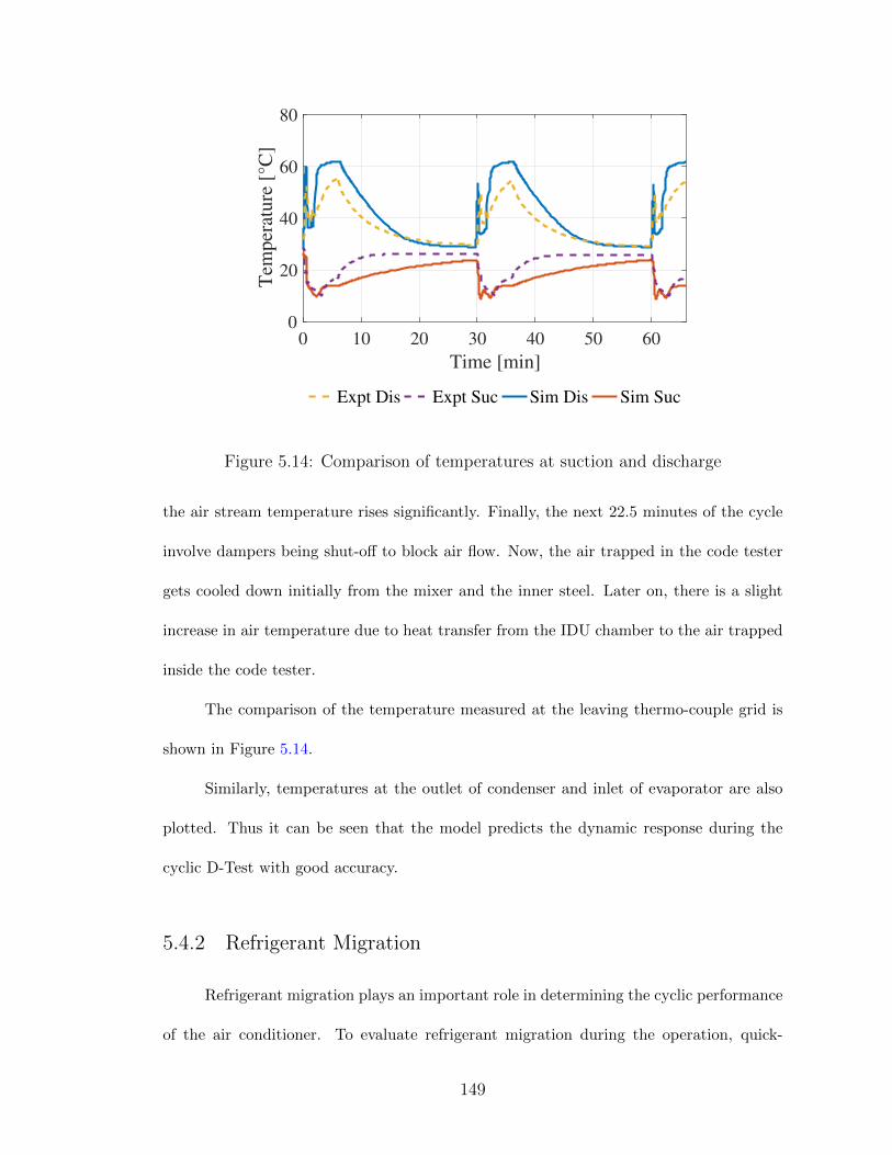
0 10 20 30 40 50 60

Time [min]

0

20

40

60

80

Tem

per

ature

[°C

]

Expt Dis Expt Suc Sim Dis Sim Suc

Figure 5.14: Comparison of temperatures at suction and discharge

the air stream temperature rises significantly. Finally, the next 22.5 minutes of the cycle

involve dampers being shut-off to block air flow. Now, the air trapped in the code tester

gets cooled down initially from the mixer and the inner steel. Later on, there is a slight

increase in air temperature due to heat transfer from the IDU chamber to the air trapped

inside the code tester.

The comparison of the temperature measured at the leaving thermo-couple grid is

shown in Figure 5.14.

Similarly, temperatures at the outlet of condenser and inlet of evaporator are also

plotted. Thus it can be seen that the model predicts the dynamic response during the

cyclic D-Test with good accuracy.

5.4.2 Refrigerant Migration

Refrigerant migration plays an important role in determining the cyclic performance

of the air conditioner. To evaluate refrigerant migration during the operation, quick-

149

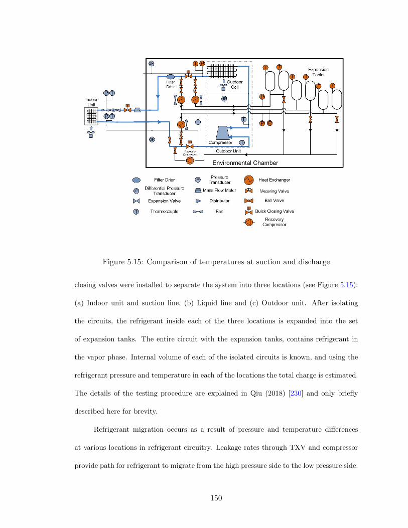
Figure 5.15: Comparison of temperatures at suction and discharge

closing valves were installed to separate the system into three locations (see Figure 5.15):

(a) Indoor unit and suction line, (b) Liquid line and (c) Outdoor unit. After isolating

the circuits, the refrigerant inside each of the three locations is expanded into the set

of expansion tanks. The entire circuit with the expansion tanks, contains refrigerant in

the vapor phase. Internal volume of each of the isolated circuits is known, and using the

refrigerant pressure and temperature in each of the locations the total charge is estimated.

The details of the testing procedure are explained in Qiu (2018) [230] and only briefly

described here for brevity.

Refrigerant migration occurs as a result of pressure and temperature differences

at various locations in refrigerant circuitry. Leakage rates through TXV and compressor

provide path for refrigerant to migrate from the high pressure side to the low pressure side.

150

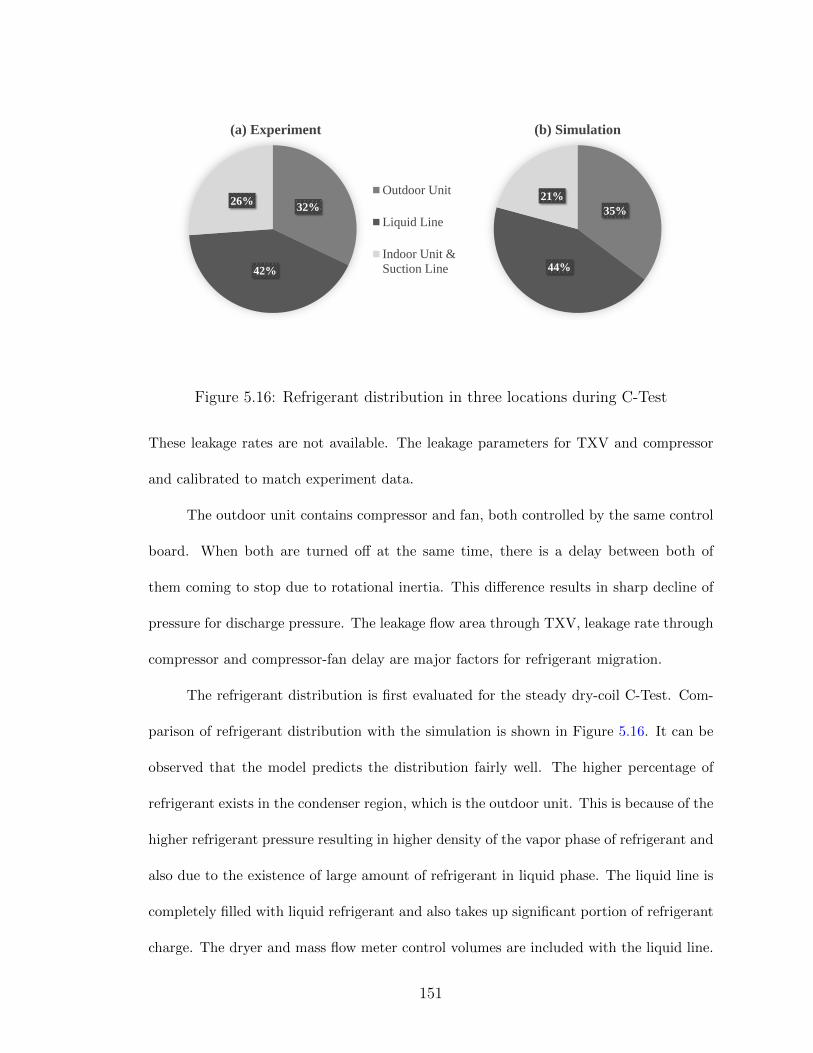
32%

42%

26%

(a) Experiment

Outdoor Unit

Liquid Line

Indoor Unit &

Suction Line

35%

44%

21%

(b) Simulation

Figure 5.16: Refrigerant distribution in three locations during C-Test

These leakage rates are not available. The leakage parameters for TXV and compressor

and calibrated to match experiment data.

The outdoor unit contains compressor and fan, both controlled by the same control

board. When both are turned off at the same time, there is a delay between both of

them coming to stop due to rotational inertia. This difference results in sharp decline of

pressure for discharge pressure. The leakage flow area through TXV, leakage rate through

compressor and compressor-fan delay are major factors for refrigerant migration.

The refrigerant distribution is first evaluated for the steady dry-coil C-Test. Com-

parison of refrigerant distribution with the simulation is shown in Figure 5.16. It can be

observed that the model predicts the distribution fairly well. The higher percentage of

refrigerant exists in the condenser region, which is the outdoor unit. This is because of the

higher refrigerant pressure resulting in higher density of the vapor phase of refrigerant and

also due to the existence of large amount of refrigerant in liquid phase. The liquid line is

completely filled with liquid refrigerant and also takes up significant portion of refrigerant

charge. The dryer and mass flow meter control volumes are included with the liquid line.

151

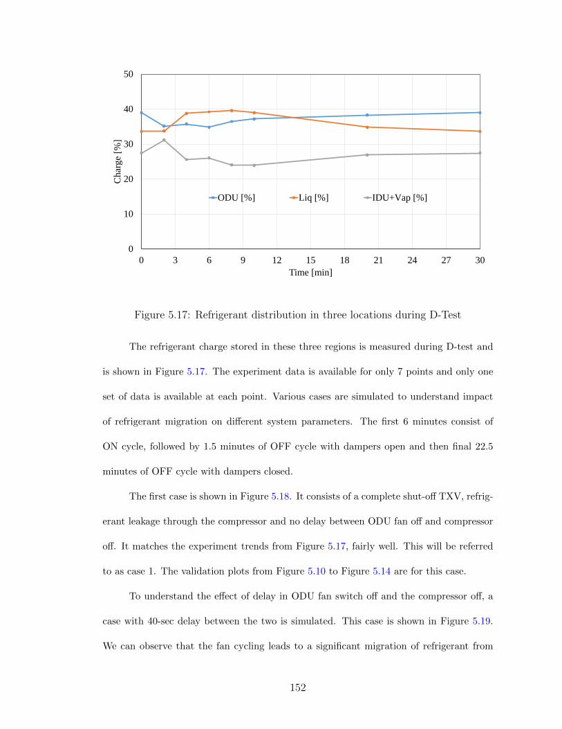
0

10

20

30

40

50

0 3 6 9 12 15 18 21 24 27 30

Char

ge

[%]

Time [min]

ODU [%] Liq [%] IDU+Vap [%]

Figure 5.17: Refrigerant distribution in three locations during D-Test

The refrigerant charge stored in these three regions is measured during D-test and

is shown in Figure 5.17. The experiment data is available for only 7 points and only one

set of data is available at each point. Various cases are simulated to understand impact

of refrigerant migration on different system parameters. The first 6 minutes consist of

ON cycle, followed by 1.5 minutes of OFF cycle with dampers open and then final 22.5

minutes of OFF cycle with dampers closed.

The first case is shown in Figure 5.18. It consists of a complete shut-off TXV, refrig-

erant leakage through the compressor and no delay between ODU fan off and compressor

off. It matches the experiment trends from Figure 5.17, fairly well. This will be referred

to as case 1. The validation plots from Figure 5.10 to Figure 5.14 are for this case.

To understand the effect of delay in ODU fan switch off and the compressor off, a

case with 40-sec delay between the two is simulated. This case is shown in Figure 5.19.

We can observe that the fan cycling leads to a significant migration of refrigerant from

152

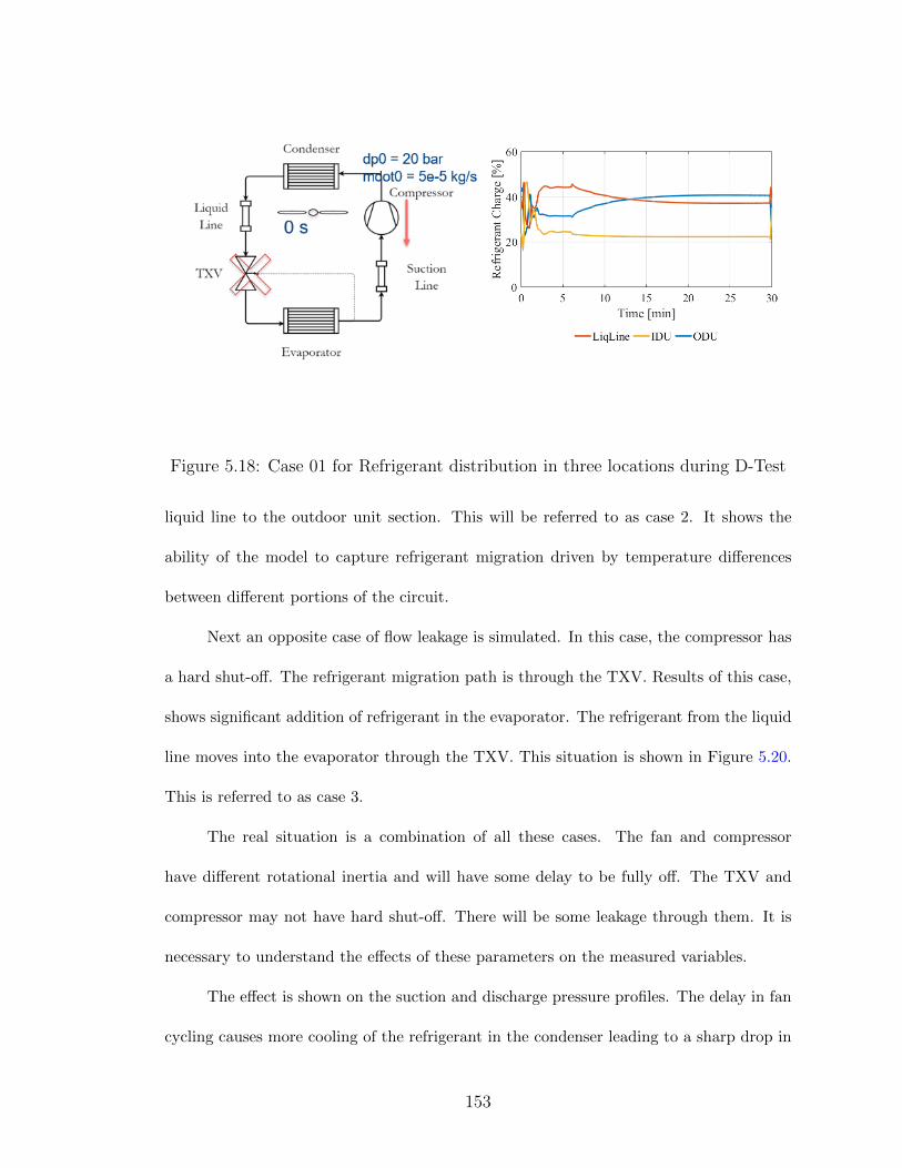
Figure 5.18: Case 01 for Refrigerant distribution in three locations during D-Test

liquid line to the outdoor unit section. This will be referred to as case 2. It shows the

ability of the model to capture refrigerant migration driven by temperature differences

between different portions of the circuit.

Next an opposite case of flow leakage is simulated. In this case, the compressor has

a hard shut-off. The refrigerant migration path is through the TXV. Results of this case,

shows significant addition of refrigerant in the evaporator. The refrigerant from the liquid

line moves into the evaporator through the TXV. This situation is shown in Figure 5.20.

This is referred to as case 3.

The real situation is a combination of all these cases. The fan and compressor

have different rotational inertia and will have some delay to be fully off. The TXV and

compressor may not have hard shut-off. There will be some leakage through them. It is

necessary to understand the effects of these parameters on the measured variables.

The effect is shown on the suction and discharge pressure profiles. The delay in fan

cycling causes more cooling of the refrigerant in the condenser leading to a sharp drop in

153

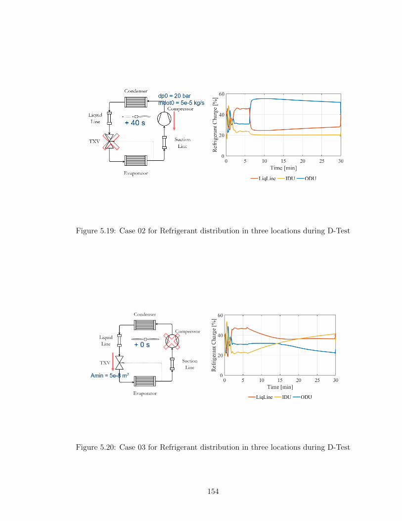
Figure 5.19: Case 02 for Refrigerant distribution in three locations during D-Test

Figure 5.20: Case 03 for Refrigerant distribution in three locations during D-Test

154

discharge pressure. Having no delay leads to a much slower decline in discharge pressure

at the onset of OFF cycle. The leakage through TXV causes rapid increase in suction

pressure at the onset of the OFF cycle. The leakage rate through TXV in the model

depends upon the flow area during the off cycle. This parameter is to be provided as an

input and calibrated to match pressure profiles.

The cyclic degradation coefficient is evaluated for cases 1 and 3. The parameters

used in evaluation for Cd are are within 4% of experiment data. However, due to the

mathematical form of Cd equation, the deviation of estimated Cd is 36% from experiment

data. We can however observe that even in the case of high migration, the Cd values

evaluated are similar. This observation is in line with experimental testing. The pressure

equalization (low pressure difference across the TXV when the system is off) does not

have much impact on Cd, if no extra two-phase refrigerant flow from the evaporator exit

is caused during the start-up.

155

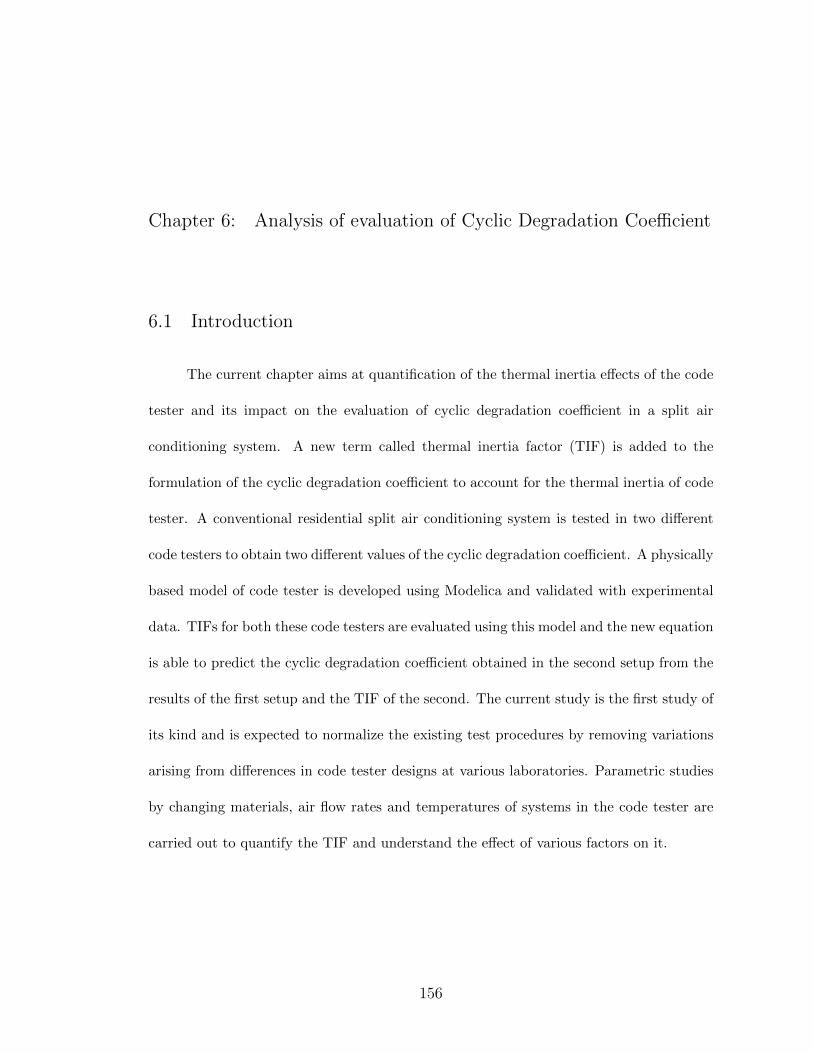
Chapter 6: Analysis of evaluation of Cyclic Degradation Coefficient

6.1 Introduction

The current chapter aims at quantification of the thermal inertia effects of the code

tester and its impact on the evaluation of cyclic degradation coefficient in a split air

conditioning system. A new term called thermal inertia factor (TIF) is added to the

formulation of the cyclic degradation coefficient to account for the thermal inertia of code

tester. A conventional residential split air conditioning system is tested in two different

code testers to obtain two different values of the cyclic degradation coefficient. A physically

based model of code tester is developed using Modelica and validated with experimental

data. TIFs for both these code testers are evaluated using this model and the new equation

is able to predict the cyclic degradation coefficient obtained in the second setup from the

results of the first setup and the TIF of the second. The current study is the first study of

its kind and is expected to normalize the existing test procedures by removing variations

arising from differences in code tester designs at various laboratories. Parametric studies

by changing materials, air flow rates and temperatures of systems in the code tester are

carried out to quantify the TIF and understand the effect of various factors on it.

156

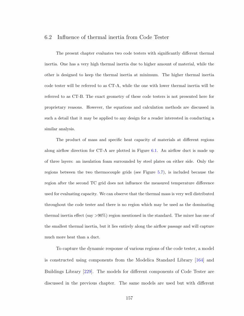
6.2 Influence of thermal inertia from Code Tester

The present chapter evaluates two code testers with significantly different thermal

inertia. One has a very high thermal inertia due to higher amount of material, while the

other is designed to keep the thermal inertia at minimum. The higher thermal inertia

code tester will be referred to as CT-A, while the one with lower thermal inertia will be

referred to as CT-B. The exact geometry of these code testers is not presented here for

proprietary reasons. However, the equations and calculation methods are discussed in

such a detail that it may be applied to any design for a reader interested in conducting a

similar analysis.

The product of mass and specific heat capacity of materials at different regions

along airflow direction for CT-A are plotted in Figure 6.1. An airflow duct is made up

of three layers: an insulation foam surrounded by steel plates on either side. Only the

regions between the two thermocouple grids (see Figure 5.7), is included because the

region after the second TC grid does not influence the measured temperature difference

used for evaluating capacity. We can observe that the thermal mass is very well distributed

throughout the code tester and there is no region which may be used as the dominating

thermal inertia effect (say >90%) region mentioned in the standard. The mixer has one of

the smallest thermal inertia, but it lies entirely along the airflow passage and will capture

much more heat than a duct.

To capture the dynamic response of various regions of the code tester, a model

is constructed using components from the Modelica Standard Library [164] and

Buildings Library [229]. The models for different components of Code Tester are

discussed in the previous chapter. The same models are used but with different

157

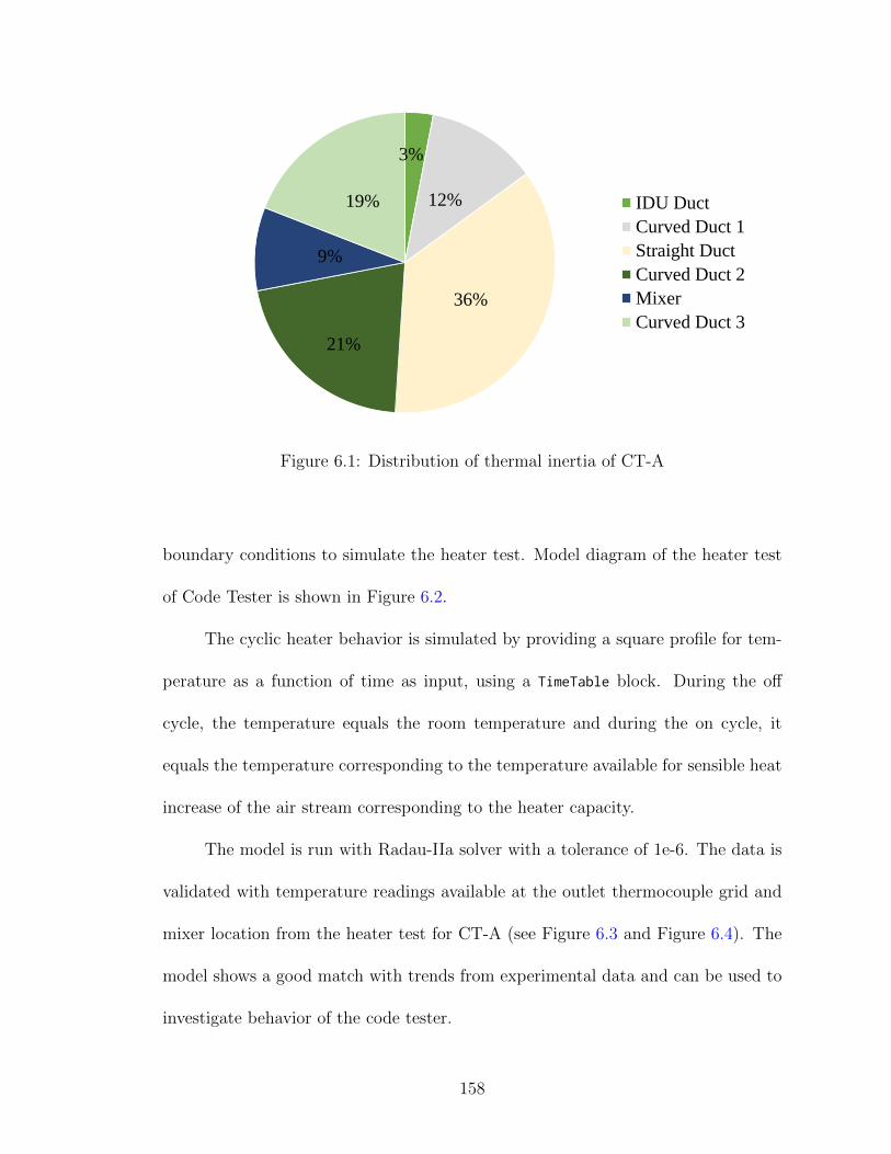
3%

12%

36%

21%

9%

19% IDU Duct

Curved Duct 1

Straight Duct

Curved Duct 2

Mixer

Curved Duct 3

Figure 6.1: Distribution of thermal inertia of CT-A

boundary conditions to simulate the heater test. Model diagram of the heater test

of Code Tester is shown in Figure 6.2.

The cyclic heater behavior is simulated by providing a square profile for tem-

perature as a function of time as input, using a TimeTable block. During the off

cycle, the temperature equals the room temperature and during the on cycle, it

equals the temperature corresponding to the temperature available for sensible heat

increase of the air stream corresponding to the heater capacity.

The model is run with Radau-IIa solver with a tolerance of 1e-6. The data is

validated with temperature readings available at the outlet thermocouple grid and

mixer location from the heater test for CT-A (see Figure 6.3 and Figure 6.4). The

model shows a good match with trends from experimental data and can be used to

investigate behavior of the code tester.

158

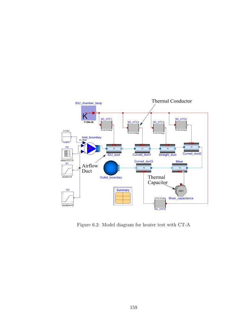
Figure 6.2: Model diagram for heater test with CT-A

159

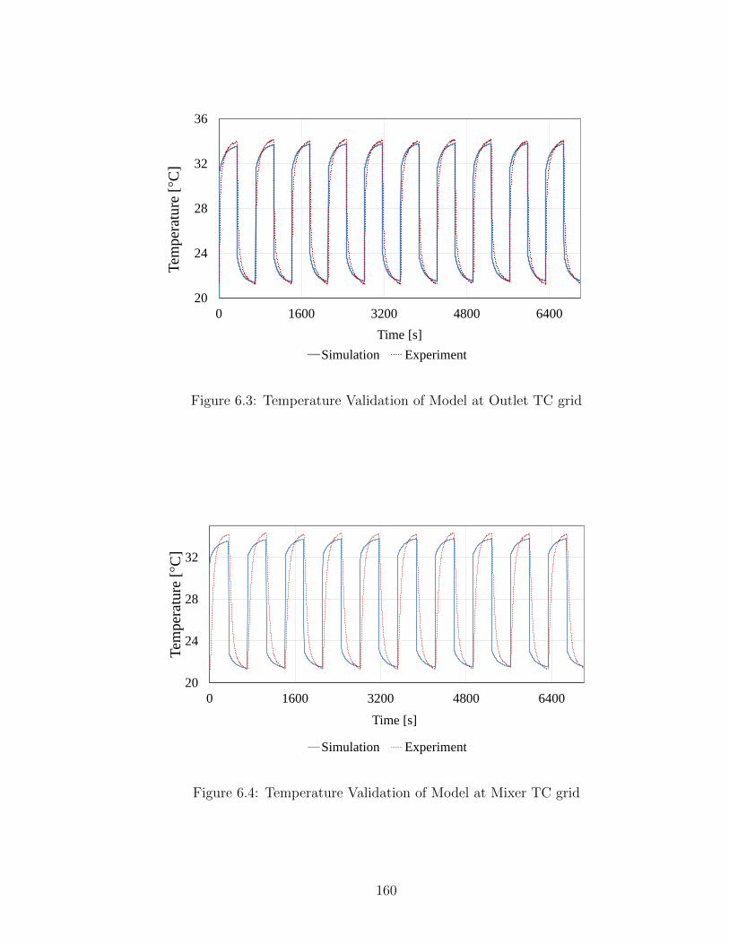
20

24

28

32

36

0 1600 3200 4800 6400

Tem

per

ature

[°C

]

Time [s]

Simulation Experiment

Figure 6.3: Temperature Validation of Model at Outlet TC grid

20

24

28

32

0 1600 3200 4800 6400

Tem

per

ature

[°C

]

Time [s]

Simulation Experiment

Figure 6.4: Temperature Validation of Model at Mixer TC grid

160

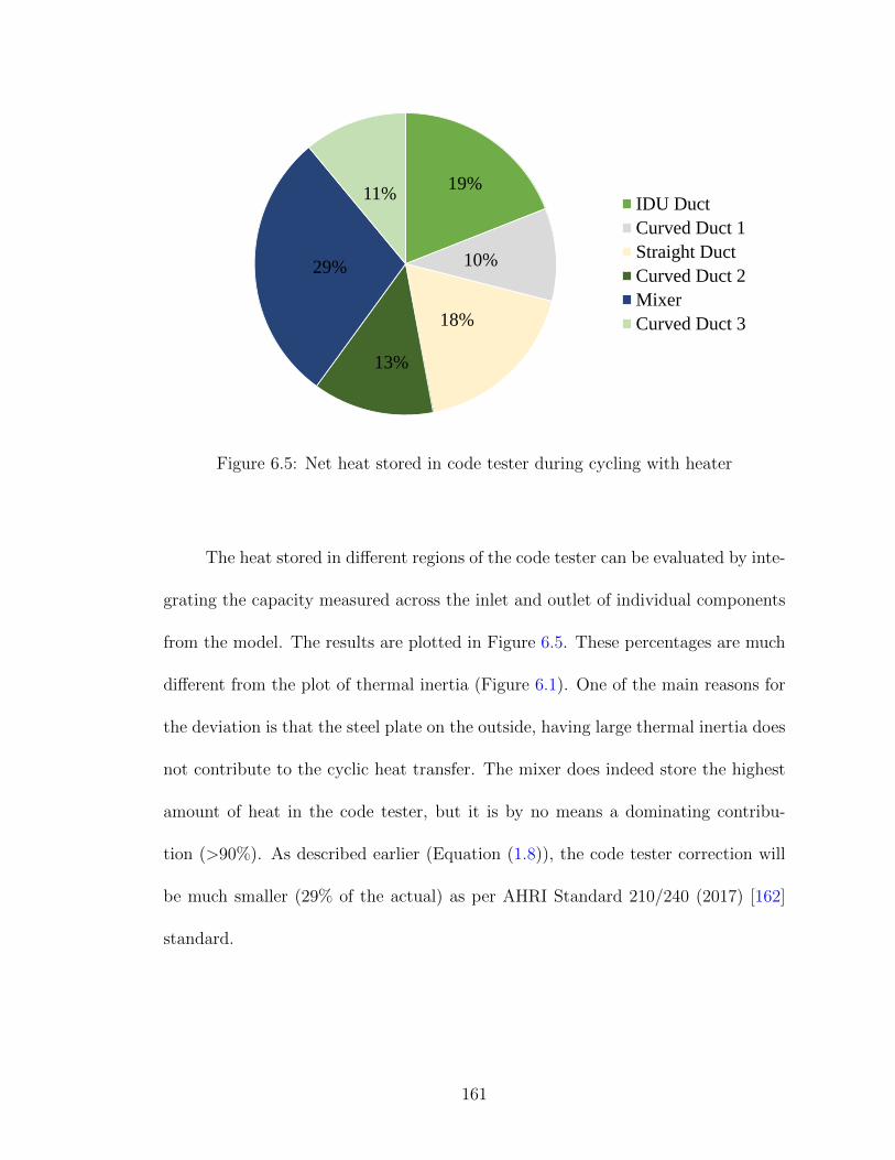
19%

10%

18%

13%

29%

11%IDU Duct

Curved Duct 1

Straight Duct

Curved Duct 2

Mixer

Curved Duct 3

Figure 6.5: Net heat stored in code tester during cycling with heater

The heat stored in different regions of the code tester can be evaluated by inte-

grating the capacity measured across the inlet and outlet of individual components

from the model. The results are plotted in Figure 6.5. These percentages are much

different from the plot of thermal inertia (Figure 6.1). One of the main reasons for

the deviation is that the steel plate on the outside, having large thermal inertia does

not contribute to the cyclic heat transfer. The mixer does indeed store the highest

amount of heat in the code tester, but it is by no means a dominating contribu-

tion (>90%). As described earlier (Equation (1.8)), the code tester correction will

be much smaller (29% of the actual) as per AHRI Standard 210/240 (2017) [162]

standard.

161

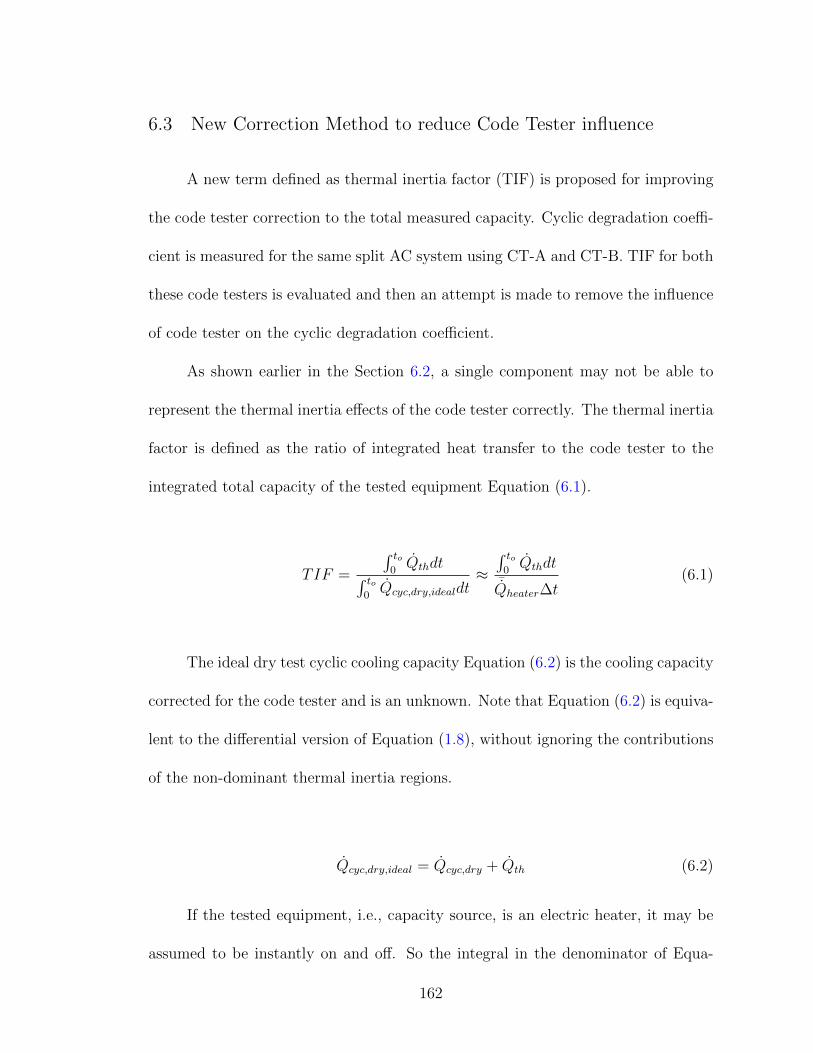
6.3 New Correction Method to reduce Code Tester influence

A new term defined as thermal inertia factor (TIF) is proposed for improving

the code tester correction to the total measured capacity. Cyclic degradation coeffi-

cient is measured for the same split AC system using CT-A and CT-B. TIF for both

these code testers is evaluated and then an attempt is made to remove the influence

of code tester on the cyclic degradation coefficient.

As shown earlier in the Section 6.2, a single component may not be able to

represent the thermal inertia effects of the code tester correctly. The thermal inertia

factor is defined as the ratio of integrated heat transfer to the code tester to the

integrated total capacity of the tested equipment Equation (6.1).

TIF =

∫ to0Qthdt∫ to

0Qcyc,dry,idealdt

≈∫ to

0Qthdt

¯Qheater∆t(6.1)

The ideal dry test cyclic cooling capacity Equation (6.2) is the cooling capacity

corrected for the code tester and is an unknown. Note that Equation (6.2) is equiva-

lent to the differential version of Equation (1.8), without ignoring the contributions

of the non-dominant thermal inertia regions.

Qcyc,dry,ideal = Qcyc,dry + Qth (6.2)

If the tested equipment, i.e., capacity source, is an electric heater, it may be

assumed to be instantly on and off. So the integral in the denominator of Equa-

162

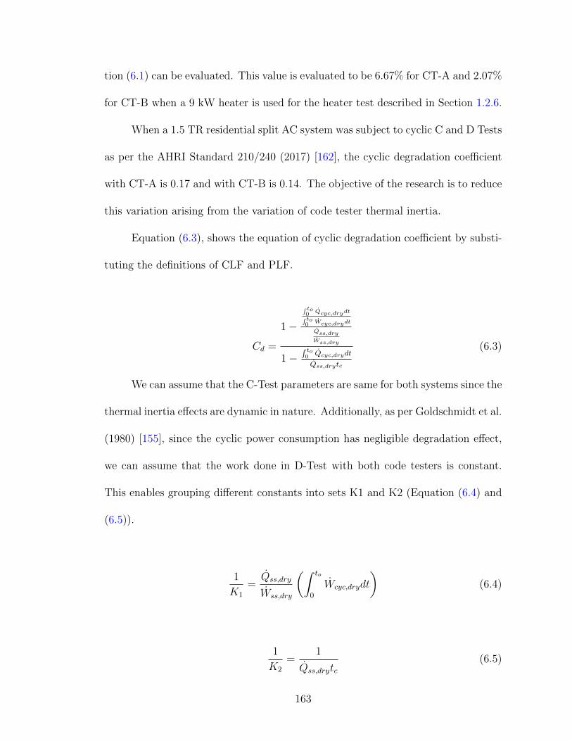
tion (6.1) can be evaluated. This value is evaluated to be 6.67% for CT-A and 2.07%

for CT-B when a 9 kW heater is used for the heater test described in Section 1.2.6.

When a 1.5 TR residential split AC system was subject to cyclic C and D Tests

as per the AHRI Standard 210/240 (2017) [162], the cyclic degradation coefficient

with CT-A is 0.17 and with CT-B is 0.14. The objective of the research is to reduce

this variation arising from the variation of code tester thermal inertia.

Equation (6.3), shows the equation of cyclic degradation coefficient by substi-

tuting the definitions of CLF and PLF.

Cd =

1−

∫ to0 Qcyc,drydt∫ to0 Wcyc,drydt

Qss,dry

Wss,dry

1−∫ to0 Qcyc,drydt

Qss,drytc

(6.3)

We can assume that the C-Test parameters are same for both systems since the

thermal inertia effects are dynamic in nature. Additionally, as per Goldschmidt et al.

(1980) [155], since the cyclic power consumption has negligible degradation effect,

we can assume that the work done in D-Test with both code testers is constant.

This enables grouping different constants into sets K1 and K2 (Equation (6.4) and

(6.5)).

1

K1

=Qss,dry

Wss,dry

(∫ to

0

Wcyc,drydt

)(6.4)

1

K2

=1

Qss,drytc(6.5)

163

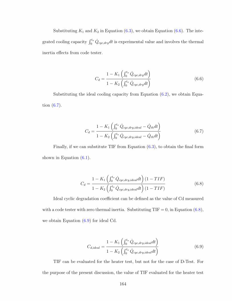
Substituting K1 and K2 in Equation (6.3), we obtain Equation (6.6). The inte-

grated cooling capacity∫ to

0Qcyc,drydt is experimental value and involves the thermal

inertia effects from code tester.

Cd =1−K1

(∫ to0Qcyc,drydt

)1−K2

(∫ to0Qcyc,drydt

) (6.6)

Substituting the ideal cooling capacity from Equation (6.2), we obtain Equa-

tion (6.7).

Cd =1−K1

(∫ to0Qcyc,dry,ideal − Qthdt

)1−K2

(∫ to0Qcyc,dry,ideal − Qthdt

) (6.7)

Finally, if we can substitute TIF from Equation (6.3), to obtain the final form

shown in Equation (6.1).

Cd =1−K1

(∫ to0Qcyc,dry,idealdt

)(1− TIF )

1−K2

(∫ to0Qcyc,dry,idealdt

)(1− TIF )

(6.8)

Ideal cyclic degradation coefficient can be defined as the value of Cd measured

with a code tester with zero thermal inertia. Substituting TIF = 0, in Equation (6.8),

we obtain Equation (6.9) for ideal Cd.

Cd,ideal =1−K1

(∫ to0Qcyc,dry,idealdt

)1−K2

(∫ to0Qcyc,dry,idealdt

) (6.9)

TIF can be evaluated for the heater test, but not for the case of D-Test. For

the purpose of the present discussion, the value of TIF evaluated for the heater test

164

flow conditions is assumed to equate to the TIF during the D-Test. It is essential to

understand the behavior of this term when the inlet flow conditions to the code tester

are modified. Parametric study of the flow conditions like chamber temperature,

heater capacity, and air flow rate to apply suitable scaling factors to the heater test

TIF is part of future work. The ideal integrated cooling capacity may be evaluated

from Equation (6.8) since measured Cd, TIF, K1 and K2 are available. Finally,

Equation (6.9) may be used to evaluate ideal Cd. The results of these calculations

are shown in Table 6.1. It can be observed that the ideal cooling capacity predicted

is fairly close, but the evaluated ideal Cd is different. The calculation does capture

qualitative trends. CT-A with higher thermal inertia needs more correction from

measured Cd to ideal Cd, compared to CT-B.

Table 6.1: Evaluation of Ideal Cd for CT-A and CT-B

Code Tester TIF Cd∫ to

0Qcyc,drydt

∫ to0Qcyc,dry,idealdt Cdideal

- [-] [-] [W − hr] [W − hr] [-]

CT-A 6.67 0.17 444.3 474.1 0.10

CT-B 2.07 0.14 461.3 471.4 0.12

The code tester model is used to conduct a parametric study for different

volume flow rates and inlet air temperatures to understand the behavior of TIF.

The results are shown in Figure 6.6. The two cases plotted are fixed volume flow

rate and fixed temperature across all the heaters. These are the two variables, which

determine the airflow inlet conditions to the code tester. It can be observed from

the graph that the volume flow rate is the main factor affecting TIF. The heater

165

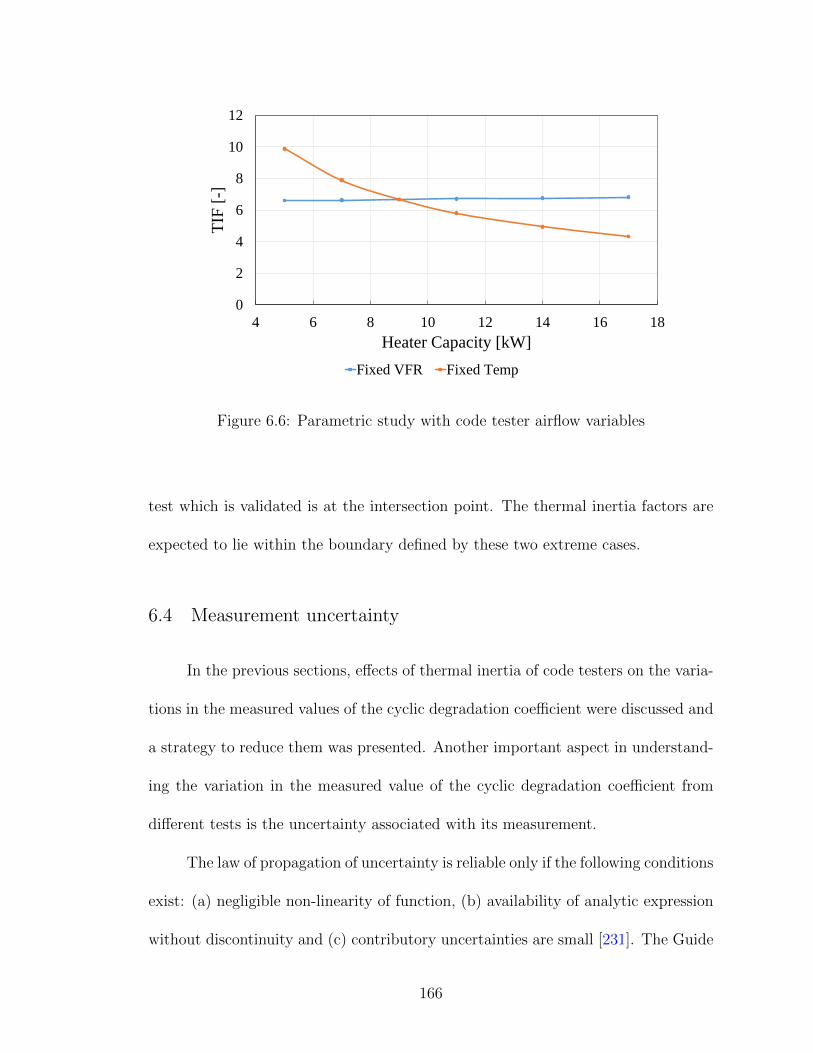
0

2

4

6

8

10

12

4 6 8 10 12 14 16 18

TIF

[-]

Heater Capacity [kW]

Fixed VFR Fixed Temp

Figure 6.6: Parametric study with code tester airflow variables

test which is validated is at the intersection point. The thermal inertia factors are

expected to lie within the boundary defined by these two extreme cases.

6.4 Measurement uncertainty

In the previous sections, effects of thermal inertia of code testers on the varia-

tions in the measured values of the cyclic degradation coefficient were discussed and

a strategy to reduce them was presented. Another important aspect in understand-

ing the variation in the measured value of the cyclic degradation coefficient from

different tests is the uncertainty associated with its measurement.

The law of propagation of uncertainty is reliable only if the following conditions

exist: (a) negligible non-linearity of function, (b) availability of analytic expression

without discontinuity and (c) contributory uncertainties are small [231]. The Guide

166

to the Expression of Uncertainty in Measurement [232], published Supplement 1 in

2008 that describes the Monte Carlo method as a general numerical implementa-

tion of the propagation of probability distributions that can be expected to pro-

vide results free of the approximations involved in the original GUM uncertainty

framework. Monte Carlo method is more reliable for a wide range of measurement

problems and so this method is used for the current investigation.

The general steps involved in a Monte Carlo simulation are [233]:

1. Determine system characteristics (defining inputs, parameters, outputs and

system model).

2. Determine inputs and parameters subject to uncertainty and assume or ob-

serve distribution characteristics.

3. Apply pseudo-random sampling to calculate values for input and parameter

random vectors.

4. Calculate and output vector using the deterministic model.

5. Analyze the results using statistical techniques.

A comprehensive evaluation of uncertainties is conducted by including sys-

tematic uncertainties from instrumentation, calibration and also the random uncer-

tainties. For the purpose of discussion, only the case of temperature measurement

at the inlet of indoor unit (TIDDB) is described. The other input parameters (see

Table 6.2) for uncertainty follow similar procedure. TIDDB is measured using a

thermocouple grid, with 12 T-type thermocouples. The uncertainty associated with

167

each thermocouple is 0.9 °F. Whenever the value of a test result is determined by

several independent methods, then the test result and its assoicated uncertainty

may be determined by weighting the means, random uncertainties and systematic

uncertainties of various methods. The weighting factor for 12 thermocouples as per

ASME PTC 19.1-2013 [234] in Appendix A-2 is calculated using Equation (6.11).

The instrument bias for the thermocouple grid is 0.26°F (Equation (6.12)).

bx = 0.9°F (6.10)

wi =(1/bx)

2∑12i=1(1/bx)2

=1

12(6.11)

bx =

√√√√ 12∑i=1

(wibx)2 = 0.26°F (6.12)

The thermocouples are calibrated with a water bath having systematic uncer-

tainty (bc) of 0.02 °F. A random uncertainty (sc) of 0.017°F is noted for the cali-

bration. The main purpose of the calibration process is to reduce the large known

systematic errors to some acceptable level. The thermocouples calibrated with the

bath are much more accurate and so the systematic uncertainty of the thermocouple

grid is taken as the root of sum of square of the systematic and random uncertainty

of the water bath used for calibration (Equation (6.13).

btot =√b2c + s2

c (6.13)

Finally, after calibration, a few readings of thermocouple grid are taken to

evaluate the random uncertainty. The standard deviation of temperature readings

168

is 0.012°F. Table 6.2 lists all the variables with their uncertainties for the evaluation

of steady dry-coil C-Test based parameters in the value of Cd. Standard error, which

is the standard deviation of the mean value of the measurement, is not included in

the estimation. Instead standard deviation itself is used. This is because the modern

data acquisition systems take several readings and the value recorded is an averaged

one itself. Including standard error in evaluation of error may lead to severe under-

prediction of uncertainty.

Table 6.2: Uncertainties for evaluation of Cd

Variable Unit Systematic Random

TIDDB °F 0.013 0.012

TIDDP °F 0.101 0.018

TLDB °F 0.013 0.063

TLDP °F 0.101 0.031

TODDB °F 0.013 0.037

PV inch H2O 0.001 0.0064

PSTAT inch H2O 0.002 0.0082

PATM inch Hg 0.003 0.0505

Total Power W 8.18 5.622

Nozzle Area ft2 0.00035 0.0

For evaluation of the Monte Carlo simulation, MATLAB [71] is used. Normal

inverse cumulative distribution function norminv is used to generate population of the

input variables from Table 6.2.

169

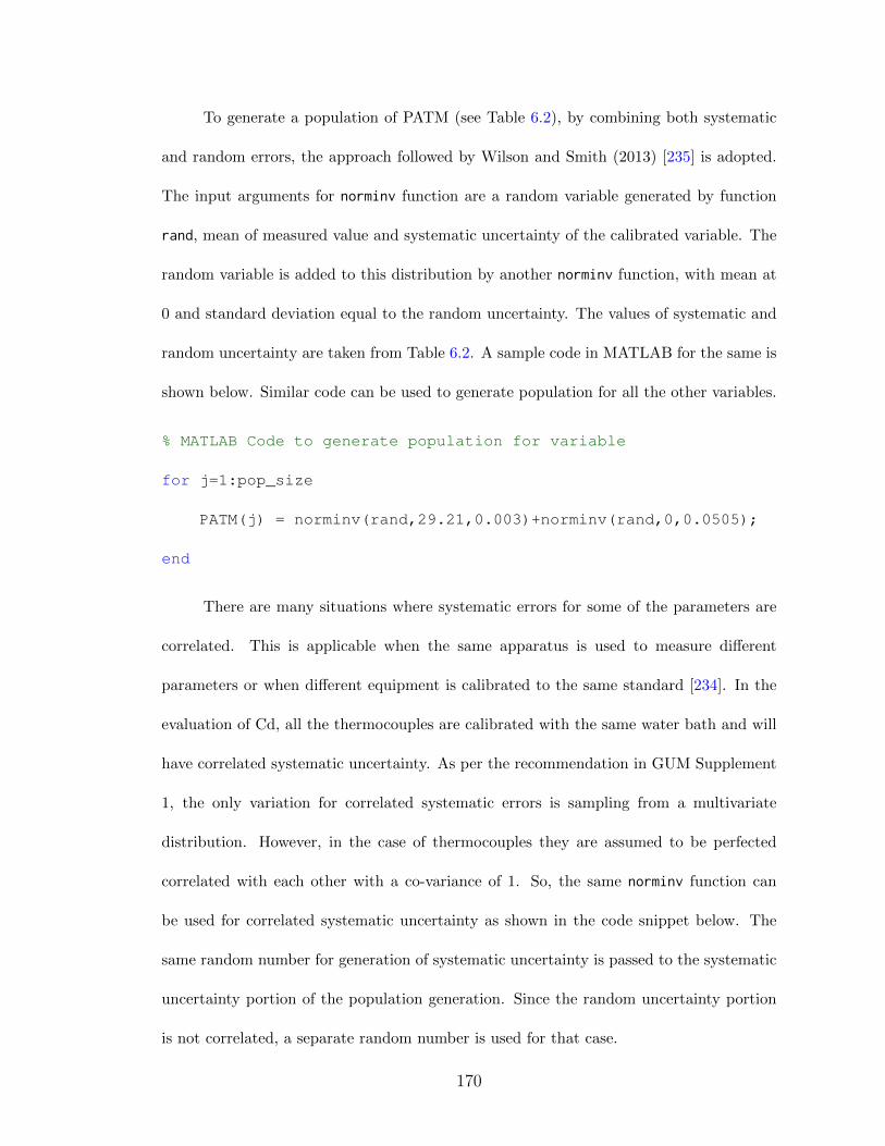
To generate a population of PATM (see Table 6.2), by combining both systematic

and random errors, the approach followed by Wilson and Smith (2013) [235] is adopted.

The input arguments for norminv function are a random variable generated by function

rand, mean of measured value and systematic uncertainty of the calibrated variable. The

random variable is added to this distribution by another norminv function, with mean at

0 and standard deviation equal to the random uncertainty. The values of systematic and

random uncertainty are taken from Table 6.2. A sample code in MATLAB for the same is

shown below. Similar code can be used to generate population for all the other variables.

% MATLAB Code to generate population for variable

for j=1:pop_size

PATM(j) = norminv(rand,29.21,0.003)+norminv(rand,0,0.0505);

end

There are many situations where systematic errors for some of the parameters are

correlated. This is applicable when the same apparatus is used to measure different

parameters or when different equipment is calibrated to the same standard [234]. In the

evaluation of Cd, all the thermocouples are calibrated with the same water bath and will

have correlated systematic uncertainty. As per the recommendation in GUM Supplement

1, the only variation for correlated systematic errors is sampling from a multivariate

distribution. However, in the case of thermocouples they are assumed to be perfected

correlated with each other with a co-variance of 1. So, the same norminv function can

be used for correlated systematic uncertainty as shown in the code snippet below. The

same random number for generation of systematic uncertainty is passed to the systematic

uncertainty portion of the population generation. Since the random uncertainty portion

is not correlated, a separate random number is used for that case.

170

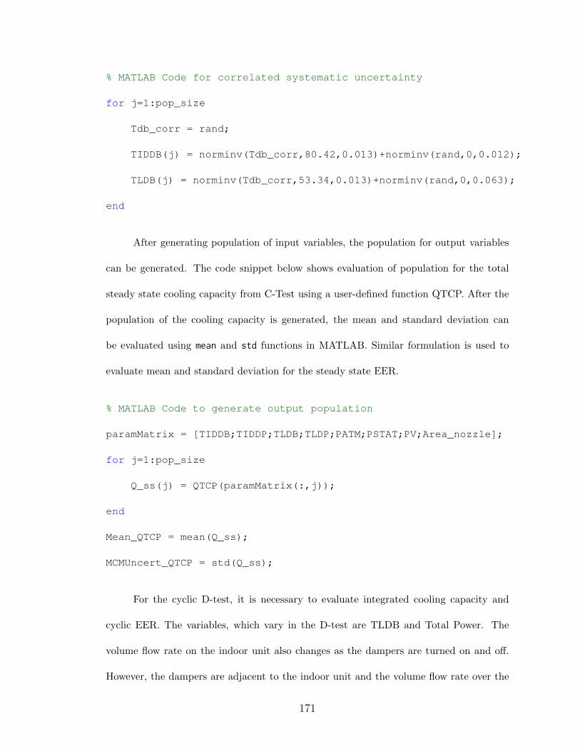
% MATLAB Code for correlated systematic uncertainty

for j=1:pop_size

Tdb_corr = rand;

TIDDB(j) = norminv(Tdb_corr,80.42,0.013)+norminv(rand,0,0.012);

TLDB(j) = norminv(Tdb_corr,53.34,0.013)+norminv(rand,0,0.063);

end

After generating population of input variables, the population for output variables

can be generated. The code snippet below shows evaluation of population for the total

steady state cooling capacity from C-Test using a user-defined function QTCP. After the

population of the cooling capacity is generated, the mean and standard deviation can

be evaluated using mean and std functions in MATLAB. Similar formulation is used to

evaluate mean and standard deviation for the steady state EER.

% MATLAB Code to generate output population

paramMatrix = [TIDDB;TIDDP;TLDB;TLDP;PATM;PSTAT;PV;Area_nozzle];

for j=1:pop_size

Q_ss(j) = QTCP(paramMatrix(:,j));

end

Mean_QTCP = mean(Q_ss);

MCMUncert_QTCP = std(Q_ss);

For the cyclic D-test, it is necessary to evaluate integrated cooling capacity and

cyclic EER. The variables, which vary in the D-test are TLDB and Total Power. The

volume flow rate on the indoor unit also changes as the dampers are turned on and off.

However, the dampers are adjacent to the indoor unit and the volume flow rate over the

171

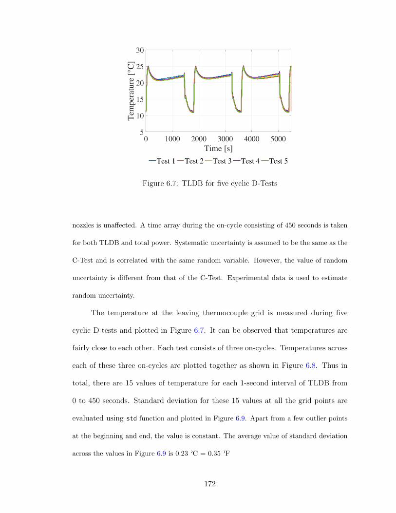
0 1000 2000 3000 4000 5000

Time [s]

5

10

15

20

25

30

Tem

per

ature

[°C

]

Test 1 Test 2 Test 3 Test 4 Test 5

Figure 6.7: TLDB for five cyclic D-Tests

nozzles is unaffected. A time array during the on-cycle consisting of 450 seconds is taken

for both TLDB and total power. Systematic uncertainty is assumed to be the same as the

C-Test and is correlated with the same random variable. However, the value of random

uncertainty is different from that of the C-Test. Experimental data is used to estimate

random uncertainty.

The temperature at the leaving thermocouple grid is measured during five

cyclic D-tests and plotted in Figure 6.7. It can be observed that temperatures are

fairly close to each other. Each test consists of three on-cycles. Temperatures across

each of these three on-cycles are plotted together as shown in Figure 6.8. Thus in

total, there are 15 values of temperature for each 1-second interval of TLDB from

0 to 450 seconds. Standard deviation for these 15 values at all the grid points are

evaluated using std function and plotted in Figure 6.9. Apart from a few outlier points

at the beginning and end, the value is constant. The average value of standard deviation

across the values in Figure 6.9 is 0.23 °C = 0.35 °F

172

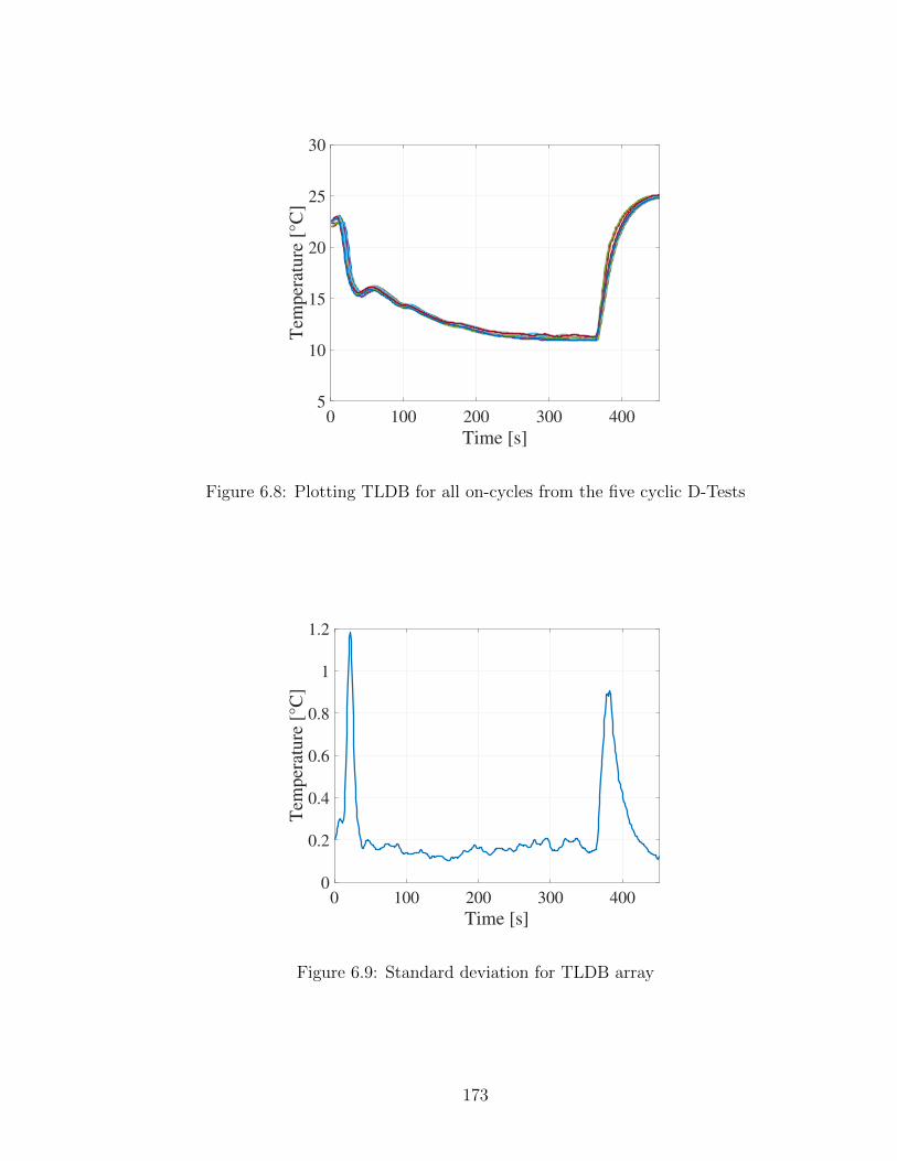
0 100 200 300 400

Time [s]

5

10

15

20

25

30

Tem

per

ature

[°C

]

Figure 6.8: Plotting TLDB for all on-cycles from the five cyclic D-Tests

0 100 200 300 400

Time [s]

0

0.2

0.4

0.6

0.8

1

1.2

Tem

per

ature

[°C

]

Figure 6.9: Standard deviation for TLDB array

173

The population of dynamic inputs for TLDB and total power can be generated

now as shown below.

% Generate population of dynamic inputs

for j=1:pop_size

for k=1:length(transpose(GRIDLVGUNITS))

TLDB_D(k,j)= norminv(Tdb_corr,GRIDLVGUNITS(k),0.013)

+norminv(rand,0,0.35);

POW_D(k,j)= norminv(pow_corr,POWER(k),8.022)

+norminv(rand,0,1.623);

end

end

The cooling capacity and EER can be evaluated at each time grid point using

the same user-defined function QTCP. With all the variables now available, population

for Cd is generated and statistics calculated. Summary of the Monte Carlo evaluation is

shown in Table 6.3. It can be observed that the experimental data matches well within

the uncertainty for the steady C-Test conditions. However, due to the lack of volume flow

rate cycling of D-Test, the integrated cooling capacity is over-predicted by the simulation.

The standard deviation of Cd evaluated from simulation is 0.006. For the five cyclic tests

conducted, the standard deviation measured is 0.007. For a 95% confidence interval, the

total variation is Cd = 0.012, which is roughly 8% of the value of Cd.

If the values of acceptable uncertainty from ASHRAE 41.2 are used (Systematic

= 0.1 °F, Random = 0.2 °F for temperature, 0.005 inch water for differential pressure),

then the deviation in measured value of Cd = 11.4% for a 95% confidence interval. The

174

measurement uncertainty is responsible for the variation in the values of ideal Cd in

Table 6.1.

Table 6.3: Uncertainties for evaluation of Cd

Variable Unit MC Mean MC Std Dev Expt Mean

Airflow ft3 min−1 615 3.54 615

Qss Btu hr−1 17339 105.04 17214

EERss Btu hr−1 W−1 13.33 0.117 13.23

qcyc Btu 1577 9.61 1516

EERcyc Btu hr−1 W−1 11.85 0.113 11.42

Cd [-] 0.1355 0.0055 0.17

Total deviation observed between Cd measured from CT-A and CT-B is about 20%

and half of it is from measurement uncertainty. Remaining influence is from the effect of

thermal inertia of code testers. It is therefore necessary to develop a more reliable method

to rate cyclic performance of air conditioners. The new term to calculate cyclic variation

should have much lesser variation in measurement. Design of code testers should also be

standardized to account for uniform effect of thermal inertia across various tests. Also

their designs should be such that the values of thermal inertia factor are low.

175

Chapter 7: Summary

7.1 Conclusions

This thesis provides several innovative ideas for more energy efficient use of HVAC

systems to provide space heating and cooling in buildings.

To address the shortcomings of existing personal conditioning systems (PCS), four

such systems are analyzed through multi-physics modeling to understand the extent of

their benefits and shortcomings. Three of the systems use different thermal storages like

chilled water, ice storage and PCM with a closed water loop, and a fourth system uses

vapor compression cycle with PCM. All the systems are in the weight range of 19-31 kg.

Chilled water-based system and ice storage based system are cost-effective compared to the

other systems. The vapor compression system consumes roughly 40% more battery power

than the water-based systems during cooling operation. However, vapor compression

system has other benefits from usability like easier thermal recharge and closed operation

for the system.

The VCS with PCM is developed into a technology called Roving Comforter (RoCo).

The first prototype used thermosiphon for recharging the PCM, which required eight hours

to re-solidify the PCM after a two hour cooling operation. A validated dynamic model for

thermosiphon is developed and then exercised to evaluate performance with compressed

expanded natural graphite (CENG) enhanced versions of the PCM. Based on the results,

176

2.2% volume fraction CENG is considered the most promising due to 51% reduction in

the discharge time for a 5% increase in weight. The coefficient of performance for overall

operation increases by 24%.

Due to regulations on the use of R134a, the dynamic performance of RoCo with

a natural refrigerant (R290) is studied. Switching to R290 shows 33% improvement in

the coefficient of performance, with additional benefits like reduced noise during cooling

operation and lesser system weight also expected.

The newer prototypes of RoCo using CENG delivered 4-hour cooling operation with

6.5-hour recharge time by thermosiphon. The performance of heat pump based recharge at

different compressor RPM was evaluated. The recharge period from heat pump operation

showed 35-55% reduction in time from thermosiphon, with a penalty of 30-35% on the

overall COP. However, the power consumption is in the order of a few hundred Wh and is

small compared to the savings from building HVAC, which typically consumes power in

kWh. Thus, heat pump recharge shows promise in comparison to the thermosiphon and

will be used in future prototypes.

Next, refrigerant migration physics is investigated for a conventional air-conditioner

undergoing cyclic testing in a code tester. The dynamic model shows the good prediction

for temperature, pressure and power measurements. Slip-ratio based void fraction model

is used to estimate refrigerant charge in each component. Refrigerant leakage through

both compressor and TXV is modeled. The model also shows robustness during off-cycle

of a cyclic test under the conditions of zero refrigerant flow. Validation for the percentage

of refrigerant in different portions of the system shows a good overall prediction for steady

state test experiment. Finally, the limitations of current HVAC rating procedure and

specifically the contribution of the code tester on the cyclic degradation coefficient (Cd)

177

is investigated. Deviations arising from assumptions used in the calculation procedure

are highlighted using a validated dynamic model for the code tester. A new term called

thermal inertia factor is defined and the Cd formula is modified using the thermal inertia

factor to remove the impact of a specific code tester design from the measured value of Cd.

Discussions on future directions aimed at improving Cd evaluation procedure is presented.

7.2 Contributions

The main contributions of this thesis are dynamic, highly reusable models capable

of analyzing a variety of complex two-phase refrigerant systems. Multi-physics insights are

also available for models incorporating electrodynamics and mechanics equations alongside

the thermal-fluid sciences.

The models are used to improve the performance of a few existing systems. It is

expected to provide interesting insights on the systems analyzed for researchers developing

similar technology and at the same time guidance on developing system models to simulate

design space. The contributions from the thesis are classified into groups below:

1. Thermosiphon modeling

First demonstration of two-phase thermosiphon modeling with Modelica in

literature

First validated numerical model for PCM-driven thermosiphon in literature

2. Personal Conditioning Systems

Identified and compared system parameters for the lightest design of four in-

novative PCS with different thermal storage through development of multi-

178

physics models

Energy efficiency improvement for RoCo by identifying best operating param-

eters in studies involving different refrigerants, phase change materials and

recharge options

3. Phase Change Material Modeling

Empirical correlation for solidification and melting of PureTemp 37 by helical

coil refrigerant tubes at RoCo operating temperatures

Strategies to implement simple and accurate PCM models for system simula-

tion in thermo-fluid systems

4. Cyclic performance of air conditioner

Develop dynamic modeling framework incorporating recommended best prac-

tices for zero flow modeling, compressor leakage, asymmetric refrigerant cir-

cuitry and void fraction model-based prediction of refrigerant charge

Develop generic reusable models for code tester components which can be

integrated with system model of air conditioner

Provide insights into refrigerant migration physics during cyclic operation of

a conventional air conditioner

5. Rating standards for evaluating cyclic performance of air conditioners

Quantify the effects of thermal inertia of code tester on the measured cyclic

degradation coefficient

Identification of uncertainty in the measured value of cyclic degradation coef-

ficient using Monte Carlo simulation

179

Recommend best practices for measurement of accurate cyclic degradation of

the conventional air conditioner

180

Bibliography

[1] U.S. Energy Information Administration. Independent statistics & analysis,2017. [Online; accessed 14-April-2017].

[2] Bryan P Rasmussen. Dynamic modeling and advanced control of air condi-tioning and refrigeration systems. PhD thesis, 2005.

[3] Vahid Vakiloroaya, Bijan Samali, Ahmad Fakhar, and Kambiz Pishghadam.A review of different strategies for hvac energy saving. Energy conversion andmanagement, 77:738–754, 2014.

[4] Marıa Ibanez-Puy, Javier Bermejo-Busto, Cesar Martın-Gomez, MarinaVidaurre-Arbizu, and Jose Antonio Sacristan-Fernandez. Thermoelectric cool-ing heating unit performance under real conditions. Applied Energy, 200:303–314, 2017.

[5] Yongqiang Luo, Ling Zhang, Zhongbing Liu, Yingzi Wang, Fangfang Meng,and Lei Xie. Modeling of the surface temperature field of a thermoelectricradiant ceiling panel system. Applied Energy, 162:675–686, 2016.

[6] Mohammad Saffari Tabalvandani, Alvaro de Gracia Cuesta, CesarFernandez Camon, and Luisa F Cabeza. Simulation-based optimization ofpcm melting temperature to improve the energy performance in buildings.Applied Energy, 2017, In Press, 2017.

[7] Na Luo, Tianzhen Hong, Hui Li, Ruoxi Jia, and Wenguo Weng. Data ana-lytics and optimization of an ice-based energy storage system for commercialbuildings. Applied Energy, 204:459–475, 2017.

[8] TX Li, DL Wu, F He, and RZ Wang. Experimental investigation on cop-per foam/hydrated salt composite phase change material for thermal energystorage. International Journal of Heat and Mass Transfer, 115:148–157, 2017.

181

[9] Xinqiao Yu, Da Yan, Kaiyu Sun, Tianzhen Hong, and Dandan Zhu. Com-parative study of the cooling energy performance of variable refrigerant flowsystems and variable air volume systems in office buildings. Applied Energy,183:725–736, 2016.

[10] Pradeep Bansal. High efficiency novel window air conditioner. Applied Energy,156:311–320, 2015.

[11] Kathrin Menberg, Yeonsook Heo, Wonjun Choi, Ryozo Ooka, Ruchi Choud-hary, and Masanori Shukuya. Exergy analysis of a hybrid ground-source heatpump system. Applied Energy, 204:31–46, 2017.

[12] Zhihua Zhou, Zhiming Zhang, Guanyi Chen, Jian Zuo, Pan Xu, Chong Meng,and Zhun Yu. Feasibility of ground coupled heat pumps in office buildings: Achina study. Applied Energy, 162:266–277, 2016.

[13] Omar Labban, Tianyi Chen, Ahmed F Ghoniem, John H Lienhard, andLeslie K Norford. Next-generation hvac: Prospects for and limitations ofdesiccant and membrane-based dehumidification and cooling. Applied Energy,200:330–346, 2017.

[14] Dominic OConnor, John Kaiser Calautit, and Ben Richard Hughes. A noveldesign of a desiccant rotary wheel for passive ventilation applications. AppliedEnergy, 179:99–109, 2016.

[15] Tao Yu, Per Heiselberg, Bo Lei, Chen Zhang, Michal Pomianowski, and Ras-mus Jensen. Experimental study on the dynamic performance of a novel sys-tem combining natural ventilation with diffuse ceiling inlet and tabs. Appliedenergy, 169:218–229, 2016.

[16] Daniel Bacellar, Vikrant Aute, Zhiwei Huang, and Reinhard Radermacher.Design optimization and validation of high-performance heat exchangers usingapproximation assisted optimization and additive manufacturing. Science andTechnology for the Built Environment, 23(6):896–911, 2017.

[17] Jun Mei and Xiaohua Xia. Energy-efficient predictive control of indoor thermalcomfort and air quality in a direct expansion air conditioning system. AppliedEnergy, 195:439–452, 2017.

[18] Jingchun Shen, Xingxing Zhang, Tong Yang, Llewellyn Tang, Ali Cheshme-hzangi, Yupeng Wu, Guiqin Huang, Dan Zhong, Peng Xu, and Shengchun Liu.Characteristic study of a novel compact solar thermal facade (stf) with inter-nally extruded pin–fin flow channel for building integration. Applied Energy,168:48–64, 2016.

[19] Adams Rackes, Ana Paula Melo, and Roberto Lamberts. Naturally comfort-able and sustainable: Informed design guidance and performance labeling forpassive commercial buildings in hot climates. Applied Energy, 174:256–274,2016.

182

[20] Ignacio Acosta, Miguel Angel Campano, and Juan Francisco Molina. Win-dow design in architecture: Analysis of energy savings for lighting and visualcomfort in residential spaces. Applied Energy, 168:493–506, 2016.

[21] Scott Hackel and Amanda Pertzborn. Effective design and operation of hy-brid ground-source heat pumps: three case studies. Energy and Buildings,43(12):3497–3504, 2011.

[22] YF Liu and RZ Wang. Method to design optimal scheme for cold storage airconditioning system. Energy conversion and management, 43(17):2357–2367,2002.

[23] Vahid Vakiloroaya, Jafar Madadnia, and Bijan Samali. Modeling and per-formance prediction of an integrated central cooling plant for hvac energyefficiency improvement. In Building Simulation, volume 6, pages 127–138.Tsinghua Univ Press, 2013.

[24] Inge Blom, Laure Itard, and Arjen Meijer. Lca-based environmental assess-ment of the use and maintenance of heating and ventilation systems in dutchdwellings. Building and Environment, 45(11):2362–2372, 2010.

[25] Jennifer OConnor. Survey on actual service lives for north american buildings.In Woodframe housing durability and disaster issues conference, Las Vegas,pages 1–9, 2004.

[26] Buildings Energy Data Book. Us department of energy, 2011, 2010.

[27] Weimin Wang, Srinivas Katipamula, Hung Ngo, Ronald Underhill, DannyTaasevigen, and Robert Lutes. Field evaluation of advanced controls for theretrofit of packaged air conditioners and heat pumps. Applied Energy, 154:344–351, 2015.

[28] Hui Zhang, Edward Arens, and Wilmer Pasut. Air temperature thresholds forindoor comfort and perceived air quality. Building Research & Information,39(2):134–144, 2011.

[29] Gail Brager, Hui Zhang, and Edward Arens. Evolving opportunities for pro-viding thermal comfort. Building Research & Information, 43(3):274–287,2015.

[30] Stanley Aronoff and Audrey G Kaplan. Total workplace performance: Re-thinking the office environment. Wdl Publications, 1995.

[31] RG Kapadia, Sanjeev Jain, and RS Agarwal. Transient characteristics ofsplit air-conditioning systems using r-22 and r-410a as refrigerants. HVAC&RResearch, 15(3):617–649, 2009.

183

[32] ARI Standard 210/240: Performance Rating of Unitary Air-Conditioning &Air-Source Heat Pump Equipment. Standard, Air Conditioning, Heating, andRefrigeration Institute, Arlington, VA, 2008.

[33] Sven Erik Mattsson, Hilding Elmqvist, and Martin Otter. Physical systemmodeling with modelica. Control Engineering Practice, 6(4):501–510, 1998.

[34] Karl Johan Astrom, Hilding Elmqvist, Sven Erik Mattsson, et al. Evolutionof continuous-time modeling and simulation. In ESM, pages 9–18, 1998.

[35] Christopher Laughman and Hongtao Qiao. Mass conserving models of vaporcompression cycles. In Proceedings of the 11th International Modelica Confer-ence, Versailles, France, September 21-23, 2015, number 118, pages 759–767.Linkoping University Electronic Press, 2015.

[36] Peter Fritzson. Principles of object-oriented modeling and simulation withModelica 3.3: a cyber-physical approach. John Wiley & Sons, 2014.

[37] Hubertus Tummescheit and Jonas Eborn. Design of a thermo-hydraulic modellibrary in Modelica. In 12th European Simulation Multiconference, 1998.

[38] Hubertus Tummescheit, Jonas Eborn, and Falko Wagner. Development of aModelica base library for modeling of thermo-hydraulic systems. In ModelicaWorkshop 2000 Proceedings, pages 41–51, 2000.

[39] Hubertus Tummescheit. Design and implementation of object-oriented modellibraries using modelica. PhD Theses, 2002.

[40] J Eborn, Hubertus Tummescheit, and W Wagner. Thermoflow, a thermo-hydraulic library in modelica. Technical report, 2001.

[41] Hilding Elmqvist, Hubertus Tummescheit, and Martin Otter. Object-orientedmodeling of thermo-fluid systems. In 3rd International Modelica Conference,pages 269–286, 2003.

[42] Jakob Munch Jensen. Dynamic modeling of thermofluid systems. 2003.

[43] Torge Pfafferott and Gerhard Schmitz. Modelling and transient simulation ofCO 2-refrigeration systems with Modelica. International journal of refrigera-tion, 27(1):42–52, 2004.

[44] Torge Pfafferott and Gerhard Schmitz. Implementation of a modelica libraryfor simulation of refrigeration systems. In Paper presented at the 3rd Interna-tional Modelica Conference, 2003.

[45] Francesco Casella, Martin Otter, Katrin Proelss, Christoph Richter, and Hu-bertus Tummescheit. The modelica fluid and media library for modeling ofincompressible and compressible thermo-fluid pipe networks. In Proceedingsof the 5th International Modelica Conference, pages 631–640, 2006.

184

[46] Christoph Richter. Proposal of new object-oriented equation-based model li-braries for thermodynamic systems. PhD thesis, 2008.

[47] Hongtao Qiao. Transient modeling of two-stage and variable refrigerant flowvapor compression systems with frosting and defrosting. PhD thesis, 2014.

[48] Staffan Haugwitz. Modelling of microturbine systems. MSc Theses, 2002.

[49] Antonio Alejandro Gomez Perez. Modelling of a gas turbine with modelica.MSc Theses, 2001.

[50] Rudiger Franke, Francesco Casella, Martin Otter, Michael Sielemann, HildingElmqvist, Mattson Sven Erik, and Olsson Hans. Stream connectors-an ex-tension of Modelica for device-oriented modeling of convective transport phe-nomena. In Proceedings of the 7th International Modelica Conference; Como;Italy; 20-22 September 2009, number 043, pages 108–121. Linkoping Univer-sity Electronic Press, 2009.

[51] Dirk Limperich, Marco Braun, K Prolß, Gerhard Schmitz, et al. Systemsimulation of automotive refrigeration cycles. In Proceedings of the 4th inter-national modelica conference, 2005.

[52] Hubertus Tummescheit, Jonas Eborn, and Katrin Prolss. AirconditioningaModelica library for dynamic simulation of AC systems. In Paper presentedat the 4th International Modelica Conference, 2005.

[53] Hongtao Qiao, Christopher R Laughman, Vikrant Aute, and Reinhard Rader-macher. An advanced switching moving boundary heat exchanger model withpressure drop. International journal of refrigeration, 65:154–171, 2016.

[54] Luca Cecchinato and Ferdinando Mancini. An intrinsically mass conservativeswitched evaporator model adopting the moving-boundary method. Interna-tional journal of refrigeration, 35(2):349–364, 2012.

[55] Christopher R Laughman and Hongtao Qiao. On the influence of state se-lection on mass conservation in dynamic vapour compression cycle models.Mathematical and Computer Modelling of Dynamical Systems, pages 1–22,2017.

[56] Christopher R Laughman, Hongtao Qiao, Vikrant Aute, and Reinhard Ra-dermacher. A comparison of transient heat pump cycle models using alter-native flow descriptions. Science and Technology for the Built Environment,21(5):666–680, 2015.

[57] Olaf Bauer. Modelling of two-phase flows with modelica. Master’s thesis,Lund Institute of Technology, 1999.

185

[58] Lord Rayleigh. LIX. On convection currents in a horizontal layer of fluid,when the higher temperature is on the under side. The London, Edinburgh,and Dublin Philosophical Magazine and Journal of Science, 32(192):529–546,1916.

[59] Flavio Dobran. Steady-state characteristics and stability thresholds of a closedtwo-phase thermosyphon. International Journal of heat and mass transfer,28(5):949–957, 1985.

[60] J G Reed and C L Tien. Modeling of the two-phase closed thermosyphon.Journal of heat transfer, 109(3):722–730, 1987.

[61] Stephane Lips, Valerie Sartre, Frederic Lefevre, Sameer Khandekar, and Jo-celyn Bonjour. Overview of heat pipe studies during the period 2010- 2015.Interfacial Phenomena and Heat Transfer, 4(1), 2016.

[62] Saffa Riffat and Xiaoli Ma. Recent developments in heat pipe technology andapplications: a review. International Journal of Low-carbon Technologies,2(2):162–177, 2007.

[63] Amir Faghri. Review and advances in heat pipe science and technology. Jour-nal of heat transfer, 134(12):123001, 2012.

[64] Charles C J Vincent and Jim B W Kok. Investigation of the overall transientperformance of the industrial two-phase closed loop thermosyphon. Interna-tional Journal of heat and mass transfer, 35(6):1419–1426, 1992.

[65] Rahmatollah Khodabandeh. Heat transfer in the evaporator of an ad-vanced two-phase thermosyphon loop. International journal of refrigeration,28(2):190–202, 2005.

[66] Rahmatollah Khodabandeh. Pressure drop in riser and evaporator in an ad-vanced two-phase thermosyphon loop. International journal of refrigeration,28(5):725–734, 2005.

[67] Penglei Zhang, Baolong Wang, Wenxing Shi, Linjun Han, and Xianting Li.Modeling and performance analysis of a two-phase thermosyphon loop withpartially/fully liquid-filled downcomer. International Journal of Refrigeration,58:172–185, 2015.

[68] Hainan Zhang, Zichao Shi, Kaitao Liu, Shuangquan Shao, Tingxiang Jin, andChangqing Tian. Experimental and numerical investigation on a co 2 loopthermosyphon for free cooling of data centers. Applied Thermal Engineering,111:1083–1090, 2017.

[69] S I Haider, Yogendra K Joshi, and Wataru Nakayama. A natural circulationmodel of the closed loop, two-phase thermosyphon for electronics cooling.Journal of heat transfer, 124(5):881–890, 2002.

186

[70] S A Klein and F L Alvarado. Engineering equation solver. F-Chart Software,Madison, WI, 1, 2002.

[71] MATLAB Users Guide. The mathworks. Inc., Natick, MA, 5:333, 1998.

[72] R T Dobson and J C Ruppersberg. Flow and heat transfer in a closed loopthermosyphon. Part ITheoretical simulation. J. Energy South. Afr, 18:32–40,2007.

[73] S Bodjona, E Videcoq, Richard Saurel, A Chinnayya, AM Benselama, andY Bertin. Transient simulation of a two-phase loop thermosyphon with amodel out of thermodynamic equilibrium. International Journal of Heat andMass Transfer, 108:2321–2332, 2017.

[74] R Srikanth, Rohit S Nair, and C Balaji. Thermosyphon assisted melting of pcminside a rectangular enclosure: A synergistic numerical approach. In Journal ofPhysics: Conference Series, volume 745, page 032130. IOP Publishing, 2016.

[75] Belen Zalba, Jose Ma Marın, Luisa F Cabeza, and Harald Mehling. Review onthermal energy storage with phase change: materials, heat transfer analysisand applications. Applied thermal engineering, 23(3):251–283, 2003.

[76] David Gonzalez-Nino, Lauren M Boteler, Dimeji Ibitayo, Nicholas RJankowski, Damian Urciuoli, Iain M Kierzewski, and Pedro O Quintero. Ex-perimental evaluation of metallic phase change materials for thermal transientmitigation. International Journal of Heat and Mass Transfer, 116:512–519,2018.

[77] Muhammad Junaid Ashraf, Hafiz Muhammad Ali, Hazrat Usman, and AdeelArshad. Experimental passive electronics cooling: Parametric investigation ofpin-fin geometries and efficient phase change materials. International Journalof Heat and Mass Transfer, 115:251–263, 2017.

[78] Adele Caron-Soupart, Jean-Francois Fourmigue, Philippe Marty, and RaphaelCouturier. Performance analysis of thermal energy storage systems using phasechange material. Applied Thermal Engineering, 98:1286–1296, 2016.

[79] Debabrata Pal and Yogendra K Joshi. Melting in a side heated tall enclosureby a uniformly dissipating heat source. International Journal of Heat andMass Transfer, 44(2):375–387, 2001.

[80] Babak Kamkari, Hossein Shokouhmand, and Frank Bruno. Experimental in-vestigation of the effect of inclination angle on convection-driven melting ofphase change material in a rectangular enclosure. International Journal ofHeat and Mass Transfer, 72:186–200, 2014.

[81] Yvan Dutil, Daniel R Rousse, Nizar Ben Salah, Stephane Lassue, and LaurentZalewski. A review on phase-change materials: mathematical modeling andsimulations. Renewable and sustainable Energy reviews, 15(1):112–130, 2011.

187

[82] Henry Hu and Stavros A Argyropoulos. Mathematical modelling of solidifi-cation and melting: a review. Modelling and Simulation in Materials Scienceand Engineering, 4(4):371, 1996.

[83] Piia Lamberg, Reijo Lehtiniemi, and Anna-Maria Henell. Numerical and ex-perimental investigation of melting and freezing processes in phase changematerial storage. International Journal of Thermal Sciences, 43(3):277–287,2004.

[84] AH Mosaffa, F Talati, H Basirat Tabrizi, and MA Rosen. Analytical mod-eling of pcm solidification in a shell and tube finned thermal storage for airconditioning systems. Energy and buildings, 49:356–361, 2012.

[85] K Azzouz, D Leducq, and D Gobin. Performance enhancement of a house-hold refrigerator by addition of latent heat storage. International Journal ofRefrigeration, 31(5):892–901, 2008.

[86] Hamid El Qarnia. Numerical analysis of a coupled solar collector latent heatstorage unit using various phase change materials for heating the water. EnergyConversion and Management, 50(2):247–254, 2009.

[87] S Bakhshipour, MS Valipour, and Y Pahamli. Parametric analysis of domesticrefrigerators using pcm heat exchanger. International Journal of Refrigeration,83:1–13, 2017.

[88] Santosh Kumar Sahoo, Prasenjit Rath, and Mihir Kumar Das. Numericalstudy of phase change material based orthotropic heat sink for thermal man-agement of electronics components. International Journal of Heat and MassTransfer, 103:855–867, 2016.

[89] Y Cao and A Faghri. A numerical analysis of phase-change problemsincluding natural convection. Journal of Heat Transfer (Transactions ofthe ASME (American Society of Mechanical Engineers), Series C);(UnitedStates), 112(3), 1990.

[90] Corinna Leonhardt and Dirk Muller. Modelling of Residential Heating Systemsusing a Phase Change Material Storage System. 43:507–512, 2009.

[91] Jochen Buschle, Wolf-Dieter Steinmann, and Rainer Tamme. Analysis ofsteam storage systems using Modelica. In Proceedings 5th Modelica Conference2006, 2006.

[92] Anton Trnık, Libor Vozar, et al. Modeling of heat capacity peaks and enthalpyjumps of phase-change materials used for thermal energy storage. Interna-tional Journal of Heat and Mass Transfer, 107:123–132, 2017.

188

[93] Anica Trp, Kristian Lenic, and Bernard Frankovic. Analysis of the influenceof operating conditions and geometric parameters on heat transfer in water-paraffin shell-and-tube latent thermal energy storage unit. Applied ThermalEngineering, 26(16):1830–1839, 2006.

[94] Benjamin J. Jones, Dawei Sun, Shankar Krishnan, and Suresh V. Garimella.Experimental and numerical study of melting in a cylinder. InternationalJournal of Heat and Mass Transfer, 49(15-16):2724–2738, 2006.

[95] Anica Trp. An experimental and numerical investigation of heat transferduring technical grade paraffin melting and solidification in a shell-and-tubelatent thermal energy storage unit. Solar Energy, 79(6):648–660, 2005.

[96] E M Sparrow, S V Patankar, and Ramadhyani S. Analysis of Melting in thePresence of Natural Convection in the Melt Region. Journal of Heat Transfer,99(4):520–526, 1977.

[97] Saied Mohammad Vakilaltojjar and W Saman. Analysis and modelling of aphase change storage system for air conditioning applications. Applied Ther-mal Engineering, 21(3):249–263, 2001.

[98] A H Mosaffa, F Talati, H Basirat Tabrizi, and M A Rosen. Analytical mod-eling of PCM solidification in a shell and tube finned thermal storage for airconditioning systems. Energy and Buildings, 49:356–361, 2012.

[99] Miroslaw Zukowski. Experimental study of short term thermal energy storageunit based on enclosed phase change material in polyethylene film bag. EnergyConversion and Management, 48(1):166–173, 2007.

[100] Michael Vynnycky and Shigeo Kimura. An analytical and numerical study ofcoupled transient natural convection and solidification in a rectangular enclo-sure. International Journal of Heat and Mass Transfer, 50(25-26):5204–5214,2007.

[101] M Costa, D Buddhi, and A Oliva. Numerical simulation of a latent heatthermal energy storage system with enhanced heat conduction. Energy Con-servation Management, Vol.39, No(3):319–330, 1998.

[102] Nourouddin Sharifi, Christopher W Robak, Theodore L Bergman, and AmirFaghri. Three-dimensional pcm melting in a vertical cylindrical enclosure in-cluding the effects of tilting. International Journal of Heat and Mass Transfer,65:798–806, 2013.

[103] Abhay Dinker, Madhu Agarwal, and G. D. Agarwal. Experimental assessmenton thermal storage performance of beeswax in a helical tube embedded storageunit. Applied Thermal Engineering, 111(September):358–368, 2017.

189

[104] Abdel Illah Nabil Korti and Fatima Zohra Tlemsani. Experimental investiga-tion of latent heat storage in a coil in PCM storage unit. Journal of EnergyStorage, 5:177–186, 2016.

[105] M H Abdel-Aziz, I Nirdosh, and G H Sedahmed. Mass and heat transfer atthe outer surface of helical coils under single and two phase flow. AppliedThermal Engineering, 103:713–719, 2016.

[106] Srbislav B Genic, Branislav M Jacimovic, Marko S Jaric, Nikola J Budimir,and Mirko M Dobrnjac. Research on the shell-side thermal performances ofheat exchangers with helical tube coils. International Journal of heat and masstransfer, 55(15-16):4295–4300, 2012.

[107] Xun Yang, Teng Xiong, Jing Liang Dong, Wen Xin Li, and Yong Wang.Investigation of the Dynamic Melting Process in a Thermal Energy StorageUnit Using a Helical Coil Heat Exchanger. Energies, 10(8):1129, 2017.

[108] Johan Akesson. Languages and Tools for Optimization of Large-Scale Systems.PhD thesis, Department of Automatic Control, Lund Institute of Technology(LTH), PO Box 118 221 00 Lund, Sweden, 2007.

[109] Tyler Hoyt, Edward Arens, and Hui Zhang. Extending air temperaturesetpoints: Simulated energy savings and design considerations for new andretrofit buildings. Building and Environment, 88:89–96, 2015.

[110] Hui Zhang, Edward Arens, and Yongchao Zhai. A review of the correc-tive power of personal comfort systems in non-neutral ambient environments.Building and Environment, 91:15–41, 2015.

[111] Arsen Krikor Melikov and Gitte L Knudsen. Human response to an individu-ally controlled microenvironment. HVAC&R Research, 13(4):645–660, 2007.

[112] Hui Zhang, Edward Arens, DongEun Kim, Elena Buchberger, Fred Bauman,and Charlie Huizenga. Comfort, perceived air quality, and work performancein a low-power task–ambient conditioning system. Building and Environment,45(1):29–39, 2010.

[113] Yongchao Zhai, Hui Zhang, Yufeng Zhang, Wilmer Pasut, Edward Arens, andQinglin Meng. Comfort under personally controlled air movement in warmand humid environments. Building and environment, 65:109–117, 2013.

[114] Fred S Bauman, Thomas G Carter, Anne V Baughman, and Edward A Arens.Field study of the impact of a desktop task/ambient conditioning system inoffice buildings. ASHRAE Transactions, 104:1153, 1998.

[115] Michal Vesely and Wim Zeiler. Personalized conditioning and its impact onthermal comfort and energy performance A review. Renewable and Sustain-able Energy Reviews, 34:401–408, 2014.

190

[116] Ning Mao, Dongmei Pan, Zhao Li, Yingjie Xu, Mengjie Song, and ShimingDeng. A numerical study on influences of building envelope heat gain onoperating performances of a bed-based task/ambient air conditioning (tac)system in energy saving and thermal comfort. Applied Energy, 192:213–221,2017.

[117] K Tsuzuki, Edward Arens, Fred Bauman, and D Wyon. Individual thermalcomfort control with desk-mounted and floor-mounted task/ambient condi-tioning (tac) systems. Indoor Air, Edinburgh, 1999.

[118] Arsen K Melikov, Radim Cermak, and Milan Majer. Personalized ventilation:evaluation of different air terminal devices. Energy and buildings, 34(8):829–836, 2002.

[119] Jing Du, Mingyin Chan, Dongmei Pan, and Shiming Deng. A numericalstudy on the effects of design/operating parameters of the radiant panel in aradiation-based task air conditioning system on indoor thermal comfort andenergy saving for a sleeping environment. Energy and Buildings, 151:250–262,2017.

[120] Nesreen Ghaddar, Kamel Ghali, and Walid Chakroun. Evaporative coolerimproves transient thermal comfort in chilled ceiling displacement ventilationconditioned space. Energy and Buildings, 61:51–60, 2013.

[121] W Chakroun, N Ghaddar, and K Ghali. Chilled ceiling and displacementventilation aided with personalized evaporative cooler. Energy and buildings,43(11):3250–3257, 2011.

[122] Wilmer Pasut, Hui Zhang, Ed Arens, and Yongchao Zhai. Energy-efficientcomfort with a heated/cooled chair: Results from human subject tests. Build-ing and Environment, 84:10–21, 2015.

[123] Shinichi Watanabe, Toshimichi Shimomura, and Hironori Miyazaki. Thermalevaluation of a chair with fans as an individually controlled system. Buildingand Environment, 44(7):1392–1398, 2009.

[124] Jianlei Niu, Naiping Gao, Ma Phoebe, and Zuo Huigang. Experimental studyon a chair-based personalized ventilation system. Building and Environment,42(2):913–925, 2007.

[125] Wenfang Song, Faming Wang, and Fanru Wei. Hybrid cooling clothing to im-prove thermal comfort of office workers in a hot indoor environment. Buildingand Environment, 100:92–101, 2016.

[126] Haneen Hamdan, Nesreen Ghaddar, Djamel Ouahrani, Kamel Ghali, andM Itani. Pcm cooling vest for improving thermal comfort in hot environment.International Journal of Thermal Sciences, 102:154–167, 2016.

191

[127] Mariam Itani, Nesreen Ghaddar, Kamel Ghali, Djamel Ouahrani, and WalidChakroun. Cooling vest with optimized pcm arrangement targeting torsosensitive areas that trigger comfort when cooled for improving human comfortin hot conditions. Energy and Buildings, 139:417–425, 2017.

[128] AD Flouris and SS Cheung. Design and control optimization of microclimateliquid cooling systems underneath protective clothing. Annals of biomedicalengineering, 34(3):359, 2006.

[129] Huantian Cao, Donna H Branson, Semra Peksoz, Jinhee Nam, and Cheryl AFarr. Fabric selection for a liquid cooling garment. Textile Research Journal,76(7):587–595, 2006.

[130] An-Shik Yang, Yang-Cheng Shih, Chun-Lung Lee, and Ming-Chen Lee. Inves-tigation of flow and heat transfer around internal channels of an air ventilationvest. Textile Research Journal, 84(4):399–410, 2014.

[131] DL Oneal and S Katipamula. Performance degradation during on-off cyclingof single-speed air conditioners and heat pumps: model development and anal-ysis. Ashrae transactions, 97(2):316–323, 1991.

[132] WH Parken, RW Beausoliel, and GE Kelly. Factors affecting the performanceof a residential air-to-air heat pump. In ASHRAE Transactions, volume 18,pages 43–44, 1976.

[133] Jun Wang and Yezheng Wu. Start-up and shut-down operation in a recip-rocating compressor refrigeration system with capillary tubes. InternationalJournal of Refrigeration, 13(3):187–190, 1990.

[134] PP Votsis, SA Tassou, DR Wilson, and CJ Marquand. Dynamic characteristicsof an air-to-water heat-pump system. International journal of refrigeration,15(2):89–94, 1992.

[135] MJP Janssen, JA De Wit, and LJM Kuijpers. Cycling losses in domesticappliances: an experimental and theoretical analysis. International Journalof Refrigeration, 15(3):152–158, 1992.

[136] Erik Bjork and Bjorn Palm. Refrigerant mass charge distribution in a domes-tic refrigerator, part i: Transient conditions. Applied Thermal Engineering,26(8):829–837, 2006.

[137] Giacomo Bagarella, Renato M Lazzarin, and Biagio Lamanna. Cycling lossesin refrigeration equipment: An experimental evaluation. International Journalof Refrigeration, 36(8):2111–2118, 2013.

[138] WJ Mulroy and DA Didion. Refrigerant migration in a split-unit air condi-tioner. discussion. ASHRAE transactions, 91(1):193–206, 1985.

192

[139] MI Belth, TE Grzymala, and DR Tree. Transient mass flow rate of a residentialair-to-air heat pump. International journal of refrigeration, 11(5):298–304,1988.

[140] Steffen Peuker and Predrag Hrnjak. Refrigerant mass and oil migration duringstart-up transient. 2008.

[141] Tingxun Li, Jian Lu, Lei Chen, Dongcai He, Xiaozhou Qiu, Hongyao Li, andZhen Liu. Measurement of refrigerant mass distribution within a r290 splitair conditioner. International Journal of Refrigeration, 57:163–172, 2015.

[142] WE Murphy and VW Goldschmidt. The degradation coefficient of a field-tested self-contained 3-ton air conditioner. ASHRAE Transactions, 85(Part2):396, 1979.

[143] Man-Hoe Kim and Clark W Bullard. Dynamic characteristics of a r-410a splitair-conditioning system. International Journal of Refrigeration, 24(7):652–659, 2001.

[144] Steffen Peuker. Experimental and Analytical Investigation of Refrigerant andLubricant Migration. PhD thesis, University of Illinois at Urbana-Champaign,Urbana, Illinois, 2010.

[145] WE Murphy and VW Goldschmidt. Cyclic characteristics of a typical resi-dential air conditioner-modeling of start-up transients. ASHRAE transactions,91(2A):427–437, 1985.

[146] WE Murphy and VW Goldschmidt. Cycling characteristics of a residen-tial air conditioner-modeling of shutdown transients. ASHRAE Transactions,92(1A):186–202, 1986.

[147] B Ozyurt and AN Egrican. Experimental investigation of charge distributionin a vapor compression refrigeration cycle. In Second IIR Workshop on Refrigerant Charge Reduction Stockholm Sweden, 2010.

[148] Bin Li, Steffen Peuker, Predrag S Hrnjak, and Andrew G Alleyne. Refrigerantmass migration modeling and simulation for air conditioning systems. AppliedThermal Engineering, 31(10):1770–1779, 2011.

[149] Satyam Bendapudi, James E Braun, and Eckhard A Groll. A comparison ofmoving-boundary and finite-volume formulations for transients in centrifugalchillers. International journal of refrigeration, 31(8):1437–1452, 2008.

[150] GE Kelly and WH Parken Jr. Method of testing, rating and estimating theseasonal performance of central air conditioners and heat pumps operating inthe cooling mode. Final Report National Bureau of Standards, Washington,DC. Center for Building Technology., 1, 1978.

193

[151] ASHRAE Standard 116-2010: Methods of Testing for Rating Seasonal Effi-ciency of Unitary Air Conditioners and Heat Pumps (ANSI Approved). Stan-dard, American Society of Heating, Refrigerating and Air-Conditioning Engi-neers, Atlanta, GA, 1992.

[152] David A Didion and George E Kelly. New testing and rating procedures forseasonal performance of heat pumps. ASHRAE Journal, 21(9):40–44, 1979.

[153] ANSI/ASHRAE 37-2009: Methods of Testing for Rating Electrically DrivenUnitary Air-Conditioning and Heat Pump Equipment. Standard, AmericanSociety of Heating, Refrigerating and Air-Conditioning Engineers, Atlanta,GA, 2009.

[154] ASHRAE Standard 41.2-1987 (RA 92): Standard Methods for Laboratory Air-Flow Measurement. Standard, American Society of Heating, Refrigerating andAir-Conditioning Engineers, Atlanta, GA, 1992.

[155] V W Goldschmidt, G H Hart, and R C Reiner. A note on the transientperformance and degradation coefficient of a field tested heat pump-coolingand heating mode. ASHRAE Transactions, 86(Part 2):368, 1980.

[156] D L O’Neal and S Katipamula. Development of nondimensional cycling modelfor estimating the seasonal performance of air conditioners. Journal of solarenergy engineering, 115(3):176–181, 1993.

[157] Srinivas Katipamula and Dennis L O’Neal. A part load factor for a heat pumpderived from laboratory measurements. Energy and buildings, 19(2):125–132,1992.

[158] Hugh I Henderson, Danny Parker, and Yu J Huang. Improving DOE-2’sRESYS routine: User defined functions to provide more accurate part loadenergy use and humidity predictions. In 2000 ACEEE Summer Study onEnergy Efficiency in Buildings - Proceedings, number Panel 1. ResidentialBuildings: Technologies, Design and Performance Analysis, pages 1.113–1.124.European Council for an Energy Efficient Economy, 2000.

[159] Ernesto Bettanini, Alessio Gastaldello, and Luigi Schibuola. Simplified modelsto simulate part load performances of air conditioning equipments. In 8thInternational IBPSA conference, Eindhoven, Netherland, 2003.

[160] ISO Standard 16358-1. Air-cooled air conditioners and air-to-air heat pumps- testing and calculating methods for seasonal performance factors - part 1:cooling seasonal performance factor. International Standards Organization,2013.

[161] E Fuentes, D A Waddicor, and J Salom. Improvements in the characteriza-tion of the efficiency degradation of water-to-water heat pumps under cyclicconditions. Applied energy, 179:778–789, 2016.

194

[162] AHRI Standard 210/240. Performance Rating of Unitary Air Conditioningand Air-Source Heat Pump Equipment. Air-Conditioning, Heating, & Refrig-eration Institute, Arlington, VA 22201, USA, 2017.

[163] Modelica. Modelica and the Modelica Association, 2017.

[164] Modelica Association. Modelica standard library. Online, URL: http://www.modelica. org/libraries/Modelica, 2008.

[165] Hongtao Qiao, Vikrant Aute, and Reinhard Radermacher. Transient modelingof a flash tank vapor injection heat pump system Part I: Model development.International journal of refrigeration, 49:169–182, 2015.

[166] Y Cao and A Faghri. A numerical analysis of phase-change problems includingnatural convection. Journal of heat transfer, 112(3):812–816, 1990.

[167] Vasilios Alexiades and Alan D Solomon. Mathematical modeling of meltingand freezing processes, hemisphere publ, 1993.

[168] Puretemp -global authority on phase change materials, 2017. [Online; accessed12-February-2017].

[169] Stuart W Churchill. Comprehensive correlating equations for heat, mass andmomentum transfer in fully developed flow in smooth tubes. Industrial &Engineering Chemistry Fundamentals, 16(1):109–116, 1977.

[170] Pengfei Li, Yaoyu Li, and John E Seem. Modelica-based dynamic modelingof a chilled-water cooling coil. HVAC&R Research, 16(1):35–58, 2010.

[171] SW Churchill and R Usagi. A general expression for the correlation of ratesof transfer and other phenomena. AIChE Journal, 18(6):1121–1128, 1972.

[172] Wolfgang Wagner and Hans-Joachim Kretzschmar. Iapws industrial formula-tion 1997 for the thermodynamic properties of water and steam. InternationalSteam Tables: Properties of Water and Steam Based on the Industrial Formu-lation IAPWS-IF97, pages 7–150, 2008.

[173] Haobo Jiang, Vikrant Aute, and Reinhard Radermacher. Coildesigner: ageneral-purpose simulation and design tool for air-to-refrigerant heat exchang-ers. International Journal of Refrigeration, 29(4):601–610, 2006.

[174] Michael Wetter, Wangda Zuo, Thierry S Nouidui, and Xiufeng Pang. Modelicabuildings library. Journal of Building Performance Simulation, 7(4):253–270,2014.

[175] YL Hao and YX Tao. Heat transfer characteristics of melting ice spheres underforced and mixed convection. Transactions-American Society of MechanicalEngineers Journal of Heat Transfer, 124(5):891–903, 2002.

195

[176] James Marco, Neelu Kumari, W Dhammika Widanage, and Peter Jones. Acell-in-the-loop approach to systems modelling and simulation of energy stor-age systems. Energies, 8(8):8244–8262, 2015.

[177] Markus Einhorn, Valerio Conte, Christian Kral, and Jurgen Fleig. Comparisonof electrical battery models using a numerically optimized parameterizationmethod. In 2011 IEEE Vehicle Power and Propulsion Conference, pages 1–7.IEEE, 2011.

[178] M Einhorn, F V Conte, C Kral, C Niklas, H Popp, and J Fleig. A modelicalibrary for simulation of electric energy storages. In Proceedings of the 8thInternational Modelica Conference; March 20th-22nd; Technical Univeristy;Dresden; Germany, number 63, pages 436–445. Linkoping University Elec-tronic Press, 2011.

[179] Muhammet Kasim Gonullu. Development of a mobile robot to be used inmobile robot research, 2013.

[180] Aspen Compressor, 2017.

[181] Yilin Du, Jan Muehlbauer, Jiazhen Ling, Vikrant Aute, Yunho Hwang, andReinhard Radermacher. Rechargeable Personal Air Conditioning Device. InASME 2016 10th International Conference on Energy Sustainability collocatedwith the ASME 2016 Power Conference and the ASME 2016 14th Interna-tional Conference on Fuel Cell Science, Engineering and Technology. Ameri-can Society of Mechanical Engineers, 2016.

[182] Shengwei Zhu, Daniel Dalgo, Jelena Srebric, and Shinsuke Kato. Cooling effi-ciency of a spot-type personalized air-conditioner. Building and Environment,121:35–48, 2017.

[183] U.S. Energy Information Administration. Independent statistics and analysis,2017.

[184] Mohammad Heidarinejad, Daniel Alejandro Dalgo, Nicholas W Mattise, andJelena Srebric. Personalized cooling as an energy efficiency technology for cityenergy footprint reduction. Journal of Cleaner Production, 171:491–505, 2018.

[185] Xavier Py, Regis Olives, and Sylvain Mauran. Paraffin/porous-graphite-matrixcomposite as a high and constant power thermal storage material. Interna-tional Journal of heat and mass transfer, 44(14):2727–2737, 2001.

[186] Yajuan Zhong, Sizhong Li, Xinghai Wei, Zhanjun Liu, Quangui Guo, JingliShi, and Lang Liu. Heat transfer enhancement of paraffin wax using com-pressed expanded natural graphite for thermal energy storage. Carbon,48(1):300–304, 2010.

196

[187] Xianglei Wang, Quangui Guo, Yajuan Zhong, Xinghai Wei, and Lang Liu.Heat transfer enhancement of neopentyl glycol using compressed expandednatural graphite for thermal energy storage. Renewable energy, 51:241–246,2013.

[188] Anne M Mallow, Omar Abdelaziz, and Samuel Graham. Thermal ChargingStudy of Compressed Expanded Natural Graphite/Phase Change MaterialComposites. Technical report, 2016.

[189] Vikrant Aute and Reinhard Radermacher. Standardized polynomials for fastevaluation of refrigerant thermophysical properties. In 15th International Re-frigeration and Air Conditioning Conference, pages 2462:1–10, Purdue, Indi-ana, USA, 2014.

[190] S Bodjona, E Videcoq, R Saurel, A Chinnayya, A M Benselama, and Y Bertin.Transient simulation of a two-phase loop thermosyphon with a model out ofthermodynamic equilibrium. International Journal of Heat and Mass Transfer,108:2321–2332, 2017.

[191] Frank P Incropera and David P Dewitt. Introduction to Heat Transfer. 2002.

[192] Henry Hu and Stavros A Argyropoulos. Mathematical modelling of solidifi-cation and melting: a review. Modelling and Simulation in Materials Scienceand Engineering, 4(4):371, 1996.

[193] Yvan Dutil, Daniel R Rousse, Nizar Ben Salah, Stephane Lassue, and LaurentZalewski. A review on phase-change materials: Mathematical modeling andsimulations. Renewable and Sustainable Energy Reviews, 15(1):112–130, 2011.

[194] M Iten and S Liu. A work procedure of utilising PCMs as thermal storagesystems based on air-TES systems. Energy Conversion and Management,77:608–627, 2014.

[195] V R Voller. Fast implicit finite-difference method for the analysis of phasechange problems. Numerical Heat Transfer, 17(2):155–169, 1990.

[196] Kevin Merlin, Didier Delaunay, Jerome Soto, and Luc Traonvouez. Heattransfer enhancement in latent heat thermal storage systems: comparativestudy of different solutions and thermal contact investigation between theexchanger and the PCM. Applied Energy, 166:107–116, 2016.

[197] M M Shah. Chart correlation for saturated boiling heat transfer: equations andfurther study. ASHRAE Trans.;(United States), 88(CONF-820112-), 1982.

[198] Eckehard F Schmidt. Warmeubergang und Druckverlust in rohrschlangen.Chemie Ingenieur Technik, 39(13):781–789, 1967.

197

[199] Rudiger Franke, Francesco Casella, Martin Otter, Michael Sielemann, HildingElmqvist, Sven Erik Mattson, and Hans Olsson. Stream Connectors AnExtension of Modelica for Device-Oriented Modeling of Convective TransportPhenomena. 43:108–121, 2009.

[200] Mirza M Shah. Comprehensive correlations for heat transfer during condensa-tion in conventional and mini/micro channels in all orientations. Internationaljournal of refrigeration, 67:22–41, 2016.

[201] Chi-Chuan Wang, Kuan-Yu Chi, and Chun-Jung Chang. Heat transfer andfriction characteristics of plain fin-and-tube heat exchangers, part ii: Corre-lation. International Journal of Heat and mass transfer, 43(15):2693–2700,2000.

[202] Stuart W Churchill and Humbert H S Chu. Correlating equations for laminarand turbulent free convection from a vertical plate. International journal ofheat and mass transfer, 18(11):1323–1329, 1975.

[203] Liu Liu, Felix Felgner, and Georg Frey. Comparison of 4 numerical solvers forstiff and hybrid systems simulation. In Emerging Technologies and FactoryAutomation (ETFA), 2010 IEEE Conference on, pages 1–8. IEEE, 2010.

[204] Yilin Du. Battery powered portable vapor compression cycle system with PCMcondenser. Master’s thesis, Department of Mechanical Engineering, Universityof Maryland, College Park, 2016.

[205] Rohit Dhumane, Anne Mallow, Yiyuan Qiao, Kyle R Gluesenkamp, SamuelGraham, Jiazhen Ling, and Reinhard Radermacher. Enhancing theThermosiphon-Driven Discharge of a Latent Heat Thermal Storage Systemused in a Personal Cooling Device. International Journal of Refrigeration, InPress, 2018.

[206] Thomas F Stocker, D Qin, G K Plattner, M Tignor, S K Allen, J Boschung,A Nauels, Y Xia, V Bex, and P M Midgley. Climate change 2013: the physicalscience basis. Intergovernmental panel on climate change, working group Icontribution to the IPCC fifth assessment report (AR5). New York, 2013.

[207] United States Environmental Protection Agency. Recent International Devel-opments under the Montreal Protocol, 2017.

[208] United Nations. Kigali Amendment to the Montreal Protocol Art IV(1), 2016.

[209] Bjorn Palm. Hydrocarbons as refrigerants in small heat pump and refrigerationsystemsa review. International journal of refrigeration, 31(4):552–563, 2008.

[210] Weier Tang, Guogeng He, Dehua Cai, Yihao Zhu, Aoni Zhang, and Qiqi Tian.The experimental investigation of refrigerant distribution and leaking char-acteristics of R290 in split type household air conditioner. Applied ThermalEngineering, 115:72–80, 2017.

198

[211] Anne Mallow, Omar Abdelaziz, and Samuel Graham. Thermal charging per-formance of enhanced phase change material composites for thermal batterydesign. International Journal of Thermal Sciences, 127:19–28, 2018.

[212] Debabrata Pal and Yogendra K Joshi. Melting in a side heated tall enclosureby a uniformly dissipating heat source. International Journal of Heat andMass Transfer, 44(2):375–387, 2001.

[213] CC Wang, WL Fu, and CT Chang. Heat transfer and friction characteristicsof typical wavy fin-and-tube heat exchangers. Experimental thermal and fluidscience, 14(2):174–186, 1997.

[214] Satish G Kandlikar. A general correlation for saturated two-phase flow boilingheat transfer inside horizontal and vertical tubes. Journal of heat transfer,112(1):219–228, 1990.

[215] FW Dittus and LMK Boelter. Heat transfer in automobile radiators of thetubular type. International Communications in Heat and Mass Transfer,12(1):3–22, 1985.

[216] Heinrich Blasius. Das ahnlichkeitsgesetz bei reibungsvorgangen influssigkeiten. In Mitteilungen uber Forschungsarbeiten auf dem Gebiete desIngenieurwesens, pages 1–41. Springer, 1913.

[217] H Muller-Steinhagen and K Heck. A simple friction pressure drop correlationfor two-phase flow in pipes. Chemical Engineering and Processing: ProcessIntensification, 20(6):297–308, 1986.

[218] S Zia Rouhani and Eva Axelsson. Calculation of void volume fraction in thesubcooled and quality boiling regions. International Journal of Heat and MassTransfer, 13(2):383–393, 1970.

[219] D Steiner. Heat transfer to boiling saturated liquids vdi-warmeatlas (vdiheat atlas). VDI-Gesellschaft Verfahrenstechnik und Chemieingenieurswesen(GCV), Dusseldorf, 1993.

[220] Leszek Wojtan, Thierry Ursenbacher, and John R Thome. Interfacial mea-surements in stratified types of flow. part ii: Measurements for r-22 and r-410a.International journal of multiphase flow, 30(2):125–137, 2004.

[221] SL Smith. Void fractions in two-phase flow: a correlation based upon an equalvelocity head model. Proceedings of the Institution of Mechanical Engineers,184(1):647–664, 1969.

[222] D Chisholm. Void fraction during two-phase flow. Journal of MechanicalEngineering Science, 15(3):235–236, 1973.

199

[223] SM Zivi. Estimation of steady-state steam void-fraction by means of theprinciple of minimum entropy production. Journal of heat transfer, 86(2):247–251, 1964.

[224] Pieter Dermont, Dirk Limperich, Johan Windahl, Katrin Prolss, and CarstenKubler. Advances of zero flow simulation of air conditioning systems usingmodelica. In The First Japanese Modelica Conferences, May 23-24, Tokyo,Japan, number 124, pages 139–144. Linkoping University Electronic Press,2016.

[225] John Gall, Daniel E Fisher, Gabrielle Corti, Stefano Marelli, and LorenzoCremaschi. Modeling of r-410a variable capacity compressor with modelicaand experimental validation. International Journal of Refrigeration, 58:90–109, 2015.

[226] Bell, Ian and Lemort, Vincent and Braun, Jim and Groll, Eckhard. In Interna-tional Compressor Engineering Conference, pages 1872:1–10, Purdue, Indiana,USA, 2008.

[227] Haorong Li and James E Braun. A method for modeling adjustable throat-area expansion valves using manufacturers’ rating data. HVAC&R Research,14(4):581–595, 2008.

[228] Stuart W Churchill and Humbert HS Chu. Correlating equations for laminarand turbulent free convection from a vertical plate. International journal ofheat and mass transfer, 18(11):1323–1329, 1975.

[229] Michael Wetter, Wangda Zuo, Thierry S Nouidui, and Xiufeng Pang. Modelicabuildings library. Journal of Building Performance Simulation, 7(4):253–270,2014.

[230] Tianyue Qiu. Refrigerant charge distribution in unitary air-conditioning units.Master’s thesis, University of Maryland, 2018.

[231] Pasquale Memmolo, Rosario Schiano Lo Moriello, Paolo Pinto, and Blandinade Iorio. On the use of numeric integration for uncertainty evaluation inindirect measurements. In Advanced Methods for Uncertainty Estimation inMeasurement, 2007 IEEE International Workshop on, pages 89–92. IEEE,2007.

[232] Bureau International des Poids et Mesures, Commission electrotechnique in-ternationale, and Organisation internationale de normalisation. Guide to theexpression of uncertainty in measurement. International Organization forStandardization, 1995.

[233] Damien John Batstone. Teaching uncertainty propagation as a core componentin process engineering statistics. Education for Chemical Engineers, 8(4):e132–e139, 2013.

200

[234] ASME PTC 19.1-2013: Test Uncertainty. Standard, American Society ofMechanical Engineers, New York, NY, 2013.

[235] Brandon M Wilson and Barton L Smith. Taylor-series and monte-carlo-method uncertainty estimation of the width of a probability distribution basedon varying bias and random error. Measurement Science and Technology,24(3):035301, 2013.

201