development of neutronic calculation schemes for
TRANSCRIPT
AIX-MARSEILLE UNIVERSITÉCEA CADARACHECEA/DEN/DER/SPRC - Laboratoire d’Études de Physique
Thèse présentée pour obtenir le grade universitaire de Docteur
Discipline : Physique et Sciences de la Matière (ED 352)Spécialité : Énergie, Rayonnement et Plasmas
Development of Neutronic Calculation Schemes forHeterogeneous Sodium-Cooled Nuclear Cores
in the APOLLO3® CodeApplication to the ASTRID Prototype
Par : Bastien FAURE
Soutenue le 27/09/2019 devant le jury composé de :
Mme. Raphaèle HERBIN, Pr. Université Aix-Marseille ExaminatriceM. Hugues DELORME, Pr. INSTN RapporteurM. Alain HÉBERT, Pr. École Polytechnique de Montréal RapporteurM. Laurent BUIRON, Dr. CEA Cadarache Directeur de thèseM. Pascal ARCHIER, Dr. CEA Cadarache ExaminateurM. Enrico GIRARDI, Dr. EDF Saclay Examinateur
Numéro national de thèse/suffixe local : 2019AIXM0289/036ED352


Dedication
Y’a pas de secrets, y’a qu’une véritée, simple, sobre, crue. . .Il faut que tu restes collé au vent. . .
Et que tu te battes, et que tu fasses aucune concession sur le reste. . .C’est. . . la nécessité d’être. Et c’est ça qu’il faut tenir. . .
Bora vocalRone & Alain Damasio
iii
Acknowledgments
J’aimerais commencer la salve des remerciements par Messieurs Pascal Archier et LaurentBuiron, qui m’ont proposé ce sujet de thèse. Je leur suis tout particulièrement reconnaissantpour la confiance qu’ils m’ont accordée, pour leur optimisme dans les moments de doute ainsique pour le soutien indéfectible de Pascal au quotidien.Je tiens ensuite à remercier Messieurs Hugues Delorme et Alain Hébert, qui ont accepté avecenthousiasme d’être rapporteurs de ce manuscrit de thèse. Je voudrais également remercierMadame Raphaèle Herbin, qui a bien voulu apporter son éclairage sur mes travaux, ainsi queMonsieur Enrico Girardi pour l’intérêt qu’il leur a manifesté.Je souhaite bien sûr remercier l’ensemble de mes collègues de travail du SPRC sans quimon séjour à Cadarache n’aurait pas été aussi enrichissant. En particulier, merci à Cyrillepour son accueil au sein du LEPh et sa porte toujours ouverte, à Jean-François V. pour nosdiscussions sur les moments, à Jean et Gérald pour leur expertise sur la physique et le calculdes réacteurs rapides, à Pierre T. de m’avoir fait relativiser sur le transport, et à Pierre S. etChristine pour leurs réponses à mes innombrables questions sur le CFV. Merci également àtous ceux qui ont fait un bout de couloir avec moi pour échanger un point de vue, raconterune buironade ou partager un café.Cette expérience étant le fruit d’une collaboration, je tiens à remercier Simone, Emiliano etFabien du CEA Saclay, qui m’ont permis de me frayer un chemin dans la matrice, ainsi queJean-Baptiste du SESI, qui m’a donné les clés de (la) Macarena.Beaucoup d’idées ayant germé à la cave, épicentre de plus d’une discussion animée, je medois d’en saluer ses résidents. Merci d’abord à ceux qui ont ouvert la voie, Timothée, Paul,Virginie, Sylvain, Juan Pablo et Luca, pour ne citer qu’eux. Merci également à Hui et Elias– on s’est tapé des barres – ainsi qu’à Jordan et Aloys. Je remercie évidemment Daniela,co-bureau idéale s’il en est, d’avoir égayé de nombreuses journées de rédaction. Merci aussi àMartin pour le Munchkin et les parties de p-&-p, ainsi qu’à Giorgio pour son goût prononcédu défi. Merci également à Elias, pour les tartes aux tomates, et à Augusto qui a passéavec brio l’épreuve d’un stage avec moi. Merci enfin à ceux qui ont fait un séjour souventtrop bref chez nous, Amazighe pour les séances de sport, Aaron et Kévin pour les souvenirsMontréalais, ainsi que tous les stagiaires qui ont animé les couloirs du 230.Bien sûr, je voudrais aussi remercier ceux qui qui ne font pas partie du sous-sol mais quim’ont soutenu pendant trois ans. En particulier, merci à Lucas pour le monde qu’on a refaità chaque soirée, et à Louis pour la colocation du Pont Rout and the minimum of potential.Je salue également tous les lézards du caillou, Avent, Océane, Jorge, Ettore, Gaby, Louis V.et Tom, pour les séances de bloc et de vol consenti.Un peu moins localement, je voudrais remercier tous mes amis qui me soutiennent depuis lelycée, la prépa, l’X et Montréal, pour les aventures que nous vivons encore aujourd’hui. Mercià mes parents et mes sœurs qui me supportent depuis près de 28 ans maintenant, ainsi qu’àClaude et Philippe pour leur hospitalité. Enfin, merci Manon pour ton soutien indéfectibleet pour le piment que tu saupoudres dans ma vie.
iv
Abstract
Sodium-cooled nuclear reactors offer interesting perspectives in terms of uranium resourceseconomy and radioactive waste management. In France, the research on the SFR technologytook a new start at the beginning of the XXIst century with the ASTRID project.Simultaneously, the rise of safety standards in the nuclear industry resulted in increasinglycomplex core concepts, with enhanced natural behavior in accidental situations. In particular,the minimization of the sodium-void reactivity worth led to the CFV concept for ASTRID.Due to increased levels of spatial heterogeneity, these innovative cores challenge classicalneutronic calculation strategies. Hence, the first objective of this thesis is the identificationof the main physical phenomena that need to be taken into account when modeling theneutronic behavior of a heterogeneous nuclear core in a fast neutron spectrum. The secondobjective is the development of appropriate calculation schemes in the APOLLO3® code,developed at CEA.After a brief reminder of neutronic calculation theory and methods, this document presentsa critical analysis of the neutronic calculation schemes available in APOLLO3® for sodium-cooled applications. This analysis highlights the necessity to model, during the cross sectionpreparation phase, angular modes of the neutron flux that are representative of the coregeometrical configuration.To meet this need in axially heterogeneous geometries, a 2D/1D approximation to the 3Dneutron transport equation is derived and implemented in APOLLO3®. In particular, itis shown that this approximation allows to consistently represent axial angular modes ofthe flux in 2D calculation domains. Besides, a new “traverse” model is proposed for thecore / reflector radial interface, as well as an innovative control rod calculation method.The combination of these methods allows to define a unique, and numerically validated,reference calculation scheme in APOLLO3®, suitable for the calculation of a wide range ofcomplex sodium-cooled nuclear cores. The discussion is finally enlarged with a reflection onthe adaptability concept for neutronic calculation schemes.
v
Résumé
Les réacteurs nucléaires refroidis au sodium offrent des perspectives intéressantes pour lafilière nucléaire car ils permettent d’exploiter tout le potentiel énergétique de l’uranium na-turel, tout en contribuant à la réduction de la radiotoxicité des déchets nucléaires.Cependant, la nécessité d’élever le niveau de sûreté de ces réacteurs aux standards du XXIesiècle tend à augmenter la complexité des cœurs. En particulier, la recherche d’un compor-tement pardonnant en situation de transitoire non protégé conduit à minimiser la réactivitéde vidange sodium : c’est l’idée du cœur CFV d’ASTRID.Du point de vue de la modélisation neutronique, cet accroissement du niveau d’hétérogé-néité géométrique constitue une difficulté supplémentaire. Ainsi, les objectifs de la thèse sontl’identification des principaux phénomènes physiques devant être pris en compte lors du calculneutronique de cœurs hétérogènes en spectre rapide, ainsi que le développement de schémasde calcul adaptés dans le code APOLLO3®, développé au CEA.Après quelques rappels théoriques et méthodologiques, ce document présente une analysecritique des schémas de calcul disponibles dans APOLLO3® pour les réacteurs refroidis ausodium. Cette analyse permet de mettre en évidence la nécessité de simuler, dès l’étape depréparation des sections efficaces, des modes angulaires du flux qui soient représentatifs dela configuration géométrique du cœur.Pour répondre à ce besoin dans le cadre de géométries présentant une forte hétérogénéitéaxiale, une approximation 2D/1D à l’équation du transport des neutrons 3D est développée.Cette dernière permet de représenter de manière cohérente, et à moindre coût, des effetsd’anisotropie axiale dans des calculs 2D. Une nouvelle modélisation de type “traverse” del’interface cœur / réflecteur est également proposée, ainsi qu’une méthode de calcul innovantedes barres de contrôle.Ces méthodes permettent, in fine, de définir un schéma de calcul de référence unique et validénumériquement, permettant de modéliser un large spectre de cœurs de réacteurs refroidis ausodium, dans APOLLO3®. De façon à élargir la portée de ce travail, le dernier chapitreprésente une réflexion sur la notion d’adaptabilité du schéma.
vi
Résumé Étendu
Chapitre 1 : Contexte
Ce travail de thèse a été réalisé au Commissariat à l’Énergie Atomique et aux ÉnergiesAlternatives (CEA) de Cadarache, en France. Il s’agit d’une contribution à la démarched’amélioration continue des outils de calcul neutronique du CEA, en support à la recherchesur les réacteurs nucléaires à neutrons rapides refroidis au sodium.En ce début de XXIe siècle, décarboner la production d’énergie apparaît comme une nécessitédans le but d’assurer les conditions d’un développement pérenne de la civilisation humaine.Dans ce cadre, l’énergie nucléaire est un candidat de substitution aux énergies fossiles tradi-tionnelles. Les réacteurs dits “rapides”, en particulier, offrent des perspectives intéressantesen termes de gestion de la ressource uranium (utilisation de l’uranium naturel et appauvrivia la transmutation d’238U en 239Pu) et pour la réduction de la radiotoxicité des déchetsnucléaires (transmutation des actinides mineurs).En France, les activités de recherche portent notamment sur le concept de Réacteur à Neu-trons Rapides refroidi au Sodium (RNR-Na), avec la définition, au CEA, d’un prototype deréacteur industrialisable nommé ASTRID.Afin d’accroître le niveau de sûreté intrinsèque d’ASTRID, de nombreuses innovations ontété proposées par rapport aux RNR-Na “traditionnels” (Phénix, Superphénix,. . . ). Au niveaudu cœur du réacteur, en particulier, la volonté de minimiser la réactivité de vide sodium aentraîné un accroissement du niveau d’hétérogénéité géométrique, dont le concept de Coeurà Faible Vidange (CFV) est emblématique.Du point de vue de la modélisation neutronique, c’est-à-dire de la résolution de l’équation dutransport des neutrons dans les cœurs des réacteurs nucléaires, cet accroissement du niveaud’hétérogénéité constitue une difficulté supplémentaire. Ainsi, les objectifs de la thèse sontl’identification des principaux phénomènes physiques devant être pris en compte lors du calculneutronique de cœurs hétérogènes en spectre rapide, ainsi que le développement de schémasde calcul adaptés aux besoins de la recherche au CEA, dans le code déterministe APOLLO3®.
Chapitre 2 : Calcul Neutronique des Réacteurs Nucléaires
Le calcul neutronique d’un réacteur nucléaire repose sur la résolution numérique de l’équationdu transport des neutrons, dont la solution est le flux neutronique ψ. Plus précisément, laplupart des problèmes de physique des réacteurs s’intéressent au problème critique suivant :
Lψ =(1kF +H
)ψ (1)
où L = Ω · ∂r + Σ (resp. F , H) est l’opérateur de transport (resp. de fission, scattering) etoù k est la valeur propre de module maximal, appelé facteur de multiplication.
vii
Résumé Étendu
Deux grand types de méthodes existent pour résoudre Eq. (1) :• Les méthodes déterministes : elles reposent sur une discrétisation de l’espace des phases
(énergie, espace et angle) de façon à construire une matrice, qui est alors inversée avecdes techniques d’algèbre linéaire.
• Les méthodes stochastiques (de Monte Carlo) : elles reposent sur la simulation d’his-toires de neutrons via le tirage de variables aléatoires de lois connues.
Étant données les performances des machines actuelles, il est impossible d’accéder au flux finen tout point de l’espace des phases. Si les méthodes de Monte Carlo permettent d’obtenir desestimateurs intégraux avec un nombre minimal d’approximations, les méthodes déterministesdoivent, quant à elles, réduire la taille de la matrice de discrétisation. Cette réduction conduità séparer le calcul du flux en plusieurs étapes : la précision de la solution finale est alorsdéterminée par les approximations faites à chaque étape (maillages, méthodes numériques),ainsi que par la qualité de l’information transmise entre les étapes (homogénéisation dessections efficaces). La définition d’un schéma de calcul est alors un problème de maximisationde la précision sous la contrainte de la ressource informatique (temps de calcul et empreintemémoire).Si l’on se fixe comme objectif le calcul d’un cœur de RNR-Na en quelques heures et sur unordinateur de bureau (i.e., muni de quelques dizaines de processeurs et de quelques dizainesde giga-octets de mémoire), il apparait qu’une phase de préparation des sections efficaces surun maillage grossier, typiquement homogène au niveau de la tranche d’assemblage et avecquelques dizaines de groupes d’énergie, est nécessaire.
Chapitre 3 : Analyse du Schéma de Calcul AP3–SFR–2016
Le schéma de calcul AP3–SFR–2016 est le schéma de référence qui était implanté en 2016dans APOLLO3® pour le calcul neutronique des RNR-Na. Ce schéma s’inspire du paradigmedes schémas réseau / cœur classiquement utilisés pour le calcul des réacteurs nucléaires :
• Étape réseau :– Le flux est calculé sur des tranches 2D d’assemblages en réseau infini (avec condi-
tions aux limites de réflexion). En particulier, les motifs sous-critiques (assem-blages fertiles, structures) sont environnés radialement d’assemblages fissiles (mo-tif cluster), de façon à pourvoir une source neutronique représentative du cœurlors du calcul de réseau.
– Les sections efficaces sont issues d’une bibliothèque de données nucléaires à 1968groupes d’énergie, préparée à partir des fichiers d’évaluation de la bibliothèqueeuropéenne JEFF-3.1.1.
– Ces sections sont autoprotégées en énergie sur les géométries de calcul 2D avecune méthode de sous-groupes, basée sur le formalisme des probabilités de premièrecollision (solveur TDT-CPM). Une méthode reposant sur l’approximation de Toneest également programmée dans APOLLO3®.
– La méthode des caractéristiques (solveur TDT-MOC) est utilisée pour le calculdu flux. Un modèle de fuite peut également être utilisé.
viii
Résumé Étendu
– Les sections efficaces sont finalement homogénéisées au niveau de chaque assem-blage et condensées sur un maillage énergétique divisé en 33 groupes. Le fluxscalaire et les moments angulaires du flux (au choix) peuvent être utilisés pourpondérer ces sections.
• Étape cœur :– Le flux est calculé sur une représentation homogénéisée (par tranche d’assemblage)
du cœur, avec 33 groupes d’énergie.– Ce flux est obtenu pour une discrétisation SN de la variable angulaire et avec une
méthode d’éléments finis discontinus de Galerkin pour la partie spatiale (solveurMINARET).
Les études menées en 2015 - 2016 au CEA ayant mis en évidence des biais systématiques surle calcul des paramètres neutroniques (facteur de multiplication et réactivité de vidange) descœurs de RNR-Na hétérogènes (cœur CFV), une analyse détaillée du schéma AP3–SFR–2016est présentée dans ce chapitre.Dans un premier temps, les méthodes utilisées lors de l’étape réseau sont validées vis-à-vis de calculs étalons Monte Carlo réalisés avec le code TRIPOLI-4®, à géométrie et donnéesnucléaires identiques. Les résultats mettent en évidence la précision du calcul du flux à l’étaperéseau : le biais sur la distribution énergétique du flux et des principaux taux de réaction estsouvent inférieur à 2% dans la zone d’énergie d’intérêt, tandis que le biais sur le facteur demultiplication est souvent inférieur à 50 pcm. Ce biais augmente cependant (jusqu’à 250 pcm)pour le calcul des barres en B4C à forte teneur en 10B, du fait d’une discrétisation spatialenon suffisante (limite des outils de modélisation). Les options (approximations) de référenceretenues pour le calcul de réseau sont les suivantes :
- Développement angulaire à l’ordre P3 (en polynômes de Legendre) de la section efficacede scattering.
- Autoprotection des résonances avec la méthode de Tone, qui s’avère suffisante en spectrerapide. En effet, cette dernière permet de gagner un facteur 20 sur le temps de calculpar rapport à la méthode des sous-groupes.
- Représentation de la dépendance de la matrice de fission à l’énergie du neutron incidentavec quatres spectres.
Dans un second temps, les méthodes d’homogénéisation d’APOLLO3® sont analysées. Pource faire, les motifs 2D de l’étape réseau (assemblages fissiles et clusters) sont recalculés avecles sections efficaces homogénéisées, soit avec le flux-scalaire, soit avec les moments angulairesdu flux. Théoriquement, cette dernière méthode est la seule à même de préserver les tauxde réactions angulaires dans la configuration homogénéisée. Cependant, il est montré que lesdeux méthodes donnent des résultats équivalents sur la plupart des motifs 2D du schémaAP3–SFR–2016. Cela suggère que les moments angulaires du flux d’ordre un et supérieurs nejouent aucun rôle dans ce type de géométrie. Si tel est le cas, il est recommandé d’utiliser leflux-scalaire pour l’homogénéisation des sections efficaces, car ce dernier est le seul qui offreune garantie de positivité de la fonction de pondération.
ix
Résumé Étendu
En revanche, l’homogénéisation de motifs 3D représentatifs d’interfaces caractéristiques duCFV (interface fissile / fertile, interface cœur / plenum) mets en évidence l’importance desmoments angulaires du flux pour la préservation de l’équation de transport homogénéisée.En particulier, la pondération des sections efficaces du plenum avec le flux-scalaire induit unbiais d’environ 1000 pcm sur le facteur de multiplication du motif 3D considéré. Ce biaisest réduit à moins de 30 pcm dès lors que les moments angulaires du flux sont utilisés pourpondérer l’information d’ordre P1 à P3.Dans tous les cas, l’homogénéisation des barres de contrôle de la réactivité (barreaux B4C)mets en évidence un biais lié à un effet d’autoprotection spatiale du flux entre les différentsbarreaux absorbants. Ce biais est traité au Chapitre 5.Dans un troisième temps, l’étape de calcul cœur du schéma AP3–SFR–2016 est confrontéeà des résultats de référence Monte Carlo sur l’exemple d’une géométrie de type CFV. Desbiais apparaissent sur la réactivité et sur l’effet de vide sodium (biais supérieur à 1.5$), maiségalement sur le calcul de la distribution spatiale du flux (bascule axiale d’environ 10%).L’étude d’un modèle simplifié d’assemblage 3D permet alors de mettre en évidence l’originedes biais : les hétérogénéités axiales donnent naissance à des modes angulaires du flux d’ordreélevés qui ne sont pas modélisés lors de l’étape de préparation des sections efficaces du schémaAP3-SFR–2016 (étape réseau). Ainsi, les sections efficaces homogénéisées ne contiennent pasl’information idoine pour espérer représenter correctement ces effets axiaux.Un biais de nature différente est également mis en évidence pour le calcul du réflecteurMgO : le motif cluster du schéma AP3–SFR–2016 n’est pas capable de simuler les effets dethermalisation neutronique. Ce motif doit également être abandonné pour espérer représentercorrectement le comportement des neutrons au niveau de l’interface cœur / réflecteur.
Chapitre 4 : Développement d’une Méthode 2D/1D pour la Préparation de Sec-tions Efficaces en Spectre Rapide et en Géométrie Axiale
Les résultats du Chapitre 3 mettent en évidence la nécessité de modéliser les modes angulairesaxiaux du flux dès l’étape de préparation des sections efficaces pour les RNR-Na. Cela peutêtre fait avec la méthode MOC-3D d’APOLLO3®, à condition de payer le prix associé enressources informatiques.Dans le cadre de cette thèse, cependant, une alternative 2D/1D au transport 3D a été dé-veloppée dans APOLLO3®. L’approximation 2D/1D consiste à considérer un problème detransport 3D comme un empilement de problèmes 2D qui s’échangent des fuites axiales. Cesfuites sont alors calculées de manière approchée sur des problèmes 1D homogénéisés.Les équations 2D/1D sont écrites sur un domaine constitué d’assemblages 3D avec des condi-tions aux limites de périodicité dans la direction radiale. Ce problème néglige l’influence duréflecteur, mais il est supposé être représentatif de cœurs de RNR-Na présentant une fortehétérogénéité axiale comme le CFV. Le système d’équations qui en résulte est le suivant :
(Ω · ∂xy + Σ
)ψi =
(Hi + 1
kFi)ψi −
µ
Axy[ψr]zi+zi−, i ∈ 1, 2, . . . (2a)(
µ∂z + Σr
)ψr =
(Hr + 1
kFr)ψr (2b)
x
Résumé Étendu
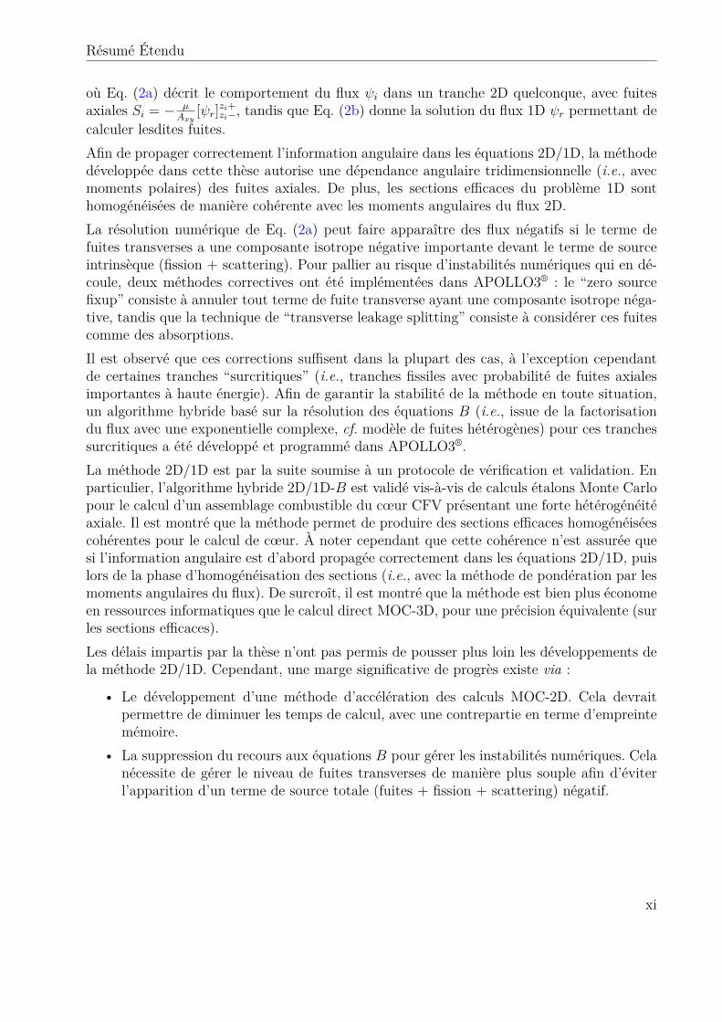
où Eq. (2a) décrit le comportement du flux ψi dans un tranche 2D quelconque, avec fuitesaxiales Si = − µ
Axy[ψr]zi+zi−, tandis que Eq. (2b) donne la solution du flux 1D ψr permettant de
calculer lesdites fuites.Afin de propager correctement l’information angulaire dans les équations 2D/1D, la méthodedéveloppée dans cette thèse autorise une dépendance angulaire tridimensionnelle (i.e., avecmoments polaires) des fuites axiales. De plus, les sections efficaces du problème 1D sonthomogénéisées de manière cohérente avec les moments angulaires du flux 2D.La résolution numérique de Eq. (2a) peut faire apparaître des flux négatifs si le terme defuites transverses a une composante isotrope négative importante devant le terme de sourceintrinsèque (fission + scattering). Pour pallier au risque d’instabilités numériques qui en dé-coule, deux méthodes correctives ont été implémentées dans APOLLO3® : le “zero sourcefixup” consiste à annuler tout terme de fuite transverse ayant une composante isotrope néga-tive, tandis que la technique de “transverse leakage splitting” consiste à considérer ces fuitescomme des absorptions.Il est observé que ces corrections suffisent dans la plupart des cas, à l’exception cependantde certaines tranches “surcritiques” (i.e., tranches fissiles avec probabilité de fuites axialesimportantes à haute énergie). Afin de garantir la stabilité de la méthode en toute situation,un algorithme hybride basé sur la résolution des équations B (i.e., issue de la factorisationdu flux avec une exponentielle complexe, cf. modèle de fuites hétérogènes) pour ces tranchessurcritiques a été développé et programmé dans APOLLO3®.La méthode 2D/1D est par la suite soumise à un protocole de vérification et validation. Enparticulier, l’algorithme hybride 2D/1D-B est validé vis-à-vis de calculs étalons Monte Carlopour le calcul d’un assemblage combustible du cœur CFV présentant une forte hétérogénéitéaxiale. Il est montré que la méthode permet de produire des sections efficaces homogénéiséescohérentes pour le calcul de cœur. À noter cependant que cette cohérence n’est assurée quesi l’information angulaire est d’abord propagée correctement dans les équations 2D/1D, puislors de la phase d’homogénéisation des sections (i.e., avec la méthode de pondération par lesmoments angulaires du flux). De surcroît, il est montré que la méthode est bien plus économeen ressources informatiques que le calcul direct MOC-3D, pour une précision équivalente (surles sections efficaces).Les délais impartis par la thèse n’ont pas permis de pousser plus loin les développements dela méthode 2D/1D. Cependant, une marge significative de progrès existe via :
• Le développement d’une méthode d’accélération des calculs MOC-2D. Cela devraitpermettre de diminuer les temps de calcul, avec une contrepartie en terme d’empreintemémoire.
• La suppression du recours aux équations B pour gérer les instabilités numériques. Celanécessite de gérer le niveau de fuites transverses de manière plus souple afin d’éviterl’apparition d’un terme de source totale (fuites + fission + scattering) négatif.
xi
Résumé Étendu
Chapitre 5 : Développement et Validation d’un Nouveau Schéma de Calcul AP3–SFR de Reference
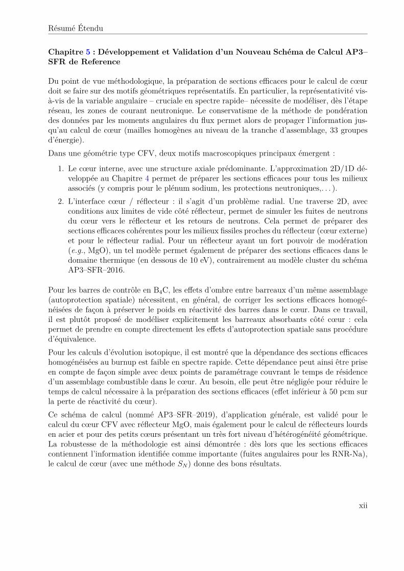
Du point de vue méthodologique, la préparation de sections efficaces pour le calcul de cœurdoit se faire sur des motifs géométriques représentatifs. En particulier, la représentativité vis-à-vis de la variable angulaire – cruciale en spectre rapide– nécessite de modéliser, dès l’étaperéseau, les zones de courant neutronique. Le conservatisme de la méthode de pondérationdes données par les moments angulaires du flux permet alors de propager l’information jus-qu’au calcul de cœur (mailles homogènes au niveau de la tranche d’assemblage, 33 groupesd’énergie).Dans une géométrie type CFV, deux motifs macroscopiques principaux émergent :
1. Le cœur interne, avec une structure axiale prédominante. L’approximation 2D/1D dé-veloppée au Chapitre 4 permet de préparer les sections efficaces pour tous les milieuxassociés (y compris pour le plénum sodium, les protections neutroniques,. . . ).
2. L’interface cœur / réflecteur : il s’agit d’un problème radial. Une traverse 2D, avecconditions aux limites de vide côté réflecteur, permet de simuler les fuites de neutronsdu cœur vers le réflecteur et les retours de neutrons. Cela permet de préparer dessections efficaces cohérentes pour les milieux fissiles proches du réflecteur (cœur externe)et pour le réflecteur radial. Pour un réflecteur ayant un fort pouvoir de modération(e.g., MgO), un tel modèle permet également de préparer des sections efficaces dans ledomaine thermique (en dessous de 10 eV), contrairement au modèle cluster du schémaAP3–SFR–2016.
Pour les barres de contrôle en B4C, les effets d’ombre entre barreaux d’un même assemblage(autoprotection spatiale) nécessitent, en général, de corriger les sections efficaces homogé-néisées de façon à préserver le poids en réactivité des barres dans le cœur. Dans ce travail,il est plutôt proposé de modéliser explicitement les barreaux absorbants côté cœur : celapermet de prendre en compte directement les effets d’autoprotection spatiale sans procédured’équivalence.Pour les calculs d’évolution isotopique, il est montré que la dépendance des sections efficaceshomogénéisées au burnup est faible en spectre rapide. Cette dépendance peut ainsi être priseen compte de façon simple avec deux points de paramétrage couvrant le temps de résidenced’un assemblage combustible dans le cœur. Au besoin, elle peut être négligée pour réduire letemps de calcul nécessaire à la préparation des sections efficaces (effet inférieur à 50 pcm surla perte de réactivité du cœur).Ce schéma de calcul (nommé AP3–SFR–2019), d’application générale, est validé pour lecalcul du cœur CFV avec réflecteur MgO, mais également pour le calcul de réflecteurs lourdsen acier et pour des petits cœurs présentant un très fort niveau d’hétérogénéité géométrique.La robustesse de la méthodologie est ainsi démontrée : dès lors que les sections efficacescontiennent l’information identifiée comme importante (fuites angulaires pour les RNR-Na),le calcul de cœur (avec une méthode SN) donne des bons résultats.
xii
Résumé Étendu
En particulier, l’ordre de grandeur des biais sur les principaux paramètres neutroniques d’in-térêt, vis-à-vis de résultats Monte Carlo, est le suivant :
- environ 50 pcm sur la réactivité ;- 50/100 pcm sur l’effet de vide sodium ;- 1% sur la distribution spatiale du taux de fission (2% max. dans les zones fissiles, 6%max. dans les mailles fertiles proches du réflecteur) ;
- 4% sur le coefficient de contre-réaction de température combustible (Doppler) ;- 2% sur le poids en réactivité des barres avec une représentation explicite des barreauxabsorbants côté cœur (contre 6% pour une homogénéisation complète des barres) ;
- 1% sur l’inventaire combustible en fin de cycle (pour un assemblage combustible réfléchiradialement).
Ces valeurs constituent une nette amélioration par rapport aux résultats de l’ancien schémaAP3–SFR–2016 : elles sont jugées satisfaisantes pour les besoins du CEA en calculs neutro-niques de référence pour l’étude de RNR-Na.De surcroît, des pistes d’amélioration sont évoquées en ce qui concerne le maillage énergétiqueà 33 groupes, peu adapté au calcul des réflecteurs aciers du fait de la présence d’une résonancede diffusion importante du 56Fe à 26 keV. Par ailleurs, le choix des motifs utilisés pour préparerles sections efficaces peut être raffiné pour prendre en compte davantage d’interfaces 3D(e.g., suiveurs de barres, milieux fertiles proches du réflecteur, barres de contrôle proche del’interface cœur / plénum,. . . ).
Chapitre 6 : Vers des Schémas Flexibles et Adaptatifs
La définition du schéma de calcul neutronique de référence tolère une contrainte informatiquerelativement élevée (temps de calcul notamment) de façon à obtenir une solution best esti-mate. Cependant, lorsque le nombre de calculs devant être réalisés augmente, la minimisationdu temps de calcul devient un enjeu primordial : il est alors nécessaire de définir des schémas“projets”. À titre d’exemples, on peut citer les besoins en études paramétriques ou en calculsde transitoires accidentels (en particulier pour les transitoires rapides associés à une variationsignificative de la forme du flux). La difficulté, à ce stade, consiste à trouver le bon niveaud’approximations, de façon à réduire significativement le temps de calcul sans dégrader outremesure la précision sur les paramètres cibles.Dans un schéma de calcul en deux étapes, la phase d’homogénéisation permet de lisser deserreurs statistiques (i.e., non systématiques) sur le calcul de flux. Ainsi, un moyen efficacede réduire la contrainte informatique pour une perte de précision maitrisée consiste à re-lâcher les paramètres de discrétisation (géométriques et de traçage) lors de l’étape réseau.Cette méthode permet de maîtriser la perte d’information sur l’ensemble des paramètresneutroniques.Une autre possibilité consiste à introduire des modèles ad hoc lors de la préparation dessections efficaces, de façon à éviter des calculs coûteux (e.g., un modèle de fuite isotrope
xiii
Résumé Étendu
pour représenter des fuites dans des géométries 2D). Tout nouveau modèle devant être validépour le calcul des paramètres neutroniques d’intérêt, cette stratégie n’est pas pertinente si l’onveut garantir la robustesse du schéma projet. Il s’agit néanmoins d’une solution pragmatiquepour définir des schémas optimisés pour le calcul d’un nombre restreint de paramètres. Laméthodologie du code ECCO, par exemple, donne de bons résultats sur le calcul de l’effet devide sodium du cœur CFV avec réflecteur MgO bien que la forme de la distribution spatialedu flux ne soit pas respectée.La marge de manœuvre pour la définition de schémas projets est plus faible au niveau ducalcul de cœur (deuxième étape du schéma). Il est ainsi montré que seul le solveur MINARETd’APOLLO3® (solveur SN) est capable de modéliser correctement les situations de vidangesodium dans des cœurs type CFV : les méthodes PN et SPN (solveurs PASTIS et MINOS)donnent des biais significatifs sur le calcul de l’effet de vide.Enfin, ce chapitre ouvre des perspectives pour la définition de schémas de calcul adaptatifs,au sens où ils s’affranchissent des choix faits au Chapitre 5 pour la définition des motifs depréparation des sections efficaces. La théorie de l’homogénéisation dynamique est présentéecomme une solution naturelle pour homogénéiser les sections efficaces à la volée avec uneprise en compte cohérente des modes angulaires du flux présents dans le cœur. La questionde la déconvolution de la source entre le maillage énergétique grossier (33 groupes) et lemaillage fin (1968 groupes) est également abordée. Enfin, des idées sont évoquées pour unegestion optimisée du partage des sections efficaces homogénéisées lors du calcul de cœur.
Chapitre 7 : Conclusion Générale
Le principal produit de ce travail est un schéma de calcul neutronique robuste et validénumériquement pour la modélisation de cœurs de RNR-Na complexes avec APOLLO3®.Nous renvoyons le lecteur aux quelques pages précédentes (ou au corps du document) pourle détail des principaux résultats (performances, limites et perspectives d’amélioration).En tout état de cause, ce travail ne répond qu’à la question des biais de calcul imputablesaux méthodes de résolution de l’équation du transport des neutrons pour les RNR-Na. Dansun contexte de sûreté nucléaire, cette étude devrait être complétée par un travail de quantifi-cation des incertitudes sur les données d’entrée (sections efficaces et données technologiques)et de propagation à travers le code sur l’évaluation des paramètres d’intérêt. De plus, desrésultats de validation expérimentale devraient être apportés : pour ce faire, un travail detransposition des expériences réalisées par le passé (de Masurca à Superphénix) vers lesdessins de cœurs modernes (CFV) est nécessaire.
xiv
Table of Contents
Dedication . . . . . . . . . . . . . . . . . . . . . . . . . . . . . . . . . . . . . . . . . iii
Acknowledgments . . . . . . . . . . . . . . . . . . . . . . . . . . . . . . . . . . . . iv
Abstract . . . . . . . . . . . . . . . . . . . . . . . . . . . . . . . . . . . . . . . . . . v
Résumé . . . . . . . . . . . . . . . . . . . . . . . . . . . . . . . . . . . . . . . . . . vi
Résumé Étendu . . . . . . . . . . . . . . . . . . . . . . . . . . . . . . . . . . . . . vii
Table of Contents . . . . . . . . . . . . . . . . . . . . . . . . . . . . . . . . . . . . xv
List of Tables . . . . . . . . . . . . . . . . . . . . . . . . . . . . . . . . . . . . . . . xix
List of Figures . . . . . . . . . . . . . . . . . . . . . . . . . . . . . . . . . . . . . . xxii
List of Acronyms and Abbreviations . . . . . . . . . . . . . . . . . . . . . . . . xxvi
Chapter 1 Introduction . . . . . . . . . . . . . . . . . . . . . . . . . . . . . . . 11.1 Prelude . . . . . . . . . . . . . . . . . . . . . . . . . . . . . . . . . . . . . . 11.2 Nuclear Energy Context . . . . . . . . . . . . . . . . . . . . . . . . . . . . . 2
1.2.1 The Climate Change Challenge . . . . . . . . . . . . . . . . . . . . . 21.2.2 The Nuclear Response . . . . . . . . . . . . . . . . . . . . . . . . . . 31.2.3 Nuclear Energy Constraints . . . . . . . . . . . . . . . . . . . . . . . 41.2.4 Perspectives . . . . . . . . . . . . . . . . . . . . . . . . . . . . . . . . 51.2.5 The ASTRID Project . . . . . . . . . . . . . . . . . . . . . . . . . . . 7
1.3 Numerical Simulation Tools Context . . . . . . . . . . . . . . . . . . . . . . 81.3.1 Reactor Design & Nuclear Safety . . . . . . . . . . . . . . . . . . . . 81.3.2 Neutronic Codes . . . . . . . . . . . . . . . . . . . . . . . . . . . . . 91.3.3 The APOLLO3® Project . . . . . . . . . . . . . . . . . . . . . . . . . 101.3.4 The VV&UQ Process . . . . . . . . . . . . . . . . . . . . . . . . . . . 10
1.4 Objectives of this Thesis . . . . . . . . . . . . . . . . . . . . . . . . . . . . . 111.5 Thesis Layout . . . . . . . . . . . . . . . . . . . . . . . . . . . . . . . . . . . 12
Chapter 2 Nuclear Reactor Neutronic Calculation: Theory & Methods . 132.1 The Neutron Transport Equation . . . . . . . . . . . . . . . . . . . . . . . . 14
2.1.1 The Neutron as a Point-Particle . . . . . . . . . . . . . . . . . . . . . 142.1.2 Derivation of the Particle Balance . . . . . . . . . . . . . . . . . . . . 142.1.3 Expression of the Collision Term . . . . . . . . . . . . . . . . . . . . 172.1.4 The NTE and its Solutions . . . . . . . . . . . . . . . . . . . . . . . . 212.1.5 The Critical Problem . . . . . . . . . . . . . . . . . . . . . . . . . . . 21
2.2 Numerical Methods for the NTE . . . . . . . . . . . . . . . . . . . . . . . . . 232.2.1 Power Method . . . . . . . . . . . . . . . . . . . . . . . . . . . . . . . 23
xv
Table of Contents
2.2.2 Multigroup Approximation . . . . . . . . . . . . . . . . . . . . . . . . 242.2.3 Spatial and Angular Discretization . . . . . . . . . . . . . . . . . . . 272.2.4 Stochastic Methods . . . . . . . . . . . . . . . . . . . . . . . . . . . . 33
2.3 The Numerical Footprint Issue . . . . . . . . . . . . . . . . . . . . . . . . . . 352.3.1 Deterministic Point of View . . . . . . . . . . . . . . . . . . . . . . . 352.3.2 Stochastic Point of View . . . . . . . . . . . . . . . . . . . . . . . . . 37
2.4 Acceleration of the NTE . . . . . . . . . . . . . . . . . . . . . . . . . . . . . 372.4.1 Parallelism . . . . . . . . . . . . . . . . . . . . . . . . . . . . . . . . . 372.4.2 Acceleration . . . . . . . . . . . . . . . . . . . . . . . . . . . . . . . . 38
2.5 Homogenization Theory . . . . . . . . . . . . . . . . . . . . . . . . . . . . . 392.5.1 The Homogenized Problem . . . . . . . . . . . . . . . . . . . . . . . . 392.5.2 The Reference Problem . . . . . . . . . . . . . . . . . . . . . . . . . . 44
2.6 Neutronic Calculation Schemes . . . . . . . . . . . . . . . . . . . . . . . . . 452.6.1 The Lattice - Core Paradigm . . . . . . . . . . . . . . . . . . . . . . 452.6.2 Resonance Self-shielding . . . . . . . . . . . . . . . . . . . . . . . . . 472.6.3 Towards Heterogeneous 3D Calculations? . . . . . . . . . . . . . . . . 50
2.7 Conclusions . . . . . . . . . . . . . . . . . . . . . . . . . . . . . . . . . . . . 51
Chapter 3 Analysis of the AP3–SFR–2016 Calculation Scheme . . . . . . 533.1 Description of the CFV . . . . . . . . . . . . . . . . . . . . . . . . . . . . . . 543.2 Description of the AP3–SFR–2016 Methodology . . . . . . . . . . . . . . . . 55
3.2.1 Cross Section Preparation . . . . . . . . . . . . . . . . . . . . . . . . 563.2.2 Core Calculations . . . . . . . . . . . . . . . . . . . . . . . . . . . . . 60
3.3 Validation of Lattice Calculations . . . . . . . . . . . . . . . . . . . . . . . . 613.3.1 Fissile Assembly . . . . . . . . . . . . . . . . . . . . . . . . . . . . . 623.3.2 Fertile Cluster . . . . . . . . . . . . . . . . . . . . . . . . . . . . . . . 643.3.3 Reflector Cluster (MgO) . . . . . . . . . . . . . . . . . . . . . . . . . 663.3.4 Control Rods (B4C) . . . . . . . . . . . . . . . . . . . . . . . . . . . 683.3.5 Other Structures . . . . . . . . . . . . . . . . . . . . . . . . . . . . . 693.3.6 Discussion . . . . . . . . . . . . . . . . . . . . . . . . . . . . . . . . . 70
3.4 Validation of Homogenization Methods . . . . . . . . . . . . . . . . . . . . . 713.4.1 Results . . . . . . . . . . . . . . . . . . . . . . . . . . . . . . . . . . . 713.4.2 Discussion . . . . . . . . . . . . . . . . . . . . . . . . . . . . . . . . . 73
3.5 Analysis of the Biases at the Core Level . . . . . . . . . . . . . . . . . . . . 733.5.1 CFV Calculation . . . . . . . . . . . . . . . . . . . . . . . . . . . . . 733.5.2 Fuel Assembly Model: Study of Axial Phenomena . . . . . . . . . . . 783.5.3 Core - Reflector Interface Model: Study of Radial Phenomena . . . . 84
3.6 Conclusions . . . . . . . . . . . . . . . . . . . . . . . . . . . . . . . . . . . . 86
Chapter 4 Development of a 2D/1D Method for Cross Section Generationin SFR Axial Geometries . . . . . . . . . . . . . . . . . . . . . . . . . . . . . . 894.1 2D/1D Methods . . . . . . . . . . . . . . . . . . . . . . . . . . . . . . . . . . 90
4.1.1 Overview . . . . . . . . . . . . . . . . . . . . . . . . . . . . . . . . . 904.1.2 General Equations . . . . . . . . . . . . . . . . . . . . . . . . . . . . 91
4.2 Application to the SFR Homogenization Problem . . . . . . . . . . . . . . . 93
xvi
Table of Contents
4.2.1 Domain Definition . . . . . . . . . . . . . . . . . . . . . . . . . . . . 934.2.2 Approximations . . . . . . . . . . . . . . . . . . . . . . . . . . . . . . 934.2.3 Solution of the 2D/1D Equations . . . . . . . . . . . . . . . . . . . . 944.2.4 Representation of the Angular Variable . . . . . . . . . . . . . . . . . 954.2.5 Generation of Few Groups Cross Sections . . . . . . . . . . . . . . . . 96
4.3 Implementation in APOLLO3® . . . . . . . . . . . . . . . . . . . . . . . . . 974.3.1 Transport Solvers . . . . . . . . . . . . . . . . . . . . . . . . . . . . . 974.3.2 Homogenization of 1D Cross Sections . . . . . . . . . . . . . . . . . . 984.3.3 Transverse Leakage Projection . . . . . . . . . . . . . . . . . . . . . . 984.3.4 Dealing with Negative Sources . . . . . . . . . . . . . . . . . . . . . . 994.3.5 Case of Overcritical Layers . . . . . . . . . . . . . . . . . . . . . . . . 1014.3.6 Case of Optically Thin Media . . . . . . . . . . . . . . . . . . . . . . 102
4.4 Verifications . . . . . . . . . . . . . . . . . . . . . . . . . . . . . . . . . . . . 1024.4.1 TDT/IDT Coupling . . . . . . . . . . . . . . . . . . . . . . . . . . . 1024.4.2 2D/1D Algorithms . . . . . . . . . . . . . . . . . . . . . . . . . . . . 106
4.5 Validation on a CFV Fuel Assembly Calculation . . . . . . . . . . . . . . . . 1114.5.1 Benchmark Description . . . . . . . . . . . . . . . . . . . . . . . . . . 1114.5.2 Convergence Assessment of 2D/1D Solution . . . . . . . . . . . . . . 1134.5.3 Validation of the Method for Cross Section Preparation . . . . . . . . 115
4.6 Definition of a Calculation Method Comparison Grid . . . . . . . . . . . . . 1184.6.1 Estimators . . . . . . . . . . . . . . . . . . . . . . . . . . . . . . . . . 1184.6.2 Application to APOLLO3® methods . . . . . . . . . . . . . . . . . . 118
4.7 Conclusions . . . . . . . . . . . . . . . . . . . . . . . . . . . . . . . . . . . . 119
Chapter 5 Development and Validation of a New AP3–SFR Reference Cal-culation Scheme . . . . . . . . . . . . . . . . . . . . . . . . . . . . . . . . . . . 1215.1 Methodology Description . . . . . . . . . . . . . . . . . . . . . . . . . . . . . 122
5.1.1 General Philosophy . . . . . . . . . . . . . . . . . . . . . . . . . . . . 1225.1.2 Application to the CFV . . . . . . . . . . . . . . . . . . . . . . . . . 123
5.2 Static Core Calculations . . . . . . . . . . . . . . . . . . . . . . . . . . . . . 1265.2.1 Validation on a 2D Core Model . . . . . . . . . . . . . . . . . . . . . 1265.2.2 Validation on a 3D CFV . . . . . . . . . . . . . . . . . . . . . . . . . 1285.2.3 Case of a Steel Reflector . . . . . . . . . . . . . . . . . . . . . . . . . 1335.2.4 Case of a Small SFR Core . . . . . . . . . . . . . . . . . . . . . . . . 1355.2.5 Discussion . . . . . . . . . . . . . . . . . . . . . . . . . . . . . . . . . 137
5.3 Control Rods Modeling . . . . . . . . . . . . . . . . . . . . . . . . . . . . . . 1375.3.1 The Spatial Self-Shielding Issue . . . . . . . . . . . . . . . . . . . . . 1375.3.2 The Heterogeneous Model Alternative . . . . . . . . . . . . . . . . . 1395.3.3 Application to a CFV . . . . . . . . . . . . . . . . . . . . . . . . . . 1415.3.4 Discussion . . . . . . . . . . . . . . . . . . . . . . . . . . . . . . . . . 144
5.4 Depletion Calculations . . . . . . . . . . . . . . . . . . . . . . . . . . . . . . 1465.4.1 The Adiabatic Approximation . . . . . . . . . . . . . . . . . . . . . . 1465.4.2 Parametrization of Cross Sections with the 2D/1D Method . . . . . . 1475.4.3 Validation on a 3D Assembly Model . . . . . . . . . . . . . . . . . . . 1485.4.4 Application to a Full CFV . . . . . . . . . . . . . . . . . . . . . . . . 155
xvii
Table of Contents
5.4.5 Discussion . . . . . . . . . . . . . . . . . . . . . . . . . . . . . . . . . 1575.5 Evaluation of Neutronic Feedback Coefficients . . . . . . . . . . . . . . . . . 157
5.5.1 General Considerations on Transient Calculations . . . . . . . . . . . 1575.5.2 Evaluation of the CFV Integral Coefficients . . . . . . . . . . . . . . 1595.5.3 Sodium Void Reactivity Worth Axial Decomposition . . . . . . . . . 160
5.6 Conclusions . . . . . . . . . . . . . . . . . . . . . . . . . . . . . . . . . . . . 161
Chapter 6 Towards Flexible & Adaptative Calculation Schemes . . . . . . 1636.1 Needs for Faster Calculation Schemes . . . . . . . . . . . . . . . . . . . . . . 164
6.1.1 Reactor Design Studies . . . . . . . . . . . . . . . . . . . . . . . . . . 1646.1.2 Multi-physics Calculations . . . . . . . . . . . . . . . . . . . . . . . . 164
6.2 Illustration: Sensitivity of an ULOF Transient to the Neutronic CalculationStrategy . . . . . . . . . . . . . . . . . . . . . . . . . . . . . . . . . . . . . . 1656.2.1 Methodology Presentation . . . . . . . . . . . . . . . . . . . . . . . . 1656.2.2 Analysis of PK Parameters . . . . . . . . . . . . . . . . . . . . . . . . 1686.2.3 Impact on the ULOF Outcome . . . . . . . . . . . . . . . . . . . . . 1706.2.4 Discussion . . . . . . . . . . . . . . . . . . . . . . . . . . . . . . . . . 172
6.3 Construction of AP3–SFR Project Methodologies . . . . . . . . . . . . . . . 1726.3.1 Strategy Assessment . . . . . . . . . . . . . . . . . . . . . . . . . . . 1726.3.2 Degradation of the Reference Options . . . . . . . . . . . . . . . . . . 1736.3.3 Resort to ad hoc Physical Models . . . . . . . . . . . . . . . . . . . . 1776.3.4 Discussion . . . . . . . . . . . . . . . . . . . . . . . . . . . . . . . . . 181
6.4 Beyond the Lattice / Core Paradigm . . . . . . . . . . . . . . . . . . . . . . 1826.4.1 Dynamic Homogenization . . . . . . . . . . . . . . . . . . . . . . . . 1826.4.2 Towards Flexible Homogenization . . . . . . . . . . . . . . . . . . . . 186
6.5 Conclusions . . . . . . . . . . . . . . . . . . . . . . . . . . . . . . . . . . . . 186
Chapter 7 General Conclusion . . . . . . . . . . . . . . . . . . . . . . . . . . . 1897.1 Main Conclusions . . . . . . . . . . . . . . . . . . . . . . . . . . . . . . . . . 1897.2 Perspectives . . . . . . . . . . . . . . . . . . . . . . . . . . . . . . . . . . . . 191
References . . . . . . . . . . . . . . . . . . . . . . . . . . . . . . . . . . . . . . . . . 193
Appendices . . . . . . . . . . . . . . . . . . . . . . . . . . . . . . . . . . . . . . . . 204A Real Spherical Harmonics . . . . . . . . . . . . . . . . . . . . . . . . . . . . 205B Angular Treatment of Spatial Symmetries . . . . . . . . . . . . . . . . . . . . 207C Additional Information on the DGFEM . . . . . . . . . . . . . . . . . . . . . 209D The CFV Design . . . . . . . . . . . . . . . . . . . . . . . . . . . . . . . . . 210E CFV Fuel Assembly Calculation: Complementary Results . . . . . . . . . . . 213F Validation of APOLLO3® 2D Depletion Calculations . . . . . . . . . . . . . . 214G Perturbation Theory and Point Kinetics . . . . . . . . . . . . . . . . . . . . 220
xviii
List of Tables
Table 2.1 Examples of parallel computing strategies for the NTE. . . . . . . . . 37Table 3.1 Tracking parameter values for TDT-MOC and TDT-CPM solutions. . 62Table 3.2 Fissile assembly 2D calculation: eigenvalue and reaction rate compar-
ison between APOLLO3® and TRIPOLI-4® (in pcm). . . . . . . . . . 63Table 3.3 Fertile cluster 2D calculation: eigenvalue and reaction rate comparison
between APOLLO3® and TRIPOLI-4® (in pcm). . . . . . . . . . . . 65Table 3.4 MgO reflector cluster 2D calculation: eigenvalue comparison between
APOLLO3® and TRIPOLI-4®. . . . . . . . . . . . . . . . . . . . . . . 67Table 3.5 Control rod 2D cluster calculations: eigenvalue comparison between
APOLLO3® and TRIPOLI-4®. . . . . . . . . . . . . . . . . . . . . . . 69Table 3.6 Structures 2D cluster calculations: eigenvalue comparison between APOL-
LO3® and TRIPOLI-4®. . . . . . . . . . . . . . . . . . . . . . . . . . 69Table 3.7 AP3–SFR–2016 memory requirements at the lattice level (with 4 pro-
cessors). . . . . . . . . . . . . . . . . . . . . . . . . . . . . . . . . . . 70Table 3.8 Eigenvalue comparison between heterogeneous 1968 group lattice cal-
culations and 33 group homogenized counterpart with APOLLO3®. . 72Table 3.9 Calculation options of MINARET. . . . . . . . . . . . . . . . . . . . 74Table 3.10 CFV calculation (without control rods): eigenvalue comparison be-
tween APOLLO3® and TRIPOLI-4®. . . . . . . . . . . . . . . . . . . 75Table 3.11 Computer requirements for a CFV calculation with MINARET (with
8 processors). . . . . . . . . . . . . . . . . . . . . . . . . . . . . . . . 77Table 3.12 CFV fuel assembly calculation: eigenvalue comparison between APOL-
LO3® and TRIPOLI-4®, with AP3–SFR–2016 cross sections. . . . . . 79Table 3.13 CFV fuel assembly calculation: eigenvalue comparison between APOL-
LO3® and TRIPOLI-4®, with 3D-MOC cross sections. . . . . . . . . . 81Table 3.14 CFV fuel assembly calculation: eigenvalue comparison between APOL-
LO3® and TRIPOLI-4®, with ECCO cross sections. . . . . . . . . . . 82Table 3.15 2D CFV core calculation: eigenvalue comparison between APOLLO3®
and TRIPOLI-4®. . . . . . . . . . . . . . . . . . . . . . . . . . . . . . 85Table 4.1 2D/1D verification test case no 1: transverse leakage source (Si) angular
moments. . . . . . . . . . . . . . . . . . . . . . . . . . . . . . . . . . 105Table 4.2 2D/1D verification test case no 1: verification of the flux conservation
relations. . . . . . . . . . . . . . . . . . . . . . . . . . . . . . . . . . . 105Table 4.3 2D/1D verification test case no 1: influence of the negative source fixup
on integrated axial flux moments∫Drψi,l0. . . . . . . . . . . . . . . . 106
Table 4.4 2D/1D verification test case no 2: convergence of 2D/1D algorithms(eigenvalue). . . . . . . . . . . . . . . . . . . . . . . . . . . . . . . . . 108
Table 4.5 2D/1D verification test case no 2: verification of the flux conservationrelations. . . . . . . . . . . . . . . . . . . . . . . . . . . . . . . . . . . 109
Table 4.6 2D/1D verification test case no 2: angular moments of the transverseleakage source Si with Algo. 6 and a TLS correction (at convergence). 109
Table 4.7 CFV fuel assembly 2D/1D calculation: convergence of Algo. 7. . . . 113
xix
List of Tables
Table 4.8 CFV fuel assembly 2D/1D calculation: influence of the initializationcondition in Algo. 7. . . . . . . . . . . . . . . . . . . . . . . . . . . . 114
Table 4.9 CFV fuel assembly 2D/1D calculation: computer requirements withAlgo. 7 (with 4 processors). . . . . . . . . . . . . . . . . . . . . . . . 115
Table 4.10 CFV fuel assembly calculation with 2D/1D cross sections: eigenvalueand sodium void worth (TRIPOLI-4® results and APOLLO3® reactiv-ity discrepancies). . . . . . . . . . . . . . . . . . . . . . . . . . . . . . 116
Table 4.11 Comparison of APOLLO3® methods for the preparation of a 3D CFVfuel assembly homogenized cross sections. . . . . . . . . . . . . . . . 119
Table 5.1 Tracking parameter values for the core / reflector traverse calculation(TDT-MOC and TDT-CPM). . . . . . . . . . . . . . . . . . . . . . . 127
Table 5.2 Computational requirements for core / reflector traverse calculation. . 127Table 5.3 2D CFV core calculation with cross sections coming from a core /
reflector traverse model: eigenvalue comparison between APOLLO3®
and TRIPOLI-4®. . . . . . . . . . . . . . . . . . . . . . . . . . . . . . 127Table 5.4 CFV calculation with the new AP3–SFR–2019 calculation scheme (with-
out control rods): eigenvalue comparison between APOLLO3® andTRIPOLI-4®. . . . . . . . . . . . . . . . . . . . . . . . . . . . . . . . 129
Table 5.5 CFV calculation with the new AP3–SFR–2019 calculation scheme (with-out control rods): maximal and mean discrepancies (APOLLO3®vs.TRIPOLI-4®) on the fission rate distribution. . . . . . . . . . . . . . 130
Table 5.6 CFV calculation: comparison of different calculation schemes. . . . . 132Table 5.7 CFV calculation with steel reflector: AP3–SFR–2019 biases on a se-
lected set of neutronic estimators. . . . . . . . . . . . . . . . . . . . . 134Table 5.8 AMR calculation: bias on neutronic estimators. . . . . . . . . . . . . 136Table 5.9 Evaluation of the reactivity bias due to the control rod cluster homog-
enization with CR-HOMO and CR-HETE models. . . . . . . . . . . . 140Table 5.10 Total control rods reactivity worth in the CFV (90 cm insertion from
parking position). . . . . . . . . . . . . . . . . . . . . . . . . . . . . . 142Table 5.11 Computer requirements for a CFV core calculation with MINARET
depending on the control rod model (with 8 processors). . . . . . . . 145Table 5.12 CFV fuel assembly depletion calculation: Pu239, Np237 and Cs133
concentrations at end of depletion (t = 1080 EFPD). . . . . . . . . . 154Table 5.13 Beginning-of-life CFV feedback coefficients. . . . . . . . . . . . . . . 160Table 5.14 CFV fuel assembly calculation: spatial decomposition of the sodium
void reactivity worth (in pcm) for a -1% perturbation of the coolantdensity. . . . . . . . . . . . . . . . . . . . . . . . . . . . . . . . . . . 161
Table 6.1 Sensitivity of CFV integral PK parameters to the neutronic calculationmethod. . . . . . . . . . . . . . . . . . . . . . . . . . . . . . . . . . . 168
Table 6.2 Tracking parameter values for TDT-MOC and TDT-CPM solutions forAP3–SFR project strategies. . . . . . . . . . . . . . . . . . . . . . . . 174
Table 6.3 Comparison of MINARET, PASTIS and MINOS solvers for a CFV(MgO reflector) flux calculation. . . . . . . . . . . . . . . . . . . . . 176
Table 6.4 Comparison of AP3–SFR and ECCO calculation strategies. . . . . . 179Table D.1 CFV main features . . . . . . . . . . . . . . . . . . . . . . . . . . . . 212
xx

List of Tables
Table E.1 Comparison of methods for the preparation of a 3D CFV fuel assemblyhomogenized cross sections (complementary results). . . . . . . . . . 213
Table F.1 Time-steps used for 2D fuel assembly depletion calculations. . . . . . 215
xxi
List of Figures
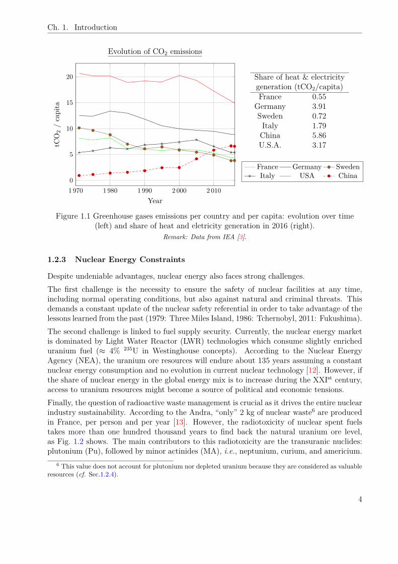
Figure 1.1 Greenhouse gases emissions per country and per capita: evolution overtime (left) and share of heat and eletricity generation in 2016 (right). 4
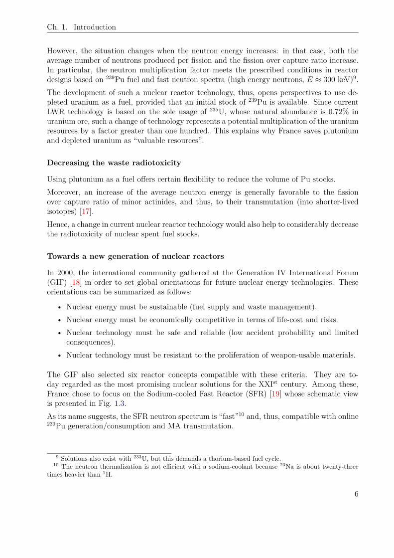
Figure 1.2 Spent fuel radiotoxicity evolution in time. . . . . . . . . . . . . . . . 5Figure 1.3 SFR schematic view. . . . . . . . . . . . . . . . . . . . . . . . . . . . 7Figure 2.1 Particle balance in six-dimensional phase space. . . . . . . . . . . . . 15Figure 2.2 Multigroup discretization. . . . . . . . . . . . . . . . . . . . . . . . . 25Figure 2.3 Discretization of space and angle for the NTE. . . . . . . . . . . . . . 27Figure 2.4 MOC discretization. . . . . . . . . . . . . . . . . . . . . . . . . . . . 29Figure 2.5 Embedded SFR typical geometries. . . . . . . . . . . . . . . . . . . . 36Figure 2.6 238U and 56Fe total cross sections. . . . . . . . . . . . . . . . . . . . . 36Figure 2.7 Replacement of a heterogeneous problem by its homogenized counterpart. 39Figure 3.1 The CFV: schematic axial cut (left) and fuel assembly radial section
(right). . . . . . . . . . . . . . . . . . . . . . . . . . . . . . . . . . . . 54Figure 3.2 AP3–SFR–2016 calculation scheme overview. . . . . . . . . . . . . . . 55Figure 3.3 Examples of geometries used for cross section preparation in the AP3–
SFR–2016 methodology (except for a., all geometries are surroundedby fissile assemblies). . . . . . . . . . . . . . . . . . . . . . . . . . . . 56
Figure 3.4 Cluster homogenization with the AP3–SFR–2016 methodology. . . . . 59Figure 3.5 Radial view of a CFV geometrical model with 2π/3 rotational symmetry. 61Figure 3.6 Fissile assembly 2D calculation: spectra comparison for 238U absorption
and 239Pu fission rates between APOLLO3® and TRIPOLI-4® (top:reaction rate, bottom: relative difference computed as ∆τ/τT4). . . . 64
Figure 3.7 Fertile cluster 2D calculation: comparison of 238U absorption rate in fer-tile assembly and 239Pu fission rate in fissile assembly between APOL-LO3® and TRIPOLI-4® (top: reaction rate, bottom: relative differencecomputed as ∆τ/τT4). . . . . . . . . . . . . . . . . . . . . . . . . . . 66
Figure 3.8 Reflector cluster 2D calculation: comparison of flux spectrum in MgOpins and 239Pu fission rates in fissile assembly between APOLLO3® andTRIPOLI-4® (top: flux or reaction rate, bottom: relative differencecomputed as ∆τ/τT4). . . . . . . . . . . . . . . . . . . . . . . . . . . 67
Figure 3.9 CSD cluster 2D calculation with 48% 10B enrichment: comparison of10B absorption and 239Pu fission rate between APOLLO3® and TRI-POLI-4® (top: reaction rate, bottom: relative difference computed as∆τ/τT4). . . . . . . . . . . . . . . . . . . . . . . . . . . . . . . . . . . 68
Figure 3.10 Radial view of a CFV spatial mesh (MINARET calculation). . . . . . 74Figure 3.11 CFV calculation (without control rods): relative difference on the fis-
sion rate distribution (computed as ∆τ/τ) between APOLLO3® andTRIPOLI-4® (axial cut from core center, i.e., assembly 30/30, to radialreflector). . . . . . . . . . . . . . . . . . . . . . . . . . . . . . . . . . 76
Figure 3.12 CFV fuel assembly calculation: comparison of fission rate distributionsbetween APOLLO3® and TRIPOLI-4®, with AP3–SFR–2016 cross sec-tions. . . . . . . . . . . . . . . . . . . . . . . . . . . . . . . . . . . . 79
xxii
List of Figures
Figure 3.13 CFV fuel assembly calculation: comparison of fission rate distributionsbetween APOLLO3® and TRIPOLI-4®, with 3D-MOC cross sections. 81
Figure 3.14 CFV fuel assembly calculation: comparison of fission rate distributionsbetween APOLLO3® and TRIPOLI-4®, with ECCO cross sections. . 82
Figure 3.15 Spectrum of axial angular flux moments in a CFV fuel assembly. . . . 83Figure 3.16 Simplified CFV 2D schematic view. . . . . . . . . . . . . . . . . . . 84Figure 3.17 2D CFV core calculation: flux comparison at the core / reflector inter-
face between APOLLO3® and TRIPOLI-4®. . . . . . . . . . . . . . . 85Figure 4.1 Example of 2D/1D discretization. . . . . . . . . . . . . . . . . . . . . 91Figure 4.2 2D/1D verification test case no 1: slab geometry. . . . . . . . . . . . . 103Figure 4.3 2D/1D verification test case no 1: angular flux moments ψr,l (1D solution).104Figure 4.4 2D/1D verification test case no 2: geometry. (a) axial layout, (b) radial
layout. . . . . . . . . . . . . . . . . . . . . . . . . . . . . . . . . . . . 107Figure 4.5 2D/1D verification test case no 2: angular flux moments ψr,l of 1D
solution. . . . . . . . . . . . . . . . . . . . . . . . . . . . . . . . . . . 109Figure 4.6 ASTRID internal fuel assembly: (a) axial layout, (b) fuel pins mesh,
(c) sodium plenum mesh, (d) axial protection mesh. . . . . . . . . . . 112Figure 4.7 CFV fuel assembly calculation with 2D/1D cross sections: fission rate
distribution (top: TRIPOLI-4® results, bottom: relative discrepancybetween APOLLO3® and TRIPOLI-4®). . . . . . . . . . . . . . . . . 117
Figure 5.1 2D reflector / core traverse model for cross section preparation withthe new AP3–SFR–2019 calculation scheme. . . . . . . . . . . . . . 124
Figure 5.2 Cross section preparation geometrical patterns for rod followers andother dummy assemblies. . . . . . . . . . . . . . . . . . . . . . . . . . 124
Figure 5.3 Neutron mean free path in a rod follower (or sodium plenum). . . . 125Figure 5.4 Cross section identification of the different media at the core level for
a CFV calculation with the new AP3–SFR–2019 methodology. . . . . 126Figure 5.5 2D CFV core calculation with cross sections coming from a core / re-
flector traverse model: flux comparison at the core / reflector interfacebetween APOLLO3® and TRIPOLI-4®. . . . . . . . . . . . . . . . . . 128
Figure 5.6 CFV calculation with the new AP3–SFR–2019 calculation scheme (with-out control rods): relative difference on the fission rate distribution(∆τ/τ) between APOLLO3® and TRIPOLI-4® (axial cut from corecenter, i.e., assembly 30/30, to radial reflector). . . . . . . . . . . . . 129
Figure 5.7 CFV calculation: fission rate distribution (TRIPOLI-4® results) andposition of the power peak (axial cut from core center, i.e., assembly30/30, to radial reflector). . . . . . . . . . . . . . . . . . . . . . . . . 131
Figure 5.8 Scalar flux ψ00 and current ψ10 shapes at the core / reflector (steel)interface in the vicinity of the 26 keV scattering resonance of 56Fe. . . 134
Figure 5.9 AMR core schematic view: radial (left) and axial (right) layouts. . . . 136Figure 5.10 Spatial self-shielding effects in SFR control rods. . . . . . . . . . . . 138Figure 5.11 Representation of the control rod heterogeneity at the core level. Left:
the control rod (in blue) is homogeneous. Right: the B4C pins (in blue)are kept heterogeneous while the rest of the control rod assembly (inpurple) is homogenized independently. . . . . . . . . . . . . . . . . . 139
xxiii
List of Figures
Figure 5.12 Evolution of the control rods reactivity worth with its insertion (top:TRIPOLI-4® S-curve and differential efficiency, bottom: discrepancybetween APOLLO3® and TRIPOLI-4®). . . . . . . . . . . . . . . . . 142
Figure 5.13 10B absorption rate in a CSD control rod inserted in the CFV (top:TRIPOLI-4® values, bottom: relative discrepancy between APOLLO3®
and TRIPOLI-4®). . . . . . . . . . . . . . . . . . . . . . . . . . . . . 143Figure 5.14 Fission rate in fuel assembly located aside a control rod (top: TRIPO-
LI-4® values, bottom: relative discrepancy between APOLLO3® andTRIPOLI-4®). . . . . . . . . . . . . . . . . . . . . . . . . . . . . . . . 144
Figure 5.15 Radial view of a spatial mesh (MINARET calculation) in a control rodwith CR-HETE model. . . . . . . . . . . . . . . . . . . . . . . . . . . 145
Figure 5.16 Fuel depletion calculations with 2D/1D method. . . . . . . . . . . . . 148Figure 5.17 CFV fuel assembly depletion calculation: reactivity loss (P = 5.4MW). 151Figure 5.18 CFV fuel assembly depletion calculation: reactivity loss (left) and re-
activity discrepancy (APOLLO3® vs. TRIPOLI-4®) with 2D or 2D/1Dcross sections (right). . . . . . . . . . . . . . . . . . . . . . . . . . . . 152
Figure 5.19 CFV fuel assembly depletion calculation: influence of the number oftabulated burnup points (in the homogenized cross section library) onthe reactivity loss (APOLLO3® with 2D/1D cross sections vs. TRI-POLI-4®). . . . . . . . . . . . . . . . . . . . . . . . . . . . . . . . . . 153
Figure 5.20 CFV fuel assembly depletion calculation: evolution of isotopic con-centrations (left) and relative discrepancy with 2D (center) or 2D/1D(right) cross sections for upper fissile zone and lower fertile blanket. . 155
Figure 5.21 CFV depletion calculation: reactivity evolution from a begining-of-life to an equilibrium situation (left) and reactivity loss/load for anarbitrary choice of fuel cycles (right). . . . . . . . . . . . . . . . . . 156
Figure 6.1 Sensitivity of the CFV axial power profile to the neutronic calculationmethod. . . . . . . . . . . . . . . . . . . . . . . . . . . . . . . . . . . 169
Figure 6.2 Sensitivity of CFV reactivity feedback coefficient axial profiles to theneutronic calculation method (left: sodium-void reactivity worth α1%
Na ,right: Doppler constant KD). . . . . . . . . . . . . . . . . . . . . . . 169
Figure 6.3 Simulation of an ULOF scenario in a CFV: influence of PK parameterson the reactor power (left) and reactivity (right). . . . . . . . . . . . 170
Figure 6.4 Simulation of an ULOF scenario in a CFV: influence of PK parameterson the coolant temperature at core outlet (left), and on the in-core fueland coolant temperatures (right). . . . . . . . . . . . . . . . . . . . . 171
Figure 6.5 Homogeneous description of geometrical domains for AP3–SFR projectcalculation schemes. . . . . . . . . . . . . . . . . . . . . . . . . . . . 175
Figure F.1 Reactivity loss for a 2D fuel assembly depletion calculation: APOL-LO3® 1968 group heterogeneous calculation (lattice) vs. TRIPOLI-4®-D vs. Serpent. . . . . . . . . . . . . . . . . . . . . . . . . . . . . . . 216
Figure F.2 Reactivity loss for a 2D fuel assembly depletion calculation: APOL-LO3® 1968 group heterogeneous calculation (lattice) vs. 33 group ho-mogeneous case. . . . . . . . . . . . . . . . . . . . . . . . . . . . . . 217
xxiv

List of Figures
Figure F.3 Evolution of fission products and actinides concentrations for a 2D fuelassembly depletion calculation. . . . . . . . . . . . . . . . . . . . . . 218
Figure F.4 Influence of leakage model on the reactivity loss at the core level (33group homogenized calculation). . . . . . . . . . . . . . . . . . . . . 219
xxv

List of Acronyms and Abbreviations
ASN Autorité de Sûreté NucléaireASTRID Advanced Sodium Technological Reactor for Industrial DemonstrationC1, C2 Combustible du Coeur 1, 2 (i.e., fissile material)CEA Commissariat à l’Énergie Atomique et aux Énergies AlternativesCMFD Coarse Mesh Finite DifferenceCFV Cœur à Faible VidangeCPM Collision Probability MethodCSD Control Shutdown DeviceDGFEM Discontinuous Galerkin Finite Element MethodDSA Diffusive Synthetic AccelerationDSD Diverse Shutdown DeviceEFPD Equivalent Full Power DayFCA Couverture Fertile Axiale (i.e., fertile material)GIF Generation IV International ForumIEA International Energy AgencyIPPC Intergovernmental Panel on Climate ChangeLEPh Laboratoire d’Études de PhysiqueLHS Left-Hand SideLWR Light Water ReactorMA Minor ActinidesMOC Method Of CharacteristicsNEA Nuclear Energy AgencyNTE Neutron Transport EquationPDF Probability Density FunctionPK Point KineticsPLN Sodium PlenumPNS Protection Neutronique Supérieure (i.e., axial protection)PWR Pressurized Water ReactorRHS Right-Hand SideSCWR Super Critical Water ReactorSFR Sodium-cooled Fast ReactorSPT Standard Perturbation TheoryTDT Two/Three Dimensional TransportTLS Transverse Leakage SplittingULOF Unprotected Loss-of-FlowVV&UQ Verification, Validation and Uncertainty QuantificationXS Cross Section
xxvi
Chapter 1 Introduction
Contents
1.1 Prelude . . . . . . . . . . . . . . . . . . . . . . . . . . . . . . . . . . 11.2 Nuclear Energy Context . . . . . . . . . . . . . . . . . . . . . . . . 2
1.2.1 The Climate Change Challenge . . . . . . . . . . . . . . . . . . . . 21.2.2 The Nuclear Response . . . . . . . . . . . . . . . . . . . . . . . . . 31.2.3 Nuclear Energy Constraints . . . . . . . . . . . . . . . . . . . . . . 41.2.4 Perspectives . . . . . . . . . . . . . . . . . . . . . . . . . . . . . . . 51.2.5 The ASTRID Project . . . . . . . . . . . . . . . . . . . . . . . . . 7
1.3 Numerical Simulation Tools Context . . . . . . . . . . . . . . . . . 81.3.1 Reactor Design & Nuclear Safety . . . . . . . . . . . . . . . . . . . 81.3.2 Neutronic Codes . . . . . . . . . . . . . . . . . . . . . . . . . . . . 91.3.3 The APOLLO3® Project . . . . . . . . . . . . . . . . . . . . . . . . 101.3.4 The VV&UQ Process . . . . . . . . . . . . . . . . . . . . . . . . . 10
1.4 Objectives of this Thesis . . . . . . . . . . . . . . . . . . . . . . . . 111.5 Thesis Layout . . . . . . . . . . . . . . . . . . . . . . . . . . . . . . . 12
1.1 Prelude
This Ph. D. thesis summarizes three years of work realized within the Laboratoire d’Étudesde Physique (LEPh) at the Commissariat à l’Énergie Atomique et aux Énergies Alternatives(CEA) of Cadarache in France.Its objective is to contribute to the continuous improvement of neutronic calculation method-ologies for Sodium-cooled Fast Reactors (SFR). It has been performed in the framework ofthe APOLLO3® code [1], which is currently being developed at CEA.In 2019, the future of the SFR technology in France may not be as bright as it was in 2016when this work started. Nevertheless, this change of direction should not stop the researchcommunity to pursue its efforts as it is part of our duty towards future generations to ensureknowledge transmission.
1
Ch. 1. Introduction
1.2 Nuclear Energy Context
1.2.1 The Climate Change Challenge
The report of the Intergovernmental Panel on Climate Change (IPPC) published in October2018 is unequivocal concerning the impact of human activities on climate change:
“Human activities are estimated to have caused approximately 1.0°C of global warmingabove pre-industrial levels, with a likely range of 0.8°C to 1.2°C. [. . . ] Estimated
anthropogenic global warming is currently increasing at 0.2°C (likely between 0.1°C and0.3°C) per decade due to past and ongoing emissions.” [2]
It also alerts on probable consequences of this climate change on the planet biodiversity,ecosystems and human well being such as sea level rise, increased risks of extreme tempera-tures, precipitations and droughts, species extinction, deterioration of human access to foodand water supplies, rising migrations and poverty. . .In order to mitigate these risks, the IPPC recommends a pathway in which the global warmingamplitude is limited to 1.5°C. This implies taking action on greenhouse gases emissionsrapidly and at the international level:
“In model pathways with no or limited overshoot of 1.5°C, global net anthropogenic CO2emissions decline by about 45% from 2010 levels by 2030 (40–60% interquartile range),
reaching net zero around 2050 (2045–2055 interquartile range).” [2]
Now, according to the International Energy Agency (IEA), energy production was responsiblefor 74% of the total greenhouse gases emissions1 in 2015 and, within the energy sector,electricity and heat generation alone accounted for 42% of the world total CO2 emissionsin 2016 [3]. Hence, reducing the share of emissions due to energy production appears as anecessity to comply with the IPPC prescriptions.The challenge is considerable for at least two reasons. First, according to the United Na-tions, a 50% increase in the world’s population is to be expected by the end of the XXIstcentury [4]. Second, the energy consumption per capita is also expected to increase substan-tially in emerging and developing countries with the rise of the standards of living.Hence, reaching the objective of zero-net greenhouse gases emissions in the energy sector willprobably mobilize all the possible solutions, including drastic changes in our ways of living toreduce our energy consumption, the resort to carbon-capture-and-storage technologies, andthe massive deployment of carbon-free energy sources.In particular, one of the key levers put forward by the IPPC is the reduction of our dependencyon fossil fuels, which represented more than 80% of the total primary energy supplies in2016 [5]:
“By mid-century, the majority of primary energy comes from non-fossil-fuels (i.e.,renewables and nuclear energy) in most 1.5°C pathways.” [6]
1 Before reallocation to consuming sectors such as industry, building or transport.
2
Ch. 1. Introduction
Among the substitution candidates, nuclear energy presents significant advantages in termsof technology maturity and energy intensity.
1.2.2 The Nuclear Response
A brief history of fission technology
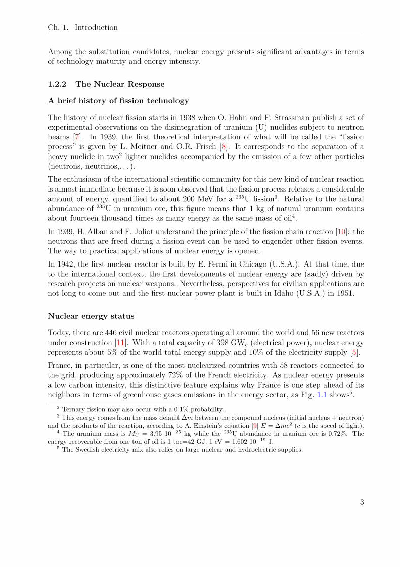
The history of nuclear fission starts in 1938 when O. Hahn and F. Strassman publish a set ofexperimental observations on the disintegration of uranium (U) nuclides subject to neutronbeams [7]. In 1939, the first theoretical interpretation of what will be called the “fissionprocess” is given by L. Meitner and O.R. Frisch [8]. It corresponds to the separation of aheavy nuclide in two2 lighter nuclides accompanied by the emission of a few other particles(neutrons, neutrinos,. . . ).The enthusiasm of the international scientific community for this new kind of nuclear reactionis almost immediate because it is soon observed that the fission process releases a considerableamount of energy, quantified to about 200 MeV for a 235U fission3. Relative to the naturalabundance of 235U in uranium ore, this figure means that 1 kg of natural uranium containsabout fourteen thousand times as many energy as the same mass of oil4.In 1939, H. Alban and F. Joliot understand the principle of the fission chain reaction [10]: theneutrons that are freed during a fission event can be used to engender other fission events.The way to practical applications of nuclear energy is opened.In 1942, the first nuclear reactor is built by E. Fermi in Chicago (U.S.A.). At that time, dueto the international context, the first developments of nuclear energy are (sadly) driven byresearch projects on nuclear weapons. Nevertheless, perspectives for civilian applications arenot long to come out and the first nuclear power plant is built in Idaho (U.S.A.) in 1951.
Nuclear energy status
Today, there are 446 civil nuclear reactors operating all around the world and 56 new reactorsunder construction [11]. With a total capacity of 398 GWe (electrical power), nuclear energyrepresents about 5% of the world total energy supply and 10% of the electricity supply [5].France, in particular, is one of the most nuclearized countries with 58 reactors connected tothe grid, producing approximately 72% of the French electricity. As nuclear energy presentsa low carbon intensity, this distinctive feature explains why France is one step ahead of itsneighbors in terms of greenhouse gases emissions in the energy sector, as Fig. 1.1 shows5.
2 Ternary fission may also occur with a 0.1% probability.3 This energy comes from the mass default ∆m between the compound nucleus (initial nucleus + neutron)
and the products of the reaction, according to A. Einstein’s equation [9] E = ∆mc2 (c is the speed of light).4 The uranium mass is MU = 3.95 10−25 kg while the 235U abundance in uranium ore is 0.72%. The
energy recoverable from one ton of oil is 1 toe=42 GJ. 1 eV = 1.602 10−19 J.5 The Swedish electricity mix also relies on large nuclear and hydroelectric supplies.
3
Ch. 1. Introduction
1 970 1 980 1 990 2 000 2 0100
5
10
15
20
Year
tCO
2/capita
Evolution of CO2 emissions
France Germany SwedenItaly USA China
Share of heat & electricitygeneration (tCO2/capita)France 0.55
Germany 3.91Sweden 0.72Italy 1.79China 5.86U.S.A. 3.17
Figure 1.1 Greenhouse gases emissions per country and per capita: evolution over time(left) and share of heat and eletricity generation in 2016 (right).
Remark: Data from IEA [3].
1.2.3 Nuclear Energy Constraints
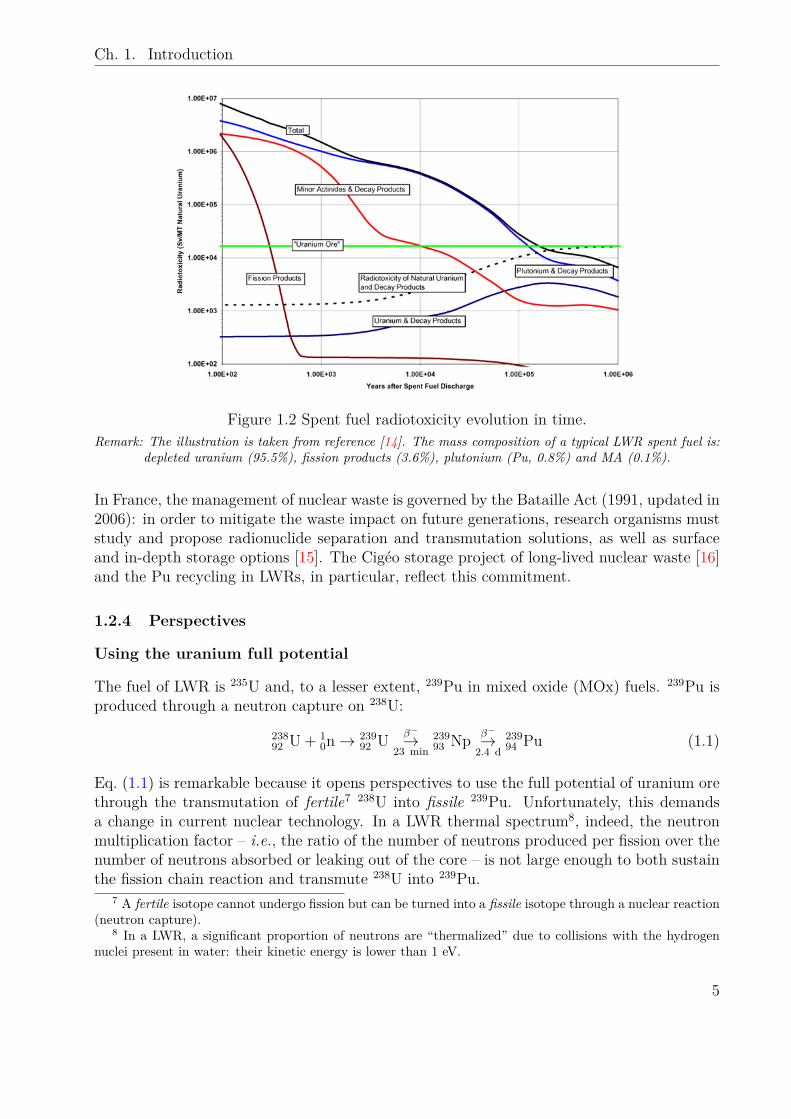
Despite undeniable advantages, nuclear energy also faces strong challenges.The first challenge is the necessity to ensure the safety of nuclear facilities at any time,including normal operating conditions, but also against natural and criminal threats. Thisdemands a constant update of the nuclear safety referential in order to take advantage of thelessons learned from the past (1979: Three Miles Island, 1986: Tchernobyl, 2011: Fukushima).The second challenge is linked to fuel supply security. Currently, the nuclear energy marketis dominated by Light Water Reactor (LWR) technologies which consume slightly enricheduranium fuel (≈ 4% 235U in Westinghouse concepts). According to the Nuclear EnergyAgency (NEA), the uranium ore resources will endure about 135 years assuming a constantnuclear energy consumption and no evolution in current nuclear technology [12]. However, ifthe share of nuclear energy in the global energy mix is to increase during the XXIst century,access to uranium resources might become a source of political and economic tensions.Finally, the question of radioactive waste management is crucial as it drives the entire nuclearindustry sustainability. According to the Andra, “only” 2 kg of nuclear waste6 are producedin France, per person and per year [13]. However, the radiotoxicity of nuclear spent fuelstakes more than one hundred thousand years to find back the natural uranium ore level,as Fig. 1.2 shows. The main contributors to this radiotoxicity are the transuranic nuclides:plutonium (Pu), followed by minor actinides (MA), i.e., neptunium, curium, and americium.
6 This value does not account for plutonium nor depleted uranium because they are considered as valuableresources (cf. Sec.1.2.4).
4
Ch. 1. Introduction
Figure 1.2 Spent fuel radiotoxicity evolution in time.Remark: The illustration is taken from reference [14]. The mass composition of a typical LWR spent fuel is:
depleted uranium (95.5%), fission products (3.6%), plutonium (Pu, 0.8%) and MA (0.1%).
In France, the management of nuclear waste is governed by the Bataille Act (1991, updated in2006): in order to mitigate the waste impact on future generations, research organisms muststudy and propose radionuclide separation and transmutation solutions, as well as surfaceand in-depth storage options [15]. The Cigéo storage project of long-lived nuclear waste [16]and the Pu recycling in LWRs, in particular, reflect this commitment.
1.2.4 Perspectives
Using the uranium full potential
The fuel of LWR is 235U and, to a lesser extent, 239Pu in mixed oxide (MOx) fuels. 239Pu isproduced through a neutron capture on 238U:
23892 U + 1
0n→ 23992 U β−→
23 min23993 Np β−→
2.4 d23994 Pu (1.1)
Eq. (1.1) is remarkable because it opens perspectives to use the full potential of uranium orethrough the transmutation of fertile7 238U into fissile 239Pu. Unfortunately, this demandsa change in current nuclear technology. In a LWR thermal spectrum8, indeed, the neutronmultiplication factor – i.e., the ratio of the number of neutrons produced per fission over thenumber of neutrons absorbed or leaking out of the core – is not large enough to both sustainthe fission chain reaction and transmute 238U into 239Pu.
7 A fertile isotope cannot undergo fission but can be turned into a fissile isotope through a nuclear reaction(neutron capture).
8 In a LWR, a significant proportion of neutrons are “thermalized” due to collisions with the hydrogennuclei present in water: their kinetic energy is lower than 1 eV.
5
Ch. 1. Introduction
However, the situation changes when the neutron energy increases: in that case, both theaverage number of neutrons produced per fission and the fission over capture ratio increase.In particular, the neutron multiplication factor meets the prescribed conditions in reactordesigns based on 239Pu fuel and fast neutron spectra (high energy neutrons, E ≈ 300 keV)9.The development of such a nuclear reactor technology, thus, opens perspectives to use de-pleted uranium as a fuel, provided that an initial stock of 239Pu is available. Since currentLWR technology is based on the sole usage of 235U, whose natural abundance is 0.72% inuranium ore, such a change of technology represents a potential multiplication of the uraniumresources by a factor greater than one hundred. This explains why France saves plutoniumand depleted uranium as “valuable resources”.
Decreasing the waste radiotoxicity
Using plutonium as a fuel offers certain flexibility to reduce the volume of Pu stocks.Moreover, an increase of the average neutron energy is generally favorable to the fissionover capture ratio of minor actinides, and thus, to their transmutation (into shorter-livedisotopes) [17].Hence, a change in current nuclear reactor technology would also help to considerably decreasethe radiotoxicity of nuclear spent fuel stocks.
Towards a new generation of nuclear reactors
In 2000, the international community gathered at the Generation IV International Forum(GIF) [18] in order to set global orientations for future nuclear energy technologies. Theseorientations can be summarized as follows:
• Nuclear energy must be sustainable (fuel supply and waste management).• Nuclear energy must be economically competitive in terms of life-cost and risks.• Nuclear technology must be safe and reliable (low accident probability and limited
consequences).• Nuclear technology must be resistant to the proliferation of weapon-usable materials.
The GIF also selected six reactor concepts compatible with these criteria. They are to-day regarded as the most promising nuclear solutions for the XXIst century. Among these,France chose to focus on the Sodium-cooled Fast Reactor (SFR) [19] whose schematic viewis presented in Fig. 1.3.As its name suggests, the SFR neutron spectrum is “fast”10 and, thus, compatible with online239Pu generation/consumption and MA transmutation.
9 Solutions also exist with 233U, but this demands a thorium-based fuel cycle.10 The neutron thermalization is not efficient with a sodium-coolant because 23Na is about twenty-three
times heavier than 1H.
6
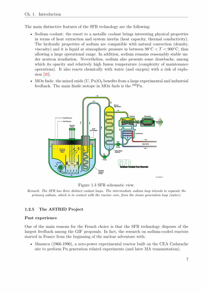
Ch. 1. Introduction
The main distinctive features of the SFR technology are the following:
• Sodium coolant: the resort to a metallic coolant brings interesting physical propertiesin terms of heat extraction and system inertia (heat capacity, thermal conductivity).The hydraulic properties of sodium are compatible with natural convection (density,viscosity) and it is liquid at atmospheric pressure in between 98C < T < 900C, thusallowing a large operational range. In addition, sodium remains reasonably stable un-der neutron irradiation. Nevertheless, sodium also presents some drawbacks, amongwhich its opacity and relatively high fusion temperature (complexity of maintenanceoperations). It also reacts chemically with water (and oxygen) with a risk of explo-sion [20].
• MOx fuels: the mixed oxide (U, Pu)O2 benefits from a large experimental and industrialfeedback. The main fissile isotope in MOx fuels is the 239Pu.
Figure 1.3 SFR schematic view.Remark: The SFR has three distinct coolant loops. The intermediate sodium loop intends to separate the
primary sodium, which is in contact with the reactor core, from the steam generation loop (water).
1.2.5 The ASTRID Project
Past experience
One of the main reasons for the French choice is that the SFR technology disposes of thelargest feedback among the GIF proposals. In fact, the research on sodium-cooled reactorsstarted in France from the beginning of the nuclear adventure with:
• Masurca (1966-1996), a zero-power experimental reactor built on the CEA Cadarachesite to perform Pu generation related experiments (and later MA transmutation).
7
Ch. 1. Introduction
• Rapsodie (1967-1983, 20 MW thermal power), an experimental SFR also built on theCadarache site. The main lessons learned from the Rapsodie experience concern thebehavior of MOx fuels under irradiation, and the core conception (hexagonal fuel as-semblies, hanging core vessel. . . ).
• Phénix (1973-2010, 250 MW electrical power), a SFR power plant prototype locatedat Marcoule. Phénix contributed to enhancing the understanding of the fuel / cladinteraction, the physics of transmutation, and the design of sodium components (pumps,heat exchangers, steam generators. . . ).
• Superphénix (1985-1997, 1200 MW electrical power), an industrial demonstrator builton the Creys-Malville site. Superphénix was stopped prematurely due to a series oftechnical difficulties, but also because of a tense political context.
Current status of ASTRID
In the framework of the Bataille Act and the GIF, the research on the SFR technology inFrance took a new start with the Advanced Sodium Technological Reactor for IndustrialDemonstration (ASTRID) project [19]. The initial strategy of the ASTRID project was tobuild a IVth-generation SFR prototype by the 2020 decade in order to prepare the deploymentof a SFR fleet by the end of the XXIst century.In order to offer flexibility in the plutonium stocks management, the ASTRID prototype wasconceived as a “breeder-and-burner” reactor, capable of either consuming Pu (with a view inreducing the Pu stocks) or producing new Pu stocks (in order to prepare the deployment ofnew SFRs). With a 1500 MW thermal power (≈ 600 MW electrical power) and a 80% loadfactor, the ASTRID prototype was initially supposed to be representative of an industrialconcept.As for the reactor design, the GIF high safety standards impulsed a series of novelties. Inparticular, this materialized with the choice of a Coeur à Faible Vidange (CFV)11 concept forthe core, technology that presents several innovative features and enhances the core naturalbehavior during accidental situations [21].Unfortunately and as mentioned in the prelude of this introduction, the aspirations of theASTRID project have been scaled down in 2017 due to a complex economic context. Never-theless, the CEA maintains research activities on the topic, with the aim of rescheduling thetimeline to the second half of the XXIst century.
1.3 Numerical Simulation Tools Context
1.3.1 Reactor Design & Nuclear Safety
The viability of a nuclear reactor design is assessed according to a set of specified criteria(economic competitiveness, electricity needs, fuel and materials availability, spent fuel re-cycling capacity, strategical orientations,. . . ). In particular, the evaluation of the criteria
11 French acronym for low-void reactivity effect core
8
Ch. 1. Introduction
that characterize the reactor physics (critical mass, pressure drop in the core, recoverableenergy,. . . ) requires a modeling phase i.e., numerical simulation capacities.Nevertheless, it is within the nuclear safety approach that the needs for high accuracy simu-lation tools are the most important.The French Act related to nuclear transparency and security (2006) defines “nuclear safety”as all the actions that are taken to prevent nuclear accidents and mitigate their consequences:
“La sûreté nucléaire est l’ensemble des dispositions techniques et des mesures d’organisationrelatives à la conception, à la construction, au fonctionnement, à l’arrêt et au
démantèlement des installations nucléaires de base, ainsi qu’au transport des substancesradioactives, prises en vue de prévenir les accidents ou d’en limiter les effets.” [22]
With this definition, the environment Act (updated in 2019) states that the authorization tobuild a nuclear facility in France is subject to a proper safety demonstration [23], whichmust itself be based on reliable simulation tools [24].In particular, the safety demonstration of a nuclear reactor must ensure:
1. Complete control of the fission chain reaction at any time.2. The capacity to extract the reactor nominal power and decay heat12.3. The confinement of radioactive materials, even in case of severe accicents (e.g., fuel
melting).
This thesis is mainly concerned about the first item of this list, i.e., ensuring the control ofthe neutron population.
1.3.2 Neutronic Codes
The behavior of the neutron population in a reactor core can be described by a neutrontransport equation13. The purpose of neutronic calculation codes is, hence, to solve thisequation.As any numerical simulation process, a neutronic calculation tool is based on:
• Models: the neutron transport equation (and physical approximations).• Input data: geometries, material compositions, neutron cross sections,. . . .• Methods to compute a set of interest parameters under the assumption that the model is
valid and the input data is correct. The choice of a set of methods defines a calculationscheme.
12 The decay heat is due to the decay of radioactive isotopes, even after the reactor shutdown. It accountsfor approximately 7% of the total power a few minutes after shutdown.
13 The neutron transport equation will be properly introduced in Chapter 2.
9
Ch. 1. Introduction
In particular, methods to solve the neutron transport equation can be classified into twocategories:
• Deterministic methods: they rely on a discretization of phase-space and the inversionof the resulting matrix with linear algebra methods.
• Stochastic methods: they rely on the random sampling of neutron histories, accordingto known probability laws, in order to build statistical estimators.
While the discretization of phase space introduces approximations in deterministic neutroniccalculations, the stochastic way is often considered as a “reference” because it requires aminimal set of such approximations.
1.3.3 The APOLLO3® Project
APOLLO3® is a deterministic code currently being developed at CEA to perform neutroniccalculations of nuclear reactor cores [1]. Relying on the legacy of the previous generation ofCEA neutronic codes (i.e., ECCO/ERANOS [25] and APOLLO2 [26]), it also takes advan-tage of the recent progress in computer hardware (parallel computer architectures, increasedprocessor power and memory) and software (code architecture, numerical methods and algo-rithms) with the aim of raising the neutronic calculation standards to a new level.APOLLO3® emerged from a necessity to propose new functionalities to allow the accuratemodeling (and hence a proper safety demonstration) of complex reactor cores, among whichthe CFV of ASTRID.In particular, APOLLO3® must provide different solutions according to the research commu-nity needs:
• The reference route for reactor safety studies: it should ensure minimized biases on allthe neutronic parameters of interest.
• The project route for reactor design purposes: it should be fast enough to performparametric studies while ensuring mastered biases compared to the reference route.
1.3.4 The VV&UQ Process
As the usage of numerical simulation tools becomes widespread in every scientific field, theconcept of code reliability has been formalized under a Verification, Validation and Uncer-tainty Quantification (VV&UQ) methodology:
1. The verification process determines whether the equations that underpin the model arecorrectly implemented in the code, and if the data flow is consistent.
2. The validation process determines the capacity of the model (including its approxima-tions) to represent the physical phenomena that want to be represented. It is based oncomparisons with:
- data from physical experiments (experimental validation);- results from reference calculation tools (numerical validation).
10
Ch. 1. Introduction
3. The uncertainty quantification process assesses our ignorance on both the input dataand the models. The uncertainty propagation through the code allows estimating thefinal variance on the parameters of interest.
While not limited to the nuclear industry, the VV&UQ now forms part of the French safetyauthority (ASN) guideline for the safety demonstration of nuclear facilities [24]. The devel-opment of APOLLO3®, in particular, is subject to this VV&UQ process.
1.4 Objectives of this Thesis
The main motivation for this work is that recent studies performed at CEA highlightedsystematic method biases on the calculation of several neutronic parameters of importance(reactivity and sodium-void reactivity worth14) of the core of ASTRID with APOLLO3® [27].
Problem statement: despite state-of-the-art methods, the calculation schemes implementedin APOLLO3® for the neutronic calculation of IVth-generation sodium-cooled nuclearreactors suffer from systematic biases that penalize a proper safety demonstration.
Thus, the two main objectives of this thesis are:1. Understand the limitations of the current APOLLO3® neutronic simulation strategy
for the calculation of complex SFR cores.2. Propose and implement new methodological solutions (calculation schemes).
More precisely, these objectives can be specified according to the needs of CEA (researchapplications). This specification results in the following list of constraints:
• The solutions proposed should allow the calculation of the main neutronic parametersof interest (reactivity, power distribution, power peak, sodium-void reactivity worthand other feedback coefficients, control rods reactivity worth, fuel inventory evolutionwith time,. . . ) with mastered and limited biases.
• A reflection on the computational constraints (calculation time and memory require-ments) should accompany the proposals, with a view in performing reference calcula-tions on desktop computers (i.e., with a few or a few tens processors and a few tensgigabytes of memory) within a reasonable amount of time.
• In the framework of the VV&UQ process of APOLLO3®, the choices made in this workshould be justified with numerical validation results (i.e., against reference stochasticmethods) and a verification work should accompany the development of new methods15.
• In addition, it is proposed to add an adaptability constraint:– the CFV of ASTRID is considered as a reference case of application, but the
solutions proposed should be robust enough to allow the modeling of a wide rangeof core designs;
14 These parameters will be introduced when required throughout this document.15 This work is not concerned by the experimental validation topic nor by the quantification of data
uncertainties.
11
Ch. 1. Introduction
– different proposals should be made in order to suit the needs of both refer-ence (minimal biases) and project calculation routes (relaxed computational con-straints).
The first item of this list deserves a special comment as the terminology “mastered and limitedbiases” is rather vague. In fact, the safety authority (ASN) does not recommend any targetaccuracy for any neutronic parameter: it is the role of the nuclear facility operator to justifythat sufficient provisions have been taken, considering the values of the calculation biasesand uncertainties. Nevertheless, the values of the biases that will be presented throughoutthis document will be discussed.
1.5 Thesis Layout
In order to provide solutions to the problem statement, this document is organized as follows:
• Chapter 2 intends to furnish a comprehensive framework for this thesis. It introducesthe neutron transport equation and the basic theory of nuclear reactor neutronic calcu-lation. The problem is considered from the computational perspective, and the conceptof neutronic calculation scheme is detailed.
• Chapter 3 presents an analysis of the SFR neutronic calculation methodology that wasimplemented in APOLLO3® when this work started (named AP3–SFR–2016). In par-ticular, the different steps of the AP3–SFR–2016 calculation scheme (i.e., homogenizedcross sections generation and core calculation) are numerically validated against refer-ence results in order to quantify elementary biases. The methodological drawbacks arethen highlighted and interpreted.
• Chapter 4 presents a novel method to lift the major inconsistency identified in Chap-ter 3, i.e., the cross section preparation phase for axially heterogeneous fuel assemblygeometries. The method relies on three-dimensional transport calculations under a“2D/1D approximation”. This approximation intends to alleviate the computationalconstraint.
• Chapter 5 proposes a general methodology for the construction of reference SFR calcu-lation schemes in APOLLO3®. The methodology relies on the preparation of few groupshomogenized cross sections over large size domains (three-dimensional fuel assemblies,core / reflector interface) in order to represent long-range neutron flux gradients. Alarge part of this chapter is devoted to the presentation of validation results for differentneutronic estimators, and different SFR cores.
• Chapter 6 addresses the question of the calculation scheme adaptability to the compu-tational constraints (i.e., for the project route). It also gives some perspectives for thedefinition of truly adaptative (i.e., with a minimal number of user-dependent choices)calculation schemes.
This document ends with a general conclusion in Chapter 7.
12
Chapter 2 Nuclear Reactor Neutronic Calculation:Theory & Methods
Abstract
This chapter is an introduction to neutron transport theory and applications for reactoranalysis. The reader is invited to use it as a “toolbox” and may eventually skip its readingwould he prefer to refer to it when needed. It is organized as follows. Sec. 2.1 presentsthe Neutron Transport Equation (NTE) and sets the notations that will be used throughoutthis document. Sec. 2.2 gives an overview of numerical methods for the NTE resolution,focusing mainly on the deterministic way (as opposed to stochastic), which constitutes themain scope of this work. Orders of magnitude of the computational requirements (calculationtime, memory) needed to solve the NTE on typical reactor problems are provided in Sec. 2.3,while solutions to fasten the NTE resolution are listed in Sec. 2.4 (NTE acceleration andparallelism) and Sec. 2.5 (homogenization theory). This chapter ends with a panorama oftypical neutronic calculation schemes (Sec. 2.6) and conclusions (Sec. 2.7).
Contents
2.1 The Neutron Transport Equation . . . . . . . . . . . . . . . . . . . 142.1.1 The Neutron as a Point-Particle . . . . . . . . . . . . . . . . . . . 142.1.2 Derivation of the Particle Balance . . . . . . . . . . . . . . . . . . 142.1.3 Expression of the Collision Term . . . . . . . . . . . . . . . . . . . 172.1.4 The NTE and its Solutions . . . . . . . . . . . . . . . . . . . . . . 212.1.5 The Critical Problem . . . . . . . . . . . . . . . . . . . . . . . . . 21
2.2 Numerical Methods for the NTE . . . . . . . . . . . . . . . . . . . 232.2.1 Power Method . . . . . . . . . . . . . . . . . . . . . . . . . . . . . 232.2.2 Multigroup Approximation . . . . . . . . . . . . . . . . . . . . . . 242.2.3 Spatial and Angular Discretization . . . . . . . . . . . . . . . . . . 272.2.4 Stochastic Methods . . . . . . . . . . . . . . . . . . . . . . . . . . 33
2.3 The Numerical Footprint Issue . . . . . . . . . . . . . . . . . . . . 352.3.1 Deterministic Point of View . . . . . . . . . . . . . . . . . . . . . . 352.3.2 Stochastic Point of View . . . . . . . . . . . . . . . . . . . . . . . . 37
2.4 Acceleration of the NTE . . . . . . . . . . . . . . . . . . . . . . . . 372.4.1 Parallelism . . . . . . . . . . . . . . . . . . . . . . . . . . . . . . . 372.4.2 Acceleration . . . . . . . . . . . . . . . . . . . . . . . . . . . . . . . 38
2.5 Homogenization Theory . . . . . . . . . . . . . . . . . . . . . . . . 392.5.1 The Homogenized Problem . . . . . . . . . . . . . . . . . . . . . . 392.5.2 The Reference Problem . . . . . . . . . . . . . . . . . . . . . . . . 44
2.6 Neutronic Calculation Schemes . . . . . . . . . . . . . . . . . . . . 452.6.1 The Lattice - Core Paradigm . . . . . . . . . . . . . . . . . . . . . 452.6.2 Resonance Self-shielding . . . . . . . . . . . . . . . . . . . . . . . . 472.6.3 Towards Heterogeneous 3D Calculations? . . . . . . . . . . . . . . 50
2.7 Conclusions . . . . . . . . . . . . . . . . . . . . . . . . . . . . . . . . 51
13
Ch. 2. Nuclear Reactor Neutronic Calculation: Theory & Methods
2.1 The Neutron Transport Equation
In a reactor core, the neutron population obeys a linear transport equation. In order toset the theoretical background of this document, this section presents its derivation. Inparticular, the approximations that underpin the NTE are recalled, and the existence ofsolutions is briefly discussed. The critical NTE, which is the main concern of this work and,more generally, of nuclear reactor neutronic analysis, is finally presented.
2.1.1 The Neutron as a Point-Particle
The neutron is a quantum system. In standard transport theories, though, a classical point-particle description is often adopted. Doing so, both the wave nature of the neutron andpolarization effects are neglected.
• The wave nature of a neutron can indeed be neglected in transport phenomena becausethe order of magnitude of its reduced wavelength λ differs from the mean free pathλmfp of the media in which it travels. In a nuclear reactor, a typical neutron mean freepath value is λmfp ≈ 1 mm-cm. As for the reduced wavelength, it can be deduced fromde Broglie’s equation:
λ = ~p
(2.1)
where ~ is the Planck constant divided by 2π and p is the neutron momentum. Since,in a reactor, a large majority of neutrons have a kinetic energy E > 0.01 eV, it directlyfollows that1:
λ < 4.55 10−11 m << λmfp (2.2)
At very low neutron energies, interference effects in crystal lattices could still be ob-served, but these phenomena are usually not significant in nuclear reactors.
• Polarization effects can arise from spin-dependent interactions between a neutron anda nucleus, or from intense external magnetic fields. If the situation is such that the av-erage population of neutrons has a non-zero polarization, the transport theory needs tobe modified. Nevertheless, these effects are neglected for practical reactor applications2.
As pointed out in the book of G. Bell and S. Glasstone [28], the advantage of the point-particle model is that the neutron can be entirely characterized by its position andvelocity (or momentum).
2.1.2 Derivation of the Particle Balance
The statistical study of the motion of a large number of particles was carried out by L. Boltz-mann in the XIXth century [29]. It gives the general framework to derive the NTE.
1 p ≈√
2mE with m = 939.6 MeV/c2 (neutron mass) and ~ = 6.58 10−16 eV.s.2 If necessary, quantum polarization effects can be taken into account with the cross section formalism,
which will be introduced in Sec. 2.1.3.
14
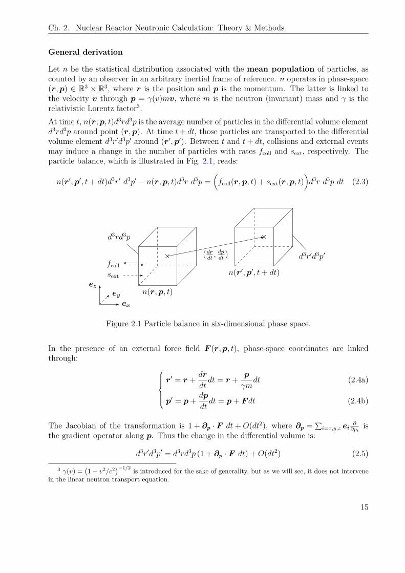
Ch. 2. Nuclear Reactor Neutronic Calculation: Theory & Methods
General derivation
Let n be the statistical distribution associated with the mean population of particles, ascounted by an observer in an arbitrary inertial frame of reference. n operates in phase-space(r,p) ∈ R3 × R3, where r is the position and p is the momentum. The latter is linked tothe velocity v through p = γ(v)mv, where m is the neutron (invariant) mass and γ is therelativistic Lorentz factor3.At time t, n(r,p, t)d3rd3p is the average number of particles in the differential volume elementd3rd3p around point (r,p). At time t+ dt, those particles are transported to the differentialvolume element d3r′d3p′ around (r′,p′). Between t and t+ dt, collisions and external eventsmay induce a change in the number of particles with rates fcoll and sext, respectively. Theparticle balance, which is illustrated in Fig. 2.1, reads:
n(r′,p′, t+ dt)d3r′ d3p′ − n(r,p, t)d3r d3p =(fcoll(r,p, t) + sext(r,p, t)
)d3r d3p dt (2.3)
×
n(r,p, t)
d3rd3p
fcollsext
×
n(r′,p′, t+ dt)
d3r′d3p′(drdt, dpdt)
ez
ex
ey
Figure 2.1 Particle balance in six-dimensional phase space.
In the presence of an external force field F (r,p, t), phase-space coordinates are linkedthrough:
r′ = r + dr
dtdt = r + p
γmdt (2.4a)
p′ = p+ dp
dtdt = p+ F dt (2.4b)
The Jacobian of the transformation is 1 + ∂p · F dt+O(dt2), where ∂p = ∑i=x,y,z ei
∂∂pi
isthe gradient operator along p. Thus the change in the differential volume is:
d3r′d3p′ = d3rd3p (1 + ∂p · F dt) +O(dt2) (2.5)
3 γ(v) =(1− v2/c2)−1/2 is introduced for the sake of generality, but as we will see, it does not intervene
in the linear neutron transport equation.
15
Ch. 2. Nuclear Reactor Neutronic Calculation: Theory & Methods
Introducing Eq. (2.5) in Eq. (2.3), the following equation is found to first order in dt:
dn
dt(r,p, t) + n(r,p, t)∂p · F (r,p, t) = fcoll(r,p, t) + sext(r,p, t) (2.6)
where we have used: n(r′,p′, t+ dt)− n(r,p, t)
dt−→t→0
dn
dt(r,p, t) (2.7a)
n(r′,p′, t+ dt) −→t→0
n(r,p, t) (2.7b)
Eq. (2.6) can also be written with the help of partial derivatives as:
∂n
∂t+ v · ∂rn+ F · ∂pn+ n ∂p · F = fcoll + sext (2.8)
where ∂r = ∑i=x,y,z ei
∂∂ri
is the spatial gradient operator.
Particular case of free particles
In reactor physics, it is often assumed that neutrons are free particles:
F = ~0 (2.9)
This assumption is valid because:• Neutrons are electrically neutral and are, thereby, not subject to electromagnetic fields4.• Gravitational forces are not significant given the low neutron mass (m = 939.6 MeV/c2)
and the short distances (≈ λmfp) it travels.• The proper mean lifetime of a free neutron (τn = 881.5 s) is large compared to the
interval between collisions, so the weak interaction (β− decay) can be neglected.• The strong interaction range is short, making it possible to account for it in fcoll:
collisions are assumed to be punctual.
As a result, the free Boltzmann equation reads:
∂n
∂t+ v · ∂rn = fcoll + sext (2.10)
The energy-angle phase-space
The variables r and p have been used to derive the NTE in a general (relativistic) framework.In neutron transport codes, though, it is usual to express the neutron density in phase-space(r, E,Ω), where E = mc2
(γ(v)− 1
)is the kinetic energy5 and Ω = v/v is the direction.
4 Polarization effects due to the neutron magnetic moment are neglected (in transport phenomena).5 In nuclear reactors, though, the relativistic correction is usually negligible because the neutron velocity
is small when compared to c (fission neutrons are born at v ≈ 0.05c). In that case, E ≈ 12mv
2 is a goodapproximation for the kinetic energy.
16
Ch. 2. Nuclear Reactor Neutronic Calculation: Theory & Methods
To operate the change of variables, hence, the Jacobian of the transformation p → (E,Ω)needs to be considered. Yet, this Jacobian is independent of t and r. Thus, it comes out asa multiplicative constant to the free Boltzmann equation. It follows that Eq. (2.10) is alsovalid in phase-space (r, E,Ω) ∈ R3 × R+ × S2, where S2 is the unit sphere.For purposes of notations, we now call:
n ≡ n(r, E,Ω, t) (2.11)
2.1.3 Expression of the Collision Term
In a nuclear reactor, the only contributors to fcoll are neutron-nuclei interactions. Indeed:
• Neutron-neutron interactions can be neglected because the number of neutrons (≈105 neutrons/cm3) is small compared to the atomic density6 (≈ 1022 at/cm3).
• Neutron-electron interactions (and a fortiori neutron-neutrino,. . . ) have very low prob-abilities.
Among neutron-nuclei interactions:• The simplest is the potential diffusion, in which the neutron is elastically scattered by
the mean field generated by the nucleus.• Other reactions involve a mechanism, proposed by N. Bohr, in which the neutron is
absorbed by the nucleus AZX, leading to the formation of a compound nucleus A+1
Z X∗
in an excited state (superscript ∗) [30]:AZX + n→ A+1
Z X∗ (2.12)
The compound nucleus then decays according to different channels:- Fission (n, f): this channels corresponds to the scission of the nucleus into two(or possibly three) lighter nuclides. It is accompanied by the emission of one orseveral secondary neutrons (and other particles). This channel is usually openedonly for heavy nuclei.
- Capture: the neutron is captured by the compound nucleus. The excess of energyresults in the emission of photons (n, γ) and/or charged particles, i.e., protons(n, p), helium nuclei (n, α),. . .
- Resonant scattering: the compound nucleus emits one (or several) new neutron(s).It can be elastic (n, n), inelastic (n, n′) or multiple7 (n,Xn) with X = 2, 3, . . .
Unfortunately, such neutron-nucleus interactions cannot be fully described by theoreticalmodels because of the complexity of the nuclear forces acting within the nucleons. Neverthe-less, the cross section formalism links the reaction rate τx,i of a particular interaction x, tothe nuclide density Ni, and to the neutron density n and velocity v according to:
τx,i = σx,iNinv (2.13)6 In a sodium–cooled nuclear reactor, typical values of neutron fluxes and kinetic energies are
φ ≈ 1014 n/cm2/s and v ≈ 0.03c.7 . . . and even compound with (n, p+ n) reactions.
17
Ch. 2. Nuclear Reactor Neutronic Calculation: Theory & Methods
The proportionality factor σx,i is called microscopic cross section: it can be obtainedthrough parametric nuclear interaction models (such as the R-matrix theory [31] or opticalmodels), that are usually fitted using experimental data.This formalism is convenient because it “hides” the complexity of the neutron-nucleus inte-raction behind effective parameters8, that can be used in transport theory. In any case,microscopic cross sections are considered as input data in this work.To simplify the notations, we now introduce the macroscopic cross section:
Σx,i = Niσx,i (2.14)
as well as the neutron flux9:
ψ(r, E,Ω, t) = n(r, E,Ω, t)v (2.15)
and the so-called “scalar flux”:
ψ00(r, E, t) =∫S2d2Ω ψ(r, E,Ω, t) (2.16)
Fission treatment
In the fission process, a fraction of neutrons (called prompt) are instantly emitted (t < 10−14 s)while others (called delayed) are emitted with a delay due to (β−, n) decays of fission products(t > 1 ms).
• The number of prompt neutrons can be expressed in terms of macroscopic fission crosssections Σf,i (for each isotope i), average number of prompt neutrons emitted per fissionevent νp,i and prompt neutrons emission spectra χp,i. In addition, it is often assumedthat fission neutron emission is isotropic in the laboratory referential. In that case, theprompt fission operator Fp can be expressed as a function of the scalar flux ψ00 as:
Fpψ(r, E,Ω, t) = 14π
∑i
∫R+dE ′νp,i(E ′)χp,i(E ′ → E)Σf,i(r, E ′, t)ψ00(r, E ′, t) (2.17)
where the sum over i is a sum over fissile isotopes. For Eq. (2.17) to be valid, the fissionspectra must be normalized, i.e.,
∫R+ χp,i(E ′ → E)dE = 1.
• Fission products are often grouped into 6 or 8 “precursors” families according to theirhalf-life. For each family k, we define the precursors concentration Ck, the decayconstant λk and the delayed neutron spectrum χd,k (also normalized to 1) so that thedelayed fission operator Fd can be written:
Fdψ(r, E,Ω, t) = 14π
∑k
χd,k(E)λkCk(r, t) (2.18)
8 In particular, relativistic effects during collisions can be taken into account in σx,i values. Nevertheless,these effects are usually negligible in nuclear reactors.
9 In reactor physics, the neutron “flux” does not have the same meaning than in other disciplines: it doesnot count a number of neutrons crossing a surface.
18
Ch. 2. Nuclear Reactor Neutronic Calculation: Theory & Methods
where the dependence on flux ψ is implicit through the equations of evolution of theprecursors’ concentrations:
∀k, dCkdt
(r, t) + λkCk(r, t) =∑i
∫R+dE ′νd,k,i(E ′)Σf,i(r, E ′, t)ψ00(r, E ′, t) (2.19)
with νd,k,i the number of precursors created (or neutrons emitted) in family k for afission of isotope i.
The total number of neutrons produced through fission is:
Fψ = Fpψ + Fdψ (2.20)
Neutronic calculations are often concerned by steady-state situations. In that case, it isuseful to define a production cross section νΣf as:
νΣf (r, E ′ → E) =∑i
νi(E ′)χi(E ′ → E)Σf,i(r, E ′) (2.21)
with: νi = νp,i +
∑k
νd,k,i (2.22a)
χi = 1νi
(∑k
νd,k,iχd,k + νp,iχp,i
)(2.22b)
so that the steady-state fission operator may be written:
Fψ(r, E,Ω) = 14π
∫R+dE ′νΣf (r, E ′ → E)ψ00(r, E ′) (2.23)
Scattering treatment
The production of neutrons by scattering channels reads:
Hψ(r, E,Ω, t) =∫
R+×S2
dE ′d2Ω′ Σs(r, E ′ → E,Ω′ ·Ω, t)ψ(r, E ′,Ω′, t) (2.24)
where Σs is the macroscopic scattering cross section. It can be written in terms of isotopicscattering cross sections Σx,i – including potential and resonant elastic x = (n, n), inelasticx = (n, n′) and multiple x = (n,Xn) scattering – and transfer probabilities px,i as:
Σs =∑i
Σ(n,n),i p(n,n),i + Σ(n,n′),i p(n,n′),i +∑X∈NX≥2
X Σ(n,Xn),i p(n,Xn),i
(2.25)
with Σx,i ≡ Σx,i(r, E ′, t) and px,i ≡ px,i(E ′ → E,Ω′ ·Ω).
19
Ch. 2. Nuclear Reactor Neutronic Calculation: Theory & Methods
With these notations, px,i(E ′ → E,Ω′ ·Ω)dE ′d2Ω′ is the probability that a neutron, scatteredby nuclide i through channel x, is sent from (E ′,Ω′) to (E,Ω) in phase-space.One may notice that the transfer probability px,i does not depend on individual incomingΩ′ and outgoing Ω neutron directions, but that it only depends on the deviation cosineµ = Ω′ ·Ω. This assumption is valid when interference effects in crystal lattices are neglected(cf. Sec. 2.1.1): media are isotropic for neutron transport.
Introducing Legendre polynomials (Pl)l∈N and real spherical harmonics (Rlm)m∈J−l:lKl∈N (see
Appendix A), the angular dependence of the scattering kernel is usually10 expanded as:
Hψ(r, E,Ω, t) =∑l∈N
2l + 14π
+l∑m=−l
∫R+dE ′ Σs,l(r, E ′ → E, t)ψlm(r, E ′, t)Rlm(Ω) (2.26)
with:Σs,l(r, E ′ → E, t) =
∫ 1
µ=−1dµ Σs(r, E ′ → E, µ, t)Pl(µ) (2.27)
The angular flux moments are defined as:
ψlm(r, E, t) =∫S2d2Ω ψ(r, E,Ω, t)RlmΩ) (2.28)
from which it can be observed that the scalar flux ψ00 defined with Eq. (2.16) is the zerothorder moment.
Removal treatment
When a neutron undergoes a collision by fission, scattering of capture, it is removed frompoint (r, E,Ω) in phase-space with rate11:
Cψ(r, E,Ω, t) = Σ(r, E, t)ψ(r, E,Ω, t) (2.29)
where the total macroscopic cross section Σ is defined as a sum of isotopic (subscript i)partial cross sections, including capture (subscript c):
Σ =∑i
Σf,i + Σ(n,n),i + Σ(n,n′),i +∑X∈NX≥2
Σ(n,Xn),i + Σc,i
(2.30)
Under the media isotropy assumption, the total cross section does not depend on the neutrondirection: Σ ≡ Σ(r, E, t).Finally, the neutron collision term fcoll in a reactor core can be written:
fcoll = −Σψ + Fψ +Hψ (2.31)10 At least within the “deterministic” framework, see Sec. 2.2.11 Cψ is also sometimes called collision density.
20
Ch. 2. Nuclear Reactor Neutronic Calculation: Theory & Methods
2.1.4 The NTE and its Solutions
Introducing the expression of fcoll in the free Boltzmann equation Eq. (2.10), the usual formof the neutron transport equation (NTE) used in reactor physics is found:(
1v
∂
∂t+ Ω · ∂r + Σ
)ψ = (F +H)ψ + sext (2.32)
where the external source sext contains “external contributions” (i.e., that do not depend onthe neutron flux) such as spontaneous fission, (α, n) reactions or auxiliary sources used forreactor start-up.At this stage, the mathematical formalization of the NTE allows discussing the existence ofsolutions. In particular, G. Allaire’s lectures [32] provide an exhaustive analysis of the topic,whose main results may be summarized as follows12:
• Under certain conditions that are met in a nuclear reactor core, the NTE admits aunique “generalized solution” as long as an initial condition is defined, i.e., ψ|t=0 = ψ0(Cauchy problem)13.
• If D is a finite domain (open set of R3, with boundary ∂D and outgoing unit vectorn+), the boundary condition corresponds to the definition of the neutron density onthe entering frontier ∂D− = (r,Ω) ∈ ∂D × S2 | Ω · n+ < 0:
∀(r,Ω) ∈ ∂D−, ψ(r, E,Ω, t) = ψin(r, E,Ω, t) (2.33)
In that case, the NTE also admits a unique generalized solution ψ, if the initial conditionψ0 and the boundary condition ψin coincide at t = 0 (on the entering frontier ∂D−).
• Furthermore, these solutions have the expected physical positiveness property (ψ ≥ 0)if the initial condition ψ0, the external source sext, and the boundary condition ψin arepositive.
The existence of solutions to the time-dependent NTE allows considering solving Eq. (2.32)numerically. When a nuclear reactor is in normal operating conditions, though, the neutronpopulation is maintained in a steady-state (or close to it). Hence, most reactor neutronicstudies avoid time-dependent calculations through the resolution of the so-called “criticalproblem”.
2.1.5 The Critical Problem
From the phenomenological point of view, fission is a chain reaction: each fission givesbirth to new neutrons that, at their turn, produce other fission events. It is then expectedthat a neutron population described by Eq. (2.32) can either diverge, die, or remain stable,depending on the system properties.
12 In G. Allaire’s lectures, though, it is considered that all the neutrons are instantly emitted during thefission process, i.e., the variation of the precursors’ concentrations is not considered in F .
13 A generalized solution is differentiable along neutron trajectories and its derivative is continuous.
21
Ch. 2. Nuclear Reactor Neutronic Calculation: Theory & Methods
More precisely, a system is:
• Subcritical if the neutron population at late times (t → ∞) is expected to die unlessan external source sext is present.
• Supercritical (or overcritical) if the neutron population at late times is expected todiverge no matter the value of sext.
• Critical if it remains stable without being sustained by an external source (sext = 0).
It is seen that the criticality condition is linked to the asymptotic properties of the NTEwhen t → ∞. Such an analysis, which leads to the λ-mode theory, is beyond the scope ofthis manuscript. Hence, we advantageously refer to the lectures of G. Allaire [32] and to thebook of G. Bell and S. Glasstone [28] for its derivation. Nevertheless, the basic result of theλ-mode theory is that:'
&
$
%
The asymptotic behavior of the neutron population in a reactor core can be deducedfrom the analysis of a steady-state critical problem that reads:
Lψ =(1kF +H
)ψ (2.34)
and whose solution (k, ψ) is a set of eigenvalues and eigenfunctions.
In Eq. (2.34), we have introduced the transport operator:
L = Ω · ∂r + Σ (2.35)
and we have canceled any temporal dependence in macroscopic cross sections (i.e., any changein material compositions).To the author’s knowledge, the existence and properties of the eigenset (k, ψ) have not beenproved in the general case. However, the Perron-Frobenius M-matrices theory provides asolid theoretical basis for the analysis of the finite-dimension case (i.e., when the operatorsL, F and H are square matrices)14.In particular, the M-matrices theory proves the existence of a non-degenerate maximal mod-ulus eigenvalue. This eigenvalue k is called effective multiplication factor and determinesthe asymptotic behavior of the real flux. The corresponding eigenvector ψ is positive withinits definition domain: it is interpreted as the asymptotic physical flux.If k is the multiplication factor, then the reactivity is defined as:
ρ = 1− 1k
(2.36)
and the criticality condition reads:
- if ρ = 0 (or k = 1) then the system is critical;14 Such a situation can always be derived from the continuous one through a discretization of the problem
(see Sec. 2.2).
22
Ch. 2. Nuclear Reactor Neutronic Calculation: Theory & Methods
- if ρ > 0 (or k > 1) then the system is supercritical;- if ρ < 0 (or k < 1) then the system is subcritical.
In any case, the calculation of the maximal modulus eigenpair (k, ψ) solution of Eq. (2.34) isthe main concern of most neutronic studies. Indeed, a reactor in normal operating conditionsis nearly critical because the fission chain reaction is maintained stable and the external sourcesext is negligible compared to the induced fission source15.The remaining if this chapter will therefore focus on the numerical resolution of the criticalproblem. Moreover, the notation (k, ψ) will name the maximal modulus eigenpair solutionof Eq. (2.34) (which is assumed to exist even in the infinite dimension general case).
2.2 Numerical Methods for the NTE
As mentioned in the introduction chapter, numerical methods to solve the critical neutrontransport equation Eq. (2.34) may be classified into two categories:
• Deterministic methods: they rely on a discretization of phase-space (r, E,Ω) andinversion of the resulting matrix.
• Stochastic methods: they make use of Monte Carlo techniques to sample neutronhistories and build statistical estimators of the quantities of interest.
While the discretization of phase space introduces approximations in deterministic NTEsolutions, the Monte Carlo way is often considered as a reference because it requires aminimal set of such approximations.In the following, the presentation mainly focuses on deterministic methods (cf. Sec. 2.2.1 to2.2.3) that form the core of this Ph. D. work. Nevertheless, the stochastic approach is alsointroduced in Sec. 2.2.4.
2.2.1 Power Method
The power method is a numerical technique for the computation of a matrix highest-moduluseigenvalue λ and corresponding eigenvector [33]. In reactor physics, it is commonly used tosolve the critical problem16.A necessary condition to use the power method is that λ is non-degenerate (i.e., the dimensionof the vectorial subspace generated by ψ is 1). Since the critical problem fulfills this condition,the power method can safely be used to solve Eq. (2.34). The algorithm is presented in Algo. 1where < . > symbolizes the integral over phase-space: < f >=
∫D×S2×R+ f .
15 Even isotopic depletion problems focus on the resolution of Eq. (2.34) because the rate of change ofisotopic densities is slow compared to the mass of the materials present in the core. As a result, the solutionof the time-dependent NTE – i.e., Eq. (2.32) – is only sought in accidental situations in which fast changesin cross sections occur.
16 Strictly speaking, the power method requires a matrix formulation (i.e., discretization) of Eq. (2.34).Nevertheless, it is also used in the framework of Monte Carlo methods (cf. Algo. 5).
23
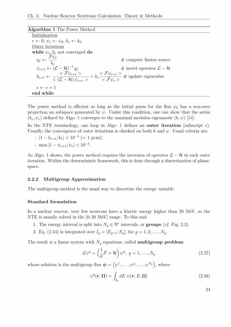
Ch. 2. Nuclear Reactor Neutronic Calculation: Theory & Methods
Algorithm 1 The Power MethodInitializatione← 0, ψe ← ψ0, ke ← k0Outer iterationswhile ψe, ke not converged doqf ←
Fψeke
# compute fission source
ψe+1 ← (L −H)−1 qf # invert operator L −Hke+1 ←
< Fψe+1 >
< (L −H)ψe+1 >= ke
< Fψe+1 >
< Fψe ># update eigenvalue
e← e+ 1end while
The power method is efficient as long as the initial guess for the flux ψ0 has a non-zeroprojection on subspace generated by ψ. Under this condition, one can show that the series(ke, ψe) defined by Algo. 1 converges to the maximal modulus eigenmode (k, ψ) [34].In the NTE terminology, one loop in Algo. 1 defines an outer iteration (subscript e).Usually, the convergence of outer iterations is checked on both k and ψ. Usual criteria are:
- |1− ke+1/ke| < 10−5 (= 1 pcm);- max |1− ψe+1/ψe| < 10−3.
As Algo. 1 shows, the power method requires the inversion of operator L −H in each outeriteration. Within the deterministic framework, this is done through a discretization of phase-space.
2.2.2 Multigroup Approximation
The multigroup method is the usual way to discretize the energy variable.
Standard formulation
In a nuclear reactor, very few neutrons have a kinetic energy higher than 20 MeV, so theNTE is usually solved in the [0; 20 MeV] range. To this end:
1. The energy interval is split into Ng ∈ N∗ intervals, or groups (cf. Fig. 2.2).2. Eq. (2.34) is integrated over Ig = [Eg+1;Eg], for g = 1, 2, . . . , Ng.
The result is a linear system with Ng equations, called multigroup problem:
Lψg =(1kF +H
)ψg, g = 1, . . . , Ng (2.37)
whose solution is the multigroup flux ψ =(ψ1, . . . , ψg, . . . , ψNg
), where:
ψg(r,Ω) =∫IgdE ψ(r, E,Ω) (2.38)
24
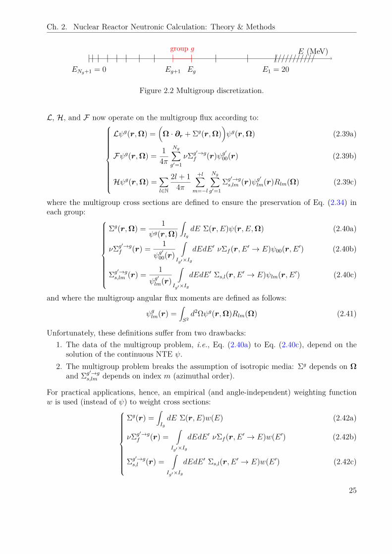
Ch. 2. Nuclear Reactor Neutronic Calculation: Theory & Methods
|ENg+1 = 0
| | | | | | | |Eg+1
|Eg
group g| | |
E1 = 20
E (MeV)///////////
Figure 2.2 Multigroup discretization.
L, H, and F now operate on the multigroup flux according to:
Lψg(r,Ω) =(Ω · ∂r + Σg(r,Ω)
)ψg(r,Ω) (2.39a)
Fψg(r,Ω) = 14π
Ng∑g′=1
νΣg′→gf (r)ψg
′
00(r) (2.39b)
Hψg(r,Ω) =∑l∈N
2l + 14π
+l∑m=−l
Ng∑g′=1
Σg′→gs,lm (r)ψg
′
lm(r)Rlm(Ω) (2.39c)
where the multigroup cross sections are defined to ensure the preservation of Eq. (2.34) ineach group:
Σg(r,Ω) = 1ψg(r,Ω)
∫IgdE Σ(r, E)ψ(r, E,Ω) (2.40a)
νΣg′→gf (r) = 1
ψg′
00(r)
∫Ig′×Ig
dEdE ′ νΣf (r, E ′ → E)ψ00(r, E ′) (2.40b)
Σg′→gs,lm (r) = 1
ψg′
lm(r)
∫Ig′×Ig
dEdE ′ Σs,l(r, E ′ → E)ψlm(r, E ′) (2.40c)
and where the multigroup angular flux moments are defined as follows:
ψglm(r) =∫S2d2Ωψg(r,Ω)Rlm(Ω) (2.41)
Unfortunately, these definitions suffer from two drawbacks:1. The data of the multigroup problem, i.e., Eq. (2.40a) to Eq. (2.40c), depend on the
solution of the continuous NTE ψ.2. The multigroup problem breaks the assumption of isotropic media: Σg depends on Ω
and Σg′→gs,lm depends on index m (azimuthal order).
For practical applications, hence, an empirical (and angle-independent) weighting functionw is used (instead of ψ) to weight cross sections:
Σg(r) =∫IgdE Σ(r, E)w(E) (2.42a)
νΣg′→gf (r) =
∫Ig′×Ig
dEdE ′ νΣf (r, E ′ → E)w(E ′) (2.42b)
Σg′→gs,l (r) =
∫Ig′×Ig
dEdE ′ Σs,l(r, E ′ → E)w(E ′) (2.42c)
25
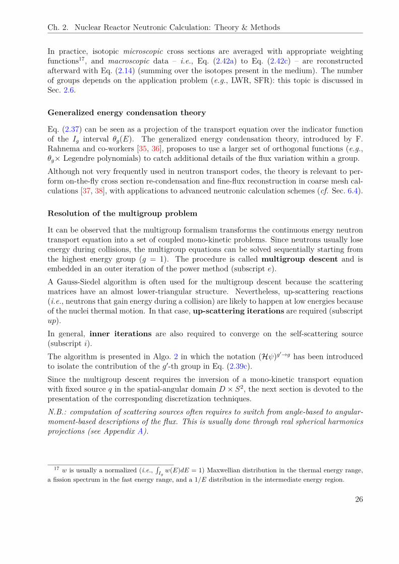
Ch. 2. Nuclear Reactor Neutronic Calculation: Theory & Methods
In practice, isotopic microscopic cross sections are averaged with appropriate weightingfunctions17, and macroscopic data – i.e., Eq. (2.42a) to Eq. (2.42c) – are reconstructedafterward with Eq. (2.14) (summing over the isotopes present in the medium). The numberof groups depends on the application problem (e.g., LWR, SFR): this topic is discussed inSec. 2.6.
Generalized energy condensation theory
Eq. (2.37) can be seen as a projection of the transport equation over the indicator functionof the Ig interval θg(E). The generalized energy condensation theory, introduced by F.Rahnema and co-workers [35, 36], proposes to use a larger set of orthogonal functions (e.g.,θg× Legendre polynomials) to catch additional details of the flux variation within a group.Although not very frequently used in neutron transport codes, the theory is relevant to per-form on-the-fly cross section re-condensation and fine-flux reconstruction in coarse mesh cal-culations [37, 38], with applications to advanced neutronic calculation schemes (cf. Sec. 6.4).
Resolution of the multigroup problem
It can be observed that the multigroup formalism transforms the continuous energy neutrontransport equation into a set of coupled mono-kinetic problems. Since neutrons usually loseenergy during collisions, the multigroup equations can be solved sequentially starting fromthe highest energy group (g = 1). The procedure is called multigroup descent and isembedded in an outer iteration of the power method (subscript e).A Gauss-Siedel algorithm is often used for the multigroup descent because the scatteringmatrices have an almost lower-triangular structure. Nevertheless, up-scattering reactions(i.e., neutrons that gain energy during a collision) are likely to happen at low energies becauseof the nuclei thermal motion. In that case, up-scattering iterations are required (subscriptup).In general, inner iterations are also required to converge on the self-scattering source(subscript i).The algorithm is presented in Algo. 2 in which the notation (Hψ)g′→g has been introducedto isolate the contribution of the g′-th group in Eq. (2.39c).Since the multigroup descent requires the inversion of a mono-kinetic transport equationwith fixed source q in the spatial-angular domain D × S2, the next section is devoted to thepresentation of the corresponding discretization techniques.N.B.: computation of scattering sources often requires to switch from angle-based to angular-moment-based descriptions of the flux. This is usually done through real spherical harmonicsprojections (see Appendix A).
17 w is usually a normalized (i.e.,∫Igw(E)dE = 1) Maxwellian distribution in the thermal energy range,
a fission spectrum in the fast energy range, and a 1/E distribution in the intermediate energy region.
26
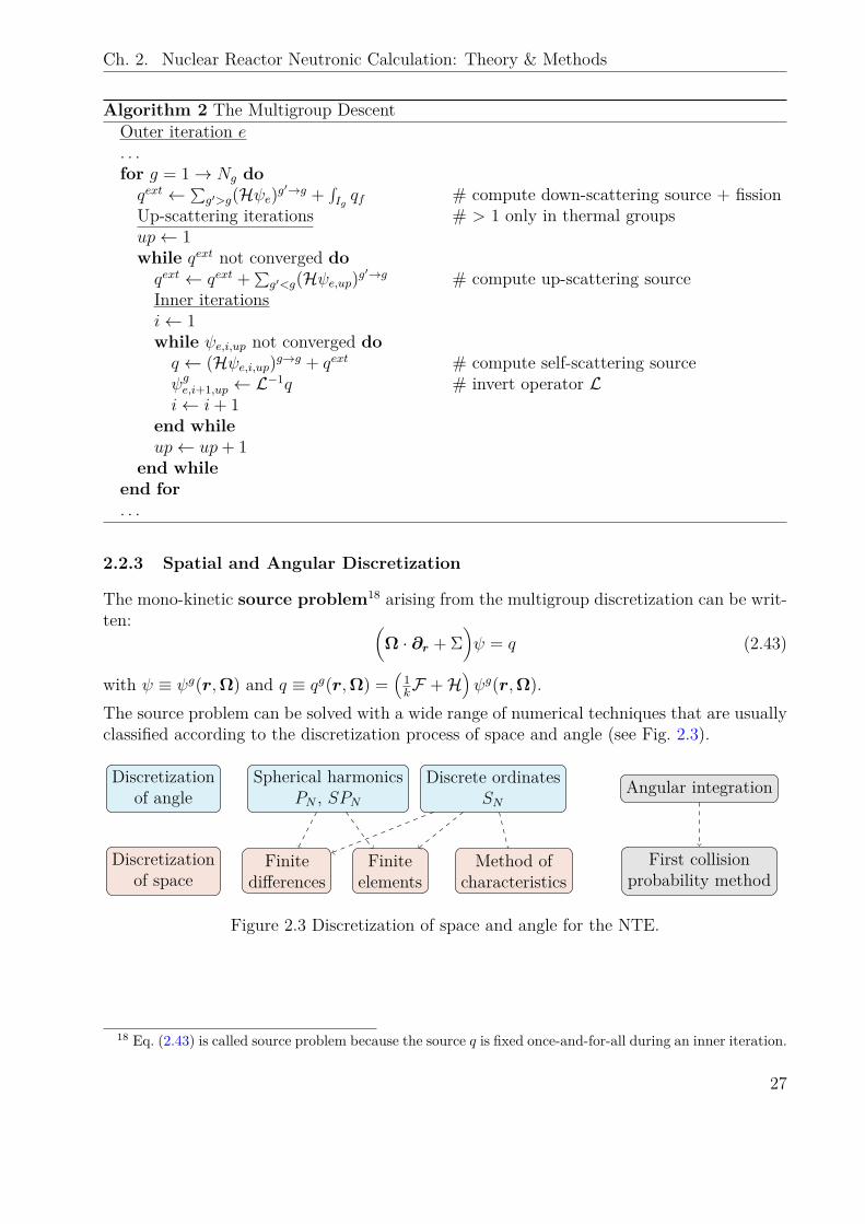
Ch. 2. Nuclear Reactor Neutronic Calculation: Theory & Methods
Algorithm 2 The Multigroup DescentOuter iteration e. . .for g = 1→ Ng doqext ← ∑
g′>g(Hψe)g′→g +
∫Igqf # compute down-scattering source + fission
Up-scattering iterations # > 1 only in thermal groupsup← 1while qext not converged doqext ← qext +∑
g′<g(Hψe,up)g′→g # compute up-scattering source
Inner iterationsi← 1while ψe,i,up not converged doq ← (Hψe,i,up)g→g + qext # compute self-scattering sourceψge,i+1,up ← L−1q # invert operator Li← i+ 1
end whileup← up+ 1
end whileend for. . .
2.2.3 Spatial and Angular Discretization
The mono-kinetic source problem18 arising from the multigroup discretization can be writ-ten: (
Ω · ∂r + Σ)ψ = q (2.43)
with ψ ≡ ψg(r,Ω) and q ≡ qg(r,Ω) =(
1kF +H
)ψg(r,Ω).
The source problem can be solved with a wide range of numerical techniques that are usuallyclassified according to the discretization process of space and angle (see Fig. 2.3).
Discretizationof angle
Spherical harmonicsPN , SPN
Discrete ordinatesSN
Angular integration
Discretizationof space
Finitedifferences
Finiteelements
Method ofcharacteristics
First collisionprobability method
Figure 2.3 Discretization of space and angle for the NTE.
18 Eq. (2.43) is called source problem because the source q is fixed once-and-for-all during an inner iteration.
27
Ch. 2. Nuclear Reactor Neutronic Calculation: Theory & Methods
In particular for the angular variable:• PN (resp. SPN) methods rely on a projection of Eq. (2.43) over a complete (resp.
partial) set of real spherical harmonics (Rlm) up to order l = N ∈ N∗.• SN methods rely on a discretization of the angular variable into a finite set of directions
(Ωn)n∈1,2,...,Nd.
The angular discretization then results in a spatial problem that can be solved with:• Finite difference or finite element methods.• The method of characteristics which relies on the integration of Eq. (2.43) along neutron
trajectories.• Collision probability methods (if the solution sought is the scalar flux ψ00 and not the
angular flux ψ).
An exhaustive description of these discretization techniques may be found in A. Hébert’sbook [39]. Now, the remaining of this section presents a particular focus on the methodsthat have been used in this work, i.e., the method of characteristics, the discrete ordinates /finite element method and the collision probability method. As we will see in Chapter 3, thesemethods constitute the building blocks of the neutronic calculation schemes implemented inAPOLLO3® for SFR applications.N.B.: The diffusion approximation of the NTE consists in replacing the transport operatorL by a diffusion operator (Fick’s law). Even though LWR neutronic calculations often relyon the diffusion approximation, it has not been considered in this work (it is known to beinaccurate for SFRs).
The method of characteristics
The Method Of Characteristics (MOC) relies on an exact integration of the NTE along neu-tron trajectories (characteristics) in 2D or 3D domains. It is capable of handling unstructured(i.e., unconstrained) geometrical meshes and therefore relies on a minimal number of approx-imations. As such, it often considered as a “reference” deterministic method. Unfortunately,its use is often restricted to limited size geometries and 2D domains (e.g., a planar assemblywith reflective boundary conditions) because of the large number of computer resources itdemands.Since neutrons are free particles, the NTE characteristics are straight lines. Let Γn be sucha line: it is parametrized by its origin r0 and direction Ω, both referenced with subscriptn. Formally, the integration of Eq. (2.43) along Γn yields the following expression for theneutron flux:
ψ(r,Ω) = e−τ(s,r,Ω)ψ(r0,Ω) +∫ s
0ds′ e−τ(s′,r,Ω)q(r − s′Ω,Ω) (2.44)
where s = |r − r0|. The optical path τ is defined as:
τ(s, r,Ω) =∫ s
0ds′Σ(r − s′Ω) (2.45)
28
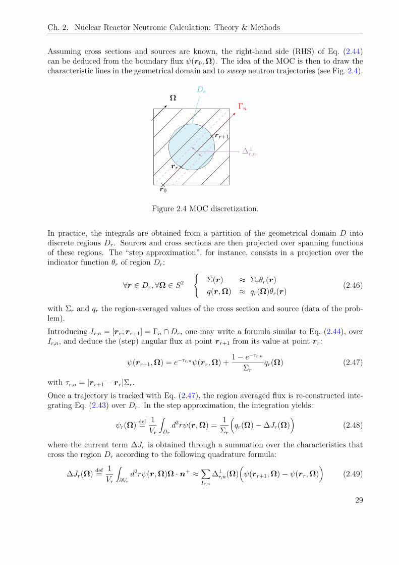
Ch. 2. Nuclear Reactor Neutronic Calculation: Theory & Methods
Assuming cross sections and sources are known, the right-hand side (RHS) of Eq. (2.44)can be deduced from the boundary flux ψ(r0,Ω). The idea of the MOC is then to draw thecharacteristic lines in the geometrical domain and to sweep neutron trajectories (see Fig. 2.4).
Dr
ΩΓn
×r0
×rr
×rr+1
∆⊥r,n
Figure 2.4 MOC discretization.
In practice, the integrals are obtained from a partition of the geometrical domain D intodiscrete regions Dr. Sources and cross sections are then projected over spanning functionsof these regions. The “step approximation”, for instance, consists in a projection over theindicator function θr of region Dr:
∀r ∈ Dr,∀Ω ∈ S2
Σ(r) ≈ Σrθr(r)q(r,Ω) ≈ qr(Ω)θr(r)
(2.46)
with Σr and qr the region-averaged values of the cross section and source (data of the prob-lem).Introducing Ir,n = [rr; rr+1] = Γn ∩Dr, one may write a formula similar to Eq. (2.44), overIr,n, and deduce the (step) angular flux at point rr+1 from its value at point rr:
ψ(rr+1,Ω) = e−τr,nψ(rr,Ω) + 1− e−τr,nΣr
qr(Ω) (2.47)
with τr,n = |rr+1 − rr|Σr.Once a trajectory is tracked with Eq. (2.47), the region averaged flux is re-constructed inte-grating Eq. (2.43) over Dr. In the step approximation, the integration yields:
ψr(Ω) def= 1Vr
∫Drd3rψ(r,Ω) = 1
Σr
(qr(Ω)−∆Jr(Ω)
)(2.48)
where the current term ∆Jr is obtained through a summation over the characteristics thatcross the region Dr according to the following quadrature formula:
∆Jr(Ω) def= 1Vr
∫∂Vr
d2rψ(r,Ω)Ω · n+ ≈∑Ir,n
∆⊥r,n(Ω)(ψ(rr+1,Ω)− ψ(rr,Ω)
)(2.49)
29
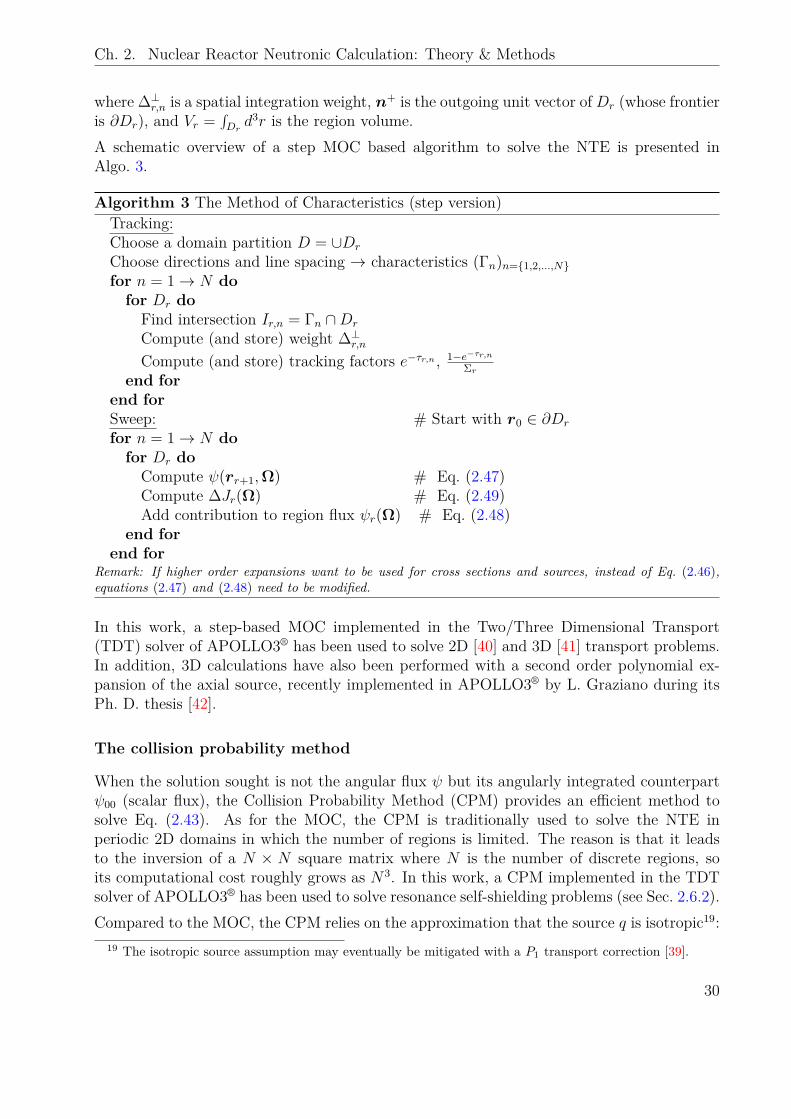
Ch. 2. Nuclear Reactor Neutronic Calculation: Theory & Methods
where ∆⊥r,n is a spatial integration weight, n+ is the outgoing unit vector ofDr (whose frontieris ∂Dr), and Vr =
∫Drd3r is the region volume.
A schematic overview of a step MOC based algorithm to solve the NTE is presented inAlgo. 3.
Algorithm 3 The Method of Characteristics (step version)Tracking:Choose a domain partition D = ∪Dr
Choose directions and line spacing → characteristics (Γn)n=1,2,...,Nfor n = 1→ N dofor Dr doFind intersection Ir,n = Γn ∩Dr
Compute (and store) weight ∆⊥r,nCompute (and store) tracking factors e−τr,n , 1−e−τr,n
Σrend for
end forSweep: # Start with r0 ∈ ∂Dr
for n = 1→ N dofor Dr doCompute ψ(rr+1,Ω) # Eq. (2.47)Compute ∆Jr(Ω) # Eq. (2.49)Add contribution to region flux ψr(Ω) # Eq. (2.48)
end forend for
Remark: If higher order expansions want to be used for cross sections and sources, instead of Eq. (2.46),equations (2.47) and (2.48) need to be modified.
In this work, a step-based MOC implemented in the Two/Three Dimensional Transport(TDT) solver of APOLLO3® has been used to solve 2D [40] and 3D [41] transport problems.In addition, 3D calculations have also been performed with a second order polynomial ex-pansion of the axial source, recently implemented in APOLLO3® by L. Graziano during itsPh. D. thesis [42].
The collision probability method
When the solution sought is not the angular flux ψ but its angularly integrated counterpartψ00 (scalar flux), the Collision Probability Method (CPM) provides an efficient method tosolve Eq. (2.43). As for the MOC, the CPM is traditionally used to solve the NTE inperiodic 2D domains in which the number of regions is limited. The reason is that it leadsto the inversion of a N × N square matrix where N is the number of discrete regions, soits computational cost roughly grows as N3. In this work, a CPM implemented in the TDTsolver of APOLLO3® has been used to solve resonance self-shielding problems (see Sec. 2.6.2).Compared to the MOC, the CPM relies on the approximation that the source q is isotropic19:
19 The isotropic source assumption may eventually be mitigated with a P1 transport correction [39].
30
Ch. 2. Nuclear Reactor Neutronic Calculation: Theory & Methods
q(r,Ω) ≈ 14πq00(r) (2.50)
Assuming that the spatial domain is indeed an infinite and periodic lattice of cells, the firstterm in the RHS of Eq. (2.44) drops (r0 →∞), so its angular integration yields:
ψ00(r) = 14π
∫S2d2Ω
∫ +∞
0ds e−τ(s,r,Ω)q00(r − sΩ) (2.51)
Introducing the change of variable r′ = r − sΩ, Eq. (2.51) can also be written (with d3r′ =s2dsd2Ω):
ψ00(r) = 14π
∫R3d3r′
e−τ(|r−r′|,r,Ω)
|r − r′|2q00(r) (2.52)
The spatial discretization process then consists in choosing N regions Di, and projecting theflux ψ00 and source q00 over the indicator functions of these regions:
∀r ∈ Di,
ψ00(r) ≈ ψiθi(r)q00(r) ≈ qiθi(r)
(2.53)
where ψi and qi are the region averaged values.When Eq. (2.53) is introduced in Eq. (2.52), a spatial integration over region Dj yields:
∀j, ψjVj =∑i
pijViqi (2.54)
where Vi =∫Did3r is the volume of region Di and pij is the reduced collision probability
defined as20:pij = 1
4π
∫Djd3r
∫∪Di
d3r′e−τ(|r−r′|,r,Ω)
|r − r′|2(2.55)
The idea of the CPM is to:
1. Compute the collision probability matrix (pij) with Eq. (2.55) where the integration isusually performed numerically through a geometry tracking.
2. Compute the neutron flux reversing the linear system defined by Eq. (2.54).
N.B.: the "real" (and not reduced) collision probability is defined as:
Pij = Σj pij (2.56)
where Σj is the total cross section of region j. It is interpreted as the probability for a neutronborn in a region Di anywhere in the lattice to undergo its first collision in Dj.
20 The integration in Eq. (2.54) is done over a particular region j but over all the repeated cells i in thelattice.
31
Ch. 2. Nuclear Reactor Neutronic Calculation: Theory & Methods
The SN discontinuous Galerkin finite element method
When the number of spatial cells grows (e.g., for whole core problems), the MOC and CPMefficiency decreases. In that case, SN based finite element methods provide an interest-ing alternative to solve the source problem, i.e., Eq. (2.43). In this work in particular, aDiscontinuous Galerkin Finite Element Method (DGFEM) implemented in the MINARETsolver [43] of APOLLO3® has been used to solve transport problems composed of severalthousand of spatial cells.The discrete ordinates (SN) discretization consists in choosing a finite set of directions(Ωn)n∈1,2,...,Nd and, for each Ωn, solving Eq. (2.43) in the spatial range (r ∈ D):(
Ωn · ∂r + Σ(r))ψn(r) = qn(r) (2.57)
where ψn ≡ ψ(r,Ωn) and qn ≡ q(r,Ωn).Finite element methods can be used to solve Eq. (2.57) relying on its weak formulation: if ψnif a solution of Eq. (2.57), then for any integrable function w defined on D, ψn must satisfythe following relation: ∫
Dw(Ωn · ∂r + Σ
)ψn =
∫Dwqn (2.58)
Within the framework of the finite element method, the geometrical domain is split into Nk
(non-overlapping) cells K, or elements21, and the flux is projected over a local polynomialbasis pk,j composed of Nj functions:
ψn(r) ≈Nk∑k=1
θk(r)Nj∑j=1
ψk,jn pk,j(r) (2.59)
where θk is the indicator function of element K.Inserting Eq. (2.59) in Eq. (2.58) and with a proper choice of Nj ×Nk linearly independentweight functions wi, it is possible to reduce the problem to the inversion of a linear system:
∀i ∈ 1; . . . ;Nj ×Nk,Nj∑j=1
Nk∑k=1
ψk,jn
∫Kwi
(Ωn · ∂r + Σ
)pk,j =
∑k
∫Kwiqn (2.60)
where ψk,jn are the unknowns.In particular, the DGFEM implemented in MINARET uses Lagrange polynomials22, bothfor the weight functions wi and the local projection basis pk,j. Besides, a particular featureof the DGFEM is that the flux is allowed to be discontinuous at the element boundaries: inMINARET, an “upwind approximation” is used to compute the gradient integral (i.e., thefirst term in the left-hand side of Eq. (2.60), see Appendix C). This approximation is notphysical, but it guarantees the method stability and allows an optimal sweep of the elements(according to the neutron propagation direction).Numerically, the DGFEM constitutes a well-posed problem for the resolution of the fixed-source mono-kinetic NTE, i.e., Eq. (2.43) [44]. The algorithm is summarized in Algo. 4.
21 In MINARET, the elements are either triangles (2D geometries) or prisms (3D domains).22 Lagrange polynomials interpolate a given number of points belonging to a particular element K.
32
Ch. 2. Nuclear Reactor Neutronic Calculation: Theory & Methods
Algorithm 4 The Discrete Ordinate Finite Element MethodChoose directions (Ωn)n=1,2,...,NChoose a domain partition into NK elements D = ∪NkKfor n = 1→ N doArrange elements according to the propagation direction Ωn: K1 → KNk
for k = 1→ Nk do∀j, compute ψk,jn # Eq. (2.60), done locally with DGFEM
end forend for
At this stage, all the methods presented so far propose to solve the critical neutron transportproblem, i.e., Eq. (2.34), through a discretization of phase-space. This approach constitutesthe deterministic way to solve the NTE (APOLLO3® way).
2.2.4 Stochastic Methods
Physically, the NTE is a statistical description of the average behavior of a neutron populationin phase-space. As a result, advantage can be taken of Monte Carlo techniques [45] to sampleneutron histories and build statistical estimators of the quantities of interest. In such astatistical approach, cross sections describe the probabilities of individual events (nuclearreactions) to occur.The advantage of the Monte Carlo approach is that it does not rely on a phase-space dis-cretization and, hence, does not suffer from the deterministic approximations. As such, it isoften considered as a reference tool to solve the neutron transport equation. Its drawback,however, is that it might require large amounts of computer resources (mostly calculationtime) to handle converged estimators.
Random events sampling
Let X be a random variable describing a statistical process (e.g., fission probability after aneutron absorption) and p its probability density function (pdf). The idea of Monte Carlomethods is to sample the possible outcomes of X according to the law p.To do so, a pseudo-random number generator – usually based on congruences – is used toproduce random numbers in the [0; 1] range. Let η be such a random number and let suppose,for the sake of simplicity, that p is defined on an interval [a; b]. Then, the possible outcomes ofX can be obtained from an inversion of the cumulative distribution function of p, accordingto the following equation:
F (x) def=∫ x
ap(x′)dx′ =
∫ η
0dη′ = η =⇒ x = F−1(η) (2.61)
Eq. (2.61) shows that a pdf sampling resumes to the inversion of its cumulative distributionfunction F . It is the founding principle of Monte Carlo methods.Let suppose for instance that a neutron is born by fission at point r. Its velocity can be ob-tained through the fission spectra pdf sampling. If the total cross section is known, it is then
33
Ch. 2. Nuclear Reactor Neutronic Calculation: Theory & Methods
possible to determine the probability the neutron has to travel a given distance before inter-acting with the medium. If the trajectory crosses the boundary of the calculation domain,the story ends. Else, a nuclear reaction occurs: two other random number sampling allowsto choose the nucleus concerned by the interaction (according to the nuclei concentrationsand total cross sections) and the reaction type (according to the partial cross section values).Depending on the outcome of the drawing, the story may end (e.g., capture) or continue (e.g.,scattering). Additional particles may eventually be simulated (fission, (n,Xn) reactions. . . ).Monte Carlo methods can also be used to solve the critical problem, i.e., Eq. (2.34): anoverview of a simplified algorithm is presented in Algo. 5. The idea is to divide the simulationinto batches and to count the fission events per batch. The first set of batches must be usedto converge on the fission source distribution, but discarded afterwards for the analysis ofthe results.
Algorithm 5 Critical Monte Carlo Power MethodChoose number of batches NB, number of neutrons per batch N and fission source S0for b = 1→ NB doSample N fission neutrons in D according to Sb−1for neutron = 1→ N dowhile neutron is alive doSample speed (energy and angle) and distance traveledif neutron is out of D thenneutron dies
elseSample nucleus and interaction iif i == scattering thencontinue
else if i == fission thenSample and store outgoing fission source Sb (according to χi, νi)neutron dies
else if i == capture thenneutron dies
end ifend if
end whileend forCompute eigenvalue estimation kb = 1
N
∫D×R3
Sb
Normalize fission source distribution Sb = Sb/kbend for
Remark: Usually, biasing techniques are used to reduce the estimators variance, and fasten Monte Carlomethods.
34
Ch. 2. Nuclear Reactor Neutronic Calculation: Theory & Methods
Estimators
The Monte Carlo method enables to model the physical process underlying the NTE. How-ever, physicists and engineers are interested in measurable quantities such as reaction rates:the system must be tallied, and estimators must be built. The calculation of the fissionsource Sb in Algo. 5 is an example of such a tally.Collision estimators, for instance, rely on counters that are incremented each time a collisionevent (e.g., scattering or capture) occurs. It is also possible to build path-length estimators,surface crossing estimators, and even analytical estimators. They can be used to computereaction rates, neutron fluxes, currents. . . Since the Monte Carlo method is a stochasticprocess, the estimators, in fact, handle a statistical description of such quantities (expectedvalues, standard deviations or higher moments).For a more extensive review of Monte Carlo methods as applied to the calculation of nuclearreactors, the interested reader is invited to consult the book of A. Haghighat [46].This description completes the presentation of the methods that can be used to solve thecritical neutron transport problem Eq. (2.34). As it is seen, the problem benefits from alarge theoretical background and even from two class of numerical methods (deterministicand stochastic) to compute its solution. When it comes to performing actual reactor neutroniccalculations, though, this apparent simplicity is confronted with a major difficulty that is thenumber of independent variables the NTE solution depends on.
2.3 The Numerical Footprint Issue
To better understand the nature of the numerical footprint issue, this section presents anaive estimate of the computer resources (calculation time and/or memory) a critical neutrontransport calculation without approximations would require.
2.3.1 Deterministic Point of View
Consider a typical SFR core composed of approximately 300 fuel assemblies (see Fig. 2.5). Ifeach fuel assembly is composed of 250 fuel pins then at least 750 radial volumes are requiredto discretize fuel, clad and coolant. Assume the core is two meters high and that 100 distinctaxial layers are sufficient to catch the axial variations of the flux. Then the number of spatialcells involved is 300× 750× 100 = 2.25 107.Now, consider that the angular variable can reasonably be represented with approximately200 discrete ordinates but that about 105 energy bins are necessary to account for resonantneutron-nucleus interaction phenomena in the energy range (see Fig. 2.6).Finally, the total number of unknowns is 2.25 107 × 200× 105 = 4.5 1014.
• In terms of numerical storage, this represents about 4 PB (= 4.1015 Bytes) of memoryin double precision floating point format (1 double = 8 B).
• In terms of computational power, this represents about 4.5 1022 operations to compute aflux solution. This figure assumes that about N2
g = 1010 operations are required for the
35
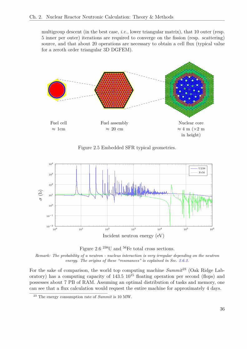
Ch. 2. Nuclear Reactor Neutronic Calculation: Theory & Methods
multigroup descent (in the best case, i.e., lower triangular matrix), that 10 outer (resp.5 inner per outer) iterations are required to converge on the fission (resp. scattering)source, and that about 20 operations are necessary to obtain a cell flux (typical valuefor a zeroth order triangular 3D DGFEM).
Fuel cell≈ 1cm
Fuel assembly≈ 20 cm
Nuclear core≈ 4 m (×2 min height)
Figure 2.5 Embedded SFR typical geometries.
100 101 102 103 104 105 10610−2
10−1
100
101
102
103
104
Incident neutron energy (eV)
σ(b)
U238Fe56
Figure 2.6 238U and 56Fe total cross sections.Remark: The probability of a neutron - nucleus interaction is very irregular depending on the neutron
energy. The origins of these “resonances” is explained in Sec. 2.6.2.
For the sake of comparison, the world top computing machine Summit23 (Oak Ridge Lab-oratory) has a computing capacity of 143.5 1015 floating operation per second (flops) andpossesses about 7 PB of RAM. Assuming an optimal distribution of tasks and memory, onecan see that a flux calculation would request the entire machine for approximately 4 days.
23 The energy consumption rate of Summit is 10 MW.
36
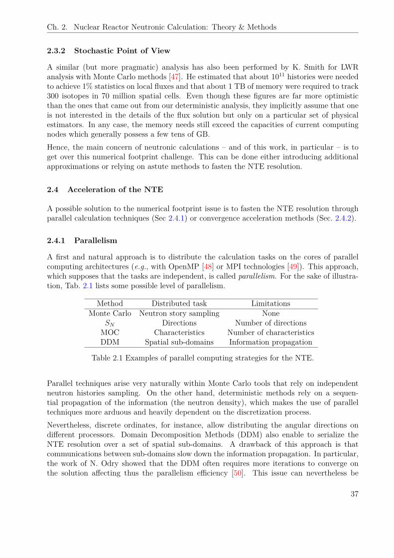
Ch. 2. Nuclear Reactor Neutronic Calculation: Theory & Methods
2.3.2 Stochastic Point of View
A similar (but more pragmatic) analysis has also been performed by K. Smith for LWRanalysis with Monte Carlo methods [47]. He estimated that about 1011 histories were neededto achieve 1% statistics on local fluxes and that about 1 TB of memory were required to track300 isotopes in 70 million spatial cells. Even though these figures are far more optimisticthan the ones that came out from our deterministic analysis, they implicitly assume that oneis not interested in the details of the flux solution but only on a particular set of physicalestimators. In any case, the memory needs still exceed the capacities of current computingnodes which generally possess a few tens of GB.Hence, the main concern of neutronic calculations – and of this work, in particular – is toget over this numerical footprint challenge. This can be done either introducing additionalapproximations or relying on astute methods to fasten the NTE resolution.
2.4 Acceleration of the NTE
A possible solution to the numerical footprint issue is to fasten the NTE resolution throughparallel calculation techniques (Sec 2.4.1) or convergence acceleration methods (Sec. 2.4.2).
2.4.1 Parallelism
A first and natural approach is to distribute the calculation tasks on the cores of parallelcomputing architectures (e.g., with OpenMP [48] or MPI technologies [49]). This approach,which supposes that the tasks are independent, is called parallelism. For the sake of illustra-tion, Tab. 2.1 lists some possible level of parallelism.
Method Distributed task LimitationsMonte Carlo Neutron story sampling None
SN Directions Number of directionsMOC Characteristics Number of characteristicsDDM Spatial sub-domains Information propagation
Table 2.1 Examples of parallel computing strategies for the NTE.
Parallel techniques arise very naturally within Monte Carlo tools that rely on independentneutron histories sampling. On the other hand, deterministic methods rely on a sequen-tial propagation of the information (the neutron density), which makes the use of paralleltechniques more arduous and heavily dependent on the discretization process.Nevertheless, discrete ordinates, for instance, allow distributing the angular directions ondifferent processors. Domain Decomposition Methods (DDM) also enable to serialize theNTE resolution over a set of spatial sub-domains. A drawback of this approach is thatcommunications between sub-domains slow down the information propagation. In particular,the work of N. Odry showed that the DDM often requires more iterations to converge onthe solution affecting thus the parallelism efficiency [50]. This issue can nevertheless be
37
Ch. 2. Nuclear Reactor Neutronic Calculation: Theory & Methods
tackled with acceleration techniques or relying on astute sub-domain ordering as proposedin reference [51].
2.4.2 Acceleration
Acceleration techniques are designed to fasten the convergence of inner (and sometimes outer)iterations in deterministic methods (see Algo. 2). They rely on the computation of a cor-rection factor between two successive iterations and can be classified into rebalancing andsynthetic techniques.
Rebalancing methods
Rebalancing consists in using a coarse mesh solution to fasten the particle transport betweendistant regions. This coarse solution is then used to adjust the flux amplitude over eachcoarse volume keeping the detailed flux distribution unchanged. Because it relies on a particlebalance between coarse cells, it may be applied to many discretizations of the NTE. Similarly,rebalancing can also be used to fasten the multigroup descent. However, the method is non-linear and its stability is, therefore, not always guaranteed [52].
Synthetic methods
Synthetic methods are based on the estimation of an error between two successive iterations.In the case of inner iterations, let ψi be the flux at iteration i, ψ∞ be the real (converged)flux and εi = ψ∞ − ψi the error. They obey the following equations:
Lψ∞ = Hψ∞ + qext (2.62a)Lψi+1 = Hψi + qext (2.62b)
and:(L −H) εi+1 = H(ψi+1 − ψi) (2.63)
where H ≡ Hg→g is the self-scattering operator (the group superscript g has been droppedout for the sake of clarity).The idea of synthetic methods is then to replace L−H in the left-hand side (LHS) of Eq. (2.63)by a simplified operator (e.g., a diffusion operator) so that εi+1 can be computed faster thanthe flux itself. Eventually, a projection operation might be necessary if the simplified operatordoes not operate on the same vector space than L and H. Finally, the accelerated flux atiteration i+ 1 is:
ψacci+1 = ψi+1 + εi+1 (2.64)
In this work, Diffusive Synthetic Acceleration (DSA) methods have been used to acceleratethe MOC and SN–DGFEM equations [43, 53, 54].It is seen that parallel and acceleration techniques allow to speed-up the NTE resolution.However, they usually increase memory requirements (acceleration factors, storage of newunknowns. . . ) and thus do not constitute a solution to the numerical storage constraint. Forfunctional core calculations then, one or several homogenization steps are often required.
38
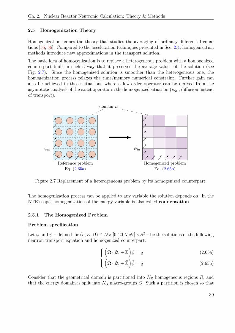
Ch. 2. Nuclear Reactor Neutronic Calculation: Theory & Methods
2.5 Homogenization Theory
Homogenization names the theory that studies the averaging of ordinary differential equa-tions [55, 56]. Compared to the acceleration techniques presented in Sec. 2.4, homogenizationmethods introduce new approximations in the transport solution.The basic idea of homogenization is to replace a heterogeneous problem with a homogenizedcounterpart built in such a way that it preserves the average values of the solution (seeFig. 2.7). Since the homogenized solution is smoother than the heterogeneous one, thehomogenization process relaxes the time/memory numerical constraint. Further gain canalso be achieved in those situations where a low-order operator can be derived from theasymptotic analysis of the exact operator in the homogenized situation (e.g., diffusion insteadof transport).
ψin ψin
domain D
Reference problemEq. (2.65a)
Homogenized problemEq. (2.65b)
Figure 2.7 Replacement of a heterogeneous problem by its homogenized counterpart.
The homogenization process can be applied to any variable the solution depends on. In theNTE scope, homogenization of the energy variable is also called condensation.
2.5.1 The Homogenized Problem
Problem specification
Let ψ and ψ – defined for (r, E,Ω) ∈ D× [0; 20 MeV]×S2 – be the solutions of the followingneutron transport equation and homogenized counterpart:
(Ω · ∂r + Σ
)ψ = q (2.65a)(
Ω · ∂r + Σ)ψ = q (2.65b)
Consider that the geometrical domain is partitioned into NR homogeneous regions R, andthat the energy domain is split into NG macro-groups G. Such a partition is chosen so that
39
Ch. 2. Nuclear Reactor Neutronic Calculation: Theory & Methods
the homogenized cross section is constant in R × G in order to smoothen the homogenizedsolution.Letting the definition of the homogenized source for later, suppose also that q is built in sucha way that:
∀R,G,∫R×G
q =∫R×G
q (2.66)
Under those conditions, it seems reasonable to ask for the homogenized problem to conservethe averaged number of neutrons and the averaged reaction rates inR×G. Those conservationrelations read:
∀R,G,
∫R×G
ψ =∫R×G
ψ (2.67a)∫R×G
Σψ =∫R×G
Σψ (2.67b)
Eq. (2.67a) and Eq. (2.67b) constitute what is expected from the homogenization process24.Assuming that these relations are fulfilled, then necessarily, the expression of a constantpiece-wise homogenized cross section in R×G should be:
∀R,G, Σ ≡ ΣGR(Ω) =
∫R×G
Σψ∫R×G
ψ(2.68)
Unfortunately, imposing the homogenized cross section definition with Eq. (2.68) is not a suf-ficient condition to ensure that the flux solution of the homogenized problem ψ will satisfythe conservation relations Eq. (2.67a) – Eq. (2.67b). The reason for this is that homoge-nization is non-linear: the solution obtained with the averaged data (homogenizedcross sections) is not the average of the reference solution.
The equivalence paradigm
The equivalence method [59, 60, 61] introduced by A. Kavenoky and A. Hébert proposes asolution to this issue. Driven by the idea that reaction rates are the only significant physicalquantities in the NTE, it furnishes a method for the definition of averaged cross sections Σthat conserve the reaction rate balance25, i.e., Eq. (2.67b). The cost to pay is, in general,the non-conservation of the averaged number of neutrons, i.e., Eq. (2.67a).
24 Specifying Eq. (2.67a) and Eq. (2.67b), it is chosen to describe a homogenization theory that preservesangular dependent fluxes and reaction rates in the homogenized situation. Many homogenization theories,though, only aim at preserving angularly integrated fluxes/rates. Moreover, some other homogenization the-ories also intend to preserve other quantities: the discontinuity factor method, introduced by K. Koebke [57]and K. Smith [58], for instance, is based on the idea that it is the response of the homogenized domain (i.e.,the outgoing angular flux) that should be preserved in the homogenized situation.
25 The equivalence method was first introduced to preserve angularly integrated reaction rates [59, 60],and later improved to preserve angular dependent quantities [61].
40
Ch. 2. Nuclear Reactor Neutronic Calculation: Theory & Methods
The sole conservation of Eq. (2.67b) implies that the homogenized cross section depends onthe homogenized flux ψ according to:
∀R,G, ΣGR =
∫R×G
Σψ∫R×G
ψ(2.69)
Clearly, Eq. (2.69) defines a non-linear problem, because ψ depends on ΣGR: the homogenized
cross section values need to be built iteratively. In particular, Eq. (2.65b) handles the ho-mogenized flux and Eq. (2.69) the homogenized cross section in R × G. Eq. (2.68) can beused as an initial guess to start the procedure.In some particular situations, though, the problem posed by Eq. (2.69) – which compriseNR × NG unknowns and equations (per direction) – is degenerate. In that case, additionalnormalization conditions might be used to restore conservation relations.
Full domain homogenization with conservative boundary conditions
A typical example of such a degenerate situation is the case of a full domain homogenization(R ≡ D) with conservative boundary conditions26, i.e., when:∫
∂DΩ · n+ψ =
∫∂D
Ω · n+ψ = 0 (2.70)
where n+ is the outgoing normal unit of D and ∂D its frontier.In that case, the subtraction of Eq. (2.65a) and Eq. (2.65b) and integration over D × Gimplies that:
∀G,∫D×G
Σψ =∫D×G
Σψ (2.71)
Hence, the reaction rates are conserved independently of the value of the homogenized crosssection. To raise the degeneracy, Eq. (2.67a) can be used as a normalization condition. Inthat case, the homogenization process fulfills its duties: both reaction rates and fluxes areconserved27. Moreover, no equivalence is required. Such a situation is typical of the so-called“lattice problem” (cf. Sec. 2.5.2).
Energy condensation
The energy integration in a macro-group G naturally suggests to use the multigroup formal-ism for the homogenized problem28: ψ ≡ (ψG)G=1,...,NG .
26 Translation boundary conditions are compatible with Eq. (2.70). Reflective boundary conditions arenot: an additional angular integration must be performed, i.e.,
∫∂D×S2 Ω · n+ψ =
∫∂D×S2 Ω · n+ψ = 0.
27 With reflective boundary condition, only the isotropic (i.e., angularly integrated) reaction rates areconserved. In that case, one might impose the conservation of scalar-fluxes.
28 Generally, the multigroup formalism is also used for the reference problem, i.e., ψ ≡ (ψg)g=1,...,Ng. In
that case, the energy integrals need to be replaced by group summations, but the condensation theory isidentical in the results.
41
Ch. 2. Nuclear Reactor Neutronic Calculation: Theory & Methods
When no spatial homogenization is performed, in particular, the integration of Eq. (2.65a)over any macro group G yields:(
Ω · ∂r +∫G Σψ∫G ψ
) ∫Gψ =
∫Gq (2.72)
In that case, the problem is linear, i.e., the solution of the homogenized multigroup problemis:
ψG =∫Gψ (2.73)
and no equivalence is needed to define the homogenized cross section:
∀G, ΣG =
∫G
Σψ∫Gψ
(2.74)
Hence, the sole energy condensation is conservative. This situation is similar to theone already discussed in Sec. 2.2.2.
Critical problem
We now turn on to the definition of the homogenized source q for the critical problem. Thesources read:
q =(1kF +H
)ψ (2.75a)
q =(1kF + H
)ψ (2.75b)
As mentioned earlier, q and q are expected to fulfill the conservation relation Eq. (2.66). In thecritical framework, though, both fission and scattering contributions should be individuallypreserved in the homogenized situation, in order to ensure a consistency between partial andtotal reaction rates. This choice leads to adopt the following conventions for production( ¯νΣf )G
′→GR and scattering (Σs)G
′→GR homogenized cross sections29:
∀R,G,G′
(νΣf )G′→G
R =
∫R×G×G′
νΣfψ∫R×G′
ψ(2.76a)
(Σs)G′→G
R =
∫R×G×G′
Σsψ∫R×G′
ψ(2.76b)
29 These are “formal” definitions. In practice, the production cross section, i.e., Eq. (2.76a), is homogenizedwith the scalar-flux (because the fission neutron emission is assumed to be isotropic in the laboratory frame),while the scattering cross section, i.e., Eq. (2.76b), is expanded in angular moments. Explicit definitions willbe given in Sec. 3.2.1 (presentation of particular APOLLO3® homogenization methods).
42
Ch. 2. Nuclear Reactor Neutronic Calculation: Theory & Methods
At this stage, one can pretend to conserve the eigenvalue if the overall leakage∫D×G×S2 Ω·∂rψ
is also preserved in the homogenized situation. This is verified, for instance, with translationor reflective boundary conditions. In particular, a full domain homogenization (or the soleenergy condensation) under such a boundary condition ensures that k = k. In case of apartial homogenization, an equivalence procedure is generally needed.
Comment on the angular variable
The angular variable is usually not homogenized. Nevertheless, the conservation of angulardependent quantities during homogenization deserves a special comment:
• Eq. (2.68) shows that the homogenization process induces an angular dependence ofthe total cross section. Thus, the homogenized NTE is usually not defined overan isotropic medium (cf. Sec. 2.1.3). This is unavoidable if the angular dependentreaction rates want to be preserved from the reference problem.
• Eq. (2.76b) also implies a full-angular dependence for the homogenized scattering crosssection (instead of a dependence on the polar cosine Ω′ · Ω). When expanded inspherical harmonics (Rlm), this means that the moments of the homogenized scatteringcross section depend on both indices l and m (instead of only l).
As a result, the conservation of angular dependent quantities requires either change in typicalneutron transport codes – that usually rely on the standard media isotropy assumption – orfurther mathematical developments to change the cross section angular dependencies.A standard yet not rigorous solution to recover the media isotropy property is the so-calledflux-volume (or scalar-flux) homogenization. It consists in replacing the angular de-pendent homogenization weight ψ by its isotropic component ψ00 (scalar flux). However,this approximation clearly implies the loss of any angular information. When a low-orderoperator such as diffusion can be derived for the homogenized problem (see Sec. 2.5.2), con-sistency can be recovered because it is always possible to build diffusion coefficients thatpreserve anisotropic transport effects. Nonetheless, if transport theory is used to solve thehomogenized problem, high-order angular effects should be accounted for.In the generalized energy condensation theory [35, 36] introduced by F. Rahnema and co-workers, the angular dependence of the total cross section is shifted into a variation termand transferred to the RHS of the NTE. A similar procedure can be found in reference [62]for spatial homogenization. In the same spirit, J.F. Vidal incorporated this variation terminto the within-group scattering rate [63] and used a least-square minimization technique todefine a conventional scattering cross section (i.e., depending only on the l-index). The ideagave birth to the flux-moments homogenization method.However, it is the opinion of some authors that the flux moments should not be used toweight cross sections because ψlm is not unconditionally positive [64].Nevertheless, both the flux-volume and flux-moments homogenization techniques form partof APOLLO3® calculation schemes. The exact equations will be presented in Sec. 3.2.
43
Ch. 2. Nuclear Reactor Neutronic Calculation: Theory & Methods
2.5.2 The Reference Problem
We now turn on to the specification of the reference problem, the issue being that homog-enization supposes that the reference flux ψ is known. But if such is the case, then theproblem is already solved so no homogenization is required. Therefore, homogenizationis helpful only if the reference situation is simpler to solve than the actual coreproblem. If meaningful homogenized cross sections want to be obtained, it should also bea good approximation of the real situation.In general, a sub-domain – typically an assembly – is extracted from the core. As a result,Eq. (2.65a) actually describes the reference flux behavior in the interior of the domain, butan approximation is introduced on the boundary condition.
The lattice model
As pointed out in Sec. 2.5.1, conservative boundary conditions are convenient in homogeniza-tion processes because, in case of a full domain homogenization, they ensure the conservationof the reaction rates even without equivalence procedure. Moreover, they naturally appearwhen one wants to model the situation of an infinite lattice of repeated assemblies, a situa-tion that is often considered to be representative of the actual configuration of a PressurizedWater Reactor (PWR) for instance. Consequently, numerous neutronic calculation schemesrely on a lattice homogenization phase to produce cross sections for the core problem.Apart from this empirical explanation, a piece of theoretical justification of the lattice- core approach can be found in the asymptotic multi-scale method first introduced byE. Larsen [65]. Originally derived for mono-kinetic transport problems, the multi-scalemethod assumes that the flux in a finite periodic lattice can be developed in a series ofthe lattice parameter ε. In the lectures of G. Allaire [32], such an expansion is written:
ψ(r,Ω) =∑i
εiui(r, rε,Ω) (2.77)
where the variable rε is defined within a lattice cell and intends to separate the periodicfast variation of the flux from its macroscopic shape. Introducing Eq. (2.77) in the NTE,it is possible to show that an equivalent diffusion problem can be derived, and that itsparameters (diffusion tensor and cross sections) are given by the solution of the individualcell transport problem with periodic boundary conditions. The result has been generalizedto the multigroup approximation by T. Travis [66].
Extension to cluster models
When the regularity property breaks down (e.g., at the core-reflector interface or in irregularcores), the lattice model is not anymore a proper approximation for the actual core situation.In that case, the boundary condition of the reference problem ψin – see Eq. (2.65a) andFig. 2.7 – should be chosen in accordance with the core situation.Up to first order, this can be done through an explicit representation of the immediateenvironment of the zone to be homogenized. A cluster model is built. A typical example
44
Ch. 2. Nuclear Reactor Neutronic Calculation: Theory & Methods
is the representation of a control rod surrounded by fuel assemblies. If the environment islarge enough, then the entering flux at the boundary of the zone to be homogenized is a goodapproximation for the core situation.It should be notified that the cluster model supposes a partial homogenization (as opposedto a full domain homogenization). Hence, an equivalence procedure is usually required topreserve the reaction rates in the homogenized cluster situation. This topic will be discussedin Chapter 3.
Other methods
If the difference between the reference and homogenized boundary conditions is small enough,it is then possible to treat it as a perturbation. Following this idea, F. Rahnema proposed theboundary condition perturbation theory [67, 68, 69] and a high-order cross section homoge-nization method [70] to account for spatial changes in the core calculation. Later, S. Douglassintroduced the possibility to take into account spectral effects through the generalized energycondensation theory [37, 38].In a more rigorous fashion, dynamic homogenization theory [64, 71] proposes to computecoarse neutron exchanges at the core level in the homogenized situation and to use them asa boundary condition for individual assembly calculations30.In any case, homogenization theory provides an efficient method to reduce the complexityof the neutron transport equation. As such, it is a fundamental piece of most neutroniccalculation strategies.
2.6 Neutronic Calculation Schemes
At this stage, all the fundamental blocks of neutronic calculations have been introduced.Hence, it is possible to propose the following definition:
A neutronic calculation scheme is a choice of numerical methods (cf. Sec. 2.2),acceleration techniques (cf. Sec. 2.4) and homogenization phases (cf. Sec. 2.5) that
allows solving (numerically) the neutron transport equation over a nuclear reactor core.
These choices usually depend on the expected accuracy and the available computer resources.For the sake of illustration, the remaining of this chapter is devoted to the presentation ofsome possible neutronic calculation strategies.
2.6.1 The Lattice - Core Paradigm
The lattice - core approach is probably the most widely used neutronic deterministic calcu-lation strategy. It relies on the production of a few groups homogenized cross sections withinthe lattice approximation (see Sec. 2.5.2) followed by a coarse mesh core calculation.
30 Neutronic calculation strategies based on dynamic homogenization techniques will be presented in Chap-ter 6.
45
Ch. 2. Nuclear Reactor Neutronic Calculation: Theory & Methods
Lattice level
At the lattice level, the number of energy groups used in the multigroup discretization usuallyvaries between a few hundred (281 in the SHEM mesh designed for LWR applications [72])up to a few thousand (1968 in the ECCO energy mesh designed for SFR technologies [73]).Nevertheless, resonance self-shielding theories are needed to account for the resonantneutron - nucleus interaction (see Fig. 2.6). This topic, which is a crucial piece of latticecalculations, is let for Sec. 2.6.2.Spatially, geometrical heterogeneities (fuel pins, clad. . . ) are usually finely described at thelattice level, and an accurate method (MOC, CPM) is used to solve the source problemEq. (2.43) in each energy group. Taking advantage of the poor level of axial heterogeneities(compared to the radial one), the lattice problem is often solved over 2D domains.Eventually, the lattice approximation can be mitigated using a leakage model. The idea isto account for the finite core dimensions through the so-called fundamental mode factor-ization:
ψg(r,Ω) = eiB·rϕg(r,Ω) (2.78)
where i is the imaginary constant, B an arbitrary vector characterizing the macroscopic fluxshape and ϕ the periodic solution of the lattice problem.According to P. Reuss:
“The fundamental mode – Eq. (2.78) – generalizes, with an analytic prolongation offunctions throughout space, the neutronic situations encountered in bare and homogeneousnuclear cores [...] it also appears in infinite and regular lattices.” [74] (in French in the text).
To put it another way, the fundamental mode allows simulating neutron leaking out of thecore at the lattice level. Introducing Eq. (2.78) in the critical NTE, i.e., Eq. (2.37), anequation is found for the periodic flux ϕ:
(Ω · ∂r + Σg + iB ·Ω)ϕg =(1kF +H
)ϕg (2.79)
If the buckling B is known, Eq. (2.79) can be solved. The theory is described in the book ofV.C. Deniz [75].The solution of the lattice level (with or without leakage model) is then used to homogenizecross sections.
Core level
At the core level, the energy mesh usually contains a few groups, and the transport operatoris often replaced by a simplified one. A typical example is the 2 group - diffusion methodologythat is used in the French industry for PWR applications.For research activities though, a few tens of groups (e.g., 33 in the ERANOS code system [25])are usually preferred. In addition, the diffusion approximation is often replaced by a PN
46
Ch. 2. Nuclear Reactor Neutronic Calculation: Theory & Methods
discretization of the angular variable. SN methods, which are more accurate, are usuallydeserved to reference calculations because they are more demanding in terms of computerresources. At this stage, finite difference and finite element methods are probably the mostcommonly used to deal with the space variable.At both lattice and core levels, acceleration techniques and different level of parallelism canbe used to speed up the NTE resolution.
2.6.2 Resonance Self-shielding
A central feature of the lattice calculation is the resonance self-shielding phase.When a neutron n is absorbed by a nuclide A
ZX, a compound nucleus A+1Z X∗ is formed in an
excited state (superscript ∗) according to Eq. (2.12) (see Sec. 2.1.3).Since the compound nucleus A+1
Z X possesses discrete energy levels, the probability of interac-tion increases substantially when the sum of the neutron and nuclide energies E(n) +E(AZX)lies in the vicinity of any of these levels. This phenomenon is called resonance and is theorigin of the peaks that can be observed on cross sections (see Fig. 2.6).The resonance self-shielding phenomenon originates from the fact that sharp variations ofcross sections induce strong flux gradients both in the energy and spatial domains. A typicalexample is the penetration of neutrons in highly absorbing materials: neutrons are absorbedin the peripheral zones of the absorber and, thus, escape from the inner region resonances.As a result, a flux depression is observed in the resonance peaks.In order to catch this resonant interaction that depends on the spatial distribution of theresonant nuclides, about one hundred thousand energy groups are required. Yet, latticecalculations are usually performed with a few hundred (or thousand) energy groups.As a result, information about the location and amplitude of resonances need to be stored inmultigroup cross section libraries in addition to the group-averaged value of cross sections.This information is used to reconstruct the fine energy variation of the flux ψ within a groupg in order to perform the cross section condensation:
σgx,y(r) =
∫IgdE σx,y(E)ψ(r, E)∫IgdE ψ(r, E)
(2.80)
where x is the interaction channel (capture, scattering. . . ) and y the nuclide31.Self-shielding methodologies can be classified into two categories:
• The first class of methods relies on an equivalence procedure between the real hetero-geneous problem and a fictitious homogeneous one. This category includes methodsbased on the Livolant–Jeanpierre approximation [26] and Stamm’ler methods [76, 77].
• The second class of methods actually solves the heterogeneous problem introducingsimplifying approximations. This category includes subgroups methods [78].
31 Strictly speaking, the self-shielded cross section should have an angular dependence, yet it is oftenneglected in practice.
47
Ch. 2. Nuclear Reactor Neutronic Calculation: Theory & Methods
For SFR applications, the second kind of methods is usually preferred. In this work in par-ticular, two methods have been used: a subgroup method inspired from the ECCO code [73]and a Tone’s method [79, 80].
Subgroup method
The implementation of the subgroup method in APOLLO3® relies on the CPM formalismintroduced in Sec. 2.2.3:
ψj(E)Vj =∑i
pij(E)qi(E)Vi (2.81)
where ψj is the flux in region j, pij is the reduced collision probability defined with Eq. (2.55),qi is the source in region i (which is assumed to be isotropic), and Vi is the volume of regioni. Compared to Eq. (2.54), the CPM equation is written over an energy continuum withEq. (2.81).The assumption of the subgroup method is that the source q is not correlated with theresonant cross section. Hence, it is supposed to be constant (not resonant):
qi(E) ≈ qgi (2.82)
Introducing Eq. (2.82) and Eq. (2.81) in Eq. (2.80), one finds the expression of the self-shielded cross section:
σgx,y,j =
∑i
Viqgi
∫IgdE σx,y(E)pij(E)
∑i
Viqgi
∫IgdE pij(E)
(2.83)
where the integrals are computed using a K-order quadrature formula, called probabilitytable, (wk, σx,y,k)k=1,...,K (per group g):
σgx,y,j =
∑i
Viqgi
∑k
wkσx,y,kpij,k∑i
Viqgi
∑k
wkpij,k(2.84)
wk and σx,y,k are the weights and values (respectively) of the resonant cross section in groupg. They are stored in the multigroup cross section library.Eq. (2.84) shows that the subgroup method requires:
- a collision probability pij,k calculation per subgroup k (i.e., several per group g);- iterations between the flux calculation and the self-shielding procedure (to retrieve thevalue of the source qgi , which depends on self-shielded cross sections).
48
Ch. 2. Nuclear Reactor Neutronic Calculation: Theory & Methods
Tone’s method
Tone’s method also assumes that Eq. (2.82) is valid. Compared to the subgroup method,though, another substantial approximation is made in order to derive a simpler equationfor the self-shielded cross section. Tone’s assumption is that the contribution to the flux inregion j coming from region i (ψij) is proportional to the group averaged value ψgij, and thatthis proportionality factor is independent of the neutron’s origin:
ψij(E) def= ViVjpij(E)qi(E) ≈ αj(E)ψgij (2.85)
with ψgij = ViVjpgijq
gi and αj(E) =
(∑i Vipij(E)Σi(E)
)/∑i Vip
gijΣi(E).
Under such an approximation and after some algebraic manipulations32, the flux can bewritten:
ψj(E) =∑i
ψij(E) =
∑i
Viqgi P
gij∑
i
ViNi,y
(σt,y(E) + σg0,i, 6y
)P gij
(2.86)
where P gij is the collision probability defined with Eq. (2.56). The contribution of the self-
shielded isotope y has been isolated in the denominator of Eq. (2.86): Ni,y is its concentrationin region i, σt,y its total microscopic cross section and σg0,i, 6y the dilution cross section:
σg0,i, 6y = 1Ni,y
∑n6=y
Ni,nσgt,n (2.87)
Finally, the expression of the self-shielded cross section is found introducing Eq. (2.86) inEq. (2.80) and using the probability table information:
σgx,y,j =
∑k
wkσx,y,kαy,k∑
k
wkαy,k
(2.88)
with:αy,k =
∑i
ViNi,y
(σt,y,k + σg0,i, 6y
)P gij (2.89)
As opposed to the subgroup method, Eq. (2.88) shows that Tone’s model:- only requires one collision probability per group g (compared to K > 1 per group forthe subgroups method);
- does not need to be coupled with the flux calculation (the source qgj does not appearin Eq. (2.88));
- but relies on an iterative calculation of the collision probability P gij that depends on the
total (self-shielded) macroscopic cross section Σgj .
32 In particular, one must use the reciprocity property pijVi = pjiVj and the conservation relation∑j pijΣj = 1.
49
Ch. 2. Nuclear Reactor Neutronic Calculation: Theory & Methods
As for Tone’s approximation, i.e., Eq. (2.85), it can be considered to be valid if the re-gions containing resonant isotopes are not correlated. The assumption is reasonable in SFRcores because, spatially, the flux is nearly flat: spatial self-shielding effects are weak for fastneutrons (above a few keV).
2.6.3 Towards Heterogeneous 3D Calculations?
While the lattice - core approach is still a standard for reactor neutronic calculations, theresearch community concentrates many efforts to provide detailed solutions to heterogeneous3D whole-core transport problems. The idea behind this sort of quest is to get rid of thefundamental mode approximation and the intermediate homogenization phase.On the Monte Carlo side, direct core calculations are now widely performed to compute inte-gral quantities (e.g., multiplication factor). They are often considered as reference methodsbecause they rely on very few approximations, as mentioned in Sec. 2.2.4. When it comesto tally local quantities (e.g., pin-wise resolution fission rates) or estimate very little effects(e.g., 1% change in the coolant density), though, the number of histories required to obtainconverged estimators becomes prohibitive.In reference [81] for instance, Y. Lee used the TRIPOLI-4® Monte Carlo code to perform 3Dwhole core burnup calculations of medium and large size SFR cores. To obtain the isotopiccompositions at end-of-cycle on an assembly-wise basis with "only" five distinct axial zones,50 hours and 48 processors were necessary.On the deterministic side, progress is also made on the road to the full heterogeneous 3Dcalculation. In reference [82], for instance, Y. Suk-Ban and E. Masiello were able to perform a3D whole core PWR calculation (case #4 in the paper) with a minimal number of spatial andangular approximations. Using differently implemented MOC solvers (short characteristicsfor IDT, 2D/1D method for nTRACER), different levels of parallelism (on angles, DDM) aswell as rebalancing acceleration techniques, the core calculations were performed in about2 hours. But, more than 330 processors and 520 GB of memory were necessary. Besides,they could not get rid of the multigroup approximation: the energy mesh included 26 energygroups requiring, thus, a cross section preparation phase.In the same spirit, S. Santandrea was able to perform a reference MOC calculation of a3D SFR fuel assembly with a fine energy mesh composed of 1968 energy groups [54]. Thesolution to this problem required up to 120 GB of memory and 15 hours with 20 processors.It still needs to be extrapolated to whole core problems.Numerous research teams around the globe also pursue the 3D whole core simulation goalas the literature review presented in reference [83] shows. Nevertheless, the trend seems tobe that these calculations will demand large scale parallel computer architectures. Becausethese supercomputers have a cost33, it can be expected with confidence that they will bereserved for exceptional situations. In any case, they will not be suited to the industry’sneeds, which demand a large number of calculations in a limited amount of time and withlimited computer resources.
33 The cost of a machine can be evaluated in dollars, but also in terms of greenhouse gases emissions.
50
Ch. 2. Nuclear Reactor Neutronic Calculation: Theory & Methods
2.7 Conclusions
The neutronic characterization of a nuclear reactor core relies on the numerical resolutionof a neutron transport equation whose solution is the neutron flux. This is usually donesolving a steady-state eigenvalue critical problem, which is supposed to be representative ofthe situation of an operating reactor in normal conditions.A calculation scheme consists in choosing an appropriate combination of numerical methods,acceleration techniques, and homogenization phases to obtain solutions to this critical prob-lem in a reasonable amount of time and with a limited resort to computer resources. Besides,physical considerations must dictate the definition of a calculation scheme, in or-der to mitigate the impact of the approximations it introduces in the solution. Itis, thus, a constrained optimization problem: the choices made depend on the target accuracyof the solution and available computational resources.As mentioned in the introduction, two types of calculation schemes are usually consideredfor the research community needs (at least at CEA in France):
• The reference calculation scheme should provide best-estimate values for all theneutronic parameters of interest, with a view in performing a nuclear reactor safetydemonstration. It affords a quite relaxed numerical constraint, i.e., a few hours percore calculation on a desktop computer with a few processors and a few gigabytes ofmemory.
• The project route should be fast enough to allow the realization of parametric studieswithin a few hours (with a few processors and a few gigabytes of memory). It affords aless strict accuracy constraint even though biases should be mastered compared to thereference calculation scheme.
The calculation schemes overview given in Sec. 2.6 shows that, in the actual state of neutronicscience, fine-group heterogeneous three-dimensional transport calculations are still out ofrange of desktop computers. Hence, the choice of a calculation scheme relying on one orseveral homogenization phases is probably the most suitable strategy to comply with therequirements of reference and project routes.Based upon these conclusions, the APOLLO3® reference calculation scheme for SFR appli-cations – as it was designed when this work started – is based on a sequential lattice / corephilosophy. As a starting point for the construction of new calculation schemes, the advan-tages and drawbacks of this philosophy are analyzed and quantified in Chapter 3.
51

This page has been left intentionally blank.
52
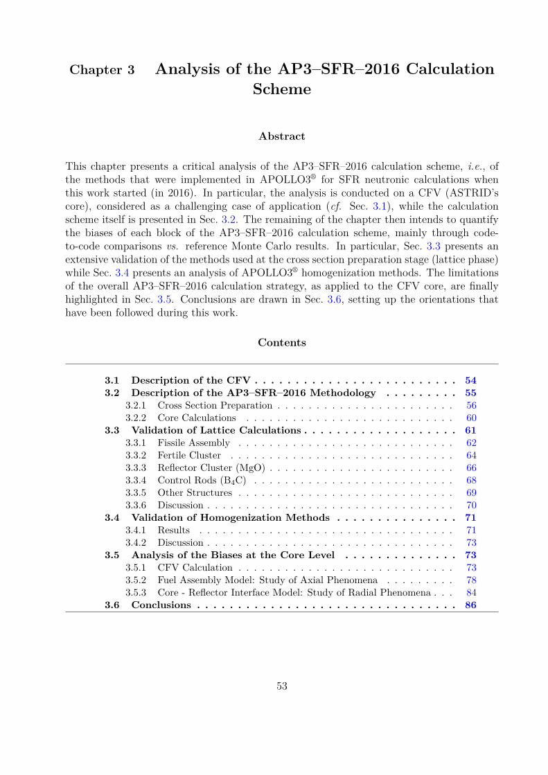
Chapter 3 Analysis of the AP3–SFR–2016 CalculationScheme
Abstract
This chapter presents a critical analysis of the AP3–SFR–2016 calculation scheme, i.e., ofthe methods that were implemented in APOLLO3® for SFR neutronic calculations whenthis work started (in 2016). In particular, the analysis is conducted on a CFV (ASTRID’score), considered as a challenging case of application (cf. Sec. 3.1), while the calculationscheme itself is presented in Sec. 3.2. The remaining of the chapter then intends to quantifythe biases of each block of the AP3–SFR–2016 calculation scheme, mainly through code-to-code comparisons vs. reference Monte Carlo results. In particular, Sec. 3.3 presents anextensive validation of the methods used at the cross section preparation stage (lattice phase)while Sec. 3.4 presents an analysis of APOLLO3® homogenization methods. The limitationsof the overall AP3–SFR–2016 calculation strategy, as applied to the CFV core, are finallyhighlighted in Sec. 3.5. Conclusions are drawn in Sec. 3.6, setting up the orientations thathave been followed during this work.
Contents
3.1 Description of the CFV . . . . . . . . . . . . . . . . . . . . . . . . . 543.2 Description of the AP3–SFR–2016 Methodology . . . . . . . . . 55
3.2.1 Cross Section Preparation . . . . . . . . . . . . . . . . . . . . . . . 563.2.2 Core Calculations . . . . . . . . . . . . . . . . . . . . . . . . . . . 60
3.3 Validation of Lattice Calculations . . . . . . . . . . . . . . . . . . . 613.3.1 Fissile Assembly . . . . . . . . . . . . . . . . . . . . . . . . . . . . 623.3.2 Fertile Cluster . . . . . . . . . . . . . . . . . . . . . . . . . . . . . 643.3.3 Reflector Cluster (MgO) . . . . . . . . . . . . . . . . . . . . . . . . 663.3.4 Control Rods (B4C) . . . . . . . . . . . . . . . . . . . . . . . . . . 683.3.5 Other Structures . . . . . . . . . . . . . . . . . . . . . . . . . . . . 693.3.6 Discussion . . . . . . . . . . . . . . . . . . . . . . . . . . . . . . . . 70
3.4 Validation of Homogenization Methods . . . . . . . . . . . . . . . 713.4.1 Results . . . . . . . . . . . . . . . . . . . . . . . . . . . . . . . . . 713.4.2 Discussion . . . . . . . . . . . . . . . . . . . . . . . . . . . . . . . . 73
3.5 Analysis of the Biases at the Core Level . . . . . . . . . . . . . . 733.5.1 CFV Calculation . . . . . . . . . . . . . . . . . . . . . . . . . . . . 733.5.2 Fuel Assembly Model: Study of Axial Phenomena . . . . . . . . . 783.5.3 Core - Reflector Interface Model: Study of Radial Phenomena . . . 84
3.6 Conclusions . . . . . . . . . . . . . . . . . . . . . . . . . . . . . . . . 86
53
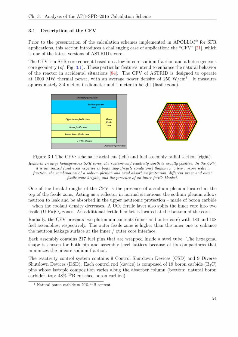
Ch. 3. Analysis of the AP3–SFR–2016 Calculation Scheme
3.1 Description of the CFV
Prior to the presentation of the calculation schemes implemented in APOLLO3® for SFRapplications, this section introduces a challenging case of application: the “CFV” [21], whichis one of the latest versions of ASTRID’s core.The CFV is a SFR core concept based on a low in-core sodium fraction and a heterogeneouscore geometry (cf. Fig. 3.1). These particular features intend to enhance the natural behaviorof the reactor in accidental situations [84]. The CFV of ASTRID is designed to operateat 1500 MW thermal power, with an average power density of 250 W/cm3. It measuresapproximately 3.4 meters in diameter and 1 meter in height (fissile zone).
Figure 3.1 The CFV: schematic axial cut (left) and fuel assembly radial section (right).Remark: In large homogeneous SFR cores, the sodium-void reactivity worth is usually positive. In the CFV,
it is minimized (and even negative in beginning-of-cycle conditions) thanks to: a low in-core sodiumfraction, the combination of a sodium plenum and axial absorbing protection, different inner and outer
fissile zone heights, and the presence of an inner fertile blanket.
One of the breakthroughs of the CFV is the presence of a sodium plenum located at thetop of the fissile zone. Acting as a reflector in normal situations, the sodium plenum allowsneutron to leak and be absorbed in the upper neutronic protection – made of boron carbide– when the coolant density decreases. A UO2 fertile layer also splits the inner core into twofissile (U,Pu)O2 zones. An additional fertile blanket is located at the bottom of the core.Radially, the CFV presents two plutonium contents (inner and outer core) with 180 and 108fuel assemblies, respectively. The outer fissile zone is higher than the inner one to enhancethe neutron leakage surface at the inner / outer core interface.Each assembly contains 217 fuel pins that are wrapped inside a steel tube. The hexagonalshape is chosen for both pin and assembly level lattices because of its compactness thatminimizes the in-core sodium fraction.The reactivity control system contains 9 Control Shutdown Devices (CSD) and 9 DiverseShutdown Devices (DSD). Each control rod (device) is composed of 19 boron carbide (B4C)pins whose isotopic composition varies along the absorber column (bottom: natural boroncarbide1, top: 48% 10B enriched boron carbide).
1 Natural boron carbide ≈ 20% 10B content.
54
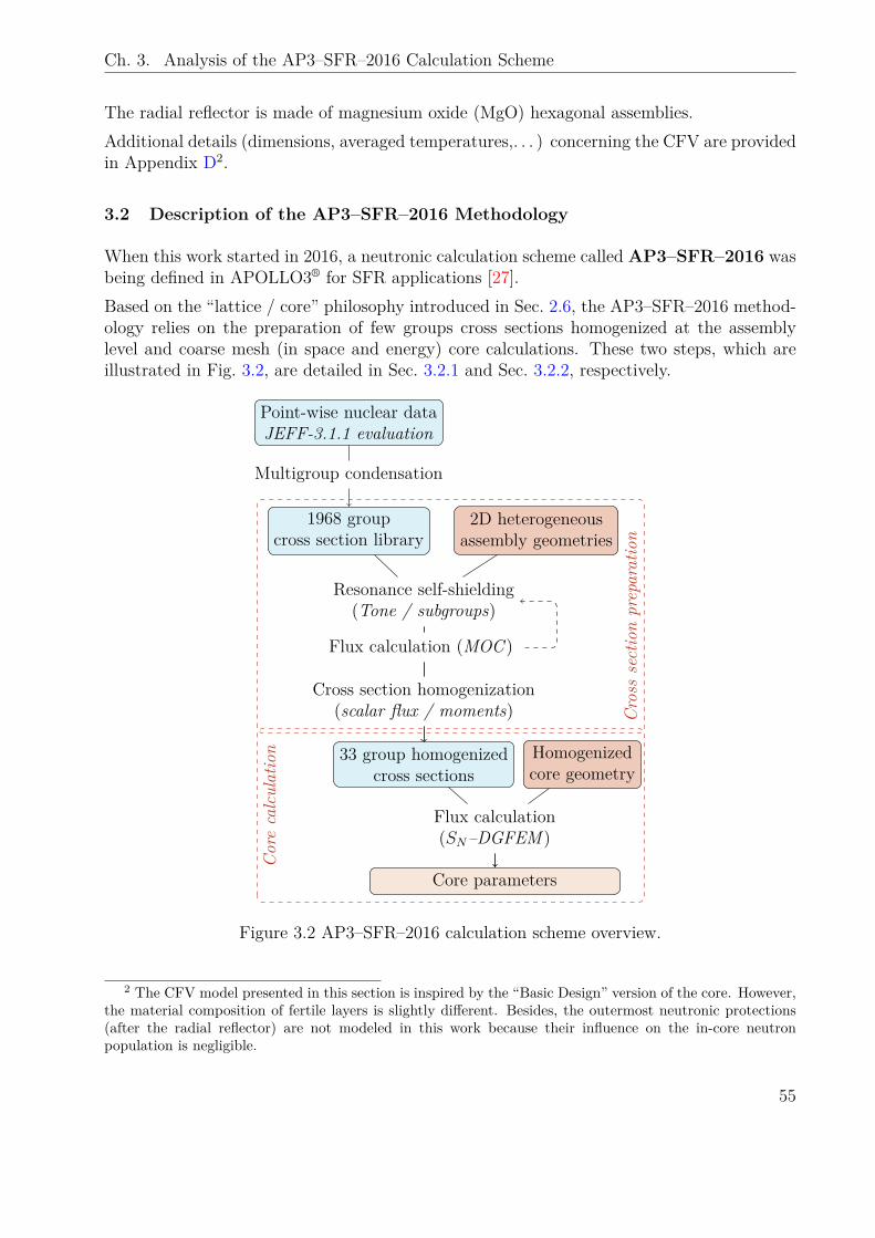
Ch. 3. Analysis of the AP3–SFR–2016 Calculation Scheme
The radial reflector is made of magnesium oxide (MgO) hexagonal assemblies.Additional details (dimensions, averaged temperatures,. . . ) concerning the CFV are providedin Appendix D2.
3.2 Description of the AP3–SFR–2016 Methodology
When this work started in 2016, a neutronic calculation scheme called AP3–SFR–2016 wasbeing defined in APOLLO3® for SFR applications [27].Based on the “lattice / core” philosophy introduced in Sec. 2.6, the AP3–SFR–2016 method-ology relies on the preparation of few groups cross sections homogenized at the assemblylevel and coarse mesh (in space and energy) core calculations. These two steps, which areillustrated in Fig. 3.2, are detailed in Sec. 3.2.1 and Sec. 3.2.2, respectively.
Point-wise nuclear dataJEFF-3.1.1 evaluation
Multigroup condensation
1968 groupcross section library
2D heterogeneousassembly geometries
Resonance self-shielding(Tone / subgroups)
Flux calculation (MOC )
Cross section homogenization(scalar flux / moments)
33 group homogenizedcross sections
Homogenizedcore geometry
Flux calculation(SN–DGFEM )
Core parameters
Crosssectionpreparation
Core
calcu
latio
n
Figure 3.2 AP3–SFR–2016 calculation scheme overview.
2 The CFV model presented in this section is inspired by the “Basic Design” version of the core. However,the material composition of fertile layers is slightly different. Besides, the outermost neutronic protections(after the radial reflector) are not modeled in this work because their influence on the in-core neutronpopulation is negligible.
55
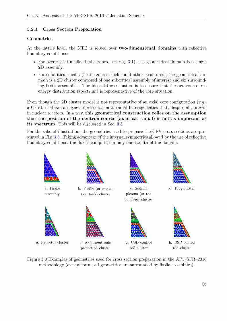
Ch. 3. Analysis of the AP3–SFR–2016 Calculation Scheme
3.2.1 Cross Section Preparation
Geometries
At the lattice level, the NTE is solved over two-dimensional domains with reflectiveboundary conditions:
• For overcritical media (fissile zones, see Fig. 3.1), the geometrical domain is a single2D assembly.
• For subcritical media (fertile zones, shields and other structures), the geometrical do-main is a 2D cluster composed of one subcritical assembly of interest and six surround-ing fissile assemblies. The idea of these clusters is to ensure that the neutron sourceenergy distribution (spectrum) is representative of the core situation.
Even though the 2D cluster model is not representative of an axial core configuration (e.g.,a CFV), it allows an exact representation of radial heterogeneities that, despite all, prevailin nuclear reactors. In a way, this geometrical construction relies on the assumptionthat the position of the neutron source (axial vs. radial) is not as important asits spectrum. This will be discussed in Sec. 3.5.For the sake of illustration, the geometries used to prepare the CFV cross sections are pre-sented in Fig. 3.3. Taking advantage of the internal symmetries allowed by the use of reflectiveboundary conditions, the flux is computed in only one-twelfth of the domain.
a. Fissileassembly
b. Fertile (or expan-sion tank) cluster
c. Sodiumplenum (or rodfollower) cluster
d. Plug cluster
e. Reflector cluster f. Axial neutronicprotection cluster
g. CSD controlrod cluster
h. DSD controlrod cluster
Figure 3.3 Examples of geometries used for cross section preparation in the AP3–SFR–2016methodology (except for a., all geometries are surrounded by fissile assemblies).
56
Ch. 3. Analysis of the AP3–SFR–2016 Calculation Scheme
Multigroup cross section library
APOLLO3® multigroup cross section libraries are built with the GALILEE processing tool [85]while nuclear data (cross sections, fission spectra,. . . ) are taken from the European JEFF-3.1.1database [86]. For SFR applications, the energy mesh is inherited from the ECCO code [73]and contains 1968 groups.
Production operator
The general expression of the multigroup production operator F is given in Eq. (2.39b).However, APOLLO3® does not handle full production cross section matrices (νΣg′→g
f ) butcollapses the dependence to the incident neutron energy into Nmg = 1 or 4 macro-groups [87].Under this approximation, F operates on the multigroup flux according to:
Fψg(r,Ω) ≈ 14π
Nmg∑mg=1
χgmg∑g′∈mg
νΣg′
f ψg′
00(r) (3.1)
where ∑g′∈mg stands for the summation over the groups g′ belonging to macro-group mg andχgmg, νΣg′
f are defined as follows:
χgmg =
∑g′∈mg
νΣg′→gf∑
g′∈mgνΣg′
f
(3.2a)
νΣg′
f =Ng∑g=1
νΣg′→gf (3.2b)
with νΣg′→gf the production cross section defined with Eq. (2.40b). In Eq. (3.1), the sum
over fissile isotopes is omitted for the sake of clarity.It can be observed that, if the macro-group set corresponds to the multigroup partition(Nmg = Ng), then Eq. (3.1) is equivalent to Eq. (2.39b). On the contrary, if a single macro-group covers the full energy range (Nmg = 1), then one finds the expression used in mostneutron transport codes, in which no dependence of the fission spectra to the incident neutronenergy is considered.
Scattering operator
Usually, the angular dependence of the multigroup scattering operator H is expanded withreal spherical harmonics according to Eq. (2.39c). For practical applications, the sum overthe Legendre moments l ∈ N is finite. If L is the expansion order, then H operates on themultigroup flux according to3:
Hψg(r,Ω) ≈L∑l=0
2l + 14π
Ng∑g′=1
Σg′→gs,l (r)
+l∑m=−l
ψg′
lm(r)Rlm(Ω) (3.3)
3 The dependence of the scattering cross section on the angular index m is neglected in Eq. (3.3) accordingto the explanations given in Sec. 2.2.2.
57
Ch. 3. Analysis of the AP3–SFR–2016 Calculation Scheme
It is said that “the scattering kernel is expanded to order PL”. In this work, P1 and P3approximations have been explored.
Resonance self-shielding
In the AP3–SFR–2016 methodology, resonant cross sections are self-shielded with the sub-group method (see Sec. 2.6.2). Nevertheless, the implementation of Tone’s method in APOL-LO3® (also presented in Sec. 2.6.2) is an occasion to review this methodology. As a result, acomparison of Tone’s and subgroup methods is presented in this chapter.In any case, both procedures rely on the CPM formalism: the calculation of the collisionprobabilities is done with the TDT solver (which offers a parallel calculation capacity).Besides, spatial regions are combined to limit the number of self-shielded cross-sections. Inparticular, the mesh coloring in Fig. 3.3 indicates the regions that share the same crosssections.For scattering reactions x = (n, n), (n, n′) . . ., transfer probabilities px,i are not self-shielded(see Eq. (2.25) for the notations). Besides, high-order angular moments of the scatteringcross section (σx,l,i with l ≥ 1) are self-shielded with the scalar flux (and not with angularfluxes as a proper energy condensation would require). Even though these approximationsintroduce errors in self-shielded cross sections, the group energy width in the 1968 groupenergy mesh is assumed to be small enough for these errors to be negligible.
Flux calculation
The domains presented in Fig. 3.3 define 2D neutron transport problems. For each domain,the neutron flux ψ (and corresponding multiplication factor k) is sought as the solution ofthe multigroup critical problem, i.e., Eq. (2.37).For the spatial and angular discretizations, APOLLO3® relies on the 2D-MOC implementedwithin the TDT solver. The MOC framework is chosen both for its accuracy and for itsability to treat arbitrarily complex meshes. In TDT, the NTE resolution is parallelized on theangular directions and the MOC solution is accelerated with a DPN synthetic operator [40].For supercritical assemblies – i.e., fissile domains, see Fig. 3.3.a –, a leakage model (seeSec. 2.6) may eventually be used to account for the flux curvature arising from the finite coredimensions. In that case, Eq. (2.79) is solved instead of Eq. (2.37).In APOLLO3®, two leakage models are implemented:
• A B-heterogeneous model which directly solves Eq. (2.79) in complex algebra pro-vided that the direction and amplitude of B is known. This model requires a specialMOC implementation in order to deal with the complex and anisotropic “cross section”Σg + iB ·Ω (see references [88, 89]).
• A B1-homogeneous model in which the leakage probability iB · Ω is replaced by itshomogeneous and isotropic counterpart DgB2 where Dg is the leakage coefficient andB is the buckling modulus.
58
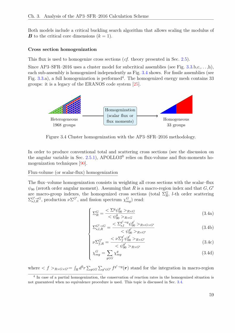
Ch. 3. Analysis of the AP3–SFR–2016 Calculation Scheme
Both models include a critical buckling search algorithm that allows scaling the modulus ofB to the critical core dimensions (k = 1).
Cross section homogenization
This flux is used to homogenize cross sections (cf. theory presented in Sec. 2.5).Since AP3–SFR–2016 uses a cluster model for subcritical assemblies (see Fig. 3.3.b,c,. . . ,h),each sub-assembly is homogenized independently as Fig. 3.4 shows. For fissile assemblies (seeFig. 3.3.a), a full homogenization is performed4. The homogenized energy mesh contains 33groups: it is a legacy of the ERANOS code system [25].
Heterogeneous1968 groups
Homogenization(scalar flux orflux moments) Homogeneous
33 groups
Figure 3.4 Cluster homogenization with the AP3–SFR–2016 methodology.
In order to produce conventional total and scattering cross sections (see the discussion onthe angular variable in Sec. 2.5.1), APOLLO3® relies on flux-volume and flux-moments ho-mogenization techniques [90].
Flux-volume (or scalar-flux) homogenization
The flux–volume homogenization consists in weighting all cross sections with the scalar–fluxψ00 (zeroth order angular moment). Assuming that R is a macro-region index and that G,G′are macro-group indexes, the homogenized cross sections (total ΣG
R, l-th order scatteringΣG′→Gs,l,R , production νΣG′ , and fission spectrum χGmg) read:
ΣGR = < Σgψg00 >R×G
< ψg00 >R×G(3.4a)
ΣG′→Gs,l,R =
< Σg′→gs,l ψg
′
00 >R×G×G′
< ψg′
00 >R×G′(3.4b)
νΣG′
f,R =< νΣg′
f ψg′
00 >R×G′
< ψg′
00 >R×G′(3.4c)
χGmg =∑g∈G
χgmg (3.4d)
where < f >R×G×G′=∫R d
3r∑g∈G
∑g′∈G′ f
g′→g(r) stand for the integration in macro-region4 In case of a partial homogenization, the conservation of reaction rates in the homogenized situation is
not guaranteed when no equivalence procedure is used. This topic is discussed in Sec. 3.4.
59
Ch. 3. Analysis of the AP3–SFR–2016 Calculation Scheme
R and summation over the groups g (and eventually g′) belonging to macro-group G (andeventually G′).In order to separate the fission spectrum and production cross section contributions, inEq. (3.4c) and Eq. (3.4d), it is assumed that the limits of the homogenized energy mesh(index G) coincide with the fission spectra energy limits (index mg) i.e., g ⊂ G⇒ g ∈ mg.This property is verified for the 33 group energy mesh of ERANOS.
Flux-moments homogenization
The flux-moments homogenization in APOLLO3® consists in using the angular flux momentsto weight scattering cross sections in order to ensure better preservation of the angulardependent reaction rates in the homogenized situation. In that case, Eq. (3.4b) needs to bereplaced by the following formula:
ΣG′→Gs,l,R =
+l∑m=−l
ΣG′→Gs,lm,R
(< ψg
′
lm >R×G′)2
+l∑m=−l
(< ψg
′
lm >R×G′)2
+ δG,G′(ΣGR − ΣG
l,R
), (3.5)
where δG,G′ is the Kronecker delta and ΣGl,R, ΣG′→G
s,lm,R are flux-moments weighted total andscattering cross sections defined as:
ΣG′→Gs,lm,R =
< Σg′→gs,l ψg
′
lm >R×G×G′
< ψg′
lm >R×G′(3.6a)
ΣGl,R =
+l∑m=−l
< ψglm >R×G< Σgψglm >R×G
+l∑m=−l
(< ψglm >R×G)2(3.6b)
The second term in the RHS of Eq. (3.5) is a correction term that allows preserving the PLequations in the homogenized situation (i.e., the equations that arise from a projection of thetransport equation over real spherical harmonics Rlm for l ≤ L). As for the summation overazimuthal indexes m in Eq. (3.5) and Eq. (3.6b), it is the result of a least-square reductionthat intends to restore a conventional form for the scattering cross section [63].The implementation of Eq. (3.5) in APOLLO3® includes a fixup to avoid a numerical diver-gence when |ΣG′→G
s,l>0,R| > ΣG′→Gs,0,R . In that case, ΣG′→G
s,l>0,R is replaced by sign(ΣG′→Gs,l>0,R)× |ΣG′→G
s,0,R |.This numerical fixup, thus, introduces an “unphysical” approximation.
3.2.2 Core Calculations
At the core level, the geometrical model is composed of homogenized assemblies whose crosssections are the output of the lattice step (see Fig. 3.5). According to the previous discus-sion, the energy mesh thus contains 33 groups. In the AP3–SFR–2016 calculation scheme,
60
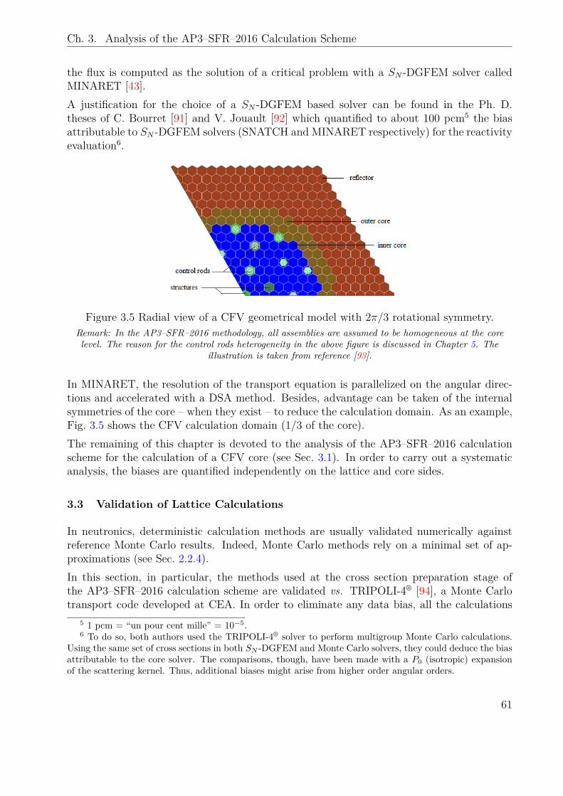
Ch. 3. Analysis of the AP3–SFR–2016 Calculation Scheme
the flux is computed as the solution of a critical problem with a SN -DGFEM solver calledMINARET [43].A justification for the choice of a SN -DGFEM based solver can be found in the Ph. D.theses of C. Bourret [91] and V. Jouault [92] which quantified to about 100 pcm5 the biasattributable to SN -DGFEM solvers (SNATCH and MINARET respectively) for the reactivityevaluation6.
Figure 3.5 Radial view of a CFV geometrical model with 2π/3 rotational symmetry.Remark: In the AP3–SFR–2016 methodology, all assemblies are assumed to be homogeneous at the corelevel. The reason for the control rods heterogeneity in the above figure is discussed in Chapter 5. The
illustration is taken from reference [93].
In MINARET, the resolution of the transport equation is parallelized on the angular direc-tions and accelerated with a DSA method. Besides, advantage can be taken of the internalsymmetries of the core – when they exist – to reduce the calculation domain. As an example,Fig. 3.5 shows the CFV calculation domain (1/3 of the core).The remaining of this chapter is devoted to the analysis of the AP3–SFR–2016 calculationscheme for the calculation of a CFV core (see Sec. 3.1). In order to carry out a systematicanalysis, the biases are quantified independently on the lattice and core sides.
3.3 Validation of Lattice Calculations
In neutronics, deterministic calculation methods are usually validated numerically againstreference Monte Carlo results. Indeed, Monte Carlo methods rely on a minimal set of ap-proximations (see Sec. 2.2.4).In this section, in particular, the methods used at the cross section preparation stage ofthe AP3–SFR–2016 calculation scheme are validated vs. TRIPOLI-4® [94], a Monte Carlotransport code developed at CEA. In order to eliminate any data bias, all the calculations
5 1 pcm = “un pour cent mille” = 10−5.6 To do so, both authors used the TRIPOLI-4® solver to perform multigroup Monte Carlo calculations.
Using the same set of cross sections in both SN -DGFEM and Monte Carlo solvers, they could deduce the biasattributable to the core solver. The comparisons, though, have been made with a P0 (isotropic) expansionof the scattering kernel. Thus, additional biases might arise from higher order angular orders.
61
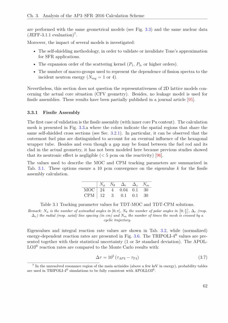
Ch. 3. Analysis of the AP3–SFR–2016 Calculation Scheme
are performed with the same geometrical models (see Fig. 3.3) and the same nuclear data(JEFF-3.1.1 evaluation)7.Moreover, the impact of several models is investigated:
• The self-shielding methodology, in order to validate or invalidate Tone’s approximationfor SFR applications.
• The expansion order of the scattering kernel (P1, P3, or higher orders).• The number of macro-groups used to represent the dependence of fission spectra to the
incident neutron energy (Nmg = 1 or 4).
Nevertheless, this section does not question the representativeness of 2D lattice models con-cerning the actual core situation (CFV geometry). Besides, no leakage model is used forfissile assemblies. These results have been partially published in a journal article [95].
3.3.1 Fissile Assembly
The first case of validation is the fissile assembly (with inner core Pu content). The calculationmesh is presented in Fig. 3.3.a where the colors indicate the spatial regions that share thesame self-shielded cross sections (see Sec. 3.2.1). In particular, it can be observed that theoutermost fuel pins are distinguished to account for an eventual influence of the hexagonalwrapper tube. Besides and even though a gap may be found between the fuel rod and itsclad in the actual geometry, it has not been modeled here because previous studies showedthat its neutronic effect is negligible (< 5 pcm on the reactivity) [96].The values used to describe the MOC and CPM tracking parameters are summarized inTab. 3.1. These options ensure a 10 pcm convergence on the eigenvalue k for the fissileassembly calculation.
Nφ Nθ ∆r ∆z Nm
MOC 24 4 0.04 0.1 30CPM 12 3 0.1 0.1 30
Table 3.1 Tracking parameter values for TDT-MOC and TDT-CPM solutions.Remark: Nφ is the number of azimuthal angles in [0;π], Nθ the number of polar angles in
[0; π2
], ∆r (resp.
∆z) the radial (resp. axial) line spacing (in cm) and Nm the number of times the mesh is crossed by acyclic trajectory.
Eigenvalues and integral reaction rate values are shown in Tab. 3.2, while (normalized)energy-dependent reaction rates are presented in Fig. 3.6. The TRIPOLI-4® values are pre-sented together with their statistical uncertainty (1 or 3σ standard deviation). The APOL-LO3® reaction rates are compared to the Monte Carlo results with:
∆τ = 105 (τAP3 − τT4) (3.7)7 In the unresolved resonance region of the main actinides (above a few keV in energy), probability tables
are used in TRIPOLI-4® simulations to be fully consistent with APOLLO3®.
62
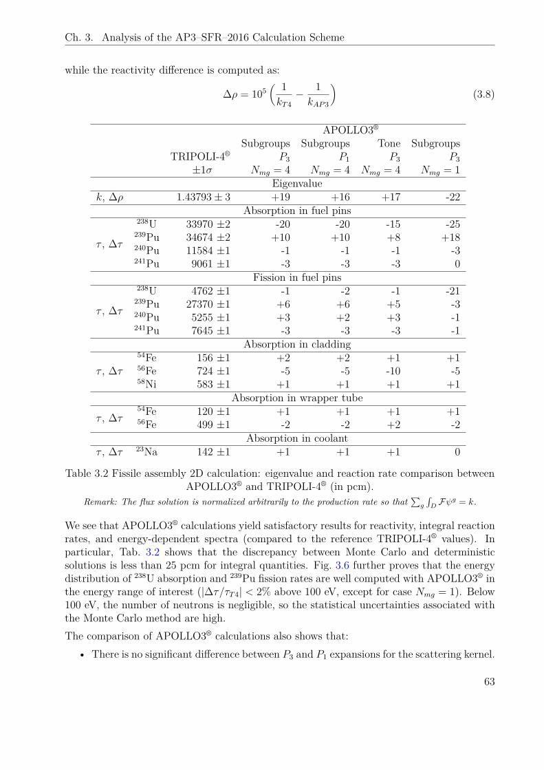
Ch. 3. Analysis of the AP3–SFR–2016 Calculation Scheme
while the reactivity difference is computed as:
∆ρ = 105( 1kT4− 1kAP3
)(3.8)
APOLLO3®
Subgroups Subgroups Tone SubgroupsTRIPOLI-4® P3 P1 P3 P3±1σ Nmg = 4 Nmg = 4 Nmg = 4 Nmg = 1
Eigenvaluek, ∆ρ 1.43793± 3 +19 +16 +17 -22
Absorption in fuel pins
τ , ∆τ
238U 33970 ±2 -20 -20 -15 -25239Pu 34674 ±2 +10 +10 +8 +18240Pu 11584 ±1 -1 -1 -1 -3241Pu 9061 ±1 -3 -3 -3 0
Fission in fuel pins
τ , ∆τ
238U 4762 ±1 -1 -2 -1 -21239Pu 27370 ±1 +6 +6 +5 -3240Pu 5255 ±1 +3 +2 +3 -1241Pu 7645 ±1 -3 -3 -3 -1
Absorption in cladding
τ , ∆τ54Fe 156 ±1 +2 +2 +1 +156Fe 724 ±1 -5 -5 -10 -558Ni 583 ±1 +1 +1 +1 +1
Absorption in wrapper tube
τ , ∆τ54Fe 120 ±1 +1 +1 +1 +156Fe 499 ±1 -2 -2 +2 -2
Absorption in coolantτ , ∆τ 23Na 142 ±1 +1 +1 +1 0
Table 3.2 Fissile assembly 2D calculation: eigenvalue and reaction rate comparison betweenAPOLLO3® and TRIPOLI-4® (in pcm).
Remark: The flux solution is normalized arbitrarily to the production rate so that∑g
∫DFψg = k.
We see that APOLLO3® calculations yield satisfactory results for reactivity, integral reactionrates, and energy-dependent spectra (compared to the reference TRIPOLI-4® values). Inparticular, Tab. 3.2 shows that the discrepancy between Monte Carlo and deterministicsolutions is less than 25 pcm for integral quantities. Fig. 3.6 further proves that the energydistribution of 238U absorption and 239Pu fission rates are well computed with APOLLO3® inthe energy range of interest (|∆τ/τT4| < 2% above 100 eV, except for case Nmg = 1). Below100 eV, the number of neutrons is negligible, so the statistical uncertainties associated withthe Monte Carlo method are high.The comparison of APOLLO3® calculations also shows that:
• There is no significant difference between P3 and P1 expansions for the scattering kernel.
63
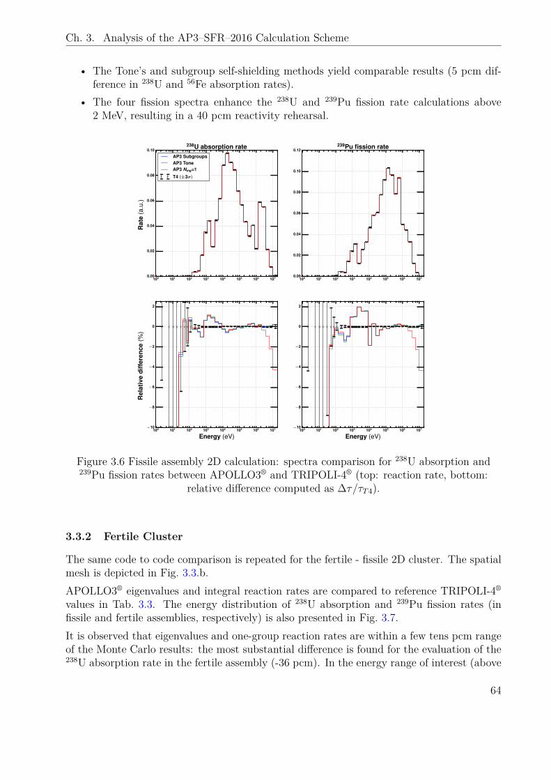
Ch. 3. Analysis of the AP3–SFR–2016 Calculation Scheme
• The Tone’s and subgroup self-shielding methods yield comparable results (5 pcm dif-ference in 238U and 56Fe absorption rates).
• The four fission spectra enhance the 238U and 239Pu fission rate calculations above2 MeV, resulting in a 40 pcm reactivity rehearsal.
100 101 102 103 104 105 106 1070.00
0.02
0.04
0.06
0.08
0.10
Rat
e(a
.u.)
238U absorption rateAP3 SubgroupsAP3 ToneAP3 Nmg=1
T4 (±3σ)
100 101 102 103 104 105 106 107
Energy (eV)
−10
−8
−6
−4
−2
0
2
Rel
ativ
edi
ffer
ence
(%)
100 101 102 103 104 105 106 1070.00
0.02
0.04
0.06
0.08
0.10
0.12239Pu fission rate
100 101 102 103 104 105 106 107
Energy (eV)
−10
−8
−6
−4
−2
0
2
Figure 3.6 Fissile assembly 2D calculation: spectra comparison for 238U absorption and239Pu fission rates between APOLLO3® and TRIPOLI-4® (top: reaction rate, bottom:
relative difference computed as ∆τ/τT4).
3.3.2 Fertile Cluster
The same code to code comparison is repeated for the fertile - fissile 2D cluster. The spatialmesh is depicted in Fig. 3.3.b.APOLLO3® eigenvalues and integral reaction rates are compared to reference TRIPOLI-4®
values in Tab. 3.3. The energy distribution of 238U absorption and 239Pu fission rates (infissile and fertile assemblies, respectively) is also presented in Fig. 3.7.It is observed that eigenvalues and one-group reaction rates are within a few tens pcm rangeof the Monte Carlo results: the most substantial difference is found for the evaluation of the238U absorption rate in the fertile assembly (-36 pcm). In the energy range of interest (above
64
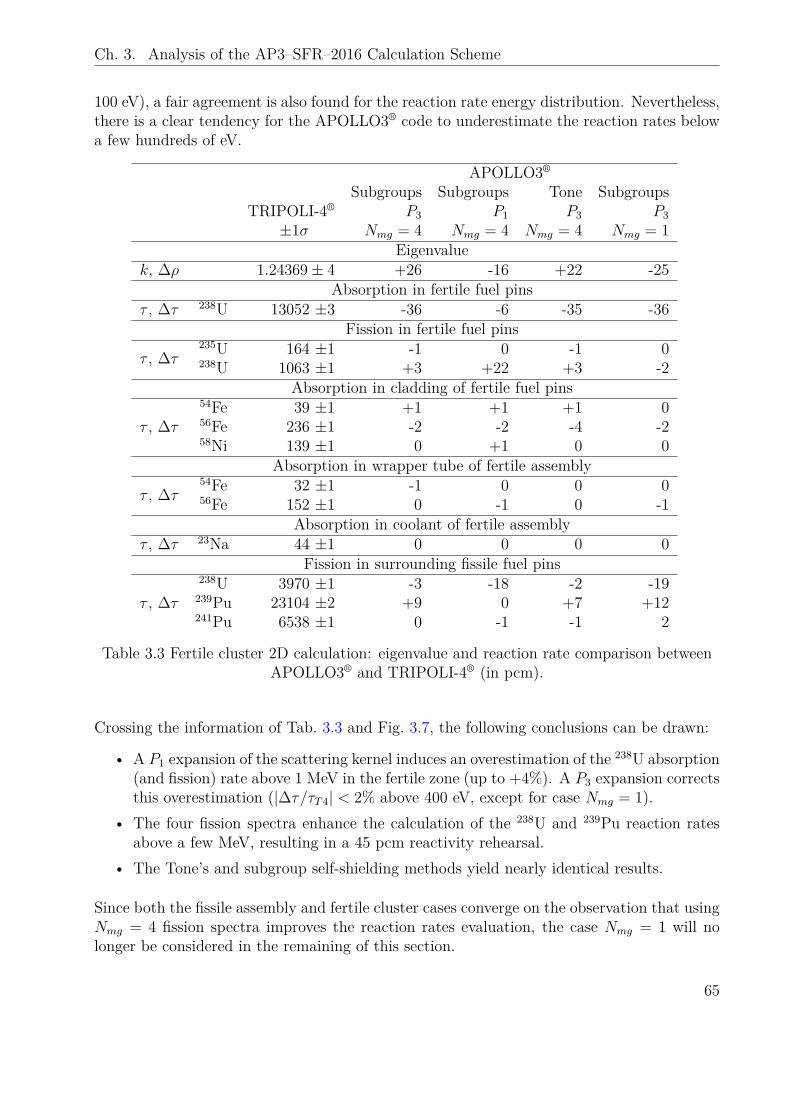
Ch. 3. Analysis of the AP3–SFR–2016 Calculation Scheme
100 eV), a fair agreement is also found for the reaction rate energy distribution. Nevertheless,there is a clear tendency for the APOLLO3® code to underestimate the reaction rates belowa few hundreds of eV.
APOLLO3®
Subgroups Subgroups Tone SubgroupsTRIPOLI-4® P3 P1 P3 P3±1σ Nmg = 4 Nmg = 4 Nmg = 4 Nmg = 1
Eigenvaluek, ∆ρ 1.24369± 4 +26 -16 +22 -25
Absorption in fertile fuel pinsτ , ∆τ 238U 13052 ±3 -36 -6 -35 -36
Fission in fertile fuel pins
τ , ∆τ235U 164 ±1 -1 0 -1 0238U 1063 ±1 +3 +22 +3 -2
Absorption in cladding of fertile fuel pins
τ , ∆τ54Fe 39 ±1 +1 +1 +1 056Fe 236 ±1 -2 -2 -4 -258Ni 139 ±1 0 +1 0 0
Absorption in wrapper tube of fertile assembly
τ , ∆τ54Fe 32 ±1 -1 0 0 056Fe 152 ±1 0 -1 0 -1
Absorption in coolant of fertile assemblyτ , ∆τ 23Na 44 ±1 0 0 0 0
Fission in surrounding fissile fuel pins
τ , ∆τ238U 3970 ±1 -3 -18 -2 -19239Pu 23104 ±2 +9 0 +7 +12241Pu 6538 ±1 0 -1 -1 2
Table 3.3 Fertile cluster 2D calculation: eigenvalue and reaction rate comparison betweenAPOLLO3® and TRIPOLI-4® (in pcm).
Crossing the information of Tab. 3.3 and Fig. 3.7, the following conclusions can be drawn:
• A P1 expansion of the scattering kernel induces an overestimation of the 238U absorption(and fission) rate above 1 MeV in the fertile zone (up to +4%). A P3 expansion correctsthis overestimation (|∆τ/τT4| < 2% above 400 eV, except for case Nmg = 1).
• The four fission spectra enhance the calculation of the 238U and 239Pu reaction ratesabove a few MeV, resulting in a 45 pcm reactivity rehearsal.
• The Tone’s and subgroup self-shielding methods yield nearly identical results.
Since both the fissile assembly and fertile cluster cases converge on the observation that usingNmg = 4 fission spectra improves the reaction rates evaluation, the case Nmg = 1 will nolonger be considered in the remaining of this section.
65
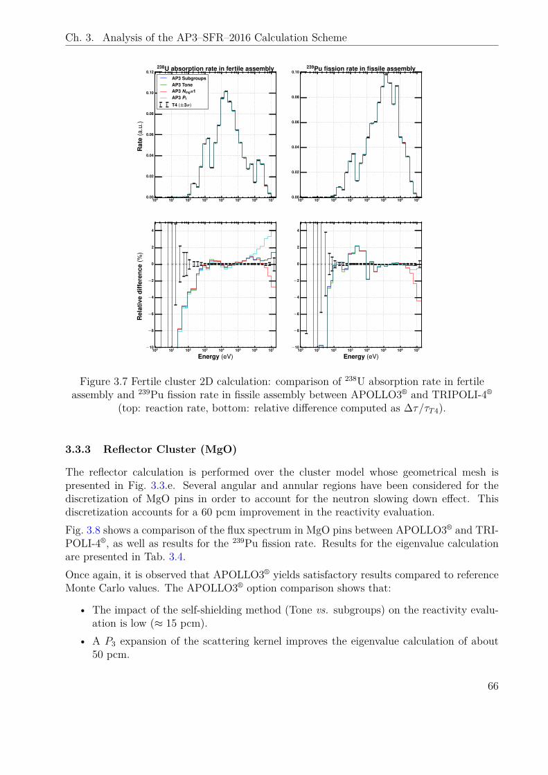
Ch. 3. Analysis of the AP3–SFR–2016 Calculation Scheme
100 101 102 103 104 105 106 1070.00
0.02
0.04
0.06
0.08
0.10
0.12
Rat
e(a
.u.)
238U absorption rate in fertile assemblyAP3 SubgroupsAP3 ToneAP3 Nmg=1AP3 P1
T4 (±3σ)
100 101 102 103 104 105 106 107
Energy (eV)
−10
−8
−6
−4
−2
0
2
4
Rel
ativ
edi
ffer
ence
(%)
100 101 102 103 104 105 106 1070.00
0.02
0.04
0.06
0.08
0.10239Pu fission rate in fissile assembly
100 101 102 103 104 105 106 107
Energy (eV)
−10
−8
−6
−4
−2
0
2
4
Figure 3.7 Fertile cluster 2D calculation: comparison of 238U absorption rate in fertileassembly and 239Pu fission rate in fissile assembly between APOLLO3® and TRIPOLI-4®
(top: reaction rate, bottom: relative difference computed as ∆τ/τT4).
3.3.3 Reflector Cluster (MgO)
The reflector calculation is performed over the cluster model whose geometrical mesh ispresented in Fig. 3.3.e. Several angular and annular regions have been considered for thediscretization of MgO pins in order to account for the neutron slowing down effect. Thisdiscretization accounts for a 60 pcm improvement in the reactivity evaluation.Fig. 3.8 shows a comparison of the flux spectrum in MgO pins between APOLLO3® and TRI-POLI-4®, as well as results for the 239Pu fission rate. Results for the eigenvalue calculationare presented in Tab. 3.4.Once again, it is observed that APOLLO3® yields satisfactory results compared to referenceMonte Carlo values. The APOLLO3® option comparison shows that:
• The impact of the self-shielding method (Tone vs. subgroups) on the reactivity evalu-ation is low (≈ 15 pcm).
• A P3 expansion of the scattering kernel improves the eigenvalue calculation of about50 pcm.
66
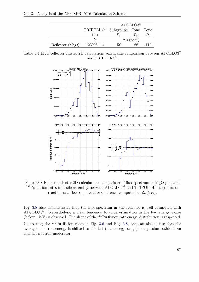
Ch. 3. Analysis of the AP3–SFR–2016 Calculation Scheme
APOLLO3®
TRIPOLI-4® Subgroups Tone Tone±1σ P3 P3 P1k ∆ρ (pcm)
Reflector (MgO) 1.23996± 4 -50 -66 -110
Table 3.4 MgO reflector cluster 2D calculation: eigenvalue comparison between APOLLO3®
and TRIPOLI-4®.
100 101 102 103 104 105 106 1070.00
0.02
0.04
0.06
0.08
0.10
Flux
(a.u
.)
Flux in MgO pinsAP3 ToneT4 (±3σ)
100 101 102 103 104 105 106 107
Energy (eV)
−10
−8
−6
−4
−2
0
2
Rel
ativ
edi
ffer
ence
(%)
100 101 102 103 104 105 106 1070.00
0.01
0.02
0.03
0.04
0.05
0.06
0.07
0.08
0.09239Pu fission rate in fissile assembly
100 101 102 103 104 105 106 107
Energy (eV)
−4
−2
0
2
4
Figure 3.8 Reflector cluster 2D calculation: comparison of flux spectrum in MgO pins and239Pu fission rates in fissile assembly between APOLLO3® and TRIPOLI-4® (top: flux or
reaction rate, bottom: relative difference computed as ∆τ/τT4).
Fig. 3.8 also demonstrates that the flux spectrum in the reflector is well computed withAPOLLO3®. Nevertheless, a clear tendency to underestimation in the low energy range(below 1 keV) is observed. The shape of the 239Pu fission rate energy distribution is respected.Comparing the 239Pu fission rates in Fig. 3.6 and Fig. 3.8, one can also notice that theaveraged neutron energy is shifted to the left (low energy range): magnesium oxide is anefficient neutron moderator.
67
Ch. 3. Analysis of the AP3–SFR–2016 Calculation Scheme
3.3.4 Control Rods (B4C)
We now move on to the validation of control rods lattice calculations. In particular, Tab. 3.5presents eigenvalue differences between APOLLO3® and TRIPOLI-4® for CSD and DSDassemblies, including different 10B enrichments (geometries are presented in Fig. 3.3.g/h).Spectral results (10B absorption and 239Pu fission rates) are exhibited in Fig. 3.9.
100 101 102 103 104 105 106 107−0.02
0.00
0.02
0.04
0.06
0.08
0.10
0.12
0.14
Rat
e(a
.u.)
10B absorption rate (48% 10B)AP3 ToneT4 (±3σ)
100 101 102 103 104 105 106 107
Energy (eV)
−10
−8
−6
−4
−2
0
2
4
Rel
ativ
edi
ffer
ence
(%)
100 101 102 103 104 105 106 1070.00
0.02
0.04
0.06
0.08
0.10
0.12
0.14239Pu fission rate in fissile assembly
100 101 102 103 104 105 106 107
Energy (eV)
−10
−8
−6
−4
−2
0
2
Figure 3.9 CSD cluster 2D calculation with 48% 10B enrichment: comparison of 10Babsorption and 239Pu fission rate between APOLLO3® and TRIPOLI-4® (top: reaction rate,
bottom: relative difference computed as ∆τ/τT4).
Tab. 3.5 shows that the eigenvalue discrepancies between APOLLO3® and TRIPOLI-4® arethe largest found until now (up to -245 pcm for a 48% 10B enriched DSD calculation witha P3 scattering law). A possible explanation is that sharp flux gradients are expected inborated absorbers and their vicinity because of the large 10B cross section value: when thespatial discretization is not refined enough8, the reaction rate distribution is not accuratelyrepresented: this is a spatial self-shielding effect9.
8 The spatial mesh discretization has not been pushed further than the one presented in Fig. 3.3.g/hbecause current tools used to provide geometry meshes for APOLLO3® have limited capacities.
9 The treatment of spatial self-shielding effects in borated absorbers is discussed in greater detail inChapter 5 (cf. Sec. 5.3).
68
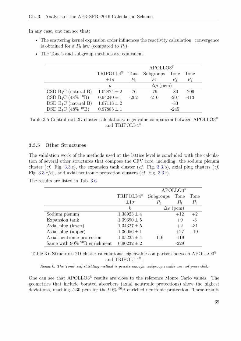
Ch. 3. Analysis of the AP3–SFR–2016 Calculation Scheme
In any case, one can see that:
• The scattering kernel expansion order influences the reactivity calculation: convergenceis obtained for a P3 law (compared to P5).
• The Tone’s and subgroup methods are equivalent.
APOLLO3®
TRIPOLI-4® Tone Subgroups Tone Tone±1σ P5 P3 P3 P1k ∆ρ (pcm)
CSD B4C (natural B) 1.02824± 2 -76 -79 -80 -209CSD B4C (48% 10B) 0.94240± 1 -202 -210 -207 -413DSD B4C (natural B) 1.07118± 2 -83DSD B4C (48% 10B) 0.97885± 1 -245
Table 3.5 Control rod 2D cluster calculations: eigenvalue comparison between APOLLO3®
and TRIPOLI-4®.
3.3.5 Other Structures
The validation work of the methods used at the lattice level is concluded with the calcula-tion of several other structures that compose the CFV core, including: the sodium plenumcluster (cf. Fig. 3.3.c), the expansion tank cluster (cf. Fig. 3.3.b), axial plug clusters (cf.Fig. 3.3.c/d), and axial neutronic protection clusters (cf. Fig. 3.3.f).The results are listed in Tab. 3.6.
APOLLO3®
TRIPOLI-4® Subgroups Tone Tone±1σ P3 P3 P1k ∆ρ (pcm)
Sodium plenum 1.38923± 4 +12 +2Expansion tank 1.39390± 5 +9 -3Axial plug (lower) 1.34327± 5 +2 -31Axial plug (upper) 1.36056± 1 +27 -19Axial neutronic protection 1.05235± 4 -116 -119Same with 90% 90B enrichment 0.90232± 2 -229
Table 3.6 Structures 2D cluster calculations: eigenvalue comparison between APOLLO3®
and TRIPOLI-4®.Remark: The Tone’ self-shielding method is precise enough: subgroup results are not presented.
One can see that APOLLO3® results are close to the reference Monte Carlo values. Thegeometries that include borated absorbers (axial neutronic protections) show the highestdeviations, reaching -230 pcm for the 90% 90B enriched neutronic protection. These results
69
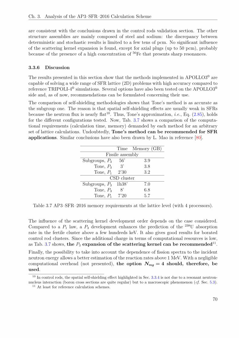
Ch. 3. Analysis of the AP3–SFR–2016 Calculation Scheme
are consistent with the conclusions drawn in the control rods validation section. The otherstructure assemblies are mainly composed of steel and sodium: the discrepancy betweendeterministic and stochastic results is limited to a few tens of pcm. No significant influenceof the scattering kernel expansion is found, except for axial plugs (up to 50 pcm), probablybecause of the presence of a high concentration of 56Fe that presents sharp resonances.
3.3.6 Discussion
The results presented in this section show that the methods implemented in APOLLO3® arecapable of solving a wide range of SFR lattice (2D) problems with high accuracy compared toreference TRIPOLI-4® simulations. Several options have also been tested on the APOLLO3®
side and, as of now, recommendations can be formulated concerning their use.The comparison of self-shielding methodologies shows that Tone’s method is as accurate asthe subgroup one. The reason is that spatial self-shielding effects are usually weak in SFRsbecause the neutron flux is nearly flat10. Thus, Tone’s approximation, i.e., Eq. (2.85), holdsfor the different configurations tested. Now, Tab. 3.7 shows a comparison of the computa-tional requirements (calculation time, memory) demanded by each method for an arbitraryset of lattice calculations. Undoubtedly, Tone’s method can be recommended for SFRapplications. Similar conclusions have also been drawn by L. Mao in reference [80].
Time Memory (GB)Fissile assembly
Subgroups, P3 56’ 3.9Tone, P3 3’ 3.8Tone, P1 2’30 3.2
CSD clusterSubgroups, P3 1h38’ 7.0
Tone, P3 8’ 6.8Tone, P1 7’20 5.7
Table 3.7 AP3–SFR–2016 memory requirements at the lattice level (with 4 processors).
The influence of the scattering kernel development order depends on the case considered.Compared to a P1 law, a P3 development enhances the prediction of the 238U absorptionrate in the fertile cluster above a few hundreds keV. It also gives good results for boratedcontrol rod clusters. Since the additional charge in terms of computational resources is low,as Tab. 3.7 shows, the P3 expansion of the scattering kernel can be recommended11.Finally, the possibility to take into account the dependence of fission spectra to the incidentneutron energy allows a better estimation of the reaction rates above 1 MeV. With a negligiblecomputational overhead (not presented), the option Nmg = 4 should, therefore, beused.
10 In control rods, the spatial self-shielding effect highlighted in Sec. 3.3.4 is not due to a resonant neutron-nucleus interaction (boron cross sections are quite regular) but to a macroscopic phenomenon (cf. Sec. 5.3).
11 At least for reference calculation schemes.
70
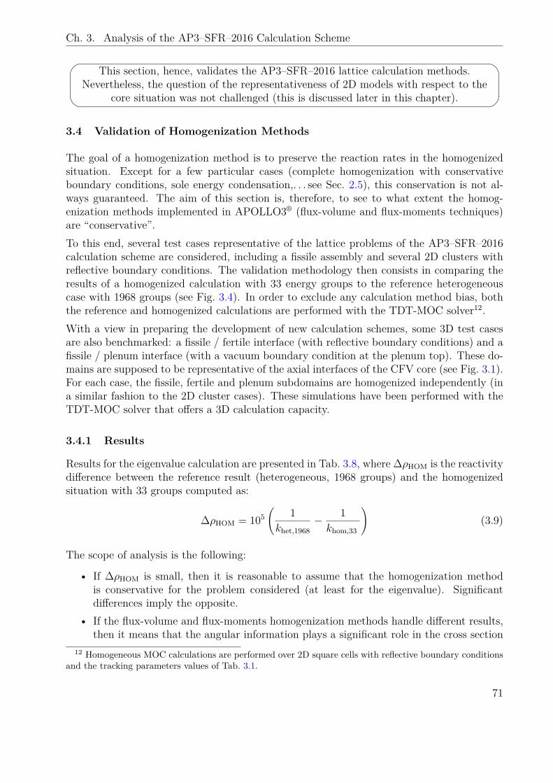
Ch. 3. Analysis of the AP3–SFR–2016 Calculation Scheme
This section, hence, validates the AP3–SFR–2016 lattice calculation methods.Nevertheless, the question of the representativeness of 2D models with respect to the
core situation was not challenged (this is discussed later in this chapter).
3.4 Validation of Homogenization Methods
The goal of a homogenization method is to preserve the reaction rates in the homogenizedsituation. Except for a few particular cases (complete homogenization with conservativeboundary conditions, sole energy condensation,. . . see Sec. 2.5), this conservation is not al-ways guaranteed. The aim of this section is, therefore, to see to what extent the homog-enization methods implemented in APOLLO3® (flux-volume and flux-moments techniques)are “conservative”.To this end, several test cases representative of the lattice problems of the AP3–SFR–2016calculation scheme are considered, including a fissile assembly and several 2D clusters withreflective boundary conditions. The validation methodology then consists in comparing theresults of a homogenized calculation with 33 energy groups to the reference heterogeneouscase with 1968 groups (see Fig. 3.4). In order to exclude any calculation method bias, boththe reference and homogenized calculations are performed with the TDT-MOC solver12.With a view in preparing the development of new calculation schemes, some 3D test casesare also benchmarked: a fissile / fertile interface (with reflective boundary conditions) and afissile / plenum interface (with a vacuum boundary condition at the plenum top). These do-mains are supposed to be representative of the axial interfaces of the CFV core (see Fig. 3.1).For each case, the fissile, fertile and plenum subdomains are homogenized independently (ina similar fashion to the 2D cluster cases). These simulations have been performed with theTDT-MOC solver that offers a 3D calculation capacity.
3.4.1 Results
Results for the eigenvalue calculation are presented in Tab. 3.8, where ∆ρHOM is the reactivitydifference between the reference result (heterogeneous, 1968 groups) and the homogenizedsituation with 33 groups computed as:
∆ρHOM = 105(
1khet,1968
− 1khom,33
)(3.9)
The scope of analysis is the following:
• If ∆ρHOM is small, then it is reasonable to assume that the homogenization methodis conservative for the problem considered (at least for the eigenvalue). Significantdifferences imply the opposite.
• If the flux-volume and flux-moments homogenization methods handle different results,then it means that the angular information plays a significant role in the cross section
12 Homogeneous MOC calculations are performed over 2D square cells with reflective boundary conditionsand the tracking parameters values of Tab. 3.1.
71
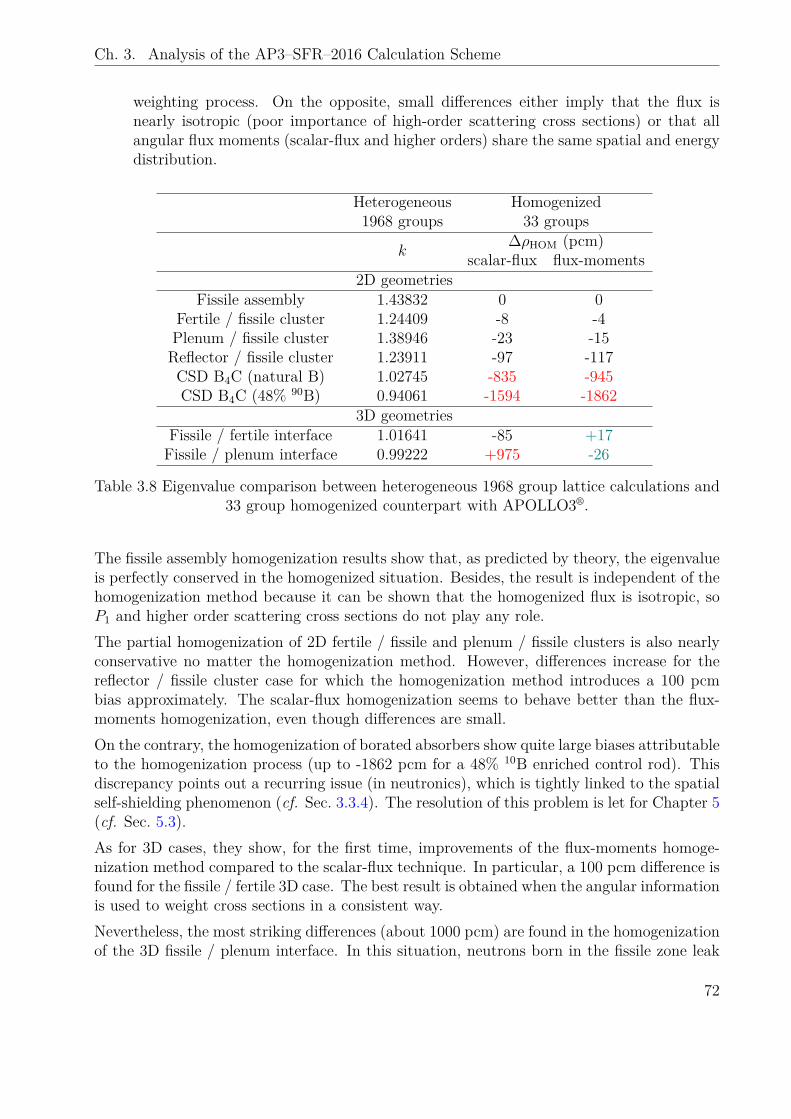
Ch. 3. Analysis of the AP3–SFR–2016 Calculation Scheme
weighting process. On the opposite, small differences either imply that the flux isnearly isotropic (poor importance of high-order scattering cross sections) or that allangular flux moments (scalar-flux and higher orders) share the same spatial and energydistribution.
Heterogeneous Homogenized1968 groups 33 groups
k∆ρHOM (pcm)
scalar-flux flux-moments2D geometries
Fissile assembly 1.43832 0 0Fertile / fissile cluster 1.24409 -8 -4Plenum / fissile cluster 1.38946 -23 -15Reflector / fissile cluster 1.23911 -97 -117CSD B4C (natural B) 1.02745 -835 -945CSD B4C (48% 90B) 0.94061 -1594 -1862
3D geometriesFissile / fertile interface 1.01641 -85 +17Fissile / plenum interface 0.99222 +975 -26
Table 3.8 Eigenvalue comparison between heterogeneous 1968 group lattice calculations and33 group homogenized counterpart with APOLLO3®.
The fissile assembly homogenization results show that, as predicted by theory, the eigenvalueis perfectly conserved in the homogenized situation. Besides, the result is independent of thehomogenization method because it can be shown that the homogenized flux is isotropic, soP1 and higher order scattering cross sections do not play any role.The partial homogenization of 2D fertile / fissile and plenum / fissile clusters is also nearlyconservative no matter the homogenization method. However, differences increase for thereflector / fissile cluster case for which the homogenization method introduces a 100 pcmbias approximately. The scalar-flux homogenization seems to behave better than the flux-moments homogenization, even though differences are small.On the contrary, the homogenization of borated absorbers show quite large biases attributableto the homogenization process (up to -1862 pcm for a 48% 10B enriched control rod). Thisdiscrepancy points out a recurring issue (in neutronics), which is tightly linked to the spatialself-shielding phenomenon (cf. Sec. 3.3.4). The resolution of this problem is let for Chapter 5(cf. Sec. 5.3).As for 3D cases, they show, for the first time, improvements of the flux-moments homoge-nization method compared to the scalar-flux technique. In particular, a 100 pcm difference isfound for the fissile / fertile 3D case. The best result is obtained when the angular informationis used to weight cross sections in a consistent way.Nevertheless, the most striking differences (about 1000 pcm) are found in the homogenizationof the 3D fissile / plenum interface. In this situation, neutrons born in the fissile zone leak
72
Ch. 3. Analysis of the AP3–SFR–2016 Calculation Scheme
out of the core through the plenum (the top boundary condition is vacuum). As a result,a neutron current runs through the geometrical domain. When not taken into account toweight cross sections, significant biases are found in the homogenized situation. In such casesthen, the flux-moments homogenization method is unavoidable.
3.4.2 Discussion
The results presented in this section show that, except for borated absorbers, the spatial ho-mogenization and 33 group energy condensation of 2D clusters used to prepare cross sectionsin the AP3–SFR–2016 methodology is nearly conservative. This observation corroboratesthe idea that no equivalence method is required to correct the neutron balance in the ho-mogenized situation.Considering that the homogenized results are independent of the homogenization method,the scalar-flux homogenization can be recommended for the homogenization of 2D clusters.The reason for this recommendation is that the independence to the homogenization methoddoes not allow to state whether P1 and higher order flux moments are close to zero, or if theyshare the same spatial and energy distribution than the scalar-flux (P0 moment)13.
#
"
!
In order to avoid inconsistent values of high-order homogenized scattering crosssections – that might arise from close to zero flux-moments weighting – the scalar-fluxshould be preferred for the homogenization of 2D clusters. However, when there is a
significant current in the calculation domain, the flux-moments homogenization shouldbe used. Else, the consistency of the homogenized results cannot be guaranteed.
This latter situation is encountered, for instance, during the homogenization of 3D patterns.However, these situations are not encountered in the AP3–SFR–2016 methodology.
3.5 Analysis of the Biases at the Core Level
This section approaches the whole core calculation problem in order to validate (or invalidate)the AP3–SFR–2016 methodology for the calculation of a CFV object. To do so, APOLLO3®
results are compared to reference Monte Carlo simulations performed over the heterogeneouscore model. The process is similar to the one presented in Sec. 3.3 for the validation ofAPOLLO3® lattice calculations.
3.5.1 CFV Calculation
According to the AP3–SFR–2016 methodology, the CFV model is composed of homogeneousmedia characterized by homogenized cross sections prepared at the lattice stage (see Fig. 3.5).In this section, though, control rods are replaced by rod followers (i.e., coolant): the controlrods modeling question, which showed large biases in the homogenization phase, is let forChapter 5.
13 The scalar flux is always positive. As such, it is a “good” weighting function.
73
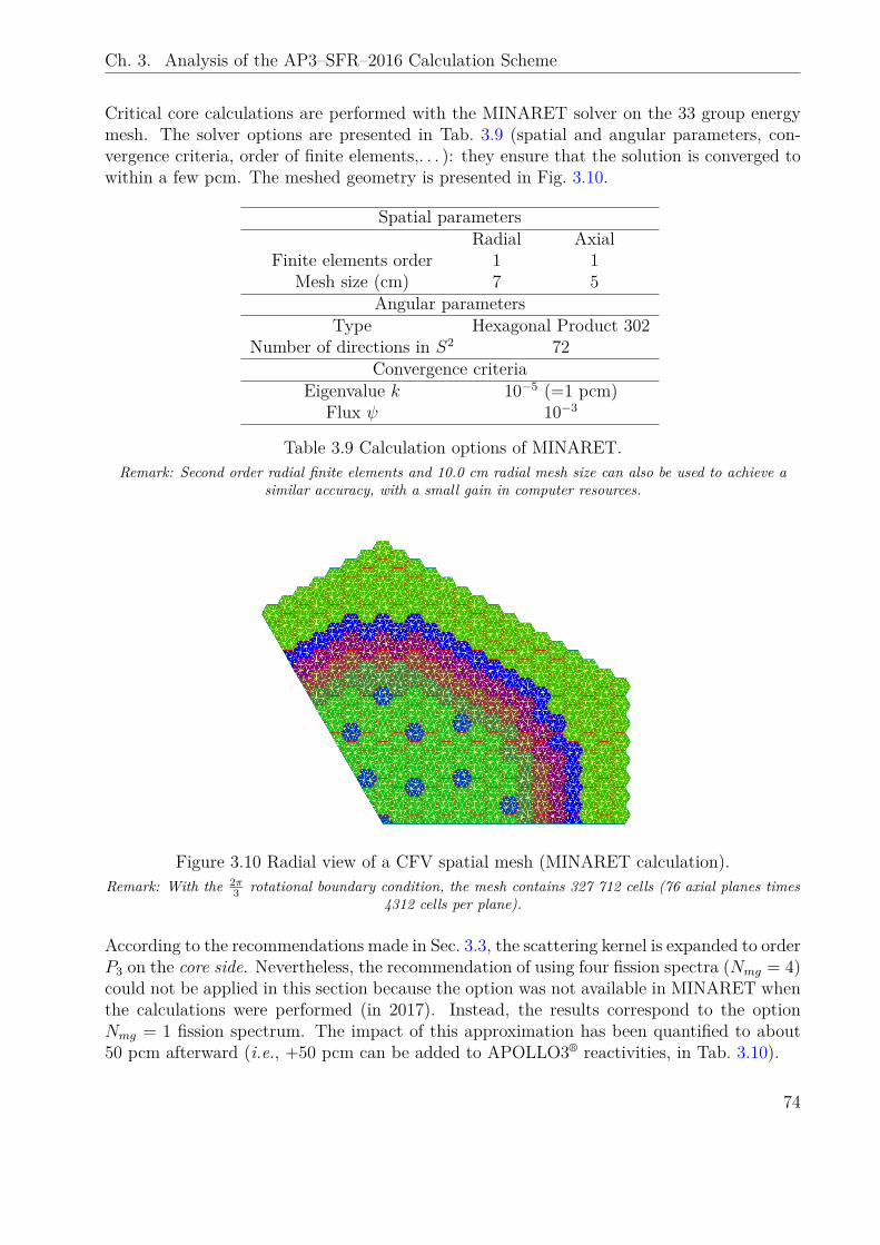
Ch. 3. Analysis of the AP3–SFR–2016 Calculation Scheme
Critical core calculations are performed with the MINARET solver on the 33 group energymesh. The solver options are presented in Tab. 3.9 (spatial and angular parameters, con-vergence criteria, order of finite elements,. . . ): they ensure that the solution is converged towithin a few pcm. The meshed geometry is presented in Fig. 3.10.
Spatial parametersRadial Axial
Finite elements order 1 1Mesh size (cm) 7 5
Angular parametersType Hexagonal Product 302
Number of directions in S2 72Convergence criteria
Eigenvalue k 10−5 (=1 pcm)Flux ψ 10−3
Table 3.9 Calculation options of MINARET.Remark: Second order radial finite elements and 10.0 cm radial mesh size can also be used to achieve a
similar accuracy, with a small gain in computer resources.
Figure 3.10 Radial view of a CFV spatial mesh (MINARET calculation).Remark: With the 2π
3 rotational boundary condition, the mesh contains 327 712 cells (76 axial planes times4312 cells per plane).
According to the recommendations made in Sec. 3.3, the scattering kernel is expanded to orderP3 on the core side. Nevertheless, the recommendation of using four fission spectra (Nmg = 4)could not be applied in this section because the option was not available in MINARET whenthe calculations were performed (in 2017). Instead, the results correspond to the optionNmg = 1 fission spectrum. The impact of this approximation has been quantified to about50 pcm afterward (i.e., +50 pcm can be added to APOLLO3® reactivities, in Tab. 3.10).
74
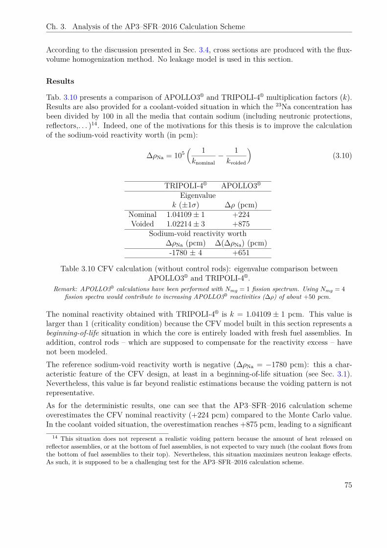
Ch. 3. Analysis of the AP3–SFR–2016 Calculation Scheme
According to the discussion presented in Sec. 3.4, cross sections are produced with the flux-volume homogenization method. No leakage model is used in this section.
Results
Tab. 3.10 presents a comparison of APOLLO3® and TRIPOLI-4® multiplication factors (k).Results are also provided for a coolant-voided situation in which the 23Na concentration hasbeen divided by 100 in all the media that contain sodium (including neutronic protections,reflectors,. . . )14. Indeed, one of the motivations for this thesis is to improve the calculationof the sodium-void reactivity worth (in pcm):
∆ρNa = 105( 1knominal
− 1kvoided
)(3.10)
TRIPOLI-4® APOLLO3®
Eigenvaluek (±1σ) ∆ρ (pcm)
Nominal 1.04109± 1 +224Voided 1.02214± 3 +875
Sodium-void reactivity worth∆ρNa (pcm) ∆(∆ρNa) (pcm)-1780 ± 4 +651
Table 3.10 CFV calculation (without control rods): eigenvalue comparison betweenAPOLLO3® and TRIPOLI-4®.
Remark: APOLLO3® calculations have been performed with Nmg = 1 fission spectrum. Using Nmg = 4fission spectra would contribute to increasing APOLLO3® reactivities (∆ρ) of about +50 pcm.
The nominal reactivity obtained with TRIPOLI-4® is k = 1.04109 ± 1 pcm. This value islarger than 1 (criticality condition) because the CFV model built in this section represents abeginning-of-life situation in which the core is entirely loaded with fresh fuel assemblies. Inaddition, control rods – which are supposed to compensate for the reactivity excess – havenot been modeled.The reference sodium-void reactivity worth is negative (∆ρNa = −1780 pcm): this a char-acteristic feature of the CFV design, at least in a beginning-of-life situation (see Sec. 3.1).Nevertheless, this value is far beyond realistic estimations because the voiding pattern is notrepresentative.As for the deterministic results, one can see that the AP3–SFR–2016 calculation schemeoverestimates the CFV nominal reactivity (+224 pcm) compared to the Monte Carlo value.In the coolant voided situation, the overestimation reaches +875 pcm, leading to a significant
14 This situation does not represent a realistic voiding pattern because the amount of heat released onreflector assemblies, or at the bottom of fuel assemblies, is not expected to vary much (the coolant flows fromthe bottom of fuel assemblies to their top). Nevertheless, this situation maximizes neutron leakage effects.As such, it is supposed to be a challenging test for the AP3–SFR–2016 calculation scheme.
75
Ch. 3. Analysis of the AP3–SFR–2016 Calculation Scheme
overestimation of the sodium-void reactivity worth (+651 pcm). These results are consistentwith the ones presented in reference [27]15.Fig. 3.11 now shows the APOLLO3® vs. TRIPOLI-4® relative discrepancy (in %) on thefission rate distribution. The illustration presents an axial cut in the core domain taken fromthe core center to its radial periphery. The (relative) statistical uncertainty on Monte Carlolocal fission rate values16 is σ ≈ 0.4%.
30/30 32/30 34/30 36/30 38/30 40/30Assembly position
100
120
140
160
180
200
Axi
alpo
sitio
n(c
m)
FCA
C1
FCA
C1
FCA
C2
SS
V
SS
V
SR
EFL
SVE
FCASPLN
+3.0
-9.7
−10
−8
−6
−4
−2
0
2
4
6
8
10
%
Figure 3.11 CFV calculation (without control rods): relative difference on the fission ratedistribution (computed as ∆τ/τ) between APOLLO3® and TRIPOLI-4® (axial cut from
core center, i.e., assembly 30/30, to radial reflector).Remark: FCA stands for fertile blankets, C1 (resp. C2) for inner (resp. outer) fissile zones, SPLN forsodium plenum, SSV for control rod follower (sodium), SREFL for reflector and SVE for expansion tank
(including a plug that is not represented).
One can see that the AP3–SFR–2016 methodology induces large discrepancies for the spatialfission rate distribution. More precisely, two tendencies can be observed:
• Axially, the APOLLO3® fission rate distribution is tilted towards the top of the core:the tilt amplitude is ≈ 10/13%, and the maximal discrepancies are found near the
15 The figures presented in reference [27] (Table IV) are ∆ρ = +256 pcm (nominal reactivity overestimation)and ∆(∆ρNa) = +219 pcm (sodium-void reactivity worth overestimation). In the paper, though, the referencevoid worth is “only” ∆ρNa = −794 pcm (different voiding pattern): the coolant voiding issue is emphasizedin our case.
16 The TRIPOLI-4® calculation ran for one week over 128 processors.
76
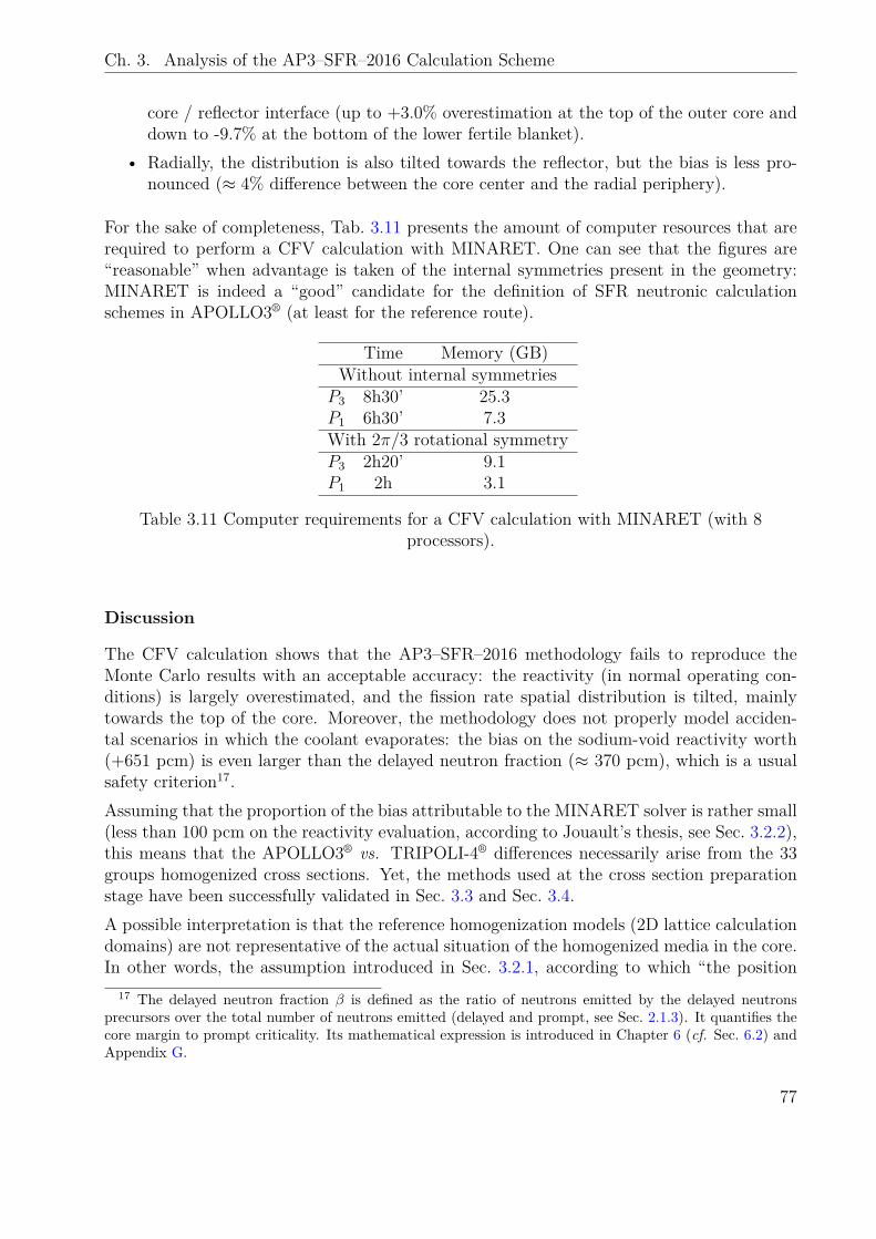
Ch. 3. Analysis of the AP3–SFR–2016 Calculation Scheme
core / reflector interface (up to +3.0% overestimation at the top of the outer core anddown to -9.7% at the bottom of the lower fertile blanket).
• Radially, the distribution is also tilted towards the reflector, but the bias is less pro-nounced (≈ 4% difference between the core center and the radial periphery).
For the sake of completeness, Tab. 3.11 presents the amount of computer resources that arerequired to perform a CFV calculation with MINARET. One can see that the figures are“reasonable” when advantage is taken of the internal symmetries present in the geometry:MINARET is indeed a “good” candidate for the definition of SFR neutronic calculationschemes in APOLLO3® (at least for the reference route).
Time Memory (GB)Without internal symmetries
P3 8h30’ 25.3P1 6h30’ 7.3With 2π/3 rotational symmetryP3 2h20’ 9.1P1 2h 3.1
Table 3.11 Computer requirements for a CFV calculation with MINARET (with 8processors).
Discussion
The CFV calculation shows that the AP3–SFR–2016 methodology fails to reproduce theMonte Carlo results with an acceptable accuracy: the reactivity (in normal operating con-ditions) is largely overestimated, and the fission rate spatial distribution is tilted, mainlytowards the top of the core. Moreover, the methodology does not properly model acciden-tal scenarios in which the coolant evaporates: the bias on the sodium-void reactivity worth(+651 pcm) is even larger than the delayed neutron fraction (≈ 370 pcm), which is a usualsafety criterion17.Assuming that the proportion of the bias attributable to the MINARET solver is rather small(less than 100 pcm on the reactivity evaluation, according to Jouault’s thesis, see Sec. 3.2.2),this means that the APOLLO3® vs. TRIPOLI-4® differences necessarily arise from the 33groups homogenized cross sections. Yet, the methods used at the cross section preparationstage have been successfully validated in Sec. 3.3 and Sec. 3.4.A possible interpretation is that the reference homogenization models (2D lattice calculationdomains) are not representative of the actual situation of the homogenized media in the core.In other words, the assumption introduced in Sec. 3.2.1, according to which “the position
17 The delayed neutron fraction β is defined as the ratio of neutrons emitted by the delayed neutronsprecursors over the total number of neutrons emitted (delayed and prompt, see Sec. 2.1.3). It quantifies thecore margin to prompt criticality. Its mathematical expression is introduced in Chapter 6 (cf. Sec. 6.2) andAppendix G.
77
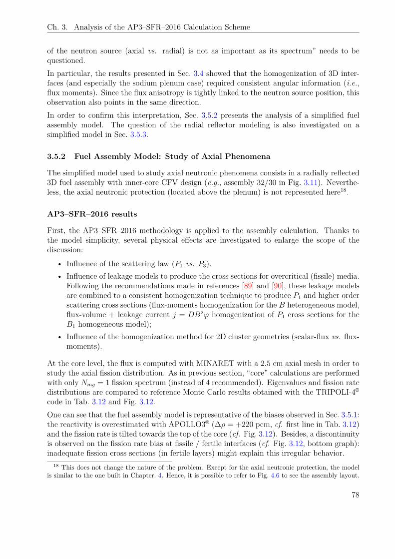
Ch. 3. Analysis of the AP3–SFR–2016 Calculation Scheme
of the neutron source (axial vs. radial) is not as important as its spectrum” needs to bequestioned.In particular, the results presented in Sec. 3.4 showed that the homogenization of 3D inter-faces (and especially the sodium plenum case) required consistent angular information (i.e.,flux moments). Since the flux anisotropy is tightly linked to the neutron source position, thisobservation also points in the same direction.In order to confirm this interpretation, Sec. 3.5.2 presents the analysis of a simplified fuelassembly model. The question of the radial reflector modeling is also investigated on asimplified model in Sec. 3.5.3.
3.5.2 Fuel Assembly Model: Study of Axial Phenomena
The simplified model used to study axial neutronic phenomena consists in a radially reflected3D fuel assembly with inner-core CFV design (e.g., assembly 32/30 in Fig. 3.11). Neverthe-less, the axial neutronic protection (located above the plenum) is not represented here18.
AP3–SFR–2016 results
First, the AP3–SFR–2016 methodology is applied to the assembly calculation. Thanks tothe model simplicity, several physical effects are investigated to enlarge the scope of thediscussion:
• Influence of the scattering law (P1 vs. P3).• Influence of leakage models to produce the cross sections for overcritical (fissile) media.
Following the recommendations made in references [89] and [90], these leakage modelsare combined to a consistent homogenization technique to produce P1 and higher orderscattering cross sections (flux-moments homogenization for the B heterogeneous model,flux-volume + leakage current j = DB2ϕ homogenization of P1 cross sections for theB1 homogeneous model);
• Influence of the homogenization method for 2D cluster geometries (scalar-flux vs. flux-moments).
At the core level, the flux is computed with MINARET with a 2.5 cm axial mesh in order tostudy the axial fission distribution. As in previous section, “core” calculations are performedwith only Nmg = 1 fission spectrum (instead of 4 recommended). Eigenvalues and fission ratedistributions are compared to reference Monte Carlo results obtained with the TRIPOLI-4®
code in Tab. 3.12 and Fig. 3.12.One can see that the fuel assembly model is representative of the biases observed in Sec. 3.5.1:the reactivity is overestimated with APOLLO3® (∆ρ = +220 pcm, cf. first line in Tab. 3.12)and the fission rate is tilted towards the top of the core (cf. Fig. 3.12). Besides, a discontinuityis observed on the fission rate bias at fissile / fertile interfaces (cf. Fig. 3.12, bottom graph):inadequate fission cross sections (in fertile layers) might explain this irregular behavior.
18 This does not change the nature of the problem. Except for the axial neutronic protection, the modelis similar to the one built in Chapter. 4. Hence, it is possible to refer to Fig. 4.6 to see the assembly layout.
78
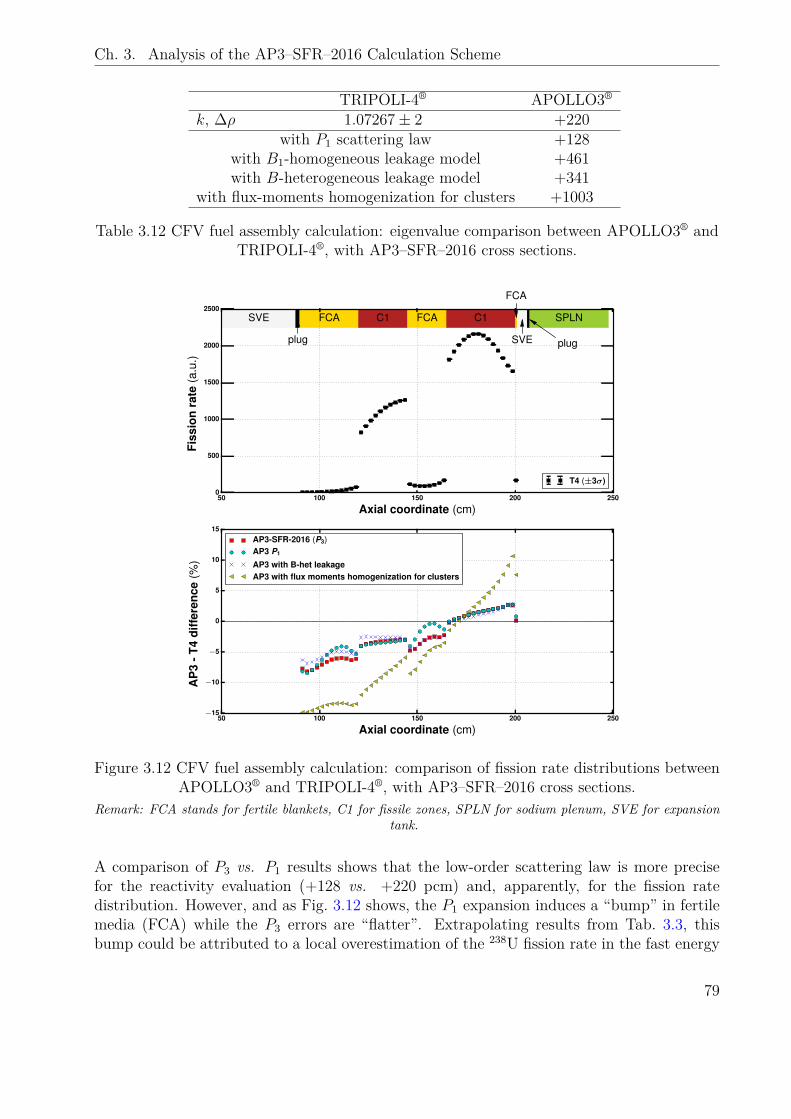
Ch. 3. Analysis of the AP3–SFR–2016 Calculation Scheme
TRIPOLI-4® APOLLO3®
k, ∆ρ 1.07267± 2 +220with P1 scattering law +128
with B1-homogeneous leakage model +461with B-heterogeneous leakage model +341
with flux-moments homogenization for clusters +1003
Table 3.12 CFV fuel assembly calculation: eigenvalue comparison between APOLLO3® andTRIPOLI-4®, with AP3–SFR–2016 cross sections.
50 100 150 200 250
Axial coordinate (cm)
0
500
1000
1500
2000
2500
Fiss
ion
rate
(a.u
.)
SVE FCA C1 FCA C1 SPLN
plug
FCA
SVE plug
T4 (±3σ)
50 100 150 200 250
Axial coordinate (cm)
−15
−10
−5
0
5
10
15
AP
3-T
4di
ffer
ence
(%)
AP3-SFR-2016 (P3)AP3 P1
AP3 with B-het leakageAP3 with flux moments homogenization for clusters
Figure 3.12 CFV fuel assembly calculation: comparison of fission rate distributions betweenAPOLLO3® and TRIPOLI-4®, with AP3–SFR–2016 cross sections.
Remark: FCA stands for fertile blankets, C1 for fissile zones, SPLN for sodium plenum, SVE for expansiontank.
A comparison of P3 vs. P1 results shows that the low-order scattering law is more precisefor the reactivity evaluation (+128 vs. +220 pcm) and, apparently, for the fission ratedistribution. However, and as Fig. 3.12 shows, the P1 expansion induces a “bump” in fertilemedia (FCA) while the P3 errors are “flatter”. Extrapolating results from Tab. 3.3, thisbump could be attributed to a local overestimation of the 238U fission rate in the fast energy
79
Ch. 3. Analysis of the AP3–SFR–2016 Calculation Scheme
range. In any case, it is probable that the apparent eigenvalue improvement due to the P1law is a consequence of several phenomena that compensate each other.As for the influence of leakage models, it is clear from Tab. 3.12 that they deteriorate theeigenvalue estimation. Nevertheless, the B-heterogeneous leakage model seems to flattenthe fission rate drift in the lower fissile zone (120 < z < 145 cm) constituting, hence, animprovement compared to the AP3–SFR–2016 methodology. This observation is consistentwith the results presented in reference [90].Finally, it is seen that the flux-moments homogenization of cross sections in 2D clustersinduces very large errors. This observation corroborates the conclusions made in Sec. 3.4.2:a scalar-flux homogenization should be preferred in those situations in which the consistencyof the angular flux moments cannot be verified. Furthermore, the result seems to confirmthat consistent angular information is required to produce axial media cross sections (i.e.,sodium plenum, fertile blankets,. . . ).
Comparison with 3D cross sections
A straightforward way to access full angular modes of the flux that are representative of thecore situation is to perform 3D-MOC calculations. In APOLLO3®, this can be done (on thelattice side) with the TDT solver.In particular, the 3D-MOC equations can be solved either assuming a step approximationfor sources and cross sections (see Sec.2.2.3) or a polynomial expansion for the axial sources(including the flux). Unfortunately, the step approximation is quite demanding in termsof computer resources, so converged solutions could not be obtained on the full assemblycase (more than 100 axial planes are required, representing more than 120 GB of memory).Hopefully, the higher order expansion implemented in APOLLO3® by L. Graziano during itsPh. D. thesis [42], and validated on the CFV fuel assembly case [54], could be used to relaxthe memory constraint (to about 40 GB).Thus, cross sections have been generated for the different media that compose the assem-bly with a second order polynomial axial expansion 3D-MOC-based solution. These crosssections have been used, in a second step, to perform the same assembly calculation inthe homogenized situation, with 33 energy groups. Since the reference and homogenizedproblems are equivalent in that case, such homogenized cross sections are supposed to bethe-best-one-could-expect.Results, including a comparison of scalar-flux vs. flux-moments homogenization methods,are presented in Tab. 3.13 and Fig. 3.13.The fission rate comparison shows that the APOLLO3® vs. TRIPOLI-4® axial drift canbe eliminated provided that the angular information (angular flux moments) is used in aconsistent way to weight cross sections. On the contrary, a 3D calculation shows almost nointerest when combined to a scalar-flux homogenization method, thus neglecting the angularmodes of the flux. In that case, the fission rate drift is comparable to the one observed withthe AP3–SFR–2016 methodology even though a significant improvement is found in fertilelayers (because the 3D-flux spectrum used to weight cross sections is more representative).These observations are consistent with the results presented in reference [97].
80
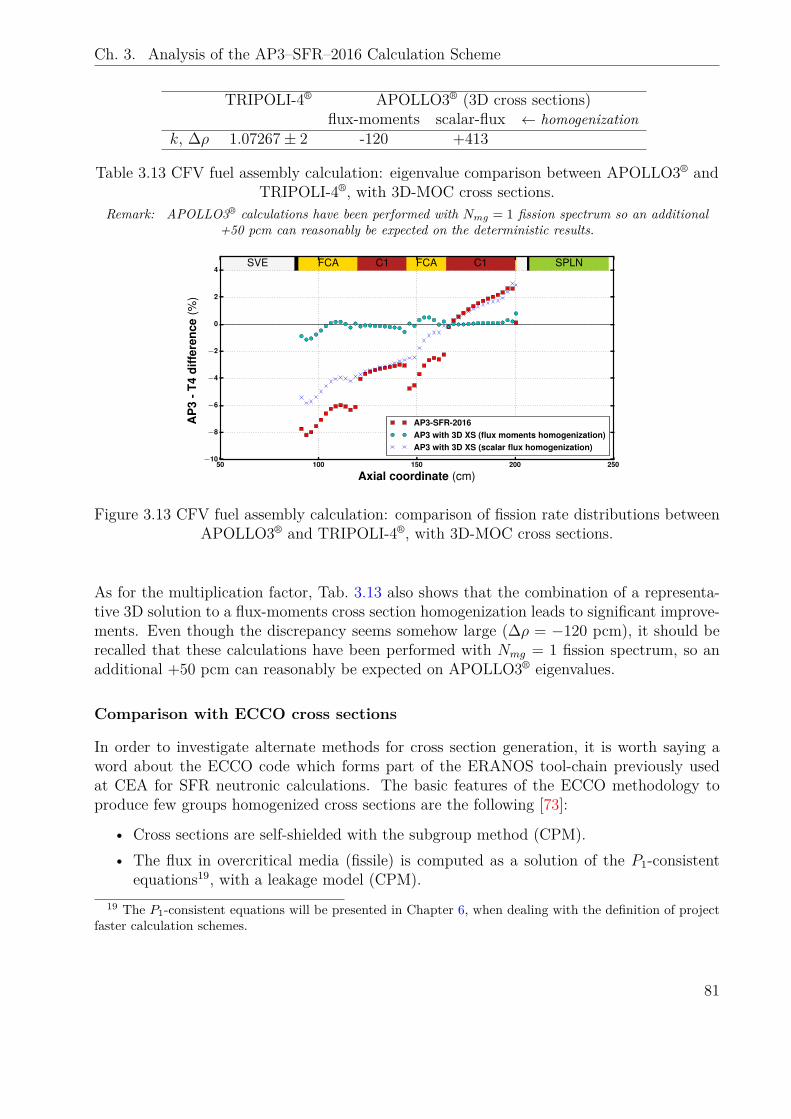
Ch. 3. Analysis of the AP3–SFR–2016 Calculation Scheme
TRIPOLI-4® APOLLO3® (3D cross sections)flux-moments scalar-flux ← homogenization
k, ∆ρ 1.07267± 2 -120 +413
Table 3.13 CFV fuel assembly calculation: eigenvalue comparison between APOLLO3® andTRIPOLI-4®, with 3D-MOC cross sections.
Remark: APOLLO3® calculations have been performed with Nmg = 1 fission spectrum so an additional+50 pcm can reasonably be expected on the deterministic results.
50 100 150 200 250
Axial coordinate (cm)
−10
−8
−6
−4
−2
0
2
4
AP
3-T
4di
ffer
ence
(%)
SVE FCA C1 FCA C1 SPLN
AP3-SFR-2016AP3 with 3D XS (flux moments homogenization)AP3 with 3D XS (scalar flux homogenization)
Figure 3.13 CFV fuel assembly calculation: comparison of fission rate distributions betweenAPOLLO3® and TRIPOLI-4®, with 3D-MOC cross sections.
As for the multiplication factor, Tab. 3.13 also shows that the combination of a representa-tive 3D solution to a flux-moments cross section homogenization leads to significant improve-ments. Even though the discrepancy seems somehow large (∆ρ = −120 pcm), it should berecalled that these calculations have been performed with Nmg = 1 fission spectrum, so anadditional +50 pcm can reasonably be expected on APOLLO3® eigenvalues.
Comparison with ECCO cross sections
In order to investigate alternate methods for cross section generation, it is worth saying aword about the ECCO code which forms part of the ERANOS tool-chain previously usedat CEA for SFR neutronic calculations. The basic features of the ECCO methodology toproduce few groups homogenized cross sections are the following [73]:
• Cross sections are self-shielded with the subgroup method (CPM).• The flux in overcritical media (fissile) is computed as a solution of the P1-consistent
equations19, with a leakage model (CPM).19 The P1-consistent equations will be presented in Chapter 6, when dealing with the definition of project
faster calculation schemes.
81
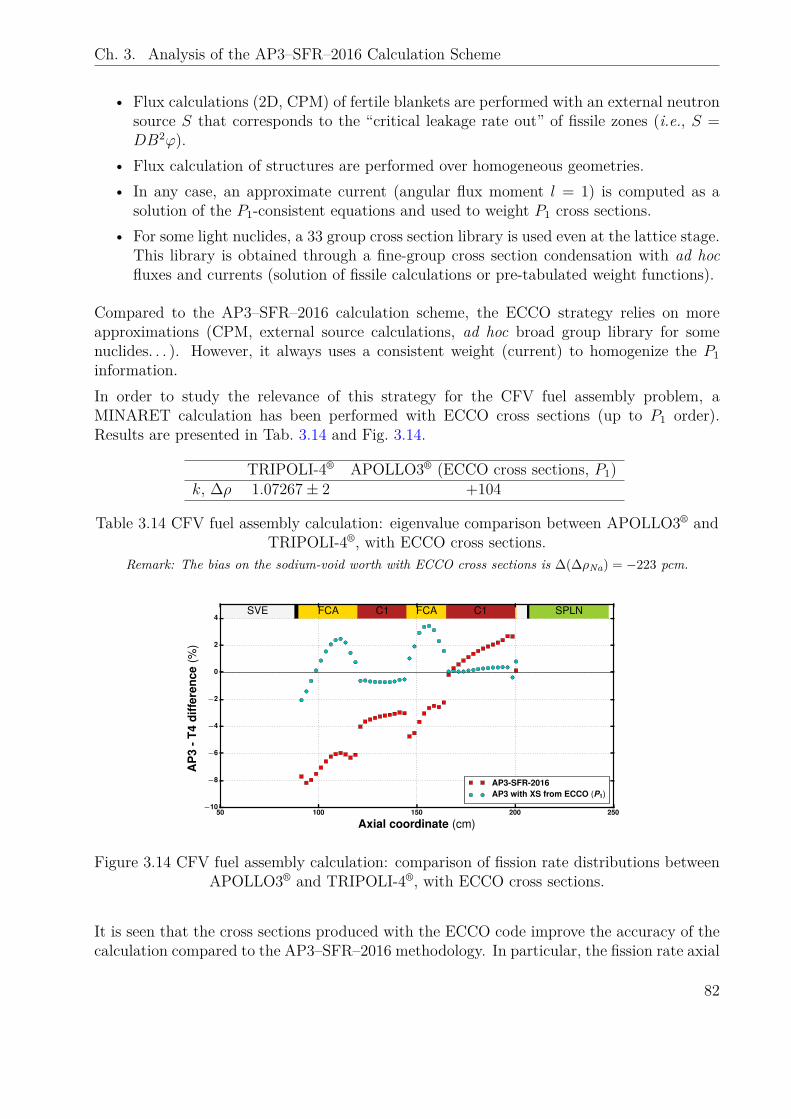
Ch. 3. Analysis of the AP3–SFR–2016 Calculation Scheme
• Flux calculations (2D, CPM) of fertile blankets are performed with an external neutronsource S that corresponds to the “critical leakage rate out” of fissile zones (i.e., S =DB2ϕ).
• Flux calculation of structures are performed over homogeneous geometries.• In any case, an approximate current (angular flux moment l = 1) is computed as a
solution of the P1-consistent equations and used to weight P1 cross sections.• For some light nuclides, a 33 group cross section library is used even at the lattice stage.
This library is obtained through a fine-group cross section condensation with ad hocfluxes and currents (solution of fissile calculations or pre-tabulated weight functions).
Compared to the AP3–SFR–2016 calculation scheme, the ECCO strategy relies on moreapproximations (CPM, external source calculations, ad hoc broad group library for somenuclides. . . ). However, it always uses a consistent weight (current) to homogenize the P1information.In order to study the relevance of this strategy for the CFV fuel assembly problem, aMINARET calculation has been performed with ECCO cross sections (up to P1 order).Results are presented in Tab. 3.14 and Fig. 3.14.
TRIPOLI-4® APOLLO3® (ECCO cross sections, P1)k, ∆ρ 1.07267± 2 +104
Table 3.14 CFV fuel assembly calculation: eigenvalue comparison between APOLLO3® andTRIPOLI-4®, with ECCO cross sections.
Remark: The bias on the sodium-void worth with ECCO cross sections is ∆(∆ρNa) = −223 pcm.
50 100 150 200 250
Axial coordinate (cm)
−10
−8
−6
−4
−2
0
2
4
AP
3-T
4di
ffer
ence
(%)
SVE FCA C1 FCA C1 SPLN
AP3-SFR-2016AP3 with XS from ECCO (P1)
Figure 3.14 CFV fuel assembly calculation: comparison of fission rate distributions betweenAPOLLO3® and TRIPOLI-4®, with ECCO cross sections.
It is seen that the cross sections produced with the ECCO code improve the accuracy of thecalculation compared to the AP3–SFR–2016 methodology. In particular, the fission rate axial
82
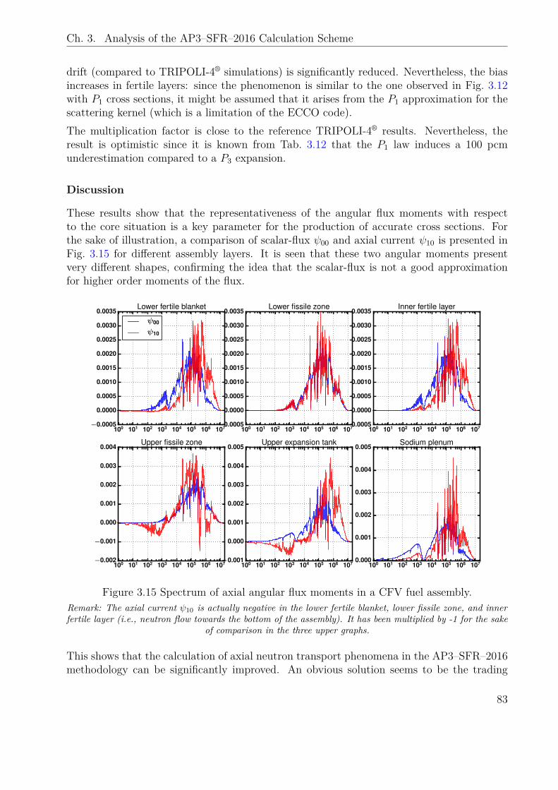
Ch. 3. Analysis of the AP3–SFR–2016 Calculation Scheme
drift (compared to TRIPOLI-4® simulations) is significantly reduced. Nevertheless, the biasincreases in fertile layers: since the phenomenon is similar to the one observed in Fig. 3.12with P1 cross sections, it might be assumed that it arises from the P1 approximation for thescattering kernel (which is a limitation of the ECCO code).The multiplication factor is close to the reference TRIPOLI-4® results. Nevertheless, theresult is optimistic since it is known from Tab. 3.12 that the P1 law induces a 100 pcmunderestimation compared to a P3 expansion.
Discussion
These results show that the representativeness of the angular flux moments with respectto the core situation is a key parameter for the production of accurate cross sections. Forthe sake of illustration, a comparison of scalar-flux ψ00 and axial current ψ10 is presented inFig. 3.15 for different assembly layers. It is seen that these two angular moments presentvery different shapes, confirming the idea that the scalar-flux is not a good approximationfor higher order moments of the flux.
100 101 102 103 104 105 106 107−0.0005
0.0000
0.0005
0.0010
0.0015
0.0020
0.0025
0.0030
0.0035Lower fertile blanket
ψ00
ψ10
100 101 102 103 104 105 106 107−0.0005
0.0000
0.0005
0.0010
0.0015
0.0020
0.0025
0.0030
0.0035Lower fissile zone
100 101 102 103 104 105 106 107−0.0005
0.0000
0.0005
0.0010
0.0015
0.0020
0.0025
0.0030
0.0035Inner fertile layer
100 101 102 103 104 105 106 107−0.002
−0.001
0.000
0.001
0.002
0.003
0.004Upper fissile zone
100 101 102 103 104 105 106 107−0.001
0.000
0.001
0.002
0.003
0.004
0.005Upper expansion tank
100 101 102 103 104 105 106 1070.000
0.001
0.002
0.003
0.004
0.005Sodium plenum
Figure 3.15 Spectrum of axial angular flux moments in a CFV fuel assembly.Remark: The axial current ψ10 is actually negative in the lower fertile blanket, lower fissile zone, and innerfertile layer (i.e., neutron flow towards the bottom of the assembly). It has been multiplied by -1 for the sake
of comparison in the three upper graphs.
This shows that the calculation of axial neutron transport phenomena in the AP3–SFR–2016methodology can be significantly improved. An obvious solution seems to be the trading
83
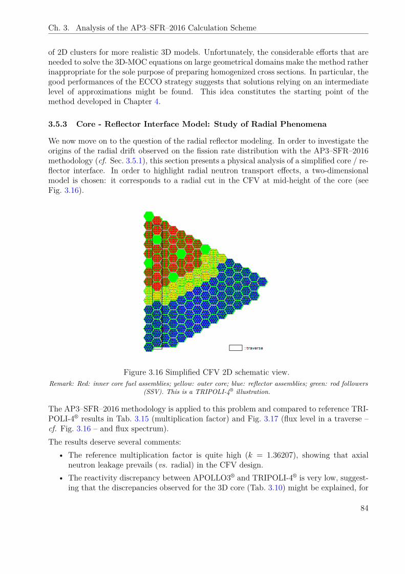
Ch. 3. Analysis of the AP3–SFR–2016 Calculation Scheme
of 2D clusters for more realistic 3D models. Unfortunately, the considerable efforts that areneeded to solve the 3D-MOC equations on large geometrical domains make the method ratherinappropriate for the sole purpose of preparing homogenized cross sections. In particular, thegood performances of the ECCO strategy suggests that solutions relying on an intermediatelevel of approximations might be found. This idea constitutes the starting point of themethod developed in Chapter 4.
3.5.3 Core - Reflector Interface Model: Study of Radial Phenomena
We now move on to the question of the radial reflector modeling. In order to investigate theorigins of the radial drift observed on the fission rate distribution with the AP3–SFR–2016methodology (cf. Sec. 3.5.1), this section presents a physical analysis of a simplified core / re-flector interface. In order to highlight radial neutron transport effects, a two-dimensionalmodel is chosen: it corresponds to a radial cut in the CFV at mid-height of the core (seeFig. 3.16).
Figure 3.16 Simplified CFV 2D schematic view.Remark: Red: inner core fuel assemblies; yellow: outer core; blue: reflector assemblies; green: rod followers
(SSV). This is a TRIPOLI-4® illustration.
The AP3–SFR–2016 methodology is applied to this problem and compared to reference TRI-POLI-4® results in Tab. 3.15 (multiplication factor) and Fig. 3.17 (flux level in a traverse –cf. Fig. 3.16 – and flux spectrum).The results deserve several comments:
• The reference multiplication factor is quite high (k = 1.36207), showing that axialneutron leakage prevails (vs. radial) in the CFV design.
• The reactivity discrepancy between APOLLO3® and TRIPOLI-4® is very low, suggest-ing that the discrepancies observed for the 3D core (Tab. 3.10) might be explained, for
84
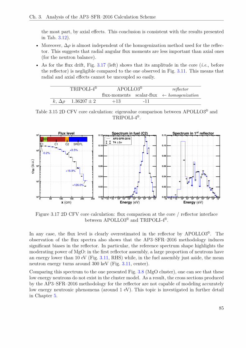
Ch. 3. Analysis of the AP3–SFR–2016 Calculation Scheme
the most part, by axial effects. This conclusion is consistent with the results presentedin Tab. 3.12).
• Moreover, ∆ρ is almost independent of the homogenization method used for the reflec-tor. This suggests that radial angular flux moments are less important than axial ones(for the neutron balance).
• As for the flux drift, Fig. 3.17 (left) shows that its amplitude in the core (i.e., beforethe reflector) is negligible compared to the one observed in Fig. 3.11. This means thatradial and axial effects cannot be uncoupled so easily.
TRIPOLI-4® APOLLO3® reflectorflux-moments scalar-flux ← homogenization
k, ∆ρ 1.36207± 2 +13 -11
Table 3.15 2D CFV core calculation: eigenvalue comparison between APOLLO3® andTRIPOLI-4®.
0 50 100 150 200 250
x (cm)
103
104
105
106
107
ψ00
(a.u
.)
-0.2%+0.5%
+16.9%
+126.0%
C1
SSV
C1 C2 SREFL
Flux level
10−3 10−2 10−1 100 101 102 103 104 105 106 107
Energy (eV)
0.00
0.02
0.04
0.06
0.08
0.10
0.12Spectrum in fuel (C2)AP3-SFR-2016T4 ±3σ
10−3 10−2 10−1 100 101 102 103 104 105 106 107
Energy (eV)
0.00
0.02
0.04
0.06
0.08
0.10
0.12Spectrum in 1st reflector
Figure 3.17 2D CFV core calculation: flux comparison at the core / reflector interfacebetween APOLLO3® and TRIPOLI-4®.
In any case, the flux level is clearly overestimated in the reflector by APOLLO3®. Theobservation of the flux spectra also shows that the AP3–SFR–2016 methodology inducessignificant biases in the reflector. In particular, the reference spectrum shape highlights themoderating power of MgO: in the first reflector assembly, a large proportion of neutrons havean energy lower than 10 eV (Fig. 3.11, RHS) while, in the fuel assembly just aside, the meanneutron energy turns around 300 keV (Fig. 3.11, center).Comparing this spectrum to the one presented Fig. 3.8 (MgO cluster), one can see that theselow energy neutrons do not exist in the cluster model. As a result, the cross sections producedby the AP3–SFR–2016 methodology for the reflector are not capable of modeling accuratelylow energy neutronic phenomena (around 1 eV). This topic is investigated in further detailin Chapter 5.
85
Ch. 3. Analysis of the AP3–SFR–2016 Calculation Scheme
3.6 Conclusions
The AP3–SFR–2016 methodology set up for the simulation of SFR cores in the APOLLO3®
code at CEA constitutes the starting point for the development of a validated referencecalculation scheme. Based upon the ECCO-ERANOS legacy, the AP3–SFR–2016 schemerelies on the lattice - core paradigm.In this chapter, the methods used at the lattice level have been successfully validated againstreference Monte Carlo calculations, showing satisfying adequacy between deterministic andstochastic results. In particular, the options that have been selected for APOLLO3® referencecalculation schemes can be summarized as follows:
• Flux calculation with the TDT-MOC solver.• Resonance self-shielding with the TDT-CPM solver under Tone’s approximation.• P3 expansion of the scattering kernel.• Representation of the dependence of fission spectra to the incident neutron energy withNmg = 4 such spectra.
The analysis of the homogenization methods implemented in APOLLO3® also allowed todetermine their range of application. In particular, the flux-moments homogenization is rec-ommended when the flux presents irregular angular modes. However, these high-order fluxmoments are often absent from the lattice calculation domains because of the 2D approx-imation and the use of reflective boundary conditions. In such situations, the scalar-fluxhomogenization should be used to avoid unphysical cross section values (unless a leakagemodel is used since, in that case, the leakage rate can be used to weight cross sections [89]).The application of the AP3–SFR–2016 calculation scheme to a CFV core design, however,showed the limitations of the methodology: significant biases were found on the multiplicationfactor (+224 pcm against reference Monte Carlo results), the flux distribution (axial andradial drifts, up to 10% overestimation) and the sodium-void reactivity worth (+651 pcm).Relying on previous works that validated the SN -DGFEM for the calculation of such SFRcores (and in particular the MINARET solver), it has been concluded that the differencesnecessarily arose from the 33 groups homogenized cross sections.Additional investigations showed that the representativeness of 2D cluster models regard-ing the core situation is questionable for media located in axial positions (fertile blankets,sodium plenum, expansion tanks. . . ). More precisely, it was proven that the cluster modelneglects the importance of the angular flux moments to preserve the neutron balance in thehomogenized situation. First tests showed that this inconsistency could be lifted either with3D calculations or with an approximate neutron current modeling through the P1 consistentequations. Doing so, it was proven that accurate results could indeed be obtained with 33groups homogenized cross sections for CFV-like core calculations.A limitation of the reflector modeling in the AP3–SFR–2016 methodology was also identifiedleading to the invalidation of the cluster model used to produce the reflector cross sections (atleast for reference calculations). Physically, this model is not capable of modeling low energyneutronic phenomena (around 1 eV) that arise from neutron moderation in magnesium oxidepins.
86
Ch. 3. Analysis of the AP3–SFR–2016 Calculation Scheme
The conclusion of these observations is that:
New methods need to be implemented in APOLLO3® to produce consistent few groupshomogenized cross sections for heterogeneous SFR cores such as the CFV.
To this end, Chapter 4 presents the development of a 2D/1D method for the productionof homogenized cross sections in axially heterogeneous geometries. This method intends toprovide an alternative to the 3D-MOC solution, whose computational cost is quite elevatedfor the sole purpose of producing homogenized cross sections20. The question of the reflectormodeling is let for Chapter 5.
20 The fuel assembly calculation presented in Sec. 3.5.2 required about 40 GB and 13 hours on 4 processors.
87

This page has been left intentionally blank.
88
Chapter 4 Development of a 2D/1D Method for CrossSection Generation in SFR Axial Geometries
Abstract
This chapter presents how a 2D/1D approximation to the 3D neutron transport equationcan be used to produce consistent cross sections for SFR cores. In order to introduce thereader to this class of methods, a panorama of 2D/1D techniques is first drawn in Sec. 4.1.The 2D/1D equations are then derived in Sec. 4.2 and it is explained how these can be usedto produce “3D equivalent” homogenized cross sections. Two algorithms are proposed tosolve the 2D/1D equations, one of which is hybridized with a B NTE solution in order toget rid of numerical instabilities inherent to the 2D/1D framework. The implementation ofthese algorithms in APOLLO3®, based on MOC solutions, is discussed in Sec. 4.3. Numericalverification tests are presented in Sec. 4.4, while validation results are exposed in Sec. 4.5,for a CFV fuel assembly calculation. The 2D/1D method is finally confronted with theother methods implemented in APOLLO3® to produce a SFR core cross sections (Sec. 4.6).Conclusions are drawn in Sec. 4.7.
Contents
4.1 2D/1D Methods . . . . . . . . . . . . . . . . . . . . . . . . . . . . . 904.1.1 Overview . . . . . . . . . . . . . . . . . . . . . . . . . . . . . . . . 904.1.2 General Equations . . . . . . . . . . . . . . . . . . . . . . . . . . . 91
4.2 Application to the SFR Homogenization Problem . . . . . . . . . 934.2.1 Domain Definition . . . . . . . . . . . . . . . . . . . . . . . . . . . 934.2.2 Approximations . . . . . . . . . . . . . . . . . . . . . . . . . . . . . 934.2.3 Solution of the 2D/1D Equations . . . . . . . . . . . . . . . . . . . 944.2.4 Representation of the Angular Variable . . . . . . . . . . . . . . . 954.2.5 Generation of Few Groups Cross Sections . . . . . . . . . . . . . . 96
4.3 Implementation in APOLLO3® . . . . . . . . . . . . . . . . . . . . 974.3.1 Transport Solvers . . . . . . . . . . . . . . . . . . . . . . . . . . . . 974.3.2 Homogenization of 1D Cross Sections . . . . . . . . . . . . . . . . 984.3.3 Transverse Leakage Projection . . . . . . . . . . . . . . . . . . . . 984.3.4 Dealing with Negative Sources . . . . . . . . . . . . . . . . . . . . 994.3.5 Case of Overcritical Layers . . . . . . . . . . . . . . . . . . . . . . 1014.3.6 Case of Optically Thin Media . . . . . . . . . . . . . . . . . . . . . 102
4.4 Verifications . . . . . . . . . . . . . . . . . . . . . . . . . . . . . . . . 1024.4.1 TDT/IDT Coupling . . . . . . . . . . . . . . . . . . . . . . . . . . 1024.4.2 2D/1D Algorithms . . . . . . . . . . . . . . . . . . . . . . . . . . . 106
4.5 Validation on a CFV Fuel Assembly Calculation . . . . . . . . . . 1114.5.1 Benchmark Description . . . . . . . . . . . . . . . . . . . . . . . . 1114.5.2 Convergence Assessment of 2D/1D Solution . . . . . . . . . . . . . 1134.5.3 Validation of the Method for Cross Section Preparation . . . . . . 115
89
Ch. 4. Development of a 2D/1D Method for Cross Section Generation in SFRs
4.6 Definition of a Calculation Method Comparison Grid . . . . . . 1184.6.1 Estimators . . . . . . . . . . . . . . . . . . . . . . . . . . . . . . . 1184.6.2 Application to APOLLO3® methods . . . . . . . . . . . . . . . . . 118
4.7 Conclusions . . . . . . . . . . . . . . . . . . . . . . . . . . . . . . . . 119
4.1 2D/1D Methods
The starting point of this chapter is a dilemma. On the one hand, the conclusion of Chapter 3is that homogenized cross sections should not be prepared with two–dimensional calculationsfor axially heterogeneous cores such as the CFV (main drawback of the AP3–SFR–2016calculation scheme). On the other hand, a three-dimensional MOC is implemented in APOL-LO3® but its computational cost is quite high for the sole purpose of preparing few groupshomogenized cross sections.An intermediate level of approximation would constitute a reasonable compromise but, un-fortunately, no such method exists in APOLLO3®. This chapter, therefore, investigates thepotential of a proposal made during this Ph. D. thesis that consists in using a 2D/1D methodto compute an approximate 3D solution. This work gave birth to a journal article [98] anda conference paper [99].
4.1.1 Overview
The 2D/1D terminology refers to a class of computational methods that proposes to solve thethree-dimensional neutron transport equation with a transverse (axial and radial) integrationtechnique. This strategy leads to the definition of a set of two-dimensional transport problemsthat are coupled one to another through axial leakage terms, which are retrieved from 1Dtransport solutions (see Fig. 4.1). The method is well suited for nuclear reactor cores inwhich the level of radial heterogeneity prevails over the axial one.The ground idea might probably be found in the work of Cho, who proposed a 2D-MOC/1D-SN “fusion method” for the CRX code [100]. At the same time, a similar method was also im-plemented in the DeCART code by another group of researchers who suggested to embed theaxial leakage calculations into 3D Coarse Mesh Finite Difference (CMFD) simulations [101].Since then, a wide range of 2D/1D methods has been proposed all around the world asefficient alternatives to direct 3D calculations. Most of these methods have been applied toLWR technologies – see references [82, 102, 103, 104] for instance – even though the strategyhas also been investigated for the Super-Critical Water Reactor (SCWR) by G. Harrison [105].Recently, 2D/1D solutions to the adjoint neutron transport problem have even been proposedby A. Zhu [106] or Q. Wu [107].In particular, the MPACT developers have been very active in the past few years providing,for the first time, a mathematical analysis of the 2D/1D equations and numerical counter-part [108]. They also lifted some of the main limitations of the method, such as the negativesource issue [109]. In MPACT, the 2D/1D method is used to perform reference LWR cal-culations with a pin-wise resolution, and it is even considered for the analysis of transientsituations [110].
90
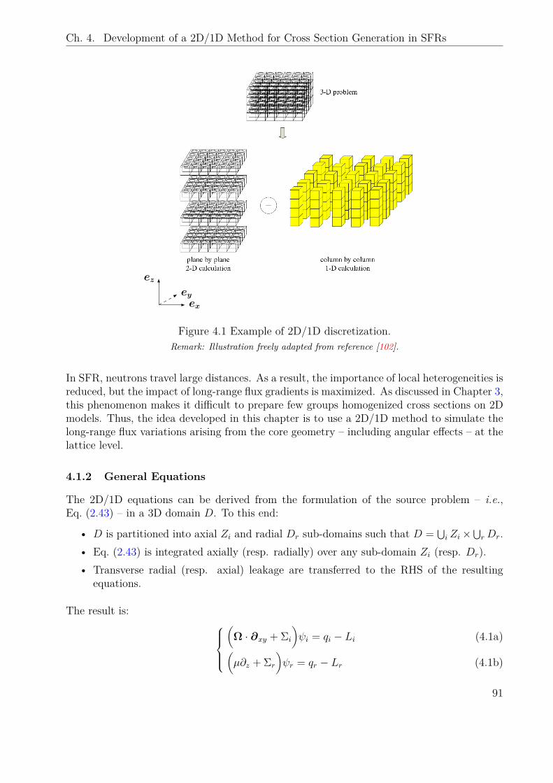
Ch. 4. Development of a 2D/1D Method for Cross Section Generation in SFRs
ez
exey
Figure 4.1 Example of 2D/1D discretization.Remark: Illustration freely adapted from reference [102].
In SFR, neutrons travel large distances. As a result, the importance of local heterogeneities isreduced, but the impact of long-range flux gradients is maximized. As discussed in Chapter 3,this phenomenon makes it difficult to prepare few groups homogenized cross sections on 2Dmodels. Thus, the idea developed in this chapter is to use a 2D/1D method to simulate thelong-range flux variations arising from the core geometry – including angular effects – at thelattice level.
4.1.2 General Equations
The 2D/1D equations can be derived from the formulation of the source problem – i.e.,Eq. (2.43) – in a 3D domain D. To this end:
• D is partitioned into axial Zi and radial Dr sub-domains such that D = ⋃i Zi×
⋃rDr.
• Eq. (2.43) is integrated axially (resp. radially) over any sub-domain Zi (resp. Dr).• Transverse radial (resp. axial) leakage are transferred to the RHS of the resulting
equations.
The result is: (Ω · ∂xy + Σi
)ψi = qi − Li (4.1a)(
µ∂z + Σr
)ψr = qr − Lr (4.1b)
91
Ch. 4. Development of a 2D/1D Method for Cross Section Generation in SFRs
where ψi, ψr are integrated fluxes:ψi(x, y,Ω) =
∫Zidz ψ(r,Ω) (4.2a)
ψr(z,Ω) =∫Drdxdy ψ(r,Ω) (4.2b)
qi, qr are integrated sources: qi(x, y,Ω) =
∫Zidz q(r,Ω) (4.3a)
qr(z,Ω) =∫Drdxdy q(r,Ω) (4.3b)
and Li, Lr are transverse leakage arising from the integration of the transverse gradient term:Li(x, y,Ω) = µ
∫Zidz ∂zψ(r,Ω) (4.4a)
Lr(z,Ω) =∫Drdxdy Ω · ∂xyψ(r,Ω) (4.4b)
In Eq. (4.1a), ∂xy = ex∂∂x
+ ey ∂∂y
is the restriction of the gradient operator to the radialvariables (x,y) while, in Eq. (4.1b), ∂z = ∂
∂zsymbolizes the partial derivative towards z.
Besides, µ = Ω · ez is the polar cosine.Finally, the expressions of the homogenized cross sections Σi and Σr are:
Σi(x, y,Ω) =
∫Zidz Σ(r)ψ(r,Ω)
ψi(x, y,Ω) (4.5a)
Σr(z,Ω) =
∫Drdxdy Σ(r)ψ(r,Ω)
ψr(z,Ω) (4.5b)
In the critical framework (see Sec. 2.1.5), the integrated sources directly read:qi =
(Hi + 1
kFi)ψi (4.6a)
qr =(Hr + 1
kFr)ψr (4.6b)
where the partial operators Hi, Fi, Hr, and Fr are constructed with the appropriate homog-enized cross sections1.At this point, Eq. (4.1a) and Eq. (4.1b) constitute the most general formulation of the 2D/1Dequations. Within this formalism, the new unknowns are the integrated fluxes ψi and ψr.However, these equations cannot be used in practice because transverse leakage Li, Lr andaveraged cross sections Σi, Σr depend on the 3D flux ψ. Thus, approximations are required.
1 The expressions of the homogenized cross sections that appear in the partial scattering and productionoperators are similar to Eq. (4.5a) and Eq. (4.5b).
92
Ch. 4. Development of a 2D/1D Method for Cross Section Generation in SFRs
4.2 Application to the SFR Homogenization Problem
4.2.1 Domain Definition
This chapter does not intend to derive a general 2D/1D method for the purpose of perform-ing whole core calculations, but rather to define an efficient method to produce consistentaveraged cross sections for axially heterogeneous SFR cores. As a result, the geometricaldomain D over which the 2D/1D equations are written only needs to be a subdomain of thecore suited for the computation of representative weight functions (flux moments).In the remaining of this document, it is therefore assumed that D is a periodic lattice ofradially repeated 3D fuel assemblies.Doing so, the influence of the radial reflector is neglected. Nevertheless, it is reasonable toassume that this model is valid for those situations in which axial flux gradients prevail overradial ones. Such conditions are met, for instance, in a CFV, as it was shown in Chapter 3.
4.2.2 Approximations
Transverse leakage
If the radial size of the unit cell of the lattice D is small enough, one can assume that no radialpartitioning is necessary for the 2D/1D equations, but only an axial splitting: D = ⋃
i Zi×Dr.Under these conditions, the assumption of radial periodicity implies that the radial leakagein Eq. (4.4b) is null:
Lr(z,Ω) = 0 (4.7)
Now, to retrieve the value of the axial leakage Li, it can be assumed that, in a SFR, neutronshave quite large mean free paths (up to a few centimeters), and thus, that the leakage radialshape is locally flat2. Hence, Li can be replaced by its averaged value Li:
Li(x, y,Ω) ≈ Li(Ω) def= 1Axy
∫Drdxdy Li(x, y,Ω) (4.8)
where Axy =∫Drdxdy. Using Eq. (4.4a), the axial leakage is finally computed as a function
of the 1D flux ψr with:
Li(Ω) = µ
Axy
∫Zidz ∂zψr(z,Ω) = µ
Axy[ψr(z,Ω)]zi+zi− (4.9)
where Zi = [zi−; zi+].
Homogenized cross sections
The Zi intervals can eventually be chosen so that, in a given layer Zi, cross sections (i.e.,material compositions) are axially invariant:
∀z ∈ Zi, ∂zΣ = 0 (4.10)2 This assumption is probably valid as long as neutrons remain in the fast energy range.
93
Ch. 4. Development of a 2D/1D Method for Cross Section Generation in SFRs
For a fuel assembly composed of fresh fuel pellets (beginning-of-cycle situation), this approx-imation is not so restrictive because the number of axial layers needed to fulfill Eq. (4.10)is typically less than 15. When the assembly burnup3 increases, though, more axial layersare needed to catch the material concentration gradients. This “restriction” is discussed inChapter 5 (cf. Sec. 5.4), when dealing with fuel depletion problems.Inserting Eq. (4.10) in Eq. (4.5a), it is found that, in the end, no homogenization procedureis necessary for the radial cross section:
∀z ∈ Zi, Σi(x, y) = Σ(r) (4.11)
and, therefore, that Σi does not depend on the angular variable.Now, assuming that the change in the radial flux shape is small along Zi, Eq. (4.5b) can bereplaced by an average counterpart:
∀z ∈ Zi, Σr(z,Ω) ≈
∫Zidz∫Drdxdy Σ(r)ψ(r,Ω)∫
Zidz ψr(z,Ω)
(4.12)
Using the assumption of axially invariant cross sections, i.e., Eq. (4.10), and the followingconservation relation: ∫
Zidz ψr(z,Ω) =
∫Drdxdy ψi(x, y,Ω) (4.13)
the axial cross section Σr can finally be obtained through a 2D flux homogenization:
∀z ∈ Zi, Σr(z,Ω) ≈ Σr,i(Ω) =
∫Drdxdy Σ(x, y)ψi(x, y,Ω)∫Drdxdy ψi(x, y,Ω)
(4.14)
4.2.3 Solution of the 2D/1D Equations
At this point, Eq. (4.7), Eq. (4.9), Eq. (4.11) and Eq. (4.14) furnish the closure formulae tothe 2D/1D equations. Once introduced in Eq. (4.1a) – Eq. (4.1b), it can be observed that:
• Eq. (4.1a) forms a 2D equation for flux ψi with imposed external source −Li.• Eq. (4.1b) defines a standard 1D problem for flux ψr with homogenized cross sections
Σr, but without transverse leakage source.
Within the critical framework (see Sec. 2.1.5), qi and qr are replaced by their expressions inEq. (4.6a) – (4.6b). The closed system of 2D/1D equations finally reads:
(Ω · ∂xy + Σ
)ψi =
(Hi + 1
kFi)ψi −
µ
Axy[ψr]zi+zi−, i ∈ 1, 2, . . . (4.15a)(
µ∂z + Σr
)ψr =
(Hr + 1
kFr)ψr (4.15b)
3 The burnup is defined as the energy released per initial mass of heavy nuclei and is an indicator of thefuel aging.
94
Ch. 4. Development of a 2D/1D Method for Cross Section Generation in SFRs
The eigenvalue of the above system (k) can be retrieved from the resolution of Eq. (4.15b),with a standard power method (cf. Sec. 2.2.1). k may, however, be imposed as an externalparameter in Eq. (4.15a) for 2D calculations. Nonetheless, when fissile materials are presentin a layer Zi, outer iterations are required to converge on the fission source distribution Fiψi.Finally, Algo. 6 presents an example of an algorithm that can be set up to solve the 2D/1Dequations4.
Algorithm 6 The 2D/1D Algorithm (general case)Initialization∀i, ψi ← ψ0
i
∀i, initialize 1D cross section Σr,i # Eq. (4.14)Initialize 1D flux ψr and eigenvalue k # Eq. (4.15b)Iterationswhile not converged∗ do∀i, compute leakage source −Li # Eq. (4.9)∀i, compute 2D flux ψi # Eq. (4.15a)∀i, compute 1D cross section Σr,i # Eq. (4.14) with flux momentsCompute 1D flux ψr and eigenvalue k # Eq. (4.15b)
end while
Remark: ∗ In APOLLO3®, the convergence of the algorithm is currently checked on the eigenvalue k. If extracontrol could be easily implemented (e.g., testing sources Li, or 1D fluxes ψr), the k-test is pretty simple andproved to perform well in the scope of this work.
Until now, the energy variable has been omitted. However, it should be understood that, inAlgo. 6, the multigroup descent is embedded within each flux calculation, i.e., in Eq. (4.15a)and Eq. (4.15b). The advantage of this approach – compared to another one in which the2D/1D spatial coupling is wrapped within the multigroup descent – is that it is not intrusivefor 2D and 1D flux solvers. Actually, Algo. 6 allows using the flux solvers as “black-boxes”,i.e., to perform the 2D/1D coupling externally.
4.2.4 Representation of the Angular Variable
Most 2D/1D methods neglect the angular dependences in the homogenized cross sections andtransverse leakage to simplify the resolution of the system. If this “isotropic approximation”might be valid for LWR applications, it was shown in Chapter 3 that the preservation ofanisotropic effects in SFR transport calculations absolutely requires angular information5.In this work, thus, both the homogenized cross section, i.e., Eq. (4.14), and the transverseaxial leakage, i.e., Eq. (4.9), are allowed to depend on the angular variable Ω. The imple-mentation of these dependencies is discussed in Sec. 4.3.2 and Sec. 4.3.3.
4 The algorithm is slightly different than the one presented in reference [98] for the initialization.5 In fact, the “isotropic approximation” was also recently questioned for LWR applications by the MPACT
development team who proposed an improvement of their 2D/1D method through anisotropic transverseleakage and polar angle homogenization [111, 112].
95
Ch. 4. Development of a 2D/1D Method for Cross Section Generation in SFRs
4.2.5 Generation of Few Groups Cross Sections
The method developed in this chapter aims at producing consistent weight functions to per-form the homogenization (including energy condensation) of cross sections in 3D geometries.With this in mind, it is reasonable to prepare the homogenized cross sections on the spatialpartition used for the 2D/1D discretization. Under this assumption, the expression of thehomogenized cross section in macro-region R = Dr × Zi and macro-group G is:
ΣGR =
∫Dr×Zi×G
Σψ∫Dr×Zi×G
ψ(4.16)
where ψ is the 3D flux.
Homogenization with 2D or 1D Fluxes?
At this stage, two strategies are possible: either use the 2D flux ψi or the 1D flux ψr.On the one hand, introducing the assumption of axially invariant cross sections, i.e., Eq. (4.10),in Eq. (4.16) one finds that ψi is indeed a consistent weight:
ΣGR =
∫Dr×G
Σ∫Ziψ∫
Dr×Zi×Gψ
=
∫Dr×G
Σψi∫Dr×G
ψi(4.17)
On the other hand, the introduction of assumption Eq. (4.12) in Eq. (4.16) also allows towrite:
ΣGR =
∫G
Σr,i
∫Ziψr∫
Dr×Zi×Gψ
=
∫Zi×G
Σr,iψr∫Zi×G
ψr(4.18)
i.e., ψr is also a consistent weight for Eq. (4.16). Thus, both formulations are equivalent6.
Comparison with the AP3–SFR–2016 methodology
The main interest of the 2D/1D equations for cross section collapsing is the representationof the angular variable.In standard 2D patterns, high-order angular modes of the flux are often close to zero be-cause anti-symmetric modes with respect to the radial plane are assumed to be null (seeAppendix B), while the use of reflective boundary conditions alters radial moments. As aconsequence, flux angular moments cannot be used to collapse in a consistent way high-ordercross sections – i.e., with Eq. (3.5).
6 In the current implementation of the 2D/1D algorithm in APOLLO3®, the data model does not allowto use the 1D flux to perform the homogenization of microscopic cross sections. Thus, Eq. (4.17) is used.
96
Ch. 4. Development of a 2D/1D Method for Cross Section Generation in SFRs
On the contrary, the 2D/1D framework involves full angular fluxes. In particular, if axialmoments exist in the 3D geometry, the information can be propagated in 2D domains pro-vided that axial leakage Li are allowed to be anisotropic. Thus, consistent flux moments canbe used to collapse cross sections. Nevertheless, this “extra-angular dimensionality” requiresa particular treatment in the flux solvers. This is discussed in Sec. 4.3.Moreover, the algorithm provides a way to compute effective cross sections in media that havea low (or null) intrinsic neutron source (e.g., fertile blankets or shields). Hence, it avoids theconstruction of ad hoc cluster geometries (or external sources as in the ECCO methodology).
4.3 Implementation in APOLLO3®
This section presents how the 2D/1D algorithm (cf. Algo. 6) has been implemented inAPOLLO3® as part of this Ph. D. thesis.
4.3.1 Transport Solvers
As discussed in Sec. 4.2.4, the general formulation of the 2D/1D equations – i.e., (4.15a) and(4.15b) – involves 3D angular representations of fluxes ψi and ψr. However, the trajectorysweep in standard 2D and 1D (MOC) solvers is usually done according to the symmetriespresent in the geometry (see Appendix B). As a consequence, some angular moments areautomatically set to 0 (e.g., angular moments that are anti-symmetric with respect to thecalculation plane) and the actual 3D angular information is lost. So particular solvers arerequired.
2D solver: TDT-B
In order to be consistent with the AP3–SFR–2016 methodology, a MOC solver is chosen tosolve Eq. (4.15a). Since the standard TDT solver of APOLLO3® does not track angles in thefull S2 angular range, a particular treatment is required.Actually, a “B version” of TDT that sweeps polar angles in the full [0;π] range is beingdeveloped in APOLLO3® by S. Santandrea to solve the “heterogeneous B equations” in 2Dgeometries – i.e., Eq. (2.79). Assuming a zero buckling (B = 0), then Eq. (2.79) is, in fact,formally identical to Eq. (4.15a)7. Thus, the TDT-B solver can be used to solve the 2Dequations.Unfortunately, the B version of TDT is still under development and lacks an accelerationtechnique (see Sec. 2.4.2). As a result, the 2D transport solution is not accelerated in thecurrent implementation of the 2D/1D algorithm, thus slowing down its resolution. Never-theless, it should be mentioned that, if the B equations cannot be accelerated (there is notheoretical proof that they can), the standard version of TDT could be used provided thatanti-symmetric angular moments with respect to the calculation plane are not assumed tobe null. Doing so, standard acceleration techniques (DSA or CMFD) could be used8 .
7 The presence of an external source S = −Li does not change the nature of the equation.8 As this manuscript is being written, S. Santandrea is working on this particular point.
97
Ch. 4. Development of a 2D/1D Method for Cross Section Generation in SFRs
1D solver: IDT
With the null radial leakage assumption, i.e., Eq. (4.7), Eq. (4.1b) becomes a standard1D eigenvalue problem and, therefore, is not subject to external angular dependences. Asa result, a standard 1D solver can be used. For this work, the short characteristics IDTsolver [113] implemented in APOLLO3® has been chosen.Strictly speaking, the solution handled by IDT is not exactly ψr, which depends on the angleΩ ∈ S2, but ψr, which depends on the polar cosine µ = Ω ·ez ∈ [−1; 1]. Both functions obeythe following relation:
ψr(z, µ) = 2πψr(z,Ω) (4.19)
4.3.2 Homogenization of 1D Cross Sections
The 2D → 1D coupling is done through the radial homogenization of 2D cross sections withEq. (4.14). A particular feature of this homogenization is that, as discussed in Sec. 4.2.4, anallowance for anisotropy in the homogenized data must be considered.In order to avoid full angular cross section dependences, though, the flux moments weight-ing technique introduced in Sec. 3.2.1 is used. Thus, the consistent angular information istransferred to the homogenized scattering cross section – which is implicit in operator Hr,see Eq. (4.6b) – with Eq. (3.5). Doing so, a conventional expression is kept for the total crosssection (and for high-order scattering cross sections).
4.3.3 Transverse Leakage Projection
The 1D → 2D coupling is done through the transverse leakage projection with Eq. (4.9).In APOLLO3®, this projection is managed through an external source object Si = −Li. Interms of the IDT solution ψr – cf. Eq. (4.19) – Si reads:
Si(Ω) = −Li(Ω) = − µ
Axy[ψr(z,Ω]zi+zi− = − µ
2πAxy[ψr(z, µ)]zi+zi− (4.20)
In particular, the angular dependence of Si is managed through real spherical harmonicsprojections:
Si(Ω) =L∑l=0
2l + 14π
+l∑m=−l
Si,lmRlm(Ω) (4.21)
Since Si does not depend on the azimuthal angle but only on the polar cosine, it is foundthat all the source angular moments Si,lm are null except when m = 0 (see Appendix A):
∀l ∈ N, Si,lm =
−1Axy
∫ +1
µ=−1dµ Pl(µ)µ
[ψr(z, µ)
]zi+zi−
if m = 0,
0 otherwise.(4.22)
Physically, Eq. (4.22) means that the only angular moment that couples the 2D and 1Dproblems is the one that is rotationally invariant around the axial axis ez.
98
Ch. 4. Development of a 2D/1D Method for Cross Section Generation in SFRs
In practice, polynomials moments of the partial fluxes are computed in IDT, up to orderL = 4, at the mesh interfaces zi as:
∀l ∈ 0, 1, ..., L = 4,
α−l (zi) =
∫ 0
−1dµ µl ψr(zi, µ)
α+l (zi) =
∫ 1
0dµ µl ψr(zi, µ)
(4.23)
and, using the definition of Legendre polynomials (see Appendix A), the source moments arecomputed as:
Si,00 = − 1Axy
[α−1 (z) + α+
1 (z)]zi+zi−
Si,10 = − 1Axy
[α−2 (z) + α+
2 (z)]zi+zi−
Si,20 = − 12Axy
[3(α−3 (z) + α+
3 (z))−(α−1 (z) + α+
1 (z))]zi+zi−
Si,30 = − 12Axy
[5(α−4 (z) + α+
4 (z))− 3
(α−2 (z) + α+
2 (z))]zi+zi−
(4.24)
These equations are the ones that have been implemented in APOLLO3® for the calculationof the transverse leakage sources9. The limitation to the P3 Legendre order is assumed to besufficient according to the conclusions of Chapter 3. It explains why the maximal order ofinterface fluxes computed with Eq. 4.23 is L = 4.Finally, the 2D equation that is solved by TDT-B is:(
Ω · ∂xy + Σi
)ψi =
(Hi + 1
kFi)ψi + Si (4.25)
4.3.4 Dealing with Negative Sources
A well-known limitation of the 2D/1D method is that there is no guarantee that the totalneutron source 1
kFiψi + Hiψi + Si appearing in the RHS of equation (4.25) is positive. As
a result, instabilities and even negative fluxes can be found when axial leakage dominatesover fission and scattering contributions. To avoid such instabilities, two “fixups” have beenimplemented in APOLLO3®: a brutal “zero source fixup” and a more conservative “transverseleakage splitting technique”.
Zero source fixup
The zero source fixup consists in neglecting those sources that have a negative isotropiccomponent:
Si,00 = 0 when Si,00 = −∫
4πd2Ω Li(Ω) < 0 (4.26)
No correction is applied to the higher order angular moments of Si in order to preservethe anisotropic information. Even though these high-order angular moments can still pose
9 Strictly speaking, a coefficient 2l + 1 is applied because of the internal data management of the code.
99
Ch. 4. Development of a 2D/1D Method for Cross Section Generation in SFRs
some problems, it has been empirically observed that the method is stable in nearly everycase. However, it does not preserve the neutron balance, so another strategy has also beenconsidered.
Transverse leakage splitting
The “Transverse Leakage Splitting (TLS)” technique has been proposed (and presented atthe PHYTRA-4 conference [99]) a few months after the first implementation of the algorithm.It is inspired by the work of the MPACT development team [109] and consists in replacingnegative sources by additional contributions in the macroscopic total cross section.In that case, whenever the isotropic component of the axial leakage is negative, Eq. (4.25) isreplaced by an equivalent counterpart:(
Ω · ∂xy + Σi
)ψi =
(Hi + 1
kFi)ψi + Si (4.27)
where the modified cross section Σi and source Si read:Σi(x, y) = Σi(x, y)− Si,00
ψi,00(x, y) (4.28a)
Si(x, y,Ω) = Si(Ω)− ψi(x, y,Ω) Si,00
ψi,00(x, y) (4.28b)
and where ψi,00 =∫S2d2Ω ψi is the scalar flux.
With the above definitions – Eq. (4.28a) and Eq. (4.28b) – one can see that Eq. (4.27) isfully consistent with Eq. (4.25): the TLS technique preserves the neutron balance.Moreover, the TLS fixup indeed cancels negative isotropic components of the source becausethe integration of Eq. (4.28b) on the solid angle S2 yields:
Si,00(x, y) =∫S2d2Ω Si(x, y,Ω) = Si,00 − ψi,00(x, y) Si,00
ψi,00(x, y) = 0 (4.29)
Nevertheless, the TLS correction introduces a spatial dependence of the source Si as Eq. (4.28b)shows. Even worse, this correction needs to be updated during the resolution of Eq. (4.27)because it depends on the flux ψi.In APOLLO3® and for convenience purposes, it has been chosen to compute the TLS cor-rection with a mean flux value ψi, which can directly be derived from the IDT 1D solutionψ:
ψi(Ω) = 1Axy
∫Drdxdy ψi(x, y,Ω) = 1
Axy
∫ zi+
zi−dz ψr(z,Ω) = 1
2πAxy
∫ zi+
zi−dz ψr(z, µ) (4.30)
Finally, the TLS correction is directly applied to the source angular moments Si,lm (as opposedto the angular source Si). So, replacing ψ with ψi in Eq. (4.28a) and Eq. (4.28b), the final
100
Ch. 4. Development of a 2D/1D Method for Cross Section Generation in SFRs
form of the TLS becomes:
Σi(x, y) ≈ Σi(x, y)− Si,00∫ zi+
zi−dz ψr,0(z)
× Axy (4.31a)
Si,l0 ≈ Si,l0 −∫ zi+
zi−dz ψr,l(z) Si,00∫ zi+
zi−dz ψr,0(z)
; l ∈ 0, 1, . . . , 4 (4.31b)
4.3.5 Case of Overcritical Layers
The “zero source” and TLS corrections presented above avoid negative fluxes in nearly allsituations. Nevertheless, it has been experimentally observed that negative fluxes would stillappear for high energy neutrons in “over-critical 2D layers”, i.e., planes for which the numberof neutrons produced by fission exceeds the number of neutrons being absorbed (core feedingzones). These planes are characterized by an infinite multiplication factor ki,∞ greater than1:
ki,∞ = < Fiψi >< (Σi −Hi)ψi >
> 1 (4.32)
with < . > the integral over phase-space.A possible reason for these instabilities is that, in the first energy groups where fission neu-trons are born, neutron mean free path values are high, thus inducing high transverse leakagevalues, with a negative isotropic component (i.e., neutrons leak). Even though the “zerosource” and TLS corrections are designed to address these negative sources, the reconstruc-tion of the angular source from its angular moments – cf. Eq. (4.21) – may eventually lead tonegative flux values during the iterative process used to solve Eq. (4.25) (inner iterations). Inparticular, this may occur when anisotropic leakage prevail over the intrinsic source (fission+ scattering) during an iteration10.In order to circumvent this issue without intervening in TDT internal algorithms, an al-lowance is made in the 2D/1D method (Algo. 6): for such overcritical 2D planes, physicalleakage may eventually be replaced by empirical ones substituting the B equation, i.e.,Eq. (2.79), to the real problem, i.e., Eq. (4.25). This choice is rather brutal, but it enlargesthe scope of the method in case negative source fixups fail.So, in the case this choice is made for over-critical planes, the buckling vector B is imposedalong the axial axis to account for axial leakage, and Eq. (2.79) is solved. The bucklingamplitude is not imposed, though, but B2 is adjusted (iteratively) to ensure a local criticalitycondition k(B2) = 1 (standard critical buckling search).While those choices are purely arbitrary, they present the advantage of considerably simpli-fying the 2D/1D algorithm since they imply that overcritical layers can be calculated onceand for all at the beginning of the iterative strategy. In that case, Algo. 6 is replaced byAlgo. 7.
10 These instabilities have never been experienced for subcritical layers (fertile media) nor structures(Fiψi = 0). In these situations, the high energy groups are “fed” with the neutrons coming from the fissilezones, and therefore, transverse leakage sources Si(= −Li) are positive. Negative sources are thereforeobserved only for lower energies, but then, anisotropic effects are less significant.
101
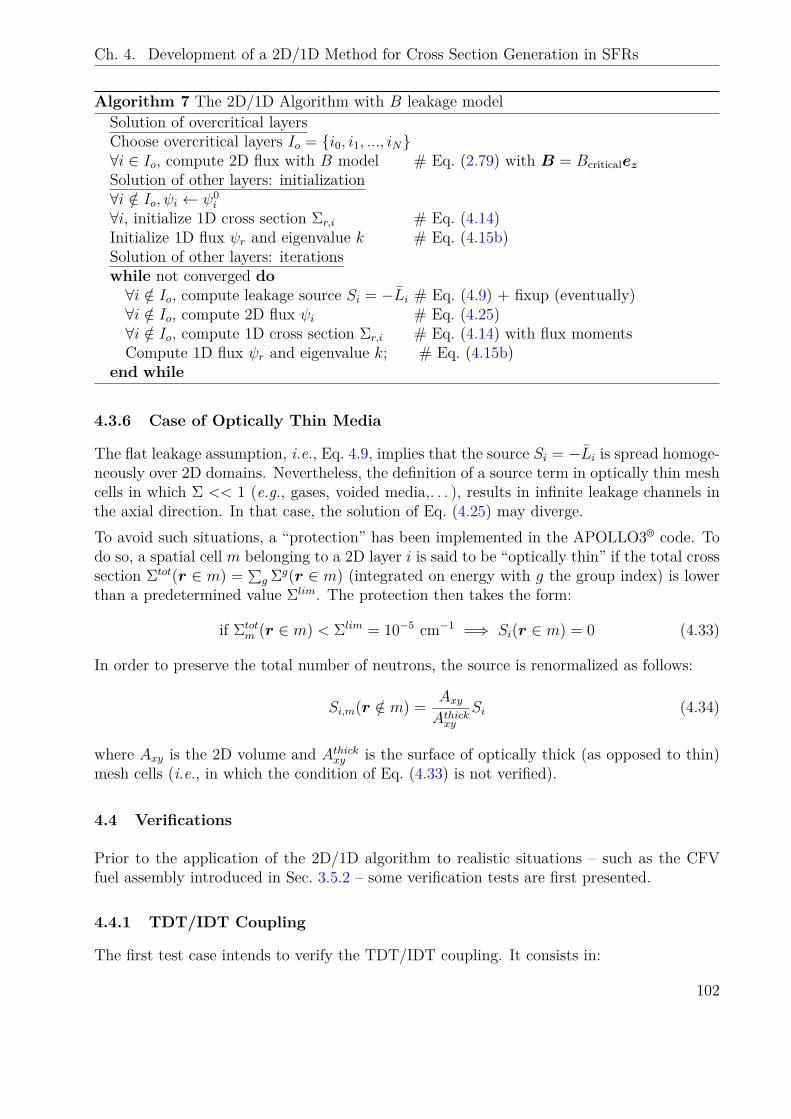
Ch. 4. Development of a 2D/1D Method for Cross Section Generation in SFRs
Algorithm 7 The 2D/1D Algorithm with B leakage modelSolution of overcritical layersChoose overcritical layers Io = i0, i1, ..., iN∀i ∈ Io, compute 2D flux with B model # Eq. (2.79) with B = BcriticalezSolution of other layers: initialization∀i /∈ Io, ψi ← ψ0
i
∀i, initialize 1D cross section Σr,i # Eq. (4.14)Initialize 1D flux ψr and eigenvalue k # Eq. (4.15b)Solution of other layers: iterationswhile not converged do∀i /∈ Io, compute leakage source Si = −Li # Eq. (4.9) + fixup (eventually)∀i /∈ Io, compute 2D flux ψi # Eq. (4.25)∀i /∈ Io, compute 1D cross section Σr,i # Eq. (4.14) with flux momentsCompute 1D flux ψr and eigenvalue k; # Eq. (4.15b)
end while
4.3.6 Case of Optically Thin Media
The flat leakage assumption, i.e., Eq. 4.9, implies that the source Si = −Li is spread homoge-neously over 2D domains. Nevertheless, the definition of a source term in optically thin meshcells in which Σ << 1 (e.g., gases, voided media,. . . ), results in infinite leakage channels inthe axial direction. In that case, the solution of Eq. (4.25) may diverge.To avoid such situations, a “protection” has been implemented in the APOLLO3® code. Todo so, a spatial cell m belonging to a 2D layer i is said to be “optically thin” if the total crosssection Σtot(r ∈ m) = ∑
g Σg(r ∈ m) (integrated on energy with g the group index) is lowerthan a predetermined value Σlim. The protection then takes the form:
if Σtotm (r ∈ m) < Σlim = 10−5 cm−1 =⇒ Si(r ∈ m) = 0 (4.33)
In order to preserve the total number of neutrons, the source is renormalized as follows:
Si,m(r /∈ m) = AxyAthickxy
Si (4.34)
where Axy is the 2D volume and Athickxy is the surface of optically thick (as opposed to thin)mesh cells (i.e., in which the condition of Eq. (4.33) is not verified).
4.4 Verifications
Prior to the application of the 2D/1D algorithm to realistic situations – such as the CFVfuel assembly introduced in Sec. 3.5.2 – some verification tests are first presented.
4.4.1 TDT/IDT Coupling
The first test case intends to verify the TDT/IDT coupling. It consists in:
102
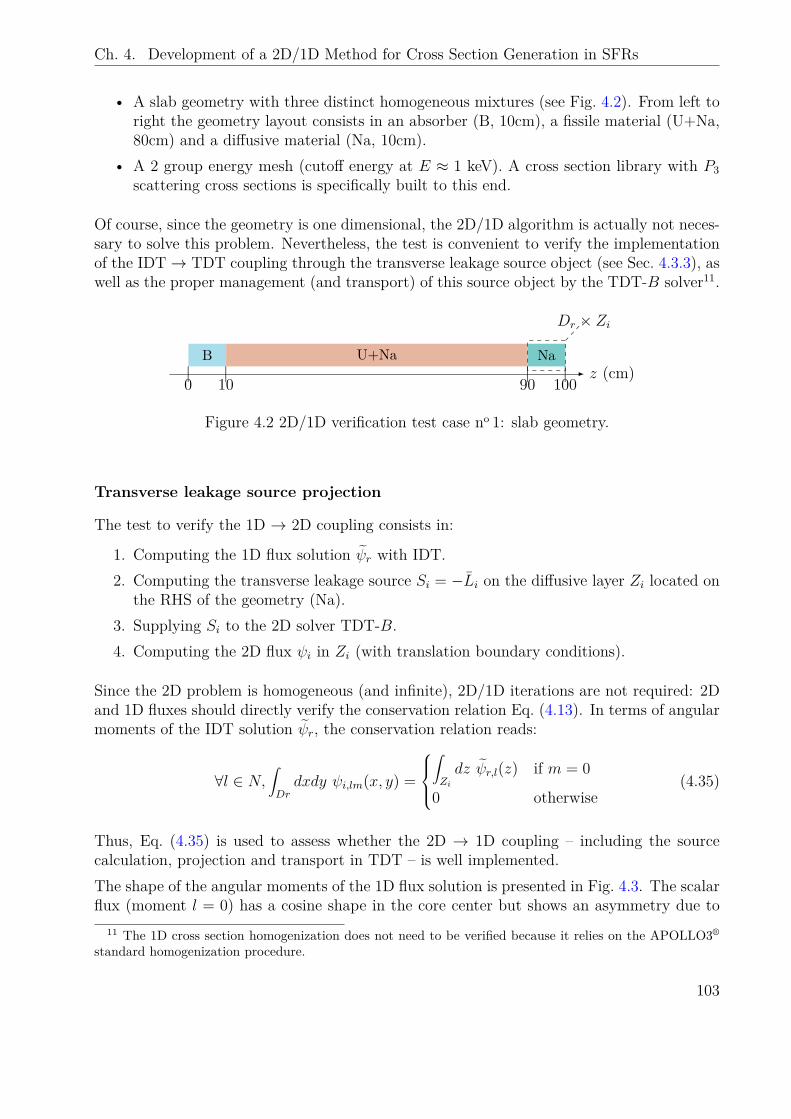
Ch. 4. Development of a 2D/1D Method for Cross Section Generation in SFRs
• A slab geometry with three distinct homogeneous mixtures (see Fig. 4.2). From left toright the geometry layout consists in an absorber (B, 10cm), a fissile material (U+Na,80cm) and a diffusive material (Na, 10cm).
• A 2 group energy mesh (cutoff energy at E ≈ 1 keV). A cross section library with P3scattering cross sections is specifically built to this end.
Of course, since the geometry is one dimensional, the 2D/1D algorithm is actually not neces-sary to solve this problem. Nevertheless, the test is convenient to verify the implementationof the IDT→ TDT coupling through the transverse leakage source object (see Sec. 4.3.3), aswell as the proper management (and transport) of this source object by the TDT-B solver11.
B U+Na Naz (cm)|
0|10
|90
|100
Dr × Zi
Figure 4.2 2D/1D verification test case no 1: slab geometry.
Transverse leakage source projection
The test to verify the 1D → 2D coupling consists in:
1. Computing the 1D flux solution ψr with IDT.2. Computing the transverse leakage source Si = −Li on the diffusive layer Zi located on
the RHS of the geometry (Na).3. Supplying Si to the 2D solver TDT-B.4. Computing the 2D flux ψi in Zi (with translation boundary conditions).
Since the 2D problem is homogeneous (and infinite), 2D/1D iterations are not required: 2Dand 1D fluxes should directly verify the conservation relation Eq. (4.13). In terms of angularmoments of the IDT solution ψr, the conservation relation reads:
∀l ∈ N,∫Drdxdy ψi,lm(x, y) =
∫Zidz ψr,l(z) if m = 0
0 otherwise(4.35)
Thus, Eq. (4.35) is used to assess whether the 2D → 1D coupling – including the sourcecalculation, projection and transport in TDT – is well implemented.The shape of the angular moments of the 1D flux solution is presented in Fig. 4.3. The scalarflux (moment l = 0) has a cosine shape in the core center but shows an asymmetry due to
11 The 1D cross section homogenization does not need to be verified because it relies on the APOLLO3®
standard homogenization procedure.
103
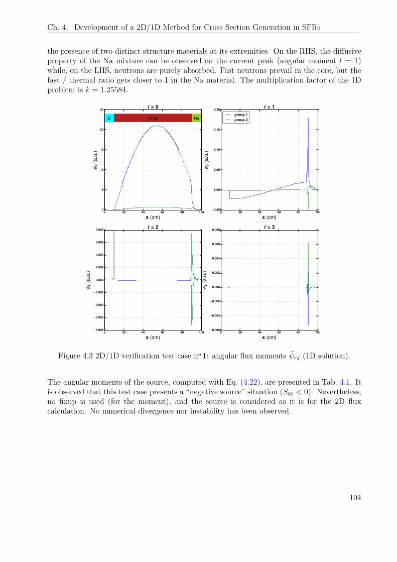
Ch. 4. Development of a 2D/1D Method for Cross Section Generation in SFRs
the presence of two distinct structure materials at its extremities. On the RHS, the diffusiveproperty of the Na mixture can be observed on the current peak (angular moment l = 1)while, on the LHS, neutrons are purely absorbed. Fast neutrons prevail in the core, but thefast / thermal ratio gets closer to 1 in the Na material. The multiplication factor of the 1Dproblem is k = 1.25584.
0 20 40 60 80 100
x (cm)
0
5
10
15
20
25
ψr
(a.u
.)
B U+Na Na
l = 0
0 20 40 60 80 100
x (cm)
−0.05
0.00
0.05
0.10
0.15
0.20
ψr
(a.u
.)
l = 1group 1group 2
0 20 40 60 80 100
x (cm)
−0.008
−0.006
−0.004
−0.002
0.000
0.002
0.004
0.006
0.008
ψr
(a.u
.)
l = 2
0 20 40 60 80 100
x (cm)
−0.006
−0.004
−0.002
0.000
0.002
0.004
0.006
0.008
ψr
(a.u
.)
l = 3
Figure 4.3 2D/1D verification test case no 1: angular flux moments ψr,l (1D solution).
The angular moments of the source, computed with Eq. (4.22), are presented in Tab. 4.1. Itis observed that this test case presents a “negative source” situation (S00 < 0). Nevertheless,no fixup is used (for the moment), and the source is considered as it is for the 2D fluxcalculation. No numerical divergence nor instability has been observed.
104
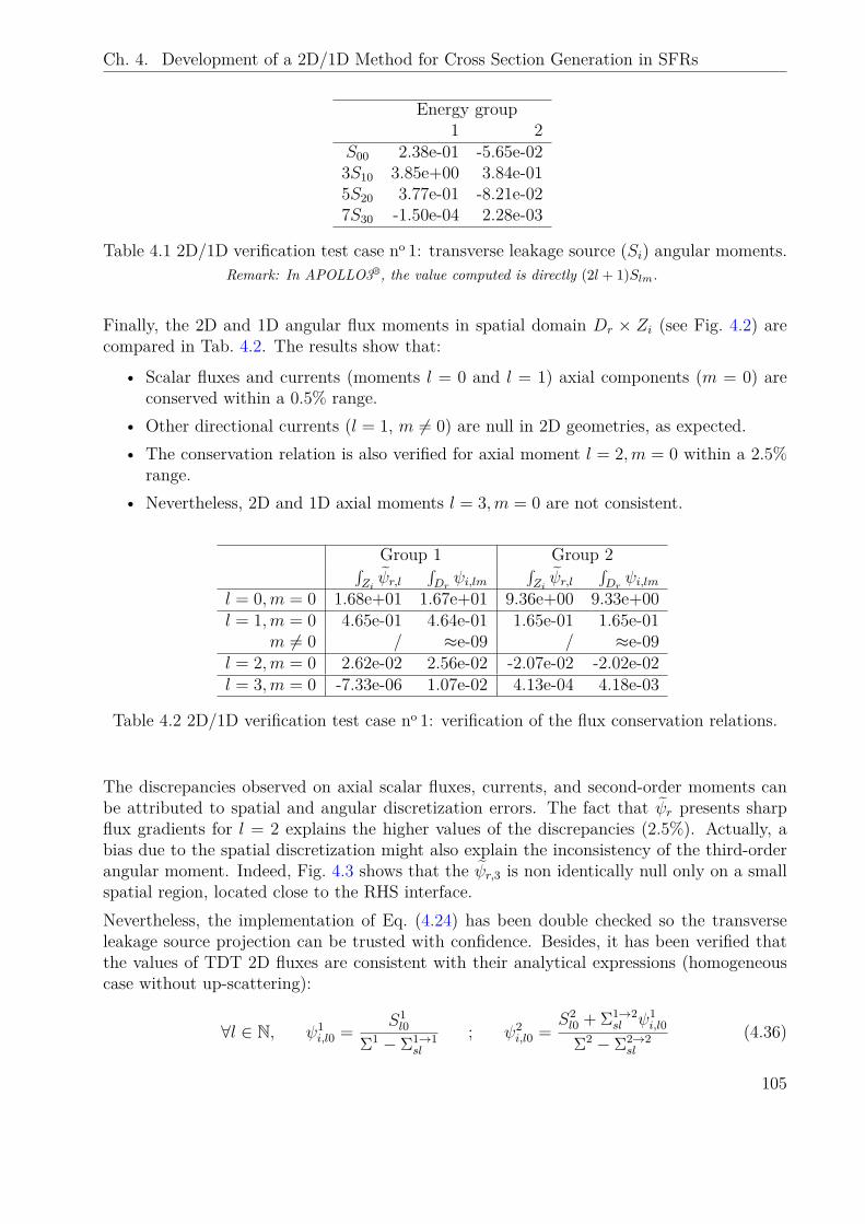
Ch. 4. Development of a 2D/1D Method for Cross Section Generation in SFRs
Energy group1 2
S00 2.38e-01 -5.65e-023S10 3.85e+00 3.84e-015S20 3.77e-01 -8.21e-027S30 -1.50e-04 2.28e-03
Table 4.1 2D/1D verification test case no 1: transverse leakage source (Si) angular moments.Remark: In APOLLO3®, the value computed is directly (2l + 1)Slm.
Finally, the 2D and 1D angular flux moments in spatial domain Dr × Zi (see Fig. 4.2) arecompared in Tab. 4.2. The results show that:
• Scalar fluxes and currents (moments l = 0 and l = 1) axial components (m = 0) areconserved within a 0.5% range.
• Other directional currents (l = 1, m 6= 0) are null in 2D geometries, as expected.• The conservation relation is also verified for axial moment l = 2,m = 0 within a 2.5%
range.• Nevertheless, 2D and 1D axial moments l = 3,m = 0 are not consistent.
Group 1 Group 2∫Ziψr,l
∫Drψi,lm
∫Ziψr,l
∫Drψi,lm
l = 0,m = 0 1.68e+01 1.67e+01 9.36e+00 9.33e+00l = 1,m = 0 4.65e-01 4.64e-01 1.65e-01 1.65e-01
m 6= 0 / ≈e-09 / ≈e-09l = 2,m = 0 2.62e-02 2.56e-02 -2.07e-02 -2.02e-02l = 3,m = 0 -7.33e-06 1.07e-02 4.13e-04 4.18e-03
Table 4.2 2D/1D verification test case no 1: verification of the flux conservation relations.
The discrepancies observed on axial scalar fluxes, currents, and second-order moments canbe attributed to spatial and angular discretization errors. The fact that ψr presents sharpflux gradients for l = 2 explains the higher values of the discrepancies (2.5%). Actually, abias due to the spatial discretization might also explain the inconsistency of the third-orderangular moment. Indeed, Fig. 4.3 shows that the ψr,3 is non identically null only on a smallspatial region, located close to the RHS interface.Nevertheless, the implementation of Eq. (4.24) has been double checked so the transverseleakage source projection can be trusted with confidence. Besides, it has been verified thatthe values of TDT 2D fluxes are consistent with their analytical expressions (homogeneouscase without up-scattering):
∀l ∈ N, ψ1i,l0 = S1
l0Σ1 − Σ1→1
sl
; ψ2i,l0 =
S2l0 + Σ1→2
sl ψ1i,l0
Σ2 − Σ2→2sl
(4.36)
105
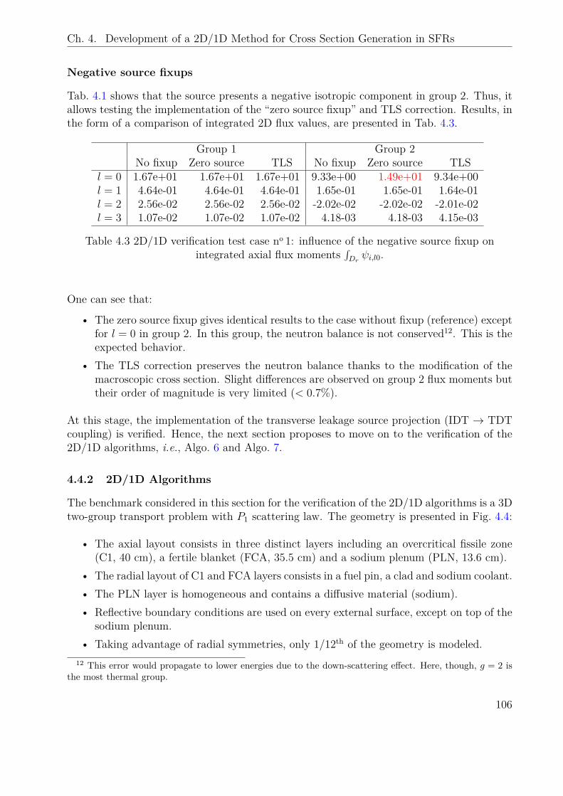
Ch. 4. Development of a 2D/1D Method for Cross Section Generation in SFRs
Negative source fixups
Tab. 4.1 shows that the source presents a negative isotropic component in group 2. Thus, itallows testing the implementation of the “zero source fixup” and TLS correction. Results, inthe form of a comparison of integrated 2D flux values, are presented in Tab. 4.3.
Group 1 Group 2No fixup Zero source TLS No fixup Zero source TLS
l = 0 1.67e+01 1.67e+01 1.67e+01 9.33e+00 1.49e+01 9.34e+00l = 1 4.64e-01 4.64e-01 4.64e-01 1.65e-01 1.65e-01 1.64e-01l = 2 2.56e-02 2.56e-02 2.56e-02 -2.02e-02 -2.02e-02 -2.01e-02l = 3 1.07e-02 1.07e-02 1.07e-02 4.18-03 4.18-03 4.15e-03
Table 4.3 2D/1D verification test case no 1: influence of the negative source fixup onintegrated axial flux moments
∫Drψi,l0.
One can see that:
• The zero source fixup gives identical results to the case without fixup (reference) exceptfor l = 0 in group 2. In this group, the neutron balance is not conserved12. This is theexpected behavior.
• The TLS correction preserves the neutron balance thanks to the modification of themacroscopic cross section. Slight differences are observed on group 2 flux moments buttheir order of magnitude is very limited (< 0.7%).
At this stage, the implementation of the transverse leakage source projection (IDT → TDTcoupling) is verified. Hence, the next section proposes to move on to the verification of the2D/1D algorithms, i.e., Algo. 6 and Algo. 7.
4.4.2 2D/1D Algorithms
The benchmark considered in this section for the verification of the 2D/1D algorithms is a 3Dtwo-group transport problem with P1 scattering law. The geometry is presented in Fig. 4.4:
• The axial layout consists in three distinct layers including an overcritical fissile zone(C1, 40 cm), a fertile blanket (FCA, 35.5 cm) and a sodium plenum (PLN, 13.6 cm).
• The radial layout of C1 and FCA layers consists in a fuel pin, a clad and sodium coolant.• The PLN layer is homogeneous and contains a diffusive material (sodium).• Reflective boundary conditions are used on every external surface, except on top of the
sodium plenum.• Taking advantage of radial symmetries, only 1/12th of the geometry is modeled.
12 This error would propagate to lower energies due to the down-scattering effect. Here, though, g = 2 isthe most thermal group.
106
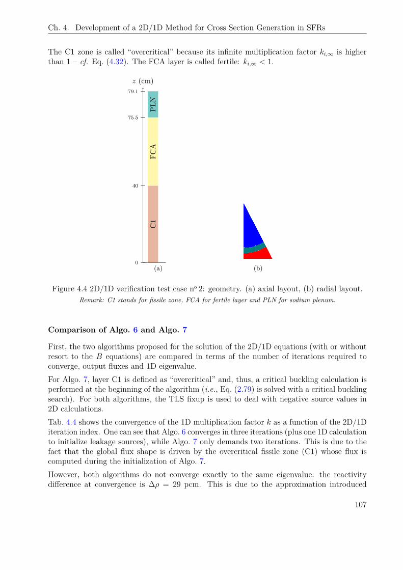
Ch. 4. Development of a 2D/1D Method for Cross Section Generation in SFRs
The C1 zone is called “overcritical” because its infinite multiplication factor ki,∞ is higherthan 1 – cf. Eq. (4.32). The FCA layer is called fertile: ki,∞ < 1.
C1
FCA
PLN
(a)
z (cm)
0
40
75.5
79.1
(b)
Figure 4.4 2D/1D verification test case no 2: geometry. (a) axial layout, (b) radial layout.Remark: C1 stands for fissile zone, FCA for fertile layer and PLN for sodium plenum.
Comparison of Algo. 6 and Algo. 7
First, the two algorithms proposed for the solution of the 2D/1D equations (with or withoutresort to the B equations) are compared in terms of the number of iterations required toconverge, output fluxes and 1D eigenvalue.For Algo. 7, layer C1 is defined as “overcritical” and, thus, a critical buckling calculation isperformed at the beginning of the algorithm (i.e., Eq. (2.79) is solved with a critical bucklingsearch). For both algorithms, the TLS fixup is used to deal with negative source values in2D calculations.Tab. 4.4 shows the convergence of the 1D multiplication factor k as a function of the 2D/1Diteration index. One can see that Algo. 6 converges in three iterations (plus one 1D calculationto initialize leakage sources), while Algo. 7 only demands two iterations. This is due to thefact that the global flux shape is driven by the overcritical fissile zone (C1) whose flux iscomputed during the initialization of Algo. 7.However, both algorithms do not converge exactly to the same eigenvalue: the reactivitydifference at convergence is ∆ρ = 29 pcm. This is due to the approximation introduced
107
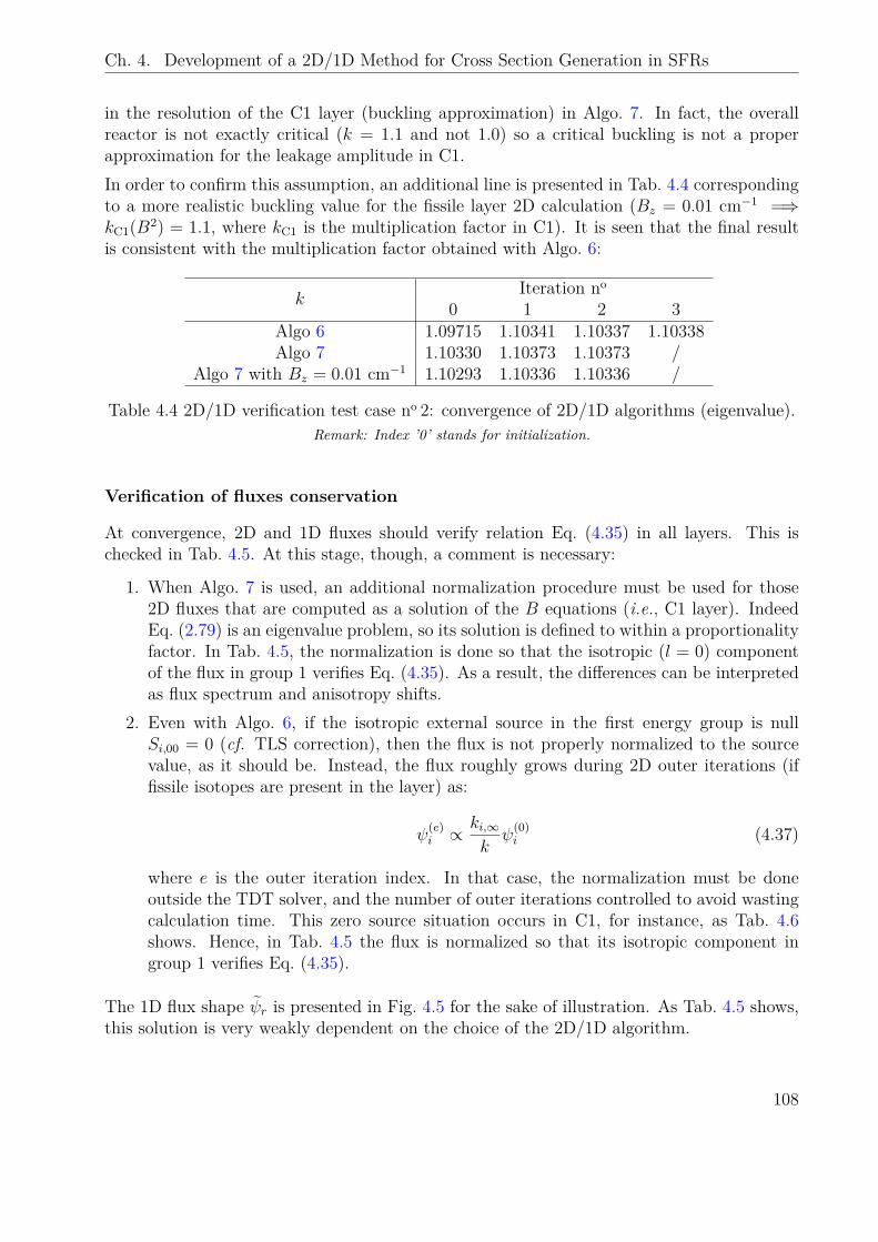
Ch. 4. Development of a 2D/1D Method for Cross Section Generation in SFRs
in the resolution of the C1 layer (buckling approximation) in Algo. 7. In fact, the overallreactor is not exactly critical (k = 1.1 and not 1.0) so a critical buckling is not a properapproximation for the leakage amplitude in C1.In order to confirm this assumption, an additional line is presented in Tab. 4.4 correspondingto a more realistic buckling value for the fissile layer 2D calculation (Bz = 0.01 cm−1 =⇒kC1(B2) = 1.1, where kC1 is the multiplication factor in C1). It is seen that the final resultis consistent with the multiplication factor obtained with Algo. 6:
kIteration no
0 1 2 3Algo 6 1.09715 1.10341 1.10337 1.10338Algo 7 1.10330 1.10373 1.10373 /
Algo 7 with Bz = 0.01 cm−1 1.10293 1.10336 1.10336 /
Table 4.4 2D/1D verification test case no 2: convergence of 2D/1D algorithms (eigenvalue).Remark: Index ’0’ stands for initialization.
Verification of fluxes conservation
At convergence, 2D and 1D fluxes should verify relation Eq. (4.35) in all layers. This ischecked in Tab. 4.5. At this stage, though, a comment is necessary:
1. When Algo. 7 is used, an additional normalization procedure must be used for those2D fluxes that are computed as a solution of the B equations (i.e., C1 layer). IndeedEq. (2.79) is an eigenvalue problem, so its solution is defined to within a proportionalityfactor. In Tab. 4.5, the normalization is done so that the isotropic (l = 0) componentof the flux in group 1 verifies Eq. (4.35). As a result, the differences can be interpretedas flux spectrum and anisotropy shifts.
2. Even with Algo. 6, if the isotropic external source in the first energy group is nullSi,00 = 0 (cf. TLS correction), then the flux is not properly normalized to the sourcevalue, as it should be. Instead, the flux roughly grows during 2D outer iterations (iffissile isotopes are present in the layer) as:
ψ(e)i ∝
ki,∞kψ
(0)i (4.37)
where e is the outer iteration index. In that case, the normalization must be doneoutside the TDT solver, and the number of outer iterations controlled to avoid wastingcalculation time. This zero source situation occurs in C1, for instance, as Tab. 4.6shows. Hence, in Tab. 4.5 the flux is normalized so that its isotropic component ingroup 1 verifies Eq. (4.35).
The 1D flux shape ψr is presented in Fig. 4.5 for the sake of illustration. As Tab. 4.5 shows,this solution is very weakly dependent on the choice of the 2D/1D algorithm.
108
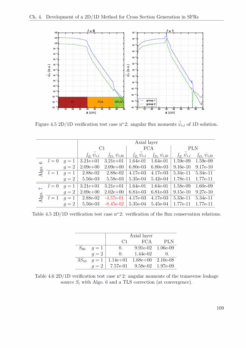
Ch. 4. Development of a 2D/1D Method for Cross Section Generation in SFRs
0 10 20 30 40 50 60 70 80 90
x (cm)
10−12
10−11
10−10
10−9
10−8
10−7
10−6
10−5
10−4
10−3
10−2
10−1
100
101
102
ψr
(a.u
.)
C1 FCA SPLN
l = 0
0 10 20 30 40 50 60 70 80 90
x (cm)
10−13
10−12
10−11
10−10
10−9
10−8
10−7
10−6
10−5
10−4
10−3
10−2
10−1
ψr
(a.u
.)
l = 1
group 1group 2
Figure 4.5 2D/1D verification test case no 2: angular flux moments ψr,l of 1D solution.
Axial layerC1 FCA PLN∫
Ziψr,l
∫Drψi,l0
∫Ziψr,l
∫Drψi,l0
∫Ziψr,l
∫Drψi,l0
Algo.
6 l = 0 g = 1 3.21e+01 3.21e+01 1.64e-01 1.64e-01 1.59e-09 1.59e-09g = 2 2.09e+00 2.09e+00 6.80e-03 6.80e-03 9.16e-10 9.17e-10
l = 1 g = 1 2.88e-02 2.88e-02 4.17e-03 4.17e-03 5.34e-11 5.34e-11g = 2 5.56e-03 5.58e-03 5.35e-04 5.42e-04 1.78e-11 1.77e-11
Algo.
7 l = 0 g = 1 3.21e+01 3.21e+01 1.64e-01 1.64e-01 1.58e-09 1.60e-09g = 2 2.09e+00 2.02e+00 6.81e-03 6.81e-03 9.15e-10 9.27e-10
l = 1 g = 1 2.88e-02 -4.57e-01 4.17e-03 4.17e-03 5.33e-11 5.34e-11g = 2 5.56e-03 -8.45e-02 5.35e-04 5.45e-04 1.77e-11 1.77e-11
Table 4.5 2D/1D verification test case no 2: verification of the flux conservation relations.
Axial layerC1 FCA PLN
S00 g = 1 0. 9.91e-02 1.06e-09g = 2 0. 1.44e-02 0.
3S10 g = 1 1.14e+01 1.68e+00 2.10e-08g = 2 7.57e-01 9.58e-02 1.97e-09
Table 4.6 2D/1D verification test case no 2: angular moments of the transverse leakagesource Si with Algo. 6 and a TLS correction (at convergence).
109
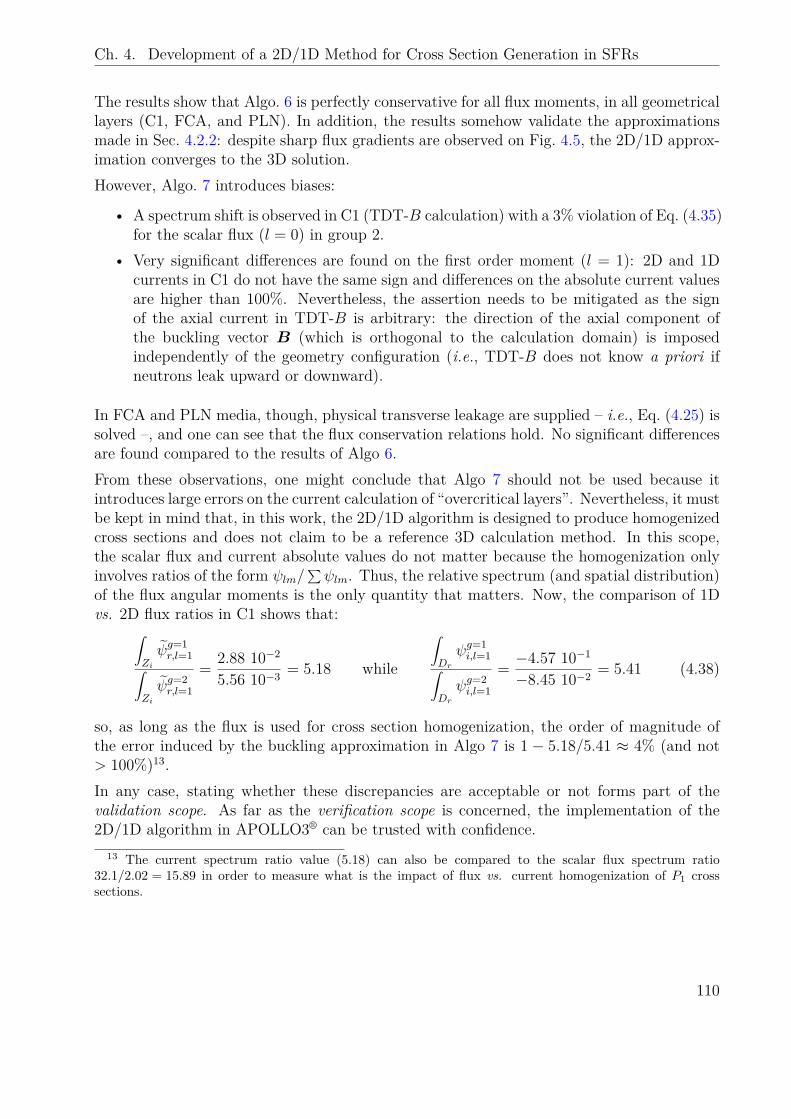
Ch. 4. Development of a 2D/1D Method for Cross Section Generation in SFRs
The results show that Algo. 6 is perfectly conservative for all flux moments, in all geometricallayers (C1, FCA, and PLN). In addition, the results somehow validate the approximationsmade in Sec. 4.2.2: despite sharp flux gradients are observed on Fig. 4.5, the 2D/1D approx-imation converges to the 3D solution.However, Algo. 7 introduces biases:
• A spectrum shift is observed in C1 (TDT-B calculation) with a 3% violation of Eq. (4.35)for the scalar flux (l = 0) in group 2.
• Very significant differences are found on the first order moment (l = 1): 2D and 1Dcurrents in C1 do not have the same sign and differences on the absolute current valuesare higher than 100%. Nevertheless, the assertion needs to be mitigated as the signof the axial current in TDT-B is arbitrary: the direction of the axial component ofthe buckling vector B (which is orthogonal to the calculation domain) is imposedindependently of the geometry configuration (i.e., TDT-B does not know a priori ifneutrons leak upward or downward).
In FCA and PLN media, though, physical transverse leakage are supplied – i.e., Eq. (4.25) issolved –, and one can see that the flux conservation relations hold. No significant differencesare found compared to the results of Algo 6.From these observations, one might conclude that Algo 7 should not be used because itintroduces large errors on the current calculation of “overcritical layers”. Nevertheless, it mustbe kept in mind that, in this work, the 2D/1D algorithm is designed to produce homogenizedcross sections and does not claim to be a reference 3D calculation method. In this scope,the scalar flux and current absolute values do not matter because the homogenization onlyinvolves ratios of the form ψlm/
∑ψlm. Thus, the relative spectrum (and spatial distribution)
of the flux angular moments is the only quantity that matters. Now, the comparison of 1Dvs. 2D flux ratios in C1 shows that:∫
Ziψg=1r,l=1∫
Ziψg=2r,l=1
= 2.88 10−2
5.56 10−3 = 5.18 while
∫Drψg=1i,l=1∫
Drψg=2i,l=1
= −4.57 10−1
−8.45 10−2 = 5.41 (4.38)
so, as long as the flux is used for cross section homogenization, the order of magnitude ofthe error induced by the buckling approximation in Algo 7 is 1 − 5.18/5.41 ≈ 4% (and not> 100%)13.In any case, stating whether these discrepancies are acceptable or not forms part of thevalidation scope. As far as the verification scope is concerned, the implementation of the2D/1D algorithm in APOLLO3® can be trusted with confidence.
13 The current spectrum ratio value (5.18) can also be compared to the scalar flux spectrum ratio32.1/2.02 = 15.89 in order to measure what is the impact of flux vs. current homogenization of P1 crosssections.
110
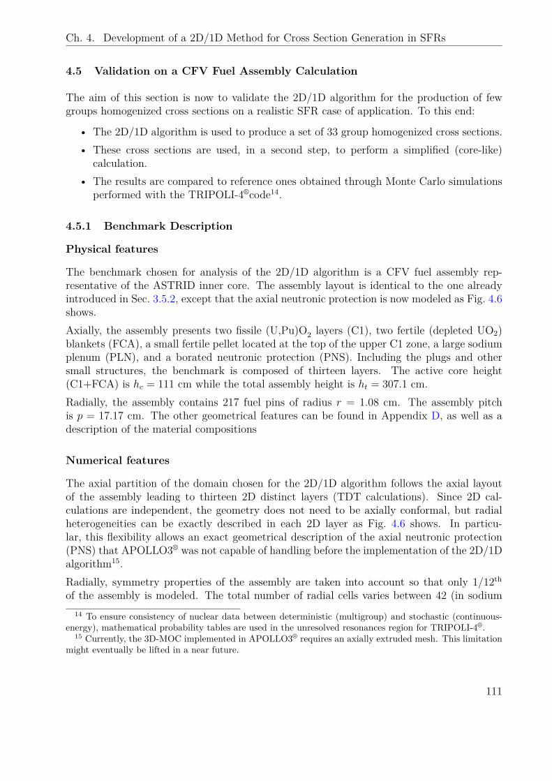
Ch. 4. Development of a 2D/1D Method for Cross Section Generation in SFRs
4.5 Validation on a CFV Fuel Assembly Calculation
The aim of this section is now to validate the 2D/1D algorithm for the production of fewgroups homogenized cross sections on a realistic SFR case of application. To this end:
• The 2D/1D algorithm is used to produce a set of 33 group homogenized cross sections.• These cross sections are used, in a second step, to perform a simplified (core-like)
calculation.• The results are compared to reference ones obtained through Monte Carlo simulations
performed with the TRIPOLI-4®code14.
4.5.1 Benchmark Description
Physical features
The benchmark chosen for analysis of the 2D/1D algorithm is a CFV fuel assembly rep-resentative of the ASTRID inner core. The assembly layout is identical to the one alreadyintroduced in Sec. 3.5.2, except that the axial neutronic protection is now modeled as Fig. 4.6shows.Axially, the assembly presents two fissile (U,Pu)O2 layers (C1), two fertile (depleted UO2)blankets (FCA), a small fertile pellet located at the top of the upper C1 zone, a large sodiumplenum (PLN), and a borated neutronic protection (PNS). Including the plugs and othersmall structures, the benchmark is composed of thirteen layers. The active core height(C1+FCA) is hc = 111 cm while the total assembly height is ht = 307.1 cm.Radially, the assembly contains 217 fuel pins of radius r = 1.08 cm. The assembly pitchis p = 17.17 cm. The other geometrical features can be found in Appendix D, as well as adescription of the material compositions
Numerical features
The axial partition of the domain chosen for the 2D/1D algorithm follows the axial layoutof the assembly leading to thirteen 2D distinct layers (TDT calculations). Since 2D cal-culations are independent, the geometry does not need to be axially conformal, but radialheterogeneities can be exactly described in each 2D layer as Fig. 4.6 shows. In particu-lar, this flexibility allows an exact geometrical description of the axial neutronic protection(PNS) that APOLLO3® was not capable of handling before the implementation of the 2D/1Dalgorithm15.Radially, symmetry properties of the assembly are taken into account so that only 1/12thof the assembly is modeled. The total number of radial cells varies between 42 (in sodium
14 To ensure consistency of nuclear data between deterministic (multigroup) and stochastic (continuous-energy), mathematical probability tables are used in the unresolved resonances region for TRIPOLI-4®.
15 Currently, the 3D-MOC implemented in APOLLO3® requires an axially extruded mesh. This limitationmight eventually be lifted in a near future.
111
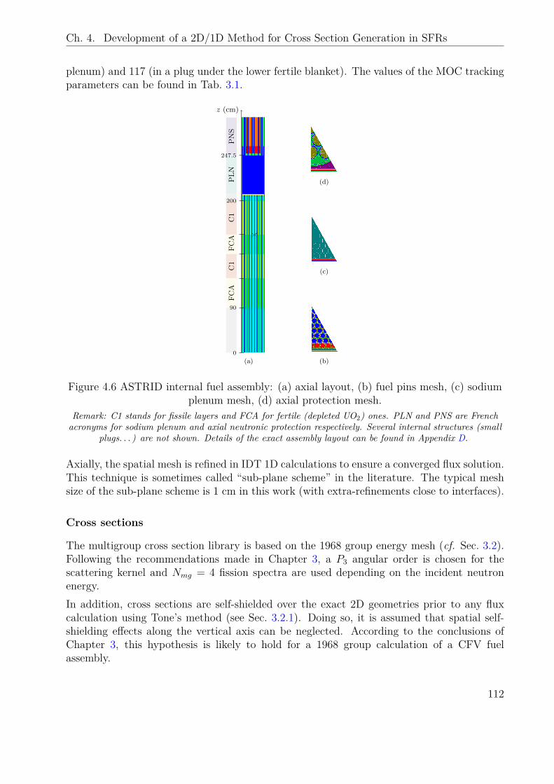
Ch. 4. Development of a 2D/1D Method for Cross Section Generation in SFRs
plenum) and 117 (in a plug under the lower fertile blanket). The values of the MOC trackingparameters can be found in Tab. 3.1.
ZFCA
C1
FCA
C1
ZPLN
PNS
(a)
z (cm)
0
90
200
247.5
(b)
(c)
(d)
Figure 4.6 ASTRID internal fuel assembly: (a) axial layout, (b) fuel pins mesh, (c) sodiumplenum mesh, (d) axial protection mesh.
Remark: C1 stands for fissile layers and FCA for fertile (depleted UO2) ones. PLN and PNS are Frenchacronyms for sodium plenum and axial neutronic protection respectively. Several internal structures (small
plugs. . . ) are not shown. Details of the exact assembly layout can be found in Appendix D.
Axially, the spatial mesh is refined in IDT 1D calculations to ensure a converged flux solution.This technique is sometimes called “sub-plane scheme” in the literature. The typical meshsize of the sub-plane scheme is 1 cm in this work (with extra-refinements close to interfaces).
Cross sections
The multigroup cross section library is based on the 1968 group energy mesh (cf. Sec. 3.2).Following the recommendations made in Chapter 3, a P3 angular order is chosen for thescattering kernel and Nmg = 4 fission spectra are used depending on the incident neutronenergy.In addition, cross sections are self-shielded over the exact 2D geometries prior to any fluxcalculation using Tone’s method (see Sec. 3.2.1). Doing so, it is assumed that spatial self-shielding effects along the vertical axis can be neglected. According to the conclusions ofChapter 3, this hypothesis is likely to hold for a 1968 group calculation of a CFV fuelassembly.
112
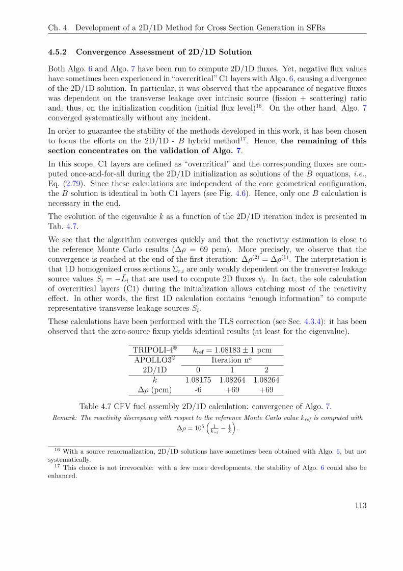
Ch. 4. Development of a 2D/1D Method for Cross Section Generation in SFRs
4.5.2 Convergence Assessment of 2D/1D Solution
Both Algo. 6 and Algo. 7 have been run to compute 2D/1D fluxes. Yet, negative flux valueshave sometimes been experienced in “overcritical” C1 layers with Algo. 6, causing a divergenceof the 2D/1D solution. In particular, it was observed that the appearance of negative fluxeswas dependent on the transverse leakage over intrinsic source (fission + scattering) ratioand, thus, on the initialization condition (initial flux level)16. On the other hand, Algo. 7converged systematically without any incident.In order to guarantee the stability of the methods developed in this work, it has been chosento focus the efforts on the 2D/1D - B hybrid method17. Hence, the remaining of thissection concentrates on the validation of Algo. 7.In this scope, C1 layers are defined as “overcritical” and the corresponding fluxes are com-puted once-and-for-all during the 2D/1D initialization as solutions of the B equations, i.e.,Eq. (2.79). Since these calculations are independent of the core geometrical configuration,the B solution is identical in both C1 layers (see Fig. 4.6). Hence, only one B calculation isnecessary in the end.The evolution of the eigenvalue k as a function of the 2D/1D iteration index is presented inTab. 4.7.We see that the algorithm converges quickly and that the reactivity estimation is close tothe reference Monte Carlo results (∆ρ = 69 pcm). More precisely, we observe that theconvergence is reached at the end of the first iteration: ∆ρ(2) = ∆ρ(1). The interpretation isthat 1D homogenized cross sections Σr,i are only weakly dependent on the transverse leakagesource values Si = −Li that are used to compute 2D fluxes ψi. In fact, the sole calculationof overcritical layers (C1) during the initialization allows catching most of the reactivityeffect. In other words, the first 1D calculation contains “enough information” to computerepresentative transverse leakage sources Si.These calculations have been performed with the TLS correction (see Sec. 4.3.4): it has beenobserved that the zero-source fixup yields identical results (at least for the eigenvalue).
TRIPOLI-4® kref = 1.08183± 1 pcmAPOLLO3® Iteration no
2D/1D 0 1 2k 1.08175 1.08264 1.08264
∆ρ (pcm) -6 +69 +69
Table 4.7 CFV fuel assembly 2D/1D calculation: convergence of Algo. 7.Remark: The reactivity discrepancy with respect to the reference Monte Carlo value kref is computed with
∆ρ = 105(
1kref− 1
k
).
16 With a source renormalization, 2D/1D solutions have sometimes been obtained with Algo. 6, but notsystematically.
17 This choice is not irrevocable: with a few more developments, the stability of Algo. 6 could also beenhanced.
113
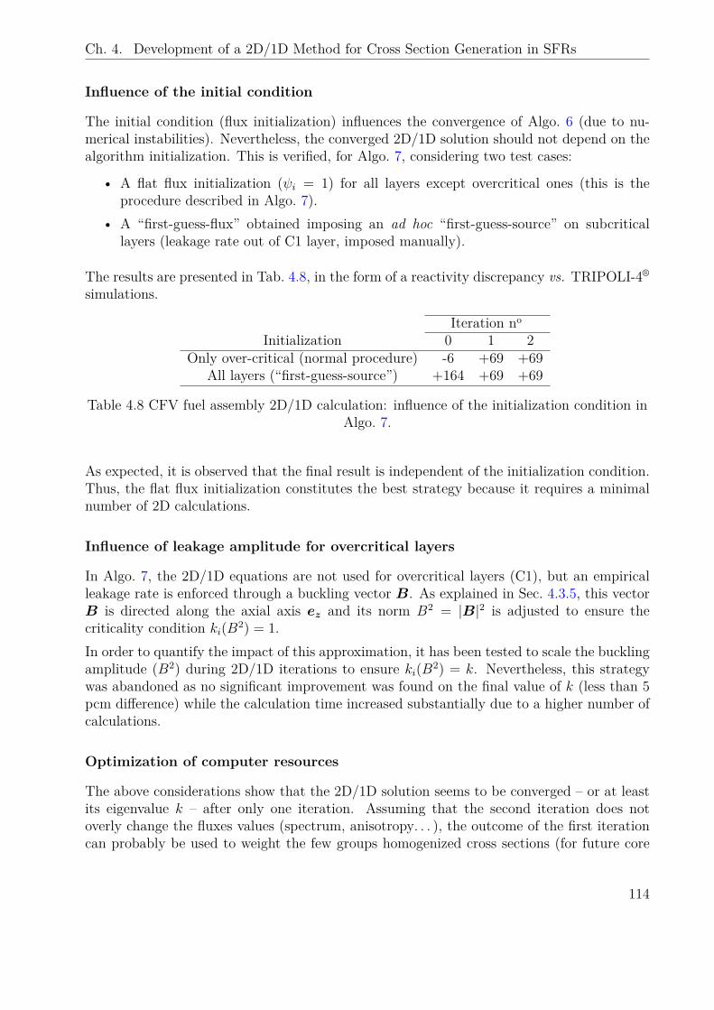
Ch. 4. Development of a 2D/1D Method for Cross Section Generation in SFRs
Influence of the initial condition
The initial condition (flux initialization) influences the convergence of Algo. 6 (due to nu-merical instabilities). Nevertheless, the converged 2D/1D solution should not depend on thealgorithm initialization. This is verified, for Algo. 7, considering two test cases:
• A flat flux initialization (ψi = 1) for all layers except overcritical ones (this is theprocedure described in Algo. 7).
• A “first-guess-flux” obtained imposing an ad hoc “first-guess-source” on subcriticallayers (leakage rate out of C1 layer, imposed manually).
The results are presented in Tab. 4.8, in the form of a reactivity discrepancy vs. TRIPOLI-4®
simulations.
Iteration noInitialization 0 1 2
Only over-critical (normal procedure) -6 +69 +69All layers (“first-guess-source”) +164 +69 +69
Table 4.8 CFV fuel assembly 2D/1D calculation: influence of the initialization condition inAlgo. 7.
As expected, it is observed that the final result is independent of the initialization condition.Thus, the flat flux initialization constitutes the best strategy because it requires a minimalnumber of 2D calculations.
Influence of leakage amplitude for overcritical layers
In Algo. 7, the 2D/1D equations are not used for overcritical layers (C1), but an empiricalleakage rate is enforced through a buckling vector B. As explained in Sec. 4.3.5, this vectorB is directed along the axial axis ez and its norm B2 = |B|2 is adjusted to ensure thecriticality condition ki(B2) = 1.In order to quantify the impact of this approximation, it has been tested to scale the bucklingamplitude (B2) during 2D/1D iterations to ensure ki(B2) = k. Nevertheless, this strategywas abandoned as no significant improvement was found on the final value of k (less than 5pcm difference) while the calculation time increased substantially due to a higher number ofcalculations.
Optimization of computer resources
The above considerations show that the 2D/1D solution seems to be converged – or at leastits eigenvalue k – after only one iteration. Assuming that the second iteration does notoverly change the fluxes values (spectrum, anisotropy. . . ), the outcome of the first iterationcan probably be used to weight the few groups homogenized cross sections (for future core
114
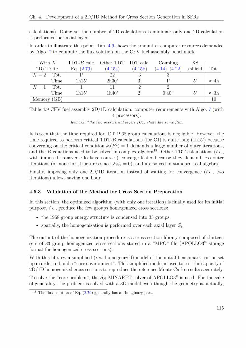
Ch. 4. Development of a 2D/1D Method for Cross Section Generation in SFRs
calculations). Doing so, the number of 2D calculations is minimal: only one 2D calculationis performed per axial layer.In order to illustrate this point, Tab. 4.9 shows the amount of computer resources demandedby Algo. 7 to compute the flux solution on the CFV fuel assembly benchmark.
With X TDT-B calc. Other TDT IDT calc. Coupling XS2D/1D ite. Eq. (2.79) (4.15a) (4.15b) (4.14)–(4.22) s.shield. Tot.
X = 2 Tot. 1∗ 22 3 3Time 1h15’ 2h30’ 3’ 1’ 5’ ≈ 4h
X = 1 Tot. 1 11 2 2Time 1h15’ 1h40’ 2’ 0’40” 5’ ≈ 3h
Memory (GB) 10
Table 4.9 CFV fuel assembly 2D/1D calculation: computer requirements with Algo. 7 (with4 processors).
Remark: ∗the two overcritical layers (C1) share the same flux.
It is seen that the time required for IDT 1968 group calculations is negligible. However, thetime required to perform critical TDT-B calculations (for C1) is quite long (1h15’) becauseconverging on the critical condition ki(B2) = 1 demands a large number of outer iterations,and the B equations need to be solved in complex algebra18. Other TDT calculations (i.e.,with imposed transverse leakage sources) converge faster because they demand less outeriterations (or none for structures since Fiψi = 0), and are solved in standard real algebra.Finally, imposing only one 2D/1D iteration instead of waiting for convergence (i.e., twoiterations) allows saving one hour.
4.5.3 Validation of the Method for Cross Section Preparation
In this section, the optimized algorithm (with only one iteration) is finally used for its initialpurpose, i.e., produce the few groups homogenized cross sections:
• the 1968 group energy structure is condensed into 33 groups;• spatially, the homogenization is performed over each axial layer Zi.
The output of the homogenization procedure is a cross section library composed of thirteensets of 33 group homogenized cross sections stored in a “MPO” file (APOLLO3® storageformat for homogenized cross sections).With this library, a simplified (i.e., homogenized) model of the initial benchmark can be setup in order to build a “core environment”. This simplified model is used to test the capacity of2D/1D homogenized cross sections to reproduce the reference Monte Carlo results accurately.To solve the “core problem”, the SN MINARET solver of APOLLO3® is used. For the sakeof generality, the problem is solved with a 3D model even though the geometry is, actually,
18 The flux solution of Eq. (2.79) generally has an imaginary part.
115
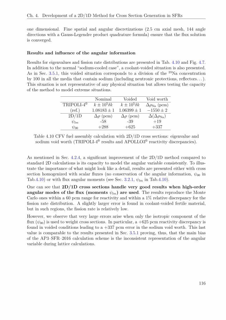
Ch. 4. Development of a 2D/1D Method for Cross Section Generation in SFRs
one dimensional. Fine spatial and angular discretizations (2.5 cm axial mesh, 144 angledirections with a Gauss-Legendre product quadrature formula) ensure that the flux solutionis converged.
Results and influence of the angular information
Results for eigenvalues and fission rate distributions are presented in Tab. 4.10 and Fig. 4.7.In addition to the normal “sodium-cooled case”, a coolant-voided situation is also presented.As in Sec. 3.5.1, this voided situation corresponds to a division of the 23Na concentrationby 100 in all the media that contain sodium (including neutronic protections, reflectors. . . ).This situation is not representative of any physical situation but allows testing the capacityof the method to model extreme situations.
Nominal Voided Void worthTRIPOLI-4® k ± 105δk k ± 105δk ∆ρNa (pcm)
(ref.) 1.08183± 1 1.06399± 1 −1550± 22D/1D ∆ρ (pcm) ∆ρ (pcm) ∆(∆ρNa)ψlm -58 -39 +19ψ00 +288 +625 +337
Table 4.10 CFV fuel assembly calculation with 2D/1D cross sections: eigenvalue andsodium void worth (TRIPOLI-4® results and APOLLO3® reactivity discrepancies).
As mentioned in Sec. 4.2.4, a significant improvement of the 2D/1D method compared tostandard 2D calculations is its capacity to model the angular variable consistently. To illus-trate the importance of what might look like a detail, results are presented either with crosssection homogenized with scalar fluxes (no conservation of the angular information, ψ00 inTab.4.10) or with flux angular moments (see Sec. 3.2.1, ψlm in Tab.4.10).One can see that 2D/1D cross sections handle very good results when high-orderangular modes of the flux (moments ψlm) are used. The results reproduce the MonteCarlo ones within a 60 pcm range for reactivity and within a 1% relative discrepancy for thefission rate distribution. A slightly larger error is found in coolant-voided fertile material,but in such regions, the fission rate is relatively low.However, we observe that very large errors arise when only the isotropic component of theflux (ψ00) is used to weight cross sections. In particular, a +625 pcm reactivity discrepancy isfound in voided conditions leading to a +337 pcm error in the sodium void worth. This lastvalue is comparable to the results presented in Sec. 3.5.1 proving, thus, that the main biasof the AP3–SFR–2016 calculation scheme is the inconsistent representation of the angularvariable during lattice calculations.
116
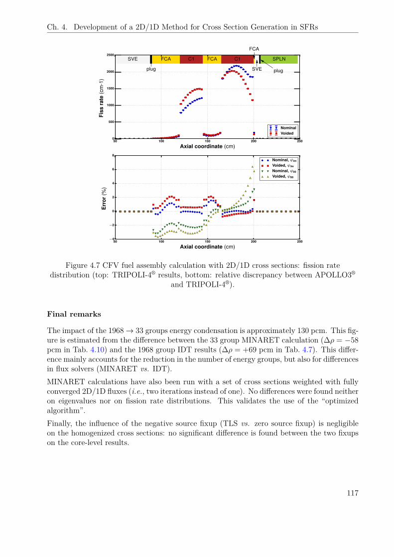
Ch. 4. Development of a 2D/1D Method for Cross Section Generation in SFRs
50 100 150 200 250
Axial coordinate (cm)
0
500
1000
1500
2000
2500
Fiss
rate
(cm
-1)
SVE FCA C1 FCA C1 SPLN
plug
FCA
SVE plug
NominalVoided
50 100 150 200 250
Axial coordinate (cm)
−4
−2
0
2
4
6
8
Err
or(%
)
Nominal, ψlm
Voided, ψlm
Nominal, ψ00
Voided, ψ00
Figure 4.7 CFV fuel assembly calculation with 2D/1D cross sections: fission ratedistribution (top: TRIPOLI-4® results, bottom: relative discrepancy between APOLLO3®
and TRIPOLI-4®).
Final remarks
The impact of the 1968→ 33 groups energy condensation is approximately 130 pcm. This fig-ure is estimated from the difference between the 33 group MINARET calculation (∆ρ = −58pcm in Tab. 4.10) and the 1968 group IDT results (∆ρ = +69 pcm in Tab. 4.7). This differ-ence mainly accounts for the reduction in the number of energy groups, but also for differencesin flux solvers (MINARET vs. IDT).MINARET calculations have also been run with a set of cross sections weighted with fullyconverged 2D/1D fluxes (i.e., two iterations instead of one). No differences were found neitheron eigenvalues nor on fission rate distributions. This validates the use of the “optimizedalgorithm”.Finally, the influence of the negative source fixup (TLS vs. zero source fixup) is negligibleon the homogenized cross sections: no significant difference is found between the two fixupson the core-level results.
117
Ch. 4. Development of a 2D/1D Method for Cross Section Generation in SFRs
4.6 Definition of a Calculation Method Comparison Grid
4.6.1 Estimators
At this stage, we propose to compare the newly implemented 2D/1D method with othercalculation methods available in APOLLO3® for the generation of homogenized cross sectionsin axially heterogeneous SFR core geometries.Since an optimum wants to be found between accuracy and massive resort to computationalresources, the following indicators are considered for the comparison:
• Calculation time and memory requirements to prepare a complete set of cross sections.• Accuracy of the homogenized calculation vs. a reference Monte Carlo solution, mea-
sured with:
– a reactivity discrepancy (global estimator);– an assessment of the local distortion of the flux distribution.
In information theory [114], the Kullback-Leibler divergence (or relative entropy) [115] isoften used to compare two distributions. In this work, we propose to use it to measure localdiscrepancies: if ψref is a reference (e.g., Monte Carlo) flux and ψ an approximate solution(e.g., APOLLO3® core calculation), both normalized to unity, we define their relative entropyas follows19,20:
Sr[ψ, ψref ] =∫
R+×D
dEd3r ψref,00(r, E) ln(ψref,00(r, E)ψ00(r, E)
)(4.39)
or, in terms of discrete distributions:
Sr[ψ, ψref ] =∑i
∑g
ψgref,00,i ln(ψgref,00,i
ψg00,i
)(4.40)
where i is the spatial cell index and g the energy group index.Sr is a dissimilarity measure: it quantifies how much “information” is lost between ψref andψ. If ψ1 and ψ2 are two flux distributions (associated with two different calculation schemes,for instance), then the comparison grid is the following:
Sr[ψ1, ψref ] < Sr[ψ2, ψref ] =⇒ ψ1 is a better approximation of ψref . (4.41)
4.6.2 Application to APOLLO3® methods
Tab. 4.11 presents an application of this comparison grid to the CFV fuel assembly benchmarkused in previous section. Some complementary results – including a comparison with themethodology of the ECCO code – are also given in Appendix E.
19 Scalar fluxes (subscript “00”) are used in the definition of Sr but, as far as the information is available,they could be replaced by angular fluxes (or any other quantity). However, scoring angular quantities is quitearduous in the stochastic framework because many neutron histories need to be sampled.
20 The relative entropy is not a metric distance because it is not symmetric.
118
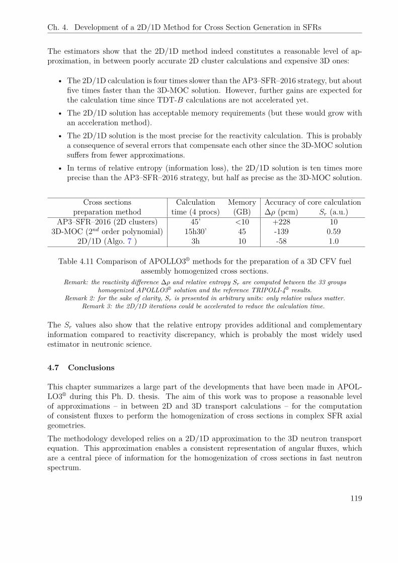
Ch. 4. Development of a 2D/1D Method for Cross Section Generation in SFRs
The estimators show that the 2D/1D method indeed constitutes a reasonable level of ap-proximation, in between poorly accurate 2D cluster calculations and expensive 3D ones:
• The 2D/1D calculation is four times slower than the AP3–SFR–2016 strategy, but aboutfive times faster than the 3D-MOC solution. However, further gains are expected forthe calculation time since TDT-B calculations are not accelerated yet.
• The 2D/1D solution has acceptable memory requirements (but these would grow withan acceleration method).
• The 2D/1D solution is the most precise for the reactivity calculation. This is probablya consequence of several errors that compensate each other since the 3D-MOC solutionsuffers from fewer approximations.
• In terms of relative entropy (information loss), the 2D/1D solution is ten times moreprecise than the AP3–SFR–2016 strategy, but half as precise as the 3D-MOC solution.
Cross sections Calculation Memory Accuracy of core calculationpreparation method time (4 procs) (GB) ∆ρ (pcm) Sr (a.u.)
AP3–SFR–2016 (2D clusters) 45’ <10 +228 103D-MOC (2nd order polynomial) 15h30’ 45 -139 0.59
2D/1D (Algo. 7 ) 3h 10 -58 1.0
Table 4.11 Comparison of APOLLO3® methods for the preparation of a 3D CFV fuelassembly homogenized cross sections.
Remark: the reactivity difference ∆ρ and relative entropy Sr are computed between the 33 groupshomogenized APOLLO3® solution and the reference TRIPOLI-4® results.
Remark 2: for the sake of clarity, Sr is presented in arbitrary units: only relative values matter.Remark 3: the 2D/1D iterations could be accelerated to reduce the calculation time.
The Sr values also show that the relative entropy provides additional and complementaryinformation compared to reactivity discrepancy, which is probably the most widely usedestimator in neutronic science.
4.7 Conclusions
This chapter summarizes a large part of the developments that have been made in APOL-LO3® during this Ph. D. thesis. The aim of this work was to propose a reasonable levelof approximations – in between 2D and 3D transport calculations – for the computationof consistent fluxes to perform the homogenization of cross sections in complex SFR axialgeometries.The methodology developed relies on a 2D/1D approximation to the 3D neutron transportequation. This approximation enables a consistent representation of angular fluxes, whichare a central piece of information for the homogenization of cross sections in fast neutronspectrum.
119
Ch. 4. Development of a 2D/1D Method for Cross Section Generation in SFRs
The 2D/1D equations have been derived in a periodic 3D domain, under the assumption thatradial leakage could be neglected to prepare cross sections in axially heterogeneous SFR cores.The main difficulties linked to the resolution of the 2D/1D system have been put forward(risk of negative fluxes), and several solutions have been proposed. Two different algorithmsemerged from the analysis: a “rigorous” method to compute 2D/1D fluxes, and a heuristicapproximation, used to bypass numerical instabilities in “overcritical” planes (hybridizationwith B leakage model).These algorithms have been implemented in the APOLLO3® code, and numerically verifiedon simple test cases. The heuristic algorithm has also been validated on a realistic CFV fuelassembly benchmark, against reference Monte Carlo results.In particular, it was shown that, as far as the cross section homogenization is concerned, theloss of information due to the 2D/1D approximation is low compared to a 3D-MOC solution,which demands about five times as much computer resources. Hence:
The 2D/1D method is relevant to produce few groups homogenized cross sections inaxially heterogeneous SFR cores (even in coolant-voided situations). Nevertheless, aproper propagation of the angular information (axial current) is mandatory. Else the
method is equivalent to a simple 2D approximation.
At this stage, thus, we have at our disposal a sufficient panel of methods to develop andvalidate advanced reference calculation schemes in APOLLO3® for complex SFR cores, suchas ASTRID’s CFV. The aim of Chapter 5 is, hence, to present such new methodologies.
120
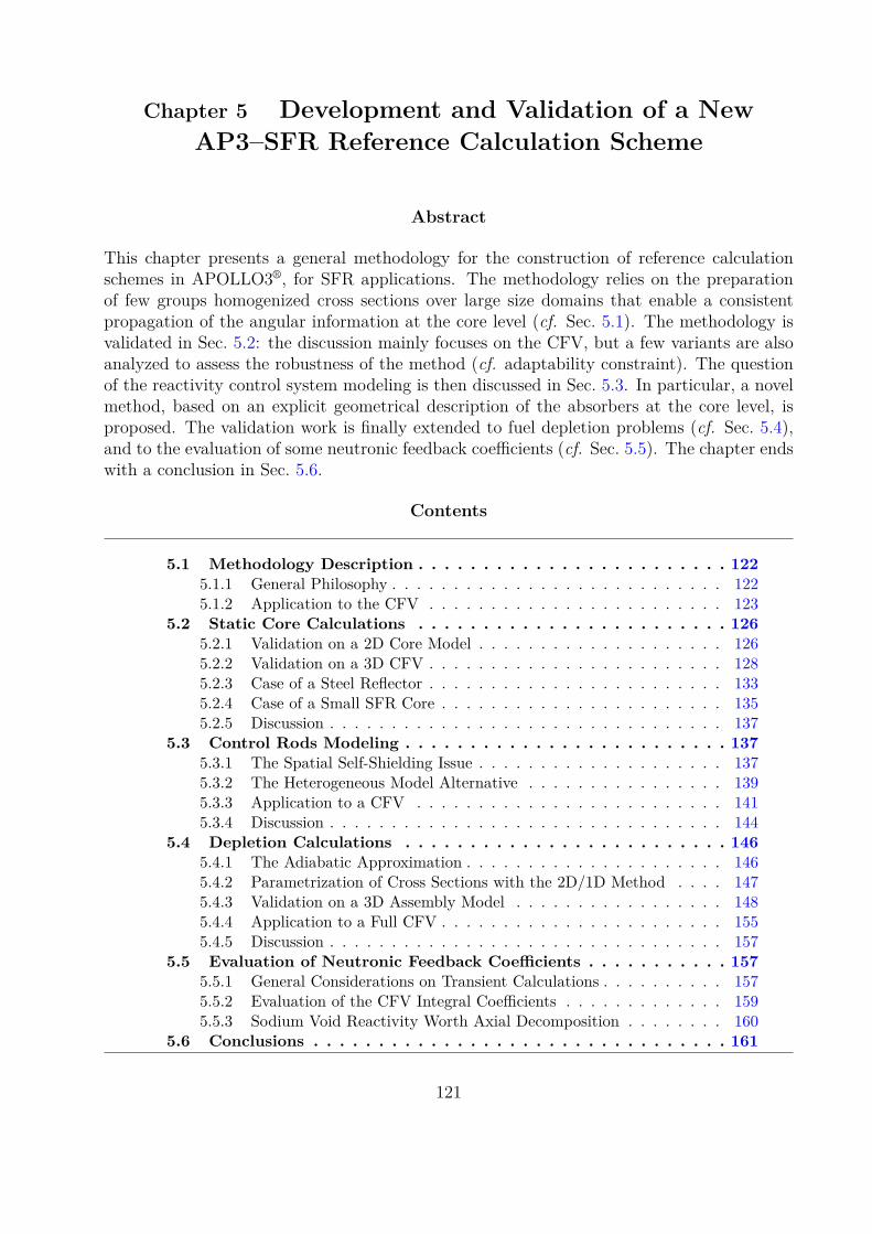
Chapter 5 Development and Validation of a NewAP3–SFR Reference Calculation Scheme
Abstract
This chapter presents a general methodology for the construction of reference calculationschemes in APOLLO3®, for SFR applications. The methodology relies on the preparationof few groups homogenized cross sections over large size domains that enable a consistentpropagation of the angular information at the core level (cf. Sec. 5.1). The methodology isvalidated in Sec. 5.2: the discussion mainly focuses on the CFV, but a few variants are alsoanalyzed to assess the robustness of the method (cf. adaptability constraint). The questionof the reactivity control system modeling is then discussed in Sec. 5.3. In particular, a novelmethod, based on an explicit geometrical description of the absorbers at the core level, isproposed. The validation work is finally extended to fuel depletion problems (cf. Sec. 5.4),and to the evaluation of some neutronic feedback coefficients (cf. Sec. 5.5). The chapter endswith a conclusion in Sec. 5.6.
Contents
5.1 Methodology Description . . . . . . . . . . . . . . . . . . . . . . . . 1225.1.1 General Philosophy . . . . . . . . . . . . . . . . . . . . . . . . . . . 1225.1.2 Application to the CFV . . . . . . . . . . . . . . . . . . . . . . . . 123
5.2 Static Core Calculations . . . . . . . . . . . . . . . . . . . . . . . . 1265.2.1 Validation on a 2D Core Model . . . . . . . . . . . . . . . . . . . . 1265.2.2 Validation on a 3D CFV . . . . . . . . . . . . . . . . . . . . . . . . 1285.2.3 Case of a Steel Reflector . . . . . . . . . . . . . . . . . . . . . . . . 1335.2.4 Case of a Small SFR Core . . . . . . . . . . . . . . . . . . . . . . . 1355.2.5 Discussion . . . . . . . . . . . . . . . . . . . . . . . . . . . . . . . . 137
5.3 Control Rods Modeling . . . . . . . . . . . . . . . . . . . . . . . . . 1375.3.1 The Spatial Self-Shielding Issue . . . . . . . . . . . . . . . . . . . . 1375.3.2 The Heterogeneous Model Alternative . . . . . . . . . . . . . . . . 1395.3.3 Application to a CFV . . . . . . . . . . . . . . . . . . . . . . . . . 1415.3.4 Discussion . . . . . . . . . . . . . . . . . . . . . . . . . . . . . . . . 144
5.4 Depletion Calculations . . . . . . . . . . . . . . . . . . . . . . . . . 1465.4.1 The Adiabatic Approximation . . . . . . . . . . . . . . . . . . . . . 1465.4.2 Parametrization of Cross Sections with the 2D/1D Method . . . . 1475.4.3 Validation on a 3D Assembly Model . . . . . . . . . . . . . . . . . 1485.4.4 Application to a Full CFV . . . . . . . . . . . . . . . . . . . . . . . 1555.4.5 Discussion . . . . . . . . . . . . . . . . . . . . . . . . . . . . . . . . 157
5.5 Evaluation of Neutronic Feedback Coefficients . . . . . . . . . . . 1575.5.1 General Considerations on Transient Calculations . . . . . . . . . . 1575.5.2 Evaluation of the CFV Integral Coefficients . . . . . . . . . . . . . 1595.5.3 Sodium Void Reactivity Worth Axial Decomposition . . . . . . . . 160
5.6 Conclusions . . . . . . . . . . . . . . . . . . . . . . . . . . . . . . . . 161
121
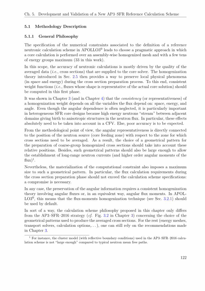
Ch. 5. Development and Validation of a New AP3–SFR Reference Calculation Scheme
5.1 Methodology Description
5.1.1 General Philosophy
The specification of the numerical constraints associated to the definition of a referenceneutronic calculation scheme in APOLLO3® leads to choose a pragmatic approach in whicha core calculation is performed over an assembly-wise homogenized mesh and with a few tensof energy groups maximum (33 in this work).In this scope, the accuracy of neutronic calculations is mostly driven by the quality of theaveraged data (i.e., cross sections) that are supplied to the core solver. The homogenizationtheory introduced in Sec. 2.5 then provides a way to preserve local physical phenomena(in space and energy) during the cross section preparation process. To this end, consistentweight functions (i.e., fluxes whose shape is representative of the actual core solution) shouldbe computed in this first phase.It was shown in Chapter 3 (and in Chapter 4) that the consistency (or representativeness) ofa homogenization weight depends on all the variables the flux depend on: space, energy, andangle. Even though the angular dependence is often neglected, it is particularly importantin heterogeneous SFR core designs because high energy neutrons “stream” between adjacentdomains giving birth to anisotropic structures in the neutron flux. In particular, these effectsabsolutely need to be taken into account in a CFV. Else, poor accuracy is to be expected.From the methodological point of view, the angular representativeness is directly connectedto the position of the neutron source (core feeding zone) with respect to the zone for whichcross sections need to be averaged. As a result, the choice of a geometrical pattern forthe preparation of coarse-group homogenized cross sections should take into account theserelative positions. Besides, such geometrical patterns should also be large enough to allowthe establishment of long-range neutron currents (and higher order angular moments of theflux)1.Nevertheless, the materialization of the computational constraint also imposes a maximumsize to such a geometrical pattern. In particular, the flux calculation requirements duringthe cross section preparation phase should not exceed the calculation scheme specifications:a compromise is necessary.In any case, the preservation of the angular information requires a consistent homogenizationtheory involving angular fluxes or, in an equivalent way, angular flux moments. In APOL-LO3®, this means that the flux-moments homogenization technique (see Sec. 3.2.1) shouldbe used by default.In sort of a way, the calculation scheme philosophy proposed in this chapter only differsfrom the AP3–SFR–2016 strategy (cf. Fig. 3.2 in Chapter 3) concerning the choice of thegeometrical patterns used to produce the averaged cross sections. For the rest (energy meshes,transport solvers, calculation options,. . . ), one can still rely on the recommendations madein Chapter 3.
1 For instance, the cluster model (with reflective boundary conditions) used in the AP3–SFR–2016 calcu-lation scheme is not “large enough” compared to typical neutron mean free paths.
122
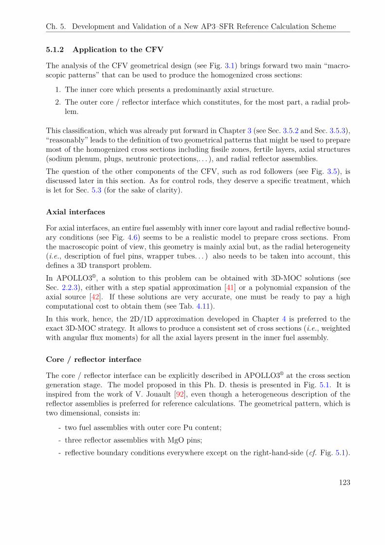
Ch. 5. Development and Validation of a New AP3–SFR Reference Calculation Scheme
5.1.2 Application to the CFV
The analysis of the CFV geometrical design (see Fig. 3.1) brings forward two main “macro-scopic patterns” that can be used to produce the homogenized cross sections:
1. The inner core which presents a predominantly axial structure.2. The outer core / reflector interface which constitutes, for the most part, a radial prob-
lem.
This classification, which was already put forward in Chapter 3 (see Sec. 3.5.2 and Sec. 3.5.3),“reasonably” leads to the definition of two geometrical patterns that might be used to preparemost of the homogenized cross sections including fissile zones, fertile layers, axial structures(sodium plenum, plugs, neutronic protections,. . . ), and radial reflector assemblies.The question of the other components of the CFV, such as rod followers (see Fig. 3.5), isdiscussed later in this section. As for control rods, they deserve a specific treatment, whichis let for Sec. 5.3 (for the sake of clarity).
Axial interfaces
For axial interfaces, an entire fuel assembly with inner core layout and radial reflective bound-ary conditions (see Fig. 4.6) seems to be a realistic model to prepare cross sections. Fromthe macroscopic point of view, this geometry is mainly axial but, as the radial heterogeneity(i.e., description of fuel pins, wrapper tubes. . . ) also needs to be taken into account, thisdefines a 3D transport problem.In APOLLO3®, a solution to this problem can be obtained with 3D-MOC solutions (seeSec. 2.2.3), either with a step spatial approximation [41] or a polynomial expansion of theaxial source [42]. If these solutions are very accurate, one must be ready to pay a highcomputational cost to obtain them (see Tab. 4.11).In this work, hence, the 2D/1D approximation developed in Chapter 4 is preferred to theexact 3D-MOC strategy. It allows to produce a consistent set of cross sections (i.e., weightedwith angular flux moments) for all the axial layers present in the inner fuel assembly.
Core / reflector interface
The core / reflector interface can be explicitly described in APOLLO3® at the cross sectiongeneration stage. The model proposed in this Ph. D. thesis is presented in Fig. 5.1. It isinspired from the work of V. Jouault [92], even though a heterogeneous description of thereflector assemblies is preferred for reference calculations. The geometrical pattern, which istwo dimensional, consists in:
- two fuel assemblies with outer core Pu content;- three reflector assemblies with MgO pins;- reflective boundary conditions everywhere except on the right-hand-side (cf. Fig. 5.1).
123
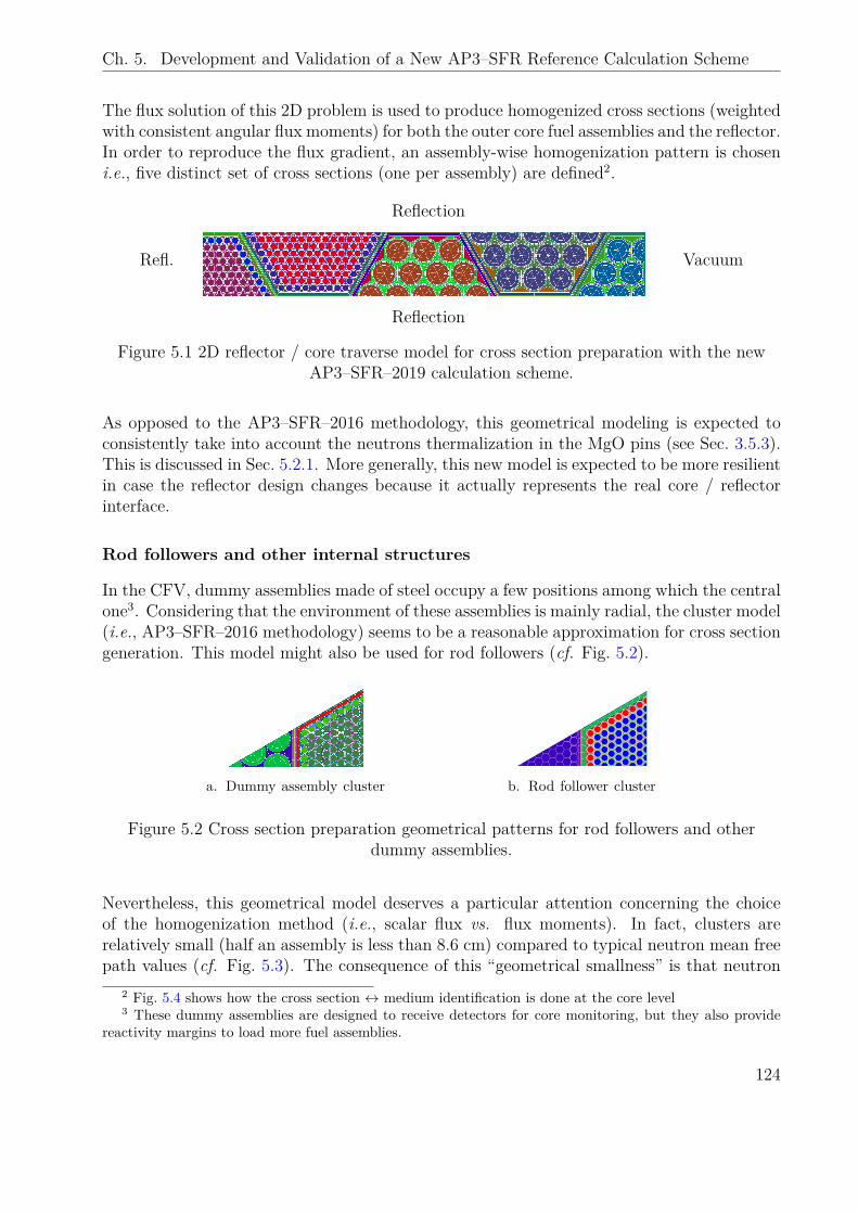
Ch. 5. Development and Validation of a New AP3–SFR Reference Calculation Scheme
The flux solution of this 2D problem is used to produce homogenized cross sections (weightedwith consistent angular flux moments) for both the outer core fuel assemblies and the reflector.In order to reproduce the flux gradient, an assembly-wise homogenization pattern is choseni.e., five distinct set of cross sections (one per assembly) are defined2.
Reflection
Refl. Vacuum
Reflection
Figure 5.1 2D reflector / core traverse model for cross section preparation with the newAP3–SFR–2019 calculation scheme.
As opposed to the AP3–SFR–2016 methodology, this geometrical modeling is expected toconsistently take into account the neutrons thermalization in the MgO pins (see Sec. 3.5.3).This is discussed in Sec. 5.2.1. More generally, this new model is expected to be more resilientin case the reflector design changes because it actually represents the real core / reflectorinterface.
Rod followers and other internal structures
In the CFV, dummy assemblies made of steel occupy a few positions among which the centralone3. Considering that the environment of these assemblies is mainly radial, the cluster model(i.e., AP3–SFR–2016 methodology) seems to be a reasonable approximation for cross sectiongeneration. This model might also be used for rod followers (cf. Fig. 5.2).
a. Dummy assembly cluster b. Rod follower cluster
Figure 5.2 Cross section preparation geometrical patterns for rod followers and otherdummy assemblies.
Nevertheless, this geometrical model deserves a particular attention concerning the choiceof the homogenization method (i.e., scalar flux vs. flux moments). In fact, clusters arerelatively small (half an assembly is less than 8.6 cm) compared to typical neutron mean freepath values (cf. Fig. 5.3). The consequence of this “geometrical smallness” is that neutron
2 Fig. 5.4 shows how the cross section ↔ medium identification is done at the core level3 These dummy assemblies are designed to receive detectors for core monitoring, but they also provide
reactivity margins to load more fuel assemblies.
124
Ch. 5. Development and Validation of a New AP3–SFR Reference Calculation Scheme
trajectories, which are usually long in optically thin media such as sodium, are altered bythe reflective boundary condition. As a result, the “anisotropy” information is perturbed.Differently said, high-order angular moments of the flux (ψlm with l > 1) are not properlycomputed despite the geometry is representative of the core situation. Hence flux momentscannot be used to weight cross sections4. For “small” 2D clusters, the scalar flux should bepreferred.
10−510−410−310−210−1 100 101 102 103 104 105 106 107 108
Energy (eV)
0
5
10
15
20
Mea
nfr
eepa
th(c
m)
Figure 5.3 Neutron mean free path in a rod follower (or sodium plenum).
Identification at the core level
The geometrical models presented above allow to prepare the homogenized cross sections forall the media present in the CFV core. The identification is presented in Fig. 5.4.In particular, the averaged cross sections used for axial positions located at the top andbottom of the outer core (e.g., sodium plenum, plugs. . . ) come from a 2D/1D calculationof the inner fuel assembly. Extra-accuracy could eventually be achieved performing another2D/1D calculation for the outer fuel assembly to provide the corresponding homogenizedcross sections. Yet, this strategy, which doubles the number of 2D/1D calculations, has notbeen considered in this work.
4 This is the origin of the large discrepancies (+1003 pcm) found in the last line of Tab. 3.12 (flux momentshomogenization) in Sec. 3.5.2 for instance.
125
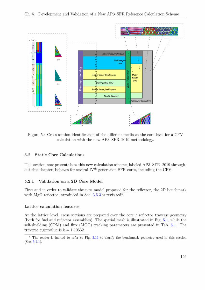
Ch. 5. Development and Validation of a New AP3–SFR Reference Calculation Scheme
ZFCA
C1
FCA
C1
ZPLN
PNS
(a)
z (cm)
0
90
200
247.5
(b)
(c)
(d)
Dum
my
asse
mbl
y
Rod
follo
wer
/////////////////////
Figure 5.4 Cross section identification of the different media at the core level for a CFVcalculation with the new AP3–SFR–2019 methodology.
5.2 Static Core Calculations
This section now presents how this new calculation scheme, labeled AP3–SFR–2019 through-out this chapter, behaves for several IVth-generation SFR cores, including the CFV.
5.2.1 Validation on a 2D Core Model
First and in order to validate the new model proposed for the reflector, the 2D benchmarkwith MgO reflector introduced in Sec. 3.5.3 is revisited5.
Lattice calculation features
At the lattice level, cross sections are prepared over the core / reflector traverse geometry(both for fuel and reflector assemblies). The spatial mesh is illustrated in Fig. 5.1, while theself-shielding (CPM) and flux (MOC) tracking parameters are presented in Tab. 5.1. Thetraverse eigenvalue is k = 1.10532.
5 The reader is invited to refer to Fig. 3.16 to clarify the benchmark geometry used in this section(Sec. 5.2.1).
126
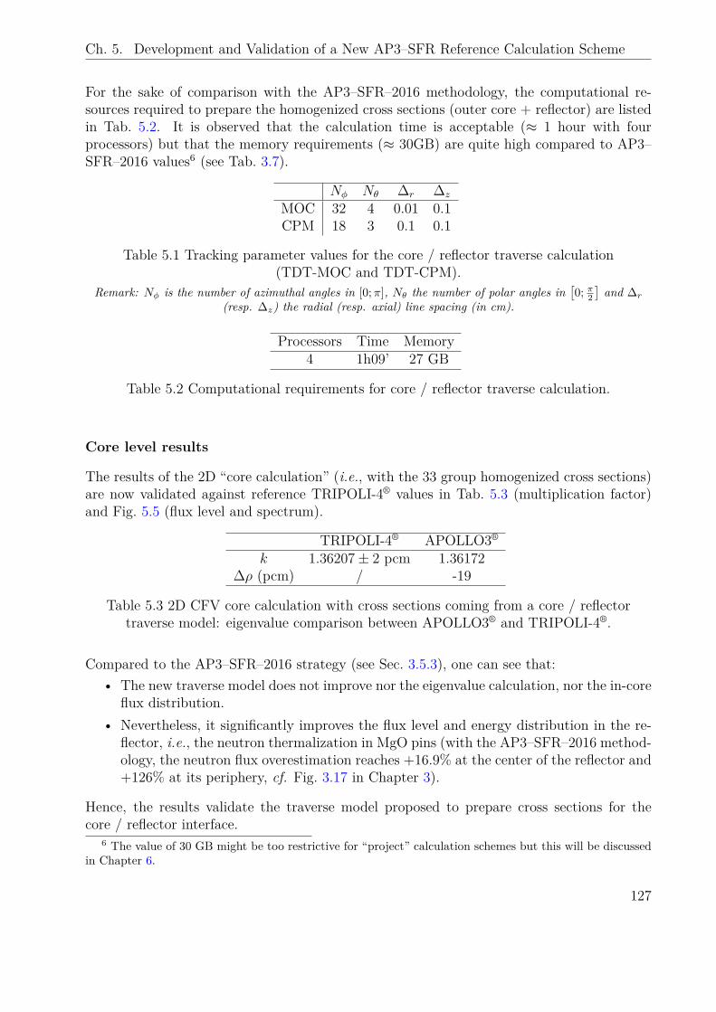
Ch. 5. Development and Validation of a New AP3–SFR Reference Calculation Scheme
For the sake of comparison with the AP3–SFR–2016 methodology, the computational re-sources required to prepare the homogenized cross sections (outer core + reflector) are listedin Tab. 5.2. It is observed that the calculation time is acceptable (≈ 1 hour with fourprocessors) but that the memory requirements (≈ 30GB) are quite high compared to AP3–SFR–2016 values6 (see Tab. 3.7).
Nφ Nθ ∆r ∆z
MOC 32 4 0.01 0.1CPM 18 3 0.1 0.1
Table 5.1 Tracking parameter values for the core / reflector traverse calculation(TDT-MOC and TDT-CPM).
Remark: Nφ is the number of azimuthal angles in [0;π], Nθ the number of polar angles in[0; π2
]and ∆r
(resp. ∆z) the radial (resp. axial) line spacing (in cm).
Processors Time Memory4 1h09’ 27 GB
Table 5.2 Computational requirements for core / reflector traverse calculation.
Core level results
The results of the 2D “core calculation” (i.e., with the 33 group homogenized cross sections)are now validated against reference TRIPOLI-4® values in Tab. 5.3 (multiplication factor)and Fig. 5.5 (flux level and spectrum).
TRIPOLI-4® APOLLO3®
k 1.36207± 2 pcm 1.36172∆ρ (pcm) / -19
Table 5.3 2D CFV core calculation with cross sections coming from a core / reflectortraverse model: eigenvalue comparison between APOLLO3® and TRIPOLI-4®.
Compared to the AP3–SFR–2016 strategy (see Sec. 3.5.3), one can see that:• The new traverse model does not improve nor the eigenvalue calculation, nor the in-core
flux distribution.• Nevertheless, it significantly improves the flux level and energy distribution in the re-
flector, i.e., the neutron thermalization in MgO pins (with the AP3–SFR–2016 method-ology, the neutron flux overestimation reaches +16.9% at the center of the reflector and+126% at its periphery, cf. Fig. 3.17 in Chapter 3).
Hence, the results validate the traverse model proposed to prepare cross sections for thecore / reflector interface.
6 The value of 30 GB might be too restrictive for “project” calculation schemes but this will be discussedin Chapter 6.
127
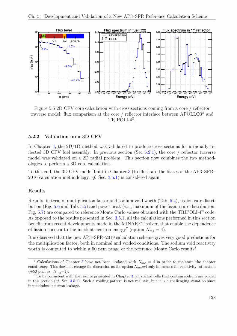
Ch. 5. Development and Validation of a New AP3–SFR Reference Calculation Scheme
0 50 100 150 200 250
x (cm)
103
104
105
106
107ψ
00(a
.u.)
0.2%-1.0%
+2.0%
+46.7%
C1
SSV
C1 C2 SREFL
Flux level
10−3 10−2 10−1 100 101 102 103 104 105 106 107
Energy (eV)
0.00
0.02
0.04
0.06
0.08
0.10
0.12Flux spectrum in fuel (C2)
AP3-SFR-2019T4 ±3σ
10−3 10−2 10−1 100 101 102 103 104 105 106 107
Energy (eV)
0.00
0.01
0.02
0.03
0.04
0.05
0.06
0.07
0.08Flux spectrum in 1st reflector
Figure 5.5 2D CFV core calculation with cross sections coming from a core / reflectortraverse model: flux comparison at the core / reflector interface between APOLLO3® and
TRIPOLI-4®.
5.2.2 Validation on a 3D CFV
In Chapter 4, the 2D/1D method was validated to produce cross sections for a radially re-flected 3D CFV fuel assembly. In previous section (Sec 5.2.1), the core / reflector traversemodel was validated on a 2D radial problem. This section now combines the two method-ologies to perform a 3D core calculation.To this end, the 3D CFV model built in Chapter 3 (to illustrate the biases of the AP3–SFR–2016 calculation methodology, cf. Sec. 3.5.1) is considered again.
Results
Results, in term of multiplication factor and sodium void worth (Tab. 5.4), fission rate distri-bution (Fig. 5.6 and Tab. 5.5) and power peak (i.e., maximum of the fission rate distribution,Fig. 5.7) are compared to reference Monte Carlo values obtained with the TRIPOLI-4® code.As opposed to the results presented in Sec. 3.5.1, all the calculations performed in this sectionbenefit from recent developments made in the MINARET solver, that enable the dependenceof fission spectra to the incident neutron energy7 (option Nmg = 4).It is observed that the new AP3–SFR–2019 calculation scheme gives very good predictions forthe multiplication factor, both in nominal and voided conditions. The sodium void reactivityworth is computed to within a 50 pcm range of the reference Monte Carlo results8.
7 Calculations of Chapter 3 have not been updated with Nmg = 4 in order to maintain the chapterconsistency. This does not change the discussion as the optionNmg=4 only influences the reactivity estimation(+50 pcm vs. Nmg=1).
8 To be consistent with the results presented in Chapter 3, all spatial cells that contain sodium are voidedin this section (cf. Sec. 3.5.1). Such a voiding pattern is not realistic, but it is a challenging situation sinceit maximizes neutron leakage.
128
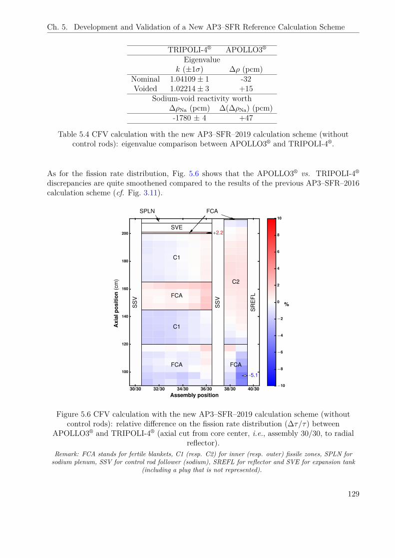
Ch. 5. Development and Validation of a New AP3–SFR Reference Calculation Scheme
TRIPOLI-4® APOLLO3®
Eigenvaluek (±1σ) ∆ρ (pcm)
Nominal 1.04109± 1 -32Voided 1.02214± 3 +15
Sodium-void reactivity worth∆ρNa (pcm) ∆(∆ρNa) (pcm)-1780 ± 4 +47
Table 5.4 CFV calculation with the new AP3–SFR–2019 calculation scheme (withoutcontrol rods): eigenvalue comparison between APOLLO3® and TRIPOLI-4®.
As for the fission rate distribution, Fig. 5.6 shows that the APOLLO3® vs. TRIPOLI-4®
discrepancies are quite smoothened compared to the results of the previous AP3–SFR–2016calculation scheme (cf. Fig. 3.11).
30/30 32/30 34/30 36/30 38/30 40/30Assembly position
100
120
140
160
180
200
Axi
alpo
sitio
n(c
m)
FCA
C1
FCA
C1
FCA
C2
SS
V
SS
V
SR
EFL
SVE
FCASPLN
+2.2
-5.1
−10
−8
−6
−4
−2
0
2
4
6
8
10
%
Figure 5.6 CFV calculation with the new AP3–SFR–2019 calculation scheme (withoutcontrol rods): relative difference on the fission rate distribution (∆τ/τ) between
APOLLO3® and TRIPOLI-4® (axial cut from core center, i.e., assembly 30/30, to radialreflector).
Remark: FCA stands for fertile blankets, C1 (resp. C2) for inner (resp. outer) fissile zones, SPLN forsodium plenum, SSV for control rod follower (sodium), SREFL for reflector and SVE for expansion tank
(including a plug that is not represented).
129
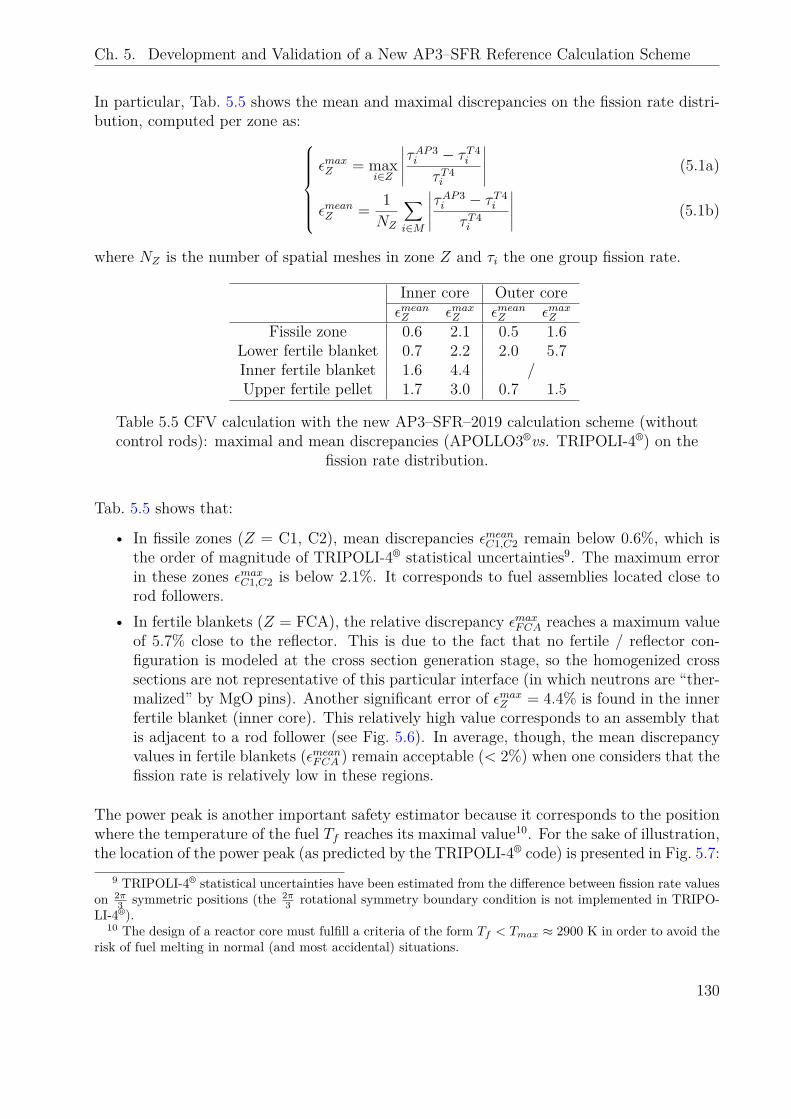
Ch. 5. Development and Validation of a New AP3–SFR Reference Calculation Scheme
In particular, Tab. 5.5 shows the mean and maximal discrepancies on the fission rate distri-bution, computed per zone as:
εmaxZ = maxi∈Z
∣∣∣∣∣τAP3i − τT4
i
τT4i
∣∣∣∣∣ (5.1a)
εmeanZ = 1NZ
∑i∈M
∣∣∣∣∣τAP3i − τT4
i
τT4i
∣∣∣∣∣ (5.1b)
where NZ is the number of spatial meshes in zone Z and τi the one group fission rate.
Inner core Outer coreεmeanZ εmaxZ εmeanZ εmaxZ
Fissile zone 0.6 2.1 0.5 1.6Lower fertile blanket 0.7 2.2 2.0 5.7Inner fertile blanket 1.6 4.4 /Upper fertile pellet 1.7 3.0 0.7 1.5
Table 5.5 CFV calculation with the new AP3–SFR–2019 calculation scheme (withoutcontrol rods): maximal and mean discrepancies (APOLLO3®vs. TRIPOLI-4®) on the
fission rate distribution.
Tab. 5.5 shows that:
• In fissile zones (Z = C1, C2), mean discrepancies εmeanC1,C2 remain below 0.6%, which isthe order of magnitude of TRIPOLI-4® statistical uncertainties9. The maximum errorin these zones εmaxC1,C2 is below 2.1%. It corresponds to fuel assemblies located close torod followers.
• In fertile blankets (Z = FCA), the relative discrepancy εmaxFCA reaches a maximum valueof 5.7% close to the reflector. This is due to the fact that no fertile / reflector con-figuration is modeled at the cross section generation stage, so the homogenized crosssections are not representative of this particular interface (in which neutrons are “ther-malized” by MgO pins). Another significant error of εmaxZ = 4.4% is found in the innerfertile blanket (inner core). This relatively high value corresponds to an assembly thatis adjacent to a rod follower (see Fig. 5.6). In average, though, the mean discrepancyvalues in fertile blankets (εmeanFCA ) remain acceptable (< 2%) when one considers that thefission rate is relatively low in these regions.
The power peak is another important safety estimator because it corresponds to the positionwhere the temperature of the fuel Tf reaches its maximal value10. For the sake of illustration,the location of the power peak (as predicted by the TRIPOLI-4® code) is presented in Fig. 5.7:
9 TRIPOLI-4® statistical uncertainties have been estimated from the difference between fission rate valueson 2π
3 symmetric positions (the 2π3 rotational symmetry boundary condition is not implemented in TRIPO-
LI-4®).10 The design of a reactor core must fulfill a criteria of the form Tf < Tmax ≈ 2900 K in order to avoid the
risk of fuel melting in normal (and most accidental) situations.
130
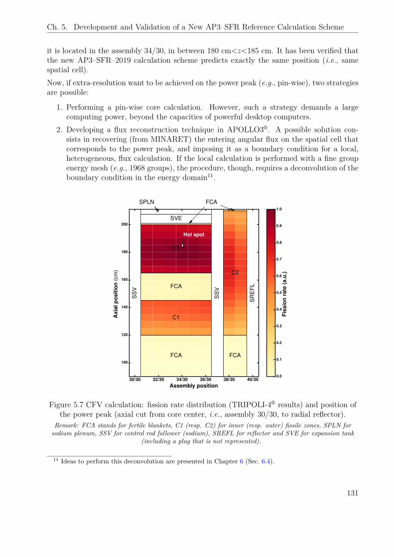
Ch. 5. Development and Validation of a New AP3–SFR Reference Calculation Scheme
it is located in the assembly 34/30, in between 180 cm<z<185 cm. It has been verified thatthe new AP3–SFR–2019 calculation scheme predicts exactly the same position (i.e., samespatial cell).Now, if extra-resolution want to be achieved on the power peak (e.g., pin-wise), two strategiesare possible:
1. Performing a pin-wise core calculation. However, such a strategy demands a largecomputing power, beyond the capacities of powerful desktop computers.
2. Developing a flux reconstruction technique in APOLLO3®. A possible solution con-sists in recovering (from MINARET) the entering angular flux on the spatial cell thatcorresponds to the power peak, and imposing it as a boundary condition for a local,heterogeneous, flux calculation. If the local calculation is performed with a fine groupenergy mesh (e.g., 1968 groups), the procedure, though, requires a deconvolution of theboundary condition in the energy domain11.
30/30 32/30 34/30 36/30 38/30 40/30Assembly position
100
120
140
160
180
200
Axi
alpo
sitio
n(c
m)
FCA
C1
FCA
C1
FCA
C2
SS
V
SS
V
SR
EFL
SVE
FCASPLN
Hot spot
0.0
0.1
0.2
0.3
0.4
0.5
0.6
0.7
0.8
0.9
1.0
Fiss
ion
rate
(a.u
.)
Figure 5.7 CFV calculation: fission rate distribution (TRIPOLI-4® results) and position ofthe power peak (axial cut from core center, i.e., assembly 30/30, to radial reflector).
Remark: FCA stands for fertile blankets, C1 (resp. C2) for inner (resp. outer) fissile zones, SPLN forsodium plenum, SSV for control rod follower (sodium), SREFL for reflector and SVE for expansion tank
(including a plug that is not represented).
11 Ideas to perform this deconvolution are presented in Chapter 6 (Sec. 6.4).
131
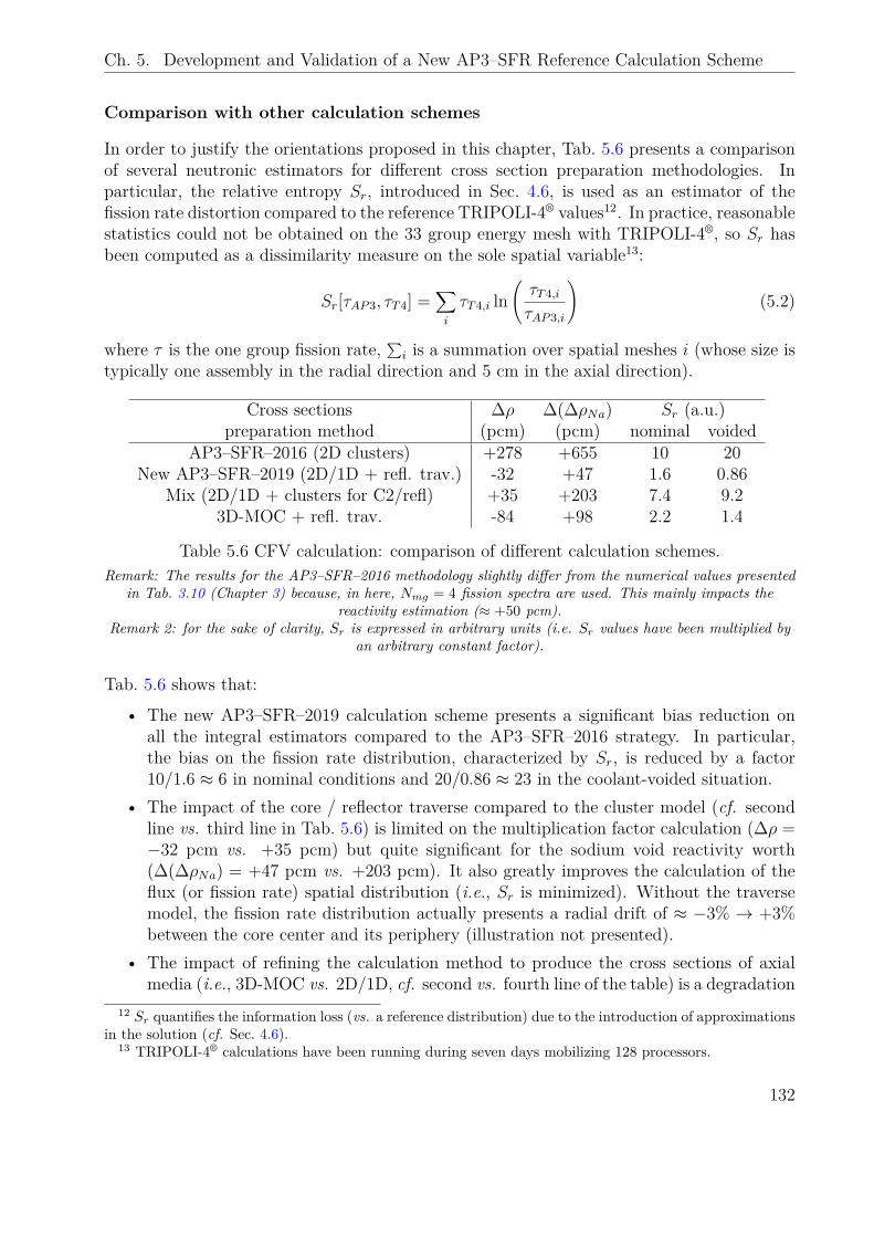
Ch. 5. Development and Validation of a New AP3–SFR Reference Calculation Scheme
Comparison with other calculation schemes
In order to justify the orientations proposed in this chapter, Tab. 5.6 presents a comparisonof several neutronic estimators for different cross section preparation methodologies. Inparticular, the relative entropy Sr, introduced in Sec. 4.6, is used as an estimator of thefission rate distortion compared to the reference TRIPOLI-4® values12. In practice, reasonablestatistics could not be obtained on the 33 group energy mesh with TRIPOLI-4®, so Sr hasbeen computed as a dissimilarity measure on the sole spatial variable13:
Sr[τAP3, τT4] =∑i
τT4,i ln(τT4,i
τAP3,i
)(5.2)
where τ is the one group fission rate, ∑i is a summation over spatial meshes i (whose size istypically one assembly in the radial direction and 5 cm in the axial direction).
Cross sections ∆ρ ∆(∆ρNa) Sr (a.u.)preparation method (pcm) (pcm) nominal voided
AP3–SFR–2016 (2D clusters) +278 +655 10 20New AP3–SFR–2019 (2D/1D + refl. trav.) -32 +47 1.6 0.86
Mix (2D/1D + clusters for C2/refl) +35 +203 7.4 9.23D-MOC + refl. trav. -84 +98 2.2 1.4
Table 5.6 CFV calculation: comparison of different calculation schemes.Remark: The results for the AP3–SFR–2016 methodology slightly differ from the numerical values presented
in Tab. 3.10 (Chapter 3) because, in here, Nmg = 4 fission spectra are used. This mainly impacts thereactivity estimation (≈ +50 pcm).
Remark 2: for the sake of clarity, Sr is expressed in arbitrary units (i.e. Sr values have been multiplied byan arbitrary constant factor).
Tab. 5.6 shows that:
• The new AP3–SFR–2019 calculation scheme presents a significant bias reduction onall the integral estimators compared to the AP3–SFR–2016 strategy. In particular,the bias on the fission rate distribution, characterized by Sr, is reduced by a factor10/1.6 ≈ 6 in nominal conditions and 20/0.86 ≈ 23 in the coolant-voided situation.
• The impact of the core / reflector traverse compared to the cluster model (cf. secondline vs. third line in Tab. 5.6) is limited on the multiplication factor calculation (∆ρ =−32 pcm vs. +35 pcm) but quite significant for the sodium void reactivity worth(∆(∆ρNa) = +47 pcm vs. +203 pcm). It also greatly improves the calculation of theflux (or fission rate) spatial distribution (i.e., Sr is minimized). Without the traversemodel, the fission rate distribution actually presents a radial drift of ≈ −3% → +3%between the core center and its periphery (illustration not presented).
• The impact of refining the calculation method to produce the cross sections of axialmedia (i.e., 3D-MOC vs. 2D/1D, cf. second vs. fourth line of the table) is a degradation
12 Sr quantifies the information loss (vs. a reference distribution) due to the introduction of approximationsin the solution (cf. Sec. 4.6).
13 TRIPOLI-4® calculations have been running during seven days mobilizing 128 processors.
132
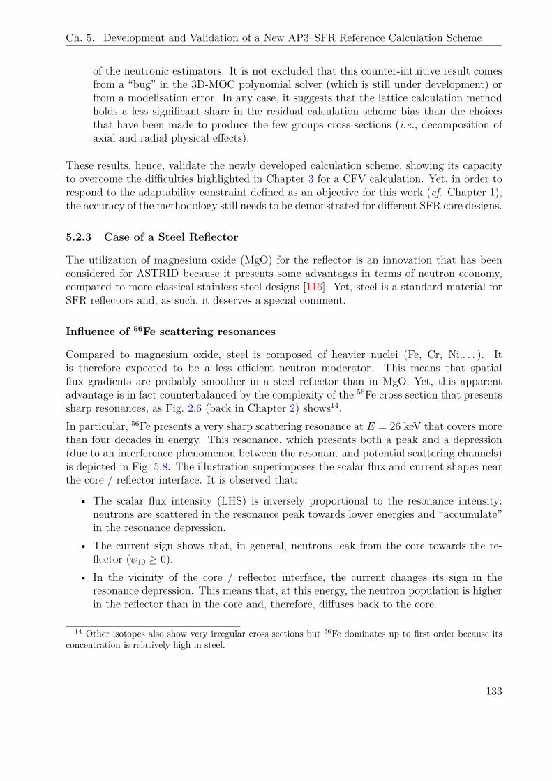
Ch. 5. Development and Validation of a New AP3–SFR Reference Calculation Scheme
of the neutronic estimators. It is not excluded that this counter-intuitive result comesfrom a “bug” in the 3D-MOC polynomial solver (which is still under development) orfrom a modelisation error. In any case, it suggests that the lattice calculation methodholds a less significant share in the residual calculation scheme bias than the choicesthat have been made to produce the few groups cross sections (i.e., decomposition ofaxial and radial physical effects).
These results, hence, validate the newly developed calculation scheme, showing its capacityto overcome the difficulties highlighted in Chapter 3 for a CFV calculation. Yet, in order torespond to the adaptability constraint defined as an objective for this work (cf. Chapter 1),the accuracy of the methodology still needs to be demonstrated for different SFR core designs.
5.2.3 Case of a Steel Reflector
The utilization of magnesium oxide (MgO) for the reflector is an innovation that has beenconsidered for ASTRID because it presents some advantages in terms of neutron economy,compared to more classical stainless steel designs [116]. Yet, steel is a standard material forSFR reflectors and, as such, it deserves a special comment.
Influence of 56Fe scattering resonances
Compared to magnesium oxide, steel is composed of heavier nuclei (Fe, Cr, Ni,. . . ). Itis therefore expected to be a less efficient neutron moderator. This means that spatialflux gradients are probably smoother in a steel reflector than in MgO. Yet, this apparentadvantage is in fact counterbalanced by the complexity of the 56Fe cross section that presentssharp resonances, as Fig. 2.6 (back in Chapter 2) shows14.In particular, 56Fe presents a very sharp scattering resonance at E = 26 keV that covers morethan four decades in energy. This resonance, which presents both a peak and a depression(due to an interference phenomenon between the resonant and potential scattering channels)is depicted in Fig. 5.8. The illustration superimposes the scalar flux and current shapes nearthe core / reflector interface. It is observed that:
• The scalar flux intensity (LHS) is inversely proportional to the resonance intensity:neutrons are scattered in the resonance peak towards lower energies and “accumulate”in the resonance depression.
• The current sign shows that, in general, neutrons leak from the core towards the re-flector (ψ10 ≥ 0).
• In the vicinity of the core / reflector interface, the current changes its sign in theresonance depression. This means that, at this energy, the neutron population is higherin the reflector than in the core and, therefore, diffuses back to the core.
14 Other isotopes also show very irregular cross sections but 56Fe dominates up to first order because itsconcentration is relatively high in steel.
133
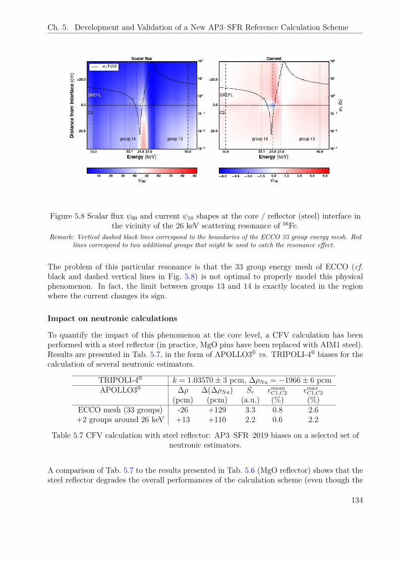
Ch. 5. Development and Validation of a New AP3–SFR Reference Calculation Scheme
Figure 5.8 Scalar flux ψ00 and current ψ10 shapes at the core / reflector (steel) interface inthe vicinity of the 26 keV scattering resonance of 56Fe.
Remark: Vertical dashed black lines correspond to the boundaries of the ECCO 33 group energy mesh. Redlines correspond to two additional groups that might be used to catch the resonance effect.
The problem of this particular resonance is that the 33 group energy mesh of ECCO (cf.black and dashed vertical lines in Fig. 5.8) is not optimal to properly model this physicalphenomenon. In fact, the limit between groups 13 and 14 is exactly located in the regionwhere the current changes its sign.
Impact on neutronic calculations
To quantify the impact of this phenomenon at the core level, a CFV calculation has beenperformed with a steel reflector (in practice, MgO pins have been replaced with AIM1 steel).Results are presented in Tab. 5.7, in the form of APOLLO3® vs. TRIPOLI-4® biases for thecalculation of several neutronic estimators.
TRIPOLI-4® k = 1.03570± 3 pcm, ∆ρNa = −1966± 6 pcmAPOLLO3® ∆ρ ∆(∆ρNa) Sr εmeanC1,C2 εmaxC1,C2
(pcm) (pcm) (a.u.) (%) (%)ECCO mesh (33 groups) -26 +129 3.3 0.8 2.6+2 groups around 26 keV +13 +110 2.2 0.6 2.2
Table 5.7 CFV calculation with steel reflector: AP3–SFR–2019 biases on a selected set ofneutronic estimators.
A comparison of Tab. 5.7 to the results presented in Tab. 5.6 (MgO reflector) shows that thesteel reflector degrades the overall performances of the calculation scheme (even though the
134
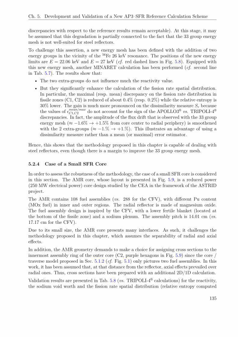
Ch. 5. Development and Validation of a New AP3–SFR Reference Calculation Scheme
discrepancies with respect to the reference results remain acceptable). At this stage, it maybe assumed that this degradation is partially connected to the fact that the 33 group energymesh is not well-suited for steel reflectors.To challenge this assertion, a new energy mesh has been defined with the addition of twoenergy groups in the vicinity of the 56Fe 26 keV resonance. The positions of the new energylimits are E = 22.06 keV and E = 27 keV (cf. red dashed lines in Fig. 5.8). Equipped withthis new energy mesh, another MINARET calculation has been performed (cf. second linein Tab. 5.7). The results show that:
• The two extra-groups do not influence much the reactivity value.• But they significantly enhance the calculation of the fission rate spatial distribution.
In particular, the maximal (resp. mean) discrepancy on the fission rate distribution infissile zones (C1, C2) is reduced of about 0.4% (resp. 0.2%) while the relative entropy is30% lower. The gain is much more pronounced on the dissimilarity measure Sr becausethe values of εmean/maxC1,C2 do not account for the sign of the APOLLO3® vs. TRIPOLI-4®
discrepancies. In fact, the amplitude of the flux drift that is observed with the 33 groupenergy mesh (≈ −1.6%→ +1.5% from core center to radial periphery) is smoothenedwith the 2 extra-groups (≈ −1.% → +1.%). This illustrates an advantage of using adissimilarity measure rather than a mean (or maximal) error estimator.
Hence, this shows that the methodology proposed in this chapter is capable of dealing withsteel reflectors, even though there is a margin to improve the 33 group energy mesh.
5.2.4 Case of a Small SFR Core
In order to assess the robustness of the methodology, the case of a small SFR core is consideredin this section. The AMR core, whose layout is presented in Fig. 5.9, is a reduced power(250 MW electrical power) core design studied by the CEA in the framework of the ASTRIDproject.The AMR contains 108 fuel assemblies (vs. 288 for the CFV), with different Pu content(MOx fuel) in inner and outer regions. The radial reflector is made of magnesium oxide.The fuel assembly design is inspired by the CFV, with a lower fertile blanket (located atthe bottom of the fissile zone) and a sodium plenum. The assembly pitch is 14.01 cm (vs.17.17 cm for the CFV).Due to its small size, the AMR core presents many interfaces. As such, it challenges themethodology proposed in this chapter, which assumes the separability of radial and axialeffects.In addition, the AMR geometry demands to make a choice for assigning cross sections to theinnermost assembly ring of the outer core (C2, purple hexagons in Fig. 5.9) since the core /traverse model proposed in Sec. 5.1.2 (cf. Fig. 5.1) only pictures two fuel assemblies. In thiswork, it has been assumed that, at that distance from the reflector, axial effects prevailed overradial ones. Thus, cross sections have been prepared with an additional 2D/1D calculation.Validation results are presented in Tab. 5.8 (vs. TRIPOLI-4® calculations) for the reactivity,the sodium void worth and the fission rate spatial distribution (relative entropy computed
135
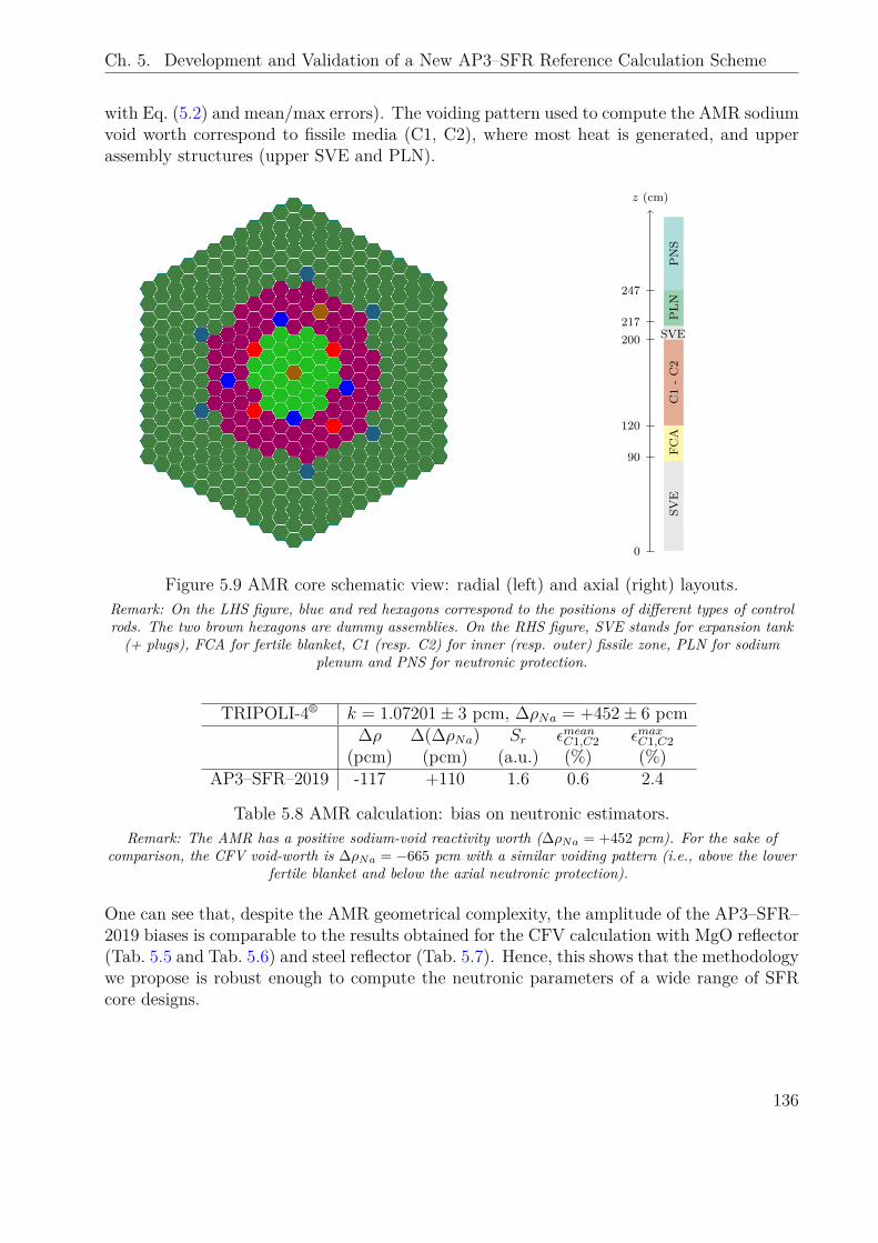
Ch. 5. Development and Validation of a New AP3–SFR Reference Calculation Scheme
with Eq. (5.2) and mean/max errors). The voiding pattern used to compute the AMR sodiumvoid worth correspond to fissile media (C1, C2), where most heat is generated, and upperassembly structures (upper SVE and PLN).
SVE
FCA
C1-C2
SVE
SVE
PLN
PNS
z (cm)
0
90
120
200217
247
Figure 5.9 AMR core schematic view: radial (left) and axial (right) layouts.Remark: On the LHS figure, blue and red hexagons correspond to the positions of different types of controlrods. The two brown hexagons are dummy assemblies. On the RHS figure, SVE stands for expansion tank(+ plugs), FCA for fertile blanket, C1 (resp. C2) for inner (resp. outer) fissile zone, PLN for sodium
plenum and PNS for neutronic protection.
TRIPOLI-4® k = 1.07201± 3 pcm, ∆ρNa = +452± 6 pcm∆ρ ∆(∆ρNa) Sr εmeanC1,C2 εmaxC1,C2
(pcm) (pcm) (a.u.) (%) (%)AP3–SFR–2019 -117 +110 1.6 0.6 2.4
Table 5.8 AMR calculation: bias on neutronic estimators.Remark: The AMR has a positive sodium-void reactivity worth (∆ρNa = +452 pcm). For the sake of
comparison, the CFV void-worth is ∆ρNa = −665 pcm with a similar voiding pattern (i.e., above the lowerfertile blanket and below the axial neutronic protection).
One can see that, despite the AMR geometrical complexity, the amplitude of the AP3–SFR–2019 biases is comparable to the results obtained for the CFV calculation with MgO reflector(Tab. 5.5 and Tab. 5.6) and steel reflector (Tab. 5.7). Hence, this shows that the methodologywe propose is robust enough to compute the neutronic parameters of a wide range of SFRcore designs.
136
Ch. 5. Development and Validation of a New AP3–SFR Reference Calculation Scheme
5.2.5 Discussion
The methodology developed in this chapter significantly improves the accuracy of
APOLLO3® neutronic calculations compared to the previous AP3–SFR–2016 strategy(cf. Chapter 3). Moreover, it is quite robust to the core design, thus reliable for
studying different core concepts.
A residual bias remains, but its amplitude is acceptable with a view in realizing a nuclearsafety demonstration: the reactivity and sodium-void worth bias values are low compared totypical delayed neutron fractions (β ≈ 370 pcm for the CFV), and the error on the fissionrate distribution is controlled.Nevertheless, the following items can still be improved (without changing the calculationscheme philosophy):
• The condensation energy mesh: the addition of two extra groups in the vicinity of the56Fe 26 keV resonance (steel reflector case) gives quite encouraging results, proving thatthe 33 group energy mesh of ECCO can be optimized.
• The modeling of rod followers (and dummy assemblies): due to the reflective boundarycondition, the cluster model (see Fig. 5.2) does not allow to weight P1 and higher ordercross sections with consistent functions (angular flux moments). The constructionof larger domains (e.g., 3D clusters), in which macroscopic flux gradients exist, islikely to enhance the calculation of the fission rate distribution in the vicinity of theseassemblies15.
In the scope of this Ph. D. work though, it has been considered that the overall calculationscheme accuracy was satisfactory. Thus, these axes of research were not explored further inorder to focus on other topics, such as the question of the control rods modeling.
5.3 Control Rods Modeling
In sodium-cooled reactor technologies, the reactivity control system is often composed ofseveral individual assemblies filled with boron carbide (B4C) pins. A recurring issue inthe modeling of such control rods is the presence of sharp flux gradients that make the crosssection homogenization task difficult. The aim of this section is to illustrate this phenomenonand to propose an alternative to overcome it. The results made the topic of a journalpaper [93], published in collaboration with two other Ph. D. students (H. Guo and E. Garcia).
5.3.1 The Spatial Self-Shielding Issue
The spatial self-shielding issue is illustrated in Fig. 5.10, which shows typical spatialdistributions of fluxes and 10B absorption rates in a SFR control rod. One can see that both
15 It may also help reducing the sodium void reactivity worth bias because rod followers constitute pref-erential axial leakage channels. In realistic situations though, these assemblies do not produce heat and,therefore, are not subject to a major decrease of the sodium density.
137
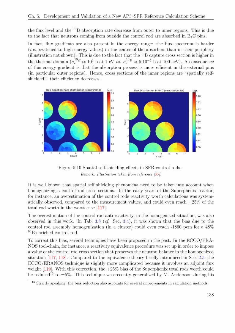
Ch. 5. Development and Validation of a New AP3–SFR Reference Calculation Scheme
the flux level and the 10B absorption rate decrease from outer to inner regions. This is dueto the fact that neutrons coming from outside the control rod are absorbed in B4C pins.In fact, flux gradients are also present in the energy range: the flux spectrum is harder(i.e., switched to high energy values) in the center of the absorbers than in their periphery(illustration not shown). This is due to the fact that the 10B capture cross section is higher inthe thermal domain (σ10Bc ≈ 102 b at 1 eV vs. σ10Bc ≈ 5.10−5 b at 100 keV). A consequenceof this energy gradient is that the absorption process is more efficient in the external pins(in particular outer regions). Hence, cross sections of the inner regions are “spatially self-shielded”: their efficiency decreases.
Figure 5.10 Spatial self-shielding effects in SFR control rods.Remark: Illustration taken from reference [93].
It is well known that spatial self shielding phenomena need to be taken into account whenhomogenizing a control rod cross sections. In the early years of the Superphenix reactor,for instance, an overestimation of the control rods reactivity worth calculations was system-atically observed, compared to the measurement values, and could even reach +25% of thetotal rod worth in the worst case [117].The overestimation of the control rod anti-reactivity, in the homogenized situation, was alsoobserved in this work. In Tab. 3.8 (cf. Sec. 3.4), it was shown that the bias due to thecontrol rod assembly homogenization (in a cluster) could even reach -1860 pcm for a 48%90B enriched control rod.To correct this bias, several techniques have been proposed in the past. In the ECCO/ERA-NOS tool-chain, for instance, a reactivity equivalence procedure was set up in order to imposea value of the control rod cross section that preserves the neutron balance in the homogenizedsituation [117, 118]. Compared to the equivalence theory briefly introduced in Sec. 2.5, theECCO/ERANOS technique is slightly more complicated because it involves an adjoint fluxweight [119]. With this correction, the +25% bias of the Superphenix total rods worth couldbe reduced16 to ±5%. This technique was recently generalized by M. Andersson during his
16 Strictly speaking, the bias reduction also accounts for several improvements in calculation methods.
138
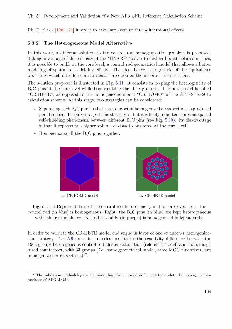
Ch. 5. Development and Validation of a New AP3–SFR Reference Calculation Scheme
Ph. D. thesis [120, 121] in order to take into account three-dimensional effects.
5.3.2 The Heterogeneous Model Alternative
In this work, a different solution to the control rod homogenization problem is proposed.Taking advantage of the capacity of the MINARET solver to deal with unstructured meshes,it is possible to build, at the core level, a control rod geometrical model that allows a bettermodeling of spatial self-shielding effects. The idea, hence, is to get rid of the equivalenceprocedure which introduces an artificial correction on the absorber cross sections.The solution proposed is illustrated in Fig. 5.11. It consists in keeping the heterogeneity ofB4C pins at the core level while homogenizing the “background”. The new model is called“CR-HETE”, as opposed to the homogeneous model “CR-HOMO” of the AP3–SFR–2016calculation scheme. At this stage, two strategies can be considered:
• Separating each B4C pin: in that case, one set of homogenized cross sections is producedper absorber. The advantage of this strategy is that it is likely to better represent spatialself-shielding phenomena between different B4C pins (see Fig. 5.10). Its disadvantageis that it represents a higher volume of data to be stored at the core level.
• Homogenizing all the B4C pins together.
a. CR-HOMO model b. CR-HETE model
Figure 5.11 Representation of the control rod heterogeneity at the core level. Left: thecontrol rod (in blue) is homogeneous. Right: the B4C pins (in blue) are kept heterogeneous
while the rest of the control rod assembly (in purple) is homogenized independently.
In order to validate the CR-HETE model and argue in favor of one or another homogeniza-tion strategy, Tab. 5.9 presents numerical results for the reactivity difference between the1968 groups heterogeneous control rod cluster calculation (reference model) and its homoge-nized counterpart, with 33 groups (i.e., same geometrical model, same MOC flux solver, buthomogenized cross sections)17.
17 The validation methodology is the same than the one used in Sec. 3.4 to validate the homogenizationmethods of APOLLO3®.
139
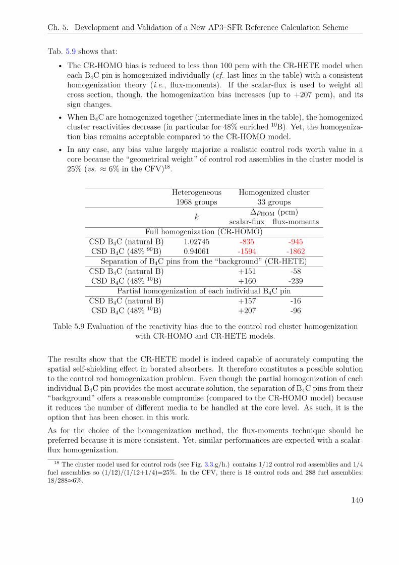
Ch. 5. Development and Validation of a New AP3–SFR Reference Calculation Scheme
Tab. 5.9 shows that:
• The CR-HOMO bias is reduced to less than 100 pcm with the CR-HETE model wheneach B4C pin is homogenized individually (cf. last lines in the table) with a consistenthomogenization theory (i.e., flux-moments). If the scalar-flux is used to weight allcross section, though, the homogenization bias increases (up to +207 pcm), and itssign changes.
• When B4C are homogenized together (intermediate lines in the table), the homogenizedcluster reactivities decrease (in particular for 48% enriched 10B). Yet, the homogeniza-tion bias remains acceptable compared to the CR-HOMO model.
• In any case, any bias value largely majorize a realistic control rods worth value in acore because the “geometrical weight” of control rod assemblies in the cluster model is25% (vs. ≈ 6% in the CFV)18.
Heterogeneous Homogenized cluster1968 groups 33 groups
k∆ρHOM (pcm)
scalar-flux flux-momentsFull homogenization (CR-HOMO)
CSD B4C (natural B) 1.02745 -835 -945CSD B4C (48% 90B) 0.94061 -1594 -1862
Separation of B4C pins from the “background” (CR-HETE)CSD B4C (natural B) +151 -58CSD B4C (48% 10B) +160 -239
Partial homogenization of each individual B4C pinCSD B4C (natural B) +157 -16CSD B4C (48% 10B) +207 -96
Table 5.9 Evaluation of the reactivity bias due to the control rod cluster homogenizationwith CR-HOMO and CR-HETE models.
The results show that the CR-HETE model is indeed capable of accurately computing thespatial self-shielding effect in borated absorbers. It therefore constitutes a possible solutionto the control rod homogenization problem. Even though the partial homogenization of eachindividual B4C pin provides the most accurate solution, the separation of B4C pins from their“background” offers a reasonable compromise (compared to the CR-HOMO model) becauseit reduces the number of different media to be handled at the core level. As such, it is theoption that has been chosen in this work.As for the choice of the homogenization method, the flux-moments technique should bepreferred because it is more consistent. Yet, similar performances are expected with a scalar-flux homogenization.
18 The cluster model used for control rods (see Fig. 3.3.g/h.) contains 1/12 control rod assemblies and 1/4fuel assemblies so (1/12)/(1/12+1/4)=25%. In the CFV, there is 18 control rods and 288 fuel assemblies:18/288≈6%.
140
Ch. 5. Development and Validation of a New AP3–SFR Reference Calculation Scheme
In the remaining of this document, the CR-HETE terminology, therefore, names the modelin which only one set of cross sections is prepared for all the absorber pins.
5.3.3 Application to a CFV
The CR-HETE model relies on a two-dimensional cross section preparation model for controlrods. Hence, one can reasonably expect that the CR-HETE model will perform well inhomogeneous cores in which axial heterogeneities are limited. Yet, the CFV design presentsstrong axial heterogeneities and, as such, is likely to challenge this assertion.The CFV (with MgO reflector) is therefore considered once again as a challenging benchmarkfor validation of the CR-HETE model. Compared to the model used in Sec. 5.2.2, the maindifference consists in the fact that the control rods system is now explicitly represented.The multiplication factor of this problem is k = 1.03603 when the entire control rods system– composed of 18 assemblies (see Sec. 3.1) – is located at its “parking” (i.e., fully with-drawn) position. The APOLLO3® vs. TRIPOLI-4® bias on the multiplication factor is∆ρ = −41 pcm. These values are consistent with the results of Sec. 5.2.2.In order to characterize the control rods system, several neutronic parameters are validated(against TRIPOLI-4® calculations) in this section:
• The control rods system total reactivity worth:
∆ρCR(zin) = 105(
1k(zout)
− 1k(zin)
)(5.3)
which is defined as the reactivity difference between a situation in which control rodsare located in their parking position zout and another situation in which they are fullyinserted in the core, at zin. In the CFV, the parking position is located in the sodiumplenum, 17.5 cm above the upper fissile zone (zout = 217.5 cm with the coordinatesystem of Fig. 5.7 for instance). In this work zin = zout − 90 cm.
• The S-curve, i.e., the function ∆ρCR(z), and the differential efficiency eCR(z) of thecontrol rods system:
eCR(z) = d∆ρCRdz
(z) (5.4)
• The spatial distribution of the 10B absorption rate in a particular rod fully inserted inthe core.
• In addition, the influence of a control rod on a neighboring fuel assembly is investigated,through the evaluation of the bias on the local fission rate distribution.
These parameters are presented in Tab. 5.10, Fig. 5.12, Fig. 5.13, and Fig. 5.14.
141
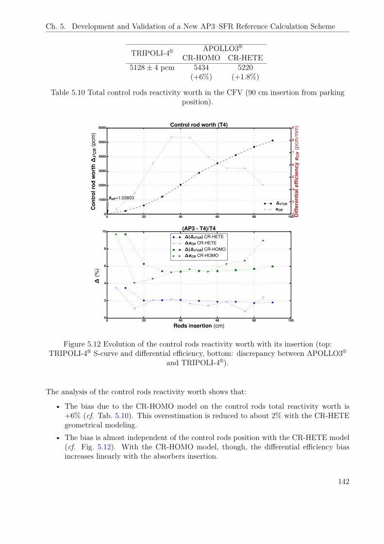
Ch. 5. Development and Validation of a New AP3–SFR Reference Calculation Scheme
TRIPOLI-4® APOLLO3®
CR-HOMO CR-HETE5128± 4 pcm 5434 5220
(+6%) (+1.8%)
Table 5.10 Total control rods reactivity worth in the CFV (90 cm insertion from parkingposition).
0 20 40 60 80 1000
1000
2000
3000
4000
5000
6000
Con
trol
rod
wor
th∆ρ
CR
(pcm
)
keff =1.03603
Control rod worth (T4)
∆ρCR
2
3
4
5
6
7
8
9
Diff
eren
tiale
ffici
ency
e CR
(pcm
/mm
)
eCR
0 20 40 60 80 100
Rods insertion (cm)
0
2
4
6
8
10
∆(%
)
(AP3 - T4)/T4∆(∆ρCR) CR-HETE∆eCR CR-HETE∆(∆ρCR) CR-HOMO∆eCR CR-HOMO
Figure 5.12 Evolution of the control rods reactivity worth with its insertion (top:TRIPOLI-4® S-curve and differential efficiency, bottom: discrepancy between APOLLO3®
and TRIPOLI-4®).
The analysis of the control rods reactivity worth shows that:
• The bias due to the CR-HOMO model on the control rods total reactivity worth is+6% (cf. Tab. 5.10). This overestimation is reduced to about 2% with the CR-HETEgeometrical modeling.
• The bias is almost independent of the control rods position with the CR-HETE model(cf. Fig. 5.12). With the CR-HOMO model, though, the differential efficiency biasincreases linearly with the absorbers insertion.
142
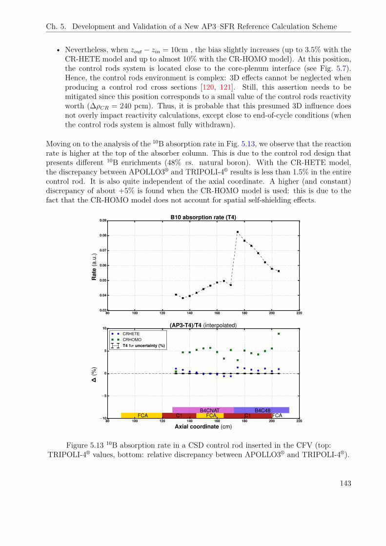
Ch. 5. Development and Validation of a New AP3–SFR Reference Calculation Scheme
• Nevertheless, when zout − zin = 10cm , the bias slightly increases (up to 3.5% with theCR-HETE model and up to almost 10% with the CR-HOMO model). At this position,the control rods system is located close to the core-plenum interface (see Fig. 5.7).Hence, the control rods environment is complex: 3D effects cannot be neglected whenproducing a control rod cross sections [120, 121]. Still, this assertion needs to bemitigated since this position corresponds to a small value of the control rods reactivityworth (∆ρCR = 240 pcm). Thus, it is probable that this presumed 3D influence doesnot overly impact reactivity calculations, except close to end-of-cycle conditions (whenthe control rods system is almost fully withdrawn).
Moving on to the analysis of the 10B absorption rate in Fig. 5.13, we observe that the reactionrate is higher at the top of the absorber column. This is due to the control rod design thatpresents different 10B enrichments (48% vs. natural boron). With the CR-HETE model,the discrepancy between APOLLO3® and TRIPOLI-4® results is less than 1.5% in the entirecontrol rod. It is also quite independent of the axial coordinate. A higher (and constant)discrepancy of about +5% is found when the CR-HOMO model is used: this is due to thefact that the CR-HOMO model does not account for spatial self-shielding effects.
80 100 120 140 160 180 200 2200.03
0.04
0.05
0.06
0.07
0.08
0.09
Rat
e(a
.u.)
B10 absorption rate (T4)
80 100 120 140 160 180 200 220
Axial coordinate (cm)
−10
−5
0
5
10
∆(%
)
FCA C1 FCA C1 FCAB4CNAT B4C48
(AP3-T4)/T4 (interpolated)CRHETECRHOMOT4 1σ uncertainty (%)
Figure 5.13 10B absorption rate in a CSD control rod inserted in the CFV (top:TRIPOLI-4® values, bottom: relative discrepancy between APOLLO3® and TRIPOLI-4®).
143
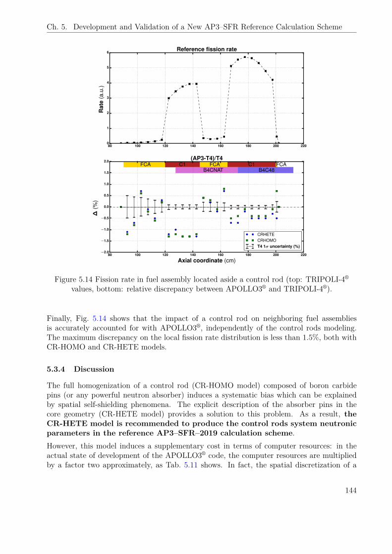
Ch. 5. Development and Validation of a New AP3–SFR Reference Calculation Scheme
80 100 120 140 160 180 200 2200
1
2
3
4
5
6
Rat
e(a
.u.)
Reference fission rate
80 100 120 140 160 180 200 220
Axial coordinate (cm)
−2.0
−1.5
−1.0
−0.5
0.0
0.5
1.0
1.5
2.0
∆(%
)
FCA C1 FCA C1 FCAB4CNAT B4C48
(AP3-T4)/T4
CRHETECRHOMOT4 1σ uncertainty (%)
Figure 5.14 Fission rate in fuel assembly located aside a control rod (top: TRIPOLI-4®
values, bottom: relative discrepancy between APOLLO3® and TRIPOLI-4®).
Finally, Fig. 5.14 shows that the impact of a control rod on neighboring fuel assembliesis accurately accounted for with APOLLO3®, independently of the control rods modeling.The maximum discrepancy on the local fission rate distribution is less than 1.5%, both withCR-HOMO and CR-HETE models.
5.3.4 Discussion
The full homogenization of a control rod (CR-HOMO model) composed of boron carbidepins (or any powerful neutron absorber) induces a systematic bias which can be explainedby spatial self-shielding phenomena. The explicit description of the absorber pins in thecore geometry (CR-HETE model) provides a solution to this problem. As a result, theCR-HETE model is recommended to produce the control rods system neutronicparameters in the reference AP3–SFR–2019 calculation scheme.However, this model induces a supplementary cost in terms of computer resources: in theactual state of development of the APOLLO3® code, the computer resources are multipliedby a factor two approximately, as Tab. 5.11 shows. In fact, the spatial discretization of a
144
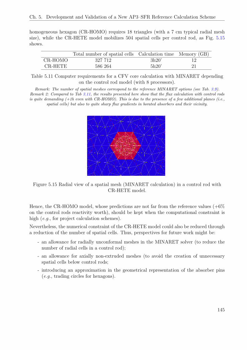
Ch. 5. Development and Validation of a New AP3–SFR Reference Calculation Scheme
homogeneous hexagon (CR-HOMO) requires 18 triangles (with a 7 cm typical radial meshsize), while the CR-HETE model mobilizes 504 spatial cells per control rod, as Fig. 5.15shows.
Total number of spatial cells Calculation time Memory (GB)CR-HOMO 327 712 3h20’ 12CR-HETE 586 264 5h20’ 21
Table 5.11 Computer requirements for a CFV core calculation with MINARET dependingon the control rod model (with 8 processors).
Remark: The number of spatial meshes correspond to the reference MINARET options (see Tab. 3.9).Remark 2: Compared to Tab 3.11, the results presented here show that the flux calculation with control rodsis quite demanding (+1h even with CR-HOMO). This is due to the presence of a few additional planes (i.e.,
spatial cells) but also to quite sharp flux gradients in borated absorbers and their vicinity.
Figure 5.15 Radial view of a spatial mesh (MINARET calculation) in a control rod withCR-HETE model.
Hence, the CR-HOMO model, whose predictions are not far from the reference values (+6%on the control rods reactivity worth), should be kept when the computational constraint ishigh (e.g., for project calculation schemes).Nevertheless, the numerical constraint of the CR-HETE model could also be reduced througha reduction of the number of spatial cells. Thus, perspectives for future work might be:
- an allowance for radially unconformal meshes in the MINARET solver (to reduce thenumber of radial cells in a control rod);
- an allowance for axially non-extruded meshes (to avoid the creation of unnecessaryspatial cells below control rods;
- introducing an approximation in the geometrical representation of the absorber pins(e.g., trading circles for hexagons).
145
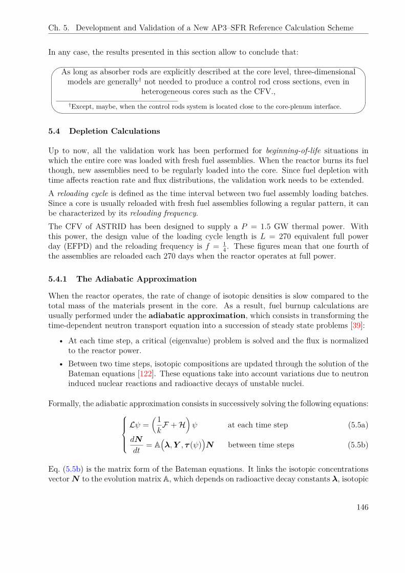
Ch. 5. Development and Validation of a New AP3–SFR Reference Calculation Scheme
In any case, the results presented in this section allow to conclude that:
As long as absorber rods are explicitly described at the core level, three-dimensionalmodels are generally† not needed to produce a control rod cross sections, even in
heterogeneous cores such as the CFV.,†Except, maybe, when the control rods system is located close to the core-plenum interface.
5.4 Depletion Calculations
Up to now, all the validation work has been performed for beginning-of-life situations inwhich the entire core was loaded with fresh fuel assemblies. When the reactor burns its fuelthough, new assemblies need to be regularly loaded into the core. Since fuel depletion withtime affects reaction rate and flux distributions, the validation work needs to be extended.A reloading cycle is defined as the time interval between two fuel assembly loading batches.Since a core is usually reloaded with fresh fuel assemblies following a regular pattern, it canbe characterized by its reloading frequency.The CFV of ASTRID has been designed to supply a P = 1.5 GW thermal power. Withthis power, the design value of the loading cycle length is L = 270 equivalent full powerday (EFPD) and the reloading frequency is f = 1
4 . These figures mean that one fourth ofthe assemblies are reloaded each 270 days when the reactor operates at full power.
5.4.1 The Adiabatic Approximation
When the reactor operates, the rate of change of isotopic densities is slow compared to thetotal mass of the materials present in the core. As a result, fuel burnup calculations areusually performed under the adiabatic approximation, which consists in transforming thetime-dependent neutron transport equation into a succession of steady state problems [39]:
• At each time step, a critical (eigenvalue) problem is solved and the flux is normalizedto the reactor power.
• Between two time steps, isotopic compositions are updated through the solution of theBateman equations [122]. These equations take into account variations due to neutroninduced nuclear reactions and radioactive decays of unstable nuclei.
Formally, the adiabatic approximation consists in successively solving the following equations:Lψ =
(1kF +H
)ψ at each time step (5.5a)
dN
dt= A
(λ,Y , τ (ψ)
)N between time steps (5.5b)
Eq. (5.5b) is the matrix form of the Bateman equations. It links the isotopic concentrationsvectorN to the evolution matrix A, which depends on radioactive decay constants λ, isotopic
146
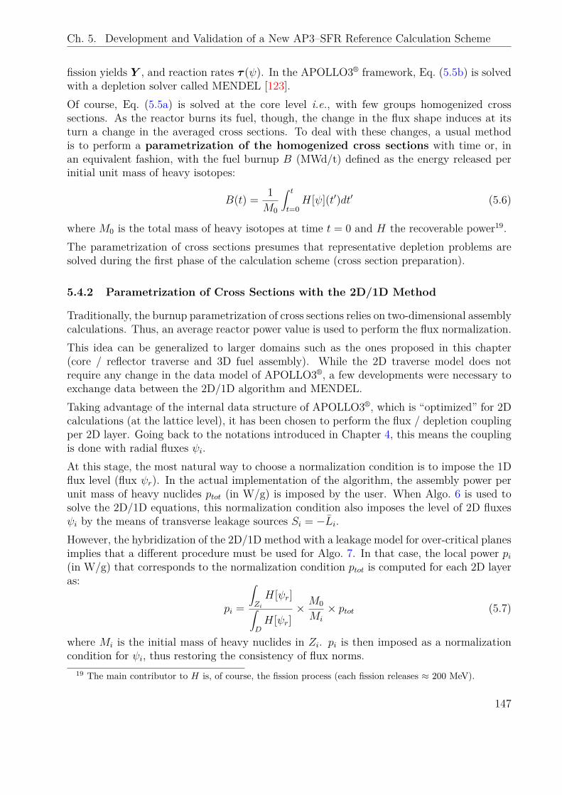
Ch. 5. Development and Validation of a New AP3–SFR Reference Calculation Scheme
fission yields Y , and reaction rates τ (ψ). In the APOLLO3® framework, Eq. (5.5b) is solvedwith a depletion solver called MENDEL [123].Of course, Eq. (5.5a) is solved at the core level i.e., with few groups homogenized crosssections. As the reactor burns its fuel, though, the change in the flux shape induces at itsturn a change in the averaged cross sections. To deal with these changes, a usual methodis to perform a parametrization of the homogenized cross sections with time or, inan equivalent fashion, with the fuel burnup B (MWd/t) defined as the energy released perinitial unit mass of heavy isotopes:
B(t) = 1M0
∫ t
t=0H[ψ](t′)dt′ (5.6)
where M0 is the total mass of heavy isotopes at time t = 0 and H the recoverable power19.The parametrization of cross sections presumes that representative depletion problems aresolved during the first phase of the calculation scheme (cross section preparation).
5.4.2 Parametrization of Cross Sections with the 2D/1D Method
Traditionally, the burnup parametrization of cross sections relies on two-dimensional assemblycalculations. Thus, an average reactor power value is used to perform the flux normalization.This idea can be generalized to larger domains such as the ones proposed in this chapter(core / reflector traverse and 3D fuel assembly). While the 2D traverse model does notrequire any change in the data model of APOLLO3®, a few developments were necessary toexchange data between the 2D/1D algorithm and MENDEL.Taking advantage of the internal data structure of APOLLO3®, which is “optimized” for 2Dcalculations (at the lattice level), it has been chosen to perform the flux / depletion couplingper 2D layer. Going back to the notations introduced in Chapter 4, this means the couplingis done with radial fluxes ψi.At this stage, the most natural way to choose a normalization condition is to impose the 1Dflux level (flux ψr). In the actual implementation of the algorithm, the assembly power perunit mass of heavy nuclides ptot (in W/g) is imposed by the user. When Algo. 6 is used tosolve the 2D/1D equations, this normalization condition also imposes the level of 2D fluxesψi by the means of transverse leakage sources Si = −Li.However, the hybridization of the 2D/1D method with a leakage model for over-critical planesimplies that a different procedure must be used for Algo. 7. In that case, the local power pi(in W/g) that corresponds to the normalization condition ptot is computed for each 2D layeras:
pi =
∫ZiH[ψr]∫
DH[ψr]
× M0
Mi
× ptot (5.7)
where Mi is the initial mass of heavy nuclides in Zi. pi is then imposed as a normalizationcondition for ψi, thus restoring the consistency of flux norms.
19 The main contributor to H is, of course, the fission process (each fission releases ≈ 200 MeV).
147
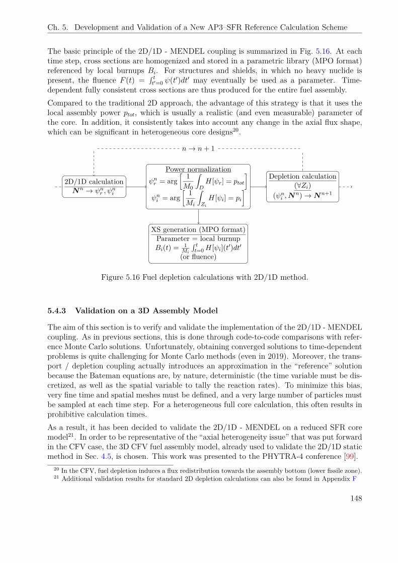
Ch. 5. Development and Validation of a New AP3–SFR Reference Calculation Scheme
The basic principle of the 2D/1D - MENDEL coupling is summarized in Fig. 5.16. At eachtime step, cross sections are homogenized and stored in a parametric library (MPO format)referenced by local burnups Bi. For structures and shields, in which no heavy nuclide ispresent, the fluence F (t) =
∫ tt′=0 ψ(t′)dt′ may eventually be used as a parameter. Time-
dependent fully consistent cross sections are thus produced for the entire fuel assembly.Compared to the traditional 2D approach, the advantage of this strategy is that it uses thelocal assembly power ptot, which is usually a realistic (and even measurable) parameter ofthe core. In addition, it consistently takes into account any change in the axial flux shape,which can be significant in heterogeneous core designs20.
2D/1D calculationNn → ψnr , ψ
ni
Power normalizationψnr = arg
[ 1M0
∫DH[ψr] = ptot
]ψni = arg
[ 1Mi
∫Zi
H[ψi] = pi
] Depletion calculation(∀Zi)
(ψni ,Nn)→Nn+1
n→ n+ 1
XS generation (MPO format)Parameter = local burnupBi(t) = 1
Mi
∫ tt=0H[ψi](t′)dt′
(or fluence)
Figure 5.16 Fuel depletion calculations with 2D/1D method.
5.4.3 Validation on a 3D Assembly Model
The aim of this section is to verify and validate the implementation of the 2D/1D - MENDELcoupling. As in previous sections, this is done through code-to-code comparisons with refer-ence Monte Carlo solutions. Unfortunately, obtaining converged solutions to time-dependentproblems is quite challenging for Monte Carlo methods (even in 2019). Moreover, the trans-port / depletion coupling actually introduces an approximation in the “reference” solutionbecause the Bateman equations are, by nature, deterministic (the time variable must be dis-cretized, as well as the spatial variable to tally the reaction rates). To minimize this bias,very fine time and spatial meshes must be defined, and a very large number of particles mustbe sampled at each time step. For a heterogeneous full core calculation, this often results inprohibitive calculation times.As a result, it has been decided to validate the 2D/1D - MENDEL on a reduced SFR coremodel21. In order to be representative of the “axial heterogeneity issue” that was put forwardin the CFV case, the 3D CFV fuel assembly model, already used to validate the 2D/1D staticmethod in Sec. 4.5, is chosen. This work was presented to the PHYTRA-4 conference [99].
20 In the CFV, fuel depletion induces a flux redistribution towards the assembly bottom (lower fissile zone).21 Additional validation results for standard 2D depletion calculations can also be found in Appendix F
148
Ch. 5. Development and Validation of a New AP3–SFR Reference Calculation Scheme
Description
The verification/validation work is done as follows:
• First, a heterogeneous 1968 group “lattice calculation” of the 3D fuel assembly is per-formed with the algorithm described in previous section (Fig. 5.16) in order to produceburnup parametrized 33 group homogenized cross sections.
• These cross sections are then used in a fuel depletion “core calculation” (i.e., withMINARET).
• Both the “lattice” and “core” results are compared to reference TRIPOLI-4® results.Moreover, some comparisons with the previous AP3–SFR–2016 calculation scheme arealso provided in order to quantify the improvements resulting from the 2D/1D method.
The depletion duration is set to 1080 EFPD which corresponds to the residence time of anassembly in ASTRID’s CFV (4 cycles of 270 EFPD). The assembly power P = 5.4 MW iskept constant during this time (typical assembly power for this core). This value correspondsto a power density ptot = 46.5 W/g.The axial partition of the domain given in Sec. 4.5.1 leads to five distinct depleting material(two C1 and three FCA, one of which does not appear in Fig. 4.6 because it is an isolatedUO2 pellet located at the top of the upper C1 zone). Even though this partition is probablyinadequate to accurately model the axial concentration gradients, this might not be so trou-blesome as long as the 2D/1D algorithm is only used to produce burnup parametrized crosssections. A finer 5 cm axial mesh is used in “core” (MINARET) calculations.The validated CEAV5 decay chain [124], which contains radioactive decay constants andisotopic fission yields for 18 heavy nuclides and 126 fission products, is used for MENDELdepletion calculations.At the end of the 2D/1D depletion calculations, an effective cross section library parametri-zed with local burnups (or fluence) is obtained and stored in the MPO format. A relativelyhigh number of time steps is chosen, leading to 17 points of tabulation in the MPO file (themaximal time-step length is 100 EFPD).The depletion calculation is then repeated in the “core environment” featuring the homoge-nized version of the assembly with 33 energy groups (as in Sec. 4.5). Taking advantage of thesimplicity of the model, a fine axial mesh (5 cm) is used to distinguish depleting materials.At this stage, the MINARET SN solver of APOLLO3® (“core solver”) is used together withMENDEL.
Cross section preparation
In order to check the correct implementation of the 2D/1D depleting algorithm, results arehere compared to independent Monte Carlo simulations. As mentioned above, the stochasticframework cannot be considered as a “true” reference method (i.e., free of any bias) inthat case because the transport / depletion coupling introduces approximations. In order toincrease our level of confidence in such a reference solution, additional 3D-MOC depletion
149
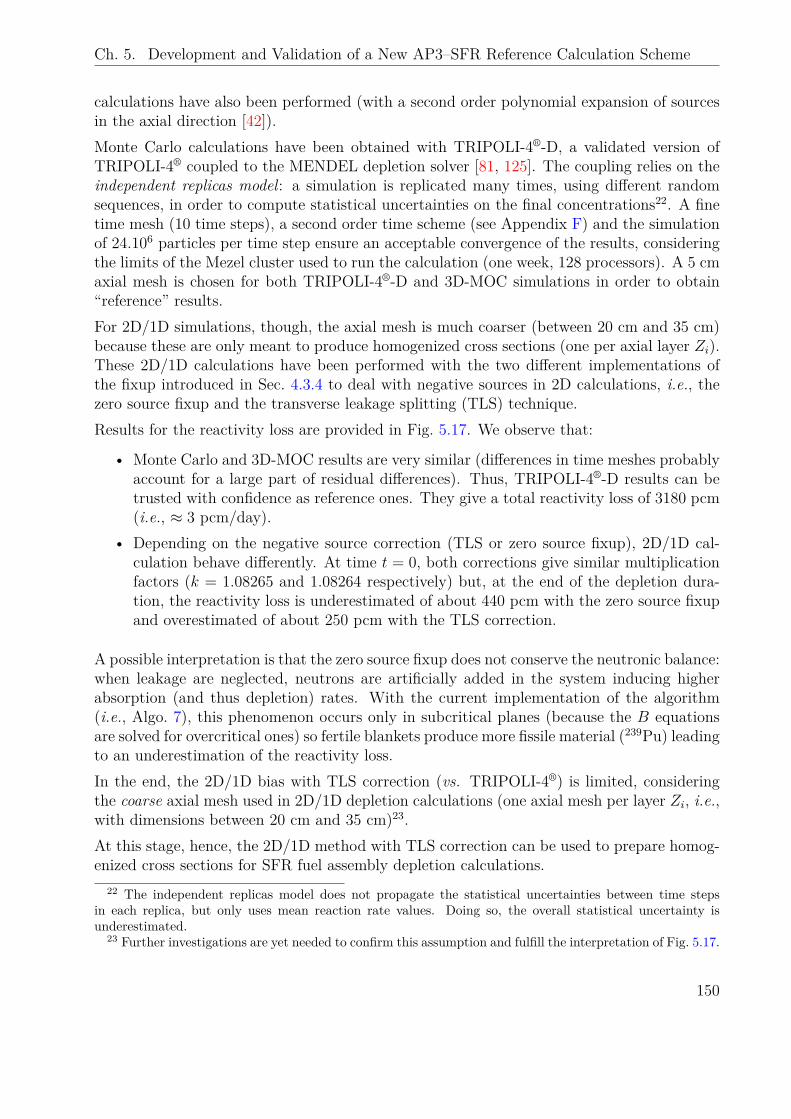
Ch. 5. Development and Validation of a New AP3–SFR Reference Calculation Scheme
calculations have also been performed (with a second order polynomial expansion of sourcesin the axial direction [42]).Monte Carlo calculations have been obtained with TRIPOLI-4®-D, a validated version ofTRIPOLI-4® coupled to the MENDEL depletion solver [81, 125]. The coupling relies on theindependent replicas model: a simulation is replicated many times, using different randomsequences, in order to compute statistical uncertainties on the final concentrations22. A finetime mesh (10 time steps), a second order time scheme (see Appendix F) and the simulationof 24.106 particles per time step ensure an acceptable convergence of the results, consideringthe limits of the Mezel cluster used to run the calculation (one week, 128 processors). A 5 cmaxial mesh is chosen for both TRIPOLI-4®-D and 3D-MOC simulations in order to obtain“reference” results.For 2D/1D simulations, though, the axial mesh is much coarser (between 20 cm and 35 cm)because these are only meant to produce homogenized cross sections (one per axial layer Zi).These 2D/1D calculations have been performed with the two different implementations ofthe fixup introduced in Sec. 4.3.4 to deal with negative sources in 2D calculations, i.e., thezero source fixup and the transverse leakage splitting (TLS) technique.Results for the reactivity loss are provided in Fig. 5.17. We observe that:
• Monte Carlo and 3D-MOC results are very similar (differences in time meshes probablyaccount for a large part of residual differences). Thus, TRIPOLI-4®-D results can betrusted with confidence as reference ones. They give a total reactivity loss of 3180 pcm(i.e., ≈ 3 pcm/day).
• Depending on the negative source correction (TLS or zero source fixup), 2D/1D cal-culation behave differently. At time t = 0, both corrections give similar multiplicationfactors (k = 1.08265 and 1.08264 respectively) but, at the end of the depletion dura-tion, the reactivity loss is underestimated of about 440 pcm with the zero source fixupand overestimated of about 250 pcm with the TLS correction.
A possible interpretation is that the zero source fixup does not conserve the neutronic balance:when leakage are neglected, neutrons are artificially added in the system inducing higherabsorption (and thus depletion) rates. With the current implementation of the algorithm(i.e., Algo. 7), this phenomenon occurs only in subcritical planes (because the B equationsare solved for overcritical ones) so fertile blankets produce more fissile material (239Pu) leadingto an underestimation of the reactivity loss.In the end, the 2D/1D bias with TLS correction (vs. TRIPOLI-4®) is limited, consideringthe coarse axial mesh used in 2D/1D depletion calculations (one axial mesh per layer Zi, i.e.,with dimensions between 20 cm and 35 cm)23.At this stage, hence, the 2D/1D method with TLS correction can be used to prepare homog-enized cross sections for SFR fuel assembly depletion calculations.
22 The independent replicas model does not propagate the statistical uncertainties between time stepsin each replica, but only uses mean reaction rate values. Doing so, the overall statistical uncertainty isunderestimated.
23 Further investigations are yet needed to confirm this assumption and fulfill the interpretation of Fig. 5.17.
150
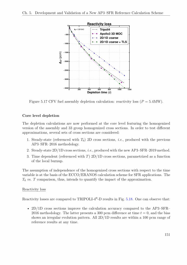
Ch. 5. Development and Validation of a New AP3–SFR Reference Calculation Scheme
0 200 400 600 800 1000 1200
Depletion time (d)
−3500
−3000
−2500
−2000
−1500
−1000
−500
0
∆ρ
(pcm
)
k0=1.081643
Reactivity lossTripoli4Apollo3 3D MOC2D/1D coarse2D/1D coarse + TLS
Figure 5.17 CFV fuel assembly depletion calculation: reactivity loss (P = 5.4MW).
Core level depletion
The depletion calculations are now performed at the core level featuring the homogenizedversion of the assembly and 33 group homogenized cross sections. In order to test differentapproximations, several sets of cross sections are considered:
1. Steady-state (referenced with T0) 2D cross sections, i.e., produced with the previousAP3–SFR–2016 methodology.
2. Steady-state 2D/1D cross sections, i.e., produced with the new AP3–SFR–2019 method.3. Time dependent (referenced with T ) 2D/1D cross sections, parametrized as a function
of the local burnup.
The assumption of independence of the homogenized cross sections with respect to the timevariable is at the basis of the ECCO/ERANOS calculation scheme for SFR applications. TheT0 vs. T comparison, thus, intends to quantify the impact of the approximation.
Reactivity loss
Reactivity losses are compared to TRIPOLI-4®-D results in Fig. 5.18. One can observe that:
• 2D/1D cross sections improve the calculation accuracy compared to the AP3–SFR–2016 methodology. The latter presents a 300 pcm difference at time t = 0, and the biasshows an irregular evolution pattern. All 2D/1D results are within a 100 pcm range ofreference results at any time.
151
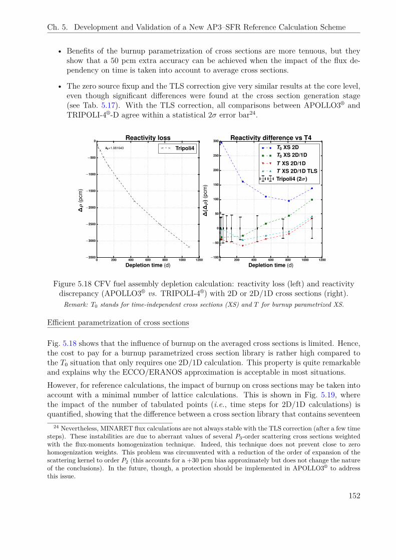
Ch. 5. Development and Validation of a New AP3–SFR Reference Calculation Scheme
• Benefits of the burnup parametrization of cross sections are more tenuous, but theyshow that a 50 pcm extra accuracy can be achieved when the impact of the flux de-pendency on time is taken into account to average cross sections.
• The zero source fixup and the TLS correction give very similar results at the core level,even though significant differences were found at the cross section generation stage(see Tab. 5.17). With the TLS correction, all comparisons between APOLLO3® andTRIPOLI-4®-D agree within a statistical 2σ error bar24.
0 200 400 600 800 1000 1200
Depletion time (d)
−3500
−3000
−2500
−2000
−1500
−1000
−500
0
∆ρ
(pcm
)
k0=1.081643
Reactivity lossTripoli4
0 200 400 600 800 1000 1200
Depletion time (d)
−100
−50
0
50
100
150
200
250
300
∆(∆
ρ)(
pcm
)
Reactivity difference vs T4T0 XS 2DT0 XS 2D/1D
T XS 2D/1DT XS 2D/1D TLSTripoli4 (2σ)
Figure 5.18 CFV fuel assembly depletion calculation: reactivity loss (left) and reactivitydiscrepancy (APOLLO3® vs. TRIPOLI-4®) with 2D or 2D/1D cross sections (right).Remark: T0 stands for time-independent cross sections (XS) and T for burnup parametrized XS.
Efficient parametrization of cross sections
Fig. 5.18 shows that the influence of burnup on the averaged cross sections is limited. Hence,the cost to pay for a burnup parametrized cross section library is rather high compared tothe T0 situation that only requires one 2D/1D calculation. This property is quite remarkableand explains why the ECCO/ERANOS approximation is acceptable in most situations.However, for reference calculations, the impact of burnup on cross sections may be taken intoaccount with a minimal number of lattice calculations. This is shown in Fig. 5.19, wherethe impact of the number of tabulated points (i.e., time steps for 2D/1D calculations) isquantified, showing that the difference between a cross section library that contains seventeen
24 Nevertheless, MINARET flux calculations are not always stable with the TLS correction (after a few timesteps). These instabilities are due to aberrant values of several P3-order scattering cross sections weightedwith the flux-moments homogenization technique. Indeed, this technique does not prevent close to zerohomogenization weights. This problem was circumvented with a reduction of the order of expansion of thescattering kernel to order P2 (this accounts for a +30 pcm bias approximately but does not change the natureof the conclusions). In the future, though, a protection should be implemented in APOLLO3® to addressthis issue.
152
Ch. 5. Development and Validation of a New AP3–SFR Reference Calculation Scheme
tabulated burnup points, and another one that only contains two such points – one at timet = 0 and one at t = 1440 EFPD (beyond the depletion duration) – is less than 20 pcm. Inother words, no intermediate calculations are in fact required but most of the effect can becaught with only two transport calculations, performed at the initial and final (or close toit) stages of the estimated depletion duration.Furthermore, taking advantage of the flexibility of the 2D/1D method, a minimalist calcula-tion has been run, in which the 2D flux ψi – i.e., the solution of Eq. (4.25) – in non-depletingplanes (i.e., structures such as the sodium plenum, or neutronic protections) is only com-puted at time t = 0. The result is presented in Fig 5.19, showing that the re-evaluation ofnon-depleting planes at the lattice level is, in fact, not necessary.
0 200 400 600 800 1000 1200
Depletion time (d)
−100
−50
0
50
100
∆(∆
ρ)(
pcm
)
17 burnup tabuled points2 burnp tab.2 burnup tab. without structures
Figure 5.19 CFV fuel assembly depletion calculation: influence of the number of tabulatedburnup points (in the homogenized cross section library) on the reactivity loss (APOLLO3®
with 2D/1D cross sections vs. TRIPOLI-4®).
Material balance
Finally, Fig. 5.20 and Tab. 5.12 show the evolution of isotopic concentrations for a selectedchoice of isotopes, including heavy nuclides and fission products. Applying previous recom-mendations, the calculation has been run with a MPO library containing only two tabulatedpoints.Tab. 5.12 shows that the final concentrations of actinides (Pu239 and Np237) and fissionproducts (Cs133) are well predicted when the 2D/1D method is used to produce the effectivecross sections. Most discrepancies are below 1% except in the upper fertile zone (1 cmFCA) for which differences can reach a few % (with both 2D and 2D/1D methods). Onthe other hand, we observe that the AP3–SFR–2016 method systematically underestimatesthe concentration values in fertile blankets and especially at the bottom of the assembly. In
153
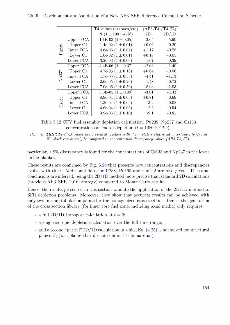
Ch. 5. Development and Validation of a New AP3–SFR Reference Calculation Scheme
T4 values (at/barn/cm) (AP3-T4)/T4 (%)N (1± 100 ∗ σ/N) 2D 2D/1D
Pu23
9
Upper FCA 1.1E-03 (1± 0.05) -2.64 -5.90Upper C1 1.4e-02 (1± 0.01) +0.06 +0.20Inner FCA 4.6e-03 (1± 0.02) +1.17 -0.28Lower C1 1.0e-02 (1± 0.01) +0.18 +0.05Lower FCA 3.2e-03 (1± 0.06) -1.67 -0.39
Np2
37Upper FCA 4.4E-06 (1± 0.37) -2.63 +1.40Upper C1 4.7e-05 (1± 0.18) +0.64 +0.56Inner FCA 1.7e-05 (1± 0.33) -4.41 +1.13Lower C1 2.6e-05 (1± 0.26) -1.48 +0.72Lower FCA 7.0e-06 (1± 0.56) -8.93 -1.03
Cs133
Upper FCA 3.3E-05 (1± 0.09) -3.01 -4.43Upper C1 8.9e-04 (1± 0.03) +0.81 -0.69Inner FCA 1.3e-04 (1± 0.04) -3.2 +0.08Lower C1 4.6e-04 (1± 0.05) -2.2 -0.54Lower FCA 3.9e-05 (1± 0.10) -9.1 -0.81
Table 5.12 CFV fuel assembly depletion calculation: Pu239, Np237 and Cs133concentrations at end of depletion (t = 1080 EFPD).
Remark: TRIPOLI-4®-D values are presented together with their relative statistical uncertainty (σ/N) in%, which can directly be compared to concentration discrepancy values (AP3-T4)/T4.
particular, a 9% discrepancy is found for the concentrations of Cs133 and Np237 in the lowerfertile blanket.These results are confirmed by Fig. 5.20 that presents how concentrations and discrepanciesevolve with time. Additional data for U238, Pd195 and Cm242 are also given. The sameconclusions are inferred, being the 2D/1D method more precise than standard 2D calculations(previous AP3–SFR–2016 strategy) compared to Monte Carlo results.Hence, the results presented in this section validate the application of the 2D/1D method toSFR depletion problems. Moreover, they show that accurate results can be achieved withonly two burnup tabulation points for the homogenized cross sections. Hence, the generationof the cross section library (for inner core fuel zone, including axial media) only requires:
- a full 2D/1D transport calculation at t = 0;- a single isotopic depletion calculation over the full time range;- and a second “partial” 2D/1D calculation in which Eq. (4.25) is not solved for structuralplanes Zi (i.e., planes that do not contain fissile material).
154
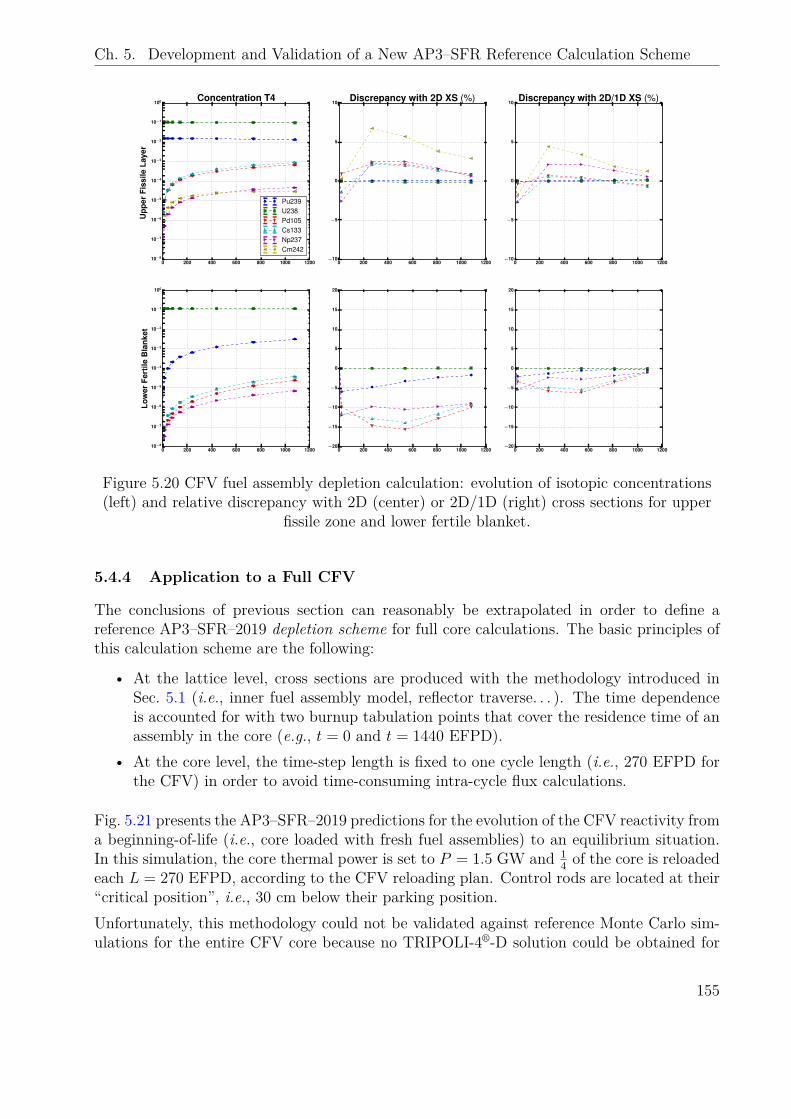
Ch. 5. Development and Validation of a New AP3–SFR Reference Calculation Scheme
0 200 400 600 800 1000 120010−8
10−7
10−6
10−5
10−4
10−3
10−2
10−1
100
Upp
erFi
ssile
Laye
r
Concentration T4
Pu239U238Pd105Cs133Np237Cm242
0 200 400 600 800 1000 1200−10
−5
0
5
10Discrepancy with 2D XS (%)
0 200 400 600 800 1000 1200−10
−5
0
5
10Discrepancy with 2D/1D XS (%)
0 200 400 600 800 1000 120010−8
10−7
10−6
10−5
10−4
10−3
10−2
10−1
100
Low
erFe
rtile
Bla
nket
0 200 400 600 800 1000 1200−20
−15
−10
−5
0
5
10
15
20
0 200 400 600 800 1000 1200−20
−15
−10
−5
0
5
10
15
20
Figure 5.20 CFV fuel assembly depletion calculation: evolution of isotopic concentrations(left) and relative discrepancy with 2D (center) or 2D/1D (right) cross sections for upper
fissile zone and lower fertile blanket.
5.4.4 Application to a Full CFV
The conclusions of previous section can reasonably be extrapolated in order to define areference AP3–SFR–2019 depletion scheme for full core calculations. The basic principles ofthis calculation scheme are the following:
• At the lattice level, cross sections are produced with the methodology introduced inSec. 5.1 (i.e., inner fuel assembly model, reflector traverse. . . ). The time dependenceis accounted for with two burnup tabulation points that cover the residence time of anassembly in the core (e.g., t = 0 and t = 1440 EFPD).
• At the core level, the time-step length is fixed to one cycle length (i.e., 270 EFPD forthe CFV) in order to avoid time-consuming intra-cycle flux calculations.
Fig. 5.21 presents the AP3–SFR–2019 predictions for the evolution of the CFV reactivity froma beginning-of-life (i.e., core loaded with fresh fuel assemblies) to an equilibrium situation.In this simulation, the core thermal power is set to P = 1.5 GW and 1
4 of the core is reloadedeach L = 270 EFPD, according to the CFV reloading plan. Control rods are located at their“critical position”, i.e., 30 cm below their parking position.Unfortunately, this methodology could not be validated against reference Monte Carlo sim-ulations for the entire CFV core because no TRIPOLI-4®-D solution could be obtained for
155
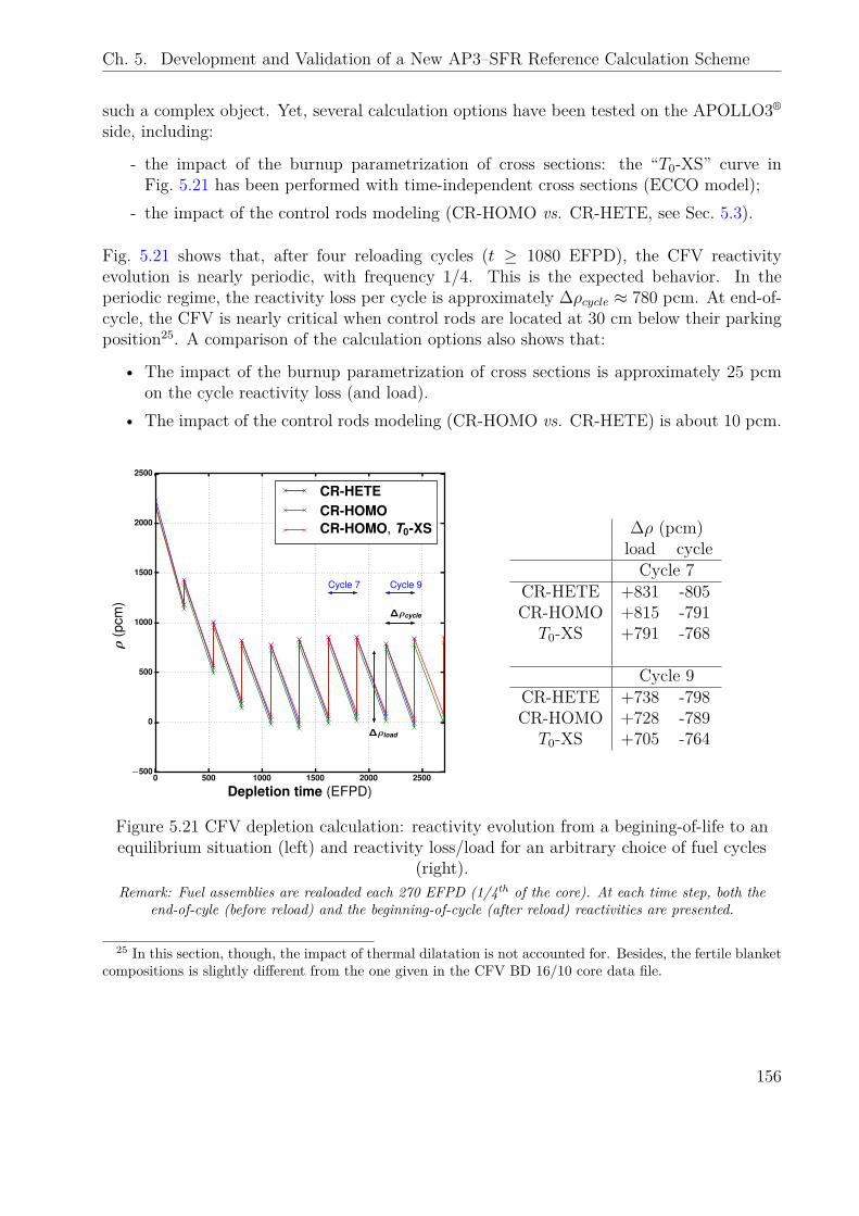
Ch. 5. Development and Validation of a New AP3–SFR Reference Calculation Scheme
such a complex object. Yet, several calculation options have been tested on the APOLLO3®
side, including:
- the impact of the burnup parametrization of cross sections: the “T0-XS” curve inFig. 5.21 has been performed with time-independent cross sections (ECCO model);
- the impact of the control rods modeling (CR-HOMO vs. CR-HETE, see Sec. 5.3).
Fig. 5.21 shows that, after four reloading cycles (t ≥ 1080 EFPD), the CFV reactivityevolution is nearly periodic, with frequency 1/4. This is the expected behavior. In theperiodic regime, the reactivity loss per cycle is approximately ∆ρcycle ≈ 780 pcm. At end-of-cycle, the CFV is nearly critical when control rods are located at 30 cm below their parkingposition25. A comparison of the calculation options also shows that:
• The impact of the burnup parametrization of cross sections is approximately 25 pcmon the cycle reactivity loss (and load).
• The impact of the control rods modeling (CR-HOMO vs. CR-HETE) is about 10 pcm.
0 500 1000 1500 2000 2500
Depletion time (EFPD)
−500
0
500
1000
1500
2000
2500
ρ(p
cm)
∆ρcycle
∆ρload
Cycle 9Cycle 7
CR-HETECR-HOMOCR-HOMO, T0-XS ∆ρ (pcm)
load cycleCycle 7
CR-HETE +831 -805CR-HOMO +815 -791T0-XS +791 -768
Cycle 9CR-HETE +738 -798CR-HOMO +728 -789T0-XS +705 -764
Figure 5.21 CFV depletion calculation: reactivity evolution from a begining-of-life to anequilibrium situation (left) and reactivity loss/load for an arbitrary choice of fuel cycles
(right).Remark: Fuel assemblies are realoaded each 270 EFPD (1/4th of the core). At each time step, both the
end-of-cyle (before reload) and the beginning-of-cycle (after reload) reactivities are presented.
25 In this section, though, the impact of thermal dilatation is not accounted for. Besides, the fertile blanketcompositions is slightly different from the one given in the CFV BD 16/10 core data file.
156
Ch. 5. Development and Validation of a New AP3–SFR Reference Calculation Scheme
5.4.5 Discussion
Fuel depletion induces a change in cross sections that, strictly speaking, needs to be takeninto account. This can be done by performing a burnup parametrization of cross sections atthe lattice level. For 33 group SFR calculations, though, this effect is limited26. Hence:
In SFR cores, the time (or burnup) dependence of cross sections can be accounted forwith only two flux calculations at the lattice level (tabulation points), one at t = 0 and
another at t = tf (residence time of an assembly in the core).
This remarkable property, which was already highlighted by A. Greganti [126], was validatedin a rigorous way for a 3D CFV fuel assembly case, and extrapolated to any other mediumsubject to depletion (e.g., fuel in core / reflector traverse model).Nevertheless, the burnup parametrization of cross sections may be safely dropped out whenthe constraint on the computational resources is severe (e.g., for project calculation schemes)because it does not overly impact the final accuracy.
5.5 Evaluation of Neutronic Feedback Coefficients
5.5.1 General Considerations on Transient Calculations
During the design phase of a nuclear reactor, one must define the steady-state normal operat-ing conditions as well as all the transient situations the reactor might face during its lifetime.The fuel depletion is an example of such a “transient” situation. In that particular case, how-ever, changes operate over very large time scales (hours, days, months) making it possible totreat these problems as a succession of steady-sate situations (adiabatic approximation).A reactor in nominal operating conditions is also supposed to face different transient situ-ations with shorter time scales (second, minute, hour). An example of a normal transientscenario is the power-load monitoring whose objective is to adapt the reactor power to theelectricity grid requirements. If the change in the reactor operating state (power, tempera-tures,. . . ) does not overly affect the flux shape, such transient situations can be accuratelysimulated with simple models such as the Point Kinetics (PK) approximation [127], whichdemand a minimal number of flux calculations.Nevertheless, the reactor might also face accidental situations. They can be classified intotwo categories:
• Accidental situations due to a loss of cooling capacity: they can be global (e.g., loss offlow in the primary, secondary or both coolant loops) or local (e.g., loss of flow in onefuel assembly).
• Reactivity insertion accidental situations, among which one can list unexpected controlrod withdrawals, core compaction, or coolant boiling situations.
26 In a LWR, this effect cannot be neglected because the production of thermal absorbers (Xe, Sm,. . . )with fuel depletion significantly shifts the neutron spectrum towards higher energies.
157
Ch. 5. Development and Validation of a New AP3–SFR Reference Calculation Scheme
In such accidental situations, the change in both the neutron flux amplitude and shape mayeventually be significant in short time frames (second, minute). This occurs, for instance,during reactivity insertion transients. In that case, large amounts of energy are inserted intothe system, giving birth to strong coupling between different physical phenomena (neutron-ics, thermo-hydraulics, mechanics. . . ). At some point, simple models (e.g., PK) need to bereplaced by more refined methods, such as the quasi-static approach [128, 129]. Unfortu-nately, these methods often demand a large number of flux calculations to update the fluxshape, i.e., massive computational capacities27.Prior to any complex calculation, though, a simple way to take a glimpse to the neutronicbehavior of a reactor is to compute neutronic feedback coefficients. The latter quantifythe reactor response (reactivity ρ) to individual perturbations (e.g., changes in the coolantdensity, fuel temperature. . . ):
• The coolant-void reactivity worth quantifies the impact of a decrease of the coolantdensity in the core. It is usually measured by the means of a reactivity difference (inpcm) or a relative variation (in pcm per % of change of the nominal coolant density,δdNa);
∆ρNa = ρvoided − ρnominal or ∆ρ%Na = ∆ρNa
|δdNa|(5.8)
• The Doppler coefficient quantifies the reactivity insertion due to a change in the fueltemperature28. It is often measured through the Doppler constant (under the assump-tion of a logarithmic law):
KD = ∆ρln(Tpert
Tref)
(5.9)
• The geometrical dilatation coefficients quantify the impact of thermal dilatations, in-cluding radial and axial expansion of clad, assembly wrapper tubes, fuel rods. . . .
At zeroth order, the safety of reactor is connected to the sign of the neutronic feedbackcoefficients: if a perturbation is such that ∆ρ < 0, then the neutronic power will naturallydecrease. In real situations, though, the different physical phenomena influence each other.Thus, the reactor safety demonstration demands to optimize the sum of all the reactivitycontributions during specified transients. This may be done through global feedback coeffi-cients, which link the reactivity change between two equilibrium states (beginning and end oftransient) to measurable parameters, such as the core inlet temperature, the coolant heating,or the reactor power. The American ABC [131] or French KGH methodologies [132] areexamples of such integral approaches.The individual neutronic feedback coefficients (coolant-void reactivity worth, Doppler con-stant. . . ) are often computed around the nominal operating point of the reactor, either with
27 Using efficiently these methods is still a topic of research today. At CEA, the multipoint kinetics [130] isenvisioned as a potential solution to design efficient quasi-static strategies (cf. G. Valocchi’s thesis at LEPh,to be published in 2020).
28 When the temperature increases, the thermal motion of nuclei modifies the shape of the cross sectionsresulting in higher absorption rates.
158
Ch. 5. Development and Validation of a New AP3–SFR Reference Calculation Scheme
two direct critical calculations (i.e., solving Eq. (2.34) in the normal and perturbed configu-rations) or using a perturbation theory formalism (see Appendix G). In the exact StandardPerturbation Theory (SPT), for instance, a reactivity variation is computed as a function ofthe direct perturbed flux ψp and adjoint nominal solution ψ† with [133]:
∆ρ =< ψ†,
(∆Fk−∆A
)ψp >
< ψ†,Fpψp >(5.10)
where ∆F = Fp −F , ∆A = Ap −A symbolize the production and absorption (A = L−H)operator perturbations, and <,> is the integral over phase-space (scalar product). Theadvantage of the perturbation formalism is that it highlights unitary operator perturbations:the contribution of any spatial cell, energy group or isotopic reaction rate can be estimated“splitting” the integral in the numerator of Eq. (5.10).In addition to their quality of physical estimators, these coefficients can also be used intransient simulation tools that rely on PK models to simulate complex transient scenarios.At CEA, CATHARE [134] and MACARENa [135] are examples of tools that are used forSFR transient assessment29.
5.5.2 Evaluation of the CFV Integral Coefficients
A reference neutronic calculation scheme should be capable of handling accurate feedbackcoefficients30. The AP3–SFR–2019 methodology proposed in this chapter already proved itscapacity to compute the CFV sodium-void reactivity worth. Yet, this was done in a non-realistic situation (99% void rate for all the core assemblies, including the radial reflector andbelow the fissile zone).The aim of this section is, therefore, to give an idea of the new AP3–SFR–2019 bias (vs.TRIPOLI-4® simulations) for the calculation of the main feedback coefficients, including thesodium-void reactivity worth in a “semi-realistic” situation and Doppler constants. Thisvalidation work has been performed for a beginning-of-life CFV (i.e., loaded with fresh fuel)because no reference (TRIPOLI-4®) results could be obtained for an equilibrium core31.The voiding geometrical pattern considered in this section corresponds to physical zoneslocated above the lower fertile blanket and below the upper neutronic protection. Thiscorresponds to 120 cm < z < 247.5 cm with the coordinate system of Fig. 5.7 for instance.Radial reflector assemblies are not voided because no extra-heat is usually generated in theseassemblies, even in abnormal situations.Two Doppler constants are computed with Eq. (5.9), one for fissile media (C1 and C2,Tref = 1474 K) and another for fertile ones (FCA, Tref = 924 K). The amplitude of the
29 MACARENa has been used in this work, see Chapter 6.30 The question of the calculation of the kinetic parameters (delayed neutron fraction β, mean generation
time Λ) is discussed in Chapter 6.31 Difficulties were found when it came to build the depleted TRIPOLI-4® model due to the large number
of depleted compositions.
159
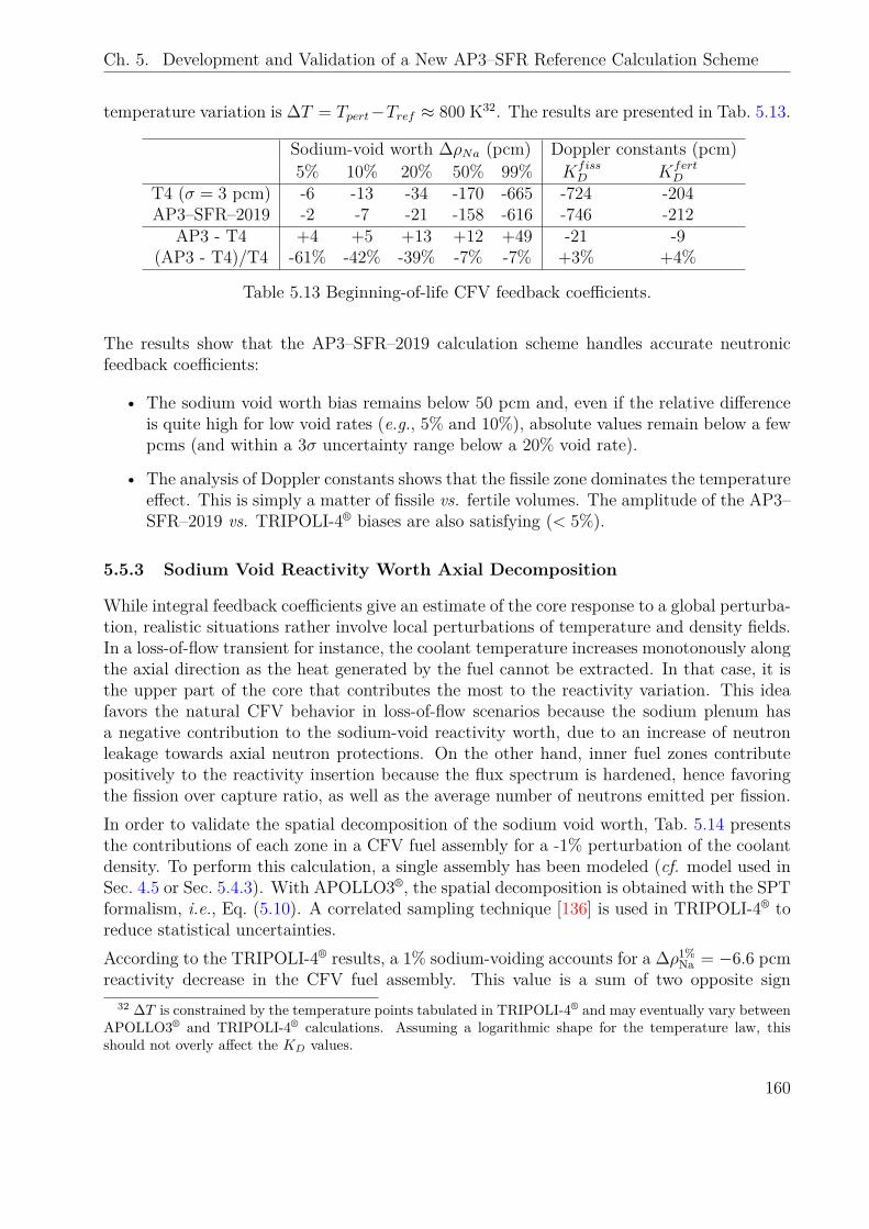
Ch. 5. Development and Validation of a New AP3–SFR Reference Calculation Scheme
temperature variation is ∆T = Tpert−Tref ≈ 800 K32. The results are presented in Tab. 5.13.
Sodium-void worth ∆ρNa (pcm) Doppler constants (pcm)5% 10% 20% 50% 99% Kfiss
D KfertD
T4 (σ = 3 pcm) -6 -13 -34 -170 -665 -724 -204AP3–SFR–2019 -2 -7 -21 -158 -616 -746 -212
AP3 - T4 +4 +5 +13 +12 +49 -21 -9(AP3 - T4)/T4 -61% -42% -39% -7% -7% +3% +4%
Table 5.13 Beginning-of-life CFV feedback coefficients.
The results show that the AP3–SFR–2019 calculation scheme handles accurate neutronicfeedback coefficients:
• The sodium void worth bias remains below 50 pcm and, even if the relative differenceis quite high for low void rates (e.g., 5% and 10%), absolute values remain below a fewpcms (and within a 3σ uncertainty range below a 20% void rate).
• The analysis of Doppler constants shows that the fissile zone dominates the temperatureeffect. This is simply a matter of fissile vs. fertile volumes. The amplitude of the AP3–SFR–2019 vs. TRIPOLI-4® biases are also satisfying (< 5%).
5.5.3 Sodium Void Reactivity Worth Axial Decomposition
While integral feedback coefficients give an estimate of the core response to a global perturba-tion, realistic situations rather involve local perturbations of temperature and density fields.In a loss-of-flow transient for instance, the coolant temperature increases monotonously alongthe axial direction as the heat generated by the fuel cannot be extracted. In that case, it isthe upper part of the core that contributes the most to the reactivity variation. This ideafavors the natural CFV behavior in loss-of-flow scenarios because the sodium plenum hasa negative contribution to the sodium-void reactivity worth, due to an increase of neutronleakage towards axial neutron protections. On the other hand, inner fuel zones contributepositively to the reactivity insertion because the flux spectrum is hardened, hence favoringthe fission over capture ratio, as well as the average number of neutrons emitted per fission.In order to validate the spatial decomposition of the sodium void worth, Tab. 5.14 presentsthe contributions of each zone in a CFV fuel assembly for a -1% perturbation of the coolantdensity. To perform this calculation, a single assembly has been modeled (cf. model used inSec. 4.5 or Sec. 5.4.3). With APOLLO3®, the spatial decomposition is obtained with the SPTformalism, i.e., Eq. (5.10). A correlated sampling technique [136] is used in TRIPOLI-4® toreduce statistical uncertainties.According to the TRIPOLI-4® results, a 1% sodium-voiding accounts for a ∆ρ1%
Na = −6.6 pcmreactivity decrease in the CFV fuel assembly. This value is a sum of two opposite sign
32 ∆T is constrained by the temperature points tabulated in TRIPOLI-4® and may eventually vary betweenAPOLLO3® and TRIPOLI-4® calculations. Assuming a logarithmic shape for the temperature law, thisshould not overly affect the KD values.
160
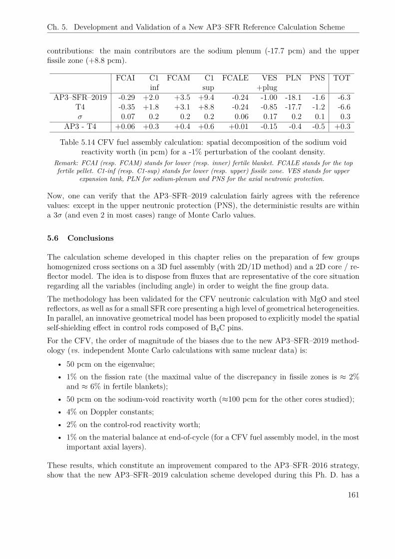
Ch. 5. Development and Validation of a New AP3–SFR Reference Calculation Scheme
contributions: the main contributors are the sodium plenum (-17.7 pcm) and the upperfissile zone (+8.8 pcm).
FCAI C1 FCAM C1 FCALE VES PLN PNS TOTinf sup +plug
AP3–SFR–2019 -0.29 +2.0 +3.5 +9.4 -0.24 -1.00 -18.1 -1.6 -6.3T4 -0.35 +1.8 +3.1 +8.8 -0.24 -0.85 -17.7 -1.2 -6.6σ 0.07 0.2 0.2 0.2 0.06 0.17 0.2 0.1 0.3
AP3 - T4 +0.06 +0.3 +0.4 +0.6 +0.01 -0.15 -0.4 -0.5 +0.3
Table 5.14 CFV fuel assembly calculation: spatial decomposition of the sodium voidreactivity worth (in pcm) for a -1% perturbation of the coolant density.
Remark: FCAI (resp. FCAM) stands for lower (resp. inner) fertile blanket. FCALE stands for the topfertile pellet. C1-inf (resp. C1-sup) stands for lower (resp. upper) fissile zone. VES stands for upper
expansion tank, PLN for sodium-plenum and PNS for the axial neutronic protection.
Now, one can verify that the AP3–SFR–2019 calculation fairly agrees with the referencevalues: except in the upper neutronic protection (PNS), the deterministic results are withina 3σ (and even 2 in most cases) range of Monte Carlo values.
5.6 Conclusions
The calculation scheme developed in this chapter relies on the preparation of few groupshomogenized cross sections on a 3D fuel assembly (with 2D/1D method) and a 2D core / re-flector model. The idea is to dispose from fluxes that are representative of the core situationregarding all the variables (including angle) in order to weight the fine group data.The methodology has been validated for the CFV neutronic calculation with MgO and steelreflectors, as well as for a small SFR core presenting a high level of geometrical heterogeneities.In parallel, an innovative geometrical model has been proposed to explicitly model the spatialself-shielding effect in control rods composed of B4C pins.For the CFV, the order of magnitude of the biases due to the new AP3–SFR–2019 method-ology (vs. independent Monte Carlo calculations with same nuclear data) is:
• 50 pcm on the eigenvalue;• 1% on the fission rate (the maximal value of the discrepancy in fissile zones is ≈ 2%
and ≈ 6% in fertile blankets);• 50 pcm on the sodium-void reactivity worth (≈100 pcm for the other cores studied);• 4% on Doppler constants;• 2% on the control-rod reactivity worth;• 1% on the material balance at end-of-cycle (for a CFV fuel assembly model, in the most
important axial layers).
These results, which constitute an improvement compared to the AP3–SFR–2016 strategy,show that the new AP3–SFR–2019 calculation scheme developed during this Ph. D. has a
161
Ch. 5. Development and Validation of a New AP3–SFR Reference Calculation Scheme
good ability to compute a wide range of neutronic parameters. Besides, it is robust to thecore design, thus matching one of the adaptability constraints defined as an objective for thiswork.From the methodological point of view, the main conclusion that can be drawn from thischapter is that:'
&
$
%
The representativeness of the geometrical patterns (including the boundary condition)used to produce the homogenized cross sections is a key parameter to define accuratecalculation schemes as it drives what physical effects are “stored” in the averagedparameters. The consistency of the homogenization theory – i.e., its capacity topreserve the average value of the solution in the homogenized situation – then
guarantees the quality of the core solution.
Unfortunately, the improvements resulting from the innovative methods proposed in thischapter have repercussions on the overall computational cost of the AP3–SFR–2019 calcu-lation scheme. A coarse estimation shows that, a complete neutronic evaluation of a CFV(including fuel depletion, feedback coefficients and S-curve) with the reference methodologydesigned in this chapter requires about five days (and 30 GB max) with 8 processors:
• Six 2D/1D calculations of the inner fuel assembly are needed to produce cross sectionsin nominal and accidental (Doppler, void) configurations at beginning and end-of-cycle.This demands approximately 9 hours (without acceleration) according to Tab. 4.11 (×2processors).
• Six core / reflector traverse calculations are also needed, i.e., approximately 3 hours(cf. Tab. 5.2, ×2 processors).
• Height cluster calculations are required (control rods, rod followers, dummy assembliesin nominal conditions) representing about 40’ (cf. Tab. 3.7, ×2 processors).
• Twelve core calculations are required to obtain an equilibrium core from a beginningof life situation. This demands approximately 40 hours with a CR-HOMO modelaccording to Tab. 5.11.
• Six core calculations are required to characterize the nominal core state with a CR-HETE model (nominal, voided, Doppler at beginning and end-of-cycle) i.e., about32 hours.
• Approximately six core calculations are finally needed to draw the S-curve of controlrods, i.e., 32 hours.
Even though these figures remain acceptable for reference calculations, they may be an issuewhen many calculations need to be performed in a limited amount of time, e.g., for parametricstudies. This is discussed in Chapter 6.Finally, it could also be objected to the methodology proposed in this chapter that thechoice of the geometrical models used to prepare the few groups homogenized cross sectionsis somehow empirical, as it is based on user-dependent physical considerations. Perspectivesto get rid of this arbitrariness are also discussed in Chapter 6.
162
Chapter 6 Towards Flexible & Adaptative CalculationSchemes
Abstract
This chapter develops the concept of adaptability for neutronic calculation schemes from twodifferent perspectives: adaptability to the computer resources constraint, but also adaptabil-ity as a form of automatization of the choices the physicist/engineer needs to make whendefining a calculation strategy. The first kind of adaptability responds to concrete engineer-ing problems that are recalled in Sec. 6.1. For the sake of illustration, the needs for accurateneutronic calculation strategies in multi-physics transient studies, in particular, are discussedin Sec. 6.2. Possible strategies to reduce the neutronic computational constraint are then as-sessed in Sec. 6.3. As for the second kind of adaptability, perspectives are given in Sec. 6.4 toget over the main drawback of the strategy proposed in Chapter 5, i.e., the arbitrariness ofthe geometrical patterns chosen to produce the few groups homogenized cross sections. Theidea is to pave the way for truly adaptative neutronic calculation methods.
Contents
6.1 Needs for Faster Calculation Schemes . . . . . . . . . . . . . . . . 1646.1.1 Reactor Design Studies . . . . . . . . . . . . . . . . . . . . . . . . 1646.1.2 Multi-physics Calculations . . . . . . . . . . . . . . . . . . . . . . . 164
6.2 Illustration: Sensitivity of an ULOF Transient to the NeutronicCalculation Strategy . . . . . . . . . . . . . . . . . . . . . . . . . . . 165
6.2.1 Methodology Presentation . . . . . . . . . . . . . . . . . . . . . . . 1656.2.2 Analysis of PK Parameters . . . . . . . . . . . . . . . . . . . . . . 1686.2.3 Impact on the ULOF Outcome . . . . . . . . . . . . . . . . . . . . 1706.2.4 Discussion . . . . . . . . . . . . . . . . . . . . . . . . . . . . . . . . 172
6.3 Construction of AP3–SFR Project Methodologies . . . . . . . . . 1726.3.1 Strategy Assessment . . . . . . . . . . . . . . . . . . . . . . . . . . 1726.3.2 Degradation of the Reference Options . . . . . . . . . . . . . . . . 1736.3.3 Resort to ad hoc Physical Models . . . . . . . . . . . . . . . . . . . 1776.3.4 Discussion . . . . . . . . . . . . . . . . . . . . . . . . . . . . . . . . 181
6.4 Beyond the Lattice / Core Paradigm . . . . . . . . . . . . . . . . 1826.4.1 Dynamic Homogenization . . . . . . . . . . . . . . . . . . . . . . . 1826.4.2 Towards Flexible Homogenization . . . . . . . . . . . . . . . . . . 186
6.5 Conclusions . . . . . . . . . . . . . . . . . . . . . . . . . . . . . . . . 186
163
Ch. 6. Towards Flexible & Adaptative Calculation Schemes
6.1 Needs for Faster Calculation Schemes
The choices made in Chapter 5 for the construction of a reference calculation scheme forSFR applications led to quite significant needs in terms of computer resources. While thestrategy ensures a best-estimate solution with mastered biases, one might desire disposingof faster methods when many calculations need to be performed. The difficulty, then, is toavoid overly degrading the accuracy of the solution.
6.1.1 Reactor Design Studies
In the research field, one is usually interested in performing parametric studies involving alarge number of core calculations (e.g., to define global orientations for a core design or tomeasure the robustness of a core to a set of perturbations). As the number of calculationincreases, the speed of execution of individual calculations becomes a crucial parameter.Hence, project calculation schemes should drastically reduce the computational footprint ofthe reference methodology.
6.1.2 Multi-physics Calculations
In a transient, the core neutronic response is just a part of the overall reactor behavior. Thus,in many practical situations, realistic numerical models need to take into account couplingbetween neutronics, thermo-hydraulics (coolant flow, thermal dilatation, boiling crisis,. . . )and mechanics (thermo-mechanical resistance, fuel-clad interaction,. . . ).As discussed in Sec. 5.5, this coupling can often be taken into account through simple models,such as the Point Kinetics (PK) approximation. In that case, a minimal number of neutroniccalculations are required and, probably, a reference calculation scheme can be used.However, when the coupling increases, it may induce significant changes in the flux shapeand, consequently, on the PK parameters. In that case, the number of neutron transportcalculations that need to be performed increases1. Again, the speed of execution of individualcore calculations becomes a key parameter for the practical realization of such transientstudies.Moreover, the share of neutronics in the final transient response is somehow diluted whenother physics (thermo-hydraulics and mechanics) are involved. In particular, determiningthis share seems to be a reasonable way to assess a target accuracy for neutronic calculationstrategies.To this end, an investigation of the sensitivity of the outcome of a transient scenario to theneutronic calculation scheme is presented in the next section.
1 Eventually, more refined models (e.g., quasi-static) can be used.
164
Ch. 6. Towards Flexible & Adaptative Calculation Schemes
6.2 Illustration: Sensitivity of an ULOF Transient to the Neutronic CalculationStrategy
More precisely, this section investigates how the outcome of an Unprotected Loss-Of-Flow(ULOF) scenario in a CFV is affected by the choices made in the neutronic strategy usedto compute the PK parameters. This work was presented to the M&C-2019 conferenceconference [137].
6.2.1 Methodology Presentation
The geometrical model
The benchmark chosen to perform this study is the 3D CFV fuel assembly model alreadypresented in Sec. 4.5 and Sec. 5.4.3 to validate the 2D/1D method in steady-state and deple-tion situations, respectively2. This geometrical model is quite simple because it neglects thequestion of the reflector modeling. Yet, it is representative of the inner core situation.
The ULOF transient
The ULOF transient is an accidental scenario characterized by an unexpected primary pumpstrip without scram. This scenario leads to a quick decrease of the sodium cooling flow rate(Q) in the core while the reactor is still in a power state.As the flow rate decreases, the reactor power (P ) varies according to the reactivity feedbackcoefficient values. At this stage, the dominant effect in a CFV is the negative reactivityinsertion that arises from the decrease of the sodium density in the plenum (see Tab. 5.14 inChapter 5 for instance).During the first phase of the ULOF scenario, the reactor power, therefore, decreases. Thephenomenology of the transient is then driven by the evolution of the power over flow–rateratio: if P/Q remains high, the heat is not extracted, and the sodium may reach its boilingpoint.When the boiling crisis starts, different outcomes may be observed depending on the value ofthe reactor power [138]. If P is low enough, the boiling front–line may remain stable, near thecore outlet, and the heat might be extracted with natural convection. Else, dynamic instabili-ties arise from the strong coupling between neutronic and thermo-hydraulic phenomena [139].If bubbles propagate to the core center, the core integrity cannot be guaranteed.
Transient simulation with MACARENa
Such an ULOF scenario has been modeled with MACARENa, which is a validated tool,developed at CEA by J.-B. Droin (during its Ph. D. thesis), for the analysis of SFR loss-of-flow transients [135, 138].
2 In order to be representative of a reactor in operating conditions, though, all material have been expandedaccording to their temperature and thermal dilatation law. Besides, the composition of fertile layers is slightlydifferent in this section.
165
Ch. 6. Towards Flexible & Adaptative Calculation Schemes
On the thermo-hydraulic side, the main features of MACARENa are:- a 0D model for the momentum conservation law of the coolant;- a 2D radial-axial simplified model (one radial mesh per material) for the energy con-servation law in order to compute the temperature fields;
- a 1D axial two-phase flow mixture model for boiling situations3.
On the neutronic side, MACARENa relies on a PK model, whose basic assumption is thatthe power spatial distribution is constant during the transient. The PK equations, which arederived in Appendix G, are the following:
dN
dt+ β − ρ
ΛN =
8∑k=1
λkCk (6.1a)
dCkdt
+ λkCk = βk
ΛN , k ∈ 1, 2, . . . , 8 (6.1b)
where N is the total number of neutrons, and Ck is the delayed neutrons precursors concen-tration in family k (cf. Sec. 2.1.3). These equations are used to compute the reactor power4:
P ∝ N (6.2)
The parameters of the PK model are:- the reactivity ρ;- the delayed neutron fractions βk (per family k) and β (total);- the mean neutron generation time Λ;- the precursors decay constants λk.
In theory, these parameters should be updated during the transient as the neutron flux shapechanges5 [127]. Except for the reactivity, though, these variations are neglected in the PKframework.The reactivity ρ is allowed to vary because it is quite sensitive to local perturbations of thereactor state (coolant density, fuel temperature. . . ). In this work, the physical phenomenathat have been considered are the sodium–void and Doppler effects. In MACARENa, ρ isre-constructed using pre-computed local feedback coefficients according to:
ρ(t) = ρ0 +∫fuel
KD(r) ln(
T (r, t)T (r, t = 0)
)d3r +
∫coolant
αNa(r)δdNa(r, t)d3r (6.3)
where KD is the Doppler constant, T the fuel temperature, αNa the sodium–void reactivitycoefficient and δdNa the relative variation of the coolant density (in % of the reference density).
3 A degradation model that enables simulating core damage from overheating is also implemented inMACARENa. Yet, no such phase is considered in this work.
4 If the residual power Pr (heat due to radioactive decay of fission products and minor actinides) remainsproportional to the total power P during the transient (Pr ≈ 7%P), it directly follows that P is proportionalto N .
5 Except for decay constants λk that are evaluated nuclear data and, therefore, do not depend on the fluxshape.
166
Ch. 6. Towards Flexible & Adaptative Calculation Schemes
Calculation of the PK parameters with APOLLO3®
The PK parameters (initial power shape P , delayed neutron factions βk, β, mean neutrongeneration time Λ and spatial reactivity feedback coefficients KD, αNa) have been producedwith APOLLO3®:
• The initial power shape P = P(ψ0) is computed as a function of the flux ψ0 solutionof the following critical problem:
Aψ0 = 1k0Fψ0 (6.4)
defined over the unperturbed reactor (with A = L −H).• The delayed neutron fractions and mean neutron generation time are computed as:
βk = < ψ†0 · Fd,kψ0 >
< ψ†0 · Fψ0 >, β =
8∑k=1
βk, Λ =< ψ†0 · 1
vψ0 >
< ψ†0 · Fψ0 >(6.5)
where < . > stands for the integral over phase-space (scalar product), Fd,k is theprecursors production operator in family k, and ψ0† is the solution of the adjointproblem corresponding to the unperturbed reactor (cf. Appendix G).
• The local (subscript i) reactivity feedback coefficients are finally computed around thenominal reactor state with the exact SPT formulae:
αδdNa,iNa = δρNa,i
δdNa
KD,i = δρDop,i
ln(T0+1000T0
)with δρp,i =
< ψ†0 ·(
1kδF − δA
)ψp >i
< ψ†0 · Fpψp >(6.6)
where p is the perturbation (void, Doppler), δF = Fp − F , δA = Ap − A are theoperator perturbations, and ψp is the perturbed (critical) flux. < . >i is the restrictionof the scalar product to spatial cell i.
All these coefficients are assumed to be constant during the transient6. This assumption isvalid if the perturbation of the neutron flux shape remains limited.In any case and as explained in the introduction of this section, the aim of this study is notto assess whether the PK approximation is valid, but to quantify the impact ofthe neutronic calculation scheme used to solve Eq. (6.4) on the transient outcome.To this end, three strategies are compared:
• The reference AP3–SFR–2019 calculation scheme developed in the framework of thisthesis (i.e., 2D/1D method to prepare the assembly cross sections). This strategyhandles best-estimate results.
• The previous AP3–SFR–2016 methodology (2D cross section preparation phase). Thisstrategy gives very poor results for a CFV neutronic calculation and, therefore, consti-tutes a “poor-estimate” method.
6 An allowance is yet made in MACARENa to take into account the non-linearity of the sodium-voidreactivity worth in the sodium plenum, with a second-order polynomial.
167
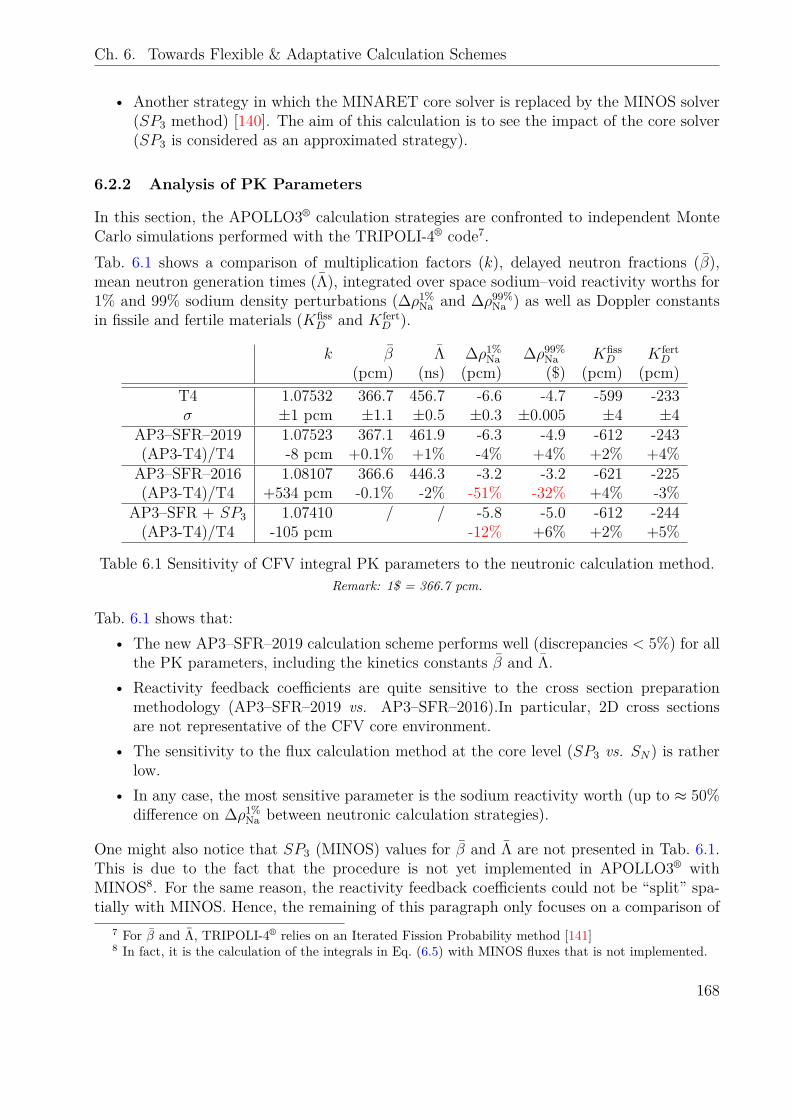
Ch. 6. Towards Flexible & Adaptative Calculation Schemes
• Another strategy in which the MINARET core solver is replaced by the MINOS solver(SP3 method) [140]. The aim of this calculation is to see the impact of the core solver(SP3 is considered as an approximated strategy).
6.2.2 Analysis of PK Parameters
In this section, the APOLLO3® calculation strategies are confronted to independent MonteCarlo simulations performed with the TRIPOLI-4® code7.Tab. 6.1 shows a comparison of multiplication factors (k), delayed neutron fractions (β),mean neutron generation times (Λ), integrated over space sodium–void reactivity worths for1% and 99% sodium density perturbations (∆ρ1%
Na and ∆ρ99%Na ) as well as Doppler constants
in fissile and fertile materials (KfissD and K fert
D ).
k β Λ ∆ρ1%Na ∆ρ99%
Na KfissD K fert
D
(pcm) (ns) (pcm) ($) (pcm) (pcm)T4 1.07532 366.7 456.7 -6.6 -4.7 -599 -233σ ±1 pcm ±1.1 ±0.5 ±0.3 ±0.005 ±4 ±4
AP3–SFR–2019 1.07523 367.1 461.9 -6.3 -4.9 -612 -243(AP3-T4)/T4 -8 pcm +0.1% +1% -4% +4% +2% +4%AP3–SFR–2016 1.08107 366.6 446.3 -3.2 -3.2 -621 -225(AP3-T4)/T4 +534 pcm -0.1% -2% -51% -32% +4% -3%
AP3–SFR + SP3 1.07410 / / -5.8 -5.0 -612 -244(AP3-T4)/T4 -105 pcm -12% +6% +2% +5%
Table 6.1 Sensitivity of CFV integral PK parameters to the neutronic calculation method.Remark: 1$ = 366.7 pcm.
Tab. 6.1 shows that:• The new AP3–SFR–2019 calculation scheme performs well (discrepancies < 5%) for all
the PK parameters, including the kinetics constants β and Λ.• Reactivity feedback coefficients are quite sensitive to the cross section preparation
methodology (AP3–SFR–2019 vs. AP3–SFR–2016).In particular, 2D cross sectionsare not representative of the CFV core environment.
• The sensitivity to the flux calculation method at the core level (SP3 vs. SN) is ratherlow.
• In any case, the most sensitive parameter is the sodium reactivity worth (up to ≈ 50%difference on ∆ρ1%
Na between neutronic calculation strategies).
One might also notice that SP3 (MINOS) values for β and Λ are not presented in Tab. 6.1.This is due to the fact that the procedure is not yet implemented in APOLLO3® withMINOS8. For the same reason, the reactivity feedback coefficients could not be “split” spa-tially with MINOS. Hence, the remaining of this paragraph only focuses on a comparison of
7 For β and Λ, TRIPOLI-4® relies on an Iterated Fission Probability method [141]8 In fact, it is the calculation of the integrals in Eq. (6.5) with MINOS fluxes that is not implemented.
168
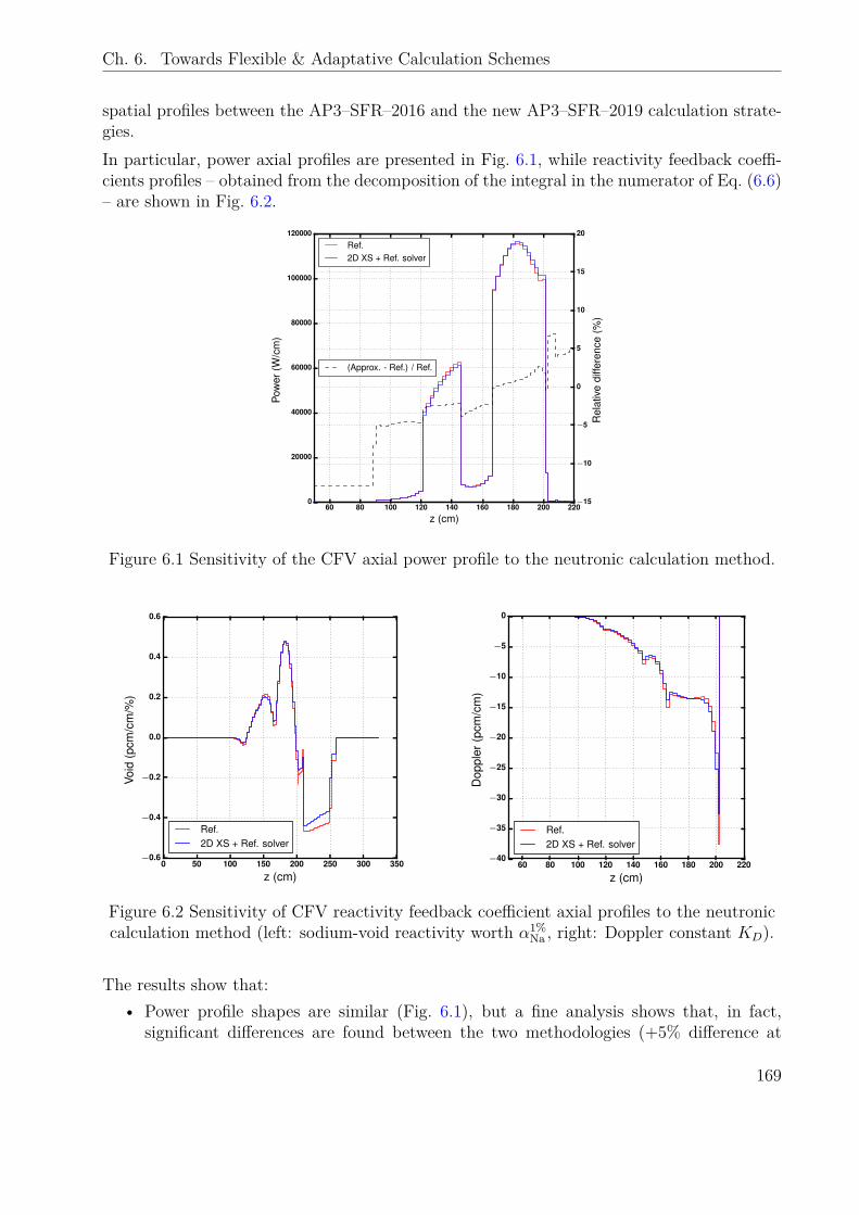
Ch. 6. Towards Flexible & Adaptative Calculation Schemes
spatial profiles between the AP3–SFR–2016 and the new AP3–SFR–2019 calculation strate-gies.In particular, power axial profiles are presented in Fig. 6.1, while reactivity feedback coeffi-cients profiles – obtained from the decomposition of the integral in the numerator of Eq. (6.6)– are shown in Fig. 6.2.
60 80 100 120 140 160 180 200 220
z (cm)
0
20000
40000
60000
80000
100000
120000
Pow
er(W
/cm
)
Ref.2D XS + Ref. solver
−15
−10
−5
0
5
10
15
20
Rel
ativ
edi
ffere
nce
(%)
(Approx. - Ref.) / Ref.
Figure 6.1 Sensitivity of the CFV axial power profile to the neutronic calculation method.
0 50 100 150 200 250 300 350
z (cm)
−0.6
−0.4
−0.2
0.0
0.2
0.4
0.6
Void
(pcm
/cm
/%)
Ref.2D XS + Ref. solver
60 80 100 120 140 160 180 200 220
z (cm)
−40
−35
−30
−25
−20
−15
−10
−5
0
Dop
pler
(pcm
/cm
)
Ref.2D XS + Ref. solver
Figure 6.2 Sensitivity of CFV reactivity feedback coefficient axial profiles to the neutroniccalculation method (left: sodium-void reactivity worth α1%
Na , right: Doppler constant KD).
The results show that:• Power profile shapes are similar (Fig. 6.1), but a fine analysis shows that, in fact,
significant differences are found between the two methodologies (+5% difference at
169
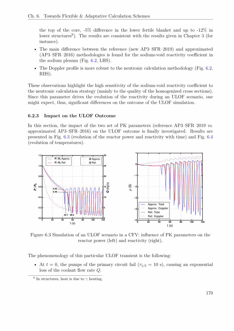
Ch. 6. Towards Flexible & Adaptative Calculation Schemes
the top of the core, -5% difference in the lower fertile blanket and up to -12% inlower structures9). The results are consistent with the results given in Chapter 3 (forinstance).
• The main difference between the reference (new AP3–SFR–2019) and approximated(AP3–SFR–2016) methodologies is found for the sodium-void reactivity coefficient inthe sodium plenum (Fig. 6.2, LHS).
• The Doppler profile is more robust to the neutronic calculation methodology (Fig. 6.2,RHS).
These observations highlight the high sensitivity of the sodium-void reactivity coefficient tothe neutronic calculation strategy (mainly to the quality of the homogenized cross sections).Since this parameter drives the evolution of the reactivity during an ULOF scenario, onemight expect, thus, significant differences on the outcome of the ULOF simulation.
6.2.3 Impact on the ULOF Outcome
In this section, the impact of the two set of PK parameters (reference AP3–SFR–2019 vs.approximated AP3–SFR–2016) on the ULOF outcome is finally investigated. Results arepresented in Fig. 6.3 (evolution of the reactor power and reactivity with time) and Fig. 6.4(evolution of temperatures).
0 20 40 60 80 100 120
t (s)
0.0
0.2
0.4
0.6
0.8
1.0
1.2
P/
P0
0.55
42.7
0.49
49.5
P/P0 Approx.P/P0 Ref.
0
5
10
15
20
25
30
Q(k
g/s)
Q Approx.Q Ref.
0 20 40 60 80 100 120
t (s)
−5
−4
−3
−2
−1
0
1
ρ($
)
Approx. TotalApprox. DopplerRef. TotalRef. Doppler
Figure 6.3 Simulation of an ULOF scenario in a CFV: influence of PK parameters on thereactor power (left) and reactivity (right).
The phenomenology of this particular ULOF transient is the following:
• At t = 0, the pumps of the primary circuit fail (τ1/2 = 10 s), causing an exponentialloss of the coolant flow rate Q.
9 In structures, heat is due to γ heating.
170
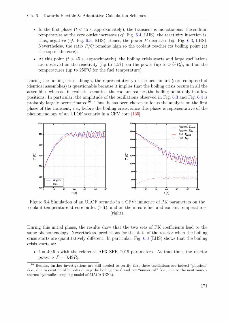
Ch. 6. Towards Flexible & Adaptative Calculation Schemes
• In the first phase (t < 45 s, approximately), the transient is monotonous: the sodiumtemperature at the core outlet increases (cf. Fig. 6.4, LHS), the reactivity insertion is,thus, negative (cf. Fig. 6.3, RHS). Hence, the power P decreases (cf. Fig. 6.3, LHS).Nevertheless, the ratio P/Q remains high so the coolant reaches its boiling point (atthe top of the core).
• At this point (t > 45 s, approximately), the boiling crisis starts and large oscillationsare observed on the reactivity (up to 4.5$), on the power (up to 50%P0), and on thetemperatures (up to 250°C for the fuel temperature).
During the boiling crisis, though, the representativity of the benchmark (core composed ofidentical assemblies) is questionable because it implies that the boiling crisis occurs in all theassemblies whereas, in realistic scenarios, the coolant reaches the boiling point only in a fewpositions. In particular, the amplitude of the oscillations observed in Fig. 6.3 and Fig. 6.4 isprobably largely overestimated10. Thus, it has been chosen to focus the analysis on the firstphase of the transient, i.e., before the boiling crisis, since this phase is representative of thephenomenology of an ULOF scenario in a CFV core [135].
0 20 40 60 80 100 120
t (s)
400
500
600
700
800
900
1000
T(C
)
Approx.Ref.
0 20 40 60 80 100 120
t (s)
400
600
800
1000
1200
1400
1600
1800
2000T
(C)
Approx. Tcomb
Approx. TNa
Ref. Tcomb
Ref. TNa
Figure 6.4 Simulation of an ULOF scenario in a CFV: influence of PK parameters on thecoolant temperature at core outlet (left), and on the in-core fuel and coolant temperatures
(right).
During this initial phase, the results show that the two sets of PK coefficients lead to thesame phenomenology. Nevertheless, predictions for the state of the reactor when the boilingcrisis starts are quantitatively different. In particular, Fig. 6.3 (LHS) shows that the boilingcrisis starts at:
• t = 49.5 s with the reference AP3–SFR–2019 parameters. At that time, the reactorpower is P = 0.49P0.
10 Besides, further investigations are still needed to certify that these oscillations are indeed “physical”(i.e., due to creation of bubbles during the boiling crisis) and not “numerical” (i.e., due to the neutronics /thermo-hydraulics coupling model of MACARENa).
171
Ch. 6. Towards Flexible & Adaptative Calculation Schemes
• t = 42.7 s (-14%) and P = 0.55P0 (+12%) with the approximated AP3–SFR–2016parameters.
These differences are discussed below.
6.2.4 Discussion
This simplified study shows that the outcome of the ULOF simulation is not overly sensi-tive to the neutronic calculation methodology. Despite very large differences are found onthe PK parameters between the new AP3–SFR–2019 and previous AP3–SFR–2016 calcu-lation schemes (up to 50% difference on the sodium-void reactivity worth), the transientphenomenology remains identical.Quantitatively, the impact of choosing one or another neutronic calculation strategy is lessthat 15% on the parameters that characterize the beginning of the boiling crisis (i.e., reactorpower and starting time). Hence, the sensibility of the ULOF outcome to the PK parameters(mainly the sodium-void reactivity worth) can be (naïvely) evaluated to about 15/50 = 0.3(in %/%). This value is rather low when one remembers that the difference on the totalsodium-void reactivity worth is more than 1.5$ between the new AP3–SFR–2019 and previousAP3–SFR–2016 methodologies (cf. Tab. 6.1).This observation points out that, for transient simulations, there is no need to improve theneutronic calculation methodology beyond a certain threshold11. In fact, the bias due toneutronic calculations is probably a minor one compared to the simplifying assumptions thatare made in this type of analyses. In particular, the most significant progress margin (inneutronics) is probably to be found in improving the neutronic / thermo-hydraulic couplingmodel before upgrading the APOLLO3® strategy itself.Hence, the resort to simplified neutronic calculation methodologies (i.e., project calculationschemes) constitute a pragmatic choice for this type of analyses.
6.3 Construction of AP3–SFR Project Methodologies
6.3.1 Strategy Assessment
Strategies for the definition of faster neutronic calculation schemes (for core conception ormulti-physics studies) may be classified into two categories:
• Strategies that rely on a degradation of the reference calculation parameters (e.g.,tracking parameters, spatial discretization, flux solvers,. . . ).
• Strategies that rely on a complete (or partial) change of the calculation scheme “phi-losophy” (e.g., changing the calculation domains, introducing ad hoc models,. . . ).
11 A similar conclusion was also drawn by C. Bourret during its Ph. D. thesis [91]: the impact of neutronicuncertainties (evaluated to ≈15% for the sodium-void reactivity worth) on the assessment of a SFR safetymargins is limited.
172
Ch. 6. Towards Flexible & Adaptative Calculation Schemes
The first kind of strategies presents an advantage compared to the second one because it maybenefit from the validation work performed for the reference calculation scheme. Hence, it isconvenient when one wants to dispose from an efficient calculation method for any neutronicparameter (e.g., multi-objective optimization, top-down studies,. . . ).Nevertheless, changing the calculation scheme philosophy may allow greater gains in terms ofcomputer resources. Yet, the validation work (vs. the reference strategy) must be performedonce again, for all the neutronic parameters. Thus, this kind of strategies is well suited whenone wants to optimize a calculation strategy for a pre-determined set of parameters (e.g.,reactivity for the optimization of a fuel Pu content).In any case, the definition of a project calculation scheme is a “user-dependent” problem.Thus, this work does not pretend judging if a gain of a factor two or three in terms ofcalculation time is sufficient, or if a multiplication by a factor two of the bias on the sodium-void worth is acceptable or not. Instead, the results that will be presented intend to highlightgeneral tendencies.
6.3.2 Degradation of the Reference Options
At the cross section preparation stage
The possibilities to degrade the options of the AP3–SFR calculation scheme at the crosssection generation stage have been investigated by A. Di Chicco, during a six-month intern-ship [142] proposed in the framework of this Ph. D. thesis. The methodology used for thiswork consisted in:
1. Realizing a sensitivity study of the homogenized cross sections to different parame-ters (CPM and MOC tracking parameters, transverse leakage source spectrum andanisotropy, level of detail in the geometry description. . . ).
2. Defining a reasonable level of approximation on these parameters according to theconclusions of the sensitivity study.
3. Verifying the performances of the degraded strategy at the core level vs. reference CFVcalculations.
Tracking parameters
The conclusions of the sensitivy study to the tracking parameters highlighted by A. Di Chiccocan be summarized as follows:
• The 33 group homogenized cross sections are not overly sensitive to the values of theCPM and MOC tracking parameters used, respectively, to self-shield cross sections andcompute the flux at the lattice level. Thus, coarse tracking parameters (see Tab. 6.2)can be used at the cross section generation stage.
• The values of the tracking parameters presented in Tab. 6.2 allow to reduce of a factorthree approximately the time required to produce the homogenized cross sections (≈1h for a 2D/1D calculation of a CFV fuel assembly and ≈ 25’ for a fuel / reflectortraverse calculation with four processors).
173
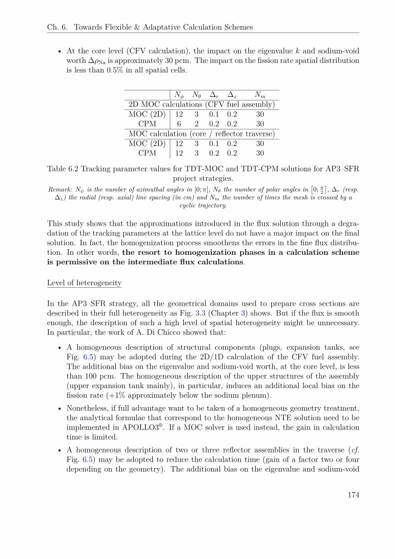
Ch. 6. Towards Flexible & Adaptative Calculation Schemes
• At the core level (CFV calculation), the impact on the eigenvalue k and sodium-voidworth ∆ρNa is approximately 30 pcm. The impact on the fission rate spatial distributionis less than 0.5% in all spatial cells.
Nφ Nθ ∆r ∆z Nm
2D MOC calculations (CFV fuel assembly)MOC (2D) 12 3 0.1 0.2 30
CPM 6 2 0.2 0.2 30MOC calculation (core / reflector traverse)MOC (2D) 12 3 0.1 0.2 30
CPM 12 3 0.2 0.2 30
Table 6.2 Tracking parameter values for TDT-MOC and TDT-CPM solutions for AP3–SFRproject strategies.
Remark: Nψ is the number of azimuthal angles in [0;π], Nθ the number of polar angles in[0; π2
], ∆r (resp.
∆z) the radial (resp. axial) line spacing (in cm) and Nm the number of times the mesh is crossed by acyclic trajectory.
This study shows that the approximations introduced in the flux solution through a degra-dation of the tracking parameters at the lattice level do not have a major impact on the finalsolution. In fact, the homogenization process smoothens the errors in the fine flux distribu-tion. In other words, the resort to homogenization phases in a calculation schemeis permissive on the intermediate flux calculations.
Level of heterogeneity
In the AP3–SFR strategy, all the geometrical domains used to prepare cross sections aredescribed in their full heterogeneity as Fig. 3.3 (Chapter 3) shows. But if the flux is smoothenough, the description of such a high level of spatial heterogeneity might be unnecessary.In particular, the work of A. Di Chicco showed that:
• A homogeneous description of structural components (plugs, expansion tanks, seeFig. 6.5) may be adopted during the 2D/1D calculation of the CFV fuel assembly.The additional bias on the eigenvalue and sodium-void worth, at the core level, is lessthan 100 pcm. The homogeneous description of the upper structures of the assembly(upper expansion tank mainly), in particular, induces an additional local bias on thefission rate (+1% approximately below the sodium plenum).
• Nonetheless, if full advantage want to be taken of a homogeneous geometry treatment,the analytical formulae that correspond to the homogeneous NTE solution need to beimplemented in APOLLO3®. If a MOC solver is used instead, the gain in calculationtime is limited.
• A homogeneous description of two or three reflector assemblies in the traverse (cf.Fig. 6.5) may be adopted to reduce the calculation time (gain of a factor two or fourdepending on the geometry). The additional bias on the eigenvalue and sodium-void
174
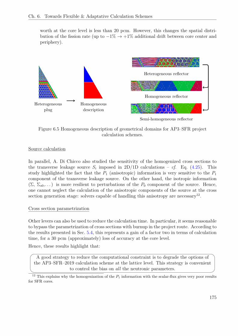
Ch. 6. Towards Flexible & Adaptative Calculation Schemes
worth at the core level is less than 20 pcm. However, this changes the spatial distri-bution of the fission rate (up to −1%→ +1% additional drift between core center andperiphery).
Heterogeneousplug
Homogeneousdescription
Heterogeneous reflector
Homogeneous reflector
Semi-homogeneous reflector
Figure 6.5 Homogeneous description of geometrical domains for AP3–SFR projectcalculation schemes.
Source calculation
In parallel, A. Di Chicco also studied the sensitivity of the homogenized cross sections tothe transverse leakage source Si imposed in 2D/1D calculations – cf. Eq. (4.25). Thisstudy highlighted the fact that the P1 (anisotropic) information is very sensitive to the P1component of the transverse leakage source. On the other hand, the isotropic information(Σ, Σs0,. . . ) is more resilient to perturbations of the P0 component of the source. Hence,one cannot neglect the calculation of the anisotropic components of the source at the crosssection generation stage: solvers capable of handling this anisotropy are necessary12.
Cross section parametrization
Other levers can also be used to reduce the calculation time. In particular, it seems reasonableto bypass the parametrization of cross sections with burnup in the project route. According tothe results presented in Sec. 5.4, this represents a gain of a factor two in terms of calculationtime, for a 30 pcm (approximately) loss of accuracy at the core level.Hence, these results highlight that:
A good strategy to reduce the computational constraint is to degrade the options ofthe AP3–SFR–2019 calculation scheme at the lattice level. This strategy is convenient
to control the bias on all the neutronic parameters.12 This explains why the homogenization of the P1 information with the scalar-flux gives very poor results
for SFR cores.
175
Ch. 6. Towards Flexible & Adaptative Calculation Schemes
At the core level
While the flux computed at the cross section generation stage is only used as a weightfunction for cross sections, the flux sought at the core level is the real solution one wants toobtain. This limits the options that can be degraded in the MINARET solver (cf. Tab. 3.9in Chapter 3). Nevertheless:
• A homogeneous description of control rods (CR-HOMO model, cf. Sec. 5.3) shouldbe preferred to the heterogeneous (CR-HETE) model which significantly increases thecomputational constraints (60% overhead).
• The P3 development of the scattering kernel may eventually be dropped out in favor ofa P1 law (15% overhead according to the conclusions of Chapter 3).
Another strategy consists in taking advantage of the other flux solvers implemented in APOL-LO3®, i.e.:
- PASTIS, a PN / SPN nodal solver developed at CEA (LEPh)13;- MINOS, a SPN solver14, already introduced in Sec. 6.1.
A comparison of the performances of these solvers is presented in Tab. 6.3. The case ofapplication is the CFV with MgO reflector (without control rods, and with a P1 scatteringlaw15).
Calculation Memory ∆ρ ∆(∆ρNa)time (GB) (pcm) (pcm)
MINARET 2h (8 proc.) 3 -141 -13MINOS SP3 20’ (1 proc.) 50 -470 -2441PASTIS SP3 20’ (1 proc.) 1 -309 -2038PASTIS P3 30’ (1 proc.) 16 +474 +503
Table 6.3 Comparison of MINARET, PASTIS and MINOS solvers for a CFV (MgOreflector) flux calculation.
Remark: Reactivity discrepancies are computed vs. a TRIPOLI-4® solution.Remark 2: All calculations have been performed with a P1 scattering law (this explains the reactivity
differences vs. previous results).
The results show that:
• The SP3 flux expansion gives very poor results for the sodium-void reactivity worth.• The memory management of the MINOS solver is not optimal.
13 Unfortunately, no reference is available online for PASTIS. The solver relies on a PN or SPN expansionof the angular variable (see Sec. 2.2.3). The “nodal” term refers to a particular class of spatial methods inwhich fluxes and currents are expanded over a pre-defined set of functions on the spatial mesh edges.
14 MINOS is also capable of solving the diffusion equation.15 With PN and SPN methods, one must not confuse the order of expansion of the scattering kernel (P1
here) and the order of expansion of the flux (P3 here).
176
Ch. 6. Towards Flexible & Adaptative Calculation Schemes
• The P3 approximation (PASTIS) significantly improves the results. Nevertheless, anon-negligible difference persists on the reactivity and on the sodium-void reactivityworth.
Another alternative could be to use a 2D radial-axial (RZ) SN solver recently implemented inAPOLLO3®. Yet, this kind of solution is probably not satisfactory when it comes to computethe fission rate spatial distribution or the control rods worth.Thus:
No clear tendency can be derived for the choice of a core solver for project applicationsin APOLLO3®. In particular, MINARET is the only solver that ensures a control of
the bias on all the neutronic parameters.
6.3.3 Resort to ad hoc Physical Models
The methodology proposed for the definition of a reference AP3–SFR–2019 calculation schemein Chapter 5 is based on the idea that consistent cross sections can be obtained through theresolution of the NTE over representative geometrical domains. Within this philosophy, nophysical models (i.e., assumptions on the flux shape) need to be introduced16. However, theresort to well-suited physical models constitutes a possible strategy to adapt the AP3–SFRcalculation scheme to the calculation constraint. In the following, a focus is made on theECCO strategy [73], which relies on a set of such physical models to prepare the homogenizedcross sections.
The ECCO strategy
Description
The purpose of the ECCO code is to prepare 33 group homogenized cross sections for SFRcore calculations.In particular, the cross sections of fissile media are weighted with a 1968 group flux computedover 2D assembly-wise heterogeneous domains. This flux is computed as a solution of the P1“consistent” equations17, which rely on the fundamental mode factorization – i.e., leakagemodel, cf. Eq. (2.78) – and an assumption of leakage isotropy. The P1 consistent equationsread:
φgj =∑i
(Sgi −Bjgi ) pgij (6.7a)
jgj =∑i
∑g′
Σg′→gs1 jg
′
i + B
3 φgi
pgij (6.7b)
16 The resort to a leakage model in the 2D/1D solution with Algo. 7 is only a sort of “fixup” to avoidnumerical divergences but, ideally, this physical model should be dropped out.
17 The “inconsistent” equations are sometimes used. They can be derived from the consistent equationsassuming Σg
′→gs1 = 0 in Eq. (6.7b).
177
Ch. 6. Towards Flexible & Adaptative Calculation Schemes
where φj is the scalar flux (in region j), jj the isotropic current, Si the isotropic source(including fission and scattering), B the buckling amplitude and pij the reduced collisionprobability – cf. Eq. (2.55) in Chapter 2. A critical buckling search loop is superimposedto the resolution of Eq. (6.7a) in order to find the value of B that corresponds to a criticalsituation, i.e., k(B2) = 1.The advantage of the P1-consistent (or inconsistent) equations is that a current jg is alwayscomputed as a part of the solution18: it can be used to weight the P1 information. However,higher angular order cross sections (i.e., P2, P3,. . . ) are not considered in the ECCO dataflow.For fertile media, the P1-consistent equations are also solved19. In that case, though, theneutron source Sj also contains an external contribution of the form:
Sgleak = DgfissB
2fissφ
gfiss (6.8)
where Dfiss, B2fiss and φfiss are respectively the leakage coefficient, buckling value and scalar
flux solution of the fissile assembly calculation. Sleak can, thus, be interpreted as a leakagerate out of a critical fissile assembly. Moreover, a special self-shielding procedure is used totake into account spatial self-shielding effects due to the fertile layer thickness [143]. In anycase, an empirical current is also available to weight the P1 information.Finally, structure calculations (plenum, plugs, reflector,. . . ) are performed over homogeneousgeometries. In that case, the CP formalism is not necessary but analytical solutions of theP1-consistent (or inconsistent) equations are directly implemented in ECCO. As for fertileblankets, the source contains a leakage contribution – cf. Eq. (6.8).Hence, one can see that the ECCO strategy is based on two main ad hoc models:
• The leakage model for fissile calculations.• The resort to an empirical leakage source to perform all other calculations.
Besides, it is worth notifying that, in ECCO, cross sections of many light isotopes are notavailable in the 1968 group energy mesh, but an ad hoc cross section library is directlyproduced in the 33 group energy mesh. This library relies on a condensation procedure,either with the flux / current solution of the fissile assembly calculation, or with a pre-tabulated solution. For such nuclides, a deconvolution procedure is used to reconstruct the1968 group cross section when the fine group flux needs to be computed.Nevertheless, the ECCO strategy relies on a consistent procedure to weight the P1 informationwith a current (as opposed to the AP3–SFR–2016 calculation strategy, cf. Chapter 3).
Results
In Sec. 3.5.2, it was shown that the production of a 3D CFV fuel assembly cross sectionswith ECCO code gave better results than the AP3–SFR–2016 calculation scheme (≈100 pcm
18 Actually, jg is a “macroscopic” current linked to the fundamental mode factorization.19 The buckling value supplied to the P1-consistent equations – i.e., Eq. (6.7a) and Eq. (6.7b) – is usually
small in fertile blankets.
178
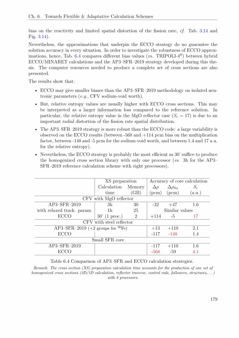
Ch. 6. Towards Flexible & Adaptative Calculation Schemes
bias on the reactivity and limited spatial distortion of the fission rate, cf. Tab. 3.14 andFig. 3.14).Nevertheless, the approximations that underpin the ECCO strategy do no guarantee thesolution accuracy in every situation. In order to investigate the robustness of ECCO approx-imations, hence, Tab. 6.4 compares different bias values (vs. TRIPOLI-4®) between hybridECCO/MINARET calculations and the AP3–SFR–2019 strategy developed during this the-sis. The computer resources needed to produce a complete set of cross sections are alsopresented.The results show that:
• ECCO may give smaller biases than the AP3–SFR–2019 methodology on isolated neu-tronic parameters (e.g., CFV sodium-void worth).
• But, relative entropy values are usually higher with ECCO cross sections. This maybe interpreted as a larger information loss compared to the reference solution. Inparticular, the relative entropy value in the MgO reflector case (Sr = 17) is due to animportant radial distortion of the fission rate spatial distribution.
• The AP3–SFR–2019 strategy is more robust than the ECCO code: a large variability isobserved on the ECCO results (between -568 and +114 pcm bias on the multiplicationfactor, between -148 and -5 pcm for the sodium-void worth, and between 1.4 and 17 a.u.for the relative entropy).
• Nevertheless, the ECCO strategy is probably the most efficient as 30’ suffice to producethe homogenized cross section library with only one processor (vs. 3h for the AP3–SFR–2019 reference calculation scheme with eight processors).
XS preparation Accuracy of core calculationCalculation Memory ∆ρ ∆ρNa Sr
time (GB) (pcm) (pcm) (a.u.)CFV with MgO reflector
AP3–SFR–2019 3h 30 -32 +47 1.6with relaxed track. param. 1h 25 Similar values
ECCO 30’ (1 proc.) 2 +114 -5 17CFV with steel reflector
AP3–SFR–2019 (+2 groups for 56Fe) +13 +110 2.1ECCO -117 -148 1.4
Small SFR coreAP3–SFR–2019 -117 +110 1.6
ECCO -568 -59 4.1
Table 6.4 Comparison of AP3–SFR and ECCO calculation strategies.Remark: The cross section (XS) preparation calculation time accounts for the production of one set of
homogenized cross sections (2D/1D calculation, reflector traverse, control rods, followers, structures,. . . )with 8 processors.
179
Ch. 6. Towards Flexible & Adaptative Calculation Schemes
The conclusion of this comparison is that:
The resort to ad hoc physical models is not a good strategy to define robust projectcalculation schemes. Nevertheless, it is the most efficient method if one is interested in
minimizing the bias on a selected set of parameters.
In this framework, some other ad hoc-models-based-strategies have been explored to defineproject calculation schemes in APOLLO3®.
Transposition in APOLLO3®
Taking inspiration on the ECCO strategy, a functionality to retrieve the leakage rate out of afissile assembly flux calculation (performed with a B1 homogeneous leakage model) has beenimplemented in APOLLO3® as part of this Ph. D. work.Nevertheless, using an isotropic source to perform the sub-critical assembly calculations is nota sufficient condition to dispose from a current (or higher angular flux moments) to weightthe P1 information. In fact, the strength of the ECCO model is that a current is alwaysavailable as part of the solution of the P1-consistent (or inconsistent) equations. In 2Dlattice calculations, though, the reflective boundary conditions make the current computedby TDT unusable. Thus, one needs to imagine other means to compute a current-like weightfunction.
Anisotropic leakage source
A possibility is to let the leakage source to have anisotropic axial components (for 2D fertileand structures calculations). This has been programmed during this Ph. D., within theframework of the B heterogeneous leakage model.However and as mentioned in Chapter 4, the only flux solver that is capable of handlinganisotropic external sources in the full S2 range20 is TDT-B. Unfortunately, this solver doesnot dispose from an acceleration technique to fasten the resolution of the MOC equations.Hence, this solution is not exploitable for the definition of project calculation schemes in thecurrent state of development of APOLLO3®.
Todorova’s current
If one assumes that Fick’s law is valid, the neutron current j =∫
4π d2ΩψΩ can be written as
a function of the scalar flux ψ00 as21:
jg = − ∂rψg00
3Σg −
∑g′
Σg→g′s1
(6.9)
20 S2 is the unit sphere.21 Eq. (6.9) can be derived from the NTE under a P1 approximation for the flux and a micro-reversibility
assumption for the linearly anisotropic scattering reaction rate [39].
180
Ch. 6. Towards Flexible & Adaptative Calculation Schemes
If one assumes that the flux gradient spectrum is proportional to the scalar flux spectrum:∂rψ
g00 ∝ ψg00 (6.10)
then the P1 information can be weighted with the following weight function:
jgTodorova(r) = ψg00(r)3(Σg(r)−∑g′ Σg′→g
s1 (r)) (6.11)
The advantage of this expression, proposed by G. Todorova in reference [144], is that it doesnot involve flux gradients that are not always available nor exploitable (depending on theboundary condition). Besides, it is always available as part of the flux solution, even if theneutron source does not have anisotropic components.Assuming that Eq. (6.11) is a valid expression for the neutron current, the P1 informationcan be homogenized as follows:
ΣG′→Gs,1,R =
< Σg′→gs,1 jg
′
Todorova >R×G×G′
< jg′
Todorova >R×G′+ δG,G′
(ΣGR − ΣG
Todorova,R
)(6.12)
where R is the macro-region index, G, G′ are macro-group indices, δG,G′ is the Kroneckerdelta and ΣG
R, ΣGTodorova,R are scalar-flux and Todorova’s current weighted total cross sections
(respectively). The introduction of a correction term on the diagonal of the scattering matrixis inspired from the flux-moments homogenization technique – cf. Eq. (3.5) in Sec. 3.2.1 –and intends to reverberate the homogenized total cross section anisotropy on the scatteringcross section.In order to test the potential of Todorova’s current, Eq. (6.12) has been implemented inAPOLLO3®, and tested on the CFV fuel assembly benchmark (cf. Sec. 4.5 for instance).More precisely, the test consisted in solving the 2D/1D equations and using Todorova’scurrent (and not the true angular current) to produce the 33 group homogenized P1 crosssections. However, the re-calculation of the same CFV fuel assembly with such homoge-nized cross sections handled very disappointing results: a -3500 pcm bias was found on theeigenvalue calculation (MINARET vs. TRIPOLI-4®).While the reason for this large discrepancy is still not fully understood22, the result is con-sistent with the observations of L. Cai, who also noticed that Todorova’s current does notperform well in every situation [145]. As a result, researches on Todorova’s current were notpursued further in this work.
6.3.4 Discussion
This work shows that two tendencies emerge for the definition of AP3–SFR project calculationschemes.If one is interested in defining a methodology that ensures a control of the bias for all theneutronic parameters, the best option probably consists in degrading the reference AP3–SFR–2019 calculation scheme. In particular, a very simple possibility is to degrade the MOCand CPM tracking parameters at the lattice level.
22 Todorova’s current is a “local” current: it is, hence, probably not representative of “macroscopic leakage”.
181
Ch. 6. Towards Flexible & Adaptative Calculation Schemes
Nevertheless, if one is only interested in a predetermined set of parameters, the resort to awider range of approximations is the most efficient strategy. For instance, implementing P1-consistent homogeneous solutions in APOLLO3® would give access to a current-like weightfunctions, that could be used to produce consistent cross sections for media such as thesodium plenum or other structures.At the core level, though, there is no fully satisfying solution for the choice of a core solver forproject applications. Nevertheless, there exist a significant margin to reduce the MINARETcalculation time through an optimization of the 33 group energy mesh. Indeed, this meshcontains ten groups below 100 eV, energy region in which the proportion of neutrons is verylow (in the active fissile zones at least). Thus, these ten groups could be collapsed into onesingle group, representing a 30% gain in terms of calculation time23.
6.4 Beyond the Lattice / Core Paradigm
In the previous section, possibilities to adapt the AP3–SFR–2019 calculation scheme to theuser computational constraints have been presented. This section now gives some perspec-tives to define truly adaptative calculation schemes, i.e., that demand a minimal numberof (arbitrary) user-dependent choices. To achieve that goal, some ideas are proposed to getover the lattice / core philosophy, which is probably the main obstacle to flexibility since itdemands to define a priori the values of the few groups homogenized cross sections, withoutany knowledge of the actual core situation.Now, if one assumes that fine-group heterogeneous 3D transport calculations will remainout of range of desktop computers for some time, new homogenization strategies need to beproposed to perform on-the-fly cross section weighting.
6.4.1 Dynamic Homogenization
Space variable
Dynamic homogenization is a sophisticated spatial homogenization technique in which theactual core solution is used to perform on-the-fly cross section weighting. It is based on theidea that the flux ψ in one assembly (or any sub-domain) is the solution of transport problemwith core eigenvalue kcore and imposed incoming fluxes ψin,core:
∀ assembly ⊂ core,
(Ω · ∂r + Σ)ψ =( 1kcoreF +H
)ψ (6.13a)
ψin = ψin,core (6.13b)where the energy group index g has been dropped out for the sake of clarity.A calculation based on a dynamic homogenization technique then consists in:
1. Computing the core solution with a low-order operator on an assembly-wise homoge-nized mesh.
23 Such a 24 group energy mesh has been briefly tested during this Ph. D. with encouraging results(approximately 20/30 pcm additional bias on the multiplication factor and sodium-void reactivity worthcompared to the 33 group energy mesh).
182
Ch. 6. Towards Flexible & Adaptative Calculation Schemes
2. Retrieving the global eigenvalue kcore and local boundary condition ψin,core.3. Computing local assembly fluxes with Eq. (6.13a) – Eq. (6.13b) in each sub-domain.4. Weighting the core parameters (cross sections) with local fluxes.5. Going back to 1. until convergence.
In point 2., the boundary condition, i.e., ψin,core, is naively retrieved from the core solution.Another possibility consists in using the local outgoing flux from neighboring assembliesψout,neighbor. In that case, though, the boundary condition must be normalized so as topreserve the core coarse exchanges [71]:
ψin(r,Ω) = ψout,neighbor(r,Ω)× Jin,core(r)Jout,neighbor(r) (6.14)
where Jin,core is the low-order operator incoming current, and Jout,neighbor is the outgoingcurrent from neighboring assemblies.
Energy variable
Assuming that the low-order operator operates on a coarse energy mesh (e.g., 33 groups) butthat a fine-group (e.g., 1968) flux calculation is performed at the assembly level, it followsthat a deconvolution procedure is needed for the boundary condition.An example of such a deconvolution formula might be found in reference [83], for instance:
ψgin(r,Ω) = ψgout,neighbor(r,Ω)×JGin,core(r)
JGout,neighbor(r) (6.15)
At this point, one can see that the dynamic homogenization technique requires a relativelyhigh number of fine-group transport calculations (one per assembly). However, this is mit-igated by the fact that these calculations are much faster than typical eigenvalue problemswith reflective boundary conditions because the core eigenvalue is imposed as a parameterand neutron trajectories are limited to the size of one single assembly.To push the efficiency further, it is possible to delegate the outer and inner iteration loops(required to converge on local fission and scattering sources24) to the coarse-group level, witha source deconvolution procedure. Some ideas to perform this deconvolution can be found inthe generalized energy condensation theory (cf. Sec. 2.2.2), but the subgroup decompositionmethod, introduced by S. Douglass and F. Rahnema in reference [38], is probably the simplestoption.The idea of the subgroup decomposition method is to write the fission and scattering sources
24 See Chapter 2 for the terminology.
183
Ch. 6. Towards Flexible & Adaptative Calculation Schemes
as functions of the coarse-group (heterogeneous) fluxes:
Fψg(r,Ω) def= 14π
Ng∑g′=1
νΣg′→gf (r)ψg
′
00(r) = 14π
NG∑G′=1
νΣG′→gf (r)ψG′00 (r) (6.16a)
Hψg(r,Ω) def=∑l∈N
2l + 14π
+l∑m=−l
Ng∑g′=1
Σg′→gs,l (r)ψg
′
lm(r)Rlm(Ω) (6.16b)
=∑l∈N
2l + 14π
+l∑m=−l
NG∑G′=1
ΣG′→gs,lm (r)ψG′lm(r)Rlm(Ω) (6.16c)
where ψG′00 and ψG′lm are the flux angular moments in macro group G′:ψG
′ =∑g′∈G′
ψg′ (6.17)
and νΣG′→gf , ΣG′→g
s,lm are coarse-to-fine-group transfer cross sections defined as follows:νΣG′→g
f (r) =∑g′∈G′ νΣg′→g
f (r)ψg′
00(r)∑g′∈G′ ψ
g′
00(r)(6.18a)
ΣG′→gs,lm (r) =
∑g′∈G′ Σg′→g
s,l (r)ψg′
lm(r)∑g′∈G′ ψ
g′
lm(r)(6.18b)
Once these coarse-to-fine-group transfer cross sections are defined, one can see that the finegroup flux ψg is, in fact, not necessary to compute the fine-group source:
qg =( 1kcoreF +H
)ψg (6.19)
but that it can be deconvoluted from the coarse-group flux solution ψG. The advantage ofthis strategy is that fine-group assembly calculations, thus, only require one single transportsweep. However, the coarse-group heterogeneous flux ψG must be computed and the coarse-to-fine-group transfer cross sections νΣG′→g
f and ΣG′→gs,lm need to stored.
Angular variable
Finally, the angular variable deserves a special comment. As this document showed in afew occasions, a consistent angular homogenization theory is a key feature for the definitionof accurate calculation schemes (at least for SFRs). With this in mind, the angular-fluxmoments homogenization technique of APOLLO3® (see Sec. 2.5.1 or Sec. 3.2.1) should beused any time a cross section homogenization phase is involved. In particular, this ensuresthe consistency25 of the coarse vs. fine-group fluxes – cf. Eq. (6.17).Besides, the representation of the angular dependence of the boundary condition in Eq. (6.15)needs to be considered with care to ensure a consistent propagation of the anisotropic infor-mation through the core.
25 Strictly speaking, the flux-moments homogenization technique is not 100% consistent due to the least-square minimization technique used to get rid of the dependence of the scattering cross section on azimuthalindex m. The fully consistent alternative would consist in adding an artificial source term in the coarse-grouptransport equation, as the generalized energy condensation theory proposes [35, 36].
184
Ch. 6. Towards Flexible & Adaptative Calculation Schemes
General algorithm
Reuniting the ideas presented above, it is possible to imagine a calculation scheme based ondynamic homogenization techniques with three different calculation levels:
- core level: the solution ψcore is defined on coarse energy and spatial meshes;- first assembly level: the solution ψG is defined within the heterogeneous assembly butover the coarse energy mesh;
- second assembly level: the solution ψg is defined on the fine-group energy mesh.
Such an algorithm is presented below (cf. Algo. 8).
Algorithm 8 Calculation Scheme based on Dynamic Homogenization# InitializationChoose assembly partition domainChoose coarse-group energy meshInitialize flux values ψcore, ψG, ψgwhile ψcore, kcore not converged do# Compute core solutionHomogenize (space + energy) XS with ψgCompute core solution (ψcore, kcore)for assembly ∈ core do# Compute coarse-group heterogeneous fluxCompute boundary condition ψGin # Eq. (6.14)Homogenize (only energy) XS with ψgCompute ψG# Compute fine-group heterogeneous fluxCompute fine-group source qg # Eq. (6.19), (6.16a), (6.16c)Compute boundary condition ψgin # Eq. (6.15)Compute coarse-to-fine group XS # Eq. (6.18a), (6.18b)Update fine-group flux ψg # only one transport sweep
end forend while
Remark: Angular flux moments are required to preserve the angular information during homogenizationphases.Remark 2: a resonance self-shielding procedure may be embedded in the fine-group flux calculation.Remark 3: XS = cross sections.
One can see that Algo. 8 allows to produce on-the-fly homogenized cross sections that takeinto account the actual core environment without the need for user interventions.Besides it provides an ideal scope for the application of domain decomposition techniques (seeSec. 2.4.1) and one can even imagine using different flux solvers depending on the assemblytype.
185
Ch. 6. Towards Flexible & Adaptative Calculation Schemes
6.4.2 Towards Flexible Homogenization
Algo. 8 provides a general framework for the definition of adaptative calculation schemes, i.e.,that rely on a minimal set of approximations. Nevertheless, one can foresee a large number offine-group transport calculations and, hence, significant needs in terms of computer resources.Nonetheless, one can imagine reducing the number of fine-group transport calculations withassembly grouping techniques. For instance, all the assemblies that share the same geometri-cal features (dimensions and cross sections) and the same core environment could be spottedwith a flag. Then, one fine-group transport calculations could be performed for a represen-tative member of such an assembly set. At the core level, all the assemblies grouped underthe same flag would then share the same homogenized cross sections.An intermediate level of approximation would consist in defining a set or representative as-semblies (e.g., 10 belonging to fissile media, 10 to fertile blankets, 5 in the sodium plenum,. . . ).At the core level, the homogenized cross sections of this representative set of assemblies couldbe assigned to any other assembly according to their “proximity” with the reference set. Thisproximity could be evaluated with a dissimilarity measure – such as the relative entropy pro-posed in Sec. 4.6 – computed, for instance, over any reaction rate (fission, absorption. . . ) ofthe core-level solution26. The only pre-requisite to perform such a dissimilarity measurementis that the two distributions compared (normalized to unity) need to be defined over thesame space (e.g., 33 group energy mesh).For SFRs, the low dependence of microscopic cross sections on the fuel burnup (cf. Sec. 5.4)even opens perspectives to use such assembly grouping techniques in core depletion problems.
6.5 Conclusions
This chapter presents two different levels of adaptability that can be developed, either tofasten the AP3–SFR–2019 calculation scheme, or to get over the traditional lattice / corephilosophy.The simplification of the reference AP3–SFR–2019 calculation, in particular, is motivated bythe needs for faster methods when many transport calculations need to be performed in alimited amount of time. At this stage, the definition of a target accuracy and an upper limitfor computer resources is a user-dependent problem. Nevertheless, our analysis showed that:
• At the lattice level, an efficient strategy to ensure a mastered bias on the largest set ofneutronic parameters is to relax the options of the reference AP3–SFR–2019 calculationscheme. This can be done either with a degradation of the MOC and CPM trackingparameters, with an allowance for homogeneous geometries (plugs for instance), ordropping the parametrization of the homogenized cross sections with burnup.
• The resort to ad hoc approximations (e.g., empirical external source calculations) isthe most efficient strategy to reduce the computational constraint, but this deterio-rates the calculation scheme robustness. Hence, this option should be privileged to
26 Using angular independent quantities seems to be a more reasonable choice for the dissimilarity measure.Else, distributions need to be oriented in space.
186
Ch. 6. Towards Flexible & Adaptative Calculation Schemes
define parameter-oriented calculation schemes. In particular, programming in APOL-LO3® some of the options available in ECCO (P1-consistent equations, semi-analyticaltransport solutions in homogeneous media, provision of a pre-weighted 33 group crosssection library,. . . ) could be beneficial in this scope.
• At the core level, MINARET is the only solver capable of accurately modeling coolant-voided situations. Hence, work is still needed to reduce the computational cost ofAPOLLO3® core calculations while ensuring mastered biases.
Following a completely different path, perspectives to improve the AP3–SFR–2019 calculationscheme defined during this thesis were proposed. These perspectives rely on dynamic ho-mogenization techniques and subgroup decomposition methods to homogenize cross sectionson-the-fly. In particular, it was shown (although speculatively) that this kind of calcula-tion schemes has a high potential to define truly adaptative strategies. Nevertheless, thesemethods involve a strong coupling between assembly and core calculations. Hence, they de-mand significant changes in the current data flow of APOLLO3®, which is optimized for thetraditional lattice / core philosophy.
187

This page has been left intentionally blank.
188
Chapter 7 General Conclusion
7.1 Main Conclusions
Sodium-cooled nuclear reactors offer interesting perspectives in terms of uranium resourceseconomy and radioactive waste management. In France, the research on the SFR technologytook a new start at the beginning of the XXIst century with the ASTRID project.Simultaneously, the rise of safety standards in the nuclear industry resulted in increasinglycomplex core concepts, with enhanced natural behavior in accidental situations. In particular,the minimization of the sodium-void reactivity worth led to the CFV concept for ASTRID.Due to increased levels of spatial heterogeneity, these innovative SFR cores challenge classicalneutronic calculation strategies, which often rely on a traditional lattice / core philosophy.Hence, the first objective of this work was to:
Understand the limitations of the current (i.e., in 2016) APOLLO3® neutronicsimulation strategy for the calculation of complex SFR cores.
To achieve that goal, a detailed analysis of the AP3–SFR–2016 neutronic calculation schemeimplemented in APOLLO3® for SFR applications was carried out in Chapter 3. This analysisdemonstrated the accuracy of the individual blocks of the calculation strategy (i.e., numberof energy groups, resonance self-shielding models, homogenization methods, flux solvers,. . . ),but it also highlighted the limitations of the cross section preparation procedure.In SFR cores, neutrons are allowed to travel over relatively large distances between collisions,typically 10 cm in sodium. In heterogeneous cores, this remarkable property leads to theestablishment of macroscopic neutron currents and, more generally, anisotropic structuresin the neutron flux. If these angular structures are not modeled during the cross sectionpreparation phase, one cannot expect to propagate the information to the core level. Hence,the basic ingredients of any homogenization-based calculation scheme are:
• The choice of consistent geometrical patterns to prepare the homogenized cross sections.In SFR cores, the main neutron leakage channels should be identified in order to allowthe modeling of macroscopic neutron currents (and higher-order angular moments).
• A consistent transport homogenization theory, i.e., that preserves the neutron balancebetween the reference and the homogenized situation. To ensure this consistency, crosssections need to be weighted with angular fluxes or, as it is done in APOLLO3®, withangular flux-moments.
The first ingredient, in particular, is absent of the AP3–SFR–2016 calculation scheme: theCFV geometry is favorable towards axial leakage (at least in the inner core) whereas crosssections are prepared over two-dimensional radial patterns. Hence, a crucial piece of (angular)information lacks in the homogenized cross section values, degrading the accuracy of the coresolution.
189
Ch. 7. General Conclusion
Based on these observations, the second objective of this work was to:
Propose and implement (in APOLLO3®) new methodological solutions (calculationschemes).
Necessarily, the modeling of macroscopic neutron currents during the cross section prepara-tion phase increases the dimensions of the geometrical domains. For the CFV, in particular,3D-MOC calculations appear as a natural solution to produce a fuel assembly cross sections.Nevertheless, this strategy suffers from two drawbacks: it has a high computational cost,and the current implementation of the MOC equations in APOLLO3® is limited to axiallyconformal geometries.Besides, this raises a crucial question: is it worth to pay the cost for high accuracy solutionswhen these are only used as weighting functions for cross sections?To answer this question, a 2D/1D alternative, enabling a proper propagation of the angularinformation, was developed in Chapter 4. The method was implemented in APOLLO3®,following a rigorous V&V protocol, and applied to the calculation of a CFV fuel assembly.The results showed that, as far as the homogenization of cross sections is concerned, themethod is as accurate as the 3D-MOC solution and about five times less demanding in termsof computer resources. The method is now available in APOLLO3®.With this new method, a proposal for a new reference AP3–SFR–2019 calculation schemewas made in Chapter 5:
• Two main macroscopic geometrical patterns were identified to prepare the few groupshomogenized cross sections: the inner fuel assembly (2D/1D solution) and the core / re-flector radial interface (2D-MOC solution).
• The SN MINARET solver was chosen to compute the flux at the core level (with 33energy groups).
• The question of the control rods modeling was also treated, through explicit modelingof the absorbers (B4C pins) at the core level. Indeed, the key parameter, in that case, isnot the neutron current, but spatial self-shielding effects between individual B4C pinswithin a control rod.
The calculation strategy was numerically validated, against reference Monte Carlo calcula-tions, for the CFV, but also for other core concepts. Hence, the solution proposed respondsto a robustness constraint, that was set as an objective for this work. In particular, the re-sults were judged satisfactory, in the scope of performing a SFR safety demonstration, for awide range of neutronic parameters (reactivity, fission rate distribution, feedback coefficients,control rods parameters, and evolution of the material balance).Chapter 6, finally, presented some possible strategies to reduce the computational cost of thenew AP3–SFR–2019 calculation scheme. On the one hand, it was argued that the best wayto ensure mastered biases on all the neutronic parameters is to degrade the reference calcu-lation options. On the other hand, it was shown that the resort to ad hoc approximationsconstitutes the most efficient strategy when one is interested in optimizing the calculationof a predetermined set of estimators. Hence, the implementation of some algorithms of the
190
Ch. 7. General Conclusion
ECCO code (solution of the P1-consistent equations and provision of a pre-weighted 33 groupcross section library mainly) could be beneficial to define efficient project routes. Neverthe-less, this chapter also showed that the only solver of APOLLO3® capable of computing theCFV sodium-void reactivity worth with acceptable accuracy is MINARET, thus limiting thepossibilities to fasten core level flux calculations for project studies.
7.2 Perspectives
In a relatively short term, the major progress axes for the reference calculation schemedeveloped in this thesis are the following:
• Optimization of the energy meshes.
– At the lattice level: a 1760 group energy mesh was recently defined at CEA(LEPh) for SFR applications. The expected gain in terms of calculation time isapproximately 10%.
– At the core level: a work is necessary to optimize the 33 group energy mesh throughan identification of the most important physical phenomena (e.g., presence of sharp56Fe resonances, removal of some thermal groups,. . . ).
• Improvement of the 2D/1D method.
– In the current implementation, the numerical stability of the 2D/1D method (cf.Algo. 6) is not guaranteed unless a B heterogeneous leakage model is used as asubstitution model in overcritical planes (cf. Algo. 7). A cleaner way to addressthese instabilities could be to normalize the flux on-the-fly in order to control theleakage over intrinsic source (fission + scattering) ratio.
– An acceleration method for the 2D-MOC solver (TDT-B) could significantly fastenthe resolution of the 2D/1D equations.
– The scope of the 2D/1D method could be enlarged to allow multiple 1D calcula-tions. Promising applications are the production of 3D-consistent cross sectionsfor control rods, for rod followers, or to improve the core / reflector model. Nev-ertheless, this requires some developments in the 2D-MOC solver to allow thecalculation of radial leakage sources. In that case, the outer iteration loop (fis-sion source calculation with power method) should be managed externally, thusrequiring a modification of the APOLLO3® data flow.
In the mid/long term, the cross section homogenization phase should be managed dynamicallyto avoid the bottleneck of the lattice / core paradigm. To this end, dynamic homogenizationtheory was introduced in Chapter 6 to avoid the boundary condition approximation duringthe cross section preparation phase. Coupled with intelligent management of the cross sectionsharing at the core level, this might constitute a promising solution for future referenceneutronic calculation schemes.As the current tendency for deterministic methods is an increase of the complexity, the attrac-tiveness of stochastic solutions rises. If deterministic solutions still remain the best-suited to
191

Ch. 7. General Conclusion
compute local estimators (fission rate distribution) and small perturbations (spatial decom-position of reactivity feedback effects), a generalization of the use of Monte Carlo methods tocompute integral estimators (reactivity, sodium-void worth, Doppler constants,. . . ) shouldnot be neglected.Finally, this work was only concerned about the question of the biases due to the neutroniccalculation method. Within a nuclear safety framework, though, this study should be com-pleted with an uncertainty quantification assessment (i.e., evaluation and propagation), andshould be confronted to experimental validation results. The latter, in particular, will de-mand a transposition work from past French experiments (from Masurca to Superphénix) tofuture SFR core designs (CFV).
192
References
[1] D. Schneider, F. Dolci, F. Gabriel, J. Palau, M. Guillo, and B. Pothet, “APOLLO3:CEA/DEN deterministic multi-purpose code for reactor physics analysis,” in Proc. Int.Conf. PHYSOR 2016 - Unifying Theory and Experiments in the 21st Century, (SunValley, Idaho, United States), American Nuclear Society, 2016.
[2] Intergovernmental Panel on Climate Change (IPPC), “Global Warming of 1.5°C- Summary for Policymakers.” https://www.ipcc.ch/sr15/chapter/summary-for-policy-makers/, 2018.
[3] International Energy Agency (IEA), “CO2 Emissions Statistics.” https://www.iea.org/statistics/co2emissions/, 2016.
[4] United Nations, Department of Economics and Social Affairs, “World Popu-lation Prospects: The 2017 Revision.” https://www.un.org/development/desa/publications/world-population-prospects-the-2017-revision.html, 2017.
[5] International Energy Agency (IEA), “World Energy Balances.” https://www.iea.org/statistics/balances/, 2016.
[6] Intergovernmental Panel on Climate Change (IPPC), “Global Warming of 1.5°C -Chapter 2: Mitigation pathways compatible with 1.5°C in the context of sustainabledevelopment.” https://www.ipcc.ch/sr15/chapter/2-0/, 2018.
[7] O. Hahn and F. Straßmann, “Über die entstehung von radiumisotopen aus uran durchbestrahlen mit schnellen und verlangsamten neutronen,” Naturwissenschaften, vol. 26,no. 46, pp. 755–756, 1938.
[8] L. Meitner and O. R. Frisch, “Disintegration of uranium by neutrons: a new type ofnuclear reaction,” A Century of Nature: Twenty-One Discoveries that Changed Scienceand the World, p. 70, 1939.
[9] A. Einstein, “Zur elektrodynamik bewegter körper,” Annalen der physik, vol. 322,no. 10, pp. 891–921, 1905.
[10] H. v. Halban, F. Joliot, L. Kowarski, and F. Perrin, “Mise en évidence d’une réactionnucléaire en chaîne au sein d’une masse uranifère,” Journal de Physique et le Radium,vol. 10, no. 10, pp. 428–429, 1939.
[11] World Nuclear Association, “World Nuclear Power Reactors & Uranium Re-quirements.” http://www.world-nuclear.org/information-library/facts-and-figures/world-nuclear-power-reactors-and-uranium-requireme.aspx, 2019.
[12] Nuclear Energy Agency, “Uranium 2018: Resources, Production and Demand.” https://www.oecd-nea.org/ndd/pubs/2018/7413-uranium-2018.pdf, 2018.
193
References
[13] Andra, “Radioactive Waste.” https://international.andra.fr/radioactive-waste-france/what-radioactive-waste/radioactive-waste.
[14] Nuclear Energy Agency, “Physics and Safety of Transmutation Systems - A Status Re-port.” https://www.oecd-nea.org/science/docs/pubs/nea6090-transmutation.pdf, 2018.
[15] Gouvernement Français, “Politique nationale pour la gestion durable des matièreset des déchets radioactifs.” https://www.legifrance.gouv.fr/affichTexte.do?cidTexte=JORFTEXT000000240700&categorieLien=id, 2006.
[16] Andra, “Cigéo.” https://www.andra.fr/cigeo.
[17] L. Buiron, “Le potentiel de transmutation des actinides mineurs: état des lieux pourles réacteurs à neutrons rapides refroidis au sodium de quatrième génération - Rapportd’Habilitation à Diriger des Recherches,” 2016.
[18] GEN IV International Forum, “GIF R&D Outlook for Generation IV Nuclear En-ergy Systems.” https://www.gen-4.org/gif/upload/docs/application/pdf/2013-09/gif_rd_outlook_for_generation_iv_nuclear_energy_systems.pdf, 2009.
[19] Monographie CEA, “IV th Generation Sodium-cooled Fast Reactors - The ASTRIDtechnological demonstrator .” http://www.cea.fr/english/Documents/corporate-publications/4th-generation-sodium-cooled-fast-reactors.pdf, 2012.
[20] L. David, Sodium-water reaction: a heterogeneous runaway process. PhD thesis, Aix-Marseille Université, 2019.
[21] T. Beck, V. Blanc, J.-M. Escleine, D. Haubensack, M. Pelletier, M. Phelip, B. Perrin,and C. Venard, “Conceptual design of ASTRID fuel sub-assemblies,” Nuclear Engi-neering and Design, vol. 315, pp. 51–60, 2017.
[22] Gouvernement Français, “Loi relative à la transparence et à la sécurité enmatière nucléaire .” https://www.legifrance.gouv.fr/affichTexte.do?cidTexte=JORFTEXT000000819043&categorieLien=id, 2006.
[23] Gouvernement Français, “Code de l’environnement.” https://www.legifrance.gouv.fr/affichCode.do?cidTexte=LEGITEXT000006074220, 2019.
[24] ASN & IRSN, “Guide 28 : Qualification des outils de calcul scientifiqueutilisés dans la démonstration de sûreté nucléaire.” https://www.asn.fr/Professionnels/Installations-nucleaires/Centrales-nucleaires/Guides-de-l-ASN-dans-le-domaine-des-installations-nucleaires/Guide-de-l-ASN-n-28-Qualification-des-outils-de-calcul-scientifique-utilises-dans-la-demonstration-de-surete-nucleaire, 2017.
[25] J.-M. Ruggieri, J. Tommasi, J.-F. Lebrat, C. Suteau, D. Plisson-Rieunier,C. De Saint Jean, G. Rimpault, and J.-C. Sublet, “ERANOS 2.1: International codesystem for GEN IV fast reactor analysis,” in Proc. Int. Conf. on Advances in NuclearPower Plants (ICAPP’06), 2006.
194
References
[26] R. Sanchez, I. Zmijarevic, M. Coste-Delclaux, E. Masiello, S. Santandrea, E. Martinolli,L. Villate, N. Schwartz, and N. Guler, “APOLLO2 year 2010,” Nuclear Engineeringand Technology, vol. 42, no. 5, pp. 474–499, 2010.
[27] P. Archier, J. Palau, J. Vidal, V. Pascal, G. Rimpault, B. Roque, and S. Santandrea,“New reference APOLLO3 calculation scheme for sodium cooled fast reactors: fromsub-assembly to full-core calculations,” in Proc. Int. Conf. PHYSOR 2016 - Unify-ing Theory and Experiments in the 21st Century, (Sun Valley, Idaho, United States),American Nuclear Society, 2016.
[28] G. I. Bell and S. Glasstone, Nuclear reactor theory. US Atomic Energy Commission,Washington, DC (United States), 1970.
[29] L. Boltzmann, Lectures on gas theory. Courier Corporation, 2012.
[30] N. Bohr, “Neutron capture and nuclear constitution,” Nature, vol. 137, pp. 334–3448,1936.
[31] E. P. Wigner and L. Eisenbud, “Higher angular momenta and long range interactionin resonance reactions,” Physical Review, vol. 72, no. 1, p. 29, 1947.
[32] G. Allaire and F. Golse, “Transport et diffusion (mat/map 567),” 2012.
[33] Y. Saad, Numerical methods for large eigenvalue problems, 2nd edition. Society forIndustrial and Applied Mathematics, 2011.
[34] F. Scheben, Iterative methods for criticality computations in neutron transport theory.PhD thesis, University of Bath, 2011.
[35] F. Rahnema, S. Douglass, and B. Forget, “Generalized energy condensation theory,”Nuclear Science and Engineering, vol. 160, no. 1, pp. 41–58, 2008.
[36] S. Douglass and F. Rahnema, “Consistent generalized energy condensation theory,”Annals of Nuclear Energy, vol. 40, no. 1, pp. 200–214, 2012.
[37] S. Douglass and F. Rahnema, “Cross section recondensation method via generalizedenergy condensation theory,” Annals of Nuclear Energy, vol. 38, no. 9, pp. 2105–2110,2011.
[38] S. Douglass and F. Rahnema, “Subgroup decomposition method,” Annals of NuclearEnergy, vol. 48, pp. 84–101, 2012.
[39] A. Hébert, Applied Reactor Physics. Presses internationales Polytechnique, 2009.
[40] S. Santandrea, “An integral multidomain DPN operator as acceleration tool for themethod of characteristics in unstructured meshes,” Nuclear Science and Engineering,vol. 155, no. 2, pp. 223–235, 2007.
195
References
[41] D. Sciannandrone, S. Santandrea, R. Sanchez, J. Vidal, et al., “Coupled fine-groupthree-dimensional flux calculation and subgroups method for a FBR hexagonal as-sembly,” in Proc. Int. Conf. on Mathematics and Computational Methods Applied toNuclear Science and Engineering (M&C2015), (Nashville, Tennesse, United States),American Nuclear Society, 2015.
[42] L. Graziano, An axial polynomial expansion and acceleration of the characteristicsmethod for the solution of the neutron transport equation. PhD thesis, Université Paris-Saclay, 2018.
[43] J.-Y. Moller, J.-J. Lautard, and D. Schneider, “MINARET, a deterministic neutrontransport solver for nuclear core calculations,” in Proc. Int. Conf. on Mathematicsand Computational Methods Applied to Nuclear Science and Engineering (M&C2011),American Nuclear Society, 2011.
[44] P. Lasaint and P.-A. Raviart, “On a finite element method for solving the neutrontransport equation,” in Mathematical aspects of finite elements in partial differentialequations, pp. 89–123, Elsevier, 1974.
[45] N. Metropolis and S. Ulam, “The Monte Carlo method,” Journal of the Americanstatistical association, vol. 44, no. 247, pp. 335–341, 1949.
[46] A. Haghighat, Monte Carlo Methods for Particle Transport. Crc Press, 2016.
[47] K. Smith, “Monte Carlo for practical LWR analysis: what’s needed to get to the goal?,”in M&C Division Computational Roundtable, American Nuclear Society Summer Meet-ing, Hollywood, FL, 2011.
[48] L. Dagum and R. Menon, “OpenMP: An industry-standard API for shared-memoryprogramming,” Computing in Science & Engineering, no. 1, pp. 46–55, 1998.
[49] W. Gropp, E. Lusk, N. Doss, and A. Skjellum, “A high-performance, portable imple-mentation of the MPI message passing interface standard,” Parallel computing, vol. 22,no. 6, pp. 789–828, 1996.
[50] N. Odry, Méthode de décomposition de domaine avec parallélisme hybride et accéléra-tion non linéaire pour la résolution de l’équation du transport Sn en géométrie non-structurée. PhD thesis, Aix-Marseille, 2016.
[51] B. S. Kirk, J. W. Peterson, R. H. Stogner, and G. F. Carey, “Libmesh: a C++ li-brary for parallel adaptive mesh refinement/coarsening simulations,” Engineering withComputers, vol. 22, no. 3-4, pp. 237–254, 2006.
[52] Y. R. Park and N. Z. Cho, “Coarse-mesh angular dependent rebalance acceleration ofthe discrete ordinates transport calculations,” Nuclear science and engineering, vol. 148,no. 3, pp. 355–373, 2004.
[53] S. Santandrea and R. Sanchez, “Analysis and improvements of the DPN accelerationtechnique for the method of characteristics in unstructured meshes,” Annals of NuclearEnergy, vol. 32, no. 2, pp. 163–193, 2005.
196
References
[54] S. Santandrea, L. Graziano, and D. Sciannandrone, “Accelerated polynomial axial ex-pansions for full 3D neutron transport MOC in the APOLLO3 code system as appliedto the ASTRID fast breeder reactor,” Annals of Nuclear Energy, vol. 113, pp. 194–236,2018.
[55] A. Bensoussan, J.-L. Lions, and G. Papanicolaou, Asymptotic analysis for periodicstructures, vol. 374. American Mathematical Soc., 2011.
[56] V. V. Jikov, S. M. Kozlov, and O. A. Oleinik, Homogenization of differential operatorsand integral functionals. Springer Science & Business Media, 2012.
[57] K. Koebke, “Advances in homogenization and dehomogenization,” in Int. Top. Mtg. onAdvances in Mathematical Methods for the Solution of Nuclear Engineering Problems,vol. 2, (Munich, Germany), 1981.
[58] K. S. Smith, “Assembly homogenization techniques for light water reactor analysis,”Progress in Nuclear Energy, vol. 17, no. 3, pp. 303–335, 1986.
[59] A. Hébert and A. Kavenoky, “Development of the SPH homogenization method,” inANS/ENS - International topical meeting on advances in mathematical methods for nu-clear engineering problems. Munich, RFA, CEA Centre d’Etudes Nucléaires de Saclay,1981.
[60] A. Hébert and G. Mathonnière, “Development of a third-generation superhomogeneisa-tion method for the homogenization of a pressurized water reactor assembly,” NuclearScience and Engineering, vol. 115, no. 2, pp. 129–141, 1993.
[61] A. Hébert, “A reformulation of the transport-transport SPH equivalence technique,”(Ottawa, Ontario, Canada), Canadian Nuclear Society, 2015.
[62] S. Yasseri and F. Rahnema, “Consistent spatial homogenization in transport theory,”Nuclear Science and Engineering, vol. 176, no. 3, pp. 292–311, 2014.
[63] J. Vidal, P. Archier, A. Calloo, P. Jacquet, J. Tommasi, and R. Le Tellier, “An improvedenergy-collapsing method for core-reflector modelization in SFR core calculations us-ing the PARIS platform,” in PHYSOR 2012 - Advances in Reactor Physics - LinkingResearch, Industry and Education, American Nuclear Society, 2012.
[64] R. Sanchez, “Assembly homogenization techniques for core calculations,” Progress inNuclear Energy, vol. 51, no. 1, pp. 14–31, 2009.
[65] E. W. Larsen, “Neutron transport and diffusion in inhomogeneous media (I),” Journalof Mathematical Physics, vol. 16, no. 7, pp. 1421–1427, 1975.
[66] T. Travis and E. Larsen, “An asymptotic, homogenized, anisotropic, multigroup diffu-sion approximation to the neutron transport equation,” in Proc. Int. Conf. The Roleof Reactor Physics toward a Sustainable Future (PHYSOR2014), American NuclearSociety, Kyoto, Japan, September, 2014.
197
References
[67] F. Rahnema, “Boundary condition perturbation theory for use in spatial homogeniza-tion methods,” Nuclear Science and Engineering, vol. 102, no. 2, pp. 183–190, 1989.
[68] M. S. McKinley and F. Rahnema, “Higher-order boundary condition perturbation the-ory for the diffusion approximation,” Nuclear Science and Engineering, vol. 136, no. 1,pp. 15–33, 2000.
[69] M. S. McKinley and F. Rahnema, “High-order boundary condition perturbation theoryfor the neutron transport equation,” Nuclear science and engineering, vol. 140, no. 3,pp. 285–294, 2002.
[70] F. Rahnema and M. S. McKinley, “High-order cross-section homogenization method,”Annals of Nuclear Energy, vol. 29, no. 7, pp. 875–899, 2002.
[71] P. Mondot and R. Sanchez, “An iterative homogenization technique that preservesassembly core exchanges,” in Proc. of SNA Conference, Paris, 2003.
[72] N. Hfaiedh and A. Santamarina, “Determination of the optimized SHEM mesh forneutron transport calculation,” Proc. Mathematics and Computation, Supercomputing,Reactor Physics and Nuclear and Biological Applications, 2005.
[73] G. Rimpault, “Algorithmic features of the ECCO cell code for treating heterogeneousfast reactor subassemblies,” in Proc. Int. Conf. on Mathematics and Computations,Reactor Physics and Environmental Analysis, American Nuclear Society, 1995.
[74] P. Reuss, Précis de neutronique. EDP sciences, 2012.
[75] V. Deniz, “The theory of neutron leakage in reactor lattices,” in CRC Handbook ofNuclear Reactor Calculations (R. Yonen, ed.), vol. II, pp. 409 – 508, CRC Press, 1986.
[76] A. Hébert and G. Marleau, “Generalization of the Stamm’ler method for the self-shielding of resonant isotopes in arbitrary geometries,” Nuclear Science and Engineer-ing, vol. 108, no. 3, pp. 230–239, 1991.
[77] A. Hébert, “Revisiting the Stamm’ler self-shielding method,” in 25th CNS AnnualConference, pp. 6–9, 2004.
[78] A. Khairallah and J. Recolin, “Calcul de l’autoprotection résonnante dans les cellulescomplexes par la méthode des sous-groupes,” in Proc. Seminar IAEA-SM-154 on Nu-merical Reactor Calculations, pp. 305–317, 1972.
[79] T. Tone, “A numerical study of heterogeneity effects in fast reactor critical assemblies,”Journal of Nuclear Science and Technology, vol. 12, no. 8, pp. 467–481, 1975.
[80] L. Mao and I. Zmijarevic, “A new Tone’s method in APOLLO3® and its applicationto fast and thermal reactor calculations,” Nuclear Engineering and Technology, vol. 49,no. 6, pp. 1269–1286, 2017.
198
References
[81] Y.-K. Lee, E. Brun, and X. Alexandre, “SFR whole core burnup calculations withTRIPOLI-4 Monte Carlo code,” in Proc. Int. Conf. PHYSOR 2014 - The Role of Re-actor Physics Toward a Sustainable Future, (Kyoto, Japan), American Nuclear Society,2014.
[82] Y. S. Ban, E. Masiello, R. Lenain, H. G. Joo, and R. Sanchez, “Code-to-code com-parisons on spatial solution capabilities and performances between nTRACER and thestandalone IDT solver of APOLLO3,” Annals of Nuclear Energy, vol. 115, pp. 573 –594, 2018.
[83] R. Sanchez, “Prospects in deterministic three-dimensional whole-core transport calcu-lations,” Nuclear Engineering and Technology, vol. 44, no. 2, pp. 113–150, 2012.
[84] P. Sciora, D. Blanchet, L. Buiron, B. Fontaine, M. Vanier, F. Varaine, C. Venard,S. Massara, A.-C. Scholer, and D. Verrier, “Low void effect core design applied on 2400MWth SFR reactor,” in International Congress on Advances in Nuclear Power Plants(ICAPP), 2011.
[85] M. Coste-Delclaux, “Galilee: A nuclear data processing system for transport, deple-tion and shielding codes,” in Proc. Int. Conf. PHYSOR 2008 - Nuclear Power: ASustainable Resource, (Interlaken, Switzerland), American Nuclear Society, 2008.
[86] A. Santamarina, D. Bernard, P. Blaise, M. Coste, A. Courcelle, T. Huynh, C. Jouanne,P. Leconte, O. Litaize, S. Mengelle, et al., “The JEFF-3.1.1 nuclear data library,” JEFFreport, vol. 22, no. 10.2, p. 2, 2009.
[87] P. Mosca, C. Mounier, P. Bellier, and I. Zmijarevic, “Improvements in transport cal-culations by the energy-dependent fission spectra and subgroup method for mutualself-shielding,” Nuclear Science and Engineering, vol. 175, no. 3, pp. 266–282, 2013.
[88] J. Tommasi, “Heterogeneous BN equations and symmetries,” Annals of Nuclear Energy,vol. 85, no. 0, pp. 145 – 158, 2015.
[89] B. Faure, “Simulation des fuites neutroniques à l’aide d’un modèle B1 hétérogène pourdes réacteurs à neutrons rapides et à eau légère,” Master’s thesis, École Polytechniquede Montréal, 2016.
[90] J.-F. Vidal, P. Archier, B. Faure, V. Jouault, J.-M. Palau, V. Pascal, G. Rimpault,F. Auffret, L. Graziano, E. Masiello, et al., “APOLLO3 homogenization techniques fortransport core calculations - Application to the ASTRID CFV core,” Nuclear Engi-neering and Technology, 2017.
[91] C. Bouret, Etudes des contre-réactions dans un réacteur à neutrons rapides à calopor-teur sodium : impact de la conception et de la neutronique sur les incertitudes. PhDthesis, 2014.
[92] V. Jouault, Amélioration de la démarche de vérification et validation du nouveau codede neutronique APOLLO3. PhD thesis, Aix-Marseille, 2017.
199
References
[93] H. Guo, E. Garcia, B. Faure, L. Buiron, P. Archier, P. Sciora, and G. Rimpault,“Advanced method for neutronic simulation of control rods in sodium fast reactors:Numerical and experimental validation,” Annals of Nuclear Energy, vol. 129, pp. 90–100, 2019.
[94] E. Brun, F. Damian, C. Diop, E. Dumonteil, F. Hugot, C. Jouanne, Y. Lee, F. Malvagi,A. Mazzolo, O. Petit, et al., “TRIPOLI-4, CEA, EDF and AREVA reference MonteCarlo code,” in SNA+ MC 2013-Joint International Conference on Supercomputing inNuclear Applications+ Monte Carlo, p. 06023, EDP Sciences, 2014.
[95] B. Faure, P. Archier, J.-F. Vidal, J. M. Palau, and L. Buiron, “Neutronic calculationof an axially heterogeneous ASTRID fuel assembly with APOLLO3: Analysis of biasesand foreseen improvements,” Annals of Nuclear Energy, vol. 115, pp. 88–104, 2018.
[96] S. Berche, “Validation de schémas de calcul APOLLO3 pour assemblages de typeRNR,” Master’s thesis, École Polytechnique de Montréal, 2015.
[97] P. Archier, J. Palau, J. Vidal, S. Santandrea, and D. Sciannandrone, “Validation ofthe newly implemented 3D TDT-MOC solver of APOLLO3 code on a whole 3D SFRheterogeneous assembly,” Proc. PHYSOR 2016, pp. 1–5, 2016.
[98] B. Faure, P. Archier, J.-F. Vidal, and L. Buiron, “A 2D/1D algorithm for effective cross-section generation in fast reactor neutronic transport calculations,” Nuclear Science andEngineering, pp. 1–12, 2018.
[99] B. Faure, P. Archier, and L. Buiron, “A 2D/1D method for consistent burnupparametrization of cross sections in SFR fuel depletion analysis,” in PHYTRA4 - Thefourth international conference on physics and technology of reactors and applications,2018.
[100] N. Z. Cho, G. S. Lee, and C. J. Park, “A fusion technique of 2D/1D methods forthree-dimensional whole-core transport calculations,” Proc. Korean Nuclear Society,2002.
[101] J.-Y. Cho, K.-S. Kim, C.-C. Lee, S.-Q. Zee, and H.-G. Joo, “Axial SPN and radial MOCcoupled whole core transport calculation,” Journal of nuclear science and technology,vol. 44, no. 9, pp. 1156–1171, 2007.
[102] G. S. Lee and N. Z. Cho, “2D/1D fusion method solutions of the three-dimensionaltransport OECD benchmark problem C5G7MOX,” Progress in Nuclear Energy, vol. 48,no. 5, pp. 410–423, 2006.
[103] X. Tang, Q. Li, X. Chai, X. Tu, W. Wu, and K. Wang, “Efficient procedure for radialMOC and axial SN coupled 3D neutron transport calculation,” in Proc. Int. Conf. onMathematics and Computational Methods Applied to Nuclear Science and Engineering(M&C2017), American Nuclear Society, 2017.
200
References
[104] Y. Jung, C. Lee, and M. Smith, “Verification of high-fidelity neutronics code PROTEUSfor C5G7 benchmark problems,” Transactions of the American Nuclear Society, SanFransisco, California, vol. 116, 2017.
[105] G. Harrisson and G. Marleau, “Simulation strategy for the evaluation of neutronicproperties of a Canadian SCWR fuel channel,” Science and Technology of NuclearInstallations, vol. 2013, 2013.
[106] A. Zhu, Y. Xu, T. Saller, and T. Downar, “The implementation and analysis of theMOC and CMFD adjoint capabilities in the 2D-1D code MPACT,” Proc. M&C 2015,pp. 19–23, 2015.
[107] Q. Wu, X. Peng, X. Tang, Y. Yu, Q. Li, and K. Wang, “Whole-core forward-adjointneutron transport solutions with coupled 2-D MOC and 1-D SN and kinetics parametercalculation,” Progress in Nuclear Energy, vol. 108, pp. 310–318, 2018.
[108] B. W. Kelley and E. W. Larsen, “A consistent 2D/1D approximation to the 3D neutrontransport equation,” Nuclear Engineering and Design, vol. 295, pp. 598 – 614, 2015.
[109] B. Collins, S. Stimpson, B. W. Kelley, M. T. Young, B. Kochunas, A. Graham, E. W.Larsen, T. Downar, and A. Godfrey, “Stability and accuracy of 3D neutron transportsimulations using the 2D/1D method in MPACT,” Journal of Computational Physics,vol. 326, pp. 612–628, 2016.
[110] B. Kochunas, D. Jabaay, B. Collins, and T. Downar, “Demonstration of neutronicscoupled to thermal-hydraulics for a full-core problem using COBRA-TF/MPACT,”CASL Document CASL-U-2014-0051-000, 2014.
[111] M. Jarret, B. Kochunas, and T. Downar, “Characterization of 2D/1D accuracy using3D MOC in MPACT,” in Proc. Int. Conf. on Mathematics and Computational MethodsApplied to Nuclear Science and Engineering (M&C2017), American Nuclear Society,2017.
[112] M. Jarrett, B. Kochunas, E. Larsen, and T. Downar, “Improved accuracy in the 2-D/1-D method with anisotropic transverse leakage and cross-section homogenization,”Nuclear Science and Engineering, vol. 192, pp. 1–21, 09 2018.
[113] I. Zmijarevic, “IDT solution to the 3D transport benchmark over a range in parameterspace,” 2008.
[114] T. M. Cover and J. A. Thomas, Elements of information theory. John Wiley & Sons,2012.
[115] S. Kullback and R. A. Leibler, “On information and sufficiency,” The annals of math-ematical statistics, vol. 22, no. 1, pp. 79–86, 1951.
[116] D. Blanchet and B. Fontaine, “Reflector and protections in a sodium-cooled fast reactor:Modelling and optimization,” in EPJ Web of Conferences, vol. 153, p. 05006, EDPSciences, 2017.
201
References
[117] J. Gauthier, J. Cabrillat, G. Palmiotti, M. Salvatores, M. Giese, M. Carta, and J. West,“Measurement and predictions of control rod worth,” Nuclear Science and Engineering,vol. 106, no. 1, pp. 18–29, 1990.
[118] S. Czernecki, F. Varaine, and J. Tommasi, “An overview of the validation process us-ing measurements performed in fast reactors Phenix and Super-Phenix,” Proc. Physor2000, pp. 7–11, 2000.
[119] J. Rowlands and C. Eaton, “The spatial averaging of cross sections for use in transporttheory reactor calculations, with an application to control rod fine homogenization,”Proc. Specialist’s Mtg. Homogenization Methods in Reactor Physics, Lugano, Switzer-land, 1978.
[120] M. Andersson, D. Blanchet, H. Nylén, and R. Jacqmin, “Control rod calculation inaxially heterogeneous fast reactors—i: Influence of the absorber environment,” NuclearScience and Engineering, vol. 185, no. 2, pp. 263–276, 2017.
[121] M. Andersson, D. Blanchet, H. Nylén, and R. Jacqmin, “Control rod calculation inaxially heterogeneous fast reactors—ii: Impact of three-dimensional homogenizationon core parameters,” Nuclear Science and Engineering, vol. 185, no. 2, pp. 277–293,2017.
[122] H. Bateman, “Solution of a system of differential equations occurring in the theoryof radioactive transformations,” vol. 15, (Cambridge, United Kingdom), pp. 423–427,Proc. Cambridge Philosophical Society, 1910.
[123] S. Lahaye, P. Bellier, H. Mao, A. Tsilanizara, and Y. Kawamoto, “First verificationand validation steps of MENDEL release 1.0 cycle code system,” PHYSOR 2014, 2014.
[124] P. Archier, S. Domanico, J. Palau, and G. Truchet, “Validation of a multi-purposedepletion chain for burnup calculations through TRIPOLI-4 calculations and IFP per-turbation method,” PHYSOR. Sun Valley, USA, 2016.
[125] E. Brun, E. Dumonteil, and F. Malvagi, “Systematic uncertainty due to statistics inMonte Carlo burnup codes: application to a simple benchmark with TRIPOLI-4-D,”Progress in Nuclear Science and Technology, vol. 2, pp. 879–885, 2011.
[126] A. Greganti, “Validation of an isotope evolution model for APOLLO3 calculations inSFR core,” Master’s thesis, École Polytechnique de Montréal, 2017.
[127] A. Henry, “The application of reactor kinetics to the analysis of experiments,” NuclearScience and Engineering, vol. 3, no. 1, pp. 52–70, 1958.
[128] K. Ott, “Quasistatic treatment of spatial phenomena in reactor dynamics,” NuclearScience and Engineering, vol. 26, no. 4, pp. 563–565, 1966.
[129] S. Dulla, E. H. Mund, and P. Ravetto, “The quasi-static method revisited,” Progressin Nuclear Energy, vol. 50, no. 8, pp. 908–920, 2008.
202
References
[130] J. Tommasi and G. Palmiotti, “Verification of iterative matrix solutions for multipointkinetics equations,” Annals of Nuclear Energy, vol. 124, pp. 357–371, 2019.
[131] D. Wade and Y. Chang, “The integral fast reactor concept: physics of operation andsafety,” Nuclear science and engineering, vol. 100, no. 4, pp. 507–524, 1988.
[132] P. Gauthé and P. Sciora, “Sensitivity studies of SFR unprotected transients with globalneutronic feedback coefficients,” in Int. Conf. on Fast Reactors and Related Fuel Cycles,2017.
[133] A. Gandini, “On the standard perturbation theory,” Nuclear Science and Engineering,vol. 79, no. 4, pp. 426–430, 1981.
[134] G. Geffraye, O. Antoni, M. Farvacque, D. Kadri, G. Lavialle, B. Rameau, and A. Ruby,“CATHARE 2 v2. 5_2: a single version for various applications,” Nuclear Engineeringand Design, vol. 241, no. 11, pp. 4456–4463, 2011.
[135] J.-B. Droin, N. Marie, A. Bachrata, F. Bertrand, E. Merle, and J.-M. Seiler, “Physicaltool for unprotected loss of flow transient simulations in a sodium fast reactor,” Annalsof nuclear energy, vol. 106, pp. 195–210, 2017.
[136] H. Rief, E. Gelbard, R. Schaefer, and K. Smith, “Review of Monte Carlo techniquesfor analyzing reactor perturbations,” Nuclear Science and Engineering, vol. 92, no. 2,pp. 289–297, 1986.
[137] B. Faure, P. Archier, P. Sciora, G. Valocchi, L. Buiron, J. Droin, and V. Pascal, “Impactof neutronic parameters in a loss-of-flow transient simulation of a low void reactivitysodium-cooled nuclear reactor,” in Proc. Int. Conf. on Mathematics and ComputationalMethods Applied to Nuclear Science and Engineering (M&C2019), 2019.
[138] J.-B. Droin, Modélisation d’un transitoire de perte de débit primaire non protégé dansun RNR-Na. PhD thesis, Université Grenoble Alpes, 2016.
[139] J.-M. Delhaye, Thermohydraulique des réacteurs (Edition révisée 2013). EDP sciences,2014.
[140] A.-M. Baudron and J.-J. Lautard, “Simplified Pn transport core calculations in theApollo3 system,” 2011.
[141] G. Truchet, P. Leconte, A. Santamarina, E. Brun, F. Damian, and A. Zoia, “Computingadjoint-weighted kinetics parameters in TRIPOLI-4® by the iterated fission probabilitymethod,” Annals of Nuclear Energy, vol. 85, pp. 17–26, 2015.
[142] A. Di Chicco, “Optimization of a calculation scheme through the parametric study ofeffective nuclear cross sections and application to the estimate of neutronic parametersof the ASTRID fast nuclear reactor,” Master’s thesis, Università di Bologna (Facoltadi Ingegneria), 2018.
[143] R. Corcuera, Méthodes théoriques pour le calcul neutronique des systèmes coeur-couverture et coeur-réflecteur des réacteurs à neutrons rapides. PhD thesis, 1974.
203
References
[144] G. Todorova, H. Nishi, and J. Ishibashi, “Transport criticality analysis of FBR MONJUinitial critical core in whole core simulation by NSHEX and GMVP,” Journal of nuclearscience and technology, vol. 41, no. 4, pp. 493–501, 2004.
[145] L. Cai, Condensation and homogenization of cross sections for the deterministic trans-port codes with Monte Carlo method: Application to the GEN IV fast neutron reactors.PhD thesis, Université Paris Sud XI, 2014.
[146] J. Lefevre, C. Mitchell, and G. Hubert, “European fast reactor design,” Nuclear Engi-neering and Design, vol. 162, no. 2-3, pp. 133–143, 1996.
[147] G. Mignot, J. Klein, M. Chenaud, C. Thevenot, A. Ravenet, M. Valentin, P. Masoni,P. Dubuisson, S. Delafontaine, L. Nicolas, et al., “Studies on French SFR advanced coredesigns,” in Proceedings of the 2008 International Congress on Advances in NuclearPower Plants - ICAPP’08, 2008.
[148] F. Varaine, N. Stauff, M. Masson, M. Pelletier, G. Mignot, G. Rimpault, A. Zaetta, andJ. Rouault, “Comparative review on different fuels for GEN IV Sodium Fast Reactors:merits and drawbacks,” in Proceedings of the 2009 International Congress on Advancesin Nuclear Power Plants - ICAPP’09, 2009.
[149] G. Rimpault, L. Buiron, P. Sciora, and F. Varaine, “Towards GEN IV SFR design:Promising ideas for large advanced SFR core designs,” in Proc. Int. Conf. PHYSOR2008 - Nuclear Power: A Sustainable Resource, (Interlaken, Switzerland), AmericanNuclear Society, 2008.
[150] B. Fontaine, N. Devictor, P. Le Coz, A. Zaetta, D. Verwaerde, and J. Hamy, “TheFrench R and D on SFR core design and ASTRID project,” in Proc. Int. Conf.GLOBAL: Toward and over the Fukushima Daiichi accident, 2011.
[151] F. Varaine, P. Marsault, M.-S. Chenaud, B. Bernardin, A. Conti, P. Sciora, C. Venard,B. Fontaine, N. Devictor, L. Martin, et al., “Pre-conceptual design study of ASTRIDcore,” in Proceedings of the 2012 International Congress on Advances in Nuclear PowerPlants-ICAPP’12, 2012.
[152] P. Sciora, L. Buiron, G. Rimpault, and F. Varaine, “A break even oxide fuel core foran innovative SFR: CEA neutronic studies,” 2009.
[153] N. Chapoutier, A. Janet, G. Nolin, M. Ricol, A. Scholer, D. Verrier, and C. Venard,“ASTRID core shielding - Design studies and benchmark analysis,” in Proceedings ofthe 2015 International Congress on Advances in Nuclear Power Plants - ICAPP’15,2015.
[154] J. Leppänen, “Serpent–a continuous-energy Monte Carlo reactor physics burnup cal-culation code,” VTT Technical Research Centre of Finland, vol. 4, 2013.
[155] M. Pusa and J. Leppänen, “Computing the matrix exponential in burnup calculations,”Nuclear science and engineering, vol. 164, no. 2, pp. 140–150, 2010.
204
Appendix A Real Spherical Harmonics
Definitions
The definitions presented in this appendix are taken from A. Hébert’s book [39].Let (O,ex,ey,ez) be a orthonormal frame and Ω ∈ S2. We define the polar cosine µ and theazimuthal angle φ such that:
Ω =√
1− µ2(
cos(φ)ex + sin(φ)ey)
+ µez (A.1)
We then introduce the Legendre Polynomials, for µ ∈ [−1; 1], with:
P0(µ) = 1, P1(µ) = µ (A.2)
and for l ≥ 1:Pl+1(µ) = 1
l + 1
((2l + 1)µPl(µ)− lPl−1(µ)
)(A.3)
In particular Eq. (A.3) yields:
P2(µ) = 12(3µ2 − 1
), P3(µ) = 1
2(5µ3 − 3µ
)(A.4)
For l ∈ N, m ∈ N, the Legendre function Pml is defined as:
Pml (µ) =
(1− µ2
)m/2 dmPldµm
(µ) (A.5)
Finally, the real spherical harmonics Rlm are defined for l ∈ N and m ∈ −l,−l + 1, . . . , las:
Rlm(Ω) ≡ Rlm(µ, φ) = αlmP|m|l (µ)Γm(φ) (A.6)
with:
αlm =
√√√√(2− δm,0)(l − |m|)!(l + |m|)! (A.7)
and:
Γm(φ) =
cos(mφ) if m ≥ 0sin(|m|φ) otherwise
(A.8)
The real spherical harmonics are often used to expand any distribution f of variable Ω as:
f(Ω) =+∞∑l=0
2l + 14π
+l∑m=−l
flmRlm(Ω) (A.9)
205
Appendix A. Real Spherical Harmonics
Orthogonality Property
The Rlm obey the following orthogonality relation:∫4πd2Ω Rlm(Ω)Rl′m′(Ω) = 4π
2l + 1δl,l′δm,m′ (A.10)
Thus, the coefficients flm in Eq. (A.9) directly read:
flm =∫
4πd2Ω f(Ω)Rlm(Ω) (A.11)
Parity Properties
The real spherical harmonics obey the following parity properties:
Rlm(−µ, φ) = (−1)l+mRlm(µ, φ) (A.12)Rlm(µ, φ+ π) = (−1)mRlm(µ, φ) (A.13)
Rlm(−Ω) = (−1)lRlm(Ω) (A.14)
Proof. Relation (A.12) is directly derived from the parity of Legendre functions:
∀l,m ≥ 0, Pml (−µ) =
(1− µ2
)m/2 dmPldµm
(−µ) = (−1)l+mPml (µ) (A.15)
which arises from the parity of Legendre polynomials:
∀l ≥ 0, Pl(−µ) = (−1)lPl(µ) (A.16)
Relation (A.13) can be deduced from the following property:
∀m ≥ 0,
cos (m(φ+ π)) = (−1)m cos(mφ)sin (m(φ+ π)) = (−1)m sin(mφ)
=⇒ Γm(φ+ π) = (−1)mΓm(φ) (A.17)
Finally, (A.12) + (A.13) =⇒ (A.14).
206
Appendix B Angular Treatment of Spatial Symmetries
We consider the following transport equation:
Aψ = 1kFψ (B.1)
where A = Ω ·∂r + Σ−H and we expand the flux ψ is in real spherical harmonics Rlm(Ω) ≡Rlm(µ, φ) as:
ψ(r,Ω) =∑l∈N
l∑m=−l
2l + 14π ψlm(r)Rlm(Ω) (B.2)
1D Case
We consider a one-dimensional (1D) geometry D. The spatial position in D is parametrizedby z = r · ez.Since D is invariant under the action of a rotational symmetry around ez then we have1:
∂ψ
∂φ(z, µ, φ) = 0 (B.3)
This expression also reads:
∑l∈N
l∑m=−l
−mψlm(z)Rl,−m(Ω) = 0 (B.4)
because:dΓmdφ
(φ) =
−m sin(mφ) if m ≥ 0−m cos(mφ) otherwise
= −mΓ−m(φ) (B.5)
Therefore, using the orthogonality property (A.10), it is found that:
∀m 6= 0, ψlm(z) = 0 (B.6)
In 1D geometries, there is only 1 angular moment per order l that respects the rotationalsymmetry.
2D Case
Consider now that D is a planar 2D geometry and that ez is normal to D. The spatialposition in D is parametrized by r = xex + yey.
1 We assume that media are isotropic (see Sec. 2.1.3).
207
Appendix B. Angular Treatment of Spatial Symmetries
Since D is invariant under the action of a planar symmetry with respect to D, we have:
ψ(r,−µ, φ) = ψ(r, µ, φ) (B.7)
Using (A.12), relation (B.7) implies that:
∑l∈N
l∑m=−l
(1− (−1)l+m
)ψlm(r)Rlm(Ω) = 0 (B.8)
or, using Eq. (A.10): (1− (−1)l+m
)ψlm(r) = 0 (B.9)
Hence:ψlm(r) = 0, if l +m is odd (B.10)
This is the situation usually encountered in 2D lattice calculations. In that case, there isl + 1 non–null angular moments per order l.
3D Case
In 3D geometries, the flux has 2l + 1 angular moments per order l.
Symmetry Breaking with External Sources
Suppose now that ψ is solution of a source problem:
Aψ = Fψ + S (B.11)
In that case, the symmetries of S also need to be taken into account. In particular, S mayhave the same spatial dimentionality than D (i.e. have 1, 2 or 3 spatial dimensions) but havea higher angular dimensionality. In that case, the angular flux moments do not necessar-ily respect the property (B.6) in a one-dimensional domain or (B.10) in a two-dimensionaldomain.Advantage is taken of this particularity in Chapter 4 in order to compute “3D flux angularmoments” in 2D geometrical domains with the 2D/1D method.
208
Appendix C Additional Information on the DGFEM
The expression of the weak formulation of the NTE over one element reads:∫Kw(Ωn · ∂r + Σ
)ψn =
∫Kwqn (C.1)
After some manipulations (integration by parts and use of Green-Ostrogradski theorem), thegradient term reads:∫
KwΩn · ∂rψn =
∫∂K
Ωn · n+wψn −∫KψnΩn · ∂rw (C.2)
In MINARET, an upwind flux ψ−n (r ∈ ∂K) = limε→0−
ψn(r + εΩn) (or boundary flux ψinn ifr − |ε|Ωn /∈ D) is used to compute the surface integral:∫
∂KΩn · n+wψn ≈
∫∂K
Ωn · n+wψ−n (C.3)
It is now convenient to introduce the lightened frontier ∂K− = r ∈ ∂K / Ωn · n+ < 0and the shadowed frontier ∂K+ = ∂K\∂K−. In the summation process over the mesh cells,a surface integral appears twice in the interior of D so that a discontinuity jump can beintroduced in Eq. (C.3):
∑k
∫∂K
Ωn · n+wψ−n =∑k
( ∫∂K−\∂D
|Ωn · n+|ψ−n(w− − w
)+∫∂K+∩∂D
|Ωn · n+|ψ−nw −∫∂K−∩∂D
|Ωn · n+|ψ−nw)
(C.4)
where w− is the weight function in the cell adjacent to K in the upwind direction.Summing Eq. (C.1) over the elements K and inserting Eq. (C.4) one finds:
∑k
( ∫Kψn(−Ωn ·∂rw+ Σw
)+∫∂K−\∂D
|Ωn ·n+|ψ−n(w− − w
)+∫∂K+∩∂D
|Ωn ·n+|ψ−nw)
=∑k
( ∫Kwqn +
∫∂K−∩∂D
|Ωn · n+|ψ−nw)
(C.5)
which is usually written locally in K, and after an integration by parts:∫Kw(Ωn · ∂r + Σ
)ψn +
∫∂K−|Ωn · n+|w
(ψn − ψ−n
)=∫Kwqn (C.6)
The final linear system solved by MINARET is finally obtained introducing the flux localexpansion Eq. (2.59) in Eq. (C.6). The elements are sweeped from the lightened to theshadowed frontier.
209
Appendix D The CFV Design
Evolution of SFR Core Designs
In 1988, the European Fast Reactor (EFR) project [146] aimed at demonstrating the econom-ical competitiveness of SFRs compared to LWRs. After the GIF [18], though, design criteriawere scaled up to include the search of a break even core and increased safety features.At CEA in France, several studies have been conducted to design SFR cores meeting thesecriteria [147, 148, 149, 150]. In particular, efforts have focused on reducing the reactivityexcess at beginning-of-cycle as well as the sodium void worth at end of cycle [151].The SFR-V2b concept [152] is an optimized core design that presents several innovativefeatures compared to the EFR project:
• The reactivity excess at beginning of cycle is reduced to about 500 pcm through anincrease of the in-core fuel volume fraction: the pin diameter increases (from 7 to about9.5 mm) in order to receive a higher fraction of fertile material (238U) and, thus, a higherbreeding ratio (break-even core).
• To maintain a sufficient margin to fuel melting with large fuel pins, the power per unitlength in a fuel pin is reduced (from about 520 to 420 W/cm) and, hence, the corevolume power (from about 300 to 200 W/cm3).
• With a larger fuel fraction, the sodium fraction is reduced and, hence, the positive com-ponent of the sodium-void reactivity worth minimized. The increase of the proportionof 238U also slightly enhances the Doppler coefficient.
• Nevertheless, the reduction of the volume power results in an increase of the coredimensions. This increase mainly concerns the core diameter (from about 4 to 5 m)while the core height remains identical (about 1 meter).
• To compensate the reduction in neutron leakage at the core radial periphery, a 30 cmsodium plenum is added at the top of the core. This combination of options (minimizedin-core sodium fraction + sodium plenum) leads to an overall reduction of the sodium-void worth (from 7$ to about 5$ at end of cycle).
• As the objective of a break-even core is achieved, outer fertile blankets are abandoned.This is a step forward to limit the risks of proliferation.
• During irradiation, though, the transmutation of in-core fertile material (238U) intofissile material (239Pu) leads to an increase of the relative power in the inner coreregion (the shape of fission distribution changes). To counterbalance this effect, whichpenalizes the margin to fuel melting, dummy assemblies are introduced in the core.The size of the outer core region (higher Pu content) is also reduced.
210
Appendix D. The CFV Design
In the end, the SFR-V2b core is break-even core with low reactivity excess, a stable powershape, and optimized neutronic feedback coefficients. Nevertheless, the logic of reducing thesodium-void reactivity worth is pursued further with the CFV [84] through the optimizationof neutron leakage at the core periphery:
• The idea of the sodium plenum (30 cm) is kept but a neutron absorber (B4C) is addedat the top of it. Such an absorber drastically reduces the number of neutrons returningto the core when the sodium density decreases.
• A fertile layer is also added in the core center, pushing the flux to the top of the coreand, hence, maximizing the plenum effect.
• The outer core is slightly higher that the inner region (of about 10 cm). This differencesmaximizes the surface between the core and the plenum and reduces the sodium-voidworth. This innovative features also flattens the power shape.
The result is a negative sodium-void worth at beginning-of-cycle and a close-to-zero coefficientat end-of-cycle.In the meantime, the removal of radial fertile blankets leads to an increase of the proportionof high-energy neutrons leaking at the core radial periphery. To prevent damages to the corevessel and limit activation on surrounding circuits (in particular in pool reactors), innovativeshielding configurations are proposed for the CFV [153]. In particular, the utilization ofmagnesium oxide (MgO) instead of steel increases neutron moderation in radial shielding:the mean free path of neutrons is reduced. When combined with neutron absorbers (such asB4C), the neutron flux in external structures is drastically reduced.An indirect benefit of the use of MgO instead of steel is that neutron moderation at the coreperiphery flattens the core power distribution (and increases neutron economy).
211
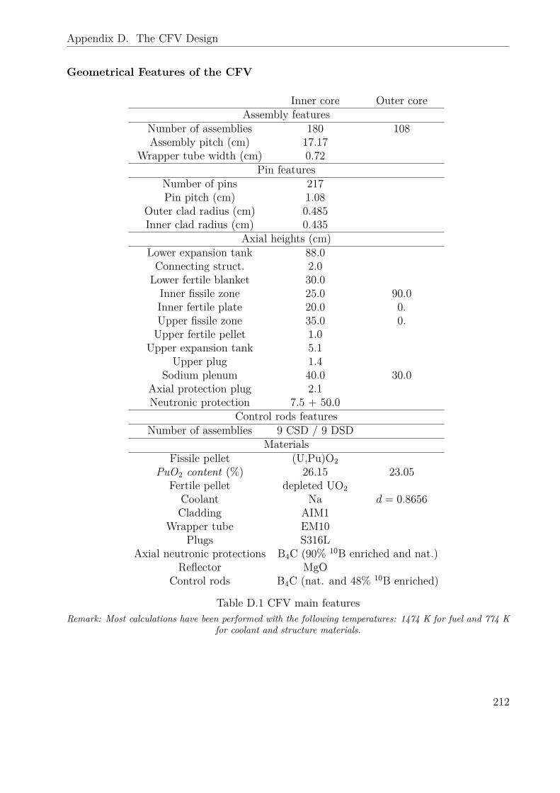
Appendix D. The CFV Design
Geometrical Features of the CFV
Inner core Outer coreAssembly features
Number of assemblies 180 108Assembly pitch (cm) 17.17
Wrapper tube width (cm) 0.72Pin features
Number of pins 217Pin pitch (cm) 1.08
Outer clad radius (cm) 0.485Inner clad radius (cm) 0.435
Axial heights (cm)Lower expansion tank 88.0Connecting struct. 2.0Lower fertile blanket 30.0Inner fissile zone 25.0 90.0Inner fertile plate 20.0 0.Upper fissile zone 35.0 0.Upper fertile pellet 1.0
Upper expansion tank 5.1Upper plug 1.4
Sodium plenum 40.0 30.0Axial protection plug 2.1Neutronic protection 7.5 + 50.0
Control rods featuresNumber of assemblies 9 CSD / 9 DSD
MaterialsFissile pellet (U,Pu)O2
PuO2 content (%) 26.15 23.05Fertile pellet depleted UO2
Coolant Na d = 0.8656Cladding AIM1
Wrapper tube EM10Plugs S316L
Axial neutronic protections B4C (90% 10B enriched and nat.)Reflector MgO
Control rods B4C (nat. and 48% 10B enriched)
Table D.1 CFV main featuresRemark: Most calculations have been performed with the following temperatures: 1474 K for fuel and 774 K
for coolant and structure materials.
212
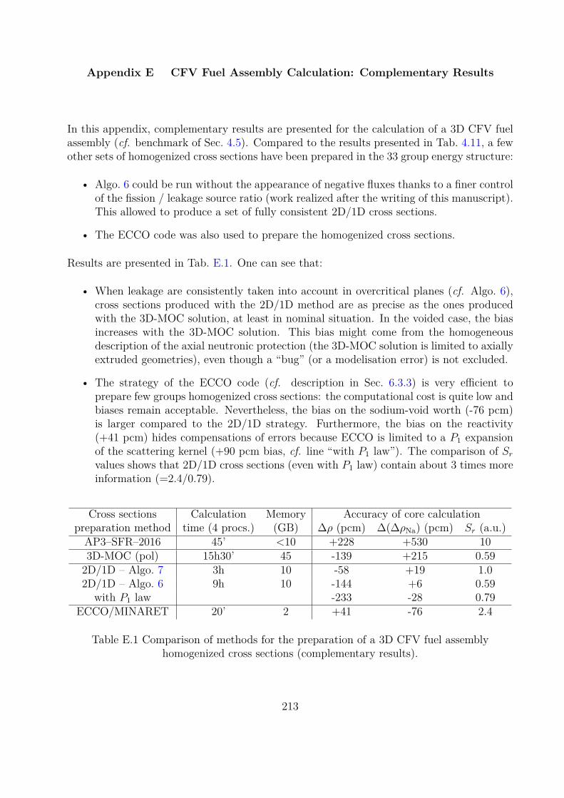
Appendix E CFV Fuel Assembly Calculation: Complementary Results
In this appendix, complementary results are presented for the calculation of a 3D CFV fuelassembly (cf. benchmark of Sec. 4.5). Compared to the results presented in Tab. 4.11, a fewother sets of homogenized cross sections have been prepared in the 33 group energy structure:
• Algo. 6 could be run without the appearance of negative fluxes thanks to a finer controlof the fission / leakage source ratio (work realized after the writing of this manuscript).This allowed to produce a set of fully consistent 2D/1D cross sections.
• The ECCO code was also used to prepare the homogenized cross sections.
Results are presented in Tab. E.1. One can see that:
• When leakage are consistently taken into account in overcritical planes (cf. Algo. 6),cross sections produced with the 2D/1D method are as precise as the ones producedwith the 3D-MOC solution, at least in nominal situation. In the voided case, the biasincreases with the 3D-MOC solution. This bias might come from the homogeneousdescription of the axial neutronic protection (the 3D-MOC solution is limited to axiallyextruded geometries), even though a “bug” (or a modelisation error) is not excluded.
• The strategy of the ECCO code (cf. description in Sec. 6.3.3) is very efficient toprepare few groups homogenized cross sections: the computational cost is quite low andbiases remain acceptable. Nevertheless, the bias on the sodium-void worth (-76 pcm)is larger compared to the 2D/1D strategy. Furthermore, the bias on the reactivity(+41 pcm) hides compensations of errors because ECCO is limited to a P1 expansionof the scattering kernel (+90 pcm bias, cf. line “with P1 law”). The comparison of Srvalues shows that 2D/1D cross sections (even with P1 law) contain about 3 times moreinformation (=2.4/0.79).
Cross sections Calculation Memory Accuracy of core calculationpreparation method time (4 procs.) (GB) ∆ρ (pcm) ∆(∆ρNa) (pcm) Sr (a.u.)AP3–SFR–2016 45’ <10 +228 +530 103D-MOC (pol) 15h30’ 45 -139 +215 0.592D/1D – Algo. 7 3h 10 -58 +19 1.02D/1D – Algo. 6 9h 10 -144 +6 0.59
with P1 law -233 -28 0.79ECCO/MINARET 20’ 2 +41 -76 2.4
Table E.1 Comparison of methods for the preparation of a 3D CFV fuel assemblyhomogenized cross sections (complementary results).
213
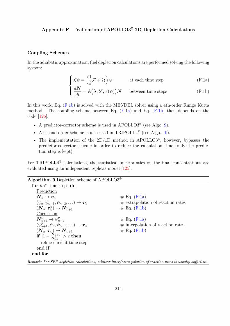
Appendix F Validation of APOLLO3® 2D Depletion Calculations
Coupling Schemes
In the adiabatic approximation, fuel depletion calculations are performed solving the followingsystem:
Lψ =(1kF +H
)ψ at each time step (F.1a)
dN
dt= A
(λ,Y , τ (ψ)
)N between time steps (F.1b)
In this work, Eq. (F.1b) is solved with the MENDEL solver using a 4th-order Runge Kuttamethod. The coupling scheme between Eq. (F.1a) and Eq. (F.1b) then depends on thecode [126]:
• A predictor-corrector scheme is used in APOLLO3® (see Algo. 9).• A second-order scheme is also used in TRIPOLI-4® (see Algo. 10).• The implementation of the 2D/1D method in APOLLO3®, however, bypasses the
predictor-corrector scheme in order to reduce the calculation time (only the predic-tion step is kept).
For TRIPOLI-4® calculations, the statistical uncertainties on the final concentrations areevaluated using an independent replicas model [125].
Algorithm 9 Depletion scheme of APOLLO3®
for n ∈ time-steps doPredictionNn → ψn # Eq. (F.1a)(ψn, ψn−1, ψn−2, . . .)→ τ pn # extrapolation of reaction rates(Nn, τ
pn)→N p
n+1 # Eq. (F.1b)CorrectionN p
n+1 → ψpn+1 # Eq. (F.1a)(ψpn+1, ψn, ψn−1, . . .)→ τ n # interpolation of reaction rates(Nn, τ n)→Nn+1 # Eq. (F.1b)if |1− Nn+1
Npn+1| > ε then
refine current time-stepend if
end for
Remark: For SFR depletion calculations, a linear inter/extra-polation of reaction rates is usually sufficient.
214
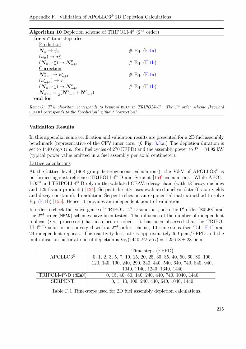
Appendix F. Validation of APOLLO3® 2D Depletion Calculations
Algorithm 10 Depletion scheme of TRIPOLI-4® (2nd order)for n ∈ time-steps doPredictionNn → ψn # Eq. (F.1a)(ψn)→ τ pn(Nn, τ
pn)→N p
n+1 # Eq. (F.1b)CorrectionN p
n+1 → ψcn+1 # Eq. (F.1a)(ψcn+1)→ τ cn(Nn, τ
cn)→N c
n+1 # Eq. (F.1b)Nn+1 = 1
2(N pn+1 +N c
n+1)end for
Remark: This algorithm corresponds to keyword MEAN in TRIPOLI-4®. The 1st order scheme (keywordEULER) corresponds to the “prediction” without “correction”.
Validation Results
In this appendix, some verification and validation results are presented for a 2D fuel assemblybenchmark (representative of the CFV inner core, cf. Fig. 3.3.a.) The depletion duration isset to 1440 days (i.e., four fuel cycles of 270 EFPD) and the assembly power to P = 84.92 kW(typical power value emitted in a fuel assembly per axial centimeter).Lattice calculationsAt the lattice level (1968 group heterogeneous calculations), the V&V of APOLLO3® isperformed against reference TRIPOLI-4®-D and Serpent [154] calculations. While APOL-LO3® and TRIPOLI-4®-D rely on the validated CEAV5 decay chain (with 18 heavy nuclidesand 126 fission products) [124], Serpent directly uses evaluated nuclear data (fission yieldsand decay constants). In addition, Serpent relies on an exponential matrix method to solveEq. (F.1b) [155]. Hence, it provides an independent point of validation.In order to check the convergence of TRIPOLI-4®-D solutions, both the 1st order (EULER) andthe 2nd order (MEAN) schemes have been tested. The influence of the number of independentreplicas (i.e., processors) has also been studied. It has been observed that the TRIPO-LI-4®-D solution is converged with a 2nd order scheme, 10 time-steps (see Tab. F.1) and24 independent replicas. The reactivity loss rate is approximately 6.9 pcm/EFPD and themultiplication factor at end of depletion is kT4(1440 EFPD) = 1.25618± 28 pcm.
Time steps (EFPD)APOLLO3® 0, 1, 2, 3, 5, 7, 10, 15, 20, 25, 30, 35, 40, 50, 60, 80, 100,
120, 140, 190, 240, 290, 340, 440, 540, 640, 740, 840, 940,1040, 1140, 1240, 1340, 1440
TRIPOLI-4®-D (MEAN) 0, 15, 40, 80, 140, 240, 440, 740, 1040, 1440SERPENT 0, 1, 10, 100, 240, 440, 640, 1040, 1440
Table F.1 Time-steps used for 2D fuel assembly depletion calculations.
215
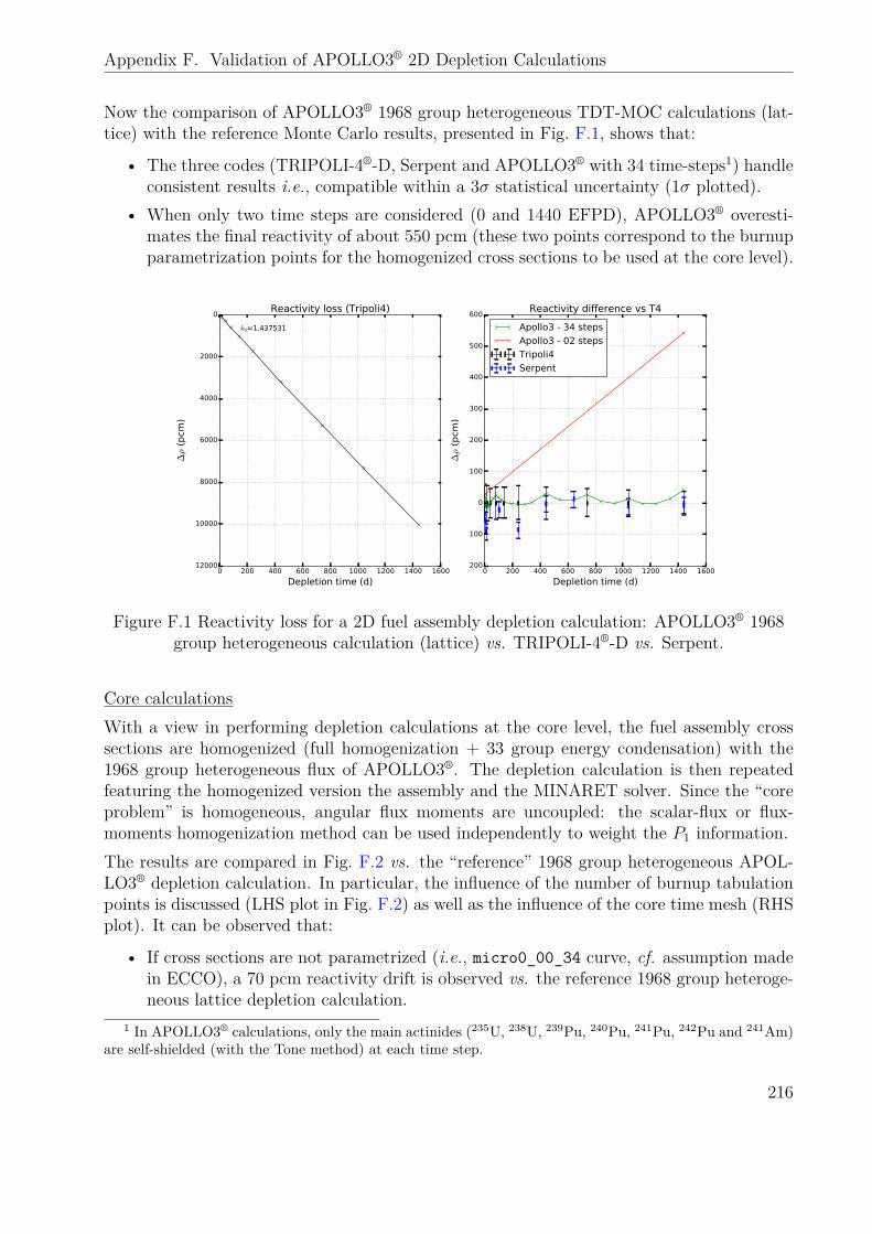
Appendix F. Validation of APOLLO3® 2D Depletion Calculations
Now the comparison of APOLLO3® 1968 group heterogeneous TDT-MOC calculations (lat-tice) with the reference Monte Carlo results, presented in Fig. F.1, shows that:
• The three codes (TRIPOLI-4®-D, Serpent and APOLLO3® with 34 time-steps1) handleconsistent results i.e., compatible within a 3σ statistical uncertainty (1σ plotted).
• When only two time steps are considered (0 and 1440 EFPD), APOLLO3® overesti-mates the final reactivity of about 550 pcm (these two points correspond to the burnupparametrization points for the homogenized cross sections to be used at the core level).
0 200 400 600 800 1000 1200 1400 1600
Depletion time (d)
−12000
−10000
−8000
−6000
−4000
−2000
0
∆ρ (pcm
)
k0=1.437531
Reactivity lo (Tripoli4)
0 200 400 600 800 1000 1200 1400 1600
Depletion time (d)
−200
−100
0
100
200
300
400
500
600
∆ρ (pcm
)
Reactivity difference v T4
Apollo3 - 34 steps
Apollo3 - 02 steps
Tripoli4
Serpent
Figure F.1 Reactivity loss for a 2D fuel assembly depletion calculation: APOLLO3® 1968group heterogeneous calculation (lattice) vs. TRIPOLI-4®-D vs. Serpent.
Core calculationsWith a view in performing depletion calculations at the core level, the fuel assembly crosssections are homogenized (full homogenization + 33 group energy condensation) with the1968 group heterogeneous flux of APOLLO3®. The depletion calculation is then repeatedfeaturing the homogenized version the assembly and the MINARET solver. Since the “coreproblem” is homogeneous, angular flux moments are uncoupled: the scalar-flux or flux-moments homogenization method can be used independently to weight the P1 information.The results are compared in Fig. F.2 vs. the “reference” 1968 group heterogeneous APOL-LO3® depletion calculation. In particular, the influence of the number of burnup tabulationpoints is discussed (LHS plot in Fig. F.2) as well as the influence of the core time mesh (RHSplot). It can be observed that:
• If cross sections are not parametrized (i.e., micro0_00_34 curve, cf. assumption madein ECCO), a 70 pcm reactivity drift is observed vs. the reference 1968 group heteroge-neous lattice depletion calculation.
1 In APOLLO3® calculations, only the main actinides (235U, 238U, 239Pu, 240Pu, 241Pu, 242Pu and 241Am)are self-shielded (with the Tone method) at each time step.
216
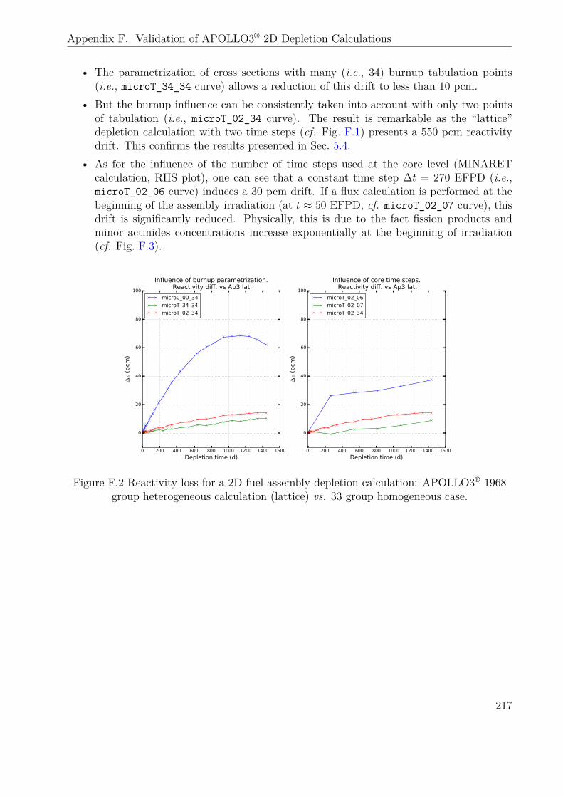
Appendix F. Validation of APOLLO3® 2D Depletion Calculations
• The parametrization of cross sections with many (i.e., 34) burnup tabulation points(i.e., microT_34_34 curve) allows a reduction of this drift to less than 10 pcm.
• But the burnup influence can be consistently taken into account with only two pointsof tabulation (i.e., microT_02_34 curve). The result is remarkable as the “lattice”depletion calculation with two time steps (cf. Fig. F.1) presents a 550 pcm reactivitydrift. This confirms the results presented in Sec. 5.4.
• As for the influence of the number of time steps used at the core level (MINARETcalculation, RHS plot), one can see that a constant time step ∆t = 270 EFPD (i.e.,microT_02_06 curve) induces a 30 pcm drift. If a flux calculation is performed at thebeginning of the assembly irradiation (at t ≈ 50 EFPD, cf. microT_02_07 curve), thisdrift is significantly reduced. Physically, this is due to the fact fission products andminor actinides concentrations increase exponentially at the beginning of irradiation(cf. Fig. F.3).
0 200 400 600 800 1000 1200 1400 1600
Depletion time (d)
0
20
40
60
80
100
∆ρ (pcm
)
Influence of burnup parametrization. Reactivity diff. vs Ap3 lat.
micro0_00_34
microT_34_34
microT_02_34
0 200 400 600 800 1000 1200 1400 1600
Depletion time (d)
0
20
40
60
80
100∆ρ (pcm
)
Influence of core time steps. Reactivity diff. vs Ap3 lat.
microT_02_06
microT_02_07
microT_02_34
Figure F.2 Reactivity loss for a 2D fuel assembly depletion calculation: APOLLO3® 1968group heterogeneous calculation (lattice) vs. 33 group homogeneous case.
217
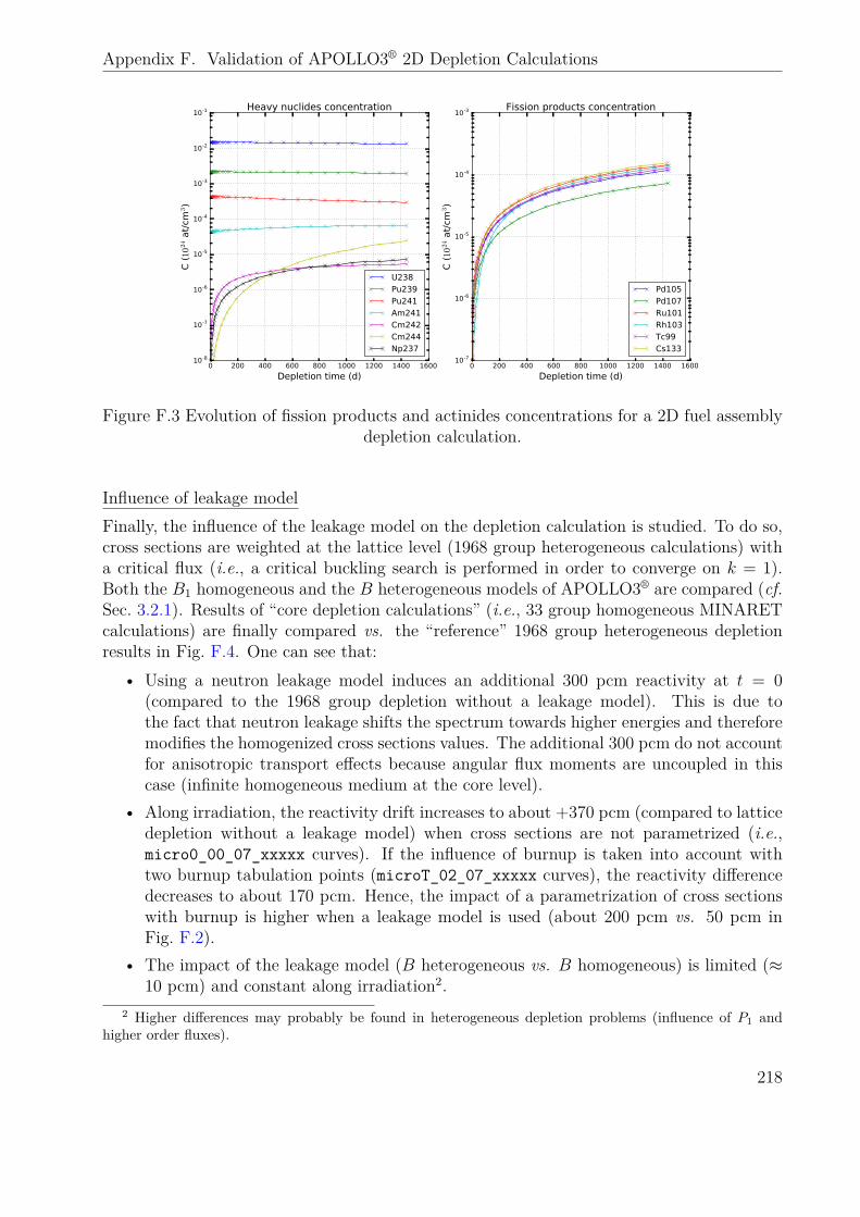
Appendix F. Validation of APOLLO3® 2D Depletion Calculations
0 200 400 600 800 1000 1200 1400 1600
Depletion time (d)
10-8
10-7
10-6
10-5
10-4
10-3
10-2
10-1
C (10
24 at/cm
3)
Heavy nuclides concentration
U238Pu239Pu241Am241Cm242Cm244Np237
0 200 400 600 800 1000 1200 1400 1600
Depletion time (d)
10-7
10-6
10-5
10-4
10-3
C (10
24 at/cm
3)
Fission products concentration
Pd105Pd107Ru101Rh103Tc99Cs133
Figure F.3 Evolution of fission products and actinides concentrations for a 2D fuel assemblydepletion calculation.
Influence of leakage modelFinally, the influence of the leakage model on the depletion calculation is studied. To do so,cross sections are weighted at the lattice level (1968 group heterogeneous calculations) witha critical flux (i.e., a critical buckling search is performed in order to converge on k = 1).Both the B1 homogeneous and the B heterogeneous models of APOLLO3® are compared (cf.Sec. 3.2.1). Results of “core depletion calculations” (i.e., 33 group homogeneous MINARETcalculations) are finally compared vs. the “reference” 1968 group heterogeneous depletionresults in Fig. F.4. One can see that:
• Using a neutron leakage model induces an additional 300 pcm reactivity at t = 0(compared to the 1968 group depletion without a leakage model). This is due tothe fact that neutron leakage shifts the spectrum towards higher energies and thereforemodifies the homogenized cross sections values. The additional 300 pcm do not accountfor anisotropic transport effects because angular flux moments are uncoupled in thiscase (infinite homogeneous medium at the core level).
• Along irradiation, the reactivity drift increases to about +370 pcm (compared to latticedepletion without a leakage model) when cross sections are not parametrized (i.e.,micro0_00_07_xxxxx curves). If the influence of burnup is taken into account withtwo burnup tabulation points (microT_02_07_xxxxx curves), the reactivity differencedecreases to about 170 pcm. Hence, the impact of a parametrization of cross sectionswith burnup is higher when a leakage model is used (about 200 pcm vs. 50 pcm inFig. F.2).
• The impact of the leakage model (B heterogeneous vs. B homogeneous) is limited (≈10 pcm) and constant along irradiation2.
2 Higher differences may probably be found in heterogeneous depletion problems (influence of P1 andhigher order fluxes).
218
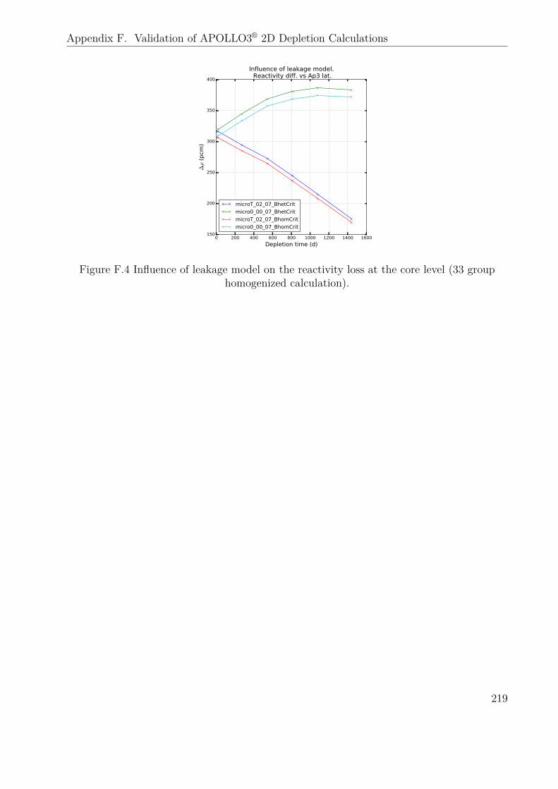
Appendix F. Validation of APOLLO3® 2D Depletion Calculations
0 200 400 600 800 1000 1200 1400 1600
Depletion time (d)
150
200
250
300
350
400
∆ρ (pcm
)
Influence of leakage model. Reactivity diff. vs Ap3 lat.
microT_02_07_BhetCrit
micro0_00_07_BhetCrit
microT_02_07_BhomCrit
micro0_00_07_BhomCrit
Figure F.4 Influence of leakage model on the reactivity loss at the core level (33 grouphomogenized calculation).
219
Appendix G Perturbation Theory and Point Kinetics
Direct and Adjoint Problems
The critical neutron transport equation can be put in the form:
Aψ = 1kFψ (G.1)
where A = L+H.Introducing the following scalar product:
< f, g >=∫D×R+×S2
d3rdEd2Ω f(r, E,Ω)g(r, E,Ω) (G.2)
it is possible to define, for each operator O, its adjoint O† such that:
∀f, g < f,Og >=< O†f, g > (G.3)
The adjoint problem corresponding to Eq. (G.1) is:
A†ψ† = 1k†F †ψ† (G.4)
Taking the scalar product of Eq. (G.1) with ψ†, it is possible to show that:
k = k† (G.5)
Standard Perturbation Theory (SPT)
The adjoint neutron transport equation is a central piece of neutronic perturbation theory.Let ψ† be the adjoint flux in a reference system and ψp the direct flux in a perturbed situation:
A†ψ† = 1kF †ψ† (G.6a)
Apψp = 1kpFpψp (G.6b)
The reactivity difference between the reference and the pertubed systems is:
∆ρ = 1k− 1kp
(G.7)
The standard perturbation theory [133] links the reactivity perturbation ∆ρ to operatorperturbations, i.e., ∆A = Ap −A and ∆F = Fp −F with:
∆ρ =< ψ†,
(∆Fk−∆A
)ψp >
< ψ†,Fpψp >(G.8)
220
Appendix G. Perturbation Theory and Point Kinetics
Proof. One can write:
< ψ†,(Ap −
Fpkp
)ψp > − <
(A† − F
†
k
)ψ†, ψp >= 0 (G.9)
i.e., using the definition of an adjoint operator:
< ψ†,(Ap −
Fpkp
)ψp > − < ψ†,
(A− F
k
)ψp >= 0 (G.10)
This expression can also be written:
< ψ†,(∆A− ∆F
k
)ψp > + < ψ†,
(1k− 1kp
)Fpψp >= 0 (G.11)
Hence:< ψ†,
(∆A− ∆F
k
)ψp > +∆ρ < ψ†,Fpψp >= 0 (G.12)
Point Kinetics
The adjoint neutron transport equation is also used in the framework of the point kineticsapproximation.In a nuclear reactor, the equations that rule the evolution of the neutron flux ψ(r, E,Ω, t)and precursors concentrations Ck(r, t) read:
1v
∂ψ
∂t+Aψ = Fpψ + 1
4π
Np∑k=1
λkχd,kCk (G.13a)
∂Ck∂t
+ λkCk =∫
R+×S2
Fd,kψ dEd2Ω, k ∈ 1, 2, . . . , Np (G.13b)
where Fp is the prompt fission operator, A = Ω · ∂r + Σ−H is the absorption operator andFd,k is the precursors production operator defined as:
Fd,kψ(r, E,Ω, t) = χd,k(E)
4π
∫R+×S2
dE ′d2Ω′ νd,k(E ′)Σf (r, E ′, t)ψ(r, E ′,Ω′, t) (G.14)
We also define the total fission operator as1:
Ft = Fp +Np∑k=1Fd,k (G.15)
In order to obtain the PK equations, one must:1 Warning: Ft corresponds to the number of neutrons emitted at time t only when the delayed neutrons
precursors are in an equilibrium state. Else, a delay must be considered.
221
Appendix G. Perturbation Theory and Point Kinetics
- multiply Eq. (G.13a) with any arbitrary weight function φ∗0 and perform an integrationover phase-space;
- multiply Eq. (G.13b) with φ∗0 × χd,k/4π and integrate over phase-space.
The result is: dN
dt+ β − ρ
ΛN =
Np∑k=1
λkCk (G.16a)
dCkdt
+ λkCk = βk
ΛN , k ∈ 1, 2, . . . , Np (G.16b)
where the unknowns are: N =< φ∗0 ·
1vψ > (G.17a)
Ck = 14π < φ∗0 · χd,kCk > (G.17b)
The parameters of the PK model are the delayed neutron fractions, per family βk and totalβ, the mean neutron generation time Λ, and the reactivity ρ:
βk = < φ∗0 · Fd,kψ >< φ∗0 · Ftψ >
, β =Np∑i=k
βk (G.18a)
Λ =< φ∗0 · 1
vψ >
< φ∗0 · Ftψ >(G.18b)
ρ = < φ∗0 · (Ft −A)ψ >< φ∗0 · Ftψ >
(G.18c)
Usually, Np =6 or 8 precursors families are considered.At this stage, no assumption is made. Yet, the lumped parameters (βk, β, Λ, and ρ) dependon the time variable. Besides, their definition assumes that the flux ψ is known.The PK approximation consists in replacing the real flux ψ by an approximation ψ0 (fluxshape) in the expressions of the delayed neutron fractions (βk, β) and mean neutron lifetime(Λ)2:
βk ≈< φ∗0 · Fd,k,0ψ0 >
< φ∗0 · F0ψ0 >, Λ ≈
< φ∗0 · 1vψ0 >
< φ∗0 · F0ψ0 >(G.19)
Usually, the flux shape ψ0 is computed as the solution of a fictitious critical problem repre-sentative of the initial state of the reactor:
A0ψ0 = 1k0F0ψ0 (G.20)
and the weight function φ∗0 is usually computed as ψ†0, i.e., the adjoint flux associated toEq. (G.20).
2 The reactivity is more dependent on local changes in the flux shape. Hence, it is usually computedotherway (e.g., with reactivity feedback coefficients).
222

This page has been left intentionally blank.
223