Development of a Calibration Standard for Spherical Aberration

David C. Compertore, Filipp V. Ignatovich, Matthew E. Herbrand, Michael A. Marcus,

Lumetrics, Inc. 1565 Jefferson Road, Rochester, NY (United States)

ABSTRACT

There are no calibration standards currently available for metrology equipment used to measure spherical aberration. We

have selected a set of plano-convex lenses that can be used as spherical aberration calibration standards. The key

parameters of the lenses were measured using a nodal optical bench and a low coherence interferometer. Spherical

aberrations of the lenses were measured using a commercially available aberrometer the CrystalWave™, based on a

Shack-Hartmann wavefront sensor. The lenses were then modeled in optical modeling software, where the spherical

curvatures of the lenses were adjusted to match the key parameters. The measured spherical aberrations were then

compared to the values provided by the modeling software.

1. INTRODUCTION

1.1 Intraocular Lenses and Spherical Aberration

Anyone making or using imaging optics may at some point run up against spherical aberration (SA). Spherical

aberration is often considered an inherent optical flaw and is present to some degree in all imaging systems1. In

particular, intraocular lens producers have a strong interest in the SA of their lenses. Intraocular lens designers and

producers often add SA to their lenses as a feature. For certain intraocular lenses, the manufacturers have made visual

performance claims, based on lenses with specific levels of SA. The claims are backed up with clinical data.

1.2 Cataracts, Surgery and Intraocular Lenses

There are two components of the human eye with significant optical power; the cornea, with about 44 D of refractive

power, and the accommodating lens, with about 21 D2. These two components combine to image the outside world onto

our retinas. All adult eyes have some degree of clouding in their natural lens. If this cloudiness progresses to the point

where vision is impaired, cataract surgery is used to correct it. During cataract surgery, the cloudy natural lens is

pulverized and removed, leaving the capsular bag empty and ready to receive an intraocular lens. The surgeon inserts an

intraocular lens through the capsularhexis into the now empty lens bag, filling the space the natural accommodating lens

vacated.

1.3 An Intraocular Lens’ Multiple Duties

An intraocular lens has many benefits. It returns sight by providing a clean and clear aperture to a once cloudy eye. Of

all surgeries performed around the world, cataract surgery is ranked number one for patient satisfaction3. Selecting the

proper dioptric power for the IOL can correct with great accuracy a person’s long standing refractive error, eliminating

the need for spectacles for distance vision. In addition, aberrations can be added to the lens, to counterbalance the

aberrations present in the patient’s cornea, and therefore sharpen the image. It is common for manufacturers to add SA to

the intraocular lens, ranging from zero to the amount equal to the opposite of the SA present in the average human

cornea. Lenses that contain zero SA, sometimes help to minimize the effects of decentering and tilt inherent in every

eye.

A spherical aberration standard lens, as a calibration artifact, will therefore help ensure consistent production quality for

intraocular lenses with targeted designed levels of spherical aberration.

1.4 Objectives

The main objective was to create a calibration kit, consisting of a set of lenses with accurately defined amounts of

spherical aberration. This set will then be simple to use and understand in the context of SA calibration. The lenses

should easily fit into an intraocular lens test bench, and should not exceed in outer diameter the size of a typical

intraocular lens, including the haptics, see Figure 1, which help center the intraocular lens in the eye after surgery.

Figure 1: Sample Intraocular Lens

2. Method

2.1 Overview

To minimize the number of lens parameters that can contribute to SA, and therefore to make the SA performance easy to

understand, we have selected plano-convex glass lenses. The SA of a plano-convex lens is well documented4, and a

plano-convex lens design is easy to model in any lens modeling software.

We modeled the transmitted spherical aberration of the lenses in Zemax. We then measured the transmitted SA of the

lenses using a Shack-Hartmann instrument, the Lumetrics® CrystalWave™. The difference between the modeled

spherical aberration and the measured spherical aberration was then compared against the acceptance criterion.

2.2 Modeling

We assume that the convex surface of the lens is perfectly spherical. A generic plano-convex lens is modeled in Zemax.

The exact modeling requires the glass material, center thickness of the lens, as well as the radius of curvature of the

convex surface.

The center thickness of the lens is measured using the Lumetrics OptiGauge™ low-coherence interferometer. The

accurate physical thickness measurement requires the knowledge of the group refractive index of the glass. The

OptiGauge™ can also be used to measure the refractive index of the lens material5. The measured thickness is then

entered into the Zemax model.

The radius of curvature of the lens is found using a Zemax merit function, which adjusts the radius of curvature based on

the effective focal length of the lens. The effective focal length of the lenses is measured using an optical nodal bench, a

NIST traceable method, by Optical Testing Laboratory, Inc. in Corvallis, OR. Zemax optimizes the curvature of the

convex lens surface in the model, until the refined model’s effective focal length matches the certified value.

After the model is refined to account for the measured effective focal length and center thickness, four model

configurations are set up in the modeling software. By convention, a plano-convex lens has a minimum of spherical

aberration, if the flat surface faces the diverging or converging beam; and maximum SA when it is oriented with the flat

surface facing the collimated beam. In creating the certifiable spherical aberration values, we use both orientations of the

lens, as well as two different aperture sizes.

The first configuration has a 5 millimeter aperture, with the flat surface of the lens facing the focal point, Figure 2. The

second configuration has a 3.6 millimeter aperture, with the flat surface facing the focal point.

Figure 2: Nominal lens orientation for model configurations 1 and 2.

The lens is flipped around to the non-standard orientation for the third configuration, with a 5 millimeter aperture, Figure

3. The fourth configuration has a 3.6 millimeter aperture, with the convex surface facing the focal point.

Figure 3: Flipped or reversed orientation for model configurations 3 and 4.

Tables 2, 3, 4 and 5 list the SA values, in the column labeled modeled spherical aberration, obtained using above steps

for different lenses and configurations.

2.3 Testing and equipment

Each lens was tested 48 times, 12 times each in four different configurations, on the Shack-Hartmann based instrument.

Mechanical fixtures were used to minimize the tip and tilt of the lenses with respect to the measurement beam within the

CrystalWaveTM

instrument. The lenses were centered within the beam by translating the lens about the optic axis to

minimize the tilt Zernike terms reported by the Shack-Hartmann. This method works well for lenses that don’t have

appreciable wedge and will typically center the lenses to within 100 microns on the optic axis. We assumed the lenses

had insignificant wedge.

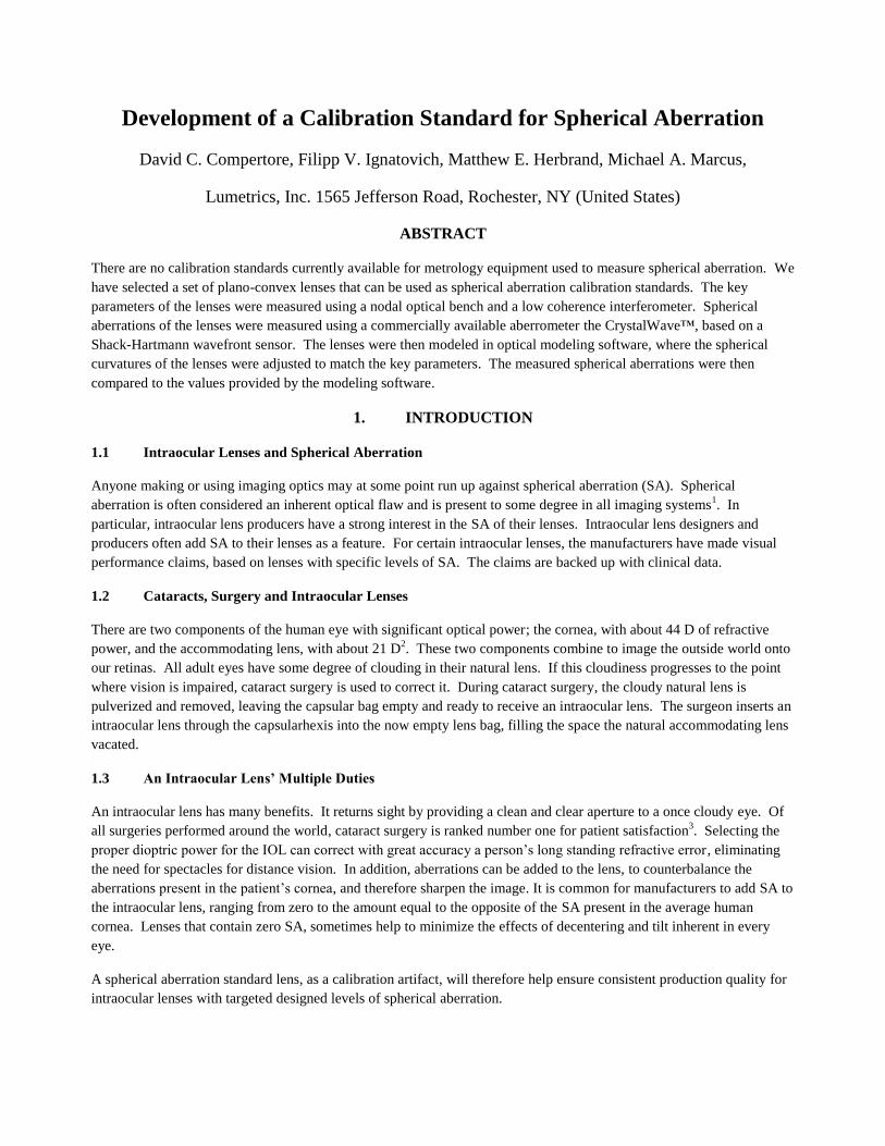
The CrystalWave™ optical configuration is shown in Figure 4. It allows an operator to quickly load and measure

intraocular and other types of lenses6.

Figure 4: CrystalWave™ optical configuration.

The automated routine moves the point light source, LED in Figure 4, to the position at which the intraocular lens

collimates the diverging beam. A collimated input into the Shack-Hartmann sensor, WFS, can be interpreted as an

object at infinity, and the point source can be interpreted as light emitted from the retina at the optic axis. Even though

the flow of light is reversed compared to the normal function of the eye, the test accurately predicts the optical response

of the intraocular lens due to the principle of reciprocity in geometrical optics7. The relay lenses, L1 and L2, keep the

pupil of the intraocular lens, IOL, conjugate with the lenslet array of the Shack-Hartmann sensor. The rate limiting

aperture, RLA, in the relay lens prevents stray light from entering the Shack-Hartmann measurement system.

Each lens is loaded in two different orientations to match those of the Zemax models, in the orientations shown in Figure

2 and 3. The aperture size is controlled by software. A physical aperture was not used to change the aperture size. Two

apertures sizes were set in software, 5 mm and 3.6 mm. The two lens orientation and two software-specified apertures

result in four total test sets per lens. Each test set contains 12 measurements. After each measurement the lens is shifted

from center, rotated, and then centered again. These additional alignment steps are used to average out the operator error

due to setup in the measurement values.

2.4 Criteria

The SA measurement value is considered valid for calibration purposes, if the modeled and the averaged measured

spherical aberration for the lens are equivalent. A difference of no more than ±0.015 microns of SA between the

modeled spherical aberration and the average measured spherical aberration was defined as being equivalent. An

absolute difference of 0.015 microns is approximately 3 times smaller than the level of change in spherical aberration a

normal eye is able to differentiate8.

3. Results

Table 1 shows the measured parameter for nine selected of-the-shelf lenses. Each lens has an alphanumeric

identification starting with the letters LS, the first column in Table 1. The second column of data contains the

manufacturer model number. The third column contains the manufacturer-specified outer diameter of the lenses. The

manufacturer-specified effective focal length of the lenses is shown in the fourth column. The fifth column contains the

effective focal length, measured by the NIST traceable method. The measured center thickness is listed in the final

column.

Table 1: Manufacturer-specified and measured lens parameters.

Lenses ID etched onto the glass

Edmund Optics Model

Diameter (nominal)

(mm)

EFL (nominal)

(mm) Certified EFL (mm)

CT measured

(mm)

LS-0388 45083 12 12 11.893 4.04319

LS-0389 45083 12 12 11.889 3.99234

LS-0390 45083 12 12 11.896 4.04347

LS-0391 49877 12 20 19.892 3.52611

LS-0392 49877 12 20 19.912 3.52496

LS-0393 49877 12 20 19.904 3.52842

LS-0394 32854 12 60 59.894 2.45257

LS-0395 32854 12 60 59.892 2.46444

LS-0396 32854 12 60 59.951 2.44459

Table 2 shows the modeled and measured SA in the nominal orientations with a 5 mm aperture. Table 3 shows the

modeled and measured SA in the reversed orientations with a 5 mm aperture. Table 4 shows the modeled and measured

SA in the nominal orientations with a 3.6 mm aperture. Table 5 shows the modeled and measured SA in the reversed

orientations with a 3.6 mm aperture. The last column of Tables 2 through 5 tabulates the difference between the

measured and modeled SA.

Table 2: The SA, in microns, aperture 5 mm, nominal orientation, modeled in Zemax using parameters from Table 1.

Lenses

modeled Spherical

Aberration

Measured Spherical

Aberration

Difference (measured -

model)

LS-0388 -0.536 -0.540 -0.004

LS-0389 -0.538 -0.540 -0.002

LS-0390 -0.536 -0.537 -0.001

LS-0391 -0.227 -0.222 0.005

LS-0392 -0.226 -0.222 0.004

LS-0393 -0.226 -0.222 0.004

LS-0394 -0.008 -0.003 0.005

LS-0395 -0.008 -0.003 0.005

LS-0396 -0.008 -0.008 0.000

Table 3: The SA, in microns, aperture 5 mm, reversed orientation, modeled in Zemax using parameters from Table 1.

Lenses

modeled Spherical

Aberration

Measured Spherical

Aberration

Difference (measured -

model)

LS-0388 -2.620 -2.723 -0.103

LS-0389 -2.622 -2.717 -0.095

LS-0390 -2.618 -2.713 -0.095

LS-0391 -0.931 -0.937 -0.006

LS-0392 -0.928 -0.931 -0.003

LS-0393 -0.929 -0.933 -0.004

LS-0394 -0.033 -0.027 0.006

LS-0395 -0.033 -0.027 0.006

LS-0396 -0.032 -0.032 0.000

Table 4: The SA, in microns, aperture 3.6 mm, nominal orientation, modeled in Zemax using parameters from Table 1.

Lenses

modeled Spherical

Aberration

Measured Spherical

Aberration

Difference (measured -

model)

LS-0388 -0.142 -0.139 0.003

LS-0389 -0.141 -0.140 0.001

LS-0390 -0.140 -0.137 0.003

LS-0391 -0.060 -0.059 0.001

LS-0392 -0.060 -0.058 0.002

LS-0393 -0.060 -0.058 0.002

LS-0394 -0.002 0.000 0.002

LS-0395 -0.002 -0.003 -0.001

LS-0396 -0.002 -0.004 -0.002

Table 5: The SA, in microns, aperture 3.6 mm, reversed orientation, modeled in Zemax using parameters from Table 1.

Lenses

modeled Spherical

Aberration

Measured Spherical

Aberration

Difference (measured -

model)

LS-0388 -0.685 -0.695 -0.010

LS-0389 -0.686 -0.697 -0.011

LS-0390 -0.685 -0.689 -0.004

LS-0391 -0.244 -0.243 0.001

LS-0392 -0.243 -0.242 0.001

LS-0393 -0.244 -0.242 0.002

LS-0394 -0.009 -0.008 0.001

LS-0395 -0.009 -0.010 -0.001

LS-0396 -0.009 -0.011 -0.002

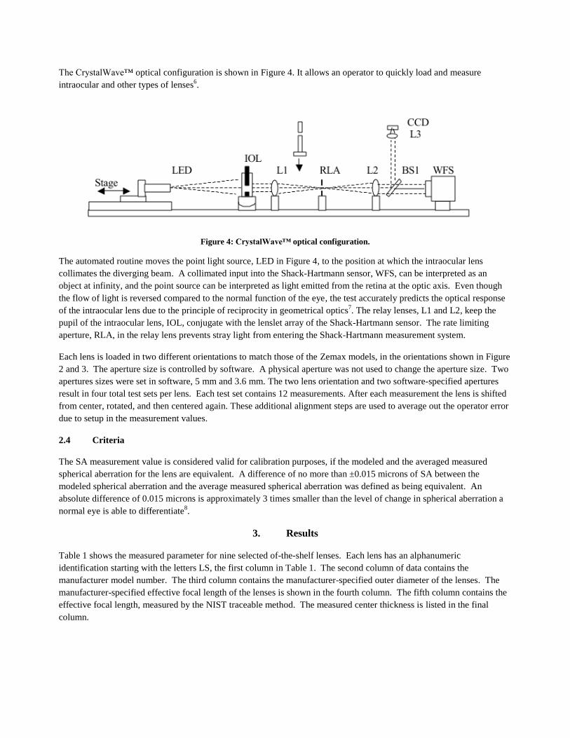
Figure 5 shows a control limit chart for lens LS-0388. The standard deviation of the 12 measurements is 1 nanometer.

The control charts for the other nominally 12 mm EFL lenses are similar.

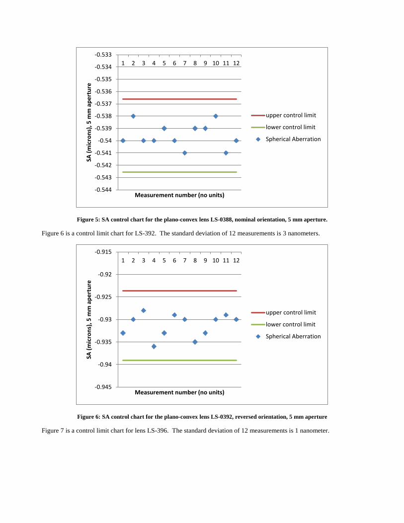
Figure 5: SA control chart for the plano-convex lens LS-0388, nominal orientation, 5 mm aperture.

Figure 6 is a control limit chart for LS-392. The standard deviation of 12 measurements is 3 nanometers.

Figure 6: SA control chart for the plano-convex lens LS-0392, reversed orientation, 5 mm aperture

Figure 7 is a control limit chart for lens LS-396. The standard deviation of 12 measurements is 1 nanometer.

-0.544

-0.543

-0.542

-0.541

-0.54

-0.539

-0.538

-0.537

-0.536

-0.535

-0.534

-0.533

1 2 3 4 5 6 7 8 9 10 11 12

SA (

mic

ron

s), 5

mm

ap

ert

ure

Measurement number (no units)

upper control limit

lower control limit

Spherical Aberration

-0.945

-0.94

-0.935

-0.93

-0.925

-0.92

-0.915

1 2 3 4 5 6 7 8 9 10 11 12

SA (

mic

ron

s), 5

mm

ap

ert

ure

Measurement number (no units)

upper control limit

lower control limit

Spherical Aberration

Figure 7: SA control chart for plano-convex lens LS-0396, reversed orientation, 3.6 mm aperture

4. Discussion

4.1 Accuracy or the Agreement between the Model and Measured Results

Figures 5, 6, and 7 are statistical control charts of the spherical aberration measurement process. If all of the measured

data falls within the upper and lower control limits the process is considered under control9. They show that the process

of measuring an intraocular lens is in control. All data points are within the upper or lower control limits for all 36

measurements. We have included only three control charts in this article. Other control charts look similar and the

measurements do not cross the control limits.

A summary of the numerical differences, in nm, between the measured and modeled SA for different lenses and

configurations are shown in Table 6. Of the 36 spherical aberration tests, 33 configurations pass the acceptance criteria

of 0.015 microns or 15 nm.

Table 6: Measured SA minus modeled SA. All numbers are in nm

nominal orientation nominal orientation reversed orientation reversed orientation

Lenses aperture = 5 mm aperture = 3.6 mm aperture = 5 mm aperture = 3.6 mm

LS-0388 -4 3 -103 -10

LS-0389 -2 1 -95 -11

LS-0390 -1 3 -95 -4

LS-0391 5 1 -6 1

LS-0392 4 2 -3 1

LS-0393 4 2 -4 2

LS-0394 5 2 6 1

LS-0395 5 -1 6 -1

-0.015

-0.014

-0.013

-0.012

-0.011

-0.01

-0.009

-0.008

-0.007

-0.006

1 2 3 4 5 6 7 8 9 10 11 12

SA (

mic

ron

s), 3

.6 m

m a

pe

rtu

re

Measurement number (no units)

upper control limit

lower control limit

Spherical Aberration

LS-0396 0 -2 0 -2

There are three test instances where the acceptance criteria are not met. All three failing instances occurred for the test

configuration where the highest spherical aberration was predicted by the model. A review of the Shack-Hartmann test

data shows, that in cases with large SA, the Shack-Hartmann operated in out-of-range conditions. Figure 8 shows an

example of a Shack-Hartmann area of interest where a neighboring lenslet’s spot is infringing, and thus affecting the SA

measurement value.

Figure 8: Illustration of the Shack-Hartmann sensor area of interest out-of-range condition, obtained for a configuration with

high SA.

This infringing spot comes at the edge of the 5 mm aperture for the 12 mm EFL lens positioned in the reverse

orientation, Figure 3. This situation represents an extreme case, as the lens under test is over two times more powerful

than the strongest intraocular lens, with its SA nearly an order of magnitude higher than the SA of the average human

eye of 0.21 microns over a 5 mm aperture2. Care should be taken to maintain SA levels below the levels that can cause

out-of-range conditions in the Shack-Hartmann sensor.

4.2 Residual Difference from Modeled to Measured Spherical Aberration

While our results show very good agreement between the modeled spherical aberration and the average measured

spherical aberration, there can be two potential sources of error. First source error comes from the assumption that the

convex surfaces of the lens are assumed to be perfectly spherical, and the flat surfaces are assumed perfectly flat. It is

likely that the spherical surfaces have a small degree of asphericity, and the flat surface is slightly curved. Such

deviations contribute to the error in the modeled value of SA. To account for the error, the convex and flat surfaces can

be measured in an interferometer, and the measured profile included in the model. Second source of error can stem from

the error in the phase index of refraction of the lens, used in the modeling (different from the group refractive index used

in thickness measurement). While the above sources of errors are very small, they can have a relatively strong influence

on the SA performance of the lens.

5. Conclusion

A simple set of plano-convex glass lenses was successfully calibrated for their spherical aberration. Measuring the

lenses in two different orientations provides a useful range of spherical aberration of interest to users of intraocular lens

and intraocular lens manufactures. Users of intraocular lenses and intraocular lens manufactures now have a tool for

maintaining the accuracy of their spherical aberration test equipment.

[1] Jenkins, F. and White, H, [Fundamentals of Optics], McGraw-Hill Book Company, New York, pages109-111,

(1957).

[2] Liou, Hwey-Lan, Brennan, Noel, A., “Anatomically Accurate, Finite Model Eye for Optical Modeling,” J. Opt. Soc.

Am. A, Vol. 14, No. 8, pages 1684-1695, (1997).

[3] Steinberg, E.P., Tielsch J.M., Schein O.D., Javitt, J.C., Sharkey, P., Cassard, S.D., Legro, M.W., Diener-West, M.,

Bass E.B., Daminano, A.M., “National study of cataract surgery outcomes, Variation in 4-month postoperative

outcomes as reflected in multiple outcome measures,” Ophthalmology, 101 (6), pages 1131-40, (1994).

[4] Sparrold, S., Lansing, A., “Spherical Aberration Compensation Plates,” Photonik International, pages 32-35, (2011).

[5] Marcus, Michael, A., Ignatovich, Filipp V., Hadcock, Kyle J., Gibson, Donald S., “Precision interferometric

measurements of refractive index of polymers in air and liquid,” Optifab, paper 8884-53, (2013).

[6] D. R. Neal, D. J. Armstrong, W.T. Turner, “Wavefront sensor for control and process monitoring in optics

manufacture,” SPIE 2993, pages 211-220, (1997).

[7] Jenkins, F. and White, H, [Fundamentals of Optics], McGraw-Hill Book Company, New York, page14, (1957).

[8] Legras, Richard, Chateau, Nicholas, Charman, Neil, W., “Assessment of Just-Noticeable Differences for Refractive

Errors and Spherical Aberration Using Visual Simulation,” OVS, Vol. 81, No. 9, pages 718-728, (2004).

[9] NIST/SEMATECH e-Handbook of Statistical Methods, http://www.itl.nist.gov/div898/handbook/ Section 6.3.1,

April 2012