arX

iv:0

706.

2344

v1 [

astr

o-ph

] 1

5 Ju

n 20

07

Detectors for the James Webb Space Telescope Near-Infrared

Spectrograph I: Readout Mode, Noise Model, and Calibration

Considerations

Bernard J. Rauscher and Ori Fox1

NASA Goddard Space Flight Center, Greenbelt, MD 20771

Bernard.J.Rauscher@nasa.gov

Pierre Ferruit2,3

Universite de Lyon, Lyon, F-69003, France

Robert J. Hill8, Augustyn Waczynski4, Yiting Wen6, Wei Xia-Serafino4, Brent Mott,

David Alexander, Clifford K. Brambora, Rebecca Derro, Chuck Engler,

Matthew B. Garrison, Thomas Johnson, Sridhar S. Manthripragada, James M. Marsh,

Cheryl Marshall, Robert J. Martineau, Kamdin B. Shakoorzadeh7, Donna Wilson,

Wayne D. Roher5, and Miles Smith

NASA Goddard Space Flight Center, Greenbelt, MD 20771

Craig Cabelli, James Garnett, Markus Loose,

Selmer Wong-Anglin, Majid Zandian, and Edward Cheng8

Teledyne Imaging Sensors, 5212 Verdugo Way, Camarillo, CA 93012

Timothy Ellis, Bryan Howe, Miriam Jurado,

Ginn Lee, John Nieznanski, Peter Wallis, and James York

ITT Space Systems Division, 1447 St. Paul Street, Rochester, NY, 14653

Michael W. Regan

Space Telescope Science Institute, 3700 San Martin Drive, Baltimore, MD 21218

Donald N.B. Hall and Klaus W. Hodapp

– 2 –

Institute for Astronomy, 640 North Aohoku Place, #209, Hilo HI 96720

and

Torsten Boker, Guido De Marchi, Peter Jakobsen, and Paolo Strada

ESTEC, Astrophysics Division, Postbus 299, Noordwijk, NL2200 AG, Netherlands

Received ; accepted

Accepted by Publications of the Astronomical Society of the Pacific

1Also at Department of Astronomy, University of Virginia, P.O. Box 4000325, Char-

lottesville, VA 22904

2Also at Universite Lyon 1, Observatoire de Lyon, 9 avenue Charles Andre, Saint-Genis

Laval, F-69230, France

3Also at CNRS, UMR 5574, Centre de Recherche Astrophysique de Lyon; Ecole Normale

Superieure de Lyon, Lyon, F-69007, France

4Global Science & Technologies, Inc., 7855 Walker Drive, Suite 200, Greenbelt, MD 20770

5Northrop Grumman Technical Services, 4276 Forbes Blvd., Lanham, MD 20706

6Muniz Engineering Inc., 7404 Executive Place, Suite 500, Lanham, MD 20706

7AK Aerospace Technology Corp., 12970 Brighton Dam Rd, Clarksville, MD 21029

8Conceptual Analytics LLC, 8209 Woburn Abbey Road, Glenn Dale, MD 20769

– 3 –

ABSTRACT

We describe how the James Webb Space Telescope (JWST) Near-Infrared

Spectrograph’s (NIRSpec’s) detectors will be read out, and present a model of

how noise scales with the number of multiple non-destructive reads sampling-

up-the-ramp. We believe that this noise model, which is validated using real

and simulated test data, is applicable to most astronomical near-infrared in-

struments. We describe some non-ideal behaviors that have been observed in

engineering grade NIRSpec detectors, and demonstrate that they are unlikely to

affect NIRSpec sensitivity, operations, or calibration. These include a HAWAII-

2RG reset anomaly and random telegraph noise (RTN). Using real test data, we

show that the reset anomaly is: (1) very nearly noiseless and (2) can be easily

calibrated out. Likewise, we show that large-amplitude RTN affects only a small

and fixed population of pixels. It can therefore be tracked using standard pixel

operability maps.

Subject headings: Astronomical Instrumentation

– 4 –

1. Introduction

The James Webb Space Telescope (JWST) was conceived as the scientific successor

to NASA’s Hubble and Spitzer space telescopes. Of all JWST “near-infrared” (NIR;

λ = 0.6− 5 µm) instruments, the Near-Infrared Spectrograph (NIRSpec) has the most

challenging detector requirements. This paper describes how we plan to operate NIRSpec’s

two 2048×2048 pixel, 5 micron cutoff (λco=5µm), Teledyne HAWAII-2RG (H2RG) sensor

chip assemblies (SCAs)1 for the most sensitive observations, and provides insights into some

non-ideal behaviors that have been observed in engineering grade NIRSpec detectors.

This paper is structured as follows. In Section 2, we provide an introduction to JWST,

NIRSpec, and NIRSpec’s detectors. We have tried to keep this discussion brief, and provide

references to more comprehensive discussions in the literature.

In Section 3, we present the NIRSpec detector subsystem’s baseline MULTIACCUM

readout mode. This section includes a detailed discussion of how total noise averages down

when multiple non-destructive reads are used sampling-up-the-ramp. MULTIACCUM

readout is quite general, and most other common readout modes, including correlated

double sampling (CDS), multiple-CDS (MCDS; also known as Fowler-N; Fowler & Gatley

1991), and straight sampling-up-the-ramp are special cases of MULTIACCUM. The general

NIR SCA noise model presented in this section, see Equation 1 & Table 2, is validated

using real and simulated test data.

Where practical, our methods and conclusions are anchored by measurement. One

advantage of the NIRSpec program is that multiple test SCAs and test facilities are

1Within NASA, individually mounted detector arrays are typically referred to as SCAs.

In the case of NIRSpec’s H2RGs, the SCA consists of HgCdTe detectors hybridized to a

readout integrated circuit and mounted on a molybdenum base (See Figure 1).

– 5 –

available. These are described in Section 4.

Section 5 describes the reset anomaly as it appears in engineering grade NIRSpec

H2RGs. The reset anomaly is fairly well-known in the NIR detector testing community.

Here we demonstrate using real test data that it is a nearly noise-less artifact for the

NIRSpec detectors that have been tested so far. We show that it straightforwardly

calibrates out from most science observations, and can therefore be safely ignored by most

JWST users. However, we show that the reset anomaly can significantly bias dark current

measurements if it is not correctly accounted for. In this paper, we describe a method of

accounting for the reset anomaly in dark current measurements by fitting a 4-parameter

function to sampled-up-the-ramp pixels.

Finally, in Section 6, we describe what is known about random telegraph noise (RTN)

within the NIRSpec program. Using real test data, we show that large-amplitude RTN

is a property of only a small and fixed population of pixels for the SCAs that have been

studied.2 Based on these data, we do not expect RTN to significantly impact NIRSpec.

While this conclusion may appear to render studies of RTN an academic exercise, it actually

mitigates that risk that RTN could have a major impact if the affected pixels were to

change from integration to integration.

Although our discussion is focused on JWST’s NIRSpec, we anticipate that much of

2It is helpful to differentiate between large-amplitude RTN, that would probably cause

a pixel to fail to meet total noise requirements, and the harder-to-find (but still important)

small-amplitude RTN (near the read noise floor of the SCA) that was included in a study by

Bacon et al. (2005). Unless otherwise indicated, we use the acronym RTN to refer to noise

that significantly exceeds the read noise floor of the SCA. These points are discussed more

fully in Section 6.

– 6 –

what we discuss will be of interest to any astronomer using H2RGs. The noise model is

quite general, and we are aware of others having observed both the reset anomaly and RTN.

However, one caveat is in order. Integration and testing of the NIRSpec detector subsystem

is just beginning now. As such, we anticipate that much remains to be learned about

NIRSpec’s detectors, and that some of the specifics presented here may change. For this

reason, we have tried to focus on general themes, rather than on the measured performance

of any particular SCA.

2. JWST, NIRSpec, and the NIRSpec Detector Subsystem

2.1. JWST Mission

JWST is a large, cold, infrared-optimized space telescope designed to enable

fundamental breakthroughs in our understanding of the formation and evolution of galaxies,

stars, and planetary systems. The project is led by the United States National Aeronautics

and Space Administration (NASA), with major contributions from the European and

Canadian Space Agencies (ESA and CSA respectively). JWST will have an approximately

6.6-m diameter aperture, be passively cooled to below T=50 K, and carry four scientific

instruments: NIRSpec, a NIR Camera (NIRCam), a NIR Tunable Filter Imager (TFI),

and a Mid-Infrared Instrument (MIRI). All four scientific instruments are located in the

Integrated Science Instruments Module (ISIM), which lies in the focal plane behind the

primary mirror. JWST is planned for launch early in the next decade on an Ariane 5 rocket

to a deep space orbit around the Sun-Earth Lagrange point L2, about 1.5×106 km from

Earth. The spacecraft will carry enough fuel for a 10-year mission.

JWST’s scientific objectives fall into four broad themes. These are as follows; (1) The

End of the Dark Ages, First Light and Re-ionization, (2) The Assembly of Galaxies, (3)

– 7 –

The Birth of Stars and Protoplanetary Systems, and (4) Planetary Systems and the Origins

of Life. Most NIR programs will require long, staring observations, limited by the zodiacal

background at L2 in the case of NIRCam and the TFI, or by detector noise in the case of

NIRSpec. For all of JWST’s NIR instruments, modest ≈100-200 kHz pixel rates will be the

rule, with total observing times per target typically >104 seconds. Teledyne H2RGs have

been selected as the detectors for all three JWST NIR instruments. For a more thorough

overview of JWST, we refer the interested reader to Gardner (2006).

2.2. NIRSpec

NIRSpec will be the first slit-based astronomical multi-object spectrograph (MOS) to

fly in space, and is designed to provide NIR spectra of faint objects at spectral resolutions

of R=100, R=1000 and R=2700. The instrument’s all-reflective wide-field optics, together

with its novel MEMS-based programmable micro-shutter array slit selection device and

H2RG detector arrays, combine to allow simultaneous observations of >100 objects within a

3.5×3.4 arcmin field of view with unprecedented sensitivity. A selectable 3×3 arcsec Integral

Field Unit (IFU) and five fixed slits are also available for detailed spectroscopic studies of

single objects. NIRSpec is presently expected to be capable of reaching a continuum flux

of 20 nJy (AB>28) in R=100 mode, and a line flux of 6 × 10−19 erg s−1 cm−2 in R=1000

mode at S/N>3 in 104 s.

NIRSpec is being built for the European Space Agency (ESA) by EADS Astrium as

part of ESA’s contribution to the JWST mission. The NIRSpec micro-shutter and detector

arrays are provided by NASA Goddard Space Flight Center (GSFC).

– 8 –

2.2.1. NIRSpec Detector Subsystem

All three NIRSpec modes (MOS, IFU and fixed slits) share the need for large-format,

high detective quantum efficiency (DQE), and ultra-low noise detectors covering the

λ=0.6− 5 µm spectral range (see Table 1). This need is fulfilled by two λco∼5 µm H2RG

SCAs. These SCAs, and the two Teledyne SIDECAR3 application specific integrated

circuits (ASICs) that will control them, represent today’s state-of-the-art. This hardware is

being delivered to the European Space Agency (ESA) by the NIRSpec Detector Subsystem

(DS) team at GSFC. The DS team will deliver a fully integrated, tested, and characterized

DS to ESA for integration into NIRSpec.

The SIDECAR ASIC and NIRSpec SCA, and indeed all JWST SCAs, recently passed

a major NASA milestone by achieving Technology Readiness Level 6 (TRL-6). TRL-6 is a

major milestone in the context of a NASA flight program because it essentially marks the

retirement of invention risk.

The DS (Figure 1) consists of the following components; focal plane assembly (FPA),

two SIDECAR ASICs, focal plane electronics (FPE), thermal and electrical harnesses, and

software. The molybdenum FPA is being built by Teledyne and their partner ITT. The two

H2RG SCAs, which are the focus of this paper, are being built by Teledyne.

The SCA, Figure 1, was designed by Teledyne and ITT. Starting from the anti-reflection

(AR) coating and going in, SCA components include; (1) AR coating, (2) 2K×2K HgCdTe

pixel array, (3) silicon readout integrated circuit (ROIC), (4) balanced composite structure

(BCS), (5) molybdenum base, (6) Rigidflex fanout circuit, and (7) µD-37 connector.

Components 1-4 are built by Teledyne and components 5-7 are provided by ITT.

Although NIRSpec’s DQE requirement is for λ=0.6− 5 µm, the HgCdTe is actually

3SIDECAR: System for Image Digitization, Enhancement, Control and Retrieval.

– 9 –

being grown with a somewhat longer cutoff wavelength near to λco ∼5.3 µm. This is done

to ensure meeting the 80% DQE requirement at λ=5 µm, and is accomplished by varying

the mole fraction of cadmium in the Hg1−xCdxTe. In practice, proportionally less cadmium

is used to achieve longer cutoffs (Brice 1987).

The H2RG ROIC and SIDECAR ASIC are both reconfigurable in software. For

example, both can accommodate up to 32 video channels. For NIRSpec, however, we plan

to use only four SCA analog outputs. This is driven by power dissipation considerations

on-orbit, and by the need to minimize system complexity. Each NIRSpec detector will

return 2048×2048 pixels of 16-bit data per frame. These will appear as a contiguous area

of 2040×2040 photo-sensitive pixels, surrounded by a 4-pixels wide border of non-photo-

sensitive reference pixels all the way around. Although the reference pixels do not respond

to light, they have been designed to electrically mimic regular pixels. Previous testing has

shown them to be highly effective at removing low frequency drifts like the “pedestal effect”

which is familiar to HST NICMOS users (Arendt, Fixsen, & Moseley 2002).

In NIRSpec, the four outputs per SCA will appear as thick, 512×2048 pixels bands

aligned with the dispersion direction. This is done to minimize the possibility of calibration

difficulties in spectra that would otherwise span multiple outputs. Raw data will be

averaged in the on-board focal plane array processor (FPAP) before being saved to the

solid state recorder, and ultimately downlinked to the ground. The FPAP is located in

the shared integrated command and data handling system (ICDH), and is not part of the

DS. Averaging is done to conserve bandwidth for the data link to the ground. Following

averaging, the data are still sampled-up-the-ramp, however each up-the-ramp data point

has lower noise and the ramp is more sparsely sampled. Detector readout will be discussed

in detail in Section 3.

Before turning to detector readout modes, it is appropriate to comment on the

– 10 –

performance of some prototype and engineering grade SCAs that have been built

so far. In some cases, most notably prototype JWST SCAs H2RG-015-5.0µm and

H2RG-006-5.0µm, the parts met demanding performance requirements including total

noise per pixel, σtotal <6 e− rms per 103 seconds integration and mean dark current,

idark≤0.010 e− s−1 pixel−1. Even with such outstanding detectors however, getting the most

out of NIRSpec will require understanding both the ideal and non-ideal detector behaviors.

3. Detector Readout Modes

For most science observations, NIRSpec’s detectors will acquire sampled-up-the-ramp

data at a constant cadence of one frame every ≈10.5 s. A frame is the unit of data that

results from sequentially clocking through and reading out a rectangular area of pixels.

Most often, this will be all of the pixels in the SCA, although smaller sub-arrays are also

possible when faster cadences are needed to observe e.g. bright targets. Although each of

JWST’s NIR instruments differs somewhat in the precise details, Figure 2 shows the JWST

NIR detector readout scheme.

Following in the footsteps of NICMOS, we have dubbed this readout pattern

MULTIACCUM. We frequently use the abbreviation MULTI-n×m, where n is the number

of equally spaced groups sampling-up-the-ramp and m is the number of averaged frames

per group. For example, in Figure 2, n=6 and m=4. If a NIRSpec user were to see a raw

H2RG FITS file, it would have dimensionality 2048×2048×n. Each group, in turn, is the

result of averaging m 2048×2048 pixel frames.

One advantage of sampled-up-the-ramp data for space platforms is that cosmic rays

can potentially be rejected with minimal data loss. Briefly stated, we anticipate that cosmic

ray hits will appear as discontinuous steps in pixel ramps. These steps can be identified,

– 11 –

and samples on either side of the hit can be used to recover the slope. This has previously

been done for the HST NICMOS instrument, and we are studying it for NIRSpec now.

In the JWST usage, the integration time, tint, is the time between digitizing pixel [0,0]

in the first frame of the first group, and digitizing the same pixel in the first frame of the

last group. The small overhead associated with finishing the last group is not included in

the integration time.

Other important time intervals include the frame time, tf , and the group time, tg. The

frame time is the time interval between reading pixel [0,0] in one frame, and reading the

same pixel in the next frame within the same group. The group time is the time interval

between reading pixel [0,0] in the first frame of one group, and reading the same pixel in

the first frame of the next group. For NIRSpec, the integration time is related to the group

time as follows, tint = (n − 1) tg.

3.1. Importance of Matching Darks/Skys

For most astronomical NIR array detectors, it is good practice to use a highly redundant

observing strategy and matching dark/sky integrations. A redundant observing strategy

is one that samples each point on the sky or spectrum using more than one pixel. This

is usually accomplished by building observations up from multiple, dithered integrations.

The advantage of this practice is that the non-ideal behavior of particular pixels tends to

average out, or can be identified using statistical tools during image stacking.

Matching darks and skys are dark or sky integrations that are taken using exactly the

same readout mode as was used to obtain the science data. For example, if the science

integrations use MULTI-22×4 readout, so should the darks. The same logic applies to

imaging observations of the sky. The advantage of matching calibration data is that

– 12 –

artifacts such as residual bias (one manifestation of the reset anomaly, Section 5) subtract

out.

For flight operations, one advantage of the MULTIACCUM readout pattern is that

matching darks can be easily made for all integration times if darks are taken for the longest

planned integration time. For example, if it is known that observers will use MULTI-22×4,

MULTI-6×4, and MULTI-66×4 integrations, a set of MULTI-66×4 darks is all that is

needed for the calibration pipeline. Darks for the shorter integration times can be made

using only the first 22 and 6 averaged groups, respectively, from the MULTI-66×4 darks.

3.2. Modeling MULTIACCUM Sampled Data

In this section, we show that a general expression for the total noise variance of an

electronically shuttered instrument using MULTIACCUM readout is,

σ2total =

12(n − 1)

mn(n + 1)σ2

read +6(n2 + 1)

5n(n + 1)(n − 1)tgf − 2(2m − 1)(n − 1)

mn(n + 1)(m − 1)tff. (1)

In this expression, σtotal is the total noise in units of e− rms, σread is the read noise per

frame in units of e− rms, and f is flux in units of e− s−1 pixel−1, where f includes photonic

current and dark current. The noise model includes read noise and shot noise on integrated

flux, which is correlated across the multiple non-destructive reads sampling-up-the-ramp.

For the special case of dark integrations, f = idark.

Equation 1 can also be used to model CDS and MCDS readout modes because

both are special cases of MULTIACCUM. Table 2 summarizes the parameters to use for

some common readout schemes. Under ultra-low photon flux and ultra-low dark current

conditions, σCDS≈√

2σread.

An electronically shuttered instrument is one which does not use an opaque shutter

to block light from the detectors in normal scientific operations. The main exception to

– 13 –

this rule is for taking dark integrations. This readout technique is in widespread use for

space-based astronomical missions, and at ground-based observatories around the world. In

an electronically shuttered instrument, the length of an integration is set by the readout

pattern, and each pixel sees constant flux during an integration.

JWST testing has demonstrated that dark-subtracted MULTI-n×m sampled data for

a pixel, (x,y), are usually well-modeled by a 2-parameter least-squares line fit of the form,

sx,y = ax,y + bx,yt, (2)

where sx,y is the integrating signal in units of e−, ax,y is the y-intercept, bx,y is the slope, and t

is time.4 This point will be elaborated on in Section 5. One widely-available implementation

is provided by IDL’s LINFIT procedure. In practice, however, we have found that it is

much more computationally efficient in IDL to work with full 2048×2048 pixel groups of

data in parallel, and we compute the standard sums for least squares line fitting ourselves.

On our Linux and OS X computers, computing the sums directly and in parallel is about

40× faster than calling LINFIT sequentially for every pixel in the cube! Moreover the

demands on random access memory are greatly reduced because it is only necessary to

4For example 73% of dark subtracted pixels in engineering grade H2RG-S015, and 76%

of dark subtracted pixels in engineering grade H2RG-S016 were well fitted by Equation 2.

Our criterion for “well fitted” is integrated chi-square probability greater than 0.1. Of the

pixels that were not well fitted, those that we examined would have been considered inop-

erable because they failed one or more operability criteria. Frequently they were obviously

noisy, with RTN being one category of noise. Although the large data sets needed for this

kind of analysis are not available for science grade SCAs H2RG-006-5.0µm and H2RG-015-

5.0µm, nothing was noted in earlier studies suggesting that dark subtracted pixels meeting

all operability are nevertheless poorly fitted by the two-parameter model.

– 14 –

read in 2048×2048 pixels at any one time. The expressions for the fitted slope, b, and

y-intercept, a, are as follows (Press et al. 1992).

b =n∑n

i=1 tisi −∑n

i=1 ti∑n

i=1 si

n∑n

i=1 t2i − (∑n

i=1 ti)2

(3)

a =

∑ni=1 t2i

∑ni=1 si −

∑ni=1 ti

∑ni=1 tisi

n∑n

i=1 t2i − (∑n

i=1 ti)2

(4)

In Equations 3-4, we have dropped the (x,y) subscripts for the sake of brevity. The terms a

and b must be computed for each pixel.

3.3. Derivation of Equation 1

To correctly model the noise reduction when using multiple non-destructive reads, one

must include correlated noise in the integrating charge. Garnett & Forrest (1993) and

Vacca, Cushing, & Rayner (2004) have done this using slightly different approaches for

sampling-up-the-ramp and MCDS readout modes. However, the JWST readout mode is

more general than either of these. Here we extend the previous analysis to cover the more

general JWST MULTIACCUM readout mode.

In MULTIACCUM readout, the data are processed in two steps, and both are

important for correctly calculating noise correlations. First, the data are averaged into

groups of m frames in the on-board FPAP. Subsequently, the n 16-bit unsigned integer

averaged groups are downlinked to the ground for line fitting using standard 2-parameter

least-squares fitting using Equation 3.

The remainder of this section is necessarily rather mathematical. Readers who are

only interested in using Equation 1 to model the noise of a detector system may wish to

skip to Section 3.4. Here we introduce no new material, other than that needed to arrive at

Equation 1.

– 15 –

Following Garnett & Forrest (1993) and Vacca, Cushing, & Rayner (2004), the

variance in the integrated signal from continuously sampled-up-the-ramp data can be

calculated using propagation of errors as follows,

σ2total = (n − 1)2

n∑

i=1

n∑

j=1

∂b

∂si

∂b

∂sjCi,j, (5)

where Ci,j is the covariance of the jth data point with respect to the ith data point, and each

si is the average of m frames. In using Equation 5, we have implicitly assumed that each

of the partial derivatives is approximately constant within the range of variation of each

si (Bevington 1969). If this were not true, we would have to include higher-order partial

derivatives. We therefore validate Equation 1 for the baseline NIRSpec readout mode in

Section 3.4.

The covariance terms, Ci,j, are important because the integrating signal randomly

walks away from the best fitting line as each successive non-destructive read is acquired.

Intuitively, when frame si is digitized, the shot noise from frame sj is already present on

the integrating node, and we see that Ci,j =sj for j <i. Vacca, Cushing, & Rayner (2004)

offer a simple derivation for this relation as follows. For any two reads, i and j, with j <i,

the associated readout values are si and sj, which are related by

si = sj + ∆i−j, (6)

where ∆i−j is the difference in e− between the two reads. One can now write,

Cj,i = 〈(sj − 〈sj〉)(si − 〈si〉)〉

=⟨

s2j

⟩

− 〈sj〉2 + 〈sj∆i−j〉 − 〈sj〉 〈∆i−j〉

= Cj,i + Cj,∆i−j

= σ2sj

= sj.

– 16 –

Because integrating electrons obey Poisson statistics, we see that Ci,j =sj for j <i.

Using Equation 3, the partial derivatives in Equation 5 are found to be,

∂b

∂si=

12i − 6(n + 1)

n(n2 − 1). (7)

Because Ci,j = Cj,i, we can rewrite Equation 5 as follows,

σ2total = (n − 1)2

{

n∑

i=1

(

∂b

∂si

)2

Ci,i + 2

n∑

i=2

i−1∑

j=1

∂b

∂si

∂b

∂sjCi,j

}

. (8)

Using Equation 7, and noting that Ci,i = σ2i and Ci,j = si where i is the first of the two

samples to be acquired, Equation 8 can be written,

σ2total = (n − 1)2

n∑

i=1

(

12i − 6 (n + 1)

n (n2 − 1)

)2(

(i − 1) tgf − 1

2(m − 1) tff + σ2

g

)

+ (9)

2 (n − 1)2n∑

i=2

i−1∑

j=1

12i − 6 (n + 1)

n (n2 − 1)

12j − 6 (n + 1)

n (n2 − 1)(j − 1) tgf.

In Equation 9, the 12(m − 1) tff term is both important and not obvious at first

glance. It comes about because each averaged point sampling-up-the-ramp is, strictly

speaking, averaged in both the x and y-axis directions. The interval over which shot noise

is integrated therefore extends from the mid-point of one group to the midpoint of the next.

However, σg already includes the shot noise from the beginning of the group to its mid

point. For this reason, we must actually subtract the 12(m − 1) tff term in Equation 9 to

avoid overcompensating for this noise. Although the amount of noise accounted for by this

term is small, it shows up clearly in the Monte Carlo simulations that were used to validate

the model.

To complete the derivation, we need an expression for σg. For the ith group, the FPAP

performs straight 16-bit integer averaging of the m frames.

〈s〉i =1

m

m∑

k=1

sk,i (10)

– 17 –

For simplicity, we do not attempt to model truncation errors associated with integer

arithmetic. As before, we use propagation of uncertainty to write an expression for σg,

σ2g =

m∑

k=1

m∑

l=1

∂ 〈s〉∂sk

∂ 〈s〉∂sl

Ck,l. (11)

Because the signal within each averaged group is referenced to the first read in that group,

the reads on one group are not correlated with those in any other. As such, all groups have

the same value of σg. Moreover, in this case, the partial derivatives in Equation 11 are both

equal to 1/m, and using Equation 10, we can write the following.

σ2g =

σ2read

m+

m∑

k=1

1

m2(k − 1) tff + 2

m∑

k=2

k−1∑

l=1

1

m2(l − 1) tff (12)

Substituting Equation 12 into Equation 9 and simplifying, we arrive at Equation 1.

3.4. Validation of Equation 1

We have validated Equation 1 using Monte Carlo simulations, by comparing our results

to others in the literature, and by modeling real data (see Section 5.2).

3.4.1. Monte Carlo Simulations

To validate Equation 1, we simulated JWST NIRSpec MULTI-22×4 integrations for a

range of fluxes. The simulation parameters were as follows; tint =890.4 s, σread =14 e− rms,

and 0.001 ≤ f < 64 e− s−1 pixel−1. Because f includes dark current, the lowest flux

simulations indicate the ultimate noise floor of the system, while higher flux pixels indicate

what might be seen when observing bright stars.

2048×2048 pixel data cubes were simulated by incrementally adding integrated flux one

frame at a time. The integrated flux during any one frame time was distributed according

– 18 –

to the Poisson distribution. Once all flux had been accumulated, normally distributed read

noise was added to all pixels in all frames. Following plans for JWST operation, the data

were then rebinned into n groups of m averaged frames. Finally, Equation 3 was used to

compute pixel slopes, these were converted into integrated signal by multiplying by the

integration time, and finally the standard deviation of each 2-dimensional 2048×2048 pixel

image was calculated.

The results, see Figure 3, are in excellent agreement with Equation 1, with all

deviations within the statistical uncertainty of the Monte Carlo simulation.

3.4.2. Comparison to other Authors

It is helpful to consider a few limiting cases for comparison to previous literature

results. For the case m = 1, straight sampling-up-the-ramp, both Garnett & Forrest

(1993) and Vacca, Cushing, & Rayner (2004) contain results that can be compared to

our Equation 1. In particular Vacca, Cushing, & Rayner ’s Equation 53 is in complete

agreement with our result.

In a similar manner, Garnett & Forrest (1993) computed the total noise in read noise

dominated and shot noise dominated regimes for continuous sampling-up-the-ramp. For

read noise dominated observations, the noise computed using Equation 1 is,

limf→0

σ2total =

12 (n − 1)

n (n + 1)σ2

read, where m = 1. (13)

For the shot noise dominated regime Equation 1 becomes,

limσread→0

σ2total =

6 (n2 + 1)

5n (n + 1)(n − 1) tgf, where m = 1. (14)

Equations 13 and 14 should compare to Garnett & Forrest ’s Equations 19 and 23

multiplied by T 2int. However, they do not, and the difference lies in differing definitions of

– 19 –

the integration time. In Garnett & Forrest (1993), the integration time, Tint, is defined as

the entire integration time on the detector node, beginning when the reset switch is opened

and ending when the final signal level is sample. For most astronomical instruments, this is

not correct, and the integration time should be defined as shown in Figure 2.

Expressing tint, the correct integration time in terms of the integration time in Garnett

and Forrest’s notation, Tint, we find,

tint = Tint − δt = Tint

n − 1

n, (15)

where δt is the time between successive pedestal or signal samples. With this correction to

Garnett & Forrest ’s Equations 19 and 23, our Equations 13-14 are in complete agreement

with theirs. For completeness, we note that a similar error exists in Garnett & Forrest ’s

results for Fowler sampling. A correction of the form,

tint = Tint − δt = Tint

(

1 − 1

2n

)

, (16)

should be made to their results for Fowler sampling.

3.5. Effect of Neglecting Covariance Terms

If covariance terms in Equation 5 are neglected, Equation 1 simplifies as follows,

σ2total =

12(n − 1)

mn(n + 1)σ2

read + (n − 1)tgf, (17)

where we have introduced the new symbol, σtotal, to unambiguously represent the

approximate noise. The first term represents read noise being averaged down, and the

second term accounts for shot noise on integrated flux under the incorrect assumption that

noise in the multiple non-destructive reads is uncorrelated.

In the following, we consider two limiting cases: (1) the read noise dominated regime

– 20 –

and (2) the shot noise dominated regime. In both cases, we compare the total noise per pixel

computed using Equation 1 to that computed using the approximate relation, Equation 17.

3.5.1. Read Noise Dominated Regime

We first consider the read noise dominated regime. This applies, for example, when

measuring the total noise of an SCA having little or no dark current under ultra-low photon

flux conditions. JWST SCA H2RG-015-5.0µm was a good example, having dark current

≤0.006 e− s−1 pixel−1 when tested at the University of Hawaii and at the Space Telescope

Science Institute/Johns Hopkins University (Rauscher et al. 2004; Figer et al. 2004). We

adopt as our metric the ratio ξ = σtotal/σtotal. For the read noise dominated case, this

simplifies to

ξ = limf→0

σtotal

σtotal

= 1, (18)

and we see that neglecting the covariance terms does not cause significant errors in this

case.

3.5.2. Shot Noise Dominated Regime

In the shot noise dominated regime, the situation is very different. Making the

simplifying assumption m=1, we compute ξ for straight sampling-up-the-ramp.

ξ = limσread→0

σtotal

σtotal

= 1.095

√

n2 + 1

n (n + 1), with m = 1. (19)

From Equation 19, we see that for large n and in the shot noise dominated regime,

Equation 17 under-estimates the total noise by 9.5%. As a cross check, we note that this

result is consistent with Garnett & Forrest ’s Equation 24. Because of this significant

error using Equation 17, it is particularly important to use Equation 1 for modeling

– 21 –

sampled-up-the-ramp data when shot noise is important. For completeness, in the baseline

NIRSpec MULTI-22×4 readout mode and in the shot noise dominated regime, ξ = 1.071

and we see that Equation 17 under-estimates the noise by 7.1%. Equation 1 should clearly

be used in this case.

4. Summary of Available SCAs and Test Facilities

The JWST Project began working with Teledyne5 on the H2RG SCA for space-

astronomy in 1998. Two pathfinder SCAs were produced during the development program.

These were the 1024×1024 pixel HAWAII-1R, the first Teledyne SCA to incorporate

reference pixels in the imaging area, and the 1024×1024 pixel HAWAII-1RG, which added

a programable guide window. Although the guide window will be used to some extent by

all JWST NIR instruments, it will be most heavily used by the TFI.

Beginning in late 2002, the first science grade H2RGs began to be produced. For

purposes of this article, a science grade SCA is one that has excellent performance, but is

nonetheless non-flight grade. Reasons why a part might be science grade, instead of flight

grade, include differences in packaging and changes in the fabrication process. Table 3

summarizes the properties of all of the SCAs that we discuss in this article. The two science

grade parts had serial numbers H2RG-006-5.0µm and H2RG-015-5.0µm. H2RG-006-5.0µm

was a fully substrate-removed part whereas the substrate-on H2RG-015-5.0µm was only

thinned. Although these two detectors were tested extensively at Teledyne, the University

of Hawaii, and at STScI/JHU, these early tests did not include the extensive sets of darks

5Teledyne Imaging Sensors was formerly known as Rockwell Scientific. To avoid confusion,

we will exclusively use the name Teledyne when referring to the company that is making

JWST’s NIR SCAs.

– 22 –

that are needed for the statistical analysis presented in Sections 5 and 6.

Beginning in 2006, the NIRSpec DS team at GSFC began to receive engineering

grade NIRSpec SCAs. Because the packaging was somewhat different to that used earlier,

Teledyne hybridized the lowest graded HgCdTe layers first. These lower grade layers have

yielded engineering grade detectors with dark current and total noise exceeding NIRSpec

requirements. However, these engineering grade detectors were also the first to be used in

a fully flight representative MULTI-22×4 readout mode, and with 50 ramps used for each

dark current and total noise test. Where possible, we have cross-checked our conclusions

based on the large data sets by comparison to available data from the earlier science grade

SCAs. For this reason, although the specific performance parameters of these engineering

grade SCAs are not fully flight representative vis-a-vis dark current and total noise, we

believe that the general conclusions regarding the reset anomaly and RTN are valid. As

new and better SCAs arrive, we plan to continue testing these parameters and others to

enable the best possible ranking for flight selection.

4.1. Test Facilities

Throughout this article, we refer freely to data acquired in the following test

laboratories.

1. NASA GSFC Detector Characterization Laboratory

2. Teledyne Imaging Sensors Test Facility

3. University of Hawaii Test Facility

4. Operations Detector Laboratory at STScI/JHU

– 23 –

In this section, we briefly describe the equipment used in each of these laboratories.

We begin, however, with a short discussion of conversion gain, which is used to convert

from instrumental analog to digital converter units (ADUs) to electrons. This important

parameter is measured by all NIRSpec test laboratories.

4.1.1. Conversion Gain

In recent years, it has become increasingly clear that inter-pixel capacitance (IPC)

can significantly affect the conversion gain of hybrid detector arrays like the H2RG

(Moore, Ninkov, & Forrest 2004, 2006; Brown et al. 2006). For this paper, which is based

on archival data, the photon transfer method was used to measure conversion gain in all

laboratories (Janesick, Klaasen, & Elliott 1987), and no correction for IPC was made.

Based on our own preliminary IPC measurements, and Brown et al. (2006)’s results for

a λco = 1.7 µm SCA, we believe that this results in systematic over-estimation of the

conversion gain (in units of e− ADU−1) by about 10%-20% for the measurements that are

reported in this article. In other words, the measurements that we report here probably

over-estimate the noise, dark current, and DQE by 10%-20%.

For the NIRSpec, we plan to measure IPC by using the H2RG SCA’s individual pixel

reset capability to directly program pixels to different voltages than their neighbors. We

believe that this will allow us to directly measure the crosstalk, and thereby the IPC. This

capability is being implemented now, and we plan to begin phasing it into NIRSpec testing

starting in late 2007.

– 24 –

4.1.2. NASA GSFC Detector Characterization Laboratory

The NASA GSFC Detector Characterization Laboratory (DCL) is a facility for the

design, integration, test, and characterization of detector systems. Major projects include

testing detectors for the NIRSpec DS and the Hubble Space Telescope Wide Field Camera

3. The DCL facility that will be used for testing the integrated NIRSpec DS consists of a

Class 100 (ISO Class 5) cleanroom and a nearby test control room. The cleanroom houses

the test dewar (containing the FPA and SIDECAR ASICs), the room temperature FPE,

laboratory array controllers, dewar temperature controllers, optical sources, dewar control,

monitoring, and interface electronics, and other support hardware. The control room houses

test control and analysis computers, including a Science Instrument Development Unit

(SIDU) and a Science Instrument Integrated Test Set (SITS) that communicate with and

command the DS. The SIDU and SITS mimic the functionality of the ICDH to facilitate

ground-based testing.

The dewar is a custom designed and built cryocooled system from Janis Research

Company, Inc. (Model: Pulse Tube Dewar, Serial Number 8862-B). The cooling is provided

by a two-stage Cryomech, Inc. Model PT407 pulse tube cryorefrigerator. The dewar

is designed to accommodate a NIRSpec FPA containing two Teledyne H2RG SCAs,

two Teledyne SIDECAR ASICs, and two NIRSpec flight-design ASIC-to-SCA cables.

The temperatures of the mounting fixtures to which the FPA and ASICs mount are

independently controlled by heaters and thermometers. The FPA and ASIC mounting

plate temperature control, as well as the dewar housekeeping temperature control and

monitoring, is provided by LakeShore Cryotronics, Inc. temperature controllers (one model

331 and two model 340s).

Non-flight-design cables connect the ASICs and the FPA thermal control circuits to

hermetic connectors on the dewars vacuum shell. External cables connect the ASICs and

– 25 –

FPA thermal control circuits to the FPE. The FPE communicates to the SIDU or the SITS

in the control room via Spacewire cables.

For the initial SCA-level tests that are discussed in this paper and diagnostics, another

cable is available inside the dewar to bypass the ASIC and ASIC-to-SCA cable, and connect

directly to either SCA to allow operating that SCA with laboratory electronics. The

laboratory electronics are Generation III controllers from Astronomical Research Cameras,

Inc. Within the NIR detector testing community, these are colloquially referred to as

“Gen-III Leach Controllers.” For this paper, a video gain of about 40× was used, resulting

in a median conversion gain, g ≈ 0.9 e−ADU−1. For SCAs H2RG-S015 and H2RG-S016,

the photon transfer method was used to measure the conversion gain of each part. For

these parts, the measured median conversion gains were g = 0.89 and 0.93 e− ADU−1

respectively. For the testing reported here, the DCL clocked SCAs at 100 kHz per pixel,

and the video bandwidth was limited to about 160 kHz using RC filters on the inputs.

4.1.3. Teledyne Imaging Sensors Test Facility

Teledyne Imaging Sensors has developed an infrared detector testing facility to support

production testing and flight detector selection for the JWST program. This focus puts

emphasis on test throughput, repeatability, and flight documentation. The importance

of test throughput is easy to see by looking at the JWST test requirements. The three

instruments using HgCdTe detectors on JWST will be producing approximately 180 SCAs

for testing. Of these, approximately 20 will be selected as flight-quality. The time period

for testing and flight-device selection is only about 1 year. Repeatability of measurements

requires a rigorous program of calibration and verification, and includes cross-checking

with external laboratories using both reference diode and SCA standards.To eliminate

the possibility of operator variability, a highly automated system of acquisition, analysis,

– 26 –

and reporting has been implemented. Lastly, since the SCAs are to be selected for space

flight use, significant effort is spent on configuration management, environmental controls,

contamination monitoring and control, and documentation.

Three cryostats perform all the testing for JWST. Each of these cryostats can

accommodate up to four H2RG sensors in one cooldown. In practice, one of the SCA

positions is frequently allocated to a “control” SCA or reference diode to verify test

consistency. All of these cryostats are custom designs, and operated with custom electronics

and software. Their internal design is such that light-tight labyrinths are included at

all mechanical interfaces, consistent with the need for low-background performance at

λ=5µm (f <0.01 e− s−1 pixel−1). Cooling is provided by CTI mechanical cryocoolers, with

the compressors located in the mezzanine above the laboratory. Each cryostat has three

separately controlled temperature zones that are cooled from a two-stage cold head. These

zones provide for a ∼ 30 K inner radiation shield, the 77 K outer radiation shield, and the

SCA temperature (typically 37 K).

For low noise testing, the custom readout electronics are operated at a 100 kHz per

pixel readout rate and the video bandwidth is limited to about 160 kHz. The video gain of

40× and 5 Volt analog-to-digital converters combine to yield a typical conversion gain of

∼0.477 e− ADU−1.

The cryostats have two basic configurations. The “Duomo” configuration has the

SCAs viewing a short, squat diffuse-gold dome that is illuminated by internal LEDs. For

each wavelength, there are 4 LEDs illuminating the dome at 90◦ azimuthal spacing. There

is enough room around the dome to place LEDs for 7 distinct wavelengths. Because the

entire SCA and dome configuration can be cooled to the 37 K operating temperature,

this configuration provides the ultimate in dark current capability. Because the LEDs are

illuminating the SCAs almost directly, there is very little attenuation of the flux. Two of the

– 27 –

three cryostats are typically used in this configuration, which is capable of demonstrating

all flight requirements except for the most stringent DQE measurements. These are limited

by the illumination uniformity at the SCAs from this physically compact arrangement

(approximately 10 to 15% variability from center to corner) and also the calibration

uncertainty of the measurement (typically ∼ 5%).

The second configuration is “Il Campanile.” This uses the same configuration of the

cryostat as Il Duomo for housing and cooling the SCAs, except that the illumination now

comes from a small aperture ∼500 mm away from the SCAs. The aperture is fed by an

integrating sphere, which in turn is fed by LEDs. The size of the aperture is adjusted to

provide the desired intensity of illumination. There are again 7 distinct LEDs that can be

commanded to illuminate the integrating sphere. Carefully designed baffles and light traps

eliminate stray light. The Il Campanile configuration requires a second, single-stage, cold

head for cooling the illumination components to ∼77 K.

In normal usage, Il Duomo configurations are used to screen incoming detectors for key

performance parameters. The acceptance thresholds (especially for DQE) are set generously

in order to avoid discarding potentially acceptable devices. The exact level depends on

program requirements, taking into consideration the typical measurement accuracy of the

system. After this initial screening, devices that are potentially flight-grade go through a

two week period of characterization, at the end of which all performance parameters are

reported. For programs requiring DQE measurements better than the ∼ 15% level, the best

devices are placed in Il Campanile for DQE characterization that can take up to one week.

Typical accuracies are wavelength-dependent, but are on the order of 5 to 10%.

For short-wave (λco =2.5 µm) devices, both configurations are sufficiently dark to

confirm performance to JWST levels. However, because the Il Campanile has a large physical

extent, cooling the baffles and supporting structure to less than ∼70 K is impractical.

– 28 –

Consequently, for the mid-wave (λco =5 µm) devices, the Il Campanile configuration will

be too warm to reach flight performance levels, but is more than adequate for DQE

measurements.

While the main application for these cryostats is JWST testing, they have been

successfully used to support other astronomy (low-background) programs, as well as for

internal process-development testing. The cryostat design is sufficiently modular to support

the differences in mechanical mounting, heat straps, connector pinouts, etc., that could be

required for testing many kinds of devices. This flexibility also drives the need for strict

configuration management during production testing, as well as a certification program for

the test stations after configuration changes.

4.1.4. University of Hawaii Test Facility

The University of Hawaii laboratory was the first test facility to convincingly

demonstrate the ultra-low dark current and noise properties of Teledyne λco =5 µm HgCdTe

for JWST. These early tests were done using a cryocooled dewar, LakeShore temperature

controllers, and a modified Leach controller. Although the University of Hawaii is now

testing using SIDECAR ASICs in lieu of Leach controllers, this paper is based on archival

data that were taken before the SIDECAR became available. When testing with the Leach

controller, the University of Hawaii typically reads out SCAs at a 100 kHz per pixel rate.

The video bandwidth is limited to about 160 kHz, and when operated at 40× video gain,

the conversion gain is about 1 e− ADU−1.

For more information about the University of Hawaii test facility, the interested reader

is referred to the following publications (Hall et al. 2000, 2004; Hall 2006).

– 29 –

4.1.5. Operations Detector Laboratory at STScI/JHU

The Operations Detector Lab (ODL) is a joint Space Telescope Science Institute/Johns

Hopkins University facility. The primary goal of the ODL is to be able to test flight-like

JWST and HST detectors to determine the best way to operate the detectors in flight.

This is a different focus that the other JWST labs in that the lab does not try to verify

requirements, but instead has the goal to optimize the total science output from the

instruments.

Currently, the lab has one IR Labs dewar that uses a CTI model 1050 cryo-cooler to

cool both the SCA and internal optics to their operational temperatures (nominally 37

and 60 K respectively). A LakeShore model 340 temperature controller is used to stabilize

the temperature of the SCA to within <1 mK per 1000 seconds. A variety of optical

configurations are available to either allow direct imaging with a Offner relay, a pinhole

camera, or a cryogenic integrating sphere. The detector is housed in a light-tight enclosure

where the upper limit on the light leak is 1 photon per 1000 seconds.

The readout electronics use a Generation II controller from Astronomical Research

Cameras Inc. Pixels are read out at a 100 kHz per output rate, and the video bandwidth is

limited to about 160 kHz using RC filters. The baseline video gain is 40× and the measured

conversion gain, g≈1 e− ADU−1.

For more information on the ODL’s test setup, the interested reader is referred to

Figer et al. (2003).

5. Reset Anomaly

It is not uncommon to observe a reset anomaly in MULTIACCUM sampled data from

JWST H2RGs (Figure 4). The anomaly is characterized by non-linearity in the early frames

– 30 –

following pixel reset. Although the reset anomaly appears to be unrelated to response

linearity6, these early frames nonetheless fall below below a line projected through the

later, asymptotic portion of the ramp. Fortunately, the reset anomaly is nearly noiseless for

JWST SCAs that have been tested so far, and it usually subtracts out during dark or sky

subtraction. Nevertheless, its potentially detrimental side effects must be considered for the

most accurate measurement of dark current.

Depending on the part, we have found that the fraction of affected pixels can range

from just a few percent to a significant fraction of the SCA. Tests of the engineering grade

λco = 5 µm NIRSpec SCA H2RG-S016 revealed that over 15% of pixels could not be

satisfactorily modeled by a straight line (Qline < 0.1). Here, Q is the integrated chi-square

probability density giving the probability that the fit’s χ2 could have been obtained by

chance fluctuation within the error bars (Press et al. 1992, Equation 6.2.3). On the other

hand, the reset anomaly was barely noticeable in at least one outstanding prototype SCA,

H2RG-015-5.0µm. This detector is one of four JWST SCAs in regular use at the University

of Hawaii 2.2-m telescope (Hall et al. 2004).

The reset anomaly can introduce systematic errors into dark current measurements if

it is not correctly accounted for. As illustrated in Figure 4, if a 2-parameter line is fitted

through all points, the early frames cause the fitted line to over-estimate the asymptotic

slope, and thereby the dark current.

One common solution is to discard the first few frames of each integration. Clearly,

this is an inefficient use of time. Furthermore, complete and unbiased removal of the reset

anomaly is non-trivial. For JWST SCAs, the reset anomaly has been observed to have time

constants ranging from seconds to hours before the pixels reach the asymptotic portion of

6For NIRSpec, we plan to confirm this by test of the integrated DS.

– 31 –

the ramp. Moreover, different pixels in the same SCA have different time constants. Even

by discarding the first few frames, it is difficult to consistently identify the asymptotic

portion of the ramp, and a systematic bias tending to over-estimate the dark current

remains.

A solution that does not require discarding data is to extract the asymptotic slope

using a function that allows for the reset anomaly early in the ramp. Recent JWST

testing has demonstrated that MULTIACCUM sampled data from pixels showing the

reset anomaly can be well-modeled by a 4-parameter function that includes linear and

exponential components. We speculate that the exponential term may be related to RC

charging effects in the ROIC/detector components of the hybrid. The equation is of the

form,

sx,y (t) = ax,y + bx,yt + cx,y exp (dx,yt) , (20)

where sx,y is the integrating signal, t is time, and ax,y, bx,y, cx,y, and dx,y are the four fitting

parameters. The parameters cx,y and dx,y are negative quantities. Bacon et al. (2004) used

the same equation for modeling the dark current of pixels in a λco =9.1 µm detector array

made by Teledyne when they were known as Rockwell Scientific. Of the non-linear pixels

(Qline < 0.1), more than 70% are well fitted by the 4-parameter model (Q4−param > 0.1).

Of the remaining non-linear pixels, many were hot pixels or were corrupted by RTN (see

Section 6).

Figure 4 shows a direct comparison of all three fitting methods. The data are taken

from a single pixel in a dark integration. A linear fit of the entire ramp clearly overestimates

the dark current. The linear fit of the asymptotic portion of the ramp and the 4-parameter

fit provide much better results. Although both of these methods are comparable in their

quality of fit, the 4-parameter fit does not require any data to be discarded. Furthermore,

the asymptotic portion of the ramp does not have to be identified for each pixel in the array.

– 32 –

5.1. Noiseless Calibration of the Reset Anomaly

NIRSpec testing has shown that the reset anomaly is highly repeatable for a given

pixel. A direct comparison of populations of pixels that both are and are not affected

by the reset anomaly indicates that the reset anomaly contributes almost no additional

noise (Figure 5). Although the dark current properties of these engineering grade SCAs

are unacceptable for NIRSpec, the noise properties of the two populations are essentially

identical.

We cross-checked these conclusions against science grade SCA H2RG-006-5.0µm.

Although the available data sets do not allow us to make the same statistical comparison

that we make above for more recent parts, we have compared the measured total noise using

88 samples taken at the beginning of MULTI-145×1 sampled integrations to 88 samples

taken at the very end. In this case, we find that using the first 88 frames degrades the total

noise by only a few percent compared to using the last 88 frames. We used 88 frames as the

basis of this comparison because the NIRSpec baseline MULTI-22×4 readout mode allows

88 frames per 1008 seconds integration.

The reset anomaly calibrates out during matching dark or sky subtraction. Figure 6

shows the subtraction of a median dark integration from an individual dark integration.

The subtraction is performed using a matching MULTI-88×1 median dark cube, which was

created from a median combination of 50 individual dark integrations, pixel-by-pixel, within

the 2048×2048×88 pixel cube. The subtracted images have offsets and residual slopes,

which are the equivalent to ax,y and bx,y, respectively, in Equation 2. The distribution of

offsets is centered at zero, which indicates that the reset anomaly has an identical shape

from one integration to the next. The scatter in the offset, ax,y, is completely dominated

by kTC noise associated with resetting the pixel at the beginning of the integration. In

Section 5.2, we show the small residual slope is consistent with shot noise on integrating

– 33 –

dark current as predicted by Equation 1 with f = idark.

5.2. Unbiased Dark Current Measurements

We tested the success of the 4-parameter model for measuring dark current using

real data from NIRSpec H2RGs. In particular, we (1) tested whether the dark current

inferred from the 4-parameter fit could account for the observed noise of the test SCAs

and (2) compared the success of the 4-parameter fit to the more traditional methods

discussed above. These tests included a statistical analysis of the noise properties of pixels

in engineering grade NIRSpec SCAs H2RG-S015 and H2RG-S016. We also performed less

extensive spot checks on engineering grade NIRSpec SCA H2RG-S002.

We expect the measured total noise to be about equal to the noise predicted by

Equation 1. The observed noise per pixel is given by the standard deviation in the pixel’s

integrated signal over many integrations. We analyzed 50 individual integrations taken

in the DCL, as described in Section 4.1.2. To remove the instrumental signature of the

reset anomaly, we subtracted a median dark integration from each individual integration.

As described in Section 5.1, the reset anomaly is highly repeatable. A nearly noiseless

subtraction was obtained, as illustrated in Figure 6. The subtraction for each pixel generally

results in a small residual slope, bx,y, with an offset, ax,y.

To calculate the noise for each pixel (x,y), we fitted a 2-parameter line to the residual

slope in each of the 50 dark subtracted integrations using Equation 2. The ax,y term, which

is completely dominated by kTC noise, was discarded. The bx,y term was used to calculate

the integrated signal as follows,

sx,y = bx,ytint. (21)

The analysis produced 50 2-dimensional images of the residual signal. As expected, the

– 34 –

mean value of each pixel is zero e− to well within the uncertainties. The noise of each pixel

was computed as follows,

σtotal [x, y] =

(

1

n − 1

n∑

i=1

(si [x, y] − 〈s [x, y]〉)2

)1/2

where n =50. (22)

Ideally, we expect the measured noise (Equation 22) to equal the modeled total noise

(Equation 1). In other words, the ratio of measured to model noise values should be 1.0. In

Equation 1, the variable f is the dark current of each pixel measured using the 4-parameter

fit. The read noise per frame, σread, is approximated using the spatial averaging technique.

In spatial averaging, two correlated double sampling (CDS) integrations, INT0 and INT1,

are used to infer the average noise. Each CDS integration is represented by a data cube.

The first two dimensions are the (x,y) pixel position, and the 3rd dimension gives the

sample number which can have the value 0 or 1. σread was calculated as follows,

σ2read =

1

2stdev ((INT1 [∗, ∗, 1] − INT1 [∗, ∗, 0]) − (INT0 [∗, ∗, 1] − INT0 [∗, ∗, 0])) . (23)

Because statistical outliers can corrupt spatial averaging noise measurements, iterative

sigma clipping with a 3σ threshold was used to reject outliers.

We analyzed the noise characteristics of pixels with the reset anomaly in SCAs

H2RG-S015 and H2RG-S016. The dark current used in Equation 1 was obtained from the

4-parameter fit. For each pixel, the measured noise was compared to the mean predicted

noise. The results are shown in Figure 8. The success of the 4-parameter fit is highlighted

by the agreement between the measured and modeled noise values. The ratio of the two

noise terms for SCAs H2RG-S015 and H2RG-S016 are 0.97 and 1.02, respectively. These

ratios are for the modes of the distributions.

For comparison purposes, the dark current was also measured using the other fitting

techniques described above: (1) linearly fitting the entire ramp and (2) linearly fitting the

asymptotic portion at the end of the ramp. For consistency, the asymptotic portion of the

– 35 –

ramp was designated to be sample numbers greater than 50. The results in Figure 8 indicate

that a linear fit of the entire ramp is a poor estimate of the dark current. The measured and

modeled noise values do not agree within an acceptable uncertainty. The linear fit of the

asymptotic portion at the end of the ramp does much better. The results are comparable to

the 4-parameter fit. The ratio of the two noise terms for SCAs H2RG-S015 and H2RG-S016

are 1.01 and 1.00, respectively. While this method provides adequate results, it requires

data to be discarded and does not provide consistent results due to varying time constants.

While we are encouraged by the excellent agreement between measured and modeled

noise for these SCAs, this agreement depends in part on the conversion gain, g. As

explained in Section 4.1.1, conversion gain was measured using the photon transfer method

(Janesick, Klaasen, & Elliott 1987), and for consistency in this argument we used the

mode of the distribution of g values for each SCA. Ideally, g would be individually

measured for each pixel, and an IPC correction would be applied. Doing this accurately

requires larger data sets than are available for these engineering grade parts, and better

knowledge of the IPC than is available at the present time. We therefore plan to revisit

the agreement between measured and modeled noise as more complete data sets, including

good measurements of IPC, become available for NIRSpec’s flight and flight spare SCAs in

late 2007 and 2008.

5.3. Note on Obtaining Convergence in 4-Parameter Fitting

We used the IDL procedure CURVEFIT for 4-parameter fitting. Unfortunately, we

find that it is often necessary to have good first-estimates of the 4-parameters in advance of

fitting a pixel to ensure convergence. For the statistical analysis that are reported here, a

small set of pixels was studied to determine reasonable starting coefficients for all pixels in

the data set. A fully automated approach is clearly preferable, and we plan to explore this

– 36 –

further in future publications.

6. Random Telegraph Noise

In this section, we show that large-amplitude RTN affects a small and fixed population

of pixels. This confirms a previous finding by C. McMurtry (pers. com. 2004). We

believe that small-amplitude RTN, close to the noise floor of the SCA, can probably be

tolerated so long as it does not cause pixels to exceed their stringent total noise budgets. If

substantiated by future testing of NIRSpec flight SCAs, we plan to monitor and track RTN

using standard pixel operability maps.

RTN has been observed in several JWST H2RG SCA’s, as well as in four H1RGs at the

University of Rochester (Bacon et al. 2005). RTN is characterized by a digital-like toggle

between two (or more) levels. For this reason, RTN has also been referred to as “popcorn

mesa noise” (Rauscher et al. 2004) and “burst noise” (Bacon et al. 2005). Because RTN

has been observed in both regular and reference pixels, the noise is thought to originate in

the ROIC. One likely explanation points to single-charge defects in the unit cell MOSFET,

which is the first amplifier seen by a detector diode.

Figure 8 illustrates a few manifestations of RTN in JWST H2RG pixels. In each

case, the data are distributed between two (or more) distinct states. The distribution

characteristics of these states, however, vary from pixel to pixel. In particular, the states

can vary in size, and the frequency and magnitude of the scatter.

These variations make the detection of RTN difficult and time consuming. We have

developed a simple algorithm to detect RTN pixels in MULTIACCUM sampled data.

The algorithm consists of a two step process designed to identify pixels that share the

following two characteristics: (1) unusually noisy sample ramps and (2) sharp rises and falls

– 37 –

associated with the digital toggle between the two states.

The first step identifies noisy ramps. Consider a typical pixel with RTN (e.g.

Figure 9a). To remove any offsets and correlated noise effects, a median dark integration is

subtracted from the individual integration (Figure 9b). The noise in this ramp is revealed

by the large degree of scatter. Two distinct readout states are revealed. While these two

states are apparent in Figure 9b by inspection, they are more clearly illustrated by the

histogram in Figure 9c. The scatter in these pixels tends to be larger than the average

scatter, σavg. We flag all pixel ramps with a sample scatter beyond ±5σavg as potential

RTN pixels. Although this high threshold has the advantage that it results in few false

detections, it also means that we miss smaller amplitude RTN pixels.

This first step, however, cannot distinguish between RTN pixels and pixels that are

naturally noisy. The algorithm tends to return false detections due to “hot” pixels that

do not necessarily exhibit the two (or more) distinct states that are associated with RTN.

These pixels have a high degree of scatter because they typically have high dark current

and poor median dark subtraction. For future detector operation, we expect to have pixel

masks which will allow us to identify and avoid these “hot” pixels. At the time of this

analysis, however, we implemented a second step to isolate RTN pixels.

This second step identifies pixel ramps that exhibit sharp, distinct rises and falls.

This characteristic is typical of RTN, which is identified by the toggling between two (or

more) levels. In comparison, the noise in “hot” pixels is due to large dark current and does

not tend to toggle up and down. Instead, the charge increases steadily, just as it does in

well-behaved pixels. The only difference is that the increase tends to be larger. Differencing

successive data points provides an easy analysis of the pixel behavior. The toggle in an

RTN pixel will produce a differential plot similar to the one shown in Figure 9d. Again, the

pixel differentials will have an average scatter, σavg. Of these pixels flagged in step one, all

– 38 –

ramp differentials with scatter beyond ±5σavg are flagged as RTN pixels.

The success of this algorithm is highlighted by its false detection rate of less than

1%. Nonetheless, we note that the algorithm’s success is limited by the chosen threshold.

For the present purpose of studying RTN characteristics, we choose a ±5σavg threshold

to best isolate pixels with RTN from pixels that may be affected by other noise sources.

Therefore, our sample of RTN pixels represents a lower limit on the actual number of RTN

pixels within the array. A ramp could potentially have two states confined within the 5σavg

threshold and would thereby go undetected. Setting the threshold lower would increase the

number of detections but it would also increase the chance of a false detection due to the

other sources of scatter. A possible solution utilizes multiple-Gaussian fitting to identify

the two unique populations apparent in Figure 9c (Bacon et al. 2005).

Using our 2-pass algorithm, we have observed large-amplitude RTN to occur in a fixed,

small subset of pixels. For SCA H2RG-S16, 99 integrations were tested. Figure 10 shows a

histogram which illustrates the repeatability of RTN detections per pixel from integration

to integration. A vast majority of pixels have zero detectable RTN features at the ±5σavg

threshold in any of the 99 integrations sampled, as indicated by the peak at bin 0, which

reaches beyond the extent of the plot to just under 100%. Less than 1% of pixels exhibited

RTN characteristics at the ±5σavg threshold. For a majority of those that did, RTN was

subsequently detected in that pixel for 99% of integrations, as indicated by the peak at

bin 99. The noticeable rise in bin 1 and fall off in bin 100 is a result of the statistical

nature of the magnitude of the scatter. These features can also be partly attributed to the

algorithm’s < 1% false detection rate.

For the engineering-grade JWST SCAs that have been studied to-date, these results for

H2RG-S16 are typical, and only a small percentage of pixels appear to show large-amplitude

RTN at T=37 K. Using a more sensitive detection algorithm, Bacon et al. (2005) found

– 39 –

that 11% of the pixels in the SCA that they tested manifested RTN at T=37 K, and

moreover that there were significant temperature dependencies. These included the size

of the largest transition decreasing with increasing temperature (Bacon et al. 2005). The

difference in the percentage of RTN pixels reflects differences in detection algorithms, and

possibly device-to-device variation.

As science and flight grade SCAs become available for JWST, we plan to continue and

extend these studies of RTN. One interesting conjecture is that there may be a continuum

of pixels affected by RTN (blending into the read noise), and that the lower one sets the

threshold, the more RTN pixels one finds. Even if this conjecture were substantiated,

however, it is not clear to us that a pixel should be disqualified from use if it meets all

operability requirements while manifesting low-level RTN. At some level, RTN becomes

one of many components that contribute to the overall noise of a pixel. Viewed in this

light, RTN is a noise component that has the advantage that it is easily identified, and can

therefore be fixed in future SCA designs.

The repeatability of large-amplitude RTN is good news. The feature is typically one

of the noise components that can cause a pixel to fail to meet operability requirements.

Locating and handling RTN pixels in real time pipelined processing is costly and inefficient.

Because large-amplitude RTN is confined to a fixed, small subset of pixels, it is a feature

that can be tracked using a pixel operability mask. Because tracking operable pixels is a

standard part of calibration for flight instruments, we expect large-amplitude RTN to have

a negligible impact on JWST calibration pipelines.

– 40 –

7. Suggestions & Plans for Future Work

Additional study is needed to understand how repeatable small-amplitude RTN is.

Although we hypothesize that small-amplitude RTN is also a property of a fixed population

of pixels, it would be good to confirm this by test. Doing this correctly requires a better

RTN detection algorithm than we have at the current time, and we plan to test this

hypothesis as better detection algorithms are developed.

Likewise, it would be helpful to know exactly where in the signal chain RTN arises.

We know that a significant fraction of the RTN, perhaps all of it, originates in the ROIC.

We know this because we see RTN in both reference pixels, which are not connected to the

HgCdTe detectors, and regular pixels. Others have also used specialized readout software

to show that RTN originates in the ROIC (Bacon et al. 2004). Simple physical arguments

suggest that the origin lies in the first MOSFET in the signal chain, although it would

clearly be better to experimentally pinpoint the origin. Doing this could facilitate design

improvements to eliminate the RTN.

For similar reasons, it would be helpful to identify the physical mechanism that is the

underlying cause of the reset anomaly. As with RTN, additional study would be helpful.

One area that we plan to explore more fully is whether the reset anomaly alters a pixel’s

response to light. Although there has been no clear evidence of this in the JWST program

so far, it will be tested when we characterize the linearity and photometric stability of the

DS.

8. Summary

In this paper, we describe the JWST NIRSpec’s baseline MULTIACCUM readout

mode, present a general noise model for NIR detector data acquired using multiple

– 41 –

non-destructive reads, and discuss recent NIRSpec SCA test results. We believe that the

noise model is applicable to most astronomical NIR instruments. Our major findings and

recommendations are as follows.

1. The total noise in common NIR detector operating modes, including CDS, MCDS

(Fowler-N), and MULTIACCUM, can be modeled using Equation 1 and the

parameters listed in Table 2. This noise model includes read noise, shot noise on

integrated charges, and covariance terms between multiple non-destructive reads. If

these covariance terms are neglected, and read noise and shot noise are simply added

in quadrature, we show that errors of ≈9.5% in the predicted noise for bright sources

are possible. The sense of the error is to under-predict noise when covariance terms

are neglected.

2. Many NIRSpec H2RG SCAs have shown a reset anomaly. This appears as non-

linearity in the early reads following reset. Although the reset anomaly does not

appear to be related to response linearity, we plan to verify this by test for NIRSpec.

If the reset anomaly is not correctly accounted for during calibration, it can lead to

systematic over-estimation of the dark current. We show how the reset anomaly can

be noise-lessly calibrated out using matching darks, and how dark current can be

accurately measured in the presence of the reset anomaly using 4-parameter fits.

3. As has previously been reported, NIRSpec H2RGs are often affected by RTN. Using

new test data, we show that large-amplitude RTN is often a property of only a small

and fixed population of pixels. For flight operations, we plan to monitor and track

RTN using pixel operability maps.

These conclusions, particularly with regard to the reset anomaly and RTN, are largely

based on testing engineering grade SCAs. This was done because the required large data

– 42 –

sets are only available from engineering grade parts at this time. We therefore plan to

confirm these findings using better SCAs as they become available.

We thank Judy Pipher, Craig McMurtry, and Bill Forrest for their many thoughtful

comments and suggestions during the preparation of this manuscript. This research was

supported by NASA and ESA as part of the James Webb Space Telescope Project. Ori

Fox wishes to thank NASA’s Graduate Student Researcher Program for a grant to the

University of Virginia.

– 43 –

REFERENCES

Arendt, R.G., Fixsen, D.J., & Moseley, S.H. 2002, ASP Conf. Ser., 281, 217

Bevington, P.R. 1969, “Data Reduction and Analysis for the Physical Sciences”, McGraw

Hill:New York

Bacon, C.M., McMurtry, C.W., Pipher, J.L., Forrest, W.J., Garnett, J.D., Lee, D., &

Edwall, D.D. 2004, Proc. SPIE, 5563, 35

Bacon, C.M., McMurtry, C.W., Pipher, J.L., Forrest, W.J., & Garnett, J.D. 2005,

Proc. SPIE, 5902, 116

Brice, J.C. 1987, “Properties of Mercury Cadmium Telluride”, Eds. J. Brice & P. Capper,

INSPEC, Institution of Electrical Engineers: London & New York

Brown, M., Schubnell, M., & Tarle, M. 2006, PASP, 118, 000

Figer, D.F. et al. 2003, Proc. SPIE, 4850, 981

Figer, D.F., Rauscher, B.J., Regan, M.W., Morse, E., Balleza, J., Bergeron, L., & Stockman,

H.S. 2004, Proc. SPIE, 5167, 270

Fowler, A. & Gatley, I. 1991, Proc. SPIE, 1541, 127

Gardner, J.P. 2006, Space Science Reviews, Vol. 123, No. 4

Garnett, J.D. & Forrest, W.J. 1993, Proc. SPIE, 1946, 395

Hall, D.N.B., Hodapp, K.W., Goldsmith, D. L., Cabelli, C., Haas, A. K., Kozlowski, L. J.,

& Vural, K. 2000, Proc. SPIE, 4008, 1268

Hall, D.N.B., Luppino, G., Hodapp, K.W., Garnett, J.D., Loose, M., & Zandian, M. 2004,

Proc. SPIE, 5499, 1

– 44 –

Hall, D.N.B. 2006, “Development of Advanced Near Infrared Focal Plane Technology

for Origins/Next Generation Space Telescope: Final Technical Report”, Report

submitted to NASA Ames Research Center for contract NAS 2-98077

Janesick, J.R., Klaasen, K.P., Elliott, T. 1987, Optical Engineering, 26(10), 972

Moore, A.C., Ninkov, Z., & Forrest, W.J. 2004, Proc. SPIE, 5167, 204

Moore, A.C., Ninkov, Z., & Forrest, W.J. 2006, Optical Engineering, 45(7), 076402-1

Press, W.T., Teukolsky, S.A., Vetterling, W.T., & Flanney, B.P. 1992, “Numerical Recipes

in C, the Art of Scientific Computing; 2nd ed.”, Cambridge University Press

Rauscher, B.J. et al. 2004, Proc. SPIE, 5487, 710

Rauscher, B.J. & Hill, R.J. 2007, “James Webb Space Telescope Near-Infrared Detectors

TRL-6 Demonstration”, NASA Report submitted to the JWST Technology

Non-Advocate Review Panel

Vacca, W.D., Cushing, M.C., & Rayner, J.T. 2004, PASP, 116, 352

This manuscript was prepared with the AAS LATEX macros v5.2.

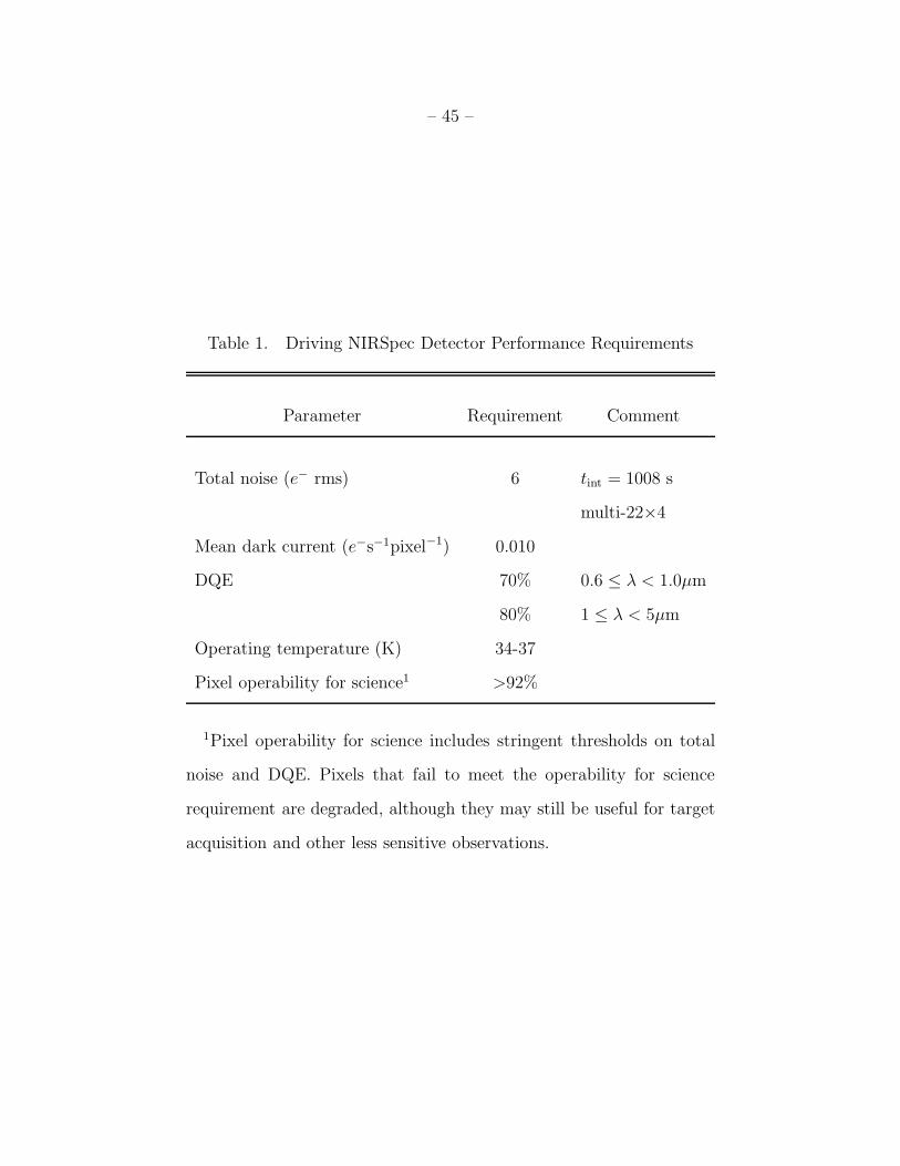
– 45 –

Table 1. Driving NIRSpec Detector Performance Requirements

Parameter Requirement Comment

Total noise (e− rms) 6 tint = 1008 s

multi-22×4

Mean dark current (e−s−1pixel−1) 0.010

DQE 70% 0.6 ≤ λ < 1.0µm

80% 1 ≤ λ < 5µm

Operating temperature (K) 34-37

Pixel operability for science1 >92%

1Pixel operability for science includes stringent thresholds on total

noise and DQE. Pixels that fail to meet the operability for science

requirement are degraded, although they may still be useful for target

acquisition and other less sensitive observations.

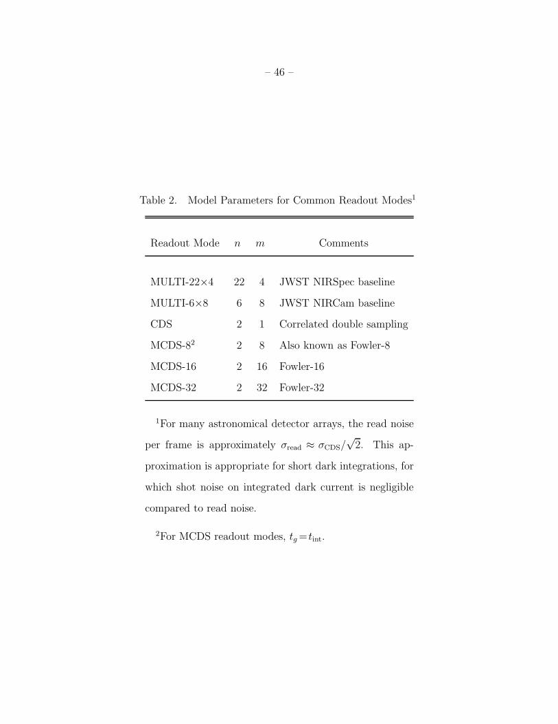
– 46 –

Table 2. Model Parameters for Common Readout Modes1

Readout Mode n m Comments

MULTI-22×4 22 4 JWST NIRSpec baseline

MULTI-6×8 6 8 JWST NIRCam baseline

CDS 2 1 Correlated double sampling

MCDS-82 2 8 Also known as Fowler-8

MCDS-16 2 16 Fowler-16

MCDS-32 2 32 Fowler-32

1For many astronomical detector arrays, the read noise

per frame is approximately σread ≈ σCDS/√

2. This ap-

proximation is appropriate for short dark integrations, for

which shot noise on integrated dark current is negligible

compared to read noise.

2For MCDS readout modes, tg = tint.

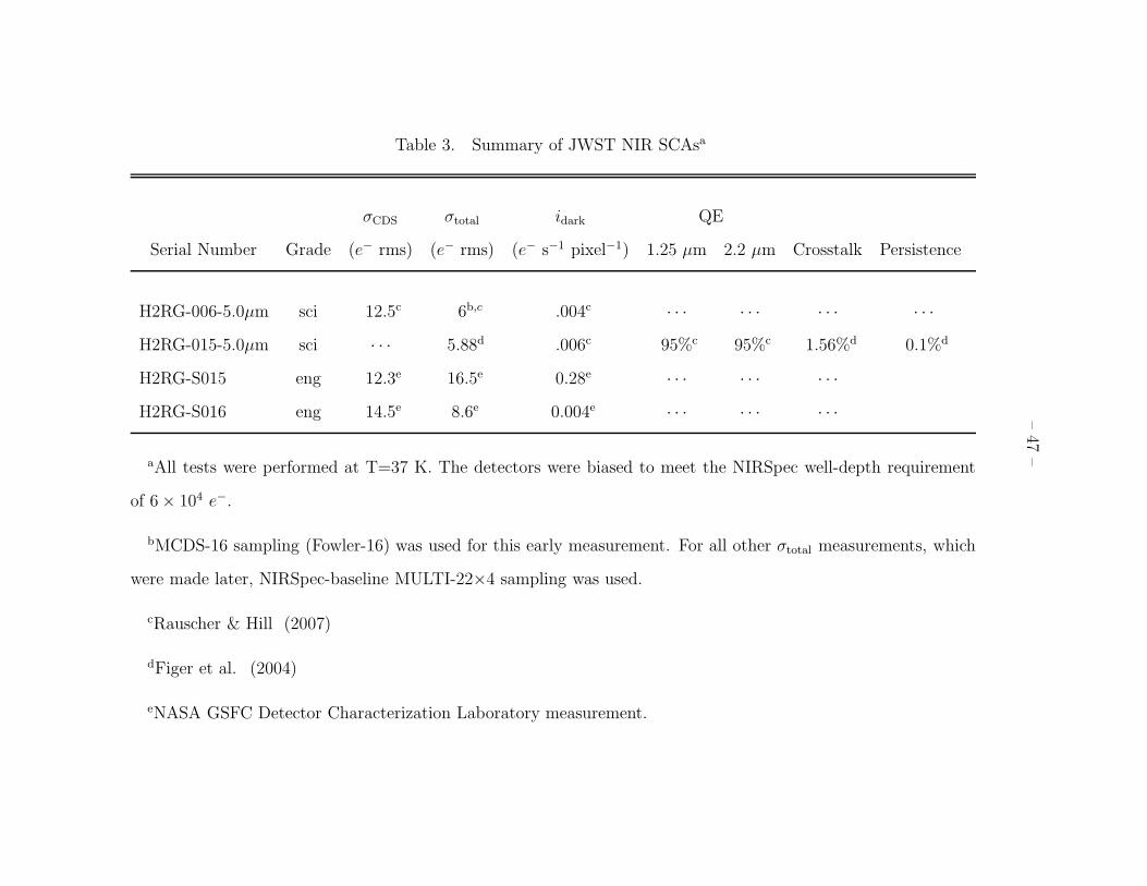
–47

–

Table 3. Summary of JWST NIR SCAsa

σCDS σtotal idark QE

Serial Number Grade (e− rms) (e− rms) (e− s−1 pixel−1) 1.25 µm 2.2 µm Crosstalk Persistence

H2RG-006-5.0µm sci 12.5c 6b,c .004c · · · · · · · · · · · ·

H2RG-015-5.0µm sci · · · 5.88d .006c 95%c 95%c 1.56%d 0.1%d

H2RG-S015 eng 12.3e 16.5e 0.28e · · · · · · · · ·

H2RG-S016 eng 14.5e 8.6e 0.004e · · · · · · · · ·

aAll tests were performed at T=37 K. The detectors were biased to meet the NIRSpec well-depth requirement

of 6 × 104 e−.

bMCDS-16 sampling (Fowler-16) was used for this early measurement. For all other σtotal measurements, which

were made later, NIRSpec-baseline MULTI-22×4 sampling was used.

cRauscher & Hill (2007)

dFiger et al. (2004)

eNASA GSFC Detector Characterization Laboratory measurement.

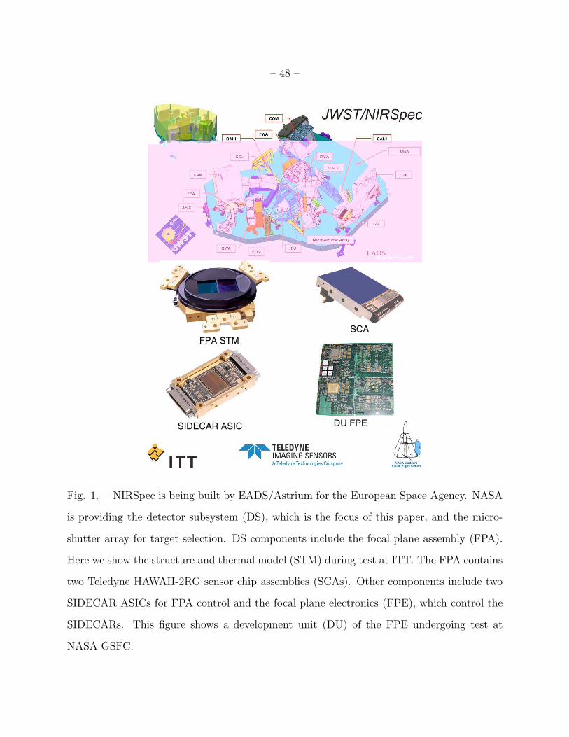
– 48 –

FPA STM

SCA

SIDECAR ASIC DU FPE

Fig. 1.— NIRSpec is being built by EADS/Astrium for the European Space Agency. NASA

is providing the detector subsystem (DS), which is the focus of this paper, and the micro-

shutter array for target selection. DS components include the focal plane assembly (FPA).

Here we show the structure and thermal model (STM) during test at ITT. The FPA contains

two Teledyne HAWAII-2RG sensor chip assemblies (SCAs). Other components include two

SIDECAR ASICs for FPA control and the focal plane electronics (FPE), which control the

SIDECARs. This figure shows a development unit (DU) of the FPE undergoing test at

NASA GSFC.

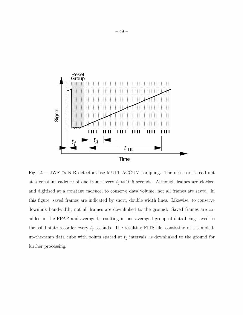
– 49 –

Time

Sig

nal

t ftg

tint

ResetGroup

Fig. 2.— JWST’s NIR detectors use MULTIACCUM sampling. The detector is read out

at a constant cadence of one frame every tf ≈ 10.5 seconds. Although frames are clocked

and digitized at a constant cadence, to conserve data volume, not all frames are saved. In

this figure, saved frames are indicated by short, double width lines. Likewise, to conserve

downlink bandwidth, not all frames are downlinked to the ground. Saved frames are co-

added in the FPAP and averaged, resulting in one averaged group of data being saved to

the solid state recorder every tg seconds. The resulting FITS file, consisting of a sampled-

up-the-ramp data cube with points spaced at tg intervals, is downlinked to the ground for

further processing.

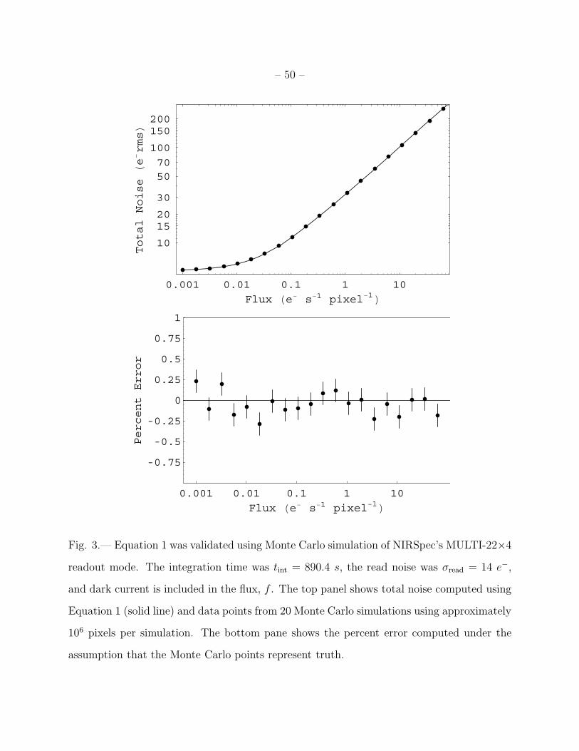
– 50 –

0.001 0.01 0.1 1 10

Flux �e� s�1 pixel�1�

10

1520

30

50

70

100

150200

Total

Noise�e�

rms�

0.001 0.01 0.1 1 10

Flux �e� s�1 pixel�1�

-0.75

-0.5

-0.25

0

0.25

0.5

0.75

1

Percent

Error

Fig. 3.— Equation 1 was validated using Monte Carlo simulation of NIRSpec’s MULTI-22×4

readout mode. The integration time was tint = 890.4 s, the read noise was σread = 14 e−,

and dark current is included in the flux, f . The top panel shows total noise computed using

Equation 1 (solid line) and data points from 20 Monte Carlo simulations using approximately

106 pixels per simulation. The bottom pane shows the percent error computed under the

assumption that the Monte Carlo points represent truth.

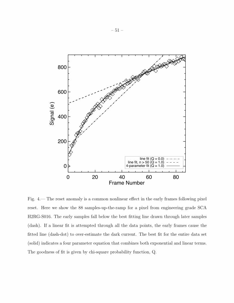
– 51 –

0 20 40 60 80Frame Number

0

200

400

600

800

Sig

nal (e

- )

4-parameter fit (Q = 1.0)line fit, n > 50 (Q = 1.0)

line fit (Q = 0.0)

Fig. 4.— The reset anomaly is a common nonlinear effect in the early frames following pixel

reset. Here we show the 88 samples-up-the-ramp for a pixel from engineering grade SCA

H2RG-S016. The early samples fall below the best fitting line drawn through later samples

(dash). If a linear fit is attempted through all the data points, the early frames cause the

fitted line (dash-dot) to over-estimate the dark current. The best fit for the entire data set

(solid) indicates a four parameter equation that combines both exponential and linear terms.

The goodness of fit is given by chi-square probability function, Q.

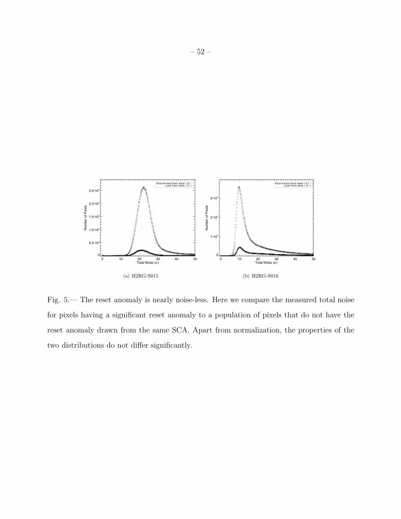
– 52 –

(a) H2RG-S015 (b) H2RG-S016

Fig. 5.— The reset anomaly is nearly noise-less. Here we compare the measured total noise

for pixels having a significant reset anomaly to a population of pixels that do not have the

reset anomaly drawn from the same SCA. Apart from normalization, the properties of the

two distributions do not differ significantly.

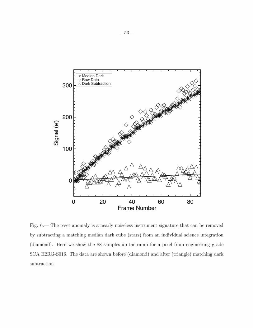
– 53 –

0 20 40 60 80Frame Number

0

100

200

300

Sig

nal (e

- )

Median DarkRaw DataDark Subtraction

Fig. 6.— The reset anomaly is a nearly noiseless instrument signature that can be removed

by subtracting a matching median dark cube (stars) from an individual science integration

(diamond). Here we show the 88 samples-up-the-ramp for a pixel from engineering grade

SCA H2RG-S016. The data are shown before (diamond) and after (triangle) matching dark

subtraction.

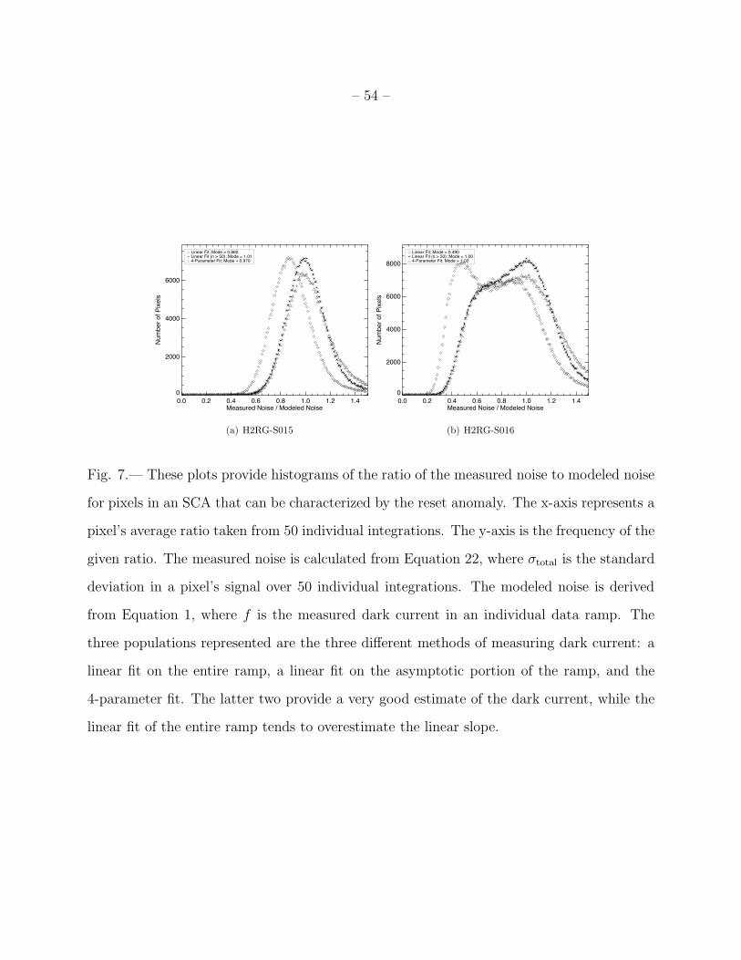
– 54 –

(a) H2RG-S015 (b) H2RG-S016

Fig. 7.— These plots provide histograms of the ratio of the measured noise to modeled noise

for pixels in an SCA that can be characterized by the reset anomaly. The x-axis represents a

pixel’s average ratio taken from 50 individual integrations. The y-axis is the frequency of the

given ratio. The measured noise is calculated from Equation 22, where σtotal is the standard

deviation in a pixel’s signal over 50 individual integrations. The modeled noise is derived

from Equation 1, where f is the measured dark current in an individual data ramp. The

three populations represented are the three different methods of measuring dark current: a

linear fit on the entire ramp, a linear fit on the asymptotic portion of the ramp, and the

4-parameter fit. The latter two provide a very good estimate of the dark current, while the

linear fit of the entire ramp tends to overestimate the linear slope.

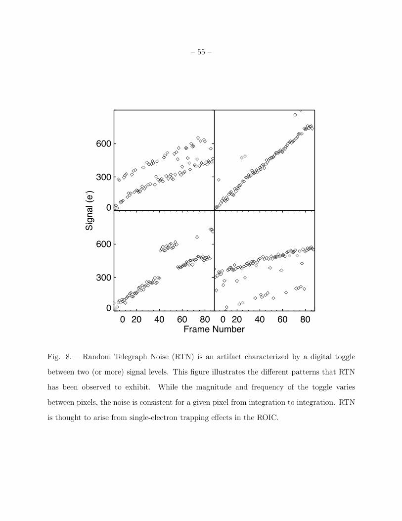
– 55 –

Frame Number

Sig

nal (e

- )

0

300

600

0 20 40 60 80

0

300

600

0 20 40 60 80

Fig. 8.— Random Telegraph Noise (RTN) is an artifact characterized by a digital toggle

between two (or more) signal levels. This figure illustrates the different patterns that RTN

has been observed to exhibit. While the magnitude and frequency of the toggle varies

between pixels, the noise is consistent for a given pixel from integration to integration. RTN

is thought to arise from single-electron trapping effects in the ROIC.

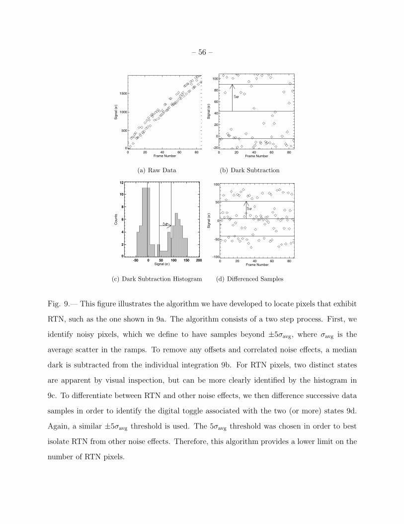
– 56 –

(a) Raw Data (b) Dark Subtraction

(c) Dark Subtraction Histogram (d) Differenced Samples

Fig. 9.— This figure illustrates the algorithm we have developed to locate pixels that exhibit

RTN, such as the one shown in 9a. The algorithm consists of a two step process. First, we

identify noisy pixels, which we define to have samples beyond ±5σavg, where σavg is the

average scatter in the ramps. To remove any offsets and correlated noise effects, a median

dark is subtracted from the individual integration 9b. For RTN pixels, two distinct states

are apparent by visual inspection, but can be more clearly identified by the histogram in

9c. To differentiate between RTN and other noise effects, we then difference successive data

samples in order to identify the digital toggle associated with the two (or more) states 9d.

Again, a similar ±5σavg threshold is used. The 5σavg threshold was chosen in order to best

isolate RTN from other noise effects. Therefore, this algorithm provides a lower limit on the

number of RTN pixels.

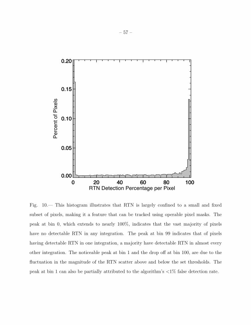
– 57 –

0 20 40 60 80 100

0.00

0.05

0.10

0.15

0.20

0 20 40 60 80 100

0.00

0.05

0.10

0.15

0.20

0 20 40 60 80 100RTN Detection Percentage per Pixel

0.00

0.05

0.10

0.15

0.20P

erc

ent

of

Pix

els

Fig. 10.— This histogram illustrates that RTN is largely confined to a small and fixed

subset of pixels, making it a feature that can be tracked using operable pixel masks. The

peak at bin 0, which extends to nearly 100%, indicates that the vast majority of pixels

have no detectable RTN in any integration. The peak at bin 99 indicates that of pixels

having detectable RTN in one integration, a majority have detectable RTN in almost every

other integration. The noticeable peak at bin 1 and the drop off at bin 100, are due to the

fluctuation in the magnitude of the RTN scatter above and below the set thresholds. The

peak at bin 1 can also be partially attributed to the algorithm’s <1% false detection rate.