2007-01-1113

Detection of Gasoline Vehicles with Gross PM Emissions

Wei Li, John F. Collins and Thomas D. Durbin Bourns College of Engineering, Center for Environmental Research and Technology (CE-CERT), University of California,

Riverside, CA 92521

Tao Huai and Alberto Ayala California Air Resources Board, Sacramento, CA 95814

Gary Full Environmental Systems Products, Tucson, AZ 85745

Claudio Mazzoleni, Nicholas J. Nussbaum, Daniel Obrist, Dongzi Zhu, Hampden D. Kuhns, and Hans Moosmϋller

Desert Research Institute, Nevada System of Higher Education, Reno, NV 89512

Copyright © 2007 SAE International

ABSTRACT

Light duty gasoline vehicles (LDGV) are estimated to contribute 40% of the total on-road mobile source tailpipe emissions of particulate matter (PM) in California. While considerable efforts have been made to reduce toxic diesel PM emissions going into the future, less emphasis has been placed on PM from LDGVs. The goals of this work were to characterize a small fleet of visibly smoking and high PM emitting LDGVs, to explore the potential PM-reduction benefits of Smog Check and of repairs, and to examine remote sensing devices (RSD) as a potential method for identifying high PM emitters in the in-use fleet.

For this study, we recruited a fleet of eight vehicles covering a spectrum of PM emission levels. PM and criteria pollutant emissions were quantified on a dynamometer and CVS dilution tunnel system over the Unified Cycle using standard methods and real time PM instruments. The vehicles were then tested using RSD equipment over a test track, tested with a standard Smog Check, and tested with a screening device during the Smog Check. The PM emission rates of the visibly smoking vehicles range from 60 to 1718 mg/mi over the UC cycle. The light or invisible smokers had PM emissions ranging from 7 to 25 mg/mi. The smoking vehicles showed particle number rates on the order of 1013~1014 particles/mi, which are 10~1000 times higher than typical FTP particle number emission rates for modern low emitting gasoline vehicles. Vehicles that had higher emission rates over the UC tests generally showed higher emissions as measured by RSD systems for the gaseous species. The relationship or scale factor between RSD PM emissions and filter mass emissions is different for each RSD method and wavelength, and

also appears to be different for black smoke than blue smoke. The effects of repairs have not yet been assessed.

INTRODUCTION

The contribution of LDGVs is an important fraction of the on-road mobile source inventory for particulate matter (PM). The 2005 California emission inventory estimates that LDGVs contribute 40% of the total on-road mobile source tailpipe emissions of PM [1]. The Department of Energy (DOE)'s Gasoline/Diesel PM Split Study in the South Coast Air Basin concluded that “Gasoline PM emissions are more important than diesel PM to ambient PM concentrations at certain times and locations. High-emitting gasoline vehicles are very important contributors to ambient PM [2].” Since the new regulations require a 90% reduction of PM emissions from heavy duty diesel engines effective 2007, understanding, characterizing and reducing PM emissions from LDGVs will become increasingly important.

Average PM emission rates from new LDGVs have dropped with the implementation of LEV and LEV II regulations. Under the California LEV II regulations, effective as of 2004, both gasoline and diesel light duty vehicles must meet a PM emission standard of 0.01 g/mile. As of 2007, heavy duty diesel vehicles must meet a standard of 0.01 g/bhp-hr, which is equivalent to roughly 0.03 g/mile. Even if all light duty vehicles emitted at the level of the LEV II standard, they could still become dominant producers of on-road PM emissions due to the enormous disparity in activity levels for light duty vehicles compared with heavy diesel vehicles.

In practice, most LDGVs do not emit as much as the LEV II standard. In fact, emission inventories start with a PM base rate of less than half the LEV II standard for LEV I and newer vehicles. However, older gasoline vehicles were not required to meet a PM standard and may emit substantially more than the new LEV II standard. Also, very worn or malfunctioning vehicles can emit ten to one hundred or more times as much as a new vehicle. Data on the frequency of such high PM emitting vehicles and on the PM emissions rate distribution for such vehicles are limited. A previous study showed that 1.11~1.75% of the vehicles in the light-duty fleet in the South Coast Air Quality Management District (SCAQMD) emit visible smoke [3].

PM emissions of smoking LDGVs have been investigated in several studies in the 1990’s [3-8] as well as the latest DOE Gasoline/Diesel PM Split Study [9]. The average PM emission rates from these studies were found to be in the range of 100-1500 mg/mi with the maximum higher than 2000 mg/mi. In contrast, several studies have shown that the PM emissions of normal emitting LDGVs are less than 5 mg/mi [4, 10-13] with those of the latest technology at around 1 mg/mi or less [14].

The identification of high PM emitters in the in-use fleet is an important aspect of any attempt to mitigate LDGV PM. Studies that have examined high PM emitters have found little or poor correlation between high PM emission rates and surrogates such as high HC, high CO, visible smoke, vehicle age, or vehicle mileage [15,16]. Thus, it is necessary to develop methods that can identify high PM emitters directly. Remote Sensing Devices (RSD) offer potential to screen very large numbers of vehicles to identify high PM emitters. Portable Emission Measurement Systems (PEMS) offer potential to quantify emissions during on-road driving. Remote sensing measurements of PM have been conducted in several studies [16-21]. RSD has been applied primarily to diesel exhaust, which generally has much higher PM emissions than gasoline exhaust on a per vehicle basis. An earlier Coordinating Research Council (CRC) study (Project No. E-56) concluded that more work was needed for the development of remote sensing measurements of PM, even for diesel exhaust [21].

The objectives of this program are threefold: to evaluate our ability to conveniently identify high gasoline PM emitters; to provide data on emission levels, Smog Check identification, repair effectiveness, and repair costs for high PM emitters; and to assess the extent of

high PM emitters in the on-road fleet. This information is needed to guide the development of effective PM control strategies. In the pilot study reported here, a total of eight vehicles of varying smoke level were tested. The test sequence for each vehicle included Smog Checks, cold-start Unified Cycles (UC), and RSD testing over a test track in CE-CERT’s parking lot. The RSD equipment for PM included infrared (IR) and ultraviolet (UV) transmissometer systems operated by Environmental Solutions Products (ESP), and a UV Lidar plus transmissometer system operated by Desert Research Institute (DRI). The Smog Checks were supplemented with the addition of a PM measurement using a tailpipe screening device (TSD) described later. Additional on-road RSD measurements were collected on a freeway on-ramp and post repair testing of the smoking vehicles is planned. These results will be presented in a subsequent publication.

EXPERIMENTAL PROCEDURES

DESCRIPTION OF VEHICLE FLEET

Vehicles were recruited through newspaper advertisement and through the campus mail system at the University of California (UC) at Riverside. The fleet included vehicles with PM emission levels estimated to range from normal emitter to heavy smoker. PM emission levels were estimated visually at idle, engine revving, and acceleration, and with a screening device at idle and engine revving. Prior to entering the program, all vehicles were inspected using a standard checklist to ensure that they were in safe mechanical and operational condition. All vehicles were tested with the in-tank gasoline (California Phase 3 Reformulated Gasoline) to represent real-world in-use conditions.

The vehicles used in this project are listed in Table 1 along with target smoke levels and target PM ranges. The fleet was chosen to include vehicles with different levels of PM emissions (light, moderate, heavy) and with different types of PM characteristics (blue, black, gray smoke). Vehicles classified as light or “invisible” smokers did not have visible smoke, but did have a noticeable PM signature as measured by the screening device. The color of “invisible” smokers was determined by observing a very small puff of smoke visible only on engine start. This distribution was chosen in order to evaluate the RSD PM measurement equipment over a full range of emissions. The fleet was not designed to be representative of the on road vehicle fleet, other than to include as broad a range as possible.

Table 1. Descriptions of Test Vehicles

# MY OEM Model Type Disp.(L) Mileage Target Smoke Type Target PM (mg/mi)

1 1997 Ford Escort PC 2.0 25,598 Normal emitter (no smoke) < 5 2 1985 Toyota Camry PC 2.0 268,423 Light Black (invisible) 25 to 75 3 1991 GMC Sonoma LDT 4.3 171,487 Light Blue (invisible) 25 to 75 4 1981 Toyota Pickup LDT 2.4 119, 728 Moderate Blue 50 to 500 5 1995 Dodge Dakota LDT 2.5 123,974 Moderate Black 50 to 500 6 1963 Studebaker Avanti PC 4.6 high Heavy Blue 50 to 500 7 1998 Toyota Camry PC 3.0 82,704 Heavy Black 50 to 500 8 1986 Mitsubishi Max LDT 2.0 163,913 Gray 50 to 500

PC = Passenger Car; LDT = Light-Duty Truck. EMISSION MEASUREMENTS

Unified Cycle Testing

All eight vehicles were tested over the UC cycle to obtain mass emission rates for total PM, total hydrocarbons (THC), nonmethane hydrocarbons (NMHC), carbon monoxide (CO), and nitrogen oxides (NOx). The UC cycle is a more aggressive cycle and more adequately covers typical driving patterns than the Federal Test Procedure (FTP). The UC cycle is a 3 phase cycle like the FTP, with cold start, hot running, and hot start bags. The cycle is 11 miles long, with a top speed of 67 miles per hour. The first two bags are known as the LA92 and have an average speed of 24.8 miles per hour, 16.4% idle, and 1.52 stops per mile. Bag 3 is a repeat of the driving pattern for bag 1 [22]. The vehicles were tested two per day over eight days in the following order: 2 8, 8 2, 3 7, 7 3, 5 1, 1 5, 4 6, 6 4.

All the tests were conducted in CE-CERT’s Vehicle Emission Research Laboratory (VERL) equipped with a Burke E. Porter 48-inch single-roll electric dynamometer and Pierburg constant volume sampling (CVS)/dilution tunnel system. A CVS flow rate of 350 standard cubic feet per minute (SCFM) was used with VERL’s 10-inch diameter dilution tunnel. The tunnel was fitted with three sampling probes located approximately 10 tunnel diameter downstream of the exhaust mixing flange. The sampling configuration, filter media, and analyses are summarized below.

Probe 1 was fitted with a three-way splitter and each channel was fitted with 47 mm, 2.0 µm pore size polytetrafluoroethylene (PTFE) membrane filters to obtain total PM mass emission rates for each phase of the UC. Each filter assembly was fitted with a primary and a backup filter, collected without secondary dilution. The PTFE filters were weighed before and after sampling to determine the collected mass using an ATI CAHN C-35 microbalance. The microbalance is located in an environmental weighing chamber maintained at a relative humidity of 45±3% and a temperature of 22±1°C. The microbalance was used without counter weight on the 200 mg full scale, which has a resolution of 1.0 µg.

Probe 2 was fitted with a TSI DustTrakTM 8520 aerosol monitor for real-time particulate mass measurements

and a TSI 3022A condensation particle counter (CPC) to obtain real-time particle number. The DustTrakTM is a light scattering instrument designed for measurement of aerosol mass in ambient air. The calibration factor supplied by the manufacturer is determined using a National Institute of Standards and Technology (NIST) standard Arizona Road Dust. Different aerosol types are expected to have different calibration factors. Prior studies at CE-CERT [23] have shown good correlation of DustTrakTM mass with standard filter mass for diesel particulates. The TSI 3022A CPC is a continuous-flow, single-particle counter that works reliably in concentrations up to 107 particles/cm3 [24]. The detectable particle size range of this CPC is 7 nm (50% detectable) to > 3 µm. During this study, the particle number was initially observed to be over the range of the CPC, therefore a dilutor was placed in front of the CPC to provide secondary dilution for CPC measurements starting with the 7th test. The dilution ratio used for the CPC during the subsequent tests was approximately 12.6:1. The DustTrak continued to sample without secondary dilution.

Probe 3 was fitted with a four way splitter. Three of the channels were fitted with 47 mm quartz fiber filters for each phase of the UC cycle, respectively. The fourth channel was fitted with a quartz filter plus PUF/XAD/PUF (PXP) cartridge to collect a cumulative sample over the entire UC cycle. Probe 2 also supplied flow for one cumulative DNPH (2,4-dinitrophenylhydrazine) cartridge sample to collect carbonyls and one cumulative Carbotrap 300 Multi-Bed Thermal Desorption (TD) tube sample to collected C4-C12 gases. All of the samples collected from probe three were collected without secondary dilution. Analysis of the chemical speciation samples was beyond the scope of the current study. The speciation samples including the collected DNPH cartridges, TD tubes, quartz filters, and PXP cartridges will be stored for possible analysis in future efforts.

The flow rates for both the PTFE and quartz filter samples were set to 30 liter per minute (LPM) for most tests. During the first test of vehicle #6 (1963 Avanti), the PTFE filters collected from phase 2 were found to be clogged. The flow rate of PTFE filter sampling for the second test of this vehicle was reduced to 15 LPM.

Idle/High Speed Idle and ASM (Smog Check) Testing

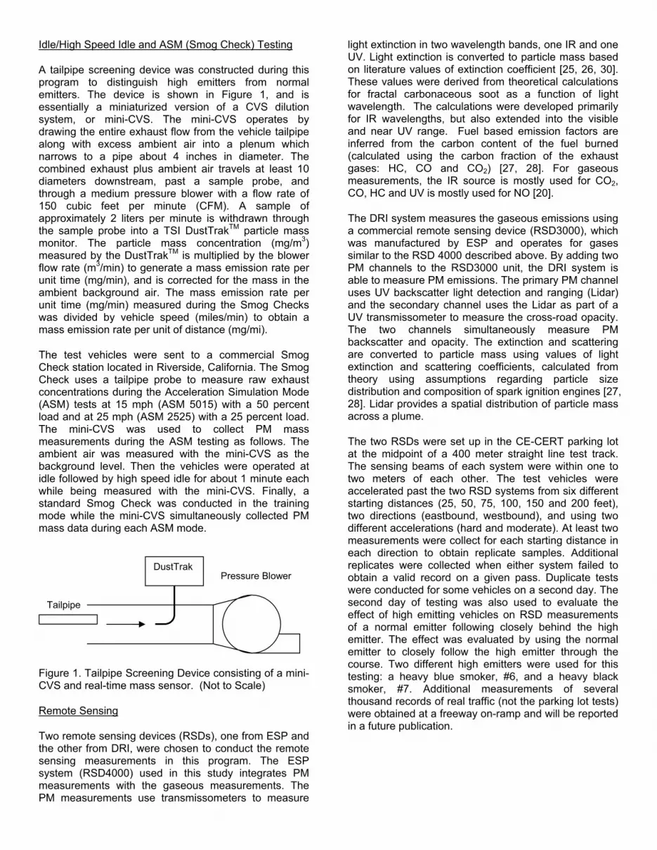
A tailpipe screening device was constructed during this program to distinguish high emitters from normal emitters. The device is shown in Figure 1, and is essentially a miniaturized version of a CVS dilution system, or mini-CVS. The mini-CVS operates by drawing the entire exhaust flow from the vehicle tailpipe along with excess ambient air into a plenum which narrows to a pipe about 4 inches in diameter. The combined exhaust plus ambient air travels at least 10 diameters downstream, past a sample probe, and through a medium pressure blower with a flow rate of 150 cubic feet per minute (CFM). A sample of approximately 2 liters per minute is withdrawn through the sample probe into a TSI DustTrakTM particle mass monitor. The particle mass concentration (mg/m3) measured by the DustTrakTM is multiplied by the blower flow rate (m3/min) to generate a mass emission rate per unit time (mg/min), and is corrected for the mass in the ambient background air. The mass emission rate per unit time (mg/min) measured during the Smog Checks was divided by vehicle speed (miles/min) to obtain a mass emission rate per unit of distance (mg/mi).

The test vehicles were sent to a commercial Smog Check station located in Riverside, California. The Smog Check uses a tailpipe probe to measure raw exhaust concentrations during the Acceleration Simulation Mode (ASM) tests at 15 mph (ASM 5015) with a 50 percent load and at 25 mph (ASM 2525) with a 25 percent load. The mini-CVS was used to collect PM mass measurements during the ASM testing as follows. The ambient air was measured with the mini-CVS as the background level. Then the vehicles were operated at idle followed by high speed idle for about 1 minute each while being measured with the mini-CVS. Finally, a standard Smog Check was conducted in the training mode while the mini-CVS simultaneously collected PM mass data during each ASM mode.

Figure 1. Tailpipe Screening Device consisting of a mini-CVS and real-time mass sensor. (Not to Scale)

Remote Sensing

Two remote sensing devices (RSDs), one from ESP and the other from DRI, were chosen to conduct the remote sensing measurements in this program. The ESP system (RSD4000) used in this study integrates PM measurements with the gaseous measurements. The PM measurements use transmissometers to measure

light extinction in two wavelength bands, one IR and one UV. Light extinction is converted to particle mass based on literature values of extinction coefficient [25, 26, 30]. These values were derived from theoretical calculations for fractal carbonaceous soot as a function of light wavelength. The calculations were developed primarily for IR wavelengths, but also extended into the visible and near UV range. Fuel based emission factors are inferred from the carbon content of the fuel burned (calculated using the carbon fraction of the exhaust gases: HC, CO and CO2) [27, 28]. For gaseous measurements, the IR source is mostly used for CO2, CO, HC and UV is mostly used for NO [20].

The DRI system measures the gaseous emissions using a commercial remote sensing device (RSD3000), which was manufactured by ESP and operates for gases similar to the RSD 4000 described above. By adding two PM channels to the RSD3000 unit, the DRI system is able to measure PM emissions. The primary PM channel uses UV backscatter light detection and ranging (Lidar) and the secondary channel uses the Lidar as part of a UV transmissometer to measure the cross-road opacity. The two channels simultaneously measure PM backscatter and opacity. The extinction and scattering are converted to particle mass using values of light extinction and scattering coefficients, calculated from theory using assumptions regarding particle size distribution and composition of spark ignition engines [27, 28]. Lidar provides a spatial distribution of particle mass across a plume.

The two RSDs were set up in the CE-CERT parking lot at the midpoint of a 400 meter straight line test track. The sensing beams of each system were within one to two meters of each other. The test vehicles were accelerated past the two RSD systems from six different starting distances (25, 50, 75, 100, 150 and 200 feet), two directions (eastbound, westbound), and using two different accelerations (hard and moderate). At least two measurements were collect for each starting distance in each direction to obtain replicate samples. Additional replicates were collected when either system failed to obtain a valid record on a given pass. Duplicate tests were conducted for some vehicles on a second day. The second day of testing was also used to evaluate the effect of high emitting vehicles on RSD measurements of a normal emitter following closely behind the high emitter. The effect was evaluated by using the normal emitter to closely follow the high emitter through the course. Two different high emitters were used for this testing: a heavy blue smoker, #6, and a heavy black smoker, #7. Additional measurements of several thousand records of real traffic (not the parking lot tests) were obtained at a freeway on-ramp and will be reported in a future publication.

DustTrak

Tailpipe

Pressure Blower

RESULTS AND DISCUSSIONS

UNIFIED CYCLE TESTS

Gaseous Emissions

Each vehicle was tested twice over the UC cycle. A weighted emission rate was calculated using the same weighting factor scheme as used for calculation of weighted FTP emissions. The UC cycle is more aggressive than the FTP and can generate higher emissions. The correction factors for converting FTP emissions to UC emissions used by EMFAC (EMission FACtor) generally range between 0.9 and 1.4, although the cycle differences will vary from vehicle to vehicle [10, 13, 29]. (EMFAC is the mobile source emission factor model used by the California Air Resources Board.) The gas phase emissions for the test vehicles are plotted in Figure 2. Note that these data are presented on a log scale. The error bars in the figure represent the high and low values of the two tests for each vehicle. Only a single test is available for vehicle #4 since the dynamometer lost communication during phase 2 of the second test for this vehicle.

The results show all the visible smokers (#4 through #8) had relatively high HC and CO emissions. Some of the higher HC and CO measurements exceeded the range of the gas analyzers, and therefore actually represent minimum possible values of HC and CO emissions. HC emissions for the visible smokers range from 2.5 to 23.5 g/mi. CO emissions for these vehicles range from 39 to 138 g/mi. For comparison, the Tier 0 and 1 standards for various passenger car and light-duty truck categories are all 0.8 g/mi or less for THC/NMHC and 9 g/mi or less for CO over the FTP. Vehicles #2 and #3 have emissions comparable to those of their certification standard over the FTP. Vehicle #5 and #7 have relatively low NOx. This could indicate that these vehicles were operating under a rich-burn condition.

0.0

0.1

1.0

10.0

100.0

1000.0

# 1 # 2 # 3 # 4 # 5 # 6 # 7 # 8

Vehicle

Emis

sion

Rat

e (g

/mi)

NMHC CO NOx

Figure 2. Gaseous Mass Emission Rates over UC

PM Emissions

The PM mass emission rates over the UC cycle for the test vehicles are presented in Figure 3. Again, only one test is reported in the figure for vehicle #4. The error bars in the figure represent the high and low values of the two tests for each vehicle. The PM emission rates of the visible smoking vehicles (#4 through #8) range from 60 to 1718 mg/mi and are in range of earlier studies [3-9]. Vehicles #1 and #3 have emission rates below the current standard (10 mg/mi, based on FTP75) and can be treated as “normal PM emitters”. The older invisible smoker (#2) has a PM emission of 25 mg/mi, which is comparable to FTP PM emission rates found in previous studies for vehicles of this vintage [4].

In Figure 3, PM emission rates from both the filter and the DustTrakTM measurements are presented. The DustTrakTM gave second-by-second PM mass concentration (mg/m3). The second-by-second concentration was multiplied by the CVS flow rate (m3/sec) then integrated over each phase of the test to generate a mass emission rate (mg/phase). The weighted emission rate over the entire cycle was calculated using the same weighting factors as FTP.

0

1

10

100

1000

10000

# 1 # 2 # 3 # 4 # 5 # 6 # 7 # 8Vehicle

Emis

sion

Rat

e (m

g/m

i)

DustTrak CFR Filter

2004+ LEV II PM Std.

Figure 3. PM Mass Emission Rates over UC

The DustTrakTM is a simple optical measurement that can be correlated with mass given a particular particle composition and size distribution. During this study, the filter based results were in general higher than the DustTrakTM results except for vehicle #6. During the tests of vehicle #6, a lot of engine oil was found on the collected filters as the filters were observed to be yellow and wet, with a strong smell. The oil that went through the sampling system clogged the filters, causing sample flow to be much lower than the desired value; thus the PM measurements underestimated the actual value and were lower than the DustTrakTM data. For vehicle #4, the sample flow was not affected by the engine oil problem, however the filters were oily, the PM was extremely high, and the relationship between DustTrakTM data and filter data was erratic.

When vehicles #4 and #6 are excluded from the analysis, the remaining vehicles show good correlation of

DustTrakTM mass with filter mass, as shown in Figure 4. Each data point in the figure represents emissions from one phase of the UC cycle. The Dustrak registers about 75% of the mass collected on the filters. However, the DustTrakTM was not designed or calibrated for vehicle exhaust particulate. The particular slope shown in Figure 4, relating mass of vehicle exhaust to corresponding mass of Arizona Road Dust, is for our high emitting LDG vehicles driven over the UC test cycle. It should not be generalized to other vehicles types or other test cycles without further research. In fact, CE-CERT’s experience with diesel particulate suggests that the slope may actually vary from individual DustTrakTM to DustTrakTM.

y = 0.7553xR2 = 0.9653

0

50

100

150

200

250

300

350

400

450

500

0 100 200 300 400 500 600 700CFR Filter (mg/mi)

Dust

Trak

(mg/

mi)

Figure 4. Correlation of DustTrakTM Data with Filter Data

0

1

10

100

1000

10000

# 1 #2 # 3 # 4 # 5 # 6 # 7

Vehicle

Em

issi

on R

ate

Particle Number Emission Rate (1.0E+11 #/mi) Particulate Mass Emission Rate (mg/mi)

Figure 5. Comparison of Particle Number Emission Rates and Mass Emission Rates for the Test Vehicles (Vehicle #8 was not included because it was measured without the dilutor and the undiluted concentrations exceeded the upper working range of the analyzer.)

Particle Number Emissions

Particle numbers were measured by the CPC for each test vehicle over the UC cycle, as shown in Figure 5. Figure 5 includes only tests where the secondary dilution system was used. A few readings for vehicle #6 were still over the CPC range even measured with the secondary dilution. The smoking vehicles tested here had particle number rates on the order of 1013~1014 particles/mi, which is 10~1000 times higher than the FTP

particle number emission rates of modern low emitting gasoline vehicles [14]. The vehicle rank for particle number emissions (#6 > #4 > #5 > #7 > #3 > #2 > #1) is basically similar to that sorted by particulate mass emission rates (#6 > #4 > #5 > #7 > #2 > #3 > #1).

Second-by-second mass emission rates and particle number emission were collected during each test. Emission rate is calculated by multiplying measured concentrations by tunnel flow rate. High mass and particle number emissions were usually generated under hard acceleration events. Figures 6 and 7 show an example of real-time particle number and emission measurements for a black smoker. The large peaks in both figures nearly coincide with each other and with hard accelerations. This emission behavior, except for absolute magnitude, is in general very similar to the emission behavior of normal low emitting gasoline vehicles [14].

0.E+00

5.E+12

1.E+13

2.E+13

2.E+13

3.E+13

0 300 600 900 1200 1500 1800 2100 2400

Time (sec)

Parti

cle

Num

ber (

#/se

c)

0

10

20

30

40

50

60

70

80

Spee

d (m

ph)

Particle Number Emission Rate Vehicle Speed

Figure 6. Real-time Particle Number Emission Rate vs. Vehicle Speed, Vehicle #5, Black Smoker

0

5

10

15

20

25

30

35

0 300 600 900 1200 1500 1800 2100 2400Time (sec)

PM (m

g/se

c)

0

10

20

30

40

50

60

70

80

Spee

d (m

ph)

Particulate Mass Emission Rate Vehicle Speed

Figure 7. Real-time Particulate Mass Emission Rate vs. Vehicle , Vehicle #5, Black Smoker

IDLE/HIGH SPEED IDLE AND ASM TESTS

Gaseous Emissions from Smog Checks

Each vehicle was tested twice at the same commercial Smog Check station located in Riverside, California (except for vehicle #5, which became impossible to start

before testing could be completed). The Smog Check results are summarized in Table 2. Before it failed to start, vehicle #5 had HC emissions that were over the range of the Smog Check gas analyzer. Three heavy smokers (#s 5, 6 and 7) were identified as gross polluters. However, one heavy smoker (vehicle #8) passed one of the two smog checks. The very light smoker (vehicle #3) passed one of its two smog checks, while the light smoker (vehicle #2) passed both of its smog checks. In comparing UC results with those from the Smog Check, it should be noted that the Smog check represents a warmed-up steady state acceleration simulation mode as opposed to the transient and cold start UC. The UC is also more aggressive than the FTP, which is used to define high emitters in comparison with certification standards.

Table 2. Smog Check Results of the Test Vehicles

First Smog Check Second Smog Check Vehicle

Pass Failed Emissions Pass Failed

Emissions 1 √ √ 2 √ √ 3 √ × HC 4 × HC, NO × NO 5 ×,GP HC, ? ×,GP HC, ? 6 ×,GP HC, CO ×,GP HC, CO 7 ×,GP HC, CO ×,GP HC, CO 8 √ × HC, CO

√：Pass; ×: Fail; GP: Gross Polluter: ?: A valid Smog Check could not be completed for vehicle #5 because the HC emission exceeded the range of the smog station gas analyzer, thus other pollutants remained unmeasured.

Particulate Measurements from the TSD

The tailpipe screening device (TSD), consisting of a mini-CVS and DustTrakTM monitor, was used to monitor PM emissions for idle, high speed idle, and ASM tests. The background ambient air was also measured and subtracted. A comparison of TSD PM emission rates

over ASM 5015/2525 and UC filter mass is presented in Figure 8. The left hand part of the figure shows that the “high PM emitters”, defined as greater than 10 mg/mi over the UC, also showed TSD PM emission rates higher than 10 mg/mi over each of the ASM test phases. The test for vehicle #5 was prematurely aborted, but part of the test was still measured and reported here. Vehicle #2 was idled for a relatively long time (> 30 minutes) before the Smog Check and generated a lot of visible white smoke, which was not typical for this vehicle during normal hot running operation. This might have caused the anomalously high TSD PM emissions measured during the ASM tests compared with the UC filter tests. The right hand part of the figure shows that the ASM TSD data set can not be used to quantitatively predict UC mass emissions.

Another way to view this data is shown in Figure 9 for idle data and in Figure 10 for ASM data, both on a log scale. Using 10 mg/mi as the cut point to distinguish the high emitters and normal emitters the cut point divides the plotting area into 4 regions. Region 1 contains normal emitters identified by both methods; Region 2 contains normal emitters identified by the Unified Cycle reference method, but misidentified as higher emitters by the TSD; Region 3 contains high emitters identified by both methods; Region 4 contains UC high emitters not identified by the TSD. In this study, all the vehicles would be identified in either region 1 (normal emitters) or region 3 (high emitters) if a 10 mg/mi cut point was used. However, if the cut point was moved up to just above 25 mg/mi, vehicle #2 would fall into the error of commission category. Overall, a larger and more representative data set and greater range of cut points would be needed to be examined to better define the effectiveness of this method for an I/M program. The fleet is small, but our results illustrate that adding a PM measurement to the Smog Check program could identify some high PM emitting vehicles that would otherwise pass through the program

0

1

10

100

1000

10000

# 1 # 2 # 3 # 4 # 5 # 6 # 7 # 8

Vehicle

Emis

sion

Rat

e (m

g/m

i)

CFR Filter ASM5015 ASM2525

0

500

1000

1500

2000

2500

3000

0 500 1000 1500 2000 2500 3000

UC Emission Rate (mg/mi)

AS

M E

mis

sion

Rat

e (m

g/m

i)

ASM5015 ASM2525

Figure 8. Comparison of PM Emission Rates over ASM 5015/2525 and UC Tests

REMOTE SENSING TESTS

Approximately 500 data records were collected with each RSD system during the course of test track measurements. The following sections discuss overall averages of all valid records collected on the test track for each vehicle. The number of valid runs in each speed and acceleration range from each RSD group do not overlap exactly because invalid results from each group occur on different runs.

Gaseous Emissions

The gaseous emissions measured with the two RSD systems along with the UC cycle tests are shown in Figures 11 through 13. The left hand side of each figure shows side by side comparison of RSD data with Unified Cycle data. The right hand side of each figure shows a scatter-plot of RSD data versus UC data. The data presented in the figures are the average over two days’ measurements where available and averaged over all starting distances. Only one remote sensing measurement was conducted on each day for vehicle #5

0.000

0.001

0.010

0.100

1.000

10.000

100.000

1000.000

0 1 10 100 1000 10000

UC Emission Rate (mg/mi)

Idle

/Hig

h Id

le E

mis

sion

Rat

e (m

g/m

in

Idle High Speed Idle

Region 3: High Emitters

Region 1: Normal Emitters

Region 2: Errors of Commission

Region 4: Errors of Omission

Figure 9. High PM Emitters Identification Efficiency of TSD over Idle/High Speed Idle Tests

0

1

10

100

1000

10000

0 1 10 100 1000 10000

UC Emission Rate (mg/mi)

ASM

Em

issi

on R

ate

(mg/

mi)

ASM5015 ASM2525

Region 3: High Emitters

Region 1: Normal Emitters

Region 2: Errors of Commission

Region 4: Errors of Omission

Figure 10. High PM Emitters Identification Efficiency of TSD over ASM Tests

before it stopped operating and no valid data from the DRI RSD are available for this vehicle.

There is good agreement between DRI and ESP RSD measurements of CO. The CO emissions from the normal and light emitters (vehicles #1, 2, and 3) are much higher when measured with RSD than with the UC reference measurements. This might be due to the fact that even the relatively clean vehicles undergo command enrichment while accelerating past the RSD sensor, but might not experience much command enrichment over the course of the UC cycle. On the test track, the driver was asked to accelerate "hard" but short of flooring the gas pedal. Accelerations from short distances ranged from about 5 to 7.5 mph/sec.

NOx emissions measured with the DRI RSD system are fairly well correlated with the UC reference NOx measurements. NOx emissions measured with the ESP RSD system are systematically higher than NOx measured with the DRI system. The reason for this has not been determined.

HC emissions measured using RSD tend to be substantially lower than emissions measured over the UC, especially for the very high HC emitters. The ESP RSD and DRI RSD measurements are more similar to each other than to the laboratory UC cycle measurements. One cause for this difference might be the difference in driving cycles. The UC cycle includes segments of cold start, idle, and deceleration not experienced by the RSD systems. The vehicle might run richer during some of those modes than during acceleration, and the catalyst is not active during cold start. Another cause for this difference could be that the RSD extinction coefficients appropriate to normal and HC emissions might overestimate the extinction efficiency of the extremely high HC levels observed for these smoking vehicles. A third possibility is that much of the HC material is in the particle phase immediately after being emitted from the tailpipe, and thus might not be seen by the transmissometer beam. In the CVS tunnel and bag during UC testing, HC could evaporate leading to high vapor phase HC. Further, any particle HC drawn into the FID analyzers would be caught on FID inlet filters and subsequently evaporate prior to being measured by the FID.

1

10

100

1000

1 2 3 4 5 6 7 8

Test Vehicle

EF (g

/kg

fuel

)UC DRI ESP

0

100

200

300

400

500

600

700

800

900

0 100 200 300 400 500 600 700 800

UC (g/kg fuel)

RSD

s (g

/kg

fuel

)

DRI ESP

Figure 11. Comparison of RSDs and Laboratory UC Measurements for CO Left: CO emission rates for each vehicle; Right: Correlation of RSDs with UC cycle measurements for each vehicle.

0

1

10

100

1 2 3 4 5 6 7 8Test Vehicle

EF (g

/kg

fuel

)

UC DRI ESP

0

5

10

15

20

25

30

35

40

0 5 10 15 20 25

UC (g/kg fuel)

RSD

s (g

/kg

fuel

)

DRI ESP

Figure 12. Comparison of RSDs and Laboratory UC Measurements for NO Left: NO emission rates for each vehicle; Right: Correlation of RSDs with UC cycle measurements for each vehicle.

0

1

10

100

1000

1 2 3 4 5 6 7 8Test Vehicle

EF (g

/kg

fuel

)

UC DRI ESP

0

20

40

60

80

100

120

0 20 40 60 80 100 120 140 160

UC (g/kg fuel)

RSD

s (g

/kg

fuel

)

DRI ESP

Figure 13. Comparison of RSDs and Laboratory UC Measurements for HC Left: HC emission rates for each vehicle; Right: Correlation of RSDs with UC cycle measurements for each vehicle.

Particulate Matter Emissions

The particulate emissions measured by the ESP RSD are expressed as a “Smoke Factor”. It is the theoretical ratio of soot mass to fuel mass at the instant of measurement and is in the unit of grams soot per 100 grams fuel [25]. Both ultraviolet (UV) and infrared (IR) wavelength channels were used in the ESP RSD. UV smoke factor is calculated from extinction at 230 nm and

using a mass extinction coefficient of 18×104 cm2/g soot. IR smoke factor is calculated from extinction at 3900 nm using a mass extinction coefficient of 0.59×104 cm2/g soot [25, 26]. The data were converted from g soot/100 g fuel to g soot/kg fuel for comparison with the other fuel based RSD emission factors.

The DRI Lidar RSD system measures particle mass from backscatter and extinction at a wavelength of 266 nm. The mass backscattering coefficient used is

0.16×104 cm2/g/sr and the mass extinction coefficient used is 10×104 cm2/g [27, 28].

The RSD data were collected while the vehicle accelerated from various starting distances. During these tests, plumes of smoke were often visible when the vehicle was accelerated from the short starting distances of 25 and 50 feet. When starting from larger distances, the smoke plumes were generally not apparent. Higher vehicle speed disperses plumes and higher engine speed probably produces more efficient combustion. The most evident plumes were generated by letting the vehicle idle at the 25 foot starting line for a minute or more, and then accelerating hard through the sensor beams.

Based on the visual observations, we expected PM emissions to correlate with starting distance as well. While the shorter distances tend to have somewhat higher emission rates, the RSD systems were generally able to detect elevated PM emissions at all starting distances, even when emissions were entirely invisible to the eye. Figures 14 through 16 show the average PM emissions for each vehicle at each starting distance. Figure 14 shows PM measured by the DRI Lidar channel, Figure 15 by UV transmissometer, and Figure 16 by IR transmissometer. There are differences between methods that vary with smoke type, and there are differences in the overall scale of the response.

The three figures indicate that the overall magnitude of PM measured by the three systems emissions are systematically different from each other, with reported mass emissions increasing in order from DRI UV, to EPS UV, to ESP IR. The absolute scale of the response is dependent on the assumptions for scattering and extinction coefficients, and one factor in the difference among the three systems is probably due to those assumed coefficients. The absolute scale of response has not been confidently established for any of the systems, and ESP makes a point of specifically naming their instrument response "Smoke Number" rather than particle mass to avoid implying an absolute level of accuracy. Only the relative response within a given system is needed to identify high emitters from low or normal emitters.

The three figures also show that the relative response of the three systems can be different from each other. The three figures are generally comparable in shape, but vehicles 6 and 7 present an interesting contrast. For vehicle 6, the UV backscatter method has a very high response, while the IR transmissometer method has a very low response. Vehicle 6 was the 1963 Avanti which produced a visually pure bluish white oil smoke. This smoke plausibly had very high UV backscatter with very little IR absorption. For vehicle 7, the opposite was true: the UV backscatter method had very little response, while the IR transmissometer method had very high response. Vehicle 7 was the 1998 Toyota Camry which produced a visually very rich black smoke. This smoke plausibly had very high IR absorption and very low

backscatter. The UV transmissometer system showed a medium to high response for both of these vehicles.

-0.5

0

0.5

1

1.5

2

2.5

1 2 3 4 5 6 7 8

Vehicle

DR

I UV

PM (g

/kg

fuel

) 25 ft50 ft75 ft100 ft150 ft200 ftLoop

Figure 14. PM Emission Factors Measured with DRI UV Backscatter Method at Various Starting Distances

0

5

10

15

20

25

1 2 3 4 5 6 7 8

Vehicle

ESP

UV

PM (g

/kg

fuel

)

25 ft50 ft75 ft100 ft150 ft200 ftLoop

Figure 15. PM Emission Factors Measured with ESP UV Transmissometer Method at Various Starting Distances

0

10

20

30

40

50

60

1 2 3 4 5 6 7 8

Vehicle

ESP

IR P

M (g

/kg

fuel

) 25 ft50 ft75 ft100 ft150 ft200 ftLoop

Figure 16. PM Emission Factors Measured with ESP IR Transmissometer Method at Various Starting Distances

CONCLUSIONS

In this study one normal emitter and seven smoking vehicles ranging from light smoker to heavy smoker were tested over the UC cycle using standard and exploratory methods, over ASM two speed tests at idle using standard and exploratory methods, and over several accelerations on a test track using RSD. The measurements included PM mass, particle number, and gas phase concentrations. Measurement results were compared among standard methods, exploratory methods, and RSD methods. Key findings of this study include:

• All the visible smokers had relatively high HC and CO emissions over the UC cycle. HC emissions for the visible smokers range from 2.5 to 23.5 g/mi. CO emissions for these vehicles range from 39 to 138 g/mi.

• The PM emission rates of the visibly smoking vehicles range from 60 to 1718 mg/mi. The light or invisible smokers had PM emissions ranging from 7 to 25 mg/mi.

• The smoking vehicles showed particle number rates on the order of 1013~1014 particles/mi, which are 10~1000 times higher than typical FTP particle number emission rates for modern low emitting gasoline vehicles.

• The Smog Check results for the test vehicles showed that some smoking vehicles could be missed under some circumstances using the current methods. But adding a PM measurement to the Smog Check program could identify some high PM emitting vehicles that would otherwise pass through the program.

• A tailpipe screening device was able to provide some differentiation between the normal PM emitters and the high PM emitters over both the idle/high speed idle test and the two-speed ASM test, depending on the cut point selected.

• Vehicles that had higher emission rates over the UC tests generally showed higher emissions as measured by RSD systems for the gaseous species.

• The relationship or scale factor between RSD PM emissions and filter mass emissions is different for each RSD method and wavelength.

All three RSD methods and the augmented ASM testing show ability to identify high PM emitters. The methods should be considered screening or identification methods. While high emitters by Unified Cycle filter methods are expected to be high emitters by ASM or RSD methods, a quantitative correlation between the methods is not expected because the Unified Cycle method measures a wide range of transient and steady state operation, while the RSD and ASM methods measure only acceleration or simulated accelerations. Further, due to differences among the ASM and RSD detection methods, the collection of vehicles identified as high emitter by each method might not overlap exactly.

The study is still ongoing. We have repaired a selection of vehicles but have not yet retested them. We are still trying to understand and resolve the differences among the RSD methods. We are comparing the results of RSD test track measurements with results of RSD on-road measurements. Recommendations for future work include selection of one or more PM indicator methods for more extensive field evaluation in which vehicles from the on-road vehicle fleet are flagged and then subjected to Unified Cycle testing. The objective would be to collect a database large enough to establish statistically meaningful relationships between screening device measurement levels and Unified Cycle filter mass measurement levels.

ACKNOWLEDGMENTS

The authors would like to thank: Bourns Inc for generous assistance in providing parking lot space for the RSD test track; the California Air Resources Board for funding this work under contract 05-323; Jim Johnson of ESP for flexibility and problem solving during setup and operation of RSD equipment; Dave Martis and Ross Rettig for operation of the VERL test cell and accommodation of smoking vehicles; and Strategic Environmental Research and Development Program project WP-1336 for funding the instrument development of the DRI Lidar System.

REFERENCES

1. California Air Resources Board. Emission Inventory. http://www.arb.ca.gov/ei/emissiondata.htm.

2. Lawson, D.R. 2005. Results form DOE’s Gasoline/Diesel PM Split Study and EPA’s High Mileage OBD Study. Presentation to the California I/M Review Committee, November 22, 2005.

3. Durbin, T. D.; Smith, M. R.; Norbeck, J. M.; Trues, T. J. 1999. Population Density, Particulate Emission Characterization, and Impact on the Particulate Inventory of Smoking Vehicles in the South Coast Air Quality Management District. Journal of the Air & Waste Management Association, 49: 28-38.

4. Cadle, S. H.; Mulawa, P.; Ragazzi, R. A.; Knapp, K. T.; Norbeck, J. M.; Durbin, T. D.; Truex, T. J.; Whitney, K. A. 1999. Exhaust Particulate Matter Emissions from In-Use Passenger Vehicles Recruited in Three Locations: CRC Project E-24. SAE Technical Paper No. 1999-01-1545.

5. Cadle, S.H.; Mulawa, P.A.; Hunsanger, E.C.; Nelson, K.; Ragazzi, R.A.; Barrett, R.; Gallagher, G.L.; Lawson, D.R.; Knapp, K.T.; Snow, R. 1999. Composition of Light-Duty Motor Vehicle Exhaust Particulate Matter in the Denver, Colorado Area. Environmental Science & Technology, 33: 2328-2339.

6. Sagebiel, J.C.; Zielinska, B.; Walsh, P.A.; Chow, J.C.; Cadle, S.H.; Mulawa, P.A.; Knapp, K.T.; Zweidinger, R.B. 1997. PM-10 Exhaust Samples Collected during IM-240 Dynamometer Tests of In-

Service Vehicles in Nevada, Environmental Science and Technology, 31: 75-83.

7. Cadle, S.H.; Mulawa, P.A.; Ball, J.; Donase, C.; Weibel, A.; Sagebiel, J.C.; Knapp, K.T.; Snow, R. 1997. Particulate Emission Rates from In Use High Emitting Vehicles Recruited in Orange County, California. Environmental Science and Technology, 31: 3405-3412.

8. Dickson, E.L.; Henning, R.C.; Oliver, W.R. 1991. Evaluation of Vehicle Emissions from the Unocal SCRAP Program. Radian Corporation Report 264-127-06-01.

9. Zielinska, B.; Sagebiel, J.; McDonald, J.D.; Whitney, K.; Lawson, D. R. 2004. Emission Rates And Comparative Chemical Composition from Selected In-Use Diesel And Gasoline-Fueled Vehicles. Journal of the Air & Waste Management Association, 54: 1138-1150.

10. Norbeck, J.M.; Durbin, T.D.; Truex, T.J. 1998. Characterization of Particulate Emissions from Gasoline-Fueled Vehicles: Final Report Submitted to California Air Resources Board.

11. Durbin, T.D.; Norbeck, J.M.; Smith, M.R.; Truex, T.J. 1999. Particulate Emission Rates from Light-Duty Vehicles in the South Coast Air Quality Management District. Environmental Science and Technology, 33: 4401-4406.

12. Maricq, M.M.; Podsiadlik, D.H.; Chase, R.E. 1999. Gasoline Vehicle Particle Size Distributions: Comparison of Steady State, FTP and US06 Measurements. Environmental Science and Technology, 33: 2007-2015.

13. Cadle, S.H.; Mulawa, P.; Groblicki, P.; Laroo, C.; Ragazzi, R.A.; Nelson, K.; Gallagher, G.; Zielinska, B. 2001. In-Use Light-Duty Gasoline Vehicle Particulate Matter Emissions on Three Driving Cycles. Environmental Science and Technology, 35: 26-32.

14. Li, W.; Collins, J.F.; Norbeck, J.M.; Cocker, D.R.; Sawant, A. 2006. Assessment of Particulate Matter Emissions from a Sample of In-Use ULEV and SULEV Vehicles. SAE Technical Paper No. 2006-01-1076.

15. EPA. 2004. The Kansas City Light-Duty Vehicle Emissions Study: Assessing PM Emissions from Gasoline Powered Motor Vehicles. Presented at the 2004 International Emissions Inventory Conference, Mobile Source Session, Clearwater, Florida, June 7-10, 2004.

16. Mazzoleni, C.; Moosmüller, H.; Kuhns, H. D.; Keislar, R. E.; Barber, P. W.; Nikolic, D.; Nussbaum, N. J.; Watson, J. G. 2004. Correlation between Automotive CO, HC, NO, and PM Emission Factors from On-Road Remote Sensing: Implications for Inspection and Maintenance Programs. Journal of Transportation Research, Part D, 9: 477-496.

17. Mazzoleni, C. H.; Kuhns, D.; Moosmüller, H.; Keislar, R. E.; Barber, P. W.; Robinson, N. F.; Watson, J. G.; Nikolic, D. 2004. On-Road Vehicle Particulate Matter and Gaseous Emission Distributions in Las

Vegas, Nevada, Compared with Other Areas. Journal of Air & Waste Management Association, 54: 711-726.

18. Morris, J.A.; Bishop, G.A.; Stedman, D.H. 1998. On-Road Remote Sensing of Heavy-Duty Diesel Truck Emissions in the Austin-San Marcos Area; University of Denver: Denver, CO, 1998.

19. Morris, J.A.; Bishop, G.A.; Stedman, D.H.; Maly, P.; Scherer, S.; Countess, R.J.; Cohen, L.H.; Countess, S.J.; Romon, R. 1999. 9th CRC on-Road Vehicle Emissions Workshop; Coordinating Research Council, Inc.: Atlanta, GA, 1999; Vol. 1, pp 4.27-24.39.

20. Kuhns, H.D.; Mazzoleni, C.; Moosmϋller, H.; Nikolic, D.; Keislar, R.E.; Barber, P.W.; Li, Z.; Etyemezian, V.; Watson, J.G. 2004. Remote Sensing of PM, NO, CO and HC Emission Factors for On-Road Gasoline and Diesel Engine Vehicles in Las Vegas, NV. Science of The Total Environment, 322: 123-137.

21. Coordinating Research Council, Inc. 2003. Remote Sensing Measurement of On-Road Heavy-Duty Diesel NOx and PM Emissions (CRC Project No. E-56).

22. California Air Resources Board. The Federal Test Procedure and Unified Cycle. California Air Resources Board’s Emission Inventory Series, Volume 1, Issue 9.

23. Moosmüller, H.; Arnott, W.P.; Rogers, C.F.; Bowen, J.L.; Gillies, J.A.; Pierson, W.E.; Collins, J.F.; Durbin, T.D.; Norbeck, J.M. 2001. Time Resolved Characterization of Diesel Particulate Emissions. 1. Instruments for Particle Mass Measurements. Environmental Science and Technology, 35:781-787.

24. TSI Inc., 2002 Model 3022A Condensation Particle Counter Instruction Manual

25. ESP. Smoke Factor Theory. Environmental Systems Products Inc. Technical Notes

26. Full, G. Smoke Measurement. Environmental Systems Products Inc. Technical Notes

27. Moosmϋller, H.; Mazzoleni, C.; Barber, P.W.; Kuhns, H.D.; Keislar, R.E.; Watson, J.G. 2003. On-road Measurement of Automotive Particle Emissions by Ultraviolet Lidar and Transmissometer: Instrument. Environmental Science & Technology, 37 : 4971-4978.

28. Barber, P.W.; Moosmϋller, H.; Keislar, R.E.; Kuhns, H.D.; Mazzoleni, C.; Watson, J.G. 2004. On-road Measurement of Automotive Particle Emissions by Ultraviolet Lidar and Transmissometer: Theory. Measurement Science & Technology, 15: 2295-2302.

29. California Air Resources Board. Methodology for Estimating Emissions from On-Road Motor Vehicles: Volume II: EMFAC7G.

30. Zahniser, Mark; McManus, Barry; Nelson, David 2002. A 2002 CRC presentation by above authors from Aerodyne. That presentation references: Markel, V.A.; Shalaev V.M. 2001 Geometrical renormalization approach to calculating optical properties of fractal carbonaceous soot. J. Opt. Soc. Am. A/ Vol. 18, No. 5/May 2001.

CONTACT

Dr. John Collins, CE-CERT, University of California, Riverside, 1084 Columbia Avenue, Riverside, CA 92507. Phone: (951) 781-5793; email: jcollins@cert.ucr.edu.

Dr. Tao Huai, California Air Resources Board, Research Division, 1001 I Street, P.O. Box 2815, Sacramento, CA 95812. Phone: (916) 324-2981; email: thuai@arb.ca.gov.

APPENDIX

The detailed data for Table 2 and Figures 2 through 16 can be found at: Light Duty Gasoline PM: Characterization of High Emitters and Valuation of Repairs for Emission Reduction, Working Summary Document, California Air Resources Board Project Contract No. 05-323. Requests for the document can be submitted to Dr. Tao Huai at (916) 324-2981 or thuai@arb.ca.gov.