deliverable 4.2. tested and validated final version of sqapp
TRANSCRIPT

Deliverable 4.2. Tested and validated final version of SQAPP
Authors: Luuk Fleskens, Coen Ritsema, Zhanguo Bai, Violette Geissen,
Jorge Mendes de Jesus, Vera da Silva, Aleid Teeuwen, Xiaomei Yang
Deliverable: 4.2
Milestone type: Report
Issue date: November 2020
Project partner: Wageningen
University, ISRIC

2
DOCUMENT SUMMARY
Project Information
Project Title Interactive Soil Quality Assessment in Europe and China for Agricultural Productivity and Environmental Resilience
Project Acronym iSQAPER
Call identifier The EU Framework Programme for Research and Innovation Horizon 2020: SFS-4-2014 Soil quality and function
Grant agreement no: 635750
Starting date 1-5-2015
End date 30-4-2020
Project duration 60 months
Web site address www.isqaper-project.eu
Project coordination Wageningen University
EU project representative & coordinator
Prof. Dr. C.J. Ritsema
Project Scientific Coordinator Dr. L. Fleskens
EU project officer Ms Adelma di Biasio
Deliverable Information
Deliverable title Tested and validated final version of SQAPP
Author L. Fleskens et al.
Author email [email protected]
Delivery Number D4.2
Work package 4
WP lead Wageningen University
Nature Public
Dissemination Report
Editor
Report due date December 2019
Report publish date November 2020
Copyright © iSQAPER project and partners

3
participant iSQAPER Participant legal name + acronym Country
1 (Coor) Wageningen University (WU) Netherlands
2 Joint Research Center (JRC) Italy
3 Research Institute of Organic Agriculture (FIBL) Switzerland
4 Universität Bern (UNIBE) Switzerland
5 University of Évora (UE) Portugal
6 Technical University of Madrid (UPM) Spain
7 Institute for European Environmental Policy (IEEP) UK and Belgium
8 Foundation for Sustainable Development of the Mediterranean (MEDES) Italy
9 ISRIC World Soil Information (ISRIC) Netherlands
10 Stichting Dienst Landbouwkundig Onderzoek (DLO) Netherlands
11 Institute of Agrophysics of the Polish Academy of Sciences (IA) Poland
12 Estonian University of Life Sciences, Institute of Agricultural and
Environmental Sciences (IAES)
Estonia
13 University of Ljubljana (UL) Slovenia
14 National Research and Development Institute for Soil Science,
Agrochemistry and Environmntal Protection (ICPA)
Romania
15 Agrarian School of Coimbra (ESAC) Portugal
16 University of Miguel Hernández (UMH) Spain
17 Agricultural University Athens (AUA) Greece
18 Institute of Agricultural Resources and Regional Planning of Chinese
Academy of Agricultural Sciences (IARRP)
China
19 Institute of Soil and Water Conservation of Chinese Academy of Sciences
(ISWC)
China
20 Soil and Fertilizer Institute of the Sichuan Academy of Agricultural
Sciences (SFI)
China
21 CorePage (CorePage) Netherlands
22 BothEnds (BothEnds) Netherlands
23 University of Pannonia (UP) Hungary
24 Institute of Soil Science of the Chinese Academy of Sciences (ISS) China
25 Gaec de la Branchette (GB) France

4
Table of Contents
1. Introduction 6
2. Process to arrive at SQAPP 8
2.1. Review of existing soil apps 8 2.2. Initial stakeholder wish-list 16 2.3. User feedback 17 2.4. Testing 25 2.5. Spatial modelling 27 2.6. Peer review 34
3. Building SQAPP 43 3.1. Premises 43 3.2. Soil indicators 45 3.3. Defining pedo-climatic zones 47 3.4. Ranging soil quality indicators 48 3.5. Scoring soil quality indicators 49 3.6. Assessing indicators 52 3.7. Recommended practices 54 3.8. Practical considerations 57
4. SQAPP architecture 58
4.1. Profile 58 4.2. Field characteristics 59 4.3. Soil properties 61 4.4. Soil threats 63 4.5. Summary and recommendations 65 4.6. More information 67
5. SQAPP data 69
5.1. Input maps 69 5.2. Matrices 70 5.3. User input 73 5.4. SQAPP output 74
6. SQAPP users 75
6.1. Farmers and land users 75 6.2. Advisors and technicians 76 6.3. Students and researchers 78

5
6.4. Policy makers 79
7. Outlook 81
7.1. New data 81 7.2. Data analysis 82 7.3. Functionality and usage 83
8. Conclusions 85 References 86
Annex 1 Full list of AMP descriptions and examples 89

6
1. Introduction
The Soil Quality App (SQAPP) is the flagship deliverable of the EU-Horizon 2020 iSQAPER
project. The SQAPP was designed with the idea that it should provide the user with the
opportunity to access fragmented data on soil quality and soil threats in an easy-to-use way.
Moreover, the user should not only receive indicator values, but be guided in interpreting
these values by providing more contextual information: is a certain indicator value high or low
in a given context? The system is set up to use soil quality and soil threat indicators for which
spatial data exist as a first estimation for soil quality parameters in a given location, but these
values can be replaced with more accurate own data by the app user. Ultimately, the user
receives, based on an assessment of the most critical issues, management recommendations
on how soil quality can be improved and soil threats be overcome.
Contextual information is provided through analysing indicators within 2098 pedoclimatic
zones build up from all relevant combinations of climate zones (n=29) and soil types (n=118),
and by distinguishing between arable land and grazing land. The comparative aspect of the
soil indicator data is then realized by calculating cumulative probability density functions for
each pedo-climatic zone. All indicator values are given as ‘best guestimate’ for the location.
The user can, after specifying some details on crops grown and pest management applied,
proceed with generating management recommendations based on these standard values, or
replace some or all indicator values with own data to get more accurate recommendations.
This design helps to make the SQAPP directly helpful by visualizing available soil information
in a systematic and easy-to-access way.
Thirdly, the SQAPP recommends agricultural management practices to improve soil quality
and/or mitigate soil threats based on an integrated assessment of the aspects most urgently
needing attention. This integrated way of considering soil quality indicators is new in
comparison to existing soil apps and indicator systems. This integration avoids consideration
of poor single indicator scores in isolation, which could have trade-offs with other soil quality
indicators that are also suboptimal.
Fourthly, although the iSQAPER project focuses on Europe and China, it quickly became clear
that the amount of work required to develop SQAPP would be more appropriately justified by
building an app with global coverage. This inclination to go global was reinforced by some
hurdles experienced along the way to harmonise European and Chinese data. As a
consequence, the pilot app was designed with global functionality in mind.
Within the project, a pilot version of SQAPP was first developed based on intensive
collaboration between researchers, intended end-users and software developers to define,
from the outset, what the most important functionalities are. Subsequently a beta-version of
SQAPP was released for testing and to collect feedback from different target audiences. These

7
were used to refine the app by addressing the main issues experienced, giving an indication
of the reliability of indicators based on validation against measured data, and elaborating and
revising the agricultural management practices recommended by the app. Additional
functionality was also added by incorporating a pesticide contamination risk module. The
result is a final tested and validated version of SQAPP.
The current report explains the functionality of the final SQAPP and the process followed to
develop it. Links to other work packages are highlighted, and an outlook for use and further
development is provided.

8
2. Process to arrive at SQAPP
2.1. Review of existing soil apps
Soil is suffering from intensive farming and unsustainable soil disturbance, leading to severe
soil degradation. Great efforts have been undertaken to deal with soil degradation and related
problems via research demonstration, agricultural extension services and policy incentives
and guidance programs. However, it remains difficult for end-users, like farmers and
agricultural workers, to understand soil information which is shown in reports or research
publications. Furthermore, access to such information in the first place is also an important
barrier to improved soil management. Both barriers can be overcome through the
development of easy-to-use interactive tools, such as mobile phone apps.
This opportunity has been acknowledged by several actors, and a range of soil-related
mobile/ipad apps have been developed. Prior to developing SQAPP we reviewed a number of
such apps, as reported earlier in Deliverable 4.1. The review was conducted through searching
on keywords in the Google Play Store and Apple Appstore, and through looking up the apps
developed as part of other (research) initiatives that we had learned about through other
means. The list is not intended to be exhaustive in terms of the number of existing soil apps,
but did attempt to capture the full range of functionalities currently available in soil-related
apps. We excluded a number of apps that are focused on offering sampling schemes for soil
sample collections and the classification of soils based on (lab-based) soil texture analysis, as
these apps do not provide soil information to the user.
When reviewing the existing apps (Table 1) we find quite a range of apps focussing on
providing access to soil information, such as SOILINFO (ISRIC, global), mySoil (British Geological
Survey, Centre for Ecology and Hydrology & Met office, UK), SoilWeb (Soil Resource Lab, USA),
CarbonToSoil (CarbonToSoil, Finland), SoilMapp (CSIRO, Australia), Soilscapes (Cranfield
University, UK), SOCit and SIFSS (James Hutton Institute, Scotland), LandPKS (USDA-ARS,
global), Soil Test Pro (USA) and the SoilCares Soil Scanner (SoilCares). These available apps
provide soil information either at the global scale (SOILINFO) or at a region scale (mySOIL,
SoilMapp, Soilscapes and SIFSS), and either focus on a range of soil properties or on single soil
property (CarbonToSoil and SOCit). In Table 1 we show a brief description of each app, and list
the platforms on which they are available (Apple, Android), the issuing organization, scale and
price (whether free or charging fees).

9
Table 1. Overview of existing soil quality apps.
Name Platform Issuer Domain Scale Price
SOILINFO
Apple, Android
ISRIC SoilInfo provides free access to soil data across borders. Available layers: soil organic carbon (g kg-1), soil pH (-), texture fractions (%), bulk density (kg m-3), cation-exchange capacity (cmol kg-1) of the fine earth fraction, coarse fragments (%), FAO World Reference Base soil classes, and USDA Soil Taxonomy suborders.
World free
mySoil
Apple, Android
British Geological Survey, Centre for Ecology and Hydrology, EU JRC, Met office
mySoil gives you access to a comprehensive European soil properties map within a single app. Discover what lies beneath your feet and help us to build a community dataset by submitting your own soil information. Discover the latest soil mapping data from across Europe. More detailed data is available for UK.
EU +
UK
free
SoilWeb
Apple Soil Resource Lab, UCDavis
GPS based, real-time access to USDA-NRCS soil survey data, formatted for the iPhone. This application retrieves graphical summaries of soil types associated with the iPhone's current geographic location, based on a user defined horizontal precision. Sketches of soil profiles are linked to their official soil series description (OSD) page. Soil series names are linked to their associated page within the CA Soil Resource Lab's online soil survey, SoilWeb.
USA free
CarbonToSoil
Apple, Android
CarbonToSoil The total amount of carbon on Earth is constant but for a balanced and healthy nature it is currently in the wrong form: as carbon dioxide in the atmosphere. In the CarbonToSoil mobile app consumers get to participate in agriculture where regenerative farming is used to draw carbon from the atmosphere into the soil more efficiently than before. Through
Finland (can be scaled up)
free

10
Name Platform Issuer Domain Scale Price
the app anyone can support farms to change their agricultural methods to regenerative farming. The app also allows the user to personally participate in food production and to see how food is grown.
SoilMapp
Apple
(only for iPad)
CSIRO SoilMapp is designed to make soil information more accessible to help Australian farmers, consultants, planners, natural resource managers, researchers and people interested in soil. SoilMapp for iPad provides direct access to best national soil data and information from the Australian Soil Resource Information System (ASRIS) and ApSoil, the database behind the agricultural computer model: APSIM.
Australia free
Soilscapes
Apple Cranfield University
The Soilscapes App is an easy-to-use soil reporting tool which produces summary soils information for a specific location, based upon the “Soilscapes” soil thematic dataset. The Soilscapes map used is a 1:250,000 scale, simplified soils dataset covering England and Wales.
England and Wales
free
SoilCares Soil Scanner
Android SoilCares The Soil Scanner will determine the amount of Nitrogen, Phosphorus and Potassium and determine the pH, cation exchange capacity, soil temperature and the organic matter level. The Soil Scanner will provide you with a list of crops suitable for your soil. You will also receive hands-on lime and fertiliser recommendations alternatives that are available in your country. This App allows you as the user of the SoilCares Soil Scanner to connect yourself to the database and obtain your results instantly via the internet.
Scanner available in Kenya, Uganda, Tanzania, Ivory Coast, Poland, Ukraine, Hungary, and the Netherlands
annual license fee; needs a separate Soil Scanner device

11
Name Platform Issuer Domain Scale Price
SOCit (Soil Organic Carbon information)
Apple James Hutton Institute
The free app is aimed at farmers, land managers and other land users who want to know how much carbon is in their soil, helping them determine fertility and appropriate use. The app uses information about the user’s position to access existing digital maps of environmental characteristics, such as elevation, climate and geology. Combining this information with data extracted automatically from a photograph of the soil of interest, it uses a sophisticated model to predict topsoil organic matter and carbon content.
Scotland free
Soil Information For Scottish Soils (SIFSS)
Apple James Hutton Institute
SIFSS (Soil Indicators for Scottish Soils) is an app that allows you to find out what soil type is in your area, to explore the characteristics of around 600 different Scottish soils, to discover the differences in soil characteristics between cultivated and uncultivated soils and to examine a range of key indicators of soil quality. You can also use the app to view all of our published soil mapping, plus a selection of our thematic maps, including the popular Land Capability for Agriculture. SIFSS is the only app that gives you access to the Soil Survey of Scotland. This information includes pH, soil carbon, N, P, K etc. directly from the James Hutton Institute database.
Scotland free
LandPKS
Apple, Android
USDA-ARS,
USAID
The LandPKS app helps users make more sustainable land management decisions allowing them to collect geo-located data about their soils, vegetation, and site characteristics; and providing useful results and information about their site. It also provides free cloud storage and sharing, which means that you and others
Global; pilot sites Kenya, Namibia, Malawi, Tanzania, Uganda, and Nepal
Free

12
Name Platform Issuer Domain Scale Price
can access your data from any computer from our Data Portal at portal.landpotential.org. The LandPKS app walks the user through how to hand texture their soil, as well as document other important site characteristics. The amount of water the soil can store for plants and water infiltration rate for the soil is then directly calculated on the phone. In addition, users receive an outline of their soil texture by depth, which is important for making decisions on agricultural land.
A LandPKS Soil Health Module has been announced but is not yet available. The Soil Health module will be a nice complement to the LandInfo module that is currently available on the LandPKS app. LandInfo measures relatively static soil properties, including texture and rock fragment volume by depth. In contrast, Soil Health measures more of the dynamic soil properties that are important for productivity.
SOILapp
Android Capsella H2020 project
SOILapp allows you to collect, visualize and share observations of soil quality using spade-test method. The spade-test is a widely used, qualitative method for performing the observation of soil conditions. It gives the observer information on soil fertility and on mechanical operations effects on its structure. By using the application for recording for soil observations, you are able to share your findings, learn from other users and seek further advice to the users' community. SOILapp guides you through an easy touch-enabled interface to define features for different
Global (generic guidance for spade test)
free

13
Name Platform Issuer Domain Scale Price
layers in a soil sample. At the end, summary features of the observation are given and shared, eventually adding comments and a short description of farm practices.
Soil Test Pro
Apple, Android
Soil Test Pro Use Soil Test Pro to order soil sampling supplies, pull precision soil samples, choose a lab from our recommended list, and ship your samples. Our Precision Ag Specialists will notify you when your lab results have been posted to your Soil Test Pro Web Headquarters, usually in 3-5 days. In addition, we will be glad to work with you to create recommendations, prescription maps and controller files. Just give us a call.
USA free but test to be paid
国家土壤信
息平台
Apple, Android
ISS soil map 1:4,000,000 and 1:6,000,000; 2nd round soil survey information; CERN long-term monitoring data and city map
China (Chinese)
free
Subsequently, a further analysis was made of the type of information each of the existing apps
provides, and for what purpose. We structured the existing apps in 7 categories (Table 2):
1. Apps providing the user with access to soil data; these apps mainly focus on giving the user easy access to existing soil data, whether at global or regional level. Communication in these apps is one-directional (information provision only), and the focus is on soil data itself, not on management advice.
2. Apps building interactive soil datasets; the mySoil app provides access to soil data, but also explicitly aims at validating such data by users to create better soil data (‘citizen science’).
3. Apps informing the user about relative soil quality scores; the SIFSS (Soil Information for Scottish Soils) app of the James Hutton Institute not only gives the user an indication on soil indicator scores, but also wheter such scores are relatively high or low for particular soil types. The user can also enter their own soil indicator data. Moreover, (relative) scores can be shown for cultivated or semi-natural soils. There is no clear link to management advice, although it is stated that is important to maintain properties such as pH, carbon content, loss on ignition and calcium content, which all affect plant growth, at optimum levels.

14
4. Apps providing management advice on a single soil quality aspect; SOCit provides advice on how to increase soil carbon sequestration. Soil organic carbon content (SOC) is an important indicator of soil quality, but overall the scope of an app focussing solely on SOC is rather narrow when considering soil quality.
5. Apps facilitating data collection for commercial (soil) management advice; these apps facilitate the link to providing commercial soil management advice, either through managing the process of soil sampling and processing of laboratory analyses (Soil test pro) or through the use of a device (Soilcares Soil Scanner) that can take readings in-situ of which the results are analysed using an online database outputting tailored management advice. While there are more examples of the first type of app, they are not free to use and merely streamline soil information provision based on soil sampling. The Soil Scanner is an innovative soil information collection system, but has as a drawback that it needs upfront investment in the device and subscription to an annual licence fee to get advice.
6. Apps guiding the user through self-assessment of soil quality; the Capsella SoilApp and LandPKS are intended to guide users through a self-assessment of soil quality (on quite different grounds, a spade-test and a landscape assessment respectively). Both apps allow users to share and learn from other users submitting their assessments. While some information is partially prefilled, the apps are not providing users with an instant answer to their questions but provide guidance instead.
7. Apps establishing cross-stakeholder collaboration for soil improvement; finally, the CarbonToSoil app offers brokering capabilities in addition to soil information: the idea here is to bring together farmers that are willing to manage their soil more sustainably, and users willing to contribute payment to support that.
Overall, when looking at the existing soil apps, they mainly are intended to provide
information about the soil. There is limited focus on providing management advice on
improving soil quality, and if such focus exists, it is either narrowly focused on particular
aspects of soil quality (SOC), or requires payment of a fee. Moreover, none of the reviewed
apps explicitly considers soil threats and management advice on how to mitigate them. Thus,
our ISQAPER aim to develop a mobile app, referred as Soil Quality Assessment Application
(SQAPP) by integrating existing soil quality data consisting of a range of physical, chemical and
biological soil quality indicators and associated soil threats was found to go beyond
functionalities currently offered by existing soil apps. Moreover, based on the information of
soil indicators and soil threats, the SQAPP will provide recommendations on how to improve
soil indicators and combat soil threats.

15
Table 2. Categorisation of existing soil apps.
Apps providing the user with access to soil data
Apps building interactive soil datasets
Apps informing the user about relative soil quality scores
Apps providing management advice on a single soil quality
aspect
Apps facilitating data collection for commercial (soil) management advice
Apps guiding the user through self-assessment of soil quality
Apps establishing cross-
stakeholder collaboration for soil improvement

16
2.2. Stakeholder wish-list for functionalities of SQAPP
As input to the development of the beta-version of the soil quality assessment tool, in WP5
multi-stakeholder case study inventories of information needs concerning soil quality and
selection of innovative practices were made and reported in Milestone 5.1. A summary of the
findings was earlier given in Deliverable 4.1 and is given in Table 3.
We distinguish four broad categories of information needs:
1. Soil information; Many stakeholders, ranging from individual farmers to high-level policy
makers, expressed a need to have better information about soils. Many of the interviewed
stakeholders displayed a keen interest in comparative soil quality data, i.e. the need to
know more about the management-varying part of soil quality. There was also widespread
interest in broader information about how soils are currently managed, how soil quality
can be assessed, what the environmental impacts of agriculture are, and how biological
soil quality can be suitably assessed.
2. Management advice; the second category related to a widely felt need to get advice on
how to improve soil quality. A long list of topics was brought up: measures to improve
soils, measures to mitigate soil threats, advice on how to enhance environmental and
economic outcomes of farming, and advice on how to most effectively use rainfall in
drought-prone environments. Such advice was not only requested by farmers, but also
identified by other stakeholders such as extension agents, researchers, environmental
NGOs and policy makers as important.
3. Awareness raising and education; although this need is of a higher abstraction level, it
was reiterated by many interviewees that in order to change unsustainable soil
management practices, awareness and education about the functioning of soils and what
constitutes good soil management is critical. This awareness raising is a cross-cutting
theme across the stakeholder landscape, from individual land users deciding about their
land management systems and practices to policy makers making the rules and regulations
about soil management.
4. Procedural; a final need expressed by multiple stakeholders was more procedural in
nature: how to exchange information about soils and innovative agricultural management
practices? How to get a quick assessment of soil quality and soil threats? These needs
confirmed the notion that developing a soil quality app would have added value in
facilitating widespread procedural issues.

17
Table 3. Categorised multi-stakeholder information needs
Soil information
• Comparative soil quality data
• Information on land management
• Information about soil quality indicators
• Information about the environmental impacts of agriculture
• Biological soil quality indicators
Management advice
• Information about soil improvement practices
• Information about measures to mitigate soil threats
• Information about opportunities for sustainable intensification
• Fertilization advice
• Increasing economic return
• Effective use of rainfall
Awareness raising and education
• Knowledge development about soils and
environmental protection
Procedural
• Opportunities for information exchange
• Quick assessment of soil indicators/soil threats
• Faster knowledge transfer
• Quick advice on soil management
• Methods for soil quality assessment
Source: based on multi-stakeholder inventories in the iSQAPER Case Study sites (Milestone 5.1).
The level of implementation of layers in the first pilot app was limited due to data processing
issues. In particular, the comparative assessment of soil quality indicators by calculating
cumulative probability density functions and establishing the minimum and maximum values
for different land cover classes within each pedo-climatic zone was very computation-
intensive. As this information and the link to management advice was deemed to be the most
important to potential app users, it was decided to proceed with the development of the pilot
app into the beta-version of the app without participatory testing of the pilot app with
stakeholders. This was to avoid the risk of stakeholders losing interest in the app by not
meeting the expectations. Instead the feedback from testing with stakeholders was based on
the beta version of the app.
2.3. User feedback SQAPP has been through a number of rounds of evaluation by different groups of stakeholders
during its development. These include: a student evaluation of the beta version with farmers
in the Valencia region, Spain; a formal evaluation of the beta version by some 90 European
stakeholders (researchers, farmers, students, advisory services and policy makers) in locations
in Slovenia, Poland, Portugal, Greece, Spain, France, Estonia, Romania and Netherlands;
evaluation following a workshop presentation by participants in the Wageningen Soil
Conference; an evaluation by some 220 participants in the 11 study site Demonstration Events
[D5.1, D6.4 and others].

18
Review of SQAPP performance has focused on three dimensions: accuracy and relevance of
the information provided, as well as its functionality as a tool in the hands of end-users. These
dimensions were defined as follows (van den Berg et al., 2018):
Accuracy
Accuracy as a concept can be defined as the difference between the estimated value and the
true value. In order to determine accuracy, quantitative measurements of data are necessary.
This is expressed by knowing or estimating the actual (true) value (Walther and Moore, 2005).
As such, the accuracy in this case can refer to the ability of the app to report information to
the best estimation of the true value. Reference values were taken from laboratory analysis
of soil samples, or from field measurement or visual soil assessment.
Relevance
The relevance of the information provided by the app can be analysed using the concept of
actionable knowledge as stated by Cash et al. (2003): “Science and technology must play a
role in sustainable development whilst effectively managing the boundaries between
knowledge and action in ways that simultaneously enhance salience, credibility and legitimacy
of the information produced”. Actionable Knowledge as a concept defines the boundaries of
stakeholder participation in the decision making process and fostering solutions together
(Geertsema et al., 2018).
The concept of actionable knowledge was channeled into the investigation of relevance.
Relevance, in the context of this evaluation process, is used to describe the meaningfulness of
the information provided by the app and subsequent action through adjustments in
management practices by the end-users. This was tested via discussion of the
recommendations with app users during interviews. We also assessed the recommendations
provided based on various levels of suitability to the specific farmers’ context.
Functionality
Functionality can be defined as the effectiveness of the app as a medium, the accessibility of
the language used, and the usability of the tool. Within the concept of usability, Iwarsson and
Ståhl (2003) suggest four components that need to be satisfied: a personal component related
to human functioning, an environmental component related to barriers within the
environment that may inhibit action, an activity component related to the activities that need
to be performed, and, finally, an analysis of the three aforementioned parts ensuring
individual and group preferences are met within the targeted environment. That means, that
the functionality of the app is not only limited by the design of the interface, but it also
19
encompasses the socio-environmental context in which the user is placed, as well as the
individual attitude towards the technology.
Accuracy assessment was an essential part of the SQAPP evaluation process as it was raised
as an important issue by stakeholders. It was in several of the rounds of evaluation integrally
included in the assessment with app users, but as it relied on testing against other data, this
part is reported in Section 2.4: Testing. The evaluation with researchers in the project plenary
meeting in Ljubljana and conference participants in the Soil Horizons workshop was labelled
as peer review and is reported in Section 2.6: Peer review.
Student evaluation of the beta version with farmers in the Valencia region, Spain
This evaluation sought to understand the accuracy and relevance of the app through assessing
how soil properties, threats, and suitable management practices are uniquely interpreted and
reported by the application, by field measurements and observations, and by farmers and
landowners themselves (Figure 1).
Figure 1. Categories of information sought from three key sources (SQAPP, field assessment, and farmer perception) (source: Van den Berg et al., 2018).

20
The report (Van den Berg et al., 2018) is accessible from iSQAPERIS1. The main
recommendations stemming from this report are shown below with an indication on how this
was included in SQAPP.
Accuracy:
A1. Insert the option to let users search and specify location using direct address and coordinate entry
This functionality has been added in SQAPP
A2. Reconsider source and evaluate accuracy
of datasets for:
● ‘Soil pH’ ● Nutrient Availability
○ ‘Exchangeable Potassium’ ○ ‘Phosphorus using the Olsen
method’ ○ ‘Total Nitrogen’
● ‘Electrical Conductivity’ ● ‘Wind erosion vulnerability
(classified)’
No better datasets were currently available. Users
can update global data with their own data. The level of reliability of datasets has been indicated in SQAPP.
A3. Work to fill gaps in datasets for:
● ‘Rainfall data’
● ‘Altitude’
● ‘Soil Wind Erosion in Agricultural
Soil’
● ‘Wind erosion vulnerability
(classified)
Rainfall and altitude data were missing from
several coastal areas due to coarse-scale native
datasets. These were extrapolated to give a better
coverage. Soil quality data is available in these
locations but no cumulative probability density
functions have been produced, which leads to lower
functionality (no recommendations for
improvement of soil quality parameters).
Relevance:
R1. Allow for entry of optional field characteristics including crop type and AMPs
Crop types and use of pesticides can now be specified by the user, as well as interest in specific AMP recommendation domains.
R2. Allow user to specify ‘user type’ during profile creation (Farmer vs Researcher) and curate recommendations accordingly
Modular user specifications have not yet been implemented. The app is intuitively organised so that different types of users can easily find the
information they are interested in.
R3. App should not give 10 AMPs arbitrarily, instead listing all that exceed a score threshold
A standard list of 10 AMPs ordered in descending order of relevance is maintained. As the AMP database has grown extensively, the risk of including less suitable AMPs has diminished.
R4. Require that ‘land cover’ be manually
entered rather than auto filling ‘arable’ or
‘other’
Further specification of land cover is now enabled,
so that users can verify whether the correct land
cover is selected and change manually if required.
1 https://www.isqaper-is.eu/sqapp-the-soil-quality-app/stakeholder-feedback/479-field-evaluation-of-sqapp-performance-in-the-greater-albaida-region

21
Functionality:
F1. Include a detailed/guided tutorial that can be reviewed by the user at any time
Information buttons have been added in SQAPP to briefly explain the elements of the app. A FAQs section has also been provided. On iSQAPERIS app users can find detailed explanation and a video tutorial about the SQAPP.
F2. Soil properties terminology has to be clarified and links to more information could be provided
Through information buttons the soil properties are explained.
F3. ‘Landscape position’ should be auto filled (locked to latitude and longitude) and not allowed to be changed manually
Landscape position is now auto-filled, but editable by the user in case the global data are found to be incorrect.
F4. Re-specifying coordinates for a saved
location should automatically update field
characteristics to match (altitude,
precipitation, landscape position, and
slope)
This has been implemented.
Formal evaluation of SQAPP beta-version in case study sites
As part of the process of developing SQAPP, the beta version was formally evaluated by some
90 European stakeholders (researchers, farmers, students, advisory services and policy
makers) in locations in Slovenia, Poland, Portugal, Greece, Spain, France, Estonia, Romania
and Netherlands. The evaluation used a standardized interview protocol and questionnaire to
collect feedback from the stakeholders on the quality and accuracy of information provided
by SQAPP and the benefits and disadvantages of its different features. The results of this
evaluation are reported in Deliverable 5.1. Key issues identified and how they were considered
in SQAPP development are listed below in Table 4.
Table 4. Key issues emerging from the formal SQAPP beta-version and how they were
addressed in SQAPP development.
Issue How dealt with in SQAPP development
Not all soil parameters relevant Most soil parameters were deemed relevant by users. When not deemed relevant, e.g. electrical conductivity, this was due to a particular aspect of soil quality (e.g. soil salinity) not being an issue locally. Still, all soil parameters are shown when data is available (and confirming that the indicator is indeed in the desired range).
Meaning of the probability density
functions
The concept has been explained in information buttons and a video tutorial.

22
Missing soil parameters: (a)
magnesium and sulphur (5
responses); (b) aggregate stability
and soil structure (5 responses); (c)
soil compaction (4 responses); and
(d) the methods used, e.g. for the
analysis of potassium, phosphorus,
pH in calcium or chloride suspension
(2 responses).
For magnesium and sulphur no spatial data was available. For aggregate stability and soil structure visual soil assessment methods need to be applied, for which also no spatial data is available. Soil compaction risk can be predicted, but requires management information and information on weather conditions which is too complex for SQAPP – instead susceptibility to soil compaction is included. The methods used have been specified.
There is a lack of clarity in the units that should be better presented and adapted. Description of the units should be added. Some units should be presented according to the location under consideration (e.g. soil nutrient in Slovenia is expressed with mg/100gr soil).
The units are explained and further specified in the information button for the soil properties. Some common conversion factors are provided in FAQs section.
The source of data should be mentioned. This lack of information sows doubt about the reliability of the parameters. For this purpose, it was suggested to include a reference range (high / medium / low) or an index of estimated accuracy level to indicate the reliability of the results.
The source of data has been mentioned, and an indication of the accuracy of each parameter tested is given (if available).
SQAPP should be available in the local language.
SQAPP has been made available in 14 languages
Soil threat threshold values are not realistic (too high) in the local context and should be in accordance with national legislation
The threshold levels were documented in Deliverable 6.1. They are used as a global reference – indeed local classifications and legislation can deviate from these, but the current version of SQAPP cannot consider nationally and regionally different threshold values.
Difficulty in understanding the outcomes of the threshold values (in a practical way) suggesting appropriate information on the thresholds values, colours (red for high risk, yellow for moderate risk, and green for low risk for threshold).
The low, medium and high risk areas are consistently colour-coded and in the overview page of soil threats each local score is labelled with the respective colour code as well. The colour coding system is explained in FAQs and video tutorial.
Include some other soil threats such as “susceptibility to pests”, contamination with pesticides and other relevant organic components
Susceptibility to pests was not deemed a soil threat per se and spatial data on soil pests is not available. For pesticide contamination risk a new module was developed and included in SQAPP.
recommendations should be restricted to the most important and innovative AMPs that can be implemented in any one location, instead of listing many practices that are out of context.
The majority of users found the number of listed AMPs (top-10) appropriate. Some users would like the recommendations to focus on fewer more focused AMPs. The top-10 is ordered in sequence from most to less relevant. The user can indicate a specific category of AMPs of interest and these will be highlighted in bold. Also the number of AMPs considered and the scoring system have

23
been expanded, which has led to lower likelihood for inappropriate AMPs being recommended.
The level of innovation of AMPs is insufficient
The AMPs have a quite broad range. The examples highlight innovative approaches within a specific AMP. A huge effort has been made to prepare 381 specific examples of AMPs, providing more inspiration to app users.
Enable the cropping system to be entered manually in order to refine the recommendations.
A further specification layer of the broad land cover categories has been implemented.
SQAPP recommends converting arable land to forest/grassland in areas where the farmers already do not have enough arable land.
The option to convert land use has been removed from the list of AMPs. Although this can be a valid option and is sometimes recommended by researchers and advisors, it was deemed offensive to farmers and land users. Hence, SQAPP now aims to provide recommendation for a given land use system, and not to change land use.
Include more information such as: yield (which crop should be planted in this area), costs, how much manure should be used per ha and what kind is recommended, the possibility to compare results from different areas.
As SQAPP is about soil quality, plant-specific aspects such as crop choice, yield expectations and fertilization levels were beyond the scope of the app development. Costs are also highly variable in practice, but a complexity factor giving an aggregate indication of the magnitude of costs, effort and know-how has been added to the AMP examples.
SQAPP feedback at demonstration events
In the final phase of iSQAPER, demonstrations events were organised in all the study sites
(with the exception of Zhifanggou Watershed) to demonstrate and discuss the local soil quality
assessment and recommended management practices provided by SQAPP (among other
things). An additional deliverable report 6.4 reports on the findings from the demonstration
events2.
A total of 483 people participated in 11 events including representatives from all the target
groups of stakeholders (farmers, advisors, suppliers, researchers, students, policy makers and
administrators). During the events feedback was collected from some 220 of the participants
in response to the following questions.
• What aspect of the SQAPP app interests you most?
The three most frequent response types from the Europeans were:
1. Data provided on soil properties “The availability of soil data for specific area.”
(male agronomist, Crete)
2 https://www.isqaper-is.eu/sqapp-the-soil-quality-app/stakeholder-feedback/411-stakeholder-feedback-at-demonstration-events

24
2. Management recommendations “Tips on how to improve soils.” (male farmer,
Slovenia)
3. Soil quality evaluation provided “Fast results about soil quality." (male student,
Estonia)
The three most frequent response types from the Chinese were:
1. Data provided on soil properties “The database is very powerful.” (male farmer,
Qiyang/Gongzhuling)
2. Potential to add own data “All users can update the data.” (female researcher
Qiyang/Gongzhuling)
3. (equally): Soil quality evaluation and Accessibility of data, ease of use “I can know
the quality of my farmland by the APP.” (female farmer, Qiyang/Gongzhuling)
“Data download is very convenient.” (male agro-technician Qiyang/Gongzhuling)
• Are there any improvements or changes you think should be made to SQAPP to make
it a tool that you would use regularly?
The most frequently requested improvement from users in both Europe and China
was to have more of the text translated from English into their own language. The
two other most frequently requested improvements from the Europeans were:
2. User input data “Inputs from users should be checked by experts since there is
always a risk for not valid data or data entry mistakes.” (female agronomist, Crete)
3. More specific recommendations for local methods/practices “Recommendations
that are more suitable in Estonian conditions.” (female student, Estonia)
The two other most frequently requested improvements from the Chinese were:
2. Android version Because, at the time of testing, SQAPP was only available on
Apple’s App Store in China, the second most frequent request was for an Android
version of the app.
3. Soil data temporal/spatial resolution “I think it needs improvement in accuracy.”
(male researcher, Qiyang/Gongzhuling)
Regarding the suggested improvements, we have worked on the translations of app
commands, AMP recommendations and additional information in 14 languages. We have
prepared guidelines for different types of users, in which farm advisors could play a role in
supporting farmers and land users to operate SQAPP effectively, and we have expanded the
portfolio of AMPs and specific examples to provide to app users. The Google Play store is not
accessible in China – an apk installer file has been shared. Accuracy issues have been
highlighted by adding a qualification for the reliability of each data layer for which we could
perform tests in iSQAPER sites.

25
2.4. Testing
Two working papers document the testing of SQAPP by comparing measured and SQAPP-
derived soil quality and soil threat parameters carried out in WP6. Teixeira and Basch (2019a)
discuss the correlation and the agreement between measured physical, chemical and
biological soil properties, and the values estimated by the Soil Quality App (SQAPP) for the
same location. Teixeira and Basch (2019b) discuss the accuracy of soil properties and soil
threats classification based on soil properties estimates of the Soil Quality App (SQAPP) and
the correlation and agreement with the soil properties and soil threats classification using
measured physical, chemical and biological soil properties, for the same location. The final
goal of these studies was to assess if SQAPP can be used to monitor soil quality improvement,
and the adequacy of the recommendation system.
Table 5 presents the correlations between measured and estimated soil parameters. Of the
13 properties analysed, only sand content showed a strong positive correlation between
measured and estimated values, 9 presented a moderate correlation and 3 a weak correlation.
6 of the moderate and weak correlations were negative. With the exception of the weak
correlated (measured/ estimated) properties (Macrofauna, N and K), and Electrical
Conductivity, all other correlations had statistical significance. For all properties, agreement
between measured and estimated values was low. The standard error of the estimate was
calculated for each SQAPP estimated soil property.
Table 5. Correlation between measured soil properties values and values estimated by SQAPP
(dependent variable).
n Measured Estimated r Regression equation R2 Stat. Sig. α SER
Sand (%) 37 [2,89] [23,82] 0.77 y = 0.4983x + 15.333 0.60 0.001 10.97
Clay (%) 37 [1,34] [5,30] 0.70 y = 0.5604x + 13.947 0.48 0.001 5.65
Silt (%) 37 [6,79] [12,57] 0.68 y = 0.3061x + 26.09 0.46 0.001 7.91
C. F. (%) 27 [0,45] [1,17] 0.70 y = 0.2375x + 4.0079 0.49 0.001 3.49
B.D.
(Mg m-3)
33 [1.03,1.75] [1.27,1.62] -0.42 y = -0.2272x + 1.7067
0.17 0.05
SOC (%) 37 [0.53,4.3] [0.7,4.6] 0.58 y = 0,4918x + 1,4866 0.34 0.01 0.87
pH 37 [4.86,8.35] [5.3,7.9] 0.57 y = 0.4482x + 3.7755 0.32 0.01 0.66
E.C.
(dS m-1)
26 [0.02,1.64] [0.1,7.2] -0.30 ns
P
(mg kg-1)
21 [4.9,583] [2.7,5.5] -0.54 y = -0.0032x + 3.9529 0.29 0.05
Exc. K
(mg kg-1)
33 [55,544] [63,489] -0.12 ns
Total N
(mg kg-1)
35 [665,3700] [570,1730] -0.08 ns
Microbial C
(g m-2)
23 [64,924] [47,150] 0.60 y = 0.0705x + 76.843 0.36 0.01 24.31
Macrofauna
(n)
19 [0,5] [1,8] -0.04 ns
C. F. (%): Coarse rock fragments (%); ns: not statistically significant; (n): number of groups
Source: Teixeira and Basch (2019a).

26
Teixeira and Basch (2019b) consider the soil threat classifications for 8 soil threats: Erosion,
Compaction, Salinization, SOM decline, Acidification, Nutrient Depletion, Contamination and
Biodiversity Depletion. For each soil, SQAPP estimates accurately classified the level of threat
(Low, Moderate, High), on average, in 53% of soil threats. The percentage of soil threats’
classes correctly identified using SQAPP estimates, per soil, varied between 14 and 83%.
Based on these studies, the following qualifications were given to the soil quality and soil
threat indicators in SQAPP (Table 6). Of all indicators, 9 are judged to have low accuracy, 8
moderate accuracy, and 2 high accuracy, whereas no verification was made for 7 indicators
(mostly soil threats).
Table 6. Accuracy indications of soil quality and soil threat parameters included in SQAPP.
Soil quality or threat parameter Accuracy in iSQAPER field tests
Physical properties
Depth to bedrock Low
Bulk density Low
Clay content Moderate
Silt content Moderate
Sand content High
Coarse fragments Moderate
Plant-available water storage capacity Not available
Chemical properties
Soil organic carbon content Moderate
Soil pH Moderate
Cation Exchange Capacity Not available
Electrical conductivity Low (only tested for low EC)
Exchangeable potassium Low
Available phosphorus using Olsen method Low
Total nitrogen Low
Biological properties
Soil microbial abundance Low
Soil macrofauna groups Low
Soil threats
Soil erosion by water Not available
Soil erosion by wind Not available
Soil compaction Moderate
Soil salinization High
Soil organic matter decline Moderate
Soil nutrient depletion Low
Soil acidification Moderate
Soil contamination by heavy metals Not available
Soil contamination by pesticides Not available
Soil biodiversity Not available

27
2.5. Spatial modelling
For agricultural policies to be targeted, management should be promoted that i) mitigates all
the most severe soil threats, and ii) improves all the soil quality characteristics furthest
removed from their potential, optimum state. Till now, however, most research has focused
on the effect of management on individual or a few combinations of soil threat/quality
indicators only, resulting in contradictory recommendations (Turpin et al. 2017). Based on the
the SQAPP management advice algorithm, a policy-oriented, spatially explicit system for need-
based and targeted agricultural management advice was developed as part of an MSc
internship project by Aleid Teeuwen in collaboration with WU and ISRIC (Teeuwen, 2020). We
used the SQAPP algorithm to map i) overall soil threat severity in Europe, ii) potential for soil
quality improvement in Europe and iii) the management practice(s) that are best suited to
alleviate soil threats and improve soil quality. In order to assess the recommendations, we
also evaluated: iv) how sensitive is our management advice was to crop choice, and v) whether
we
could optimize the management advice with different methods for weighing on the basis of
soil quality indicators and soil threats.
A large range of agricultural management practices (AMPs) were considered as possible
means to alleviate soil threats and improve soil quality through improved terrain
management, soil management, vegetation management, water management, nutrient
management, pest management, pollutant management and grazing management. For a
given location, a management advice was created in two steps. First, we checked whether the
AMP could be applied given the land cover, slope, annual precipitation, landscape position,
soil depth, soil texture and stoniness in that location. Terraces, for instance, cannot be
implemented on grazing land, on slopes shallower than 5%, on flat plains, or on soils that are
very shallow, or contain more than 50% sand. Second, we ranked the AMPs according to their
combined effect on soil quality and soil threat indicators. Negative, neutral and positive effects
were given values of -1, 0, and 1, respectively. In order to ensure that the management advice
was location-specific, only effects on soil threat indicators with medium or high threat levels,
and on soil quality indicators with a relative performance ≤ 33% were considered.
Calculations were set up to be able to run the procedures on a high performance computer
cluster facility. This procedure is finalized, but needs further tweaks to produce European scale
maps. Tests of the procedure were therefore done on NUTS2 regions encompassing the 10
European iSQAPER case study sites (see Figure 2). Most, but not all, soil quality indicators in
most, but not all regions, were no more than one standard deviation away from 50%
improvement potential (Figure 3). Notably high relative improvement potentials for CEC were
found in the Netherlands, for bulk density in Greece, for nitrogen in the Netherlands and
Greece, for SOC in all regions except Estonia, and for water holding capacity in Greece. Notably

28
low relative improvement potentials for CEC were found in Estonia, Greece, Romania and
Slovenia, for bulk density in Poland, for potassium in Estonia, Spain and Romania, for microbial
abundance in the Netherlands, for phosphorus in the Netherlands and Poland, and for pH in
Greece and Spain (Figure 3). Average soil quality improvement potential, however, did not
vary much from region to region. With average improvement potentials of 34% and 31%,
respectively, Slovenia and Estonia had the highest average relative soil quality, whilst Greece
and Portugal had the lowest average relative soil quality, with 60% and 55% average
improvement potential, respectively (Figure 3, Figure 4).
Figure 2. Regions selected for spatial analysis.
Average soil threat severity differed across regions and indicators (Figure 5). Yet, not all
indicators were subject to spatial variation: the range of average soil threat severity ±
the standard deviation of the average soil threat severity due to contamination, nutrient
depletion, and salinization, were low, high, and low, respectively, in all regions. On
average, the threat level was 1.70 ± 0.25 (low to intermediate) (Figure 5; Figure 6). Crete
(NUTS2 code EL43), Zahodna (SI04) and Valencia (ES52) had the highest threat levels,
amongst others due to high levels of acidification (Crete and Valencia), wind erosion
(Crete and Valencia), water erosion (Crete and Zahodna), biodiversity decline (Zahodna)
and contamination (Zahodna). In some maps, artefacts of low-resolution indicators are
readily visible.

29
Figure 3. Average soil quality improvement potential (± standard deviation) per region and soil quality indicator. The number of data points per soil threat indicator for all regions combined is written above each soil threat, and overall averages are shown on in the most right column (overall).
Figure 4. Average relative improvement potential (%) in the selected 10 regions. Minimum and maximum averages improvement potential are displayed in the upper left corners.

30
Figure 5. Average soil threat severity level (± standard deviation) per region and soil threat. The number of data points per soil threat for all regions combined is written above each soil threat, and overall averages are shown on in the most-right column
Figure 6. Average soil threat severity level for each of the 10 selected regions. Minimum and maximum averages are displayed in the upper left corners.

31
The additive scores used to rank AMPs in the SQAPP algorithm were found to differ in space
and vary among AMPs (Figure 7). The highest obtained additive scores ranged from 8 in
Hungary (HU23), Murcia (ES62), Poland (PL31) and Estonia (EE00), to 11 in Valencia (ES52)
(Figure 8). The number of AMPs achieving those highest scores ranged from 1 to 69. Areas
where one AMP was the single best practice were rare, as were areas where more than ten
AMPs obtained the highest attainable additive score.
Figure 7. The additive scores obtained by one AMP (agroforestry) in each of the selected European regions, using the SQAPP algorithm (scenario A). The numbers in the upper corners of each map show the maximum and minimum scores obtained by each AMP and their associated colour.

32
Figure 8. The highest obtained additive scores in each selected European regions, using the SQAPP algorithm (scenario A). The numbers in the upper corners of each map show the maximum and minimum scores obtained by each AMP and their associated colours.
Looking at all AMPs achieving the highest scores and not only the AMPs achieving the highest
scores alone, we see that a great diversity of AMPs were recommended (Figure 9), amongst
which the most common were compost application (14), crop rotation/diversification (20),
growing halophytes (28), minimum-tillage (44), no-tillage (45) and straw interlayer burial (62).
Moving away from the highest scores to the second highest and down to the tenth highest
scores, the diversity of management practices being recommended increased (Figure 9).
When assuming cereals or root crops were produced, the most common agricultural
management practices were the same as in the absence of any cropping system assumption.
Assuming permanent crops were grown, also resulted in many of the same management
practices being recommended as in the absence of any cropping system assumption, with the
exception of crop rotation and straw interlayer burial. Assuming the land was pasture or

33
rangeland, however, management practices such as animal manure application (2), area
closure (3), bunds (8), sprinkler irrigation (61) and vegetative strips (69) were more commonly
recommended (Figure 10). In rangeland specifically, rangeland rehabilitation (53) was also a
commonly recommended practice. Moving away from the highest scores to the second
highest and down to the tenth highest scores, the diversity of management practices being
recommended increased (Figure 10).
Figure 9. The frequency at which AMPs obtained the highest attainable scores (top 1), second highest attainable scores (top 2), third highest (top 3), and onwards to the tenth highest attainable scores (top 10), in all the selected European regions combined, using the SQAPP algorithm.
Figure 10. The frequency at which AMPs obtained the highest attainable scores (top 1), or one of the ten highest attainable scores (top 10), in all the selected European regions combined, using the SQAPP algorithm.

34
The assessment of the AMPs advised revealed that there were seldomly any practices that
were considered to be single best. Instead, two or several AMPs were deemed equally
suitable. In an attempt to optimize the SQAPP algorithm, we assessed whether specifying
cropping systems would reduce the number of equally suitable AMPs. This was effective for
some cropping systems, but not for the most dominant annual cropping system in Europe:
cereals. Adapting the algorithm itself and allowing for a more continuous scoring of AMP
suitability did successfully reduce the number of equally suitable AMPs, but revealed that one
single AMP, compost application, was recommended almost everywhere. The cause of the
dominance of this AMP was a systematic bias towards well-rounded AMPs (i.e. AMPs that
have a positive, though possibly small, effect on many indicators) that was built into the SQAPP
algorithm. We suggest that this bias may be overcome by distinguishing between small and
large positive effects.
In order to avoid the current bias towards well-rounded AMPs and AMPs addressing high, but
still unimportant relative electrical conductivity improvement potentials, we recommend to:
1. Consider the effect of AMPs on electrical conductivity/salinity not in relative, but in
absolute terms where thresholds are used to indicate whether the electrical conductivity
needs to be addressed or not.
2. Select and further developing a weighing method that allows for a (more) continuous
scoring of AMPs so that the number of AMPs obtaining the highest attainable score is
reduced and may be visualised in space.
3. Improve the table containing the effects of AMPs on soil threat and soil quality indicators
(positive = +1, neutral = 0 or negative = -1), so that not only the presence and direction of
an effect is indicated, but also its magnitude. We suggest to start by indicating whether
positive effects are large (in which case they might be attributed a large positive effect =
+2). We assume this will lessen the bias towards well-rounded practices substantially.
4. Replace low-resolution indicators, low-coverage indicators and low-quality indicators and
background data:
- Low-resolution data: soil compaction, global biodiversity index, precipitation, Koppen
climate zone
- Low-coverage data: soil loss due to wind erosion, wind erosion vulnerability, water
erosion vulnerability, soil compaction, Koppen climate zone and CEC and phosphorus
- Low-quality data: phosphorus, nitrogen and potassium.
2.6. Peer review
Internal review session at plenary iSQAPER meeting Ljubljana
A review session was organized at the plenary iSQAPER project meeting in Ljubljana with
project participants in order to review the SQAPP and inform any final adjustments to be

35
made. The session was born out of a felt need to conduct a peer-review of SQAAP within and
outside iSQAPER, to discuss issues concerning the validation of SQAPP against measurements,
data origin, data coverage, reliability and accuracy of the data, use of pedo-transfer functions
if possible, and the possibility for users to include data and feedback (so that users will not
just discard the app, but will make it better and interactive). Four parallel sessions were
organized, and each participant could rotate to 3 groups to provide input on specific themes.
The themes distinguished were: a) soil quality; b) soil threats; c) AMP recommendations; d)
user experience. Tables 7-10 below indicate the points raised and how they were addressed.
Soil quality/soil properties
Table 7. Issues raised concerning soil quality/soil properties and how they were addressed.
Issue raised How addressed in SQAPP development
• Where do the data come from? Important to
add in the app information about database,
number of samples used for make the
scoring curve, resolution (area used for the
scoring curve). This information should be
added in a button called: more information
in the app.
The data source and reliability of spatial data is mentioned in info buttons. These data are interpolated across varying scales with variable numbers of samples depending on the original studies. Pedoclimatic zones used are not easily mappable (too many zones, too dispersed zones). A future option is to include statistics on its total area and spatial distribution.
• Some of the results that we get from the app
are really wrong (completely out of reality:
nutrients and OM for example) → for this we
need to be more detailed? but how to be
more detailed (difficult because of temporal
and spatial variation, especially for biology)?
This aspect can be solved by better datasets. But these were not (timely) available at global/pan-European/China scale. For now a reliability estimate is provided in info buttons. The challenge for dynamic indicators is even larger. Standardized measurement protocols for sampling on which to base or verify spatial data is one aspect, allowing the user to input data on dynamic dependent variables might be another, but as SQAPP is intended for monitoring long-term changes rather then short-term variations this was not considered a priority.
• Maybe use pedotransfer functions or feedback from the users, we need more details!
Linked to the above point, some experimentation was done with pedotransfer functions in WP6. This could be a promising avenue to replace poor indicator maps.
• Maybe gather more data from other
European projects!
Data layers were sourced from other projects. Few projects have produced large scale datasets.
• Important to include a message which says
that the results are only an approximation.
This is made clear in the disclaimer of SQAPP for the app as a whole, and in info sheets for specific types of users.
• The feedback should be added in some way
(but maybe problems with data: fines given
This point addresses the interactive reporting of soil data and how to overcome issues with using

36
to people or also we should find a way to
control the quality of the data)= this is also
the point of the interactive part of the app
user contributed data. We will make a start with assessing user-contributed data that are less likely to be inaccurate, e.g. evaluations of AMPs. Using data to improve datasets is a long-term goal towards SQAPP can evolve, potentially catalyzed by social functionality or use of the app for mandatory reporting requirements.
• But how to include new indicators? New indicators require an app update, can be data-driven or functionality driven (e.g. the inclusion of a pesticide module relying on user data on pesticide use has already been pursued).
• Indicators: Active lime content (Spain very
calcareous area); Drainage class
New datasets can be included in a future release.
Soil threats
Table 8. Issues raised concerning soil threats and how they were addressed.
Issue raised How addressed in SQAPP development
• Reliability of the data = state clearly; sometime very bad results (for example peatlands= they found less OM)
The data source and reliability of spatial data is mentioned in info buttons.
• Conversion factors Common conversion factors are provided in info buttons.
• Easiness and effectiveness of the indicators?
More for extension, not for farmers=
training
The classification system of soil threats is simple with three colour codes. The exact determination of the soil threats may be complicated; farmers should focus on those relevant in the local area, supported by extension.
• Farmers not sure how to assess the severity
of threats
The tool can function for awareness creation about soil threats. Providing own data may indeed be complex for farmers. Advisors and researchers could take the lead here.
• Add nuances and not total values The colour coding scheme of threat levels gives an indicative idea about the severity of soil threats. For the functioning of SQAPP these are more important than the actual absolute values.
• Feedback= we need to make sure that they
are used
It will be interesting to monitor the feedback for soil properties (for which farmers and land users often have data) vs. those of soil threats. For use see also the same point in Table 7.
37
AMP recommendations
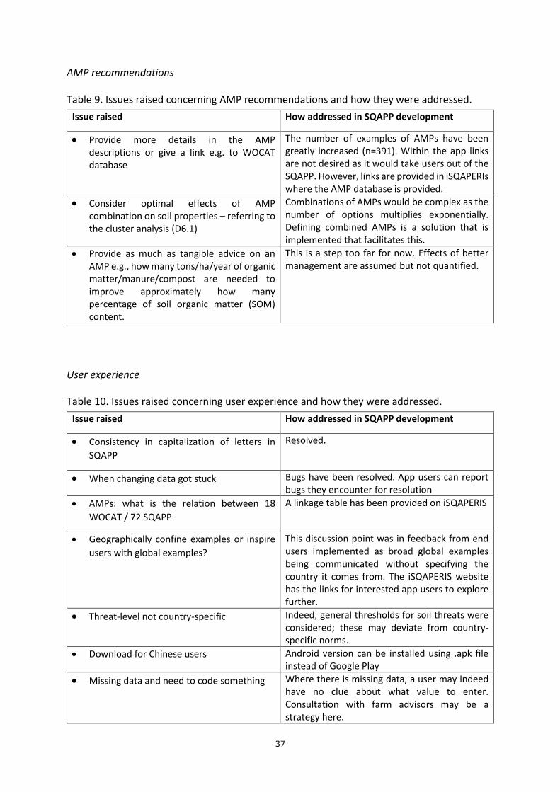
Table 9. Issues raised concerning AMP recommendations and how they were addressed.
Issue raised How addressed in SQAPP development
• Provide more details in the AMP descriptions or give a link e.g. to WOCAT database
The number of examples of AMPs have been greatly increased (n=391). Within the app links are not desired as it would take users out of the SQAPP. However, links are provided in iSQAPERIs where the AMP database is provided.
• Consider optimal effects of AMP combination on soil properties – referring to the cluster analysis (D6.1)
Combinations of AMPs would be complex as the number of options multiplies exponentially. Defining combined AMPs is a solution that is implemented that facilitates this.
• Provide as much as tangible advice on an AMP e.g., how many tons/ha/year of organic matter/manure/compost are needed to improve approximately how many percentage of soil organic matter (SOM) content.
This is a step too far for now. Effects of better management are assumed but not quantified.
User experience
Table 10. Issues raised concerning user experience and how they were addressed.
Issue raised How addressed in SQAPP development
• Consistency in capitalization of letters in
SQAPP
Resolved.
• When changing data got stuck Bugs have been resolved. App users can report bugs they encounter for resolution
• AMPs: what is the relation between 18
WOCAT / 72 SQAPP
A linkage table has been provided on iSQAPERIS
• Geographically confine examples or inspire
users with global examples?
This discussion point was in feedback from end users implemented as broad global examples being communicated without specifying the country it comes from. The iSQAPERIS website has the links for interested app users to explore further.
• Threat-level not country-specific Indeed, general thresholds for soil threats were considered; these may deviate from country-specific norms.
• Download for Chinese users Android version can be installed using .apk file instead of Google Play
• Missing data and need to code something Where there is missing data, a user may indeed have no clue about what value to enter. Consultation with farm advisors may be a strategy here.

38
• User guide/Youtube video Instruction video has been prepared
• Are you curious about your soil intro screen:
repeat at every start-up
If the user logs out or did not log into the app in the first place this is the case
• Explain why SQAPP is different from other
soil apps
Fact sheets, instruction video and background information explain what SQAPP can do
• Make a flyer to attract people to download
the app
Materials have been produced and are used to launch SQAPP on World Soil Day 2020
• Add info button for (characteristics – specify
land cover)
• Add conversion units in info button soil
properties and soil threats
• Add technical details about soil parameters
such as bulk density and coarse fragments in
info button
• Add axis titles and an explanation for
cumulative density functions, perhaps add a
screen between values and cumulative
density functions to explain the curve
• Change “Provide feedback” to “Improve
your data”
These practical suggestions have been implemented in info buttons and instruction materials
• At the end of the SQAPP screens, include
questions on barriers to implementation
The current set-up of the evaluation screen requires the user to evaluate AMPs as either already implemented, inappropriate, potentially interesting and definitely interesting – the latter two are taken forward for ranking as exploratory options. It is assumed that the user is made aware about these options but not necessarily already has a clear idea about them and possible barriers to implementation. This aspect could be explored in the future.
External review session at Soil Horizons workshop at the Wageningen Soil Conference
August 2019
The iSQAPER and LANDMARK projects joined together to hold a side event on soil quality and
soil functions at the Wageningen Soil Conference in August 2019. The workshop, attended by
ca. 100 participants, included a demonstration of SQAPP and the collection of feedback from
workshop participants. Figure 11 gives a first impression of the perception of SQAPP. It is
viewed as simple, quick, easy and global.

39
Figure 11. One word evaluation of SQAPP by workshop participants.
In focus group demonstrations and discussions of SQAPP a number of issues were raised by
the participants. These have been listed in Table 11 together with a comment on how these
were or could be addressed in (future) SQAPP development.
Table 11. Issues raised by external experts and how they were addressed.
Issue raised How addressed in SQAPP development
• Recommendations are only accessible if you are registered / logged in. This doesn't have to be necessary, right?
Recommendations are given based on field characteristics for which user input is required. This requires to save user input for a location first, which is why registering is required to view recommendations. Registering is a quick process, as only an email and password are required and no further personal data are solicited.
• Is it possible to display the uncertainties in
the data in the app? Via a pop-up with a
disclaimer, for example
Yes this has been implemented
• Can a farmer indicate which objectives he /
she considers important? For example, a
farmer who has an above-average interest in
climate, if he can indicate this with a kind of
slider at the beginning, and then also receive
other recommendations, more focused on
climate than on production, for example
The implicit objective in SQAPP is that the ensemble of poorly scoring relative soil quality parameters and high risk soil threats are addressed. Soil quality is hypothesized to support multiple ecosystem services which could be considered objectives. But the SQAPP cannot indicate if and how much individual ecosystem services are improved. What the farmer can do

40
is specify the domain of management recommendations (s)he is interested in to get those recommendations highlighted. Alternatively, farmers can be pointed to the iSQAPERIS website where the full overview of AMPs and examples can be consulted per domain.
• Can we register whether the
recommendations are actually being
followed up on? By means of an extra button
"I am going to implement this". It is
interesting to see how much effect the app
actually has, and encourages action
In the final screen, the app user is asked to answer the question “Do you think you will implement one of the recommendations?” While less definite action-oriented, this formulation is truer to what can be measured, namely the intention of the user, rather than actual implementation.
• Can you see where in the world how many
people use the app?
Yes, there are two ways to do this. First, data on saved locations can be analysed to this effect. However, anyone can save a location anywhere in the world, so this information may not tell much about the geographical spread of users. The second source of data are the statistics from the app stores on app downloads in different countries. This statistic gives good data on the spatial distribution of app downloads, but not on its actual use.
• Idea for a follow-up project: link SQAPP and
Soil Navigator
SQAPP offers the potential to link to other apps. Within the current project this was not an objective, but further development of functionality is on the radar of the development theme.
• As the privacy conditions are now, the data
entered by the user himself may not be used
to improve the databases. If we ultimately
want that, then the conditions must be
changed, and the users until now be asked if
they are still okay with their data being used
The privacy conditions state that data may be used:
- To improve SQAPP and the information it provides to you
- For scientific research purposes Individual (point) data will not be disclosed for privacy reasons. In the future, one may conceive that user-contributed point data could be explicitly intended for building up trusted, open access sample data, but this is currently not the case. In this case, users would be asked to explicitly state their point-data can be made public so that it does not affect data already contributed.
• For regions where more specific data is available (eg NL) also use this
As the relative soil quality is determined based on data for pedo-climatic zones which often occur in multiple regions/countries, ideally the same data source is used. Juxtaposing more specific data for defined areas would still mean that all probability density curves for affected pedo-climatic zones has to be recalculated. These factors make that adding local datasets is

41
not as easy as it seems. An alternative is to calculate the pedo-climatic zones with the more specific dataset only. This would then give higher quality results in the area considered, but the data to construct the probability density curves would also be available for the region only.
• Add a notification (pop-up) to the soil properties: “If you have better data yourself, you can enter it here”. Now you really have to look for this possibility.
The button text “Provide feedback” has been renamed to “Enter own data” to clarify this issue.
• It would be useful for policy makers if SQAPP could be used on a regional scale, instead of point / plot
As indicated in Section 2.5, a regional scale implementation has been set up. As SQAPP relies partially on user input, there are some scenario options (land cover and crop data) that need to be defined for a ‘real’ regional application. A regional application was not envisaged as part of the project concept, but has emerged as a potential powerful future development.
• Add euros Data on costs of AMPs and examples of AMPs is scarce and tend to vary significantly. Some require a piece of equipment (used on an unknown number of hectares), others may require costs for investment and maintenance over several years. Another aspect could be availability of subsidies for implementation, which tend to change over time and are region-specific. That is why we have for now chosen a simple ‘complexity’ indicator giving a qualitative scoring of cost, labour and know-how needed.
• Provide more information about how the graphs are constructed. For example: what about if all the soils in your pedoclimatic zone are super bad, except yours? Then this one will come out very well, while it might not be that good at all. And is it possible to show the graphs only the data of your pedoclimatic zone from your country? "Farmers don't find it interesting to compare themselves with people from other countries," it was noted.
The procedure to construct probability density functions is explained in FAQs and instruction video. Indeed, theoretically all soils in a pedo-climatic zones could be bad/degraded. As management information is not (yet) taken into account in the construction of maps, this may particularly apply to the ranges in natural areas being reduced and not represented as land cover is a co-variate in most soil data mapping procedures. Still, the relative score does indicate this would then be the best farmer in the pedo-climatic zone. Regionalizing of the pedoclimatic zones to countries would introduce other biases and limit the comparability in smaller countries while still not offering a more regional perspective in very large ones. A country-specific approach to pedo-climatic zones would be more useful if based on a dedicated higher accuracy soil data system for that country.
• The practical details of the recommendations are also important, if a farmer really wants to apply them. Can we
Links within the app would be confusing as it requires the user to navigate away from the app. The iSQAPERIS section on AMPs in SQAPP is

42
possibly here. refer (link) to the info in WOCAT?
referred to as a first-stop portal for further advice and links.
• Idea: Integrate feature that brings together users with the same threats / recommendations in the same region. So that a kind of study clubs can arise around a specific theme
Innovations for social collaboration are indeed an important future development potential for SQAPP.
• Expectations management: clearly indicate that this tool is a support, and not the hard truth.
Under the About section we have added the following text: “ Scale is an important consideration when using this app. The analysis provided is based on global and regional data and should not be interpreted as exact data for a specific point on the map, such as your garden or farm field. Within the app, you may upload local data to refine the soil quality analysis and resulting recommendations. European and Chinese geography contains the richest data layers within SQAPP.”
• Idea: add intro text (eg after choosing the location, before viewing soil properties). Indicate here what the app does and does not do. Similar to previous comments on disclaimer / expectations management
Support text is provided in information buttons and the more information section in SQAPP in order not to break the functional flow of the app.
• Introduce SQAPP in study clubs (such as Kringloopwijzer in K&K) to make it land with farmers
Information sheets on the use of SQAPP by various audiences have been produced. Following the launch event we will monitor and target groups
• Do not throw the app over the fence when the project is over, keep maintaining! And implement it in education; learned young is done old.
Fully agreed! SQAPP has already been integrated in the student education of participating organisations.

43
3. Building SQAPP
3.1. Premises
The SQAPP was designed with the idea that it should provide the user with the opportunity to access fragmented data on soil quality and soil threats in an easy-to-use way. Moreover, the user should not only receive indicator values, but be guided in interpreting these values by providing more contextual information: is a certain indicator value high or low in a given context? Such contextual information is provided through analysing indicators within combinations of climate zones and soil types, and by distinguishing between arable land and grazing land. Finally, the user should receive, based on an assessment of the most critical issues, management recommendations on how soil quality can be improved and soil threats be overcome. A second consideration in designing SQAPP was the idea to use soil quality and soil threat indicators for which spatial data exist. This way, it is possible to provide the user with data for any indicator for which data exist for a given location, in combination with the comparative contextual information. The comparative aspect of the soil indicator data is then realized by calculating cumulative probability density functions for each pedo-climatic zone. All indicator values are given as ‘best guestimate’ for the location. The user can proceed with generating management recommendations based on these standard values, or replace some or all indicator values with own data to get more accurate recommendations. This design helps to make the SQAPP directly helpful by visualizing available soil information in a systematic and easy-to-access way. Thirdly, the SQAPP recommends agricultural management practices to improve soil quality and/or mitigate soil threats based on an integrated assessment of the aspects most urgently needing attention. This integrated way of considering soil quality indicators is new in comparison to existing soil apps and indicator systems. This integration avoids consideration of poor single indicator scores in isolation, which could have trade-offs with other soil quality indicators that are also suboptimal. Fourthly, although the iSQAPER project focuses on Europe and China, it quickly became clear that the amount of work required to develop SQAPP would be more appropriately justified by building an app with global coverage. This inclination to go global was reinforced by some hurdles experienced along the way to harmonise European and Chinese data (see below). As a consequence, the app was designed with global functionality in mind. The overall procedure to develop SQAPP is given in Figure 12. These steps include: 1. Selecting soil quality indicators; based on the review of soil quality indicators in WP3, a
selection of the most commonly used was made. For these indicators, we examined availability in terms of global datasets. All relevant indicators for which maps existed were retained as input data layers. Similarly, maps of soil threats were reviewed. Here, available global datasets were used; in Europe some further soil threats were included based on soil threat maps with European coverage.
2. Defining pedo-climatic zones; as one of the principles underpinning SQAPP is a relative assessment of soil indicators, appropriate zones with similar conditions need to be

44
defined. Within WP2, pedo-climatic zones were developed for both Europe and China (Deliverable 2.1). As the basic climate zones distinguished in these classifications were not comparable and because there were some conversion issues to reclassify Chinese soil types to WRB (World Reference Base) soil types, the resulting pedo-climatic zones in Europe and China were not directly comparable, and moreover, did not cover other areas of the world. This became an issue for calculating relative soil indicator scores at global level. To resolve this issue, a new pedo-climatic zonation was produced within WP4 for the purpose of calculating consistent data layers for the app.
3. Ranging soil quality indicators; once indicators are selected and pedo-climatic zones are defined, it is possible to calculate cumulative probability density functions for each indicator in each pedo-climatic zone. These cumulative probability density functions become the basis for the relative assessment of soil quality. Moreover, within each pedo-climatic zone, attention also needs to be paid to the land use/cover, as land use is known to greatly influence the indicator scores of several soil indicators. To account for this issue, separate calculations are made for the minimum and maximum scores of each indicator in each pedo-climatic zone, specific for arable and grazing land respectively.
4. Scoring indicators; the relative scores of soil property values are considered based on their position on the cumulative probability density curves. That means (considering whether indicators are of the ‘more is better’ or ‘more is worse’ type), that the bottom 33% of the frequency distribution are considered as low, and the top 33% as high, with medium the outcome for intermediate values. For soil threats, absolute, expert-based values were considered based on the work conducted in WP6 (Milestone 6.2).
5. Assessing indicators; this step concerns the calculation of the potential for soil improvement (percent score) across all soil property indicators, and the calculation of the average soil threat level (on a bar slider between low and high). All poor performing soil property indicators and soil threats are considered as urgent aspects to be addressed.
6. Recommended practices; the final step in the SQAPP is to recommend agricultural management practices based on the overall soil quality score and most urgent soil quality aspects to be addressed. Underlying the recommendations is the development of a large matrix table of the agricultural management practices and a) applicability factors – defining where each of the AMPs is applicable; and b) effectiveness – where the impact on soil property and soil threat indicators of each AMP are scored. The 10 AMPs reaching the highest overall score for the combination of soil properties and soil threats to be addressed in a given location are presented to the app user.

45
Figure 12. Overview of the procedures followed to develop SQAPP, including links to different work packages.
3.2. Soil indicators
The soil property and soil threat indicators considered for the app are based on respective
reviews of indicators in WP3 and WP6. Bünemann et al. (2018) reviewed the most common
soil properties in minimum datasets, showing a dominance of physical and particular chemical
soil properties, and a underrepresentation of biological soil properties. This dominance
remained when considering available spatial datasets (Figure 13). Two datasets that were not
included as frequently used indicators in the overview of Bünemann et al (2018) were added:
coarse fragments (physical property) and number of macrofauna groups (biological property).
Milestone report 6.2 provided the list of soil threats for availability of spatial datasets (in
Europe as a minimum) was already taken as a starting point. Later on, some of the datasets
were replaced with newer/better datasets (e.g. Copper in European topsoils), but the
indicators remained the same. An exception to this is the soil threat of pesticide
contamination. No maps of pesticide pollution are available, but a procedure was designed by
which users can, based on their use of fungicides, herbicides and insecticides, get an estimate
for the pesticide environmental concentration (PEC) of their soils at the moment of application
and after 100 days.

46
Although PECs are publicly available, up to now they were never compiled into a database and
explored as such. This is specially surprising since the presence of mixtures of pesticide
residues in soils is the rule rather than the exception. The steps followed to set up the pesticide
module included i) to identify the active substances allowed in different crop-EU region units;
and (ii) to compile representative uses and PECs of currently approved active substances into
a single database. Of the active substances allowed on the EU market under the EC Regulation
1107/2009 concerning the placing of Plant Protection Products on the EU market (EC, 2009;
EC, 2019), there were 230 synthetic pesticides applied as fungicide/herbicide/insecticide for
which soil degradation data was available. The physical-chemical properties of these 230
active substances, environmental fate data, and (eco-)toxicological data were extracted from
the Pesticide Properties DataBase - PPDB (PPDB, 2019).
Representative uses refer to authorised good agricultural practices, covering the crops and EU
regions to which the active substance is allowed to be applied, as well as recommended timing
for pesticide applications, frequency of applications, interval between applications, and
application rate per treatment. The representative use of active substances can be found in
the individual active substance EU dossiers, publicly available via EFSA (EFSA, 2020).
Recommended application rates aim at effective pest control while keeping risk to humans,
animals, plants and environment at acceptable levels. Active substance representative uses
are used to obtain active substances’ predicted environmental concentrations in soil (PECs),
which are used as exposure proxies in environmental risk assessments, including by the EC
(Ockleford et al., 2017). Da Silva et al. (in preparation) explains the procedure in full.
Figure 13. Most frequently used soil quality indicators (Bünemann et al., 2018) and selected indicators in SQAPP for which spatial datasets needed to be available.

47
3.3. Defining pedo-climatic zones
The pedoclimatic zones were defined based on the overlay of climate zones (Figure 14, Peel
et al., 2007) and WRB (Rev. 2015) world soil map (Figure 15). This leads to 29 x 118 = 3422
potential combinations, of which 2098 indeed have overlap and were defined as pedo-climatic
zones.
Figure 14. Global map of Köppen-Geiger climate zones (n=29) (source: Peel et al., 2007).
Figure 15. Global map of WRB (rev. 2015) soil types (n=118).

48
3.4. Ranging soil quality indicators
Ranges for soil quality indicators were constructed for each indicator and pedo-climatic zone.
Figure 16 gives some examples of cumulative probability density functions as displayed in
SQAPP. The minimum and maximum values are calculated separately for each pedo-climatic
zone and land use/land cover class (arable land and grazing land). The visualization of
probability density functions is done in plots where on the x-axis is the score of the soil
parameter, and on the y-axis the cumulative frequency (0-100%). Minimum and maximum
scores, which in the pilot app were always indicated by red (undesired value) and green
(desired value) markers, were later replaced by grey markers if either minimum or maximum
values (or both) could not be interpreted as desired value (e.g. maximum soil organic carbon
(SOC) value was indicated with a grey instead of green marker, as very high SOC content
cannot be taken as indicator of superior soil quality.
The calculations required for the construction of cumulative probability density functions
were very computationally intensive. The data to construct each curve are sent from the ISRIC
REST to the app using 255 values along the curve.
For PECs a different approach was taken. Based on ordering the PECs associated with active
substances from high to low and from low to high, the worst-case and best-case scenario for
a given number of pesticides applied can be given (Figure 17, indicated by the red and green
dotted lines, respectively). When the user knows the number of fungicides, herbicides and
insecticides applied, summing the orderings of each type gives a narrower range of possible
PEC values, indicated by the yellow markers in Figure 17. If the user would know the exact
active substances applied, the range can be further reduced and a specific value is given (in
SQAPP indicated by a cyan marker).
Figure 16. Examples of cumulative probability density functions in SQAPP with indication of the value on the actual location (yellow marker), minimum (red marker) and maximum values (green marker).

49
Figure 17. Principle of the construction of PEC ranges – for a given number of pesticides the predicted PEC will range between the maximum and minimum values indicated by the red and green dotted lines, and can be narrowed down by partial identification of active ingredients to the range between the yellow markers.
3.5. Scoring soil quality indicators
Empirical cumulative probability density curves were produced for each soil quality indicator
in every pedo-climatic zone. The density curves were based on empirical probability density
histograms with 256 bands between the lowest and highest value of each soil quality indicator
in every pedo-climatic zone. The cumulative probability (%) corresponding to the actual soil
quality indicator value in a given location, was then considered to be the relative performance
of that soil quality indicator at that location. The potential improvement of that soil quality
indicator at that location was then considered to be the absolute cumulative probability
corresponding to the best attainable value minus the relative performance of that indicator
(e.g. 7%, Figure 18) of the soil quality indicator (Table 12).
The overall soil quality improvement potential was then considered to be the average
improvement potential of all soil quality indicators. The number of soil quality indicators
considered was dependant on data availability. Some soil quality indicators, for instance, were
only available for countries within the European Union.

50
Figure 18. An illustrative example of how the relative improvement potential of a soil quality indicator is calculated. In this example 0.2 is the lowest observed soil organic carbon (SOC) content, and 5.6 is the highest observed SOC content for a specific pedo-climatic zone. 1.3 is the SOC value in our location of interest. Via the cumulative probability curve, we can relate this value to a relative performance of 7%. This means that within this specific pedo-climatic zone, only 7% have a SOC content of 1.3 or lower. The SOC content improvement potential is the absolute cumulative probability linked to the best attainable value (100% linked to 5.6%) minus the relative performance of 7%.
Table 12. Soil quality indicators and optimums used to define relative improvement potential. References: (a) Panagos et al. (2015), (b) Borrelli et al. (2017), (c) Shangguan et al. (2014), (d) Hengl et al. (2017), (e) Lado et al. (2008), (f) Nicholsen & Chambers (2008), (g) Orgiazzi et al. (2016).
Soil quality indicator (reference) Unit Best attainable value (optimum)
Bulk density (d) kg m-3 Minimum
Cation exchange capacity (d) cmol kg-1 Maximum
Electrical conductivity (c) dS kg-1 Minimum
Exchangeable potassium (c) cmol kg-1 Maximum
Soil microbial abundance (g) Maximum
Soil organic carbon content (d) % Maximum
pH (d) 7
Olsen-extracted phosphorus* (c) mg kg-1 Maximum
Plant available water storage capacity mm Maximum
Total soil nitrogen (c) g kg-1 Maximum

51
Figure 19. Soil threat thresholds and classification as implemented in SQAPP.
SOIL THREAT and indicator THRESHOLDS
Soil erosion by water
Soil loss (t/ha/year) 0-2 2-10 >10
Vulnerability (class) low medium high
Soil erosion by wind
Soil loss (t/ha/year) 0-0.5 0.5-3 >3
Vulnerability (class) low medium high
Soil compaction
Natural susceptibility low medium high
Soil salinisation
Electrical conductivity (dS/m) 0-2 2-4 >4
Soil organic matter decline
Soil organic carbon content (%) 0-1 1-2 >2
Soil nutrient depletion
Exchangeable K (cmol/kg) 0-0.2 0.2-0.3 >0.3
Available P (Olsen method) (mg/kg) 0-20 20-40 >40
Total N (g/kg) 0-1 1-2 >2
Soil acidification
Soil pH <5.5 5.5-6.5 6.5-7.5 7.5-8 >8
Soil contamination
Arsenic (mg/kg) 0-37.5 37.5-50 >50
Cadmium (mg/kg) 0-2.25 2.25-3 >3
Chromium (mg/kg) 0-300 300-400 >400
Copper (mg/kg) pH <5.5 0-60 60-80 >80
pH 5.5-6.0 0-75 75-100 >100
pH 6.0-7.0 0-101.3 101.3-135 >135
ph >7.0 0-135 135-200 >200
Lead (mg/kg) 0-225 225-300 >300
Mercury (mg/kg) 0-0.75 0.75-1 >1
Nickel (mg/kg) pH <5.5 0-37.5 37.5-50 >50
pH 5.5-6.0 0-45 45-60 >60
pH 6.0-7.0 0-56.25 56.25-75 >75
ph >7.0 0-82.5 82.5-110 >110
Zinc (mg/kg) 0-150 150-200 >200
Soil biodiversity
Soil biodiversity index low medium high

52
Figure 19 provides an overview of the threshold values for soil threat indicators based on
Milestone 6.2. For the soil threat of risk of pesticide contamination, two scores were
considered (Figure 20):
i) of the total number of each type of pesticide ranked from low to high, the PEC
score of the 0.25 percentile pesticide was considered the upper boundary for
a low risk (green). The 0.75 percentile pesticide constitutes the lower boundary
for high risk (red). Intermediate PEC scores are classified as moderate (orange).
ii) The number of pesticides applied was also considered as a factor influencing
pesticide contamination risk, as cocktails of pesticides may present additional
threats to the environment. Five pesticides was considered the upper threshold
for a low threat (green) and ten pesticides the maximum for a moderate threat
(orange). If more than ten pesticides are applied the PEC indicator is classified
as high (red).
Figure 20. Soil threat scoring of PEC as indicator for pesticide contamination risk. The classification is based on two criteria: 1) the PEC score of the 0.25 and 0.75 percentile ranked pesticide; 2) the number of pesticides applied. Resulting areas in the graph are classified as low risk (green), medium risk (orange) and high risk (red).
3.6. Assessing indicators
The indicators are assessed by i) calculating an overall potential for soil property
improvement; ii) calculating an overall soil threat level; and iii) listing the top-3 soil properties
and soil threats needing attention (Figure 21).

53
Figure 21. Overall summary of soil property and soil threat indicator scores in SQAPP.
The potential for soil improvement is expressed as a percentage. For any given land use, the
average soil would score 50%. Scores of less than 50% mean the soil is better than average;
scores greater than 50% indicate that the soil is poorer than average. Extreme values (close to
0 or 100%) are rare due to the skewed distributions and not all soil quality indicators scoring
good or bad across the board.
The soil parameters needing attention are those with a potential for improvement score of
higher than 67% (i.e. at least a third of soils in the same pedo-climatic zone and under the
same land use score better for these parameters).
For any given land use, only soil parameters that can be improved by management are taken
into account. The actual values of each these parameters is assessed by comparing the
location-specific value with the optimum value found in all locations with similar climate and
soil type for a certain land use (arable or grassland). The optimal value is either the minimum
or maximum value depending on the soil parameter, or an optimum value in the case of pH.
The percentile rank of the location assessed within the range of values determines the
improvement score, which can theoretically range between 0 and 100%. The average of the
improvement scores for individual soil parameters is calculated for the overall potential for
soil improvement score.
The overall threat level is the arithmetic mean of individual soil threat scores for which data is
available (low=1, medium=2, high=3). For “soil nutrient depletion” and “contamination by
heavy metals” only the worst individual score of nutrients or metals is taken into account.
Soil threats needing attention are all those individual threats with a high score.

54
3.7. Recommended practices
Finally, agricultural management practices are recommended in response to the
underperforming soil properties and most important soil threats. To define the recommended
practices two steps were taken: 1) establishing a classification of agricultural management
practices; 2) establishing an expert-opinion based matrix table of the applicability and
effectiveness of AMPs. The final recommendation is made based on simple additive scoring.
Table 13 shows the broad groups (9) of AMPs and AMP categories (34) considered. Under the
latter, a total of 89 AMPs has been distinguished (for example, the category cross-slope
barriers represents two AMPs, bunds and terraces). A total of 391 example AMPs have been
selected to illustrate the different AMPs. The descriptions of AMPs and examples are provided
in Annex 1. An illustrated overview of the AMPs and examples is also given on the iSQAPERIS
website3, where app users and other interested parties can browse through them and link to
website providing further information.
The applicability limitations and effects of these AMPs on soil properties and soil threats are
established in a matrix. The selection of AMPs on the basis of this matrix to generate
recommendations is exemplified in Figure 22. Up to 10 individual AMPs are suggested in a
given location where the app user is requesting solutions. Applicability limitations are
assessed on the basis of (specific) land use, landform, annual precipitation, slope, soil depth,
soil texture and coarse fragments. All AMPs are either scored 0 (not applicable) or 1
(applicable). Effectiveness is considered using a four-class system: definite positive effect (2);
probable positive effect (1), unknown or no effect (0) or negative effect (-1).
Figure 22. Example of the ranking of different AMPs for a given set of identified problems.
3 https://www.isqaper-is.eu/sqapp-the-soil-quality-app/amps-in-sqapp

55
Table 13. Overview of AMPs included in SQAPP, classified in AMP broad classes and AMP
categories distinguished as possible recommendation domains.
AMP broad class AMP category AMP Terrain management
Cross-slope barriers 1 Bunds 2 Trenches and infiltration ditches 3 Terraces 4 Trashlines Runoff control 5 Half-moon terraces
6 Gully rehabilitation Soil management Tillage 7 No tillage 8 Minimum tillage 9 Contour ploughing 10 Strip tillage 11 Subsoiling 12 Roughening the soil surface 13 Raised beds Traffic management 14 Avoidance of traffic 15 Controlled traffic 16 Respect wheel load carrying capacity Soil replacement 17 Claying soils 18 Adding sand Soil amendments 19 Soil conditioners 20 Liming 21 Alkalinity management 22 Straw interlayer burial Conservation agriculture 23 Conservation agriculture Vegetation management
Vegetation cover 24 Permanent green cover in orchards 25 Cover crops 26 Grassland renewal 27 Rangeland rehabilitation Fallow management 28 Planted fallow Vegetation bands 29 Vegetative strips 30 Riparian buffer zones and filter strips 31 Shelterbelts 32 Semi-natural landscape elements 33 Strip cropping Crop choice 34 Deep rooted crops 35 Intercropping 36 Growing halophytes Crop rotation/diversification 37 Crop rotation/diversification 38 Herb-rich grassland Multi-layered vegetation 39 Agroforestry
40 Silvopasture Water management Diversion 41 Diverting water flow Drainage 42 Intercepting drains 43 Subsurface drains 44 Surface drains

56
AMP broad class AMP category AMP Water management (continued)
Water harvesting 45 Planting pits 46 Ridge-furrow systems 47 Ridge-furrow systems for perennial crops 48 Micro-basins Water conservation 49 Inorganic mulching Water distribution 50 Water distribution in rangelands Irrigation 51 Drip irrigation 52 Surface irrigation 53 Pivot irrigation 54 Sprinkler irrigation Irrigation management 55 Leaching salts 56 Minimizing saline water irrigation 57 Reduced water use in rice cultivation Irrigation scheduling 58 Irrigation optimization 59 Supplemental irrigation Runoff conveyance 60 Artificial grassed or paved waterways
Carbon and nutrient management
Organic amendments 61 Liquid manure or slurry 62 Animal manure 63 Compost 64 Biochar 65 Biofertilizers Inorganic amendments 66 Inorganic fertilizers Green manuring 67 Green manure 68 Leguminous crops Crop residue management 69 Retaining crop residues 70 In situ composting Mulching 71 Mulching with pruning materials 72 Straw mulching
Pest management Weed management 73 Mechanical weed control 74 Chemical weed control 75 Biological weed control Pest management 76 Biological pest control 77 Physical pest control 78 Chemical pest control Disease management 79 Physical disease control 80 Chemical disease control 81 Biological disease control Pollutant management
Remediation 82 Phytoremediation Balanced applications 83 Integrated pest and disease management 84 Integrated nutrient management 85 Automated targetting
Grazing management
Grazing management 86 Controlled and rotational grazing 87 Area closure 88 Pasture monitoring Trampling management 89 Avoiding pugging of paddocks

57
3.8. Practical considerations
The pilot app was developed for mobile phones/notepads operating under either Apple iOS
or Android. These two platforms together cover >97% of smartphones. For geolocation, Bing
maps was used as Google products are banned from use in China.

58
4. SQAPP architecture
4.1. Profile
Upon installing SQAPP, the user can choose to register or use the SQAPP for observing soil
data. To register, an email address and password are required. The user can change the
language from the opening screen or the profile screen (Figure 23). Currently the app is
available in 14 languages: English, Dutch, Chinese, Estonian, French, German, Greek,
Hungarian, Italian, Polish, Portuguese, Romanian, Slovenian and Spanish. Registered users can
save locations and get recommendations. If a user does not register, (s)he can still explore soil
properties and soil threat data, but will not be able to receive recommendations. The user can
search or move to a location of interest to explore soil data. If the user allows the app to access
the GPS location, the default location will be the current position of the user’s mobile device.
From the profile screen, users can access previously saved locations, their profile data (name
and password), and language settings.
Figure 24. SQAPP intro screen where the user can register (left), main screen if user chooses not to
register (middle) and profile screen where the user can also select ‘My profile’ to register (right).

59
4.2. Field characteristics
Once a location is selected, the user can edit field characteristics. Going through the field
characteristics is required in order to receive recommendations. Respective screens in the
field characteristics module are shown in Figure 25. On the first characteristics screen the user
can:
▪ Give the location a memorable name (the default is an automated sequential location
numbering)
▪ Edit the altitude, precipitation, mean annual temperature and slope information
available from global data. Precipitation and slope information may affect
recommendations, mean annual temperature affects the rate of pesticide degradation.
▪ Select the right landscape position and land cover. These are prefilled from global data,
but the user can correct or further specify these. Both characteristics will affect the
agricultural management practices recommended. Recommendations are only given for
arable and grassland: for ‘other’ land use soil property and soil threat data can still be
consulted and edited, but no recommendations are given. Land cover, and its further
specification in the second field characteristics screen, will furthermore determine the
list of pesticide active substances authorized for use.
On the second field characteristics screen, the user can:
▪ Further specify the land cover with specific types of crops or grazing types. These may in
some cases refine the agricultural management practices that will be recommended and
be used to select the appropriate pesticides active substances authorized for use.
▪ Indicate the use of pesticides. To do this, they first have to select the last crop grown,
and then check whether they have used herbicides, fungicides and/or insecticides. They
may then either indicate the number of components used, or select the specific active
substances applied from a list on a pop-up screen. The lists show crop-specific active
substances authorized for use in three European zones (North, Central and South).
Outside of Europe, the lists show all active substances authorized for use in Europe. The
respective lists are ordered in sequence of high-to-low expected pesticide environmental
concentration (PEC) one day after application. The aggregate expected influence on
pesticide contamination (based on PEC score and number of active substances used) will
be shown in the ‘Soil threats’ screen.
▪ Indicate any specific category or categories of management recommendations they are
interested in. Agricultural management practices belonging to the selected categories
will later on in the ‘Recommendations’ screen be presented in bold.
▪ Confirm the edits made to return to the main screen from where they can then proceed
to view the soil properties, soil threats and recommendations for the location.

60
Figure 25. Field characteristics screens 1/2 and 2/2, pop-up screen for selecting applied fungicides (listed in decreasing order of expected PEC after 1 day – relative PEC levels after 1 day and after 100 days are indicated by bars in dark and light grey), the field characteristics 2/2 screen after filling pesticides used and recommendation domains, and the main screen with the recommendations screen now available after having filled the field characteristics.

61
4.3. Soil properties
The soil properties screen shows an overview of the available data grouped under soil physical,
chemical and biological properties (Figure 26). By clicking on the graph symbol, a cumulative
density function of the values of the selected property for all locations within a specific
pedoclimatic zone is visualized. This graph screen shows:
▪ The minimum and maximum value of the indicator scores within the pedoclimatic zone for
the selected land use (i.e. arable, grassland, or the full range for ‘other’).
▪ Whether these minimum and maximum values signify a negative, undesired (red dot
symbol) or positive, desired (green dot symbol) soil property score, or whether the value
cannot be attributed a desired or undesired score (grey dot symbol).
▪ The global data value available for the location (yellow diamond symbol). Position on the
graph relative to the y-axis shows the percentage of locations having a lower score.
▪ Visualization of symbols can be switched on and off by clicking on the symbol in the legend,
which is helpful if multiple symbols overlap.
Clicking the ‘Enter own data’ button opens a pop-up screen allowing the user to enter their
own data for the selected property. They can specify a value, indicate whether this value
concerns an estimate, field measurement or lab result, and the date the data was acquired.
By sending this feedback, the value entered is saved for the specified location, and the user
returns to the cumulative density graph, where the entered value is now visible with a blue
diamond symbol. Returning to the soil property overview screen, the modified value is now
visible in blue text. Once the user has checked all data and updated soil properties for which
they have data, they can return to the main menu.

62
Figure 26. Soil properties overview screen, cumulative probability graph screen for soil microbial abundance, and pop-up screen to enter own data (top). When returning to the cumulative probability graph, the entered data is now visible (blue marker), and when returning to the overview screen the entered data is now also listed in blue font.

63
4.4. Soil threats
The soil threats screen shows an overview of the available data grouped under soil threat
categories: soil erosion by water, soil erosion by wind, soil compaction, soil salinization, soil
organic matter decline, soil nutrient depletion, soil acidification, soil contamination and soil
biodiversity (Figure 27). Next to the value of the soil threat indicators, this screen also
visualizes the soil threat classifications of these values by depicting a green, yellow or red
background colour for low, medium and high soil threat classifications, respectively. By
clicking on the graph symbol, a cumulative density function of the values of the selected soil
threat for all locations within a specific pedoclimatic zone is visualized. This graph screen
shows:
▪ The minimum and maximum value of the indicator scores within the pedoclimatic zone for
the selected land use (i.e. arable, grassland, or the full range for ‘other’).
▪ Whether these minimum and maximum values signify a negative, undesired (red dot
symbol) or positive, desired (green dot symbol) soil property score, or whether the value
cannot be attributed a desired or undesired score (grey dot symbol).
▪ The global data value available for the location (yellow diamond symbol). Position on the
graph relative to the y-axis shows the percentage of locations having a lower score.
▪ The background of the graph, indicating whether the indicator score represents a low
(green), medium (yellow) or high (red) threat classification.
▪ Visualization of symbols can be switched on and off by clicking on the symbol in the legend,
which is helpful if multiple symbols overlap.
Clicking the ‘Enter own data’ button opens a pop-up screen allowing the user to enter their
own data for the selected soil threat indicator. They can specify a value, indicate whether this
value concerns an estimate, field measurement or lab result, and the date the data was
acquired. By sending this feedback, the value entered is saved for the specified location, and
the user returns to the cumulative density graph, where the entered value is now visible with
a blue diamond symbol. Returning to the soil threats overview screen, the modified value is
now visible in blue text, and the soil threat class modified accordingly (in this case from
moderate to high). Once the user has checked all data and updated soil threat indicators for
which they have data, they can return to the main menu.

64
Figure 27. Soil threats overview screen (note colour-coded risk levels – green: low; orange: medium; red: high), cumulative probability graph screen for soil organic carbon content with graph background showing threat levels, and pop-up screen to enter own data (top). When returning to the cumulative probability graph, the entered data is now visible (blue marker), and when returning to the overview screen the entered data is now also listed in blue font (note that the value entered is classified as high soil threat level).

65
4.5. Summary and recommendations
After the user has reviewed field characteristics, soil properties and soil threats, pressing the
recommendations button in the main screen first opens the summary screen (Figure 28) which
features two overall indicators:
▪ The overall potential for soil property improvement, expressed in a percentage 0-100%.
An average soil would score 50%, so a score lower or higher than 50% is respectively
below-average and above-average. Due to the averaging across multiple soil properties,
extreme values (close to 0% and 100%) are rare and mostly relate to locations where the
number of soil properties for which there is data is limited. Below the overall indicator is
a list of individual soil properties for which the improvement potential is 67% or larger.
▪ The overall indicative soil threat level, expressed as a bar ranging from low to high. Like
for soil parameters, the indicator score is calculated by averaging the soil threat scores
across indicators (whereby for nutrient depletion and heavy metal contamination only the
worst item is considered). Below the bar is a list of soil threats that are classified as high.
By clicking on the ‘recommendations’ button the user proceeds to the recommendations
overview screen listing the 10 agricultural management practices with the highest score for
the location-specific combination of soil properties and soil threats requiring attention. The
list is shown with those AMPs belonging to the recommendation areas of interest specified by
the user in the field characteristics (2/2) screen formatted in bold. For each AMP, the user can
see further information by clicking on the ‘i’ symbol on the left-hand side, and review the AMP
by selecting the indicator symbol on the right-hand side.
When clicking the ‘i’ symbol, the user sees a description of the AMP and its categorization.
Between 1-8 specific examples of each AMP can be viewed and scrolled through by clicking
on the ‘view examples’ button. Examples are given a level of complexity rating and illustrated.
The reviewing of the AMPs is done by qualifying them as already implemented, inappropriate,
potentially interesting or definitely interesting.
After the reviewing of individual AMPs, the ones of interest are shown in the next screen
where the user can order them in order of interest (Figure 29). After the ordering, a feedback
screen is shown with two simple questions (1. Were the recommendations useful for you? 2.
Do you think you will implement one of the recommendations?) and an open feedback field.
Upon (later) revisiting of the same location, the user ratings of the AMPs are brought in
remembrance, but those that were definitely interesting are left open for a possible new
evaluation (note: also the other ratings can be changed).

66
Figure 28. Summary overview screen with potential for soil property improvement score and overall soil threat level, the recommendations screen listing the 10 highest scoring AMPs, and AMP information screen for minimum tillage (top). By clicking ‘showing examples’ a scrollable pop-up screen opens with photos and short descriptions. By clicking the indicator symbol, each AMP can be evaluated, as shown in the final overview.

67
Figure 29. Your rankings screen where the user can swap the order of (potentially) interesting AMPs, after which a final review screen with two questions pops up. Upon later revisiting the recommendations overview screen, all evaluations are saved except the definitely interesting ones (for which the user can now indicate whether they were implemented or otherwise; other evaluations can be changed too).
4.6. More information
By clicking on the ‘More information’ link in the main screen, a series of background
information and interaction options are accessible, including the following (Figure 30):
▪ About – a brief description of the purpose and functionality of the app
▪ Disclaimer – a legal text explaining that the app is freely supplied but that no rights can
be claimed from (implications of) its use.
▪ Privacy policy – a legal text explaining how user data is handled and how it conforms
to the European GDPR regulations.
▪ Credits – a description of the third party data sources, development partners and
financing.
▪ Feedback – a free-form field to send feedback and questions to the app development
team.
▪ FAQ – a list of frequently asked questions and answers.

68
Figure 30. Information overview screen with buttons to access further information or provide feedback on the app.

69
5. SQAPP data
5.1. Input maps for SQAPP The following data sets were used for building the final version of the SQAPP: ▪ Soilgrids (www.soilgrids.org), at 250 m resolution, has been used for the following soil
parameters with global coverage: absolute depth to bedrock, bulk density, texture,
available soil water capacity, soil organic carbon content, cation exchange capacity, soil pH
and its derived soil acidification. For further information on Soilgrids see the paper by
Hengl et al. (2017).
▪ European Soil Data Centre (ESDAC) (https://esdac.jrc.ec.europa.eu/ - Panagos et al., 2012) has been used for the following soil threat data with European or global coverage: soil erosion by water (Panagos et al., 2015), soil erosion by wind (Borrelli et al., 2017), susceptibility to soil compaction (Houšková and Van Liedekerke, 2008), soil contamination by heavy metals (Rodriguez Lado et al., 2008), except for copper for which Ballabio et al. (2018) was used. Global Soil Biodiversity Atlas Maps have been used for the following soil biological data: global estimates of soil microbial abundance and soil macrofauna (Serna-Chavez et al., 2013), and soil macrofauna data (courtesy of Dr Jerôme Mathieu of University Pierre and Marie Curie, Paris VI, manuscript in preparation).
▪ Global Soil Dataset for Earth System Modelling (http://globalchange.bnu.edu.cn/research/soilw) has been used for: electrical conductivity, exchangeable potassium, phosphorus using Olsen method, and total nitrogen (Shangguang et al., 2014).
More in particular, the following data layers are incorporated in the final version of SQAPP: Global background info at 250m resolution
1. Altitude (m, a.s.l.) 2. Slope (%) 3. Precipitation (mm/year) 4. Average anual temperature (°C) 5. Landscape (breaks-foothills, flat plains, high mountains-deep canyons, hills, low hills,
low mountains, smooth plains) 6. Land cover in 2010 at 30m resolution 7. Pedoclimatic zones (n=2098)
Global soil properties in 0-30cm depth at 250m resolution
1. Soil types (WRB) 2. SOC (%) 3. pH (H2O) 4. Sand (%) 5. Silt (%) 6. Clay (%)

70
7. Coarse fragments (%) 8. Bulk density (kg/m3) 9. CEC (cmolc/kg ) 10. Depth to bedrock (cm) 11. Available soil water capacity (volumetric fraction) with FC = pF 2.0 12. Available soil water capacity (volumetric fraction) with FC = pF 2.3 13. Available soil water capacity (volumetric fraction) with FC = pF 2.5 14. Non-available soil water capacity or permanent wilting point (PWP) (volumetric
fraction) with FC = pF 4.2 Global soil nutrients in 0-30cm depth at 250m resolution
1. Total N (g/kg) 2. Total P (g/kg) 3. Total K (g/kg) 4. Electrical conductivity (dS/m) 5. P (Olsen, ppm/weight) 6. Exchangeable K (cmol/kg)
Global and regional soil threats and reclassification (low, medium, high) at 250m resolution
1. Soil loss by water erosion in Europe and reclassification 2. Soil loss by wind erosion in European agricultural soils and reclassification 3. Global water erosion vulnerability reclassification 4. Global wind erosion vulnerability reclassification 5. Natural soil susceptibility to compaction in Europe and reclassification 6. Arsenic in European soils 7. Cadmium in European soils 8. Chromium in European soils 9. Copper in European soils 10. Mercury in European soils 11. Nickel in European soils 12. Lead in European soils 13. Zinc in European soils 14. Global soil biodiversity index reclassification 15. Global estimates of soil microbial abundance and reclassification 16. Global soil macrofauna and reclassification
5.2. Matrices
Eight data matrices are included in the SQAPP database in its content management system.
Two of these relate to respectively the applicability limitations and effects of AMPs on soil
properties and soil threats, while the remaining six are the active substances’ expected PECs
for respectively fungicides, herbicides and insecticides at two moments: one day and 100 days
after application.

71
The structure of the matrices is as follows:
1. Applicability limitations of AMPs. For each AMP, applicability is defined in binary (0/1) fashion for:
▪ Land cover class and subtype ▪ Slope class: Flat (0-2%); Gentle (2-5%); Moderate (5-10%); Rolling (10-15%); Hilly
(15-30%); Steep (30-60%); Very Steep (>60%) ▪ Annual precipitation class: 0-250 mm; 251-500 mm; 501 - 750 mm; 751 - 1000 mm;
1001 - 1500 mm; 1501 - 2000 mm; >2000 mm ▪ Landscape position: Breaks-foothills; Flat Plains; High Mountains-deep Canyons;
Hills; Low Hills; Low Mountains; Smooth Plains ▪ Soil depth class: Very Shallow (0-20 cm); Shallow (20-50 cm); Moderately Deep (50-
80 cm); Deep (80-120 cm); Very Deep (> 120 cm) ▪ Soil texture class: Coarse (sand > 50%); Fine (clay > 40%); Medium (other) ▪ Stoniness class: None (coarse Fragments <2%); Slightly (coarse Fragments 2-10%);
Moderately (coarse Fragments 10-25%); Excessively (coarse Fragments >25%)
2. Effects of AMPs on soil properties and soil threats, defined in the following classification: negative effect: -1; no, ambiguous or unknown: 0; slight or very long-term positive effect: 1; definite positive effect: 2. Effects can be entered for the following parameters (in bold the ones that are actually implemented in SQAPP) – note that some of these double as soil property and soil threat indicator:
▪ Bulk density (fine earth) ▪ Plant-available water storage capacity ▪ Soil organic carbon content (fine earth fraction) ▪ Soil pH ▪ Electrical conductivity ▪ CEC ▪ Exchangeable potassium ▪ Amount of phosphorus using Olsen method ▪ Total nitrogen ▪ Soil microbial abundance ▪ Soil macrofauna groups ▪ Clay ▪ Silt ▪ Sand ▪ Coarse fragments (volume) ▪ Depth to bedrock ▪ Global water erosion vulnerability, or soil water erosion in Europe ▪ Global wind erosion vulnerability, or soil wind erosion in European agricultural
soils ▪ Natural soil susceptibility to compaction ▪ Contamination (linked to highest ranked heavy metal risk) ▪ Pesticide residues (after 1 day) ▪ Pesticide residues (after 100 days)

72
3. PECs (mg/kg) for individual active substances of fungicides expected 1 day after application:
▪ Different regions: Central Europe (CEU); Northern Europe (NEU); Southern Europe (SEU); Rest of the world (ROW)
▪ Different average annual temperature: 10°C; 20°C ▪ Different crop types: cereals; maize; root crops; non-permanent industrial crops;
grassland; permanent crops; vineyards; dry pulses, vegetables and flowers
4. PECs (mg/kg) for individual active substances of fungicides expected 100 days after application:
▪ Different regions: Central Europe (CEU); Northern Europe (NEU); Southern Europe (SEU); Rest of the world (ROW)
▪ Different average annual temperature: 10°C; 20°C ▪ Different crop types: cereals; maize; root crops; non-permanent industrial crops;
grassland; permanent crops; vineyards; dry pulses, vegetables and flowers
5. PECs (mg/kg) for individual active substances of insecticides expected 1 day after application:
▪ Different regions: Central Europe (CEU); Northern Europe (NEU); Southern Europe (SEU); Rest of the world (ROW)
▪ Different average annual temperature: 10°C; 20°C ▪ Different crop types: cereals; maize; root crops; non-permanent industrial crops;
grassland; permanent crops; vineyards; dry pulses, vegetables and flowers
6. PECs (mg/kg) for individual active substances of insecticides expected 100 days after application:
▪ Different regions: Central Europe (CEU); Northern Europe (NEU); Southern Europe (SEU); Rest of the world (ROW)
▪ Different average annual temperature: 10°C; 20°C ▪ Different crop types: cereals; maize; root crops; non-permanent industrial crops;
grassland; permanent crops; vineyards; dry pulses, vegetables and flowers
7. PECs (mg/kg) for individual active substances of herbicides expected 1 day after application:
▪ Different regions: Central Europe (CEU); Northern Europe (NEU); Southern Europe (SEU); Rest of the world (ROW)
▪ Different average annual temperature: 10°C; 20°C ▪ Different crop types: cereals; maize; root crops; non-permanent industrial crops;
grassland; permanent crops; vineyards; dry pulses, vegetables and flowers
8. PECs (mg/kg) for individual active substances of herbicides expected 100 days after application:
▪ Different regions: Central Europe (CEU); Northern Europe (NEU); Southern Europe (SEU); Rest of the world (ROW)

73
▪ Different average annual temperature: 10°C; 20°C ▪ Different crop types: cereals; maize; root crops; non-permanent industrial crops;
grassland; permanent crops; vineyards; dry pulses, vegetables and flowers
5.3. User input
User input in SQAPP is used to refine the projected soil threat of soil contamination by
pesticides and to tailor the recommended AMPs to land use subtype selected by the user. For
these inputs a selection of the user is required as global data provides only a limited
specification of land cover and no information on pesticide use:
▪ Land cover: arable land; grazing land; permanent crops without soil cover; permanent crops with soil cover; vegetables; other
▪ Land cover specification depending on land cover: - For arable land: cereals; maize; rice; root crops; oleaginous crops;
leguminous crops; other - For grazing land: pasture (intensively managed); rangeland (extensively
managed) - Permanent crops (both types): vineyards; olives/nut trees; citrus; fruit
trees; other - Vegetables: indoor vegetables; open field vegetables
▪ Pesticide use: types used (fungicides; herbicides; insecticides), number used, specific active substances used.
Other input data used by SQAPP can be adjusted by the user if they have their own (more
precise) data. This applies to all types of information:
▪ Field characteristics ▪ Soil parameters ▪ Soil threats
Next, there are a series of user preferences that are considered and saved for a specific
location of interest:
▪ Specific interest in recommendation domains: terrain management; soil management; vegetation management; carbon and nutrient management; pest management; pollutant management; grazing management
▪ Qualifications of recommended AMPs: implemented; inappropriate; potentially interesting; definitely interesting
▪ Rankings of AMPs deemed potentially and definitely interesting by the user
Finally, users can provide feedback to the app development team:

74
▪ Through giving feedback on the recommended AMPs (2 evaluation questions and comment box at the end of a use cycle)
▪ Through the generic feedback field under ‘More information’.
5.4. SQAPP output
To the app user, the SQAPP provides data on:
▪ Field characteristics (coordinates, altitude, annual precipitation, mean annual temperature, landscape position, slope and land cover)
▪ Soil properties (indicator scores: for the specific location; the minimum and maximum of the selected pedoclimatic zone and broad land cover type; the cumulative frequency of scores within the zone and relative position of the specific location)
▪ Soil threats (indicator scores: for the specific location; the minimum and maximum of the selected pedoclimatic zone and broad land cover type; the cumulative frequency of scores within the zone and relative position of the specific location; the overall soil threat classification and local soil threat level)
▪ Soil improvement potential score, overall soil threat level indication and specific soil parameters and soil threats requiring attention
▪ Recommendations of the 10 most effective AMPs to deal with the location-specific combination of soil properties and soil threats requiring attention.
The SQAPP content management system records the following information:
1. User data (email; password - for ensuring app functionality to the user only) 2. Saved locations and field characteristics 3. Location-specific recommendations generated and evaluated by users 4. Location-specific user-suggested data (parameter, global data value, user-specified
value, how this data was acquired and when)

75
6. SQAPP users
6.1. Farmers and land users
Farmers and land users are the first core group of intended app users. The main features of
interest for this group are: a) comparative soil quality assessment, allowing to compare their
fields’ soil quality with those of under the same land use, in similar soil types and climate
zones; and b) the management recommendations of specific AMPs.
This group of SQAPP users is specifically suggested to register in order to be able to store
information about their fields and receive recommendations. More specifically, it is suggested
to save field locations with a plot name (or other identifier) and date in the name. This may
be useful when experimenting with new AMPs and reassessment of a field’s soil quality at a
later point in time. By doing this, the previous information does not have to be overwritten
and remains available, and can be used to track progress towards improved soil quality over
time.
Often, farmers and land users will have data about their fields’ soil. Entering those data is
recommended in order to get more tailored AMP recommendations, as some of the global
data layers have been shown to be of poor quality, and none of the datasets takes specific
local soil management history into account. There are also a number of instances in the app
where user input about land management is required, and this group is the key user group
that is able to use actual data, e.g. about (rotational) crops grown on a field and pesticides
applied. Defining these correctly also enhances the management recommendations by
SQAPP. In the case of pesticides, for many farmers this will probably be the first time that they
will get an estimate for the pesticide environmental concentration in their field.
Evaluating the AMPs suggested by SQAPP is another important aspect of the use of the app
by this group. As with improved or updated data the suggested AMPs may change, it is good
practice to take some time to go through the evaluation and indicate which AMPs are already
applied, inappropriate, potentially interesting or definitely interesting. As these user-specified
evaluations are stored, they can be reviewed at a later time. Also, if a large number of app
users evaluates AMP suggestions, researchers can analyse the data and improve the AMP
recommendations, e.g. by removing those that are consistently evaluated as inappropriate.
When farmers and land users have selected AMPs that are potentially or definitely interesting,
they can search for more information about these. A first recommended portal is the
iSQAPERis section on agricultural management practices recommended by SQAPP

76
(https://www.isqaper-is.eu/sqapp-the-soil-quality-app/amps-in-sqapp). Here, links to
websites with more details are provided. This section on iSQAPERis is also of interest to this
group in its own right as it provides access to the full set of AMPs that can be browsed at
convenience for inspiration.
Throughout the development process of SQAPP, farmers and land users have indicated a
number of concerns and ideas about the app. The most common ones are listed in Table 14.
Table 14. Key concerns expressed by farmers and land users during SQAPP development and
solutions.
Key concern Solution
Availability of SQAPP in own language SQAPP is available in 14 languages
Poor quality of global soil data User can update with their own data
Soil data is provided in different units Conversion factors are provided
AMP recommendations are too general 391 specific examples of AMPs have been incorporated
AMPs already implemented or inappropriate
AMP recommendations have been revised; user can record which AMPs are already implemented and which are inappropriate
Would like to have spatial information SQAPP is a point-based tool. Multiple points can be recorded within/across fields.
Would like to be able to import soil data Follow-up work can be done to link SQAPP with other tools
Would like to be able to export soil data To be considered in the future
Would like to have information on policy support for AMPs
Follow-up work can be done to link SQAPP to national greening measures support information. As these tend to change a support strategy to keep this information updated is necessary
Who has access to my data? The privacy policy describes the potential use of data. App developers can use the data to improve SQAPP and report on the use of SQAPP, but will never disseminate point data. (Currently, there is no way to verify the accuracy of user input, so user supplied data cannot be taken for granted to be accurate)
6.2. Advisors and technicians
Advisors and technicians can use SQAPP as a tool to assist them in advising farmers and land
users. As they have a network of farmers and land users that they interact with, they are a key
target audience in order to explain SQAPP, report on accuracy issues, and keeping abreast of
interesting AMPs for the area they operate in. They may be particularly interested in: a) having

77
access to global soil data and relative soil quality assessment scores as a quick-scan tool; and
b) the portfolio of AMPs and specific AMPs frequently recommended for the area they operate
in.
This group of SQAPP users is also suggested to register in order to be able to store information
about fields and management recommendations. Rather than having accurate data on specific
field locations, they may populate saved locations with typical data in order to verify AMPs
that are recommended, and keep a list of priority AMPs on which to document interesting
information to disseminate to farmers and land users.
They can support farmers and land users with access to data about their fields’ soil to enter
their data and discuss the tailored AMP recommendations suggested by SQAPP with them.
They also play a crucial role in identifying alternatives, e.g. to reduce the use of pesticides with
high environmental impact, and experiences with the use of AMPs in experimental settings
and/or by other farmers in the region. As they potentially review a large number of AMP
suggestions, their feedback to the researchers that develop SQAPP is particularly useful. The
iSQAPERis section on agricultural management practices may be an interesting resource for
this group.
Throughout the development process of SQAPP, advisors and technicians have indicated a
number of concerns and ideas about the app. The most common ones are listed in Table 15.
Table 15. Key concerns expressed by advisors and technicians during SQAPP development and solutions.
Key concern Solution
Reaching farmers and land users with the right information
Especially younger farmers are interested in apps as a tool
Availability of SQAPP in local language SQAPP is available in 14 languages
Quality of user input data Advisors working with farmers to complete data input
AMP recommendations are too general 391 specific examples of AMPs have been incorporated
More information on the ways to calculate probability distributions and soil quality score
Information buttons explain main points in the app; instruction video and explanations available on iSQAPERIS
Possibility to consider local/national datasets
Potential to apply SQAPP principles on local datasets; integrating in global data may not be straightforward because of different methods used. This was not taken forward within the scope of the project.
Interacting with researchers to obtain the latest insights in new AMPs
SQAPP can play a role but exchanges through collaborative events and projects remains key.

78
6.3. Students and researchers
Students and researchers are an important group of intended app users. The main features of
interest for this group are: a) access to global soil data and relative soil quality information,
using SQAPP as a convenient first-stop data source; b) information about relevant soil threats
at a location of interest; and c) learning about AMPs recommended for a certain location.
Depending on interest to consult recommendations, this group of SQAPP users can either
register in order to be able to receive recommendations or use the app without making an
account. Logging in with an account is helpful if repeated readings are going to be taken and
having access to the data from these points is important (e.g. for sampling during field work).
For this group, the distribution of soil parameter values and relative position of a field in
relation to other fields with similar land use and pedo-climatic conditions can be insightful
information. It is helpful to complement SQAPP readings with visual soil assessment methods
if no other data is available to cross-check estimates using different methods. The use of
SQAPP for this group can be: a) exploratory – considering different points in an area to get an
idea about the variability of soil conditions or about potential soil quality scores; b) gather
proxy soil data – collect results from SQAPP as a first indication of local conditions to be cross-
checked with other data later; c) as primary data source – caution should be taken with this,
but for soil parameters with high or reasonable confidence, for non-critical applications this
could be a viable data source.
SQAPP can also be used as a data collection tool while doing research with farmers and land
users, where data from these farmers can be registered in SQAPP, whether this relates to the
soil parameters or feedback regarding different AMP suggestions. Students can learn directly
from SQAPP (exploratory use), or by comparing SQAPP data with other data sources, e.g. to
conduct an accuracy assessment (analytical use of proxy data). The full overview of AMPs in
SQAPP on iSQAPERIS can also serve as a learning resource.
This group can also perform a key role in validating SQAPP and reporting of soil data. Through
feeding back this information within SQAPP or to the researchers that developed the app,
improvements can be made. This can consist of refinements of the current data and data
processing methods in SQAPP, or development of new functionality and modules.
Throughout the development process of SQAPP, students and researchers have indicated a
number of concerns and ideas about the app. The most common ones are listed in Table 16.

79
Table 16. Key concerns expressed by students and researchers during SQAPP development
and solutions.
Key concern Solution
Clear information on the source of the data Pop-up screen mentioning the source of each soil parameter
Clear indication of the uncertainty of the data
Pop-up screen indicating the reliability of each soil parameter
Clear disclaimer on what the app can and cannot do
Disclaimer is included in SQAPP
Incorporation of new datasets Datasets can be updated as and when better data are available. New datasets can be added, requires app update
Would like to be able to export soil data To be considered in the future
Knowing which pedoclimatic zone a location belongs to and where comparable conditions occur
The SQAPP API can be consulted for the pedoclimatic zone on the location; spatial SQAPP data can be further developed – was not considered in iSQAPER
6.4. Policy makers
Policy makers may not be core users of the app themselves, but awareness of soil quality, soil
threats and AMPs that can be implemented to improve poor conditions is essential in order
to make the right policy decisions. They may furthermore be interested in the potential of
SQAPP to act as an interactive soil quality assessment tool, i.e. its potential for self-reporting.
The main features of interest for this group are: a) option to have bidirectional exchange of
soil data with farmers and land users; b) relative quality and soil threat information, allowing
to plan priority interventions.
This group may not directly use SQAPP themselves, but often, farmers and land users will have
data about their fields’ soil. Entering those data is directly relevant for farmers and land users
in order to get more tailored AMP recommendations, and indispensable in case of data about
land management, e.g. about (rotational) crops grown on a field and pesticides applied as
there are no global datasets available about such management information. This aggregation
of user input about field data and relevant AMPs recommended based on the best available
data could potentially be used to help formulate policy. The SQAPP could help to fill some gaps
in granular, field level data. This could potentially be a significant assistance in future planning
and policy formulation.
Gathering more information about the farmers’ and land users’ viewpoint on AMPs suggested
by SQAPP is another important aspect of interest for policy makers. As farmers and land users

80
can evaluate the AMPs suggested, indicating which ones they have already implemented,
deem inappropriate, or find potentially or definitively interesting, new data is being generated
on the relevance of AMPs. If a large number of app users evaluates AMP suggestions,
researchers can analyse the data and improve the AMP recommendations, e.g. by removing
those that are consistently evaluated as inappropriate. This information could be useful in the
formulation of future policy initiatives and serve as useful quantitative feedback on the utility
and desirability of certain AMPs.
SQAPP can provide tailored advice to farmers and land managers. The advice is taken from a
database on AMPs available as a portal in a dedicated iSQAPERis section on agricultural
management practices recommended by SQAPP (https://www.isqaper-is.eu/sqapp-the-soil-
quality-app/amps-in-sqapp). Here, links to websites with more details are provided. This
portal and the app could serve as the basis for decision support to farmers and land managers
in future.
The rules used in SQAPP to calculate the potential for soil quality improvement and overall
soil threat level, and the ranking of AMPs have also been worked out in a spatial model. Policy
makers may be particularly interested in such a spatial representation as it allows to assess
priority areas for soil quality improvement, and the most important AMPs recommended to
address site-specific combinations of poor scores on soil quality parameters and high soil
threat risks.
81
7. Outlook
7.1. New data
New data can be considered in different ways:
▪ Updated zonations of soils and/or climate zones
▪ Updated data layers
▪ New data layers
▪ User input
Updated zonations are the most profound change in the SQAPP database, as all soil parameter
distributions are made for specific pedo-climatic zones. If the base zones change, all data has
to be recalculated. We have already made a new pedo-climatic zone map, replacing climate
data by Peel et al. (2007) by those of Beck et al. (2018). This new map has a much improved
spatial resolution and solves some issues of missing land territory in sea-land boundary areas.
Re-analysis of all other data layers was not possible within the scope of the iSQAPER project
and the new pedoclimatic zones map will be used in a future update.
Data layers can be updated if better data becomes available. E.g. for copper, such an update
has already been performed. Other data layers that have become available and would be
useful to consider in a future revision of SQAPP include:
▪ Topsoil nitrogen (N), phosphorus (P) and potassium (K) content in Europe (Ballabio et al.,
2019) and soil total nitrogen in China (Zhou et al., 2020). These data could replace the data
of Shangguan et al. (2014) that has been found to be inaccurate in iSQAPER field sites.
There are some difficulties with this replacement, as the modeled soil parameters are not
the same (total instead of available nutrients), and the new data are only available in
Europe (with gaps for non-EU countries).
▪ Nitrogen content is also newly included in the revised SOILGRIDS data (2020). SOILGRIDS
is used for predictions of bulk density, texture, coarse fragments, CEC, SOC and pH. All
these layers have been produced with improved data modelling procedures and more
extensive measured soil data.
▪ Global soil erosion by water (Borelli et al., 2017). This dataset could replace the soil erosion
by water in Europe dataset (Panagos et al., 2015).
New data layers can also be added. When adding new data layers, AMP matrices may need to
be extended with these layers to recommend practices that can mitigate low scores of the
newly included soil parameters. Potential new data could include:
▪ calcium carbonates (CaCO3) and C:N ratio in European topsoils (Ballabio et al., 2019)
▪ depth-to-bedrock map of China (Yan et al., 2020)

82
▪ global distribution of earth worm diversity (Phillips et al., 2019)
▪ soil nematode abundance and functional group composition at a global scale (Van den
Hoogen et al., 2019)
▪ soil loss due to crop harvesting in Europe (Panagos et al., 2019)
▪ global gridded maps of the top 20 crop-specific pesticide application rates (Maggi et al.,
2019)
More data can also be derived from app users. An obvious entry point is to offer the user the
opportunity to specify AMPs already implemented. These could then be excluded from the list
of recommendations. A difficulty introduced with this approach is that the effects of additional
AMPs should then ideally consider the incremental effect on top of that of currently
implemented AMPs. The vast range of potential combinations of AMPs makes this hard to do.
A second option is to qualify user data entry – either by differentiating types of accounts (e.g.
expert users that declare to submit only trustable data) or asking confirmation from users
about the quality of data entered (either a self-declaration or proof). Various specifications of
management can be conceived as useful for additional soil threat assessments, e.g.
fertilization rates, or for more targeted recommendations, e.g. presence of animals on the
farm or in the region.
7.2. Data analysis
The SQAPP database will grow as more users start to use the app. Many different analyses will
be possible based on user and user-contributed data, e.g.:
▪ Geographical and temporal patterns of SQAPP use.
▪ Selections of AMPs that are implemented, inappropriate, or potentially or definitely
interesting. These could be linked to pedo-climatic zones or countries, the soil quality and
soil threat indicators, land use and crops/grazing types. Assumed should be that
evaluations of AMPs are consciously made.
▪ Correlating user-contributed and global data on various soil quality and soil threat
parameters. To do this, first, a solution should be found to ensure (or test) the veracity of
user-contributed data.
▪ Analysing pesticide application data, again on the assumption that user selections are
accurate.
The calculation rules of SQAPP can also be implemented spatially as shown in Section 2.5.
European or global maps of (relative) soil quality and overall soil threat level, and of the
number of AMPs suitable for the location and the best scoring AMP are key outputs of interest
for research and policy users.

83
7.3. Functionality and usage
There are 1892 registered SQAPP users in the app’s content management system before the
final SQAPP was officially launched, i.e. individuals who installed SQAPP on their mobile phone
and registered as a user. 8164 locations are saved. Users do not need to be physically located
at the position saved, but the global spread does seem to indicate the SQAPP is used on all
continents already (Figure 31).
Figure 31. Locations saved in SQAPP.

84
1418 pieces of user soil data have been entered. This feature of SQAPP is hence so far not used as much as the direct consultation of global soil data. 242 sets of recommendations have been saved, i.e. so far only a small percentage of users has examined the recommendations by SQAPP. Users can however also delete locations and associated recommendations. Dissemination of information and instructions on the use of SQAPP, and availability of recommendations in a variety of languages is expected to lead to a rise in the number and percentage of users exploring management recommendations. Future work can explore more in-depth the uses of SQAPP. Multiple directions of providing further functionality can be added. A basic one would be to give the user some insight in the pedo-climatic zone a soil on a location belongs to. This information is already available in the data source of the app (ISRIC REST API), but not communicated to the SQAPP user. The areas of pedo-climatic zones differ significantly. Hence, showing the area with comparable soil and climatic conditions on a map is frequently not useful as no areas are discernible. An alternative visualization would make more sense, e.g. by showing the total area of that pedo-climatic zone, and give a breakdown of countries with the highest area of those zones. Showing a map with the variability of pedo-climatic zones in an area (or also of soil quality and soil threat parameters) may also be of interest, although judging whether the pedo-climatic zoning is correct is difficult for laymen. Functionality can also be enhanced in terms of links with other apps, tracking progress towards soil quality improvement over time, links to other (nearby) users with expertise in applying certain AMPs – providing social interaction options, and providing information on policy support available.
85
8. Conclusions The Soil Quality App (SQAPP) is the flagship deliverable of the EU-Horizon 2020 iSQAPER
project. The SQAPP was designed with the idea that it should provide the user with the
opportunity to access fragmented data on soil quality and soil threats in an easy-to-use way.
Moreover, the user should not only receive indicator values, but be guided in interpreting
these values by providing more contextual information: is a certain indicator value high or low
in a given context. The system is set up to use soil quality and soil threat indicators for which
spatial data exist as a first estimation for soil quality parameters in a given location, but these
values can be replaced with more accurate own data by the app user. Ultimately, the user
receives, based on an assessment of the most critical issues, management recommendations
on how soil quality can be improved and soil threats be overcome.
SQAPP was built through various rounds of stakeholder consultation, testing and review.
Rounds of stakeholder consultation included interviews with stakeholders in the iSQAPER
studies; a field evaluation of SQAPP performance; a formal evaluation of the beta version by
some 90 European stakeholders (researchers, farmers, students, advisory services and policy
makers) in locations in Slovenia, Poland, Portugal, Greece, Spain, France, Estonia, Romania
and Netherlands; an evaluation by some 220 participants in the 11 study site Demonstration
Events. The beta-version of SQAPP was also tested by comparing measured and SQAPP-
derived soil quality and soil threat parameters to determine the level of accuracy with which
SQAPP describes a location. SQAPP was also subjected to two peer-reviews sessions, one
internal review conducted with the iSQAPER partners and concerned with issues concerning
the validation of SQAPP against measurements, data origin, data coverage, reliability and
accuracy of the data, and the possibility for users to include data and feedback, and the other
with scientists at the Soil Horizons workshop at the Wageningen Soil Conference.
Accuracy of spatial soil data was found to be low 9 indicators, moderate for 8 indicators and
high for 2 indicators, whereas no verification was made for 7 indicators (mostly soil threats).
Although SQAPP has been found easy to use, over the course of the iSQAPER project
considerable recommendations were given for improvement, explanation, translation, and
statements about data quality and legal aspects of data handling. This report has documented
these steps and how they were addressed. The final SQAPP is now ready as a tool for different
types of users (farmers and land users, advisors and technicians, students and researchers,
and policy makers) for whom guidance is provided about ways in which SQAPP can be useful
for them. The tool includes a novel pesticide contamination risk module that can inform land
users probably in many cases for the first time about the soil threat of pesticide
contamination. SQAPP includes a database of 89 AMPs and provides 391 examples of these
AMPs to inspire land users to practice more sustainable soil management. SQAPP is available
from Apple and Google Play app stores, in 14 languages: Chinese, Dutch, English, Estonian,
French, German, Greek, Hungarian, Italian, Polish, Portuguese, Romanian, Slovenian, Spanish.

86
References
Ballabio, C., Panagos, P., Lugato, E., Huang, J. H., Orgiazzi, A., Jones, A., ... & Montanarella, L. (2018). Copper distribution in European topsoils: An assessment based on LUCAS soil survey. Science of The Total Environment, 636, 282-298.
Barão L and Basch G. 2017. Identification of parameter/indicator set for testing and evaluating the
impact on soil quality and crop production parameters. Milestone 6.2, iSQAPER project. Beck, H. E., Zimmermann, N. E., McVicar, T. R., Vergopolan, N., Berg, A., & Wood, E. F. (2018). Present
and future Köppen-Geiger climate classification maps at 1-km resolution. Scientific data, 5, 180214. Borrelli P, Lugato E, Montanarella L, Panagos P., 2017. A New Assessment of Soil Loss Due to Wind
Erosion in European Agricultural Soils Using a Quantitative Spatially Distributed Modelling Approach. Land Degradation and Development, 28, 335-344.
van den Berg, P, Steward, C.R., Vidal Morant, M., Ongus, E., & van der Zaan, T. (2018). Evaluation of
the performance of the Soil Quality APP (SQAPP) for the greater Albaida region. Available from https://www.isqaper-is.eu/
Bünemann, E. K., Bongiorno, G., Bai, Z., Creamer, R. E., De Deyn, G., de Goede, R., ... & Pulleman, M.
(2018). Soil quality–A critical review. Soil Biology and Biochemistry, 120, 105-125. Cash, D.W., Clark, W.C., Alcock, F., Dickson, N.M., Eckley, N., Guston, D.H., Jäger, J. and Mitchell, R.B.,
(2003). Knowledge systems for sustainable development. Proceedings of the national academy of sciences, 100(14), pp.8086-8091.
EC, 2009. Regulation (EC) No 1107/2009 Of The European Parliament And Of The Council of 21 October
2009 concerning the placing of plant protection products on the market and repealing Council Directives 79/117/EEC and 91/414/EEC. Official Journal of the European Union L 309/1.
EC, 2019. EU pesticides database - active substances. Last access May 2019.
https://ec.europa.eu/food/plant/pesticides/eu-pesticides-database/public/?event=homepage&language=EN
EFSA, 2020. List of available rapporteur Member State assessment reports.
https://www.efsa.europa.eu/en/consultations/consultationsclosed?title=active%20substance Geertsema, W., Rossing, W.A., Landis, D.A., Bianchi, F.J., Rijn, P.C., Schaminée, J.H., Tscharntke, T. and
Werf, W., (2016). Actionable knowledge for ecological intensification of agriculture. Frontiers in Ecology and the Environment, 14(4), pp.209-216.
Hengl, T., de Jesus, J. M., Heuvelink, G. B., Gonzalez, M. R., Kilibarda, M., Blagotić, A., ... & Guevara, M.
A. (2017). SoilGrids250m: Global gridded soil information based on machine learning. PLoS one, 12(2), e0169748.
Houkova B, Liedekerke MV. Map for Europe of Natural Susceptibility of Soils to Compaction. Land
Management and Natural Hazards Unit, Institute for Environment & Sustainability, European Commission DG Joint Research Centre 2008.

87
Iwarsson, S. And Ståhl, A. (2003). Accessibility, usability and universal design—positioning and definition of concepts describing person-environment relationships. Disability and Rehabilitation, 25(2), pp.57-66.
Lado LR, Hengl T, Reuter HI., 2008. Heavy metals in European soils: A geostatistical analysis of the
FOREGS Geochemical database. Geoderma, 148, 189-199. Maggi, F., Tang, F. H., la Cecilia, D., & McBratney, A. (2019). PEST-CHEMGRIDS, global gridded maps of
the top 20 crop-specific pesticide application rates from 2015 to 2025. Scientific data, 6(1), 1-20. Ockleford C, Adriaanse P, Berny P, Brock T, Duquesne S, Grilli S, et al. (2017). Scientific opinion
addressing the state of the science on risk assessment of plant protection products for in-soil organisms. EFSA J. 15 2017.
Orgiazzi, A., R. D. Bardgett, and E. Barrios. 2016. Global soil biodiversity atlas. European Commission Panagos, P., Van Liedekerke, M., Jones, A., & Montanarella, L. (2012). European Soil Data Centre:
Response to European policy support and public data requirements. Land use policy, 29(2), 329-338.
Panagos P, Borrelli P, Poesen J, Ballabio C, Lugato E, Meusburger K, et al., 2015. The new assessment
of soil loss by water erosion in Europe. Environmental Science & Policy, 54, 438-447. Peel, M. C., Finlayson, B. L., & McMahon, T. A. (2007). Updated world map of the Köppen-Geiger
climate classification. Hydrology and earth system sciences discussions, 4(2), 439-473. Phillips, H. R., Guerra, C. A., Bartz, M. L., Briones, M. J., Brown, G., Crowther, T. W., ... & Orgiazzi, A.
(2019). Global distribution of earthworm diversity. Science, 366(6464), 480-485. PPDB, 2020 - Pesticide Properties DataBase, University of Hertfordshire. Last access 20 April 2020
https://sitem.herts.ac.uk/aeru/ppdb/en/atoz.htm. Serna-Chavez HM, Fierer N, van Bodegom PM., 2013. Global drivers and patterns of microbial
abundance in soil. Global Ecology and Biogeography, 22, 1162-1172. Shangguan W, Dai Y, Duan Q, Liu B, Yuan H., 2014. A global soil data set for earth system modeling.
Journal of Advances in Modeling Earth Systems, 6, 249-263. Teeuwen, A. (2020). Need-based and spatially explicit agricultural management advice for soil quality
improvement. Wageningen University and Research MSc internship report Soil physics and Land Management 55 pp
Teixeira, F. & Basch, G. (2019a). Report on SQAPP Assessment as a tool to monitor soil quality
improvement. Part 1: Correlation results and discussion. Working Paper iSQAPER project, University of Évora, 15 pp.
Teixeira, F., Basch, G. (2019b). Report on SQAPP Assessment as a tool to monitor soil quality
improvement. Part 2: Soil threats, Soil Quality Index and recommendations for SQAPP. Working Paper iSQAPER project, University of Évora, 21 pp.

88
Turpin, N., H. Ten Berge, C. Grignani, G. Guzmán, K. Vanderlinden, H.-H. Steinmann, G. Siebielec, A. Spiegel, E. Perret, and G. Ruysschaert. 2017. An assessment of policies affecting Sustainable Soil Management in Europe and selected member states. Land Use Policy 66:241-249.
Van Den Hoogen, J., Geisen, S., Routh, D., Ferris, H., Traunspurger, W., Wardle, D. A., ... & Bardgett, R.
D. (2019). Soil nematode abundance and functional group composition at a global scale. Nature, 572(7768), 194-198.
Walther, B. and Moore, J. (2005). The concepts of bias, precision and accuracy, and their use in testing
the performance of species richness estimators, with a literature review of estimator performance. Ecography, 28(6), pp.815-829.
Yan, F., Shangguan, W., Zhang, J., & Hu, B. (2020). Depth-to-bedrock map of China at a spatial
resolution of 100 meters. Scientific Data, 7(1), 1-13. Zhou, Y., Xue, J., Chen, S., Zhou, Y., Liang, Z., Wang, N., & Shi, Z. (2020). Fine-Resolution Mapping of
Soil Total Nitrogen across China Based on Weighted Model Averaging. Remote Sensing, 12(1), 85.

89
Annex 1 Full list of AMP descriptions and examples No. English
1 AMP name Bunds
AMP description
A bund is a line of stones or earth constructed along contour lines. It helps control soil erosion by surface water runoff and allows water to infiltrate, leading to better crop water availability. Over time bunds often gradually form into terraces.
Example 1 name Earth bunds
Example 1 description
An earth bund is constructed by piling a ridge of soil along contour lines to intercept runoff.
Example 2 name Earth bunds with tied ridges
Example 2 description
An earth bund is constructed by digging a shallow ditch along contour lines and piling the earth downslope to intercept runoff. Tied ridges connect the ditch to the bund.
Example 3 name Stone-faced soil bunds
Example 3 description
An earth bund with ditch and tied ridges is constructed along contour lines to intercept runoff. The bund is reinforced by a stone wall.
Example 4 name Stone lines
Example 4 description
Rows of loose stones are laid along contour lines as a semi-permeable sheet erosion control structure, slowing down the speed of runoff, filtering it and spreading it over the field.
Example 5 name Fanya juu terraces
Example 5 description
Earth bunds are created by digging a trench along contour lines and piling the soil upslope to form an embankment that is often stabilized with fodder grasses or shrubs.
Example 6 name Rock strip
Example 6 description
A substantial construction of stones and rocks is piled along the contour line to reduce soil erosion in hilly areas.
2 AMP name Trenches and infiltration ditches
AMP description
A trench or infiltration ditch is a deep and narrow ground excavation. Dug along contour lines, trenches and infiltration ditches are used to harvest surface water runoff and trap sediment, limiting soil erosion and often leading to progressive terrace formation.
Example 1 name Contour trenches with bunds
Example 1 description
A 1.5 m wide trench is dug along contour lines with the soil piled in a bund alongside to reduce the velocity of runoff, conserve moisture in situ and increase ground water recharge. It is appropriate for use in light soils.
Example 2 name Soil-faced deep trench bunds
Example 2 description
A deep trench is dug along contour lines with the soil piled in a compacted bund on the downslope side to harvest surface water and sediment runoff.
Example 3 name Contour tied trenches
Example 3 description
Trenches with tied downslope soil bunds are constructed along contour lines to trap surface water runoff and sediment from degraded uplands.
Example 4 name Contour tied trenches with uphill bund

90
Example 4 description
A contour trench is excavated along contour lines to trap runoff and increase infiltration. The trenches are tied, and the excavated soil piled upslope to speed up terrace formation.
Example 5 name Infiltration trenches
Example 5 description
A trench with a trapezoidal cross-section is excavated along contour lines to trap runoff and increase infiltration with the aim of improving groundwater recharge and plant growth.
Example 6 name Retention ditches
Example 6 description
A larger infiltration or retention ditch is constructed to trap runoff and increase infiltration for the benefit of the crops.
Example 7 name Infiltration ditches and ponding banks
Example 7 description
A larger scale construction of contour ditches and ponding banks is made to improve rainwater infiltration, groundwater recharge and enhance plant growth while safely discharging excess water to avoid erosion.
3 AMP name Terraces
AMP description
Terraces are a relatively flat areas constructed on sloping land to reduce surface water runoff and erosion and enable more effective farming. A terraced landscape resembles a large flight of steps with the risers often reinforced with stone to prevent erosion.
Example 1 name Traditional earth bench terraces
Example 1 description
Level bench terraces are constructed with risers protected by fodder grasses, used for (irrigated) crop production.
Example 2 name Small level bench terraces
Example 2 description
Narrow terraces are constructed for growing perennial and horticultural crops on hillsides.
Example 3 name Agricultural terraces with dry stone walls
Example 3 description
Dry stone walls are built to reinforce the face of the terrace, creating agricultural land, minimizing soil erosion and retaining soil moisture on steep mountain slopes.
Example 4 name Graded stone wall terraces
Example 4 description
Stone walls are built by digging a shallow trench into which large foundation stones are laid followed by rows of smaller stones. New stones are added to the walls each year to preserve and maintain them. The same methods have been used for generations.
Example 5 name Loess terraces
Example 5 description
Level bench terraces are built on highly erodible loess soils. Terraces like this allow cultivation but should be maintained properly to avoid topsoil losses.
Example 6 name Small bench terraces
Example 6 description
Small bench terraces are constructed along contour lines with a permanent green cover stabilizing the steep terrace face.
Example 7 name Bench terraces
Example 7 description
Wide bench terraces like this require substantial soil mobilization and can only be constructed in deep soils. Large individual terrace plots facilitate cultivation.
Example 8 name Stone wall bench terraces

91
Example 8 description
Bench terraces supported by stone walls like these are very labour intensive to construct but lead to less loss of land and highly stable terraces.
4 AMP name Trashlines
AMP description
Trashlines are strips of crop residues and/or weeds laid in bands across the slope of annual crop fields to conserve soil and water and to incorporate organic matter into the soil. They form semi-permeable barriers that decrease the surface water runoff velocity and increase the infiltration while allowing passage of excess runoff.
Example 1 name Long-duration trashlines
Example 1 description
Long-duration trashlines are left in place for four seasons before being dug into the soil when they are significantly decomposed. New trashlines are then established between the former lines.
Example 2 name Mobile thrashlines
Example 2 description
Mobile thrashlines are laid out anew annually or biannually. Partially non-decomposed, the material from the old trashlines continues to perform a role as mulch.
Example 3 name Squared trashlines
Example 3 description
Trashlines are placed to form a rectangular basin, with main lines constructed along the contour. The technique is multi-purpose including water harvesting, soil trapping, and soil fertility improvement.
Example 4 name
Example 4 description
Example 5 name
Example 5 description
Example 6 name
Example 6 description
5 AMP name Half-moon terraces
AMP description
Half-moon terraces are stone or earth embankments built in the shape of a semicircle with the tips of the bund on the contour. They can be used for individual shrubs or trees or arranged in staggered rows, so that overflow from one row runs downslope into the next. Their purpose is to collect and concentrate surface water runoff to increase water availability for plant growth.
Example 1 name Semi-circular earth bunds
Example 1 description
Semi-circular earth bunds are used to rehabilitate degraded, denuded and hardened land for crop growing, grazing or forestry.
Example 2 name Half-moon terraces for trees
Example 2 description
Half-moon shaped basins are dug in the soil to collect water and enhance moisture availability. Smaller, closely spaced half-moons are better for growing trees and shrubs.
Example 3 name Mini half-moon stone terraces
Example 3 description
Mini terraces with a stone wall at the edge, spaced in a staggered pattern are used for planting fruit trees. The aim is to conserve water and increase fertilizer efficiency by reducing runoff losses.
Example 4 name Large semi-circular stone bunds

92
Example 4 description
Semi-circular stone bunds are constructed by excavating a foundation and building a stone embankment that tapers in height towards the tips in order to enable the removal of excess runoff. Within the semicircle 1-3 tree planting pits can be excavated.
Example 5 name La Geria half-moons for vines
Example 5 description
At La Geria, vines are planted in cone-shaped pits that are protected against the prevalent wind by half-moon stone bunds. Vines are rooted into fertile soil that is covered with a layer of mineral-rich volcanic ash.
Example 6 name Example 6 description
6 AMP name Gully rehabilitation
AMP description
Gully rehabilitation serves to mitigate gully development or rehabilitate degraded lands. Frequently the aim is to reduce surface water flow velocity and/or protect gully banks and heads through construction of checkdams. While interventions do have on-site effects, they are often undertaken with off-site interests in mind.
Example 1 name Check dams from stem cuttings
Example 1 description
Stem cuttings from trees that have the ability to strike root are used to rehabilitate gullies. These living barriers retard concentrated runoff and fill the gullies gradually with sediment.
Example 2 name Gully control by plantation of Atriplex
Example 2 description
Gullied slopes are rehabilitated by a plantation of Atriplex halimus fodder shrubs. The treated area is fenced off to facilitate plant growth and diversity.
Example 3 name Filling gullies with vegetative structures
Example 3 description
Barriers of willow branches and live mulberry cuttings are used to trap loess soil eroded by runoff to reclaim and infill eroded gullies.
Example 4 name Gully rehabilitation using gabions and vegetative cover
Example 4 description
Gabions with plantations of spanish drok (Spartium junceum L) are used to stabilize a gully.
Example 5 name Gully control through silt fences, erosion blankets and brush packing
Example 5 description
Gullies with active erosion are rehabilitated by re-sloping the banks of the gully to manage the energy of the water entering the system. Bare soil is protected from erosion by covering it with erosion blankets and brush packing.
Example 6 name Permeable rock dams
Example 6 description
Permeable rock dams are built in gullies serve to restore seriously degraded farmland and forest/rangeland. They slow the flow of floodwaters and spread the water over adjacent land.
7 AMP name No tillage
AMP description
No tillage is a soil management practice where, except for a small furrow for planting and/or placement of fertilizers, the soil is not disturbed by tillage. Ideally, residues from previous crops remain on the soil surface and weeds are managed by other means than burying/tillage. The main goal is erosion control through better soil structure and soil surface cover.
Example 1 name Direct drilling

93
Example 1 description
Specialist direct seed drills place the seeds in the residues of the previous crop without the need for ploughing.
Example 2 name No-till perennial cropping
Example 2 description
In an orchard under no tillage only occasional use is made of disc-ploughing, mowing, grazing or herbicide application for weed control.
Example 3 name Animal draft zero tillage
Example 3 description
An animal drawn mechanical planter is used to plant directly in untilled soil to minimize soil disturbance and leave a cover of crop residues to conserve the soil and water.
Example 4 name Example 4 description
Example 5 name Example 5 description
Example 6 name Example 6 description
8 AMP name Minimum tillage
AMP description
Minimum tillage is a soil conservation practice that aims to reduce soil disturbance to the minimum necessary for successful crop production while not turning the soil over. It is a contrast to intensive tillage which changes the soil structure using ploughs.
Example 1 name Minimizing tillage operations
Example 1 description
Tillage is reduced to a combined, one-pass seedbed preparation and sowing operation. Additional shallow stubble cultivation may be used after harvesting.
Example 2 name Non-inversion tillage
Example 2 description
Non-inversion tillage is a tillage method that does not turn the soil over. Usually only the upper 10-18 cm of the soil surface is tilled.
Example 3 name Alternate inter-row minimum tillage in vineyards
Example 3 description
Minimum tillage in vineyards is performed in alternate inter-row zones, to prevent soil compaction and maintain partial vegetation cover.
Example 4 name Example 4 description
Example 5 name Example 5 description
Example 6 name Example 6 description
9 AMP name Contour ploughing
AMP description
In the practice of contour ploughing the soil is ploughed along the contour, perpendicular to the direction of slope. The aim is to decrease the velocity of surface water runoff and soil erosion by concentrating water in the furrows and increasing infiltration. It is especially important at the beginning of the rainy season when there is little vegetation cover.
Example 1 name Conventional contour ploughing

94
Example 1 description
Ploughing and all cultivation is carried out along the contour lines, reducing soil erosion.
Example 2 name Contour-planted trees intercropped with annual crops
Example 2 description
Olive trees, planted in lines along the contour, are intercropped with an annual crop.
Example 3 name Contour strip tillage
Example 3 description
Contour tillage is combined with strip tillage enabled through GPS tractor guidance combines residue cover and tillage along contour lines to reduce soil erosion.
Example 4 name Example 4 description
Example 5 name Example 5 description
Example 6 name Example 6 description 10 AMP name Strip tillage
AMP description
Strip tillage is a soil cultivation practice that limits tillage to strips of land in which a crop is planted. The inter-strip area is not tilled with benefits for soil structure, moisture conservation, erosion control, prevention of weeds, and operational cost savings.
Example 1 name Maize strip tillage
Example 1 description
Soil strips 30 cm wide are cultivated and sown with maize seeds. The area between strips is left with a protective vegetation cover.
Example 2 name Strip tillage conservation farming
Example 2 description
A strip of soil is loosened with a strip tillage tool pulled by a draft animal to reduce soil disturbance and improve soil and water conservation.
Example 3 name Strip tillage wheat cultivation
Example 3 description
Wheat is sown in rows with using a strip tiller machine immediately after rice harvesting so that retained soil moisture can germinate the wheat seeds.
Example 4 name Example 4 description
Example 5 name Example 5 description
Example 6 name Example 6 description 11 AMP name Subsoiling
AMP description
Subsoiling is a tillage practice that loosens the subsoil with minimum disturbance of the topsoil. It is primarily used to control plough pans.
Example 1 name Subsoiling with mulching
Example 1 description
A subsoil plough is used to loosen subsoils while leaving the surface soil undisturbed. A stubble mulch is kept on the soil surface.
Example 2 name No tillage preceded by subsoiling

95
Example 2 description
A subsoiler at a 50 cm depth is used every 5 years in combination no tillage cultivation.
Example 3 name Decompactor
Example 3 description
A decompactor is a large subsoiler implement that lifts the soil at a depth of 30-40 cm by 5 cm and moves it sideways; hardpan soil layers are broken so that the permeability and structure of the soil is greatly improved.
Example 4 name Example 4 description
Example 5 name Example 5 description
Example 6 name Example 6 description 12 AMP name Roughening the soil surface
AMP description
Roughening the soil surface is a temporary erosion control practice that increases the relief of a bare soil surface to reduce wind velocity, surface water runoff, increase infiltration and trap sediment.
Example 1 name Tilling strips
Example 1 description
Strips are tilled across 50% of the field perpendicular to the expected wind direction. This is a temporary wind erosion control measure, the success of which depends on climatic, soil, and cover conditions.
Example 2 name Emergency tillage
Example 2 description
As a last resort wind erosion control practice, emergency tillage makes the soil surface rougher by producing clods and surface ridges that trap moving soil particles.
Example 3 name Example 3 description
Example 4 name Example 4 description
Example 5 name Example 5 description
Example 6 name Example 6 description 13 AMP name Raised beds
AMP description
Use of raised beds is an agronomic method which seeks to create more favourable environmental conditions for germination and crop development. It can be used in areas of poor drainage, salt accumulation and strong wind erosion.
Example 1 name Raised beds
Example 1 description
Raised beds 1 m wide and 15 cm high are constructed to ease operations such as watering and weeding. They reduce water losses and keep roots from getting waterlogged.
Example 2 name Terra Preta raised garden beds
Example 2 description
Raised beds made from Terra Preta (an anthrosol) are constructed perpendicular to the slope direction. Terra Preta is formed by layering

96
organic matter with biochar (charcoal) and ash. The beds are highly fertile and can be used to grow crops in areas where the soil is severely degraded.
Example 3 name Double dug beds
Example 3 description
Infertile sub-soil is excavated and replaced with topsoil mixed with farmyard manure to form the planting bed. The increased soil depth provides higher moisture retention in the rootzone.
Example 4 name Raised beds to enable farming in marshland
Example 4 description
Wide raised beds and ditches are constructed on marshy land. By building up the beds over a period of years it becomes possible to grow a variety plants and seedlings and the soil becomes stable enough to support tree crops.
Example 5 name Example 5 description
Example 6 name Example 6 description 14 AMP Avoidance of traffic
AMP description
Traffic on wet soil causes soil compaction. Where it is physically and economically possible traffic should be avoided: wet soil should not be ploughed or crossed by machines, carts or livestock.
Example 1 name Umbilical slurry system with wide spreaders
Example 1 description
Wide slurry spreaders, in which umbilical systems are connected to a tank through a draghose, avoid traffic on large parts of the field and hence reduce compaction.
Example 2 name Example 2 description
Example 3 name Example 3 description
Example 4 name Example 4 description
Example 5 name Example 5 description
Example 6 name Example 6 description 15 AMP Controlled traffic
AMP description
Controlled traffic is a method for reducing soil compaction by confining all heavy traffic to permanent uncropped wheel tracks or tramlines. It can be used as an element of precision agriculture.
Example 1 name No tillage with controlled traffic
Example 1 description
All heavy traffic is confined to permanent uncropped wheel tracks or tramlines. This is facilitated by all farm equipment sharing the same wheelbase width. Between the tramlines no tillage cultivation is used.
Example 2 name Single wheel passage

97
Example 2 description
The three-wheeled, self-propelled slurry applicator causes less compaction than the usual tractor/trailer combination by reducing the area of soil that experiences more than one wheel passage.
Example 3 name On-land ploughing
Example 3 description
On-land ploughs are used to plough while the tractor pulling it is driving next to (rather than in) the furrow. This avoids compaction of the cultivated soil.
Example 4 name Example 4 description
Example 5 name Example 5 description
Example 6 name Example 6 description 16 AMP Respect wheel load carrying capacity
AMP description
Wheel load carrying capacity is a measure of soil strength. Wheel load is calculated for specific tyres and inflation pressures and, to avoid soil stress, should not exceed carrying capacity. It is a useful and easily interpreted parameter for portraying compaction risk and is therefore respecting it is an effective guide for preventing soil compaction.
Example 1 name Modest wheel loads and inflation pressures
Example 1 description
Modest wheel loads and tyre inflation pressures result in higher soil pore volume, lower penetration resistance and higher hydraulic conductivity than a higher wheel load.
Example 2 name Wide tires
Example 2 description
Lower weight tractors with wide tyres distribute wheel load, resulting in less soil compaction.
Example 3 name Assess risk of soil compaction
Example 3 description
Terranimo® is a computer model that predicts the risk of soil compaction by farm machinery for real operating conditions. It classifies this risk, helping the farm manager to decide on the use of agricultural machines to avoid soil structure damage.
Example 4 name Tractors on tracks
Example 4 description
Tracks distribute pressure over a larger soil surface helping to avoid compaction (under dry conditions).
Example 5 name Example 5 description
Example 6 name Example 6 description 17 AMP Claying soils
AMP description
Claying soils is the practice of adding and mixing (specific types of) clay to soil to improve plant growth and health. The type and quantity of clay added depends on the current soil composition, the climate and type of crop.
Example 1 name Clay spreading

98
Example 1 description
Carry graders are used to excavate the clay subsoil and spread it in strips across the field. The source of the clay-rich subsoil needs to be located near the site of application.
Example 2 name Clay spading
Example 2 description
Clay spading involves shallow delving tines that penetrate the soil to a depth of 50 cm. Rotary spaders, deep-rippers or shallow delving can be used to lift the in situ subsoil clay.
Example 3 name Claying to reduce water repellence
Example 3 description
Claying is used to remediate water repellence by incorporating clay-rich soil into water repellent topsoil. This is achieved by either importing clay rich soils or mixing different soil layers.
Example 4 name
Example 4 description
Example 5 name
Example 5 description
Example 6 name Example 6 description 18 AMP Adding sand
AMP description
Adding sand is the practice of spreading sand or sandy soil on agricultural soil to improve drainage, increase infiltration and reduce evaporation. It may also help to increase soil depth and add nutrients to degraded soil.
Example 1 name Adding white sand
Example 1 description
White sand is added to soil to improve infiltration and reduced cracking of topsoil, leading to increased moisture in subsoil. White soil also reduces evaporation (less absorption of sunlight) and repels insects.
Example 2 name Adding red soil
Example 2 description
Adding red (fertile, nutrient rich) valley soil to degraded soil on slopes increases the soil depth and adds nutrients. It combats erosion and nutrient depletion.
Example 3 name Creating a sand substrate
Example 3 description
Sand is brought from a nearby source to create a new substrate for tree crops that require permeable, light-textured soils with a low clay content.
Example 4 name
Example 4 description
Example 5 name
Example 5 description
Example 6 name Example 6 description 19 AMP Soil conditioners
AMP description
Applied in a thin protective layer, soil conditioners can stabilize a soil surface protecting it from wind and water erosion, retaining soil moisture and/or minimizing evaporation for some weeks. Soil conditioning products are based on liquid polymers, lignite wax or by-products from the sugar and paper industry.

99
Example 1 name Biosolids
Example 1 description
Biosolids (treated sewage sludge) are applied as a protective, fertilizing layer to the topsoil. Their use needs to be controlled because long-term application increases the amounts of heavy metals and other trace elements in the soil.
Example 2 name Paper Crumble
Example 2 description
Paper Crumble is a by-product of the paper industry consisting of odourless woody fibres. When spread on agricultural fields it boosts organic matter content and improves the soil structure of arable land.
Example 3 name Superabsorbant polymers
Example 3 description
Superabsorbant polymers are functionally inert polymers with good water absorption and holding capacity. Spread on the soil surface they turn into a natural gel and protect the soil beneath.
Example 4 name
Example 4 description
Example 5 name
Example 5 description
Example 6 name
Example 6 description
20 AMP Liming
AMP description
Liming is the application of calcium- and magnesium-rich materials such as marl, chalk, limestone, or hydrated lime to soil. These alkaline materials neutralize soil acidity, often improving plant growth and increasing the activity of soil bacteria. However, over-application may result in harm to plants.
Example 1 name Agricultural lime
Example 1 description
Agricultural lime (ground limestone or chalk) is spread on the soil surface as a cheap method of adjusting soil pH. Varying release rates help to regulate the pH over several years.
Example 2 name Granulated lime
Example 2 description
Granulated lime is ground much more finely (< 0.1mm) than agricultural lime and then formed into granules. It reacts faster than agricultural lime and allows field pH to be kept more precisely at the desired level.
Example 3 name Dolomitic lime
Example 3 description
Crushed dolomitic limestone contains a mixture of calcium and magnesium carbonates. It is specifically recommended for use in magnesium-deficient soils and, if it is cheaper, is an alternative to agricultural lime.
Example 4 name Gypsum
Example 4 description
Gypsum (calcium sulphate) changes soil pH very slightly. It is more soluble than lime so the calcium can move further down into the soil, inhibiting aluminium uptake at depth, promoting deeper rooting and allowing plants to take up more water and nutrients.
Example 5 name Shell grit
Example 5 description
Used as a pH regulator, shell grit has a long-term (>3 years) and long-lived effect, so that micro-organisms in the soil are not disturbed. Being much coarser than lime, grit is not so susceptible to wind erosion.

100
Example 6 name Example 6 description 21 AMP Alkalinity management
AMP description
Alkalinity management is needed in agricultural soils with pH >8.4. This occurs in poorly drained soils where evaporation concentrates sodium bicarbonate (alkali) at or near the soil surface. Management consists of improving drainage and/or acidification (either by applying calcium as gypsum or by applying an acid to dissolve calcium already in the soil). This is followed by leaching of the salts.
Example 1 name Calcareous soils management
Example 1 description
Water-logged fields with high pH are reclaimed for cultivation by a combination of drainage channel construction and injecting ammonia as an acidifying agent to dissolve calcium carbonates.
Example 2 name Applying gypsum
Example 2 description
Gypsum (calcium sulphate) is applied to alkaline soils to provide soluble Ca2+ to displace Na+ and maintain infiltration rates. Mixing gypsum to a depth of 15 cm is more effective than surface application. Flushing of salts is also needed.
Example 3 name Applying elemental sulphur, aluminum sulphate or pyrite
Example 3 description
Sulphur is applied to alkaline soils to lower the pH by biological oxidation, producing sulphuric acid. Cost-effectiveness may be an issue, but sulphur and sulphates may reduce pH faster than gypsum.
Example 4 name Example 4 description
Example 5 name Example 5 description
Example 6 name Example 6 description 22 AMP Straw interlayer burial
AMP description
This is a measure in which a straw interlayer is buried in the soil by tillage to act as a barrier to upward moving salts. Straw (e.g. from maize) is buried at a depth of 20-40 cm at a rate of 6 tonnes per hectare.
Example 1 name Straw interlayer burial
Example 1 description
A straw layer is buried deep in the soil to serve as a water and salt transport barrier, inhibiting evaporation-induced movement of salts from the subsoil and shallow groundwater to the topsoil.
Example 2 name
Example 2 description
Example 3 name
Example 3 description
Example 4 name
Example 4 description
Example 5 name
Example 5 description

101
Example 6 name Example 6 description 23 AMP Conservation agriculture
AMP description
Conservation agriculture aims to achieve sustainable and profitable agriculture through the application of three principles: minimal soil disturbance, permanent soil cover and crop rotations.
Example 1 name Conservation agriculture
Example 1 description
No tillage and residue management are used to improve soil fertility and increase sustainable crop production.
Example 2 name Large-scale conservation agriculture
Example 2 description
Maize and soy seeds are planted directly into the soil with the previous crop stubble remaining in situ. This reduces soil erosion and saves costs.
Example 3 name Conservation agriculture for maize-legume systems
Example 3 description
Maize seeds are planted directly into a dense legume (velvet bean) cover crop. The practice addresses challenges of land degradation, low crop yields, low incomes, high production costs and climate change.
Example 4 name Conservation agriculture for smallholders
Example 4 description
Residues of the previous crop are not removed but left on the soil surface. The new crop is planted directly through the mulch using minimum tillage.
Example 5 name
Example 5 description
Example 6 name
Example 6 description
24 AMP Permanent green cover in orchards
AMP description
An underlayer of planted or spontaneous vegetation keeps the soil permanently covered, protecting it from the physical impact of water, wind and exposure to the sun. It is relevant for agricultural land under permanent crops that would otherwise have a bare surface.
Example 1 name Green cover in vineyards
Example 1 description
A natural grass cover is established in vineyards to control soil erosion, reduce the use of herbicides and increase biodiversity.
Example 2 name Grass cover in orchard
Example 2 description
A permanent cover of spontaneous or sown perennial grasses is established between rows in orchards to prevent water erosion and limit the leaching of nutrients (particularly nitrates) and pesticides.
Example 3 name Cover crops for nematode management
Example 3 description
A five-species mix of radish and mustard is established between the rows of walnut trees. In addition to the fertility and soil structure benefits, the cover crop helps create an environment beneficial to soil microbes and reduces nematode pressure.
Example 4 name
Example 4 description
Example 5 name
Example 5 description

102
Example 6 name Example 6 description 25 AMP Cover crops
AMP description
Cover crops are crops planted after the harvest of the primary crop or as an understorey between crops. They are used primarily to manage soil erosion but may also increase soil organic matter, improve water infiltration and provide species diversity in the cropping system.
Example 1 name Cover crop in maize
Example 1 description
Cover crops are planted between rows of a maize crop with the primary aim of improving or maintaining ecosystem quality.
Example 2 name Cover crops in organic vineyard
Example 2 description
Minimum tillage with rye (Secale cereale) and false brome (Brachypodium distachyon) used as cover crops protects the soil against erosion and increases soil organic matter content.
Example 3 name
Example 3 description Cover crops in olive groves
A false brome (Brachypodium distachyon) cover crop is planted the first year to protect against water erosion. Thereafter additional grasses, barley and sainfoin (Onobrychis viciifolia) are planted annually in November.
Example 4 name Continuous soil cover on croplands
Example 4 description
Cover crops are sown after the main crop has been harvested to maintain a continuous soil cover. At the end of the crop cycle, they are ploughed in as green manure to improve soil organic matter content, nutrient cycle and fertility.
Example 5 name Intercropping of grass and maize to increase soil organic matter
Example 5 description
When the main maize crop has reached knee height, Italian rye grass is sown as an intercrop. The grass is ploughed into the soil several months after the maize harvest, improving soil organic matter content and reducing nutrient leaching.
Example 6 name Example 6 description
26 AMP Grassland renewal
AMP description
Grassland renewal is usually carried out if the herbage production or quality of the existing sward is lower than its potential. Low performance is often caused by a single or a series of incidents.
Example 1 name Over-seeding
Example 1 description
Without taking it out of production, seed is drilled into existing grassland in a process called over-seeding or stitching in. Livestock is allowed on the over-seeded ley after ten days when the new seedlings have established.
Example 2 name Intensive grazing areas on low productive slopes
Example 2 description
Soil is ploughed in the autumn and vetch and/or oats are sown. The growing plants are grazed in spring.
Example 3 name Postpone grassland renewal
Example 3 description
The ploughing of a rotational grassland field is postponed for one or two years to reduce nutrient losses and organic matter decomposition. Grassland is kept for 6-7 years instead of 5.

103
Example 4 name Pasture manuring
Example 4 description
Manure is applied to increase grass recovery and reduce shrub encroachment. The practice is used on animal husbandry farms with either deep litter housing systems or manure heaps.
Example 5 name Example 5 description
Example 6 name Example 6 description 27 AMP Rangeland rehabilitation
AMP description
Rehabilitation through fertilization and reseeding is an effective approach to restoring degraded rangelands. It includes the application of organic and inorganic fertilizers and direct seeding with native perennial grasses. The practice enhances soil cover and recovers rangeland productivity.
Example 1 name Restoration of degraded rangeland
Example 1 description
Treatments including over-seeding with grass and supplementing with lime, cattle dung and “brush packing” are used to eradicate invasive species and revegetate degraded rangelands.
Example 2 name Rehabilitation and protection
Example 2 description
Fencing and seeding with locally adapted herbaceous plants are used to rehabilitate degraded rangeland.
Example 3 name Fertilizing and re-seeding
Example 3 description
Small amounts of inorganic fertilizer and seeds are spread on degraded rangelands.
Example 4 name Rehabilitation with alfalfa
Example 4 description
Alfalfa seeds are broadcast sown on degraded pasture. The area is quarantined for three years to allow the pasture to restore sufficiently.
Example 5 name Community supported pasture and rangeland rehabilitation
Example 5 description
The selection and reintroduction of key pasture and fodder species to strategic areas is supported by structural works and stakeholder participation.
Example 6 name Bush thinning and manual or mechanized biomass processing
Example 6 description
Bushes are thinned manually or by a semi-mechanized means and the cut material is left to dry or chipped. Bush thinning is carried out to restore degraded rangeland by stimulating the re-growth of grasses previously suppressed by excess bush.
28 AMP Planted fallow
AMP description
Grasses or cover crops are planted during extended fallow periods to help increase the fertility of degraded soils. Planted fallows are especially relevant if the process of natural vegetation recovery is expected to be slow or undesirable.
Example 1 name Fallow restoration by no tillage seeding
Example 1 description
No tillage disc harrowing and low density seeding of forage grass are used to restore natural steppe vegetation for fodder production and biodiversity conservation.
Example 2 name Catch crops

104
Example 2 description
Catch crops are planted to retain and recycle soil nutrients and prevent leaching. When the catch crop is terminated, these nutrients are then released back into the soil for the following crop.
Example 3 name Dedicating a full season to green manures
Example 3 description
Annual green manure species are grown for a full season as part of the crop rotation. This allows flexibility in timing the termination of the green manure and planting the next crop, e.g. to allow soil moisture to be replenished in dry areas.
Example 4 name Planted fallows for weed management
Example 4 description
Dense cover crops are planted during the fallow period, suppressing the majority of the weeds and significantly reducing their ability to reproduce.
Example 5 name Improved fallow
Example 5 description
Fallow is enriched with fast-growing trees, shrubs or vines. This agroforestry practice has its origins in slash-and-burn agriculture. Improved fallow accelerates the process of soil rehabilitation.
Example 6 name Multiple-season green manures
Example 6 description
Perennial legume green manures are planted and allowed to grow for multiple seasons in order to improve soil fertility, reduce soil compaction, erosion and weed pressure, and promote biodiversity. The trade-off with not producing a crop has to be considered, but green manures can provide fodder.
Example 7 name Leguminous crop in plots temporarily set outside the crop rotation
Example 7 description
A plot is cultivated with perennial legumes and set temporarily outside the crop rotation for 4-5 years to recover its soil fertility and reduce the need for biocides while providing supplemental income.
Example 8 name Perennial herbaceous fodder plants
Example 8 description
Perennial herbaceous fodder plants such as alfa-alfa and esparzet are cultivated for fodder production and to fertilize unproductive cropland. They can be harvested for 6-10 years without tillage.
29 AMP Vegetative strips
AMP description
Vegetative strips consisting of grasses or shrubs planted along contour lines are used as a measure to control erosion, reduce and filter runoff and preserve sediment.
Example 1 name Slope subdivision with a grass strip
Example 1 description
A field at risk of erosion by water is divided by a grass strip that prevents soil loss and further damage to the field and downstream areas and infrastructure during heavy rainfall.
Example 2 name Planted vegetative strips
Example 2 description
Economic crops and forage are planted in strips along contour lines to control soil loss through erosion.
Example 3 name Natural vegetative strips
Example 3 description
Within individual plots, strips of land along contour lines are left unploughed in order to form permanent, cross-slope barriers of naturally established grasses and herbs.
Example 4 name Progressive bench terraces formed by a vetiver hedge system and trees

105
Example 4 description
Vetiver grass hedges are planted along contour lines. Successive deposits of sediment collect on the upslope side. To improve slope stabilization in the long term, new trees are planted along the downslope edge of the hedges.
Example 5 name Grass strips
Example 5 description
Grass strips are planted to slow runoff, increase infiltration and retain sediment. The strips get bigger as the sediment builds up which maintains their capacity to retain water.
Example 6 name Aloe vera living hedges
Example 6 description
Living hedges of Aloe vera are planted along contour lines to form a barrier that efficiently retains eroded sediments and surface runoff. The hedges stabilize the soil and improve infiltration and soil structure.
30 AMP Riparian buffer zones and filter strips
AMP description
A riparian buffer zone/filter strip is an area of land kept under permanent vegetation to help maintain soil and surface water quality. Buffer zones trap sediment and enhance filtration of nutrients and pesticides by slowing runoff that could enter the local surface waters.
Example 1 name Grass-covered riparian buffer strips
Example 1 description
A grass strip is established along cropland waterways to prevent soil and nutrient losses and eutrophication of downstream waterbodies.
Example 2 name Tree row and grass strip to sustain riparian zones
Example 2 description
Tree lines with adjacent grass strips are planted to form a productive and protective riparian area retaining sediments and chemicals used on the field, preventing river pollution and stabilizing the river bank.
Example 3 name Cultivation of bamboo
Example 3 description
Bamboo is planted along the river bank to fix the soil with its deep and widespread roots and control soil erosion during the rainy season when there are high water levels and increased flow velocity.
Example 4 name Vegetative filter strip
Example 4 description
Narrow grassed waterways are installed on the edges of agricultural fields. Besides reducing sediment in storm water runoff, these vegetative filter strips also reduce surface water contamination.
Example 5 name Buffer zones
Example 5 description
Agroforestry and multipurpose trees are planted in buffer zones to protect water bodies and wetland riparian habitats.
Example 6 name Fenced natural waterways
Example 6 description
Natural waterways are fenced in pasture areas. This is very effective at reducing contaminant loads by 10 to 90 %, depending on the nature of the contaminants and local situation.
31 AMP Shelterbelts
AMP description
Shelter belts or windbreak plantations are usually made up of one or more rows of trees or shrubs providing shelter from wind and protection from erosion. They are commonly planted in hedgerows around the edges of fields on farms.
Example 1 name Shelterbelts as farmland boundaries in sandy areas
Example 1 description
Belts of trees are planted in a rectangular grid pattern or in strips, within and on the periphery of farmland, to act as windbreaks.

106
Example 2 name Shelterbelts made of leguminous trees and shrubs
Example 2 description
Shelterbelts of leguminous trees and shrubs are planted to protect annual crops from wind erosion. Soil properties can be improved through nitrogen fixation and the provision of organic matter (leaves).
Example 3 name Multifunctional windbreaks
Example 3 description
Herbaceous plants or trees are planted along property boundaries to serve as windbreaks and as sources of fodder and fuel.
Example 4 name Bamboo for fencing and wind protection
Example 4 description
Bamboo is planted for fencing agricultural land, protecting it from strong winds and reducing the need to exploit the forest for wood. Bamboo shoots are also a source of nutrition and income generation.
Example 5 name Pasture-protective forest shelterbelts
Example 5 description
Wide strips of large shrubs are cultivated perpendicular to the prevailing wind direction to protect pasture. The shelterbelts increase the ecological complexity and forage capacity of desert pastures.
Example 6 name Live fences in areas with strong winds
Example 6 description
Shrubs such as sea buckthorn are planted as live fences to protect the cultivation of grain, potato and forage crops in areas with strong winds. The live fences also keep livestock out of the field.
Example 7 name Wind forest strips on sandy soils
Example 7 description
A shelterbelt of different varieties of willow, poplar and sea-buckthorn is established to reduce wind speed and protect irrigated cropland from sand deposition.
Example 8 name Boundary trees as windbreakers
Example 8 description
Trees (mainly Grevilia robusta) are planted about 1m apart along the edges of fields to protect against wind.
32 AMP Semi-natural landscape elements
AMP description
Semi-natural landscape elements include trees or rows of trees, bushes, springs, dikes, hedges, hollow roads, and (parts of) fields that are set aside such as ditches and pools. These elements often give a specific character to a region. They attract fauna and flora that can be natural enemies of pests.
Example 1 name Rows of trees
Example 1 description
Rows of trees help protect soils from erosion, attract fauna, provide shade and tree products.
Example 2 name Farmstead boundaries
Example 2 description
Farmstead boundaries provide habitat and feeding resources for wildlife and facilitate mobility of wildlife through the landscape.
Example 3 name Herb strips
Example 3 description
Herbs are planted in strips to provide additional revenue and as an important food source for pollinator species.
Example 4 name Field margins
Example 4 description
Uncultivated field margins provide habitat and feeding resources for wildlife, protect other features (e.g. hedgerows, watercourses) from farm operations, and act as wildlife corridors.
Example 5 name Dry stone walls

107
Example 5 description
Dry stone walls are an important habitat for small reptiles, insects, mammals and birds. They also affect the micro-climate and provide cultural character to the landscape.
Example 6 name Hedges
Example 6 description
Hedges are an important element of cultural landscapes, provide a host of resources for wildlife (food, shelter, nesting sites, refuge from farm operations) and create corridors across the landscape.
Example 7 name Shrub buffer strip with bund
Example 7 description
Belts of shrub or grass are planted on level bunds constructed along contour lines in gently sloping farmland.
Example 8 name Trees as buffer zones
Example 8 description
Trees are planted between different cultivation zones to prevent pests from crossing between zones and provide a haven for endemic flora and fauna.
33 AMP Strip cropping
AMP description
In the practice of strip cropping, fields are partitioned into long narrow strips and cultivated as part of a crop rotation system. Strip cropping is mainly practiced to control pests by using crops which differ in pathogen susceptibility. It is sometimes also used to prevent soil erosion by wind or water.
Example 1 name Flower strips for biological pest control
Example 1 description
Flower strips are planted in rice fields as habitats for beneficial pest-controlling arthropods.
Example 2 name Strip farming
Example 2 description
Cereals are grown in a strip-fallow pattern to protect the soil from wind. Strips 50 m wide are oriented perpendicular to the wind direction. Cereal and fallow strips alternate from year to year.
Example 3 name Strip intercropping
Example 3 description
Several crops are grown in narrow (<3 m) strips next to each other. This intercropping increases biodiversity, inhibits the spread of pests and diseases and allows optimal use of nutrients, water and sunlight.
Example 4 name Contour strip cropping
Example 4 description
Alternate strips of row and cover crops or small grains are planted along contour lines. Runoff from the row crop strip is trapped in the neighbouring strip, reducing soil erosion and pollution of waterways.
Example 5 name Example 5 description
Example 6 name Example 6 description 34 AMP Deep rooted crops
AMP description
Growing deep rooted crops can break up compacted soils and improve soil quality. Deep rooted crops can be perennial plants like alfalfa or annuals like forage radish. As part of a crop rotation, deep rooted crops also enable a more balanced soil fertility management.
Example 1 name Deep rooted cover crops Example 1 description

108
Cover crops with well-developed rooting systems are specifically planted to improve soil structure through natural decompaction and increase carbon sequestration within the soil profile.
Example 2 name
Example 2 description Perennial shrubs
The perennial Korshinsk pea shrub (Caragana korshinskii) is used to protect soil from water and wind erosion. It has long roots and can extract water from deep soil layers. Rhizobium in its root can increase soil fertility.
Example 3 name
Example 3 description Alfalfa intercropping in terraced fruit orchard
Alfalfa and fruit trees are intercropped in a terraced orchard for fruit and fodder production and soil and water conservation. Because it fixes nitrogen, alfalfa also increases soil fertility.
Example 4 name
Example 4 description Biodrilling cover crops
Dicotyledonous crops with long taproots like radish, rape and lupine are used to counter soil compaction because they create deep root channels by “biodrilling”, aiding infiltration, gas exchange, and rootability.
Example 5 name Example 5 description
Example 6 name
Example 6 description 35 AMP Intercropping
AMP description
Intercropping involves growing two or more crops in proximity. Intercropping is used to produce greater yield by making use of resources or ecological processes. Intercropping is also used as a method to spread production risk.
Example 1 name Maize and beans
Example 1 description
Soybean and maize are planted together in the same field to increase soil fertility, yield and financial return. Soybean helps to fix nitrogen in the soil, reducing the net demand for fertilizers.
Example 2 name Vegetables
Example 2 description
Alternate rows of different vegetables such as lettuce, pak choi, escarole, choy sum and morning glory are intercropped to reduce damage from insects.
Example 3 name Orchard trees and wheat
Example 3 description
Wheat is intercropped in an existing orchard. Between the trees which are planted along contour lines, a 3 m wide grass strip is left uncultivated to control runoff and to protect the ground from splash erosion.
Example 4 name Cashew nut trees and peanuts
Example 4 description
Intercropping of annual peanuts with cashew trees fills the free space of land between the trees, prevents soil erosion and improves soil fertility.
Example 5 name Fruit trees and cash crops
Example 5 description
Intercropping of pineapple between mango and orange trees helps to maintain soil nutrients while enhancing potential economic benefits through producing a bigger variety of crops.
Example 6 name Maize and chilli peppers
Example 6 description
Intercropping maize and the high value cash crop chilli peppers helps to control erosion, enhance water and nutrient use efficiency, control pests and diseases, and shows improved resilience to drought.

109
36 AMP Growing halophytes
AMP description
Halophytes are salt-tolerant plants. They can be used for human consumption, forage and animal feed or as oilseed and energy crops. They can also be used for desalination and phytoremediation purposes.
Example 1 name Halophytic grasses for rehabilitation of severely saline soil
Example 1 description
Halophytic grasses (such as Dixie grass) are planted as a cover crop for the ecological restoration of severely salt-affected soil. The grasses maintain a soil cover, enhance biodiversity and can be used as cattle feed.
Example 2 name Salt-tolerant vegetables in salt-affected soil
Example 2 description
Salt-tolerant vegetables (e.g. beets, radish, kale, spinach, tomato) are grown in saline soils on a rotational basis. Double-row beds minimize salt accumulation around the seeds with furrow irrigation.
Example 3 name Sea wattle (Acacia ampliceps) to remediate severely salt-affected land
Example 3 description
The leguminous shrub Salt wattle (Acacia ampliceps) is planted on dikes in severely salt-affected land. Over time the soil becomes less saline, the shrubs improve the microclimate, understorey plant species improve and the branches can be used for forage and fuel.
Example 4 name Apocynum to protect and profit from saline soils
Example 4 description
Drought- and salt-tolerant dogbane (Apocynum pictum and A. venetum) species are planted to protect barren saline soils from wind erosion. They are deep-rooted plants that tap groundwater and (importantly) are also cash crops.
Example 5 name Indigofera (Indigofera tinctoria) to restore marginal lands
Example 5 description
Cultivation of Indigofera (Indigofera tinctoria) can restore degraded saline lands with low agricultural potential. The plant produces natural indigo dye that is of high commercial value.
Example 6 name Poplar trees for bio-drainage
Example 6 description
Poplar trees, known for their tolerance to waterlogging and salinity, are planted to provide ‘bio-drainage' and wood. Excess water is rapidly taken up and transpired, improving conditions for annual crops.
37 AMP Crop rotation/diversification
AMP description
Crop rotation is the practice of growing different crops in succession on a piece of land to avoid exhausting the soil. It reduces soil erosion, increases fertility and yield, and controls weeds, pests and diseases.
Example 1 name Crop rotation with legumes
Example 1 description
Legumes are included in a crop rotation with cereals and other crops because of their nitrogen fixation potential. Legumes help to maintain soil fertility and reduce the use of fertilizer.
Example 2 name Crop rotation to promote safe vegetables
Example 2 description
Vegetables from different plant families are include in the rotation. The occurrence of pests and diseases is reduced, and crop production improved with reduced use of chemical fertilizers and pesticides.
Example 3 name Organic agriculture
Example 3 description
Organic agriculture is based on a 5 year crop rotation with no use of artificial plant protection products and mineral fertilizers. Nitrogen is introduced via organic manure, legume crops and residues.

110
Example 4 name Cereals and fodder legumes (lupine)
Example 4 description
Lupine is included in a biennial crop rotation with cereals. Lupine is able to grow on poor and stony soils, it improves soil quality, controls erosion and provides fodder.
Example 5 name Rotation program
Example 5 description
A diverse rotation of at least five crops within a farm is used for more biodiversity and less intensive cultivation practice. There are positive impacts on the soil and reduced use of inputs.
Example 6 name Agroforestry community garden
Example 6 description
A rotation of horticulture (during the dry season) and millet (during the rainy season) is used within an agroforestry system, enclosed and protected by a live fence of Prosopis juliflora.
Example 7 name Diversification of crops in salinized soils with legumes and green manure
Example 7 description
An existing crop rotation is improved by including legumes and green manure: wheat/legumes/ green manure/cotton ensures year-round soil cover and slows down secondary salinization.
Example 8 name Crop diversification with the application of rotation techniques
Example 8 description
Crop diversification is achieved with rotating eleven crop varieties each with an average lifespan of 3 months: spring onions, anise basil, Cambodian mint, bok choy, choy sum, escarole, mint, long beans, cucumbers, bitter melons and lettuce.
38 AMP Herb-rich grassland
AMP description
The provision of herb-rich grasslands give livestock a better mixture of minerals and trace elements during grazing, while also improving soil structure and below and aboveground biodiversity. Less supplements need to be added to the roughage and less fertilizer applied.
Example 1 name Productive herb-rich grasslands
Example 1 description
Productive herb-rich grasslands are sown using seed-mixtures balancing functional agrobiodiversity and biodiversity by supplying nectar and pollen for flower-visiting insects.
Example 2 name Extensive herb-rich grasslands
Example 2 description
A diversity of legumes is sown alongside grasses in a composition adjusted to the geobotanic conditions (landform, soil type and moisture regime) and cultural history.
Example 3 name Pharmacy meadows
Example 3 description
Seed mixtures of 15-17 species are sown in pharmacy meadows to maintain and increase the productivity of grasslands while improving the health of the animals.
Example 4 name
Example 4 description
Example 5 name
Example 5 description
Example 6 name
Example 6 description
39 AMP Agroforestry

111
AMP description
Agroforestry is the practice of integrating the use of woody perennials with agricultural crops and/or animals for a variety of benefits and services including: better use of soil and water resources; multiple fuel, fodder and food products; a diversity of habitats for wildlife species.
Example 1 name Orchard-based agroforestry
Example 1 description
Legumes and cereals are planted in fruit orchards that are orientated according to the prevailing wind direction. The system provides protection against strong winds, rain and flooding, enhances soil quality and produces a variety of crops.
Example 2 name Silvo-arable agroforestry system
Example 2 description
Tree belts 14 m wide are planted in fields that are 40 m wide to enable mechanized cultivation of annual crops. Environmental and economic benefits include higher biodiversity, income and labour diversification, lower energy inputs and reinforcement of natural pest control.
Example 3 name Agrisilvicultural agroforestry system
Example 3 description
Agricultural (intercropping, manure/ compost/mulching), vegetative (Napier grass strips, trees planting) and structural (ditches) measures are combined to maximize overall land yield in a sustainable manner.
Example 4 name Intensive irrigated fruit tree-vegetables agroforestry intercropping system
Example 4 description
A rotation of vegetables are intercropped between mango trees to create permanent soil cover impeding weed growth while reducing evaporation and soil erosion.
Example 5 name Coffee agroforestry shade system
Example 5 description
Coffee is grown under shade trees on mixed farms to reduce yield fluctuations and create more diverse, profitable, healthy and sustainable land-use systems.
Example 6 name Dynamic agroforestry system
Example 6 description
Different canopy strata are used for different crops in a highly diversified agroforestry system mimicking the phases of natural succession. Pruning and selective weeding enhance the dynamic development of plant synergies.
Example 7 name Assisted natural regeneration
Example 7 description
Tree seedlings growing naturally on crop-, forest- or rangeland are selected, protected and preserved. The recommended density on cropland is 60-80 trees per hectare.
40 AMP Silvopasture
AMP description
Silvopasture is the practice of integrating trees, forage and the grazing of domesticated animals in a mutually beneficial way. It utilizes the principles of managed grazing and is one of several distinct forms of agroforestry.
Example 1 name Assisted natural regeneration
Example 1 description
Shoots from stumps of woody and herbaceous vegetation are identified and preserved on communal land used for agro-pastoralism, silvo-pastoralism or pastoralism.
Example 2 name Silvopastoral plantings
Example 2 description
Soil preparation work and planting of fodder shrubs are used to increase rangeland productivity, produce firewood and mitigate wind erosion.
Example 3 name Parkland agroforestry
112
Example 3 description
Naturally growing, valuable trees are protected and nurtured on cropping and grazing lands to provide food and nutritional security for both human and livestock populations and to protect and enrich soils.
Example 4 name Silvopastoral agroforestry system
Example 4 description
Trees such as Ceratonia siliqua (carob) are planted within grazing land. Once established, grazing can continue. Soil is stabilized and improved and the landscape, biodiversity and income are diversified.
Example 5 name Multi-purpose tree species for pasture supplementation
Example 5 description
Multi-purpose tree species (such as Calliandra calothyrsus) are planted to improve pasture for soil fertility improvement and livestock production.
Example 6 name
Example 6 description
41 AMP Diverting water flow
AMP description
Diverting water flow involves reshaping fields or field boundaries to divert water to other locations, e.g. to prevent the creation of rills and gullies.
Example 1 name Fascine drainage
Example 1 description
Fascine drains are constructed as fishbone-shaped trenches and used to drain excess water from elevated lands that might affect plots of land or houses below. They also help to prevent landslides and gullies.
Example 2 name Drainage ditches in steep sloping cropland
Example 2 description
Drainage ditches are dug with a gradient of 10-20% in steep cropland areas to reduce soil erosion by diverting excess rainwater.
Example 3 name Landslide prevention using drainage trenches lined with fast growing trees
Example 3 description
Linear gravel bed ditches lined with local tree species are constructed at an angle across the hillslope to channel surface runoff towards the main watershed tributary in land prone to waterlogging.
Example 4 name Cascading ditches with sediment traps
Example 4 description
Cascading ditches, silt traps and a larger catch basin are built between pineapple fields to collect runoff during rain and minimise transport of eroded soils to natural water bodies.
Example 5 name Water run-off control plan on cultivated land
Example 5 description
Contour banks with a slight gradient are constructed to intercept overland flow on cultivated land. These discharge into larger watercourses that run directly downhill. The contour banks shorten the slope in order to reduce flow velocity and prevent soil erosion.
Example 6 name
Example 6 description
42 AMP Intercepting drains
AMP description
Intercepting or cut-off drains aim to control soil moisture in fields by bypassing water flow before it enters the field. Cut-off drains in saline areas can divert and remove surface water that would otherwise recharge groundwater. Surface drains should be stabilized with fencing and vegetation cover.
Example 1 name Gravel curtain drains
113
Example 1 description
Gravel is laid in a ditch (often combined with a perforated pipe) to form a curtain drain that acts like a gutter system removing water from a protected area.
Example 2 name Seepage interceptor drains
Example 2 description
Drains are dug at the bottom of a sloping field to intercept the downhill flow of subsurface water. At these locations water can be pushed to the surface due to the sudden gradient change and differences in soil type.
Example 3 name Cut-off drains
Example 3 description
A cut-off drainage ditch is dug by hand hoe with a gradient of 15-50% to facilitate water removal from sloping agricultural land without scouring the soil.
Example 4 name Anti-salt dike
Example 4 description
A retention dike is constructed to avoid the intrusion of saline estuary water into paddy fields during the dry season. The dike is equipped with a sluice that is opened in the wet season so that excess water can flow to the river.
Example 5 name
Example 5 description
Example 6 name
Example 6 description 43 AMP Subsurface drains
AMP description
Subsurface drains remove excess groundwater. Most commonly, they are used to drain water from the rootzone to improve aeration, crop production and bearing capacity. Specific drainage systems can also help to regulate CO2 emissions and salinity.
Example 1 name Submerged drains
Example 1 description
Submerged drains are installed in grassland on peat soils to decrease soil subsidence and CO2 and N2O emissions and to maintain suitable groundwater levels for grassland production and grazing. They can be used to allow an inflow of water in summer (to avoid peat oxidation) or outflow in the winter (to remove surplus water).
Example 2 name Buried pipe drains
Example 2 description
Corrugated, flexible and perforated plastic pipelines are wrapped with filter material to improve the permeability around the pipes. These drains help to control the groundwater levels in agricultural fields.
Example 3 name Controlled drainage
Example 3 description
A water structure is used to manage the depth of the drainage outlet, providing control over the outflow of soil water from a field, e.g. to prevent outflow during drier periods when no drainage is required.
Example 4 name Sub-soil drainage pipes
Example 4 description
Sub-soil perforated drainage pipes are laid in agricultural fields to prevent waterlogging and enhance infiltration. Improved salt removal is another beneficial side effect.
Example 5 name Mole drains
Example 5 description
A ripper blade with a cylindrical foot (mole) is pulled through heavy clay subsoils to create an unlined channel or mole drain.
Example 6 name Tubewell drainage
114
Example 6 description
Ground water is pumped out of a specially dug tubewell to control the salinity and water table level. The amount of ground water removed is equal to the drained surplus water.
44 AMP Surface drains
AMP description
Surface drains divert and remove excess water by means of improved natural channels or constructed drains, supplemented when necessary by shaping and grading the land surface to form such drains.
Example 1 name Bedded drainage system
Example 1 description
The ground surface is shaped into parallel convex surfaces (humps) separated by hollows. The humps in such a bedded drainage system shed excess moisture relatively quickly while the hollows act as shallow surface drains.
Example 2 name Drainage ditches
Example 2 description
Artificial drainage ditches are constructed to transport excess surface water or collect water from other types of drain.
Example 3 name
Example 3 description
Example 4 name
Example 4 description
Example 5 name
Example 5 description
Example 6 name
Example 6 description
45 AMP Planting pits
AMP description
Planting pits are a form of in situ rainwater harvesting for the benefit of the plants and crops grown in the pits. In addition to collecting moisture, the pits facilitate the creation of favorable micro-climates and fertilization.
Example 1 name Small planting pits
Example 1 description
Maize, sorghum and millet plants are cultivated in their own micro pits in order to improve water harvesting and efficient use of precipitation.
Example 2 name Nine maize pits
Example 2 description
Nine maize plants are planted in pits at a spacing of 30x30 cm. The pits collect runoff from impermeable soils to enhance plant water availability.
Example 3 name Banana planting pits
Example 3 description
Pits in banana plantations are filled with a mixture of manure, organic material and soil to improve soil moisture and fertility and enhance production. Relatively large pits are needed.
Example 4 name Vertical growing of potatoes in pits
Example 4 description
Potatoes are grown in vertical pits. Compost or enriched soil is gradually added as the plants grow to keep the potatoes covered. They are also watered regularly.
Example 5 name Precision conservation agriculture
Example 5 description
Mulch and small doses of nitrogen-based fertilizer (either organic and/or inorganic) are precision-applied. This is facilitated through the
115
establishment of planting pits and combines aspects of conservation agriculture.
Example 6 name Rehabilitating land with planting pits and stone lines
Example 6 description
Degraded barren land covered with a hard crust is rehabilitated through manured planting pits in combination with contour stone lines. The pits are used for millet and sorghum production.
46 AMP Ridge-furrow systems
AMP description
Ridge-furrow systems direct water to furrows, creating more favourable growing conditions. The ridges are sometimes covered with plastic mulch for maximum water harvesting.
Example 1 name Dyker
Example 1 description
Using a Dyker (an add-on tool for a potato planting machine) holes are dug into the bottom of the furrows between the potato ridges, generating traverse dykes for water storage.
Example 2 name Ox-ploughed furrows
Example 2 description
Ox-ploughed furrows are constructed to harvest water and to prepare seedbeds. The micro-catchment created extends water availability for plant growth and also enhances seed germination.
Example 3 name Micro-ridging for water harvesting
Example 3 description
Small micro-basins, locally called “cajetes”, are made after ploughing to facilitate the supply of water, taking advantage of scarce rainfall, and increasing production.
Example 4 name Ridges for cassava
Example 4 description
Planting bulky root crops such as cassava in ridges facilitates root development and crop harvesting, while also serving the purpose of water harvesting.
Example 5 name Cross-tied contour ridges
Example 5 description
Cross-tied planting ridges are created to catch rainwater for the benefit of young perennial crops. They are suited to areas of water deficit where it is not feasible to provide a soil cover and enhance infiltration and reduce runoff.
Example 6 name Briggs Tied Ridger
Example 6 description
Use of the Briggs Tied Ridger, developed to prevent rain and irrigation water runoff from sloping land, gives a dramatic reduction in surface erosion, fertilizer loss and water requirement.
Example 7 name Ridge-furrow system with plastic mulch
Example 7 description
Plastic mulch covers two ridges (planting zones) while the furrow between them serves as a rainwater harvesting zone. This ridge-furrow system facilitates supplementary irrigation and reduces weeds.
47 AMP Ridge-furrow systems for perennial crops
AMP description
Ridge-furrow is an agronomic system to direct water to furrows, creating more favourable growing conditions. In perennial crops it also reduces runoff and soil erosion.
Example 1 name Furrow-enhanced runoff harvesting
Example 1 description
V-shaped furrows are constructed in a sloping orchard to harvest runoff. The furrows collect rainwater and supply the trees with extra water during a rain event.
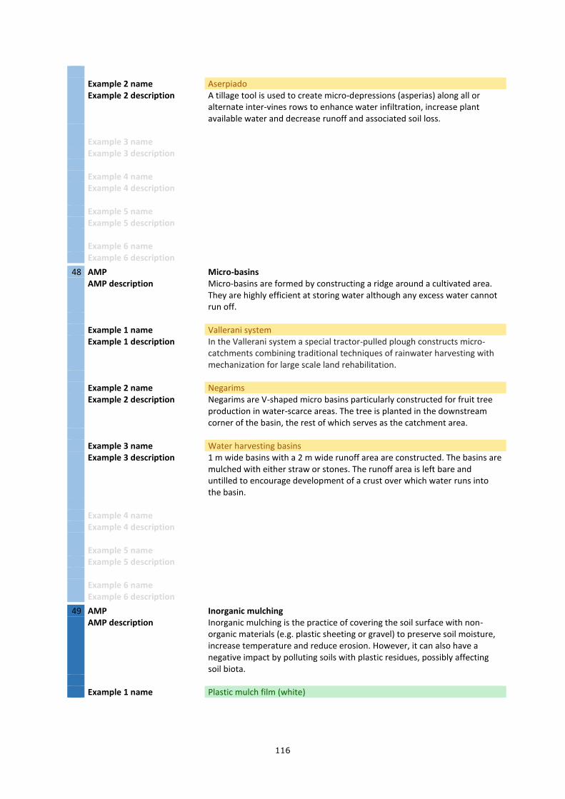
116
Example 2 name Aserpiado
Example 2 description
A tillage tool is used to create micro-depressions (asperias) along all or alternate inter-vines rows to enhance water infiltration, increase plant available water and decrease runoff and associated soil loss.
Example 3 name
Example 3 description
Example 4 name
Example 4 description
Example 5 name
Example 5 description
Example 6 name
Example 6 description
48 AMP Micro-basins
AMP description
Micro-basins are formed by constructing a ridge around a cultivated area. They are highly efficient at storing water although any excess water cannot run off.
Example 1 name Vallerani system
Example 1 description
In the Vallerani system a special tractor-pulled plough constructs micro-catchments combining traditional techniques of rainwater harvesting with mechanization for large scale land rehabilitation.
Example 2 name Negarims
Example 2 description
Negarims are V-shaped micro basins particularly constructed for fruit tree production in water-scarce areas. The tree is planted in the downstream corner of the basin, the rest of which serves as the catchment area.
Example 3 name Water harvesting basins
Example 3 description
1 m wide basins with a 2 m wide runoff area are constructed. The basins are mulched with either straw or stones. The runoff area is left bare and untilled to encourage development of a crust over which water runs into the basin.
Example 4 name
Example 4 description
Example 5 name
Example 5 description
Example 6 name
Example 6 description
49 AMP Inorganic mulching
AMP description
Inorganic mulching is the practice of covering the soil surface with non-organic materials (e.g. plastic sheeting or gravel) to preserve soil moisture, increase temperature and reduce erosion. However, it can also have a negative impact by polluting soils with plastic residues, possibly affecting soil biota.
Example 1 name Plastic mulch film (white)

117
Example 1 description
Plastic mulch film is used to suppress weeds and conserve water. Crops grow through slits or holes in the thin plastic sheeting. White or metalized films lead to cooler soil and reflection of sunlight to plants.
Example 2 name Plastic mulch film (black)
Example 2 description
Plastic mulch film is used to control weeds, retain soil moisture, save water and reduces maintenance labour. Black films prevent weed growth but do not transmit light to heat up the soil.
Example 3 name Biodegradable plastic mulch
Example 3 description
Biodegradable plastic mulches are used as an alternative to conventional polyethylene mulch and can be tilled into soil where they are expected to biodegrade.
Example 4 name Polytunnels
Example 4 description
Polytunnels are typically made from steel and covered in polythene and are usually semi-circular, square or elongated in shape. They are used to create a favourable micro-climate and protect crops from extreme conditions.
Example 5 name Gravel mulching
Example 5 description
In arid regions, light weight gravel is applied to a depth of at least 1 cm around more mature plants. The mulch reduces soil moisture loss through evaporation, while still obtaining a significant yield.
Example 6 name
Example 6 description
50 AMP Water distribution in rangelands
AMP description
The practice of managing the distribution of water resources in rangelands is crucial because forage utilization decreases rapidly as the distance to water increases. Animals will overuse sites near water locations rather than walk greater distances to abundant forage. Water requirements of grazing animals must be considered when planning water resources, and vary with species and class of animal, nature of the forage and weather.
Example 1 name Improved well distribution
Example 1 description
Water points are optimally and efficiently distributed in rangeland to ensure a balanced distribution of herds and avoid overuse of vegetation around a limited number of wells.
Example 2 name Water points fed by springs and streams
Example 2 description
Water from springs or other sources is brought to water points in pastures. This greatly increases livestock productivity and reproductive performance, reduces erosion from cattle tracks in critical locations surrounding springs, and protect springs from being destroyed by the animals.
Example 3 name Water harvesting for livestock watering point
Example 3 description
An artificial watershed (of ca. 100 m2) is installed in remote locations with poor access to water. The watershed is built from cement and drains into a well or tank to collect water during the winter for use during the dry season for livestock watering.
Example 4 name Planning water points for rotational grazing
Example 4 description
A rotational grazing scheme is introduced following the establishment of new watering points to provide water in summer. The scheme ensures longer growing times for grass recovery on pastures and increases quantity and quality of pastures.

118
Example 5 name Example 5 description
Example 6 name Example 6 description 51 AMP Drip irrigation
AMP description
Drip irrigation is a method of controlled irrigation in which water is slowly delivered to the root systems of multiple plants. Water is either dripped onto the soil surface above the roots or delivered directly to the root zone. It is often preferred to flood (surface) irrigation because less water is used and lost to evaporation.
Example 1 name Drip irrigation
Example 1 description
Drip irrigation is used to provide a constant water supply to crops, minimizing water and labour use while improving crop growth and yield. Salinization of the soil is minimized by efficient water use.
Example 2 name Low-cost drip irrigation
Example 2 description
Water is precisely delivered to crops through perforated tubes. In this low-cost drip irrigation system, the pressure is supplied by connecting the tubes to a raised water tank.
Example 3 name Polyethylene sheeting and intermittent cloth strips
Example 3 description
Polyethylene sheeting and spaced cloth strips are used to deliver water to individual plants when poor quality irrigation water could clog nozzles.
Example 4 name Subsurface drip irrigation
Example 4 description
A low-pressure, high efficiency irrigation system is used in which buried drip tubes or drip tape meet crop water needs. Subsurface drip irrigation minimizes evaporation losses and reduces weed pressure.
Example 5 name Orchard drip irrigation
Example 5 description
A network of valves, pipes, tubes and nozzles are used in an orchard drip irrigation scheme to allow water to drip directly onto the root zone of the trees.
Example 6 name
Example 6 description
52 AMP Surface irrigation
AMP description
Surface irrigation is a technique where water is applied to the soil surface and distributed by gravity. This is the most common form of irrigation, in many parts of the world virtually unchanged for thousands of years. However, the water distribution is uncontrolled and therefore inherently inefficient.
Example 1 name Furrow irrigation
Example 1 description
In furrow irrigation small parallel channels are constructed along the field length in the direction of the predominant slope. Water is applied to the top end of each furrow and flows down the field.
Example 2 name Level basin irrigation
Example 2 description
Water is applied rapidly to the entire basin and it is allowed to infiltrate. Level basin irrigation is favoured in soils with relatively low infiltration rates.
Example 3 name Border irrigation

119
Example 3 description
A field is divided into strips (usually from 6 to 30 m wide) separated by border ridges running down the slope. The area between the ridges is flooded during irrigation.
Example 4 name Laser leveling of fields
Example 4 description
Preparation of fields for irrigation with the use of a laser planner ensures uniform surface leveling. Water is distributed equally across the field providing water savings and increased yield.
Example 5 name Surge irrigation
Example 5 description
Water is pulsed on and off according to a planned schedule rather than being supplied constantly. Surge irrigation is an advanced variant of furrow irrigation.
Example 6 name Furrow irrigation with alternating dry and wet furrows
Example 6 description
Dry and watered furrows are rotated. In limited water conditions, irrigation with alternating furrows is an effective way to reduce water use while maintaining crops in good vegetative state.
Example 7 name Contour basins
Example 7 description
The field is divided into a number of terraced rectangular bays. Water is applied to the highest bay and cascades downhill through consecutive bays. Contour basins are a variant of basin irrigation.
53 AMP Pivot irrigation
AMP description
Pivot irrigation is a method of overhead crop irrigation in which equipment rotates around a pivot and crops are watered with sprinklers. An area centred on the pivot is irrigated, often creating a circular pattern in crops when viewed from above.
Example 1 name Center-pivot irrigation
Example 1 description
Irrigation pipe and sprinklers rotate round a central pivot which supplies the water. The system is used in large relatively flat fields.
Example 2 name Lateral-move irrigation
Example 2 description
A lateral-move irrigation system is configured to move in a straight line and water is supplied by an irrigation channel running the length of the field. While suited to rectangular fields, it requires complex guiding systems.
Example 3 name End gun pivot irrigation
Example 3 description
Water guns attached to the ends of a pivot system are used to effectively irrigate additional land. Relatively high pressure is needed to supply the guns with enough water.
Example 4 name
Example 4 description
Example 5 name Example 5 description
Example 6 name Example 6 description 54 AMP Sprinkler irrigation
AMP description
Sprinkler irrigation is a method of applying water that simulates natural rainfall. Water is distributed through a system of pipes, usually by pumping. It is then sprayed into the air through sprinklers so that it breaks up into small drops which fall on the ground.

120
Example 1 name Impact sprinklers
Example 1 description
Impact sprinklers are driven in a circular motion by the force of the outgoing water. They can be used to water large areas of land, albeit unevenly because the larger water drops fall closer to the sprinkler than the smaller.
Example 2 name Micro-sprinkler irrigation
Example 2 description
Small-sized water droplets are delivered through a rotating head. This micro sprinkler system allows longer watering time with less runoff.
Example 3 name Travelling big gun
Example 3 description
Water is delivered to the crop by a large-capacity, high pressure nozzle. The travelling big gun is pulled along a track in the field by a wheel that winds up the water hose.
Example 4 name Underground sprinkler system
Example 4 description
Underground sprinkler systems are installed with some effort. They are only considered to be viable for perennial crops and are often located in orchards.
Example 5 name
Example 5 description
Example 6 name
Example 6 description
55 AMP Leaching salts
AMP description
Leaching is a practical way of removing excess salts. It is effective only to the extent that water moves down through the soil profile and below the root zone. It is often accomplished by occasional excessive irrigation applications to dissolve, dilute and move the salts.
Example 1 name Continuous ponding
Example 1 description
Water is impounded using a surface irrigation method. Continuous ponding reduces water use efficiency but increases velocity of salt leaching.
Example 2 name Intermittent ponding
Example 2 description
The rise in water table following ponding is allowed to subside before water is next applied. Leaching salt with intermittent ponding is appropriate in poorly drained areas with low evaporative demand.
Example 3 name Rainwater leaching
Example 3 description
In areas where good quality water is scarce, rainwater is collected during the rainy (monsoon) period to be used for salt leaching.
Example 4 name Sprinkler leaching
Example 4 description
Sprinkler irrigation is used to leach salt with the advantage that water can be applied to unprepared fields. It is an efficient method on coarser textured soils as application losses are lower than with surface irrigation.
Example 5 name Alternate row irrigation
Example 5 description
Alternate row irrigation is used in high water table areas to reduce salt accumulation. Every other row is flooded to remove salts into the unirrigated area.
Example 6 name Example 6 description

121
56 AMP Minimizing saline water irrigation
AMP description
Applications of saline irrigation water are minimized to reduce accumulation of salts in the soil. This can be done by using water from precipitation more effectively to reduce the amount of irrigation required or by replacing saline irrigation water with better quality water from other sources.
Example 1 name Pipe irrigation
Example 1 description
Pipes are used to draw less saline water from nearby rivers in order to minimize the salinization of agricultural fields. Pipes also reduce water loss by seepage during transport.
Example 2 name Rainwater storage Example 2 description
Rainwater is stored for later use to minimize the application of saline irrigation water. This is useful in areas of irregular rainfall where irrigation is required during dry seasons.
Example 3 name Example 3 description More reliance on rainwater
More direct use is made of rainwater to reduce reliance on saline irrigation water. However, it is difficult to plan and other water conservation strategies also need to be used.
Example 4 name Example 4 description
Example 5 name Example 5 description
Example 6 name Example 6 description 57 AMP Reduced water use in rice cultivation
AMP description
Paddy rice is conventionally grown in anaerobic conditions for 80% of the growing period, requiring high amounts of irrigation water. Reduced use of water is recommended for increased productivity, adaptation to water scarcity and reduction of methane emissions (potentially offset by carbon dioxide emissions).
Example 1 name System of Rice Intensification
Example 1 description
System of Rice Intensification (SRI) is a climate-smart, agro-ecological methodology for increasing rice productivity by 1) early plant establishment; 2) reduced plant density; 3) soil enrichment with organic matter; and 4) reduced and controlled water application.
Example 2 name Rice intensification through organic rice-duck farming
Example 2 description
The usual rice farming system (seedling condition, planting distance, irrigation time and water requirement) is modified, an organic fertilization scheme is introduced, and ducks are incorporated in the system. Ducks help weeding, pest biocontrol and fertilization.
Example 3 name Alternate wetting and drying
Example 3 description
Rice fields are flooded to a depth of 5 cm then allowed to dry. They are flooded again when the water level (monitored by perforated PVC tubes) reaches 15 cm below the soil surface. The practice decreases water use while having no impact on yield, decreases methane emissions and water pump fuel consumption.
Example 4 name Aerobic rice

122
Example 4 description
Specifically developed “aerobic rice” varieties are grown in well-drained, non-puddled, and non-saturated soils. The system aims for yields of at least 4-6 tons per hectare. Crop rotation replaces flooding for weed management.
Example 5 name Saturated soil culture
Example 5 description
The soil is kept as close to saturation as possible by shallow irrigations (of about 1 cm floodwater) a day or so after the disappearance of standing water. It leads to water savings at slight yield impact (4-9%).
Example 6 name Example 6 description
58 AMP Irrigation optimization
AMP description
Irrigation optimization is a water-saving scheme using precise irrigation scheduling. Irrigation system managers determine the correct frequency and duration of watering to minimize costs and maximize yields.
Example 1 name Soil sensor network
Example 1 description
Sensors are used to measure soil moisture and temperature at different depths in the rooting zone. The farmer can retrieve the data at any time using his mobile phone or computer.
Example 2 name Portable soil moisture sensor
Example 2 description
Soil moisture sensors are used by the farmer to manage seasonal water application. This smart irrigation is essential to refine irrigation techniques and to meet specific soil and crop needs.
Example 3 name Local agreements on irrigation management
Example 3 description
Local agreements between water users are made to prevent and manage conflicts concerning irrigation water. Under conditions of water scarcity, agreements ensure that irrigation water is used rationally and sustainably.
Example 4 name Alternate wetting and drying
Example 4 description
Irrigation is only supplied to a (rice) field whenever the soil moisture content reaches a certain level. This scheduling reduces water input without significantly affecting the yield.
Example 5 name
Example 5 description
Example 6 name
Example 6 description
59 AMP Supplemental irrigation
AMP description
Supplemental irrigation is the addition of small amounts of water to rainfed crops during times when rainfall is insufficient for normal plant growth in order to improve and stabilize yields.
Example 1 name Cisterns and water tanks
Example 1 description
Cisterns and water tanks are used to store rainfall and runoff water for multiple purposes such as drinking water for human and animal consumption and supplemental irrigation.
Example 2 name Plastic-lined pond
Example 2 description
A plastic-lined pond is created to store water for irrigating crops in periods of low rainfall when plant growth would be otherwise limited.

123
Example 3 name Deficit irrigation
Example 3 description
A moderate plant water deficit is maintained to improve the quality of some crops such as grapes. While irrigation scheduling is often used to maintain soil water content near field capacity, deficit irrigation requires accurate soil moisture or plant 'stress' sensing, the ability to estimate crop water demand, and the ability to irrigate frequently.
Example 4 name Off-season irrigation
Example 4 description
Supplemental water is applied to fields and pastures during the off-season pre-seeding period when irrigation water is available and not being used by other farmers. Water accumulates at depths of 1.5-2 m in the soil and is available for pasture and crop growth in spring and early summer.
Example 5 name
Example 5 description
Example 6 name
Example 6 description
60 AMP Artificial grassed or paved waterways
AMP description
A grassed waterway is a natural or constructed ditch, usually broad and less steeply sloping than the rest of the field. It is used to conduct surface water from or through cropland, enhancing infiltration, trapping eroded sediment and helping prevent the development of gullies.
Example 1 name Grassed waterways
Example 1 description
Grassed waterways are constructed along natural drainage lines in a field or in an existing watercourse to control erosion. They reduce damage from storm events to agricultural fields.
Example 2 name Paved waterways
Example 2 description
An artificial drainage channel, lined with stones, is constructed along the steepest slope. This paved waterway receives runoff from cutoff drains and graded structures, discharging it to the natural waterway without causing erosion.
Example 3 name Controlled waterways
Example 3 description
Bio-engineered retaining walls are built using bamboo poles, rocks and soil-filled sacks across the slope and strengthened by grass planted on top. Erosion is reduced during the rainy season and water is conserved during the dry season.
Example 4 name Sunken gully pits
Example 4 description
Sunken gully pits are dug to trap water, enhance groundwater recharge and to reduce flow velocity. These pits are often provided with spillways for excess water runoff.
Example 5 name
Example 5 description
Example 6 name
Example 6 description
61 AMP Liquid manure or slurry
AMP description
Application of liquid manure is a common method for supplying nutrients. It also forms a thin layer on the soil surface to protect from wind erosion. There is a potential risk of eutrophication affecting water quality.

124
Example 1 name Land surface spreading
Example 1 description
Manure is spread on the soil surface as a convenient way to fertilize fields. However, uneven distribution, soil compaction, nitrate leaching and runoff are issues that should be taken into account.
Example 2 name Manure irrigation
Example 2 description
Liquid manure (effluent) is applied to cropland through a sprinkler irrigation system. Manure irrigation is likely to result in uneven application and poses threats like surface runoff and environmental pollution.
Example 3 name Slurry injection
Example 3 description
Using a specialized implement, slurry is injected in narrow bands directly into the soil or on the soil surface, often underneath the crop canopy. Slurry injection is one of the most affordable ways for farmers to fertilize their fields and reduces odour, nutrient runoff and gaseous emissions.
Example 4 name Umbilical slurry injection
Example 4 description
An injection system with an umbilical pipe is used to inject slurry into the soil. The practice reduces the threat of soil compaction and allows use of lighter tractors.
Example 5 name Real-time slurry analysis
Example 5 description
NIR sensors are used to measure the components of the slurry during tank filling or application, allowing more precision in manure application. Application rates can also be adjusted to crop performance on a field.
Example 6 name Example 6 description
62 AMP Animal manure
AMP description
Animal manure is commonly applied to supply nutrients to a field. Addition of organic matter is generally a secondary objective, but it is an important way of avoiding soil organic matter depletion. There is a potential risk of eutrophication affecting water quality.
Example 1 name Farmyard manure
Example 1 description
Farmyard manure is a mixture of dung, urine, bedding material and fodder residues left to decompose for > 4 months. It is spread using a rear discharge spreader or wheelbarrow and incorporated into the soil to increase soil fertility and structure.
Example 2 name Chicken manure
Example 2 description
Chicken manure should be mixed with straw before application. It contains high levels of nitrogen, phosphorus and potassium and improves soil structure. It can also be used for composting.
Example 3 name Corralling
Example 3 description
Animals are corralled on cropland for the mutual benefit of both crop farmers and pastoralists. Crop residues are used as fodder and animal dung is used as a fertilizer.
Example 4 name Manure application in dripper points
Example 4 description
Manure is annually applied to holes dug at the foot of orchard trees underneath the nozzle locations of a drip irrigation system. This enhances soil organic content over the long term, impacting orchard productivity and making the trees less prone to pests and diseases.
Example 5 name

125
Example 5 description
Example 6 name
Example 6 description
63 AMP Compost
AMP description
Composting is decomposing organic matter for recycling as a fertilizer and soil amendment. Compost is a key ingredient in organic farming.
Example 1 name Compost (making and) application
Example 1 description
Farmyard manure, a mixture of dung, urine, bedding material and fodder residues, is left to decompose for > 4 months. It is spread on the soil using a rear discharge spreader or wheelbarrow and incorporated to increase soil fertility and structure.
Example 2 name Vermicompost (making and) application
Example 2 description
Vermicompost is produced by the decomposition of organic waste at ambient temperature through the synergistic actions of earthworms and microbes. It has a high nutrient content and contains beneficial soil microorganisms, humic acids and enzymes.
Example 3 name Anaerobic digestate
Example 3 description
Biodegradable materials are decomposed in a controlled manner in the absence of oxygen. Digestate and methane are the end products. Digestate may be separated in solid and liquid fractions.
Example 4 name Carbon enrichment with industrial organic waste recycling
Example 4 description
Agricultural soils are enriched with locally available industrial organic matter waste (e.g. sugarcane filter cake, sawdust, coarse wood chips). Such carbon enrichment is a win-win solution for organic matter waste recycling and soil quality.
Example 5 name Micronized organic fertilizers
Example 5 description
Specifically developed micronized organic fertilizers are applied through an irrigation system. Before and/or after fertigation, irrigation lines should be cleaned by flushing with water.
Example 6 name
Example 6 description
64 AMP Biochar
AMP description
Biochar is produced from pyrolysis (thermal decomposition of biomass in partial or total absence of oxygen) of plant and waste feedstock and is used as a soil amendment. Biochar is a stable solid, rich in carbon and can have benefits for plant growth. Its particle size distribution and carbon storage fertilizer (P, K, S, and Mg only) and liming properties vary.
Example 1 name Biochar application for carbon sequestration
Example 1 description
Biochar is applied every few years to increase carbon sequestration. In order to contribute to climate regulation, the quality of the pyrolysis process, its carbon storage value, application rate and deep incorporation in the soil are important. Improved productivity may avoid future need for further land conversion.
Example 2 name Biochar application for land restoration
Example 2 description
Biochar is used as a soil amendment for land restoration. It can enhance the cation exchange capacity and absorb nutrients for slow release. Initially it is

126
important to mix biochar with nutrient-rich organic material such as manure or compost. The largest effect on yield is seen on degraded land.
Example 3 name Biochar application for prevention of nutrient leaching and pollution
Example 3 description
Biochar is applied to soil to prevent nutrient leaching. It can also raise the pH and reduce problems with aluminum toxicity and heavy metals. However, due to strong sorption of pesticides, increased pesticide concentrations can also build up.
Example 4 name Biochar application to make dryland agriculture more resilient to drought
Example 4 description
Biochar is applied to soils to make dryland agriculture more resilient to water deficiency. Acting over a long period, biochar improves soil moisture and nutrient capacity, activates microorganisms and raises pH.
Example 5 name
Example 5 description
Example 6 name
Example 6 description
65 AMP Biofertilizers
AMP description
A biofertilizer is a substance containing living micro-organisms. When applied to seeds, plant surfaces or soil the organisms colonize the rhizosphere or the interior of the plant, promoting growth by increasing the supply or availability of primary nutrients.
Example 1 name Rhizobium inoculation
Example 1 description
Rhizobium inoculation is used to ensure adequate nitrogen (N) for legumes. Rhizobium infects the roots of leguminous plants and produces nodules where it fixes nitrogen gas from the atmosphere, which becomes available to the host plant.
Example 2 name Azospirillum / Azotobacter inoculation
Example 2 description
Azospirillum and Azotobacter inoculation is used in various cereals and other crops. They are nitrogen-fixing bacteria that live around the roots of plants in a rhizosphere association. The bacteria feed on plant exudates while promoting plant growth.
Example 3 name Blue Green Algae inoculation
Example 3 description
Blue green algae (Anabaena) inoculation is used for paddy rice. Anabaena in association with water fern (Azolla) fixes 60 kg N/ha/season and also enriches soils with organic matter.
Example 4 name Mycorrizhae
Example 4 description
Mycorrizhae inoculant is applied when seeding crops or pasture. Mycorrhizae are able to create a vast connective network between the roots of a plant and the soil around them, which allows the fungus to uptake nutrients such as nitrogen and phosphorus for the plant and increase the surface area of the roots.
Example 5 name Phosphate solubilizing bacteria
Example 5 description
Soil is inoculated with phosphate solubilizing bacteria (PSB) capable of dissolving inorganic phosphorus from insoluble compounds. As P-fertilizer is rapidly immobilized, PSB soil inoculum plays an important role in making P available for crops.
Example 6 name
Example 6 description

127
66 AMP Inorganic fertilizers
AMP description
Inorganic fertilizers (e.g. N, P and K or micro-nutrients like boron, copper, cobalt) are applied either singly or mixed to enhance plant growth. Overfertilization may lead to pollution.
Example 1 name Broadcast fertilizer application
Example 1 description
Fertilizer is broadcast spread on field crops, with or without being incorporated into the soil. A first (basal dressing) application is made at the time of planting/seeding and, in some crops, a top dressing of nitrogenous fertilizer is given to growing plants.
Example 2 name Band placement and side dressing
Example 2 description
Fertilizer is applied in bands where developing roots will easily reach it (e.g. 5 cm to the side and below the seed row). Band placement is more localized and reduces nutrient losses. When row crops develop, further fertilizer may be given as a side dressing.
Example 3 name Slow- and controlled-release fertilizers
Example 3 description
A single pre-planting application of a slow- or controlled-release fertilizer is made to ensure gradual or staged availability of nutrients for efficient plant growth. Such fertilizers lower operational costs and reduce losses.
Example 4 name Microdosing
Example 4 description
Fertilizer (NPK 16-16-16; or DAP) is applied at a micro-dose of 0.3 g per planting station. This is equivalent to 3-8 kg fertilizer/ha, depending on planting pattern. Microdosing is combined with seed priming (soaking seeds for 8 hours prior to sowing) to boost yield.
Example 5 name Fertigation
Example 5 description
In fertigation fertilizers, soil and water amendments and other water-soluble products are injected into an irrigation system. Fertigation allows continuous, gradual fertilization of crops.
Example 6 name Foliar application
Example 6 description
Foliar sprays are widely used to apply micronutrients (especially iron and manganese) to many crops. Foliar application is also an effective way to remediate nutrient deficiencies as and when they become apparent.
67 AMP Green manure
AMP description
Green manure or catch crops are rotation crops that are ploughed into the soil or spread on it rather than being harvested. They provide nutrients and organic matter for the subsequent crop. Growing green manure is crucial for maintenance or improvement of soil fertility.
Example 1 name Tancy Phacelia
Example 1 description
Tancy Phacelia is grown as a green manure. It is an annual species native to drylands, and adds organic matter, nitrogen and other nutrients to the soil while at the same time decreasing weeds.
Example 2 name Mexican Sunflower
Example 2 description
Leaves of the Mexican sunflower (Tithonia diversifolia) are used as a green manure. The sunflower grows along roadsides or farm boundaries and its leaf has a high nitrogen and phosphorus content.
Example 3 name Sesbania

128
Example 3 description
Sesbania is grown as a green manure. It is a versatile species primarily used between rice crops or as an intercrop in transplanted rice. It enhances soil structure and soil fertility.
Example 4 name Sorghum
Example 4 description
Sorghum is used in green house cultivations as a green manure in crop rotation (e.g. with tomato plants). It aims to reduce pest cycles and soil borne diseases while improving soil structure and nutrient content.
Example 5 name Green manure in orchards
Example 5 description
Nitrogen-fixing green manure species are planted around orchard trees. This is an ecological option to maintain and enhance soil fertility.
Example 6 name
Example 6 description
68 AMP Leguminous crops
AMP description
Leguminous crops are those which belong to the pea family (Leguminosae). Plants in this family generally have root nodules hosting rhizobium bacteria that fix nitrogen from the atmosphere. When plant residues decompose, this fixed nitrogen can increase soil nitrogen content.
Example 1 name Leguminous annuals
Example 1 description
Leguminous annuals (such as crimson clover, hairy vetch and field peas) are used in a crop rotation to fix nitrogen in the soil for the next year or growing season.
Example 2 name Fodder legumes
Example 2 description
Leguminous crops are often used as a relay crop or intercropped with maize, millet and rice to enhance the soil fertility. Fodder legumes are viable alternatives in regions with an established diary industry.
Example 3 name Leguminous crop in plots temporarily set outside the crop rotation
Example 3 description
A plot is cultivated with perennials legumes and set temporarily outside the crop rotation for 4-5 years to recover its soil fertility and reduce the need for biocides while providing supplemental income.
Example 4 name Leguminous perennials
Example 4 description
Leguminous perennial crops (such as red, white and sweet clover) are used to fix nitrogen in the soil for the next couple of years.
Example 5 name Leguminous shrubs
Example 5 description
Leguminous shrubs and trees are used to fix nitrogen to the soil for multiple years. These species often also enhance the biodiversity in an area but are not commonly used within agricultural practice.
Example 6 name Leguminous tree shelterbelts
Example 6 description
Barriers of leguminous trees or shrubs are established along field boundaries to provide a favourable micro-climate and protect against wind erosion. They also enhance soil properties by fixing nitrogen to the soil and providing organic matter.
69 AMP Retaining crop residues
AMP description
The practice of retaining crop residues involves keeping crop stubble on the field, rather than removing it. This can offer many benefits including increased soil organic matter, improved soil structure and plant nutrient cycling.

129
Example 1 name High stubble cutting height
Example 1 description
High stubble cutting height is used to leave more organic material on the field and reduce the time taken to harvest the crop. For increased nutrient cycling and disease control the stubble is chopped and incorporated into the soil.
Example 2 name Stubble management
Example 2 description
Crop residues are chopped and incorporated in the topsoil where they decompose. Properly used this leads to higher soil fertility and less disease. However, an excessive amount of stubble can obstruct subsequent seeding operations.
Example 3 name Residue incorporation
Example 3 description
Crop residues are left on agricultural fields. Incorporating residues in the soil will enhance organic matter content and improve the soil structure.
Example 4 name Return process residues
Example 4 description
Process residues (such as husks, seeds, bagasse and roots) are returned to the field as fertilizers or animal fodder.
Example 5 name Example 5 description
Example 6 name Example 6 description 70 AMP In situ composting
AMP description
In the practice of in situ composting crop residues, green and farmyard manures, organic waste and ashes are composted in the field in trenches or pits. Crops are directly grown on or next to the pits which also serve to harvest rainwater and regulate soil moisture. Organic matter recycling like this can be developed into a circular system, depending on what materials are available locally.
Example 1 name In situ compost cultivation
Example 1 description
Trenches (0.6 m x 0.6 m and 0.9 m apart) are dug across the slope, filled with organic residues and backfilled with soil until slightly below the soil surface to capture runoff. Water and nutrient demanding crops are grown in the trenches, leguminous crops in between.
Example 2 name Kibanja cropping system
Example 2 description
Compost pits (3x3 m in size and 0.6 m deep) are dug between 4 widely spaced banana plants and filled with farm manure, crop residues and ash. They are covered with soil to activate nutrient release though microbial disintegration and avoid volatilization of greenhouse gases.
Example 3 name
Example 3 description
Example 4 name
Example 4 description
Example 5 name Example 5 description
Example 6 name Example 6 description

130
71 AMP Mulching with pruning materials
AMP description
Mulching with pruning materials (such as chipped branches) is an effective soil management practice to reduce surface runoff, conserve soil moisture and control water erosion. Prunings have several advantages over other mulching materials such as low cost and ready availability, especially in orchards.
Example 1 name Bark mulch
Example 1 description
Bark mulch is applied to the bare soil surrounding trees in orchards. It is a relatively cheap method of suppressing and controlling weed growth, while at the same time retaining soil moisture and enhancing fertility.
Example 2 name Chipped branches
Example 2 description
Chipped branches from trees are used to cover bare soil, reducing surface water runoff after heavy rainfall and increasing soil organic matter content through decomposition.
Example 3 name Leaf prunings
Example 3 description
Leaf prunings (e.g. from bananas) are applied to the soil surface, enhancing organic matter content, reducing evaporation and protecting against erosion.
Example 4 name Wood chips
Example 4 description
Wood chips are used as a soil mulch. Because they are a highly resistant organic material, wood chips are ideal for increasing stable organic matter in the soil. Once incorporated, wood chips are slowly broken down by the soil fauna and (partly) converted into humus.
Example 5 name
Example 5 description
Example 6 name
Example 6 description
72 AMP Straw mulching
AMP description
Straw mulching is the practice of spreading a layer of straw on the soil surface. The straw can be the residue from a harvested crop or sourced from elsewhere. The practice aims to conserve moisture, improve fertility and health of the soil and reduce weed growth.
Example 1 name Grass mulch
Example 1 description
Grass mulch is applied to the soil surface to reduce moisture stress, increase soil water retention, reduce soil erosion and improve soil organic matter content with the aim of increasing crop productivity.
Example 2 name Straw mulch
Example 2 description
Straw mulch is applied to the soil surface. It is effective weed control and soil erosion prevention, conserves moisture and increases soil organic matter content.
Example 3 name Spreading straw residues
Example 3 description
Rice straw is left on the field after mechanized harvesting. Successive crops benefit from increased moisture and nutrient levels in the soil.
Example 4 name
Example 4 description
Example 5 name

131
Example 5 description
Example 6 name
Example 6 description
73 AMP Mechanical weed control
AMP description
Mechanical weed control is the physical removal of weeds by mowing, cutting and pulling. Other alternatives include using hot water, a flame thrower or laser.
Example 1 name Duckfoot-bladed hoe
Example 1 description
The duckfoot-bladed hoe is often used in tractor-pulled cultivators, but a single hoe can also be used manually to get rid of the weeds which are not too close to the crops.
Example 2 name Finger weeder
Example 2 description
When the crop is at a mature stage (with a well-developed root system) a finger weeder is used to remove weeds that grow within difficult to access crop rows.
Example 3 name False seedbed technique
Example 3 description
A regular seedbed is created but, before it is used, the weeds are allowed to germinate and are mechanically removed before the actual crop is planted or sown.
Example 4 name Interrow cultivator
Example 4 description
Interrow cultivators are used to accurately hoe between rows of growing crops to cut off the weeds just below the surface. Interrow cultivators are fully adjustable and configured to suit any row width or combination of widths.
Example 5 name Weed flame throwers
Example 5 description
Weed flame throwers are used to burn weeds on a plot prior to seeding/planting as an effective method of removing them. When used in dry areas extra care should be given to the surrounding environment to avoid wildfires. There are also selective inter-row flame weeders.
Example 6 name Wheel hoe
Example 6 description
A wheel hoe is used in smaller plots to remove weeds between crop rows. It is a cheaper version of the duckfoot-bladed hoe.
Example 7 name Mowing
Example 7 description
Mowing is used as an effective weeding method if the weeds do not have to be removed completely and the crop is not at risk of being damaged by the operation. Swing-arm mowers are particularly well-suited to mowing perennial crops.
Example 8 name Weed control using steam
Example 8 description
Steam is used to set back weed development with heat but without additional fire risk. Due to the latent heat of condensation it provides rapid heat transfer and it can operate well in windy and wet conditions.
74 AMP Chemical weed control
AMP description
Chemical weed control is the removal of weeds using herbicides of different types (e.g. emergence and contact herbicides). Herbicides can pollute soils and water and might affect soil and aquatic life.
Example 1 name Selective herbicides

132
Example 1 description
Selective herbicides are used to destroy only weeds without harming the crop. Their selectivity is based on translocation, differential absorption, physical or physiological differences between plant species.
Example 2 name Non-selective herbicides
Example 2 description
Non-selective herbicides are often used to clear waste land. They eradicate all plant material they come into contact with. It is important that the herbicides applied pose a minimal risk (through contamination of groundwater, air or crops) to public health.
Example 3 name Organic herbicides
Example 3 description
Organic herbicides are usually used alongside mechanical weed control. They are often non-selective and potentially replace synthetic herbicides, though may be less effective.
Example 4 name Vinegar application
Example 4 description
Vinegar solutions (of 5-20%) are used to control weeds. However, vinegar mainly destroys surface growth and often the root system remains intact. Repeated treatment is therefore recommended.
Example 5 name Example 5 description
Example 6 name Example 6 description
75 AMP Biological weed control
AMP description
Biological weed control uses other organisms to remove or control the weeds. It relies on predation, parasitism, herbivory or other natural mechanisms and typically also involves an active human management role.
Example 1 name Animal grazing
Example 1 description
Herbivores with different preferences can be used to control certain weeds. Goats are browsers that can control toxic or thorny plants (e.g. leafy spurge, knapweed). Care should be taken that grazing animals do not feed on crops.
Example 2 name Grazing as part of integrated weed control practice
Example 2 description
Sheep are used to graze vineyards during autumn and winter when the vines are dormant. This is an example of an integrated weed control practice.
Example 3 name Biological control agents
Example 3 description
The alligator weed flea beetle (Agasicles hygrophila) is used as an agent for the biological control of the aquatic plant alligator weed.
Example 4 name Mycoherbicides
Example 4 description
Fungi (like Chondrostereum purpureum and Lasiodiplodia pseudotheobromae) are applied as mycoherbicides to 'weed' trees. The fungus is applied directly to the trees in a nutrient paste or inserted as a capsule in the stem.
Example 5 name Conservation biocontrol
Example 5 description
Existing natural enemies of weeds and other pests are protected or provided with habitats. This conservation biocontrol is the main strategy for promoting weed seed removal by predators and microorganisms.
Example 6 name
Example 6 description

133
76 AMP Biological pest control
AMP description
Biological pest control is a method of controlling pests (such as insects, mites, weeds and plant diseases) using other organisms. It relies on predation, parasitism, herbivory, or other natural mechanisms, but typically also involves an active human management role.
Example 1 name Importation of natural predators
Example 1 description
A pest’s natural enemies (e.g. beetles or larvae) are introduced to a new locale. It is important to note that this kind of introduction may have additional consequences.
Example 2 name Improve habitat for native fauna
Example 2 description
Pests can be controlled and combatted by improving the habitat for fauna, thus attracting native predators, parasites or herbivores. Active management is required to (re-) establish and maintain the native fauna.
Example 3 name Inductive augmentation
Example 3 description
Natural predators (e.g. ladybirds) of a particular pest (e.g. aphids) are released to augment the predator population in an area.
Example 4 name Hoverflies
Example 4 description
Hoverflies (syrphids) are used as a biological pest control. In their larval stage hoverflies are capable of consuming vast amounts of small-soft-bodied insects daily.
Example 5 name Green lacewings
Example 5 description
After they have hatched, the larvae of Green lacewings are distributed by sprinkling. They feed on aphids, small worms, eggs, mites and thrips.
Example 6 name Beneficial nematodes
Example 6 description
Beneficial nematodes (such as the Heterorhabditis bacteriophora) are applied to control different beetle larvae in the soil. The nematodes use the larvae as hosts, killing them in the process.
Example 7 name Push-Pull integrated pest management
Example 7 description
In an area affected by stemborer moths, maize is intercropped with a repellent “push” plant (e.g. desmodium). The plot is surrounded by an “pull” plant (e.g. napier grass), attractive to the moths but which secretes a sticky substance trapping their larvae.
77 AMP Physical pest control
AMP description
Physical pest control is a method of removing insects and small rodents by trapping, setting up barriers or kaolin sprays to prevent further crop damage. It also includes controlling pests before plants are sown.
Example 1 name Insect traps
Example 1 description
Coloured traps emitting pheromones are set up in agricultural fields to attract and kill flying insect pests. These traps are intended to provide an effective replacement for expensive insecticides.
Example 2 name Tree bufferzone
Example 2 description
Indigenous trees are used to create a buffer zone between fields, preventing the spread of diseases. The trees also enhance the biodiversity of the area.
Example 3 name Kaolin spray

134
Example 3 description
Kaolin (a clay mineral) is sprayed onto tree and vegetable crops. The spray leaves a particle film that protects from pests and environmental stresses.
Example 4 name Rodent traps
Example 4 description
Traps are placed at strategic locations to capture or kill rodents that often cause serious harm to crops and plants.
Example 5 name Fences
Example 5 description
Fences are constructed from (typically locally grown) wooden poles and galvanized iron netting (for example to keep wild boars off pasture).
Example 6 name Nets and nethouses
Example 6 description
Nets are used in fruit cultivation to protect against birds. A net house is a structure that is enclosed by a nylon net (like a mosquito net) protecting vegetables from insects and damage by rainfall, wind and sunlight.
Example 7 name Temporary inundation
Example 7 description
Bulb fields are temporarily inundated to clear the soil of nematodes, weeds and bulb residues. Inundation reduces the use of chemical pesticides and the submerged plots are popular with birds attracted by mosquito larvae, worms, and water fleas.
78 AMP Chemical pest control
AMP description
Chemical pest control uses pesticides to control pest populations. Pesticides can be sprayed or added as seed dressings. Application of pesticides may contaminate soil and water, and might have negative impacts on soil and aquatic life.
Example 1 name Systemic insecticides
Example 1 description
Systemic insecticides are applied as a drench to the crop or as a granule to the soil. They are water soluble and become absorbed and distributed systemically throughout the whole plant. When insects feed on the plant, they ingest the insecticide.
Example 2 name Contact insecticides
Example 2 description
Contact insecticides are commonly sprayed onto the crop. They are designed to be toxic upon direct contact with insects and include inorganic insecticides (containing metals and sulfur), organic insecticides (synthetically produced) and natural insecticides (like pyrethrum and neem oil).
Example 3 name Insect growth regulators
Example 3 description
Insect growth regulators (such as Diflubenzuron which is used to control caterpillars and Hydroprene which is used to control cockroaches and moths) are used to control insect populations. IGRs makes use of insect hormones to inhibit their growth.
Example 4 name Rodenticides
Example 4 description
Rodenticides are used to reduce rodent populations by poisoning them via ingestion, either being lethal after one exposure or multiple exposures. Rodents are sometimes very harmful for agriculture.
Example 5 name Botanical pesticides
Example 5 description
Tree rosin, oleoresin (produced by conifer species) and neem oil are applied as botanic pesticides. These are some of the many organic compounds produced by plants to defend themselves from predation.
Example 6 name

135
Example 6 description 79 AMP Physical disease control
AMP description
Physical disease control involves targeted applications of hot water, steam, hot air, fire or flooding to combat plant diseases. It can also include actions and barriers to avoid contamination.
Example 1 name Hot water seed treatment
Example 1 description
Seeds are treated with hot water as an effective way to kill pathogens (especially bacteria and viruses) without affecting seed quality.
Example 2 name Soil solarization
Example 2 description
The soil surface is covered with transparent plastic film, taking advantage of solar radiation to heat the soil to temperatures that are lethal to many fungal pathogens and nematodes.
Example 3 name Soil steam sterilization
Example 3 description
Soil in open fields or greenhouses is sterilized using steam. The steam kills plant pathogens (bacteria, fungi, viruses) by causing vital cellular proteins to unfold.
Example 4 name Burning crop and pruning residues
Example 4 description
For diseases for which no cure exists, infected crop and pruning residues are burned as a last resort option. Burning is an effective control of all kinds of pathogens.
Example 5 name Flooding
Example 5 description
Temporary flooding is used as an effective method to control plant-parasitic nematodes and other soilborne pathogens.
Example 6 name Cleaning farming equipment
Example 6 description
Farming equipment is cleaned to remove contaminated debris and soil that can harbor pathogens (such as Verticillium or nematodes) and prevent their introduction into non-infested fields.
Example 7 name Pre-harvest fruit bagging
Example 7 description
Bags are placed around the growing fruit as a means of physical protection. They: improve the visual quality of fruit by promoting skin colouration, reducing blemishes, sunburn and cracking; change the micro-environment for fruit development; reduce the incidence of disease, insect and bird damage; and reduce agrochemical residues.
80 AMP Chemical disease control
AMP description
Chemical disease control is the application of pesticides to combat plant diseases. There are numerous pesticides available for different diseases. Application of pesticides may pollute soils and water and affect soil and aquatic life.
Example 1 name Treated seeds and planting materials
Example 1 description
Seeds or planting materials are treated with fungicides for protection against fungi causing seed rot, seedling rot (damping off) and seedling diseases, especially when planted in cold, wet fields.
Example 2 name Soil-applied fungicides
Example 2 description
Soil-applied fungicides are used to control soilborne diseases (such as Rhizoctonia solani (black scurf) and Phytophthora erythroseptica (pink rot) in potatoes) either prior to seeding or by in-furrow application during seeding.

136
Example 3 name Foliar fungicides
Example 3 description
Fungicides are applied to the plant leaves prior to pathogen establishment or appearance of symptoms as a method of controlling disease. Systemic fungicides can eradicate specific pathogens even after they have become established in the host tissue.
Example 4 name Injecting pesticides
Example 4 description
Systemic pesticides are injected directly into the xylem of perennials. They are distributed throughout the plant with the transpiration stream to protect against pathogens.
Example 5 name Applying antibiotics
Example 5 description
Antibiotics (substances produced by micro-organisms that are capable of destroying or injuring living organisms) are used to combat several bacterial plant infections. The relatively rapid build-up of resistance is problematic.
Example 6 name Soil fumigation
Example 6 description
Fumigants are used before planting in order to eradicate nematodes and fungi in the soil profile. The practice carries a high environmental risk (because of toxicity and dosage of fumigants used) and is strictly regulated.
81 AMP Biological disease control
AMP description
Biological disease control is the suppression of diseases caused by organisms by one or more other organisms (often referred to as natural enemies). This may involve disease-resistant plant varieties, or the purposeful utilization of introduced or resident living organisms to suppress the activities and populations plant pathogens.
Example 1 name Choosing disease-resistant varieties
Example 1 description
Disease-resistant plants are chosen to eliminate the need for additional efforts to reduce losses caused by a specific disease. Resistant plants are developed using standard breeding procedures (selection and/or hybridization) or through genetic engineering.
Example 2 name Biofungicides
Example 2 description
Biofungicides (based on Trichoderma viride) are used for seed and soil treatment to suppress various diseases caused by fungal pathogens (e.g. Rhizoctonia, Pythium, Armillaria).
Example 3 name Antagonistic bacteria as nematicide
Example 3 description
Pasteuria nishizawae (an obligate bacterial pathogen of the soybean cyst nematode) is added as a seed treatment causing immediate infection, stopping the nematode feeding and reproducing and ultimately killing it.
Example 4 name Antibiotic suppression
Example 4 description
Antibiotics are applied to the crop by spray, with ground equipment or added into an irrigation system. They are microbial toxins, some of which have been shown to be particularly effective at suppressing plant pathogens and the diseases they cause (e.g. Bacillus Amyloliquefaciens, Pseudomonas fluorescens).
Example 5 name Antagonistic bacteria outcompeting pathogenic ones
Example 5 description
Non-pathogenic soil bacterium (Rhizobium rhizogenes, strain K1026) is applied by spraying or soaking. It colonizes wounded plant tissue and blocks infections by the predominant crown gall-causing pathogenic agrobacteria that infect nut trees (almonds, walnuts), stone fruit trees (peach, plum, apricot, cherry), roses, euonymus and many other horticultural crops.

137
Example 6 name Grafting
Example 6 description
Plants with a higher resistance to pest and diseases are produced by grafting seedlings onto resistant root stocks of other plants (e.g. courgette onto wild eggplant).
82 AMP Phytoremediation
AMP description
Phytoremediation (including phytostabilization, phytodegradation, phytoextraction and phytovolatilization) is the practice of using living green plants to immobilize or adsorb contaminants from polluted soil. It is a cost-effective and environmentally friendly approach to tackling contamination issues.
Example 1 name Phytoextraction using Indian mustard
Example 1 description
Indian mustard (Brassica juncea) is planted in areas contaminated with heavy metals. It produces high quantities of biomass in which a range of heavy metals are hyperaccumulated or volatilized. Aboveground parts can be removed (phytoextraction) while roots contribute to phytostabilization.
Example 2 name Phytoextraction and phytodegradation using willow short-rotation coppice
Example 2 description
Willow (Salix sp.) is grown to remediate soil contaminated with heavy metals including zinc, nickel and cadmium. It is a fast-growing species that is also effective for phytodegradation of organic pollutants and as a bio-energy crop.
Example 3 name Phytoextraction and phytodegradation using poplar short-rotation coppice
Example 3 description
Poplar (Populus sp.) is grown in a short-rotation coppice. Due to its extensive root system, high water uptake, rapid growth and large biomass production it is effective for phytodegradation of organic pollutants, as a phytoextraction strategy for most heavy metals and is a valuable bio-energy crop.
Example 4 name Phytodegradation of pesticides using Indian grass
Example 4 description
Indian grass (Sorghastrum nutans) is grown with other grass species on contaminated soil. Indian grass is tolerant of most herbicides and of climatic extremes. In mixed stands it develops a rhizosphere with microflora that can readily detoxify pesticide residues and reduce rates of pesticide leaching.
Example 5 name Phytoextraction using sunflower
Example 5 description
Sunflowers (Helianthus Annuus) are grown to remediate soils contaminated with heavy metals such as cadmium, chromium, lead and zinc. The plants accumulate the metals in their shoots and leaves (phytoextraction).
Example 6 name Phytostabilization using Miscanthus
Example 6 description
Miscanthus is a perennial grass grown on soils contaminated with heavy metals. Revenue can be obtained with this green-energy crop without presenting a risk to human or animal health while heavy metals are stabilized.
Example 7 name Phytovolatilization of arsenic using Pteris vittata
Example 7 description
The Chinese ladder brake fern (Pteris vittate) is grown to rehabilitate soil contaminated with arsenic. The fern is a hyperaccumulator of arsenic, volatizing 90% of what it takes up so no removal of plant parts is needed. It requires subtropical growing conditions.
83 AMP Integrated pest and disease management

138
AMP description
Integrated pest and disease management is a broad-based approach that considers all available pest and disease control techniques and integrates appropriate measures. The aim is to discourage the development of pest populations and diseases, keeping interventions to levels that are economically justified, and reducing or minimizing risks to the environment, soil and aquatic life and human health.
Example 1 name Pest and disease monitoring
Example 1 description
Several tools are available for pest and disease monitoring including apps for disease recognition and sticky traps for insect monitoring. Monitoring is the basis for integrated pest and disease management.
Example 2 name Push-Pull integrated pest and soil fertility management
Example 2 description
In an area affected by stemborer moths, maize is intercropped with a repellent “push” plant (e.g. desmodium). The plot is surrounded by an “pull” plant (e.g. napier grass), attractive to the moths but which secretes a sticky substance trapping their larvae.
Example 3 name Pheromone dispensers
Example 3 description
Pheromone dispensers are used to disrupt the mating of certain insects (e.g. moths in vineyards) in order to increase yield while at the same time preserving biodiversity and the sensitive balance of the ecosystem. Pheromone use diminishes the need for insecticides.
Example 4 name Winter food fields
Example 4 description
Winter food fields are not harvested and ploughed until the following spring. They serve as an important food source of grains and herbs and provide refuge for wintering field birds and mice. A more complete food web develops, ensuring lower sensitivity to pests and diseases.
Example 5 name Tree buffer zones
Example 5 description
Indigenous trees are used to create a buffer zone between fields, preventing the spread of diseases. The trees also enhance the biodiversity of the area.
Example 6 name Flower strips for biological pest control
Example 6 description
Flower strips are planted in rice fields as habitats for beneficial arthropods which control pests. This prevents pest outbreaks and limits the need for chemical control.
Example 7 name Grafting
Example 7 description
Plants with a higher resistance to pests and diseases are created by grafting seedlings onto resistant root stocks of other plants (e.g. tomatoes onto wild eggplant).
Example 8 name Optimal timing of pesticide applications
Example 8 description
The timing of herbicide and pesticide applications is optimized to reduce the amount applied. Multiple factors (including the time of day, season, stage of crop growth and local weather conditions) should be taken into account in order to make most efficient use of the products and reduce unnecessary pollution.
84 AMP Integrated nutrient management
AMP description
Integrated nutrient management utilizes soil, nutrient, water, crop, and vegetation management practices with the aim of improving and sustaining soil fertility and land productivity and reducing environmental degradation.
Example 1 name Replacing mineral fertilizers with organic matter input

139
Example 1 description
Mineral fertilizers are (partly) replaced by organic fertilizers in order to increase organic matter input and improve soil quality in general, reduce wind erosion, reduce nitrate leaching, increase soil biodiversity and make the soil more resilient to stress factors like drought or excessive rainfall.
Example 2 name Balanced fertilization
Example 2 description
Different types of fertilizer (such as compost, mineral fertilizers, gypsum and micro-nutrients) are applied at adjusted, balanced rates to improve soil nutrient status, prevent nutrient mining and increase water holding capacity and crop productivity.
Example 3 name Manure separation to better distribute organic matter at farm level
Example 3 description
Slurry manure is fed through a separator into a thick fraction (rich in P and used in maize fields or as a substrate in cow stables) and a thin fraction (rich in N and used on other parts of the farm or exported from the farm to be treated for discharge in the environment).
Example 4 name Foliar fertilizer applications
Example 4 description
Essential plant nutrients are applied as corrective foliar fertilizer based on visual symptoms or plant tissue tests to complement initial soil application. Nutrient concentration and day temperature should be optimal to avoid leaf burning.
Example 5 name Manure management plan
Example 5 description
A simple manure management plan is drawn up identifying fields (or parts of fields) where spreading restrictions apply and crops that most efficiently use manure.
Example 6 name Carbon farming
Example 6 description
Practices are implemented that are known to improve the rate at which CO2 is removed from the atmosphere and converted to plant material and/or soil organic matter. Such carbon farming practices can be holistically inventoried using a carbon farm plan.
85 AMP Automated targetting
AMP description
Automated targeting is the application of smart farming techniques offered by artificial intelligence for implementing agronomic activities only where they are needed, saving on energy consumption and use of chemical inputs.
Example 1 name Weed mapping
Example 1 description
Weed distribution and density are photographed from ground level or from a drone. The images are uploaded to an app that displays weed density maps at field and farm level that can be used to prioritize and target weed control.
Example 2 name Targeted weed spraying
Example 2 description
Plant recognition technology is mounted on a crop spraying system to identify and target particular weed species. This enables a vast reduction in herbicide use.
Example 3 name Robotic weeder
Example 3 description
Robotic weeders that orientate themselves in the field by means of GPS, cameras and sensors are used to target weed species. The robot arm sprays minimal amounts of herbicides on the identified weeds, leading to vast reductions in herbicide use.
Example 4 name Automated pest monitoring

140
Example 4 description
Camera-equipped pheromone insect traps are used for automated pest monitoring. Pictures from traps are uploaded to a website where image processing and analytical software are used to recognize and monitor pests and provide recommendations.
Example 5 name Greenhouse plant disease predictions
Example 5 description
Ambient monitoring sensors are combined with weather forecasts and other data to accurately predict the risk of disease outbreak and enable targeted intervention. Plant diseases can be difficult to control because once the signs have manifested, it is too late to take preventive action.
Example 6 name Satellite imagery-based recommendations
Example 6 description
High resolution satellite imagery is analyzed together with agronomic data to provide recommendations for variable fertilizer or plant protection applications that can be imported to computer-managed farm equipment for implementation.
86 AMP Controlled and rotational grazing
AMP description
Controlled grazing is the practice of regulating the amount of grazing time and consumption levels in a pasture in order to prevent overgrazing and soil degradation. It can be applied in a rotational system, whereby livestock is allowed periodically on fields enabling effective recovery and maintaining pasture in good condition.
Example 1 name Rotational grazing
Example 1 description
The grazing area is subdivided into a number of enclosures that are successively grazed by the animals. This rotational grazing ensures that not all the area is grazed simultaneously.
Example 2 name Split ranch grazing
Example 2 description
Livestock is concentrated on half the available land for a full year, allowing the other half to recover. This split ranch grazing requires less fencing than more complex systems, without compromising sustainability or ecological function.
Example 3 name Ecograzing
Example 3 description
Two herds are rotated on three paddocks adjusted according to climate and the state of the native perennial, productive and palatable grasses. In this ecograzing scheme all paddocks get wet season rest for 2 years out of 3.
Example 4 name Combined herding for planned grazing
Example 4 description
Livestock from all households is combined each day into a single herd that is driven to designated portions of the communal grazing area. Two adaptable grazing plans are developed each year, one for when perennial grasses are growing and the other when they are dormant.
Example 5 name Fast rotational intensive grazing
Example 5 description
Grazing land is divided into many small paddocks using electric fences. The paddocks are intensively grazed for short times before the animals are moved on according to a grazing plan. This holistic management approach increases productivity and improves soil health and pasture cover and species composition. Long recovery periods also provide an opportunity for the natural regeneration of tree cover.
Example 6 name Ecosystem-wide seasonal grazing management in community land
Example 6 description
Grazing is community-governed to maintain spatial and temporal heterogeneity of pasture, improving pasture quality and quantity. This is

141
achieved through tight controls on settlement areas, grazing patterns and water points and local knowledge of herders.
Example 7 name Daily and seasonal rotation on grassland
Example 7 description
A rotation system is used whereby the herder moves with the grazing animals staying between one week and one month in a different base. From each base, different directions are taken daily.
87 AMP Area closure
AMP description
Area closure is the practice of enclosing and protecting an area of degraded land from human use and animal interference to permit natural rehabilitation. It can be enhanced by additional vegetative and structural conservation measures.
Example 1 name Rangeland resting
Example 1 description
Rangeland is protected by excluding grazing for 2-3 years (depending on ecosystem resilience and climatic conditions) to allow the plant cover to recover.
Example 2 name Area closure with enrichment planting
Example 2 description
Degraded land is protected from human and animal interference for 3-5 years. This area closure is complemented with maintenance of terraces, enrichment and overseeding of grasses to enhance growth of natural vegetation and biodiversity.
Example 3 name Area closure for fodder and alternative income
Example 3 description
An area of degraded land is enclosed and protected from human and animal interference for natural rehabilitation, enhanced by additional vegetative and structural conservation measures. Enclosed areas provide fodder and timber after 7-8 years.
Example 4 name Dry-season fodder reserves (Ngitili)
Example 4 description
Ngitili are traditional enclosures used for in-situ conservation and rehabilitation of vegetation. For initial regeneration of denuded land exclusion for up to 5 years is needed. Thereafter seasonal exclusion from the onset of the rainy season till the peak of dry season is practiced.
Example 5 name Sand dune stabilisation
Example 5 description
Three measures are combined to stabilize sand dunes over a number of years: enclosure; millet stalk palisade construction; and regeneration and planting of native vegetation.
Example 6 name Area closure and reforestation
Example 6 description
Degraded arid lands are reforested with Acacia (A. tortilis, a native drought-tolerant species) by planting the trees in pits and protecting the area with fencing. The aim is to restore and rehabilitate the forest-steppe ecosystem.
Example 7 name Summer resting
Example 7 description
During summer, when rangelands suffer from seasonal water stress, Mediterranean pastoralists move their flocks to deciduous forest where the animals can still find green grass. This action prevents excessive pressure on the rangelands.
88 AMP Pasture monitoring
AMP description
The practice of pasture monitoring enables timely detection of changes in the condition and productivity of pastures caused by both anthropogenic and climatic factors. It also facilitates assessment of such changes in order to prevent and control pasture degradation.

142
Example 1 name Grazing Response Index
Example 1 description
The Grazing Response Index is calculated by managers to evaluate the frequency and intensity of pasture grazing and periods of recovery. This enables them to determine which pasture to use next and to estimate intensity of use.
Example 2 name Monitoring vegetation cover index
Example 2 description
A Vegetation Cover Index is calculated annually, derived from measurements of woody and herbaceous cover and woody species diversity. The index is used to monitor changes in ecological status with reference to an initial benchmark.
Example 3 name Monitoring the condition of pastures
Example 3 description
Georeferenced monitoring of pasture condition is carried out in 1 m2 sample plots. The plots are photographed and soil threat severity, vegetation height and cover (of palatable and non-palatable species) and fodder yield are recorded. The purpose is to detect and assess changes in condition and productivity to prevent pasture degradation.
Example 4 name Example 4 description
Example 5 name Example 5 description
Example 6 name Example 6 description 89 AMP Avoiding pugging of paddocks
AMP description
Avoiding animal grazing on wet soils minimizes the structural damage (or pugging) that is easily caused by treading and trampling. Soil pore space is destroyed, reducing infiltration rates, increasing waterlogging, compaction and erosion and degrading the pasture quality.
Example 1 name Sacrifice paddock
Example 1 description
A sacrifice paddock (usually one with a run-down pasture) is selected to move cows onto during wet conditions. After the winter, summer fodder crop may be grown to level and restore the soil, and pasture is re-sown the following autumn.
Example 2 name On-off grazing
Example 2 description
In on-off grazing, cows are allowed to graze in 1-2 short periods (2-4 hours) per day and are then moved off the pasture to a stand-off area. Grass of good length and density is needed to reduce susceptibility to pugging.
Example 3 name Selecting pasture with tall grasses
Example 3 description
When soils are wet, pastures with tall fescue and other sod-forming perennials are grazed. Tall grasses have a flotation effect and greater root mass that help limit soil damage and expedite regrowth. Cows need to walk less far to obtain enough grazing, reducing pugging.
Example 4 name Slow pasture rotation
Example 4 description
A slow pasture rotation is used. If the rotation is too fast, pasture cannot reach optimum growing height, more supplementary feed is needed in winter and livestock will return to the wet paddock sooner, causing greater damage.

143
Example 5 name Block grazing with temporary fencing
Example 5 description
Grazing in square or rectangular areas is used instead of elongated strips to help avoid cows walking up and down the fence line. Shifting fences and back fencing are additional strategies to avoid trampling.
Example 6 name Stand-off pad
Example 6 description
A purpose-built, drained stand-off pad is constructed where livestock can be held for long periods when it is not suitable for them to be on pasture.
Example 7 name Feedpad
Example 7 description
A feedpad is used for regular supplementary feeding and loafing of cattle on an area of land that is either formed with a solid foundation and/or concreted to establish a permanent facility.
Example 8 name Visual soil assessment of pugging to support management
Example 8 description
Visual soil assessment, monitoring of soil moisture and weather forecasts are used to decide on grazing management.