deconvolution of mixtures of lognormal components from particle size distributions
TRANSCRIPT
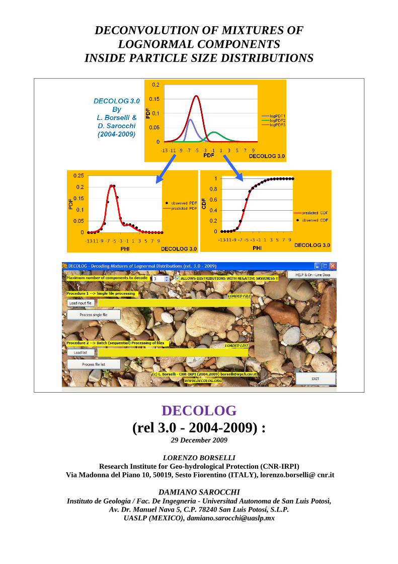
DECONVOLUTION OF MIXTURES OF
LOGNORMAL COMPONENTS
INSIDE PARTICLE SIZE DISTRIBUTIONS
DECOLOG
(rel 3.0 - 2004-2009) : 29 December 2009
LORENZO BORSELLI
Research Institute for Geo-hydrological Protection (CNR-IRPI)
Via Madonna del Piano 10, 50019, Sesto Fiorentino (ITALY), lorenzo.borselli@ cnr.it
DAMIANO SAROCCHI Instituto de Geologia / Fac. De Ingegneria - Universitad Autonoma de San Luis Potosì,
Av. Dr. Manuel Nava 5, C.P. 78240 San Luis Potosí, S.L.P.
UASLP (MEXICO), [email protected]
DECOLOG (rel 3.0 2004,09) - L. Borselli & D. Sarocchi – www.decolog.org
_______________________________________________________________________________________________
1
Table of Contents 1-Aims of DECOLOG software ........................................................................................................................... 2
2-The new release 3.0 of DECOLOG ................................................................................................................. 2
3-The log2 grain size scale in sedimentology. ................................................................................................... 2
4-The lognormal distribution –adopted until version DECOLOG release 2.2 included ..................................... 3
5-The lognormal distribution –adopted in the DECOLOG release 3.0.............................................................. 4
6-The statistical parameters from a lognormal population .............................................................................. 6
6-The mixture of lognormal distribution ........................................................................................................... 6
8-Input data ....................................................................................................................................................... 7
9-More than one file to be process ................................................................................................................... 7
10-Decoding with non linear multi-objective global optimization .................................................................... 8
11-DECOLOG User Interface .............................................................................................................................. 9
12-The Decolog Output .................................................................................................................................. 10
13-Installation of DECOLOG 3.0. ...................................................................................................................... 14
14-References .................................................................................................................................................. 14
DECOLOG (rel 3.0 2004,09) - L. Borselli & D. Sarocchi – www.decolog.org
_______________________________________________________________________________________________
2
1-Aims of DECOLOG software
Experimentally derived particle size distribution often shown multimodal shape and this
characteristic is usually interpreted as a mixture of two or more populations. The origin of these
mixture has been commonly interpreted as due to he complex processes linked to the origin of
the sediment ad clasts , to the transport and final deposition, or in other terms, the geological cycle
of sediment transport and evolution, the weathering and pedogenenetic process may affect the final
distribution of particles present in the sampled deposit.
The basic idea that the all the processes responsible of the deposit leave some trace of them in the
special characteristics of the mixture and their population. We assume that the mixture maintain
encoded in its global distribution
Aim of DECOLOG software is develop a solution to decode the information present in the natural
mixture of particles/sediments using, as paradigm, the log-normal distribution and particularly a
defined mixture of these distributions.
DECOLOG performs this operation using innovative techniques of optimization and in automatic
way without needs of special efforts from user as the initial guessing of Peaks of the observed
distribution ... the easiness of use is one of the most innovative and appreciated characteristics of
current version of DECOLOG
This software is released as FREEWARE for the scientific community. This imply that is released
and downloadable for free, but without warranties .
The authors of this software want acknowledge the people that with their testing activities and
suggestions help us to improve the performance of DECOLOG. Suggestions from the future users
are welcomed and greatly appreciated.
2-The new release 3.0 of DECOLOG
The release 3.0 of DECOLOG contains some improvements and mainly an important
upgrade.
The main upgrade is the new optimization engine that allows to consider components
(lognormal distributions) with negative skewness (so left tailed). To do that we use a
generalized four parameters lognormal distribution.
The internal optimization engine of DECOLOG has been greatly improved using last findings
in Multiobjective optimization algorithms based on Differential evolution (DE) and
trigonometric differential evolution(TDE). That’s improving the speed of convergence and
reliability and reproducibility of final results. The new optimization engine has been also
implemented in old version of the software. So a new updated version DECOLOG 2.2 is
provided with the new one DECOLOG 3.0
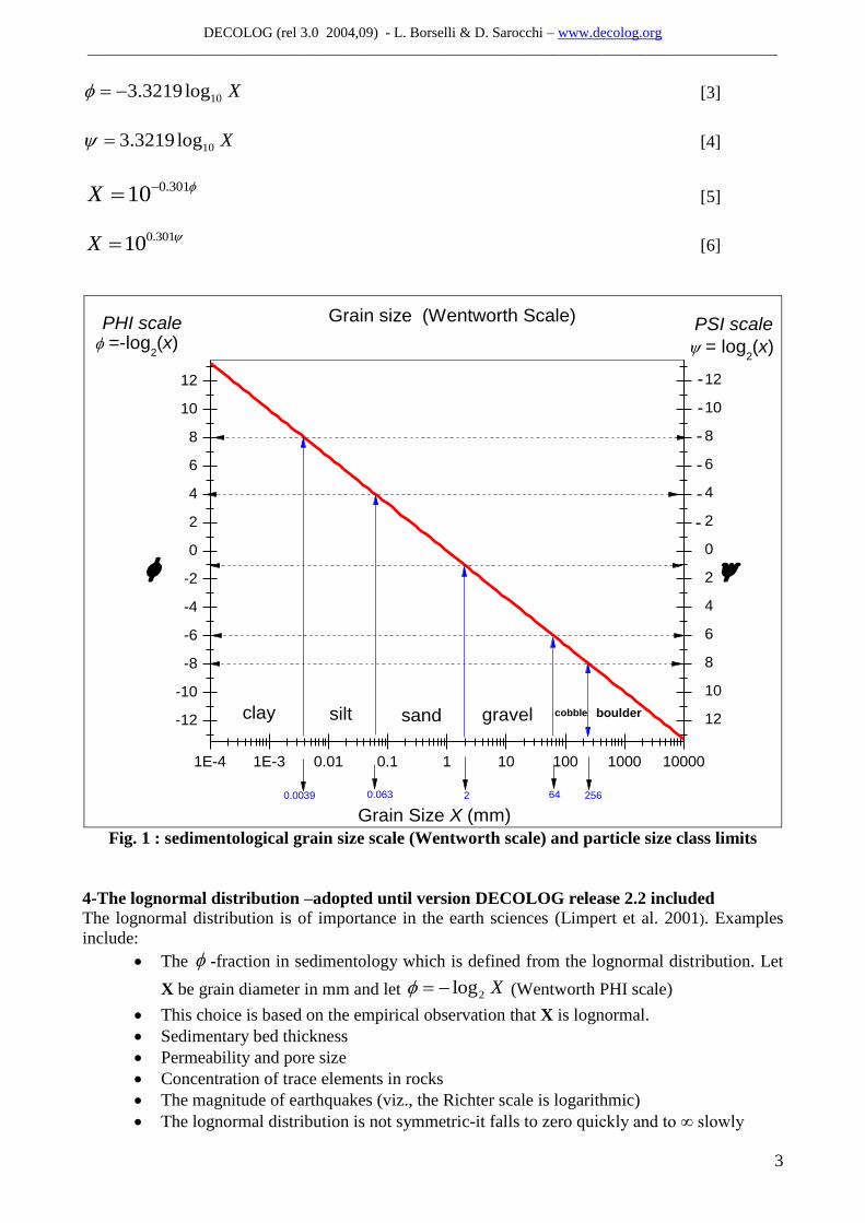
3-The log2 grain size scale in sedimentology.
The grains size distribution, according to sedimentological standard, is expressed in PHI scale
(Wentworth scale).:
2log X [1]
.
And the alternative is the PSI scale:
2log X [2]
where
X is the grains size diameter (mm).
Are useful the following approximate expressions for direct and inverse computation:
DECOLOG (rel 3.0 2004,09) - L. Borselli & D. Sarocchi – www.decolog.org
_______________________________________________________________________________________________
3
103.3219 log X [3]
103.3219 log X [4]
0.301
10X
[5]
0.301
10X
[6]
1E-4 1E-3 0.01 0.1 1 10 100 1000 10000
-12
-10
-8
-6
-4
-2
0
2
4
6
8
10
12
12
10
8
6
4
2
0
2
4
6
8
10
12
= log2(x)
-
-
-
-
-
Grain Size X (mm)
sandclay silt gravel bouldercobble
-
PHI scale PSI scaleGrain size (Wentworth Scale)
2566420.0630.0039
=-log2(x)
Fig. 1 : sedimentological grain size scale (Wentworth scale) and particle size class limits
4-The lognormal distribution –adopted until version DECOLOG release 2.2 included
The lognormal distribution is of importance in the earth sciences (Limpert et al. 2001). Examples
include:
The -fraction in sedimentology which is defined from the lognormal distribution. Let
X be grain diameter in mm and let 2log X (Wentworth PHI scale)
This choice is based on the empirical observation that X is lognormal.
Sedimentary bed thickness
Permeability and pore size
Concentration of trace elements in rocks
The magnitude of earthquakes (viz., the Richter scale is logarithmic)
The lognormal distribution is not symmetric-it falls to zero quickly and to ∞ slowly
DECOLOG (rel 3.0 2004,09) - L. Borselli & D. Sarocchi – www.decolog.org
_______________________________________________________________________________________________
4
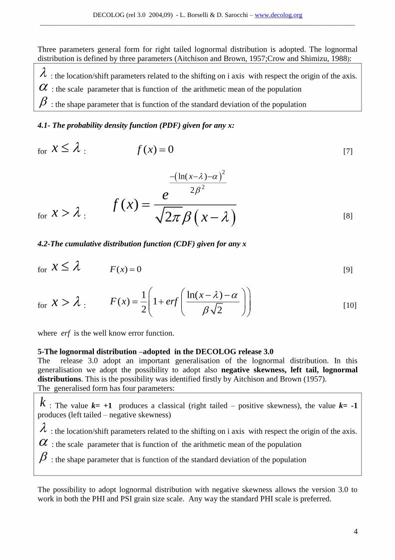
Three parameters general form for right tailed lognormal distribution is adopted. The lognormal
distribution is defined by three parameters (Aitchison and Brown, 1957;Crow and Shimizu, 1988):
: the location/shift parameters related to the shifting on i axis with respect the origin of the axis.
: the scale parameter that is function of the arithmetic mean of the population
: the shape parameter that is function of the standard deviation of the population
4.1- The probability density function (PDF) given for any x:
for x : ( ) 0f x [7]
for x :
2
2
ln( )
2
( )2
x
ef x
x
[8]
4.2-The cumulative distribution function (CDF) given for any x
for x ( ) 0F x [9]
for x :
1 ln( )( ) 1
2 2
xF x erf
[10]
where erf is the well know error function.
5-The lognormal distribution –adopted in the DECOLOG release 3.0
The release 3.0 adopt an important generalisation of the lognormal distribution. In this
generalisation we adopt the possibility to adopt also negative skewness, left tail, lognormal
distributions. This is the possibility was identified firstly by Aitchison and Brown (1957).
The generalised form has four parameters:
k : The value k= +1 produces a classical (right tailed – positive skewness), the value k= -1
produces (left tailed – negative skewness)
: the location/shift parameters related to the shifting on i axis with respect the origin of the axis.
: the scale parameter that is function of the arithmetic mean of the population
: the shape parameter that is function of the standard deviation of the population
The possibility to adopt lognormal distribution with negative skewness allows the version 3.0 to
work in both the PHI and PSI grain size scale. Any way the standard PHI scale is preferred.
DECOLOG (rel 3.0 2004,09) - L. Borselli & D. Sarocchi – www.decolog.org
_______________________________________________________________________________________________
5
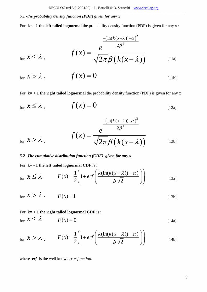
5.1 -the probability density function (PDF) given for any x
For k= - 1 the left tailed lognormal the probability density function (PDF) is given for any x :
for x :
2
2
ln( ( ))
2
( )2 ( )
k x
ef x
k x
[11a]
for x : ( ) 0f x [11b]
For k= + 1 the right tailed lognormal the probability density function (PDF) is given for any x
for x : ( ) 0f x [12a]
for x :
2
2
ln( ( ))
2
( )2 ( )
k x
ef x
k x
[12b]
5.2 -The cumulative distribution function (CDF) given for any x
For k= - 1 the left tailed lognormal CDF is :
for x
1 (ln( ( )) )( ) 1
2 2
k k xF x erf
[13a]
for x : ( ) 1F x [13b]
For k= + 1 the right tailed lognormal CDF is :
for x ( ) 0F x [14a]
for x :
1 (ln( ( )) )( ) 1
2 2
k k xF x erf
[14b]
where erf is the well know error function.
DECOLOG (rel 3.0 2004,09) - L. Borselli & D. Sarocchi – www.decolog.org
_______________________________________________________________________________________________
6
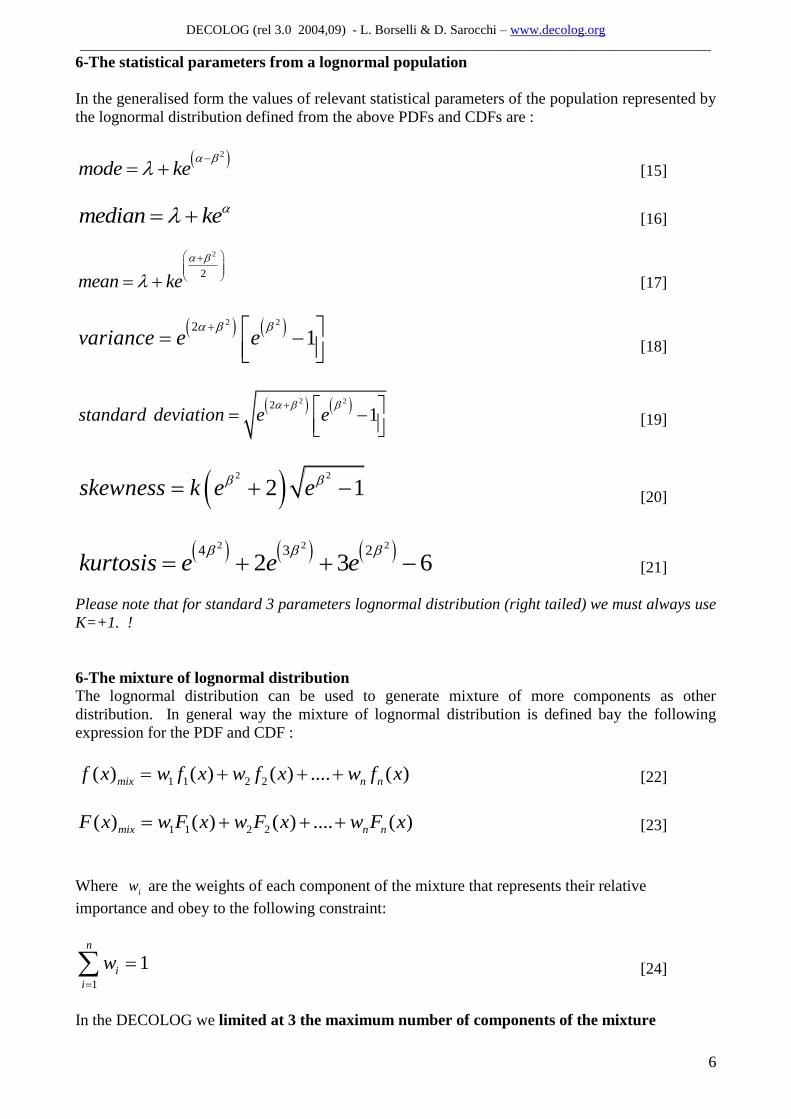
6-The statistical parameters from a lognormal population
In the generalised form the values of relevant statistical parameters of the population represented by
the lognormal distribution defined from the above PDFs and CDFs are :
2
mode ke
[15]
median ke [16]
2
2mean ke
[17]
2 221variance e e
[18]
2 22
1standard deviation e e
[19]
2 2
2 1skewness k e e
[20]
2 2 24 3 2
2 3 6kurtosis e e e
[21]
Please note that for standard 3 parameters lognormal distribution (right tailed) we must always use
K=+1. !
6-The mixture of lognormal distribution
The lognormal distribution can be used to generate mixture of more components as other
distribution. In general way the mixture of lognormal distribution is defined bay the following
expression for the PDF and CDF :
1 1 2 2( ) ( ) ( ) .... ( )mix n nf x w f x w f x w f x [22]
1 1 2 2( ) ( ) ( ) .... ( )mix n nF x w F x w F x w F x [23]
Where iw are the weights of each component of the mixture that represents their relative
importance and obey to the following constraint:
1
1n
i
i
w
[24]
In the DECOLOG we limited at 3 the maximum number of components of the mixture
DECOLOG (rel 3.0 2004,09) - L. Borselli & D. Sarocchi – www.decolog.org
_______________________________________________________________________________________________
7
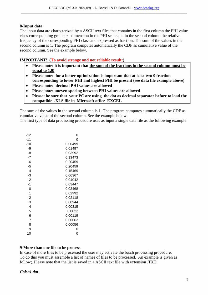
8-Input data
The input data are characterized by a ASCII text files that contains in the first column the PHI value
class corresponding grain size dimension in the PHI scale and in the second column the relative
frequency of the corresponding PHI class and expressed as fraction. The sum of the values in the
second column is 1. The program computes automatically the CDF as cumulative value of the
second column. See the example below.
IMPORTANT! (To avoid strange and not reliable result:)
Please note: it is important that the sum of the fractions in the second column must be
equal to 1.0!
Please note: for a better optimization is important that at least two 0 fraction
corresponding to lower PHI and highest PHI be present (see data file example above)
Please note: decimal PHI values are allowed
Please note: uneven spacing between PHI values are allowed
Please: be sure that your PC are using the dot as decimal separator before to load the
compatible .XLS file in Microsoft office EXCEL
The sum of the values in the second column is 1. The program computes automatically the CDF as
cumulative value of the second column. See the example below.
The first type of data processing procedure uses as input a single data file as the following example:
-12 0
-11 0
-10 0.00499
-9 0.01497
-8 0.03992
-7 0.13473
-6 0.20459
-5 0.20459
-4 0.15469
-3 0.06367
-2 0.04042
-1 0.03447
0 0.03468
1 0.02992
2 0.02118
3 0.00944
4 0.00315
5 0.0022
6 0.00119
7 0.00062
8 0.00056
9 0
10 0
9-More than one file to be process
In case of more files to be processed the user may activate the batch processing procedure.
To do this you must assemble a list of names of files to be processed. An example is given as
follow;. Please note that the list is saved in a ASCII text file with extension .TXT:
Colsa1.dat
DECOLOG (rel 3.0 2004,09) - L. Borselli & D. Sarocchi – www.decolog.org
_______________________________________________________________________________________________
8
Colsa1b.dat
Colsa2a.dat
Colsa3.dat
……
…….
The file that contains the list to be processed is loaded by the processing procedure 2. Each file in
the list is processed sequentially and as output a new filename, with extension XLS is saved on hard
disk in the same location of the input files.
10-Decoding with non linear multi-objective global optimization
A non linear multiobjective global optimization procedure has been developed to complete in
efficient and robust way the decoding process. The optimization process allow to obtain the
parameters , , ,i i i i ik w for each distribution. The common ways to fit sample/observed
distribution with a theoretical one is the fitting the observed PDF or alternatively using the observed
CDF (Macdonald PDM, Green PEJ (1998),).
The fitting of the PDF of the CDF pose different problems. For example the two form or represent
the distribution has a different mathematical and analytical significance. The PDF is the first
derivative of the CDF form. This fact implies that during the fitting the small peaks in the PDF may
be traduced in erroneous influence in peaks guessing. This problem has a different role in CDF
because the local pecks are identified mainly as local increase of slope. In the CDF small peaks may
be obliterate from the cumulative process when we have high function value. Limiting the fitting to
the PDF alone we can observe always that the successive comparison of the derived CDF with the
observed may have poor performances.
This problem has been overcome in DECOLOG using a heuristic procedure. We established a
concurrent fitting of the PDF and CDF observed by way of a multi-objective optimization
minimizing at the same time the errors in the PDF and CDF. Because the tho objective are
concurrent each optimum may be partially in conflict with the other establishing dominance.
So to obtain a result we transform the multi-obective process for a computation purpose in a single
objective optimization. Do realize this we use the methodology described by (Anderson, 2000 ) or
use as objective function a weighted sum of single objective functions relative to each concurrent
process. Each objective function must have a common range of variation (e.g.[0.0,1.0]) and the
weights must be chosen in a way that de dominance of each objective is reduced.
Our final single objective function is the following:
min (1 )CDF PDF ffW K W E [25]
And where:
1CDF PDF
W W [26]
Where K is the Kolmogorov-Smirnov parameters (Chakravarti 1967) or the maximum difference,
ranging between 0.0 and 1.0, between the observed and computed CDF in the same observed
points.
ffE is the model efficiency parameter developed by Nash and Sutcliffe (1970) that has a well
recognised performances for non linear fitting. These parameters vary between 1.0 (perfect fitting)
and (worst fitting).
DECOLOG (rel 3.0 2004,09) - L. Borselli & D. Sarocchi – www.decolog.org
_______________________________________________________________________________________________
9
,CDF PDFW W are tow weights that are identified with numerous tests allow to reduce greatly the
dominance of each single objective balancing at runtime the different efficiency in the fitting of the
PDF and the CDF.
In the case of 3 components we hace a maximum of 11 parameter to optimize. In this case the
large number of parameters to optimize requires an adequate degree of freedom, so an adequate
number of data points in the distribution observed.
The global optimization algorithm is based on Differential evolution (DE) (Storn and Price
,1997a,1997b; Storn 1999). The DECOLOG code has been implemented in Object Pascal
programming language and FPC compiler rel 2.2.4 (www.freepascal.org).
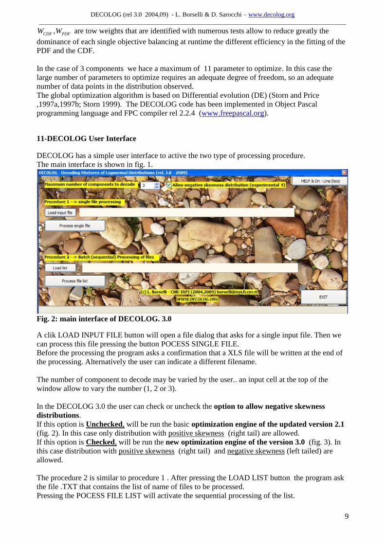
11-DECOLOG User Interface
DECOLOG has a simple user interface to active the two type of processing procedure.
The main interface is shown in fig. 1.
Fig. 2: main interface of DECOLOG. 3.0
A clik LOAD INPUT FILE button will open a file dialog that asks for a single input file. Then we
can process this file pressing the button POCESS SINGLE FILE.
Before the processing the program asks a confirmation that a XLS file will be written at the end of
the processing. Alternatively the user can indicate a different filename.
The number of component to decode may be varied by the user.. an input cell at the top of the
window allow to vary the number (1, 2 or 3).
In the DECOLOG 3.0 the user can check or uncheck the option to allow negative skewness
distributions.
If this option is Unchecked, will be run the basic optimization engine of the updated version 2.1
(fig. 2). In this case only distribution with positive skewness (right tail) are allowed.
If this option is Checked, will be run the new optimization engine of the version 3.0 (fig. 3). In
this case distribution with positive skewness (right tail) and negative skewness (left tailed) are
allowed.
The procedure 2 is similar to procedure 1 . After pressing the LOAD LIST button the program ask
the file .TXT that contains the list of name of files to be processed.
Pressing the POCESS FILE LIST will activate the sequential processing of the list.
DECOLOG (rel 3.0 2004,09) - L. Borselli & D. Sarocchi – www.decolog.org
_______________________________________________________________________________________________
10
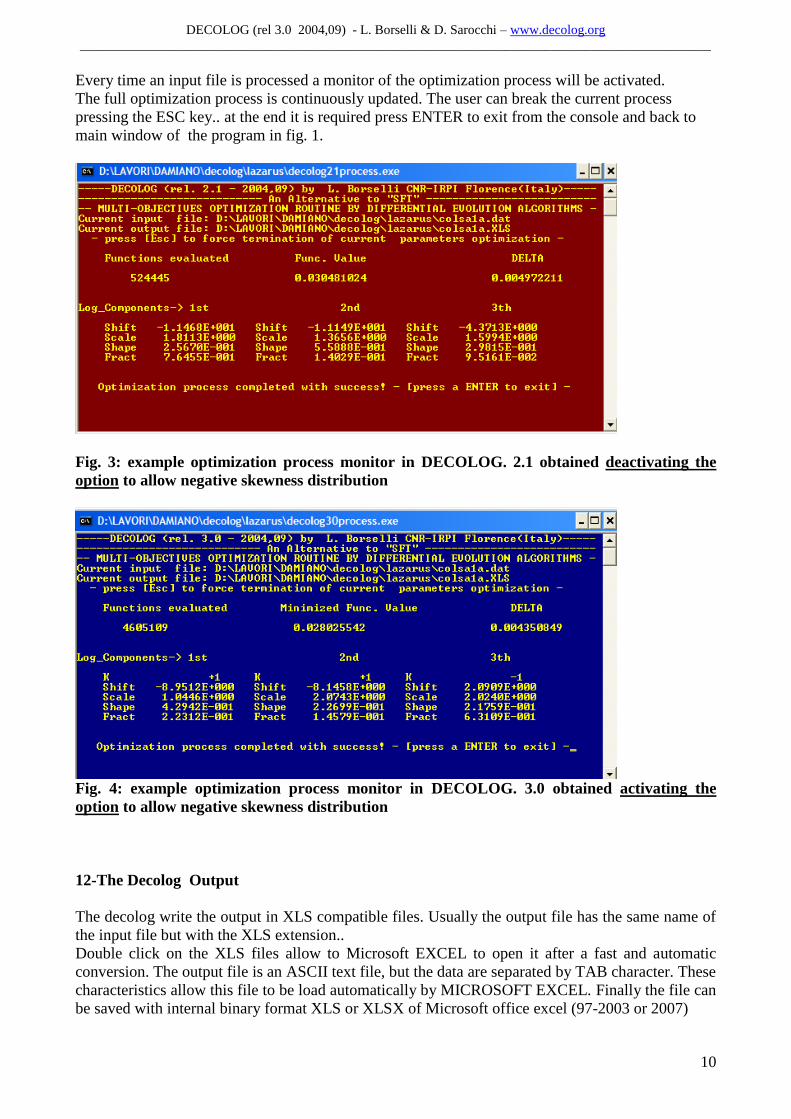
Every time an input file is processed a monitor of the optimization process will be activated.
The full optimization process is continuously updated. The user can break the current process
pressing the ESC key.. at the end it is required press ENTER to exit from the console and back to
main window of the program in fig. 1.
Fig. 3: example optimization process monitor in DECOLOG. 2.1 obtained deactivating the
option to allow negative skewness distribution
Fig. 4: example optimization process monitor in DECOLOG. 3.0 obtained activating the
option to allow negative skewness distribution
12-The Decolog Output
The decolog write the output in XLS compatible files. Usually the output file has the same name of
the input file but with the XLS extension..
Double click on the XLS files allow to Microsoft EXCEL to open it after a fast and automatic
conversion. The output file is an ASCII text file, but the data are separated by TAB character. These
characteristics allow this file to be load automatically by MICROSOFT EXCEL. Finally the file can
be saved with internal binary format XLS or XLSX of Microsoft office excel (97-2003 or 2007)
DECOLOG (rel 3.0 2004,09) - L. Borselli & D. Sarocchi – www.decolog.org
_______________________________________________________________________________________________
11
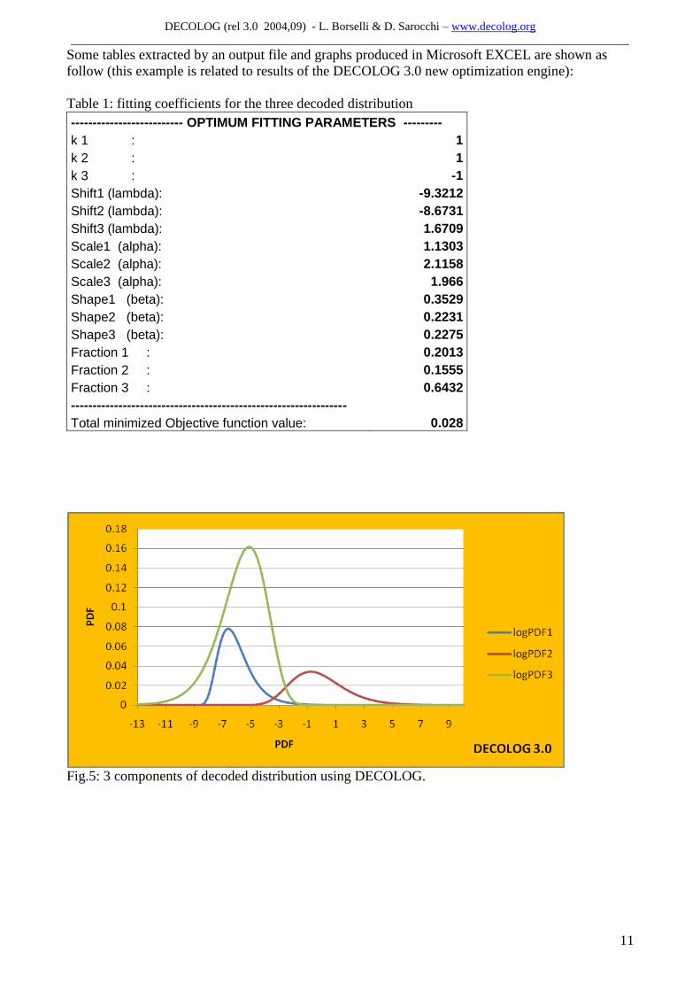
Some tables extracted by an output file and graphs produced in Microsoft EXCEL are shown as
follow (this example is related to results of the DECOLOG 3.0 new optimization engine):
Table 1: fitting coefficients for the three decoded distribution
-------------------------- OPTIMUM FITTING PARAMETERS ---------
k 1 : 1
k 2 : 1
k 3 : -1
Shift1 (lambda): -9.3212
Shift2 (lambda): -8.6731
Shift3 (lambda): 1.6709
Scale1 (alpha): 1.1303
Scale2 (alpha): 2.1158
Scale3 (alpha): 1.966
Shape1 (beta): 0.3529
Shape2 (beta): 0.2231
Shape3 (beta): 0.2275
Fraction 1 : 0.2013
Fraction 2 : 0.1555
Fraction 3 : 0.6432
----------------------------------------------------------------
Total minimized Objective function value: 0.028
Fig.5: 3 components of decoded distribution using DECOLOG.
DECOLOG (rel 3.0 2004,09) - L. Borselli & D. Sarocchi – www.decolog.org
_______________________________________________________________________________________________
12
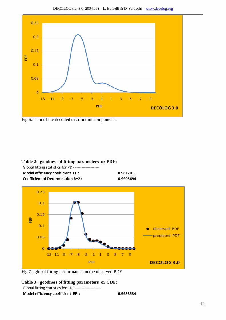
Fig 6.: sum of the decoded distribution components.
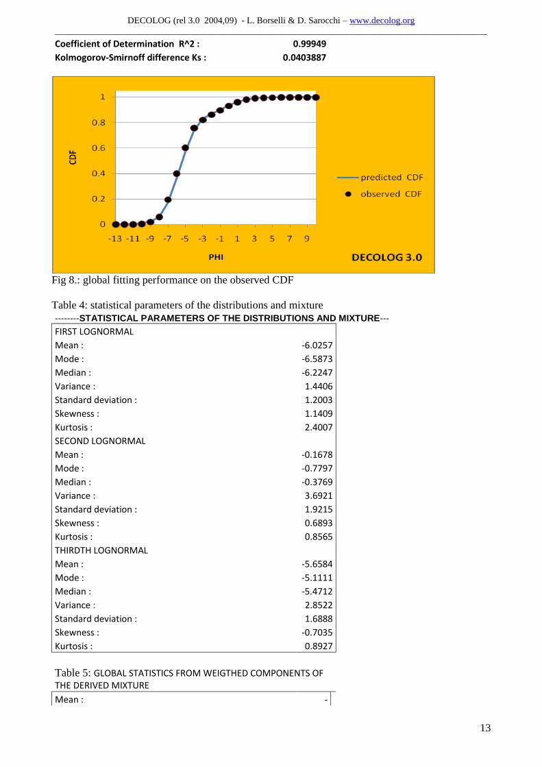
Table 2: goodness of fitting parameters or PDF:
Global fitting statistics for PDF -------------------
Model efficiency coefficient EF : 0.9812011
Coefficient of Determination R^2 : 0.9905694
Fig 7.: global fitting performance on the observed PDF
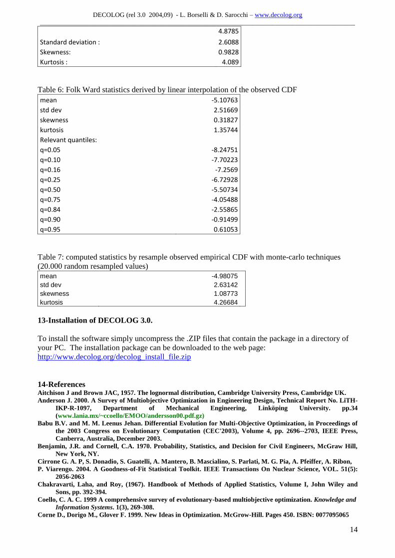
Table 3: goodness of fitting parameters or CDF:
Global fitting statistics for CDF --------------------
Model efficiency coefficient EF : 0.9988534
DECOLOG (rel 3.0 2004,09) - L. Borselli & D. Sarocchi – www.decolog.org
_______________________________________________________________________________________________
13
Coefficient of Determination R^2 : 0.99949
Kolmogorov-Smirnoff difference Ks : 0.0403887
Fig 8.: global fitting performance on the observed CDF
Table 4: statistical parameters of the distributions and mixture
--------STATISTICAL PARAMETERS OF THE DISTRIBUTIONS AND MIXTURE---
FIRST LOGNORMAL Mean : -6.0257
Mode : -6.5873
Median : -6.2247
Variance : 1.4406
Standard deviation : 1.2003
Skewness : 1.1409
Kurtosis : 2.4007
SECOND LOGNORMAL Mean : -0.1678
Mode : -0.7797
Median : -0.3769
Variance : 3.6921
Standard deviation : 1.9215
Skewness : 0.6893
Kurtosis : 0.8565
THIRDTH LOGNORMAL Mean : -5.6584
Mode : -5.1111
Median : -5.4712
Variance : 2.8522
Standard deviation : 1.6888
Skewness : -0.7035
Kurtosis : 0.8927
Table 5: GLOBAL STATISTICS FROM WEIGTHED COMPONENTS OF THE DERIVED MIXTURE
Mean : -
DECOLOG (rel 3.0 2004,09) - L. Borselli & D. Sarocchi – www.decolog.org
_______________________________________________________________________________________________
14
4.8785
Standard deviation : 2.6088
Skewness: 0.9828
Kurtosis : 4.089
Table 6: Folk Ward statistics derived by linear interpolation of the observed CDF
mean -5.10763
std dev 2.51669
skewness 0.31827
kurtosis 1.35744
Relevant quantiles: q=0.05 -8.24751
q=0.10 -7.70223
q=0.16 -7.2569
q=0.25 -6.72928
q=0.50 -5.50734
q=0.75 -4.05488
q=0.84 -2.55865
q=0.90 -0.91499
q=0.95 0.61053
Table 7: computed statistics by resample observed empirical CDF with monte-carlo techniques
(20.000 random resampled values)
mean -4.98075
std dev 2.63142
skewness 1.08773
kurtosis 4.26684
13-Installation of DECOLOG 3.0.
To install the software simply uncompress the .ZIP files that contain the package in a directory of
your PC. The installation package can be downloaded to the web page:
http://www.decolog.org/decolog_install_file.zip
14-References Aitchison J and Brown JAC, 1957. The lognormal distribution, Cambridge University Press, Cambridge UK.
Anderson J. 2000. A Survey of Multiobjective Optimization in Engineering Design, Technical Report No. LiTH-
IKP-R-1097, Department of Mechanical Engineering, Linköping University. pp.34
(www.lania.mx/~ccoello/EMOO/andersson00.pdf.gz)
Babu B.V. and M. M. Leenus Jehan. Differential Evolution for Multi-Objective Optimization, in Proceedings of
the 2003 Congress on Evolutionary Computation (CEC'2003), Volume 4, pp. 2696--2703, IEEE Press,
Canberra, Australia, December 2003.
Benjamin, J.R. and Cornell, C.A. 1970. Probability, Statistics, and Decision for Civil Engineers, McGraw Hill,
New York, NY.
Cirrone G. A. P, S. Donadio, S. Guatelli, A. Mantero, B. Mascialino, S. Parlati, M. G. Pia, A. Pfeiffer, A. Ribon,
P. Viarengo. 2004. A Goodness-of-Fit Statistical Toolkit. IEEE Transactions On Nuclear Science, VOL. 51(5):
2056-2063
Chakravarti, Laha, and Roy, (1967). Handbook of Methods of Applied Statistics, Volume I, John Wiley and
Sons, pp. 392-394.
Coello, C. A. C. 1999 A comprehensive survey of evolutionary-based multiobjective optimization. Knowledge and
Information Systems. 1(3), 269-308.
Corne D., Dorigo M., Glover F. 1999. New Ideas in Optimization. McGrow-Hill. Pages 450. ISBN: 0077095065
DECOLOG (rel 3.0 2004,09) - L. Borselli & D. Sarocchi – www.decolog.org
_______________________________________________________________________________________________
15
Crow EL and Shimizu K Eds, 1988. Lognormal Distributions: Theory and Application, Dekker, New York.
Kolmogorov A. N.,1933..Sulla determinazione empirica di una legge di distribuzione. Giornale Dell’istituto
Italiano Degli Attuari, vol. 4, pp. 83–91, 1933.
Kuiper N. H.,1960. Tests concerning random points on a circle. Proc.Koninkl. Neder. Akad. van Wettensch. A,
vol. 63, pp. 38–47, 1960
Limpert E, Stahel WA and Abbt M, 2001. Lognormal distributions across the sciences: keys and clues.
Bioscience 51 (5), 341-352
Macdonald PDM, Green PEJ (1998) User's guide to program MIX: an interactive program for fitting mixtures
of distributions. Ichthus Data Systems, Ontario, Canada
Madavan; N.K. Multiobjective Optimization using a Pareto Differential Evolution Approach, in IEEE Proc. Of
Congress on Evolutionary Computation (CEC’2002), vol. 1, pp. 1145-1150, 2002.
Nash, J. E. and J. V. Sutcliffe (1970), River flow forecasting through conceptual models part I — A discussion of
principles, Journal of Hydrology, 10 (3), 282–290.
Smirnov N. V. 1939. Sur les écarts de la courbe de distribution empirique (Russian/French summary),”
Matematiceskii Sbornik N.S., vol. 6, pp. 3–26, 1939.
Smirnov N. V., 1948. Table for estimating the goodness-of-fit of empirical distributions. Ann. Math. Statist., vol.
19, pp. 279–281.
Storn R., 1999. System design by Constraint Adaptation and Differential Evolution, IEEE Transactions on
Evolutionary Computation, 3(1): 22-34. Storn R., Price K1.; Differential Evolution - A Simple and Efficient
Heuristic for Global Optimization over Continuous Spaces, Technical Report TR-95-012, ICSI, 1995.
Storn R.and Price K., 1997. Differential Evolution-a simple and efficient heuristic for global optimization over
continuous spaces, Journal of Global Optimization, 11: 341-359.
Storn, R. and Price, K., 1997. Differential Evolution: Numerical Optimization Made Easy, Dr. Dobb's Journal,
April 97, 18 - 24.
Wanga Y., Yamb R.C.M., M. J. Zuoc. 2004. A multi-criterion evaluation approach to selection of the best
statistical distribution. Computers & Industrial Engineering 47 :165–180. doi:10.1016/j.cie.2004.06.003