decision-mapping: a tool for consistent and complete decisions in process synthesis

Pergamon Chemical Engineering Science, Vol. 50, No. 11, pp. 1755 1768, 1995 Copyright ~ 1995 Elsevier Science Ltd

Printed in Great Britain. All rights reserved 0009 2509/95 $9.50 + 0.00

0009-2509(95)00034-8

DECISION-MAPPING: A TOOL FOR CONSISTENT AND COMPLETE DECISIONS IN PROCESS SYNTHESIS

F. FRIEDLER *'*''~'~, J. B. VARGA *'ll and L. T. FAN t * Department of Systems Engineering, Research Institute of Chemical Engineering, Hungarian Academy of

Sciences, Veszpr6m, Pf. 125, H-8201, Hungary t Department of Chemical Engineering, Kansas State University, Manhattan, KS 66506, U.S.A.

(Received 2 February 1994; accepted in revised form 2 January 1995)

Akstraet--Decisions involved in process synthesis are often more complex than those involved in other disciplines. This arises from the fact that such decisions are concerned with specification or identification of highly interconnected systems, e.g. process structures, which may contain a multitude of recycling loops. It appears that no rigorous technique is available, which is capable of representing exactly and organizing effciently the system of decisions for a process synthesis problem. A novel mathematical notion, decision-mapping, has been introduced in this work to render the complex decisions in process design and synthesis consistent and complete. The basic terminologies of decision-mapping, including extension, equivalence, completeness, complementariness, and active domain, have been defined based on rigorous set-theoretic formalism, and the most important properties of decision-mappings have been identified and proved. Decision-mapping, as a rigorousl2~ established technique, is directly applicable in developing efficient and exact process synthesis methods or improving existing methods. The applicability and meritorious features of this new technique are illustrated by synthesizing a large scale process.

l. INTRODUCTION

Efforts to apply mathematical programming methods to process synthesis have yielded encouraging results; nevertheless, a number of major issues remain un- resolved. The principal ones are establishment of the mathematical foundation necessary to validate the algorithms for optimal process synthesis, and the reduction in the complexity of the mathematical programming algorithms for process synthesis.

A thorough understanding of the unique combinatorial properties of process structures enables us to validate rigorously the algorithms for process synthesis and to reduce drastically the complexity of these algorithms. In principle, two types of ap- proaches are available for this purpose; they are logical formulation (Raman and Grossmann, 1993) and combinatorics (Friedler et aL, 1992c).

Combinatorics has been adopted in the present approach. The fundamental combinatorial properties of feasible process structures have been expressed as a set of axioms (Friedler et al., 1992b, c). For the MINLP model of process synthesis, these axioms constrain the set of possible values of the integer variables to the set of combinatorially feasible values, thereby reducing the size of the search space by many

orders of magnitude. Although these axioms consti- tute a rigorous foundation for the combinatorial seg- ment of process synthesis, they do not directly give rise to the computational algorithms for process synthesis. The reason is that the axioms express self- evident facts instead of procedures, and thus, they are not in procedural form. The present work introduces a new combinatorial technique that is mathematically rigorous, i.e. decision-mapping, for direct application to developing and describing the algorithms for process synthesis. This technique is capable of representing process networks or structures of any type and size. For example, a structure containing any number of recyclings with arbitrary sizes can be represented in synthesizing a process by this technique. Decision- mapping has been developed with rigorous mathematical formalism and validated by resorting to the combinatorial axioms of process synthesis; therefore, any algorithm based on the decision-mapping can also be validated rigorously.

The focus of the present work is on the total flowsheet synthesis [see e.g. Siirola and Rudd (1971), Lu and Motard (1985) and Douglas (1988)]. Neverthe- less, the results are applicable directly or can be ex- tended to other classes of process synthesis.

Also at the Department of Computer Science, University of Veszpr6m, Veszpr6m, Hungary.

~t Also at the Department of Computer Science, A. Jozsef University, Szeged, Hungary.

Author to whom correspondence should be addressed at Research Institute of Chemical Engineering, Hungarian Academy of Sciences, Veszpr6m, Pf. 125, H-8201, Hungary.

2. UNAMBIGUOUS STRUCTURAL REPRESENTATION: P-GRAPH

For formally analyzing process structures in process synthesis, an unambiguous structural representation is required. Process graph or P-graph, which is a directed bipartite graph, has been introduced for this purpose [see Friedler et al. (1992c)]. A brief description of P-graph is given below.

1755

1756

Let M be a given finite nonempty set of objects, usually material species or materials, that can be transformed in the process under consideration. Transformation between two subsets of M occurs in an operating unit. It is necessary to link this operating unit to other operating units through the elements of these two subsets of M.

Let O be the set of operating units to be considered in synthesis; then, O G ~ (M)xfa (M) where 0 c~ M = 0. If (~t, fl) is an operating unit, i.e. (~t, fl)e O, then a is called the input set, and fl, the output set of this operating unit. Pair (M, O) is termed a process 9raph or P-oraph with the set of vertices M u 0 and the set of arcs {(x,y)ly=(~,fl)eO and x~ ~} w {(y,x)ly = (a, fl)e O and xe fl}. P-graph (M,O) is defined to be a subgraph of (M',O'), i.e. (M,O) ~_ (M',O'), if M ~_ M' and O ~ O'. The union of two P-graphs (Ml,0t) and (M2, O2), (Mt,Ot)u(M2,02), is defined to be P-graph (MI w M2, 01 w 02). The indeoree of vertex X, d- (X), is defined to be the number of arcs with endpoint X. If X is a material, then broadly speaking, d- (X) is the number of operating units producing material X.

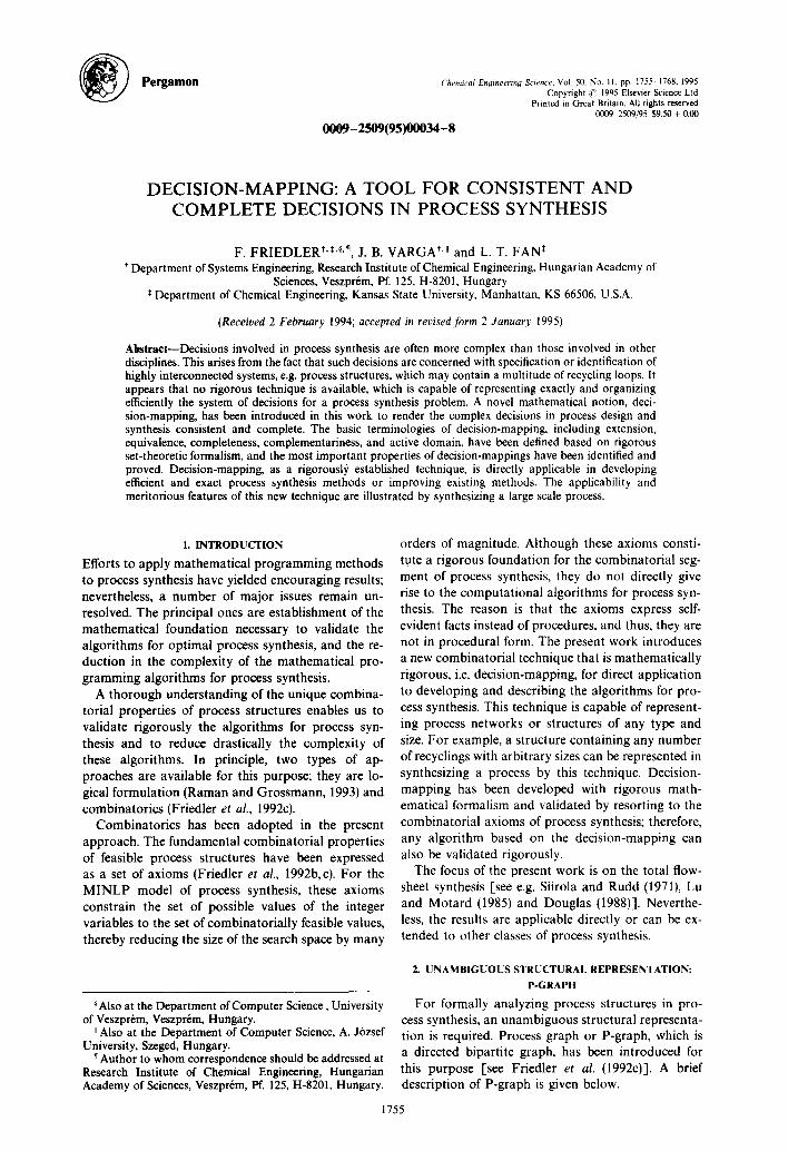
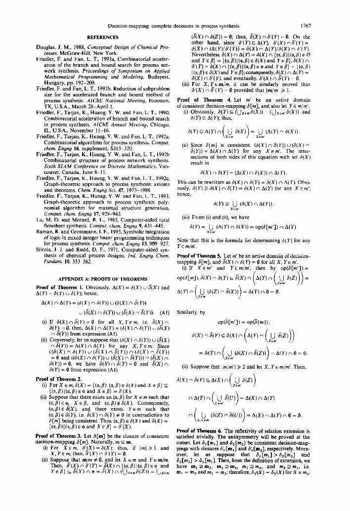
Example 1. Let us suppose that set Mt of materials and set O1 of operating units of P-graph (M1, O1) be given as

Mt = {A,B,C,O,E,F,G,H,I,J,K,L}

and

01 = {({C},{A,F}),({D},{A,B}),({E,F},{C}),

({F, G}, {C, O}), ({G, H}, {D}), ({J}, {F}),

t{K,L},{n})}. P-graph (M1,01) is depicted in Fig. 1. Note that the input and output sets of operating unit 1, ({C},{A,F}), are {C} and {A,F}, respectively, and that the indegree of vertex A, d - ( A ) , is 2 since two operating units produce material A.

I J K L

A B

Fig. 1. P-graph(M~,O~)where A, B, C,D,E,F, G,H,I,J, K, and L are the materials, and 1, 2, 3, 4, 5, 6, and 7 are the

operating units.

F. FRIEDLER et al.

P-graph (M,O) contains the interconnections among the units of O. Each feasible process corres- ponds to a subgraph of (M, O); this subgraph can be generated by decision-mappings.

3. DECISION-MAPPING: DEFINITIONS AND SUPPORTING THEOREMS

Rigor and clarity demand that various terminologies introduced in this work be couched in the parlance of mathematical formalism. A mapping or function determines a unique "value" for an argu- ment; the set of possible arguments, D, is called the domain; and the set of possible "values", R, is the range of the mapping or function. Mapping or function f determines a "value", i.e. f(x)~ R for each xe D. A mapping or function f therefore, can be defined as a special subset of the Cartesian product of D and R, D x R, i.e. f is a set of pairs (x,y) where xe D and y =f(x)~ R. This set of pairs is denoted by f[D]. Thus, while the name of a mapping fo110wed by an element of its domain in parentheses represents the value determined by the mapping, e.g. f(x), a mapping name followed by the domain in square brackets represents the mapping, e.g. f[D]. The notations of this type will appear throughout this paper.

Let us suppose that P-graph (M, O) represents the interconnections of the operating units of a synthesis problem. Then, for the set of materials M and the set of operating units O, O _~ ~(M) x ~(M) holds. Let us now induce mapping A from the set of materials to the set of subsets of the set of operating units, i.e. from M to ~o(O). This mapping determines the set of operating units producing material X for any X~ M; consequently, A(X) = {(a, fl)l(a, fl)~ O and Xe fl}.

Def in i t ion I. Let m be a subset of M, and X be an element of m; moreover, let 6(X) be a subset of A(X). Then, mapping 6 from set m to the set of subsets of set O, 6I'm] = {(X,6(X)[X~ m}, is defined to be a decision-mapping on m, with m being the domain of the mapping. Decision-mapping 61 ]-mx] is defined to be the restriction of decision-mapping 62[m2] to ml if ml ~m2 and 6t['mt-] = {(X,62(X))lXemt}. Thus, the "value" of 6t is equal to that of 62 for any element of m t.

Mapping AIM] = {(X, A(X))[X~ M} can also be considered as a decision-mapping; it will be termed as the maximal decision-mappin 9.

E x a m p l e 2. Let us revisit Example 1. According to the definition of At (X), sets At(A) through At(L) can be given for P-graph (Mr, O1) as follows:

A~(.4) =

AI(B) =

AI(C) =

AI(D) =

At(E) =

At(F) =

{ ({C}, {A, F}), ({D}, {A, B})}

{I{O},{A,8})} {({E, F}, {C}), ({F, G}, {C, D})}

{({F, G}, {C, D}), ({G, H}, {D})}

0

{({C}, {A, F}), ({J}, {F})}

Decision-mapping: complete decisions in process synthesis

At(G)=¢

At(H) = {({K, L}, {H})}

At(l) = At(J) = At(K) = AI(L) = 0.

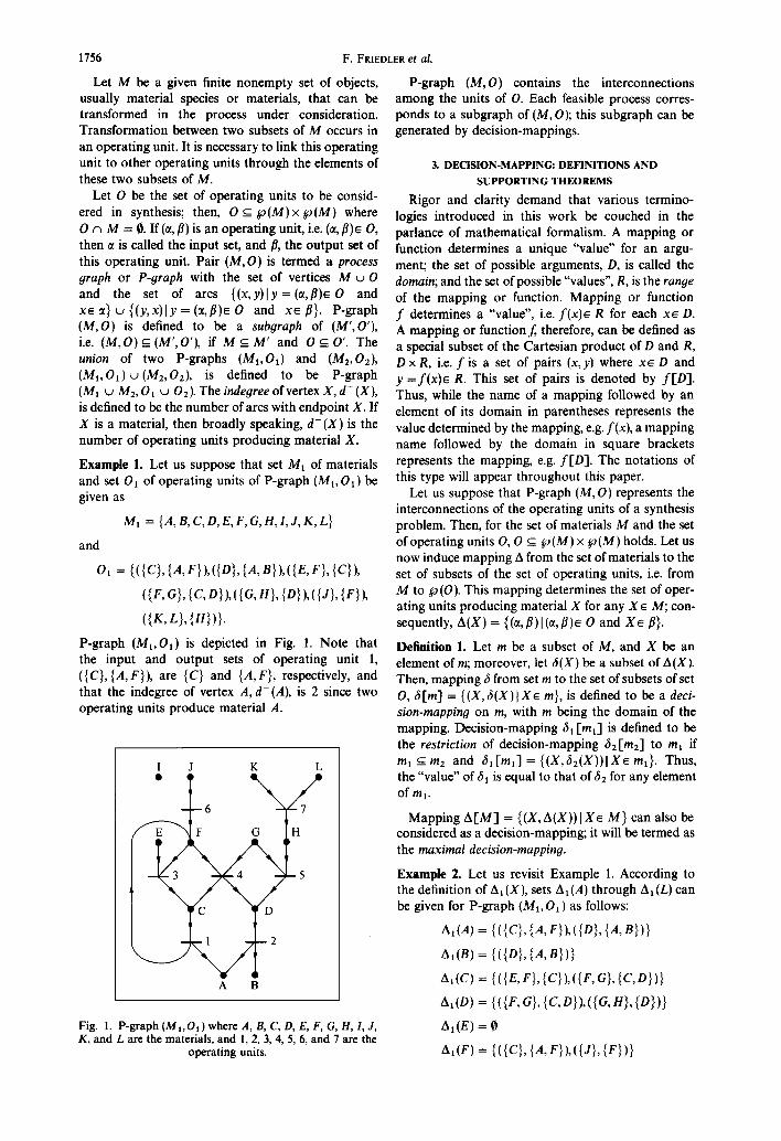
Let us now define decision-mapping fil for P-graph (Mr, 01 ) of this example. The domain, rnl, of fit must be a subset of Mr, e.g., ml = {A,D,H}. Suppose that fit(A) = { ({D} ,{A,B})} , f i1 (O)= {({F,G},{C,D}) , ({G,H},{D})}, and f i t (H)=0. Obviously, fit(a)~_ AI(A), 61(O) - At(D), and fit(H) ~- AI(H); therefore, 61[mt] = {(A, fil(A)),(D, fil(O)),(H, fil(H))} = {(A, {({D},{A,B})}),(D,{({F,G},{C,D}), ({G,H},{D})}), (H, 0)} is a decision-mapping of the example.

The rigorous definition of a P-graph of a decision- mapping requires additional tools other than those currently available as will be elaborated later. Never- theless, for illustration, let us consider the operating units include in the range of a decision-mapping as its P-graph. The P-graph of decision-mapping fil [ml] of Example 2 is illustrated in Fig. 2.

To examine the major properties of process structures, special class of decision-mapping must be introduced.

Definition 2. The complement of decision-mapping film] is defined by 6[m] = {(X, Y)IX~ m and Y = A(X)/fi(X)}; thus, for Xe m, 6(X) = A(X)/fi(X). Since fi(X) is a set of operating units producing material X, 6(X) is the set of operating units producing X, but are not included in fi(X).

The consistency of decisions is crucial in synthesizing a process. For example, we can decide indepen- dently that an operating unit producing materials X and Y be included in a process for the production of material X and be excluded from the production of material Y, thereby giving rise to a contradiction in the system of decisions. To avoid such a contradiction, consistent decision-mappings must be considered.

Definition 3. Decision-mapping fi[m] is said to be consistent if ]ml ~< 1 or (fi(X) n fi(Y)) w (S(X) c~ S(Y)) = A(X) n A(Y) for any X, Ye m; otherwise, it

F G H

D

2

/ A B

Fig. 2. P-graph of decision-mapping ,51 [ml].

1757

is inconsistent. Let m' ~_ m. We say that the decision- mapping fi [m] is consistent on m' if the decision-mapping fi[m'] is consistent, where 6[m'] denotes the restriction of fi [m] to m'. Obviously, if fi [m] is consistent, then it is consistent on any subset of m.

In other words, a decision-mapping is considered to be consistent if every operating unit producing materials X and Y is included in or excluded from both 6(X) and fi(Y). Another equivalent definition for consistency can be established by the following theorem.

Theorem 1. Decision-mappin9 fi [m] for which I ml/> 1 is consistent if and only if fi(X) c~ S(Y) = O for all X, Ye m.

The proofs of the above theorem and all other theorems are given in Appendix A.

Example 3. Decision-mapping fit [mt] in Example 2 is consistent because fit(A) n SI(D ) = 0; fit(A) n St(H) = 0; St(A) n fit(D) = O; 6t(A) n fit(H) = O; fit(D) c~ 6 , (n) = 0; and 6t(D) n f i ,(n) = O. Never- theless, decision-mapping fi2[m2] = fit [ml] w {(C, { ({E, F}, {C})})} is inconsistent since fi2(O) r~ $2(C) = {({F,G}, {C,D})}¢0. In fi2[m2], operating unit ({ F, G}, {C, D}) is simultaneously included and excluded from the consideration, thereby resulting in a contradiction in the system of decisions.

It is of importance to decide which decision-mappings be considered equivalent. For example, decision-mapping fi3[mt ~ {B}] = fitEmt] w {(B,{({D}, {A, B})})} is different from fit [ml]; nevertheless, both yield an identical structure, thus implying that these two decision-mappings have some equivalence; see Fig. 2. This type of equivalence will be established on the closure of the decision-mapping. For this purpose, let the set of operating units of decision-mapping fi [m] be denoted by op(fi [m]), and the set of materials of set 0 of operating units, by mat(o); hence,

op(fi[m])= U fi(x) and mat(o)= U (~uf l ) . X e m (a,O)eo

Definition 4. For consistent decision-mapping fi [m], let o = op(fi[m]), m = mat(o) u m, and fi'[m] = {(x, r ) l xe m and Y = {(ct, fl) I(~t, fl)e o and Xe fl}}. Then, 6' [m] is defined to be the closure of fi [m], and 6[m] is said to be closed if 6Ira] = fi'[m]. Naturally, the closure of a consistent decision-mapping is closed.

Example 4. Referring to Example 2, the closure of decision-mapping fit [m 1 ], fi~ [m t ], follows Definition 4. Domain ml is the union of set ml and the set of materials involved in the operating units, i.e., ml = ml ~ {B,C,F,G}. Hence 6][mt] = {(A,{({D}, {A,B})}),(B,{({D},{A,B})}),(C,{({F,G},{C,D})}), (D, { ( {F, G}, {C,D}),({G, H}, {D})}),(F,O),(G,O), (H, O) }.

An important relation of a decision-mapping and its closure are expressed by the following theorem.

Theorem 2. Let fi'[m] be the closure of consistent decision-mappin9 film]; then, f i (X)= fi'(X) for all Xe m, i.e. fi[m] is the restriction of fi'[m] to m.

CES 50-II-F

1758 F. FRIEDLER et al.

Theorem 2 implies that if 6 ' [m] is the closure of consistent decision-mapping 61-m], then, 6 [m] __q 6'/-m]. It is essential to inquire if the closure preserves the consistency.

Theorem 3. The closure of a consistent decision-mapping is consistent.

The equivalence of decision-mappings can be established on their closure as stated in the following definition.

Definition 5. Two consistent decision-mappings are defined to be equivalent if their closure is common.

Naturally, a consistent decision-mapping is equivalent to its closure. The relation "equivalent" has the mathematically required properties of an equivalence relation: It is reflexive, symmetric, and transitive.

Example 5. Decision-mapping 64[{B,D}]={(B, {({D},{A,B})}),(D,{({F,G},{C,D}),({G,H},{D})})} has the same closure as g~ [m~] in Example 2; therefore, they are equivalent.

The restriction of a consistent decision-mapping is often equivalent to itself; nevertheless, this is not always the case. The definition given below serves to examine if a restriction preserves the equivalence.

Definition 6. m' is said to be an active domain of decision-mapping 6[m] if m' ~ m, op(g[m']) = op(6 [m]), and op (g[m']) = op(g[m] ).

Note that m is always an active domain of decision-mapping 6 [m], and that a decision-mapping can have multiple active domains. It is sufficient, however, to define a decision-mapping on any of its active domains as stated in the following theorem.

Theorem 4. Let 6[m] be a consistent decision-mapping. Then, it is determined on its whole domain, m, if it is given only on one of its active domains.

According to the next theorem, it is sufficient to examine the consistency of a decision-mapping on any of its active domains.

Theorem 5. Ira decision-mapping is consistent on one of its active domains, then, it is consistent.

If a consistent system of decisions is incomplete in synthesizing a process, the additional decisions should be made by preserving its consistency. The following definition formalizes this requirement as an extension of a decision-mapping.

Definition 7. Let 61[ml] and 62[m2] be consistent decision-mappings, with their closures, 6~[mt] and 6~ [m2], respectively. Then, 61 [ml] is defined to be an extension of 62[m2] if

(i) ml ~-m2, (ii) 62[m2] is the restriction of 61[ml] to m2, i.e.

mt ~ m2 and 61(X) = 62(X) for X e m2, and (iii) 6'1(X) ~ 6'2(X) for X e m2/m2.

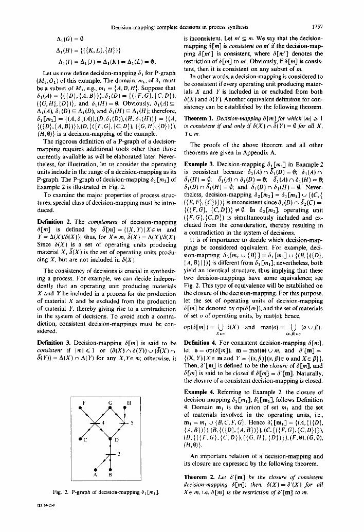
E F G H

A

Fig. 3. P-graph of decision-mapping 65 [ml w {C}].

That 61[ml] is an extension of 62 Ira2-] is denoted by 61 [ml] > 62[me]. Naturally, the closure of a consistent decision-mapping is its extension.

Example 6. Decision-mapping gs[ml w {C}] = 61 [ml] u {(C, {({E, F}, {C}),({F,G}, {C,D})})} is an extension of decision-mapping 6~l'mt] because it satisfies every requirement stated in Definition 7. The P-graph of decision-mapping 65[ml w {C}] is given in Fig. 3.

A major property of relation extension is expressed by the following statement.

Theorem 6. Relation extension is a partial order on the set of consistent decision-mappings.

4. REPRESENTATION OF A PROCESS GRAPH BY DECISION-MAPPING

With the necessary tools in hand, the relationship between the P-graphs and decision-mappings can now be examined. Let P-graph (re, o) be a specific subgraph of P-graph (M,O); then, m ~_ M, o __q O, O~_~d(M)×~d(M), and o~_~d(m)x~(m). Let us assume that m = mat(o).

Definition 8. m' is an active set of P-graph (m, o), if m' _ m and f l n m' :/: 0 for any (c~,fl)e o.

Thus, at least one output material of each operating unit of P-graph (m,o) is represented in its active set. Naturally, set m is active if, for any (~,fl)e o, fl ~ 0; conversely, P-graph (re, o) has no active set if there exists (ct, fl)E o such that fl = 0. This type of operating units has no practical value; thus, we suppose that fl # 0 for any operating unit (~,fl).

Definition 9. Let m' be an active set of P-graph (m, o); then, 6 [m'] is defined to be a decision-mapping of P-graph (re, o), if 6[m'] = {(X, Y ) I X e m' and Y={(~t, f l)l t~,fl)eo and X¢fl}}, i.e. if 3 ( X ) = {(~,fl)[(~,fl)e o and X e fl} for X e m'. Since m' is an active set, o = op(6[m']).

Example 7. Again referring to Example 2, both {A,D,H} and {B, C,D,H} are active sets of the

Decision-mapping: complete

P-graph given in Fig. 2. For these active sets, 6 ' [ { A , D , H } ] = { (A ,{ ({D} ,{A ,B})} ) , (D,{ ({F ,G} , {C,D}),({G,H},{D})}),(H,O)} and 6"[{B,C,D,H}] = {(B, { ( { D } , { A , B } ) } ) , ( C , { ( {F , G}, { C , D } ) } ) , ( D , {({F, q}, {C,D}),({G,H},{D})}),(H,O)} are two decision-mappings of this P-graph. Since they have identical closure, these decision-mappings are equivalent. The following theorems need be proved, however, to demonstrate that it is the case in general, i.e. the different decision-mappings of the same P-graph are always equivalent.

Theorem 7. The decision-mappings of P-graph (m, o) are consistent.

If the decision-mapping of a P-graph is given on the entire set of materials, then it is closed as stated in the following theorem.

Theorem 8. Decision-mapping ~[m] of P-graph (m, o) is closed.

The connection between the active set and active domain is expressed as a theorem as follows:

Theorem 9. Active set m' of P-graph (m, o) is an active domain of its decision-mapping ~ [m], if op(~[m']) = op(~[m]).

Since a P-graph may have multiple active sets, it may also have different decision-mappings. The principal question whether these decision-mappings are equivalent, is answered by the following theorem that ensures the validity of Definition 9.

Theorem 10. The decision-mappings of P-graph (m, o) are equivalent provided that m = mat(o).

Let us suppose that part of a process has been designed or it is temporarily assumed when synthesizing a process, e.g. a substructure is given by a decision-mapping. Then, the remaining part should be described in accordance with the previous decisions. The definition given below formalizes this requirement.

Definition 10. Let P-graphs a~ = ( m l , 0 0 and a2 =(m2,02) be given, where ml = mat(01), m2 = mat(02), ml c_ M, m2 ~- M, 01 -~ O, and 02 -~ O. Let ~1 [m~] be a decision-mapping of al. Then, tr2 is said to be an extension of trl relative to ~ ImP] if there exists a decision-mapping 62[m[] of tr 2 such that ~2[m~,] > ~1 [-m~].

Since the same structure may have different decision-mappings, the extension of a structure may de- pend on the particular decision-mapping considered. For example, both 61[ml] and 661"ml ~ {C}] = f i l [ml] u {(C,({F,G},{C,D}))} are decision-mappings of the P-graph given in Fig. 2; nevertheless, decision-mapping 6s[ml u {C}] of Example 6 is the extension of 61 [m~], but it is not the extension of ~6[ml ky {C}].

Theorem 11. Let 6Ira'] be a consistent decision-mapping; o = op(~[m']); and m = mat(o) u m ' . Then,

decisions in process synthesis 1759

(i) (m, o) is a P-graph, (ii) m' is an active set of P-graph (m, o), and (iii) ~ [m'] is a decision-mapping of P-graph (re, o).

This theorem suggests the definition for the P-graph of a decision-mapping.

Definition 11. The P-graph of consistent decision-mapping 6[m"] is defined to be (m, o) where o = op( f [m' ] ) and m = mat(o) • m'.

The following two theorems establish this definition.

Theorem 12. Let 6[m'-] be a consistent decision-mapping and (m, o) be its P-graph. I f re" is an active domain off[re"], then m" is an active set of(re, o).

Theorem 13. Equivalent decision-mappings have the same P-graph.

A path in a decision-mapping can analogously be defined as a path in a P-graph. Since this term has a special significance, it is explicitly defined below.

Definition 12. Let Yle op(6[m]) and X,~ mat(op (6[m])); then, there is a path between operating unit Yt and material X, in decision-mapping 3 [m] if and only if there exists a sequence YI, X x , Y2, X2 .... , Y,, X, such that Y~f(Xi) ( i = 1,2 . . . . . n) and X i¢ma t i" ({Y/+t}) (i = 1,2 . . . . . n - 1) where maP" determines the set of input materials for a set of operating units.

Example 8. A path exists between operating unit ({G,H},{D}) and material A in decision-mapping 3~[ml] in Example 2, since we have sequence ({G,H},{D}), D, ({D},{A,B}), A, which satisfies the requirements of Definition 12 (see Fig. 2).

5. DECISION-MAPPINGS AND THE COMBINATORIAL AXIOMS OF PROCESS SYNTHESIS

The MINLP model of a process synthesis problem gives rise to difficulties of both combinatorial and continuous nature even though they are not totally independent of each other. While several methods are available for mitigating the difficulties of the continuous nature, this is not the case for the difficulties of the combinatorial nature. To develop an exact and efficient algorithmic or mathematical programming method for process synthesis, therefore, it is necessary to comprehend the major combinatorial properties of process structures; moreover, these properties should be taken into account in search for the optimal process structures.

Suppose that sets P, R, and O are known for set M of materials given, where P is the set of products, R is the set of raw materials, and O is the set of operating units. The relation among these sets can be expressed as P c M , R c M , P ~ R = 0 , M n 0 = O, and O G CO(M) x co(M). Triplet (P,R,O) defines a synthesis problem, if none of sets P, R, and O is empty. The process structures for synthesis problem (P,R,O) are the subgraphs of P-graph (M,O); however, the P-graph of a feasible process must always conform to certain combinatorial properties.

1760

These properties have been expressed as a set of axioms; moreover, P-graphs satisfying these axioms are defined to be the solution-structures of the synthesis problem [Friedler et al. (1992c), also see Appen- dix B for a brief summary].

The axioms of process synthesis can also be expressed by the help of the decision-mapping. This form is advantageous in developing algorithms for process synthesis.

Definition 13. Let m be a subset of M for P-graph (M, O) and let ~ [m] be a consistent decision-mapping. Then, 6 [m] is defined to be a combina tor ia l l y f eas ib l e

decision-mapping of synthesis problem (P, R, O) if it satisfies the following axioms.

(91) P __q mat(op(c~[m])). (D2) For any x e mat(op(c~[m])),c~(x)= 0 if and

only if xe R. (D3) If oe op(~[m]), then an xe P exists such that

there is a path from o to x in c~ [m].

It can be proved that a decision-mapping is combinatorially feasible if and only if its P-graph is a solution-structure of (P, R, O). On the other hand, for any solution-structure (m, o), its decision-mapping c~ [m] is combinatorially feasible. Thus, Definition 13, together with Definition 11, results in a description of the solution-structures of synthesis problem (P, R, O).

F. FRIEDLER et al.

6. APPLICATION OF DECISION-MAPPINGS FOR THE COMBINATORIAL ALGORITHMS OF PROCESS

SYNTHESIS

Fundamental combinatorial algorithms have been developed through the decision-mapping. Such algorithms include those for the generation of the super-structure (maximal structure) and the set of

J K L

2

A B

Fig. 5. Maximal structure of Example 1.

input: M, P, R, A[M]; comment : P, R, A[M] belong to synthesis problem (P, R, O), where PcM, RcM, PnR = 0, A(x) = {(ct, [3)l(oq [~)~ O & xe ~}, A(x) = O ¢:* xe R, A[M] = {(x, A(x))lx~ M}, 8Ira] is a decision-mapping on (M, O);

output: all solution-structures of synthesis problem (P, R, O); global variables: R, A[M];

begin ifP = 0 then stop; SSG(P, O, O) end

procedure SSG(p, m, 8[m]): begin ifp = O then begin write 8[m]; comment: 8[m] defines a solution-structure;

return end let x~ p; C:= ~o(a(x))\{O}; for all ce C do

begin

if Vye m, c~8(y) = O & (A(x)\c)nS(y) = O then

begin 8[mw{x}]:= 8[m]w{(x, c)}; SSG(pumatin (c))\(Rumu{x}), mu{x}, 8[mu{x}]) end

end return end

Fig. 4. Algorithm SSG for generating the solution-structures of a synthesis problem.

Decision-mapping: complete decisions in process synthesis

Table 1. Recursive steps of algorithm SSG in generating the solution-structures of Example 9

1761

Number Depth of Parameter Parameter Parameter of call recursion p m 6 [m] Remark

1 0 {A} 0 0 Initial call 2 1 {C} {A} {(A,{1})} 3 2 {F} {A,C} {(A, {1}),(C, {3})} 4 3 0 {A,C,F} {(A,{1}),(C,{3}),(F,{1})} Solution #1 5 3 0 {A,C,F} {(a, {1}),(C,{3}),(F,{1,6})} Solution #2 6 2 {F} { A , C } {(A,{1}),(C,{4})} 7 3 0 {A,C,F} {(A,{1}),(C,{4}),(F,{I})} Solution #3 8 3 0 {A,C,F} {(A,{1}),(c,{a}),(F,{1,6})} Solution #4 9 2 {F} {A,C} {(A, {1}),(C, {3,4})}

10 3 0 {A,C,F} {(A,{I}),(C,{3,4}),(F,{1})} Solution #5 11 3 0 {A,C,F} {(A,{1}),(C,{3,a}),(F,{1,6})} Solution #6 12 1 {O} {A} {(A,{2})} 13 2 {F} {A,D} {(A, {2}),(D, {4})} 14 3 0 {A,D,F} {(A,{2}I,(D,{4}),(F,{6})} Solution #7 15 2 {n} [a,o} {(A,{2}t,(O,{5})} 16 3 0 {A,D,H} {(A,{2}),(D,{5}),(H,{7})} Solution #8 17 2 {F,H} {A,D} {(A, {2}),(D, {4, 5})} 18 3 {H} {A,D,F} {(A,{2}),(D,{4,5}),(F,{6})} 19 4 0 {A,D,F,H} {(A,{Z}),(D,{4,5}),(F,{6}),(H,{7})} Solution #9 20 1 {C,D} {a} {(A, {1,2})} 21 2 {D,F} {a,c} {(A, { 1,2}),(C, {3})} 22 3 {F,H} { A , C , D } {(A,{l,2}),(C,{3}),(D,{5})} 23 4 {H} {A,C,D,F} {(A,{1, Z}),(C,{3}),(D,{5}),(F,{1})} 24 5 0 {A,C,D,F,H} {(A,{I,2}),(C,{3}),(D,{5}),(F,{1}),(H,{7})} Solution #10 25 4 {H} {A,C,D,F} {(A,{1,2}),(C,{3}),(D,{5}),(F,{1,6})} 26 5 0 {A,C,D,F,H} {(A,{1,Z}),(C,{3}),(D,{5}),(F,{1,6}),(H,{7})} Solution #11 27 2 {D,F} {A,C} {(A, { 1,2}),(C, {4})} 28 3 {F} {A,C,D} {(A,{I,2}),(C,{4}),(D,{4})} 29 4 0 {A,C,D,F} {(A,{I,2}),(C,{4}),(D,{4}),(F,{I})} Solution #12 30 4 0 {A,C,D,F} {(A,{I,2}),(C,{4}),(D,{4}),(F;{1,6})} Solution #13 31 3 {F,H} { A , C , D } {(A,{I,2}),(C,{4}),(D,{4,5})} 32 4 {H} {A,C,D,F} {(A,{I,Z}),(C,{4}),(D,{4,5}),(F,{1})} 33 5 0 {A,C,D,F,H} {(A,{1,2}),(C,{4}),(D,{4,5}),(F,{1}),(H,{7})} Solution #14 34 4 {H} {A,C,D,F} {(A,{1, Z}),(C,{4}),(D,{4,5}),(F,{1,6})} 35 5 0 {A,C,D,F,H} {(A,{1,2}),(C,{4}),(D,{4,5}),(F,{1,6}),(H,{7})} Solution #15 36 2 {D,F} {A,C} {(a, {1, 2}),(C, I3,4}) } 37 3 {F} {A,C,D} {(A,{1,2}),(C,{3,a}),(D,{4})} 38 4 0 {A,C,D,F} {(A,{1,2}),(C,{3,a}),(D,{a}),(F,{1})} Solution #16 39 4 0 {A,C,D,F} {(A,{1,2}),(C,{3,4}),(D,{a}),(F,{1,6})} Solution #17 40 3 {F,H} { A , C , D } {(A,{I,2}),(C,{3,4}),(D,{4,5})} 41 4 {H} {A,C,D,F} {(A,{1,2}),(C,{3,4}),(D,{4,5}),(F,{1})} 42 5 0 {A,C,D,F,H} {(A,{1,Z}j,(C,{3,4}),(D,{4,5}J,(F,{1}),(H,{7})} Solution #18 43 4 {H} {A,C,D,F} {(A,{1,2}),(C,{3,4}),(D,{4,5}),(F,{1,6})} 44 5 0 {A,C,D,F,H} {(A,{1,2}),(C,{3,4}),(D,{4,5}),(F,{l,6}),(H,{7})} Solution #19

solution-structures (Friedler et al., 1992a, 1993). These algorithms, in turn, have given rise to the so-called accelerated branch and bound algorithm of process synthesis that is highly efficient (Friedler et al., 1990; Friedler and Fan 1993a, b). This accelerated branch and bound algorithm not only is mathematically veri- fiable but also effectively minimizes the number and sizes of the subproblems to be solved for generating

the optimal solution. The decision-mapping and the resultant algorithms manipulate process structures explicitly; hence, the user's decisions can be incorpor- ated interactively into the algorithmic decision procedure of process synthesis.

For illustration, let us consider algorithm SSG for generating the solution-structures of synthesis problem (P,R,O). This procedure is given in Fig. 4


A I.

J

6

3 F

^ 2.

J J K

J

6

F G F G ~ , N /

D D ~ D

A 3. ^ 4. ^ 5.

L K L K L

6

F G~ D F G /

A 6. A B 7. A B 8.

F G H i t / F

C D

A B 9. A B 10.

I K L J

f 6

F G F G

A B II. A a 12. A B

K L J K L

13.

7 6 7

F G H F G H F G ~ 4 G

A B 14. A B 15. A B 16. j K L J K L

6 7 6 7

F G F G H F G H

A a 17. A a 18, A n 19.

Fig. 6. Solution-structures of Example 9 generated by algorithm SSG.

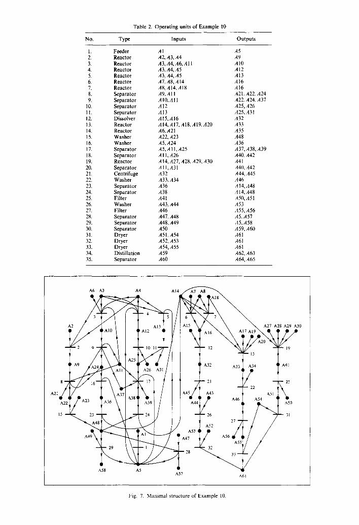
Table 2. Operating units of Example 10

No. Type Inputs Outputs

1. Feeder A 1 A 5 2. Reactor A2, A3, A4 A9 3. Reactor A3, A4, A6, A 11 A 10 4. Reactor A3, A4, A5 A 12 5. Reactor A3, A4, A5 A 13 6. Reactor A7, A8, A 14 A 16 7. React or A 8, A 14, A 18 A 16 8. Separator A9, A 11 A21, A22, A24 9. Separator A 10, A 11 A22, A24, A37

10. Separator A 12 A25, A26 11. Separator A 13 A25, A31 12. Dissolver A15,A16 A32 13. Reactor A14,A17, A18,AI9, A20 A33 14. Reactor A6, A21 A35 15. Washer A22, A23 A48 16. Washer A 5, A24 A 36 17. Separator A5, AI 1, A25 A37, A38, A39 18. Separator A 11, A26 A40, A42 19. Reactor AI4, A27, A28, A29, A30 A41 20. Separator A 11, A 31 A 40, A42 21. Centrifuge A32 A44, A45 22. Washer A33, A34 A46 23. Separator A36 A 14, A48 24. Separator A38 A 14, A48 25. Filter A41 A 50, A 51 26. Washer A43, A44 A 53 27. Filter A46 A55, A56 28. Separator A47, A48 A5, A57 29. Separator A48, A49 A5, A58 30. Separator A 50 A 59, A 60 31. Dryer A51,A54 A61 32. Dryer A52, A 53 A61 33. Dryer A54, A55 A61 34. Distillation A59 A62, A63 35. Separator A60 A64, A65

A21

A6 A

A! A57 A61

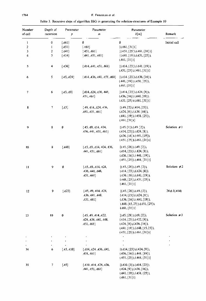
Fig. 7. Maximal structure of Example 10.


Table 3. Recursive steps of algorithm SSG in generating the solution-structures of Example 10


1 0 {A61} 0 0 Initial call 2 1 {A51} {A61} {(A61, {31})} 3 2 { A 4 1 } {A51,A61} { (A51, {25}),(A61, {31 })} 4 3 { A 1 4 } {A41,A51,A61} {(A41, { 19}),(A51, {25}),

(A61,{31})}

5 4 {A36} {AIa, A41,A51,A61} {(A 14, {23}),(A41, { 19}), (A51, {25}),(A61, {31})}

6 5 {A5,A24} {AI4,A36,A41,A51,A61} {(A14, {23}),(A36, { 16}), (A41, { 19}),(A51, {25}), (A61,{31})}

7 6 {a5,a9} {A14,A24, A36, A41 , {(A14,{23}),(A24,{8}), A51,A61} (A36, { 16}), (A41, { 19}),

(a51, {25}), (A61, {31 })}

8 7 { A 5 } {A9,A14,A24,A36, {(A9, {2}),(A 14, {23}), A41,A51, A61} (A24, {8}), (A36, { 16}),

(A41, { 19}), (A51, {25}), (A61, {31})}

9 8 0 {A5,A9, AI4, A24, {(A5, { l}),(a9, {2}), Solution #1 A36,Aal, A51,A61} (A 14, {23}), (A24, {8}),

(A36, { 16] ), (An1, { 19}), (A51, {25}),(A61, {31})}

10 8 { A 4 8 } {A5,A9,A14, A24,A36, {(A5, {28}),(A9, {2}), A41,A51,A61} (A14, {23}),(A24, {8}),

(A36, {16}), (A41, { 19}), (a51, {25}), (A61, {31})}

11 9 0 {A5,A9,A14,A24, {(a5, {28}),(A9, {2}), Solution #2 A36, a41, A48, (A 14, {23}), (A24, {8}), A51,.461} (A36, { 16}),(A41, {19}),

(A48, {23}), (A51, {25}), (A61,{31})}

12 9 {A22} {A5, A9, A14, A24, {(a5, {28}),(A9, {2}), 24 ¢ 6(A 14) A36, a41, A48, (A 14, {23}), (A24, {8} ), A51,A61} (A36, { 16}), (a41, {19}),

(A48, { 15, 23} ), (as 1, {25}), (A61,{31}1}

13 10 0 {A5,A9,A14, AZ2, {(A5, {28}),(A9, {2}), Solution #3 A24,A36, A41, A48, (a 14, {23} ), (A22, {8}), A51,A61 } (A24, {8}), (A36, { 16}),

(A41, { 19}), (A48, { 15,23}), (A51, {25}), (a61, {31})}

34 6 {A5, A10} {AI4,A24,A36,A41, {(A14,{23}),(A24,{9}), A51,A61 } (A36, { 16}),(A41, {19}),

(A51, {25}), (A61, {31})}

35 7 {A5} {AlO, AI4, A24,A36, {(A 10, {3}), (A 14, {23}), A41, A51, A61 } (A24, {9}), (A36, { 16}),

(A41, {19}), (A51, {25}), (A61, {31})}

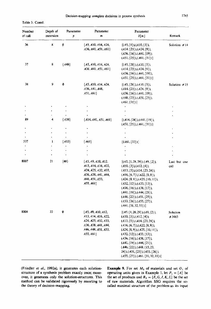
Decision-mapping: complete decisions in process synthesis 1765

Table 3. Contd.


36 8 0 {A5,AlO, AI4,A24, {(A5, { 1}),(A10, {3}), Solution #14 A36,A41, A51,A61} (A 14, {23}), (A24, {9}),

(A36, { 16}), (A41, {19}), (A51, {25}),(A61, {31})}

37 8 {A48} {A5,AlO, A14,A24, {(A5, {28}), (A 10, {3}), A36,A41,A51,A61} (A 14, {23}), (A24, {9}),

(A36, {16}), (A41, {19}), (A51, {25}),(A61, {31})}

38 9 0 {A5,AlO, A14,A24, {(A5, {28}),(A 10, {3}), Solution #15 A36, A41, A48, CA 14, {23 }), (A24, {9} ), A51,A61} (A36, {16}),(A41, { 19}),

(A48, {23}), (A51, {25}), (A61,{31})}

89 4 { A 3 8 } {A14,A41,A51,A61} {(A 14, {24}),(A41, { 19}), (A51, {25}), (A61, {31})}

537 1 {A53} {A61} {(A61, {32})}

8007 21 { 4 8 } {A5,A9,AIO, A12, A13,A14,AI6,A22, A24, A25, A32, A33, A36, A38, A41, A44, A46, A5 l, A53, A55,A61}

8008 22 0 {A5,A9,AIO, A12, AI3,AI4,A16,A22, A24, A25, A32, A33, A36, A38, A41, A44, A46, A48, AS1, A53, A55,A61}

{(A5, { 1, 28, 29} ), (A9, {2} ), (A10, {3}), (A 12, {4}), (A 13, {5} ), (A 14, {23, 24} ), (A 16, {6, 7} ), (A22, {8, 9} ), (A24, {8, 9}),(A25, {10, 11}), (A32, { 12}),(A33, { 13}), (A36, { 16}),(A38, { 17}), (A41, { 19}),(A44, {21 }), (A46, {22}), (A51, {25}), (A53, {26}), (A55, {27}), (A61, {31, 32, 33})}

{(A5, {1,28, 29}),(A9, {2}), (A10, {3}),(A 12, {4}), (A13, {5})AA 14, {23, 24}), (A16, {6, 7}), (A22, {8,9}), (A24, {8,9}),(A25, {10,11}), (A32, { 12}), (A33, { 13}), (A36, { 16}),(A38, {17}), (A41, { 19}), (A44, {21 }), (A46, {22}), (A48, { 15, 23, 24}),(A51, {25}),(A53, {26} ), (A55, {27}), (A61, {31, 32, 33})}

Last but one call

Solution # 3465

(Friedler et al., 1992a), it generates each solution- structure of a synthesis problem exactly once; moreover, it generates only the solution-structures. This method can be validated rigorously by resorting to the theory of decision-mapping.

Example 9. For set Mt of materials and set O1 of operating units given in Example 1, let Pl = {A} be the set of products and R1 = {E, G, J, K, L} be the set of raw materials. Algorithm SSG requires the so- called maximal structure of the problem as its input


(see Appendix B). This maximal structure, given in Fig. 5, has been created by algorithm MSG (Friedler et al., 1993). Algorithm SSG generates the decision- mappings of the solution-structures recursively; the "values" of the parameters for each recursive step is listed in Table 1. Note that the number and order of calls and the order of the generation of the individual solution-structures may be effected by the implementation of algorithm SSG, nevertheless, the set of solution-structures is obviously invariant for the implementation. During the generation of solution- structures, the decision-mapping in the third parameter of algorithm SSG represents a solution-structure if the first parameter of algorithm SSG, set p, is empty. It occurs nineteen times in solving this example, thereby resulting in 19 solution-structures, as illustrated in Fig. 6.

Example 10. Let us now consider solution-structures of an industrial process synthesis problem. For this purpose the process synthesis problem introduced in Friedler et al. (1992a) is re-examined again. In this problem set M of materials has 65 elements, M = {A1,A2 . . . . . A65}, where R = {A1,A2,A3,A4, A6, A7, A8, Al l ,A15, A17,A18, A19, A20, A23, A27, A28, A29, A30, A34, A43, A47, A49, A52, A54} is the set of raw materials. Moreover, 35 operating units are available for producing the product, material A61; these operating units are listed in Table 2. The maximal structure of the problem is given in Fig. 7. The recursive steps of algorithm SSG in generating the solution-structures of this example are listed in Table 3. For instance, the first solution-structure in Table 3 is composed of operating units 1, 2, 8, 16, 19, 23, 25, and 31 of the maximal structure.

In addition to being a fundamental algorithm of the accelerated branch and bound algorithm, algorithm SSG is also capable of directly generating the mathematically valid disjunctive normal form for synthesis problems to serve as the inputs of synthesis methods based on logical formulation [see e.g. Raman and Grossmann (1993)].

7. CONCLUDING REMARKS

A novel mathematical notion, decision-mapping, has been introduced to render the complex decision systems of process synthesis consistent and complete. The major properties of decision-mapping have been identified and proved; moreover, its relationship to P-graphs has been established. The application of decision-mapping is illustrated by generating the solution-structures of an industrial process synthesis problem. The result indicates that it is highly efficient, exact, and useful.

Acknowledgements--The authors thank Professor B. Imreh of Department of Computer Science, University of Szeged, Hungary, for critically reviewing our manuscript. This research was partially supported by the Hungarian Academy of Sciences. Although the research described in this article has been funded in part by the United States Environmental Protection Agency under assistance agreement R-819653 to

the Great Plains-Rocky Mountain Hazardous Substance Research Center for U.S. EPA Regions 7 and 8 with head- quarters at Kansas State University, it has not been sub- jected to the Agency's peer and administrative review and, therefore, may not necessarily reflect the views of the Agency. No official endorsement should be inferred. This research was partially supported by the Kansas State University Center for Hazardous Substance Research.

d - ( X )

f(x)

iff (m, o), (M, O) m, M mat

mat in

o,0 op P R (P, R, O)

S(P, R, O)

[yi,y~] f[O]

Greek letters ~(P, R, O)

NOTATION

indegree of vertex X, i.e. the number of arcs with endpoint X "value" determined by the mapping or function for an element of the domain, x if and only if P-graph set of materials set of materials involved in a set of operating units set of input materials for a set of operating units set of operating units operating units of decision-mapping set of products set of raw materials synthesis problem defined by the specific set of products (P), raw materials (R), and operating units (O) set of solution-structures for synthesis problem (P, R, O) path in P-graph mapping or function, where f is the name, D is the domain of the mapping or function

maximal structure for the synthesis problem (P, R, O)

tr P-graph A maximal decision-mapping ~5 decision-mapping c5 complement of decision-mapping c5

Mathematical symbols 0 empty set

power set V for any 3 there exists x Cartesian product { } set II cardinality of a set \ set difference ( c ) ~ (proper) subset or subgraph • element ¢ not an element c~ intersection of sets or graphs u union of sets or graphs > extension defined on decision-map-

pings

Decision-mapping: complete decisions in process synthesis 1767

REFERENCES (~(X) ca 6(Z)) = 0; thus, 6(X) ca 6'(Y) = O. On the

Douglas, J. M., 1988, Conceptual Design of Chemical Pro- cesses. McGraw-Hill, New York.

Friedler, F. and Fan, L. T., 1993a, Combinatorial acceleration of the branch and bound search for process network synthesis. Proceedings of Symposium on Applied Mathematical Profframmin9 and Modelin#, Budapest, Hungary, pp. 192-200.

Friedler, F. and Fan, L. T., 1993b, Reduction of subproblem size for the accelerated branch and bound method of process synthesis. AIChE National Meetin~, Houston, TX, U.S.A., March 28-April 1.

Friedler, F., Tarjan, K., Huang, Y. W. and Fan, L. T., 1990, Combinatorial acceleration of branch and bound search in process synthesis. AIChE Annual Meetin#, Chicago, IL, U.S.A., November 11-16.

Friedler, F., Tarjan, K., Huang, Y. W. and Fan, L. T., 1992a, Combinatorial algorithms for process synthesis. Comput. chem. Enong 16, supplement, $313-320.

Friedler, F., Tarjan, K., Huang, Y. W. and Fan, L. T., 1992b Combinatorial structure of process network synthesis. Sixth SIAM Conference on Discrete Mathematics, Van- couver, Canada, June 8-11.

Friedler, F., Tarjan, K., Huang, Y. W. and Fan, L. T., 1992c, Graph-theoretic approach to process synthesis: axioms and theorems. Chem. Engng Sci. 47, 1973-1988.

Friedler, F., Tarjan, K., Hunag, Y. W. and Fan, L. T., 1993, Graph-theoretic approach to process synthesis: poly- nomial algorithm for maximal structure generation. Comput. chem. Engng 17, 929-942.

Lu, M. D. and Motard, R. L., 1985, Computer-aided total flowsheet synthesis. Comput. chem. Engng 9, 431-445.

Raman, R. and Grossmann, I. E., 1993, Symbolic integration of logic in mixed-integer linear programming techniques for process synthesis. Comput. chem. Engng 13, 909-927.

Siirola, J. J. and Rudd, D. F., 1971, Computer-aided synthesis of chemical process designs. Ind. Engng Chem. Fundam. 10, 353-362.

APPENDIX A: PROOFS OF THEOREMS

Proof of Theorem 1. Obviously, A(X) = fi(X) u 3(X) and A(Y) = 6(Y) w 3(Y); hence,

A(X) ca A(Y) = (6(X) ca 6(Y)) w (6(X) ca 3(Y))

(3(X) ca 3(Y)) ~ (S(X) ca 3(Y)). (A1)

(i) If 3 ( X ) c a S ( Y ) = 0 for all X, Yem, i.e. 6(X)ca 6(Y~ = 0, then, A(X) ca A(Y) = (3(X) ca 3(Y)) ~ (6(X) ca ~(Y)) from expression (A1).

(ii) Conversely, let us suppose that (6(X) ca 3(Y)) ~ (S(X) nS(Y) )=A(X)CaA(Y) for any X , Y ~ m . Since

( (6 (X) ca 6(Y)) ~ (~(X) ca 3(Y)) ca (3 (X) ca ~-(Y)) = 0 and ((6(X) ca 6(Y)) ~ ($(X) ca ~-(Y))) ca (~-(X)

6 ( Y ) ) = 0 , we have 6(X) c a 3 ( Y ) = 0 and 3(X) ca 6(Y) = 0 from expression (A1).

Proof of Theorem 2. (i) F o r X e m , 6(X)= {(~,/~)l(~,fl)~ 6 (X)and X e fl} ~_

{(~,fl)l(~,/~) ~ o and X e/~} = ,~'(X). (ii) Suppose that there exists an (a,/~) for X e m such that

(~ , f l )eo, X e / L and (~,/~)¢6(X). Consequently, (~ , f l )eS(X), and there exists Y e m such that (a, fl) E 6(Y), i.e. S(X) ca 6(Y) 4 :0 in contradiction to 6[m] being consistent. Thus, (~,fl) ~ 6(X) and 3(X) = {(~,fl)l(~,fl) ~ o and X ~ fl} = 3'(X).

Proof of Theorem 3. Let 6 [m] be the closure of consistent decision-mapping 3[m]. Naturally, m G m.

(i) For X ~ m , 6 ' (X)=f(X); thus, if Iml> / l and X, Ye m, then, 3 '(X) ca 6'(Y) = O.

(ii) Suppose that m/m q: 0, and let X ~ m and Y ~ m/m. Then, # ( X ) ca 3'(Y) = cS(X) ca {(~,f l ) l (~,f l )eo and r e fl} ~_ $(X) ca o = S(X) n ( U z ~ , , f ( z ) ) = Uz~,, ,

other hand, since 6'(Y)c_A(Y), 3'(X)ca3'(Y)= 6(X) ca (A( Y)/ f '( Y)) = 3(X) ca A( Y)/ f ( X ) ca 6'(Y). Nevertheless, 6(X) ca A(Y) = 6(X) ca {(a, fl)l(~,fl) e O and Y~ fl} = {(~,fl)l(a, fl) ~ ~5(X) and Ye fl}, 6(X) ca 6'(Y) = 3(X) ca {(a, fl)l(~,~) e o and Ye fl} = {(~,fl) I(~, fl) e 3(X) and Y ~/~}; consequently, 6(_X) ca A(Y) = 6(X) ca 6'(Y), and eventually, 3'(X) ca 6'(Y) = O.

(iii) For X, Y~ m/m, it can be similarly proved that 3'(X) ca ~-'(Y) = 0 provided that ]m/ml >/1.

Proof of Theorem 4. Let m' be an active domain of consistent decision-mapping 3[ml, and also let YE m/m'.

(i) Obviously, 6(Y) _c (Ux~,. 3(x) ) = (Ux~,~, 6(x)) and 6(Y) ~_ A(Y); thus,

(ii) Since 3[m] is consistent, (6(X) ca 3(Y)) u (~ (X) ca ~ ( Y ) ) = A ( X ) C a A ( ¥ ) for any XEm'. The inter- sections of both sides of this equation with set 3(X) result in

fi(X) ca 3(Y) = (A(X) ca 6(X)) ca A{Y).

This can be rewritten as fi(X) ca 6(Y) = fi(X) ca A(Y). Obvi- ously, fi(Y) ~ 6(X) ca 6(Y) = 6(X) c~ A(Y) for any X ~ m'; hence,

f lY) -D U (6(x)caA(Y)) . X~m'

(iii) From (i) and OiL we have

3(Y) = ~ (A(Y) ca 3(X)) = op ( f [m ' ] ) ca A(Y). X~m'

Note that this is the formula for determining 6(Y) for any Y ~ m/m'.

Proof of Theorem 5. Let m' be an active domain of decision- mapping 6[m], and 3(X) ca 6(Y) = 0 for all X, Y~ m'.

(i) If X ~ m ' and YEm/m', then by o p ( f [ m ' ] ) =

Similarly, by

op(3[m']) = op(~[m]),

(ii) Suppose that Im/m'l/> 2 and let X, Y s m/m'. Then,

Proof of Theorem 6. The reflexivity of relation extension is satisfied trivially. The antisymmetry will be proved at the outset. Let 61 [mr] and ~2[m2] be consistent decision-mappings with closures ~ [m l] and 61 [m2], respectively. More- over, let us suppose that t$1 [ml] >. t~2 Im2] and 62 [m2l > 61 [ml]. Then, from the definition of extension, we have m l ~ m 2 , m 2 - ~ m l , m l ~ m 2 , and m e - m 1 , i.e. ml = m2 and ml = m2; therefore, 6 t (X) = 62(X) for X E m>

1768

The proof of transitivity follows. Let us suppose that 3 t [ml] > f2['m2] and f2['m2] > f3[m3]; then, we need to prove that 61[ml] > 63[m3]. The first and second condi- tions of extension are satisfied, since the relations "subset" and "equal to" are also transitive. From fit [ml] > 32 Ira2], 6'1(X) = 62(X), 62(X) = 6;(X) for X • m2, and 6'~(X) =_ 6'2(X) for X e m2/m2. Hence, 6'~(X) ~_ f'2(X) for X e m 2 . 62[m2]>ff[m3]; hence, 6'2(X)D_f'3(X) for X • m3/m3. Thus, we have 6](X) _D 6'3(X) for X • mf/m 3.

Proof of Theorem 7. Let m' be an active set of P-graph (m, 0), and suppose that I m'l/> 2; moreover, let X and Y be elements of re'. I fA(X) n A(Y) = 0, then, 6-(X) n 6(Y) = 0. Let us suppose that A (X) c~ A (Y) :# 0 and let (~, fl ) be an element of A(X)c~A(Y); then, X, YEfl. If (~,fl)~o, then, (~,fl) • 6(X) and (~,fl) ~ f(Y), i.e. (~,fl) • 6(X) c~ 6(Y). If (~,fl) ¢ o, then, (~,#) ~ 6(X), (~,#) • &(X), and (~,fl) • 6(Y); thus, (cqfl) • $(X) c~ S(Y).

Proof of Theorem 8. Let 3 [ m ] = { ( X , Y ) I X • m and Y = {(a, fl)[(~, fl) • o and X • fl} } be the decision-mapping of(re, o) on m. Since m is an active set, ~x~=b(X) = o, o = o, and for P-graph (m, o), ~¢=.#)~o(a u fl) ~ m; thus, m = m and ~' [m] = ~ [ m ] .

Proofof Theorem 9. Let rim] be a decision-mapping and m' be an active set of P-graph (re, o). Then, for any (~t, fl)~ o, there exists an X • m ' such that (ct, f l)~f(X); thus, o=Ux~m,f(X). Since m'c_m, we have ~x~,,,f(X)c_ Ux , , , f (X )= o_. Thus, Ux_~m,b(X)= Ux,=f(X). The assumption, op(3 [m']) = op(6 [m]), implies that m' is an active domain of 6[m].

Proof of Theorem 10. By Theorems 7 and 8, decision-mapping 6 Ira] of P-graph (m, o) is consistent and it is also closed. Let us suppose that there exists another active set ml of P-graph (re, o); then, by Theorem 7, decision-mapping 61 I-m1] of P-graph (m, o) is consistent. Since ml is an active set of (m, o), o = op(fx [ml]). Then, by the assumption that m = mat(o), the closure of 61 [ml] is equal to the closure of 6[m]; thus, they are equivalent.

Proof of Theorem 11. (i) m c~ o = 0 and o _ go(m) × go(m) are trivially satisfied.

F. FRIEDLER et al.

(ii) From the construction of o, it follows that m' is an active set of P-graph (m, o).

(iii) 6 [m'] is a decision-mapping of P-graph (m, o): For all X • m', 6(X) ~ { (~t, fl) • o and X • fl} follows from the construction of o; the equality also holds, since 6 [m'] is consistent.

Proof of Theorem 12. Let 6[m'] be a consistent decision- mapping; m" be an active domain- of 61-m']; and (m, o) be the P-graph of 6[m']. Since m" is active domain of f[m'], o = Ux~m' f (X) = ~x~=,,f(X). Thus, for all (~,fl) • o, there exists X • m" such that (~, fl) • f(X), i.e., fl c~ m" is not empty.

Proof of Theorem 13. Let 61 [ml ] and 62 [m2] be two equivalent consistent decision-mappings. By definition, they share a closure; thus ol = U x . . . . 61(X1) = ~xz~m262(X2)= 02. It follows that the material sets constructed according to Definition 11 are also identical.

APPENDIX B: FORMAL DEFINITIONS OF PROCESS SYNTHESIS AND COMBINATORIAL PROPERTIES OF

FEASIBLE PROCESS STRUCTURES Let M be a finite nonempty set of objects, usually mater-

ials. A synthesis problem is defined to be a triplet (P,R,O) where P( c M) is a set of final products; R( c M) is a set of raw materials (P c~ R = 0); and O _c (go(M)× go(M)) is a set of operating units. This triplet determines a P-graph which is defined by pair (M, O) in the usual fashion. If (Yi-t, Yi) is an arc of the P-graph for i = 1,2 . . . . . n, then [Yo,Y,] is a path in P-graph (M, O).

P-graph (m, o) is a solution-structure of synthesis problem (P, R, O) if it satisfies the following axioms:

(S1) P c_ m; ($2) VX E m, d-(X) = 0 iff X • R; ($3) o _ O; ($4) Vyo e o, 3 path [Y0, Y.], where y. • P; ($5) ¥X • m, 3(ct, fl) • o such that X ~ (ct u fl).

The set of solution-structures of synthesis problem (P, R, O) is denoted by S(P,R,O). P-graph #(P,R,O) is defined to be the maximal structure of synthesis problem (P, R, O) by the following equation: p(P, R, O) = UqeS(P,R,O ) a.

decision-mapping: a tool for consistent and complete decisions in process synthesis

Documents