czech aerospace - haw hamburg
TRANSCRIPT

LETECKÝzzpprraavvooddaajj
ISSN 1211—877X
In this issue:Propeller Control LoopModel Developmentand Simulation ofTransient Behavior
Sensor Analysis forTEASER Project
Calculation ofTemperature Fields ofVibrating CompositeParts
Wind TunnelResearch of WingtipDevices
Cooling of ElectronicsInstalled in PassengerSeats of CivilAeroplanes and itsTesting
Simulation of RigidProjectile Impact onthe Real AircraftStructure
Unmanned AircraftStructural Model andits FEM Analysis
CZECHCZECHAEROSPACEPP rr oo cc ee ee dd ii nn gg ss
No. 2 / 2009
Au
gu
st
2
00
9

VÝZKUMNÝ A ZKUŠEBNÍ LETECKÝ ÚSTAV, a.s.Editorial address: Aeronautical Research and Test Institute / VZLÚ, Plc.
Beranových 130, 199 05 Prague 9, LetňanyCzech RepublicPhone.: +420-225 115 223, Fax: +420-869 20 518
Editor-in-Chief: Ladislav Vymětal (e-mail: [email protected])Editor & Litho: Stanislav Dudek (e-mail: [email protected])
Editorial Board:Chairman: Milan Holl, President ALVVice-Chairman Vlastimil Havelka, ALVMembers: Jan Bartoň, Tomáš Bělohradský, Vladimír Daněk,
Luboš Janko, Petr Kudrna, Pavel Kučera, Oldřich Matoušek,Zdeněk Pátek, Antonín Píštěk
Publisher: Czech Aerospace Manufacturers Association / ALV, PragueBeranových 130, 199 05 Prague 9, LetňanyCzech RepublicID. No. 65991303
Printing: Studio Winter Ltd. Prague
Periodicity: Three times per year. Press Reg. No. MK ČR E 181312.
Subscription and ordering information available at the editorial address. Legal liability for publishedmanuscripts’ originality holds the author. Manuscripts contributed are not returned automatically toauthors unless otherwise agreed. Notes and rules for the authors are published at our Internet pageshttp://www.vzlu.cz/.
Czech AEROSPACE ProceedingsLetecký zpravodaj
2/2009
© 2009 ALV /Association of Aviation Manufacturers, All rights reserved. No part of this publication maybe translated, reproduced, stored in a retrieval system or transmitted in any form or by any other means, electronic,
mechanical, photocopying, recording or otherwise without prior permission of the publisher.
ISSN 1211 - 877X
LE TECK Ýzzpprraavvooddaajj
J O U R N A L F O R C Z E C H A E R O S P A C E R E S E A R C H
CZECHCZECHA E R O S P A C EPP rr oo cc ee ee dd ii nn gg ss
EUROPEAN UNIONEUROPEAN REGIONAL DEVELOPMENT FUNDINVESTMENT IN YOUR FUTURE
Contents / ObsahCalculation of Temperature Fields of Vibrating Composite PartsVýpočet teplotních polí kmitajícího kompozitního díluIng. Vilém Pompe, Ph.D. / VZLÚ, Plc., Prague
NASPRO 3.0 — Software Tool for Transformation and Vizualization of Aircraft Structure ModalAnalysis ResultsNASPRO 3.0 — programový prostředek pro transformaci a vizualizaci výsledků modální analýzyleteckých konstrukcíIng. David Gallovič, Ing. Jiří Čečrdle, Ph.D. / VZLÚ, Plc., Prague
Sensor Analysis for TEASER ProjectAnalýza senzoru pro projekt TEASERViktor Fedosov / VZLÚ, Plc., Prague
Propeller Control Loop Model Development and Simulation of Transient BehaviorVývoj modelu regulační smyčky vrtule a simulace přechodových stavůIng. Jaroslav Braťka / VZLÚ, Plc., Prague
Unmanned Aircraft Structural Model and its FEM Analysis for Strength EvaluationStrukturální model bezpilotního letounu a jeho MKP pevnostní analýzaAleksander Olejnik, Stanisław Kachel, Robert Rogólski, Piotr Leszczyński, Military University of Technology,Faculty of Mechanics, Warsaw, Poland
Simulation of Rigid Projectile Impact on the Real Aircraft StructureSimulace nárazu tuhého projektilu na reálnou leteckou konstrukciIng. Radek Doubrava, Ph.D. / VZLÚ, Plc., Prague
Wind Tunnel Research of Wingtip DevicesVýzkum konců křídla v aerodynamickém tuneluJan Červinka, Zdeněk Pátek / VZLÚ, Plc., Prague
Cooling of Electronics Installed in Passenger Seats of Civil Aeroplanes and its TestingChlazení elektroniky instalované v sedadlech cestujících v dopravních letounechJiří Myslivec, VZLÚ, Plc., Prague
The Fast Transient Processes Simulation by Using IST Electro Hydraulic Test Control SystemSimulace rychlých přechodových dějů elektrohydraulickým zkušebním systémem ISTMartin Oberthor, Jiří Nejedlo / VZLÚ, Plc., Prague
Influence of Silumine Castings Microstructure on Component Failure ResistanceVliv mikrostruktury odlitků vyrobených ze siluminu na odolnost součásti proti mechanickému porušeníMiroslava Machková, Roman Růžek / VZLÚ, Plc., Prague; Drahomíra Janová / Institute of Material Scienceand Engineering, Brno University of Technology, Brno
Preliminary Sizing of Large Propeller Driven AeroplanesPředběžný výpočet rozměrů velkého vrtulového letounuProf. Dieter Scholz, Mihaela Niţă / Hamburg University of Applied Sciences, Hamburg, Germany
1 L E T E C K Ý Z P R A V O D A J 2 / 2 0 0 9
2
4
7
10
14
18
21
27
30
36
41
C Z E C H A E R O S P A C E P R O C E E D I N G S 2
1 IntroductionThe heat-up of a vibrating body is a notorious phenomenonwhich may be put to various uses. Energy supplied for thevibration is attenuated, converted into heat, and it leaves thevolume of the vibrating body through its surface. The escapingheat can be recorded by means of a thermographic camera andthe obtained information can subsequently be assessed usingan appropriate method.
For example, the comparison of thermographs of variousbodies is typically used to disclose certain inherent defects.There are thermographic methods applied to assess the state oftension of bodies and, no less importantly, to assess local heat-up, which might prove critical for certain material groups. TheAeronautical Research and Test Institute also employ thermo-graphy as the method of contactless identification of naturalvibration modes of composite propeller blades and optimizati-on of the number and location of strain gauges for their modaltesting during rotation.
One specifically problematic group comprises fatigue testsof composite parts (either simple samples or structural units,etc.) that have to take place at high deflection amplitudes andhigh testing frequencies. Potential spontaneous heat-up may
pose the risk of overheating of the composite matrix andoccurrence of irregular defect. This will cause distortion of theresults, which can be avoided using appropriate combination ofthe testing frequency and the maximum deflection amplitude.
Description of the MethodFor the purposes of material heating, the following relationbetween heat and temperature is assumed (see e.g. [1]):
(1)In order to deal with laminate material composed of individu-al monolayers the relation (1) has to be modified so that heatcapacity of the laminate element is expressed as the sum of thecapacities of the individual layers:
(2)
Relation (2) transcribed for one kilogram of material usingarea ”S“ of element ”e“ of the FEM mesh, thickness and den-sity of individual monolayers:
(3)
From which the specific heat capacity of the laminate elementis derived as:
(4)
The value required for heating of one element can be expres-sed as:
(5)The vibrating body is deformed and accumulates mechanicalenergy one part of which is converted into heat through theprocess of loss. For the sake of simplicity we will limit oursel-ves to natural vibration modes and the corresponding frequen-cies.
Within one period the analyzed element ”e“ reaches twoamplitudes, therefore it can be assumed that the correspon-ding heat loss relates to double amount of the value of the
Calculation of Temperature Fieldsof Vibrating Composite PartsVýpočet teplotních polí kmitajícího kompozitního díluIng. Vilém Pompe, Ph.D. / VZLÚ, Plc., Prague, Aircraft Propellers Dept.Composite parts vibrating on a resonant frequency produce heat which can be recorded by an infrared camera. Thethermographs obtained have various forms of exploitation, e.g. inspection of local temperatures, contact free identifi-cation of natural vibration modes or selection of optimal location of strain gauges.The thermographs are not always available and a theoretical analysis is necessary. FEM analysis and a set of experi-mental data can be used. A new computational method is tested using data obtained from measurements on composi-te propeller blades.
Kompozitní díl kmitající na rezonanční frekvenci produkuje teplo, které lze zachytit termovizní kamerou. Obdrženétermogramy je pak možno využít k různým účelům, například pro kontrolu lokálních teplot, nebo pro bezkontaktníidentifikaci vlastních tvarů kmitání, či k výběru vhodných míst pro instalaci tenzometrů.V některých případech nelze získat termografické snímky a je nezbytné nahradit je výpočtem. K tomu je možno vy-užít výsledky MKP výpočtu a materiálové konstanty, které jsou získávány experimentální cestou. Výpočtová metodaje v současnosti testována s využitím výsledků experimentu provedeného na kompozitních vrtulových listech.
Keywords: composite, temperature fields, FEM, thermographs, vibrations, propeller, blade.
TCQ ∆⋅=∆
∑=
⋅⋅∆=∆i
ii mcTQ1
e
n
i
iiie
m
tcS
Tq
∑=
⋅⋅⋅⋅∆=∆ 1
ρ
e
n
i
iiie
em
tcS
c
∑=
⋅⋅⋅= 1
ρ
eeee TmcQ ∆⋅⋅=∆
Symbols∆Q, ∆q Heat increase, specific heat increase . . . . . . . . . . .[J, J/kg]C, c Heat capacity, specific heat capacity . . . . . . .[J/K, J/kg.K]∆T Temperature variation . . . . . . . . . . . . . . . . . . .[K, deg. C]m Mass . . . . . . . . . . . . . . . . . . . . . . . . . . . . . . . . . . . . .[kg]∆U Strain energy increment . . . . . . . . . . . . . . . . . . . . . . . . .[J]S Area . . . . . . . . . . . . . . . . . . . . . . . . . . . . . . . . .[m2, mm2]t Thickness . . . . . . . . . . . . . . . . . . . . . . . . . . . . . .[m, mm]ρ Density . . . . . . . . . . . . . . . . . . . . . . . . . . . . . . . . .[kg/m3]ξ Loss coefficient . . . . . . . . . . . . . . . . . . . . . . . . . . . . . . .[1]F Active force . . . . . . . . . . . . . . . . . . . . . . . . . . . . . . . . .[N]K Stiffness . . . . . . . . . . . . . . . . . . . . . . . . . . . .[N/m, N/mm]∆l Deflection, amplitude of deflection . . . . . . . . . . .[m, mm]FEM Finite Element Method
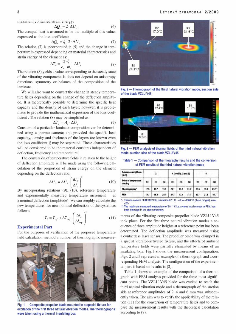
maximum contained strain energy:(6)
The escaped heat is assumed to be the multiple of this value,expressed as the loss coefficient:
(7)The relation (7) is incorporated in (5) and the change in tem-perature is expressed depending on material characteristics andstrain energy of the element as:
(8)
The relation (8) yields a value corresponding to the steady stateof the vibrating component. It does not depend on anisotropydirections, symmetry or balance of the composition of thelaminate.
We will also want to convert the change in steady tempera-ture fields depending on the change of the deflection amplitu-de. It is theoretically possible to determine the specific heatcapacity and the density of each layer; however, it is proble-matic to provide the mathematical expression of the loss coef-ficient . The relation (8) may be simplified as:
(9)Constant of a particular laminate composition can be determi-ned using a thermo camera; and provided the specific heatcapacity, density and thickness of the layers are known eventhe loss coefficient ξ may be separated. These characteristicswill be considered to be the material constants independent ofdeflection, frequency and temperature.
The conversion of temperature fields in relation to the heightof deflection amplitude will be made using the following cal-culation of the proportion of strain energy on the elementdepending on the deflection ratio:
(10)
By incorporating relations (9), (10), reference temperatureand experimentally measured temperature increment ata nominal deflection (amplitude) we can roughly calculate thenew temperature for new nominal deflection of the system asfollows:
(11)
Experimental PartFor the purposes of verification of the proposed temperaturefield calculation method a number of thermographic measure-
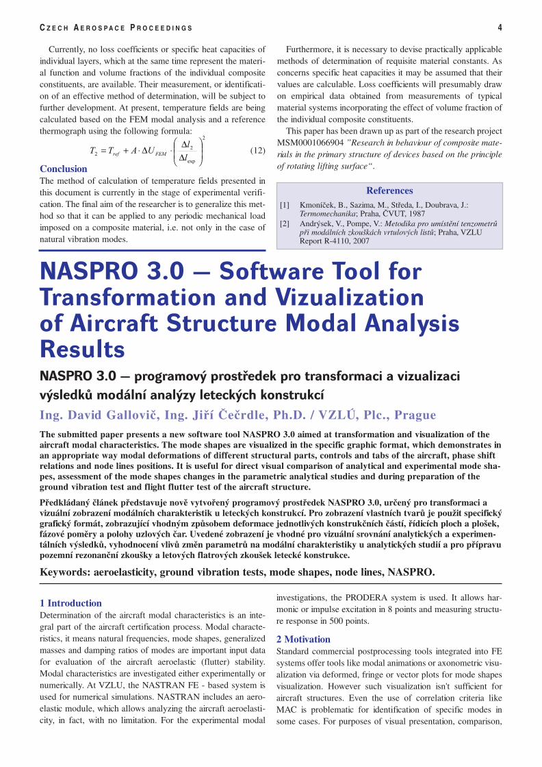
ments of the vibrating composite propeller blade VZLÚ V45took place. For the first three natural vibration modes a se-quence of three amplitude heights at a reference point has beendetermined. The deflection amplitude was measured usinga contactless laser sensor. The propeller blade was clamped ina special vibrator-activated fixture, and the effects of ambienttemperature fields were partially eliminated by means of aninsulating box. Fig.1 shows the measurement configuration,Figs. 2 and 3 represent an example of a thermograph and a cor-responding FEM analysis. The configuration of the experimen-tal part is based on results in [2].
Table 1 shows an example of the comparison of a thermo-graph with FEM analysis provided for the three most signifi-cant points. The VZLÚ V45 blade was excited to reach thethird natural vibration mode and a thermograph of the suctionside at reference amplitudes of 2, 4 and 6 mm was subsequ-ently taken. The aim was to verify the applicability of the rela-tion (11) for the conversion of temperature fields and to com-pare the measurement results with the theoretical calculationaccording to (8).
3 L E T E C K Ý Z P R A V O D A J 2 / 2 0 0 9
ee UQ ∆⋅≈∆ 2
ee UQ ∆⋅⋅=∆ 2ξ
e
ee
e Umc
T ∆⋅⋅⋅=∆ ξ2
eee UAT ∆⋅=∆
2
1
212
∆∆
⋅∆=∆l
lUU
2
exp
2
exp2
∆∆
⋅∆+=l
lTTT ref
Fig. 1 — Composite propeller blade mounted in a special fixture forexcitation of the first three natural vibration modes. The thermographswere taken using a thermal insulating box
Fig. 2 — Thermograph of the third natural vibration mode, suction sideof the blade VZLÚ V45
Fig. 3 — FEM analysis of thermal fields of the third natural vibrationmode, suction side of the blade VZLÚ V45
Table 1 — Comparison of thermography results and the conversionof FEM results of the third natural vibration mode
*) Thermo camera FLIR SC-2000, resolution 0.1° C, -40 to +1500° C (three ranges), error±2%.
**) The maximum measured temperature of 50.1° C i.e. a value much closer to FEM. hasbeen detected in the close proximity.
Currently, no loss coefficients or specific heat capacities ofindividual layers, which at the same time represent the materi-al function and volume fractions of the individual compositeconstituents, are available. Their measurement, or identificati-on of an effective method of determination, will be subject tofurther development. At present, temperature fields are beingcalculated based on the FEM modal analysis and a referencethermograph using the following formula:
(12)
ConclusionThe method of calculation of temperature fields presented inthis document is currently in the stage of experimental verifi-cation. The final aim of the researcher is to generalize this met-hod so that it can be applied to any periodic mechanical loadimposed on a composite material, i.e. not only in the case ofnatural vibration modes.
1 IntroductionDetermination of the aircraft modal characteristics is an inte-gral part of the aircraft certification process. Modal characte-ristics, it means natural frequencies, mode shapes, generalizedmasses and damping ratios of modes are important input datafor evaluation of the aircraft aeroelastic (flutter) stability.Modal characteristics are investigated either experimentally ornumerically. At VZLU, the NASTRAN FE - based system isused for numerical simulations. NASTRAN includes an aero-elastic module, which allows analyzing the aircraft aeroelasti-city, in fact, with no limitation. For the experimental modal
investigations, the PRODERA system is used. It allows har-monic or impulse excitation in 8 points and measuring structu-re response in 500 points.
2 MotivationStandard commercial postprocessing tools integrated into FEsystems offer tools like modal animations or axonometric visu-alization via deformed, fringe or vector plots for mode shapesvisualization. However such visualization isn't sufficient foraircraft structures. Even the use of correlation criteria likeMAC is problematic for identification of specific modes insome cases. For purposes of visual presentation, comparison,
C Z E C H A E R O S P A C E P R O C E E D I N G S 4
References[1] Kmoníček, B., Sazima, M., Středa, I., Doubrava, J.:
Termomechanika; Praha, ČVUT, 1987[2] Andrýsek, V., Pompe, V.: Metodika pro umístění tenzometrů
při modálních zkouškách vrtulových listů; Praha, VZLUReport R-4110, 2007
2
exp
2
2
∆∆
⋅∆⋅+=l
lUATT FEMref
Furthermore, it is necessary to devise practically applicablemethods of determination of requisite material constants. Asconcerns specific heat capacities it may be assumed that theirvalues are calculable. Loss coefficients will presumably drawon empirical data obtained from measurements of typicalmaterial systems incorporating the effect of volume fraction ofthe individual composite constituents.
This paper has been drawn up as part of the research projectMSM0001066904 ”Research in behaviour of composite mate-rials in the primary structure of devices based on the principleof rotating lifting surface“.
NASPRO 3.0 — Software Tool forTransformation and Vizualizationof Aircraft Structure Modal AnalysisResultsNASPRO 3.0 — programový prostředek pro transformaci a vizualizacivýsledků modální analýzy leteckých konstrukcí
Ing. David Gallovič, Ing. Jiří Čečrdle, Ph.D. / VZLÚ, Plc., Prague
The submitted paper presents a new software tool NASPRO 3.0 aimed at transformation and visualization of theaircraft modal characteristics. The mode shapes are visualized in the specific graphic format, which demonstrates inan appropriate way modal deformations of different structural parts, controls and tabs of the aircraft, phase shiftrelations and node lines positions. It is useful for direct visual comparison of analytical and experimental mode sha-pes, assessment of the mode shapes changes in the parametric analytical studies and during preparation of theground vibration test and flight flutter test of the aircraft structure.
Předkládaný článek představuje nově vytvořený programový prostředek NASPRO 3.0, určený pro transformaci avizuální zobrazení modálních charakteristik u leteckých konstrukcí. Pro zobrazení vlastních tvarů je použit specifickýgrafický formát, zobrazující vhodným způsobem deformace jednotlivých konstrukčních částí, řídicích ploch a plošek,fázové poměry a polohy uzlových čar. Uvedené zobrazení je vhodné pro vizuální srovnání analytických a experimen-tálních výsledků, vyhodnocení vlivů změn parametrů na modální charakteristiky u analytických studií a pro přípravupozemní rezonanční zkoušky a letových flatrových zkoušek letecké konstrukce.
Keywords: aeroelasticity, ground vibration tests, mode shapes, node lines, NASPRO.
assessment of differences and changes, a specific graphicformat has been created [1]. This graphic standarddemonstrates in an appropriate way modal deformationsof different structural parts, controls and tabs of the air-craft, phase shift relations and the node lines positions. It isa standard output of the ground vibration tests (GVT) perfor-med by the VZLU modal test laboratory. Therefore it is pos-sible to use it for the direct visual comparison of analytical andexperimental mode shapes. Such kind of analytical shapesvisualization is useful in the preparation phase of GVT. Theknowledge in the mode shapes and locations of the node linesis important for the appropriate emplacement of exciters andaccelerometers during GVT. The node lines position is alsorequired for the calculations of control surface dynamic balan-cing with respect to the other main mode shapes. Besides, it isalso important for the preparation of flight flutter tests (FFT)for appropriate emplacement of the impulse rocket exciters,since the design of exciters installation usually precedes theGVT. Finally the visualization format is useful for assessmentof the mode shapes changes in the parametric analytical studi-es as well.
For this purpose, the SW tool named NASPRO 2.0 has beendeveloped in the early nineties. The program, built by theTurbo Pascal operated on the MS.DOS operating system.However, this tool is unserviceable today. Moreover, the sour-ce code is not at disposal, therefore any improvement is impos-sible. The new SW tool NASPRO 3.0 replaces this obsoletetool.
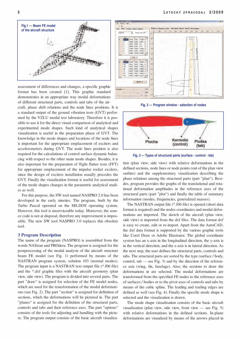
3 Program DescriptionThe name of the program (NASPRO) is assembled from thewords NAStran and PROdera. The program is assigned for thepostprocessing of the modal analysis of the aircraft structurebeam FE model (see Fig. 1) performed by means of theNASTRAN program system, solution 103 (normal modes).The program input is a NASTRAN text output file (*.f06 file)and the *.dxf graphic files with the aircraft geometry (planview, side view). The program is divided into several parts. Thepart ”draw“ is assigned for selection of the FE model nodes,which are used for the transformation of the modal deformati-ons (see Fig. 2). The part ”section“ is assigned for definition ofsections, which the deformations will be pictured in. The part”planes“ is assigned for the definition of the structural parts,controls and tabs and their reference axes. The part ”options“consists of the tools for adjusting and handling with the pictu-re. The program output consists of the basic aircraft visualiza-
tion (plan view, side view) with relative deformations in thedefined sections, node lines or node points (out of the plan viewoutline) and the supplementary visualization describing thephase relations among the structural parts (part ”plan“). Besi-des, program provides the graphs of the translational and rota-tional deformation amplitudes in the reference axes of thestructural parts (part ”plot“) and finally the table of summaryinformation (modes, frequencies, generalized masses).
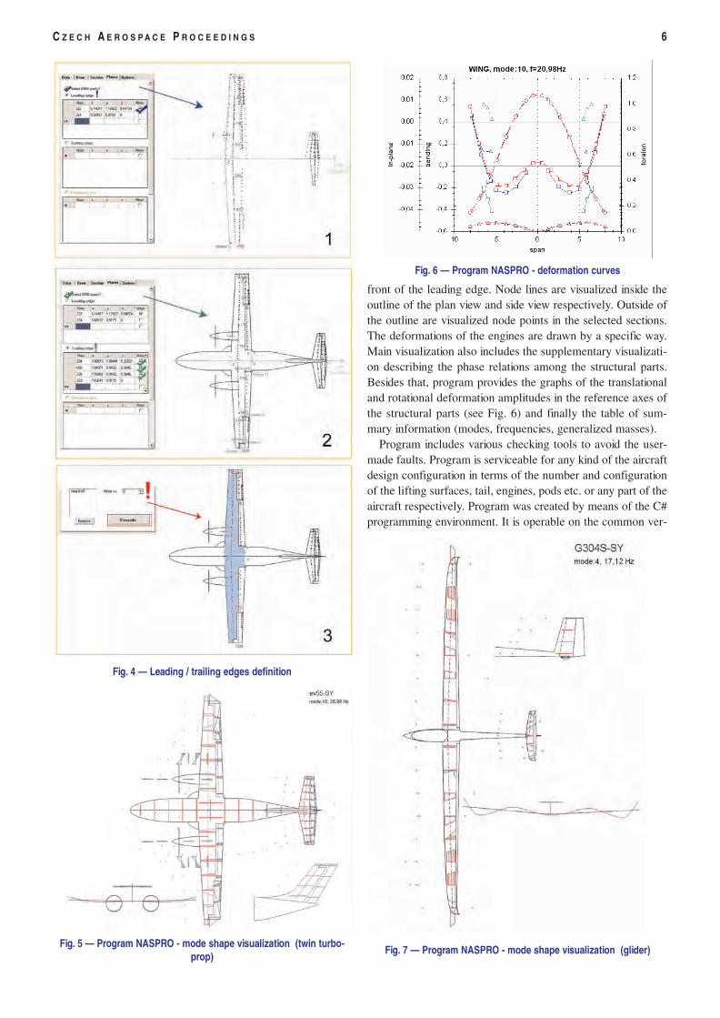
The NASTRAN output file (*.f06 file) is opened (short dataformat is required) and the nodes coordinates and modal defor-mations are imported. The sketch of the aircraft (plan view,side view) is imported from the dxf files. The data format dxfis easy to create, edit or re-import. Apart from the AutoCAD,the dxf data format is supported by the various graphic toolslike Corel Draw or Adobe Illustrator. The global coordinatesystem has an x-axis in the longitudinal direction, the y-axis isin the vertical direction, and the z-axis is in lateral direction. Asthe next step, the user defines the structural parts, controls andtabs. The structural parts are sorted by the type (surface / body,control, tab — see Fig. 3) and by the direction of the referen-ce axis (wing, fin, fuselage). Also, the sections to draw thedeformations in are selected. The modal deformations aretransformed from the specified FE nodes to the reference axesof surfaces / bodies or to the pivot axes of controls and tabs bymeans of the cubic spline. The leading and trailing edges aredefined as well (see Fig. 4). Finally the specific mode shape isselected and the visualization is drawn.
The mode shape vizualization consists of the basic aircraftvisualization (plan view, side view, front view — see Fig. 5)with relative deformations in the defined sections. In-planedeformations are visualized by means of the arrows placed in
5 L E T E C K Ý Z P R A V O D A J 2 / 2 0 0 9
Fig.1 — Beam FE modelof the aircraft structure
Fig. 2 — Program window - selection of nodes
Fig. 3 — Types of structural parts (surface - control - tab)
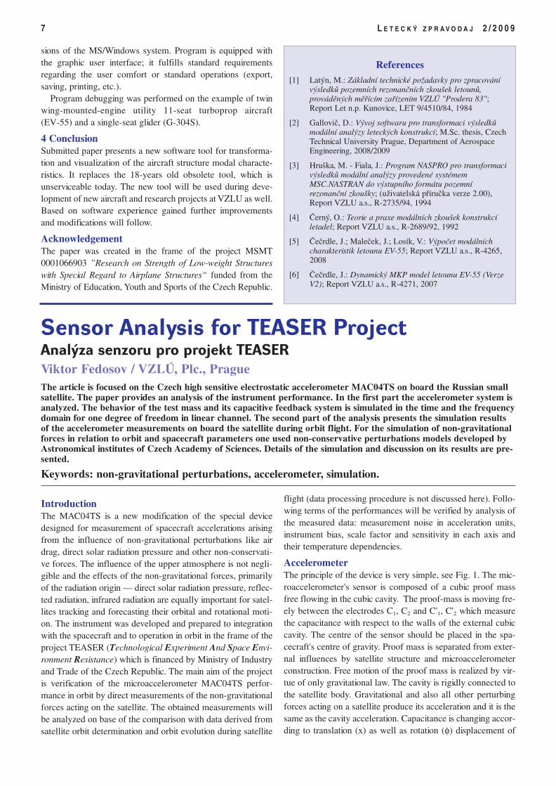
front of the leading edge. Node lines are visualized inside theoutline of the plan view and side view respectively. Outside ofthe outline are visualized node points in the selected sections.The deformations of the engines are drawn by a specific way.Main visualization also includes the supplementary visualizati-on describing the phase relations among the structural parts.Besides that, program provides the graphs of the translationaland rotational deformation amplitudes in the reference axes ofthe structural parts (see Fig. 6) and finally the table of sum-mary information (modes, frequencies, generalized masses).
Program includes various checking tools to avoid the user-made faults. Program is serviceable for any kind of the aircraftdesign configuration in terms of the number and configurationof the lifting surfaces, tail, engines, pods etc. or any part of theaircraft respectively. Program was created by means of the C#programming environment. It is operable on the common ver-
C Z E C H A E R O S P A C E P R O C E E D I N G S 6
Fig. 4 — Leading / trailing edges definition
Fig. 6 — Program NASPRO - deformation curves
Fig. 5 — Program NASPRO - mode shape visualization (twin turbo-prop)
Fig. 7 — Program NASPRO - mode shape visualization (glider)
sions of the MS/Windows system. Program is equipped withthe graphic user interface; it fulfills standard requirementsregarding the user comfort or standard operations (export,saving, printing, etc.).
Program debugging was performed on the example of twinwing-mounted-engine utility 11-seat turboprop aircraft(EV-55) and a single-seat glider (G-304S).
4 ConclusionSubmitted paper presents a new software tool for transforma-tion and visualization of the aircraft structure modal characte-ristics. It replaces the 18-years old obsolete tool, which isunserviceable today. The new tool will be used during deve-lopment of new aircraft and research projects at VZLU as well.Based on software experience gained further improvementsand modifications will follow.
AcknowledgementThe paper was created in the frame of the project MSMT0001066903 ”Research on Strength of Low-weight Structureswith Special Regard to Airplane Structures“ funded from theMinistry of Education, Youth and Sports of the Czech Republic.
Introduction The MAC04TS is a new modification of the special devicedesigned for measurement of spacecraft accelerations arisingfrom the influence of non-gravitational perturbations like airdrag, direct solar radiation pressure and other non-conservati-ve forces. The influence of the upper atmosphere is not negli-gible and the effects of the non-gravitational forces, primarilyof the radiation origin — direct solar radiation pressure, reflec-ted radiation, infrared radiation are equally important for satel-lites tracking and forecasting their orbital and rotational moti-on. The instrument was developed and prepared to integrationwith the spacecraft and to operation in orbit in the frame of theproject TEASER (Technological Experiment And Space Envi-ronment Resistance) which is financed by Ministry of Industryand Trade of the Czech Republic. The main aim of the projectis verification of the microaccelerometer MAC04TS perfor-mance in orbit by direct measurements of the non-gravitationalforces acting on the satellite. The obtained measurements willbe analyzed on base of the comparison with data derived fromsatellite orbit determination and orbit evolution during satellite
flight (data processing procedure is not discussed here). Follo-wing terms of the performances will be verified by analysis ofthe measured data: measurement noise in acceleration units,instrument bias, scale factor and sensitivity in each axis andtheir temperature dependencies.
AccelerometerThe principle of the device is very simple, see Fig. 1. The mic-roaccelerometer's sensor is composed of a cubic proof massfree flowing in the cubic cavity. The proof-mass is moving fre-ely between the electrodes C1, C2 and C'1, C'2 which measurethe capacitance with respect to the walls of the external cubiccavity. The centre of the sensor should be placed in the spa-cecraft's centre of gravity. Proof mass is separated from exter-nal influences by satellite structure and microaccelerometerconstruction. Free motion of the proof mass is realized by vir-tue of only gravitational law. The cavity is rigidly connected tothe satellite body. Gravitational and also all other perturbingforces acting on a satellite produce its acceleration and it is thesame as the cavity acceleration. Capacitance is changing accor-ding to translation (x) as well as rotation (φ) displacement of
7 L E T E C K Ý Z P R A V O D A J 2 / 2 0 0 9
References
[1] Latýn, M.: Základní technické požadavky pro zpracovánívýsledků pozemních rezonančních zkoušek letounů,prováděných měřícím zařízením VZLÚ "Prodera 83";Report Let n.p. Kunovice, LET 9/4510/84, 1984
[2] Gallovič, D.: Vývoj softwaru pro transformaci výsledkůmodální analýzy leteckých konstrukcí; M.Sc. thesis, CzechTechnical University Prague, Department of AerospaceEngineering, 2008/2009
[3] Hruška, M. - Fiala, J.: Program NASPRO pro transformacivýsledků modální analýzy provedené systémemMSC.NASTRAN do výstupního formátu pozemnírezonanční zkoušky; (uživatelská příručka verze 2.00),Report VZLU a.s., R-2735/94, 1994
[4] Černý, O.: Teorie a praxe modálních zkoušek konstrukcíletadel; Report VZLU a.s., R-2689/92, 1992
[5] Čečrdle, J.; Maleček, J.; Losík, V.: Výpočet modálníchcharakteristik letounu EV-55; Report VZLU a.s., R-4265,2008
[6] Čečrdle, J.: Dynamický MKP model letounu EV-55 (VerzeV2); Report VZLU a.s., R-4271, 2007
Sensor Analysis for TEASER ProjectAnalýza senzoru pro projekt TEASERViktor Fedosov / VZLÚ, Plc., PragueThe article is focused on the Czech high sensitive electrostatic accelerometer MAC04TS on board the Russian smallsatellite. The paper provides an analysis of the instrument performance. In the first part the accelerometer system isanalyzed. The behavior of the test mass and its capacitive feedback system is simulated in the time and the frequencydomain for one degree of freedom in linear channel. The second part of the analysis presents the simulation resultsof the accelerometer measurements on board the satellite during orbit flight. For the simulation of non-gravitationalforces in relation to orbit and spacecraft parameters one used non-conservative perturbations models developed byAstronomical institutes of Czech Academy of Sciences. Details of the simulation and discussion on its results are pre-sented.
Keywords: non-gravitational perturbations, accelerometer, simulation.
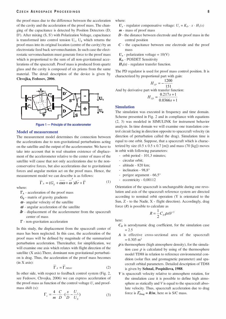
the proof-mass due to the difference between the accelerationof the cavity and the acceleration of the proof mass. The chan-ging of the capacitance is detected by Position Detectors (D;D'). After mixing (S, S') with Polarization Voltage, capacitanceis transformed into control tension Ux, Uφ which returns theproof-mass into its original location (centre of the cavity) by anelectrostatic feed back servomechanism. In such case the elect-rostatic servomechanism must generate force to the proof masswhich is proportional to the sum of all non-gravitational acce-lerations of the spacecraft. Proof mass is produced from quartzglass and the cavity is composed of six prisms from the samematerial. The detail description of the device is given byChvojka, Fedosov, 2006.
Model of measurement The measurement model determines the connection betweenthe accelerations due to non-gravitational perturbations actingon the satellite and the output of the accelerometer. We have totake into account that in real situation existence of displace-ment of the accelerometer relative to the center of mass of thesatellite will cause that not only accelerations due to the non-conservative forces, but also accelerations due to gravitationalforces and angular motion act on the proof mass. Hence, themeasurement model we can describe is as follows:
(1)
where:ΓΓA - acceleration of the proof massGij - matrix of gravity gradientsωω - angular velocity of the satelliteωω' - angular acceleration of the satelliteδδr - displacement of the accelerometer from the spacecraft
center of mass ΓΓ - non-gravitation acceleration
In this study, the displacement from the spacecraft center ofmass has been neglected. In this case, the acceleration of theproof mass will be defined by magnitude of the summarizedperturbation acceleration. Thereinafter, for simplification, wewill examine one axis which relates with flight direction of thesatellite (X axis).There, dominant non-gravitational perturbati-on is drag. Thus, the acceleration of the proof mass becomes(in X axis):
(2)
In other side, with respect to feedback control system (Fig. 2,see Fedosov, Chvojka, 2006) we can express acceleration ofthe proof-mass as function of the control voltage Ux and proof-mass shift (x):
(3)
where:Ux - regulator compensative voltage: Ux = KD ⋅ x ⋅ H1(s)m - mass of proof massD - the distance between electrode and the proof mass in the
central positionC - the capacitance between one electrode and the proof
massUo - polarization voltage = 10(V)KD - POSDET SensitivityH1(s) - regulator transfer function.
The PD regulator is used for proof mass control position. It ischaracterized by proportional part with gain:
And by derivative part with transfer function:
Simulation The simulation was executed in frequency and time domain.Scheme presented in Fig. 2 and in compliance with equations(2, 3) was modeled in SIMULINK for instrument behavioranalysis. In time domain we will examine one translation con-trol circuit facing in direction opposite to spacecraft velocity (indirection of perturbation called the drag). Simulation time isequal to one orbit. Suppose, that a spacecraft which is charac-terized by size (0.5 x 0.5 x 0.7 [m]) and mass (70 [kg]) movesin orbit with following parameters:
- orbit period - 101,3 minutes;- circular orbit;- altitude - 820 km;- inclination - 98,8°- perigee argument - 66,5°- eccentricity - 0,00112
Orientation of the spacecraft is unchangeable during one revo-lution and axis of the spacecraft reference system are directedaccording to nominal orbit operation (Y is orientated to theSun, Z - to the Nadir, X - flight direction). Accordingly, dragforce (R) is possible to calculate as
here:CD is aerodynamic drag coefficient, for the simulation case
= 2.5A is effective cross-sectional area of the spacecraft
= 0.305 m2
ρρ is thermosphere (high atmosphere density), for the simula-tion case ρ is calculated by using of the thermospheremodel TD88 in relation to reference environmental con-dition (solar flux and geomagnetic parameter) and spa-cecraft orbital parameters. Detailed description of TD88is given by Sehnal, Pospisilova, 1988.
V is spacecraft velocity relative to atmosphere rotation, forthe simulation case it is possible to define high atmo-sphere as statically and V is equal to the spacecraft abso-lute velocity. Thus, spacecraft acceleration due to dragforce is ΓΓDrag = R/m, here m is S/C mass.
C Z E C H A E R O S P A C E P R O C E E D I N G S 8
Figure 1 — Principle of the accelerometer
Γ+
′++=Γ rGijA δωωω )(
DRAGA Γ=Γ
)(
4
0U
U
D
x
D
C
m
x
x −⋅⋅=Γ
151
12001 −=PH
10366.0
1217.01 +
+=s
sH D
2
2
1AVCR D ρ=
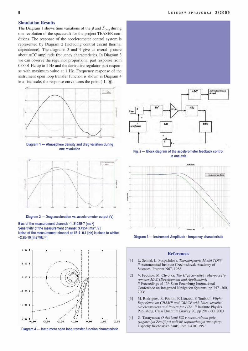
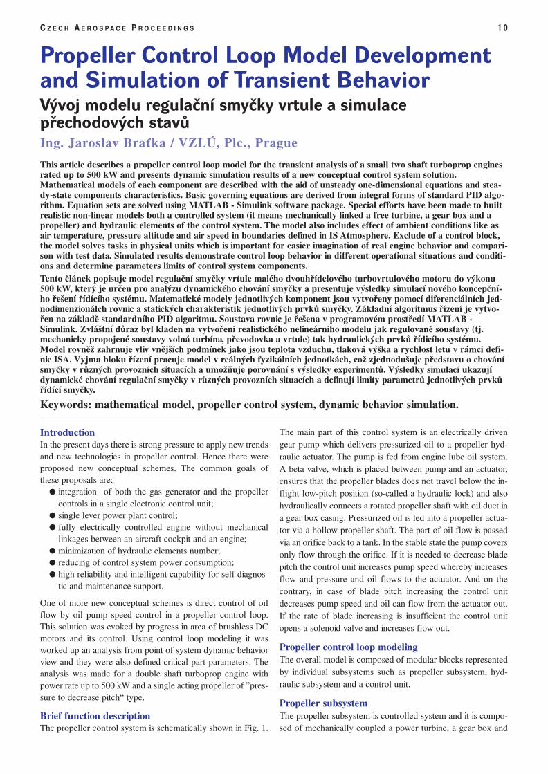
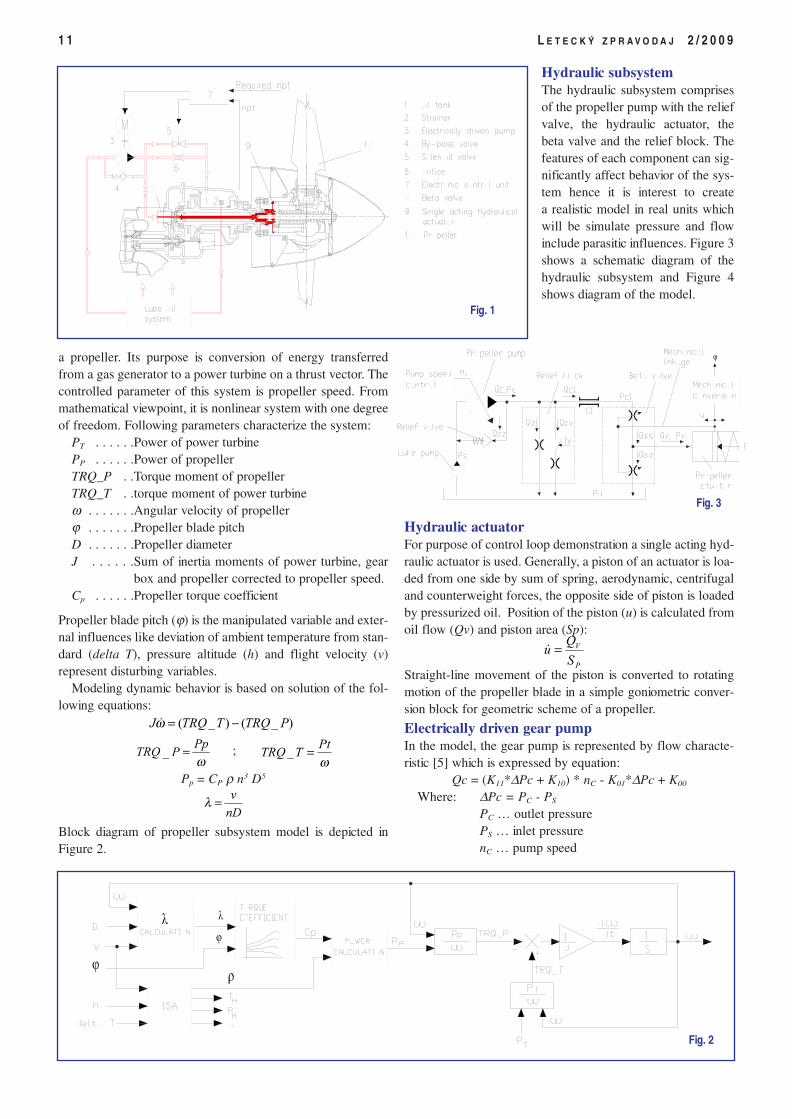
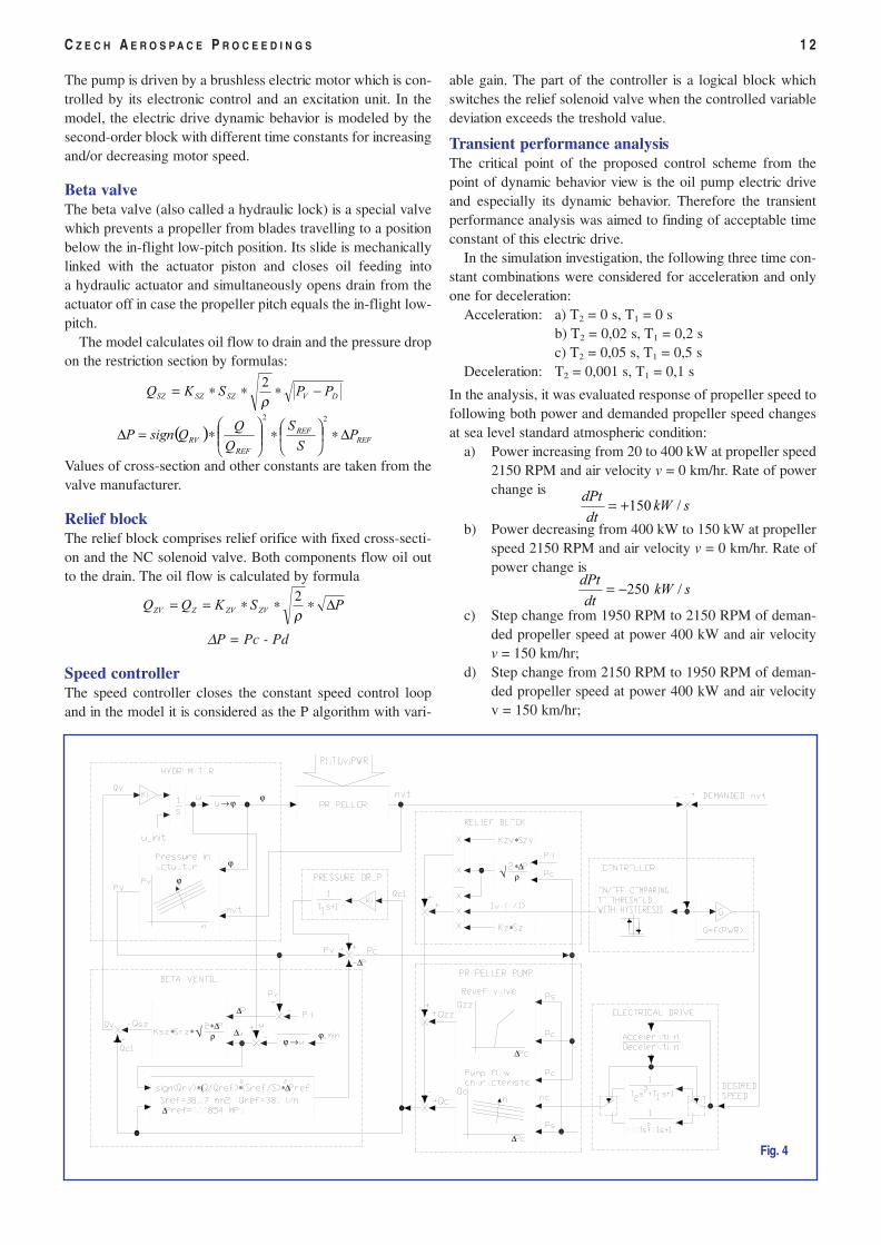
Simulation Results The Diagram 1 shows time variations of the ρρ and ΓΓDrag duringone revolution of the spacecraft for the project TEASER con-ditions. The response of the accelerometer control system isrepresented by Diagram 2 (including control circuit thermaldependence). The diagrams 3 and 4 give us overall pictureabout ACC amplitude frequency characteristics. In Diagram 3we can observe the regulator proportional part response from0.0001 Hz up to 1 Hz and the derivative regulator part respon-se with maximum value at 1 Hz. Frequency response of theinstrument open loop transfer function is shown in Diagram 4in a fine scale, the response curve turns the point (-1, 0j).
9 L E T E C K Ý Z P R A V O D A J 2 / 2 0 0 9
Fig. 2 — Block diagram of the accelerometer feedback controlin one axis
Diagram 1 — Atmosphere density and drag variation duringone revolution
Diagram 4 — Instrument open loop transfer function characteristic
Diagram 2 — Drag acceleration vs. accelerometer output (V)
Bias of the measurement channel: -1. 3102E-7 [ms-2]Sensitivity of the measurement channel: 3.4954 [ms-2 /V]Noise of the measurement channel at 1E-4 -0.1 [Hz] is close to white:~2.2E-10 [ms-2/Hz1/2]
References
[1] L. Sehnal. L. Pospishilova: Thermospheric Model TD88;// Astronomical Institute Czechoslovak Academy ofSciences, Preprint N67, 1988
[2] V. Fedosov, M. Chvojka: The High Sensitivity Microaccele-rometer MAC (Development and Application);// Proceedings of 13th Saint Petersburg InternationalConference on Integrated Navigation Systems, pp 357 -360,2006
[3] M. Rodrigues, B. Foulon, F. Liorzou, P. Touboul: FlightExperience on CHAMP and CRACE with Ultra-sensitiveAccelerometers and Return for LISA; // Institute PhysicsPublishing, Class Quantum Gravity 20, pp 291-300, 2003
[4] G. Taratynova: O dvizhenii ISZ v necentralnom poletyagoteniya Zemlji pri nalichii soprotivleniya atmosfery;Uspechy fizicheskikh nauk, Tom LXIII, 1957
Diagram 3 — Instrument Amplitude - frequency characteristic
IntroductionIn the present days there is strong pressure to apply new trendsand new technologies in propeller control. Hence there wereproposed new conceptual schemes. The common goals ofthese proposals are:
� integration of both the gas generator and the propellercontrols in a single electronic control unit;
� single lever power plant control;� fully electrically controlled engine without mechanical
linkages between an aircraft cockpit and an engine;� minimization of hydraulic elements number;� reducing of control system power consumption;� high reliability and intelligent capability for self diagnos-
tic and maintenance support.
One of more new conceptual schemes is direct control of oilflow by oil pump speed control in a propeller control loop.This solution was evoked by progress in area of brushless DCmotors and its control. Using control loop modeling it wasworked up an analysis from point of system dynamic behaviorview and they were also defined critical part parameters. Theanalysis was made for a double shaft turboprop engine withpower rate up to 500 kW and a single acting propeller of ”pres-sure to decrease pitch“ type.
Brief function descriptionThe propeller control system is schematically shown in Fig. 1.
The main part of this control system is an electrically drivengear pump which delivers pressurized oil to a propeller hyd-raulic actuator. The pump is fed from engine lube oil system.A beta valve, which is placed between pump and an actuator,ensures that the propeller blades does not travel below the in-flight low-pitch position (so-called a hydraulic lock) and alsohydraulically connects a rotated propeller shaft with oil duct ina gear box casing. Pressurized oil is led into a propeller actua-tor via a hollow propeller shaft. The part of oil flow is passedvia an orifice back to a tank. In the stable state the pump coversonly flow through the orifice. If it is needed to decrease bladepitch the control unit increases pump speed whereby increasesflow and pressure and oil flows to the actuator. And on thecontrary, in case of blade pitch increasing the control unitdecreases pump speed and oil can flow from the actuator out.If the rate of blade increasing is insufficient the control unitopens a solenoid valve and increases flow out.
Propeller control loop modelingThe overall model is composed of modular blocks representedby individual subsystems such as propeller subsystem, hyd-raulic subsystem and a control unit.
Propeller subsystemThe propeller subsystem is controlled system and it is compo-sed of mechanically coupled a power turbine, a gear box and
C Z E C H A E R O S P A C E P R O C E E D I N G S 1 0
Propeller Control Loop Model Developmentand Simulation of Transient BehaviorVývoj modelu regulační smyčky vrtule a simulacepřechodových stavůIng. Jaroslav Braťka / VZLÚ, Plc., Prague
This article describes a propeller control loop model for the transient analysis of a small two shaft turboprop enginesrated up to 500 kW and presents dynamic simulation results of a new conceptual control system solution.Mathematical models of each component are described with the aid of unsteady one-dimensional equations and stea-dy-state components characteristics. Basic governing equations are derived from integral forms of standard PID algo-rithm. Equation sets are solved using MATLAB - Simulink software package. Special efforts have been made to builtrealistic non-linear models both a controlled system (it means mechanically linked a free turbine, a gear box and apropeller) and hydraulic elements of the control system. The model also includes effect of ambient conditions like asair temperature, pressure altitude and air speed in boundaries defined in IS Atmosphere. Exclude of a control block,the model solves tasks in physical units which is important for easier imagination of real engine behavior and compari-son with test data. Simulated results demonstrate control loop behavior in different operational situations and conditi-ons and determine parameters limits of control system components.Tento článek popisuje model regulační smyčky vrtule malého dvouhřídelového turbovrtulového motoru do výkonu500 kW, který je určen pro analýzu dynamického chování smyčky a presentuje výsledky simulací nového koncepční-ho řešení řídícího systému. Matematické modely jednotlivých komponent jsou vytvořeny pomocí diferenciálních jed-nodimenzionálch rovnic a statických charakteristik jednotlivých prvků smyčky. Základní algoritmus řízení je vytvo-řen na základě standardního PID algoritmu. Soustava rovnic je řešena v programovém prostředí MATLAB -Simulink. Zvláštní důraz byl kladen na vytvoření realistického nelineárního modelu jak regulované soustavy (tj.mechanicky propojené soustavy volná turbína, převodovka a vrtule) tak hydraulických prvků řídicího systému.Model rovněž zahrnuje vliv vnějších podmínek jako jsou teplota vzduchu, tlaková výška a rychlost letu v rámci defi-nic ISA. Vyjma bloku řízení pracuje model v reálných fyzikálních jednotkách, což zjednodušuje představu o chovánísmyčky v různých provozních situacích a umožňuje porovnání s výsledky experimentů. Výsledky simulací ukazujídynamické chování regulační smyčky v různých provozních situacích a definují limity parametrů jednotlivých prvkůřídící smyčky.
Keywords: mathematical model, propeller control system, dynamic behavior simulation.
a propeller. Its purpose is conversion of energy transferredfrom a gas generator to a power turbine on a thrust vector. Thecontrolled parameter of this system is propeller speed. Frommathematical viewpoint, it is nonlinear system with one degreeof freedom. Following parameters characterize the system:
PT . . . . . .Power of power turbinePP . . . . . .Power of propellerTRQ_P . .Torque moment of propellerTRQ_T . .torque moment of power turbineω . . . . . . .Angular velocity of propellerϕ . . . . . . .Propeller blade pitchD . . . . . . .Propeller diameterJ . . . . . .Sum of inertia moments of power turbine, gear
box and propeller corrected to propeller speed.Cp . . . . . .Propeller torque coefficient
Propeller blade pitch (ϕ) is the manipulated variable and exter-nal influences like deviation of ambient temperature from stan-dard (delta T), pressure altitude (h) and flight velocity (v)represent disturbing variables.
Modeling dynamic behavior is based on solution of the fol-lowing equations:
;
Pp = CP ρ n3 D5
Block diagram of propeller subsystem model is depicted inFigure 2.
Hydraulic subsystemThe hydraulic subsystem comprisesof the propeller pump with the reliefvalve, the hydraulic actuator, thebeta valve and the relief block. Thefeatures of each component can sig-nificantly affect behavior of the sys-tem hence it is interest to createa realistic model in real units whichwill be simulate pressure and flowinclude parasitic influences. Figure 3shows a schematic diagram of thehydraulic subsystem and Figure 4shows diagram of the model.
Hydraulic actuatorFor purpose of control loop demonstration a single acting hyd-raulic actuator is used. Generally, a piston of an actuator is loa-ded from one side by sum of spring, aerodynamic, centrifugaland counterweight forces, the opposite side of piston is loadedby pressurized oil. Position of the piston (u) is calculated fromoil flow (Qv) and piston area (Sp):
Straight-line movement of the piston is converted to rotatingmotion of the propeller blade in a simple goniometric conver-sion block for geometric scheme of a propeller.
Electrically driven gear pumpIn the model, the gear pump is represented by flow characte-ristic [5] which is expressed by equation:
Qc = (K11*∆Pc + K10) * nC - K01*∆Pc + K00
Where: ∆Pc = PC - PS
PC … outlet pressurePS … inlet pressurenC … pump speed
1 1 L E T E C K Ý Z P R A V O D A J 2 / 2 0 0 9
Fig. 1
)_()_( PTRQTTRQJ −=ω&
ωPp
PTRQ =_ωPt
TTRQ =_
nD
v=λ
Fig. 2
Fig. 3
P
V
S
Qu =&
The pump is driven by a brushless electric motor which is con-trolled by its electronic control and an excitation unit. In themodel, the electric drive dynamic behavior is modeled by thesecond-order block with different time constants for increasingand/or decreasing motor speed.
Beta valveThe beta valve (also called a hydraulic lock) is a special valvewhich prevents a propeller from blades travelling to a positionbelow the in-flight low-pitch position. Its slide is mechanicallylinked with the actuator piston and closes oil feeding intoa hydraulic actuator and simultaneously opens drain from theactuator off in case the propeller pitch equals the in-flight low-pitch.
The model calculates oil flow to drain and the pressure dropon the restriction section by formulas:
Values of cross-section and other constants are taken from thevalve manufacturer.
Relief blockThe relief block comprises relief orifice with fixed cross-secti-on and the NC solenoid valve. Both components flow oil outto the drain. The oil flow is calculated by formula
∆P = Pc - Pd
Speed controllerThe speed controller closes the constant speed control loopand in the model it is considered as the P algorithm with vari-
able gain. The part of the controller is a logical block whichswitches the relief solenoid valve when the controlled variabledeviation exceeds the treshold value.
Transient performance analysisThe critical point of the proposed control scheme from thepoint of dynamic behavior view is the oil pump electric driveand especially its dynamic behavior. Therefore the transientperformance analysis was aimed to finding of acceptable timeconstant of this electric drive.
In the simulation investigation, the following three time con-stant combinations were considered for acceleration and onlyone for deceleration:
Acceleration: a) T2 = 0 s, T1 = 0 sb) T2 = 0,02 s, T1 = 0,2 sc) T2 = 0,05 s, T1 = 0,5 s
Deceleration: T2 = 0,001 s, T1 = 0,1 s
In the analysis, it was evaluated response of propeller speed tofollowing both power and demanded propeller speed changesat sea level standard atmospheric condition:
a) Power increasing from 20 to 400 kW at propeller speed2150 RPM and air velocity v = 0 km/hr. Rate of powerchange is
b) Power decreasing from 400 kW to 150 kW at propellerspeed 2150 RPM and air velocity v = 0 km/hr. Rate ofpower change is
c) Step change from 1950 RPM to 2150 RPM of deman-ded propeller speed at power 400 kW and air velocityv = 150 km/hr;
d) Step change from 2150 RPM to 1950 RPM of deman-ded propeller speed at power 400 kW and air velocityv = 150 km/hr;
C Z E C H A E R O S P A C E P R O C E E D I N G S 1 2
DVSZSZSZ PPSKQ −∗∗∗=ρ2
( )
REF
REF
REF
RV PS
S
Q
QQsignP ∆∗
∗
∗=∆
22
PSKQQ ZVZVZZV ∆∗∗∗==
ρ2
∗( ∗ ∗∆
∆
∗ ∗∗∆√ ρ
ϕ → ϕ∆
∆
ϕ
ϕ
→ ϕ ϕ
∆
∆
∆
∗∆√ ρ
∗
∗
Fig. 4
skW
dt
dPt/150+=
skW
dt
dPt/250−=
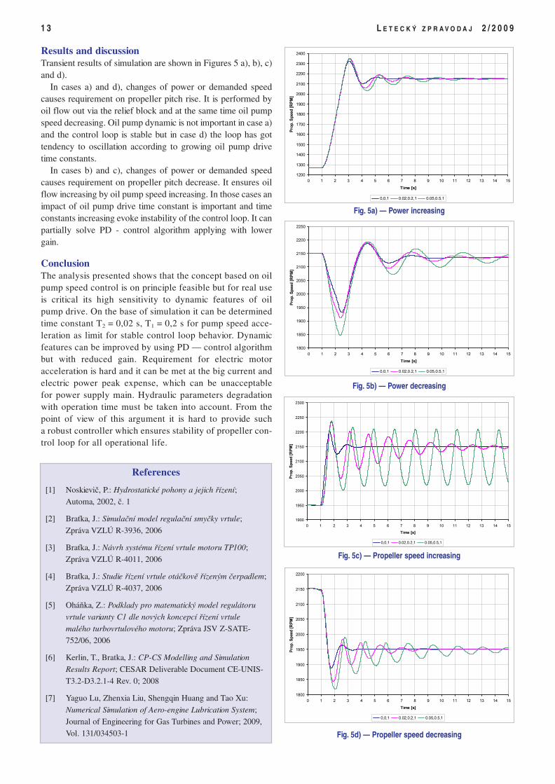
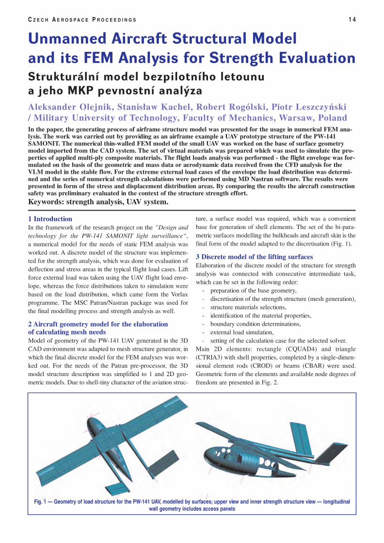
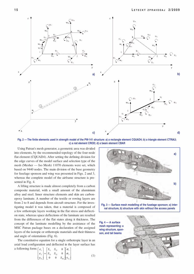
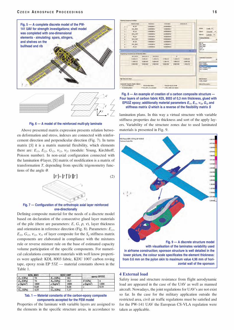
Results and discussionTransient results of simulation are shown in Figures 5 a), b), c)and d).
In cases a) and d), changes of power or demanded speedcauses requirement on propeller pitch rise. It is performed byoil flow out via the relief block and at the same time oil pumpspeed decreasing. Oil pump dynamic is not important in case a)and the control loop is stable but in case d) the loop has gottendency to oscillation according to growing oil pump drivetime constants.
In cases b) and c), changes of power or demanded speedcauses requirement on propeller pitch decrease. It ensures oilflow increasing by oil pump speed increasing. In those cases animpact of oil pump drive time constant is important and timeconstants increasing evoke instability of the control loop. It canpartially solve PD - control algorithm applying with lowergain.
ConclusionThe analysis presented shows that the concept based on oilpump speed control is on principle feasible but for real useis critical its high sensitivity to dynamic features of oilpump drive. On the base of simulation it can be determinedtime constant T2 = 0,02 s, T1 = 0,2 s for pump speed acce-leration as limit for stable control loop behavior. Dynamicfeatures can be improved by using PD — control algorithmbut with reduced gain. Requirement for electric motoracceleration is hard and it can be met at the big current andelectric power peak expense, which can be unacceptablefor power supply main. Hydraulic parameters degradationwith operation time must be taken into account. From thepoint of view of this argument it is hard to provide sucha robust controller which ensures stability of propeller con-trol loop for all operational life.
1 3 L E T E C K Ý Z P R A V O D A J 2 / 2 0 0 9
References
[1] Noskievič, P.: Hydrostatické pohony a jejich řízení;Automa, 2002, č. 1
[2] Braťka, J.: Simulační model regulační smyčky vrtule;Zpráva VZLÚ R-3936, 2006
[3] Braťka, J.: Návrh systému řízení vrtule motoru TP100;Zpráva VZLÚ R-4011, 2006
[4] Braťka, J.: Studie řízení vrtule otáčkově řízeným čerpadlem;Zpráva VZLÚ R-4037, 2006
[5] Oháňka, Z.: Podklady pro matematický model regulátoruvrtule varianty C1 dle nových koncepcí řízení vrtulemalého turbovrtulového motoru; Zpráva JSV Z-SATE-752/06, 2006
[6] Kerlin, T., Bratka, J.: CP-CS Modelling and SimulationResults Report; CESAR Deliverable Document CE-UNIS-T3.2-D3.2.1-4 Rev. 0; 2008
[7] Yaguo Lu, Zhenxia Liu, Shengqin Huang and Tao Xu:Numerical Simulation of Aero-engine Lubrication System;Journal of Engineering for Gas Turbines and Power; 2009,Vol. 131/034503-1
1200
1300
1400
1500
1600
1700
1800
1900
2000
2100
2200
2300
2400
0 1 2 3 4 5 6 7 8 9 10 11 12 13 14 15
Time [s]
Pro
p. S
peed
[RP
M]
0,0,1 0.02,0.2,1 0.05,0.5,1
1800
1850
1900
1950
2000
2050
2100
2150
2200
2250
0 1 2 3 4 5 6 7 8 9 10 11 12 13 14 15
Time [s]
Pro
p. S
peed
[RP
M]
0,0,1 0.02,0.2,1 0.05,0.5,1
1900
1950
2000
2050
2100
2150
2200
2250
2300
0 1 2 3 4 5 6 7 8 9 10 11 12 13 14 15
Time [s]
Pro
p. S
pee
d [
RP
M]
0,0,1 0.02,0.2,1 0.05,0.5,1
1800
1850
1900
1950
2000
2050
2100
2150
2200
0 1 2 3 4 5 6 7 8 9 10 11 12 13 14 15
Time [s]
Pro
p. S
pee
d [R
PM
]
0,0,1 0.02,0.2,1 0.05,0.5,1
Fig. 5a) — Power increasing
Fig. 5b) — Power decreasing
Fig. 5c) — Propeller speed increasing
Fig. 5d) — Propeller speed decreasing
1 IntroductionIn the framework of the research project on the ”Design andtechnology for the PW-141 SAMONIT light surveillance“,a numerical model for the needs of static FEM analysis wasworked out. A discrete model of the structure was implemen-ted for the strength analysis, which was done for evaluation ofdeflection and stress areas in the typical flight load cases. Liftforce external load was taken using the UAV flight load enve-lope, whereas the force distributions taken to simulation werebased on the load distribution, which came form the Vorlaxprogramme. The MSC Patran/Nastran package was used forthe final modelling process and strength analysis as well.
2 Aircraft geometry model for the elaborationof calculating mesh needs Model of geometry of the PW-141 UAV generated in the 3DCAD environment was adapted to mesh structure generator, inwhich the final discrete model for the FEM analyses was wor-ked out. For the needs of the Patran pre-processor, the 3Dmodel structure description was simplified to 1 and 2D geo-metric models. Due to shell-tiny character of the aviation struc-
ture, a surface model was required, which was a convenientbase for generation of shell elements. The set of the bi-para-metric surfaces modelling the bulkheads and aircraft skin is thefinal form of the model adapted to the discretisation (Fig. 1).
3 Discrete model of the lifting surfacesElaboration of the discrete model of the structure for strengthanalysis was connected with consecutive intermediate task,which can be set in the following order:
- preparation of the base geometry,- discretisation of the strength structure (mesh generation),- structure materials selections,- identification of the material properties,- boundary condition determinations,- external load simulation,- setting of the calculation case for the selected solver.
Main 2D elements: rectangle (CQUAD4) and triangle(CTRIA3) with shell properties, completed by a single-dimen-sional element rods (CROD) or beams (CBAR) were used.Geometric form of the elements and available node degrees offreedom are presented in Fig. 2.
C Z E C H A E R O S P A C E P R O C E E D I N G S 1 4
Unmanned Aircraft Structural Modeland its FEM Analysis for Strength EvaluationStrukturální model bezpilotního letounua jeho MKP pevnostní analýzaAleksander Olejnik, Stanisław Kachel, Robert Rogólski, Piotr Leszczyński/ Military University of Technology, Faculty of Mechanics, Warsaw, PolandIn the paper, the generating process of airframe structure model was presented for the usage in numerical FEM ana-lysis. The work was carried out by providing as an airframe example a UAV prototype structure of the PW-141SAMONIT. The numerical thin-walled FEM model of the small UAV was worked on the base of surface geometrymodel imported from the CAD system. The set of virtual materials was prepared which was used to simulate the pro-perties of applied multi-ply composite materials. The flight loads analysis was performed - the flight envelope was for-mulated on the basis of the geometric and mass data or aerodynamic data received from the CFD analysis for theVLM model in the stable flow. For the extreme external load cases of the envelope the load distribution was determi-ned and the series of numerical strength calculations were performed using MD Nastran software. The results werepresented in form of the stress and displacement distribution areas. By comparing the results the aircraft constructionsafety was preliminary evaluated in the context of the structure strength effort.Keywords: strength analysis, UAV system.
Fig. 1 — Geometry of load structure for the PW-141 UAV, modelled by surfaces; upper view and inner strength structure view — longitudinal
wall geometry includes access panels
Using Patran's mesh generator, a geometric area was dividedinto elements, by the recommended topology of the four-nodeflat element (CQUAD4). After setting the defining division forthe edge curves of the model surface and selection type of themesh (Mesher — Iso Mesh) 11070 elements were set, whichbased on 9440 nodes. The main division of the base geometryfor fuselage sponson and wing was presented in Figs. 2 and 3,whereas the complete model of the airframe structure is pre-sented in Fig. 4.
A lifting structure is made almost completely from a carboncomposite material, with a small amount of the aluminiumalloy and steel. Inner structure elements and skin are carbon-epoxy laminate. A number of the textile or rowing layers arefrom 2 to 8 and depends from aircraft structure. For the inves-tigating model it was taken, that a material is composed ofa few orthotropic layers working in the flat stress and deflecti-on state, whereas space deflections of the laminate are resultedfrom the differences of the flat states along it thickness. Theconcept of the laminate modelling by the assistance of theMSC Patran package bases on a declaration of the assignedlayers of the isotopic or orthotropic materials and their thinnessand angle of orientations (Fig. 6).
The constitutive equation for a single orthotropic layer in anaxial load configuration and deflected in the layer surface hasa following form:
(1)
1 5 L E T E C K Ý Z P R A V O D A J 2 / 2 0 0 9
j
uj
ui
i
x
y
z
Fig. 2 — The finite elements used in strength model of the PW-141 structure: a) a rectangle element CQUAD4; b) a triangle element CTRIA3;c) a rod element CROD; d) a beam element CBAR
a) b)
c) d)
Fig. 3 — Surface mesh modelling of the fuselage sponson; a) inter-nal structure, b) structure with skin without the access panels
a)
b)
Fig. 4 — A surfacemesh representing: awing structure, spon-son, and tail beams
=
12
2
1
66
2221
1211
12
2
1
00
0
0
τσσ
γεε
S
SS
SS
Above presented matrix expression presents relation betwe-en deformation and stress, indexes are connected with reinfor-cement direction and perpendicular direction (Fig. 7). In turnsmatrix [S] it is a matrix material flexibility, which elementsthere are: E11, E22, G12, ν12, ν21 (module: Young, Kirchhoff,Poisson number). In non-axial configuration connected withthe lamination θ layer, [S] matrix of modification is a matrix oftransformation T, depending from specific trigonometry func-tions of the angle θ:
(2)
Defining composite material for the needs of a discrete modelbased on declaration of the consecutive glued layer materialsof the pile (there are parameters: E, G, ρ, ν), layer thicknessand orientation in reference direction (Fig. 8). Parameters: E11,E22, G12, ν12, ν21 of layer composite for the Sij stiffness matrixcomponents are elaborated in compliance with the mixturesrule or reverse mixture rule on the base of estimated capacityvolume participation of the specific components. For numeri-cal calculations component materials with well know properti-es were applied: KDL 8003 fabric, KDU 1007 carbon rovingtape, epoxy resin EP 53Z — material constants shown in theTable 1.
Properties of the laminate with variable layers are assigned tothe elements in the specific structure areas, in accordance to
lamination plans. In this way a virtual structure with variablestiffness properties due to thickness and sort of the apply lay-ers. Variability of the structure zones due to used laminatedmaterials is presented in Fig. 9.
4 External load Safety issue and structure resistance from flight aerodynamicload are appeared in the case of the UAV as well as mannedaircraft. Nowadays, the joint regulations for UAV's are not existso far. In the case for the military application outside therestricted area, civil air traffic regulations must be satisfied andfor the PW-141 UAV the European CS-VLA regulation weretaken as applicable.
C Z E C H A E R O S P A C E P R O C E E D I N G S 1 6
Fig. 5 — A complete discrete model of the PW-141 UAV for strength investigations; shell modelwas completed with one-dimensionalelements - simulating: spars, stingers,and shelves on thebullhead and rib
-è
è
x y z
Fig. 6 — A model of the reinforced multi-ply laminate
Fig. 8 — An example of creation of a carbon composite structure —Four layers of carbon fabric KDL 8003 of 0,3 mm thickness, glued with
EP53Z epoxy; additionally material parameters E11, E11, νν12, G12 andstiffness matrix Q which is a reverse of the flexibility matrix S
Fig. 7 — Configuration of the orthotropic axial layer reinforcedone-directionally
Tab. 1 — Material constants of the carbon-epoxy compositecomponents accepted for the FEM model
[ ] [ ] [ ][ ]TSTST='
1
2
Fig. 9 — A discrete structure modelwith visualisation of the laminates variability used
in airframe construction; sponson structure is well detailed in thelower picture, the colour scale specificates the element thickness:
from 0.6 mm on the pylon skin to maximum value 4,96 mm of hori-zontal wall of the sponson
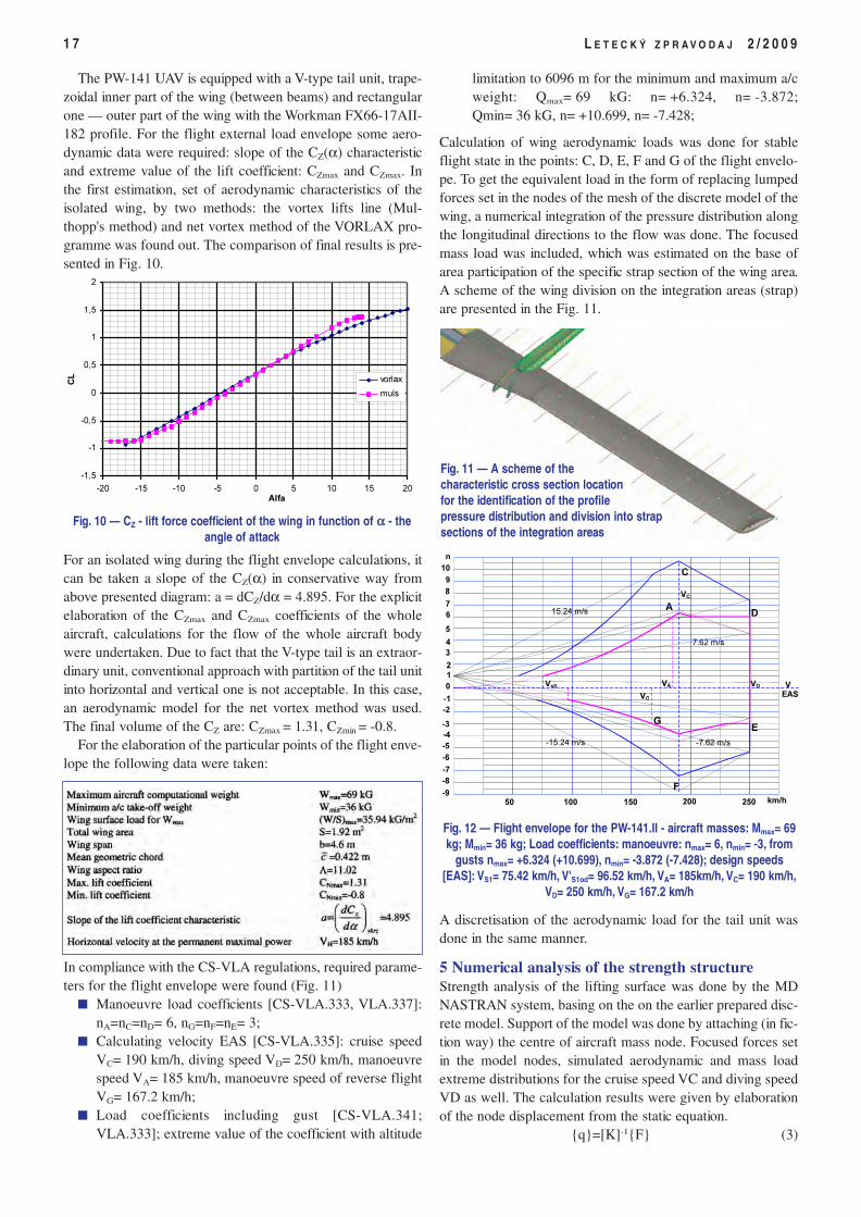
The PW-141 UAV is equipped with a V-type tail unit, trape-zoidal inner part of the wing (between beams) and rectangularone — outer part of the wing with the Workman FX66-17AII-182 profile. For the flight external load envelope some aero-dynamic data were required: slope of the CZ(α) characteristicand extreme value of the lift coefficient: CZmax and CZmax. Inthe first estimation, set of aerodynamic characteristics of theisolated wing, by two methods: the vortex lifts line (Mul-thopp's method) and net vortex method of the VORLAX pro-gramme was found out. The comparison of final results is pre-sented in Fig. 10.
For an isolated wing during the flight envelope calculations, itcan be taken a slope of the CZ(α) in conservative way fromabove presented diagram: a = dCZ/dα = 4.895. For the explicitelaboration of the CZmax and CZmax coefficients of the wholeaircraft, calculations for the flow of the whole aircraft bodywere undertaken. Due to fact that the V-type tail is an extraor-dinary unit, conventional approach with partition of the tail unitinto horizontal and vertical one is not acceptable. In this case,an aerodynamic model for the net vortex method was used.The final volume of the CZ are: CZmax = 1.31, CZmin = -0.8.
For the elaboration of the particular points of the flight enve-lope the following data were taken:
In compliance with the CS-VLA regulations, required parame-ters for the flight envelope were found (Fig. 11)
� Manoeuvre load coefficients [CS-VLA.333, VLA.337]:nA=nC=nD= 6, nG=nF=nE= 3;
� Calculating velocity EAS [CS-VLA.335]: cruise speedVC= 190 km/h, diving speed VD= 250 km/h, manoeuvrespeed VA= 185 km/h, manoeuvre speed of reverse flightVG= 167.2 km/h;
� Load coefficients including gust [CS-VLA.341;VLA.333]; extreme value of the coefficient with altitude
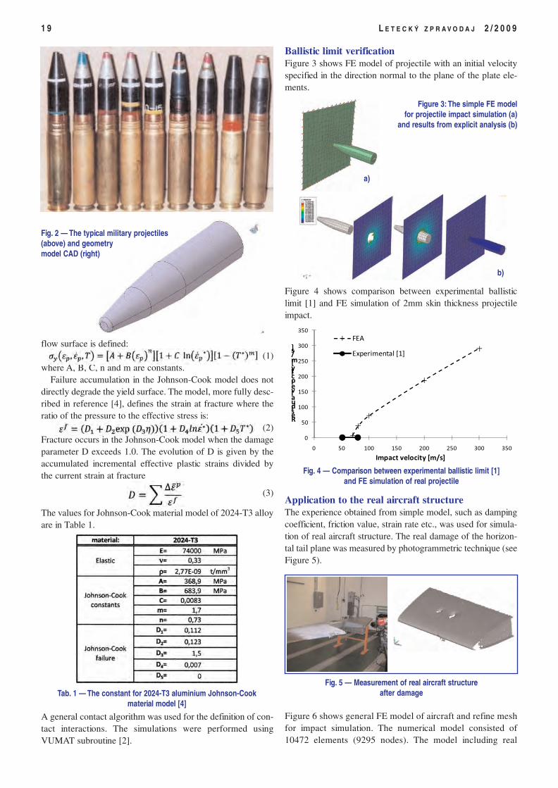
limitation to 6096 m for the minimum and maximum a/cweight: Qmax= 69 kG: n= +6.324, n= -3.872;Qmin= 36 kG, n= +10.699, n= -7.428;
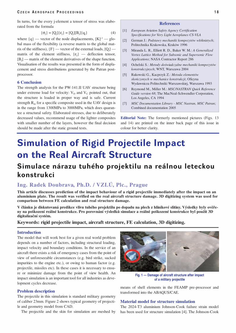
Calculation of wing aerodynamic loads was done for stableflight state in the points: C, D, E, F and G of the flight envelo-pe. To get the equivalent load in the form of replacing lumpedforces set in the nodes of the mesh of the discrete model of thewing, a numerical integration of the pressure distribution alongthe longitudinal directions to the flow was done. The focusedmass load was included, which was estimated on the base ofarea participation of the specific strap section of the wing area.A scheme of the wing division on the integration areas (strap)are presented in the Fig. 11.
A discretisation of the aerodynamic load for the tail unit wasdone in the same manner.
5 Numerical analysis of the strength structureStrength analysis of the lifting surface was done by the MDNASTRAN system, basing on the on the earlier prepared disc-rete model. Support of the model was done by attaching (in fic-tion way) the centre of aircraft mass node. Focused forces setin the model nodes, simulated aerodynamic and mass loadextreme distributions for the cruise speed VC and diving speedVD as well. The calculation results were given by elaborationof the node displacement from the static equation.
{q}=[K]-1{F} (3)
1 7 L E T E C K Ý Z P R A V O D A J 2 / 2 0 0 9
Fig. 10 — CZ - lift force coefficient of the wing in function of αα - theangle of attack
Fig. 12 — Flight envelope for the PW-141.II - aircraft masses: Mmax= 69kg; Mmin= 36 kg; Load coefficients: manoeuvre: nmax= 6, nmin= -3, from
gusts nmax= +6.324 (+10.699), nmin= -3.872 (-7.428); design speeds[EAS]: VS1= 75.42 km/h, V'S1od= 96.52 km/h, VA= 185km/h, VC= 190 km/h,
VD= 250 km/h, VG= 167.2 km/h
-1,5
-1
-0,5
0
0,5
1
1,5
2
-20 -15 -10 -5 0 5 10 15 20Alfa
CL vorlax
muls
Fig. 11 — A scheme of thecharacteristic cross section locationfor the identification of the profilepressure distribution and division into strapsections of the integration areas
100 250 km/h 200
7.62 m/s
0
-3
A
1
2
3
4
5
6
7
8
9
n
-1
-2
-4
-5
-6
-8
V
EAS
VA
VG
Vs0
VC
VD
C
D
E
F
G
15.24 m/s
-15.24 m/s -7.62 m/s
-7
10
-9
150 50
In turns, for the every j-element a tensor of stress was elabo-rated from the formula
{σj} = [Qj]{εj} = [Qj][Bj]{qj} (4)
where {q} — vector of the node displacements, [K]-1 — glo-bal mass of the flexibility (a reverse matrix to the global mat-rix of the stiffness), {F} — vector of the external loads, [Qj] —matrix of the element stiffness, {εj} — deflection tensor,[Bj] — matrix of the element derivatives of the shape function.Visualisation of the results was presented in the form of displa-cement and stress distributions generated by the Patran post-processor.
6 ConclusionThe strength analysis for the PW-141.II UAV structure beingunder extreme load for velocity: VD and VC pointed out, thatthe structure is loaded in proper way and is safe. Currentstrength Rm for a specific composite used in the UAV design isin the range from 1300MPa to 3000MPa, which does quaran-tee a structural safety. Elaborated stresses, due to deliberatelydecreased values, recommend usage of the lighter compositeswith smaller number of the layers, however the final decisionshould be made after the static ground tests.
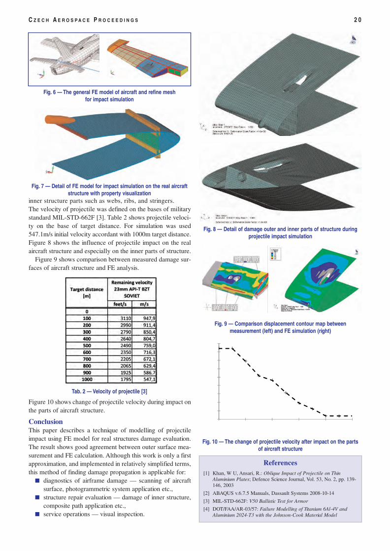
IntroductionThe model that will work best for a given real world problemdepends on a number of factors, including structural loading,impact velocity and boundary conditions. In the service of anaircraft there exists a risk of emergency cases from the point ofview of unforeseeable circumstances (e.g. bird strike, suckedimpurities to the engine etc.), or owing to human factor (e.g.projectile, missiles etc). In these cases it is necessary to ensu-re or minimize damage from the point of view health. Animpact simulation is an important tool for all industries as deve-lopment cycles decrease.
Problem descriptionThe projectile in this simulation is standard military geometryof caliber 23mm. Figure 2 shows typical geometry of projecti-le and geometry model from CAD.
The projectile and the skin for simulation are meshed by
means of shell elements in the FEAMP pre-processor andtransformed into the ABAQUS/CAE.
Material model for structure simulationThe 2024-T3 aluminium Johnson-Cook failure strain modelhas been used for structure simulation [4]. The Johnson-Cook
C Z E C H A E R O S P A C E P R O C E E D I N G S 1 8
Simulation of Rigid Projectile Impacton the Real Aircraft StructureSimulace nárazu tuhého projektilu na reálnou leteckoukonstrukciIng. Radek Doubrava, Ph.D. / VZLÚ, Plc., PragueThis article discusses prediction of the impact behaviour of a rigid projectile immediately after the impact on analuminium plate. The result was verified on the real aircraft structure damage. 3D digitizing system was used forcomparison between FE calculation and real structure damage.
V článku je diskutovaná predikce vlivu tuhého projektilu po dopadu na plech z hliníkové slitiny. Výsledky byly ověře-ny na poškození reálné konstrukce. Pro porovnání výsledků simulace a reálně poškozené konstrukce byl použit 3Ddigitalizační systém.
Keywords: rigid projectile impact, aircraft structure, FE calculation, 3D digitizing.
References
[1] European Aviation Safety Agency CertificationSpecifications for Very Light Aeroplanes CS-VLA
[2] German J.: Podstawy mechaniki kompozytów włóknistych;Politechnika Krakowska, Kraków 1996
[3] Miranda L. R., Elliott R. D., Baker W. M.: A GeneralizedVortex Lattice Method for Subsonic and Supersonic FlowApplications; NASA Contractor Report 286
[4] Ochelski S.: Metody doświadczalne mechaniki kompozytówkonstrukcyjnych; WNT, Warszawa 2004
[5] Rakowski G., Kacprzyk Z.: Metoda elementówskończonych w mechanice konstrukcji; OficynaWydawnicza Politechniki Warszawskiej, Warszawa 1993
[6] Reymond M., Miller M.: MSC/NASTRAN Quick ReferenceGuide version 68; The MacNeal-Schwendler Corporation,Los Angeles, CA 1994
[7] MSC Documentation Library - MSC Nastran, MSC Patran;Combined documentation 2005
Editorial Note: The formerly mentioned pictures (Figs. 13and 14) are printed on the inner back page of this issue incolour for better clarity.
Fig. 1 — Damage of aircraft structure after impactof a military projectile
flow surface is defined:(1)
where A, B, C, n and m are constants. Failure accumulation in the Johnson-Cook model does not
directly degrade the yield surface. The model, more fully desc-ribed in reference [4], defines the strain at fracture where theratio of the pressure to the effective stress is:
(2)Fracture occurs in the Johnson-Cook model when the damageparameter D exceeds 1.0. The evolution of D is given by theaccumulated incremental effective plastic strains divided bythe current strain at fracture
(3)
The values for Johnson-Cook material model of 2024-T3 alloyare in Table 1.
A general contact algorithm was used for the definition of con-tact interactions. The simulations were performed usingVUMAT subroutine [2].
Ballistic limit verificationFigure 3 shows FE model of projectile with an initial velocityspecified in the direction normal to the plane of the plate ele-ments.
Figure 4 shows comparison between experimental ballisticlimit [1] and FE simulation of 2mm skin thickness projectileimpact.
Application to the real aircraft structureThe experience obtained from simple model, such as dampingcoefficient, friction value, strain rate etc., was used for simula-tion of real aircraft structure. The real damage of the horizon-tal tail plane was measured by photogrammetric technique (seeFigure 5).
Figure 6 shows general FE model of aircraft and refine meshfor impact simulation. The numerical model consisted of10472 elements (9295 nodes). The model including real
1 9 L E T E C K Ý Z P R A V O D A J 2 / 2 0 0 9
Tab. 1 — The constant for 2024-T3 aluminium Johnson-Cookmaterial model [4]
Fig. 5 — Measurement of real aircraft structureafter damage
Fig. 2 — The typical military projectiles(above) and geometrymodel CAD (right)
Figure 3: The simple FE modelfor projectile impact simulation (a)
and results from explicit analysis (b)
a)
b)
0
50
100
150
200
250
300
350
0 50 100 150 200 250 300 350
Residual velocity [m/s]
Impact velocity [m/s]
FEA
Experimental [1]
Fig. 4 — Comparison between experimental ballistic limit [1]and FE simulation of real projectile
inner structure parts such as webs, ribs, and stringers.The velocity of projectile was defined on the bases of militarystandard MIL-STD-662F [3]. Table 2 shows projectile veloci-ty on the base of target distance. For simulation was used547.1m/s initial velocity accordant with 1000m target distance.Figure 8 shows the influence of projectile impact on the realaircraft structure and especially on the inner parts of structure.
Figure 9 shows comparison between measured damage sur-faces of aircraft structure and FE analysis.
Figure 10 shows change of projectile velocity during impact onthe parts of aircraft structure.
ConclusionThis paper describes a technique of modelling of projectileimpact using FE model for real structures damage evaluation.The result shows good agreement between outer surface mea-surement and FE calculation. Although this work is only a firstapproximation, and implemented in relatively simplified terms,this method of finding damage propagation is applicable for:
� diagnostics of airframe damage — scanning of aircraftsurface, photogrammetric system application etc.,
� structure repair evaluation — damage of inner structure,composite path application etc.,
� service operations — visual inspection.
C Z E C H A E R O S P A C E P R O C E E D I N G S 2 0
References[1] Khan, W U, Ansari, R.: Oblique Impact of Projectile on Thin
Aluminium Plates; Defence Science Journal, Vol. 53, No. 2, pp. 139-146, 2003
[2] ABAQUS v.6.7.5 Manuals, Dassault Systems 2008-10-14
[3] MIL-STD-662F: V50 Ballistic Test for Armor
[4] DOT/FAA/AR-03/57: Failure Modelling of Titanium 6Al-4V andAluminium 2024-T3 with the Johnson-Cook Material Model
Fig. 6 — The general FE model of aircraft and refine meshfor impact simulation
Fig. 7 — Detail of FE model for impact simulation on the real aircraftstructure with property visualization
Tab. 2 — Velocity of projectile [3]
Fig. 10 — The change of projectile velocity after impact on the partsof aircraft structure
Fig. 9 — Comparison displacement contour map betweenmeasurement (left) and FE simulation (right)
Fig. 8 — Detail of damage outer and inner parts of structure duringprojectile impact simulation
1 IntroductionPossibility to influence the aerodynamic performance ofa wing by using shaped wingtips has been known for deca-des [1] [2] [3], for example F. Lanchester patented the end-plate even in 1897. A new impulse was given by Whitcombwork [4] and since then increasing attention is continuouslypaid to this specific area of the wing design. But there is lackof published validated best-practice approaches for theirdesign, rare exception is presented by ESDU [5], that isfocused mainly on large transport aircraft.
In general, the different wingtip devices are concisely att-ributed with increase of the efficient wing aspect ratio, whichmanifests primordially by the reduction of the induced dragand by the increase of the maximum lift. This supposition isgenerally correct but the resulting global aerodynamic per-formance of a wing with different wingtip devices is not soevident because the criteria could be various. It is necessaryto include the total drag, but for example also the lateral cha-racteristics, etc. Sometimes also the literary sources give dif-ferent results even for very similar cases. In addition, alsoother than aerodynamic considerations (strength, flutter, ...)shall be taken into account in a comprehensive wingletassessment.
The aim of the presented testing was basic comparison ofthe influence of several wingtips on global aerodynamic per-formance. The wingtip devices were intentionally chosen asdistinctively different, from simple extension of span to spe-cifically designed dedicated winglet. The studied straightwing corresponds to low-speed commuter or general aviati-on aircraft.
2 Wing model and testing
2.1 Basic wingA model of a turbulent wing of a generic aircraft of generalaviation category was used. The supposed aircraft is twin tur-boprop of business category with cruise speed of approx. 400kph (210 kts).
Basic geometric characteristics of the wing are given in Tab.1 below:
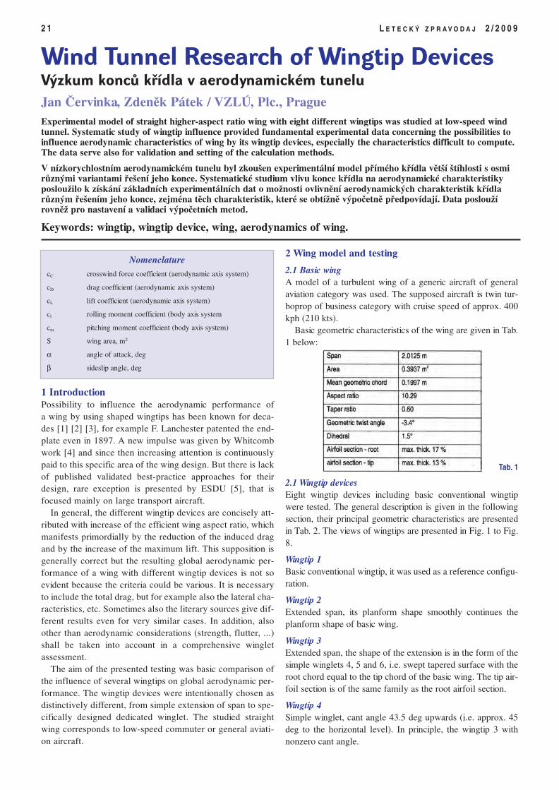
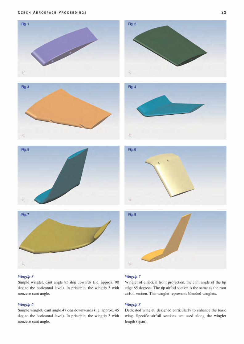
2.1 Wingtip devicesEight wingtip devices including basic conventional wingtipwere tested. The general description is given in the followingsection, their principal geometric characteristics are presentedin Tab. 2. The views of wingtips are presented in Fig. 1 to Fig.8.
Wingtip 1Basic conventional wingtip, it was used as a reference configu-ration.
Wingtip 2Extended span, its planform shape smoothly continues theplanform shape of basic wing.
Wingtip 3Extended span, the shape of the extension is in the form of thesimple winglets 4, 5 and 6, i.e. swept tapered surface with theroot chord equal to the tip chord of the basic wing. The tip air-foil section is of the same family as the root airfoil section.
Wingtip 4Simple winglet, cant angle 43.5 deg upwards (i.e. approx. 45deg to the horizontal level). In principle, the wingtip 3 withnonzero cant angle.
2 1 L E T E C K Ý Z P R A V O D A J 2 / 2 0 0 9
Wind Tunnel Research of Wingtip DevicesVýzkum konců křídla v aerodynamickém tuneluJan Červinka, Zdeněk Pátek / VZLÚ, Plc., PragueExperimental model of straight higher-aspect ratio wing with eight different wingtips was studied at low-speed windtunnel. Systematic study of wingtip influence provided fundamental experimental data concerning the possibilities toinfluence aerodynamic characteristics of wing by its wingtip devices, especially the characteristics difficult to compute.The data serve also for validation and setting of the calculation methods.
V nízkorychlostním aerodynamickém tunelu byl zkoušen experimentální model přímého křídla větší štíhlosti s osmirůznými variantami řešení jeho konce. Systematické studium vlivu konce křídla na aerodynamické charakteristikyposloužilo k získání základních experimentálních dat o možnosti ovlivnění aerodynamických charakteristik křídlarůzným řešením jeho konce, zejména těch charakteristik, které se obtížně výpočetně předpovídají. Data posloužírovněž pro nastavení a validaci výpočetních metod.
Keywords: wingtip, wingtip device, wing, aerodynamics of wing.
Nomenclature
cC crosswind force coefficient (aerodynamic axis system)
cD drag coefficient (aerodynamic axis system)
cL lift coefficient (aerodynamic axis system)
cl rolling moment coefficient (body axis system
cm pitching moment coefficient (body axis system)
S wing area, m2
α angle of attack, deg
β sideslip angle, deg
Tab. 1
C Z E C H A E R O S P A C E P R O C E E D I N G S 2 2
Wingtip 5Simple winglet, cant angle 85 deg upwards (i.e. approx. 90deg to the horizontal level). In principle, the wingtip 3 withnonzero cant angle.
Wingtip 6Simple winglet, cant angle 47 deg downwards (i.e. approx. 45deg to the horizontal level). In principle, the wingtip 3 withnonzero cant angle.
Wingtip 7Winglet of elliptical front projection, the cant angle of the tipedge 85 degrees. The tip airfoil section is the same as the rootairfoil section. This winglet represents blended winglets.
Wingtip 8Dedicated winglet, designed particularly to enhance the basicwing. Specific airfoil sections are used along the wingletlength (span).
Fig. 1 Fig. 2
Fig. 3 Fig. 4
Fig. 5 Fig. 6
Fig. 7 Fig. 8
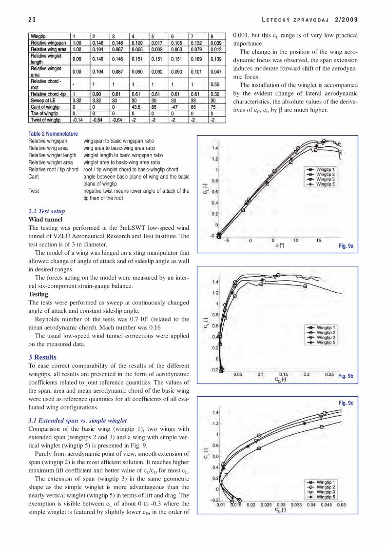
Table 2 NomenclatureRelative wingspan wingspan to basic wingspan ratioRelative wing area wing area to basic-wing area ratioRelative winglet length winglet length to basic wingspan ratioRelative winglet area winglet area to basic-wing area ratioRelative root / tip chord root / tip winglet chord to basic-wingtip chordCant angle between basic plane of wing and the basic
plane of wingtipTwist negative twist means lower angle of attack of the
tip than of the root
2.2 Test setupWind tunnelThe testing was performed in the 3mLSWT low-speed windtunnel of VZLÚ Aeronautical Research and Test Institute. Thetest section is of 3 m diameter.
The model of a wing was hinged on a sting manipulator thatallowed change of angle of attack and of sideslip angle as wellin desired ranges.
The forces acting on the model were measured by an inter-nal six-component strain-gauge balance.TestingThe tests were performed as sweep at continuously changedangle of attack and constant sideslip angle.
Reynolds number of the tests was 0.7·106 (related to themean aerodynamic chord), Mach number was 0.16
The usual low-speed wind tunnel corrections were appliedon the measured data.
3 ResultsTo ease correct comparability of the results of the differentwingtips, all results are presented in the form of aerodynamiccoefficients related to joint reference quantities. The values ofthe span, area and mean aerodynamic chord of the basic wingwere used as reference quantities for all coefficients of all eva-luated wing configurations.
3.1 Extended span vs. simple wingletComparison of the basic wing (wingtip 1), two wings withextended span (wingtips 2 and 3) and a wing with simple ver-tical winglet (wingtip 5) is presented in Fig. 9.
Purely from aerodynamic point of view, smooth extension ofspan (wingtip 2) is the most efficient solution. It reaches highermaximum lift coefficient and better value of cL/cD for most cL.
The extension of span (wingtip 3) in the same geometricshape as the simple winglet is more advantageous than thenearly vertical winglet (wingtip 5) in terms of lift and drag. Theexemption is visible between cL of about 0 to -0.3 where thesimple winglet is featured by slightly lower cD, in the order of
0.001, but this cL range is of very low practicalimportance.
The change in the position of the wing aero-dynamic focus was observed, the span extensioninduces moderate forward shift of the aerodyna-mic focus.
The installation of the winglet is accompaniedby the evident change of lateral aerodynamiccharacteristics, the absolute values of the deriva-tives of cC, cl, by β are much higher.
2 3 L E T E C K Ý Z P R A V O D A J 2 / 2 0 0 9
Fig. 9a
Fig. 9b
Fig. 9c
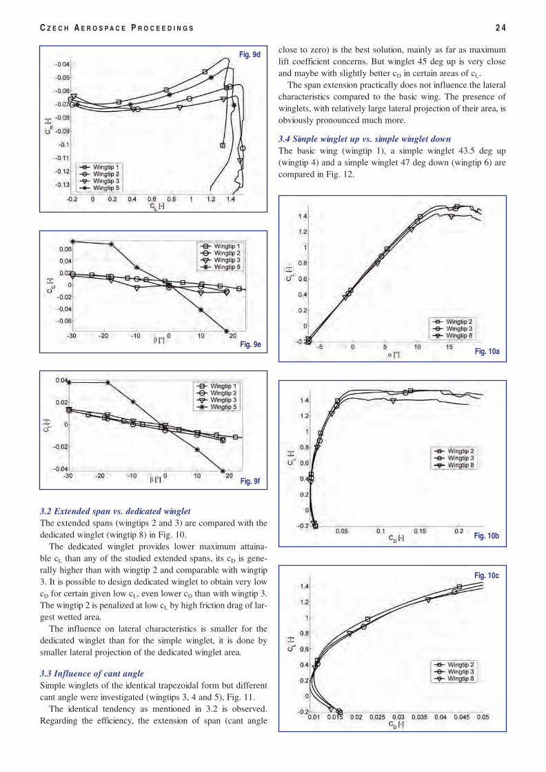
3.2 Extended span vs. dedicated wingletThe extended spans (wingtips 2 and 3) are compared with thededicated winglet (wingtip 8) in Fig. 10.
The dedicated winglet provides lower maximum attaina-ble cL than any of the studied extended spans, its cD is gene-rally higher than with wingtip 2 and comparable with wingtip3. It is possible to design dedicated winglet to obtain very lowcD for certain given low cL, even lower cD than with wingtip 3.The wingtip 2 is penalized at low cL by high friction drag of lar-gest wetted area.
The influence on lateral characteristics is smaller for thededicated winglet than for the simple winglet, it is done bysmaller lateral projection of the dedicated winglet area.
3.3 Influence of cant angleSimple winglets of the identical trapezoidal form but differentcant angle were investigated (wingtips 3, 4 and 5), Fig. 11.
The identical tendency as mentioned in 3.2 is observed.Regarding the efficiency, the extension of span (cant angle
close to zero) is the best solution, mainly as far as maximumlift coefficient concerns. But winglet 45 deg up is very closeand maybe with slightly better cD in certain areas of cL.
The span extension practically does not influence the lateralcharacteristics compared to the basic wing. The presence ofwinglets, with relatively large lateral projection of their area, isobviously pronounced much more.
3.4 Simple winglet up vs. simple winglet downThe basic wing (wingtip 1), a simple winglet 43.5 deg up(wingtip 4) and a simple winglet 47 deg down (wingtip 6) arecompared in Fig. 12.
C Z E C H A E R O S P A C E P R O C E E D I N G S 2 4
Fig. 9d
Fig. 10a
Fig. 10b
Fig. 10c
Fig. 9e
Fig. 9f
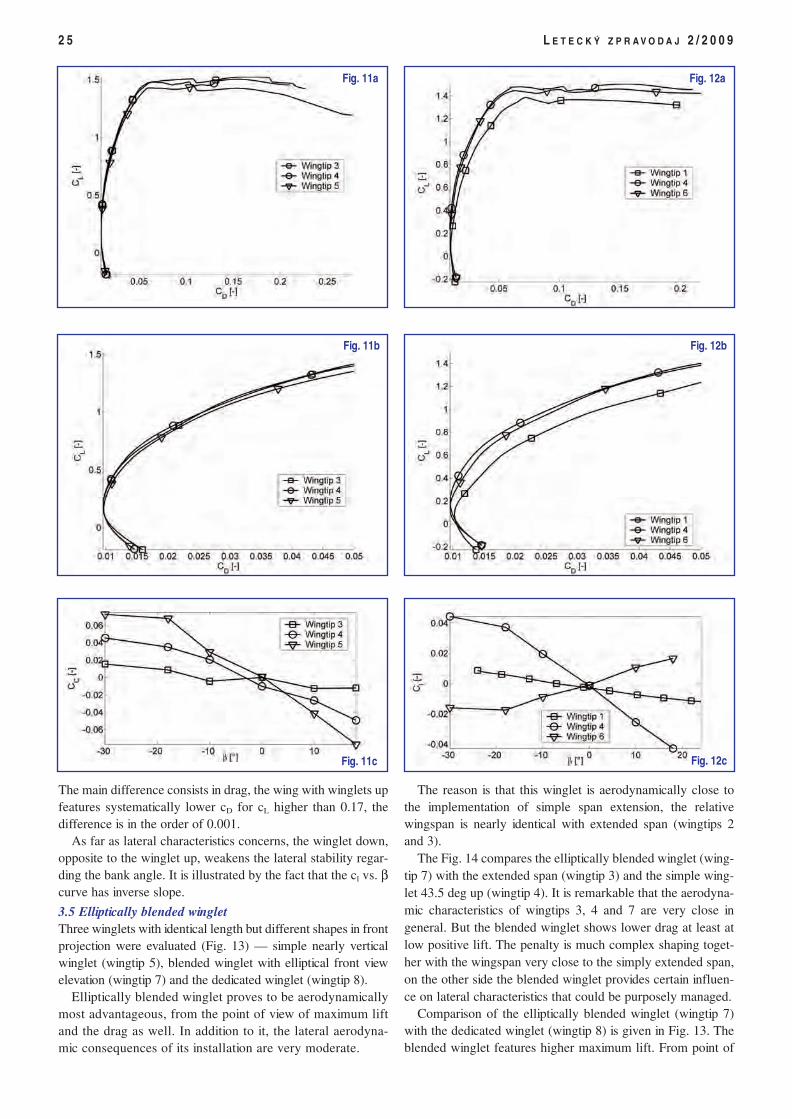
The main difference consists in drag, the wing with winglets upfeatures systematically lower cD for cL higher than 0.17, thedifference is in the order of 0.001.
As far as lateral characteristics concerns, the winglet down,opposite to the winglet up, weakens the lateral stability regar-ding the bank angle. It is illustrated by the fact that the cl vs. βcurve has inverse slope.
3.5 Elliptically blended wingletThree winglets with identical length but different shapes in frontprojection were evaluated (Fig. 13) — simple nearly verticalwinglet (wingtip 5), blended winglet with elliptical front viewelevation (wingtip 7) and the dedicated winglet (wingtip 8).
Elliptically blended winglet proves to be aerodynamicallymost advantageous, from the point of view of maximum liftand the drag as well. In addition to it, the lateral aerodyna-mic consequences of its installation are very moderate.
The reason is that this winglet is aerodynamically close tothe implementation of simple span extension, the relativewingspan is nearly identical with extended span (wingtips 2and 3).
The Fig. 14 compares the elliptically blended winglet (wing-tip 7) with the extended span (wingtip 3) and the simple wing-let 43.5 deg up (wingtip 4). It is remarkable that the aerodyna-mic characteristics of wingtips 3, 4 and 7 are very close ingeneral. But the blended winglet shows lower drag at least atlow positive lift. The penalty is much complex shaping toget-her with the wingspan very close to the simply extended span,on the other side the blended winglet provides certain influen-ce on lateral characteristics that could be purposely managed.
Comparison of the elliptically blended winglet (wingtip 7)with the dedicated winglet (wingtip 8) is given in Fig. 13. Theblended winglet features higher maximum lift. From point of
2 5 L E T E C K Ý Z P R A V O D A J 2 / 2 0 0 9
Fig. 11a
Fig. 11b
Fig. 11c
Fig. 12a
Fig. 12b
Fig. 12c
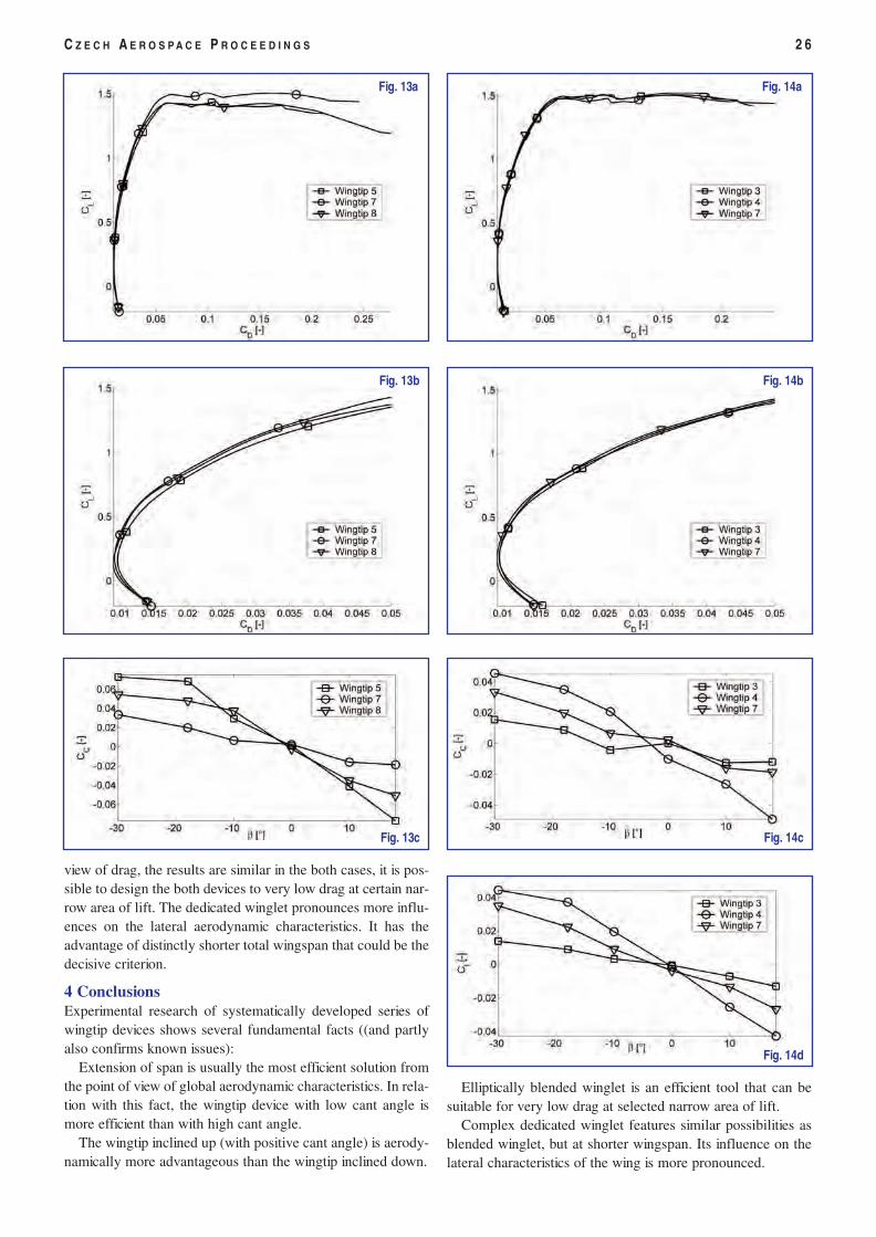
view of drag, the results are similar in the both cases, it is pos-sible to design the both devices to very low drag at certain nar-row area of lift. The dedicated winglet pronounces more influ-ences on the lateral aerodynamic characteristics. It has theadvantage of distinctly shorter total wingspan that could be thedecisive criterion.
4 ConclusionsExperimental research of systematically developed series ofwingtip devices shows several fundamental facts ((and partlyalso confirms known issues):
Extension of span is usually the most efficient solution fromthe point of view of global aerodynamic characteristics. In rela-tion with this fact, the wingtip device with low cant angle ismore efficient than with high cant angle.
The wingtip inclined up (with positive cant angle) is aerody-namically more advantageous than the wingtip inclined down.
Elliptically blended winglet is an efficient tool that can besuitable for very low drag at selected narrow area of lift.
Complex dedicated winglet features similar possibilities asblended winglet, but at shorter wingspan. Its influence on thelateral characteristics of the wing is more pronounced.
C Z E C H A E R O S P A C E P R O C E E D I N G S 2 6
Fig. 13a
Fig. 13b
Fig. 13c
Fig. 14a
Fig. 14b
Fig. 14c
Fig. 14d
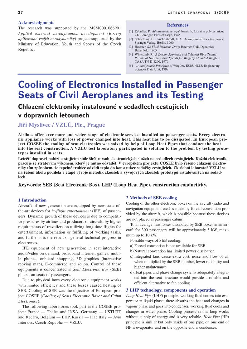
AcknowledgmentsThe research was supported by the MSM0001066901Applied external aerodynamics development (Rozvojaplikované vnější aerodynamiky) project supported by theMinistry of Education, Youth and Sports of the CzechRepublic.
1 IntroductionAircraft of new generation are equipped by new state-of-the-art devices for in-flight entertainment (IFE) of passen-gers. Dynamic growth of these devices is due to competiti-ve pressures by airlines and producers of aircraft, by higherrequirements of travellers on utilizing long time flights forentertainment, information or fulfilling of working tasks,and further it is the result of general technical progress inelectronics.
IFE equipment of new generation: in seat interactiveaudio/video on demand, broadband internet, games, mobi-le phones, onboard shopping, 3D graphics (interactivemoving map), E-commerce and so on. Control of theseequipments is concentrated in Seat Electronic Box (SEB)placed on seats of passengers.
Due to physical laws every electronic equipment workswith limited efficiency and these losses caused heating ofSEB. Cooling of SEB was the objective of European pro-ject COSEE (Cooling of Seats Electronic Boxes and CabinElectronics).
The following laboratories took part in the COSEE pro-ject: France — Thales and INSA, Germany — USTUTTand Recaro, Belgium — EHP, Russia — ITP, Italy — AvioInteriors, Czech Republic — VZLU.
2 Methods of SEB coolingCooling of the other electronic boxes on the aircraft (radio andnavigation equipment etc.) is made by forced convention pro-vided by the aircraft, which is possible because these devicesare not placed in passenger cabins.
Total average heat losses dissipated by SEB boxes in an air-craft for 300 passengers will be approximately 5 kW, maxi-mum up to 10 kW.
Possible ways of SEB cooling:a) Forced convention is not available for SEBb) Natural convention has limited power dissipationc) Integrated fans cause extra cost, noise and flow of air
when multiplied by the SEB number, lower reliability andhigher maintenance
d) Heat pipes and phase change systems adequately integra-ted into the seat structure would provide a reliable andefficient alternative to fan cooling
3 LHP technology, components and operationLoop Heat Pipe (LHP) principle: working fluid comes into eva-porator in liquid phase, there absorbs the heat and changes invapour phase and goes into condenser, working fluid cools andchanges in water phase. Cooling process in this loop workswithout supply of energy and is very reliable. Heat Pipe (HP)principle is similar but only inside of one pipe, on one end ofHP is evaporator and on the opposite end is condenser.
2 7 L E T E C K Ý Z P R A V O D A J 2 / 2 0 0 9
Cooling of Electronics Installed in PassengerSeats of Civil Aeroplanes and its TestingChlazení elektroniky instalované v sedadlech cestujícíchv dopravních letounechJiří Myslivec / VZLÚ, Plc., Prague
Airlines offer ever more and wider range of electronic services installed on passenger seats. Every electro-nic appliance works with loss of power changed into heat. This heat has to be dissipated. In European pro-ject COSEE the cooling of seat electronics was solved by help of Loop Heat Pipes that conduct the heatinto the seat construction. A VZLU test laboratory participated in solution to the problem by testing proto-types installed in seats.Letečtí dopravci nabízí cestujícím stále širší rozsah elektronických služeb na sedadlech cestujících. Každá elektronikapracuje se ztrátovým výkonem, který je nutno odvádět. V evropském projektu COSEE bylo řešeno chlazení elektro-niky tím způsobem, že tepelné trubice odvádí teplo do konstrukce sedačky cestujících. Zkušební laboratoř VZLU sena řešení úkolu podílela v etapě vývoje metodik zkoušek a vývojových zkoušek prototypů instalovaných na sedad-lech.
Keywords: SEB (Seat Electronic Box), LHP (Loop Heat Pipe), construction conductivity.
References[1] Rebuffet, P.: Aérodynamique expérimentale; Librairie polytechnique
Ch. Béranger, Paris et Liege, 1945[2] Schlichting, H., Truckenbrodt, E. A.: Aerodynamik des Flugzeuges;
Springer Verlag, Berlin, 1960[3] Hoerner, S.: Fluid Dynamic Drag; Hoerner Fluid Dynamics,
Bakerfield, 1965[4] Whitcomb, R.: A Design Approach and Selected Wind-Tunnel
Results at High Subsonic Speeds for Wing-Tip Mounted Winglets;NASA TN D-8260, 1976
[5] -, Aerodynamic Principles of Winglets, ESDU 9813, EngineeringSciences Data Unit, 1998
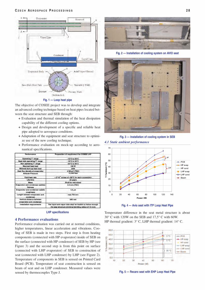
The objective of COSEE project was to develop and integratean advanced cooling technique based on heat pipes located bet-ween the seat structure and SEB through:
+ Evaluation and thermal simulation of the heat dissipationcapability of the different cooling options.
+ Design and development of a specific and reliable heatpipe adopted to aerospace conditions.
+ Adaptation of the equipment and seat structure to optimi-ze use of the new cooling technique.
+ Performance evaluation on mock-up according to aero-nautical specifications.
4 Performance evaluationsPerformance evaluation was carried out at normal conditions,higher temperatures, linear acceleration and vibrations. Coo-ling of SEB is made in two steps. First step is from heatingcomponents (connected with HP evaporator) inside of SEB onthe surface (connected with HP condenser) of SEB by HP (seeFigure 3) and the second step is from this point on surface(connected with LHP evaporator) of SEB to construction ofseat (connected with LHP condenser) by LHP (see Figure 2).Temperature of components in SEB is sensed on Printed CardBoard (PCB). Temperature of seat construction is sensed onbeam of seat and on LHP condenser. Measured values weresensed by thermocouples Type J.
4.1 Static ambient performance
Temperature difference in the seat metal structure is about30° C with 120W on the SEB and 17,5° C with 60W.HP thermal gradient: 3° C, LHP thermal gradient: 14° C.
C Z E C H A E R O S P A C E P R O C E E D I N G S 2 8
Fig. 1 — Loop heat pipe
Fig. 2 — Installation of cooling system on AVIO seat
Fig. 3 — Installation of cooling system in SEB
Fig. 4 — Avio seat with ITP Loop Heat Pipe
LHP specifications
0
10
20
30
40
50
60
70
0 20 40 60 80 100 120 140
Power (W)
T-T
amb
ien
t (°
C) PCB
HP evap
HP cond
LHP evap
LHP cond
Beam
HP
LHP
Fig. 5 — Recaro seat with EHP Loop Heat Pipe
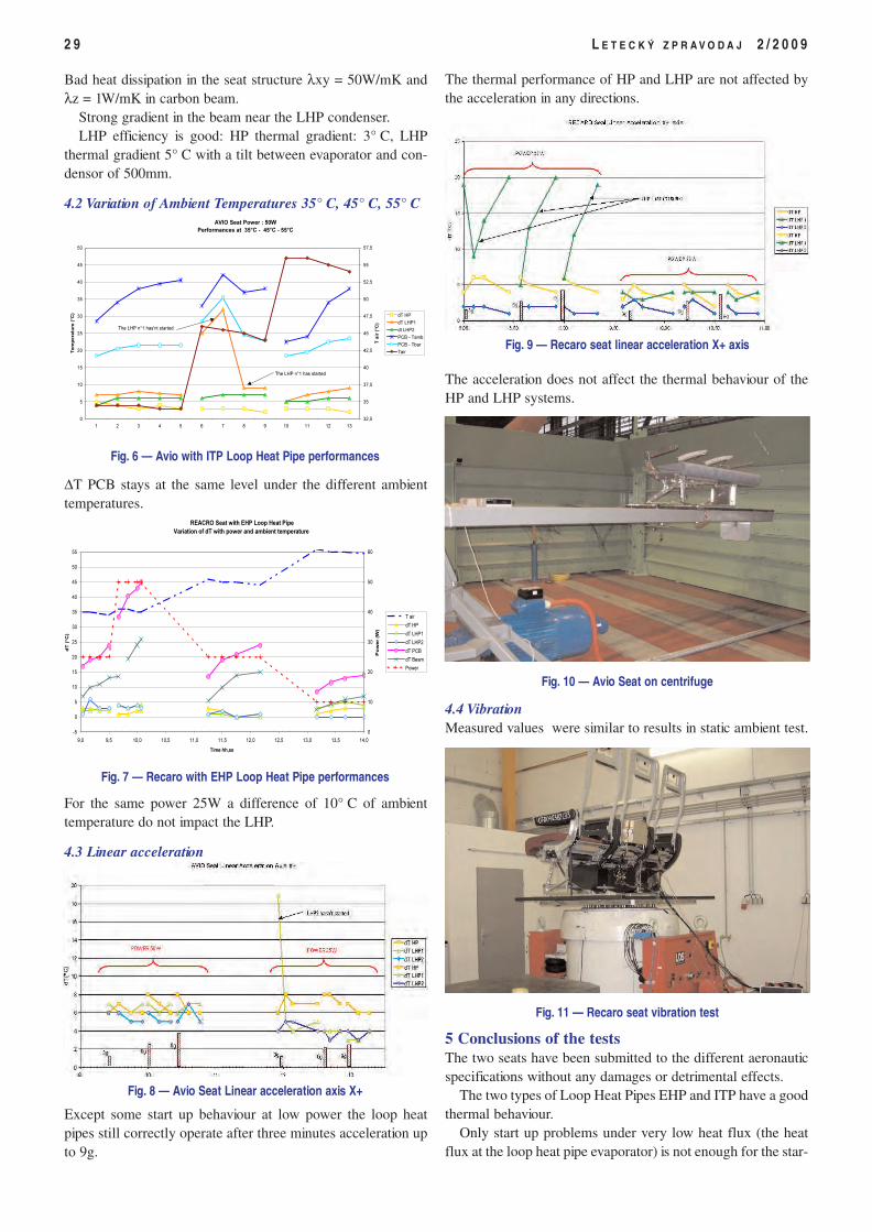
Bad heat dissipation in the seat structure λxy = 50W/mK andλz = 1W/mK in carbon beam.
Strong gradient in the beam near the LHP condenser.LHP efficiency is good: HP thermal gradient: 3° C, LHP
thermal gradient 5° C with a tilt between evaporator and con-densor of 500mm.
4.2 Variation of Ambient Temperatures 35° C, 45° C, 55° C
∆T PCB stays at the same level under the different ambienttemperatures.
For the same power 25W a difference of 10° C of ambienttemperature do not impact the LHP.
4.3 Linear acceleration
Except some start up behaviour at low power the loop heatpipes still correctly operate after three minutes acceleration upto 9g.
The thermal performance of HP and LHP are not affected bythe acceleration in any directions.
The acceleration does not affect the thermal behaviour of theHP and LHP systems.
4.4 VibrationMeasured values were similar to results in static ambient test.
5 Conclusions of the testsThe two seats have been submitted to the different aeronauticspecifications without any damages or detrimental effects.
The two types of Loop Heat Pipes EHP and ITP have a goodthermal behaviour.
Only start up problems under very low heat flux (the heatflux at the loop heat pipe evaporator) is not enough for the star-
2 9 L E T E C K Ý Z P R A V O D A J 2 / 2 0 0 9
Fig. 7 — Recaro with EHP Loop Heat Pipe performances
REACRO Seat with EHP Loop Heat Pipe Variation of dT with power and ambient temperature
-5
0
5
10
15
20
25
30
35
40
45
50
55
9,0 9,5 10,0 10,5 11,0 11,5 12,0 12,5 13,0 13,5 14,0
Time hh,ss
dT
(°C
)
0
10
20
30
40
50
60
Po
wer
(W)
T air
dT HP
dT LHP1
dT LHP2
dT PCB
dT Beam
Power
Fig. 8 — Avio Seat Linear acceleration axis X+
Fig. 9 — Recaro seat linear acceleration X+ axis
Fig. 10 — Avio Seat on centrifuge
Fig. 6 — Avio with ITP Loop Heat Pipe performances
AVIO Seat Power : 50W Performances at 35°C - 45°C - 55°C
0
5
10
15
20
25
30
35
40
45
50
1 2 3 4 5 6 7 8 9 10 11 12 13
Tem
pera
ture
(°C
)
32,5
35
37,5
40
42,5
45
47,5
50
52,5
55
57,5
T a
ir (
°C)
dT HP
dT LHP1
dt LHP2
PCB - Tamb
PCB - Tbar
Tair
The LHP n°1 has'nt started
The LHP n°1 has started
Fig. 11 — Recaro seat vibration test
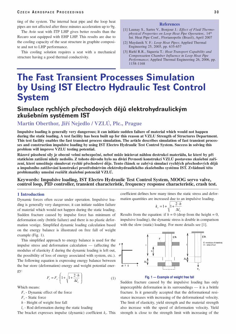
ting of the system. The internal heat pipe and the loop heatpipes are not affected after three minutes acceleration up to 9g.
The Avio seat with ITP LHP gives better results than theRecaro seat equipped with EHP LHP. This results are due tothe cooling capacity of the seat structure in graphite composi-te and not to LHP performance.
This cooling solution requires a seat with a mechanicalstructure having a good thermal conductivity.
1 IntroductionDynamic forces often occur under operation. Impulsive loa-ding is generally very dangerous; it can initiate sudden failureof material which would not happen during the static loading.Sudden fracture caused by impulse force has minimum ofdeformation only (brittle failure) and there is no plastic defor-mation vestige. Simplified dynamic loading calculation basedon the energy balance is illustrated on free fall of weightexample (Fig. 1).
This simplified approach to energy balance is used for theimpulse stress and deformation calculation — (affecting themodulus of elasticity E during the dynamic loading is left out,the possibility of loss of energy associated with system, etc.).The following equation is expressing energy balance betweenthe bar store (deformation) energy and weight potential ener-gy:
(1)
Which means:Fr - Dynamic effect of the forceFs - Static forceh - Height of weight free fallls - Rod deformation during the static loading
The bracket expresses impulse (dynamic) coefficient kr. This
coefficient defines how many times the static stress and defor-mation quantities are increased due to an impulsive loading.
Results from the equation: if h = 0 (drop from the height = 0,impulsive loading), the dynamic stress is double in comparisonwith the slow (static) loading. For more details see [1].
Fig. 1 — Example of weight free fallSudden fracture caused by the impulsive loading has onlyimperceptible deformation in its surroundings — it is a brittlefracture. Is it generally accepted that the deformational resi-stance increases with increasing of the deformational velocity.The limit of elasticity, yield strength and the material strengthalso increase with the speed of deformation velocity. Yieldstrength is close to the strength limit with increasing of the
C Z E C H A E R O S P A C E P R O C E E D I N G S 3 0
The Fast Transient Processes Simulationby Using IST Electro Hydraulic Test ControlSystemSimulace rychlých přechodových dějů elektrohydraulickýmzkušebním systémem ISTMartin Oberthor, Jiří Nejedlo / VZLÚ, Plc., PragueImpulsive loading is generally very dangerous; it can initiate sudden failure of material which would not happenduring the static loading. A test facility has been built up for this reason at VZLU Strength of Structures Department.This test facility enables the fast transient process simulation. The article describes simulation of fast transient proces-ses and construction impulsive loading by using IST Electro Hydraulic Test Control System. Success in solving thisproblem will improve VZLU testing potential.Rázové působení síly je obecně velmi nebezpečné, neboť může iniciovat náhlou destrukci materiálu, ke které by přistatickém zatížení nikdy nedošlo. Z tohoto důvodu bylo na divizi Pevnosti konstrukcí VZLÚ postaveno zkušební zaří-zení, které umožňuje simulovat rychlé přechodové děje. Tento článek se zabývá simulací rychlých přechodových dějůa impulsního zatěžování konstrukcí prostřednictvím elektrohydraulického zkušebního systému IST. Zvládnutí tétoproblematiky umožní rozšířit zkušební potenciál VZLÚ.
Keywords: Impulsive loading, IST Electro Hydraulic Test Control System, MOOG servo valve,control loop, PID controller, transient characteristic, frequency response characteristic, crash test.
References[1] Launay S., Sartre V., Bonjour J.: Effect of Fluid Thermo-
physical Properties on Loop Heat Pipe Operation;. 14th
Int. Heat Pipe Conf., Florianopolis (Brasil), April 2007
[2] Maydanik Y. F.: Loop Heat Pipes; Applied ThermalEngineering 25, 2005, pp. 635-657
[3] Riehl R.R., Siqueria T.: Heat Transport Capability andCompensation Chamber Influence in Loop Heat PipePerformance; Applied Thermal Engineering 26, 2006, pp.1158-1168
∆
⋅++⋅=s
srl
hFF
211
s
rl
hk
∆⋅++= 2
11
F
dF
t dt ? 0
l
h
Älr
E?A F
l
Äls
E?A
Fs
E -modulus of elasticity A – area of cut
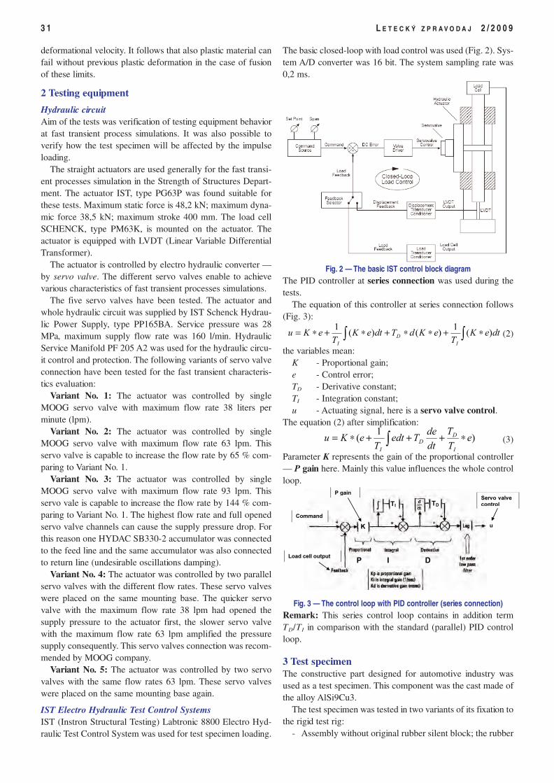
deformational velocity. It follows that also plastic material canfail without previous plastic deformation in the case of fusionof these limits.
2 Testing equipment
Hydraulic circuitAim of the tests was verification of testing equipment behaviorat fast transient process simulations. It was also possible toverify how the test specimen will be affected by the impulseloading.
The straight actuators are used generally for the fast transi-ent processes simulation in the Strength of Structures Depart-ment. The actuator IST, type PG63P was found suitable forthese tests. Maximum static force is 48,2 kN; maximum dyna-mic force 38,5 kN; maximum stroke 400 mm. The load cellSCHENCK, type PM63K, is mounted on the actuator. Theactuator is equipped with LVDT (Linear Variable DifferentialTransformer).
The actuator is controlled by electro hydraulic converter —by servo valve. The different servo valves enable to achievevarious characteristics of fast transient processes simulations.
The five servo valves have been tested. The actuator andwhole hydraulic circuit was supplied by IST Schenck Hydrau-lic Power Supply, type PP165BA. Service pressure was 28MPa, maximum supply flow rate was 160 l/min. HydraulicService Manifold PF 205 A2 was used for the hydraulic circu-it control and protection. The following variants of servo valveconnection have been tested for the fast transient characteris-tics evaluation:
Variant No. 1: The actuator was controlled by singleMOOG servo valve with maximum flow rate 38 liters perminute (lpm).
Variant No. 2: The actuator was controlled by singleMOOG servo valve with maximum flow rate 63 lpm. Thisservo valve is capable to increase the flow rate by 65 % com-paring to Variant No. 1.
Variant No. 3: The actuator was controlled by singleMOOG servo valve with maximum flow rate 93 lpm. Thisservo vale is capable to increase the flow rate by 144 % com-paring to Variant No. 1. The highest flow rate and full openedservo valve channels can cause the supply pressure drop. Forthis reason one HYDAC SB330-2 accumulator was connectedto the feed line and the same accumulator was also connectedto return line (undesirable oscillations damping).
Variant No. 4: The actuator was controlled by two parallelservo valves with the different flow rates. These servo valveswere placed on the same mounting base. The quicker servovalve with the maximum flow rate 38 lpm had opened thesupply pressure to the actuator first, the slower servo valvewith the maximum flow rate 63 lpm amplified the pressuresupply consequently. This servo valves connection was recom-mended by MOOG company.
Variant No. 5: The actuator was controlled by two servovalves with the same flow rates 63 lpm. These servo valveswere placed on the same mounting base again.
IST Electro Hydraulic Test Control Systems IST (Instron Structural Testing) Labtronic 8800 Electro Hyd-raulic Test Control System was used for test specimen loading.
The basic closed-loop with load control was used (Fig. 2). Sys-tem A/D converter was 16 bit. The system sampling rate was0,2 ms.
Fig. 2 — The basic IST control block diagramThe PID controller at series connection was used during thetests.
The equation of this controller at series connection follows(Fig. 3):
(2)
the variables mean:K - Proportional gain;e - Control error;TD - Derivative constant;TI - Integration constant;u - Actuating signal, here is a servo valve control.
The equation (2) after simplification:
(3)
Parameter K represents the gain of the proportional controller— P gain here. Mainly this value influences the whole controlloop.
Fig. 3 — The control loop with PID controller (series connection)Remark: This series control loop contains in addition termTD/TI in comparison with the standard (parallel) PID controlloop.
3 Test specimenThe constructive part designed for automotive industry wasused as a test specimen. This component was the cast made ofthe alloy AlSi9Cu3.
The test specimen was tested in two variants of its fixation tothe rigid test rig:
- Assembly without original rubber silent block; the rubber
3 1 L E T E C K Ý Z P R A V O D A J 2 / 2 0 0 9
∫∫ ∗+∗∗+∗+∗= dteK
TeKdTdteK
TeKu
I
D
I
)(1
)()(1
)
1( e
T
T
dt
deTedt
TeKu
I
DD
I
∗+++∗= ∫
P I D
TI TD
P gain Servo valve control
Load cell output
K u
Command
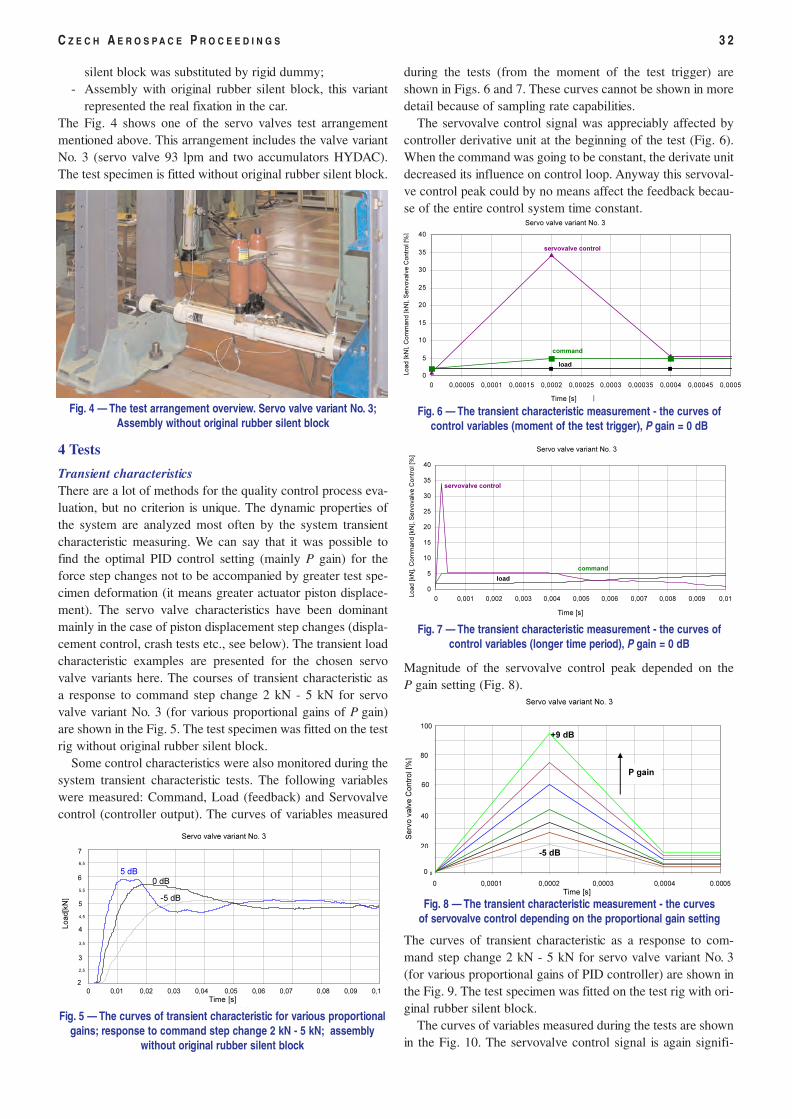
silent block was substituted by rigid dummy;- Assembly with original rubber silent block, this variant
represented the real fixation in the car.The Fig. 4 shows one of the servo valves test arrangementmentioned above. This arrangement includes the valve variantNo. 3 (servo valve 93 lpm and two accumulators HYDAC).The test specimen is fitted without original rubber silent block.
Fig. 4 — The test arrangement overview. Servo valve variant No. 3;Assembly without original rubber silent block
4 Tests
Transient characteristicsThere are a lot of methods for the quality control process eva-luation, but no criterion is unique. The dynamic properties ofthe system are analyzed most often by the system transientcharacteristic measuring. We can say that it was possible tofind the optimal PID control setting (mainly P gain) for theforce step changes not to be accompanied by greater test spe-cimen deformation (it means greater actuator piston displace-ment). The servo valve characteristics have been dominantmainly in the case of piston displacement step changes (displa-cement control, crash tests etc., see below). The transient loadcharacteristic examples are presented for the chosen servovalve variants here. The courses of transient characteristic asa response to command step change 2 kN - 5 kN for servovalve variant No. 3 (for various proportional gains of P gain)are shown in the Fig. 5. The test specimen was fitted on the testrig without original rubber silent block.
Some control characteristics were also monitored during thesystem transient characteristic tests. The following variableswere measured: Command, Load (feedback) and Servovalvecontrol (controller output). The curves of variables measured
during the tests (from the moment of the test trigger) areshown in Figs. 6 and 7. These curves cannot be shown in moredetail because of sampling rate capabilities.
The servovalve control signal was appreciably affected bycontroller derivative unit at the beginning of the test (Fig. 6).When the command was going to be constant, the derivate unitdecreased its influence on control loop. Anyway this servoval-ve control peak could by no means affect the feedback becau-se of the entire control system time constant.
Magnitude of the servovalve control peak depended on theP gain setting (Fig. 8).
The curves of transient characteristic as a response to com-mand step change 2 kN - 5 kN for servo valve variant No. 3(for various proportional gains of PID controller) are shown inthe Fig. 9. The test specimen was fitted on the test rig with ori-ginal rubber silent block.
The curves of variables measured during the tests are shownin the Fig. 10. The servovalve control signal is again signifi-
C Z E C H A E R O S P A C E P R O C E E D I N G S 3 2
skok 2-5kN
2
2,5
3
3,5
4
4,5
5
5,5
6
6,5
7
0 0,01 0,02 0,03 0,04 0,05 0,06 0,07 0,08 0,09 0,1
èas [s]
síla
[kN
]
Servo valve variant No. 3
Time [s]
L
oad[k
N]
5 dB 0 dB
-5 dB
0 0,01 0,02 0,03 0,04 0,05 0,06 0,07 0,08 0,09 0,1 Time [s]
7
6
5
4
3
2
Fig. 5 — The curves of transient characteristic for various proportionalgains; response to command step change 2 kN - 5 kN; assembly
without original rubber silent block
Serv o 93lpm , skok 2-5kN
POROVNÁNÍ PRÙBÌHU SERVOVENTILU PRO RÙZNÁ ZESÍLENÍ
0
10
20
30
40
50
60
70
80
90
100
0 0,00005 0,0001 0,00015 0,0002 0,00025 0,0003 0,00035 0,0004 0,00045 0,0005
èas [s]
síla
[kN
]
-5 dB
+9 dB
P gain
Servo valve variant No. 3
Time [s]
S
erv
o v
alv
e C
ontr
ol [
%]
0 0,0001 0,0002 0,0003 0,0004 0.0005 Time [s]
100
80
60
40
20
0
Serv
o v
alv
e C
ontr
ol [
%]
Fig. 8 — The transient characteristic measurement - the curves of servovalve control depending on the proportional gain setting
0
5
10
15
20
25
30
35
40
0 0,00005 0,0001 0,00015 0,0002 0,00025 0,0003 0,00035 0,0004 0,00045 0,0005
tim e [s ]
co
mm
an
d,
loa
d,
se
rvo
va
lve
servovalve control
Servo valve variant No. 3
Time [s] Load [
kN], C
om
mand [kN
], S
erv
ova
lve C
ontr
ol [
%]
command
load
Fig. 6 — The transient characteristic measurement - the curves ofcontrol variables (moment of the test trigger), P gain = 0 dB
Serv o 93lpm, mìøení snímaných v elièin, P=0dB
0
5
10
15
20
25
30
35
40
0 0,001 0,002 0,003 0,004 0,005 0,006 0,007 0,008 0,009 0,01
tim e [s]
com
man
d, l
oad
, ser
vova
lve
Load [
kN], C
om
mand [kN
], S
erv
ova
lve C
ontr
ol [
%]
servovalve control
command
load
Time [s]
Servo valve variant No. 3
Fig. 7 — The transient characteristic measurement - the curves ofcontrol variables (longer time period), P gain = 0 dB
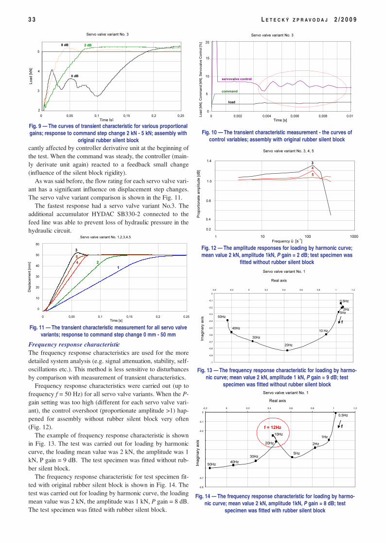
cantly affected by controller derivative unit at the beginning ofthe test. When the command was steady, the controller (main-ly derivate unit again) reacted to a feedback small change(influence of the silent block rigidity).
As was said before, the flow rating for each servo valve vari-ant has a significant influence on displacement step changes.The servo valve variant comparison is shown in the Fig. 11.
The fastest response had a servo valve variant No.3. Theadditional accumulator HYDAC SB330-2 connected to thefeed line was able to prevent loss of hydraulic pressure in thehydraulic circuit.
Frequency response characteristicThe frequency response characteristics are used for the moredetailed system analysis (e.g. signal attenuation, stability, self-oscillations etc.). This method is less sensitive to disturbancesby comparison with measurement of transient characteristics.
Frequency response characteristics were carried out (up tofrequency f = 50 Hz) for all servo valve variants. When the P-gain setting was too high (different for each servo valve vari-ant), the control overshoot (proportionate amplitude >1) hap-pened for assembly without rubber silent block very often(Fig. 12).
The example of frequency response characteristic is shownin Fig. 13. The test was carried out for loading by harmoniccurve, the loading mean value was 2 kN, the amplitude was 1kN, P gain = 9 dB. The test specimen was fitted without rub-ber silent block.
The frequency response characteristic for test specimen fit-ted with original rubber silent block is shown in Fig. 14. Thetest was carried out for loading by harmonic curve, the loadingmean value was 2 kN, the amplitude was 1 kN, P gain = 8 dB.The test specimen was fitted with rubber silent block.
3 3 L E T E C K Ý Z P R A V O D A J 2 / 2 0 0 9
0
10
20
30
40
50
60
0 0,05 0,1 0,15 0,2 0,25
t [s]
dis
pla
cem
ent
[mm
]
Servo valve variant No. 1,2,3,4,5
Time [s]
Dis
pla
cem
ent
[mm
]
1 2
3
5
4
60
50
40
30
20
10
0
D
isp
lace
me
nt
[mm
]
0 0,05 0,1 0,15 0,2 0.25 Time [s]
Fig. 11 — The transient characteristic measurement for all servo valve variants; response to command step change 0 mm - 50 mm
POROVNÁNÍ ZESÍLENÍ - DO PØÍSPÌVKU
2
2,5
3
3,5
4
4,5
5
5,5
0 0,05 0,1 0,15 0,2 0,25
èas [s]
síla
[kN
]
5
4
3
2
0 dB
Time [s]
Load [kN
] Servo valve variant No. 3
2 dB 8 dB
0 0,05 0,1 0,15 0,2 0,25 Time [s]
2
Fig. 9 — The curves of transient characteristic for various proportionalgains; response to command step change 2 kN - 5 kN; assembly with
original rubber silent block
Prùbìh mìøených v elièin,
0
5
10
15
20
0 0,001 0,002 0,003 0,004 0,005 0,006 0,007 0,008 0,009 0,01
èas [s]
síla
[kN
]
Servo valve variant No. 3
Time [s]
servovalve control
command
load
Load [
kN], C
om
mand [kN
], S
erv
ova
lve C
ontr
ol [
%]
0 0,002 0,004 0,006 0,008 0.01 Time [s]
20
15
10
5
0
Load [
kN], C
om
mand [kN
], S
erv
ova
lve C
ontr
ol [
%]
Fig. 10 — The transient characteristic measurement - the curves ofcontrol variables; assembly with original rubber silent block
P=2dB
0
0,2
0,4
0,6
0,8
1
1,2
1,4
1 10 100 1000
f [Hz]
delta
A [-
]
Servo valve variant No. 3, 4, 5
Frequency ù [s-1]
P
roport
ionate
am
plit
ude [dB
]
3 4
5
1 10 100 1000 Frequency ù [s-1]
1.4
1.0
0.8
0.4
0.2
P
roport
ionate
am
plit
ude [dB
]
Fig. 12 — The amplitude responses for loading by harmonic curve;mean value 2 kN, amplitude 1kN, P gain = 2 dB; test specimen was
fitted without rubber silent block
1 Hz
Serv o383lpm, P=9dB
-1
-0,9
-0,8
-0,7
-0,6
-0,5
-0,4
-0,3
-0,2
-0,1
0
-0,4 -0,2 0 0,2 0,4 0,6 0,8 1 1,2
Re
Im
Servo valve variant No. 1
Imagin
ary
axi
s
Real axis
f
0,5Hz
2Hz
5Hz
10 Hz
20Hz
30Hz
40Hz
50Hz
Fig. 13 — The frequency response characteristic for loading by harmo-nic curve; mean value 2 kN, amplitude 1 kN, P gain = 9 dB; test
specimen was fitted without rubber silent block
silentblok, Serv o 38lpm, P=8dB, do èlánku
-0,8
-0,7
-0,6
-0,5
-0,4
-0,3
-0,2
-0,1
0
-0,2 0 0,2 0,4 0,6 0,8 1 1,2
Re
Servo valve variant No. 1
Im
ag
ina
ry a
xis
Real axis
f = 12Hz
f
50Hz 40Hz
30Hz
20Hz
10Hz
5Hz
2Hz
1Hz
0,5Hz
Fig. 14 — The frequency response characteristic for loading by harmo-nic curve; mean value 2 kN, amplitude 1kN, P gain = 8 dB; test
specimen was fitted with rubber silent block
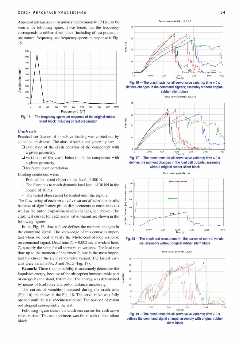
Apparent attenuation at frequency approximately 12 Hz can beseen in the following figure. It was found, that this frequencycorresponds to rubber silent block (including of test preparati-on) natural frequency, see frequency spectrum response in Fig.15.
Crash testsPractical verification of impulsive loading was carried out byso-called crash tests. The aims of such a test generally are:
❑ evaluation of the crash behavior of the component witha given geometry,
❑ validation of the crash behavior of the component witha given geometry,
❑ test/simulation correlation
Loading conditions were:- Preload the tested object on the level of 500 N.- The force has to reach dynamic load level of 30 kN in the
course of 10 ms.- The tested object must be loaded until the rupture.
The flow rating of each servo valve variant affected the resultsbecause of significance piston displacements at crash tests (aswell as the piston displacement step changes, see above). Thecrash test curves for each servo valve variant are shown in thefollowing figures.
In the Fig. 16, time = 0 sec defines the moment changes inthe command signal. The knowledge of this course is impor-tant when we need to verify the whole control loop responseon command signal. Dead time Td = 0,002 sec is evident here.Td is nearly the same for all servo valve variants. The load ricetime up to the moment of specimen failure is the most impor-tant for chosen the right servo valve variant. The fastest vari-ants were variants No. 3 and No. 5 (Fig. 17).
Remark: There is no possibility to accurately determine theimpulsive energy, because of the absorption immeasurable partof energy by the stand, fixture etc. The energy was determinedby means of load force and piston distance measuring.
The curves of variables measured during the crash tests(Fig. 16) are shown in the Fig. 18. The servo valve was fullyopened until the test specimen rupture. The position of pistonrod stopped subsequently the test.
Following figure shows the crash test curves for each servovalve variant. The test specimen was fitted with rubber silentblock.
C Z E C H A E R O S P A C E P R O C E E D I N G S 3 4
0
100
200
300
400
500
600
700
800
900
0 100 200 300 400 500 600 700 800 900 1000
omega[….
a [m
/s^
2]
Frequency ù [s-1]
A
cce
lera
tion [m
/s2]
Fig. 15 — The frequency spectrum response of the original rubbersilent block including of test preparation
Srov nání hydromotoru PG63 pro rùzné v arianty zapoj ení
CRASH SMIG X+
start od zmìny command signalu
0
5
10
15
20
25
30
35
40
0 0,005 0,01 0,015 0,02 0,025 0,03
èas [s]
síl
a [k
N]
Time [s]
Load [kN
]
Servo valve variant No. 1,2,3,4,5
1 2
4 3 5
0 0,005 0,01 0,015 0,02 0.025 0,03 Time [s]
40
30
20
10
0
L
oad
[kN
]
Td
Fig. 16 — The crash tests for all servo valve variants; time = 0 sdefines changes in the command signals; assembly without original
rubber silent blockSrov nání hydromotoru PG63 pro rùzné v arianty zapojení
CRASH SMIG X+
start od zmìny síly
0
5
10
15
20
25
30
35
40
0 0,005 0,01 0,015 0,02 0,025 0,03
èas [s]
síla
[kN
]Load [k
N]
Servo valve variant No. 1,2,3,4,5
1 2 4 3
5
Time [s]
0 0,005 0,01 0,015 0,02 0.025 0,03 Time [s]
40
30
20
10
0
Load [kN
]
Fig. 17 — The crash tests for all servo valve variants; time = 0 sdefines the moment changes in the load cell outputs; assembly
without original rubber silent block
crash X +, serv o38+63lpm - prùbìh mìøených v elièin
0
20
40
60
80
100
0 0,005 0,01 0,015 0,02 0,025 0,03
èas [s]
[kN
, %, m
m]
servovalve control
Servo valve variant N o. 4
Time [s]
Load [kN
], C
om
mand
[kN
], S
erv
ova
lve c
ontr
ol [
%]
command
load
0 0,0 05 0,01 0,015 0,02 0,025 0,03 Time [s]
100
80
60
40
20
0 Load [kN
], C
om
mand
[kN
], S
erv
ova
lve c
ontr
ol
Fig. 18 — The crash test measurement - the curves of control variab-les; assembly without original rubber silent block
Srovnání hydromotoru PG63 pro rùzné varianty zapojeníCRASH SMIG X+
0
5
10
15
20
25
30
35
0 0,005 0,01 0,015 0,02 0,025 0,03 0,035 0,04 0,045 0,05
èas [s]
síla
[kN
]
Time [s]
Servo valve variant No. 2,3,4,5
2 4 3
5
0 0,01 0,02 0,03 0,04 0,05 Time [s]
35
30
20
25
15
10
5
0
L
oad
[kN
]
Fig. 19 — The crash tests for all servo valve variants; time = 0 sdefines the command signal change; assembly with original rubber
silent block
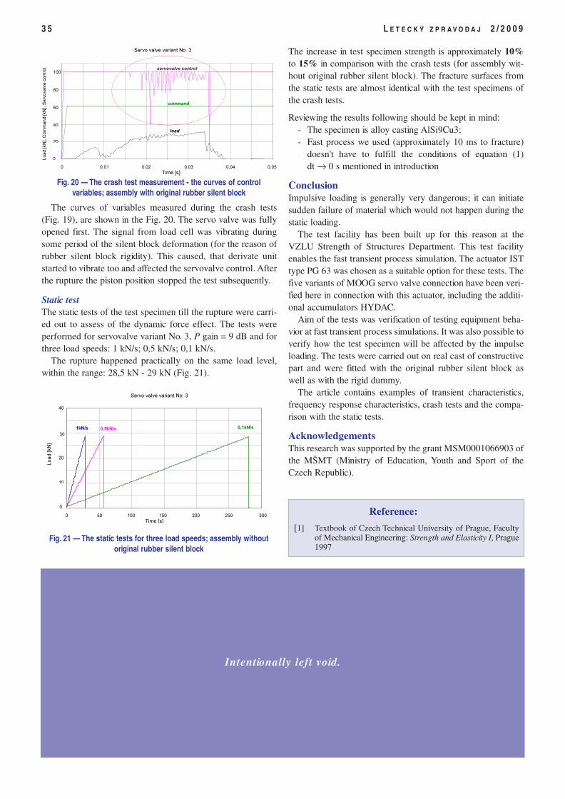
The curves of variables measured during the crash tests(Fig. 19), are shown in the Fig. 20. The servo valve was fullyopened first. The signal from load cell was vibrating duringsome period of the silent block deformation (for the reason ofrubber silent block rigidity). This caused, that derivate unitstarted to vibrate too and affected the servovalve control. Afterthe rupture the piston position stopped the test subsequently.
Static testThe static tests of the test specimen till the rupture were carri-ed out to assess of the dynamic force effect. The tests wereperformed for servovalve variant No. 3, P gain = 9 dB and forthree load speeds: 1 kN/s; 0,5 kN/s; 0,1 kN/s.
The rupture happened practically on the same load level,within the range: 28,5 kN - 29 kN (Fig. 21).
The increase in test specimen strength is approximately 10%to 15% in comparison with the crash tests (for assembly wit-hout original rubber silent block). The fracture surfaces fromthe static tests are almost identical with the test specimens ofthe crash tests.
Reviewing the results following should be kept in mind:- The specimen is alloy casting AlSi9Cu3;- Fast process we used (approximately 10 ms to fracture)
doesn't have to fulfill the conditions of equation (1)dt → 0 s mentioned in introduction
ConclusionImpulsive loading is generally very dangerous; it can initiatesudden failure of material which would not happen during thestatic loading.
The test facility has been built up for this reason at theVZLU Strength of Structures Department. This test facilityenables the fast transient process simulation. The actuator ISTtype PG 63 was chosen as a suitable option for these tests. Thefive variants of MOOG servo valve connection have been veri-fied here in connection with this actuator, including the additi-onal accumulators HYDAC.
Aim of the tests was verification of testing equipment beha-vior at fast transient process simulations. It was also possible toverify how the test specimen will be affected by the impulseloading. The tests were carried out on real cast of constructivepart and were fitted with the original rubber silent block aswell as with the rigid dummy.
The article contains examples of transient characteristics,frequency response characteristics, crash tests and the compa-rison with the static tests.
AcknowledgementsThis research was supported by the grant MSM0001066903 ofthe MŠMT (Ministry of Education, Youth and Sport of theCzech Republic).
3 5 L E T E C K Ý Z P R A V O D A J 2 / 2 0 0 9
Reference:
[1] Textbook of Czech Technical University of Prague, Facultyof Mechanical Engineering: Strength and Elasticity I, Prague1997
CRASH SMIG X+ SILENTBLOK, servo93lpm
0
20
40
60
80
100
0 0,005 0,01 0,015 0,02 0,025 0,03 0,035 0,04 0,045 0,05
èas [s]
síla
[kN
]
servovalve control
Servo valve variant No. 3
Time [s]
command
load
0 0,01 0,02 0,03 0,04 0,05 Time [s]
100
80
60
40
20
0Load [
kN], C
om
mand [kN
], S
erv
ova
lve c
ontr
ol
Fig. 20 — The crash test measurement - the curves of controlvariables; assembly with original rubber silent block
statika - v arianta 3
0
5
10
15
20
25
30
35
40
0 50 100 150 200 250 300
èas [s]
síla
[kN
]
Time [s]
Load [kN
]
Servo valve variant No. 3
1kN/s 0,5kN/s 0,1kN/s
0 50 100 150 200 250 300 Time [s]
L
oad
[kN
]
40
30
20
10
0
Fig. 21 — The static tests for three load speeds; assembly withoutoriginal rubber silent block
Intentionally left void.
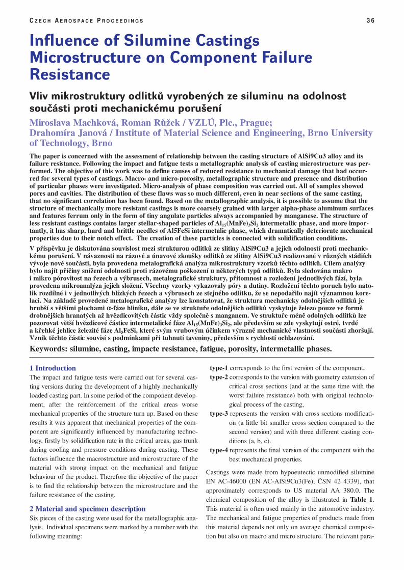
1 IntroductionThe impact and fatigue tests were carried out for several cas-ting versions during the development of a highly mechanicallyloaded casting part. In some period of the component develop-ment, after the reinforcement of the critical areas worsemechanical properties of the structure turn up. Based on theseresults it was apparent that mechanical properties of the com-ponent are significantly influenced by manufacturing techno-logy, firstly by solidification rate in the critical areas, gas trunkduring cooling and pressure conditions during casting. Thesefactors influence the macrostructure and microstructure of thematerial with strong impact on the mechanical and fatiguebehaviour of the product. Therefore the objective of the paperis to find the relationship between the microstructure and thefailure resistance of the casting.
2 Material and specimen descriptionSix pieces of the casting were used for the metallographic ana-lysis. Individual specimens were marked by a number with thefollowing meaning:
type-1 corresponds to the first version of the component,type-2 corresponds to the version with geometry extension of
critical cross sections (and at the same time with theworst failure resistance) both with original technolo-gical process of the casting,
type-3 represents the version with cross sections modificati-on (a little bit smaller cross section compared to thesecond version) and with three different casting con-ditions (a, b, c).
type-4 represents the final version of the component with thebest mechanical properties.
Castings were made from hypoeutectic unmodified silumineEN AC-46000 (EN AC-AlSi9Cu3(Fe), ČSN 42 4339), thatapproximately corresponds to US material AA 380.0. Thechemical composition of the alloy is illustrated in Table 1.This material is often used mainly in the automotive industry.The mechanical and fatigue properties of products made fromthis material depends not only on average chemical composi-tion but also on macro and micro structure. The relevant para-
C Z E C H A E R O S P A C E P R O C E E D I N G S 3 6
Influence of Silumine CastingsMicrostructure on Component FailureResistanceVliv mikrostruktury odlitků vyrobených ze siluminu na odolnostsoučásti proti mechanickému porušeníMiroslava Machková, Roman Růžek / VZLÚ, Plc., Prague;Drahomíra Janová / Institute of Material Science and Engineering, Brno Universityof Technology, BrnoThe paper is concerned with the assessment of relationship between the casting structure of AlSi9Cu3 alloy and itsfailure resistance. Following the impact and fatigue tests a metallographic analysis of casting microstructure was per-formed. The objective of this work was to define causes of reduced resistance to mechanical damage that had occur-red for several types of castings. Macro- and micro-porosity, metallographic structure and presence and distributionof particular phases were investigated. Micro-analysis of phase composition was carried out. All of samples showedpores and cavities. The distribution of these flaws was so much different, even in near sections of the same casting,that no significant correlation has been found. Based on the metallographic analysis, it is possible to assume that thestructure of mechanically more resistant castings is more coarsely grained with larger alpha-phase aluminum surfacesand features ferrum only in the form of tiny angulate particles always accompanied by manganese. The structure ofless resistant castings contains larger stellar-shaped particles of Al15(MnFe)3Si2 intermetallic phase, and more impor-tantly, it has sharp, hard and brittle needles of Al5FeSi intermetalic phase, which dramatically deteriorate mechanicalproperties due to their notch effect. The creation of these particles is connected with solidification conditions.
V příspěvku je diskutována souvislost mezi strukturou odlitků ze slitiny AlSi9Cu3 a jejich odolností proti mechanic-kému porušení. V návaznosti na rázové a únavové zkoušky odlitků ze slitiny AlSi9Cu3 realizované v různých stádiíchvývoje nové součásti, byla provedena metalografická analýza mikrostruktury vzorků těchto odlitků. Cílem analýzybylo najít příčiny snížení odolnosti proti rázovému poškození u některých typů odlitků. Byla sledována makroi mikro pórovitost na řezech a výbrusech, metalografické struktury, přítomnost a rozložení jednotlivých fází, bylaprovedena mikroanalýza jejich složení. Všechny vzorky vykazovaly póry a dutiny. Rozložení těchto poruch bylo nato-lik rozdílné i v jednotlivých blízkých řezech a výbrusech ze stejného odlitku, že se nepodařilo najít významnou kore-laci. Na základě provedené metalografické analýzy lze konstatovat, že struktura mechanicky odolnějších odlitků jehrubší s většími plochami αα-fáze hliníku, dále se ve struktuře odolnějších odlitků vyskytuje železo pouze ve formědrobnějších hranatých až hvězdicovitých částic vždy společně s manganem. Ve struktuře méně odolných odlitků lzepozorovat větší hvězdicové částice intermetalické fáze Al15(MnFe)3Si2, ale především se zde vyskytují ostré, tvrdéa křehké jehlice železité fáze Al5FeSi, které svým vrubovým účinkem výrazně mechanické vlastnosti součásti zhoršují.Vznik těchto částic souvisí s podmínkami při tuhnutí taveniny, především s rychlostí ochlazování.
Keywords: silumine, casting, impacte resistance, fatigue, porosity, intermetallic phases.
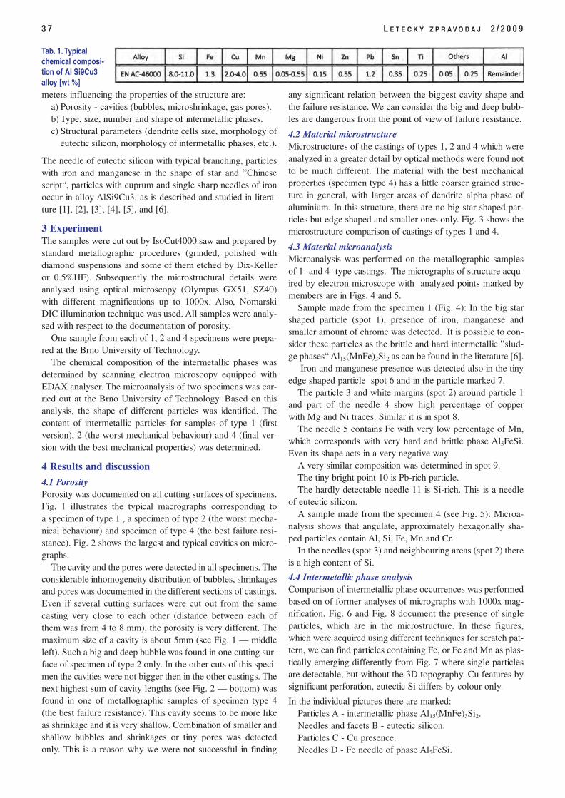
meters influencing the properties of the structure are:a) Porosity - cavities (bubbles, microshrinkage, gas pores). b) Type, size, number and shape of intermetallic phases. c) Structural parameters (dendrite cells size, morphology of
eutectic silicon, morphology of intermetallic phases, etc.).
The needle of eutectic silicon with typical branching, particleswith iron and manganese in the shape of star and ”Chinesescript“, particles with cuprum and single sharp needles of ironoccur in alloy AlSi9Cu3, as is described and studied in litera-ture [1], [2], [3], [4], [5], and [6].
3 ExperimentThe samples were cut out by IsoCut4000 saw and prepared bystandard metallographic procedures (grinded, polished withdiamond suspensions and some of them etched by Dix-Kelleror 0.5%HF). Subsequently the microstructural details wereanalysed using optical microscopy (Olympus GX51, SZ40)with different magnifications up to 1000x. Also, NomarskiDIC illumination technique was used. All samples were analy-sed with respect to the documentation of porosity.
One sample from each of 1, 2 and 4 specimens were prepa-red at the Brno University of Technology.
The chemical composition of the intermetallic phases wasdetermined by scanning electron microscopy equipped withEDAX analyser. The microanalysis of two specimens was car-ried out at the Brno University of Technology. Based on thisanalysis, the shape of different particles was identified. Thecontent of intermetallic particles for samples of type 1 (firstversion), 2 (the worst mechanical behaviour) and 4 (final ver-sion with the best mechanical properties) was determined.
4 Results and discussion
4.1 PorosityPorosity was documented on all cutting surfaces of specimens.Fig. 1 illustrates the typical macrographs corresponding toa specimen of type 1 , a specimen of type 2 (the worst mecha-nical behaviour) and specimen of type 4 (the best failure resi-stance). Fig. 2 shows the largest and typical cavities on micro-graphs.
The cavity and the pores were detected in all specimens. Theconsiderable inhomogeneity distribution of bubbles, shrinkagesand pores was documented in the different sections of castings.Even if several cutting surfaces were cut out from the samecasting very close to each other (distance between each ofthem was from 4 to 8 mm), the porosity is very different. Themaximum size of a cavity is about 5mm (see Fig. 1 — middleleft). Such a big and deep bubble was found in one cutting sur-face of specimen of type 2 only. In the other cuts of this speci-men the cavities were not bigger then in the other castings. Thenext highest sum of cavity lengths (see Fig. 2 — bottom) wasfound in one of metallographic samples of specimen type 4(the best failure resistance). This cavity seems to be more likeas shrinkage and it is very shallow. Combination of smaller andshallow bubbles and shrinkages or tiny pores was detectedonly. This is a reason why we were not successful in finding
any significant relation between the biggest cavity shape andthe failure resistance. We can consider the big and deep bubb-les are dangerous from the point of view of failure resistance.
4.2 Material microstructureMicrostructures of the castings of types 1, 2 and 4 which wereanalyzed in a greater detail by optical methods were found notto be much different. The material with the best mechanicalproperties (specimen type 4) has a little coarser grained struc-ture in general, with larger areas of dendrite alpha phase ofaluminium. In this structure, there are no big star shaped par-ticles but edge shaped and smaller ones only. Fig. 3 shows themicrostructure comparison of castings of types 1 and 4.
4.3 Material microanalysisMicroanalysis was performed on the metallographic samplesof 1- and 4- type castings. The micrographs of structure acqu-ired by electron microscope with analyzed points marked bymembers are in Figs. 4 and 5.
Sample made from the specimen 1 (Fig. 4): In the big starshaped particle (spot 1), presence of iron, manganese andsmaller amount of chrome was detected. It is possible to con-sider these particles as the brittle and hard intermetallic ”slud-ge phases“ Al15(MnFe)3Si2 as can be found in the literature [6].
Iron and manganese presence was detected also in the tinyedge shaped particle spot 6 and in the particle marked 7.
The particle 3 and white margins (spot 2) around particle 1and part of the needle 4 show high percentage of copperwith Mg and Ni traces. Similar it is in spot 8.
The needle 5 contains Fe with very low percentage of Mn,which corresponds with very hard and brittle phase Al5FeSi.Even its shape acts in a very negative way.
A very similar composition was determined in spot 9.The tiny bright point 10 is Pb-rich particle.The hardly detectable needle 11 is Si-rich. This is a needle
of eutectic silicon. A sample made from the specimen 4 (see Fig. 5): Microa-
nalysis shows that angulate, approximately hexagonally sha-ped particles contain Al, Si, Fe, Mn and Cr.
In the needles (spot 3) and neighbouring areas (spot 2) thereis a high content of Si.
4.4 Intermetallic phase analysisComparison of intermetallic phase occurrences was performedbased on of former analyses of micrographs with 1000x mag-nification. Fig. 6 and Fig. 8 document the presence of singleparticles, which are in the microstructure. In these figures,which were acquired using different techniques for scratch pat-tern, we can find particles containing Fe, or Fe and Mn as plas-tically emerging differently from Fig. 7 where single particlesare detectable, but without the 3D topography. Cu features bysignificant perforation, eutectic Si differs by colour only.
In the individual pictures there are marked:Particles A - intermetallic phase Al15(MnFe)3Si2. Needles and facets B - eutectic silicon.Particles C - Cu presence. Needles D - Fe needle of phase Al5FeSi.
3 7 L E T E C K Ý Z P R A V O D A J 2 / 2 0 0 9
Tab. 1. Typicalchemical composi-tion of Al Si9Cu3alloy [wt %]
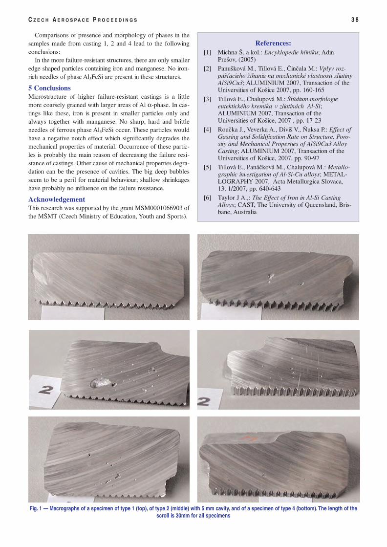
Comparisons of presence and morphology of phases in thesamples made from casting 1, 2 and 4 lead to the followingconclusions:
In the more failure-resistant structures, there are only smalleredge shaped particles containing iron and manganese. No iron-rich needles of phase Al5FeSi are present in these structures.
5 ConclusionsMicrostructure of higher failure-resistant castings is a littlemore coarsely grained with larger areas of Al α-phase. In cas-tings like these, iron is present in smaller particles only andalways together with manganese. No sharp, hard and brittleneedles of ferrous phase Al5FeSi occur. These particles wouldhave a negative notch effect which significantly degrades themechanical properties of material. Occurrence of these partic-les is probably the main reason of decreasing the failure resi-stance of castings. Other cause of mechanical properties degra-dation can be the presence of cavities. The big deep bubblesseem to be a peril for material behaviour; shallow shrinkageshave probably no influence on the failure resistance.
AcknowledgementThis research was supported by the grant MSM0001066903 ofthe MŠMT (Czech Ministry of Education, Youth and Sports).
C Z E C H A E R O S P A C E P R O C E E D I N G S 3 8
References:[1] Michna Š. a kol.: Encyklopedie hliníku; Adin
Prešov, (2005)[2] Panušková M., Tillová E., Činčala M.: Vplyv roz-
púšťacieho žíhania na mechanické vlastnosti zliatinyAlSi9Cu3; ALUMINIUM 2007, Transaction of theUniversities of Košice 2007, pp. 160-165
[3] Tillová E., Chalupová M.: Štúdium morfologieeutektického kremíka, v zliatinách Al-Si;ALUMINIUM 2007, Transaction of theUniversities of Košice, 2007 , pp. 17-23
[4] Roučka J., Veverka A., Diviš V., Ňuksa P.: Effect ofGassing and Solidification Rate on Structure, Poro-sity and Mechanical Properties of AlSi9Cu3 AlloyCasting; ALUMINIUM 2007, Transaction of theUniversities of Košice, 2007, pp. 90-97
[5] Tillová E., Panáčková M., Chalupová M.: Metallo-graphic investigation of Al-Si-Cu alloys; METAL-LOGRAPHY 2007, Acta Metallurgica Slovaca,13, 1/2007, pp. 640-643
[6] Taylor J A.,: The Effect of Iron in Al-Si CastingAlloys; CAST, The University of Queensland, Bris-bane, Australia
Fig. 1 — Macrographs of a specimen of type 1 (top), of type 2 (middle) with 5 mm cavity, and of a specimen of type 4 (bottom). The length of thescroll is 30mm for all specimens
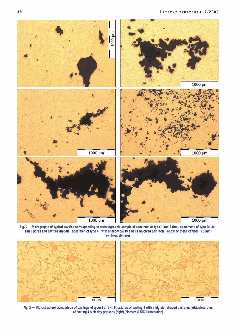
3 9 L E T E C K Ý Z P R A V O D A J 2 / 2 0 0 9
Fig. 2 — Micrographs of typical cavities corresponding to metallographic sample of specimen of type 1 and 2 (top), specimens of type 3c, 3a -small pores and cavities (middle), specimen of type 4 - with shallow cavity and its revolved part (total length of these cavities is 5 mm)
(without etching)
Fig. 3 — Microstructure comparison of castings of types1 and 4. Structures of casting 1 with a big star shaped particles (left), structuresof casting 4 with tiny particles (right).(Nomarski DIC illumination)
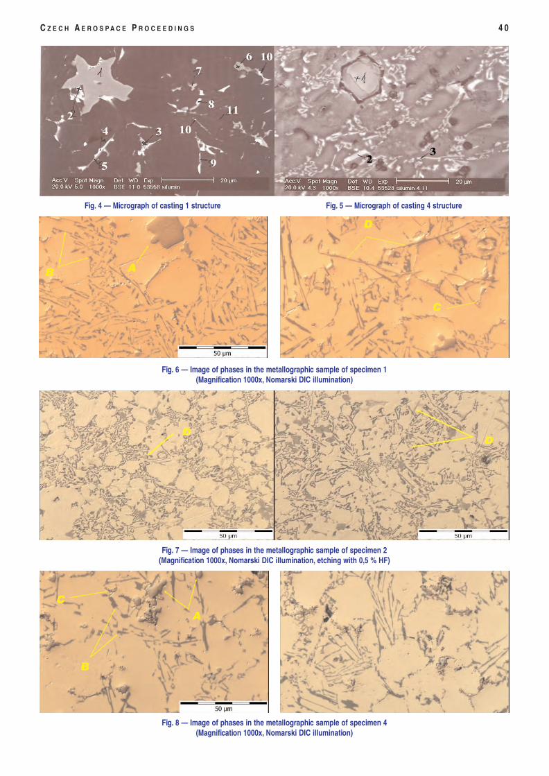
C Z E C H A E R O S P A C E P R O C E E D I N G S 4 0
7
6
4
2
8 11
9
3 10
10
5 2
3
Fig. 4 — Micrograph of casting 1 structure Fig. 5 — Micrograph of casting 4 structure
Fig. 6 — Image of phases in the metallographic sample of specimen 1(Magnification 1000x, Nomarski DIC illumination)
Fig. 7 — Image of phases in the metallographic sample of specimen 2(Magnification 1000x, Nomarski DIC illumination, etching with 0,5 % HF)
Fig. 8 — Image of phases in the metallographic sample of specimen 4(Magnification 1000x, Nomarski DIC illumination)
1 Introduction1.1 Preliminary SizingIn literature and in practice, aircraft development has beenrepeatedly broken down into different phases. Various approa-ches have been followed. Figure 1 shows one approach ofdividing aircraft development into phases and shows keymilestones. The development of large civil aircraft has inspiredthis example. Typical aircraft design activities take part prima-rily in the feasibility, concept and definition phase. Prelimina-ry sizing is the first step in aircraft design and as such part ofthe feasibility phase, which is followed by conceptual designin the concept phase.
Preliminary sizing of an aircraft is possible without knowledgeof the aircraft's geometry. In preliminary sizing the aircraft ismore or less reduced to a point mass. However concrete ideasabout the aircraft need to exist:
� What type of configuration will be selected?� What aspect ratio can be expected?� What cruise Mach number and type of propulsion system
will be selected?
With these first considerations, realistic requirements can beformulated. These requirements (some of them depending onthe certification rules — see below) will enter the preliminarysizing phase:
� Payload mPL ,� Range R,� Mach number in cruise MCR or speed VCR ,� Take-off field length sTOFL ,� Landing field length sLFL , approach speed VAPP or stall
speed VS ,� Climb gradient γ during second segment,� Climb gradient γ during missed approach.
Preliminary sizing yields basic aircraft parameters like� Take-off mass mMTO ,� Fuel mass mF ,� Operating empty mass mOE ,� Wing area SW ,� Take-off thrust TTO or take-off power PTO .
1.2 Aeroplane Categories, Propulsion Systemand Certification RulesWhen attempting to do the preliminary sizing of a passengeraircraft, it has to be differentiated
a) the type of propulsion system (propeller or jet),b) the certification rules for the aircraft.
The certification rules depend as much on the category andsize of the aircraft as on the propulsion system. Let's differen-tiate these categories of aeroplanes:
1 Large jet aeroplanes are certified to CS-25 [CS-25] res-pectively FAR Part 25 [FAR Part 25],
2 Very light jets are certified to CS-23 [CS-23] respective-ly FAR Part 23 [FAR Part 23],
3 Large propeller driven aeroplanes are also certified toCS-25 respectively FAR Part 25
4 Smaller propeller driven aeroplanes (normal, utility, aero-batic and commuter aeroplanes) are certified to CS-23respectively FAR Part 23,
5 Very light propeller driven aeroplanes (up to a maximumtake-off mass of 750 kg) can be certified to CS-VLA[CS-VLA],
4 1 L E T E C K Ý Z P R A V O D A J 2 / 2 0 0 9
Preliminary Sizing of Large PropellerDriven AeroplanesPředběžný výpočet rozměrů velkého vrtulového letounuProf. Dieter Scholz, Mihaela Niţă / Hamburg University of Applied Sciences,Hamburg, GermanyDifferent types of aeroplanes (small / large, propeller / jet) require their own type of preliminary sizing method. Oneof theses methods differs only in a few but important aspects from the other. For the sake of efficient teaching of stu-dents and easy application in practice, the authors ask for the definition of a set of clearly defined step by step preli-minary sizing methods. Based on the rather well known sizing method for large jet aeroplanes, the paper derivesa preliminary sizing method for large propeller driven aeroplanes. In this way the paper tries to contribute to the defi-nition of the set of methods. The sizing methods are all based on a matching chart that helps to graphically solvea two-dimensional optimization problem. The matching chart draws the optimization variable thrust-to-weight ratio(for jets) respectively power to mass ratio (propeller driven planes) versus wing loading for all basic requirements,which the aeroplane has to fulfill. The sizing method for propeller driven large aeroplanes is explained in detail andapplied to a redesign study of the ATR 72. All equations are given in a form readily available for use. This requires insome cases the evaluation of proportionality factors based on aircraft statistics. Given are factors taking into accountstatistics for landing distance, take-off distance and maximum glide ratio for large propeller driven passenger aircraft.Furthermore, generic equations for the variation of power with altitude and speed of turboprop engines is given aswell as a chart to determine the propeller efficiency.
Keywords: aircraft, design, preliminary sizing, matching chart, propeller, ATR 72, redesign.
Fig. 1 — Phases of aircraft development
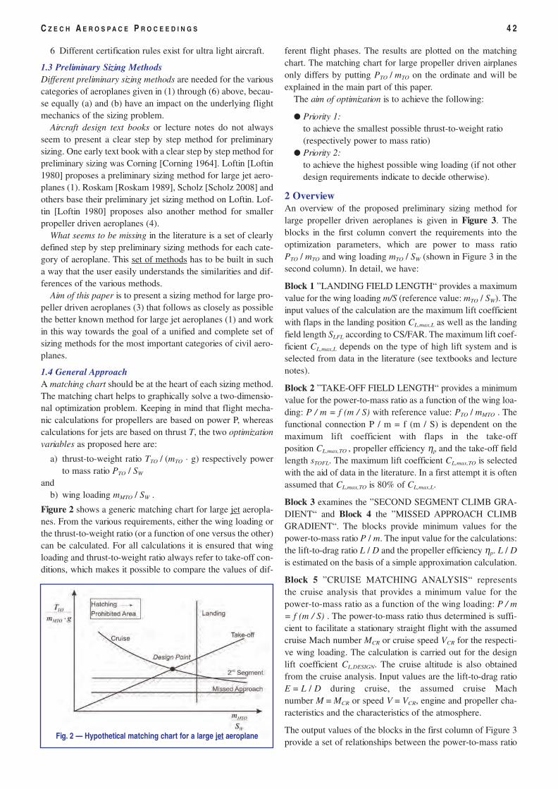
6 Different certification rules exist for ultra light aircraft.
1.3 Preliminary Sizing MethodsDifferent preliminary sizing methods are needed for the variouscategories of aeroplanes given in (1) through (6) above, becau-se equally (a) and (b) have an impact on the underlying flightmechanics of the sizing problem.
Aircraft design text books or lecture notes do not alwaysseem to present a clear step by step method for preliminarysizing. One early text book with a clear step by step method forpreliminary sizing was Corning [Corning 1964]. Loftin [Loftin1980] proposes a preliminary sizing method for large jet aero-planes (1). Roskam [Roskam 1989], Scholz [Scholz 2008] andothers base their preliminary jet sizing method on Loftin. Lof-tin [Loftin 1980] proposes also another method for smallerpropeller driven aeroplanes (4).
What seems to be missing in the literature is a set of clearlydefined step by step preliminary sizing methods for each cate-gory of aeroplane. This set of methods has to be built in sucha way that the user easily understands the similarities and dif-ferences of the various methods.
Aim of this paper is to present a sizing method for large pro-peller driven aeroplanes (3) that follows as closely as possiblethe better known method for large jet aeroplanes (1) and workin this way towards the goal of a unified and complete set ofsizing methods for the most important categories of civil aero-planes.
1.4 General ApproachA matching chart should be at the heart of each sizing method.The matching chart helps to graphically solve a two-dimensio-nal optimization problem. Keeping in mind that flight mecha-nic calculations for propellers are based on power P, whereascalculations for jets are based on thrust T, the two optimizationvariables as proposed here are:
a) thrust-to-weight ratio TTO / (mTO ⋅ g) respectively powerto mass ratio PTO / SW
andb) wing loading mMTO / SW .
Figure 2 shows a generic matching chart for large jet aeropla-nes. From the various requirements, either the wing loading orthe thrust-to-weight ratio (or a function of one versus the other)can be calculated. For all calculations it is ensured that wingloading and thrust-to-weight ratio always refer to take-off con-ditions, which makes it possible to compare the values of dif-
ferent flight phases. The results are plotted on the matchingchart. The matching chart for large propeller driven airplanesonly differs by putting PTO / mTO on the ordinate and will beexplained in the main part of this paper.
The aim of optimization is to achieve the following:
� Priority 1:to achieve the smallest possible thrust-to-weight ratio(respectively power to mass ratio)
� Priority 2:to achieve the highest possible wing loading (if not otherdesign requirements indicate to decide otherwise).
2 OverviewAn overview of the proposed preliminary sizing method forlarge propeller driven aeroplanes is given in Figure 3. Theblocks in the first column convert the requirements into theoptimization parameters, which are power to mass ratioPTO / mTO and wing loading mTO / SW (shown in Figure 3 in thesecond column). In detail, we have:
Block 1 ”LANDING FIELD LENGTH“ provides a maximumvalue for the wing loading m/S (reference value: mTO / SW). Theinput values of the calculation are the maximum lift coefficientwith flaps in the landing position CL,max,L as well as the landingfield length SLFL according to CS/FAR. The maximum lift coef-ficient CL,max,L depends on the type of high lift system and isselected from data in the literature (see textbooks and lecturenotes).
Block 2 ”TAKE-OFF FIELD LENGTH“ provides a minimumvalue for the power-to-mass ratio as a function of the wing loa-ding: P / m = f (m / S) with reference value: PTO / mMTO . Thefunctional connection P / m = f (m / S) is dependent on themaximum lift coefficient with flaps in the take-offposition CL,max,TO , propeller efficiency ηp and the take-off fieldlength sTOFL. The maximum lift coefficient CL,max,TO is selectedwith the aid of data in the literature. In a first attempt it is oftenassumed that CL,max,TO is 80% of CL,max,L.
Block 3 examines the ”SECOND SEGMENT CLIMB GRA-DIENT“ and Block 4 the ”MISSED APPROACH CLIMBGRADIENT“. The blocks provide minimum values for thepower-to-mass ratio P / m. The input value for the calculations:the lift-to-drag ratio L / D and the propeller efficiency ηp. L / Dis estimated on the basis of a simple approximation calculation.
Block 5 ”CRUISE MATCHING ANALYSIS“ representsthe cruise analysis that provides a minimum value for thepower-to-mass ratio as a function of the wing loading: P / m= f (m / S) . The power-to-mass ratio thus determined is suffi-cient to facilitate a stationary straight flight with the assumedcruise Mach number MCR or cruise speed VCR for the respecti-ve wing loading. The calculation is carried out for the designlift coefficient CL,DESIGN. The cruise altitude is also obtainedfrom the cruise analysis. Input values are the lift-to-drag ratioE = L / D during cruise, the assumed cruise Machnumber M = MCR or speed V = VCR, engine and propeller cha-racteristics and the characteristics of the atmosphere.
The output values of the blocks in the first column of Figure 3provide a set of relationships between the power-to-mass ratio
C Z E C H A E R O S P A C E P R O C E E D I N G S 4 2
Fig. 2 — Hypothetical matching chart for a large jet aeroplane
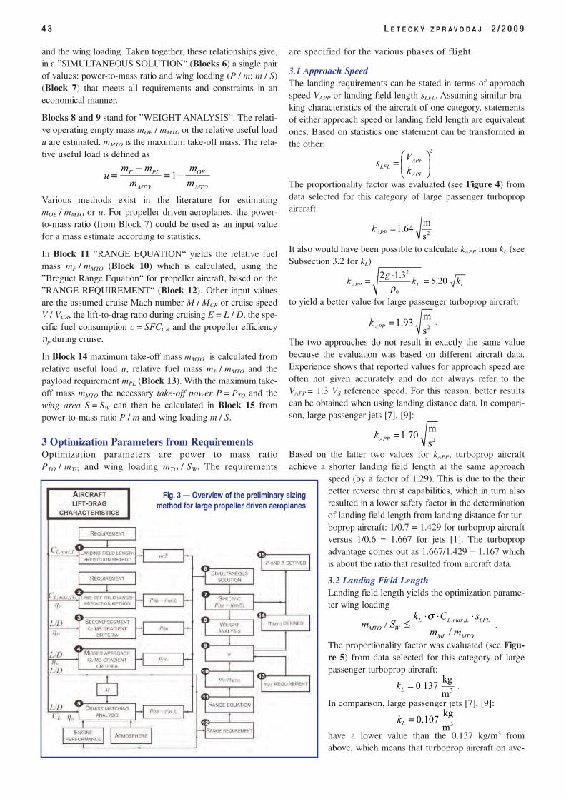
and the wing loading. Taken together, these relationships give,in a ”SIMULTANEOUS SOLUTION“ (Blocks 6) a single pairof values: power-to-mass ratio and wing loading (P / m; m / S)(Block 7) that meets all requirements and constraints in aneconomical manner.
Blocks 8 and 9 stand for ”WEIGHT ANALYSIS“. The relati-ve operating empty mass mOE / mMTO or the relative useful loadu are estimated. mMTO is the maximum take-off mass. The rela-tive useful load is defined as
Various methods exist in the literature for estimatingmOE / mMTO or u. For propeller driven aeroplanes, the power-to-mass ratio (from Block 7) could be used as an input valuefor a mass estimate according to statistics.
In Block 11 ”RANGE EQUATION“ yields the relative fuelmass mF / mMTO (Block 10) which is calculated, using the”Breguet Range Equation“ for propeller aircraft, based on the”RANGE REQUIREMENT“ (Block 12). Other input valuesare the assumed cruise Mach number M / MCR or cruise speedV / VCR, the lift-to-drag ratio during cruising E = L / D, the spe-cific fuel consumption c = SFCCR and the propeller efficiencyηp during cruise.
In Block 14 maximum take-off mass mMTO is calculated fromrelative useful load u, relative fuel mass mF / mMTO and thepayload requirement mPL (Block 13). With the maximum take-off mass mMTO the necessary take-off power P = PTO and thewing area S = SW can then be calculated in Block 15 frompower-to-mass ratio P / m and wing loading m / S.
3 Optimization Parameters from RequirementsOptimization parameters are power to mass ratioPTO / mTO and wing loading mTO / SW. The requirements
are specified for the various phases of flight.
3.1 Approach SpeedThe landing requirements can be stated in terms of approachspeed VAPP or landing field length sLFL. Assuming similar bra-king characteristics of the aircraft of one category, statementsof either approach speed or landing field length are equivalentones. Based on statistics one statement can be transformed inthe other:
The proportionality factor was evaluated (see Figure 4) fromdata selected for this category of large passenger turbopropaircraft:
It also would have been possible to calculate kAPP from kL (seeSubsection 3.2 for kL)
to yield a better value for large passenger turboprop aircraft:
.
The two approaches do not result in exactly the same valuebecause the evaluation was based on different aircraft data.Experience shows that reported values for approach speed areoften not given accurately and do not always refer to theVAPP = 1.3 VS reference speed. For this reason, better resultscan be obtained when using landing distance data. In compari-son, large passenger jets [7], [9]:
.
Based on the latter two values for kAPP, turboprop aircraftachieve a shorter landing field length at the same approach
speed (by a factor of 1.29). This is due to the theirbetter reverse thrust capabilities, which in turn alsoresulted in a lower safety factor in the determinationof landing field length from landing distance for tur-boprop aircraft: 1/0.7 = 1.429 for turboprop aircraftversus 1/0.6 = 1.667 for jets [1]. The turbopropadvantage comes out as 1.667/1.429 = 1.167 whichis about the ratio that resulted from aircraft data.
3.2 Landing Field LengthLanding field length yields the optimization parame-ter wing loading
.
The proportionality factor was evaluated (see Figu-re 5) from data selected for this category of largepassenger turboprop aircraft:
.
In comparison, large passenger jets [7], [9]:
have a lower value than the 0.137 kg/m3 fromabove, which means that turboprop aircraft on ave-
4 3 L E T E C K Ý Z P R A V O D A J 2 / 2 0 0 9
u
m m
m
m
m
F PL
MTO
OE
MTO
=+
= −1
Fig. 3 — Overview of the preliminary sizingmethod for large propeller driven aeroplanes
2
APPLFL
APP
Vs
k
=
2
m1.64
sAPPk =
2
0
2 1.35.20APP L L
gk k k
ρ⋅= =
2
m1.93
sAPPk =
2
m1.70
sAPPk =
, ,
//
L L max L LFL
MTO W
ML MTO
k C sm S
m m
σ⋅ ⋅ ⋅≤
3
kg0.137
mLk =
3
kg0.107
mLk =
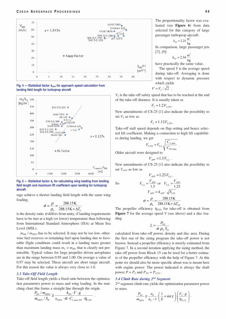
rage achieve a shorter landing field length with the same wingloading.
is the density ratio. σ differs from unity, if landing requirementshave to be met at a high (or lower) temperature than followingfrom International Standard Atmosphere (ISA) at Mean SeaLevel (MSL).
mML / mMTO has to be selected. It may not be too low, other-wise fuel reserves or remaining fuel upon landing due to favo-rable flight conditions could result in a landing mass greaterthan maximum landing mass mL > mML that is clearly not per-missible. Typical values for large propeller driven aeroplanesare in the range between 0.95 and 1.00. On average a value of0.97 may be selected. These aircraft are short range aircraft.For this reason the value is always very close to 1.0.
3.3 Take-Off Field LengthTake-off field length yields a fixed ratio between the optimiza-tion parameters power to mass and wing loading. In the mat-ching chart this forms a straight line through the origin.
.
The proportionality factor was eva-luated (see Figure 6) from dataselected for this category of largepassenger turboprop aircraft:
In comparison, large passenger jets[7], [9]:
have practically the same value.The speed V is the average speed
during take-off. Averaging is donewith respect to dynamic pressurewhich yields
.
V2 is the take-off safety speed that has to be reached at the endof the take-off distance. It is usually taken as
.
New amendments of CS-25 [1] also indicate the possibility toset V2 as low as
.
Take-off stall speed depends on flap setting and hence selec-ted lift coefficient. Making a connection to high lift capabiliti-es during landing, we get
.
Older aircraft were designed to
.
New amendments of CS-25 [1] also indicate the possibility toset VAPP as low as
.
So or
The propeller efficiency ηP,TO for take-off is obtained fromFigure 7 for the average speed V (see above) and a disc loa-ding
calculated from take-off power, density and disc area. Duringthe first run of the sizing program the take-off power is notknown. Instead a propeller efficiency is merely estimated fromFigure 7. In a second iteration applying the sizing method, thetake-off power from Block 15 can be used for a better estima-te of the propeller efficiency with the help of Figure 7. At thispoint we should also be more specific about was is meant herewith engine power: The power indicated is always the shaftpower P = PS and PTO = PS,TO .
3.4 Climb Rate during 2nd Segment2nd segment climb rate yields the optimization parameter powerto mass
.
C Z E C H A E R O S P A C E P R O C E E D I N G S 4 4
Fig. 4 — Statistical factor kAPP for approach speed calculation fromlanding field length for turboprop aircraft
Fig. 5 — Statistical factor kL for calculating wing loading from landingfield length and maximum lift coefficient upon landing for turbopropaircraft
0
288.15K
288.15K LT
ρσρ
= =+ ∆
, , ,
/
/
TO MTO TO
MTO W TOFL L max TO P TO
P m k V g
m S s Cσ η⋅ ⋅≥
⋅ ⋅ ⋅
2
,
1sin
1
TO E
MTO E P CL
P n V g
m n Eγ
η ⋅ ≥ ⋅ + ⋅ −
3m
2.25kg
TOk =
3m
2.34kg
TOk =
2 / 2V V=
2 ,1.2 S TOV V=
2 ,1.13 S TOV V=
,max
, ,
,max
L
S TO S L
TO
CV V
C=
,1.3APP S LV V=
,1.23APP S LV V=
,
1.3
APPS L
VV =
,
1.23
APPS L
VV =
APP APP LFLV k S= ⋅
0
288.15K
288.15K TOT
ρσρ
= =+ ∆
0
TO
D
PL
Sσ ρ=
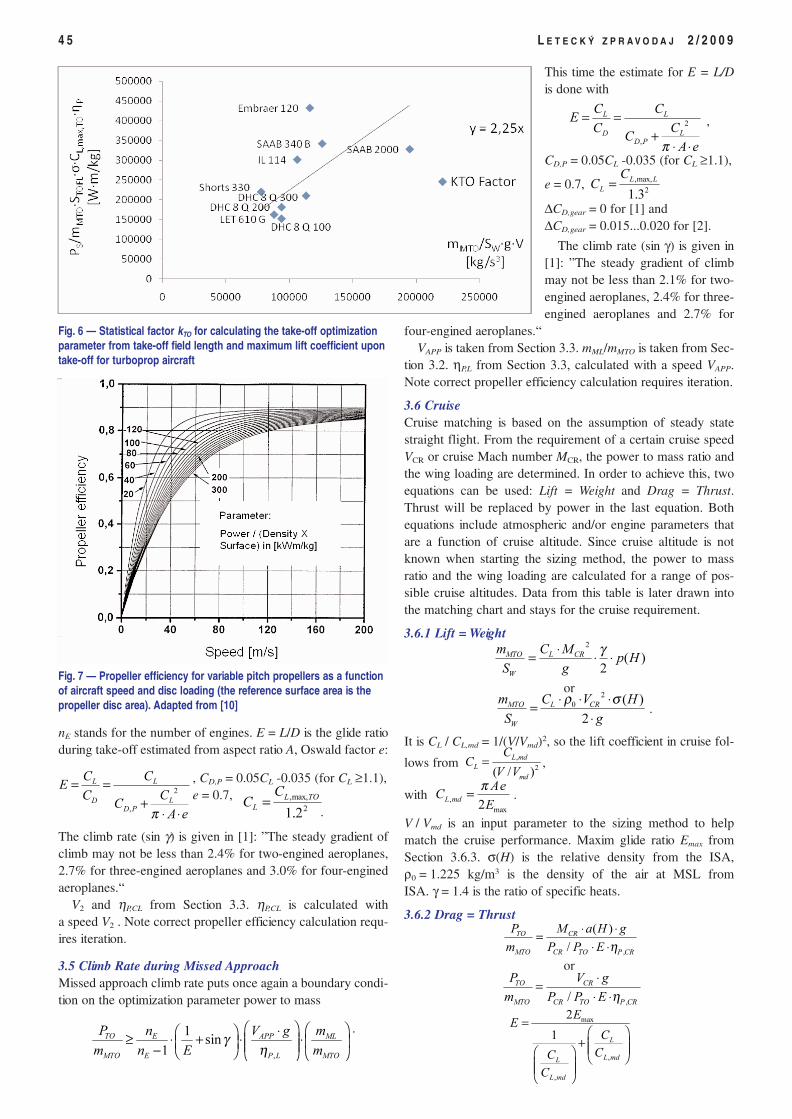
nE stands for the number of engines. E = L/D is the glide ratioduring take-off estimated from aspect ratio A, Oswald factor e:
, CD,P = 0.05CL -0.035 (for CL ≥1.1),e = 0.7,
.
The climb rate (sin γ) is given in [1]: ”The steady gradient ofclimb may not be less than 2.4% for two-engined aeroplanes,2.7% for three-engined aeroplanes and 3.0% for four-enginedaeroplanes.“
V2 and ηP,CL from Section 3.3. ηP,CL is calculated witha speed V2 . Note correct propeller efficiency calculation requ-ires iteration.
3.5 Climb Rate during Missed ApproachMissed approach climb rate puts once again a boundary condi-tion on the optimization parameter power to mass
.
This time the estimate for E = L/Dis done with
,
CD,P = 0.05CL -0.035 (for CL ≥1.1),
e = 0.7,
∆CD,gear = 0 for [1] and∆CD,gear = 0.015...0.020 for [2].
The climb rate (sin γ) is given in[1]: ”The steady gradient of climbmay not be less than 2.1% for two-engined aeroplanes, 2.4% for three-engined aeroplanes and 2.7% for
four-engined aeroplanes.“VAPP is taken from Section 3.3. mML/mMTO is taken from Sec-
tion 3.2. ηP,L from Section 3.3, calculated with a speed VAPP.Note correct propeller efficiency calculation requires iteration.
3.6 CruiseCruise matching is based on the assumption of steady statestraight flight. From the requirement of a certain cruise speedVCR or cruise Mach number MCR, the power to mass ratio andthe wing loading are determined. In order to achieve this, twoequations can be used: Lift = Weight and Drag = Thrust.Thrust will be replaced by power in the last equation. Bothequations include atmospheric and/or engine parameters thatare a function of cruise altitude. Since cruise altitude is notknown when starting the sizing method, the power to massratio and the wing loading are calculated for a range of pos-sible cruise altitudes. Data from this table is later drawn intothe matching chart and stays for the cruise requirement.
3.6.1 Lift = Weight
or
.
It is CL / CL,md = 1/(V/Vmd)2, so the lift coefficient in cruise fol-
lows from ,
with .
V / Vmd is an input parameter to the sizing method to helpmatch the cruise performance. Maxim glide ratio Emax fromSection 3.6.3. σ(H) is the relative density from the ISA,ρ0 = 1.225 kg/m3 is the density of the air at MSL fromISA. γ = 1.4 is the ratio of specific heats.
3.6.2 Drag = Thrust
or
4 5 L E T E C K Ý Z P R A V O D A J 2 / 2 0 0 9
Fig. 6 — Statistical factor kTO for calculating the take-off optimizationparameter from take-off field length and maximum lift coefficient upontake-off for turboprop aircraft
Fig. 7 — Propeller efficiency for variable pitch propellers as a functionof aircraft speed and disc loading (the reference surface area is thepropeller disc area). Adapted from [10]
2
,
L L
LDD P
C CE
CCC
A eπ
= =+
⋅ ⋅
2
,
L L
LDD P
C CE
CCC
A eπ
= =+
⋅ ⋅
,max,
21.2
L TO
L
CC =
,
1sin
1
TO E APP ML
MTO E P L MTO
P n V g m
m n E mγ
η ⋅ ≥ ⋅ + ⋅ ⋅ −
,max,
21.3
L L
L
CC =
2
( )2
MTO L CR
W
m C Mp H
S g
γ⋅= ⋅ ⋅
2
0 ( )
2
MTO L CR
W
m C V H
S g
ρ σ⋅ ⋅ ⋅=⋅
,
( )
/
TO CR
MTO CR TO P CR
P M a H g
m P P E η⋅ ⋅=
⋅ ⋅
,/
TO CR
MTO CR TO P CR
P V g
m P P E η⋅=
⋅ ⋅
,
2( / )
L md
L
md
CC
V V=
,
max2L md
AeC
E
π=
max
,
,
2
1 L
L mdL
L md
EE
C
CC
C
=
+
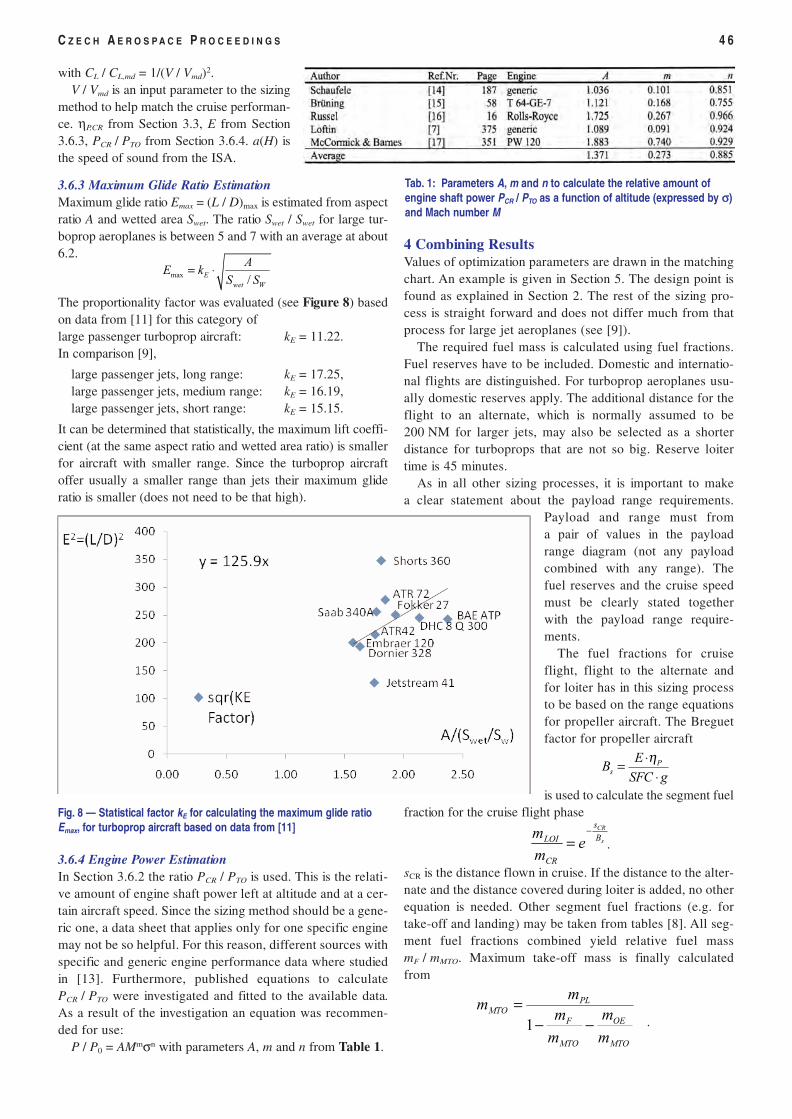
with CL / CL,md = 1/(V / Vmd)2.V / Vmd is an input parameter to the sizing
method to help match the cruise performan-ce. ηP,CR from Section 3.3, E from Section3.6.3, PCR / PTO from Section 3.6.4. a(H) isthe speed of sound from the ISA.
3.6.3 Maximum Glide Ratio EstimationMaximum glide ratio Emax = (L / D)max is estimated from aspectratio A and wetted area Swet. The ratio Swet / Swet for large tur-boprop aeroplanes is between 5 and 7 with an average at about6.2.
The proportionality factor was evaluated (see Figure 8) basedon data from [11] for this category oflarge passenger turboprop aircraft: kE = 11.22. In comparison [9],
large passenger jets, long range: kE = 17.25,large passenger jets, medium range: kE = 16.19,large passenger jets, short range: kE = 15.15.
It can be determined that statistically, the maximum lift coeffi-cient (at the same aspect ratio and wetted area ratio) is smallerfor aircraft with smaller range. Since the turboprop aircraftoffer usually a smaller range than jets their maximum glideratio is smaller (does not need to be that high).
3.6.4 Engine Power EstimationIn Section 3.6.2 the ratio PCR / PTO is used. This is the relati-ve amount of engine shaft power left at altitude and at a cer-tain aircraft speed. Since the sizing method should be a gene-ric one, a data sheet that applies only for one specific enginemay not be so helpful. For this reason, different sources withspecific and generic engine performance data where studiedin [13]. Furthermore, published equations to calculatePCR / PTO were investigated and fitted to the available data.As a result of the investigation an equation was recommen-ded for use:
P / P0 = AMmσn with parameters A, m and n from Table 1.
4 Combining ResultsValues of optimization parameters are drawn in the matchingchart. An example is given in Section 5. The design point isfound as explained in Section 2. The rest of the sizing pro-cess is straight forward and does not differ much from thatprocess for large jet aeroplanes (see [9]).
The required fuel mass is calculated using fuel fractions.Fuel reserves have to be included. Domestic and internatio-nal flights are distinguished. For turboprop aeroplanes usu-ally domestic reserves apply. The additional distance for theflight to an alternate, which is normally assumed to be200 NM for larger jets, may also be selected as a shorterdistance for turboprops that are not so big. Reserve loitertime is 45 minutes.
As in all other sizing processes, it is important to makea clear statement about the payload range requirements.
Payload and range must froma pair of values in the payloadrange diagram (not any payloadcombined with any range). Thefuel reserves and the cruise speedmust be clearly stated togetherwith the payload range require-ments.
The fuel fractions for cruiseflight, flight to the alternate andfor loiter has in this sizing processto be based on the range equationsfor propeller aircraft. The Breguetfactor for propeller aircraft
is used to calculate the segment fuelfraction for the cruise flight phase
.
sCR is the distance flown in cruise. If the distance to the alter-nate and the distance covered during loiter is added, no otherequation is needed. Other segment fuel fractions (e.g. fortake-off and landing) may be taken from tables [8]. All seg-ment fuel fractions combined yield relative fuel massmF / mMTO. Maximum take-off mass is finally calculatedfrom
.
C Z E C H A E R O S P A C E P R O C E E D I N G S 4 6
max/
E
wet W
AE k
S S= ⋅
Fig. 8 — Statistical factor kE for calculating the maximum glide ratioEmax, for turboprop aircraft based on data from [11]
Tab. 1: Parameters A, m and n to calculate the relative amount ofengine shaft power PCR / PTO as a function of altitude (expressed by σσ)and Mach number M
P
s
EB
SFC g
η⋅=⋅
s
CR
B
s
CR
LOI em
m −=
MTO
OE
MTO
F
PLMTO
m
m
m
m
mm
−−=
1
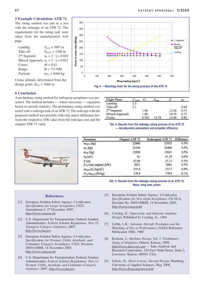
5 Example Calculation: ATR 72The sizing method was put to a testwith the redesign of an ATR 72. Therequirements for the sizing task weretaken from the manufacturers webpage.
Landing: SLFL = 1067 mTake off: STOFL = 1290 m2nd Segment: nE = 2 γ = 0.024Missed Approach: nE = 2 γ = 0.021Cruise: M = 0.41Range: R = 715 NMPayload: mPL = 6460 kg
Cruise altitude, determined from thedesign point: HCR = 3888 m.
6 ConclusionA preliminary sizing method for turboprop aeroplanes was pre-sented. The method includes — where necessary — equationsbased on aircraft statistics. The preliminary sizing method wastested with a redesign task of an ATR 72. The redesign with theproposed method was possible with only minor difference bet-ween the respective ATR value from the redesign case and theoriginal ATR 72 value.
4 7 L E T E C K Ý Z P R A V O D A J 2 / 2 0 0 9
Tab. 2: Results from the redesign sizing process of an ATR 72— Aerodynamic parameters and propeller efficiency
Tab. 3: Results from the redesign sizing process of an ATR 72:Mass, wing area, power
0
50
100
150
200
250
300
350
400
0 100 200 300 400 500 600 700
Wing loading [kg/m2]
Po
wer
to m
ass r
ati
o [
W/k
g]
2. Segment
MissedApproachTake off
Landing
Fig, 9 — Matching chart for the sizing process of the ATR 72
References:
[1] European Aviation Safety Agency: CertificationSpecifications for Large Aeroplanes, CS25,Amendment 4, 27 December 2007,http://www.easa.eu.int
[2] U.S. Department for Transportation, Federal AviationAdministration: Federal Aviation Regulations, Part 25,Transport Category Airplanes, 2007,http://www.faa.gov
[3] European Aviation Safety Agency: CertificationSpecifications for Normal, Utility, Aerobatic, andCommuter Category Aeroplanes, CS23, Decision2003/14/RM, 14 November 2003,http://www.easa.eu.int
[4] U.S. Department for Transportation, Federal AviationAdministration: Federal Aviation Regulations, Part 23,Normal, Utility, Aerobatic and Commuter CategoryAirplanes, 2007, http://www.faa.gov
[5] European Aviation Safety Agency: CertificationSpecifications for Very Light Aeroplanes, CS-VLA,Decision No. 2003/18/RM, 14 November 2003,http://www.easa.eu.int
[6] Corning, G.: Supersonic and Subsonic AirplaneDesign; Published by Corning, G., 1964
[7] Loftin, L.K.: Subsonic Aircraft: Evolution and theMatching of Size to Performance; NASA ReferencePublication 1060, 1980
[8] Roskam, J.: Airplane Design. Vol. 1: PreliminarySizing of Airplanes; Ottawa, Kansas, 1989,http://www.darcorp.com — Sale: Analysis andResearch Corporation, 120 East Ninth Street, Suite 2,Lawrence, Kansas, 66044, USA.
[9] Scholz, D.: Short Course, Aircraft Design; HamburgUniversity of Applied Sciences, May 2008,http://www.flugzeugentwurf.de

C Z E C H A E R O S P A C E P R O C E E D I N G S 4 8
Room for Your Notes
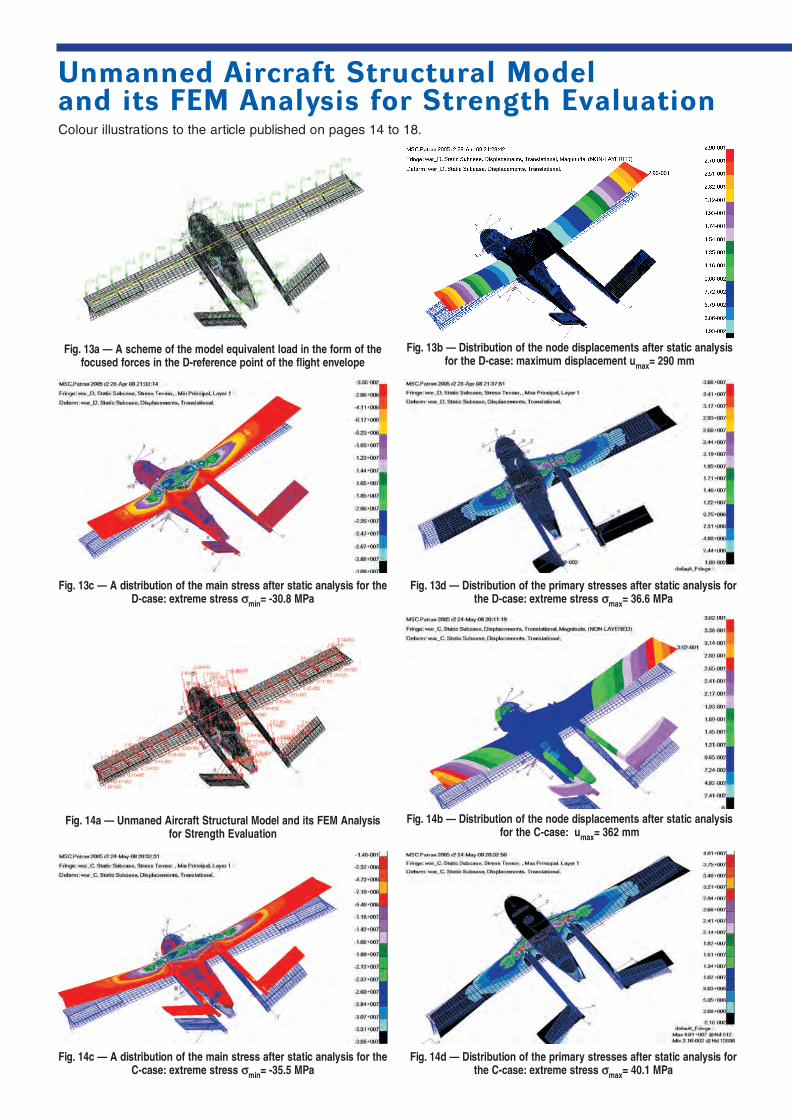
Unmanned Aircraft Structural Modeland its FEM Analysis for Strength EvaluationColour illustrations to the article published on pages 14 to 18.
Fig. 13a — A scheme of the model equivalent load in the form of thefocused forces in the D-reference point of the flight envelope
Fig. 13b — Distribution of the node displacements after static analysisfor the D-case: maximum displacement umax= 290 mm
Fig. 13c — A distribution of the main stress after static analysis for theD-case: extreme stress σσmin= -30.8 MPa
Fig. 13d — Distribution of the primary stresses after static analysis forthe D-case: extreme stress σσmax= 36.6 MPa
Fig. 14a — Unmaned Aircraft Structural Model and its FEM Analysisfor Strength Evaluation
Fig. 14b — Distribution of the node displacements after static analysisfor the C-case: umax= 362 mm
Fig. 14c — A distribution of the main stress after static analysis for theC-case: extreme stress σσmin= -35.5 MPa
Fig. 14d — Distribution of the primary stresses after static analysis forthe C-case: extreme stress σσmax= 40.1 MPa

Calculation of Temperature Fields of Vibrating Composite Parts
© A S S O C I A T I O N O F A V I A T I O N
M A N U F A C T U R E R S
(Left) Damage of composite blade caused byintensive vibrations and consequently byoverheating
(Below) FEM analysis predicts the same failurecaused by overheating
(Left) Strain-gauging of composite blade rootsection gives important information aboutstresses and vibration levels
The whole view of the mobile test bed ofcomposite propellers is depicted on title page
(Left) Infrared image of overheating of composi-te blade caused by intensive vibrations
(Below) The location of overheatingcorresponds to the location of matrix failure