cs488/688 - introduction to computer graphics spring 2018
TRANSCRIPT

CS488/688 - Introduction to Computer Graphics
Spring 2018
School of Computer Science, University of Waterloo
Instructor: Gladimir V. G. Baranoski, DC3520Regular Office Hours: Friday 4-5PM
Project Extended Office Hours: June 22, Friday 4-6PMProject Extended Office Hours: June 29, Friday 4-6PM
Lecture Times: Monday and Wednesday, from 4-5:20PM, MC4041.
Revised Schedule
Week Date Assignments/Project/Exams2 May 9, Wednesday Assignment 02 May 9, Wednesday Tutorial (5:30PM-6:30PM, Room MC4063)2 May 10, Thursday Tutorial (5:30PM-6:30PM, Room MC4063)3 May 16, Wednesday Assignment 15 May 30, Wednesday Assignment 26 June 6, Wednesday Midterm Exam (4PM, Room MC4020)7 June 13, Wednesday Assignment 38 June 20, Wednesday Assignment 49 June 25, Monday Project Proposal10 July 4 Wednesday Revised Project Proposal13 July 23, Monday Project Code13 July 24, Tuesday Project Demos13 July 25, Wednesday Project Demos13 July 25, Wednesday Project Report (4PM, Room MC4041)
Important Notes: The deadline for the submission of assignment code is 3:30PM on the daysspecified as the assignment due dates. The deadline for the project code is 8:00PM on the day spec-ified above. Assignments and project materials submitted after these deadlines will receive ZEROmarks. Although the revised project proposal is not marked, if it is not submitted on the due datespecified above, the project will receive ZERO marks. Assignments and project written documents(reports and proposals) should be handed in at the beginning (first five minutes) of the lectures givenat the above specified due dates. Assignments will be returned in class after they have been marked.
Course TAs:
• Petri Varsa ([email protected]). Office hours: Monday, 11AM-12PM, UndergraduateGraphics Lab, MC3007.
• Mark Iwanchyshyn ([email protected]). Office hours: Tuesday, 11AM-12PM,Undergraduate Graphics Lab, MC3007.
CONTENTS 2
Contents
1 Administration 91.1 General Information . . . . . . . . . . . . . . . . . . . . . . . . . . . . . . . . . . . . 91.2 Topics Covered . . . . . . . . . . . . . . . . . . . . . . . . . . . . . . . . . . . . . . . 101.3 Assignments . . . . . . . . . . . . . . . . . . . . . . . . . . . . . . . . . . . . . . . . . 10
2 Introduction 132.1 History . . . . . . . . . . . . . . . . . . . . . . . . . . . . . . . . . . . . . . . . . . . 132.2 Pipeline . . . . . . . . . . . . . . . . . . . . . . . . . . . . . . . . . . . . . . . . . . . 142.3 Primitives . . . . . . . . . . . . . . . . . . . . . . . . . . . . . . . . . . . . . . . . . . 152.4 Algorithms . . . . . . . . . . . . . . . . . . . . . . . . . . . . . . . . . . . . . . . . . 162.5 APIs . . . . . . . . . . . . . . . . . . . . . . . . . . . . . . . . . . . . . . . . . . . . . 16
3 Devices and Device Independence 173.1 Calligraphic and Raster Devices . . . . . . . . . . . . . . . . . . . . . . . . . . . . . . 173.2 How a Monitor Works . . . . . . . . . . . . . . . . . . . . . . . . . . . . . . . . . . . 173.3 Physical Devices . . . . . . . . . . . . . . . . . . . . . . . . . . . . . . . . . . . . . . 18
4 Device Interfaces 214.1 Device Input Modes . . . . . . . . . . . . . . . . . . . . . . . . . . . . . . . . . . . . 214.2 Application Structure . . . . . . . . . . . . . . . . . . . . . . . . . . . . . . . . . . . 214.3 Polling and Sampling . . . . . . . . . . . . . . . . . . . . . . . . . . . . . . . . . . . . 224.4 Event Queues . . . . . . . . . . . . . . . . . . . . . . . . . . . . . . . . . . . . . . . . 224.5 Toolkits and Callbacks . . . . . . . . . . . . . . . . . . . . . . . . . . . . . . . . . . . 234.6 Example for Discussion . . . . . . . . . . . . . . . . . . . . . . . . . . . . . . . . . . 24
5 Geometries 275.1 Vector Spaces . . . . . . . . . . . . . . . . . . . . . . . . . . . . . . . . . . . . . . . . 275.2 Affine Spaces . . . . . . . . . . . . . . . . . . . . . . . . . . . . . . . . . . . . . . . . 275.3 Euclidean Spaces . . . . . . . . . . . . . . . . . . . . . . . . . . . . . . . . . . . . . . 285.4 Cartesian Space . . . . . . . . . . . . . . . . . . . . . . . . . . . . . . . . . . . . . . . 295.5 Why Vector Spaces Inadequate . . . . . . . . . . . . . . . . . . . . . . . . . . . . . . 295.6 Summary of Geometric Spaces . . . . . . . . . . . . . . . . . . . . . . . . . . . . . . 30
6 Affine Geometry and Transformations 316.1 Linear Combinations . . . . . . . . . . . . . . . . . . . . . . . . . . . . . . . . . . . . 316.2 Affine Combinations . . . . . . . . . . . . . . . . . . . . . . . . . . . . . . . . . . . . 316.3 Affine Transformations . . . . . . . . . . . . . . . . . . . . . . . . . . . . . . . . . . . 336.4 Matrix Representation of Transformations . . . . . . . . . . . . . . . . . . . . . . . . 356.5 Geometric Transformations . . . . . . . . . . . . . . . . . . . . . . . . . . . . . . . . 366.6 Compositions of Transformations . . . . . . . . . . . . . . . . . . . . . . . . . . . . . 376.7 Change of Basis . . . . . . . . . . . . . . . . . . . . . . . . . . . . . . . . . . . . . . . 386.8 Ambiguity . . . . . . . . . . . . . . . . . . . . . . . . . . . . . . . . . . . . . . . . . . 416.9 3D Transformations . . . . . . . . . . . . . . . . . . . . . . . . . . . . . . . . . . . . 426.10 World and Viewing Frames . . . . . . . . . . . . . . . . . . . . . . . . . . . . . . . . 44
CONTENTS 3
6.11 Normals . . . . . . . . . . . . . . . . . . . . . . . . . . . . . . . . . . . . . . . . . . . 47
7 Windows, Viewports, NDC 497.1 Window to Viewport Mapping . . . . . . . . . . . . . . . . . . . . . . . . . . . . . . 497.2 Normalized Device Coordinates . . . . . . . . . . . . . . . . . . . . . . . . . . . . . . 50
8 Clipping 538.1 Clipping . . . . . . . . . . . . . . . . . . . . . . . . . . . . . . . . . . . . . . . . . . . 53
9 Projections and Projective Transformations 579.1 Projections . . . . . . . . . . . . . . . . . . . . . . . . . . . . . . . . . . . . . . . . . 579.2 Why Map Z? . . . . . . . . . . . . . . . . . . . . . . . . . . . . . . . . . . . . . . . . 629.3 Mapping Z . . . . . . . . . . . . . . . . . . . . . . . . . . . . . . . . . . . . . . . . . 649.4 3D Clipping . . . . . . . . . . . . . . . . . . . . . . . . . . . . . . . . . . . . . . . . . 669.5 Homogeneous Clipping . . . . . . . . . . . . . . . . . . . . . . . . . . . . . . . . . . . 669.6 Pinhole Camera vs. Camera vs. Perception . . . . . . . . . . . . . . . . . . . . . . . 68
10 Transformation Applications and Extensions 7310.1 Rendering Pipeline Revisited . . . . . . . . . . . . . . . . . . . . . . . . . . . . . . . 7310.2 Derivation by Composition . . . . . . . . . . . . . . . . . . . . . . . . . . . . . . . . 7310.3 3D Rotation User Interfaces . . . . . . . . . . . . . . . . . . . . . . . . . . . . . . . . 7510.4 The Virtual Sphere . . . . . . . . . . . . . . . . . . . . . . . . . . . . . . . . . . . . . 75
11 Polygons 7711.1 Polygons – Introduction . . . . . . . . . . . . . . . . . . . . . . . . . . . . . . . . . . 7711.2 Polygon Clipping . . . . . . . . . . . . . . . . . . . . . . . . . . . . . . . . . . . . . . 7811.3 Polygon Scan Conversion . . . . . . . . . . . . . . . . . . . . . . . . . . . . . . . . . 8111.4 Dos and Don’ts . . . . . . . . . . . . . . . . . . . . . . . . . . . . . . . . . . . . . . . 82
12 Hidden Surface Removal 8512.1 Hidden Surface Removal . . . . . . . . . . . . . . . . . . . . . . . . . . . . . . . . . . 8512.2 Backface Culling . . . . . . . . . . . . . . . . . . . . . . . . . . . . . . . . . . . . . . 8512.3 Painter’s Algorithm . . . . . . . . . . . . . . . . . . . . . . . . . . . . . . . . . . . . 8612.4 Warnock’s Algorithm . . . . . . . . . . . . . . . . . . . . . . . . . . . . . . . . . . . . 8712.5 Z-Buffer Algorithm . . . . . . . . . . . . . . . . . . . . . . . . . . . . . . . . . . . . . 8812.6 Comparison of Algorithms . . . . . . . . . . . . . . . . . . . . . . . . . . . . . . . . . 89
13 Hierarchical Models and Transformations 9113.1 Hierarchical Transformations . . . . . . . . . . . . . . . . . . . . . . . . . . . . . . . 9113.2 Hierarchical Data Structures . . . . . . . . . . . . . . . . . . . . . . . . . . . . . . . 93
14 Picking and 3D Selection 9914.1 Picking and 3D Selection . . . . . . . . . . . . . . . . . . . . . . . . . . . . . . . . . 99
15 Colour and the Human Visual System 10115.1 Colour . . . . . . . . . . . . . . . . . . . . . . . . . . . . . . . . . . . . . . . . . . . . 101
CONTENTS 4
16 Reflection and Light Source Models 10516.1 Goals . . . . . . . . . . . . . . . . . . . . . . . . . . . . . . . . . . . . . . . . . . . . 10516.2 Lambertian Reflection . . . . . . . . . . . . . . . . . . . . . . . . . . . . . . . . . . . 10516.3 Attenuation . . . . . . . . . . . . . . . . . . . . . . . . . . . . . . . . . . . . . . . . . 10716.4 Coloured Lights, Multiple Lights, and Ambient Light . . . . . . . . . . . . . . . . . 10916.5 Specular Reflection . . . . . . . . . . . . . . . . . . . . . . . . . . . . . . . . . . . . 110
17 Shading 11317.1 Introduction . . . . . . . . . . . . . . . . . . . . . . . . . . . . . . . . . . . . . . . . . 11317.2 Gouraud Shading . . . . . . . . . . . . . . . . . . . . . . . . . . . . . . . . . . . . . . 11317.3 Phong Shading . . . . . . . . . . . . . . . . . . . . . . . . . . . . . . . . . . . . . . . 117
18 Ray Tracing 11918.1 Fundamentals . . . . . . . . . . . . . . . . . . . . . . . . . . . . . . . . . . . . . . . . 11918.2 Intersection Computations . . . . . . . . . . . . . . . . . . . . . . . . . . . . . . . . . 12018.3 Shading . . . . . . . . . . . . . . . . . . . . . . . . . . . . . . . . . . . . . . . . . . . 12318.4 Recursive Ray Tracing . . . . . . . . . . . . . . . . . . . . . . . . . . . . . . . . . . . 12518.5 Surface Information . . . . . . . . . . . . . . . . . . . . . . . . . . . . . . . . . . . . 12618.6 Modeling and CSG . . . . . . . . . . . . . . . . . . . . . . . . . . . . . . . . . . . . . 12818.7 Texture Mapping . . . . . . . . . . . . . . . . . . . . . . . . . . . . . . . . . . . . . . 13018.8 Bounding Boxes, Spatial Subdivision . . . . . . . . . . . . . . . . . . . . . . . . . . . 133
19 Aliasing 13719.1 Aliasing . . . . . . . . . . . . . . . . . . . . . . . . . . . . . . . . . . . . . . . . . . . 137
20 Bidirectional Tracing 14320.1 Missing Effects . . . . . . . . . . . . . . . . . . . . . . . . . . . . . . . . . . . . . . . 14320.2 Radiosity . . . . . . . . . . . . . . . . . . . . . . . . . . . . . . . . . . . . . . . . . . 14320.3 Distribution Ray Tracing . . . . . . . . . . . . . . . . . . . . . . . . . . . . . . . . . 14420.4 Bidirectional Path Tracing . . . . . . . . . . . . . . . . . . . . . . . . . . . . . . . . . 14420.5 Photon Maps . . . . . . . . . . . . . . . . . . . . . . . . . . . . . . . . . . . . . . . . 14520.6 Metropolis Algorithm . . . . . . . . . . . . . . . . . . . . . . . . . . . . . . . . . . . 146
21 Radiosity 14721.1 Definitions and Overview . . . . . . . . . . . . . . . . . . . . . . . . . . . . . . . . . 14721.2 Form Factors . . . . . . . . . . . . . . . . . . . . . . . . . . . . . . . . . . . . . . . . 15221.3 Progressive Refinement . . . . . . . . . . . . . . . . . . . . . . . . . . . . . . . . . . . 15521.4 Meshing in Radiosity . . . . . . . . . . . . . . . . . . . . . . . . . . . . . . . . . . . . 15721.5 Stocastic Methods — Radiosity Without Form Factors . . . . . . . . . . . . . . . . . 159
22 Photon Maps 16122.1 Overview . . . . . . . . . . . . . . . . . . . . . . . . . . . . . . . . . . . . . . . . . . 161
23 Graphics Hardware 16523.1 Graphics Hardware . . . . . . . . . . . . . . . . . . . . . . . . . . . . . . . . . . . . . 16523.2 High-Level Shading Languages . . . . . . . . . . . . . . . . . . . . . . . . . . . . . . 166
CONTENTS 5
24 Shadows 17124.1 Overview . . . . . . . . . . . . . . . . . . . . . . . . . . . . . . . . . . . . . . . . . . 17124.2 Projective Shadows . . . . . . . . . . . . . . . . . . . . . . . . . . . . . . . . . . . . . 17124.3 Shadow Maps . . . . . . . . . . . . . . . . . . . . . . . . . . . . . . . . . . . . . . . . 17224.4 Shadow Volumes . . . . . . . . . . . . . . . . . . . . . . . . . . . . . . . . . . . . . . 175
25 Modeling of Various Things 17925.1 Fractal Mountains . . . . . . . . . . . . . . . . . . . . . . . . . . . . . . . . . . . . . 17925.2 L-system Plants . . . . . . . . . . . . . . . . . . . . . . . . . . . . . . . . . . . . . . . 18025.3 Buildings . . . . . . . . . . . . . . . . . . . . . . . . . . . . . . . . . . . . . . . . . . 18125.4 Particle Systems . . . . . . . . . . . . . . . . . . . . . . . . . . . . . . . . . . . . . . 188
26 Polyhedral Data Structures 19126.1 Storage Models . . . . . . . . . . . . . . . . . . . . . . . . . . . . . . . . . . . . . . . 19126.2 Euler’s Formula . . . . . . . . . . . . . . . . . . . . . . . . . . . . . . . . . . . . . . . 19326.3 Winged Edge . . . . . . . . . . . . . . . . . . . . . . . . . . . . . . . . . . . . . . . . 19426.4 Mesh Compression . . . . . . . . . . . . . . . . . . . . . . . . . . . . . . . . . . . . . 199
27 Splines 20127.1 Constructing Curve Segments . . . . . . . . . . . . . . . . . . . . . . . . . . . . . . . 20127.2 Bernstein Polynomials . . . . . . . . . . . . . . . . . . . . . . . . . . . . . . . . . . . 20427.3 Bezier Splines . . . . . . . . . . . . . . . . . . . . . . . . . . . . . . . . . . . . . . . . 20527.4 Spline Continuity . . . . . . . . . . . . . . . . . . . . . . . . . . . . . . . . . . . . . . 20827.5 Tensor Product Patches . . . . . . . . . . . . . . . . . . . . . . . . . . . . . . . . . . 21427.6 Barycentric Coordinates . . . . . . . . . . . . . . . . . . . . . . . . . . . . . . . . . . 21727.7 Triangular Patches . . . . . . . . . . . . . . . . . . . . . . . . . . . . . . . . . . . . . 21827.8 Subdivision Surfaces . . . . . . . . . . . . . . . . . . . . . . . . . . . . . . . . . . . . 22027.9 Implicit Surfaces . . . . . . . . . . . . . . . . . . . . . . . . . . . . . . . . . . . . . . 22327.10Wavelets . . . . . . . . . . . . . . . . . . . . . . . . . . . . . . . . . . . . . . . . . . . 227
28 Non-Photorealistic Rendering 23328.1 2D NPR . . . . . . . . . . . . . . . . . . . . . . . . . . . . . . . . . . . . . . . . . . . 23328.2 3D NPR . . . . . . . . . . . . . . . . . . . . . . . . . . . . . . . . . . . . . . . . . . . 239
29 Volume Rendering 24329.1 Volume Rendering . . . . . . . . . . . . . . . . . . . . . . . . . . . . . . . . . . . . . 243
30 Animation 24730.1 Overview . . . . . . . . . . . . . . . . . . . . . . . . . . . . . . . . . . . . . . . . . . 24730.2 Traditional 2D Cel Animation . . . . . . . . . . . . . . . . . . . . . . . . . . . . . . . 24730.3 Automated Keyframing . . . . . . . . . . . . . . . . . . . . . . . . . . . . . . . . . . 24830.4 Functional Animation . . . . . . . . . . . . . . . . . . . . . . . . . . . . . . . . . . . 24830.5 Motion Path Animation . . . . . . . . . . . . . . . . . . . . . . . . . . . . . . . . . . 25030.6 Orientation and Interpolation . . . . . . . . . . . . . . . . . . . . . . . . . . . . . . . 25230.7 Quaternions . . . . . . . . . . . . . . . . . . . . . . . . . . . . . . . . . . . . . . . . . 25430.8 Animating Camera Motion . . . . . . . . . . . . . . . . . . . . . . . . . . . . . . . . 256
CONTENTS 6
30.9 Tools for Shape Animation . . . . . . . . . . . . . . . . . . . . . . . . . . . . . . . . 25830.10Kinematics and Inverse Kinematics . . . . . . . . . . . . . . . . . . . . . . . . . . . . 26030.11Physically-Based Animation . . . . . . . . . . . . . . . . . . . . . . . . . . . . . . . . 26130.12Human Motion . . . . . . . . . . . . . . . . . . . . . . . . . . . . . . . . . . . . . . . 26330.13Sensor-Actuator Networks . . . . . . . . . . . . . . . . . . . . . . . . . . . . . . . . . 26430.14Biologically-Based Simulation . . . . . . . . . . . . . . . . . . . . . . . . . . . . . . . 26530.15Morphing . . . . . . . . . . . . . . . . . . . . . . . . . . . . . . . . . . . . . . . . . . 26630.16Motion Capture . . . . . . . . . . . . . . . . . . . . . . . . . . . . . . . . . . . . . . . 26730.17Flocking . . . . . . . . . . . . . . . . . . . . . . . . . . . . . . . . . . . . . . . . . . . 268
31 Computational Geometry 27131.1 Introduction . . . . . . . . . . . . . . . . . . . . . . . . . . . . . . . . . . . . . . . . . 27131.2 Data Structures . . . . . . . . . . . . . . . . . . . . . . . . . . . . . . . . . . . . . . . 27131.3 Convex Hull . . . . . . . . . . . . . . . . . . . . . . . . . . . . . . . . . . . . . . . . . 27431.4 Voronoi Diagrams . . . . . . . . . . . . . . . . . . . . . . . . . . . . . . . . . . . . . 27531.5 Delaunay Triangulation . . . . . . . . . . . . . . . . . . . . . . . . . . . . . . . . . . 27631.6 More Computational Geometry . . . . . . . . . . . . . . . . . . . . . . . . . . . . . . 279
32 Assignments 28132.1 Assignment 0: Introduction . . . . . . . . . . . . . . . . . . . . . . . . . . . . . . . . 28132.2 Assignment 1: Introduction to OpenGL . . . . . . . . . . . . . . . . . . . . . . . . . 28132.3 Assignment 2: Frames and Perspective . . . . . . . . . . . . . . . . . . . . . . . . . . 28232.4 Assignment 3: Hierarchical Modelling . . . . . . . . . . . . . . . . . . . . . . . . . . 28332.5 Assignment 4: A Raytracer . . . . . . . . . . . . . . . . . . . . . . . . . . . . . . . . 28432.6 Assignment 5: The Project . . . . . . . . . . . . . . . . . . . . . . . . . . . . . . . . 285

CONTENTS 7
These notes contain the material that appears on the overhead slides (or on the computer)shown in class. You should, however, read the course text and attend lectures to fill in the missingdetails. The material in this course is organized around the assignments, with the material at theend of the course being a sequence of topics not covered on the assignments. Some of the imagesshown on the slides cannot be included in the printed course notes for copyright reasons.
The following former CS 488/688 students have images appearing in these notes:
• Tobias Arrskog
• Franke Belme
• Jerome Carriere
• Bryan Chan
• Stephen Chow
• David Cope
• Eric Hall
• Matthew Hill
• Andrew Lau
• Henry Lau
• Tom Lee
• Bonnie Liu
• Ian McIntyre
• Ryan Meridith-Jones
• Zaid Mian
• Ashraf Michail
• Mike Neame
• Mathieu Nocenti
• Jeremy Sharpe
• Stephen Sheeler
• Selina Siu
2 INTRODUCTION 13
2 Introduction
2.1 History
A Brief History of Computer Graphics
Early 60s: Computer animations for physical simulation;Edward Zajac displays satellite research using CG in 1961
1963: Sutherland (MIT)Sketchpad (direct manipulation, CAD)
Calligraphic (vector) display devicesInteractive techniquesDouglas Engelbart invents the mouse.
1968: Evans & Sutherland founded
1969: First SIGGRAPH
Late 60’s to late 70’s: Utah Dynasty
1970: Pierre Bezier develops Bezier curves
1971: Gouraud Shading
1972: Pong developed
1973: Westworld, The first film to use computer animation
1974: Ed Catmull develops z-buffer (Utah)First Computer Animated Short, Hunger :Keyframe animation and morphing
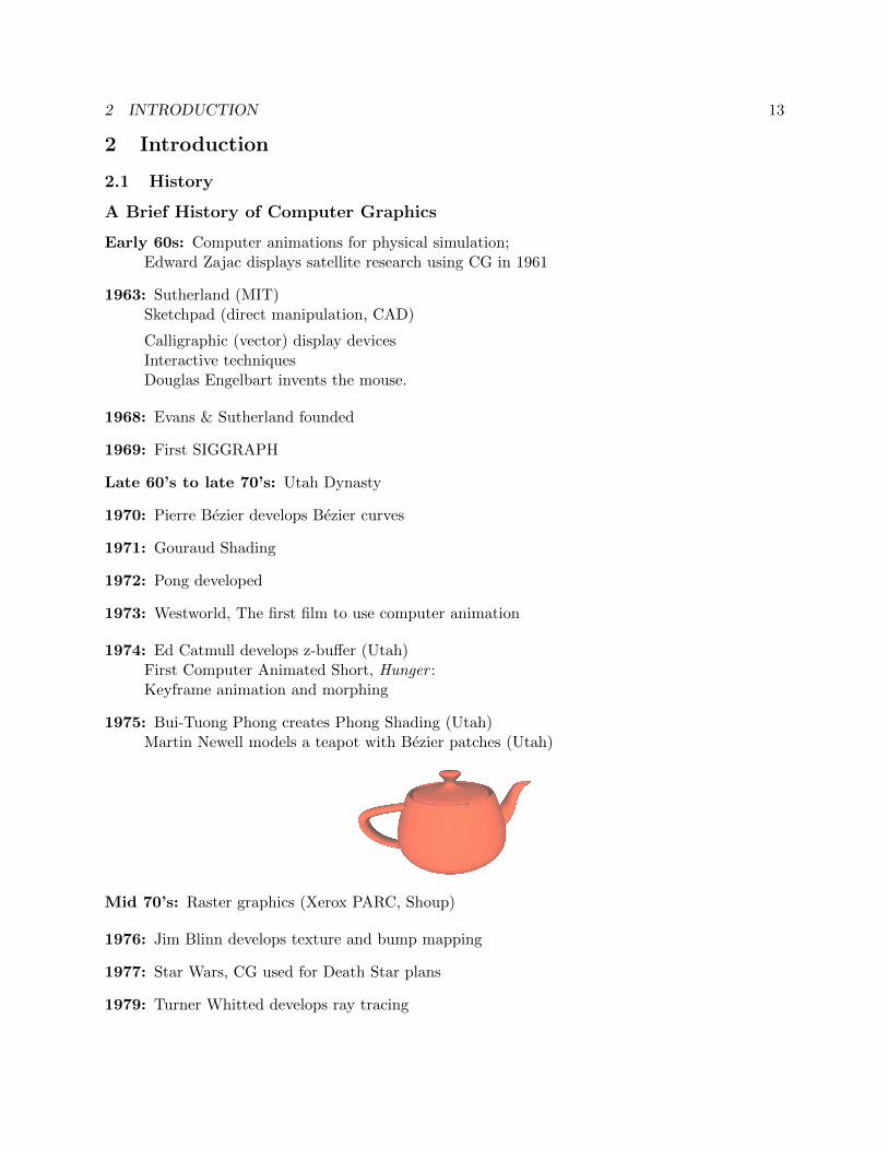
1975: Bui-Tuong Phong creates Phong Shading (Utah)Martin Newell models a teapot with Bezier patches (Utah)
Mid 70’s: Raster graphics (Xerox PARC, Shoup)
1976: Jim Blinn develops texture and bump mapping
1977: Star Wars, CG used for Death Star plans
1979: Turner Whitted develops ray tracing
Pipeline 2.1 14
Mid 70’s - 80’s: Quest for realismradiosity; also mainstream real-time applications.
1982: Tron, Wrath of Khan. Particle systems and obvious CG
1984: The Last Starfighter, CG replaces physical models. Early attempts at realism using CG
1986: First CG animation nominated for an Academy Award: Luxo Jr. (Pixar)
1989: Tin Toy (Pixar) wins Academy Award
The Abyss: first 3D CGmovie character
1993: Jurassic Park—game changer
1995: Toy Story (Pixar and Disney), first full length fully computer-generated 3Danimation
Reboot,
the first fully 3D CG Saturday morning cartoonBabylon 5, the first TV show to routinely use CG models
late 90’s: Interactive environments, scientific/medical visualization, artistic rendering, image basedrendering, photon maps, etc.
00’s: Real-time photorealistic rendering on consumer hardware.
(Readings: Watt, Preface (optional), Hearn and Baker, Chapter 1 (optional), Red book [Foley,van Dam et al: Introduction to Computer Graphics], Chapter 1 (optional). White book [Foley, vanDam et al: Computer Graphics: Principles and Practice, 2nd ed.], Chapter 1 (optional). )
2.2 Pipeline
We begin with a description of forward rendering, which is the kind of rendering usually sup-ported in hardware and is the model OpenGL uses. In forward rendering, rendering primitives aretransformed, usually in a conceptual pipeline, from the model to the device.
However, raytracing, which we will consider later in the course, is a form of backward ren-dering. In backward rendering, we start with a point in the image and work out what modelprimitives project to it.
Both approaches have advantages and disadvantages.
The Graphics Pipeline
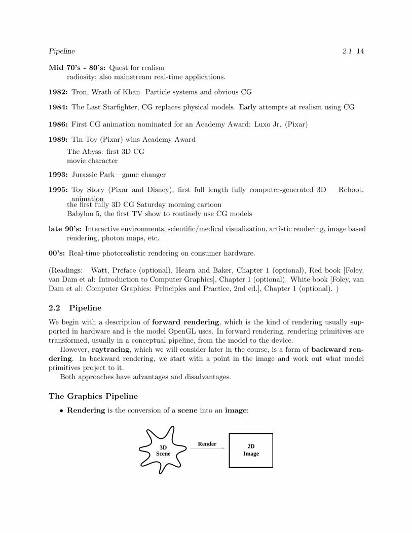
• Rendering is the conversion of a scene into an image:
Render
Scene2D3D
Image
Primitives 2.2 15
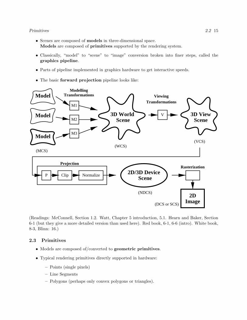
• Scenes are composed of models in three-dimensional space.Models are composed of primitives supported by the rendering system.
• Classically, “model” to “scene” to “image” conversion broken into finer steps, called thegraphics pipeline.
• Parts of pipeline implemented in graphics hardware to get interactive speeds.
• The basic forward projection pipeline looks like:
Normalize Clip
(DCS or SCS)
(MCS)(WCS)
(VCS)
Model
Model
Model
ModellingTransformations
3D World Scene Scene
3D View
Scene
(NDCS)
ViewingTransformations
V
M3
M2
M1
2D/3D DeviceP
ProjectionRasterization
Image2D
(Readings: McConnell, Section 1.2. Watt, Chapter 5 introduction, 5.1. Hearn and Baker, Section6-1 (but they give a more detailed version than used here). Red book, 6-1, 6-6 (intro). White book,8-3, Blinn: 16.)
2.3 Primitives
• Models are composed of/converted to geometric primitives.
• Typical rendering primitives directly supported in hardware:
– Points (single pixels)
– Line Segments
– Polygons (perhaps only convex polygons or triangles).
Algorithms 2.3 16
• Modelling primitives also include
– Piecewise polynomial (spline) curves
– Piecewise polynomial (spline) surfaces
– Implicit surfaces (quadrics, blobbies, etc)
– Other...
2.4 Algorithms
A number of basic algorithms are needed:
• Transformation: Convert representations of models/primitives from one coordinate systemto another.
• Clipping/Hidden Surface Removal: Remove primitives and parts of primitives that arenot visible on the display.
• Rasterization: Convert a projected screen-space primitive to a set of pixels.
Later, we will look at some more advanced algorithms:
• Picking: Select a 3D object by clicking an input device over a pixel location.
• Shading and Illumination: Simulate the interaction of light with a scene.
• Animation: Simulate movement by rendering a sequence of frames.
2.5 APIs
Application Programming Interfaces (APIs):
Xlib, GDI: 2D rasterization.
PostScript, PDF, SVG: 2D transformations, 2D rasterization
OpenGL, Direct3D: 3D pipeline
APIs provide access to rendering hardware via a conceptual model.
APIs hide which graphics algorithms are or are not implemented in hardware by simulating missingpieces in software.
3 DEVICES AND DEVICE INDEPENDENCE 17
3 Devices and Device Independence
3.1 Calligraphic and Raster Devices
Calligraphics and Raster Devices
Calligraphic Display Devices draw polygon and line segments directly:
• Plotters
• Direct Beam Control CRTs
• Laser Light Projection Systems
represent an image as a regular grid of samples.
Raster Display Devices • Each sample is usually called a pixel (“picture element”)
• Rendering requires rasterization algorithms to quickly determine a sampled repre-sentation of geometric primitives.
3.2 How a Monitor Works
How a CRT Works
Raster Cathode Ray Tubes (CRTs) Once was most common display device
• Capable of high resolution.
• Good colour fidelity.
• High contrast (100:1).
• High update rates.
Electron beam scanned in regular pattern of horizontal scanlines.
Raster images stored in a frame buffer.
Intensity of electron beam modified by the pixel value.
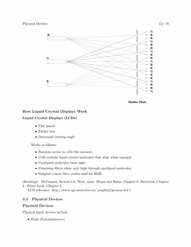
Colour CRTs have three different colours of phosphor and three independent electron guns.
Shadow Masks allow each gun to irradiate only one colour of phosphor.
Physical Devices 3.2 18
G
Shadow Mask
GRB
R
G
B
B
B
B
B
B
R
R
R
R
R
G
G
G
G
G
How Liquid Crystal Displays Work
Liquid Crystal Displays (LCDs)
• Flat panels
• Flicker free
• Decreased viewing angle
Works as follows:
• Random access to cells like memory.
• Cells contain liquid crystal molecules that align when charged.
• Unaligned molecules twist light.
• Polarizing filters allow only light through unaligned molecules.
• Subpixel colour filter masks used for RGB.
(Readings: McConnell, Section 1.6. Watt, none. Hearn and Baker, Chapter 2. Red book, Chapter4. White book, Chapter 4.
LCD reference: http://www.cgl.uwaterloo.ca/˜pogilhul/present/lcd )
3.3 Physical Devices
Physical Devices
Physical input devices include
• Dials (Potentiometers)

Device Interfaces 3 19
• Sliders
• Pushbuttons
• Switches
• Keyboards (collections of pushbuttons called “keys”)
• Trackballs (relative motion)
• Mice (relative motion)
• Joysticks (relative motion, direction)
• Tablets (absolute position)
• Etc.
Need some abstractions to keep organized. . .(Readings: Watt: none. Hearn and Baker, Chapter 8. Red book: 8.1. White book: 8.1. )

Device Interfaces 3 20
4 DEVICE INTERFACES 21
4 Device Interfaces
4.1 Device Input Modes
Device Input Modes
Input from devices may be managed in different ways:
Request Mode: Alternating application and device execution
• application requests input and then suspends execution;
• device wakes up, provides input and then suspends execution;
• application resumes execution, processes input.
Sample Mode: Concurrent application and device execution
• device continually updates register(s)/memory location(s);
• application may read at any time.
Event Mode: Concurrent application and device execution together with a concurrent queuemanagement service
• device continually offers input to the queue
• application may request selections and services from the queue
(or the queue may interrupt the application).
4.2 Application Structure
Application Structure
With respect to device input modes, applications may be structured to engage in
• requesting
• polling or sampling
• event processing
Events may or may not be interruptive.If not interruptive, they may be read in a
• blocking
• non-blocking
fashion.
Event Queues 4.3 22
4.3 Polling and Sampling
Polling
In polling,
• Value of input device constantly checked in a tight loop
• Wait for a change in status
Generally, polling is inefficient and should be avoided, particularly in time-sharing systems.
Sampling
In sampling, value of an input device is read and then the program proceeds.
• No tight loop
• Typically used to track sequence of actions (the mouse)
4.4 Event Queues
Event Queues
• Device is monitored by an asynchronous process.
• Upon change in status of device, this process places a record into an event queue.
• Application can request read-out of queue:
– Number of events
– First waiting event
– Highest priority event
– First event of some category
– All events
• Application can also
– Specify which events should be placed in queue
– Clear and reset the queue
– Etc.
Toolkits and Callbacks 4.4 23
Event Loop
• With this model, events processed in event loop
while ( event = NextEvent() )
switch (event.type)
case MOUSE_BUTTON:...
case MOUSE_MOVE:...
...
For more sophisticated queue management,
• application merely registers event-process pairs
• queue manager does all the rest
“if event E then invoke process P.”
• Events can be restricted to particular areas of the screen, based on the cursor position.
• Events can be very general or specific:
– A mouse button or keyboard key is depressed.
– The cursor enters a window.
– The cursor has moved more than a certain amount.
– An Expose event is triggered under X when a window becomes visible.
– A Configure event is triggered when a window is resized.
– A timer event may occur after a certain interval.
4.5 Toolkits and Callbacks
Toolkits and Callbacks
Event-loop processing can be generalized:
• Instead of switch, use table lookup.
• Each table entry associates an event with a callback function.
• When event occurs, corresponding callback is invoked.
• Provide an API to make and delete table entries.
• Divide screen into parcels, and assign different callbacks to different parcels (X Windows doesthis).
• Event manager does most or all of the administration.

Example for Discussion 4.5 24
Modular UI functionality is provided through a set of widgets:
• Widgets are parcels of the screen that can respond to events.
Graphical representation that suggests function.
• Widgets may respond to events with a change in appearance, as well as issuing callbacks.
• Widgets are arranged in a parent/child hierarchy.
– Event-process definition for parent may apply to child, and child may add additionalevent-process definitions
– Event-process definition for parent may be redefined within child
• Widgets may have multiple parts, and in fact may be composed of other widgets in a hierarchy.
Some UI toolkits:
• Tk
• Tkinter
• Motif
• Gtk
• Qt
• WxWindows
• FLTK
• AWT
• Swing
• XUL
• . . .
UI toolkits recommended for projects: Gtkmm, GLUT, SDL.
4.6 Example for Discussion
Example for Discussion
#include <QApplication>
#include <QDesktopWidget>
#include <QPushButton>
void test() std::cout << "Hello, World!" << std::endl;
int main( int argc, char *argv[] )
QApplication app(argc, argv);

Geometries 4 25
QMainWindow window;
window.resize(window.sizeHint());
QPushButton* pb = new QPushButton("Click me!");
window.setCentralWidget(pb);
QObject::connect(pb, SIGNAL(clicked()), &window, SLOT(close()));
window.show();
return app.exec();

Geometries 4 26
5 GEOMETRIES 27
5 Geometries
5.1 Vector Spaces
Vector Spaces
Definition:
• Set of vectors V.
• Two operations. For ~v, ~u ∈ V:
Addition: ~u+ ~v ∈ V.
Scalar multiplication: α~u ∈ V, where α is a member of some field F, (i.e. R).
Axioms:
Addition Commutes: ~u+ ~v = ~v + ~u.
Addition Associates: (~u+ ~v) + ~w = ~u+ (~v + ~w).
Scalar Multiplication Distributes: α(~u+ ~v) = α~u+ α~v.
Unique Zero Element: ~0 + ~u = ~u.
Field Unit Element: 1~u = ~u.
Span:
• Suppose B = ~v1, ~v2, . . . , ~vn.• B spans V iff any ~v ∈ V can be written as ~v =
∑ni=1 αi~vi.
• ∑ni=1 αi~vi is a linear combination of the vectors in B.
Basis:
• Any minimal spanning set is a basis.
• All bases are the same size.
Dimension:
• The number of vectors in any basis.
• We will work in 2 and 3 dimensional spaces.
5.2 Affine Spaces
Affine Space
Definition: Set of Vectors V and a Set of Points P
• Vectors V form a vector space.
• Points can be combined with vectors to make new points:P + ~v ⇒ Q with P,Q ∈ P and ~v ∈ V.
Euclidean Spaces 5.2 28
Frame: An affine extension of a basis:Requires a vector basis plus a point O (the origin):
F = (~v1, ~v2, . . . , ~vn,O)
Dimension: The dimension of an affine space is the same as that of V.
5.3 Euclidean Spaces
Euclidean Spaces
Metric Space: Any space with a distance metric d(P,Q) defined on its elements.
Distance Metric:
• Metric d(P,Q) must satisfy the following axioms:
1. d(P,Q) ≥ 0
2. d(P,Q) = 0 iff P = Q.
3. d(P,Q) = d(Q,P ).
4. d(P,Q) ≤ d(P,R) + d(R,Q).
• Distance is intrinsic to the space, and not a property of the frame.
Euclidean Space: Metric is based on a dot (inner) product:
d2(P,Q) = (P −Q) · (P −Q)
Dot product:
(~u+ ~v) · ~w = ~u · ~w + ~v · ~w,α(~u · ~v) = (α~u) · ~v
= ~u · (α~v)
~u · ~v = ~v · ~u.
Norm:|~u| =
√~u · ~u.
Angles:
cos(∠~u~v) =~u · ~v|~u||~v|
Perpendicularity:~u · ~v = 0 ⇒ ~u ⊥ ~v
Perpendicularity is not an affine concept! There is no notion of angles in affine space.
Why Vector Spaces Inadequate 5.4 29
5.4 Cartesian Space
Cartesian Space
Cartesian Space: A Euclidean space with an standard orthonormal frame (~ı,~,~k,O).
Orthogonal: ~ı · ~ = ~ · ~k = ~k ·~ı = 0.
Normal: |~ı| = |~| = |~k| = 1.
Notation: Specify the Standard Frame as FS = (~ı,~,~k,O).
As defined previously, points and vectors are
• Different objects.
• Have different operations.
• Behave differently under transformation.
Coordinates: Use an “an extra coordinate”:
• 0 for vectors: ~v = (vx, vy, vz, 0) means ~v = vx~ı+ vy~+ vz~k.
• 1 for points: P = (px, py, pz, 1) means P = px~i+ py~j + pz~k +O.• Later we’ll see other ways to view the fourth coordinate.
• Coordinates have no meaning without an associated frame!
– Sometimes we’ll omit the extra coordinate . . .point or vector by context.
– Sometimes we may not state the frame . . .the Standard Frame is assumed.
5.5 Why Vector Spaces Inadequate
• Why not use vector spaces instead of affine spaces?
If we trace the tips of the vectors, then we get curves, etc.
• First problem: no metric
Solution: Add a metric to vector space
• Bigger problem:
– Want to represent objects will small number of “representatives”
Example: three points to represent a triangle
– Want to translate, rotate, etc., our objects by translating, rotating, etc., the represen-tatives
(vectors don’t translate, so we would have to define translation)
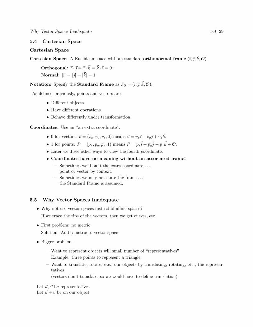
Let ~u, ~v be representativesLet ~u+ ~v be on our object
Summary of Geometric Spaces 5.5 30
~u~u + ~v
~v
Let T (~u) be translation by ~t defined as T (~u) = ~u+ ~t.Then
T (~u+ ~v) = ~u+ ~v + ~t
6= T (~u) + T (~v)
= ~u+ ~v + 2~t
Note: this definition of translation only used on this slide! Normally, translation isidentity on vectors!
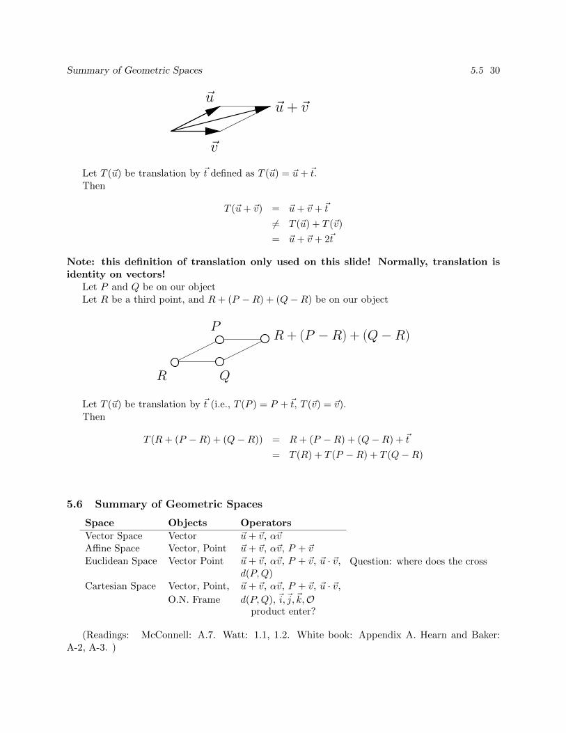
Let P and Q be on our objectLet R be a third point, and R+ (P −R) + (Q−R) be on our object
QR
PR + (P −R) + (Q−R)
Let T (~u) be translation by ~t (i.e., T (P ) = P + ~t, T (~v) = ~v).Then
T (R+ (P −R) + (Q−R)) = R+ (P −R) + (Q−R) + ~t
= T (R) + T (P −R) + T (Q−R)
5.6 Summary of Geometric Spaces
Space Objects Operators
Vector Space Vector ~u+ ~v, α~vAffine Space Vector, Point ~u+ ~v, α~v, P + ~vEuclidean Space Vector Point ~u+ ~v, α~v, P + ~v, ~u · ~v,
d(P,Q)Cartesian Space Vector, Point, ~u+ ~v, α~v, P + ~v, ~u · ~v,
O.N. Frame d(P,Q), ~i,~j,~k,O
Question: where does the cross
product enter?
(Readings: McConnell: A.7. Watt: 1.1, 1.2. White book: Appendix A. Hearn and Baker:A-2, A-3. )

6 AFFINE GEOMETRY AND TRANSFORMATIONS 31
6 Affine Geometry and Transformations
6.1 Linear Combinations
Linear Combinations
Vectors:V = ~u, ~u+ ~v, α~u
By Extension: ∑i
αi~ui (no restriction on αi)
Linear Transformations:
T (~u+ ~v) = T (~u) + T (~v), T (α~u) = αT (~u)
By Extension:
T (∑i
αi~ui) =∑i
αiT (~ui)
Points:P = P, P + ~u = Q
By Extension...
6.2 Affine Combinations
Affine Combinations
Define Point Subtraction:
Q− P means ~v ∈ V such that Q = P + ~v for P,Q ∈ P.
By Extension: ∑αiPi is a vector iff
∑αi = 0
Define Point Blending:
Q = (1− a)Q1 + aQ2 means Q = Q1 + a(Q2 −Q1) with Q ∈ P
Alternatively:
we may write Q = a1Q1 + a2Q2 where a1 + a2 = 1.
By Extension: ∑aiPi is a point iff
∑ai = 1
Geometrically:
Affine Transformations 6.2 32
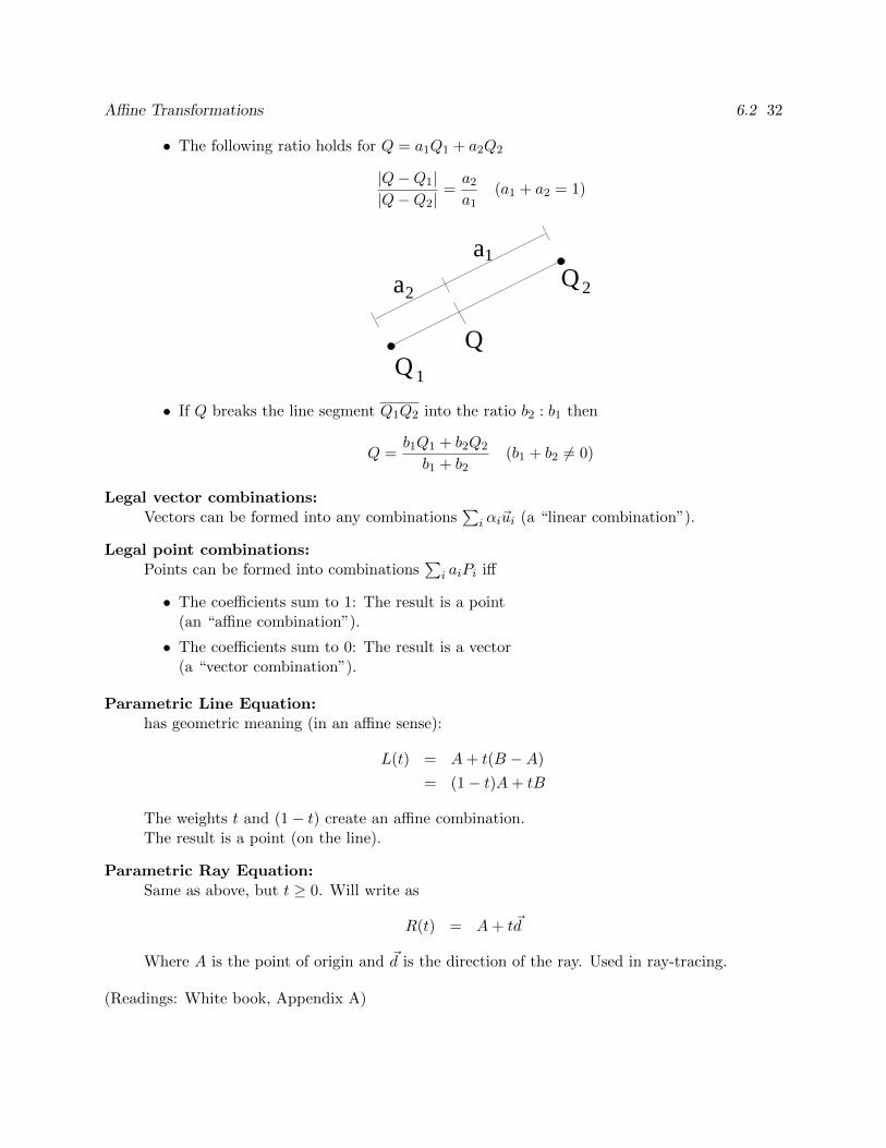
• The following ratio holds for Q = a1Q1 + a2Q2
|Q−Q1||Q−Q2|
=a2
a1(a1 + a2 = 1)
a
a1
Q 1
Q 22
Q
• If Q breaks the line segment Q1Q2 into the ratio b2 : b1 then
Q =b1Q1 + b2Q2
b1 + b2(b1 + b2 6= 0)
Legal vector combinations:Vectors can be formed into any combinations
∑i αi~ui (a “linear combination”).
Legal point combinations:Points can be formed into combinations
∑i aiPi iff
• The coefficients sum to 1: The result is a point(an “affine combination”).
• The coefficients sum to 0: The result is a vector(a “vector combination”).
Parametric Line Equation:has geometric meaning (in an affine sense):
L(t) = A+ t(B −A)
= (1− t)A+ tB
The weights t and (1− t) create an affine combination.The result is a point (on the line).
Parametric Ray Equation:Same as above, but t ≥ 0. Will write as
R(t) = A+ t~d
Where A is the point of origin and ~d is the direction of the ray. Used in ray-tracing.
(Readings: White book, Appendix A)
Affine Transformations 6.2 33
6.3 Affine Transformations
Affine Transformations
Let T : A1 7−→ A2, where A1 and A2 are affine spaces.
Then T is said to be an affine transformation if:
• T maps vectors to vectors and points to points
• T is a linear transformation on the vectors
• T (P + ~u) = T (P ) + T (~u)
By Extension:
T preserves affine combinations on the points:
T (a1Q1 + · · ·+ anQn) = a1T (Q1) + · · ·+ anT (Qn),
If∑ai = 1, result is a point.
If∑ai = 0, result is a vector.
Affine vs Linear
Which is a larger class of transformations: Affine or Linear?
• All affine transformations are linear transformations on vectors.
• Consider identity transformation on vectors.
There is one such linear transformation.
• Consider Translations:
– Identity transformation on vectors
– Infinite number different ones (based on effect on points)
Thus, there are an infinite number of affine transformations that are identity transformationon vectors.
• What makes affine transformations a bigger class than linear transformation is their transla-tional behaviour on points.
Extending Affine Transformations to Vectors
Suppose we only have T defined on points.
Define T (~v) as follows:
• There exist points Q and R such that ~v = Q−R.
• Define T (~v) to be T (Q)− T (R).
Matrix Representation of Transformations 6.3 34
Note that Q and R are not unique.
The definition works for P + ~v:
T (P + ~v) = T (P +Q−R)
= T (P ) + T (Q)− T (R)
= T (P ) + T (~v)
Can now show that the definition is well defined.
Theorem: Affine transformations map parallel lines to parallel lines.
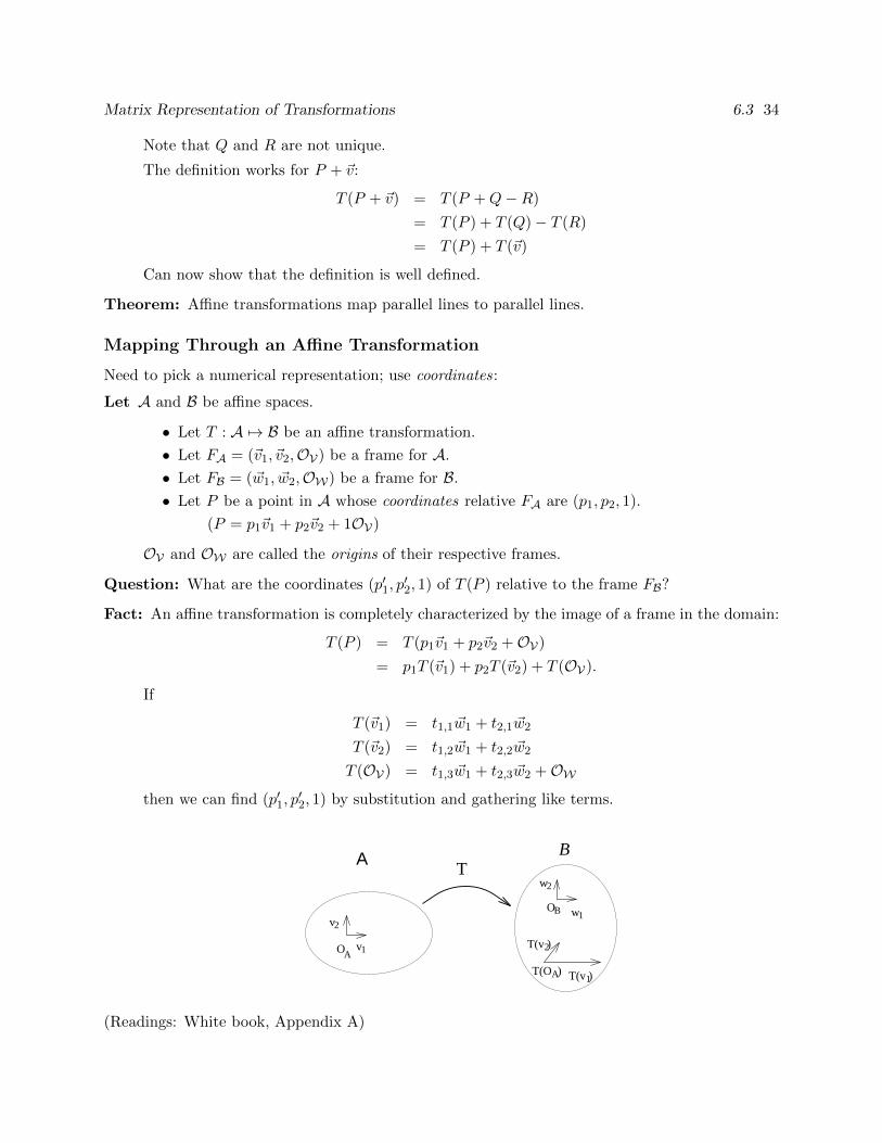
Mapping Through an Affine Transformation
Need to pick a numerical representation; use coordinates:
Let A and B be affine spaces.
• Let T : A 7→ B be an affine transformation.
• Let FA = (~v1, ~v2,OV) be a frame for A.
• Let FB = (~w1, ~w2,OW) be a frame for B.
• Let P be a point in A whose coordinates relative FA are (p1, p2, 1).
(P = p1~v1 + p2~v2 + 1OV)
OV and OW are called the origins of their respective frames.
Question: What are the coordinates (p′1, p′2, 1) of T (P ) relative to the frame FB?
Fact: An affine transformation is completely characterized by the image of a frame in the domain:
T (P ) = T (p1~v1 + p2~v2 +OV)
= p1T (~v1) + p2T (~v2) + T (OV).
If
T (~v1) = t1,1 ~w1 + t2,1 ~w2
T (~v2) = t1,2 ~w1 + t2,2 ~w2
T (OV) = t1,3 ~w1 + t2,3 ~w2 +OWthen we can find (p′1, p
′2, 1) by substitution and gathering like terms.
2
v1OA
BO w1
w2
v
TΑ B
T(v )2
T(v )1T(O )A
(Readings: White book, Appendix A)
Geometric Transformations 6.4 35
6.4 Matrix Representation of Transformations
Matrix Representation of Transformations
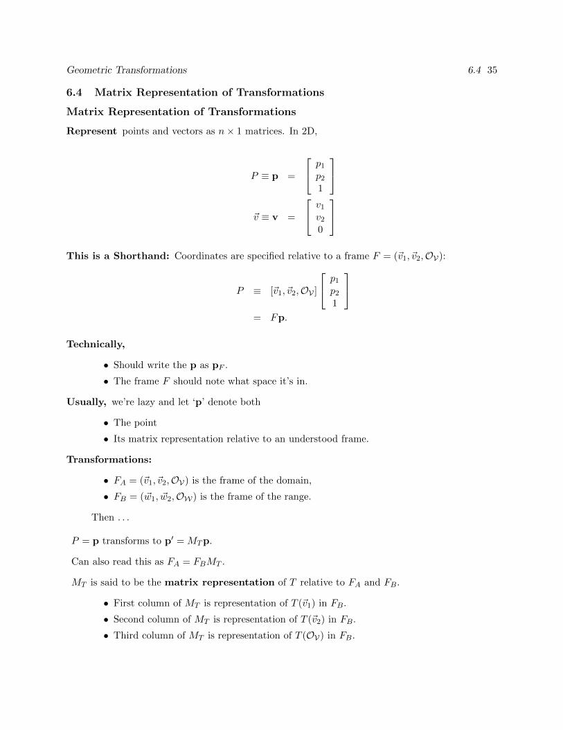
Represent points and vectors as n× 1 matrices. In 2D,
P ≡ p =
p1
p2
1
~v ≡ v =
v1
v2
0
This is a Shorthand: Coordinates are specified relative to a frame F = (~v1, ~v2,OV):
P ≡ [~v1, ~v2,OV ]
p1
p2
1
= Fp.
Technically,
• Should write the p as pF .
• The frame F should note what space it’s in.
Usually, we’re lazy and let ‘p’ denote both
• The point
• Its matrix representation relative to an understood frame.
Transformations:
• FA = (~v1, ~v2,OV) is the frame of the domain,
• FB = (~w1, ~w2,OW) is the frame of the range.
Then . . .
P = p transforms to p′ = MTp.
Can also read this as FA = FBMT .
MT is said to be the matrix representation of T relative to FA and FB.
• First column of MT is representation of T (~v1) in FB.
• Second column of MT is representation of T (~v2) in FB.
• Third column of MT is representation of T (OV) in FB.
Geometric Transformations 6.4 36
6.5 Geometric Transformations
Geometric Transformations
Construct matrices for simple geometric transformations.
Combine simple transformations into more complex ones.
• Assume that the range and domain frames are the Standard Frame.
• Will begin with 2D, generalize later.
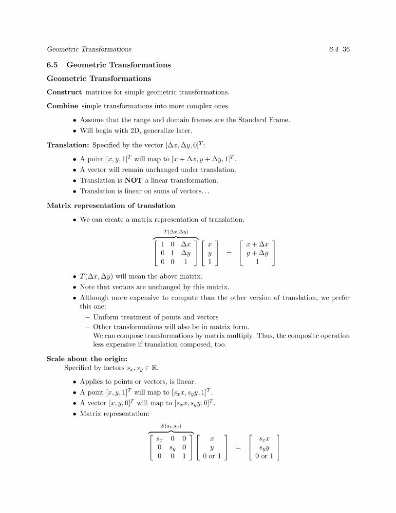
Translation: Specified by the vector [∆x,∆y, 0]T :
• A point [x, y, 1]T will map to [x+ ∆x, y + ∆y, 1]T .
• A vector will remain unchanged under translation.
• Translation is NOT a linear transformation.
• Translation is linear on sums of vectors. . .
Matrix representation of translation
• We can create a matrix representation of translation:
T (∆x,∆y)︷ ︸︸ ︷ 1 0 ∆x0 1 ∆y0 0 1
xy1
=
x+ ∆xy + ∆y
1
• T (∆x,∆y) will mean the above matrix.
• Note that vectors are unchanged by this matrix.
• Although more expensive to compute than the other version of translation, we preferthis one:
– Uniform treatment of points and vectors
– Other transformations will also be in matrix form.We can compose transformations by matrix multiply. Thus, the composite operationless expensive if translation composed, too.
Scale about the origin:Specified by factors sx, sy ∈ R.
• Applies to points or vectors, is linear.
• A point [x, y, 1]T will map to [sxx, syy, 1]T .
• A vector [x, y, 0]T will map to [sxx, syy, 0]T .
• Matrix representation:
S(sx,sy)︷ ︸︸ ︷ sx 0 00 sy 00 0 1
xy
0 or 1
=
sxxsyy
0 or 1
Compositions of Transformations 6.5 37
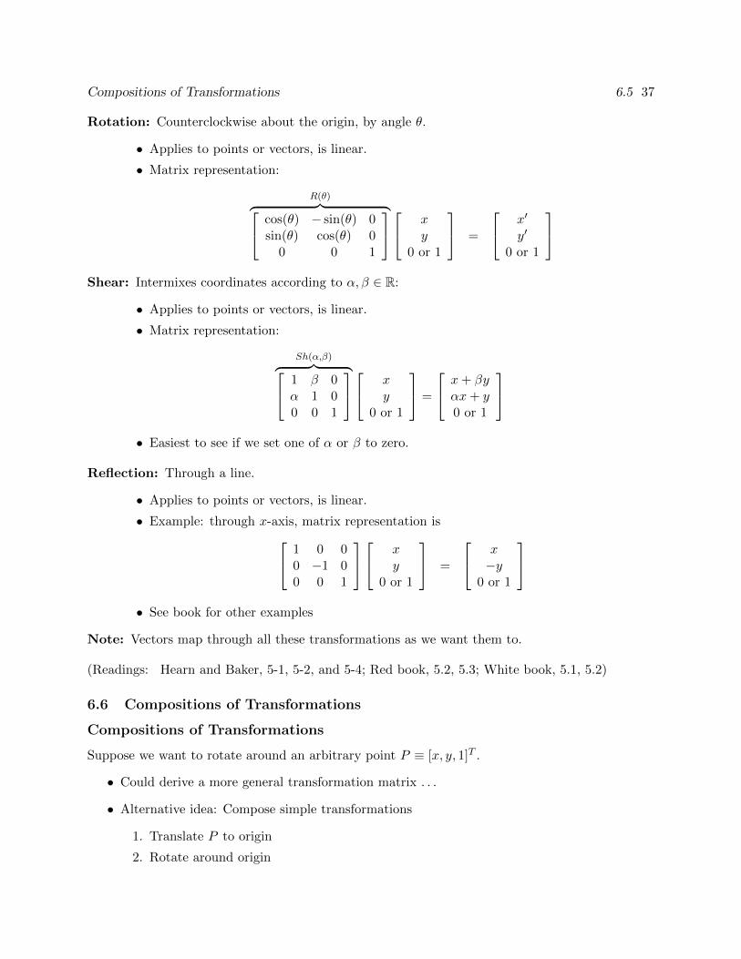
Rotation: Counterclockwise about the origin, by angle θ.
• Applies to points or vectors, is linear.
• Matrix representation:
R(θ)︷ ︸︸ ︷ cos(θ) − sin(θ) 0sin(θ) cos(θ) 0
0 0 1
xy
0 or 1
=
x′
y′
0 or 1
Shear: Intermixes coordinates according to α, β ∈ R:
• Applies to points or vectors, is linear.
• Matrix representation:
Sh(α,β)︷ ︸︸ ︷ 1 β 0α 1 00 0 1
xy
0 or 1
=
x+ βyαx+ y0 or 1
• Easiest to see if we set one of α or β to zero.
Reflection: Through a line.
• Applies to points or vectors, is linear.
• Example: through x-axis, matrix representation is 1 0 00 −1 00 0 1
xy
0 or 1
=
x−y
0 or 1
• See book for other examples
Note: Vectors map through all these transformations as we want them to.
(Readings: Hearn and Baker, 5-1, 5-2, and 5-4; Red book, 5.2, 5.3; White book, 5.1, 5.2)
6.6 Compositions of Transformations
Compositions of Transformations
Suppose we want to rotate around an arbitrary point P ≡ [x, y, 1]T .
• Could derive a more general transformation matrix . . .
• Alternative idea: Compose simple transformations
1. Translate P to origin
2. Rotate around origin
Change of Basis 6.6 38
3. Translate origin back to P
• Suppose P = [xo, yo, 1]T
• The the desired transformation is
T (xo, yo) R(θ) T (−xo,−yo)
=
1 0 xo0 1 yo0 0 1
cos(θ) − sin(θ) 0
sin(θ) cos(θ) 00 0 1
1 0 −xo
0 1 −yo0 0 1
=
cos(θ) − sin(θ) xo(1− cos(θ)) + yo sin(θ)sin(θ) cos(θ) yo(1− cos(θ))− xo sin(θ)
0 0 1
• Note where P maps: to P .
• Won’t compute these matrices analytically;Just use the basic transformations,and run the matrix multiply numerically.
Order is important!
T (−∆x,−∆y) T (∆x,∆y) R(θ) = R(θ)
6= T (−∆x,−∆y) R(θ) T (∆x,∆y).
(Readings: McConnell, 3.1.6; Hearn and Baker, Section 5-3; Red book, 5.4; White book, 5.3 )
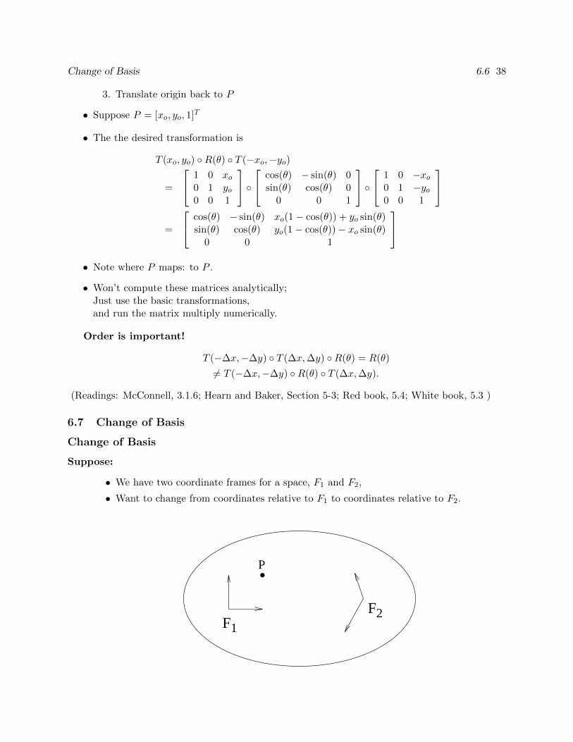
6.7 Change of Basis
Change of Basis
Suppose:
• We have two coordinate frames for a space, F1 and F2,
• Want to change from coordinates relative to F1 to coordinates relative to F2.
1
F2F
P
Change of Basis 6.6 39
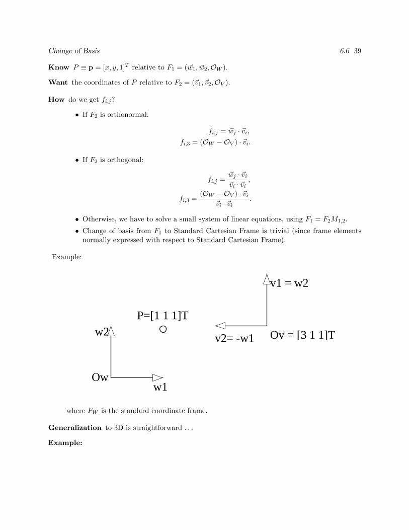
Know P ≡ p = [x, y, 1]T relative to F1 = (~w1, ~w2,OW ).
Want the coordinates of P relative to F2 = (~v1, ~v2,OV ).
How do we get fi,j?
• If F2 is orthonormal:
fi,j = ~wj · ~vi,fi,3 = (OW −OV ) · ~vi.
• If F2 is orthogonal:
fi,j =~wj · ~vi~vi · ~vi
,
fi,3 =(OW −OV ) · ~vi
~vi · ~vi.
• Otherwise, we have to solve a small system of linear equations, using F1 = F2M1,2.
• Change of basis from F1 to Standard Cartesian Frame is trivial (since frame elementsnormally expressed with respect to Standard Cartesian Frame).
Example:
v1 = w2
v2= -w1
Ow
Ov = [3 1 1]T
P=[1 1 1]T
w1
w2
where FW is the standard coordinate frame.
Generalization to 3D is straightforward . . .
Example:
Ambiguity 6.7 40
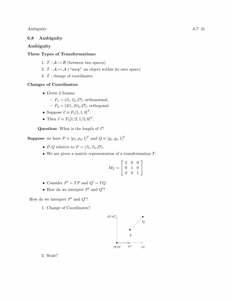
• Define two frames:
FW = (~w1, ~w2, ~w3,OW )
=
1000
,
0100
,
0010
,
0001
FV = (~v1, ~v2, ~v3,OV )
=
√
2/2√2/200
,
0010
,√
2/2
−√
2/200
,
1031
• All coordinates are specified relative to the standard frame in a Cartesian 3 space.
• In this example, FW is the standard frame.
• Note that both FW and FV are orthonormal.
• The matrix mapping FW to FV is given by
M =
√
2/2√
2/2 0 −√
2/20 0 1 −3√2/2 −
√2/2 0 −
√2/2
0 0 0 1
• Question: What is the matrix mapping from FV to FW ?
Notes
• On the computer, frame elements usually specified in Standard Frame for space.
Eg, a frame F = [~v1, ~v2, OV ] is given by
[ [v1x, v1y, 0]T , [v2x, v2y, 0]T , [v3x, v3y, 1]T ]
relative to Standard Frame.
Question: What are coordinates of these basis elements relative to F?
• Frames are usually orthonormal.
• A point “mapped” by a change of basis does not change;
We have merely expressed its coordinates relative to a different frame.
(Readings: Watt: 1.1.1. Hearn and Baker: Section 5-5 (not as general as here, though). Redbook: 5.9. White book: 5.8.)
Ambiguity 6.7 41
6.8 Ambiguity
Ambiguity
Three Types of Transformations:
1. T : A 7→ B (between two spaces)
2. T : A 7→ A (“warp” an object within its own space)
3. T : change of coordinates
Changes of Coordinates:
• Given 2 frames:
– F1 = (~v1, ~v2,O), orthonormal,
– F2 = (2~v1, 2~v2,O), orthogonal.
• Suppose ~v ≡ F1[1, 1, 0]T .
• Then ~v ≡ F2[1/2, 1/2, 0]T .
Question: What is the length of ~v?
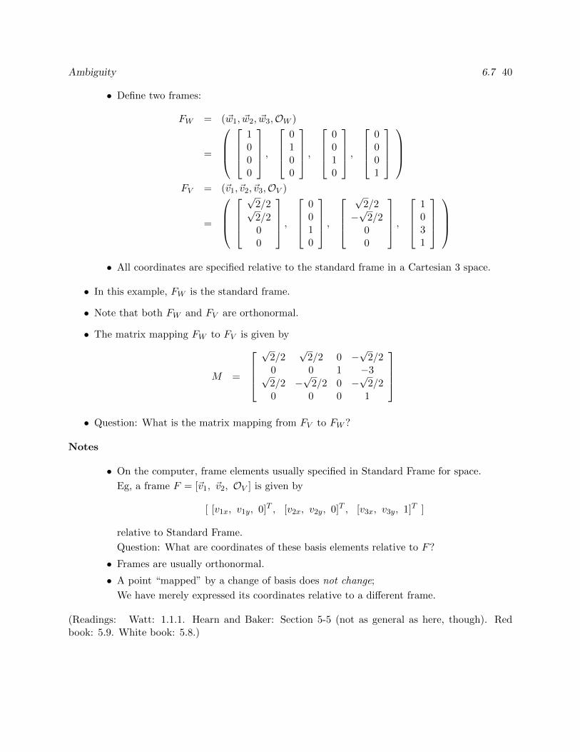
Suppose we have P ≡ [p1, p2, 1]T and Q ≡ [q1, q2, 1]T
• P,Q relative to F = (~v1, ~v2,O),
• We are given a matrix representation of a transformation T :
MT =
2 0 00 1 00 0 1
• Consider P ′ = TP and Q′ = TQ.
• How do we interpret P ′ and Q′?
How do we interpret P ′ and Q′?
1. Change of Coordinates?
v1O=O’ v1’
v2=v2’
P
Q
2. Scale?
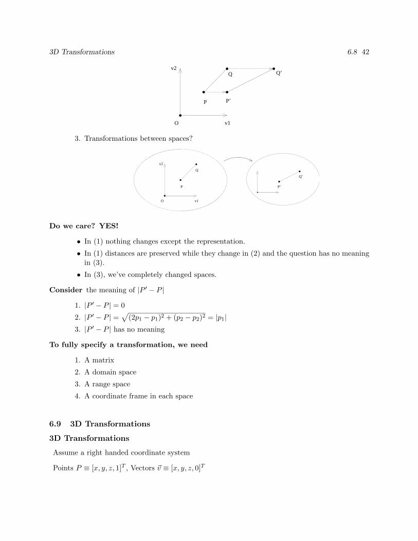
3D Transformations 6.8 42
Q
P
O v1
v2
P’
Q’
3. Transformations between spaces?
v1
P
Q
O
v2
P’
Q’
Do we care? YES!
• In (1) nothing changes except the representation.
• In (1) distances are preserved while they change in (2) and the question has no meaningin (3).
• In (3), we’ve completely changed spaces.
Consider the meaning of |P ′ − P |
1. |P ′ − P | = 0
2. |P ′ − P | =√
(2p1 − p1)2 + (p2 − p2)2 = |p1|3. |P ′ − P | has no meaning
To fully specify a transformation, we need
1. A matrix
2. A domain space
3. A range space
4. A coordinate frame in each space
6.9 3D Transformations
3D Transformations
Assume a right handed coordinate system
Points P ≡ [x, y, z, 1]T , Vectors ~v ≡ [x, y, z, 0]T
3D Transformations 6.8 43
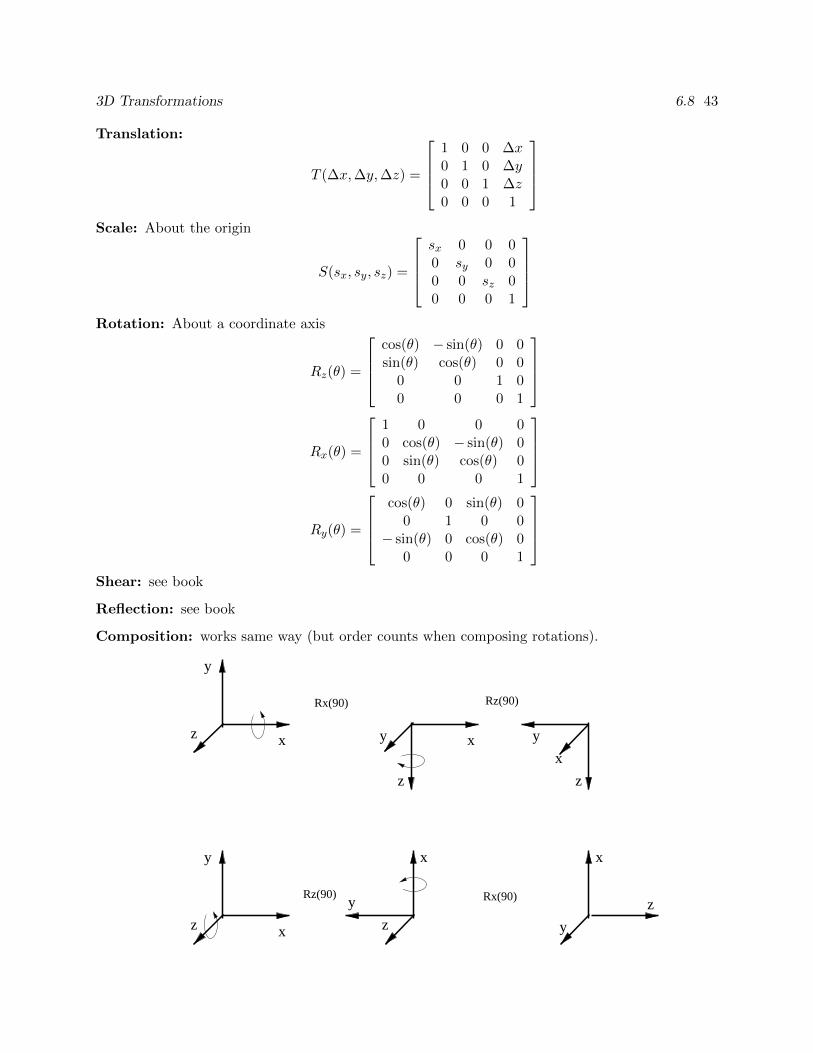
Translation:
T (∆x,∆y,∆z) =
1 0 0 ∆x0 1 0 ∆y0 0 1 ∆z0 0 0 1
Scale: About the origin
S(sx, sy, sz) =
sx 0 0 00 sy 0 00 0 sz 00 0 0 1
Rotation: About a coordinate axis
Rz(θ) =
cos(θ) − sin(θ) 0 0sin(θ) cos(θ) 0 0
0 0 1 00 0 0 1
Rx(θ) =
1 0 0 00 cos(θ) − sin(θ) 00 sin(θ) cos(θ) 00 0 0 1
Ry(θ) =
cos(θ) 0 sin(θ) 0
0 1 0 0− sin(θ) 0 cos(θ) 0
0 0 0 1
Shear: see book
Reflection: see book
Composition: works same way (but order counts when composing rotations).
xz
y
xz
y x
z
y
z
y
xxy
z
z
x
y
Rz(90)Rx(90)
Rx(90)Rz(90)
World and Viewing Frames 6.9 44
(Readings: McConnell 3.1; Hearn and Baker, Chapter 11; Red book, 5.7; White book, 5.6 )
6.10 World and Viewing Frames
World and Viewing Frames
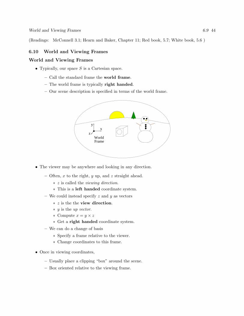
• Typically, our space S is a Cartesian space.
– Call the standard frame the world frame.
– The world frame is typically right handed.
– Our scene description is specified in terms of the world frame.
.....WorldFrame
zx
y
• The viewer may be anywhere and looking in any direction.
– Often, x to the right, y up, and z straight ahead.
∗ z is called the viewing direction.
∗ This is a left handed coordinate system.
– We could instead specify z and y as vectors
∗ z is the the view direction.
∗ y is the up vector.
∗ Compute x = y × z∗ Get a right handed coordinate system.
– We can do a change of basis
∗ Specify a frame relative to the viewer.
∗ Change coordinates to this frame.
• Once in viewing coordinates,
– Usually place a clipping “box” around the scene.
– Box oriented relative to the viewing frame.
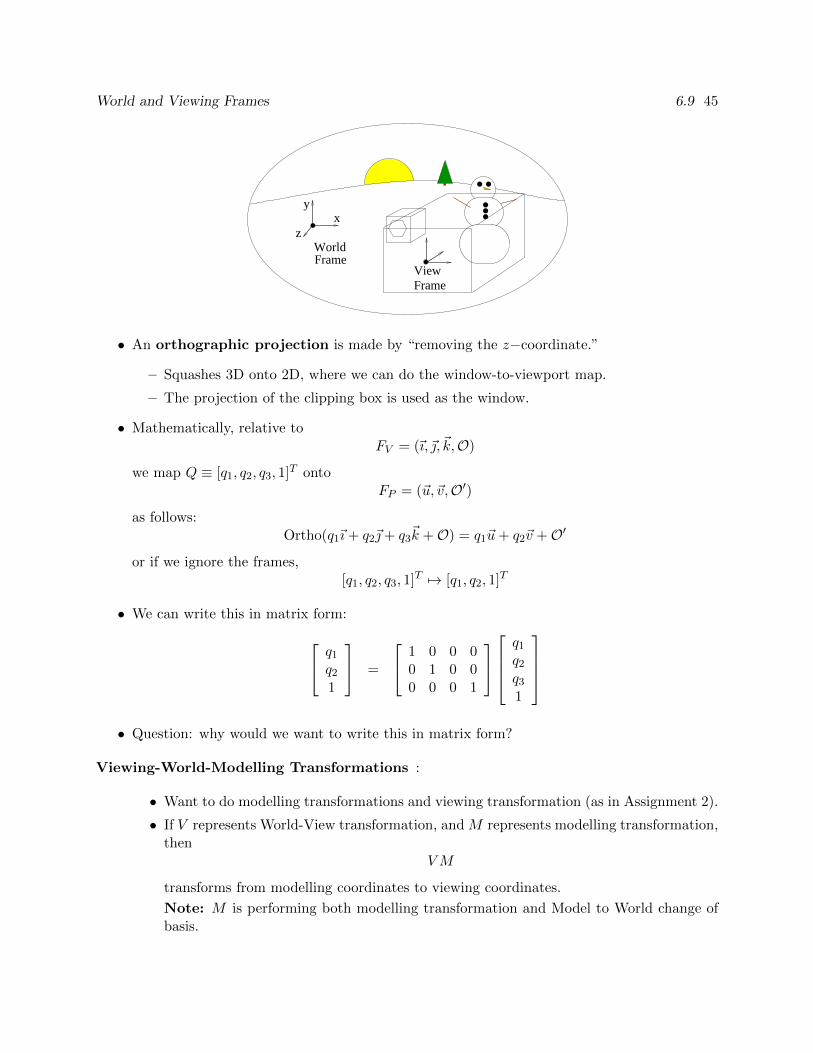
World and Viewing Frames 6.9 45
.....ViewFrame
WorldFrame
zx
y
• An orthographic projection is made by “removing the z−coordinate.”
– Squashes 3D onto 2D, where we can do the window-to-viewport map.
– The projection of the clipping box is used as the window.
• Mathematically, relative toFV = (~ı,~,~k,O)
we map Q ≡ [q1, q2, q3, 1]T ontoFP = (~u,~v,O′)
as follows:Ortho(q1~ı+ q2~+ q3
~k +O) = q1~u+ q2~v +O′
or if we ignore the frames,[q1, q2, q3, 1]T 7→ [q1, q2, 1]T
• We can write this in matrix form: q1
q2
1
=
1 0 0 00 1 0 00 0 0 1
q1
q2
q3
1
• Question: why would we want to write this in matrix form?
Viewing-World-Modelling Transformations :
• Want to do modelling transformations and viewing transformation (as in Assignment 2).
• If V represents World-View transformation, and M represents modelling transformation,then
VM
transforms from modelling coordinates to viewing coordinates.
Note: M is performing both modelling transformation and Model to World change ofbasis.
World and Viewing Frames 6.9 46
• Question: If we transform the viewing frame (relative to viewing frame) how do weadjust V ?
• Question: If we transform model (relative to modelling frame) how do we adjust M?
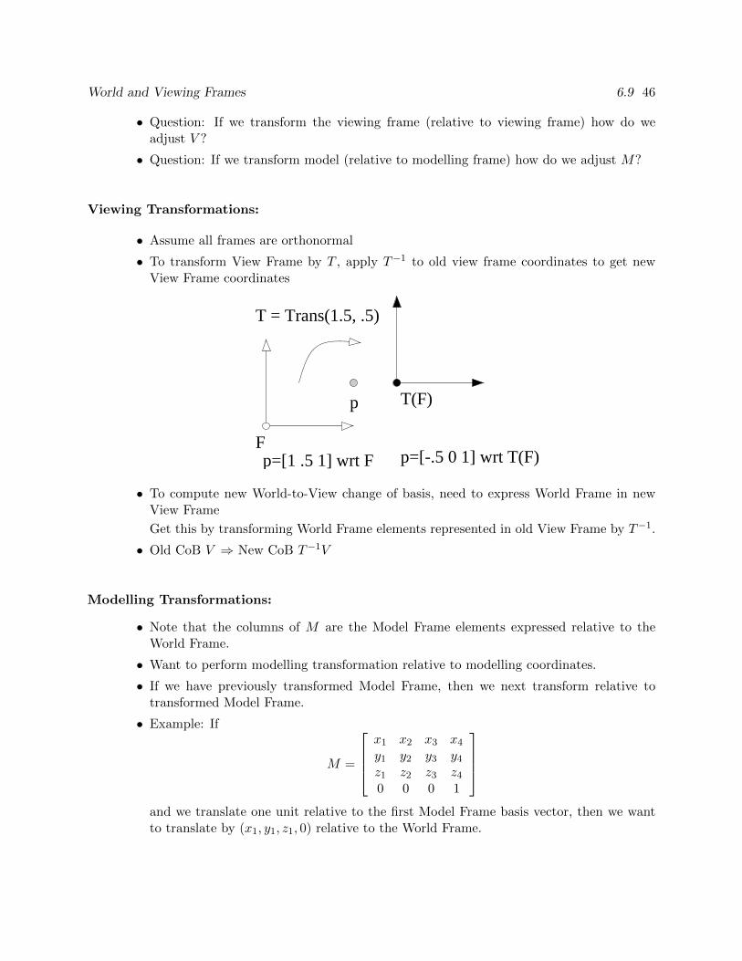
Viewing Transformations:
• Assume all frames are orthonormal
• To transform View Frame by T , apply T−1 to old view frame coordinates to get newView Frame coordinates
T = Trans(1.5, .5)
p
F
T(F)
p=[1 .5 1] wrt F p=[-.5 0 1] wrt T(F)
• To compute new World-to-View change of basis, need to express World Frame in newView Frame
Get this by transforming World Frame elements represented in old View Frame by T−1.
• Old CoB V ⇒ New CoB T−1V
Modelling Transformations:
• Note that the columns of M are the Model Frame elements expressed relative to theWorld Frame.
• Want to perform modelling transformation relative to modelling coordinates.
• If we have previously transformed Model Frame, then we next transform relative totransformed Model Frame.
• Example: If
M =
x1 x2 x3 x4
y1 y2 y3 y4
z1 z2 z3 z4
0 0 0 1
and we translate one unit relative to the first Model Frame basis vector, then we wantto translate by (x1, y1, z1, 0) relative to the World Frame.
Normals 6.10 47
• Could write this as
M ′ =
1 0 0 x1
0 1 0 y1
0 0 1 z1
0 0 0 1
·M =
x1 x2 x3 x4 + x1
y1 y2 y3 y4 + y1
z1 z2 z3 z4 + z1
0 0 0 1
• But this is also equal to
M ′ = M ·
1 0 0 10 1 0 00 0 1 00 0 0 1
=
x1 x2 x3 x4 + x1
y1 y2 y3 y4 + y1
z1 z2 z3 z4 + z1
0 0 0 1
• In general, if we want to transform by T our model relative to the current Model Frame,
thenMT
yields that transformation.• Summary:
Modelling transformations embodied in matrix M
World-to-View change of basis in matrix V
VM transforms from modelling coordinates to viewing coordinates
If we further transform the View Frame by T relative to the View Frame, then the newchange-of-basis matrix V ′ is given by
V ′ = T−1V
If we further transform the model by T relative to the modelling frame, the new modellingtransformation M ′ is given by
M ′ = MT
• For Assignment 2, need to do further dissection of transformations, but this is the basicidea.
(Readings: Hearn and Baker, Section 6-2, first part of Section 12-3; Red book, 6.7; White book,6.6 )
6.11 Normals
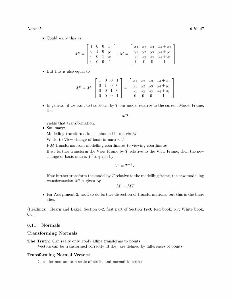
Transforming Normals
The Truth: Can really only apply affine transforms to points.Vectors can be transformed correctly iff they are defined by differences of points.
Transforming Normal Vectors:
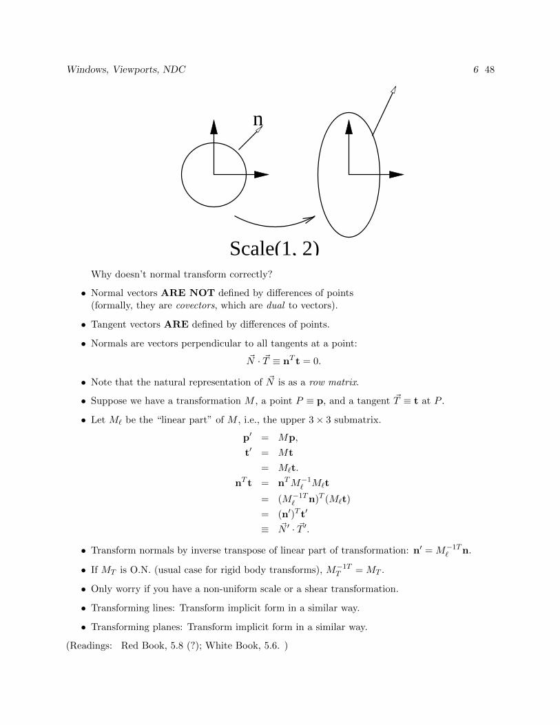
Consider non-uniform scale of circle, and normal to circle:
Windows, Viewports, NDC 6 48
n
Scale(1, 2)Why doesn’t normal transform correctly?
• Normal vectors ARE NOT defined by differences of points(formally, they are covectors, which are dual to vectors).
• Tangent vectors ARE defined by differences of points.
• Normals are vectors perpendicular to all tangents at a point:
~N · ~T ≡ nT t = 0.
• Note that the natural representation of ~N is as a row matrix.
• Suppose we have a transformation M , a point P ≡ p, and a tangent ~T ≡ t at P .
• Let M` be the “linear part” of M , i.e., the upper 3× 3 submatrix.
p′ = Mp,
t′ = Mt
= M`t.
nT t = nTM−1` M`t
= (M−1T` n)T (M`t)
= (n′)T t′
≡ ~N ′ · ~T ′.
• Transform normals by inverse transpose of linear part of transformation: n′ = M−1T` n.
• If MT is O.N. (usual case for rigid body transforms), M−1TT = MT .
• Only worry if you have a non-uniform scale or a shear transformation.
• Transforming lines: Transform implicit form in a similar way.
• Transforming planes: Transform implicit form in a similar way.
(Readings: Red Book, 5.8 (?); White Book, 5.6. )
7 WINDOWS, VIEWPORTS, NDC 49
7 Windows, Viewports, NDC
7.1 Window to Viewport Mapping
Window to Viewport Mapping
• Start with 3D scene, but eventually project to 2D scene
• 2D scene is infinite plane. Device has a finite visible rectangle.What do we do?
• Answer: map rectangular region of 2D device scene to device.
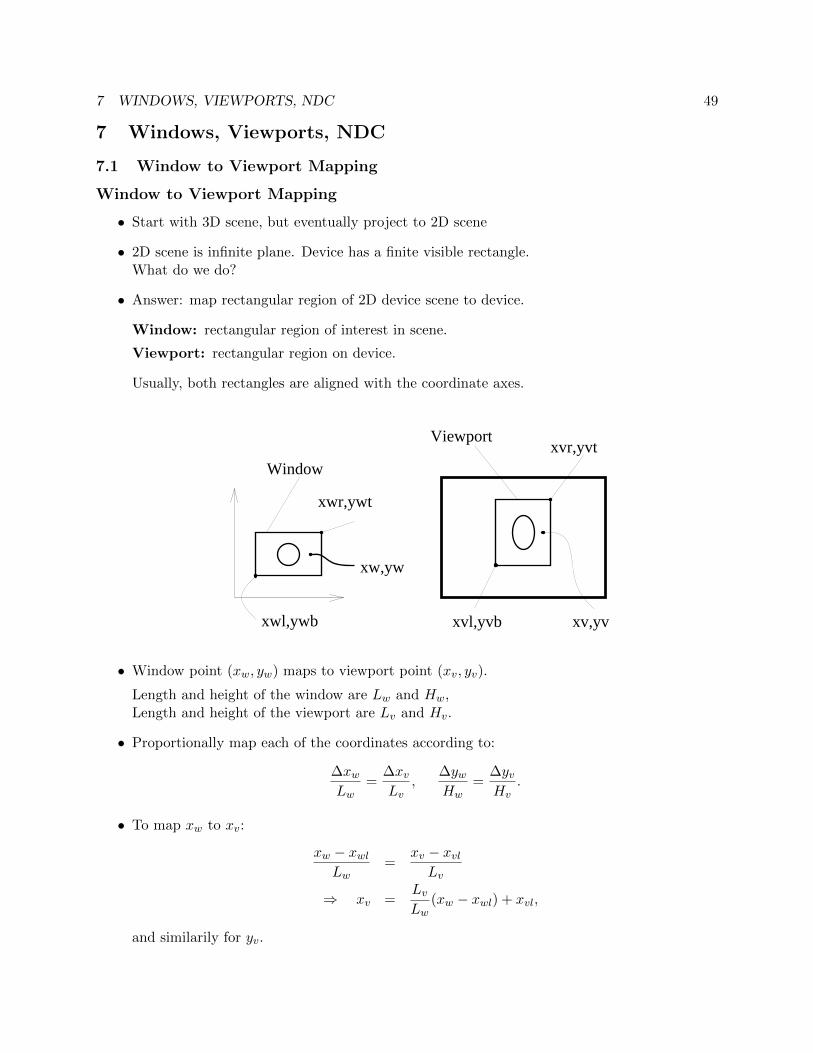
Window: rectangular region of interest in scene.
Viewport: rectangular region on device.
Usually, both rectangles are aligned with the coordinate axes.
xw,yw
xwr,ywt
xwl,ywb xvl,yvb xv,yv
xvr,yvtWindow
Viewport
• Window point (xw, yw) maps to viewport point (xv, yv).
Length and height of the window are Lw and Hw,Length and height of the viewport are Lv and Hv.
• Proportionally map each of the coordinates according to:
∆xwLw
=∆xvLv
,∆ywHw
=∆yvHv
.
• To map xw to xv:
xw − xwlLw
=xv − xvlLv
⇒ xv =LvLw
(xw − xwl) + xvl,
and similarily for yv.
Normalized Device Coordinates 7.1 50
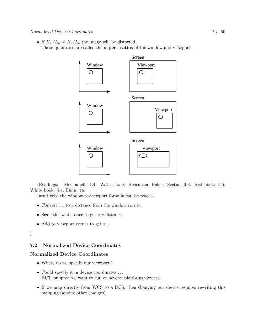
• If Hw/Lw 6= Hv/Lv the image will be distorted.These quantities are called the aspect ratios of the window and viewport.
Viewport
Viewport
Screen
Window
Viewport
Screen
Window
Screen
Window
(Readings: McConnell: 1.4. Watt: none. Hearn and Baker: Section 6-3. Red book: 5.5.White book: 5.4, Blinn: 16.
Intuitively, the window-to-viewport formula can be read as:
• Convert xw to a distance from the window corner.
• Scale this w distance to get a v distance.
• Add to viewport corner to get xv.
)
7.2 Normalized Device Coordinates
Normalized Device Coordinates
• Where do we specify our viewport?
• Could specify it in device coordinates . . .BUT, suppose we want to run on several platforms/devices
• If we map directly from WCS to a DCS, then changing our device requires rewriting thismapping (among other changes).
Clipping 7 51
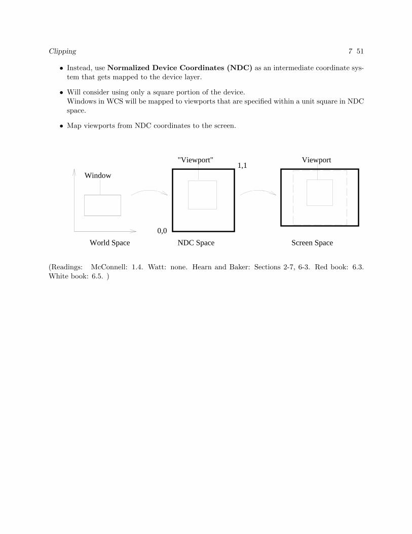
• Instead, use Normalized Device Coordinates (NDC) as an intermediate coordinate sys-tem that gets mapped to the device layer.
• Will consider using only a square portion of the device.Windows in WCS will be mapped to viewports that are specified within a unit square in NDCspace.
• Map viewports from NDC coordinates to the screen.
Window
World Space NDC Space Screen Space
0,0
1,1Viewport"Viewport"
(Readings: McConnell: 1.4. Watt: none. Hearn and Baker: Sections 2-7, 6-3. Red book: 6.3.White book: 6.5. )

Clipping 7 52
8 CLIPPING 53
8 Clipping
8.1 Clipping
Clipping
Clipping: Remove points outside a region of interest.
• Discard (parts of) primitives outside our window. . .
Point clipping: Remove points outside window.
• A point is either entirely inside the region or not.
Line clipping: Remove portion of line segment outside window.
• Line segments can straddle the region boundary.
• Liang-Barsky algorithm efficiently clips line segments to a halfspace.
• Halfspaces can be combined to bound a convex region.
• Can use some of the ideas in Liang-Barsky to clip points.
Parametric representation of line:
L(t) = (1− t)A+ tB
or equivalentlyL(t) = A+ t(B −A)
• A and B are non-coincident points.
• For t ∈ R, L(t) defines an infinite line.
• For t ∈ [0, 1], L(t) defines a line segment from A to B.
• Good for generating points on a line.
• Not so good for testing if a given point is on a line.
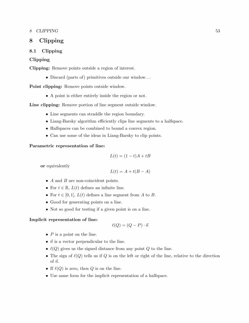
Implicit representation of line:`(Q) = (Q− P ) · ~n
• P is a point on the line.
• ~n is a vector perpendicular to the line.
• `(Q) gives us the signed distance from any point Q to the line.
• The sign of `(Q) tells us if Q is on the left or right of the line, relative to the directionof ~n.
• If `(Q) is zero, then Q is on the line.
• Use same form for the implicit representation of a halfspace.
Clipping 8.0 54
n
P
Q
Clipping a point to a halfspace:
• Represent window edge as implicit line/halfspace.
• Use the implicit form of edge to classify a point Q.
• Must choose a convention for the normal:points to the inside.
• Check the sign of `(Q):
– If `(Q) > 0, then Q is inside.
– Otherwise clip (discard) Q:It is on the edge or outside.May want to keep things on the boundary.
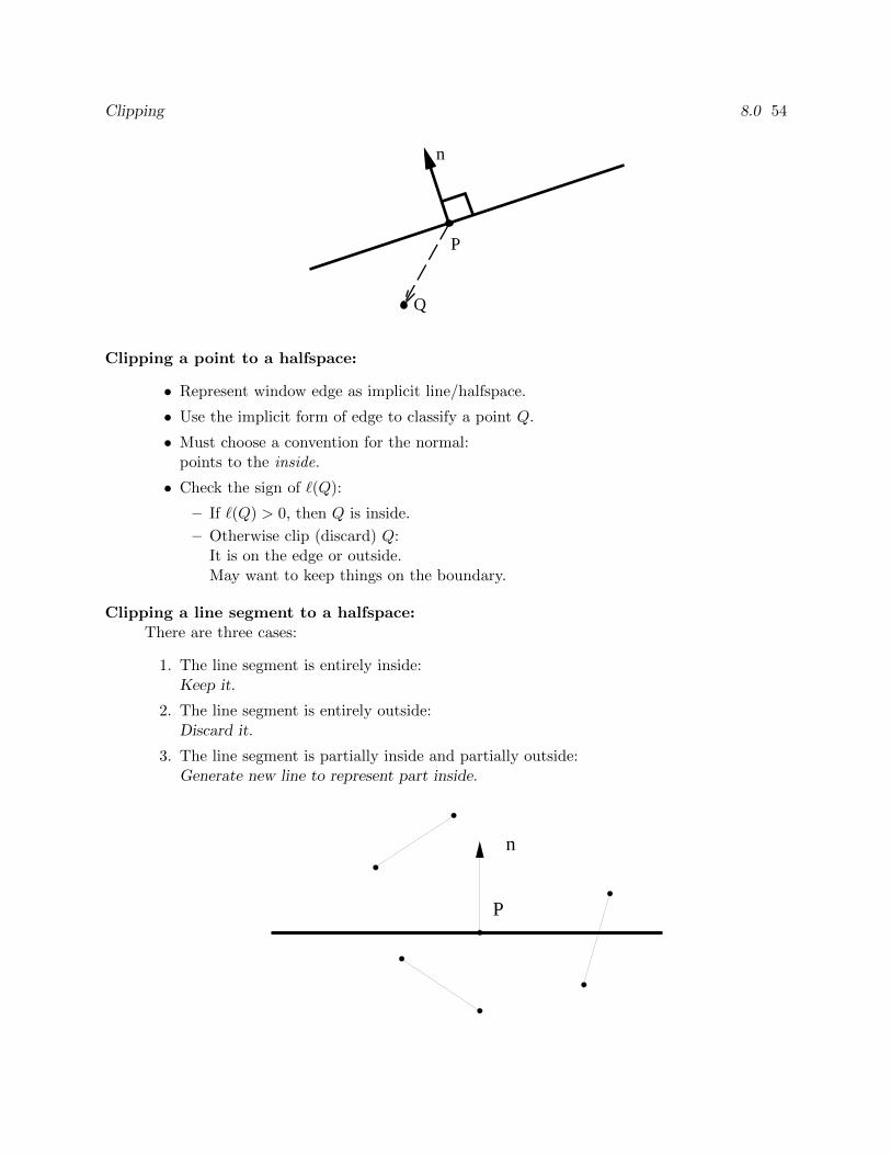
Clipping a line segment to a halfspace:There are three cases:
1. The line segment is entirely inside:Keep it.
2. The line segment is entirely outside:Discard it.
3. The line segment is partially inside and partially outside:Generate new line to represent part inside.
n
P
Clipping 8.0 55
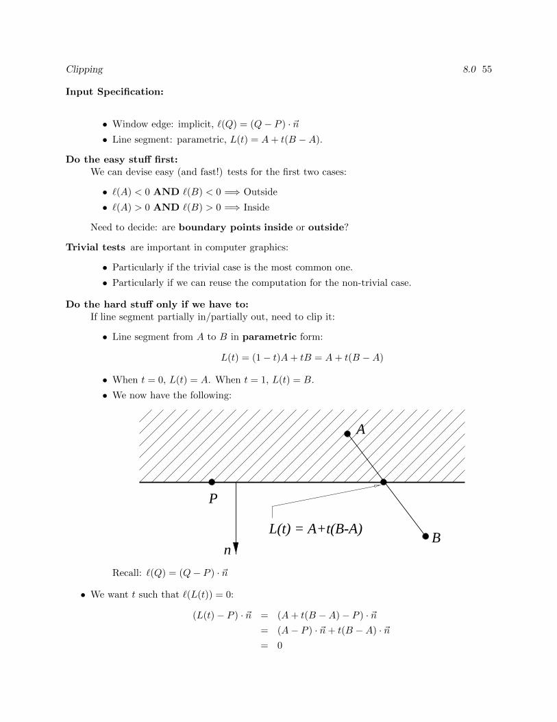
Input Specification:
• Window edge: implicit, `(Q) = (Q− P ) · ~n• Line segment: parametric, L(t) = A+ t(B −A).
Do the easy stuff first:We can devise easy (and fast!) tests for the first two cases:
• `(A) < 0 AND `(B) < 0 =⇒ Outside
• `(A) > 0 AND `(B) > 0 =⇒ Inside
Need to decide: are boundary points inside or outside?
Trivial tests are important in computer graphics:
• Particularly if the trivial case is the most common one.
• Particularly if we can reuse the computation for the non-trivial case.
Do the hard stuff only if we have to:If line segment partially in/partially out, need to clip it:
• Line segment from A to B in parametric form:
L(t) = (1− t)A+ tB = A+ t(B −A)
• When t = 0, L(t) = A. When t = 1, L(t) = B.
• We now have the following:
L(t) = A+t(B-A)
P
A
Bn
Recall: `(Q) = (Q− P ) · ~n
• We want t such that `(L(t)) = 0:
(L(t)− P ) · ~n = (A+ t(B −A)− P ) · ~n= (A− P ) · ~n+ t(B −A) · ~n= 0
Projections and Projective Transformations 8 56
• Solving for t gives us
t =(A− P ) · ~n(A−B) · ~n
• NOTE:The values we use for our simple test can be reused to compute t:
t =(A− P ) · ~n
(A− P ) · ~n− (B − P ) · ~n
Clipping a line segment to a window:Just clip to each of four halfspaces in turn.
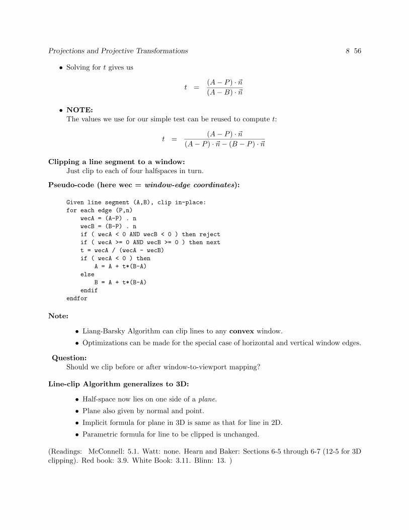
Pseudo-code (here wec = window-edge coordinates):
Given line segment (A,B), clip in-place:
for each edge (P,n)
wecA = (A-P) . n
wecB = (B-P) . n
if ( wecA < 0 AND wecB < 0 ) then reject
if ( wecA >= 0 AND wecB >= 0 ) then next
t = wecA / (wecA - wecB)
if ( wecA < 0 ) then
A = A + t*(B-A)
else
B = A + t*(B-A)
endif
endfor
Note:
• Liang-Barsky Algorithm can clip lines to any convex window.
• Optimizations can be made for the special case of horizontal and vertical window edges.
Question:Should we clip before or after window-to-viewport mapping?
Line-clip Algorithm generalizes to 3D:
• Half-space now lies on one side of a plane.
• Plane also given by normal and point.
• Implicit formula for plane in 3D is same as that for line in 2D.
• Parametric formula for line to be clipped is unchanged.
(Readings: McConnell: 5.1. Watt: none. Hearn and Baker: Sections 6-5 through 6-7 (12-5 for 3Dclipping). Red book: 3.9. White Book: 3.11. Blinn: 13. )
9 PROJECTIONS AND PROJECTIVE TRANSFORMATIONS 57
9 Projections and Projective Transformations
9.1 Projections
Projections
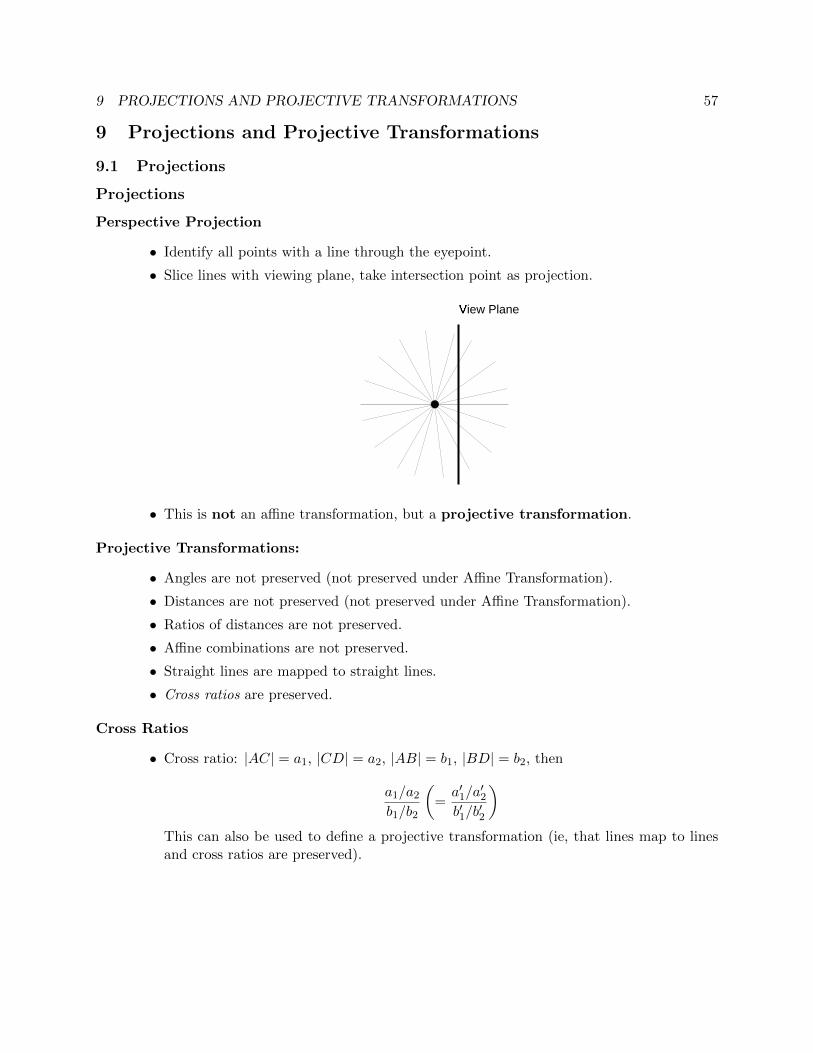
Perspective Projection
• Identify all points with a line through the eyepoint.
• Slice lines with viewing plane, take intersection point as projection.
View Plane
• This is not an affine transformation, but a projective transformation.
Projective Transformations:
• Angles are not preserved (not preserved under Affine Transformation).
• Distances are not preserved (not preserved under Affine Transformation).
• Ratios of distances are not preserved.
• Affine combinations are not preserved.
• Straight lines are mapped to straight lines.
• Cross ratios are preserved.
Cross Ratios
• Cross ratio: |AC| = a1, |CD| = a2, |AB| = b1, |BD| = b2, then
a1/a2
b1/b2
(=a′1/a
′2
b′1/b′2
)This can also be used to define a projective transformation (ie, that lines map to linesand cross ratios are preserved).
Projections 9.0 58
AB
C
D
a1
b1
a 2
b 2
2A’B’
C’
D’
1a’
a’
2b’
1b’
P
Comparison:Affine Transformations Projective TransformationsImage of 2 points on a line Image of 3 points on a linedetermine image of line determine image of lineImage of 3 points on a plane Image of 4 points on a planedetermine image of plane determine image of planeIn dimension n space, In dimension n space,image of n+ 1 points/vectors image of n+ 2 points/vectorsdefines affine map. defines projective map.Vectors map to vectors Mapping of vector is ill-defined~v = Q−R = R− S ⇒ ~v = Q−R = R− S but
A(Q)−A(R) = A(R)−A(S) P (Q)− P (R) 6= P (R)− P (S)
Q
R
SA
A(R)
A(Q)
A(S)
Q
R
S
P(Q)
P(R)
P(S)P
Can represent with matrix multiply Can represent with matrix multiply(sort of) and normalization
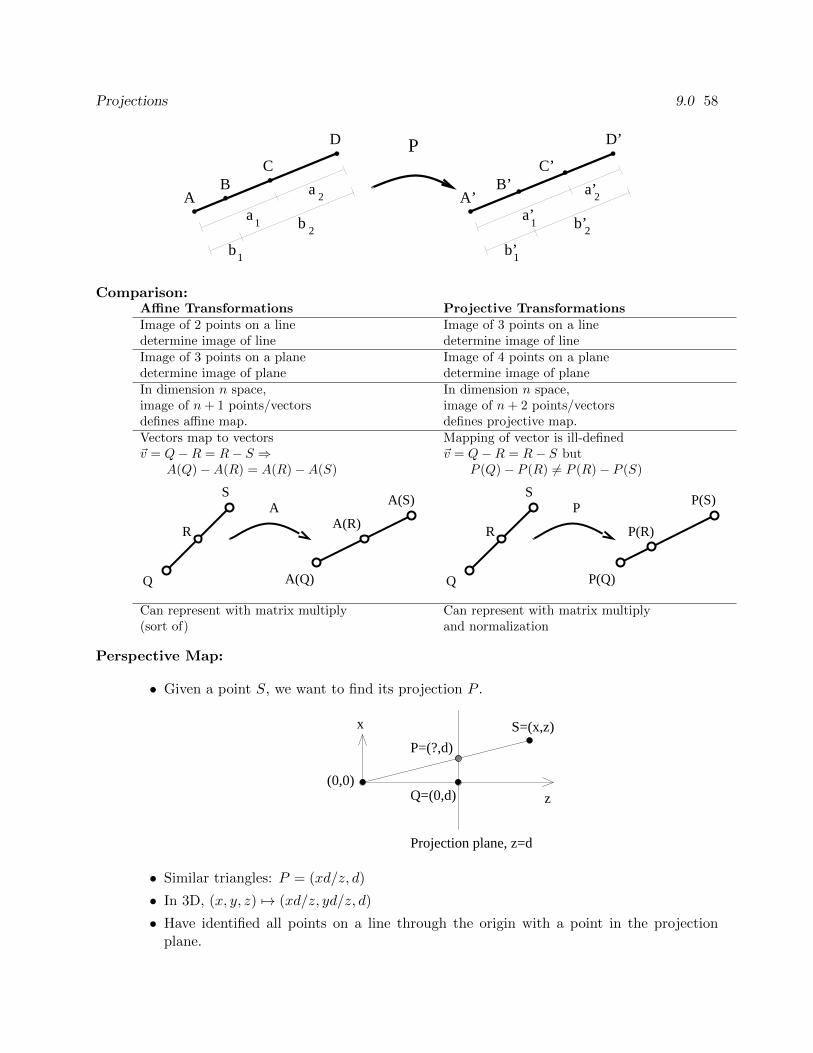
Perspective Map:
• Given a point S, we want to find its projection P .
Projection plane, z=d
z
x
Q=(0,d)
S=(x,z)
(0,0)
P=(?,d)
• Similar triangles: P = (xd/z, d)
• In 3D, (x, y, z) 7→ (xd/z, yd/z, d)
• Have identified all points on a line through the origin with a point in the projectionplane.
Projections 9.0 59
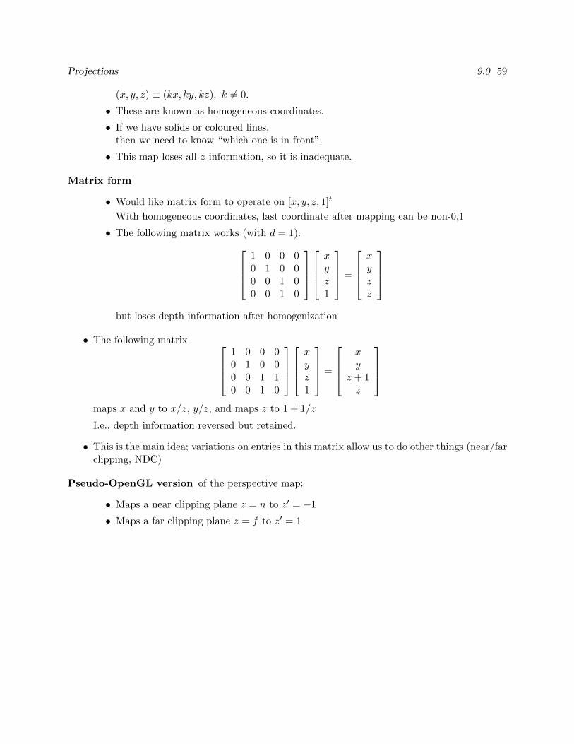
(x, y, z) ≡ (kx, ky, kz), k 6= 0.
• These are known as homogeneous coordinates.
• If we have solids or coloured lines,then we need to know “which one is in front”.
• This map loses all z information, so it is inadequate.
Matrix form
• Would like matrix form to operate on [x, y, z, 1]t
With homogeneous coordinates, last coordinate after mapping can be non-0,1
• The following matrix works (with d = 1):1 0 0 00 1 0 00 0 1 00 0 1 0
xyz1
=
xyzz
but loses depth information after homogenization
• The following matrix 1 0 0 00 1 0 00 0 1 10 0 1 0
xyz1
=
xy
z + 1z
maps x and y to x/z, y/z, and maps z to 1 + 1/z
I.e., depth information reversed but retained.
• This is the main idea; variations on entries in this matrix allow us to do other things (near/farclipping, NDC)
Pseudo-OpenGL version of the perspective map:
• Maps a near clipping plane z = n to z′ = −1
• Maps a far clipping plane z = f to z′ = 1
Projections 9.0 60
n
f
(1,1,1)
(-1,-1,-1)
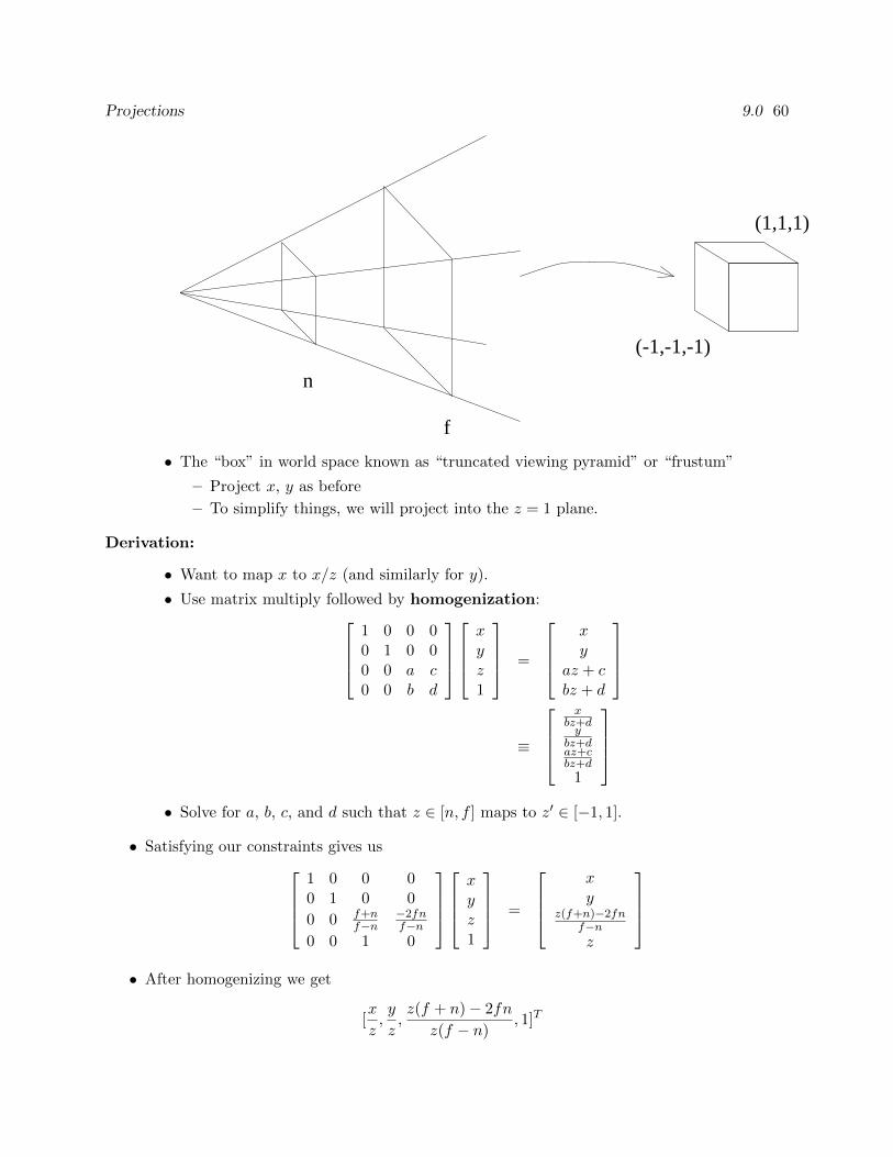
• The “box” in world space known as “truncated viewing pyramid” or “frustum”
– Project x, y as before
– To simplify things, we will project into the z = 1 plane.
Derivation:
• Want to map x to x/z (and similarly for y).
• Use matrix multiply followed by homogenization:1 0 0 00 1 0 00 0 a c0 0 b d
xyz1
=
xy
az + cbz + d
≡
x
bz+dy
bz+daz+cbz+d
1
• Solve for a, b, c, and d such that z ∈ [n, f ] maps to z′ ∈ [−1, 1].
• Satisfying our constraints gives us1 0 0 00 1 0 0
0 0 f+nf−n
−2fnf−n
0 0 1 0
xyz1
=
xy
z(f+n)−2fnf−nz
• After homogenizing we get
[x
z,y
z,z(f + n)− 2fn
z(f − n), 1]T
Why Map Z? 9.1 61
• Could use this formula instead of performing the matrix multiply followed by the division . . .
• If we multiply this matrix in with the geometric transforms,the only additional work is the divide.
The OpenGL perspective matrix uses
• a = −f+nf−n and b = −1.
– OpenGL looks down z = −1 rather than z = 1.
– Note that when you specify n and f ,they are given as positive distances down z = −1.
• The upper left entries are very different.
– OpenGL uses this one matrix to both project and map to NDC.
– How do we set x or y to map to [−1, 1]?
– We don’t want to do both because we may not have square windows.
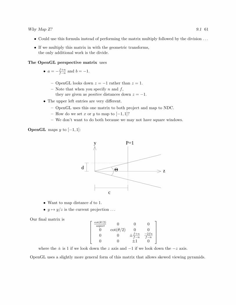
OpenGL maps y to [−1, 1]:
O
y P=1
z
c
d
• Want to map distance d to 1.
• y 7→ y/z is the current projection . . .
Our final matrix is cot(θ/2)aspect 0 0 0
0 cot(θ/2) 0 0
0 0 ±f+nf−n
−2fnf−n
0 0 ±1 0
where the ± is 1 if we look down the z axis and −1 if we look down the −z axis.
OpenGL uses a slightly more general form of this matrix that allows skewed viewing pyramids.
Why Map Z? 9.1 62
9.2 Why Map Z?
Why Map Z?
• 3D 7→ 2D projections map all z to same value.
• Need z to determine occlusion, so a 3D to 2D projective transformation doesn’t work.
• Further, we want 3D lines to map to 3D lines (this is useful in hidden surface removal)
• The mapping (x, y, z, 1) 7→ (xn/z, yn/z, n, 1) maps lines to lines, but loses all depth informa-tion.
• We could use
(x, y, z, 1) 7→ (xn
z,yn
z, z, 1)
Thus, if we map the endpoints of a line segment, these end points will have the same relativedepths after this mapping.
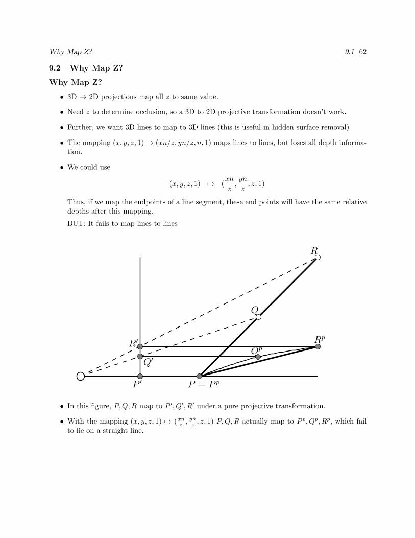
BUT: It fails to map lines to lines
R′
P ′ P = P p
Rp
Q
R
Qp
Q′
• In this figure, P,Q,R map to P ′, Q′, R′ under a pure projective transformation.
• With the mapping (x, y, z, 1) 7→ (xnz ,ynz , z, 1) P,Q,R actually map to P p, Qp, Rp, which fail
to lie on a straight line.
Mapping Z 9.2 63
Qp
R
Q
Rp
P = P p
S
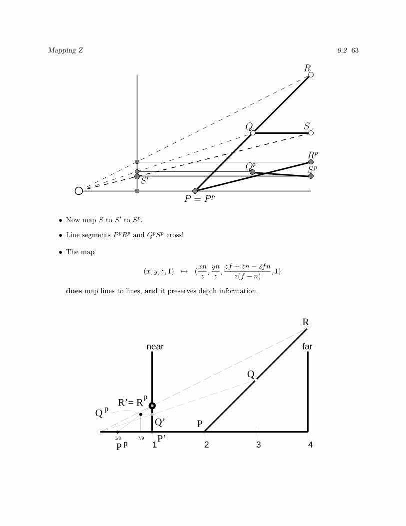
S ′Sp
• Now map S to S′ to Sp.
• Line segments P pRp and QpSp cross!
• The map
(x, y, z, 1) 7→ (xn
z,yn
z,zf + zn− 2fn
z(f − n), 1)
does map lines to lines, and it preserves depth information.
Q
R
Q’
P’
Rp
Q p
P
pP
R’=
2 31 47/91/3
near far
Mapping Z 9.2 64
9.3 Mapping Z
Mapping Z
• It’s clear how x and y map. How about z?
• The z map affects: clipping, numerics
z 7→ zf + zn− 2fn
z(f − n)= P (z)
• We know P (f) = 1 and P (n) = −1. What maps to 0?
P (z) = 0
⇒ zf+zn−2fnz(f−n) = 0
⇒ z =2fn
f + n
Note that f2 + fn > 2fn > fn+ n2 so
f >2fn
f + n> n
• What happens as z goes to 0 or to infinity?
limz→0+
P (z) =−2fn
z(f − n)= −∞
limz→0−
P (z) =−2fn
z(f − n)= +∞
limz→+∞
P (z) =z(f + n)
z(f − n)
=f + n
f − n
limz→−∞
P (z) =z(f + n)
z(f − n)
=f + n
f − n
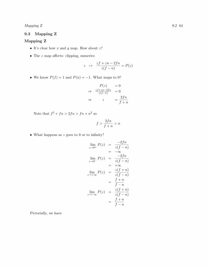
Pictorially, we have
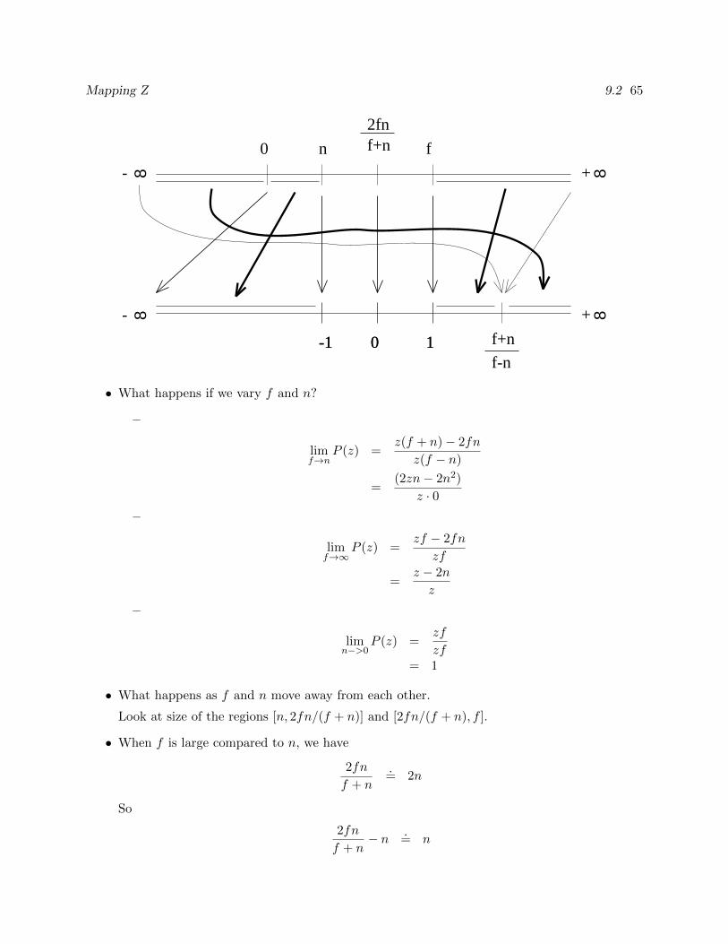
Mapping Z 9.2 65
-1 0 1-1 0 1
8-
8- 8+
8+
f-n
n f0
2fnf+n
f+n
• What happens if we vary f and n?
–
limf→n
P (z) =z(f + n)− 2fn
z(f − n)
=(2zn− 2n2)
z · 0–
limf→∞
P (z) =zf − 2fn
zf
=z − 2n
z
–
limn−>0
P (z) =zf
zf= 1
• What happens as f and n move away from each other.
Look at size of the regions [n, 2fn/(f + n)] and [2fn/(f + n), f ].
• When f is large compared to n, we have
2fn
f + n
.= 2n
So
2fn
f + n− n .
= n
3D Clipping 9.3 66
and
f − 2fn
f + n
.= f − 2n.
But both intervals are mapped to a region of size 1.
9.4 3D Clipping
3D Clipping
• When do we clip in 3D?
We should clip to the near plane before we project. Otherwise, we might attempt to projecta point with z = 0 and then x/z and y/z are undefined.
• We could clip to all 6 sides of the truncated viewing pyramid.
But the plane equations are simpler if we clip after projection, because all sides of volumeare parallel to coordinate plane.
• Clipping to a plane in 3D is identical to clipping to a line in 2D.
• We can also clip in homogeneous coordinates.
(Readings: Red Book, 6.6.4; White book, 6.5.4. )
9.5 Homogeneous Clipping
Homogeneous Clipping
Projection: transform and homogenize
• Linear transformationnr 0 0 00 ns 0 0
0 0 f+nf−n − 2fn
f−n0 0 1 0
xyz1
=
xyzw
• Homogenization
xyzw
=
x/wy/wz/w
1
=
XYZ1
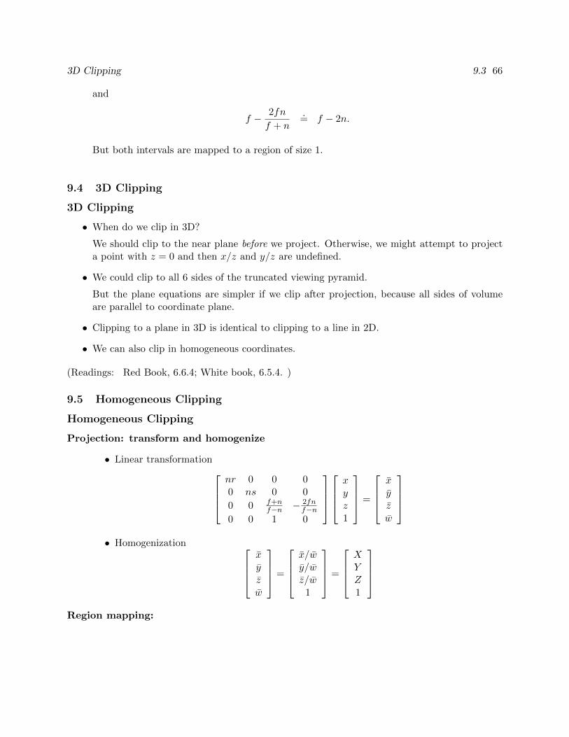
Region mapping:
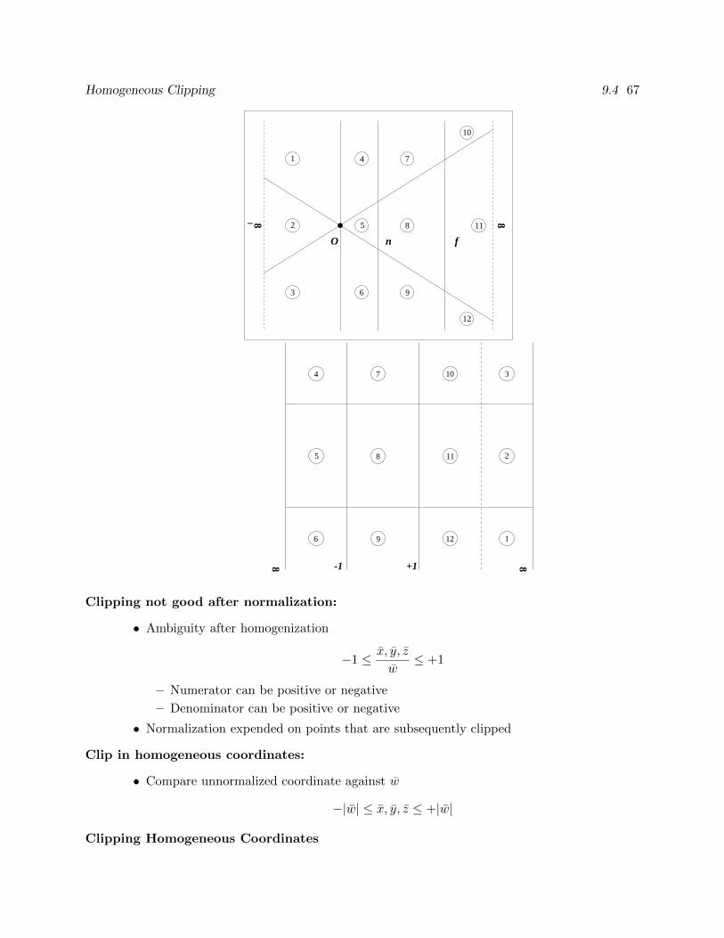
Homogeneous Clipping 9.4 67
8−
10
12
fnO
1
2
4
5
7
8 11
963
8
8
9
7 10
11
12
3
2
1
8
4
5
6
8 -1 +1
Clipping not good after normalization:
• Ambiguity after homogenization
−1 ≤ x, y, z
w≤ +1
– Numerator can be positive or negative
– Denominator can be positive or negative
• Normalization expended on points that are subsequently clipped
Clip in homogeneous coordinates:
• Compare unnormalized coordinate against w
−|w| ≤ x, y, z ≤ +|w|
Clipping Homogeneous Coordinates
Pinhole Camera vs. Camera vs. Perception 9.5 68
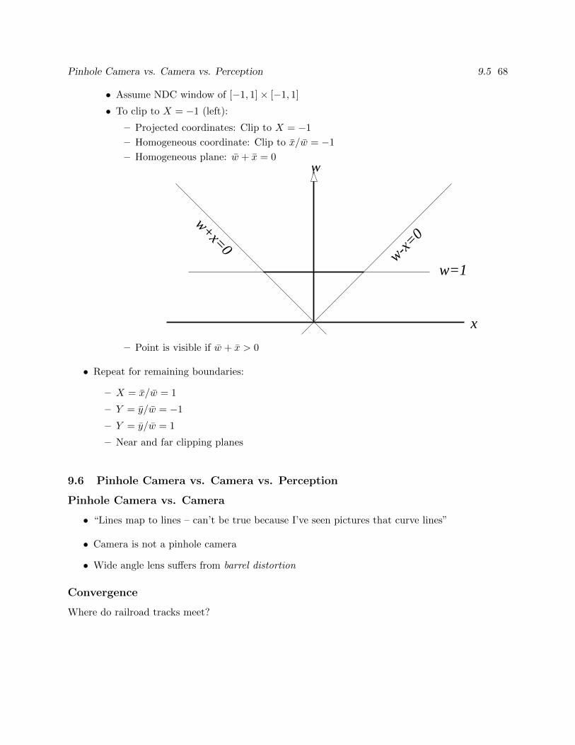
• Assume NDC window of [−1, 1]× [−1, 1]
• To clip to X = −1 (left):
– Projected coordinates: Clip to X = −1
– Homogeneous coordinate: Clip to x/w = −1
– Homogeneous plane: w + x = 0
w+x=0
w=1
x
w
w-x=0
– Point is visible if w + x > 0
• Repeat for remaining boundaries:
– X = x/w = 1
– Y = y/w = −1
– Y = y/w = 1
– Near and far clipping planes
9.6 Pinhole Camera vs. Camera vs. Perception
Pinhole Camera vs. Camera
• “Lines map to lines – can’t be true because I’ve seen pictures that curve lines”
• Camera is not a pinhole camera
• Wide angle lens suffers from barrel distortion
Convergence
Where do railroad tracks meet?
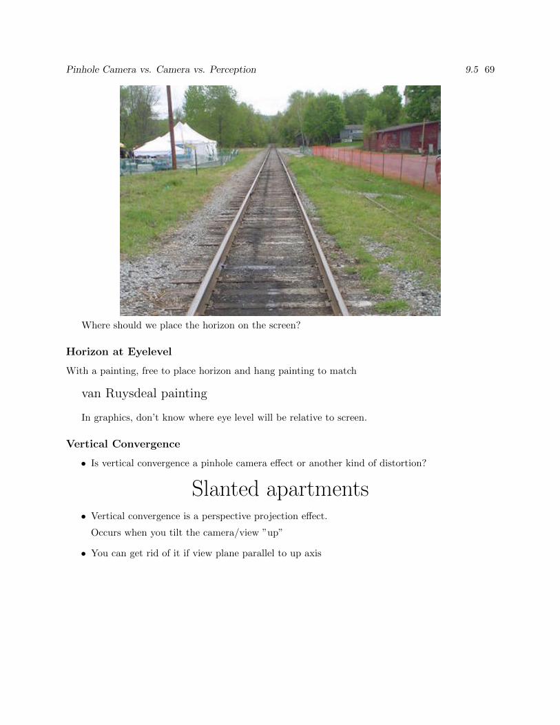
Pinhole Camera vs. Camera vs. Perception 9.5 69
Where should we place the horizon on the screen?
Horizon at Eyelevel
With a painting, free to place horizon and hang painting to match
van Ruysdeal painting
In graphics, don’t know where eye level will be relative to screen.
Vertical Convergence
• Is vertical convergence a pinhole camera effect or another kind of distortion?
Slanted apartments• Vertical convergence is a perspective projection effect.
Occurs when you tilt the camera/view ”up”
• You can get rid of it if view plane parallel to up axis
Pinhole Camera vs. Camera vs. Perception 9.5 70
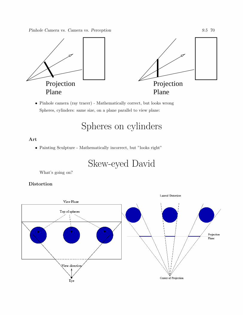
ProjectionPlane
ProjectionPlane
• Pinhole camera (ray tracer) - Mathematically correct, but looks wrong
Spheres, cylinders: same size, on a plane parallel to view plane:
Spheres on cylindersArt
• Painting Sculpture - Mathematically incorrect, but ”looks right”
Skew-eyed DavidWhat’s going on?
Distortion
Transformation Applications and Extensions 9 71
Spheres
Spheres, and lots of them!Occurs in Computer Graphics Images
Ben-hur races in front of distorted columnsIn Real Life
• Eye/attention only on small part of field of view
Sphere looks circular
• Rest of field of view is “there”
Peripheral spheres not circular, but not focus of attentionand you don’t notice
• When you look at different object, you shift projection plane
Different sphere looks circular
• In painting, all spheres drawn as circular
When not looking at them, they are mathematically wrongbut since not focus of attention they are “close enough”
• In graphics...

Transformation Applications and Extensions 9 72
10 TRANSFORMATION APPLICATIONS AND EXTENSIONS 73
10 Transformation Applications and Extensions
10.1 Rendering Pipeline Revisited
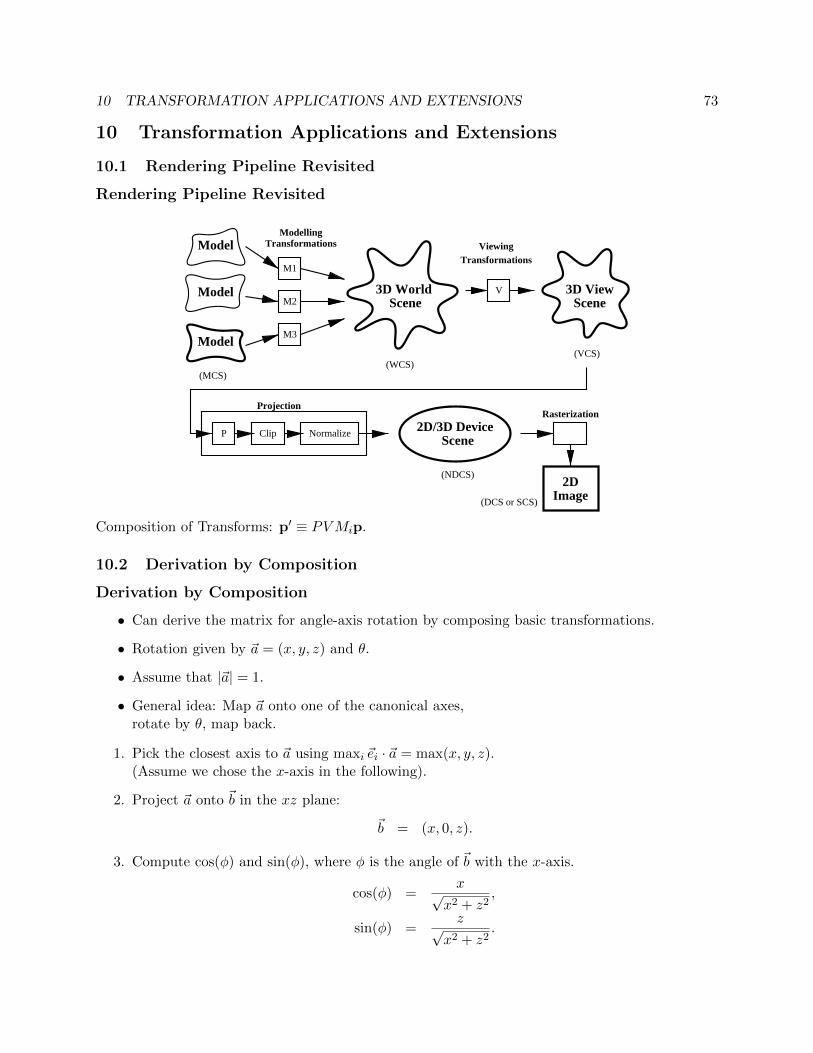
Rendering Pipeline Revisited
Normalize Clip
(DCS or SCS)
(MCS)(WCS)
(VCS)
Model
Model
Model
ModellingTransformations
3D World Scene Scene
3D View
Scene
(NDCS)
ViewingTransformations
V
M3
M2
M1
2D/3D DeviceP
ProjectionRasterization
Image2D
Composition of Transforms: p′ ≡ PVMip.
10.2 Derivation by Composition
Derivation by Composition
• Can derive the matrix for angle-axis rotation by composing basic transformations.
• Rotation given by ~a = (x, y, z) and θ.
• Assume that |~a| = 1.
• General idea: Map ~a onto one of the canonical axes,rotate by θ, map back.
1. Pick the closest axis to ~a using maxi ~ei · ~a = max(x, y, z).(Assume we chose the x-axis in the following).
2. Project ~a onto ~b in the xz plane:
~b = (x, 0, z).
3. Compute cos(φ) and sin(φ), where φ is the angle of ~b with the x-axis.
cos(φ) =x√
x2 + z2,
sin(φ) =z√
x2 + z2.
3D Rotation User Interfaces 10.2 74
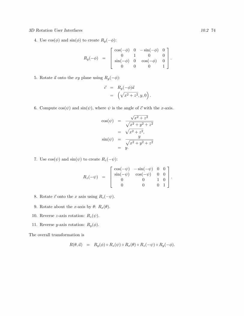
4. Use cos(φ) and sin(φ) to create Ry(−φ):
Ry(−φ) =
cos(−φ) 0 − sin(−φ) 0
0 1 0 0sin(−φ) 0 cos(−φ) 0
0 0 0 1
.5. Rotate ~a onto the xy plane using Ry(−φ):
~c = Ry(−φ)~a
=(√
x2 + z2, y, 0).
6. Compute cos(ψ) and sin(ψ), where ψ is the angle of ~c with the x-axis.
cos(ψ) =
√x2 + z2√
x2 + y2 + z2
=√x2 + z2,
sin(ψ) =y√
x2 + y2 + z2
= y.
7. Use cos(ψ) and sin(ψ) to create Rz(−ψ):
Rz(−ψ) =
cos(−ψ) − sin(−ψ) 0 0sin(−ψ) cos(−ψ) 0 0
0 0 1 00 0 0 1
.8. Rotate ~c onto the x axis using Rz(−ψ).
9. Rotate about the x-axis by θ: Rx(θ).
10. Reverse z-axis rotation: Rz(ψ).
11. Reverse y-axis rotation: Ry(φ).
The overall transformation is
R(θ,~a) = Ry(φ) Rz(ψ) Rx(θ) Rz(−ψ) Ry(−φ).
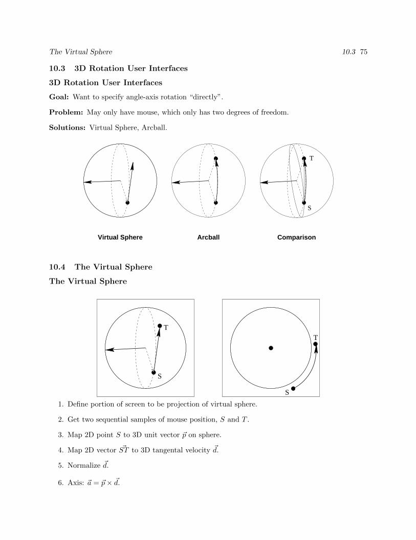
The Virtual Sphere 10.3 75
10.3 3D Rotation User Interfaces
3D Rotation User Interfaces
Goal: Want to specify angle-axis rotation “directly”.
Problem: May only have mouse, which only has two degrees of freedom.
Solutions: Virtual Sphere, Arcball.
Virtual Sphere Arcball
S
T
Comparison
10.4 The Virtual Sphere
The Virtual Sphere
T
S
S
T
1. Define portion of screen to be projection of virtual sphere.
2. Get two sequential samples of mouse position, S and T .
3. Map 2D point S to 3D unit vector ~p on sphere.
4. Map 2D vector ~ST to 3D tangental velocity ~d.
5. Normalize ~d.
6. Axis: ~a = ~p× ~d.

Polygons 10 76
7. Angle: θ = α| ~ST |.(Choose α so a 180 rotation can be obtained.)
8. Save T to use as S for next time.
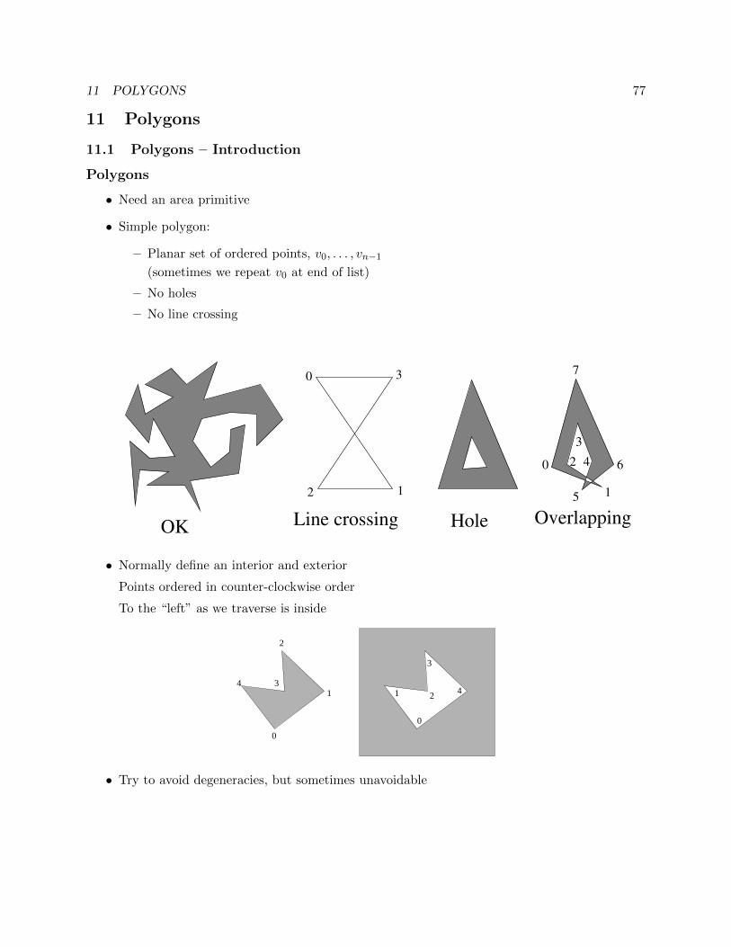
11 POLYGONS 77
11 Polygons
11.1 Polygons – Introduction
Polygons
• Need an area primitive
• Simple polygon:
– Planar set of ordered points, v0, . . . , vn−1
(sometimes we repeat v0 at end of list)
– No holes
– No line crossing
1
30
2
0
1
3
4
5
6
7
2
OK Line crossing Hole Overlapping
• Normally define an interior and exterior
Points ordered in counter-clockwise order
To the “left” as we traverse is inside
3
4
0
24
1
0
1
2
3
• Try to avoid degeneracies, but sometimes unavoidable
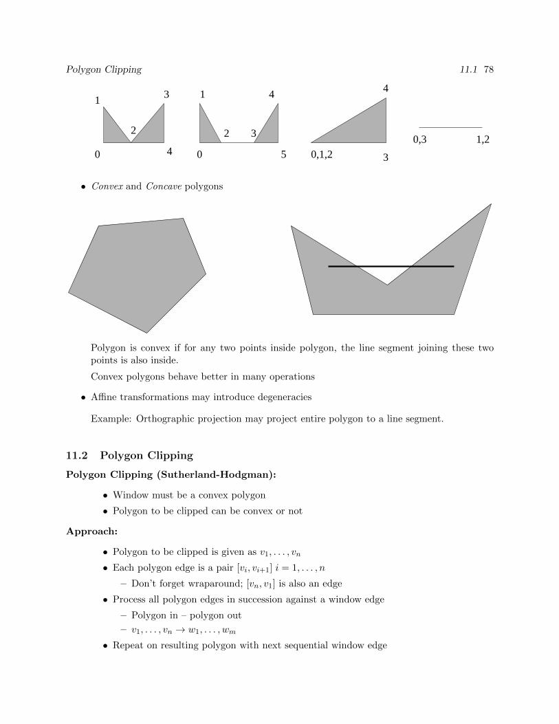
Polygon Clipping 11.1 78
0
1
2
3
4 0
1
1,22 3
4
5 0,1,2 3
4
0,3
• Convex and Concave polygons
Polygon is convex if for any two points inside polygon, the line segment joining these twopoints is also inside.
Convex polygons behave better in many operations
• Affine transformations may introduce degeneracies
Example: Orthographic projection may project entire polygon to a line segment.
11.2 Polygon Clipping
Polygon Clipping (Sutherland-Hodgman):
• Window must be a convex polygon
• Polygon to be clipped can be convex or not
Approach:
• Polygon to be clipped is given as v1, . . . , vn
• Each polygon edge is a pair [vi, vi+1] i = 1, . . . , n
– Don’t forget wraparound; [vn, v1] is also an edge
• Process all polygon edges in succession against a window edge
– Polygon in – polygon out
– v1, . . . , vn → w1, . . . , wm
• Repeat on resulting polygon with next sequential window edge
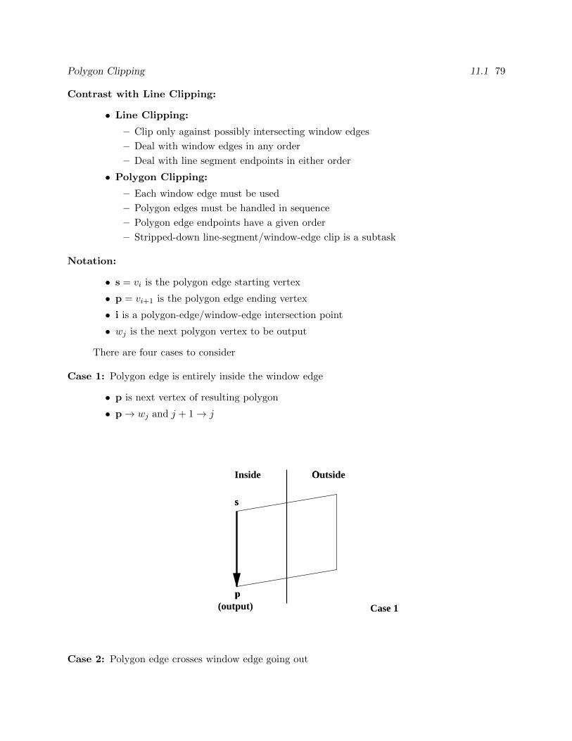
Polygon Clipping 11.1 79
Contrast with Line Clipping:
• Line Clipping:
– Clip only against possibly intersecting window edges
– Deal with window edges in any order
– Deal with line segment endpoints in either order
• Polygon Clipping:
– Each window edge must be used
– Polygon edges must be handled in sequence
– Polygon edge endpoints have a given order
– Stripped-down line-segment/window-edge clip is a subtask
Notation:
• s = vi is the polygon edge starting vertex
• p = vi+1 is the polygon edge ending vertex
• i is a polygon-edge/window-edge intersection point
• wj is the next polygon vertex to be output
There are four cases to consider
Case 1: Polygon edge is entirely inside the window edge
• p is next vertex of resulting polygon
• p→ wj and j + 1→ j
s
p
(output) Case 1
Outside
Inside
Case 2: Polygon edge crosses window edge going out
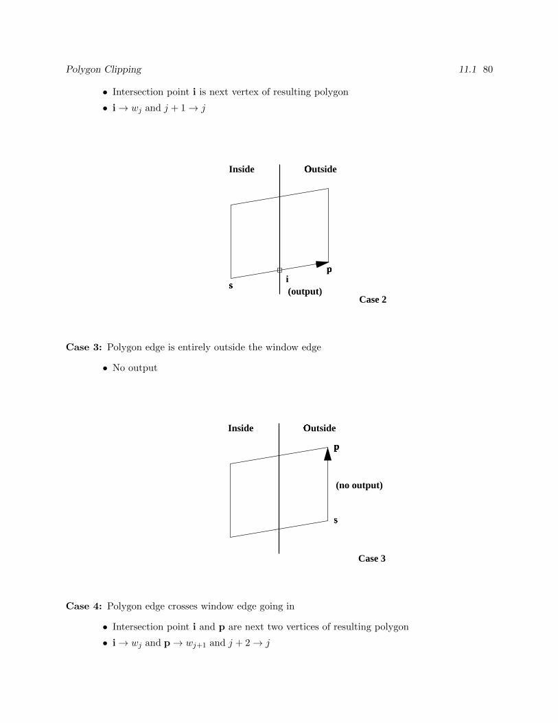
Polygon Clipping 11.1 80
• Intersection point i is next vertex of resulting polygon
• i→ wj and j + 1→ j
sp
i(output)
Case 2
Outside
Inside
Case 3: Polygon edge is entirely outside the window edge
• No output
Case 3
s
p
(no output)
Outside
Inside
Case 4: Polygon edge crosses window edge going in
• Intersection point i and p are next two vertices of resulting polygon
• i→ wj and p→ wj+1 and j + 2→ j
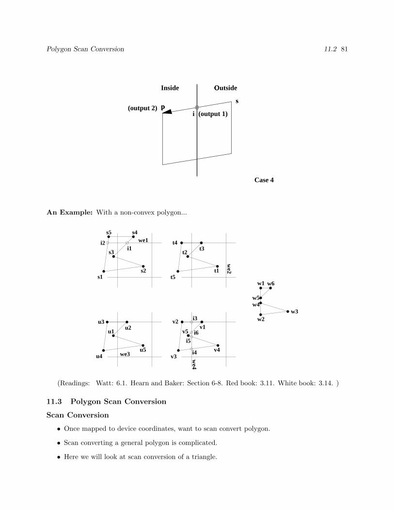
Polygon Scan Conversion 11.2 81
Case 4
i
sp
(output 1)(output 2)
Outside
Inside
An Example: With a non-convex polygon...
w6
we2
we1
we3
we4
i3
i1i2
s1
s3
s2
s4s5
t1
t2t3
t4
t5
u1u2
u3
u4u5
v1v2
v3v4
v5
i4
i5i6
w1
w2w3
w4w5
(Readings: Watt: 6.1. Hearn and Baker: Section 6-8. Red book: 3.11. White book: 3.14. )
11.3 Polygon Scan Conversion
Scan Conversion
• Once mapped to device coordinates, want to scan convert polygon.
• Scan converting a general polygon is complicated.
• Here we will look at scan conversion of a triangle.
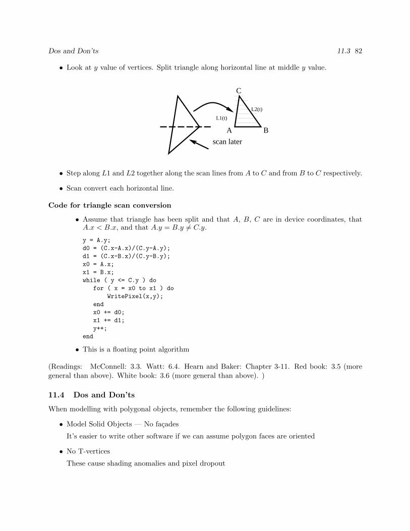
Dos and Don’ts 11.3 82
• Look at y value of vertices. Split triangle along horizontal line at middle y value.
scan later
L1(t)
L2(t)
A B
C
• Step along L1 and L2 together along the scan lines from A to C and from B to C respectively.
• Scan convert each horizontal line.
Code for triangle scan conversion
• Assume that triangle has been split and that A, B, C are in device coordinates, thatA.x < B.x, and that A.y = B.y 6= C.y.
y = A.y;
d0 = (C.x-A.x)/(C.y-A.y);
d1 = (C.x-B.x)/(C.y-B.y);
x0 = A.x;
x1 = B.x;
while ( y <= C.y ) do
for ( x = x0 to x1 ) do
WritePixel(x,y);
end
x0 += d0;
x1 += d1;
y++;
end
• This is a floating point algorithm
(Readings: McConnell: 3.3. Watt: 6.4. Hearn and Baker: Chapter 3-11. Red book: 3.5 (moregeneral than above). White book: 3.6 (more general than above). )
11.4 Dos and Don’ts
When modelling with polygonal objects, remember the following guidelines:
• Model Solid Objects — No facades
It’s easier to write other software if we can assume polygon faces are oriented
• No T-vertices
These cause shading anomalies and pixel dropout

Hidden Surface Removal 11 83
• No overlapping co-planar faces
Violates solid object constraint.
If different colours, then psychedelic effect due to floating point roundoff
• Well shaped polygon
Equilateral triangle is best.
Long, skinny triangles pose problems for numerical algorithms
Bad Polygon Examples

Hidden Surface Removal 11 84
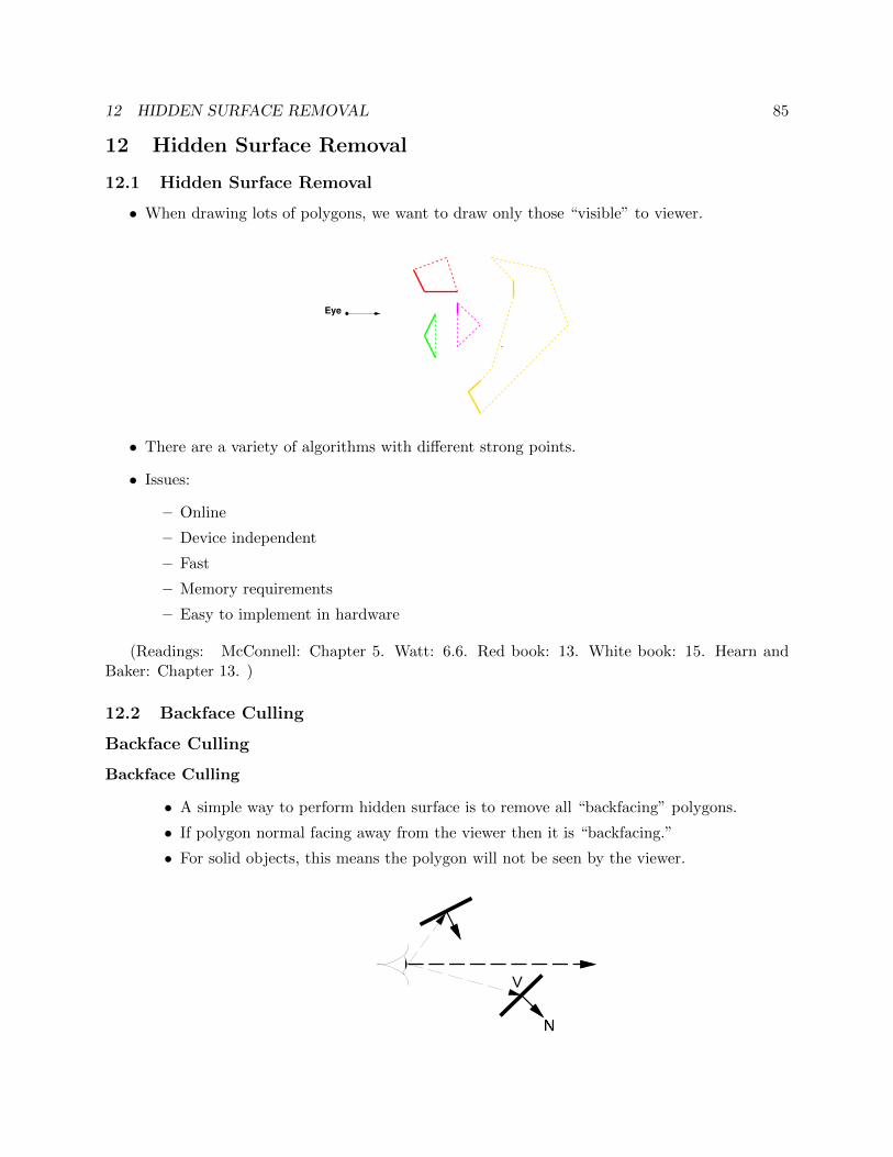
12 HIDDEN SURFACE REMOVAL 85
12 Hidden Surface Removal
12.1 Hidden Surface Removal
• When drawing lots of polygons, we want to draw only those “visible” to viewer.
Eye
• There are a variety of algorithms with different strong points.
• Issues:
– Online
– Device independent
– Fast
– Memory requirements
– Easy to implement in hardware
(Readings: McConnell: Chapter 5. Watt: 6.6. Red book: 13. White book: 15. Hearn andBaker: Chapter 13. )
12.2 Backface Culling
Backface Culling
Backface Culling
• A simple way to perform hidden surface is to remove all “backfacing” polygons.
• If polygon normal facing away from the viewer then it is “backfacing.”
• For solid objects, this means the polygon will not be seen by the viewer.
N
V
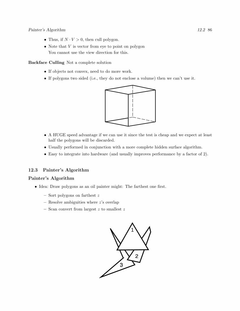
Painter’s Algorithm 12.2 86
• Thus, if N · V > 0, then cull polygon.
• Note that V is vector from eye to point on polygon
You cannot use the view direction for this.
Backface Culling Not a complete solution
• If objects not convex, need to do more work.
• If polygons two sided (i.e., they do not enclose a volume) then we can’t use it.
• A HUGE speed advantage if we can use it since the test is cheap and we expect at leasthalf the polygons will be discarded.
• Usually performed in conjunction with a more complete hidden surface algorithm.
• Easy to integrate into hardware (and usually improves performance by a factor of 2).
12.3 Painter’s Algorithm
Painter’s Algorithm
• Idea: Draw polygons as an oil painter might: The farthest one first.
– Sort polygons on farthest z
– Resolve ambiguities where z’s overlap
– Scan convert from largest z to smallest z
2
3
1

Warnock’s Algorithm 12.3 87
• Since closest drawn last, it will be on top (and therefore it will be seen).
• Need all polygons at once in order to sort.
Painter’s Algorithm — Z overlap
• Some cases are easy:
x
y
x
y
z=2
z=3z=1
• But other cases are nasty!
x
y
x
y
(have to split polygons)
• Ω(n2) algorithm, lots of subtle detail
12.4 Warnock’s Algorithm
Warnock’s Algorithm
• A divide and conquer algorithm
Warnock(PolyList PL, ViewPort VP)
If ( PL simple in VP) then
Draw PL in VP
else
Split VP vertically and horizontally into VP1,VP2,VP3,VP4
Warnock(PL in VP1, VP1)
Warnock(PL in VP2, VP2)
Warnock(PL in VP3, VP3)
Warnock(PL in VP4, VP4)
end
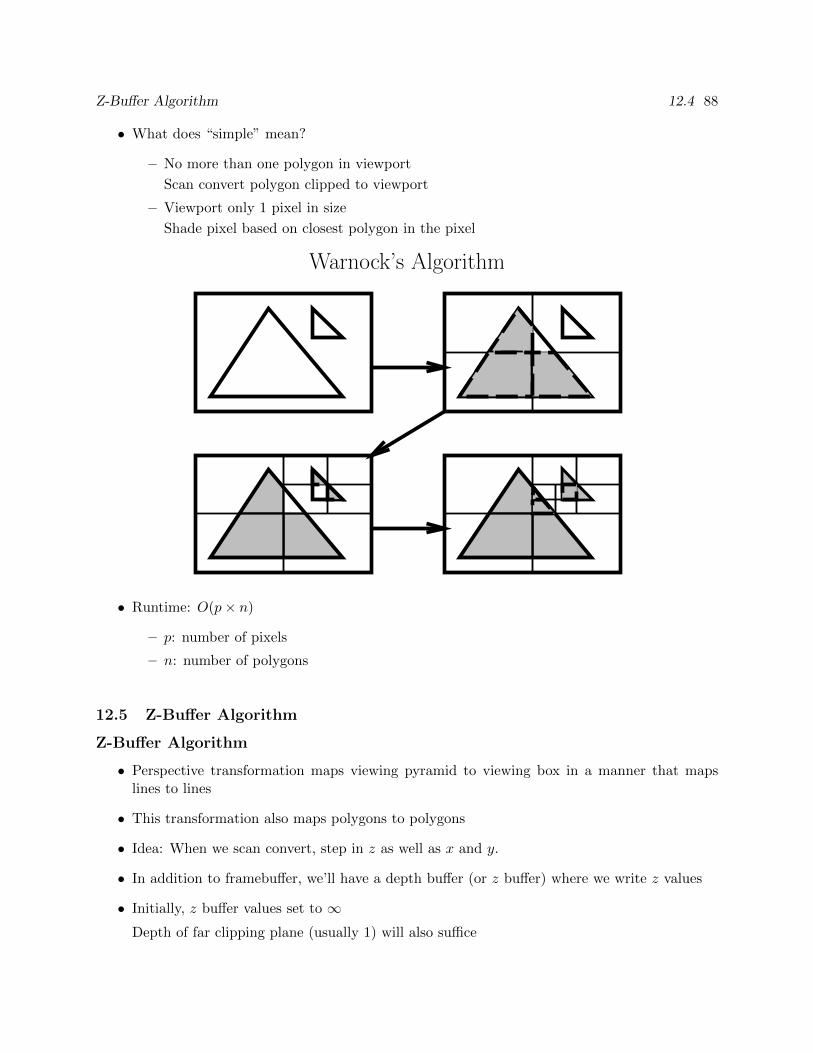
Z-Buffer Algorithm 12.4 88
• What does “simple” mean?
– No more than one polygon in viewport
Scan convert polygon clipped to viewport
– Viewport only 1 pixel in size
Shade pixel based on closest polygon in the pixel
Warnock’s Algorithm
• Runtime: O(p× n)
– p: number of pixels
– n: number of polygons
12.5 Z-Buffer Algorithm
Z-Buffer Algorithm
• Perspective transformation maps viewing pyramid to viewing box in a manner that mapslines to lines
• This transformation also maps polygons to polygons
• Idea: When we scan convert, step in z as well as x and y.
• In addition to framebuffer, we’ll have a depth buffer (or z buffer) where we write z values
• Initially, z buffer values set to ∞Depth of far clipping plane (usually 1) will also suffice
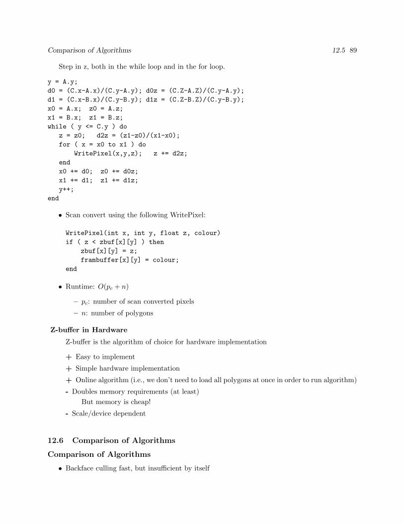
Comparison of Algorithms 12.5 89
Step in z, both in the while loop and in the for loop.
y = A.y;
d0 = (C.x-A.x)/(C.y-A.y); d0z = (C.Z-A.Z)/(C.y-A.y);
d1 = (C.x-B.x)/(C.y-B.y); d1z = (C.Z-B.Z)/(C.y-B.y);
x0 = A.x; z0 = A.z;
x1 = B.x; z1 = B.z;
while ( y <= C.y ) do
z = z0; d2z = (z1-z0)/(x1-x0);
for ( x = x0 to x1 ) do
WritePixel(x,y,z); z += d2z;
end
x0 += d0; z0 += d0z;
x1 += d1; z1 += d1z;
y++;
end
• Scan convert using the following WritePixel:
WritePixel(int x, int y, float z, colour)
if ( z < zbuf[x][y] ) then
zbuf[x][y] = z;
frambuffer[x][y] = colour;
end
• Runtime: O(pc + n)
– pc: number of scan converted pixels
– n: number of polygons
Z-buffer in Hardware
Z-buffer is the algorithm of choice for hardware implementation
+ Easy to implement
+ Simple hardware implementation
+ Online algorithm (i.e., we don’t need to load all polygons at once in order to run algorithm)
- Doubles memory requirements (at least)
But memory is cheap!
- Scale/device dependent
12.6 Comparison of Algorithms
Comparison of Algorithms
• Backface culling fast, but insufficient by itself
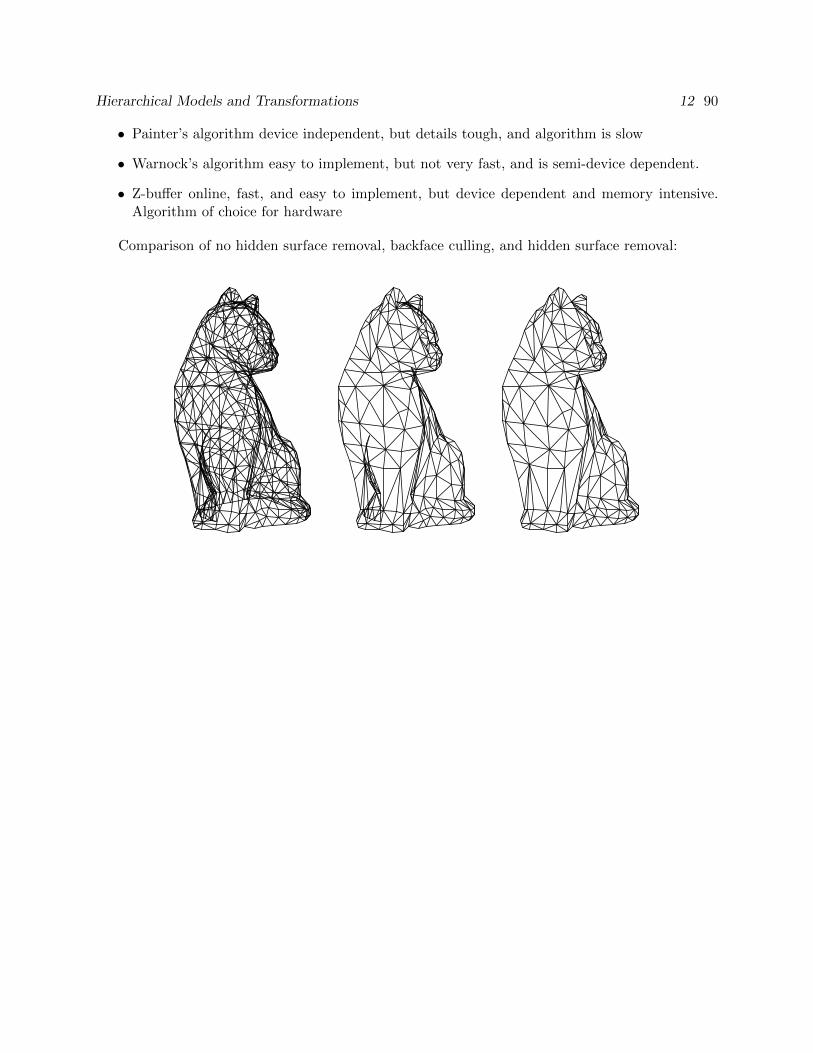
Hierarchical Models and Transformations 12 90
• Painter’s algorithm device independent, but details tough, and algorithm is slow
• Warnock’s algorithm easy to implement, but not very fast, and is semi-device dependent.
• Z-buffer online, fast, and easy to implement, but device dependent and memory intensive.Algorithm of choice for hardware
Comparison of no hidden surface removal, backface culling, and hidden surface removal:
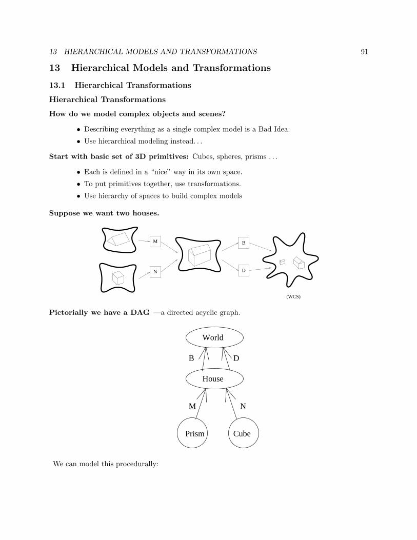
13 HIERARCHICAL MODELS AND TRANSFORMATIONS 91
13 Hierarchical Models and Transformations
13.1 Hierarchical Transformations
Hierarchical Transformations
How do we model complex objects and scenes?
• Describing everything as a single complex model is a Bad Idea.
• Use hierarchical modeling instead. . .
Start with basic set of 3D primitives: Cubes, spheres, prisms . . .
• Each is defined in a “nice” way in its own space.
• To put primitives together, use transformations.
• Use hierarchy of spaces to build complex models
Suppose we want two houses.
B
(WCS)
M
N D
Pictorially we have a DAG —a directed acyclic graph.
CubePrism
DB
NM
House
World
We can model this procedurally:
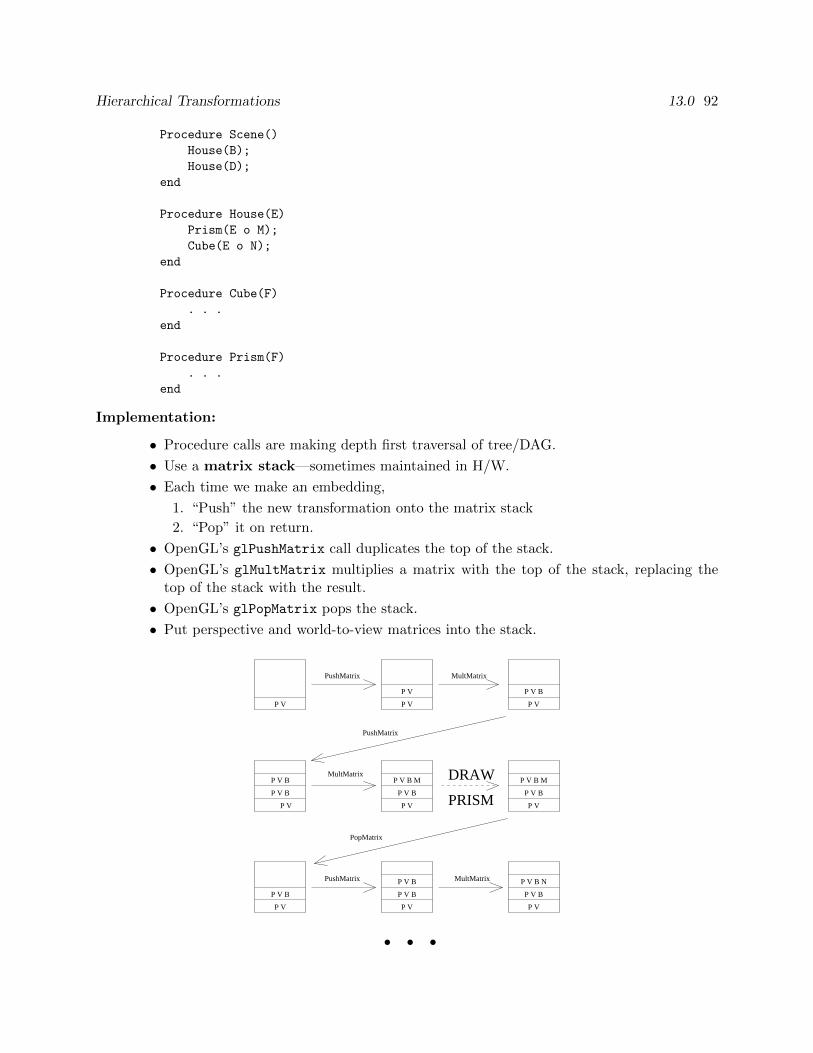
Hierarchical Transformations 13.0 92
Procedure Scene()
House(B);
House(D);
end
Procedure House(E)
Prism(E o M);
Cube(E o N);
end
Procedure Cube(F)
. . .
end
Procedure Prism(F)
. . .
end
Implementation:
• Procedure calls are making depth first traversal of tree/DAG.
• Use a matrix stack—sometimes maintained in H/W.
• Each time we make an embedding,
1. “Push” the new transformation onto the matrix stack
2. “Pop” it on return.
• OpenGL’s glPushMatrix call duplicates the top of the stack.
• OpenGL’s glMultMatrix multiplies a matrix with the top of the stack, replacing thetop of the stack with the result.
• OpenGL’s glPopMatrix pops the stack.
• Put perspective and world-to-view matrices into the stack.
P V
DRAW
PRISM
PushMatrix MultMatrix
MultMatrix
PopMatrix
PushMatrix
PushMatrix MultMatrix
. . .
P V
P V
P V
P V B
P V
P V B
P V B
P V
P V B M
P V B
P V
P V B M
P V B
P V
P V B
P V
P V B
P V B
P V
P V B N
P V B
Hierarchical Data Structures 13.1 93
Code now looks like
Procedure Scene()
MultMatrix(P);
MultMatrix(V);
PushMatrix();
MultMatrix(B);
House();
PopMatrix();
PushMatrix();
MultMatrix(D);
House();
PopMatrix();
end
Procedure House()
PushMatrix();
MultMatrix(M);
Prism();
Popmatrix();
PushMatrix();
MultMatrix(N);
Cube();
Popmatrix();
end
Procedure Cube() Procedure Prism()
. . . . . .
end end
13.2 Hierarchical Data Structures
Hierarchical Data Structures
• Don’t want to write a program for each scene
Instead, develop a data structure and traverse it.
• Consider the following DAG:
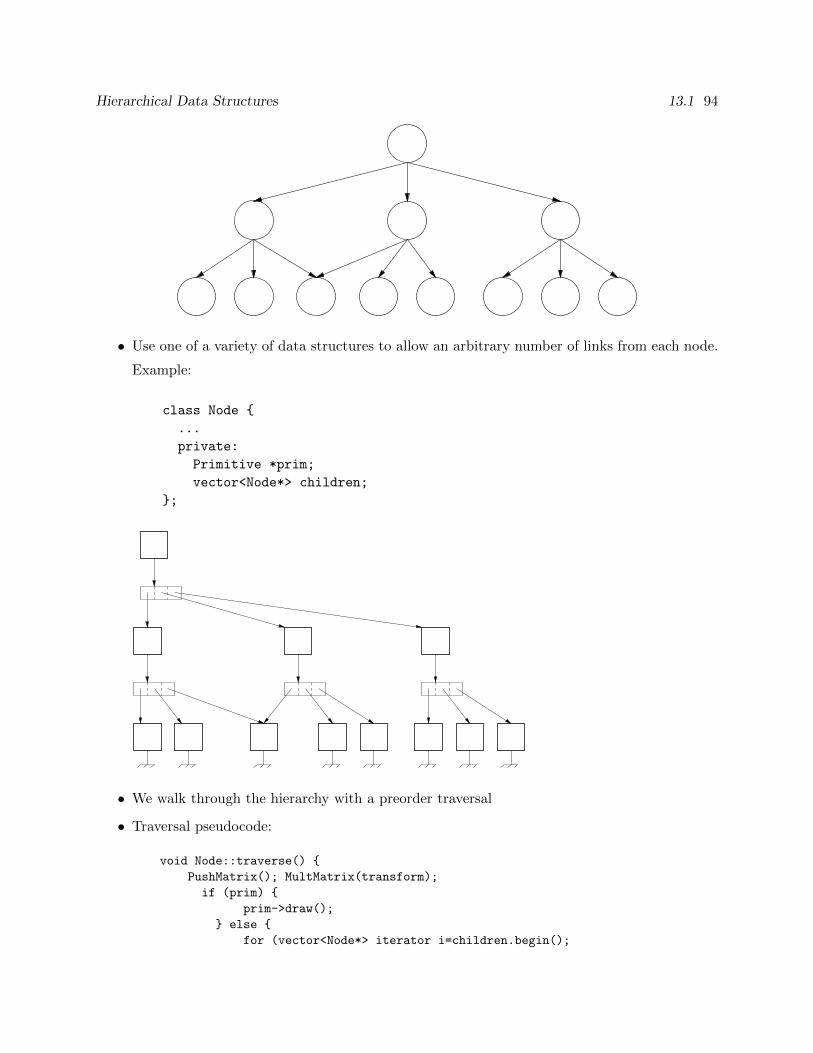
Hierarchical Data Structures 13.1 94
• Use one of a variety of data structures to allow an arbitrary number of links from each node.
Example:
class Node
...
private:
Primitive *prim;
vector<Node*> children;
;
• We walk through the hierarchy with a preorder traversal
• Traversal pseudocode:
void Node::traverse()
PushMatrix(); MultMatrix(transform);
if (prim)
prim->draw();
else
for (vector<Node*> iterator i=children.begin();
Hierarchical Data Structures 13.1 95
i != children.end(); ++i)
(*i)->traverse();
PopMatrix();
A3/A4 House Code
scene = gr.transform( ’scene’ )
# Assume we have predefined materials ’red’, ’green’ and ’blue’
house = gr.node( ’house’ )
prism = gr.polyhedron( ’prism’, ... )
roof = gr.node( ’roof’ )
roof:add_child( prism )
roof:translate( 0,1,0 )
house:add_child( roof )
frame = gr.cube( ’frame’ )
house:add_child( frame )
farmhouse = gr.node( ’farmhouse’ )
farmhouse:add_child( house )
farmhouse:set_material( green )
(continued on next slide)(continuation from previous slide)
barn = gr.node( ’barn’ )
barn:add_child( house )
barn:set_material( red )
barn:translate( 2,0,3 ) ; barn:scale( 2,2,2 ) ; barn:rotate( ’Y’, 30 )
doghouse = gr.node( ’doghouse’ )
doghouse:add_child( house )
doghouse:set_material( blue )
doghouse:translate(1.5, 0, -0.2 ) ; doghouse:scale( 0.2,0.2,0.2 )
doghouse:rotate( ’Y’, -15 ) )
scene:add_child( farmhouse )
scene:add_child( barn )
scene:add_child( doghouse )
# Later in the code...
... gr.render( scene ) ...
Improved A3/A4 House Code
# Assume materials are defined
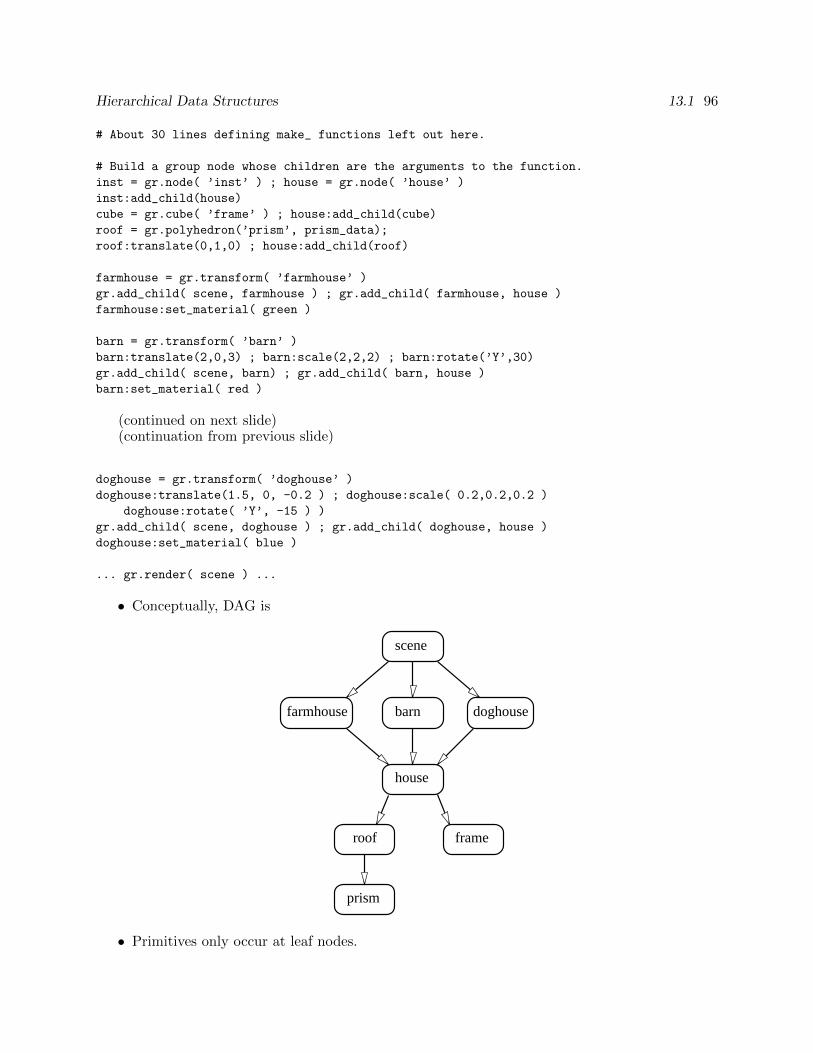
Hierarchical Data Structures 13.1 96
# About 30 lines defining make_ functions left out here.
# Build a group node whose children are the arguments to the function.
inst = gr.node( ’inst’ ) ; house = gr.node( ’house’ )
inst:add_child(house)
cube = gr.cube( ’frame’ ) ; house:add_child(cube)
roof = gr.polyhedron(’prism’, prism_data);
roof:translate(0,1,0) ; house:add_child(roof)
farmhouse = gr.transform( ’farmhouse’ )
gr.add_child( scene, farmhouse ) ; gr.add_child( farmhouse, house )
farmhouse:set_material( green )
barn = gr.transform( ’barn’ )
barn:translate(2,0,3) ; barn:scale(2,2,2) ; barn:rotate(’Y’,30)
gr.add_child( scene, barn) ; gr.add_child( barn, house )
barn:set_material( red )
(continued on next slide)(continuation from previous slide)
doghouse = gr.transform( ’doghouse’ )
doghouse:translate(1.5, 0, -0.2 ) ; doghouse:scale( 0.2,0.2,0.2 )
doghouse:rotate( ’Y’, -15 ) )
gr.add_child( scene, doghouse ) ; gr.add_child( doghouse, house )
doghouse:set_material( blue )
... gr.render( scene ) ...
• Conceptually, DAG is
frameroof
prism
house
doghouse
scene
farmhouse barn
• Primitives only occur at leaf nodes.
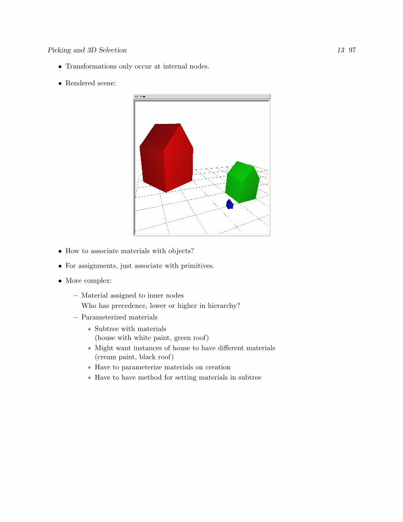
Picking and 3D Selection 13 97
• Transformations only occur at internal nodes.
• Rendered scene:
• How to associate materials with objects?
• For assignments, just associate with primitives.
• More complex:
– Material assigned to inner nodes
Who has precedence, lower or higher in hierarchy?
– Parameterized materials
∗ Subtree with materials(house with white paint, green roof)
∗ Might want instances of house to have different materials(cream paint, black roof)
∗ Have to parameterize materials on creation
∗ Have to have method for setting materials in subtree

Picking and 3D Selection 13 98
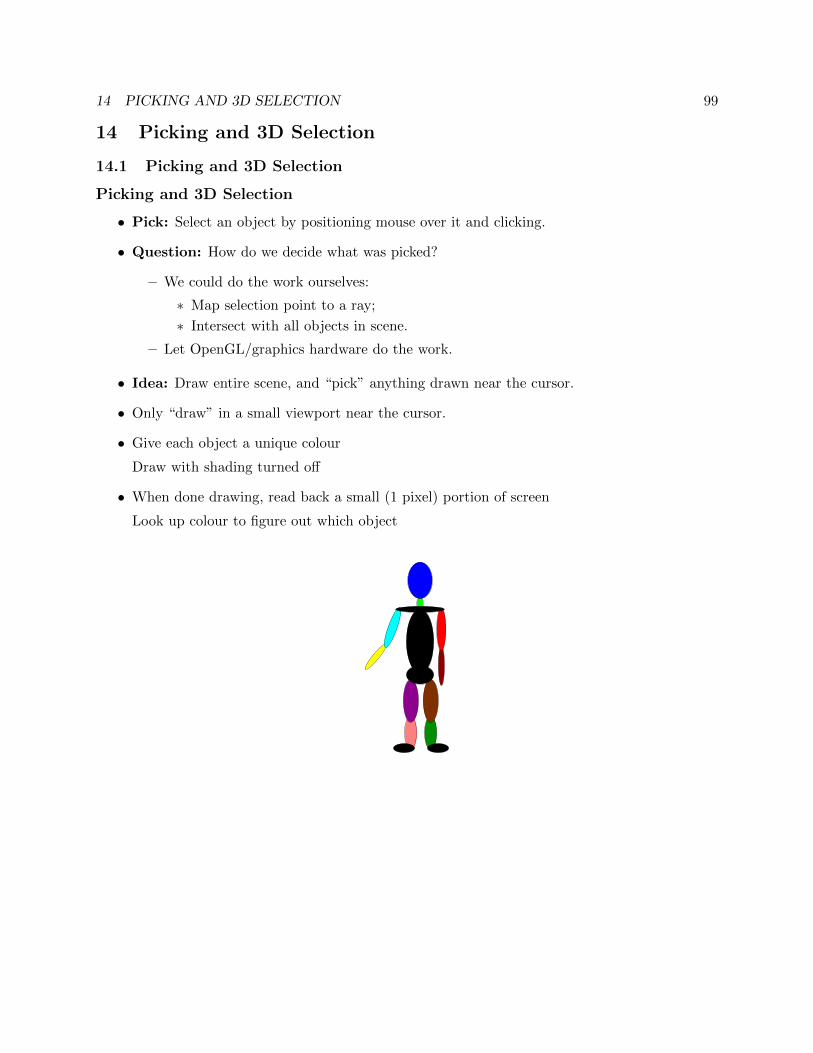
14 PICKING AND 3D SELECTION 99
14 Picking and 3D Selection
14.1 Picking and 3D Selection
Picking and 3D Selection
• Pick: Select an object by positioning mouse over it and clicking.
• Question: How do we decide what was picked?
– We could do the work ourselves:
∗ Map selection point to a ray;
∗ Intersect with all objects in scene.
– Let OpenGL/graphics hardware do the work.
• Idea: Draw entire scene, and “pick” anything drawn near the cursor.
• Only “draw” in a small viewport near the cursor.
• Give each object a unique colour
Draw with shading turned off
• When done drawing, read back a small (1 pixel) portion of screen
Look up colour to figure out which object

Colour and the Human Visual System 14 100
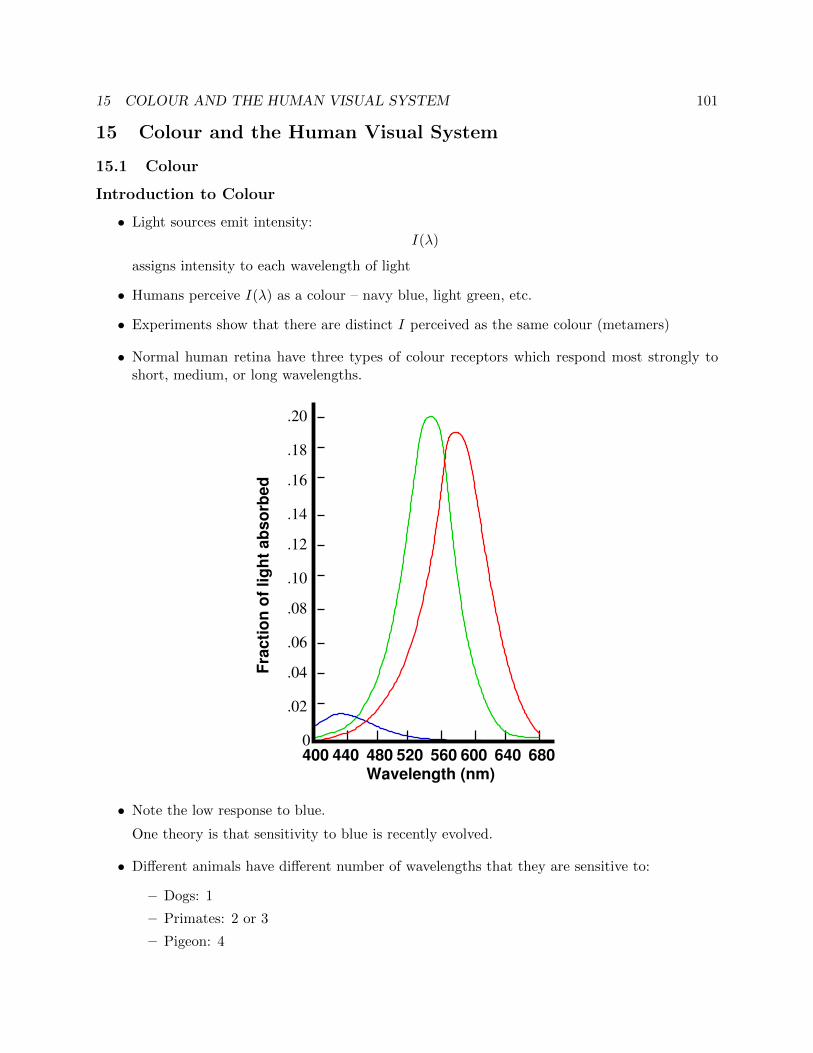
15 COLOUR AND THE HUMAN VISUAL SYSTEM 101
15 Colour and the Human Visual System
15.1 Colour
Introduction to Colour
• Light sources emit intensity:I(λ)
assigns intensity to each wavelength of light
• Humans perceive I(λ) as a colour – navy blue, light green, etc.
• Experiments show that there are distinct I perceived as the same colour (metamers)
• Normal human retina have three types of colour receptors which respond most strongly toshort, medium, or long wavelengths.
.02
.04
.06
.08
.12
.10
.14
.16
.18
.20
0
680640600560520480440400Wavelength (nm)
Fra
cti
on
of
lig
ht
ab
so
rbed
• Note the low response to blue.
One theory is that sensitivity to blue is recently evolved.
• Different animals have different number of wavelengths that they are sensitive to:
– Dogs: 1
– Primates: 2 or 3
– Pigeon: 4
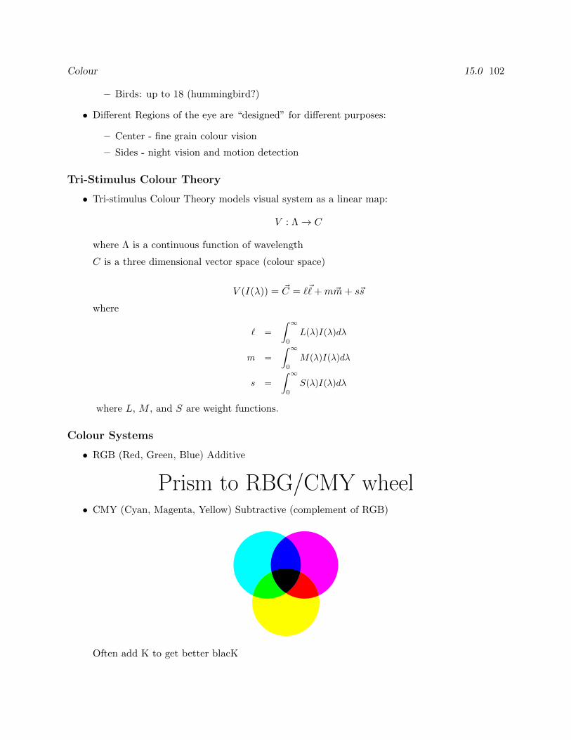
Colour 15.0 102
– Birds: up to 18 (hummingbird?)
• Different Regions of the eye are “designed” for different purposes:
– Center - fine grain colour vision
– Sides - night vision and motion detection
Tri-Stimulus Colour Theory
• Tri-stimulus Colour Theory models visual system as a linear map:
V : Λ→ C
where Λ is a continuous function of wavelength
C is a three dimensional vector space (colour space)
V (I(λ)) = ~C = `~+m~m+ s~s
where
` =
∫ ∞
0
L(λ)I(λ)dλ
m =
∫ ∞
0
M(λ)I(λ)dλ
s =
∫ ∞
0
S(λ)I(λ)dλ
where L, M , and S are weight functions.
Colour Systems
• RGB (Red, Green, Blue) Additive
Prism to RBG/CMY wheel• CMY (Cyan, Magenta, Yellow) Subtractive (complement of RGB)
Often add K to get better blacK
Reflection and Light Source Models 15 103
• HSV (Hue, Saturation, Value) Cone shaped colour space
Hue-Saturation wheel:
Hue (circular), saturation (radial)
Also HSL (double cone)
• CIE XYZ (Colour by committee) More complete colour space
Also L*u*v and L*a*b
• YIQ (Y == Luminance == CIE Y; IQ encode colour)
Backwards compatible with black-and-white TV (only show Y)

Reflection and Light Source Models 15 104
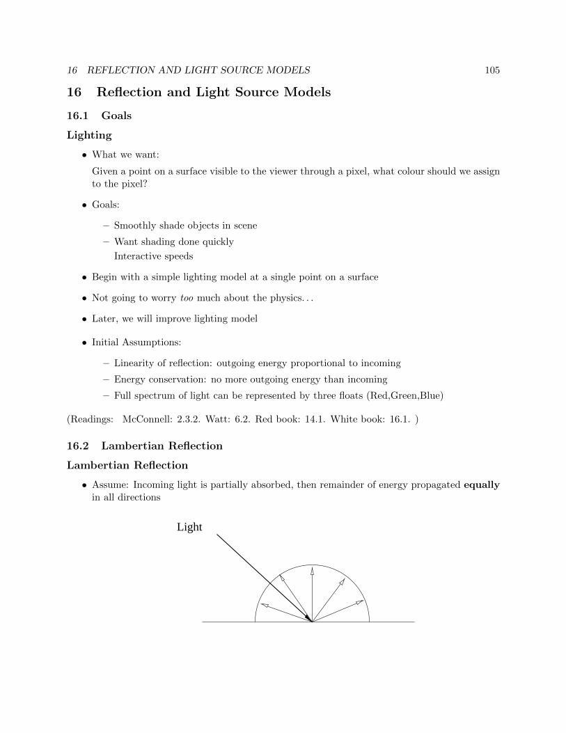
16 REFLECTION AND LIGHT SOURCE MODELS 105
16 Reflection and Light Source Models
16.1 Goals
Lighting
• What we want:
Given a point on a surface visible to the viewer through a pixel, what colour should we assignto the pixel?
• Goals:
– Smoothly shade objects in scene
– Want shading done quickly
Interactive speeds
• Begin with a simple lighting model at a single point on a surface
• Not going to worry too much about the physics. . .
• Later, we will improve lighting model
• Initial Assumptions:
– Linearity of reflection: outgoing energy proportional to incoming
– Energy conservation: no more outgoing energy than incoming
– Full spectrum of light can be represented by three floats (Red,Green,Blue)
(Readings: McConnell: 2.3.2. Watt: 6.2. Red book: 14.1. White book: 16.1. )
16.2 Lambertian Reflection
Lambertian Reflection
• Assume: Incoming light is partially absorbed, then remainder of energy propagated equallyin all directions
Light
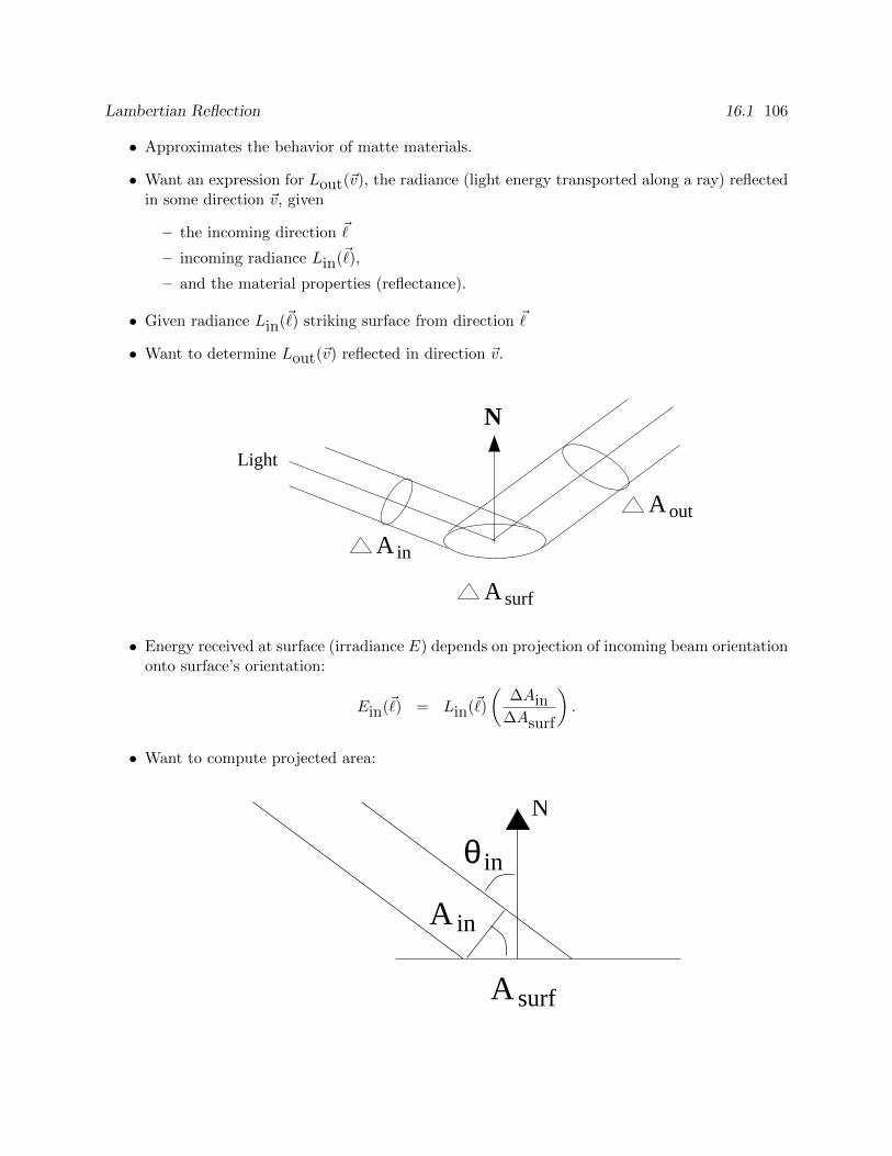
Lambertian Reflection 16.1 106
• Approximates the behavior of matte materials.
• Want an expression for Lout(~v), the radiance (light energy transported along a ray) reflectedin some direction ~v, given
– the incoming direction ~
– incoming radiance Lin(~),
– and the material properties (reflectance).
• Given radiance Lin(~) striking surface from direction ~
• Want to determine Lout(~v) reflected in direction ~v.
A
A
A
N
surf
in
out
Light
• Energy received at surface (irradiance E) depends on projection of incoming beam orientationonto surface’s orientation:
Ein(~) = Lin(~)
(∆Ain
∆Asurf
).
• Want to compute projected area:
in
A in
θN
A surf
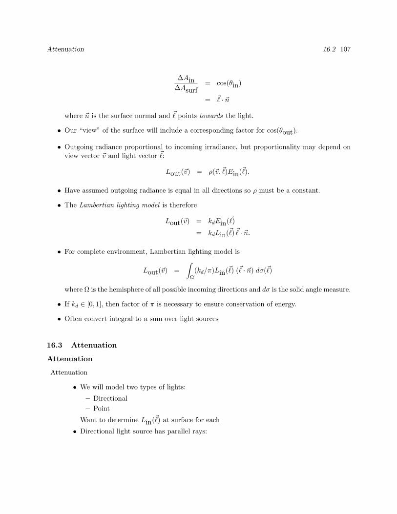
Attenuation 16.2 107
∆Ain∆Asurf
= cos(θin)
= ~ · ~n
where ~n is the surface normal and ~ points towards the light.
• Our “view” of the surface will include a corresponding factor for cos(θout).
• Outgoing radiance proportional to incoming irradiance, but proportionality may depend onview vector ~v and light vector ~:
Lout(~v) = ρ(~v, ~)Ein(~).
• Have assumed outgoing radiance is equal in all directions so ρ must be a constant.
• The Lambertian lighting model is therefore
Lout(~v) = kdEin(~)
= kdLin(~) ~ · ~n.
• For complete environment, Lambertian lighting model is
Lout(~v) =
∫Ω
(kd/π)Lin(~) (~ · ~n) dσ(~)
where Ω is the hemisphere of all possible incoming directions and dσ is the solid angle measure.
• If kd ∈ [0, 1], then factor of π is necessary to ensure conservation of energy.
• Often convert integral to a sum over light sources
16.3 Attenuation
Attenuation
Attenuation
• We will model two types of lights:
– Directional
– Point
Want to determine Lin(~) at surface for each
• Directional light source has parallel rays:
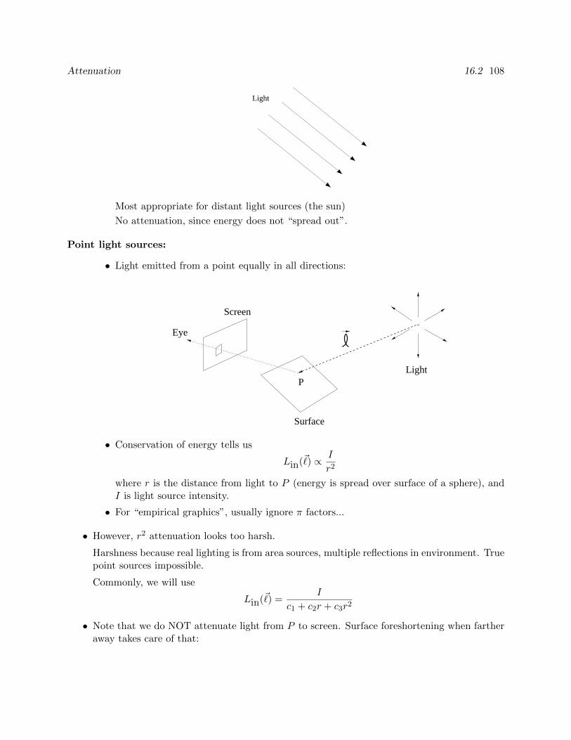
Attenuation 16.2 108
Light
Most appropriate for distant light sources (the sun)
No attenuation, since energy does not “spread out”.
Point light sources:
• Light emitted from a point equally in all directions:
P
Surface
Light
Eye
Screen
• Conservation of energy tells us
Lin(~) ∝ I
r2
where r is the distance from light to P (energy is spread over surface of a sphere), andI is light source intensity.
• For “empirical graphics”, usually ignore π factors...
• However, r2 attenuation looks too harsh.
Harshness because real lighting is from area sources, multiple reflections in environment. Truepoint sources impossible.
Commonly, we will use
Lin(~) =I
c1 + c2r + c3r2
• Note that we do NOT attenuate light from P to screen. Surface foreshortening when fartheraway takes care of that:
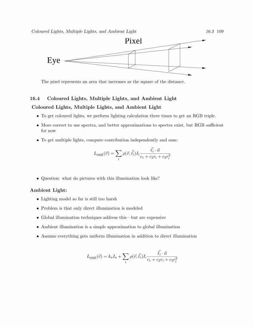
Coloured Lights, Multiple Lights, and Ambient Light 16.3 109
Pixel
Eye
The pixel represents an area that increases as the square of the distance.
16.4 Coloured Lights, Multiple Lights, and Ambient Light
Coloured Lights, Multiple Lights, and Ambient Light
• To get coloured lights, we perform lighting calculation three times to get an RGB triple.
• More correct to use spectra, and better approximations to spectra exist, but RGB sufficientfor now
• To get multiple lights, compute contribution independently and sum:
Lout(~v) =∑i
ρ(~v, ~i)Ii~i · ~n
c1 + c2ri + c3r2i
• Question: what do pictures with this illumination look like?
Ambient Light:
• Lighting model so far is still too harsh
• Problem is that only direct illumination is modeled
• Global illumination techniques address this—but are expensive
• Ambient illumination is a simple approximation to global illumination
• Assume everything gets uniform illumination in addition to direct illumination
Lout(~v) = kaIa +∑i
ρ(~v, ~i)Ii~i · ~n
c1 + c2ri + c3r2i
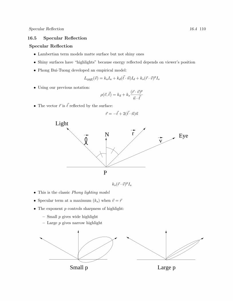
Specular Reflection 16.4 110
16.5 Specular Reflection
Specular Reflection
• Lambertian term models matte surface but not shiny ones
• Shiny surfaces have “highlights” because energy reflected depends on viewer’s position
• Phong Bui-Tuong developed an empirical model:
Lout(~v) = kaIa + kd(~ · ~n)Id + ks(~r · ~v)pIs
• Using our previous notation:
ρ(~v, ~) = kd + ks(~r · ~v)p
~n · ~
• The vector ~r is ~ reflected by the surface:
~r = −~+ 2(~ · ~n)~n
v
Light
N Eye
P
r
ks(~r · ~v)pIs
• This is the classic Phong lighting model
• Specular term at a maximum (ks) when ~v = ~r
• The exponent p controls sharpness of highlight:
– Small p gives wide highlight
– Large p gives narrow highlight
Large pSmall p
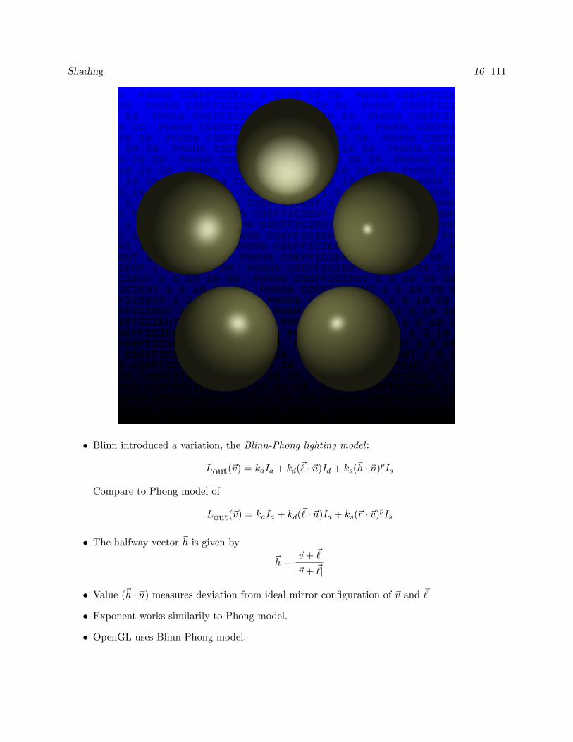
Shading 16 111
• Blinn introduced a variation, the Blinn-Phong lighting model :
Lout(~v) = kaIa + kd(~ · ~n)Id + ks(~h · ~n)pIs
Compare to Phong model of
Lout(~v) = kaIa + kd(~ · ~n)Id + ks(~r · ~v)pIs
• The halfway vector ~h is given by
~h =~v + ~
|~v + ~|
• Value (~h · ~n) measures deviation from ideal mirror configuration of ~v and ~
• Exponent works similarily to Phong model.
• OpenGL uses Blinn-Phong model.

Shading 16 112
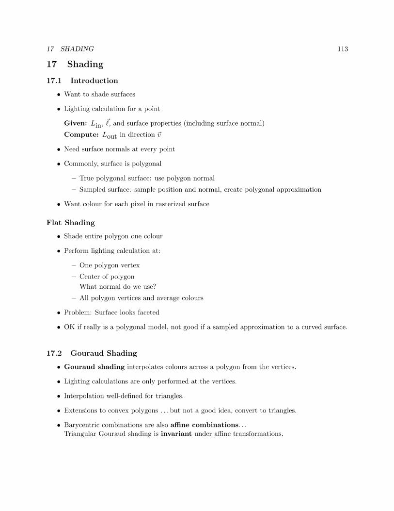
17 SHADING 113
17 Shading
17.1 Introduction
• Want to shade surfaces
• Lighting calculation for a point
Given: Lin, ~, and surface properties (including surface normal)
Compute: Lout in direction ~v
• Need surface normals at every point
• Commonly, surface is polygonal
– True polygonal surface: use polygon normal
– Sampled surface: sample position and normal, create polygonal approximation
• Want colour for each pixel in rasterized surface
Flat Shading
• Shade entire polygon one colour
• Perform lighting calculation at:
– One polygon vertex
– Center of polygon
What normal do we use?
– All polygon vertices and average colours
• Problem: Surface looks faceted
• OK if really is a polygonal model, not good if a sampled approximation to a curved surface.
17.2 Gouraud Shading
• Gouraud shading interpolates colours across a polygon from the vertices.
• Lighting calculations are only performed at the vertices.
• Interpolation well-defined for triangles.
• Extensions to convex polygons . . . but not a good idea, convert to triangles.
• Barycentric combinations are also affine combinations. . .Triangular Gouraud shading is invariant under affine transformations.
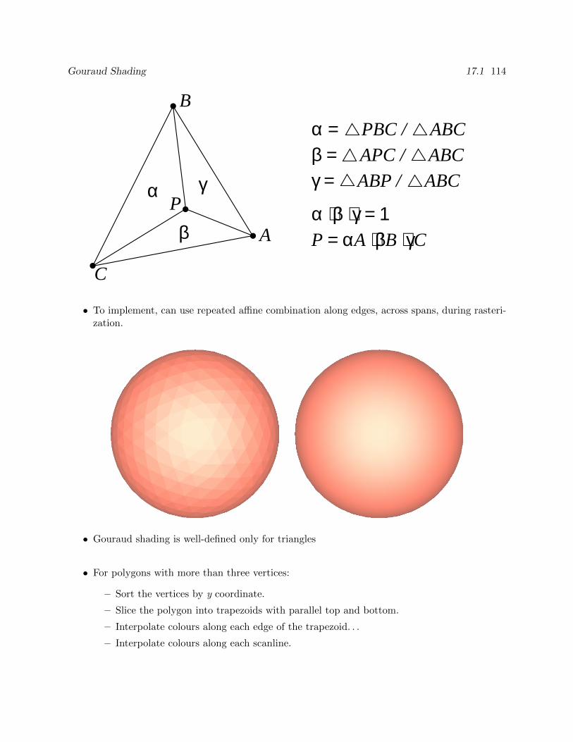
Gouraud Shading 17.1 114
A
α
β
γ
C
P
B
α = PBC / ABC
P = αA + βB + γCα + β + γ = 1
γ = ABP / ABCβ = APC / ABC
• To implement, can use repeated affine combination along edges, across spans, during rasteri-zation.
• Gouraud shading is well-defined only for triangles
• For polygons with more than three vertices:
– Sort the vertices by y coordinate.
– Slice the polygon into trapezoids with parallel top and bottom.
– Interpolate colours along each edge of the trapezoid. . .
– Interpolate colours along each scanline.
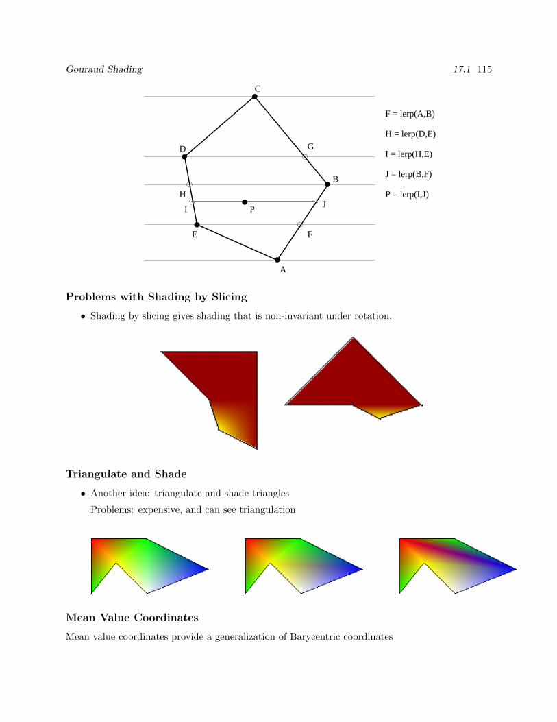
Gouraud Shading 17.1 115
P
A
B
C
D
E F
G
H
I J
F = lerp(A,B)
H = lerp(D,E)
I = lerp(H,E)
J = lerp(B,F)
P = lerp(I,J)
Problems with Shading by Slicing
• Shading by slicing gives shading that is non-invariant under rotation.
Triangulate and Shade
• Another idea: triangulate and shade triangles
Problems: expensive, and can see triangulation
Mean Value Coordinates
Mean value coordinates provide a generalization of Barycentric coordinates
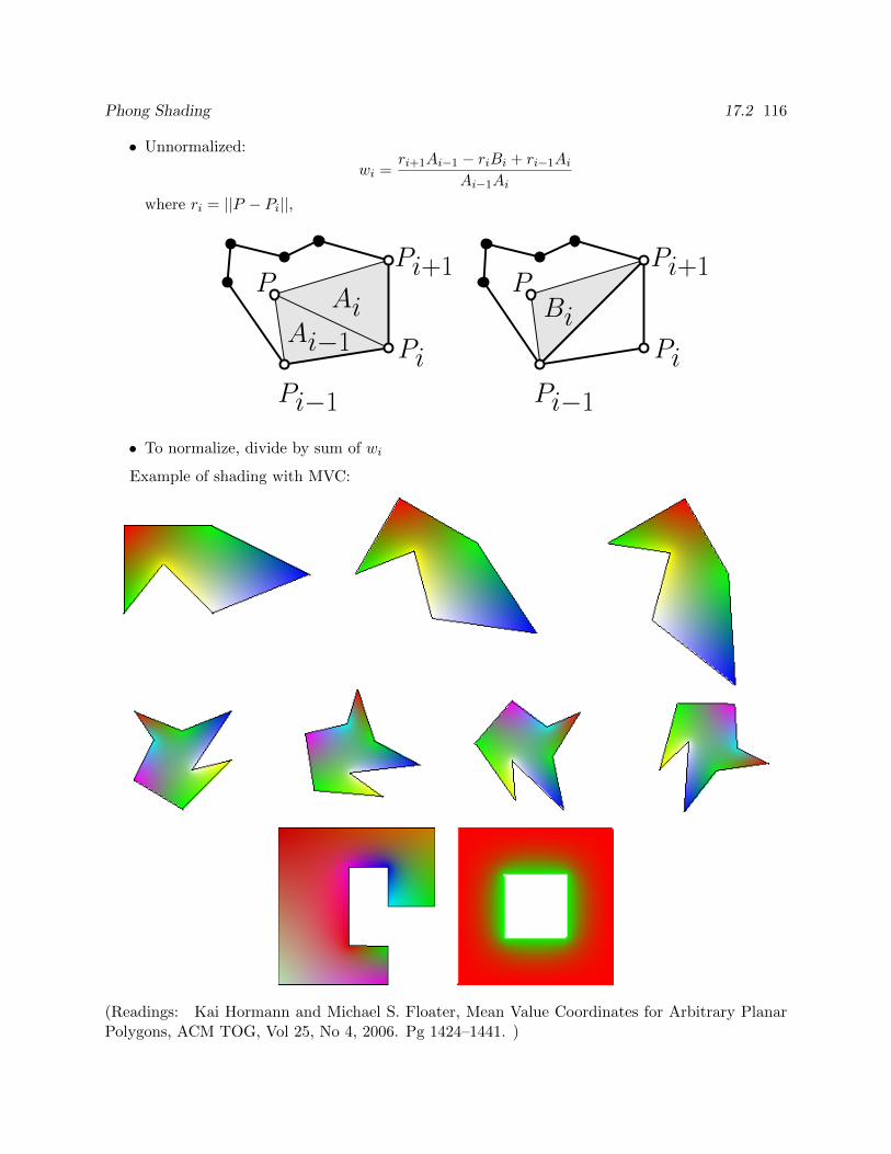
Phong Shading 17.2 116
• Unnormalized:
wi =ri+1Ai−1 − riBi + ri−1Ai
Ai−1Ai
where ri = ||P − Pi||,
Pi+1P
Pi
Pi−1
Ai−1
Ai
Pi+1P
Pi
Pi−1
Bi
• To normalize, divide by sum of wi
Example of shading with MVC:
(Readings: Kai Hormann and Michael S. Floater, Mean Value Coordinates for Arbitrary PlanarPolygons, ACM TOG, Vol 25, No 4, 2006. Pg 1424–1441. )
Ray Tracing 17 117
17.3 Phong Shading
• Phong Shading interpolates lighting model parameters, not colours.
• Much better rendition of highlights.
• A normal is specified at each vertex of a polygon.
• Vertex normals are independent of the polygon normal.
• Vertex normals should relate to the surface being approximated by the polygonal mesh.
• The normal is interpolated across the polygon (using Gouraud techniques).
• At each pixel,
– Interpolate the normal. . .
– Interpolate other shading parameters. . .
– Compute the view and light vectors. . .
– Evaluate the lighting model.
• The lighting model does not have to be the Phong lighting model!
• Normal interpolation is nominally done by vector addition and renormalization.
• Several “fast” approximations are possible.
• The view and light vectors may also be interpolated or approximated.
• Phong shading can be simulated with programmable vertex and fragment shaders on moderngraphics hardware:
– Classic Gouraud shading is linear in device space.
– Modern graphics hardware performs rational linear interpolation
– Interpolate normals, view vectors, and light vectors using generic interpolation hardware
– Usually also interpolate diffuse term after computing it in vertex shader.
– Other kinds of advanced shading possible

Ray Tracing 17 118
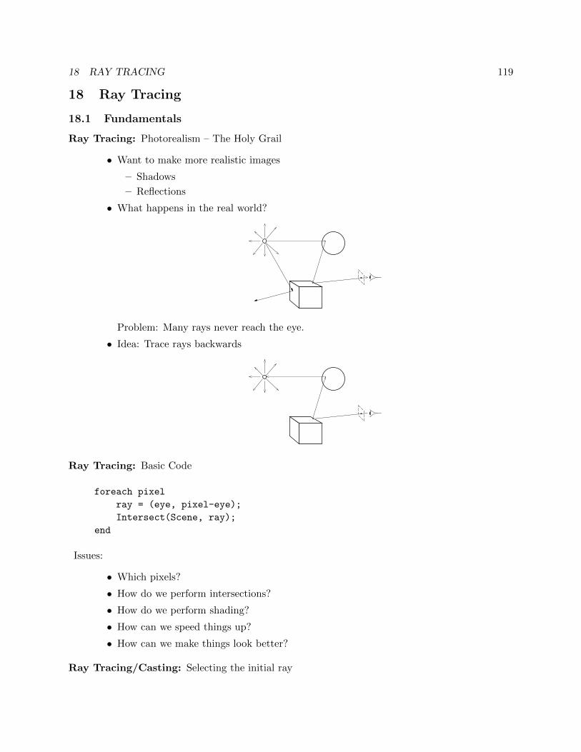
18 RAY TRACING 119
18 Ray Tracing
18.1 Fundamentals
Ray Tracing: Photorealism – The Holy Grail
• Want to make more realistic images
– Shadows
– Reflections
• What happens in the real world?
Problem: Many rays never reach the eye.
• Idea: Trace rays backwards
Ray Tracing: Basic Code
foreach pixel
ray = (eye, pixel-eye);
Intersect(Scene, ray);
end
Issues:
• Which pixels?
• How do we perform intersections?
• How do we perform shading?
• How can we speed things up?
• How can we make things look better?
Ray Tracing/Casting: Selecting the initial ray
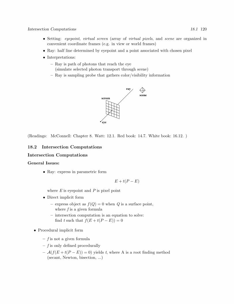
Intersection Computations 18.1 120
• Setting: eyepoint, virtual screen (array of virtual pixels, and scene are organized inconvenient coordinate frames (e.g. in view or world frames)
• Ray: half line determined by eyepoint and a point associated with chosen pixel
• Interpretations:
– Ray is path of photons that reach the eye(simulate selected photon transport through scene)
– Ray is sampling probe that gathers color/visibility information
ray
scene
eye
screen
(Readings: McConnell: Chapter 8. Watt: 12.1. Red book: 14.7. White book: 16.12. )
18.2 Intersection Computations
Intersection Computations
General Issues:
• Ray: express in parametric form
E + t(P − E)
where E is eyepoint and P is pixel point
• Direct implicit form
– express object as f(Q) = 0 when Q is a surface point,where f is a given formula
– intersection computation is an equation to solve:find t such that f(E + t(P − E)) = 0
• Procedural implicit form
– f is not a given formula
– f is only defined procedurally
– A(f(E + t(P − E)) = 0) yields t, where A is a root finding method(secant, Newton, bisection, ...)
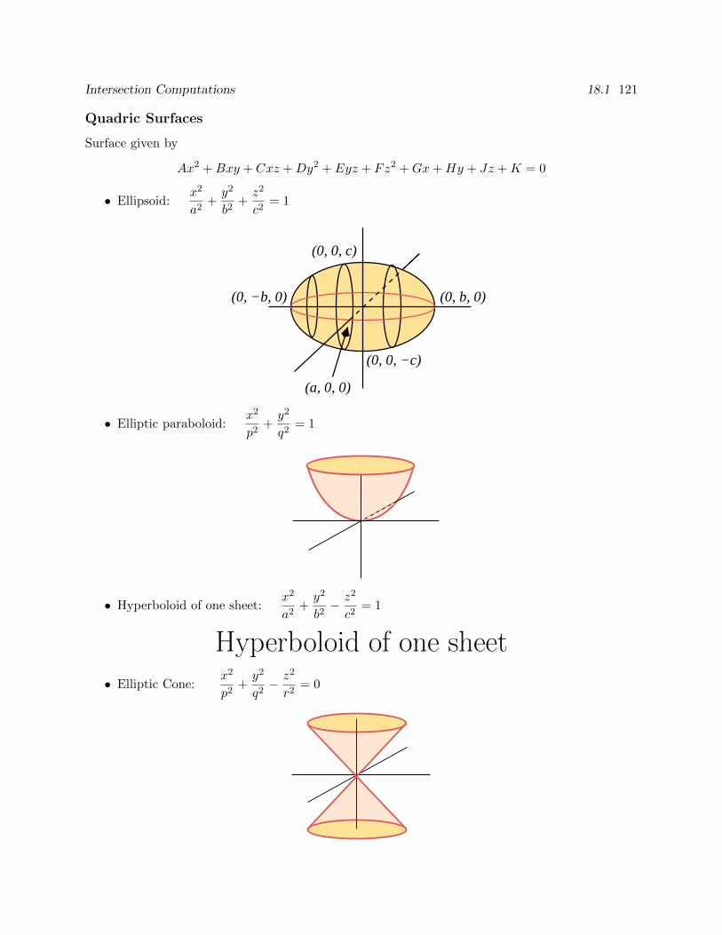
Intersection Computations 18.1 121
Quadric Surfaces
Surface given by
Ax2 +Bxy + Cxz +Dy2 + Eyz + Fz2 +Gx+Hy + Jz +K = 0
• Ellipsoid:x2
a2+y2
b2+z2
c2= 1
(0, 0, c)
(0, b, 0)(0, −b, 0)
(0, 0, −c)
(a, 0, 0)
• Elliptic paraboloid:x2
p2+y2
q2= 1
• Hyperboloid of one sheet:x2
a2+y2
b2− z2
c2= 1
Hyperboloid of one sheet
• Elliptic Cone:x2
p2+y2
q2− z2
r2= 0
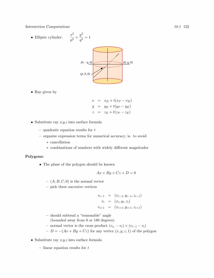
Intersection Computations 18.1 122
• Elliptic cylinder:x2
p2+y2
q2= 1
(0, −q, 0) (0, q, 0)
(p, 0, 0)
• Ray given by
x = xE + t(xP − xE)
y = yE + t(yP − yE)
z = zE + t(zP − zE)
• Substitute ray x,y,z into surface formula
– quadratic equation results for t
– organize expression terms for numerical accuracy; ie. to avoid
∗ cancellation
∗ combinations of numbers with widely different magnitudes
Polygons:
• The plane of the polygon should be known
Ax+By + Cz +D = 0
– (A,B,C, 0) is the normal vector
– pick three succesive vertices
vi−1 = (xi−1, yi−1, zi−1)
vi = (xi, yi, zi)
vi+1 = (xi+1, yi+1, zi+1)
– should subtend a “reasonable” angle(bounded away from 0 or 180 degrees)
– normal vector is the cross product (vi1 − vi)× (vi−1 − vi)– D = −(Ax+By + Cz) for any vertex (x, y, z, 1) of the polygon
• Substitute ray x,y,z into surface formula
– linear equation results for t
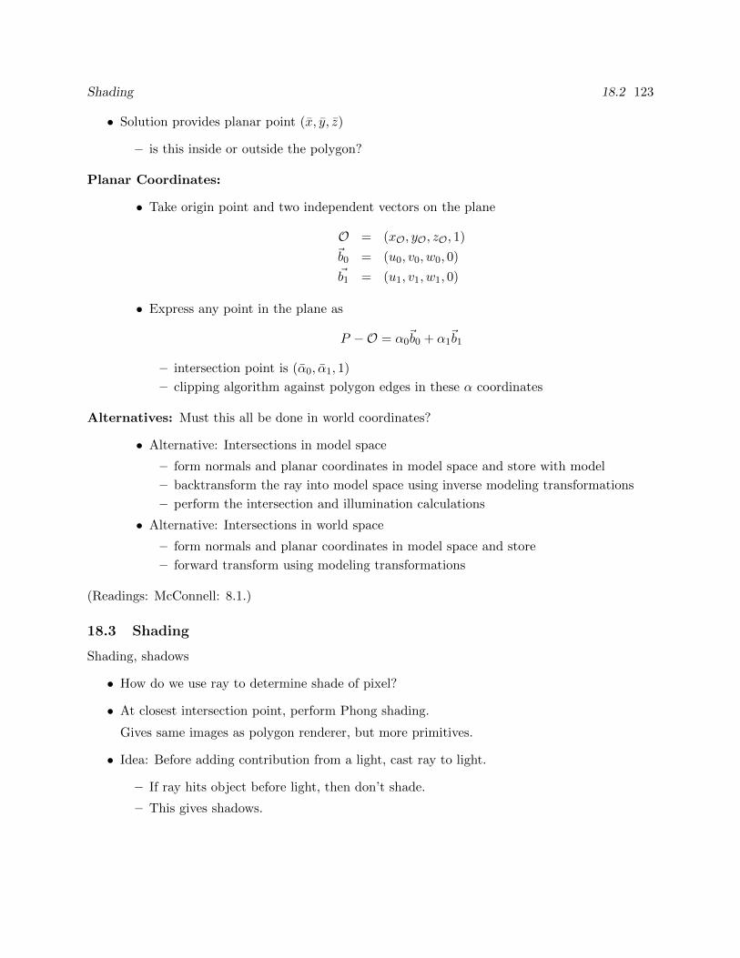
Shading 18.2 123
• Solution provides planar point (x, y, z)
– is this inside or outside the polygon?
Planar Coordinates:
• Take origin point and two independent vectors on the plane
O = (xO, yO, zO, 1)
~b0 = (u0, v0, w0, 0)
~b1 = (u1, v1, w1, 0)
• Express any point in the plane as
P −O = α0~b0 + α1
~b1
– intersection point is (α0, α1, 1)
– clipping algorithm against polygon edges in these α coordinates
Alternatives: Must this all be done in world coordinates?
• Alternative: Intersections in model space
– form normals and planar coordinates in model space and store with model
– backtransform the ray into model space using inverse modeling transformations
– perform the intersection and illumination calculations
• Alternative: Intersections in world space
– form normals and planar coordinates in model space and store
– forward transform using modeling transformations
(Readings: McConnell: 8.1.)
18.3 Shading
Shading, shadows
• How do we use ray to determine shade of pixel?
• At closest intersection point, perform Phong shading.
Gives same images as polygon renderer, but more primitives.
• Idea: Before adding contribution from a light, cast ray to light.
– If ray hits object before light, then don’t shade.
– This gives shadows.
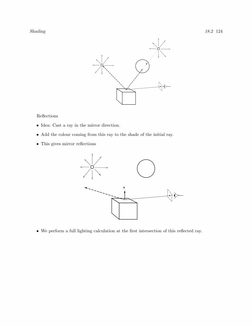
Shading 18.2 124
Reflections
• Idea: Cast a ray in the mirror direction.
• Add the colour coming from this ray to the shade of the initial ray.
• This gives mirror reflections
N
• We perform a full lighting calculation at the first intersection of this reflected ray.
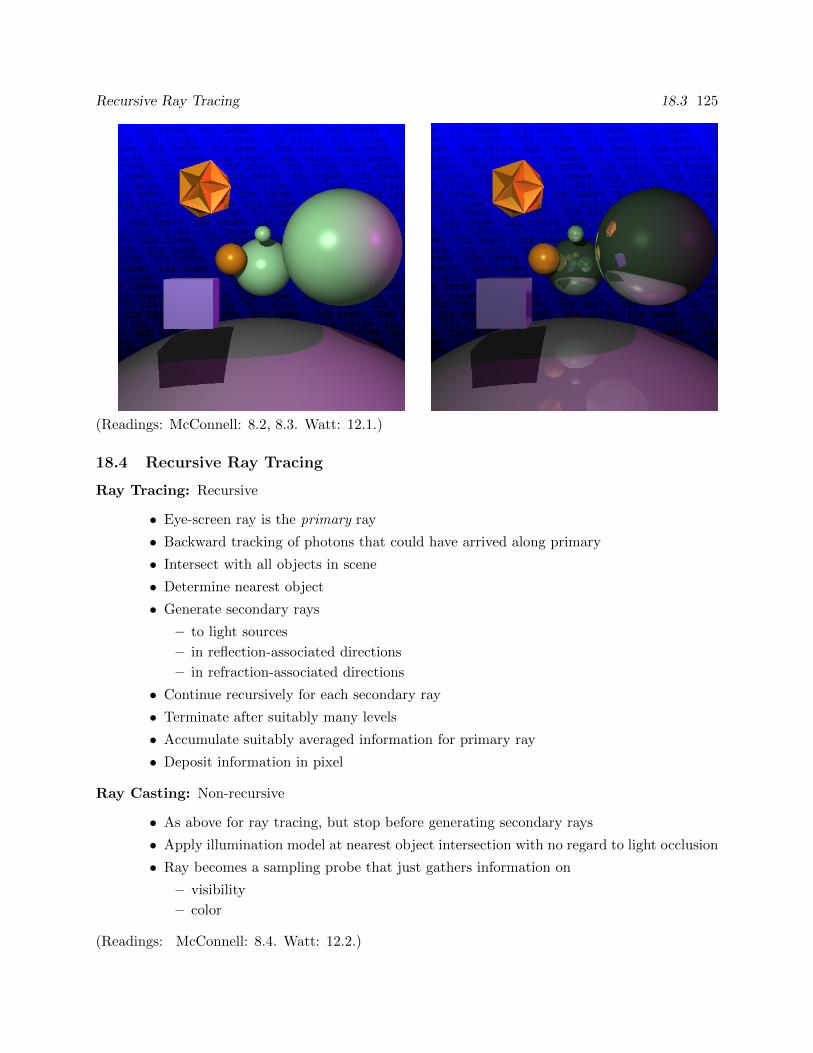
Recursive Ray Tracing 18.3 125
(Readings: McConnell: 8.2, 8.3. Watt: 12.1.)
18.4 Recursive Ray Tracing
Ray Tracing: Recursive
• Eye-screen ray is the primary ray
• Backward tracking of photons that could have arrived along primary
• Intersect with all objects in scene
• Determine nearest object
• Generate secondary rays
– to light sources
– in reflection-associated directions
– in refraction-associated directions
• Continue recursively for each secondary ray
• Terminate after suitably many levels
• Accumulate suitably averaged information for primary ray
• Deposit information in pixel
Ray Casting: Non-recursive
• As above for ray tracing, but stop before generating secondary rays
• Apply illumination model at nearest object intersection with no regard to light occlusion
• Ray becomes a sampling probe that just gathers information on
– visibility
– color
(Readings: McConnell: 8.4. Watt: 12.2.)
Surface Information 18.4 126
18.5 Surface Information
Surface Normals:
• Illumination models require:
– surface normal vectors at intersection points
– ray-surface intersection computation must also yield a normal
– light-source directions must be established at intersection
– shadow information determined by light-ray intersections with other objects
• Normals to polygons:
– provided by planar normal
– provided by cross product of adjacent edges
– Or use Phong normal interpolation if normals specified at vertices
• Normals to any implicit surface (eg. quadrics)
– move from (x, y, z) to (x+ ∆x, y + ∆y, z + ∆z) which is maximally far from the surface
– direction of greatest increase to f(x, y, z)
• Taylor series:
f(x+ ∆x, y + ∆y, z + ∆z) = f(x, y, z) + [∆x,∆y,∆z]
∂f∂x
∂f∂y
∂f∂z
+ · · ·
– maximality for the gradient vector of f
– not normalized
• Normal to a quadric surface 2Ax+By + Cz +GBx+ 2Dy + Ez +HCx+ Ey + 2Fz + J
0
Normal Transformations: How do affine transformations affect surface normals?
• Let Pa and Pb be any two points on object
– arbitrarily close
– ~n · (Pb − Pa) = 0
– using transpose notation: (~n)T (Pb − Pa) = 0
• After an affine transformation on Pa,Pb:
M(Pb − Pa) = MPb −MPa
we want (N~n) to be a normal for some transformation N:
(N~n)TM(Pb − Pa) = 0
=⇒ ~nTNTM(Pb − Pa)and this certainly holds if N = (M−1)T
Modeling and CSG 18.5 127
• Only the upper 3-by-3 portion of M is pertinent for vectors
• Translation:
(M−1)T =
1 0 0 00 1 0 00 0 1 0−∆x −∆y −∆z 1
−→ 1 0 0
0 1 00 0 1
1 0 0
0 1 00 0 1
nxnynz0
=
nxnynz0
=⇒ no change to the normal
• Rotation (example):
(M−1)T =
cos(−θ) sin(−θ) 0 0− sin(−θ) cos(−θ) 0 0
0 0 1 00 0 0 1
T
=
cos(θ) sin(θ) 0 0− sin(θ) cos(θ) 0 0
0 0 1 00 0 0 1
−→
cos(θ) sin(θ) 0− sin(θ) cos(θ) 0
0 0 1
=⇒ rotation applied unchanged to normal
• Scale:
(M−1)T =
1sx
0 0 0
0 1sy
0 0
0 0 1sz
0
0 0 0 1
−→
1sx
0 0
0 1sy
0
0 0 1sz
1sx
0 0
0 1sy
0
0 0 1sz
nx
ny
nz
0
=
nxsxnysynzsz
0
=⇒ reciprocal scale applied to normal
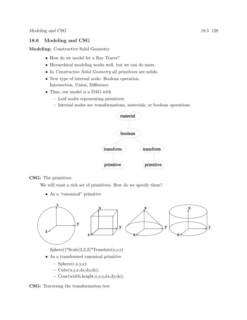
Modeling and CSG 18.5 128
18.6 Modeling and CSG
Modeling: Constructive Solid Geometry
• How do we model for a Ray Tracer?
• Hierarchical modeling works well, but we can do more.
• In Constructive Solid Geometry all primitives are solids.
• New type of internal node: Boolean operation.
Intersection, Union, Difference
• Thus, our model is a DAG with
– Leaf nodes representing primitives
– Internal nodes are transformations, materials, or boolean operations.
material
boolean
transform transform
primitive primitive
CSG: The primitives
We will want a rich set of primitives. How do we specify them?
• As a “canonical” primitive
x
y
z
x
y
z
x
y
z
x
y
z
Sphere()*Scale(2,2,2)*Translate(x,y,z)
• As a transformed canonical primitive
– Sphere(r,x,y,z);
– Cube(x,y,z,dx,dy,dz);
– Cone(width,height,x,y,z,dx,dy,dz);
CSG: Traversing the transformation tree
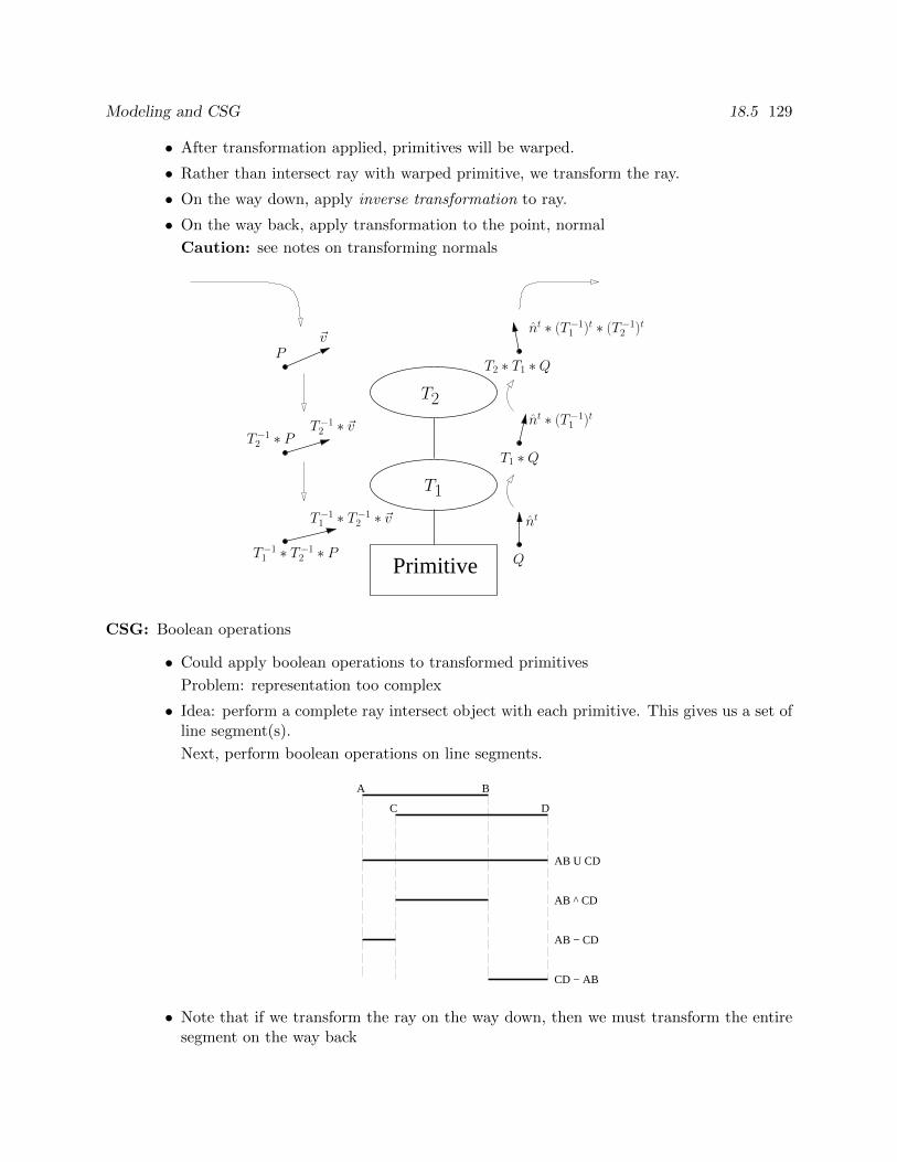
Modeling and CSG 18.5 129
• After transformation applied, primitives will be warped.
• Rather than intersect ray with warped primitive, we transform the ray.
• On the way down, apply inverse transformation to ray.
• On the way back, apply transformation to the point, normal
Caution: see notes on transforming normals
Primitive
T2 ∗ T1 ∗Q
nt ∗ (T−11 )t ∗ (T−12 )t
T1
T2nt ∗ (T−11 )t
P~v
T−12 ∗ PT−12 ∗ ~v
T−11 ∗ T−12 ∗ P
T−11 ∗ T−12 ∗ ~v
Q
nt
T1 ∗Q
CSG: Boolean operations
• Could apply boolean operations to transformed primitives
Problem: representation too complex
• Idea: perform a complete ray intersect object with each primitive. This gives us a set ofline segment(s).
Next, perform boolean operations on line segments.
A B
C D
AB U CD
AB ^ CD
AB − CD
CD − AB
• Note that if we transform the ray on the way down, then we must transform the entiresegment on the way back
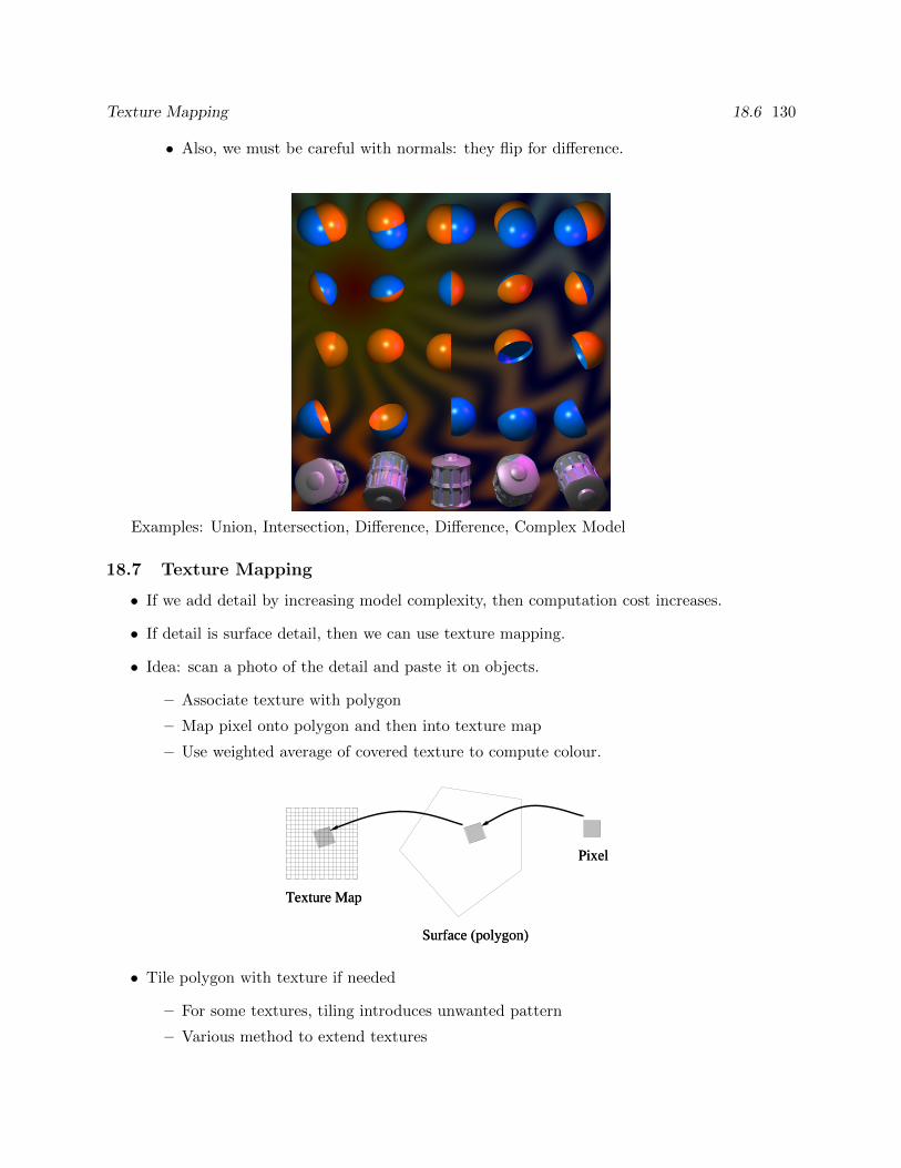
Texture Mapping 18.6 130
• Also, we must be careful with normals: they flip for difference.
Examples: Union, Intersection, Difference, Difference, Complex Model
18.7 Texture Mapping
• If we add detail by increasing model complexity, then computation cost increases.
• If detail is surface detail, then we can use texture mapping.
• Idea: scan a photo of the detail and paste it on objects.
– Associate texture with polygon
– Map pixel onto polygon and then into texture map
– Use weighted average of covered texture to compute colour.
Pixel
Surface (polygon)
Texture Map
• Tile polygon with texture if needed
– For some textures, tiling introduces unwanted pattern
– Various method to extend textures
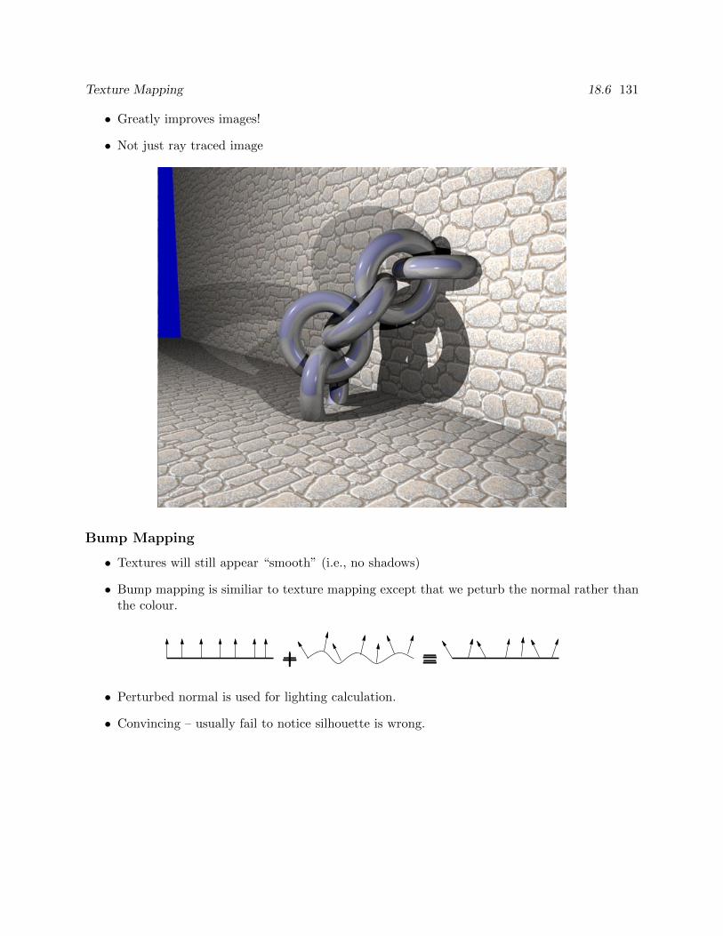
Texture Mapping 18.6 131
• Greatly improves images!
• Not just ray traced image
Bump Mapping
• Textures will still appear “smooth” (i.e., no shadows)
• Bump mapping is similiar to texture mapping except that we peturb the normal rather thanthe colour.
+ =• Perturbed normal is used for lighting calculation.
• Convincing – usually fail to notice silhouette is wrong.
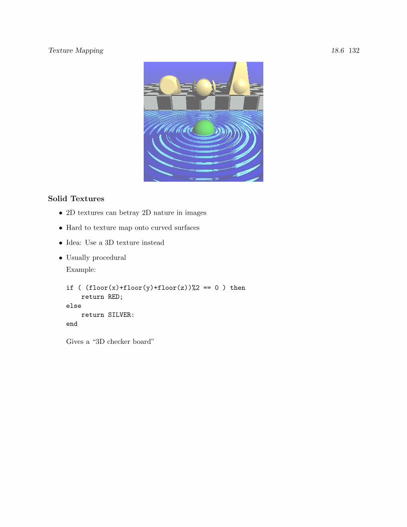
Texture Mapping 18.6 132
Solid Textures
• 2D textures can betray 2D nature in images
• Hard to texture map onto curved surfaces
• Idea: Use a 3D texture instead
• Usually procedural
Example:
if ( (floor(x)+floor(y)+floor(z))%2 == 0 ) then
return RED;
else
return SILVER:
end
Gives a “3D checker board”
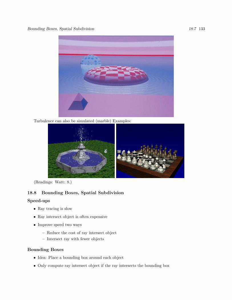
Bounding Boxes, Spatial Subdivision 18.7 133
Turbulence can also be simulated (marble) Examples:
(Readings: Watt: 8.)
18.8 Bounding Boxes, Spatial Subdivision
Speed-ups
• Ray tracing is slow
• Ray intersect object is often expensive
• Improve speed two ways
– Reduce the cost of ray intersect object
– Intersect ray with fewer objects
Bounding Boxes
• Idea: Place a bounding box around each object
• Only compute ray intersect object if the ray intersects the bounding box
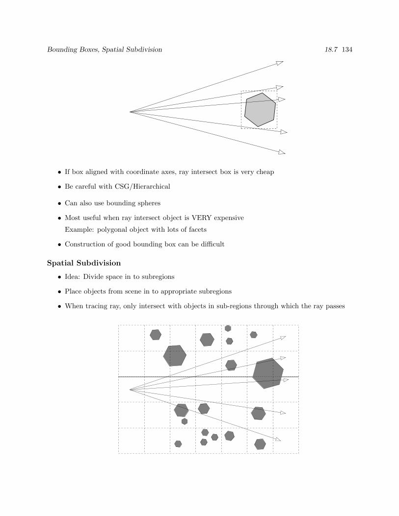
Bounding Boxes, Spatial Subdivision 18.7 134
• If box aligned with coordinate axes, ray intersect box is very cheap
• Be careful with CSG/Hierarchical
• Can also use bounding spheres
• Most useful when ray intersect object is VERY expensive
Example: polygonal object with lots of facets
• Construction of good bounding box can be difficult
Spatial Subdivision
• Idea: Divide space in to subregions
• Place objects from scene in to appropriate subregions
• When tracing ray, only intersect with objects in sub-regions through which the ray passes

Aliasing 18 135
• Useful when lots of small objects in scene
• Determining subdivision is difficult

Aliasing 18 136
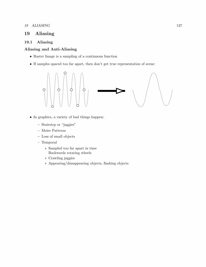
19 ALIASING 137
19 Aliasing
19.1 Aliasing
Aliasing and Anti-Aliasing
• Raster Image is a sampling of a continuous function
• If samples spaced too far apart, then don’t get true representation of scene:
• In graphics, a variety of bad things happen:
– Stairstep or “jaggies”
– Moire Patterns
– Loss of small objects
– Temporal
∗ Sampled too far apart in timeBackwards rotating wheels
∗ Crawling jaggies
∗ Appearing/dissappearing objects, flashing objects
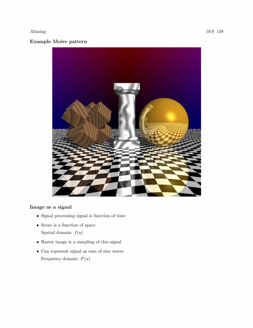
Aliasing 19.0 138
Example Moire pattern
Image as a signal
• Signal processing signal is function of time
• Scene is a function of space
Spatial domain: f(u)
• Raster image is a sampling of this signal
• Can represent signal as sum of sine waves
Frequency domain: F (u)
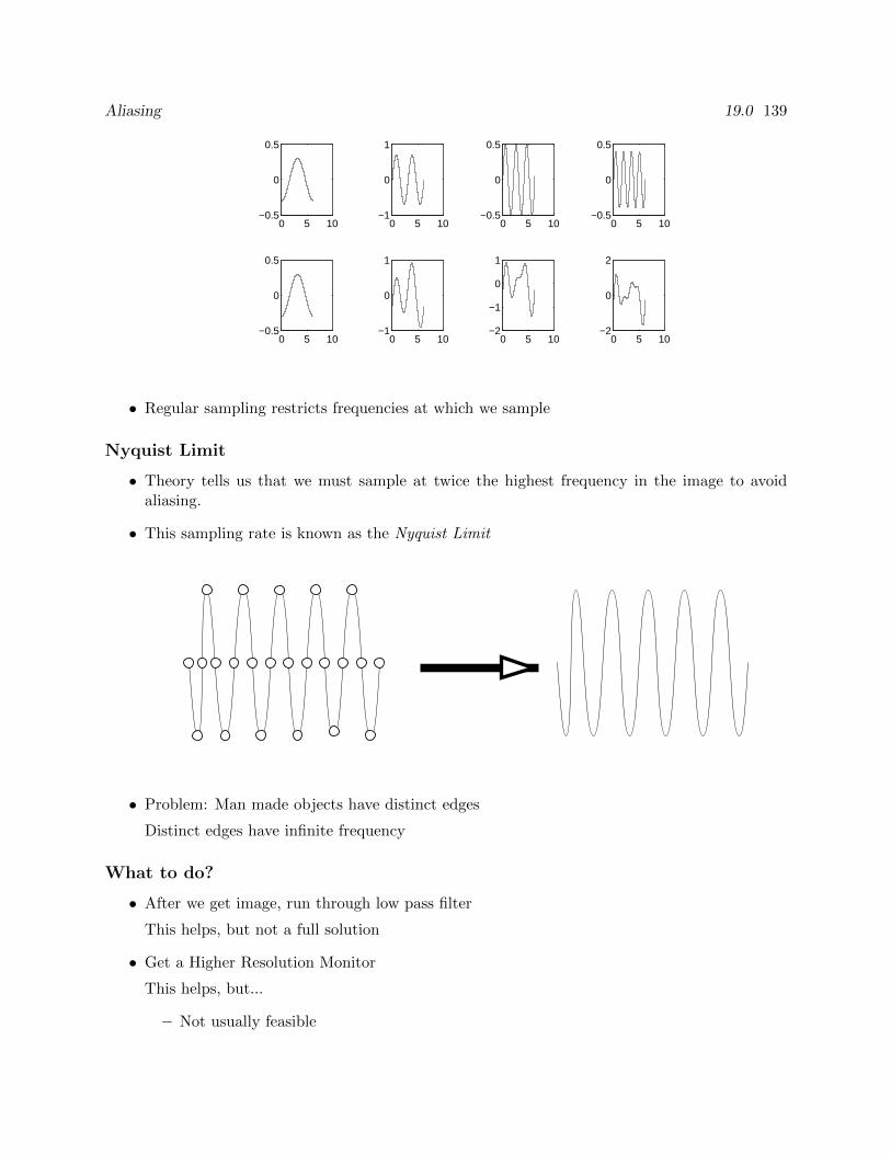
Aliasing 19.0 139
0 5 10−0.5
0
0.5
0 5 10−0.5
0
0.5
0 5 10−1
0
1
0 5 10−1
0
1
0 5 10−0.5
0
0.5
0 5 10−2
−1
0
1
0 5 10−0.5
0
0.5
0 5 10−2
0
2
• Regular sampling restricts frequencies at which we sample
Nyquist Limit
• Theory tells us that we must sample at twice the highest frequency in the image to avoidaliasing.
• This sampling rate is known as the Nyquist Limit
• Problem: Man made objects have distinct edges
Distinct edges have infinite frequency
What to do?
• After we get image, run through low pass filter
This helps, but not a full solution
• Get a Higher Resolution Monitor
This helps, but...
– Not usually feasible
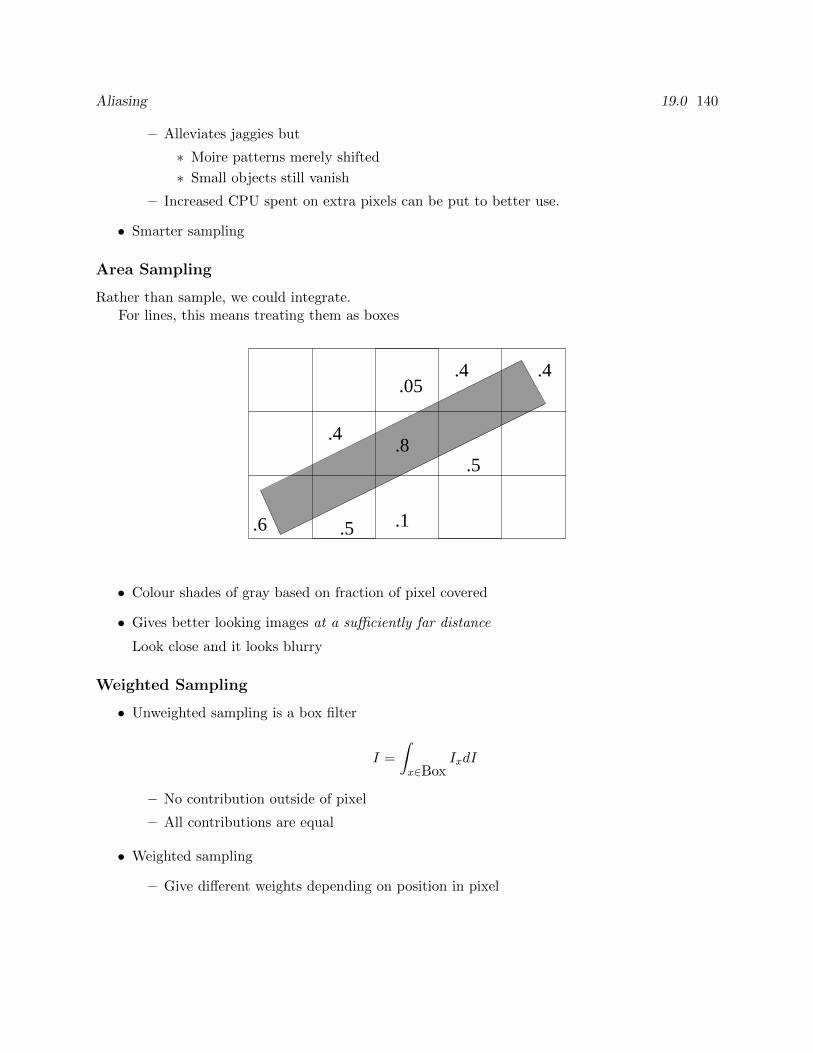
Aliasing 19.0 140
– Alleviates jaggies but
∗ Moire patterns merely shifted
∗ Small objects still vanish
– Increased CPU spent on extra pixels can be put to better use.
• Smarter sampling
Area Sampling
Rather than sample, we could integrate.For lines, this means treating them as boxes
.1
.5
.4
.5
.05
.8
.4 .4
.6
• Colour shades of gray based on fraction of pixel covered
• Gives better looking images at a sufficiently far distance
Look close and it looks blurry
Weighted Sampling
• Unweighted sampling is a box filter
I =
∫x∈Box
IxdI
– No contribution outside of pixel
– All contributions are equal
• Weighted sampling
– Give different weights depending on position in pixel
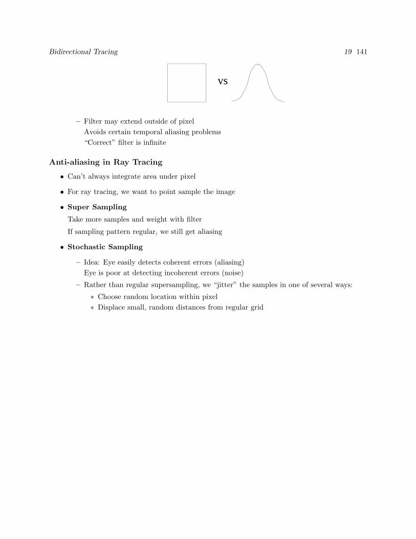
Bidirectional Tracing 19 141
vs
– Filter may extend outside of pixel
Avoids certain temporal aliasing problems
“Correct” filter is infinite
Anti-aliasing in Ray Tracing
• Can’t always integrate area under pixel
• For ray tracing, we want to point sample the image
• Super Sampling
Take more samples and weight with filter
If sampling pattern regular, we still get aliasing
• Stochastic Sampling
– Idea: Eye easily detects coherent errors (aliasing)
Eye is poor at detecting incoherent errors (noise)
– Rather than regular supersampling, we “jitter” the samples in one of several ways:
∗ Choose random location within pixel
∗ Displace small, random distances from regular grid

Bidirectional Tracing 19 142
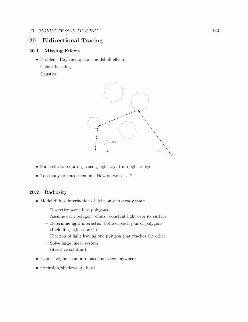
20 BIDIRECTIONAL TRACING 143
20 Bidirectional Tracing
20.1 Missing Effects
• Problem: Raytracing can’t model all effects
Colour bleeding
Caustics
Lens
• Some effects requiring tracing light rays from light to eye
• Too many to trace them all. How do we select?
20.2 Radiosity
• Model diffuse interfaction of light only in steady state
– Discretize scene into polygons
Assume each polygon “emits” constant light over its surface
– Determine light interaction between each pair of polygons
(Including light sources)
Fraction of light leaving one polygon that reaches the other
– Solve large linear system
(iterative solution)
• Expensive, but compute once and view anywhere
• Occlusion/shadows are hard
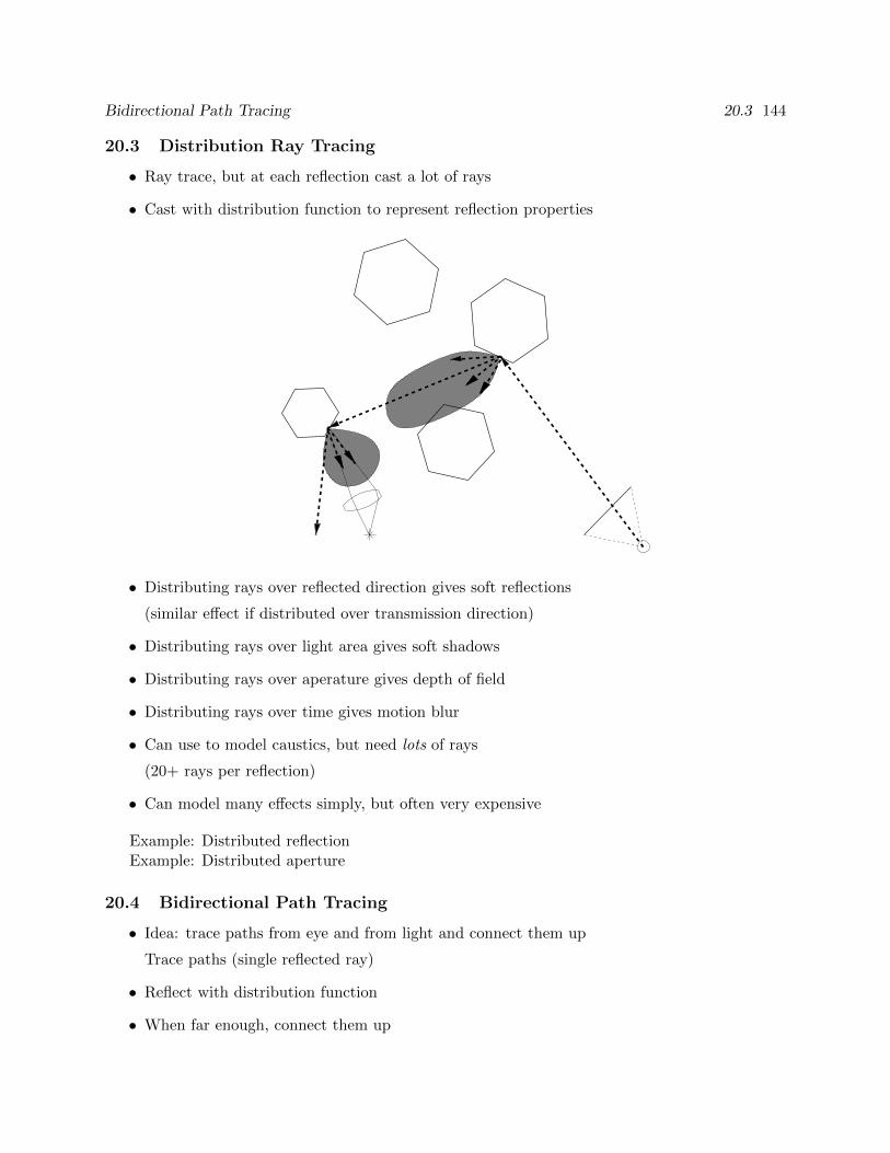
Bidirectional Path Tracing 20.3 144
20.3 Distribution Ray Tracing
• Ray trace, but at each reflection cast a lot of rays
• Cast with distribution function to represent reflection properties
• Distributing rays over reflected direction gives soft reflections
(similar effect if distributed over transmission direction)
• Distributing rays over light area gives soft shadows
• Distributing rays over aperature gives depth of field
• Distributing rays over time gives motion blur
• Can use to model caustics, but need lots of rays
(20+ rays per reflection)
• Can model many effects simply, but often very expensive
Example: Distributed reflectionExample: Distributed aperture
20.4 Bidirectional Path Tracing
• Idea: trace paths from eye and from light and connect them up
Trace paths (single reflected ray)
• Reflect with distribution function
• When far enough, connect them up
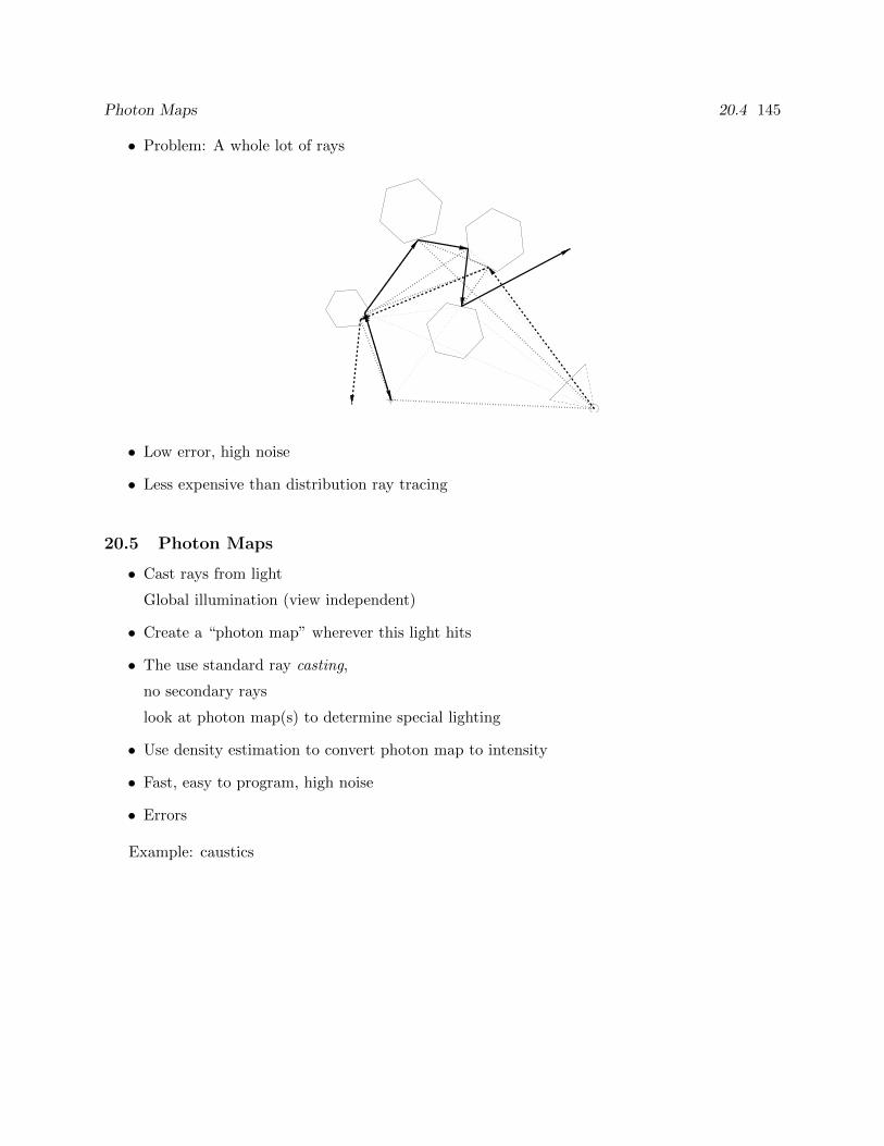
Photon Maps 20.4 145
• Problem: A whole lot of rays
• Low error, high noise
• Less expensive than distribution ray tracing
20.5 Photon Maps
• Cast rays from light
Global illumination (view independent)
• Create a “photon map” wherever this light hits
• The use standard ray casting,
no secondary rays
look at photon map(s) to determine special lighting
• Use density estimation to convert photon map to intensity
• Fast, easy to program, high noise
• Errors
Example: caustics
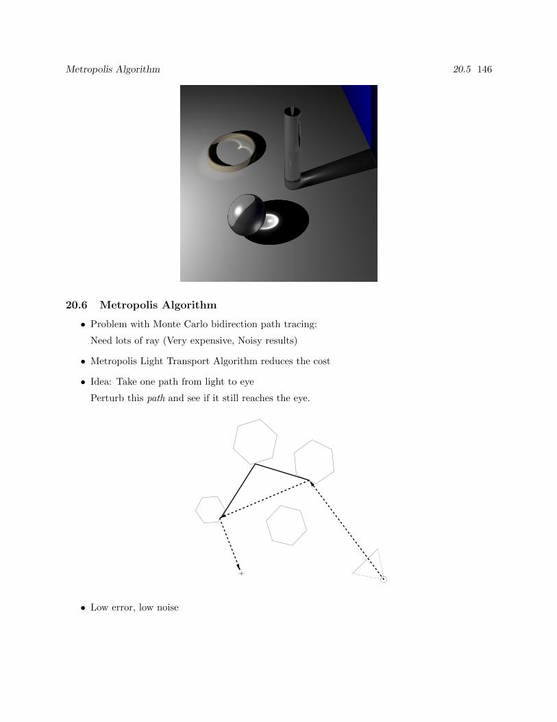
Metropolis Algorithm 20.5 146
20.6 Metropolis Algorithm
• Problem with Monte Carlo bidirection path tracing:
Need lots of ray (Very expensive, Noisy results)
• Metropolis Light Transport Algorithm reduces the cost
• Idea: Take one path from light to eye
Perturb this path and see if it still reaches the eye.
• Low error, low noise
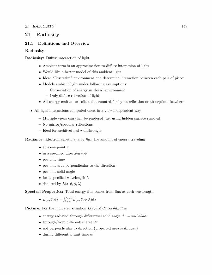
21 RADIOSITY 147
21 Radiosity
21.1 Definitions and Overview
Radiosity
Radiosity: Diffuse interaction of light
• Ambient term is an approximation to diffuse interaction of light
• Would like a better model of this ambient light
• Idea: “Discretize” environment and determine interaction between each pair of pieces.
• Models ambient light under following assumptions:
– Conservation of energy in closed environment
– Only diffuse reflection of light
• All energy emitted or reflected accounted for by its reflection or absorption elsewhere
• All light interactions computed once, in a view independent way
– Multiple views can then be rendered just using hidden surface removal
– No mirror/specular reflections
– Ideal for architectural walkthroughs
Radiance: Electromagnetic energy flux, the amount of energy traveling
• at some point x
• in a specified direction θ,φ
• per unit time
• per unit area perpendicular to the direction
• per unit solid angle
• for a specified wavelength λ
• denoted by L(x, θ, φ, λ)
Spectral Properties: Total energy flux comes from flux at each wavelength
• L(x, θ, φ) =∫ λmax
λminL(x, θ, φ, λ)dλ
Picture: For the indicated situation L(x, θ, φ)dx cos θdωdt is
• energy radiated through differential solid angle dω = sin θdθdφ
• through/from differential area dx
• not perpendicular to direction (projected area is dx cos θ)
• during differential unit time dt
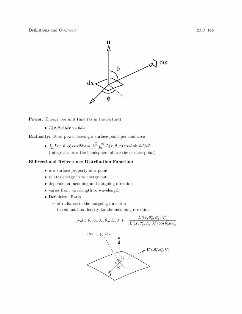
Definitions and Overview 21.0 148
θ
φ
dω
dx
n
Power: Energy per unit time (as in the picture)
• L(x, θ, φ)dx cos θdω
Radiosity: Total power leaving a surface point per unit area
•∫
Ω L(x, θ, φ) cos θdω =∫ π
20
∫ 2π0 L(x, θ, φ) cos θ sin θdφdθ
(integral is over the hemisphere above the surface point)
Bidirectional Reflectance Distribution Function:
• is a surface property at a point
• relates energy in to energy out
• depends on incoming and outgoing directions
• varies from wavelength to wavelength
• Definition: Ratio
– of radiance in the outgoing direction
– to radiant flux density for the incoming direction
ρbd(x, θi, φi, λi, θo, φo, λo) =Lo(x, θox, φ
ox, λ
o)
Li(x, θix, φix, λ
i) cos θixdωix
n
t
x
Li(x,θ ix ,φ i
x , λi )
Lo(x,θox ,φ o
x , λo)
θox
φ ox
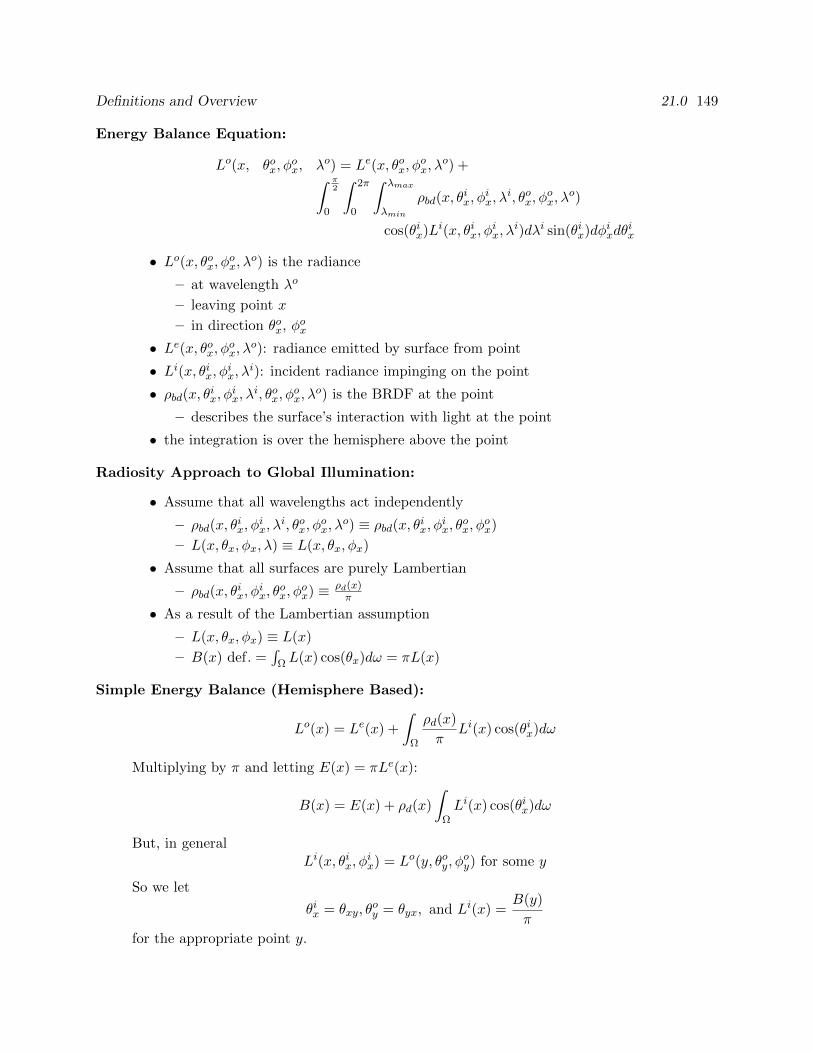
Definitions and Overview 21.0 149
Energy Balance Equation:
Lo(x, θox, φox, λo) = Le(x, θox, φ
ox, λ
o) +∫ π2
0
∫ 2π
0
∫ λmax
λmin
ρbd(x, θix, φ
ix, λ
i, θox, φox, λ
o)
cos(θix)Li(x, θix, φix, λ
i)dλi sin(θix)dφixdθix
• Lo(x, θox, φox, λo) is the radiance
– at wavelength λo
– leaving point x
– in direction θox, φox
• Le(x, θox, φox, λo): radiance emitted by surface from point
• Li(x, θix, φix, λi): incident radiance impinging on the point
• ρbd(x, θix, φix, λi, θox, φox, λo) is the BRDF at the point
– describes the surface’s interaction with light at the point
• the integration is over the hemisphere above the point
Radiosity Approach to Global Illumination:
• Assume that all wavelengths act independently
– ρbd(x, θix, φ
ix, λ
i, θox, φox, λ
o) ≡ ρbd(x, θix, φix, θox, φox)
– L(x, θx, φx, λ) ≡ L(x, θx, φx)
• Assume that all surfaces are purely Lambertian
– ρbd(x, θix, φ
ix, θ
ox, φ
ox) ≡ ρd(x)
π
• As a result of the Lambertian assumption
– L(x, θx, φx) ≡ L(x)
– B(x) def. =∫
Ω L(x) cos(θx)dω = πL(x)
Simple Energy Balance (Hemisphere Based):
Lo(x) = Le(x) +
∫Ω
ρd(x)
πLi(x) cos(θix)dω
Multiplying by π and letting E(x) = πLe(x):
B(x) = E(x) + ρd(x)
∫ΩLi(x) cos(θix)dω
But, in generalLi(x, θix, φ
ix) = Lo(y, θoy, φ
oy) for some y
So we let
θix = θxy, θoy = θyx, and Li(x) =
B(y)
π
for the appropriate point y.
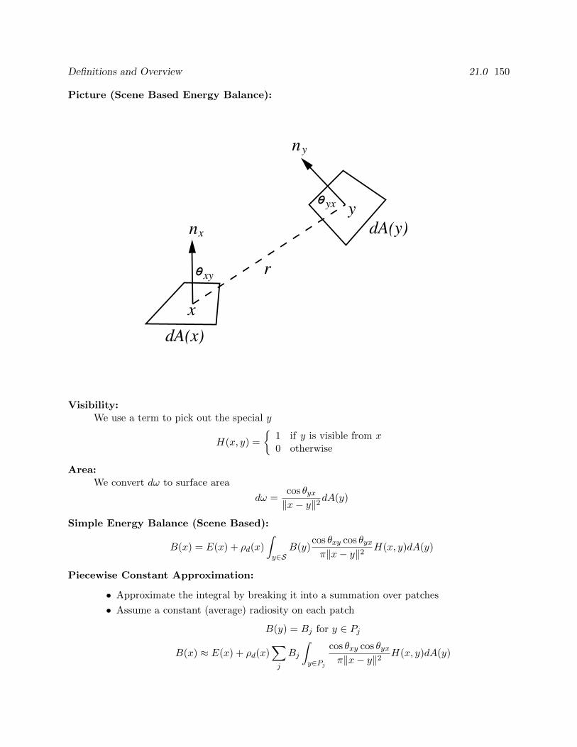
Definitions and Overview 21.0 150
Picture (Scene Based Energy Balance):
n
n
x
y
x
y
xy
yx
r
dA(x)
dA(y)
Visibility:We use a term to pick out the special y
H(x, y) =
1 if y is visible from x0 otherwise
Area:We convert dω to surface area
dω =cos θyx‖x− y‖2dA(y)
Simple Energy Balance (Scene Based):
B(x) = E(x) + ρd(x)
∫y∈S
B(y)cos θxy cos θyxπ‖x− y‖2 H(x, y)dA(y)
Piecewise Constant Approximation:
• Approximate the integral by breaking it into a summation over patches
• Assume a constant (average) radiosity on each patch
B(y) = Bj for y ∈ Pj
B(x) ≈ E(x) + ρd(x)∑j
Bj
∫y∈Pj
cos θxy cos θyxπ‖x− y‖2 H(x, y)dA(y)
Definitions and Overview 21.0 151
• Solve only for a per-patch average density
– ρd(x) ≈ ρi for x ∈ Pi– Bi ≈ 1
Ai
∫x∈Pi B(x)dA(x)
– Ei ≈ 1Ai
∫x∈Pi E(x)dA(x)
Piecewise Constant Radiosity Approximation:
Bi = Ei + ρi∑j
Bj1
Ai
∫x∈Pi
∫y∈Pj
cos θi cos θj
π‖x− y‖2 HijdAjdAi
Form Factor:
Fij =1
Ai
∫x∈Pi
∫y∈Pj
cos θi cos θj
π‖x− y‖2 HijdAjdAi
Note, by symmetry, that we haveAiFij = AjFji
Linear Equations: (by Summetry)
Bi = Ei + ρi∑j
FijBj
Bi = Ei + ρi∑j
FjiAjAiBj
Radiosity: (Summary)
• Discretize scene into n patches (polygons) each of which emits and reflects light uniformlyunder its entire area.
• Radiosity emitted by patch i is given by
Bi = Ei + ρi∑j
FijBj
= Ei + ρi∑j
FjiAjAiBj
– Bi, Bj : radiosity in energy/unit-time/unit-area
– Ei: light emitted from patch i
– ρi: patch i’s reflectivity
– Fj,i: Form factor specifying fraction of energy leaving j that reaches i (accounts forshape, orientation, occulsion)
– Ai, Aj : Area of patches
Radiosity: Full Matrix Solution
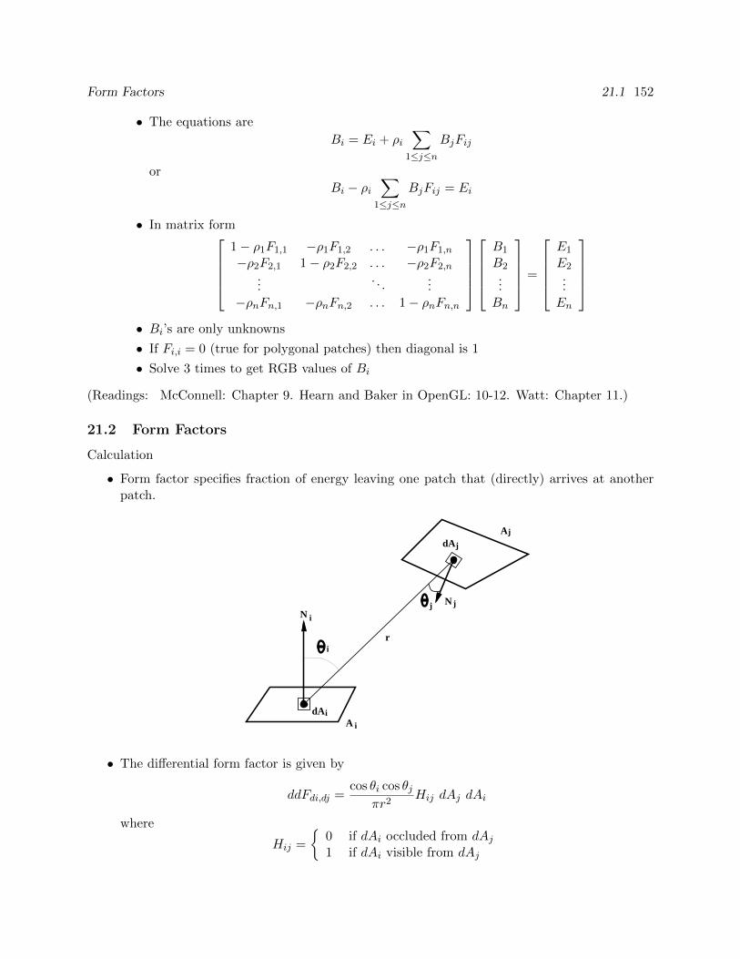
Form Factors 21.1 152
• The equations are
Bi = Ei + ρi∑
1≤j≤nBjFij
orBi − ρi
∑1≤j≤n
BjFij = Ei
• In matrix form1− ρ1F1,1 −ρ1F1,2 . . . −ρ1F1,n
−ρ2F2,1 1− ρ2F2,2 . . . −ρ2F2,n...
. . ....
−ρnFn,1 −ρnFn,2 . . . 1− ρnFn,n
B1
B2...Bn
=
E1
E2...En
• Bi’s are only unknowns
• If Fi,i = 0 (true for polygonal patches) then diagonal is 1
• Solve 3 times to get RGB values of Bi
(Readings: McConnell: Chapter 9. Hearn and Baker in OpenGL: 10-12. Watt: Chapter 11.)
21.2 Form Factors
Calculation
• Form factor specifies fraction of energy leaving one patch that (directly) arrives at anotherpatch.
dA
i
j
A
A
i
j
i
jdA
iNjN
r
• The differential form factor is given by
ddFdi,dj =cos θi cos θj
πr2Hij dAj dAi
where
Hij =
0 if dAi occluded from dAj1 if dAi visible from dAj
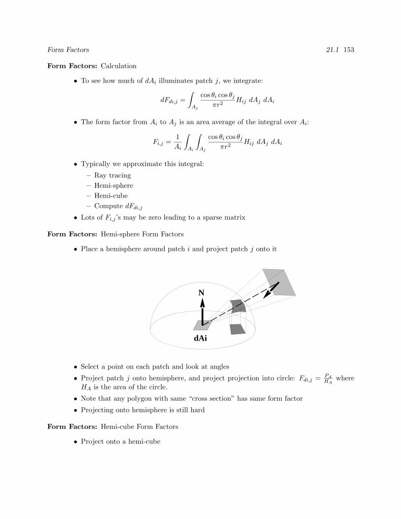
Form Factors 21.1 153
Form Factors: Calculation
• To see how much of dAi illuminates patch j, we integrate:
dFdi,j =
∫Aj
cos θi cos θjπr2
Hij dAj dAi
• The form factor from Ai to Aj is an area average of the integral over Ai:
Fi,j =1
Ai
∫Ai
∫Aj
cos θi cos θjπr2
Hij dAj dAi
• Typically we approximate this integral:
– Ray tracing
– Hemi-sphere
– Hemi-cube
– Compute dFdi,j
• Lots of Fi,j ’s may be zero leading to a sparse matrix
Form Factors: Hemi-sphere Form Factors
• Place a hemisphere around patch i and project patch j onto it
N
dAi
• Select a point on each patch and look at angles
• Project patch j onto hemisphere, and project projection into circle: Fdi,j = PAHA
whereHA is the area of the circle.
• Note that any polygon with same “cross section” has same form factor
• Projecting onto hemisphere is still hard
Form Factors: Hemi-cube Form Factors
• Project onto a hemi-cube
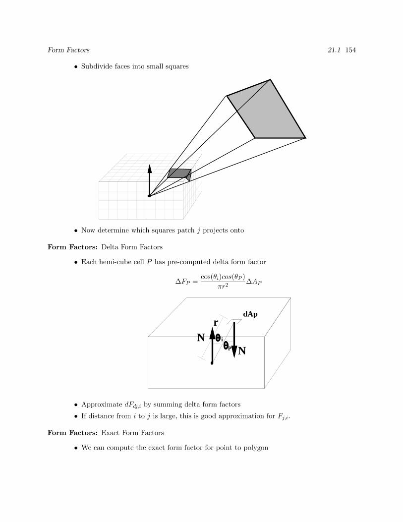
Form Factors 21.1 154
• Subdivide faces into small squares
• Now determine which squares patch j projects onto
Form Factors: Delta Form Factors
• Each hemi-cube cell P has pre-computed delta form factor
∆FP =cos(θi)cos(θP )
πr2∆AP
i
P
dApr
NN
• Approximate dFdj,i by summing delta form factors
• If distance from i to j is large, this is good approximation for Fj,i.
Form Factors: Exact Form Factors
• We can compute the exact form factor for point to polygon
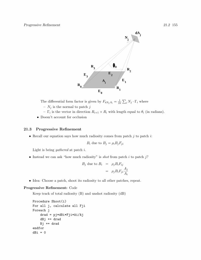
Progressive Refinement 21.2 155
E0
R0
dAj
Nj
Ai
E1
E2E
3
R1
R2
R3 0
The differential form factor is given by FdAjAi = 12π
∑iNj · Γi where
– Nj is the normal to patch j
– Γi is the vector in direction Ri+1 ×Ri with length equal to θi (in radians).
• Doesn’t account for occlusion
21.3 Progressive Refinement
• Recall our equation says how much radiosity comes from patch j to patch i:
Bi due to Bj = ρiBjFji
Light is being gathered at patch i.
• Instead we can ask “how much radiosity” is shot from patch i to patch j?
Bj due to Bi = ρjBiFij
= ρjBiFjiAjAi
• Idea: Choose a patch, shoot its radiosity to all other patches, repeat.
Progressive Refinement: Code
Keep track of total radiosity (B) and unshot radiosity (dB)
Procedure Shoot(i)
For all j, calculate all Fji
Foreach j
drad = pj*dBi*Fji*Ai/Aj
dBj += drad
Bj += drad
endfor
dBi = 0
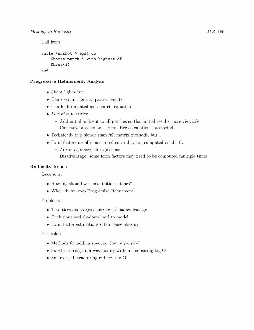
Meshing in Radiosity 21.3 156
Call from
while (unshot > eps) do
Choose patch i with highest dB
Shoot(i)
end
Progressive Refinement: Analysis
• Shoot lights first
• Can stop and look at partial results
• Can be formulated as a matrix equation
• Lots of cute tricks:
– Add initial ambient to all patches so that initial results more viewable
– Can move objects and lights after calculation has started
• Technically it is slower than full matrix methods, but...
• Form factors usually not stored since they are computed on the fly
– Advantage: save storage space
– Disadvantage: some form factors may need to be computed multiple times
Radiosity Issues
Questions:
• How big should we make initial patches?
• When do we stop Progressive-Refinement?
Problems
• T-vertices and edges cause light/shadow leakage
• Occlusions and shadows hard to model
• Form factor estimations often cause aliasing
Extensions
• Methods for adding specular (but expensive)
• Substructuring improves quality without increasing big-O
• Smarter substructuring reduces big-O
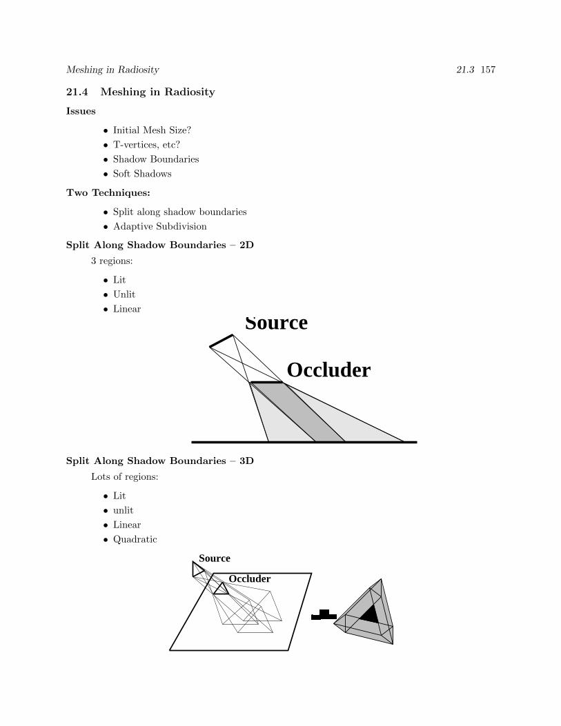
Meshing in Radiosity 21.3 157
21.4 Meshing in Radiosity
Issues
• Initial Mesh Size?
• T-vertices, etc?
• Shadow Boundaries
• Soft Shadows
Two Techniques:
• Split along shadow boundaries
• Adaptive Subdivision
Split Along Shadow Boundaries – 2D
3 regions:
• Lit
• Unlit
• Linear
Source
Occluder
Split Along Shadow Boundaries – 3D
Lots of regions:
• Lit
• unlit
• Linear
• Quadratic
Source
Occluder
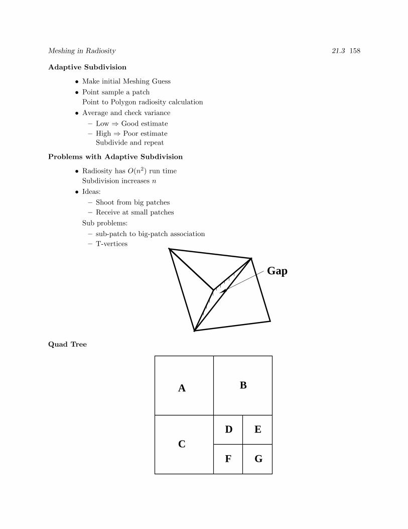
Meshing in Radiosity 21.3 158
Adaptive Subdivision
• Make initial Meshing Guess
• Point sample a patch
Point to Polygon radiosity calculation
• Average and check variance
– Low ⇒ Good estimate
– High ⇒ Poor estimateSubdivide and repeat
Problems with Adaptive Subdivision
• Radiosity has O(n2) run time
Subdivision increases n
• Ideas:
– Shoot from big patches
– Receive at small patches
Sub problems:
– sub-patch to big-patch association
– T-vertices
Gap
Quad Tree
F
D E
G
A
C
B
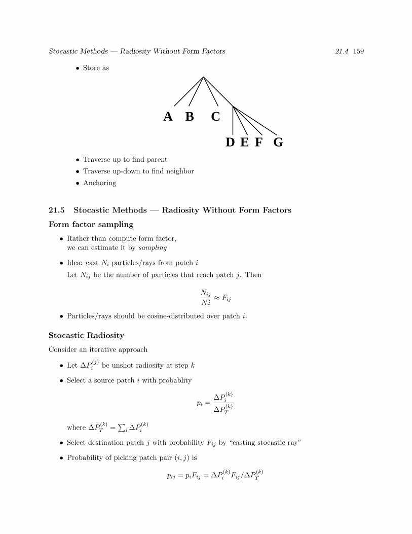
Stocastic Methods — Radiosity Without Form Factors 21.4 159
• Store as
A B C
D E F G• Traverse up to find parent
• Traverse up-down to find neighbor
• Anchoring
21.5 Stocastic Methods — Radiosity Without Form Factors
Form factor sampling
• Rather than compute form factor,we can estimate it by sampling
• Idea: cast Ni particles/rays from patch i
Let Nij be the number of particles that reach patch j. Then
Nij
Ni≈ Fij
• Particles/rays should be cosine-distributed over patch i.
Stocastic Radiosity
Consider an iterative approach
• Let ∆P(j)i be unshot radiosity at step k
• Select a source patch i with probablity
pi =∆P
(k)i
∆P(k)T
where ∆P(k)T =
∑i ∆P
(k)i
• Select destination patch j with probability Fij by “casting stocastic ray”
• Probability of picking patch pair (i, j) is
pij = piFij = ∆P(k)i Fij/∆P
(k)T
Photon Maps 21 160
• Estimate for ∆P(k+1)i becomes
∆P(k+1)i ≈ 1
N
N∑s=1
∆P(k)jsFjs,lsρlsδls,i
∆P(k)jsFjs,ls/∆P
(k)T
= ρi∆P(k)T
Ni
N
Stocastic Radiosity: Code
Procedure Shoot(i)
For Ni times
Sample random point x on Si
Sample cosine-distribution direction T at x
Determine nearest patch j in direction T from x
dPj += 1/N * rho j * DPT
endfor
Call from
while (unshot > eps) do
For each patch i
Shoot(i)
Update total power, set DPi to dPi, clear dPi
Compute new DPT
end
(Readings: Based on exposition in Advanced Global Illumination, Dutre, Bala, and Bekaert.)
Evaluation
• Much faster than form factor methods
• Noise, noise, noise
Need to filter
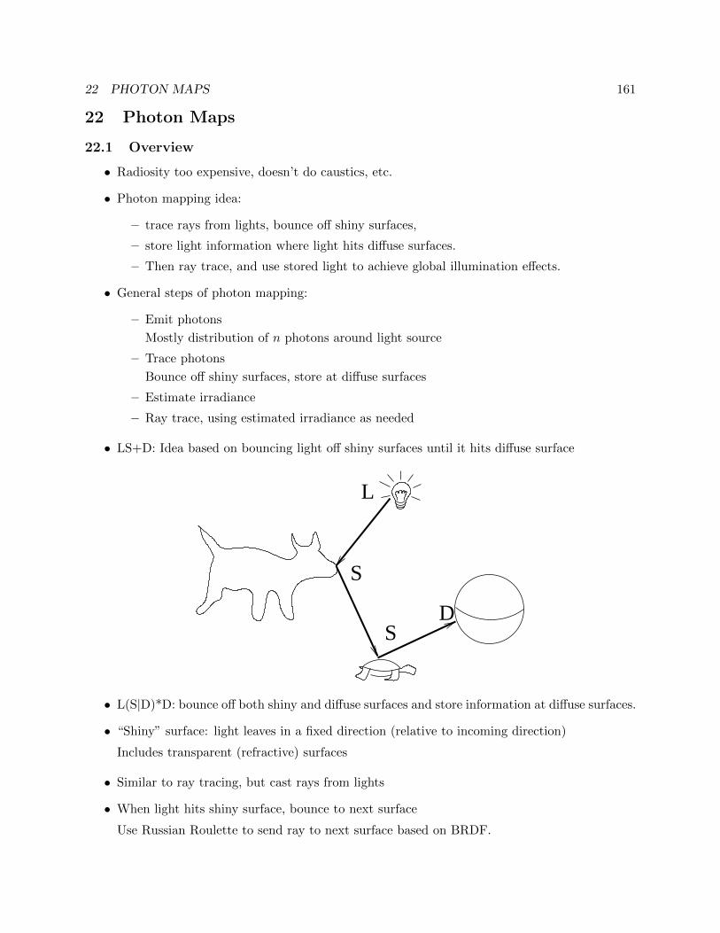
22 PHOTON MAPS 161
22 Photon Maps
22.1 Overview
• Radiosity too expensive, doesn’t do caustics, etc.
• Photon mapping idea:
– trace rays from lights, bounce off shiny surfaces,
– store light information where light hits diffuse surfaces.
– Then ray trace, and use stored light to achieve global illumination effects.
• General steps of photon mapping:
– Emit photons
Mostly distribution of n photons around light source
– Trace photons
Bounce off shiny surfaces, store at diffuse surfaces
– Estimate irradiance
– Ray trace, using estimated irradiance as needed
• LS+D: Idea based on bouncing light off shiny surfaces until it hits diffuse surface
S
SD
L
• L(S|D)*D: bounce off both shiny and diffuse surfaces and store information at diffuse surfaces.
• “Shiny” surface: light leaves in a fixed direction (relative to incoming direction)
Includes transparent (refractive) surfaces
• Similar to ray tracing, but cast rays from lights
• When light hits shiny surface, bounce to next surface
Use Russian Roulette to send ray to next surface based on BRDF.
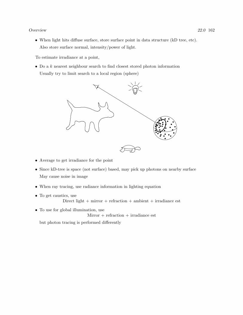
Overview 22.0 162
• When light hits diffuse surface, store surface point in data structure (kD tree, etc).
Also store surface normal, intensity/power of light.
To estimate irradiance at a point,
• Do a k nearest neighbour search to find closest stored photon information
Usually try to limit search to a local region (sphere)
• Average to get irradiance for the point
• Since kD-tree is space (not surface) based, may pick up photons on nearby surface
May cause noise in image
• When ray tracing, use radiance information in lighting equation
• To get caustics, useDirect light + mirror + refraction + ambient + irradiance est
• To use for global illumination, useMirror + refraction + irradiance est
but photon tracing is performed differently
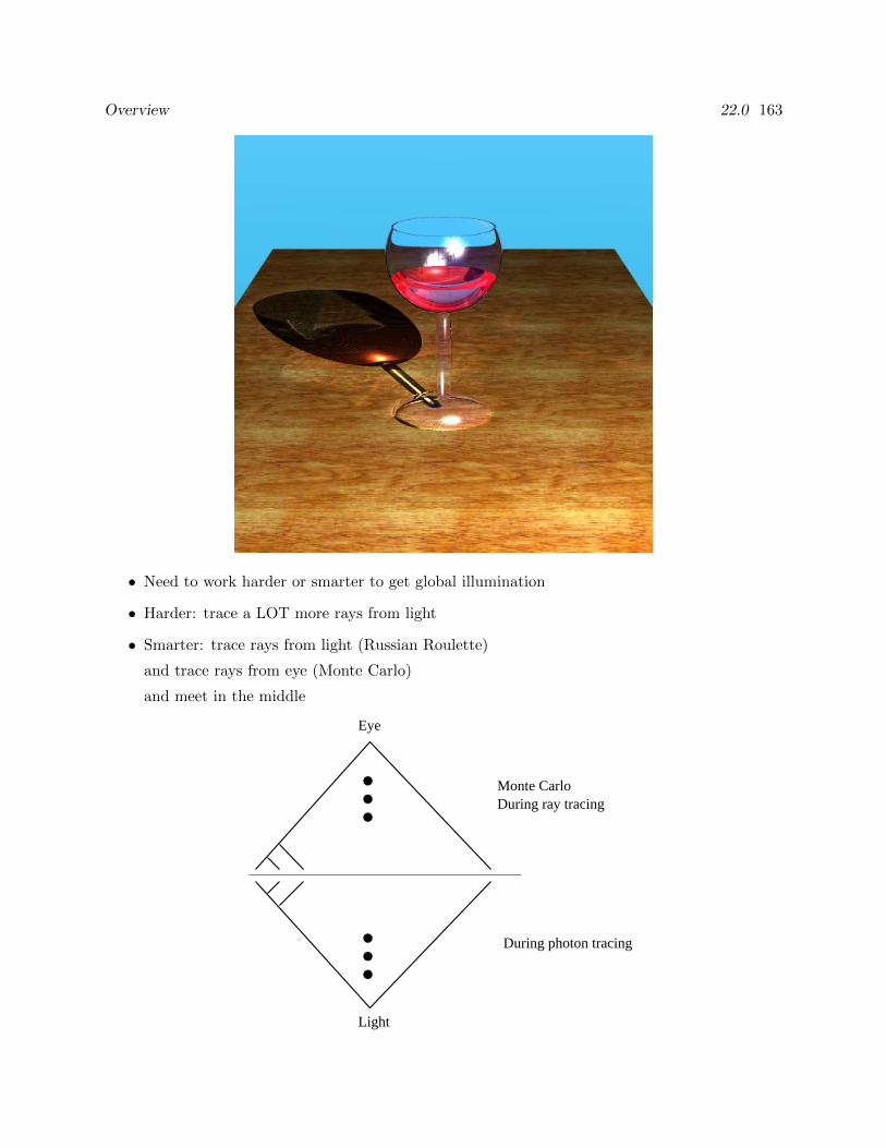
Overview 22.0 163
• Need to work harder or smarter to get global illumination
• Harder: trace a LOT more rays from light
• Smarter: trace rays from light (Russian Roulette)
and trace rays from eye (Monte Carlo)
and meet in the middle
Monte CarloDuring ray tracing
During photon tracing
Light
Eye
...
...
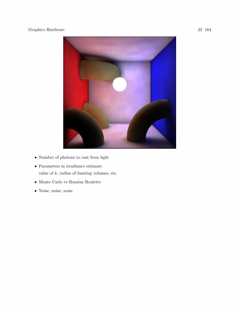
Graphics Hardware 22 164
• Number of photons to cast from light
• Parameters in irradiance estimate
value of k, radius of limiting volumes, etc.
• Monte Carlo vs Russian Roulette
• Noise, noise, noise
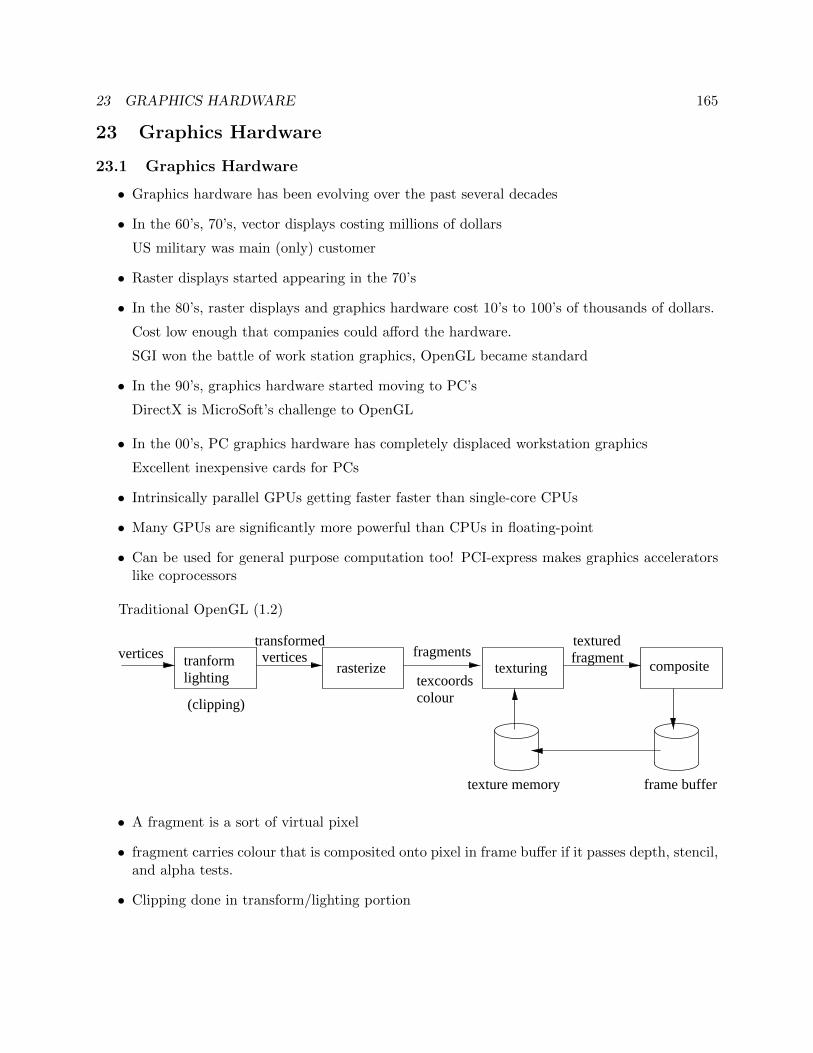
23 GRAPHICS HARDWARE 165
23 Graphics Hardware
23.1 Graphics Hardware
• Graphics hardware has been evolving over the past several decades
• In the 60’s, 70’s, vector displays costing millions of dollars
US military was main (only) customer
• Raster displays started appearing in the 70’s
• In the 80’s, raster displays and graphics hardware cost 10’s to 100’s of thousands of dollars.
Cost low enough that companies could afford the hardware.
SGI won the battle of work station graphics, OpenGL became standard
• In the 90’s, graphics hardware started moving to PC’s
DirectX is MicroSoft’s challenge to OpenGL
• In the 00’s, PC graphics hardware has completely displaced workstation graphics
Excellent inexpensive cards for PCs
• Intrinsically parallel GPUs getting faster faster than single-core CPUs
• Many GPUs are significantly more powerful than CPUs in floating-point
• Can be used for general purpose computation too! PCI-express makes graphics acceleratorslike coprocessors
Traditional OpenGL (1.2)
rasterizetranformlighting
verticestexturing
fragmentsverticestransformed
(clipping)
fragmenttextured
composite
texture memory frame buffer
texcoordscolour
• A fragment is a sort of virtual pixel
• fragment carries colour that is composited onto pixel in frame buffer if it passes depth, stencil,and alpha tests.
• Clipping done in transform/lighting portion
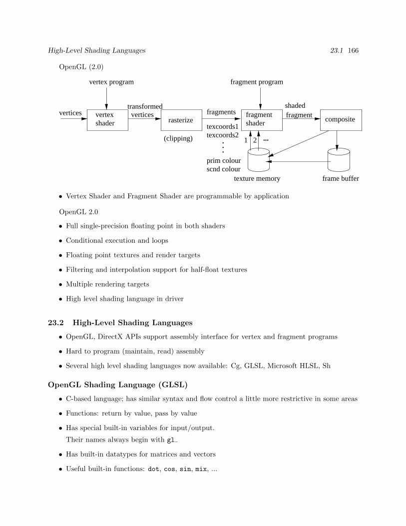
High-Level Shading Languages 23.1 166
OpenGL (2.0)
.
.
.
rasterizevertices fragmentsvertices
transformedfragment
composite
texture memory frame buffer
(clipping)
fragmentshader
shaded
vertex program fragment program
shadervertex
texcoords1texcoords2
scnd colourprim colour
1 2 ...
• Vertex Shader and Fragment Shader are programmable by application
OpenGL 2.0
• Full single-precision floating point in both shaders
• Conditional execution and loops
• Floating point textures and render targets
• Filtering and interpolation support for half-float textures
• Multiple rendering targets
• High level shading language in driver
23.2 High-Level Shading Languages
• OpenGL, DirectX APIs support assembly interface for vertex and fragment programs
• Hard to program (maintain, read) assembly
• Several high level shading languages now available: Cg, GLSL, Microsoft HLSL, Sh
OpenGL Shading Language (GLSL)
• C-based language; has similar syntax and flow control a little more restrictive in some areas
• Functions: return by value, pass by value
• Has special built-in variables for input/output.
Their names always begin with gl
• Has built-in datatypes for matrices and vectors
• Useful built-in functions: dot, cos, sin, mix, ...
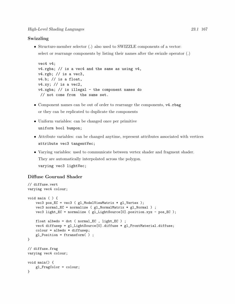
High-Level Shading Languages 23.1 167
Swizzling
• Structure-member selector (.) also used to SWIZZLE components of a vector:
select or rearrange components by listing their names after the swizzle operator (.)
vec4 v4;
v4.rgba; // is a vec4 and the same as using v4,
v4.rgb; // is a vec3,
v4.b; // is a float,
v4.xy; // is a vec2,
v4.xgba; // is illegal - the component names do
// not come from the same set.
• Component names can be out of order to rearrange the components, v4.rbag
or they can be replicated to duplicate the components
• Uniform variables: can be changed once per primitive
uniform bool bumpon;
• Attribute variables: can be changed anytime, represent attributes associated with vertices
attribute vec3 tangentVec;
• Varying variables: used to communicate between vertex shader and fragment shader.
They are automatically interpolated across the polygon.
varying vec3 lightVec;
Diffuse Gouruad Shader
// diffuse.vert
varying vec4 colour;
void main ( )
vec3 pos_EC = vec3 ( gl_ModelViewMatrix * gl_Vertex );
vec3 normal_EC = normalize ( gl_NormalMatrix * gl_Normal ) ;
vec3 light_EC = normalize ( gl_LightSource[0].position.xyz - pos_EC );
float albedo = dot ( normal_EC , light_EC ) ;
vec4 diffusep = gl_LightSource[0].diffuse * gl_FrontMaterial.diffuse;
colour = albedo * diffusep;
gl_Position = ftransform( ) ;
// diffuse.frag
varying vec4 colour;
void main()
gl_FragColor = colour;
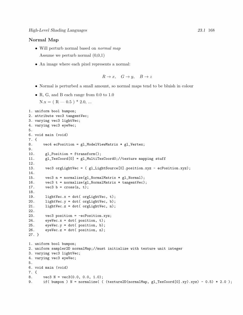
High-Level Shading Languages 23.1 168
Normal Map
• Will perturb normal based on normal map
Assume we perturb normal (0,0,1)
• An image where each pixel represents a normal:
R→ x, G→ y, B → z
• Normal is perturbed a small amount, so normal maps tend to be bluish in colour
• R, G, and B each range from 0.0 to 1.0
N.x = ( R — 0.5 ) * 2.0, ...
1. uniform bool bumpon;
2. attribute vec3 tangentVec;
3. varying vec3 lightVec;
4. varying vec3 eyeVec;
5.
6. void main (void)
7.
8. vec4 ecPosition = gl_ModelViewMatrix * gl_Vertex;
9.
10. gl_Position = ftransform();
11. gl_TexCoord[0] = gl_MultiTexCoord0;//texture mapping stuff
12.
13. vec3 orgLightVec = ( gl_LightSource[0].position.xyz - ecPosition.xyz);
14.
15. vec3 n = normalize(gl_NormalMatrix * gl_Normal);
16. vec3 t = normalize(gl_NormalMatrix * tangentVec);
17. vec3 b = cross(n, t);
18.
19. lightVec.x = dot( orgLightVec, t);
20. lightVec.y = dot( orgLightVec, b);
21. lightVec.z = dot( orgLightVec, n);
22.
23. vec3 position = -ecPosition.xyz;
24. eyeVec.x = dot( position, t);
25. eyeVec.y = dot( position, b);
26. eyeVec.z = dot( position, n);
27.
1. uniform bool bumpon;
2. uniform sampler2D normalMap;//must initialize with texture unit integer
3. varying vec3 lightVec;
4. varying vec3 eyeVec;
5.
6. void main (void)
7.
8. vec3 N = vec3(0.0, 0.0, 1.0);
9. if( bumpon ) N = normalize( ( (texture2D(normalMap, gl_TexCoord[0].xy).xyz) - 0.5) * 2.0 );
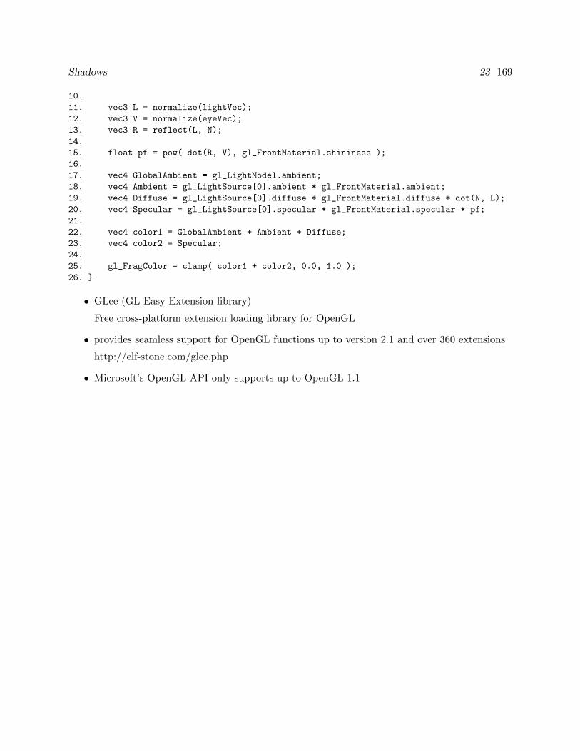
Shadows 23 169
10.
11. vec3 L = normalize(lightVec);
12. vec3 V = normalize(eyeVec);
13. vec3 R = reflect(L, N);
14.
15. float pf = pow( dot(R, V), gl_FrontMaterial.shininess );
16.
17. vec4 GlobalAmbient = gl_LightModel.ambient;
18. vec4 Ambient = gl_LightSource[0].ambient * gl_FrontMaterial.ambient;
19. vec4 Diffuse = gl_LightSource[0].diffuse * gl_FrontMaterial.diffuse * dot(N, L);
20. vec4 Specular = gl_LightSource[0].specular * gl_FrontMaterial.specular * pf;
21.
22. vec4 color1 = GlobalAmbient + Ambient + Diffuse;
23. vec4 color2 = Specular;
24.
25. gl_FragColor = clamp( color1 + color2, 0.0, 1.0 );
26.
• GLee (GL Easy Extension library)
Free cross-platform extension loading library for OpenGL
• provides seamless support for OpenGL functions up to version 2.1 and over 360 extensions
http://elf-stone.com/glee.php
• Microsoft’s OpenGL API only supports up to OpenGL 1.1

Shadows 23 170
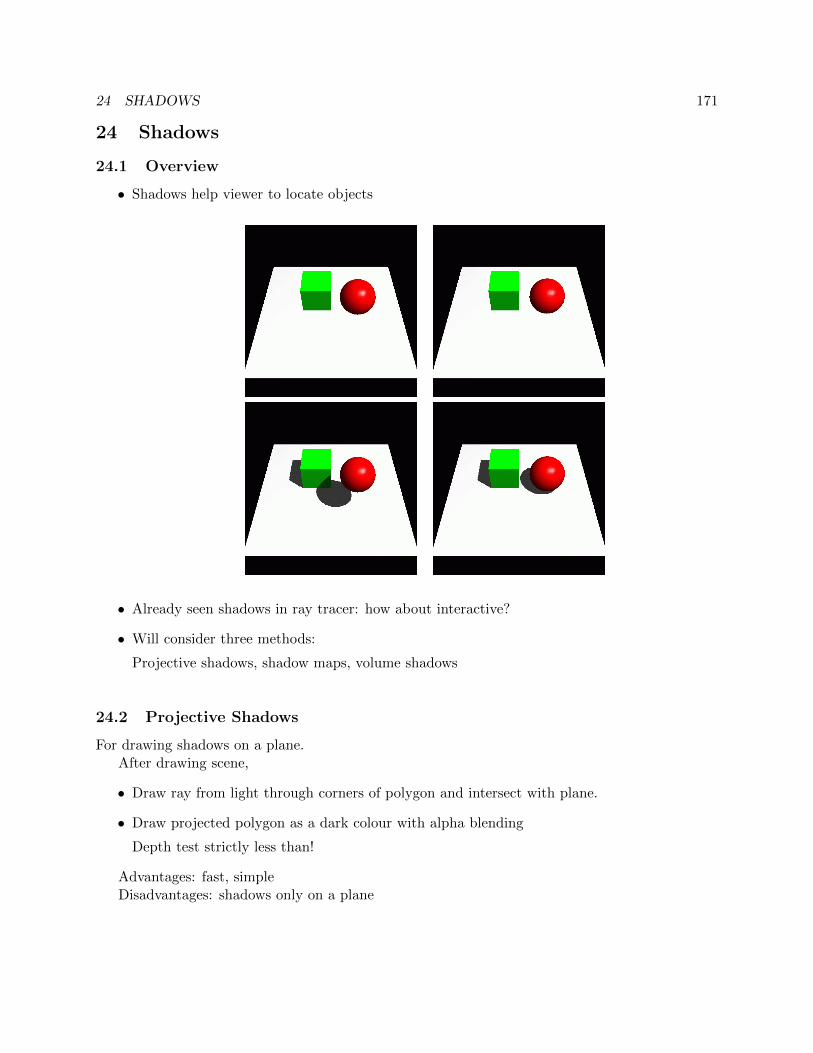
24 SHADOWS 171
24 Shadows
24.1 Overview
• Shadows help viewer to locate objects
• Already seen shadows in ray tracer: how about interactive?
• Will consider three methods:
Projective shadows, shadow maps, volume shadows
24.2 Projective Shadows
For drawing shadows on a plane.After drawing scene,
• Draw ray from light through corners of polygon and intersect with plane.
• Draw projected polygon as a dark colour with alpha blending
Depth test strictly less than!
Advantages: fast, simpleDisadvantages: shadows only on a plane
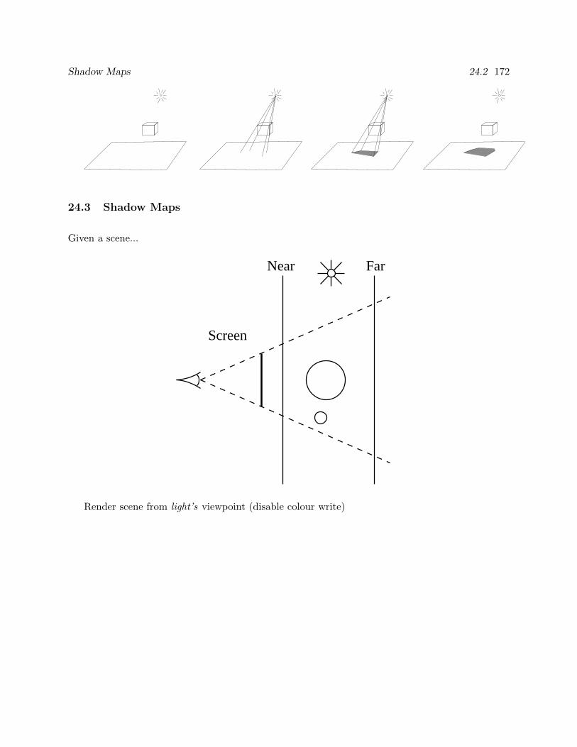
Shadow Maps 24.2 172
24.3 Shadow Maps
Given a scene...
Screen
Near Far
Render scene from light’s viewpoint (disable colour write)
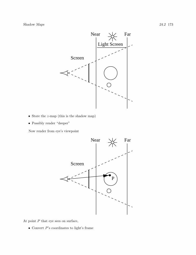
Shadow Maps 24.2 173
Light Screen
Screen
Near Far
• Store the z-map (this is the shadow map)
• Possibly render “deeper”
Now render from eye’s viewpoint
Screen
Near Far
P
At point P that eye sees on surface,
• Convert P ’s coordinates to light’s frame
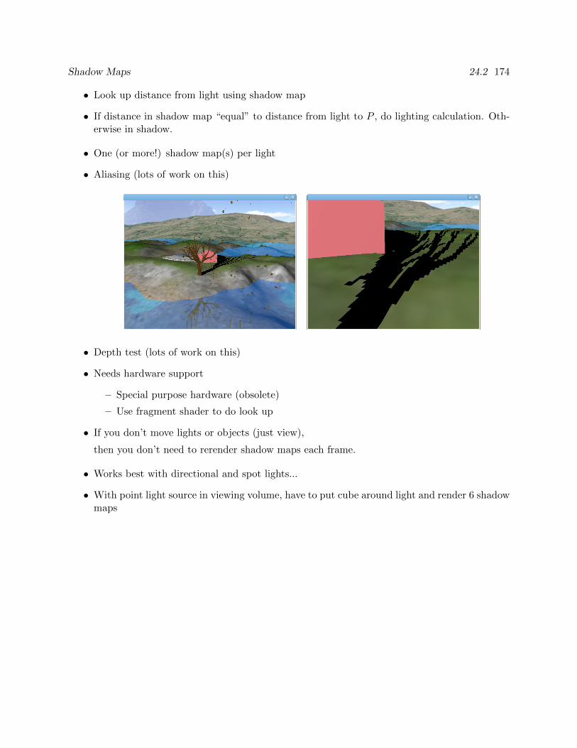
Shadow Maps 24.2 174
• Look up distance from light using shadow map
• If distance in shadow map “equal” to distance from light to P , do lighting calculation. Oth-erwise in shadow.
• One (or more!) shadow map(s) per light
• Aliasing (lots of work on this)
• Depth test (lots of work on this)
• Needs hardware support
– Special purpose hardware (obsolete)
– Use fragment shader to do look up
• If you don’t move lights or objects (just view),
then you don’t need to rerender shadow maps each frame.
• Works best with directional and spot lights...
• With point light source in viewing volume, have to put cube around light and render 6 shadowmaps
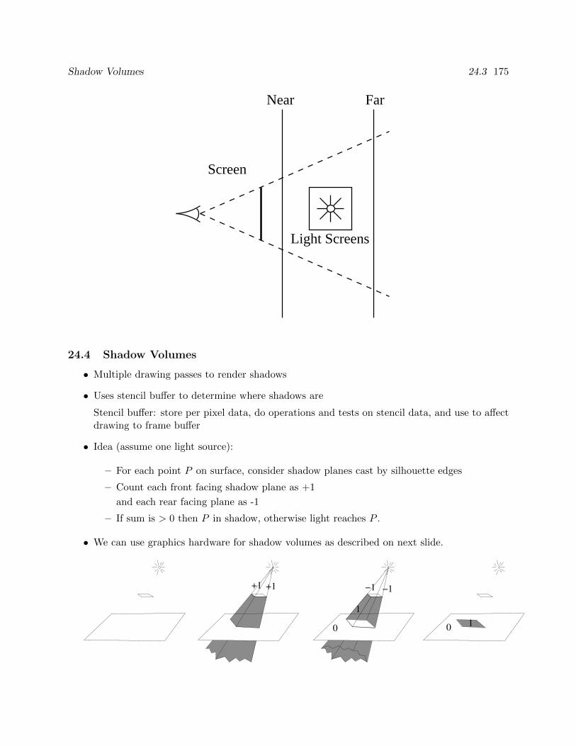
Shadow Volumes 24.3 175
Screen
Near Far
Light Screens
24.4 Shadow Volumes
• Multiple drawing passes to render shadows
• Uses stencil buffer to determine where shadows are
Stencil buffer: store per pixel data, do operations and tests on stencil data, and use to affectdrawing to frame buffer
• Idea (assume one light source):
– For each point P on surface, consider shadow planes cast by silhouette edges
– Count each front facing shadow plane as +1
and each rear facing plane as -1
– If sum is > 0 then P in shadow, otherwise light reaches P .
• We can use graphics hardware for shadow volumes as described on next slide.
+1 +1
0
1
−1 −1
10
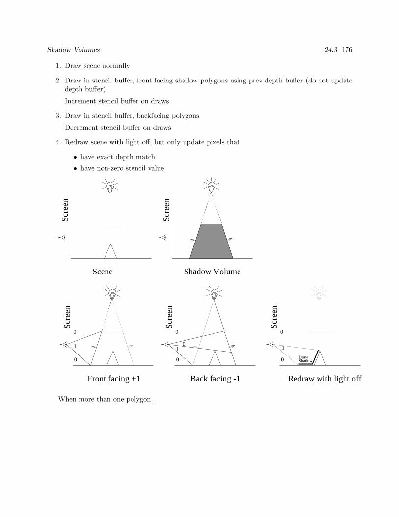
Shadow Volumes 24.3 176
1. Draw scene normally
2. Draw in stencil buffer, front facing shadow polygons using prev depth buffer (do not updatedepth buffer)
Increment stencil buffer on draws
3. Draw in stencil buffer, backfacing polygons
Decrement stencil buffer on draws
4. Redraw scene with light off, but only update pixels that
• have exact depth match
• have non-zero stencil value
ShadowDraw
Redraw with light off
0
Scre
en
0
1
Scene Shadow Volume
Scre
en
Scre
en
Front facing +1
0
1
0
Scre
en
Back facing -1
0
Scre
en
1
0
0
When more than one polygon...
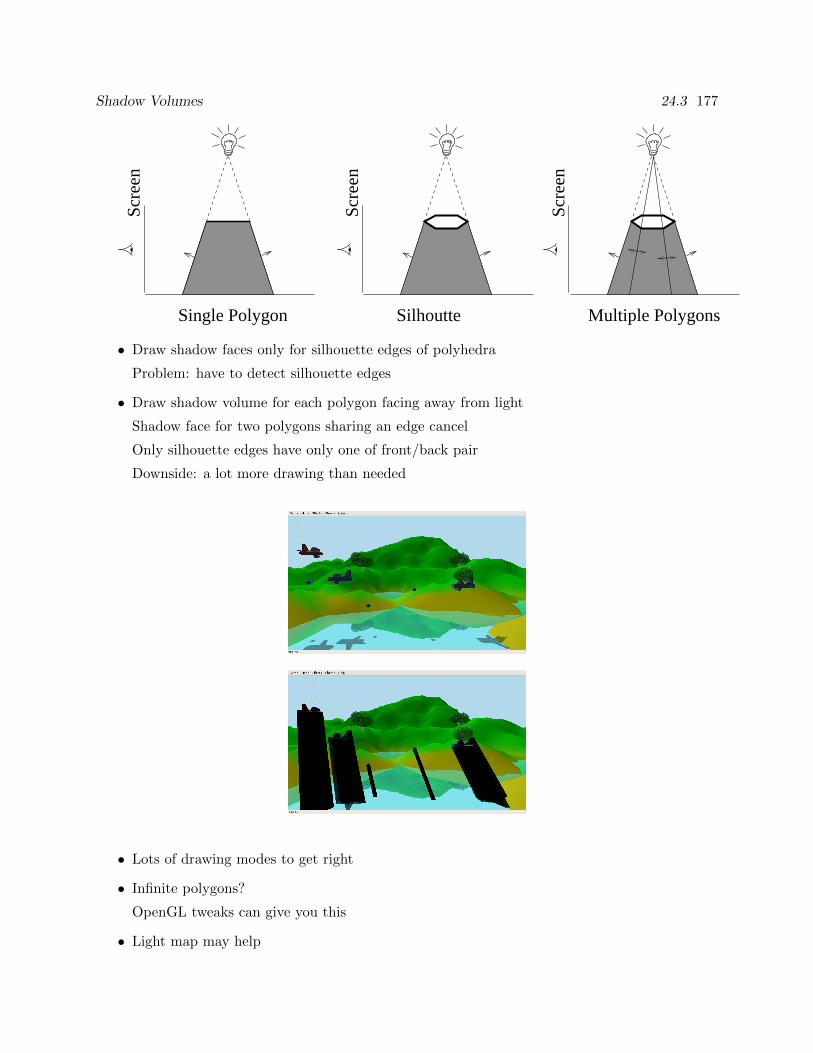
Shadow Volumes 24.3 177
Scre
en
Single Polygon
Scre
en
Silhoutte
Scre
en
Multiple Polygons
• Draw shadow faces only for silhouette edges of polyhedra
Problem: have to detect silhouette edges
• Draw shadow volume for each polygon facing away from light
Shadow face for two polygons sharing an edge cancel
Only silhouette edges have only one of front/back pair
Downside: a lot more drawing than needed
• Lots of drawing modes to get right
• Infinite polygons?
OpenGL tweaks can give you this
• Light map may help

Modeling of Various Things 24 178
• Problems if viewpoint inside shadow volume
• Need to repeat for each light
(Readings: McConnell, Chapter 7.)
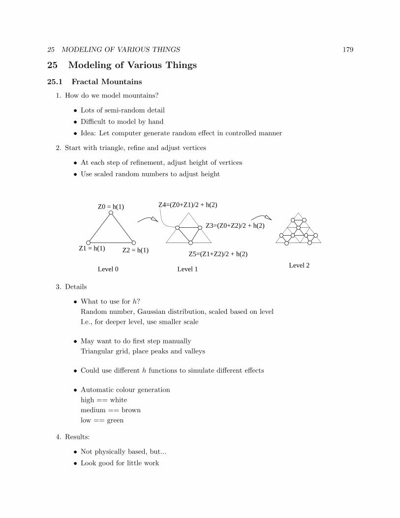
25 MODELING OF VARIOUS THINGS 179
25 Modeling of Various Things
25.1 Fractal Mountains
1. How do we model mountains?
• Lots of semi-random detail
• Difficult to model by hand
• Idea: Let computer generate random effect in controlled manner
2. Start with triangle, refine and adjust vertices
• At each step of refinement, adjust height of vertices
• Use scaled random numbers to adjust height
Level 1Level 0 Level 2
Z1 = h(1)
Z3=(Z0+Z2)/2 + h(2)
Z5=(Z1+Z2)/2 + h(2)
Z4=(Z0+Z1)/2 + h(2)Z0 = h(1)
Z2 = h(1)
3. Details
• What to use for h?
Random number, Gaussian distribution, scaled based on level
I.e., for deeper level, use smaller scale
• May want to do first step manually
Triangular grid, place peaks and valleys
• Could use different h functions to simulate different effects
• Automatic colour generation
high == white
medium == brown
low == green
4. Results:
• Not physically based, but...
• Look good for little work
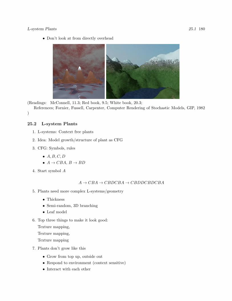
L-system Plants 25.1 180
• Don’t look at from directly overhead
(Readings: McConnell, 11.3; Red book, 9.5; White book, 20.3;References; Fornier, Fussell, Carpenter, Computer Rendering of Stochastic Models, GIP, 1982
)
25.2 L-system Plants
1. L-systems: Context free plants
2. Idea: Model growth/structure of plant as CFG
3. CFG: Symbols, rules
• A,B,C,D• A→ CBA, B → BD
4. Start symbol A
A→ CBA→ CBDCBA→ CBDDCBDCBA
5. Plants need more complex L-systems/geometry
• Thickness
• Semi-random, 3D branching
• Leaf model
6. Top three things to make it look good:
Texture mapping,
Texture mapping,
Texture mapping
7. Plants don’t grow like this
• Grow from top up, outside out
• Respond to environment (context sensitive)
• Interact with each other
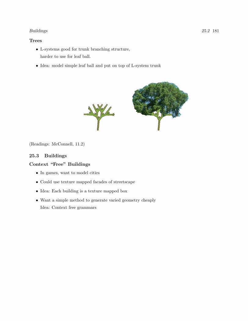
Buildings 25.2 181
Trees
• L-systems good for trunk branching structure,
harder to use for leaf ball.
• Idea: model simple leaf ball and put on top of L-system trunk
(Readings: McConnell, 11.2)
25.3 Buildings
Context “Free” Buildings
• In games, want to model cities
• Could use texture mapped facades of streetscape
• Idea: Each building is a texture mapped box
• Want a simple method to generate varied geometry cheaply
Idea: Context free grammars
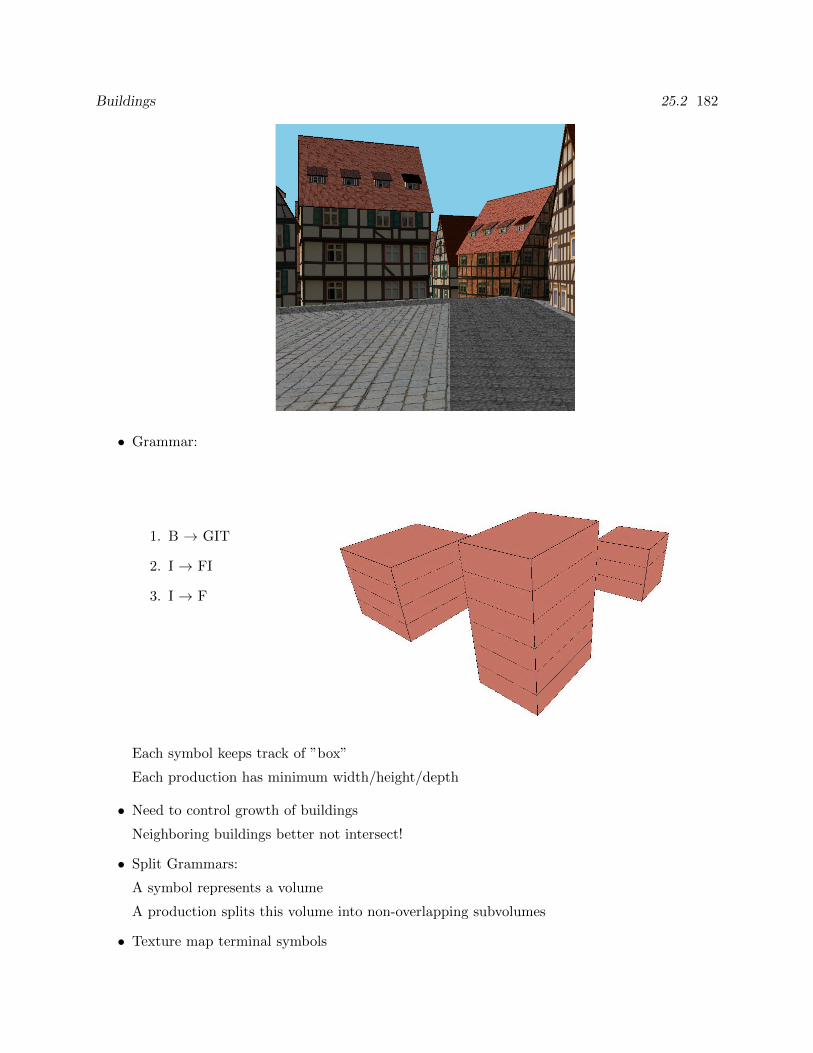
Buildings 25.2 182
• Grammar:
1. B → GIT
2. I → FI
3. I → F
Each symbol keeps track of ”box”
Each production has minimum width/height/depth
• Need to control growth of buildings
Neighboring buildings better not intersect!
• Split Grammars:
A symbol represents a volume
A production splits this volume into non-overlapping subvolumes
• Texture map terminal symbols
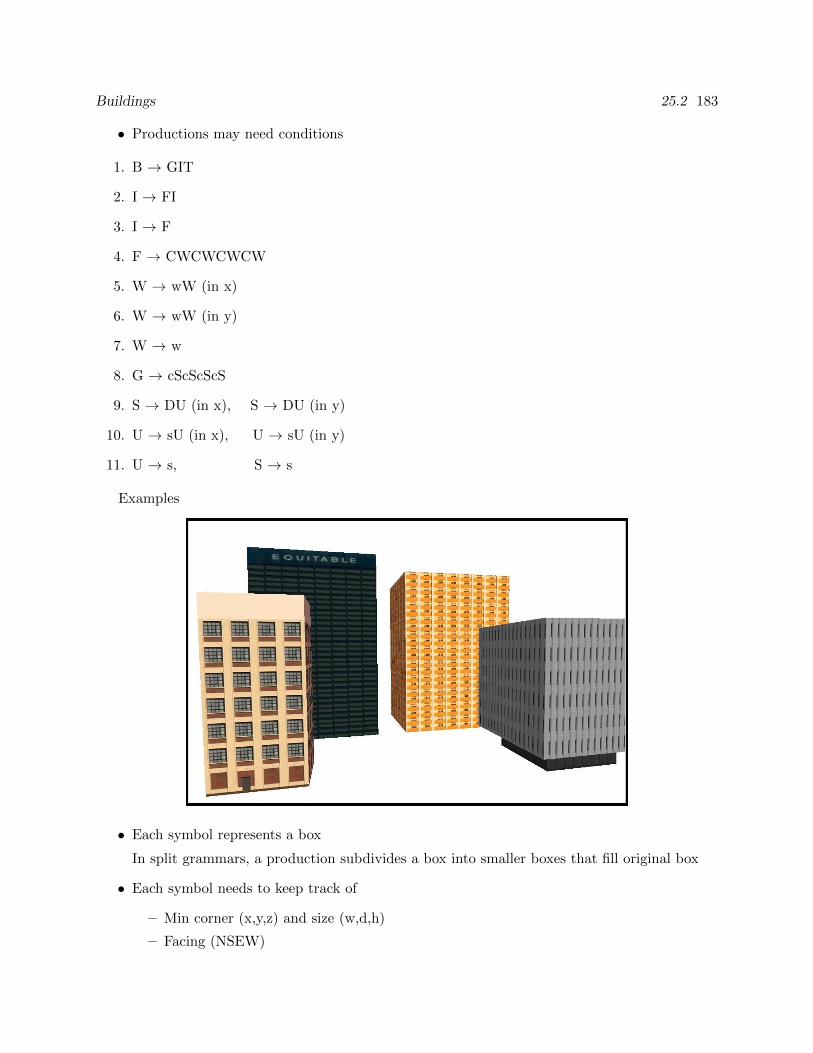
Buildings 25.2 183
• Productions may need conditions
1. B → GIT
2. I → FI
3. I → F
4. F → CWCWCWCW
5. W → wW (in x)
6. W → wW (in y)
7. W → w
8. G → cScScScS
9. S → DU (in x), S → DU (in y)
10. U → sU (in x), U → sU (in y)
11. U → s, S → s
Examples
• Each symbol represents a box
In split grammars, a production subdivides a box into smaller boxes that fill original box
• Each symbol needs to keep track of
– Min corner (x,y,z) and size (w,d,h)
– Facing (NSEW)
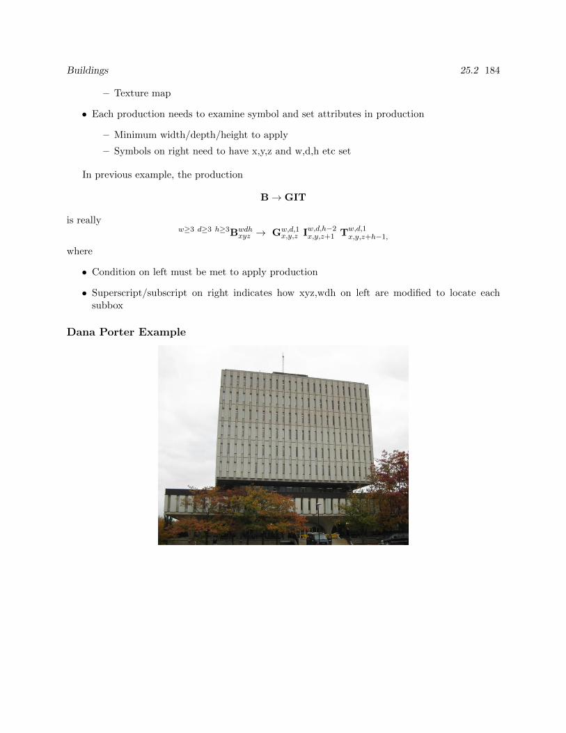
Buildings 25.2 184
– Texture map
• Each production needs to examine symbol and set attributes in production
– Minimum width/depth/height to apply
– Symbols on right need to have x,y,z and w,d,h etc set
In previous example, the production
B→ GIT
is reallyw≥3 d≥3 h≥3Bwdh
xyz → Gw,d,1x,y,z Iw,d,h−2
x,y,z+1 Tw,d,1x,y,z+h−1,
where
• Condition on left must be met to apply production
• Superscript/subscript on right indicates how xyz,wdh on left are modified to locate eachsubbox
Dana Porter Example
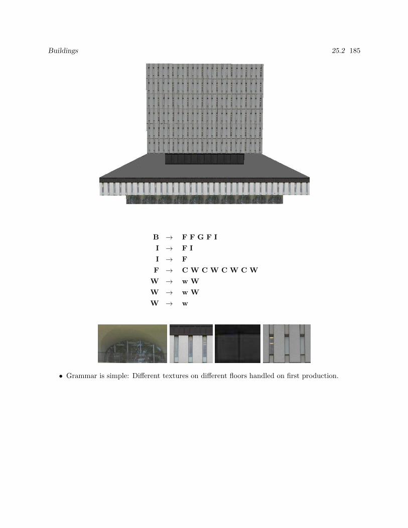
Buildings 25.2 185
B → F F G F I
I → F I
I → F
F → C W C W C W C W
W → w W
W → w W
W → w
• Grammar is simple: Different textures on different floors handled on first production.
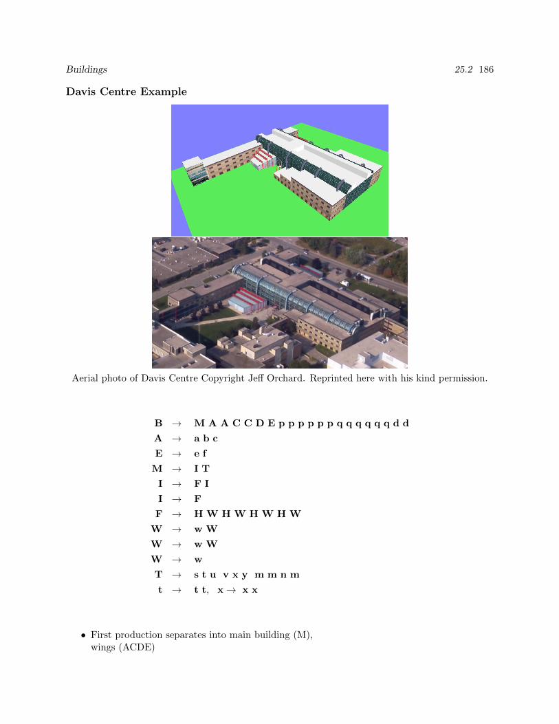
Buildings 25.2 186
Davis Centre Example
Aerial photo of Davis Centre Copyright Jeff Orchard. Reprinted here with his kind permission.
B → M A A C C D E p p p p p p q q q q q q d d
A → a b c
E → e f
M → I T
I → F I
I → F
F → H W H W H W H W
W → w W
W → w W
W → w
T → s t u v x y m m n m
t → t t, x→ x x
• First production separates into main building (M),wings (ACDE)
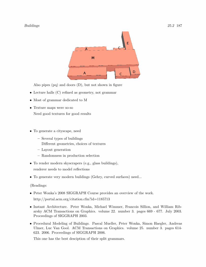
Buildings 25.2 187
Also pipes (pq) and doors (D), but not shown in figure
• Lecture halls (C) refined as geometry, not grammar
• Most of grammar dedicated to M
• Texture maps were so-so
Need good textures for good results
• To generate a cityscape, need
– Several types of buildings
Different geometries, choices of textures
– Layout generation
– Randomness in production selection
• To render modern skyscrapers (e.g., glass buildings),
renderer needs to model reflections
• To generate very modern buildings (Gehry, curved surfaces) need...
(Readings:
• Peter Wonka’s 2008 SIGGRAPH Course provides an overview of the work.
http://portal.acm.org/citation.cfm?id=1185713
• Instant Architecture. Peter Wonka, Michael Wimmer, Francois Sillion, and William Rib-arsky ACM Transactions on Graphics. volume 22. number 3. pages 669 - 677. July 2003.Proceedings of SIGGRAPH 2003.
• Procedural Modeling of Buildings. Pascal Mueller, Peter Wonka, Simon Haegler, AndreasUlmer, Luc Van Gool. ACM Transactions on Graphics. volume 25. number 3. pages 614-623. 2006. Proceedings of SIGGRAPH 2006.
This one has the best desciption of their split grammars.
Particle Systems 25.3 188
• Image-based Procedural Modeling of Facades. Pascal Mueller, Gang Zeng, Peter Wonka, LucVan Gool ACM Transactions on Graphics, volume 26, number 3, article number 85. pages1-9. 2007. Proceedings of SIGGRAPH 2007.
This paper describes how to get better textures from a picture of the side of a building, andhow to automatically extrude it to get a 3D face.
)
25.4 Particle Systems
• How do we model “fuzzy” objects? Objects with
– “soft” boundary
– changing boundary
– chaotic behavior
Examples: Clouds, fire, water, grass, fur
• Could texture map “fuzziness,” but changing shape is hard
• Another way is with Particle Systems
Basic idea: model fuzzy objects as large collection of particles
Used to model “Genesis” effect in The Wrath of Kahn
• Animate fuzzy or gaseous objects as a changing cloud of “particles”
• Aim for overall effects by having many, simple particles
• Each particle has properties:
– Geometry (point, sphere, line segment)
– Position
– Velocity vector
– Size
– Colour
– Transparency
– State
– Lifetime
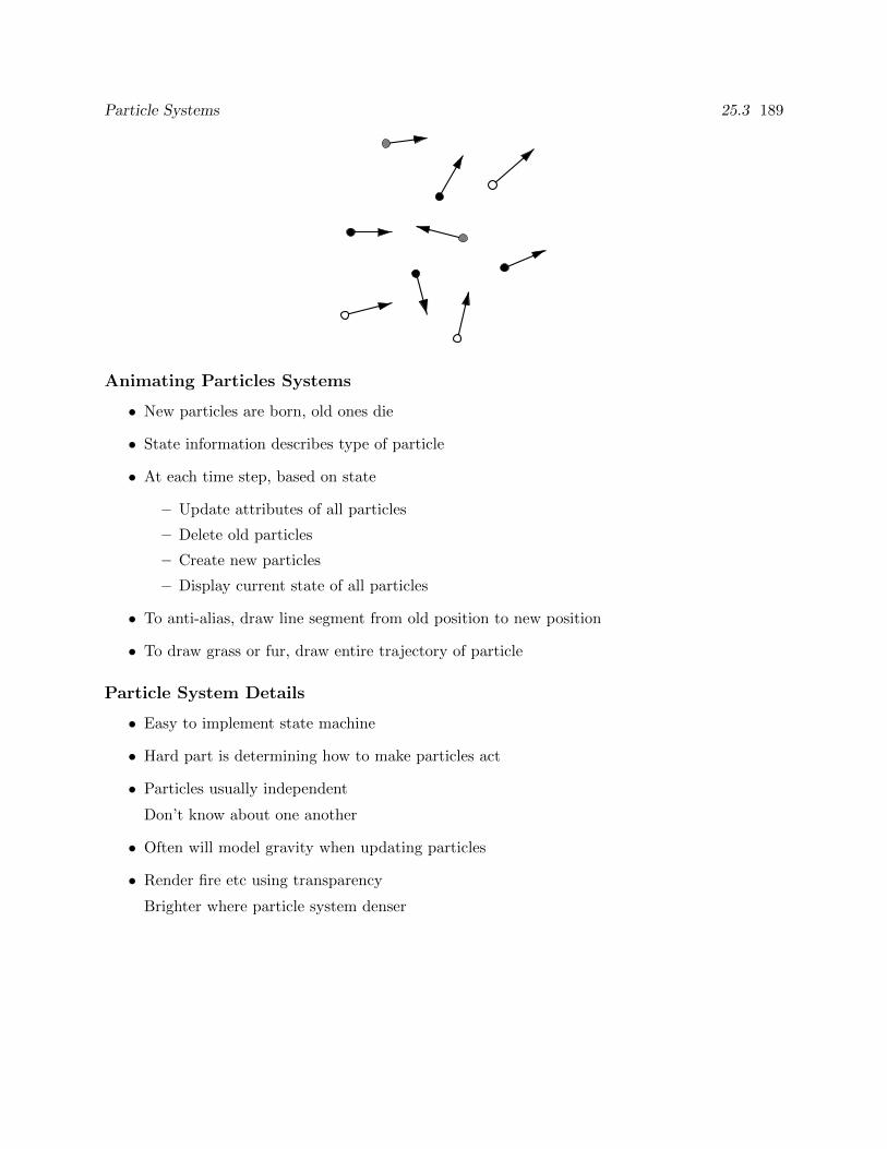
Particle Systems 25.3 189
Animating Particles Systems
• New particles are born, old ones die
• State information describes type of particle
• At each time step, based on state
– Update attributes of all particles
– Delete old particles
– Create new particles
– Display current state of all particles
• To anti-alias, draw line segment from old position to new position
• To draw grass or fur, draw entire trajectory of particle
Particle System Details
• Easy to implement state machine
• Hard part is determining how to make particles act
• Particles usually independent
Don’t know about one another
• Often will model gravity when updating particles
• Render fire etc using transparency
Brighter where particle system denser
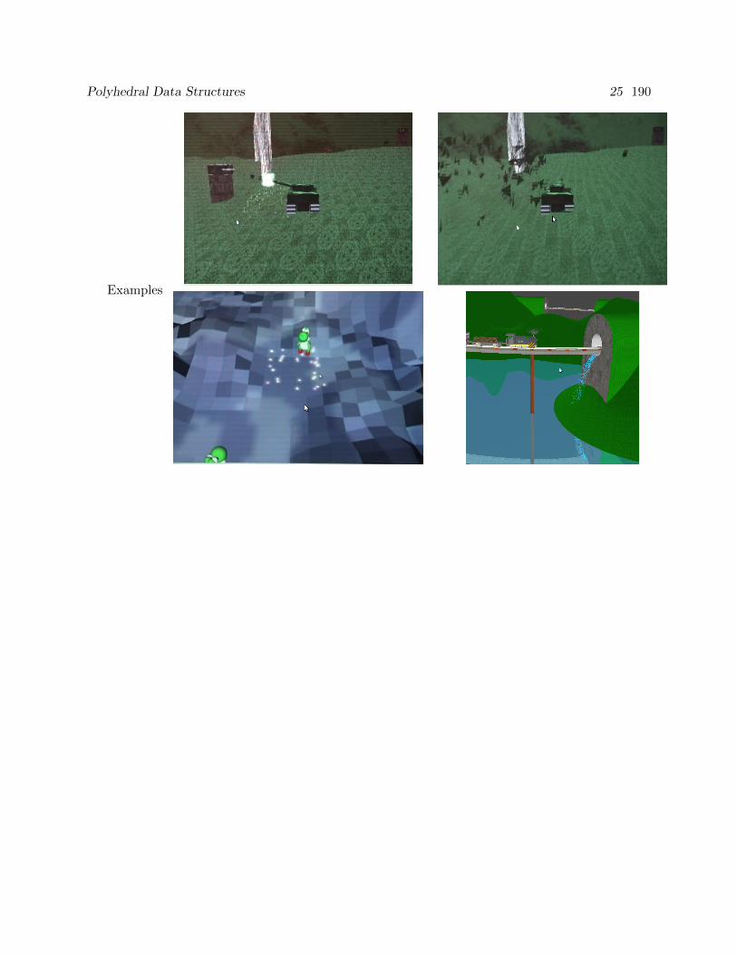
Polyhedral Data Structures 25 190
Examples
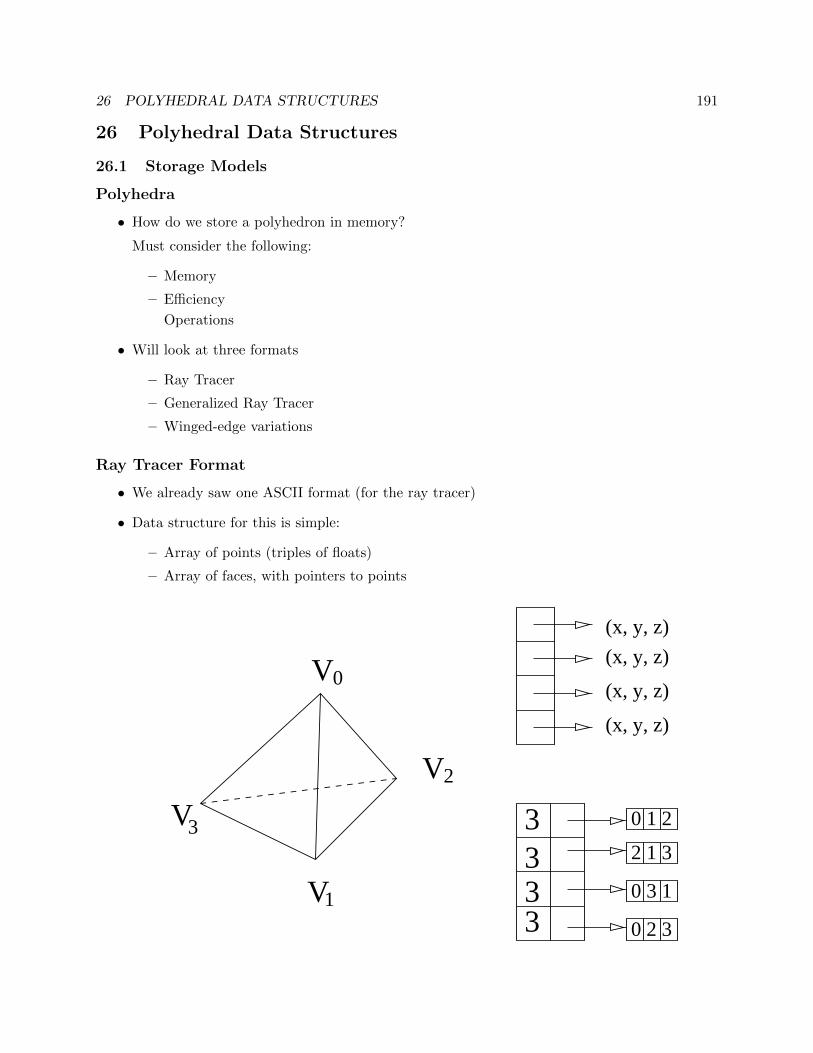
26 POLYHEDRAL DATA STRUCTURES 191
26 Polyhedral Data Structures
26.1 Storage Models
Polyhedra
• How do we store a polyhedron in memory?
Must consider the following:
– Memory
– Efficiency
Operations
• Will look at three formats
– Ray Tracer
– Generalized Ray Tracer
– Winged-edge variations
Ray Tracer Format
• We already saw one ASCII format (for the ray tracer)
• Data structure for this is simple:
– Array of points (triples of floats)
– Array of faces, with pointers to points
3333
0 1 2
2 1 33
0 3 1
0 2 3
(x, y, z)
(x, y, z)
(x, y, z)
(x, y, z)
V
V
V
V
0
2
1
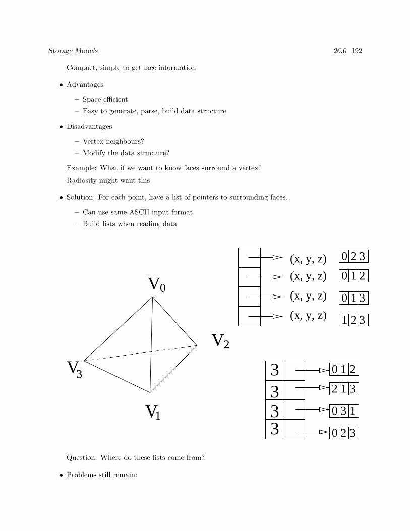
Storage Models 26.0 192
Compact, simple to get face information
• Advantages
– Space efficient
– Easy to generate, parse, build data structure
• Disadvantages
– Vertex neighbours?
– Modify the data structure?
Example: What if we want to know faces surround a vertex?
Radiosity might want this
• Solution: For each point, have a list of pointers to surrounding faces.
– Can use same ASCII input format
– Build lists when reading data
(x, y, z)
(x, y, z)
(x, y, z)
(x, y, z)
0 1 2
2 1 3
0 3 1
0 2 3
1 2 3
V
V
V
V
0
2
1
3 3333
0 2 3
0 1 2
0 1 3
Question: Where do these lists come from?
• Problems still remain:
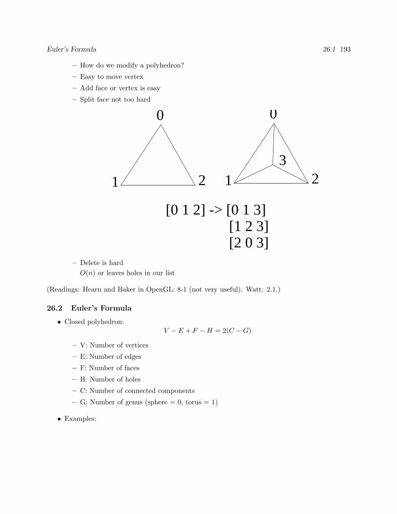
Euler’s Formula 26.1 193
– How do we modify a polyhedron?
– Easy to move vertex
– Add face or vertex is easy
– Split face not too hard
[1 2 3] [2 0 3]
[0 1 2] -> [0 1 3]
21
0
13
0
2
– Delete is hard
O(n) or leaves holes in our list
(Readings: Hearn and Baker in OpenGL: 8-1 (not very useful). Watt: 2.1.)
26.2 Euler’s Formula
• Closed polyhedron:V − E + F −H = 2(C −G)
– V: Number of vertices
– E: Number of edges
– F: Number of faces
– H: Number of holes
– C: Number of connected components
– G: Number of genus (sphere = 0, torus = 1)
• Examples:
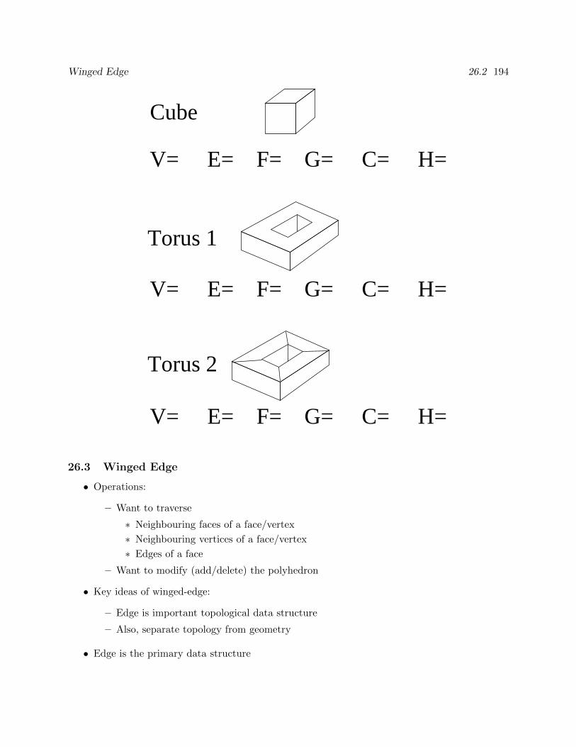
Winged Edge 26.2 194
V= E= F= G= C= H=
Cube
Torus 2
Torus 1
V= E= F= G= C= H=
V= E= F= G= C= H=
26.3 Winged Edge
• Operations:
– Want to traverse
∗ Neighbouring faces of a face/vertex
∗ Neighbouring vertices of a face/vertex
∗ Edges of a face
– Want to modify (add/delete) the polyhedron
• Key ideas of winged-edge:
– Edge is important topological data structure
– Also, separate topology from geometry
• Edge is the primary data structure
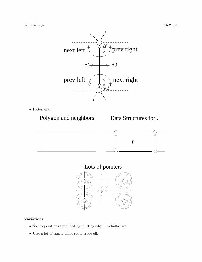
Winged Edge 26.2 195
v1
f1 f2
prev right
next right
next left
prev leftv2
• Pictorially:
F
F
Lots of pointers
Polygon and neighbors Data Structures for...
Variations
• Some operations simplified by splitting edge into half-edges
• Uses a lot of space. Time-space trade-off.
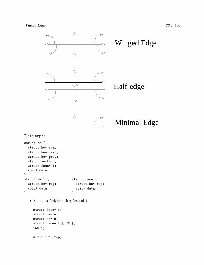
Winged Edge 26.2 196
Minimal Edge
Winged Edge
Half-edge
Data types
struct he
struct he* sym;
struct he* next;
struct he* prev;
struct vert* v;
struct face* f;
void* data;
struct vert struct face
struct he* rep; struct he* rep;
void* data; void* data;
• Example: Neighbouring faces of f
struct face* f;
struct he* e;
struct he* s;
struct face* fl[LOTS];
int i;
s = e = f->rep;
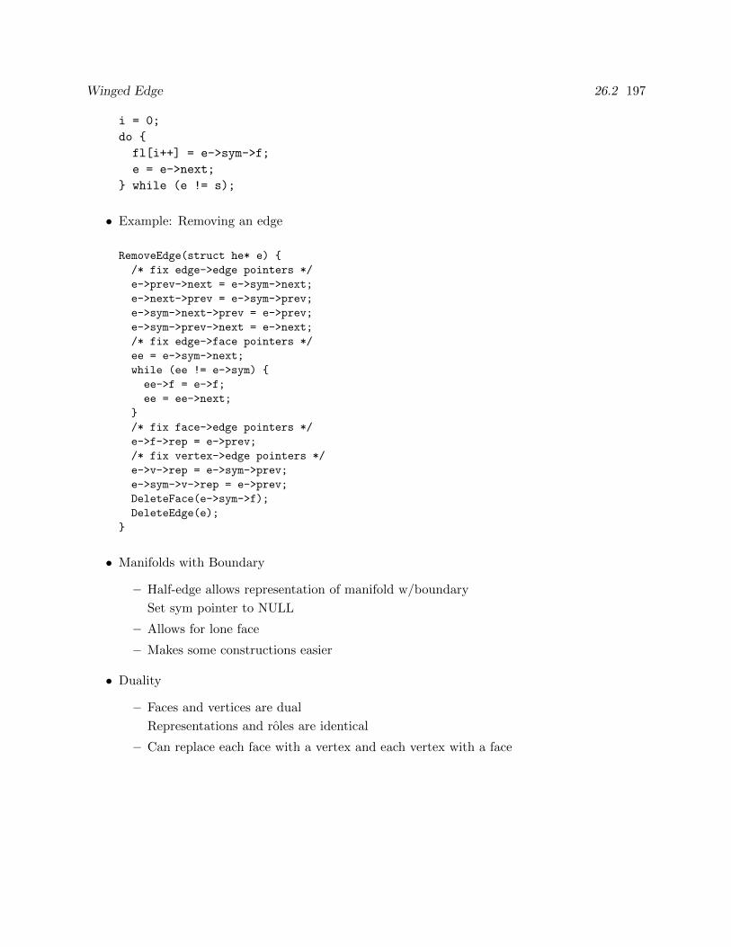
Winged Edge 26.2 197
i = 0;
do
fl[i++] = e->sym->f;
e = e->next;
while (e != s);
• Example: Removing an edge
RemoveEdge(struct he* e)
/* fix edge->edge pointers */
e->prev->next = e->sym->next;
e->next->prev = e->sym->prev;
e->sym->next->prev = e->prev;
e->sym->prev->next = e->next;
/* fix edge->face pointers */
ee = e->sym->next;
while (ee != e->sym)
ee->f = e->f;
ee = ee->next;
/* fix face->edge pointers */
e->f->rep = e->prev;
/* fix vertex->edge pointers */
e->v->rep = e->sym->prev;
e->sym->v->rep = e->prev;
DeleteFace(e->sym->f);
DeleteEdge(e);
• Manifolds with Boundary
– Half-edge allows representation of manifold w/boundary
Set sym pointer to NULL
– Allows for lone face
– Makes some constructions easier
• Duality
– Faces and vertices are dual
Representations and roles are identical
– Can replace each face with a vertex and each vertex with a face
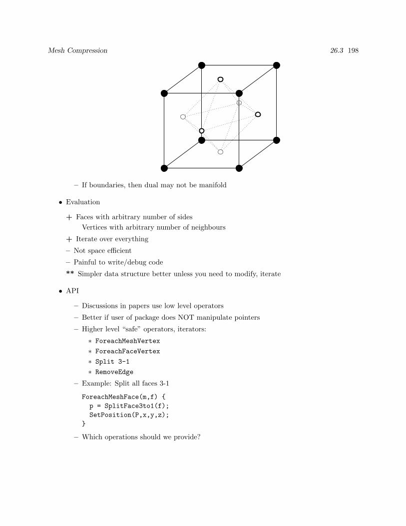
Mesh Compression 26.3 198
– If boundaries, then dual may not be manifold
• Evaluation
+ Faces with arbitrary number of sides
Vertices with arbitrary number of neighbours
+ Iterate over everything
– Not space efficient
– Painful to write/debug code
** Simpler data structure better unless you need to modify, iterate
• API
– Discussions in papers use low level operators
– Better if user of package does NOT manipulate pointers
– Higher level “safe” operators, iterators:
∗ ForeachMeshVertex
∗ ForeachFaceVertex
∗ Split 3-1
∗ RemoveEdge
– Example: Split all faces 3-1
ForeachMeshFace(m,f)
p = SplitFace3to1(f);
SetPosition(P,x,y,z);
– Which operations should we provide?
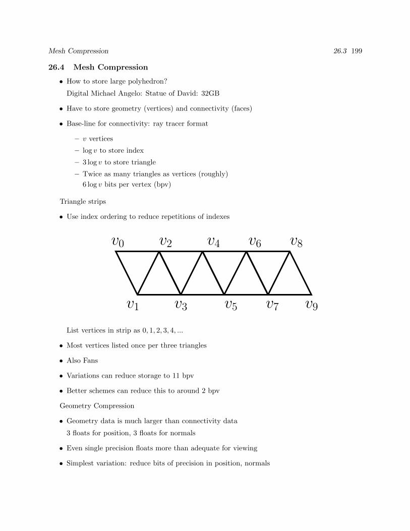
Mesh Compression 26.3 199
26.4 Mesh Compression
• How to store large polyhedron?
Digital Michael Angelo: Statue of David: 32GB
• Have to store geometry (vertices) and connectivity (faces)
• Base-line for connectivity: ray tracer format
– v vertices
– log v to store index
– 3 log v to store triangle
– Twice as many triangles as vertices (roughly)
6 log v bits per vertex (bpv)
Triangle strips
• Use index ordering to reduce repetitions of indexes
v2 v4 v6 v8v0
v1 v3 v5 v7 v9
List vertices in strip as 0, 1, 2, 3, 4, ...
• Most vertices listed once per three triangles
• Also Fans
• Variations can reduce storage to 11 bpv
• Better schemes can reduce this to around 2 bpv
Geometry Compression
• Geometry data is much larger than connectivity data
3 floats for position, 3 floats for normals
• Even single precision floats more than adequate for viewing
• Simplest variation: reduce bits of precision in position, normals
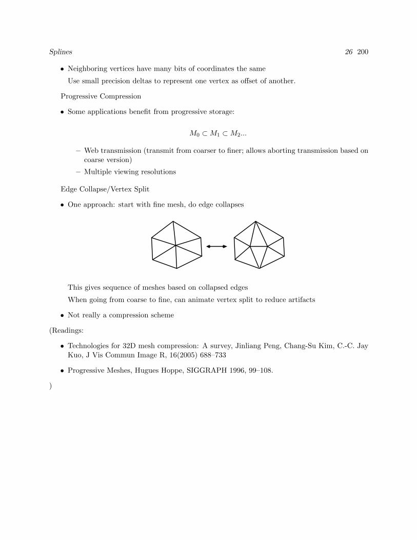
Splines 26 200
• Neighboring vertices have many bits of coordinates the same
Use small precision deltas to represent one vertex as offset of another.
Progressive Compression
• Some applications benefit from progressive storage:
M0 ⊂M1 ⊂M2...
– Web transmission (transmit from coarser to finer; allows aborting transmission based oncoarse version)
– Multiple viewing resolutions
Edge Collapse/Vertex Split
• One approach: start with fine mesh, do edge collapses
This gives sequence of meshes based on collapsed edges
When going from coarse to fine, can animate vertex split to reduce artifacts
• Not really a compression scheme
(Readings:
• Technologies for 32D mesh compression: A survey, Jinliang Peng, Chang-Su Kim, C.-C. JayKuo, J Vis Commun Image R, 16(2005) 688–733
• Progressive Meshes, Hugues Hoppe, SIGGRAPH 1996, 99–108.
)
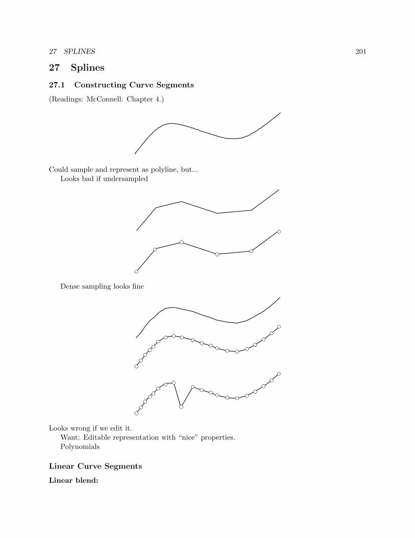
27 SPLINES 201
27 Splines
27.1 Constructing Curve Segments
(Readings: McConnell: Chapter 4.)
Could sample and represent as polyline, but...Looks bad if undersampled
Dense sampling looks fine
Looks wrong if we edit it.Want: Editable representation with “nice” properties.Polynomials
Linear Curve Segments
Linear blend:
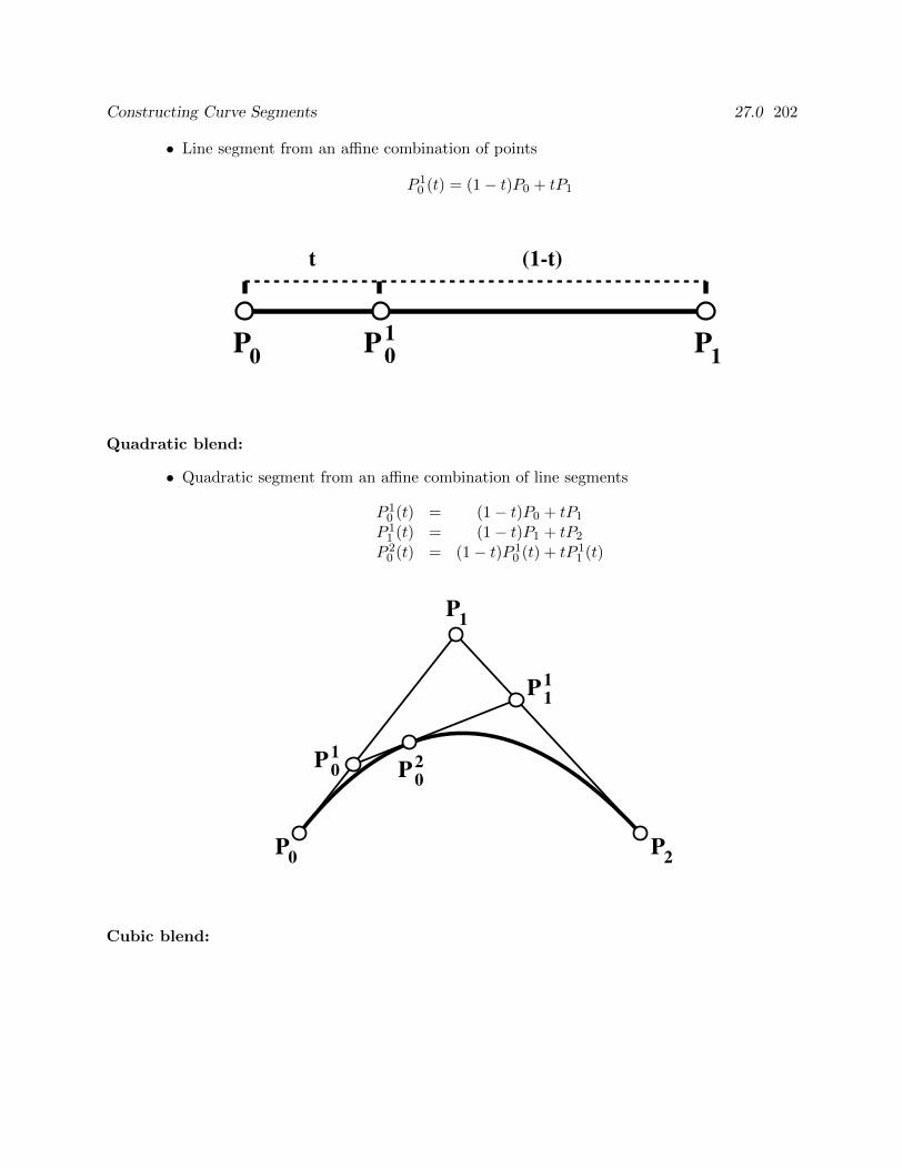
Constructing Curve Segments 27.0 202
• Line segment from an affine combination of points
P 10 (t) = (1− t)P0 + tP1
P0 P1P01
t (1-t)
Quadratic blend:
• Quadratic segment from an affine combination of line segments
P 10 (t) = (1− t)P0 + tP1
P 11 (t) = (1− t)P1 + tP2
P 20 (t) = (1− t)P 1
0 (t) + tP 11 (t)
0P 2P
1P
P01
P11
P02
Cubic blend:
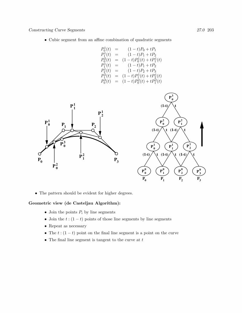
Constructing Curve Segments 27.0 203
• Cubic segment from an affine combination of quadratic segments
P 10 (t) = (1− t)P0 + tP1
P 11 (t) = (1− t)P1 + tP2
P 20 (t) = (1− t)P 1
0 (t) + tP 11 (t)
P 11 (t) = (1− t)P1 + tP2
P 12 (t) = (1− t)P2 + tP3
P 21 (t) = (1− t)P 1
1 (t) + tP 12 (t)
P 30 (t) = (1− t)P 2
0 (t) + tP 21 (t)
0P
2P1P
3P
P01
P11
P21
P02
P12
P03
(1-t) t (1-t) (1-t)t t
(1-t) t (1-t) t
(1-t) t
0P 1P 2P 3P
P01 P1
1 P21
P02 P1
2
P03
P00 P1
0 P20 P3
0
• The pattern should be evident for higher degrees.
Geometric view (de Casteljau Algorithm):
• Join the points Pi by line segments
• Join the t : (1− t) points of those line segments by line segments
• Repeat as necessary
• The t : (1− t) point on the final line segment is a point on the curve
• The final line segment is tangent to the curve at t
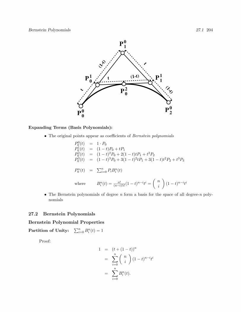
Bernstein Polynomials 27.1 204
t
(1-t)
t (1-t)(1-t)
t
P00 P2
0
P10
P02
P01 P1
1
Expanding Terms (Basis Polynomials):
• The original points appear as coefficients of Bernstein polynomials
P 00 (t) = 1 · P0
P 10 (t) = (1− t)P0 + tP1
P 20 (t) = (1− t)2P0 + 2(1− t)tP1 + t2P2
P 30 (t) = (1− t)3P0 + 3(1− t)2tP1 + 3(1− t)t2P2 + t3P3
Pn0 (t) =∑n
i=0 PiBni (t)
where Bni (t) = n!
(n−i)!i!(1− t)n−iti =
(ni
)(1− t)n−iti
• The Bernstein polynomials of degree n form a basis for the space of all degree-n poly-nomials
27.2 Bernstein Polynomials
Bernstein Polynomial Properties
Partition of Unity:∑n
i=0Bni (t) = 1
Proof:
1 = (t+ (1− t))n
=
n∑i=0
(ni
)(1− t)n−iti
=
n∑i=0
Bni (t).
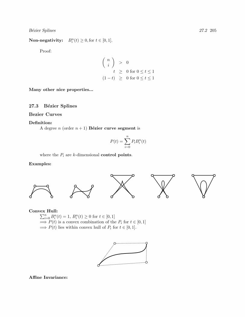
Bezier Splines 27.2 205
Non-negativity: Bni (t) ≥ 0, for t ∈ [0, 1].
Proof: (ni
)> 0
t ≥ 0 for 0 ≤ t ≤ 1
(1− t) ≥ 0 for 0 ≤ t ≤ 1
Many other nice properties...
27.3 Bezier Splines
Bezier Curves
Definition:A degree n (order n+ 1) Bezier curve segment is
P (t) =n∑i=0
PiBni (t)
where the Pi are k-dimensional control points.
Examples:
Convex Hull:∑ni=0B
ni (t) = 1, Bn
i (t) ≥ 0 for t ∈ [0, 1]=⇒ P (t) is a convex combination of the Pi for t ∈ [0, 1]=⇒ P (t) lies within convex hull of Pi for t ∈ [0, 1].
Affine Invariance:
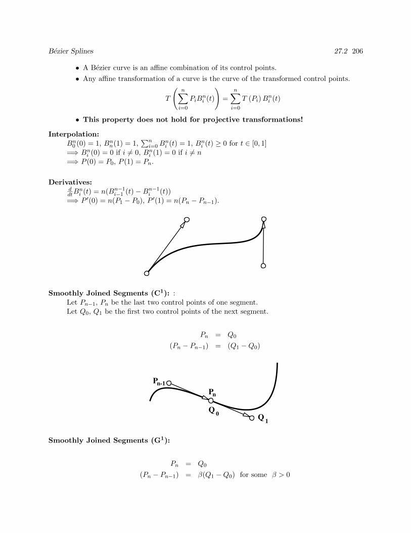
Bezier Splines 27.2 206
• A Bezier curve is an affine combination of its control points.
• Any affine transformation of a curve is the curve of the transformed control points.
T
(n∑i=0
PiBni (t)
)=
n∑i=0
T (Pi)Bni (t)
• This property does not hold for projective transformations!
Interpolation:Bn
0 (0) = 1, Bnn(1) = 1,
∑ni=0B
ni (t) = 1, Bn
i (t) ≥ 0 for t ∈ [0, 1]=⇒ Bn
i (0) = 0 if i 6= 0, Bni (1) = 0 if i 6= n
=⇒ P (0) = P0, P (1) = Pn.
Derivatives:ddtB
ni (t) = n(Bn−1
i−1 (t)−Bn−1i (t))
=⇒ P ′(0) = n(P1 − P0), P ′(1) = n(Pn − Pn−1).
Smoothly Joined Segments (C1): :Let Pn−1, Pn be the last two control points of one segment.Let Q0, Q1 be the first two control points of the next segment.
Pn = Q0
(Pn − Pn−1) = (Q1 −Q0)
Pn
Pn-1
Q 0 Q 1
Smoothly Joined Segments (G1):
Pn = Q0
(Pn − Pn−1) = β(Q1 −Q0) for some β > 0
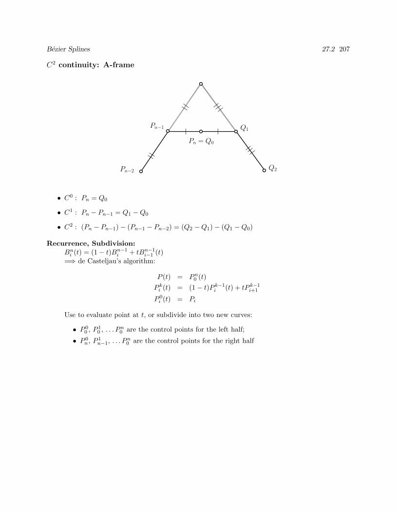
Bezier Splines 27.2 207
C2 continuity: A-frame
Q2Pn−2
Pn−1 Q1
Pn = Q0
• C0 : Pn = Q0
• C1 : Pn − Pn−1 = Q1 −Q0
• C2 : (Pn − Pn−1)− (Pn−1 − Pn−2) = (Q2 −Q1)− (Q1 −Q0)
Recurrence, Subdivision:Bni (t) = (1− t)Bn−1
i + tBn−1i−1 (t)
=⇒ de Casteljau’s algorithm:
P (t) = Pn0 (t)
P ki (t) = (1− t)P k−1i (t) + tP k−1
i+1
P 0i (t) = Pi
Use to evaluate point at t, or subdivide into two new curves:
• P 00 , P 1
0 , . . .Pn0 are the control points for the left half;
• P 0n , P 1
n−1, . . .Pn0 are the control points for the right half
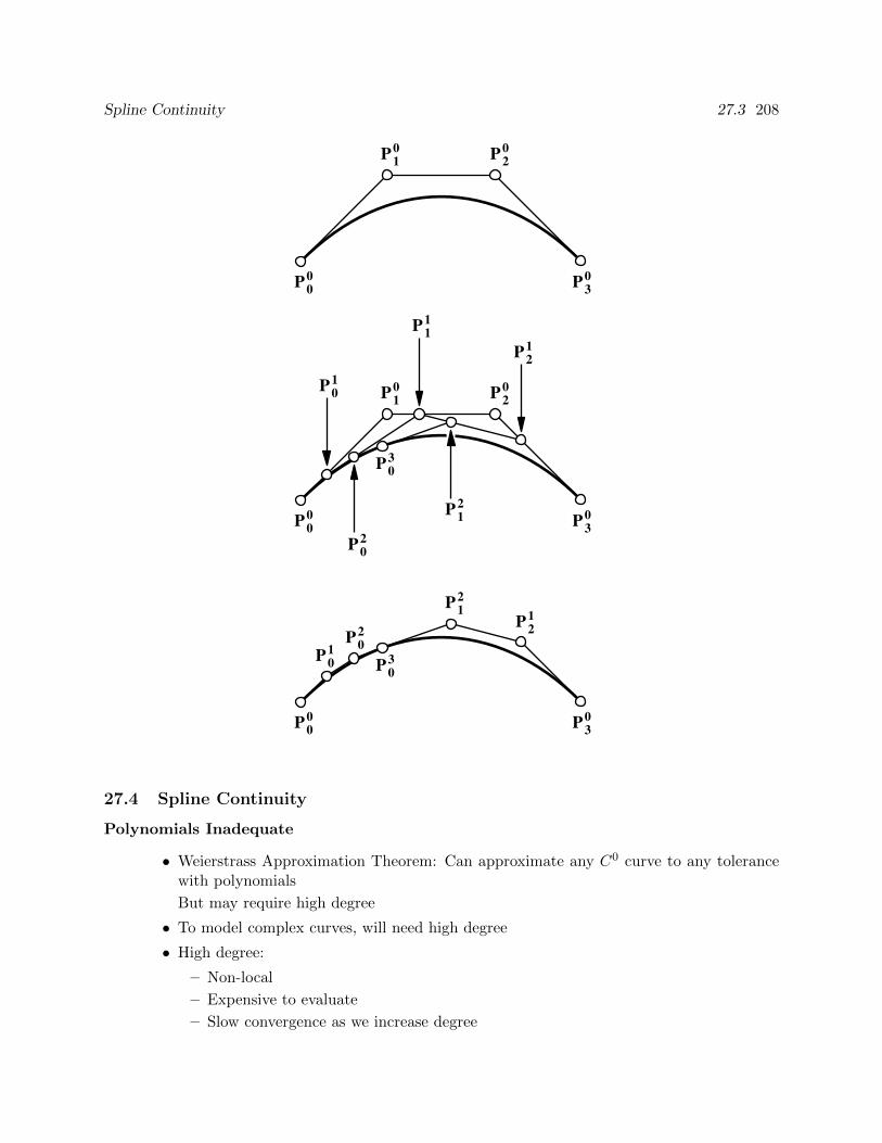
Spline Continuity 27.3 208
P01
P11
P21
P02
P12
P03
P00
P10 P2
0
P30
P00
P10 P2
0
P30
P01
P21
P02
P12
P03
P00 P3
0
27.4 Spline Continuity
Polynomials Inadequate
• Weierstrass Approximation Theorem: Can approximate any C0 curve to any tolerancewith polynomials
But may require high degree
• To model complex curves, will need high degree
• High degree:
– Non-local
– Expensive to evaluate
– Slow convergence as we increase degree
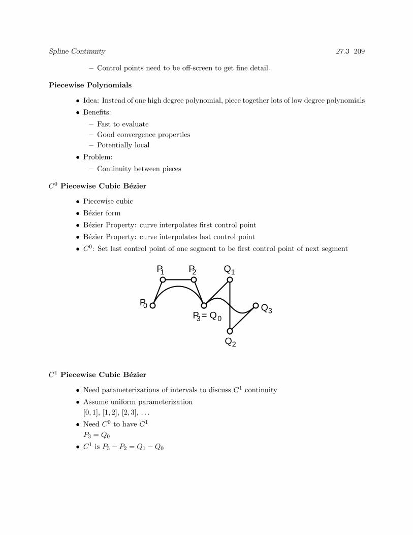
Spline Continuity 27.3 209
– Control points need to be off-screen to get fine detail.
Piecewise Polynomials
• Idea: Instead of one high degree polynomial, piece together lots of low degree polynomials
• Benefits:
– Fast to evaluate
– Good convergence properties
– Potentially local
• Problem:
– Continuity between pieces
C0 Piecewise Cubic Bezier
• Piecewise cubic
• Bezier form
• Bezier Property: curve interpolates first control point
• Bezier Property: curve interpolates last control point
• C0: Set last control point of one segment to be first control point of next segment
P
P P
P = Q
Q
Q
Q0
1 2
3 0
1
2
3
C1 Piecewise Cubic Bezier
• Need parameterizations of intervals to discuss C1 continuity
• Assume uniform parameterization
[0, 1], [1, 2], [2, 3], . . .
• Need C0 to have C1
P3 = Q0
• C1 is P3 − P2 = Q1 −Q0
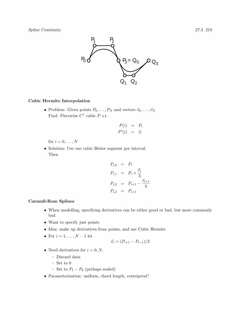
Spline Continuity 27.3 210
P
P P
P = Q
Q Q
Q0
1 2
3 0
1 2
3
Cubic Hermite Interpolation
• Problem: Given points P0, . . . , PN and vectors ~v0, . . . , ~vN
Find: Piecewise C1 cubic P s.t.
P (i) = Pi
P ′(i) = ~vi
for i = 0, . . . , N
• Solution: Use one cubic Bezier segment per interval
Then
Pi,0 = Pi
Pi,1 = Pi +~vi3
Pi,2 = Pi+1 −~vi+1
3Pi,3 = Pi+1
Catmull-Rom Splines
• When modelling, specifying derivatives can be either good or bad, but more commonlybad
• Want to specify just points
• Idea: make up derivatives from points, and use Cubic Hermite
• For i = 1, . . . , N − 1 let~vi = (Pi+1 − Pi−1)/2
• Need derivatives for i = 0, N .
– Discard data
– Set to 0
– Set to P1 − P0 (perhaps scaled)
• Parameterization: uniform, chord length, centripetal?
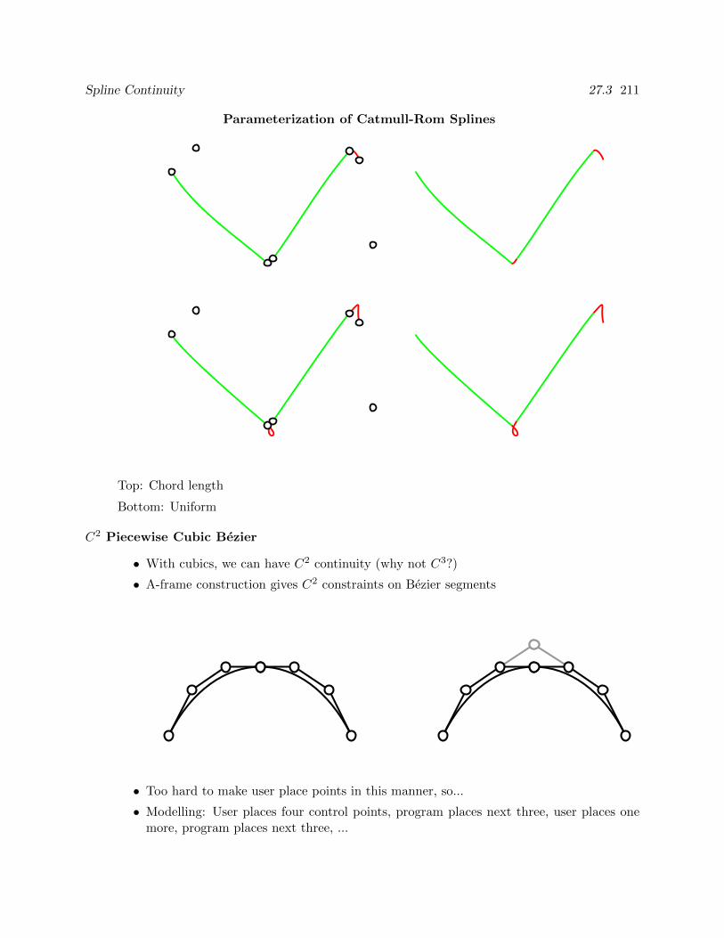
Spline Continuity 27.3 211
Parameterization of Catmull-Rom Splines
Top: Chord length
Bottom: Uniform
C2 Piecewise Cubic Bezier
• With cubics, we can have C2 continuity (why not C3?)
• A-frame construction gives C2 constraints on Bezier segments
• Too hard to make user place points in this manner, so...
• Modelling: User places four control points, program places next three, user places onemore, program places next three, ...
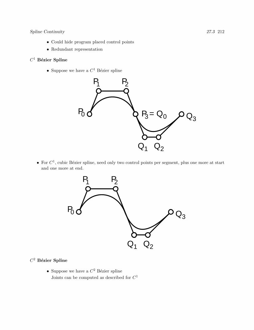
Spline Continuity 27.3 212
• Could hide program placed control points
• Redundant representation
C1 Bezier Spline
• Suppose we have a C1 Bezier spline
P
P P
P = Q
Q Q
Q0
1 2
3 0
1 2
3
• For C1, cubic Bezier spline, need only two control points per segment, plus one more at startand one more at end.
P
P P
Q Q
Q0
1 2
1 2
3
C2 Bezier Spline
• Suppose we have a C2 Bezier spline
Joints can be computed as described for C1
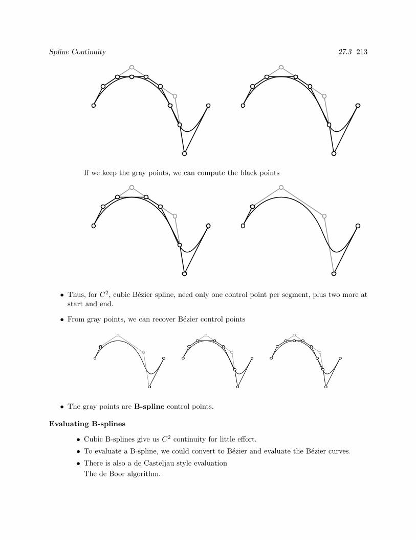
Spline Continuity 27.3 213
If we keep the gray points, we can compute the black points
• Thus, for C2, cubic Bezier spline, need only one control point per segment, plus two more atstart and end.
• From gray points, we can recover Bezier control points
• The gray points are B-spline control points.
Evaluating B-splines
• Cubic B-splines give us C2 continuity for little effort.
• To evaluate a B-spline, we could convert to Bezier and evaluate the Bezier curves.
• There is also a de Casteljau style evaluation
The de Boor algorithm.
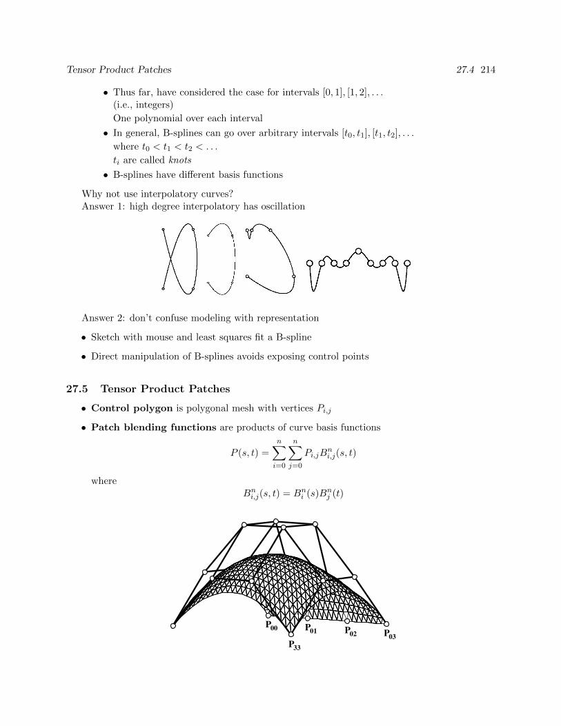
Tensor Product Patches 27.4 214
• Thus far, have considered the case for intervals [0, 1], [1, 2], . . .(i.e., integers)
One polynomial over each interval
• In general, B-splines can go over arbitrary intervals [t0, t1], [t1, t2], . . .
where t0 < t1 < t2 < . . .
ti are called knots
• B-splines have different basis functions
Why not use interpolatory curves?Answer 1: high degree interpolatory has oscillation
Answer 2: don’t confuse modeling with representation
• Sketch with mouse and least squares fit a B-spline
• Direct manipulation of B-splines avoids exposing control points
27.5 Tensor Product Patches
• Control polygon is polygonal mesh with vertices Pi,j
• Patch blending functions are products of curve basis functions
P (s, t) =n∑i=0
n∑j=0
Pi,jBni,j(s, t)
whereBni,j(s, t) = Bn
i (s)Bnj (t)
P00 P01 P02 P03P33
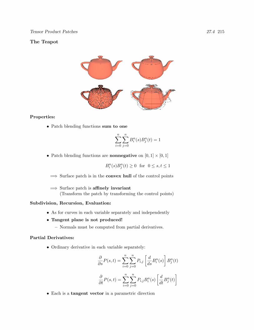
Tensor Product Patches 27.4 215
The Teapot
Properties:
• Patch blending functions sum to one
n∑i=0
n∑j=0
Bni (s)Bn
j (t) = 1
• Patch blending functions are nonnegative on [0, 1]× [0, 1]
Bni (s)Bn
j (t) ≥ 0 for 0 ≤ s, t ≤ 1
=⇒ Surface patch is in the convex hull of the control points
=⇒ Surface patch is affinely invariant(Transform the patch by transforming the control points)
Subdivision, Recursion, Evaluation:
• As for curves in each variable separately and independently
• Tangent plane is not produced!
– Normals must be computed from partial derivatives.
Partial Derivatives:
• Ordinary derivative in each variable separately:
∂
∂sP (s, t) =
n∑i=0
n∑j=0
Pi,j
[d
dsBni (s)
]Bnj (t)
∂
∂tP (s, t) =
n∑i=0
n∑j=0
Pi,jBni (s)
[d
dtBnj (t)
]• Each is a tangent vector in a parametric direction
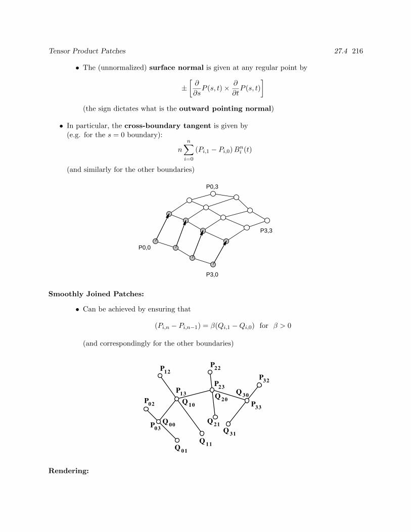
Tensor Product Patches 27.4 216
• The (unnormalized) surface normal is given at any regular point by
±[∂
∂sP (s, t)× ∂
∂tP (s, t)
](the sign dictates what is the outward pointing normal)
• In particular, the cross-boundary tangent is given by(e.g. for the s = 0 boundary):
nn∑i=0
(Pi,1 − Pi,0)Bni (t)
(and similarly for the other boundaries)
P0,0
P0,3
P3,0
P3,3
Smoothly Joined Patches:
• Can be achieved by ensuring that
(Pi,n − Pi,n−1) = β(Qi,1 −Qi,0) for β > 0
(and correspondingly for the other boundaries)
P03
P13
P23
P33P02
P12P22
P32
Q 01
Q 11
Q 21Q 31
Q 00
Q 10Q 20
Q 30
Rendering:
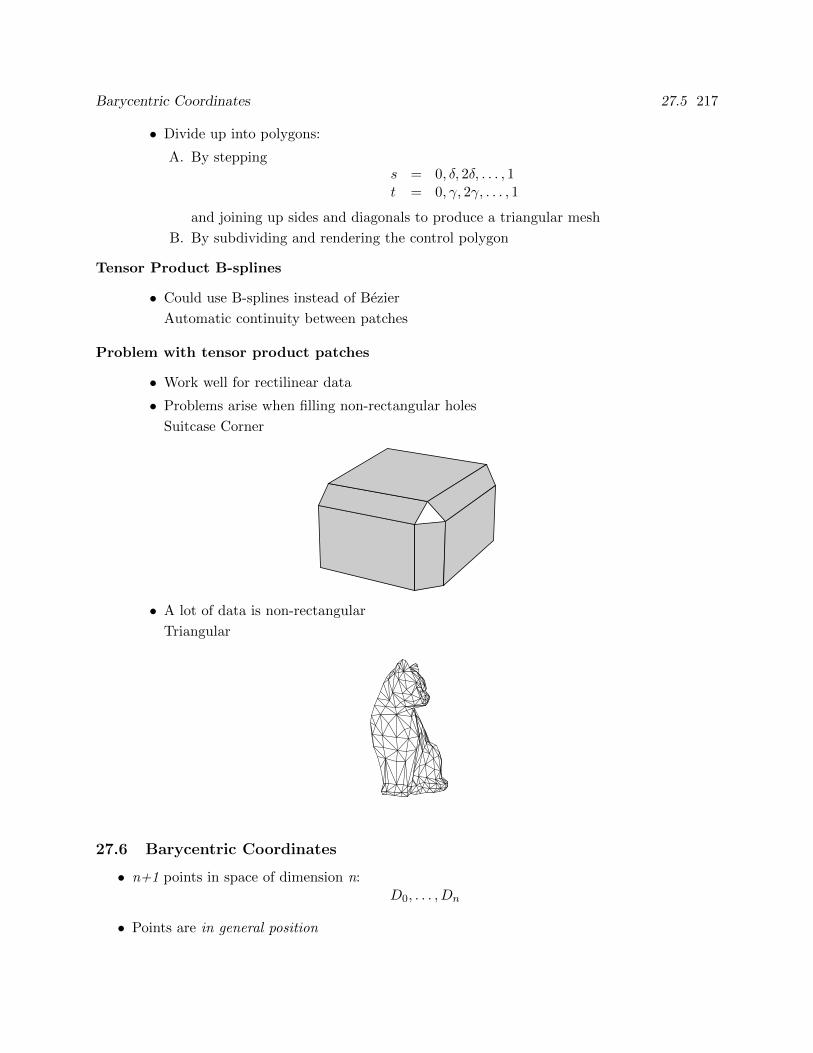
Barycentric Coordinates 27.5 217
• Divide up into polygons:
A. By steppings = 0, δ, 2δ, . . . , 1t = 0, γ, 2γ, . . . , 1
and joining up sides and diagonals to produce a triangular mesh
B. By subdividing and rendering the control polygon
Tensor Product B-splines
• Could use B-splines instead of Bezier
Automatic continuity between patches
Problem with tensor product patches
• Work well for rectilinear data
• Problems arise when filling non-rectangular holes
Suitcase Corner
• A lot of data is non-rectangular
Triangular
27.6 Barycentric Coordinates
• n+1 points in space of dimension n:D0, . . . , Dn
• Points are in general position
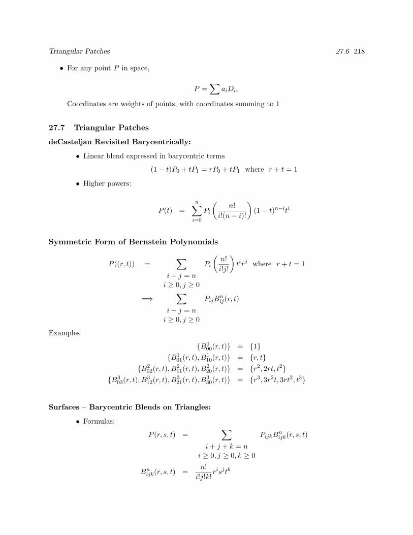
Triangular Patches 27.6 218
• For any point P in space,
P =∑
aiDi,
Coordinates are weights of points, with coordinates summing to 1
27.7 Triangular Patches
deCasteljau Revisited Barycentrically:
• Linear blend expressed in barycentric terms
(1− t)P0 + tP1 = rP0 + tP1 where r + t = 1
• Higher powers:
P (t) =n∑i=0
Pi
(n!
i!(n− i)!
)(1− t)n−iti
Symmetric Form of Bernstein Polynomials
P ((r, t)) =∑
i+ j = ni ≥ 0, j ≥ 0
Pi
(n!
i!j!
)tirj where r + t = 1
=⇒∑
i+ j = ni ≥ 0, j ≥ 0
PijBnij(r, t)
Examples
B000(r, t) = 1
B101(r, t), B1
10(r, t) = r, tB2
02(r, t), B211(r, t), B2
20(r, t) = r2, 2rt, t2B3
03(r, t), B312(r, t), B3
21(r, t), B330(r, t) = r3, 3r2t, 3rt2, t3
Surfaces – Barycentric Blends on Triangles:
• Formulas:
P (r, s, t) =∑
i+ j + k = ni ≥ 0, j ≥ 0, k ≥ 0
PijkBnijk(r, s, t)
Bnijk(r, s, t) =
n!
i!j!k!risjtk
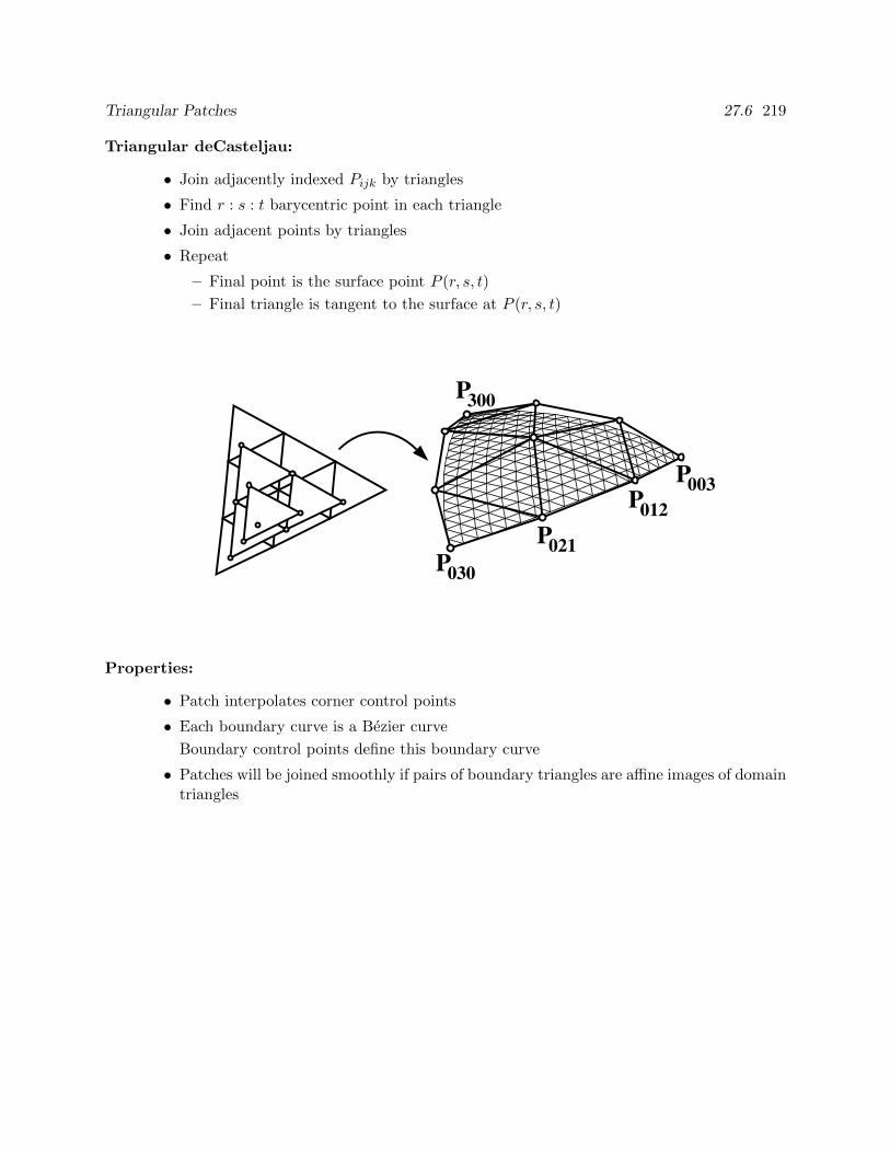
Triangular Patches 27.6 219
Triangular deCasteljau:
• Join adjacently indexed Pijk by triangles
• Find r : s : t barycentric point in each triangle
• Join adjacent points by triangles
• Repeat
– Final point is the surface point P (r, s, t)
– Final triangle is tangent to the surface at P (r, s, t)
P030
P021
P012
P003
P300
Properties:
• Patch interpolates corner control points
• Each boundary curve is a Bezier curve
Boundary control points define this boundary curve
• Patches will be joined smoothly if pairs of boundary triangles are affine images of domaintriangles
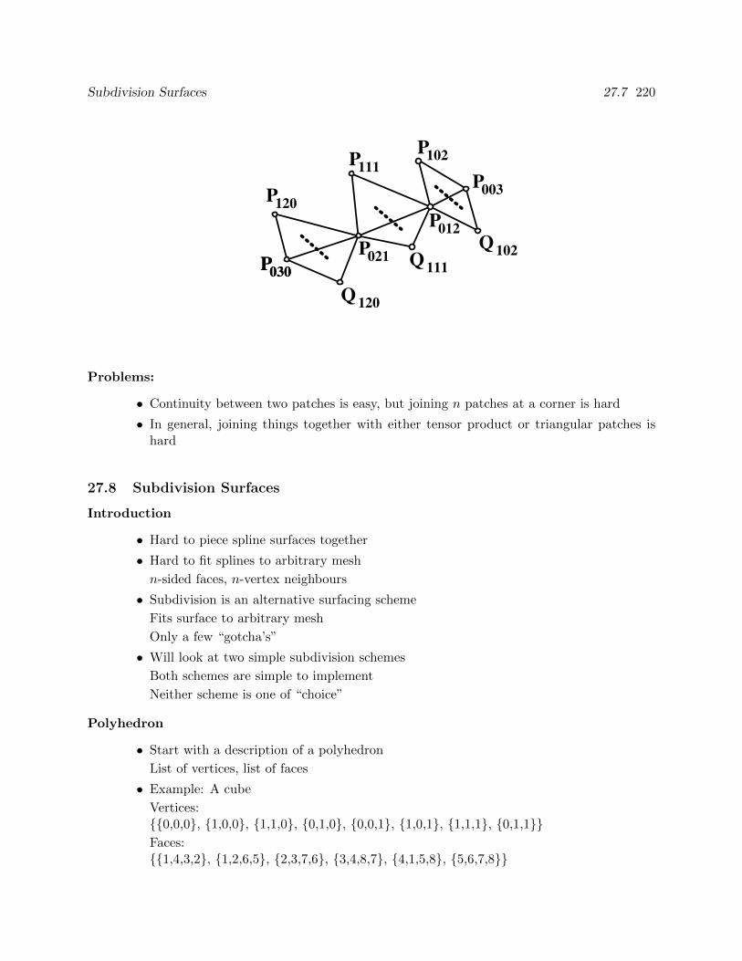
Subdivision Surfaces 27.7 220
P030P021
P012
P003P120
P111
P030
P102
Q 120
Q 111
Q 102
Problems:
• Continuity between two patches is easy, but joining n patches at a corner is hard
• In general, joining things together with either tensor product or triangular patches ishard
27.8 Subdivision Surfaces
Introduction
• Hard to piece spline surfaces together
• Hard to fit splines to arbitrary mesh
n-sided faces, n-vertex neighbours
• Subdivision is an alternative surfacing scheme
Fits surface to arbitrary mesh
Only a few “gotcha’s”
• Will look at two simple subdivision schemes
Both schemes are simple to implement
Neither scheme is one of “choice”
Polyhedron
• Start with a description of a polyhedron
List of vertices, list of faces
• Example: A cube
Vertices:0,0,0, 1,0,0, 1,1,0, 0,1,0, 0,0,1, 1,0,1, 1,1,1, 0,1,1Faces:1,4,3,2, 1,2,6,5, 2,3,7,6, 3,4,8,7, 4,1,5,8, 5,6,7,8
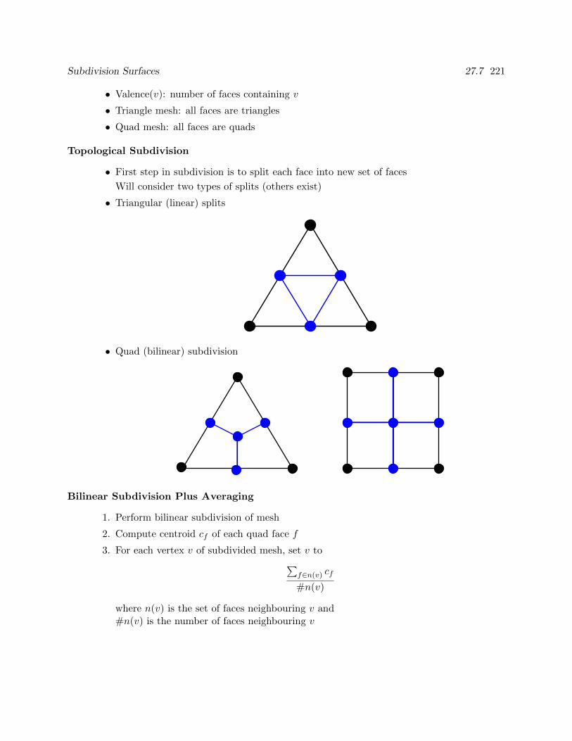
Subdivision Surfaces 27.7 221
• Valence(v): number of faces containing v
• Triangle mesh: all faces are triangles
• Quad mesh: all faces are quads
Topological Subdivision
• First step in subdivision is to split each face into new set of faces
Will consider two types of splits (others exist)
• Triangular (linear) splits
• Quad (bilinear) subdivision
Bilinear Subdivision Plus Averaging
1. Perform bilinear subdivision of mesh
2. Compute centroid cf of each quad face f
3. For each vertex v of subdivided mesh, set v to∑f∈n(v) cf
#n(v)
where n(v) is the set of faces neighbouring v and#n(v) is the number of faces neighbouring v
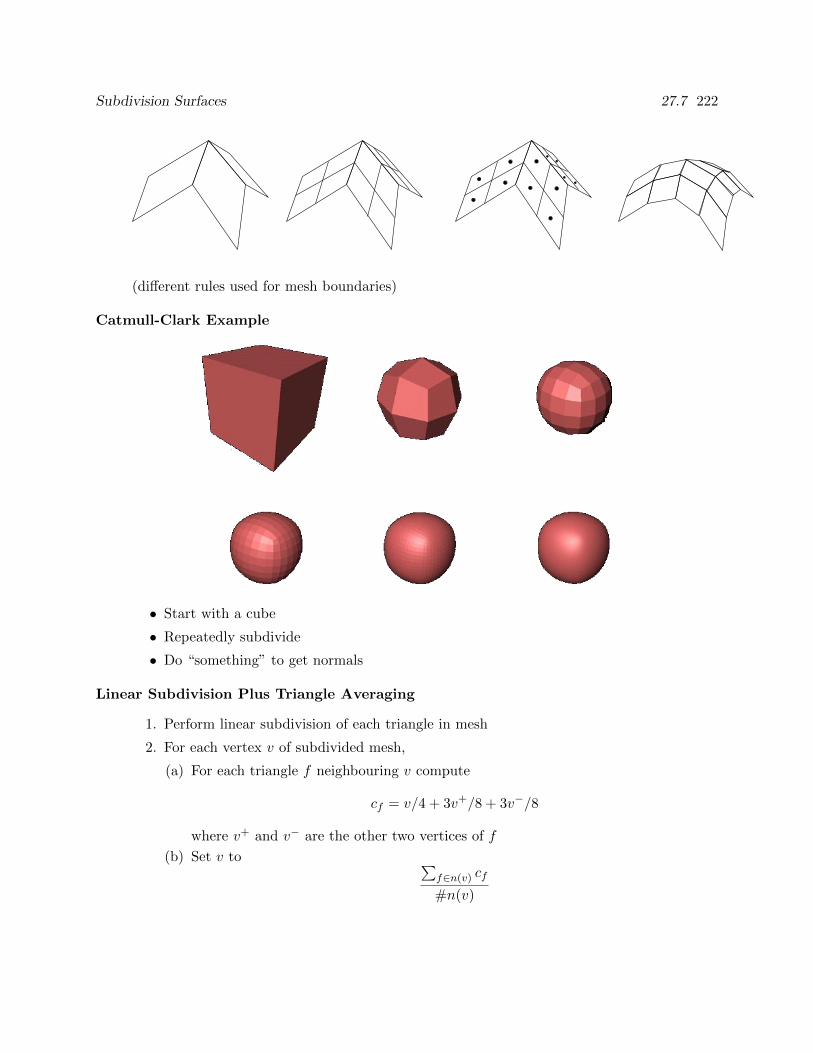
Subdivision Surfaces 27.7 222
(different rules used for mesh boundaries)
Catmull-Clark Example
• Start with a cube
• Repeatedly subdivide
• Do “something” to get normals
Linear Subdivision Plus Triangle Averaging
1. Perform linear subdivision of each triangle in mesh
2. For each vertex v of subdivided mesh,
(a) For each triangle f neighbouring v compute
cf = v/4 + 3v+/8 + 3v−/8
where v+ and v− are the other two vertices of f
(b) Set v to ∑f∈n(v) cf
#n(v)
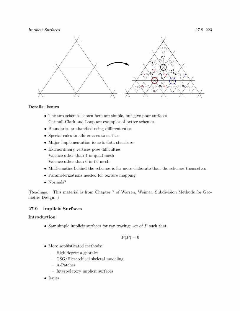
Implicit Surfaces 27.8 223
Details, Issues
• The two schemes shown here are simple, but give poor surfaces
Catmull-Clark and Loop are examples of better schemes
• Boundaries are handled using different rules
• Special rules to add creases to surface
• Major implementation issue is data structure
• Extraordinary vertices pose difficulties
Valence other than 4 in quad mesh
Valence other than 6 in tri mesh
• Mathematics behind the schemes is far more elaborate than the schemes themselves
• Parameterizations needed for texture mapping
• Normals?
(Readings: This material is from Chapter 7 of Warren, Weimer, Subdivision Methods for Geo-metric Design. )
27.9 Implicit Surfaces
Introduction
• Saw simple implicit surfaces for ray tracing: set of P such that
F (P ) = 0
• More sophisticated methods:
– High degree algebraics
– CSG/Hierarchical skeletal modeling
– A-Patches
– Interpolatory implicit surfaces
• Issues
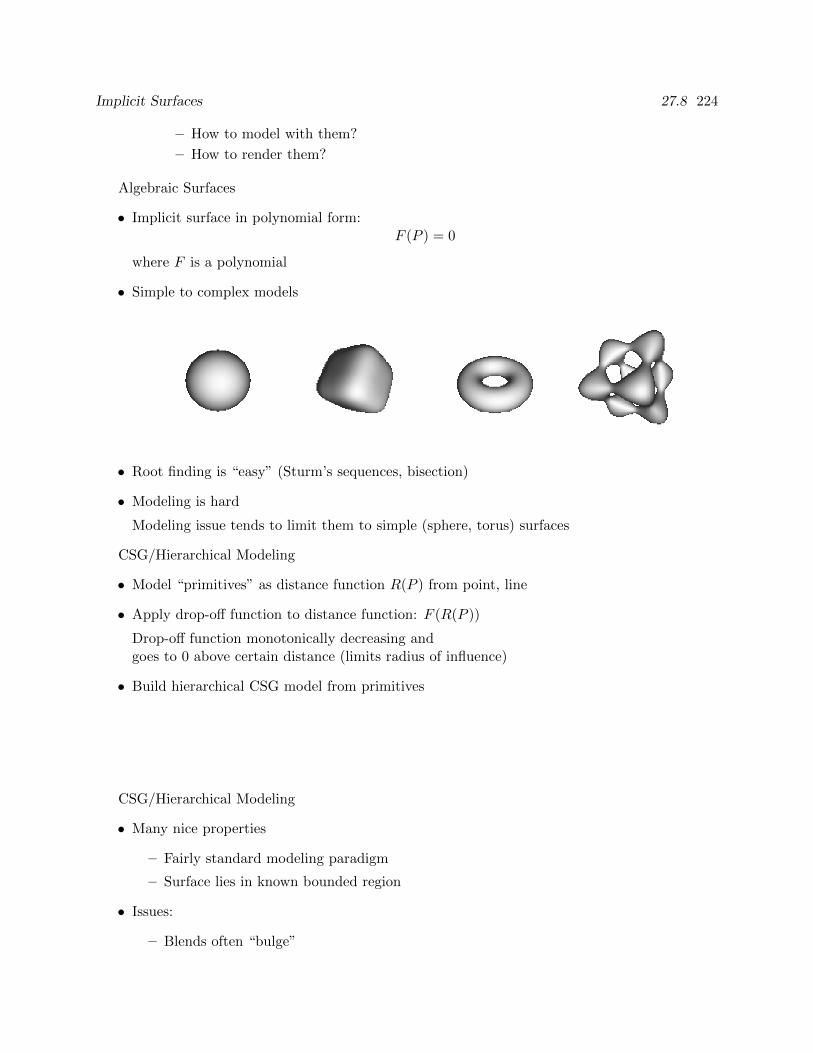
Implicit Surfaces 27.8 224
– How to model with them?
– How to render them?
Algebraic Surfaces
• Implicit surface in polynomial form:F (P ) = 0
where F is a polynomial
• Simple to complex models
• Root finding is “easy” (Sturm’s sequences, bisection)
• Modeling is hard
Modeling issue tends to limit them to simple (sphere, torus) surfaces
CSG/Hierarchical Modeling
• Model “primitives” as distance function R(P ) from point, line
• Apply drop-off function to distance function: F (R(P ))
Drop-off function monotonically decreasing andgoes to 0 above certain distance (limits radius of influence)
• Build hierarchical CSG model from primitives
CSG/Hierarchical Modeling
• Many nice properties
– Fairly standard modeling paradigm
– Surface lies in known bounded region
• Issues:
– Blends often “bulge”
Implicit Surfaces 27.8 225
– Modeling is as complex as using standard CSG modeling
Interpolatory Implicit Surfaces
• Given: a polyhedron with vertices VFind: an implicit surface F such that F (vi) = 0 for vi ∈ V .
• One solutions involves using radial basis function
ri(v) = |v − vi|3
We then construct
F (v) =
∑vi∈V
φiri(v)
+ P (v)
where P is a linear polynomial.
• The conditions F (vi) = 0 give a system of linear equations to solve for φ (need 4 additionalequations for P ).
Interpolatory Implicit Surfaces—Non-zero constraints
• We need at least one constraint NOT on the implicit surface,or will obtain trivial solution of φi = 0.
• Interior and exterior constraints(v s.t. F (v) > 0 or F (v) < 0 respectively)
• Interior/exterior constraints also specify topology
• One approach is “normal constraints”
– At each vi ∈ V , associate normal ni.
– Constraint is F (vi + εni) = 1 (with ε = 0.01 for example).
– Solve with other constraints
– Solution will interpolate positional constraints (F (vi) = 0) but only approximate normalconstraints
Example: 800 vertices and normals
BunnyRendering Implicit Surfaces
• Ray Tracing
– Root finding
∗ Reasonable for algebraics (Sturm sequences)
∗ Need numerical methods for general implicits
– Sphere tracing—variation on ray tracing
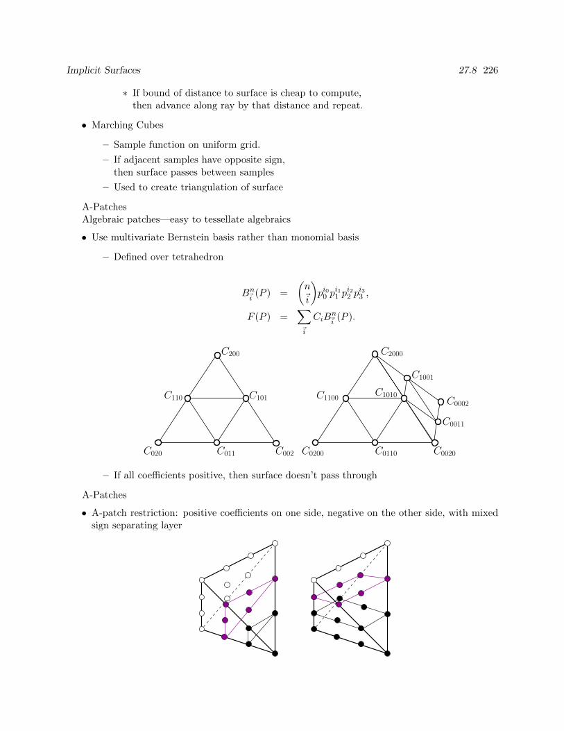
Implicit Surfaces 27.8 226
∗ If bound of distance to surface is cheap to compute,then advance along ray by that distance and repeat.
• Marching Cubes
– Sample function on uniform grid.
– If adjacent samples have opposite sign,then surface passes between samples
– Used to create triangulation of surface
A-PatchesAlgebraic patches—easy to tessellate algebraics
• Use multivariate Bernstein basis rather than monomial basis
– Defined over tetrahedron
Bn~i
(P ) =
(n~i
)pi00 p
i11 p
i22 p
i33 ,
F (P ) =∑~i
CiBn~i
(P ).
C0020C0110C0200
C1010
C0011
C011C020
C110
C002
C200
C101 C1100
C1001
C2000
C0002
– If all coefficients positive, then surface doesn’t pass through
A-Patches
• A-patch restriction: positive coefficients on one side, negative on the other side, with mixedsign separating layer
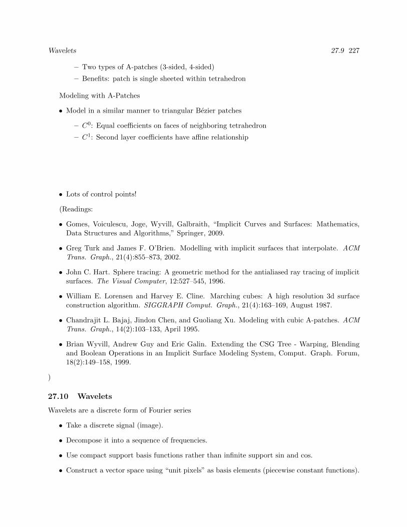
Wavelets 27.9 227
– Two types of A-patches (3-sided, 4-sided)
– Benefits: patch is single sheeted within tetrahedron
Modeling with A-Patches
• Model in a similar manner to triangular Bezier patches
– C0: Equal coefficients on faces of neighboring tetrahedron
– C1: Second layer coefficients have affine relationship
• Lots of control points!
(Readings:
• Gomes, Voiculescu, Joge, Wyvill, Galbraith, “Implicit Curves and Surfaces: Mathematics,Data Structures and Algorithms,” Springer, 2009.
• Greg Turk and James F. O’Brien. Modelling with implicit surfaces that interpolate. ACMTrans. Graph., 21(4):855–873, 2002.
• John C. Hart. Sphere tracing: A geometric method for the antialiased ray tracing of implicitsurfaces. The Visual Computer, 12:527–545, 1996.
• William E. Lorensen and Harvey E. Cline. Marching cubes: A high resolution 3d surfaceconstruction algorithm. SIGGRAPH Comput. Graph., 21(4):163–169, August 1987.
• Chandrajit L. Bajaj, Jindon Chen, and Guoliang Xu. Modeling with cubic A-patches. ACMTrans. Graph., 14(2):103–133, April 1995.
• Brian Wyvill, Andrew Guy and Eric Galin. Extending the CSG Tree - Warping, Blendingand Boolean Operations in an Implicit Surface Modeling System, Comput. Graph. Forum,18(2):149–158, 1999.
)
27.10 Wavelets
Wavelets are a discrete form of Fourier series
• Take a discrete signal (image).
• Decompose it into a sequence of frequencies.
• Use compact support basis functions rather than infinite support sin and cos.
• Construct a vector space using “unit pixels” as basis elements (piecewise constant functions).
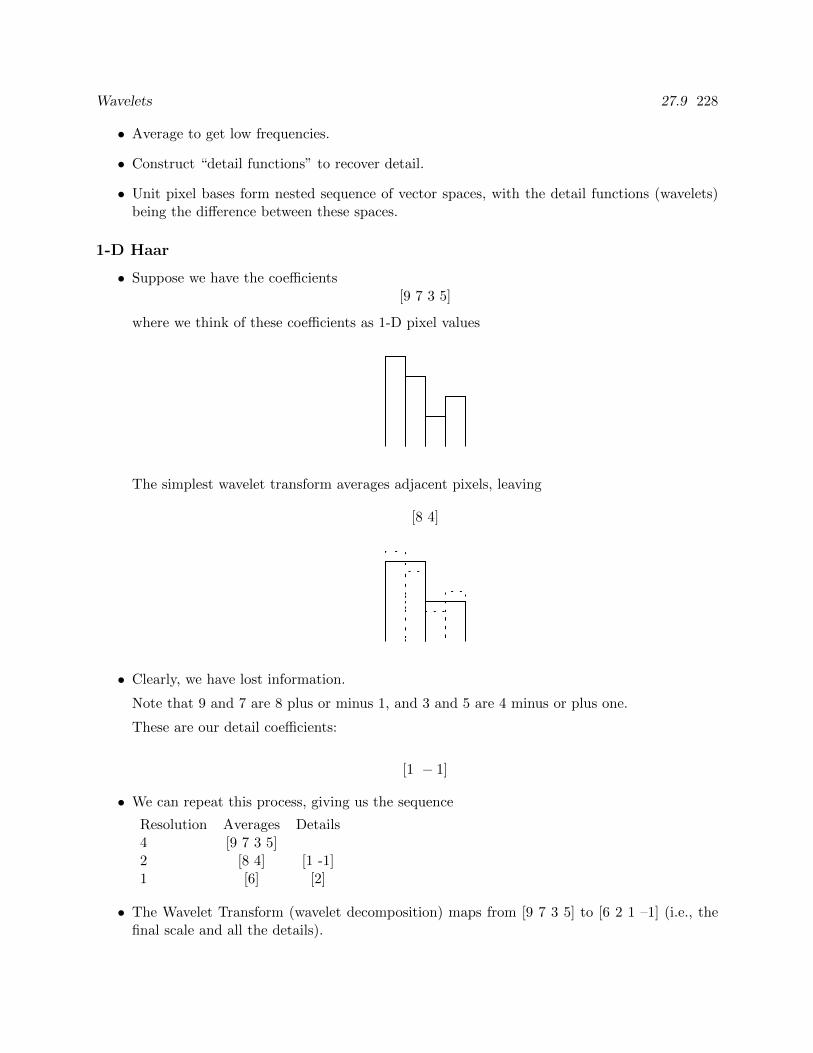
Wavelets 27.9 228
• Average to get low frequencies.
• Construct “detail functions” to recover detail.
• Unit pixel bases form nested sequence of vector spaces, with the detail functions (wavelets)being the difference between these spaces.
1-D Haar
• Suppose we have the coefficients[9 7 3 5]
where we think of these coefficients as 1-D pixel values
The simplest wavelet transform averages adjacent pixels, leaving
[8 4]
• Clearly, we have lost information.
Note that 9 and 7 are 8 plus or minus 1, and 3 and 5 are 4 minus or plus one.
These are our detail coefficients:
[1 − 1]
• We can repeat this process, giving us the sequence
Resolution Averages Details4 [9 7 3 5]2 [8 4] [1 -1]1 [6] [2]
• The Wavelet Transform (wavelet decomposition) maps from [9 7 3 5] to [6 2 1 –1] (i.e., thefinal scale and all the details).
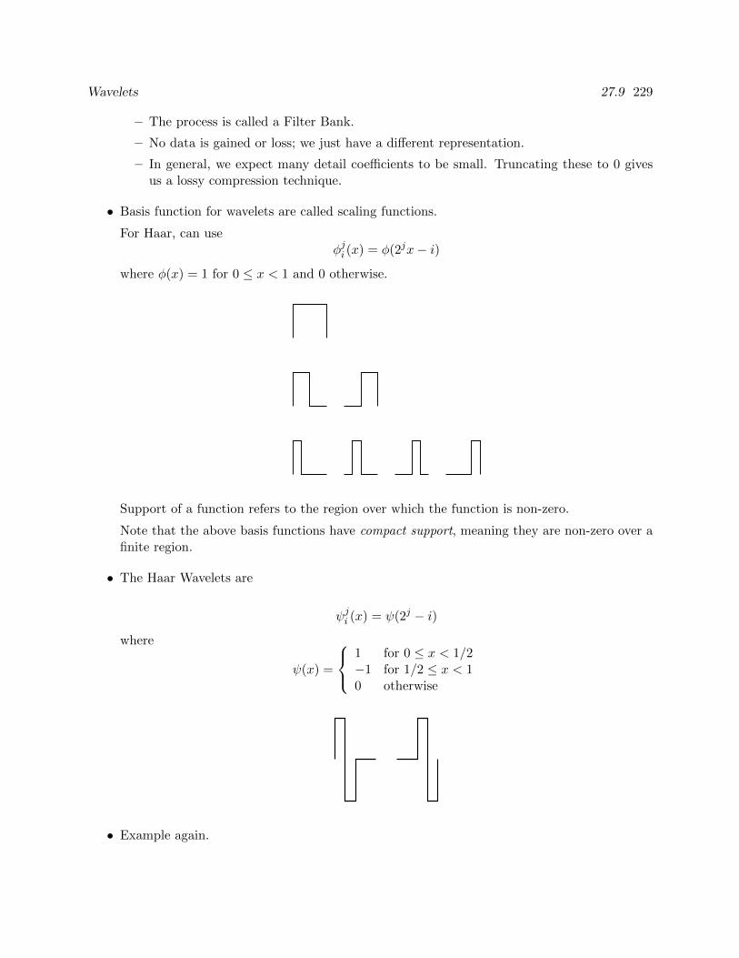
Wavelets 27.9 229
– The process is called a Filter Bank.
– No data is gained or loss; we just have a different representation.
– In general, we expect many detail coefficients to be small. Truncating these to 0 givesus a lossy compression technique.
• Basis function for wavelets are called scaling functions.
For Haar, can useφji (x) = φ(2jx− i)
where φ(x) = 1 for 0 ≤ x < 1 and 0 otherwise.
Support of a function refers to the region over which the function is non-zero.
Note that the above basis functions have compact support, meaning they are non-zero over afinite region.
• The Haar Wavelets are
ψji (x) = ψ(2j − i)where
ψ(x) =
1 for 0 ≤ x < 1/2−1 for 1/2 ≤ x < 10 otherwise
• Example again.
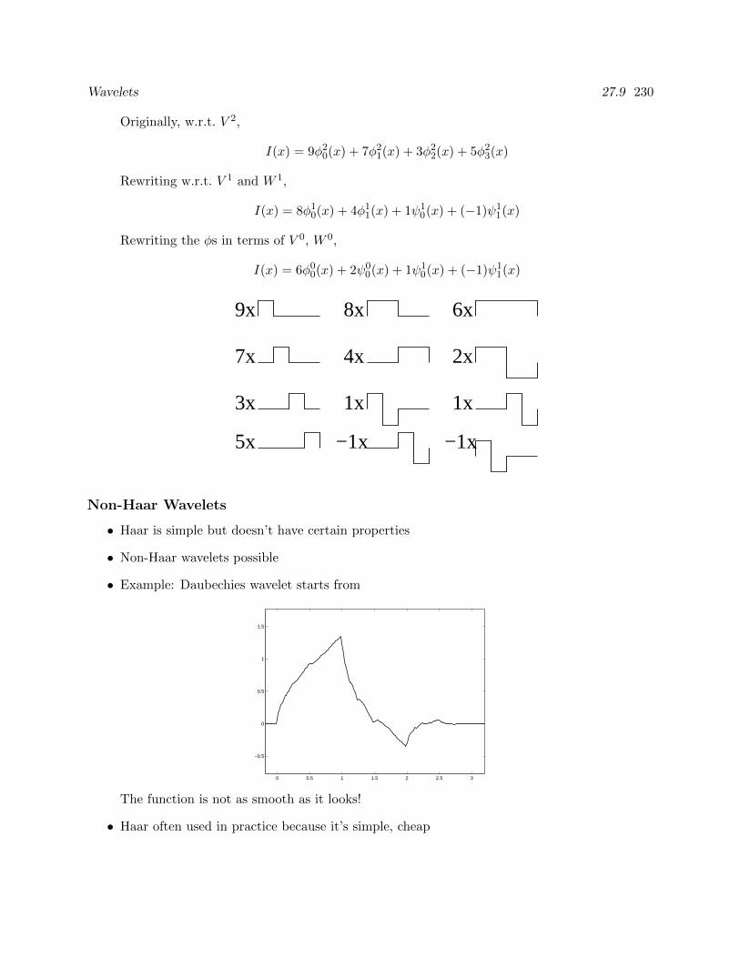
Wavelets 27.9 230
Originally, w.r.t. V 2,
I(x) = 9φ20(x) + 7φ2
1(x) + 3φ22(x) + 5φ2
3(x)
Rewriting w.r.t. V 1 and W 1,
I(x) = 8φ10(x) + 4φ1
1(x) + 1ψ10(x) + (−1)ψ1
1(x)
Rewriting the φs in terms of V 0, W 0,
I(x) = 6φ00(x) + 2ψ0
0(x) + 1ψ10(x) + (−1)ψ1
1(x)
9x
7x
8x
1x
−1x
4x
−1x
1x
2x
6x
3x
5x
Non-Haar Wavelets
• Haar is simple but doesn’t have certain properties
• Non-Haar wavelets possible
• Example: Daubechies wavelet starts from
0 0.5 1 1.5 2 2.5 3
−0.5
0
0.5
1
1.5
The function is not as smooth as it looks!
• Haar often used in practice because it’s simple, cheap
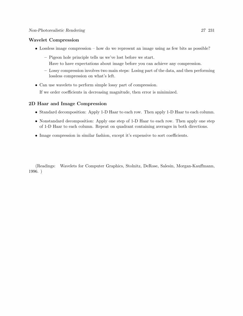
Non-Photorealistic Rendering 27 231
Wavelet Compression
• Lossless image compression – how do we represent an image using as few bits as possible?
– Pigeon hole principle tells us we’ve lost before we start.
Have to have expectations about image before you can achieve any compression.
– Lossy compression involves two main steps: Losing part of the data, and then performinglossless compression on what’s left.
• Can use wavelets to perform simple lossy part of compression.
If we order coefficients in decreasing magnitude, then error is minimized.
2D Haar and Image Compression
• Standard decomposition: Apply 1-D Haar to each row. Then apply 1-D Haar to each column.
• Nonstandard decomposition: Apply one step of 1-D Haar to each row. Then apply one stepof 1-D Haar to each column. Repeat on quadrant containing averages in both directions.
• Image compression in similar fashion, except it’s expensive to sort coefficients.
(Readings: Wavelets for Computer Graphics, Stolnitz, DeRose, Salesin, Morgan-Kauffmann,1996. )

Non-Photorealistic Rendering 27 232
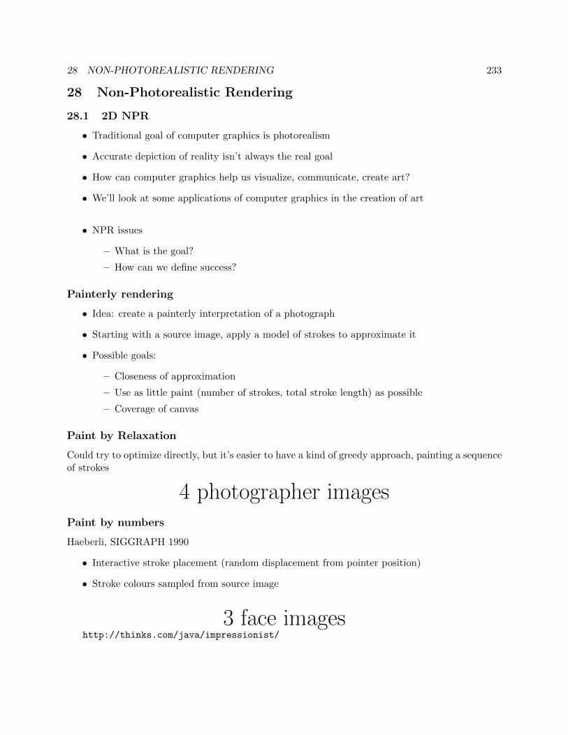
28 NON-PHOTOREALISTIC RENDERING 233
28 Non-Photorealistic Rendering
28.1 2D NPR
• Traditional goal of computer graphics is photorealism
• Accurate depiction of reality isn’t always the real goal
• How can computer graphics help us visualize, communicate, create art?
• We’ll look at some applications of computer graphics in the creation of art
• NPR issues
– What is the goal?
– How can we define success?
Painterly rendering
• Idea: create a painterly interpretation of a photograph
• Starting with a source image, apply a model of strokes to approximate it
• Possible goals:
– Closeness of approximation
– Use as little paint (number of strokes, total stroke length) as possible
– Coverage of canvas
Paint by Relaxation
Could try to optimize directly, but it’s easier to have a kind of greedy approach, painting a sequenceof strokes
4 photographer imagesPaint by numbers
Haeberli, SIGGRAPH 1990
• Interactive stroke placement (random displacement from pointer position)
• Stroke colours sampled from source image
3 face imageshttp://thinks.com/java/impressionist/
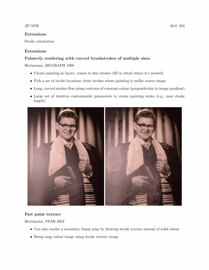
2D NPR 28.0 234
Extensions
Stroke orientation
Extensions
Painterly rendering with curved brushstrokes of multiple sizes
Hertzmann, SIGGRAPH 1998
• Create painting in layers: coarse to fine strokes (fill in detail where it’s needed)
• Pick a set of stroke locations; draw strokes where painting is unlike source image
• Long, curved strokes flow along contours of constant colour (perpendicular to image gradient)
• Large set of intuitive customizable parameters to create painting styles (e.g., max strokelength)
Fast paint texture
Hertzmann, NPAR 2002
• Can also render a secondary bump map by drawing stroke texture instead of solid colour
• Bump map colour image using stroke texture image

2D NPR 28.0 235
4 stroke images
4 palm tree images
6 skeleton imagesStylization and abstraction of photographs
DeCarlo and Santella, SIGGRAPH 2002
• Stroke models follow image features, but they don’t understand the image. How can we applyan NPR filter in a meaningful way?
• Let a person determine importance by having them look at the source image and trackingtheir eye movements
• Not strokes, but large regions of constant colour
• Edges drawn as well
Woman with guitar photo
Woman with guitar NPR imageSimulating natural media
• Implement a physical simulation to approximate the behaviour and appearance of a traditionalartistic medium
Computer-Generated Watercolor
Curtis, Anderson, Seims, Fleischer and Salesin, SIGGRAPH 1997
• Realistic simulation of the appearance of watercolour paints
• Treat the painting as a big fluid flow simulation
• Navier-Stokes equations to push fluid around on top of the paper
• Fluid and paper exchange pigment
• Paper propagates water via capillary action

2D NPR 28.0 236
Photo of watercolour brush strokesReal paint
Simulation of watercolour brush strokesSimulated
Samples of watercolour paint simulations
Fruit, and lots of it!Pencil Rendering
Sousa and Buchanan, GI 1999, CGF 2000
• Simulation of pencil lead and paper, derived from close observation of real materials
• Model the geometry of the pencil tip, pressure on page
• Graphite particles can move to and from paper, so system can model pencils, erasers, andblenders
• Pressure affects geometry of paper, and therefore appearance of future strokes
Real and simulated pencil
Crumpled paper
photo and 2 NPR pencil sketches of girlBatik
MooseEmbroidery
Chen, McCool, Kitamoto, Mann, GI 2012
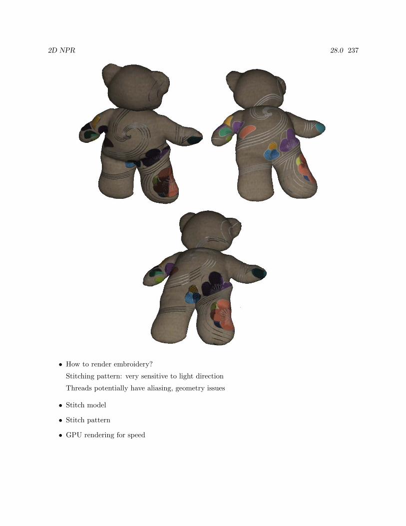
2D NPR 28.0 237
• How to render embroidery?
Stitching pattern: very sensitive to light direction
Threads potentially have aliasing, geometry issues
• Stitch model
• Stitch pattern
• GPU rendering for speed
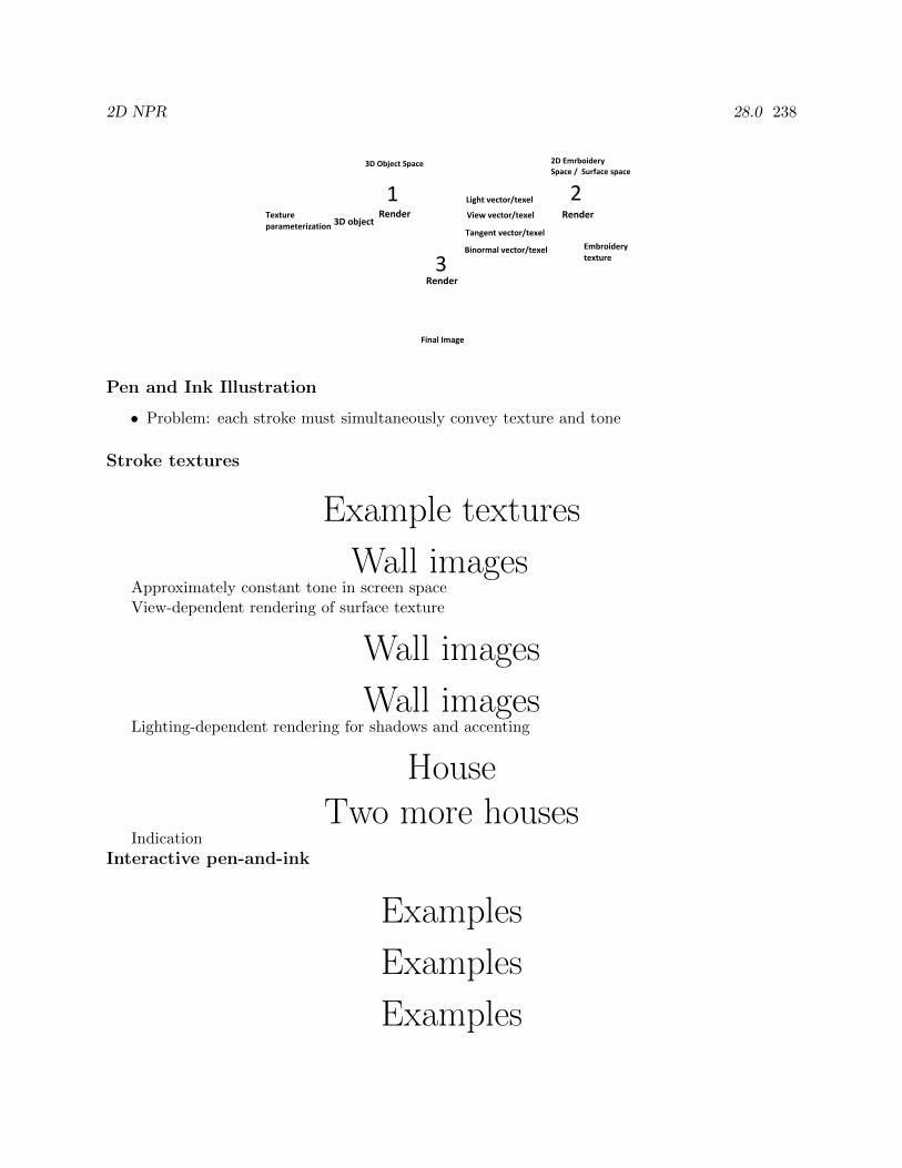
2D NPR 28.0 238
Texture
parameterization
3D Object Space
Render
Light vector/texel
View vector/texel
Tangent vector/texel
Binormal vector/texel
Render
2D Emrboidery
Space / Surface space
Embroidery
texture
Final Image
Render
1 2
3
3D object
Pen and Ink Illustration
• Problem: each stroke must simultaneously convey texture and tone
Stroke textures
Example textures
Wall imagesApproximately constant tone in screen spaceView-dependent rendering of surface texture
Wall images
Wall imagesLighting-dependent rendering for shadows and accenting
HouseTwo more houses
Indication
Interactive pen-and-ink
Examples
Examples
Examples
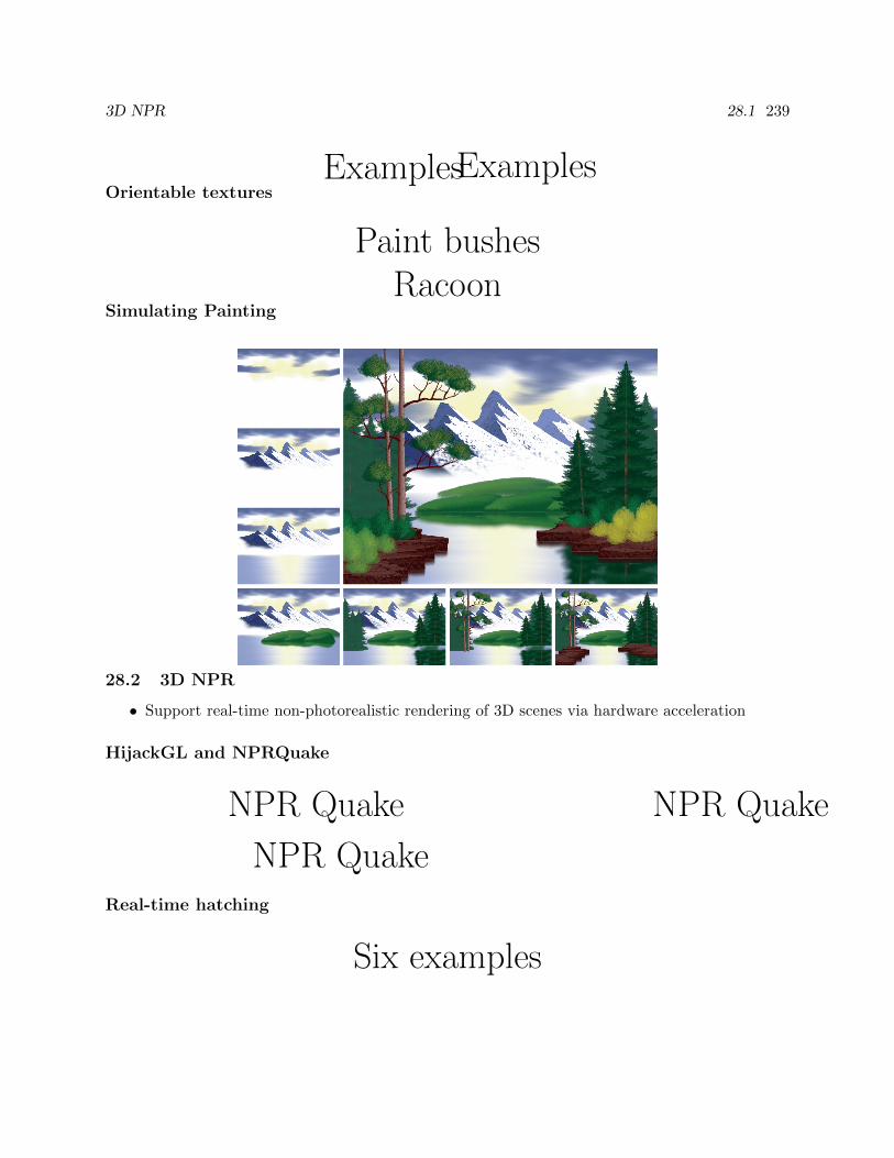
3D NPR 28.1 239
ExamplesExamplesOrientable textures
Paint bushesRacoon
Simulating Painting
28.2 3D NPR
• Support real-time non-photorealistic rendering of 3D scenes via hardware acceleration
HijackGL and NPRQuake
NPR Quake NPR Quake
NPR QuakeReal-time hatching
Six examples
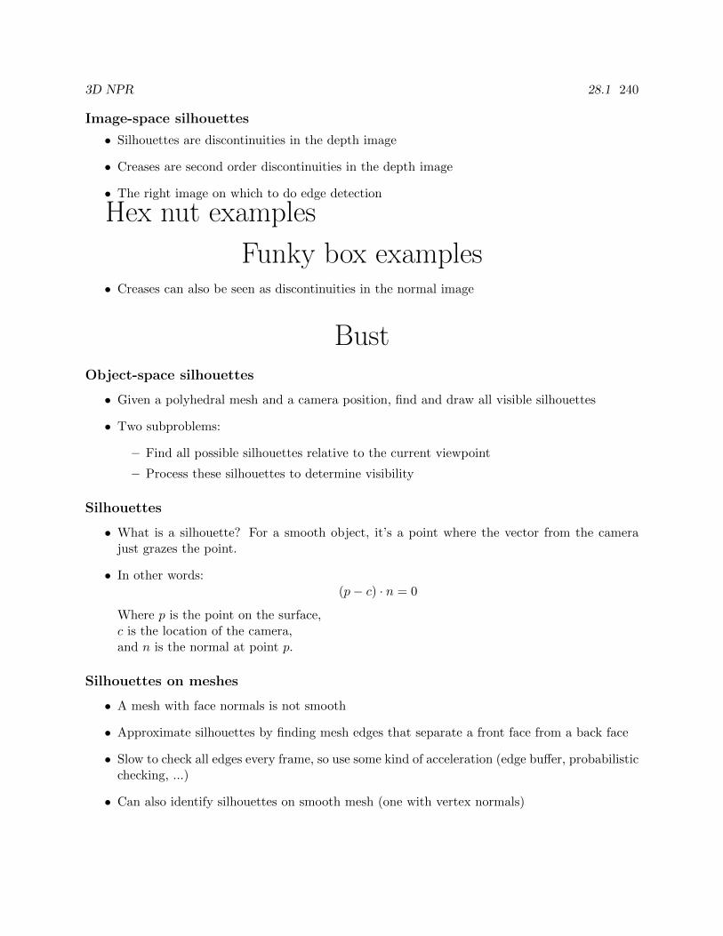
3D NPR 28.1 240
Image-space silhouettes
• Silhouettes are discontinuities in the depth image
• Creases are second order discontinuities in the depth image
• The right image on which to do edge detection
Hex nut examples
Funky box examples• Creases can also be seen as discontinuities in the normal image
BustObject-space silhouettes
• Given a polyhedral mesh and a camera position, find and draw all visible silhouettes
• Two subproblems:
– Find all possible silhouettes relative to the current viewpoint
– Process these silhouettes to determine visibility
Silhouettes
• What is a silhouette? For a smooth object, it’s a point where the vector from the camerajust grazes the point.
• In other words:(p− c) · n = 0
Where p is the point on the surface,c is the location of the camera,and n is the normal at point p.
Silhouettes on meshes
• A mesh with face normals is not smooth
• Approximate silhouettes by finding mesh edges that separate a front face from a back face
• Slow to check all edges every frame, so use some kind of acceleration (edge buffer, probabilisticchecking, ...)
• Can also identify silhouettes on smooth mesh (one with vertex normals)
3D NPR 28.1 241
Silhouette visibility
• Just because an edge is a silhouette doesn’t mean it’s visible:
– Occlusion by another object
– Occlusion by another part of the same object
– Partially visible
• Need to decide, for every silhouette edge, which parts are visible
Image-space visibility processing
• Turn on depth buffering
• Draw all mesh faces in background colour
• Draw all silhouette edges, give every edge a unique colour that identifies it
• Frame buffer now holds pixel-accurate image of which pieces of silhouettes are visible
Stylized silhouettes
• Use visibility to guide placement of stylized strokes along paths
• Parameterization and temporal coherence are still problems
Toon shading
• Cartoons typically use a small range of colours for each object in a scene
– Shadow, body, and sometimes highlight
• Easy to simulate in ray tracer or real-time
– Quantize by diffuse attenuation to two or three colours
Elf girl RosesToon shading in OpenGL
• Perform diffuse lighting computation at every vertex in software
• Use diffuse brightness as parameter to a one-dimensional texture map
– Map has only two or three colours
• Sample the texture with nearest-neighbour interpolation: deliberately not blended
• Can be on the GPU as a fragment program
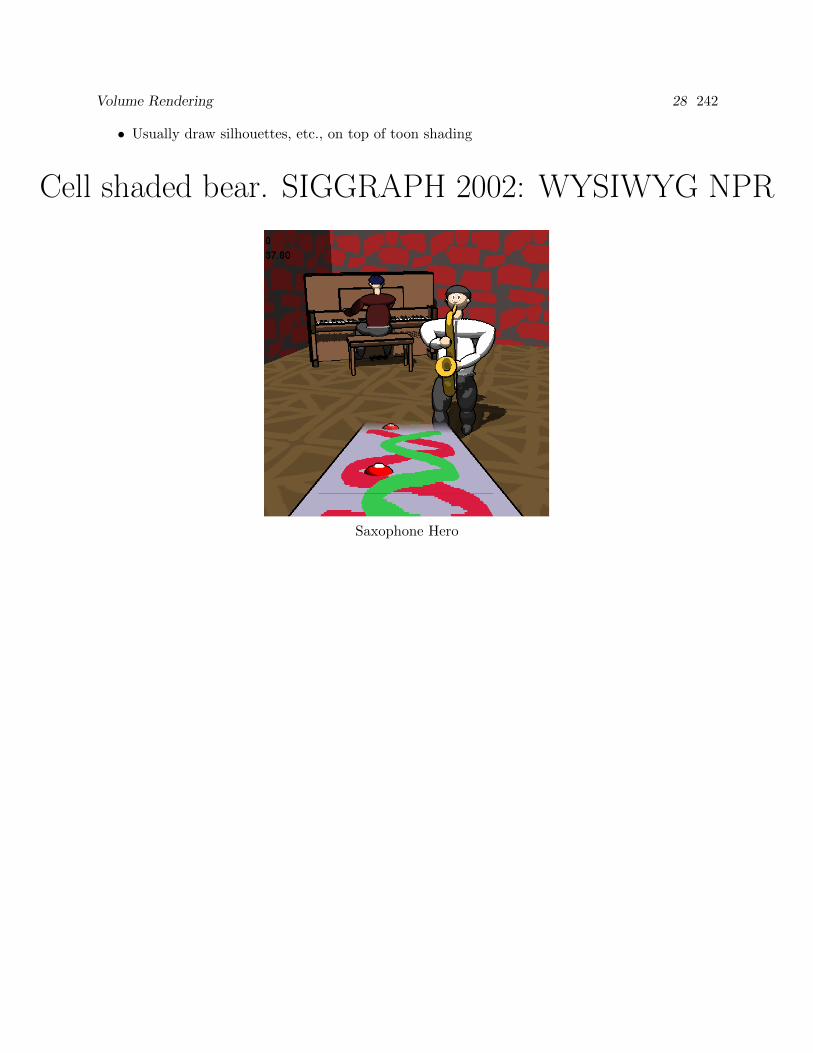
Volume Rendering 28 242
• Usually draw silhouettes, etc., on top of toon shading
Cell shaded bear. SIGGRAPH 2002: WYSIWYG NPR
Saxophone Hero
29 VOLUME RENDERING 243
29 Volume Rendering
29.1 Volume Rendering
Volume Data
• scalar field
– like temperature in room at each (x, y, z)
• many applications
– medical (MRI, CT, PET)
– geophysical
– fluid dynamics
Volume Data
VR Data - engine, gutsVisible Human Project
Visble Human slicesSeismic Data
Seismic DataData Format
• 3D array of scalars (a volume)
– 2563 or 5123 common
– 32-128 MB, pretty big
Seismic data (for oil exploration) will be 100’s of GB or more
– but each slice a low-res image
• each volume element is a voxel
– often 16 bits per voxel
– several bits for segmentation
(bone,muscle,fluid,...)
– most bits for intensity
Volume Rendering 29.0 244
Displaying Volume Data
• How do we display volume data?
Data on “outside” hides data on “inside”
– Transparency
– Slicing
– Segmentation and selective display
• How do we render volume data?
Sampling issues
Volume Slicing
• combine slices of volume
– use 2D texture-mapping for each slice
– use alpha buffer to blend slices
• can use 3D textures if enough memory
• quick method
• rough results
Volume Slicing
Volume Slicing
Ian’s BrainRendering Pipeline
• segmentation
• gradient computation
• resampling
• classification
• shading
• compositing
Volume Rendering 29.0 245
Segmentation
• marking voxels according to type
• medical volumes: skin, bone, muscle, air, fluids, ...
• geological volumes: sand, slate, oil, ...
• manual procedure, need good software
• problems:
– noise
– overlapping intensity ranges
Segmentation
Labled gutsGradient Computation
• gradient shows density changes
• useful for illumination model
• gradient magnitude like edge detection
– can build isosurfaces
– can colour according to magnitude
Gradient Computation
Xray of foot x 3Resampling
• forward method
– splat voxels onto screen
– must interpolate to get pixel values
• reverse method
– is ray-casting through volume
– resample along ray
– collect intensity/gradient info for pixel
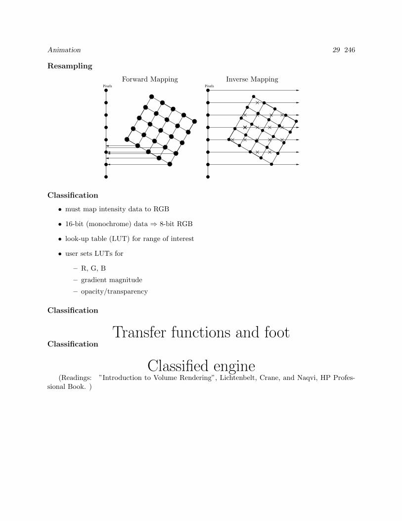
Animation 29 246
Resampling
Forward Mapping Inverse MappingPixels Pixels
Classification
• must map intensity data to RGB
• 16-bit (monochrome) data ⇒ 8-bit RGB
• look-up table (LUT) for range of interest
• user sets LUTs for
– R, G, B
– gradient magnitude
– opacity/transparency
Classification
Transfer functions and footClassification
Classified engine(Readings: ”Introduction to Volume Rendering”, Lichtenbelt, Crane, and Naqvi, HP Profes-
sional Book. )
30 ANIMATION 247
30 Animation
30.1 Overview
Computer Animation
Animation: Rapid display of slightly different images create the illusion of motion.
Conventional approach: Keyframed animation
Keyframes, inbetween frames
Computer Assisted:
• Human key frames, computer inbetweening
• Supporting techniques:
Squish-box deformations and skeletons, motion capture, kinematics and inverse kine-matics.
• Other animation approaches:
Physically-based dynamics, constraint-based animation, procedural animation, behav-ioral animation.
(Readings: McConnell, Chapter 10.)
30.2 Traditional 2D Cel Animation
Traditional 2D Cel Animation
• Traditional animation is labor intensive.
– Start with story board.
– Master artist draws keyframes to define action.
– Sweat-shop artists draw inbetween frames to complete animation.
• A few traditional animation rules:
– Stretch and squash (anti-aliasing), timing, secondary actions
– Exaggeration, appeal, follow through
– Anticipation, staging.
– Be careful with camera
∗ Smooth changes
∗ Few changes
• Disney was the most successful, but it was high risk.
Functional Animation 30.3 248
30.3 Automated Keyframing
• Replace the human inbetweener with interpolation algorithms.
• Keyframes correspond to settings of parameters at different points in time.
+ The computer provides repeatability and automatic management of keyframes.
– Interpolation is not as smart as a human inbetweener.
Animator may have to provide more key frames and/or additional information to get a goodresult.
Utility
A good keyframe system limits the number and maximizes the utility of key parameters.
• Immediate geometric or visible significance.
Entries in a transformation matrix are not good parameters.
• Static properties maintained automatically.
• Relationships between parts of articulated objects maintained automatically.
• Interpolation routines geared towards parameter types.
Motion paths, orientation, camera attitude, and surface properties: different types of control.
• Real-time interface to interactively set parameters and iteratively improve the animation.
30.4 Functional Animation
• Independent scalar function specified for each “keyframed” parameter.
• Basic capability that supports others.
• Most useful for truly scalar quantities:brightness of a light source
• Splines useful for representing functions.
• Continuity control a must: both automatic maintenance and selective breaking.
• The functions can be edited both explicitly, as graphs, or implicitly, through a direct manip-ulation interface.
Functional Animation 30.3 249
Linear Interpolation
• Basic interpolation technique for supporting animation is linear interpolation, or the lerp.
• Given two parameters p0 and p1 at times t0 and t1,an intermediate value is
p(t) =t1 − tt1 − t0
p0 +t− t0t1 − t0
p1.
• Advantages and Disadvantages:
– Discontinuities in derivative exist at all key frame points.
+ The rate of change within a segment is constant(can easily be controlled).
Controlling Velocity
Given a constant rate of change, can create variable rate of change.Given any function τ = f(t), reparameterize with τ .For the lerp,
p(τ) = p(f(t)) =f(t1)− f(t)
f(t1)− f(t0)p0 +
f(t)− f(t0)
f(t1)− f(t0)p1.
Spline Interpolation
Instead of linear interpolation, spline interpolation can be used.
+ Continuity control can be obtained.
+ Fewer keyframes may be required for a given level of “quality”.
– Control points for the splines may have to be computed based on interpolation constraints atthe control points.
– Extra information may be required at keyframes, such as tangent vectors.
– Splines are more expensive to evaluate. (non-issue)
– Splines are more difficult to implement. (non-issue)
Transformation Matrix Animation
• One way to support an animation capability:interpolate a transformation matrix.
• Keyframes are “poses” of objects given by the animator.
• Functional animation applied independently to all entries of the transformation matrix.
Does not support animation of rigid bodies!
Motion Path Animation 30.4 250
• Given two poses of an object that differ by a 180 rotation.
• Under linear interpolation, object will turn inside out,
collapse to a plane in the middle of the interpolation.
Rigid Body Animation
• Rigid body transformations only have 6 degrees of freedom
General affine transformations have 12.
• To obtain good interpolation we have to consider separately
– three degrees of freedom from translation
– three that result from orientation.
30.5 Motion Path Animation
Want to translate a point through space along a given path.We would like:
• Independent control of velocity along path.
• Continuity control.
While splines can easily support continuity control, velocity control is more difficult.
Motion Path Spline Interpolation Problems
Spline position interpolation gives continuity control over changes position, but:
• Visually notice discontinuities in 2nd derivative – need C3 splines (degree 4).
• Equal increment in spline parameter does not correspond to equal increment in distance alongthe spline.
• Different segments of the spline with the same parametric length can have different physicallengths.
• If we parameterize the spline directly with time objects will move at a non-uniform speed.
Arc Length Parameterization
1. Given spline path P (u) = [x(u), y(u), z(u)], compute arclength of spline as a function of u:s = A(u).
2. Find the inverse of A(u): u = A−1(s).
3. Substitute u = A−1(s) into P (u) to find motion path parameterized by arclength, s: P (s) =P (A−1(s)).
u (and thus s) should be global parameters, extending across all segments of the original spline.
Motion Path Animation 30.4 251
Velocity Control
To control velocity along a spline motion path,
• Let s = f(t) specify distance along the spline as a function of time t.
• The function f(t), being just a scalar value, can be supported with a functional animationtechnique (i.e., another spline).
• The function f(t) may be specifed as the integral of yet another function, v(t) = df(t)/dt,the velocity.
Integral of a spline function can be found analytically, through a computation of the controlpoints.
• The motion path as a function of time t is thus given by P (A−1(f(t))).
Problems with Arc-Length Parameterization
1. The arc-length s = A(u) is given by the integral
s = A(u) =
∫ u
0
√(dx(v)
dv
)2
+
(dy(v)
dv
)2
+
(dz(v)
dv
)2
dv
No analytic solution if the motion path is a cubic spline.
2. Since A(u) has no analytic form, A−1(s) has no analytic form.
Issues in Real-Time Animation
• Exact arc-length parameterization not feasible.
• Alternative: compute points on the spline at equally-spaced parametric values,use linear interpolation along these chords.
• The linear interpolation should consider the distance between samples to maintain constantvelocity.
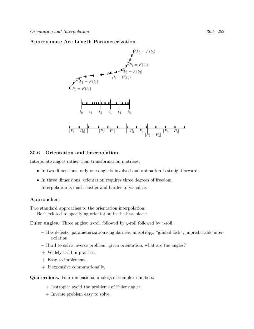
Orientation and Interpolation 30.5 252
Approximate Arc Length Parameterization
t0 t1 t2 t3 t5t4
|P1 − P0| |P5 − P4||P2 − P3||P3 − P2||P2 − P1|
P0 = F (t0)
P1 = F (t1)
P5 = F (t5)
P4 = F (t4)
P3 = F (t3)
P2 = F (t2)
30.6 Orientation and Interpolation
Interpolate angles rather than transformation matrices.
• In two dimensions, only one angle is involved and animation is straightforward.
• In three dimensions, orientation requires three degrees of freedom.
Interpolation is much nastier and harder to visualize.
Approaches
Two standard approaches to the orientation interpolation.Both related to specifying orientation in the first place:
Euler angles. Three angles: x-roll followed by y-roll followed by z-roll.
– Has defects: parameterization singularities, anisotropy, “gimbal lock”, unpredictable inter-polation.
– Hard to solve inverse problem: given orientation, what are the angles?
+ Widely used in practice.
+ Easy to implement.
+ Inexpensive computationally.
Quaternions. Four-dimensional analogs of complex numbers.
+ Isotropic: avoid the problems of Euler angles.
+ Inverse problem easy to solve.
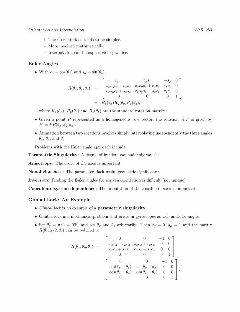
Orientation and Interpolation 30.5 253
+ The user interface tends to be simpler.
– More involved mathmatically.
– Interpolation can be expensive in practice.
Euler Angles
• With ca = cos(θa) and sa = sin(θa),
R(θx, θy, θz) =
cycz cysz −sy 0
sxsycz − cxsz sxsysz + cxcz sxcy 0cxsycz + sxsz cxsysz − sxcz cxcy 0
0 0 0 1
= Rx(θx)Ry(θy)Rz(θz),
where Rx(θx), Ry(θy) and Rz(θz) are the standard rotation matrices.
• Given a point P represented as a homogeneous row vector, the rotation of P is given byP ′ = PR(θx, θy, θz).
• Animation between two rotations involves simply interpolating independently the three anglesθx, θy, and θz.
Problems with the Euler angle approach include:
Parametric Singularity: A degree of freedom can suddenly vanish.
Anisotropy: The order of the axes is important.
Nonobviousness: The parameters lack useful geometric significance.
Inversion: Finding the Euler angles for a given orientation is difficult (not unique).
Coordinate system dependence: The orientation of the coordinate axes is important.
Gimbal Lock: An Example
• Gimbal lock is an example of a parametric singularity.
• Gimbal lock is a mechanical problem that arises in gyroscopes as well as Euler angles.
• Set θy = π/2 = 90, and set θx and θz arbitrarily. Then cy = 0, sy = 1 and the matrixR(θx, π/2, θz) can be reduced to
R(θx, θy, θz) =
0 0 −1 0
sxcz − cxsz sxsz + cxcz 0 0cxcz + sxsz cxsz − sxcz 0 0
0 0 0 1
=
0 0 −1 0
sin(θx − θz) cos(θx − θz) 0 0cos(θx − θz) sin(θx − θz) 0 0
0 0 0 1
.
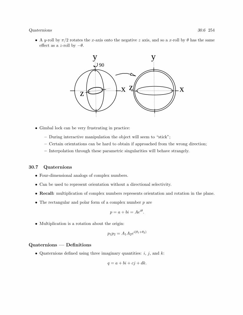
Quaternions 30.6 254
• A y-roll by π/2 rotates the x-axis onto the negative z axis, and so a x-roll by θ has the sameeffect as a z-roll by −θ.
x
y90
x
y
zz
• Gimbal lock can be very frustrating in practice:
– During interactive manipulation the object will seem to “stick”;
– Certain orientations can be hard to obtain if approached from the wrong direction;
– Interpolation through these parametric singularities will behave strangely.
30.7 Quaternions
• Four-dimensional analogs of complex numbers.
• Can be used to represent orientation without a directional selectivity.
• Recall: multiplication of complex numbers represents orientation and rotation in the plane.
• The rectangular and polar form of a complex number p are
p = a+ bi = Aeiθ.
• Multiplication is a rotation about the origin:
p1p2 = A1A2ei(θ1+θ2)
Quaternions — Definitions
• Quaternions defined using three imaginary quantities: i, j, and k:
q = a+ bi+ cj + dk.
Quaternions 30.6 255
• Rules for combining these imaginary quatities:
i2 = j2 = k2 = −1,
ij = −ji = k,
jk = −kj = i,
ki = −ik = j.
• Rules sufficient to define multiplication for quaternions.
• Quaternion multiplication does not commute.
• A quaternion can be broken into a scalar and a vector part:
q = (s,~v) = s+ v1i+ v2j + v3k.
• In vector notation, product of two quaternions is
q1q2 = (s1s2 − ~v1 · ~v2, s1~v2 + s2~v1 + ~v1 × ~v2).
• Quaternions also have conjugates: q = (s,−~v).
• The norm of a quaternion is defined by
|(s,~v)| =√s2 + v2
1 + v22 + v2
3.
Unit Quaternions
• Unit quaternions have unit norms
• Isomorphic to orientations
• The unit quaternion given byqr = (cos(θ), sin(θ)~v)
is equivalent to a rotation by an angle of 2θ around the unit ~v.
Note that qr is equivalent to −qr when interpreted as an orientation.
Rotations and Quaternions
• Points in space can be represented by quaternions with a zero scalar part.
• Point P is represented by the quaternion
qP = (0, P ).
• The rotation of a point P by qr isqP ′ = qrqP q
−1r .
• For unit quaternions, the inverse is equivalent to the conjugate.
Animating Camera Motion 30.7 256
Advantages of Quaternions
• Doing rotation this way is fairly perverse, but:
1. For many applications, the independent definition of an axis of rotation and an anglemakes sense.
2. The definition of an orientation by a quaternion is coordinate system independent andisotropic.
3. Spherical interpolation of quaternions gives better results than interpolation of Eulerangles.
Interpolating Unit Quaternions
• Linear interpolation on all the entries of the quaternion does not have unit norm.
Angular velocity is not constant if we renormalize.
• Spherical linear interpolation (slerp):
– Consider the quaternions as vectors, and find the angle between them:
ω = cos−1(q1 · q2).
– Given a parameter u ∈ [0, 1], the slerp is
q(u) = q1sin((1− u)ω)
sin(ω)+ q2
sin(uω)
sin(ω).
30.8 Animating Camera Motion
• Requirements for camera motion are different from object motion:
– Specification of camera motion has a long cinematic tradition that should be respected.
– The camera should always be level, unless we specify otherwise.
– The image of objects of interest should be stable on the film plane.
Camera Cinematic Terminology
Dolly: Move forward, along the line of sight of the camera (towards the object of interest).
Track: Move horizontally, perpendicular to the line of sight of the camera. More generally, movein a horizontal plane.
Crane: Raise the camera vertically.
Tilt (Bank): Rotate about the horizontal axis perpendicular to the line of sight of the camera.
Pan (Yaw): Rotate about the vertical axis of the camera (after tilt).
In addition, cameras have other parameters that can be animated:
Tools for Shape Animation 30.8 257
Zoom (in, out): Change the angular field of view of the camera.
Focus: Change the focal depth, i.e., the distance at which objects are in focus.
Depth of Field: Changing the aperture size has the effect of changing the depth of field, i.e. therange of depths over which objects can be considered to be in focus.
Camera Cinematics
• An animated zoom changes perspective, which can be disturbing.
Use dolly to enlarge the image of an object of interest.
• The camera should almost never be rotated about its view direction
Unless a seasick audience is the objective.
• Changing the focal depth can be used to track objects of interest,
but a sophisticated renderer is required to simulate focus.
• Use smooth spline animation for camera animation.
Quick camera moves should normally be replaced by cuts
(instantaneous changes of scene) unless a special effect is desired.
• Animation of spotlight sources is similar to the animation of a camera.
Support of a “light’s-eye-view”, therefore, is often useful.
Camera Animation Specification
• With a camera, usually more interested in what it’s looking at than its exact orientation
• Camera animation may be specified by
– A motion path for the camera itself.
– A motion path for a lookat point
(possibly derived from the motion of an object of interest).
• Camera moved along the motion path and the orientation of camera determined by the lookatpoint.
• Ideally, “focus would be pulled” to match the distance to object of interest.
• Tilt might be constrained to lie within certain bounds.
Tools for Shape Animation 30.8 258
30.9 Tools for Shape Animation
Skeletons
• Given a model with large number of vertices, vertices can be grouped and manipulated as aunit.
Example: in an arm, all points describing the forearm move more-or-less as a rigid body.
• Connectivity between groups can be represented by tying each group to a “bone” and arrang-ing bones in an articulated “skeleton”.
• The bone and all its associated vertices are treated as a single rigid object for the purposesof transformation.
• Movement of the bones is constrained by the joints in the skeleton.
• Different kinds of joints (revolute, hinge, ball) can support specific types of motion.
• An animation can be previewed using only the bones, speeding rendering time.
• In the final rendering, the model is shown without bones.
• Enhancement: vertices may be influenced by more than one bone.
Results in more flexible and realistic surface near joints.
Example: a kneecap and its skin surface affected by both the femur and shinbone, and assumea position halfway between either.
Skeleton/skinning exampleFree-Form Deformations
• Sometimes, skelton cannot capture desired shape change of an object.
• Example: The “squash and stretch” of a bouncing ball as it hits the ground.
• Such global changes in shape can be expressed using a deformation.
• A deformation
– Changes the space around an object
– Nonlinear transformation
– New coordinates for every point in space are determined as functions of the old coordi-nates.
Kinematics and Inverse Kinematics 30.9 259
Process
1. Place rectangular “squish box” object to be animated.
2. The coordinates of all points within the box are determined relative to the frame given bythe box.
Suppose a vertex P can be expressed as [u, v, w] relative to the coordinates of the box.
3. The new coordinates of P are given by a tensor product Bezier spline Bn1,n2,n3(u, v, w) withcontrol points Pi,j,k.
4. If the Pi,j,k have coordinates
Pi,j,k = [i/(n1 + 1), j/(n2 + 1), k/(n3 + 1)],
the transformation is given by the identity:
[u, v, w] = Bn1,n2,n3(u, v, w).
Normally the control points are initially set to these values and are moved to effect a defor-mation.
FFD Issues
• Continuity conditions can be enforced.
Example: A hand is being deformed but the arm is not.
The control points along the edge of the box that cuts the wrist should not be moved, northe next layer.
This maintains both position and derivative continuity across the wrist.
• The object should be finely tesselated or radical deformations will not work properly.
• Not volume preserving.
For realistic animation, typically only small deformations are used.
• Modeling UI non-trivial
Manipulating control points inadequate
Skeletons and FFDs
• Skeletons and free-form deformations can be used simultaneously.
• The number of control points in a free-form deformation can be large
• If moved in groups relative to skeleton, excellent animation control can be obtained for arbi-trary models.
Physically-Based Animation 30.10 260
30.10 Kinematics and Inverse Kinematics
Kinematics and Inverse Kinematics
Kinematics: The study of motion independent of the forces that cause the motion. Includesposition, velocity, acceleration.
Forward kinematics: The determination of the
• positions,
• velocities,
• accelerations
of all the links in an articulated model given the
• position,
• velocity,
• acceleration
of the root of the model and all the transformations between links.
• Forward kinematics is a necessity for skeletal keyframed animation
• Easy to implement.
Inverse kinematics: The derivation of the motion of intermediate links in an articulated bodygiven the motion of some key links.
Inverse Kinematics
• Often nonlinear, underdetermined or overdetermined, possibly ill-conditioned.
• Complexity of determining solution proportional to number of free links.
• One free joint between two fixed ones can be solved fairly efficiently, for example, with onlyone spare degree of freedom.
• Extra constraints may be needed to obtain a unique and stable solution.
– Example: Requiring a joint to point downwards as a gross approximation to gravity
– Joint motion constraints (hinge vs. revolute vs. ball) are also useful.
• Additional optimization objectives
– Resulting optimization problem solved iteratively as an animation proceeds.
– Example optimization objectives:
∗ minimize the kinetic energy of structure;
∗ minimize the total elevation of the structure;
∗ minimize the maximum (or average) angular torque.
Physically-Based Animation 30.10 261
30.11 Physically-Based Animation
Idea: to obtain a physically plausible animation, simulate the laws of Newtonian physics.In contrast to kinematics, this is called a dynamics approach.
• Have to control objects by manipulating forces and torques, either directly or indirectly.
• Animated objects may be passive: bouncing balls, jello, wall of bricks falling down, etc.
Inverse dynamics is difficult
• Finding forces to move a physical object along a desired path
• Most current applications are “passive” variety
• Useful for secondary effects in keyframe animation:
– a mouse character’s ears should flap when it shakes its head,
– a T. Rex’s gut should sway while it runs,
– a feather in a cap should wave when wind blows on it,
– cloth should drape around an actor and respond to his/her/its movements,
– a wall of bricks should fall down when a superhero crashes into it.
Caution: simulated secondary effects can make bad keyframed animation look even worse!
Simulation
Setting up and solving a physically-based animation proceeds as follows:
1. Create a model with physical attributes: mass, moment of inertia, elasticity, etc.
2. Derive differential equations by applying the laws of Newtonian physics.
3. Define initial conditions, i.e., initial velocities and positions.
4. Supply functions for external forces (possibly via keyframing).
5. Solve the differential equations to derive animation, i.e., motion of all objects in scene as afunction of time.
Spring-Mass Models
Create a model:
• Composed of a mesh of point masses mi connected by springs with spring constants kij andrest lengths `ij .
• Let Pi(t) = [xi(t), yi(t), zi(t)] be the position of mass mi at time t.
• Let Ni be all masses connected to mass mi.
If j ∈ Ni, then mi and mj are connected by a spring.
Physically-Based Animation 30.10 262
• Springs exert force proportional to displacement from rest length, in a direction that tendsto restore the rest length:
~fsij(t) = −kij(`ij − |Pi(t)− Pj(t)|)Pi(t)− Pj(t)|Pi(t)− Pj(t)|
,
~fsi (t) =∑j∈Ni
~fsij(t).
• Masses assumed embedded in a medium that provides a damping force of
~fd = −ρi~vi(t),
~vi(t) is velocity of mi at time t.
• Motion of each mass governed by second order ordinary differential equation:
mi~a(t) = −ρi~v(t) + ~fsi (t) + ~fei (t).
~fei (t) is the sum of external forces on node i and
~a =
[d2xi(t)
dt2,d2yi(t)
dt2,d2zi(t)
dt2
],
~v =
[dxi(t)
dt,dyi(t)
dt,dzi(t)
dt
]• Initial conditions: user supplies initial positions of all masses and velocities.
• The user supplies external forces: gravity, collision forces, keyframed forces, wind, hydrody-namic resistance, etc. as a function of time.
• Simulation.
– Factor second-order ODE into two coupled first-order ODE’s:
~v = [vxi(t), vyi(t), vzi(t)]
=
[dxi(t)
dt,dyi(t)
dt,dzi(t)
dt
],
~a =
[dvxi(t)
dt,dvyi(t)
dt2,dvzi(t)
dt
],
=1
mi
(−ρi~v(t) + ~fsi (t) + ~fei (t)
).
– Solve using your favourite ODE solver.
The simplest technique is the Euler step:
∗ Pick a ∆t.
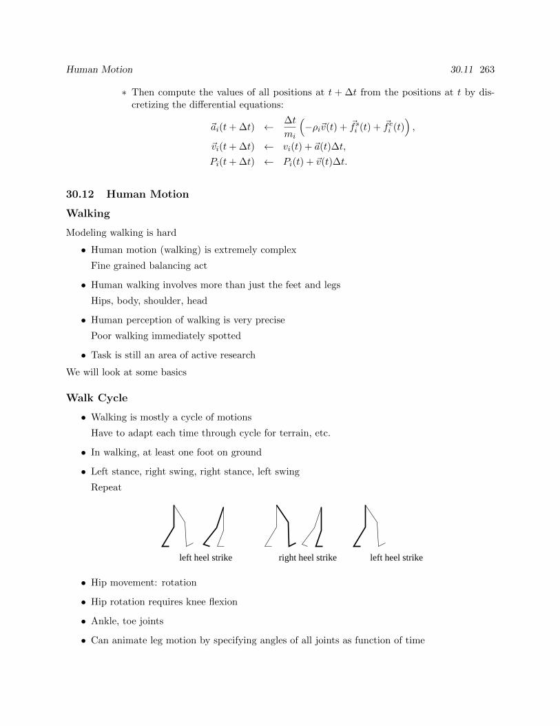
Human Motion 30.11 263
∗ Then compute the values of all positions at t + ∆t from the positions at t by dis-cretizing the differential equations:
~ai(t+ ∆t) ← ∆t
mi
(−ρi~v(t) + ~fsi (t) + ~fei (t)
),
~vi(t+ ∆t) ← vi(t) + ~a(t)∆t,
Pi(t+ ∆t) ← Pi(t) + ~v(t)∆t.
30.12 Human Motion
Walking
Modeling walking is hard
• Human motion (walking) is extremely complex
Fine grained balancing act
• Human walking involves more than just the feet and legs
Hips, body, shoulder, head
• Human perception of walking is very precise
Poor walking immediately spotted
• Task is still an area of active research
We will look at some basics
Walk Cycle
• Walking is mostly a cycle of motions
Have to adapt each time through cycle for terrain, etc.
• In walking, at least one foot on ground
• Left stance, right swing, right stance, left swing
Repeat
left heel strike left heel strikeright heel strike
• Hip movement: rotation
• Hip rotation requires knee flexion
• Ankle, toe joints
• Can animate leg motion by specifying angles of all joints as function of time

Sensor-Actuator Networks 30.12 264
30.13 Sensor-Actuator Networks
Sensor-Actuator Networks
• van de Panne
• Model creature as set of
– Links
– Sensors
– Actuators
• SAN relates sensors and actuators
• Control uses sensor data to apply forces thru actuators
Links
• Rigid
• Have mass
• May restrict to planar for simplicity
Sensors : 4 types
• Touch (picture)
• Angle (picture)
• Eye - used to find target
• Length (picture)
Actuators
• Length/linear
– push/pull points
– max/min, strength
• Angle
– create torques
– max/min angle, strength
Motion
• Evaluation metric
– Distance traveled
– Don’t fall over
• Generate random controllers and evaluate with metric
• Try lots, and fine tune the best
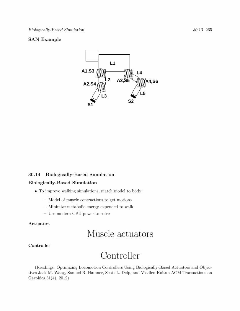
Biologically-Based Simulation 30.13 265
SAN Example
L1
L3
L4
L5
A1,S3
S1S2
A2,S4A3,S5L2 A4,S6
30.14 Biologically-Based Simulation
Biologically-Based Simulation
• To improve walking simulations, match model to body:
– Model of muscle contractions to get motions
– Minimize metabolic energy expended to walk
– Use modern CPU power to solve
Actuators
Muscle actuatorsController
Controller(Readings: Optimizing Locomotion Controllers Using Biologically-Based Actuators and Objec-
tives Jack M. Wang, Samuel R. Hamner, Scott L. Delp, and Vladlen Koltun ACM Transactions onGraphics 31(4), 2012)
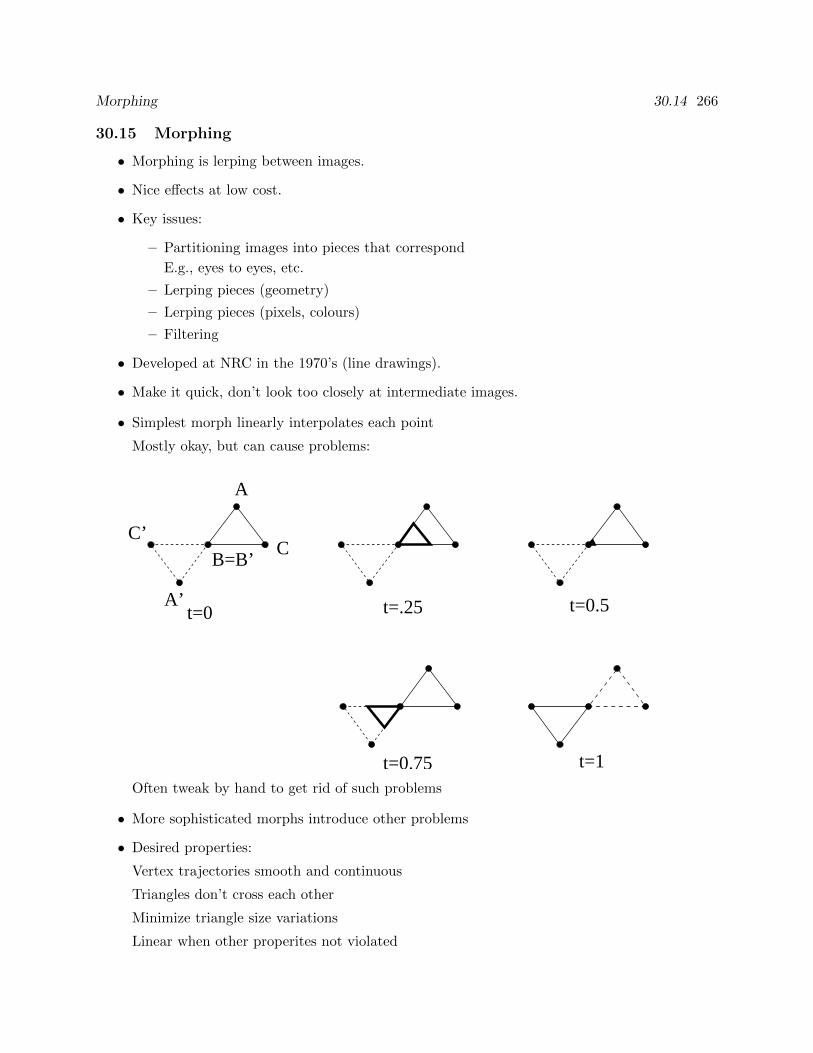
Morphing 30.14 266
30.15 Morphing
• Morphing is lerping between images.
• Nice effects at low cost.
• Key issues:
– Partitioning images into pieces that correspond
E.g., eyes to eyes, etc.
– Lerping pieces (geometry)
– Lerping pieces (pixels, colours)
– Filtering
• Developed at NRC in the 1970’s (line drawings).
• Make it quick, don’t look too closely at intermediate images.
• Simplest morph linearly interpolates each point
Mostly okay, but can cause problems:
B=B’C
A
C’
A’t=0 t=.25 t=0.5
t=1t=0.75Often tweak by hand to get rid of such problems
• More sophisticated morphs introduce other problems
• Desired properties:
Vertex trajectories smooth and continuous
Triangles don’t cross each other
Minimize triangle size variations
Linear when other properites not violated
Motion Capture 30.15 267
Morphing Example — associating key points30.16 Motion Capture
• Keyframing complex actions (walking, etc) requires a lot of key frames.
• Instead, capture motion from real objects.
Creatures and/or actors performing the desired motion.
• The positions of key points on the actor are tracked
these motions are mapped to corresponding points in the model.
• May be necessary to generate secondary actions for the computer model.
(tracking is expensive)
• Tracking technologies include
1. Electromagnetic position and orientation sensors.
– Requires a wire to each sensor.
– Readings can be distorted by metal and magnetic fields.
– Limited working volume.
2. Ultrasonic rangefinder triangulation.
– Cheaper but less accurate than magnetic sensors.
3. Optical triangulation.
– Reflective or emissive markers are attached to objects
– Two cameras triangulate position
– Can track more points cheaply, without wires
– Points can be occluded.
4. Body suit.
• Fibers in instrumented clothing detect angles of all joints.
Body suit motion capture
5. Rotoscoping.
– Arbitrary video from two cameras converted to motion paths
∗ manual selection of key points
∗ computer vision
– Prone to error and occlusion.
– Tedious if done manually.
Flocking 30.16 268
6. Puppetry.
– Real-time data collected from an arbitrary input device
– Mapped to an computer model, which is displayed in real time during capture.
– A special-purpose input device in the shape of the object being animated may bebuilt.
• Motion capture tends to require more-or-less exotic technology.
• Even puppetry requires at least real-time graphics.
• Technical problems with motion capture include:
– How do we map motion paths to objects of a different shape and scale (the ostrich-to-T.Rex problem)?
– How do we deal with noise and missing data?
– How can we reduce the number of samples?
– How can we generalize motion? I.e. we have a walk and a turn. How do we get an actorto follow a path?
• Perceptual problem:
Motion capture animations often look too stiff
30.17 Flocking
• Want to animate groups of animals
Birds, fish, herds
• Motion of individuals is semi-independent
Too many individuals to key frame each one
• Fewer elements than particle systems, but more interelement interaction
• Relative placing not rigid
Flock of birds vs airplanes in formation
(migrating geese, etc., being more like the latter)
Two main forces at work
• Collision avoidance
– Avoid hitting objects (trees, buildings, etc.)
– Avoid hitting one another
• Flock centering
– Each member trying to remain a member of flock
– Global flock centering too restricting
Does not allow flock splitting to pass around objects

Flocking 30.16 269
Local Control
• Controlling each flock member with local behaviour rules
Computationally desirable
Appears to be how flocks work in real world
• No reference to global conditions of flock, environment
• Three things to model:
– Physics
Gravity, collisions
– Perception
Information flock member has with which to make decisions
– Reasoning/reaction
Rules by which flock member decides where to go
Perception
• Aware of itself and two or three neighbors
• What’s in front of it
• Doesn’t follow a designated leader
• No knowledge of global center
Reasoning/reaction
• Collision avoidance
• Flock centering
• Velocity matching
Try to match velocity of neighbors
Helps with flock centering and helps avoid collisions
Additional details
• Global control
Animator needs to direct flock.
• Flock leader
Usually one member whose path is scripted (global control)
Not realistic (leader changes in real flocks),but usually not noticed and easier to deal with

Computational Geometry 30 270
• Splitting and Rejoining
Flocks pass around objects, splitting them
Difficult to balance rejoining with collision avoidance
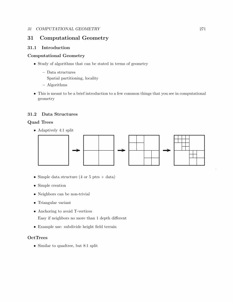
31 COMPUTATIONAL GEOMETRY 271
31 Computational Geometry
31.1 Introduction
Computational Geometry
• Study of algorithms that can be stated in terms of geometry
– Data structures
Spatial partitioning, locality
– Algorithms
• This is meant to be a brief introduction to a few common things that you see in computationalgeometry
31.2 Data Structures
Quad Trees
• Adaptively 4:1 split
• Simple data structure (4 or 5 ptrs + data)
• Simple creation
• Neighbors can be non-trivial
• Triangular variant
• Anchoring to avoid T-vertices
Easy if neighbors no more than 1 depth different
• Example use: subdivide height field terrain
OctTrees
• Similar to quadtree, but 8:1 split
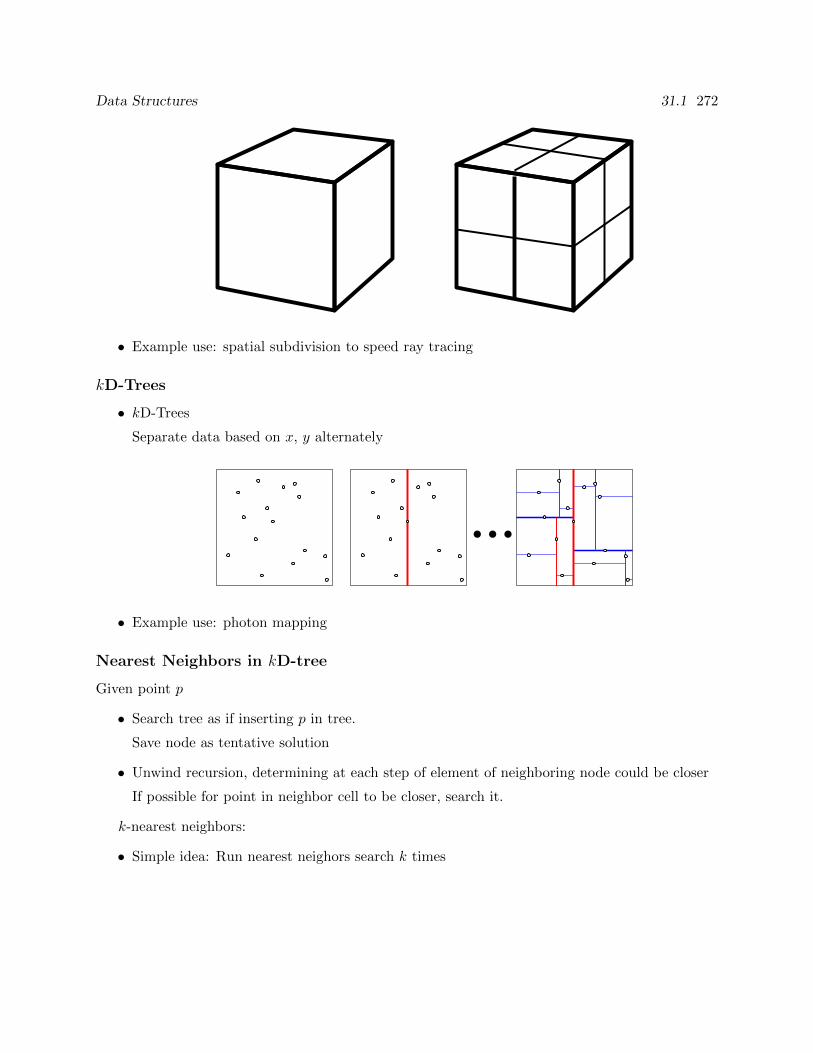
Data Structures 31.1 272
• Example use: spatial subdivision to speed ray tracing
kD-Trees
• kD-Trees
Separate data based on x, y alternately
...
• Example use: photon mapping
Nearest Neighbors in kD-tree
Given point p
• Search tree as if inserting p in tree.
Save node as tentative solution
• Unwind recursion, determining at each step of element of neighboring node could be closer
If possible for point in neighbor cell to be closer, search it.
k-nearest neighbors:
• Simple idea: Run nearest neighors search k times
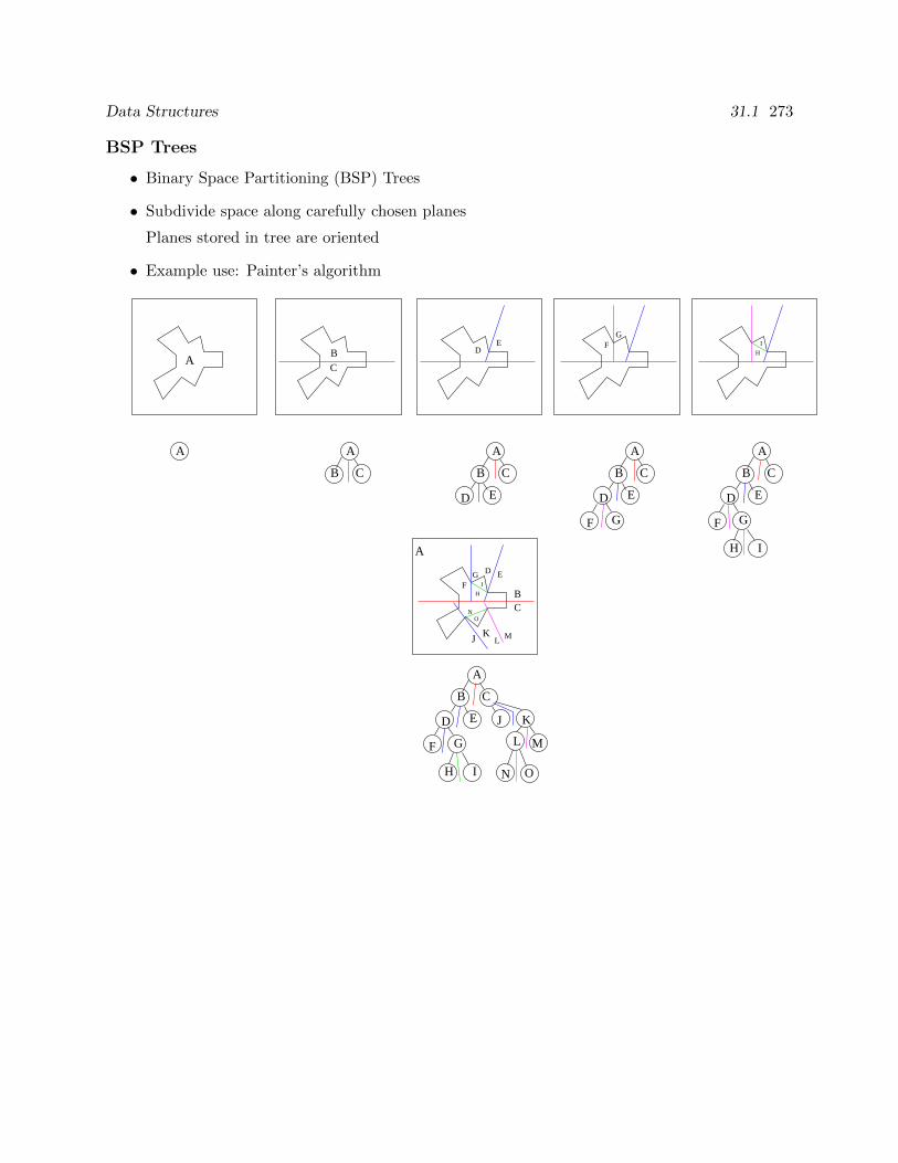
Data Structures 31.1 273
BSP Trees
• Binary Space Partitioning (BSP) Trees
• Subdivide space along carefully chosen planes
Planes stored in tree are oriented
• Example use: Painter’s algorithm
ID
E
C
FG
FG ED
B
BC
A
KJ LM
ON
H
I
H
A
A
CB
A
C
D E
B
A
C
D E
F
B
G
A
I
G
A
H
C
D E
F
B
A
J K
L M
N O
G
C
D E
F
B
H I
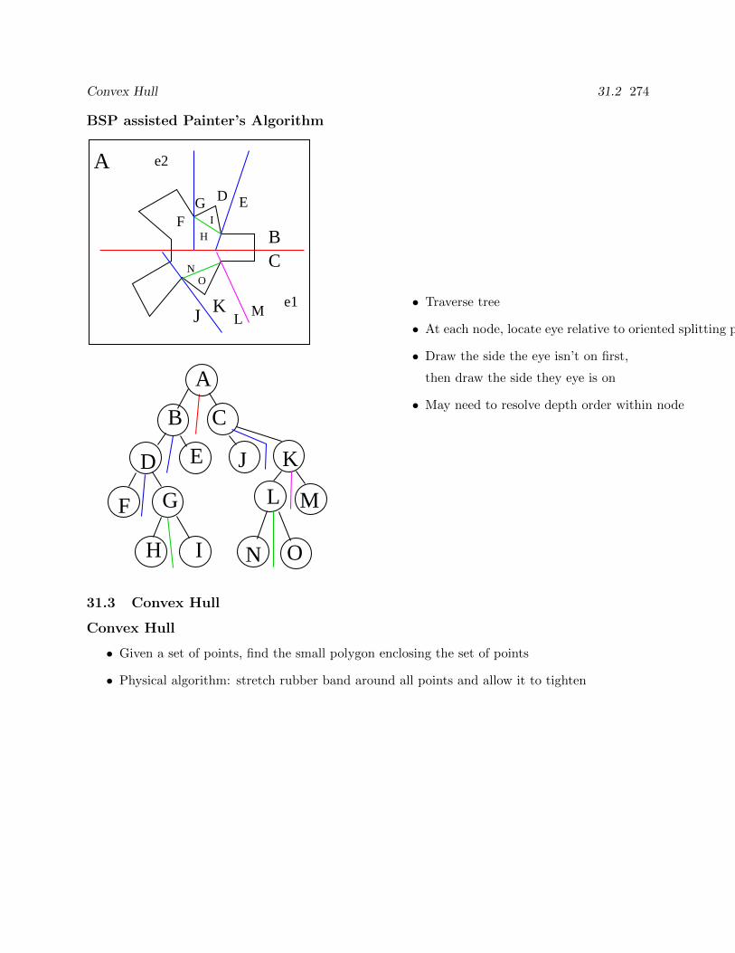
Convex Hull 31.2 274
BSP assisted Painter’s Algorithm
ON
ML
KJ
A
G
IH
B
F
e2
e1
I
H
NO
MLJ K
A
CB
D EGF
ED
C
• Traverse tree
• At each node, locate eye relative to oriented splitting plane
• Draw the side the eye isn’t on first,
then draw the side they eye is on
• May need to resolve depth order within node
31.3 Convex Hull
Convex Hull
• Given a set of points, find the small polygon enclosing the set of points
• Physical algorithm: stretch rubber band around all points and allow it to tighten
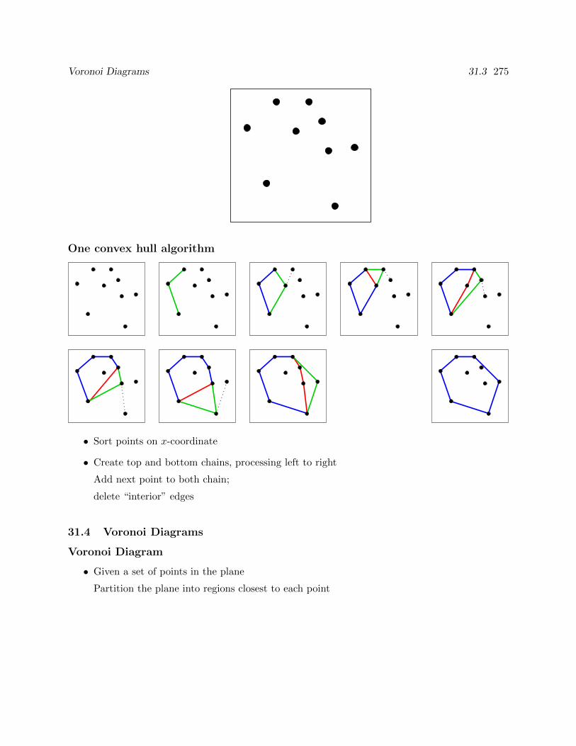
Voronoi Diagrams 31.3 275
One convex hull algorithm
• Sort points on x-coordinate
• Create top and bottom chains, processing left to right
Add next point to both chain;
delete “interior” edges
31.4 Voronoi Diagrams
Voronoi Diagram
• Given a set of points in the plane
Partition the plane into regions closest to each point
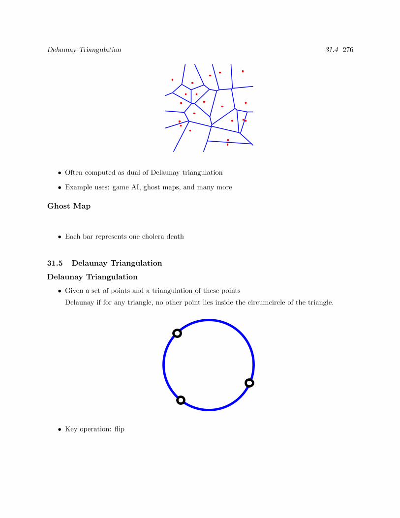
Delaunay Triangulation 31.4 276
• Often computed as dual of Delaunay triangulation
• Example uses: game AI, ghost maps, and many more
Ghost Map
• Each bar represents one cholera death
31.5 Delaunay Triangulation
Delaunay Triangulation
• Given a set of points and a triangulation of these points
Delaunay if for any triangle, no other point lies inside the circumcircle of the triangle.
• Key operation: flip
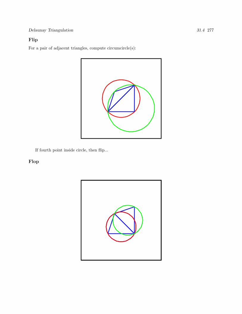
Delaunay Triangulation 31.4 277
Flip
For a pair of adjacent triangles, compute circumcircle(s):
If fourth point inside circle, then flip...
Flop
For a pair of adjacent triangles, compute circumcircle(s):
If fourth point inside circle, then flip...
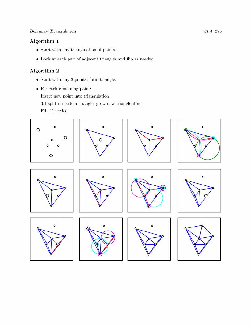
Delaunay Triangulation 31.4 278
Algorithm 1
• Start with any triangulation of points
• Look at each pair of adjacent triangles and flip as needed
Algorithm 2
• Start with any 3 points; form triangle.
• For each remaining point:
Insert new point into triangulation
3:1 split if inside a triangle, grow new triangle if not
Flip if needed
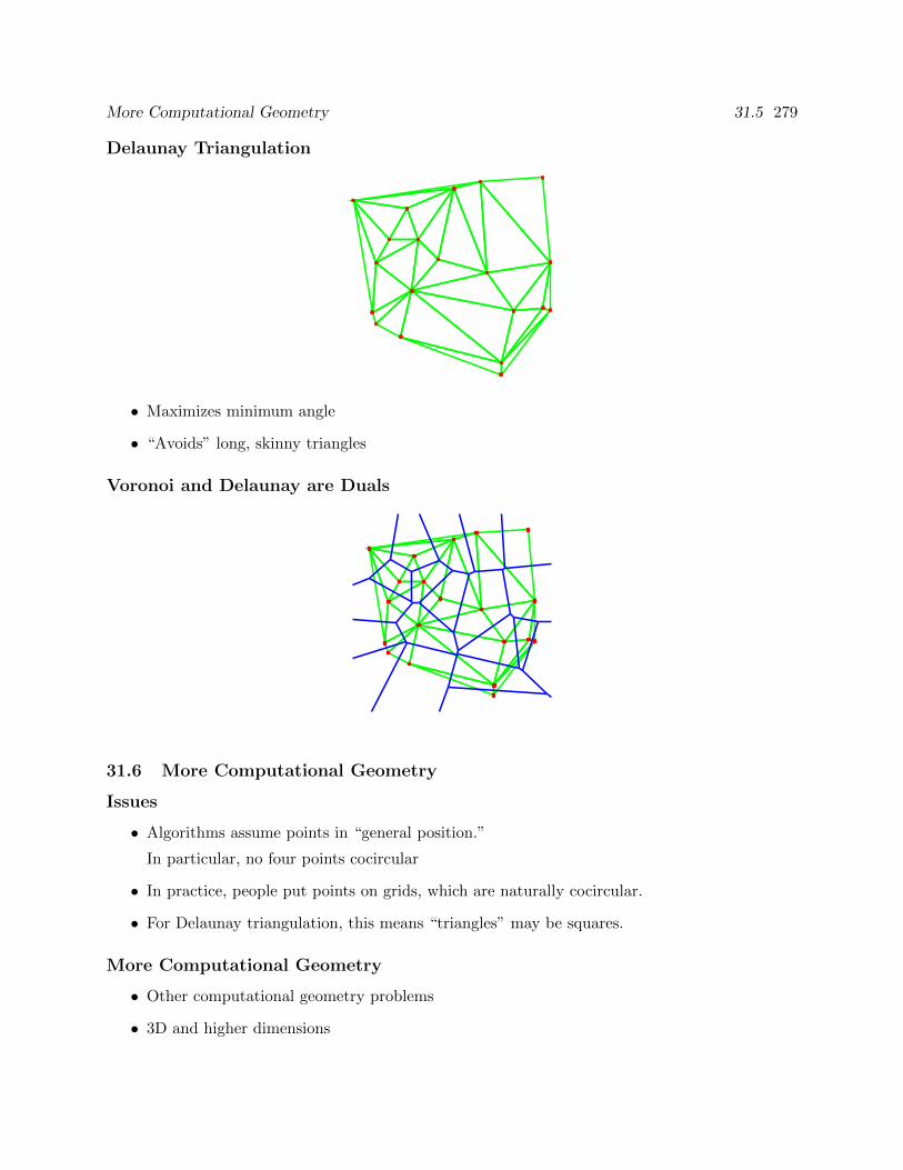
More Computational Geometry 31.5 279
Delaunay Triangulation
• Maximizes minimum angle
• “Avoids” long, skinny triangles
Voronoi and Delaunay are Duals
31.6 More Computational Geometry
Issues
• Algorithms assume points in “general position.”
In particular, no four points cocircular
• In practice, people put points on grids, which are naturally cocircular.
• For Delaunay triangulation, this means “triangles” may be squares.
More Computational Geometry
• Other computational geometry problems
• 3D and higher dimensions

Assignments 31 280
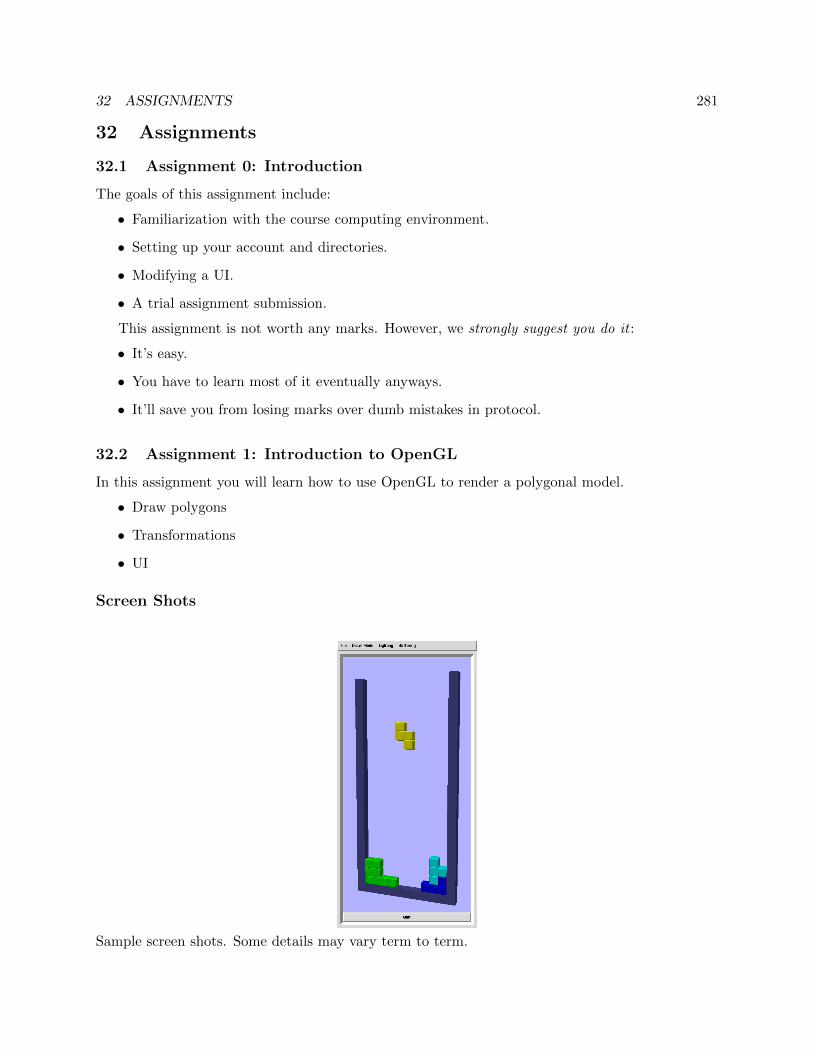
32 ASSIGNMENTS 281
32 Assignments
32.1 Assignment 0: Introduction
The goals of this assignment include:
• Familiarization with the course computing environment.
• Setting up your account and directories.
• Modifying a UI.
• A trial assignment submission.
This assignment is not worth any marks. However, we strongly suggest you do it :
• It’s easy.
• You have to learn most of it eventually anyways.
• It’ll save you from losing marks over dumb mistakes in protocol.
32.2 Assignment 1: Introduction to OpenGL
In this assignment you will learn how to use OpenGL to render a polygonal model.
• Draw polygons
• Transformations
• UI
Screen Shots
Sample screen shots. Some details may vary term to term.
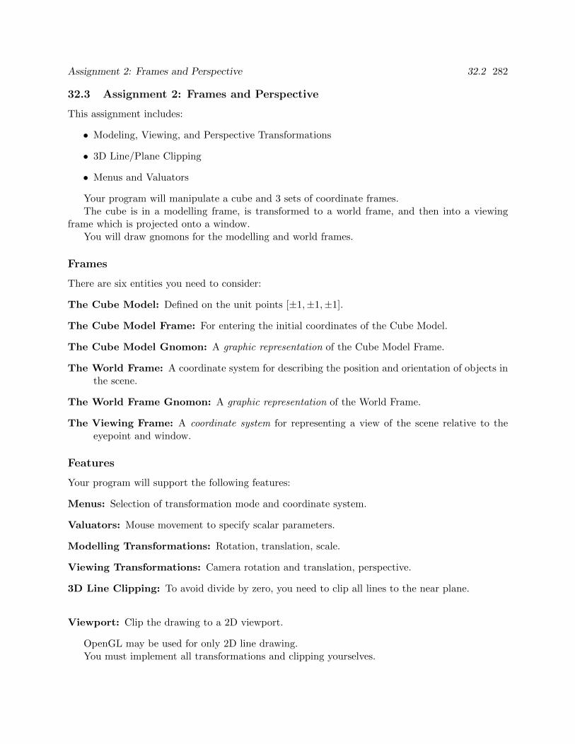
Assignment 2: Frames and Perspective 32.2 282
32.3 Assignment 2: Frames and Perspective
This assignment includes:
• Modeling, Viewing, and Perspective Transformations
• 3D Line/Plane Clipping
• Menus and Valuators
Your program will manipulate a cube and 3 sets of coordinate frames.The cube is in a modelling frame, is transformed to a world frame, and then into a viewing
frame which is projected onto a window.You will draw gnomons for the modelling and world frames.
Frames
There are six entities you need to consider:
The Cube Model: Defined on the unit points [±1,±1,±1].
The Cube Model Frame: For entering the initial coordinates of the Cube Model.
The Cube Model Gnomon: A graphic representation of the Cube Model Frame.
The World Frame: A coordinate system for describing the position and orientation of objects inthe scene.
The World Frame Gnomon: A graphic representation of the World Frame.
The Viewing Frame: A coordinate system for representing a view of the scene relative to theeyepoint and window.
Features
Your program will support the following features:
Menus: Selection of transformation mode and coordinate system.
Valuators: Mouse movement to specify scalar parameters.
Modelling Transformations: Rotation, translation, scale.
Viewing Transformations: Camera rotation and translation, perspective.
3D Line Clipping: To avoid divide by zero, you need to clip all lines to the near plane.
Viewport: Clip the drawing to a 2D viewport.
OpenGL may be used for only 2D line drawing.You must implement all transformations and clipping yourselves.
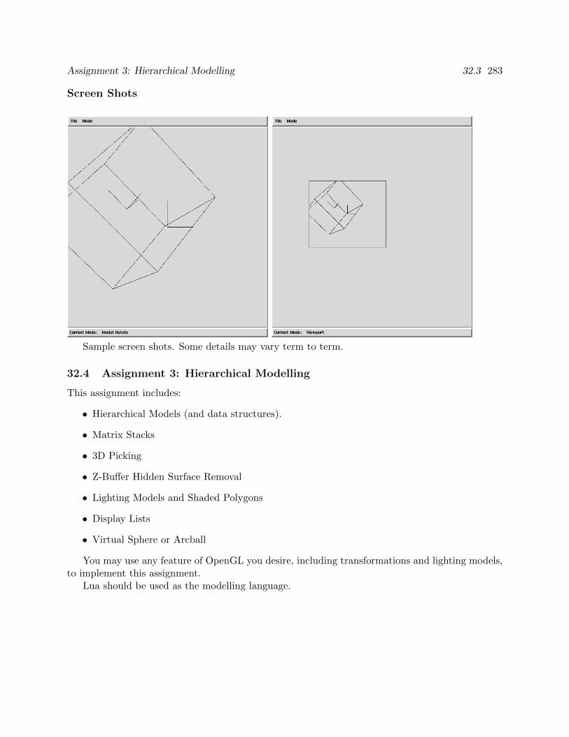
Assignment 3: Hierarchical Modelling 32.3 283
Screen Shots
Sample screen shots. Some details may vary term to term.
32.4 Assignment 3: Hierarchical Modelling
This assignment includes:
• Hierarchical Models (and data structures).
• Matrix Stacks
• 3D Picking
• Z-Buffer Hidden Surface Removal
• Lighting Models and Shaded Polygons
• Display Lists
• Virtual Sphere or Arcball
You may use any feature of OpenGL you desire, including transformations and lighting models,to implement this assignment.
Lua should be used as the modelling language.
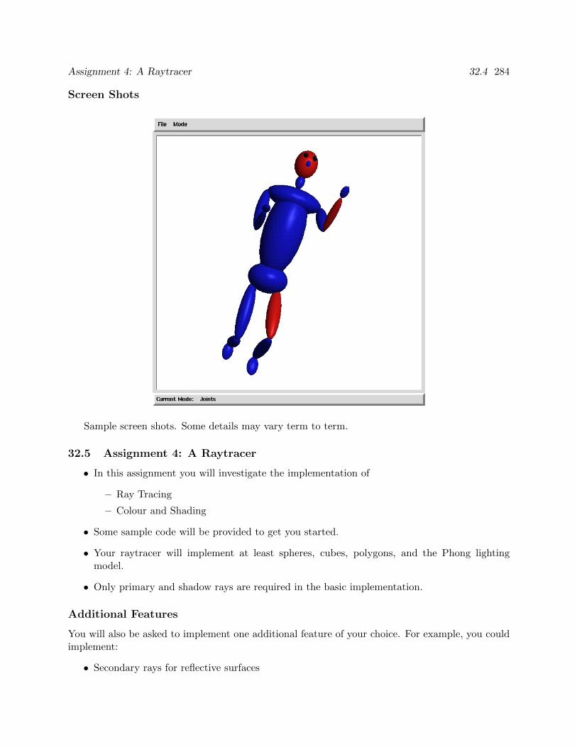
Assignment 4: A Raytracer 32.4 284
Screen Shots
Sample screen shots. Some details may vary term to term.
32.5 Assignment 4: A Raytracer
• In this assignment you will investigate the implementation of
– Ray Tracing
– Colour and Shading
• Some sample code will be provided to get you started.
• Your raytracer will implement at least spheres, cubes, polygons, and the Phong lightingmodel.
• Only primary and shadow rays are required in the basic implementation.
Additional Features
You will also be asked to implement one additional feature of your choice. For example, you couldimplement:
• Secondary rays for reflective surfaces
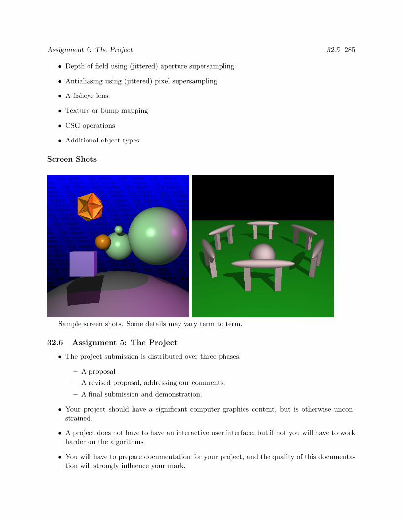
Assignment 5: The Project 32.5 285
• Depth of field using (jittered) aperture supersampling
• Antialiasing using (jittered) pixel supersampling
• A fisheye lens
• Texture or bump mapping
• CSG operations
• Additional object types
Screen Shots
Sample screen shots. Some details may vary term to term.
32.6 Assignment 5: The Project
• The project submission is distributed over three phases:
– A proposal
– A revised proposal, addressing our comments.
– A final submission and demonstration.
• Your project should have a significant computer graphics content, but is otherwise uncon-strained.
• A project does not have to have an interactive user interface, but if not you will have to workharder on the algorithms
• You will have to prepare documentation for your project, and the quality of this documenta-tion will strongly influence your mark.
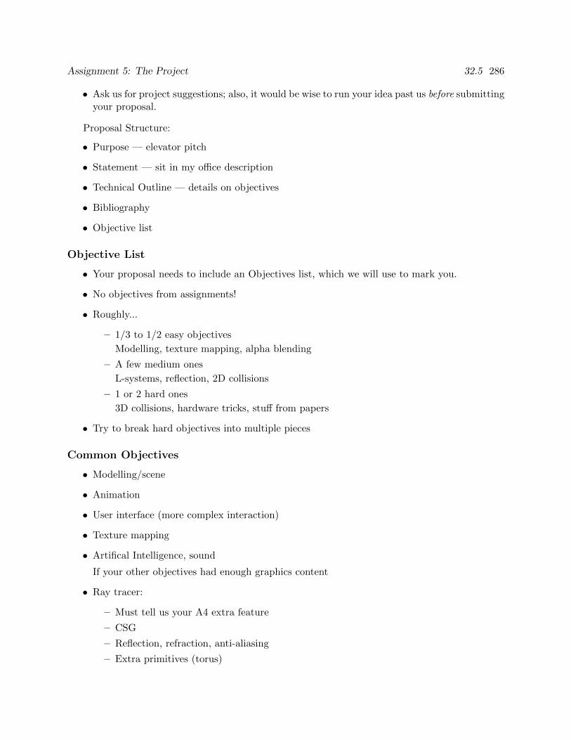
Assignment 5: The Project 32.5 286
• Ask us for project suggestions; also, it would be wise to run your idea past us before submittingyour proposal.
Proposal Structure:
• Purpose — elevator pitch
• Statement — sit in my office description
• Technical Outline — details on objectives
• Bibliography
• Objective list
Objective List
• Your proposal needs to include an Objectives list, which we will use to mark you.
• No objectives from assignments!
• Roughly...
– 1/3 to 1/2 easy objectives
Modelling, texture mapping, alpha blending
– A few medium ones
L-systems, reflection, 2D collisions
– 1 or 2 hard ones
3D collisions, hardware tricks, stuff from papers
• Try to break hard objectives into multiple pieces
Common Objectives
• Modelling/scene
• Animation
• User interface (more complex interaction)
• Texture mapping
• Artifical Intelligence, sound
If your other objectives had enough graphics content
• Ray tracer:
– Must tell us your A4 extra feature
– CSG
– Reflection, refraction, anti-aliasing
– Extra primitives (torus)
Assignment 5: The Project 32.5 287
Warm/cold Fuzzies About Objectives
• Think about what subjective mark you could get
Technical, artistic, documentation, difficulty
• Negative subjective marks for not using what you’ve learned
eg, flat shading in OpenGL projects
• Get advise from TAs and profs
• Beware of too easy/too hard projects
You can always do extra stuff
• Make objectives, not subjective
“Good UI” is subjective...
• When wondering if something makes a good project, try making an objective list for it.
General Project Categories
• Virtual World Exploration
Includes most games
• 2D Games (chess, risk, etc.)
Usually hard to get 10 objectives
• Simulation (physics, cloth, etc.)
Usually focussed on one harder technique/paper
• Ray Tracing
• Animated Movie
Simple key framing, ray trace the frames
OpenGL vs Ray Tracing
OpenGL Projects
• Interactive
• Avoid UI intensive projects
• Try to have a purpose (game, etc)
Ray Tracing
• Must get 9/10 on A4 to do ray tracing project
• Easier to come up with objective list

Assignment 5: The Project 32.5 288
• Design objectives around a scene
Photograph or real object you want to ray trace
• Nice scene must be one objective!
Describe it
Other Stuff
• Technical outline should clarify objectives
• You can start before you get proposal back
• Avoid dynamic memory
• See TAs if you have problems
Don’t spend 2 days hacking at it
• If running out of time, prof or TA can give advice on what objectives to tackle
• Project is marked on objective list of revised proposal.