cross-correlation analysis and interpretation of spaced-receiver measurements
TRANSCRIPT
Radio Science, Volume 23, Number 2, Pages 141-162, March-April 1988
Cross-correlation analysis and interpretation of spaced-receiver measurements
Emanoel Costa •
Physics Research Division, Emmanuel College, Boston, Massachusetts
Paul F. Fou•7ere and Santimay Basu
Ionospheric Physics Division, Air Force Geophysics Laboratory, Hanscorn Air Force Base, Massachusetts
(Received May 11, 1987; revised November 16, 1987; accepted December 8, 1987.)
Two algorithms which provide a statistical treatment to the estimation of the parameters of the cross-correlation analysis of spaced-receiver data are reviewed. Their results are compared using sig- nals: (1) transmitted by a quasi-stationary polar beacon and received at Goose Bay, Labrador (53.3øN, 60.3øW); and (2) transmitted by the orbiting Hilat satellite and received at Tromso, Norway (69.7øN, 18.9øE). A good general agreement is displayed in this comparison. The former experiment indicates the possibility of extreme daily variations in the anisotropy of the ground diffraction pattern and in the true drift velocity of the in situ irregularities. The latter experiment displays geometrical enhancements in the intensity scintillation index S,•, in the rms phase fluctuation a• and in the axial ratio of the ellipse which characterizes the anisotropy of the ground diffraction pattern, around the region of local L shell alignment of the ray paths. Increases of these parameters also are observed northward of Tromso. These observations are thus consistent with a morphological model for anisotropy of high-latitude nighttime F region irregularities proposed in the literature. Next, a possible dependence of the results of the spaced-receiver measurements on the receiver baselines is discussed. It is argued that this mecha- nism could be responsible for the relatively small values of the anisotropy of the diffraction pattern obtained from the Hilat measurements at Tromso. Finally, a procedure which combines a simple propagation model of the spaced-receiver experiment with a nonlinear minimization algorithm is proposed to estimate the anisotropy of the in situ irregularities from that of the diffraction pattern.
1. INTRODUCTION
The cross-correlation analysis of spaced-receiver data has been developed from the original idea that signals received on the ground by spaced probes after an interaction with the ionosphere display similar structures displaced in time. Dividing the separations between the probes by the respective average time delays between the similar structures, an initial esti- mate for an apparent drift velocity of the diffraction pattern defined on the ground can be obtained. A refinement of this idea uses the autocorrelation and
the cross-correlation functions of the received signals to also estimate the anisotropy and the true drift velocity of this diffraction pattern. This radio tech- nique is relatively well established [Mitra, 1949;
•Now at Centro de Estudos em Telecommunica•oes, Pontiffca Universidade Cat61ica do Rio de Janeiro, Brazil.
Copyright 1988 by the American Geophysical Union.
Paper number 7S0931. 0048-6604/88/007S-0931 $08.00
Bri•7•7s et al., 1950; Phillips and Spencer, 1955; Kent and Koster, 1966; Rino and Livin•tston, 1982] and has been applied to ionospheric studies at the equatorial region [Basu et al., 1986], in mid-latitudes [Moor- croft and Arima, 1972] and at high latitudes [Liv- in•7ston et al., 1982].
Several algorithms have been proposed in the literature to perform the cross-correlation analysis of spaced-receiver data. Two of these, which not only recognize the statistical nature of the present prob- lem but also are well suited for implementation in digital computers, are reviewed here. The first algo- rithm is a slightly generalized version of that pro- posed by Fedor [1967]. The second has been suggest- ed by Rino and Livingston [1982], based on a pre- vious work by Armstrong and Coles [1972], devoted to interplanetary scintillation studies. Results from the two algorithms are compared, using signals: (1) transmitted by a quasi-geostationary polar beacon and received at Goose Bay, Labrador (53.3øN, 60.3øW); and (2) transmitted by the orbiting Hilat satellite and received at Tromso, Norway (69.7øN,
141

142 COSTA ET AL.: ANALYSIS OF SPACED-RECEIVER MEASUREMENTS
18.9øE). In spite of the different features of the two algorithms, a good general agreement between their results is observed. Possible sources of occasionally observed differences also are discussed. The results of
experiment 1 display extreme daily variations of the anisotropy and the true drift velocity of the ground diffraction pattern. Temporal variations of these pa- rameters occurring on short time scales also are ob- served. Experiment 2 seems to reproduce, at Tromso, the morphological results from the Poker Flat/Wide- band spaced-receiver measurements [Fremouw et al., 1978; Rino et al., 1978; Livingston et al., 1982]. It is observed, however, that the anisotropy of the ground diffraction pattern resulting from the Tromso/Hilat measurements seems to be less significant than the similar result from the Goose Bay/polar beacon or the Poker Flat/Wideband experiments. There is theo- retical (and not entirely conclusive) evidence that this difference may be due to a scale size dependence of the anisotropy of the in situ irregularities. This evi- dence is briefly reviewed. Another possible expla- nation for the above observation, also discussed here, is the dependence of the results from the spaced- receiver analysis on the distance between the probes [Golley and Rossiter, 1970].
To interpret the measurements in terms of the ani- sotropy and the drift velocity of the in situ irregu- larities, a propagation model of the spaced-receiver experiment is presented. This model assumes (1) a "space-time" correlation function for the random fluctuations in the electron density of the ionosphere whose surfaces of constant correlation levels are
characterized by concentric ellipsoids, and (2) a re- lationship between the fluctuations in the phase of the received signal and the irregularities in the elec- tron density in the F region given by geometrical optics. A simple equation is then obtained for the drift velocity of the ground diffraction pattern as a function of the drift velocity of the in situ irregu- larities and the satellite velocity. When the satellite velocity is negligible (such as in the case of geosta- tionary or quasi-geostationary satellites), it is easy to estimate the drift velocity of the ionosphere from that of the diffraction pattern. Further, it is shown that the ellipses which characterize the anisotropy of the diffraction pattern are geometrical projections along the ray path onto the ground of the anisotropy ellip- soids of the in situ irregularities. Since there is a con- tinuum of ellipsoids which could be projected onto the same ellipse, the estimation of the anisotropy of the in situ irregularities from that of the diffraction
pattern is not so straightforward as in the case of the drift velocity. It is suggested, however, that, under a few assumptions, it is possible to estimate an average anisotropy of a certain volume of the ionosphere from the observation of multiple and reasonably dif- ferent anisotropy ellipses of the ground diffraction pattern. This is accomplished by an "inversion" of the propagation model, performed by a nonlinear minimization of the rms error between measured and
calculated values of the anisotropy of the diffraction pattern.
2. ALGORITHMS FOR THE CORRELATION ANALYSIS
OF SPACED-RECEIVER DATA
Assume the existence of n r receivers on the ground, located at x i = (Xi, Yi), i = 1, 2, ..., nr, which simulta- neously receive transionospheric signals si(t ). It is also assumed that these signals are stationary, with zero mean and unit standard deviation, and are sam-
pled at the frequency f•. Further, it is assumed that the correlation functions pi•(zk)= (si(t)s•(t + where z& = (k - 1)/fs, with k = 1, 2 ..... N, have been calculated for all possible combinations of indices i andj.
Apparently, the most general characterization for these correlation functions assumes that they are spe- cial cases of a single function of three variables. Of these three variables, two represent the vector spac- ing between receivers and the other time delay be- tween different observations. These variables are
combined into a single argument, in such a way that surfaces of constant argument define, in this three- dimensional space, ellipsoids of different sizes but of constant shape. That is,
where
Pij(Ik) = R{[A• T' O' A•] 1/2} (1)
(2)
AZ r= (Axij, Ayij, •), Axij = xj- xi, Ayij and the superscript T will always represent the trans- pose of a matrix. The parameters a, b, c, f, g and h are constants to be estimated by the analysis. It is suf- ficiently general for the present purposes to assume that R is a decreasing function of its argument, nor- malized in such a way that R(0)= 1. The original justification for this characterization of the corre- lation functions can be found in Briggs et al. [1950]. It will be seen in a later section that it also is consis-
= Yj- Yi
COSTA ET AL.' ANALYSIS OF SPACED-RECEIVER MEASUREMENTS 143
/
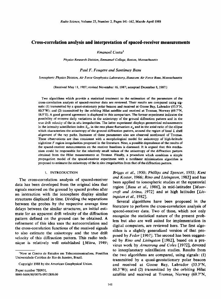
I Fig. 1. Sketch of auto- and cross-correlation functions of
spaced receiver signals, showing the time delays used by the modi- fied Fedor (MF) algorithm.
tent with an analogous characterization of the random electron density fluctuations in the iono- sphere, combined with a simple thin phase-screen scintillation model.
Two algorithms which have been proposed to de- termine the constants of the ellipsoids will be com- pared. Besides being well suited for implementation in digital computers, both use the redundant infor- mation available in the correlation functions to
create generally overdetermined systems of linear equations, which are then solved using the least squares method. This approach thus recognizes the statistical nature of the problem. Therefore, in prin- ciple, the solutions so obtained would be more accu- rate than those resulting from any algorithm using only the minimum amount of information.
The first algorithm is a slightly modified version of that suggested by Fedor [1967], wh/•ch originally as- sumed a Gaussian form for the function R. As it will
be seen, the autocorrelation function (i -j in (1)) pro- vides all the information on R which is necessary for the estimation of the parameters. The Gaussian as- sumption can thus be avoided.
Let R c be the value of the cross-correlation func- tion pij(rc) at the time delay r c . One can calculate, using a reasonable interpolation method, the time delay z a such that R c = pkk(ra), as illustrated in Figure 1. From the equality pij(rc)= pkn(r,) and the assumption that R is a decreasing function, it follows that
2 2 (•/c)[ax •- O- ax - cTc •] = • - •c (3)
This expression can be used as a building block for a nF x 5 system of linear equations D s ß U s =T 5, where Us r - (a, h, b,f, g)/c. The nF rows in this system are obtained by selecting different combinations of cross-correlation, autocorrelation functions and time delays r c in (3), from which the values of the elements of the matrices Ds(n F x 5) and T•(nF x 1) are easily inferred.
The second algorithm has been proposed by Rino and Livingston [1982], based on a previous work by Armstrong and Coles [1972]. This algorithm, which is fully described in the previous references, uses the maxima and the crossings of the correlation func- tions to determine, in a two-step procedure, the un- known coefficients in (2). That is, after all maxima and crossings of correlation functions have been esti- mated, an analogous nat , x 3 linear system D 3 ß U 3 = T 3 , where U3 r -(a, h, b)/c, is obtained. Once this system of equations is solved, the values for a/c, h/c and b/c can be substituted into another nat. x 2 linear system D 2 ß U 2 = T 2 . Here, U2 r = (V x, V•) co- incides with the drift velocity V of the diffraction pattern defined on the ground.
The linear systems obtained, all of the form D-U -T, are generally overdetermined and should be solved by the least squares method. Assuming the observations T are uncorrelated, it follows that the
general solution to those systems is of the form
U = (Dr- D)- • ß Dr- T (4)
As pointed out by Fedor [1967] and Banertl [1960], the observations T actually are correlated. The avail- able solution to this more general situation is rela- tively cumbersome, since it involves the calculation and inversion of the covariance matrix of the obser-
vations, a formidable task even for the most powerful computers. Fortunately, as indicated by Scheff• [1959], the estimate represented by (4) will still con- verge to the desired solution as the number of obser- vations increases.
Once the parameters of the ellipsoids are deter- mined, those characterizing the anisotropy, the true drift velocity and the characteristic velocity of the diffraction pattern are calculated as prescribed by Kent and Koster [1966]. The anisotropy is characterized by the common axial ratio AR and orientation •P• of the major axes of the similar el- lipses along which the ellipsoids in (1) intersect the plane r = 0. The true drift velocity of the diffraction pattern is defined in terms of its amplitude V and its direction •Pv- The characteristic velocity Vc, defined
144 COSTA ET AL.: ANALYSIS OF SPACED-RECEIVER MEASUREMENTS
by Briggs et al. [1950], provides a measure of the amount of internal motion taking place in the dif- fraction pattern.
It should be realized that the fact that normalized
(with respect to c) coefficients have been obtained by the two algorithms imposes no limitation on the cal- culation of the parameters AR, •, V, • and V•. That is, due to assumptions associated with (1), it has been found that these parameters depend on the common shape of the ellipsoids, but not on their sizes.
Omitting the indices, the argument within square brackets in (1) can be rewritten in the form
AZ x- O- AZ = + k• • (5) Ay- •r] •h bJ•Ay- •r]
where c = k + (aV• + 2hV, • + bV•). As discussed by Briggs [1968], the first term in the right-hand side of (5) represents the "frozen-in" motion contribution to the correlation functions. The term kr • represents the random motion contribution to the same func-
tions. There is then an implicit assumption in (1) that these two motions additively contribute to the corre- lation functions through the same (quadratic) func- tional form. Also, it can be shown that k = 0 is equivalent to •/V = 0. Results show that • some- times is a nonnegligible fraction of V, indicating that a pure "frozen-in" motion is not always in good agreement with the observations. However, it is seen that assuming k = 0, besides artificially imposing the condition • = 0, will only affect the value of c. Since, as seen in the previous paragraph, this has no effect on the common shape of the ellipsoids, one con- cludes that, within the scope of the present theory, the pure "frozen-in" assumption will provide aniso- tropies and drift velocities of the diffraction pattern which are no different from those calculated by the general equation (1).
Another implicit assumption is that (5) characterizes an ellipsoid. Obviously, this is only true when the same equation defines a positive-definite quadratic form. That is, one should have a > 0, ab -he> 0 and k > 0. Imposing these nonlinear con-
straints upon the solution of the system D-U = T by the least squares method would certainly increase the level of difficulty o[ the present problem, as well as the computer time needed to solve it. Instead, it has been preferred to let those conditions result from the "good behavior" of the experimental data.
Before commenting on some possible conse- quences of this approach, it will be useful to summa-
rize some aspects of the algorithms already described. As previously indicated, the main feature of the Rino- Livingston algorithm is its use of only the time delays for maxima of the cross-correlation functions or the crossings between pairs of (auto- or cross) correlation functions. On the other hand, as indicat- ed by (3), the modified Fedor algorithm uses time delays for all available observations of the cross cor- relation functions. Thus at least in principle, the modified Fedor algorithm will operate over a larger range of time delays than that of the Rino-Livingston algorithm.
Further, it should be mentioned that skewness is usually observed around the maxima of the mea- sured cross-correlation functions. Skewness has been
explained in terms of random velocity fluctuations in the ionosphere or regular velocity variations along the ray path [McGee, 1966; Bri•7gs and Golley, 1968; Wernik et al., 1983]. This feature has been neglected in (1). Occasionally, this disagreement becomes a serious source of difficulty, causing at least one of the algorithms to estimate a set of parameters which does not satisfy the inequalities characterizing a positive-definite quadratic form. When this happens, it has been chosen to reject the whole set. Fortu- nately, as the results to be discussed in a later section will show, the discrepancy between modeled (through (1)) and measured correlation functions is not severe enough to prevent the algorithms to calculate a con- sistent set of parameters in a large fraction of the cases analyzed.
On the other hand, moderate to small skewness of the cross-correlation functions, combined with the difference in the ranges of time delays over which the two algorithms operate or even with the different ways through which they process the data, could be translated into differences between their estimates.
Again, the results to be presented later will show that, although there occasionally are significant dif- ferences, the agreement between the two algorithms is generally good.
3. A MODEL OF THE SPACED-RECEIVER
EXPERIMENT
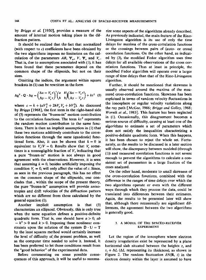
Let the region of the ionosphere where electron density irregularities exist be represented by a plane horizontal slab situated between the heights z i and zi q- AL (AL representing its thickness), as shown in Figure 2. The random fluctuation 6N(R, t) in the electron density within the layer is assumed to have
COSTA ET AL.' ANALYSIS OF SPACED-RECEIVER MEASUREMENTS 145
V$
x(north)
z (down)
Fig. 2. Geometry assumed by the model of the spaced-receiver experiment.
zero mean, total power equal to (6N 2) and to be homogeneous and anisotropic, with its "space-time" correlation function being characterized by
pN(AR, A'•) -- RN{[Ar 2 q- (At/B) 2
+ (asia) • + (a,/c)•] '/•} = g•(p) (6)
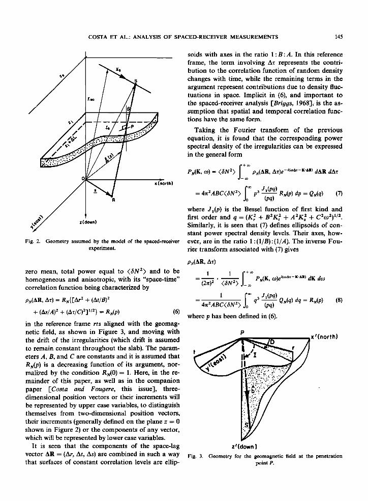
in the reference frame rts aligned with the geomag- netic field, as shown in Figure 3, and moving with the drift of the irregularities (which drift is assumed to remain constant throughout the slab). The param- eters ,4, B, and C are constants and it is assumed that Rs(p) is a decreasing function of its argument, nor- malized by the condition Rs(O ) - 1. Here, in the re- mainder of this paper, as well as in the companion paper [Costa and Fougere, this issue], three- dimensional position vectors or their increments will be represented by upper case variables, to distinguish themselves from two-dimensional position vectors, their increments (generally defined on the plane z -- 0 shown in Figure 2) or the components of any vector, which will be represented by lower case variables.
It is seen that the components of the space-lag vector AR = (Ar, At, As) are combined in such a way that surfaces of constant correlation levels are ellip-
soids with axes in the ratio I:B:A. In this reference
frame, the term involving Az represents the contri- bution to the correlation function of random density changes with time, while the remaining terms in the argument represent contributions due to density fluc- tuations in space. Implicit in (6), and important to the spaced-receiver analysis [Briggs, 1968],-is the as- sumption that spatial and temporal correlation func- tions have the same form.
Taking the Fourier transform of the previous equation, it is found that the corresponding power spectral density of the irregularities can be expressed in the general form
PN(K, 09)= (rSN 2 ) •_•-o• pN(AR, Az)e -i"øa*-K'sm dAR dA•
= 4rc2ABC(•N 2) p3 J•(Pq) RN(p ) dp = QN(q) (7) (pq)
where J•(p) is the Bessel function of first kind and first order and q = (K• 2 + B2K• 2 + A2K• 2 + C2(_D2) 1/2. Similarly, it is seen that (7) defines ellipsoids of con- stant power spectral density levels. Their axes, how- ever, are in the ratio 1 :(I/B):(1/,4). The inverse Fou- rier transform associated with (7) gives
ps(AR,
Ps(K, fo)e i{a'A;-K'a'll) dK do (2:re) 2 <•N2> o•
J,(Pq) q3 QN(q) dq = RN(p) (8)
4rc2ABC(rSN 2 )
where p has been defined in (6).
x/(north)
Fig. 3.
z/(down )
Geometry for the geomagnetic field at the penetration point P.
146 COSTA ET AL.' ANALYSIS OF SPACED-RECEIVER MEASUREMENTS
To evaluate the effects of the medium on a signal transmitted by a satellite S and received on the ground, it is convenient to characterize the corre- lation function of the density fluctuations in a differ- ent reference frame. This will be done by initially applying two successive rotations AX' = R• ß AR and AX"= R 2 ß AX'. The former is performed around the penetration point P (where the ray path intersects the plane at the center of the irregularity layer), being characterized in Figure 3. On the other hand, the reference frame x"y"z" has its axes respectively aligned with the northward, eastward and downward directions defined at the origin O shown in Figure 2 (that is, they are parallel to the axes x, y and z). The latter rotation thus takes the sphericity of the earth into account. It is assumed, however, that both refer- ence frames x'y'z' and x"y"z" are also moving with the drift velocity of the irregularities. Performing the indicated transformations, the correlation function of the density fluctuation can be written in the reference frame x"y"z" as
pN(AX", A•)
= RN{[(AX") T. A •. C A. AX" + (At/C)2] •/2} (9a)
where
(AX") r = (Ax", Ay", Az")
C,,,, - cos 2 D sin 2 I + cos 2 D cos 2 I/A :• + sin 2 D/B :• (9b)
Cy.v = sin 2 D sin 2 I + sin 2 D cos 2 I/A • + cos 2 D/B 2 (9c)
C== = cos 2 I + sin 2 I/A 2 (9d)
C,,y - Cy,, = cos D sin D(sin 2 I + cos 2 I/A 2 -- 1/B 2) (9e)
C,,• = C•,, = --cos D cos I sin I(1 -- 1/A 2) (9f)
Cy• = C•y = --sin D cos I sin I(1 -- 1/A 2) (9g) and
Finally, it is important to observe that the density irregularities 8•(X, t), defined in the reference frame xyz (fixed with respect to the receivers) shown in Figure 2, are related to 8N(X", t) through
6•4/•(X, t) = 6N(X -- X o -- vnt, t) (10)
where X o = (Xo, Yo, Zo) defines the position of the origin of the reference frame x"y"z" with respect to the reference frame xyz at t = 0 and VD is the drift velocity of the irregularities.
There is a vast literature describing the propaga- tion of radio waves through continuous random media [Tatarskii, 1971; Yeh and Liu, 1982, and refer- ences therein]. It is immediately evident that more elaborate models lead to extremely complex math- ematical equations, which generally are solved nu- merically. Although it may be important to model the spaced-receiver experiment more accurately in the future, this will make it considerably more diffi- cult to interpret the measurements or to explore the possibility of unambiguously estimating the ani- stotropy of the ionospheric irregularities from the measured anisotropy of the ground diffraction pat- tern. On the other hand, it has been shown [Rino, 1982; Rino and Livingston, 1982] that, in spite of its limitations, the geometrical optics relationship be- tween 5•(x, t) and the phase fluctuations 5•b(x, t) of the transionospheric signals received on the ground is able to provide useful insight into ionospheric scin- tillation and the spaced-receiver experiment. This re- lationship is given by
5q•(x, t)= -- re ,• o • c• dl (11) ray path
where re(=2.82 x 10 -15 m) is the classical electron radius and 2 o is the free space wavelength of the transmitted signal.
cos 0v cos 0R cos (2v- 2R) [ +sin0vsin0R
A= {cos0 Rsin(2 v-2R) •sin 0e cos 0 R cos (2 v 2R) x• _ cos 0e sin 0R
-cos 0 v sin (2v - 2R)
cos (2•,- 2R) - sin 0v sin (2v - 2R)
cos 0 v sin 0 - sin 0v cos 0 sin 0R sin
sin 0v sin -{- COS O v COS O R
(9h)
In the above equations, D and I are, respectively, the declination and the dip angle of the geomagnetic field, 0v, R represent colatitudes, '•v,R represent lon- gitudes, the subscripts P and R indicate the penetra- tion point and the receiver, respectively, and the superscript T again indicates the transpose of a matrix.
Assuming that a satellite is the source of the trans- mitted signals, there are two typical situations in the spaced-receiver experiment. The first involves a ve- hicle with near circular, low-altitude orbit, such as the Hilat satellite (830-km-high orbit, with an 82 ø inclination and orbital velocity of 7.4 km/s). The second involves signals transmitted from geostation-
COSTA ET AL.' ANALYSIS OF SPACED-RECEIVER MEASUREMENTS 147
ary or quasi-stationary satellites. In both cases, the source can be assumed to be moving with a constant horizontal velocity in the plane z = zs shown in Figure 2, for the short period of time involved in the analysis of each sample of data. Thus in both cases the position !(z, t) of the point of the ray path situ- ated at the height z at time t can be characterized by the general equation
!(z, t) = rs(t ) + [x - rs(t)](z s - z)/z s (12)
where, as shown in Figure 2, rs(t)= rso + v s t is the satellite position vector (assumed to be always con- tained in the plane z = Zs), rso = rs(O ), Vs is the (hori- zontal) satellite velocity and x is the receiver position (on the plane z = 0).
Combining (10)-(12) and using the relationship dl = sec 0 dz (where 0 is the angle between the ray path and the vertical at the penetration point P), followed by a change of variables, it is found that
6qS(x, t) = --Fe,• SeC 0 6N{[(z s -- z i -- z')/Zs]X
+ [(z• + z')/Zs](rso,, + Vs t)
-- vvnt -- Xon, z' + 2 i -- vvzt -- z o, t} dz' (13)
where the subscripts H and z indicate components of a vector in the horizontal plane or in the z direction, respectively. Using this basic result to calculate the "space-time" correlation function of the phase fluctu- ations of the received signals, one gets
2 2g (rSN 2 )AL sec 2 0 • r e
• (1 - I z' I/•)•{[(Zs - z)/Zs]•X AL
-[v•n- (zi/Zs)Vs]Az + tan 0
2 2•(6N 2) •L sec 2 0 ß z'- v.• •z, •z} dz' • re
ß a•{[(z•- z,)/•s](•x - v •)
+ tan Okn z', z', •z} dz' (14)
where 4•o is the rms phase fluctuation,/•n is the unit vector resulting from the projection of SR (vector defining the ray path) onto the horizontal plane z = 0 and
V = [Zs/(Z s - zi)][vDn- tan OknvD•- (zi/Zs)Vs] (15)
In the last step of (14), it has been assumed that AL is large in comparison with the decorrelation distance of the density fluctuation in the z direction.
In (14) and (15), the effects of the oblique propaga- tion on p•(Ax, Az) are considered through the terms involving tan 01• n [Rino and Frernouw, 1977]. Fur- ther comments on the meaning of one of these terms will be represented at the end of this section. Equa- tion (14) clearly shows that the spatial and temporal behavior of p•(Ax, Az) can be fully described by a general function of both Au = (Ax- V Az) and Az, regardless of the functional form taken by p•r(AR, Az). Comparing this result with the right-hand side of (5), it is immediately concluded that (15) relates the drift velocity V of the ground diffraction pattern to the drift velocity of the irregularities in the iono- sphere and the satellite velocity. For stationary or quasi-stationary satellites, v• tends to zero and V is essentially a function of the ionospheric drift. On the other hand, (15) is dominated by v• for low-altitude, near-circular orbit satellites (such as Hilat). It is also seen that V simultaneously depends on both the horizontal and the vertical components of the iono- spheric drift. That is, it is theoretically impossible to separate the two components from a single measure- ment of V.
Substituting the horizontal space lags indicated in the integrand of (14) for Ax" and Ay" in (9), one gets
•p• p½(Ax, Az) = •P•o sec2 0 •_+ ©
+ (Az/C) 2 + 2(C•,•, Au,• + C;• Auy)z' + C;•z'2] •/2} dz' (16)
2 2• (6N 2) AL. The coefficients C;x to where •b•o = r e C'zz in this equation result from the substitution indi- cated above in a straightforward manner. Applying a linear change of variables to the integrand in (16), one immediately identifies
2 j.(• (•jN 2 ) Am sec 2 0 R•(Iz'l) dz'/x/• (17a)
and
t>,(Ax, Az) =' + (c;Zo - zt)/C;z] az'
'_+• •,,(I z' I) clz' = •,{[(c;• Zo- z•)/c;B •/•} (•7•,)
where Zo is the term independent from z' and 2Zx is
148 COSTA ET AL.: ANALYSIS OF SPACED-RECEIVER MEASUREMENTS
the coefficient of the linear term in z', both obtained
from the argument within square brackets in that equation. The last step in (17b) holds regardless of the functional form for R•v(p). From the assumed properties for this function, it follows that Rs(p) also is a decreasing function of its argument, such that Rs(O ) = 1. The argument within parentheses in (17b) can be rewritten in the form
c'=Zo = -
= ("q7 c:.c;x- c:.c,.-
A comparison between (5) and (18) immediately shows that (17b) has the same form as (1), thus lend- ing full support to the assumptions in the previous section. As explained in the companion paper [Costa and Fou•ere, this issue], (17a), (17b) and (18) would have to be extended if it were important to explain some fine details in the observed cross-correlation
functions (namely, the skewness around their respec- tive maxima).
Assume strictly "frozen-in" irregularities (that is, neglect the terms involving (At/C)2), as well as a ref- erence frame moving with the drift of the ground diffraction pattern. To further simplify the discussion, let z s >> z•, in (14). Under these assumptions, the arguments within brackets in (9a), (16), and (18) become completely independent of At. It can then be shown analytically that the ellipse characterized by equating the argument of Ro(p) in (17b) to a constant (say, Co) is the geometrical projection along the ray path onto the plane containing the receivers (z = 0 in Figure 2) of the ellipsoid
(AX") T- G'-AX"= (AX") T- A T- G- A. AX = C• (19)
characterized by the term within square brackets in (9a). This result is identical to the one previously derived by Moorcroft and Arima [1972], except for these authors' assumption of a vertical ray path. To see that it is also valid in the present general geome- try, consider the equation, parametric in w, for the ray path
x = x o + w sin 0 cos • (20a)
Y = Yo + w sin 0 sin • (20b)
z = w cos 0 (20c)
Here, it is assumed that the ray path intersects the
ground plane at (x o, Yo, O) and that its direction in space is defined by the angles 0 and •b. Solving the third equation for w and substituting the result into the other two, the new equation, parametric in z, for the ray path becomes
x = x o + z tan 0 cos •b = x o + tan Okn,,z (21a)
Y = Yo + z tan 0 sin •b = Yo + tan Oknyz (2lb)
where/c n = (knx, kny ) = (cos 4•, sin 4•). This equation is identical to the relationship shown to exist in (14) between the horizontal argument and the variable of integration z', after the ground space lag Ax is appro- priately scaled by the ratio (z s - zi)/z s .
The result represented by (18) and (19), which has been confirmed by the present authors with necessary calculations, is expected, on physical grounds, from the relationship between the phase fluctuations and the irregularities in the ionospheric density given by the geometrical optics.
4. RESULTS FROM AURORAL-REGION
MEASUREMENTS
In this and the following sections, spaced-receiver measurements carried out at two auroral-region sta- tions will be described. Results provided by the two previously described algorithms will be compared and interpreted in terms of the corresponding param- eters of the electron density irregularities in the iono- sphere.
Motivated by the proven success of the maximum entropy method (MEM) of power spectrum analysis as applied to ionospheric scintillation data [Fougere, 1985], it was decided to use multichannel MEM for the present correlation analysis. Throughout this paper all estimates from the time series data, of the autocorrelation function (ACF) in three channels and of the cross-correlation function (CCF) between all pairs of channels were obtained using the multichan- nel maximum entropy method. The Burg technique [Burg, 1975, 1981] was generalized independently and nearly simultaneously by four different authors: Jones [1978], Nuttall [1976], Strand [1977], and Morf et al. [1978]. The program used in the present research was put together by R. G. Currie (private communication, 1980) using parts of Jones' program and parts of Strand's program modified by using some of Morf et al.'s ideas. Fougere [1981] added a set of subroutines which find for each channel, the accurate location and height of all spectral peaks and the integral under the spectrum. The integral under

COSTA ET AL.: ANALYSIS OF SPACED-RECEIVER MEASUREMENTS 149
the spectrum is used in conjunction with Parseval's theorem to check the accuracy of the computed spec- trum. The present authors modified the program fur- ther to make it yield conveniently the estimated ACFs and CCFs. The first M + 1 correlation coef-
ficients (where M is the order of the autoregression) are directly estimated by the recursive algorithm de- scribed by Jones [1978]. Higher order coefficients also are directly estimated, by the generalization of the Yule-Walker equations described by Strand [1977]. Thus, it is not necessary to apply the fast Fourier transform to the maximum entropy spectrum to obtain the desired correlation coefficients. Indeed, it is not even necessary to estimate this spectrum for the present application.
4.1. Quasi-stationary satellite observations at Goose Bay, Labrador
In the first experiment to be discussed, the inten- sity of the signal transmitted at apparently 250 MHz from a quasi-geostationary polar beacon and re- ceived by three spaced receivers at Goose Bay, Lab- rador (53.3øN, 60.3øW), on March 7 and 8, 1982, was recorded between 0400 UT and 0530 UT. On both
days, the elevations of the ray paths were approxi- mately equal to 45 ø, the corrected geomagnetic lati- tude (CGL) of their 350-km penetration points re- mained closest to 65øN and the vehicle was due
northeast of the receiving station. The three receivers defined an isosceles right triangle on the ground, with smaller sides equal to 500 m. These sides were rota- ted clockwise by 18 ø from the westward and north- ward directions, respectively. The received signals were sampled at 50 Hz. The satellite frequency was updated every 168 s, thus creating a loss of lock during a fraction of this time, in the beginning. As a result, and also due to some preprocessing of the received information, data blocks of 72-s length (cor- responding to 3600 observations of the signal inten- sity per channel) approximately centered at the middle of each cycle were used in the correlation analysis. A more detailed description of the receiving system and preprocessing of the data was presented by Basu et al. [1985].
These authors also discussed the time history of the scintillation index S 4, the rms phase fluctuation a• and the decorrelation time observed on the 2 days. On March 7, they obtained 0.5-decorrelation times of the intensity signal of the order of a few
seconds and average values of a• approximately equal to 2 radians. On March 8, however, the 0.5- decorrelation time was of the order of a few tenths of
a second only and a• was generally greater than 4 radians, sometimes exhibiting peaks which surpassed the 10-radian level. On the other hand, the average values of the observed scintillation index S4 remained virtually at the same level on both days (S•ave • 0.7).
In their discussion of these observations, Basu et
al. [1985] emphasized the great impact of irregularity drift variations on intensity decorrelation times and magnitudes of phase scintillation. Indeed, it has been crudely estimated from the raw data that the average time delay between similar structures observed on different channels was relatively high (of the order of 10 s, and sometimes even larger) on March 7 and much smaller (1 s to 2 s ) on March 8. Very different apparent velocities would then result from the ratios of the distance between two receivers and the corre-
sponding time delays obtained on the 2 days. The data also indicate that as these time delays increase, the signal structures in different channels become in- creasingly different. The above feature reflects the ef- fects of temporal variations of the in situ irregu- larities, and, as a result, the largest time delays are generally associated with the lowest correlation coef- ficients between the corresponding signals. This situ- ation, which occurred principally on March 7, fre- quently yielded correlation functions whose main and secondary lobes were approximately of the same magnitude, a less than ideal condition for the corre- lation analysis of spaced receiver data.
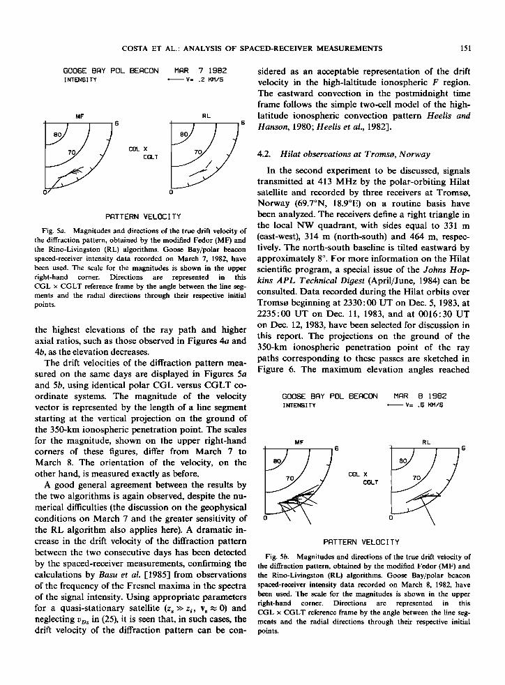
The anisotropies of the diffraction pattern ob- tained on March 7 and 8 are represented in Figures 4a and 4b, respectively. Each figure shows two sec- tors of a circle covering corrected geomagnetic lati- tudes (CGL) from 60 ø to 90 ø and corrected geomag- netic local times (CGLT) from 0000 to 0600. These sectors separately exhibit the results obtained using the modified-Fedor (MF) and the Rino-Livingston (RL) algorithms. Axial ratios are represented by the length of a line segment centered at the vertical pro- jection on the ground of the 350-km ionospheric pen- etration point of the ray path. On the upper right- hand corners of both figures, line segments corre- sponding to an axial ratio of 20 are shown. The orientations of the major axes of the anisotropy el- lipses are measured by the angle between the radial direction through each penetration point (indicating the local northward direction in the polar CGL x CGLT coordinate system) and the corre-
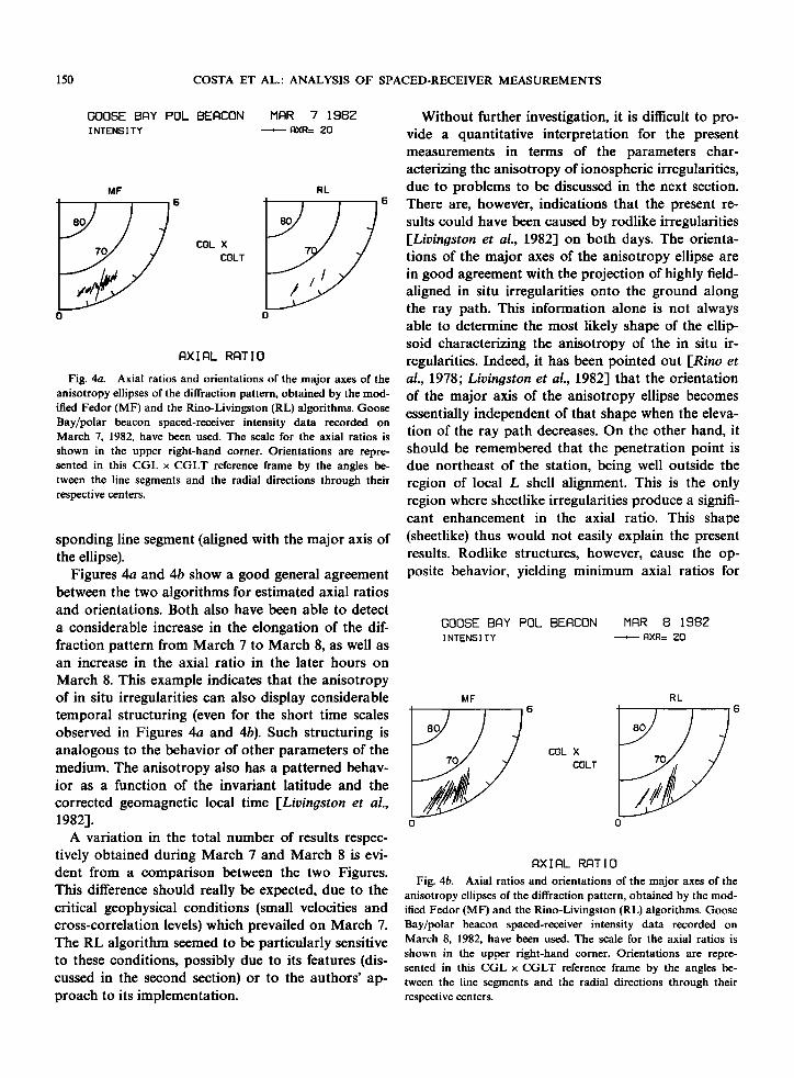
150 COSTA ET AL.: ANALYSIS OF SPACED-RECEIVER MEASUREMENTS
GOOSE BAY POL BEACON MAR '7 1987 INTENSITY , AXR= ZO
MF RL 6
COL X
COLT /
o o
AXIAL RATIO
Fig. 4a. Axial ratios and orientations of the major axes of the anisotropy ellipses of the diffraction pattern, obtained by the mod- ified Fedor (MF) and the Rino-Livingston (RL) algorithms. Goose Bay/polar beacon spaced-receiver intensity data recorded on March 7, 1982, have been used. The scale for the axial ratios is
shown in the upper right-hand corner. Orientations are repre- sented in this CGL x COLT reference frame by the angles be- tween the line segments and the radial directions through their respective centers.
sponding line segment (aligned with the major axis of the ellipse).
Figures 4a and 4b show a good general agreement between the two algorithms for estimated axial ratios and orientations. Both also have been able to detect
a considerable increase in the elongation of the dif- fraction pattern from March 7 to March 8, as well as an increase in the axial ratio in the later hours on
March 8. This example indicates that the anisotropy of in situ irregularities can also display considerable temporal structuring (even for the short time scales observed in Figures 4a and 4b). Such structuring is analogous to the behavior of other parameters of the medium. The anisotropy also has a patterned behav- ior as a function of the invariant latitude and the
corrected geomagnetic local time [Livingston et al., 1982].
A variation in the total number of results respec- tively obtained during March 7 and March 8 is evi- dent from a comparison between the two Figures. This difference should really be expected, due to the critical geophysical conditions (small velocities and cross-correlation levels)which prevailed on March 7. The RL algorithm seemed to be particularly sensitive to these conditions, possibly due to its features (dis- cussed in the second section) or to the authors' ap- proach to its implementation.
Without further investigation, it is difficult to pro- vide a quantitative interpretation for the present measurements in terms of the parameters char- acterizing the anisotropy of ionospheric irregularities, due to problems to be discussed in the next section. There are, however, indications that the present re- sults could have been caused by rodlike irregularities [Livingston et al., 1982] on both days. The orienta- tions of the major axes of the anisotropy ellipse are in good agreement with the projection of highly field- aligned in situ irregularities onto the ground along the ray path. This information alone is not always able to determine the most likely shape of the ellip- soid characterizing the anisotropy of the in situ ir- regularities. Indeed, it has been pointed out [Rino et al., 1978; Livingston et al., 1982] that the orientation of the major axis of the anisotropy ellipse becomes essentially independent of that shape when the eleva- tion of the ray path decreases. On the other hand, it should be remembered that the penetration point is due northeast of the station, being well outside the region of local L shell alignment. This is the only region where sheetlike irregularities produce a signifi- cant enhancement in the axial ratio. This shape (sheetlike) thus would not easily explain the present results. Rodlike structures, however, cause the op- posite behavior, yielding minimum axial ratios for
GOOSE BAY POL BEACON MAR 8 1982' INTENSITY , AXR= ZO
MF RL
COL X
7•a,// COLT
0 0
AXIAL RATIO
Fig. 4b. Axial ratios and orientations of the major axes of the anisotropy ellipses of the diffraction pattern, obtained by the mod- ified Fedor (MF) and the Rino-Livingston (RL) algorithms. Goose Bay/polar beacon spaced-receiver intensity data recorded on March 8, 1982, have been used. The scale for the axial ratios is
shown in the upper right-hand corner. Orientations are repre- sented in this COL x CGLT reference frame by the angles be- tween the line segments and the radial directions through their respective centers.
COSTA ET AL.: ANALYSIS OF SPACED-RECEIVER MEASUREMENTS 151
GOOSE BAY POL BEACON MAR 7 1982 sidered as an acceptable representation of the drift INIEN$IIY , V= .2 KM/$ velocity in the high-laltitude ionospheric F region.
The eastward convection in the postmidnight time frame follows the simple two-cell model of the high-
•r •t. latitude ionospheric convection pattern Heelis and s s Hanson, 1980; Heelis et al., 1982].
80 80
70 cot x 7o 4.2. Hilat observations at Tromso, Norway CELT
0• In the second experiment to be discussed, signals transmitted at 413 MHz by the polar-orbiting Hilat 0 satellite and recorded by three receivers at Tromso,
PATTERN VELOCI TY
Fig. 5a. Magnitudes and directions of the true drift velocity of the diffraction pattern, obtained by the modified Fedor (MF) and the Rino-Livingston (RL) algorithms. Goose Bay/polar beacon spaced-receiver intensity data recorded on March 7, 1982, have been used. The scale for the magnitudes is shown in the upper right-hand corner. Directions are represented in this CGL x CGLT reference frame by the angle between the line seg- ments and the radial directions through their respective initial points.
the highest elevations of the ray path and higher axial ratios, such as those observed in Figures 4a and 4b, as the elevation decreases.
The drift velocities of the diffraction pattern mea- sured on the same days are displayed in Figures 5a and 5b, using identical polar CGL versus CGLT co- ordinate systems. The magnitude of the velocity vector is represented by the length of a line segment starting at the vertical projection on the ground of the 350-km ionospheric penetration point. The scales for the magnitude, shown on the upper right-hand corners of these figures, differ from March 7 to March 8. The orientation of the velocity, on the other hand, is measured exactly as before.
A good general agreement between the results by the two algorithms is again observed, despite the nu- merical difficulties (the discussion on the geophysical conditions on March 7 and the greater sensitivity of the RL algorithm also applies here). A dramatic in- crease in the drift velocity of the diffraction pattern between the two consecutive days has been detected by the spaced-receiver measurements, confirming the calculations by Basu et al. [1985] from observations of the frequency of the Fresnel maxima in the spectra of the signal intensity. Using appropriate parameters for a quasi-stationary satellite (z s >> zi, Vs • 0) and neglecting v•>z in (25), it is seen that, in such cases, the drift velocity of the diffraction pattern can be con-
Norway (69.7øN, 18.9øE) on a routine basis have been analyzed. The receivers define a right triangle in the local NW quadrant, with sides equal to 331 m (east-west), 314 m (north-south) and 464 m, respec- tively. The north-south baseline is tilted eastward by approximately 8 ø. For more information on the Hilat scientific program, a special issue of the Johns Hop- kins APL Technical Digest (April/June, 1984)can be consulted. Data recorded during the Hilat orbits over Tromso beginning at 2330:00 UT on Dec. 5, 1983, at 2235:00 UT on Dec. 11, 1983, and at 0016:30 UT on Dec. 12, 1983, have been selected for discussion in
this report. The projections on the ground of the 350-km ionospheric penetration point of the ray paths corresponding to these passes are sketched in Figure 6. The maximum elevation angles reached
GOOSE BAY POL BEACON MAR 8 1982 INTENSITY , V= .S KM/S
MF RL
COL X
CELT
0
PATTERN VELOCI TY
Fig. 5b. Magnitudes and directions of the true drift velocity of the diffraction pattern, obtained by the modified Fedor (MF) and the Rino-Livingston (RL) algorithms. Goose Bay/polar beacon spaced-receiver intensity data recorded on March 8, 1982, have been used. The scale for the magnitudes is shown in the upper right-hand corner. Directions are represented in this CGL x CGLT reference frame by the angle between the line seg- ments and the radial directions through their respective initial points.
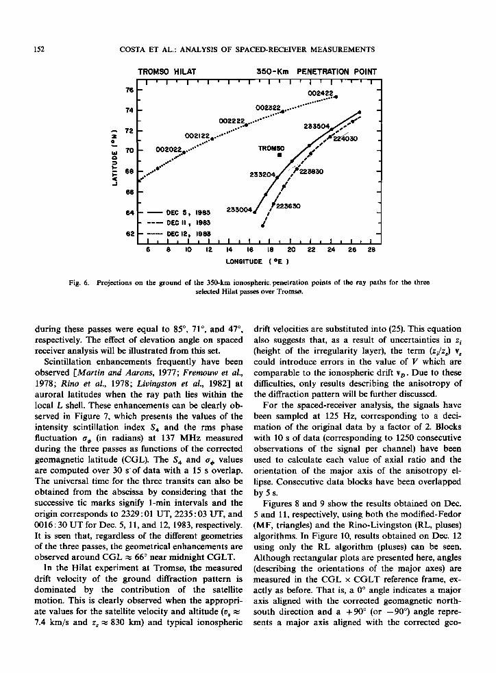
152 COSTA ET AL.: ANALYSIS OF SPACED-RECEIVER MEASUREMENTS
Fig. 6.
TROMSO HILAT $50-Km PENETRATION POINT
76
eeeeee
ooz..z. .............. _ I- - -
• L 002022. ..... '"' TROMSO /A.•,' _ ---/-.:-:"" ß ./I' _ ß e ee ß ß '
..... :
''f' A ./ o,c,,,,,, h'"-
62
6 8 I0 12 14 16 18 20 22 24 26 28
LONGITUDE ( øE )
Projections on the ground of the 350-km ionospheric. penetration points of the ray paths for the three selected Hilat passes over Tromse.
during these passes were equal to 85 ̧ , 71 ̧ , and 47 ̧ , respectively. The effect of elevation angle on spaced receiver analysis will be illustrated from this set.
Scintillation enhancements frequently have been observed [Martin and Aarons, 1977; Frernouw et al., 1978; Rino et al., 1978; Livingston et al., 1982] at auroral latitudes when the ray path lies within the local L shell. These enhancements can be clearly ob- served in Figure 7, which presents the values of the intensity scintillation index S,• and the rms phase fluctuation a, (in radians) at 137 MHz measured during the three passes as functions of the corrected geomagnetic latitude (CGL). The S,• and c, values are computed over 30 s' of data with a 15 s overlap. The universal time for the three transits can also be
obtained from the abscissa by considering that the successive tic marks signify 1-min intervals and the origin corresponds to 2329:01 UT, 2235:03 UT, and 0016:30 UT for Dec. 5, 11, and 12, 1983, respectively. It is seen that, regardless of the different geometries of the three passes, the geometrical enhancements are observed around CGL ,• 66 ̧ near midnight CGLT.
In the Hilat experiment at Tromso, the measured drift velocity of the ground diffraction pattern is dominated by the contribution of the satellite motion. This is clearly observed when the appropri- ate values for the satellite velocity and altitude (rs • 7.4 km/s and zs ,• 830 km) and typical ionospheric
drift velocities are substituted into (25). This equation also suggests that, as a result of uncertainties in zi (height of the irregularity layer), the term (zi/z,) v, could introduce errors in the value of V which are
comparable to the ionospheric drift v D. Due to these difficulties, only results describing the anisotropy of the diffraction pattern will be further discussed.
For the spaced-receiver analysis, the signals have been sampled at 125 Hz, corresponding to a deci- mation of the original data by a factor of 2. Blocks with 10 s of data (corresponding to 1250 consecutive observations of the signal per channel) have been used to calculate each value of axial ratio and the
orientation of the major axis of the anisotropy el- lipse. Consecutive data blocks have been overlapped bySs.
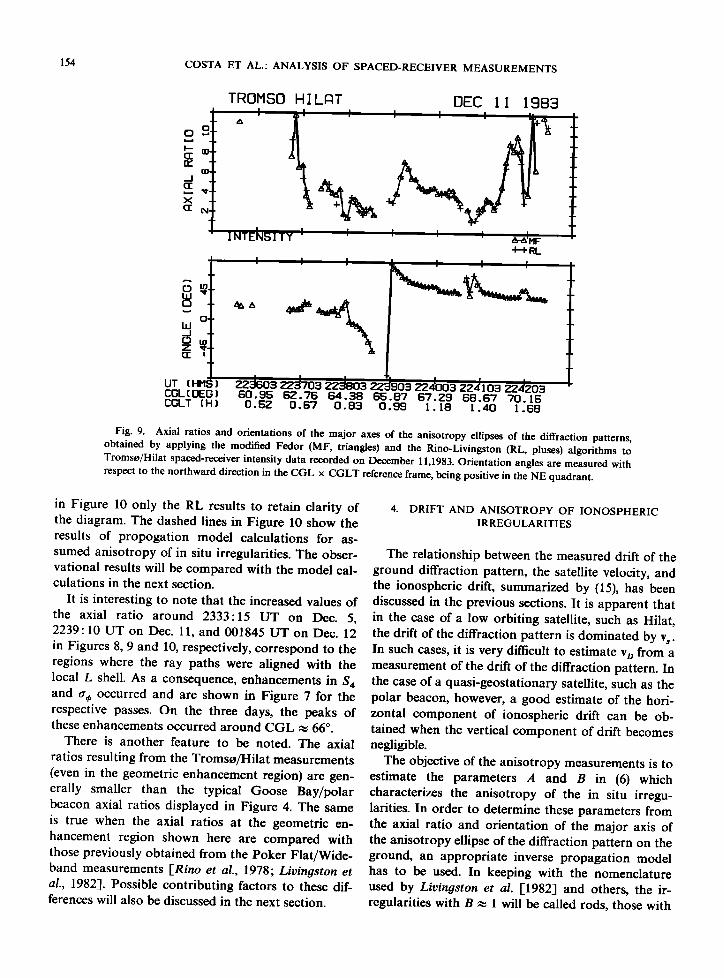
Figures 8 and 9 show the results obtained on Dec. 5 and 11, respectively, using both the modified-Fedor (MF, triangles) and the Rino-Livingston (RL, pluses) algorithms. In Figure 10, results obtained on Dec. 12 using only the RL algorithm (pluses) can be seen. Although rectangular plots are presented here, angles (describing the orientations of the major axes) are measured in the CGL x CGLT reference frame, ex- actly as before. That is, a 0 ̧ angle indicates a major axis aligned with the corrected geomagnetic north- south direction and a + 90 ̧ (or -90 ¸) angle repre- sents a major axis aligned with the corrected geo-
_
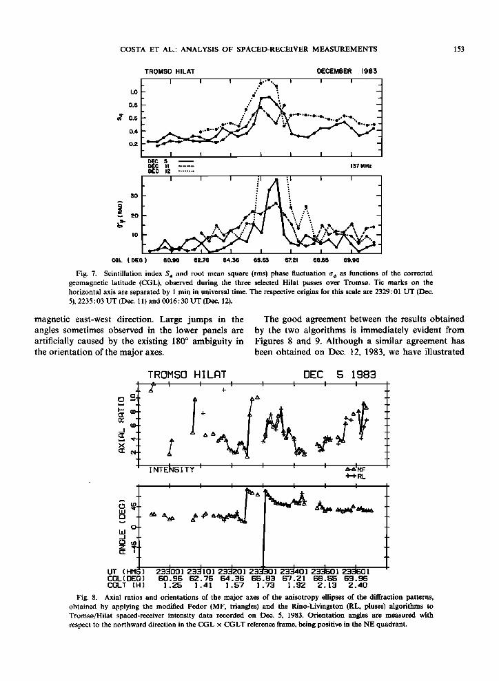
COSTA ET AL.' ANALYSIS OF SPACED-RECEIVER MEASUREMENTS 153
TROMSO HILAT DECEMBER 198:5
L I I I •,..,m,. I I I 1.0 ø '
0.• /' •:• • m 0.6 • • • • -•-• •" '•'.e' "
[.X 0., ..' • • •
/ I I I I i I I - DEC 5 DEC II .... 157MHz DEC 12 ........
. I I I :1• :1 I I ß • ...... . . .•• • s •
CGL ( DEG ) 60.96 62.76 64.56 65.• 67.21 68.55 69.96
Fig. 7. Scintillation index S• and root mean square (rms) phase fluctuation • as functions of the corrected geomagnetic latitude (CGL), observed during the three selected Hilat passes over Tromse. Tic marks on the horizontal axis are separated by 1 min in universal time. The respective orions for this scale are 2329:01 UT (Dec. 5), 2235:03 UT (Dec. 11) and •16:30 UT (Dec. 12).
magnetic east-west direction. Large jumps in the angles sometimes observed in the lower panels are artificially caused by the existing 180 ø ambiguity in the orientation of the major axes.
The good agreement between the results obtained by the two algorithms is immediately evident from Figures 8 and 9. Although a similar agreement has been obtained on Dec. 12, 1983, we have illustrated
z C[ m
UT ( HM: ) COL ( DEG ) COLT (H)
TROHSO HI Lg:IT
,
iNTEnSiTY I ) I )
i I I I I ,
DEC S 1983 I I I I I I
I • RL
I I
Fig. 8. Axial ratios and orientations of the major axes of the anisotropy ellipses of the diffraction patterns, obtained by applying the modified Fedor (MF, triangles) and the Rino-Livingston (RL, pluses) algorithms to Tromso/Hilat spaced-receiver intensity data recorded on Dec. 5, 1983. Orientation angles are measured with respect to the northward direction in the CGL x CGLT reference frame, being positive in the NE quadrant.
154 COSTA ET AL.: ANALYSIS OF SPACED-RECEIVER MEASUREMENTS
X -
(• (•1-
z
UT (HM: } CGL ( OEG ) COLT (H)
TROM$O
I NTEmXisI TY I
HILAT
I I I
DEC 11 1983
I i I • RL
zztoo zz, zzzo 87 67.z9 68.67 70.16
Fig. 9. Axial ratios and orientations of the major axes of the anisotropy ellipses of the diffraction patterns, obtained by applying the modified Fedor (MF, triangles) and the Rino-Livingston (RL, pluses) algorithms to Tromso/Hilat spaced-receiver intensity data recorded on December 11,1983. Orientation angles are measured with respect to the northward direction in the CGL x CGLT reference frame, being positive in the NE quadrant.
in Figure 10 only the RL results to retain clarity of the diagram. The dashed lines in Figure 10 show the results of propogation model calculations for as- sumed anisotropy of in situ irregularities. The obser- vational results will be compared with the model cal- culations in the next section.
It is interesting to note that the increased values of the axial ratio around 2333:15 UT on Dec. 5, 2239:10 UT on Dec. 11, and 001845 UT on Dec. 12 in Figures 8, 9 and 10, respectively, correspond to the regions where the ray paths were aligned with the local L shell. As a consequence, enhancements in S,• and t% occurred and are shown in Figure 7 for the respective passes. On the three days, the peaks of these enhancements occurred around CGL • 66 ø.
There is another feature to be noted. The axial ratios resulting from the Tromso/Hilat measurements (even in the geometric enhancement region) are gen- erally smaller than the typical Goose Bay/polar beacon axial ratios displayed in Figure 4. The same is true when the axial ratios at the geometric en- hancement region shown here are compared with those previously obtained from the Poker Flat/Wide- band measurements [Rino et al., 1978; Livingston et al., 1982]. Possible contributing factors to these dif- ferences will also be discussed in the next section.
4. DRIFT AND ANISOTROPY OF IONOSPHERIC IRREGULARITIES
The relationship between the measured drift of the ground diffraction pattern, the satellite velocity, and the ionospheric drift, summarized by (15), has been discussed in the previous sections. It is apparent that in the case of a low orbiting satellite, such as Hilat, the drift of the diffraction pattern is dominated by v s . In such cases, it is very difficult to estimate vo from a measurement of the drift of the diffraction pattern. In the case of a quasi-geostationary satellite, such as the polar beacon, however, a good estimate of the hori- zontal component of ionospheric drift can be ob- tained when the vertical component of drift becomes negligible.
The objective of the anisotropy measurements is to estimate the parameters A and B in (6) which characterizes the anisotropy of the in situ irregu- larities. In order to determine these parameters from the axial ratio and orientation of the major axis of the anisotropy ellipse of the diffraction pattern on the ground, an appropriate inverse propagation model has to be used. In keeping with the nomenclature used by Livingston et al. [1982] and others, the ir- regularities with B • 1 will be called rods, those with

COSTA ET AL.: ANALYSIS OF SPACED-RECEIVER MEASUREMENTS 155
TROMSO HILAT DEC 12 198•5
UT (HMS)
CGL ( DEG ) 65.24 66.60 67.80 68.87 69.90 70.9:5 71.94
CGLT (H) 1.52 1.75 1.99 2.24 2.51 2.8:5 $.21
• I I I i i i i 4
I I I I I I I
• I RL
PHASE ..... MODEL
• •;,•ii ['"'I ' , , , ' , I ' iil ! •11 i I - '11 ' ! ! ! • 45 ,I • , -
,., 0
JJ I * .L.,, ] .•! il• i:•le,..,•l• -
O01850 O01950 00•050 00•1 $0 00• $0 00'•$•) 00•4:50
Fig. 10. Axial ratios and orientations of the major axes of the anisotropy ellipses of the diffraction pattern, obtained by applying the Rino-Livingston (RL, pluses) algorithm in Tromse/Hilat spaced-receiver phase data recorded on December 12, 1983. Orientation angles are measured with respect to the northward direction in the CGL x CGLT reference frame, being positive in the NE quadrant. Dashed lines show results of calculations by the propagation model, using the values for A and B displayed in Figure 11.
A • B > 1 will be referred as sheets and those with
A > B > 1 as wings. The isotropic irregularities will be described by A • B • 1.
It has been shown in the discussion on (18) and (19) that the anisotropy ellipse of the diffraction pat- tern is the geometrical projection along the ray path onto the ground of the ellipsoid defining the ani- sotropy of the in situ irregularities. Since different ellipsoids could project onto the same ellipse, it is not possible to associate a unique pair (A, B) to each single observation of the axial ratio and orientation of the major axis of the anisotropy ellipse. However, it should be possible, under a few obvious conditions, to reconstruct a single ellipsoid from multiple projec- tions on the ground. First, the projections should all correspond to the same ellipsoid. Further, it is neces- sary that these projections be reasonably different from each other. That is, they should correspond to reasonably different ray paths.
These conditions are not easily met in the case of a quasi-geostationary satellite where the ray path moves very slowly, penetrating the ionosphere at ap- proximately constant aspect angles. In view of this,
we shall not attempt to derive a more quantitative estimate of the anisotropy of the in situ irregularities for the Goose Bay/polar beacon experiment.
In the case of a low-orbiting satellite, the ray path experiences fast variations in azimuth and elevation. This is one of the desired conditions which has been
established above. However, the underlying con- straint to preserve the anisotropy of the in situ ir- regularities requires the measurement set to en- compass a small spatial scan of the ionosphere.
Consistent with these conflicting requirements, an average ionospheric anisotropy can be estimated from the minimum adequate number of observations of the anisotropy ellipse of the diffraction pattern by an inversion of the propagation model.
5.1. Irregularity anisotropy by error minimization procedure
In this section, we shall attempt to determine the anisotropy coefficients A and B through the mini- mization of the rms errors between measured and
calculated (by the model) values of the axial ratio

156 COSTA ET AL.' ANALYSIS OF SPACED-RECEIVER MEASUREMENTS
and the orientation of the major axis of the ani- sotropy ellipse of the diffraction pattern. More pre- cisely, given a set of consecutive observations (R., W,), n = 1, ..., No, it is desired to find (A, B) in the region A > B > 1 (since the irregularities are sup- posed to be preferentially elongated along the geo- magnetic field lines) which minimizes
No
e = • {JR,cos 2W,-- r(A, B' p.) cos 2½(A, B; p,)]2
+ JR,sin 2W,-- r(A, B' p, sin 2½(A, B' p,)]2} No
-- • {[R.- r(A, B' p.)]2 + 4R.r(A, B' p.)
ß sin 2 [kii n -- ½(A, B' Pn)]} (22)
where r (A, B; Pn) and ½ (A, B; Pn) are the respective values of the axial ratio and the orientation of the
diffraction pattern calculated by the model as func- tions of A, B and Pn' The vector Pn gathers all the remaining parameters of the model (such as the height of the penetration point, azimuth and eleva- tion of the ray path, geomagnetic field declination and dip angle, and so on), assumed to be known at the instant of time t n that the pair (Rn, tPn) has been observed (n = 1, ..., No). The angles in the first part of (22) are multiplied by 2 to account for the 180 ø ambiguity in the orientation of the major axis of the anisotropy ellipse. It is seen that the final expression for e displays the intuitively desired properties' the rms error tends to zero when, simultaneously, mea- sured and calculated axial ratios are equal and mea- sured and calculated orientations differ by an arbi- trary integer multiple of 180 ø . It should also be ob- served that the value found for e at the solution (A, B) can be considered as an indicator of its quality' the higher the error is, the less reliable the solution is.
A computer code to minimize (22) has been imple- ,
mented by combining the propagation model already described with subroutine ZXSSQ, available from the International Mathematical Subroutine Library (IMSL). This subroutine is based on a derivative-free analogue of the Levenberg-Marquardt algorithm for nonlinear least squares approximation [Brown and Dennis, 1972]. To guarantee that the solutions are constrained to the region A > B > 1, the following transformation has been used
A= 1 +(A 0-- 1) sin 2t (23a)
B= 1 +(A o-- 1) sin 2u (23b)
where A 0 is an arbitrarily large constant. The mini- mization is initially performed over the un- constrained two-dimensional space (t, u), the solution being then substituted back into (23) to calculate the desired anisotropy of the in situ irregularities.
This procedure has been tested initially using arti- ficial data. In order to generate this data set, irregu- larities with known anisotropy (A, B) were uniformly distributed through the ionosphere. Next an artificial satellite mimicking a Hilat orbit was allowed to scan through the ionosphere. By the use of the propaga- tion model, the ground diffraction pattern was artifi- cially generated and the axial ratio and orientation of the diffraction pattern determined. The error mini- mization procedure, outlined above, was next used in conjunction with the inverse propagation model to recover the assumed values of A and B. The tests
were successful in all three types of assumed aniso- tropies.
The minimization procedure has been applied to results obtained by the Rino-Livingston algorithm operating on Tromso Hilat data and shown in Figure 10. Here, three consecutive observations (R,,, Win), m = M- 1, M, M + 1 have been used to esti- mate the values for A and B at the instant of time
corresponding to the central observation (m = M). M has then been incremented by 1 and the process has been successively repeated until the data have been exhausted. The estimated values for these parameters are shown in Figure 11. These values have also been applied to the model to calculate the corresponding parameters of the anisotropy ellipse of the diffraction pattern. The calculated axial ratios and orientations are shown in Figure 10 (dashed curve). The good agreement between measured and calculated aniso- tropies of the diffraction pattern is evident.
There are reasons to believe that the most out-
standing features in Figure 11 (a 20: 16: 1 sheet at 0018:30 UT and a winglike structure immediately after 0022:30 UT) are not real, but are artificially generated when the inversion of the model becomes unstable. The examples in Livingston et al. [1982] also indicate that there are regions along the passes (where the elevation angles of the ray paths are gen- erally low) in which the model predicts very similar values of axial ratios (and orientations) from very different combinations of A and B.
Apart from these regions, Figure 11 shows a com- plex structuring of the F region irregularities, with moderate to small sheets (particularly in the geo- metrical enhancement region, around 0018:45 UT)

COSTA ET AL.: ANALYSIS OF SPACED-RECEIVER MEASUREMENTS 157
TROMSO HILAT DEC 12 198:5 I I i I I I :1
.
zo
16
4
AS
ZO
16
8
4
UT ( HMS ) 001850 001950 002030 002,130 002250 002330 002430
CGL ( DEG ) 65.24 66.60 67.80 68.87 69.90 70.9:5 71.94
CGLT (H) 1.52 1.75 1.99 2.24 2.51 2.8:5
Fig. 11. Values for the parameters A and B characterizing the anisotropy of the in situ irregularities, obtained from the application of the minimization procedure to the Rino-Livingston (RL, pluses) results shown in Figure 10.
giving way to moderate to small rods or isotropic irregularities at later times (northward of Tromso). Further, from a comparison between the axial ratios in Figures 8-10, one would expect a similar behavior of the irregularities on the other 2 days. High axial ratios are obtained in the region of local L shell alignment due to the presence of sheetlike irregu- larities. In addition, there is a clear indication of the presence of rodlike irregularities northward of Tromso on these days (later than 2335:30 UT on December 5, 1983, and 2241:03 UT on December 11, 1983). These results thus seem to reproduce at Tromso those results which emerged from the Poker Flat/Wideband experiment [Livingston et al., 1982].
The present example thus shows encouraging re- sults of a numerical technique to estimate the ani- sotropy of in situ irregularities from the measure- ments of analogous parameters of the ground diffrac- tion pattern. A study is being initiated to better characterize its sensitivity to perturbations in the input data and its ability to converge to correct solu- tions for a large set of practical conditions.
Comparing each of the time histories of the rms phase fluctuation a• or the scintillation index S,• (shown in Figure 7) with that of the axial ratio mea-
sured on the same day (respectively shown in Figures 8-10), one can observe the importance of the ani- sotropy in relation to the scintillation magnitudes. Since the axial ratio does not depend on the strength of the irregularities, the observed enhancements of S,• and a• result from the geometrical factors that are sensitively controlled by the anisotropy parameters.
The elongations of the irregularities inferred from Figures 8-10 are considerably smaller than those de- tected by the Goose Bay/polar beacon measurements previously discussed (particularly those obtained on March 8, 1982). They also seem to be typically smaller than the elongations resulting from the Wi- deband program [Livingston et al., 1982].
An explanation for smaller-than-expected values of the axial ratio of the ground diffraction pattern in- volves effects of the distances between the receivers
on the measurements. Golley and Rossiter [1970] have used an array of 89 dipoles filling a circle of diameter 1 km (with the dipoles located at the nodes of a 91.4-me grid) to (1) compare results from the spatial correlation analysis [Briggs, 1968] with those from the temporal correlation analysis of spaced- receiver data, and (2) compare results from the tem- poral correlation analysis, using different receiver
158 COSTA ET AL.' ANALYSIS OF SPACED-RECEIVER MEASUREMENTS
layouts. Some of their findings on the behaviors of the parameters of the ground diffraction pattern can be summarized as follows: (1) the drift velocities re- sulting from the temporal correlation analysis in- crease with the triangle size, tending however to a limiting value which is very nearly equal to the drift velocity obtained from the spatial correlation tech- nique; (2) the directions of the drift velocity obtained from the temporal correlation technique have not shown any systematic dependence on the triangle size, being in good agreement with the respective values calculated by the other technique; (3) the scale of the correlation ellipses, defined as their radius in the direction of the drift, varies with increasing trian- gle sizes, in a similar manner to that of the drift velocity; (4) the major axis of the correlation ellipse tends to be aligned along the triangle hypotenuse for small triangles, but this tendency decreases as the size of the triangle increases; (5) the size of the triangle at which the drift velocity reaches a limiting value de- pends on the scale of the pattern. Although vari- ations of the measured axial ratios with the triangle size have not been explicity studied in that reference, the above results, at least, leave the door open to this relationship. In addition, the observation of irregu- larity fluctuations with large scale sizes by small triangles would result in essentially equal received signals, with negligible time delays between similar structures detected in different channels. In this situ-
ation, the spaced-receiver analysis would tend to identify a larger number of isotropic diffraction pat- terns than it should. On the other hand, when the separations between the antennas become very large, there is an increasing possibility that structures de- tected by one ray path be missed by at least one of the other ray paths. There would then be very little correlation between the signals and the spaced- receiver analysis would break down. It should be noted that, in a power-law environment, the former situation is potentially more damaging, since large structures also carry more power.
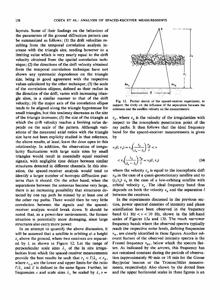
In an attempt to quantify the above discussion, it will be assumed that a satellite is orbiting at a height z s above the ground, where two receivers are separat- ed by l, as shown in Figure 12. Let the range of perpendicular scale sizes 2•_ of the in situ irregu- larities from which the spaced-receiver measurements provide the best results be such that r• < 1'/2•_ < r 2 , where r•. 2 are the lower and upper limits for the ratio l'/2_• and 2' is defined in the same figure. Further, let frequencies v and scale sizes 2•_ be scaled by 2_• v =
s
Rx I Rx 2 _
ß .
Fig. 12. Partial sketch of the spaced-receiver experiment, to support the study on the influence of the separation between the antennas and the satellite velocity on the measurements.
vp, where vp is the velocity of the irregularities with respect to the ionospheric penetration point of the ray paths. It then follows that the ideal frequency band for the spaced-receiver measurements is given by
vi(l; ri) = ri -- < v Z s -- Z i l
< r 2 • = v2(l; r•) (24) Z s -- Z i
where the velocity up is equal to the ionospheric drift uo in the case of a quasi-geostationary satellite and to (zi/Zs).U s in the case of a low-orbiting satellite with orbital velocity u s . The ideal frequency band thus depends on both the velocity % and the separation l between the receivers.
In the experiments discussed in the previous sec- tion, power spectral densities of intensity and phase scintillation have been observed in the frequency band 0.1 Hz < v < 10 Hz, shown in the left-hand scales of Figures 13a and 13b. The much narrower frequency bands where the observed spectra typically reach the respective noise levels, defining frequencies v•, are clearly identified in these figures. Another rel- evant feature of the observed intensity spectra is the Fresnel &equency v r•, below which the spectra flat- ten. As indicated by the arrows, this frequency has not remained constant during the periods of observa- tion (approximately 90 min or 10 min for the Goose Bay/polar beacon or the Tromso/Hilat measure- ments, respectively). Also shown by the dotted lines and the upper horizontal scales in these figures is an
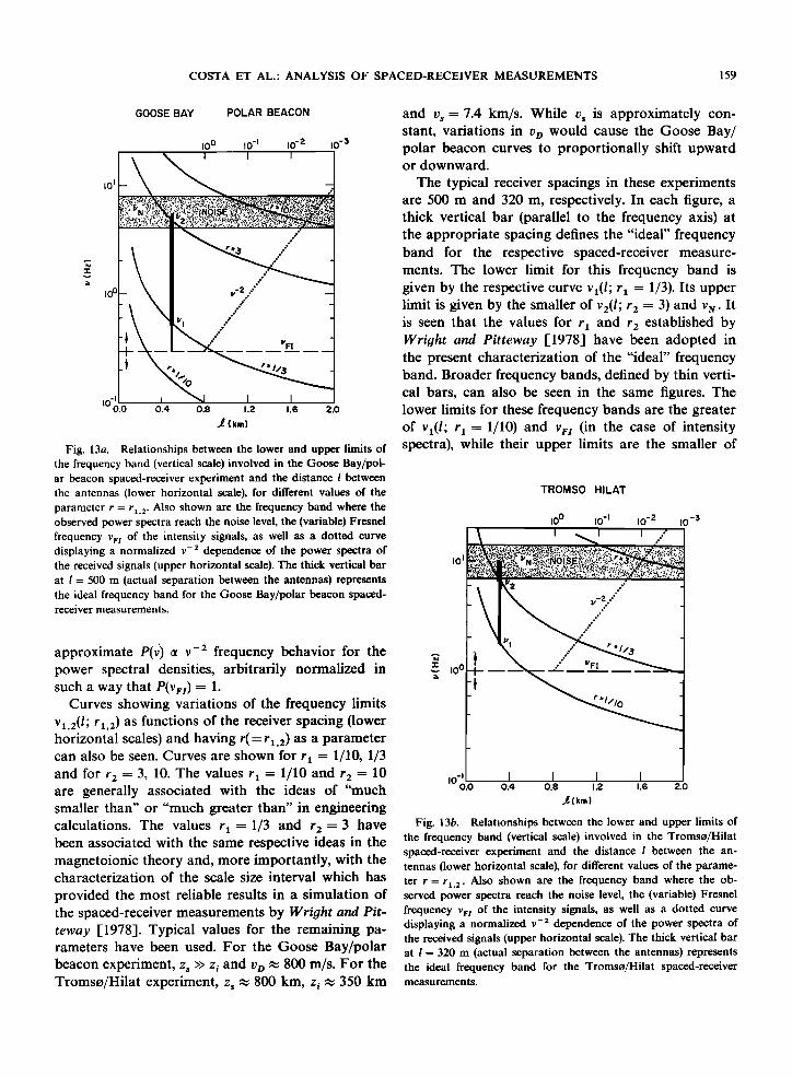
COSTA ET AL.' ANALYSIS OF SPACED-RECEIVER MEASUREMENTS 159
GOOSE BAY POLAR BEACON
I0 0 I0 -I I0 -2 I0 -:5
I01
I0 o
0.4 0.8 1.2 1.6 2.0
• (km)
Fig. 13a. Relationships between the lower and upper limits of the frequency band (vertical scale) involved in the Goose Bay/pol- ar beacon spaced-receiver experiment and the distance I between the antennas (lower horizontal scale), for different values of the
parameter r = r•. 2. Also shown are the frequency band where the observed power spectra reach the noise level, the (variable) Fresnel frequency vr• of the intensity signals, as well as a dotted curve displaying a normalized v -2 dependence of the power spectra of the received signals (upper horizontal scale). The thick vertical bar at I = 500 m (actual separation between the antennas) represents the ideal frequency band for the Goose Bay/polar beacon spaced- receiver measurements.
approximate P(•) c• v -2 frequency behavior for the power spectral densities, arbitrarily normalized in such a way that P(vFt ) - 1.
Curves showing variations of the frequency limits v•,2(/; r•,2) as functions of the receiver spacing (lower horizontal scales) and having r(= r•,2) as a parameter can also be seen. Curves are shown for r• = 1/10, 1/3 and for r 2 = 3, 10. The values rx = 1/10 and r 2 = 10 are generally associated with the ideas of "much smaller than" or "much greater than" in engineering calculations. The values rx = 1/3 and r 2 = 3 have been associated with the same respective ideas in the magnetoionic theory and, more importantly, with the characterization of the scale size interval which has
provided the most reliable results in a simulation of the spaced-receiver measurements by Wright and Pit- teway [1978]. Typical values for the remaining pa- rameters have been used. For the Goose Bay/polar beacon experiment, z s >> z i and vt• • 800 m/s. For the Tromso/Hilat experiment, z s • 800 km, zi • 350 km
and Vs = 7.4 km/s. While Vs is approximately con- stant, variations in v•> would cause the Goose Bay/ polar beacon curves to proportionally shift upward or downward.
The typical receiver spacings in these experiments are 500 m and 320 m, respectively. In each figure, a thick vertical bar (parallel to the frequency axis) at the appropriate spacing defines the "ideal" frequency band for the respective spaced-receiver measure- ments. The lower limit for this frequency band is given by the respective curve v•(l; r• = 1/3). Its upper limit is given by the smaller of v2(/; r 2 = 3) and v•. It is seen that the values for r• and r 2 established by Wri•tht and Pitteway [1978] have been adopted in the present characterization of the "ideal" frequency band. Broader frequency bands, defined by thin verti- cal bars, can also be seen in the same figures. The lower limits for these frequency bands are the greater of v•(l; r• = 1/10) and vF• (in the case of intensity spectra), while their upper limits are the smaller of
TROMSO HILAT
i01
i0 -I 0.0
I0 0 I0 '1 10-2 I0-$
5 •o o
0.4 0.8 1.2 1.6 2.0
.,• (krn)
Fig. 13b. Relationships between the lower and upper limits of the frequency band (vertical scale) involved in the Tromso/Hilat spaced-receiver experiment and the distance I between the an- tennas (lower horizontal scale), for different values of the parame- ter r = r•. 2. Also shown are the frequency band where the ob- served power spectra reach the noise level, the (variable) Fresnel frequency vr• of the intensity signals, as well as a dotted curve displaying a normalized v -2 dependence of the power spectra of the received signals (upper horizontal scale). The thick vertical bar at I-- 320 m (actual separation between the antennas) represents the ideal frequency band for the Tromso/Hilat spaced-receiver measurements.
160 COSTA ET AL.: ANALYSIS OF SPACED-RECEIVER MEASUREMENTS
v2(/; r 2 --10) and v•v. Since scale sizes reasonably larger than the respective receiver spacing are now considered, a degradation of the results from the spaced-receiver analysis applied over this broader frequency band is more likely to occur, according to the above reasoning.
Finally, note that the "ideal" frequency band for the spaced-receiver analysis is relatively well matched with the available frequency band (between vv• nd vN) for scintillation observations in the case of the Goose
Bay/polar beacon experiment. The relative mismatch between these two frequency bands in the case of the Tromso/Hilat measurements could be partially re- sponsible for the small axial ratios obtained for the anisotropy ellipse of the diffraction pattern. One ob- vious way of obtaining a better match between these two frequency bands is to bandpass filter the original signals to reject the components outside the "ideal" frequency band as much as possible. One alternative to this procedure would be to apply the spectral analysis of spaced-receiver data described in the com- panion paper [Costa and Fougere, 1987] upon the "ideal" frequency band only. Figure 13b shows, how- ever, that neither solution is totally effective in the present case, since both are equivalent to rejecting a very high percentage of the total available power. Nevertheless, in support of the above arguments, one of the examples (using Tromso/Hilat data recorded on December 5, 1983) of the application of the spec- tral analysis upon a slightly broader frequency band than the "ideal" has shown an increase in the axial
ratio around the geometrical enhancement region. The present arguments could also explain the ap-
parently higher axial ratios resulting from the Poker Flat/Wideband measurements. While the relevant parameters of the Wideband and Hilat satellites were similar, the typical antenna separation at Poker Flat was approximately equal to 900 m. This is a more favorable situation to spaced-receiver measurements employing such a low-orbiting satellite as the source of the signals, as a diagram analogous to that in Figure 13b would show.
6. SUMMARY
Two algorithms which provide a statistical treat- ment to the estimation of the parameters of the spaced-receiver analysis have been reviewed in this contribution. Both operate on the autocorrelation and cross-correlation functions of the received sig- nals, which are modeled by a decreasing function of
two spatial variables (representing distances between receivers) and the time delay, all combined into a positive-definite quadratic form. That is, it is as- sumed that, for a fixed instant of time, lines of con- stant correlation levels define ellipses, which characterize the anisotropy of the ground diffraction pattern.
In general, a good agreement has been found be- tween the results from the two algorithms. However, in a relatively small percentage of the observations, at least one of the algorithms has collapsed or a difference has been detected between their results. It
has been shown [McGee, 1966; Briggs and Golley, 1968; Wernik et al., 1983] that random or regular velocity changes along the ray path could be trans- lated into cross-correlation functions which are not
symmetric around their maxima, thus leading to a disagreement between the data and the present model, represented by (1). Also, the algorithm sug- gested by Rino and Livingston [1982] uses only the time delays for the maxima and the crossings of the correlation functions to estimate the anisotropy and the drift velocity of the diffraction pattern. On the other hand, the generalized version of the Fedor [1967] algorithm presented here uses the information provided by the correlation functions more fully. This disagreement between the data and their model and the different approaches of the algorithms to the same estimation problem are the most likely expla- nations for the observed differences in their results.
The spaced-receiver analysis of signals transmitted from a quasi-geostationary polar beacon and re- ceived at Goose Bay has shown a great variability in the anisotropy and the drift velocity of the diffraction pattern observed on 2 consecutive days. Variations of these parameters on shorter time scales have also been detected. Relatively high axial ratios of the ani- sotropy ellipse of the diffraction pattern have been observed. Considering the relatively low elevation angles of the ray paths (approximately 45ø), these values seem to indicate the presence of rodlike in situ irregularities northward of Goose Bay. Further, the essentially eastward drift velocities measured on both days between 0400 UT and 0530 UT follow the pat- tern of eastward plasma drift in the auroral zone during this time sector [Heelis and Hanson, 1980; Heelis et al., 1982].
Signals transmitted by the Hilat satellite and re- ceived at Tromso have also been analyzed. The re- sults seem to reproduce those observed during the Poker Flat/Wideband experiment [Frernouw et al.,

COSTA ET AL.: ANALYSIS OF SPACED-RECEIVER MEASUREMENTS 161
1977; Rino et al., 1978; Livingston et al., 1982]. That is, enhancements of the axial ratio are observed
around the region of local L shell alignment of the ray path, indicating the presence of sheetlike irregu- larities. Further, the observed increase of the axial ratio at the later parts of the orbits selected for analysis indicates the existence of rodlike irregu- larities northward of Tromso. Analogous behaviors have also been observed in the scintillation index S,• and in the rms phase fluctuation a,. Within the scope of the present theory, the axial ratio does not depend on the strength of the in situ irregularities. The above result thus seems to indicate that changes in the anisotropy of the irregularities may play an important role in the observed variations in S4 and
It has also been observed that the axial ratios re-
sulting from the Tromso/Hilat measurements are smaller than their equivalents from the Goose Bay/ polar beacon or the Poker Flat/Wideband experi- ments. Since different receiver separations and/or sat- ellites with different velocities have been employed, these experiments sample irregularities with different scale sizes. Any dependence of the anisotropy of the in situ irregularities on their scale sizes (caused, for instance, by mechanisms responsible for their gener- ation or removal) could, in principle, be translated into differences in the axial ratios. It is not clear,
however, whether such a dependence would be strong enough to explain the above observations. Further, structures with scale sizes much larger than those which would be ideally sampled by the particu- lar experiment would be detected by all the receivers almost simultaneously, thus tending to indicate the presence of more isotropic irregularities. This mecha- nism is reinforced by the fact that, in a power-law environment, structures with larger scale sizes also carry more power. It has been indicated that the Tromso/Hilat experiment, due to the relatively small separations between the receivers, seems to have been particularly affected by this mechanism.
Finally, a simple propagation model of the spaced- receiver experiment has been presented. It has shown that the anisotropy ellipses of the diffraction pattern are geometrical projections along the ray path onto the ground of the assumed ellipsoids which characterize the anisotropy of the in situ irregu- larities. Since a continuum of ellipsoids project onto the same ellipse, it is not theoretically possible to associate a unique set of parameters specifying the anisotropy of the irregularities to each observation of
the anisotropy of the ground diffraction pattern. A numerical technique has been proposed which associ- ates an average anisotropy of a volume in the iono- spheric F region to multiple observations of the ani- sotropy ellipse of the diffraction pattern. A nonlinear minimization of the rms error between measured and
calculated (by the propagation model) values of this parameter is used in this procedure. The importance of using observations of the anisotropy ellipse corre- sponding to ray paths which penetrate the iono- sphere with reasonably different aspect angles has been emphasized. When this condition is not met, the procedure becomes very unstable, and small pertur- bations in the data could lead to large departures from the true value of the anisotropy of the F region irregularities. Thus to use this procedure more ef- fectively in the future, it is important, as a continu- ation of the present work, to define its stability region more precisely.
Acknowledgments. This work has been performed while E.C. was on a sabbatical leave of absence from CETUC-PUC/RJ, Rio de Janeiro, Brazil. He would like to thank his colleagues and friends from the Physics Research Division, Emmanuel College, and the Ionospheric Effects Branch, Air Force Geophysics Lab- oratory, for the stimulating scientific environment and the contin- ued demonstrations of hospitality during this period. The dis- cussions within the Hilat scientific community have also been greatly appreciated. The authors thank Sunanda Basu for her genuine interest and many valuable suggestions, which led to im- provements in the present work. They also wish to acknowledge the essential role of Elizabeth Galligan in the tedious and time- consuming preprocessing of the data. The work at Emmanuel College was partially supported by AFGL contract F1928-86-K- 0038, and by an AFGL laboratory director's fund, ILIR 5B01.
REFERENCES
Armstrong, J. W., and W. A. Coles, Analysis of three-station inter- planetary scintillation, J. Geophys. Res., 77, 4602-4610, 1972.
Banerji, R. B., Radio-measurements of ionospheric drift as a prob- lem in parameter estimation, in Statistical Methods in Radio Wave Propagation, edited by W. C. Hoffman, Pergamon, New York, 1960.
Basu, S., Su. Basu, J. LaBelle, E. Kudeki, B. G. Fejer, M. C. Kelley, H. E. Whitney, and A. Bushby, Gigahertz scintillations and spaced receiver drift measurements during Project Condor equatorial F region rocket campaign in Peru, J. Geophys. Res., 91, 5526-5538, 1986.
Basu, Su., S. Basu, E. MacKenzie, and H. E. Whitney, Morpholo- gy of phase and intensity scintillations in the auroral oval and polar cap, Radio Sci., 20, 347-356, 1985.
Briggs, B. H., On the analysis of moving patterns in geophysics, I, Correlation analysis, J. Atrnos. Terr. Phys., 30, 1777-1788, 1968.
Briggs, B. H., and M. G. Golley, A test for dispersion in F-region drifts observed by the radio star scintillation method, J. Atrnos. Terr. Phys., 30, 963-973, 1968.
162 COSTA ET AL.: ANALYSIS OF SPACED-RECEIVER MEASUREMENTS
Briggs, B. H., G. J. Phillips, and D. H. Shinn, The analysis of observations on spaced receivers of the fading of radio signals, Proc. Phys. Soc. London, Sec. B, 63, 106-121, 1950.
Brown, K. M., and J. E. Dennis, Jr., Derivative free analogues of the Levenberg-Marquardt and Gauss algorithms for nonlinear least squares approximation, Num. Math., 18, 289-297, 1972.
Burg, J.P., Maximum entropy spectral analysis, Ph.D. thesis, 123 pp., Stanford Univ., Palo Alto, Calif., 1975.
Burg, J.P., A new analysis technique for time series data, in Modern Spectrum Analysis, edited by D. G. Childers, IEEE Press, New York, 1981.
Costa, E., and P. F. Fougere, Cross-spectral analysis of spaced- receiver measurements, Radio Sci., this issue.
Fedor, L. S., A statistical approach to the determination of three- dimensional ionospheric drifts, J. Geophys. Res., 72, 5401, 1967.
Fougere, P. F., Spontaneous line splitting in multichannel maxi- mum entropy power spectra, paper presented at First Acoustics, Speech and Signal Processing Workshop on Spectral Esti- mation, ASSP, Hamilton, Ont., Canada, 1981.
Fougere, P. F., On the accuracy of spectrum analysis of red noise processes using maximum entropy and periodogram methods: Simulation studies and application to geophysical data, J. Geo- phys. Res., 90, 4355-4366, 1985.
Fremouw, E. J., R. L. Leadabrand, R. C. Livingston, M.D. Cous- ins, C. L. Rino, B.C. Fair, and R. A. Long, Early result from the DNA Wideband satellite experiment: Complex-signal scintil- lations, Radio Sci., 13, 167-187, 1978.
Golley, M. G., and D. E. Rossiter, Some tests of methods of analysi• of ionospheric drift records using an array of 89 aerials, J. Atmos. Terr. Phys., 32, 1215-1233, 1970.
Heelis, R. A., and W. B. Hanson, High-latitude ion convection in the nighttime F region, J. Geophys. Res., 85, 1995-2002, 1980.
Heelis, R. A., J. K. Lowell, and R. W. Spiro, A model of the high-latitude ionospheric convection pattern, J. Geophys. Res., 87, 6339-6345, 1982.
Jones, R. H., Multivariate autoregression estimation using re- siduals, in Applied Time Series Analysis, edited by D. Findley, Academic, Orlando, Fla., 1978.
Kent, G. S., and J. R. Koster, Some studies of nighttime F-layer irregularities at the equator using very high frequency signals radiated from earth satellite, Ann. Geophys., 22, 405-417, 1966.
Livingston, R. C., C. L. Rino, J. Owen, and R. T. Tsunoda, The anisotropy of high-latitude nighttime F region irregularities, J. Geophys. Res., 87, 10,519-10,526, 1982.
Martin, E., and J. Aarons, F layer scintillations and the aurora, J. Geophys. Res., 82, 2717-2722, 1977.
McGee, C. R., On the nature of movements in the ionosphere, J. Atmos. Terr. Phys., 28, 861-869, 1966.
Mitra, A. N., A radio method of measuring winds in the iono- sphere, Proc. Inst. Elec. Eng., 96, 441-446, 1949.
Moorcroft, D. R., and K. S. Arima, The shape of the F-region irregularities which produce satellite scintillations: Evidence for axial asymmetry, J. Atmos. Terr. Phys., 34, 437-450, 1972.
Morf, M., A. Vieira, D. T. L. Lee, and T. Kailath, Recursive multi- channel maximum entropy spectral estimation, IEEE Trans. Geosci. Electron., GE-16, 85-94, 1978.
Nuttall, A. H., Multivariate linear predictive spectral analysis em- ploying weighted forward and backward averaging: A gener- alization of Burg's algorithm, Tech. Rep. 5501, Nav. Under- water Syst. Cent., New London, Conn., 1976.
Phillips, G. J., and M. Spencer, The effects of anisometric ampli- tude patterns in the measurements of ionospheric drifts, Proc. Phys. Soc. London, Sec. B, 68, 481-492, 1955.
Rino, C. L., On the application of phase screen models to the interpretation of ionospheric scintillation data, Radio Sci., 17, 855-867, 1982.
Rino, C. L., and E. J. Fremouw, The angle dependence of singly scattered wavefields, J. Atmos. Terr. Phys., 39, 859-868, 1977.
Rino, C. L., and R. C. Livingston, On the analysis and interpreta- tion of spaced-receiver measurements of transionospheric radio waves, Radio Sci., 17, 845-854, 1982.
Rino, C. L., R. C. Livingston, and S. J. Matthews, Evidence for sheetlike auroral ionospheric irregularities, Geophys. Res. Lett., 5, 1039-1042, 1978.
Scheft6, H., The Analysis of Variance, John Wiley, New York, 1959.
Strand, O. N., Multichannel complex maximum entropy (autore- gression) spectral analysis, IEEE Trans. Auto. Contr., AC-22, 634-640, 1977.
Tatarskil, V. I., The effects of the turbulent atmosphere on wave propagation, Nat. Tech. Inform. Serv., Springfield, Va., 1971.
Wernik, A. W., C.-H. Liu, and K. C. Yeh, Modeling of spaced- receiver scintillation measurements, Radio Sci., 18, 743-764, 1983.
Wright, J. W., and M. L. Pitteway, Computer simulation of iono- spheric radio drift measurements, and their analysis by corre- lation methods, Radio Sci., 13, 189-210, 1978.
Yeh, K. C., and C. H. Liu, Radio wave scintillations in the iono-
sphere, Proc. IEEE, 70, 324-360, 1982.
S. Basu and P. F. Fougere, Ionospheric Physics Division, Air Force Geophysics Laboratory, Hanscom Air Force Base, MA 01731.
E. Costa, CETUC-PUC/RJ, Rua Marqu6s de S5o Vicente 225, 22453 Rio de Janeiro R J, Brazil.