arX

iv:m

ath/

0602

261v

1 [

mat

h.PR

] 1

2 Fe

b 20

06

Critical Branching Regenerative Processes with

Migration

George P. YanevDepartment of Mathematics

University of South Florida

St. Petersburg, FL, U.S.A.

Kosto V. MitovDepartment of Informatics and Mathematics

Air Force Academy G. Benkovski

Pleven, Bulgaria

Nick M. Yanev

Institute of Mathematics and Informatics

Bulgarian Academy of Sciences

Sofia, Bulgaria

SUMMARY

This paper demonstrates a new regeneration processes technology making useof positive stable distributions. We study the asymptotic behavior of branch-ing processes with a randomly controlled migration component. Using the newmethod, we confirm some known results and establish new limit theorems thathold in a more general setting.

Key Words and Phrases: stable laws; alternating regenerative processes; lim-iting distributions; branching processes with random migration.AMS 2000 Subject Classification: Primary 60K05, 60J80, Secondary 60F05.

1 Introduction

It is well-known that stable distributions play an important role in probabilitytheory in general and in the theory of summation of random variables in partic-ular. Zolotarev (1983) and Uchaikin and Zolotorev (1999) give a comprehensivereview of the available results in this research area. As it is pointed out in thesereferences, stable laws have an extremely rich and diverse set of applications in

1

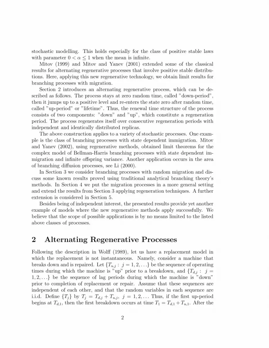
stochastic modelling. This holds especially for the class of positive stable lawswith parameter 0 < α ≤ 1 when the mean is infinite.

Mitov (1999) and Mitov and Yanev (2001) extended some of the classicalresults for alternating regenerative processes that involve positive stable distribu-tions. Here, applying this new regenerative technology, we obtain limit results forbranching processes with migration.

Section 2 introduces an alternating regenerative process, which can be de-scribed as follows. The process stays at zero random time, called ”down-period”,then it jumps up to a positive level and re-enters the state zero after random time,called ”up-period” or ”lifetime”. Thus, the renewal time structure of the processconsists of two components: ”down” and ”up”, which constitute a regenerationperiod. The process regenerates itself over consecutive regeneration periods withindependent and identically distributed replicas.

The above construction applies to a variety of stochastic processes. One exam-ple is the class of branching processes with state dependent immigration. Mitovand Yanev (2002), using regenerative methods, obtained limit theorems for thecomplex model of Bellman-Harris branching processes with state dependent im-migration and infinite offspring variance. Another application occurs in the areaof branching diffusion processes, see Li (2000).

In Section 3 we consider branching processes with random migration and dis-cuss some known results proved using traditional analytical branching theory’smethods. In Section 4 we put the migration processes in a more general settingand extend the results from Section 3 applying regeneration techniques. A furtherextension is considered in Section 5.

Besides being of independent interest, the presented results provide yet anotherexample of models where the new regenerative methods apply successfully. Webelieve that the scope of possible applications is by no means limited to the listedabove classes of processes.

2 Alternating Regenerative Processes

Following the description in Wolff (1989), let us have a replacement model inwhich the replacement is not instantaneous. Namely, consider a machine thatbreaks down and is repaired. Let Tu,j : j = 1, 2, . . . be the sequence of operatingtimes during which the machine is ”up” prior to a breakdown, and Td,j : j =1, 2, . . . be the sequence of lag periods during which the machine is ”down”prior to completion of replacement or repair. Assume that these sequences areindependent of each other, and that the random variables in each sequence arei.i.d. Define Tj by Tj = Td,j + Tu,j, j = 1, 2, . . . Thus, if the first up-periodbegins at Td,1, then the first breakdown occurs at time T1 = Td,1 + Tu,1. After the

2

replacement (or repair) the machine will start working again at T1 +Td,2 until theend of the second up-period T2 = T1 + Td,2 + Tu,2, and so on. Call Tj a repaircycle, and consider the renewal process N(t) generated by the sequence of timesbetween successive replacements Tj, i.e.,

N(t) = maxn ≥ 0 : Sn ≤ t, (2.1)

where

S0 = 0, Sn =n∑

j=1

Tj, n = 1, 2, . . .

N(t) is the number of repairs (replacements) completed by time t.Let us associate with each Tu,j a stochastic process zj(t) : 0 ≤ t ≤ Tu,j,

called cycle (or tour), j = 1, 2, . . ., such that

zj(0) ≥ 0, zj(t) > 0 for 0 < t < Tu,j, zj(Tu,j) = 0.

Assume that each zj(t) has state space (R+,B+) where R+ = [0,∞) and B+ is theBorel σfield. The cycles are mutually independent and stochastically equivalent.Also, for each j, zj(t) may depend on Tu,j but is independent of Tu,i : i 6= j.

Further on, consider the process σ(t) defined by

σ(t) = t − SN(t) − Td,N(t)+1. (2.2)

Clearly, σ(t) can be positive or negative and σ(t) = σ+(t)−σ−(t), where σ+(t) =maxσ(t), 0 is the attained duration of the up-period in progress, whereas σ−(t) =max−σ(t), 0 is the remaining time till the end of the down-period in progress.

Now, we are in a position to define an alternating regenerative process Z(t).Definition 1 An alternating regenerative process Z(t) : t ≥ 0 is defined by

Z(t) =

zN(t)+1(σ(t)) when σ(t) ≥ 0,0 when σ(t) < 0.

An example of alternating regenerative process is the regenerative processwith a reward structure discussed in Wolff (1989), Chapter 2. Another exampleis provided by the Bellman-Harris branching processes with immigration at zeroonly, studied by Mitov and Yanev (2002).

Further on, we will need three groups of assumptions.Assumptions A For the down-time component Td,j with cdf A(x) we assume

eitherETd,j < ∞

orETd,j = ∞ and 1 − A(t) ∼ t−αLA(t) as t → ∞, (2.3)

3

where α ∈ (12, 1] and LA(·) is a slowly varying function at infinity (svf), i.e.,

Td,j , j ≥ 1 belong to the normal domain of attraction of a stable law with param-eter α.

Assumptions B For the up-time component Tu,j with cdf F (x) we assumeeither

ETu,j < ∞

orETu,j = ∞ and 1 − F (t) ∼ t−βLF (t) as t → ∞, (2.4)

where β ∈ (12, 1] and LF (·) is a svf, i.e., Tu,j, j ≥ 1 belong to the normal domain

of attraction of a stable law with parameter β.Assumptions C For the cycle zj(t) : 0 ≤ t ≤ Tu,j, where j = 1, 2, . . . we

assume

limt→∞

P

zj(t)

R(t)≤ x|Tu,j > t

= D(x), (2.5)

where R(t) = L(t)tγ , γ ≥ 0 for some svf L(t) and D(x) is a proper cdf on (0,∞).

Basic Regeneration Theorem (BRT) (Mitov and Yanev (2001), Mitov (1999))Let Assumptions A – C hold. Set

c = limt→∞

1 − A(t)

1 − F (t).

I. Suppose that ETu,j is infinite and (2.4) holds with 12

< β < 1. Let x ≥ 0.a. If 0 ≤ c < ∞, then

limt→∞

P

Z(t)

R(t)≤ x

=c + G(x)

c + 1, (2.6)

where

G(x) =1

B(1 − β, β)

∫ 1

0D(xu−γ)u−β(1 − u)β−1du, (2.7)

and B(·, ·) stands for Beta function.b. If c = ∞, then

limt→∞

P

Z(t)

R(t)≤ x|Z(t) > 0

=1

B(1 − β, α)

∫ 1

0D(xu−γ)u−β(1 − u)α−1du. (2.8)

II. Suppose that ETu,j is infinite and (2.4) holds with β = 1. Assume (2.5)with D(0) = 0 and let 0 < x < 1.

a. If 0 ≤ c < ∞, then

limt→∞

P

mF (R−1(Z(t)))

mF (t)≤ x

=c + x

c + 1, (2.9)

4

where R−1(·) is the inverse function of R(·) and mF (t) =∫ t0 1 − F (x)dx.

b. If c = ∞, then

limt→∞

P

mF (R−1(Z(t)))

mF (t)≤ x|Z(t) > 0

= x, (2.10)

where R−1(·) and mF (t) are defined above in part a.III. Suppose that ETd,j is infinite and (2.3) holds. If ETu,j < ∞, then

limt→∞

P Z(t) ≤ x|Z(t) > 0 =1

ETu,1

∫ ∞

0P z1(y) ≤ x, Tu,1 > y dy. (2.11)

Remark Notice that, if both ETd,j and ETu,j are finite, then by the classicalregeneration theorem (see e.g. Sigman and Wolf (1993), Theorem 2.1)

limt→∞

P Z(t) ≤ x =1

ETd,1 + ETu,1

∫ ∞

0P z1(y) ≤ x, Td,1 + Tu,1 > y dy. (2.12)

The BRT in the non-lattice case was proved by Mitov and Yanev (2001) andin the lattice case by Mitov (1999). In the next section, applying the BRT, weobtain limit theorems for a class of branching processes with random migration.

3 Branching Processes with Migration

Let us have on a probability space (Ω,F , P ) three independent sets of non-negativeinteger-valued i.i.d. random variables as follows.

i. offspring variables: Xit : i = 1, 2, . . . ; t = 0, 1, . . .;ii. immigration variables: (I+

t , Iot ) : t = 0, 1, . . .;

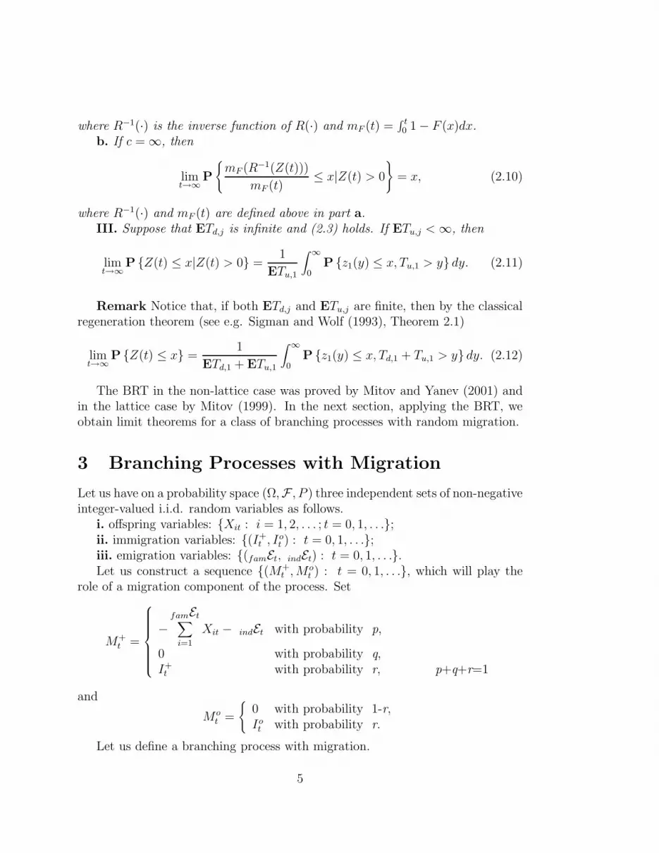
iii. emigration variables: (famEt, indEt) : t = 0, 1, . . ..Let us construct a sequence (M+

t , Mot ) : t = 0, 1, . . ., which will play the

role of a migration component of the process. Set

M+t =

−famEt∑

i=1

Xit − indEt with probability p,

0 with probability q,I+t with probability r, p+q+r=1

and

Mot =

0 with probability 1-r,Iot with probability r.

Let us define a branching process with migration.

5

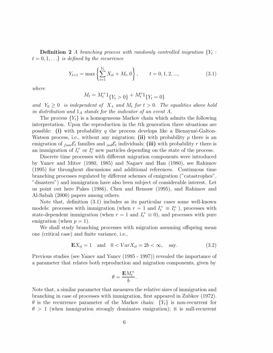
Definition 2 A branching process with randomly controlled migration Yt :t = 0, 1, . . . is defined by the recurrence

Yt+1 = max

Yt∑

i=1

Xit + Mt, 0

, t = 0, 1, 2, ..., (3.1)

whereMt = M+

t 1Yt > 0 + Mot 1Yt = 0

and Y0 ≥ 0 is independent of X·t and Mt for t > 0. The equalities above holdin distribution and 1A stands for the indicator of an event A.

The process Yt is a homogeneous Markov chain which admits the followinginterpretation. Upon the reproduction in the tth generation three situations arepossible: (i) with probability q the process develops like a Bienayme-Galton-Watson process, i.e., without any migration; (ii) with probability p there is anemigration of famEt families and indEt individuals; (iii) with probability r there isan immigration of I+

t or Iot new particles depending on the state of the process.

Discrete time processes with different migration components were introducedby Yanev and Mitov (1980, 1985) and Nagaev and Han (1980), see Rahimov(1995) for throughout discussions and additional references. Continuous timebranching processes regulated by different schemes of emigration (”catastrophes”,”disasters”) and immigration have also been subject of considerable interest. Letus point out here Pakes (1986), Chen and Rensaw (1995), and Rahimov andAl-Sabah (2000) papers among others.

Note that, definition (3.1) includes as its particular cases some well-knownmodels: processes with immigration (when r = 1 and I+

t ≡ Iot ), processes with

state-dependent immigration (when r = 1 and I+t ≡ 0), and processes with pure

emigration (when p = 1).We shall study branching processes with migration assuming offspring mean

one (critical case) and finite variance, i.e.,

EXit = 1 and 0 < V arXit = 2b < ∞, say. (3.2)

Previous studies (see Yanev and Yanev (1995 - 1997)) revealed the importance ofa parameter that relates both reproduction and migration components, given by

θ =EM+

t

b.

Note that, a similar parameter that measures the relative sizes of immigration andbranching in case of processes with immigration, first appeared in Zubkov (1972).θ is the recurrence parameter of the Markov chain: Yt is non-recurrent forθ > 1 (when immigration strongly dominates emigration); it is null-recurrent

6

for 0 ≤ θ < 1 (when immigration mildly dominates emigration), and positiverecurrent for θ < 0 (when emigration dominates immigration). In the border caseθ = 1 the chain is either non-recurrent or null-recurrent depending on some extramoment assumptions.

Further on, we need additional assumptions for the migration component asfollows

0 < EI+t < ∞, 0 < EIo

t < ∞,0 ≤ famEt ≤ C1 < ∞, 0 ≤ indEt ≤ C2 < ∞, a.s..

(3.3)

The following theorem gives the limiting behavior of Yt.

Theorem 3.1 (Yanev and Yanev (1996)) Suppose that Yt is critical with finiteoffspring variance, i.e., (3.2). Also, assume that the migration satisfies (3.3).

I. If θ > 0, thenYt

btd→ Γ(θ, 1),

where the limit is Gamma distributed with parameters θ and 1.II. If θ = 0 and EI+2

t < ∞, then

log Yt

log td→ U(0, 1),

where the limit is uniformly distributed on the unit interval.III. If θ < 0, then Yt possesses a limiting stationary distribution, i.e.,

Ytd→ Y∞.

The above theorem was proved using some traditional branching process the-ory methods including functional equations for pgf’s, Laplace transforms, Taube-rian theorems etc. In the next section we will extend the above results makinguse of some probabilistic arguments and the BRT from Section 2.

4 Regeneration and Migration

Consider the branching migration process (3.1) with Mot ≡ 0, i.e., migration is

not permitted when the process is in state zero. That is,

Y ot+1 = max

Y ot∑

i=1

Xit + M+t 1Y 0

t >0, 0

, t = 0, 1, 2, ..., (4.1)

where Y o0 ≥ 0 is independent of X·t and M+

t for t ≥ 1. Call this a process withmigration stopped at zero.

7

Since the state zero is a reflective barrier, the Markov chain Yt is an regen-erative process. Indeed, using the notations from Section 2, Yt stays at zerorandom time Td,1, which has the geometric distribution

PTd,1 = k = Pk−1Mot = 0(1 − PMo

t = 0), k = 1, 2, . . . (4.2)

In the end of this down-period the process jumps up to a random level I0Td,1

and

evolves according to the rules in the model (3.1) until it hits zero again in the endof its lifetime Tu,1. Thus, T1 = Td,1+Tu,1 forms the first period of regeneration andthe evolution of the process repeats in the next such periods, i.e., Yt+T1

: t ≥ 0is stochastically equivalent to Yt : t ≥ 0. Let Td,j , j = 1, 2, . . . be i.i.d. copiesof Td,1 given by (4.2). Also, let Y o

j,t : j = 1, 2, . . . be a sequence of branchingprocesses with migration stopped at zero defined by (4.1), having lifetimes Tu,j,i.e., for j = 1, 2, . . .

Y oj,0 ≥ 0, Y o

j,t > 0 for 0 < t < Tu,j, Y oj,Tu,j

= 0.

Now, it is not difficult to see, that (3.1) is a particular case of Definition 1 withcycle process Y o

j,t : t = 0, 1, . . . Tu,j. Indeed, Yt is an alternative regenerativeprocess with cycle process zj(t) ≡ Y o

j,t and Td,j given by (4.2).Let us generalize the migration process (3.1) as follows:i. First, assume that the down-periods Td,j : j = 1, 2, . . . have a cdf A(x),

which is not necessarily the geometric one from (4.2).ii. Secondly, assume that the mean of Td,j : j = 1, 2, . . . is not constrained

to be finite. If ETd,j = ∞, assume that Td,j ’s belong to the domain of attractionof a stable law and their cdf F (t) satisfies (2.4).

Appealing to Definition 1, we construct a generalized version of Yt with i.and ii. above as follows

Definition 3 A branching regenerative process with migration denoted byZt : t = 0, 1, . . . is defined by

Zt =

Y oN(t)+1, σ(t) when σ(t) ≥ 0,

0 when σ(t) < 0,

where the cycles Y oj,t are processes with migration stopped at zero; N(t) and σ(t)

are defined by (2.1) and (2.2), respectively.Example Using the well-known duality between a branching process and a

M/M/1 queue, let us describe a situation where the above construction applies.Consider a queueing model in which customers arrive following a Poisson process.Then the successive times Tj from the commencement of the jth busy period tothe start of the next busy period form a renewal process. Each Tj is composed of abusy portion Tu,j and an idle portion Td,j, when the queue is not empty or empty,

8

respectively. Assuming that the customers, arriving during the service time of acustomer, are his/her ”offspring”, we obtain a branching regenerative process. Theimmigration component accounts for a policy when certain customers (probablycoming from a second source) accumulate and will be served after completing theservice time of a ”generation”. Alternatively, some customers (called ”emigrants”)may leave the system prior to their service.

Further on, we will assume that some reproduction and immigration momentsare finite as follows

EI+2t < ∞, when θ = 0

EI+(1−θ)t < ∞, EX2

1t log(1 + X1t) < ∞ when − 1 < θ < 0EI+2

t log2(1 + I+t ) < ∞, EX2

1t log2(1 + X1t) < ∞ when θ = −1

EI+(1−θ)t < ∞, EX1−θ

1t < ∞ when θ < −1.

(4.3)

Let us summarize for more convenient references some results for processeswith migration stopped at zero that are proved in Yanev and Yanev (1995-2002).

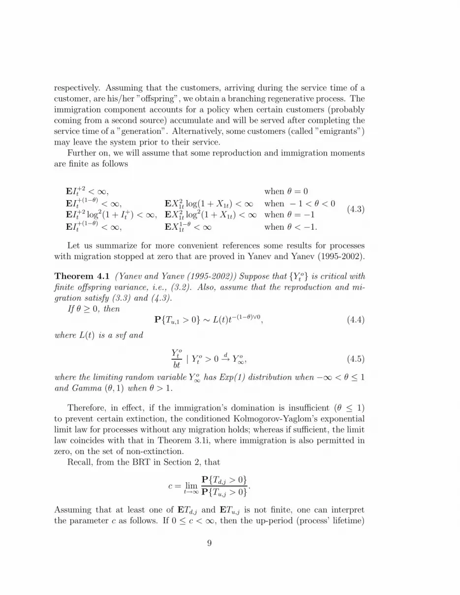
Theorem 4.1 (Yanev and Yanev (1995-2002)) Suppose that Y ot is critical with

finite offspring variance, i.e., (3.2). Also, assume that the reproduction and mi-gration satisfy (3.3) and (4.3).

If θ ≥ 0, thenPTu,1 > 0 ∼ L(t)t−(1−θ)∨0, (4.4)

where L(t) is a svf and

Y ot

bt| Y o

t > 0d→ Y o

∞, (4.5)

where the limiting random variable Y o∞ has Exp(1) distribution when −∞ < θ ≤ 1

and Gamma (θ, 1) when θ > 1.

Therefore, in effect, if the immigration’s domination is insufficient (θ ≤ 1)to prevent certain extinction, the conditioned Kolmogorov-Yaglom’s exponentiallimit law for processes without any migration holds; whereas if sufficient, the limitlaw coincides with that in Theorem 3.1i, where immigration is also permitted inzero, on the set of non-extinction.

Recall, from the BRT in Section 2, that

c = limt→∞

PTd,j > 0

PTu,j > 0.

Assuming that at least one of ETd,j and ETu,j is not finite, one can interpretthe parameter c as follows. If 0 ≤ c < ∞, then the up-period (process’ lifetime)

9

has length asymptotically bigger than the down-period (stay at zero); whereas ifc = ∞, then the process spends more time at zero then up.

Now, we are in a position to prove the main limit theorem for branchingregenerative processes with migration.

Theorem 4.2 Suppose that Zt is critical with finite offspring variance, i.e.,(3.2). Also, assume that the reproduction and migration satisfy (3.3) and (4.3).

I. Let 0 < θ < 1/2 and suppose that either ETd,j < ∞ or ETd,j = ∞ and (2.3)holds.

a. If 0 ≤ c < ∞, then

Zt

btd→ Z∞, (4.6)

where EZ∞ = θ/(c + 1) and for x ≥ 0

PZ∞ ≤ x = 1 −1

(c + 1)B(θ, 1 − θ)

∫ 1

0e−x/yyθ−1(1 − y)−θdy. (4.7)

b. If c = ∞, then

Zt

bt| Zt > 0

d→ Z∞, (4.8)

where EZ∞ = θ/(θ + α) and for x ≥ 0

PZ∞ ≤ x = 1 −1

B(θ, α)

∫ 1

0e−x/yyθ−1(1 − y)α−1dy. (4.9)

II. Let θ = 0.a. If ETd,j < ∞, then

log Zt

log td→ U(0, 1),

where the limit is uniformly distributed on the unit interval.b. Assume ETd,j = ∞ and (2.3). i. If 0 ≤ c < ∞, then

log Zt

log td→ Z∞,

where PZ∞ ≤ x = (c + x)/(c + 1) for 0 ≤ x ≤ 1.ii. If c = ∞, then

log Zt

log t| Zt > 0

d→ U(0, 1),

where the limit is uniformly distributed on the unit interval.III. Let θ < 0.

10

a. If ETd,j < ∞, then Zt possesses a limiting stationary distribution, i.e.,

Ztd→ Z∞

and for x ≥ 0

PZ∞ ≤ x =1

ET1

∞∑

k=0

PY o1,k ≤ x, T1 > k.

b. If ETd,j = ∞ and (2.3) holds, then

Zt | Zt > 0d→ Z∞

and for x ≥ 0

PZ∞ ≤ x =1

ETu,1

∞∑

k=0

PY o1,k ≤ x, Tu,1 > k.

Proof We shall apply the BRT to Zt. I. First note that, (4.4) implies

PTu,1 > t ∼ L(t)t−(1−θ)

and hence (2.4) holds with β = 1 − θ. Furthermore, by (4.5),

limt→∞

P

Y ot

bt≤ x|Y o

t > 0

= 1 − e−x. (4.10)

Thus, (2.5) holds with R(t) = bt and D(x) = 1 − e−x. Now, (2.6) and (2.7) leadto (4.6) with

PZ∞ ≤ x =c

c + 1+

1

(c + 1)B(θ, 1 − θ)

∫ 1

0(1 − ex/u)u−(1−θ)(1 − u)−θdu

= 1 −1

(c + 1)B(θ, 1 − θ)

∫ 1

0ex/uuθ−1(1 − u)−θdu,

which proves (4.7). Integrating 1−PZ∞ ≤ x, it is not difficult to obtain EZ∞.Similarly, taking into account (4.10) and (2.8), one can obtain (4.8) and (4.9).

II. In this case we have from (4.4) that

PTu,1 > t ∼ C0t−1,

for some positive constant C0. Thus, (2.4) holds with β = 1 and mf (t) ∼ C0 log t.On the other hand, (4.10) still applies and hence R(t) = bt and D(x) = 1 − e−x

with D(0) = 0 . Finally,

mF (M−1(Zt))

mF (t)∼

log Zt

log t.

11

Now, part IIa follows from (2.9), taking into account that ETd,j < ∞, whichresults in c = 0. Similarly, (2.9) and (2.10) imply IIbi and IIbii, respectively.

III. According to Theorem 4.1, we have ETu,j < ∞. In case of ETd,j < ∞,the classical regeneration theorem applies and (2.12) leads to IIIa. If ETd,j = ∞,then (2.11) holds and hence IIIb.

It is interesting to compare Theorem 3.1 for Yt with Theorem 4.2 for Zt.Recall that the former assumes a geometric distributed Td,j with ETd,j < ∞,whereas the later holds for Td,j , not constrained to one specific distribution andthat might have a finite or infinite mean. For all values of θ, if ETd,j = ∞ and c =∞, i.e., asymptotically the down-period dominates the up-period, Theorem 4.2represents new conditional limit results, on the set of non-extinction. The case offinite ETd,j results in unconditional limit results and if θ ≤ 0 then the results inTheorem 3.1II extend to the more general process Zt. In the intermediate casewhen ETd,j = ∞ but 0 ≤ c < ∞, i.e., the up-period dominates the down one, weobtain unconditional limit results when θ ≥ 0 and a conditional one when θ < 0.

It is worth mentioning the generality we gain in Theorem 4.2 due to the newregeneration methods of proof versus the traditional probability generation func-tions based techniques used to obtain Theorem 3.1. One limitation of the newapproach is that it does not apply for θ ≥ 1/2.

5 One Extension

The results presented in Section 4 can be extended by relaxing the conditionthat EY o

j,t < ∞. Instead, let us assume that the immigration at zero belongsto the domain of attraction of a stable law with parameter 0 < ρ ≤ 1. For asimilar extension in case of processes with immigration at zero only, see Ivanoffand Seneta (1985). Further on, we will need the following result.

Theorem 5.1 (Yanev and Yanev (1997)) Suppose that Y ot is critical with finite

offspring variance, i.e., (3.2). Also, assume that the reproduction and migrationsatisfy (3.3) and EI+2

t < ∞ when θ = 0.I. If θ + ρ ≥ 1, then

PTu,1 > 0 ∼ K(t)t−(1−θ)∨0, (5.1)

where K(t) is a svf andY o

t

bt| Y o

t > 0d→ Y o

∞,

where the limit Y o∞ has Exp(1) distribution when −∞ < θ ≤ 1 and Gamma (θ, 1)

when θ > 1.

12

II. If θ + ρ < 1, then

PTu,1 > 0 ∼ K(t)t−ρ,

where K(t) is a svf andY o

t

bt| Y o

t > 0d→ Y o

∞, (5.2)

where the limit Y o∞ has a proper cdf with Laplace transform given by

ϕ(λ) = 1 −λρ(1 − θ − ρ)

(1 + λ)θ+ρB(1 − ρ, 1 − θ) − λθ

∫ 1

0

1

(1 − y)ρ(1 + λy)θ+1dy. (5.3)

Let us point out that, if θ+ρ < 1 then the rate of convergence in (5.1) dependson ρ only. One can say that Io

t , the ancestors’ distribution for Y ot , dominates the

migration component. Indeed, in this case the limit in (5.2) and Iot share the

domain of attraction of the same stable law with parameter ρ. If θ + ρ ≥ 1, thenthe form of the limiting distribution depends essentially on θ and one might saythat in this case the migration component is dominating.

Applying the BRT and Theorem 5.1, we obtain the following limit theorem.

Theorem 5.2 Suppose that Zt is critical with finite offspring variance, i.e.,(3.2). Also, assume that the reproduction and migration satisfy (3.3) and EI+2

t < ∞when θ = 0.

I. If 0 < θ < 1/2 and 1/2 < ρ < 1, such that ρ + θ ≥ 1, then the limit resultsin Theorem 4.2I extend to Zt, under the same assumptions on c.

II. Assume θ < 1/2 and 1/2 < ρ < 1, such that ρ + θ < 1.a. If 0 ≤ c < ∞, then

Zt

btd→ Z∞,

where the limit Z∞ has Laplace transform

Ee−λZ∞ (5.4)

=1

c + 1

(

1 −Iλ/λ+1(ρ, 1 − θ − ρ)

(λ + 1)θ−

λθ

B(1 − ρ, ρ)

∫ 1

0

∫ 1

0

u1−ρ(1 + λyu)−θ−1

(1 − u)1−ρ(1 − y)ρdydu

)

where Ix(a, b) = Bx(a, b)/B(a, b).b. If c = ∞, then

Zt

bt| Zt > 0

d→ Z∞,

where the limit Z∞ has Laplace transform

Ee−λZ∞ (5.5)

= 1 −Iλ/λ+1(α, 1 − θ − ρ)

Cλ(α, θ, ρ)−

λθ

B(1 − ρ, α)

∫ 1

0

∫ 1

0

u1−ρ(1 + λyu)−θ−1

(1 − u)1−α(1 − y)ρdydu,

13

where Cλ(α, θ, ρ) = λα−ρ(α + 1 − θ − ρ)/(

(λ + 1)α−θ−ρB(1 − θ, α + 1 − ρ))

.

If either c = 0 or c = ∞, then the limiting distributions in (5.4) and (5.5)belong to the normal domain of attraction of a stable law with parameter ρ ∈ (1

2, 1).

III. If θ ≤ 0 and ρ = 1, then the limit results in Theorem 4.2II extend to Zt,under the same assumptions on Td,j and c .

Proof I. Under the hypotheses, Theorem 5.1 implies PTu,1 > t ∼ K(t)t−(1−θ)

and limt→∞ P Y ot /(bt) ≤ x|Y o

t > 0 = 1 − e−x. The rest of the proof repeats thearguments in that of Theorem 4.2I.

II. Let us apply the BRT again. According to Theorem 5.1

PTu,1 > t ∼ K(t)t−ρ.

Thus, (2.4) holds with β = ρ. On the other hand, by the same theorem,

limt→∞

P

Y ot

bt≤ x|Y o

t > 0

= Y o∞

and the limiting random variable has a proper cdf H(x) with Laplace transformgiven by (5.3). Let 0 ≤ c < ∞. Then (2.6) with (2.7) (note that γ = 1 and β = ρ)implies the limiting result IIa and

Ee−λZ∞ =∫ ∞

0e−λxd

c + G(x)

c + 1

=λ

c + 1

∫ ∞

0e−λxG(x)dx

=λ

(c + 1)B(1 − ρ, ρ)

∫ 1

0u−ρ(1 − u)ρ−1

∫ ∞

0e−λxD(x/u)dxdu

=λ

(c + 1)B(1 − ρ, ρ)

∫ 1

0u−ρ(1 − u)ρ−1

∫ ∞

0e−λuyD(y)dydu

=1

(c + 1)B(1 − ρ, ρ)

∫ 1

0u−ρ(1 − u)ρ−1ϕ(λu)du,

where ϕ(·) is given by (5.3). After replacing ϕ(λu) with (5.3) and using well-known properties of the incomplete Beta function, we obtain (5.4). The casec = ∞ follows similarly by (2.8).

Let us prove that if c = 0 then the limiting distribution with (5.4) belongs tothe normal domain of attraction of a stable law with parameter ρ. Indeed, settingH(x) = PZ∞ ≤ x, from (5.4) since Ix(a, b) ∼ const. xa, we obtain as λ → 0+

∫ ∞

0e−λx(1 − H(x))du =

1 − Ee−λZ∞

λ∼ const.λρ−1.

14

Now, by Karamata’s Tauberian theorem∫ t0 1 − H(x)dx ∼ const.t1−ρ as t → ∞.

Thus, 1 − H(x) ∼ const.xρ, which was to be proved. The statement for c = ∞follows similarly from (5.5).

III. Since ρ = 1, Theorem 5.1 yields PTu,1 > t ∼ K(t)t−1 and alsolimt→∞ P Y o

t /(bt) ≤ x|Y ot > 0 = 1 − e−x. We complete the proof of III by re-

peating the arguments in the proof of Theorem 4.2II.Remarks Notice the new limiting distributions that appear in Theorem 5.2II,

when the immigration at zero Iot dominates the migration component . If either

c = 0 or c = ∞, then the limiting distributions belong to the same stable law’sdomain as the immigration at zero Io

t . We can also deduce that they have nomass at zero. Indeed if c = 0, then one can show (see Yanev and Yanev (1997))that limλ→∞(c + 1)(1 − Ee−λZ∞) = 1 and hence limλ→∞ Ee−λZ∞ = 0. The casec = ∞ is similar. Finally, it is interesting to see that if θ = 0, then the Laplacetransform in IIa. simplifies to (1 − Iλ/(λ+1)(ρ, 1 − ρ))/(c + 1). This extends theresult from (5.3) when ϕ(λ) = 1 − (λ/λ + 1)ρ. If θ = 0 and c = ∞ we haveEe−λZ∞ = 1 − Iλ/(λ+1)(α, 1 − ρ))/Cλ(α, 0, ρ).

Acknowledgments This research is supported in part by NFSI of Bulgaria,grant No. MM 1101/2001.

References

[1] Chen, A. Y. and Renshaw, E. (1995). Markov branching processes regulatedby emigration and large immigration, Stochastic Proc. Appl., 57, 339-359.

[2] Ivanoff B. G. and Seneta, E. (1985). The critical branching process withimmigration stopped at zero, J. Appl. Prob., 22, 223-227.

[3] Mitov, K. V. (1999). Limit theorems for regenerative excursion processes,Serdica Math. J., 25, 19-40.

[4] Mitov, K. V. and Yanev, N. M. (2001). Regenerative processes in the infinitemean cycle case, J. Appl. Prob., 38, 165-179.

[5] Mitov, K. V. and Yanev, N. M. (2002). Critical Bellman-Harris branch-ing processes with infinite variance allowing state dependent immigration,Stochastic Models, 18, 281-300.

[6] Nagaev, S. V. and Han, L. V. (1980). Limit theorems for critical Galton-Watson branching process with migration, Theory Probab. Appl., 25, 514-525.

[7] Li, Z. H. (2000). Asymptotic behavior of continuous time and state branchingprocesses, J. Austral. Math. Soc. (Ser. A), 68, 68-84.

[8] Pakes, A. G. (1986). Some properties of a branching process with groupimmigration and emigration, Adv. Appl. Probab., 18, 628-645.

15

[9] Rahimov, I. (1995). Random Sums and Branching Processes, LNS 96,Springer, Berlin.

[10] Rahimov, I. and Al-Sabah, W.S. (2000). Branching processes with decreasingimmigration and tribal emigration, Arab J. Math. Sci., 6(2), 81-97.

[11] Sigman, K. and Wolff, R. W. (1993). A review of regenerative processes,SIAM Review, 35, 269-288.

[12] Uchaikin, V. V. and Zolotarev, V. M. (1999). Chance and Stability. Sta-ble Distributions and Their Applications, Modern Prob. and Stats., VSP,Utrecht.

[13] Wolff, R. W. (1989). Stochastic Modelling and the Theory of Queues, PrenticeHall, Englewood Cliffs.

[14] Yanev, G. P. and Yanev, N.M. (1995). Critical branching processes withrandom migration, In: Ed. C. C. Heyde, Branching Processes, LNS 99,Springer, New York, 36-45.

[15] Yanev, G. P. and Yanev, N. M. (1996). Branching processes with two typesof emigration and state dependent immigration, In: Eds. C.C. Hayde, Yu. V.Prohorov, R. Pyke, S.T. Rachev Athens Conference on Applied Probabilityand Time Series Analysis, Volume 1: Applied Probability, LNS 114, Springer,New York, 216-228.

[16] Yanev, G. P. and Yanev, N. M. (1997). Limit theorems for branching pro-cesses with random migration stopped at zero, In: Eds. K.B. Athreya and P.Jagers Classical and Modern Branching processes, IMA Volumes in Math.and Its Appl., Springer, New York, 323-336.

[17] Yanev, G. P. and Yanev, N. M. (2002). A critical branching process withstationary-limiting distribution, (submitted).

[18] Yanev, N. M. and Mitov, K. V. (1980). Controlled branching processes: Thecase of random migration, C. R. Acad. Bulg. Sci., 33, 433-435.

[19] Yanev, N. M. and Mitov, K.V. (1985). Critical branching processes withnon-homogeneous migration, Ann. Probab., 13, 923-933.

[20] Zolotarev, V. M. (1983). One-dimensional stable distributions, Nauka,Moscow, (In Russian).

[21] Zubkov, A. M. (1972). Life-periods of a branching process with immigration,Theory Prob. Appl., 17, 174-183.

16