COVERT COMMUNICATION NETWORKS

A Dissertation

by

TIMOTHY GLEN NIX

Submitted to the Office of Graduate Studies ofTexas A&M University

in partial fulfillment of the requirements for the degree of

DOCTOR OF PHILOSOPHY

Chair of Committee, Riccardo BettatiCommittee Members, Jyh-Charn Liu

Andreas KlappeneckerJonathan Rogers

Head of Department, Duncan Walker

August 2013

Major Subject: Computer Science

Copyright 2013 Timothy Glen Nix

ABSTRACT

A covert communications network (CCN) is a connected, overlay peer-to-peer

network used to support communications within a group in which the survival of

the group depends on the confidentiality and anonymity of communications, on con-

cealment of participation in the network to both other members of the group and

external eavesdroppers, and finally on resilience against disconnection. In this disser-

tation, we describe the challenges and requirements for such a system. We consider

the topologies of resilient covert communications networks that: (1) minimize the

impact on the network in the event of a subverted node; and (2) maximize the con-

nectivity of the survivor network with the removal of the subverted node and its

closed neighborhood. We analyze the properties of resilient covert networks, pro-

pose measurements for determining the suitability of a topology for use in a covert

communication network, and determine the properties of an optimal covert network

topology. We analyze multiple topologies and identify two constructions that are

capable of generating optimal topologies. We then extend these constructions to

produce near-optimal topologies that can “grow” as new nodes join the network. We

also address protocols for membership management and routing. Finally, we describe

the architecture of a prototype system for instantiating a CCN.

ii

ACKNOWLEDGEMENTS

A research project like this is never the work of anyone alone. The contributions

of many different people, in their different ways, have made this possible. I would

like to extend my appreciation especially to the following.

First and foremost, thank God for His grace and wisdom as He has guided me

throughout my life: ”I can do all things through Christ who strengthens me.” (Philip-

pians 4:13). Next, I want to thank my wife Heather for her love, support and encour-

agement. She is my pillar of strength. I also thank my two wonderful boys, Chaney

and Elias. I am so proud to be their Dad. Thanks for understanding on those late

nights and weekends when I was working instead of playing. Thanks to my parents

for instilling in me a willingness to work and a love of learning.

I would like to express my appreciation to my advisor and mentor, Dr. Riccardo

Bettati for his wisdom and instruction over the past three years. Any lasting impact

from this work is due to his guidance and any mistakes are mine alone.

I also want to thank the United States Army for 22 years of opportunities and

experience, including this research. A special thanks to my brothers and sisters in

the U.S. Armed Forces, especially those who have influenced and encouraged me

through shared hardships and numerous deployments.

De oppresso liber.

iii

TABLE OF CONTENTS

Page

ABSTRACT . . . . . . . . . . . . . . . . . . . . . . . . . . . . . . . . . . . . ii

ACKNOWLEDGEMENTS . . . . . . . . . . . . . . . . . . . . . . . . . . . . iii

TABLE OF CONTENTS . . . . . . . . . . . . . . . . . . . . . . . . . . . . . iv

LIST OF FIGURES . . . . . . . . . . . . . . . . . . . . . . . . . . . . . . . . ix

LIST OF TABLES . . . . . . . . . . . . . . . . . . . . . . . . . . . . . . . . . xii

1. INTRODUCTION TO COVERT COMMUNICATION NETWORKS . . . 1

1.1 The Need for Covert Communication . . . . . . . . . . . . . . . . . . 2

1.2 The Criteria for a CCN . . . . . . . . . . . . . . . . . . . . . . . . . . 2

1.3 Outlook . . . . . . . . . . . . . . . . . . . . . . . . . . . . . . . . . . 5

2. PREVIOUS WORK IN AREAS RELATING TO COVERT COMMUNI-CATION NETWORKS . . . . . . . . . . . . . . . . . . . . . . . . . . . . 7

2.1 Cryptography . . . . . . . . . . . . . . . . . . . . . . . . . . . . . . . 7

2.2 Steganography . . . . . . . . . . . . . . . . . . . . . . . . . . . . . . . 8

2.3 Covert Channels . . . . . . . . . . . . . . . . . . . . . . . . . . . . . 8

2.4 Anonymity Networks . . . . . . . . . . . . . . . . . . . . . . . . . . . 9

2.4.1 Mix Networks . . . . . . . . . . . . . . . . . . . . . . . . . . . 11

2.4.2 Low-Latency Anonymity Networks . . . . . . . . . . . . . . . 13

2.4.3 DC Networks . . . . . . . . . . . . . . . . . . . . . . . . . . . 16

2.5 Membership-Concealing Overlay Networks . . . . . . . . . . . . . . . 17

2.6 Underground and Covert Networks . . . . . . . . . . . . . . . . . . . 18

2.7 Delay-Tolerant Networks . . . . . . . . . . . . . . . . . . . . . . . . . 19

2.8 Conclusions . . . . . . . . . . . . . . . . . . . . . . . . . . . . . . . . 19

3. BASIC STRUCTURE AND OPERATION OF A COVERT COMMUNI-CATION NETWORK . . . . . . . . . . . . . . . . . . . . . . . . . . . . . 21

iv

3.1 End-to-end Communication . . . . . . . . . . . . . . . . . . . . . . . 22

3.1.1 Communication between Neighbors . . . . . . . . . . . . . . . 23

3.1.2 Pseudonyms . . . . . . . . . . . . . . . . . . . . . . . . . . . . 25

3.1.3 CCN Message Confidentiality . . . . . . . . . . . . . . . . . . 26

3.2 Topology Considerations . . . . . . . . . . . . . . . . . . . . . . . . . 27

3.2.1 Threat Model . . . . . . . . . . . . . . . . . . . . . . . . . . . 28

3.2.2 Network Resiliency . . . . . . . . . . . . . . . . . . . . . . . . 29

3.2.3 Deterministic versus Random Topology Construction . . . . . 31

3.2.4 Structured versus Unstructured Topologies . . . . . . . . . . . 31

3.3 Communications Considerations . . . . . . . . . . . . . . . . . . . . . 32

3.3.1 No Specialized Equipment Required . . . . . . . . . . . . . . . 32

3.3.2 Open versus Closed Infrastructure . . . . . . . . . . . . . . . . 32

3.3.3 Decentralized Control . . . . . . . . . . . . . . . . . . . . . . . 34

3.3.4 Effects of Network Promiscuity and Trust . . . . . . . . . . . 35

3.4 Conclusions . . . . . . . . . . . . . . . . . . . . . . . . . . . . . . . . 35

4. TOPOLOGY MEASUREMENT IN COVERT COMMUNICATION NET-WORKS . . . . . . . . . . . . . . . . . . . . . . . . . . . . . . . . . . . . . 37

4.1 Global Subversion Impedance . . . . . . . . . . . . . . . . . . . . . . 38

4.2 Optimal Covert Communications Network Topology . . . . . . . . . . 41

4.3 Examples of Optimal Graphs . . . . . . . . . . . . . . . . . . . . . . 46

4.3.1 Girth-5 Cages . . . . . . . . . . . . . . . . . . . . . . . . . . . 46

4.3.2 Gunther-Hartnell Construction . . . . . . . . . . . . . . . . . 48

4.4 Conclusions . . . . . . . . . . . . . . . . . . . . . . . . . . . . . . . . 50

5. DETERMINISTIC TOPOLOGY ANALYSIS FOR CCNs . . . . . . . . . . 51

5.1 Resilience versus Survivability . . . . . . . . . . . . . . . . . . . . . . 51

5.2 Worst Case Subversion versus Uniformly Probable Subversion . . . . 52

5.3 Average Local Subversion Impedance . . . . . . . . . . . . . . . . . . 53

5.4 An Analysis of Common Network Topologies for Use in CCNs . . . . 54

5.4.1 Paths . . . . . . . . . . . . . . . . . . . . . . . . . . . . . . . 54

v

5.4.2 Cycles . . . . . . . . . . . . . . . . . . . . . . . . . . . . . . . 56

5.4.3 Stars . . . . . . . . . . . . . . . . . . . . . . . . . . . . . . . . 58

5.4.4 Cliques . . . . . . . . . . . . . . . . . . . . . . . . . . . . . . . 58

5.4.5 Fifth-Column Graphs . . . . . . . . . . . . . . . . . . . . . . . 59

5.4.6 Hypercubes . . . . . . . . . . . . . . . . . . . . . . . . . . . . 61

5.5 The Modified Robertson Construction . . . . . . . . . . . . . . . . . 62

5.5.1 Robertson Construction . . . . . . . . . . . . . . . . . . . . . 63

5.5.2 Modified Robertson Construction . . . . . . . . . . . . . . . . 65

5.5.3 Analysis of the Modified Robertson Construction . . . . . . . 70

5.6 Moving Towards Dynamic Construction . . . . . . . . . . . . . . . . . 72

5.6.1 Option 1: Choose a Large Enough p . . . . . . . . . . . . . . 73

5.6.2 Option 2: Reconstruct the Network When Necessary . . . . . 73

5.6.3 Option 3: Grow the Network Linearly . . . . . . . . . . . . . . 74

5.7 The Extended Gunther-Hartnell Construction . . . . . . . . . . . . . 74

5.8 Conclusions . . . . . . . . . . . . . . . . . . . . . . . . . . . . . . . . 77

6. RANDOM TOPOLOGY ANALYSIS FOR CCNs . . . . . . . . . . . . . . 81

6.1 Expected Local Subversion Impedance . . . . . . . . . . . . . . . . . 82

6.2 Expected Global Subversion Impedance . . . . . . . . . . . . . . . . . 84

6.3 Erdos-Renyi Random Graphs . . . . . . . . . . . . . . . . . . . . . . 85

6.3.1 Results for the Expected Local Subversion Impedance . . . . . 86

6.3.2 Results for the Expected Secrecy . . . . . . . . . . . . . . . . 87

6.3.3 Results for the Expected Resilience . . . . . . . . . . . . . . . 88

6.3.4 Towards a Closed Form for E[δ(G)] . . . . . . . . . . . . . . . 90

6.3.5 Towards a Closed Form Estimate for E[γ(G, v)] . . . . . . . . 94

6.3.6 Results for the Expected Global Subversion Impedance . . . . 97

6.4 Scale-free Random Graphs . . . . . . . . . . . . . . . . . . . . . . . . 99

6.5 Conclusions . . . . . . . . . . . . . . . . . . . . . . . . . . . . . . . . 101

7. MEMBERSHIP MANAGEMENT IN A COVERT COMMUNICATIONNETWORK . . . . . . . . . . . . . . . . . . . . . . . . . . . . . . . . . . . 103

vi

7.1 Initial Vetting and Shared Credentials . . . . . . . . . . . . . . . . . 103

7.2 First Contact . . . . . . . . . . . . . . . . . . . . . . . . . . . . . . . 104

7.2.1 Current Node Determination . . . . . . . . . . . . . . . . . . . 105

7.2.2 Direct First Contact . . . . . . . . . . . . . . . . . . . . . . . 105

7.2.3 Indirect First Contact . . . . . . . . . . . . . . . . . . . . . . 106

7.3 Basic Join Protocol . . . . . . . . . . . . . . . . . . . . . . . . . . . . 107

7.3.1 Protocol 1 - First Contact . . . . . . . . . . . . . . . . . . . . 107

7.3.2 Protocol 2 - Increasing Connectivity . . . . . . . . . . . . . . 109

7.4 Attacks Against the Basic Join Protocol . . . . . . . . . . . . . . . . 110

7.4.1 Man-in-the-Middle Attacks . . . . . . . . . . . . . . . . . . . . 110

7.4.2 Sybil Attack . . . . . . . . . . . . . . . . . . . . . . . . . . . . 110

7.4.3 Collusion Attack . . . . . . . . . . . . . . . . . . . . . . . . . 111

7.5 Distributed Join Protocol . . . . . . . . . . . . . . . . . . . . . . . . 111

7.6 Generating the Shared-Secret . . . . . . . . . . . . . . . . . . . . . . 111

7.6.1 Protocol 3 - Single Node Shared-Secret Generation . . . . . . 112

7.6.2 Protocol 4 - Distributed Shared-Secret Generation . . . . . . . 113

7.7 Attacks Against the Distributed Join Protocol . . . . . . . . . . . . . 114

7.7.1 Dealing with Node Departure or Node Failure . . . . . . . . . 114

7.8 Conclusions . . . . . . . . . . . . . . . . . . . . . . . . . . . . . . . . 115

8. ROUTING IN A COVERT COMMUNICATION NETWORK . . . . . . . 116

8.1 General Approaches to Routing . . . . . . . . . . . . . . . . . . . . . 116

8.1.1 Shortest Path Routing . . . . . . . . . . . . . . . . . . . . . . 117

8.1.2 Routing by Selective Flooding . . . . . . . . . . . . . . . . . . 118

8.2 Routing in Deterministic Topologies . . . . . . . . . . . . . . . . . . . 119

8.2.1 Routing in Gunther-Hartnell Topologies . . . . . . . . . . . . 120

8.2.2 Routing in Extended Robertson Construction Topologies . . . 122

8.3 Deadlocks and Circular Routing . . . . . . . . . . . . . . . . . . . . . 125

8.4 Conclusions . . . . . . . . . . . . . . . . . . . . . . . . . . . . . . . . 126

9. IMPLEMENTATION AND RESULTS . . . . . . . . . . . . . . . . . . . . 128

vii

9.1 The Channel Layer . . . . . . . . . . . . . . . . . . . . . . . . . . . . 130

9.1.1 TCP Channel . . . . . . . . . . . . . . . . . . . . . . . . . . . 132

9.1.2 UDP Channel . . . . . . . . . . . . . . . . . . . . . . . . . . . 133

9.1.3 Remailer Channel . . . . . . . . . . . . . . . . . . . . . . . . . 133

9.2 Channel Manager Layer . . . . . . . . . . . . . . . . . . . . . . . . . 134

9.3 The Membership Concealing Layer . . . . . . . . . . . . . . . . . . . 134

9.3.1 Anonymity Preserving Routing . . . . . . . . . . . . . . . . . 135

9.3.2 Single-hop Security . . . . . . . . . . . . . . . . . . . . . . . . 135

9.4 The Transport Layer . . . . . . . . . . . . . . . . . . . . . . . . . . . 136

9.5 The Application Layer . . . . . . . . . . . . . . . . . . . . . . . . . . 137

9.5.1 File Sharing . . . . . . . . . . . . . . . . . . . . . . . . . . . . 137

9.5.2 VoIP and VTC . . . . . . . . . . . . . . . . . . . . . . . . . . 137

9.5.3 Electronic Mail . . . . . . . . . . . . . . . . . . . . . . . . . . 138

9.5.4 Web Browsing . . . . . . . . . . . . . . . . . . . . . . . . . . . 138

9.6 A Test Application . . . . . . . . . . . . . . . . . . . . . . . . . . . . 138

9.6.1 Connecting to the Browser . . . . . . . . . . . . . . . . . . . . 140

9.6.2 Connecting to the Proxy . . . . . . . . . . . . . . . . . . . . . 140

9.6.3 The Intermediate Nodes . . . . . . . . . . . . . . . . . . . . . 141

9.6.4 Results . . . . . . . . . . . . . . . . . . . . . . . . . . . . . . . 141

9.7 Conclusions . . . . . . . . . . . . . . . . . . . . . . . . . . . . . . . . 142

10. CONCLUSIONS . . . . . . . . . . . . . . . . . . . . . . . . . . . . . . . . 143

REFERENCES . . . . . . . . . . . . . . . . . . . . . . . . . . . . . . . . . . . 146

APPENDIX A. GRAPH THEORY TERMS AND NOTATION . . . . . . . . 154

viii

LIST OF FIGURES

FIGURE Page

3.1 Example CCN . . . . . . . . . . . . . . . . . . . . . . . . . . . . . . . 22

3.2 Path topology on 5 nodes, P5 . . . . . . . . . . . . . . . . . . . . . . 30

4.1 Plots of the anticipated γ∗(G) for k-regular, k-connected G ∈ Gn withgirth(G) ≥ 5 (should it exist) for each k and each n. . . . . . . . . . 41

4.2 (3; 5)-cage - The Petersen graph and associated survivor graph . . . . 47

4.3 Gunther-Hartnell construction, Cl3. . . . . . . . . . . . . . . . . . . . 49

5.1 Path topology on 5 nodes, P5 . . . . . . . . . . . . . . . . . . . . . . 55

5.2 Cycle topology on 8 nodes, C8 . . . . . . . . . . . . . . . . . . . . . . 56

5.3 Star topology on 8 nodes, S8. . . . . . . . . . . . . . . . . . . . . . . 57

5.4 Clique topology on 5 nodes, K5. . . . . . . . . . . . . . . . . . . . . . 59

5.5 Fifth-column network on 25 nodes, F5. . . . . . . . . . . . . . . . . . 60

5.6 A 4-Hypercube or Tesseract. . . . . . . . . . . . . . . . . . . . . . . . 61

5.7 Robertson construction of the Hoffman-Singleton graph. . . . . . . . 63

5.8 (3; 5)-cage - The Peterson graph . . . . . . . . . . . . . . . . . . . . . 64

5.9 Robertson’s Method for constructing the Hoffman-Singleton graph [6]. 65

5.10 Modified Robertson construction. . . . . . . . . . . . . . . . . . . . . 66

5.11 Ways to NOT connect pentagons and pentagrams. . . . . . . . . . . . 67

5.12 Percent error between γ∗(G) and the upper bound on graphs con-structed using the Modified Robertson construction for various basesize p. . . . . . . . . . . . . . . . . . . . . . . . . . . . . . . . . . . . 70

5.13 Extended Robertson construction. . . . . . . . . . . . . . . . . . . . . 75

5.14 Subversion impedance for graphs of order 3 ≤ n ≤ 100 using theExtended Robertson construction. . . . . . . . . . . . . . . . . . . . . 76

ix

5.15 Subversion impedance for graphs of arbitrary order using the Ex-tended Robertson construction (at the limit). . . . . . . . . . . . . . 77

5.16 Extended Gunther-Hartnell construction. . . . . . . . . . . . . . . . . 78

5.17 Subversion impedance for graphs of arbitrary order using the Gunther-Hartnell construction. . . . . . . . . . . . . . . . . . . . . . . . . . . . 79

5.18 Subversion impedance for graphs of order for k = 25 using the Gunther-Hartnell construction. . . . . . . . . . . . . . . . . . . . . . . . . . . . 80

6.1 A Gn,p random graph with n = 40 and p = 0.15. . . . . . . . . . . . . 85

6.2 Comparison of the expected local subversion impedance among Gn,p

with increasing n and p. (95% CI) . . . . . . . . . . . . . . . . . . . . 87

6.3 Comparison of the expected secrecy among Gn,p with increasing n andp. (95% CI) . . . . . . . . . . . . . . . . . . . . . . . . . . . . . . . . 88

6.4 Comparison of the expected resilience among Gn,p with increasing nand p. (95% CI) . . . . . . . . . . . . . . . . . . . . . . . . . . . . . . 89

6.5 Comparison of the expected resilience determined from averaging theresilience of generated random graphs (solid plots) with the lowerbound generated by Equation 6.9 (hollow plots). . . . . . . . . . . . . 89

6.6 The error between the expected minimum degree derived from simu-lations and µ1:n. . . . . . . . . . . . . . . . . . . . . . . . . . . . . . . 91

6.7 Comparison of the expected resilience with the closed-form estimates. 95

6.8 Average covariance for graphs in Gn,p with 10 ≤ n ≤ 100 and p = 0.15,p = 0.25, and p = 0.35, respectively. (95% CI) . . . . . . . . . . . . . 96

6.9 Comparison of the expected local subversion impedance derived fromsimulations (95% CI) with the closed-form estimates. . . . . . . . . . 97

6.10 The error between the expected local subversion impedance derivedfrom simulations and the closed-form estimates. . . . . . . . . . . . . 98

6.11 Comparison of the expected global subversion impedance among Gn,p

with increasing n and p. (95% CI) . . . . . . . . . . . . . . . . . . . . 98

6.12 The expected local subversion impedance for BA topologies with 3 ≤m ≤ 5. (95% CI) . . . . . . . . . . . . . . . . . . . . . . . . . . . . . 100

8.1 Path topology on 5 nodes, P5 . . . . . . . . . . . . . . . . . . . . . . 119

x

8.2 Gunther-Hartnell topology on 12 nodes (Cl3) . . . . . . . . . . . . . . 120

8.3 Routing in a Gunther-Hartnell topology. . . . . . . . . . . . . . . . . 122

8.4 Growth of a GH topology . . . . . . . . . . . . . . . . . . . . . . . . 123

8.5 Routing in an Extended Robertson topology. . . . . . . . . . . . . . . 124

9.1 CCN architecture . . . . . . . . . . . . . . . . . . . . . . . . . . . . . 129

9.2 Example CCN . . . . . . . . . . . . . . . . . . . . . . . . . . . . . . . 130

9.3 Example application . . . . . . . . . . . . . . . . . . . . . . . . . . . 139

9.4 Network latency relative to number of CCN nodes used (CI = 95%). . 141

xi

LIST OF TABLES

TABLE Page

6.1 Error (difference) between p and p′ . . . . . . . . . . . . . . . . . . . 94

A.1 Table of symbols used. . . . . . . . . . . . . . . . . . . . . . . . . . . 156

xii

1. INTRODUCTION TO COVERT COMMUNICATION NETWORKS

The Internet is a great conduit for the promulgation of freedom of speech and

protection from censorship. For many people, the Internet has provided a vehicle

through which they can communicate, connect, organize and support one another.

However, many who send emails, surf web sites, or chat with acquaintances do so

assuming that their communications will never be observed by anyone other than

their intended recipient. For most people, a sense of privacy is assured by simply

using the Internet in a way that is legal and inconspicuous. Unfortunately, they are

relying on the relative obscurity of their communication instead of the protection of

any formal mechanisms. Often, people are relatively safe in their communication,

not because they are unobservable, but because they are uninteresting to a potential

adversary. Thus, the Internet provides only the illusion of privacy. We see this

demonstrated again and again in cases when people lose jobs, relationships, or worse

from the revelation of communication intended to remain private.

Various technologies have attempted to provide users with protection from the

milieu of threats to their privacy. Through the use of codewords or message encryp-

tion, users are able to protect the content of their messages. Through steganography,

covert channels and anonymity protocols, they are able to communicate in a more

covert fashion; that is, the communication itself is hidden from an observer. Many

of these approaches have been used in one form or another throughout history. With

the advent of the Internet, these approaches have been adapted with significant suc-

cess. In some cases, however, these approaches do not individually provide adequate

protection.

1

1.1 The Need for Covert Communication

Consider the case in which members of some oppressed minority, suffering at the

hands of an authoritative regime due to political, religious or cultural differences need

to communicate with each other in the presence of a powerful adversary. We assume

that the adversary can monitor and correlate traffic across large portions of the net-

work or pressure ISPs to map IP addresses to real-word identities. Examples of such

groups include so-called insurgencies and resistance movements [32] where a number

of agents operate and communicate undetected by intelligence and law enforcement

agencies. Similarly, news organizations may communicate with individuals despite

network communication surveillance. Political groups may need to organize demon-

strations in a way to prevent reaction by their opponents [40]. Finally, groups may

need to communicate in situations where authorities seek to silence any activities

that may be seen as subversive [64].

In this dissertation, we study the feasibility of communication tools to protect

participants in such high-risk environments from being discovered. For this, we start

with the premise that a peer-to-peer (P2P) overlay network architecture is a good

starting point for this investigation.

1.2 The Criteria for a CCN

The criteria for this type of network are significantly more stringent than for

traditional privacy and anonymity networks such as Tor [17]. Traditional means of

Internet communications, such as email and instant messaging, would not be pro-

tected. Though encrypted traffic would provide confidentiality, the adversary could

easily identify those communicating with known dissidents or persons of interest.

The group could use anonymous communications systems, which provide mes-

sage anonymity. Using such systems, the adversary would be unable to tell (1) the

2

contents of the message; (2) the origin of the message; or (3) the destination of the

message. Such systems satisfy confidentiality requirements through cryptography

and provide unlinkability between messages and participants [9, 10, 12, 17, 21]. This

would provide some level of protection. However, anonymity networks do not at-

tempt to obscure their presence; so if the authorities are able to affiliate the use of

the anonymity system with activity deemed subversive, then simply participating in

the network may be sufficient to place participants at risk.

It is important to distinguish anonymity from pseudonymity. Pseudonymity is the

use of pseudonyms as identifiers [49]. Pseudonyms provide network identities that

are unlinkable to real-world identities [9, 50]. Thus, pseudonyms provide persistent

identities within a network that allow participants to communicate in such a way

that is resistant to correlation with their real-world identities.

Membership concealment, orthogonal to both encryption and anonymity, ensures

that any eavesdropper (either internal or external to the communication network)

will have low probability of identifying participants [61]. When examining traffic

across an anonymity network, if the adversary can correlate a network address such

as an IP or email address to a real-world identity, then membership concealment is

compromised.

Resilience is the ability of a network to maintain connectivity among participants

in the presence of node failures. Though, important to any network, given the

nature of a group relying on a CCN, the threat to the group posed by a powerful

adversary, the membership-concealment topological limitations, and the difficulty of

reestablishing network connectivity in the event of node failures/subversions, covert

communication networks must be particularly resilient against disconnection.

As such, the communication network used by the group has four criteria. First,

the communication has to be private; that is, the communication is protected against

3

an adversary reading the contents of the message. Second, the communication has

to be anonymous; that is, the adversary shall not identify who among the partici-

pants talks to whom. Third, the network participation must be concealed; that is,

the adversary must also not be able to identify whether a particular individual is

a participant in the network. Finally, the network must be resilient against discon-

nection; that is, it must remain connected even if the adversary is able to subvert a

participating node.

To avoid confusion, we need to clarify the terms covert and clandestine. Accord-

ing to the United States Department of Defense Joint Pub 1-02, a covert operation

is an operation that is so planned and executed as to conceal the identity of or per-

mit plausible denial by the sponsor [32]. In contrast, clandestine operations place

the emphasis on concealment of the operation rather than on concealment of the

identity of the sponsor. We modify these definitions to fit our context such that

clandestine conceals the object while covert conceals the identity of the participants.

We distinguish covert communication from membership concealment in that covert

communication is resilient against disconnection. Thus, we now define covert com-

munications networks.

Definition 1.2.1. A covert communications network (CCN) is a connected,

overlay, peer-to-peer (P2P) network being used to support communications within a

group in which the survival of the group depends on confidentiality and anonymity for

communications, concealment of participation in the network to both other members

of the group and external eavesdroppers, and resilience against disconnection.

Such networks include traditional privacy preserving scenarios, clandestine net-

works, sensor networks deployed in adversarial environments, and many others.

4

1.3 Outlook

In this dissertation, we explore these requirements in further detail and address

their application to Covert Communication Networks. The goal of this research is to

provide the basis and design for an application that will protect both the identity of

the members of at-risk groups and the communication of such a group while providing

resilient networks that are resistant to disconnection.

In Section 2, we review the state of the field in areas related to covert commu-

nication networks. We briefly introduce steganography and covert channels. We

describe several anonymous communication systems and a membership-concealing

overlay network. We also briefly describe delay-tolerant networks.

In Section 3, we provide an operational overview of CCNs. This section provides

a high-level view of a CCN and describes some of the design choices available. We

also introduce the importance of topology in a CCN and describe our threat model.

Section 4 presents an approach to measuring CCN topologies in order to balance

the membership concealment and resilience requirements. This measure, subversion

impedance, provides a way to classify the appropriateness of a topology for use in a

CCN. Results in this section were published in [44].

Section 5 measures the suitability of several common topologies for use within

a CCN. This section extends the work in the previous section: first, by describing

and applying subversion impedance in the average case to several common peer-

to-peer topologies; then, by describing two topology construction algorithms with

near-optimal subversion impedance that can contain an arbitrary number of nodes.

Some of the results in this section were published in [45].

Section 6 measures the suitability of several common random topologies for use

within a CCN. First, we extend our subversion impedance measures for application

5

on random graphs. Then, we examine Erdos-Renyi random graphs and the Barabasi-

Albert construction for scale-free graphs, analyzing each for their suitability for use

in CCNs.

Section 7 examines membership management. Membership management in CCNs

is much more difficult in CCNs given the need for membership-concealment. Thus,

steps must be taken to protect network addresses. This has significant impact on

the join protocol and healing from node failures.

Section 8 examines routing within a CCN. Routing in CCNs is fairly straightfor-

ward. The constructions for deterministic topologies are such that nodes can locally

calculate routing paths for traffic. In random topologies, we can easily apply common

Internet routing approaches.

Section 9 describes the results of our prototype implementation, and concluding

remarks are in Section 10.

6

2. PREVIOUS WORK IN AREAS RELATING TO COVERT

COMMUNICATION NETWORKS

The objective of covert communications is to protect both the communication

and the communicating parties. By its nature, covert communication is very close to

information hiding techniques from steganography and covert channels as well as net-

works that protect their participants such as anonymity networks, and membership-

concealing overlay networks. Covert communication rely on cryptography for con-

fidentiality of the communication and extends membership-concealing overlay net-

works in such a way as to make them resilient to disconnection. In the follow-

ing sections, we give an overview of cryptography, steganography and covert chan-

nels, describe the underlying technologies for anonymity networks and membership-

concealing overlay networks, and compare the objectives and requirements of these

networks to that of covert communication networks.

2.1 Cryptography

Cryptography provides confidentiality by rendering the communication unread-

able to an eavesdropper. The most common methods used in computer networking

can be classified as either symmetric or asymmetric cryptography. In symmetric

cryptography, the sender and receiver share a common key used to encrypt and de-

crypt message traffic. In asymmetric cryptography, a sender uses a public key to

encrypt message traffic. The receiver has a private key to decrypt message traffic.

Thus, the public key can be publicly advertised and distributed, but any message

encrypted with the public key can only be decrypted by the owner of the private key.

Symmetric encryption and decryption is usually faster to compute than asym-

metric encryption and decryption. Thus, for near-real-time private communication,

7

asymmetric cryptography is used to exchange symmetric keys which are then used

for the remainder of the session.

2.2 Steganography

Steganography has been used in various forms for thousands of years [11, 48].

In steganography, messages are embedded in some other form of information, such

as an image, text, video or audio in such a way as to conceal the message. Most

steganographic techniques used today on the Internet exploit the structure of popular

file formats. The message, known as the plaintext, is embedded in a covertext or

coverfile producing a stegotext which is then sent to the recipient.

This may be accomplished by simply appending the plaintext after the EOF

(end of file) tag in a JPEG coverfile [11]. The added data is ignored by computer

applications and the image is unaffected. More sophisticated approaches embed

data in the least significant bits of the coverfile [60, 65]. With these approaches, the

embedded data is inconspicuous even when examining the raw file, and the coverfile

is modified in a way that is only detectable if the modified file can be compared with

the original.

Steganography provides communication between parties such that the existence

of the communication is unknown to an eavesdropper. Steganographic messages are

less likely to arouse suspicion than encrypted messages; thus, protecting both the

message and the communicating parties.

2.3 Covert Channels

Covert channels are used for the secret transfer of information [69]. Similar

to steganography, covert channels hide communication by embedding the message.

However, instead of hiding a message in other content, covert channels usually ei-

ther use something unintended as a communication channel or use a communication

8

channel in an unintended way in order to hide and transmit a message, allowing

messages to be transmitted in plain sight of possible observers such that they remain

undetected; instead, relying on “security through obscurity”.

Use of covert channels in computer systems were first described by Lampson in

1973 as a means for a high security level process to leak information to another

low security level process within a mainframe [35]. In computer networking, covert

channels are often described as transmission channels used to transfer data in a

manner that violates security policy [59]. As such, they exploit network protocols

by using them in unintended ways as message carriers. For example, the message

could be encoded in unused or reserved bits of frame or packet headers [29, 34, 69].

More complex mechanisms manipulate inter-packet timing in order to pass a covert

message [7, 47].

Though the messages are concealed, steganography and covert channels do not

necessarily hide the fact that communication is occurring. If the source and destina-

tion of the communication is identifiable, then the communication is only clandestine.

As such, an adversary can treat any message traffic with a known subversive as sus-

picious regardless of the message contents. However, they hide the intended message

while providing mechanisms to facilitate the creation of a “cover for action”; that

is, the credible pretext for the communication to occur. As such, neither steganog-

raphy nor covert channels provide membership concealment. Such techniques can,

however, be combined with other approaches to ensure that the communication is,

in fact, covert.

2.4 Anonymity Networks

While encryption, steganography, and covert channels all hide the content of a

message, anonymous communication attempts to hide the sender and/or receiver of

9

the message. More formally, the anonymity of a subject describes how identifiable

the subject is among a set of other subjects. A number of metrics exist that attempt

to measure anonymity, of which the simplest and most intuitive is the anonymity

set [49]. The anonymity set of a subject s describes the set of other subjects among

which s is not indistinguishable. Thus, anonymity enhancing technologies attempt

to enlarge the anonymity set, and their effectiveness is measured in the resulting

order of the anonymity set. More sophisticated measures attempt to capture the

probability distribution of identification within the anonymity set [15, 24] or even

capture systemic biases in the identification [70]. In anonymity communication sys-

tems, this is achieved by de-linking the real-world identity of network participants

from the messages sent over the network.

For example, in traditional P2P overlay networks, where anonymity is not an

issue, IP headers are sent unencrypted to facilitate end-to-end routing. As a result

of this, the IP information is visible to an adversary that is in a position to observe

the message traffic (perhaps observing at a firewall or router along the path). The

adversary can use the information from the IP header to correlate the message to

both a source and destination.

Anonymity networks have been studied and deployed for several years. An anony-

mous network may provide sender anonymity through unlinkability between the

sender and the message or receiver anonymity through unlinkability between the

receiver and the message, or both. Formally, unlinkability of two or more items of

interest from an attacker’s perspective means that within the system, the attacker

cannot sufficiently distinguish whether these items of interest are related or not [49].

We say that an anonymity network provides unlinkability if an adversary cannot

determine if two nodes are communicating. These networks are primarily built from

the foundational ideas of David Chaum and are usually classified as either mix-style

10

networks or DC-networks [9, 10].

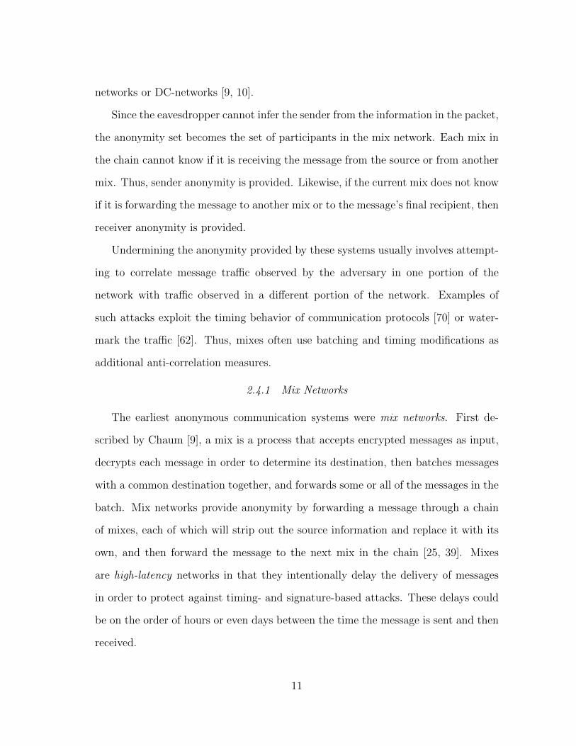
Since the eavesdropper cannot infer the sender from the information in the packet,

the anonymity set becomes the set of participants in the mix network. Each mix in

the chain cannot know if it is receiving the message from the source or from another

mix. Thus, sender anonymity is provided. Likewise, if the current mix does not know

if it is forwarding the message to another mix or to the message’s final recipient, then

receiver anonymity is provided.

Undermining the anonymity provided by these systems usually involves attempt-

ing to correlate message traffic observed by the adversary in one portion of the

network with traffic observed in a different portion of the network. Examples of

such attacks exploit the timing behavior of communication protocols [70] or water-

mark the traffic [62]. Thus, mixes often use batching and timing modifications as

additional anti-correlation measures.

2.4.1 Mix Networks

The earliest anonymous communication systems were mix networks. First de-

scribed by Chaum [9], a mix is a process that accepts encrypted messages as input,

decrypts each message in order to determine its destination, then batches messages

with a common destination together, and forwards some or all of the messages in the

batch. Mix networks provide anonymity by forwarding a message through a chain

of mixes, each of which will strip out the source information and replace it with its

own, and then forward the message to the next mix in the chain [25, 39]. Mixes

are high-latency networks in that they intentionally delay the delivery of messages

in order to protect against timing- and signature-based attacks. These delays could

be on the order of hours or even days between the time the message is sent and then

received.

11

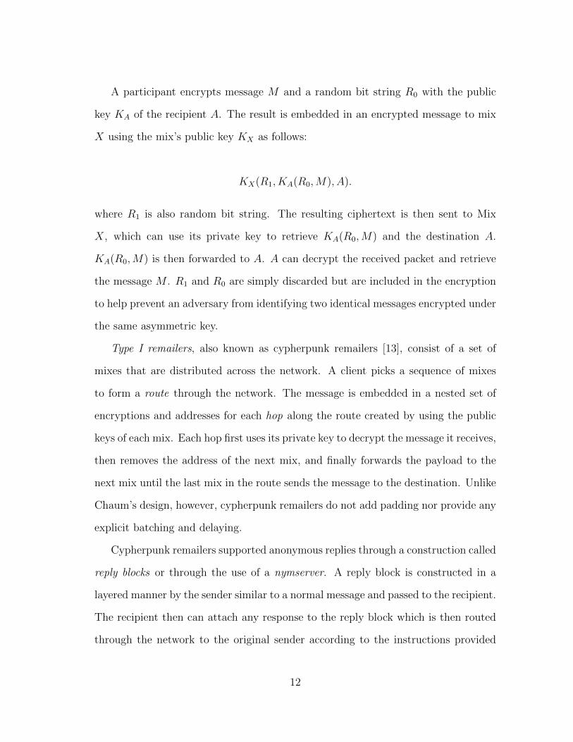
A participant encrypts message M and a random bit string R0 with the public

key KA of the recipient A. The result is embedded in an encrypted message to mix

X using the mix’s public key KX as follows:

KX(R1, KA(R0,M), A).

where R1 is also random bit string. The resulting ciphertext is then sent to Mix

X, which can use its private key to retrieve KA(R0,M) and the destination A.

KA(R0,M) is then forwarded to A. A can decrypt the received packet and retrieve

the message M . R1 and R0 are simply discarded but are included in the encryption

to help prevent an adversary from identifying two identical messages encrypted under

the same asymmetric key.

Type I remailers, also known as cypherpunk remailers [13], consist of a set of

mixes that are distributed across the network. A client picks a sequence of mixes

to form a route through the network. The message is embedded in a nested set of

encryptions and addresses for each hop along the route created by using the public

keys of each mix. Each hop first uses its private key to decrypt the message it receives,

then removes the address of the next mix, and finally forwards the payload to the

next mix until the last mix in the route sends the message to the destination. Unlike

Chaum’s design, however, cypherpunk remailers do not add padding nor provide any

explicit batching and delaying.

Cypherpunk remailers supported anonymous replies through a construction called

reply blocks or through the use of a nymserver. A reply block is constructed in a

layered manner by the sender similar to a normal message and passed to the recipient.

The recipient then can attach any response to the reply block which is then routed

through the network to the original sender according to the instructions provided

12

by the reply block. Alternatively, a sender could send the constructed reply block

to a nymserver. The nymserver stores the reply block and allocates a temporary

pseudonym associated with the received reply block, storing the pair in a database.

When the nymserver receives a message addressed to the pseudonym, it forwards

the message through the remailer network using the stored reply block for that

pseudonym.

The Type II remailer, also known as Mixmaster, adds message padding and batch-

ing [42]. Furthermore, Mixmaster tries to defeat replay attacks by recording the

packet IDs included in the message header. If a mix receives a duplicate message,

the duplicate is simply discarded. Mixmaster does not include support for anony-

mous replies.

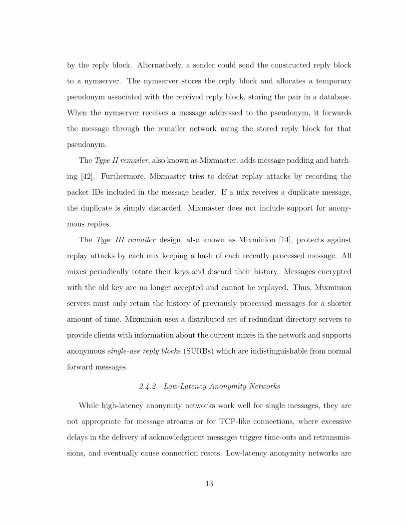
The Type III remailer design, also known as Mixminion [14], protects against

replay attacks by each mix keeping a hash of each recently processed message. All

mixes periodically rotate their keys and discard their history. Messages encrypted

with the old key are no longer accepted and cannot be replayed. Thus, Mixminion

servers must only retain the history of previously processed messages for a shorter

amount of time. Mixminion uses a distributed set of redundant directory servers to

provide clients with information about the current mixes in the network and supports

anonymous single-use reply blocks (SURBs) which are indistinguishable from normal

forward messages.

2.4.2 Low-Latency Anonymity Networks

While high-latency anonymity networks work well for single messages, they are

not appropriate for message streams or for TCP-like connections, where excessive

delays in the delivery of acknowledgment messages trigger time-outs and retransmis-

sions, and eventually cause connection resets. Low-latency anonymity networks are

13

architected to carry latency sensitive communication (inclusive TCP connections).

Low-latency anonymity systems are often based on the notion of a proxy. While

mixes explicitly batch and reorder incoming messages, proxies simply forward all

incoming traffic (e.g., the packets of a TCP connection) immediately and typically

without packet reordering.

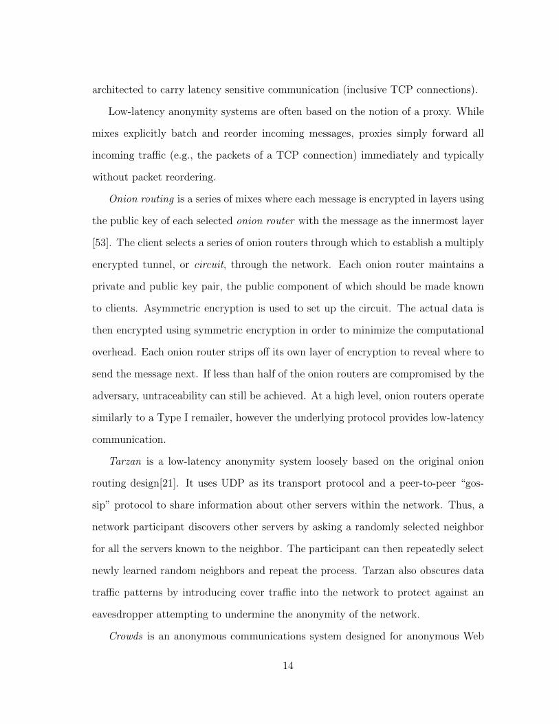
Onion routing is a series of mixes where each message is encrypted in layers using

the public key of each selected onion router with the message as the innermost layer

[53]. The client selects a series of onion routers through which to establish a multiply

encrypted tunnel, or circuit, through the network. Each onion router maintains a

private and public key pair, the public component of which should be made known

to clients. Asymmetric encryption is used to set up the circuit. The actual data is

then encrypted using symmetric encryption in order to minimize the computational

overhead. Each onion router strips off its own layer of encryption to reveal where to

send the message next. If less than half of the onion routers are compromised by the

adversary, untraceability can still be achieved. At a high level, onion routers operate

similarly to a Type I remailer, however the underlying protocol provides low-latency

communication.

Tarzan is a low-latency anonymity system loosely based on the original onion

routing design[21]. It uses UDP as its transport protocol and a peer-to-peer “gos-

sip” protocol to share information about other servers within the network. Thus, a

network participant discovers other servers by asking a randomly selected neighbor

for all the servers known to the neighbor. The participant can then repeatedly select

newly learned random neighbors and repeat the process. Tarzan also obscures data

traffic patterns by introducing cover traffic into the network to protect against an

eavesdropper attempting to undermine the anonymity of the network.

Crowds is an anonymous communications system designed for anonymous Web

14

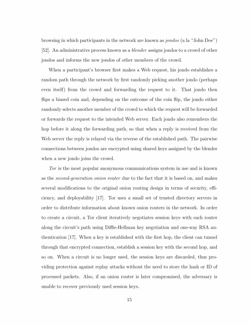
browsing in which participants in the network are known as jondos (a la “John Doe”)

[52]. An administrative process known as a blender assigns jondos to a crowd of other

jondos and informs the new jondos of other members of the crowd.

When a participant’s browser first makes a Web request, his jondo establishes a

random path through the network by first randomly picking another jondo (perhaps

even itself) from the crowd and forwarding the request to it. That jondo then

flips a biased coin and, depending on the outcome of the coin flip, the jondo either

randomly selects another member of the crowd to which the request will be forwarded

or forwards the request to the intended Web server. Each jondo also remembers the

hop before it along the forwarding path, so that when a reply is received from the

Web server the reply is relayed via the reverse of the established path. The pairwise

connections between jondos are encrypted using shared keys assigned by the blender

when a new jondo joins the crowd.

Tor is the most popular anonymous communications system in use and is known

as the second-generation onion router due to the fact that it is based on, and makes

several modifications to the original onion routing design in terms of security, effi-

ciency, and deployability [17]. Tor uses a small set of trusted directory servers in

order to distribute information about known onion routers in the network. In order

to create a circuit, a Tor client iteratively negotiates session keys with each router

along the circuit’s path using Diffie-Hellman key negotiation and one-way RSA au-

thentication [17]. When a key is established with the first hop, the client can tunnel

through that encrypted connection, establish a session key with the second hop, and

so on. When a circuit is no longer used, the session keys are discarded, thus pro-

viding protection against replay attacks without the need to store the hash or ID of

processed packets. Also, if an onion router is later compromised, the adversary is

unable to recover previously used session keys.

15

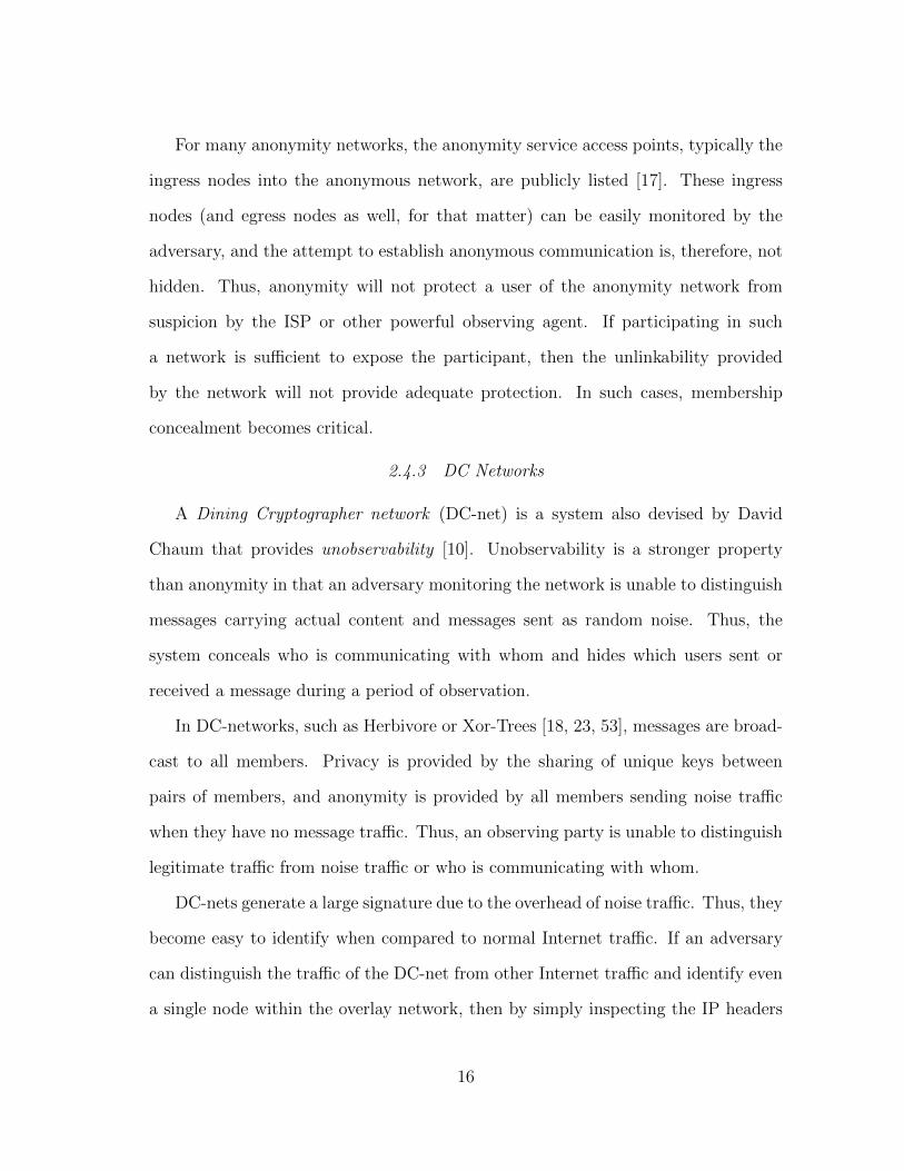
For many anonymity networks, the anonymity service access points, typically the

ingress nodes into the anonymous network, are publicly listed [17]. These ingress

nodes (and egress nodes as well, for that matter) can be easily monitored by the

adversary, and the attempt to establish anonymous communication is, therefore, not

hidden. Thus, anonymity will not protect a user of the anonymity network from

suspicion by the ISP or other powerful observing agent. If participating in such

a network is sufficient to expose the participant, then the unlinkability provided

by the network will not provide adequate protection. In such cases, membership

concealment becomes critical.

2.4.3 DC Networks

A Dining Cryptographer network (DC-net) is a system also devised by David

Chaum that provides unobservability [10]. Unobservability is a stronger property

than anonymity in that an adversary monitoring the network is unable to distinguish

messages carrying actual content and messages sent as random noise. Thus, the

system conceals who is communicating with whom and hides which users sent or

received a message during a period of observation.

In DC-networks, such as Herbivore or Xor-Trees [18, 23, 53], messages are broad-

cast to all members. Privacy is provided by the sharing of unique keys between

pairs of members, and anonymity is provided by all members sending noise traffic

when they have no message traffic. Thus, an observing party is unable to distinguish

legitimate traffic from noise traffic or who is communicating with whom.

DC-nets generate a large signature due to the overhead of noise traffic. Thus, they

become easy to identify when compared to normal Internet traffic. If an adversary

can distinguish the traffic of the DC-net from other Internet traffic and identify even

a single node within the overlay network, then by simply inspecting the IP headers

16

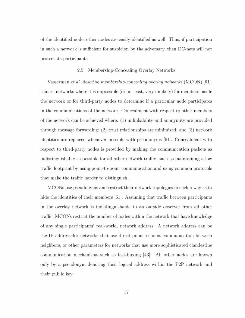
of the identified node, other nodes are easily identified as well. Thus, if participation

in such a network is sufficient for suspicion by the adversary, then DC-nets will not

protect its participants.

2.5 Membership-Concealing Overlay Networks

Vasserman et al. describe membership-concealing overlay networks (MCON) [61],

that is, networks where it is impossible (or, at least, very unlikely) for members inside

the network or for third-party nodes to determine if a particular node participates

in the communications of the network. Concealment with respect to other members

of the network can be achieved where: (1) unlinkability and anonymity are provided

through message forwarding; (2) trust relationships are minimized; and (3) network

identities are replaced whenever possible with pseudonyms [61]. Concealment with

respect to third-party nodes is provided by making the communication packets as

indistinguishable as possible for all other network traffic, such as maintaining a low

traffic footprint by using point-to-point communication and using common protocols

that make the traffic harder to distinguish.

MCONs use pseudonyms and restrict their network topologies in such a way as to

hide the identities of their members [61]. Assuming that traffic between participants

in the overlay network is indistinguishable to an outside observer from all other

traffic, MCONs restrict the number of nodes within the network that have knowledge

of any single participants’ real-world, network address. A network address can be

the IP address–for networks that use direct point-to-point communication between

neighbors, or other parameters for networks that use more sophisticated clandestine

communication mechanisms such as fast-fluxing [43]. All other nodes are known

only by a pseudonym denoting their logical address within the P2P network and

their public key.

17

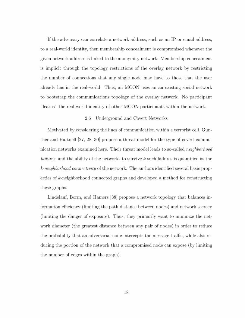
If the adversary can correlate a network address, such as an IP or email address,

to a real-world identity, then membership concealment is compromised whenever the

given network address is linked to the anonymity network. Membership concealment

is implicit through the topology restrictions of the overlay network by restricting

the number of connections that any single node may have to those that the user

already has in the real-world. Thus, an MCON uses an an existing social network

to bootstrap the communications topology of the overlay network. No participant

“learns” the real-world identity of other MCON participants within the network.

2.6 Underground and Covert Networks

Motivated by considering the lines of communication within a terrorist cell, Gun-

ther and Hartnell [27, 28, 30] propose a threat model for the type of covert commu-

nication networks examined here. Their threat model leads to so-called neighborhood

failures, and the ability of the networks to survive k such failures is quantified as the

k-neighborhood connectivity of the network. The authors identified several basic prop-

erties of k-neighborhood connected graphs and developed a method for constructing

these graphs.

Lindelauf, Borm, and Hamers [38] propose a network topology that balances in-

formation efficiency (limiting the path distance between nodes) and network secrecy

(limiting the danger of exposure). Thus, they primarily want to minimize the net-

work diameter (the greatest distance between any pair of nodes) in order to reduce

the probability that an adversarial node intercepts the message traffic, while also re-

ducing the portion of the network that a compromised node can expose (by limiting

the number of edges within the graph).

18

2.7 Delay-Tolerant Networks

Delay (disruption) tolerant networks (DTN) describe a general class of commu-

nications protocols designed to allow nodes within the network to successfully prop-

agate reliable traffic despite intermittent connectivity [8, 20]. The DTN architecture

was designed to accommodate not only network connection disruption, but also to

provide a framework for dealing with the sort of heterogeneity found at sensor net-

work gateways (and other gateways, more generally). DTN can use a multitude of

different delivery protocols including TCP/IP, raw Ethernet, serial lines, or hand-

carried storage drives for delivery. As each of these protocols provide somewhat dif-

ferent semantics, a collection of protocol-specific convergence layer adapters (CLAs)

provide the functions necessary to carry DTN protocol data units (called bundles)

on each of the corresponding protocols.

Though not often associated with anonymous and covert communication, DTN

research is of particular interest for implementing resilient mix networks. Both DTNs

and anonymity networks use intermediate nodes to route message traffic. Low-

latency anonymity networks are vulnerable to traffic analysis attacks that can cor-

relate message timing across the network and thus undermine the anonymity. Mix

networks prevent these attacks by intentionally introducing additional latency. Thus,

when latency is not a concern, DTNs can provide insight into implementing CCNs

that protect anonymity and membership concealment while being resilient as well.

2.8 Conclusions

Each of the research areas discussed provides some form of protection to par-

ticipants communicating with one another in the presence of an adversary. How-

ever, each on their own does not provide resilient networks with adequate protection

against discovery of participants. We now examine covert communication networks

19

which integrate aspects of the fields discussed above. In the following secions, we

discuss the architecture and properties of covert communication networks and de-

scribe how they provide resilience, anonymity and membership concealment for their

participants.

20

3. BASIC STRUCTURE AND OPERATION OF A COVERT

COMMUNICATION NETWORK

Throughout this work we start from the premise that a peer-to-peer overlay of

mix-like nodes is an appropriate basis for the development of a membership con-

cealing, anonymous system. Given the peer-to-peer nature of such a system, the

failure to protect any specific user affects the system as a whole, since the adversary

may infer the membership of other users from the traffic emanating from the first

victim to its peers. Mechanisms at multiple levels must be in place to protect the

communication and the membership of participants.

Thus, we realize a CCN as a peer-to-peer overlay network, where traffic is routed

from a source node to a destination node by relying on intermediate nodes to for-

ward traffic through the network. Each participant acts, in traditional peer-to-peer

manner, both as sender/receiver of data and as a router within the network. Two

participants are neighbors in the CCN when they are directly connected to each

other in the overlay topology with no intermediate nodes between them. Neighbor

nodes in the CCN know of each other’s network address (e.g., IP or email address)

and neighbor-to-neighbor traffic is forwarded using whatever underlying transmission

protocol has been negotiated by the nodes at join time. Nodes that are not neighbors

never exchange traffic directly. Instead, messages are routed through intermediary

nodes. Traffic is routed end-to-end through the network by using logical addresses

and is forwarded through a sequence of neighboring nodes until the destination is

reached.

1Portions of this section are reprinted with permission from “Subversion Impedance in CovertCommunication Networks” by Timothy Nix and Riccardo Bettati, 2012, In Proceedings of the 2012IEEE 11th International Conference on Trust, Security and Privacy in Computing and Communi-cations (TrustCom), pages 458-465, Copyright [2012] by IEEE.

21

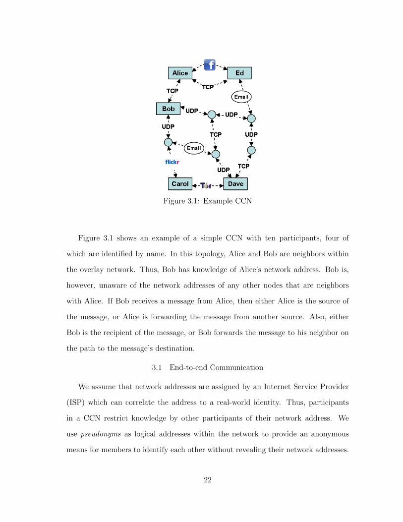
Figure 3.1: Example CCN

Figure 3.1 shows an example of a simple CCN with ten participants, four of

which are identified by name. In this topology, Alice and Bob are neighbors within

the overlay network. Thus, Bob has knowledge of Alice’s network address. Bob is,

however, unaware of the network addresses of any other nodes that are neighbors

with Alice. If Bob receives a message from Alice, then either Alice is the source of

the message, or Alice is forwarding the message from another source. Also, either

Bob is the recipient of the message, or Bob forwards the message to his neighbor on

the path to the message’s destination.

3.1 End-to-end Communication

We assume that network addresses are assigned by an Internet Service Provider

(ISP) which can correlate the address to a real-world identity. Thus, participants

in a CCN restrict knowledge by other participants of their network address. We

use pseudonyms as logical addresses within the network to provide an anonymous

means for members to identify each other without revealing their network addresses.

22

Pseudonyms could be a unique username selected by the participant; a random string

or set of digits; the participant’s public key; or a numerical value associated with

their location within the CCN overlay topology.

Pseudonyms are used by intermediate nodes to identify a message’s destination.

When a node receives data, it replaces the network address associated with the data,

with its own network address and forwards the data to the next neighbor along the

route. Thus, for each message, we have a source node, a destination node, and zero

or more intermediate nodes that forward the message in a way as to delink the sender

and the receiver.

3.1.1 Communication between Neighbors

Communication between neighbors in the CCN overlay is carried over what we

call channels. Channels can be of different channel types, which in turn specify the

implementation of each channel. Each channel type will have different performance

characteristics in support of the communication requirements of the group. Different

channel types can be easily developed based on the particular requirements of the

group. For example, channels can be instantiated using: the user datagram proto-

col (UDP), the transmission control protocol (TCP), simple mail transfer protocol

(SMTP) (i.e., email), covert channels, steganographic messages passed between nodes

using either file-transfer protocol (FTP) or a shared repository (such as Facebook,

Flickr, Twitter, etc.), or any other network communication protocol.

Channels are either low-latency or high-latency, each of which offers its own trade-

offs between performance and anonymity. Low latency communication provides near-

real-time communication for group members at the risk of providing an adversary

with timing signatures for tracing packets across the overlay network, thus under-

mining anonymity. If near-real-time communication is not required, then nodes can

23

provide the full functionality of a mix by both batching messages and introducing

variations in timing to obscure communication signatures and increase anonymity.

A node may have multiple channels from which to choose in order to transmit data

to a particular neighbor. The channel type used to communicate between neighbors

is negotiated as part of the join protocol of a new node, and the channels used by

the network are instantiated at each node immediately after joining the network and

selected for use based on the requirements of each specific message.

In Figure 3.1 Alice had two neighbors: Bob and Ed. In one case, Alice com-

municates through Bob using a TCP channel, and communicates through Ed using

either a TCP channel or Facebook. Facebook, Flickr and other social network and

file sharing sites can be used to pass messages embedded in photos or music files

using standard steganographic techniques. Alice needs only to provide Ed with the

account and filename to successfully pass the message. Thus, Alice can send data

to Ed in more than one way. For latency-sensitive communication, they can select

to use the TCP channel, while the Facebook channel can be used for the remaining

communication.

During establishment of the overlay network (typically as part of the join protocol

discussed in Section 8) neighboring nodes discover and negotiate the set of channels

to be provided. During the connection establishment, each node selects from among

the available channels the particular channel to be used on the outgoing link to the

next node in the overlay network.

3.1.1.1 Pushing vs. Pulling Data

As in most peer-to-peer networks, each node in the CCN operates as both a

server and a client. We make the distinction between the two by denoting the client

as the process that initiates the communication. Data can be pulled or pushed by

24

a channel, as necessary. In the first case, when the channel receives a message, the

message is buffered until it is requested by the appropriate neighbor. The process is

repeated at each node, propagating across the network until the data packet reaches

its destination. In the second case, when a node receives data that needs to be

forwarded, the node automatically connects to the appropriate neighbor and forwards

the message.

The polling of adjacent nodes provides a basis for message batching and timing

disruption. These are two key characteristics of early Mix networks [13]. However,

the timing of the polling could potentially provide a signature that would under-

mine membership concealment. Randomizing the time periods between polls would

disrupt the timing and provide protection against these types of attacks.

Message pushing, on the other hand, minimizes propagation delay between adja-

cent nodes if the message is sent immediately. If messages are also routed along the

fastest route, then the source-to-destination propagation delay is minimized. This

is essential when near-real-time communication is necessary, such as voice-over-IP

(VoIP) or video teleconferencing.

3.1.2 Pseudonyms

Pseudonyms are identifiers that should not be linkable to the real identities of

the participants. In other words, a pseudonym is an identifier of a subject other

than one of the subject’s real names [53]. Thus, pseudonyms provide a means for

non-adjacent nodes within a covert communication network to communicate with

each other without needing to share their network addresses.

Pseudonyms could be a unique username selected by the participant, a random

string or set of digits, the participant’s public key, or a numerical value associated

with their location within the CCN overlay topology. Participants distribute their

25

pseudonym as a means for other nodes to communicate with them. In our imple-

mentation, pseudonyms correspond to a logical location within the network topology

in order to facilitate routing.

3.1.3 CCN Message Confidentiality

Cryptography provides message confidentiality. Though orthogonal to anonymity

and membership concealment, confidentiality is an inherent requirement in a CCN.

Given the threat model, we use cryptography to guard message confidentiality.

Thus, all traffic within the CCN is encrypted. Encryption occurs at two levels.

First, we have end-to-end cryptography where the source encrypts the payload so

that it is only readable by the destination. Second, we have hop-level cryptography,

where a node along the route encrypts the data packet so that it is only readable by

the next node along the route. Since messages are also re-encrypted every time they

are forwarded by a node, this also provides protection against the adversary tracing

messages across the network.

CCNs can use either symmetric or asymmetric cryptography. Similar to other

Internet protocols such as transport layer security (TLS), symmetric cryptography

is used for low-latency communication. For exchanging symmetric keys, asymmetric

cryptography is used. It can also be used for encrypting and decrypting delay-tolerant

traffic.

Public keys are shared in a distributed manner among the CCN nodes via a web

of trust. In the web of trust, keys propagate across the network as they are shared

from neighbor to neighbor. As long as two or more paths exist between any two

nodes, attempts to corrupt public keys or execute a man-in-the-middle attack are

detectable. Thus, there is no need for a central certificate authority.

26

3.2 Topology Considerations

The ability of a CCN to protect the identity of participants depends to a large ex-

tent on the connectivity between nodes who posses the network address of each other.

Most, if not all, of the research conducted on underground, covert and membership

concealing networks to date has therefore focused on the topology of the network

[30, 38, 61]. The idea behind these topologies is to minimize the damage done by

the subversion of a node. Gunther and Hartnell [30] examined network topologies

that either maximize the number of survivors in the event of the deletion of a closed

neighborhood of nodes; or are resilient (i.e., remain connected) from multiple sub-

versions. In the first case, they found various tree structures to be optimal. In the

second, they demonstrated a construction for k-neighbor-connected graphs; that is,

graphs that remain connected from the removal of k closed neighborhoods of nodes.

Lindelauf et al. [38], on the other hand, examined topologies that optimized

the trade-off between: (1) minimizing the number of edges that a message must

travel and, thus, the probability that a message is intercepted by an adversary (thus,

increasing node degree); and (2) minimizing the number of nodes that any subverted

node might compromise (thus, decreasing node degree). They found that complete

graphs provided the optimal solution in low threat areas, i.e., low probability of node

subversion; whereas, the star graph and a cellular network provided the optimal

topology for conditions with a higher probability of subversion. Unfortunately, the

complete graph does not provide membership concealment in that any participant has

knowledge of all other participants’ network addresses. Star graphs are not resilient

against disconnection. Rather, CCN topologies need high connectivity for resilience

but must also be as sparsely connected as possible in order to protect membership

concealment.

27

3.2.1 Threat Model

Our network participants, Alice and Bob, are legitimate members of the CCN.

We assume that Alice and Bob wish to communicate over the covert communication

network. Eve is the powerful adversary attempting to gain information about the

covert communication network and identify its participants. If Eve learns the network

address of either Alice or Bob, we consider this information sufficient and necessary

to then identify Alice’s or Bob’s real-world identity. For example, if Eve learns a

participant’s IP address using the ISP database, she can determine the owner of the

IP address and then use this information to identify Alice and Bob.

We define Bob’s network promiscuity as the number of other participants that

have knowledge of his network identity. Then, Bob’s membership concealment is

reduced in proportion to his network promiscuity. The more participants that have

knowledge of Bob’s network identity, the higher the probability that the adversarial

node Eve knows Bob’s network identity and can, thus, correlate his network identity

to his real-world identity.

In our threat model, a node is subverted when Eve successfully attacks the node.

A node might be subverted in a variety of ways: Either Alice or Bob could betray the

group and switch to the side of the adversary, Eve. Similarly, Eve could infect a node

in a way that allows her to monitor communications across this node. Finally, Eve

could infiltrate the network by successfully joining. Nodes attached to the betrayed

node are then considered compromised because their owners might be identified by

their network address. The subverted node can directly monitor communications

with the compromised nodes and can provide this information to the adversary.

If a node is suspected of being subverted, then both the node and all connected

nodes are removed from the network: either the owners of the compromised nodes are

28

arrested, or the network membership successfully identifies the subverted node and

disconnects from it and its compromised neighbors. This particular threat model was

used by Gunther and Hartnell in their examination of the communication topologies

of underground resistance movements (covert communication networks) [30]. With

no loss of generality, we treat the subversion of multiple nodes as separate events.

3.2.2 Network Resiliency

We want our network to be resilient against partitioning. In the event of the

subversion of a node and the compromise of its neighbors, we want to maximize the

chance that the network remains connected.

Therefore, we want a network topology that minimizes the number of nodes

that will potentially connect to Alice. This way, if Alice’s node becomes subverted,

then the number of compromised nodes is also minimized. However, we also want

a network topology that is resilient against disconnection through the removal of

multiple neighborhoods of nodes.

As long as connectivity cost is not an issue, the effect of single-node failures

in traditional networks can be easily countered by making networks more dense.

A fully-connected or complete network is a communication network in which every

pair of nodes is adjacent. Such a complete network provides (1) the shortest path

length between any two nodes minimizing communications time; and (2) the highest

degree of path redundancy and protection against network partition. If we were

only concerned over the loss of a single node in the event of a subversion, then the

connectivity of the surviving network would decrease by one, and the network would

remain connected for any graph with more than two nodes. Given our threat model,

the problem with a complete graph, of course, is that the subversion of any single

node results in the compromise of the entire network.

29

On the other hand, a tree is an undirected graph in which any two nodes are

connected by exactly one simple path. If minimizing connectivity were our only

concern, then a tree would be the ideal structure since it provides a communications

path between all nodes while minimizing the order of each node, and thus, the

damage resulting from the subversion of any node. In [30], Hartnell and Gunther

initially focus on several types of trees as being resilient to subversions. In a tree-like

network topology, however, the subversion of any node may lead to a partitioning of

the network. The surviving components would then be unable to communicate with

each other.

The above examples illustrate that covert communication networks must natu-

rally balance the level of connectivity of nodes against the size of their neighborhood.

They must be highly connected in order to be resilient against disconnection. They

must also be as sparsely connected as possible in order to minimize network promis-

cuity.

Network resiliency also provides multiple paths between nodes. Thus, traffic could

still be routed even if some portion of the nodes were down. We can also use network

resiliency to detect attempts by an adversary to corrupt network traffic. Copies of

the same message could be sent along different paths. These copies could then be

compared by the destination node to ensure message integrity and identify subverted

nodes that may attempt to modify packets. However, if not strictly managed, this

approach could result in a significant amount of traffic creating an easily identifiable

signature to an adversary.

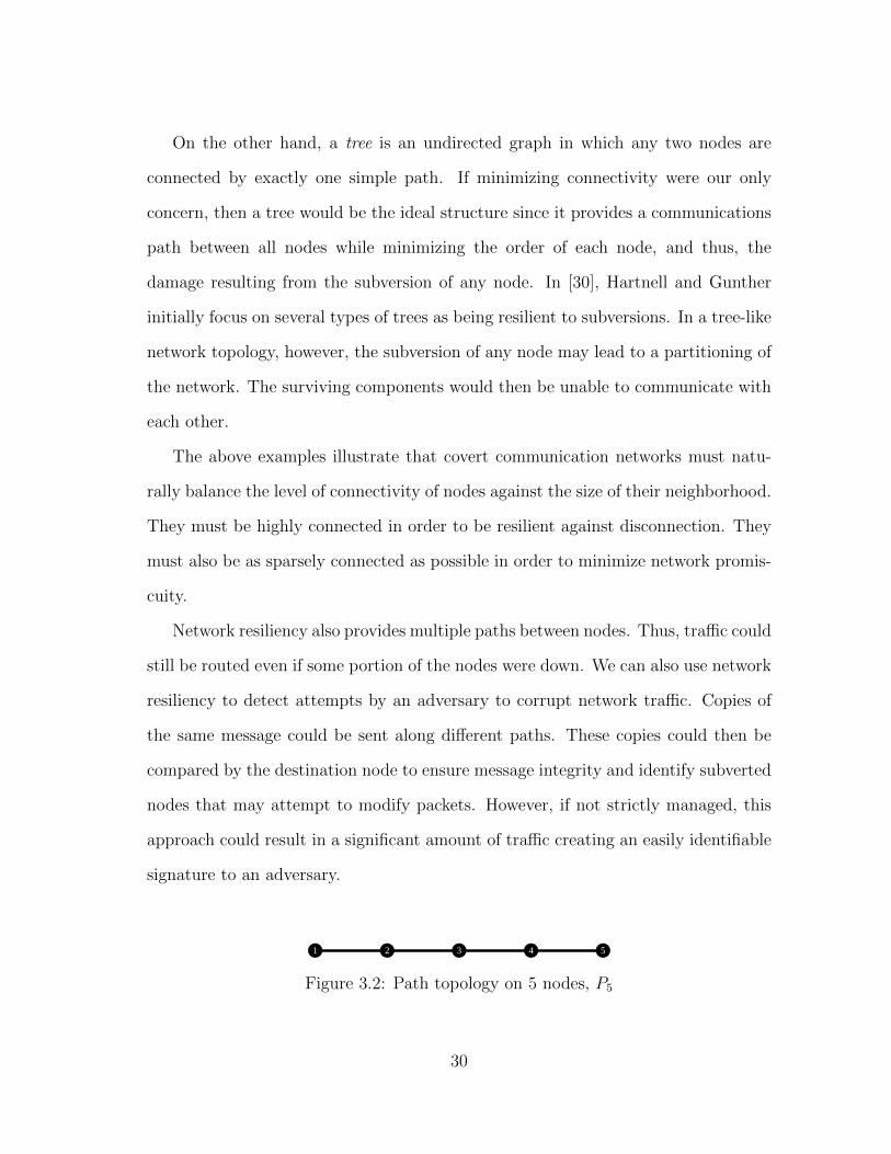
1 2 3 4 5

Figure 3.2: Path topology on 5 nodes, P5

30

3.2.3 Deterministic versus Random Topology Construction

Deterministic topologies are those in which the direct connections established

within the topology are deterministic. Thus, the topology of the network is defined as

a function of the number of nodes. A given node within the network might have been

located at a different point within the topology if it had joined at a different time,

but the overall topology for a given number of nodes remains the same. Figure 3.2

shows a simple path topology on 5 nodes. An example of a deterministic construction

for a path topology on n nodes is one in which Node vn connects to the next node

that joins, vn+1.

Random topology constructions are those in which, as new nodes join the network,

neighbor connections are randomly determined. Thus, even the topology of two

different overlay networks with the same number of nodes is likely to be different.

3.2.4 Structured versus Unstructured Topologies

In a structured topology, the location of the participant in the covert commu-

nication network (not to be confused with the network address within the larger

network) is arranged and assigned in a structured manner. Chord [57] and CAN [51]

rely on a random but structured topology to facilitate node joins and data lookup.

In Chord and CAN, a node’s logical location within the overlay network can be

considered the node’s pseudonym. As we will see in Section 4 and Section 5, the

k-neighbor-connected networks constructed by Gunther and Hartnell [30] and the

characteristics of cages can be used as structured topologies. As we will see in Sec-

tion 8, pseudonyms can be structured as logical addresses, indicating where in the

overlay topology a node is located and, thus, facilitate routing.

In unstructured topologies, pseudonyms do not correspond to a node’s logical

address within the topology. Thus, nodes must advertise their logical address to

31

other nodes to facilitate routing. This can be done easily using traditional network

approaches to node discovery, but it does increase the communication signature of

the network and the complexity of each node.

3.3 Communications Considerations

Though many of the same principals that we have discussed thus far can apply to

a variety of communication networks, we have defined CCNs as an overlay network.

We now examine the rationale behind this decision and some other design choices

with regard to CCNs as overlay networks.

3.3.1 No Specialized Equipment Required

Concealed communication can be established using specialized technology, such

as spread-spectrum transmitters. However, in practice, use of such additional hard-

ware comes at a cost; it has to be acquired, distributed, maintained, and, in many

cases, possession of the specialized equipment is enough to compromise membership

anonymity. Thus, specialized equipment limits who can participate in the network.

In contrast, computers are becoming more and more common in most countries.

Ownership of a computer is usually not suspicious. This also allows the covert com-

munication network to be implemented in software at the application level with low

signature for detection. Techniques used to conceal computer viruses can also be

used to further conceal and obfuscate the presence or purpose of the covert commu-

nication network application, such as embedding the communication software within

another benign application.

3.3.2 Open versus Closed Infrastructure

An open infrastructure does not require participants to be actual members of

the network. If Bob wants to participate in the covert communication network but

32

does not want to join the network, then he will need to use an actual member

node as an entry point into the network. Likewise, if Alice is the recipient of Bob’s

message, and she is not a member of the network, then a member node will need

to be used as an exit point from the network to Alice. In either case, the fact

that Bob and Alice participate in the system is known to the entry and exit nodes,

respectively. Open infrastructures leave both the entry and exit nodes of the network

and the participants vulnerable: on the one hand, the entry and exit nodes in an

open infrastructure are likely to connect to many participants; and on the other hand,

participants might have to establish connections (or “tunnels”) through potentially

large numbers of entry and exit nodes, making it known to them that the participants

are engaging in covert communication. If participants use the same entry and exit

points each time, they limit their own exposure, but their lack of membership in

the network as router nodes reduces the potential resiliency of the network. If all

members act in this manner, the result is a network with no intermediate nodes

providing anonymity.

A closed infrastructure provides a higher degree of anonymity for all nodes. If

Alice and Bob are members of the network, then a node adjacent to and receiving

a message from Alice will not know whether she is the originator of the message,

or simply another link in the routing chain. Furthermore, no nodes are required to

serve as entry or exit nodes and, thus, consistently connecting to new nodes. As a

result, any covert communication network that gains anonymity and unlinkability by

using network members as mixes, onion routers, etc. requires a closed infrastructure.

We note that this distinction in effectiveness between open and closed infrastruc-

tures is quite common: for example, reliable multicast protocols come in open and

closed forms, and it is a well-known fact that closed infrastructures are more reliable.

These benefits come at the cost of having to explicitly maintain the membership in

33

the network.

3.3.3 Decentralized Control

The history of P2P file sharing networks such as Napster, Gnutella, Chord and

CAN [26, 51, 57] has shown that distributed control mechanisms are superior to

centralized control mechanisms which limit reliability and scalability. It also limits

membership concealment. For example, Tor relies on the public list of onion routers

that allow participants to build their circuits through the network [17]. Thus, a

powerful adversary might be able to monitor traffic at a network firewall or ISP

gateway and identify packets destined for Tor and learn the identities of participants.

The Distributed Hash Table (DHT) in Chord provides a means to store pseudonyms

and public encryption keys in a decentralized manner within a P2P network. Coupled

with a structured network organization, a DHT provides a mechanism for information

lookup and retrieval within a P2P network and has no single point of failure.

Both of these structures grow by inserting new nodes into the existing network

topology. Though a given node may have a limited number of neighbors to which

it passes message traffic, it will have been connected to a larger number of nodes

throughout this lifetime. For example, if a new node is inserted “between” Alice and

Bob, Bob will “forget” Alice’s network address and retain the network address of the

new node. This works fine in most cases, but in a covert communication network

where we must limit Bob’s network promiscuity, this approach will not work. If Eve

successfully infiltrates the network, then there is no limit to the number of network

participants that she will compromise as long as she remains a member. Instead, in

a covert communication network, we must constrain the network promiscuity of all

nodes over their lifetime.

Thus, we want decentralized control in a covert communication network. DHTs

34

would provide a mechanism for storing pseudonyms and their associated crypto-

graphic keys. However, we must restrict dynamic aspects of P2P networks in ways

that fix the network promiscuity and maximize the anonymity of participants.

3.3.4 Effects of Network Promiscuity and Trust

Increasing network promiscuity by revealing one’s network address to another

node reduces membership concealment and increases the probability of compromise

in the event of a subversion. Thus, members are more likely to be willing to reveal

their network address to a participant that they already know rather than to a

stranger. Vasserman et al. [61] use out-of-network, personal relationships with which

to build MCONs. This is due to the inherent risk associated with revealing one’s

network address to a participant that is also a stranger. Revealing one’s network

address to another is a statement of trust.

3.4 Conclusions

The research community is increasingly becoming aware that traditional sender-

receiver anonymity measures are not sufficient to participants in anonymity systems.

Rather, membership concealment and concealment of anonymity infrastructure itself

are important when stakes are high and/or when the anonymity infrastructure cannot

escape a global adversary deployed across multiple jurisdictional domains.

In this section, we examined essential requirements and design choices for covert

communication networks. By definition, trust entails a component of risk. In some

circumstances, use of a covert communication network is a life-and-death decision.

Thus, the network should not induce more risk than absolutely necessary. Covert

communications networks attempt to minimize this risk while providing partici-

pants with a resilient communications network that provides privacy, anonymity,

and membership-concealment. This type of network is promising for high risk situ-

35

ations. We now examine the trade-off between resilient topologies and membership-

concealment in order to find topologies that are suitable for CCNs.

36

4. TOPOLOGY MEASUREMENT IN COVERT COMMUNICATION

NETWORKS

As discussed in Section 3.2.2, the design of a resilient network for covert com-

munication requires the careful trade-off between minimizing the number of nodes

affected by the presence of a subverted node (we denote this as secrecy) and maxi-

mizing the resilience of the network to remain connected despite multiple subversions

(we denote this as resilience). In the following, we develop a measure that integrates

both secrecy and resilience in order to determine the topology of a resilient covert

communications network. Appendix A provides an overview of the graph theoretic

terms and symbols used in the following sections.

In [37, 38], Lindelauf et al. define a topology performance measure on a graph,

G,

µ(G) = S(G)I(G) ,

where S(G) is the secrecy measure and I(G) is the average performance of the net-

work. The average performance, I(G), is defined by the (normalized) reciprocal of

the total network distance. Thus, topologies with high average performance have

shorter distances between nodes with the best performance being a fully-connected

network. Their secrecy measure is defined as

2Portions of this section are reprinted with permission from “Subversion Impedance in CovertCommunication Networks” by Timothy Nix and Riccardo Bettati, 2012, In Proceedings of the 2012IEEE 11th International Conference on Trust, Security and Privacy in Computing and Communi-cations (TrustCom), pages 458-465, Copyright [2012] by IEEE.

3Portions of this section are reprinted with permission from “Topology Construction of Near-Optimal Covert Communications Networks” by Timothy Nix and Riccardo Bettati, 2012, In Pro-ceedings of the 2012 International Symposium on Pervasive Systems, Algorithms, and Networks(ISPAN), pages 135-142, Copyright [2012] by IEEE.

37

S(G) =∑i∈V

αi(G)ui(G) ,

where αi(G) is the a priori probability that upon surveillance individual i will be

exposed as a member of the network, and ui is the fraction of the network that

remains unexposed when i is detected.

Our approach is similar to Lindelauf et al. [38] in that we optimize two compet-

ing requirements. Furthermore, we borrow their secrecy measure though we modify

it for our given threat model. The secrecy measure used by Lindelauf examines

the proportion of nodes that remain after the subversion of a node. However, their

secrecy measure incorporates the probability that each given node within the net-

work is subverted. This provides an interesting degree of freedom within the design

space, allowing them to calculate their measure based on the a priori probability

distribution of node subversions.

The a priori probability distribution of node subversion quantifies the realistic

probability of subversion associated with each node. However, it is difficult, if not

impossible, to assign meaningful probability values to each node. The a priori prob-

ability distribution reflects the behaviors of the network members and is constantly

changing based on those behaviors. However, meaningful analysis can be done by

simplifying the a priori probability distribution for subversion to either the worst-

case, as we show in the Section 4.1, or a uniform case, as we show later in Section 5.

4.1 Global Subversion Impedance

Definition 4.1.1. We define our secrecy measure, S, to be the proportion of

the nodes that survive the subversion of node v ∈ V . In other words, S(G, v) is

the order of the survivor graph, |H(G, v)| = |G − N [v]| divided by the order of the

original graph, |G|. Recall that the subversion of node v ensures that both v and its

38

neighborhood, N(v), is affected. Thus,

S(G, v) =|H(G, v)||G|

. (4.1)

We assume that |G| > 3 and G is connected. In the worst case, when G is

complete, G = N [v], so S(G, v) = |G−N [v]| = 0. In the best case, if v is a leaf and

deg(v) = 1, then |N [v]| = 2.

Definition 4.1.2. We define our resilience measure, K, to be the proportion of

the connectivity, κ, that survives the cut of N [v]. In other words,

K(G, v) =κ(H(G, v))

κ(G). (4.2)

Again, we assume G is connected and, thus, κ(G) ≥ 1. In the best case, κ is not

reduced after removing N [v]; for example by removing a leaf and adjacent node in

any linear graph, so K(G, v) = 1 . In the worst case, when G is a complete graph,

then K(G, v) = 0, or if the cut of N [v] produces a disconnected graph, then the

result is κ(H(G, v)) = 0.

Definition 4.1.3. We call the local subversion impedance of a covert commu-

nications network G on node v as γ(G, v), where:

γ(G, v) = S(G, v)K(G, v) . (4.3)

We are interested in network topologies that have a high γ(G, v) in the worst

case. So, we must first examine the worst case for a given graph. We denote v∗ as

the node in a graph, G, such that the cut of v∗ and its neighborhood minimizes the

local subversion impedance of the network G:

39

v∗ = argmin{γ(G, v) | for all v ∈ V } . (4.4)

Thus, v∗ can be thought of as the node whose subversion has the worst-case effect on

the covert communication network. The effect of subverting v∗ in G is the (global)

subversion impedance of the network G.

Definition 4.1.4. The (global) subversion impedance of a covert communica-

tions network G is γ∗(G), where:

γ∗(G) = γ(G, v∗) = minv∈V

γ(G, v) . (4.5)

If any subverted node in G produces a disconnected graph, then γ∗(G) = 0. We refer

to the worst-case survivor graph as H∗(G) = H(G, v∗). Thus,

γ∗(G) =|H∗(G)||G|

× κ(H∗(G))

κ(G). (4.6)

Finally, consider the set of all graphs of a given order, n, which we denote Gn.

Definition 4.1.5. We call the graph Gnopt ∈ Gn an optimal covert communica-

tions network (OCCN) if γ∗(Gnopt) ≥ γ∗(G) for all G ∈ Gn.

Definition 4.1.6. We call the optimal subversion impedance of all graphs in

Gn as Γ(n) = γ∗(Gnopt). Formally,

Γ(n) = maxG∈Gn

γ∗(G) .

Thus, given our subversion impedance, we now have a way to quantify the suit-

ability of a covert communications network on n nodes; that is, for a network to

tolerate neighborhood subversions. However, identifying optimal graphs with naıve

40

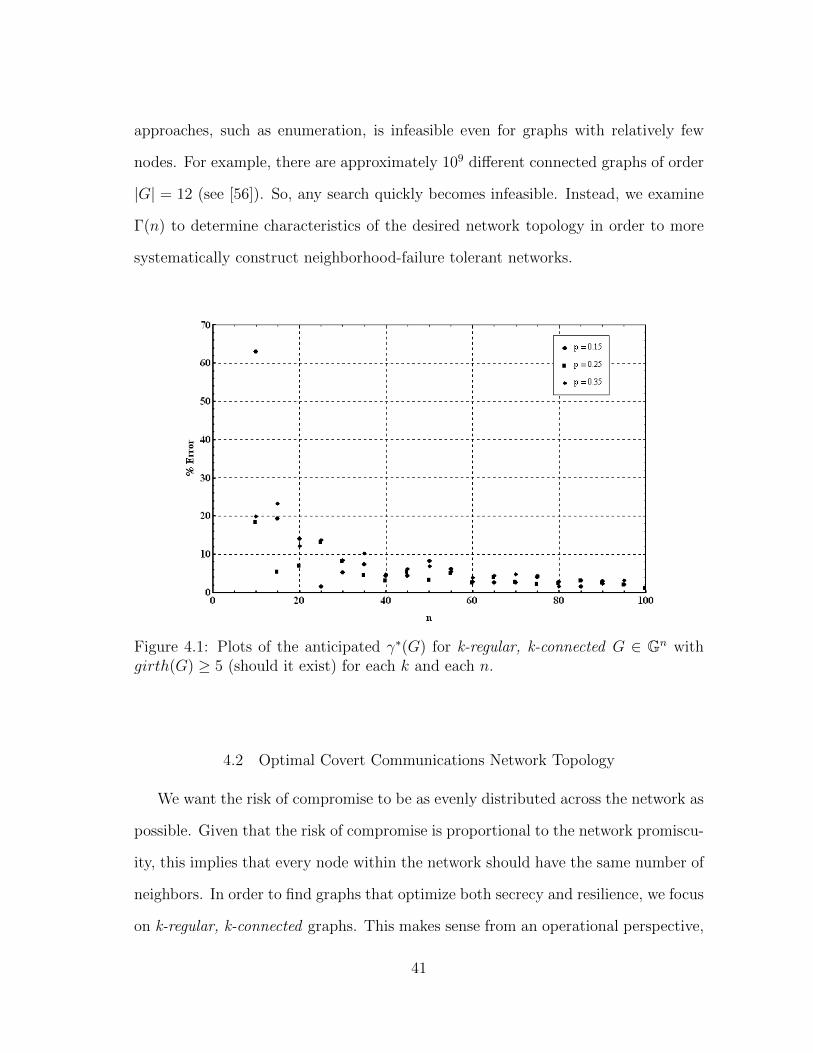
approaches, such as enumeration, is infeasible even for graphs with relatively few

nodes. For example, there are approximately 109 different connected graphs of order

|G| = 12 (see [56]). So, any search quickly becomes infeasible. Instead, we examine

Γ(n) to determine characteristics of the desired network topology in order to more

systematically construct neighborhood-failure tolerant networks.

Figure 4.1: Plots of the anticipated γ∗(G) for k-regular, k-connected G ∈ Gn withgirth(G) ≥ 5 (should it exist) for each k and each n.

4.2 Optimal Covert Communications Network Topology

We want the risk of compromise to be as evenly distributed across the network as

possible. Given that the risk of compromise is proportional to the network promiscu-

ity, this implies that every node within the network should have the same number of

neighbors. In order to find graphs that optimize both secrecy and resilience, we focus

on k-regular, k-connected graphs. This makes sense from an operational perspective,

41

since we want the risk of being affected by a subverted node to be distributed as

evenly across the participants as possible. Also, it simplifies our analysis.

For k-regular, k-connected graphs, we can precisely determine the connectivity

and order of the worst-case survivor graph. In the following, we show that a large-

enough girth of a k-regular, k-connected graph will ensure that the minimum degree

in the worst-case survival graph is only one less than the minimum degree in the

original graph; that is, δ(H∗(G)) = δ(G)− 1. For k-regular, k-connected graphs, this

also minimizes reduction in the connectivity and so helps overall resilience.

Lemma 4.2.1. Given a k-regular, k-connected graph G with girth(G) ≥ 5, the

worst-case survivor graph has a minimum degree of δ(G)− 1. In other words,

δ(H∗(G)) = δ(G)− 1 . (4.7)

Proof. We prove Lemma 4.2.1 by showing that, given a graph G = (V,E) with

girth(G) ≥ 5, the high girth means that multiple nodes in the same neighborhood

are not adjacent to a node that is not in the neighborhood. So, let {v1, v2} ∈ N(vo).

Then v1vov2 is a path. If v3 /∈ N [vo] is adjacent to v1 then the path becomes v3v1vov2

and cannot be adjacent to any other nodes in N [vo] (otherwise a 4-cycle would exist,

which contradicts our assumption that girth(G) ≥ 5). Thus, in the survivor graph, v3

has lost, at most, one edge. Since G is k-regular, k-connected, then by Equation A.2,

in G, deg(v3) = δ(G), whereas in H∗(G), deg(v3) = δ(H∗(G)) = δ(G)− 1.

Lemma 4.2.2. If G is k-regular, k-connected with girth(G) ≥ 5, then the connec-

tivity of the worst-case survivor graph is k − 1. More formally,

κ(H∗(G)) = δ(G)− 1 = k − 1 . (4.8)

42

Proof. Let G be k-regular, k-connected with girth(G) ≥ 5. Then for every node,

each edge corresponds to an independent path to all other edges. Removing N [v]

means removing, at most, one edge from nodes within the surviving graph, and from

Lemma 4.2.1, δ(H∗(G)) = δ(G)−1. For each of those nodes vi that lost one adjacent

node, all remaining edges still correspond to an independent path to all remaining

nodes. Therefore, κ(H∗(G)) = deg(vi) = δ(H∗(G)) = δ(G)−1. Since this holds true

regardless of the node v selected, it hold true for v∗. Thus, κ(H∗(G)) = δ(G)− 1 =

k − 1.

Lemma 4.2.3. If a graph G with order n is k-regular, k-connected, then the order

of the worst-case survivor graph is n− k − 1. Formally, we say

|H∗(G)| = |G| − δ(G)− 1 = n− k − 1 . (4.9)

Proof. Let G be k-regular, k-connected. Then every node v ∈ V has a deg(v) =

δ(G) = ∆(G) = k. Removing N [v∗] means removing k + 1 nodes from the original

graph G to create the survivor graph H(G, v). Since this holds true regardless of the

node v selected, it hold true for v∗. Thus, |H(G, v)| = |H∗(G)| = |G| − δ(G) − 1 =

G− k − 1.

Corollary 4.2.1. Assume a k-regular, k-connected graphG of order n with girth(G) ≥

5 exists, then the subversion impedance of G is

γ∗(G) =n− k − 1

n× k − 1

k. (4.10)

Figure 4.1 plots the subversion impedance for k-regular, k-connected graphs with

girth(G) ≥ 5 as a function of the graph order for increasing values of k. Each plot

represents a different value for k = {2, 3, 4, 5, 6} using Equation 4.10 from Corol-

43

lary 4.2.1. The optimal subversion impedance Γ(n) is the maximum S(G)K(G) pos-

sible for a given n. Note that, we are not guaranteed that a k-regular, k-connected

graph exists if k > 2. However, in the following, we use the plots from Equation 4.10

to determine the bounds on the optimal subversion impedance Γ(n) for k-regular,

k-connected graphs of order n, and thus, for arbitrary graphs of order n.

Lemma 4.2.4. For all k-regular, k-connected graphs, G ∈ Gn with girth(G) ≥ 5,

Γ(n) ≥ n− 3

2n.

Proof. For all n ≥ 5, a cycle, Cn, can be constructed. Since Cn is 2-regular, 2-

connected, by Corollary 4.2.1,

γ∗(Cn) =n− 3

2n.

Then, using Definition 4.1.6, we know that the optimal k-regular, k-connected graph

has a γ∗ at least as large. Thus, Γ(n) ≥ γ∗(Cn) gives a lower bound on Γ(n).

We see in Figure 4.1 that, as the order n of the graphs increases, the values of k

that provides the highest γ∗(·) also increase in a stepwise manner. Thus, we can use

Equation 4.10 as a means for quantifying the upper bound of Γ(n). We generate the

value for the optimum k (hereafter denoted as k∗) for the specific ranges of graph

order by calculating γ∗(G) for various k and then selecting

k∗ = arg maxkγ∗(G).

Theorem 4.2.1. For all k-regular, k-connected graphs G of order n, the upper bound

of the optimal subversion impedance Γ(n) is

44

γ∗(G) ≤ n− k∗ − 1

n× k∗ − 1

k∗,

with

k∗ =

⌈−1 +

√4n− 3

2

⌉. (4.11)

Proof. In order to determine when k∗ increases, we examine Figure 4.1. We need to

determine the transition points on the curves where k∗ increases by 1 to maintain

the optimal value Γ(n). At these points, using Equation 4.10, we get,

[n− k∗ − 1

n

][k∗ − 1

k∗

]=

[n− (k∗ + 1)− 1

n

][(k∗ + 1)− 1

k∗ + 1

].

Solving for k∗ and recognizing that k∗ must be a positive integer gives us,

k∗ =

⌈−1 +

√4n− 3

2

⌉.

Thus, we can solve for k∗ as a function of the graph order, n, in order to determine

the upper bound of Γ(n).

Corollary 4.2.2. For a given k with k ∈ N and k ≥ 2, the order, n, of an optimal

graph is bounded by:

k2 − k + 2 ≤ n ≤ k2 + k + 1 (4.12)

Theorem 4.2.2. A k-regular, k-connected graph G with order n,

k =

⌈−1 +

√4n− 3

2

⌉and girth(G) ≥ 5 is an optimal covert communications network (OCCN) on n nodes

45

(i.e., G = Gnopt).

Proof. Given a graph G that is k-regular, k-connected, then by Corollary 4.2.1, we

know that γ∗(G) is determined by Equation 4.10. Assuming k is determined from

Equation 4.11, then from Theorem 4.2.1, the upper bound of γ∗(G) is also determined

by Equation 4.10. Thus, the value for γ∗(G) = Γ(n) the upper bound. So, by

Definition 4.1.5. G is an OCCN.

With the groundwork laid out in this section, we proceed to define engineering

guidelines for the design of resilient covert communication networks in the next

section. We start by looking for a class or family of graphs that are k-regular, k-

connected and girth(G) ≥ 5.

4.3 Examples of Optimal Graphs

Following the previous discussion, we focus our attention to k-regular, k-connected

graphs with girth(G) ≥ 5. A particularly interesting family of such graphs are so-

called cage graphs.

4.3.1 Girth-5 Cages

A (k; girth)-graph is a k-regular graph with the given girth. A (k; girth)-cage is

a (k; girth)-graph with the smallest possible order. Fu, et al. have proven that all

cages are at least 2-connected, all cubic cages (3, girth)-cage are 3-connected, and

conjectured that all simple (k; girth)-cages are k-connected [22]. Thus, we first look

to (k; girth)-cages in order to find Gnopt.

First, we examine the unique (3; 5)-cage, better known as the Petersen graph [66],

shown in Figure 4.2. As expected, it is 3-regular and 3-connected with girth(G) = 5,

and order |G| = 10. If N [v∗] is removed from this graph, the result is the induced

subgraph shown on the right in Figure 4.2. In this case, the survivor graph con-

46

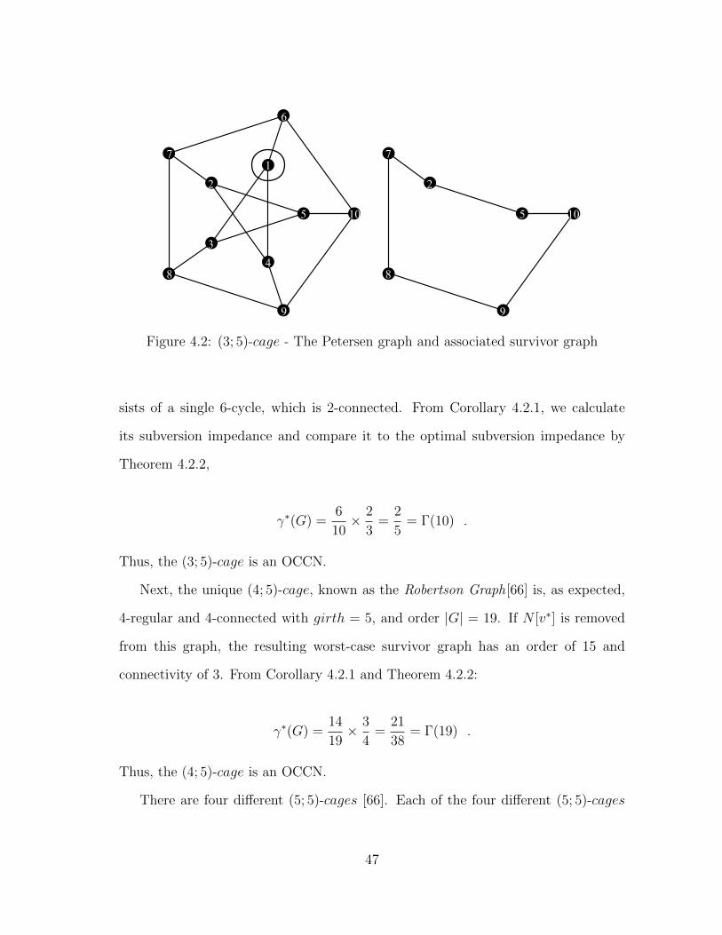
1

2

3

4

5

6

7

8

9

10

1

2

3

4

5

6

7

8

9

10

Figure 4.2: (3; 5)-cage - The Petersen graph and associated survivor graph

sists of a single 6-cycle, which is 2-connected. From Corollary 4.2.1, we calculate

its subversion impedance and compare it to the optimal subversion impedance by

Theorem 4.2.2,

γ∗(G) =6

10× 2

3=

2

5= Γ(10) .

Thus, the (3; 5)-cage is an OCCN.

Next, the unique (4; 5)-cage, known as the Robertson Graph[66] is, as expected,

4-regular and 4-connected with girth = 5, and order |G| = 19. If N [v∗] is removed

from this graph, the resulting worst-case survivor graph has an order of 15 and

connectivity of 3. From Corollary 4.2.1 and Theorem 4.2.2:

γ∗(G) =14

19× 3

4=

21

38= Γ(19) .

Thus, the (4; 5)-cage is an OCCN.

There are four different (5; 5)-cages [66]. Each of the four different (5; 5)-cages

47

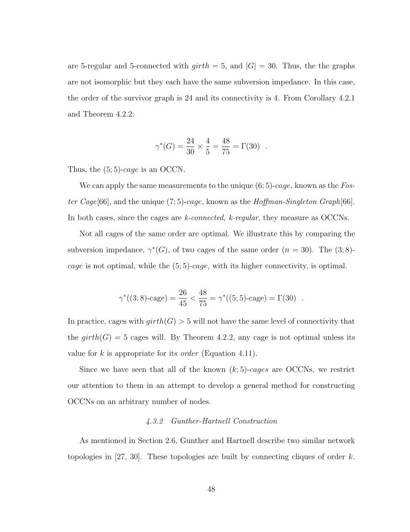
are 5-regular and 5-connected with girth = 5, and |G| = 30. Thus, the the graphs

are not isomorphic but they each have the same subversion impedance. In this case,

the order of the survivor graph is 24 and its connectivity is 4. From Corollary 4.2.1

and Theorem 4.2.2:

γ∗(G) =24

30× 4

5=

48

75= Γ(30) .

Thus, the (5; 5)-cage is an OCCN.

We can apply the same measurements to the unique (6; 5)-cage, known as the Fos-

ter Cage[66], and the unique (7; 5)-cage, known as the Hoffman-Singleton Graph[66].

In both cases, since the cages are k-connected, k-regular, they measure as OCCNs.

Not all cages of the same order are optimal. We illustrate this by comparing the

subversion impedance, γ∗(G), of two cages of the same order (n = 30). The (3; 8)-

cage is not optimal, while the (5; 5)-cage, with its higher connectivity, is optimal.

γ∗((3; 8)-cage) =26

45<

48

75= γ∗((5; 5)-cage) = Γ(30) .

In practice, cages with girth(G) > 5 will not have the same level of connectivity that

the girth(G) = 5 cages will. By Theorem 4.2.2, any cage is not optimal unless its

value for k is appropriate for its order (Equation 4.11).

Since we have seen that all of the known (k; 5)-cages are OCCNs, we restrict

our attention to them in an attempt to develop a general method for constructing

OCCNs on an arbitrary number of nodes.

4.3.2 Gunther-Hartnell Construction

As mentioned in Section 2.6, Gunther and Hartnell describe two similar network

topologies in [27, 30]. These topologies are built by connecting cliques of order k.

48

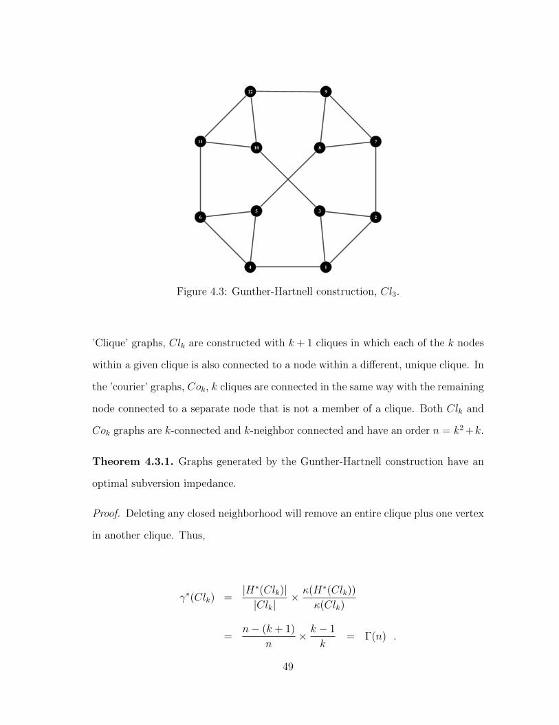
2

1

35

4

6

8

7

9

11

10

12

Figure 4.3: Gunther-Hartnell construction, Cl3.

’Clique’ graphs, Clk are constructed with k + 1 cliques in which each of the k nodes

within a given clique is also connected to a node within a different, unique clique. In

the ’courier’ graphs, Cok, k cliques are connected in the same way with the remaining

node connected to a separate node that is not a member of a clique. Both Clk and

Cok graphs are k-connected and k-neighbor connected and have an order n = k2 +k.

Theorem 4.3.1. Graphs generated by the Gunther-Hartnell construction have an

optimal subversion impedance.

Proof. Deleting any closed neighborhood will remove an entire clique plus one vertex

in another clique. Thus,

γ∗(Clk) =|H∗(Clk)||Clk|

× κ(H∗(Clk))

κ(Clk)

=n− (k + 1)

n× k − 1

k= Γ(n) .

49

and, from Equation 4.12

k2 − k + 2 ≤ k2 + k ≤ k2 + k + 1 .

Thus, topologies constructed using the Gunther-Hartnell method have optimal sub-

version impedance.

4.4 Conclusions

In this section, we have presented an approach for measuring the suitability of

topologies for use in CCNs. We refer to this measure as subversion impedance. The

higher the subversion impedance of a topology, the better it is at balancing secrecy

and resilience. We have found that the family of (k; 5)-cages are optimal, but there

are only a limited number of these graphs that are known, and no algorithm is known

that will construct optimal graphs of arbitrary order. We also demonstrated that

topologies built using the Gunther-Hartnell construction also have optimal subver-

sion impedance. Though more robust than cage construction, the Gunther-Hartnell

construction will not create topologies of arbitrary order. In Section 5, we present

constructions for each of these graph families that have near-optimal subversion

impedance for networks of arbitrary order.

50

5. DETERMINISTIC TOPOLOGY ANALYSIS FOR CCNs

Covert communication networks must be connected in order to enable commu-

nications between any pair of nodes. Given our particular threat model, we want

networks that are as sparsely connected as possible in order to minimize network

promiscuity but resilient against disconnection even after the removal of one or more

closed neighborhoods. As discussed in Section 3.2.1, low network promiscuity can

be achieved through a sparsely connected topology such as that of a tree. A tree

topology can become partitioned after a single subversion but will often minimize

the number of nodes compromised from a single subversion. On the other hand, a

more densely connected graph is more resilient but, thus, will usually have larger

numbers of nodes directly affected by the subversion of a single node.

5.1 Resilience versus Survivability

Gunther-Hartnell topologies, described in [30] and Section 4.3.2, are resilient to

k subversions, but each subversion removes k + 1 nodes from the network. For

this reason, Gunther and Hartnell refer to these topologies as being k-neighbor-

connected. Removing k + 1 neighborhoods eliminates all nodes within the topology.

This topology construction offers optimal global subversion impedance when the

graph contains k(k+1) nodes. Other topology constructions, on the same number of

nodes and similar number of edges, might become disconnected after the removal of

fewer closed neighborhoods but require the removal of more closed neighborhoods in

order to deplete the network. Based on the priorities of the organization relying on

the CCN, the organization must determine whether it is better to maintain a topology

that remains connected through multiple subversions or becomes disconnected at

some point in order to provide a greater degree of node survivability.

51

From the adversary’s perspective, the problem of bringing down all the nodes in

a CCN is related to the problem of constructing a dominating set of a graph. For a

given graph, G = (V,E), a dominating set is a set of nodes W ⊆ V such that every

node in the graph G is a neighbor of at least one element of W [36]. The minimum

dominating set (MDS) problem, a classical problem within computer science and

graph theory, is to find a minimum such W for a given graph. Thus, in order

to collect the network addresses of all participants within the CCN, the adversary

would need to subvert at least W nodes. Even assuming that the adversary knows

the network topology, finding a minimum dominating set is NP-hard in general. In

the following, we will focus on networks with large MDSs.

5.2 Worst Case Subversion versus Uniformly Probable Subversion

As discussed in Section 4, the a priori subversion probability distribution is dif-

ficult to quantify. It can be simplified to either the worst-case or the uniform case.

Analyzing both cases is important in assessing CCN topologies.

We do not wish to allow topologies that protect some nodes by placing others at

risk. No one will want to participate within the CCN if there is a chance that they will

be sacrificed to the adversary in order to protect the other nodes. Instead, we would

prefer topologies in which most nodes have a similar local subversion impedance

and the global subversion impedance is not significantly lower than the average local

subversion impedance.

For a given graph G, the global subversion impedance γ∗(G) gives us the worst

case measure. We make the assumption that the adversary had sufficient knowledge

to subvert the node that would do the greatest damage to the network. However,

in practical terms, this will rarely be the case. A uniform distribution provides a

differing a priori probability distribution for node subversion—one in which every

52

node in the network has the same chance of being subverted. Thus, as a different

measure for the topology suitability in CCNs, we examine cases in which the a

priori subversion probability is equal for all nodes. Thus, the risk to the network is

measured as the average local subversion impedance.

5.3 Average Local Subversion Impedance

We modify the global subversion impedance measure so that it is calculated as

the average local subversion impedance instead of the worst-case local subversion

impedance. By extension, we also specify the average secrecy measure and the aver-

age resilience measure.

Definition 5.3.1. The average (local) subversion impedance on graph G is:

〈γ(G)〉 =1

|G|∑v∈V

γ(G, v) . (5.1)

Definition 5.3.2. The average secrecy measure on a given graph G is:

〈S(G)〉 =1

|G|∑v∈V

S(G, v)

=|G| − 〈d(G)〉 − 1

|G|, (5.2)

where 〈d(G)〉 is the average node degree within the network.

Definition 5.3.3. The average resilience measure on a given graph G is:

〈K(G)〉 =1

|G|∑v∈V

κ(H(G, v))

κ(G). (5.3)

Each of these measures give us insight into the usefulness of topologies for use in

53

a CCN. Given that the average degree is easily calculated for many types of deter-

ministic topologies, the average secrecy measure 〈S(G)〉 is often easily determine.

However, since vertex connectivity is a global property of a graph and is often diffi-

cult to easily determine for topologies with an arbitrary number of nodes, 〈K(G)〉,

in turn, is not easily reducible in the same manner as 〈S(G)〉. The complexity of cal-

culating γ∗(G) is dominated by the complexity of calculating the vertex connectivity

of G.

Given 〈S(G)〉 and 〈K(G)〉, we want to clarify that,

〈γ(G)〉 6= 〈S(G)〉 × 〈K(G)〉 ,

unless either S(G, v) or K(G, v) are constant for all v ∈ V (for example, in symmetric

topologies).

With both the measure for global subversion impedance and the measure for

average local subversion impedance, we now examine various P2P network topologies

for suitability of use within covert communications networks.

5.4 An Analysis of Common Network Topologies for Use in CCNs

We now examine some common deterministic topologies used in overlay networks.

We use our measures for subversion impedance to assess the suitability of each topol-

ogy for use in a CCN.

5.4.1 Paths

A path, Pn, topology consists of a linear chain of n nodes. Except the two nodes

on each end, which are attached to only one adjacent node, all nodes are attached

to two adjacent nodes. As new nodes join the network, they connect to the node at

either end of the topology. Figure 5.1 shows an example of a path topology on five

54

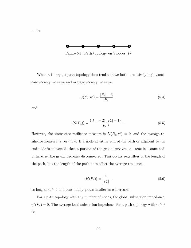
nodes.

1 2 3 4 5

Figure 5.1: Path topology on 5 nodes, P5

When n is large, a path topology does tend to have both a relatively high worst-

case secrecy measure and average secrecy measure:

S(Pn, v∗) =

|Pn| − 3

|Pn|, (5.4)

and

〈S(Pn)〉 =(|Pn| − 2)(|Pn| − 1)

|Pn|2. (5.5)

However, the worst-case resilience measure is K(Pn, v∗) = 0, and the average re-

silience measure is very low. If a node at either end of the path or adjacent to the

end node is subverted, then a portion of the graph survives and remains connected.

Otherwise, the graph becomes disconnected. This occurs regardless of the length of

the path, but the length of the path does affect the average resilience,

〈K(Pn)〉 =4

|Pn|, (5.6)

as long as n ≥ 4 and continually grows smaller as n increases.

For a path topology with any number of nodes, the global subversion impedance,

γ∗(Pn) = 0. The average local subversion impedance for a path topology with n ≥ 3

is:

55

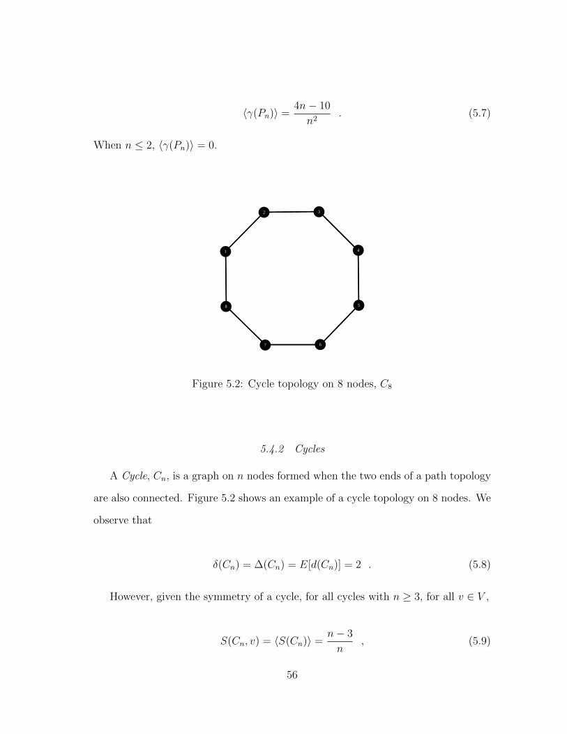
〈γ(Pn)〉 =4n− 10

n2. (5.7)

When n ≤ 2, 〈γ(Pn)〉 = 0.

1

2 3

4

5

67

8

Figure 5.2: Cycle topology on 8 nodes, C8

5.4.2 Cycles

A Cycle, Cn, is a graph on n nodes formed when the two ends of a path topology

are also connected. Figure 5.2 shows an example of a cycle topology on 8 nodes. We

observe that

δ(Cn) = ∆(Cn) = E[d(Cn)] = 2 . (5.8)

However, given the symmetry of a cycle, for all cycles with n ≥ 3, for all v ∈ V ,

S(Cn, v) = 〈S(Cn)〉 =n− 3

n, (5.9)

56

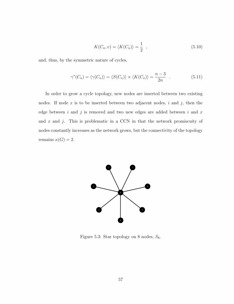
K(Cn, v) = 〈K(Cn)〉 =1

2, (5.10)

and, thus, by the symmetric nature of cycles,

γ∗(Cn) = 〈γ(Cn)〉 = 〈S(Cn)〉 × 〈K(Cn)〉 =n− 3

2n. (5.11)

In order to grow a cycle topology, new nodes are inserted between two existing

nodes. If node x is to be inserted between two adjacent nodes, i and j, then the

edge between i and j is removed and two new edges are added between i and x

and x and j. This is problematic in a CCN in that the network promiscuity of

nodes constantly increases as the network grows, but the connectivity of the topology

remains κ(G) = 2.

1

2

3

4

5

6

7

8

Figure 5.3: Star topology on 8 nodes, S8.

57

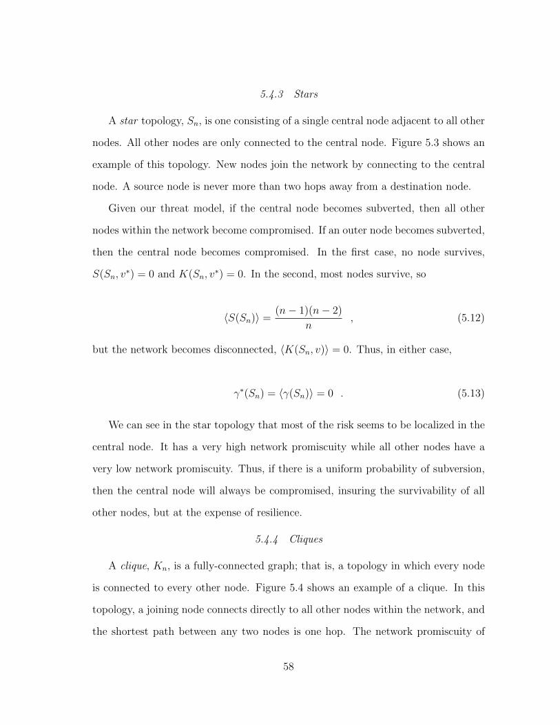
5.4.3 Stars

A star topology, Sn, is one consisting of a single central node adjacent to all other

nodes. All other nodes are only connected to the central node. Figure 5.3 shows an

example of this topology. New nodes join the network by connecting to the central

node. A source node is never more than two hops away from a destination node.

Given our threat model, if the central node becomes subverted, then all other

nodes within the network become compromised. If an outer node becomes subverted,

then the central node becomes compromised. In the first case, no node survives,

S(Sn, v∗) = 0 and K(Sn, v

∗) = 0. In the second, most nodes survive, so

〈S(Sn)〉 =(n− 1)(n− 2)

n, (5.12)

but the network becomes disconnected, 〈K(Sn, v)〉 = 0. Thus, in either case,

γ∗(Sn) = 〈γ(Sn)〉 = 0 . (5.13)

We can see in the star topology that most of the risk seems to be localized in the

central node. It has a very high network promiscuity while all other nodes have a

very low network promiscuity. Thus, if there is a uniform probability of subversion,

then the central node will always be compromised, insuring the survivability of all

other nodes, but at the expense of resilience.

5.4.4 Cliques

A clique, Kn, is a fully-connected graph; that is, a topology in which every node

is connected to every other node. Figure 5.4 shows an example of a clique. In this

topology, a joining node connects directly to all other nodes within the network, and

the shortest path between any two nodes is one hop. The network promiscuity of

58

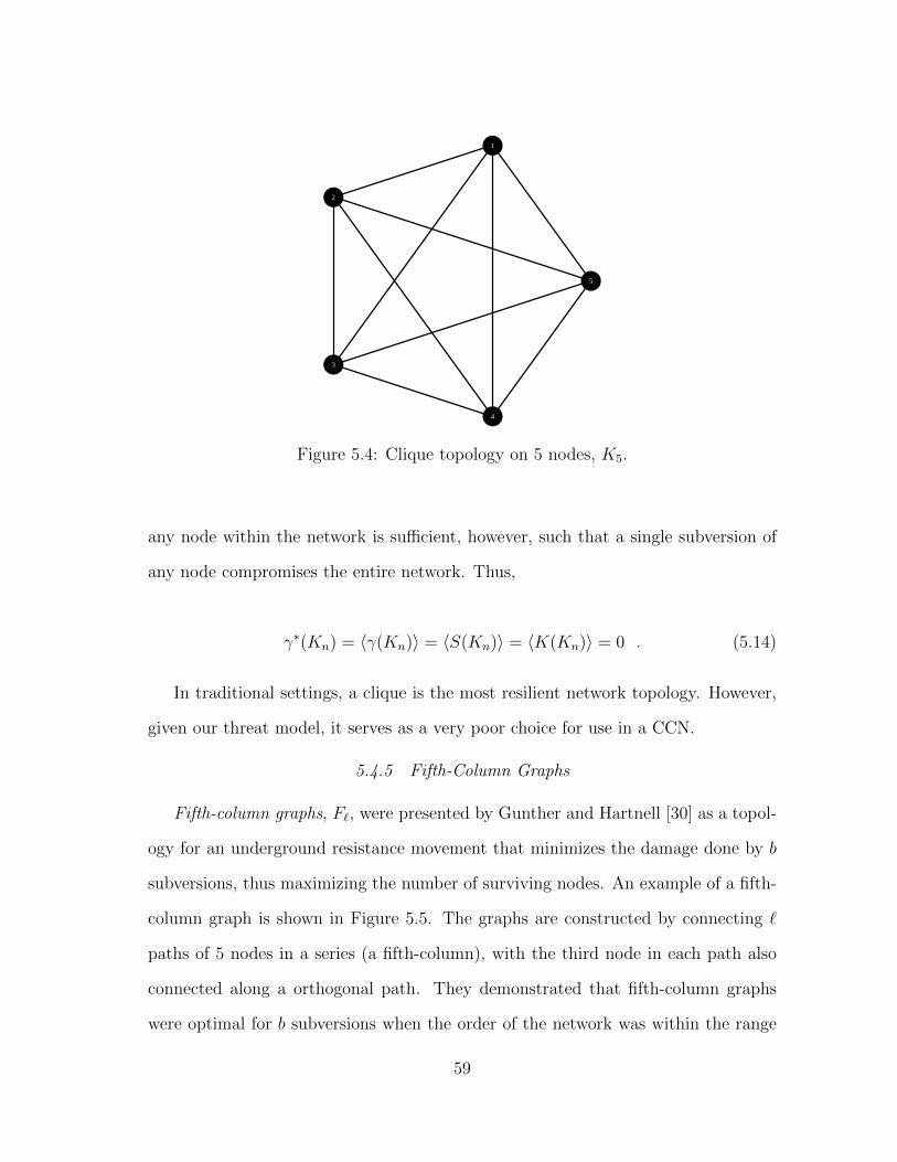
1

2

3

4

5

Figure 5.4: Clique topology on 5 nodes, K5.

any node within the network is sufficient, however, such that a single subversion of

any node compromises the entire network. Thus,

γ∗(Kn) = 〈γ(Kn)〉 = 〈S(Kn)〉 = 〈K(Kn)〉 = 0 . (5.14)

In traditional settings, a clique is the most resilient network topology. However,

given our threat model, it serves as a very poor choice for use in a CCN.

5.4.5 Fifth-Column Graphs

Fifth-column graphs, F`, were presented by Gunther and Hartnell [30] as a topol-

ogy for an underground resistance movement that minimizes the damage done by b

subversions, thus maximizing the number of surviving nodes. An example of a fifth-

column graph is shown in Figure 5.5. The graphs are constructed by connecting `

paths of 5 nodes in a series (a fifth-column), with the third node in each path also

connected along a orthogonal path. They demonstrated that fifth-column graphs

were optimal for b subversions when the order of the network was within the range

59

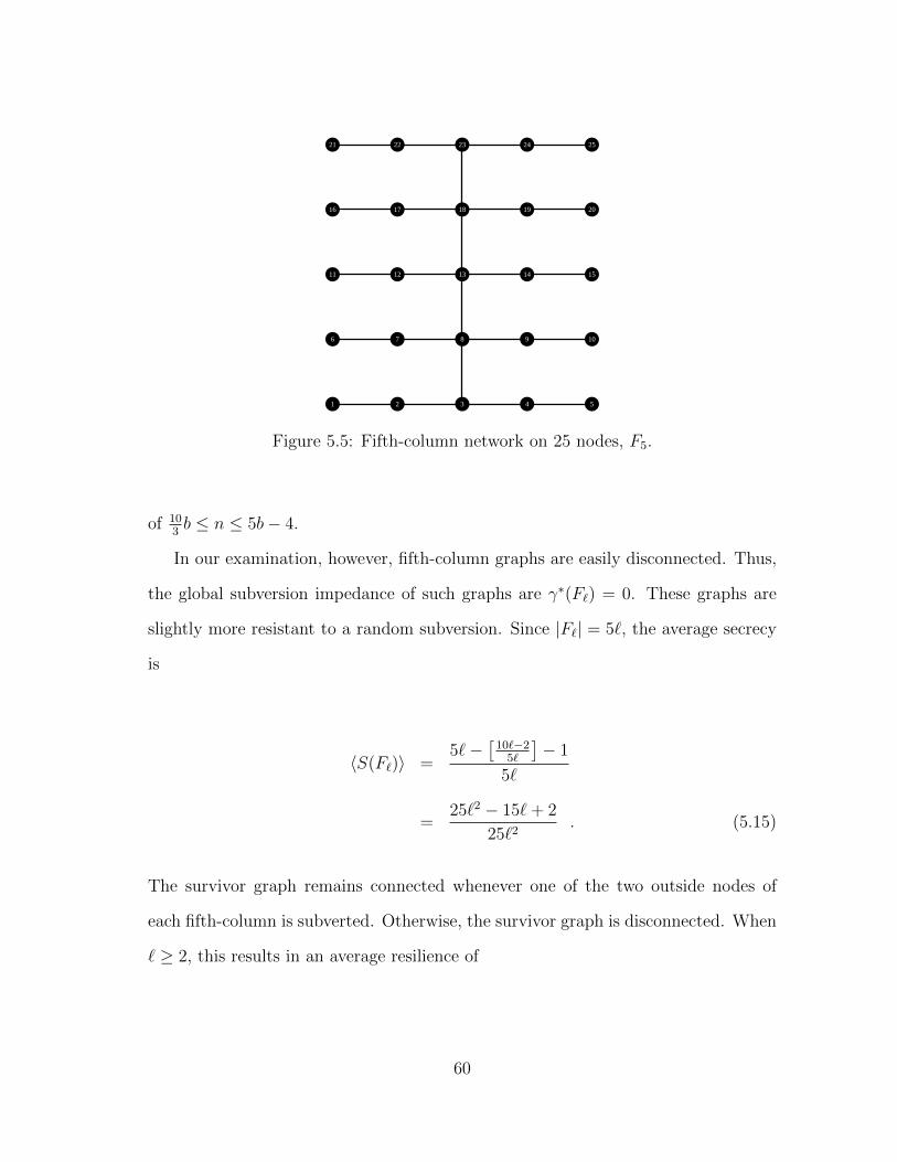
1 2 3 4 5

6 7 8 9 10

11 12 13 14 15

16 17 18 19 20

21 22 23 24 25

Figure 5.5: Fifth-column network on 25 nodes, F5.

of 103b ≤ n ≤ 5b− 4.

In our examination, however, fifth-column graphs are easily disconnected. Thus,

the global subversion impedance of such graphs are γ∗(F`) = 0. These graphs are

slightly more resistant to a random subversion. Since |F`| = 5`, the average secrecy

is

〈S(F`)〉 =5`−

[10`−25`

]− 1

5`

=25`2 − 15`+ 2

25`2. (5.15)

The survivor graph remains connected whenever one of the two outside nodes of

each fifth-column is subverted. Otherwise, the survivor graph is disconnected. When

` ≥ 2, this results in an average resilience of

60

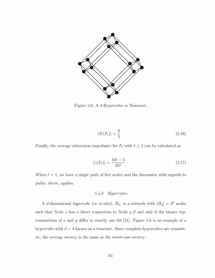
1

2

3

4

5

6

7

8

9

10

11

12

13

14

15

16

Figure 5.6: A 4-Hypercube or Tesseract.

〈K(F`)〉 =2

5. (5.16)

Finally, the average subversion impedance for F` with ` ≥ 2 can be calculated as

〈γ(F`)〉 =10`− 4

25`. (5.17)

When ` = 1, we have a single path of five nodes and the discussion with regards to

paths, above, applies.

5.4.6 Hypercubes

A d-dimensional hypercube (or d-cube), Hd, is a network with |Hd| = 2d nodes

such that Node x has a direct connection to Node y if and only if the binary rep-

resentations of x and y differ in exactly one bit [41]. Figure 5.6 is an example of a

hypercube with d = 4 known as a tesseract. Since complete hypercubes are symmet-

ric, the average secrecy is the same as the worst-case secrecy:

61

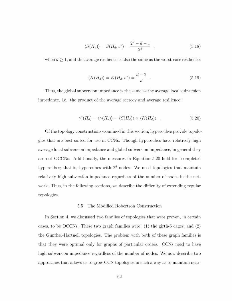
〈S(Hd)〉 = S(Hd, v∗) =

2d − d− 1

2d, (5.18)

when d ≥ 1, and the average resilience is also the same as the worst-case resilience:

〈K(Hd)〉 = K(Hd, v∗) =

d− 2

d. (5.19)

Thus, the global subversion impedance is the same as the average local subversion

impedance, i.e., the product of the average secrecy and average resilience:

γ∗(Hd) = 〈γ(Hd)〉 = 〈S(Hd)〉 × 〈K(Hd)〉 . (5.20)

Of the topology constructions examined in this section, hypercubes provide topolo-

gies that are best suited for use in CCNs. Though hypercubes have relatively high

average local subversion impedance and global subversion impedance, in general they

are not OCCNs. Additionally, the measures in Equation 5.20 hold for “complete”

hypercubes; that is, hypercubes with 2d nodes. We need topologies that maintain

relatively high subversion impedance regardless of the number of nodes in the net-

work. Thus, in the following sections, we describe the difficulty of extending regular

topologies.

5.5 The Modified Robertson Construction

In Section 4, we discussed two families of topologies that were proven, in certain

cases, to be OCCNs. These two graph families were: (1) the girth-5 cages; and (2)

the Gunther-Hartnell topologies. The problem with both of these graph families is

that they were optimal only for graphs of particular orders. CCNs need to have

high subversion impedance regardless of the number of nodes. We now describe two

approaches that allows us to grow CCN topologies in such a way as to maintain near-

62

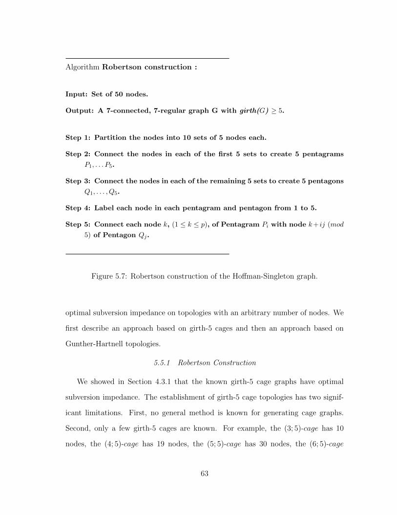
Algorithm Robertson construction :

Input: Set of 50 nodes.

Output: A 7-connected, 7-regular graph G with girth(G) ≥ 5.

Step 1: Partition the nodes into 10 sets of 5 nodes each.

Step 2: Connect the nodes in each of the first 5 sets to create 5 pentagrams

P1, . . . P5.

Step 3: Connect the nodes in each of the remaining 5 sets to create 5 pentagons

Q1, . . . , Q5.

Step 4: Label each node in each pentagram and pentagon from 1 to 5.

Step 5: Connect each node k, (1 ≤ k ≤ p), of Pentagram Pi with node k+ ij (mod

5) of Pentagon Qj.

Figure 5.7: Robertson construction of the Hoffman-Singleton graph.

optimal subversion impedance on topologies with an arbitrary number of nodes. We

first describe an approach based on girth-5 cages and then an approach based on

Gunther-Hartnell topologies.

5.5.1 Robertson Construction

We showed in Section 4.3.1 that the known girth-5 cage graphs have optimal

subversion impedance. The establishment of girth-5 cage topologies has two signif-

icant limitations. First, no general method is known for generating cage graphs.

Second, only a few girth-5 cages are known. For example, the (3; 5)-cage has 10

nodes, the (4; 5)-cage has 19 nodes, the (5; 5)-cage has 30 nodes, the (6; 5)-cage

63

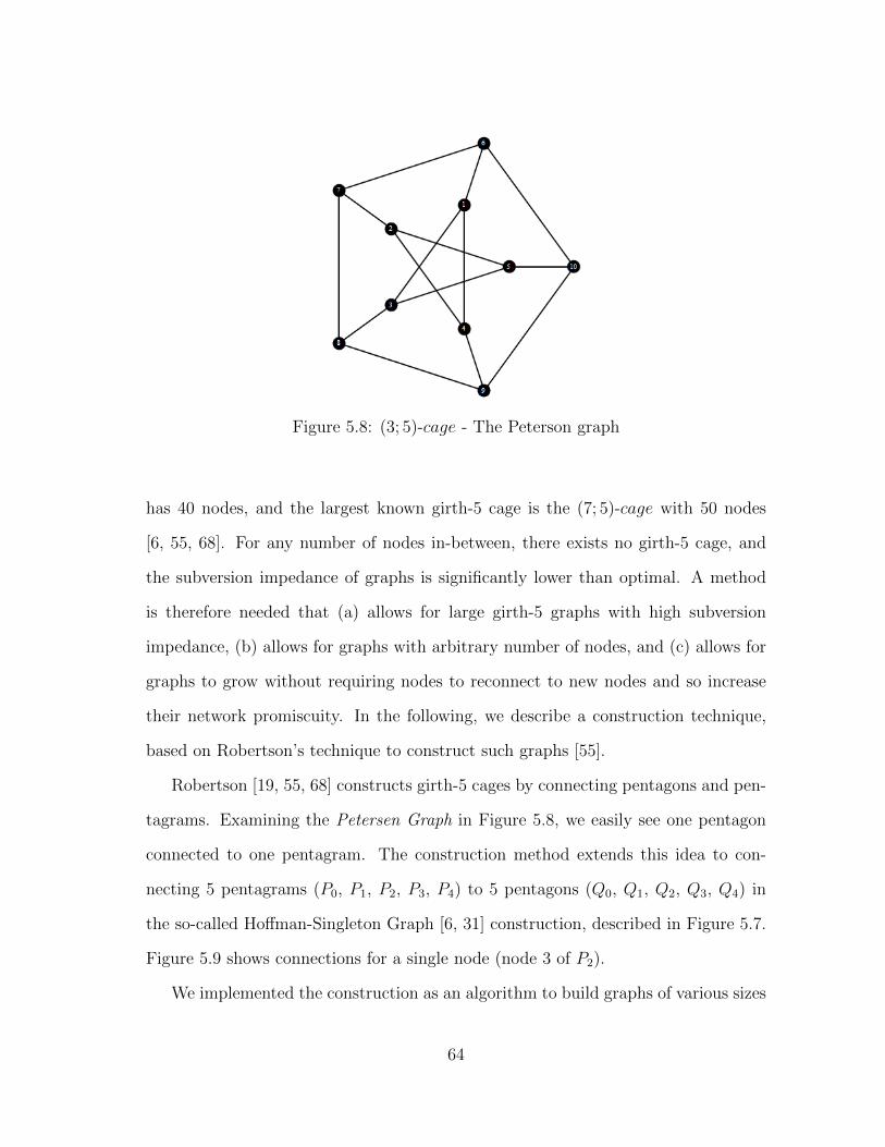
Figure 5.8: (3; 5)-cage - The Peterson graph

has 40 nodes, and the largest known girth-5 cage is the (7; 5)-cage with 50 nodes

[6, 55, 68]. For any number of nodes in-between, there exists no girth-5 cage, and

the subversion impedance of graphs is significantly lower than optimal. A method

is therefore needed that (a) allows for large girth-5 graphs with high subversion

impedance, (b) allows for graphs with arbitrary number of nodes, and (c) allows for

graphs to grow without requiring nodes to reconnect to new nodes and so increase

their network promiscuity. In the following, we describe a construction technique,

based on Robertson’s technique to construct such graphs [55].

Robertson [19, 55, 68] constructs girth-5 cages by connecting pentagons and pen-

tagrams. Examining the Petersen Graph in Figure 5.8, we easily see one pentagon

connected to one pentagram. The construction method extends this idea to con-

necting 5 pentagrams (P0, P1, P2, P3, P4) to 5 pentagons (Q0, Q1, Q2, Q3, Q4) in

the so-called Hoffman-Singleton Graph [6, 31] construction, described in Figure 5.7.

Figure 5.9 shows connections for a single node (node 3 of P2).

We implemented the construction as an algorithm to build graphs of various sizes

64

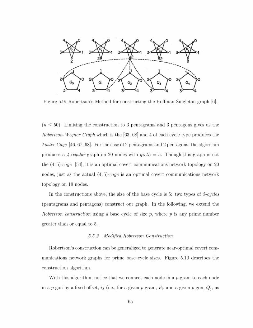
Figure 5.9: Robertson’s Method for constructing the Hoffman-Singleton graph [6].

(n ≤ 50). Limiting the construction to 3 pentagrams and 3 pentagons gives us the

Robertson-Wegner Graph which is the [63, 68] and 4 of each cycle type produces the

Foster Cage [46, 67, 68]. For the case of 2 pentagrams and 2 pentagons, the algorithm

produces a 4-regular graph on 20 nodes with girth = 5. Though this graph is not

the (4; 5)-cage [54], it is an optimal covert communications network topology on 20

nodes, just as the actual (4; 5)-cage is an optimal covert communications network

topology on 19 nodes.

In the constructions above, the size of the base cycle is 5: two types of 5-cycles

(pentagrams and pentagons) construct our graph. In the following, we extend the

Robertson construction using a base cycle of size p, where p is any prime number

greater than or equal to 5.

5.5.2 Modified Robertson Construction

Robertson’s construction can be generalized to generate near-optimal covert com-

munications network graphs for prime base cycle sizes. Figure 5.10 describes the

construction algorithm.

With this algorithm, notice that we connect each node in a p-gram to each node

in a p-gon by a fixed offset, ij (i.e., for a given p-gram, Pi, and a given p-gon, Qj, as

65

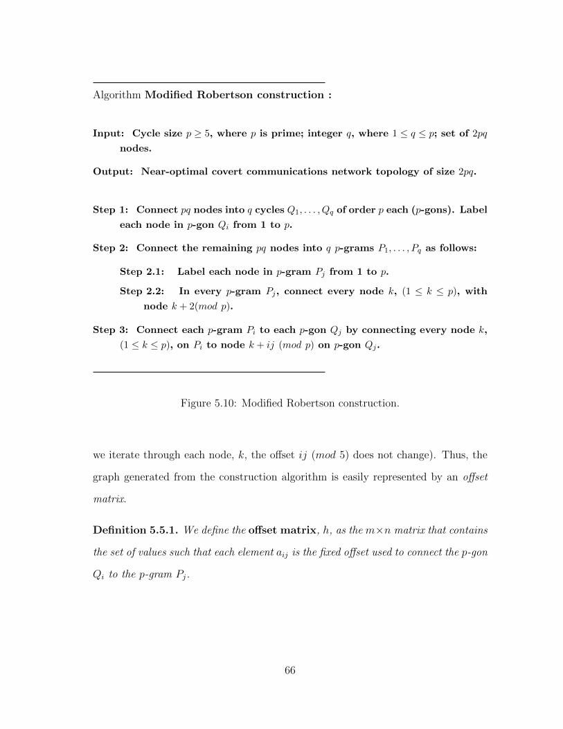
Algorithm Modified Robertson construction :

Input: Cycle size p ≥ 5, where p is prime; integer q, where 1 ≤ q ≤ p; set of 2pq

nodes.

Output: Near-optimal covert communications network topology of size 2pq.

Step 1: Connect pq nodes into q cycles Q1, . . . , Qq of order p each (p-gons). Label

each node in p-gon Qi from 1 to p.

Step 2: Connect the remaining pq nodes into q p-grams P1, . . . , Pq as follows:

Step 2.1: Label each node in p-gram Pj from 1 to p.

Step 2.2: In every p-gram Pj, connect every node k, (1 ≤ k ≤ p), with

node k + 2(mod p).

Step 3: Connect each p-gram Pi to each p-gon Qj by connecting every node k,

(1 ≤ k ≤ p), on Pi to node k + ij (mod p) on p-gon Qj.

Figure 5.10: Modified Robertson construction.

we iterate through each node, k, the offset ij (mod 5) does not change). Thus, the

graph generated from the construction algorithm is easily represented by an offset

matrix.

Definition 5.5.1. We define the offset matrix, h, as the m×n matrix that contains

the set of values such that each element aij is the fixed offset used to connect the p-gon

Qi to the p-gram Pj.

66

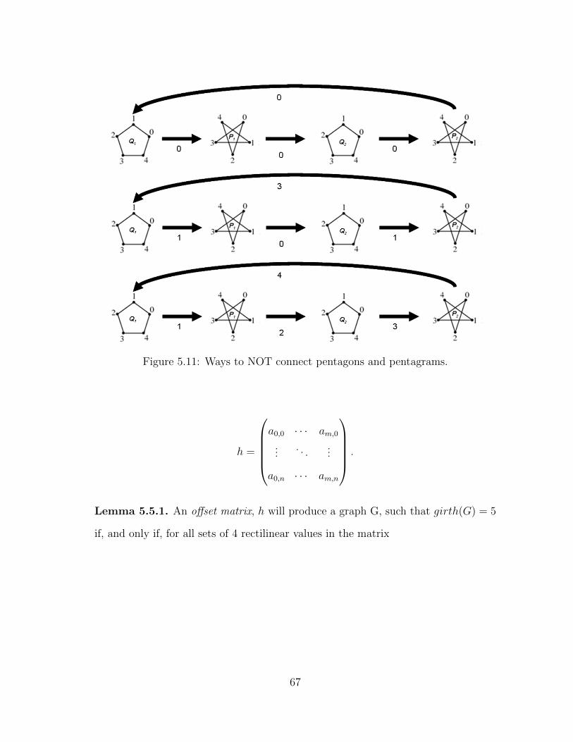
Figure 5.11: Ways to NOT connect pentagons and pentagrams.

h =

a0,0 · · · am,0

.... . .

...

a0,n · · · am,n

.

Lemma 5.5.1. An offset matrix, h will produce a graph G, such that girth(G) = 5

if, and only if, for all sets of 4 rectilinear values in the matrix

67

h =

......

· · · ai1j1 · · · ai2j1 · · ·...

...

· · · ai1j2 · · · ai2j2 · · ·...

...

where i1 6= i2 and j1 6= j2,

[ai1j1 + ai2j2 ]p 6= [ai1j2 + ai2j1 ]p .

Proof. By construction, we are connecting nodes in a p-gram to nodes in a p-gon

and vice-versa. In order to construct a graph of girth 4, the algorithm would need

to construct at least one cycle of length 4. In order for such a cycle to exist, there

would have to exist a set of nodes vA and vC on two different p-gons and vB and vD

on two different p-grams such that vA would connect to vB, vB to vC , vC to vD, and

vD back to vA.

This occurs only when the offsets sum to a multiple of the size of the base cycle.

Figure 5.11 shows the case for p = 5. Notice that the offsets are directional. In the

notation of our offset matrix, each entry in h is from the ith p-gram to the jth p-gon.

Thus,

ai1j1 − ai1j2 + ai2j1 − ai2j2 6≡ 0 (mod p) ,

which is equivalent to

[ai1j1 + ai2j2 ]p 6= [ai1j2 + ai2j1 ]p .

68

Thus, completing the proof.

Theorem 5.5.1. An offset matrix, h with entries ai,j = ij (mod p) will produce a

graph G with girth(G) = 5 if, and only if, (1) the matrix is no larger than p × p;

and (2) p is prime.

Proof. Let [ai1j1 + ai2j2 ]p 6= [ai1j2 + ai2j1 ]p. Then,

[ai1j1 + ai2j2 ]p 6= [ai1j2 + ai2j1 ]p

[i1 · j1]p + [i2 · j2]p 6= [i1 · j2]p + [i2 · j1]p

for i1 6= i2 and j1 6= j2. And,

[i1j1]p + [i2j2]p 6= [i1j2]p + [i2j1]p

[i1j1 + i2j2]p 6= [i1j2 + i2j1]p

[i1j1 + i2j2]p − [i1j2 + i2j1]p 6= 0

[(ij − in) + (mn−mj)]p 6= 0

[i1(j1 − j2) + i2(j2 − j1)]p 6= 0

[(j1 − j2)(i1 − i2)]p 6= 0

If our offset matrix is p×p or smaller, then 0 ≤ i, j < p and−p < (i1−i2), (j1−j2) < p.

Since i1 6= i2 and j1 6= j2 then i1 − i2 6= 0 and j1 − j2 6= 0. If p is prime, then all

values of (i1− i2) and (j1−j2) will be co-prime with p. Thus, for no values of i1, i2, j1

and j2 is [(j1 − j2)(i1 − i2)]p 6= 0. On the other hand, if p is not prime, then there is

69

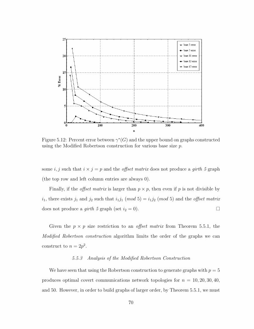
Figure 5.12: Percent error between γ∗(G) and the upper bound on graphs constructedusing the Modified Robertson construction for various base size p.

some i, j such that i× j = p and the offset matrix does not produce a girth 5 graph

(the top row and left column entries are always 0).

Finally, if the offset matrix is larger than p× p, then even if p is not divisible by

i1, there exists j1 and j2 such that i1j1 (mod 5) = i1j2 (mod 5) and the offset matrix

does not produce a girth 5 graph (set i2 = 0).

Given the p × p size restriction to an offset matrix from Theorem 5.5.1, the

Modified Robertson construction algorithm limits the order of the graphs we can

construct to n = 2p2.

5.5.3 Analysis of the Modified Robertson Construction

We have seen that using the Robertson construction to generate graphs with p = 5

produces optimal covert communications network topologies for n = 10, 20, 30, 40,

and 50. However, in order to build graphs of larger order, by Theorem 5.5.1, we must

70

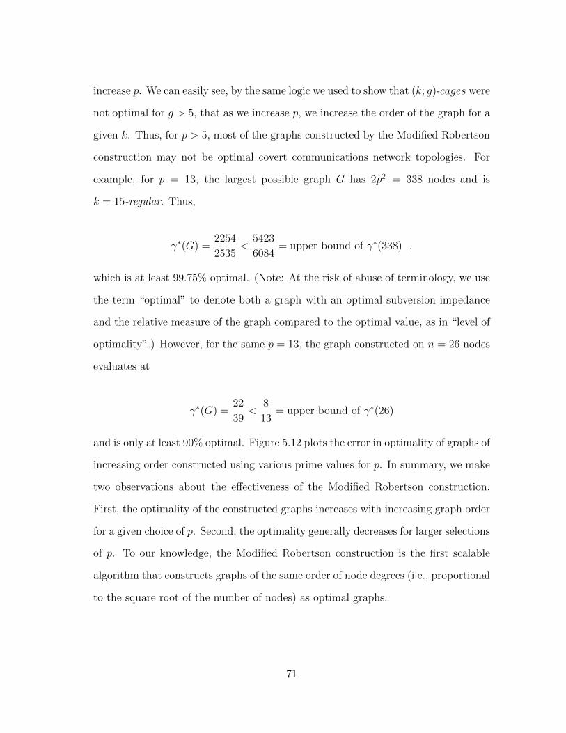
increase p. We can easily see, by the same logic we used to show that (k; g)-cages were

not optimal for g > 5, that as we increase p, we increase the order of the graph for a

given k. Thus, for p > 5, most of the graphs constructed by the Modified Robertson

construction may not be optimal covert communications network topologies. For

example, for p = 13, the largest possible graph G has 2p2 = 338 nodes and is

k = 15-regular. Thus,

γ∗(G) =2254

2535<

5423

6084= upper bound of γ∗(338) ,

which is at least 99.75% optimal. (Note: At the risk of abuse of terminology, we use

the term “optimal” to denote both a graph with an optimal subversion impedance

and the relative measure of the graph compared to the optimal value, as in “level of

optimality”.) However, for the same p = 13, the graph constructed on n = 26 nodes

evaluates at

γ∗(G) =22

39<

8

13= upper bound of γ∗(26)

and is only at least 90% optimal. Figure 5.12 plots the error in optimality of graphs of

increasing order constructed using various prime values for p. In summary, we make

two observations about the effectiveness of the Modified Robertson construction.

First, the optimality of the constructed graphs increases with increasing graph order

for a given choice of p. Second, the optimality generally decreases for larger selections

of p. To our knowledge, the Modified Robertson construction is the first scalable

algorithm that constructs graphs of the same order of node degrees (i.e., proportional

to the square root of the number of nodes) as optimal graphs.

71

5.6 Moving Towards Dynamic Construction

Up to this point, our construction algorithms have been static; for a given number

of nodes n, the objective was to construct an optimal or near-optimal graph. The

Modified Robertson construction could potentially provide a mechanism for a more

dynamic approach to graph construction. In dynamic construction, we are looking

to “grow” our graphs. This may happen in response to additional nodes joining the

network. Thus, we might begin with a set of nodes, say n ≤ 50, and construct a

graph using a base cycle of p = 5. As we increase n up to 50, we can “grow” our

network in such a way that we are assured that the graph is optimal for n = 10k

for k = {1, 2, 3, 4, 5}. However, once we fill the graph to its maximum order (by

Theorem 5.5.1), we can no longer “grow” the graph using the base cycle of 5.

Limited by a maximum graph order for a given base cycle, to “grow” our graphs

to an arbitrary size, we have three options:

• Option 1: A priori select a base cycle large enough to accommodate our an-

ticipated maximum network size;

• Option 2: Grow to the maximum size relative to base size (n = 2p2), then

dissolve established connections and reconstruct the network with a larger base

cycle; or

• Option 3: Set a given base cycle p and connectivity k and then grow the net-

work linearly beyond the limit of 2p2 by using a different construction.

In the following, we will briefly discuss each of these options.

72

5.6.1 Option 1: Choose a Large Enough p

If we know ahead of time exactly what the order n of our network will be, then

we can choose the smallest base cycle p such that n ≤ 2p2. This will insure that our

constructed network is as close to Gnopt as our algorithm can produce. Of course, as

indicated earlier, if our estimated order proves to be too small, then our network will

reach its maximum and we will need to resort to a different option. Furthermore,

since the network may initially be significantly smaller than 2p2, it will have a signif-

icantly lower optimality than when it reaches its expected order. However, the error

in optimality is bounded by Theorem 1 and Lemma 4 in Section 4.

5.6.2 Option 2: Reconstruct the Network When Necessary

Another option would be to maintain the smallest base cycle possible given the

current order n. For example, a base cycle of p = 5 is used until the network

reaches n = 2p2 = 50. Then, existing connections (i.e. edges) are dissolved and

nodes establish new connections with the next higher base cycle (p = 7). This

allows for unlimited growth with a tightly bounded error in optimality. However,

the overhead of having nodes reconnect in a new network is very high, and the

risk of the network being discovered through elevated signaling and other protocol

activity during network “restructuring” is significant. Also, each time a node builds a

new neighborhood after each base cycle change, their network promiscuity increases.

Thus, the probability of connecting to a subverted node increases, and a subverted

node could compromise many more nodes than were in their initial neighborhood

and further degrade membership concealment.

73

5.6.3 Option 3: Grow the Network Linearly

Alternatively, the base cycle size can be kept fixed, and the network can grow

beyond the 2p2 limit by slightly altering the construction algorithm. Figure 5.13

presents an extension of the Modified Robertson construction for generating topolo-

gies of arbitrary size. It works by connecting multiple Modified Robertson construc-

tion topologies in a series.

Figure 5.14 graphs the subversion impedance of a linearly grown network with a

base cycle p = 5 compared to the optimal subversion impedance. For 5 ≤ n ≤ 50,

there are the previously mentioned optimal covert communications network topolo-

gies. For other values, most have relatively high subversion impedance. A couple

(i.e., n = 51) have a subversion impedance of 0. In this case, the majority of the

nodes are well protected, but the new node is easily partitioned from the network

given the worst-case subversion.

Figure 5.15 graphs the subversion impedance at the limit when n � 100. The

subversion impedance becomes periodic over the range of 40k+50 ≤ n ≤ 40(k+1)+50

with higher risk of partitioning for the newly joined nodes at 40k+ 51 and 40k+ 52.

5.7 The Extended Gunther-Hartnell Construction

Next, we try to extend our observations of the Gunther-Hartnell construction and

see if we can generate near-optimal topologies from this approach.

Similar to the Extended Robertson construction, the Extended Gunther-Hartnell

construction allows us to grow network topologies with an arbitrary number of

nodes and relatively high subversion impedance. Figure 5.17 shows the subversion

impedance for topologies with order 1 ≤ n ≤ 100. We see that the subversion

impedance goes to zero whenever a new clique is started. The risk of partitioning

even in these cases is heavily weighted towards the new node. The new clique con-

74

Algorithm Extended Robertson construction :

Input: Cycle size p ≥ 5, where p is prime; set of n nodes.

Output: Near-optimal covert communications network topology on n nodes.

Step 1: Construct the offset matrix h with entries aij as follows:

Step 2.1: Let h be a q × r matrix where q = d n2pe and r = b n2p + 0.5c.

Step 2.2: Assign each entry of h as aij = −1.

Step 2.3: Let s = d g1p−1e.

Step 2.4: For each integer value of 0 ≤ m < s, 1 ≤ i ≤ p and 1 ≤ i ≤ p:

Step 2.4.1: Let x = i+ (mp−m) and y = j + (mp−m).

Step 2.4.2: If x ≤ q and y ≤ r, then change the value of axy as follows:

If [(x+m)(mod 2p)] > p or [(y+m)(mod 2p)] > p then axy = ij(mod p).

Otherwise, axy = (i− 1)(j − 1)(mod p).

Step 2: Connect pq nodes into q cycles Q1, . . . , Qq of order p each (p-gons).

Label each node in p-gon Qi from 1 to p.

Step 3: Connect the remaining nodes into r p-grams P1, . . . , Pr as follows:

Step 3.1: Label each node in p-gram Pj from 1 to p.

Step 3.2: In every p-gram Pj, connect every node k, (1 ≤ k ≤ p), with

node (k + 2)(mod p).

Step 4: If aij ≥ 0, then connect each p-gram Pi to each p-gon Qj by connecting

every node k, (1 ≤ k ≤ p), on Pi to node (k + aij)(mod p) on p-gon Qj.

Figure 5.13: Extended Robertson construction.

75

æ

æ æ æ

æ

æ

æ æ

æ

æ

æ

ææ

æ

æ

æ

æ

ææ

æ

æ

ææ

æ

æ

æ

æ

æ æ æ

ææ æ æ

æ

æ

æ

æ æ æ

æ

æ æ æ

æ

æ

æ æ

æ æ

æ

æ æ æ

æ

æ

æ

æ æ æ

æ

æ æ æ

æ

æ

æ

æ æ æ

æ

æ æ æ

æ

æ

æ

æ æ æ

æ

æ æ æ

æ

æ

æ æ

æ

æ ECR

GHGL

20 40 60 800.0

0.2

0.4

0.6

0.8

1.0

n

Γ*

HGL

Figure 5.14: Subversion impedance for graphs of order 3 ≤ n ≤ 100 using theExtended Robertson construction.

tains only one node with a single connection to a separate clique. If the separate

clique is removed in accordance with our threat model, then the new node becomes

partitioned from the rest of the network. If a second node is added to the clique,

then the topology is, again, resilient to partitioning.

For graphs of arbitrary order with relatively few nodes, the Extended Gunther-

Hartnell construction suffers from a higher risk of partitioning in that the subversion

impedance is zero more often. However, as the number of nodes increase, new cliques

are created less often. For a topology with n > 625, 50 new nodes can be added

before starting a new clique. At this size, the subversion impedance is zero less often

than if the Extended Robertson construction was used. The subversion impedance

for this range is shown in Figure 5.18.

However, a considerable benefit of the Extended Gunther-Hartnell construction

is that, regardless of the number of nodes in the topology, if n = k(k + 1) for

76

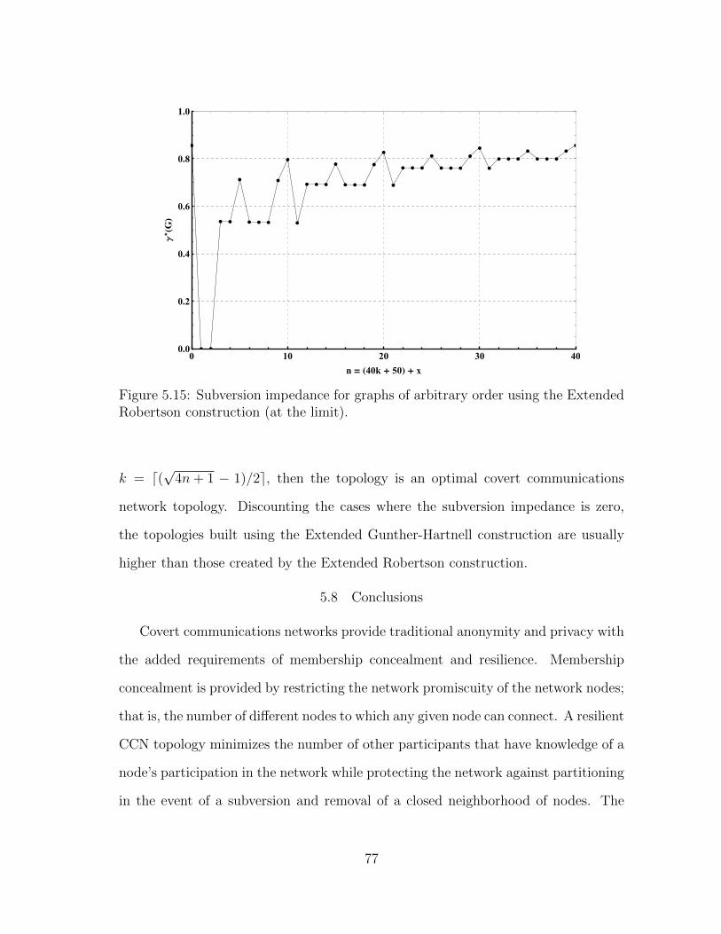
æ

æ æ

æ æ

æ

æ æ æ

æ

æ

æ

æ æ æ

æ

æ æ æ

æ

æ

æ

æ æ æ

æ

æ æ æ

æ

æ

æ

æ æ æ

æ

æ æ æ

æ

æ

0 10 20 30 400.0

0.2

0.4

0.6

0.8

1.0

n = H40k + 50L + x

Γ*

HGL

Figure 5.15: Subversion impedance for graphs of arbitrary order using the ExtendedRobertson construction (at the limit).

k = d(√

4n+ 1 − 1)/2e, then the topology is an optimal covert communications

network topology. Discounting the cases where the subversion impedance is zero,

the topologies built using the Extended Gunther-Hartnell construction are usually

higher than those created by the Extended Robertson construction.

5.8 Conclusions

Covert communications networks provide traditional anonymity and privacy with

the added requirements of membership concealment and resilience. Membership

concealment is provided by restricting the network promiscuity of the network nodes;

that is, the number of different nodes to which any given node can connect. A resilient

CCN topology minimizes the number of other participants that have knowledge of a

node’s participation in the network while protecting the network against partitioning

in the event of a subversion and removal of a closed neighborhood of nodes. The

77

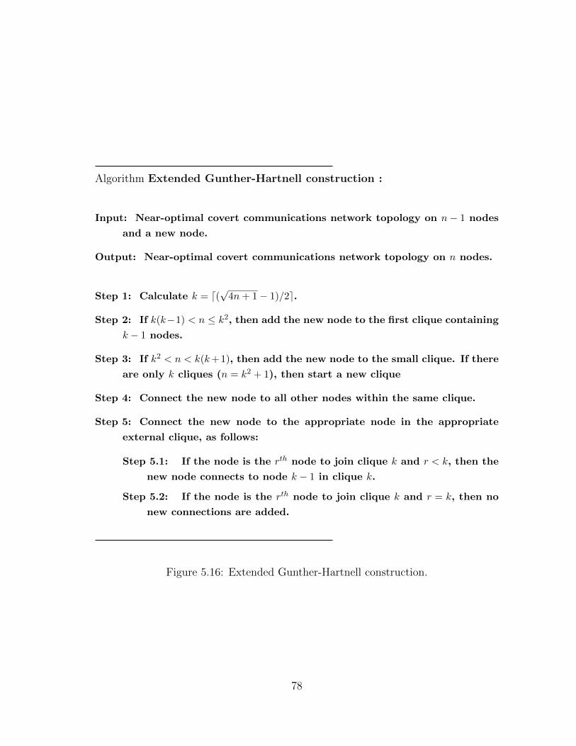
Algorithm Extended Gunther-Hartnell construction :

Input: Near-optimal covert communications network topology on n− 1 nodes

and a new node.

Output: Near-optimal covert communications network topology on n nodes.

Step 1: Calculate k = d(√4n+ 1− 1)/2e.

Step 2: If k(k−1) < n ≤ k2, then add the new node to the first clique containing

k − 1 nodes.

Step 3: If k2 < n < k(k+1), then add the new node to the small clique. If there

are only k cliques (n = k2 + 1), then start a new clique

Step 4: Connect the new node to all other nodes within the same clique.

Step 5: Connect the new node to the appropriate node in the appropriate

external clique, as follows:

Step 5.1: If the node is the rth node to join clique k and r < k, then the

new node connects to node k − 1 in clique k.

Step 5.2: If the node is the rth node to join clique k and r = k, then no

new connections are added.

Figure 5.16: Extended Gunther-Hartnell construction.

78

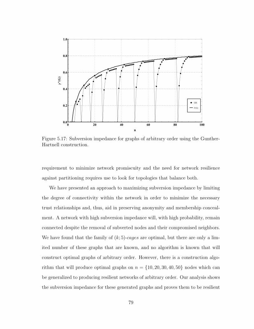
ææææ

æ

æ

æ

æ

æ

æ

æ

æ

æ

æ

æ

æ

æ

æ

æ

ææ

ææ

æ

æ

æ

æ

æ

æ

ææ

ææææ

æ

æ

æ

æ

æ

æ

æææææææ

æ

æ

æ

æ

æ

æ

æææææææææ

æ

æ

æ

æ

æ

æ

æ

ææææææææææ

æ

æ

æ

æ

æ

æ

æ

æ

æææææææææææ

æ GH

GHGL

0 20 40 60 80 1000.0

0.2

0.4

0.6

0.8

1.0

n

Γ*

HGL

Figure 5.17: Subversion impedance for graphs of arbitrary order using the Gunther-Hartnell construction.

requirement to minimize network promiscuity and the need for network resilience

against partitioning requires use to look for topologies that balance both.

We have presented an approach to maximizing subversion impedance by limiting

the degree of connectivity within the network in order to minimize the necessary

trust relationships and, thus, aid in preserving anonymity and membership conceal-

ment. A network with high subversion impedance will, with high probability, remain

connected despite the removal of subverted nodes and their compromised neighbors.

We have found that the family of (k; 5)-cages are optimal, but there are only a lim-

ited number of these graphs that are known, and no algorithm is known that will

construct optimal graphs of arbitrary order. However, there is a construction algo-

rithm that will produce optimal graphs on n = {10, 20, 30, 40, 50} nodes which can

be generalized to producing resilient networks of arbitrary order. Our analysis shows

the subversion impedance for these generated graphs and proves them to be resilient

79

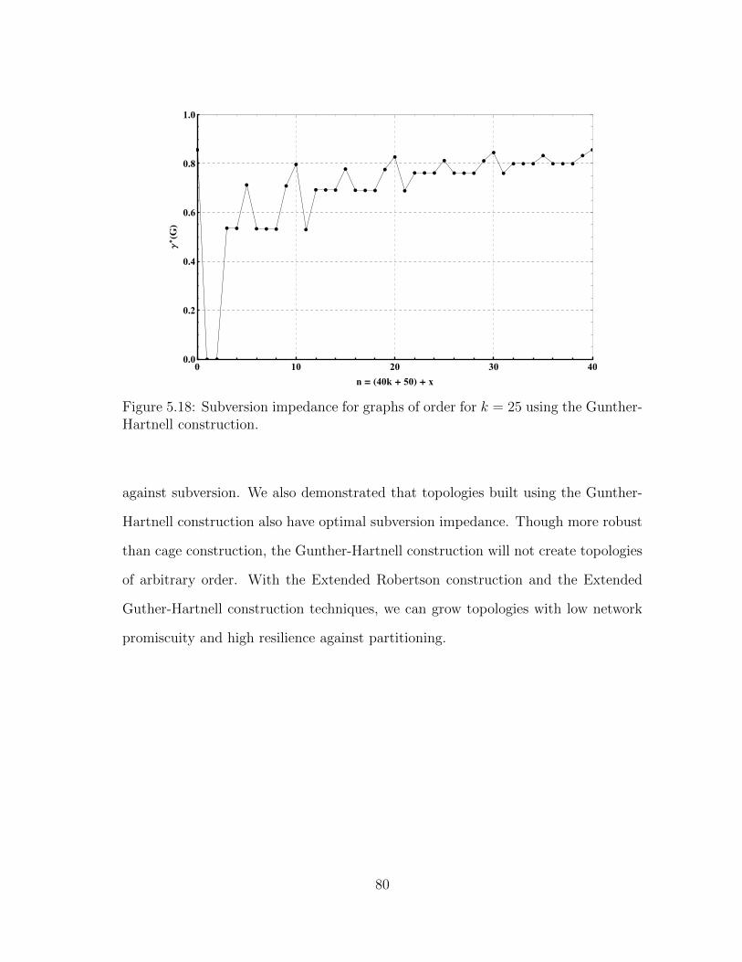
æ

æ æ

æ æ

æ

æ æ æ

æ

æ

æ

æ æ æ

æ

æ æ æ

æ

æ

æ

æ æ æ

æ

æ æ æ

æ

æ

æ

æ æ æ

æ

æ æ æ

æ

æ

0 10 20 30 400.0

0.2

0.4

0.6

0.8

1.0

n = H40k + 50L + x

Γ*

HGL

Figure 5.18: Subversion impedance for graphs of order for k = 25 using the Gunther-Hartnell construction.

against subversion. We also demonstrated that topologies built using the Gunther-

Hartnell construction also have optimal subversion impedance. Though more robust

than cage construction, the Gunther-Hartnell construction will not create topologies

of arbitrary order. With the Extended Robertson construction and the Extended

Guther-Hartnell construction techniques, we can grow topologies with low network

promiscuity and high resilience against partitioning.

80

6. RANDOM TOPOLOGY ANALYSIS FOR CCNs

The topologies discussed in Section 5 all were deterministic, that is, any newly

joining node would join the network at a well-defined location in the network ac-

cording to a well-defined global ordering. In practice, such approaches can be rarely

implemented in a CCN, mainly for two reasons. First, the join protocol would need

to determine the global location of the new node in the network which in turn would

require the network to determine (and possibly leak) information about the prospec-

tive neighbors of the new node. Second, the join protocol would need to be globally

serialized. As a result, CCNs in practice would prevalently be non-deterministic, and

would therefore have random topologies.

Examining subversion impedance in random topologies is somewhat trickier than

in deterministic topologies, as there are many different graphs that can be generated

for a given number of nodes.

Now, consider a random graph processes, G, in which a random graph evolves

as the number of nodes, n, increases. We refer to the set of possible random graphs

on n nodes as a family of random graphs denoted by Gn, where n is fixed. Now, we

develop measures on families of random graphs to determine their suitability for use

in CCNs.

As with the previous measures, we are interested in the risk incurred by the

average participant when a node is subverted, uniformly, at random, as well as the

case when the subverted node causes the most damage possible. Thus, we specify the

expected local subversion impedance as a measure of the risk incurred by a random

node and the expected global subversion impedance as the risk incurred by a node in

the worst case for all graphs G ∈ Gn.

81

6.1 Expected Local Subversion Impedance

Recall that for deterministic topologies, we use the measures of secrecy, S(G, v),

and resilience, K(G, v), for a given graph G and vertex v. Similarly, we use the

measures of average local subversion impedance, 〈γ(G)〉, average secrecy, 〈S(G)〉,

average resilience, 〈K(G)〉, and global subversion impedance, γ∗(G), for a given

graph, G.

Definition 6.1.1. The expected local subversion impedance, E[γ(G)], is the ex-

pected value of the local subversion impedance, 〈γ(G)〉, for all graphs G ∈ Gn;

E[γ(G)] =∑G∈Gn

〈γ(G)〉Pr(G) , (6.1)

where Pr(G) is the probability G occurs within Gn.

By extension, we can define both the expected secrecy measure and the expected

resilience measure.

Definition 6.1.2. The expected secrecy for all graphs G ∈ Gn is:

E[S(G, v)] =∑G∈Gn

〈S(G, v)〉Pr(G)

=n− E[d(v)]− 1

n, (6.2)

where E[d(v)] is the expected degree of node v ∈ V within the network topology,

G(V,E) ∈ Gn.

Definition 6.1.3. The expected resilience for all graphs G ∈ Gn is:

82

E[K(G, v)] =∑G∈Gn

〈K(G)〉Pr(G)

=1

n

∑G∈Gn

∑v∈V

κ(H(G, v))

κ(G)Pr(G) (6.3)

We would like to be able to easily estimate the expected local subversion impedance

on random graphs from Gn. Of course, since higher connectivity implies larger

neighborhoods, E[S(G, v)] and E[K(G, v)] are correlated. Thus, we can expect

Cov[S(G, v), K(G, v)] 6= 0. Thus, in order to calculate the expected local subver-

sion impedance from the expected secrecy and the expected resilience, we use the

following equation:

E[γ(G)] = E[S(G, v)]E[K(G, v)] + Cov[S(G, v), K(G, v)] . (6.4)

With regards to determining the expected secrecy, the expected degree is easily

calculated for many types of random topologies. However, the expected resilience

is much more difficult to calculate. We can apply Jenson’s inequality [41] on the

expected resilience measure to get a lower bound on the expected resilience. Let

E[κ(G)] be the expected vertex connectivity on a graph G ∈ Gn on n nodes and let

E[κ(H(G, v))] be the expected connectivity of a survivor graph H(G, v) ∈ H(Gn),

where H(Gn) is the set of survivor graphs generated from the removal of a random

closed neighborhood from a graph in Gn. Then

83

E[K(G, v)] = E

[κ(H(G, v))

κ(G)

]

≥ E[κ(H(G, v))]

E[κ(G)]. (6.5)

From here, we need to establish the closeness of this bound, look for ways to

estimate the vertex connectivity, and determine the covariance between E[S(G, v)]

and E[K(G, v)]–all of which are dependent on the particular random graph process

used.

6.2 Expected Global Subversion Impedance

Even in random topologies, we are still concerned about worst-case subversions.

In assessing a randomized graph process, the expected global subversion impedance

will measure the expected worst-case.

Definition 6.2.1. The expected global subversion impedance, E[γ∗(G)], is the ex-

pected value of the global subversion impedance, γ∗(G), for all graphs G ∈ Gn;

E[γ∗(G)] =∑G∈Gn

γ∗(G)Pr(G) , (6.6)

where Pr(G) is the probability of G being occurring within the family, Gn.

In the following, we analyze Erdos-Renyi and scale-free (Barabasi-Albert) random

graphs in order to determine their suitability as CCN topologies. We develop a

closed-form estimate for the expected local subversion impedance for Erdos-Renyi

random graphs.

84

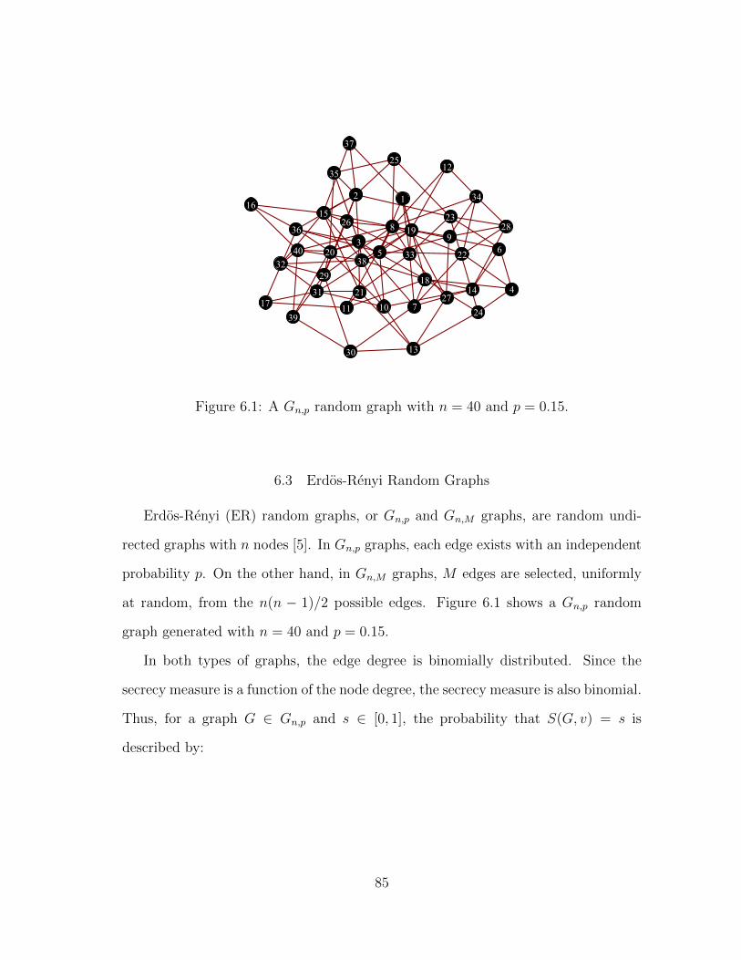
12

3

4

56

7

8

9

1011

12

13

14

15

16

17

18

19

20

21

22

23

24

25

26

27

28

29

30

31

32

33

34

35

36

37

38

39

40

Figure 6.1: A Gn,p random graph with n = 40 and p = 0.15.

6.3 Erdos-Renyi Random Graphs

Erdos-Renyi (ER) random graphs, or Gn,p and Gn,M graphs, are random undi-

rected graphs with n nodes [5]. In Gn,p graphs, each edge exists with an independent

probability p. On the other hand, in Gn,M graphs, M edges are selected, uniformly

at random, from the n(n − 1)/2 possible edges. Figure 6.1 shows a Gn,p random

graph generated with n = 40 and p = 0.15.

In both types of graphs, the edge degree is binomially distributed. Since the

secrecy measure is a function of the node degree, the secrecy measure is also binomial.

Thus, for a graph G ∈ Gn,p and s ∈ [0, 1], the probability that S(G, v) = s is

described by:

85

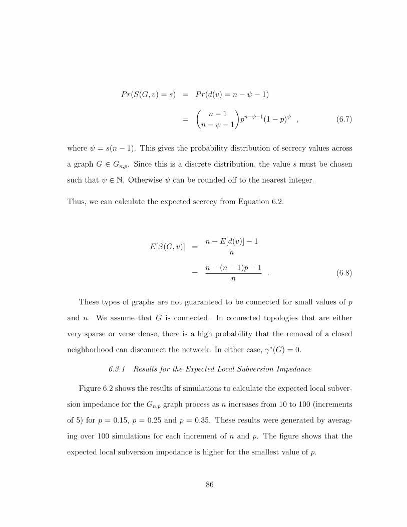
Pr(S(G, v) = s) = Pr(d(v) = n− ψ − 1)

=

(n− 1

n− ψ − 1

)pn−ψ−1(1− p)ψ , (6.7)

where ψ = s(n− 1). This gives the probability distribution of secrecy values across

a graph G ∈ Gn,p. Since this is a discrete distribution, the value s must be chosen

such that ψ ∈ N. Otherwise ψ can be rounded off to the nearest integer.

Thus, we can calculate the expected secrecy from Equation 6.2:

E[S(G, v)] =n− E[d(v)]− 1

n

=n− (n− 1)p− 1

n. (6.8)

These types of graphs are not guaranteed to be connected for small values of p

and n. We assume that G is connected. In connected topologies that are either

very sparse or verse dense, there is a high probability that the removal of a closed

neighborhood can disconnect the network. In either case, γ∗(G) = 0.

6.3.1 Results for the Expected Local Subversion Impedance

Figure 6.2 shows the results of simulations to calculate the expected local subver-

sion impedance for the Gn,p graph process as n increases from 10 to 100 (increments

of 5) for p = 0.15, p = 0.25 and p = 0.35. These results were generated by averag-

ing over 100 simulations for each increment of n and p. The figure shows that the

expected local subversion impedance is higher for the smallest value of p.

86

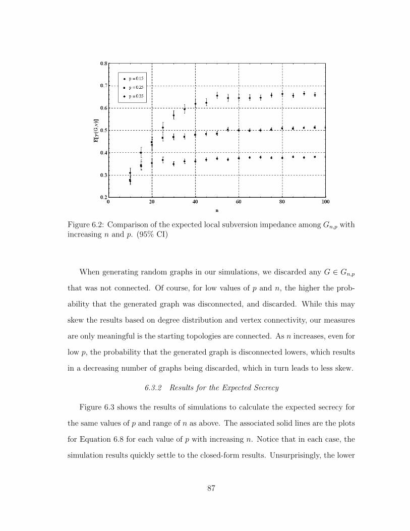
Figure 6.2: Comparison of the expected local subversion impedance among Gn,p withincreasing n and p. (95% CI)

When generating random graphs in our simulations, we discarded any G ∈ Gn,p

that was not connected. Of course, for low values of p and n, the higher the prob-

ability that the generated graph was disconnected, and discarded. While this may

skew the results based on degree distribution and vertex connectivity, our measures

are only meaningful is the starting topologies are connected. As n increases, even for

low p, the probability that the generated graph is disconnected lowers, which results

in a decreasing number of graphs being discarded, which in turn leads to less skew.

6.3.2 Results for the Expected Secrecy

Figure 6.3 shows the results of simulations to calculate the expected secrecy for

the same values of p and range of n as above. The associated solid lines are the plots

for Equation 6.8 for each value of p with increasing n. Notice that in each case, the

simulation results quickly settle to the closed-form results. Unsurprisingly, the lower

87

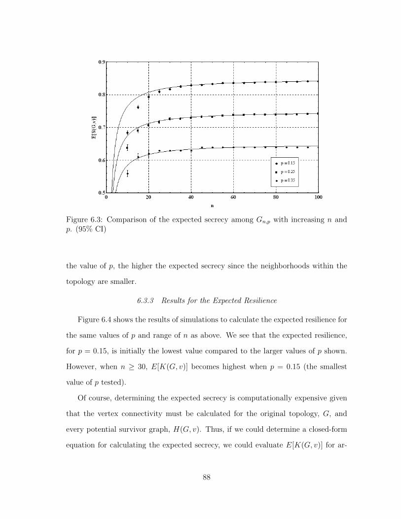
Figure 6.3: Comparison of the expected secrecy among Gn,p with increasing n andp. (95% CI)

the value of p, the higher the expected secrecy since the neighborhoods within the

topology are smaller.

6.3.3 Results for the Expected Resilience

Figure 6.4 shows the results of simulations to calculate the expected resilience for

the same values of p and range of n as above. We see that the expected resilience,

for p = 0.15, is initially the lowest value compared to the larger values of p shown.

However, when n ≥ 30, E[K(G, v)] becomes highest when p = 0.15 (the smallest

value of p tested).

Of course, determining the expected secrecy is computationally expensive given

that the vertex connectivity must be calculated for the original topology, G, and

every potential survivor graph, H(G, v). Thus, if we could determine a closed-form

equation for calculating the expected secrecy, we could evaluate E[K(G, v)] for ar-

88

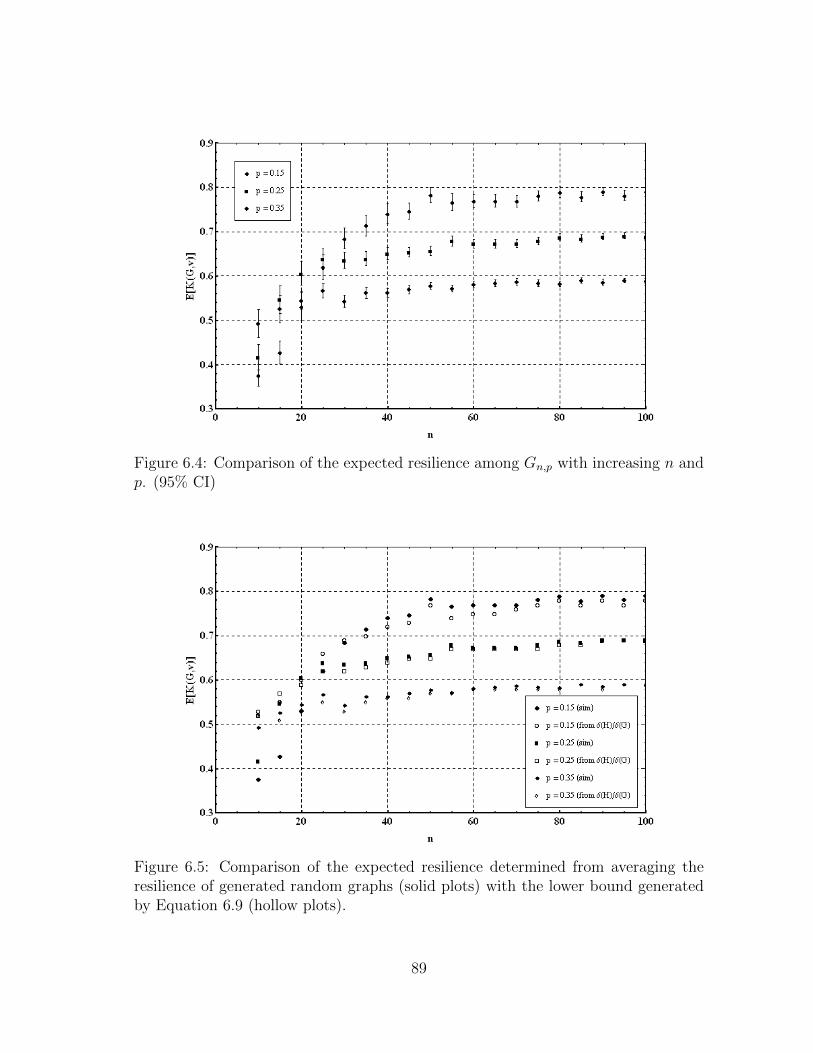
Figure 6.4: Comparison of the expected resilience among Gn,p with increasing n andp. (95% CI)

Figure 6.5: Comparison of the expected resilience determined from averaging theresilience of generated random graphs (solid plots) with the lower bound generatedby Equation 6.9 (hollow plots).

89

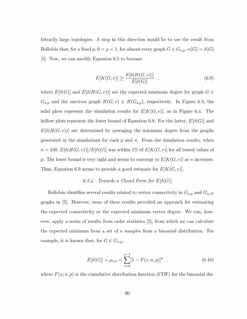
bitrarily large topologies. A step in this direction would be to use the result from

Bollobas that, for a fixed p, 0 < p < 1, for almost every graph G ∈ Gn,p, κ(G) = δ(G)

[5]. Now, we can modify Equation 6.5 to become

E[K(G, v)] ≥ E[δ(H(G, v))]

E[δ(G)], (6.9)

where E[δ(G)] and E[δ(H(G, v))] are the expected minimum degree for graph G ∈

Gn,p and the survivor graph H(G, v) ∈ H(Gn,p), respectively. In Figure 6.5, the

solid plots represent the simulation results for E[K(G, v)], as in Figure 6.4. The

hollow plots represent the lower bound of Equation 6.9. For the latter, E[δ(G)] and

E[δ(H(G, v))] are determined by averaging the minimum degree from the graphs

generated in the simulations for each p and n. From the simulation results, when

n = 100, E[δ(H(G, v))]/E[δ(G)] was within 1% of E[K(G, v)] for all tested values of

p. The lower bound is very tight and seems to converge to E[K(G, v)] as n increases.

Thus, Equation 6.9 seems to provide a good estimate for E[K(G, v)].

6.3.4 Towards a Closed Form for E[δ(G)]

Bollobas identifies several results related to vertex connectivity in Gn,p and Gn,M

graphs in [5]. However, none of these results provided an approach for estimating

the expected connectivity or the expected minimum vertex degree. We can, how-

ever, apply a series of results from order statistics [2], from which we can calculate

the expected minimum from a set of n samples from a binomial distribution. For

example, it is known that, for G ∈ Gn,p,

E[δ(G)] = µ1:n =n−1∑x=0

[1− F (x;n, p)]n , (6.10)

where F (x;n, p) is the cumulative distribution function (CDF) for the binomial dis-

90

Figure 6.6: The error between the expected minimum degree derived from simula-tions and µ1:n.

tribution [2]. In this expression, the term µ1:n is used to denote the expected smallest

value in a sample of n elements.

Figure 6.6 shows the error between the calculated estimates from simulation,

E[δ(G)]sim, and the expectation as calculated from Equation 6.10. For n = 100, the

calculated estimates have an error of just over 2%, but which quickly falls off. For

n ≥ 1000, all test values (p ∈ [0.15, 0.35]) have an error of less than 1%. In fact,

with these results, we assume that, as n increases,

|E[δ(G)]sim − µ1:n|E[δ(G)]sim

→ 0 . (6.11)

Using Equation 6.9 gives us a good estimate for E[δ(G)] for large n, but what

about E[δ(H(G, v))]? We know the expected number of nodes in H(G, v), but does

Equation 6.9 still give a good estimate for the connectivity of the survivor graph?

91

Theorem 6.3.1. Let G(V,E) ∈ Gn,p for n ≥ 1 and p ∈ [0, 1], and let H(G, v) ⊂

G be the survivor graph resulting from G − N [v] for some vertex v ∈ V . Then,

H(G, v) ∈ Gn′,p′ with

n′ = n− E[d(v)]− 1 , (6.12)

and

p′ → p , (6.13)

as n→∞.

Proof. The expected number of nodes in the closed neighborhood of v is E[d(v)] + 1,

with

E[d(v)] = (n− 1)p ≈ np , (6.14)

for large n. Thus, the expected number of nodes, n′, in H(G, v) is the number of

nodes in G minus the expected size of the closed neighborhood:

|H(G, v)| = n′ = n− E[d(v)]− 1 . (6.15)

The expected number of edges, M , in G is:

M := E[||G||] =n(n− 1)

2p .

If the nodes within the closed neighborhood shared no edges, we could expect N [v] to

have E[d(v)]2 edges. However, at least some of the nodes in the closed neighborhood

may have been connected and therefore share edges, so we must be sure not to

92

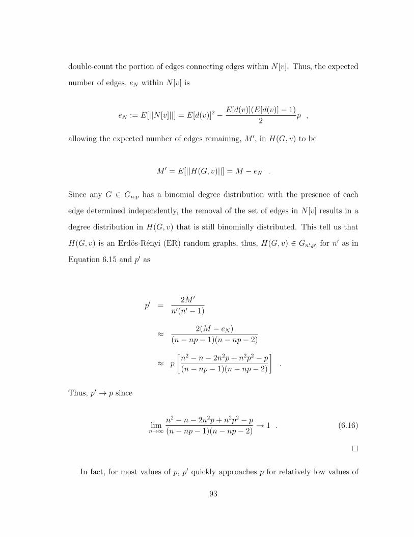
double-count the portion of edges connecting edges within N [v]. Thus, the expected

number of edges, eN within N [v] is

eN := E[||N [v]||] = E[d(v)]2 − E[d(v)](E[d(v)]− 1)

2p ,

allowing the expected number of edges remaining, M ′, in H(G, v) to be

M ′ = E[||H(G, v)||] = M − eN .

Since any G ∈ Gn,p has a binomial degree distribution with the presence of each

edge determined independently, the removal of the set of edges in N [v] results in a

degree distribution in H(G, v) that is still binomially distributed. This tell us that

H(G, v) is an Erdos-Renyi (ER) random graphs, thus, H(G, v) ∈ Gn′,p′ for n′ as in

Equation 6.15 and p′ as

p′ =2M ′

n′(n′ − 1)

≈ 2(M − eN)

(n− np− 1)(n− np− 2)

≈ p

[n2 − n− 2n2p+ n2p2 − p(n− np− 1)(n− np− 2)

].

Thus, p′ → p since

limn→∞

n2 − n− 2n2p+ n2p2 − p(n− np− 1)(n− np− 2)

→ 1 . (6.16)

In fact, for most values of p, p′ quickly approaches p for relatively low values of

93

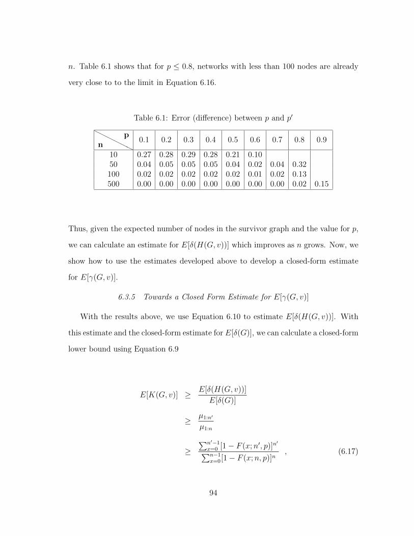
n. Table 6.1 shows that for p ≤ 0.8, networks with less than 100 nodes are already

very close to to the limit in Equation 6.16.

Table 6.1: Error (difference) between p and p′

HHHH

HHnp

0.1 0.2 0.3 0.4 0.5 0.6 0.7 0.8 0.9

10 0.27 0.28 0.29 0.28 0.21 0.1050 0.04 0.05 0.05 0.05 0.04 0.02 0.04 0.32100 0.02 0.02 0.02 0.02 0.02 0.01 0.02 0.13500 0.00 0.00 0.00 0.00 0.00 0.00 0.00 0.02 0.15

Thus, given the expected number of nodes in the survivor graph and the value for p,

we can calculate an estimate for E[δ(H(G, v))] which improves as n grows. Now, we

show how to use the estimates developed above to develop a closed-form estimate

for E[γ(G, v)].

6.3.5 Towards a Closed Form Estimate for E[γ(G, v)]

With the results above, we use Equation 6.10 to estimate E[δ(H(G, v))]. With

this estimate and the closed-form estimate for E[δ(G)], we can calculate a closed-form

lower bound using Equation 6.9

E[K(G, v)] ≥ E[δ(H(G, v))]

E[δ(G)]

≥ µ1:n′

µ1:n

≥∑n′−1

x=0 [1− F (x;n′, p)]n′∑n−1

x=0[1− F (x;n, p)]n, (6.17)

94

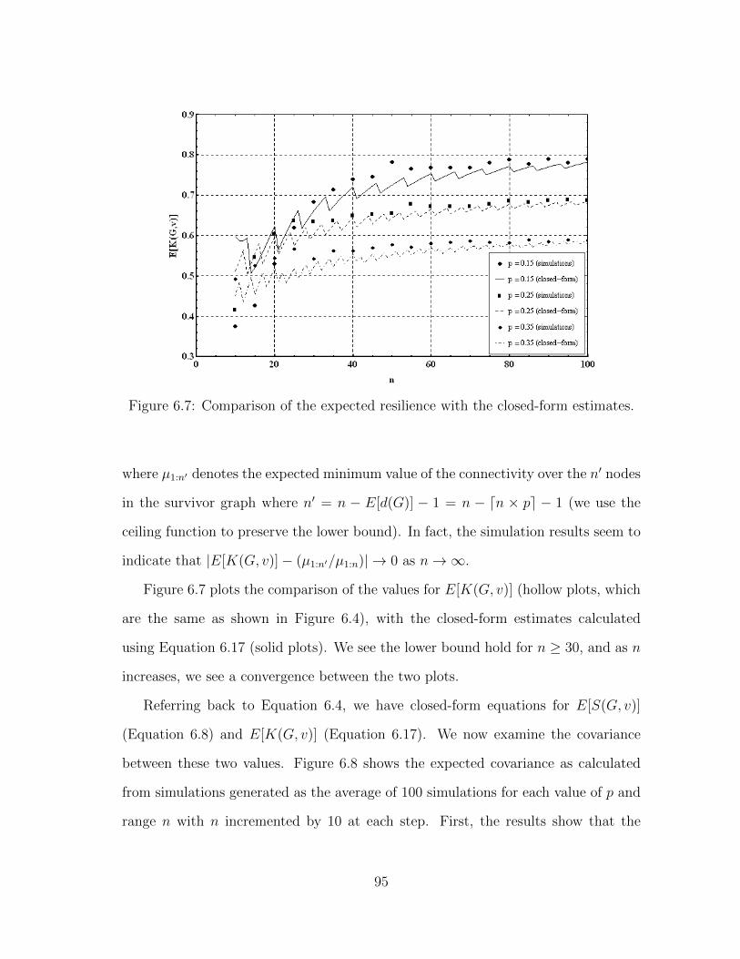
Figure 6.7: Comparison of the expected resilience with the closed-form estimates.

where µ1:n′ denotes the expected minimum value of the connectivity over the n′ nodes

in the survivor graph where n′ = n − E[d(G)] − 1 = n − dn × pe − 1 (we use the

ceiling function to preserve the lower bound). In fact, the simulation results seem to

indicate that |E[K(G, v)]− (µ1:n′/µ1:n)| → 0 as n→∞.

Figure 6.7 plots the comparison of the values for E[K(G, v)] (hollow plots, which

are the same as shown in Figure 6.4), with the closed-form estimates calculated

using Equation 6.17 (solid plots). We see the lower bound hold for n ≥ 30, and as n

increases, we see a convergence between the two plots.

Referring back to Equation 6.4, we have closed-form equations for E[S(G, v)]

(Equation 6.8) and E[K(G, v)] (Equation 6.17). We now examine the covariance

between these two values. Figure 6.8 shows the expected covariance as calculated

from simulations generated as the average of 100 simulations for each value of p and

range n with n incremented by 10 at each step. First, the results show that the

95

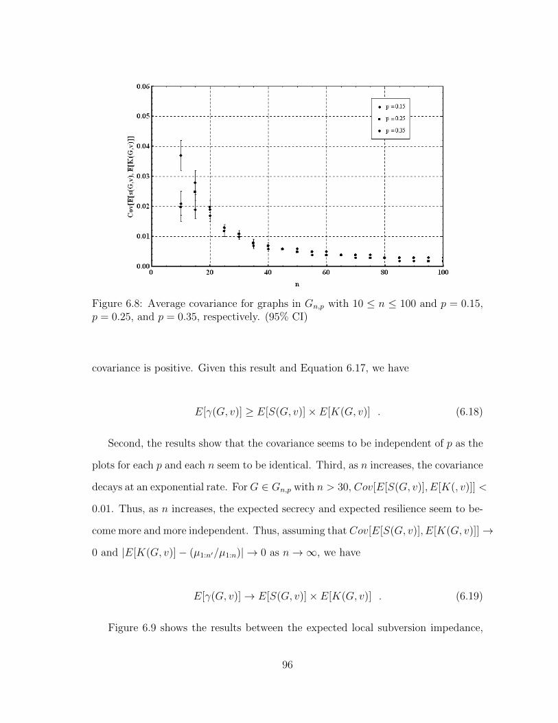
Figure 6.8: Average covariance for graphs in Gn,p with 10 ≤ n ≤ 100 and p = 0.15,p = 0.25, and p = 0.35, respectively. (95% CI)

covariance is positive. Given this result and Equation 6.17, we have

E[γ(G, v)] ≥ E[S(G, v)]× E[K(G, v)] . (6.18)

Second, the results show that the covariance seems to be independent of p as the

plots for each p and each n seem to be identical. Third, as n increases, the covariance

decays at an exponential rate. ForG ∈ Gn,p with n > 30, Cov[E[S(G, v)], E[K(, v)]] <

0.01. Thus, as n increases, the expected secrecy and expected resilience seem to be-

come more and more independent. Thus, assuming that Cov[E[S(G, v)], E[K(G, v)]]→

0 and |E[K(G, v)]− (µ1:n′/µ1:n)| → 0 as n→∞, we have

E[γ(G, v)]→ E[S(G, v)]× E[K(G, v)] . (6.19)

Figure 6.9 shows the results between the expected local subversion impedance,

96

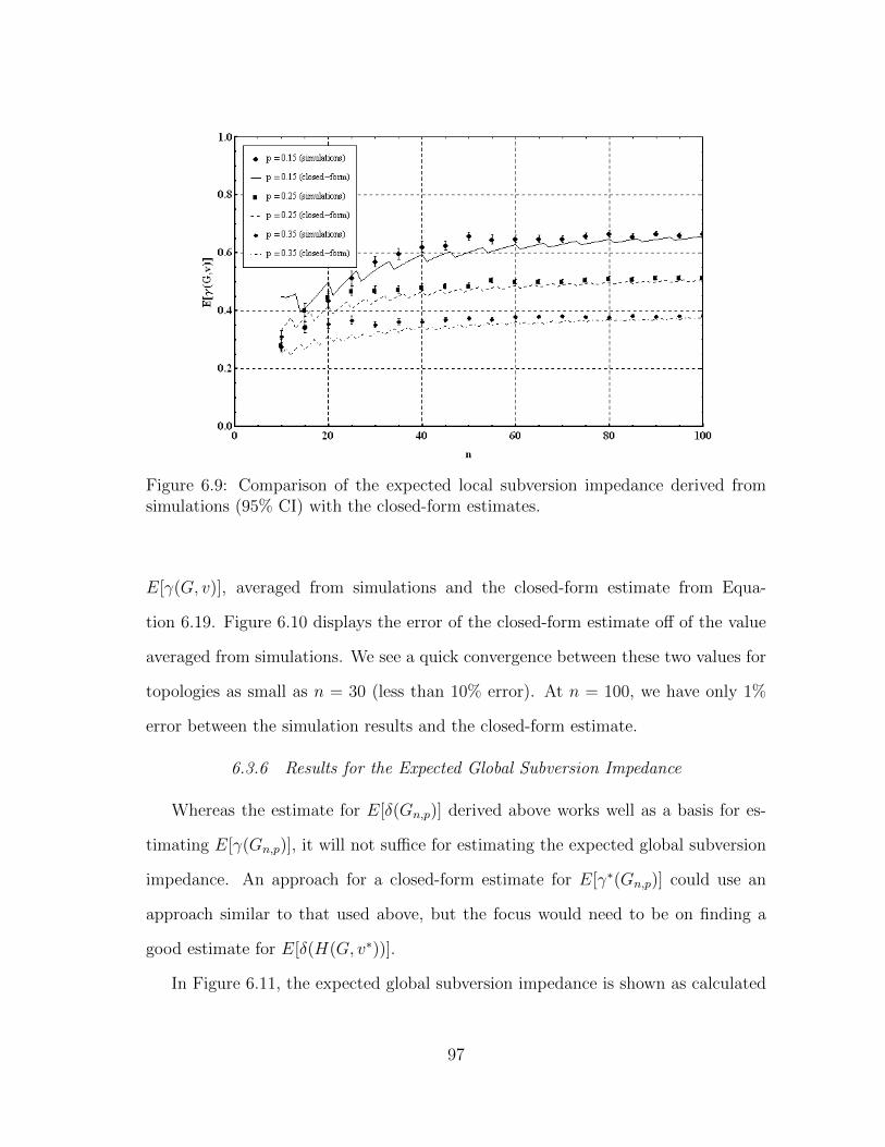
Figure 6.9: Comparison of the expected local subversion impedance derived fromsimulations (95% CI) with the closed-form estimates.

E[γ(G, v)], averaged from simulations and the closed-form estimate from Equa-

tion 6.19. Figure 6.10 displays the error of the closed-form estimate off of the value

averaged from simulations. We see a quick convergence between these two values for

topologies as small as n = 30 (less than 10% error). At n = 100, we have only 1%

error between the simulation results and the closed-form estimate.

6.3.6 Results for the Expected Global Subversion Impedance

Whereas the estimate for E[δ(Gn,p)] derived above works well as a basis for es-

timating E[γ(Gn,p)], it will not suffice for estimating the expected global subversion

impedance. An approach for a closed-form estimate for E[γ∗(Gn,p)] could use an

approach similar to that used above, but the focus would need to be on finding a

good estimate for E[δ(H(G, v∗))].

In Figure 6.11, the expected global subversion impedance is shown as calculated

97

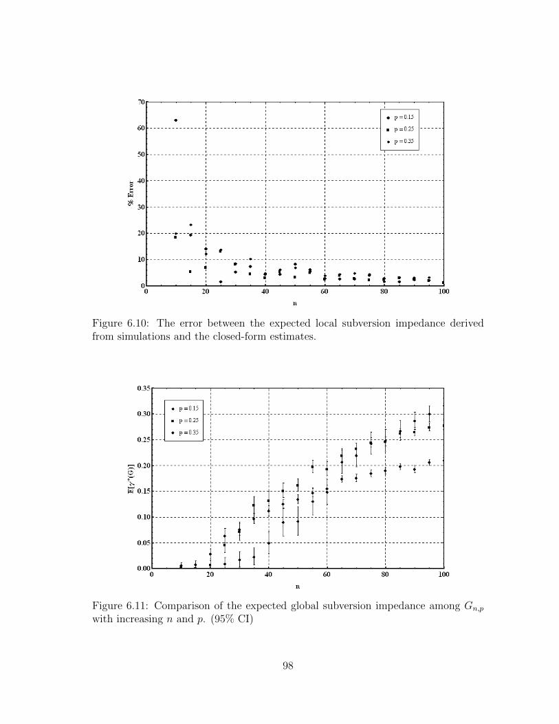
Figure 6.10: The error between the expected local subversion impedance derivedfrom simulations and the closed-form estimates.

Figure 6.11: Comparison of the expected global subversion impedance among Gn,p

with increasing n and p. (95% CI)

98

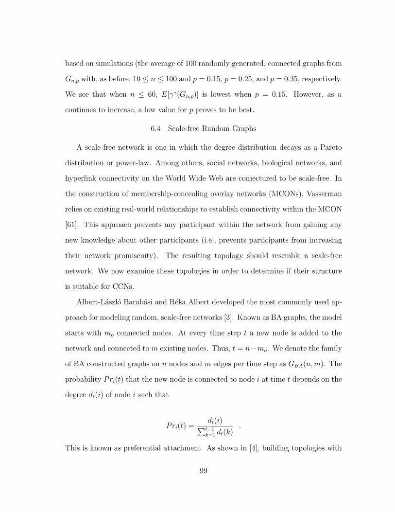
based on simulations (the average of 100 randomly generated, connected graphs from

Gn,p with, as before, 10 ≤ n ≤ 100 and p = 0.15, p = 0.25, and p = 0.35, respectively.

We see that when n ≤ 60, E[γ∗(Gn,p)] is lowest when p = 0.15. However, as n

continues to increase, a low value for p proves to be best.

6.4 Scale-free Random Graphs

A scale-free network is one in which the degree distribution decays as a Pareto

distribution or power-law. Among others, social networks, biological networks, and

hyperlink connectivity on the World Wide Web are conjectured to be scale-free. In

the construction of membership-concealing overlay networks (MCONs), Vasserman

relies on existing real-world relationships to establish connectivity within the MCON

[61]. This approach prevents any participant within the network from gaining any

new knowledge about other participants (i.e., prevents participants from increasing

their network promiscuity). The resulting topology should resemble a scale-free

network. We now examine these topologies in order to determine if their structure

is suitable for CCNs.

Albert-Laszlo Barabasi and Reka Albert developed the most commonly used ap-

proach for modeling random, scale-free networks [3]. Known as BA graphs, the model

starts with mo connected nodes. At every time step t a new node is added to the

network and connected to m existing nodes. Thus, t = n−mo. We denote the family

of BA constructed graphs on n nodes and m edges per time step as GBA(n,m). The

probability Pri(t) that the new node is connected to node i at time t depends on the

degree dt(i) of node i such that

Pri(t) =dt(i)∑t−1k=1 dt(k)

.

This is known as preferential attachment. As shown in [4], building topologies with

99

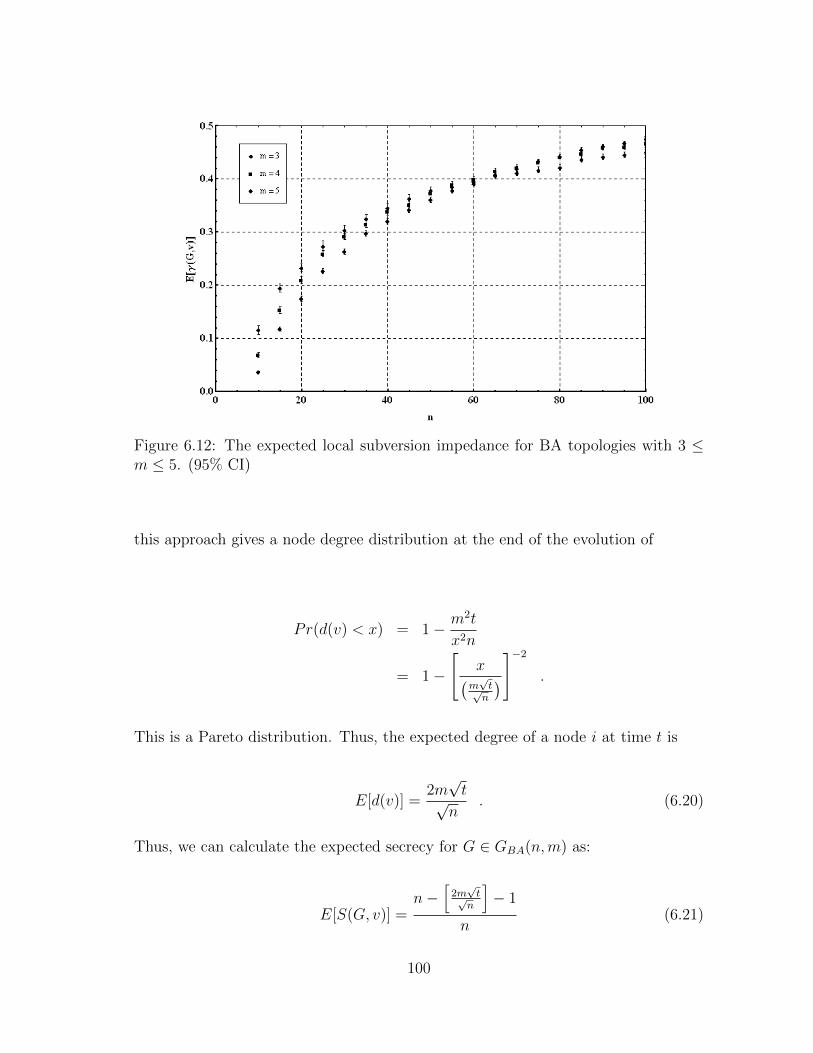
Figure 6.12: The expected local subversion impedance for BA topologies with 3 ≤m ≤ 5. (95% CI)

this approach gives a node degree distribution at the end of the evolution of

Pr(d(v) < x) = 1− m2t

x2n

= 1−

[x(m√t√n

)]−2 .

This is a Pareto distribution. Thus, the expected degree of a node i at time t is

E[d(v)] =2m√t√

n. (6.20)

Thus, we can calculate the expected secrecy for G ∈ GBA(n,m) as:

E[S(G, v)] =n−

[2m√t√

n

]− 1

n(6.21)

100

For the expected resilience, we need the expected connectivity of the original

graph, G ∈ GBA, and the expected connectivity of the survivor graph, H(G, v),

using the BA construction. The expected connectivity of the original topology is

equal to the expected minimum degree,

E[κ(G)] = E[δ(G)] .

The expected connectivity of the survivor graph is much less clear. Unfortunately,

we can’t use the same approach to calculate the expected connectivity of the survivor

graph that we used earlier for Erdos-Renyi graphs because the survivor graph is no

longer a scale-free graph.

Figure 6.12 shows the expected local subversion impedance for 10 ≤ n ≤ 100

where each plot is the mean of 100 randomly generated topologies at a given order

and the order is increased by 5 at each step. We see that these topologies perform

moderately well in the average case with an expected local subversion impedance

at around E[γ(G)] ≈ 0.47 for the values of m that we examined (3 ≤ m ≤ 5).

Unfortunately, in the worst case, these topologies were almost always disconnected

resulting in E[γ∗(GBA)] ≈ 0 for 3 ≤ m ≤ 5 and n ≤ 100. As n and m increase, the

probability that the survivor graph remains connected also increases, but not at a

rate that showed any promise for the use of scale-free graphs in CCNs.

6.5 Conclusions

Our analysis was motivated by [1], in which Reka Albert, Hawoong Jeong, and

Albert-Laszlo Barabasi compare the effects of random and worst case attacks in

Erdos-Renyi random graphs and scale-free random graphs as single nodes are re-

moved. Likewise, we examine the effects of neighborhood failures on these same two

families of random graphs in both the random and worst case.

101

In the previous sections, we defined measures for assessing the suitability of a ran-

dom topology for a CCN. With these measures, we analyzed Erdos-Renyi Random

Graphs and scale-free graphs from the Barabasi-Albert construction. We also deter-

mined a closed form estimate for the expected local subversion impedance of Gn,p

graphs and a closed form estimate for the expected secrecy of a BA topology. For

the parameters examined, the expected local subversion impedance in Gn,p topologies

was significantly higher than that of BA topologies. BA topologies also have very

poor expected global subversion impedance. The homogenous nature of Gn,p graphs

make them less vulnerable to catastrophic damage resulting from subversions.

102

7. MEMBERSHIP MANAGEMENT IN A COVERT COMMUNICATION

NETWORK

Joining a covert communications network (CCN) is risky both for the network

participants as well as for the prospective participant. The existing network partici-

pants want a discerning way to protect against adversarial infiltration. A prospective

participant will want to make sure that the CCN it is joining is legitimate and that

he will not be placed at an inordinate risk by the other network participants. There-

fore, a join protocol has to be in place that enables prospective nodes to join the

network while preserving membership concealment.

We are interested in protocols that allows nodes to join the network in a manner

that: (1) protect against unnecessary exposure of the identity of each participating

node; (2) do not generate a large communication signature–that is, members of a

CCN should not be identified as such by their communication patterns; and (3) do

not rely on the secrecy of either the software or protocols used.

7.1 Initial Vetting and Shared Credentials

Traditional P2P networks are not concerned with membership concealment and,

therefore, are open to anyone who wishes to join. Often, the network addresses of

existing nodes are publicly advertised in order to provide a point of connectivity for

new nodes. When a new node wants to join, it connects to an existing node, and

the address information of the new node is shared across the network in a promis-

cuous manner allowing other nodes to establish direct connections to the new node

or establish direct connections to other existing nodes according to their topology

management scheme (e.g., CAN [51] and Chord [57]). Even in anonymity networks

such as [16, 21, 23, 52], membership concealment is not addressed. As a result, nodes

103

in such systems display network promiscuity, which affects membership concealment

and provides easy ways of infiltration for an adversary interested in discovering the

network addresses of participants.

An exception is Membership-Concealing Overlay Networks in which Vasserman

et al. restrict direct connections within the network topology to those that already

exist in personal relationships [61]. This approach is limiting, however, in that it does

not allow direct connections to be established between participants that do not know

each other already and thus limits the topology and the growth of the network. For

the network to grow, a mediation mechanism must be in place that allows previously

unrelated nodes to enter into a trust relation that allows for establishment of a direct

connection. Typically, one would have to rely on some out-of-band mechanism that

provides a baseline of trust between the network participants and the prospective

participant and allows the exchange of credentials needed to connect the new node

to the existing network. Ideally, in a CCN, we would like an approach that does not

require an out-of-band communication between the current CCN participants and a

prospective participant. However, we are unaware of an approach that would protect

against adversarial infiltration of the CCN without some sort of shared secret between

the new prospect and an existing CCN participant. Therefore, we must assume that

some form of vetting (for example, as part of a separate recruiting process) restricts

membership to only those that possess the shared secret.

7.2 First Contact

We distinguished between the participant, the participant’s node, vi, and the

node’s pseudonym, Pi, we also specify the network address of the node, Ai. Thus,

if node, vj is a neighbor to vi within the CCN topology, then vj knows node vi’s

address, Ai. We consider first contact to be the event in which a current node, vcurr,

104

within the CCN establishes direct communication with the new node, vnew, that is

joining the CCN. The current node is, of course, the network presence of a participant

already connected within the network; while, the new node is the network presence of

the prospective participant. The current node is connected to other nodes within the

CCN, and the new node is not yet connected to the CCN. The connection between

the two nodes, vcurr and vnew, is established by each node revealing their network

address, Acurr and Anew respectively, to each other resulting in an increase in both

nodes’ network promiscuity.

7.2.1 Current Node Determination

For ease of description, we assume that each node in the network is able, if

required, to determine the set of current nodes, Vcurr that will establish direct con-

nections to the new node. Among this set, Vcurr, the current node, vcurr ∈ Vcurr

that will establish first contact can be arbitrarily selected based on the needs of the

network. The newest node from Vcurr may be selected and thus exposed to more risk

on the basis that it is more expendable. On the other hand, the same logic can be

used to argue that the newest node is the least trustworthy. Thus, the oldest node

may be selected as vcurr. A third option would be to choose a random node from

Vcurr to act as vcurr. Of course, this approach would require agreement from all nodes

within Vcurr.

7.2.2 Direct First Contact

A naive approach for first contact would allow the new node to contact the current

node directly. The credentials provided to the new node may contain the network

address for a current member of the network, allowing the new node to directly

connect to the current member. Assuming that traffic is secured via asymmetric

encryption, the new node requires the public key of the current node to be provided

105

as part of the “out-of-band” credentials. The risk associated with this approach is

that the network address of the current node is being provided “in-the-clear”. If the

new node does not follow-up and use the information to establish the connection, the

network promiscuity of the current node just increased without tangible benefit to

the network. In addition, the CCN still must manage the topology as if the current

node was connected to the new node. This approach seems to place an inordinate

risk on the current node through the potential for premature exposure. A method

must be devised that avoids the type of exposure.

7.2.3 Indirect First Contact

We prevent premature exposure of the address, Acurr, of node vcurr by pushing

the associated risk to the new node. In this approach, the new node is provided with

the reference to a public repository that allows some form of information sharing

(e.g. Flickr or Facebook) and half of an asymmetric key. The new node encrypts

its network address using the provided key, and uploads it to the repository. The

current node has the other half of the asymmetric key pair. The current node checks

the repository to detect the presence of the uploaded information, downloads the

payload, and uses its half of the key pair to decrypt the network address of the new

node. Then, the current node uses that information to establish direct connectivity

with the new node.

In this approach, the current node is not at risk of premature exposure, and the

new node assumes an initial level of risk that is on par with other CCN nodes. Once

first contact is made between the current node and the new node, the current node

passes its knowledge of the CCN to the new node (i.e., the public keys of all known

CCN nodes). This allows the new node to calculate with which other current nodes

that it needs to establish connections (i.e., Vcurr). Then, the new node can request

106

to establish direct connections with the appropriate nodes.

7.3 Basic Join Protocol

The following two protocols provide the basic mechanism for a potential partici-

pant to join a CCN. The first protocol focuses on establishing first contact between

the potential participant and the CCN, and the second protocol is to establish addi-

tional connections between the new node and the CCN. Both protocols accomplish

their functions in a manner that prevents unnecessary increases in network promis-

cuity.

7.3.1 Protocol 1 - First Contact

The purpose of the following protocol is to establish first contact between vnew

and vcurr. Once complete, vnew will be connected to the CCN and have vcurr as its

only neighbor.

A-1. The new prospect instantiates node, vnew with a network address, Anew, and

key pair (Kpubnew, K

prinew).

A-2. Node vnew has a pseudonym, Pnew, half of an asymmetric key pair, KA, and

the repository location, Lshare–provided out-of-band.

A-3. The current node vcurr has a pseudonym, Pcurr, a network address, Acurr,

the repository location, Lshare, and the other half of an asymmetric key pair,

K−A, such that, for a message, M ,

KA(K−A(M)) = K−A(KA(M)) = M .

A-4. Node vnew encrypts its pseudonym and network address, KA(Pnew, Anew, Kpubnew)

and uploads the encrypted data to Lshare.

107

A-5. Node vcurr periodically checks Lshare, and, when detected, downloads from

Lshare

KA(Pnew, Anew, Kpubnew) . (7.1)

A-6. Node vcurr decrypts K−A(KA(Pnew, Anew, Kpubnew)), adds (Pnew, K

pubnew) to its

key table, adds (Pnew, Anew) to its routing table, and adds Anew to its list

of neighbors,

N(vcurr) = {· · · , Anew} .

A-7. Node vcurr sends a connect request, Kpubnew(Pnew, Pcurr, Cr, Acurr, K

pubcurr) to

node vnew.

A-8. Node vnew receives and decrypts the connection request from vcurr and, if

vcurr is the expected node in accordance with the desired topology, sends a

connection accept to vcurr,

Kpubcurr(Pcurr, Pnew, Ca) ,

adds (Pcurr, Kpubcurr) to its key table, add (Pcurr, Acurr) to its routing table,

and adds Acurr to its list of neighbors,

N(vnew) = {Acurr} .

A-9. Node vcurr receives and decrypts K−A(KA(Pcurr, Pnew, CA)) and exchanges

additional channel information and generates symmetric keys with vnew, as

108

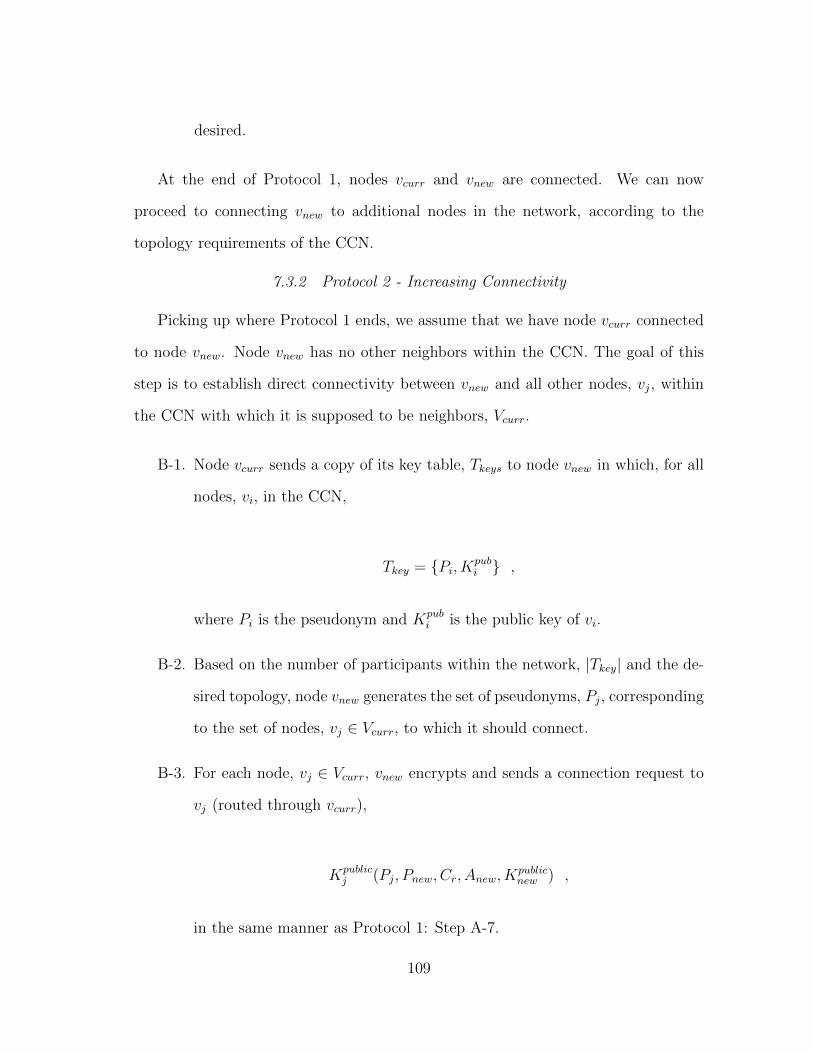
desired.

At the end of Protocol 1, nodes vcurr and vnew are connected. We can now

proceed to connecting vnew to additional nodes in the network, according to the

topology requirements of the CCN.

7.3.2 Protocol 2 - Increasing Connectivity

Picking up where Protocol 1 ends, we assume that we have node vcurr connected

to node vnew. Node vnew has no other neighbors within the CCN. The goal of this

step is to establish direct connectivity between vnew and all other nodes, vj, within

the CCN with which it is supposed to be neighbors, Vcurr.

B-1. Node vcurr sends a copy of its key table, Tkeys to node vnew in which, for all

nodes, vi, in the CCN,

Tkey = {Pi, Kpubi } ,

where Pi is the pseudonym and Kpubi is the public key of vi.

B-2. Based on the number of participants within the network, |Tkey| and the de-

sired topology, node vnew generates the set of pseudonyms, Pj, corresponding

to the set of nodes, vj ∈ Vcurr, to which it should connect.

B-3. For each node, vj ∈ Vcurr, vnew encrypts and sends a connection request to

vj (routed through vcurr),

Kpublicj (Pj, Pnew, Cr, Anew, K

publicnew ) ,

in the same manner as Protocol 1: Step A-7.

109

B-4. Each node vj receiving a connection request from vnew decrypts the request

and determines if it should be connected to vnew. If so, vj sends a connection

accept to vnew and adds vnew to its list of neighbors in the same manner as

in Protocol 1: A-8, above.

B-5. Node vnew exchanges additional channel information and generates symmet-

ric keys with each neighbor, vj, as desired.

At this point, the node vnew is a member of the CCN. We will now proceed to

analyze the resilience of the join protocol against a number of attacks.

7.4 Attacks Against the Basic Join Protocol

7.4.1 Man-in-the-Middle Attacks

Unfortunately, the approach described above is vulnerable to a man-in-the-middle

attack when the current node establishes first contact. Node vcurr could corrupt the

process by mimicking the join process in such a way that the multiple connections

established by the new node are, in fact, all with node vcurr.

7.4.2 Sybil Attack

The approach above is vulnerable to a limited Sybil attack by vcurr. The current

node could create a fictitious vnew and, thus, gain knowledge of the set of addresses

from all other nodes that become neighbors with vnew, thus undermining the mem-

bership concealment of the CCN.

Careful selection of vcurr will mitigate this vulnerability. Selecting vcurr as the

oldest node in Vcurr insures that, arguably, the most trustworthy node is the one

selected to establish first contact. In this approach, a limited set of nodes will act

as vcurr relative to the number of nodes within the network. On the other hand,

110

selecting the newest node as vcurr means that the same node will only act in that

capacity once, thus limiting the rate of infiltration by false nodes.

Use of a recruiter separate from the participant operating vcurr will mitigate the

participant’s ability to add a false node (assuming a trustworthy recruiter), but moves

the threat of a Sybil attack to the recruiter. Groups using a CCN will need to decide

where they are most vulnerable and where they would rather incur risk.

7.4.3 Collusion Attack

Assuming that the join protocol was executed without subversion, multiple nodes

could collude to undermine the anonymity of the network by sharing the addresses

of their topological neighbors. However, though individual nodes may gain infor-

mation about participants, there is no net gain in information from the colluding

nodes. Without loss of generality, we treat colluding nodes as multiple, independent

subversions.

7.5 Distributed Join Protocol

In order to mitigate attacks from vcurr, we can modify Protocol 1 in Section 7.3.1

and Protocol 2 in Section 7.3.2 so that each node vj (and no others) shares K−A

and Lshare. Then, each node vj individually downloads KA(Pnew, Anew, Kpubnew) from

Lshare, decrypts it, and sends vnew a connection request. This allows each node vj to

independently connect to vnew instead of using vcurr as the intermediary.

7.6 Generating the Shared-Secret

Protocol 1 and Protocol 2 started with the nodes vcurr and vnew already in pos-

session of their portion of the necessary credentials, that is, the shared-secret was

already generated and shared. The following two protocols assume the existence of a

recruiter node, vR, providing the communication transfer point between the network

111

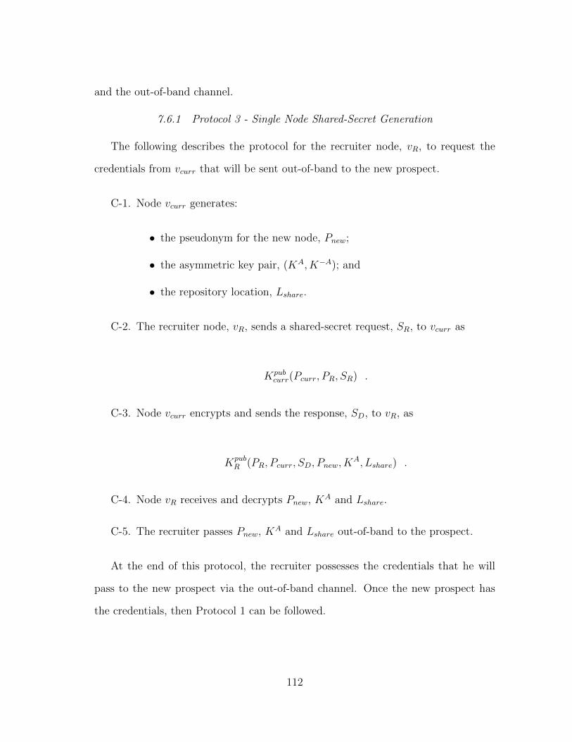
and the out-of-band channel.

7.6.1 Protocol 3 - Single Node Shared-Secret Generation

The following describes the protocol for the recruiter node, vR, to request the

credentials from vcurr that will be sent out-of-band to the new prospect.

C-1. Node vcurr generates:

• the pseudonym for the new node, Pnew;

• the asymmetric key pair, (KA, K−A); and

• the repository location, Lshare.

C-2. The recruiter node, vR, sends a shared-secret request, SR, to vcurr as

Kpubcurr(Pcurr, PR, SR) .

C-3. Node vcurr encrypts and sends the response, SD, to vR, as

KpubR (PR, Pcurr, SD, Pnew, K

A, Lshare) .

C-4. Node vR receives and decrypts Pnew, KA and Lshare.

C-5. The recruiter passes Pnew, KA and Lshare out-of-band to the prospect.

At the end of this protocol, the recruiter possesses the credentials that he will

pass to the new prospect via the out-of-band channel. Once the new prospect has

the credentials, then Protocol 1 can be followed.

112

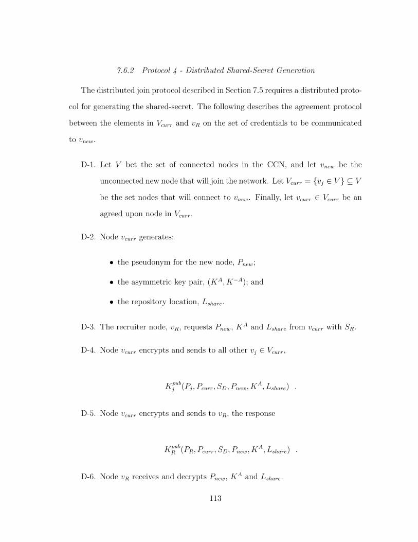
7.6.2 Protocol 4 - Distributed Shared-Secret Generation

The distributed join protocol described in Section 7.5 requires a distributed proto-

col for generating the shared-secret. The following describes the agreement protocol

between the elements in Vcurr and vR on the set of credentials to be communicated

to vnew.

D-1. Let V bet the set of connected nodes in the CCN, and let vnew be the

unconnected new node that will join the network. Let Vcurr = {vj ∈ V } ⊆ V

be the set nodes that will connect to vnew. Finally, let vcurr ∈ Vcurr be an

agreed upon node in Vcurr.

D-2. Node vcurr generates:

• the pseudonym for the new node, Pnew;

• the asymmetric key pair, (KA, K−A); and

• the repository location, Lshare.

D-3. The recruiter node, vR, requests Pnew, KA and Lshare from vcurr with SR.

D-4. Node vcurr encrypts and sends to all other vj ∈ Vcurr,

Kpubj (Pj, Pcurr, SD, Pnew, K

A, Lshare) .

D-5. Node vcurr encrypts and sends to vR, the response

KpubR (PR, Pcurr, SD, Pnew, K

A, Lshare) .

D-6. Node vR receives and decrypts Pnew, KA and Lshare.

113

D-7. Node vR encrypts and sends to all vj ∈ Vcurr,

Kpubj (Pj, PR, SD, Pnew, K

A, Lshare) .

D-8. Each node vj ∈ Vcurr receives, decrypts, and compares the results they

received from vcurr and vR. If the results match, they each respond SD.

Otherwise, to both vR and all other vj, they respond with an error flag, ER.

D-9. The recruiter passes Pnew, KA and Lshare out-of-band to the prospect.

At the end of this protocol, all members vj ∈ Vcurr possess the needed creden-

tials to independently check the repository for the arrival of vnew and the recruiter

possesses the credentials that he will pass to the new prospect via the out-of-band

channel. Once the new prospect has the credentials, then the distributed join pro-

tocol can be followed.

7.7 Attacks Against the Distributed Join Protocol

The distributed join protocol protects against the attacks described earlier by

forcing distributed checks and balances between nodes. The network does become

more vulnerable to many of these same attacks by the recruiter vR, but now the

problem is one of robust out-of-band vetting of the recruiter. Appropriate vetting is

then controlled by policy to address the needs of the CCN.

7.7.1 Dealing with Node Departure or Node Failure

Given the need to restrict network promiscuity and protect membership conceal-

ment, traditional approaches to network healing are not allowed. Thus, stopped or

failed nodes need to rejoin the network in the same location within the topology. For

low-latency requirements, sufficient nodes need to be active to maintain a connected

114

topology with low network distance between the communicating nodes. Thus, failed

nodes would need to quickly reset and rejoin the network. Of course, if the CCN is re-

stricted to high-latency communication, then it is delay-tolerant. In a delay-tolerant

CCN, nodes have much more flexibility in how long they can be dormant.

7.8 Conclusions

Joining a CCN is more complicated than joining a P2P network not concerned

with both membership concealment and resiliency. While no known protocol is

known that will eliminate the risk of all participants, the protocols examined attempt

to minimize the exposure of the participants to a powerful adversary. Through proper

vetting of prospective participants, distributed checks and balances between nodes,

and minimizing network promiscuity, groups can protect both themselves and their

communication.

115

8. ROUTING IN A COVERT COMMUNICATION NETWORK

Routing across a CCN relies on the use of pseudonyms as the logical address and

relies on the type of topology used. Topologies are considered either deterministic or

random. Deterministic topologies are those in which the connections between nodes

are deterministically determined, and similarly, random topologies are those in which

the connections between nodes are randomly determined. We examined deterministic

construction approaches in Sections 4 and 5. We examined random constructions in

Section 6. In this section, we examine approaches to routing in CCNs. First, we

provide an overview of some general algorithms that work regardless of the overlay

topology. Then, we describe approaches for routing in deterministic topologies with

specific algorithms for the Gunther-Hartnell and Extended Robertson construction

topologies.

8.1 General Approaches to Routing

CCN messages are routed across the network from the source node, vs, to the

destination node, vd, by relying on intermediate nodes to forward traffic through the

network. Thus, each node, vi, also acts as a router within the network. When node

vi receives a message, it examines the message destination pseudonym. If vi is the

intended destination, then the node keeps and processes the message. Otherwise,

node vi looks up the destination in the routing table in order to determine to which

neighbor to forward the packet. Then, it re-encrypts the data for the next hop,

replaces the network address (e.g., IP address) associated with the data with its own

network address, and forwards the data to the next neighbor along the route to the

destination.

Some overlay networks, most prominently Tor [16], use source routing, where

116

the route to the destination is determined in a separate topology step, and is then

included as part of the message. No local routing tables need to be maintained. This

form of source routing is naturally detrimental to membership concealment, as much

of the global topology information (the source routes) is now available at all nodes

in the network.

In the following, we will briefly summarize routing algorithms that are topologi-

cally agnostic, that is, they can successfully route in any CCN topology.

8.1.1 Shortest Path Routing

Shortest path routing is a basic approach to routing with several different algo-

rithms that are widely used. These algorithms are easily adapted for use within a

CCN. As the name suggests, the shortest path routing algorithm attempts to deter-

mine how to go from the source node to the destination node in the fewest hops, the

shortest geographic distance, or the fastest path as possible. Two popular shortest

path routing algorithms are the link-state routing algorithm and the distance-vector

routing algorithm. These routing algorithms are well studied and easily ported to a

CCN.

In the link-state algorithm, each node talks to all other nodes within the network

providing them with the latency costs from it to its connected neighbors. The node

passes a separate entry for each neighbor consisting of its logical address, the neigh-

bor’s logical address and the latency estimate between the two. Each node can then

use this information to build up and update its routing tables, determining the path

with the lowest latency path to each node based on the accumulated estimates that it

receives from all other nodes. Membership concealment is preserved because, though

each node uses network addresses to communicate with its neighbors in determining

latency, the network addresses are not shared. Instead, the logical addresses are used

117

to communicate the routing table updates.

In the distance-vector algorithm, each node talks only to its connected neighbors

providing least-cost estimates from itself to all other known nodes in the network.

Similar to the link-state algorithm, the distance-vector algorithm communicates the

destination of each latency estimate by its pseudonym. The distance-vector algorithm

has less computational complexity and message overhead since each node is sharing

latency estimates only with its neighbors. However, it suffers from the count-to-

infinity problem, which is the slow recognition of the network to realize when a

node becomes unavailable for routing. There are solutions to the count-to-infinity

problem, but it requires additional complexity in the routing algorithm. On the other

hand, the link-state algorithm does not have the count-to-infinity problem, but does

require significantly more traffic to maintain, creating a more detectable signature.

8.1.2 Routing by Selective Flooding

Selective flooding provides routing without the need for maintaining routing ta-

bles. A node would simply forward a packet to all neighboring nodes, except the

one from which it received the message. This approach, however, would require a

mechanism to prevent messages from being forwarded forever. A time-to-live field

could be added to the packet. The value in this field would be decremented at each

intermediate node until it reached zero, at which point the packet would no longer

be forwarded. Another option is to buffer forwarded packets for some period of time

such that those with duplicate payloads are not forwarded. However, flooding also

raises the signature of the network and may allow it to stand out more easily against

the other network traffic, thus making it more easily detected. Furthermore, since

packets are re-encrypted for each hop, flooding is very computationally expensive.

Selective flooding could also be used in a more limited way to update routing

118

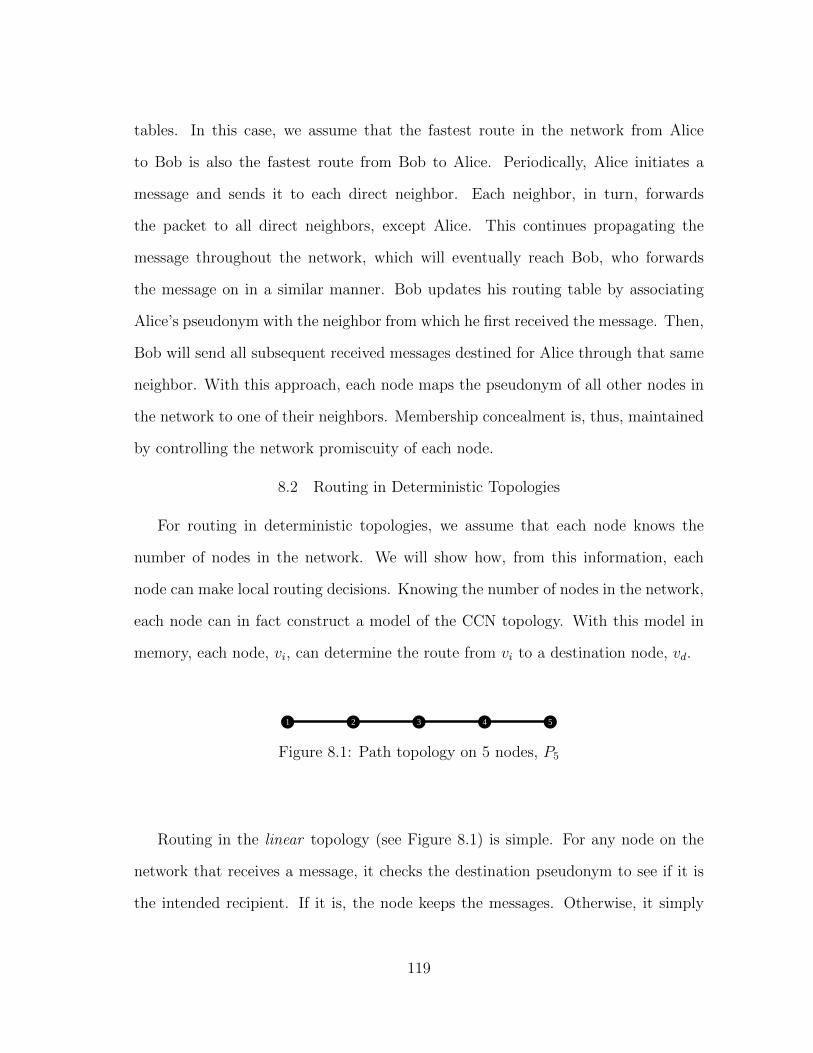
tables. In this case, we assume that the fastest route in the network from Alice

to Bob is also the fastest route from Bob to Alice. Periodically, Alice initiates a

message and sends it to each direct neighbor. Each neighbor, in turn, forwards

the packet to all direct neighbors, except Alice. This continues propagating the

message throughout the network, which will eventually reach Bob, who forwards

the message on in a similar manner. Bob updates his routing table by associating

Alice’s pseudonym with the neighbor from which he first received the message. Then,

Bob will send all subsequent received messages destined for Alice through that same

neighbor. With this approach, each node maps the pseudonym of all other nodes in

the network to one of their neighbors. Membership concealment is, thus, maintained

by controlling the network promiscuity of each node.

8.2 Routing in Deterministic Topologies

For routing in deterministic topologies, we assume that each node knows the

number of nodes in the network. We will show how, from this information, each

node can make local routing decisions. Knowing the number of nodes in the network,

each node can in fact construct a model of the CCN topology. With this model in

memory, each node, vi, can determine the route from vi to a destination node, vd.

1 2 3 4 5

Figure 8.1: Path topology on 5 nodes, P5

Routing in the linear topology (see Figure 8.1) is simple. For any node on the

network that receives a message, it checks the destination pseudonym to see if it is

the intended recipient. If it is, the node keeps the messages. Otherwise, it simply

119

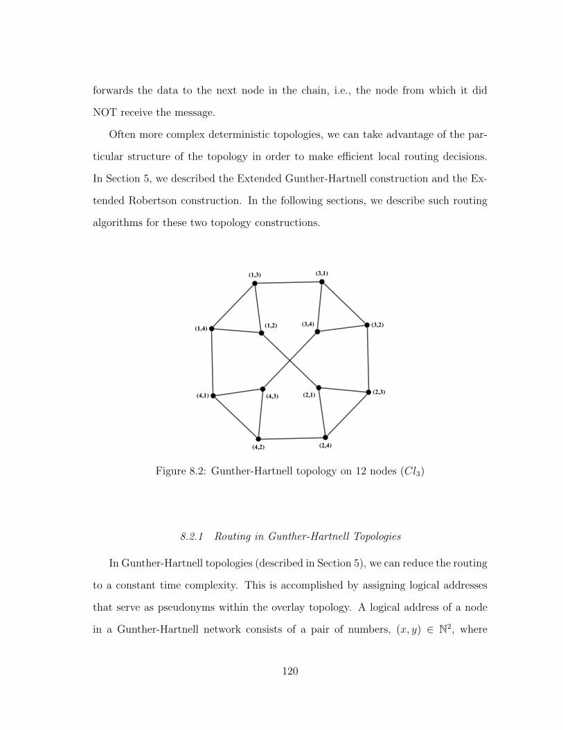
forwards the data to the next node in the chain, i.e., the node from which it did

NOT receive the message.

Often more complex deterministic topologies, we can take advantage of the par-

ticular structure of the topology in order to make efficient local routing decisions.

In Section 5, we described the Extended Gunther-Hartnell construction and the Ex-

tended Robertson construction. In the following sections, we describe such routing

algorithms for these two topology constructions.

H1,2LH1,4L

H1,3L

H2,1L

H2,4L

H2,3LH4,1L

H4,2L

H4,3L

H3,1L

H3,2LH3,4L

Figure 8.2: Gunther-Hartnell topology on 12 nodes (Cl3)

8.2.1 Routing in Gunther-Hartnell Topologies

In Gunther-Hartnell topologies (described in Section 5), we can reduce the routing

to a constant time complexity. This is accomplished by assigning logical addresses

that serve as pseudonyms within the overlay topology. A logical address of a node

in a Gunther-Hartnell network consists of a pair of numbers, (x, y) ∈ N2, where

120

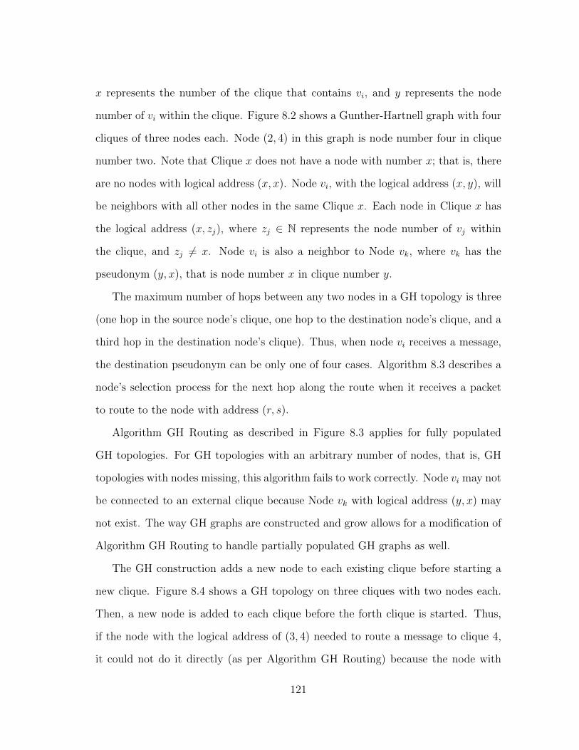
x represents the number of the clique that contains vi, and y represents the node

number of vi within the clique. Figure 8.2 shows a Gunther-Hartnell graph with four

cliques of three nodes each. Node (2, 4) in this graph is node number four in clique

number two. Note that Clique x does not have a node with number x; that is, there

are no nodes with logical address (x, x). Node vi, with the logical address (x, y), will

be neighbors with all other nodes in the same Clique x. Each node in Clique x has

the logical address (x, zj), where zj ∈ N represents the node number of vj within

the clique, and zj 6= x. Node vi is also a neighbor to Node vk, where vk has the

pseudonym (y, x), that is node number x in clique number y.

The maximum number of hops between any two nodes in a GH topology is three

(one hop in the source node’s clique, one hop to the destination node’s clique, and a

third hop in the destination node’s clique). Thus, when node vi receives a message,

the destination pseudonym can be only one of four cases. Algorithm 8.3 describes a

node’s selection process for the next hop along the route when it receives a packet

to route to the node with address (r, s).

Algorithm GH Routing as described in Figure 8.3 applies for fully populated

GH topologies. For GH topologies with an arbitrary number of nodes, that is, GH

topologies with nodes missing, this algorithm fails to work correctly. Node vi may not

be connected to an external clique because Node vk with logical address (y, x) may

not exist. The way GH graphs are constructed and grow allows for a modification of

Algorithm GH Routing to handle partially populated GH graphs as well.

The GH construction adds a new node to each existing clique before starting a

new clique. Figure 8.4 shows a GH topology on three cliques with two nodes each.

Then, a new node is added to each clique before the forth clique is started. Thus,

if the node with the logical address of (3, 4) needed to route a message to clique 4,

it could not do it directly (as per Algorithm GH Routing) because the node with

121

Algorithm GH Routing :

Input: Current node with address (x, y) and destination node with address (r, s).

Output: Next hop along the shortest route or null to indicate termination.

Step 1: If x 6= r and x 6= s, then destination is in an unrelated clique; return

(x, r).

Step 2: If r = y, then destination is in the neighboring clique; return (y, x).

Step 3: If r = x and s 6= y, then the destination is a neighbor; return (x, s).

Step 4: If (x, y) = (r, s) then the destination is reached; return null.

Figure 8.3: Routing in a Gunther-Hartnell topology.

address (4, 3) does not exist. Instead, the message needs to be routed to either Clique

1 or Clique 2, since these are the only cliques that can reach Clique 4 from Clique

3. This can be predicted locally by the node at (3, 4) and an alternate route can be

chosen. This adds, at most, two more hops to the route.

8.2.2 Routing in Extended Robertson Construction Topologies

In Section 5 we described the Extended Robertson construction. Topologies were

generated with this construction by forming cycles of order p ∈ N, where p is prime.

The cycles are then connected to each other according to the generated offset matrix,

which specifies which p-gram should connect to which p-gon and the associated offset

between the cycles. A logical address to each node in this topology consists of the

triplet (x, y, z), where x ∈ N denotes the cycle pair, y ∈ {0, 1} denotes whether the

cycle is a p-gram or a p-gon, and 1 ≥ z ≥ p denotes the node number within the

122

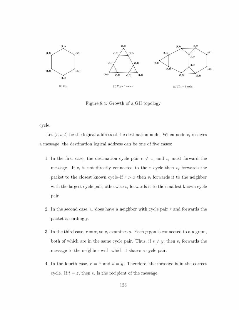
H1,3L

H1,2L

H2,1L

H2,3L

H3,2L

H3,1L

HaL Cl2.

H1,2LH1,3L

H1,4L

H2,1L

H2,3L H2,4L

H3,1L

H3,2LH3,4L

HbL Cl2 + 3 nodes.

H1,2L

H1,3L H1,4L

H2,1L

H2,3L H2,4L

H3,1L

H3,2LH3,4L

H4,1L

H4,2L

HcL CL3 - 1 node.

Figure 8.4: Growth of a GH topology

cycle.

Let (r, s, t) be the logical address of the destination node. When node vi receives

a message, the destination logical address can be one of five cases:

1. In the first case, the destination cycle pair r 6= x, and vi must forward the

message. If vi is not directly connected to the r cycle then vi forwards the

packet to the closest known cycle–if r > x then vi forwards it to the neighbor

with the largest cycle pair, otherwise vi forwards it to the smallest known cycle

pair.

2. In the second case, vi does have a neighbor with cycle pair r and forwards the

packet accordingly.

3. In the third case, r = x, so vi examines s. Each p-gon is connected to a p-gram,

both of which are in the same cycle pair. Thus, if s 6= y, then vi forwards the

message to the neighbor with which it shares a cycle pair.

4. In the fourth case, r = x and s = y. Therefore, the message is in the correct

cycle. If t = z, then vi is the recipient of the message.

123

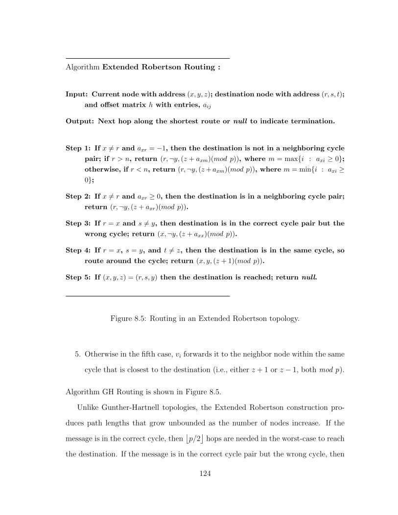
Algorithm Extended Robertson Routing :

Input: Current node with address (x, y, z); destination node with address (r, s, t);

and offset matrix h with entries, aij

Output: Next hop along the shortest route or null to indicate termination.

Step 1: If x 6= r and axr = −1, then the destination is not in a neighboring cycle

pair; if r > n, return (r,¬y, (z + axm)(mod p)), where m = max{i : axi ≥ 0};otherwise, if r < n, return (r,¬y, (z+ axm)(mod p)), where m = min{i : axi ≥0};

Step 2: If x 6= r and axr ≥ 0, then the destination is in a neighboring cycle pair;

return (r,¬y, (z + axr)(mod p)).

Step 3: If r = x and s 6= y, then destination is in the correct cycle pair but the

wrong cycle; return (x,¬y, (z + axx)(mod p)).

Step 4: If r = x, s = y, and t 6= z, then the destination is in the same cycle, so

route around the cycle; return (x, y, (z + 1)(mod p)).

Step 5: If (x, y, z) = (r, s, y) then the destination is reached; return null.

Figure 8.5: Routing in an Extended Robertson topology.

5. Otherwise in the fifth case, vi forwards it to the neighbor node within the same

cycle that is closest to the destination (i.e., either z + 1 or z− 1, both mod p).

Algorithm GH Routing is shown in Figure 8.5.

Unlike Gunther-Hartnell topologies, the Extended Robertson construction pro-

duces path lengths that grow unbounded as the number of nodes increase. If the

message is in the correct cycle, then⌊p/2⌋

hops are needed in the worst-case to reach

the destination. If the message is in the correct cycle pair but the wrong cycle, then

124

1 hop will get it to the correct cycle. If the message is not in the correct cycle pair,

then the number of hops is dependent on the number of nodes in the network as⌈(n− 50)/40

⌉+ 1.

Thus, in an Extended Robertson construction topology with n nodes and cycle

size p, in the worst-case, the number of hops required for routing will be:

⌈n− 50

40

⌉+

⌊p

2

⌋+ 2 . (8.1)

This gives a linear time complexity for routing in an Extended Robertson construc-

tion topology.

It will often be the case where the last cycle pair within the construction is

incomplete. In these cases, the routing algorithm in Figure 8.5 may fail if the last

hop along the expected path does not exist. However, assuming that each node

knows the actual size of the network, the benefit of deterministic topologies such

as the Extended Robertson construction is that each node can locally construct a

model of the network topology; then, with a little more complexity in steps 2, 3 and

4 in the routing algorithm, anticipate routing failures and adjust the routing path

along existing nodes.

8.3 Deadlocks and Circular Routing

One common difficulty in efficient routing in deterministic networks is the need to

avoid deadlocks and circular routing. Deadlocks can occur in the Gunther-Hartnell

and Extended Robertson construction routing algorithms when the neighbor re-

turned by the algorithm has failed. As presented, the algorithms assume that all

nodes within the network are operational. In order to circumvent this problem, ad-

ditional algorithmic complexity is needed to identify failed neighbors and advertise

to other nodes that the failed neighbor is unreachable.

125

Circular routing would only occur in the case where a new node has joined the

network but not all nodes have been notified yet so that they update their internal

model. Thus, if Node vi with the updated view of the network routes to Node vj, but

Node vj has not been updated and expects to route through Node vi then, unless

either node recognizes that returned packets, the two nodes will pass the packet

back and forth until Node vj is updated. However, the problem would occur on the

border between the neighboring updated node and the non-updated node. Thus, the

update would be passed to vj and then the packet returned. The update would then

proceed the packet and fan out into the network. The misrouted packet would then

be routed according to the new network configuration from its current location to

the destination.

8.4 Conclusions

Deterministic topologies with relatively high subversion impedance, such as the

Gunther-Hartnell and Extended Robertson constructions, offer an internal structure

that facilitates efficient routing. We have shown that for the Gunther-Hartnell and

Extended Robertson constructions routing schemes with local routing decisions exist.

Even when topologies are not complete, that is, some nodes are missing, these routing

schemes remain effective (after some minor modifications) provided that: (a) all

nodes know the number of nodes in the system, and (b) the way the network grows

when nodes are added follows a given pattern, which we described.

Other deterministic topologies with very efficient routing algorithms, for example

hypercubes and bit-flipping-based routing, can be amenable to routing for incomplete

topologies [33]. While the Gunther-Hartnell and Extended Robertson constructions

routing algorithms can handle incompletely populated topologies, they assume that

all joined nodes in the network are functional. When arbitrary nodes fail, the rout-

126

ing can not adapt. To handle arbitrary node failures, one would need to borrow

techniques from common network routing protocols, which can be easily ported to

CCNs and offer more flexible routing at the expense of a higher network signature,

either through redundancy of message traffic or traffic needed to maintain routing

tables. In either case, routing can be done in a way that preserves the anonymity,

membership concealment and resiliency of CCNs.

127

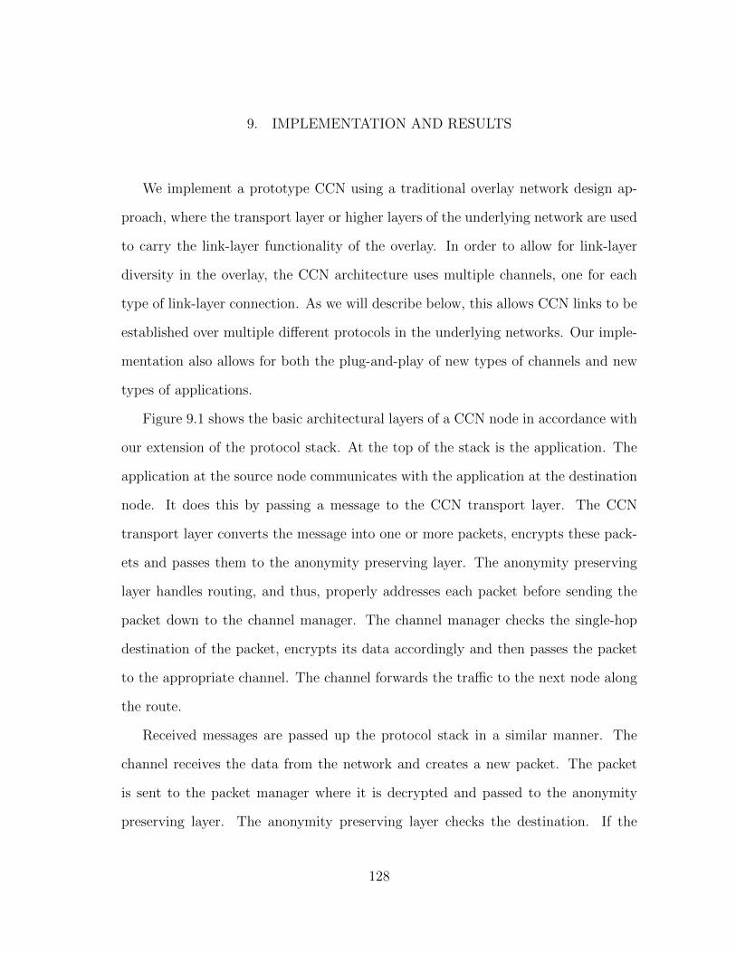
9. IMPLEMENTATION AND RESULTS

We implement a prototype CCN using a traditional overlay network design ap-

proach, where the transport layer or higher layers of the underlying network are used

to carry the link-layer functionality of the overlay. In order to allow for link-layer

diversity in the overlay, the CCN architecture uses multiple channels, one for each

type of link-layer connection. As we will describe below, this allows CCN links to be

established over multiple different protocols in the underlying networks. Our imple-

mentation also allows for both the plug-and-play of new types of channels and new

types of applications.

Figure 9.1 shows the basic architectural layers of a CCN node in accordance with

our extension of the protocol stack. At the top of the stack is the application. The

application at the source node communicates with the application at the destination

node. It does this by passing a message to the CCN transport layer. The CCN

transport layer converts the message into one or more packets, encrypts these pack-

ets and passes them to the anonymity preserving layer. The anonymity preserving

layer handles routing, and thus, properly addresses each packet before sending the

packet down to the channel manager. The channel manager checks the single-hop

destination of the packet, encrypts its data accordingly and then passes the packet

to the appropriate channel. The channel forwards the traffic to the next node along

the route.

Received messages are passed up the protocol stack in a similar manner. The

channel receives the data from the network and creates a new packet. The packet

is sent to the packet manager where it is decrypted and passed to the anonymity

preserving layer. The anonymity preserving layer checks the destination. If the

128

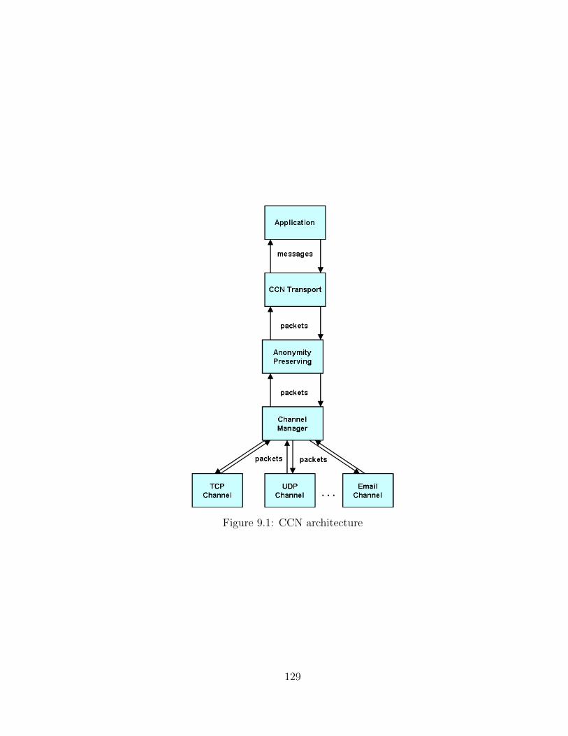
Figure 9.1: CCN architecture

129

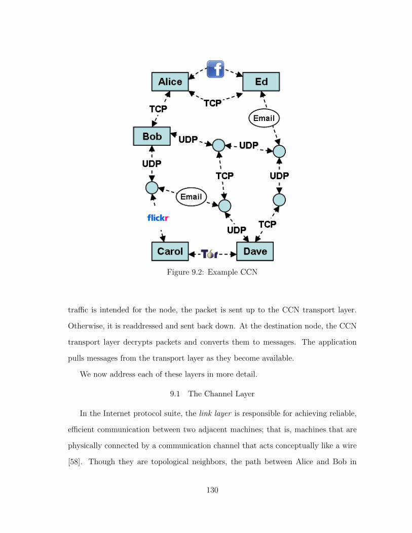
Figure 9.2: Example CCN

traffic is intended for the node, the packet is sent up to the CCN transport layer.

Otherwise, it is readdressed and sent back down. At the destination node, the CCN

transport layer decrypts packets and converts them to messages. The application

pulls messages from the transport layer as they become available.

We now address each of these layers in more detail.

9.1 The Channel Layer

In the Internet protocol suite, the link layer is responsible for achieving reliable,

efficient communication between two adjacent machines; that is, machines that are

physically connected by a communication channel that acts conceptually like a wire

[58]. Though they are topological neighbors, the path between Alice and Bob in

130

Figure 9.2 consists of multiple hops between devices, including switches, routers,

firewalls, etc. As the link layer is responsible for communications at each of these

hops, within a CCN, the channel layer provides communication between topolog-

ical neighbors and provides the services within the overlay network that the link

layer provides to the underlying network. The channel layer consists of one or more

channels that pass data between adjacent nodes.

The channel layer provides single-hop communication within the overlay network.

Each channel will have different performance characteristics in support of the com-

munications requirements of the group. In our implementation, one channel utilizes

user datagram protocol (UDP) to provide low latency support for near-real-time

communication at the expense of an increased risk of detectability, and transmission

control protocol (TCP) to provide additional protection against dropped packets at

the expense of increased latency. A third channel implements the functionality of

a mix [9] providing high level resilience against attacks that attempt to undermine

anonymity. Additional channels can be easily developed based on the particular

requirements of the group.

Thus, Alice can send data to Bob in a variety of ways. The type of channel used

is dependent on the type of service needed at the higher levels. Each type of channel

offers trade-offs between performance and anonymity. Low latency communication

provides near-real-time communication for group members at the risk of providing

an adversary with timing signatures for tracing packets across the overlay network,

thus undermining anonymity. If near-real-time communication is not required, then

nodes can both batch messages and introduce variations in timing to obscure com-

munication signatures and increase anonymity. We assume that the channels used

by the network are agreed upon by the participants and instantiated at each node.

131

9.1.1 TCP Channel

The most straightforward channels to implement are based on UDP and TCP.

These common types of connections address the relevant reliability issues that need

to be dealt with at the channel layer. In a standard network, we think of the media

access control (MAC) address as the link layer address. However, in the overlay

topology of a CCN, an IP address would act as a CCN channel layer address. In

both the UDP and TCP channels, the channel maintains a table of the IP address and

ports of trusted neighbors. Data received from an unknown IP address is discarded.

TCP provides a reliable transmission of data between adjacent nodes. TCP

supports acknowledged connection-oriented service between adjacent nodes. In a

CCN, a TCP Channel instantiates two sockets to each of its neighbors: one socket

is for sending data; and another socket is for receiving data. We implement TCP

as an asynchronous socket server on each node. This allows the node to handle

connections from multiple neighbors simultaneously. When data needs to be sent on

the TCP channel to a particular neighbor, the channel checks to see if a socket exists

for sending. If not, it connects to the TCP server of the neighbor and a thread is

spawned on each node to manage the communications on this socket. Thus, a single

socket can be used repeatedly for communication between nodes, thus, minimizing

the overhead of the three-way handshake needed to set-up a TCP connection. Since

a node only communicates at the channel level with its topological neighbors, only

a relatively small number of sockets need to be maintained.

The TCP channel will ensure that a packet payload arrives across a single hop in

order and without data loss. However, it makes no guarantees that the end-to-end

traffic will arrive in order and without data loss. End-to-end packet ordering and

data loss is handled by the CCN transport layer.

132

9.1.2 UDP Channel

UDP provides only a basic communication service between nodes. The delivery

guarantees provided by TCP are not provided by UDP. Under UDP, datagrams are

sent from one node to another with no expectation for an acknowledgment and

no timeout. However, UDP is important in situations when low latency is more

importance than data loss.

UDP offers unacknowledged connectionless service between adjacent nodes in a

straightforward manner. It can be modified easily for acknowledged connectionless

service. Though it may affect performance, acknowledgment can always be handled

at higher layers between the source node and destination node.

9.1.3 Remailer Channel

Traditional mix networks provide anonymity by sending messages through a series

of email servers, each of which replace the source header information with its own

to delink the source from the destination; wait some random period of time before

resending to prevent timing correlation attacks; and batch multiple messages together

to prevent message identification by message size [9, 14, 25]. This is easily integrated

into our system at the channel layer.

To facilitate this channel, each node registers a disposable email address (e.g.,

gmail) to which their neighbors could send or forward email. Similar to most email

clients, the channel checks this email account periodically and processes any received

email. The channel maintains a table of trusted neighbors identified by their IP

address and email address. Emails from non-neighbors are discarded. A received

email is debatched, if necessary, into separate payloads and a packet is generated for

separate payload.

Packets to be sent are stored in a buffer for a short period of time. This disrupts

133

the timing of the traffic and allows the node to collect email from multiple neighbors.

Periodically, packets destined to the same neighbor are batched appropriately and

sent as an email to the email address of the appropriate neighbor.

9.2 Channel Manager Layer

The channel manager is responsible for instantiating and monitoring all channels

used by the node and for hop-level encryption and decryption. Thus, the channel

manager will start and gracefully shutdown each channel, as necessary; decrypt data

it receives from any channel; encrypt data being sent to a neighbor; and pass data

between the anonymity preserving layer and the appropriate channel.

The channel manager has an asymmetric key pair which it uses for decryption of

the data it receives from a channel. It also maintains a table of public keys for all

trusted neighbors. When data is to be sent or forwarded to a neighbor, the channel

manager uses the appropriate key. For some communication, the channel manager

can negotiate symmetric keys for follow-on communications, i.e., TLS. Each sym-

metric key is used to encrypt and decrypt traffic with a single neighbor. Periodically,

the node or its neighbor will negotiate a new symmetric key.

Once received data is decrypted, its packet is passed to the anonymity preserving

layer. Likewise, once data to be sent is encrypted, the packet is passed to the

appropriate channel.

9.3 The Membership Concealing Layer

The membership concealing layer is responsible for determining how packets are

routed from source to destination. This layer is analogous to the network layer in

the Internet protocol suite. In a CCN, the anonymity preserving layer is responsible

for maintaining a routing table that associates node pseudonyms with a neighbor

network address. This layer also provides a level of security.

134

For example, in Figure 9.2, if Alice wants to communicate with Dave, her mes-

sage must route through both Bob and Carol. The anonymity preserving layer is

responsible for determining to which neighbor the packet needs to be sent in order

for it to reach its destination.

9.3.1 Anonymity Preserving Routing

The anonymity preserving layer of a node examines the destination logical address

of an arriving message. If the given node is the destination, then the packet is passed

to the transport layer. If not, then the node determines to which neighbor to route

the packet. Then, it passes the updated packet to the channel manager layer for

encryption and transmission.

9.3.2 Single-hop Security

The anonymity preserving layer is the appropriate layer for implementing security

protocols that validate singe-hop traffic. For example, a simple approach might be

to check the single-hop time-stamp of the data packet and reject it if the time stamp

is outside some reasonable window of expected transmission latency. This approach

would protect against replay attacks by an adversary.

Also, if routing by selective flooding is used, though the end-to-end data cannot

be read, this layer can compare the data it receives from one neighbor against the

data it receives from its other neighbors to detect attempts made by an adversary

at watermarking. Each node would receive the same packet multiple times from

different, independent routes. Any discrepancy between the packet copies could

indicate an attempt by an adversary to tamper with message traffic. More complex

approaches could be based on this approach allowing neighbors to act cooperatively

to detect subversions.

135

9.4 The Transport Layer

The transport layer is responsible for packet creation, packet buffering, packet

ordering and end-to-end cryptography. The transport layer receives a message from

the application layer and breaks it down into one or more packets based on the desired

packet size relative to the message size. These packets are ordered by sequence

numbers and sent to the destination transport layer.

The destination transport layer buffer stores packets that are passed from the

anonymity preserving layer until the application layer is ready for them. Because

many channels are asynchronous or unreliable, packets may arrive out of sequence.

Sequence numbers are used to preserve ordering. Packets are inserted into the buffer

based on their sequence number. The starting sequence number and ending sequence

number provide a means of synchronizing the end-to-end session and requesting lost

portions of data. Coupled with the source field and application identifier, it also

allows for separate buffering for different applications and different sessions. If all

packets are received, the set of packets is converted into a single message and buffered

until retrieved by the application.

The same cryptographic functionality provided at the channel manager layer for

single-hop communication is provided for end-to-end communication at the transport

layer. Asymmetric encryption is used for high latency communication and negotia-

tion of symmetric keys for low latency communication.

The transport layer can also take steps to assess the validity of received traffic.

The additional packet information provided by the source node can be used to detect

subversions that were missed at the routing layer.

136

9.5 The Application Layer

The application layer contains a variety of protocols that are commonly needed,

such as file transfer and various other general and special-purpose facilities. The

plug-and-play design of the architecture allows for the development of additional

applications, as needed.

9.5.1 File Sharing

The heart of most all applications within a CCN is file sharing. The application

divides up the file into a set of messages and each message is passed to the CCN

transport layer. Files could be any other type of data, including text, voice, or image

based. The anonymity, latency and delivery guarantees required by file-sharing are

dependent on the needs of the user.

9.5.2 VoIP and VTC

VoIP and VTC require low latency between the source and destination nodes.

The CCN topology, of course, adds latency because it extends the hop distance from

the source to the destination by routing the traffic through a series of intermediate

nodes. This restricts the channel layer services to those that minimize latency. These

types of services increase the risk of undermining sender-receiver unlinkability.

VTC is especially data heavy and, thus, creates a significant signature. Though

routing by flooding would propagate traffic from the source to the destination along

the fastest route, it would require significant bandwidth and could create serious

congestion issues. More importantly, the signature created by flooding video traffic

could be very distinguishable from the background Internet traffic and significantly

undermine membership concealment.

137

9.5.3 Electronic Mail

In our implementation, we have a channel that pulls and forwards packet data

from email accounts associated with legitimate neighbors. This type of channel is

high latency, but allows for the batching of multiple data packets. These two features

provide high resilience against attacks attempting to undermine the anonymity of

the network. A simple CCN email application would serve as a client that would

pass message traffic to and from the email channel.

9.5.4 Web Browsing

Risk to membership concealment increases if a node allows traffic to ”exit” the

network (e.g., a Tor exit node). Exit nodes are susceptible to identification by honey

pot web sites run by adversaries. Use of a CCN to access public web sites incur an

increased level of risk and must be used cautiously.

However, assume that a CCN node is running an application that passes traffic

to and from a web proxy. Then, network participants using an Internet browser

connecting to an application on their own node could surf anonymously in a way

that localizes the risk of compromise to a single node.

Another approach is if one or more nodes in the network run web servers that

are accessible by other network members. The web server would only accept traffic

from adjacent nodes. These adjacent nodes only accept traffic from their neighbors,

and so forth. Thus, traffic to the web server is restricted to members of the network.

9.6 A Test Application

In order to test our architecture, we developed an application that would com-

municate with an Internet browser and another that would communicate with a web

proxy. Figure 9.3 shows the structure of the network. In this set-up, the participant,

138

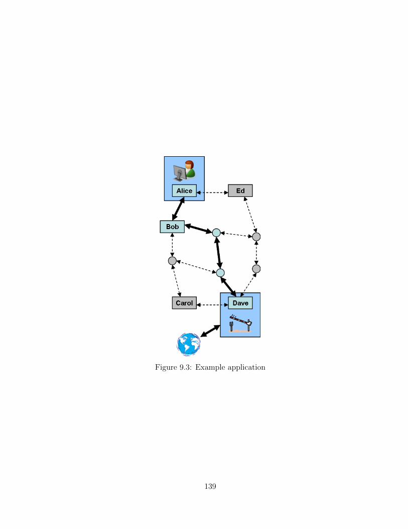
Figure 9.3: Example application

139

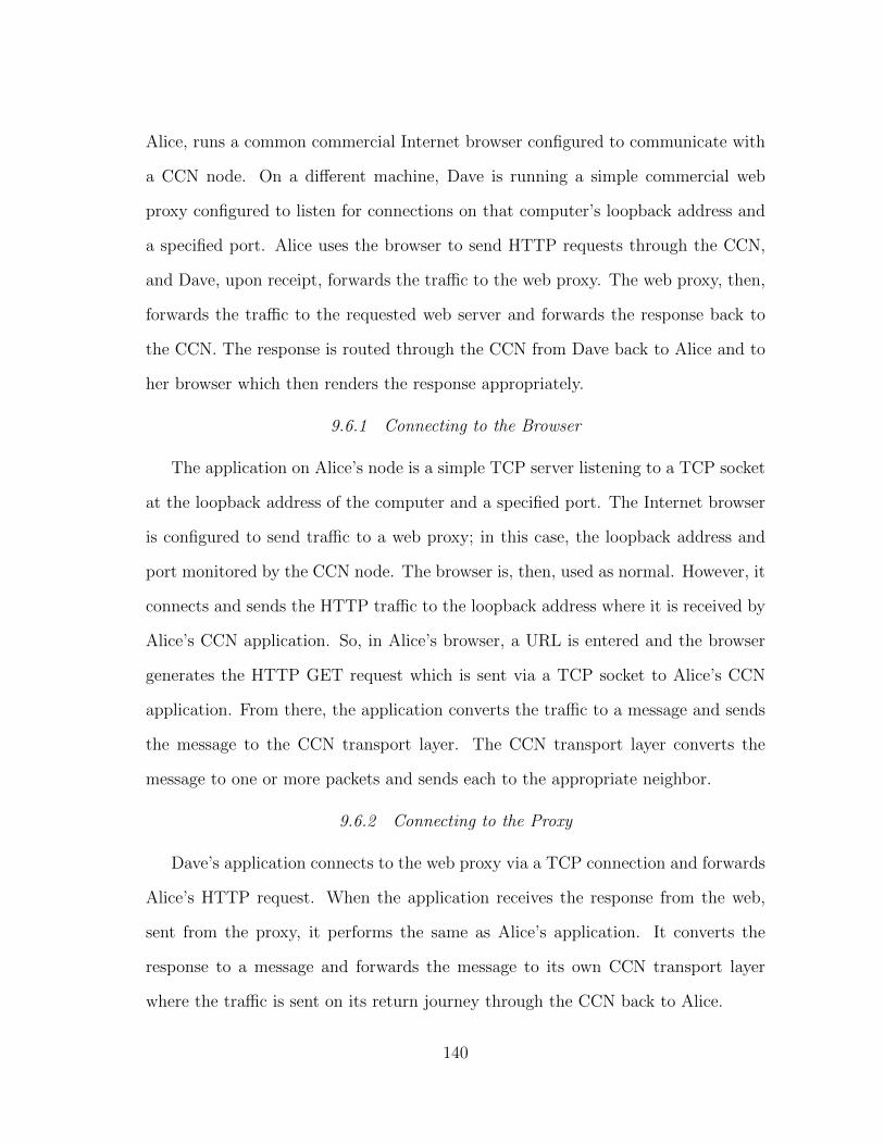
Alice, runs a common commercial Internet browser configured to communicate with

a CCN node. On a different machine, Dave is running a simple commercial web

proxy configured to listen for connections on that computer’s loopback address and

a specified port. Alice uses the browser to send HTTP requests through the CCN,

and Dave, upon receipt, forwards the traffic to the web proxy. The web proxy, then,

forwards the traffic to the requested web server and forwards the response back to

the CCN. The response is routed through the CCN from Dave back to Alice and to

her browser which then renders the response appropriately.

9.6.1 Connecting to the Browser

The application on Alice’s node is a simple TCP server listening to a TCP socket

at the loopback address of the computer and a specified port. The Internet browser

is configured to send traffic to a web proxy; in this case, the loopback address and

port monitored by the CCN node. The browser is, then, used as normal. However, it

connects and sends the HTTP traffic to the loopback address where it is received by

Alice’s CCN application. So, in Alice’s browser, a URL is entered and the browser

generates the HTTP GET request which is sent via a TCP socket to Alice’s CCN

application. From there, the application converts the traffic to a message and sends

the message to the CCN transport layer. The CCN transport layer converts the

message to one or more packets and sends each to the appropriate neighbor.

9.6.2 Connecting to the Proxy

Dave’s application connects to the web proxy via a TCP connection and forwards

Alice’s HTTP request. When the application receives the response from the web,

sent from the proxy, it performs the same as Alice’s application. It converts the

response to a message and forwards the message to its own CCN transport layer

where the traffic is sent on its return journey through the CCN back to Alice.

140

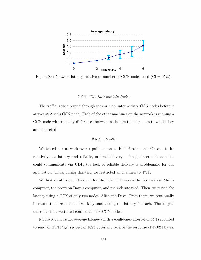
Average Latency

0.0

0.5

1.0

1.5

2.0

2.5

0 2 4 6CCN Nodes

Seconds

Figure 9.4: Network latency relative to number of CCN nodes used (CI = 95%).

9.6.3 The Intermediate Nodes

The traffic is then routed through zero or more intermediate CCN nodes before it

arrives at Alice’s CCN node. Each of the other machines on the network is running a

CCN node with the only differences between nodes are the neighbors to which they

are connected.

9.6.4 Results

We tested our network over a public subnet. HTTP relies on TCP due to its

relatively low latency and reliable, ordered delivery. Though intermediate nodes

could communicate via UDP, the lack of reliable delivery is problematic for our

application. Thus, during this test, we restricted all channels to TCP.

We first established a baseline for the latency between the browser on Alice’s

computer, the proxy on Dave’s computer, and the web site used. Then, we tested the

latency using a CCN of only two nodes, Alice and Dave. From there, we continually

increased the size of the network by one, testing the latency for each. The longest

the route that we tested consisted of six CCN nodes.

Figure 9.4 shows the average latency (with a confidence interval of 95%) required

to send an HTTP get request of 1023 bytes and receive the response of 47,024 bytes.

141

The baseline gives an average time of 0.06 seconds. Routing the traffic through a

CCN with two nodes increases the average latency to 0.30 seconds. The longest

route we tested involved six CCN nodes. The average latency in this case was 1.57

seconds.

We would see the highest latency during the first trial of each test. On a CCN of

two nodes, the latency on the first trial was 0.60 seconds higher than average, and on

a CCN of six nodes, the latency was 1.10 seconds higher than average. During the

first trial, each node is establishing TCP connections via the three-way handshake

with neighbors along the route. Once these connections were established, they are

maintained for the second and subsequent trials, resulting in a much lower latency.

9.7 Conclusions

In the previous sections, we described the architecture for our prototype imple-

mentation of a covert communication network. By definition, trust entails a com-

ponent of risk. In some circumstances, use of a covert communication network is

a life-and-death decision. Thus, the network should not induce more risk than ab-

solutely necessary. Covert communications networks attempt to minimize this risk

while providing participants with a resilient communications network. This type of

network is promising for high risk situations.

As previously isolated groups become connected via the Internet and gain access

to information and ideas deemed subversive by their authorities, CCNs will become

an important tool in the fight against censorship. Even more liberal societies are

seeing government attempts at information control. Ultimately, CCNs can help

bring freedom of speech to those who have never had it and guard it for those that

are seeing it threatened.

142

10. CONCLUSIONS

In this dissertation, we have presented the motivation and requirements for covert

communication networks. As we defined in Section 1, we identify the need for the

ability to communicate in a way that ensures (a) confidentiality and anonymity of

the communication; (b) concealment of participation in the network to both other

members of the group and external eavesdroppers; and (c) resilience against discon-

nection. As a possible solution we propose covert communication networks, which

are architected as overlay, peer-to-peer (P2P) networks over existing communication

infrastructures. We rely on standard methods of cryptography to provide confiden-

tiality, draw on techniques from mix-style networks for anonymity, and extend the

application of membership-concealing overlay networks in order to protect the iden-

tity of network participants while providing resiliency against network partitioning.

We described the requirements of a CCN and the trade-offs between high-latency

and low-latency communication within such a network. We discussed the mechanisms

for confidential and anonymous communication and examined the trade-offs between

node survivability and network connectivity and described various single-hop channel

implementations.

In order to measure topologies for suitability of use in covert communication

networks, we defined several measures based on what we call subversion impedance.

Subversion impedance quantifies the balance in a topology between membership con-

cealment and resilience. By determining the subversion impedance in the worst case

and the average case, we can assess the risk to participants associated with a partic-

ular network overlay topology. Using these measures, we identified two constructions

(the Extended Robertson construction and the Extended Gunther-Hartnell construc-

143

tion) that allow the network to grow as new nodes join and which generate topologies

with near-optimal subversion impedance regardless of the number of nodes.

We also defined measures of subversion impedance for assessing families of ran-

dom graph topologies and used these measures to analyze Erdos-Renyi (ER) and

Barabasi-Albert (BA) random graphs. We learned that, for the range of graphs

examined, ER graphs have higher expected local subversion impedance than BA

graphs. Furthermore, the expected global subversion impedance of BA graphs is

very low with the connectivity rarely surviving the removal of the worst-case neigh-

borhood. Additionally in Gn,p graphs, we found a good closed-form estimate for

both the expected connectivity using order statistics and the expected local subver-

sion impedance.

Given the need to preserve membership concealment, membership management

is especially difficult in a covert communication network. As such, we developed

algorithms for joining a covert communication network. These algorithms protect

against unnecessary exposure of network addresses while allowing new nodes to in-

crease their connectivity for resilience. We discussed approaches for dealing with

node departure and described approaches to healing damage to the topology to re-

tain high subversion impedance.

We discussed general approaches to routing that are easily ported for use in covert

communication networks and developed efficient routing protocols in support of the

Extended Robertson construction and the Extended Gunther-Hartnell construction.

Incorporating the ideas above, we designed, built, and tested a prototype system

for instantiating a CCN. We described the system architecture and design choice

reasoning. This system supports high- and low-latency channels, single-hop and end-

to-end routing. It also encapsulates topology management and associated protocols

and provides a proof-of-concept interface for use with both off-the-shelf and custom

144

applications.

As network communication becomes more and more ubiquitous, applications need

to keep pace that will protect both the communication and the communicators. It

is our hope that the work described here is a meaningful contribution to the field

of network privacy and is of benefit to those on the front lines in the fight against

oppression and tyranny.

145

REFERENCES

[1] R. Albert, H. Jeong, and A.-L. Barabasi. Error and Attack Tolerance of Com-

plex Networks. Nature, 406:378–382, July 2000.

[2] Barry C. Arnold, N. Balakrishnan, and H. N. Nagaraja. A First Course in

Order Statistics. Classics in Applied Mathematics. SIAM, 2008.

[3] Albert-Laszlo Barabasi and Reka Albert. Emergence of Scaling in Random

Networks. Science, 286:509–512, October 1999.

[4] Albert-Laszlo Barabasi, Reka Albert, and Hawoong Jeong. Mean Field The-

ory for Scale-free Random Networks. Physica A Statistical Mechanics and Its

Applications, 272:173–187, October 1999.

[5] Bela Bollobas. Random Graphs. Cambridge Studies in Advanced Mathematics.

Cambridge University Press, 2001.

[6] John Adrian Bondy. Graph Theory with Applications. Elsevier Science Ltd,

1976.

[7] Serdar Cabuk, Carla E. Brodley, and Clay Shields. IP Covert Channel De-

tection. ACM Transactions on Information and System Security (TISSEC),

12(4):22:1–22:29, April 2009.

[8] V. Cerf, S. Burleigh, A. Hooke, L. Torgerson, R. Durst, K. Scott, K. Fall, and

H. Weiss. RFC 4838, Delay-Tolerant Networking Architecture. Available at

http://tools.ietf.org/html/rfc4838, 2007.

[9] David L. Chaum. Untraceable Electronic Mail, Return Addresses, and Digital

Pseudonyms. Communications of the ACM, 24(2):84–90, February 1981.

[10] David L. Chaum. Security Without Identification: Transaction Systems to

Make Big Brother Obsolete. Communications of the ACM, 28(10):1030–1044,

146

October 1985.

[11] Abbas Cheddad, Joan Condell, Kevin Curran, and Paul Mc Kevitt. Digital Im-

age Steganography: Survey and Analysis of Current Methods. Signal Processing,

90(3):727–752, 2010.

[12] Ian Clarke, Oskar Sandberg, Brandon Wiley, and Theodore W. Hong. Freenet:

A Distributed Anonymous Information Storage and Retrieval System. In In-

ternational Workshop on Designing Privacy Enhancing Technologies: Design

Issues in Anonymity and Unobservability, pages 46–66. Springer-Verlag, 2001.

[13] George Danezis, Claudia Diaz, and Paul Syverson. Systems for Anonymous

Communication. In B. Rosenberg and D. Stinson, editors, CRC Handbook of

Financial Cryptography and Security, pages 341–390. CRC Press, 2010.

[14] George Danezis, Roger Dingledine, David Hopwood, and Nick Mathewson.

Mixminion: Design of a Type III Anonymous Remailer Protocol. In Proceedings

of the 2003 IEEE Symposium on Security and Privacy, pages 2–15, 2003.

[15] Yuxin Deng, Jun Pang, and Peng Wu. Measuring Anonymity with Relative

Entropy. In Proceedings of the 4th International Conference on Formal Aspects

in Security and Trust (FAST’06), pages 65–79. Springer-Verlag, 2007.

[16] Roger Dingledine, Nick Mathewson, and Paul Syverson. Tor: The Second-

Generation Onion Router. In Proceedings of the 13th USENIX Security Sympo-

sium, pages 303–320, 2004.

[17] Roger Dingledine and Paul Syverson. Reliable MIX Cascade Networks through

Reputation. In Proceedings of the 6th International Conference on Financial

Cryptography (FC’02), pages 253–268. Springer-Verlag, 2003.

[18] Shlomi Dolev and Rafail Ostrobsky. Xor-Trees for Efficient Anonymous Mul-

ticast and Reception. ACM Transactions on Information and System Security

(TISSEC), 3(2):63–84, May 2000.

147

[19] Geoffrey Exoo and Robert Jajcay. Dynamic Cage Survey. The Electronic Jour-

nal of Combinatorics, 15, 2008.

[20] K. Fall and S. Farrell. DTN: An Architectural Retrospective. IEEE Journal on

Selected Areas in Communications, 26(5):828–836, May 2008.

[21] Michael J. Freedman and Robert Morris. Tarzan: A Peer-to-Peer Anonymizing

Network Layer. In Proceedings of the 9th ACM Conference on Computer and

communications security (CCS ’02), pages 193–206, New York, New York, 2002.

ACM.

[22] H. L. Fu, K. C. Huang, and C. A. Rodger. Connectivity of Cages. Journal of

Graph Theory, 24(2):187–191, 1997.

[23] Sharad Goel, Mark Robson, Milo Polte, and Emin Sirer. Herbivore: A Scalable

and Efficient Protocol for Anonymous Communication. Technical report, Cornell

University, 2003.

[24] Yong Guan, Xinwen Fu, Riccarso Bettati, and Wei Zhao. An Optimal Strategy

for AnonymousCommunication Protocols. In Proceedingsof the 22nd Interna-

tional Conference on Distributed Computing Systems, ICDS, pages 257–266,

2002.

[25] Ceki Gulcu and Gene Tsudik. Mixing Email with BABEL. In Symposium on

Network and Distributed System Security, pages 2–16, 1996.

[26] P. Krishna Gummadi, Stefan Saroiu, and Steven D. Gribble. A Measurement

Study of Napster and Gnutella as Examples of Peer-to-Peer File Sharing Sys-

tems. SIGCOMM Comput. Commun. Rev., 32(1):82–82, January 2002.

[27] G. Gunther. Neighbour-Connectivity in Regular Graphs. Discrete Applied Math-

ematics, 11(3):233–243, 1985.

[28] G. Gunther, B. L. Hartnell, and R. Nowakowski. Neighbor-Connected Graphs

and Projective Planes. Networks, 17(2):241–247, 1987.

148

[29] Theodore G. Handel and II Maxwell T. Sandford. Hiding Data in the OSI Net-

work Model. In Proceedings of the First International Workshop on Information

Hiding, pages 23–38, London, UK, 1996. Springer-Verlag.

[30] B. Hartnell and G. Gunther. Security of Underground Resistance Movements. In

Nasrullah Memon, Jonathan Farley, David Hicks, and Torben Rosenorn, editors,

Mathematical Methods in Counterterrorism, pages 185–204. Springer, 2009.

[31] A. J. Hoffman and R. R. Singleton. On Moore Graphs with Diameters 2 and 3.

IBM J. Res. Dev., 4(5):497–504, November 1960.

[32] DoD Joint Publication 1-02. Department of Defense Dictionary of Military and

Associated Terms. Department of Defense, November 2010.

[33] H. P. Katseff. Incomplete Hypercubes. IEEE Transactions on Computers,

37(5):604–608, 1988.

[34] Deepa Kundur and Kamran Ahsan. Practical Internet Steganography: Data

Hiding in IP. In Proceedings of the Texas Workshop on Security of Information

Systems, April 2003.

[35] Butler W. Lampson. A Note on the Confinement Problem. Communications of

the ACM, 16(10):613–615, October 1973.

[36] Christoph Lenzen and Roger Wattenhofer. Minimum Dominating Set Approx-

imation in Graphs of Bounded Arboricity. In Nancy A. Lynch and Alexan-

der A. Shvartsman, editors, Distributed Computing, volume 6343, pages 510–

524. Springer, 2010.

[37] R. Lindelauf, P. Borm, and H. Hamers. The Influence of Secrecy on the Commu-

nication Structure of Covert Networks. Social Networks, 31(2):126–137, 2009.

[38] R. Lindelauf, P. Borm, and H. Hamers. On Heterogeneous Covert Networks. In

Nasrullah Memon, Jonathan Farley, David Hicks, and Torben Rosenorn, editors,

Mathematical Methods in Counterterrorism, pages 215–228. Springer, 2009.

149

[39] Pilar Manzanares-Lopez, Juan Pedro Munoz-Gea, Josemaria Malgosa-Sanahuja,

and Juan Carlos Sanchez-Aarnoutse. Anonymity in P2P Systems. In Xuemin

Shen, Heather Yu, John Buford, and Mursalin Akon, editors, Handbook of Peer-

to-Peer Networking, pages 785–812. Springer, 2010.

[40] Nick Mathewson and Roger Dingledine. Practical Traffic Analysis: Extending

and Resisting Statistical Disclosure. In Proceedings of the 4th International

Conference on Privacy Enhancing Technologies, PET’04, pages 17–34. Springer-

Verlag, 2005.

[41] Michael Mitzenmacher and Eli Upfal. Probability and Computing - Randomized

Algorithms and Probabilistic Analysis. Cambridge University Press, 2005.

[42] C. Moller, L. Cottrell, P. Palfrader, and L. Sassaman. Mixmas-

ter Protocol–Version 2. Available at http://tools.ietf.org/html/

draft-sassaman-mixmaster-03, 2005.

[43] J. Nazario and T. Holz. As the Net Churns: Fast-Flux Botnet Observations.

In 3rd International Conference on Malicious and Unwanted Software, pages

24–31, 2008.

[44] Timothy Nix and Riccardo Bettati. Subversion Impedance in Covert Commu-

nication Networks. In Proceedings of the 2012 IEEE 11th International Confer-

ence on Trust, Security and Privacy in Computing and Communications (Trust-

Com’12), pages 458–465. IEEE, June 2012.

[45] Timothy Nix and Riccardo Bettati. Topology Construction of Near-Optimal

Covert Communications Networks. In Proceedings of the 2012 International

Symposium on Pervasive Systems, Algorithms, and Networks (ISPAN’12), pages

135–142. IEEE, 2012.

[46] M. O’Keefe and Pak-Ken Wong. A Smallest Graph of Girth 5 and Valency 6.

J. Comb. Theory, Ser. B, 26(2):145–149, 1979.

150

[47] Michael A. Padlipsky, David W. Snow, and Paul A. Karger. Limitations of

End-to-End Encryption in Secure Computer Networks. Technical Report ESD-

TR-78-158, The MITRE Corporation: Bedford MA, HQ Electronic Systems

Division, Hanscom AFB, MA, August 1978.

[48] Fabien A. P. Petitcolas, Ross J. Anderson, and Markus G. Kuhn. Information

Hiding - A Survey. Proceedings of the IEEE, 87(7):1062–1078, 1999.

[49] Andreas Pfitzmann and Marit Hansen. A Terminology for Talking about Pri-

vacy by Data Minimization: Anonymity, Unlinkability, Undetectability, Unob-

servability, Pseudonymity, and Identity Management. Available at http://

dud.inf.tu-dresden.de/literatur/Anon\_Terminology\_v0.34.pdf, Au-

gust 2010. v0.34.

[50] Josyula R. Rao and Pankaj Rohatgi. Can Pseudonymity Really Guarantee

Privacy? In Proceedings of the 9th Conference on USENIX Security Symposium

- Volume 9, SSYM’00, pages 85–96, Berkeley, CA, 2000. USENIX Association.

[51] Sylvia Ratnasamy, Paul Francis, Mark Handley, Richard Karp, and Scott

Shenker. A Scalable Content-Addressable Network. In Proceedings of the 2001

Conference on Applications, Technologies, Architectures, and Protocols for Com-

puter Communications, SIGCOMM ’01, pages 161–172, New York, New York,

2001. ACM.

[52] Michael K. Reiter and Aviel D. Rubin. Crowds: Anonymity for Web Transac-

tions. ACM Transactions on Information and System Security, 1:66–92, 1998.

[53] Jian Ren and Jie Wu. Survey on Anonymous Communications in Computer

Networks. Computer Communications, 33(4):420–431, March 2010.

[54] N. Robertson. The Smallest Graph of Girth 5 and Valency 4. Bull. Amer. Math.

Soc., 70:824–825, 1964.

[55] N. Robertson. Graphs Minimal under Girth, Valency and Connectivity Con-

151

straints. PhD thesis, University of Waterloo, 1969.

[56] Neil J. A. Sloane. The On-Line Encyclopedia of Integer Sequences. Available at

http://oeis.org/A000088, March 2012.

[57] Ion Stoica, Robert Morris, David Liben-Nowell, David R. Karger, M. Frans

Kaashoek, Frank Dabek, and Hari Balakrishnan. Chord: a Scalable Peer-to-

Peer Lookup Protocol for Internet Applications. IEEE/ACM Transactions on

Networking, 11(1):17–32, February 2003.

[58] Andrew Tanenbaum. Computer Networks. Prentice Hall Professional Technical

Reference, 4th edition, 2002.

[59] Maarten Van Horenbeeck. Deception on the Network: Thinking Differently

about Covert Channels. In Proceedings of the 7th Australian Information War-

fare and Security Conference, Perth, Western Australia, December 2006. School

of Computer and Information Science, Edith Cowan University.

[60] Ron G. van Schyndel, Andrew Z. Tirkel, and Charles F. Osborne. A Digital

Watermark. In Proceedings 1994 International Conference on Image Processing,

ICIP, pages 86–90. IEEE, November 1994.

[61] Eugene Y. Vasserman, Rob Jansen, James Tyra, Nicholas Hopper, and Yongdae

Kim. Membership-Concealing Overlay Networks. In Proceedings of the 16th

ACM Conference on Computer and Communications Security (CCS ’09), pages

390–399, New York, New York, 2009. ACM.

[62] Xinyuan Wang, Shiping Chen, and Sushil Jajodia. Network Flow Watermarking

Attack on Low-Latency Anonymous Communication Systems. In IEEE Sympo-

sium on Security and Privacy, pages 116–130, 2007.

[63] G. Wegner. A Smallest Graph of Girth 5 and Valency 5. Journal of Combina-

torial Theory, Series B, 14(3):203–208, 1973.

[64] Philipp Winter and Stefen Lindskog. How the Great Firewall of China Is Block-

152

ing Tor. In 2nd USENIX Workshop on Free and Open Communications on the

Internet (FOCI’12). USENIX Association, 2012.

[65] Raymond B. Wolfgang and Edward J. Delp. A Watermark for Digital Images. In

Proceedings of the IEEE International Conference on Image Processing, pages

219–222, September 1996.

[66] Wolfram Research, Inc. Mathematica, Version 9.0, 2013.

[67] Pak Ken Wong. On the Uniqueness of the Smallest Graphs of Girth 5 and

Valency 6. Journal of Graph Theory, 3:407–409, 1978.

[68] Pak Ken Wong. Cages – a Survey. Journal of Graph Theory, 6(1):1–22, 1982.

[69] S. Zander, G. Armitage, and P. Branch. Covert Channels and Countermeasures

in Computer Network Protocols. IEEE Communications Magazine, 45(12):136–

142, December 2007.

[70] Ye Zhu, Xinwen Fu, Bryan Graham, Riccardo Bettati, and Wei Zhao.

Correlation-Based Traffic Analysis Attacks on Anonymity Networks. IEEE

Transactions on Parallel and Distributed Systems, 21(7):954–967, 2010.

153

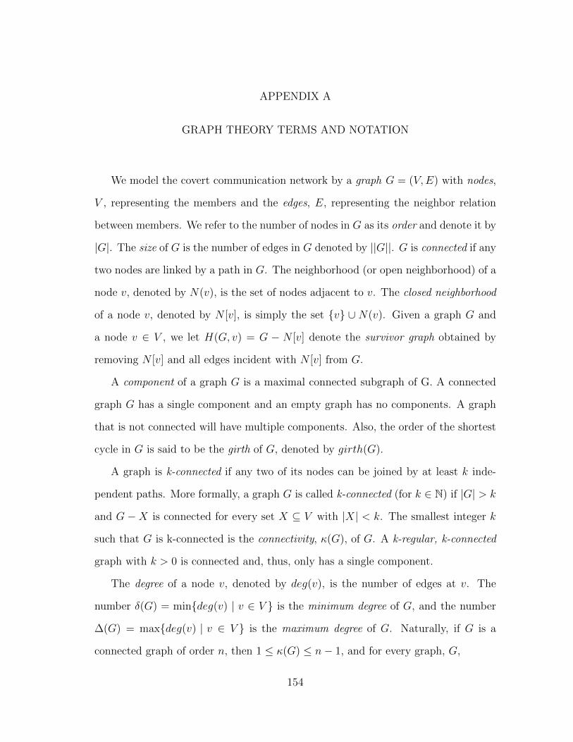
APPENDIX A

GRAPH THEORY TERMS AND NOTATION

We model the covert communication network by a graph G = (V,E) with nodes,

V , representing the members and the edges, E, representing the neighbor relation

between members. We refer to the number of nodes in G as its order and denote it by

|G|. The size of G is the number of edges in G denoted by ||G||. G is connected if any

two nodes are linked by a path in G. The neighborhood (or open neighborhood) of a

node v, denoted by N(v), is the set of nodes adjacent to v. The closed neighborhood

of a node v, denoted by N [v], is simply the set {v} ∪ N(v). Given a graph G and

a node v ∈ V , we let H(G, v) = G − N [v] denote the survivor graph obtained by

removing N [v] and all edges incident with N [v] from G.

A component of a graph G is a maximal connected subgraph of G. A connected

graph G has a single component and an empty graph has no components. A graph

that is not connected will have multiple components. Also, the order of the shortest

cycle in G is said to be the girth of G, denoted by girth(G).

A graph is k-connected if any two of its nodes can be joined by at least k inde-

pendent paths. More formally, a graph G is called k-connected (for k ∈ N) if |G| > k

and G −X is connected for every set X ⊆ V with |X| < k. The smallest integer k

such that G is k-connected is the connectivity, κ(G), of G. A k-regular, k-connected

graph with k > 0 is connected and, thus, only has a single component.

The degree of a node v, denoted by deg(v), is the number of edges at v. The

number δ(G) = min{deg(v) | v ∈ V } is the minimum degree of G, and the number

∆(G) = max{deg(v) | v ∈ V } is the maximum degree of G. Naturally, if G is a

connected graph of order n, then 1 ≤ κ(G) ≤ n− 1, and for every graph, G,

154

κ(G) ≤ δ(G) . (A.1)

If all the nodes of G have the same degree k, then G is said to be k-regular. If

graph G is k-regular and k-connected, then

κ(G) = δ(G) = ∆(G) . (A.2)

We refer the reader to Table A.1 for a summary of the graph theoretic notation

used.

155

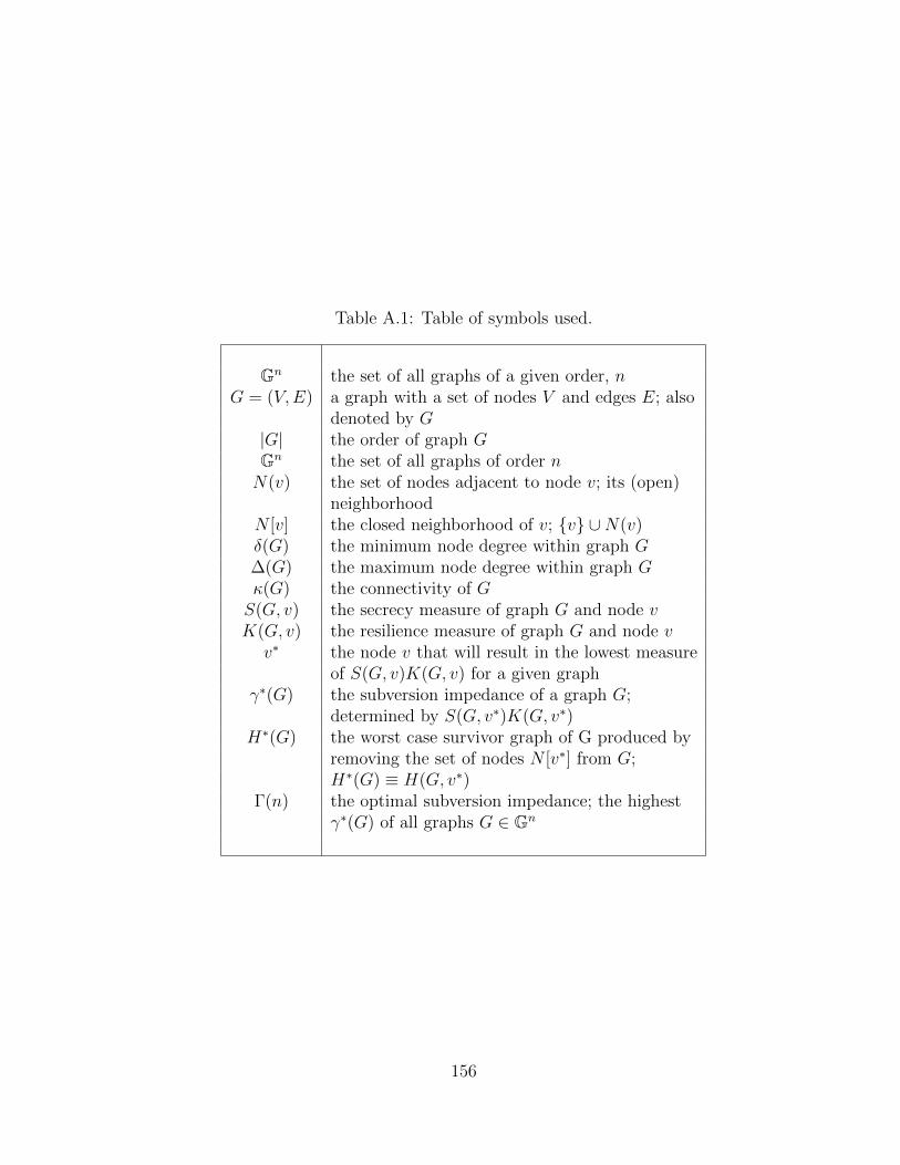
Table A.1: Table of symbols used.

Gn the set of all graphs of a given order, nG = (V,E) a graph with a set of nodes V and edges E; also

denoted by G|G| the order of graph GGn the set of all graphs of order nN(v) the set of nodes adjacent to node v; its (open)

neighborhoodN [v] the closed neighborhood of v; {v} ∪N(v)δ(G) the minimum node degree within graph G∆(G) the maximum node degree within graph Gκ(G) the connectivity of GS(G, v) the secrecy measure of graph G and node vK(G, v) the resilience measure of graph G and node vv∗ the node v that will result in the lowest measure

of S(G, v)K(G, v) for a given graphγ∗(G) the subversion impedance of a graph G;

determined by S(G, v∗)K(G, v∗)H∗(G) the worst case survivor graph of G produced by

removing the set of nodes N [v∗] from G;H∗(G) ≡ H(G, v∗)

Γ(n) the optimal subversion impedance; the highestγ∗(G) of all graphs G ∈ Gn

156