covering problems in facility location: a review

Computers & Industrial Engineering 62 (2012) 368–407

Contents lists available at SciVerse ScienceDirect

Computers & Industrial Engineering

journal homepage: www.elsevier .com/ locate/caie

Survey

Covering problems in facility location: A review

Reza Zanjirani Farahani a,⇑, Nasrin Asgari b,1, Nooshin Heidari c, Mahtab Hosseininia c, Mark Goh d,e

a Department of Informatics and Operations Management, Kingston Business School, Kingston University, Kingston Hill, Kingston Upon Thames, Surrey KT2 7LB, UKb Centre for Maritime Studies, 12 Prince George’s Park, National University of Singapore, Singapore 118411, Singaporec Department of Industrial Engineering, Amirkabir University of Technology, Tehran, Irand School of Business, 15 Kent Ridge Drive, National University of Singapore, Singapore 119245, Singaporee School of Management, University of South Australia, Adelaide, Australia

a r t i c l e i n f o

Article history:Received 16 August 2010Received in revised form 25 August 2011Accepted 27 August 2011Available online 1 September 2011

Keywords:Facility locationCovering problemMathematical formulationSurvey

0360-8352/$ - see front matter Crown Copyright � 2doi:10.1016/j.cie.2011.08.020

⇑ Corresponding author. Tel.: +44 (0)20 8417 5165E-mail addresses: [email protected] (R.Z. F

(N. Asgari), [email protected] (M. Goh).1 Fax: +65 6775 6762.

a b s t r a c t

In this study, we review the covering problems in facility location. Here, besides a number of reviews oncovering problems, a comprehensive review of models, solutions and applications related to the coveringproblem is presented after Schilling, Jayaraman, and Barkhi (1993). This survey tries to review all aspectsof the covering problems by stressing the works after Schilling, Jayaraman, and Barkhi (1993). We firstpresent the covering problems and then investigate solutions and applications. A summary and futureworks conclude the paper.

Crown Copyright � 2011 Published by Elsevier Ltd. All rights reserved.

1. Introduction Aslanzadeh, 2009). Therefore, the concept of coverage is related

Facility location is a critical component of strategic planning fora broad spectrum of public and private firms (Owen & Daskin,1998). For this, it is necessary to consider many criteria such as costor distance from demand points. Many models have been made tohelp decision making in this area. The readers who are interested inlearning about facility location models are referred to the works ofFrancis and White (1974), Handler and Mirchandani (1979), Love,Morris, and Wesolowsky (1988), Francis, McGinnis, and White(1992), Mirchandani and Francis (1990), Daskin (1995), Drezner(1995), Drezner and Hamacher (2002), Nickel and Puerto (2005),Church and Murray (2009) and Farahani and Hekmatfar (2009).

One of the most popular models among facility location modelsis covering problem. While covering models are not new they havealways been very attractive for research. This is due to its applica-bility in real-world life, especially for service and emergency facil-ities. In some covering problems, a customer should be served by atleast one facility within a given critical distance (not necessarilythe nearest facility). In most of the covering problems, customersreceive services by facilities depending on the distance betweenthe customer and facilities. The customer can receive service fromeach facility which its distance from customer is equal or less thana predefined number. This critical predefined number is calledcoverage distance or coverage radius (Fallah, NaimiSadigh, &

011 Published by Elsevier Ltd. All r

; fax: +44 (0)20 8417 5024.arahani), [email protected]

to a satisfactory method rather than a best possible one. Many ofthe problems like determining the number and locations of publicschools, police stations, libraries, hospitals, public buildings, postoffices, parks, military vases, radar installations, branch banks,shopping centers and waste-disposal facilities can be formulatedas covering problems (Francis & White, 1974). The scope of thissurvey is exclusively limited to the review of articles related tocovering problem in facility location.

Schilling, Jayaraman, and Barkhi (1993) present a literature re-view on covering problems in facility location. Since they present avery comprehensive review considering publications up to 1991,we have tried to consider covering researches after this time. How-ever, this paper also covers some older papers that are both veryimportant and basic from classification point of view or have notbeen in the domain of Schilling et al. (1993).

Schilling et al. (1993) classify models which use the concept ofcovering in two categories: (1) Set Covering Problem (SCP) wherecoverage is required and (2) Maximal Covering Location Problem(MCLP) where coverage is optimized. For each category, theyprovide taxonomy according to topological structure, nature ofdemand, characteristic of facility to be sited and application inpublic or private sectors. Also, based on solution methods – eitheroptimal or heuristic – a classification is proposed. Owen andDaskin (1998) present an overview of facility location literatureconsiderings stochastic or dynamic problem characteristics.Conforti, Cornuéjols, Kapoor, and VuŠkovic (2001) study resultsand also open problems on perfect, ideal and balanced metricsrelated to set packing and set covering problem. Also Berman,

ights reserved.

http://dx.doi.org/10.1016/j.cie.2011.08.020

mailto:[email protected]



http://dx.doi.org/10.1016/j.cie.2011.08.020

http://www.sciencedirect.com/science/journal/03608352

http://www.elsevier.com/locate/caie

R.Z. Farahani et al. / Computers & Industrial Engineering 62 (2012) 368–407 369

Drezner, and Krass (2010b) present an overview of covering modelconcentrate on three areas: (i) gradual covering model, (ii) cooper-ative covering model and (iii) variable radius model.

We have searched SCOPUS, one of the largest title, abstract andkeyword databases to check the related works and to see the trendof those research works over time (since 1992 till 1 February2011). Thus, we tested different keywords in this database. Finally,we made the following decision as a suitable combination:

(TITLE-ABS-KEY (covering AND location) AND TITLE-ABS-KEY(model OR problem OR facility)) AND PUBYEAR AFT 1991.

A 1531 cases were found. We have presented the most impor-tant parts of SCOPUS report in Table 1. Excluding 2011 (becausewe are in early February 2011 now) as the table shows, there is

Table 1SCOPUS’s report based on search in ‘‘location’’ and ‘‘covering’’.

Source title Author name

European Journal of Operational Research (30) ReVelle, C. (14)Computers and Operations Research (28) Berman, O. (12)Lecture Notes in Computer Science Including Church, R. L. (11)Subseries Lecture Notes in Artificial Intelligence and Murray, A. T. (11)Lecture Notes in Bioinformatics (27) Marianov, V. (8)Astrophysical Journal (23) Drezner, Z. (7)Proceedings of SPIE the International Society for Krass, D. (7)Optical Engineering (18) Lowe, T. J. (7)Astronomy and Astrophysics (16) Tamir, A. (6)Journal of Biogeography (16) Galvao, R. D. (6)Journal of the Operational Research Society (15) Serra, D. (6)Global Ecology and Biogeography (14) Wesolowsky, G. O. (5)Annals of Operations Research (13) Laporte, G. (5)Forest Ecology and Management (11) Kara, B. Y. (5)Journal of Geophysical Research D Atmospheres (9) Francis, R. L. (5)Socio Economic Planning Sciences (9) Plastria, F. (5)Atmospheric Environment (9) Lorena, L. A. N. (5)Location Science (8) Kraemer, S. B. (4)Transportation Research Record (7) Batta, R. (4)Papers in Regional Science (7) Hoefer, M. (4)Computers and Industrial Engineering (7) Crenshaw, D. M. (4)Networks (7) DeLand, M. T. (4)Proceedings of the National Academy of Sciences of Drezner, Z. (4)the United States of America (7) Gencer, C. (4)Field Crops Research (7) Gerrard, R. A. (4)Advances in Space Research (6) Emir-Farinas, H. (4)International Geoscience and Remote Sensing Lilley, D. G. (4)Symposium IGARSS (6) Saydam, C. (4)Discrete Applied Mathematics (6) Selim, H. (3)Journal of Climate (5) Cabello, S. (3)Remote Sensing of Environment (5) Jogloy, S. (3)International Journal of Climatology (5) Van Dishoeck, E. F.Pure and Applied Geophysics (5) (3)Lecture Notes in Computer Science (5) Vanhaverbeke, L. (3)Annales Geophysicae (5) Morabito, R. (3)IIE Transactions Institute of Industrial Engineers (5) Brandenberg, R. (3)International Journal of Heat and Mass Transfer (4) Schobel, A. (3)Operations Research Letters (4) Bottino, A. (3)Transportation Science (4) Blake, G. A. (3)Icarus (4) Schierbeck, J. (3)Journal of Vegetation Science (4) Williams, J. C. (3)Theoretical and Applied Genetics (4) Kotha, S. (3)Annals of Glaciology (4) Wu, N. W. (3)Journal of Hydrology (4) Gibson, A. (3)Water Science and Technology (4) Yang, C. (3)Journal of Molecular Biology (4) Mahlooji, H. (3)Monthly Weather Review (4) Laurentini, A. (3)Monthly Notices of the Royal Astronomical Society Roth, L. (3)(4) Dreyer, L. C. (3)Tectonophysics (4)Neuroimage (3)Health Physics (3)Naval Research Logistics (3)American Society of Mechanical Engineers PressureVessels and Piping Division Publication PVP (3)Natural Hazards (3)Hydrology and Earth System Sciences Discussions (3)

an increasing trend in the number of published documents on cov-ering in different areas. The numbers in parentheses of the tableshow the number of found related issues. However, since someof the found articles in SCOPUS are not related to the scope of thispaper we have not included them. Among the sources the highestpriority has been given to journal papers, conference papers andbooks, respectively.

2. Basic models and classification

With respect to history and origination, for the first time Hakimi(1965) introduces covering problems. The model is aimed to

Year Document type Subject area

2010 Article Engineering (409)(165) (1072)

Earth and Planetary Sciences (326)2009 Conference(178) Paper Computer Science (253)

(348)2008 Environmental Science (231)(178) Review

(40) Mathematics (172)2007(128) Article in Social Sciences (160)

Press (26)2006 Decision Sciences (159)(103) Conference

Review (6) Agricultural and Biological Sciences (159)2005(115) Business Medicine (128)

Article (3)2004 Physics and Astronomy (111)(93) Short

Survey (3) Biochemistry, Genetics and Molecular2003 Biology (101)(66) Note (1)

Business, Management and Accounting2002 Report (1) (58)(62)

Undefined Energy (51)2001 (16)(57) Chemical Engineering (45)

2000 Materials Science (36)(58)

Neuroscience (35)1999(51) Economics, Econometrics and Finance

(23)1998(55) Chemistry (19)

1997 Immunology and Microbiology (18)(52)

Multidisciplinary (16)1996(49) Health Professions (15)

1995 Psychology (13)(22)

Pharmacology, Toxicology and1994 Pharmaceutics (12)(31)

Veterinary (6)1993(25) Nursing (3)

1992 Dentistry (3)(28)

Arts and Humanities (2)Undefined (9)

370 R.Z. Farahani et al. / Computers & Industrial Engineering 62 (2012) 368–407

determine the minimum number of police needed to cover nodes(i) on a network of highways.

He formulates the problem as a vertex-covering problem in agraph. By considering graph G with the same weight assigned toits all branches (equal one), V as the set of vertices of graph G, Was a subset of V, d showing distance and S as a maximum accept-able service distance (or time), the subset of W covers G if:

dðv i;wÞ 6 S i ¼ 1; . . . ;n ð1Þ

where

dðv i;wÞ ¼Min½dðv i;v1Þ;dðv i; v2Þ; . . . ;dðv i; vqÞ� ð2Þ

The first mathematical model in covering problems wasdeveloped by Toregas, Swain, ReVelle, and Bergman (1971). Theyconsider modeling the location of emergency service facilities asfollows:

i: the index of demand nodes,j: the index of facilities,Ni: the set of potential locations within S so that Ni = {jjdij 6 S},xj: a binary decision variable indicating whether the facilitylocated at point j or not,dij: the distance between demand node i and facility j, andS: a maximum acceptable service distance. The model is asfollows:

Min z ¼Xn

j¼1

xj ð3Þ

S:T:Xj2Ni

xj P 1 i ¼ 1; . . . ;m ð4Þ

xj 2 f0;1g j ¼ 1; . . . ;n ð5Þ

Objective function (3) minimizes the total number of locatedfacilities. Constraint (4) shows the service requirement for demandnode i and constraint (5) is the integrality constraint.

Among the books that have dealt with covering problems in de-tail including solution techniques, we believe that Francis andWhite (1974) contribute significantly. Francis and White (1974)present covering problems well; they divide it into two major cat-egories that will be covered in this section, and Francis et al. (1992)talk about covering problems under two categories: network loca-tion problem and cyclic network problems. For the network locationproblem, they initially focus on a special kind of networks which isacyclic (so-called tree). Tree is an acyclic network with a uniqueshortest path between each two nodes that makes it easier thana general network to solve. Therefore, considering symmetry, pos-itivity, triangle inequality and convexity properties, the problemcan be solved efficiently. These properties and changing a generalnetwork to an acyclic one can be used as an approximation to cre-ate a ‘‘quick and dirty’’ solution for the problem.

Since set covering problems and maximal covering locationproblems are two traditional classifications for covering models,in this section we present the original mathematical formulationsfor these two categories and also direct extensions of these models.

2.1. The Set Covering Problem (SCP)

The set covering problem tries to minimize location cost satis-fying a specified level of coverage. The mathematical formulationof this problem is as follows:

i: the index of demand nodes,j: the index of facilities,

xj: a binary decision variable indicating whether the facilitylocated at point j or not,S: the maximum acceptable service distance,cj: the fixed cost of locating facility at node j andaij: a binary parameter is 1 if distance from candidate place j tothe existing facility (customer) i is not greater than S. The modelis as follows:

MinXn

j¼1

cjxj ð6Þ

S:T:Xn

j¼1

aij � xj P 1 8 i ði ¼ 1; . . . ;mÞ ð7Þ

xj 2 f0;1g j ¼ 1; . . . ;n ð8Þ

Objective function (6) minimizes the cost of locating facilities.The mentioned model is called Weighted Set Covering Problem(WSCP) and also non-unicost set covering problem. If the locationcosts for all the facilities are the same, the objective function can besimplified as (3).

Objective function (3) is equivalent to minimization of the num-ber of located facilities. If we substitute objective function (3) withthe objective of WSCP, the resulting model can be called MinimumCardinality Set Covering Problem (MCSCP) and also unicost set cov-ering problem. Vasko and Wilson (1986) show that, from computa-tional time point of view, solving MCSCP is more difficult thanWSCP.

In order to cover the nodes, constraint (7) enforces that for eachdemand node, at least one facility must be located within the set Ni

of candidate facility sites. Constraint (8) is the integralityconstraint.

The following subsections include several direct extensions ofthe SCP.

2.1.1. LSCP (location set covering problem) Implicit and ExplicitMurray, Tong, and Kim (2010) present two models called LSCP-

Implicit and LSCP-Explicit. LSCP-Implicit model assumes that eachdemand area can be covered not only by one facility but also bytwo or more so that each facility covers a percentage of demand.The notation of the model is as follows:

i: the index of demand area,j: the index of facilities,k: the index of coverage levels,xj: a binary decision variable indicating whether the facilitylocated at point j or not,Yik: a binary decision variable equal one if area i is covered atlevel k and otherwise 0,bk: the minimum required percentage of coverage at level k,ak: the minimum number of required facilities for coveringcompletely at kth level, andXik: the set of potential facilities cover area i at least bk.

LSCP-Implicit mathematical model is as follows:

Min z ¼X

j

xj ð9Þ

S:T:Xj2Xik

xj P akYik 8 i; k ð10ÞXk

Yik ¼ 1 8 i ð11Þ

Yik 2 f0;1g 8 i; k ð12Þxj 2 f0;1g 8 j ð13Þ


Objective function (9) minimizes the cost of locating facilities.Constraint (10) states that for completely covering demand areaat level k, ak facilities should be located. Constraint (11) ensuresthe existence of the coverage at level k. Constraints (12) and (13)are the integrality constraints.

Explicit coverage considers the coverage provided to a demandarea by a specific set of facilities tracking facilities combination.Consider the following notation:

l: the index of facility configuration,Wik: the set of k facility configurations completely cover area i,Dikl: the set of k facilities in lth configuration which covers area icompletely, andZikl: a binary decision variable, it equals to 1 if area i is coveredby configuration l at level k and otherwise 0.

LSCP-Explicit mathematical model is as follows:

Min z ¼X

j

xj ð14Þ

S:T:Xk

Xl2Wik

Zikl ¼ 18 i ð15Þ

xj P Zikl 8 i; k; l 2 Wik; j 2 Dikl ð16ÞZikl 2 f0;1g 8 i; k; l 2 wik ð17Þxj 2 f0;1g 8 j ð18Þ

Constraint (15) states that in order to completely cover demandarea, a k-facility configuration should be chosen. Constraint (16)indicates a configuration can be assumed only when the requiredfacilities are located. Constraints (17) and (18) are the integralityconstraints.

2.1.2. Capacitated SCPIn the above SCP formulation there is no distinction between

nodes based on demand size. The located facilities are uncapacitat-ed; i.e. there is no limitation for the capacity of a new located facil-ity. Therefore, each node, whether it contains a single customer ora large number of customers (and consequently a large portion ofthe total demand), must be covered within the specified distance,regardless of cost (Owen & Daskin, 1998). Most of the papers incovering literature consider uncapacitated SCP. For instance, Kolenand Tamir (1990) concentrate only on the uncapacitated versions ofthe covering problems. They consider three types of costs with a gi-ven set of facility location problems with focus on covering, centerand median problems: (i) set up cost, (ii) transportation cost and(iii) penalty cost. They believe that in covering problem commonobjective functions are minimizing ‘‘the sum of the set up costsand penalty costs’’. These researchers consider budget constraint,client constraints and facility constraint in their model. However,in most real-world applications of covering problems consideringcapacitated facilities are more realistic. For example, Current andStorbeck (1988) add facility capacity restrictions to the problemand present a capacitated version of SCP formulations.

2.1.3. Quadratics SCPBazaraa and Goode (1975) extend classical SCP to quadratic

case. In other words, instead of the objective function (6) thatcan be expressed as C � X, they are using XT � C � X where the con-straints are of the inequality type. Hence, C � X is cost of locatingnew facilities and XT � C � X is cost of relationship between each pairof the new facilities. They do not talk about the application of theirmodel but we may interpret that like in the traditional QuadraticAssignment Problem (QAP) in which there is a relation also be-tween the new located facilities.

2.1.4. Multiple optimal SCPLove et al. (1988) deal with covering models in a book chapter

entitled ‘‘site-selecting location-allocation models’’. They intro-duce set covering under the minimax criterion. In this problem,knowing the optimal number of the new facilities needed for totalcoverage, say m, and provided that there are multiple optimalsolutions for the problem, we are willing to find the location ofm new facilities somehow it is more attractive for a decision ma-ker. As such, a secondary criterion here minimizes maximumtime (or distance) for all the demand points to their nearestfacility.

2.1.5. Covering Tour Problem (CTP)Gendreau, Laporte, and Semet (1997b) develop an integer linear

programming formulation for covering tour problem on a graph.Consider the following notation:

i, j, k, l: the indices of vertices,V: the set of vertices that can be covered,W: the set of vertices that must be covered,T: the set of vertices that must be visited,S0: any subset of V,S0l : S0l ¼ fvk 2 V jdik ¼ 1g where dlk is a binary coefficients, itequals to 1 when vl 2W can be covered by vk 2 V.E: the set of edges (E = {(vi, vj)jvi, vj 2 V [W, i < j}),G: G = (V [W, E),xij: a binary decision variable indicates whether edge (vi,vj)belongs to the tour or not,yk: a binary decision variable, it equals to 1 if vk 2 V belongs tothe tour T, andcij: the cost of belonging edge (vi,vj) to the tour.

The goal is determining a minimum length Hamiltonian cycleon a sub-set of V such that every vertex of W is within a pre-specified distance from the cycle. The mathematical model is asfollows:

Min z ¼Xi�j

cijxij ð19Þ

S:T:Xvk2s0

l

yk P 1 v l 2W ð20Þ

Xi�k

xik þXj�k

xkj ¼ 2yk vk 2 V ð21Þ

Xv i2S0 ;v j2VnS0

orv j2S0 ;v i2VnS0

xij P 2ytðS0 � V ;2 6 jS0j 6 n� 2; T n S0 – /; v t 2 S0Þ

ð22Þ

xij 2 f0;1g 1 6 i < j 6 n ð23Þyk ¼ 1 vk 2 T ð24Þyk 2 f0;1g vk 2 V n T ð25Þ

Objective function (19) minimizes tour total cost. Constraint(20) states that each vertex of W should be covered by the tour,constraints (21) and (22) are degree and connectivity constraintsrespectively and constraints (23)–(25) impose the integralityrequirements.

2.1.6. Path covering problemsBoffey and Narula (1998) consider path covering problems with

emphasizing on multi-path (especially double path) models. Inmost of the covering problems, the facilities are considered to


be small in size in proportion to their location region and can beassumed as points. Therefore, we can term these problems as pointcover. Sometimes, we face application of covering problems withone-dimensional facilities like paths and trees in which the shapeof facilities cannot be neglected. Subway (e.g. metro, tube, under-ground) and highways are suitable examples for facilities of thesekinds. They define Maximum Population Shortest Path (MPSP) as tofind a path through the network such that the path length is min-imized and the population coverage is maximized. Accordingly,they introduce 2-MPSP as the problem of finding two paths suchthat the combined path length is minimized and population cover-age, at least once, is maximized. They also develop two Lagrangiansolution approaches for solving the 2-MPSP problem. Consider thefollowing notation for MPSP:

i, j, k, O, D: the indices of vertices,V: the set of vertices (V = {1, . . . ,n}),E: the set of edges,G: G (V,E),xij: a binary decision variable, it is 1 if the solution path containsarc ij, and 0 otherwise,zk: a binary decision variable, it is 1 if node k is covered by thepath, and 0 otherwise,dij: the weight (length) of arc ij 2 E, andhk: the weight (population) of vertex k.

Max z1 ¼Xk2V

hkzk ð26Þ

Min z2 ¼Xij2E

dijxij

S:T:

Xijij2E

xij �Xijji2E

xij ¼�1 if j ¼ O

0 if j – O;D

1 if j ¼ D

8><>: ð27Þ

Xjjij2E

xij � zi P 0 8 i – D ð28Þ

xij; zk 2 f0;1g 8 ij 2 E; k 2 V ð29Þ

Objective functions (26) minimize the length of path and alsomaximize the population coverage. Constraint set (27) identifiesconditions which flow be conserved on the route taken by flowingof one unit from node O to node D. Constraint (28) considers thevariable xij in terms of covering node j. Constraint (29) is the inte-grality constraint.

Here consider the following notation for 2-MPSP:

r: the index of path,xr

ij: a binary decision variable, it is 1 if path r contains arc ij, and0 otherwise, andzr

k: a binary decision variable, it is 1 if node k is covered by pathr, and 0 otherwise.

Max z1 ¼Xk2V

hk z1k þ z2

k

� �ð30Þ

Min z2 ¼Xij2E

dij x1ij þ x2

ij

� �S:T:

Xi

xrij �

Xk

xrjk ¼

�1 if j ¼ O0 if j – O; D;

1 if j ¼ D

8><>: r ¼ 1;2 ð31Þ

Xjjij2E

xrij ¼ zr

i 8 i – j; r ¼ 1;2 ð32Þ

z1k þ z2

k 6 1 8 k 2 V ð33Þxr

ij; zrk 2 f0;1g 8 i; j; r ð34Þ

Objective functions (30) try to find two paths such that thelength of path minimized and also cover (at least once) maximized.Constraints in set (31) determine flow conservation and also per-mission of loops. Constraint set (32) considers the variable x1

ij andx2

ij in terms of covering node. Constraint (33) states the interactionbetween the paths. Constraint (34) is the integrality constraint.

2.1.7. Probabilistic SCPWe can consider each of deterministic parameters of a SCP as

probabilistic to create a probabilistic SCP. ReVelle and Hogan(1989b) present a probabilistic version of SCP and call it probabilis-tic Location Set Covering Problem (PLSCP). Their model considersdynamic aspect of location problems especially in emergencyfacilities. In emergency facilities sometimes vehicles are notavailable when they are called. They propose two mathematicalformulations for this problem. The notation of the main model isas follows:

xj: a binary decision variable indicating whether the facilitylocated at point j or not,a: the required amount of probability,Fi: Cumulative the number of calls per hour at node i multipliedby the average duration of a call (h), andbi: the smallest integer satisfying 1� ðFi=biÞbi P a.

The model is as follows:

Min z ¼Xn

j¼1

xj ð35Þ

S:T:Xj2Ni

xj P bi8 i ð36Þ

xj 2 f0;1g 8 j ð37ÞThe first derivation of their model is ‘‘a-reliable P-center prob-

lem’’ aims to find the location of P facilities in order to minimizingmaximum time between availability of a reliable service.

The second derivation of their model is ‘‘the maximum reliabil-ity location problem’’ which aims to find the location of P facilitiesin order to maximize the minimum reliability of services.

Beraldi and Ruszczynski (2002) develop probabilistic set cover-ing problem. In this problem,

xj: a binary decision variable indicating whether the facilitylocated at point j or not,A: 0–1 covering matrix; element ij is 1 if potentially the facilitylocated at point j can cover demand point i,f: a random binary vector and

p 2 (0,1): the prespecified reliability. The model is as follows:

Min z ¼Xn

j¼1

xj ð38Þ

S:T:PfAx P fgP p ð39Þxj 2 f0;1g 8 j ð40Þ

Constraint (39) states that covering constraint must be satisfiedwith some prescribed probability.

Saxena, Goyal, and Lejeune (2010) present some mixed integerprogram formulations for the above probabilistic SCP. Consider thefollowing notation:


u: a random vector u = (u1, . . . ,uM) (u 2 RM),ut: the sub-vector of u formed by components in Mt fort = 1, . . . ,L,F: F:{0,1}M ? R is the cumulative distribution function of n andu 2 {0,1}M, F(u) = p(f 6 u),Ft: the restriction of F to Mt for t 2 {1, . . . ,L} where M1, . . . ,ML is apartition of M,St: the set of binary vectors either p-efficient or dominate a p-efficient point of Ft,It: the set of p-inefficient points of Ft,ui: ui ¼min aT

i x;1� �

i 2 M where ai denotes the ith row of A,gt: gt = lnFt(ut) t 2 {1, . . . ,L}, andv: v 2 St [ It.

The MIP model is as follows:

Min z ¼X

j

xj ð41Þ

S:T:Ax P u ð42Þ1 6

Xi2Mt ;v i¼0

ui 8 v 2 St ; 8 t 2 f1; . . . ; Lg ð43Þ

XL

t¼1

gt P ln p ð44Þ

gt 6 ðln FtðvÞÞ 1�X

i2Mt ;v i¼0

ui

!8 v 2 St; 8 t 2 f1; . . . ; Lg ð45Þ

ui 2 f0;1g 8 i 2 M ð46Þxj 2 f0;1g 8 j ð47Þ

Objective function (41) and constraints (42) and (43) are basicrelations in set covering problem. They prove (44) and (45) arean equivalent conversion of (39). They propose two other equiva-lent formulations for above model.

2.1.8. Stochastic SCPHwang (2002) aims to design a supply chain logistics system.

The problem is solved in two stages. In the first stage a mathemat-ical programming model is developed to determine minimumnumber of warehouses/distribution centers (W/D) among anumber of discrete potential sites. This is a stochastic set coveringproblem so that the probability of each demand point beingcovered is not less than a critical level. This problem is solved using0–1 programming method. Consider the following notation:

xj: a binary decision variable indicating whether the facilitylocated at point j or not,cij: the logistic cost incurred between nodes i and j,Ai: a required service level,ri: critical service level, andaij: a binary parameter, it is 1 if prob(cij 6 Ai) P ri and otherwise 0.


MinXn

j¼1

xj ð48Þ

S:T:Xn

j¼1

aij:xj P 1 8 i ði ¼ 1; . . . ;mÞ ð49Þ

xj 2 f0;1g j ¼ 1; . . . ;n ð50Þ

Objective function (48) and constraints (49) and (50) are basicrelations in set covering problem. But (49) is an extension of thetraditional deterministic function into stochastic space considering

the new probabilistic definition of aij. In the model, it is assumedthat all warehouse and distribution centers are always available.Also Hwang proposes other models in which availability of all facil-ities is relaxed. The second stage is related to a vehicle routingproblem that is solved using genetic algorithm.

Baron, Berman, Kim, and Krass (2009) develop a set coveringproblem to a general class of Location Problems with Stochastic De-mand and Congestion (LPSDC). They deal with a location-allocationproblem. As their model application is in emergency systems withmobile servers, it is very important that an arriving call be re-sponded by a server. With respect to this constraint, the objectiveis minimizing the total number of servers. They consider the prob-lem on an undirected network. Consider the following notation:

x(j): the number of servers to be placed at site j,Ai(X): the availability for node i, anda: a 2 (0,1) is the minimum required availability for node i.

It is assumed that an allocation vector X is given and relatedqueuing system represented by X is stable.

Min z ¼X

j

xðjÞ ð51Þ

S:T:AiðXÞP a 8 i ð52ÞxðjÞ ¼ 0;1; . . . 8 j ð53Þ

The model tries to minimize the total number of located serverson a network while satisfying the needed availability a at all nodes.

2.1.9. Fuzzy SCPIn order to consider uncertainty in a classical SCP, Hwang,

Chiang, and Liu (2004) propose fuzzy set-covering model. They tryto find an optimal a-cover with respect to a given set Ni and the de-sired degree a, for each j 2 Ni, the membership grade i is no lessthan the level degree a. This formulation can be reduced to a non-linear integer programming problem that is solved using optimiza-tion software. The notation of the model is as follows:

I: the subset of integers (I = {1, . . . ,m}),J: the subset of integers (J = {1, . . . ,n}),cj: the cost of locating facility at j,a: the desired degree of fuzzy cover,lj(i): the membership grade of i 2 I,ePj: ePj ¼ fði;ljðiÞÞ : i 2 Ig is a fuzzy subset of i, and

xj: xj ¼ 1 ePj 2 ~p�

0 otherwise

�,

Min z ¼Xn

j¼1

cjxj ð54Þ

S:T:

1�Yn

j¼1

ð1� ljðiÞxjÞP a 8 i ð55Þ

xj 2 f0;1g 8 j ð56Þ

Chiang, Hwang, and Liu (2005) obtain a simplified model ofHwang et al. (2004) model. They reformulate the model as follows:

Min z ¼Xn

j¼1

cjxj ð57Þ

S:T:Xn

j¼1

xj½� lnð1� ljðiÞÞ�P � lnð1� aÞ ð58Þ

xj 2 f0;1g 8 j ð59Þ


2.1.10. Multiple coverage SCPKolen and Tamir (1990) discuss multiple coverage problems. In

this problem, each existing demand node must be served by anumber of new facilities and this number depends on the type ofnew facilities. There is also an upper bound for the number of facil-ities that must be located at a given potential site.

2.1.11. Backup coverage SCPsErdemir et al. (2010) propose two models to locate aero med-

ical and ground ambulance service which are based on SCP andMCLP. They define coverage as a combination of both responsetime and total service time and consider three type of it: (i)Ground emergency medical service coverage. (ii) Air emergencymedical service coverage. (iii) Joint coverage of ground and airemergency medical service thorough transfer point. The node iscovered by closet emergency medical service, if it is fulfilled theresponse time and service time limits. The proposed model coversboth crash nodes and paths (nodes and links of network). There-fore the uncertainty in spatial distribution of demand nodes isaddressed. Also by considering unavailability of ground emer-gency medical service, the backup coverage is modeled. Considerthe following notation:

a: index of potential ground ambulance locations,h: index of potential air ambulance locations,r: index of potential transfer point locations,j: index of crash nodes,k: index of crash paths,MA: the set of potential ground ambulance locations,MH: the set of potential air ambulance locations,MR: the set of potential transfer point locations,N: the set of crash nodes,P: the set of crash paths,xa: a binary decision variable, it is 1 if a ground ambulance islocated at a,yh: a binary decision variable, it is 1 if an air ambulance islocated at h,zr: a binary decision variable, it is 1 if a transfer point is locatedat r,uj: a binary decision variable, it is 1 if node/path j is covered byat least one of located air ambulances, and if node/path j is cov-ered by at least two ground ambulances and/or combinations,vja: a binary decision variable, it is 1 if node/path j is covered byground ambulance a,lahr: a binary decision variable, it is 1 if ground ambulance, airambulance and a transfer point are located at a, h and rrespectively,cA: the cost of locating ground ambulance,cH: the cost of locating air ambulance,cR: the cost of locating transfer point,Aaj(Aak): a binary parameter, it is 1 if potential ground ambu-lance location a covers node j (path k),Ahj(Ahk): a binary parameter, it is 1 if potential air ambulancelocation h covers node j (path k),Aahrj(Aahrk): a binary parameter, it is 1 if potential ground a air hambulance, and transfer point r covers node j (path k), ande: a very small number.

The Set Cover Backup Model (SCBM) is as follows:

MinXa2MA

cAxa þX

h2MH

cHyh þXr2MR

cRzr �X

j2N[P

uj � e ð60Þ

S:T:Xh2MH

Ahjyh P uj 8 j 2 N [ P ð61Þ

Aajxa þX

h2MH

Xr2MR

Aahrjlahr P v ja 8 j 2 N [ P; 8 a 2 MA ð62Þ

Xa2MA

v ja ¼ 2 � ð1� ujÞ 8 j 2 N [ P ð63Þ

xa P lahr 8 a 2 MA; h 2 MH; r 2 MR ð64Þyh P lahr 8 a 2 MA; h 2 MH; r 2 MR ð65Þzr P lahr 8 a 2 MA; h 2 MH; r 2 MR ð66Þxa þ yh þ zr � lahr 6 2 8 a 2 MA; h 2 MH; r 2 MR ð67Þxa; yh; zr; lahr;uj;v ja 2 f0;1g 8 a 2 MA; h 2 MH; r 2 MR;

j 2 N [ P ð68Þ

The objective function minimizes the total cost whereas pre-vents allotting two different ground ambulance to cover node/pathj, if there is at least one air ambulance covering node j. Constraints(61)–(63) indicate that all crash nodes and paths are covered atleast once by an air ambulance or twice by a ground ambulanceor combination of ground and air ambulance. Constraints (64)–(67) ensure that all emergency medical service must be locatedto provide joint coverage of ground and air emergency medical ser-vice thorough transfer point.

2.1.12. Multi-Criteria SCP (MCSC)Liu (1993) introduces multi-criteria SCP. In this problem, there

are several predetermined attributes with separate covering ma-trix for each attribute. An existing facility will be covered if fromeither attribute point of view it is covered. Also, there is one objec-tive function for each attribute in terms of cost. Liu, thus develops agreedy heuristic algorithm to solve this problem.

2.1.13. Covering gamesHoefer (2006) and Cardinal and Hoefer (2010) consider a non-

cooperative games coming from combinatorial SCPs and investi-gate cost sharing between non-cooperative agents. There is agame for k players (each service facility that is potentially ableto serve/ cover existing facilities, is a player) and each playerwants to satisfy a subset of the constraints. Therefore, the strat-egy is chosen by each of them so that a subset of nodes on a net-work is covered whereas total contribution exceeds the cost.Hoefer (2006) presents a polynomial time algorithms to calculateNash equilibrium for this problem. The notation of the model isas follows:

j: index of vertices on a network,t: index of edges on a network,V: the set of vertices on a network (jVj = n),E: the set of edges on a network (jEj = m),G: G = (V,E),xj: the amount of bought units of resource j,cj: the cost of integral unit of resource j,atj: The non-negative (rational) entry, andbt: The non-negative (rational) entry.

MinXn

j¼1

cjxj ð69Þ

S:T:Xn

j¼1

atjxj P bt t ¼ 1; . . . ;m ð70Þ

xj 2 N j ¼ 1; . . . ;n ð71Þ

The objective function (54) minimizes the total cost of boughtunits. Constraint (70) ensures the necessary amount of boughtunits are provided.


2.1.14. Other variants of SCPDaskin (1995) focuses on variants of the set covering location

modelin his book; whereby he includes secondary objectives thatare important in facility location like: (i) one of the extensions triesto choose one of the optimal solutions that maximizes the numberof demand nodes covered at least once (ex. twice); this can also beseen in Church and Murray (2009) in their book. (ii) In anotherextension, he considers that we are not facing a from-scratch loca-tion planning problem. In other words, there are several existingfacilities and then we want to add new facilities for total coverage.Daskin (1995) explains a reformulation of the objective function byusing maximum number of existing facilities trying to use maxi-mum number of them.

Chen and Yuan (2010) study the coverage problem in cellularnetwork. They formulate two models that minimize the requiredpower while the service area is fully covered. Overlap constraintbetween adjacent cells is also considered which ensures handoverbetween them. The notation of the first model is as follows:

i, h: indices of broadcast channels,j, k: indices of test points,F 0iðjÞ: index of jth test point position (j 2 Ji) in the sortedsequence of cell i,Fi(j): the inverse of F 0iðjÞ,I: the set of cells (I = {1, . . . ,n}),J: the set of test points (J = {1, . . . ,m}),Ji: the set of test points that can be potentially covered by celli(mi = jJij),Ij: the set of potentially covering cell of j(nj = jIjj),Jih: the minimum amount to be covered by both cell i and hðJih ¼ Ji \ Jh; mih ¼ jJihjÞ,D: the set of adjacent cells that overlap with each other,Fi: a bijection such that sort Pij in ascending order (Fi:Ji ?{1, . . . ,mi}),F 0i: a bijection such that sort Pij in descending order (Fi:Ji ?{1, . . . ,mi}),xij: a binary decision variable, it is 1 if the power of cell i equalsPij,zih

j : a binary decision variable, it is 1 if test point j is covered byboth cell i and h,dih: the minimum amount to be covered by both cell i and h,Pij: the minimum amount of power required to cover test pointj 2 J by cell i 2 I,n: number of cells,m: number of test points,nj: number of potentially covering cell o j, andmi: number of test points that can be potentially covered by cell i.

The first model is as follows:

MinXi2I

Xj2Ji

Pijxij ð72Þ

S:T:Xi2Ij

Xmi

k¼F 0iðjÞ

xiðkÞ P 1 j 2 J ð73ÞXj2Ji

xij ¼ 1 i 2 I ð74Þ

Xmi

k¼F 0iðjÞ

xiðkÞ þXmh

k¼F 0hðjÞ

xhðkÞ ¼ zihj þ 1 ði;hÞ 2 D; j 2 Jih : Ij ¼ fi;hg ð75Þ

Xmi

k¼F 0iðjÞ

xiðkÞ þXmh

k¼F 0hðjÞ

xhðkÞ P 2zihj ði;hÞ 2 D; j 2 Jih : fi;hg � Ij ð76ÞX

j2Jih

zihj P dih ði;hÞ 2 D ð77Þ

xij 2 f0;1g i 2 I; j 2 Ji ð78Þzih

j 2 f0;1gði; hÞ 2 D; j 2 Jih ð79ÞConstraints (73) and (74) ensure that all test points are covered

by exactly one of broadcast channel. Constraints (75) and (76) indi-cate that zih

j ¼ 1, if both cell i and h cover test point j. Constraint(77) ensures the required overlap.

The second model is more effective than the first one. Consideradditional notation as follows:

l: index of coverage level (l 2 {2, . . . ,mi}),Jihðil�1Þ : Jihðil�1Þ ¼ fj 2 JihjPij 6 Piðl�1Þg,L(il � 1,h): the minimum power of cell h that can meet the cov-erage and overlap constraints of test points in Jih, provided thatcell i uses level l � 1, andPi(l): the lth level of cell i power in a sorted sequence.

Chen and Yuan (2010) prove that there is an equivalent for theabove model which is as follows:

MinXi2I

Xj2Ji

Pijxij ð80Þ

S:T:Xl�1

k¼1

xiðkÞ 6Xmh

k¼Lðil�1 ;hÞxhðkÞ ði;hÞ 2 D; l 2 f2; . . . ;nig : FiðlÞ 2 Jih ð81Þ

Xi2Ij

Xmi

k¼F 0iðjÞ

xiðkÞ P 1 j 2 J ð82Þ

zihj 2 f0;1g ði;hÞ 2 D; j 2 Jih ð83Þ

2.2. The Maximal Covering Location Problem (MCLP)

In many practical applications, allocated resources (e.g. budget)are not sufficient to cover all of existing facilities (e.g. customers)with desired level of coverage. Therefore, Church and ReVelle(1974) develop maximal covering location model. This model max-imizes the amount of demand covered within the acceptable ser-vice distance S by locating a given fixed number of new facilities.

In order to formulate this problem we use the following set ofnotations:

i: the index of demand nodes,j: the index of facilities,hi: given number that shows the number of demands at node i(this is something like the number of population at node),S: the time (or distance) standard within which a server isdesired to be found,P: the total required server to be located,aij: A binary parameter is 1 if distance from candidate place j tothe existing facility (customer) i is not greater than S,xj: binary variable indicating a facility is positioned at j or not, andzi: binary decision variable is 1 if node i is covered, otherwise 0.

Thus maximal covering location problem can be formulated asfollows:

MaxX

i

hi:zi ð84Þ

S:T:

zi 6X

j

aij � xj 8 i ð85ÞXj

xj 6 P ð86Þ

zi 2 f0;1g 8 i ð87Þxj 2 f0;1g 8 j ð88Þ


Objective function (84) maximizes the covered demands. Con-straint (85) explains relation between the coverage and locationvariables and states that demand node j is covered if at least onefacility at one of the potential sites able to cover node j, is located.Constraint (86) limits the number of located facilities to P. Con-straints (87) and (88) are integrality constraints.

White and Case (1974) consider the weights of all demandpoints as equal. Klastorin (1979) demonstrates how MCLP can beformulated as Generalized Assignment Problems (GAP). Therefore,they find maximum number of demand nodes that are covered.Daskin (1995) introduces the maximal coverage location modelas one of the variants of set covering.

2.2.1. MCLP implicit and explicitMurray et al. (2010) present MCLP-Implicit model as:

i: the index of demand area,j: the index of facilities,k: the index of coverage levels,xj: a binary decision variable indicating whether the facilitylocated at point j or not,Yik: a binary decision variable equal one if area i is covered atlevel k and otherwise 0,zi: a binary decision variable is 1 if node i is covered,otherwise 0,bk: the minimum required percentage of coverage at level k,ak: the minimum number of required facilities for coveringcompletely at kth level,Xik: the set of potential facilities cover area i at least bk,hi: given number that shows the number of demands at node i(this is something like the number of population at node), andP: total required number of facilities to be located.


MaxX

i

hi � zi ð89Þ

S:T:Xj2Xik

xj P akYik 8 i; k ð90Þ

Xk

Yik ¼ zi 8 i ð91Þ

Xj

xj ¼ P ð92Þ

zi 2 f0;1g 8 i ð93Þxj 2 f0;1g 8 j ð94ÞYik 2 f0;1g 8 i; k ð95Þ

Objective function (89) maximizes the total demand covered.Constraint (90) expresses the relation between facility locationvariable and coverage demand. Constraint (91) ensures providedcoverage at level k. Constraint (92) states the total number offacilities. Constraints (93)–(95) are the integrality constraints.

Considering above and the following notation, the MCLP-Explicit model is as follows:

W0ik: the set of k facility configurations partially covers area i,D0ikl: a set of k facilities in lth configuration which covers area ipartially,cikl: a fraction of ith demand covered by k facilities in l configu-ration andZikl: a binary decision variable, it equals to 1 if area i is coveredby configuration l at level k and otherwise 0.


MaxX

i

Xk

Xl2W0ik

hiciklZikl ð96Þ

S:T:Xk

Xl2W0ik

Zikl 6 1 ð97Þ

xj P Zikl 8 i; k; l 2 W0ik; j 2 D0ikl ð98ÞXj

xj ¼ P ð99Þ

Zikl ¼ f0;1g 8 i; k; l 2 w0ik ð100Þxj 2 f0;1g 8 j ð101Þ

Objective function (96) maximizes the total demand covered.Constraint (97) stipulates that at most one-level configurationcombination can account for the coverage of demand area i. Con-straint (98) limits coverage to that provide by sited facilities. Con-straint (99) states the total number of facilities. Constraints (100)and (101) are the integrality constraints.

2.2.2. Planar maximal coveringChurch (1984) introduces MCLP on the plane; in other words,

the potential sites for locating the new facilities are not on the net-work or discrete (and finite). He develops the planar maximal cov-ering location problem under (i) Euclidean distance measure(PMCE) and (ii) rectilinear distance measure (PMCR).

2.2.3. Capacitated MCLPLike it was said for capacitated SCP, Current and Storbeck (1988)

also apply the same facility capacity restrictions to the MCLPproblem and present a capacitated version of MCLP formulation.

2.2.4. MCLP with a criticality index analysis metricOztekin, Pajouh, Delen, and Swim (2010) present RFID network

design methodology for asset tracking in healthcare. In their modelthe reachable readers for completely coverage is less than the re-quired number, so the goal is to find the best location for availablereader so that maximize system efficiency.

Consider the following notation:

i: the index of demand square, i = 1, . . . ,n,j: the index of reader nods, j = 1, . . . ,m,k: the index of assets type, k = 1, . . . , l,zi: a binary variable is 1 if demand square i is covered by at leastone reader and 0 otherwise,xj: a binary decision variable is 1 if a reader is located at readernode j, otherwise 0,Ni: the set of reader nodes (j) that can cover demand square i.Ni = {j/lij 6 s},P: the fixed number of readers,s: read range of the reader,lij: the distance between these reader nodes and demandsquare i,w1 and w2: the weight of two part of the objective function,sk: the importance level of asset k in emergency cases evaluatedby experts based on a five-point Likert scale,fki: number of times asset k passes through demand square i in aday,(dt)ki: average of time that asset k spends in demand square i ina day, andci: the criticality index of demand squarei calculated as:

ci ¼Xl

k¼1

fki � ðdtÞki � sk



Max w1

Xi

ci:zi

!�w2

Xn

i¼1

Xj2Ni

xj

!� zi

!ð102Þ

S:T:

zi 6Xj2Ni

xj 6 zi �m 8 i ð103ÞXj

xj ¼ P ð104Þ

zi 2 f0;1g 8 i ð105Þxj 2 f0;1g 8 j ð106Þ

Objective function (102) maximizes the total covered criticalityindices of demand squares and also minimizes the reader collision.Constraint (103) assures coverage of demand square while havingreaders on reader nodes. Constraint (104) expresses total numberof reader nodes. Constraints (105) and (106) are the integralityconstraints.

2.2.5. MCLP with mandatory closeness constraintsLove et al. (1988) in their book chapter introduce maximal cover-

ing with mandatory closeness constraints. In this problem, knowingthe optimal number of the new facilities needed for total coverage,say P, and provided that there are multiple optimal solutions for theproblem, the decision maker ignores the average closeness of re-sponse to their nearest service center; but seeks location for the Pfacilities to maximize population covered within a desired time ordistance. They do this using a binary variable to decide assignmentdemand point to a facility and adding a set of constraints.

2.2.6. Probabilistic MCLPReVelle and Hogan (1989a) present a probabilistic version of

MCLP and call it Maximum Available Location Problem (MALP). Theytry to locate P facilities so that with the probability a maximize thecovered population that can find an available server. They intro-duce MALP I that utilizes the local busy fraction and MALP II thatuses a system wide busy probability.

2.2.7. MALP IIn this model, consider the following notation:

i: the index of demand area,j: the index of facility sites,S: maximum distance or time that a demand point can be fromits nearest facility,dij: the shortest time (or distance) from site j to demand i,Ni: Ni = {j/dij 6 S},xj: a binary decision variable is 1 if a facility is located at node j,otherwise 0,zik: a binary variable indicates whether the demand area i has atleast k servers within S or not,P: total number of facilities,hi: the population at node i,�d: the average duration of a call,b: defined as b = [log (1 � a)/logq] where a is the reliability andq ¼ �d �

Pi2Ihi=24

Pj2Jxj.

The model is as follows considering all variables are 0, 1:

Max z ¼X

i

hizib ð107Þ

S:T:Xb

k¼1

zik 6Xj2Ni

xj 8 i ð108Þ

zik 6 zik�1 8 i; k ¼ 2; . . . ; b ð109ÞXj

xj ¼ P ð110Þ

Objective function (107) maximizes the population coveredwith reliability a, while constraint (108) determines the requiredconnection between variables and constraint (109) states credithigher levels of coverage in the suitable order. Constraint (110) ex-presses the total number of facilities.

2.2.8. MALP IIIn MALP II, maximizing the population of demand areas

having bi servers within S or maximizing the population withservice available with alpha reliability is considered. The pre-sented model for MALP II is the same as MALP I by changing binto bi defined as the smallest integer satisfying 1� ðhi=biÞbi P afor each i.

Marianov and ReVelle (1994) consider dependency betweenserver availabilities and extend PLSCP by using queuing theory.They call their model queuing probabilistic location set coveringproblem (Q-PLSCP) and their solution technique, Maximum Avail-ability Sitting Heuristic (MASH). The presented model is the sameas PLSCP discussed by ReVelle and Hogan (1989b) with the differ-ence in definition of variable bi as the smallest integer that satisfies

1bi !

qbii

� �.1þ qi þ 1

2!q2

i þ . . .þ 1bi !

qbii

� �6 1� a; qi is the utilization

ratio of queuing theory.Drezner (1995) includes two book chapters regarding covering

problems: (i) Marianov and ReVelle (1995) present models for sit-ting emergency services. They use in their book chapter the sim-ple deterministic covering model, the maximum populationcoverage version, two kinds of models developed to address con-gestion (deterministic redundant coverage and probabilistic mod-el); (ii) Ghosh, McLafferty, and Carig (1995) apply coveringmodels for service center location in their book chapter. They pres-ent two case studies that can also be considered as the applica-tions of location-allocation models for planning a network ofservice centers.

2.2.9. Maximum covering location-interdiction problemO’Hanley and Church (2011) present a facility location-interdic-

tion model maximizing initial coverage and minimizing coveragelevel following the worst-case interdiction pattern. Consider thefollowing notation:

i: the index of demand nodes,j: the index of all potential facility locations,k: the index of p numbered facilities locations, k = 1, . . . ,p,x: the index of feasible interdiction template,Ni: the set of sites covering demand node i,X: the set of all possible interdiction templates,Gx: the set of facility indices k including interdictiontemplate x,h > 0: weight given before interdiction to the demand-weightedcoverage,z0: demand-weighted coverage level when the worst-case inter-diction pattern occurs,hi: amount of demand at node i,yi: a binary variable shows if demand i covered before interdic-tion occurrence (=1) or not (=0),xjk: a binary variable shows the kth facility locate in jth locationor not, andy0ix: a binary variable determines whether node i is coveredwhen interdiction pattern x occurs or not.


The MIP formulation of that model is as follows:

Max z ¼ hXi2I

hiyi þ z0 ð111Þ

S:T:Xj

xjk ¼ 1 8 k 2 K ð112ÞXk2K

xjk 6 1 8 j ð113ÞXk2K

Xj2Ni

xjk P yi 8 i ð114ÞXk2KnGx

Xj2Ni

xjk P y0ix 8 x 2 X; i ð115ÞXi

hiy0ix P z0 8 x 2 X ð116Þ

xjk 2 f0;1g 8 j; k; yi 6 1 8 i; y0ix 6 1 8 i;x ð117Þ

Objective function (111) maximizes covered demand beforeand after interdiction, constraint (112) expresses that each facilityk should choose one location, constraint (113) ensures that it is notpossible to have two facilities in one location, constraint (114)states coverage of node i with open facility before occurring inter-diction, constraint (115) states coverage of node i with open noninterdicted facility and constraint (116) specifies the minimumamount of demand-weighted coverage level. Constraint (117) ex-press the integrality variable xjk, while binding the pre-interdictionand postinterdiction coverage variables yi and y0ix to be less than orequal to one.

The bi-level MIP formulation of above model is as follows:

r: the number of interdictions,xj: a binary decision variable is 1 if a facility is located at node j,otherwise 0,y0i: a binary variable shows if demand i is covered before inter-diction occurrence (=1) or not (=0) andu0j: a binary variable shows if facility j is interdicted (=1) or not(=0).

The mathematical model is:

Max z ¼ hXi2I

hiyi þ z0 ð118Þ

S:T:Xj2Ni

xj 6 yi 8 i ð119Þ

Min z0 ¼X

i

hiy0i ð120ÞXj

u0j ¼ r ð121Þ

y0i þ u0j P xj 8 i; 8 j 2 Ni ð122ÞXj

xj ¼ P ð123Þ

u0j 2 f0;1g 8 j y0i P 0 8 i ð124Þ

yi 6 1 8 i xj 2 f0;1g 8 j ð125Þ

Constraint (119) states the coverage of node i with open facilitybefore occurring interdiction, while the objective function (120)minimizes the demand-weighted coverage after interdiction, con-straint (121) limits the number of interdictions. Constraint (122)states that each facility covering customer i should be interdicted.Constraint (123) expresses the total number of facilities. Con-straints (124) are the integrality constraint while binding the

post-interdiction coverage variables to be greater than or equalto zero. Constraints (125) also are the integrality constraint andlimit the pre-interdiction coverage variables to be less than orequal to one.

2.2.10. Median Tour Problem (MTP) and Maximal Covering TourProblem (MCTP)

Current and Schilling (1994) introduce Median Tour Problem(MTP) and Maximal Covering Tour Problem (MCTP) which are bicri-terion routing problems. These problems have applications in mo-bile service delivery systems (e.g. healthcare systems, overnightmail delivery) and distributed computer networks. In the prob-lems, there is a tour that must visit only P of the n nodes on thenetwork. One of the objectives minimizes of total tour length andthe other maximizes access to the tour for the nodes not directlyon it.

We explain MCTP which looks for a tour among n nodes; thetour must visit exactly P of the n nodes. Given a directed graphG = (V,E):

jS0j: the cardinality of set S0 (any subset of V),Q: node set in S used for sub-tour elimination constrainsxij: the binary variable indicates whether the arc from node i tonode j is on the tour or not,zi: the binary variable; it is 0 if the demand node i is covered bya stop and 1 otherwise,hi: demand at node i,s: maximal covering distanceNi: set of nodes within covering radius of node i, Ni ¼ fjjdij 6 sgcij: the cost of including the path connecting nodes i and j on thetour andP: the number of stops on the tour.

Considering z0T ¼P

i

Pjcijxij, z0c ¼

Pihizi � i, the mathematical

model is as follows:

Min z ¼ z0T ; z0c

� �ð126Þ

S:T:Xi

xij �X

k

xjk ¼ 0 8 j ð127Þ

Xj

Xi

xij ¼ P ð128Þ

Xi2Q

Xj2Q

xij 6 jS0j � 1 S0 � V ; 2 6 jS0j < P ð129Þ

xij 2 f0;1g ði; jÞ 2 E ð130ÞXl

Xj2Ni

xlj þ zi P 1 8 i ð131Þ

zi P 0 8 i ð132Þ

Objective function (126) minimizes two objective functionsincluding the total length of the tour and also the total demandweighted travel distance which the demand at the nodes encoun-ters reaching their nearest stop on the tour. Constraint sets (127)–(130) show that the solution contains a single tour (constraint(129) is used for sub-tour elimination) with p stops and constraintsets (131) and (132) ensure that zi = 1, for all nodes i which are notcovered by the tour.

2.2.11. Partial coverage problemOne of the key assumptions of the MCLP is that coverage is bin-

ary; it means customer is either fully covered if there is a facilitywithin distance S from the located facility; otherwise it is not


covered at all. In some of the real-world applications, such binaryassumptions can be released; this can lead to partial coveringproblem. In partial covering, the coverage level provided by thefacility acts as a decreasing function of the distance from thefacility to the customer’s location. Therefore, we will have somefully covered customers (those are in S covering radius) and theothers are partially covered customers (Berman & Krass, 2002).This model has applications in supermarkets like super-drugstorechains (Jones & Simmons, 1993).

2.2.12. Generalized MCLP (GMCLP)Berman and Krass (2002) present Generalized Maximal Cover

Location Problem (GMCLP). In this problem, partial coverage of cus-tomers is modeled where the level of coverage is a non-increasingstep function of the distance to the nearest facility. Application ofthis model is in locating retail facilities.

Considering network G = (N,E) and following notations:

N00: a set of potential locations,S0: the given set of facility locations,hi: a positive weight assigned to each node i 2 N of network,d(j, i): shortest distance between any two points i, j 2 G,k: the coverage radii such as S0

i ¼ 0 < S1i < � � � < Sk

i ¼/ with therelated coverage level as r1

i ¼ 1 > r2i > � � � > rk

i P 0,dðS0; iÞ : dðS0; iÞ ¼minj2S0dðj; iÞNðS0; lÞ : NðS0; lÞ ¼ i 2 N=Sl�1

i 6 dðS0; iÞ 6 Sli

n oFor a given set of facility location S0 and level l 6 k, the GMCLP is

written as:

MaxS0�N00 ;jS0 j¼m

zðS0Þ ¼Xk

l¼1

Xi2NðS0 ;lÞ

hirli ð133Þ

They develop several integer programming formulations for thisproblem and also show that this problem is equivalent to the unca-pacitated Facility Location Problem (UFLP).

Alexandris and Giannikos (2010) propose an integer program-ming model for partial coverage. By applying Geographic Informa-tion System (GIS), demand points are considered as a spatialobjects rather than single points. Empirical results indicate thatthe proposed model present larger proportion of coverage thanthe traditional ones. The notation of the model is as follows:

i: index of demand areas,j: index of candidate facility locations,I: the set of demand areas,J: the set of all candidate locations,Ni: the set of locations that can cover demand area Ai,Wi: the set of candidate locations j that partially cover demandarea Ai at least b times but less than 100%,xj: a binary decision variable, it is 1 if a server is located in loca-tion j,zi: a binary decision variable, it is 1 if demand area Ai is coveredby at least one server,vi: a binary decision variable, it is 1 if demand area Ai is partiallycovered at least h times,b: minimum acceptable coverage percent (b 2 [0,100]),h: minimum number of partial coverage facilities needed forcomplete coverage,aij: a binary decision parameter, it is 1 if server located at j fullycovered demand area Ai,Di: maximum acceptable distance for demand area Ai,hi: the benefit of fully covering demand area Ai,a: the proportion of fully coverage benefit, andp: number of servers.


MaxXi2I

hizi ð134Þ

S:T:Xj2J

aijxj P zi � v i 8 i 2 I ð135ÞXj2J

xj ¼ p ð136ÞXj2Wi

xj P h � v i 8 i 2 I ð137Þ

xj; zi;v i 2 f0;1g 8 i 2 I; j 2 J ð138Þ

Objective function (134) maximizes the coverage of demandareas regardless of whether the areas are fully or partially covered.Constraint (135) indicates that if demand area Ai is not partiallycovered, it is necessary to locate a fully covering facility. Constraint(136) determines the number of available servers. Constraint (137)ensures that if vi = 1, then demand area Ai is partially covered by atleast h facilities.

In cases that there is difference between partial and fully cover-age, the following model is considered:

MaxXi2I

hiðzi þ av iÞ ð139Þ

S:T:Xj2J

aijxj P zi 8 i 2 I ð140ÞXj2J

xj ¼ p ð141ÞXj2Wi

xj P h � v i 8 i 2 I ð142Þ

zi þ v i 6 1 8 i 2 I ð143Þxj; zi;v i 2 f0;1g 8 i; j ð144Þ

Constraint (140) indicates that if zi = 1, then demand area Ai iscovered by at least one server. Constraint (143) expresses that de-mand area may be fully or partially covered, but not both.

2.2.13. Gradual coverageBerman, Krass, and Drezner (2003) extend GMCLP named grad-

ual coverage decay model. They consider a generalization of MCLPwith two coverage radii S1 and S2 (S1 < S2). If a demand point canbe covered with its closest facility in less than distance S1, it willbe ‘‘fully covered’’, if distance is between S1 and S2, the demandpoint will be partially covered. Finally, if the distance is more thanS2, the demand point will never be covered. They consider theirmodel on a network. Consider the following notation:

hi: demand weight associated with node i,S0: the set of facilities located in network G,P: the total number of facilities,di(j): the shortest distance between node i and j,diðS0Þ : diðS0Þ ¼minj2S0diðjÞ,fi(di(S0)): the coverage decay function, and

ciðdiðS0ÞÞ ¼hi diðS0Þ 6 S1

hifiðdiðS0ÞÞ S1 < diðS0Þ 6 S2

0 diðS0Þ > S2

8<:9=;: the covered

demand weight of node i.

The mathematical model is as follows:

MaxS0�G;jS0 j¼P

z ¼X

i

ciðdiðS0ÞÞ ð145Þ

Objective function (145) maximizes the total covered weighteddemand by locating P facilities.


Drezner, Wesolowsky, and Drezner (2004) solve the gradualcoverage problem on plane. They consider a minimum distancewithin which all the demand points are covered with negligiblecost and; a maximum distance covered with constant cost. Be-tween these minimum and maximum distances, there is a linearcost based on the distance (d). They show that this formulationcan be converted into the Weber problem by imposing a specialstructure on the cost function. The presented model minimizesthe Berman et al. (2003)’s objective function in which S1

i ; S2i are

the minimum and maximum distance associated with demand

point i and ciðdÞ ¼0 d 6 S1

i

hiðd� S1i Þ S1

i < d 6 S2i

hiðS2i � S1

i Þ d > S2i

8><>:9>=>;. Drezner, Drezner,

and Goldstein (2010) present stochastic gradual cover model con-sidering discontinuity cover in the maximal cover model. In theirmodel, the minimum and maximum distances for gradual covermodel are random variables. The notation of the model is asfollows:

i: index of demand points,US1 ðdÞ: the density function of the probability that S1 is at dis-tance d,US2 ðdÞ: the density function of the probability that S2 is at dis-tance d,di(X): the distance between demand point i and the facility,hi: the demand weight associated with node I, andc(d): the expected coverage at distance d cðdÞ ¼ prðS1 P dÞþ

�R d0

R1d

u�du�v US1 ðvÞUS2 ðuÞdudvÞ


MaxX

zðXÞ ¼Xn

i¼1

hic½diðXÞ�( )

ð146Þ

Karasakal and Karasakal (2004) also develop a formulation for asimilar problem and call it MCLP in presence of partial coverage.However, we believe that their problem is a gradual coverage prob-lem. Consider the following notation:

Mi: the set of facility locations that fully or partially covers thedemand node i,zij: a binary variable shows the demand at node i is fully or par-tially covered by a facility at j or not,xj: a binary variable equal 1 if facility located at j, otherwise 0,P: the total number of facilities,S and T: the maximum full and partial coverage distance respec-tively (T > S),dij: the distance between the facility j and the demand node i,f(dij): partial coverage function, andcij: the level of coverage provided by the facility j to the demandnode i.

cij ¼1 if dij 6 Sf ðdijÞ if S < dij 6 T;

0 otherwise

8><>: ð0 < f ðdijÞ < 1Þ


MaxX

i

Xj2Mi

cijzij ð147Þ

S:T:zij 6 xj 8 i; 8 j 2 Mi ð148ÞXj2Mi

zij 6 1 8 i ð149Þ

Xj

xj ¼ P ð150Þ

zij 2 f0;1g 8 i; 8 j 2 Mi ð151Þxj 2 f0;1g 8 j ð152Þ

Objective function (147) maximizes the coverage level. Con-straint (148) states that if there is no facility inj, all related zij’s willbe forced to become 0. Constraint (149) expresses that demandnode will be covered by at most one facility. Constraint (150) im-poses the total number of facilities. Constraints (151) and (152)are integrality constraints.

Berman and Wang (2011) develop a gradual covering locationmodel in which weights of demand nodes on a network are ran-dom variables following an unknown distribution. Given intervalof all possible weights of nodes, the objective function minimizesmaximum uncovered demand. Consider the following notation:

i, j: indices of nodes on a network,V: the set of nodes on a network,E: the set of links on a network,G: G = (V,E),x, y: the location of facilities,dij: the length of link (i, j) 2 E,di(x): the shortest distance between node i and x 2 G,Ci(x): a portion of demand weight at node i that is covered bythe facility located at x,

CiðxÞ ¼

1 diðxÞ 6 bSieSi�diðxÞeSi�bSi

bSi < diðxÞ < eSi

0 diðxÞP eSi

8>>><>>>:h�i : given lower bound of demand weight at node i,hþi : given upper bound of demand weight at node i,hi: the demand weight at node i hi 2 h�i ; h

þi

� �� ,

R: the Cartesian product of interval h�i ;hþi

� �,

H: H = {hiji 2 N} 2 R is a weight scenario andFðH; xÞ : FðH; xÞ ¼

Pi2NCiðxÞhi is a total weight covered by the

facility.

Berman and Wang (2011) model the problem as follows; it isminimization of a nonlinear objective function without anyconstraint:

Minx2GfMax

y2GMax

H2RfFðH; yÞ � FðH; xÞgg ð153Þ

They show under some conditions, the problem is equivalenttraditional location problems like to the minmax regret medianproblem.

2.2.14. Backup Coverage Location Problem (BCLP)Hogan and ReVelle (1986) define backup coverage as a case in

which an extra facility can cover a demand node so that the backupcoverage of the node will equal the demand at that node. This con-cept is applicable for both SCP and MCLP.

Pirkul and Schilling (1989) present a model formulation whereeach new facility is capacitated and primary and backup servicesare provided to each demand node. When a demand arrives atthe system it would not be covered when all the facilities thatare capable of covering the demand, are engaged in serving otherdemands. They develop a solution procedure to solve this MCLPproblem using Lagrangian relaxation.

Church and Murray (2009) in their book also introduce advancetopics in covering models including backup coverage.

Curtin, Hayslett-McCall, and Qiu (2010) propose a methodfor integrating geographic information system with linear


programming optimization in order to present alternative optimalsolutions. Also they develop a backup coverage model in order tolocate police patrol. In this model each demand node can be cov-ered by any number of facilities. Considering the followingnotations:

i: the index of known incident locations,j: the index of potential locations for police patrol commandcenters,I: the set of known incident locations,J: the set of potential locations for police patrol commandcenters,Ni: Ni = {j 2 Jjdij 6 S},xj: a binary decision variable, it is 1 if police patrol is located atlocation j,zi: a binary decision variable, it is 1 if an incident location at i iscovered by at least one located police patrol area,hi: the weight or priority of crime incident at incident location i,andp: the number of police patrol areas to be located.

The Police Patrol Area Covering (PPAC) model is as follows:

MaxX

i

hi:zi ð154Þ

S:T:Xj2Ni

xj P zi 8 i 2 I ð155ÞXj2J

xj ¼ p ð156Þ

xj 2 f0;1g 8 j 2 J ð157Þzi 2 f0;1; . . . ;p� 1;pg 8 i 2 I ð158Þ

As mentioned before, Erdemir et al. (2010) propose modelwhich imposes limits on budget. The model maximizes a weightedcombination of first coverage. Consider additional notation asfollows:

a: index of potential ground ambulance locations,h: index of potential air ambulance locations,r: index of potential transfer point locations,j: index of crash nodes,k: index of crash paths,MA: the set of potential ground ambulance locations,MH: the set of potential air ambulance locations,MR: the set of potential transfer point locations,N: the set of crash nodes,P: the set of crash paths,xa: a binary decision variable, it is 1 if a ground ambulance islocated at a,yh: a binary decision variable, it is 1 if an air ambulance islocated at h,zr: a binary decision variable, it is 1 if a transfer point is locatedat r,uj: a binary decision variable, it is 1 if node/path j is covered byat least one of located air ambulances, and if node/path j is cov-ered by at least two ground ambulances and/or combinations,vja: a binary decision variable, it is 1 if node/path j is covered byground ambulance a,lahr: a binary decision variable, it is 1 if ground ambulance, airambulance and a transfer point are located at a, h and rrespectively,fj: a binary decision variable, it is 1 if node/path j is covered atleast once,bj: a binary decision variable, it is 1 if backup coverage isassigned to node/path j,

gj: a binary decision variable, it is 1 if backup coverage is notneeded for node/ path j by locating at least one air ambulancethat covers j(gj = ujbj 2 {0,1}),cA: the cost of locating ground ambulance,cH: the cost of locating air ambulance,cR: the cost of locating transfer point,B: the maximum budget of locating emergency medicalservices;dj: the weight of node/ path j, andh: weight of first coverage (0 < h < 1).Aaj(Aak): a binary parameter, it is 1 if potential ground ambu-lance location a covers node j (path k),Ahj(Ahk): a binary parameter, it is 1 if potential air ambulancelocation h covers node j (path k),Aahrj(Aahrk): a binary parameter, it is 1 if potential ground a air hambulance, and transfer point r covers node j (path k), ande: a very small number.

The maximal cover for a given budget model is as follows:

Max hX

j2N[P

djfj þ ð1� hÞX

j2N[P

djbj

!þ e �

Xj2N[P

uj ð159Þ

S:T:Xa2MA

cAxa þX

h2MH

cHyh þX

r2fMR�NlgcRzr 6 B ð160ÞX

a2MA

Aajxa þX

h2MH

Ahjyh þXa2MA

Xh2MH

Xr2MR

Aahrjlahr P fj

8 j 2 N [ P ð161ÞXh2MH

Ahjyh P gj 8 j 2 N [ P ð162Þ

Aajxa þX

h2MH

Xr2MR

Aahrjlahr P v ja8 j 2 N [ P ð163ÞXa2MA

v ja ¼ 2bj � 2gj 8 j 2 N [ P ð164Þ

xa P lahr 8 a 2 MA; h 2 MH; r 2 MR ð165Þyh P lahr 8 a 2 MA; h 2 MH; r 2 MR ð166Þzr P lahr 8 a 2 MA; h 2 MH; r 2 MR ð167Þxa þ yh þ zr � lahr 6 2 8 a 2 MA; h 2 MH; r 2 MR ð168Þuj P gj 8 j 2 N [ P ð169Þbj P gj 8 j 2 N [ P ð170Þuj þ bj � gj 6 1 8 j 2 N [ P ð171Þfj; xa; yh; zr ; lahr;uj;v ja; bj; gj 2 f0;1g 8 a 2 MA;h 2 MH;

r 2 MR; j 2 N [ P ð172Þ

Constraint (160) ensures that budget does not exceed B. Con-straint (161) indicates that demand node is fulfilled if it is coveredby at least one ground, air or joint ground and air emergency ser-vices. Constraints (162)–(164) satisfy backup coverage. Constraints(165)–(168) ensure that all emergency medical service must be lo-cated to provide joint coverage of ground and air emergency med-ical service thorough transfer point.

2.2.15. p-Maximal cover problemBerman (1994) shows relationship between p-maximal cover

problem and p-partial center problem on network. The p-maximalcover problem finds a set of locations for p new facilities to maxi-mize total covered demand; this demand must be at most S unitsfar from the closest facility. The p-partial center problem attemptsto find a set of locations for P facilities to minimize maximumdistance between the closest facility and the covered demand.Berman (1994) solves a bi-objective problem with these twoobjective functions. He presents an algorithm to obtain all Pareto


locations on a tree network with one facility. He also shows thatgeneral networks’ optimal solution will be a Pareto location.

2.2.16. Quadratic MCLPMost of the available literature on covering problems focus on

the demands that are produced on the nodes of a network. Erdemiret al. (2008) assume that demands can be originated from bothnodes and paths. They present two kinds of formulations to con-sider this issue implicitly and explicitly. Consider the followingnotation:

i: the index of demand nodes,j: the index of facility locations,k: the index of demand paths,xj: a binary variable equal 1 if facility located at j, otherwise 0,zi: a binary variable equal 1 if node i is covered, otherwise 0,lk: a binary variable indicating path k is covered or not,yj1 j2¼ xj1 � xj2 : a binary variable defining whether the facilities

are located at both j1 and j2 or not,aij:is equal 1 if facility j covers point i, otherwise 0,aj1j2k: is equal 1 if facility j1 and j2 cover path k, otherwise 0,P: the total number of facilities,wt: the assigned weight to time slot t,hit: the amount of demand at point i (i 2 N) at time t, andhkt: the mean demand at path k (k 2 K) at time t.

The nonlinear mathematical formulation is as follows:

MaxX

i

Xt

wthitzi þXk2K

Xt

wthktlk ð173Þ

S:T:Xj

aijxj P zi 8 i ð174ÞXaj1 j2kxj1 xj2 P lk 8 k 2 K ð175ÞX

j

xj 6 P ð176Þ

lk 2 f0;1g 8 k 2 K ð177Þxj 2 f0;1g 8 j ð178Þzi 2 f0;1g 8 i ð179Þ

Objective function (173) maximizes the total nodal and path de-mand coverage. Constraints (174) and (175) express that node iand path k can be covered when they are covered at least once.Constraint (176) states that at most P facilities can be located. Con-straints (177)–(179) are integrality constraints.

They try to implement their solution for a case study to locatecellular base stations in Erie County, New York State, USA. Sincethe explicit model is quadratic, they call this model quadratic max-imal covering location problem.

2.2.17. Multiple facility quantity-of-coverageJia, Ordonez, and Dessouky (2007) consider large-scale facility

locations for medical supplies. In fact, they formulate their prob-lem as a MCLP with multiple facility quantity-of-coverage andquality-of-coverage requirements. In addition to the formulationand solution techniques, to show an illustrative real-world exam-ple, they use the population density Pattern for Los AngelesCounty. In this large-scale example they consider the centroid ofeach census tract as a demand point, so that the number of demandpoints in this example is 2054 discrete points with different popu-lation densities. Consider the following notation:

i: the index of demand nodes,j: the index of facility locations,r: level of quality, r = 1, . . . ,q,

xj: a binary variable equal 1 if facility located at j, otherwise 0,zr

i : a binary variable determining demand node i is covered atquality level r or not,dij: the distance from eligible facility location j to demandnode i,P: the total number of facilities,hi: the population of demand node i,Q r

i : The minimum required assigned facilities to demand node iin order to satisfying quality level r at node i,wr: The assigned weight for the facilities having quality level r,Sr

i : The required distance for demand node i serviced at qualitylevel r, and

zrij ¼

1 dij 6 Sri

0 otherwise

�The model is as follows:

MaxX

r

Xi

wrhizri ð180Þ

S:T:Xj

zrijxj P Q r

i zri r ¼ 1; . . . ; q; 8 i ð181ÞX

j

xj 6 P ð182Þ

zri ¼ f0;1g r ¼ 1; . . . ; q; 8 i ð183Þ

xj 2 f0;1g 8 j ð184Þ

Objective function (180) maximizes the total covered demand.Constraint (181) determines that demand node i is covered at qual-ity level r only if there are more than Qr

i facilities located within therelated distance constraint servicing it. Constraint (182) states thatat most P facilities can be located. Constraints (183) and (184) areintegrality constraints.

2.2.18. Complementary edge covering problemNaimi Sadigh, Mozafari, and husseinzadeh Kashan (2010) pres-

ent a model for complementary edge covering problem. In thismodel edges are allowed to be partially covered. The notation ofthe model is as follows:

i, j, k: indices of vertices on a network,V: the set of vertices on a network,E: E = {(vi, vj)jvi, vj 2 V, i – j} is the set of edges on a network,G: G = (V,E),xk: a binary decision variable, it is 1 if a facility is located at ver-tex k,zkij: a binary decision variable, it is 1 if the facility located at ver-tex k covers edge (vi,vj) through vi,n: number of nodes on a network,ck: the cost of locating a facility at vertex k,hkij: the portion of edge (vi, vj) which is covered by vertex kthrough vi, anddij: the length of edge (vi,vj).


MinXn

k¼1

ckxk ð185Þ

S:T:Xn

k¼1

hkijzkij þXn

k¼1

hkjizkji P dij ðv i;v jÞ 2 E; i < j ð186Þ

zkij 6 xk

zkji 6 xk

�k ¼ 1;2; . . . ;n ðv i; v jÞ 2 E; i < j ð187Þ


Pnk¼1

zkij 6 1

Pnk¼1

zkji 6 1

8>>><>>>: ðv i;v jÞ 2 E; i < j ð188Þ

0 6 xk 6 1 k ¼ 1;2; . . . ;n ð189Þzkij 2 f0;1g k ¼ 1;2; . . . ; n ðv i;v jÞ 2 E ð190Þzkij ¼ 08 hkij ¼ 0 ð191Þ

The objective function minimizes the cost of locating facilities.Constraint (186) expresses that all of the edge are covered throughthe located facilities. Constraint (187) indicates that if a facility lo-cated at vertex k, edge is covered partially or completely. Con-straint (188) is a supplement to constraint (186) and ensuresthat each edge (vi,vj) is covered by its end points vi and vj.

2.2.19. Other variants of the MCLPNozick (2001) develops fixed charge facility location problem

with coverage restriction. It considers how to identify locationfor facilities that minimizes cost while maintaining an appropriatelevel of service. She presents two Lagrangian relaxation based heu-ristics for solving the problem. Consider the following notation:

i: the index of demand nodes,j: the index of facilities,xj: a binary decision variable indicating whether the facilitylocated at point j or not,cj:fixed cost of locating a facility at j,hi:demand at node i,dij: distance between node i and facility j;c0: the cost of each demand for each distance,V: the sum of permissible uncovered demands,zij: is equal 0 if demand point i is covered by facility j, otherwise1, andYij: a fraction of demand i served by jth facility.


MinX

j

cjxj þ c0X

ij

hidijYij ð192Þ

S:T:Xj

Y ij ¼ 1 8 i ð193Þ

Yij 6 xj 8 i; j ð194ÞXij

hizijYij 6 V ð195Þ

Yij P 0 8 i; j ð196Þxj 2 f0;1g 8 j ð197Þ

Objective function (192) minimizes the total cost while con-straints (193), (194), (196) and (197) are the same as fixed chargefacility location model constraints and constraint (195) ensures thatthe solution covers at least minimum required amount of demands.

Xia et al. (2010) propose a model for banking facility locationproblem which maximizes the profit of facility network. The profitfunction consists of revenue and costs. The notation of the model isas follows:

i: index of demand nodes,j: index of candidate facility locations,k: index of facility type,I: the set of demand nodes,J: the set of candidate facility locations,K: the set of facility type,xk

j : a binary decisionvariable, it is 1 if a k-type facility is located at j,

zi: the percent of demands covered at node i(zi 2 [0,1]),Nk: the number of permitted the k-type facilities,Ok: the operation cost for the k-type facilities,Rk

j : the rental cost for the k-type facility at node j,Sk: the maximum acceptable distance of k-type facility,dij: the distance between node i and node j,hi: demand amount of node i, andf kðdijÞ : f kðdijÞ ¼Max 0;1� dij

Sk

n ois the coverage function.

MaxXi2I

hizi �Xj2J

Xk2K

ðOk þ Rkj Þxk

j ð198Þ

S:T:Xk2K

xkj 6 1 8 j 2 J ð199ÞX

j2J

xkj 6 Nk 8 k 2 K ð200Þ

zi 6 1 8 i 2 I ð201Þzi 6

Xj2J

Xk2K

f kðdijÞxkj 8 i 2 I ð202Þ

Constraint (199) indicates that for each candidate location onlyone type of facility can be considered. Constraint (200) imposeslimits on the number of each type of facility. Constraint (201) im-plies that each demand node can be covered fully. Constraint (202)ensures that maximum coverage of node i is equal to all coverageof facilities for node i.

Lee and Murray (2010) present a maximal wireless coveringmodel with survivability constraint for Wi-Fi mesh network. InWi-Fi mesh network, each Wi-Fi router connected to other Wi-Firouter without any wires if the distance between them is not morethan given number. On the other hand, some of them must be con-nected to the infrastructure. The model proposes maximal cover-age with reliable provision of services based on networkconnectivity. Consider the following notation:

i: index of demand nodes,j, l, r, t: indices of potential sites,c: index of DSL central office,I: the set of demand nodes,J: the set of potential sites for Wi-Fi routers,M: the set of existing DSL central offices,Ni: Ni = {j 2 Jjdij 6 S},u: u = {j 2 Jjdcj 6 L, c 2M},Xj: Xj = {l 2 Jjdjl 6W, j – l},xj: a binary decision variable, it is 1 if a Wi-Fi routers is locatedat j,zi: a binary decision variable, it is 1 if a demand node i iscovered,f rtjl : a binary decision variable, it is 1 if a flow (j, l) exists along

with path {r, t},krt: a binary decision variable, it is 1 if a logical path {r, t} exists,hi: the population at demand node i,p: the required number of Wi-Fi routers,q: the required number of Wi-Fi routers for wired connection toexisting central offices,k: the required number of disjoint paths,dij: the shortest distance from demand node i to Wi-Fi routerlocate at j,djc: the shortest distance from Wi-Fi router locate at j to DSLcentral offices located at c,djl: the shortest distance between Wi-Fi router locate at j and l,S: the coverage standard for Wi-Fi,T: the Coverage standard for DSL central office, andW: the maximum acceptable distance for Wi-Fi router point topoint interconnection.



MaxXi2I

hizi ð203Þ

S:T:

zi 6Xj2Ni

xj 8 i 2 I ð204ÞXj2J

xj ¼ p ð205Þ

f rtjl 6

xj

xl

�8 j; r 2 J; t 2 u; l 2 Xj; r – t ð206Þ

2f rtjl � ðxr þ xtÞ 6 0 8 j; r 2 J; t 2 u; l 2 Xj; r – t ð207Þ

krt P xr þ xt � 1 8 r 2 J; t 2 u; r – t ð208Þxr P krt 8 r 2 J; t 2 u; r – t ð209Þxt P krt 8 r 2 J; t 2 u; r – t ð210Þ

Xl2Xj

f rtjl �

Xl2Xj

f rtlj ¼

kkrt if j ¼ r;

8 j; r 2 J; t 2 u; r – t

�kkrt if j ¼ t;

8 j; r 2 J; t 2 u; r – t

0 otherwise8 j; r 2 J; t 2 u; j – r – t

8>>>>>>>><>>>>>>>>:ð211Þ

Xl2Xj

f rtjl 6 1 8 j; r 2 J; t 2 u; j – r – t ð212Þ

Xt2u

xt P q ð213Þ

zi; xj 2 f0;1g 8 i 2 I; j 2 J ð214Þf rtjl 2 f0;1g 8 j; r 2 J; t 2 u; l 2 Xj; r – t ð215Þkrt 2 f0;1g 8 r 2 J; t 2 u; r – t ð216Þ

The objective function maximizes the coverage of population byestablishing Wi-Fi routers. Constraint (204) indicates that demandnode i is covered if at least one Wi-Fi routers covers that node. Con-straint (206) expresses that flow between any Wi-Fi routers j and lexists if Wi-Fi routers located at j and l. Constraints (208)–(210)ensure that logical path to locate Wi-Fi routers exist. Constraint(211) expresses the survivability constraint. Constraint (212) en-sures that if a node is not a source or destination, then at mostone unit flow to it. Constraint (213) implies that the number of po-tential sites to locate wired connection to existing DSL is at least q.

3. Other extended models

In this section, we introduce other extensions of covering mod-els that are not easily related to SCP or MCLP; but are somehow re-lated to the nature of covering problems.

3.1. Anti-covering

Moon and Chaudhry (1984) introduce the Anti-Covering LocationProblem (ACLP) that maximizes the set of selected location sites sothat there are no two selected sites within a pre-specified distance.Consider the following notation:

i: the index of demand nodes,j: the index of facilities,dij: the distance between vertex i and vertex j,S: a maximum acceptable service distance, and

Ni: the set of potential locations within S so that Ni = {j 2 Jjdij 6

S, i – j},xj: a binary decision variable indicating whether the facilitylocated at point j or not,M: a large positive number. The model is as follows:

Max z ¼Xj2J

xj ð217Þ

S:T:

Mð1� xiÞPXj2Ni

xj i 2 J ð218Þ

xj 2 f0;1g 8 j ð219Þ

Objective function (217) maximizes the set of selected locationsites. Constraint (218) states that the value of xj is not affected byxi = 0 when j 2 Ni, but when xi = 1, all of the mentioned xj must takea value 0. Constraint (219) is the integrality constraint.

3.2. Indirect covering tree problem

Hutson and ReVelle (1993) develop two types of covering prob-lems on tree. They focus on a spanning tree of a network: (i) TheMinimum Cost Covering Sub-tree (MCCS) is used in SCP to findthe minimum cost collection of arcs in form of a sub-tree; wheresatisfaction of covering constraints for nodes of the network is ob-served. To solve this problem they use reduction techniques and(ii) The Maximal Indirect Covering Sub-tree (MICS) is used forMCLP; where the sub-tree maximizes the demand within a stan-dard distance of the sub-tree’s nodes.

Williams (2003) presents four new bi-objective binary program-ming models; one to minimize the total distance of the sub-tree, andother to maximize the sub-tree’s coverage of demand at nodes.These two models are related to direct and indirect coverage on asingle spanning tree parent. Indirect coverage needs that a node iswithin a threshold distance S > 0 of the sub-tree and direct coveragerequires that a node connects to the sub-tree. Williams, thus, devel-ops new formulations for the original problems posed by Hutsonand ReVelle (1993). The other two models are related to the applica-tions of direct and indirect coverage with multiple parents. Considerthe following notation for multiple parents:

i, j, k: the indices of nodes,t: the index of candidate parent spanning tree,N: the set of nodes,T: the set of candidate parent spanning tree,Tij: the set of spanning tree t that contain directed arc (i, j),N0: the union of the sets of non-leaf nodes, taken over all parentspanning tree t,Sk: the set of node i that are within the distance standard S ofnode k,A: the union of directed arc sets, taken over all candidate parentspanning tree t,Pj: the set of directed arc (i, j) that are incident to and directedinto node j in any candidate parent spanning tree t,Fj: the set of arc (j,k) that are incident to and directed out ofnode j in any candidate parent spanning tree t,xij: a binary decision variable, it is 1 if directed arc (i, j) and nodei are selected for subtree,yj: a binary decision variable, it is 1 if node j is selected as ter-minus of the for subtree,zk: a binary decision variable, it is 1 if node k is covered eitherdirectly or indirectly by the subtree,ui: a binary decision variable, it is 1 if node i is covered eitherindirectly,vt: a binary decision variable, it is 1 if spanning tree t is selectedas the parent of the subtree,


(i, j): the arc that directs node i to node j,n: number of nodes on a network,cij: the cost or length of arc (i, j),hi: the demand or population of node i, if node i is covereddirectly, andh0i: the demand or population of node i, if node i is covered indi-rectly ðh0i 6 hiÞ.

Maximum direct covering tree model for multiple parent treesis:

MinXði;jÞ2A

cijxij ð220Þ

MaxXði;jÞ2A

hixij þXj2N0

hjyj ð221Þ

S:T:

xij �Xðj;kÞ2Fj

xjk � yj 6 0 8 ði; jÞ 2 A ð222Þ

Xj2N0

yj ¼ 1 ð223Þ

yj �Xði;jÞ2Pj

xij 6 0 8 j 2 N0 ð224Þ

xij �Xt2Tij

v t 6 0 8 ði; jÞ 2 A ð225ÞXt2T

v t ¼ 1 ð226Þ

xij; yj;v t 2 f0;1g 8 i; j; t ð227Þ

The first objective function minimizes the total cost of sub-treeover the entire arc set A and second objective function maximizesthe total node population covered directly by the sub-tree.

Constraint (222) indicates that if arc (i, j) is selected for sub-tree,node j will be selected as the sub-tree’s terminus. Constraint (223)expresses that exactly one eligible node will be selected as a sub-tree’s terminus. Both of these constraints ensure the connectivityof nodes. Constraint (224) enforces that at least one arc will appearin sub-tree by requiring that if node j is selected as a sub-tree’s ter-minus. Constraint (225) indicates that arc (i, j) can be selected onlyif one of candidate parent spanning trees containing that arc is se-lected. Constraint (226) requires that exactly one candidate span-ning tree be selected as the sub-tree’s parent. Also Maximumindirect covering tree model is:

MinXði;jÞ2A

cijxij ð228Þ

MaxXi2N

h0iui þXði;jÞ2A

hi � h0i� �

xij þXj2N0ðhj � h0jÞyj ð229Þ

S:T:

xij �Xðj;kÞ2Fj

xjk � yj 6 0 8 ði; jÞ 2 A ð230Þ

Xj2N0

yj ¼ 1 ð231Þ

yj �Xði;jÞ2Pj

xij 6 0 8 j 2 N0 ð232Þ

xij �Xt2Tij

v t 6 0 8 ði; jÞ 2 A ð233Þ

Xt2T

v t ¼ 1 ð234Þ

uk �Xi2Sk

Xði;jÞ2Fi

xij �Xj2Sk

yj 6 0 8 k 2 N ð235Þ

xij; yj;v t 2 f0;1g 8 i; j; t ð236Þ

Objective function (229) maximizes combined direct and indi-rect coverage of population. Constraints (235) guarantee the indi-rect coverage conditions.

3.3. Hub covering problem

Campbell (1994) introduces hub covering problem. He presentsan integer programming formulation for this problem. Hubs arefacilities that serve as transshipment points in networks like trans-portation network and telecommunication network. In a hub net-work, nodes are divided into two groups: hubs and non-hubs(spokes) so that flow between each OD (origin–destination) pairsof non-hub nodes passes only through hubs. In hub covering prob-lem, a pair of hub nodes (which are all connected together) coveran OD pair if the travel time (cost) from O to D is less than apre-specified limit. Consider the following notation:

i, j, k, m: the indices of nodes on a network,yk: a binary decision variable, it is 1 if location k is a hub,zijkm: a binary decision variable, it is 1 if hubs k and m coveredO–D pair (i, j),uij: a binary decision variable, it is 1 if O–D pair (i, j) uncovered,xijkm: the fraction of flow from location i to location j that isoccurred via hubs at location k and m in that order,ck: the fixed cost to establish a hub at location k,pij: the penalty for leaving O–D pair (i, j) uncovered,hij: the flow from location i to location j, andp: the numbers of hubs to be located.

The hub set covering model tries to locate the hubs in order tocover all demands. The mathematical model is as follows:

MinX

K

ckyk ð237Þ

S:T:xijkm 6 yk 8 i; j; k;m ð238Þxijkm 6 ym 8 i; j; k;m ð239ÞX

k

Xm

xijkmzijkm P 1 8 i; j ð240Þ

yk 2 f0;1g 8 k ð241Þ

If the cost to cover all O–D pairs is greater than the availablebudget, some of O–D pairs must be uncovered. In this situationthe model is as follows:

MinX

k

ckyk þX

i

Xj

pijuij ð242Þ

S:T:Xk

Xm

xijkmzijkm þ uij P 1 8 i; j ð243Þ

xijkm 6 yk 8 i; j; k;m ð244Þxijkm 6 ym 8 i; j; k;m ð245Þyk 2 f0;1g 8 k ð246Þ

This model minimizes the total cost while uncovered O–D pairsare also minimized.

The hub maximal covering location model is as follows:

MaxX

i

Xj

Xk

Xm

hijxijkmzijkm ð247Þ

S:T:Xk

yk ¼ P ð248Þ

0 6 xijkm 6 1 8 i; j; k;m ð249Þ

Xk
Xm

xijkm ¼ 1 8 i; j ð250Þ

xijkm 6 yk 8 i; j; k;m ð251Þxijkm 6 ym 8 i; j; k;m ð252Þyk 2 f0;1g 8 k ð253Þ

This model maximizes the demand covered with a given num-ber of hub facilities.

Campbell (1994) develops the basic formulation for the hub setcovering problem to cover all demand nodes (HCV). In another var-iation, due to limited budget, he proposes another formulation; inthis case like in MCLP there are some uncovered nodes (HCV-P).This formulation is very similar to Kolen and Tamir (1990). In an-other option, he designs a hub Maximal Covering Problem (HMCV)in which maximization of the demand covered with a given num-ber of hub facilities is investigated. Finally, he introduces hub cov-ering problems with spoke flow thresholds.

Kara and Tansel (2003) present a new integer programming for-mulation of the hub covering problem which is different fromCampbell’s formulation. They provide three linearizations for theCampbell’s model and also one new model. Then they comparethe formulations in terms of computational performance. Thenotation of the model is:

i, j, k, r: the indices of nodes on a network,a(i): the hub that serves node i (a(i) 2 H),N: the set of nodes on the network (cities),H: the set of nodes that specify the location of hubs (H � N),zik: a binary decision variable, it is 1 if node i is covered from ahub at node k,dij: the travel time between node i to node j (dij = dji,dij + djk P dik " i, j, k 2 N),a: the discount factor for hub-to-hub transportation,S: the predetermined bound for travel time between any pair ofcities, andn: number of nodes on a network.

The combinatorial formulation of the model is as follows:

MinjHjH�N ð254ÞS:T:diaðiÞ þ adaðiÞaðjÞ þ daðjÞj 6 S 8 i; j 2 N; aðiÞ 2 H;8 i ð255Þ

It is assumed that each node is served by a single hub. Thismodel minimizes number of hubs whereas the travel time betweenany pairs of nodes is not more than the cover radius. Since thismodel is NP-complete, they propose an integer programming for-mulation as follows:

MinX

k

zkk ð256Þ

S:T:ðdir þ adrk þ djkÞzirzjk 6 S 8 i; j; k; r ð257ÞX

k

zik ¼ 1 8 i 2 N ð258Þ

zik 6 zkk 8 i; k 2 N ð259Þzik 2 f0;1g 8 i; k 2 N ð260Þ

Constraint (257) ensures that cover radius is met. Constraint(258) and (260) ensure that every node is assigned to exactly onehub. Constrain (259) ensures that assignment is made, since ahub locates at node k.

3.4. Hierarchical covering problem

Some of the facility location problems are hierarchical in nature.For example, the health care system consists of local clinics, hospi-

tals and medical centers. Hierarchical facility location problemscan be divided into two major groups: (i) successively inclusive facil-ity hierarchy (nested) in which facility at level k provides services 1through k and (ii) successively exclusive facility hierarchy (non-nested) in which a facility level k provides only services of level k.

Moore and ReVelle (1982) define a nested hierarchical maximalcovering problem and develop an integer programming problemfor it. The objective is the maximization of covered population gi-ven specific limits on either the number of each type of facility oron the total investment that can be made in all facility types. Theyuse a relaxed LP supplemented by branch and bound to solve themodel. Consider the following notation:

i: index of demand points,j, k: Indices of potential facility location,I: the set of demand points,J: the set of potential facility locations,MAi: MAi ¼ fj 2 Jjdij 6 SIAg,MBi: MBi ¼ fk 2 Kjdik 6 SIBg,NBi: NBi ¼ fk 2 Kjdik 6 TIBg,zi: a binary decision variable, it is 1 if demand node i isuncovered,xj: a binary decision variable, it is 1 if facility A is sited at node j,xk: a binary decision variable, it is 1 if facility B is sited at node k,dij: the shortest distance from node i to node j,SIA: the maximum acceptable service level for type A facilityoffering type A services,SIB: the maximum acceptable service level for type B facilityoffering type A services,TIB: the maximum acceptable service level for type B facilityoffering type B services,hi: the population of node,p: the number of A facilities to be sited, andq: the number of B facilities to be sited.

The mathematical model is:

MinXi2I

hizi ð261Þ

S:T:Xj2MAi

xj þX

k2MBi

xk þ zi P 1 8 i 2 I ð262ÞXk2NBi

xk þ zi P 1 8 i 2 I ð263ÞXk2J

xk ¼ q ð264ÞXj2J

xj ¼ P ð265Þ

xj; xk; zi 2 f0;1g ð266Þ

Constraint (262) ensures that demand of node i will be coveredif there is type A facility within SIA distance or type B facility withinSIB distance. Constraint (263) allows node i to be covered for type Bservices if there is a type B facility within TIB distance. Constraints(264) and (265) limit the investment in facilities.

Lee and Lee (2010) propose hierarchical covering location mod-el which is based on partial coverage. In this model if distance fromdemand node i to facility is less than a given threshold, the node i isfully covered. On the other hand if the distance is beyond pre-specified range, it is partially covered. The notation of the modelis as follows:

i: index of potential facility sites,j: index of customer nodes,k: index of service type,


l: index of facility level,zjik: a binary decision variable; it is 1 if a customer at node i iscovered with service type k by a facility located at site j,xjl: a binary decision variable; it is 1 if a facility of level l isestablished at site j,Sk: the maximum acceptable distance for full coverage of ser-vice type k,Tk: the maximum acceptable distance for partial coverage ofservice type k,

cjik: cjik ¼ f ðdji; Sk; TkÞ ¼1 dji 6 Sk

b Sk < dji 6 Tk

0 dji > Tk

8<: is the coverage ratio

provided by service type k of the facility j to the customernode i,hik: the population of customers at node i who need servicetype k,tjk: the capacity of service type k at node j when the facility isestablished,I: the number of potential sites,J: the number of customer nodes,K: the number of service type,L: the number of facility level,pl: the number of established facilities with service level l, andb: the portion of partial coverage (0 6 b < 1).


MaxXi2I

Xj2J

Xk2K

cjikhikzjik ð267Þ

S:T:

zjik 6XL

l¼k

xjl 8 i; j; k ð268ÞXj2J

zjik 6 1 8 i; k ð269ÞXj2J

xjl 6 pl 8 l ð270ÞXi2I

hikzjik 6 tjk 8 j; k ð271ÞXl2L

xjl 6 1 8 j ð272Þ

zjik; xjl 2 f0;1g 8 i; j; k; l ð273Þ

The objective function maximizes all level of facility coverages.Constraint (268) ensures that demand node i is covered if a facilitywith at least the same level as customers need is located. Con-straint (269) indicates that each demand node i will be coveredby at most one facility. Constraint (270) imposes limitations onthe number of facilities in each level. Constraint (271) states thatthe total available service of each facility does not exceed its capac-ity. Constraint (272) indicates that each facility can be located inone site.

3.5. Coherent covering location problem

Serra (1996) offers a formulation for the hierarchical coveringlocation problem. Coherency is defined as the property in whichall of the areas allocated to a facility at one hierarchical levelshould belong to one and the same district in the next level. Themathematical formulation is developed for two hierarchical facilitylevels by maximizing the coverage while ensuring coherency. Con-sider the following notation:

i: index of demand points,j: index of potential facility locations of type A,k: index of potential facility locations of type B,

I: the set of demand points,J: the set of potential facility locations,MAi: MAi ¼ fj 2 Jjdij 6 SIAg,MBi: MBi ¼ fk 2 Kjdik 6 SIBg,NBi: NBi ¼ fk 2 Kjdik 6 TIBg,Oj: Oj ¼ fk 2 Kjdjk 6 SABg,zA

i : a binary decision variable; it is 1 if area is covered by type Afacility,zB

i : a binary decision variable; it is 1 if area is covered by type Bfacility,xj: a binary decision variable, it is 1 if type A facility is locatedat j,xk: a binary decision variable, it is 1 if type B facility is locatedat k,dij: the shortest distance from node i to node j,SIA: the maximum acceptable distance for type A facility offeringtype A services,SIB: the maximum acceptable distance for type B facility offeringtype A services,TIB: the maximum acceptable distance for type B facility offeringtype B services,SAB: the maximum acceptable distance from a type A to a type Bfacility,hi: the population at node i,p: the number of type A facilities to be sited, andq: the number of type B facilities to be sited.

The mathematical formulation of the problem is as follows:

MaxXi2I

hizAi ð274Þ

MaxXi2I

hizBi ð275Þ

S:T:

zAi 6

Xj2MAi

xj þX

k2MBi

xk 8 i 2 I ð276Þ

zBi 6

Xk2NBi

xk 8 i 2 I ð277Þ

xj 6Xk2Oj

xk 8 j 2 J ð278Þ

Xj2J

xj ¼ p ð279Þ

Xk2K

xk ¼ q ð280Þ

zAi ; z

Bi ; xj; xk 2 f0;1g 8 i 2 I; j 2 J; k 2 K ð281Þ

The objective functions maximize demand covered by type Aand B facilities. The constraint (276) indicates that if distance fromtype A facilities is less than SIA or distance from type B facilities isless than SIB, the node is covered. The constraint (277) ensuresnode i to be covered for type B services if there is a type B facilitywithin TIB. The constraint (278) ensures coherency and expressesthat a type A facility has to be within SAB from any type B facility.Constraints (279) and (280) determine the number of type A andtype B facilities.

3.6. Spatial covering problem

Murray (2005) develops a new binary set covering problem forthe spatial objective. The model considers a minimum acceptablecoverage percent and minimum number of partial coveragefacilities needed for complete coverage. Consider the followingnotation:


i: index of demand areas,j: index of potential facility sites,Xi: the set of candidate facilities that at least b% partially covernode i,xj: a binary variable is equal to 1 if potential facility site j isselected for service establishment, otherwise 0,si: a binary variable equal 1 if node i covered partially at least atimes and otherwise equal to 0,aij: is 1 if area i is suitably served by a potential facility at site j;and 0 otherwise,b: the minimum acceptable coverage percent,a: the minimum number of partial coverage facilities requiredcovering completely andwj: the weighted cost.


MinX

j

wjxj ð282Þ

S:T:Xj

aijxj P 1� si 8 i ð283ÞXi2Xi

xj P asi 8 i ð284Þ

sj 2 f0;1g 8 j ð285Þxj 2 f0;1g 8 j ð286Þ

The objective function (282) minimizes the total weighted cost.Constraint (283) ensures required coverage of each i provided by atleast one located facility and constraint (284) ensures having min-imum number of facilities to partially covered node i. Constraint(285) and (286) are the integral constraints.

Murray and Tong (2007) extend the model of Church (1984) to aspatial covering problem. Their model finds location of facilities inthe plane. The model works for line or polygon features. They callthe problem extended planar maximal covering location problem-Euclidean (EPMCE). They try to apply model to locate some sirensfor emergency warning.

Murray, O’Kelly, and Church (2008) try to find a way to repre-sent a study region in a mathematical environment. Instead ofusing usual historical approach which considers a region as anirregular pattern of points they try to represent a region as a regu-lar pattern of points. They compare efficiency of considering differ-ent pattern on covering an area.

3.7. Set packing and the SCP

Conforti et al. (2001) in a review paper survey the matrices aris-ing in connection with set covering problems. This is the left handside matrix related to the integer programming model. They dis-cuss this subject in terms of perfect, ideal and balanced matrices.

3.8. Maximum Expected Coverage Location Problem (MEXCLP)

Daskin (1982) introduces application of an ‘‘Expected CoveringModel’’ to Emergency Medical Service (EMS) systems. Later, Daskin(1983) develops Maximum Expected Coverage Location Problem(MEXCLP). Given the probability for each vehicle being busy, thismodel locates P facilities at potential locations on a network in or-der to maximize the covered expected population within a thresh-old service distance (S). Again, he considers the application of thismodel to EMS system.

Daskin (1995) in his book also presents MEXCLP in which afixed number of facilities are located to maximize the expectedcovered demands by an available facility. In this problem he de-

fines a parameter q that is system-wide average probability show-ing that a facility is busy. One of the applications for this problemcan be in locating ambulances to serve people; this is one of thevariants that are emphasized in Church and Murray (2009), too.

3.9. Merging local reliability and expected coverage: LR-MEXCLP

Sorensen and Church (2010) combine local-reliability estimatesof MALP (Maximum Availability Location Problem) introduced byReVelle and Hogan (1989a) with the objective of MEXCLP maximiz-ing expected covered demands. Consider the following notation:

i: index of demand nodes,j: index of facilities,k: index of servers,Ni: set of sites (or nodes) that can cover i,xj: a binary variable is equal 1 if a server locates at j, otherwise0,Yi,k: a binary variable equal 1 if node i is covered by k serversand otherwise 0.hi: the demand of node i,P: the number of servers to locate andqi,k: the reliability of service at node i given k servers.


MaxXn

i¼1

Xp

k¼1

hiqi;kYi;k ð287Þ

S:T:Xj2Ni

xj �Xp

k¼1

kYi;k P 0 i ¼ 1; . . . ;n ð288Þ

Xp

k¼1

Yi;k 6 1 i ¼ 1; . . . ;n ð289ÞXj

xj ¼ P ð290Þ

Yi;k ¼ f0;1g i ¼ 1; . . . ;n; k ¼ 1; . . . ;p ð291Þxj 2 f0;1g 8 j ð292Þ

The objective function (287) maximizes the total demand con-sidering reliability of coverage. Constraint (288) determines thenumber of required servers for covering specific node. Constraint(289) assures existence of at least one Yi,k for any demand node.Constraint (290) states the total number of facilities. Constraints(291) and (292) are the integral constraints.

3.10. Integration of multiple and backup coverage models withMEXCLP

Daskin, Hogan, and ReVelle (1988) integrate multiple, backupcoverage models with MEXCLP and develop a formulation whichis modeled on backup coverage with probabilistic situation.

3.11. Double coverage

Gendreau, Laporte, and Semet (1997a) develop a coverage mod-el for locating ambulances. They define two coverage radii S1 and S2

with S1 < S2. All demand points must be covered within S2 and aproportion of demands, say a, must be covered within S1. The nota-tion and mathematical formulation of the model is:

i: index of demand points,j: index of potential location sites,


V: the set of demand points (V = {v1, . . . ,vn}),W: the set of potential location sites ðW ¼ fvnþ1; . . . ;vnþmgÞ,E: the set of edges on a network (E = {(vi,vj)jvi 2 V andvj 2W}),G ¼ ðV \W; EÞ,xj: an integer variable indicating the number of ambulanceslocated at vn+j 2W,zk

i : a binary decision variable; it is 1 if vi is covered at least ktimes within radius S1 (k = 1,2),S1: the coverage radius,S2: the coverage radius ðS2 > S1Þ; hi: demand at vertex vi 2 V,Pj: upper bound on number of facility to be located number ofambulances located at vn+j 2W, a: the parameter which indi-cates that proportion of the total demands that must be coveredwithin S1 units,

aij ¼1 di;nþj 6 S1

0 otherwise

�8 v i 2 V ; vnþj 2W;

bij ¼1 di;nþj 6 S2

0 otherwise

(8 v i 2 V ; vnþj 2W;

n: number of demand points, andm: number of potential location sites.

MaxXn

i¼1

hiz2i ð293Þ

S:T:Xm

j¼1

bijxj P 1 8 v i 2 V ð294Þ

Xn

i¼1

hiz1i P a

Xn

i¼1

hi ð295Þ

Xm

j¼1

aijxj P z1i þ z2

i 8 v i 2 V ð296Þ

z2i 6 z1

i 8 v i 2 V ð297ÞXm

j¼1

xj ¼ p ð298Þ

xj 6 Pj 8 vnþj 2W ð299Þz1

i ; z2i 2 f0;1g 8 v i 2 V ð300Þ

xj integer 8 vnþj 2W ð301Þ

The model maximizes the total demand covered at least twice with-in S1 units. Constraint (294) and (295) indicate the single and dou-ble coverage requirements. Constraint (296) calculates the numberof ambulances covering vi within S1 units. Constraint (297) ensuresthat a vertex vi cannot be covered at least twice, if it is not coveredat least once. Constraints (298), (299) and (301) limit the number ofambulances at each site.

3.12. Partial set cover

This problem is defined on a hypergraph H = (V,E) in which eachnode has a non-negative weight (w:V ? R+), and each edge has anon-negative length (l:E ? R+). For a given threshold (S 2 R+), theobjective function finds a subset of nodes with minimum totalcost; the constraint is to cover at least length of the edges (as longas the threshold) (Yehuda, 2001). Bläser (2003) also studies the k-partial (weighted) SCP and its special case, the k-partial vertex cov-er problem. The model finds a minimum subcolloction among allsubcollections of finite universe that covered at least k elements.

3.13. Combination of MEXLCP and DSM

Chuang and Lin (2007) combine MEXLCP with DSM and formu-late MEXCLP-DS. This formulation can model double standard cov-erage with probabilistic situation. They use this model for anambulance location problem. This model aims at providing suffi-cient coverage of emergency medical services once an ambulanceis dispatched in response to a call for a real case. The notation ofthe model is as follows:

i: index of demand points,j: index of facility locations,zji: a binary decision variable; it is 1 if node i is covered by atleast j facilities,xi: the number of ambulances at node i,hi: the population of demand node i,S1: The coverage radius,a: the proportion of the total demands that must be coveredwithin S1 units,p: the probability of a facility being busy,pj: the probability of call occurred at node j,q: total number of ambulances, andm: the number of demand points.

The mathematical formulation of MEXCLP-DS model is:

MaxXq

j¼1

Xm

i¼1

hjð1� pÞpq�1zjipi ð302Þ

S:T:Xq

j¼1

Xm

i¼1

hjzjipi P aXq

j¼1

Xm

i¼1

hjpi ð303Þ

Xm

i¼1

xi PXq

j¼1

Xm

i¼1

zji ð304Þ

Xm

i¼1

xi 6 q ð305Þ

The objective function of the model maximizes expected num-ber of covered demands. Constraint (303) ensures that proportiona portion of demand is covered. Constraint (304) indicates that thetotal number of ambulances at all nodes must be greater than thenumber of facilities covering node j within S1 radius. Constraint(305) expresses that the total number of ambulances at all nodesmust be less than the total number of ambulances.

3.14. Undesirable covering problem

Facilities can be divided into desirable and undesirable (likegarbage dump sites, chemical plants, nuclear reactors, militaryinstallations, prisons and polluting plants). The second group itselfcan be categorized as noxious (hazardous to health) and obnoxious(nuisance to lifestyle) facilities.

Drezner and Wesolowsky (1994) consider an obnoxious facilitylocation problem, which is used when some nodes with theirweights are given and a boundary circle containing weightedpoints is defined. The problem finds the location of an interior cov-ering circles of a given radius that encloses the smallest weight ofpoints. They present an algorithm to solve this problem.

In the context of obnoxious covering problems, Berman,Drezner, and Wesolowsky (1996) try to find location of a new facil-ity on a network in order to minimize total weight of nodes withina pre-specified distance S. They formulate the problem, extend analgorithm to solve it and do some sensitivity analysis on the valueof S. The notation of the model is as follows:


i, j: indices of nodes on a network,V: the set of nodes on a network,E: the set of links on a network,G: G = (V,E),I(x): I(x) = {ijdi(x) < S},x: the location of any point on network,S: the minimum distance radius,hi: the weight of node i,dij: the length of link (i, j) 2 E, anddi(x): the shortest distance between point x 2 G and node i 2 N.


Minx2G

Xi2IðxÞ

hi

( )ð306Þ

Plastria and Carrizosa (1999) formulate a bi-objective undesir-able facility location problem in the plane. In this problem, anundesirable facility must be located within some feasible region;the region can have any shape in the plane or on a planar network.The notation of bi-objective model is as follows:

i: index of points on the plane,I: a finite subset of R2 which includes points of the plane (pop-ulation centers),J: the closed feasible region (J � R2), I(x,S): I(x,S) = {i 2 Ijki �xk < S},S: the coverage radius,x: the location of the facility (x 2 J), andh: I ? R+ allocate each i 2 I positive weight h(i).

The bi-objective model is as follows:

Min covðx; SÞ ¼X

i2Iðx;SÞhðiÞ ð307Þ

Max Sx2J;S2Rþ

ð308Þ

I(x,S) considers open circular disks of radius S and center x. Theobjective functions of the problems are: (i) maximization of a ra-dius of influence and (ii) minimization of the total coveredpopulation.

Berman and Huang (2008) investigate Minimum Covering Loca-tion Problem with Distance Constraints (MCLPDC). The objectivefunction minimizes the total demand covered through locating afixed number of facilities with distance constraints on a network.The major constraint of this problem is that no two facilities are al-lowed to be closer than a pre-specified distance. In order to modelthe problem, five mathematical programming formulations arepresented. Also two Lagrangian relaxation heuristics, Tabu searchand Greedy heuristic are proposed to solve it. Then from the view-point of running time comparison is made. The notation of themodel is as follows:

i: index of demand points,j, k: indices of facility locations,V: The set of nodes on a network,E: The set of edges on a network,G: G = (V,E),M: the set of potential locations,Mi: Mi = {j 2Mjd(j, i) < S},xj: a binary decision variable, it is 1 if a facility located at pointj 2M,X: X = (x1, . . . ,xp) is the location set of facilities,zi: a binary decision variable, it is 1 if node i 2 N is covered by afacility with coverage radius S,d(j, i): the distance between node j and i,

d(i,X): d(i,X) = min{d(i,xj)}16j6p,S: the coverage radius,R: the minimum distance between facilities,hi: the weight associated with node i,n: number of nodes on network,m: number of potential locations, andp: the number of facilities to be located.

The first formulation of the problem (MCLPDC1) is:

MinXn

i¼1

hizi ð309Þ

S:T:xj þ xk 6 1 8 j; k 2 M 3 dðj; kÞ < R ð310Þzi P xj 8 i 2 V ; j 2 Mi ð311ÞXm

j¼1

xj ¼ p ð312Þ

zi; xj 2 f0;1g 8 i 2 V ; j 2 M ð313Þ

Constraint (310) ensures that distance between two facilitiesmust be less than R. Constraint (311) indicates that node i willbe covered if distance with j is less than S. Constraint (312) deter-mines number of facilities that must be located.

It is evident that pair wise constraints of (310) are a special caseof clique constraints. So the second formulation of the problem(MCLPDC2) is proposed as follows:

V0: V0 = M,E0: E0 = {(j,k)jd(j,k) < R, j – k},G0: G0 = (V0,E0),MC: the set of all maximal cliques on G0, andC: the maximal clique on G0.

MinXn

i¼1

hizi ð314Þ

S:T:Xk2C

xk 6 1 8 C 2 MC ð315Þ

zi P xj 8 i 2 V ; j 2 Mi ð316ÞXm

j¼1

xj ¼ p ð317Þ

zi; xj 2 f0;1g 8 i 2 V ; j 2 M ð318Þ

The LP relaxation of MCLPDC2 presents at least as good andtighter bound than the LP relaxation of MCLPDC1.

The third formulation of the problem (MCLPDC3) is:

Qj ¼ fk 2 Mjdðk; jÞ < R; k – jg:

MinXn

i¼1

hizi ð319Þ

S:T:

pð1� xjÞPXk2Qj

xk j 2 M ð320Þ


j¼1

xj ¼ p ð322Þ

zi; xj 2 f0;1g 8 i 2 V ; j 2 M ð323Þ

Constraint (320) ensures that distance between two facilities isat least R. It is clear that MCLPDC3 has a fewer constraints thanMCLPDC1.


The fourth formulation of the problem (MCLPDC4) is:

nj: minimum coefficient necessary to impose spatial restrictionbetween members of the set Qj.

MinXn

i¼1

hizi ð324Þ

S:T:

njð1� xjÞPXk2Qj

xk j 2 M ð325Þ


j¼1

xj ¼ p ð327Þ

zi; xj 2 f0;1g 8 i 2 V ; j 2 M ð328Þ

The fifth formulation of the problem (MCLPDC5) is:

Q 0j ¼ fkjk 2 Q j [ fjg; k R Cjg;

L1: the set of all Cj(j 2M),L2: the set of all nonempty Q 0jðj 2 MÞ,n0j: minimum coefficient necessary to impose spatial restrictionbetween members of the set Q 0j, andCj: the maximal clique which includes node j of G0.

MinXn

i¼1

hizi ð329Þ

S:T:Xk2Cj

xk 6 1 8 Cj 2 L1 ð330Þ

n0jð1� xjÞPXk2Q 0j

xk 8 Q 0j 2 L2 ð331Þ


j¼1

xj ¼ p ð333Þ

zi; xj 2 f0;1g 8 i 2 V ; j 2 M ð334Þ

3.15. Semi-obnoxious covering problem

Ohsawa and Tamura (2003) present a semi-obnoxious coveringmodel in a continuous plane to locate one facility. They considertwo objectives: (i) maximization of the distance to the nearest res-idents and (ii) minimization of the summation of distances to allthe farthest users. They focus on two two-dimensional areas spe-cial cases including (1) the elliptic maximin and rectangular mini-sum criteria problem and (2) the rectangular maximin andminimax criteria problem. The polynomial-time algorithm is pro-posed to find the efficient set. The model of the problem is asfollows:

X � Rn (n P 3) (it is closed and bounded to oX),

I�: index set of inhabitant who repels the facility,I+: index set of distinct users who attracts the facility,z: decision variable for location of facility,xi: the site of the ith inhabitant, andyi: the site of the ith user.

Maxz2X

Minkz� xiki2I�

ð335Þ

Minz2X

Maxkz� yiki2Iþ

!ð336Þ

Ohsawa, Plastria, and Tamura (2006) in another research con-sider location of a semi-obnoxious facility within a convex poly-gon. They focus on the closest points and farthest pointsconcurrently using Euclidean distances and call it push and pullpartial covering criteria. For this problem they develop a polyno-mial algorithm, too. They also discuss the tradeoff for full and par-tial covering for this problem. The model is formulated as follows:

X � Rn(n P 3) (it is closed and bounded to oX),

I: index set of inhabitants who repels the facility (jIjP 2),z: the decision variable for location of facility,X = {x1, . . . ,xjIj}: site of the ith inhabitant,n�: the number of inhabitants that are neglected farther fromthe facility, andn+: the number of inhabitants that are neglected.

Maxz2X

MaxJ� # I;jJ�j¼jIj�n� Minkz� xjkj2J�

! !ð337Þ

Minz2X

MinJþ # I;jJþj¼jIj�nþ Maxkz� xjkj2Jþ

! !ð338Þ

The first objective function maximizes the nearest distancefrom the facility to jIj � n� inhabitants and second objective func-tion minimizes the farthest distance from the facility jIj � n+.

3.16. Maximum Covering Route Extension Problem (MCREP)

Matisziw, Murray, and Kim (2006) design a bi-objective Maxi-mum Covering Route Extension Problem (MCREP) to extend existingservice network through prioritizing route and stop additions. Thefirst objective function maximizes demand coverage and the sec-ond minimizes added value length. They test the model for thebus route system in the Columbus. Consider the followingnotation:

i,j: index of potential candidate stops,k: index of demand areas,r: index of clique sets (entire set = R),T: the set of beginning terminal nodes t,E: the set of destination nodes e,Mk: set of stops j which cover demand k,Cr: subset of stops for that one j covers same demand as otherstops,Nj: {i/ arc{i, j} is defined},Nt: {t/ arc{t, j} is defined},Ne: {e/ arc{i, e} is defined},zj: a binary variable equal 1 if potential stop j used as a stop andotherwise equal 0,xij: a binary variable equal 1 if arc {i, j} is on the solution pathand otherwise equal 0,yk: a binary variable equal 1 if demand k is covered and other-wise equal 0,ak: the demand of area k,dij: the network distance between stop i and j when directlyconnected,p: the number of stops to locate.


MaxX

k

ak � yk ð339Þ

MinX

i

Xj

dijxij ð340Þ

S:T:Xj2Nt

xtj ¼ zt 8 t 2 T ð341Þ

Xi2Ne
xie ¼ ze 8 e 2 E ð342ÞXi2Nj ;i–e;j

xij �X

l2Nj ;l–t;j

xjl ¼ 0 8 j; j – t; e ð343ÞXj–t;e

zj ¼ P ð344Þ

zj �Xi–j

xij 6 0 8 j; j – t ð345Þ

zi �Xi–j

xij 6 0 8 i; i – e ð346Þ

yk 6Xj2Mk

zj 8 k ð347ÞXj2Cr

zj 6 1 8 r 2 R ð348Þ

zj ¼ 0;1; yk ¼ 0;1; xij ¼ 0;1 8 i; j; k ð349ÞThe objective functions (339) and (340) maximize total cover-

age demand and also minimize the length of route respectively.Constraint (341) ensures that in an existing route, a beginningnode t can be considered as a potential starting point in the routeextension. Constraint (342) states that an ending node e will be inestablished route if it is selected. Constraints (343) ensure the out-going flows of all entering arcs related to each node. Constraints(344) state the number of required stops. Constraints (345) and(346) ensure that any chosen stops are located on connected paths.Constraints (347) states that demand k can be covered if there isone or more sited stops for serving it. Constraints (348) are pairwise clique constraints while the last constraints (349) are integralconstraints.

3.17. Bi-objective: primary and secondary coverage

Kim and Murray (2008) develop a model to maximize primaryand secondary coverage where the number of serving facilities ona continuous space is given. They represent a bi-objective modelincluding binary variables. The objective functions maximize ac-tual primary and backup coverage respectively, i.e. they are consid-ering error and uncertainty reduction. They test the model for thebus route system in Columbus, Ohio. They, hence, deal with the re-sponse to the modifiable Areal Unit Problem (MAUP) in the contextof multi-objective facility location problem (Farahani, SteadieSeifi,& Asgari, 2010). Consider the following notation:

i: index of demandj: index of potential facility locations,Ni: {jjeij=1},eij: a binary variable equal 1 if demand i is covered by a poten-tial facility j, otherwise 0,zi: a binary variable showing the demand i is covered (=1) or not(=0),xj: a binary variable showing whether the facility is located at j(=1) or not (=0),ui: a binary variable showing whether the demand i is coveredtwice (=1) or not (=0),ai: the importance of demand i,P: the number of facilities to be located.

The backup coverage location problem is as follows:

MaxX

i

aizi ð350Þ

MaxX

i

aiui ð351Þ

S:T:Xj2Ni

xj � zi � ui P 0 8 i ð352Þ

ui � zi 6 0 8 i ð353ÞXj

xj ¼ P ð354Þ

ui ¼ f0;1g 8 i ð355Þzi 2 f0;1g 8 i ð356Þxj 2 f0;1g j ¼ 1; . . . ;n ð357Þ

The objective functions (350) and (351) maximize primary andbackup coverages. Constraint (352) quantifies the number of facil-ities. Constraint (353) ensures that backup coverage can be existedonly after receiving primary coverage. Constraint (354) states thenumber of facilities to be located. The last three constraints(355)–(357) are integral constraints.

3.18. Circular covering

Matisziw and Murray (2009) develop two algorithms to site apoint facility with circular covering radius on a non-convex regionwith uniformly distributed demand in order to find the biggest ra-dius. Naturally, their algorithm can also be used to solve the prob-lem with convex region which, they call as Continuous MaximalCovering Problem: 1-facility (CMCP-1). The notation of the modelis as follows:

k: index for continuous component of X,G � R2: the region that maximal coverage of demand is desired,X ¼ V \ G: the portion (s) of region that facility covers,Xk: kth continuous component of X ðX ¼ [kXkÞ,(x,y): the decision variable for location of facility,d(G): continuous demand distribution function within G, andS: the service area of facility sited at (x,y).

Maxðx;yÞX

k

Z ZXk

dðGÞdðGÞ ð358Þ

It is assumed that "(x,y) 2 G can be a potential facility sites. TheCMCP-1 identifies the location of facility so that maximum amountof continuous demand d(G) in G is covered within a specified ser-vice area.

3.19. Continuous demand on the plane

One of the derivations in covering problems can be continuouscovering problems that can have many applications in real-worldproblems as well. While few updated references related to this areacan be found (e.g. Drezner & Suzuki, 2009), most of the researchworks on covering problems have been limited to discrete and net-work space. Nevertheless, a discrete space can sometimes be esti-mated to be a continuous space. A fairly comprehensive referenceregarding continuous covering problems is Plastria (2002). He listsin his book chapter variants of continuous location problem as fol-lows: Full covering, Maximal covering, Empty covering, Minimalcovering, Push–Pull covering models, Positioning models and mul-tiple facility covering models.

Drezner and Suzuki (2009) solve a covering problem where de-mand is continuous. In the problem, radius and number of facilitiesare given. They find the location of facilities to maximize the cov-ered area. They investigate on the plane and solve the problem forlocating up to P = 50 facilities.

3.20. Covering reliability

Berman, Krass, and Wang (2006) present a model to obtainthe minimum number of facilities whereas lost demand is re-duced. They believe that there are two causes to loss demand:


(i) Insufficient coverage when a facility is located far from cus-tomers and (ii) Congestion when customers have to spend muchtime in queue. Therefore, they consider up-levels of lost demandfor both causes. This problem is called fixed facility LocationProblem with Stochastic Demands and Congestion (LPSDC). Thenotation of the model is as follows:

i: index of demand points,j, l: indices of candidate facility locations,k: index of coverage levels,V: the set of nodes on a network,E: the set of edges on a network,G: G = (V,E),J: the set of candidate facility locations (J � V),

bki

n o: the set of K coverage levels for node i b1

i ¼ 1 > b2i > � � � >

�bk

i P 0Þ,Sk

i

n o: the set of K + 1 coverage radii for node i 0 ¼ S0

i < S1i <

�S2

i < � � � < Ski ¼ 1Þ,

xj: a binary decision variable, it is 1 if a facility is located at nodej 2 J,zij: a binary decision variable, it is 1 if a facility is located at nodej serves node i,k: the arrival rate of aggregate demands at nodes of thenetwork,l: number of customers serves per unit of time by the server,a: the capacity of the system,hi: the demand weight at node i,dij: the shortest distance between any two nodes i, j 2 G,Cij: the coverage level of node i from a facility located at j 2 G,U1: the upper bound for proportion of demands lost due tocongestion,U2i: the upper bound on the fraction of demands that is lost dueto insufficient coverage at node i,kj,U1: the unique arrival rate which ensures the fraction of lostdemand due to congestion equals to U1, andM: M = Max {dij, i 2 V, j 2 J} is the maximum distance betweenany demand nodes, andK: number of coverage level.

By considering following assumptions:

Aggregate customers demand arrival is Poisson process. Depending on the distance between facility and node i, custom-

ers are covered at different levels which obtain asCij ¼ bk

i if Sk�1i 6 dij 6 Sk

i k ¼ 1; . . . ;K. Each Facility serves the customers as a M/M/1/a queuing

system.


MinXj2J

xj ð359Þ

S:T:Xj2J

zij ¼ 1 8 i 2 V ð360Þ

xj P zij 8 i 2 V ; j 2 J ð361ÞXj2J

zijdij þ ðM � dilÞzl 6 M 8 i 2 V ; l 2 J ð362ÞXj2J

zijð1� CijÞ 6 U2i 8 i 2 V ð363ÞXi2N

zijCijhik 6 kj;U1 8 j 2 J ð364Þ

xj; zij 2 f0;1g 8 i 2 N; j 2 J ð365Þ

Constraint (360) expresses that each node is served by only onefacility. Constraint (361) guarantees that a node is served by onlyopen facility. Constraint (362) ensures that customers are servedfrom the closest facility. Constraints (363) and (364) limit demandlost due to insufficient coverage.

Berman, Huang, Kim, and Menezes (2007) consider problem oflocating set of facilities on a network to maximize captured de-mand. Since demands are stochastic and also congestion exists atfacilities, maximization of expected captured demand is investi-gated. In this problem, customers travel to their closest facility toget service. In case the facility is full, they will go to the next-closest facility. They propose an iterative approximation procedureto calibrate the demand rates called Demand Assignment andCalibration (DAC) and develop two heuristics for the problem.The notation of the model is as follows:

i: index of nodes,j, k: indices of facilities,V: set of nodes on a network,E: set of edge on a network,G: G = (V,E),S: set of facilities (S = {1, . . . ,p}),L: multi-set of locations (L = {L(1), . . . ,L(p)} = {L1, . . . ,Lp}),L(j): location of facility j 2 S,

S(i): set of sequence of facilities to be visited by customer from

node i SðiÞ ¼ SðiÞ1 ; SðiÞ2 ; . . . ; SðiÞp

n o� �,

L(i): set of locations correspond to SðiÞ LðiÞ ¼ LðiÞ1 ; LðiÞ2 ; . . . ; LðiÞp

n o� �,

Bi SðiÞj

� �: long run fraction of time that facility SðiÞj presents ser-

vice to demand originating from node i, while facilities

SðiÞ0 ; SðiÞ1 ; . . . ; SðiÞj�1 are not available,

k: the arrival rate of demand process,l: the number of customers serves per unit of time,hi: the fraction of total population associated with node i,n: number of nodes on a network,p: number of facilities to be located,dij: the shortest distance between any two point i, j 2 G,f ðdijÞ : f ðdijÞ ¼maxf1� dij=ðadmaxÞ;0g is the fraction of demandsfrom any node willing to visit facility j from customer’s currentlocation i,c: the capacity of the system,a: the distance sensitivity of customers, andadmax: the threshold distance.

Consider the following assumptions:

demand arrival processes at node i is distributed according toPoisson process with mean khi (it is assumed that k = 1), each facility serves the customers as a M/M/1/c queuing system,

and customers do not visit the facilities beyond the threshold

distance.

The objective function of the model is as follows:

MaxXi2N

hi

Xp

j¼1

Bi SðiÞj

� �Yj

k¼1

f d LðiÞk�1; LðiÞk

� �� ð366Þ

This function maximizes the total expected demand captured by Pfacilities.

3.21. Defensive covering

Church, Scaparra, and Middleton (2004) propose that problemsin the facilities and their services can be lost due to natural


or man-made disasters (international strike). They call this inten-tional strike against a system ‘‘interdiction’’. They also deal withsupply or service system including components that are vulnerableto interdiction. They propose two new spatial optimization modelscalled (i) the Maximal Covering Problem and the r-Interdiction Cov-ering (RIC) problem (ii) the p-Median Problem and the r-Interdic-tion/ Median Problem. The first model is related to this reviewpaper. The r-Interdiction Covering problem is defined as follows:‘‘Of the p different service locations, find the subset of r facilities,which when removed, maximizes the resulting drop in coverage’’.

Consider the following notation:

i: The index of demand points,j: index of existing facility locations,J: the set of existing facilities locations,Ni: Ni = {jjsite j covers demand i},xj: a binary decision variable; it is 1 if a facility located at j 2 J iseliminated,zi: a binary decision variable; it is 1 if demand point i is nolonger covered,hi: measure of demand at node i, andr: the number of facilities that must be eliminated. The RICmodel is formulated as follows:

MaxX

i

hizi ð367Þ

S:T:zi 6 xj 8 i; 8 j 2 Ni \ J ð368ÞX

j2J

xj ¼ r ð369Þ

zi; xj 2 f0;1g 8 i; j ð370Þ

The objective function maximizes the amount of demands thatare not covered after interdiction. Constraint (368) indicates thatzi = 0 unless each facility site in J that covers i is eliminated. Con-straint (369) imposes limits on the number of facilities that mustbe eliminated.

They use CPLEX and the Swain data set (Swain, 1971) including55 demand points to solve both problems.

Berman, Drezner, Drezner, and Wesolowsky (2009) presentdefensive maximal covering problem. They consider locating p facil-ities on the nodes of a network by constructing a leader–followerproblem. The problem assumes that the leader wants to locatefacilities to maximize coverage of demand existing on the nodeswhereas the follower likes disconnect the most damaging linkwhen the leader’s p locations are determined. Consider the follow-ing notation:

i, j: indices of nodes on a network,k: index of links on a network,V: The set of nodes on a network (jVj = n),E: The set of links on a network (jEj = m),G: G = (V,E),zij: a binary decision variable; it is 1 if i covers nodej,zijk: a binary decision variable; it is 1 if i covers node j when linkk is missing,xi: a binary decision variable; it is 1 if a facility is located at nodei,yj: a binary decision variable; it is 1 if node j is covered when alllinks are usable and is not covered if the selected link is missing,yjk: a binary decision variable; it is 1 if node j is covered whenlink k is missing,Ik: a binary decision variable; it is 1 if k is removed,M: the maximum cover,p: number of facilities,

n: number of nodes, andm: number of links.

The follower’s problem is formulated as:

MaxXj2V

hjyj ð371Þ

S:T:

1� 1p

Xk2E

Ik

Xi2V

zijkxi

( )P yj 8 j 2 V ð372ÞX

i2V

zijxi P yj 8 j 2 V ð373ÞXk

Ik ¼ 1 ð374Þ

yj; Ik 2 f0;1g 8 j 2 V ; k 2 E ð375Þ

The leader’s problem is as follows:

Max fMg ð376ÞS:T:X

j2V

hjyjk P M 8 k 2 E ð377ÞXi2V

zijkxi P yjk 8 j 2 V ; k 2 E ð378ÞXi

xi ¼ P ð379Þ

xi; yjk 2 f0;1g 8 j 2 V ; k 2 E ð380Þ

3.22. Cooperative covering problem

Berman, Drezner, and Krass (2010a) focus on cooperative loca-tion problems including covering problems. In this problem, eachfacility sends a signal, the strength of which depends on the dis-tance. On the other hand, demand points receive the aggregatedemitted signals. A demand point is covered if its aggregate signalis more than a given threshold. Their paper focuses on cooperationof facilities and shows that the results in this situation, where eachdemand point receives signal from all combination of facilities, arebetter than coverage in traditional case where coverage is only pro-vided by the closest facility. They mention different applicationsfor this problem and solve the problem on the plane using real datain North Orange County, California. They call these problemsCooperative Location Set Cover Problem (CLSCP) and CooperativeMaximum Covering Location Problem (CMCLP). The notation of themodel is as follows:

i: index of demand points,j, k: indices of candidate facility locations,N: The set of demand points,X: the location space,N(x,S,p): N(x,S,p) = {i 2 Nj/i(x) P S} is the set of all coveredpoints,xj: the unknown location of facility j 2 {1, . . . ,p}(xj 2 X),x: the facility location vector x = (x1, . . . ,xp),p: the number of facilities to be located (known or unknown),hi: the weight associated with demand point i 2 N,H: H ¼

Pi2Nhi is the total available demand,

di(xj): the distance between demand point i 2 N and facility j,/(d): the strength of the signal at distance d from the facility,/i(x): /iðxÞ ¼

Ppk¼1/ðdiðxkÞÞ is an overall signal at point i 2 N,

S: The threshold of coverage,C(x,S,p): Cðx; S; pÞ ¼

Pi2Nðx;S;pÞhi is the total coverage, and

a: the proportion of total demand covered.


The CLSCP model minimizes the number of facilities p and theirlocation x required to cover a specified proportion of total de-mands. The model is as follows:

MinfPgx

ð381Þ

S:T:Cðx; S;pÞP aH ð382Þ

The CMCLP, for a given number p of facilities and threshold S,finds the location x to cover maximum C(x,S,p). The model is asfollows:

MaxxfCðx; S;pÞg ð383Þ

Table 2Characteristics to classify covering problems.

Characteristics

Model notes Sub-characteristics Description orclassification

Symbol

Coverage – Total TPartial P

Systemparameters

Topological structure General network N (G)Tree network N (T)Plane P

Travel time ordistance

Deterministic DProbabilistic PStochastic SFuzzy F

Characteristics offacilities

Potential location Finite FInfinite I

Facilities capacity Capacitated CUncapacitated U

Differentiationbetween facility

Homogenous HHeterogeneous N

Desirability Desirable DUndesirable USemi-obnoxious S

Characteristics ofmodels

Number of periods Single period SMulti periods M

Objective function Deterministic DProbabilistic PStochastic SFuzzy F

Constraints Deterministic DProbabilistic/Stochastic

P

Fuzzy F

3.23. Variable covering radii

Berman, Drezner, Krass, and Wesolowsky (2009) consider a cov-ering problem where covering radius is a variable. They interest tofind optimum radii beside number and location of facilities. Theobjective function minimizes the cost of locating facilities with re-spect to covering all demand points. They present mathematicalplaner and discrete models and solutions for the discrete problemand heuristic approaches to solve large scale problems in the plane.The planer model is as follows:

i: index of demand points,j: index of facility locations,p: the unknown number of facilities,Xj:Xj = (xj,yj) is the unknown location of facilities j (j = 1, . . . ,p),X: The vector {Xj},Zij: a binary decision variable; it is 1 if demand point i isassigned to facility j,Z: the matrix {Zij},Sj: Sj = Max16i6n{Zijdi(Xj)} is the unknown coverage radius forfacility j,P: P = {p, X, (S1, . . . ,Sp)} is the facility set which indicates thenumber, locations and coverage radii of the facilities,n: the number of demand points,(ai,bi): the location of demand point i,di(Xj): the Euclidean distance between demand point i and facil-ity j,F: the non-negative fixed cost of locating one facility, and/(S): the variable cost of locating a facility of radius S.


Min FðX;Y; PÞ ¼ PF þXp

j¼1

uðMax16i6nfZijdiðXjÞgÞ ð384Þ

S:T:Xp

j¼1

Zij ¼ 1 ð385Þ

Zij 2 f0;1g 8 i 2 f1; . . . ;ng; j 2 f1; . . . ; pg ð386Þ

For discrete variable radius covering model, it is assumed thatthere is a finite set of potential facility locations. Consider the fol-lowing notation:

i, j: indices of nodes on a network,N: the set of nodes on a network,xj: a binary decision variable, it is 1 if a facility is located at nodej 2 N,zij: a binary decision variable, it is 1 if node i is assigned to nodej,/j(S): the cost of locating a facility with coverage radius S atnode j,

Fj: the fixed cost of locating a facility at node j, anddij: the shortest distance between i, j 2 N.


MinXn

j¼1

Fjxj þXn

j¼1

/jðMaxi¼1;...;ndijzijÞ ð387Þ

S:T:Xn

j¼1

zij ¼ 1 8 i 2 N ð388Þ

zij 6 xj 8 i; j 2 N ð389Þxj; zij 2 f0;1g 8 i; j 2 N ð390Þ

Constraint (388) indicates that each node is assigned to a facil-ity. Constraint (389) ensures that node i is not assigned to node junless there is a facility on node j.

3.24. Disk cover

Berg, Cabello, and Har-Peled (2006) study two continuous facil-ity-location problems in their book chapter: (i) placing m unitdisks, to maximize the total weight of the points inside the unionof the disks and (ii) placing a single disk with center in a given con-stant-complexity region X to minimize the total weight of thepoints inside the disk. They develop approximation algorithmsfor these problems.


3.25. Demand aggregation

In most covering problems, we need to know demand points,but usually aggregation of demand points is used in modeling. Nat-urally there will be an error in the aggregation. Emir-Farinas andFrancis (2005) identify the magnitude of the error for planar cover-ing location models. Francis, Lowe, Rayco, and Tamir (2009) discussabout aggregation approaches and present different aggregationerror measures to identify their effectiveness.

Table 2 presents some characteristics to classify the above men-tioned covering problems, which is mostly based on Schilling et al.(1993). Thereafter, the above papers are summarized in Table 3based on these characteristics. Table 3 also includes researchesthat focus on defining a new covering problem. In other words,these works contribute towards changing assumptions, objectivefunctions and constraints of classical covering models. In addition,most of them present mathematical models as a part of their con-tribution rather than stressing on solution techniques.

4. Solutions

4.1. Focus on models and solutions

Bazaraa and Goode (1975) develop a heuristic for their qua-dratic SCP. This problem is a non-linear binary model; their iter-ative algorithm uses cutting planes to exclude both integer andnon-linear solutions in each iteration. Handler and Mirchandani (1979) in their book ‘‘Location on net-

works’’ have not dedicated a chapter to covering problems. Butin chapter 3 ‘‘Minimax locations (Centers) on a network’’ whenthey are concentrating on solution techniques for the classic‘‘center problem’’ they also describe a technique that solvestheir problem in large scale through solving a series of smallcovering problems sequentially. It can be said that they are talk-ing about a transformation between center problem and cover-ing problem; with changing covering radius this technique cansolve the center problem with minor computational efforts. Wenote that they assume there is a routine to solve covering prob-lem in advance. Vasko and Wilson (1986) develop hybrid algorithms for WSCP

and MCSCP problems and compare their efficiency againsttwo common greedy heuristics algorithms. While the hybridalgorithms performance is better, they show that in the worstcase WSCP is as difficult as MCSCP but usually MCSCP is moredifficult than WSCP. Love et al. (1988) introduce some solution procedures like

reduction rules, cutting plane procedure and Kolesar-Walkerheuristic. Kolen and Tamir (1990) present mathematical models for the

above mentioned multiple coverage problems and widely usebalanced matrix (for the 0–1 covering matrix) to develop solu-tion technique. For the acyclic network problems, Francis et al. (1992) present

some rules including row infeasibility, row feasibility, row dom-inance and column dominance to reduce the size of the set cov-ering problem. Current and Schilling (1994) develop a heuristic to generate a

set of Pareto solutions to solve their bi-objective maximal cov-ering tour problem. Since, the problem is a multi-objective deci-sion making problem, they find a set of efficient solutions notjust one ideal solution as there can be no ideal solution forthe problem. Daskin (1995) describes set covering problem in detail and

shows how this problem can be solved using branch-and-boundmethod. He also uses some heuristic methods like greedy add-

ing algorithm and Lagrangian relaxation in solving the maxi-mum covering location model. Gendreau et al. (1997a) develop a tabu search heuristic for their

double coverage ambulance location problem using randomlygenerated data and real data that provides near-optimal solu-tions in the modest computing times. Gendreau et al. (1997b) develop an exact branch-and-cut algo-

rithm and a heuristic for the covering tour problem. Plastria and Carrizosa (1999) design a low complexity algorithm

for their bi-objective undesirable facility location problem.Complexity of this algorithm is O(n3) on the plane for a fixedfeasible region and O(n2) for a planar network. Their algorithmcan find all non dominated solutions. Yehuda (2001) presents an O(jVj2 + H) time algorithm for the

partial set cover problem where V is the number of verticesand H is the size of the given hypergraph. Beraldi and Ruszczynski (2002) propose a special branch and

bound algorithm and also several greedy heuristics to solvetheir probabilistic set covering problem. Bläser (2003) designs an exact algorithm for study of the k-par-

tial vertex cover problem and shows this problem can be solvedin polynomial time for a certain k. Karasakal and Karasakal (2004) develop a Lagrangian relaxation

solution procedure for their gradual coverage problem; how-ever they call their problem as MCLP in the presence of partialcoverage. Berman and Krass (2005) propose an Integer Programming (IP)

for Uncapacitated Facility Location Problem (UFLP). MCLP canbe considered in this category of location problems. Their newformulation leads to improvement in computational time. Berman et al. (2006) develop an exact linear integer formula-

tion, probabilistic search and tabu search heuristics for theirfixed facility LPSDC problem. Huang, Liu, and Chandramouli (2006) develop Linear Feature

Covering Problem (LFCP) with distance constraints. This problemconsists of m polylines and n potential points located at a Carte-sian plane. They consider polylines as lines composed of linearline segments. Also a critical distance S, a desired balance dis-tance D, and an integer number P are given. They want to findP out of n new facilities so that the total length of those poly-lines lying within distance R of at least one point is maximized;this is the first objective function. The second objective functionis distance balancing objective. They use a GIS to transformtheir bi-objective continuous problem to a discrete problem.They solve the discrete optimization problem by an ant algo-rithm. Since their problem is named Linear Feature CoveringProblem (LFCP) they call the algorithm the LFCP-Ant algorithm. Chuang and Lin (2007) develop a genetic algorithm for their

MEXLCP-DS model. Using ‘‘Big Triangle Small Triangle’’ (BTST) method, Drezner

(2007) suggests a general upper bound for location problems;he applies the proposed procedure on nine different locationproblems including gradual covering problem and demon-strates the efficiency of his procedure. Jia et al. (2007) develop a genetic algorithm, a locate-allocate

heuristic and a Lagrangian relaxation solution to solve theirlarge scale maximal covering problem with multiple facilityquantity-of-coverage and quality-of-coverage requirements. Berman and Huang (2008) develop three heuristics and meta-

heuristics for their Minimum Covering Location Problem withDistance Constraints (MCLPDC) problem: (i) a greedy algorithm,(ii) a tabu search and (iii) a Lagrangian relaxation technique. As mentioned before, Erdemir et al. (2008) present two kinds of

formulations to consider demand produced in both nodes andpaths. They show this implicitly and explicitly. For the explicitmodel, they develop quadratic MCLP formulation and solve it


using a greedy heuristic supported by simulated annealing. Forthe implicit model they develop a geometric approach and aheuristic to solve it. Rajagopalan, Saydam, and Xiao (2008) extend Marianov and

ReVelle (1994) Q-PLSCP to consider dynamic situations. Theycall this model Dynamic Available Coverage Location (DACL).They use a reactive tabu search to solve their problem anduse a real-world data from Mecklenburg County, NorthCarolina. Berman, Drezner, Drezner, et al. (2009) present an efficient solv-

ing approach for the follower’s problem and an efficient algo-rithm to solve leader’s problem by an ascent algorithm,simulated annealing and tabu search. Berman et al. (2010a) formulate CMSCP and CMCLP mathemat-

ically and solve them in the plane for the Euclidean distancemeasure. They develop optimal and heuristic algorithms forthese problems. They also test the problems using a real-casedata with discrete demand and many random test problemsin the plane. Berman, Drezner, Krass, et al. (2009) extend maximal covering

problem on a network that some of the weights can be negative.This problem can be considered as a combination of attractiveand obnoxious facilities. In fact their problem is a gradual cov-erage that is solved using integer programming, heuristic andmeta-heuristic (simulated annealing). Their research result dis-tinguishes the simulated annealing is more efficient solutiontechnique than tabu search and ascent algorithm to solve theproblem. Berman et al. (2009) discuss MCLP on a network with negative

weights. They formulate the problem using integer program-ming and compare the solutions resulted from ILOG CPLEXagainst some proposed heuristic algorithms (namely an ascentalgorithm, and simulated annealing) over 40 test problems.They show that the simulated annealing approach provides bet-ter results. Chen and Yuan (2010) develop a tabu search algorithm for min-

imum Power Covering with Overlap (MPCO) problem. Compu-tation results indicate that the proposed algorithm is capableof solving large problem. Curtin et al. (2010) propose solution process for PPAC model

which is based on constraint method of multi objectiveprogramming. Drezner et al. (2010) solve the stochastic gradual cover location

problem by the global optimization technique ‘‘Big TriangleSmall Triangle’’ (BTST) approach, based on branch and boundalgorithm and show the effectiveness of it by some computa-tional results. Erdemir et al. (2010) propose a greedy heuristic algorithm on

order to SCBM and MCGBM. Comparison with CPLEX indicatesthat the algorithm presents high quality solution much fasterthan CPLEX. Lee and Lee (2010) propose solution procedure for hierarchical

facility location problem partial coverage. It consists of twophases. In the first phase, by employing hierarchical allocationmethod, initial solution is obtained and in second phase, basedon tabu search, the solution is improved with location and allo-cation heuristic method. Naimi Sadigh et al. (2010) develop tabu search algorithm to

solve complementary edge covering problem. Computationalresults indicate that proposed algorithm solve the problem upto 40 vertices and 456 edges optimally. O’Hanley and Church (2011) present a MIP and also bi-level-

MIP formulation for maximum covering location-interdictionproblem and use a decomposition algorithm to solve its bi-level-MIP formulation by showing that its speed is faster thanbranch and bound algorithm.

Oztekin et al. (2010) present a methodology for RFID networkdesign in healthcare facilities and use genetic algorithm to solveit. They test their methodology and present GA in StillwaterMedical Center. Sivan, Harini, and Rangan (2010) study the Conditional Covering

Problem (CCP) on the paths and also interval graphs. The CCPconsiders a graph with the set of its vertexes represent as thedemand nodes and also potential facility location. The modelminimizes the location cost by covering all demand points inwhich each vertex cannot cover itself but only can cover theother vertexes lie in defined radius cover. They present aO(n3) algorithm for CCP on path, O(n2) algorithm to solve CCPon paths when the cost is unity and also extension of it forCCP on interval graphs. Sorensen and Church (2010) use ILOG CPLEX mixed-integer

program solver to solve MEXCLP, MALP and also LR-MEXCLP,result in convergence to optimality in all cases. Berman and Wang (2011) develop an algorithm for gradual cov-

ering location problem with complexity O(n4l2). Also, byemploying linear coverage decay function, an improved solu-tion approach with complexity O(n2l2logn) is proposed. Xia et al. (2010) develop hybrid nested partitions algorithm for

banking facility location problem.

Table 4 presents the literatures that have concentrated on solu-tion techniques for solving a variation of covering problems. Someof them do not have any contribution on defining a new problem.However, the papers that have contribution not only on problemdefinition and mathematical formulation but also in solution tech-niques are also included in Table 4. Therefore, Table 4 includes fea-tures and attributes more than that of Table 3. The additional partsconsider solution specifications. However, we have tried to avoidduplication in references while preparing Tables 3 and 4. The con-tents of Table 4 are the same as in Table 3 except for few additionsthat are self-explanatory. However, the terms ‘‘Unit cost’’ and‘‘Non-unit cost’’ in Table 4 are to be read thus: The papers includingobjective function that either clearly talking about cost (e.g. loca-tion fixed cost) or do not say anything about the dimension ofweights (but the weights can be interpreted as cost) are catego-rized as ‘‘Unit cost’’. The other papers that either clearly mention-ing the meaning of the weights (e.g. population) or are using equalcosts/ weights so that WSCP is transformed to MCSCP are lying un-der ‘‘Non-unit cost’’.

4.2. Focus on solution

Since covering problems are very hard to solve (e.g. the simpleSCP is a NP complete problem; Garey & Johnson, 1979) many algo-rithms have been developed to solve it.

4.2.1. The SCP

Roth (1969) develops a probabilistic approach to obtain optimalsolutions for large covering problem (up to m � n 6 0.5 106) –refer to Section 2 for definition of m and n. However, this paperis not in a location context. Based on Bellmore and Ratlief (1971) an optimal solution to a

weighted SCP is a basic feasible solution to its correspondingLP. They prove a property of the weighted SCP and propose aheuristic algorithm for it that can solve the problem up to30 90. Guha (1973) present a list of reduction and additional rules to

solve a set covering problem in which constraints (4) are theequality constraints. Church and ReVelle (1974) offer relaxed linear programming

followed by branch and bound as needed to solve MCLP.

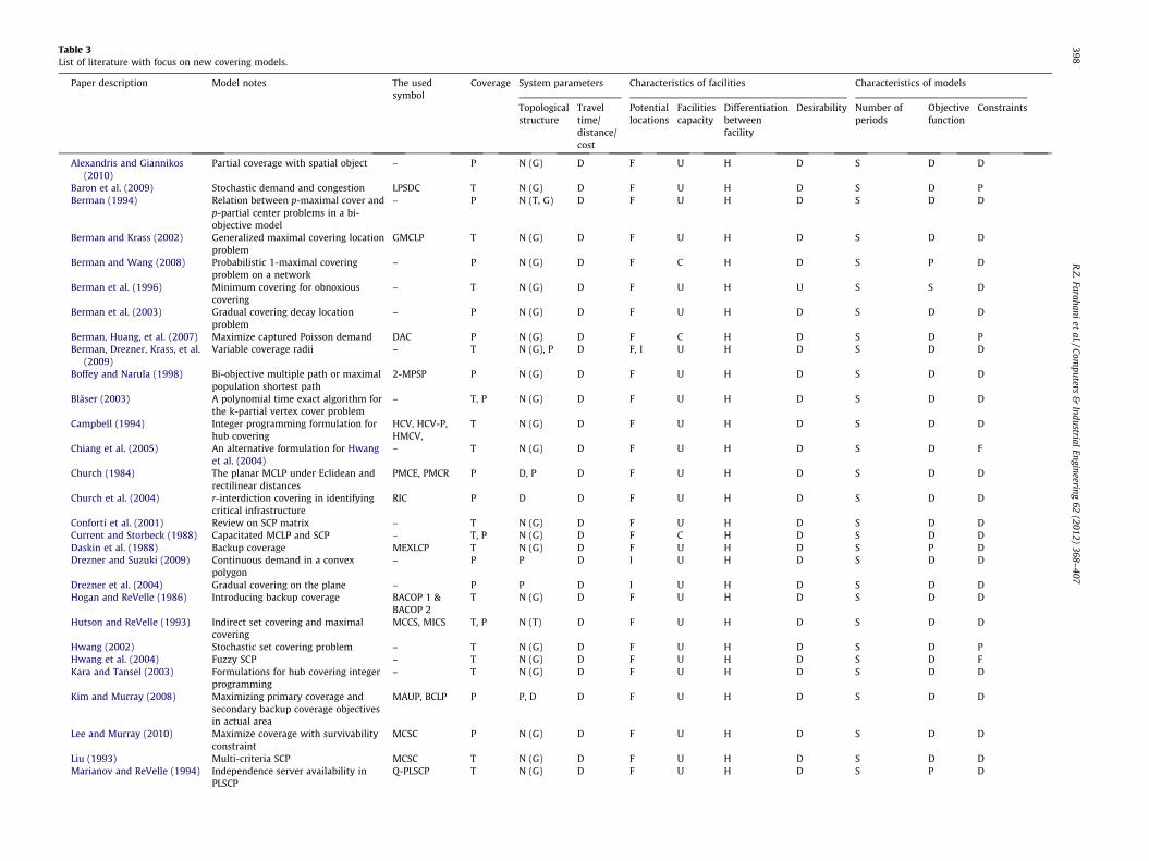
Table 3List of literature with focus on new covering models.

Paper description Model notes The usedsymbol

Coverage System parameters Characteristics of facilities Characteristics of models

Topologicalstructure

Traveltime/distance/cost

Potentiallocations

Facilitiescapacity

Differentiationbetweenfacility

Desirability Number ofperiods

Objectivefunction

Constraints

Alexandris and Giannikos(2010)

Partial coverage with spatial object – P N (G) D F U H D S D D

Baron et al. (2009) Stochastic demand and congestion LPSDC T N (G) D F U H D S D PBerman (1994) Relation between p-maximal cover and

p-partial center problems in a bi-objective model

– P N (T, G) D F U H D S D D

Berman and Krass (2002) Generalized maximal covering locationproblem

GMCLP T N (G) D F U H D S D D

Berman and Wang (2008) Probabilistic 1-maximal coveringproblem on a network

– P N (G) D F C H D S P D

Berman et al. (1996) Minimum covering for obnoxiouscovering

– T N (G) D F U H U S S D

Berman et al. (2003) Gradual covering decay locationproblem

– P N (G) D F U H D S D D

Berman, Huang, et al. (2007) Maximize captured Poisson demand DAC P N (G) D F C H D S D PBerman, Drezner, Krass, et al.

(2009)Variable coverage radii – T N (G), P D F, I U H D S D D

Boffey and Narula (1998) Bi-objective multiple path or maximalpopulation shortest path

2-MPSP P N (G) D F U H D S D D

Bläser (2003) A polynomial time exact algorithm forthe k-partial vertex cover problem

– T, P N (G) D F U H D S D D

Campbell (1994) Integer programming formulation forhub covering

HCV, HCV-P,HMCV,

T N (G) D F U H D S D D

Chiang et al. (2005) An alternative formulation for Hwanget al. (2004)

– T N (G) D F U H D S D F

Church (1984) The planar MCLP under Eclidean andrectilinear distances

PMCE, PMCR P D, P D F U H D S D D

Church et al. (2004) r-interdiction covering in identifyingcritical infrastructure

RIC P D D F U H D S D D

Conforti et al. (2001) Review on SCP matrix – T N (G) D F U H D S D DCurrent and Storbeck (1988) Capacitated MCLP and SCP – T, P N (G) D F C H D S D DDaskin et al. (1988) Backup coverage MEXLCP T N (G) D F U H D S P DDrezner and Suzuki (2009) Continuous demand in a convex

polygon– P P D I U H D S D D

Drezner et al. (2004) Gradual covering on the plane – P P D I U H D S D DHogan and ReVelle (1986) Introducing backup coverage BACOP 1 &

BACOP 2T N (G) D F U H D S D D

Hutson and ReVelle (1993) Indirect set covering and maximalcovering

MCCS, MICS T, P N (T) D F U H D S D D

Hwang (2002) Stochastic set covering problem – T N (G) D F U H D S D PHwang et al. (2004) Fuzzy SCP – T N (G) D F U H D S D FKara and Tansel (2003) Formulations for hub covering integer

programming– T N (G) D F U H D S D D

Kim and Murray (2008) Maximizing primary coverage andsecondary backup coverage objectivesin actual area

MAUP, BCLP P P, D D F U H D S D D

Lee and Murray (2010) Maximize coverage with survivabilityconstraint

MCSC P N (G) D F U H D S D D

Liu (1993) Multi-criteria SCP MCSC T N (G) D F U H D S D DMarianov and ReVelle (1994) Independence server availability in

PLSCPQ-PLSCP T N (G) D F U H D S P D

398R

.Z.Farahaniet

al./Computers

&Industrial

Engineering62

(2012)368–

407

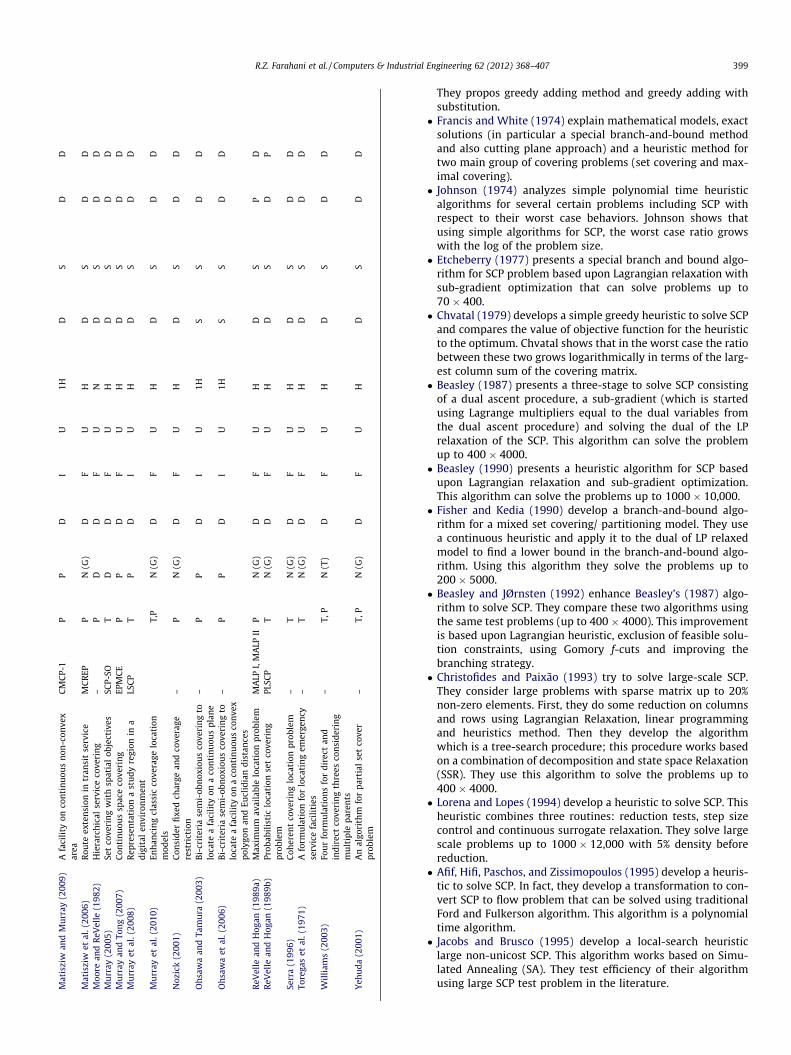
Mat

iszi

wan

dM

urr

ay(2

009)

Afa

cili

tyon

con

tin

uou

sn

on-c

onve

xar

eaC

MC

P-1

PP

DI

U1H

DS

DD

Mat

iszi

wet

al.(

2006

)R

oute

exte

nsi

onin

tran

sit

serv

ice

MC

REP

PN

(G)

DF

UH

DS

DD

Moo

rean

dR

eVel

le(1

982)

Hie

rarc

hic

alse

rvic

eco

veri

ng

–P

DD

FU

ND

SD

DM

urr

ay(2

005)

Set

cove

rin

gw

ith

spat

ial

obje

ctiv

esSC

P-SO

TD

DF

UH

DS

DD

Mu

rray

and

Ton

g(2

007)

Con

tin

uou

ssp

ace

cove

rin

gEP

MC

EP

PD

FU

HD

SD

DM

urr

ayet

al.(

2008

)R

epre

sen

tati

ona

stu

dyre

gion

ina

digi

tal

envi

ron

men

tLS

CP

TP

DI

UH

DS

DD

Mu

rray

etal

.(20

10)

Enh

anci

ng

clas

sic

cove

rage

loca

tion

mod

els

T,P

N(G

)D

FU

HD

SD

D

Noz

ick

(200

1)C

onsi

der

fixe

dch

arge

and

cove

rage

rest

rict

ion

–P

N(G

)D

FU

HD

SD

D

Oh

saw

aan

dTa

mu

ra(2

003)

Bi-

crit

eria

sem

i-ob

nox

iou

sco

veri

ng

tolo

cate

afa

cili

tyon

aco

nti

nu

ous

plan

e–

PP

DI

U1H

SS

DD

Oh

saw

aet

al.(

2006

)B

i-cr

iter

iase

mi-

obn

oxio

us

cove

rin

gto

loca

tea

faci

lity

ona

con

tin

uou

sco

nve

xpo

lygo

nan

dEu

clid

ian

dist

ance

s

–P

PD

IU

1HS

SD

D

ReV

elle

and

Hog

an(1

989a

)M

axim

um

avai

labl

elo

cati

onpr

oble

mM

ALP

I,M

ALP

IIP

N(G

)D

FU

HD

SP

DR

eVel

lean

dH

ogan

(198

9b)

Prob

abil

isti

clo

cati

onse

tco

veri

ng

prob

lem

PLSC

PT

N(G

)D

FU

HD

SD

P

Serr

a(1

996)

Coh

eren

tco

veri

ng

loca

tion

prob

lem

–T

N(G

)D

FU

HD

SD

DTo

rega

set

al.(

1971

)A

form

ula

tion

for

loca

tin

gem

erge

ncy

serv

ice

faci

liti

es–

TN

(G)

DF

UH

DS

DD

Wil

liam

s(2

003)

Fou

rfo

rmu

lati

ons

for

dire

ctan

din

dire

ctco

veri

ng

thre

esco

nsi

deri

ng

mu

ltip

lepa

ren

ts

–T,

PN

(T)

DF

UH

DS

DD

Yeh

uda

(200

1)A

nal

gori

thm

for

part

ial

set

cove

rpr

oble

m–

T,P

N(G

)D

FU

HD

SD

D


They propos greedy adding method and greedy adding withsubstitution. Francis and White (1974) explain mathematical models, exact

solutions (in particular a special branch-and-bound methodand also cutting plane approach) and a heuristic method fortwo main group of covering problems (set covering and max-imal covering). Johnson (1974) analyzes simple polynomial time heuristic

algorithms for several certain problems including SCP withrespect to their worst case behaviors. Johnson shows thatusing simple algorithms for SCP, the worst case ratio growswith the log of the problem size. Etcheberry (1977) presents a special branch and bound algo-

rithm for SCP problem based upon Lagrangian relaxation withsub-gradient optimization that can solve problems up to70 400. Chvatal (1979) develops a simple greedy heuristic to solve SCP

and compares the value of objective function for the heuristicto the optimum. Chvatal shows that in the worst case the ratiobetween these two grows logarithmically in terms of the larg-est column sum of the covering matrix. Beasley (1987) presents a three-stage to solve SCP consisting

of a dual ascent procedure, a sub-gradient (which is startedusing Lagrange multipliers equal to the dual variables fromthe dual ascent procedure) and solving the dual of the LPrelaxation of the SCP. This algorithm can solve the problemup to 400 4000. Beasley (1990) presents a heuristic algorithm for SCP based

upon Lagrangian relaxation and sub-gradient optimization.This algorithm can solve the problems up to 1000 10,000. Fisher and Kedia (1990) develop a branch-and-bound algo-

rithm for a mixed set covering/ partitioning model. They usea continuous heuristic and apply it to the dual of LP relaxedmodel to find a lower bound in the branch-and-bound algo-rithm. Using this algorithm they solve the problems up to200 5000. Beasley and JØrnsten (1992) enhance Beasley’s (1987) algo-

rithm to solve SCP. They compare these two algorithms usingthe same test problems (up to 400 4000). This improvementis based upon Lagrangian heuristic, exclusion of feasible solu-tion constraints, using Gomory f-cuts and improving thebranching strategy. Christofides and Paixão (1993) try to solve large-scale SCP.

They consider large problems with sparse matrix up to 20%non-zero elements. First, they do some reduction on columnsand rows using Lagrangian Relaxation, linear programmingand heuristics method. Then they develop the algorithmwhich is a tree-search procedure; this procedure works basedon a combination of decomposition and state space Relaxation(SSR). They use this algorithm to solve the problems up to400 4000. Lorena and Lopes (1994) develop a heuristic to solve SCP. This

heuristic combines three routines: reduction tests, step sizecontrol and continuous surrogate relaxation. They solve largescale problems up to 1000 12,000 with 5% density beforereduction. Afif, Hifi, Paschos, and Zissimopoulos (1995) develop a heuris-

tic to solve SCP. In fact, they develop a transformation to con-vert SCP to flow problem that can be solved using traditionalFord and Fulkerson algorithm. This algorithm is a polynomialtime algorithm. Jacobs and Brusco (1995) develop a local-search heuristic

large non-unicost SCP. This algorithm works based on Simu-lated Annealing (SA). They test efficiency of their algorithmusing large SCP test problem in the literature.

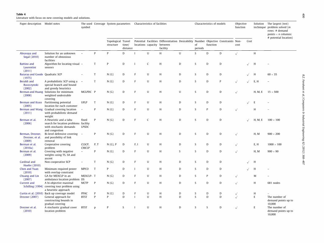
Table 4Literature with focus on new covering models and solutions.

Paper description Model notes The usedsymbol

Coverage System parameters Characteristics of facilities Characteristics of models Objectivefunction

Solutiontechnique

The largest (test)problem solved (mrows: # demandpoints n columns:# potential location)

Topologicalstructure

Traveltime/distance

Potentiallocations

Facilitiescapacity

Differentiationbetweenfacility

Desirability Numberofperiods

Objectivefunction

Constraints Non-cost

Cost

Abravaya andSegal (2010)

Solution for an unknownnumber of obnoxiousfacilities

– P P D I U H U S D Dp

H

Battino andLaurentini(2011)

Algorithm for locating visualsensors

– T P D I C H D S D Dp

H –

Bazaraa and Goode(1975)

Quadratic SCP – T N (G) D F U H D S D Dp

H 60 35

Beraldi andRuszczynski(2002)

A probabilistic SCP using aspecial branch and boundand greedy heuristics

– T N (G) D F U H D S D Pp p

E, H –

Berman and Huang(2008)

Solutions for minimumweighted undesirablecovering

MCLPDC P N (G) D F U H U S D Dp

H, M, E 15 500

Berman and Krass(2005)

Partitioning potentiallocation for each customer

UFLP T N (G) D F U H D S D Dp

E –

Berman and Wang(2011)

Gradual covering locationwith probabilistic demandweight

– P N (G) D F U H D S P Dp

H –

Berman et al.(2006)

A Heuristic and a tabusearch for location problemswith stochastic demandsand congestion

fixedfacilityLPSDC

P N (G) D F C H D S D Dp

H, M, E 100 100

Berman, Drezner,Drezner, et al.(2009)

Bi-level defensive coveringand possibility of linkremoval

– P N (G) D F U H D S D Dp

H, M 900 200

Berman et al.(2010a)

Cooperative coveringproblem

CLSCP,CMCLP

P, T N (G), P D F, I U H D S D Dp

E, H 1000 100

Berman et al.(2009)

Covering with negativeweights using TS, SA andascent

– P N (G) D F U H S S D Dp

H, M 900 90

Cardinal andHoefer (2010)

Non-cooperative SCP – T N (G) D F U H D S D Dp

H

Chen and Yuan(2010)

Minimum required powerwith overlap constraint

MPCO T P D I U H D S D Dp

H –

Chuang and Lin(2007)

GA for MEXCLP in anambulance location problem

MEXCLP-DS

T N (G) D F U H D S P Dp

M –

Current andSchilling (1994)

A bi-objective maximalcovering tour problem usinga heuristic approach

MCTP P N (G) D F U H D S D Dp

H 681 nodes

Curtin et al. (2010) Back up coverage model PPAC P N (G) D F U H D S D Dp

H –Drezner (2007) General approach for

constructing bounds ingradual covering

BTST P P D I U H D S D Dp

E The number ofdemand points up to10,000

Drezner et al.(2010)

A stochastic gradual coverlocation problem

BTST p P S I U H D S S Dp

E The number ofdemand points up to10,000

400R

.Z.Farahaniet

al./Computers

&Industrial

Engineering62

(2012)368–

407

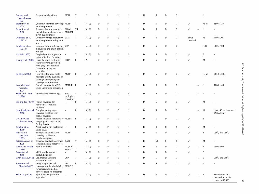
Drezner andWesolowsky(1994)

Propose an algorithm MCLP T P D I U H U S D D H

Erdemir et al.(2008)

Quadratic maximal coveringlocation problem

MCLP T N (G) D F U H D S D Dp

M, H 150 120

Erdemir et al.(2010)

Set cover backup coveragemodel; Maximal cover for agiven budget model

SCBMMCGBM

T P N (G) D I U H D S D Dp p

H –

Gendreau et al.(1997a)

Double coverage ambulancelocation problem using tabusearch

DSM T N (G) D F U H D S D D Totaldemand

M 400 70

Gendreau et al.(1997b)

Covering tour problem usinga heuristic and exact branchand cut

CTP T N (G) D F U H D S D D E, H 600 100

Hakimi (1965) Graph theoretic approachusing a Boolean function

– T N (G) D F U H D S D Dp

E –

Huang et al. (2006) Fuzzy bi-objective linearfeature covering problemwith poly lines distanceconstraints using antalgorithm

LFCP P P D F U H D S F Fp

M –

Jia et al. (2007) Heuristics for large scalemultiple facility quantity-of-coverage and quality-of-coverage requirements

MCLP P N (G) D F U N D S D Dp

H, M 2054 200

Karasakal andKarasakal(2004)

Partial coverage in MCLPusing Lagrangian relaxation

MCLP-P P N (G) D F U H D S D Dp

H 1000 40

Kolen and Tamir(1990)

Introduction to covering SCP,multiplecovering

– N (G) D F U H D S D Dp

– –

Lee and Lee (2010) Partial coverage forhierarchical locationproblem

– P N (G) D F C H D S D Dp

M –

Naimi Sadigh et al.(2010)

Complementary edgecovering problem withpartial coverage

– P N (G) D F C H D S D Dp

M Up to 40 vertices and456 edges.

O’Hanley andChurch (2011)

robust coverage networks tohedge against worst-casefacility losses

MCLIP P N (G) D F U N D S D Dp

E

Oztekin et al.(2010)

Asset tracking in healthcareusing MCLP

– P N (G) D F U H D S D Dp

M –

Plastria andCarrizosa(1999)

Bi-objective undesirablecovering problem oncontinuous plane

MCLP T P D I U H U S D Dp

E O(n2) and O(n3)

Rajagopalan et al.(2008)

Dynamic available coveragelocation using a reactive TS

DACL T N (G) D F U H D M P Dp

M –

Vasko and Wilson(1986)

Hybrid heuristic MCSCP,WSCP

T N (G) D F U H D S D Dp p

H 200 500

Saxena et al.(2010)

MIP formulation forprobabilistic SCP

– T N (G) D F U H D S D Pp

E

Sivan et al. (2010) Conditional CoveringProblem on path

CCP T N (G) D F U H D S D Dp

E O(n2) and O(n3)

Sorensen andChurch (2010)

Integrating expectedcoverage and local reliabilityfor emergency medicalservices location problems

LR-MEXCLP

P N (G) D F U H D S D Dp

H –

Xia et al. (2010) Hybrid nested partitionalgorithm

– P N (G) D F U H D S D Dp p

H The number ofdemand points isequal to 45,000

R.Z.Farahani

etal./Com

puters&

IndustrialEngineering

62(2012)

368–407

401


Balas and Carrera (1996) present a branch-and-bound algo-rithm to solve SCP. This algorithm combine the standard sub-gradient method with primal and dual heuristics, therebyenabling it to solve problems up to 1000 10,000 with 5%density. Beasley and Chu (1996) develop a Genetic Algorithm (GA) meta-

heuristic for non-unicost SCP. They can solve problems up to1000 10,000. Al-Sultan, Hussain, and Nizami (1996) also pro-pose a genetic algorithm that can solve SCP problems up to1000 12,000. Grossman and Wool (1997) try to compare efficiency of differ-

ent algorithms to solve uni-cost SCP. They compare nineapproximation algorithms including several greedy variants,fractional relaxations, randomized algorithms and a neural net-work algorithm. In this study, they consider test problems up to500 5000 and two sets up to 28,160 5000. The results showthat round and greedy algorithms perform better. Haddadi (1997) propose a Lagrangian heuristic for large but low

density SCPs. This method is based on Lagrangian duality,greedy heuristic, sub gradient optimization and redundant cov-ers that can solve problems as large as 1000 10,000. Ceria, Nobili, and Sassano (1998) develop a Lagrangian-based

heuristic for solving large-scale SCP that can solve problemsup to 4872 968,672. Their problem originates from a real-world case in crew scheduling of the Italian Railways Company.They make use of variable fixing in designing their algorithm. Brusco, Jacobs, and Thompson (1999) develop a Simulated

Annealing (SA) meta-heuristic for a non-unicost SCP. This algo-rithm solves problems with up to 800 8000 with 10% densityin covering matrix. Caprara, Fischetti, and Toth (1999) present a Lagrangian-based

heuristic large scale SCP. In fact, they solve Ceria et al. (1998)problem for the Italian Railways Company in the same size,but their algorithm is more efficient. In the same way, basedon the initial definition of a core problem (which here isupdated dynamically), and on a primal–dual sub-gradient com-bined with column fixing they design the Lagrangian basedheuristic. Caprara, Toth, and Fischetti (2000) do a survey with focus on the

most recent and effective heuristics and exact approaches devel-oped to solve SCP. They use the test problems on Beasley’s ORLibrary which are up to 1000 10,000 with 5% density in cover-ing matrix. They show that the state-of-the-art general-purposeILP solvers like CPLEX (they had 4.0.8) and MINTO (they had 2.3)are competitive with the best exact algorithms in the literature.They also show that the performance of these ILP solvers can beimproved using an external pre-processing procedure. Hifi, Paschos, and Zissimopoulos (2000) develop an approxi-

mate algorithm to solve WSCP. They consider ideas from neuralnetwork model, the Boltzmann Machine (BM), and combinato-rial optimization. They show that the developed BM-model ismore powerful than both GH (greedy SC algorithm) and LH(Lagrangian heuristic) when dealing with instance smaller than100 nodes. The percentage of the optimal solutions provided byBM is largely higher than the others. Also, BM converges veryfast and with linear function to the size of the instances. Ohlsson, Peterson, and Söderberg (2001) develop an Artificial

Neural Network (ANN) to solve non-unicost SCP. This algorithmis a mean field feedback ANN that uses multi-linear penaltyfunction to encode the inequality constraint. They solve someavailable test problems with sizes from 200 1000 up to5000 1,000,000 with acceptable error in reasonable time. Solar, Parada, and Urrutia (2002) present a Parallel Genetic

Algorithm (PGA) to solve the SCP. This algorithm tries to takethe advantage of the inherent the parallelism GA to improveperformance. They compare this algorithm with SA and TS using

available test problems in OR Library with sizes from200 1000 up to 500 5000. Gomes, Meneses, Pardalos, and Viana (2006) compare perfor-

mances of different approximate algorithms including round,dual-LP, primal–dual, and greedy to solve the Vertex CoverProblem (VCP) and the SCP. For the VCP they used three algo-rithms and the performance ranking is greedy, dual-LP andround, respectively. For the SCP they implement all of the fouralgorithms. All of the algorithms are fast, and the greedy algo-rithm performs well in all instances. On average, the roundand primal–dual perform worse than the two others. Lan and DePuy (2006) actually discuss several randomization

methods and memory mechanisms for meta-heuristic for ran-domized property search (Meta-RaPS). They look for severaleffective algorithms to maintain a good balance between ran-domness and memory. They test their achievement on the SCPtest instances. Based on their results, for the memory mecha-nisms, the method of partial construction performs better thanpriority rule with element fitness. Incorporating memory intoMeta-RaPS can improve the solution quality for the construc-tion phase. Yagiura, Kishida, and Ibaraki (2006) develop a local search algo-

rithm, which is based on the 3-flip neighborhood (3-FNLS), forthe SCP. This algorithm which includes implementation of theneighborhood search, reducing the neighborhood size, strategicoscillation mechanism based on the adaptive control of penaltyweights, the size reduction and approach by using Lagrangianrelaxation can solve problems from 200 1000 to 4872 968,672 and density from 2% (in smaller sizes) downwards to0.2% (in larger sizes). Bautista and Pereira (2007) develop a GRASP algorithm to solve

the unicost SCP. The algorithm uses a local improvement proce-dure to solve problems up to 28,160 11,264. Crema, Loreto, and Raydan (2007) develop a method to solve

integer programming problems and Lagrangean dualproblems; they combine the sub-gradient method with thespectral choice of step length and a momentum term. To showthe efficiency of their algorithm they use small and mediumsizes SCPs. Galinier and Hertz (2007) propose three exact algorithms for

solving LSCP which is the large SCP (kind of SCP that potentiallocations are very large sets that are possibly infinite). Two ofthe algorithms (removal and insertion) determine minimal cov-ers and the third one (hitting set) produces minimum covers.They also developed heuristic versions of these algorithmsand analyzed them. Lan and DePuy (2007) present a heuristic algorithm to solve

both unicost and non-unicost SCP. They apply basic Meta-RaPS(it has already been discussed) and a heuristic that introducesrandomness into a greedy heuristic to construct a feasiblesolution. Test problems up to 100 10,000 (non-unicost) and28,160 11,264 (unicost) has been tested on this algorithm. Saxena et al. (2010) present an algorithm to solve probabilistic

set covering problem and implement it for the MIP form of itusing linear programming module (OsiClp) of COIN-OR and alsoCPLEX (version 9.0) testing 10,000 probabilistic examples. Straitiff and Cromley (2010) present a methodology for solving

location set covering problem considering distributed demandover a limited area and nondefined potential location for facili-ties. They use GIS and K = 3 central place lattices. Battino and Laurentini (2011) propose an algorithm to locate

visual sensors in order to cover interior of polynomial environ-ment. The algorithm is based on Edge Covering (EC) algorithm.By employing EC algorithm, the set S which covers edges isobtained and then if it does not cover interior of polynomialenvironment, S is modified


4.2.2. The MCLP

Downs and Camm (1996) develop an exact algorithm to solveMCLP. In fact, they design a special branch-and-bound that usesdual-based method and a greedy heuristic. They test theiralgorithm on large networks with up to 25,000 nodes existingin the literature and also on three real cases. Galvão and ReVelle (1996) develop a Lagrangian heuristics for

MCLP. They define upper bounds using vertex addition/ substi-tution method and lower bounds using a sub-gradient algo-rithm and can be used to solve problem on networks with upto 150 nodes. Resende (1998) develops a Greedy Randomized Adaptive Search

Procedure (GRASP) for MCLP. Resende also presents an upperbound for the problem that is extracted using a LP. This algo-rithm solves problems with up to 9996 demand points with0.75653% density in covering matrix. Galvão, Espejo, and Boffey (2000) try to compare heuristic

algorithms designed for the MCLP which are based on Lagrang-ian and surrogate relaxations. They use test problems in theliterature that are networks with 55–900 vertices. They showthat there is no significant difference between these methods. Gandhi, Khuller, and Srinivasan (2001) develop an f-approxima-

tion polynomial time algorithm for partial covering that com-bines primal dual algorithm with a threshold method. Later,Gandhi, Khuller, and Srinivasan (2004) improve this algorithmby applying ‘‘level-sets’’ distribution. Abravaya and Segal (2010) propose an optimization algorithm

and an efficient 12-approximation algorithm for locating an

unknown number of obnoxious facilities on the plane as manyas possible. By applying optimization algorithm, based on shift-ing strategy, a PTAS is designated. In this problem minimumdistance between each demand point and facilities is at least Sand minimum distance between each pair of facilities is atleast T.

4.2.3. Other extensions

Aytug and Saydam (2002) develop genetic algorithm for solvinglarge-scale MEXCLP against Daskin’s heuristic. Their algorithmcan solve problems with up to 1600 nodes on a network. Berman, Verter, and Kara (2007) show that in the area of Haz-

Mat transportation, the problem of quick arrival of responseteams at the accident site can be represented as a maximalarc-covering model. ReVelle, Scholssberg, and Williams (2008) apply the meta-heu-

ristic concentration to solve large MCLPs. They solve problemswith 900 nodes and 20 existing facilities.

5. Applications and real-world cases

5.1. Applications

This section is dedicated to the literature that addresses appli-cation of covering problems in facility location without focusingon a special real problem in certain place of the world. In fact, cov-ering problems were originally introduced by Toregas et al. (1971)to model and locate emergency service facilities (and especially firestations) as a SCP with equal costs.

Schilling et al. (1993) in their review paper divide the applica-tions into two main categories: (i) public sector and (ii) private sec-tor, as decision makers in these two categories are looking fordifferent objectives (Farahani, Asgari, & Davarzani, 2009). Publicsectors like governmental organizations look for maximizing ser-vicing to the people using limited resources like in MCLP; while

private sectors look for maximizing (minimizing) their profit (cost)like in SCP.

There are many instances of covering-type considerationsincorporated in the literature like network interdiction, forestmanagement, and ecological conservation. However, Schillinget al. (1993) mention following applications for coveringproblems:– Bus stop location.– Terrain visibility.– Fire company relocation.– Fire service sitting.– Fire equipment allocation. Pastor (1994) uses MCLP to locate a network of bank branches. Daskin (1995) explains two applications of set covering

problem:– Airline crew scheduling.– Tool selection in flexible manufacturing systems. Boffey and Narula (1998) list examples of applications such as:

– Oil spill equipment.– Archaeological settlement pattern.– Rural health centers.– Direct mail marketing.– Health care units.– Essential air services.– Ambulances.– Early detection of glaucoma.– Health care centers.– Disease eradication.– Emergency Medical Services (EMS) vehicles.

Mandell (1998) develops a MEXCLP model for locating EMSsystems. Badri, Mortagy, and Colonel (1998) develop a multiple conflic-

tive objective model to locate fire stations. Freling, Huisman, and Wagelmans (2003) use SCP in vehicle and

crew scheduling. Drezner et al. (2004, 2010) present some general applications of

the gradual covering problem and it’s stochastic kind including– The delivery problem.– Competitive location.– Dense competition.– The radio, TV, or cellular transmitter problem.– Medical facility location problem. Coslovich, Pesenti, and Ukovich (2006) use SCP as part of a solu-

tion technique for fleet management problem in containertrucking industry. Hollis, Forbes, and Douglas (2006) use SCP as part of a solution

technique for multi-depot combined vehicle and crew schedul-ing problem. Chuang and Lin (2007) use a combination of MEXLCP with DSM

for an ambulance location problem to prove sufficient coverageof EMSs. Jans and Degraeve (2008) present use of SCP for lottery

problem. Mirchandani and Li (2010) use SCP and MCLP models to locate a

Surveillance Infrastructure in and Near Ports or on Other PlanarSurfaces to Monitor Flows and develop Lagrangian heuristic anda two-stage procedure with a conquer-and-divide scaling tosolve them. Sorensen and Church (2010) use LR-MEXCLP for emergency

medical services location problems. Wang, Ghosh, and Daskin (2010) review on sensor localization

problem categorized into proximity-based localization, range-based localization and angle-based localization.

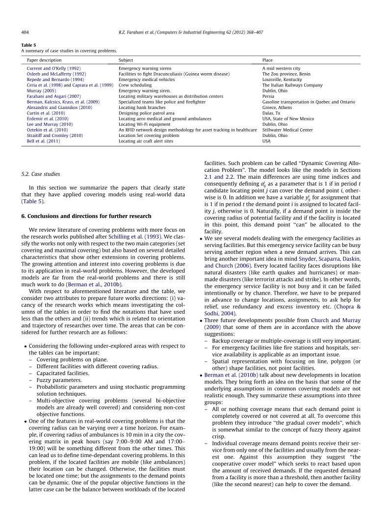
Table 5A summary of case studies in covering problems.

Paper description Subject Place

Current and O’Kelly (1992) Emergency warning sirens A mid western cityOsleeb and McLafferty (1992) Facilities to fight Dracunculiasis (Guinea worm disease) The Zou province, BeninRepede and Bernardo (1994) Emergency medical vehicles Louisville, KentuckyCeria et al. (1998) and Caprara et al. (1999) Crew scheduling The Italian Railways CompanyMurray (2005) Emergency warning siren. Dublin, OhioFarahani and Asgari (2007) Locating military warehouses as distribution centers PersiaBerman, Kalcsics, Krass, et al. (2009) Specialized teams like police and firefighter Gasoline transportation in Quebec and OntarioAlexandris and Giannikos (2010) Locating bank branches Greece, AthensCurtin et al. (2010) Designing police patrol area Dalas, TxErdemir et al. (2010) Locating aero medical and ground ambulances USA, State of New MexicoLee and Murray (2010) Locating Wi-Fi equipment Dublin, OhioOztekin et al. (2010) An RFID network design methodology for asset tracking in healthcare Stillwater Medical CenterStraitiff and Cromley (2010) Location Set covering problem Dublin, OhioBell et al. (2011) Locating air craft alert sites USA


5.2. Case studies

In this section we summarize the papers that clearly statethat they have applied covering models using real-world data(Table 5).

6. Conclusions and directions for further research

We review literature of covering problems with more focus onthe research works published after Schilling et al. (1993). We clas-sify the works not only with respect to the two main categories (setcovering and maximal covering) but also based on several detailedcharacteristics that show other extensions in covering problems.The growing attention and interest into covering problems is dueto its application in real-world problems. However, the developedmodels are far from the real-world problems and there is stillmuch work to do (Berman et al., 2010b).

With respect to aforementioned literature and the table, weconsider two attributes to prepare future works directions: (i) va-cancy of the research works which means investigating the col-umns of the tables in order to find the notations that have usedless than the others and (ii) trends which is related to orientationand trajectory of researches over time. The areas that can be con-sidered for further research are as follows:

Considering the following under-explored areas with respect tothe tables can be important:– Covering problems on plane.– Different facilities with different covering radius.– Capacitated facilities.– Fuzzy parameters.– Probabilistic parameters and using stochastic programming

solution techniques.– Multi-objective covering problems (several bi-objective

models are already well covered) and considering non-costobjective functions.

One of the features in real-world covering problems is that thecovering radius can be varying over a time horizon. For exam-ple, if covering radius of ambulances is 10 min in a city the cov-ering matrix in peak hours (say 7:00–9:00 AM and 17:00–19:00) will be something different from the other times. Thiscan lead us to define time-dependant covering problems. In thisproblem, if the located facilities are mobile (like ambulances)their location can be changed. Otherwise, the facilities mustbe located one time; but the assignments to the demand pointscan be dynamic. One of the popular objective functions in thelatter case can be the balance between workloads of the located

facilities. Such problem can be called ‘‘Dynamic Covering Allo-cation Problem’’. The model looks like the models in Sections2.1 and 2.2. The main differences are using time indices andconsequently defining at

ij as a parameter that is 1 if in period tcandidate locating point j can cover the demand point i, other-wise is 0. In addition we have a variable yt

ij for assignment thatis 1 if in period t the demand point i is assigned to located facil-ity j, otherwise is 0. Naturally, if a demand point is inside thecovering radius of potential facility and if the facility is locatedin this point, this demand point ‘‘can’’ be allocated to thefacility. We see several models dealing with the emergency facilities as

serving facilities. But this emergency service facility can be busyserving another region when a new demand arrives. This canbring another important idea in mind Snyder, Scaparra, Daskin,and Church (2006). Every located facility faces disruptions likenatural disasters (like earth quakes and hurricanes) or man-made disasters (like terrorist attacks and strike). In other words,the emergency service facility is not busy and it can be failedintentionally or by chance. Therefore, we have to be preparedin advance to change locations, assignments, to ask help forrelief, use redundancy and excess inventory etc. (Chopra &Sodhi, 2004). Three future developments possible from Church and Murray

(2009) that some of them are in accordance with the abovesuggestions:– Backup coverage or multiple-coverage is still very important.– For emergency facilities like fire stations and hospitals, ser-

vice availability is applicable as an important issue.– Spatial representation with focusing on line, polygon (or

other) shape facilities, not point facilities. Berman et al. (2010b) talk about new developments in location

models. They bring forth an idea on the basis that some of theunderlying assumptions in common covering models are notrealistic enough. They summarize these assumptions into threegroups:– All or nothing coverage means that each demand point is

completely covered or not covered at all. To overcome thisproblem they introduce ‘‘the gradual cover models’’, whichis somewhat similar to the concept of fuzzy theory againstcrisp.

– Individual coverage means demand points receive their ser-vice from only one of the facilities and usually from the near-est one. Against this assumption they suggest ‘‘thecooperative cover model’’ which seeks to react based uponthe amount of received demands. If the requested demandfrom a facility is more than a threshold, then another facility(like the second nearest) can help to cover the demand.


– Fixed coverage radius that is the opposite of ‘‘variable radiusmodel’’. Variable radius model assumes that due to the factthat constructing the facilities are very costly and most ofthe time there is budget constraint for locating facilities,the new model tries to identify where and what kind of facil-ities should be installed. Naturally, different facilities havedifferent costs and different covering radius.

Berman, Drezner, Drezner, et al. (2009) consider a defensivemaximal covering model on a network; it is assumed that oneof the links of the network will become unusable due to anattack (terrorist or a natural disaster). We can consider anattack to our new located facilities. i.e. while we prefer to locatenew facilities somehow to cover more populations an attackerin the worst case decides to attack to the crowded centers. In location-reliability problems most of the time we consider a

failure probability as given. The question is how we can calcu-late this probability in real-world problems. These events arelow-probability high-consequence events like incidents involv-ing hazardous materials. In other words, these probabilities areusually unknown, since these events are rare and we cannotfind sufficient data to estimate these probabilities. On the otherhand, if we consider a long term historical data that are not reli-able because of the drastic changes that occur in world, theprobability would not be the same as in the past. One solutionto this problem is considering a very risk-averse planner whodoes not know this probability but who wants to consider theworst case scenario (Szeto, Farahani, & Sumalee, 2010). Anotherextension of this problem is considering more than one attacksimultaneously. Moreover, we can consider a mixed strategy;i.e. since these problems are solvable using game theoreticapproach and those are usually non-cooperative, maybe thereis not any equilibrium point for the problem; but we will havedifferent probability for attack to different facilities.

Acknowledgment

The authors indebted to Prof. Oded Berman who provided usseveral important and related references and gave some importantcomments on the paper. The authors also would like to thankanonymous referees for their constructive suggestions, which im-proved the content.

References

Abravaya, S., & Segal, M. (2010). Maximizing the number of obnoxious facilities tolocate within a bounded region. Computers and Operations Research, 37,163–171.

Afif, M., Hifi, M., Paschos, V. T., & Zissimopoulos, V. (1995). A new efficient heuristicfor the minimum set covering problem. Journal of the Operational ResearchSociety, 46(10), 1260–1268.

Alexandris, G., & Giannikos, I. (2010). A new model for maximal coverage exploitinggis capabilities. European Journal of Operational Research, 202, 328–338.

Al-Sultan, K. S., Hussain, M. F., & Nizami, J. S. (1996). A genetic algorithm for the setcovering problem. The Journal of the Operational Research Society, 47(5),702–709.

Aytug, H., & Saydam, C. (2002). Solving large-scale maximum expected coveringlocation problems by genetic algorithms: A comparative study. European Journalof Operational Research, 141(3), 480–494.

Badri, M. A., Mortagy, A. K., & Colonel, A. A. (1998). A multi-objective model forlocating fire stations. European Journal of Operational Research, 110, 243–260.

Balas, E., & Carrera, M. C. (1996). A dynamic sub gradient-based branch-and-boundprocedure for set covering. Operations Research, 44(6), 875–890.

Baron, O., Berman, O., Kim, S., & Krass, D. (2009). Ensuring feasibility in locationproblems with stochastic demands and congestion. IIE Transactions, 41(4),467–481.

Battino, A., & Laurentini, A. (2011). A nearly optimal algorithm for covering theinterior of an art gallery. Pattern Recognition, 44, 1048–1056.

Bautista, J., & Pereira, J. (2007). A GRASP algorithm to solve the unicost set coveringproblem. Computers and Operations Research, 34(10), 3162–3173.

Bazaraa, M. S., & Goode, J. J. (1975). A cutting plane algorithm for the quadratic setcovering problem. Operations Research, 23(1), 150–158.

Beasley, J. E. (1987). An algorithm for set covering problem. European Journal ofOperational Research, 31, 85–93.

Beasley, J. E. (1990). A Lagrangian heuristic for set-covering problems. NavalResearch Logistics, 37, 151–164.

Beasley, J. E., & Chu, P. C. (1996). A genetic algorithm for the set covering. EuropeanJournal of Operational Research, 94(2), 392–404.

Beasley, J. E., & JØrnsten, K. (1992). Enhancing an algorithm for set coveringproblems. European Journal of Operational Research, 58, 293–300.

Bell, J. E., Griffis, S. E., Cunningham, W. A., III, & Eberlan, J. A. (2011). Locationoptimization of strategic alert sites for homeland defense. Omega, 39, 151–158.

Bellmore, M., & Ratlief, H. D. (1971). Set covering and involuntary bases.Management Science, 18, 194–206.

Beraldi, P., & Ruszczynski, A. (2002). The probabilistic set-covering problem.Operations Research, 50(6), 956–967.

Berg, M., Cabello, S., & Har-Peled, S. (2006). Covering many or few points with unitdisks. In T. Erlebach & C. Kaklamanis (Eds.), WAOA 2006. LNCS (Vol. 4368,pp. 55–68). Berlin: Springer-Verlag.

Berman, O. (1994). The p maximal cover–p partial center problem on networks.European Journal of Operational Research, 72(2), 432–442.

Berman, O., Drezner, T., Drezner, Z., & Wesolowsky, G. O. (2009). A defensivemaximal covering problem on a network. International Transactions inOperational Research, 16, 69–86.

Berman, O., Drezner, Z., & Krass, D. (2010a). Cooperative cover location problems:The planar case. IIE Transactions, 42(3), 232–246.

Berman, O., Drezner, Z., & Krass, D. (2010b). Generalized coverage: Newdevelopments in covering location models. Computers & Operations Research,37(10), 1675–1687.

Berman, O., Drezner, Z., Krass, D., & Wesolowsky, G. O. (2009). The variable radiuscovering problem. European Journal of Operational Research, 196, 516–525.

Berman, O., Drezner, Z., & Wesolowsky, G. O. (1996). Minimum covering criterionfor obnoxious facility location on a network. Networks, 28, 1–5.

Berman, O., Drezner, Z., & Wesolowsky, G. O. (2009). The maximal covering problemwith some negative weights. Geographical Analysis, 41, 30–42.

Berman, O., & Huang, R. (2008). The minimum weighted covering location problemwith distance constraints. Computers and Operations Research, 35(2), 365–372.

Berman, O., Huang, R., Kim, S., & Menezes, M. B. C. (2007). Locating capacitatedfacilities to maximize captured demand. IIE Transactions, 39(11), 1015–1029.

Berman, O., Kalcsics, G., Krass, D., & Nickel, S. (2009). The ordered gradual coveringlocation problem on a network. Discrete Applied Mathematics, 157(18),3689–3707.

Berman, O., & Krass, D. (2002). The generalized maximal covering location problem.Computers and Operations Research, 29, 563–581.

Berman, O., & Krass, D. (2005). An improved IP formulation for the uncapacitatedfacility location problem: Capitalizing on objective function structure. Annals ofOperations Research, 136, 21–34.

Berman, O., Krass, D., & Drezner, Z. (2003). The gradual covering decay locationproblem on a network. European Journal of Operational Research, 151, 474–480.

Berman, O., Krass, d., & Wang, J. (2006). Locating service facilities to reduce lossdemand. IIE Transactions, 38(11), 933–946.

Berman, O., Verter, V., & Kara, B. (2007). Designing emergency response networksfor hazardous materials transportation. Computers and Operations Research, 34,1374–1388.

Berman, O., & Wang, J. (2008). The probabilistic 1-maximal covering problem on anetwork with discrete demand weights. Journal of Operational Research Society,59, 1398–1405.

Berman, O., & Wang, J. (2011). The minmax regret gradual covering locationproblem on a network with incomplete information of demand weights.European Journal of Operational Research Society, 208, 233–238.

Bläser, M. (2003). Computing small partial coverings. Information Processing Letters,85, 327–331.

Boffey, B., & Narula, S. C. (1998). Models for multi-path covering-routing problems.Annals of Operations Research, 82, 331–342.

Brusco, M. J., Jacobs, L. W., & Thompson, G. M. (1999). A morphing procedure tosupplement a simulated annealing heuristic for cost- and coverage-correlatedweighted set-covering problems. Annals of Operations Research, 86, 611–627.

Campbell, J. F. (1994). Integer programming formulations of discrete hub locationproblems. European Journal of Operational Research, 72(2), 387–405.

Caprara, A., Fischetti, M., & Toth, P. (1999). A heuristic method for the set coveringproblem. Operations Research, 47(5), 730–743.

Caprara, A., Toth, P., & Fischetti, M. (2000). Algorithms for the set covering problem.Annals of Operations Research, 98, 353–371.

Cardinal, J., & Hoefer, M. (2010). Non-cooperative facility location and coveringgames. Theoretical Computer Science, 411, 1855–1876.

Ceria, S., Nobili, P., & Sassano, A. (1998). A Lagrangian-based heuristic for large-scaleset covering problems. Mathematical Programming, 81(2), 215–228.

Chen, L., & Yuan, D. (2010). Solving a minimum-power covering problem withoverlap constraint for cellular network design. European Journal of OperationalResearch, 203, 714–723.

Chiang, C. I., Hwang, M. J., & Liu, Y. H. (2005). An alternative formulation for certainfuzzy set-covering Problems. Mathematical and Computer Modelling, 42,363–365.

Chopra, S., & Sodhi, M. S. (2004). Managing risk to avoid supply-chain breakdown.MIT Sloan Management Review, 46(1), 53–61.

Christofides, N., & Paixão, J. (1993). Algorithms for large scale set covering problems.Annals of Operations Research, 43, 261–277.


Chuang, C., & Lin, R. (2007). A maximum expected covering model for an ambulancelocation problem. Journal of the Chinese Institute of Industrial Engineers, 24(6),468–474.

Church, R. L. (1984). The planar maximal covering location problem. Journal ofRegional Science, 2(24), 185–201.

Church, R. L., & Murray, A. T. (2009). Business site section, location analysis and GIS.New York: Wiley.

Church, R. L., & ReVelle, C. (1974). The maximal covering location problem. Papers ofthe Regional Science Association, 32, 101–118.

Church, R. L., Scaparra, M. P., & Middleton, R. S. (2004). Identifying criticalinfrastructure: The median and covering facility interdiction problems. Annalsof the Association of American Geographers, 94(3), 491–502.

Chvatal, V. (1979). A greedy heuristic for the set covering problem. Mathematics ofOperations Research, 4(3), 233–235.

Conforti, M., Cornuéjols, G., Kapoor, A., & VuŠkovic, K. (2001). Perfect, ideal andbalanced matrices. European Journal of Operational Research, 133, 455–461.

Coslovich, L., Pesenti, R., & Ukovich, W. (2006). Minimizing fleet operating costs fora container transportation company. European Journal of Operational Research,171, 776–786.

Crema, A., Loreto, M., & Raydan, M. (2007). Spectral projected subgradient with amomentum term for the lagrangian dual approach. Computers and OperationsResearch, 34(10), 3174–3186.

Current, J. R., & O’Kelly, M. (1992). Locating emergency warning sirens. DecisionSciences, 23(1), 221–234.

Current, J. R., & Schilling, D. A. (1994). The median tour and maximal coveringproblems. European Journal of Operations Research, 73, 114–126.

Current, J. R., & Storbeck, J. E. (1988). Capacitated covering models. Environment andPlanning B: Planning and Design, 15(2), 153–163.

Curtin, K. M., Hayslett-McCall, K., & Qiu, F. (2010). Determining optimal policepatrol areas with maximal covering and backup covering location models.Networks and Spatial Economics, 10(1), 125–145.

Daskin, M. S. (1982). Application of an expected covering model to emergencymedical service system design. Decision Sciences, 13, 416–439.

Daskin, M. S. (1983). A maximal expected covering location model, formulationproperties and heuristic solution. Transportation Science, 17, 48–69.

Daskin, M. S. (1995). Network and discrete location: Models, algorithms andapplications. New York, US: John Wiley and Sons.

Daskin, M. S., Hogan, K., & ReVelle, C. (1988). Integration of multiple excess backupand expected covering models. Environment and Planning B: Planning and Design,15, 15–35.

Downs, B. T., & Camm, J. D. (1996). An exact algorithm for the maximal coveringlocation problem. Naval Research Logistics, 43(3), 435–461.

Drezner, Z. (Ed.). (1995). Facility location: A survey of applications and methods.Berlin, Germany: Springer Verlag.

Drezner, Z. (2007). A general global optimization approach for solving locationproblems in the plane. Journal of Global Optimization, 37(2), 305–319.

Drezner, T., Drezner, Z., & Goldstein, Z. (2010). A stochastic gradual cover locationproblem. Wiley InterScience. 57, 367-372.

Drezner, Z., & Hamacher, H. W. (Eds.). (2002). Facility location: Applications andtheory. Berlin, Germany: Springer-Verlag.

Drezner, Z., & Suzuki, A. (2009). Covering continuous demand in the plane. Journal ofthe Operational Research Society, 1–4.

Drezner, Z., & Wesolowsky, G. O. (1994). Finding the circle or rectangle containingthe minimum weight of points. Location Science, 2, 83–90.

Drezner, Z., Wesolowsky, G. O., & Drezner, T. (2004). The gradual covering problem.Naval Research Logistics, 51(6), 841–855.

Emir-Farinas, H., & Francis, R. L. (2005). Demand point aggregation for planarcovering location models. Annals of Operations Research, 136, 175–192.

Erdemir, E. T., Batta, R., Spielman, S., Rogerson, P. A., Blatt, A., & Flanigan, M. (2008).Location coverage models with demand originating from nodes and paths:Application to cellular network design. European Journal of Operational Research,190(3), 610–632.

Erdemir, E. T., Batta, R., Spielman, S., Rogerson, P. A., Blatt, A., & Flanigan, M. (2010).Joint ground and air emergency medical services coverage models: A greedyheuristic solution approach. European Journal of Operational Research, 207,736–749.

Etcheberry, J. (1977). The set-covering problem: A new implicit enumerationalgorithm. Operations Research, 25(5), 760–772.

Fallah, H., NaimiSadigh, A., & Aslanzadeh, M. (2009). Covering problem. In Facilitylocation: Concepts, models, algorithms and case studies. Heidelberg, Germany:Physica Verlag.

Farahani, R. Z., & Asgari, N. (2007). Combination of MCDM and covering techniquesin a hierarchical model for facility location: A case study. European Journal ofOperational Research, 176, 1839–1858.

Farahani, R. Z., Asgari, N., & Davarzani, H. (Eds.). (2009). Supply chain and logistics innational, international and governmental environments. Heidelberg, Germany:Physica Verlag.

Farahani, R. Z., & Hekmatfar, M. (Eds.). (2009). Facility location: Concepts, models,algorithms and case studies. Heidelberg, Germany: Physica Verlag.

Farahani, R. Z., SteadieSeifi, M., & Asgari, N. (2010). Multiple criteria facility locationproblems: A survey. Applied Mathematical Modelling, 34(7), 1689–1709.

Fisher, M. L., & Kedia, P. (1990). Optimal solution of set covering/ partitioningproblems using dual heuristics. Management Science, 36(6), 674–688.

Francis, R. L., Lowe, T. J., Rayco, M. B., & Tamir, A. (2009). Aggregation error forlocation models: Survey and analysis. Annals of Operations Research, 167(1),171–208.

Francis, R. L., McGinnis, L. F., & White, J. A. (1992). Facility layout and location: Ananalytical approach (2nd ed.). Englewood Cliffs, NJ, US: Prentice-Hall.

Francis, R. L., & White, J. A. (1974). Facility layout and location an analytical approach(1st ed.). Englewood Cliffs, NJ, US: Prentice-Hall.

Freling, R., Huisman, D., & Wagelmans, A. P. M. (2003). Models and algorithmsfor integration of vehicle and crew scheduling. Journal of Scheduling, 1(6),63–85.

Galinier, P., & Hertz, A. (2007). Solution techniques for the large set coveringproblem. Discrete Applied Mathematics, 155(3), 312–326.

Galvão, R. D., Espejo, L. G. A., & Boffey, B. (2000). A comparison of Lagrangian andsurrogate relaxations for the maximal covering location problem. EuropeanJournal of Operational Research, 124, 377–389.

Galvão, R. D., & ReVelle, C. S. (1996). A Lagrangian heuristic for the maximalcovering location problem. European Journal of Operational Research, 88,114–123.

Gandhi, R., Khuller, S., & Srinivasan, A. (2001), Approximation algorithms for partialcovering problems. In Proceeding of international colloquium on automata,languages, and programming (pp. 225-236).

Gandhi, R., Khuller, S., & Srinivasan, A. (2004). Approximation algorithms for partialcovering problems. Journal of Algorithms, 53(1), 55–84.

Garey, M. R., & Johnson, D. S. (1979). Computers and intractability: A guide to thetheory of np-completeness. New York, US: W.H. Freemann and Company.

Gendreau, M., Laporte, G., & Semet, F. (1997a). Solving an ambulance location modelby Tabu search. Location Science, 5, 75–88.

Gendreau, M., Laporte, G., & Semet, F. (1997b). The covering tour problem.Operations Research, 45(4), 568–576.

Ghosh, A., McLafferty, S., & Carig, C. S. (1995). Multifacility retail networks. InFacility location: A survey of applications and methods. Berlin Germany: SpringerVerlag.

Gomes, F. C., Meneses, C. N., Pardalos, P. M., & Viana, G. V. R. (2006). Experimentalanalysis of approximation algorithms for the vertex cover and set coveringproblems. Computers and Operations Research, 33(12), 3520–3534.

Grossman, T., & Wool, A. (1997). Computational experience with approximationalgorithms for the set covering problem. European Journal of OperationalResearch, 101(1), 81–92.

Guha, D. K. (1973). The set-covering problem with equality constraints. OperationsResearch, Mathematical Programming and Its Applications, 21(1), 348–351.

Haddadi, S. (1997). Simple Lagrangian heuristic for the set covering problem.European Journal of Operational Research, 97(1), 200–204.

Hakimi, S. L. (1965). Optimum distribution of switching centers in a communicationnetwork and some related graph theoretic problems. Operations Research, 13,462–475.

Handler, G. Y., & Mirchandani, P. B. (1979). Location on networks: Theory andalgorithms. Cambridge, MA: MIT Press.

Hifi, M., Paschos, V. T., & Zissimopoulos, V. (2000). A neural network for theminimum set covering problem. Chaos, Solitons & Fractals, 11, 2079–2089.

Hoefer, M. (2006). Non-cooperative facility location and covering games. In T. Asano(Ed.), ISAAC. LNCS (Vol. 4288, pp. 369–378). Heidelberg Germany: SpringerVerlag.

Hogan, K., & ReVelle, C. (1986). Concepts and applications of backup coverage.Management Science, 32, 1434–1444.

Hollis, B. L., Forbes, M. A., & Douglas, B. E. (2006). Vehicle routing and crewscheduling for metropolitan mail distribution at Australia post. European Journalof Operational Research, 173, 133–150.

Huang, B., Liu, N., & Chandramouli, M. (2006). A GIS supported Ant algorithm for thelinear feature covering problem with distance constraints. Decision SupportSystems, 42, 1063–1075.

Hutson, V. A., & ReVelle, C. S. (1993). Indirect covering tree problems on spanningtree networks. European Journal of Operational Research, 65(1), 20–32.

Hwang, H. (2002). Design of supply-chain logistics system considering service level.Computers and Industrial Engineering, 43, 283–297.

Hwang, M. J., Chiang, C. I., & Liu, Y. H. (2004). Solving a fuzzy set-covering problem.Mathematical and Computer Modelling, 40, 861–865.

Jacobs, L. W., & Brusco, M. J. (1995). A local search heuristic for large set-coveringproblems. Naval Research Logistics, 42, 1129–1140.

Jans, R., & Degraeve, Z. (2008). A note on a symmetrical set covering problem: Thelottery problem. European Journal of Operational Research, 186, 104–110.

Jia, H., Ordonez, F., & Dessouky, M. M. (2007). Solution approaches for facilitylocation of medical supplies for large-scale emergencies. Computers andOperations Research, 52, 257–276.

Johnson, D. S. (1974). Approximation algorithms for combinatorial problems.Journal of Computer and System Sciences, 9, 256–278.

Jones, K., & Simmons, J. (1993). Location, location, location: Analyzing the retailenvironment. Toronto, Canada: Nelson.

Karasakal, O., & Karasakal, E. K. (2004). A maximal covering location model in thepresence of partial coverage. Computers and Operations Research, 31, 1515–1526.

Kara, B. Y., & Tansel, B. C. (2003). The single assignment hub covering problem:Models and linearization. Journal of the Operational Research Society, 54, 59–64.

Kim, K., & Murray, A. T. (2008). Enhancing spatial representation in primary andsecondary coverage location modeling. Journal of Regional Science, 48, 745–768.

Klastorin, T. D. (1979). On the maximal covering location problem and thegeneralized assignment problems. Management Science, 25(1), 107–112.

Kolen, A., & Tamir, A. (1990). Covering problems. In P. B. Mirchandani & R. L. Francis(Eds.), Discrete location theory (pp. 263–304). New York, US: Wiley-Interscience.


Lan, G., & DePuy, G. W. (2006). On the effectiveness of incorporating randomnessand memory into a multi-start metaheuristic with application to the setcovering problem. Computers and Industrial Engineering, 51(3), 362–374.

Lan, G., & DePuy, G. W. (2007). Whitehouse, an effective and simple heuristic for theset covering problem. European Journal of Operational Research, 176(3),1387–1403.

Lee, J. M., & Lee, Y. H. (2010). Tabu based heuristics for the generalized hierarchicalcovering location problem. Computers & Industrial Engineering, 58, 638–645.

Lee, G., & Murray, A. T. (2010). Maximal covering with network survivabilityrequirements in wireless mesh networks. Computers, Environment and UrbanSystems, 34, 49–57.

Liu, Y. H. (1993). A heuristic algorithm for the multi criteria set-covering problems.Applied Mathematics Letters, 6, 21–23.

Lorena, L. A. N., & Lopes, F. B. (1994). A surrogate heuristic for set covering problems.European Journal of Operational Research, 79, 138–150.

Love, R., Morris, J., & Wesolowsky, G. O. (1988). Facility location: Models and methods.Amsterdam, The Netherlands: North-Holland.

Mandell, M. B. (1998). Covering models for two-tiered emergency medical servicessystems. Location Science, 6, 355–368.

Marianov, V., & ReVelle, C. (1994). The queuing probabilistic location set coveringproblem and some extensions. Socio-Economic Planning Sciences, 28, 167–178.

Marianov, V., & ReVelle, C. (1995). Siting emergency services. In Z. Drezner (Ed.),Facility location: A survey of applications and methods. Berlin, Germany: SpringerVerlag.

Matisziw, T. C., & Murray, A. T. (2009). Siting a facility in continuous space tomaximize coverage of continuously distributed demand. Socio-EconomicPlanning Sciences, 43, 131–139.

Matisziw, T. C., Murray, A. T., & Kim, C. (2006). Strategic route extension in transitnetworks. European Journal of Operational Research, 171, 661–673.

Mirchandani, P. B., & Francis, R. L. (Eds.). (1990). Discrete location theory. New York,US: Wiley-Interscience-Interscience.

Mirchandani, P. B., & Li, J. Q. (2010). Locating a surveillance infrastructure in andnear ports or on other planar surfaces to monitor flows. Computer-Aided Civiland Infrastructure Engineering, 25, 89–100.

Moon, I. D., & Chaudhry, S. (1984). An analysis of network location problems withdistance constraints. Management Science, 30, 290–307.

Moore, G., & ReVelle, C. (1982). The hierarchical service location problem.Management Science, 28(7), 775–780.

Murray, A. T. (2005). Geography in coverage modeling: Exploiting spatial structureto address complementary partial service of areas. Annals of the Association ofAmerican Geographers, 95, 761–772.

Murray, A. T., O’Kelly, M. E., & Church, R. L. (2008). Regional service coveragemodeling. Computers and Operations Research, 35, 339–355.

Murray, A. T., & Tong, D. (2007). Coverage optimization in continuous space facilitysiting. International Journal of Geographical Information Sciences, 21, 757–776.

Murray, A. T., Tong, D., & Kim, K. (2010). Enhancing classic coverage locationmodels. International Regional Science Review, 33(2), 115–133.

Naimi Sadigh, A., Mozafari, M., & husseinzadeh Kashan, A. (2010). A mixed integerlinear program and Tabu search approach for the complementary edge coveringproblem. Advances in Engineering Software, 41, 762–768.

Nickel, S., & Puerto, J. (2005). Location theory: A unified approach. Berlin, Germany:Springer Verlag.

Nozick, L. K. (2001). The fixed charge facility location problem with coveragerestriction. Transportation Research Part E, 37, 281–296.

O’Hanley, J. R., & Church, R. L. (2011). Designing robust coverage networks to hedgeagainst worst-case facility losses. European Journal of Operational Research, 209,23–36.

Ohlsson, M., Peterson, C., & Söderberg, B. (2001). An efficient mean field approach tothe set covering problem. European Journal of Operational Research, 133(3),583–595.

Ohsawa, Y., Plastria, F., & Tamura, K. (2006). Euclidean push-pull partial coveringproblems. Computers and Operations Research, 33, 3566–3582.

Ohsawa, Y., & Tamura, K. (2003). Efficient location for a semi-obnoxious facility.Annals of Operations Research, 123, 173–188.

Osleeb, J. P., & McLafferty, S. (1992). A weighted covering model to aid indracunculiasis eradication. Papers in Regional Science, 71(3), 243–257.

Owen, S. H., & Daskin, M. S. (1998). Strategic facility location: A review. EuropeanJournal of Operational Research, 111, 423–447.

Oztekin, A., Pajouh, F. M., Delen, D., & Swim, L. K. (2010). An RFID network designmethodology for asset tracking in healthcare. Decision Support Systems, 49,100–109.

Pastor, J. T. (1994). Bicriterion programs and managerial locations: Application tothe banking sector. Journal of the Operational Research Society, 45, 1351–1362.

Pirkul, H., & Schilling, D. (1989). The capacitated maximal covering locationproblem with backup service. Annals of Operations Research, 18, 141–154.

Plastria, F. (2002). Continuous covering location problems. In Z. Drezner & H. W.Hamacher (Eds.), Facility location: Applications and theory (pp. 37–79). Berlin,Germany: Springer-Verlag.

Plastria, F., & Carrizosa, E. (1999). Undesirable facility location with minimalcovering objectives. European Journal of Operational Research, 119, 158–180.

Rajagopalan, H. K., Saydam, C., & Xiao, J. (2008). A multiperiod set covering locationmodel for dynamic redeployment of ambulances. Computers and OperationsResearch, 35, 814–826.

Repede, J., & Bernardo, J. (1994). Developing and validating a decision supportsystem for locating emergency medical vehicles in Louisville, Kentucky.European Journal of Operations Research, 75, 567–581.

Resende, M. C. (1998). Computing approximate solutions of the maximum coveringproblem with GRASP. Journal of Heuristics, 4, 161–177.

ReVelle, C., & Hogan, K. (1989a). The maximum availability location problem.Transportation Science, 23, 192–200.

ReVelle, C., & Hogan, K. (1989b). The maximum reliability location problem andalpha-reliable p-center problems: Derivatives of the probabilistic location setcovering problem. Annals of Operations Research, 18, 155–174.

ReVelle, C., Scholssberg, M., & Williams, J. (2008). Solving the maximal coveringlocation problem with heuristic concentration. Computers and OperationsResearch, 35, 427–435.

Roth, R. (1969). Computer solutions to minimum cover problem. OperationsResearch, 17, 455–465.

Saxena, A., Goyal, V., & Lejeune, M. A. (2010). MIP reformulations of the probabilisticset covering problem. Mathematical Programming, Series A, 121, 1–31.

Schilling, D. A., Jayaraman, V., & Barkhi, R. (1993). A review of covering problem infacility location. Location Science, 1(1), 25–55.

Serra, D. (1996). The coherent covering location problem. The Journal of the RegionalScience Association International, 75, 79–101.

Sivan, B., Harini, S., & Rangan, C. P. (2010). On conditional covering problem.Mathematics in Computer Science, 3, 97–107.

Snyder, L. V., Scaparra, P. M., Daskin, M. S., & Church, R. L. (2006). Planning fordisruptions in supply chain networks. Tutorials in Operations Research, INFORMS.

Solar, M., Parada, V., & Urrutia, R. (2002). A parallel genetic algorithm to solvethe set covering problem. Computers and Operations Research, 29(9), 1221–1235.

Sorensen, P., & Church, R. (2010). Integrating expected coverage and local reliabilityfor emergency medical services location problems. Socio-Economic PlanningSciences, 44, 8–18.

Straitiff, S. L., & Cromley, R. G. (2010). Using GIS and K = 3 central place lattices forefficient solutions to the location set-covering problem in a bounded plane.Transactions in GIS, 14(3), 331–349.

Swain, R. (1971). A decomposition algorithm for a class of facility location problems.Ph.D. dissertation, Cornell University.

Szeto, W. Y., Farahani, R. Z., Sumalee, A. (2010). A multiple-demon approach torouting and scheduling hazmats in transport networks with multiple origin-destination pairs. Working paper.

Toregas, C., Swain, R., ReVelle, C., & Bergman, L. (1971). The location of emergencyservices facilities. Operations Research, 19, 1363–1373.

Vasko, F. J., & Wilson, G. R. (1986). Hybrid heuristics for minimum cardinality setcovering problems. Naval Research Logistics, 33(2), 241–249.

Wang, J., Ghosh, R. K., & Daskin, S. (2010). A survey on sensor localization. Journal ofControl Theory and Applications, 8(1), 2–11.

White, J. A., & Case, K. E. (1974). On covering problems and the central facilitieslocation problem. Geographical Analysis, 6, 281–293.

Williams, J. C. (2003). Optimal direct and indirect covering trees. Annals ofOperations Research, 123, 265–284.

Xia, L., Yin, W., Dong, J., Wu, T., Xie, M., & Zhao, Y. (2010). Hybrid nested partitionsalgorithm for banking facility location problems. IEEE Transaction on automationScieince and Engineering, 7(3), 654–658.

Yagiura, M., Kishida, M., & Ibaraki, T. (2006). A 3-flip neighborhood local search forthe set covering problem. European Journal of Operational Research, 172(2),472–499.

Yehuda, R. (2001). Using homogeneous weights for approximating the partial coverproblem. Journal of Algorithms, 39(2), 137–144.

covering problems in facility location: a review

Documents