countermeasures to side-channel attacks and secure multi
TRANSCRIPT
HAL Id: tel-01415754https://hal.inria.fr/tel-01415754
Submitted on 23 Dec 2016
HAL is a multi-disciplinary open accessarchive for the deposit and dissemination of sci-entific research documents, whether they are pub-lished or not. The documents may come fromteaching and research institutions in France orabroad, or from public or private research centers.
L’archive ouverte pluridisciplinaire HAL, estdestinée au dépôt et à la diffusion de documentsscientifiques de niveau recherche, publiés ou non,émanant des établissements d’enseignement et derecherche français ou étrangers, des laboratoirespublics ou privés.
Countermeasures to side-channel attacks and securemulti-party computation.
Adrian Thillard
To cite this version:Adrian Thillard. Countermeasures to side-channel attacks and secure multi-party computation.. Cryp-tography and Security [cs.CR]. Ecole normale supérieure - ENS PARIS; PSL Research University, 2016.English. tel-01415754
THÈSE DE DOCTORAT
de l’Université de recherche Paris Sciences et LettresPSL Research University
Préparée à l’École normale supérieure
Countermeasures to side-channel attacksand secure multi-party computation.
École doctorale n386Sciences Mathématiques de Paris Centre
Spécialité Informatique
Soutenue par Adrian THILLARDle 12 décembre 2016
Dirigée parEmmanuel PROUFFet Damien VERGNAUD
ÉCOLE NORMALE
S U P É R I E U R E
RESEARCH UNIVERSITY PARIS
COMPOSITION DU JURY
M. PROUFF EmmanuelSafran Identity & SecurityDirecteur de thèse
M. VERGNAUD DamienÉcole normale supérieureDirecteur de thèse
M. CORON Jean-SébastienUniversité du LuxembourgRapporteur
Mme. OSWALD ElisabethUniversity of BristolRapporteur
M. GILBERT HenriAgence Nationale de la Sécuritédes Systèmes d’InformationMembre du jury
M. ISHAI YuvalTechnionMembre du jury
M. ZEMOR GillesUniversité de BordeauxMembre du jury
Contents
Contents 2
1 Evaluation of Embedded Cryptography 91.1 History . . . . . . . . . . . . . . . . . . . . . . . . . . . . . . . . . . . . . . . . . . . 91.2 Common Criteria . . . . . . . . . . . . . . . . . . . . . . . . . . . . . . . . . . . . . . 101.3 Penetration testing . . . . . . . . . . . . . . . . . . . . . . . . . . . . . . . . . . . . . 141.4 Evaluation of smart cards and related devices . . . . . . . . . . . . . . . . . . . . . . 15
2 Side-Channel Analysis 192.1 Introduction . . . . . . . . . . . . . . . . . . . . . . . . . . . . . . . . . . . . . . . . . 192.2 Principle . . . . . . . . . . . . . . . . . . . . . . . . . . . . . . . . . . . . . . . . . . . 192.3 Examples of side-channel attacks . . . . . . . . . . . . . . . . . . . . . . . . . . . . . 222.4 Problem Modeling . . . . . . . . . . . . . . . . . . . . . . . . . . . . . . . . . . . . . 242.5 Countermeasures . . . . . . . . . . . . . . . . . . . . . . . . . . . . . . . . . . . . . . 27
2.5.1 Masking . . . . . . . . . . . . . . . . . . . . . . . . . . . . . . . . . . . . . . . 272.5.2 Hiding . . . . . . . . . . . . . . . . . . . . . . . . . . . . . . . . . . . . . . . . 33
2.6 Randomness complexity . . . . . . . . . . . . . . . . . . . . . . . . . . . . . . . . . . 342.7 Effectiveness of side-channel attacks . . . . . . . . . . . . . . . . . . . . . . . . . . . 34
3 Estimating the Success Rate of Side-Channel Attacks 373.1 Introduction . . . . . . . . . . . . . . . . . . . . . . . . . . . . . . . . . . . . . . . . . 373.2 Preliminaries . . . . . . . . . . . . . . . . . . . . . . . . . . . . . . . . . . . . . . . . 413.3 Side-Channel Model . . . . . . . . . . . . . . . . . . . . . . . . . . . . . . . . . . . . 41
3.3.1 Leakage Model . . . . . . . . . . . . . . . . . . . . . . . . . . . . . . . . . . . 423.3.2 Side-Channel Attacks . . . . . . . . . . . . . . . . . . . . . . . . . . . . . . . 42
3.4 Estimating the Success Rate . . . . . . . . . . . . . . . . . . . . . . . . . . . . . . . . 433.5 Application to the Correlation Distinguisher . . . . . . . . . . . . . . . . . . . . . . . 453.6 Application to the Likelihood Distinguisher . . . . . . . . . . . . . . . . . . . . . . . 513.7 Empirical Validation of the Gaussian Approximation . . . . . . . . . . . . . . . . . . 523.8 Practical Experiments . . . . . . . . . . . . . . . . . . . . . . . . . . . . . . . . . . . 543.9 Confidence in a result . . . . . . . . . . . . . . . . . . . . . . . . . . . . . . . . . . . 56
3.9.1 Confidence in an hypothesis . . . . . . . . . . . . . . . . . . . . . . . . . . . . 583.9.2 Discussion and empirical study of convergence and score rules . . . . . . . . . 593.9.3 Learning from past attacks . . . . . . . . . . . . . . . . . . . . . . . . . . . . 60
3.10 Conclusion . . . . . . . . . . . . . . . . . . . . . . . . . . . . . . . . . . . . . . . . . 66
4 Randomness Complexity of Private Circuits for Multiplication 674.1 Introduction . . . . . . . . . . . . . . . . . . . . . . . . . . . . . . . . . . . . . . . . . 67
2
CONTENTS 3
4.1.1 Our Problem . . . . . . . . . . . . . . . . . . . . . . . . . . . . . . . . . . . . 684.1.2 Our Contributions . . . . . . . . . . . . . . . . . . . . . . . . . . . . . . . . . 69
4.2 Preliminaries . . . . . . . . . . . . . . . . . . . . . . . . . . . . . . . . . . . . . . . . 714.2.1 Notations . . . . . . . . . . . . . . . . . . . . . . . . . . . . . . . . . . . . . . 714.2.2 Private Circuits . . . . . . . . . . . . . . . . . . . . . . . . . . . . . . . . . . . 724.2.3 ISW Algorithm . . . . . . . . . . . . . . . . . . . . . . . . . . . . . . . . . . . 73
4.3 Algebraic Characterization . . . . . . . . . . . . . . . . . . . . . . . . . . . . . . . . 744.3.1 Matrix Notation . . . . . . . . . . . . . . . . . . . . . . . . . . . . . . . . . . 744.3.2 Algebraic Condition . . . . . . . . . . . . . . . . . . . . . . . . . . . . . . . . 754.3.3 Algebraic Characterization . . . . . . . . . . . . . . . . . . . . . . . . . . . . 754.3.4 Approach extension . . . . . . . . . . . . . . . . . . . . . . . . . . . . . . . . 78
4.4 Theoretical Lower and Upper Bounds . . . . . . . . . . . . . . . . . . . . . . . . . . 804.4.1 A Splitting Lemma . . . . . . . . . . . . . . . . . . . . . . . . . . . . . . . . . 814.4.2 Simple Linear Lower Bound . . . . . . . . . . . . . . . . . . . . . . . . . . . . 824.4.3 Better Linear Lower Bound . . . . . . . . . . . . . . . . . . . . . . . . . . . . 834.4.4 (Non-Constructive) Quasi-Linear Upper Bound . . . . . . . . . . . . . . . . . 85
4.5 New Construction . . . . . . . . . . . . . . . . . . . . . . . . . . . . . . . . . . . . . 874.6 Optimal Small Cases . . . . . . . . . . . . . . . . . . . . . . . . . . . . . . . . . . . . 934.7 Composition . . . . . . . . . . . . . . . . . . . . . . . . . . . . . . . . . . . . . . . . 94
4.7.1 Compositional Security Notions . . . . . . . . . . . . . . . . . . . . . . . . . . 944.7.2 Building Compositions with our New Algorithms . . . . . . . . . . . . . . . . 96
4.8 New Automatic Tool for Finding Attacks . . . . . . . . . . . . . . . . . . . . . . . . 974.8.1 Algorithm of the Tool . . . . . . . . . . . . . . . . . . . . . . . . . . . . . . . 974.8.2 Information Set Decoding and Error Probability . . . . . . . . . . . . . . . . 994.8.3 The Tool . . . . . . . . . . . . . . . . . . . . . . . . . . . . . . . . . . . . . . 1004.8.4 Complexity Comparison . . . . . . . . . . . . . . . . . . . . . . . . . . . . . . 100
5 Private Veto with Constant Randomness 1015.1 Introduction . . . . . . . . . . . . . . . . . . . . . . . . . . . . . . . . . . . . . . . . . 101
5.1.1 Previous work . . . . . . . . . . . . . . . . . . . . . . . . . . . . . . . . . . . . 1025.1.2 Contributions . . . . . . . . . . . . . . . . . . . . . . . . . . . . . . . . . . . . 103
5.2 Notations and Preliminaries . . . . . . . . . . . . . . . . . . . . . . . . . . . . . . . . 1045.3 A lower bound . . . . . . . . . . . . . . . . . . . . . . . . . . . . . . . . . . . . . . . 106
5.3.1 Problem Formalisation and Notations . . . . . . . . . . . . . . . . . . . . . . 1075.3.2 Proof’s Part 1: Both Random Bits Belong to the Same Player . . . . . . . . 1075.3.3 Proof’s part 2: Both bits held by different players . . . . . . . . . . . . . . . 109
5.4 Private Evaluation of AND-n for n = 3 . . . . . . . . . . . . . . . . . . . . . . . . . . 1115.5 Private Evaluation of AND-n for n = 4, 5 . . . . . . . . . . . . . . . . . . . . . . . . . 1165.6 Private Evaluation of AND-n for any n = 3 · 2j . . . . . . . . . . . . . . . . . . . . . . 119
5.6.1 Core Idea . . . . . . . . . . . . . . . . . . . . . . . . . . . . . . . . . . . . . . 1195.6.2 Formal Description . . . . . . . . . . . . . . . . . . . . . . . . . . . . . . . . . 121
5.7 Private AND evaluation with any number of players . . . . . . . . . . . . . . . . . . . 1275.8 Direct Extension of the Results . . . . . . . . . . . . . . . . . . . . . . . . . . . . . . 1305.9 Diminution of the random complexity of the KOR protocol . . . . . . . . . . . . . . 1305.10 Conclusion . . . . . . . . . . . . . . . . . . . . . . . . . . . . . . . . . . . . . . . . . 131
6 Conclusion and Perspectives 133

4 CONTENTS
Bibliography 135
CONTENTS 5
RemerciementsLa section que vous avez sous vos yeux sera, pour l’écrasante majorité d’entre vous, je le crains, la
seule partie que vous lirez de tout ce manuscrit. En fait, même, il y a des chances pour que certainsd’entre vous (pas forcément les plus égoïstes d’ailleurs), n’y fassiez qu’un rapide parcours visuel pourdétecter la présence rassurante de votre nom, ainsi que d’un éventuel petit mot l’accompagnant. Acause de ma pudeur, ce petit mot, sachez-le, ne saura pas retranscrire avec perfection l’affection quej’ai pour vous. Si jamais, par mégarde, maladresse, malice, malveillance, méchanceté, ou malignité,vous pensez que je vous ai oublié, sachez qu’il n’en est rien et que vous êtes spécial. C’est pourquoije’ai simplement gardé une place spéciale pour vous dans le cryptogramme apparaissant à la fin deces remerciements. Afin de vous le prouver, vous pourrez venir me voir et je me ferai une joie devous générer une clef personnalisée, que vous n’aurez qu’à xorer afin que vous puissiez découvrirpar vous-même toute l’estime et l’amour que je vous porte.
Je pense que la façon la plus naturelle de remercier toutes les personnes qui ont compté pendantces trois années est de procéder par ordre chronologique. C’est donc logiquement que je tienstout d’abord à remercier mes parents, pour leur soutien indéfectible et pour tout ce qu’ils m’ontappris. La liberté qu’ils m’ont laissé est un véritable trésor, et les leçons qu’ils m’ont apporté (etm’apportent encore) m’ont considérablement enrichi. J’étends ces remerciements à l’ensemble dema famille, et particulièrement à mon cousin Jérôme, avec qui j’ai partagé beaucoup d’expériences,et qui a su être à mes côtés dans de nombreux moments importants.
J’aimerais remercier mes professeurs de mathématiques de collège et de lycée, monsieur Forcetet monsieur Wybrecht, qui m’ont donné goût à leur matière et m’ont permis de m’orienter vers unediscipline aussi amusante et fascinante.
Je remercie également mes amis rencontrés tout au long de mes années d’études (mais pasforcément sur les bancs), et avec qui j’ai gardé le contact pendant ces années: Mathieu (actuellementen camping à Azeroth), David (enfin monté dans la grande ville, prêt à réconcilier les ondes et lesparticules), Baptiste (sans le mode hyène, mais avec le costume de bucheron), Adrien (championrégional du lancer de table), Rodolphe (pour ses conseils diététiques et ses burgers), Fabien (quim’aura appris à apprécier les travaux de Louis Pasteur et la fragilité des chaises), Cyril (qui vientrégulièrement se perdre dans le froid au milieu de formations), Eloi (je pense que je n’ai rien ledroit de leak ici sous peine de représailles), Alberto (qui a réussi l’année parfaite), Jean-Christophe(pour tout), Lionel (qui va finir par faire une indigestion de pommes !), Natalya (qui vit une belleaventure outre-atlantique), Irene (su temperamento es mejor que un sandwich), Laia (que es muchomás que un gran guía turística), Maxime (et papa écureuil... un truc bien cancer).
J’adresse également de sincères remerciements à une bande du passé dont j’ai eu l’occasion derecroiser quelques membres au bord de l’eau et au fil du temps: Victor, Déborah, Lucie, Agathe,Clara, Valentin, Hugo, Benjamin, Jilian, Thomas, Laurie et Cloé.
Je suis énormément redevable à mes encadrants de stages successifs, Nicolas et Laurent enseconde année de Master, ainsi évidemment que Christophe en première année, avec qui j’ai coécritmon premier article, et auprès duquel j’ai passé trois mois très riches en enseignements, qui sontdevenus le socle d’une partie de mes recherches.
Je remercie tous les gens que j’ai pu rencontrer à l’ANSSI, et tout particulièrement les membrespassés et présents du laboratoire auquel j’appartiens: Thomas (avec un remerciement particulierpour ses conseils de lecture qui m’ont fait découvrir Céline et Kundera), Victor (ou les plusieurspersonnes qui prennent son identité et se relaient pour faire des manips, de la recherche, et assurerune présence continue dans tous les festivals, boites de nuit, bars d’Europe, de Californie, du Nevada,d’Asie, sans jamais éprouver le besoin de dormir plus de 4 heures), Jean-Claude (qui a réussi à mefaire comprendre les subtilités d’instuments tels que le biniou, ce qui n’est pas rien), Karim (avec qui
6 CONTENTS
j’ai partagé mon bureau de nombreuses soirées, bercées par nos écoutes -et de façon moins avouable,nos chants- de the Great Gig in the Sky), Guillaume (avec qui je partage désormais mon bureau, etqui aime bien une expression qui parle de table), Patrick (ou plutôt Docteur Patrick), Marc (qui m’afait ouvrir les yeux sur le type de restaurants fréquentés par nos élus), Ryad (qui sait à peu près toutfaire sauf se tromper ou proposer un burrito après 11h45), et Manuel (qui sait bien faire chaufferses neurones). A l’ajout de ces membres, je veux adresser un énorme merci à Emmanuel, qui apassé quelques années parmi nous, et a accepté d’encadrer cette thèse. Sa disponibilité extrême,ses idées, son savoir, sa rigueur, et son amour du vin versé (parfois à côté du verre) ont rendu lesnombreuses réunions agréables, les rédactions d’articles tout à fait supportables, et mon vécu dela thèse inoubliable. Je suis très heureux d’avoir pu faire ma thèse dans de telles conditions, etje remercie particulièrement les gens de l’ANSSI que j’ai eu le plaisir et la chance de cotoyer etavec qui j’ai pu travailler. Merci à Jean-Pierre, Jérôme, Yannick, Brice, Thomas, Aurélie, Jean-René, Jérémy, Joana, Henri, Valentin, Philippe, Pierre-Michel, Chaouki, José, Christophe, Benoît,Damien, Emmanuel, Eric, Patrick, Emmanuel, Arnaud, Arnaud, Arnauld, Mathieu, Anaël, Pierre,Alain, Mickaël, fkz, kutio, Lucas, Soline, Jonathan, Jérôme, Alexandre, Moïse, Eric, Coralie etDaniel et Yann. Je remercie également toute ma hiérarchie (là encore, passée et actuelle), pouravoir permis, voire même encouragé, mon lancement dans cette aventure. Merci donc à Eliane,Loic, Benjamin, José et Vincent.
J’aimerais adresser de sincères remerciements à tout le laboratoire de cryptologie de l’ENS,qui m’a accueilli pendant cette thèse. Je remercie particulièrement Damien pour avoir acceptéde m’encadrer. Son soutien et ses compétences m’ont particulièrement impressionné pendant nosnombreuses discussions, et je pense avoir beaucoup appris à ses côtés. Je remercie les membrespermanents (passés et présents, vous commencez à être habitués) du laboratoire: David, Michel,Vadim, Hoeteck, Céline, Hieu et Georg. Evidemment, je remercie chaleureusement tous les étu-diants qui ont partagé l’open-space avec moi, et supporté mes bonjours qui duraient, parait-il,un peu longtemps. Je remercie donc Geoffroy (celui qui en fait joue vraiment du piano), Fabrice(l’oracle du laboratoire), Pierre-Alain (qui m’avait fichu une bonne trouille en regardant le site webque j’avais mis en place pour le challenge CHES...), Thierry (pour son sourire permanent), Houda(désormais partie dans des aventures nippones), Michele (che voglio la aqua), Rafael (qui se lèvequand on lui dit bonjour, lui), Florian (qui trouve toujours plein de problèmes mais se plaint quandon lui demande de trouver un anagramme qui n’en est pas un), Thomas (le maître-ponceur, ducde la pétanque et prince des petits-fours), Alain (qui a partagé pas mal de déboires siultanément àmoi, mais dont le sommet du talent est, il faut bien l’avouer, la réservation airbnb), Razvan (pourle voyage en train), Romain (qui n’aime pas mes suggestions de cadeau), Mario (whose look on a lotof things is particularly unique, always funny, and often appreciable), Sylvain (pour ses éclats derire) Jérémy (désormais parti dans des aventures limougeaudes), Aurélien (vraiment, merci d’avoirapporté un jeu où je suis totalement imbattable, ça fait plaisir), Louiza (qui a une bonne place dansl’open space mais risque la regretter avec le bruit de l’ordinateur en face d’elle), Anca (cel mai bunedardeuse din Paris), Antonia (für alle seine Unterstützung, seine Freude und seine Musik), Sonia(qui m’a donné l’idée de faire des remerciements aussi longs, tellement j’ai pu lire le début de sathèse de nombreuses fois), Dahmun (la plus belle rencontre que j’ai faite en conférence, et un guideexceptionnel si vous voulez visiter la Bretagne -ou compter un troupeau), et Pierrick (qui n’usurpepas son titre d’âme du laboratoire, et sans lequel ce dernier perdrait une belle part de cohésion etd’amitié). Je remercie également Simon et Rémi, avec qui j’ai toujours eu des conversations trèsenrichissantes. J’adresse aussi un merci (et aussi un bon courage) aux personnes que je n’ai quetrop peu vues (soit par ma présence au laboratoire trop faible, soit par leur arrivée trop tardive):Quentin, Balthazar, Pooya, Michele, et Julia.
Je voudrais remercier également le personnel administratif du département informatique, pour
CONTENTS 7
m’avoir accompagné lors des quelques démarches que j’ai eu à faire. Merci à Joëlle, Lydie, Nathalie,Michelle, Lise-Marie et Valérie.
Je remercie tous les gens que j’ai pu rencontrer grâce à la cryptologie depuis que j’ai commencéma thèse. Ils sont très nombreux, mais j’aimerais remercier tout particulièrement pour tous lesbons moments passés en conférence, en bar, en soirée, en montagne, en boite, ou au bord dela mer, Romain, Vincent, Elise, Tom, Colin, Tancrède, Nicolas, Julien, Eleonora, Jérôme, Jean-Christophe, Ange, Gilles, Luk, Yannick, Annelie, Sylvain, Hélène, Ronan, Renaud, Rina, Aurore,Frédéric, Pascal, Julia, Matthieu (qui est également un de mes chers co-auteurs, et qui fait sansdoute partie, comme Victor, du gang des gens qui ne dorment pas), Pierre-Yvan, Philippe, Olivier,Guénaël, Julien, Céline, Cyril, Karim, Ninon, Pierre, Léo, Antoine, Damien.
Je tiens à remercier les gens que j’ai pu rencontrer au cours de ces années à Paris (ou pendantquelques voyages). Auprès de chacune d’entre elles, j’ai pu évoluer et apprécier une différentefacette du monde dans lequel nous vivons. Merci à Eyandé (qui a mis la barre haut dès le départ),Jérémy (qui sait toujours trouver les mots justes), Divya (et sa pétillance), Simon (l’homme le pluscred du monde), Wuz (le meilleur modérateur du pire site), 0ver (et sa passion pour l’adansoniadigitata), ivanlef0u (nunuche !), Pseeko (pour ses douces mélodies à la basse), Elmi (pour les follesparties de cartes), Djo, Jérémy, Diane, Paul (pour l’invention du livre de plomb et la découvertede bars parisiens étranges), Priscila (que amplió mi vida), Thania, Romain (qui est quand mêmetrès fort en quizz), Myriam (pour toutes les aventures musicales que nous avons vécues), Raphael,Raphael, Alexis, Charlene, Raphael et Miyu.
Je veux aussi remercier Jean-Sébastien Coron et Elisabeth Oswald pour avoir accepté de rap-porter pour ma thèse, ainsi que Henri Gilbert, Yuval Ishai et Gilles Zémor pour avoir accepté deprendre part au jury. Je remercie également tous les gens venus assister à ma soutenance, et vousaussi, qui lisez ces remerciements.
Pour terminer, j’aimerais remercier Anne, pour tout son support pendant la rédaction de cemanuscrit, et pour avoir accepté les quelques sacrifices qui en ont découlé, tout en continuant dem’apporter un immense bonheur jour après jour.
J’aimerais ajouter ici quelques remerciements supplémentaires, pour une foule de gens qui m’ontaccompagné pendant ces trois années, et dont la contribution ne peut pas être négligée. Mal-heureusement, je ne pourrais pas tous les citer, cependant, j’éprouve une gratitude démesuréepour, dans l’ordre:
Bob Dylan, Jean-Jacques Goldman, Akira Kurosawa, Leonard Cohen, Francis Ford Coppola,Harrison Ford, Stephen King, Jimmy Hendrix, Richard Wright, Alan Moore, Michel Gondry, MickJagger, Mylène Farmer, James Deen, Louis-Ferdinand Céline, Trey Parker, Johann Sebastian Bach,Daniel Day Lewis, Orson Welles, Peter Dinklage, Sid Meier, J. R. R. Tolkien, Akira Toriyama,Lindsey Stirling, Tom Morello, Matt Stone, Matthew Bellamy, Alain Chabat, Salvador Dalí, DavidLynch, Diplo, Antoine Daniel, Gérard Depardieu, Sébastien Rassiat, Madonna, Quentin Tarantino,Voltaire, Louise Fletcher, Bruce Willis, Joe Pesci, Bernard Blier, Naomi Watts, Sam Mendes,Tim Commerford, Ray Manzarek, Robert De Niro, Johann Wolfgang von Goethe, Frederic Molas,Syd Barrett, Frank Miller, Roger Waters, Paul McCartney, Steven Spielberg, Lana del Rey, PattiSmith, Heath Ledger, Milan Kundera, Laurent Baffie, Zack de la Rocha, Rihanna, Jodie Foster,Ringo Starr, Leonard de Vinci, Marlon Brando, David Gilmour, Brad Pitt, Lady Gaga, Luc Besson,Uma Thurman, Arthur Rimbaud, Fauve 6=, Christopher Nolan, Jacques Brel, Chuck Palahniuk,John Lennon, Karim Debbache, Jim Morrison, Christopher Wolstenholme, Ludwig van Beethoven,Justin Theroux, Robby Krieger, Xavier Dolan, Matt Groening, Alfred Hitchcock, Orelsan, Christo-pher Lloyd, David Fincher, Anthony Hopkins, Shane Carruth, Stanley Kubrick, Thomas Bangal-ter, Joan Miro, Serge Gainsbourg, Charlie Watts, Nick Mason, Douglas Rain, Arthur C. Clarke,Keith Richards, Bob Marley, Tori Black, Jean-Luc Godard, Lexi Belle, Leon Tolstoï, Alan Walker,
8 CONTENTS
Christopher Walken, Michael Madsen, Ke$ha, Katy Perry, Ridley Scott, Eminem, Hector Berlioz,John Irving, Skrillex, Dominic Howard, Peter Jackson, George Harrison, Luke Rhinehart, BrianDe Palma, Edgar Allan Poe, John Densmore, James Caan, Wolfgang Amadeus Mozart, Alexan-dre Astier, Anne-Louis Girodet, Milos Forman, Albert Camus, Friedrich Nietzsche, Pablo Picasso,Tim Burton, Terry Pratchett, Bruce Springsteen, Abella Anderson, Robert Zemeckis, AlejandroIñárritu, Jack Nicholson, Martin Scorcese, Steeve Bourdieu, James Joyce, David Carradine, JérémyAmzallag, David Bowie, Michel Hazanavicius, Brad Wilk, Emma Stone, Guy-Manuel de Homem-Christo , Faye Reagan, Felix Jaehn, John Travolta, Odieux Connard, Bill Wyman, Gringe, AntonínDvořák.
Etant friand d’énigmes et de challenges, je vous propose finalement, si jamais vous vous ennuyezpendant de longues soirées d’hiver, ou bien que vous éprouvez le besoin de vous occuper lors d’unpassage un peu long d’une présentation, le cryptogramme suivant à résoudre. Le gagnant pourraprétendre à un lot exceptionnel comprenant un exemplaire dédicacé de ce manuscrit et un regardimpressionné.
79+1, 94+3, 33-5, 29-2, 104-4, 18-7, 150+3, 115-3, 112-1, 51-8, 27+6, 54+3, 87+2, 116+4,22+5, 49-1, 96-1, 55-2, 108+5, 20+6, 99+11, 26+2, 10+3, 3-2, 66-3, 16+5, 146-2, 53+6, 125+2,133+5, 7+4, 70-8, 80+2, 113+5, 98+2, 73-2, 138+5, 102+3, 89-1, 101-1, 56-3, 35-2, 59+3, 44+3,129-1, 13-1, 83+2, 135-7, 147-2, 63+2, 57+5, 60+4, 130-1, 152-1, 82-1, 48-3, 139+7, 142-2, 118+3,15-5, 93+3, 109-7, 69-4, 25+7, 21-2, 122+1, 128+3, 58-1, 1-2, 90+2, 6+3, 78+4, 105-6, 88+4,119-4, 100-2, 111+6, 38+3, 4+2, 120+4, 123+3, 85+2, 46-5, 71-1, 23+2, 68-3, 19-4, 140+2, 43+7,50+4
Chapter 1
Evaluation of EmbeddedCryptography
Schätzen ist Schaffen: hört es, ihr Schaffenden!Schätzen selber ist aller geschätzten Dinge Schatz und Kleinod.
Friedrich Nietzsche - Also sprach Zarathustra
1.1 HistoryCryptosystems are present in a lot of devices used in everyday life, such as smart cards, smartphones,set-top-boxes, or passports. All those products embed cryptography for various purposes, rangingfrom the privacy of user’s data in his phone, to the security of banking transactions. Nonetheless,implementing cryptographic algorithms in such constraint environments is a challenging task, andthe apparition of side-channel analysis in the 90’s [Koc96] showed that specific precautions shouldbe taken. Indeed, specific emanations about the manipulation of variables can occur when suchalgorithms are performed. On embedded devices, these emanations are quite easy to observe, andmay hence hinder the strength of the underlying cryptography. Recent works [GST14; GPPT15;GPT15; GPPT16; GPP+16] have illustrated that these phenomena can also be observed on largerdevices, such as laptops or desktops.
To ensure reliability on the designer’s and reseller’s claims of security, guidelines and standardshave been published by governments and economic interests groups. One of the earliest examples ofsuch standardisation effort is the Trusted Computer System Evaluation Criteria (TCSEC) [Def85],often referred to as the orange book, released by the United States Government Department ofDefence in 1983, and updated in 1985. This book was the first part of a whole collection of standardson computer security, named the rainbow series after their colourful covers. This standard definedfour divisions A, B, C, D of decreasing level of security. The level achieved by the evaluated systemwas determined by a list of requirements on hardware and software protections and resilience againsta vast class of attacks.
Inspired by this work, France, Germany, the Netherlands and the United Kingdom publishedin 1990 the Information Technology Security Evaluation Criteria (ITSEC), which was standardisedby the European Union one year later [EC90]. This document introduced the term of targetof evaluation (TOE) to design the part of the device subjected to a detailed examination. In
9
10 CHAPTER 1. EVALUATION OF EMBEDDED CRYPTOGRAPHY
particular, its functionality, effectiveness and correctness are studied. This time, the product canobtain one of six levels of security (E1 to E6), reflecting the requirements in terms of developmentand operational processes and environment.
In 1993, the Canadian Trusted Computer Product Evaluation Criteria (CTCPEC) was intro-duced by the Communications Security Establishment Canada. The goal of this standard is to buildupon ITSEC and TCSEC to fix their respective shortcomings. In particular, the observation thatthe orange book put a strong emphasis on confidentiality of data and not much on integrity led theCTCPEC to include a part on the evaluation of mechanisms preventing unauthorised modifications.
1.2 Common CriteriaThe TCSEC, ITSEC and CTCPEC standards were unified and superseded in 1999 by the CommonCriteria for Information Technology Security Evaluation (Common Criteria, or CC), through thecreation of the international standard ISO/IEC 15408 [ISO]. Even though this norm has beenrevised several times since its creation (at the time of writing, Common Criteria are in version 3.1revision 4), their philosophy has stayed the same. Common Criteria define three entities aroundthe life of a security product: the designer, which imagines and produces it, the evaluator (or Infor-mation Technology Security Evaluation Facility (ITSEF)), which tests the resilience of the productagainst attacks and the certification body (oftentimes a governmental organism - like ANSSI), whichensures the quality and pertinence of the results of the evaluation, and the end user, to which thetested device is sold.
The process in the common criteria setting starts by the designer’s will to certify a product,in order to provide a certain assurance on its technical level, and, consequently, to be able to sellit to end users seeking for strong security properties. To this end, a request is registered by acertification body of its choice. The designer must specifically define the target of evaluation, andlist its claimed security features. The document describing these features is called the SecurityTarget (ST), and is formally constituted of a list of Security Functional requirements (SFR), whichspecify individual security functions. To ease the redaction of the ST, the CC propose a catalogueof standard SFRs, and several Protection Profiles (PP), which serve as guidelines. Precisely, a PPis a collection of security features, descriptions of use environments, threats, and requirements,stating the security problem for a given family of products. Examples of PPs include smart cards,firewalls, anti-virus, or trusted environment systems. The designer also claims, through the securitytarget, the assurance level of the product which is the target of the evaluation.
In CC, seven Evaluation Assurance Levels (EAL) are defined, of increasing insurance of strength:
• Functionally Tested (EAL1): provides an evaluation of the TOE through basic analysis ofthe SFRs, supported by a functional testing and a simple penetration testing. EAL1 can besuccessfully conducted without assistance from the developer of the TOE.
• Structurally Tested (EAL2): provides an evaluation of the TOE through a vulnerability analy-sis demonstrating resistance against basic penetration attacks, evidence of developer testing,and confirmation of those tests. EAL2 requires the provision of a basic description of thearchitecture of the TOE.
• Methodically Tested and Checked (EAL3): provides an evaluation of the TOE on the samebasis as EAL2, enhanced with a more complete documentation. In particular, EAL3 requirescontrols of development environments, and the furniture of a more complete architecturaldesign of the TOE.
1.2. COMMON CRITERIA 11
• Methodically Designed, Tested and Reviewed (EAL4): provides an evaluation of the TOEthrough a vulnerability analysis demonstrating resistance against enhanced penetration at-tacks. EAL4 requires the furniture of an implementation representation (for example, thesource code) of all security functions.
• Semi-formally Designed and Tested (EAL5): provides an evaluation of the TOE through avulnerability analysis demonstrating resistance against advanced penetration attacks. EAL5requires semi-formal design descriptions of the TOE and a structured and analysable descrip-tion of its architecture.
• Semi-formally Verified Design and Tested (EAL6): provides an evaluation of the TOE througha vulnerability analysis demonstrating resistance against high-level penetration attacks. EAL6requires formal design descriptions of the TOE and its architecture, and controls the struc-tured development process.
• Formally Verified Design and Tested (EAL7): provides an evaluation of the TOE on thesame basis as EAL6, enhanced with an assurance that the TOE was formally designed. Inparticular, EAL7 requires a comprehensive analysis using formal representations and formalcorrespondence, as well as a comprehensive analysis of the TOE.
The process of evaluation is thoroughly described in the Common Methodology for InformationTechnology Security Evaluation ([CEM]). The evaluator is charged to verify the SFRs of the securitytarget, according to the claimed Evaluation Assurance Level. To this end, the ITSEF verifies theclaims through five conformity classes and one attack class. Each class is subdivided in one orseveral families, and the product is evaluated against each requirement corresponding to thesefamilies:
• ADV Development: provides information about the TOE. The knowledge obtained by thisinformation is used as the basis for conducting vulnerability analysis and testing upon theTOE. The class encompasses requirements for structuring and representing the security func-tions at various levels and forms of abstraction. It is subdivided in 6 families: Security Ar-chitecture (ADV_ARC), Functional specification (ADV_FSP), Implementation representa-tion (ADV_IMP), TOE Security Functions internals (ADV_INT), Security policy modelling(ADV_SPM), TOE design (ADV_TDS).
• AGD Guidance documents: provides the requirements for guidance documentation for alluser roles. The description of all relevant aspects for the secure handling of the TOE ismandatory. The class also addresses the possibility of incorrect configuration of the TOE.The class is subdivided in 2 families: Operational user guidance (AGD_OPE), Preparativeprocedures (AGD_PRE).
• ALC Life-cycle support: establishes discipline and control in the processes of refinement of theTOE during its development and maintenance. This class allows for an accurate definition ofwhether the TOE is under the responsibility of the developer or user depending on the phaseof its life. It is subdivided in 7 families: Configuration Management capabilities (ALC_CMC),Configuration Management scope (ALC_CMS), Delivery (ALC_DEL), Development security(ALC_DVS), Flaw remediation (ALC_FLR), Life-cycle definition (ALC_LCD), Tools andtechniques (ALC_TAT).
• ASE Security Target evaluation: evaluated the soundness and internal consistency, and, if theST is an instantiation of one or several protection profiles, that this instantiation is correct.
12 CHAPTER 1. EVALUATION OF EMBEDDED CRYPTOGRAPHY
This class is subdivided in 7 families: ST introduction (ASE_INT), Conformance claims(ASE_CCL), Security problem definition (ASE_SPD), Security objectives (ASE_OBJ), Ex-tended components definition (ASE_ECD), Security requirements (ASE_REQ), TOE sum-mary specification (ASE_TSS).
• ATE Tests: provides assurance that the TOE Security Functions behave as described (inthe specification, TOE design, and implementation representation). Two families of thisclass address the completeness of developer testing. The two others address the documen-tation and performance of those tests. The class is hence subdivided in 4 families: Cover-age (ATE_COV), Depth (ATE_DPT), Functional tests (ATE_FUN), Independent testing(ATE_IND).
• AVA Vulnerability assessment: addresses the possibility of exploitable vulnerabilities intro-duced in the development or the operation of the TOE. This is the only attack class ofthe Common Criteria framework. This class is subdivided in a single family: Vulnerabilityanalysis (AVA_VAN).
For each family, the product is attributed a grade (from 1 to 6)1 depending on the met require-ments. The norm defines precisely the requirements needed to achieve each grade in each family.The obtention of a given Evaluation Assurance Level depends on all the grades obtained duringthe evaluation. Table 1.1 summarises the required grades for the obtention of the EAL levels.
Sometimes, an Evaluation Assurance Level can be augmented, that is, the requirements for acertain family can be upped to a greater grade than the one required by the level. For example, aproduct can be certified EAL4, with a grade in the AVA_VAN family of 5, instead of the required 3.The product is hence certified with an Evaluation Assurance Level 4, augmented with AVA_VAN5. This is sometimes written by simply adding a + sign: the product is certified EAL4+. Notehowever that the + sign only signifies that the Evaluation Assurance Level is augmented, but donot tell which class or family has actually met higher requirements.
Based on its analyses, the evaluator redacts an Evaluation Technical Report (ETR), where itsmethodology is described, and which supports or denies the claimed security features of the product.This report is transmitted to the certification body, which validates or invalidates it, allowing tojudge for the security of the TOE. If the features claimed by the TOE are not met, the designer canmodify its design and recommendation guides to better resist the attacks or problems discovered bythe evaluation. This process can be repeated as many times as wanted, until the evaluator claimsthe security of the product, and the certification body validates the report. The certification bodyhence issues a certificate, mentioning the Evaluation Assurance Level of the chip, which can thenbe presented by the designer to the end users. The ETR is however kept confidential.
This certificate may be valid in several countries, thanks to the existence of the CommonCriteria Recognition Arrangement (CCRA). This arrangement is signed by 17 countries, that allhave a certification body and can hence actually produce certificates: Australia, Canada, France,Germany, India, Italy, Japan, Malaysia, Netherlands, New Zealand, Norway, Republic of Korea,Spain, Sweden, Turkey, United Kingdom, United States. Moreover, 10 other countries recognisethese evaluations: Austria, Czech Republic, Denmark, Finland, Greece, Hungary, Israel, Pakistan,Qatar, Singapore. The members of CCRA agreed on recognition of certificates claiming EvaluationAssurance Levels 1 and 2 as well as the family ALC_FLR. The members of the Senior OfficialsGroup Information Systems Security (SOG-IS), a committee working together to define and up-date Protection Profiles and coordinate the standardisation of CC, composed by Austria, Finland,
1For some of the families, the maximum grade is less than 6.
1.2. COMMON CRITERIA 13
Class Family Assurance Components by EALEAL1 EAL2 EAL3 EAL4 EAL5 EAL6 EAL7
Development
ADV_ARC 1 1 1 1 1 1ADV_FSP 1 2 3 4 5 5 6ADV_IMP 1 1 2 2ADV_INT 2 3 3ADV_SPM 1 1ADV_TDS 1 2 3 4 5 6
Guidance Documents AGD_OPE 1 1 1 1 1 1 1AGD_PRE 1 1 1 1 1 1 1
Life-cycle support
ALC_CMC 1 2 3 4 4 5 5ALC_CMS 1 2 3 4 5 5 5ALC_DEL 1 1 1 1 1 1ALC_DVS 1 1 1 2 2ALC_FLRALC_LCD 1 1 1 1 2ALC_TAT 1 2 3 3
ST evaluation
ASE_CCL 1 1 1 1 1 1 1ASE_ECD 1 1 1 1 1 1 1ASE_INT 1 1 1 1 1 1 1ASE_OBJ 1 2 2 2 2 2 2ASE_REQ 1 2 2 2 2 2 2ASE_SPD 1 1 1 1 1 1ASE_TSS 1 1 1 1 1 1 1
Tests
ATE_COV 1 2 2 2 3 3ATE_DPT 1 1 3 3 4ATE_FUN 1 1 1 1 2 2ATE_IND 1 2 2 2 2 2 3
Vulnerability assessment AVA_VAN 1 2 2 3 4 5 5
Table 1.1: Required grades for the obtention of EAL levels.
France, Germany, Italy, Netherlands, Norway, Spain, Sweden and United Kingdom recognise cer-tificate until EAL4. The ex-members of the ITSEC consortium (France, Germany, the Netherlandsand the United Kingdom) also recognise with each others certificates of any Evaluation AssuranceLevel.
Nonetheless, despite its will of genericity, Common Criteria are not the only evaluation andcertification scheme. Indeed, a wide range of criticism has been directed towards this model. Themain drawbacks are the length and cost of evaluation. Indeed, the whole process for the obtention ofa CC certificate induces an overhead of at least 6 months, sometimes more depending on the aimedEAL, while the overhead costs range from several dozens of thousands euros to several hundredsof thousands euros. Several specific alternatives to CC have then be proposed. For example, onecan cite the US’s Federal Information Processing Standard (FIPS) 140-2, or France’s Certificationde Sécurité de Premier Niveau (CSPN), both of which aiming at a lower assurance of security,but faster and cheaper evaluations, and many private schemes, such as EMVCo certifications forbanking smart cards and payment terminal, aiming at more specific tests and evaluations.
14 CHAPTER 1. EVALUATION OF EMBEDDED CRYPTOGRAPHY
1.3 Penetration testingEvery evaluation process aiming at the issuance of a high level certificate should contain a phase ofpenetration testing, ie., a phase where the evaluator tries to circumvent all the protections of theevaluated product to retrieve sensitive information (secret keys, personal data, etc.). This phase iscritical, as its goal is to reflect the resilience of the product in the field, in the hands of maliciousattackers. Consequently, it is often the longest and costliest part of the evaluation. In the CommonCriteria, this phase is reflected by the family AVA_VAN.
In this thesis, we will mainly focus on the context of side-channel attacks on embedded cryp-tography. The general consensus on these attacks is that, by collecting a large enough number ofobservations, and considering a huge number of points of interest and a perfect knowledge of thetarget, it is always possible to retrieve information on the targeted sensitive data (see Chapter 2 formore concrete bounds). However, such ideal attacks would sometimes require unrealistic amountsof time and/or money to be actually performed. The goal of the penetration testing phase can thenrather be seen as an estimation of how realistic these attacks are against the evaluated product.
In the Common Criteria, as well as in several other schemes, the realism issue is captured bythe notion of attack potential. The grade attributed in the AVA_VAN family corresponds to theresilience of the product against an adversary with basic, enhanced-basic, moderate, or high attackpotential. Roughly, an adversary with a basic (resp. enhanced-basic, moderate, high) attackpotential is an adversary that can only perform at most basic (resp. enhanced-basic, moderate,high) attacks. This approach hence induces a hierarchisation of the attacks, and necessitates ametric to compare them. This metric is defined by the norm thanks to a cotation table, associatingto each attack a score, reflecting its difficulty to perform. The goal of the table is to rate thedifficulty of performing the attack against several criteria, and to give a global score by summingthese ratings. The sum is directly translated to an attack potential: less than 9 points makes abasic attack, less than 14 points makes an enhanced-basic attack, etc. The rating criteria are:
• elapsed time: the time required to perform the attack, in days, months, or years
• expertise: the expertise of the attacker, from the layman to the necessity of having multipleexperts in various domains
• knowledge of the TOE : the amount of information needed about the evaluated product, fromits source code, to its datasheets, or precise layout
• access to the TOE/window of opportunity: the access opportunity to the TOE, usually mean-ing the number and variety of products that are needed to mount the attack
• equipement: the equipement needed to perform the attack, from simple pen and paper tomulti-million specifically crafted devices.
In previous revisions of the Common Criteria, the cotation table was also divided in two parts:the identification part, aiming at reflecting the difficulty for an adversary to find the attack and theexploitation part, which reflected the difficulty to actually perform it once all details were knownand published. This distinction is no longer applied in the latest revision.
It is interesting to note how the Common Criteria assessment of the dangerosity of an attackdiffers from the classical cryptanalytical approach. In the classical approach, cryptanalyses areconsidered according to their complexity classes, for example logarithmic, linear, polynomial, or(sub)exponential, in one or several parameters. Such complexity can be computed for time andmemory, sometimes even very explicitly, allowing for an accurate evaluation of the requirements
1.4. EVALUATION OF SMART CARDS AND RELATED DEVICES 15
for an attacker to perform this attack. However, these evaluations alone do not tell if the attackis actually feasible, especially for very borderline bounds. Consequently the classical notion ofcomplexity sometimes fail to give a practical answer to the security of an implementation.
Take for example the classic case of a bruteforce attack on the Data Encryption Standard(DES). The feasibility of the exhaustion of the 256 possible keys depends on numerous factorsthat have to be taken into account. An obvious factor is the cost of devices built for this specificissue in a reasonable, practical time. As early as 1976, Diffie and Hellman estimated that sucha machine would cost about $20 million [Des]. In 1998, the Electronic Frontier Foundation builtsuch a machine for less than $250 thousand, a cost that was reduced to less than $10 thousandswith the construction of COPACOBANA in 2006 [KPP+06]. Nowadays, such an exhaustion canbe performed as a service, for only a few hundreds dollars2. This simple example shows that thetime complexity of 256 was, during all these times, reachable for different attackers. However,the complexity alone does not allow to judge for this feasibility. Simply stating the complexityof an attack also overlooks the specifics of the algorithm itself. Especially, the execution times ofasymmetric algorithms are several orders of magnitude higher than the one of symmetric algorithms.How would one qualify an attack which necessitates the exhaustion of 256 RSA keys, given thatone execution of RSA algorithm takes around 210 times longer than one execution of DES (see forexample [GPW+04; STC07])?
The cotation table precisely aims at answering all those shortcomings, by translating each aspectof the attack into one or several practically measurable criteria. The notion of time complexityis replaced by the notion of time itself, and the specific devices which can be built correspond topoints in the equipement criterion, that can be rated with more or less points depending on theircost. This results in an accurate grade reflecting the practical relevance of an attack, whereas theclassical complexity approach would sometimes fail to do so.
1.4 Evaluation of smart cards and related devicesSmart cards and related devices are of particular relevance in the scope of this thesis. Indeed, thenumerous constraints of size, consumption, and usability make them a prime target to the attacksand constructions described in this manuscript. We hence chose to further describe the specificitiesof their evaluation.
In fact, numerous documents have been produced by several working groups of the SOG-IS todefine attack potentials depending on the product type. Consequently, specifications have beenwritten for the evaluation of particular products, such as hardware devices with security boxes, orsmartcards. We describe hereafter the specificities of the so-called Application of Attack Potentialto Smartcards [Lib], that is, the specificities of the vulnerability analysis of such devices.
This document, along with the other documents produced by the SOG-IS, is presented as an in-terpretation of the Common Methodology for Information Technology Security Evaluation (CEM),based on the experience of smartcard CC evaluation and several working groups of industrials,academics, and certification bodies. Nonetheless, some aspects of the CEM are in fact modified bythis document, such as the precise way of rating attacks, or new criteria. As such, this documentsupersedes the CEM on several points.
The main difference with the CEM is that, in the context of smartcards and similar devices, thedistinction between identification and exploitation part is kept. The identification is defined as theeffort required to create the attack and to demonstrate that it can be successfully applied to the
2A specific DES challenge was also broken in 1997 through distributed computing. It is however difficult toaccurately assess the cost of this attack.
16 CHAPTER 1. EVALUATION OF EMBEDDED CRYPTOGRAPHY
TOE. The exploitation is defined as the effort required to reproduce the attack on another TOE,while following a tutorial describing it in details. The final score of the attack is then computed byadding the scores obtained in both parts.
The rating criteria vary slightly from the CEM. Obviously, both the identification and theexploitation part are separately rated against all the criteria, each with a specific notation. Wedescribe hereafter the criteria and their changes from the CEM:
• elapsed time: further granularity is introduced, distinguishing from less than one hour, lessthan one day, less than one week, less than one month, more than one month, or unpractical.
• expertise: several types of experts are defined, depending of their domain of knowledge. Ex-amples are given, including expertise in chemistry, focused ion beam manipulation, chemistry,cryptography, side-channel analysis, reverse engineering, etc. To reflect the diversity of such avast array of fields, a new level multiple expert is introduced, rating higher than the conservedlevels expert, proficient and layman. This level is chosen when the attack requires expertisefrom different domains. It should be noted that for this level to apply, the expertise fieldsmust be strictly different.
• knowledge of the TOE : any information required for the exploitation phase is not consideredfor the identification (this information should be in the description of the attack already). Thecriterion distinguishes between public information, restricted information such as guidancedocuments or administrative documents which can leak during the various phases of smartcarddevelopments, sensitive information such as high or low level design of the architecture, criticalinformation such as the source code or design, and very critical hardware design.
• access to the TOE : defined as the number of samples required to perform the attack. Insome cases, the attack can succeed only with a small probability depending on the device, oreven destroy some devices. The number of devices is then taken into account for the rating,depending on whether the attack requires less than 10 samples, less than 30 samples, lessthan 100 samples, more than 100 samples, or if it is unpractical.
• equipement: a list of tools is provided, ranging from UV-light emitter to atomic force micro-scope. Each of this tool is assigned a level, being standard, specialised or bespoke. These levelsare completed by the possibility of using no equipement, or using multiple bespoke tools.
An important notion introduced by this document is the definition of open samples, and ofsamples with known secrets. Within the context of CC, it is sometimes possible for an ITSEF tohave access of an exact copy of the TOE, where the evaluator can load specific software, or setcertain variables at chosen values. Such copies are called open samples. The evaluator can forexample use open samples to fix secret keys or random numbers used by cryptographic algorithms,hence allowing an easier characterisation of the behaviour of the device. This characterisation canthen be used to perform a realistic attack on the TOE. A simple example of the use of open samplesis the so-called template attack, which is described in Chapter 2. We also explain in Chapter 3 howthe characterisation of a chip can be used to efficiently deduce the probability of success of variousclassical attack. The samples with known secrets cover the same notion, but consider devices wheresecret parameters are known, instead of chosen by the evaluator. The use of open samples andsamples with known secrets in an evaluation is hence added as a (single) rating criterion. Therating for open samples models the difficulty for an attacker to have access to such a device, whichcould occur as a leak during the development process. The rating for samples with known secrets

1.4. EVALUATION OF SMART CARDS AND RELATED DEVICES 17
reflects the difficulty for an attacker to find a copy of the TOE where secrets can be deduced, eitherfrom leaks of specific documentations, or the use of copies in lower security schemes.

Chapter 2
Side-Channel Analysis
We don’t need the key. We’ll break in.Zack de la Rocha - Know your enemy
2.1 IntroductionThe first known example of side-channel analysis dates back to World War I. For cost reasons,telephone wires were built such that only one signal wire was deployed, while the ground wasused for the return circuit. Some information was hence propagating directly in the ground. TheGerman army used valve amplifiers and stuck electrodes in the trenches in order to intercept suchcompromising signals [Bau04].
In 1943, a Bell’s researcher observed peaks on an oscilloscope while he was typing on a distantdevice. By studying these peaks, he was able to retrieve the pressed keys on the computer [NSA].The discovery triggered the launch of the TEMPEST program by the National Security Agency, inan effort to study these compromising emanations. The first academic result on this topic appearedin a 1985 paper by Van Eck [Eck85], describing how to use these techniques to reconstruct a videosignal.
In 1996, Kocher published the first public side-channel analysis of a cryptographic implementa-tion [Koc96]. In this paper, he showed how the execution time of an implementation can leak infor-mation on the secret value being manipulated. In 1998, Kocher et al. showed how such informationcan be obtained by observing the power consumption of a device during a computation [KJJ99].Following these seminal works, more and more side-channels were used to retrieve information onmanipulated data: electromagnetic emanations [QS01], temperature [HS14], acoustics [GST14],...
2.2 PrincipleMost cryptosystems are now built in accordance to Kerckhoffs’s principle: the construction of thewhole system is public, and its security only resides in a small secret parameter known as the key.
In classical cryptanalysis hence, following this principle, an attacker tries to recover the secretkey knowing the algorithm description and some inputs and/or outputs of this algorithm.
This approach however fails to take into account the implementation of the targeted crypto-graphic algorithm. The algorithm is indeed seen as a black box, in the sense that no internal
19
20 CHAPTER 2. SIDE-CHANNEL ANALYSIS
variable manipulated during the execution can be observed. Nonetheless, the implementation ofthe algorithm can have a tremendous and devastating effect on the security of such algorithms, asillustrated by the examples in Section 2.1.
Side-channel analysis captures the possibility for an attacker to get information about theinternal variables manipulated by the algorithm. A side-channel attack is an attack where physicalobservations about the device are used to recover a secret parameter manipulated by it. Oftentimesthis parameter is the key itself.
A side-channel attack can be described as the succession of four distinct but related phases:
1. Sensitive data identification. The attacker studies the cryptographic algorithm and its imple-mentation to find a sensitive intermediate value vk. A sensitive value is a value that can beexpressed as a deterministic part of the plaintext and a guessable part k? of the secret key(for example, an Sbox output). Note that the identification of a sensitive value can eitherbe the result of a careful analysis of the algorithm or the consequence of observations aboutthe device behaviour. In this last case, several statistical techniques can be used, such assignal-to-noise ratio or t-test approaches.
2. Leakage collection phase. The attacker observes the device behaviour during the manipulationof the identified sensitive variable. Using a particular setting depending on the physicalobservable of his choice, he collects several leakages (`k?,i)i characterizing the manipulationof the data, while being provided a constant key k? and various plaintexts (pi)i.
3. Hypotheses construction. The attacker exhausts all possible values for k?. For each hypothesisk and for each plaintext pi, he computes the corresponding sensitive variable (vk,i) hypothet-ically manipulated by the device. Then, the attacker chooses a leakage model function m, tomap the value of the sensitive data towards the estimated leakage. He hence obtains (hk,i)i,where for every i, we have hk,i = m(vk,i).
4. Distinguishing. The attacker compares the leakages (`k?,i)i obtained in the second phase withall hypotheses (m(vk,i))i he constructed in third phase. This comparison is done using somestatistical distinguisher and lays the most likely value for the used key.
According to this description, side-channel attacks can hence differ on the targeted variable, themeasurement setup, the leakage model, and the statistical distinguisher.
Targeted variable
The targeted variable heavily depends on the targeted algorithm. It must be small enough to allowan exhaustion of all its possible values in the third phase. Usually, it corresponds to an informationdepending on both the plaintext and a small part of the key. Its size is typically less than 32 bits.For example, the typical targeted value in an AES implementation is the 8-bits output of the firstsubstitution table. The set of all guessable key hypotheses is denoted K.
Measurement setup
The measurement setup heavily depends on the chosen physical observable. However, the generalsetting is often similar, and is illustrated in Figure 2.1. In this figure, the targeted device is a smartcard.
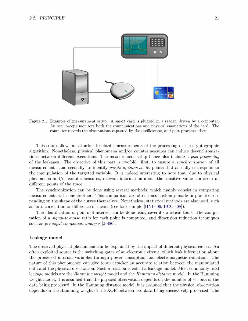
2.2. PRINCIPLE 21
Figure 2.1: Example of measurement setup. A smart card is plugged in a reader, driven by a computer.An oscilloscope monitors both the communications and physical emanations of the card. Thecomputer records the observations captured by the oscilloscope, and post-processes them.
This setup allows an attacker to obtain measurements of the processing of the cryptographicalgorithm. Nonetheless, physical phenomena and/or countermeasures can induce desynchroniza-tions between different executions. The measurement setup hence also include a post-processingof the leakages. The objective of this part is twofold: first, to ensure a synchronization of allmeasurements, and secondly, to identify points of interest, ie. points that actually correspond tothe manipulation of the targeted variable. It is indeed interesting to note that, due to physicalphenomena and/or countermeasures, relevant information about the sensitive value can occur atdifferent points of the trace.
The synchronization can be done using several methods, which mainly consist in comparingmeasurements with one another. This comparison are oftentimes customly made in practice, de-pending on the shape of the curves themselves. Nonetheless, statistical methods are also used, suchas auto-correlation or difference of means (see for example [HNI+06; RCC+08]).
The identification of points of interest can be done using several statistical tools. The compu-tation of a signal-to-noise ratio for each point is computed, and dimension reduction techniquessuch as principal component analysis [Jol86].
Leakage model
The observed physical phenomena can be explained by the impact of different physical causes. Anoften exploited source is the switching gates of an electronic circuit, which leak information aboutthe processed internal variables through power consuption and electromagnetic radiation. Thenature of this phenomenon can give to an attacker an accurate relation between the manipulateddata and the physical observation. Such a relation is called a leakage model. Most commonly usedleakage models are the Hamming weight model and the Hamming distance model. In the Hammingweight model, it is assumed that the physical observation depends on the number of set bits of thedata being processed. In the Hamming distance model, it is assumed that the physical observationdepends on the Hamming weight of the XOR between two data being successively processed. The
22 CHAPTER 2. SIDE-CHANNEL ANALYSIS
idea capture that both of these models is that each bit leaks information independently, through thecharge or decharge of its corresponding gate. More complexes models are sometimes used, whichcan consider cross-impacts on those charges, considering that physical effects occuring on a gatecan also impact its neighbours. Actually, the modelisation of these behaviors is a complex issue,and has been the subject of several researches. We describe in Section 2.4 a wider state-of-the-arton this subject.
Statistical Distinguisher
As highlighted by our description of an attack in Phase 4, the notion of statistical distinguisheris essential in side-channel analysis. We must hence introduce some notations from the field ofstatistics and probabilites in order to allow for a formal explanation. In the following, calligraphicletters, like X , are used to denote definition sets of random variables denoted in capital letters, likeX. Any realization of a random variable on this set denoted in lowercase, like x. The probability ofan event ev is denoted P [ev]. The size of the collection of inputs (pi)i, and equivalently of leakages(`i)i is denoted by n. Each leakage `i is moreover defined as a vector of a finite integer t points.
The statistical distinguisher takes as input the leakages (`i)i obtained in Phase 2 and thehypotheses (hk,i)i) obtained in Phase 3. It outputs a score for each key hypothesis k, whichmeasures how much the associated collection matches the leakages. In order to allow for thedistinguishing, an order needs to be defined on the scores. Most of the time, the scores take valuesin R, with its standard order. These distinguishers come from the world of statistics or machinelearning. For example, we can cite the linear correlation coefficient [Pea95], the Kullback–Leiblerdivergence [KL51], the difference of means [Fis20] or the maximum likelihood [Fis22].
2.3 Examples of side-channel attacksSeveral types of side-channel attacks have been introduced in the last two decades. Most of themare agnostic with regard to the targeted variable and measurement setup. We propose hereafter toshortly describe some of the most commonly used side-channel attacks:
Template analysis
Template analysis was introduced in 2002 by Chari, Rao and Rohatgi [CRR03]. The attacker isassumed to be able to perform encryptions with the secret key of his choice on the targeted device,or a similar one [CK14]. Using this ability, he collects several leakage traces and uses them toextract as many meaningful statistical moments as possible for each possible key. Specifically, aGaussian model approach [Tre68; CRR03] is usually performed, considering a Gaussian noise andthe need to estimate statistical moments up to the second order. For each sensitive value vk, theadversary is hence able to compute the associated leakage distribution (also called template in thiscontext) Dk composed of a mean vector µk and a covariance matrix Σk.
The model function m of a template analysis simply maps back every value vk,i to its estimatedleakage distribution Dk. A maximum-likelihood approach is hence performed.
In the Gaussian model, for a single observation (ie. when n = 1), the score of the hypothesis kis given by the likelihood:
ML(`i, hk,i) = ML(`i,Dk) = 1√(2π)tdet(Σk)
e−(`i−µk)>(Σk)−1(`i−µk)
2 . (2.1)
2.3. EXAMPLES OF SIDE-CHANNEL ATTACKS 23
Furthermore, in the case where several observations are made, the score of the hypothesis k isgiven by:
ML((`i)i, (hk,i)i) =∏i
ML(`i, hk,i). (2.2)
Remark 2.3.1. The computation of ML((`i)i, (hk,i)i) involves the product of several small values.When the number of observations is too high, this score can hence be so small that it lies belowmost systems precision. To avoid such a problem, which would cause the impossibility of computinga maximum-likelihood, this score is often replaced in practice by the equivalent log-likelihood, ie. itslogarithmic value. Consequently, the score is given by:
log-ML((`i)i, (hk,i)i) =∑i
log-ML(`i, hk,i), (2.3)
where log-ML(`i, hk,i) = log(ML(`i, hk,i)).
Linear regression analysis
Linear regression analysis was introduced in 2005 by Schindler, Lemke and Paar [SLP05].The linear regression analysis (similarly to all the following examples of side-channel attacks)
performs on univariate leakages, that is, leakages considering only one point. Consequently, theattack is either performed sequentially on each point of the acquired leakage, or the leakages arereduced to only one point, which is done during the post-processing part of the measurement setup.
The dimension of every vector `i being t = 1, the collection of leakages can be seen as an-dimensional vector `, of coordinates (`i)i.
The statistical distinguisher makes extensive use of linear algebra: it performs linear regressionsof the leakage against functions of the hypotheses’ bits, and compares the goodness of fit of theseregressions. Specifically, an attacker chooses a regression basis of functions (gj(·))j . The leakageof an hypothesis vk,i is then represented as the polynomial p(vk,i) = ∑
j αjgj(vk,i), where (αj)j arecoefficients in R. The goal of the linear regression is to find the collection of coefficients (αj)j suchthat the values (p(vk,i))i are as close as the observed leakages (`i)i as possible. To perform thisregression, for each k, the functions (gj(vk,i))j are evaluated, and form an n rows matrix Mk.
The score for k is then given by the goodness of fit:
LRA((`i)i, (hk,i)i)) = LRA(`,Mk)) = ||`−Mk((Mk)>Mk)−1(Mk)>`||1n
∑ni=1(`i − ¯)2 , (2.4)
where || · || denotes the Euclidean distance, n denotes the number of measurements, and (¯) denotesthe mean 1
n
∑i `i of `. It is interesting to note that the vector ((Mk)>Mk)−1(Mk)>` gives the
coefficients (αj)j of the regression of the leakages on the basis chosen by the attacker, with respectto hypothesis k.
Correlation power analysis
Correlation power analysis was introduced in 2004 by Brier, Clavier and Olivier [BCO04]. Themodel function maps the hypothetic sensitive variable towards an element of R. Usually, thechosen function is the Hamming weight of this value, but several other model functions can beused. The statistical distinguisher is the Pearson linear correlation coefficient. Denoting by ¯ (resp.hk) the mean 1
n
∑i `i (resp. 1
n
∑i hk,i), the score is given by:
CPA((`i)i, (hk,i)i)) =1n
∑ni=1(`i − ¯) · (hk,i − hk)√
1n
∑ni=1(`i − ¯)2
√1n
∑ni=1(hk,i − hk)2
· (2.5)
24 CHAPTER 2. SIDE-CHANNEL ANALYSIS
Differential power analysis
Differential power analysis was introduced in 1999 by Kocher, Jaffe and Jun [KJJ99]. The statisticaldistinguisher is the difference of means. In this context, the values taken by the hypotheses arereduced to a set of cardinal 2. Without loss of generality, we denote these two possible values 0and 1. Usually, the model function maps the sensitive variable towards the value of one specific bit(for example, its least significant bit). Using these notations, and the same as introduced for thecorrelation power analysis, the score is hence:
DPA((`i)i, (hk,i)i)) =∑i|hk,i=0 `i
#(i|hk,i = 0) −∑i|hk,i=1 `i
#(i|hk,i = 1) · (2.6)
Remark 2.3.2. Is is argued in [DPRS11] that the differential power analysis, correlation poweranalysis and linear regression analysis are not only asymptotically equivalent when the numberof observations increase, but can also be rewritten one in function of the other, only by refiningthe used model leakage. Specifially, the differential and correlation power analysis can be seen asspecific cases of linear regression analysis.
Simple power analysis
Simple power analysis was introduced in 1996 by Kocher [Koc96]. It can be seen as an implicittemplate analysis, where only a very limited number of templates -typically two- is used. Instead ofcollecting these patterns by performing encryptions with a known secret, the attacker is supposedto know them beforehand, or at least distinguish between them, because of their small number andsimplicity.
2.4 Problem ModelingState of the art
The study of the effectiveness of side-channel attacks and their countermeasures requires a formalframework. In 2003, Ishai, Sahai and Wagner introduced in [ISW03] the d-probing model, wherean attacker can learn the exact value of a bounded number d of intermediate values during a com-putation. Furthermore, they proposed a method to transform any black-box circuit implementinga function to an equivalent circuit secure in this model. This paper proposed a method to buildprivate circuits resistant in such a model, at a cost of a size blow-up quadratic in d. Nonetheless,even though this paradigm is convenient to write security proofs, it does not accurately representa side-channel attacker. Indeed, this setting supposes that the attacker knows the exact value ofonly the d targeted intermediate variables, and fails to capture the whole information available.In particular, to achieve a good understanding of side-channel analysis, it is necessary to define amodel that captures all the information that is leaked to the adversary.
The first general approach towards this understanding is the physically observable cryptographyframework introduced by Micali and Reyzin in [MR04], which allows to represent any physicalimplementation. A very important axiom in this model is that only computation leaks information.This founding work paved the way for subsequent works on the resilience of cryptographic imple-mentations against side-channel attacks, in particular the seminal paper written by Dziembowskiand Pietrzak [DP08], which introduced the notion of continuous leakage model to the world ofside-channel, that is, the assumption that only a bounded amount of information about the ma-nipulated variable can leak during a given period. In this model, Dziembowski and Pietrzak were
2.4. PROBLEM MODELING 25
moreover able to construct a particular cipher proven to be resilient against any side-channel attack,using a pseudo-random number generator. However, the overhead (in terms of computation time,memory, and randomness) induced by this construction is too high to be considered as practical.Moreover, as argued by Standaert in [Sta11], the continuous leakage model is too theoretical, asit encompasses a very strong and unrealistic attacker. Specifically, the model allows the attackerto arbitrarly define the leakage function, even if it could revert the cryptographic properties of thealgorithm itself. The paper [FRR+10] proposed an alternative approach, by restraining the choiceof the leakage model to functions in the complexity class AC0, ie. which circuit is of constant depthand polynomialy sized in the number of inputs. Sadly, this class is too small to actually describeall practical attacks. For example, the parity function is not in AC0 [FSS84]. Another approachproposed in the same paper is a slight variation on the probing model, considering a possible erroron each read bit with a fixed probability. It is nonetheless unclear how realistic this leakage modelfits the physical reality of power and/or electromagnetic leakages.
A more realistic approach was proposed in [CJRR99] by Chari et al., introducing the noisyleakage model. This model considers that the physical observable is a noisy observation of a deter-ministic function of the sensitive variable. This is particularly relevant in the practical case, as itseems to accurately capture physical phenomena induced by both the device architecture and theattacker’s measurement setup [MOP07]. This work moreover focuses on the case where the noiseis Gaussian. This noise model is generally considered to be a good approximation of the reality.Indeed, the central limit theorem ensures that the sum of noises caused by enough different sourcesconverges towards a Gaussian distribution. The paper [CJRR99] however restrains its study to thecase where the sensitive value is only one bit, shared as a sum of d bits (cf. 2.5.1). Nonetheless,this model allows to formally evaluate the effectiveness of a side-channel attack in this context.Precisely, for any side-channel attack to succeed in distinguishing the secret bit with probability α,the number of measurements n is lower bounded, by a value depending on the standard deviationσ of the Gaussian noise and the number d of shares:
n > σt+4 logα
logσ . (2.7)
This work was generalized by Prouff and Rivain in 2013 [PR13] by getting rid of the single-bit limitation, and allowing for arbitrary noise. This study extends to the analysis of any affinefunction or multiplication. Even more, these results can be composed to the protection of a wholecryptographic algorithm, by assuming the presence of leak-free gates ie. components allowing torefresh the sharing of a variable. These gates allow them to compose several secure operations whilemaintaining a security all along the execution of the algorithm. Furthermore, this constructionallows them to prove information-theoretical results about the security of the obtained circuit. Forany manipulated variable X, the authors model the leakage obtained by an attacker by a non-deterministic function L(X). This non-deterministic part can be represented in several ways. Thismodeling can be seen as a generalization of an often chosen model: the additive noisy leakage,where L(X) is written as the sum of a noise B and a deterministic function ϕ of the manipulatedvariable X:
L(X) = ϕ(X) +B. (2.8)In [PR13], the authors choose to model the noise of a leakage by the bias introduced on the
distribution of the manipulated random variable. For a manipulated variable X, and a measuredleakage L(X), the bias β(X|L(X)) of X given L(X) is defined as the expected statistical distancebetween X and X|L(X):
β(X|L(X)) =∑y
P [L(X) = y] ·∆(X, (X|L(X) = y)), (2.9)
26 CHAPTER 2. SIDE-CHANNEL ANALYSIS
where ∆(X,X|L(X) = y) = ||PX − PX|L(X)=y||, with || · || denoting the Euclidean distance, andPX (resp. PX|L(X)=y) denoting the vector (P [X = x])x (resp. (P [X = x|Y = y])x). The bias is aninformation metric between X and L(X). Note that if X and L(X) are independent, the bias isnull. It is deeply related to the mutual information MI between the random variables X and L(X),that is the difference between the Shannon entropies [Sha48] of X and of X|L(X).
Indeed, by assuming a uniform distribution of X in a set of cardinality N , the mutual informa-tion between the sensitive variable X and its leakage L(X) can be bounded:
MI(X,L(X)) ≤ N
ln 2β(X|L(X)). (2.10)
This property is the cornerstone of the proofs in [PR13]. Assuming that the designer of a circuitcan control a noise parameter ω, and that, at any point of the execution, the bias between themanipulated variable and the leakage never exceeds 1
ω (this assumption defines the so-called 1ω -
noisy leakage model), the authors show that the information an attacker can get by looking at awhole execution is upper bounded by ω−(d+1).
The approach in [PR13] suffers from several shortcomings: it requires the existence of leak-freegates, the attacker can only access to randomly generated inputs, and the proof method is hardto generalize to new protection schemes. The next year, Duc et al. solved these shortcomingsin [DDF14], and proved a reduction from the noisy leakage model used in [PR13] to the probingmodel used in [ISW03], in which proofs are more convenient. Specifically, they proved that forany attacker in the 1
ω -noisy leakage model introduced in [PR13], there exists an attacker in thed-probing model, where d is a value linear in 1
ω . This is of particular interest, since it implies thatany circuit proven secure in the d-probing model is also secure in the 1
ω -noisy leakage model forsome ω. However, the expression of d as a linear function of 1
ω implies large constants, which renderthe obtained security impractical.
The link between these models have further been studied in [DFS15b; DFS15a]. In particular,it is shown in these papers that, if a circuit is secure in the d-probing model, then the probability ofdistinguishing the correct key among |K| hypotheses is upper bounded by |K| · 2−d/9, if the leakageL(X) satisfies, at each time:
MI(X,L(X)) ≤ 2 · (|K| · (28d+ 16))−2. (2.11)
These results imply that any proof of security obtained in the probing model can be transcribedas a proof of security in the noisy leakage model. Namely, if a construction is proven secure in theprobing model (where the amount of observations an adversary can have is bounded), then thereexists a bound on the amount of information one can have by observing the whole computationin the noisy leakage model. This is particularly interesting, since proofs in the probing model areeasier.
We now formally describe a side-channel attack based on the noisy leakage model, which closelycorresponds to a practical setting. This description is based on the one made in [PR13].
Algorithm
An algorithm is modeled by a sequence of elementary calculations (Ci)i implemented by Turingmachines possessing a set of adresses called the state. An elementary calculation reads its input andwrites its output on the state. When an elementary calculation Ci is invoked, its input is writtenfrom the state to its input tape, then Ci is executed, and its output is written back to the state.
2.5. COUNTERMEASURES 27
Physical implementation
Similarly to an algorithm, its physical implementation is modeled by a sequence of physical ele-mentary calculations. A physical elementary calculation is simply an elementary calculation Ciassociated with a leakage function Li(·). A leakage function is defined as a function taking twoparameters: the first one corresponds to the value of the part of the state accessed by its corre-sponding elementary calculation, and the second one is a random chain modeling the leakage noise.Denoting I = (Ci, Li)i the physical implementation of an algorithm, each execution of I leaks thevalues Li(Zi, ri)i, where Zi designs the part of the state accessed by Ci before its execution andri the corresponding random chain. By definition, the different ri are supposed mutually indepen-dent. For the sake of simplicity, we will often omit the random chain and write Li(Zi) the leakagecorresponding to the value Zi. In this sense, Li(Zi) can be seen as the result of a probabilisticTuring machine. When only one variable is considered, we will omit the index i and simply writeL(Z).
Noisy leakage model
In the noisy leakage model, the leakage L(Z) occuring during the manipulation of an intermediatevalue Z is modeled as a non-deterministic function of Z. In the remaining of this thesis, we willoften consider a particular case, corresponding to the additive noisy leakage model, as described inEquation 2.8. Even more specifically, we will model L(Z) as:
L(Z) = ϕ(Z) +B, (2.12)
where ϕ is an unknown deterministic function depending on the architecture and where B is aGaussian noise of null mean and of variance σ2: B ∼ N (0, σ2). We will often instanciate, ϕ asthe Hamming weight or Hamming distance. Note that, according to this definition, the leakage onvariable Z only depends on Z, though ϕ could somehow capture information about previous states.This is a slight imperfection of the model. This simple model will be used as a basic brick of ourstudy of side-channel attacks effectiveness in Chapter 3.
Moreover, the distribution fL(Z) of the leakage L(Z) is a Gaussian mixture sastisfying:
fL(Z) =∑
ε∈Im(ϕ)P [ϕ(Z) = ε] N (ε, σ2). (2.13)
We will use this observation in the study of the particular case of maximum-likelihood inSection 3.6.
2.5 CountermeasuresOne can distinguish two main families of countermeasures against side-channel analysis. The firstone, called masking, modifies the algorithm in order to make the sensitive variables manipulatedindependent from the secret key. The second one, called hiding, covers the processing of thealgorithm by noise in order to make the exploitation of the observed signal too difficult.
2.5.1 MaskingA brief history
The first countermeasure against side-channel analysis actually appeared alongside the first attackin the seminal paper of Kocher [Koc96]. The idea is to introduce randomness in the computation of
28 CHAPTER 2. SIDE-CHANNEL ANALYSIS
the algorithm, in order to mask the sensitive data manipulated by the algorithm. The countermea-sure modifies the input m fed into the RSA algorithm thanks to a uniformly drawn random valuer. Instead of cumputing a ciphertext c defined as c = md mod N , the algorithm now computesa ciphertext c′ defined as c′ = (mre)d mod N . Then, the ciphertext c is retrieved by computingc = (c′r−1) mod N . Due to the multiplication by re, the intermediate values manipulated duringthe computation of c′ are not trivially deduced from md. The information that can be retrieved bythe attacker on the private exponent is hence smaller.
This approach was generalized and applied to symmetric algorithms independently by Goubinand Patarin [GP99] and Chari et al. [CJRR99]. Usually, for historical reasons the countermeasureapplied to asymmetric algorithms is called blinding, while it is called masking when applied tosymmetrical algorithms. Nonetheless, the modus operandi of the countermeasures stays the same.This family of countermeasures affects the distinguishing phase of the attack, by shrinking thestatistical dependencies between the manipulated variables and the secret data. The impact ofmasking is nowadays well understood thanks to the works of modeling described in 2.4.
Formally, each sensitive variable x is divided into d+1 variables xi0≤i≤d referred to as shares.Among those values, d are generated uniformly at random and the last one is computed such thatthe combination of the d+ 1 shares, according to a chosen composition law ?, is equal to the initialvariable x, ie., x = x0 ? · · ·?xd. One of the shares say x0 is sometimes referred to as masked variableand the other shares x1, · · ·xd as the masks. For the masking approach to be sound, it is requiredthat the masks are uniformly and independently generated. In that case, the (d+1)-tuple of sharescan be modeled as a random vector (X0, · · · , Xd) where for i ≥ 1, the Xi are mutually independentrandom variables with uniform distribution on X , and X0 is computed such that it holds:
x =Fdi=0Xi. (2.14)
The choice of the law ? depends on the algorithm and its implementation. The most trivialinstantiations are with the bitwise addition (aka. XOR or addition in the field of two elements)law ⊕ or with the field product law ×, respectively used by the Boolean sharing [GP99; CJRR99]and multiplicative sharing [AG01]. More complex instantiations can be deduced from descriptionsof other secret sharing schemes, such as Shamir’s secret sharing scheme [Sha79] or inner maskingproduct [BFGV12; BFG15].
Remark 2.5.1. For security reasons, ? should form a group law on the definition set of the sensitivevariables x. This property has been sometimes overlooked and provoked flaws in some schemes. Forexample, the multiplicative masking proposed in [AG01] could not mask the value 0, which howeverwas in the definition set of x. This allows a statistical attack breaking the scheme’s security [GT03].Multiplicative masking is however a possible construction when the definition set does not includethe value 0, as illustrated in [GPQ10]. Its use in practical settings is nonetheless quite costly dueto the workarounds required to solve the 0 problem.
Remark 2.5.2. In an implementation protected by making, the sensitive variable x is not manip-ulated anymore, but all shares are manipulated instead. Often, these manipulations are sequential.An immediate consequence is that the attacker cannot obtain a leakage depending on x anymore,but he can instead obtain a leakage tuple L corresponding to the different leakages of each share:
L = (L0, · · · , Ld), (2.15)
wherer Li denotes the leakage associated to the random value Xi, for any i < d+ 1. The obtentionof such a tuple can lead to so-called high order side-channel attacks, which aim at recovering thesensitive value x by studying the distribution of L. We will detail and study the effectiveness ofsuch attacks in Chapter 3.
2.5. COUNTERMEASURES 29
The inverse operation of masking, constisting in the retrieval of x from the shares xi0≤i≤d isreferred as a reconstruction, and can be performed thanks to Equation 2.14.
Remark 2.5.3. The so-called threshold implementations [BGG+14] are a family of countermea-sures, extending the idea of masking, in a wider model. In this model, additional physical leaks canoccur, such as leakages due to glitches, where more than one variable is involved in each observa-tion. Glitches are unwanted transitions at the output of gates resulting from differences in signalsarrival time. The number of such transitions can be detected by side-channel analysis and revealinformation about the sensitive value. Threshold implementations hence increase the number ofshares used in the classical masking countermeasures, to ensure that these leaks do not induce asecurity flaw (see for example [RBN+15]).
Masking as linear codes
All these countermeasures except multiplicative masking can be expressed in the domain of linearerror correcting codes theory. This link was first made by Massey in [Mas93], and allows for abetter understanding of the mathematical properties of these constructions. The author provedan equivalence between linear coding theory and linear secret-sharing techniques. The sharing canhence be reformulated in those terms. To proceed to the sharing of a sensitive value x into d + 1shares x0, · · · , xd, a linear code C of length d + 2, dimension n and minimal distance δ is chosen.Denoting the minimal distance of its dual code C⊥ by δ⊥, the results of [Mas93] imply that, as longas δ, δ⊥ ≥ 2, one can build a sharing scheme from C. Then, n−1 random variables r1, · · · , rn−1 areuniformly drawn, and the vector (x, r1, · · · , rn−1) is encoded by C hence obtaining the codeword(x, x0, x1, · · · , xd). Denoting by G the generator matrix of C, we have:
(x, r1, · · · , rn−1) ·G = (x, x0, x1, · · · , xd). (2.16)
The reconstruction of the shared variable x is hence seen as a decoding problem: severalshares (xi)i are known, and the reconstruction of x amounts to the decoding of the codeword(x, x0, x1, · · · , xd). Note that this procedure must also be performed securely. Formally, a vectorλ = (λi)i exists, such that x = ∑
i λixi. In secret-sharing theory, a set of indices I such that theshares xi|i ∈ I allow for the reconstruction of x is called a qualified set. The set of qualifiedsets is further called an access structure. It is argued in [Mas93] that the access structure of asecret-sharing scheme is entirely defined by the dual code C⊥.
In [CCG+07], Chen et al. furthermore studied the security properties of such a construction.Considering x as the realization of a random variable X and each xi as the realization of a randomvariable Xi, they show that, for any set of indices I of cardinality less than δ⊥ − 2, the mutualinformation between X and (Xi)i∈I is null. Moreover, the authors prove that there exists a set Iof cardinality d− δ + 3 such that x can be reconstructed from the shares (xi)i∈I .
These results are of particular interest in the case of maximum distance separable (MDS) codes,ie. codes whose parameters achieve the so-called Singleton bound, ie. verify the equation δ =d + 2 − n + 1 = d − n + 3. Indeed, if C is MDS, then, C⊥ is also MDS. Therefore we have thatδ⊥ = d + 2 − (d + 2 − n) + 1 = n + 1. This results applied to the bounds of [CCG+07] showthat no information can be retrieved on the shared variable when the number of known shares isstrictly lower than n, but that n shares suffice to reconstruct x. Such a scheme is called a thresholdsecret-sharing scheme.
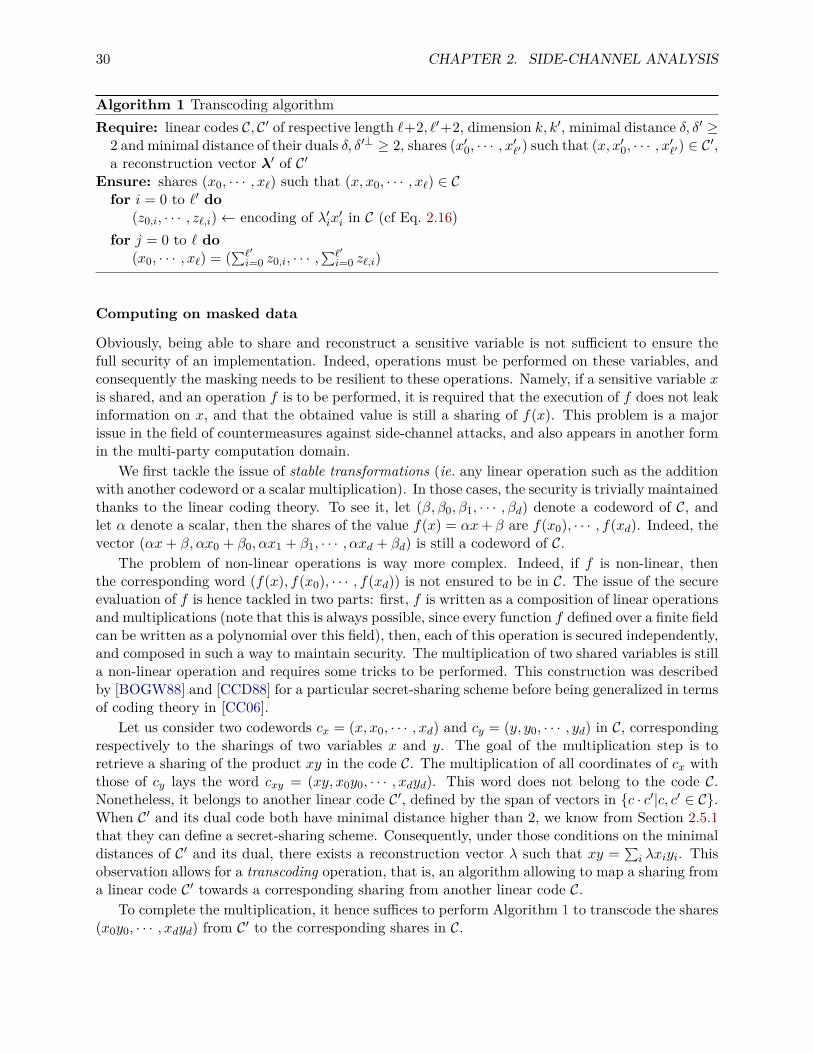
30 CHAPTER 2. SIDE-CHANNEL ANALYSIS
Algorithm 1 Transcoding algorithmRequire: linear codes C, C′ of respective length `+2, `′+2, dimension k, k′, minimal distance δ, δ′ ≥
2 and minimal distance of their duals δ, δ′⊥ ≥ 2, shares (x′0, · · · , x′`′) such that (x, x′0, · · · , x′`′) ∈ C′,a reconstruction vector λ′ of C′
Ensure: shares (x0, · · · , x`) such that (x, x0, · · · , x`) ∈ Cfor i = 0 to `′ do
(z0,i, · · · , z`,i)← encoding of λ′ix′i in C (cf Eq. 2.16)for j = 0 to ` do
(x0, · · · , x`) = (∑`′i=0 z0,i, · · · ,
∑`′i=0 z`,i)
Computing on masked data
Obviously, being able to share and reconstruct a sensitive variable is not sufficient to ensure thefull security of an implementation. Indeed, operations must be performed on these variables, andconsequently the masking needs to be resilient to these operations. Namely, if a sensitive variable xis shared, and an operation f is to be performed, it is required that the execution of f does not leakinformation on x, and that the obtained value is still a sharing of f(x). This problem is a majorissue in the field of countermeasures against side-channel attacks, and also appears in another formin the multi-party computation domain.
We first tackle the issue of stable transformations (ie. any linear operation such as the additionwith another codeword or a scalar multiplication). In those cases, the security is trivially maintainedthanks to the linear coding theory. To see it, let (β, β0, β1, · · · , βd) denote a codeword of C, andlet α denote a scalar, then the shares of the value f(x) = αx+ β are f(x0), · · · , f(xd). Indeed, thevector (αx+ β, αx0 + β0, αx1 + β1, · · · , αxd + βd) is still a codeword of C.
The problem of non-linear operations is way more complex. Indeed, if f is non-linear, thenthe corresponding word (f(x), f(x0), · · · , f(xd)) is not ensured to be in C. The issue of the secureevaluation of f is hence tackled in two parts: first, f is written as a composition of linear operationsand multiplications (note that this is always possible, since every function f defined over a finite fieldcan be written as a polynomial over this field), then, each of this operation is secured independently,and composed in such a way to maintain security. The multiplication of two shared variables is stilla non-linear operation and requires some tricks to be performed. This construction was describedby [BOGW88] and [CCD88] for a particular secret-sharing scheme before being generalized in termsof coding theory in [CC06].
Let us consider two codewords cx = (x, x0, · · · , xd) and cy = (y, y0, · · · , yd) in C, correspondingrespectively to the sharings of two variables x and y. The goal of the multiplication step is toretrieve a sharing of the product xy in the code C. The multiplication of all coordinates of cx withthose of cy lays the word cxy = (xy, x0y0, · · · , xdyd). This word does not belong to the code C.Nonetheless, it belongs to another linear code C′, defined by the span of vectors in c · c′|c, c′ ∈ C.When C′ and its dual code both have minimal distance higher than 2, we know from Section 2.5.1that they can define a secret-sharing scheme. Consequently, under those conditions on the minimaldistances of C′ and its dual, there exists a reconstruction vector λ such that xy = ∑
i λxiyi. Thisobservation allows for a transcoding operation, that is, an algorithm allowing to map a sharing froma linear code C′ towards a corresponding sharing from another linear code C.
To complete the multiplication, it hence suffices to perform Algorithm 1 to transcode the shares(x0y0, · · · , xdyd) from C′ to the corresponding shares in C.
2.5. COUNTERMEASURES 31
Remark 2.5.4. The protocol described in Algorithm 1 is furthermore a secure transcoding opera-tion, in the sense that, as long as the respective minimal distances δ, δ′, δ⊥, δ′⊥, of C,C ′ and theirduals are greater than 2, any set of at most max(d′⊥, d)−2 intermediate values is independent fromthe shared variable.
Being the cornerstone of the evaluation of the multiplication, the transcoding operation hasbeen the subject of several works, proposing new algorithms to achieve more efficient or moresecure results. Some other constructions can be found for example in [GM11; CPR12].
Sometimes, the code C′ resulting from the coordinate-wise product of the codewords of C doesnot verify the requirements on the minimal distance. For example, for the code associated tothe Boolean sharing, which we describe lower, the code C′ is exactly the whole space on which C isdefined. Consequently, the corresponding minimal distance is 1. In this case, the described trick canbe adapted, by replacing the code C′ by the code C?, where the coordinate-wise product is replacedby the outer product, viewed as a vector. The transcoding operation described in Algorithm 1 canthen be used. We study particularly this setting in Chapter 4 of this thesis, and we propose newefficient solutions, that can be written as new transcoding procedures.
Even with clever tricks, dealing with linear operations is still cheaper than dealing with non-linear ones. Consequently, to improve performance, the decomposition of the function f mustminimize the number of non-linear operations. These last years, the protection of the symmetricalalgorithms, especially AES, has been studied. In AES, the only non linear part is the substitutionlayer, itself composed of small non-linear functions (called Sboxes). The decomposition of the AES’-Sbox function has consequently been the subject of several studies. The element manipulated bythese functions are in a field of characteristic 2, hence the squares operations are linear. Rivainand Prouff showed in [RP10] that this function can be evaluated using as few as 4 multiplications,and proposed a secure scheme for it, by extending the seminal construction of [ISW03] from F2 toF28 . The problem of the minimization of non-linear operations in the expression of Sboxes in fieldsof characteristic 2 has recently been tackled by the works of [CGP+12; RV13; CRV14; GPS14;CPRR15]. These papers allow to prove lower bounds on the number of such operations that onecan obtain by decomposing any polynomial function on a field of characteristic 2, and they provideseveral constructions to efficiently find good decompositions.
In [GHS12], Gentry et al. proposed a new decomposition of the AES Sbox where 2 out of 4multiplications are computed in parallel. Moreover, it can be observed that these two multiplica-tions have a common input. Recently, Coron et al. [CGPZ16] took advantage of this parallelizationto further reduce the complexity of the evaluation. Though not really reducing the number ofmultiplications in the expression of the Sbox, the authors design a trick to artifically reduce thecomputation complexity, by introducing the notion of common shares. Denoting by c · a and c · bthe two parallel multiplications occuring in the construction of [GHS12], they set the first half ofthe sharing of b as equal to the first half of the sharing of a. Consequently, part of the operationsperformed to compute c · a and c · b are similar, and can hence be computed only once. This trickallows to reduce the number of multiplications in the AES Sbox evaluation to the equivalent of 2.8instead of 4.
The composition of several secure constructions, or gadgets, is a prime issue in the design ofsecure evaluations. Indeed, the succession of two secure gadgets is not necessarly secure: oneneeds to prove that combining observations between both gadgets does not give information aboutthe manipulated sensitive values. To allow proofs of compositions, the notion of strong non-interference (SNI) was introduced by Barthe et al. in [BBD+15a], extending the previous notionof non-interference (NI) defined in [BBD+15b]. Essentially, a gadget is said t-SNI if it can besimulated using a number of each of its input shares that is only bounded by the number of ob-
32 CHAPTER 2. SIDE-CHANNEL ANALYSIS
servations made by the adversary on inner variables manipulation, and is independent from thenumber of observations made on output values, as long as the total number of observations doesnot exceed t. This definition directly implies that a t-SNI algorithm is t-secure. Indeed, for anyt variables observed by an attacker, it is possible to perfectly simulate the distribution of thesevariables from some random bits and a set of less than t inputs. The composition of two t-SNIalgorithms is itself t-SNI. The composition of t-NI and t-SNI gadgets is not necessarly t-SNI, andsuch constructions must hence be proven otherwise. We extensively use these notions in Chapter 4to prove the security of our constructions.
Examples of secret sharing schemes
For illustration purposes, we describe hereafter the matrices Gbool, GIP and GSSS , respectivelycorresponding to the Boolean sharing, inner product masking, and Shamir’s scheme, and the gen-erator matrices Hbool, HIP and HSSS of their dual codes. For any integer n, we denote by In then-dimensional identity matrix.
In the Boolean sharing, the sensitive value x is divided in d + 1 shares through the law ⊕.Hence, Gbool is simply the parity matrix:
Gbool =
Id+1
1...1
.The generator matrix Hbool of the dual code is therefore:
Hbool = (−1, · · · ,−1, 1).
The masking of a sensitive value through inner product sharing is described in [BFG15]. Thesharing is in fact very similar to the Boolean sharing’s one. In fact, the only difference is that thelast share is not computed using a XOR law, but with an inner product with a publicly knownvector (1, l1, l2, · · · , ld). This allow us for the description of the generator matrix GIP :
GIP =
Id+1
1l1...ld
.The generator matrix HIP of the dual code is therefore:
HIP = (−1,−l2, · · · ,−ld, 1).
In Shamir’s secret sharing, the shares correspond to evaluations of a certain polynomial in d+1different public points αi, for i ∈ [0, d]. This is equivalent to a Reed-Solomon code, where thecoefficients of the polynomial correspond to the input vector. In particular, the sensitive value isthe constant term of this polynomial. Consequently, GSSS is the Vandermonde matrix:
GSSS =
1 1 · · · 10 α0 · · · αd0 α2
0 · · · α2d
......
......
0 αn−10 · · · αn−1
d
.
2.5. COUNTERMEASURES 33
The dual code is therefore also a Reed-Solomon code, of generator matrix HSSS :
HSSS =
1 1 · · · 10 α0 · · · αd0 α2
0 · · · α2d
......
......
0 αd−n−10 · · · αd−n−1
d
.
Remark 2.5.5. All these codes are MDS. Note that, contrary to the Boolean sharing or theinner product masking, where the dimension of the code has to be d + 1, Shamir’s secret sharingscheme allows for arbitrary dimension n. The corresponding dual codes for Boolean sharing andinner product masking are therefore of dimension 1, and consequently, reconstructions with theseschemes require that all shares are known. Shamir’s secret sharing allow for more a complex accessstructure, ie. every set of shares of cardinality higher than a chosen dimension n.
2.5.2 Hiding
Another approach is taken by so-called hiding countermeasures, introduced in [KJJ99]. The goalof such countermeasures is to hide the manipulation of data among a lot of noise. Using thisapproach, the sensitive variable is indeed manipulated by the device, but the exploitation of theleakage obtained by the attacker is very difficult. This family of countermeasures target the leakagecollection phase of the attack, by increasing the difficulty of the signal resynchronisation and theidentification of the correct instant when the sensitive value is manipulated.
The first approach designed to achieve such a feit is the so-called balancing method. Thiscountermeasure aims at the insurance of a balance of the power consumed by an electronic devicein such a way that, at each time, the consumption is as constant as possible. The obtained signalis consequently unrelated to the data being processed. Several means have been considered toreach this goal: balanced gate constructions [KJJ99], dual-rail precharge logic [PM05], modificationof current mode [MSH+04] and asynchronous logic [MMC+02]. Through theoretically efficient,these countermeasures are very hard to implement in practice. Indeed, the power consumptionof electronic devices depends on a large number of parameters on which the modern designer haslittle to no control, such as wire routing, capacitive effects or even cross-talk between wires. Thesecountermeasures are therefore seldom used in the real world.
The second approach is built on the idea of artificially inducing noise in the measurementthemselves. We can further separate this approach in two sub-families, the first one hiding therelevant signal with amplitude noise, and the second one hiding it with temporal noise. With theamplitude approach, the device will perform unrelated operations at the exact same time as therelevant computation is being performed. The amplitude of the resulting signal obtained by anattacker will hence be polluted by the unrelated operations. Nonetheless, this countermeasure isalso difficult to efficiently implement. Indeed, while a power measurement of the whole device wouldbe affected, a very local measurement of the electromagnetic emanations could be unaffected byoperations occuring in another area. The temporal approach uses random interruptions, randomaccesses, and temporal duplications of algorithms to hide the relevant operation among dummy ones.The relevant signal is hence temporaly lost in the middle of a lot of noise. An usual circumventionto this countermeasure applies integrating techniques on the signal in order to fall back into anamplitude noise problem [CCD00].
34 CHAPTER 2. SIDE-CHANNEL ANALYSIS
2.6 Randomness complexityMost countermeasures described in Section 2.5 make use of randomness. Hiding countermeasuresmight require randomness to shuffle executions, and insert unpredictable delays. Masking coun-termeasures require randomness to share variables such that the manipulations are uncorrelatedto the secret. Moreover, operations manipulating masked values induce an overhead in term ofneeded randoms during the transcoding part. Quite surprisingly, the problem of the amount ofrandomness required by those countermeasures is often overlooked.
The production of random bits is however a complex issue in the design of secure devices. Indeed,in practice, randomness is often generated using the succession of sophisticated components: a truerandom number generator (TRNG) exploits an unpredictable process, such as analog phenomena,to accumulate entropy and output random bits, which are then retreated by a deterministic randomnumber generator (DRBG), such as a cryptographic algorithm. The unpredictability of the TRNGis ensured physically, and that of the DRBG is ensured computationally and/or statistically. Inaddition of being a theoreitcal chicken-and-egg problem, this whole process often suffers from a lowthroughput and a long execution time, and countermeasures usually require a lot of randomnessto efficiently secure algorithms. Indeed, in general, for a DRBG based on a 128-bit block cipher,one call to this block cipher enables to generate 128 pseudorandom bits (see [BK12]). However,one invocation of the standard AES-128 block cipher with the ISW multiplication requires as muchas 30,720 random bits (6 random bytes per multiplication, 4 multiplications per S-box [RP10])to protect the multiplications when masked at the low order d = 3, which corresponds to 240preliminary calls to the DRBG.
We hence argue that the amount of randomness required by countermeasures against side-channel attacks should be estimated along the classical evaluations of time, area and number ofoperations. To the best of our knowledge however, this problem was only tackled in the seminalpaper of [ISW03]. In Chapters 4 and 5, we put a primary focus on the notion of randomnesscomplexity, that is, the amount of randomness needed to achieve secure constructions. Respectively,we evaluate this complexity in several new proposed computations of non-linear operations onmasked variables, and on new protocols allowing to securely compute a veto.
2.7 Effectiveness of side-channel attacksThe wide variety of side-channel attacks available in the state of the art calls for the need to comparetheir respective effectiveness. Indeed, in the constraints of limited time and resources, designers,evaluators and attackers are not able to perform all attacks, and a choice must hence be made.This choice is mostly driven by the chance of success of an analysis, that is, the probability for anattacker to retrieve the secret variable manipulated by the device in the least possible number ofobservations.
This need for a classification of attacks based on their chance of success led the community toapply the notion of success rate to side-channel analysis. The success rate measures the probabilityof success of an attack.
In [WO11b], Whitnall and Oswald proposed a framework to further compare side-channel at-tacks and their distinguishers, using several criteria:
• Correct key ranking: the position of the correct key when ranked by score value.
• Relative distinguishing margin: the difference between the scores of the correct key and thebest alternative, normalized by the variance of scores.
2.7. EFFECTIVENESS OF SIDE-CHANNEL ATTACKS 35
• Absolute distinguishing margin: the difference between the scores of the correct key and thebest alternative, divided by this expected difference in a noiseless setting.
• Standard score: the number of standard deviations above or below the mean for the correctkey score.
The authors also added two other criteria regarding the cardinality of the set of plaintextsrequired for an attack to be successful: the average critical support and the critical support for p%success rate, respectively corresponding to the average required cardinality of the set for the attackto be successful, and to the cardinality for which the rate of success is at least p%.
All these criteria are of interest to compare different side-channel attacks. However, the mainissue for a practical attacker is that they all rely on a posteriori results, that is, they measure theeffectiveness of an attack after it has been performed. Oftentimes, for example, the success rate isestimated empirically: the attack is repeated a large number of times, and the number of successesis counted, allowing for the computation of the empirical success rate SRemp:
SRemp = number of successesnumber of attacks · (2.17)
Such an estimation is hence very dependent of the number of attacks, and consequently ofthe time and resources deployed by the attacker. It is hence oftentimes impractical to compute.Moreover, the clever choice of an attack should rely on an a priori approach, allowing the estimationof effectiveness before it is even performed.
We tackle this problem in Chapter 3, by reviewing state of the art approaches to theoreticallyestimate the success rate, and we extend those works to a whole family of side-channel attacks,based on so-called additive distinguishers. Moreover, we give rationales for the practical interest ofthis approach in the choice of an attack, by illustrating how the characterization of a device andmeasurement setup is much cheaper to perform than the attack itself.

Chapter 3
Estimating the Success Rate ofSide-Channel Attacks
My success rate is 100%. Do the math.Charlie Sheen
In this chapter, we propose to tackle out the problematic of success rate’s evaluation. Part ofthis work has been the subject of two papers published in the workshop on Cryptographic Hardwareand Embedded Systems in 2013 [TPR13] and 2014 [LPR+14].
3.1 IntroductionSide-channel attacks against block cipher implementations usually consider the secret as a tupleof so-called subkeys and apply a divide-and-conquer strategy to recover them separately. Duringthe conquering phase, a partial attack, limited in time and space, is run against each subkey.Heuristics are then applied to decide on the success or unsuccess of each of these attacks. Subkeyscorresponding to attack failures are deduced by exhaustive search. In practice, this last step isoften executed either for efficiency reasons or because it is assumed that there is no chance to getthe missing subkeys directly by side channel analysis. This description makes apparent that theattack effectiveness greatly depends on the heuristic applied by the adversary. Indeed, incorrectheuristics leave the subsequent exhaustive search little chance to succeed.
As described in Section 2.2, a partial attack is performed on a finite set of measurements andaims at the recovery of a correct subkey k∗ among a small set K of hypotheses (usually, |K| = 28
or 216). For such a purpose, a score is computed for every subkey hypothesis k ∈ K, leading to anordered scores vector. The position rk of an hypothesis k in this vector is called its rank. Note thatthe notion of rank of an hypothesis trivially extends the correct key ranking criteria described inSection 2.7. The attack is said to be successful if rk∗ equals 1. Extending this notion, an attack issaid o-th order successful if rk∗ is lower than or equal to o.
Depending on the context, the secret k∗ can either be known or unknown. Before putting aproduct in the field, resilience of its cryptographic implementations against side-channel attacks isoften evaluated both by their designers and by independent evaluation laboratories. In this context,k∗ is often known and/or chosen, allowing for a very accurate assessment of the implementation’ssecurity. Once in the field, the profile of attacker changes for someone more malicious. The approach
37
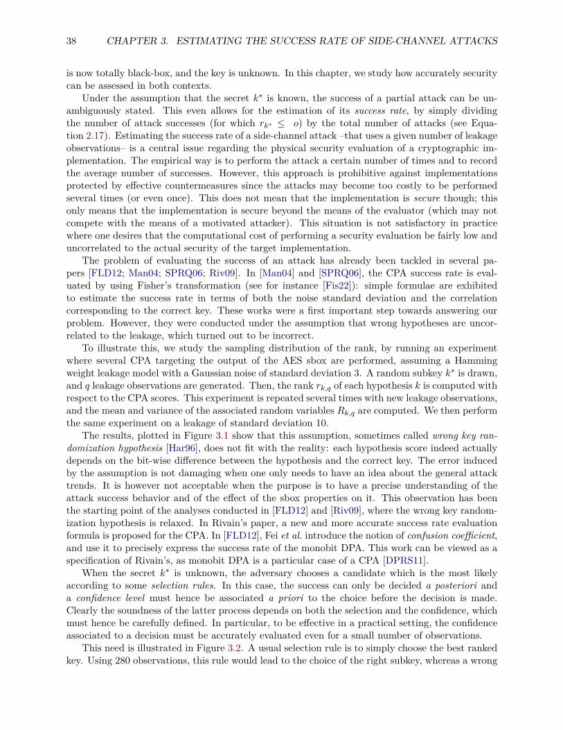
38 CHAPTER 3. ESTIMATING THE SUCCESS RATE OF SIDE-CHANNEL ATTACKS
is now totally black-box, and the key is unknown. In this chapter, we study how accurately securitycan be assessed in both contexts.
Under the assumption that the secret k∗ is known, the success of a partial attack can be un-ambiguously stated. This even allows for the estimation of its success rate, by simply dividingthe number of attack successes (for which rk∗ ≤ o) by the total number of attacks (see Equa-tion 2.17). Estimating the success rate of a side-channel attack –that uses a given number of leakageobservations– is a central issue regarding the physical security evaluation of a cryptographic im-plementation. The empirical way is to perform the attack a certain number of times and to recordthe average number of successes. However, this approach is prohibitive against implementationsprotected by effective countermeasures since the attacks may become too costly to be performedseveral times (or even once). This does not mean that the implementation is secure though; thisonly means that the implementation is secure beyond the means of the evaluator (which may notcompete with the means of a motivated attacker). This situation is not satisfactory in practicewhere one desires that the computational cost of performing a security evaluation be fairly low anduncorrelated to the actual security of the target implementation.
The problem of evaluating the success of an attack has already been tackled in several pa-pers [FLD12; Man04; SPRQ06; Riv09]. In [Man04] and [SPRQ06], the CPA success rate is eval-uated by using Fisher’s transformation (see for instance [Fis22]): simple formulae are exhibitedto estimate the success rate in terms of both the noise standard deviation and the correlationcorresponding to the correct key. These works were a first important step towards answering ourproblem. However, they were conducted under the assumption that wrong hypotheses are uncor-related to the leakage, which turned out to be incorrect.
To illustrate this, we study the sampling distribution of the rank, by running an experimentwhere several CPA targeting the output of the AES sbox are performed, assuming a Hammingweight leakage model with a Gaussian noise of standard deviation 3. A random subkey k∗ is drawn,and q leakage observations are generated. Then, the rank rk,q of each hypothesis k is computed withrespect to the CPA scores. This experiment is repeated several times with new leakage observations,and the mean and variance of the associated random variables Rk,q are computed. We then performthe same experiment on a leakage of standard deviation 10.
The results, plotted in Figure 3.1 show that this assumption, sometimes called wrong key ran-domization hypothesis [Har96], does not fit with the reality: each hypothesis score indeed actuallydepends on the bit-wise difference between the hypothesis and the correct key. The error inducedby the assumption is not damaging when one only needs to have an idea about the general attacktrends. It is however not acceptable when the purpose is to have a precise understanding of theattack success behavior and of the effect of the sbox properties on it. This observation has beenthe starting point of the analyses conducted in [FLD12] and [Riv09], where the wrong key random-ization hypothesis is relaxed. In Rivain’s paper, a new and more accurate success rate evaluationformula is proposed for the CPA. In [FLD12], Fei et al. introduce the notion of confusion coefficient,and use it to precisely express the success rate of the monobit DPA. This work can be viewed as aspecification of Rivain’s, as monobit DPA is a particular case of a CPA [DPRS11].
When the secret k∗ is unknown, the adversary chooses a candidate which is the most likelyaccording to some selection rules. In this case, the success can only be decided a posteriori anda confidence level must hence be associated a priori to the choice before the decision is made.Clearly the soundness of the latter process depends on both the selection and the confidence, whichmust hence be carefully defined. In particular, to be effective in a practical setting, the confidenceassociated to a decision must be accurately evaluated even for a small number of observations.
This need is illustrated in Figure 3.2. A usual selection rule is to simply choose the best rankedkey. Using 280 observations, this rule would lead to the choice of the right subkey, whereas a wrong
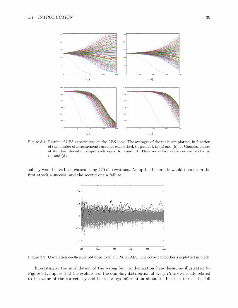
3.1. INTRODUCTION 39
0
50
100
150
200
250
1 10 100 1000 10000
(a)
0
50
100
150
200
250
1 10 100 1000 10000
(b)
0
1000
2000
3000
4000
5000
6000
1 10 100 1000 10000
(c)
0
1000
2000
3000
4000
5000
6000
1 10 100 1000 10000
(d)
Figure 3.1: Results of CPA experiments on the AES sbox. The averages of the ranks are plotted, in functionof the number of measurements used for each attack (logscaled), in (a) and (b) for Gaussian noisesof standard deviation respectively equal to 3 and 10. Their respective variances are plotted in(c) and (d).
subkey would have been chosen using 420 observations. An optimal heuristic would then deem thefirst attack a success, and the second one a failure.
Figure 3.2: Correlation coefficients obtained from a CPA on AES. The correct hypothesis is plotted in black.
Interestingly, the invalidation of the wrong key randomization hypothesis, as illustrated byFigure 3.1, implies that the evolution of the sampling distribution of every Rk is eventually relatedto the value of the correct key and hence brings information about it. In other terms, the full
40 CHAPTER 3. ESTIMATING THE SUCCESS RATE OF SIDE-CHANNEL ATTACKS
vector of ranks gives information on the correct key (and not only the hypothesis ranked first).Based on this observation, it seems natural to use this information to increase the attack efficiencyand/or the confidence in the attack results. To be able to precisely assess both kinds of increase,the distributions of all the variables Rk therefore need to be understood. Bearing this in mind,we now formalize some information that an adversary can obtain while performing a side-channelattack on a set of q independent observations. Scores are computed using a progressive approach,i.e. taking an increasing number of traces into account. Namely, the scores are computed afterq1 < q observations, then again after q2 > q1 observations, and so on until the q observations havebeen considered. This approach enables the computation of the matrix1:
Ms =
s(1, q1) s(1, q2) · · · s(1, q)...
... . . . ...s(|K|, q1) s(|K|, q2) · · · s(|K|, q)
,where s(k, qi) denotes the score of the hypothesis k computed using qi observations.
According to the Neyman-Pearson lemma [NP33], an optimal selection rule would then requirethe knowledge of the statistical distribution of this matrix when the correct subkey is known. Ina real attack setup however, the latter subkey is unknown and one then has to proceed with alikelihood-ratio approach in order to retrieve it. Even optimal from an effectiveness point of view,this approach is not realistic as it reposes on two major issues: the knowledge of the distribution ofthe matrix (which requires a theoretical study over highly dimensional data) and the computationand storage of every score (which may require a lot of time and memory). Moreover, one couldwonder if all the information contained in the matrix is relevant, or if there is some redundancy. Onthe opposite side, the actual attacks only use small parts of the available information. For example,the classical selection of the best ranked key simply amounts to choose the maximum of the lastcolumn of scores inMs. Between those two extrem approaches, one could wonder if other tractableparts of the matrix can be used to give better selection rules or better confidence estimators.
Several criteria indicating the effectiveness of side-channels have also been studied to compareside-channel attacks (e.g. [WO11a]). Among those, the particular behavior of the right subkeyranking have been exploited in [NSGD11] to propose an improvement of the attack efficiencywhen the correct key is unknown. This approach illustrates the importance of such criteria inpractical attacks, but it is purely empirical. To optimize the exhaustive search phase, the authorsof [VGRS11] propose an algorithm taking as inputs the confidence of the results of each partialattack, thus illustrating the need for a precise study of this problem.
In this chapter, we propose a methodology to estimate the success rate of side-channel attackstargeting implementations protected by masking. Our methodology is based on the approach pro-posed by Rivain in [Riv09] in the context of first-order side-channel attacks. It trivially extends tofirst order side-channel attacks against unprotected implementations. The principle of this approachis to study the multivariate distribution of the score vector resulting from an attack. Specifically,Rivain suggests to approximate this distribution by a multivariate Gaussian distribution, whichis sound in the context of additive distinguishers such as the correlation and the likelihood. Wegeneralize this approach to high order side-channel analysis (HO-SCA) and we show how to de-rive the distribution parameters with respect to the leakage parameters. We show that using thismethodology makes it possible to accurately estimate the success rate of a high order side-channelattack based on a simple profiling of the leakage parameters. Moreover, we demonstrate the sound-ness of our methodology by comparing its results to various attack experiments against masked
1Note that this matrix does not capture all the information available to an attacker. Indeed, for example all setsof size q1 could be used to gain information, not only the first set of measurements.
3.2. PRELIMINARIES 41
AES implementations running on two different microcontrollers. We also introduce the notion ofconfidence level, aiming at evaluating the probability of correctness of a side-channel attack result.
3.2 Preliminaries
The expectation and the variance of a random variable X are respectively denoted by E [X] andVar [X]. The covariance between two random variables X and Y is denoted by Cov [X,Y ].
The Gaussian distribution of dimension T with expectation vectorm in RT and T×T covariancematrix Σ is denoted by N (m,Σ), and the corresponding probability density function (pdf) isdenoted by φm,Σ. We recall that this pdf is defined for every x ∈ RT as
φm,Σ(x) = 1√(2π)T |Σ|
exp(−1
2(x−m)ᵀ ·Σ−1 · (x−m)), (3.1)
where (x −m)ᵀ denotes the transpose of the vector (x −m) and |Σ| denotes the determinant ofthe matrix Σ. The corresponding cumulative distribution function (cdf) is denoted Φm,Σ and isdefined for a pair of vectors a = (a1, a2, . . . , aT ) and b = (b1, b2, . . . , bT ) over (R∪−∞,+∞)T by
Φm,Σ(a, b) =∫ b1
a1
∫ b2
a2· · ·∫ bT
aT
φm,Σ(x) dx . (3.2)
If the dimension T equals 1, then the Gaussian distribution is said to be univariate and itscovariance matrix is reduced to the variance of the single coordinate denoted σ2. If T is greaterthan 1, the Gaussian distribution is said to be multivariate.
3.3 Side-Channel Model
We consider a cryptographic algorithm protected by masking and running on a leaking device. A(high order) side-channel attack exploits the leakage resulting from intermediate computations inorder to recover (part of) the secret involved in the cryptographic algorithm. Let s denote such anintermediate variable satisfying:
s = ϕ(x, k∗) , (3.3)
where x is (part of) the public input of the algorithm, k∗ is (part of) the secret input of thealgorithm, and ϕ is some function from X ×K to S.
As described in Section 2.5.1, for an implementation protected with masking, such a variables is never stored nor handled in clear but in the form of several, say d + 1, shares s0, s1, . . . , sdsatisfying the relation
s0 ? s1 ? · · · ? sd = s (3.4)
for some operation ?. In the common case of Boolean masking this operation is the bitwise additionmodulo 2 (or XOR, denoted ⊕), but it might be some other group addition law. In that case, itcan be noted that the (d + 1)-tuple of shares can be modeled as a random vector (S0, S1, . . . , Sd)where S0 = s ⊕⊕d
j=1 Sj and, for j > 1, the Sj are mutually independent random variables withuniform distribution over S.
42 CHAPTER 3. ESTIMATING THE SUCCESS RATE OF SIDE-CHANNEL ATTACKS
3.3.1 Leakage ModelAs stated in Remark 2.5.2, during the execution of the algorithm, the processing of each share Sjproduces some leakage Lj revealing some information about the share value, hence forming theleakage tuple
L = (L0, L1, . . . , Ld) . (3.5)
We shall sometimes use the alternative notation Ls or Lx,k∗ to indicate that the leakage arises forthe shared value s = ϕ(x, k∗).
In this chapter, we use the leakage model described in Section 2.4, in particular the additiveGaussian noisy leakage. Therefore, Equation 2.12 implies that, for every j ≤ d+1, we have: shares,the leakage has a Gaussian distribution. This assumption is referred
Lj = fj(Sj) +Nj , (3.6)
where fj is a deterministic function.As a final assumption, we consider that for any fixed values of the shares, the leakage components
are independent. That is, for every (s0, s1, . . . , sd) ∈ Sd+1, the random variables (Lj | Sj = sj) aremutually independent. Under the Gaussian noise assumption, this simply means that the noisesNj are mutually independent, and that is why we shall refer this assumption as the independentnoises assumption.
Remark 3.3.1. For the sake of simplicity, we consider that all the leakages Lj have the samedimension T . Note that our analysis could be easily extended to the general case where eachleakage Lj has its own dimension Tj .
3.3.2 Side-Channel AttacksIn a side-channel attack (SCA), the adversary aims to extract information about k∗ by monitoringthe leakage of the shares. Specifically, the adversary observes several samples `i ∈ L of the leakageLxi,k∗ , corresponding to some public input xi that he may either choose or just know. According tothe above leakage model, the leakage space L is defined as L = RT×(d+1) and each leakage samplecan be written as
`i = (`i,0, `i,1, · · · , `i,d) , (3.7)
with `i,j ∈ RT for every j. Moreover, the Gaussian noise assumption implies that each leakagesample coordinate can be further written as
`i,j = fj(si,j) + ni,j , (3.8)
where si,1, si,2, . . . , si,d are d random mask values, where si,0 = ϕ(xi, k∗) ⊕⊕dj=1 si,j , and where
ni,0, ni,1, . . . , ni,d are samples of the Gaussian noises N0, N1, . . . , Nd.Once several, say q, leakage samples have been collected, the adversary makes use of a distin-
guisher, that is a function mapping the input-leakage samples (x1, `1), (x2, `2), . . . , (xq, `q) to somescore vector d = (dk)k∈K ∈ R|K|. If the distinguisher is sound and if the leakage brings enoughinformation on the shares, then the equality
k∗ = argmaxk∈K
dk
should hold with a probability substantially greater than 1|K| .
3.4. ESTIMATING THE SUCCESS RATE 43
In what follows, we shall consider a natural equivalence relation between distinguishers. We saythat two score vectors are rank-equivalent if for every n ∈ 1, 2, . . . , |K|, the n coordinates withhighest scores are the same for the two vectors. Two distinguishers d and d′ are then said equivalent,denoted d ≡ d′ if for every (xi, `i)i ∈ (X × L)q, the score vectors d
((xi, `i)i
)and d′
((xi, `i)i
)are
rank-equivalent.
In this chapter, we focus on additive distinguishers which we formally define hereafter.
Definition 3.3.2. A distinguisher d is additive if for every (x1, x2, . . . , xq) ∈ X q, there exists afamily of functions gx,k : L → R ; (x, k) ∈ X × K such that for every (`1, `2, . . . , `q) ∈ Lq wehave
d((xi, `i)i
)= (dk)k∈K with dk = 1
q
q∑i=1
gxi,k(`i) for every k ∈ K.
A distinguisher equivalent to an additive distinguisher as defined above is also said to be additive.
It was shown in [Riv09] that the widely used first-order correlation and likelihood distinguishersare both additive distinguishers in the sense of the above definition. We will show in Sections 3.5and 3.6 that their high order counterparts are also additive.
3.4 Estimating the Success RateIn this section, we generalize the methodology introduced in [Riv09] to high order side-channelattacks as modeled in the previous section. Namely, we show how to get a sound estimation of theattack success rate by studying the multivariate probability distribution of the score vector for thecase of additive distinguishers.
The success rate of a high order side-channel attack, denoted Succdx,k∗ , is defined with respect to
some input vector x = (x1, x2, . . . , xq), some secret k∗, and some distinguisher d, as the probability:
P[k∗ = argmax
k∈Kdk∣∣∣ `1
$←− Lx1,k∗ ; . . . ; `q $←− Lxq ,k∗ ; (dk)k∈K = d((xi, `i)i
)],
where `i $←− Lxi,k∗ means randomly sampling `i according to the distribution of Lxi,k∗ .
Remark 3.4.1. For the sake of generality, we chose to fix the input vector x as a parameter of theattack so that we do not need to assume any specific strategy for the choice of the public inputs.However, we will investigate the particular setting where the xi are uniformly distributed.
According to Definition 3.3.2, the score vector (dk)k∈K resulting from an additive distinguishersatisfies
dk = 1q
q∑i=1
gxi,k(`i) , (3.9)
for some gx,k : L → R. Then a simple application of the central limit theorem yields the fol-lowing result, where we define the occurrence ratio τx of an element x ∈ X in the input vector(x1, x2, . . . , xq) as
τx = |i; xi = x|q
. (3.10)
44 CHAPTER 3. ESTIMATING THE SUCCESS RATE OF SIDE-CHANNEL ATTACKS
Proposition 3.4.2. The distribution of the score vector (dk)k∈K tends toward a multivariate Gaus-sian distribution as q grows, with expectation vector (E [dk])k∈K satisfying
E [dk] =∑x∈X
τx E [gx,k(Lx,k∗)] (3.11)
for every k ∈ K, and with covariance matrix (Cov [dk1 , dk2 ])(k1,k2)∈K2 satisfying
Cov [dk1 , dk2 ] = 1q
∑x∈X
τx Cov [gx,k1(Lx,k∗), gx,k2(Lx,k∗)] (3.12)
for every (k1, k2) ∈ K2.
Proof. The first statement results by definition of additive distinguishers and the central limittheorem. Equation (3.11) and Equation (3.12) directly hold by mutual independence between theleakage samples.
The above proposition shows that for a sufficient number of leakage observations, the distribu-tion of the score vector d = (dk)k∈K can be soundly estimated by a multivariate Gaussian. As in[Riv09], we now define the comparison vector as the (|K| − 1)-size vector c = (ck)k∈K/k∗ whosecoordinates satisfy
ck = dk∗ − dk , (3.13)
for every k ∈ K/k∗. The comparison vector is a linear transformation of the score vector by a((|K| − 1) × |K|)-matrix P whose expression straightforwardly follows from Equation (3.13). Thisimplies that the distribution of the comparison vector can also be soundly estimated by a multi-variate Gaussian distribution N (mc,Σc) where mc = P ·md and Σc = P ·Σd · P ′. Moreover, bydefinition of the comparison vector, an attack is successful (ie. the correct secret k∗ is ranked firstin the score vector) if and only if all the coordinates of the comparison vector are positive. Wededuce that the success rate Succd
x,k∗ of a distinguisher d satisfies
Succdx,k∗ = P[c > 0] ≈ Φmc,Σc
(0,∞
)(3.14)
where Φm,Σ denotes the Gaussian cdf as defined in Equation (3.2), 0 denotes the null vector, and∞ denotes the vector (∞,∞, . . . ,∞).
Remark 3.4.3. In [SMY06], Standaert et al. propose to extend the notion of success rate todifferent orders. The o-th order success rate of a side-channel attack is defined as the probabilitythat the target secret k∗ is ranked among the o first key guesses by the score vector. The authorsof [SMY06] also suggest to consider the so-called guessing entropy, which is defined as the expectedrank of the good key guess in the score vector [Mas94; Cac97]. As shown in [Riv09], both thesuccess rate of any order and the guessing entropy can be estimated using a similar approach asabove.
Methodology.
According to the above analysis, we propose the following methodology for an evaluator of somecryptographic algorithm to estimate the success rate of a (HO-)SCA against his (masked) imple-mentation. We consider that the evaluator has access to the random masks generated during thecomputation, and is therefore able to predict the value of each share involved in the successiveexecution of the protected algorithm. The methodology is composed of three main steps:
3.5. APPLICATION TO THE CORRELATION DISTINGUISHER 45
1. Profile the leakage of every share using standard estimation techniques. Under the Gaussianleakage assumption, this estimation amounts to compute the sample means and the samplecovariance matrices of the leakage (Li | Si = s) for every share Si and every possible value s ∈S based on a set of collected leakage samples. using for instance linear regression techniquesas described in [SLP05].
2. Use Proposition 3.4.2 to compute the expectation vector and covariance matrix of the scorevector with respect to the leakage parameters.
3. Deduce the parameters of the comparison vector distribution and evaluate the success rateaccording to Equation (3.14).
The precision of the obtained estimation is impacted by two main factors:
• the accuracy of the leakage parameter estimations, and
• the tightness of the Gaussian approximation arising in Proposition 3.4.2.
The accurate estimation of leakage parameters has been a widely investigated issue and efficienttechniques are known to deal with it (see for instance [CRR03; SLP05; APSQ06; GLRP06]). Ba-sically, the more noisy the leakage, the more samples must be used to get an accurate estimation.Note that in our approach, the evaluator only has to estimate first-order leakage parameters withrespect to the share values. Practical aspects of leakage parameter estimation are further discussedin Section 3.8.
On the other hand, the Gaussian approximation is the main issue in our approach. One canfairly expect that if the considered implementation is not too weak, the convergence toward theGaussian distribution should be rather fast compared to the number of leakage observations requiredto succeed the HO-SCA. In order to validate this intuition, we provide in Section 3.7 an empiricalvalidation of the Gaussian approximation.
3.5 Application to the Correlation DistinguisherIn this section, we apply the general methodology described in Section 3.4 when the linear correla-tion coefficient is used as a distinguisher [BCO04]. To simplify the explanations and developments,we assume that the dimension T of the components Lj of the leakage vector L equals 1. This impliesin particular that the Lj follow a univariate Gaussian distribution with zero mean and varianceσ2j (instead of a Gaussian multivariate distribution N (0,Σj)). The reasoning straightforwardly
extends to the case T > 1. For two samples x = (x1, x2, . . . , xq) ∈ Rq and y = (y1, y2, . . . , yq) ∈ Rq,the linear coefficient is defined by
ρ(x,y) =1q
∑qi=1(xi − x) · (yi − y)√
1q
∑i(xi − x)2 ·
√1q
∑i(yi − y)2
, (3.15)
where x (resp. y) denotes the sample mean q−1∑i xi (resp. q−1∑
i yi).In the context of HO-SCA, the correlation coefficient is used together with a model function
m : X × K 7→ R and a combining function C : L 7→ R (see for instance [PRB10]). The combiningfunction is involved to map a leakage sample into a univariate sample combining the leakages ofthe different shares. On the other hand, the model function computes some expected value for
46 CHAPTER 3. ESTIMATING THE SUCCESS RATE OF SIDE-CHANNEL ATTACKS
the combined leakage with respect to some input x and some guess k on the target secret. Thecorrelation distinguisher dcor is then defined as
dcor((xi, `i)i
)= ρ
((m(xi, k))i, (C(`i))i
). (3.16)
The following proposition extends the analysis conducted in [Riv09] and states that the (highorder) correlation distinguisher dcor is additive. This particularly implies that the methodologydescribed in Section 3.4 can be applied to this distinguisher.
Proposition 3.5.1. For any model function m : X×K 7→ R and any combining function C : L 7→ R,the correlation distinguisher dcor is additive. Moreover, dcor is equivalent to the distinguisher d′cordefined for every (xi, `i)i ∈ (X ×L)q by
d′cor((xi, `i)i
)=(1q
q∑i=1
gxi,k(`i))k∈K
,
where the function gx,k : L→ R satisfies
gx,k(`) = 1sk
(m(x, k)− mk) · C(`) , (3.17)
for every (x, k) ∈ X ×K, with mk = 1q
∑i m(xi, k) and sk =
√1q
∑i(m(xi, k)− mk)2.
Proof. Let (dk)k∈K = dcor((xi, `i)i
)and (d′k)k∈K = d′cor
((xi, `i)i
)for some input-leakage samples
(xi, `i)i6q ∈ (X × L)q. We have:
dk = 1sC
∑qi=1(m(xi, k)− mk)C(`i)
sk= 1
sCd′k ,
where sC =√
1q
∑i(C(`i)− C)2 with C = 1
q
∑i C(`i).
Since sC is strictly positive and constant with respect to the guess k, the score vectors (dk)k∈Kand (d′k)k∈K are clearly rank-equivalent, implying that the distinguishers dcor and d′cor are equiv-alent. Moreover, after denoting by gx,k the function `i 7→ s−1
k (m(x, k) − mk)C(`i), we get d′k =1q
∑qi=1 gxi,k(`i), which implies that d′cor is additive.
Remark 3.5.2. If we focus on the uniform setting where the input vector x = (x1, x2, . . . , xq) isbalanced (meaning that each value x ∈ X have an occurrence ratio of τx = 1
|X |), then mk and skare constant with respect to k and dcor is equivalent to another simpler distinguisher:
d′′cor :((xi, `i)i
) 7→ (1q
∑im(xi, k) · C(`i)
)k∈K
. (3.18)
Confusion coefficient
We propose hereafter to show how our approach can be seen as an extension to the work of Fei etal. [FLD12], which is itself an extension of the notion of transparency order introduced in [Pro05](see also the recent publication [CSM+14], which redefines this notion). We apply our approach tothe first-order attack, and illustrate how the notion of confusion coefficient can be extended in thissetting. In [FLD12], the confusion coefficient associated to a key k was defined for the mono-bitDPA as the probability on x that the prediction m(x, k) differs from the correct prediction m(x, k).In a multi-bit setting, we modify this definition in order to accurately capture the confusing effectof the cryptographic operation between predicted values.
3.5. APPLICATION TO THE CORRELATION DISTINGUISHER 47
Definition 3.5.3. Let k∗ denote the correct key of a cryptographic implementation, and k any keyin the set of possible keys K. Let x denote an element of the set of possible inputs X . Let m denotea modeling function. The CPA confusion coefficient κk is then defined as:
κk = 1#X
∑x∈X
m(x, k)m(x, k∗).
Remark 3.5.4. In the case of a first-order CPA, the confusion coefficient allows for the expressionof the parameters of the multivariate normal law followed by d′′cor, hence recovering the resultsof [Riv09]. Indeed, the expectation of the score d′′k associated to a key hypothesis k is equal to theconfusion coefficient κk. Furthermore, in the particular case where all occurrences ratios are equal,the covariance matrix associated to the distribution of d′′cor can also be expressed with confusioncoefficients: namely, each coefficient of coordinate (i, j) of this matrix is equal to σ2
N κi⊕j .
In Figure 3.3 we illustrate the CPA confusion coefficient in the case where m is the compositionof the Hamming weight with some classical sboxes. This figure, along with Remark 3.5.4 gives astraightforward intuition on why CPA performs differently depending on the targeted sbox. Indeed,one can observe a stronger dispersion in the DES and PRESENT sboxes than in the AES sbox.
Application to the Normalized Product Combining.
Let us now study the particular case of the high order correlation distinguisher based on thecentered product combining function [PRB10]. This combining function is defined for univariateshare leakages (ie. for T = 1 in the model of Section 3.3), namely its domain is L = Rd+1. Forevery (`0, `1, . . . , `d) ∈ L, it is defined as
C(`0, `1, . . . , `d) =d∏j=0
(`j − µj) , (3.19)
where µj denotes the leakage expectation E [Lj ].Note that in practice, the adversary does not know the exact expectation µj but he can estimate
it based on leakage samples. As argued in [PRB10], the number of leakage samples required tosucceed a HO-SCA is substantially greater than the number of leakage samples required to getprecise estimations of the expectations µj . Therefore, we can soundly assume that the µj inEquation (3.19) are the exact expectations E [Lj ]. Note that replacing them by inexact estimationswould not change our analysis.
We recall that, according to the leakage model presented in Section 3.3.1, the j-th leakagecomponent Lj satisfies Lj = fj(Sj) + Nj where fj : s 7→ mj,s and Nj ∼ N (0, σ2
j ). Since the noiseNj is centered in 0, we have E [fj(Sj)] = E [Lj ] = µj . Moreover, we shall denote νj = Var [fj(Sj)].By uniformity of Sj over S, we have:
µj = 1|S|
∑s∈S
mj,s and νj = 1|S|
∑s∈S
(mj,s − µj)2 . (3.20)
In the following we shall further denote, for every s ∈ S,
αs := 1|S|d
∑s1∈S
∑s2∈S· · ·
∑sd∈S
d∏j=0
(mj,sj − µj) (3.21)
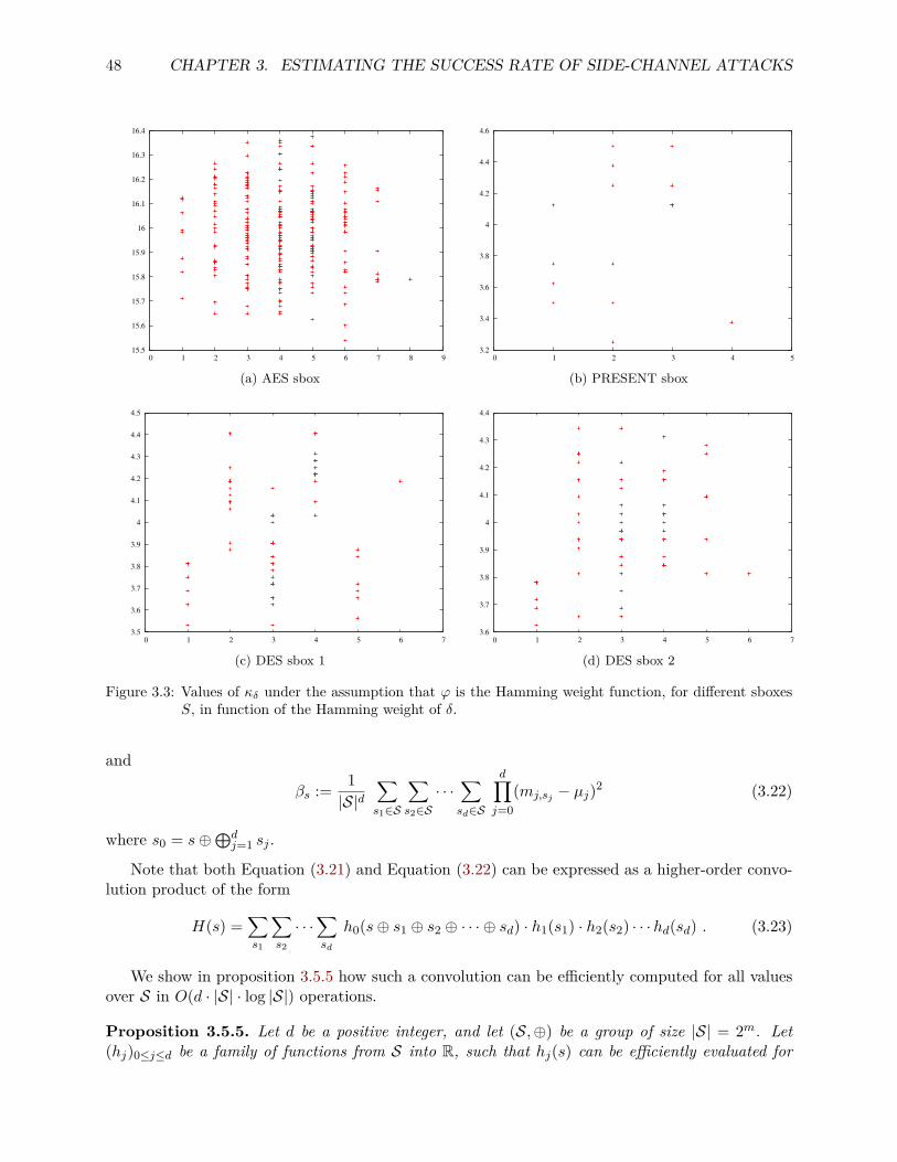
48 CHAPTER 3. ESTIMATING THE SUCCESS RATE OF SIDE-CHANNEL ATTACKS
15.5
15.6
15.7
15.8
15.9
16
16.1
16.2
16.3
16.4
0 1 2 3 4 5 6 7 8 9
(a) AES sbox
3.2
3.4
3.6
3.8
4
4.2
4.4
4.6
0 1 2 3 4 5
(b) PRESENT sbox
3.5
3.6
3.7
3.8
3.9
4
4.1
4.2
4.3
4.4
4.5
0 1 2 3 4 5 6 7
(c) DES sbox 1
3.6
3.7
3.8
3.9
4
4.1
4.2
4.3
4.4
0 1 2 3 4 5 6 7
(d) DES sbox 2
Figure 3.3: Values of κδ under the assumption that ϕ is the Hamming weight function, for different sboxesS, in function of the Hamming weight of δ.
and
βs := 1|S|d
∑s1∈S
∑s2∈S· · ·
∑sd∈S
d∏j=0
(mj,sj − µj)2 (3.22)
where s0 = s⊕⊕dj=1 sj .
Note that both Equation (3.21) and Equation (3.22) can be expressed as a higher-order convo-lution product of the form
H(s) =∑s1
∑s2
· · ·∑sd
h0(s⊕ s1 ⊕ s2 ⊕ · · · ⊕ sd) · h1(s1) · h2(s2) · · ·hd(sd) . (3.23)
We show in proposition 3.5.5 how such a convolution can be efficiently computed for all valuesover S in O(d · |S| · log |S|) operations.
Proposition 3.5.5. Let d be a positive integer, and let (S,⊕) be a group of size |S| = 2m. Let(hj)0≤j≤d be a family of functions from S into R, such that hj(s) can be efficiently evaluated for
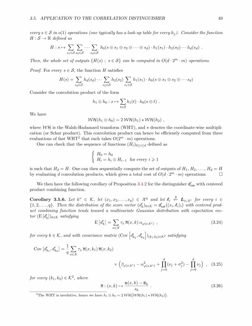
3.5. APPLICATION TO THE CORRELATION DISTINGUISHER 49
every s ∈ S in o(1) operations (one typically has a look-up table for every hj). Consider the functionH : S → R defined as
H : s 7→∑s1∈S
∑s2∈S· · ·
∑sd∈S
h0(s⊕ s1 ⊕ s2 ⊕ · · · ⊕ sd) · h1(s1) · h2(s2) · · ·hd(sd) .
Then, the whole set of outputs H(s) ; s ∈ S can be computed in O(d · 2m ·m) operations.
Proof. For every s ∈ S, the function H satisfies
H(s) =∑sd∈S
hd(sd) · · ·∑s2∈S
h2(s2)∑s1∈S
h1(s1) · h0(s⊕ s1 ⊕ s2 ⊕ · · · sd)
Consider the convolution product of the form
h1 ⊗ h0 : s 7→∑t∈S
h1(t) · h0(s⊕ t) .
We haveWH(h1 ⊗ h0) = 2WH(h1) ?WH(h2) ,
where WH is the Walsh-Hadamard transform (WHT), and ? denotes the coordinate-wise multipli-cation (or Schur product). This convolution product can hence be efficiently computed from threeevaluations of fast WHT2 that each takes O(2m ·m) operations.
One can check that the sequence of functions (Hi)0≤i≤d defined asH0 = h0Hi = hi ⊗Hi−1 for every i > 1
is such that Hd = H. One can then sequentially compute the set of outputs of H1, H2, . . . , Hd = Hby evaluating d convolution products, which gives a total cost of O(d · 2m ·m) operations.
We then have the following corollary of Proposition 3.4.2 for the distinguisher d′cor with centeredproduct combining function.
Corollary 3.5.6. Let k∗ ∈ K, let (x1, x2, . . . , xq) ∈ X q and let `i $←− Lxi,k∗ for every i ∈1, 2, . . . , q. Then the distribution of the score vector (d′k)k∈K = d′cor
((xi, `i)i
)with centered prod-
uct combining function tends toward a multivariate Gaussian distribution with expectation vec-tor (E [d′k])k∈K satisfying
E[d′k]
=∑x∈X
τx M(x, k) αϕ(x,k∗) , (3.24)
for every k ∈ K, and with covariance matrix (Cov[d′k1
, d′k2
])(k1,k2)∈K2 satisfying
Cov[d′k1 , d
′k2
]= 1q
∑x∈X
τx M(x, k1) M(x, k2)
×(βϕ(x,k∗) − α2
ϕ(x,k∗) +d∏j=0
(νj + σ2j )−
d∏j=0
νj), (3.25)
for every (k1, k2) ∈ K2, whereM : (x, k) 7→ m(x, k)− mk
sk. (3.26)
2The WHT is involutive, hence we have h1 ⊗ h0 = 2WH(WH(h1) ?WH(h2)
).
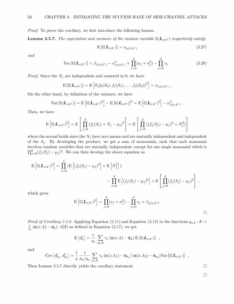
50 CHAPTER 3. ESTIMATING THE SUCCESS RATE OF SIDE-CHANNEL ATTACKS
Proof. To prove the corollary, we first introduce the following lemma.
Lemma 3.5.7. The expectation and variance of the random variable C(Lx,k∗) respectively satisfy
E [C(Lx,k∗)] = αϕ(x,k∗) (3.27)
and
Var [C(Lx,k∗)] = βϕ(x,k∗) − α2ϕ(x,k∗) +
d∏j=0
(νj + σ2j )−
d∏j=0
νj . (3.28)
Proof. Since the Nj are independent and centered in 0, we have
E [C(Lx,k∗)] = E[C(f0(S0), f1(S1), . . . , fd(Sd)
)2] = αϕ(x,k∗) ,
On the other hand, by definition of the variance, we have
Var [C(Lx,k∗)] = E[C(Lx,k∗)2
]− E [C(Lx,k∗)]2 = E
[C(Lx,k∗)2
]− α2
ϕ(x,k∗) .
Then, we have
E[C(Lx,k∗)2
]= E
d∏j=0
(fj(Sj) +Nj − µj
)2 = E
d∏j=0
((fj(Sj)− µj)2 +N2
j
)where the second holds since theNj have zero means and are mutually independent and independentof the Sj . By developing the product, we get a sum of monomials, such that each monomialinvolves random variables that are mutually independent, except for one single monomial which is∏dj=0(fj(Sj)− µj)2. We can then develop the above equation as
E[C(Lx,k∗)2
]=
d∏j=0
(E[(fj(Sj)− µj)2
]+ E
[N2j
] )
−d∏j=0
E[(fj(Sj)− µj)2
]+ E
d∏j=0
(fj(Sj)− µj)2
,
which gives
E[C(Lx,k∗)2
]=
d∏j=0
(νj + σ2j )−
d∏j=0
νj + βϕ(x,k∗).
Proof of Corollary 3.5.6. Applying Equation (3.11) and Equation (3.12) to the functions gx,k : ` 7→1sk
(m(x, k)− mk) · C(`) as defined in Equation (3.17), we get
E[d′k]
= 1sk
∑x∈X
τx (m(x, k)− mk) E [C(Lx,k∗)] ,
andCov
[d′k1 , d
′k2
]= 1q
1sk1sk2
∑x∈X
τx (m(x, k1)− mk1) (m(x, k2)− mk2)Var [C(Lx,k∗)] ,
Then Lemma 3.5.7 directly yields the corollary statement.
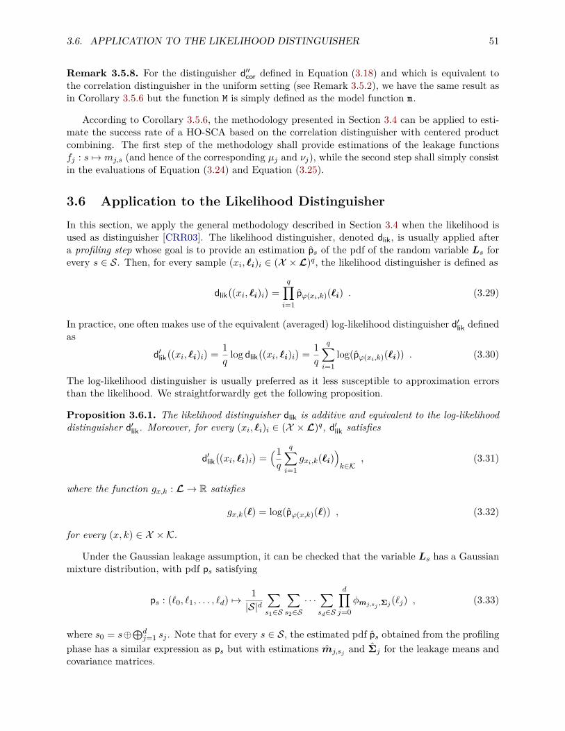
3.6. APPLICATION TO THE LIKELIHOOD DISTINGUISHER 51
Remark 3.5.8. For the distinguisher d′′cor defined in Equation (3.18) and which is equivalent tothe correlation distinguisher in the uniform setting (see Remark 3.5.2), we have the same result asin Corollary 3.5.6 but the function M is simply defined as the model function m.
According to Corollary 3.5.6, the methodology presented in Section 3.4 can be applied to esti-mate the success rate of a HO-SCA based on the correlation distinguisher with centered productcombining. The first step of the methodology shall provide estimations of the leakage functionsfj : s 7→ mj,s (and hence of the corresponding µj and νj), while the second step shall simply consistin the evaluations of Equation (3.24) and Equation (3.25).
3.6 Application to the Likelihood DistinguisherIn this section, we apply the general methodology described in Section 3.4 when the likelihood isused as distinguisher [CRR03]. The likelihood distinguisher, denoted dlik, is usually applied aftera profiling step whose goal is to provide an estimation ps of the pdf of the random variable Ls forevery s ∈ S. Then, for every sample (xi, `i)i ∈ (X ×L)q, the likelihood distinguisher is defined as
dlik((xi, `i)i
)=
q∏i=1
pϕ(xi,k)(`i) . (3.29)
In practice, one often makes use of the equivalent (averaged) log-likelihood distinguisher d′lik definedas
d′lik((xi, `i)i
)= 1q
log dlik((xi, `i)i
)= 1q
q∑i=1
log(pϕ(xi,k)(`i)) . (3.30)
The log-likelihood distinguisher is usually preferred as it less susceptible to approximation errorsthan the likelihood. We straightforwardly get the following proposition.
Proposition 3.6.1. The likelihood distinguisher dlik is additive and equivalent to the log-likelihooddistinguisher d′lik. Moreover, for every (xi, `i)i ∈ (X ×L)q, d′lik satisfies
d′lik((xi, `i)i
)=(1q
q∑i=1
gxi,k(`i))k∈K
, (3.31)
where the function gx,k : L→ R satisfies
gx,k(`) = log(pϕ(x,k)(`)) , (3.32)
for every (x, k) ∈ X ×K.
Under the Gaussian leakage assumption, it can be checked that the variable Ls has a Gaussianmixture distribution, with pdf ps satisfying
ps : (`0, `1, . . . , `d) 7→1|S|d
∑s1∈S
∑s2∈S· · ·
∑sd∈S
d∏j=0
φmj,sj,Σj (`j) , (3.33)
where s0 = s⊕⊕dj=1 sj . Note that for every s ∈ S, the estimated pdf ps obtained from the profiling
phase has a similar expression as ps but with estimations mj,sj and Σj for the leakage means andcovariance matrices.
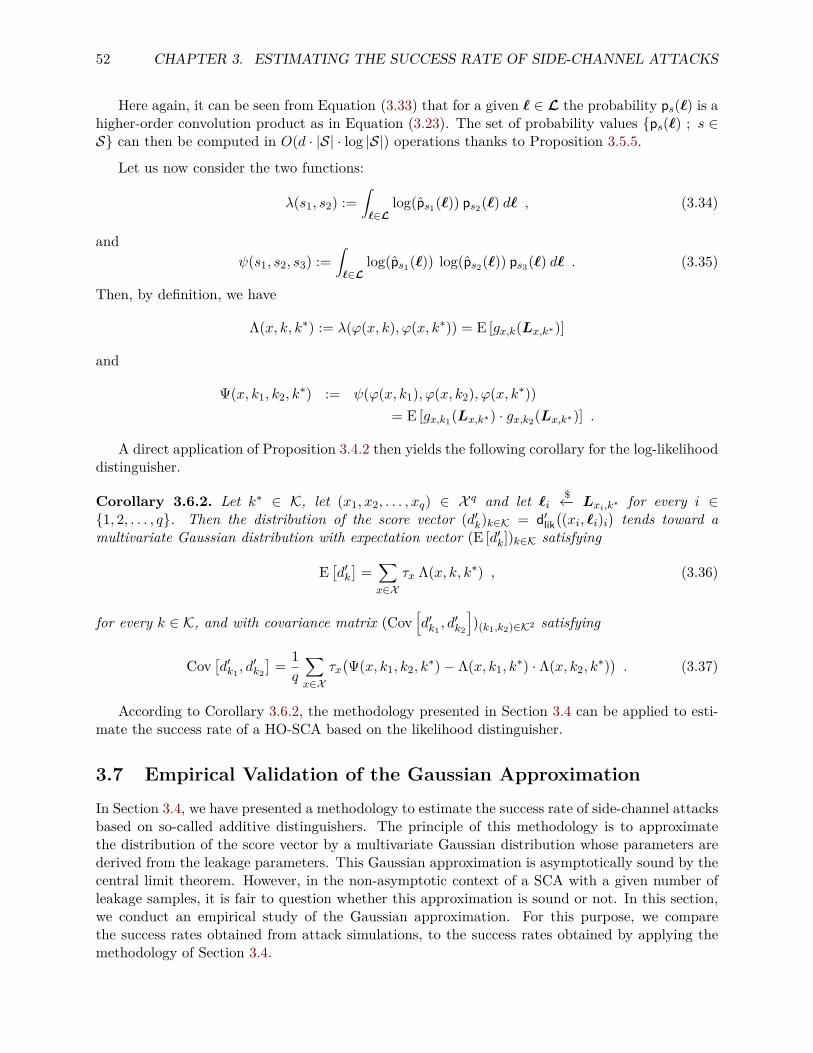
52 CHAPTER 3. ESTIMATING THE SUCCESS RATE OF SIDE-CHANNEL ATTACKS
Here again, it can be seen from Equation (3.33) that for a given ` ∈ L the probability ps(`) is ahigher-order convolution product as in Equation (3.23). The set of probability values ps(`) ; s ∈S can then be computed in O(d · |S| · log |S|) operations thanks to Proposition 3.5.5.
Let us now consider the two functions:
λ(s1, s2) :=∫`∈L
log(ps1(`)) ps2(`) d` , (3.34)
andψ(s1, s2, s3) :=
∫`∈L
log(ps1(`)) log(ps2(`)) ps3(`) d` . (3.35)
Then, by definition, we have
Λ(x, k, k∗) := λ(ϕ(x, k), ϕ(x, k∗)) = E [gx,k(Lx,k∗)]
and
Ψ(x, k1, k2, k∗) := ψ(ϕ(x, k1), ϕ(x, k2), ϕ(x, k∗))
= E [gx,k1(Lx,k∗) · gx,k2(Lx,k∗)] .
A direct application of Proposition 3.4.2 then yields the following corollary for the log-likelihooddistinguisher.
Corollary 3.6.2. Let k∗ ∈ K, let (x1, x2, . . . , xq) ∈ X q and let `i $←− Lxi,k∗ for every i ∈1, 2, . . . , q. Then the distribution of the score vector (d′k)k∈K = d′lik
((xi, `i)i
)tends toward a
multivariate Gaussian distribution with expectation vector (E [d′k])k∈K satisfying
E[d′k]
=∑x∈X
τx Λ(x, k, k∗) , (3.36)
for every k ∈ K, and with covariance matrix (Cov[d′k1
, d′k2
])(k1,k2)∈K2 satisfying
Cov[d′k1 , d
′k2
]= 1q
∑x∈X
τx(Ψ(x, k1, k2, k
∗)− Λ(x, k1, k∗) · Λ(x, k2, k
∗)). (3.37)
According to Corollary 3.6.2, the methodology presented in Section 3.4 can be applied to esti-mate the success rate of a HO-SCA based on the likelihood distinguisher.
3.7 Empirical Validation of the Gaussian ApproximationIn Section 3.4, we have presented a methodology to estimate the success rate of side-channel attacksbased on so-called additive distinguishers. The principle of this methodology is to approximatethe distribution of the score vector by a multivariate Gaussian distribution whose parameters arederived from the leakage parameters. This Gaussian approximation is asymptotically sound by thecentral limit theorem. However, in the non-asymptotic context of a SCA with a given number ofleakage samples, it is fair to question whether this approximation is sound or not. In this section,we conduct an empirical study of the Gaussian approximation. For this purpose, we comparethe success rates obtained from attack simulations, to the success rates obtained by applying themethodology of Section 3.4.
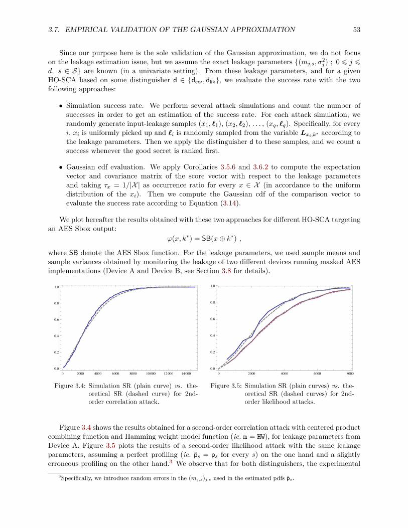
3.7. EMPIRICAL VALIDATION OF THE GAUSSIAN APPROXIMATION 53
Since our purpose here is the sole validation of the Gaussian approximation, we do not focuson the leakage estimation issue, but we assume the exact leakage parameters (mj,s, σ
2j ) ; 0 6 j 6
d, s ∈ S are known (in a univariate setting). From these leakage parameters, and for a givenHO-SCA based on some distinguisher d ∈ dcor, dlik, we evaluate the success rate with the twofollowing approaches:
• Simulation success rate. We perform several attack simulations and count the number ofsuccesses in order to get an estimation of the success rate. For each attack simulation, werandomly generate input-leakage samples (x1, `1), (x2, `2), . . . , (xq, `q). Specifically, for everyi, xi is uniformly picked up and `i is randomly sampled from the variable Lxi,k∗ according tothe leakage parameters. Then we apply the distinguisher d to these samples, and we count asuccess whenever the good secret is ranked first.
• Gaussian cdf evaluation. We apply Corollaries 3.5.6 and 3.6.2 to compute the expectationvector and covariance matrix of the score vector with respect to the leakage parametersand taking τx = 1/|X | as occurrence ratio for every x ∈ X (in accordance to the uniformdistribution of the xi). Then we compute the Gaussian cdf of the comparison vector toevaluate the success rate according to Equation (3.14).
We plot hereafter the results obtained with these two approaches for different HO-SCA targetingan AES Sbox output:
ϕ(x, k∗) = SB(x⊕ k∗) ,
where SB denote the AES Sbox function. For the leakage parameters, we used sample means andsample variances obtained by monitoring the leakage of two different devices running masked AESimplementations (Device A and Device B, see Section 3.8 for details).
0 2000 4000 6000 8000 10000 12000 140000.0
0.2
0.4
0.6
0.8
1.0
Figure 3.4: Simulation SR (plain curve) vs. the-oretical SR (dashed curve) for 2nd-order correlation attack.
0 2000 4000 6000 80000.0
0.2
0.4
0.6
0.8
1.0
Figure 3.5: Simulation SR (plain curves) vs. the-oretical SR (dashed curves) for 2nd-order likelihood attacks.
Figure 3.4 shows the results obtained for a second-order correlation attack with centered productcombining function and Hamming weight model function (ie. m = HW), for leakage parameters fromDevice A. Figure 3.5 plots the results of a second-order likelihood attack with the same leakageparameters, assuming a perfect profiling (ie. ps = ps for every s) on the one hand and a slightlyerroneous profiling on the other hand.3 We observe that for both distinguishers, the experimental
3Specifically, we introduce random errors in the (mj,s)j,s used in the estimated pdfs ps.
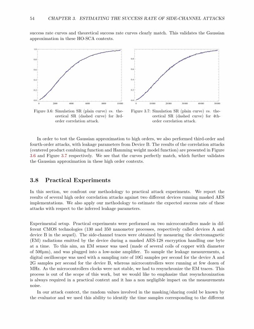
54 CHAPTER 3. ESTIMATING THE SUCCESS RATE OF SIDE-CHANNEL ATTACKS
success rate curves and theoretical success rate curves clearly match. This validates the Gaussianapproximation in these HO-SCA contexts.
0 2000 4000 6000 8000 100000.0
0.2
0.4
0.6
0.8
1.0
Figure 3.6: Simulation SR (plain curve) vs. the-oretical SR (dashed curve) for 3rd-order correlation attack.
0 10000 20000 30000 40000 500000.0
0.2
0.4
0.6
0.8
Figure 3.7: Simulation SR (plain curve) vs. the-oretical SR (dashed curve) for 4th-order correlation attack.
In order to test the Gaussian approximation to high orders, we also performed third-order andfourth-order attacks, with leakage parameters from Device B. The results of the correlation attacks(centered product combining function and Hamming weight model function) are presented in Figure3.6 and Figure 3.7 respectively. We see that the curves perfectly match, which further validatesthe Gaussian approximation in these high order contexts.
3.8 Practical Experiments
In this section, we confront our methodology to practical attack experiments. We report theresults of several high order correlation attacks against two different devices running masked AESimplementations. We also apply our methodology to estimate the expected success rate of theseattacks with respect to the inferred leakage parameters.
Experimental setup. Practical experiments were performed on two microcontrollers made in dif-ferent CMOS technologies (130 and 350 nanometer processes, respectively called devices A anddevice B in the sequel). The side-channel traces were obtained by measuring the electromagnetic(EM) radiations emitted by the device during a masked AES-128 encryption handling one byteat a time. To this aim, an EM sensor was used (made of several coils of copper with diameterof 500µm), and was plugged into a low-noise amplifier. To sample the leakage measurements, adigital oscilloscope was used with a sampling rate of 10G samples per second for the device A and2G samples per second for the device B, whereas microcontrollers were running at few dozen ofMHz. As the microcontrollers clocks were not stable, we had to resynchronize the EM traces. Thisprocess is out of the scope of this work, but we would like to emphasize that resynchronizationis always required in a practical context and it has a non negligible impact on the measurementsnoise.
In our attack context, the random values involved in the masking/sharing could be known bythe evaluator and we used this ability to identify the time samples corresponding to the different
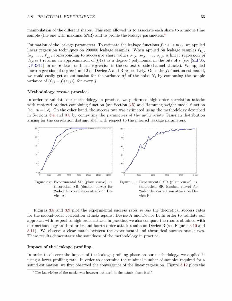
3.8. PRACTICAL EXPERIMENTS 55
manipulation of the different shares. This step allowed us to associate each share to a unique timesample (the one with maximal SNR) and to profile the leakage parameters.4
Estimation of the leakage parameters. To estimate the leakage functions fj : s 7→ mj,s, we appliedlinear regression techniques on 200000 leakage samples. When applied on leakage samples `1,j ,`2,j , . . . , `q,j , corresponding to successive share values s1,j , s2,j , . . . , sq,j , a linear regression ofdegree t returns an approximation of fj(s) as a degree-t polynomial in the bits of s (see [SLP05;DPRS11] for more detail on linear regression in the context of side-channel attacks). We appliedlinear regression of degree 1 and 2 on Device A and B respectively. Once the fj function estimated,we could easily get an estimation for the variance σ2
j of the noise Nj by computing the samplevariance of (`i,j − fj(si,j))i for every j.
Methodology versus practice.
In order to validate our methodology in practice, we performed high order correlation attackswith centered product combining function (see Section 3.5) and Hamming weight model function(ie. m = HW). On the other hand, the success rate was estimated using the methodology describedin Sections 3.4 and 3.5 by computing the parameters of the multivariate Gaussian distributionarising for the correlation distinguisher with respect to the inferred leakage parameters.
0 2000 4000 6000 8000 10000 12000 140000
20
40
60
80
100
Figure 3.8: Experimental SR (plain curve) vs.theoretical SR (dashed curve) for2nd-order correlation attack on De-vice A.
0 2000 4000 6000 8000 100000
20
40
60
80
100
Figure 3.9: Experimental SR (plain curve) vs.theoretical SR (dashed curve) for2nd-order correlation attack on De-vice B.
Figures 3.8 and 3.9 plot the experimental success rates versus the theoretical success ratesfor the second-order correlation attacks against Device A and Device B. In order to validate ourapproach with respect to high order attacks in practice, we also compare the results obtained withour methodology to third-order and fourth-order attack results on Device B (see Figures 3.10 and3.11). We observe a clear match between the experimental and theoretical success rate curves.These results demonstrate the soundness of the methodology in practice.
Impact of the leakage profiling.
In order to observe the impact of the leakage profiling phase on our methodology, we applied itusing a lower profiling rate. In order to determine the minimal number of samples required for asound estimation, we first observed the convergence of the linear regression. Figure 3.12 plots the
4The knowledge of the masks was however not used in the attack phase itself.
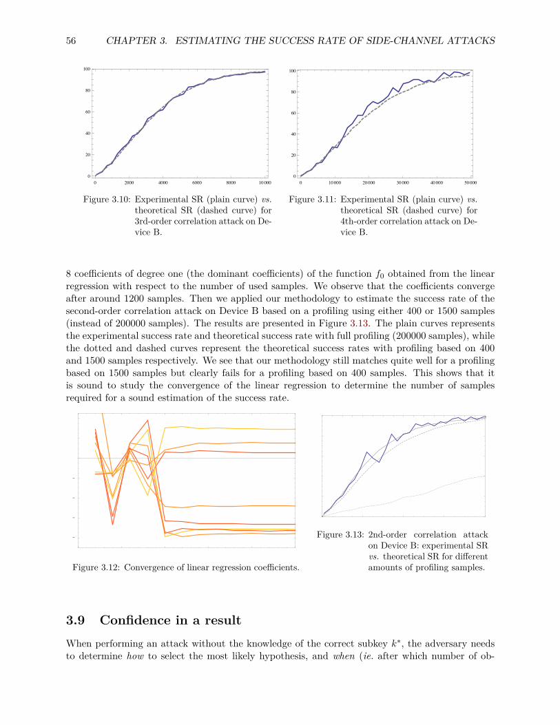
56 CHAPTER 3. ESTIMATING THE SUCCESS RATE OF SIDE-CHANNEL ATTACKS
0 2000 4000 6000 8000 100000
20
40
60
80
100
Figure 3.10: Experimental SR (plain curve) vs.theoretical SR (dashed curve) for3rd-order correlation attack on De-vice B.
0 10000 20000 30000 40000 500000
20
40
60
80
100
Figure 3.11: Experimental SR (plain curve) vs.theoretical SR (dashed curve) for4th-order correlation attack on De-vice B.
8 coefficients of degree one (the dominant coefficients) of the function f0 obtained from the linearregression with respect to the number of used samples. We observe that the coefficients convergeafter around 1200 samples. Then we applied our methodology to estimate the success rate of thesecond-order correlation attack on Device B based on a profiling using either 400 or 1500 samples(instead of 200000 samples). The results are presented in Figure 3.13. The plain curves representsthe experimental success rate and theoretical success rate with full profiling (200000 samples), whilethe dotted and dashed curves represent the theoretical success rates with profiling based on 400and 1500 samples respectively. We see that our methodology still matches quite well for a profilingbased on 1500 samples but clearly fails for a profiling based on 400 samples. This shows that itis sound to study the convergence of the linear regression to determine the number of samplesrequired for a sound estimation of the success rate.
0 500 1000 1500 2000 2500
-8
-6
-4
-2
0
2
4
Figure 3.12: Convergence of linear regression coefficients.
0 2000 4000 6000 80000
20
40
60
80
100
Figure 3.13: 2nd-order correlation attackon Device B: experimental SRvs. theoretical SR for differentamounts of profiling samples.
3.9 Confidence in a resultWhen performing an attack without the knowledge of the correct subkey k∗, the adversary needsto determine how to select the most likely hypothesis, and when (ie. after which number of ob-
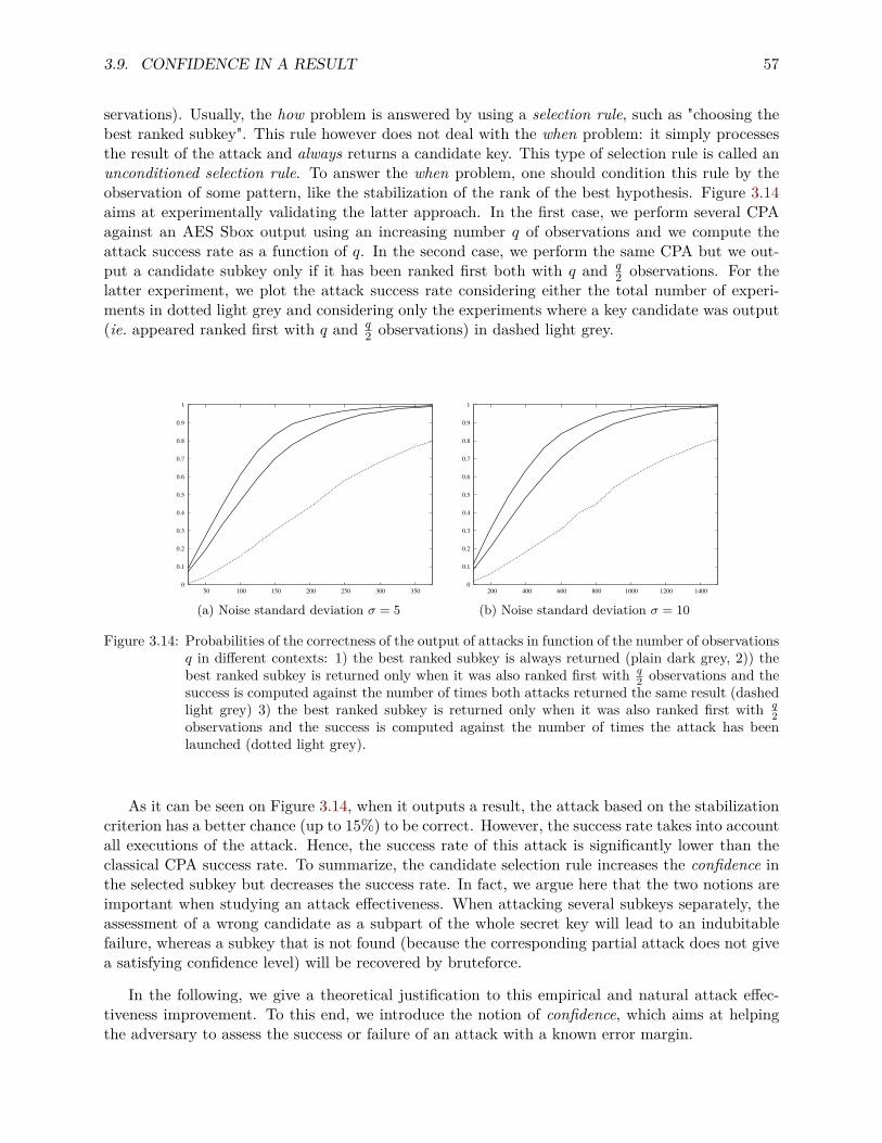
3.9. CONFIDENCE IN A RESULT 57
servations). Usually, the how problem is answered by using a selection rule, such as "choosing thebest ranked subkey". This rule however does not deal with the when problem: it simply processesthe result of the attack and always returns a candidate key. This type of selection rule is called anunconditioned selection rule. To answer the when problem, one should condition this rule by theobservation of some pattern, like the stabilization of the rank of the best hypothesis. Figure 3.14aims at experimentally validating the latter approach. In the first case, we perform several CPAagainst an AES Sbox output using an increasing number q of observations and we compute theattack success rate as a function of q. In the second case, we perform the same CPA but we out-put a candidate subkey only if it has been ranked first both with q and q
2 observations. For thelatter experiment, we plot the attack success rate considering either the total number of experi-ments in dotted light grey and considering only the experiments where a key candidate was output(ie. appeared ranked first with q and q
2 observations) in dashed light grey.
0
0.1
0.2
0.3
0.4
0.5
0.6
0.7
0.8
0.9
1
50 100 150 200 250 300 350
(a) Noise standard deviation σ = 5
0
0.1
0.2
0.3
0.4
0.5
0.6
0.7
0.8
0.9
1
200 400 600 800 1000 1200 1400
(b) Noise standard deviation σ = 10
Figure 3.14: Probabilities of the correctness of the output of attacks in function of the number of observationsq in different contexts: 1) the best ranked subkey is always returned (plain dark grey, 2)) thebest ranked subkey is returned only when it was also ranked first with q
2 observations and thesuccess is computed against the number of times both attacks returned the same result (dashedlight grey) 3) the best ranked subkey is returned only when it was also ranked first with q
2observations and the success is computed against the number of times the attack has beenlaunched (dotted light grey).
As it can be seen on Figure 3.14, when it outputs a result, the attack based on the stabilizationcriterion has a better chance (up to 15%) to be correct. However, the success rate takes into accountall executions of the attack. Hence, the success rate of this attack is significantly lower than theclassical CPA success rate. To summarize, the candidate selection rule increases the confidence inthe selected subkey but decreases the success rate. In fact, we argue here that the two notions areimportant when studying an attack effectiveness. When attacking several subkeys separately, theassessment of a wrong candidate as a subpart of the whole secret key will lead to an indubitablefailure, whereas a subkey that is not found (because the corresponding partial attack does not givea satisfying confidence level) will be recovered by bruteforce.
In the following, we give a theoretical justification to this empirical and natural attack effec-tiveness improvement. To this end, we introduce the notion of confidence, which aims at helpingthe adversary to assess the success or failure of an attack with a known error margin.
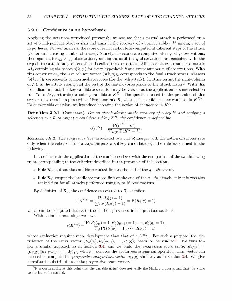
58 CHAPTER 3. ESTIMATING THE SUCCESS RATE OF SIDE-CHANNEL ATTACKS
3.9.1 Confidence in an hypothesisApplying the notations introduced previously, we assume that a partial attack is performed on aset of q independent observations and aims at the recovery of a correct subkey k∗ among a set ofhypotheses. For our analysis, the score of each candidate is computed at different steps of the attack(ie. for an increasing number of traces). Namely, the scores are computed after q1 < q observations,then again after q2 > q1 observations, and so on until the q observations are considered. In thesequel, the attack on qi observations is called the i-th attack. All those attacks result in a matrixMs containing the scores s(k, qi) for every hypothesis k and every number qi of observations. Withthis construction, the last column vector (s(k, q))k corresponds to the final attack scores, whereas(s(k, qi))k corresponds to intermediate scores (for the i-th attack). In other terms, the right-columnofMs is the attack result, and the rest of the matrix corresponds to the attack history. With thisformalism in hand, the key candidate selection may be viewed as the application of some selectionrule R to Ms, returning a subkey candidate KR. The question raised in the preamble of thissection may then be rephrased as: "For some rule R, what is the confidence one can have in KR?".To answer this question, we introduce hereafter the notion of confidence in KR.
Definition 3.9.1 (Confidence). For an attack aiming at the recovery of a key k∗ and applying aselection rule R to output a candidate subkey KR, the confidence is defined by:
c(KR) = P(KR = k∗)∑k∈KP(KR = k) .
Remark 3.9.2. The confidence level associated to a rule R merges with the notion of success rateonly when the selection rule always outputs a subkey candidate, eg. the rule R0 defined in thefollowing.
Let us illustrate the application of the confidence level with the comparison of the two followingrules, corresponding to the criterion described in the preamble of this section:
• Rule R0: output the candidate ranked first at the end of the q − th attack.
• Rule Rt: output the candidate ranked first at the end of the q− th attack, only if it was alsoranked first for all attacks performed using qt to N observations.
By definition of R0, the confidence associated to R0 satisfies:
c(KR0) = P(R0(q) = 1)∑δ P(Rδ(q) = 1) = P(R0(q) = 1),
which can be computed thanks to the method presented in the previous sections.With a similar reasoning, we have:
c(KRt) = P(R0(qt) = 1, R0(qt+1) = 1, · · · , R0(q) = 1)∑δ P(Rδ(qt) = 1, , · · · , Rδ(q) = 1) ,
whose evaluation requires more development than that of c(KR0). For such a purpose, the dis-tribution of the ranks vector (Rδ(qt), Rδ(qt+1), · · · , Rδ(q)) needs to be studied5. We thus fol-low a similar approach as in Section 3.4, and we build the progressive score vector dδ,t(q) =(dδ(qt)||dδ(qt+1)|| · · · ||dδ(q)) where || denotes the vector concatenation operator. This vector canbe used to compute the progressive comparison vector cδ,t(q) similarly as in Section 3.4. We givehereafter the distribution of the progressive score vector.
5It is worth noting at this point that the variable Rδ(qi) does not verify the Markov property, and that the wholevector has to be studied.
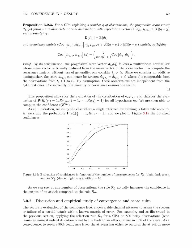
3.9. CONFIDENCE IN A RESULT 59
Proposition 3.9.3. For a CPA exploiting a number q of observations, the progressive score vectordδ,t(q) follows a multivariate normal distribution with expectation vector (E [dk,t])k∈K, a |K|(q− qt)vector satisfying:
E [dk,t] = E [dk]
and covariance matrix (Cov[dk1,ti , dk2,tj
])(k1,k2)∈K2 a |K|(q − qt)× |K|(q − qt) matrix, satisfying
Cov[dk1,ti , dk2,tj
](q) =
(q
max(ti, tj)Cov [dk1 , dk2 ]
).
Proof. By its construction, the progressive score vector dδ,t(q) follows a multivariate normal lawwhose mean vector is trivially deduced from the mean vector of the score vector. To compute thecovariance matrix, without loss of generality, one consider tj > ti. Since we consider an additivedistinguisher, the score dk2,tj can hence be written dk2,tj = dk2,ti + d, where d is computable fromthe observations from ti + 1 to tj . By assumption, these observations are independent from theti-th first ones. Consequently, the linearity of covariance ensures the result.
This proposition allows for the evaluation of the distribution of dδ,t(q), and thus for the eval-uation of P(Rδ(qt) = 1, Rδ(qt+1) = 1, · · · , Rδ(q) = 1) for all hypotheses kδ. We are then able tocompute the confidence c(KRt).
As an illustration, we study the case where a single intermediate ranking is taken into account,ie. we study the probability P(Rδ( q2) = 1, Rδ(q) = 1), and we plot in Figure 3.15 the obtainedconfidences.
Figure 3.15: Evaluation of confidences in function of the number of measurements for R0 (plain dark grey),and for R q
2(dashed light grey), with σ = 10.
As we can see, at any number of observations, the rule R q2actually increases the confidence in
the output of an attack compared to the rule R0.
3.9.2 Discussion and empirical study of convergence and score rulesThe accurate evaluation of the confidence level allows a side-channel attacker to assess the successor failure of a partial attack with a known margin of error. For example, and as illustrated inthe previous section, applying the selection rule R0 for a CPA on 800 noisy observations (withGaussian noise standard deviation equal to 10) leads to an attack failure in 18% of the cases. As aconsequence, to reach a 90% confidence level, the attacker has either to perform the attack on more
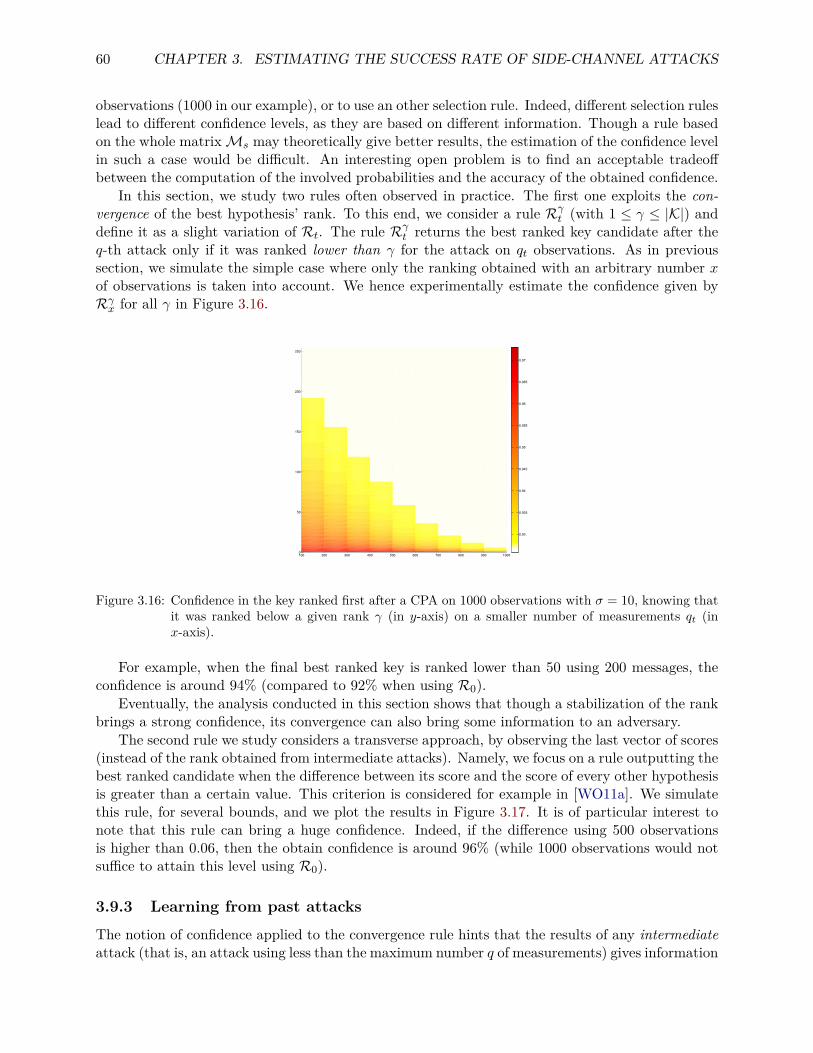
60 CHAPTER 3. ESTIMATING THE SUCCESS RATE OF SIDE-CHANNEL ATTACKS
observations (1000 in our example), or to use an other selection rule. Indeed, different selection ruleslead to different confidence levels, as they are based on different information. Though a rule basedon the whole matrixMs may theoretically give better results, the estimation of the confidence levelin such a case would be difficult. An interesting open problem is to find an acceptable tradeoffbetween the computation of the involved probabilities and the accuracy of the obtained confidence.
In this section, we study two rules often observed in practice. The first one exploits the con-vergence of the best hypothesis’ rank. To this end, we consider a rule Rγt (with 1 ≤ γ ≤ |K|) anddefine it as a slight variation of Rt. The rule Rγt returns the best ranked key candidate after theq-th attack only if it was ranked lower than γ for the attack on qt observations. As in previoussection, we simulate the simple case where only the ranking obtained with an arbitrary number xof observations is taken into account. We hence experimentally estimate the confidence given byRγx for all γ in Figure 3.16.
100 200 300 400 500 600 700 800 900 10000
50
100
150
200
250
0.93
0.935
0.94
0.945
0.95
0.955
0.96
0.965
0.97
Figure 3.16: Confidence in the key ranked first after a CPA on 1000 observations with σ = 10, knowing thatit was ranked below a given rank γ (in y-axis) on a smaller number of measurements qt (inx-axis).
For example, when the final best ranked key is ranked lower than 50 using 200 messages, theconfidence is around 94% (compared to 92% when using R0).
Eventually, the analysis conducted in this section shows that though a stabilization of the rankbrings a strong confidence, its convergence can also bring some information to an adversary.
The second rule we study considers a transverse approach, by observing the last vector of scores(instead of the rank obtained from intermediate attacks). Namely, we focus on a rule outputting thebest ranked candidate when the difference between its score and the score of every other hypothesisis greater than a certain value. This criterion is considered for example in [WO11a]. We simulatethis rule, for several bounds, and we plot the results in Figure 3.17. It is of particular interest tonote that this rule can bring a huge confidence. Indeed, if the difference using 500 observationsis higher than 0.06, then the obtain confidence is around 96% (while 1000 observations would notsuffice to attain this level using R0).
3.9.3 Learning from past attacksThe notion of confidence applied to the convergence rule hints that the results of any intermediateattack (that is, an attack using less than the maximum number q of measurements) gives information
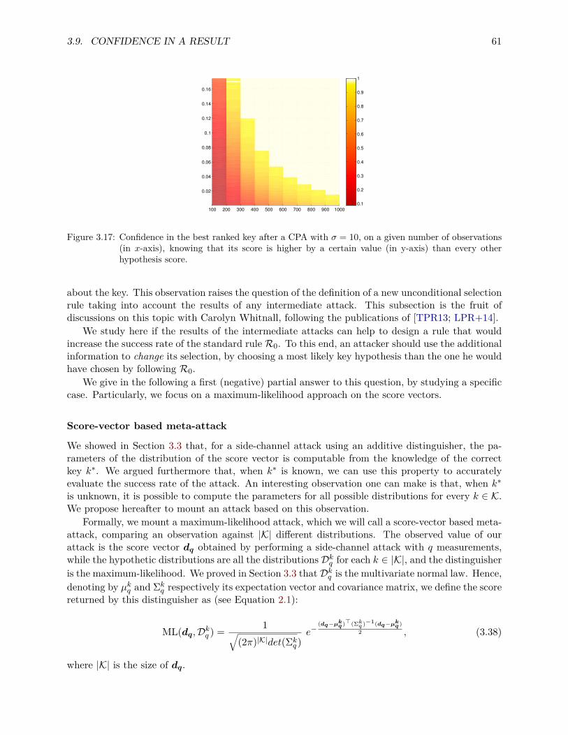
3.9. CONFIDENCE IN A RESULT 61
100 200 300 400 500 600 700 800 900 1000
0.02
0.04
0.06
0.08
0.1
0.12
0.14
0.16
0.1
0.2
0.3
0.4
0.5
0.6
0.7
0.8
0.9
1
Figure 3.17: Confidence in the best ranked key after a CPA with σ = 10, on a given number of observations(in x-axis), knowing that its score is higher by a certain value (in y-axis) than every otherhypothesis score.
about the key. This observation raises the question of the definition of a new unconditional selectionrule taking into account the results of any intermediate attack. This subsection is the fruit ofdiscussions on this topic with Carolyn Whitnall, following the publications of [TPR13; LPR+14].
We study here if the results of the intermediate attacks can help to design a rule that wouldincrease the success rate of the standard rule R0. To this end, an attacker should use the additionalinformation to change its selection, by choosing a most likely key hypothesis than the one he wouldhave chosen by following R0.
We give in the following a first (negative) partial answer to this question, by studying a specificcase. Particularly, we focus on a maximum-likelihood approach on the score vectors.
Score-vector based meta-attack
We showed in Section 3.3 that, for a side-channel attack using an additive distinguisher, the pa-rameters of the distribution of the score vector is computable from the knowledge of the correctkey k∗. We argued furthermore that, when k∗ is known, we can use this property to accuratelyevaluate the success rate of the attack. An interesting observation one can make is that, when k∗is unknown, it is possible to compute the parameters for all possible distributions for every k ∈ K.We propose hereafter to mount an attack based on this observation.
Formally, we mount a maximum-likelihood attack, which we will call a score-vector based meta-attack, comparing an observation against |K| different distributions. The observed value of ourattack is the score vector dq obtained by performing a side-channel attack with q measurements,while the hypothetic distributions are all the distributions Dkq for each k ∈ |K|, and the distinguisheris the maximum-likelihood. We proved in Section 3.3 that Dkq is the multivariate normal law. Hence,denoting by µkq and Σk
q respectively its expectation vector and covariance matrix, we define the scorereturned by this distinguisher as (see Equation 2.1):
ML(dq,Dkq ) = 1√(2π)|K|det(Σk
q )e−
(dq−µkq )>(Σkq )−1(dq−µkq )2 , (3.38)
where |K| is the size of dq.
62 CHAPTER 3. ESTIMATING THE SUCCESS RATE OF SIDE-CHANNEL ATTACKS
For the convenience of our following proofs, we also introduce the following statistical toolML(dq,Dkq ), defined as:
ML(dq,Dkq ) = (dq − µkq)>(Σkq )−1(dq − µkq). (3.39)
Problem description
In order to get a sense of the impact of intermediate attacks on the likelihood of correctness ofa key hypothesis, we consider the following setting. Similarly to the setting of Section 3.9, weconsider several sets of strictly increasing numbers q1, q2, · · · qn of measurements. As in [Riv09], weassume a uniform setting, that is, that all occurrences ratio (see Equation 3.10) are equal. Notethat this requirement is trivially fulfilled if the attacker is in a chosen-plaintext scenario. Then,n side-channel attacks based on the same additive distinguisher are performed, respectively usingq1, q2, · · · qn measurements. These attacks respectively lay n scores vector dq1 ,dq2 , · · · ,dqn . Wethen perform two score-vector based meta-attacks. The first one is performed on dqn . The secondone is performed on the concatenation of all scores vector dq = dq1 ||dq2 || · · ·dqn6. (Note thatthe size of dq, is now n|K| instead of |K|). Our goal is to compare the two distinguishers of theseattacks. We will in fact prove that they are equivalent, thus hinting that the past results are uselessfor the construction of a good selection rule. Precisely, we will prove the following Theorem:
Theorem 3.9.4. Let q1, q2, · · · qn be strictly positive increasing integers. In the uniform setting,when q1 is high enough, there exist a real numbers α > 0 such that, for any hypothesis k ∈ K, itholds:
ML(dq,Dkq ) = αML(dqn ,Dkqn). (3.40)
Proof of Theorem 3.9.4
The core of the proof for this theorem relies on the following Lemma:
Lemma 3.9.5. Let q1, q2, · · · qn be strictly positive increasing integers. In the uniform setting, whenq1 is high enough, there exist a real number γ, such that, for any hypothesis k ∈ K, it holds:
ML(dq,Dkq ) = ML(dqn ,Dkqn) + γ. (3.41)
To be able to prove this, we claim the following Lemma:
Lemma 3.9.6. In the uniform setting, for any key hypothesis k, and for any number of measure-ments q, the covariance matrix Σk
q is constant.
Proof. Let k1, k2 be two key hypotheses in K. In the uniform setting, it is proven in [Riv09]that the distributions Dk1
q and Dk2q are identical up to a rearrangement of the coordinates (a
⊕-rotation) of the corresponding score vectors dk1q ,d
k2q . We denote by dk1
i (resp. dk2i ) the i-th
coordinate of dk1q (resp. dk2
q ). It follows that, for any two hypotheses k, k′ in K, the equalityCov(dk1
k⊕k1, dk1k′⊕k1
) = Cov(dk2k⊕k2
, dk2k′⊕k2
) holds. Hence, the covariance matrices are identical for allconsidered distributions.
6One can check that this concatenation also trivially follows a multivariate normal law when q1 is large enough,thanks to the arguments of 3.3.
3.9. CONFIDENCE IN A RESULT 63
In the following, we hence omit the index k in the notation of the covariance matrices. Letus now study the distribution Dkq of the concatenation vector dkq obtained when considering k asthe correct hypothesis. By construction, Dkq is also a multivariate normal law, and we denote itsparameters such that: Dkq = N (µkq ,Σk
q ). The following lemma allows to express those parametersfrom those of Dkqn :
Lemma 3.9.7. In the uniform setting, for any strictly increasing natural numbers q1, q2, · · · qn, theexpectation vector µkq can be expressed as:
µkq = µkqn ||µkqn ||µkqn || · · · ||µkqn ,
and the covariance matrix Σkq is constant for any k ∈ K and can be expressed thanks to the covari-
ance matrix Σqn as:
Σkq = qn
q1−1Σqn q2−1Σqn q3−1Σqn · · · q−1
n Σqn
q2−1Σqn q2−1Σqn q3−1Σqn · · · q−1n Σqn
q3−1Σqn q3−1Σqn q3−1Σqn · · · q−1n Σqn
......
......
...q−1n Σqn q−1
n Σqn q−1n Σqn · · · q−1
n Σqn
.
Proof. Since, for any k, dkq = dkq1 ||dkq2 ||dkq3 || · · · ||dkqn , the parameters of Dkq can be deduced exactlyas in Proposition 3.9.3. This, together with Lemma 3.9.6 lays the result.
Consequently, we will also omit the index k in the notation of this covariance matrix. Let usnow study the expression of ML(dq,Dkq ):
ML(dq,Dkq ) = (dq − µkq)>(Σq)−1(dq − µkq). (3.42)
We see Σ−1q as a n×n block matrix and we denote Σ−1
q [i, j] its block of coordinate (i, j). UsingLemma 3.9.7, Equation 3.42 can be rewritten as:
ML(dq,Dkq ) =∑i,j
(dqi − µkqn)>Σ−1q [i, j] (dqj − µkqn). (3.43)
Let us now focus on the inversion of Σq. Denoting by I|K| the |K|-th dimension identity matrix,we deduce from Lemma 3.9.7:
Σ−1q = q−1
n
Σ−1qn 0 0 · · · 00 Σ−1
qn 0 · · · 00 0 Σ−1
qn · · · 0...
......
......
0 0 0 · · · Σ−1qn
q1−1I|K| q2−1I|K| q3−1I|K| · · · q−1
n I|K|q2−1I|K| q2−1I|K| q3−1I|K| · · · q−1
n I|K|q3−1I|K| q3−1I|K| q3−1I|K| · · · q−1
n I|K|...
......
......
q−1n I|K| q−1
n I|K| q−1n I|K| · · · q−1
n I|K|
−1
,
(3.44)
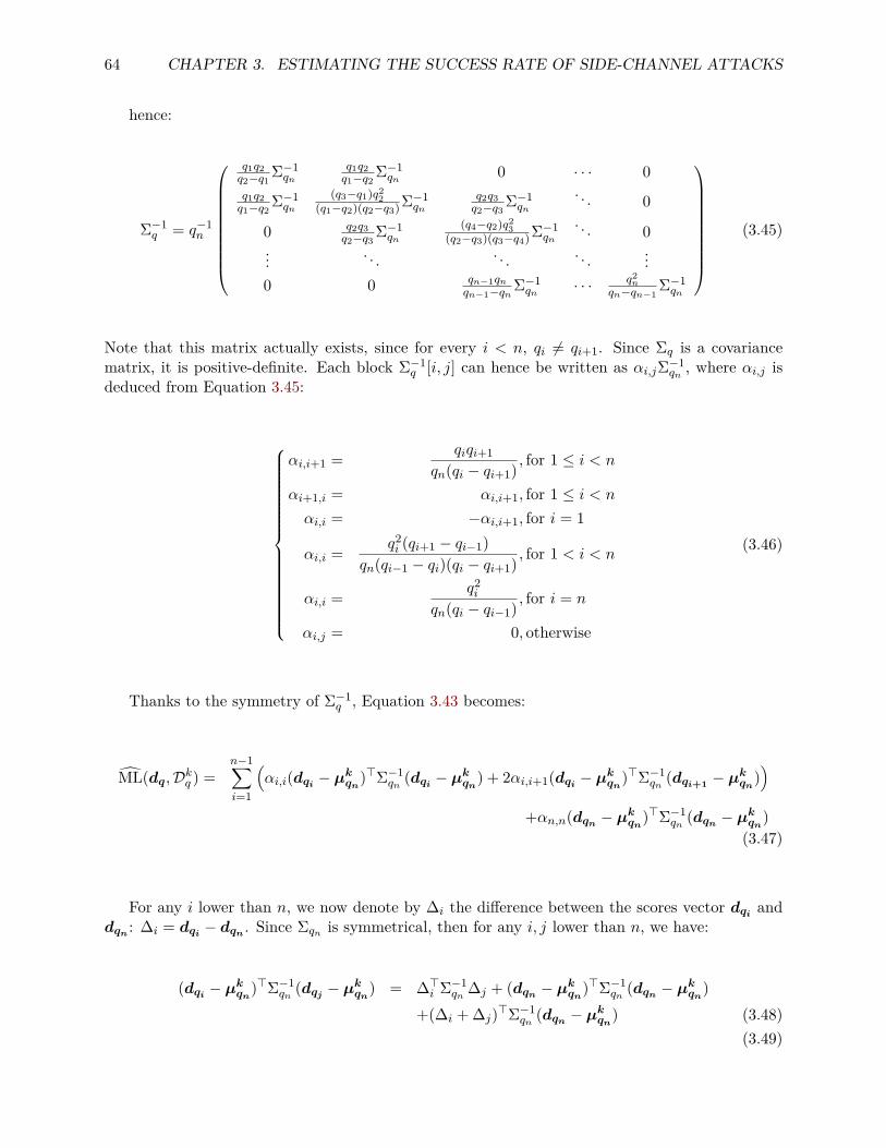
64 CHAPTER 3. ESTIMATING THE SUCCESS RATE OF SIDE-CHANNEL ATTACKS
hence:
Σ−1q = q−1
n
q1q2q2−q1 Σ−1
qnq1q2q1−q2 Σ−1
qn 0 · · · 0q1q2q1−q2 Σ−1
qn(q3−q1)q2
2(q1−q2)(q2−q3)Σ−1
qnq2q3q2−q3 Σ−1
qn
. . . 0
0 q2q3q2−q3 Σ−1
qn(q4−q2)q2
3(q2−q3)(q3−q4)Σ−1
qn
. . . 0... . . . . . . . . . ...0 0 qn−1qn
qn−1−qnΣ−1qn · · · q2
nqn−qn−1
Σ−1qn
(3.45)
Note that this matrix actually exists, since for every i < n, qi 6= qi+1. Since Σq is a covariancematrix, it is positive-definite. Each block Σ−1
q [i, j] can hence be written as αi,jΣ−1qn , where αi,j is
deduced from Equation 3.45:
αi,i+1 = qiqi+1qn(qi − qi+1) , for 1 ≤ i < n
αi+1,i = αi,i+1, for 1 ≤ i < n
αi,i = −αi,i+1, for i = 1
αi,i = q2i (qi+1 − qi−1)
qn(qi−1 − qi)(qi − qi+1) , for 1 < i < n
αi,i = q2i
qn(qi − qi−1) , for i = n
αi,j = 0, otherwise
(3.46)
Thanks to the symmetry of Σ−1q , Equation 3.43 becomes:
ML(dq,Dkq ) =n−1∑i=1
(αi,i(dqi − µkqn)>Σ−1
qn (dqi − µkqn) + 2αi,i+1(dqi − µkqn)>Σ−1qn (dqi+1 − µkqn)
)+αn,n(dqn − µkqn)>Σ−1
qn (dqn − µkqn)(3.47)
For any i lower than n, we now denote by ∆i the difference between the scores vector dqi anddqn : ∆i = dqi − dqn . Since Σqn is symmetrical, then for any i, j lower than n, we have:
(dqi − µkqn)>Σ−1qn (dqj − µkqn) = ∆>i Σ−1
qn ∆j + (dqn − µkqn)>Σ−1qn (dqn − µkqn)
+(∆i + ∆j)>Σ−1qn (dqn − µkqn) (3.48)
(3.49)
3.9. CONFIDENCE IN A RESULT 65
Hence, Equation 3.47 becomes:
ML(dq,Dkq ) =n−1∑i=1
αi,i(∆>i Σ−1qn ∆i + ML(dqn ,Dkqn) + 2∆>i Σ−1
qn (dqn − µkqn))
+2n−1∑i=1
αi,i+1(∆>i Σ−1qn ∆i+1 + ML(dqn ,Dkqn) + (∆i + ∆i+1)>Σ−1
qn (dqn − µkqn))
+αn,nML(dqn ,Dkqn) (3.50)
= (αn,n +n−1∑i=1
(αi,i + 2αi,i+1))ML(dqn ,Dkqn)
+n−1∑i=1
∆>i Σ−1qn (αi,i∆i + 2αi,i+1∆i+1)
+2n−1∑i=1
((αi,i + αi,i+1)∆i + αi,i+1∆i+1)>Σ−1qn (dqn − µkqn)). (3.51)
Let us simplify this equation. First, from Equations 3.44 and 3.45 we have:
n−1∑i=1
((αi,i+αi,i+1)∆i+αi,i+1∆i+1) = (α1,1+α1,2)∆1+αn−1,n∆n+n−1∑i=2
(αi,i+αi,i+1+αi−1,i)∆i. (3.52)
Trivially, we have ∆n = 0, and it can easily be checked that α1,1 + α1,2 = 0. Let us study thelast part of the sum from the expression of Σq. For any 1 < i < n, we get:
αi,i + αi,i+1 + αi−1,i = q2i (qi+1 − qi−1)
qn(qi−1 − qi)(qi − qi+1) + qiqi+1qn(qi − qi+1) + qiqi−1
qn(qi−1 − qi)= 0. (3.53)
Consequently, Equation 3.50 becomes:
ML(dq,Dkq ) = (αn,n+n−1∑i=1
(αi,i+2αi,i+1))ML(dqn ,Dkqn)+n−1∑i=1
∆>i Σ−1qn (αi,i∆i+2αi,i+1∆i+1). (3.54)
Moreover, from Equation 3.53 it holds that α1,2 = −α1,1 and that αi,i + αi,i+1 = −αi−1,i for1 < i < n. Therefore, we obtain: αn,n +∑n−1
i=1 (αi,i + 2αi,i+1) = αn,n + αn−1,n = 1. And thus weget:
ML(dq,Dkq ) = ML(dqn ,Dkqn) +n−1∑i=1
∆>i Σ−1qn (αi,i∆i + 2αi,i+1∆i+1). (3.55)
It is clear that nothing except ML(dqn ,Dkqn) depends on k in the right term of this equation.This concludes the proof of Lemma 3.9.5.
To prove Theorem 3.9.4, we start from Lemma 3.9.5, and use properties of the exponentialfunction. Reusing the notation γ of this lemma, we get for any hypothesis k ∈ K:
e−ML(dq ,Dkq )
2 = e−γ2 · e−
ML(dqn ,Dkqn
)2 . (3.56)
From Lemma 3.9.7 (resp. 3.9.6), we moreover know that, for any hypothesis k ∈ K, the covari-ance matrix Σk
qn (resp Σkq ) is constant, and can be denoted Σqn (resp. Σq). Hence, multiplying
Equation 3.56 by a constant, we obtain:
66 CHAPTER 3. ESTIMATING THE SUCCESS RATE OF SIDE-CHANNEL ATTACKS
1√(2π)n|K|det(Σq)
e−ML(dq ,Dkq )
2 = e−γ2√
(2π)n|K|det(Σq)· e−
ML(dqn ,Dkqn
)2 . (3.57)
Finally, this equation lays:
ML(dq,Dkq ) = e−γ2
√(2π)(1−n)|K|det(Σqn)
det(Σq)·ML(dqn ,Dkqn). (3.58)
Note that nothing in the right term of this equation depends on k except for ML(dqn ,Dkqn).Moreover, since Σqn and Σq are covariance matrices, their determinant are strictly positive, andhence the square root is well defined and non-zero. Since the exponential function is strictly positiveon R, Equation 3.58 finishes the proof of Theorem 3.9.4.
3.10 ConclusionIn this chapter we have studied the methods for assessing the security of cryptographic implemen-tations against side-channel attacks, both in the context of a known and an unknown key. In thecontext of a known key, we have presented a methodology to evaluate the success rate of side-channelattacks. We have shown how to apply this methodology in the particular cases of attacks based onthe correlation and likelihood distinguishers. The soundness of our approach has been validated bysimulations and experiments performed on different microcontrollers. Using this methodology, anevaluator can estimate the side-channel resistance of his masked cryptographic implementation atthe cost of inferring a few linear regression coefficients. In the context of an unknown key, we give arationale for the use of some empirical criteria (such as the convergence of the best hypothesis’ ranktowards 1) as indicators of the attack success. We hence involve the notion of confidence to allowfor the accurate estimation of this success. As an avenue for further research, this work opens thenew problem of the exhibition of novel selection rules allowing to efficiently and accurately evaluatethe confidence in a side-channel attack while conserving an acceptable success rate.
Chapter 4
Randomness Complexity of PrivateCircuits for Multiplication
Après son retour de Zurich à Prague, Tomas fut pris de malaise à l’idéeque sa rencontre avec Tereza avait été le résultat de six improbables hasards.
Milan Kundera - L’insoutenable légèreté de l’être
Many cryptographic algorithms are vulnerable to side-channel analysis and several leakagemodels have been introduced to better understand these flaws. In 2003, Ishai, Sahai and Wagnerintroduced the d-probing security model, in which an attacker can observe at most d intermediatevalues during a processing. They also proposed an algorithm that securely performs the multipli-cation of 2 bits in this model, using only d(d + 1)/2 random bits to protect the computation. Westudy the randomness complexity of multiplication algorithms secure in the d-probing model. Wepropose several contributions: we provide new theoretical characterizations and constructions, newpractical constructions and a new efficient algorithmic tool to analyze the security of such schemes.
We start with a theoretical treatment of the subject: we propose an algebraic model for mul-tiplication algorithms and exhibit an algebraic characterization of the security in the d-probingmodel. Using this characterization, we prove a linear (in d) lower bound and a quasi-linear (non-constructive) upper bound for this randomness cost. Then, we construct a new generic algorithmto perform secure multiplication in the d-probing model that only uses d+ d2/4 random bits.
From a practical point of view, we consider the important cases d ≤ 4 that are actually used incurrent real-life implementations and we build algorithms with a randomness complexity matchingour theoretical lower bound for these small-order cases. Finally, still using our algebraic charac-terization, we provide a new dedicated verification tool, based on information set decoding, whichaims at finding attacks on algorithms for fixed order d at a very low computational cost. Part ofthis work has been published at the Eurocrypt conference [BBP+16].
4.1 IntroductionMost commonly used cryptographic algorithms are now considered secure against classical black-box attacks, when the adversary has only knowledge of their inputs or outputs. Today, it is howeverwell known that their implementations are vulnerable to side-channel attacks, as revealed in theacademic community by Kocher in 1996 [Koc96]. These attacks exploit the physical emanations of
67
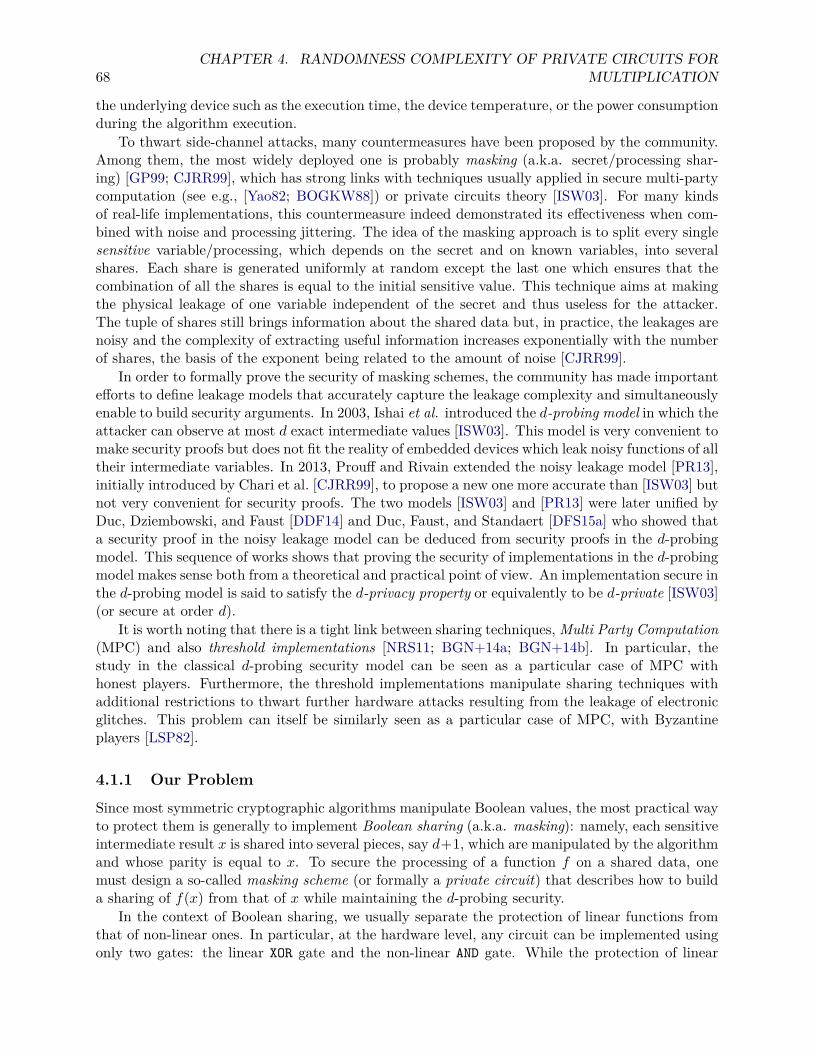
68CHAPTER 4. RANDOMNESS COMPLEXITY OF PRIVATE CIRCUITS FOR
MULTIPLICATION
the underlying device such as the execution time, the device temperature, or the power consumptionduring the algorithm execution.
To thwart side-channel attacks, many countermeasures have been proposed by the community.Among them, the most widely deployed one is probably masking (a.k.a. secret/processing shar-ing) [GP99; CJRR99], which has strong links with techniques usually applied in secure multi-partycomputation (see e.g., [Yao82; BOGKW88]) or private circuits theory [ISW03]. For many kindsof real-life implementations, this countermeasure indeed demonstrated its effectiveness when com-bined with noise and processing jittering. The idea of the masking approach is to split every singlesensitive variable/processing, which depends on the secret and on known variables, into severalshares. Each share is generated uniformly at random except the last one which ensures that thecombination of all the shares is equal to the initial sensitive value. This technique aims at makingthe physical leakage of one variable independent of the secret and thus useless for the attacker.The tuple of shares still brings information about the shared data but, in practice, the leakages arenoisy and the complexity of extracting useful information increases exponentially with the numberof shares, the basis of the exponent being related to the amount of noise [CJRR99].
In order to formally prove the security of masking schemes, the community has made importantefforts to define leakage models that accurately capture the leakage complexity and simultaneouslyenable to build security arguments. In 2003, Ishai et al. introduced the d-probing model in which theattacker can observe at most d exact intermediate values [ISW03]. This model is very convenient tomake security proofs but does not fit the reality of embedded devices which leak noisy functions of alltheir intermediate variables. In 2013, Prouff and Rivain extended the noisy leakage model [PR13],initially introduced by Chari et al. [CJRR99], to propose a new one more accurate than [ISW03] butnot very convenient for security proofs. The two models [ISW03] and [PR13] were later unified byDuc, Dziembowski, and Faust [DDF14] and Duc, Faust, and Standaert [DFS15a] who showed thata security proof in the noisy leakage model can be deduced from security proofs in the d-probingmodel. This sequence of works shows that proving the security of implementations in the d-probingmodel makes sense both from a theoretical and practical point of view. An implementation secure inthe d-probing model is said to satisfy the d-privacy property or equivalently to be d-private [ISW03](or secure at order d).
It is worth noting that there is a tight link between sharing techniques, Multi Party Computation(MPC) and also threshold implementations [NRS11; BGN+14a; BGN+14b]. In particular, thestudy in the classical d-probing security model can be seen as a particular case of MPC withhonest players. Furthermore, the threshold implementations manipulate sharing techniques withadditional restrictions to thwart further hardware attacks resulting from the leakage of electronicglitches. This problem can itself be similarly seen as a particular case of MPC, with Byzantineplayers [LSP82].
4.1.1 Our ProblemSince most symmetric cryptographic algorithms manipulate Boolean values, the most practical wayto protect them is generally to implement Boolean sharing (a.k.a. masking): namely, each sensitiveintermediate result x is shared into several pieces, say d+1, which are manipulated by the algorithmand whose parity is equal to x. To secure the processing of a function f on a shared data, onemust design a so-called masking scheme (or formally a private circuit) that describes how to builda sharing of f(x) from that of x while maintaining the d-probing security.
In the context of Boolean sharing, we usually separate the protection of linear functions fromthat of non-linear ones. In particular, at the hardware level, any circuit can be implemented usingonly two gates: the linear XOR gate and the non-linear AND gate. While the protection of linear
4.1. INTRODUCTION 69
operations (e.g., XOR) is straightforward since the initial function f can be applied to each shareseparately, it becomes more difficult for non-linear operations (e.g., AND). In these cases, the sharescannot be manipulated separately and must generally be processed all together to compute thecorrect result. These values must then be further protected using additional random bits whichresults in an important timing overhead.
State-of-the-art solutions to implement Boolean sharing on non-linear functions [RP10; CPRR14]have focused on optimizing the computation complexity. Surprisingly, the amount of necessary ran-dom bits has only been in the scope of the seminal paper of Ishai, Sahai and Wagner [ISW03]. Inthis work, the authors proposed and proved a clever construction (further referred to as ISW mul-tiplication) allowing to compute the multiplication of two shared bits by using d(d+ 1)/2 randombits, that is, half as many random bits as the straightforward solution uses. Their construction hassince become a cornerstone of secure implementations [RP10; DDF14; DFS15b; RBN+15]. Evenif this result is very important, the quantity of randomness remains very expensive to generate inembedded cryptographic implementations. Indeed, such a generation is usually performed using aphysical generator followed by a deterministic random bit generator (DRBG). In addition of being atheoretical “chicken-and-egg” problem for this DRBG protection, in practice the physical generatorhas often a low throughput and the DRBG is also time-consuming. In general, for a DRBG basedon a 128-bit block cipher, one call to this block cipher enables to generate 128 pseudo-randombits1 (see [BK12]). However, one invocation of the standard AES-128 block cipher with the ISWmultiplication requires as much as 30,720 random bits (6 random bytes per multiplication, 4 mul-tiplications per S-box [RP10]) to protect the multiplications when masked at the low order d = 3,which corresponds to 240 preliminary calls to the DRBG.
4.1.2 Our ContributionsWe analyze the quantity of randomness required to define a d-private multiplication algorithm atany order d. Given the sharings a = (ai)0≤i≤d, b = (bi)0≤i≤d of two bits a and b, the problem wetackle out is to find the minimal number of random bits necessary to securely compute a sharing(ci)0≤i≤d of the bit c = ab with a d-private algorithm. We limit our scope to the construction ofa multiplication based on the sum of shares’ products. That is, as in [ISW03], we start with thepairwise products of a’s and b’s shares and we work on optimizing their sum into d+ 1 shares withas few random bits as possible. We show that this reduces to studying the randomness complexityof some particular d-private compression algorithm that securely transforms the (d + 1)2 shares’products into d+ 1 shares of c. In our study we make extensive use of the following theorem thatgives an alternative characterization of the d-privacy:Theorem 4.3.1 (informal). A compression algorithm is d-private if and only if there does notexist a set of ` intermediate results p1, . . . , p` such that ` 6 d and ∑`
i=1 pi can be written asaᵀ ·M · b with M being some matrix such that the all-ones vector is in the row space or in thecolumn space of M .
From this theorem, we deduce the following lower bound on the randomness complexity:Theorems 4.4.3–4.4.4 (informal). If d > 3 (resp. d = 2), then a d-private compression algo-rithm for multiplication must involve at least d+ 1 random bits (resp. 2).
This theorem shows that the randomness complexity is in Ω(d). Following the probabilisticmethod, we additionally prove the following theorem which claims that there exists a d-private
1Actually, the generation of pseudo-random bits roughly corresponds to the execution of a block cipher but weshould also consider the regular internal state update.
70CHAPTER 4. RANDOMNESS COMPLEXITY OF PRIVATE CIRCUITS FOR
MULTIPLICATION
0.5 1 1.5 2 2.5 3 3.5 4 4.5 5 5.5 6 6.5 7 7.5 8 8.50
5
10
15
20
25
30
35
masking order d
rand
omne
ssco
mpl
exity
ISW ([ISW03])lower bound (Section 4.4)
new construction (Section 4.5)small programs (Section 4.6)
Figure 4.1: Randomness complexity of d-private multiplication algorithms
multiplication algorithm with randomness complexity O(d · log d). This provides a quasi-linearupper bound O(d · log d) for the randomness complexity, when d→∞.Theorem 4.4.6 (informal). There exists a d-private multiplication algorithm with randomnesscomplexity O(d · log d), when d→∞.
This upper bound is non-constructive: we show that a randomly chosen multiplication algorithm(in some carefully designed family of multiplication algorithms using O(d · log d) random bits) isd-private with non-zero probability. This means that there exists one algorithm in this family whichis d-private.
In order to explicitly construct private algorithms with low randomness, we analyze the ISWmultiplication to bring out necessary and sufficient conditions on the use of the random bits.In particular, we identify necessary chainings and we notice that some random bits may be usedseveral times at several locations to protect more shares’ products, while in the ISW multiplication,each random bit is only used twice. From this analysis, we deduce a new d-private multiplicationalgorithm requiring bd2/4c + d random bits instead of d(d + 1)/2. As a positive side-effect, ournew construction also reduces the algorithmic complexity of ISW multiplication (i.e., its numberof operations).
Based on this generic construction, we then try to optimize some widely used small orderinstances. In particular, we bring out new multiplication algorithms, for the orders d = 2, 3 and4, which exactly achieve our proven linear lower bound while maintaining the d-privacy. Namely,we present the optimal multiplication algorithms for orders 2, 3 and 4 when summing the shares’products into d+1 shares. We formally verify their security using the tool provided in [BBD+15b].Figure 4.1 illustrates the randomness complexity of our constructions (for general orders d andsmall orders) and our lower bound.
Note that while the ISW algorithm was initially given for multiplications of bits, it was laterextended by Rivain and Prouff in [RP10] for any multiplication in F2n . In the following, for thesake of simplicity, we refer to binary multiplications (n = 1) for our constructions, but note thatall of them can also be adapted to multiplication in F2n .
Contrary to the ISW algorithm, our new constructions are not directly composable — in the
4.2. PRELIMINARIES 71
sense of Strong Non-Interferent (SNI) in [BBD+15a] — at any order. Fortunately, they can still beused in compositions instead of the ISW algorithms at carefully chosen locations. In this chapter,we thus recall the different security properties related to compositions and we show that in theAES example, our new constructions can replace half the ISW ones while preserving the d-privacyof the whole algorithm.
Finally, while the tool provided in [BBD+15b] — which is based on Easycrypt — is able toreveal potential attack paths and formally prove security in the d-probing model with full confidence,it is limited to the verification of small orders (d = 6 in our case). Therefore, we propose a newdedicated probabilistic verification tool, which aims at finding attacks in fixed order private circuits(or equivalently masking schemes) at a very low cost. The tool is developed in Sage (Python) [Sage]and though less generic than [BBD+15b] it is orders of magnitude faster. It relies on some heuristicassumption (i.e. it cannot be used to actually prove the security) but it usually finds attacks veryswiftly for any practical order d. It makes use of information set decoding (a technique fromcoding theory introduced to the cryptographic community for the security analysis of the McEliececryptosystem in [Pra62; McE78]).
4.2 Preliminaries
This section defines the notations and basic notions that we use in this chapter, but also someelementary constructions we refer to. In particular, we introduce the notion of d-private compressionalgorithm for multiplication and we present its only concrete instance which was proposed by Ishai,Sahai, and Wagner [ISW03].
4.2.1 Notations
For a set S, we denote by |S| its cardinality, and by s $← S the operation of picking up an element sof S uniformly at random. We denote by Fq the finite field with q elements. Vectors are denoted bylower case bold font letters, and matrices are denoted by upper case bold font letters. All vectorsare column vectors unless otherwise specified. The kernel (resp. the image) of the linear mapassociated to a matrix M is denoted by ker(M) (resp. im(M)). For a vector x, we denote by xiits i-th coordinate and by HW(x) its Hamming weight (i.e., the number of its coordinates that aredifferent from 0).
For any fixed n ≥ 1, let Un ∈ Fn×n2 denote the matrix whose coefficients ui,j equal 1 for all1 ≤ i, j ≤ n. Let 0n,` ∈ Fn×`2 denote the matrix whose coefficients are all 0. Let un ∈ Fn2 denotethe vector (1, . . . , 1)ᵀ and 0n ∈ Fn2 denote the vector (0, . . . , 0)ᵀ. For vectors x1, . . . ,xt in Fn2 wedenote 〈x1, . . . ,xt〉 the vector space generated by the set x1, . . . ,xt.
We say that an expression f(x1, . . . , xn, r) functionally depends on the variable r if there existsa1, . . . , an such that the function r 7→ f(a1, . . . , an, r) is not constant.
For an algorithm A, we denote by y ← A(x1, x2, . . . ) the operation of running A on inputs(x1, x2, . . . ) and letting y denote the output. Moreover, if A is randomized, we denote by y
$←A(x1, x2, . . . ; r) the operation of running A on inputs (x1, x2, . . . ) and with uniform randomness r(or with fresh randomness if r is not specified) and letting y denote the output. The probabilitydensity function associated to a discrete random variable X defined over S (e.g., F2) is the functionwhich maps x ∈ S to P [X = x ]. It is denoted by X or by Xr if there is a need to precise therandomness source r over which the distribution is considered.
72CHAPTER 4. RANDOMNESS COMPLEXITY OF PRIVATE CIRCUITS FOR
MULTIPLICATION
4.2.2 Private CircuitsWe examine the privacy property in the setting of Boolean circuits and start with the definitionof circuit and randomized circuit given in [ISW03]. A deterministic circuit C is a directed acyclicgraph whose vertices are Boolean gates and whose edges are wires. A randomized circuit is acircuit augmented with random-bit gates. A random-bit gate is a gate with fan-in 0 that producesa random bit and sends it along its output wire; the bit is selected uniformly and independentlyof everything else afresh for each invocation of the circuit. From the two previous notions, we maydeduce the following definition of a private circuit inspired from [IKL+13].
Definition 4.2.1. [IKL+13] A private circuit for f : Fn2 → Fm2 is defined by a triple (I, C,O),where
• I: Fn2 → Fn′2 is a randomized circuit with uniform randomness ρ and called input encoder;
• C is a randomized boolean circuit with input in Fn′2 , output in Fm′2 , and uniform randomnessr ∈ Ft2;
• O: Fm′2 → Fm2 is a circuit, called output decoder.
We say that C is a d-private implementation of f with encoder I and decoder O if the followingrequirements hold:
• Correctness: for any input w ∈ Fn2 , P [O(C(I(w; ρ); r)) = f(w) ] = 1, where the probability isover the randomness ρ and r;
• Privacy: for any w,w′ ∈ Fn2 and any set P of d wires in C, the distributions CP (I(w; ρ); r)ρ,rand CP (I(w′; ρ); r)ρ,r are identical, where CP (I(w; ρ); r) denotes the list of the d values onthe wires from P .
Remark 4.2.2. It may be noticed that the notions of d-privacy and of security in the d-probingmodel used, e.g., in [BBD+15b] are perfectly equivalent.
Unless noted otherwise, we assume I and O to be the following canonical encoder and decoder:I encodes each bit-coordinate b of its input w by a block (bj)0≤j≤d of d+ 1 random bits with parityb, and O takes the parity of each block of d+ 1 bits. Each block (bj)0≤j≤d is called a sharing of band each bj is called a share of b.
From now on, the wires in a set P used to attack an implementation are referred as the probes andthe corresponding values in CP (I(w; ρ); r) as the intermediate results. To simplify the descriptions,a probe p is sometimes used to directly denote the corresponding result. A set of probes P suchthat the distributions CP (I(w; ρ); r)ρ,r and CP (I(w′; ρ); r)ρ,r are not identical for some inputsw,w′ ∈ Fn2 shall be called an attack. When the inputs w are clear from the context, the distributionCP (I(w; ρ); r)ρ,r is simplified to (p)p∈P .
We now introduce the notions of multiplication algorithm and of d-compression algorithm formultiplication. In this chapter, we deeply study d-private multiplication algorithms and d-privatecompression algorithms for multiplication.
Definition 4.2.3. A multiplication algorithm is a circuit for the multiplication of 2 bits (i.e., withf being the function f : (a, b) ∈ F2
2 7→ a · b ∈ F2), using the canonical encoder and decoder.
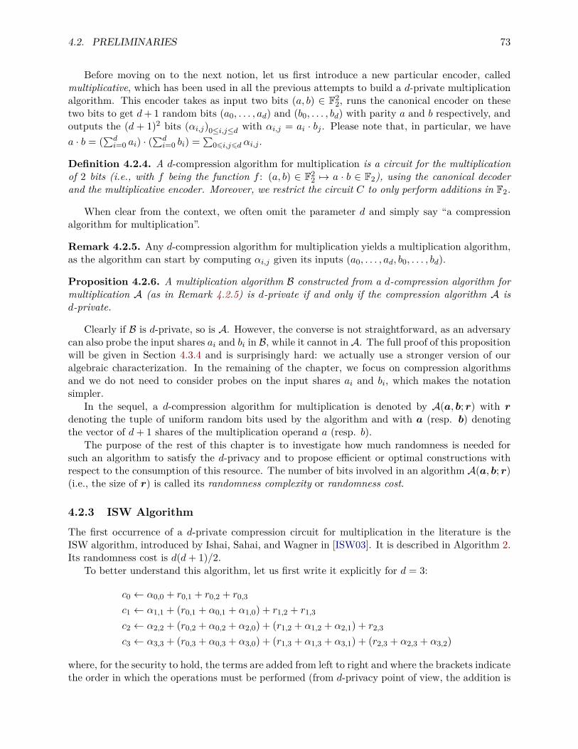
4.2. PRELIMINARIES 73
Before moving on to the next notion, let us first introduce a new particular encoder, calledmultiplicative, which has been used in all the previous attempts to build a d-private multiplicationalgorithm. This encoder takes as input two bits (a, b) ∈ F2
2, runs the canonical encoder on thesetwo bits to get d+ 1 random bits (a0, . . . , ad) and (b0, . . . , bd) with parity a and b respectively, andoutputs the (d + 1)2 bits (αi,j)0≤i,j≤d with αi,j = ai · bj . Please note that, in particular, we havea · b = (∑d
i=0 ai) · (∑di=0 bi) = ∑
06i,j6d αi,j .
Definition 4.2.4. A d-compression algorithm for multiplication is a circuit for the multiplicationof 2 bits (i.e., with f being the function f : (a, b) ∈ F2
2 7→ a · b ∈ F2), using the canonical decoderand the multiplicative encoder. Moreover, we restrict the circuit C to only perform additions in F2.
When clear from the context, we often omit the parameter d and simply say “a compressionalgorithm for multiplication”.
Remark 4.2.5. Any d-compression algorithm for multiplication yields a multiplication algorithm,as the algorithm can start by computing αi,j given its inputs (a0, . . . , ad, b0, . . . , bd).
Proposition 4.2.6. A multiplication algorithm B constructed from a d-compression algorithm formultiplication A (as in Remark 4.2.5) is d-private if and only if the compression algorithm A isd-private.
Clearly if B is d-private, so is A. However, the converse is not straightforward, as an adversarycan also probe the input shares ai and bi in B, while it cannot in A. The full proof of this propositionwill be given in Section 4.3.4 and is surprisingly hard: we actually use a stronger version of ouralgebraic characterization. In the remaining of the chapter, we focus on compression algorithmsand we do not need to consider probes on the input shares ai and bi, which makes the notationsimpler.
In the sequel, a d-compression algorithm for multiplication is denoted by A(a, b; r) with rdenoting the tuple of uniform random bits used by the algorithm and with a (resp. b) denotingthe vector of d+ 1 shares of the multiplication operand a (resp. b).
The purpose of the rest of this chapter is to investigate how much randomness is needed forsuch an algorithm to satisfy the d-privacy and to propose efficient or optimal constructions withrespect to the consumption of this resource. The number of bits involved in an algorithm A(a, b; r)(i.e., the size of r) is called its randomness complexity or randomness cost.
4.2.3 ISW AlgorithmThe first occurrence of a d-private compression circuit for multiplication in the literature is theISW algorithm, introduced by Ishai, Sahai, and Wagner in [ISW03]. It is described in Algorithm 2.Its randomness cost is d(d+ 1)/2.
To better understand this algorithm, let us first write it explicitly for d = 3:
c0 ← α0,0 + r0,1 + r0,2 + r0,3
c1 ← α1,1 + (r0,1 + α0,1 + α1,0) + r1,2 + r1,3
c2 ← α2,2 + (r0,2 + α0,2 + α2,0) + (r1,2 + α1,2 + α2,1) + r2,3
c3 ← α3,3 + (r0,3 + α0,3 + α3,0) + (r1,3 + α1,3 + α3,1) + (r2,3 + α2,3 + α3,2)
where, for the security to hold, the terms are added from left to right and where the brackets indicatethe order in which the operations must be performed (from d-privacy point of view, the addition is
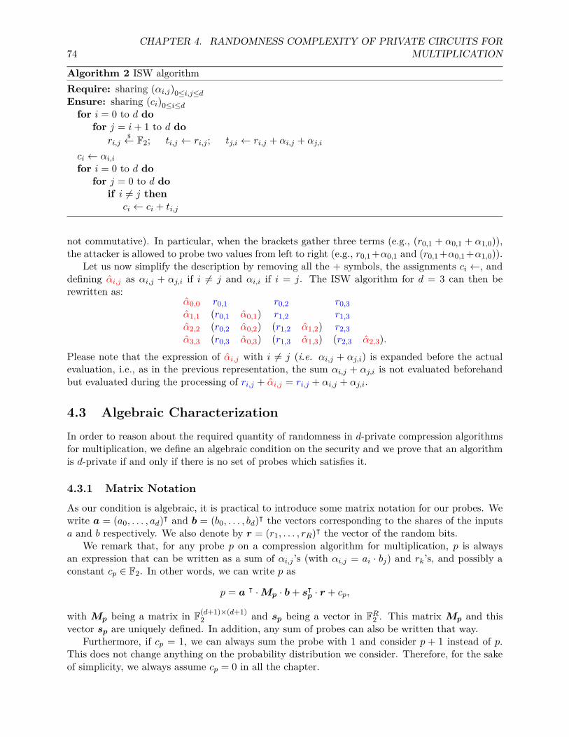
74CHAPTER 4. RANDOMNESS COMPLEXITY OF PRIVATE CIRCUITS FOR
MULTIPLICATION
Algorithm 2 ISW algorithmRequire: sharing (αi,j)0≤i,j≤dEnsure: sharing (ci)0≤i≤dfor i = 0 to d do
for j = i+ 1 to d dori,j
$← F2; ti,j ← ri,j ; tj,i ← ri,j + αi,j + αj,i
ci ← αi,ifor i = 0 to d do
for j = 0 to d doif i 6= j then
ci ← ci + ti,j
not commutative). In particular, when the brackets gather three terms (e.g., (r0,1 + α0,1 + α1,0)),the attacker is allowed to probe two values from left to right (e.g., r0,1 +α0,1 and (r0,1 +α0,1 +α1,0)).
Let us now simplify the description by removing all the + symbols, the assignments ci ←, anddefining αi,j as αi,j + αj,i if i 6= j and αi,i if i = j. The ISW algorithm for d = 3 can then berewritten as:
α0,0 r0,1 r0,2 r0,3α1,1 (r0,1 α0,1) r1,2 r1,3α2,2 (r0,2 α0,2) (r1,2 α1,2) r2,3α3,3 (r0,3 α0,3) (r1,3 α1,3) (r2,3 α2,3).
Please note that the expression of αi,j with i 6= j (i.e. αi,j + αj,i) is expanded before the actualevaluation, i.e., as in the previous representation, the sum αi,j + αj,i is not evaluated beforehandbut evaluated during the processing of ri,j + αi,j = ri,j + αi,j + αj,i.
4.3 Algebraic CharacterizationIn order to reason about the required quantity of randomness in d-private compression algorithmsfor multiplication, we define an algebraic condition on the security and we prove that an algorithmis d-private if and only if there is no set of probes which satisfies it.
4.3.1 Matrix NotationAs our condition is algebraic, it is practical to introduce some matrix notation for our probes. Wewrite a = (a0, . . . , ad)ᵀ and b = (b0, . . . , bd)ᵀ the vectors corresponding to the shares of the inputsa and b respectively. We also denote by r = (r1, . . . , rR)ᵀ the vector of the random bits.
We remark that, for any probe p on a compression algorithm for multiplication, p is alwaysan expression that can be written as a sum of αi,j ’s (with αi,j = ai · bj) and rk’s, and possibly aconstant cp ∈ F2. In other words, we can write p as
p = a ᵀ ·Mp · b+ sᵀp · r + cp,
with Mp being a matrix in F(d+1)×(d+1)2 and sp being a vector in FR2 . This matrix Mp and this
vector sp are uniquely defined. In addition, any sum of probes can also be written that way.Furthermore, if cp = 1, we can always sum the probe with 1 and consider p + 1 instead of p.
This does not change anything on the probability distribution we consider. Therefore, for the sakeof simplicity, we always assume cp = 0 in all the chapter.
4.3. ALGEBRAIC CHARACTERIZATION 75
4.3.2 Algebraic ConditionWe now introduce our algebraic condition:
Condition 1. A set of probes P = p1, . . . , p` on a d-compression algorithm for multiplicationsatisfies Condition 1 if and only if the expression f = ∑`
i=1 pi can be written as f = a ᵀ ·M · bwith M being some matrix such that ud+1 is in the row space or the column space of M .
As seen previously, the expression f can always be written as
f = a ᵀ ·M · b+ s ᵀ · r,
for some matrix M and some vector s. Therefore, what the condition enforces is that s = 0R (orin other words, f does not functionally depend on any random bit) and the column space or therow space of M contains the vector ud+1.A Weaker Condition. To better understand Condition 1, let us introduce a weaker conditionwhich is often easier to deal with:
Condition 2 (weak condition). A set of probes P = p1, . . . , p` on a d-compression algorithm formultiplication satisfies Condition 2 if and only if the expression f = ∑`
i=1 pi does not functionallydepend on any rk and there exists a map γ: 0, . . . , d → 0, . . . , d such that f does functionallydepend on every (αi,γ(i))0≤i≤d or on every (αγ(i),i)0≤i≤d.
This condition could be reformulated as: f = ∑`i=1 pi functionally depends on either all the ai’s
or all the bi’s and does not functionally depend on any rk. It is easy to see that any set P verifyingCondition 1 also verifies Condition 2.
4.3.3 Algebraic CharacterizationTheorem 4.3.1. Let A be a d-compression algorithm for multiplication. Then, A is d-private ifand only if there does not exist a set P = p1, . . . , p` of ` ≤ d probes that satisfies Condition 1.Furthermore any set P = p1, . . . , p` satisfying Condition 1 is an attack.
Please note that Theorem 4.3.1 would not be valid with Condition 2 (instead of Condition 1).Let us indeed consider the following 2-compression scheme for multiplication:
α2,0 r1 α0,0 r2 α0,2α2,1 r1 α1,1 r3 α1,2α1,0 r2 α0,1 r3 α2,2
It is easy to see that the only set of probes satisfying Condition 2 is
P = α2,0 + r1 + α0,0, α2,1 + r1 + α1,1 .
However, this set does not satisfy Condition 1, and in fact, this compression algorithm is 2-private.
Proof. Direction 1: Left to right. We prove hereafter that if A is d-private, then there does notexist a set P = p1, . . . , p` of ` ≤ d probes that satisfies Condition 1.
By contrapositive, let us assume that there exists a set P = p1, . . . , p` of at most d probesthat satisfies Condition 1. Let M be the matrix such that f = ∑`
i=1 pi = a ᵀ ·M · b and let us
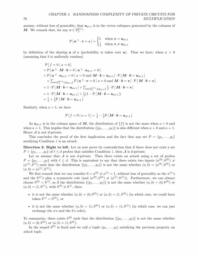
76CHAPTER 4. RANDOMNESS COMPLEXITY OF PRIVATE CIRCUITS FOR
MULTIPLICATION
assume, without loss of generality, that ud+1 is in the vector subspace generated by the columns ofM . We remark that, for any v ∈ Fd+1
2 :
P [a ᵀ · v = a ] =
1 when v = ud+112 when v 6= ud+1
by definition of the sharing a of a (probability is taken over a). Thus we have, when a = 0(assuming that b is uniformly random)
P [ f = 0 | a = 0 ]= P [a ᵀ ·M · b = 0 | a ᵀ · ud+1 = 0 ]= P [a ᵀ · ud+1 = 0 | a = 0 and M · b = ud+1 ] · P [M · b = ud+1 ]
+∑v∈Fd+1
2 \ud+1 P [a ᵀ · v = 0 | a = 0 and M · b = v ] · P [M · b = v ]
= 1 · P [M · b = ud+1 ] +∑v∈Fd+1
2 \ud+112 · P [M · b = v ]
= 1 · P [M · b = ud+1 ] + 12(1− P [M · b = ud+1 ])
= 12 + 1
2P [M · b = ud+1 ].
Similarly, when a = 1, we have
P [ f = 0 | a = 1 ] = 12 − 1
2P [M · b = ud+1 ].
As ud+1 is in the column space of M , the distribution of f is not the same when a = 0 andwhen a = 1. This implies that the distribution (p1, . . . , p`) is also different when a = 0 and a = 1.Hence A is not d-private.
This concludes the proof of the first implication and the fact that any set P = p1, . . . , p`satisfying Condition 1 is an attack.Direction 2: Right to left. Let us now prove by contradiction that if there does not exist a setP = p1, . . . , p` of ` ≤ d probes that satisfies Condition 1, then A is d-private.
Let us assume that A is not d-private. Then there exists an attack using a set of probesP = p1, . . . , p` with ` ≤ d. This is equivalent to say that there exists two inputs (a(0), b(0)) 6=(a(1), b(1)) such that the distribution (p1, . . . , p`) is not the same whether (a, b) = (a(0), b(0)) or(a, b) = (a(1), b(1)).
We first remark that we can consider 0 = a(0) 6= a(1) = 1, without loss of generality as the a(i)’sand the b(i)’s play a symmetric role (and (a(0), b(0)) 6= (a(1), b(1))). Furthermore, we can alwayschoose b(0) = b(1), as if the distribution (p1, . . . , p`) is not the same whether (a, b) = (0, b(0)) or(a, b) = (1, b(1)), with b(0) 6= b(1), then:
• it is not the same whether (a, b) = (0, b(0)) or (a, b) = (1, b(0)) (in which case, we could havetaken b(1) = b(0)), or
• it is not the same whether (a, b) = (1, b(0)) or (a, b) = (1, b(1)) (in which case, we can justexchange the a’s and the b’s roles).
To summarize, there exists b(0) such that the distribution (p1, . . . , p`) is not the same whether(a, b) = (0, b(0)) or (a, b) = (1, b(0)).
In the sequel b(0) is fixed and we call a tuple (p1, . . . , p`) satisfying the previous property anattack tuple.
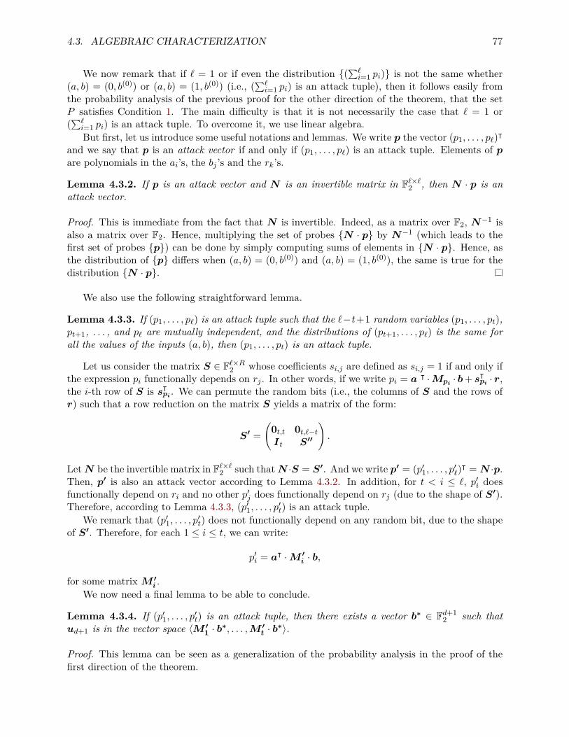
4.3. ALGEBRAIC CHARACTERIZATION 77
We now remark that if ` = 1 or if even the distribution (∑`i=1 pi) is not the same whether
(a, b) = (0, b(0)) or (a, b) = (1, b(0)) (i.e., (∑`i=1 pi) is an attack tuple), then it follows easily from
the probability analysis of the previous proof for the other direction of the theorem, that the setP satisfies Condition 1. The main difficulty is that it is not necessarily the case that ` = 1 or(∑`
i=1 pi) is an attack tuple. To overcome it, we use linear algebra.But first, let us introduce some useful notations and lemmas. We write p the vector (p1, . . . , p`)ᵀ
and we say that p is an attack vector if and only if (p1, . . . , p`) is an attack tuple. Elements of pare polynomials in the ai’s, the bj ’s and the rk’s.
Lemma 4.3.2. If p is an attack vector and N is an invertible matrix in F`×`2 , then N · p is anattack vector.
Proof. This is immediate from the fact that N is invertible. Indeed, as a matrix over F2, N−1 isalso a matrix over F2. Hence, multiplying the set of probes N · p by N−1 (which leads to thefirst set of probes p) can be done by simply computing sums of elements in N · p. Hence, asthe distribution of p differs when (a, b) = (0, b(0)) and (a, b) = (1, b(0)), the same is true for thedistribution N · p.
We also use the following straightforward lemma.
Lemma 4.3.3. If (p1, . . . , p`) is an attack tuple such that the `−t+1 random variables (p1, . . . , pt),pt+1, . . . , and p` are mutually independent, and the distributions of (pt+1, . . . , p`) is the same forall the values of the inputs (a, b), then (p1, . . . , pt) is an attack tuple.
Let us consider the matrix S ∈ F`×R2 whose coefficients si,j are defined as si,j = 1 if and only ifthe expression pi functionally depends on rj . In other words, if we write pi = a ᵀ ·Mpi · b+ sᵀpi · r,the i-th row of S is sᵀpi . We can permute the random bits (i.e., the columns of S and the rows ofr) such that a row reduction on the matrix S yields a matrix of the form:
S′ =(
0t,t 0t,`−tIt S′′
).
LetN be the invertible matrix in F`×`2 such thatN ·S = S′. And we write p′ = (p′1, . . . , p′`)ᵀ = N ·p.Then, p′ is also an attack vector according to Lemma 4.3.2. In addition, for t < i ≤ `, p′i doesfunctionally depend on ri and no other p′j does functionally depend on rj (due to the shape of S′).Therefore, according to Lemma 4.3.3, (p′1, . . . , p′t) is an attack tuple.
We remark that (p′1, . . . , p′t) does not functionally depend on any random bit, due to the shapeof S′. Therefore, for each 1 ≤ i ≤ t, we can write:
p′i = aᵀ ·M ′i · b,
for some matrix M ′i .
We now need a final lemma to be able to conclude.
Lemma 4.3.4. If (p′1, . . . , p′t) is an attack tuple, then there exists a vector b∗ ∈ Fd+12 such that
ud+1 is in the vector space 〈M ′1 · b∗, . . . ,M ′
t · b∗〉.
Proof. This lemma can be seen as a generalization of the probability analysis in the proof of thefirst direction of the theorem.
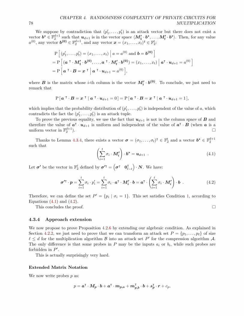
78CHAPTER 4. RANDOMNESS COMPLEXITY OF PRIVATE CIRCUITS FOR
MULTIPLICATION
We suppose by contradiction that (p′1, . . . , p′t) is an attack vector but there does not exist avector b∗ ∈ Fd+1
2 such that ud+1 is in the vector space 〈M ′1 · b∗, . . . ,M ′
t · b∗〉. Then, for any valuea(0), any vector b(0) ∈ Fd+1
2 , and any vector x = (x1, . . . , xt)ᵀ ∈ Ft2:
P[
(p′1, . . . , p′t) = (x1, . . . , xt)∣∣∣ a = a(0) and b = b(0)
]= P
[(a ᵀ ·M ′
1 · b(0), . . . ,a ᵀ ·M ′t · b(0)) = (x1, . . . , xt)
∣∣∣ aᵀ · ud+1 = a(0)]
= P[a ᵀ ·B = x ᵀ
∣∣∣ a ᵀ · ud+1 = a(0)],
where B is the matrix whose i-th column is the vector M ′i · b(0). To conclude, we just need to
remark that
P [a ᵀ ·B = x ᵀ | a ᵀ · ud+1 = 0 ] = P [a ᵀ ·B = x ᵀ | a ᵀ · ud+1 = 1 ],
which implies that the probability distribution of (p′1, . . . , p′t) is independent of the value of a, whichcontradicts the fact the (p′1, . . . , p′t) is an attack tuple.
To prove the previous equality, we use the fact that ud+1 is not in the column space of B andtherefore the value of aᵀ · ud+1 is uniform and independent of the value of aᵀ · B (when a is auniform vector in Fd+1
2 ).
Thanks to Lemma 4.3.4, there exists a vector σ = (σ1, . . . , σt)ᵀ ∈ Ft2 and a vector b∗ ∈ Fd+12
such that (t∑i=1
σi ·M ′i
)· b∗ = ud+1 . (4.1)
Let σ′ be the vector in F`2 defined by σ′ᵀ =(σᵀ 0ᵀ`−t
)·N . We have:
σ′ᵀ · p =t∑i=1
σi · p′i =t∑i=1
σi · aᵀ ·M ′i · b = aᵀ ·
(t∑i=1
σi ·M ′i
)· b . (4.2)
Therefore, we can define the set P ′ = pi | σi = 1. This set satisfies Condition 1, according toEquations (4.1) and (4.2).
This concludes the proof.
4.3.4 Approach extensionWe now propose to prove Proposition 4.2.6 by extending our algebraic condition. As explained inSection 4.2.2, we just need to prove that we can transform an attack set P = p1, . . . , p` of size` ≤ d for the multiplication algorithm B into an attack set P ′ for the compression algorithm A.The only difference is that some probes in P may be the inputs ai or bi, while such probes areforbidden in P ′.
This is actually surprisingly very hard.
Extended Matrix Notation
We now write probes p as:
p = aᵀ ·Mp · b+ aᵀ ·mp,a +mᵀp,b · b+ sᵀp · r + cp,
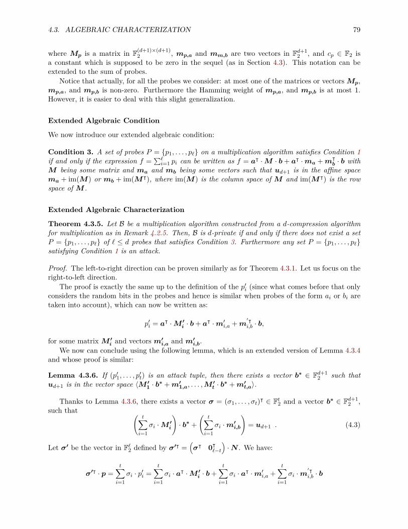
4.3. ALGEBRAIC CHARACTERIZATION 79
where Mp is a matrix in F(d+1)×(d+1)2 , mp,a and mm,b are two vectors in Fd+1
2 , and cp ∈ F2 isa constant which is supposed to be zero in the sequel (as in Section 4.3). This notation can beextended to the sum of probes.
Notice that actually, for all the probes we consider: at most one of the matrices or vectorsMp,mp,a, and mp,b is non-zero. Furthermore the Hamming weight of mp,a, and mp,b is at most 1.However, it is easier to deal with this slight generalization.
Extended Algebraic Condition
We now introduce our extended algebraic condition:
Condition 3. A set of probes P = p1, . . . , p` on a multiplication algorithm satisfies Condition 1if and only if the expression f = ∑`
i=1 pi can be written as f = aᵀ ·M · b+ aᵀ ·ma +mᵀb · b withM being some matrix and ma and mb being some vectors such that ud+1 is in the affine spacema + im(M) or mb + im(Mᵀ), where im(M) is the column space of M and im(Mᵀ) is the rowspace of M .
Extended Algebraic Characterization
Theorem 4.3.5. Let B be a multiplication algorithm constructed from a d-compression algorithmfor multiplication as in Remark 4.2.5. Then, B is d-private if and only if there does not exist a setP = p1, . . . , p` of ` ≤ d probes that satisfies Condition 3. Furthermore any set P = p1, . . . , p`satisfying Condition 1 is an attack.
Proof. The left-to-right direction can be proven similarly as for Theorem 4.3.1. Let us focus on theright-to-left direction.
The proof is exactly the same up to the definition of the p′i (since what comes before that onlyconsiders the random bits in the probes and hence is similar when probes of the form ai or bi aretaken into account), which can now be written as:
p′i = aᵀ ·M ′i · b+ aᵀ ·m′i,a +m
′ᵀi,b · b,
for some matrix M ′i and vectors m′i,a and m′i,b.
We now can conclude using the following lemma, which is an extended version of Lemma 4.3.4and whose proof is similar:
Lemma 4.3.6. If (p′1, . . . , p′t) is an attack tuple, then there exists a vector b∗ ∈ Fd+12 such that
ud+1 is in the vector space 〈M ′1 · b∗ +m′1,a, . . . ,M ′
t · b∗ +m′t,a〉.
Thanks to Lemma 4.3.6, there exists a vector σ = (σ1, . . . , σt)ᵀ ∈ Ft2 and a vector b∗ ∈ Fd+12 ,
such that (t∑i=1
σi ·M ′i
)· b∗ +
(t∑i=1
σi ·m′i,b)
= ud+1 . (4.3)
Let σ′ be the vector in F`2 defined by σ′ᵀ =(σᵀ 0ᵀ`−t
)·N . We have:
σ′ᵀ · p =t∑i=1
σi · p′i =t∑i=1
σi · aᵀ ·M ′i · b+
t∑i=1
σi · aᵀ ·m′i,a +t∑i=1
σi ·m′ᵀi,b · b
80CHAPTER 4. RANDOMNESS COMPLEXITY OF PRIVATE CIRCUITS FOR
MULTIPLICATION
so that:
σ′ᵀ · p = aᵀ ·(
t∑i=1
σi ·M ′i
)· b+ aᵀ ·
(t∑i=1
σi ·m′i,a)
+(
t∑i=1
σi ·m′ᵀi,b
)· b . (4.4)
Therefore, we can define the set P ′ = pi | σi = 1. This set satisfies Condition 3, according toEquations (4.3) and (4.4).
This concludes the proof.
Proof of Proposition 4.2.6
We can now prove Proposition 4.2.6.
Proof. Let us suppose by contraposition that B is not d-private. Thanks to Theorem 4.3.5, thismeans that there exists a set of probes P = p1, . . . , p` satisfying Condition 3. We suppose withoutloss of generality that: ∑
i=1pi = aᵀ ·M · b+ aᵀ ·ma +mᵀb · b
and ud+1 is in the affine space ma + im(M).From the shapes of possibles probes, we know that for any i, if ma,i = 1, then one of the probe
pj has to be ai. Let us spit our set of probes P in three sets:
• P1 contains all the probes pj such that pj = ai and ma,i = 1;
• P2 contains all the probes which are not of the form ai or bj ;
• P3 contains all the other probes.
We remark that: ∑p∈P1∪P2
p = aᵀ ·M · b+ aᵀ ·ma.
Let b∗ ∈ Fd+12 be a vector such that ud+1 = ma + B · b∗. The Hamming weight of ma is
exactly the cardinality of P1 and is at most d. Therefore, b∗ 6= 0d+1 and we can arbitrarily choose0 ≤ j∗ ≤ d such that b∗j∗ = 1. Finally, let us set P ′1 = αi,j∗ | ma,i = 1. We can write∑
p∈P ′1∪P2
p = aᵀ ·M ′ · b,
and we have that:M ′ · b∗ = M · b∗ +ma = ud+1.
Therefore P ′1∪P2 is a set of probes (for the compression algorithmA) which satisfies Condition 1.This concludes the proof.
4.4 Theoretical Lower and Upper BoundsIn this section, we exhibit lower and upper bounds for the randomness complexity of a d-privatecompression algorithm for multiplication. We first prove an algebraic result and an intermediatelemma that we then use to show that at least d + 1 random bits are required to construct a d-private compression algorithm for multiplication, for any d ≥ 3 (and 2 random bits are requiredfor d = 2). Finally, we provide a (non-constructive) proof that for large enough d, there exists ad-private multiplication algorithm with a randomness complexity O(d · log d).
4.4. THEORETICAL LOWER AND UPPER BOUNDS 81
4.4.1 A Splitting LemmaWe first prove an algebraic result, stated in the lemma below, that we further use to proveLemma 4.4.2. The latter allows us to easily exhibit attacks in order to prove our lower bounds.
Lemma 4.4.1. Let n ≥ 1. Let M0,M1 ∈ Fn×n2 such that M0 +M1 = Un. Then, there exists avector v ∈ Fn2 such that:
M0 · v = un or M1 · v = un or Mᵀ0 · v = un or Mᵀ
1 · v = un .
Proof. We show the above lemma by induction on n.Base case: for n = 1,M0,M1,U ∈ F2, soM0 +M1 = 1, which impliesM0 = 1 orM1 = 1 andthe claim immediately follows.Inductive case: let us assume that the claim holds for a fixed n ≥ 1. Let us consider two matricesM0,M1 ∈ F(n+1)×(n+1)
2 such that M0 +M1 = Un+1.Clearly, if M0 (or M1) is invertible, then the claim is true (as un+1 is in its range). Then, let
us assume that M0 is not invertible. Then, there exists a non-zero vector x ∈ ker(M0). Now, asim(Un+1) = 0n+1,un+1, if Un+1 · x = un+1, then M1 · x = un+1 and the claim is true. Hence,clearly, the claim is true if ker(M0) 6= ker(M1) (with the symmetric remark). The same remarkshold when considering matrices Mᵀ
0 and Mᵀ1.
Hence, the only remaining case to consider is when ker(M0) 6= 0n+1, ker(Mᵀ0) 6= 0n+1 and
when ker(M0) = ker(M1) and ker(Mᵀ0) = ker(Mᵀ
1). In particular, we have ker(M0) ⊆ ker(Un+1)and ker(Mᵀ
0) ⊆ ker(Un+1).Let x ∈ ker(M0) (and then x ∈ ker(M1) as well) be a non-zero vector. Up to some rear-
rangement of the columns of M0 and M1 (by permuting some columns), we can assume withoutloss of generality that x = (1, . . . , 1, 0, . . . , 0)ᵀ. Let X denote the matrix (x, e2, . . . , en+1) whereei = (0, . . . , 0, 1, 0, . . . , 0)ᵀ is the i-th canonical vector of length n+ 1, so that it has a 1 in the i-thposition and 0’s everywhere else.
Now, let y ∈ ker(Mᵀ0) (and then y ∈ ker(Mᵀ
1) as well) be a non-zero vector, so yᵀ ·Mᵀ0 =
0ᵀn+1. Moreover, up to some rearrangement of the rows of M0 and M1, we can assume thaty = (1, . . . , 1, 0, . . . , 0)ᵀ. Let Y denote the matrix (y, e2, . . . , en+1).
Please note that rearrangements apply to the columns in the first case and to the rows in thesecond case, so we can assume without loss of generality that there exists both x ∈ ker(M0) andy ∈ ker(Mᵀ
0) with the above form and matrices X and Y are well defined.We now define the matrices M ′
0 = Y ᵀ ·M0 ·X and M ′1 = Y ᵀ ·M1 ·X. We have:
M ′0 =
(yᵀ
0n In
)·M0 ·
(x
0ᵀnIn
)=(
yᵀ
0n In
)·(0n+1 M
(1)0
)where M (1)
0 is the matrix extracted from M0 by removing its first column. Hence:
M ′0 =
(0 0ᵀn0n M
(1,1)0
)
where M (1,1)0 is the matrix extracted from M0 by removing its first column and its first row.
Similar equation holds for M ′1 as well. Thus, it is clear that:
M ′0 +M ′
1 =(
0 0ᵀn0n Un
).
82CHAPTER 4. RANDOMNESS COMPLEXITY OF PRIVATE CIRCUITS FOR
MULTIPLICATION
Let us consider the matrices M ′′0 and M ′′
1 in Fn×n2 that are extracted from matrices M ′0 and M ′
1by removing their first row and their first column (i.e., M ′′
i = M′(1,1)i with the previous notation).
Then, it is clear that M ′′0 +M ′′
1 = Un. As matrices in Fn×n2 , by induction hypothesis, there existsv′′ ∈ Fn2 such that at least one of the 4 propositions from Lemma 4.4.1 holds. We can assumewithout loss of generality that M ′′
0 · v′′ = un.
Let v′ =(
0v′′
)∈ Fn+1
2 . Then, we have:
M ′0 · v′ =
(0 0ᵀn0n M ′′
0
)·(
0v′′
)=(
0n · v′′M ′′
0 · v′′)
=(
0un
).
Now, let v = X ·v′ and w = M0 ·w, so Y ᵀ ·w = Y ᵀ ·M0X ·v′ = M ′0 ·v′ =
(0un
). Moreover,
as Y is invertible, w is the unique vector such that Y ᵀ ·w =(
0un
). Finally, as the vector un+1
satisfies Y ᵀ · un+1 =(
0un
), then w = un+1, and the claim follows for n + 1, since v satisfies
M0 · v = w = un+1.Conclusion: The claim follows for any n ≥ 1, and so does Lemma 4.4.1.
We can now easily prove the following statement that is our main tool for proving our lowerbounds, as explained after its proof.
Lemma 4.4.2. Let A be a d-compression algorithm for multiplication. If there exist two sets S1and S2 of at most d probes such that si = ∑
p∈Si p does not functionally depend on any of therandom bits, for i ∈ 0, 1, and such that s0 + s1 = a · b, then A is not d-private.
Proof. Let A, S0, S1, s0 and s1 defined in the above statement. Then, there exists M i ∈F(d+1)×(d+1)
2 such that si = aᵀ ·M i ·b, for i ∈ 0, 1. Furthermore, as s0 + s1 = a · b = aᵀ ·Ud+1 ·b,we have M0 +M1 = Ud+1. Hence, via Lemma 4.4.1, there exists v ∈ Fd+1
2 and i ∈ 0, 1 suchthat M i · v = ud+1 or Mᵀ
i · v = ud+1. This means that ud+1 is in the row subspace or in thecolumn subspace of M i, and therefore, Mi satisfies Condition 1. Therefore, as |Si| ≤ d, applyingTheorem 4.3.1, A is not d-private. Lemma 4.4.2 follows.
We use the above lemma to prove our lower bounds as follows: for proving that at least R(d)random bits are required in order to achieve d-privacy for a compression algorithm for multiplica-tion, we prove that any algorithm with a lower randomness complexity is not d-private by exhibitingtwo sets of probes S0 and S1 that satisfy the requirements of Lemma 4.4.2.
4.4.2 Simple Linear Lower BoundAs a warm-up, we show that at least d random bits are required, for d > 2.
Theorem 4.4.3. Let d > 2. Let us consider a d-compression algorithm for multiplication A. If Auses only d− 1 random bits, then A is not d-private.
Proof. Let r1, . . . , rd−1 denote the random bits used by A. Let c0, . . . , cd denote the outputs of A.Let us define N ∈ F(d−1)×d
2 as the matrix whose coefficients ni,j are equal to 1 if and only if cj
4.4. THEORETICAL LOWER AND UPPER BOUNDS 83
functionally depends on ri, for 1 6 i 6 d− 1 and 1 6 j 6 d. Please note in particular that N doesnot depend on c0.
As a matrix over F2 with d columns and d− 1 rows, there is necessarily a vector w ∈ Fd2 withw 6= 0d such that N ·w = 0d−1.
The latter implies that the expression s0 = ∑di=1wi · ci does not functionally depend on any
of the rk’s. Furthermore, by correctness, we also have that s1 = c0 + ∑di=1(1 − wi) · ci does not
functionally depend on any of the rk’s, and s0 + s1 = ∑di=0 ci = a · b. Then, the sets of probes
S0 = ci | wi = 1 and S1 = c0 ∪ ci | wi = 0 (whose cardinalities are at most d) satisfy therequirements of Lemma 4.4.2, and then, A is not d-private. Theorem 4.4.3 follows.
4.4.3 Better Linear Lower BoundWe now show that at least d+ 1 random bits are actually required if d > 3.
Theorem 4.4.4. Let d > 3. Let us consider a d-compression algorithm for multiplication A. If Auses only d random bits, then A is not d-private.
Proof. Let r1, . . . , rd denote the random bits used by A. Let c0, . . . , cd denote the outputs of A.The proof is organized through 4 steps as follows:
1. we prove that at least one ci (further referred to as c0) functionally depends on at least twodistinct random bits,
2. we prove that at least two shares c0 and cj (further referred to as c1) both functionally dependon at least two distinct random bits,
3. we prove that at least one random bit r1 is such that no additive share functionally dependson only r1,
4. we exhibit an attack.
Step 1: c0 functionally depends on at least two distinct random bits.
Let us first show that at least one of the (ci)06i6d functionally depends on two different randombits. By contradiction, let us assume that every (ci)06i6d functionally depends on at most 1 randombit. Then, as there are d random bits, it implies that, either one ci does not functionally depend onany random bit, or there exist i < j such that ci and cj functionally depend on the same randombit:
• In the first case, let us assume that c0 does not functionally depend on any random bit.Then, by correctness, neither does∑d
i=1 ci. Then, S0 = c0 and S1 = c1, . . . , cd satisfy therequirements of Lemma 4.4.2 and A is not d-private.
• In the second case, let us assume without loss of generality that c0 and c1 functionally dependon the same random bit (and only on this one by assumption). Then, c0 + c1 does notdepend on any random bit and so does ∑d
i=2 ci via correctness. Then, S0 = c0, c1 andS1 = c2, . . . , cd satisfy the requirements of Lemma 4.4.2 and A is not d-private.
Then, we can now assume without loss of generality that c0 functionally depends on at least twodistinct random bits.
84CHAPTER 4. RANDOMNESS COMPLEXITY OF PRIVATE CIRCUITS FOR
MULTIPLICATION
Step 2: both c0 and c1 functionally depend on at least two distinct random bits.
By contradiction, let us now assume that for all 1 ≤ i ≤ d, ci functionally depends on onlyone random bit. In order to achieve correctness, there must exist ci, cj with 1 ≤ i < j ≤ d thatrespectively depend on the first and second of the two distinct random bits on which c0 functionallydepends on. As we assume that there are d random bits in total, all the d random bits on whichthe ci’s functionally depend on for i > 1 have to be different. Hence, we can assume without lossof generality that ci functionally depends on ri, for 1 ≤ i ≤ d. Thus, by correctness, c0 functionallydepends on all ri for i = 1, . . . , d.
Then, we can simply probe the first subsum p of c0 that functionally depends on at least 2distinct random bits (actually, any subsum that functionally depends on at least 2 and at mostd− 1 random bits would work).
Let us denote by I = i1, i2 the set of indices corresponding to the random bits on which pfunctionally depends on. Then, S0 = p, ci1 , ci2 and S1 = c0, p ∪ ci | i ∈ 1, . . . , d\i1, i2satisfy the requirements of Lemma 4.4.2 and A is not d-private.
Therefore, it is not possible that every ci for 1 ≤ i ≤ d functionally depends on only one randombit and thus, there are at least two ci, cj with i 6= j that functionally depend on at least 2 distinctrandom bits. We can assume without loss of generality that c0 and c1 each functionally depend onat least 2 distinct random bits.
Step 3: r1 is such that no ci (for i = 0, . . . , d) functionally depends on only r1 (and onno other random bits).
By correctness, c0 functionally depends on all the random bits on which ∑di=1 ci functionally de-
pends on. We just proved that c1 functionally depends on at least two distinct bits. Also, allrandom bits have to be used (otherwise there are at most d − 1 bits and Theorem 4.4.3 alreadyproves that A is not d-private). Consequently, each of the at most d − 2 random bits on whichc1 does not functionally depend on have to satisfy that at least one of the ci for 2 ≤ i ≤ d func-tionally depends on this random bit. Thus, it is not possible that all ci for i > 2 functionallydepend on only 1 random bit (otherwise, there would exist 2 6 i1 < i2 6 d such that ci1 andci2 functionally depend only on the same random bit. Indeed, in that case, S0 = ci1 , ci2 andS1 = c0 ∪ ci | i ∈ 1, . . . , d\i1, i2 satisfy the requirements of Lemma 4.4.2 and A is notd-private.
Thus, this proves that at least one of the random bits, say r1 without loss of generality, is suchthat no ci (for i = 0, . . . , d) functionally depends on only r1 (and on no other random bits).
Step 4: there exists an attack with at most d probes.
Let us now consider, similarly to what we did in the proof of Theorem 4.4.3, the matrix N ∈ Fd×d2defined as the matrix whose coefficients ni,j are equal to 1 if and only if cj functionally depends onthe random bit ri, for 1 6 i, j 6 d. Please note once again that this matrix does not depend of c0.In order to prevent the same kind of attack than the one we used in the proof of Theorem 4.4.3,it is clear that this matrix has to be invertible. Hence, there exists w ∈ Fd2 such that N ·w = e1where e1 denotes the first vector of the canonical basis of Fd2. Moreover, since c0 and ∑d
i=1 ci bothfunctionally depends on the same at least 2 distinct random bits, then by correctness, we havew 6= 1d. Also, the Hamming weight of w is at least 2, since r1 never appears alone in an additiveshare, which implies that e1 is not a column in N . Hence, we have 2 6 HW(w) 6 d− 1.
To conclude the proof, we just note that S0 = r′, c0∪ci | wi = 0 and S1 = r′∪ci | wi = 1satisfy the requirements of Lemma 4.4.2 and A is not d-private.
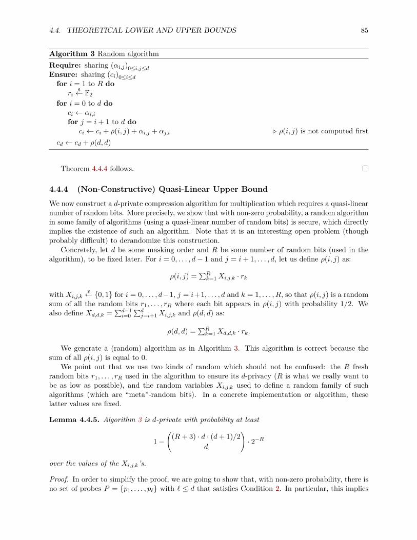
4.4. THEORETICAL LOWER AND UPPER BOUNDS 85
Algorithm 3 Random algorithmRequire: sharing (αi,j)0≤i,j≤dEnsure: sharing (ci)0≤i≤dfor i = 1 to R do
ri$← F2
for i = 0 to d doci ← αi,ifor j = i+ 1 to d do
ci ← ci + ρ(i, j) + αi,j + αj,i . ρ(i, j) is not computed firstcd ← cd + ρ(d, d)
Theorem 4.4.4 follows.
4.4.4 (Non-Constructive) Quasi-Linear Upper BoundWe now construct a d-private compression algorithm for multiplication which requires a quasi-linearnumber of random bits. More precisely, we show that with non-zero probability, a random algorithmin some family of algorithms (using a quasi-linear number of random bits) is secure, which directlyimplies the existence of such an algorithm. Note that it is an interesting open problem (thoughprobably difficult) to derandomize this construction.
Concretely, let d be some masking order and R be some number of random bits (used in thealgorithm), to be fixed later. For i = 0, . . . , d− 1 and j = i+ 1, . . . , d, let us define ρ(i, j) as:
ρ(i, j) = ∑Rk=1Xi,j,k · rk
with Xi,j,k$← 0, 1 for i = 0, . . . , d−1, j = i+1, . . . , d and k = 1, . . . , R, so that ρ(i, j) is a random
sum of all the random bits r1, . . . , rR where each bit appears in ρ(i, j) with probability 1/2. Wealso define Xd,d,k = ∑d−1
i=0∑dj=i+1Xi,j,k and ρ(d, d) as:
ρ(d, d) = ∑Rk=1Xd,d,k · rk.
We generate a (random) algorithm as in Algorithm 3. This algorithm is correct because thesum of all ρ(i, j) is equal to 0.
We point out that we use two kinds of random which should not be confused: the R freshrandom bits r1, . . . , rR used in the algorithm to ensure its d-privacy (R is what we really want tobe as low as possible), and the random variables Xi,j,k used to define a random family of suchalgorithms (which are “meta”-random bits). In a concrete implementation or algorithm, theselatter values are fixed.
Lemma 4.4.5. Algorithm 3 is d-private with probability at least
1−(
(R+ 3) · d · (d+ 1)/2d
)· 2−R
over the values of the Xi,j,k’s.
Proof. In order to simplify the proof, we are going to show that, with non-zero probability, there isno set of probes P = p1, . . . , p` with ` ≤ d that satisfies Condition 2. In particular, this implies
86CHAPTER 4. RANDOMNESS COMPLEXITY OF PRIVATE CIRCUITS FOR
MULTIPLICATION
that, with non-zero probability, there is no set of probes P = p1, . . . , p` with ` ≤ d that satisfiesCondition 1, which, via Theorem 4.3.1, is equivalent to the algorithm being d-private.
One can only consider sets of exactly d probes as if there is a set of ` < d probes P ′ that satisfiesCondition 2, one can always complete P ′ into a set P with exactly d probes by adding d− ` timesthe same probe on some input αi,j such that P ′ initially does not depend on αi,j . That is, if M ′
denotes the matrix such that ∑p′∈P ′ p′ = a ·M ′ · b, one could complete P ′ with any αi,j such that
m′i,j = 0, so that P , with ∑p∈P p = a ·M · b still satisfies Condition 2 if P ′ initially satisfied thecondition.
Thus, let us consider an arbitrary set of d probes P = p1, . . . , pd and let us bound theprobability that P satisfies Condition 2. Let f = ∑d
i=1 pi. Let us first show that f has to containat least one ρ(i, j) (meaning that it appears an odd number of times in the sum). Let us assumethe contrary, so f does not contain any ρ(i, j). Every ρ(i, j) appears only once in the shares (inthe share ci precisely). Then, one can assume that every probe is made on the same share. Let usassume (without loss of generality) that every probe is made on c0. If no probe contains any ρ(0, j),then clearly P cannot satisfy Condition 2 as this means that each probe contain at most one α0,j ,to P cannot contain more than d different α0,j . Hence, at least one (so at least two) probe containsat least one ρ(0, j). We note that every probe has one of the following form: either it is exactly arandom rk, a share α0,j , a certain ρ(0, j), a certain ρ(0, j)+α0,j or ρ(0, j)+α0,j +αj,0, or a subsum(starting from α0,0) of c0. Every form gives at most one α0,j with a new index j except probes onsubsums. However, in any subsum, there is always a random ρ(i, j) between α0,j and α0,j+1 andone needs to get all the d+ 1 indices to get a set satisfying Condition 2. Then, it is clear that onecannot achieve this unless there is a ρ(i, j) that does not cancel out in the sum, which is exactlywhat we wanted to show. Now, let 1 ≤ k ≤ R be an integer and let us compute the probability(over the Xi,j,k’s) that f contains rk. There exists some set S of pairs (i, j), such that f is the sumof ∑(i,j)∈S Xi,j,k · rk and some other expression not containing any Xi,j,k · rk. From the previouspoint, S is not empty. Furthermore, as there are d + 1 outputs c0, . . . , cd and as there are only dprobes, S cannot contain all the possible pairs (i, j), and therefore, all the random variables Xi,j,k
for (i, j) ∈ S are mutually independent. Therefore, ∑(i,j)∈S Xi,j,k is 1 with probability 1/2 andf functionally depends on the random rk with probability 1/2. As there are R possible randombits, f does not functionally depend on any rk (and then P satisfies Condition 2) with probability(1/2)R.
There are N possibles probes with
N ≤ d · (d+ 1)2 +R+ (R+ 2) · d · (d− 1)
2 ≤ (R+ 3) · d · (d+ 1)2 ,
as every ρ contains at most R random bits rk. Also, there are(Nd
)possible sets P = p1, . . . , pd.
Therefore, by union bound, the above algorithm is not secure (so there is an attack) with probabilityat most (
N
d
)/2R ≤
((R+ 3) · d · (d+ 1)/2
d
)· 2−R
which concludes the proof of Lemma 4.4.5.
Theorem 4.4.6. For some R = O(d · log d), there exists a choice of ρ(i, j) such that Algorithm 3is a d-private d-compression algorithm for multiplication, when d→∞.
We just need to remark that for some R = O(d · log d), the probability that Algorithm 3 isd-private, according to Lemma 4.4.5 is non-zero.
4.5. NEW CONSTRUCTION 87
Proof. We remark that a random algorithm as defined in Algorithm 3 and Lemma 4.4.5 is securewith probability at least
1−(
(R+ 3) · d · (d+ 1)/2d
)· 2−R ≥ 1− ((R+ 3) · d · (d+ 1)/2)d · 2−R
= 1− 2d·log((R+3)·d·(d+1)/2)−R.
When this probability is greater than 0, then there exists necessarily a choice of ρ(i, j) leading toa secure algorithm. This condition can be rewritten as:
d · log((R+ 3) · d · (d+ 1)/2)−R < 0.
Let us take R = K · d · log d− 3 with K some constant to be fixed later. As d · (d+ 1)/2 ≤ d2, wehave
d · log((R+ 3) · d · (d+ 1)/2)−R ≤ d · log(K · d3 · log d)−K · d · log d+ 3= d · ((3−K) · log d+ logK + log log d) + 3
When K is large enough, this is always negative. Theorem 4.4.6 easily follows.
4.5 New ConstructionThe goal of this section is to propose a new d-private multiplication algorithm. Compared to theconstruction in [ISW03], our construction halves the number of required random bits. It is thereforethe most efficient existing construction of a d-private multiplication.
Some rationales behind our new construction may be found in the two following necessaryconditions deduced from a careful study of the original work of Ishai, Sahai and Wagner [ISW03].
Lemma 4.5.1. Let A(a, b; r) be a d-compression algorithm for multiplication. Let f be an inter-mediate result taking the form f = aᵀ ·M · b + sᵀ · r. Let t denote the greatest Hamming weightof an element in the vector subspace generated by the rows of M or by the columns of M . IfHW(s) < t− 1, then A(a, b; r) is not d-private.
Proof. By definition of s, the value aᵀ ·M · b can be recovered by probing f and then each of theHW(s) < t− 1 random bits on which sᵀ · r functionally depends and by summing all these probes.Let P1 = f, p1, . . . , pj with j < t− 1 denote the set of these at most t− 1 probes. Then, we justshowed that f +∑j
i=1 pi = aᵀ ·M · b.To conclude the proof, we want to argue that there is a set of at most d − (t − 1) probes
P2 = p′1, . . . , p′k such that f +∑ji=1 pi +∑k
`=1 p′` = aᵀ ·M ′ · b, where M ′ is a matrix such that
ud+1 is in its row space or in its column space. If such a set P2 exists, then the set of probesP1 ∪ P2 (whose cardinality is at most d) satisfies Condition 1, and then A is not d-private, viaTheorem 4.3.1.
We now use the fact that there is a vector of Hamming weight t in the row space or in the columnspace of M . We can assume (without loss of generality) that there exists a vector w ∈ Fd+1
2 ofHamming weight t in the column subspace of M , so that w = ∑
j∈Jmj , with J ⊆ 0, . . . , d andmj the j-th column vector of M . Let i1, . . . , id+1−t denote the indices i of w such that wi = 0.Then, let j ∈ J , we claim that P2 = αi1,j , . . . , αid+1−t,j allows us to conclude the proof. Pleasenote that all these values are probes of intermediate values of A.
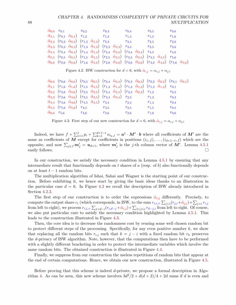
88CHAPTER 4. RANDOMNESS COMPLEXITY OF PRIVATE CIRCUITS FOR
MULTIPLICATION
α0,0 r0,1 r0,2 r0,3 r0,4 r0,5 r0,6α1,1 (r0,1 α0,1) r1,2 r1,3 r1,4 r1,5 r1,6α2,2 (r0,2 α0,2) (r1,2 α1,2) r2,3 r2,4 r2,5 r2,6α3,3 (r0,3 α0,3) (r1,3 α1,3) (r2,3 α2,3) r3,4 r3,5 r3,6α4,4 (r0,4 α0,4) (r1,4 α1,4) (r2,4 α2,4) (r3,4 α3,4) r4,5 r4,6α5,5 (r0,5 α0,5) (r1,5 α1,5) (r2,5 α2,5) (r3,5 α3,5) (r4,5 α4,5) r5,6α6,6 (r0,6 α0,6) (r1,6 α1,6) (r2,6 α2,6) (r3,6 α3,6) (r4,6 α4,6) (r5,6 α5,6)
Figure 4.2: ISW construction for d = 6, with αi,j = αi,j + αj,i
α0,0 (r0,6 α0,6) (r0,5 α0,5) (r0,4 α0,4) (r0,3 α0,3) (r0,2 α0,2) (r0,1 α0,1)α1,1 (r1,6 α1,6) (r1,5 α1,5) (r1,4 α1,4) (r1,3 α1,3) (r1,2 α1,2) r0,1α2,2 (r2,6 α2,6) (r2,5 α2,5) (r2,4 α2,4) (r2,3 α2,3) r1,2 r0,2α3,3 (r3,6 α3,6) (r3,5 α3,5) (r3,4 α3,4) r2,3 r1,3 r0,3α4,4 (r4,6 α4,6) (r4,5 α4,5) r3,4 r2,4 r1,4 r0,4α5,5 (r5,6 α5,6) r4,5 r3,5 r2,5 r1,5 r0,5α6,6 r5,6 r4,6 r3,6 r2,6 r1,6 r0,6
Figure 4.3: First step of our new construction for d = 6, with αi,j = αi,j + αj,i
Indeed, we have f +∑ji=1 pi +∑d+1−t
k=1 αik,j = aᵀ ·M ′ · b where all coefficients of M ′ are thesame as coefficients of M except for coefficients in positions (i1, j), . . . , (id+1−t, j) which are theopposite, and now ∑
j∈Jm′j = ud+1, where m′j is the j-th column vector of M ′. Lemma 4.5.1
easily follows.
In our construction, we satisfy the necessary condition in Lemma 4.5.1 by ensuring that anyintermediate result that functionally depends on t shares of a (resp. of b) also functionally dependson at least t− 1 random bits.
The multiplication algorithm of Ishai, Sahai and Wagner is the starting point of our construc-tion. Before exhibiting it, we hence start by giving the basic ideas thanks to an illustration inthe particular case d = 6. In Figure 4.2 we recall the description of ISW already introduced inSection 4.2.3.
The first step of our construction is to order the expressions αi,j differently. Precisely, tocompute the output share ci (which corresponds, in ISW, to the sum ri,i,+
∑j<i(rj,i+αj,i)+∑j>i ri,j
from left to right), we process ri,i,+∑j<d−i(ri,d−j+αi,j)+∑16j6i rd−j,i from left to right. Of course,
we also put particular care to satisfy the necessary condition highlighted by Lemma 4.5.1. Thisleads to the construction illustrated in Figure 4.3.
Then, the core idea is to decrease the randomness cost by reusing some well chosen random bitto protect different steps of the processing. Specifically, for any even positive number k, we showthat replacing all the random bits ri,j such that k = j − i with a fixed random bit rk preservesthe d-privacy of ISW algorithm. Note, however, that the computations then have to be performedwith a slightly different bracketing in order to protect the intermediate variables which involve thesame random bits. The obtained construction is illustrated in Figure 4.4.
Finally, we suppress from our construction the useless repetitions of random bits that appear atthe end of certain computations. Hence, we obtain our new construction, illustrated in Figure 4.5.
Before proving that this scheme is indeed d-private, we propose a formal description in Algo-rithm 4. As can be seen, this new scheme involves 3d2/2 + d(d + 2)/4 + 2d sums if d is even and
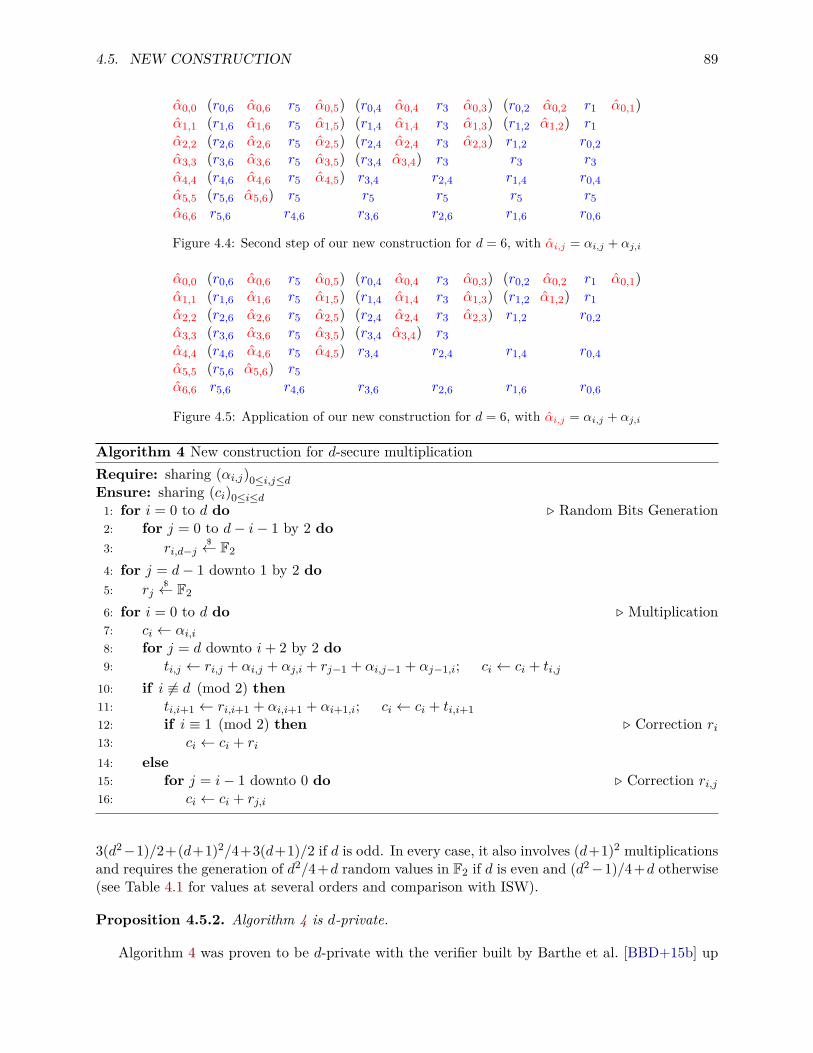
4.5. NEW CONSTRUCTION 89
α0,0 (r0,6 α0,6 r5 α0,5) (r0,4 α0,4 r3 α0,3) (r0,2 α0,2 r1 α0,1)α1,1 (r1,6 α1,6 r5 α1,5) (r1,4 α1,4 r3 α1,3) (r1,2 α1,2) r1α2,2 (r2,6 α2,6 r5 α2,5) (r2,4 α2,4 r3 α2,3) r1,2 r0,2α3,3 (r3,6 α3,6 r5 α3,5) (r3,4 α3,4) r3 r3 r3α4,4 (r4,6 α4,6 r5 α4,5) r3,4 r2,4 r1,4 r0,4α5,5 (r5,6 α5,6) r5 r5 r5 r5 r5α6,6 r5,6 r4,6 r3,6 r2,6 r1,6 r0,6
Figure 4.4: Second step of our new construction for d = 6, with αi,j = αi,j + αj,i
α0,0 (r0,6 α0,6 r5 α0,5) (r0,4 α0,4 r3 α0,3) (r0,2 α0,2 r1 α0,1)α1,1 (r1,6 α1,6 r5 α1,5) (r1,4 α1,4 r3 α1,3) (r1,2 α1,2) r1α2,2 (r2,6 α2,6 r5 α2,5) (r2,4 α2,4 r3 α2,3) r1,2 r0,2α3,3 (r3,6 α3,6 r5 α3,5) (r3,4 α3,4) r3α4,4 (r4,6 α4,6 r5 α4,5) r3,4 r2,4 r1,4 r0,4α5,5 (r5,6 α5,6) r5α6,6 r5,6 r4,6 r3,6 r2,6 r1,6 r0,6
Figure 4.5: Application of our new construction for d = 6, with αi,j = αi,j + αj,i
Algorithm 4 New construction for d-secure multiplicationRequire: sharing (αi,j)0≤i,j≤dEnsure: sharing (ci)0≤i≤d1: for i = 0 to d do . Random Bits Generation2: for j = 0 to d− i− 1 by 2 do3: ri,d−j
$← F2
4: for j = d− 1 downto 1 by 2 do5: rj
$← F2
6: for i = 0 to d do . Multiplication7: ci ← αi,i8: for j = d downto i+ 2 by 2 do9: ti,j ← ri,j + αi,j + αj,i + rj−1 + αi,j−1 + αj−1,i; ci ← ci + ti,j
10: if i 6≡ d (mod 2) then11: ti,i+1 ← ri,i+1 + αi,i+1 + αi+1,i; ci ← ci + ti,i+112: if i ≡ 1 (mod 2) then . Correction ri13: ci ← ci + ri14: else15: for j = i− 1 downto 0 do . Correction ri,j16: ci ← ci + rj,i
3(d2−1)/2+(d+1)2/4+3(d+1)/2 if d is odd. In every case, it also involves (d+1)2 multiplicationsand requires the generation of d2/4+d random values in F2 if d is even and (d2−1)/4+d otherwise(see Table 4.1 for values at several orders and comparison with ISW).
Proposition 4.5.2. Algorithm 4 is d-private.
Algorithm 4 was proven to be d-private with the verifier built by Barthe et al. [BBD+15b] up
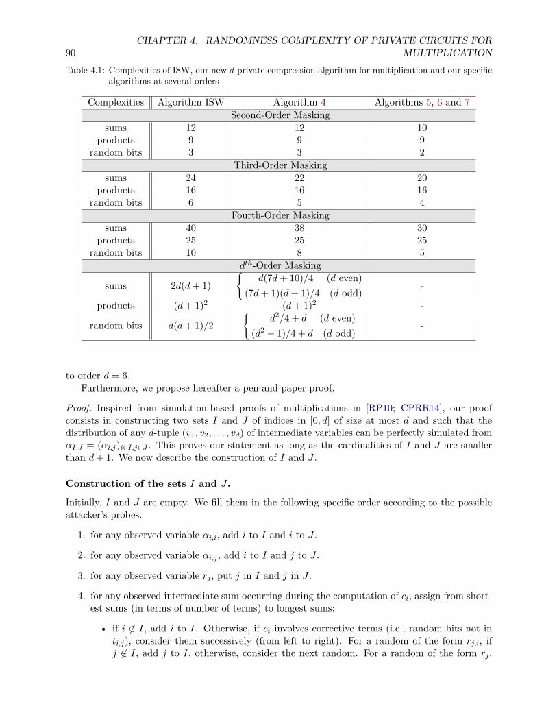
90CHAPTER 4. RANDOMNESS COMPLEXITY OF PRIVATE CIRCUITS FOR
MULTIPLICATIONTable 4.1: Complexities of ISW, our new d-private compression algorithm for multiplication and our specific
algorithms at several orders
Complexities Algorithm ISW Algorithm 4 Algorithms 5, 6 and 7Second-Order Masking
sums 12 12 10products 9 9 9
random bits 3 3 2Third-Order Masking
sums 24 22 20products 16 16 16
random bits 6 5 4Fourth-Order Masking
sums 40 38 30products 25 25 25
random bits 10 8 5dth-Order Masking
sums 2d(d+ 1)
d(7d+ 10)/4 (d even)(7d+ 1)(d+ 1)/4 (d odd)
-
products (d+ 1)2 (d+ 1)2 -
random bits d(d+ 1)/2
d2/4 + d (d even)(d2 − 1)/4 + d (d odd)
-
to order d = 6.Furthermore, we propose hereafter a pen-and-paper proof.
Proof. Inspired from simulation-based proofs of multiplications in [RP10; CPRR14], our proofconsists in constructing two sets I and J of indices in [0, d] of size at most d and such that thedistribution of any d-tuple (v1, v2, . . . , vd) of intermediate variables can be perfectly simulated fromαI,J = (αi,j)i∈I,j∈J . This proves our statement as long as the cardinalities of I and J are smallerthan d+ 1. We now describe the construction of I and J .
Construction of the sets I and J .
Initially, I and J are empty. We fill them in the following specific order according to the possibleattacker’s probes.
1. for any observed variable αi,i, add i to I and i to J .
2. for any observed variable αi,j , add i to I and j to J .
3. for any observed variable rj , put j in I and j in J .
4. for any observed intermediate sum occurring during the computation of ci, assign from short-est sums (in terms of number of terms) to longest sums:
• if i 6∈ I, add i to I. Otherwise, if ci involves corrective terms (i.e., random bits not inti,j), consider them successively (from left to right). For a random of the form rj,i, ifj 6∈ I, add j to I, otherwise, consider the next random. For a random of the form rj ,
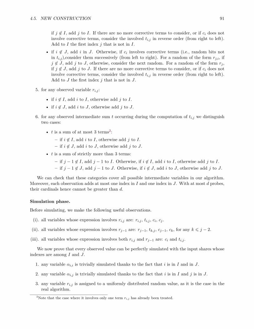
4.5. NEW CONSTRUCTION 91
if j 6∈ I, add j to I. If there are no more corrective terms to consider, or if ci does notinvolve corrective terms, consider the involved ti,j in reverse order (from right to left).Add to I the first index j that is not in I.
• if i 6∈ J , add i in J . Otherwise, if ci involves corrective terms (i.e., random bits notin ti,j),consider them successively (from left to right). For a random of the form rj,i, ifj 6∈ J , add j to J , otherwise, consider the next random. For a random of the form rj ,if j 6∈ J , add j to J . If there are no more corrective terms to consider, or if ci does notinvolve corrective terms, consider the involved ti,j in reverse order (from right to left).Add to J the first index j that is not in J .
5. for any observed variable ri,j :
• if i 6∈ I, add i to I, otherwise add j to I.• if i 6∈ J , add i to J , otherwise add j to J .
6. for any observed intermediate sum t occurring during the computation of ti,j we distinguishtwo cases:
• t is a sum of at most 3 terms2:– if i 6∈ I, add i to I, otherwise add j to I.– if i 6∈ J , add i to J , otherwise add j to J .
• t is a sum of strictly more than 3 terms:– if j − 1 6∈ I, add j − 1 to I. Otherwise, if i 6∈ I, add i to I, otherwise add j to I.– if j − 1 6∈ J , add j − 1 to J . Otherwise, if i 6∈ J , add i to J , otherwise add j to J .
We can check that these categories cover all possible intermediate variables in our algorithm.Moreover, each observation adds at most one index in I and one index in J . With at most d probes,their cardinals hence cannot be greater than d.
Simulation phase.
Before simulating, we make the following useful observations.
(i). all variables whose expression involves ri,j are: ri,j , ti,j , ci, cj .
(ii). all variables whose expression involves rj−1 are: rj−1, tk,j , cj−1, ck, for any k 6 j − 2.
(iii). all variables whose expression involves both ri,j and rj−1 are: ci and ti,j .
We now prove that every observed value can be perfectly simulated with the input shares whoseindexes are among I and J .
1. any variable αi,i is trivially simulated thanks to the fact that i is in I and in J .
2. any variable αi,j is trivially simulated thanks to the fact that i is in I and j is in J .
3. any variable ri,j is assigned to a uniformly distributed random value, as it is the case in thereal algorithm.
2Note that the case where it involves only one term ri,j has already been treated.
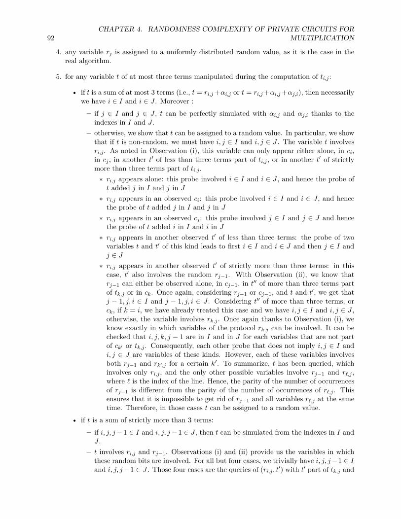
92CHAPTER 4. RANDOMNESS COMPLEXITY OF PRIVATE CIRCUITS FOR
MULTIPLICATION
4. any variable rj is assigned to a uniformly distributed random value, as it is the case in thereal algorithm.
5. for any variable t of at most three terms manipulated during the computation of ti,j :
• if t is a sum of at most 3 terms (i.e., t = ri,j+αi,j or t = ri,j+αi,j+αj,i), then necessarilywe have i ∈ I and i ∈ J . Moreover :– if j ∈ I and j ∈ J , t can be perfectly simulated with αi,j and αj,i thanks to the
indexes in I and J .– otherwise, we show that t can be assigned to a random value. In particular, we show
that if t is non-random, we must have i, j ∈ I and i, j ∈ J . The variable t involvesri,j . As noted in Observation (i), this variable can only appear either alone, in ci,in cj , in another t′ of less than three terms part of ti,j , or in another t′ of strictlymore than three terms part of ti,j .
∗ ri,j appears alone: this probe involved i ∈ I and i ∈ J , and hence the probe oft added j in I and j in J
∗ ri,j appears in an observed ci: this probe involved i ∈ I and i ∈ J , and hencethe probe of t added j in I and j in J
∗ ri,j appears in an observed cj : this probe involved j ∈ I and j ∈ J and hencethe probe of t added i in I and i in J
∗ ri,j appears in another observed t′ of less than three terms: the probe of twovariables t and t′ of this kind leads to first i ∈ I and i ∈ J and then j ∈ I andj ∈ J
∗ ri,j appears in another observed t′ of strictly more than three terms: in thiscase, t′ also involves the random rj−1. With Observation (ii), we know thatrj−1 can either be observed alone, in cj−1, in t′′ of more than three terms partof tk,j or in ck. Once again, considering rj−1 or cj−1, and t and t′, we get thatj − 1, j, i ∈ I and j − 1, j, i ∈ J . Considering t′′ of more than three terms, orck, if k = i, we have already treated this case and we have i, j ∈ I and i, j ∈ J ,otherwise, the variable involves rk,j . Once again thanks to Observation (i), weknow exactly in which variables of the protocol rk,j can be involved. It can bechecked that i, j, k, j − 1 are in I and in J for each variables that are not partof ck′ or tk,j . Consequently, each other probe that does not imply i, j ∈ I andi, j ∈ J are variables of these kinds. However, each of these variables involvesboth rj−1 and rk′,j for a certain k′. To summarize, t has been queried, whichinvolves only ri,j , and the only other possible variables involve rj−1 and r`,j ,where ` is the index of the line. Hence, the parity of the number of occurrencesof rj−1 is different from the parity of the number of occurrences of r`,j . Thisensures that it is impossible to get rid of rj−1 and all variables r`,j at the sametime. Therefore, in those cases t can be assigned to a random value.
• if t is a sum of strictly more than 3 terms:– if i, j, j− 1 ∈ I and i, j, j− 1 ∈ J , then t can be simulated from the indexes in I andJ .
– t involves ri,j and rj−1. Observations (i) and (ii) provide us the variables in whichthese random bits are involved. For all but four cases, we trivially have i, j, j−1 ∈ Iand i, j, j−1 ∈ J . Those four cases are the queries of (ri,j , t′) with t′ part of tk,j and
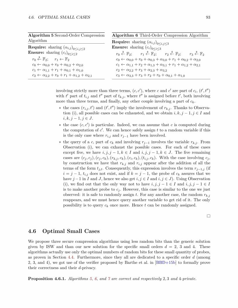
4.6. OPTIMAL SMALL CASES 93
Algorithm 5 Second-Order CompressionAlgorithmRequire: sharing (αi,j)0≤i,j≤2Ensure: sharing (ci)0≤i≤2r0
$← F2; r1 ← F2c0 ← α0,0 + r0 + α0,2 + α2,0c1 ← α1,1 + r1 + α0,1 + α1,0c2 ← α2,2 + r0 + r1 + α1,2 + α2,1
Algorithm 6 Third-Order Compression AlgorithmRequire: sharing (αi,j)0≤i,j≤3Ensure: sharing (ci)0≤i≤3r0
$← F2; r1$← F2; r2
$← F2; r3$← F2
c0 ← α0,0 + r0 + α0,3 + α3,0 + r1 + α0,2 + α2,0c1 ← α1,1 + r2 + α1,3 + α3,1 + r1 + α1,2 + α2,1c2 ← α2,2 + r3 + α2,3 + α3,2c3 ← α3,3 + r3 + r2 + r0 + α0,1 + α1,0
involving strictly more than three terms, (c, c′), where c and c′ are part of ci, (t′, t′′)with t′ part of ti,j and t′′ part of tk,j , where t′′ is assigned before t′, both involvingmore than three terms, and finally, any other couple involving a part of ck.
∗ the cases (ri,j , t′) and (t′, t′′) imply the involvement of rk,j . Thanks to Observa-tion (i), all possible cases can be exhausted, and we obtain i, k, j − 1, j ∈ I andi, k, j − 1, j ∈ J .
∗ the case (c, c′) is particular. Indeed, we can assume that c is computed duringthe computation of c′. We can hence safely assign t to a random variable if thisis the only case where ri,j and rj−1 have been involved.
∗ the query of a c, part of ck and involving rj−1 involves the variable rk,j . FromObservation (i), we can exhaust the possible cases. For each of these casesexcept five, we have i, j, j − 1, k ∈ I and i, j, j − 1, k ∈ J . The five remainingcases are (cj , cj), (cj , ck), (rk,j , ck), (ci, ck), (ti,j , ck). With the case involving cj ,by construction we have that rk,j and ri,j appear after the addition of all theterms of the form tj,`. Consequently, this expression involves the term rj−1,j (ifi = j − 1, ti,j does not exist, and if k = j − 1, the probe of ck assures that wehave j−1 in I and J , hence we also get i, j ∈ I and i, j ∈ J). Using Observation(i), we find out that the only way not to have i, j, j − 1 ∈ I and i, j, j − 1 ∈ Iis to make another probe to cj . However, this case is similar to the one we justobserved: it is safe to randomly assign t. For any another case, the random rk,jreappears, and we must hence query another variable to get rid of it. The onlypossibility is to query ck once more. Hence t can be randomly assigned.
4.6 Optimal Small CasesWe propose three secure compression algorithms using less random bits than the generic solutiongiven by ISW and than our new solution for the specific small orders d = 2, 3 and 4. Thesealgorithms actually use only the optimal numbers of random bits for these small quantity of probes,as proven in Section 4.4. Furthermore, since they all are dedicated to a specific order d (among2, 3, and 4), we got use of the verifier proposed by Barthe et al. in [BBD+15b] to formally provetheir correctness and their d-privacy.
Proposition 4.6.1. Algorithms 5, 6, and 7 are correct and respectively 2, 3 and 4-private.
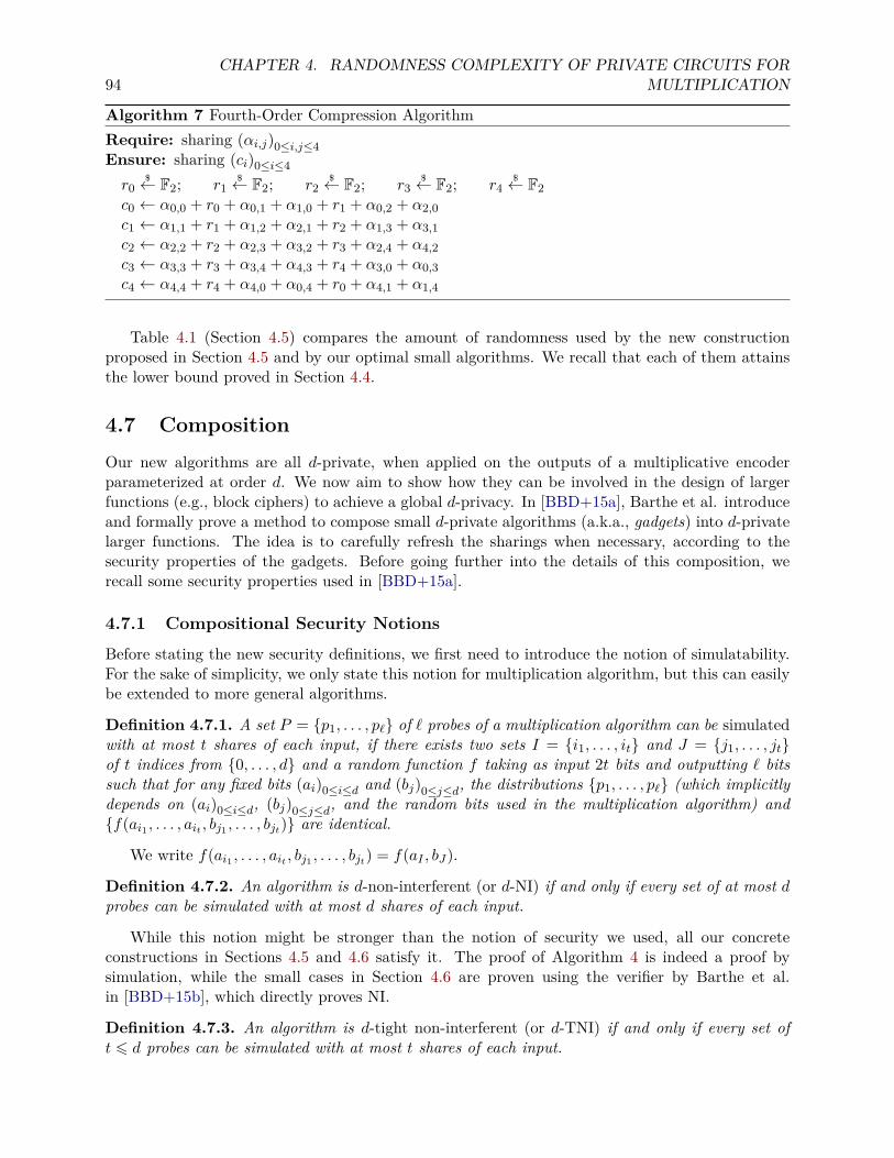
94CHAPTER 4. RANDOMNESS COMPLEXITY OF PRIVATE CIRCUITS FOR
MULTIPLICATION
Algorithm 7 Fourth-Order Compression AlgorithmRequire: sharing (αi,j)0≤i,j≤4Ensure: sharing (ci)0≤i≤4r0
$← F2; r1$← F2; r2
$← F2; r3$← F2; r4
$← F2c0 ← α0,0 + r0 + α0,1 + α1,0 + r1 + α0,2 + α2,0c1 ← α1,1 + r1 + α1,2 + α2,1 + r2 + α1,3 + α3,1c2 ← α2,2 + r2 + α2,3 + α3,2 + r3 + α2,4 + α4,2c3 ← α3,3 + r3 + α3,4 + α4,3 + r4 + α3,0 + α0,3c4 ← α4,4 + r4 + α4,0 + α0,4 + r0 + α4,1 + α1,4
Table 4.1 (Section 4.5) compares the amount of randomness used by the new constructionproposed in Section 4.5 and by our optimal small algorithms. We recall that each of them attainsthe lower bound proved in Section 4.4.
4.7 CompositionOur new algorithms are all d-private, when applied on the outputs of a multiplicative encoderparameterized at order d. We now aim to show how they can be involved in the design of largerfunctions (e.g., block ciphers) to achieve a global d-privacy. In [BBD+15a], Barthe et al. introduceand formally prove a method to compose small d-private algorithms (a.k.a., gadgets) into d-privatelarger functions. The idea is to carefully refresh the sharings when necessary, according to thesecurity properties of the gadgets. Before going further into the details of this composition, werecall some security properties used in [BBD+15a].
4.7.1 Compositional Security NotionsBefore stating the new security definitions, we first need to introduce the notion of simulatability.For the sake of simplicity, we only state this notion for multiplication algorithm, but this can easilybe extended to more general algorithms.
Definition 4.7.1. A set P = p1, . . . , p` of ` probes of a multiplication algorithm can be simulatedwith at most t shares of each input, if there exists two sets I = i1, . . . , it and J = j1, . . . , jtof t indices from 0, . . . , d and a random function f taking as input 2t bits and outputting ` bitssuch that for any fixed bits (ai)0≤i≤d and (bj)0≤j≤d, the distributions p1, . . . , p` (which implicitlydepends on (ai)0≤i≤d, (bj)0≤j≤d, and the random bits used in the multiplication algorithm) andf(ai1 , . . . , ait , bj1 , . . . , bjt) are identical.
We write f(ai1 , . . . , ait , bj1 , . . . , bjt) = f(aI , bJ).
Definition 4.7.2. An algorithm is d-non-interferent (or d-NI) if and only if every set of at most dprobes can be simulated with at most d shares of each input.
While this notion might be stronger than the notion of security we used, all our concreteconstructions in Sections 4.5 and 4.6 satisfy it. The proof of Algorithm 4 is indeed a proof bysimulation, while the small cases in Section 4.6 are proven using the verifier by Barthe et al.in [BBD+15b], which directly proves NI.
Definition 4.7.3. An algorithm is d-tight non-interferent (or d-TNI) if and only if every set oft 6 d probes can be simulated with at most t shares of each input.
4.7. COMPOSITION 95
While this notion of d-tight non-interference was assumed to be stronger than the notion ofd-non-interference in [BBD+15a], we show hereafter that these two security notions are actuallyequivalent. In particular, this means that all our concrete constructions are also TNI.
Proposition 4.7.4. (d-NI ⇔ d-TNI) An algorithm is d-non-interferent if and only if it is d-tightnon-interferent.
Proof. The right-to-left implication is straightforward from the definitions. Let us thus considerthe left-to-right direction.
For that purpose, we first need to introduce a technical lemma. Again, for the sake of simplic-ity, we only consider multiplication algorithm, with only two inputs, but the proof can easily begeneralized to any algorithm.
Lemma 4.7.5. Let P = p1, . . . , p` be a set of ` probes which can be simulated by the sets (I, J)and also by the sets (I ′, J ′). Then it can also be simulated by (I ∩ I ′, J ∩ J ′).
Proof. Let f the function corresponding to I, J and f ′ the function corresponding to I ′, J ′. Wehave that for any bits (ai)0≤i≤d and (bj)0≤j≤d, the distributions p1, . . . , p`, f(aI , bJ), andf ′(aI′ , bJ ′) are identical. Therefore, f does not depend on ai nor bj for i ∈ I \ I ′ and j ∈ J \ J ′,since f ′ does not depend on them. Thus, P can be simulated by only shares from I ∩ I ′, J ∩ J ′(using the function f where the inputs corresponding to ai and bj for i ∈ I \ I ′ and j ∈ J \ J ′ arejust set to zero, for example).
We now assume that an algorithm A is d-NI, that is, every set of at most d probes can besimulated with at most d shares of each input. Now, by contradiction, let us consider a set Pwith minimal cardinality t < d of probes on A, such that it cannot be simulated by at most tshares of each input. Let us consider the sets I, J corresponding to the intersection of all sets I ′, J ′(respectively) such that the set P can be simulated by I ′, J ′. The sets I, J also simulate P thanksto Lemma 4.7.5. Furthermore, by hypothesis, t < |I| ≤ d or t < |J | ≤ d. Without loss of generality,let us suppose that |I| > t.
Let i∗ be an arbitrary element of 0, . . . , d \ I (which is not an empty set as |I| ≤ d). Let usnow consider the set of probes P ′ = P ∪ ai∗. By hypothesis, P ′ can be simulated by at most|P ′| = t+ 1 shares of each input. Let I ′, J ′ two sets of size at most t+ 1 simulating P ′. These twosets also simulate P ⊆ P ′, therefore, I ∩ I ′, J ∩ J ′ also simulate P . Furthermore, i∗ ∈ I, as all theshares ai are independent. Since i∗ /∈ I, |I ∩ I ′| ≤ t and I ∩ I ′ ( I, which contradicts the fact thatI and J were the intersection of all sets I ′′, J ′′ simulating P .
Definition 4.7.6. An algorithm A is d-strong non-interferent (or d-SNI) if and only if for everyset I of t1 probes on intermediate variables (i.e., no output wires or shares) and every set O of t2probes on output shares such that t1 + t2 6 d, the set I ∪ O of probes can be simulated by only t1shares of each input.
The composition of two d-SNI algorithms is itself d-SNI, while that of d-TNI algorithms is notnecessarily d-TNI. This implies that d-SNI gadgets can be directly composed while maintaining thed-privacy property, whereas a so-called refreshing gadget must sometimes be involved before thecomposition of d-TNI algorithms. Since the latter refreshing gadgets consume the same quantityof random values as ISW, limiting their use is crucial if the goal is to reduce the global amount ofrandomness.
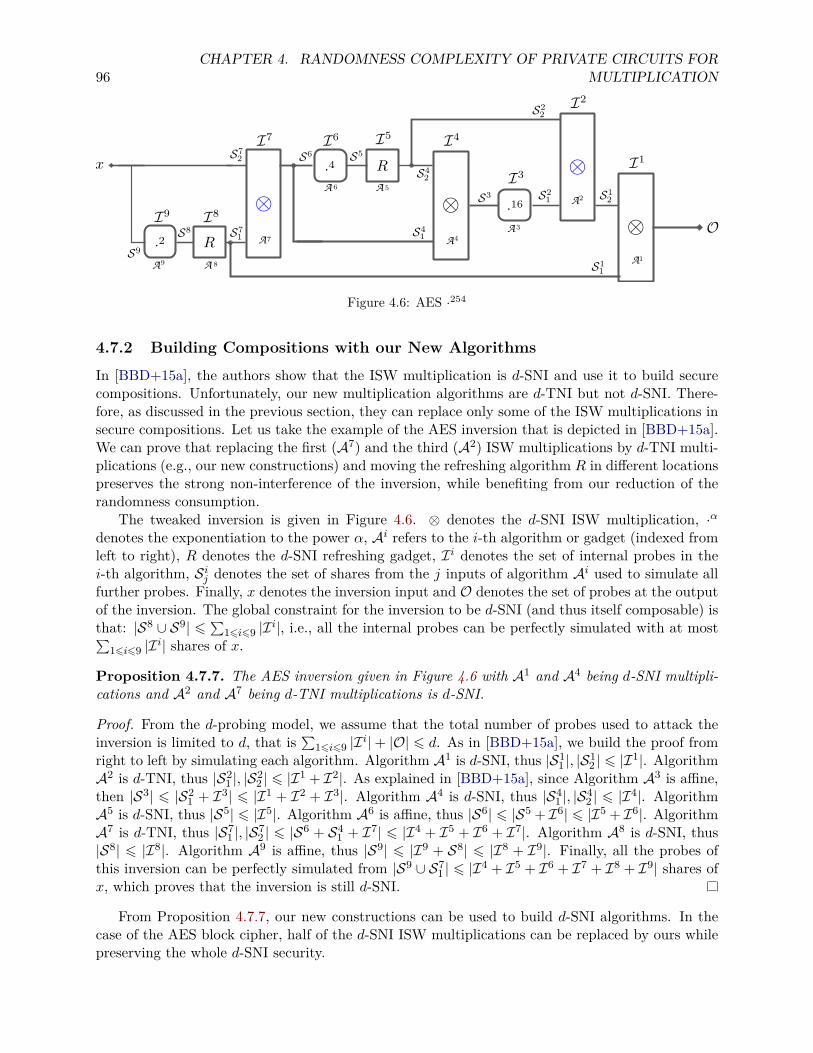
96CHAPTER 4. RANDOMNESS COMPLEXITY OF PRIVATE CIRCUITS FOR
MULTIPLICATION
A A
A
A A
AA
A
A
Figure 4.6: AES ·254
4.7.2 Building Compositions with our New AlgorithmsIn [BBD+15a], the authors show that the ISW multiplication is d-SNI and use it to build securecompositions. Unfortunately, our new multiplication algorithms are d-TNI but not d-SNI. There-fore, as discussed in the previous section, they can replace only some of the ISW multiplications insecure compositions. Let us take the example of the AES inversion that is depicted in [BBD+15a].We can prove that replacing the first (A7) and the third (A2) ISW multiplications by d-TNI multi-plications (e.g., our new constructions) and moving the refreshing algorithm R in different locationspreserves the strong non-interference of the inversion, while benefiting from our reduction of therandomness consumption.
The tweaked inversion is given in Figure 4.6. ⊗ denotes the d-SNI ISW multiplication, ·αdenotes the exponentiation to the power α, Ai refers to the i-th algorithm or gadget (indexed fromleft to right), R denotes the d-SNI refreshing gadget, Ii denotes the set of internal probes in thei-th algorithm, Sij denotes the set of shares from the j inputs of algorithm Ai used to simulate allfurther probes. Finally, x denotes the inversion input and O denotes the set of probes at the outputof the inversion. The global constraint for the inversion to be d-SNI (and thus itself composable) isthat: |S8 ∪ S9| 6 ∑16i69 |Ii|, i.e., all the internal probes can be perfectly simulated with at most∑
16i69 |Ii| shares of x.
Proposition 4.7.7. The AES inversion given in Figure 4.6 with A1 and A4 being d-SNI multipli-cations and A2 and A7 being d-TNI multiplications is d-SNI.
Proof. From the d-probing model, we assume that the total number of probes used to attack theinversion is limited to d, that is ∑16i69 |Ii|+ |O| 6 d. As in [BBD+15a], we build the proof fromright to left by simulating each algorithm. Algorithm A1 is d-SNI, thus |S1
1 |, |S12 | 6 |I1|. Algorithm
A2 is d-TNI, thus |S21 |, |S2
2 | 6 |I1 + I2|. As explained in [BBD+15a], since Algorithm A3 is affine,then |S3| 6 |S2
1 + I3| 6 |I1 + I2 + I3|. Algorithm A4 is d-SNI, thus |S41 |, |S4
2 | 6 |I4|. AlgorithmA5 is d-SNI, thus |S5| 6 |I5|. Algorithm A6 is affine, thus |S6| 6 |S5 + I6| 6 |I5 + I6|. AlgorithmA7 is d-TNI, thus |S7
1 |, |S72 | 6 |S6 + S4
1 + I7| 6 |I4 + I5 + I6 + I7|. Algorithm A8 is d-SNI, thus|S8| 6 |I8|. Algorithm A9 is affine, thus |S9| 6 |I9 + S8| 6 |I8 + I9|. Finally, all the probes ofthis inversion can be perfectly simulated from |S9 ∪ S7
1 | 6 |I4 + I5 + I6 + I7 + I8 + I9| shares ofx, which proves that the inversion is still d-SNI.
From Proposition 4.7.7, our new constructions can be used to build d-SNI algorithms. In thecase of the AES block cipher, half of the d-SNI ISW multiplications can be replaced by ours whilepreserving the whole d-SNI security.
4.8. NEW AUTOMATIC TOOL FOR FINDING ATTACKS 97
4.8 New Automatic Tool for Finding AttacksIn this section, we describe a new automatic tool for finding attacks on compression algorithms formultiplication which is developed in Sage (Python) [Sage]. Compared to the verifier developed byBarthe et al. [BBD+15b] and based on Easycrypt, to find attacks in practice, our tool is not asgeneric as it focuses on compression algorithms for multiplication and its soundness is not perfect(and relies on some heuristic assumption). Nevertheless, it is order of magnitudes faster.
A non-perfect soundness means that the algorithm may not find an attack and can only guar-antee that there does not exist an attack except with probability ε. We believe that, in practice,this limitation is not a big issue as if ε is small enough (e.g., 2−20), a software bug is much morelikely than an attack on the scheme. Furthermore, the running time of the algorithm dependsonly linearly on log(1/ε). Concretely, for all the schemes we manually tested for d = 3, 4, 5 and 6,attacks on invalid schemes were found almost immediately. If not used to formally prove schemes,our tool can at least be used to quickly eliminate (most) incorrect schemes, and enables to focusefforts on trying to prove “non-trivially-broken” schemes.
4.8.1 Algorithm of the ToolFrom Theorem 4.3.1, in order to find an attack P = p1, . . . , p` with ` ≤ d, we just need to find aset P = p1, . . . , p` satisfying Condition 1. If no such set P exists, the compression algorithm formultiplication is d-private.
A naive way to check the existence of such a set P is to enumerate all the sets of d probes. How-ever, there are
(Nd
)such sets, with N being the number of intermediate variables of the algorithm.
For instance, to achieve 4-privacy, our construction (see Section 4.6) uses N = 81 intermediatevariables, which makes more than 220 sets of four variables to test. In [BBD+15b], the authorsproposed a faster way of enumerating these sets by considering larger sets which are still indepen-dent from the secret. However, their method falls short for the compression algorithms proposedhere as soon as d > 6, as shown in Section 4.8.4. Furthermore even for d = 3, 4, 5, their tool takesseveral minutes to prove security (around 5 minutes to check security of Algorithm 4 with d = 5)or to find an attack for incorrect schemes, which prevent people from quickly checking the validityof a newly designed scheme.
To counteract this issue, we design a new tool which is completely different and which borrowsideas from coding theory to enumerate the sets of d or less intermediate variables. Let γ1, . . . , γνbe all the intermediate results whose expression functionally depends on at least one random andγ′1, . . . , γ
′ν′ be the other intermediate results that we refer to as deterministic intermediate results
(ν + ν ′ = N). We remark that all the αi,j = aibj are intermediate results and that no intermediateresult can functionally depend on more than one shares’ product αi,j = aibj without also dependingon a random bit. Otherwise, the compression algorithm would not be d-private, according toLemma 4.5.1. As this condition can be easily tested, we now assume that the only deterministicintermediate results are the αi,j = aibj that we refer to as γ′k in the following. As an example,intermediate results of Algorithm 5 are depicted in Table 4.2.
An attack set P = p1, . . . , p` can then be separated into two sets Q = γi1 , . . . , γiδ andQ′ = γi′1 , . . . , γi′δ′, with ` = δ + δ′ ≤ d. We remark that necessarily ∑p∈Q p does not functionallydepend on any random value. Actually, we even have the following lemma:
Lemma 4.8.1. Let A(a, b; r) be a compression algorithm for multiplication. Then A is d-privateif and only if there does not exist a set of non-deterministic probes Q = γi1 , . . . , γiδ with δ 6 dsuch that ∑p∈Q p = a ᵀ ·M · b where the column space or the row space of M contains a vector ofHamming weight at least δ + 1.
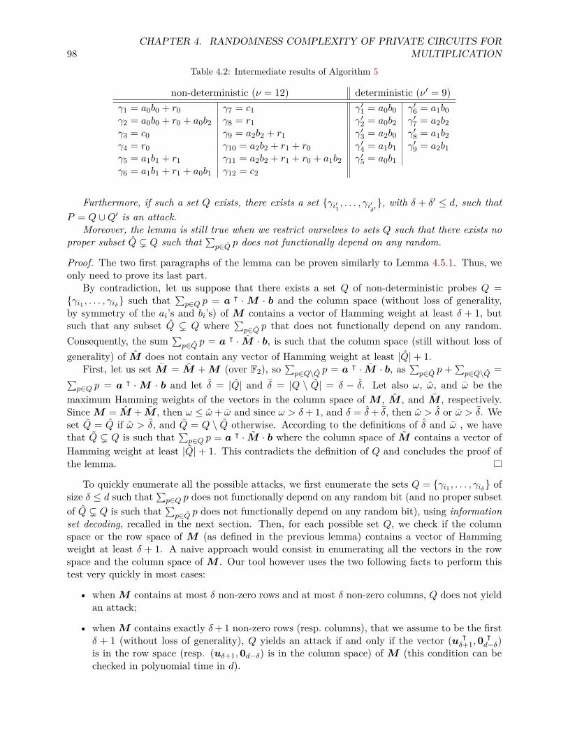
98CHAPTER 4. RANDOMNESS COMPLEXITY OF PRIVATE CIRCUITS FOR
MULTIPLICATIONTable 4.2: Intermediate results of Algorithm 5
non-deterministic (ν = 12) deterministic (ν ′ = 9)γ1 = a0b0 + r0 γ7 = c1 γ′1 = a0b0 γ′6 = a1b0γ2 = a0b0 + r0 + a0b2 γ8 = r1 γ′2 = a0b2 γ′7 = a2b2γ3 = c0 γ9 = a2b2 + r1 γ′3 = a2b0 γ′8 = a1b2γ4 = r0 γ10 = a2b2 + r1 + r0 γ′4 = a1b1 γ′9 = a2b1γ5 = a1b1 + r1 γ11 = a2b2 + r1 + r0 + a1b2 γ′5 = a0b1γ6 = a1b1 + r1 + a0b1 γ12 = c2
Furthermore, if such a set Q exists, there exists a set γi′1 , . . . , γi′δ′, with δ + δ′ ≤ d, such thatP = Q ∪Q′ is an attack.
Moreover, the lemma is still true when we restrict ourselves to sets Q such that there exists noproper subset Q ( Q such that ∑p∈Q p does not functionally depend on any random.
Proof. The two first paragraphs of the lemma can be proven similarly to Lemma 4.5.1. Thus, weonly need to prove its last part.
By contradiction, let us suppose that there exists a set Q of non-deterministic probes Q =γi1 , . . . , γiδ such that ∑p∈Q p = a ᵀ ·M · b and the column space (without loss of generality,by symmetry of the ai’s and bi’s) of M contains a vector of Hamming weight at least δ + 1, butsuch that any subset Q ( Q where ∑p∈Q p that does not functionally depend on any random.Consequently, the sum ∑
p∈Q p = a ᵀ · M · b, is such that the column space (still without loss ofgenerality) of M does not contain any vector of Hamming weight at least |Q|+ 1.
First, let us set M = M +M (over F2), so∑p∈Q\Q p = a ᵀ · M · b, as ∑p∈Q p +∑
p∈Q\Q =∑p∈Q p = a ᵀ ·M · b and let δ = |Q| and δ = |Q \ Q| = δ − δ. Let also ω, ω, and ω be the
maximum Hamming weights of the vectors in the column space of M , M , and M , respectively.Since M = M + M , then ω ≤ ω+ ω and since ω > δ+ 1, and δ = δ+ δ, then ω > δ or ω > δ. Weset Q = Q if ω > δ, and Q = Q \ Q otherwise. According to the definitions of δ and ω , we havethat Q ( Q is such that ∑p∈Q p = a ᵀ · M · b where the column space of M contains a vector ofHamming weight at least |Q| + 1. This contradicts the definition of Q and concludes the proof ofthe lemma.
To quickly enumerate all the possible attacks, we first enumerate the sets Q = γi1 , . . . , γiδ ofsize δ ≤ d such that∑p∈Q p does not functionally depend on any random bit (and no proper subsetof Q ( Q is such that ∑p∈Q p does not functionally depend on any random bit), using informationset decoding, recalled in the next section. Then, for each possible set Q, we check if the columnspace or the row space of M (as defined in the previous lemma) contains a vector of Hammingweight at least δ + 1. A naive approach would consist in enumerating all the vectors in the rowspace and the column space of M . Our tool however uses the two following facts to perform thistest very quickly in most cases:
• whenM contains at most δ non-zero rows and at most δ non-zero columns, Q does not yieldan attack;
• whenM contains exactly δ+ 1 non-zero rows (resp. columns), that we assume to be the firstδ + 1 (without loss of generality), Q yields an attack if and only if the vector (u ᵀδ+1,0
ᵀd−δ)
is in the row space (resp. (uδ+1,0d−δ) is in the column space) of M (this condition can bechecked in polynomial time in d).
4.8. NEW AUTOMATIC TOOL FOR FINDING ATTACKS 99
4.8.2 Information Set Decoding and Error ProbabilityWe now explain how to perform the enumeration step of our algorithm using information setdecoding. Information set decoding was introduced in the original security analysis of the McEliececryptosystem in [Pra62; McE78] as a way to break the McEliece cryptosystem by finding small codewords in a random linear code. It was further explored by Lee and Brickell in [LB88]. We shouldpoint out that since then, many improvements were proposed, e.g., in [Leo88; Ste88]. However, forthe sake of simplicity and because it already gives very good results, we use the original informationset decoding algorithm. Furthermore, it is not clear that the aforementioned improvements alsoapply in our case, as the codes we consider are far from the Singleton bound.
We assume that random bits are denoted r1, . . . , rR. For each intermediate γk containing somerandom bit, we associate the vector τ ∈ ZR2 , where τi = 1 if and only if γk functionally depends onthe random bit ri. We then consider the matrix Γ ∈ ZR×ν2 whose k-th column is τ . For instance,for Algorithm 5, we have:
γ1 γ2 γ3 γ4 γ5 γ6 γ7 γ8 γ9 γ10 γ11 γ12
Γ =(
1 1 1 1 0 0 0 0 1 1 1 10 0 0 0 1 1 1 1 0 1 1 1
)r0r1
.
For every δ ≤ d, enumerating the sets Q = γi1 , . . . , γiδ, such that∑p∈Q p does not functionallydepend on any random, consists in enumerating the vectors x of Hamming weight δ such that Γ·x =0 (specifically, i1, . . . , iδ are the coordinates of the non-zero components of x). Furthermore, wecan restrict ourselves to vector x such that no vector x < x satisfies Γ · x = 0 (where x < x meansthat x 6= x and for any 1 ≤ i ≤ ν, if xi = 0 then xi = 0), since we can restrict ourselves to setsQ such that no proper subset Q ( Q is such that ∑p∈Q p does not functionally depend on anyrandom bit. This is close to the problem of finding code words x of small Hamming weight for thelinear code of parity matrix Γ and we show this can be solved using information set decoding.
The basic idea is the following one. We first apply a row-reduction to Γ. Let us call the resultingmatrix Γ′. We remark that, for any vector x, Γ ·x = 0 if and only if Γ′ ·x = 0 and thus we can useΓ′ instead of Γ in our problem. We assume in a first time that the first R columns of Γ are linearlyindependent (recall that the number ν of columns of Γ is much larger than its number R of rows), sothat the R first columns of Γ′ forms an identity matrix. Then, for any k∗ > R, if the k∗-th columnof Γ′ has Hamming weight at most d− 1, we can consider the vector x defined as xk∗ = 1, xk = 1when Γ′k,k∗ = 1, and xk = 0 otherwise; and this vector satisfies the conditions we were looking for:its Hamming weight is at most d and Γ′ · x = 0. That way, we have quickly enumerated all thevectors x of Hamming weight at most d such that Γ′ ·x = 0 and with the additional property thatxk = 0 for all k > R except for at most3 one index k∗. Without the condition Γ′ · x = 0, there are(ν −R+ 1) ·∑d−1
i=0(Ri
)+(Rd
)such vectors, as there are ∑d
i=0(Ri
)vectors x such that HW(x) ≤ d and
xk = 0 for every k > R, and there are (ν−R) ·∑d−1i=0
(Ri
)vectors x such that HW(x) ≤ d and xk = 1,
for a single k > R.In other words, using row-reduction, we have been able to check (ν − R + 1) ·∑d−1
i=0(Ri
)+(Rd
)possible vectors x among at most ∑d
i=1(νi
)vectors which could be used to mount an attack, by
testing at most ν −R vectors.4
3We have seen that for one index k∗, but it is easy to see that, as the first R columns of Γ′ form an identitymatrix, there does not exist such vector x so that xk = 0 for all k > R anyway.
4There are exactly∑d
i=1
(νi
)vectors of Hamming weight at most d, but here we recall that we only consider
vectors x satisfying the following additional condition: there is no vector x < x such that Γ · x = 0. We also remarkthat the vectors x generated by the described algorithm all satisfy this additional condition.
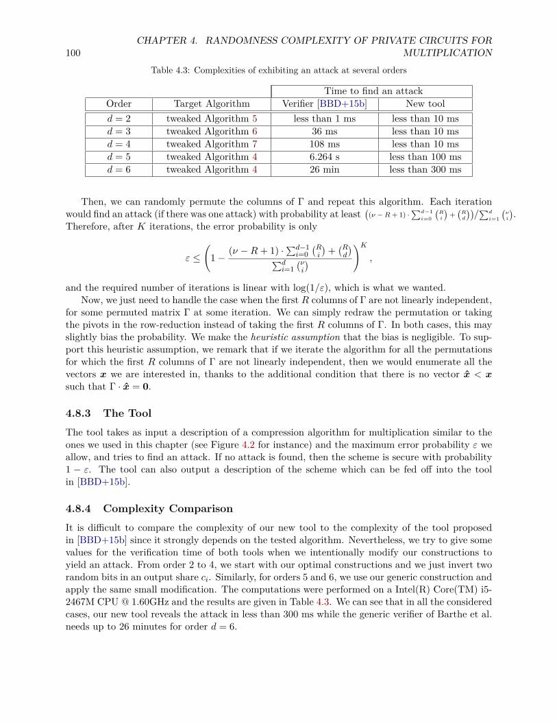
100CHAPTER 4. RANDOMNESS COMPLEXITY OF PRIVATE CIRCUITS FOR
MULTIPLICATIONTable 4.3: Complexities of exhibiting an attack at several orders
Time to find an attackOrder Target Algorithm Verifier [BBD+15b] New toold = 2 tweaked Algorithm 5 less than 1 ms less than 10 msd = 3 tweaked Algorithm 6 36 ms less than 10 msd = 4 tweaked Algorithm 7 108 ms less than 10 msd = 5 tweaked Algorithm 4 6.264 s less than 100 msd = 6 tweaked Algorithm 4 26 min less than 300 ms
Then, we can randomly permute the columns of Γ and repeat this algorithm. Each iterationwould find an attack (if there was one attack) with probability at least ((ν −R+ 1) ·
∑d−1i=0
(Ri
)+(Rd
))/∑d
i=1
(νi
).Therefore, after K iterations, the error probability is only
ε ≤(
1− (ν −R+ 1) ·∑d−1i=0
(Ri
)+(Rd
)∑di=1
(νi
) )K,
and the required number of iterations is linear with log(1/ε), which is what we wanted.Now, we just need to handle the case when the first R columns of Γ are not linearly independent,
for some permuted matrix Γ at some iteration. We can simply redraw the permutation or takingthe pivots in the row-reduction instead of taking the first R columns of Γ. In both cases, this mayslightly bias the probability. We make the heuristic assumption that the bias is negligible. To sup-port this heuristic assumption, we remark that if we iterate the algorithm for all the permutationsfor which the first R columns of Γ are not linearly independent, then we would enumerate all thevectors x we are interested in, thanks to the additional condition that there is no vector x < xsuch that Γ · x = 0.
4.8.3 The ToolThe tool takes as input a description of a compression algorithm for multiplication similar to theones we used in this chapter (see Figure 4.2 for instance) and the maximum error probability ε weallow, and tries to find an attack. If no attack is found, then the scheme is secure with probability1 − ε. The tool can also output a description of the scheme which can be fed off into the toolin [BBD+15b].
4.8.4 Complexity ComparisonIt is difficult to compare the complexity of our new tool to the complexity of the tool proposedin [BBD+15b] since it strongly depends on the tested algorithm. Nevertheless, we try to give somevalues for the verification time of both tools when we intentionally modify our constructions toyield an attack. From order 2 to 4, we start with our optimal constructions and we just invert tworandom bits in an output share ci. Similarly, for orders 5 and 6, we use our generic construction andapply the same small modification. The computations were performed on a Intel(R) Core(TM) i5-2467M CPU @ 1.60GHz and the results are given in Table 4.3. We can see that in all the consideredcases, our new tool reveals the attack in less than 300 ms while the generic verifier of Barthe et al.needs up to 26 minutes for order d = 6.
Chapter 5
Private Veto with ConstantRandomness
Quando você diz sim para outros, certifique-se de não estar dizendo não a si mesmo.Paulo Coelho
In this chapter, we formalize and study the problem of private veto protocols. A private vetoprotocol allows a set of players to test whether there is general agreement on a given decision whilekeeping each player’s choice secret. We consider the problem of n honest-but-curious players withprivate bits x1, . . . , xn who wish to compute their AND value x1 ∧ · · · ∧ xn in such a way that,after the execution of the protocol, no player obtains any information about the inputs of theremaining players (other than what can be deduced from their own inputs and the AND value). Thisproblem can be seen as the counterpart of the classical problem of the secure XOR evaluation. Thestudy of private veto protocols can then be seen a first step towards the secure evaluation of anyBoolean function, through its expression in an algebraic normal form. In distributed protocols, it isnatural to consider randomness as a resource like space and time and we here study the amount ofrandomness needed in such private protocols. However, the problem of the randomness complexityof the secure evaluation of private veto protocols was never tackled specifically. We propose inthis chapter a protocol that requires as few as 6 random bits for three players and we present aprotocol for all n ∈ N with less than 26 random bits. In the particular case where n belongs tothe infinite geometric progression of integers 3 · 2i, i ∈ N, our proposal uses only 12 random bits.The conception of our protocols is modular which allows us to present the general solution in arecursive way (with simplified correctness and privacy proofs).
5.1 Introduction
A private veto protocol should only reveal whether there is consensus, rather than an individualcount of the number of agreeing and disagreeing players. We propose several concrete constructionsfor this problem and prove their security in the information-theoretic security model. We notablypropose a protocol that requires as few as 6 random bits for three players and a generic protocolthat constantly uses 12 random bits for an unbounded number of players (of a particular form).
101
102 CHAPTER 5. PRIVATE VETO WITH CONSTANT RANDOMNESS
5.1.1 Previous work
Secure distributed computation is the problem of cooperative evaluation of a function such thatthe output becomes commonly known while the inputs remain secret. More precisely, a privatemulti-party protocol allows a set of players to compute a function of the players’ private inputs insuch a way that each player learns the result but no player learns anything about another’s privateinput.
The basic problem of designing private protocols for arbitrary functions was first solved fortwo players by Yao [Yao86], and for any number of players by Goldreich et al. [GMW87]. Thesesolutions rely on unproven computational assumptions and Ben-Or et al. [BOGW88], and Chaum etal. [CCD88] later removed the reliance on such assumptions. In these latter works, no assumptionis made about the computing power of the players and security proofs rely on information-theoreticarguments. In this setting, an adversary (passive or active) may control some corrupted playersbut the communication channels are assumed to be private (i.e. players are connected via idealpoint-to-point authenticated and encrypted channels).
In the case of passive adversaries (i.e. when the corrupted parties are honest-but-curious) theprotocols proposed in [BOGW88; CCD88] are secure against adversaries corrupting up to t < n/2players. In the case of active adversaries, where the corrupted players may arbitrarily deviate fromthe protocol, the threshold is reduced from n/2 to n/3. In this chapter, we consider only the securityin the information-theoretic setting against a passive adversary and the t-privacy property meansthat any passive coalition of at most t players cannot learn anything from the execution of theprotocol (except what is implied by the result and its own private input). We define formally thisnotion of information-theoretical privacy in Section 5.2. In this honest-but-curious model enforcingthe correctness constraint is usually easy, but enforcing the privacy constraint is hard.
As argued in Section 2.6, randomness plays a crucial role in several areas of computer science,including probabilistic algorithms, cryptography, and distributed computing. Random bits arehard to produce and devices that generate them, such as Geiger counters and Zener diodes areslow. It can be readily seen that, except for degenerate cases, randomness is essential to maintainprivacy in multi-party computation. In order to compute a function f : (Zp)n → Zp (with p arational prime number) of n players’ private inputs (with n < p), while satisfying the t-privacy,the protocols from [BOGW88; CCD88] require Ω(ntm log(p)) random bits, where m denotes thenumber of multiplication gates in the arithmetic circuit representing the function f . Since then,considerable effort has been devoted to reduce the number of random bits used by secure multi-partyprotocols.
Explicit results on the so-called randomness complexity of secure distributed computation areknown only for the computation of the specific function XOR-n : 0, 1n → 0, 1, (x1, . . . , xn) 7→x1 ⊕ · · · ⊕ xn. It can be easily seen that one random bit is necessary and sufficient to computethe XOR-n function in a 1-private way (using n rounds of communication). In [KM96], Kushilevitzand Mansour proved that Ω(t) bits are necessary, and O(t2 log(n/t)) are sufficient, for the t-privatecomputation of the XOR-n function. A lower bound Ω(logn) was later given by Gál and Rosénin [GR03] for any t > 2 (proving that the upper bound from [KM96] is tight, up to constantfactors, for any fixed constant t). It is also known that there exists a 1-private protocol in only 2communication rounds using n−2 random bits (other tradeoffs between randomness complexity andround complexity are given in [KR98]). Several works also analyse the randomness complexity ofthe secure evaluation of the XOR-n function on multiple instances and prove that one can “amortize”the randomness on several executions of the protocol [KOR03; BGP07].
Even if the properties for the XOR-n function are well-understood, very few studies show how toreduce the randomness complexity of other arbitrary functions, even simple. In particular, finding
5.1. INTRODUCTION 103
good upper bounds on the randomness complexity of useful functions such as the AND-n : 0, 1n →0, 1, (x1, . . . , xn) 7→ x1∧· · ·∧xn is of high interest. In [KOR99], Kushilevitz et al. proved that theclass of Boolean functions that can be 1-privately evaluated by n players with a constant number ofrandom bits are exactly those with O(n)-complexity size circuits. Their proof is constructive andtheir construction gives a solution for the AND-n function using 73 random bits (for n > 8 players).More precisely, their protocol requires 72m/(n− 1) + 1 random bits for the private evaluation of aBoolean function that can be computed with a Boolean circuit withm binary gates. The underlyingidea is to “recycle” the randomness in the protocol by distributing it to different players. Of course,this idea must be pursued with caution, since reusing randomness may hinder the security of theprotocols. In [CKOR00], Canetti et al. then proved that t-private computations of functions withsize m Boolean circuit (ie. m logical gates) and n inputs is possible using O(poly(t) ·(log(n)+m/n))random bits.
In spite of these very strong results, the exact randomness complexity of simple Boolean func-tions is still not well-understood. In particular, the situation is more complex for the AND-n functionthan for the XOR-n. The analysis of the randomness complexity of this function (or equivalentlyof OR-n) is therefore interesting and challenging. It is the main goal of the present chapter toinvestigate this problem. One application of such protocols is for private veto [KY03] (or related“dining cryptographers” [Cha88]1), since it allows to take decisions by some jury, which must beunanimous, without ever revealing the possible vetoing party(-ies). Another motivation for thestudy of the AND-n function is that they form, together with the XOR-n function, a basis for theBoolean algebra: simple and efficient protocols for their private evaluation should therefore lead tosimple and efficient protocols for the private evaluation of any Boolean function.
5.1.2 ContributionsUsing the seminal protocol from [BOGW88] (with the improvement proposed in [GRR98]), oneobtains a 1-private protocol for the AND-3 function (with 3 players) which requires 36 random bits.In this computation, the players compute shares of the output of an arithmetic gate given shares ofthe input wires of that gate (using Shamir’s secret sharing [Sha79]). Therefore, each player has toshare his private input bit using a linear polynomial over the finite field F4 and each multiplicationrequires a re-sharing of the result with another linear polynomial over F4. Note that this protocolfollows closely the transcoding method described in Algorithm 1 (Section 2.5.1). Surprisingly, to thebest of our knowledge, this simple protocol is the most randomness-efficient that has been proposedin the literature. Our first contribution is to propose an alternative protocol with a randomnesscomplexity reduced to 6 bits. It seems very difficult to prove a tight lower bound on this randomnesscomplexity. Obviously no deterministic protocol can exist and we prove that protocols using lessthan two random bits cannot be private (Section 5.3). Applying the same ideas as for AND-3, wepropose private protocols for the private evaluation of AND-n for n ∈ [4, 15], with the improvedrandomness complexity given in Table 5.1. Our approach is modular and is based on protocols forprivate computation of several functions that are of independent interest. In particular, they allowus to present a randomness-efficient 1-private protocol for the MAJORITY3 function and we use themin our improved protocol for the AND-n function when n is large.
As mentioned above, for n > 16, the protocol with the lowest randomness complexity is thegeneric protocol from [KOR99] which requires 73 random bits. In this chapter, we present a 1-
1Chaum introduced the dining cryptographers problem in 1988 [Cha88]: several cryptographers want to find outwhether the National Security Agency (NSA) or (exactly) one of them pays for the dinner, while respecting eachother’s right to make a payment anonymously. His famous protocol computes the OR-n function for arbitrary n usingn random bits but only for the case where the Hamming weight of the inputs vector is 0 or 1.
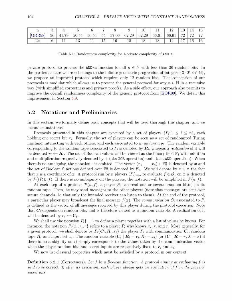
104 CHAPTER 5. PRIVATE VETO WITH CONSTANT RANDOMNESS
n 3 4 5 6 7 8 9 10 11 12 13 14 15[GRR98] 36 41.79 50.54 50.54 54 57.06 62.29 62.29 66.61 66.61 72 72 72
Us 6 11 13 11 15 16 15 18 18 12 17 16 16
Table 5.1: Randomness complexity for 1-private complexity of AND-n.
private protocol to process the AND-n function for all n ∈ N with less than 26 random bits. Inthe particular case where n belongs to the infinite geometric progression of integers 3 · 2i, i ∈ N,we propose an improved protocol which requires only 12 random bits. The conception of ourprotocols is modular which allows us to present the general protocol for any n ∈ N in a recursiveway (with simplified correctness and privacy proofs). As a side effect, our approach also permits toimprove the overall randomness complexity of the generic protocol from [KOR99]. We detail thisimprovement in Section 5.9.
5.2 Notations and PreliminariesIn this section, we formally define basic concepts that will be used thorough this chapter, and weintroduce notations.
Protocols presented in this chapter are executed by a set of players Pi; 1 ≤ i ≤ n, eachholding one secret bit xi. Formally, the set of players can be seen as a set of randomized Turingmachine, interacting with each others, and each associated to a random tape. The random variablecorresponding to the random tape associated to Pi is denoted by Ri, whereas a realization of it willbe denoted ri ← Ri. The set of Boolean values will be viewed as the binary field F2 with additionand multiplication respectively denoted by + (aka XOR operation) and · (aka AND operation). Whenthere is no ambiguity, the notation · is omitted. The vector (x1, . . . , xn) ∈ Fn2 is denoted by x andthe set of Boolean functions defined over Fn2 is denoted by Bn. We will denote by x ∈ x the factthat x is a coordinate of x. A protocol run by n players (Pi)i6n to evaluate f ∈ Bn on x is denotedby P((Pi)i, f). If there is no ambiguity on the players, the notation will be simplified in P(n, f).
At each step of a protocol P(n, f), a player Pi can read one or several random bit(s) on itsrandom tape. Then, he may send messages to the other players (note that messages are sent oversecure channels, ie. that only the intended receiver can listen to them). At the end of the protocol,a particular player may broadcast the final message f(x). The communication Ci associated to Piis defined as the vector of all messages received by this player during the protocol execution. Notethat Ci depends on random bits, and is therefore viewed as a random variable. A realization of itwill be denoted by ci ← Ci.
We shall use the notation Pi. . . to define a player together with a list of values he knows. Forinstance, the notation Pixi, ri, r refers to a player Pi who knows xi, ri and r. More generally, fora given protocol, we shall denote by PiCi,Ri, xi the player Pi with communication Ci, randomtape Ri and input bit xi. The random variable (Ci | Ri = ri, Xi = xi) (or (C | R = r, X = x) ifthere is no ambiguity on i) simply corresponds to the values taken by the communication vectorwhen the player random bits and secret inputs are respectively fixed to ri and xi.
We now list classical properties which must be satisfied by a protocol in our context.
Definition 5.2.1 (Correctness). Let f be a Boolean function. A protocol aiming at evaluating f issaid to be correct if, after its execution, each player always gets an evaluation of f in the players’secret bits.
5.2. NOTATIONS AND PRELIMINARIES 105
Definition 5.2.2 (Privacy). A protocol P((PiXi)i6n, f) is said to be private with respect to theplayer PC,R, X with X ∈X = (X1, . . . , Xn), if for every message c ← C, every r ← R, everyvector x←X and every bit b← B, the following equality holds: Pr (C = c|R = r,X = x, f(X) = b) =Pr (C = c|R = r, X = x, f(X) = b) , where the probability is taken on the supports of C,R,X. Aprotocol is said to be private if it is private with respect to all players taking part in it.
The privacy property states that any player taking part in the protocol does not learn moreinformation about the other player’s inputs than that he can deduce from its own input x andthe result of the evaluation f(x). To prove the privacy of some protocols, we will also need thefollowing property.
Definition 5.2.3 (Instance-Secrecy). A protocol P((PiXi)i6n, f) is said to satisfy the instance-secrecy property with respect to the player PC,R, X with X ∈ X = (X1, . . . , Xn), if forevery message c ← C, every r ← R and every vector x ← X, the following equality holds:Pr (C = c|R = r,X = x) = Pr (C = c|R = r, X = x) , where the probability is taken on the sup-ports of C,R,X. A protocol is said to satisfy the instance-secrecy property if it satisfies it withrespect to all players taking part in it.
The instance-secrecy property states that a player learns nothing about the other players’ secretsduring the protocol execution, including the result of the protocol itself (which is the difference withthe privacy property that allows each player to know the result). Indeed, several protocols built inthe next sections do not directly return the evaluation of a function f , but an encoding of it. Theencoding of a variable y is here defined as a pair (y + r, r) such that y and r are independent. Forprotocols returning such an encoding of a function evaluation f(x), the instance-secrecy propertyimplies that no player learns f(x), which itself implies that no player learns both f(x) + r and r.
In the following lemma, we exhibit a particular situation where stating the instance-secrecy prop-erty of a protocol with respect to a player is relatively easy.
Lemma 5.2.4. Let P be a protocol with players PiXi. Let PC,R, x be one these players. Ifthe random variable (C | R = r, X = x) is independent of X = (X1, . . . , Xn) for any r ← R andany x← X, then the protocol satisfies the instance-secrecy property with respect to P.
Proof. Let C ′ denote the random variable (C | R = r, X = x). If C ′ is independent of X, thenP (C′ = c′|X = x) = P (C′ = c′) for any c′ ← C ′. This directly implies that P satisfies theinstance-secrecy property with respect to P.
In our proofs, we will extensively use the following notion of functional independence:
Definition 5.2.5 (Functional Independence). Let n and i be positive integers such that i ∈ [1;n]and let f ∈ Bn. If f satisfies f(x1, . . . , xi, . . . , xn) = f(x1, . . . , xi+1, . . . , xn) for every (x1, . . . , xn) ∈Fn2 , then f is said to be functionally independent of xi, which is denoted by f ⊥ xi. Let x be a vectorcomposed of coordinates of (x1, . . . , xn). The function f is said to be functionally independent ofx, denoted f ⊥ x, if it is independent of every coordinate of x.
Remark 5.2.6. The functional independence is closely related to the classic notion of sensitivity:a function f is functionally independent of the variable xi if and only if f is not sensitive to xi. Thefunctional independence implies the statistical one, whereas the converse is false. Definition 5.2.5directly extends to random variables: if a random variable Y can be described as a functiondepending only on variables statistically independent from a random variable X, then X ⊥ Y .
106 CHAPTER 5. PRIVATE VETO WITH CONSTANT RANDOMNESS
Remark 5.2.7. The notion of functional dependence is trivially defined as the contrary of thefunctional independence: if f is not functionally independent of xi, it is functionally dependent onxi.
In the privacy proofs done in this chapter, we will often use the following Lemmas 5.2.8 and5.2.9 which establish a link between the notions of statistical and functional dependencies in someuseful contexts.
Lemma 5.2.8. Let R,X and V be three random vectors such that R is uniformly distributedand independent of X, and V is a function of X and R. If any non-zero linear combinationof coordinates of V can be written g(X,R) + R with R ∈ R and g ⊥ R, then V is statisticallyindependent of X.
Proof. Since every coordinate of R is uniform, then any variable taking the form g(X,R) + Rwith g ⊥ R is uniform. Moreover, the functional independence between g and R implies that thisuniformity holds even knowingX = x for any x. We deduce that (V |X = x) is uniform whateverx, which implies the independence between V and X.
Lemma 5.2.9. Let X,Y,R be three random variables, such that R is uniformly distributed, and Xand Y are functions. If X ⊥ R and Y ⊥ R then X + Y +R is statistically independent of (X,Y ).
Proof. Since X ⊥ R and Y ⊥ R, then (X + Y ) ⊥ R. Moreover, since R is uniformly distributed,then X + Y +R is also uniformly distributed, and statistically independent of (X,Y ).
The main purpose of this chapter is to reduce the number of random bits required to evaluatesome particular Boolean functions, while continuing to satisfy the privacy property. We definehereafter the randomness complexity of a protocol.
Definition 5.2.10 (Randomness Complexity). A protocol is said to be d-random if, for any exe-cution, the total number of random bits used by the players is at most d.
5.3 A lower boundThe private processing of the AND-n function has been proven to be infeasible for n = 2 [BOGW88].The exhibition of a private protocol involving the minimal number of three players is therefore anatural problem.
In this section, we restrict our study to what we further design as oblivious protocols, ie. pro-tocols where, for any execution, the players generating/reading the random bits are always thesame.
This section presents the proof of the following theorem:
Theorem 5.3.1. The minimal randomness complexity of any 1-private oblivious protocol computingthe AND-3 function is strictly higher than 2.
We reason ad absurdio and distinguish two cases: at the beginning of the protocol, eitherboth random bits are known by a single player, or are held by two different players. We denotethose random bits by r1 and r2 respectively. Before giving the proof we start by introducing aformalisation of our problem in terms of circuit privacy [SYY99].
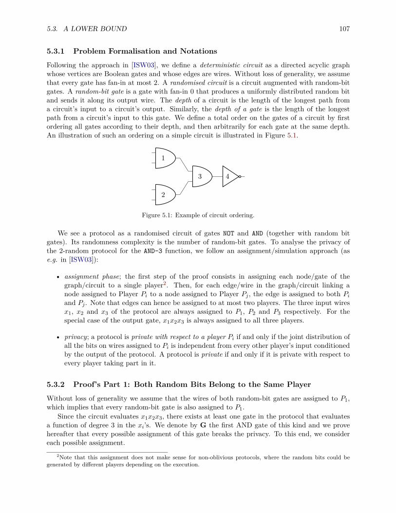
5.3. A LOWER BOUND 107
5.3.1 Problem Formalisation and NotationsFollowing the approach in [ISW03], we define a deterministic circuit as a directed acyclic graphwhose vertices are Boolean gates and whose edges are wires. Without loss of generality, we assumethat every gate has fan-in at most 2. A randomised circuit is a circuit augmented with random-bitgates. A random-bit gate is a gate with fan-in 0 that produces a uniformly distributed random bitand sends it along its output wire. The depth of a circuit is the length of the longest path froma circuit’s input to a circuit’s output. Similarly, the depth of a gate is the length of the longestpath from a circuit’s input to this gate. We define a total order on the gates of a circuit by firstordering all gates according to their depth, and then arbitrarily for each gate at the same depth.An illustration of such an ordering on a simple circuit is illustrated in Figure 5.1.
1
2
3 4
Figure 5.1: Example of circuit ordering.
We see a protocol as a randomised circuit of gates NOT and AND (together with random bitgates). Its randomness complexity is the number of random-bit gates. To analyse the privacy ofthe 2-random protocol for the AND-3 function, we follow an assignment/simulation approach (ase.g. in [ISW03]):
• assignment phase; the first step of the proof consists in assigning each node/gate of thegraph/circuit to a single player2. Then, for each edge/wire in the graph/circuit linking anode assigned to Player Pi to a node assigned to Player Pj , the edge is assigned to both Piand Pj . Note that edges can hence be assigned to at most two players. The three input wiresx1, x2 and x3 of the protocol are always assigned to P1, P2 and P3 respectively. For thespecial case of the output gate, x1x2x3 is always assigned to all three players.
• privacy; a protocol is private with respect to a player Pi if and only if the joint distribution ofall the bits on wires assigned to Pi is independent from every other player’s input conditionedby the output of the protocol. A protocol is private if and only if it is private with respect toevery player taking part in it.
5.3.2 Proof’s Part 1: Both Random Bits Belong to the Same PlayerWithout loss of generality we assume that the wires of both random-bit gates are assigned to P1,which implies that every random-bit gate is also assigned to P1.
Since the circuit evaluates x1x2x3, there exists at least one gate in the protocol that evaluatesa function of degree 3 in the xi’s. We denote by G the first AND gate of this kind and we provehereafter that every possible assignment of this gate breaks the privacy. To this end, we considereach possible assignment.
2Note that this assignment does not make sense for non-oblivious protocols, where the random bits could begenerated by different players depending on the execution.
108 CHAPTER 5. PRIVATE VETO WITH CONSTANT RANDOMNESS
• case G assigned to P1: by construction, at least one input wire of G functionally dependson x2 or on x3. The value on this wire is denoted by v: by definition, there exists a Booleanfunction f such that v = f(x1, x2, x3, r1, r2) and f(x1, x2, x3, r1, r2) is functionally dependenton x2, x3. Since P1 knows v, r1, r2, x1 (by assignment), it can then be deduced that P1can retrieve information on x2, x3 (by definition of the functional dependence, there existscertain r1, r2, x1, such that v becomes a non constant function of x2, x3). Consequently,privacy is broken.
• case G assigned to P2 (symmetric case for P3): by construction, at least one input wire of Gis of degree 2 in the xi’s, while the other one is of degree 1 or 2 in the xi’s, and both wiresare assigned to P2. To maintain privacy, the degree 2 wire has to be additively protected bya random bit (ie., a random bit has to be used as a mask), and the other wire must either beequal to x2 or to be additively protected by a different random bit.We denote by w one of these wires which functionally depends on x2. According to whatwe just said, w is hence either x2, or can be without loss of generality expressed as f2 ⊕ R,where f2 functionally depends on x2 and on no random bit, and R ∈ r1, r2, r1 ⊕ r2. Wedenote by v the value on the other wire, which must hence functionally depend on either x1or x3 (or both) and must additively involve R′, with R′ ∈ r1, r2, r1 ⊕ r2 \ R. Without lossof generality, in the following, we will always set R = r2 and R′ = r1.By construction, and according to the inputs of G, the algebraic normal form of the Booleanfunction representing the output of G involves the term f2r1, where f2 depends on x2.The output of the circuit being x1x2x3, there must hence be another gate in the circuitcomputing a Boolean function involving f2r1. Here are the ways this can be achieved:
1. a gate G0 evaluates a product between f2 and r1
2. a gate G1 evaluates a product between f2 and a value of the form r1 ⊕ · · · ⊕ r2 and agate G2 evaluates f2r2
3. a gate G1 evaluates a product between f2 and a value of the form v⊕· · ·⊕ r1 and a gateG2 evaluates a product between f2 and v
4. a gate G1 evaluates a product between a value of the form f2 ⊕ · · · ⊕ r2 and a value ofthe form v ⊕ · · · ⊕ r1 and a gate G2 evaluates r1r2.
Let us study separately each of these cases. We will show that every possible assignment ofG0,G1 or G2 breaks the privacy:
1. Since one of the two input wires of G0 is f2, privacy can only be maintained if G0 isassigned to P2. However, if G0 is assigned to P2, then by construction the other inputwire is also assigned to P2. This implies that r1 is also assigned to P2. The set ofwires assigned to P2 hence contains f2, r1, w, v. Denote by fv the Boolean functionevaluating v. Since fv functionally depends on either x1 or x3 and fv functionallydepends on r1, privacy is broken.
2. Since both G1 and G2 have an input wire whose value is f2, then both G1 and G2 mustbe assigned to P2. Consequently, the assignment of P2 contains r2, r1 ⊕ · · · ⊕ r2, v.Denote by fv the Boolean function evaluating v. Since fv functionally depends on eitherx1 or x3 and fv functionally depends on r1, privacy is broken.
3. Since both G1 and G2 have an input wire whose value is f2, then both G1 and G2 mustbe assigned to P2. Consequently, the assignment of P2 contains r2, v ⊕ · · · ⊕ r1, v, v.

5.3. A LOWER BOUND 109
Denote by fv the Boolean function evaluating v. Since fv functionally depends on eitherx1 or x3 and fv depends on r1, privacy is broken.
4. Let us denote by v′ the value f2 ⊕ · · · ⊕ r2, and by respectively fv and f ′v the Booleanfunctions evaluating v and v′. We focus on the player that G1 can be assigned to. Firstof all, if G1 is assigned to P1, its assignment contains v′, r1, r2. Since f2 dependson x2, hence privacy is broken. If G1 is assigned to P2, hence its assignment containsv′, v, v ⊕ · · · ⊕ r1. Since fv functionally depends on either x1 or x3 and fv depends onr1, privacy is broken. If G1 is assigned to P3, his assignment contains v′, v ⊕ · · · ⊕ r1.In this case, ifG2 is assigned to P2, privacy is broken because fv functionally depends onr1 and on x1 or x3. If G2 is assigned to P3, privacy is broken because fv′ depends on r2and on x2. Consequently, r1r2 can only be known by P1. Hence no further message canbe sent without breaking privacy and consequently it is impossible to compute x1x2x3.
Hence, no oblivious protocol using only two random bits drawn by the same player and allowingfor the 1-private secure computation of the AND of three players can exist.
5.3.3 Proof’s part 2: Both bits held by different playersWe consider that both random-bit gates (and their wires) are assigned to two different players,without loss of generality P1 and P2, to which are assigned respectively r1 and r2. Consider thefirst AND gate G which evaluates a value of degree 3 in xi’s.
• case G assigned to P1 (the case is symmetric for P2):
As in the previous subsection, we denote by w one of the input wires of G which functionallydepends on x1 (w is either x1 or can be without loss of generality expressed as f1⊕R, wheref1 functionally depends on x1, and R ∈ r1, r2, r1⊕ r2); and we denote by v the value on theother wire, which must hence functionally depend on either x2 or x3 (or both) and additivelyinvolve R′, with R′ ∈ r1, r2, r1⊕ r2 \R. Without loss of generality, in the following, we willalways set R = r1 and R′ = r2. Similarly, we denote by v the input of G that is not w. Theoutput of G can be evaluated by a Boolean function. We can show similarly to the previouscase, that the ANF of this function involves the term f1r2, where f1 depends on x1.
The output of the circuit being x1x2x3, there must hence be another gate in the circuitcomputing a Boolean function involving f1r2. Here are all the possible ways this can beachieved:
1. a gate G0 evaluates a product between f1 and r2
2. a gate G1 evaluates a product between f1 and a value of the form r1 ⊕ · · · ⊕ r2 and agate G2 evaluates f1r1
3. a gate G1 evaluates a product between f1 and a value of the form v⊕· · ·⊕ r2 and a gateG2 evaluates a product between f1 and v
4. a gate G1 evaluates a product between a value of the form f1 ⊕ · · · ⊕ r1 and a value ofthe form v ⊕ · · · ⊕ r2 and a gate G2 evaluates r1r2.
Let us study separately each of these cases. We will show that every possible assignment ofG0,G1 or G2 breaks the privacy:
110 CHAPTER 5. PRIVATE VETO WITH CONSTANT RANDOMNESS
1. Since one of the input wires of G0 is f1, privacy can only be maintained if this gateis assigned to P1. Its assignment hence contains f1, r2, v. Denote by fv the Booleanfunction evaluating v. Since fv functionally depends on either x2 or x3 and the onlyrandom bit fv depends on is r2, privacy is broken.
2. Since one of the input wires of G1 is f1, privacy can only be maintained if this gate isassigned to P1. Its assignment hence contains r1, f1, r1⊕ · · · ⊕ r2, v. Denote by fv theBoolean function evaluating v. Since fv functionally depends on either x2 or x3 and fvdepends on r2, privacy is broken.
3. Since one of the input wires of G1 is f1, privacy can only be maintained if this gate isassigned to P1. Its assignment hence contains r1, f1, v ⊕ · · · ⊕ r2, v. Denote by fv theBoolean function evaluating v. Since fv functionally depends on either x2 or x3 and fvfunctionally depends on r2, privacy is broken.
4. We denote by v′ the value of the form f1⊕ · · · ⊕ r1. We focus on the player that G1 canbe assigned to. If it is assigned to P1, then his assignment contains v, v′, r1. Denoteby fv the Boolean function evaluating v. P1 obtains information on x2 or x3 thanks tothe fact that fv is functionally dependent on one of these variables. If it is assigned toP2 then his assignment contains v′, v ⊕ · · · ⊕ r2. Hence G2 can only be assigned toP3 (whose assignment hence contains r1, v ⊕ · · · ⊕ r2 and hence no further messagecan be assigned to any player without breaking privacy. Consequently it is impossibleto compute x1x2x3. Similarly, if G1 is assigned to P3 then G2 can only be assigned toP2 and for the same reason, it is impossible to compute x1x2x3.
• caseG assigned to P3: Similarly, we denote by w one of the input wires ofG which functionallydepends on x3 (w is either x3 or can be without loss of generality expressed as f3⊕R, wheref3 functionally depends on x3 and on no random bit, and R ∈ r1, r2, r1⊕r2); and we denoteby v the value on the other wire, which must hence functionally depend on either x1 or x2(or both) and additively involve R′, with R′ ∈ r1, r2, r1⊕ r2\R. Without loss of generality,in the following, we will always set R = r2 and R′ = r1. Similarly, we denote by v the inputof G that is not w. The output of G can be evaluated by a Boolean function. We can showsimilarly to the previous case, that the ANF of this function involves the term f3r1, where f3functionally depends on x3.The output of the circuit being x1x2x3, there must hence be another gate in the circuitcomputing a Boolean function involving f3r1. Here are the ways this can be achieved:
1. a gate G0 evaluates a product between f3 and r1
2. a gate G1 evaluates a product between f3 and a value of the form r1 ⊕ · · · ⊕ r2 and agate G2 evaluates f3r2
3. a gate G1 evaluates a product between f3 and a value of the form v⊕· · ·⊕ r1 and a gateG2 evaluates a product between f3 and v
4. a gate G1 evaluates a product between a value of the form f3 ⊕ · · · ⊕ r2 and a value ofthe form v ⊕ · · · ⊕ r1 and a gate G2 evaluates r1r2.
Let us study separately each of these cases. We will show that every possible assignment ofG0,G1 or G2 breaks the privacy:
1. Since f3 is an input of G, then this gate must be assigned to P3. Hence its assignmentcontains v, r1, and privacy is broken because v functionally depends on x1 or x2.
5.4. PRIVATE EVALUATION OF AND-n FOR n = 3 111
2. Since f3 is an input of G, then this gate must be assigned to P3. Hence its assignmentcontains v, r1, r1 ⊕ · · · ⊕ r2, w, and privacy is broken because v functionally dependson x1 or x2.
3. Since f3 is an input of G, then this gate must be assigned to P3. Hence its assignmentcontains v, r1, v ⊕ · · · ⊕ r1, and privacy is broken because v functionally depends onx1 or x2.
4. If G2 is assigned to a player, then this player knows both r1 and r2. This is the firstcase of our proof, and we already proved that such protocol is impossible.
Hence, no protocol using only two random bits drawn by different players and allowing for the1-private secure computation of the AND of three players can exist.
5.4 Private Evaluation of AND-n for n = 3To the best of our knowledge, the most random-efficient 1-private protocol for the AND-3 functionrequires 36 random bits and is based on [BOGW88; GRR98].
In this section, we tackle this problem by describing a 6-random protocol allowing to processAND-3 in a 1-private way. We also propose an alternative protocol where the result is returned inan encoded form, and therefore stays unknown to any player. It will be the cornerstone of ourgeneral protocol presented in Sections 5.6 and 5.7.
Let us recall the goal of our protocol. Three players P1x1, P2x2, P3x3 are provided with alimited number of independent3 and uniformly distributed random bits. At each round, a player canread one or several random bit(s) on its random tape, and send one or several message(s) to otherplayers. After the execution of the protocol, each player must know the value AND(x1, x2, x3) =x1x2x3 (correctness property), but must not learn more information on (x1, x2, x3) than that givenby its own input xi and AND(x1, x2, x3) (privacy property). This section aims at describing a protocolPAND-3 verifying these two properties with a randomness complexity equal to 6. This protocol isthe composition of the three following protocols P−AND-2, P(1)
AND-2 and PXOR.The first protocol, P−AND-2 allows three players to process the multiplication of two of their secrets,
while satisfying the instance-secrecy property. It is 3-random and, at the end of its execution, theAND of the two secrets is encoded among the players who own these secrets.
Protocol P−AND-2
Require: players Paxa,Ra, Pbxb,Rb and PcRcEnsure: Pb gets xaxb + r with r a random bit known by Pc only
round 1 : Players Pa and Pb read random bits r1 and r2 on their respective random tapesPa sends m1 = xa + r1 to Pb and r1 to PcPb sends m2 = xb + r2 to Pa and r2 to Pcround 2 : Pc reads a random bit r on its random tapePc sends m3 = r1r2 + r to Paround 3 : Pa sends m4 = m3 +m2xa to Pb . m4 = r1r2 + r + (xb + r2)xaPb computes m5 = m4 + r2m1 . m5 = xaxb + r
3For the ease of exposition, we assume that the players are provided with random tapes. However, we do notconsider the model in which parties receive a sample from a predetermined joint distribution where random stringsare correlated as in [IKM+13]. When two players have the same random bit r in their random tape, we actuallyassume that one player has picked r uniformly at random and has then sent it to the other player.
112 CHAPTER 5. PRIVATE VETO WITH CONSTANT RANDOMNESS
We describe hereafter two other protocols P(1)AND-2 and PXOR. The first one is very close to P−AND-2;
the main difference is that one of the secrets which must be multiplied by the protocol comes inan encoded form at input. It is also 3-random and outputs a refreshed encoding of the AND ofthe encoded input and the other secret. The protocol PXOR allows n players to privately processthe addition of two of their secrets. It is well-known that it is impossible to privately computethe addition of n > 3 inputs deterministically but this is not the case for two inputs. The simplesolution that we propose for PXOR is indeed deterministic. It will be used each time we shall needto recover and broadcast a value owned in an encoded form by a set of players.
We can now present our new 6-random protocol allowing three players to process the multiplica-tion of their respective secrets. We present two versions of it: the first one provides the players withan encoding of the evaluation, whereas the second one allows all of them to know the evaluationitself. Before executing the protocols, the three players P1, P2 and P3 are respectively providedwith the random tapes R1, R2 ∪ R′2 and R3 ∪ R′3. Random tapes Ri (resp. R′i) will be usedwhen executing protocol P−AND-2 (resp. P(1)
AND-2). Before the execution of the protocol, each playerfills his random tape such that: R1 ← r1, R2 ← r2, R′2 ← r′1, R3 ← r, R′3 ← r′2, r′′.This implies that each player has initially generated the random bits he is going to use during theprotocol. This assumption will be useful in the next section as it will enable the reuse of somerandom bits when executing several protocols in parallel or sequentially. At the end of this sectionwe propose another protocol that will be useful in the next section. This protocol is very close toP(1)
AND-2: it allows three players to process the encoding of the multiplication of two encoded secrets.The protocol is 5-random. The correctness of all protocols can be directly checked thanks to thecomments inserted in the algorithms descriptions.
Protocol P(1)AND-2
Require: players Paxa + r′,Ra, Pbxb, r′,Rb and PcEnsure: Pa gets xaxb + r′′ with r′′ a random bit known by Pb only
round 1 : Players Pa and Pb read a random bit r′1 and r′2 on their tapesPa sends m1 = (xa + r′) + r′1 to Pb and r′1 to PcPb sends m2 = xb + r′2 to Pa and r′2 to Pcround 2 : Pb reads a random bit r′′ on its random tapePb sends m3 = (m1 + r′)xb + r′′ to Pc
. m3 = (xa + r′1)xb + r′′
round 3 : Pc sends m4 = m3 + r′1r′2 to Pa
. m4 = xaxb + r′1(xb + r′2) + r′′
Pa computes m5 = m4 + r′1m2. m5 = xaxb + r′′
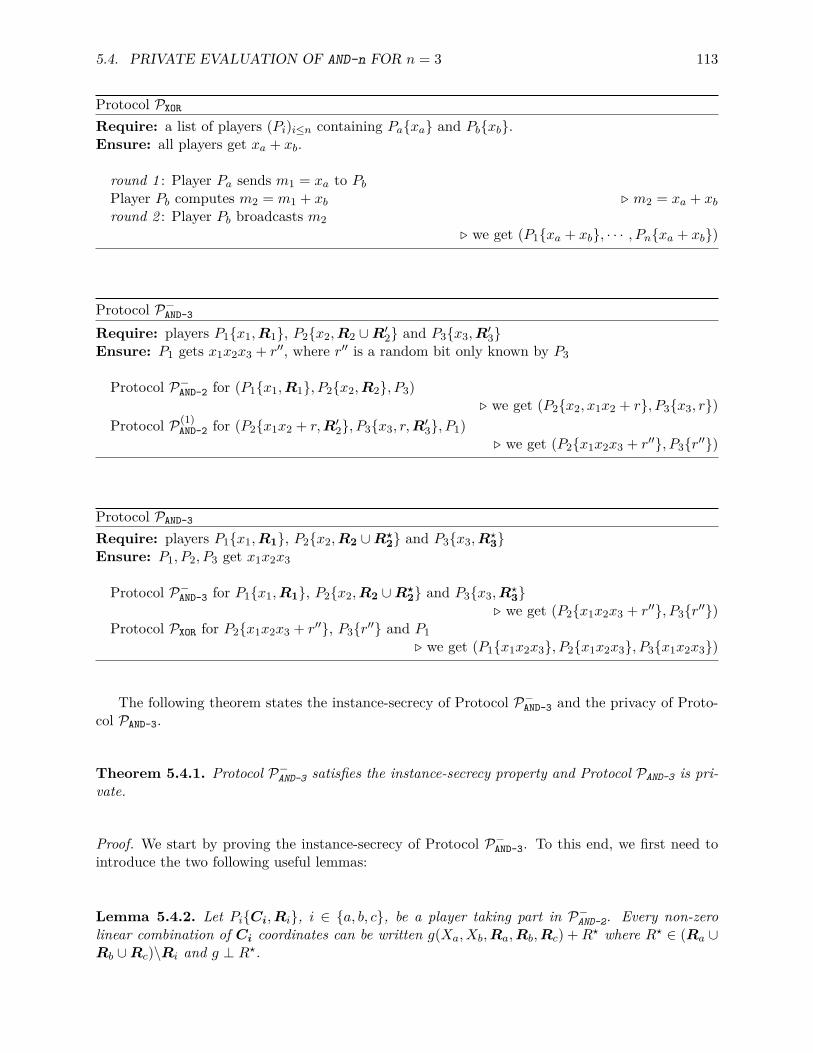
5.4. PRIVATE EVALUATION OF AND-n FOR n = 3 113
Protocol PXOR
Require: a list of players (Pi)i≤n containing Paxa and Pbxb.Ensure: all players get xa + xb.
round 1 : Player Pa sends m1 = xa to PbPlayer Pb computes m2 = m1 + xb . m2 = xa + xbround 2 : Player Pb broadcasts m2
. we get (P1xa + xb, · · · , Pnxa + xb)
Protocol P−AND-3
Require: players P1x1,R1, P2x2,R2 ∪R′2 and P3x3,R′3Ensure: P1 gets x1x2x3 + r′′, where r′′ is a random bit only known by P3
Protocol P−AND-2 for (P1x1,R1, P2x2,R2, P3). we get (P2x2, x1x2 + r, P3x3, r)
Protocol P(1)AND-2 for (P2x1x2 + r,R′2, P3x3, r,R′3, P1)
. we get (P2x1x2x3 + r′′, P3r′′)
Protocol PAND-3
Require: players P1x1,R1, P2x2,R2 ∪R?2 and P3x3,R?3
Ensure: P1, P2, P3 get x1x2x3
Protocol P−AND-3 for P1x1,R1, P2x2,R2 ∪R?2 and P3x3,R?3
. we get (P2x1x2x3 + r′′, P3r′′)Protocol PXOR for P2x1x2x3 + r′′, P3r′′ and P1
. we get (P1x1x2x3, P2x1x2x3, P3x1x2x3)
The following theorem states the instance-secrecy of Protocol P−AND-3 and the privacy of Proto-col PAND-3.
Theorem 5.4.1. Protocol P−AND-3 satisfies the instance-secrecy property and Protocol PAND-3 is pri-vate.
Proof. We start by proving the instance-secrecy of Protocol P−AND-3. To this end, we first need tointroduce the two following useful lemmas:
Lemma 5.4.2. Let PiCi,Ri, i ∈ a, b, c, be a player taking part in P−AND-2. Every non-zerolinear combination of Ci coordinates can be written g(Xa, Xb,Ra,Rb,Rc) +R? where R? ∈ (Ra ∪Rb ∪Rc)\Ri and g ⊥ R?.
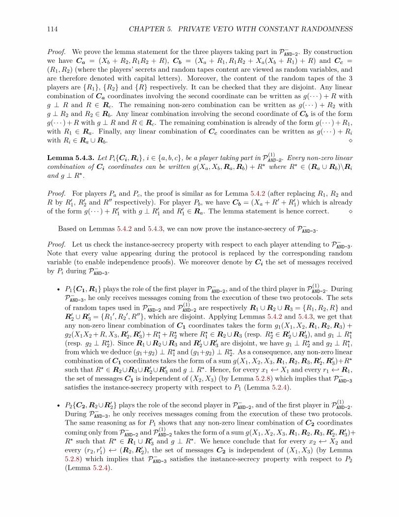
114 CHAPTER 5. PRIVATE VETO WITH CONSTANT RANDOMNESS
Proof. We prove the lemma statement for the three players taking part in P−AND-2. By constructionwe have Ca = (Xb + R2, R1R2 + R), Cb = (Xa + R1, R1R2 + Xa(Xb + R1) + R) and Cc =(R1, R2) (where the players’ secrets and random tapes content are viewed as random variables, andare therefore denoted with capital letters). Moreover, the content of the random tapes of the 3players are R1, R2 and R respectively. It can be checked that they are disjoint. Any linearcombination of Ca coordinates involving the second coordinate can be written as g(· · · ) + R withg ⊥ R and R ∈ Rc. The remaining non-zero combination can be written as g(· · · ) + R2 withg ⊥ R2 and R2 ∈ Rb. Any linear combination involving the second coordinate of Cb is of the formg(· · · ) +R with g ⊥ R and R ∈ Rc. The remaining combination is already of the form g(· · · ) +R1,with R1 ∈ Ra. Finally, any linear combination of Cc coordinates can be written as g(· · · ) + Riwith Ri ∈ Ra ∪Rb.
Lemma 5.4.3. Let PiCi,Ri, i ∈ a, b, c, be a player taking part in P(1)AND-2. Every non-zero linear
combination of Ci coordinates can be written g(Xa, Xb,Ra,Rb) + R? where R? ∈ (Ra ∪ Rb)\Ri
and g ⊥ R?.
Proof. For players Pa and Pc, the proof is similar as for Lemma 5.4.2 (after replacing R1, R2 andR by R′1, R′2 and R′′ respectively). For player Pb, we have Cb = (Xa + R′ + R′1) which is alreadyof the form g(· · · ) +R′1 with g ⊥ R′1 and R′1 ∈ Ra. The lemma statement is hence correct.
Based on Lemmas 5.4.2 and 5.4.3, we can now prove the instance-secrecy of P−AND-3.
Proof. Let us check the instance-secrecy property with respect to each player attending to P−AND-3.Note that every value appearing during the protocol is replaced by the corresponding randomvariable (to enable independence proofs). We moreover denote by Ci the set of messages receivedby Pi during P−AND-3.
• P1C1,R1 plays the role of the first player in P−AND-2, and of the third player in P(1)AND-2. During
P−AND-3, he only receives messages coming from the execution of these two protocols. The setsof random tapes used in P−AND-2 and P(1)
AND-2 are respectively R1 ∪R2 ∪R3 = R1, R2, R andR′2 ∪R′3 = R1
′, R2′, R′′, which are disjoint. Applying Lemmas 5.4.2 and 5.4.3, we get that
any non-zero linear combination of C1 coordinates takes the form g1(X1, X2,R1,R2,R3) +g2(X1X2 +R,X3,R′2,R
′3) +R?1 +R?2 where R?1 ∈ R2∪R3 (resp. R?2 ∈ R′2∪R′3), and g1 ⊥ R?1
(resp. g2 ⊥ R?2). Since R1∪R2∪R3 and R′2∪R′3 are disjoint, we have g1 ⊥ R?2 and g2 ⊥ R?1,from which we deduce (g1+g2) ⊥ R?1 and (g1+g2) ⊥ R?2. As a consequence, any non-zero linearcombination ofC1 coordinates takes the form of a sum g(X1, X2, X3,R1,R2,R3,R′2,R
′3)+R?
such that R? ∈ R2∪R3∪R′2∪R′3 and g ⊥ R?. Hence, for every x1 ← X1 and every r1 ← R1,the set of messages C1 is independent of (X2, X3) (by Lemma 5.2.8) which implies that P−AND-3satisfies the instance-secrecy property with respect to P1 (Lemma 5.2.4).
• P2C2,R2∪R′2 plays the role of the second player in P−AND-2, and of the first player in P(1)AND-2.
During P−AND-3, he only receives messages coming from the execution of these two protocols.The same reasoning as for P1 shows that any non-zero linear combination of C2 coordinatescoming only from P−AND-2 and P(1)
AND-2 takes the form of a sum g(X1, X2, X3,R1,R2,R3,R′2,R′3)+
R? such that R? ∈ R1 ∪R′3 and g ⊥ R?. We hence conclude that for every x2 ← X2 andevery (r2, r′1) ← (R2,R′2), the set of messages C2 is independent of (X1, X3) (by Lemma5.2.8) which implies that P−AND-3 satisfies the instance-secrecy property with respect to P2(Lemma 5.2.4).
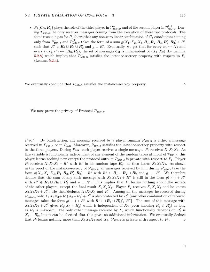
5.4. PRIVATE EVALUATION OF AND-n FOR n = 3 115
• P3C3,R′3 plays the role of the third player in P−AND-2, and of the second player in P(1)
AND-2. Dur-ing P−AND-3, he only receives messages coming from the execution of these two protocols. Thesame reasoning as for P1 shows that any non-zero linear combination ofC3 coordinates comingonly from P−AND-2 and P(1)
AND-2 takes the form of a sum g(X1, X2, X3,R1,R2,R3,R′2,R′3) +R?
such that R? ∈ R1 ∪R2 ∪R′2 and g ⊥ R?. Eventually, we get that for every x3 ← X3 andevery (r, r′2, r′′) ← (R3,R′3), the set of messages C3 is independent of (X1, X2) (by Lemma5.2.8) which implies that P−AND-3 satisfies the instance-secrecy property with respect to P3(Lemma 5.2.4).
We eventually conclude that P−AND-3 satisfies the instance-secrecy property.
We now prove the privacy of Protocol PAND-3.
Proof. By construction, any message received by a player running PAND-3 is either a messagereceived in P−AND-3 or in PXOR. Moreover, P−AND-3 satisfies the instance-secrecy property with respectto the three players. During PXOR, each player receives a single message. P1 receives X1X2X3. Asthis variable is functionally independent of any element of the random tapes at input of PAND-3, thisplayer learns nothing new except the protocol output: PAND-3 is private with respect to P1. PlayerP3 receives X1X2X3 + R′′ with R′′ in his random tape R′3: he then learns X1X2X3. As shownin the proof of the instance-secrecy of P−AND-3, all messages received by him during P−AND-3 take theform g(X1, X2, X3,R1,R2,R′2,R
′3) + R? with R? ∈ R1 ∪ R2 ∪ R′2 and g ⊥ R?. We therefore
deduce that the sum of any such message with X1X2X3 + R′′ is still in the form g(· · · ) + R?
with R? ∈ R1 ∪ R2 ∪ R′2 and g ⊥ R?. This implies that P3 learns nothing about the secretsof the other players, except the final result X1X2X3. Player P2 receives X1X2X3 and he knowsX1X2X3 + R′′. He then deduces X1X2X3 and R′′. Among all the messages he received duringP−AND-3, only X1X2X3+R′1(X3+R′2)+R′′ is also protected by R′′ (any other combination of receivedmessages takes the form g(· · · ) + R? with R? ∈ (R1 ∪R′3)\R′′. The sum of this message withX1X2X3 + R′′ gives R′1(X3 + R′2) which is independent of X3 (even knowing R′1 ∈ R′2) as longas R′2 is unknown. The only other message received by P2 which functionally depends on R′2 isX3 + R′2, but it can be checked that this gives no additional information. We eventually deducethat P2 learns nothing more than X1X2X3 and X2: PAND-3 is private with respect to P2.
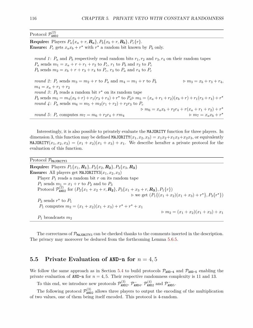
116 CHAPTER 5. PRIVATE VETO WITH CONSTANT RANDOMNESS
Protocol P(2)AND2
Require: Players Paxa + r,Ra, Pbxb + r,Rb, Pcr.Ensure: Pc gets xaxb + r? with r? a random bit known by Pb only.
round 1 : Pa and Pb respectively read random bits r1, r2 and r3, r4 on their random tapesPa sends m1 = xa + r + r1 + r2 to Pc, r1 to Pb and r2 to PcPb sends m2 = xb + r + r3 + r4 to Pc, r3 to Pa and r4 to Pc
round 2 : Pc sends m3 = m2 + r to Pa and m4 = m1 + r to Pb . m3 = xb + r3 + r4,m4 = xa + r1 + r2round 3 : Pb reads a random bit r? on its random tapePb sends m5 = m4(xb + r) + r1(r3 + r4) + r? to Pa. m5 = (xa + r1 + r2)(xb + r) + r1(r3 + r4) + r?
round 4 : Pa sends m6 = m5 +m3(r1 + r2) + r2r3 to Pc. m6 = xaxb + r2r4 + r(xa + r1 + r2) + r?
round 5 : Pc computes m7 = m6 + r2r4 + rm4 . m7 = xaxb + r?
Interestingly, it is also possible to privately evaluate the MAJORITY function for three players. Indimension 3, this function may be defined MAJORITY(x1, x2, x3) = x1x2+x1x3+x2x3, or equivalentlyMAJORITY(x1, x2, x3) = (x1 + x2)(x1 + x3) + x1. We describe herafter a private protocol for theevaluation of this function.
Protocol PMAJORITY3
Require: Players P1x1,R1, P2x2,R2, P3x3,R3Ensure: All players get MAJORITY3(x1, x2, x3)
Player P1 reads a random bit r on its random tapeP1 sends m1 = x1 + r to P2 and to P3Protocol P(2)
AND2 for (P2x1 + x2 + r,R2, P3x1 + x3 + r,R3, P1r). we get (P1(x1 + x2)(x1 + x3) + r?, P3r?)
P3 sends r? to P1P1 computes m2 = (x1 + x2)(x1 + x3) + r? + r? + x1
. m2 = (x1 + x2)(x1 + x3) + x1P1 broadcasts m2
The correctness of PMAJORITY3 can be checked thanks to the comments inserted in the description.The privacy may moreover be deduced from the forthcoming Lemma 5.6.5.
5.5 Private Evaluation of AND-n for n = 4, 5
We follow the same approach as in Section 5.4 to build protocols PAND-4 and PAND-5 enabling theprivate evaluation of AND-n for n = 4, 5. Their respective randomness complexity is 11 and 13.
To this end, we introduce new protocols P(3)AND2, P−AND4, P
(4)AND2 and P−AND5.
The following protocol P(3)AND2 allows three players to output the encoding of the multiplication
of two values, one of them being itself encoded. This protocol is 4-random.
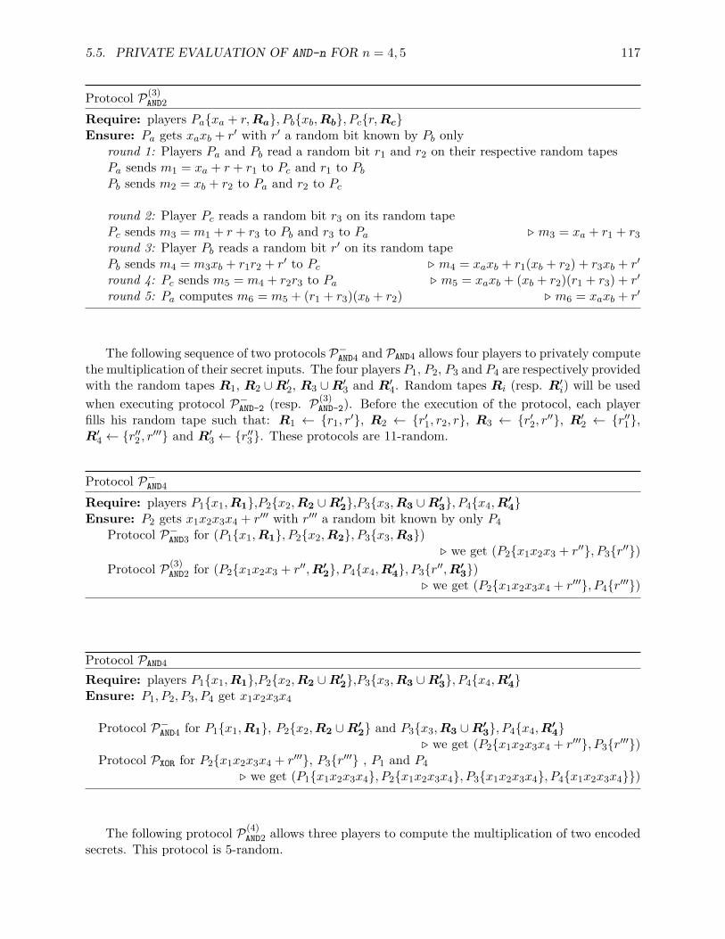
5.5. PRIVATE EVALUATION OF AND-n FOR n = 4, 5 117
Protocol P(3)AND2
Require: players Paxa + r,Ra, Pbxb,Rb, Pcr,RcEnsure: Pa gets xaxb + r′ with r′ a random bit known by Pb only
round 1: Players Pa and Pb read a random bit r1 and r2 on their respective random tapesPa sends m1 = xa + r + r1 to Pc and r1 to PbPb sends m2 = xb + r2 to Pa and r2 to Pc
round 2: Player Pc reads a random bit r3 on its random tapePc sends m3 = m1 + r + r3 to Pb and r3 to Pa . m3 = xa + r1 + r3round 3: Player Pb reads a random bit r′ on its random tapePb sends m4 = m3xb + r1r2 + r′ to Pc . m4 = xaxb + r1(xb + r2) + r3xb + r′
round 4: Pc sends m5 = m4 + r2r3 to Pa . m5 = xaxb + (xb + r2)(r1 + r3) + r′
round 5: Pa computes m6 = m5 + (r1 + r3)(xb + r2) . m6 = xaxb + r′
The following sequence of two protocols P−AND4 and PAND4 allows four players to privately computethe multiplication of their secret inputs. The four players P1, P2, P3 and P4 are respectively providedwith the random tapes R1, R2 ∪R′2, R3 ∪R′3 and R′4. Random tapes Ri (resp. R′i) will be usedwhen executing protocol P−AND-2 (resp. P(3)
AND-2). Before the execution of the protocol, each playerfills his random tape such that: R1 ← r1, r′, R2 ← r′1, r2, r, R3 ← r′2, r′′, R′2 ← r′′1,R′4 ← r′′2 , r′′′ and R′3 ← r′′3. These protocols are 11-random.
Protocol P−AND4
Require: players P1x1,R1,P2x2,R2 ∪R′2,P3x3,R3 ∪R′3, P4x4,R′4Ensure: P2 gets x1x2x3x4 + r′′′ with r′′′ a random bit known by only P4
Protocol P−AND3 for (P1x1,R1, P2x2,R2, P3x3,R3). we get (P2x1x2x3 + r′′, P3r′′)
Protocol P(3)AND2 for (P2x1x2x3 + r′′,R′2, P4x4,R′4, P3r′′,R′3)
. we get (P2x1x2x3x4 + r′′′, P4r′′′)
Protocol PAND4
Require: players P1x1,R1,P2x2,R2 ∪R′2,P3x3,R3 ∪R′3, P4x4,R′4Ensure: P1, P2, P3, P4 get x1x2x3x4
Protocol P−AND4 for P1x1,R1, P2x2,R2 ∪R′2 and P3x3,R3 ∪R′3, P4x4,R′4. we get (P2x1x2x3x4 + r′′′, P3r′′′)
Protocol PXOR for P2x1x2x3x4 + r′′′, P3r′′′ , P1 and P4. we get (P1x1x2x3x4, P2x1x2x3x4, P3x1x2x3x4, P4x1x2x3x4)
The following protocol P(4)AND2 allows three players to compute the multiplication of two encoded
secrets. This protocol is 5-random.
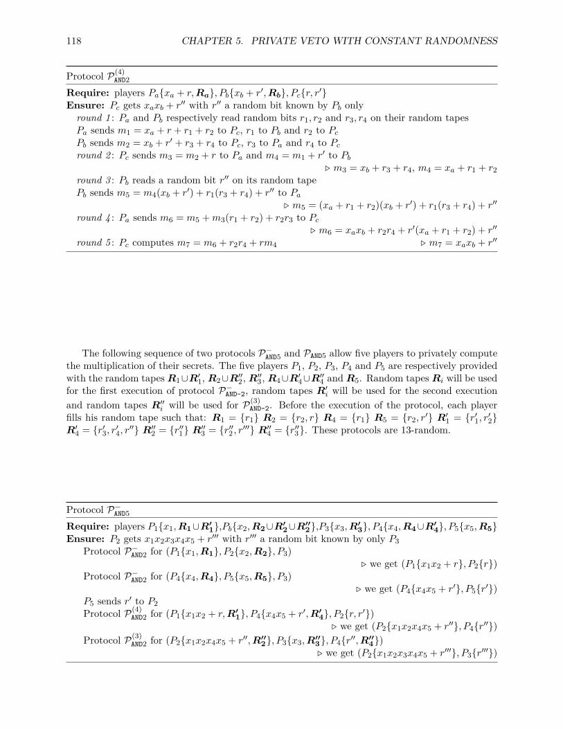
118 CHAPTER 5. PRIVATE VETO WITH CONSTANT RANDOMNESS
Protocol P(4)AND2
Require: players Paxa + r,Ra, Pbxb + r′,Rb, Pcr, r′Ensure: Pc gets xaxb + r′′ with r′′ a random bit known by Pb onlyround 1 : Pa and Pb respectively read random bits r1, r2 and r3, r4 on their random tapesPa sends m1 = xa + r + r1 + r2 to Pc, r1 to Pb and r2 to PcPb sends m2 = xb + r′ + r3 + r4 to Pc, r3 to Pa and r4 to Pcround 2 : Pc sends m3 = m2 + r to Pa and m4 = m1 + r′ to Pb
. m3 = xb + r3 + r4, m4 = xa + r1 + r2round 3 : Pb reads a random bit r′′ on its random tapePb sends m5 = m4(xb + r′) + r1(r3 + r4) + r′′ to Pa
. m5 = (xa + r1 + r2)(xb + r′) + r1(r3 + r4) + r′′
round 4 : Pa sends m6 = m5 +m3(r1 + r2) + r2r3 to Pc. m6 = xaxb + r2r4 + r′(xa + r1 + r2) + r′′
round 5 : Pc computes m7 = m6 + r2r4 + rm4 . m7 = xaxb + r′′
The following sequence of two protocols P−AND5 and PAND5 allow five players to privately computethe multiplication of their secrets. The five players P1, P2, P3, P4 and P5 are respectively providedwith the random tapes R1∪R′1, R2∪R′′2, R′′3, R4∪R′4∪R′′4 and R5. Random tapes Ri will be usedfor the first execution of protocol P−AND-2, random tapes R′i will be used for the second executionand random tapes R′′i will be used for P(3)
AND-2. Before the execution of the protocol, each playerfills his random tape such that: R1 = r1 R2 = r2, r R4 = r1 R5 = r2, r′ R′1 = r′1, r′2R′4 = r′3, r′4, r′′ R′′2 = r′′1 R′′3 = r′′2 , r′′′ R′′4 = r′′3. These protocols are 13-random.
Protocol P−AND5
Require: players P1x1,R1∪R′1,Pbx2,R2∪R′2∪R′′2,P3x3,R′3, P4x4,R4∪R′4, P5x5,R5Ensure: P2 gets x1x2x3x4x5 + r′′′ with r′′′ a random bit known by only P3
Protocol P−AND2 for (P1x1,R1, P2x2,R2, P3). we get (P1x1x2 + r, P2r)
Protocol P−AND2 for (P4x4,R4, P5x5,R5, P3). we get (P4x4x5 + r′, P5r′)
P5 sends r′ to P2Protocol P(4)
AND2 for (P1x1x2 + r,R′1, P4x4x5 + r′,R′4, P2r, r′). we get (P2x1x2x4x5 + r′′, P4r′′)
Protocol P(3)AND2 for (P2x1x2x4x5 + r′′,R′′2, P3x3,R′′3, P4r′′,R′′4)
. we get (P2x1x2x3x4x5 + r′′′, P3r′′′)
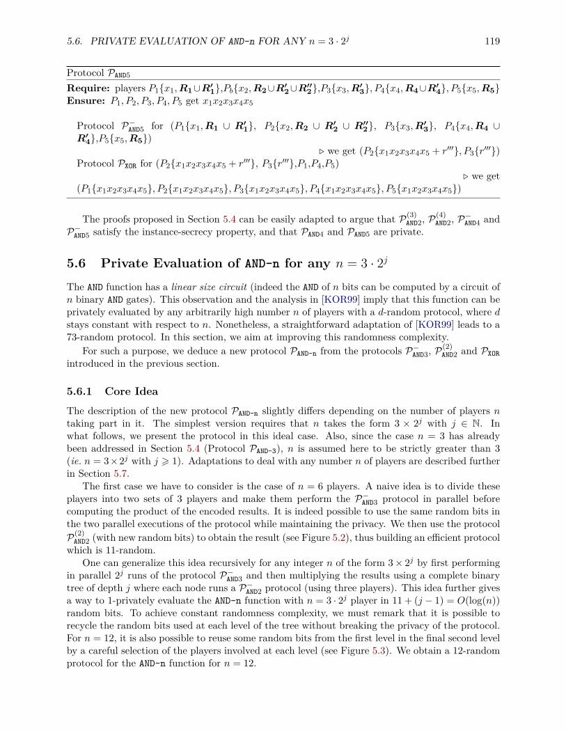
5.6. PRIVATE EVALUATION OF AND-n FOR ANY n = 3 · 2j 119
Protocol PAND5
Require: players P1x1,R1∪R′1,Pbx2,R2∪R′2∪R′′2,P3x3,R′3, P4x4,R4∪R′4, P5x5,R5Ensure: P1, P2, P3, P4, P5 get x1x2x3x4x5
Protocol P−AND5 for (P1x1,R1 ∪ R′1, P2x2,R2 ∪ R′2 ∪ R′′2, P3x3,R′3, P4x4,R4 ∪R′4,P5x5,R5)
. we get (P2x1x2x3x4x5 + r′′′, P3r′′′)Protocol PXOR for (P2x1x2x3x4x5 + r′′′, P3r′′′,P1,P4,P5)
. we get(P1x1x2x3x4x5, P2x1x2x3x4x5, P3x1x2x3x4x5, P4x1x2x3x4x5, P5x1x2x3x4x5)
The proofs proposed in Section 5.4 can be easily adapted to argue that P(3)AND2, P
(4)AND2, P−AND4 and
P−AND5 satisfy the instance-secrecy property, and that PAND4 and PAND5 are private.
5.6 Private Evaluation of AND-n for any n = 3 · 2j
The AND function has a linear size circuit (indeed the AND of n bits can be computed by a circuit ofn binary AND gates). This observation and the analysis in [KOR99] imply that this function can beprivately evaluated by any arbitrarily high number n of players with a d-random protocol, where dstays constant with respect to n. Nonetheless, a straightforward adaptation of [KOR99] leads to a73-random protocol. In this section, we aim at improving this randomness complexity.
For such a purpose, we deduce a new protocol PAND-n from the protocols P−AND3, P(2)AND2 and PXOR
introduced in the previous section.
5.6.1 Core IdeaThe description of the new protocol PAND-n slightly differs depending on the number of players ntaking part in it. The simplest version requires that n takes the form 3 × 2j with j ∈ N. Inwhat follows, we present the protocol in this ideal case. Also, since the case n = 3 has alreadybeen addressed in Section 5.4 (Protocol PAND-3), n is assumed here to be strictly greater than 3(ie. n = 3×2j with j > 1). Adaptations to deal with any number n of players are described furtherin Section 5.7.
The first case we have to consider is the case of n = 6 players. A naive idea is to divide theseplayers into two sets of 3 players and make them perform the P−AND3 protocol in parallel beforecomputing the product of the encoded results. It is indeed possible to use the same random bits inthe two parallel executions of the protocol while maintaining the privacy. We then use the protocolP(2)
AND2 (with new random bits) to obtain the result (see Figure 5.2), thus building an efficient protocolwhich is 11-random.
One can generalize this idea recursively for any integer n of the form 3× 2j by first performingin parallel 2j runs of the protocol P−AND3 and then multiplying the results using a complete binarytree of depth j where each node runs a P−AND2 protocol (using three players). This idea further givesa way to 1-privately evaluate the AND-n function with n = 3 · 2j player in 11 + (j − 1) = O(log(n))random bits. To achieve constant randomness complexity, we must remark that it is possible torecycle the random bits used at each level of the tree without breaking the privacy of the protocol.For n = 12, it is also possible to reuse some random bits from the first level in the final second levelby a careful selection of the players involved at each level (see Figure 5.3). We obtain a 12-randomprotocol for the AND-n function for n = 12.
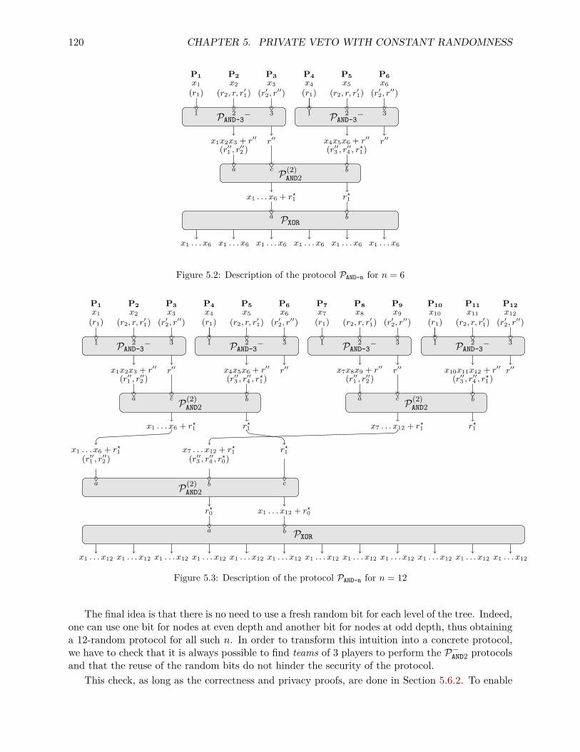
120 CHAPTER 5. PRIVATE VETO WITH CONSTANT RANDOMNESS
1 2 3PAND-3−
P1x1
(r1)
P2x2
(r2, r, r′1)
x1x2x3 + r′′
(r′′1 , r′′2 )
P3x3
(r′2, r′′)
r′′
1 2 3PAND-3−
P4x4
(r1)
P5x5
(r2, r, r′1)
P6x6
(r′2, r′′)
x4x5x6 + r′′
(r′′3 , r′′4 , r?1)r′′
P(2)AND2
a c b
x1 . . . x6 + r?1 r?1
a bPXOR
x1 . . . x6 x1 . . . x6 x1 . . . x6 x1 . . . x6 x1 . . . x6 x1 . . . x6
Figure 5.2: Description of the protocol PAND-n for n = 6
1 2 3PAND-3−
P1x1
(r1)
P2x2
(r2, r, r′1)
x1x2x3 + r′′
(r′′1 , r′′2 )
P3x3
(r′2, r′′)
r′′
1 2 3PAND-3−
P4x4
(r1)
P5x5
(r2, r, r′1)
P6x6
(r′2, r′′)
x4x5x6 + r′′
(r′′3 , r′′4 , r?1)r′′
P(2)AND2
a c b
x1 . . . x6 + r?1 r?1
1 2 3PAND-3−
P7x7
(r1)
P8x8
(r2, r, r′1)
x7x8x9 + r′′
(r′′1 , r′′2 )
P9x9
(r′2, r′′)
r′′
1 2 3PAND-3−
P10x10(r1)
P11x11
(r2, r, r′1)
P12x12
(r′2, r′′)
x10x11x12 + r′′
(r′′3 , r′′4 , r?1)r′′
P(2)AND2
a c b
x7 . . . x12 + r?1 r?1
x7 . . . x12 + r?1(r′′3 , r′′4 , r?0)
x1 . . . x6 + r?1(r′′1 , r′′2 )
r?1
P(2)AND2
b ca
x1 . . . x12 + r?0r?0
a b PXOR
x1 . . . x12 x1 . . . x12 x1 . . . x12 x1 . . . x12 x1 . . . x12 x1 . . . x12 x1 . . . x12 x1 . . . x12 x1 . . . x12 x1 . . . x12 x1 . . . x12 x1 . . . x12
Figure 5.3: Description of the protocol PAND-n for n = 12
The final idea is that there is no need to use a fresh random bit for each level of the tree. Indeed,one can use one bit for nodes at even depth and another bit for nodes at odd depth, thus obtaininga 12-random protocol for all such n. In order to transform this intuition into a concrete protocol,we have to check that it is always possible to find teams of 3 players to perform the P−AND2 protocolsand that the reuse of the random bits do not hinder the security of the protocol.
This check, as long as the correctness and privacy proofs, are done in Section 5.6.2. To enable
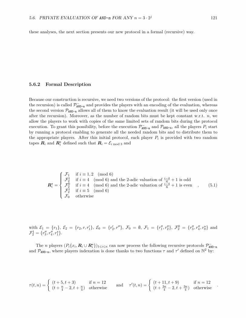
5.6. PRIVATE EVALUATION OF AND-n FOR ANY n = 3 · 2j 121
these analyses, the next section presents our new protocol in a formal (recursive) way.
5.6.2 Formal Description
Because our construction is recursive, we need two versions of the protocol: the first version (used inthe recursion) is called P−AND-n and provides the players with an encoding of the evaluation, whereasthe second version PAND-n allows all of them to know the evaluation result (it will be used only onceafter the recursion). Moreover, as the number of random bits must be kept constant w.r.t. n, weallow the players to work with copies of the same limited sets of random bits during the protocolexecution. To grant this possibility, before the execution P−AND-n and PAND-n, all the players Pi startby running a protocol enabling to generate all the needed random bits and to distribute them tothe appropriate players. After this initial protocol, each player Pi is provided with two randomtapes Ri and R?
i defined such that Ri = Ei mod 3 and
R?i =
F1 if i ≡ 1, 2 (mod 6)F1
2 if i ≡ 4 (mod 6) and the 2-adic valuation of i−46 + 1 is odd
F02 if i ≡ 4 (mod 6) and the 2-adic valuation of i−4
6 + 1 is evenF1
2 if i ≡ 5 (mod 6)F0 otherwise
, (5.1)
with E1 = r1, E2 = r2, r, r′1, E0 = r′2, r′′, F0 = ∅, F1 = r′′1 , r′′2, F02 = r′′3 , r′′4 , r?0 and
F12 = r′′3 , r′′4 , r?1.
The n players (Pixi,Ri ∪R?i )16i6n can now process the following recursive protocols P−AND-n
and PAND-n, where players indexation is done thanks to two functions τ and τ ′ defined on N2 by:
τ(t, n) =
(t+ 5, t+ 3) if n = 12(t+ n
4 − 2, t+ n4 ) otherwise and τ ′(t, n) =
(t+ 11, t+ 9) if n = 12(t+ 3n
4 − 2, t+ 3n4 ) otherwise .
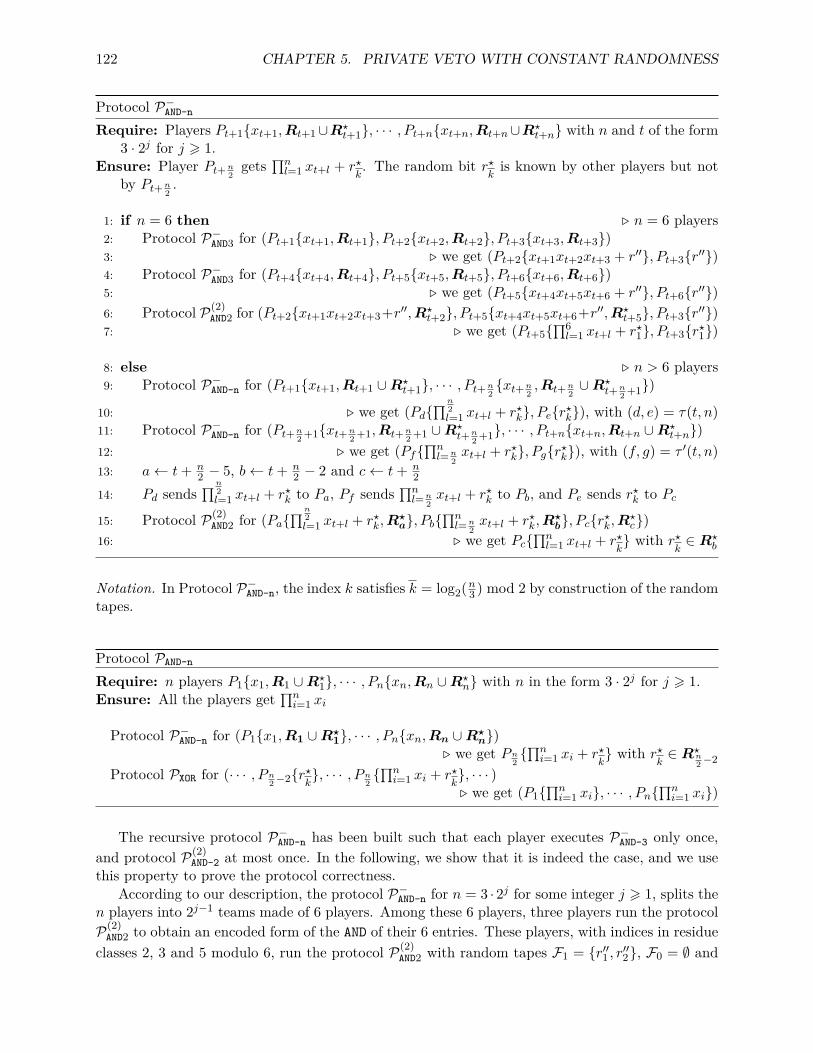
122 CHAPTER 5. PRIVATE VETO WITH CONSTANT RANDOMNESS
Protocol P−AND-n
Require: Players Pt+1xt+1,Rt+1∪R?t+1, · · · , Pt+nxt+n,Rt+n∪R?
t+n with n and t of the form3 · 2j for j > 1.
Ensure: Player Pt+n2gets ∏n
l=1 xt+l + r?k. The random bit r?
kis known by other players but not
by Pt+n2.
1: if n = 6 then . n = 6 players2: Protocol P−AND3 for (Pt+1xt+1,Rt+1, Pt+2xt+2,Rt+2, Pt+3xt+3,Rt+3)3: . we get (Pt+2xt+1xt+2xt+3 + r′′, Pt+3r′′)4: Protocol P−AND3 for (Pt+4xt+4,Rt+4, Pt+5xt+5,Rt+5, Pt+6xt+6,Rt+6)5: . we get (Pt+5xt+4xt+5xt+6 + r′′, Pt+6r′′)6: Protocol P(2)
AND2 for (Pt+2xt+1xt+2xt+3+r′′,R?t+2, Pt+5xt+4xt+5xt+6+r′′,R?
t+5, Pt+3r′′)7: . we get (Pt+5
∏6l=1 xt+l + r?1, Pt+3r?1)
8: else . n > 6 players9: Protocol P−AND-n for (Pt+1xt+1,Rt+1 ∪R?
t+1, · · · , Pt+n2xt+n
2,Rt+n
2∪R?
t+n2 +1)
10: . we get (Pd∏n
2l=1 xt+l + r?k, Per?k), with (d, e) = τ(t, n)
11: Protocol P−AND-n for (Pt+n2 +1xt+n
2 +1,Rt+n2 +1 ∪R?
t+n2 +1, · · · , Pt+nxt+n,Rt+n ∪R?
t+n)12: . we get (Pf
∏nl=n
2xt+l + r?k, Pgr?k), with (f, g) = τ ′(t, n)
13: a← t+ n2 − 5, b← t+ n
2 − 2 and c← t+ n2
14: Pd sends ∏n2l=1 xt+l + r?k to Pa, Pf sends ∏n
l=n2xt+l + r?k to Pb, and Pe sends r?k to Pc
15: Protocol P(2)AND2 for (Pa
∏n2l=1 xt+l + r?k,R
?a, Pb
∏nl=n
2xt+l + r?k,R
?b, Pcr?k,R?
c)16: . we get Pc
∏nl=1 xt+l + r?
k with r?
k∈ R?
b
Notation. In Protocol P−AND-n, the index k satisfies k = log2(n3 ) mod 2 by construction of the randomtapes.
Protocol PAND-n
Require: n players P1x1,R1 ∪R?1, · · · , Pnxn,Rn ∪R?
n with n in the form 3 · 2j for j > 1.Ensure: All the players get ∏n
i=1 xi
Protocol P−AND-n for (P1x1,R1 ∪R?1, · · · , Pnxn,Rn ∪R?n). we get Pn
2∏n
i=1 xi + r?k with r?
k∈ R?
n2−2
Protocol PXOR for (· · · , Pn2−2r?k, · · · , Pn
2∏n
i=1 xi + r?k, · · · ). we get (P1
∏ni=1 xi, · · · , Pn
∏ni=1 xi)
The recursive protocol P−AND-n has been built such that each player executes P−AND-3 only once,and protocol P(2)
AND-2 at most once. In the following, we show that it is indeed the case, and we usethis property to prove the protocol correctness.
According to our description, the protocol P−AND-n for n = 3 · 2j for some integer j > 1, splits then players into 2j−1 teams made of 6 players. Among these 6 players, three players run the protocolP(2)
AND2 to obtain an encoded form of the AND of their 6 entries. These players, with indices in residueclasses 2, 3 and 5 modulo 6, run the protocol P(2)
AND2 with random tapes F1 = r′′1 , r′′2, F0 = ∅ and
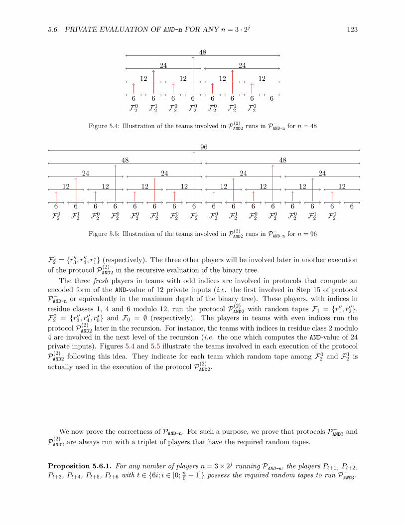
5.6. PRIVATE EVALUATION OF AND-n FOR ANY n = 3 · 2j 123
6 6 6 6 6 6 6 6
12 12 12 12
24 24
48
F02 F0
2 F02 F0
2F12 F1
2F02
Figure 5.4: Illustration of the teams involved in P(2)AND2 runs in P−
AND-n for n = 48
6 6 6 6 6 6 6 6 6 6 6 6 6 6 6 6
12 12 12 12 12 12 12 12
24 24 24 24
48 48
96
F02 F0
2 F02 F0
2 F02 F0
2 F02 F0
2F12 F1
2 F12 F1
2F02 F0
2F12
Figure 5.5: Illustration of the teams involved in P(2)AND2 runs in P−
AND-n for n = 96
F12 = r′′3 , r′′4 , r?1 (respectively). The three other players will be involved later in another execution
of the protocol P(2)AND2 in the recursive evaluation of the binary tree.
The three fresh players in teams with odd indices are involved in protocols that compute anencoded form of the AND-value of 12 private inputs (i.e. the first involved in Step 15 of protocolP−AND-n or equivalently in the maximum depth of the binary tree). These players, with indices inresidue classes 1, 4 and 6 modulo 12, run the protocol P(2)
AND2 with random tapes F1 = r′′1 , r′′2,F0
2 = r′′3 , r′′4 , r?0 and F0 = ∅ (respectively). The players in teams with even indices run theprotocol P(2)
AND2 later in the recursion. For instance, the teams with indices in residue class 2 modulo4 are involved in the next level of the recursion (i.e. the one which computes the AND-value of 24private inputs). Figures 5.4 and 5.5 illustrate the teams involved in each execution of the protocolP(2)
AND2 following this idea. They indicate for each team which random tape among F02 and F1
2 isactually used in the execution of the protocol P(2)
AND2.
We now prove the correctness of PAND-n. For such a purpose, we prove that protocols P−AND3 andP(2)
AND2 are always run with a triplet of players that have the required random tapes.
Proposition 5.6.1. For any number of players n = 3× 2j running P−AND-n, the players Pt+1, Pt+2,Pt+3, Pt+4, Pt+5, Pt+6 with t ∈ 6i; i ∈ [0; n6 − 1] possess the required random tapes to run P−AND3.
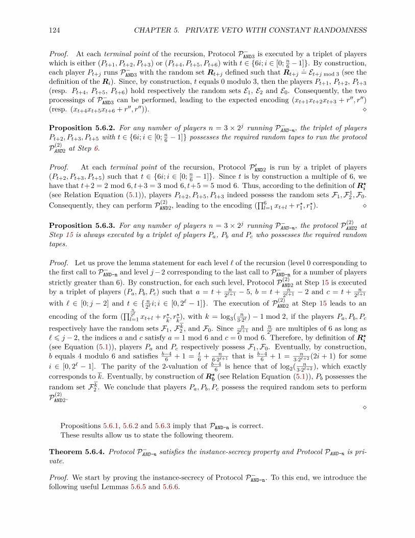
124 CHAPTER 5. PRIVATE VETO WITH CONSTANT RANDOMNESS
Proof. At each terminal point of the recursion, Protocol P−AND3 is executed by a triplet of playerswhich is either (Pt+1, Pt+2, Pt+3) or (Pt+4, Pt+5, Pt+6) with t ∈ 6i; i ∈ [0; n6 − 1]. By construction,each player Pt+j runs P−AND3 with the random set Rt+j defined such that Rt+j
.= Et+j mod 3 (see thedefinition of the Ri). Since, by construction, t equals 0 modulo 3, then the players Pt+1, Pt+2, Pt+3(resp. Pt+4, Pt+5, Pt+6) hold respectively the random sets E1, E2 and E0. Consequently, the twoprocessings of P−AND3 can be performed, leading to the expected encoding (xt+1xt+2xt+3 + r′′, r′′)(resp. (xt+4xt+5xt+6 + r′′, r′′)).
Proposition 5.6.2. For any number of players n = 3 × 2j running P−AND-n, the triplet of playersPt+2, Pt+3, Pt+5 with t ∈ 6i; i ∈ [0; n6 − 1] possesses the required random tapes to run the protocolP(2)
AND2 at Step 6.
Proof. At each terminal point of the recursion, Protocol P ′AND2 is run by a triplet of players(Pt+2, Pt+3, Pt+5) such that t ∈ 6i; i ∈ [0; n6 − 1]. Since t is by construction a multiple of 6, wehave that t+2 = 2 mod 6, t+3 = 3 mod 6, t+5 = 5 mod 6. Thus, according to the definition of R?i(see Relation Equation (5.1)), players Pt+2, Pt+5, Pt+3 indeed possess the random sets F1,F1
2 ,F0.Consequently, they can perform P(2)
AND2, leading to the encoding (∏6l=1 xt+l + r?1, r
?1).
Proposition 5.6.3. For any number of players n = 3 × 2j running P−AND-n, the protocol P(2)AND2 at
Step 15 is always executed by a triplet of players Pa, Pb and Pc who possesses the required randomtapes.
Proof. Let us prove the lemma statement for each level ` of the recursion (level 0 corresponding tothe first call to P−AND-n and level j−2 corresponding to the last call to P−AND-n for a number of playersstrictly greater than 6). By construction, for each such level, Protocol P(2)
AND2 at Step 15 is executedby a triplet of players (Pa, Pb, Pc) such that a = t + n
2`+1 − 5, b = t + n2`+1 − 2 and c = t + n
2`+1
with ` ∈ [0; j − 2] and t ∈ n2` i; i ∈ [0, 2` − 1]. The execution of P(2)AND2 at Step 15 leads to an
encoding of the form (∏ n
2`l=1 xt+l + r?
k, r?k), with k = log3( n
3·2` ) − 1 mod 2, if the players Pa, Pb, Pcrespectively have the random sets F1, Fk2 , and F0. Since n
2`+1 and n2` are multiples of 6 as long as
` 6 j − 2, the indices a and c satisfy a = 1 mod 6 and c = 0 mod 6. Therefore, by definition of R?i(see Equation (5.1)), players Pa and Pc respectively possess F1,F0. Eventually, by construction,b equals 4 modulo 6 and satisfies b−4
6 + 1 = t6 + n
6·2`+1 that is b−46 + 1 = n
3·2`+2 (2i + 1) for somei ∈ [0, 2` − 1]. The parity of the 2-valuation of b−4
6 is hence that of log2( n3·2`+2 ), which exactly
corresponds to k. Eventually, by construction of R?b (see Relation Equation (5.1)), Pb possesses therandom set Fk2 . We conclude that players Pa, Pb, Pc possess the required random sets to performP(2)
AND2.
Propositions 5.6.1, 5.6.2 and 5.6.3 imply that PAND-n is correct.These results allow us to state the following theorem.
Theorem 5.6.4. Protocol P−AND-n satisfies the instance-secrecy property and Protocol PAND-n is pri-vate.
Proof. We start by proving the instance-secrecy of Protocol P−AND-n. To this end, we introduce thefollowing useful Lemmas 5.6.5 and 5.6.6.
5.6. PRIVATE EVALUATION OF AND-n FOR ANY n = 3 · 2j 125
Lemma 5.6.5. Let PiCi,Ri be a player taking part in P(2)AND2. Every non-zero linear combination
of coordinates of Ci can be written as g(Xa, Xb,Ra,Rb,Rc) +R? where R? ∈ (Ra ∪Rb ∪Rc) \Riand g ⊥ R?.
Proof. We prove the lemma statement for the three players taking part in P(2)AND2. By construction
we haveCa = (R3, Xb+R3+R4, (Xa+R1+R2)(Xb+R)+R1(R3+R4)+R?), Cb = (R1, Xa+R1+R2)and Cc = (Xa+R+R1 +R2, R2, Xb+R+R3 +R4, R4, XaXb+R2R4 +R(Xa+R1 +R2)+R?) (wherethe player’s secrets and random tapes content are viewed as random variables, and are thereforedenoted by capital letters). Moreover, the random tapes of the 3 players are R1, R2, R3, R4, R?and ∅ respectively. They are disjoint. Any linear combination of Ca coordinates involving thethird coordinate can be written as g(· · · ) + R?, where g(· · · ) ⊥ R? and R? ∈ Rb. Any othercombination involving the second coordinate can be written g(· · · )+R4, with g ⊥ R4 and R4 ∈ Rb.The remaining non-zero combination takes the form g(· · · ) + R3 with g ⊥ R3 and R3 ∈ Rb.This concludes the proof for player Pa. Any linear combination of coordinates of Cb involving itssecond coordinate can be written g(· · · ) + R2 with g ⊥ R2 and R2 ∈ Ra, and the only remainingcombination can be written g(· · · ) + R1 with g ⊥ R1 and R1 ∈ Ra. The lemma statement henceholds for player Pb. Finally, any linear combination of coordinates ofCc involving the last coordinatecan be written as g(· · · ) + R? with g ⊥ R?, R? ∈ Rb. Any other combination involving the first(resp. third) coordinate can be written respectively g(· · · ) + R1 (resp. g(· · · ) + R3), with g ⊥ R1(resp. g ⊥ R3) and R1 ∈ Ra (resp. R3 ∈ Rb). Any other combination involving its second (resp.fourth) coordinate takes the form g(· · · ) +R2 (resp. g(· · · ) +R4), with g ⊥ R2 (resp. g ⊥ R4) andR2 ∈ Ra (resp. R4 ∈ Rb).
Lemma 5.6.6. During the execution of P−AND-n, any player executes P(2)AND2 at most once.
Proof. By assumption in P−AND-n, the number of players n verifies n = 3 ·2j for some positive integerj. Due to the recursive construction of our protocol, every player Pi such that i = 2, 3, 5 mod 6executes P(2)
AND2 at Step 6, when P−AND-n reaches a terminal point. During the other level of therecursions (not terminal), executions of P(2)
AND2 (at Step 15) are performed by players of indicesa = t+ n
2`+1 −5, b = t+ n2`+1 −2 and c = t+ n
2`+1 with ` ∈ [0; j−2] and t ∈ n2` i; i ∈ [0, 2`−1]. Forsuch values ` and t, it can be checked that t+ n
2`+1 is a multiple of 6 which implies a ≡ 1 (mod 6),b ≡ 4 (mod 6) and c ≡ 0 (mod 6). This shows that no player can participate to the executionof P(2)
AND2 at both Steps 6 and 15 of the recursion. Moreover, for x ∈ 1, 4, 6, ` ∈ [0; j − 2] andi ∈ [0, 2` − 1], it can be checked that the function x, `, i 7→ n
2`+1 (2i + 1) + x − 6 is injective, whichimplies that no player can perform P(2)
AND2 at Step 15 more than once during the recursion.
We can now prove the instance-secrecy of P−AND-n.
Proof. We reason by induction.Basis. We assume n = 6. In this case, players P1, P4 and P6 run no other protocol than P−AND3
(and only once) and hence only receive messages during this execution. Moreover, P−AND3 satisfiesthe instance-secrecy property with respect to these players. For any other player P , all receivedmessages are either received during P−AND3 or P(2)
AND2. Lemma 5.6.5 ensures that any non-zero linearcombination involving only messages of P−AND3 or of P(2)
AND2 takes the form g(· · · ) + R with R notin the random tape of P and g ⊥ R. Moreover, no message sent in P−AND3 functionally dependson any random bit used in P(2)
AND2 (they indeed both use disjoint triplets of random tapes). Thus,Lemma 5.2.9 ensures that every linear combination of messages received during P(2)
AND2 and P−AND3takes the form g(· · · )+R with R not in the random tape of P and g ⊥ R. Lemma 5.2.8 thus implies
126 CHAPTER 5. PRIVATE VETO WITH CONSTANT RANDOMNESS
that the communication vector received by any player PXi is independent of (X1, · · · , X6)|Xi =xi for any xi ∈ F2, which itself implies that P−AND-n satisfies the instance-secrecy property for n = 6(Lemma 5.2.4).
Induction. We assume that (H1) P−AND-n satisfies the instance-secrecy property for an integern such that n = 3× 2j , and (H2) every non-zero linear combination of coordinates of the commu-nication vector C(n)
i received by a player PiRi during P−AND-n can be written as g(· · · ) +R withR /∈ Ri ∪R?
i and g ⊥ R.We consider now the execution of P−AND-n for 2n players. By construction, the communication
C(2n)i received by each player PiRi can be written as (C(n)
i ,C′i,C′′i ), where C(n)
i is the com-munication received by Pi during the execution of P−AND-n for n players (Step 9 or Step 11), C′′iis the communication received during the execution of P(2)
AND2 at Step 15, and C′i is the communi-cation received between these two calls (Step 14). Note that, for all but three players, we haveC′i = C′′i = 0. Thus, by hypothesis, P−AND-n satisfies the instance-secrecy property with respect toall these players and their communication vectors C(2n)
i satisfy Hypothesis (H2) for 2n instead ofn.
For any of the three remaining players Pi with i ∈ a, b, c, we deduce from Lemma 5.6.6 andC′′i 6= 0 that no message in C(n)
i has been received during the execution of P(2)AND2. As a consequence,
no message in C(n)i functionally depends on R?
i (the random tape used by Pi to execute P(2)AND2).
The single message in C′i can be written g′(· · · ) +R?k. Moreover, by construction, indices a, b andc respectively equal n − 5, n − 2 and n. The same reasoning as in the proof of Proposition 5.6.3then shows that R?
a = F1, R?b = Fk2 and R?
c = F0. For every i ∈ a, b, c, we deduce that thesingle message in C′i is functionally independent of the random tapes R?
a, R?b and R?
c used in P(2)AND2.
Together with Lemma 5.6.5, this independency implies that any non-zero linear combination of C′iwith elements in C′′i takes the form g(· · · ) + R with R ∈ (R?
a ∪R?b ∪R?
c)\(R?i ) and g ⊥ R. Since
no message in C(n)i functionally depends on R?
a ∪R?b ∪R?
c , we eventually deduce from Hypothesis(H2) that any non-zero linear combination of messages from C
(2n)i can be written as g(· · · ) + R
with R ∈ (Ra ∪R?a ∪Rb ∪R?
b ∪Rc ∪R?c)\(Ri ∪R?
i ) and g ⊥ R. Thanks to Lemma 5.2.8, we henceconclude that P−AND-n satisfies the instance-secrecy property with respect to the three players Pa, Pband Pc and that their communication vectors C(2n)
i satisfy Hypothesis (H2) for 2n instead of n.We have shown that P−AND-n satisfies the instance-secrecy property for 2n players if it satisfies
the instance-secrecy property for n in the form 3 · 2j . As the instance-secrecy property is true forn = 6 we can conclude that the proposition statement is true for any n in the form 3 ·2j with j > 1.
We now prove the privacy of Protocol PAND-n.
Proof. By construction, any message received by a player running PAND-n is either a messagereceived in P−AND-n or in PXOR. Moreover, P−AND-n satisfies the instance-secrecy property with respectto every player. During PXOR, each player receives a single message. All players but Pn
2and Pn
2−2,who played respectively the roles of Pc and Pb during the last call to P(2)
AND2, receive∏ni=1Xi and
learn nothing new except the protocol output.
• Player Pn2−2 receives ∏n
i=1Xi + R?kand knows R?
k. He then deduced ∏n
i=1Xi but learnsnothing new: PAND-n is private w.r.t Pn
2−2.
• Player Pn2receives∏n
i=1Xi and knows∏ni=1Xi+R?k. He then deduces R?
kwho is used to secure
communications during executions of P(2)AND2. Due to Lemma 5.6.6, Pn
2ran the latter protocol
5.7. PRIVATE AND EVALUATION WITH ANY NUMBER OF PLAYERS 127
only once. Hence, his communication vector contains a single message which functionallydepends on R?
k, which is ∏n
i=1Xi + R′′2R′′4 + R?k(
∏n/2i=1Xi + R′′1 + R′′2) + R?
k. The sum of this
message with ∏ni=1Xi +R?
kgives R′′2R′′4 +R?k(
∏n/2l=1 Xi +R′′1 +R′′2). Since Pn
2also received R′′2
and R′′4 during P(2)AND2, he can deduce the value ∏n/2
i=1Xi +R′′1 . The latter one is still protectedby R′′1 which is unknown to Pn
2. Among the other messages received by Pn
2during P(2)
AND2, only∏n/2i=1Xi + R′′1 + R′′2 functionally depends on R′′1 , however this message brings no additional
information. We therefore deduce that Pn2learns nothing more than his secret and the final
result: PAND-n is private w.r.t. Pn2.
Eventually, we get that PAND-n is private with respect to all the players, which concludes the proof.
5.7 Private AND evaluation with any number of playersIn this section, we describe the protocol P?AND-n allowing the private multiplication of any number nof input bits. It completes the protocol PAND-n presented in Sections 4 for any number n of playerstaking the form 3 × 2j . As Section 5.5 addresses the particular cases n = 4, 5, we focus hereafteron the case n > 6.
Protocol P?AND-n mainly consists in two separate instances of P−AND-n for two sets of players ofsame cardinal n′ defined as the largest integer of the form 3× 2j which is smaller than n. The firstinstance of P−AND-n is performed by players (P1, · · · , Pn′) and it returns an encoding of x1 · · ·xn′ .Since n′ and n satisfy 2n′ > n, the second execution of P−AND-n involves not only the remaining players(Pn′+1, · · · , Pn), but also dummy players (holding a public input 1) who are actually personified byplayers involved in the first instance. For the sake of clarity, we assume that each dummy player(Pn+1, · · · , P2n′) is in fact simulated by the corresponding player Pn−n′+i. Eventually, the secondexecution of P−AND-n returns an encoding of xn′ , · · · , xn. A further execution of P(4)
AND2 thereforesuffices to provide players with an encoding of x1 · · ·xn. Finally, running PXOR ensures that everyplayer get the expected result. Each player Pi is provided with the random tapes Ri, R?
i and R′i.Random tapes Ri and R?
i will be used for the executions of P−AND-n and random tapes R′i will beused for P(4)
AND2. Before running the protocol, players fill their random tapes such that:
Ri =
r1 if i ≡ 1 (mod 3) and i ≤ n′, s1 if i ≡ 1 (mod 3) and i > n′
r2, r, r′1 if i ≡ 2 (mod 3) and i ≤ n′, s2, s, s′1 if i ≡ 2 (mod 3) and i > n′
r′2, r′′ if i ≡ 0 (mod 3) and i ≤ n′, s′2, s′′ if i ≡ 0 (mod 3) and i > n′
R?i =
r′′1 , r′′2 if i ≡ 1, 2 (mod 6) and i ≤ n′r′′3 , r′′4 , r?1 if i ≡ 4 (mod 6) and the 2-adic valuation of i−4
6 + 1 is odd and i ≤ n′r′′3 , r′′4 , r?0 if i ≡ 4 (mod 6) and the 2-adic valuation of i−4
6 + 1 is not odd and i ≤ n′r′′3 , r′′4 , r?1 if i ≡ 5 (mod 6) and i ≤ n′s′′1, s′′2 if i ≡ 1, 2 (mod 6) and i > n′
s′′3, s′′4, s?1 if i ≡ 4 (mod 6) and the 2-adic valuation of i−46 + 1 is odd and i > n′
s′′3, s′′4, s?0 if i ≡ 4 (mod 6) and the 2-adic valuation of i−46 + 1 is not odd and i > n′
s′′3, s′′4, s?1 if i ≡ 5 (mod 6) and i > n′
∅ otherwise
128 CHAPTER 5. PRIVATE VETO WITH CONSTANT RANDOMNESS
R′i =
r′′1 , r′′2 if i = n′ − 5r′′3 , r′′4 , r? if i = n′ − 2∅ otherwise
We hence get the following 26-random protocol:
Protocol P?−AND-n
Require: n players P1x1,R1 ∪R?1 ∪R′1, · · · , Pnxn,Rn ∪R?n ∪R′nEnsure: Player Pn′ gets
∏ni=1 xi + r? where r? is a random bit known byPn′−2 only
Protocol P−AND-n for (P1x1,R1 ∪R?1, · · · , Pn′xn′ ∪Rn′ ,R?n′). we get (Pn′
2x1 · · ·xn′ + r?k, Pn′
2 −2r?k)
Protocol P−AND-n for (Pn′+1xn′+1,Rn′+1 ∪R?n′+1, · · · , P2n′1,R2n′ ∪R2n′?)
. we get (P 3n′2xn′+1 · · ·xn + s?k, P 3n′
2 −2s?k)
Pn′2sends x1 · · ·xn′ + r?k to Pn′−5
P 3n′2
sends xn′+1 · · ·xn + s?k to Pn′−2
Pn′2 −2 sends r?k to Pn′
P 3n′2
sends s?k to Pn′
Protocol P(4)AND2 for (Pn′−5x1 · · ·xn′ + r?k,R
′n′−5, Pn′−2xn′+1 · · ·xn + s?k,R
′n′−2, Pn′r?k, s?k)
. we get (Pn′∏ni=1 xi + r?, Pn′−2r?)
Protocol P?AND-n
Require: n players P1x1,R1 ∪R?1, · · · , Pnxn,Rn ∪R?
n with n in the form 3 · 2j for j > 1.Ensure: All the players get ∏n
i=1 xi
Protocol P?−AND-n for (P1x1,R1 ∪R?1 ∪R′1, · · · , Pnxn,Rn ∪R?n ∪R′n). we get Pn′
∏ni=1 xi + r? with r? ∈ R′n′−2
Protocol PXOR for (· · · , Pn′2 −2r
?, · · · , Pn′∏ni=1 xi + r?, · · · )
. we get (P1∏ni=1 xi, · · ·Pn
∏ni=1 xi)
The correctness of P?AND-n can be checked thanks to the comments inserted in the protocoldescription. We now state the following theorem:
We then deduce the following theorem:
Theorem 5.7.1. Protocol P?−AND-n satisfies the instance-secrecy property and Protocol P?AND-n isprivate for any number of players.
Proof. We start by proving the instance-secrecy of Protocol P?AND-n. To this end, we introduce thefollowing lemma:
Lemma 5.7.2. In protocol PAND-n with n = 3× 2j and j > 1, the players Pn−5, Pn−2 and Pn neverexecute P(2)
AND2.
5.7. PRIVATE AND EVALUATION WITH ANY NUMBER OF PLAYERS 129
Proof. Since n = 3 × 2j , we have n − 5 = 1 mod 6, n − 2 = 4 mod 6 and n = 0 mod 6.Thus, none of these players can execute P(2)
AND2 during a terminal point of P−AND-n. As previouslystated, when not in a terminal point, executions of P(2)
AND2 are performed by players of indicesa = t + n
2`+1 − 5, b = t + n2`+1 − 2 and c = t + n
2`+1 with ` ∈ [0, j − 2] and t ∈ n2` i; i ∈ [0, 2` − 1].Thus, players Pn−5, Pn−2 and Pn perform P(2)
AND2 at Step 15 if and only if the equation t+ n2`+1 = n
has a solution. However, due to the expression of t, it can be checked that this equation is equivalentto 2i + 1 = 2`+1, which accepts no solution. Consequently, players Pn−5, Pn−2, Pn do not performP(2)
AND2.
We can now prove the instance-secrecy of Protocol P?AND-n:
Proof. By construction, the communication C(n)i received by each player Pi can be written as
(C(1)i ,C
(2)i ,C
(3)i ), where C(1)
i is the communication received during the first execution of P−AND-n
with n′ players, C(2)i is the communication received during the second execution of P−AND-n with n′
players, and C(3)i is the communication received during the execution of P(4)
AND2. Note that, for allplayers but Pn′−5, Pn′−2, Pn′ , we have C(3)
i = 0.Let us first recall that n′ in P?−AND-n corresponds to the largest value of the form 3 · 2j which is
smaller than n. We denote by I1 (resp. I2) the union of intervals [1, n− n′] ∪ [n′ + 1, n] (resp. theinterval [n− n′ + 1, n′]). The set n′ − 5, n′ − 2, n′ is moreover denoted by I3.
By construction, players Pi with index i ∈ I1 participated in a single execution of P−AND-n (andthus C(n)
i equals either C(1)i if i ∈ [1, n−n′] or C(2)
i if i ∈ [n′+ 1, n]). The remaining players withi ∈ I2 participated in both executions.
• In the case i ∈ I1\I3, we deduce from Lemma 5.2.8 that any non-zero linear combination ofC
(n)i coordinates can be written as g(· · · )+R with g ⊥ R and R ∈ (⋃n′l=1(Rl∪R?l ))\(Ri∪R?i )
or R ∈ (⋃2n′l=n′+1(Rl ∪ R?l )) \ (Ri ∪ R?i ). We hence deduce from Lemma 5.2.8 that P?−AND-n
satisfies the instance-secrecy property with respect to players Pi with i ∈ I1\I3.
• In the case i ∈ I2\I3, the players Pi have not only their random tapes Ri ∪R?i but also therandom tapes Rn′+i∪R?n′+i (to play the role of the dummy players Pn′+i). By construction,no message sent in C(2)
i is functionally dependent of any random bit in ⋃n′l=1(Rl ∪ R?l )
(involved in C(1)i ), hence any non-zero linear combination of C(n)
i can be written as g(· · · )+Rwith g ⊥ R and R ∈ (⋃2n′
l=1(Rl∪R?l ))\(Ri∪R?i∪Rn′+i∪R?n′+i). We deduce from Lemma 5.2.8that P?−AND-n satisfies the instance-secrecy property with respect to players Pi with i ∈ I2\I3.
• For players Pi with i ∈ I3 (who also played the roles of the dummy players with indices in2n′−5, 2n′−2, 2n′ during the second call to P−AND-n), Lemma 5.7.2 imply that every non-zerolinear combination of C(1)
i coordinates can be written as g(· · · )+R with R ∈ (⋃n′l=1(Rl))\Riand g ⊥ R. Similarly, every non-zero linear combination of C(2)
i coordinates can be writtenas g(· · · ) +R, with R ∈ (⋃2n′
l=n′+1(Rl)) \Rn′+i and g ⊥ S. Moreover, we have that any non-linear combination of C(3)
i coordinates takes the form g(· · · ) +R, with R ∈ (⋃2n′l=1(R′l)) \R′i
and g ⊥ R. Since every message in C(1)i or C(2)
i is functionally independent of any elementin ⋃2n′
l=1R′l, we have that every non-zero linear combination involving a coordinate of C(3)
i
can be written as g(· · · ) + R′, with R′ ∈ (⋃2n′l=1(R′l)) \ (R′i) and g ⊥ R′. Finally, since no
message sent in C(2)i is functionally dependent on any random bit in ⋃n′l=1(Rl ∪R?l ), we get
that any non-zero linear combination of C(n)i can be written as g(· · · ) + R with g ⊥ R and
130 CHAPTER 5. PRIVATE VETO WITH CONSTANT RANDOMNESS
R ∈ (⋃2n′l=1(Rl ∪R?l )) \ (Ri ∪R?i ∪Rn′+i ∪R?n′+i ∪R′i). Thanks to Lemma 5.2.8, we hence
conclude that P?−AND-n satisfies the instance-secrecy property with respect to Pi with i ∈ I3.
We eventually conclude that P?−AND-n satisfies the instance-secrecy property. Since P?−AND-n satisfiesthe instance-secrecy property, the proof of the privacy of PAND-n follows.
According to the definition of our random tapes, P?AND-n uses 26 random bits.
5.8 Direct Extension of the ResultsAll the protocols described in this paper can be straightforwardly extended to privately evaluatethe multiplication in any finite ring R. The randomness complexity of our protocols is multipliedby the binary logarithm of the cardinality of R.
Proposition 5.8.1. Let R be a finite ring with multiplication law denoted by ×. Let n be a positiveinteger and let MUL-n denotes the function (x1, · · · , xn) ∈ R 7→ x1 × · · · × xn. Then, for every n,there exists a private protocol P(n, MUL-n) with randomness complexity equal to 12 · log2(#R) if ntakes the form 3 · 2j or 26 · log2(#R) otherwise.
To the best of our knowledge, the protocol described in [KOR99] cannot be adapted to thisgeneral case. Our proposal is hence of particular relevance in this context.
The construction of [KOR99] is however still relevant, as it considers a much larger class offunctions. We propose in Section 5.9 an improvement to its randomness complexity.
5.9 Diminution of the random complexity of the KOR protocolIn this section, we adapt the protocol proposed [KOR99] and show how its random complexity canbe straightforwardly improved by our results.
We start by giving a very high level description of the approach.The n players P1, . . . , Pn taking part in the protocol from [KOR99] are divided into two groups
∆1 = P1, · · · , Pbn2 c, and ∆2 = Pbn2 c+1, · · · , Pn. The player P1 plays the role of a randomnessplayer. That is, P1 reads every random bit used in the protocol and distributes some of them tothe other players. Players in ∆1 \ P1 are further separated in k ' n
6 teams T1, · · · , Tk of threeplayers. We denote by Ai, Bi, Ci the three players forming the i-th team Ti.
The function evaluated by the n players is considered as a circuit taking as inputs each player’ssecret, as well as their negations. The circuit is assumed to be composed of only AND and OR gatesof fan-in 2 and arbitrary fan-out. The number of gates in this circuit is denoted m.
At the beginning of the protocol, P1 reads a random bit r0 and sends it to each player in ∆1.Then, each player Pi ∈ ∆1 sends xi + r0 to Pi+bn2 c. The idea of the protocol is to use the teamsT1, · · · , Tk to simulate the m gates of the circuit. Specifically, each team will be responsible for thesimulation of at most m
k gates. The protocol ensures that each time a team is evaluating a functionc = f(a, b), the players Ai and Bi should hold respectively a⊕ rd and b⊕ rd where rd is a randombit known by P1 only. Through a particular interaction between Ai, Bi, Ci and P1, the protocolensures that Ci gets the value c⊕ sd, where sd is a random bit known by P1 only. When the finalgate has been simulated, the output of the evaluated function is then computed with the protocolPXOR.
5.10. CONCLUSION 131
The randomness complexity of this protocol is limited by the fact that, each team evaluatingits j-th gate, will use the same set Rj of random bits. Therefore, the random complexity of thisprotocol is exactly (α+ 2)× m
k + 1, where α is the number of random bits used to simulate a gate.Since k ≈ n
6 , then for each function for which the number of gates m is a linear function of thenumber of players n, this randomness complexity is constant. In the protocol given in [KOR99],we have α = 10. Note that in the particular case of the AND function, we have m = n − 1, andtherefore the protocol needs 6× 12 + 1 = 73 random bits.
The results we presented in Section 4 allow for the reduction of the number α, and therefore forthe reduction of the random complexity of such a protocol for any function which can be evaluatedwith a linear circuit. Indeed, for evaluating an AND gate, players A,B,C just need to perform theprotocol P(2)
AND2 with random tapes provided by P1. The evaluation of any OR gate is trivial thanksto De Morgan’s theorem: instead of performing P(2)
AND2 with inputs a+ rd, b+ rd, players perform itwith inputs a+ rd + 1, b+ rd + 1, ensuring the return of c+ rd + 1, which gives c+ rd. Since P(2)
AND2is 5-random, we get that α = 5.
Therefore, each function f can be securely computed with 42× mn−1 + 1 random bits, where m
is the number of gates of the circuit evaluating f , and n is the number of input variables.
5.10 ConclusionThis chapter opens the study of the exact randomness complexity of private veto protocols. Inaddition to its intrinsic interest, the analysis of this problem has already found applications inother private protocols (as shown in Sections 5.8 and 5.9) and raises several questions for futureresearch.
For 1-private protocols, the tantalizing open problem is naturally to provide a non-trivial lowerbound on the randomness complexity of the evaluation of the AND-n function. Even for threeplayers, it seems very difficult to prove that a protocol requires more than 3 random bits. Fort > 2, the results from [KM96] and [GR03] imply that Ω(max(t, log(n))) random bits are necessaryfor the t-private computation of the AND-n function. The most random-efficient t-private protocolfor t > 2 requires O(poly(t) log(n)) random bits [CKOR00]. It is an interesting open problem todevelop new techniques for proving improved lower bounds and/or to find better constructionsthan those proposed here (for t = 1). Finally, finding tradeoffs between randomness complexityand round complexity for private veto protocols (on one or several instances) also deserves furtherattention.

Chapter 6
Conclusion and Perspectives
During these three years, we have addressed several issues concerning embedded cryptography. Inthis manuscript, we chose to present three distinct but related topics.
First, we introduced a novel methodology allowing to estimate the success rate of side-channelattacks, without even having to perform them. This methodology could help evaluators and de-signers to get a strong sense of the security of their products, in a limited time. We also gave somerationales about the confidence one can have in the results of such attacks when they are actuallyperformed. Part of these results have been presented at the CHES conference ([TPR13; LPR+14]).
Then, we tackled the problem of the randomness complexity of the multiplication. Our approachstudied the design of private circuits allowing to compute the product of two shared variables. Wedeeply analyzed this problem, and offered bounds on such a complexity, as well as concrete provenconstructions. We also studied the composition of these algorithms, allowing for the design ofcircuits implementing whole cryptographic functions. These results could help designers to achievesecure implementations, while maintaining correct performance. Part of these results have beenpresentend at the Eurocrypt conference ([BBP+16]).
Finally, we addressed the construction of 1-private veto protocols, in the honest but curiousmodel. We gave lower and upper bounds on the randomness complexity of such protocols. We thenused several small protocols as basic bricks to modularly construct secure solutions to this problem.Our ideas allow for the secure computation of more complex functions, such as the majority, orfield products. This work is unpublished.
We also tackled other topics, that are not presented in this manuscript.Just before the official beginning of this thesis, we addressed at the Fault Diagnosis and Tol-
erance in Cryptography conference (FDTC) ([LRT12]) the issue of fault attacks. Fault attacksconsists in the perturbation of a device while it is performing a cryptographic algorithm, in orderto obtain erroneous ciphertexts. These erroneous ciphertexts are then compared with the corre-sponding expected correct ciphertexts, thanks to a statistical treatment, allowing to retrieve thesecret key. The main contribution of our paper was to present several attacks against countermea-sures supposed to thwart these attacks, proving their inefficiency by using simple mathematicalproperties. We then proposed several other constructions to prevent such attacks.
We continued with the subject of fault attacks at the FDTC conference ([FJLT13]). This time,we demonstrated how it is possible to actually attack cryptographic algorithms with faults, withoutthe knowledge of the expected correct ciphertexts. We validated our approach against AES. Theseresults show the inefficiency of a family of protocol countermeasures which prevented the sameplaintext to be encrypted twice.
Finally, we provided at the PKC conference ([BCTV16]) a toolbox based on analytic combi-
133

134 CHAPTER 6. CONCLUSION AND PERSPECTIVES
natorics to ease some public-key cryptanalysis methods based on Coppersmith’s algorithm. Theuse of this toolbox allows to easily recover known results, sometimes even allowing more accurateestimations of their complexities.
All those subjects are still opened for further interesting and exciting researches.

Bibliography
[AG01] Mehdi-Laurent Akkar and Christophe Giraud. “An Implementation of DES andAES, Secure against Some Attacks”. In: CHES 2001. Ed. by Çetin Kaya Koç, DavidNaccache, and Christof Paar. Vol. 2162. LNCS. Springer, Heidelberg, May 2001,pp. 309–318 (cit. on p. 28).
[APSQ06] Cédric Archambeau, Eric Peeters, François-Xavier Standaert, and Jean-JacquesQuisquater. “Template Attacks in Principal Subspaces”. In: CHES 2006. Ed. byLouis Goubin and Mitsuru Matsui. Vol. 4249. LNCS. Springer, Heidelberg, Oct.2006, pp. 1–14 (cit. on p. 45).
[Bau04] Arthur O. Bauer. Some aspects of military line communication as deployed by theGerman armed forces prior to 1945. 2004 (cit. on p. 19).
[BBD+15a] Gilles Barthe, Sonia Belaïd, François Dupressoir, Pierre-Alain Fouque, and Ben-jamin Grégoire. Compositional Verification of Higher-Order Masking: Applicationto a Verifying Masking Compiler. Cryptology ePrint Archive, Report 2015/506.http://eprint.iacr.org/2015/506. 2015 (cit. on pp. 31, 71, 94–96).
[BBD+15b] Gilles Barthe, Sonia Belaïd, François Dupressoir, Pierre-Alain Fouque, BenjaminGrégoire, and Pierre-Yves Strub. “Verified Proofs of Higher-Order Masking”. In:EUROCRYPT 2015, Part I. Ed. by Elisabeth Oswald and Marc Fischlin. Vol. 9056.LNCS. Springer, Heidelberg, Apr. 2015, pp. 457–485. doi: 10.1007/978-3-662-46800-5_18 (cit. on pp. 31, 70–72, 89, 93, 94, 97, 100).
[BBP+16] Sonia Belaïd, Fabrice Benhamouda, Alain Passelègue, Emmanuel Prouff, AdrianThillard, and Damien Vergnaud. “Randomness Complexity of Private Circuits forMultiplication”. In: Eurocrypt. Springer, 2016. doi: http://doi.org/10.1007/978-3-662-49896-5_22 (cit. on pp. 67, 133).
[BCO04] Eric Brier, Christophe Clavier, and Francis Olivier. “Correlation Power Analysiswith a Leakage Model”. In: CHES 2004. Ed. by Marc Joye and Jean-JacquesQuisquater. Vol. 3156. LNCS. Springer, Heidelberg, Aug. 2004, pp. 16–29 (cit. onpp. 23, 45).
[BCTV16] Fabrice Benhamouda, Céline Chevalier, Adrian Thillard, and Damien Vergnaud.“Easing Coppersmith Methods Using Analytic Combinatorics: Applications to Public-Key Cryptography with Weak Pseudorandomness”. In: (2016), pp. 36–66 (cit. onp. 133).
[BFG15] Josep Balasch, Sebastian Faust, and Benedikt Gierlichs. “Inner Product MaskingRevisited”. In: EUROCRYPT 2015, Part I. Ed. by Elisabeth Oswald and MarcFischlin. Vol. 9056. LNCS. Springer, Heidelberg, Apr. 2015, pp. 486–510. doi: 10.1007/978-3-662-46800-5_19 (cit. on pp. 28, 32).
135

136 BIBLIOGRAPHY
[BFGV12] Josep Balasch, Sebastian Faust, Benedikt Gierlichs, and Ingrid Verbauwhede. “The-ory and Practice of a Leakage Resilient Masking Scheme”. In: ASIACRYPT 2012.Ed. by Xiaoyun Wang and Kazue Sako. Vol. 7658. LNCS. Springer, Heidelberg, Dec.2012, pp. 758–775. doi: 10.1007/978-3-642-34961-4_45 (cit. on p. 28).
[BGG+14] Josep Balasch, Benedikt Gierlichs, Vincent Grosso, Oscar Reparaz, and François-Xavier Standaert. “On the Cost of Lazy Engineering for Masked Software Imple-mentations”. In: (2014), pp. 64–81. doi: 10.1007/978-3-319-16763-3_5. url:http://dx.doi.org/10.1007/978-3-319-16763-3_5 (cit. on p. 29).
[BGN+14a] Begül Bilgin, Benedikt Gierlichs, Svetla Nikova, Ventzislav Nikov, and Vincent Rij-men. “A More Efficient AES Threshold Implementation”. In: AFRICACRYPT 14.Ed. by David Pointcheval and Damien Vergnaud. Vol. 8469. LNCS. Springer, Hei-delberg, May 2014, pp. 267–284. doi: 10.1007/978-3-319-06734-6_17 (cit. onp. 68).
[BGN+14b] Begül Bilgin, Benedikt Gierlichs, Svetla Nikova, Ventzislav Nikov, and Vincent Ri-jmen. “Higher-Order Threshold Implementations”. In: ASIACRYPT 2014, Part II.Ed. by Palash Sarkar and Tetsu Iwata. Vol. 8874. LNCS. Springer, Heidelberg, Dec.2014, pp. 326–343. doi: 10.1007/978-3-662-45608-8_18 (cit. on p. 68).
[BGP07] Carlo Blundo, Clemente Galdi, and Giuseppe Persiano. “Low-randomness constant-round private XOR computations”. In: Int. J. Inf. Sec. 6.1 (2007), pp. 15–26 (cit. onp. 102).
[BK12] Elaine B. Barker and John M. Kelsey. SP 800-90A. Recommendation for Ran-dom Number Generation Using Deterministic Random Bit Generators. Tech. rep.Gaithersburg, MD, United States, 2012 (cit. on pp. 34, 69).
[BOGKW88] Michael Ben-Or, Shafi Goldwasser, Joe Kilian, and Avi Wigderson. “Multi-Prover In-teractive Proofs: How to Remove Intractability Assumptions”. In: 20th ACM STOC.ACM Press, May 1988, pp. 113–131 (cit. on p. 68).
[BOGW88] Michael Ben-Or, Shafi Goldwasser, and Avi Wigderson. “Completeness Theorems forNon-Cryptographic Fault-Tolerant Distributed Computation (Extended Abstract)”.In: 20th ACM STOC. ACM Press, May 1988, pp. 1–10 (cit. on pp. 30, 102, 103, 106,111).
[Cac97] Cachin. “Entropy Measures and Unconditional Security in Cryptography”. PhDthesis. 1997 (cit. on p. 44).
[CC06] Hao Chen and Ronald Cramer. “Algebraic Geometric Secret Sharing Schemes andSecure Multi-Party Computations over Small Fields”. In: CRYPTO 2006. Ed. byCynthia Dwork. Vol. 4117. LNCS. Springer, Heidelberg, Aug. 2006, pp. 521–536(cit. on p. 30).
[CCD00] Christophe Clavier, Jean-Sébastien Coron, and Nora Dabbous. “Differential PowerAnalysis in the Presence of Hardware Countermeasures”. In: CHES 2000. Ed. byÇetin Kaya Koç and Christof Paar. Vol. 1965. LNCS. Springer, Heidelberg, Aug.2000, pp. 252–263 (cit. on p. 33).
[CCD88] David Chaum, Claude Crépeau, and Ivan Damgård. “Multiparty UnconditionallySecure Protocols (Extended Abstract)”. In: 20th ACM STOC. ACM Press, May1988, pp. 11–19 (cit. on pp. 30, 102).

BIBLIOGRAPHY 137
[CCG+07] Hao Chen, Ronald Cramer, Shafi Goldwasser, Robbert de Haan, and Vinod Vaikun-tanathan. “Secure Computation from Random Error Correcting Codes”. In: EURO-CRYPT 2007. Ed. by Moni Naor. Vol. 4515. LNCS. Springer, Heidelberg, May 2007,pp. 291–310 (cit. on p. 29).
[CEM] CEM. Common Methodology for Information Technology Security Evaluation. url:http://www.commoncriteriaportal.org/files/ccfiles/CEMV3.1R3.pdf (cit.on p. 11).
[CGP+12] Claude Carlet, Louis Goubin, Emmanuel Prouff, Michaël Quisquater, and MatthieuRivain. “Higher-Order Masking Schemes for S-Boxes”. In: FSE 2012. Ed. by AnneCanteaut. Vol. 7549. LNCS. Springer, Heidelberg, Mar. 2012, pp. 366–384 (cit. onp. 31).
[CGPZ16] Jean-Sébastien Coron, Aurélien Greuet, Emmanuel Prouff, and Rina Zeitoun. “FasterEvaluation of SBoxes via Common Shares”. In: Cryptographic Hardware and Em-bedded Systems - CHES 2016 - 18th International Conference, Santa Barbara, CA,USA, August 17-19, 2016, Proceedings. Ed. by Benedikt Gierlichs and Axel Y.Poschmann. Vol. 9813. Lecture Notes in Computer Science. Springer, 2016, pp. 498–514. isbn: 978-3-662-53139-6. doi: 10.1007/978-3-662-53140-2_24. url: http://dx.doi.org/10.1007/978-3-662-53140-2_24 (cit. on p. 31).
[Cha88] David Chaum. “The Dining Cryptographers Problem: Unconditional Sender andRecipient Untraceability”. In: Journal of Cryptology 1.1 (1988), pp. 65–75 (cit. onp. 103).
[CJRR99] Suresh Chari, Charanjit S. Jutla, Josyula R. Rao, and Pankaj Rohatgi. “TowardsSound Approaches to Counteract Power-Analysis Attacks”. In: CRYPTO’99. Ed. byMichael J. Wiener. Vol. 1666. LNCS. Springer, Heidelberg, Aug. 1999, pp. 398–412(cit. on pp. 25, 28, 68).
[CK14] Omar Choudary and Markus G. Kuhn. Template Attacks on Different Devices. Cryp-tology ePrint Archive, Report 2014/459. http://eprint.iacr.org/2014/459. 2014(cit. on p. 22).
[CKOR00] Ran Canetti, Eyal Kushilevitz, Rafail Ostrovsky, and Adi Rosén. “Randomnessversus Fault-Tolerance”. In: Journal of Cryptology 13.1 (2000), pp. 107–142 (cit. onpp. 103, 131).
[CPR12] Jean-Sebastien Coron, Emmanuel Prouff, and Thomas Roche. “On the use of Shamir’ssecret sharing against side-channel analysis”. In: (2012) (cit. on p. 31).
[CPRR14] Jean-Sébastien Coron, Emmanuel Prouff, Matthieu Rivain, and Thomas Roche.“Higher-Order Side Channel Security and Mask Refreshing”. In: FSE 2013. Ed.by Shiho Moriai. Vol. 8424. LNCS. Springer, Heidelberg, Mar. 2014, pp. 410–424.doi: 10.1007/978-3-662-43933-3_21 (cit. on pp. 69, 90).
[CPRR15] Claude Carlet, Emmanuel Prouff, Matthieu Rivain, and Thomas Roche. “AlgebraicDecomposition for Probing Security”. In: CRYPTO 2015, Part I. Ed. by RosarioGennaro and Matthew J. B. Robshaw. Vol. 9215. LNCS. Springer, Heidelberg, Aug.2015, pp. 742–763. doi: 10.1007/978-3-662-47989-6_36 (cit. on p. 31).
[CRR03] Suresh Chari, Josyula R. Rao, and Pankaj Rohatgi. “Template Attacks”. In: CHES 2002.Ed. by Burton S. Kaliski Jr., Çetin Kaya Koç, and Christof Paar. Vol. 2523. LNCS.Springer, Heidelberg, Aug. 2003, pp. 13–28 (cit. on pp. 22, 45, 51).

138 BIBLIOGRAPHY
[CRV14] Jean-Sébastien Coron, Arnab Roy, and Srinivas Vivek. “Fast Evaluation of Polyno-mials over Binary Finite Fields and Application to Side-Channel Countermeasures”.In: CHES 2014. Ed. by Lejla Batina and Matthew Robshaw. Vol. 8731. LNCS.Springer, Heidelberg, Sept. 2014, pp. 170–187. doi: 10.1007/978-3-662-44709-3_10 (cit. on p. 31).
[CSM+14] Kaushik Chakraborty, Sumanta Sarkar, Subhamoy Maitra, Bodhisatwa Mazumdar,Debdeep Mukhopadhyay, and Emmanuel Prouff. Redefining the Transparency Order.Cryptology ePrint Archive, Report 2014/367. http://eprint.iacr.org/2014/367.2014 (cit. on p. 46).
[DDF14] Alexandre Duc, Stefan Dziembowski, and Sebastian Faust. “Unifying Leakage Mod-els: From Probing Attacks to Noisy Leakage”. In: EUROCRYPT 2014. Ed. by PhongQ. Nguyen and Elisabeth Oswald. Vol. 8441. LNCS. Springer, Heidelberg, May 2014,pp. 423–440. doi: 10.1007/978-3-642-55220-5_24 (cit. on pp. 26, 68, 69).
[Def85] Department of Defense. Trusted Computer System Evaluation Criteria. 1985. url:http://csrc.nist.gov/publications/secpubs/rainbow/std001.txt (cit. onp. 9).
[Des] DES (Data Encryption Standard) Review at Stanford University. url: http://www.toad.com/des-stanford-meeting.html (cit. on p. 15).
[DFS15a] Alexandre Duc, Sebastian Faust, and François-Xavier Standaert. “Making MaskingSecurity Proofs Concrete - Or How to Evaluate the Security of Any Leaking De-vice”. In: EUROCRYPT 2015, Part I. Ed. by Elisabeth Oswald and Marc Fischlin.Vol. 9056. LNCS. Springer, Heidelberg, Apr. 2015, pp. 401–429. doi: 10.1007/978-3-662-46800-5_16 (cit. on pp. 26, 68).
[DFS15b] Stefan Dziembowski, Sebastian Faust, and Maciej Skorski. “Noisy Leakage Revis-ited”. In: EUROCRYPT 2015, Part II. Ed. by Elisabeth Oswald and Marc Fischlin.Vol. 9057. LNCS. Springer, Heidelberg, Apr. 2015, pp. 159–188. doi: 10.1007/978-3-662-46803-6_6 (cit. on pp. 26, 69).
[DP08] Stefan Dziembowski and Krzysztof Pietrzak. “Leakage-Resilient Cryptography”. In:49th FOCS. IEEE Computer Society Press, Oct. 2008, pp. 293–302 (cit. on p. 24).
[DPRS11] Julien Doget, Emmanuel Prouff, Matthieu Rivain, and François-Xavier Standaert.Univariate Side Channel Attacks and Leakage Modeling. Cryptology ePrint Archive,Report 2011/302. http://eprint.iacr.org/2011/302. 2011 (cit. on pp. 24, 38,55).
[EC90] Commission of the European Communities. Information Technology Security Eval-uation Criteria. 1990. url: http://www.ssi.gouv.fr/uploads/2015/01/ITSEC-uk.pdf (cit. on p. 9).
[Eck85] Wim Van Eck. Electromagnetic Radiation from Video Display Units: An Eavesdrop-ping Risk? 1985 (cit. on p. 19).
[Fis20] R.A. Fisher. “A mathematical examination of the methods of determining the accu-racy of an observation by the mean error, and by the mean square error”. In: Mon.Notices Roy. Astron. Society (1920) (cit. on p. 22).
[Fis22] R.A. Fisher. “On the mathematical foundations of theoretical statistics”. In: Philo-sophical Transactions of the Royal Society (1922) (cit. on pp. 22, 38).

BIBLIOGRAPHY 139
[FJLT13] Thomas Fuhr, Éliane Jaulmes, Victor Lomné, and Adrian Thillard. “Fault Attackson AES with Faulty Ciphertexts Only”. In: (2013), pp. 108–118 (cit. on p. 133).
[FLD12] Yunsi Fei, Qiasi Luo, and A. Adam Ding. “A Statistical Model for DPA with NovelAlgorithmic Confusion Analysis”. In: CHES 2012. Ed. by Emmanuel Prouff andPatrick Schaumont. Vol. 7428. LNCS. Springer, Heidelberg, Sept. 2012, pp. 233–250(cit. on pp. 38, 46).
[FRR+10] Sebastian Faust, Tal Rabin, Leonid Reyzin, Eran Tromer, and Vinod Vaikuntanathan.“Protecting Circuits from Leakage: the Computationally-Bounded and Noisy Cases”.In: EUROCRYPT 2010. Ed. by Henri Gilbert. Vol. 6110. LNCS. Springer, Heidel-berg, May 2010, pp. 135–156 (cit. on p. 25).
[FSS84] Merrick L. Furst, James B. Saxe, and Michael Sipser. “Parity, Circuits, and thePolynomial-Time Hierarchy”. In: Mathematical Systems Theory 17.1 (1984), pp. 13–27. doi: 10.1007/BF01744431. url: http://dx.doi.org/10.1007/BF01744431(cit. on p. 25).
[GHS12] Craig Gentry, Shai Halevi, and Nigel P. Smart. “Homomorphic Evaluation of theAES Circuit”. In: CRYPTO 2012. Ed. by Reihaneh Safavi-Naini and Ran Canetti.Vol. 7417. LNCS. Springer, Heidelberg, Aug. 2012, pp. 850–867 (cit. on p. 31).
[GLRP06] Benedikt Gierlichs, Kerstin Lemke-Rust, and Christof Paar. “Templates vs. Stochas-tic Methods”. In: CHES 2006. Ed. by Louis Goubin and Mitsuru Matsui. Vol. 4249.LNCS. Springer, Heidelberg, Oct. 2006, pp. 15–29 (cit. on p. 45).
[GM11] Louis Goubin and Ange Martinelli. “Protecting AES with Shamir’s Secret SharingScheme”. In: CHES 2011. Ed. by Bart Preneel and Tsuyoshi Takagi. Vol. 6917.LNCS. Springer, Heidelberg, 2011, pp. 79–94 (cit. on p. 31).
[GMW87] Oded Goldreich, Silvio Micali, and Avi Wigderson. “How to Play any Mental Gameor A Completeness Theorem for Protocols with Honest Majority”. In: 19th ACMSTOC. Ed. by Alfred Aho. ACM Press, May 1987, pp. 218–229 (cit. on p. 102).
[GP99] Louis Goubin and Jacques Patarin. “DES and Differential Power Analysis (The“Duplication” Method)”. In: CHES’99. Ed. by Çetin Kaya Koç and Christof Paar.Vol. 1717. LNCS. Springer, Heidelberg, Aug. 1999, pp. 158–172 (cit. on pp. 28, 68).
[GPP+16] Daniel Genkin, Lev Pachmanov, Itamar Pipman, Adi Shamir, and Eran Tromer.“Physical key extraction attacks on PCs”. In: Commun. ACM 59.6 (2016), pp. 70–79. doi: 10.1145/2851486. url: http://doi.acm.org/10.1145/2851486 (cit. onp. 9).
[GPPT15] Daniel Genkin, Lev Pachmanov, Itamar Pipman, and Eran Tromer. “Stealing Keysfrom PCs Using a Radio: Cheap Electromagnetic Attacks on Windowed Exponen-tiation”. In: CHES 2015. Ed. by Tim Güneysu and Helena Handschuh. Vol. 9293.LNCS. Springer, Heidelberg, Sept. 2015, pp. 207–228. doi: 10.1007/978-3-662-48324-4_11 (cit. on p. 9).
[GPPT16] Daniel Genkin, Lev Pachmanov, Itamar Pipman, and Eran Tromer. “ECDH Key-Extraction via Low-Bandwidth Electromagnetic Attacks on PCs”. In: Topics inCryptology - CT-RSA 2016 - The Cryptographers’ Track at the RSA Conference2016, San Francisco, CA, USA, February 29 - March 4, 2016, Proceedings. 2016,pp. 219–235 (cit. on p. 9).

140 BIBLIOGRAPHY
[GPQ10] Laurie Genelle, Emmanuel Prouff, and Michaël Quisquater. “Secure MultiplicativeMasking of Power Functions”. In: ACNS 10. Ed. by Jianying Zhou and Moti Yung.Vol. 6123. LNCS. Springer, Heidelberg, June 2010, pp. 200–217 (cit. on p. 28).
[GPS14] Vincent Grosso, Emmanuel Prouff, and François-Xavier Standaert. “Efficient MaskedS-Boxes Processing - A Step Forward -”. In: AFRICACRYPT 14. Ed. by DavidPointcheval and Damien Vergnaud. Vol. 8469. LNCS. Springer, Heidelberg, May2014, pp. 251–266. doi: 10.1007/978-3-319-06734-6_16 (cit. on p. 31).
[GPT15] Daniel Genkin, Itamar Pipman, and Eran Tromer. “Get your hands off my laptop:physical side-channel key-extraction attacks on PCs - Extended version”. In: J.Cryptographic Engineering 5.2 (2015), pp. 95–112 (cit. on p. 9).
[GPW+04] Nils Gura, Arun Patel, Arvinderpal Wander, Hans Eberle, and Sheueling ChangShantz. “Comparing Elliptic Curve Cryptography and RSA on 8-bit CPUs”. In:CHES 2004. Ed. by Marc Joye and Jean-Jacques Quisquater. Vol. 3156. LNCS.Springer, Heidelberg, Aug. 2004, pp. 119–132 (cit. on p. 15).
[GR03] Anna Gál and Adi Rosén. “Lower bounds on the amount of randomness in privatecomputation”. In: 35th ACM STOC. ACM Press, June 2003, pp. 659–666 (cit. onpp. 102, 131).
[GRR98] Rosario Gennaro, Michael O. Rabin, and Tal Rabin. “Simplified VSS and Fact-TrackMultiparty Computations with Applications to Threshold Cryptography”. In: 17thACM PODC. Ed. by Brian A. Coan and Yehuda Afek. ACM, 1998, pp. 101–111(cit. on pp. 103, 104, 111).
[GST14] Daniel Genkin, Adi Shamir, and Eran Tromer. “RSA Key Extraction via Low-Bandwidth Acoustic Cryptanalysis”. In: CRYPTO 2014, Part I. Ed. by Juan A.Garay and Rosario Gennaro. Vol. 8616. LNCS. Springer, Heidelberg, Aug. 2014,pp. 444–461. doi: 10.1007/978-3-662-44371-2_25 (cit. on pp. 9, 19).
[GT03] Jovan Dj. Golic and Christophe Tymen. “Multiplicative Masking and Power Anal-ysis of AES”. In: CHES 2002. Ed. by Burton S. Kaliski Jr., Çetin Kaya Koç, andChristof Paar. Vol. 2523. LNCS. Springer, Heidelberg, Aug. 2003, pp. 198–212 (cit.on p. 28).
[Har96] C. Harpes. “Cryptanalysis of iterated block ciphers”. In: ETH Series in InformationProcessing 7 (1996) (cit. on p. 38).
[HNI+06] Naofumi Homma, Sei Nagashima, Yuichi Imai, Takafumi Aoki, and Akashi Satoh.“High-Resolution Side-Channel Attack Using Phase-BasedWaveformMatching”. In:CHES 2006. Ed. by Louis Goubin and Mitsuru Matsui. Vol. 4249. LNCS. Springer,Heidelberg, Oct. 2006, pp. 187–200 (cit. on p. 21).
[HS14] Michael Hutter and Jörn-Marc Schmidt. The Temperature Side Channel and HeatingFault Attacks. Cryptology ePrint Archive, Report 2014/190. http://eprint.iacr.org/2014/190. 2014 (cit. on p. 19).
[IKL+13] Yuval Ishai, Eyal Kushilevitz, Xin Li, Rafail Ostrovsky, Manoj Prabhakaran, AmitSahai, and David Zuckerman. “Robust Pseudorandom Generators”. In: ICALP2013, Part I. Ed. by Fedor V. Fomin, Rusins Freivalds, Marta Z. Kwiatkowska,and David Peleg. Vol. 7965. LNCS. Springer, Heidelberg, July 2013, pp. 576–588.doi: 10.1007/978-3-642-39206-1_49 (cit. on p. 72).
BIBLIOGRAPHY 141
[IKM+13] Yuval Ishai, Eyal Kushilevitz, Sigurd Meldgaard, Claudio Orlandi, and Anat Paskin-Cherniavsky. “On the Power of Correlated Randomness in Secure Computation”.In: TCC 2013. Ed. by Amit Sahai. Vol. 7785. LNCS. Springer, Heidelberg, Mar.2013, pp. 600–620. doi: 10.1007/978-3-642-36594-2_34 (cit. on p. 111).
[ISO] ISO. Information technology – Security techniques – Evaluation criteria for IT se-curity. url: http://www.iso.org/iso/catalogue_detail.htm?csnumber=50341(cit. on p. 10).
[ISW03] Yuval Ishai, Amit Sahai, and David Wagner. “Private Circuits: Securing Hardwareagainst Probing Attacks”. In: CRYPTO 2003. Ed. by Dan Boneh. Vol. 2729. LNCS.Springer, Heidelberg, Aug. 2003, pp. 463–481 (cit. on pp. 24, 26, 31, 34, 68–73, 87,107).
[Jol86] I. T. Jolliffe. Principal Component Analysis. 1986 (cit. on p. 21).[KJJ99] Paul C. Kocher, Joshua Jaffe, and Benjamin Jun. “Differential Power Analysis”. In:
CRYPTO’99. Ed. by Michael J. Wiener. Vol. 1666. LNCS. Springer, Heidelberg,Aug. 1999, pp. 388–397 (cit. on pp. 19, 24, 33).
[KL51] S. Kullback and R.A. Leibler. “On information and sufficiency”. In: Annals of Math-ematical Statistics. 1951, pp. 79–86 (cit. on p. 22).
[KM96] Eyal Kushilevitz and Yishay Mansour. “Randomness in Private Computations”. In:15th ACM PODC. Ed. by James E. Burns and Yoram Moses. ACM, Aug. 1996,pp. 181–190 (cit. on pp. 102, 131).
[Koc96] Paul C. Kocher. “Timing Attacks on Implementations of Diffie-Hellman, RSA, DSS,and Other Systems”. In: CRYPTO’96. Ed. by Neal Koblitz. Vol. 1109. LNCS.Springer, Heidelberg, Aug. 1996, pp. 104–113 (cit. on pp. 9, 19, 24, 27, 67).
[KOR03] Eyal Kushilevitz, Rafail Ostrovsky, and Adi Rosén. “Amortizing Randomness in Pri-vate Multiparty Computations”. In: SIAM J. Discrete Math. 16.4 (2003), pp. 533–544 (cit. on p. 102).
[KOR99] Eyal Kushilevitz, Rafail Ostrovsky, and Adi Rosén. “Characterizing Linear SizeCircuits in Terms of Pricacy”. In: J. Comput. Syst. Sci. 58.1 (1999), pp. 129–136(cit. on pp. 103, 104, 119, 130, 131).
[KPP+06] Sandeep Kumar, Christof Paar, Jan Pelzl, Gerd Pfeiffer, and Manfred Schimm-ler. “Breaking Ciphers with COPACOBANA - A Cost-Optimized Parallel CodeBreaker”. In: CHES 2006. Ed. by Louis Goubin and Mitsuru Matsui. Vol. 4249.LNCS. Springer, Heidelberg, Oct. 2006, pp. 101–118 (cit. on p. 15).
[KR98] Eyal Kushilevitz and Adi Rosén. “A Randomness-Rounds Tradeoff in Private Com-putation”. In: SIAM J. Discrete Math. 11.1 (1998), pp. 61–80 (cit. on p. 102).
[KY03] Aggelos Kiayias and Moti Yung. “Non-interactive Zero-Sharing with Applicationsto Private Distributed Decision Making”. In: FC 2003. Ed. by Rebecca Wright.Vol. 2742. LNCS. Springer, Heidelberg, Jan. 2003, pp. 303–320 (cit. on p. 103).
[LB88] Pil Joong Lee and Ernest F. Brickell. “An Observation on the Security of McEliece’sPublic-Key Cryptosystem”. In: EUROCRYPT’88. Ed. by C. G. Günther. Vol. 330.LNCS. Springer, Heidelberg, May 1988, pp. 275–280 (cit. on p. 99).
[Leo88] Jeffrey S. Leon. “A probabilistic algorithm for computing minimum weights of largeerror-correcting codes”. In: IEEE Transactions on Information Theory 34.5 (1988),pp. 1354–1359 (cit. on p. 99).
142 BIBLIOGRAPHY
[Lib] Joint Interpretation Library. Application of Attack Potential to Smartcards. url:http://www.sogis.org/documents/cc/domains/sc/JIL- Application- of-Attack-Potential-to-Smartcards-v2-9.pdf (cit. on p. 15).
[LPR+14] Victor Lomné, Emmanuel Prouff, Matthieu Rivain, Thomas Roche, and AdrianThillard. “How to Estimate the Success Rate of Higher-Order Side-Channel At-tacks”. In: CHES 2014. Ed. by Lejla Batina and Matthew Robshaw. Vol. 8731.LNCS. Springer, Heidelberg, Sept. 2014, pp. 35–54. doi: 10.1007/978- 3- 662-44709-3_3 (cit. on pp. 37, 61, 133).
[LRT12] Victor Lomné, Thomas Roche, and Adrian Thillard. “On the Need of Randomnessin Fault Attack Countermeasures - Application to AES”. In: (2012), pp. 85–94 (cit.on p. 133).
[LSP82] Leslie Lamport, Robert E. Shostak, and Marshall C. Pease. “The Byzantine GeneralsProblem”. In: ACM Trans. Program. Lang. Syst. 4.3 (1982), pp. 382–401 (cit. onp. 68).
[Man04] Stefan Mangard. “Hardware Countermeasures against DPA? A Statistical Analysisof Their Effectiveness”. In: CT-RSA 2004. Ed. by Tatsuaki Okamoto. Vol. 2964.LNCS. Springer, Heidelberg, Feb. 2004, pp. 222–235 (cit. on p. 38).
[Mas93] James L. Massey. “Minimal Codewords and Secret Sharing”. In: Proceedings of the6th Joint Swedish-Russian International Workshop on Information Theory. 1993,pp. 276–279 (cit. on p. 29).
[Mas94] J. Massey. “Guessing and Entropy”. In: IEEE International Symposium on Infor-mation Theory (1994) (cit. on p. 44).
[McE78] Robert J McEliece. “A public-key cryptosystem based on algebraic coding theory”.In: DSN progress report 42.44 (1978), pp. 114–116 (cit. on pp. 71, 99).
[MMC+02] S.W. Moore, R.D. Mullins, P.A. Cunningham, R.J. Anderson, and G.S. Taylor.“Improving smart card security using self-timed circuits”. In: ASYNC 211 (2002)(cit. on p. 33).
[MOP07] Stefan Mangard, Elisabeth Oswald, and Thomas Popp. Power Analysis Attacks -Revealing the Secrets of Smartcards. Ed. by Springer. 2007 (cit. on p. 25).
[MR04] Silvio Micali and Leonid Reyzin. “Physically Observable Cryptography (ExtendedAbstract)”. In: TCC 2004. Ed. by Moni Naor. Vol. 2951. LNCS. Springer, Heidel-berg, Feb. 2004, pp. 278–296 (cit. on p. 24).
[MSH+04] F Mace, Francois-Xavier Standaert, I Hassoune, Jean-Jacques Quisquater, and Jean-Damien Legat. “A dynamic current mode logic to counteract power analysis”. In:DCIS Conference on Design Of Circuits and Integrated Systems 11 (2004), pp. 186–191 (cit. on p. 33).
[NP33] J. Neyman and E.S. Pearson. “On the problem of the most efficient tests of statisticalhypotheses.” In: Philosophical Transactions of the Royal Society of London, seriesA, Containing Papers of a Mathematical or Physical Character (1933) (cit. on p. 40).
[NRS11] Svetla Nikova, Vincent Rijmen, and Martin Schläffer. “Secure Hardware Implemen-tation of Nonlinear Functions in the Presence of Glitches”. In: Journal of Cryptology24.2 (Apr. 2011), pp. 292–321 (cit. on p. 68).
[NSA] National Security Agency NSA. TEMPEST: A Signal Problem (cit. on p. 19).
BIBLIOGRAPHY 143
[NSGD11] M. Nassar, Y. Souissu, S. Guilley, and J.-L. Danger. “Rank Correction: A New Side-Channel Approach for Secret Key Recovery”. In: InfoSecHiComNet (2011) (cit. onp. 40).
[Pea95] Karl Pearson. “Notes on regression and inheritance in the case of two parents”. In:Proceedings of the Royal Society of London. 1895, pp. 240–242 (cit. on p. 22).
[PM05] Thomas Popp and Stefan Mangard. “Masked Dual-Rail Pre-charge Logic: DPA-Resistance Without Routing Constraints”. In: CHES 2005. Ed. by Josyula R. Raoand Berk Sunar. Vol. 3659. LNCS. Springer, Heidelberg, 2005, pp. 172–186 (cit. onp. 33).
[PR13] Emmanuel Prouff and Matthieu Rivain. “Masking against Side-Channel Attacks:A Formal Security Proof”. In: EUROCRYPT 2013. Ed. by Thomas Johansson andPhong Q. Nguyen. Vol. 7881. LNCS. Springer, Heidelberg, May 2013, pp. 142–159.doi: 10.1007/978-3-642-38348-9_9 (cit. on pp. 25, 26, 68).
[Pra62] E. Prange. “The use of information sets in decoding cyclic codes”. In: InformationTheory, IRE Transactions on 8.5 (Sept. 1962), pp. 5–9. issn: 0096-1000. doi: 10.1109/TIT.1962.1057777 (cit. on pp. 71, 99).
[PRB10] Emmanuel Prouff, Matthieu Rivain, and Régis Bévan. Statistical Analysis of SecondOrder Differential Power Analysis. Cryptology ePrint Archive, Report 2010/646.http://eprint.iacr.org/2010/646. 2010 (cit. on pp. 45, 47).
[Pro05] Emmanuel Prouff. “DPA Attacks and S-Boxes”. In: FSE 2005. Ed. by Henri Gilbertand Helena Handschuh. Vol. 3557. LNCS. Springer, Heidelberg, Feb. 2005, pp. 424–441 (cit. on p. 46).
[QS01] Jean-Jacques Quisquater and David Samyde. “Electromagnetic analysis(EMA): Mea-sures and counter-measures for smart cards”. In: 2140 (2001), pp. 200–210 (cit. onp. 19).
[RBN+15] Oscar Reparaz, Begül Bilgin, Svetla Nikova, Benedikt Gierlichs, and Ingrid Ver-bauwhede. “Consolidating Masking Schemes”. In: CRYPTO 2015, Part I. Ed. byRosario Gennaro and Matthew J. B. Robshaw. Vol. 9215. LNCS. Springer, Heidel-berg, Aug. 2015, pp. 764–783. doi: 10.1007/978- 3- 662- 47989- 6_37 (cit. onpp. 29, 69).
[RCC+08] Denis Réal, Cécile Canovas, Jessy Clédière, M’hamed Drissi, and Frédéric Valette.“Defeating classical Hardware Countermeasures: a new processing for Side ChannelAnalysis”. In: (2008), pp. 1274–1279. doi: 10.1109/DATE.2008.4484854. url:http://dx.doi.org/10.1109/DATE.2008.4484854 (cit. on p. 21).
[Riv09] Matthieu Rivain. “On the Exact Success Rate of Side Channel Analysis in theGaussian Model”. In: SAC 2008. Ed. by Roberto Maria Avanzi, Liam Keliher, andFrancesco Sica. Vol. 5381. LNCS. Springer, Heidelberg, Aug. 2009, pp. 165–183 (cit.on pp. 38, 40, 43, 44, 46, 47, 62).
[RP10] Matthieu Rivain and Emmanuel Prouff. “Provably Secure Higher-Order Maskingof AES”. In: CHES 2010. Ed. by Stefan Mangard and François-Xavier Standaert.Vol. 6225. LNCS. Springer, Heidelberg, Aug. 2010, pp. 413–427 (cit. on pp. 31, 34,69, 70, 90).
144 BIBLIOGRAPHY
[RV13] Arnab Roy and Srinivas Vivek. “Analysis and Improvement of the Generic Higher-Order Masking Scheme of FSE 2012”. In: CHES 2013. Ed. by Guido Bertoni andJean-Sébastien Coron. Vol. 8086. LNCS. Springer, Heidelberg, Aug. 2013, pp. 417–434. doi: 10.1007/978-3-642-40349-1_24 (cit. on p. 31).
[Sage] The Sage Developers. Sage Mathematics Software (Version 6.8). http : / / www .sagemath.org. 2015. doi: 10.5281/zenodo.28513 (cit. on pp. 71, 97).
[Sha48] Claude E. Shannon. “A Mathematical Theory of Communication”. In: 27.3 (1948),pp. 379–423 (cit. on p. 26).
[Sha79] Adi Shamir. “How to Share a Secret”. In: Communications of the Association forComputing Machinery 22.11 (Nov. 1979), pp. 612–613 (cit. on pp. 28, 103).
[SLP05] Werner Schindler, Kerstin Lemke, and Christof Paar. “A Stochastic Model for Dif-ferential Side Channel Cryptanalysis”. In: CHES 2005. Ed. by Josyula R. Rao andBerk Sunar. Vol. 3659. LNCS. Springer, Heidelberg, 2005, pp. 30–46 (cit. on pp. 23,45, 55).
[SMY06] Francois-Xavier Standaert, Tal G. Malkin, and Moti Yung. A Unified Framework forthe Analysis of Side-Channel Key Recovery Attacks (extended version). CryptologyePrint Archive, Report 2006/139. http://eprint.iacr.org/2006/139. 2006 (cit.on p. 44).
[SPRQ06] FX. Standaert, Eric Peeters, Gael Rouvroy, and Jean-Jacques Quisquater. “AnOverview of Power Analysis Attacks Against Field Programmable Gate Arrays”.In: Proceedings of the IEEE 94 (Feb. 2006) (cit. on p. 38).
[Sta11] Francois-Xavier Standaert. “Leakage Resilient Cryptography: a Practical Overview”.In: Proceedings of the ECRYPT Workshop on Symmetric Encryption (2011) (cit. onp. 25).
[STC07] Rinne S., Eisennbarth T., and Paar C. “Performance Analysis of ContemporaryLightweight Block Ciphers on 8-bit Microcontrollers.” In: SPEED Software Perfor-mance Enhancement for Encryption and Decryption (2007) (cit. on p. 15).
[Ste88] Jacques Stern. “A method for finding codewords of small weight”. In: Coding The-ory and Applications, 3rd International Colloquium, Toulon, France, November 2-4,1988, Proceedings. Ed. by Gérard D. Cohen and Jacques Wolfmann. Vol. 388. Lec-ture Notes in Computer Science. Springer, 1988, pp. 106–113 (cit. on p. 99).
[SYY99] Tomas Sander, Adam Young, and Moti Yung. “Non-Interactive CryptoComputingFor NC1”. In: 40th FOCS. IEEE Computer Society Press, Oct. 1999, pp. 554–567(cit. on p. 106).
[TPR13] Adrian Thillard, Emmanuel Prouff, and Thomas Roche. “Success through Confi-dence: Evaluating the Effectiveness of a Side-Channel Attack”. In: CHES 2013. Ed.by Guido Bertoni and Jean-Sébastien Coron. Vol. 8086. LNCS. Springer, Heidel-berg, Aug. 2013, pp. 21–36. doi: 10.1007/978-3-642-40349-1_2 (cit. on pp. 37,61, 133).
[Tre68] Harry L. Van Trees. “Detection, Estimation, and Modulation Theory”. In: JohnWiley & Sons (1968) (cit. on p. 22).
BIBLIOGRAPHY 145
[VGRS11] Nicolas Veyrat-Charvillon, Benoît Gérard, Mathieu Renauld, and François-XavierStandaert. An optimal Key Enumeration Algorithm and its Application to Side-Channel Attacks. Cryptology ePrint Archive, Report 2011/610. http://eprint.iacr.org/2011/610. 2011 (cit. on p. 40).
[WO11a] Carolyn Whitnall and Elisabeth Oswald. “A Comprehensive Evaluation of MutualInformation Analysis Using a Fair Evaluation Framework”. In: CRYPTO 2011. Ed.by Phillip Rogaway. Vol. 6841. LNCS. Springer, Heidelberg, Aug. 2011, pp. 316–334(cit. on pp. 40, 60).
[WO11b] Carolyn Whitnall and Elisabeth Oswald. A Fair Evaluation Framework for Com-paring Side-Channel Distinguishers. Cryptology ePrint Archive, Report 2011/403.http://eprint.iacr.org/2011/403. 2011 (cit. on p. 34).
[Yao82] Andrew Chi-Chih Yao. “Protocols for Secure Computations (Extended Abstract)”.In: 23rd FOCS. IEEE Computer Society Press, Nov. 1982, pp. 160–164 (cit. onp. 68).
[Yao86] Andrew Chi-Chih Yao. “How to Generate and Exchange Secrets (Extended Ab-stract)”. In: 27th FOCS. IEEE Computer Society Press, Oct. 1986, pp. 162–167(cit. on p. 102).

RésuméLes cryptosystèmes sont présents dans de nombreuxappareils utilisés dans la vie courante, tels que lescartes à puces, ordiphones, ou passeports. La sécu-rité de ces appareils est menacée par les attaques parcanaux auxiliaires, où un attaquant observe leur com-portement physique pour obtenir de l’information surles secrets manipulés. L’évaluation de la résiliencede ces produits contre de telles attaques est obliga-toire afin de s’assurer la robustesse de la cryptogra-phie embarquée. Dans cette thèse, nous exhibonsune méthodologie pour évaluer efficacement le tauxde succès d’attaques par canaux auxiliaires, sans avoirbesoin de les réaliser en pratique. En particulier,nous étendons les résultats obtenus par Rivain en2009, et nous exhibons des formules permettant de cal-culer précisément le taux de succès d’attaques d’ordresupérieur. Cette approche permet une estimationrapide de la probabilité de succès de telles attaques.Puis, nous étudions pour la première fois depuis le pa-pier séminal de Ishai, Sahai et Wagner en 2003 le prob-lème de la quantité d’aléa nécessaire dans la réalisa-tion sécurisée d’une multiplication de deux bits. Nousfournissons des constructions explicites pour des or-dres pratiques de masquage, et prouvons leur sécuritéet optimalité. Finalement, nous proposons un pro-tocole permettant le calcul sécurisé d’un veto parmiun nombre de joueurs arbitrairement grand, tout enmaintenant un nombre constant de bits aléatoires.Notre construction permet également la multiplica-tion sécurisée de n’importe quel nombre d’élémentsd’un corps fini.
Mots Cléscanaux auxiliaires, cryptographie, aléa, calcul multi-parties, masquage
AbstractCryptosystems are present in a lot of everyday lifedevices, such as smart cards, smartphones, set-top-boxes or passports. The security of these devices isthreatened by side-channel attacks, where an attackerobserves their physical behavior to learn informationabout the manipulated secrets. The evaluation of theresilience of products against such attacks is manda-tory to ensure the robustness of the embedded cryp-tography. In this thesis, we exhibit a methodologyto efficiently evaluate the success rate of side-channelattacks, without the need to actually perform them.In particular, we build upon a paper written by Ri-vain in 2009, and exhibit explicit formulaes allowingto accurately compute the success rate of high-orderside-channel attacks. We compare this theoretical ap-proach against practical experiments. This approachallows for a quick assessment of the probability of suc-cess of any attack based on an additive distinguisher.We then tackle the issue of countermeasures againstside- channel attacks. To the best of our knowledge,we study for the first time since the seminal paperof Ishai, Sahai and Wagner in 2003 the issue of theamount of randomness in those countermeasures. Weimprove the state of the art constructions and showseveral constructions and bounds on the number ofrandom bits needed to securely perform the multipli-cation of two bits. We provide specific constructionsfor practical orders of masking, and prove their secu-rity and optimality. Finally, we propose a protocolallowing for the private computation of a secure vetoamong an arbitrary large number of players, whileusing a constant number of random bits. Our con-struction also allows for the secure multiplication ofany number of elements of a finite field.
Keywordsside-channel, cryptography, randomness, multi-partycomputation, masking