Symmetry, Integrability and Geometry: Methods and Applications SIGMA 9 (2013), 057, 28 pages

Contractions of 2D 2nd Order Quantum

Superintegrable Systems and the Askey Scheme

for Hypergeometric Orthogonal Polynomials

Ernest G. KALNINS †, Willard MILLER Jr. ‡ and Sarah POST §

† Department of Mathematics, University of Waikato, Hamilton, New Zealand

E-mail: math0236@waikato.ac.nz

‡ School of Mathematics, University of Minnesota, Minneapolis, MN, 55455, USA

E-mail: miller@ima.umn.edu

§ Department of Mathematics, U. Hawai‘i at Manoa, Honolulu, HI, 96822, USA

E-mail: spost@hawaii.edu

Received May 29, 2013, in final form September 26, 2013; Published online October 02, 2013

http://dx.doi.org/10.3842/SIGMA.2013.057

Abstract. We show explicitly that all 2nd order superintegrable systems in 2 dimensions arelimiting cases of a single system: the generic 3-parameter potential on the 2-sphere, S9 in ourlisting. We extend the Wigner–Inonu method of Lie algebra contractions to contractions ofquadratic algebras and show that all of the quadratic symmetry algebras of these systems arecontractions of that of S9. Amazingly, all of the relevant contractions of these superintegrablesystems on flat space and the sphere are uniquely induced by the well known Lie algebracontractions of e(2) and so(3). By contracting function space realizations of irreduciblerepresentations of the S9 algebra (which give the structure equations for Racah/Wilsonpolynomials) to the other superintegrable systems, and using Wigner’s idea of “saving”a representation, we obtain the full Askey scheme of hypergeometric orthogonal polynomials.This relationship directly ties the polynomials and their structure equations to physicalphenomena. It is more general because it applies to all special functions that arise fromthese systems via separation of variables, not just those of hypergeometric type, and itextends to higher dimensions.

Key words: Askey scheme; hypergeometric orthogonal polynomials; quadratic algebras

2010 Mathematics Subject Classification: 33C45; 33D45; 33D80; 81R05; 81R12

1 Introduction

A quantum superintegrable system is an integrable Hamiltonian system on an n-dimensionalRiemannian/pseudo-Riemannian manifold with potential, H = ∆n + V , that admits 2n− 1 al-gebraically independent partial differential operators commuting with H, apparently the maxi-mum possible. Superintegrability captures the properties of quantum Hamiltonian systems thatallow the Schrodinger eigenvalue problem HΨ = EΨ to be solved exactly, analytically and al-gebraically, see [35] and references therein. A system is of order N if the maximum order of thesymmetry operators, other thanH, isN . The simplest examples of such systems are the 1st ordersuperintegrable systems given by the potential-free Hamiltonian on 2D Euclidean or Minkowskispace and on the 2-sphere. These are the Euclidean Helmholtz equation (P 2

1 + P 22 )Φ = −λ2Φ

(or the Klein–Gordon equation (P 21 − P 2

2 )Φ = −λ2Φ), and the Laplace–Beltrami eigenvalueequation on the 2-sphere (J2

1 + J22 + J2

3 )Ψ = −j(j + 1)Ψ. Here the symmetry algebras areLie algebras. The symmetry generators in the first case are P1, P2, J and the commutatorsclose at 1st order to form the Lie algebra e(2). In the second case the generators are J1, J2, J3

arX

iv:1

212.

4766

v3 [

mat

h-ph

] 2

Oct

201

3

2 E.G. Kalnins, W. Miller Jr. and S. Post

and the symmetry algebra is the Lie algebra so(3). The irreducible representations of so(3)are labeled by the integer j and are 2j + 1 dimensional. From this, one can deduce that theHilbert solution space of the eigenvalue equation breaks into a direct sum of eigenspaces, eachwith eigenvalue −j(j + 1) for integer j and with multiplicity 2j + 1. One can find 2-variabledifferential operator models of these irreducible representations in which the eigenfunctions of J3are the spherical harmonics Yj,n. Similarly we can find models of the infinite dimensional ir-reducible representations of e(2) for any λ > 0 such that the eigenfunctions of J are Besselfunctions Jn.

It was exactly these systems which motivated the pioneering work of Inonu and Wigner [14]on Lie algebra contractions. While that paper introduced Lie algebra contractions in general,the motivation and virtually all the examples were of symmetry groups of these systems. In [14]it was shown that so(3) contracts to e(2). In the physical space this can be accomplishedby letting the radius of the sphere go to infinity, so that the surface flattens out. Underthis limit the Laplace–Beltrami eigenvalue equation goes to the Helmholtz equation. Also,the irreducible representations of the eigenspaces of the equation on the sphere go to thosein Euclidean space but only if one “saves” the representation by passing through a sequenceof values of j going to infinity [14, 37]. Similarly the 2j + 1 dimensional models for so(3)go to models for e(2) as j → ∞ and the spherical harmonics converge to Bessel functions.The various special functions that arise from these eigenvalue equations via separation of vari-ables are also related by this contraction, e.g. [15, 23, 37]. In his lecture notes [37], Wigneremployed 1-variable differential operator models of the irreducible e(2) and so(3) representa-tions. In these cases, the irreducible representations are given by elementary functions, ex-ponentials and monomials, but they made it easy for Wigner to “save” a representation forcontractions and, as he pointed out, they also told us the expansion coefficients expressingone basis of separable solutions of the original eigenvalue equations in terms of another, e.g.plane waves in terms of spherical waves. This last is extended in the book [34] where themodels are used to expand, say, parabolic cylindrical wave solutions in terms of spherical solu-tions.

In this paper we have extended these ideas to the more complicated case of 2nd order su-perintegrable systems, still in 2D, where there are potentials. All such systems are known.There are about 58 types on a variety of manifolds but under the Stackel transform [17],an invertible structure preserving mapping, they divide into 12 equivalence classes [20, 32].Now the symmetry algebra is a quadratic algebra, not usually a Lie algebra, and the ir-reducible representations of this algebra determine the eigenvalues of H and their multipli-city [3, 4, 5, 6, 11, 12, 33, 40].

We introduce the notion of quadratic algebra contractions in general, but focus on the specialcase of contractions of superintegrable systems. We demonstrate explicitly that up to Stackeltransform, all the 2nd order superintegrable systems are limiting cases of a single system: thegeneric 3-parameter potential on the 2-sphere, S9 in our listing. Analogously all quadratic sym-metry algebras of these systems are contractions of S9. Amazingly, all of the required quadraticalgebra contractions are uniquely induced by Lie algebra contractions of e(2) and so(3), thebroken symmetries of the underlying spaces. These contractions have been long since classified,e.g. [39]. In this paper we just list the coordinate contractions and the induced limits of the po-tentials. In a forthcoming article [27] the proof will be given that these Lie algebra contractionsof so(3) and e(2) uniquely lift to contractions of superintegrable systems on the sphere and flatspace, including the potentials (modulo the choice of basis for the potentials). Thus, the limitsof the physical systems and associated limit of representations, while apparently somewhat arbi-trary, are in fact completely determined by the possible contractions of the algebras. Again theeigenvalues of the Schrodinger operator can be computed from the irreducible representationsof the quadratic algebras and the multiplicities of the eigenvalues from the dimensions of these

Contractions of Quantum Superintegrable Systems and the Askey Scheme 3

representations. Just as before we can find contractions that relate the physical systems and wecan “save” a representation in the contraction of the quadratic algebras.

A new feature is that 1-variable difference operator models of the quadratic algebras becomeimportant. Their eigenfunctions are special functions different from the separated solutions ofthe original quantum operators and not the completely elementary functions of the 1st ordersuperintegrable case. Indeed, the irreducible representations of S9 have a realization in termsof difference operators in 1 variable, exactly the structure algebra for the Wilson and Racahpolynomials [24]! Indeed this algebra is exactly the Askey–Wilson algebra for q = 1 and theRacah algebra QR(3) [7, 10, 11, 38]. In a recent paper, Genest, Vinet and Zhedanov [9] givean elegant, algebraic proof of the equivalence between the symmetry algebra for S9 and theRacah problem of su(1, 1). By contracting these representations to obtain the representationsof the quadratic symmetry algebras of the other superintegrable systems, we obtain the fullAskey scheme of orthogonal hypergeometric polynomials [29, 30]. Thus under contractions wecan relate eigenfunctions of the difference operator models as well as separable solutions of theoriginal Schrodinger eigenvalue equations. The whole procedure is very natural and it is clearthat the Askey scheme is directly related to the contraction picture.

This relationship ties the structure equations directly to physical phenomena. In some cases,e.g. for Hahn polynomials, we have contractions leading to structure equations not obeyed by thefull family of Hahn polynomials. These families with higher than usual symmetry we refer to as“special”. The structure theory exposes these “special” systems in a natural manner. Similarly,for the Meixner–Pollaczek and Pseudo Jacobi polynomials and special cases of the Wilson, con-tinuous Hahn and continuous dual Hahn polynomials, there are instances where the parametersin these functions occur in complex conjugate pairs and a real three term recurrence relationexists, so that the polynomials are orthogonal with respect to a positive weight function. Inthese instances, the quantum Hamiltonian is PT-symmetric in the sense that the scalar potentialV (x, y) satisfies V (x, y) = V (y, x). Here T means time inversion (complex conjugation) and Pmeans permutation. When the Hamiltonian admits PT symmetry then even though the poten-tial is complex, the bound state energy eigenvalues must be real. PT symmetry in physics is con-troversial but the mathematics is clear [36]. The usual meaning of P in physics is space inversion,so that PT symmetry requires V (x, y) = V (−x,−y), but the outcome is the same: the potentialis complex but the energy eigenvalues are real. The superintegrable system S6, an analog of the2D hydrogen atom on the 2-sphere, is an example of PT symmetry in the standard sense [19].

Finally, we mention that this method of contractions is quite general. It applies to all specialfunctions that arise from these systems via separation of variables, not just polynomials ofhypergeometric type, and it extends to higher dimensions, [26]. The special functions arisingfrom the models can be described as the coefficients in the expansion of a separable eigenbasisfor the original quantum system in terms of another separable eigenbasis. The functions inthe Askey scheme are all hypergeometric polynomials that arise as the expansion coefficientsrelating two separable eigenbases that are both of hypergeometric type. Thus, as described inSections 5 and 6, there are some contractions which do not fit in the Askey scheme since thephysical system fails to have such a pair of separable eigenbases. There are also contractionsof S9 to systems that admit 3 independent symmetry operators and are related to the Askeyscheme but are such that the metric becomes singular. We refer to these systems as “singular”and treat them in Section 7.

The paper is organized as follows. In Section 2 we give a brief introduction to superintegrablesystems and list the equivalence class of the physical systems. In Section 3, we describe “natural”contractions of quadratic algebras. Section 4 describes the model for S9 given in terms of theWilson/Racah polynomials. Sections 5, 6, 7 and 8 contain the contractions. Section 9 containssome concluding remarks. We use the notation of [1] to express all of the orthogonal polynomialsin this paper.

4 E.G. Kalnins, W. Miller Jr. and S. Post

2 Superintegrable systems

Now we provide more detail about 2nd order superintegrable systems in 2D. In local coordi-

nates xi, the Hamiltonian takes the form H = ∆2 +V (x) where ∆2 = 1√g

2∑ij=1

∂i(gij√g∂j) is the

Laplace–Beltrami operator in these coordinates, gij(x) is the contravariant metric tensor and g isthe determinant of the covariant metric tensor. A 2nd order symmetry operator for this system

is a partial differential operator L = 1√g

2∑ij=1

∂i(Lij(x)

√g∂j) + W (x), where Lij is a symmetric

contravariant tensor, such that [H,L] ≡ HL−LH = 0. These operators are formally self-adjointwith respect to the bilinear product 〈f1, f2〉g =

∫f1(x)f2(x)

√g(x) dx1dx2 on the manifold [25].

The system is 2nd order superintegrable if there are two symmetry operators L1, L2 such that theset {H,L1, L2} is algebraically independent, i.e., there is no nontrivial polynomial P (H,L1, L2),symmetric in L1, L2 such that P ≡ 0. Note that if there is only one symmetry operator L1

then the system is 2nd order integrable. The requirement that two symmetry operators existis highly restrictive. It turns out for our treatment of 2nd order 2D quantum superintegrablesystems the values of the mass m and Planck’s constant ~ are immaterial, so we have normalizedour Hamiltonians as given.

Since every 2D Riemannian space is conformally flat, we can always assume the existence ofCartesian-like coordinates x1, x2 such that

H =1

λ(x)(∂11 + ∂22) + V (x), Lk =

1

λ(x)

2∑i,j=1

∂i(Lij(k)λ∂j

)+W(k)(x), k = 1, 2.

The commutation relations [H,Lk] = 0, k = 1, 2, put conditions on the potentials W(1), W(2),enabling us to solve for the partial derivatives ∂iW(k) in terms of the function V and its 1stderivatives. The integrability conditions ∂1(∂2W(k)) = ∂2(∂1W(k)), the Bertrand–Darboux equa-tions [16] lead to the necessary and sufficient condition that V must satisfy a pair of coupledlinear equations of the form

V22 − V11 = A22V1 +B22V2, V12 = A12V1 +B12V2, (2.1)

for locally analytic functions Aij(x), Bij(x). Here Vi = ∂iV , etc. We call these the canonicalequations. If the integrability equations for (2.1) are satisfied identically then the solution spacefor the canonical equations is 4-dimensional and we can always express the general solution inthe form V (x) = a1V(1)(x) + a2V(2)(x) + a3V(3)(x) + a4 where a4 is a trivial additive constant.In this case we say that the potential is nondegenerate and refer to it as 3-parameter. Anotherpossibility is that the solution space is 2-dimensional with general solution V (x) = a1V(1)(x)+a2.In this case we say that the potential is degenerate and refer to it as 1-parameter. Everydegenerate potential can be obtained from some nondegenerate potential by restricting theparameters. It is not just a restriction, however, because the structure of the symmetry algebrachanges. A formally skew-adjoint 1st order symmetry may appear and this induces a new 2ndorder symmetry. The last possibility is that the integrability conditions are satisfied only bya constant potential. In that case we refer to the system as free; the equation HΨ = EΨ isjust the Laplace–Beltrami eigenvalue equation. The case of a two-parameter potential doesn’toccur, i.e., any 2-parameter potential extends to a 3-parameter potential [20].

All of these systems have the remarkable property that the symmetry algebras generatedby H, L1, L2 for nondegenerate potentials close under commutation. Define the 3rd ordercommutation R by R = [L1, L2]. Then the fourth order operators [R,L1], [R,L2] are containedin the associative algebra of symmetrized products of the generators [16]:

[Lj , R] =∑

0≤e1+e2+e3≤2M (j)e1,e2,e3

{Le11 , L

e22

}He3 , ek ≥ 0, L0

k = I,

Contractions of Quantum Superintegrable Systems and the Askey Scheme 5

where {L1, L2} = L1L2 +L2L1 is the symmetrizer. Also the 6th order operator R2 is containedin the algebra of symmetrized products up to 3rd order:

R2 −∑

0≤e1+e2+e3≤3Ne1,e2,e3

{Le11 , L

e22

}He3 = 0. (2.2)

In both equations the constants M(j)e1,e2,e3 and Ne1,e2,e3 are polynomials in the parameters a1, a2,

a3 of degree 2− e1 − e2 − e3 and 3− e1 − e2 − e3, respectively.

For systems with one parameter potentials the situation is different [20]. There are 4 ge-nerators: one 1st order X and 3 second order H, L1, L2. The commutators [X,L1], [X,L2] are2nd order and expressed as

[X,Lj ] =∑

0≤e1+e2+e3+e4≤1P (j)e1,e2,e3,e4

{Le11 , L

e22 , X

2e3}He4 , j = 1, 2, (2.3)

where {Le11 , Le22 , X

2e3+1} is the symmetrizer of three operators and has 6 terms and X0=H0=I.The commutator [L1, L2] is 3rd order, skew adjoint, and expressed as

[L1, L2] =∑

0≤e1+e2+e3+e4≤1Qe1,e2,e3,e4

{Le11 L

e22 , X

2e3+1}He4 .

Finally, since there are at most 3 algebraically independent generators, there must be a polyno-mial identity satisfied by the 4 generators. It is of 4th order:

G ≡∑

0≤e1+e2+e3+e4≤2Se1,e2,e3,e4

{Le11 , L

e22 , X

2e3}He4 = 0. (2.4)

The constants P(j)e1,e2,e3,e4 , Qe1,e2,e3,e4 and Se1,e2,e3,e4 are polynomials in the parameter a1 of

degrees 1− e1 − e2 − e3 − e4, 1− e1 − e2 − e3 − e4 and 2− e1 − e2 − e3 − e4, respectively.

All of the possibilities have been classified. The classification is simplified greatly by use of theStackel transform, an invertible structure preserving mapping from a superintegrable system onone manifold to a superintegrable system on another manifold [16, 21, 26]. Thus, if we know thestructure equations for H then we know the structure equations for any system Stackel equivalentto H. For our study we can restrict ourselves to a choice of one representative system in eachequivalence class. There are 13 Stackel equivalence classes of systems with nonfree potentialsbut one is an isolated Euclidean singleton unrelated to the Askey scheme. In [17], it is shownthat every 2nd order 2D superintegrable system is Stackel equivalent to a constant curvaturesystem, so we will choose our examples in flat space and on complex 2-spheres. In [22] all 21such systems in flat space are determined up to conjugacy under the complex Euclidean groupand all 9 nonzero constant curvature spaces are determined up to conjugacy under the complexorthogonal group. (Some of these systems are Stackel equivalent to one another [32].) We willuse the notation given there. There are thus 6 Stackel equivalence classes of nondegeneratepotentials and 6 of degenerate potentials.

2.1 Six nondegenerate superintegrable systems

In this section, we fix some notation. Let s21 +s22 +s23 = 1 be the embedding of the unit 2-spherein 3D Euclidean space and z = x+ iy, z = x− iy. Define J3 = s1∂s2 − s2∂s1 to be the generatorof rotations about the s3 axis, with J1, J2 obtained by cyclic permutation. On the Euclideanplane, we shall also use J3 to denote the generator of rotations about the origin. In complexcoordinates, derivatives are expressed as ∂ = ∂z, ∂ = ∂z. As in the previous section R = [L1, L2].

6 E.G. Kalnins, W. Miller Jr. and S. Post

1) Quantum S9. This quantum superintegrable system is defined as

H = J21 + J2

2 + J23 +

a1s21

+a2s22

+a3s23,

L1 = J21 +

a3s22

s23+a2s

23

s22, L2 = J2

2 +a1s

23

s21+a3s

21

s23.

The algebra is given by

[Li, R] = 4{Li, Lk} − 4{Li, Lj} − (8 + 16aj)Lj + (8 + 16ak)Lk + 8(aj − ak),

R2 =8

3{L1, L2, L3} − (16a1 + 12)L2

1 − (16a2 + 12)L22 − (16a3 + 12)L2

3

+52

3

({L1, L2}+ {L2, L3}+ {L3, L1}

)+

1

3(16 + 176a1)L1 +

1

3(16 + 176a2)L2

+1

3(16 + 176a3)L3 +

32

3(a1 + a2 + a3) + 48(a1a2 + a2a3 + a3a1) + 64a1a2a3.

Here, {i, j, k} is a cyclic permutation of {1, 2, 3} and L3 is given by L3 = H−L1−L2−a1−a2−a3.2) Quantum E1. The quantum system is defined by

H = ∂2x + ∂2y + a1(x2 + y2

)+a2x2

+a3y2,

L1 = ∂2y + a1y2 +

a3y2, L2 = (x∂y − y∂x)2 +

(a2y

2

x2+a3x

2

y2

).

The algebra relations are

[L1, R] = 8L1H − 8L21 + 16a1L2 − 8a1(1 + 2a2 + 2a3),

[L2, R] = 8{L1, L2} − 4L2H − 16(1 + a2 + a3)L1 + 8(1 + 2a3)H,

R2 =8

3

({L1, L2, H} − {L1, L1, L2}

)− (16a3 + 12)H2

−(

176

3+ 16a2 + 16a3

)L21 − 16a1L

22 +

(176

3+ 32a3

)L1H

+176a1

3L2 −

16a13

(12a2a3 + 9a2 + 9a3 + 2) . (2.5)

3) Quantum E2. The generators are

H = ∂2x + ∂2y + a1(4x2 + y2

)+ a2x+

a3y2,

L1 = ∂2y + a1y2 +

a3y2, L2 =

1

2

{(x∂y − y∂x), ∂y

}− y2

(a1x−

a24

)+a3x

y2.

The algebra is defined by

[L1, R] = 2a2L2 + 16a1L2, [L2, R] = −2L21 + 4L2

2 − 4L2H + 2a2L3 − a1(8a3 + 6),

R2 = 4L22 + 4L1H + 16a1L

22 − 2a2{L1, L2}+ (12 + 16a3)a1L1 + 32a21L3 − a22

(a3 +

3

4

).

4) Quantum E3′. The quantum system is defined by

H = ∂2x + ∂2y + a1(x2 + y2

)+ a2x+ a3y +

a22 + a234a1

,

Contractions of Quantum Superintegrable Systems and the Askey Scheme 7

L1 = ∂2y + a1y2 + a3y +

a234a1

, L2 = 2∂x∂y +2(a1x+ a2)(2a1y + a3)

2a1,

with algebra relations

[L1, R] = −4a1L2, [L2, R] = 16a1L1 + 8a1H,

R2 = 16a1L1H − 16a1L21 − 4a1L

22 − 16a21. (2.6)

5) Quantum E8. The quantum system is defined by (∂ = ∂z, ∂ = ∂z):

H = 4∂∂ + a1zz +a2z

z3+a3z2,

L1 = −∂2 − a14z2 +

a22z2

, L2 = −(z∂ − z∂

)2+a2z

2

z2+a3z

z.

The algebra relations are

[L1, R] = −8L21 + 2a1a2, [L2, R] = 8{L1, L2} − 16L1 − 2a3H,

R2 = 8{L21, L2

}− 176

3L21 − a3L1H + a2H

2 − 4a1a2L2 −a1(3a

23 − 4a2)

3.

6) Quantum E10. The quantum system is defined by

H = 4∂∂ + a1

(zz − 1

2z3)

+ a2

(z − 3

2z2)

+ a3z,

L1 = −∂2 − a1z2

4− a2z

2+a312,

L2 ={z∂ − z∂, ∂

}− ∂2 −

(2z + z2

)(a1(2z − 3z2)

16− a2z

2+a34

).

The algebra relations are

[L1, R] = 2a1L1 −a222− a1a3

6, [L2, R] = 24L2

1 + 4a3L1 − 2a1L2 + a2H,

R2 = −16L31 −

a14H2 + 2a1{L1, L2} − 2a2L1H − 4a3L

21

−(a22 +

a1a33

)L2 −

a2a33

H − a21 +a3327.

2.2 Six degenerate superintegrable systems

7) Quantum S3 (Higgs oscillator). The system is the same as S9 with a1 = a2 = 0, a3 = a.The symmetry algebra is generated by

X = J3, L1 = J21 +

as22s23, L2 =

1

2(J1J2 + J2J1)−

as1s2s23

.

The structure relations for the algebra are given by

[L1, X] = 2L2, [L2, X] = −X2 − 2L1 +H − a,

[L1, L2] = −(L1X +XL1)−(

1

2+ 2a

)X,

0 ={L1, X

2}

+ 2L21 + 2L2

2 − 2L1H +5 + 4a

2X2 − 2aL1 − a. (2.7)

8 E.G. Kalnins, W. Miller Jr. and S. Post

8) Quantum E14. The system is defined by

H = ∂2x + ∂2y +a

z2, X = ∂, L1 =

i

2

{z∂ + z∂, ∂

}+a

z, L2 =

(z∂ + z∂

)2+az

z,

with structure equations

[L1, L2] = −{X,L2} −1

2X, [X,L1] = −X2, [X,L2] = 2L1,

L21 +XL2X − bH −

1

4X2 = 0.

9) Quantum E6. The system is defined by

H = ∂2x + ∂2y +a

x2, X = ∂y,

L1 = (x∂y − y∂x)2 +ay2

x2, L2 =

1

2{x∂y − y∂x, ∂x} −

ay

x2,

with symmetry algebra

[L1, L2] = −{X,L1} −(

2a+1

2

)X, [L2, X] = H −X2, [L1, X] = 2L2,

L22 +

1

4

{L1, X

2}

+1

2XL1X − L1H +

(a+

3

4

)X2 = 0.

10) Quantum E5. The system is defined by

H = ∂2x + ∂2y + ax, X = ∂y, L1 = ∂xy +1

2ay, L2 =

1

2{x∂y − y∂x, ∂y} −

1

4ay2.

The structure equations are

[L1, L2] = 2X3 −HX, [L1, X] = −a2, [L2, X] = L1,

X4 −HX2 + L21 + aL2 = 0.

11) Quantum E4. The system is defined by

H = ∂2x + ∂2y + a(x+ iy), X = ∂x + i∂y,

L1 = ∂2x + ax, L2 =i

2{x∂y − y∂x, X} −

a

4(x+ iy)2.

The structure equations are

[L1, X] = a, [L2, X] = X2, [L1, L2] = X3 +HX − {L1, X} ,X4 − 2

{L1, X

2}

+ 2HX2 +H2 + 4aL2 = 0.

12) Quantum E3 (isotropic oscillator). The system is determined by

H = ∂2x + ∂2y + a(x2 + y2

), X = x∂y − y∂x, L1 = ∂2y + ay2, L2 = ∂xy + axy.

The structure equations are

[L1, X] = 2L2, [L2, X] = H − 2L1, [L1, L2] = −2aX,

L21 + L2

2 − L1H + aX2 − a = 0.

Contractions of Quantum Superintegrable Systems and the Askey Scheme 9

2.3 Two free (1st order) quantum superintegrable systems

1) The 2-sphere. Here s21 + s22 + s23 = 1 is the embedding of the unit 2-sphere in Euclideanspace, and the Hamiltonian is H = J2

1 +J22 +J2

3 , where J3 = s1∂s2−s2∂s1 and J2, J3 are obtainedby cyclic permutations of 1, 2, 3. The basis symmetries are J1, J2, J3. They generate the Liealgebra so(3) with relations [J1, J2] = −J3, [J2, J3] = −J1, [J3, J1] = −J2 and Casimir H.

2) The Euclidean plane. Here H = ∂2x + ∂2y with basis symmetries P1 = ∂x, P2 = ∂y andM = x∂y − y∂x. The symmetry Lie algebra is e(2) with relations [P1, P2] = 0, [P1,M ] = P2,[P2,M ] = −P1 and Casimir H.

3 Contractions of superintegrable systems

We will give a detailed treatment of contractions in another publication [27], but here we justdescribe “natural” contractions. Suppose we have a nondegenerate superintegrable system withgenerators H, L1, L2 and structure equations (2.2), defining a quadratic algebra Q. If we makea change of basis to new generators H, L1, L2 and parameters a1, a2, a3 such thatL1

L2

H

=

A1,1 A1,2 A1,3

A2,1 A2,2 A2,3

0 0 A3,3

L1

L2

H

+

B1,1 B1,2 B1,3

B2,1 B2,2 B2,3

B3,1 B3,2 B3,3

a1a2a3

,a1a2a3

=

C1,1 C1,2 C1,3

C2,1 C2,2 C2,3

C3,1 C3,2 C3,3

a1a2a3

for some 3 × 3 constant matrices A = (Ai,j), B, C such that detA · detC 6= 0, we will havethe same system with new structure equations of the form (2.2) for R = [L1, L2], [Lj , R], R2,but with transformed structure constants. (Strictly speaking, since the space of potentials is4-dimensional, we should have a term a4 in the above expressions. However, normally, this termcan be absorbed into H.) We choose a continuous 1-parameter family of basis transformationmatrices A(ε), B(ε), C(ε), 0 < ε ≤ 1 such that A(1) = C(1) is the identity matrix, B(1) = 0and detA(ε) 6= 0, detC(ε) 6= 0. Now suppose as ε → 0 the basis change becomes singular (i.e.,the limits of A, B, C either do not exist or, if they exist do not satisfy detA(0) detC(0) 6= 0)but the structure equations involving A(ε), B(ε), C(ε), go to a limit, defining a new quadraticalgebra Q′. We call Q′ a contraction of Q in analogy with Lie algebra contractions [14].

For a degenerate superintegrable system with generators H, X, L1, L2 and structure equa-tions (2.3), (2.4), defining a quadratic algebra Q, a change of basis to new generators H, X, L1,L2 and parameter a such that a = Ca, and

L1

L2

H

X

=

A1,1 A1,2 A1,3 0A2,1 A2,2 A2,3 0

0 0 A3,3 00 0 0 A4,4

L1

L2

HX

+

B1

B2

B3

0

a

for some 4 × 4 matrix A = (Ai,j) with detA 6= 0, complex 4-vector B and constant C 6= 0yields the same superintegrable system with new structure equations of the form (2.3), (2.4)for [X, Lj ], [L1, L2], and G = 0, but with transformed structure constants. (Again, strictlyspeaking, since the space of potentials is 2-dimensional, we should have a constant term c′ inthe above expressions but, normally, this term can be absorbed into H.) Suppose we choosea continuous 1-parameter family of basis transformation matrices A(ε), B(ε), C(ε), 0 < ε ≤ 1such that A(1) is the identity matrix, B(1) = 0, C(1) = 1, and detA(ε) 6= 0, C(ε) 6= 0. Nowsuppose as ε → 0 the basis change becomes singular (i.e., the limits of A, B, C either do notexist or, exist but do not satisfy C(0) detA(0) 6= 0), but that the structure equations involving

10 E.G. Kalnins, W. Miller Jr. and S. Post

A(ε), B(ε), C(ε) go to a finite limit, thus defining a new quadratic algebra Q′. We call Q′

a contraction of Q.It has been established that all 2nd order 2D superintegrable systems can be obtained from

system S9 by limiting processes in the coordinates and/or a Stackel transformation, e.g. [18, 28].All systems listed in Subsection 2.1 are limits of S9. It follows that the quadratic algebrasgenerated by each system are contractions of the algebra of S9. (However, in general an abstractquadratic algebra may not be associated with a superintegrable system and a contraction ofa quadratic algebra associated with one superintegrable system to a quadratic algebra associatedwith another superintegrable system does not necessarily imply that this is associated witha coordinate limit process.)

4 Models of superintegrable systems

A representation of a quadratic algebra is a homomorphism of the algebra into the associativealgebra of linear operators on some vector space. In this paper a model is a faithful representationin which the vector space is a space of polynomials in one complex variable and the action isvia differential/difference operators acting on that space. We will study classes of irreduciblerepresentations realized by these models. Suppose a superintegrable system with quadraticalgebra Q contracts to a superintegrable system with quadratic algebra Q′ via a continuousfamily of transformations indexed by the parameter ε. If we have a model of an irreduciblerepresentation of Q we can try to “save” this representation by passing through a continuousfamily of irreducible representations of Q(ε) in the model to obtain a representation of Q′ inthe limit. We will show that as a byproduct of contractions to systems from S9 for which wesave representations in the limit, we obtain the Askey scheme for hypergeometric orthogonalpolynomials. In all the models to follow, the polynomials we classify are eigenfunctions offormally self-adjoint or formally skew-adjoint operators. To present compact results we willnot derive the weight functions for the orthogonality; they can be found in [29]. They can bedetermined by requiring that the 2nd order operators H, L1, L2 are formally self-adjoint andthe 1st order operator X is formally skew-adjoint. See [26] for some examples of this approach.

4.1 The S9 model

There is no differential model for S9 but a difference operator model yielding structure equationsfor the Racah and Wilson polynomials [24]. Recall that the Wilson polynomials are defined as

wn(t2)≡ wn(t2, a, b, c, d) = (a+ b)n(a+ c)n(a+ d)n

× 4F3

(−n, a+ b+ c+ d+ n− 1, a− t, a+ ta+ b, a+ c, a+ d

; 1

)= (a+ b)n(a+ c)n(a+ d)nΦ(a,b,c,d)

n

(t2), (4.1)

where (a)n is the Pochhammer symbol and 4F3(1) is a hypergeometric function of unit argument.The polynomial wn

(t2)

is symmetric in a, b, c, d. For the finite dimensional representationsthe spectrum of t2 is {(a + k)2, k = 0, 1, . . . ,m} and the orthogonal basis eigenfunctions areRacah polynomials. In the infinite dimensional case they are Wilson polynomials. They areeigenfunctions for the difference operator τ∗τ defined via

τ =1

2t

(E

1/2t − E−1/2t

),

τ∗ =1

2t

[(a+ t)(b+ t)(c+ t)(d+ t)E

1/2t − (a− t)(b− t)(c− t)(d− t)E−1/2t

],

with EAt F (t) = F (t+A).

Contractions of Quantum Superintegrable Systems and the Askey Scheme 11

A finite or infinite dimensional bounded below representation is defined by the followingoperators

L1 = −4τ∗τ − 2(α2 + 1)(α3 + 1) +1

2, L2 = −4t2 + α2

1 + α23 −

1

2, H = E,

where ai = 14 − α

2i . The energy of the system is

E = −4(m+ 1)(m+ 1 + α1 + α2 + α3) + 2(α1α2 + α1α3 + α2α3) + α21 + α2

2 + α23 −

1

4,

and the constants of the Wilson polynomials are chosen as

a = −1

2(α1 + α3 + 1)−m, d = α2 +m+ 1 +

1

2(α1 + α3 + 1),

b =1

2(α1 + α3 + 1), c =

1

2(−α1 + α3 + 1).

Here n = 0, 1, . . . ,m if m is a nonnegative integer and n = 0, 1, . . . otherwise.Taking a basis as

fn,m ≡ Φ(a,b,c,d)n

(t2),

we find the action of the model on the basis is

L1fn,m = −(

4n2 + 4n[α2 + α3 + 1] + 2[α2 + 1][α3 + 1]− 1

2

)fn,m,

L2fn,m = K(n+ 1, n)fn+1,m +K(n− 1, n)fn−1,m +

(K(n, n) + α2

1 + α23 −

1

2

)fn,m,

Hfm,n = Efn,m,

with

K(n+ 1, n) =(α3 + 1 + α2 + n) (m− n) (m− n+ α1) (1 + α2 + n)

(α3 + 1 + α2 + 2n) (α3 + 2 + α2 + 2n),

K(n− 1, n) =n (α3 + n) (α1 + α3 + 1 + α2 +m+ n) (1 + α3 + α2 +m+ n)

(α3 + 1 + α2 + 2n) (α3 + α2 + 2n),

K(n, n) =

(1

2(α1 + α3 + 1)−m

)2

−K(n+ 1, n)−K(n− 1, n).

5 Nondegenerate to nondegenerate limits

5.1 Contractions S9 → E1

There are at least two ways to take this contraction; it is possible to contract the sphere aboutthe point (0, 1, 0) which gives the contraction of representation in terms of Wilson polynomialsto continuous dual Hahn polynomials. Contracting about the point (1, 0, 0) leads to continuousHahn polynomials or Jacobi polynomials. The continuous dual Hahn and continuous Hahn poly-nomials correspond to the same superintegrable system but they are eigenfunctions of differentgenerators. For the finite dimensional restrictions (m a positive integer) we have the restrictionsof Racah polynomials to dual Hahn and Hahn, respectively.

We would like to mention that the algebra associated with the Hartmann potential (a speciali-zation of E1) has already been associated with the Hahn algebra and the overlap coefficientsof separable solutions have been expressed in terms of Hahn polynomials [13]. As this section

12 E.G. Kalnins, W. Miller Jr. and S. Post

shows, the algebra can be directly obtained by the canonical Lie algebra contraction from so(3)to e(2).

1) Wilson → Continuous dual Hahn. For the first limit, in the quantum system, wecontract about the point (0, 1, 0) so that the points of our two dimensional space lie in the plane(x, 1, y). We set s1 =

√εx, s2 =

√1− s21 − s23 ≈ 1 − ε

2(x2 + y2), s3 =√εy, for small ε. The

coupling constants are transformed asa1a2a3

=

0 ε2 01 0 00 0 1

a1a2a3

,

and we get E1 as ε→ 0. This gives the quadratic algebra contraction defined by the contractionof the operatorsL1

L2

H

=

ε 0 00 1 00 0 ε

L1

L2

H

+

0 0 00 0 00 −ε 0

a1a2a3

.

As in S9, it is advantageous in the model to express the 3 coupling constants as quadraticfunctions of other parameters, so thata1a2

a3

=

−β2114 − β

22

14 − β

23

=

ε2

4 − ε2α2

214 − α

21

14 − α

23

(5.1)

with α2 →∞ to save the representation.In the contraction limit the operators tend to

L′1 = limε→0

L1 = −4τ ′∗τ ′ − 2β1(β3 + 1), L′2 = limε→0

L2 = −4t2 + β22 + β23 −1

2,

H ′ = limε→0

H = E′. (5.2)

The energy of the system is now

E′ = −2β1 (2m+ 2 + β2 + β3) .

The eigenfunction of L1, the Wilson polynomials, transform in the contraction limit to theeigenfunctions of L′1, the dual Hahn polynomials Sn,

Sn(− t2, a′, b′, c′

)= (a′ + b′)n(a′ + c′)n3F2

(−n, a′ + t, a′ − t

a′ + b′, a′ + c′; 1

)where the constants of the dual Hahn polynomials are

a′ = −1

2(β2 + β3 + 1)−m, b′ =

1

2(β2 + β3 + 1), c′ =

1

2(−β2 + β3 + 1).

Again, n = 0, 1, . . . ,m if m is a nonnegative integer and n = 0, 1, . . . otherwise. The operators τ ′∗

and τ ′ are given by

τ ′ = τ =1

2t

(E

1/2t − E−1/2t

),

τ ′∗ =β12t

[(a′ + t)(b′ + t)(c′ + t)E

1/2t − (a′ − t)(b′ − t)(c′ − t)E−1/2t

].

Contractions of Quantum Superintegrable Systems and the Askey Scheme 13

Taking a basis as

f ′n,m ≡Sn(−t2, a′, b′, c′)

(a′ + b′)n(a′ + c′)n,

we find that the action of the model is

L′1f′n,m = −2β1 (2n+ β3 + 1) f ′n,m,

L′2f′n,m = K ′(n+ 1, n)f ′n+1,m +K ′(n− 1, n)f ′n−1,m +

(K ′(n, n) + β22 + β23 −

1

2

)fn,m,

H ′fm,n = E′fn,m,

with

K ′(n+ 1, n) = (m− n) (m− n+ β2) , K ′(n− 1, n) = n(n+ β3),

K ′(n, n) =

(1

2(β2 + β3 + 1)−m

)2

−K ′(n+ 1, n)−K ′(n− 1, n). (5.3)

2) Wilson → Continuous Hahn. For the next limit, we contract about the point (1, 0, 0) sothat the points of our two dimensional space lie in the plane (1, x, y). We set s1 =

√1− s21 − s23 ≈

1− ε2(x2 + y2), s2 =

√εx, s3 =

√εy, for small ε. The coupling constants are transformed asa1a2

a3

=

ε2 0 00 1 00 0 1

a1a2a3

,

and we get E1 as ε→ 0. This gives the quadratic algebra contractionL1

L2

H

=

0 ε 01 0 00 0 ε

L1

L2

H

+

0 0 00 0 0−ε 0 0

a1a2a3

. (5.4)

In terms of the constants of (5.1) the transformation gives

a1a2a3

=

−β2114 − β

22

14 − β

23

=

ε2

4 − ε2α2

114 − α

22

14 − α

23

,

with α1 →∞.

Saving a representation: We set

t = −x+β12ε

+m+1

2(β3 + 1).

In the contraction limit, the operators are defined as L′i = limε→0

Li with

L′1 = 2β1 (2x− 2m− β3 − 1) ,

L′2 = −4(B(x)Ex + C(x)E−1x −B(x)− C(x)

)− 2(β2 + 1)(β3 + 1) +

1

2,

H ′ = −2β1(2m+ 2 + β2 + β3), (5.5)

14 E.G. Kalnins, W. Miller Jr. and S. Post

where B(x) = (x−m)(x+β2+1), C(x) = x(x−m−1−β3). The operators L′1, L′2 and H ′ satisfy

the algebra relations in (2.5). The eigenfunction of L1, the Wilson polynomials, transform inthe contraction limit to the eigenfunctions of L′2, which are the Hahn polynomials, f ′m,n = Qn,

Qn(x;β2, β3,m) = 3F2

(−n, β2 + β3 + n+ 1, −x−m, β2 + 1

; 1

).

The action of the operators on this basis is given by

L′1f′n,m = K ′(n+ 1, n)f ′n+1,m +K ′(n, n)f ′n,m +K ′(n− 1, n)f ′n−1,n,

L′2f′n,m = −

(4n2 + 4n[β2 + β3 + 1] + 2[β2 + 1][β3 + 1]− 1

2

)f ′n,m,

K ′(n+ 1, n) = −4β1(m− n)(n+ β2 + β3 + 1)(n+ β2 + 1)

(2n+ β2 + β3 + 1)(2n+ β2 + β3 + 2),

K ′(n− 1, n) = −4β1n(n+ β3)(m+ n+ β2 + β3 + 1)

(2n+ β2 + β3 + 1)(2n+ β2 + β3),

K ′(n, n) = −2β1(2m+ β3 + 1)−K ′(n+ 1, n)−K(n− 1, n).

If β2 = β3 there is still a real 3-term recurrence relation. In the original quantum systemthe potential is PT-symmetric even though complex, so the energy spectrum is real. In thiscase one studies the original system and its dual and obtains biorthogonality, rather than anorthonormal basis.

3) Wilson → Jacobi. The previous contraction is undefined when α1 = β1 = 0. However,we can save this representation by setting

m =

√−E′

2√ε− 1 +

β2 + β32

, t =

√−E′

2√ε

√1 + x

2,

for E′ a constant and letting m → ∞. Then, the contraction (5.4) gives a contraction of themodel for S9 to a differential operator model for E1 with β1 = 0:

H ′ =E′, L′1 =E′

2(x+ 1),

L′2 =4(1− x2

)∂2x + 4

[β3 − β2 − (β2 + β3 + 2)x

]∂x − 2(β2 + 1)(β3 + 1) +

1

2. (5.6)

The eigenfunctions for L1, the Wilson polynomials, tend in the limit to eigenfunction of L′2which are the Jacobi polynomials:

P β2,β3n (x) =(β2 + 1)n

n!2F1

(−n, β2 + β3 + n+ 1β2 + 1

;x− 1

2

). (5.7)

Taking a basis as fn = n!(β2+1)n

P β2, β3n (x), we find that the action of the operators is

L′1f′n = K ′(n+ 1, n)f ′n+1 +K ′(n− 1, n)fn−1 +K ′(n, n)fn,

L′2f′n = −4n(n+ β2 + β3 + 1)− 2(β2 + 1)(β3 + 1) +

1

2,

with

K ′(n+ 1, n) =E′(β2 + β3 + n+ 1)(β2 + n+ 1)

(β2 + β3 + 2n+ 1)(β2 + β3 + 2n+ 2),

Contractions of Quantum Superintegrable Systems and the Askey Scheme 15

K ′(n− 1, n) =E′n(n+ β3)

(β2 + β3 + 2n)(β2 + β3 + 2n+ 1),

K ′(n, n) = E′ −K ′(n+ 1, n)−K ′(n− 1, n).

In this case the basis functions above, suitably renormalized, are pseudo Jacobi polyno-mials [2]. If β2 = β3 there is a real 3-term recurrence relation and the potential is PT-symmetricso E is real. Then one studies the original system and its dual and obtains biorthogonality ofthe basis functions.

5.2 Contractions E1 → E8

In the contraction limit from E1 to E8, the Jacobi polynomials are obtained. This is in agreementwith the fact that the E8 structure algebra coincides with the quadratic Jacobi algebra QJ(3)defined in [11].

1) Hahn → Jacobi. Here, we express 2D Euclidean space in complex variables and letz →∞, z → 0 as

x =1

2

(√εz + zε−

12), y =

−i2

(√εz − zε−

12).

The coupling constants are transformed asa1a2a3

=

1 0 00 −8ε2 −8ε2

0 4ε −4ε

a1a2a3

,

and the system E8 is obtained by the following singular limit:L1

L2

H

=

ε 0 00 1 00 0 1

L1

L2

H

+

0 0 00 1 10 0 0

a1a2a3

. (5.8)

Consider the second E1 model above, based on the Hahn polynomials. For simplicity of themodel, we introduce new parameters γi as ina1a2

a3

=

−γ2116γ23 +O(ε)

8γ3(γ2 − 2) +O(ε)

=

−β21−4ε2(1− 2β22 − 2β23)−4ε

(β22 − β23

) . (5.9)

We save the representation via (5.9) and the following change of variable

x =γ3ε

(1− t

2

).

In the contraction limit L′i = limε→0

Li (5.8), the model becomes

L′1 = −2γ1γ3t, L′2 = 4(1− t2

)∂2t + 4(2m+ γ2 − γ2t)∂t − (γ2 − 1)2,

H ′ = −2γ1(2m+ γ2).

The eigenfunctions for L2 (5.5), Hahn polynomials, tend in the limit to eigenfunctions of L′2,Jacobi polynomials

P−m−1,γ2+m−1n (t) =(−m)nn!

2F1

(−n n+ γ2 + 1

−m ;1− t

2

),

16 E.G. Kalnins, W. Miller Jr. and S. Post

with the normalization limε→0

fm,n = f ′m,n = n!(−m)n

P−m−1,γ2+m−1n (t). The action of the operators

on this basis becomes

L′1f′n = K ′(n+ 1, n)f ′n+1 +K ′(n− 1, n)fn−1 +K ′(n, n)fn,

L′2f′n =

[−4n(n+ γ2 − 1)− (γ2 − 1)2

]f ′n,

with

K ′(n+ 1, n) = −4γ1γ3(m− n)(n+ γ2 − 1)

(2n+ γ2 − 1)(2n+ γ2),

K ′(n− 1, n) =4γ1γ3n(n+m+ γ2 − 1)

(2n+ γ2 − 1)(2n+ γ2 − 2),

K(n, n) = −2γ1γ3 −K(n+ 1, n)−K(n− 1, n).

Note that this model gives a finite dimensional representation in the case that m is a positiveinteger. This is in contrast to the previous model based on Jacobi polynomials (5.7) whichgives only infinite dimensional representations and in agreement with the fact that the classicalphysical system E1 with a1 = 0 has only unbounded trajectories.

2) Jacobi → Generalized Bessel polynomials. The same contraction (5.8) acting on themodel for E1 with a1 = 0 (5.6), gives a model based on the generalized Bessel polynomials [31]:

L′1 = −γ3E′t, L′2 = −4t2∂2t − 4(1 + γ2t)∂t − (γ2 − 1)2, H ′ = E′,

where we have used the change of variable x = −2γ3t/ε.

5.3 Contraction E1 → E3′

1) Dual Hahn → Meixner, Krawtchouk, and Meixner–Pollaczek. For this contraction,we make a contraction which is not “natural” in the sense of Section 3. Beginning with thequantum E1 system, the change of variables

x→ x+

√2c2

ε√−a′1

+a′22a′1

, y → y +

√2c1

ε√−a′1

+a′32a′1

has a finite limit for the following change of parameters

a1 =1

4a′1, a2 = −c

21

ε2, a3 = −c

22

ε2,

and operators

H ′ = limε→0

H +(c1 + c2)

√−a′1

ε= ∂2x + ∂2y + a′1

(x2 + y2

)+ a′2x+ +a′3y +

(a′2)2 + (a′3)

2

4a′1,

L′1 = limε→0

L1 +c1√−a′1ε

= ∂2y + a′1y2 + a′3y +

(a′3)2

4a′1,

L′2 = − ε4

√−a′1c1c2

L2 −ε

2

√−a′1c1c2 = ∂x∂y + a′1xy +

a′22x+

a′32y +

a′2a′3

4a′1

+c2

2√c1c2

H ′ +c1 − c22√c1c2

L′1.

It’s clear that these operators generate the algebra E3′ (2.6).

Contractions of Quantum Superintegrable Systems and the Askey Scheme 17

In terms of the constants used in the first model for E1 (5.2), the βi, become

β1 =√−a1 =

1

2ω, β2 =

c1ε

+O(ε), β3 =c2ε

+O(ε).

Here, we have introduced the new constant ω. The model (5.2) has a finite limit under thechange of variable t = x−m− 1/2 + ε−1(c1 + c2)/2. The following operators thus form a modelfor the E3′ algebra:

H ′ = −2ω(m+ 1), L′1 =2ωc2c1 + c2

[B(x)Ex + C(x)E−1x − (B(x) + C(x))

]− ω,

B(x) =

(−c1c2

)(x−m), C(x) = x, L′2 =

ω(c1 + c2)√c1c2

(2x− 2m+ 1) .

The eigenfunctions of L′1 are given by Meixner polynomials

f ′n,m = 2F1

(−n, −x−m, ; 1− 1

c

), (5.10)

which have been obtained as limits of Hahn polynomials. Here, c = −c1/c2. In the case where mis a positive integer the Meixner polynomials reduce to Krawtchouk polynomials.

The action of the model on this basis is given by

L′1f′n,m = −ω(2n+ 1),

L′2f′n,m = K ′(n+ 1, n)f ′n+1,m +K ′(n− 1, n)f ′n−1,m +K ′(n, n)f ′n,m,

with

K ′(n+ 1, n) =2ω(m− n)c1√

c1c2, K ′(n− 1, n) =

−2ωnc2√c1c2

,

K ′(n, n) =ω(c1 + c2)(2m+ 1)

√c1c2

−K ′(n+ 1, n)−K ′(n− 1, n),

which agrees with the limit of the action of the E1 model on the dual Hahn basis (5.3).Recall that in the model for the system E1, the dual Hahn polynomials had a real 3-term

recurrence relation when the system itself was PT -symmetric. If we retain this restriction in thelimit, the constant c is required to have modulus 1, c = e2iφ, and a′2 = a′3 in the physical system.In this case, the Meixner–Pollaczek polynomials are obtained as a limit of the dual Hahn

P λn (x;φ) =(−m)nn!

einφ 2F1

(−n, −m

2 + ix−m, ; 1− e−2iφ

).

Here, we have made a change of variables x→ ix+m/2.The related E3′ quantum system has special properties. We choose it as

H = ∂xx + ∂yy − ω2(x2 + y2

)+ a′2x+ a2

′y − a′22 + a′22

4ω2,

where ω > 0. This system admits PT -symmetry; the potential V is complex but the bound-stateeigenvalues are real:

Em = −2ω(n1 + n2 + 1), n1 + n2 = m = 0, 1, 2, . . . .

Here, H is not self-adjoint but its basis vectors and the basis vectors of its adjoint H∗ arebiorthogonal.

18 E.G. Kalnins, W. Miller Jr. and S. Post

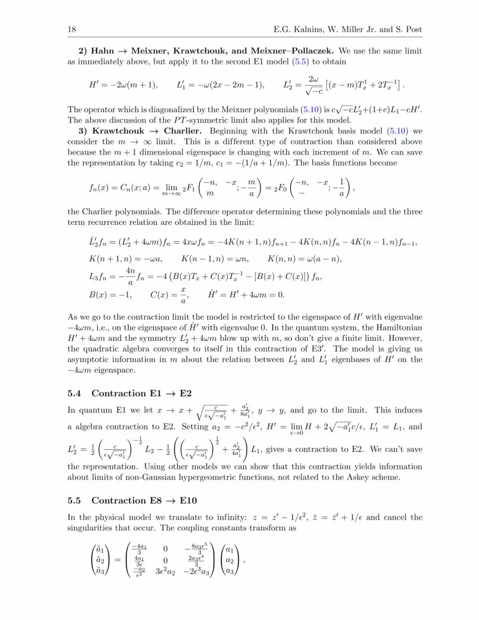
2) Hahn → Meixner, Krawtchouk, and Meixner–Pollaczek. We use the same limitas immediately above, but apply it to the second E1 model (5.5) to obtain

H ′ = −2ω(m+ 1), L′1 = −ω(2x− 2m− 1), L′2 =2ω√−c[(x−m)T 1

x + 2T−1x

].

The operator which is diagonalized by the Meixner polynomials (5.10) is c√−cL′2+(1+c)L1−cH ′.

The above discussion of the PT -symmetric limit also applies for this model.

3) Krawtchouk → Charlier. Beginning with the Krawtchouk basis model (5.10) weconsider the m → ∞ limit. This is a different type of contraction than considered abovebecause the m + 1 dimensional eigenspace is changing with each increment of m. We can savethe representation by taking c2 = 1/m, c1 = −(1/a+ 1/m). The basis functions become

fn(x) = Cn(x; a) = limm→∞ 2F1

(−n, −xm

;−ma

)= 2F0

(−n, −x− ;−1

a

),

the Charlier polynomials. The difference operator determining these polynomials and the threeterm recurrence relation are obtained in the limit:

L′2fn = (L′2 + 4ωm)fn = 4xωfn = −4K(n+ 1, n)fn+1 − 4K(n, n)fn − 4K(n− 1, n)fn−1,

K(n+ 1, n) = −ωa, K(n− 1, n) = ωn, K(n, n) = ω(a− n),

L3fn = −4n

afn = −4

(B(x)Tx + C(x)T−1x − [B(x) + C(x)]

)fn,

B(x) = −1, C(x) =x

a, H ′ = H ′ + 4ωm = 0.

As we go to the contraction limit the model is restricted to the eigenspace of H ′ with eigenvalue−4ωm, i.e., on the eigenspace of H ′ with eigenvalue 0. In the quantum system, the HamiltonianH ′ + 4ωm and the symmetry L′2 + 4ωm blow up with m, so don’t give a finite limit. However,the quadratic algebra converges to itself in this contraction of E3′. The model is giving usasymptotic information in m about the relation between L′2 and L′1 eigenbases of H ′ on the−4ωm eigenspace.

5.4 Contraction E1 → E2

In quantum E1 we let x → x +√

c

ε√−a′1

+a′28a′1

, y → y, and go to the limit. This induces

a algebra contraction to E2. Setting a2 = −c2/ε2, H ′ = limε→0

H + 2√−a′1c/ε, L′1 = L1, and

L′2 = 12

(c

ε√−a′1

)− 12

L2 − 12

((c

ε√−a′1

) 12

+a′24a′1

)L1, gives a contraction to E2. We can’t save

the representation. Using other models we can show that this contraction yields informationabout limits of non-Gaussian hypergeometric functions, not related to the Askey scheme.

5.5 Contraction E8 → E10

In the physical model we translate to infinity: z = z′ − 1/ε2, z = z′ + 1/ε and cancel thesingularities that occur. The coupling constants transform asa1a2

a3

=

−4a13 0 −8a3ε5

34a13ε 0 2a3ε4

3−a2ε2

3ε2a2 −2ε3a3

a1a2a3

,

Contractions of Quantum Superintegrable Systems and the Askey Scheme 19

and the system E10 is obtained by the following singular limit:L1

L2

H

=

1 0 0− 1ε2

ε2 12ε

0 0 1

L1

L2

H

+

16ε2

0 − ε3

614ε4

−14

ε2

1ε3

ε −ε2

a1a2a3

.

We can not save the representation. As in the previous case, it is possible to use other modelsto show that this contraction yields information about limits of non-Gaussian hypergeometricfunctions, not related to the Askey scheme.

6 Nondegenerate to degenerate contractions

This appears initially a mere restriction of the 3-parameter potential to 1-parameter. However,after restriction one 2nd order generator Li becomes a perfect square Li = X2. The spectrumof Li is nonnegative but that of X can take both positive/negative values. This results ina virtual doubling of the support of the measure in the finite case. Also, the commutator of Xand the remaining 2nd order symmetry leads to a new 2nd order symmetry. In [27] we will showhow this Casimir follows directly as a contraction from the expression for R2.

6.1 Contraction S9 → S3

1) Wilson → special dual Hahn (1st model). The quantum system E3 (2.2) is given inthe singular limit from system S9 (4.1) by

a2 = a3 = ε→ 0, a1 = a1,

X ′2 = limε→0

L1, L′2 = limε→0

L2, L′1 = [X ′, L′2]. (6.1)

The operators in this contraction differ from those given in Subsection 2.2 by a cyclic permuta-tion of the coordinates si → si+1. Now we investigate how the difference operator realization ofS9 contracts to irreducible representations of the S3 symmetry algebra. This is more complicatedsince the original restricted algebra is now contained as a proper subalgebra of the contractedalgebra.

The contraction (6.1) is realized in the model by setting α2 = α3 = −1/2 and α1 = α (thesubscript is dropped in this model since there is now a sole α). The restricted operators thenbecome H ′ = E′ with E′ = −4(m+ 1)(m+ α)− (α− 1)2 + 1

4 and

X ′2 = −4τ∗τ, L′2 = −4t2 + α2 − 1

4.

The eigenfunctions for X ′2, the Wilson polynomials, become

Φ±n(t2)

= 4F3

(−n, n, −4m+2α+1

4 − t, −4m+2α+14 + t

−m, −m− α, 12

; 1

). (6.2)

Here n = 0, 1, . . . ,m if m is a nonnegative integer and n = 0, 1, . . . otherwise. For finitedimensional representations, the spectrum of t is the set {α2 + 1

4 + m − k, k = 0, 1, . . . ,m}.Note that the restricted polynomial functions (6.2) are no longer the correct basis functionsfor the contracted superintegrable system. To see this, we consider the contracted expansioncoefficients

L′2fn,m = K(n+ 1, n)fn+1,m +K(n− 1, n)fn−1,m +

(K(n, n) + α2

1 −1

4

)fn,m,

20 E.G. Kalnins, W. Miller Jr. and S. Post

with

K(n+ 1, n) =1

4(m− n+ α) (m− n) , K(n− 1, n) =

1

4(m+ n+ α) (m+ n) ,

K(n, n) =

(1

2

(α+

1

2

)−m

)2

−K(n+ 1, n)−K(n− 1, n).

Indeed K(n − 1, n) no longer vanishes for n = 0, so f0,m is no longer the lowest weight eigen-function. Note that f−1,m = f1,m is still a polynomial in t2. To understand the contraction weset n = N −M/2 where N is a nonnegative integer and M = 2m. Then the equations for theK’s become

K(N + 1, N) =1

4(M −N + α) (M −N) , K(N − 1, N) =

1

4N (N + α) ,

and the three term recurrence relation gives a new set of orthogonal polynomials for repre-sentations of S3. The lowest eigenfunction occurs for N = 0; if M is a nonnegative integerthe representation is (2m + 1)-dimensional with highest eigenfunction for N = M . The basisfunctions which satisfy this three-term recurrence are

fN,M(t2)

=(α+ 1)N

(−α−M)N3F2

(−N, −s, s+ 2α+ 1−M, 1 + α

; 1

). (6.3)

The relation between t and s is s = 2t−α− 1/2. Here fN is a polynomial of order 2N in s andof order n in λ(s) = s(s+ 2α+ 1), a special case of dual Hahn polynomials. These special dualHahn polynomials are associated with the difference operator,

X = i(B(s)Es + C(s)E−1s

), (6.4)

with B(s) + C(s) = M defined as

B(s) =(s+ 2α+ 1)(M − s)

2s+ 2α+ 1, C(s) =

s(s+M + 2α+ 1)

2s+ 2α+ 1.

The operators which form a model for the algebra (2.2) are X (6.4) along with

L1 = −(s+ α+

1

2

)2

+ α2 − 1

4, L2 = [L1, X]. (6.5)

For finite dimensional representations the spectrum of s is {0, 1, . . . ,M}.What is the relation between the functions (6.2) and the proper basis functions (6.3)? Note

this model X, L1, L2 can be obtained from the contracted model X ′, L′1, L′2 by conjugating by

the “ground state” of the contracted model Φ−M2

(t2). We find explicitly the gauge function

Φ−M2

(t2)

=

(12 −

M2

)k(−α−M)k(

12

)k

(− α− M

2

)k

,

when t is evaluated at the weights

t =α

2+

1

4+M

2− k, k = 0, 1, . . . ,

M

2. (6.6)

So, the operator X ′ is related to X via conjugation by Φ−M2

(t2).

Note that the functions Φn

(t2)

are only defined for discrete values of t (6.6). However, on thisrestricted set the functions Φ−M

2+N and fN,M satisfy exactly the same three term recurrence

Contractions of Quantum Superintegrable Systems and the Askey Scheme 21

formula under multiplication by −4t2−a, with the bottom of the weight ladder at N = 0. Fromthis we find the identity

Φ−M2

(t2)fN,M

(t2)

= Φ−M2+N

(t2), t =

α

2+

1

4+M

2− k.

Since Φ−M2

(t2)

= ΦM2

(t2)

this relation implies that fM,M

(t2)

= 1 when restricted to the spec-

trum of t.2) Wilson → special Hahn (2nd model). The quantum system S3 (2.7) can also be

obtained from system S9 (4.1) by

a1 = a3 = ε→ 0, a2 =1

4− α2,

L′1 = limε→0

L1, X ′2 = limε→0

L2, L′2 = [X ′, L′1].

Again, the physical model obtained by this contraction is related to the that given in Subsec-tion 2.2 by a cyclic permutation of the coordinates si → si−1.

In this limit, the operator X2 can be immediately factorized to obtain the skew-adjointoperator X = 2it. Taking x = t+m, we find the operators in our model are

L′1 = −[B(x)Ex + C(x)E−1x −B(x)− C(x)

]− α− 1

2,

B(x) = (x− 2m)(x+ α+ 1), C(x) = x(x− 2m− α− 1),

X ′ = 2i(x−m), L′2 = [X ′, L1], (6.7)

which is diagonalized by Hahn polynomials

fk,m = 3F2

(−k, k + 2α+ 1, −xα+ 1, −2m

; 1

)= Qk(x;α, α, 2m),

L′1fk,m =

(−(k + α+

1

2

)2

+ α2 − 1

4

)fk,m, k = 0, 1, . . . , 2m.

These polynomials satisfy special recurrence relations not obeyed by general Hahn polynomials.Note that the dimension of the representation space has jumped from m+1 to 2m+1. Comparingthese eigenfunctions with the limit of the Wilson polynomials,

limε→0

L′1fn,m =

(−(

2n+ α+1

2

)2

+ α− 1

4

)fn,m,

fn,m(t) = 4F3

(−n, n+ α+ 1

2 , −m− t, −m+ t−m, 1

2 −m, α+ 1; 1

),

n = 0, 1, . . . ,m, we see that in the limit only about half of the spectrum is uncovered. Notethat, the functions fn,m are even functions of t whereas fk,m(−t) = (−1)kfk,m(t).

The recurrences for multiplication by 2it and −4t2 are compatible, so we obtain the followingidentity relating a special case of Wilson polynomials with a special case of the Hahn polynomials:

4F3

(−n, n+ α+ 1

2 , −m− t, −m+ t−m, 1

2 −m, α+ 1; 1

)= 3F2

(−2n, 2n+ 2α+ 1, −t−mα+ 1, −2m

; 1

), n = 0, 1, . . . ,m.

(This is a limit of Singh’s q-series quadratic transformation, [8, p. 89].)

22 E.G. Kalnins, W. Miller Jr. and S. Post

6.2 Contraction E1 → E6

Jacobi → Gegenbauer. By setting a1 = 0, a3 = 0 in system E1 we obtain the system E6.The contraction of the operators takes the form

X ′2 = limε→0

L1, L′1 = limε→0

L2, L′2 =1

2[L′1, X

′]. (6.8)

To investigate the effect of this contraction on the models, we begin with the differentialoperator model of E1 (5.6) with β1 = 1/2 and β3 = 1/2. As in the previous section, we nowhave only one parameter so we drop the subscript and simply write a2 = 1/4 − β2. After thechange of basis (6.8), the operator X ′2 is then given by X ′2 = E′(x+1)/2, suggesting the changeof variables x = 2t2 − 1. The model becomes H ′ = E′ and

X ′ =√E′t, L′1 =

(1− t2

)∂2t − 2t(1 + β)∂t − β −

1

2, L′2 =

1

2[L′1, X

′]. (6.9)

The eigenfunctions of L′1 are given by the Gegenbauer polynomials,

Cβ+1/2k (t) =

(2β + 1)kk!

2F1

(−k, 2β + 1 + kβ + 1

;1− t

2

).

The eigenfunction of L2 in the model for E1, contract to eigenfunctions of L′1

fn = 2F1

(−n, β + n+ 1/2β + 1

; t2 − 1

).

The expansion coefficients of the action of X ′2 on this basis are

K ′(n+ 1, n) =2E′(2β + 2n+ 1)(β + n+ 1)

(2β + 4n+ 1)(2β + 4n+ 3),

K ′(n− 1, n) =E′2n(2n− 1)

(2β + 4n− 1)(2β + 4n+ 1),

K ′(n, n) = E′ −K ′(n+ 1, n)−K ′(n− 1, n),

which suggests half-integer values for n in the model. Indeed, the contraction limit of the basispolynomials gives only half the spectrum. The full spectrum is obtained from eigenfunctionsof L′1 obtained directly as

gk(t) =k!

(2β + 1)kCβ+1/2k (t), k = 0, 1, 2, . . . . (6.10)

These polynomials are related to fn (the contracted basis) as fn(t) = g2k(t), giving the followingidentity:

2F1

(−k, β + k + 1/2β + 1

; t2 − 1

)= 2F1

(−2k, 2β + 1 + 2kβ + 1

;t− 1

2

).

6.3 Contraction E8(a1 = 0) → E14

This contraction leads to Bessel functions, not to orthogonal polynomials.

Contractions of Quantum Superintegrable Systems and the Askey Scheme 23

7 Degenerate/singular system contractions

7.1 Contraction S3 → E3

Special dual Hahn → Special Krawtchouk. In model (6.5) we set a = ε2a,L1

L2

H

X

=

ε 0 0 00 ε 0 00 0 ε 00 0 0 1

L1

L2

HX

+

00−ε0

a

and obtain in the limit L′i = limε→

Li with a′ = limε→

a ≡ −ω2. The model becomes

H ′ = −2ω(M + 1), iX ′ = (s−M)E1 − sE−1,L′1 = ω(2s+ 2M + 3), L′2 = −ω(s−M)E1 − sE−1.

The basis functions for this representation are

fN = (−1)N 2F1

(−N, −s−M ; 2

),

special Krawtchouk or Meixner polynomials, depending on whether M is a positive integer.The eigenvalues of iX ′ are M,M − 2, . . . ,−M in the finite case. The action of L′1 is L′1fN =(N −M)fN+1 − (M + 1)fN −NfN−1, and the action of L′2 follows from commutation relation[L′1, X

′] = 2L′2.For the second model (6.7), after contraction we have

L1 = ω((x− 2m)E + xE−1(−2m− 1)

), X = 2i(x−m),

L2 = −iω((x− 2m)E − xE−1

).

The eigenvalues of L1 are −ω(2k + 1), k = 0, 1, . . . , 2m for finite dimensional representations,and the corresponding eigenfunctions are special:

fk(x) = 2F1

(−k, −x−2m

; 2

).

7.2 Contraction E1(a1 = 0) → sl(2)

Jacobi → Laguerre. We use model (5.6) and let β3 = 1/√ε, E′ = 2/ε, (1− x)/2 = εv, ε→ 0.

The new basis functions are

gn = 1F1

(−n

β2 + 1; v

), (7.1)

Laguerre polynomials. The operators that correspond to this limit are

S1 = limε→0

H − L1, S2 = limε→0

εL2, K = limε→0

L1.

The model contracts to K = 1 and

S1 = 2v, S2 = 4v∂vv + 4(−v + β2 + 1)∂v − 2(β2 + 1),

whose action on the basis (7.1) is

S1gn = 2vgn = −2(β2 + n+ 1)gn+1 − 2(β2 + 2n+ 1)gn − 2ngn−1,

S2gn =[4v∂vv + 4(−v + β2 + 1)∂v − 2(β2 + 1)

]gn.

24 E.G. Kalnins, W. Miller Jr. and S. Post

The corresponding limit in the physical system is obtained by taking y = y′/√ε, β3 = 1/ε, so

that the limit corresponds to a subclass of singular quantum systems. Indeed, letting ε → 0,

K = 1y′2 (a constant that we can set to 1), S1 = ∂xx +

14−β2

2

x2, S2 = ∂xx +

14−β2

2

x2−x2, we find that

S1, S2 generate the Lie structure algebra sl(2).

7.3 Contraction E6 → oscillator algebra

Gegenbauer → Hermite. The E6 algebra contracts to a Lie algebra under the following limit

L1 = limε→0

εL1, L2 = limε→0

εL2, H = limε→0

εH, X = X, a =1

ε2. (7.2)

Under this contraction, the algebra relations become

[L2, X] = 2L1, [L2, L1] = 2X, [X, L1] = −H.

We use the Gegenbauer model (6.9) for E6 and with basis functions gk(t) (6.10). The repre-sentation can be saved by taking β = 1/ε, t =

√εu and E = E/ε. The model becomes

X =√Eu, L1 = ∂uu − 2u∂u − 1, L2 =

1

2[L1, X].

In this limit, the Gegenbauer polynomials tend to the Hermite polynomials,

Hk(u)

2k/2k!= lim

λ→∞

Cλk ( u√λ

)

λk/2, λ = β +

1

2→∞.

In the original quantum system we set x = t/√ε and a = 1/ε2. Then, for ε → 0 in the

contraction (7.2), we have

L1 = t2∂yy − y2/t2, L2 = y/t2, X = ∂y, H = −1/t2.

Note that operators X, L1, L2, H determine the oscillator algebra, the Lie algebra generated bythe annihilation/creation operators for bosons, a, a∗, the number of particles operator N = a∗aand the identity I.

8 Contractions to Laplace–Beltrami equations

8.1 Contraction E6 → e(2)

Jacobi → Tchebicheff. We contract to the free space Hamiltonian by setting a → 0, i.e.β → −1/2. In the limit we find the continuous Tchebicheff polynomials gk(x) = 2Tk(x) =

k lims→0

Csk(v)s .

After the contraction we have L2 = J2, J =√

1− v2∂v, and J generates the new symmetryX1 = [J , X2] = 2iM

√1− v2. Since [X1, X2] = 0 and L1 = 1

2{J , X1}, the quadratic algebra nowcloses to e(2) the Euclidean Lie algebra.

8.2 Contraction S3 → so(3)

Dual Hahn → Special Krawtchouk. We use model (6.3). In the finite case the multiplicityof E is M+1. To go to the Laplace–Beltrami eigenvalue equation on the sphere we let α→ −1/2.

In this limit, cancellation occurs and we have X = (s−M)2 E1− (s+M)

2 E−1, L2 = S2, S = is. From

[X,S] we obtain Y = (s−M)2 E1 + (s+M)

2 E−1 and these 3 generators define the Lie algebra so(3).

Contractions of Quantum Superintegrable Systems and the Askey Scheme 25

Figure 1. The Askey scheme and contractions of superintegrable systems.

With this new symmetry the dimension of the finite representations becomes 2M + 1, the basisfunctions are polynomials in s, rather than s2 and the spectrum of s is −M,−M + 1, . . . ,M .The new basis polynomials are

2F1

(−N, −s−M−2M

; 2

),

special Krawtchouk polynomials KN (s + M ; 12 , 2M) in the finite dimensional case and special

Meixner polynomials MN (s+M ;−2M,−1) in the infinite case.

9 The contraction scheme and final comments

The top half of Fig. 1 shows the standard Askey scheme indicating which orthogonal polynomialscan be obtained by pointwise limits from other polynomials and, ultimately, from the Wilson or

26 E.G. Kalnins, W. Miller Jr. and S. Post

Figure 2. The Askey contraction scheme.

Racah polynomials. The bottom half of Fig. 1 shows how each of the superintegrable systems canbe obtained by a series of contractions from the generic system S9. Not all possible contractionsare listed, partly due to complexity and partly to keep the graph from being too cluttered. (Forexample, all nondegenerate and degenerate superintegrable systems contract to the Euclideansystem H = ∂xx + ∂yy.) The singular systems are superintegrable in the sense that they have 3algebraically independent generators, but the coefficient matrix of the 2nd order terms in theHamiltonian is singular. Fig. 2 shows which orthogonal polynomials are associated with modelsof which quantum superintegrable system and how contractions enable us to reach all of thesefunctions from S9. Again not all contractions have been exhibited, but enough to demonstratethat the Askey scheme is a consequence of the contraction structure linking 2nd order quantumsuperintegrable systems in 2D. It is worth remarking that forthcoming papers by us will simplifyconsiderably the compexity of our approach, [27]. We will show that the structure equationsfor nondegenerate superintegrable systems can be derived directly from the expression for R2

alone, and the structure equations for degenerate superintegrable systems can be derived, up

Contractions of Quantum Superintegrable Systems and the Askey Scheme 27

to a multiplicative factor, from the Casimir alone. It will also be demonstrated that all of thecontractions of quadratic algebras in the Askey scheme can be induced by natural contractionsof the Lie algebras e(2,C) (6 possible contractions) and o(3,C) (4 possible contractions).

This method obviously extends to 2nd order systems in more variables. A start on this studycan be found in [26]. To extend the method to Askey–Wilson polynomials we would need tofind appropriate q-quantum mechanical systems with q-symmetry algebras and we have not yetbeen able to do so.

Acknowledgment

This work was partially supported by a grant from the Simons Foundation (# 208754 to WillardMiller, Jr.). The authors would also like to thank the referees for their valuable comments andsuggestions.

References

[1] Andrews G.E., Askey R., Roy R., Special functions, Encyclopedia of Mathematics and its Applications,Vol. 71, Cambridge University Press, Cambridge, 1999.

[2] Askey R., An integral of Ramanujan and orthogonal polynomials, J. Indian Math. Soc. (N.S.) 51 (1987),27–36.

[3] Bonatsos D., Daskaloyannis C., Kokkotas K., Deformed oscillator algebras for two-dimensional quantumsuperintegrable systems, Phys. Rev. A 50 (1994), 3700–3709, hep-th/9309088.

[4] Daskaloyannis C., Quadratic Poisson algebras of two-dimensional classical superintegrable systems andquadratic associative algebras of quantum superintegrable systems, J. Math. Phys. 42 (2001), 1100–1119,math-ph/0003017.

[5] Daskaloyannis C., Tanoudis Y., Quantum superintegrable systems with quadratic integrals on a two dimen-sional manifold, J. Math. Phys. 48 (2007), 072108, 22 pages, math-ph/0607058.

[6] Daskaloyannis C., Ypsilantis K., Unified treatment and classification of superintegrable systems with inte-grals quadratic in momenta on a two-dimensional manifold, J. Math. Phys. 47 (2006), 042904, 38 pages,math-ph/0412055.

[7] Gao S., Wang Y., Hou B., The classification of Leonard triples of Racah type, Linear Algebra Appl. 439(2013), 1834–1861.

[8] Gasper G., Rahman M., Basic hypergeometric series, Encyclopedia of Mathematics and its Applications,Vol. 35, Cambridge University Press, Cambridge, 1990.

[9] Genest V.X., Vinet L., Zhedanov A., Superintegrability in two dimensions and the Racah–Wilson algebra,arXiv:1307.5539.

[10] Granovskii Y.I., Lutzenko I.M., Zhedanov A.S., Mutual integrability, quadratic algebras, and dynamicalsymmetry, Ann. Physics 217 (1992), 1–20.

[11] Granovskii Y.I., Zhedanov A.S., Lutsenko I.M., Quadratic algebras and dynamics in curved space. I. Anoscillator, Theoret. and Math. Phys. 91 (1992), 474–480.

[12] Granovskii Y.I., Zhedanov A.S., Lutsenko I.M., Quadratic algebras and dynamics in curved space. II. TheKepler problem, Theoret. and Math. Phys. 91 (1992), 604–612.

[13] Granovskii Y.I., Zhedanov A.S., Lutzenko I.M., Quadratic algebra as a “hidden” symmetry of the Hartmannpotential, J. Phys. A: Math. Gen. 24 (1991), 3887–3894.

[14] Inonu E., Wigner E.P., On the contraction of groups and their representations, Proc. Nat. Acad. Sci. USA39 (1953), 510–524.

[15] Izmest’ev A.A., Pogosyan G.S., Sissakian A.N., Winternitz P., Contractions of Lie algebras and separationof variables, J. Phys. A: Math. Gen. 29 (1996), 5949–5962.

[16] Kalnins E.G., Kress J.M., Miller Jr. W., Second order superintegrable systems in conformally flat spaces.I. 2D classical structure theory, J. Math. Phys. 46 (2005), 053509, 28 pages.

[17] Kalnins E.G., Kress J.M., Miller Jr. W., Second order superintegrable systems in conformally flat spaces.II. The classical two-dimensional Stackel transform, J. Math. Phys. 46 (2005), 053510, 15 pages.

28 E.G. Kalnins, W. Miller Jr. and S. Post

[18] Kalnins E.G., Kress J.M., Miller Jr. W., Nondegenerate 2D complex Euclidean superintegrable systems andalgebraic varieties, J. Phys. A: Math. Theor. 40 (2007), 3399–3411, arXiv:0708.3044.

[19] Kalnins E.G., Kress J.M., Miller Jr. W., Structure relations for the symmetry algebras of quantum super-integrable systems, J. Phys. Conf. Ser. 343 (2012), 012075, 12 pages.

[20] Kalnins E.G., Kress J.M., Miller Jr. W., Post S., Structure theory for second order 2D superintegrablesystems with 1-parameter potentials, SIGMA 5 (2009), 008, 24 pages, arXiv:0901.3081.

[21] Kalnins E.G., Kress J.M., Miller Jr. W., Winternitz P., Superintegrable systems in Darboux spaces, J. Math.Phys. 44 (2003), 5811–5848, math-ph/0307039.

[22] Kalnins E.G., Kress J.M., Pogosyan G.S., Miller Jr. W., Completeness of superintegrability in two-dimensional constant-curvature spaces, J. Phys. A: Math. Gen. 34 (2001), 4705–4720, math-ph/0102006.

[23] Kalnins E.G., Miller Jr. W., Pogosyan G.S., Contractions of Lie algebras: applications to special functionsand separation of variables, J. Phys. A: Math. Gen. 32 (1999), 4709–4732.

[24] Kalnins E.G., Miller Jr. W., Post S., Wilson polynomials and the generic superintegrable system on the2-sphere, J. Phys. A: Math. Theor. 40 (2007), 11525–11538.

[25] Kalnins E.G., Miller Jr. W., Post S., Models for the 3D singular isotropic oscillator quadratic algebra, Phys.Atomic Nuclei 73 (2010), 359–366.

[26] Kalnins E.G., Miller Jr. W., Post S., Two-variable Wilson polynomials and the generic superintegrablesystem on the 3-sphere, SIGMA 7 (2011), 051, 26 pages, arXiv:1010.3032.

[27] Kalnins E.G., Miller Jr. W., Subag E., Heinenen R., Contractions of 2nd order superintegrable systems in2D, in preparation.

[28] Kalnins E.G., Williams G.C., Miller Jr. W., Pogosyan G.S., On superintegrable symmetry-breaking poten-tials in N -dimensional Euclidean space, J. Phys. A: Math. Gen. 35 (2002), 4755–4773.

[29] Koekoek R., Lesky P.A., Swarttouw R.F., Hypergeometric orthogonal polynomials and their q-analogues,Springer Monographs in Mathematics, Springer-Verlag, Berlin, 2010.

[30] Koornwinder T.H., Group theoretic interpretations of Askey’s scheme of hypergeometric orthogonal polyno-mials, in Orthogonal Polynomials and their Applications (Segovia, 1986), Lecture Notes in Math., Vol. 1329,Springer, Berlin, 1988, 46–72.

[31] Krall H.L., Frink O., A new class of orthogonal polynomials: the Bessel polynomials, Trans. Amer. Math.Soc. 65 (1949), 100–115.

[32] Kress J.M., Equivalence of superintegrable systems in two dimensions, Phys. Atomic Nuclei 70 (2007),560–566.

[33] Letourneau P., Vinet L., Superintegrable systems: polynomial algebras and quasi-exactly solvable Hamilto-nians, Ann. Physics 243 (1995), 144–168.

[34] Miller Jr. W., Symmetry and separation of variables, Encyclopedia of Mathematics and its Applications,Vol. 4, Addison-Wesley Publishing Co., Reading, Mass. – London – Amsterdam, 1977.

[35] Miller Jr. W., Post S., Winternitz P., Classical and quantum superintegrability with applications, J. Phys. A:Math. Theor., to appear, arXiv:1309.2694.

[36] Mostafazadeh A., Pseudo-Hermiticity versus PT symmetry: the necessary condition for the reality of thespectrum of a non-Hermitian Hamiltonian, J. Math. Phys. 43 (2002), 205–214, math-ph/0107001.

[37] Talman J.D., Special functions: a group theoretic approach (based on lectures by Eugene P. Wigner),W.A. Benjamin, Inc., New York – Amsterdam, 1968.

[38] Terwilliger P., The universal Askey–Wilson algebra and the equitable presentation of Uq(sl2), SIGMA 7(2011), 099, 26 pages, arXiv:1107.3544.

[39] Weimar-Woods E., The three-dimensional real Lie algebras and their contractions, J. Math. Phys. 32 (1991),2028–2033.

[40] Zhedanov A.S., “Hidden symmetry” of Askey–Wilson polynomials, Theoret. and Math. Phys. 89 (1991),1146–1157.