constructions for higher dimensional perfect multifactors

Constructions for Higher Dimensional Perfect

Multifactors

Garth Isaak∗

AMS subject 05B99 (94A55)keywords: de Bruijn cycles, perfect maps

Abstract

Perfect maps, factors and multifactors can be viewed as higher dimen-sional analogues of de Bruijn cycles and factored versions of these cycles.We present a unified framework for two basic techniques, concatenationand integration (also called the inverse of Lempel’s homomorphism), usedto construct perfect multifactors. This framework simplifies proofs ofknown results and allows for extension of the basic constructions. Inparticular, we give the first general results on the inverse of Lempel’shomomorphism in dimensions three and higher.

1 Introduction

What has come to be known as a de Bruijn cycle (see [4] for more history) isa periodic k-ary string in which every k-ary substring of a given size appearsexactly once (periodically). For example, in the period nine string

001121022|001121022|0011 . . .

each ternary string of length two appears exactly once with period nine. Wewill usually represent such a string with a fundamental block, writing 001121022with the periodicity understood. The position of a substring is its location inthe block, starting with position 0. So in the example above 00 appears inposition 0, 21 in position 4 and 20 in position 8.

There has been some recent interest in higher dimensional analogues of deBruijn cycles. These have been called de Bruijn tori and perfect maps. Viewing

0 0 1 00 0 0 10 1 1 11 0 1 1

∗Department of Mathematics, Lehigh University, Bethlehem, PA 18015 [email protected] supported by grants from the ONR and the Reidler Foundation

1

2 G. Isaak

periodically in both dimensions (toroidally), each binary 2 × 2 array appearsexactly once, for example, 0 1

0 0 in position (0, 1) and 1 10 0 in position (3, 3).

There are obvious necessary conditions for the existence of such maps and it isconjectured that these are also sufficient. These conditions are noted in Lemma3 and the conjecture following the lemma.

Although there have been various methods of constructing perfect maps,two techniques have played a central role. The method of concatenation wasintroduced and developed by Ma [10], Cock [1] and Etzion [2] and has beendescribed for all dimensions. The method of integration (sometimes called theinverse of Lempel’s homomorphism) was introduced in Fan, Fan, Ma and Sui[3]. Methods for integration of perfect factors have been extended and refinedby a number of authors, however only in one and two dimensions. In particular,when the entries are from a finite field, Paterson [15], [16] made use of thelinear complexity of a sequence to allow repeated applications of integration.With this, he showed that obvious necessary conditions for the existence of2-dimensional k-ary de Bruijn tori are sufficient when k is a prime power.

Applying the techniques of concatenation and integration requires introduc-tion of two new objects, perfect factors, which generalize perfect maps and ageneralization of perfect factors called perfect multifactors.

Perfect factors can be thought of as a factorization of a de Bruijn cycle (ortorus) into a collection of smaller cycles (tori). Perfect factors were introducedby Lempel [9]. Two dimensional perfect factors are mentioned in [18] and higherdimensional versions in [6]. Extensive study of one dimensional perfect factorscan be found in [2] and [16].

Perfect multifactors are perfect factors in which each substring (subarray) ofa given size appears several times, once in each location relative to a given mod-ulus. Perfect multifactors were introduced by Mitchell [11]. Two dimensionalperfect multifactors were introduced by Paterson [18]. Perfect multifactors wereintroduced and have been used to produce other perfect factors over non primepower alphabets. See for example [11], [14], [18], or see [12] for another varia-tion. We will not discuss these applications here but rather discuss the role ofperfect multifactors in concatenation and integration.

In order to have enough power to attack problems of constructing perfectmaps, we must look at the broader problem of constructing perfect multifactors.Perfect factors in dimension d−1 along with one dimensional perfect multifactorsare used in concatenation to produce d dimensional perfect maps (and factors).Perfect multifactors in dimension d − 1 are a key to applying integration indimension d.

We now briefly discuss repeated applications of the constructions describedin this paper. Repeated applications of integration can be done by switchingthe direction along which integration occurs as in [5] for the two dimensionalcase. The extra flexibility in higher dimensions should allow even more with thisapproach. Repeated applications of integration can also be done using linearcomplexity of a sequence when the alphabet is a finite field as in [15] and [16].It seems possible that these approaches for repeated application of integration

Perfect Multifactors 3

applied to the new results on integration in higher dimensions could provide abasis for a proof that the obvious necessary conditions (see Lemma 3) for k-aryde Bruijn tori in higher dimensions can be shown to be sufficient when k is aprime power. However for general multifactors and even for de Bruijn tori whenthe alphabet size k is not a prime power other methods will likely be needed.Indeed, the general cases have not even been settled in 1 and 2 dimensions fornon-prime power alphabets.

In this paper we will begin by giving a number of motivating examples inSection 2. In Section 3 we will give more formal definitions and discuss obvi-ous necessary conditions which are believed to be sufficient. In Section 4 wedescribe general results for the construction methods of concatenation and in-tegration. For concatenation almost all of the cases where our results applyhave been mentioned previously in the literature, but they have not all beenwritten down in a unified format. To aid this, we will introduce another classof one-dimensional strings, perfect multifactor pairs, which have implicitly beenused in previous works. For integration, what has been missing is a descriptionof this construction in dimensions 3 and higher as well as integration applied toperfect multifactors in two dimensions. Additionally, the role of perfect multi-factors in integration has usually not been made explicit. We will do so here.This allows us to state new broad results for integration.

2 Examples

The notation for discussing perfect multifactors can get quite cumbersome. Inthis section we present a number of examples to illustrate perfect multifactorsas well as the methods of integration and concatenation. A more formal pre-sentation will be in Sections 3 and 4. We adopt the notation of [8], informallyin this section and formally in the next.

Example 1: Let us begin with a simple example. Recall the de Bruijn cycle

001121022

from the introduction. It is a 3-ary string of period 9 in which each length2 substring appears exactly once. We will call this a (9; 2)3-dBS (de Bruijnsequence). Consider the two dimensional array

0 0 0 1 0 0 0 1 00 0 1 2 2 1 2 2 11 1 1 1 2 1 2 1 11 1 2 0 0 2 0 0 22 2 1 2 0 1 0 2 11 1 0 2 1 0 1 2 00 0 2 0 1 2 1 0 22 2 2 0 2 2 2 0 22 2 0 1 1 0 1 1 0

Viewing this 9× 9 array toroidally, every 2× 2 3-ary subarray appears exactlyonce. This is called a ((9, 9); (2, 2))3-dBT (de Bruijn torus).

The method of construction is the simplest version of concatenation. Eachcolumn is a shifted copy of the previous de Bruijn cycle. The shifts follow the

4 G. Isaak

pattern 012345678. Column 1 is obtained by shifting column 0 by 0, column2 is obtained by shifting column 1 by 1, .... The last 8 indicates that shiftingcolumn 8 returns us to the start, column 0 so we can view the array periodically(or as a torus). The subarray 0 1

1 2 appears in position (0, 2) since 01 and 12appear in 001121022 shifted by 2, hence we look for this subarray where a shiftof 2 occurs, starting in column 2. Similarly, each subarray can be found andbecause of the size, each must appear exactly once.

Example 2: Consider the string

000011210220112102201121022

obtained by writing three 0’s followed by three copies of the string 01121022(i.e., the de Bruijn cycle 001121022 with the first 0 deleted). In this string withperiod 27, every 3-ary substring of length 2 appears exactly 3 times, once ineach position modulo 3. We call this a (27; 2; 1)3[3]-PMF (perfect multifactor).Shifting by 3 and by 6 we get two additional strings

022000011210220112102201121 121022000011210220112102201

for a set of 3, period 27 strings in which each length 2 substring appears appearsexactly once in each position modulo 9; a (27; 2; 3)3[9]-PMF. These will be theset of 3 starters for integration in our next example.

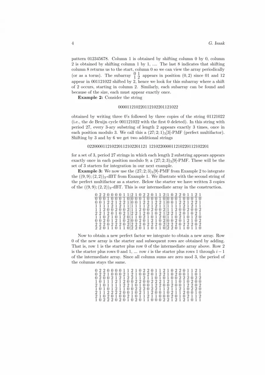
Example 3: We now use the (27; 2; 3)3[9]-PMF from Example 2 to integratethe ((9, 9); (2, 2))3-dBT from Example 1. We illustrate with the second string ofthe perfect multifactor as a starter. Below the starter we have written 3 copiesof the ((9, 9); (2, 2))3-dBT. This is our intermediate array in the construction.

0 2 2 0 0 0 0 1 1 2 1 0 2 2 0 1 1 2 1 0 2 2 0 1 1 2 10 0 0 1 0 0 0 1 0 0 0 0 1 0 0 0 1 0 0 0 0 1 0 0 0 1 00 0 1 2 2 1 2 2 1 0 0 1 2 2 1 2 2 1 0 0 1 2 2 1 2 2 11 1 1 1 2 1 2 1 1 1 1 1 1 2 1 2 1 1 1 1 1 1 2 1 2 1 11 1 2 0 0 2 0 0 2 1 1 2 0 0 2 0 0 2 1 1 2 0 0 2 0 0 22 2 1 2 0 1 0 2 1 2 2 1 2 0 1 0 2 1 2 2 1 2 0 1 0 2 11 1 0 2 1 0 1 2 0 1 1 0 2 1 0 1 2 0 1 1 0 2 1 0 1 2 00 0 2 0 1 2 1 0 2 0 0 2 0 1 2 1 0 2 0 0 2 0 1 2 1 0 22 2 2 0 2 2 2 0 2 2 2 2 0 2 2 2 0 2 2 2 2 0 2 2 2 0 22 2 0 1 1 0 1 1 0 2 2 0 1 1 0 1 1 0 2 2 0 1 1 0 1 1 0

Now to obtain a new perfect factor we integrate to obtain a new array. Row0 of the new array is the starter and subsequent rows are obtained by adding.That is, row 1 is the starter plus row 0 of the intermediate array above. Row 2is the starter plus rows 0 and 1, ... row i is the starter plus rows 1 through i− 1of the intermediate array. Since all column sums are zero mod 3, the period ofthe columns stays the same.

0 2 2 0 0 0 0 1 1 2 1 0 2 2 0 1 1 2 1 0 2 2 0 1 1 2 10 2 2 1 0 0 0 2 1 2 1 0 0 2 0 1 2 2 1 0 2 0 0 1 1 0 10 2 0 0 2 1 2 1 2 2 1 1 2 1 1 0 1 0 1 0 0 2 2 2 0 2 21 0 1 1 1 2 1 2 0 0 2 2 0 0 2 2 2 1 2 1 1 0 1 0 2 0 02 1 0 1 1 1 1 2 2 1 0 1 0 0 1 2 2 0 0 2 0 0 1 2 2 0 21 0 1 0 1 2 1 1 0 0 2 2 2 0 2 2 1 1 2 1 1 2 1 0 2 2 02 1 1 2 2 2 2 0 0 1 0 2 1 1 2 0 0 1 0 2 1 1 2 0 0 1 02 1 0 2 0 1 0 0 2 1 0 1 1 2 1 1 0 0 0 2 0 1 0 2 1 1 21 0 2 2 2 0 2 0 1 0 2 0 1 1 0 0 0 2 2 1 2 1 2 1 0 1 1


Doing the same thing with the other two possible starters produces three3-ary 9 × 27 arrays in which we claim that every 3-ary 3× 2 subarray appearsexactly once. We call this a ((9, 27); (3, 2); 3)23-PF (perfect factor).

For example, try to find the subarray0 01 22 0

. Look at the differences (mod

3) between row 0 and row 1 and between row 1 and row 2. These differencesgive 1 2

1 1 which occurs in position (1, 2) in the ((9, 9); (2, 2))3-dBT of Example

1. The sum of the entries on these two columns above 1 21 1 is 0 1 . In the

addition we need to ‘arrive’ at position (1, 2) (mod (9, 9)) with a sum of 0 0 ,the first row of the array we are looking for. Thus the starter plus 0 1 mustbe 0 0 (the first row of our particular subarray). So we need to find 0 2 inthe starter in a position 2 modulo 9. This occurs with the second starter in

position 11. Thus we find0 01 22 0

in row 1 column 11 of the new array. Similarly,

since every length 2 substring appears in the set of 3 starters in every positionmodulo 9, we can find every 3× 2 subarray. In this example we have integratedalong columns, (the first coordinate dimension), when we describe integrationin general we integrate along dimension d, so one should take the transpose ofour examples to be consistent with that notation.

Example 4: In Example 2, the column sums are zero mod 3. Here wegive an example of integration when the column sums are a nonzero constant.Consider the two dimensional array

0 3 2 21 2 3 32 1 1 03 0 0 1

Viewing this 4× 4 array toroidally, every 1× 2 4-ary subarray appears exactlyonce. So this is a ((4, 4); (1, 2))4-dBT (de Bruijn torus). Note that the columnsums are 2 mod 4. Consider also the collection of strings

0 0 0 0

2 2 2 2

1 1 1 1

3 3 3 3

0 1 0 1

2 3 2 3

1 0 1 0

3 2 3 2

0 2 0 2

2 0 2 0

0 3 0 3

2 1 2 1

1 2 1 2

3 0 3 0

1 3 1 3

3 1 3 1

This is a set of 16 period 4 strings in which each 4-ary length 2 substring appearsexactly once in each position modulo 4. We call this a (4; 2; 16)4[4]-PMF (perfectmultifactor). However there is an additional property, doing arithmetic mod 4the two strings in each column differ by 2 2 2 2 . Thinking of the entries fromZ4 and {0, 2} as a subgroup of Z4 we call this an equivalence class perfectmultifactor modulo {0, 2} an denote it (4; 2; 16)Z4|{0,2}[4]-EPMF. Picking onestring from each column we get what we call a set of representatives modulo{0, 2}. Now when we integrate as in example 2, use only one representativefrom each column in the list. The column lengths double (since in order toget column sums 0, we need two copies of the 4 × 4 arrays placed vertically).Illustrating, along the lines of example 2 with 0 1 0 1 as a starter we get thefollowing, with the intermediate array on the left and the integrated array onthe right

6 G. Isaak

0 1 0 10 3 2 21 2 3 32 1 1 03 0 0 10 3 2 21 2 3 32 1 1 03 0 0 1

0 1 0 10 0 2 31 2 1 23 3 2 22 3 2 32 2 0 13 0 3 01 1 0 0

Note that rows i and i + 4 (modulo 8) differ by the constant string of 2’s. Forexample adding 2 (arithmetic modulo 4) to each of the entries of 1 2 1 2 ofrow 2 we get 3 0 3 0 , row 6.

Doing this with one of the strings from each column of the list of the equiv-alence class perfect multifactor we obtain a set of eight 8 × 4 arrays in whicheach 4-ary 2× 2 subarray appears exactly once, a ((8, 4); (2, 2); 8)24-PF.

For example, try to find the subarray 0 13 0 . The difference (mod 4) between

the rows is 3 3 which occurs in position (1, 2) of the de Bruijn torus. The sumof the entries above these columns in the de Bruijn torus is 2 2 . In this casewe need to ‘arrive’ at position (1, 2) with sum 0 1 , the first row of the arraywe are looking for. Thus the starter plus 2 2 must be 0 1 . So we need to find2 3 in a position 2 modulo 4 of a starter. This occurs in the third column ofthe list. However, we choose the other string 0 1 0 1 as our starter so insteadof finding our array in row 1 we find it in row 5. This is because the first 4 rowsof integration ‘change’ the 0 1 0 1 to 2 3 2 3 with 2 3 in position 2 mod 4as needed.

Example 5: In Example 2, what we did was copy a two dimensional arrayseveral times, and used a starter such that every substring appeared in everyposition modulo the number of columns. Working in three dimensions, imaginethe array we wish to integrate as a box. We arrange copies of the box in somerectangular pattern and overlay a two dimensional starter. The starter musthave the property that every 2 dimensional subarray appears exactly once ineach position modulo the size of the ‘tops’ of the boxes. That is, we need atwo dimensional perfect multifactor. In general, we need a (d− 1) dimensionalperfect multifactor to integrate a d dimensional perfect factor.

Example 6: We now illustrate building a 2 dimensional perfect multifactor.Begin with a (4; 2, 2)12[2]-PMF (perfect multifactor) 0011 1001 , a set of 2 binary1 dimensional strings with period 4 in which each substring of length 2 appearsexactly once in each position modulo 2. We will concatenate these to form thecolumns of a two dimensional perfect multifactor. In the previous example wespecified column shifts. Here we must specify shifts as well as a selection ofwhich column to use. The shifts must be multiples of 2 because of the modulus,so our strings times 2 give the shifts.

Consider the following

times 2 = shifts 0000 0000 1111 1111column selection 0011 1001 0011 1001

In this set of four pairs of 4-tuples, each possible shift (0 or 1) appears once witheach possible pair from 00, 01, 10, 11 (which specifies the column selection) in


each position modulo 2. We will call this a (4; (1, 2), 4)(2,2)[2]-PMFP (perfectmultifactor pair). Using this, with (the transpose of) 0011 called column #0and (the transpose of) 1001 called column #1 we get four 4× 4 arrays

0 0 1 10 0 0 01 1 0 01 1 1 1

1 0 0 10 0 0 00 1 1 01 1 1 1

0 1 1 00 1 0 11 0 0 11 0 1 0

1 1 0 00 1 0 10 0 1 11 0 1 0

In the fourth array, from the fourth term 11111001 of the PMFP, we start column

0 equal to column #1, then column 2 is column #0 shifted by 2 = 2 ·1. Column3 is column # 0 shifted by 2 = 2 ·1 from the previous column (a total shift of 4,which is equivalent to a shift of 0 since the columns have height 4). Column 4is column #1 shifted by 2 = 2 · 1 from the previous column. The last column isagain shifted by 2 = 2 ·1 for a total shift of 0, modulo 4, which is what is neededso that we ‘return’ to the first column and the period of the rows remains 4.

We claim that every 2 × 2 subarray appears exactly once in each positionmodulo (2, 2) in one of the 4 arrays. So this is a ((4, 4); (2, 2); 4)22[(2, 2)]-PMF(perfect multifactor).

For example, to find 0 11 1 in position (1, 0) modulo (2, 2) first observe that

the first column 01 of our subarray appears modulo 1 in position 1 in column

#0 and the second column 11 appears modulo 1 in position 3 in column #1.

The positions differ by 2. So, we must find the column pair 0, 1 along withthe shift 1 (since we multiply shifts by 2) in position 0 modulo 2 in our perfectmultifactor pair. This is in position 4 in the fourth set. So we find 0 1

1 1 modulo(1, 0) in column 2 of the fourth array. This is in position (1, 2) of the array.

3 Basics

In this section we give more formal definitions as well as stating necessary con-ditions for existence of perfect multifactors.

We will denote (non-periodic) vectors as ~V = (v1, v2, . . . , vd) and write〈~V 〉 = Πd

i=1vd. Deleting the last coordinate from ~V will result in~V − = (v1, v2, . . . , vd−1). We will also write ~V + for (d + 1)-dimensional vec-tors that agree with ~V on the first d coordinates, with vd+1 specified in eachparticular case. For two vectors ~I = (i1, i2, . . . , id) and ~J = (j1, j2, . . . , jd) co-ordinatewise multiplication will be ~I · ~J = (i1j1, i2j2, . . . , idjd) and addition isordinary vector addition ~I + ~J = (i1 + j1, i2 + j2, . . . , id + jd).

For an array A we will denote the entry in position ~I = (i1, i2, . . . , id) by [A]~I .A periodic array A with period ~R = (r1, r2, . . . , rd) is an infinite array such thatfor all ~J , [A] ~J = [A] ~J+~R. For ease of notation we will consider only indices withnon-negative integral values. A fundamental block of A is an array consistingof ri consecutive rows in the ith dimension for i = 1, 2, . . . , d. Repeating such ablock produces A. We will sometimes refer to a fundamental block of A as A

8 G. Isaak

when there is no chance of confusion. A fundamental block of a one dimensionalperiodic array could also be viewed as a vector.

If a matrix B of size ~S appears in A in positions ~I through ~I+~S we say that Bappears in A at position ~I. We say that B appears in location ~J = (j1, j2, . . . , jd)modulo ~N = (n1, n2, . . . , nd) if B appears in position ~I = (i1, i2, . . . , id) andix ≡ jx (mod nx) for x = 1, 2, . . . , d. Usually when we say that B appearsin position ~I = (i1, i2, . . . , id) in a period ~R array, we will pick those ix with0 ≤ ix < ri. When we say that a subarray B of A appears exactly once, we meanexactly once in any fundamental block. When looking only at a fundamentalblock, addition on the subscripts in the ith dimension is performed modulo ri.

The projection of a d-dimensional periodic array A onto the zth hyperplane indimension d is the (d− 1) dimensional array consisting of entries [A]~I for whichid = z. A projection of A along ~J = (j1, j2, . . . , jd−1) is a one dimensionalarray consisting of entries [A]~I for ~I− = ~J . We will refer to such projections asprojections along direction d.

An array will be called K-ary if the entries are from an alphabet (set) K. Ifwe are only concerned about the size of K and not its structure we will writek-ary where k = |K|. Sometimes we need additional additive structure on thealphabet. When we refer to an alphabet as a group we will assume the group isof the form Za1 ×Za2 ×· · ·×Zan for some integers n and a1, a2, . . . , an. We willalso sometimes view an element of Za1 × Za2 × · · · × Zan as a length n vectorwith entries from Z in the obvious manner. More formally, if the term from Zai

is the congruence class [x] then the ith component of the vector viewed in Z isthe unique integer in {0, 1, . . . , ai − 1} congruent to x modulo ai.

We will write gcd(a, b) for greatest common divisor and lcm(a, b) for leastcommon multiple.

Definition 1 A (~R; ~U ; τ)dK [ ~N ] Perfect Multifactor (PMF) is a collection of τ

d-dimensional periodic arrays with period ~R = (r1, r2, . . . , rd), with entries froman alphabet K and such that every K-ary size ~U = (u1, u2, . . . , ud) subarrayappears exactly once in each location modulo ~N = (n1, n2, . . . , nd). We assumethat ri is a multiple of ni for i = 1, 2, . . . , d. Sometimes we will only be concernedabout the size k of K and not its structure, in which case we will replace K withk in the notation.

Usually PMF’s are defined referring only to the size |K| and not the structureof the alphabet K. We have included the structure of K in our definition becausewe will need additive properties in K for our constructions.

The following lemma which relates the parameters of PMFs is easily verifiedby equating the number of distinct positions in a fundamental block and thenumber of appearances of subarrays, recalling that each particular subarray ofsize ~U appears exactly once for each location modulo ~N .

Lemma 1 For a (~R; ~U ; τ)dK [ ~N ] PMF (perfect multifactor) we have

〈~R〉τ = |K|〈~U〉〈 ~N〉. (1)


Additionally, if A is a set of τ period ~R, K-ary arrays in which each K-ary size~U subarray appears at least once (i.e., in some array) in each location modulo~N and if (1) holds, then A is a (~R; ~U ; τ)d

K [ ~N ] PMF (perfect multifactor).

Definition 2 A (~R; ~U ; τ)dK Perfect Factor (PF) is a perfect multifactor in which

~N = (1, 1, . . . , 1). When τ = 1 (there is only one array) we have what is calleda de Bruijn cycle in dimension 1 and a de Bruijn torus in higher dimensions.These are also called perfect maps. In this case we will write (~R; ~U)d

K-dBT.(This last notation appears only in the examples.)

Definition 3 Let K be a group and H a subgroup of K. An (~R; ~U ; τ)dK|H [ ~N ]

Equivalence Class Perfect Multifactor modulo H (EPMF) is a K-ary perfectmultifactor with the additional condition that the τ arrays can be partitionedinto a collection of size |H| parts with the arrays in part z labeledA(z, 1), A(z, 2), . . . , A(z, |H|) such that for all i, j there is a c ∈ H with A(z, j)−A(z, i) equal to the constant array having each entry c. A set of representativesmodulo H is obtained by selecting from each part one of the arrays.

Note that when H = {0}, the trivial group then an EPMF is just a PMF.

Definition 4 A (Q; (u, v), τ)K,L[N ] Perfect Multifactor Pair (PMFP) is a col-lection of τ period Q sequences consisting of ordered pairs from an alphabet K×Lsuch that every pairing of a K-ary size u string in the first coordinate with anL-ary size v string in the second coordinate occurs in each location modulo N .We will denote a perfect multifactor pair by (A : B) where A indicates the col-lection of sequences for the first coordinate and B the collection of sequences forthe second coordinate.

The next lemma follows in the same manner as Lemma 1.

Lemma 2 For a (Q; (u, v), τ)K,L[N ] PMFP (perfect multifactor pair) we have

Qτ = |K|u|L|vN. (2)

Additionally, if A is a set of τ period Q sequences of pairs from an alphabetK ×L in which each K-ary length u string in the first coordinate is paired witheach L-ary length v string in the second coordinate at least once (i.e., in somepair) in each location modulo N and if (2) holds, then A is a (Q; (u, v), τ)K,L[N ]PMFP (perfect multifactor pair).

Definition 5 The shift operator E~S applied to an array A shifts the location

indices so that the entry in position ~S appears in position (0, 0, 0, . . .). So, ingeneral, [E ~S(A)]~I = [A]~I+~S .

The following Lemma and conjecture have been noted numerous times andin the general form here in [8]. Part (i) of the lemma follows from Lemma 1.Part (ii) follows by considering the all 0 subarray of size ~U and noting that itappears exactly once in each location modulo ~N .

10 G. Isaak

Lemma 3 Suppose there exists a (~R; ~U ; τ)dK [ ~N ]-PMF (Perfect multifactor).

Then

(i) 〈~R〉τ = |K|〈~U〉〈 ~N〉 and

(ii) For each i either (a) ni = 1 and ri ≥ ui or (b) ni > 1 and ri > ui.

It is conjectured that except possibly for some very ‘small’ values of the ri

(ri = ui +1 for example) the necessary conditions implied by the lemma are alsosufficient. For many cases, particularly in one and two dimensions, sufficiencyhas been shown. See for example [7], [8], [11], [14], [17], [18]. However, fortwo and higher dimensional multifactors and three and higher dimensions in allcases the results have been fairly restricted. As previously discussed, the newresults for integration in higher dimensions in Section 4 should be a useful toolin covering more of these cases.

4 Constructions

In this section we describe two basic construction methods, concatenation andintegration of perfect multifactors. We then give our main results for situa-tions where these constructions produce new perfect multifactors. The proofsfollow the same patterns that have been developed in the literature previously.Indeed they may appear shorter because we separate out the key tools of con-structing perfect multifactors. Once we do the work of getting the appropriateterminology and statements, the proofs are straightforward. We hope that thiswill aid in avoiding redundancy in future proofs and focus the development ofconstructions for perfect multifactors.

4.1 Concatenation

We begin with concatenation. We briefly outline various steps towards describ-ing this in the broadest setting. Two dimensional concatenation of binary deBruijn cycles appears in [10] and of perfect factors in [2]. Two dimensionalconcatenation of perfect factors over general alphabets appears in [17]. Higherdimensional concatenation of de Bruijn cycles over general alphabets appearsin [1] and of perfect factors in [6]. Two dimensional concatenation of perfectmultifactors appears in [18]. A special case of creating multifactors when theshift vector does not have zero sum appears in [1], however most of what wedo in this case is new. Here we also include higher dimensional concatenationof perfect multifactors. In every case, the key is ‘lining’ up selection of factorswith shift patterns, and has been done previously by specific construction in theproof. By introducing perfect multifactor pairs, we separate out this key part ofthe proof, simplifying the proof for concatenation. Of course then more needsto be said about perfect multifactor pairs and we will do this below.

Construction 1 (Concatenation) Let A = A(1), A(2), . . . , A(τ) be a col-lection of d-dimensional period ~R arrays. Let B = B(1), B(2), . . . , B(ρ) and


C = C(1), C(2), . . . , C(ρ) be collections of ρ (one-dimensional) strings, eachstring with period Q. The entries of the C(i) are from the alphabet {1, 2, . . . , τ}.For some ~N , the entries of the B(i) are from the group H = Zr1/n1 × Zr2/n2 ×· · ·Zrd/nd

and satisfy the following. There exists a c ∈ H such that for j =

1, 2, . . . , ρ we haveQ∑

h=1

[B(j)]h = c. That is, the sum of entries in a fundamental

block is c. We call the pair (B : C) the indexer.Then concatenating A using indexer (B : C) produces a new collection of

(d+1)-dimensional arrays D(1), D(2), . . . , D(ρ) each with period ~R+ where thefirst d coordinates of ~R+ are the same as ~R and r+

d+1 equals Q times the orderof c in H.

To describe the entries, define S(j, z) ∈ H by S(j, z) =∑z−1

h=0[B(j)]h. Thesum is 0 if z = 0. We can view S(j, z) as a length d vector with entries inZ and write this as ~S(j, z). Then ~N · ~S(j, z) = (n1s1, n2s2, . . . , ndsd). Forj = 1, 2, . . . , ρ and for ~I = (i1, i2 . . . , id+1) with id+1 = z, we have

[D(j)]~I = [A([C(j)]z)]~I−+ ~N ·~S(j,z) =[E

~I−+ ~N ·~S(j,z)A([C(j)]z)]

~I.

In other words, the projections of D(j) onto hyperplanes in dimension d + 1are shifted factors from A. The selection of which factor is determined by Cand the shifts are multiples of ~N determined by B.

To check that concatenation is well defined we only need to check that theperiods are correct. For the first d dimensions this follows immediately fromthe observations about projections above. For dimension d + 1 this followsby observing that the projection onto the Q hyperplane in dimension (d + 1)is shifted c ‘times’ ~N (coordinatewise multiplication) relative to the projectiononto the 0 hyperplane in dimension (d+1). If η is the order of c, then ηc = 0 andthe projection onto the Qη hyperplane is shifted by 0 relative to the projectiononto the 0 hyperplane. That is, they are shifted the same amount. Also sincethe B(i) have period Q, the projections onto the 0 and the Qη hyperplanes arethe same factor from A.

For the next theorem, the case c = 0 is the one that has been covered pre-viously. We also include c 6= 0 for completeness. Even though the possibilitiesfor c 6= 0 are fairly restricted we believe there may be some use in constructingexceptional perfect multifactors.

Theorem 1 Let A be a (~R; ~V ; τ)dG[ ~N ] PMF (perfect multifactor). Let H =

Zr1/n1 × Zr2/n2 × · · ·Zrd/ndand let H ′ = {1, 2, . . . , τ}. Let (B : C) be a

(Q; (U − 1, U); ρ)H,H′ [M ] PMFP (perfect multifactor pair) with the followingproperty. There exists c ∈ H such that each string B(j) in B satisfiesQ∑

h=1

[B(j)]h = c. That is, the entries in each fundamental block sum to c.

Then,

12 G. Isaak

• If c = 0 ∈ H, concatenation using (B : C) as indexer yields a(~R+; ~V +; ρ)d+1

G [ ~N+] PMF (perfect multifactor) where the first d coordi-nates of ~N+, ~R+ and ~V + are the same as ~N , ~R and ~V and n+

d+1 = M ,r+d+1 = Q and v+

d+1 = U .

• If c 6= 0 ∈ H and additionally we have the following: If c is viewed asa vector ~C = (c1, c2, . . . , cd) with entries from Z and for i = 1, 2, . . . , d

we have ηi =ri/ni

gcd(ri/ni, ci)(i.e., the order of ci in Zri/ni

is ηi), then

gcd (ηi, ci) = 1. Also, for i 6= j, gcd(ηi, ηj) = 1. Then concatenation using(B : C) as indexer yields a (~R+; ~V +; ρ)d+1

G [ ~N∗] PMF (perfect multifactor)where the first d coordinates of ~R+ and ~V + are the same as ~R and ~Vwith r+

d+1 = QΠdi=1ηi and v+

d+1 = U . Also ~N∗ is given by n∗j = niηi forj = 1, 2, . . . , d and n∗d+1 = M .

Proof: Observe that when c = 0 each ηi = 1. Thus c = 0 is included also in thec 6= 0 case and we need only consider c 6= 0. Let D denote the PMF formed byconcatenation.

The periodicity and the number of factors ρ for D follow from the discussionthat concatenation is well defined and from the definition of concatenation. Weneed only observe that for c 6= 0 as in the statement of the theorem, the orderof c in H is Πd

i=1ηi.By Lemma 1 we need only to check that equation (1) holds and that each

subarray of size ~V + appears at least once in some array D(j) of D in eachlocation modulo ~N∗.

From Lemma 1 applied to A and Lemma 2 applied to (B : C) we have

〈~R〉τ = |G|〈~V 〉〈 ~N〉 and Qρ = |H|U−1|H ′|UM =

(〈~R〉〈 ~N〉

)U−1

τUM. Then with

〈~R+〉 = 〈~R〉rd+1 = 〈~R〉QΠdi=1ηi and 〈~V +〉 = 〈~V 〉vd+1 = 〈~V 〉U and

〈 ~N∗〉 = Πd+1i=1 n∗i = n∗d+1Π

di=1niηi = M〈 ~N〉Πd

i=1ηi we get

〈~R+〉ρ = 〈~R〉 (Πdi=1ηi

)Qρ

= 〈~R〉 (Πdi=1ηi

)(〈~R〉〈 ~N〉

)U−1

τUM

=(|G|〈~V 〉〈 ~N〉

)U MΠdi=1ηi

〈 ~N〉U−1

= |G|〈~V +〉〈 ~N∗〉.So D satisfies equation (1).

Now, for an arbitrary G-ary size ~V + array D′ and an arbitrary location ~L∗

we must find D′ in some position ~I ≡ ~L∗ modulo ~N∗ in some factor of D.Let D′

h be the projection of D′ onto the h hyperplane in dimension (d + 1)for h = 0, 1, . . . , (U − 1). If ~L∗ = (l∗1, l

∗2, . . . , l

∗d+1) let l′i ≡ l∗i (mod ni) for i =


1, 2, . . . , d and let ~L′ = (l′1, l′2, . . . , l

′d). Then D′

h appears in position ~J ′(h) ≡ ~L′

(mod ~N) in some factor A(f(h)) of A. Since the ~J ′(h) ≡ ~L′ (mod ~N), for h =0, 1, . . . , (U − 2) we have ~J ′(h+1)− ~J ′(h) = (v1, v2, . . . , vd)h · (n1, n2, . . . , nd) =~Vh · ~N where the vi can be viewed as elements of Zri/ni

and the ~Vh as ele-ments Vh of H = Zr1/n1 × Zr2/n2 × · · ·Zrd/nd

. Hence (V1, V2, . . . , VU−2) is alength (U − 1) string in H. Then (V1, V2, . . . , VU−2) appears together with(f(0), f(1), . . . , f(U − 1)) in position l′d+1 ≡ l∗d+1 (mod M) in some factor(B : C)(j) of (B : C).

Then, D′ appears in position ~I ′ in D(j) where i′d+1 = l′d+1 and for x =1, 2, . . . , d, i′x ≡ l′x (mod ni). In fact, ~I ′ is such that ~I− + ~N · ~S(j, l′d+1) = ~J ′(0).Now, since gcd (ηi, ci) = 1, there exists zx ∈ {0, 1, . . . , ηx−1} with i′x+zxnxcx ≡l∗x (mod n∗x). (Recall n∗x = nxηx.) Since, for x 6= y, gcd(ηx, ηy) = 1, there existsm ∈ {0, 1, . . . , Πd

i=1ηi} with mc = (z1, z2, . . . , zd) (in H). Then D′ appears inD in position ~I with ix = i′x + zxnxcx for x = 1, 2, . . . , d and id+1 = l′d+1 + mQ.For x = 1, 2, . . . , d we already have ix = i′x +zxnxcx ≡ l∗x (mod n∗x) from above.Also from (B : C) we have Q a multiple of M = n∗d+1. Along with l′d+1 ≡ l∗d+1

(mod M) we get id+1 ≡ l∗d+1 (mod n∗d+1). Hence, ~I ′ ≡ ~L∗ (mod ~N∗) as needed.2

4.2 Integration

As with concatenation we will briefly outline the various steps toward the ap-plication of integration in the broad setting given here. One dimensional inte-gration in the context of binary perfect factors was first discussed by [9] andextended to prime power alphabets with a discussion of repeated application in[2] and [16]. Two dimensional integration of de Bruijn tori in the binary caseappears in [3]. Two dimensional integration of de Bruijn tori over general al-phabets appears in [5] and [17]. In [17] there is further discussion of complexityin the new tori to allow repeated application of integration. The binary twodimensional case with constant (non-zero) sums is discussed in [3]. Althoughintegration of factors and multifactors in two dimensions has not been discussedit is the same as for perfect maps. Here we include integration in dimensionsthree and higher. Previous proofs have included construction of specific perfectmultifactors for starters. Our proof is essentially the same as previous proofs,but by making explicit the role of perfect multifactors as starters for integrationthe proof appears simpler. The construction of perfect multifactors is covered byour concatenation result and inductively by the integration result. Additionally,our approach to multifactors as starters is what allows the extension to higherdimensions. We describe integration along direction d to simplify notation. Tointegrate along other directions simply ‘transpose’ the dimensions.

Construction 2 (Integration) Let A = A(1), A(2), . . . , A(ρ) be a collectionof G-ary d-dimensional period ~Q arrays with the sum of entries in each (onedimensional) projection along direction d equal to a constant c ∈ G. Let B =B(1), B(2), . . . , B(τ) be a collection of (d−1)-dimensional period ~R arrays with

14 G. Isaak

ri a multiple of qi for i = 1, 2, . . . , (d− 1). We call B the starter.Then integrating A with starter B produces a new collection D(i, j) (for

i = 1, 2, . . . , ρ and j = 1, 2, . . . , τ) of d-dimensional arrays with period ~R+

where the first (d−1) coordinates of ~R+ are the same as ~R and r+d = ηqd where

η is the order of c in G.To describe the entries, let ~e(d) be the d-dimensional unit vector in direction

d, i.e., ~e(d) = (0, 0, . . . , 0, 1). For ~I = (i1, i2 . . . , id) with id = z, we have

[D(i, j)]~I = [B(j)]~I− +z∑

h=1

[A(i)]~I−h~e(d).

The sum term is zero when z = 0.

In other words, looking at a projection along direction d, the entry in positionzero is from the starter and the ith entry is the sum of the starter entry plusentries in positions zero to i− 1 from the corresponding projections along d inA. So the ith entry of a projection (i > 0) in D is the (i− 1)st entry of D plusthe (i− 1)st entry of the corresponding projection of A.

One dimensional integration of a sequence (a0, a1, a2, . . .) with starter s pro-duces the sequence (s, s+a0, s+a0+a1, s+a0+a1+a2, . . . , ). For d dimensionalintegration we integrate each one dimensional projection along direction d withstarter from the appropriate position in the (d− 1) dimensional starter.

To check that integration is well defined we only need to check that theperiods are correct. For the first (d − 1) dimensions this follows immediatelyfrom the periodicity of A and of the starter B. For dimension d this follows byobserving that the projection along d is the starter plus sums of entries from theprojection along d in A. The projection onto the 0 hyperplane in dimension d isan entry s from the starter. The projection onto the qd hyperplane in dimensiond is s plus c since we sum along all entries of A. Then the projection onto theηqd hyperplane is s + ηc = s and D has period (in dimension d) ηqd.

As with concatenation, the case c = 0 in the following theorem is probablythe most important but we include the general case for completeness. For certainsituations the c 6= 0 case may prove valuable.

Theorem 2 Let A be a ( ~Q; ~U ; ρ)dG[ ~N ] PMF (perfect multifactor) with the sum

of entries in each (one dimensional) projection along direction d equal to aconstant c ∈ G. Let ~Q− and ~U− be obtained from ~Q and ~U by deleting the dth

dimension.Then,

• If c = 0, let B be a (~R; ~U−; τ)d−1G|H [ ~Q−] EPMF (equivalence class perfect

multifactor modulo H). Integrating A with starter B yields a(~R+; ~U∗; ρτ)d

G|H [ ~N ] EPMF (equivalence class perfect multifactor modulo

H) where ~U∗ = ~U + ~e(d) and r+d = qd.

• If c 6= 0, let H ′ be the subgroup generated by c. Let B be a set of rep-resentatives modulo H ′ of a (~R; ~U−; τ)d−1

G|H′ [ ~Q−] EPMF (equivalence class


perfect multifactor modulo H ′). Integrating A with starter B yields a(~R+; ~U∗; ρτ/|H ′|)d

G[ ~N ] PMF (perfect multifactor) where ~U∗ = ~U + ~e(d)and r+

d = |H ′|qd.

Proof: Observe that when c = 0, |H ′| = 1. Thus, except for the equivalenceclass modulo H portion, the c = 0 case is included in the case c 6= 0. So for nowwe will consider c 6= 0. Let D denote the PMF formed by integration.

The periodicity and the number of factors ρτ/|H ′| for D follow from thediscussion that integration is well defined and from the definition of integration.

By Lemma 1 we need only to check that equation (1) holds and that eachsubarray of size ~U∗ appears at least once in some array D(i, j) of D in eachlocation modulo ~N .

From Lemma 1 applied to A and B we have 〈 ~Q〉ρ = |G|〈~U〉〈 ~N〉 and〈~R〉τ = |G|〈~U−〉〈 ~Q−〉. Then, with 〈 ~Q〉 = 〈 ~Q−〉qd and 〈~R+〉 = 〈~R〉r+

d = 〈~R〉|H ′|qd

and 〈~U∗〉 = Πdi=1u

∗i = u∗dΠ

d−1i=1 u∗i = (ud + 1)Πd−1

i=1 ui = 〈~U〉+ 〈~U−〉 we get

〈~R+〉 ρτ

|H ′| = 〈~R〉ρτ |H ′|qd

|H ′|

= |G|〈~U−〉〈 ~Q−〉 |G|〈~U〉〈 ~N〉〈 ~Q〉

qd

= |G|〈~U−〉+〈~U〉〈 ~N〉〈~Q−〉qd

〈 ~Q〉= |G|〈~U∗〉〈 ~N〉.

So D satisfies equation (1).Now, for an arbitrary G-ary size ~U∗ array D′ and an arbitrary location ~L

we must find D′ in some position ~I ≡ ~L modulo ~N in some factor of D.Let D′

h be the projection of D′ onto the h hyperplane in dimension d forh = 0, 1, . . . , u∗d − 1. Let D′′ be the size ~U array with projection D′′

h onto the hhyperplane in dimension d equal to D′

h+1 −D′h for h = 0, 1, . . . , ud − 1 (recall

ud = u∗d − 1). D′′ appears in position ~I ′′ ≡ ~L (mod ~N) in some factor A(j) ofA since A is a PMF. Let A(j)h be the projection of A(j) onto the h hyperplane

in dimension d and let A′′ be the size ~U− array in position ~I ′′− ofi′′d−1∑

h=0

A(j)h.

Let B′ be the size ~U− array with B′ = D′0 −A′′.

Now, since B is a set of representatives modulo H ′ for the PMF B, thereexists some c′′ ∈ H ′ and x and B′′ with B′′ − B′ the constant array withall entries c′′ and with B′′ appearing in some position ~I ′ ≡ ~I ′′− (mod ~Q−) inthe factor B(x) selected as one of the representatives modulo H ′. Since H ′ isgenerated by c and since c′′ ∈ H ′, we have c′′ = γc for some γ ∈ {0, 1, . . . , |H ′|−1}.

Then D′ appears in position ~I ≡ ~L (mod ~N) in factor D(j, x) of D. Here,for h = 1, 2, . . . (d − 1), ih = i′h and id = i′′d + γqd. By ~I ′′ ≡ ~L (mod ~N) and

16 G. Isaak

~I ′ ≡ ~I ′′ (mod ~Q) with qx a multiple of nx (since A is a PMF) for x = 1, 2, . . . , d

we get ~I ≡ ~L (mod ~N).

With ~I as in the previous paragraph and using the definition of integrationwe get

[D(j, x)]~I = [B(x)]~I− +i′′d +γqd∑

h=1

[A(j)]~I−h~e(d)

= [B(x)]~I′ + γc +i′′d∑

h=1

[A(j)]~I−h~e(d)

since the sum of entries along direction d in a fundamental block is c. Recallingthe alternate view on integration in term of projections we see that the size~U− array in position ~I− of the projection of D(j, x) onto the i′′d hyperplanein dimension d is the sum of size ~U− arrays in position ~I− from B(x) andfrom the projections of A(j) onto the i′′d − h hyperplanes in dimension d forh = 1, 2, . . . , i′′d plus an array with all entries γc = c′′. That is, the array isB′′ plus

∑i′′d−1h=0 A(j)h plus the array with all entries c′′. But this is just D′

0.Again using the description of integration in terms of projections, we see thatthe projection of D(j, x) onto the id + 1 hyperplane is D′

0 plus the projectionof A(j) onto the i′′d hyperplane. This is D′

0 plus D′1 − D′

0 or just D′1. Then,

generally for z = 1, 2, . . . , u∗d, the projection of D(j, x) onto the id+z hyperplaneis D′

0 +∑z−1

h=0 A(j)i′′d +h = D′0 +

∑z−1h=0 D′′

h = D′0 +

∑z−1h=0(D

′h+1 −D′

h) = D′z. So

D′ appears in position ~I in D(j, x).

When c = 0 we need to show that the D(i, j) can be partitioned into partsof size |H| with difference a constant as required for an EPMF. Note that[D(i, j)]~I − [D(i, j′)]~I = [B(j)]~I− − [B(j′)]~I− . So an equivalence partition on Bcarries over to a partition on D. 2

Observe that when c = 0 we could use just a PMF for a starter since wecould pick H to be the trivial subgroup. Observe also that when c 6= 0 we useonly a set of representatives for a starter, so we do do not have the partitionson B and hence do not get D to be an EPMF.

Consider also repeated applications of integration. Something can be saidalong the lines of [17] when the alphabet is a finite field. Also, in [14] repeatedapplication of integration is discussed when the alphabet is Zc where c is squarefree. These results hold promise to carry over in certain cases and should be quiteuseful. However in the most general setting here involving equivalence classes,multifactors and general alphabets the results do not carry over. Observe thatif the entries are from Za1 × Za2 × · · ·Zal

with W = lcm(a1, a2, . . . , al) then inany dimension in which ri/qi is a multiple of W , the sums will be zero and wewill be able to integrate the new factor along that direction. In three and higherdimensions this should allow quite a bit of flexibility for repeated integration.


4.3 Perfect Multifactor Pairs

Here we briefly discuss perfect multifactor pairs. We give one simple construc-tion that is essentially the one used (although without this notation) withinprevious proofs for integration in the literature. See [7] for another type ofconstruction in a special case.

Lemma 4 Let A be a (R;u; τ)1G[N ] PMF (perfect multifactor) and let B bea (Q; v; ρ)1H [R] PMF (perfect multifactor). Let (A : B) denote the set of τρsequences of ordered pairs obtained by pairing each sequence of A with each se-quence of B. Then (A : B) is a (Q; (u, v); τρ)G,H [N ] PMFP (perfect multifactorpair).

Proof: Observe that a fundamental block of a sequence in (A : B) consists ofone fundamental block of B in the second coordinate along with Q/R copies ofone fundamental block of A in the first coordinate. So the pairs have periodQ. There are τ sequences in A and ρ sequences in B so the number of pairsof sequences is τρ. By Lemma 1, we have Rτ = N |G|u and Qρ = R|H|v fromthe PMFs A and B. Thus we have Qτρ = N |G|u|H|v as required for a PMFPin Lemma 2. By Lemma 2, it remains to show that each length u string µin A is paired with each length v string ν in B in each location z modulo N .Note that N divides R since A is a PMF. We know that µ appears in positionx ≡ z (mod N) in some sequence A(i) in A. Also, ν appears in position y ≡ x(mod R) in some B(j). Then the pair (µ : ν) appears in position y ≡ z (mod N)in the sequence obtained by pairing A(i) and B(j). 2

General results for perfect multifactors needed to construct PMFPs can befound in [19] and [11]. With care in the choice of PMFs we can get PMFPs withthe additional properties in terms of zero sums needed for concatenation.

5 Conclusion

We have described in a broad setting two techniques, concatenation and inte-gration that have been used for constructing higher dimensional analogues of deBruijn cycles (perfect maps). These methods also construct perfect factors andmultifactors which are inductively used in the constructions. We have new re-sults for using concatenation to produce perfect multifactors as well as the firstdescription of integration in dimensions three and higher. This framework setsthe stage for constructing large new families of perfect multifactors in higherdimensions, although many details remain to carry this program out completely.

Acknowledgements: The author would like to thank the referees for a carefulreading of the paper and their helpful comments.

18 G. Isaak

References

[1] J.C. Cock, Toroidal tilings from de Bruijn-Good cyclic sequences, DiscreteMath. 70 (1988), 209–210.

[2] T. Etzion, Constructions for perfect maps and pseudo-random arrays,IEEE Trans. Inform. Theory IT-34 (1988), 1308–1316.

[3] C.T. Fan, S.M. Fan, S.L. Ma, and M.K. Siu, On de Bruijn arrays, ArsCombin. 19 (1985), 205–213.

[4] H.M. Fredricksen, A survey of full length nonlinear shift register cyclealgorithms, SIAM Rev. 24 (1982), 195–221.

[5] G. Hurlbert and G. Isaak, On the de Bruijn torus problem, J. Combin.Theory Ser. A 64 (1993), 50–62.

[6] G. Hurlbert and G. Isaak, New constructions for de bruijn tori, Des. CodesCryptogr. 6 (1995), 47–56.

[7] G. Hurlbert and G. Isaak, On higher dimensional perfect factors, ArsCombin. 45 (1997), 229–239.

[8] G. Hurlbert, C.J. Mitchell and K.G. Paterson, On the existence of debruijn tori with two by two windows, J. Combin. Theory Ser. A 76 (1996),213–230.

[9] A. Lempel, On a homomorphism of the de bruijn graph and its applica-tions to the design of feedback shift registers, IEEE Trans. Comput. C-19(1970), 1204–1209.

[10] S.L. Ma, A note on binary arrays with a certain window property, IEEETrans. Inform. Theory IT-30 (1984), 774–775.

[11] C.J. Mitchell, Constructing c-ary perfect factors, Des. Codes Cryptogr. 4(1994), 341–368.

[12] C.J. Mitchell, De Bruijn sequence and perfect factors, SIAM J. DiscreteMath. 10 (1997), 270–281.

[13] C.J. Mitchell and K.G. Paterson, Decoding perfect maps, Des. CodesCryptogr. 4 (1994), 11–30.

[14] C.J. Mitchell and K.G. Paterson, Perfect factors from cyclic codes andinterleaving, SIAM J. Discete Math. 11 (1998), 241–264.

[15] K.G. Paterson, Perfect maps, IEEE Trans. Inform. Theory IT-40 (1994),743–753.

[16] K.G. Paterson, Perfect factors in the de bruijn graph, Des. Codes Cryp-togr. 5 (1995), 115–138.


[17] K.G. Paterson, New classes of perfect maps I, J. Combin. Theory Ser. A73 (1996), 302–334.

[18] K.G. Paterson, New classes of perfect maps II, J. Combin. Theory Ser. A73 (1996), 335–345.

[19] M. Sagan, On the existence of a maximal (k, m)-cycle, Demonstratio Math.14 (1981), 145–150.

constructions for higher dimensional perfect multifactors

Documents