Construction of the Utility Function Using a

Non-linear Best Fit Optimisation Approach

Eberhard, A.1, Schreider, S.1 and Stojkov, L.1

1School of Mathematical & Geospatial Sciences RMIT University, Melbourne, VIC; Australia.

Email: laura.stojkov@rmit.edu.au

Keywords: General equilibrium, economic modelling, utility function, optimisation

EXTENDED ABSTRACT

The 1994 water reforms of the Council of Aus-tralian Governments (COAG) were the very sig-nificant changes in Australia’s water resourcemanagement practice. The COAG reforms werean integrated package of changes aimed at im-proving both the efficiency of water use and thecondition of Australia’s waterways. The majorchange associated to these reforms was the sep-aration of land and water rights of the ownersand the ability to trade these rights separately,subject to ecological, social and financial con-straints.It is hoped that these water market reforms willbring the economics of the agricultural to thesituation where all parties are better off: farm-ers can sell their water rights for their real costand the water allocation in general shall be-come more efficient. However, some negativeimpacts are possible. For instance, will the shiftof water rights from the region of lower returnto the regions with more profitable industriescreate the situation when the first region hasnot enough funds to support the regional watersupply infrastructure causing a series of unfor-tunate social and economic consequences? Ifwater rights are transferred from the predom-inantly grazing land and pastures of northernVictoria (the Goulburn catchment) to the hor-ticultural region of Sunrasia and the wine pro-ducing regions of South Australia, the first re-gion would not be able to maintain the systemof reservoirs and water carrier channels impact-ing negatively on tourism, regional income andemployment opportunities in the region. Forbetter prediction of consequences of these re-forms, economic modelling is necessary. Thecomputable (CGE) is one of the most power-ful tools allowing researchers to deal with thisproblem.In the household consumption formulations ofCGE modelling a utility function is usually se-lected a priori without taking into considerationthe detailed structure of preferences for goods

and services. The most commonly used func-tional forms are the Cobb-Douglas and CESutility functions. Only relative few parametersof these functions are estimated using the realdata on consumer preferences, raising questionsas to their representativeness. This paper out-lines a method via which a purpose built utilityfunction is derived based on real consumer de-mand data. The method best fits a utility fromthe class studied by (Afriat, 1967) and is basedon revealed preference theory. Such methodscan only work exactly if the Generalised Axiomof Revealed Preference (GARP) holds (Fostel,2004). Consequently a non-liner best fit opti-misation algorithm is devised to find the min-imum residuals that allow the GARP to holdand hence an Afriat like utility to be fitted.All CGE algorithms are based on a best esti-mate of the current state of the economy pro-vided by the input-output table. These valuesmaximise the underlying (real) utility subjectto the budget constraint. Thus we impose ad-ditional constraints to ensure the equilibrium ofthe fitted utility exists and coincides with theentries in the input-output tables. Thus we ar-rive at a mathematical program with equilib-rium constraints (MPEC), the equilibrium con-straints being those associated with the implicitutility maximization problem, tied to the input-output tables estimates. It is well known thatMPECs are more difficult to solve than a stan-dard nonlinear optimization problems, often re-quiring purpose built solvers. In this paper weutilise a mathematical method that allows us toformulate and solve our MPEC as a standardnonlinear programming problem for small datasets.

The goal of this research is to provide a tech-nique to allow researchers to more accuratelyestimate the cross-elasticities of all commoditiesincluded in the modelling. Its intended that thederived utility function will be used to updatethe current regional CGE model with a view toachieve more accurate realistic predictions.

1047

1 INTRODUCTION

1 Background

The traditional approach to the agriculturalmarket modelling is based on the LP optimi-sation technique, where the revenue of the re-gional economy or individual irrigator is max-imised subject to the availability of a set of lim-ited resources (land, water, capital, labour etc.)Several economic models have been developedin order to predict volumes and prices of watertraded. An overview of such modelling can befound in (Schreider et al. 2005); (Weinmannet al., 2005). The most commonly used modelthe Australian water market were suggested inworks of economists from the Victorian Depart-ment of Primary Industry (Eigenraam, 1999)and the Australian Bureau of Resource Eco-nomics (McClintock et al.,2000).The major limitation of the linear optimisa-tion models is that they treat the economicprocess from the partial equilibrium point ofview where the prices for the most part of com-modities are given exogenously. The applica-tion of computable general equilibrium models(CGE) is a step ahead compared to the partialequilibrium paradigm. CGE models are widelyused in Australia (see for instance, Dixon et al.,1982) and world-wide (Ginsburgh and Keyser,1997). Derivation of the demand functions foreach commodity and a primary factor is a cen-tral part of any computable general equilibrium(CGE) modelling work.Traditionally, the formulation of the consumerproblem for the CGE model postulates thatthe explicit form of the utility function is givena priori as some generalisations of the Cobb-Douglas utility functions, demonstrating theconstant return to scale, constant elasticity ofsubstitution and constant ratio of elasticities ofsubstitution.

2 Rationales

In this work we apply techniques from general-ized convexity, monotonicity and optimisationto the estimation of the utility functions thatare used in the CGE modelling of water mar-ket and in the agricultural economics. Such es-timation techniques will have significant valuewhen applied to recently developed mathemati-cal models of the agricultural economy of north-ern Victoria. Apart from the pure academicvalue of the results obtained we expect to im-prove on the classical CGE economic modellingused to explain and predict water market trans-actions. Another important rationale of the im-plemented work is that it allows researchers andwater authorities to better understand other

socio-economical processes which cannot be de-scribed within the classical CGE paradigm. Theresults obtained form this research project couldbe used for natural resource management pur-poses by relevant state authorities for differenteconomic regions, for instance in the regionsof irrigated agriculture as the Goulburn catch-ment, and all around Australia.

3 First pass approach

A central part of any computable general equi-librium (CGE) modelling work is determina-tion of a consumer demand function. Thisfunction should be derived for each commod-ity and primary factor constituting the mod-elling system. This problem is usually solved asa Lagrangian formulation when a utility func-tion is maximised for a given budget constraint.The maximization of the utility function sub-ject to budget constraints will remain the pri-mary framework but will now provide the up-per level part of a bi-level optimization prob-lem. The lower level corresponding a best fitfor the utility functions subject to available re-vealed preference data. This later problem canbe treated as a member of the family of Math-ematical Programming with Equilibrium Con-straints (MPECs).The Lagrangian technique will not be availablesince the lower level problem (the best fit utilityproblem) will only give the utility function indi-rectly as the solution of an optimization prob-lem. The fitted utility being of the Afriat classis piecewise affine giving rise to a linear pro-gram utility maximization problem in the upperlevel. When we try and fit a concave functionto a set of data we need the imposition of addi-tional constraints to select from the equivalenceclass of utility functions “consistent” with thedata. Also when a non-market variable existsit is useful to first fit the indirect utility to thedata and infer the direct utility subsequently.Such considerations lead one to consider maxi-mal and minimal representatives of this equiva-lence class.This paper reports the first stage of the projectwhere we use artificially simulated bundles ofcommodities taken from a known utility in or-der to test our best fit approximation algo-rithm. Two utility functions, Cobb-Douglasand Constant Elasticity of substitution (CES)were selected as these are commonly used inCGE modelling. The Cobb-Douglas utility isdefined as U(Xi, ..., Xn) =

∏ni=1 Xi

αi , where∑i αi = 1. This function represents the de-

mand of commodities with respect to commod-ity costs and household income. Where α rep-resents the commodity share of good i in the

1048

total household expenditure. A larger value ofα implies that the commodity holds a greatersales share. Commodity demand of i will de-crease with cost increase of commodity i or de-crease in household income. Price elasticity ofdemand is unitary, therefore a 10% increase inprice will lead to a 10% decrease in demand.Cross-price elasticity for this case is zero, hencethe demand of one commodity is not depen-dent on the other. The CES utility function isdefined as U(Xi, ..., Xn) =

(∑ni=1 αiXi

−ρ)− 1

ρ ,where ρ = 1−s

s (s > 0, s 6= 1). Commoditiesare considered to be: 1). Unitary Elastic: If ass → 1the CES function behaves like the Cobb-Douglas function. 2). Perfect Complements:As s → 0 the CES approaches the Leontief func-tion where commodities are consumed jointly tosatisfy the consumer. Hence price elasticity ofdemand is inelastic as a consumer will not giveup more of one commodity for the other. 3).Perfect Substitutes: As s →∞ both goods canbe substituted whilst still achieving maximumutility. This displays price elastic demand. Thealgorithm used in the approximation is detailedin Section 2 of this paper.

2 METHOD

A utility function u : <n+ → < is often used

to reflects the preference structure with respectto possible consumption. It is well known thatunder minimal assumptions we can define aconsumer preference yRx via a utility usingy ∈ Su(x) := {z ∈ K | u(z) ≥ u(x)}. It is natu-ral to assume u is non-decreasing on it domain<n

+ of positive commodity bundles and nonsa-tiated (i.e. “no flats”). A preference R inducesa demand relation DR in that (x, x∗) ∈ DR ifand only if we are within budget x ∈ BG(x∗) :={y ≥ 0 | 〈y, x∗〉 := y1x

∗1 + · · ·+ ynx∗n ≤ 1} and

xRy for all y ∈ BG(x∗) (we have rescaledthe unit of money so that the budget w =1). This amounts to the solution of the fol-lowing optimization problem (parameterised byx∗) v (x∗) := max {u (x) | 〈y, x∗〉 ≤ 1}, whichdefines the so called indirect utility v. Un-der mild assumptions we may recover the di-rect utility via the duality formula u(x) =inf {v(x∗) | 〈x, x∗〉 ≤ 1}.In consumer preference theory we have onlyaccess to finite sample of such pairs X :={(xi, x

∗i ) ∈ DR, i ∈ I} where I := {1, . . . ,m}.

We say that x is a revealed preference to y when(x, x∗) ∈ DR and 〈x∗, x − y〉 ≥ 0n denotingthis by x ºDR y. That is, y was in budget as〈x∗, x〉 ≥ 〈x∗, y〉 but as (x, x∗) ∈ DR we havex chosen instead of y. Such a finite expendi-ture configuration, X gives rise to a partial or-der ºRvia the transitive closure of ºDRwhere

x ºR y when there exists x = x0, x1, . . . , xn = ywith xi+1 ºDR xi for all i. Similarly we de-note x ÂR y when x ºR y and there exists iwith xi+1 ÂDR xi or 〈x∗i+1, xi+1 − xi〉 > 0 for(xi, x

∗i ) ∈ DR. The generalised axiom of re-

vealed preference (GARP) says that there cannot exists a cycle {(xi, x

∗i ) | i = 0, . . . , n} (with

x0 = xn+1) such that all 〈x∗i+1, xi+1 − xi〉 ≥ 0unless 〈x∗i+1, xi+1− xi〉 = 0. The GARP is nec-essary and sufficient for the existence of a pref-erence order º on X such that x º y wheneverx ºR y and x  y whenever x ÂR y. That isºR rationalises X . The fundamental problemof consumer preference theory is the questionas to how to fit an unknown utility u given onlya finite expenditure configuration, X .This brings us to the classical work of (Afriat,1967) and (Fostel, 2004). Under the assumptionof the GARP there is a feasible solution to the”Afriat” inequalities

φj ≤ φi + λi〈x∗i , xj − xi〉 for i, j ∈ I. (1)

When we have such a solution we may then de-fine a concave utility via

u− (x) := min {φ1 + λ1〈x∗i , x− x1〉, . . .. . . , φm + λm〈x∗m, x− xm〉}

with the properties: 1). u (xj) = φi for j ∈ Isince by definition and the Afriat inequalities

u− (xj) = min {φ1 + λ1〈x∗i , xj − x1〉, . . .. . . , φm + λm〈x∗m, xj − xm〉}

= φj + λj〈x∗j , xj − xj〉 = φj .

2). If x is within budget for price x∗i but is notpreferred to the “revealed preference” xj i.e.

〈x∗j , x〉 ≤ 〈x∗j , xj〉( = 1) ⇒ u− (x) ≤ u− (xj)

since u (x) ≤ φj + λj〈x∗j , x− xj〉 ≤ φj = u− (xj) .

3). Also

u− (x)− u− (xi) ≤ φi + λi〈x∗i , x− xi〉 − φi

= 〈λix∗i , x− xi〉

or equivalently λix∗i ∈ ∂ (−u−) (xi).

What happened when there are errors and theGARP does not hold? We assume the error inGARP is due to inaccurate values of {xi}i∈I

then we need to introduce errors {si}i∈I andmove xi to xi + si (but enforce s0 = 0) andconsider:

min(φ,λ,s)

∑

i∈I, i 6=0

|si|2

subject toφj − φi ≤ λi [〈x∗i , xj − xi〉+ 〈x∗i , sj − si〉]

for i, j ∈ I and for all i, λi ≥ 1.(2)

1049

and placing u− (x) = min {φi + λi〈x∗i , x− xi − si〉}for all x.In practise economist have merged a set of data{(xi, x

∗i )∗}

i∈Iinto a one estimate of the true

equilibrium state of the system (x0, x∗0). Thus

we require (x0, x∗0) to be a solution of the op-

timization problem. Let w denote the budgetthen

maxx

t

Subject to u− (x) ≥ t and 〈x, x∗0〉 = w

This has a Lagrangian

L (x, η0, η) := t− η0 (〈x, x∗0〉 − w)

−∑

i

ηi (t− φi − λi〈x∗i , x− xi − si〉)

which gives rise to the optimality conditions (re-placing ηi ← ηi/η0 so that

∑mi=1 ηi = 1/η0 > 0

assuming 〈x, x∗0〉 = w)

x∗0 =∑

i

ηiλix∗i with ηi ≥ 0

0 ≥ t− φi − λi〈x∗i , x− xi − si〉 ,and ηi (t− φi − λi〈x∗i , x− xi − si〉) = 0.

Including this into the utility fitting problem(assuming 〈x0, x

∗0〉 = w) we arrive at the opti-

mization problem

min(φ,λ,s,t,η)

∑

i∈I, i 6=0

|si|2 (U-MPEC)

subject toφj − φi ≤ λi [〈x∗i , xj − xi〉+ 〈x∗i , sj − si〉]

for i, j ∈ I, x∗0 =∑

i

ηiλix∗i with

κi = λi〈x∗i , x0 − xi − si〉 − t + φi,λi ≥ 1, ηi ≥ 0 and κi ≥ 0

and ηiκi = 0 for all i

which is a mathematical program with equi-librium constraints (MPEC). One may easilychange the norm used in the objective substitut-ing it with the one norm (the sum of modulus)or the infinity norm (the maximum of modulus)i.e. ∑

i∈I, i 6=0

|si| or maxi=1,...,m

|si|.

This may improve performance in the presenceof outliers.Usually such problem need purpose built solversbut by relaxing the equilibrium constraintηiκi = 0 to ηiκi ≤ 0 in conjunction with ηi ≥ 0and κi ≥ 0 we obtain an equivalent formula-tion to which the standard sequential quadraticprogramming problem is applicable when sam-ple size m are less than 25. If one tries fits

the indirect utility −v to the inverted dataX T := {(x∗i , xi) | (xi, x

∗i ) ∈ X} one obtains

v+ and by association u+ (x) := (v+)∗ (x) =infx∗ {〈x, x∗〉 − v+ (x∗)} which can be shown tobe the largest concave utility consistent with Xwhile u− is the smallest.

3 RESULTS

1 Cobb-Douglas Utility

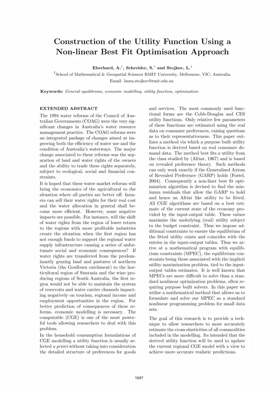
Random price data was generated for 20 sam-ples of commodity bundles of size 2. The de-mand data was obtained for both commoditiesby maximising the Cobb-Douglas utility func-tion subject to the pricing constraint. The firstpricing samples give X1 and X2 as 0.8 and 0.6respectively where this represents the system atequilibrium. Small randomness in the demanddata was added to each commodity demand asto model small “hiccup” in the system or pos-sible errors in the data gathering process. Inall simulations we do not perturb the first datavalue as this represents the true state of thesystem and this value has been circled in bluein our plots. The parameter α was varied todemonstrate uniform shares, biased shares to-wards commodity X1 and strongly biased sharestowards commodity X1.

0 2 4 6 80

2

4

6

8

X1

X 2

Cobb−Douglas

2

22 2

4

44

6

6

0 2 4 6 80

2

4

6

8

X1

X 2

U−MPEC

0

2

22

4

44 4

6

6

Figure 1. Equal shares of commodities X1

and X2 with α = 0.50.

The level curves show indifference towards com-modity bundles and it can be concluded that theconsumers satisfaction will be reached by any

1050

choice made along the level curve. A consumerwill always choose to maximise utility thereforea commodity bundle that sits on the upmostlevel curve that intersects the budget constraintwill always be chosen. For the 20 samples cho-sen a combined value of commodities 1 and 2 areconsumed to maximise consumer utility basedon the pricing bundle.

In Figure 1 a uniform distribution of householdshares of commodities 1 and 2 is displayed. The“true” optimal value (X1, X2) = (0.8, 0.6) iscontained in the blue circle. The U-MPEC util-ity gives a similar curve to the Cobb-Douglaswhere the data is more congested. As the datadisperses the utility approximation flattens out.

0 2 4 6 80

2

4

6

8

X1

X 2

Cobb−Douglas

2

22 2

4

4

4

6

6

0 2 4 6 80

2

4

6

8

X1

X 2

U−MPEC

0

2

2

4

44

6

6

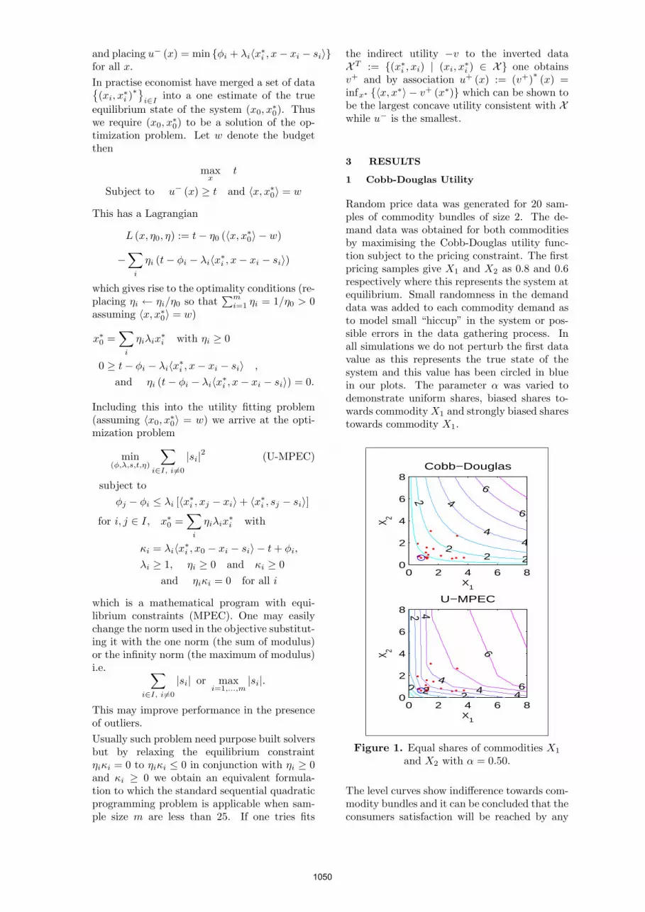
Figure 2. Biased shares of commodity X1

with α1 = 0.67 and α2 = 0.33.

In Figure 2 demand with a biased towards com-modity X1 has shifted data so that utility ismaximised for larger quantities of commodityX1 with less of commodity X2 consumed. The“true” optimal value (X1, X2) = (1.1, 0.4) iscontained in the blue circle. Level curves inboth graphs decline more steeply to accom-modate the shift in demand. The utility ap-proximation is comparing well with the Cobb-Douglas utility.

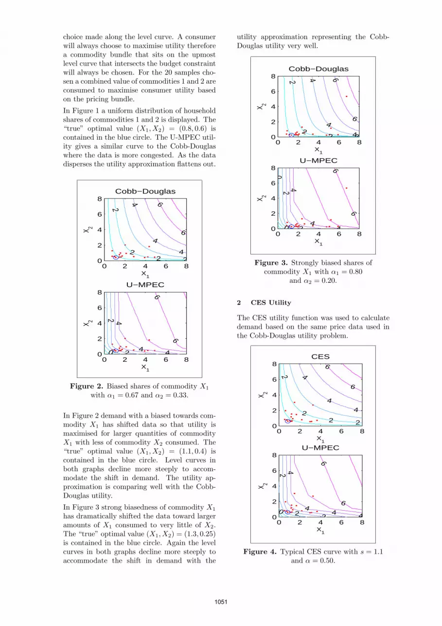
In Figure 3 strong biasedness of commodity X1

has dramatically shifted the data toward largeramounts of X1 consumed to very little of X2.The “true” optimal value (X1, X2) = (1.3, 0.25)is contained in the blue circle. Again the levelcurves in both graphs decline more steeply toaccommodate the shift in demand with the

utility approximation representing the Cobb-Douglas utility very well.

0 2 4 6 80

2

4

6

8

X1

X 2

Cobb−Douglas

2

22 2

44

4

66

0 2 4 6 80

2

4

6

8

X1

X 2

U−MPEC0

0

2

2

4

44

6

6

Figure 3. Strongly biased shares ofcommodity X1 with α1 = 0.80

and α2 = 0.20.

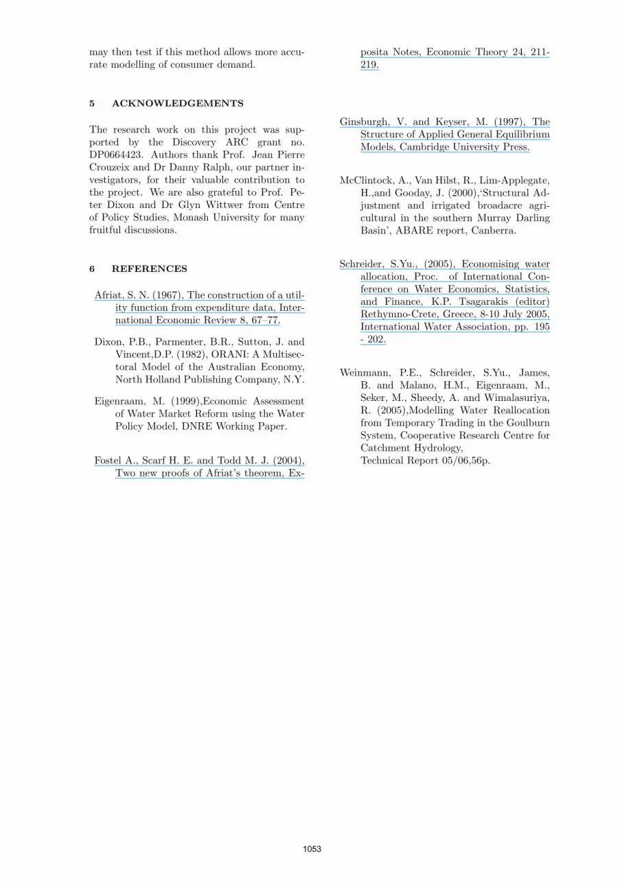
2 CES Utility

The CES utility function was used to calculatedemand based on the same price data used inthe Cobb-Douglas utility problem.

0 2 4 6 80

2

4

6

8

X1

X 2

CES

2

22 2

4

4

4

6

6

0 2 4 6 80

2

4

6

8

X1

X 2

U−MPEC

0

2

2 2

4

44 4

6

6

Figure 4. Typical CES curve with s = 1.1and α = 0.50.

1051

Typically s is chosen to be 1.1 as it closelyrepresents the Cobb-Douglas utility functionwith slightly greater price elasticity of demand.Hence a 10% increase in price will lead to a 11%decrease in demand. In Figure 4 the CES util-ity approaches unitary elasticity as the valueof s is close to 1. The “true” optimal value(X1, X2) = (0.8, 0.6) is contained in the bluecircle.The U-MPEC has compares well with thelevel curves of the CES utility around the regionof the data set but the approximation appearsto degrade as we move away from the regionwithin which the simulated data falls.

0 2 4 6 80

2

4

6

8

X1

X 2

CES

2

2 2 2

4

4 4

6

6

0 2 4 6 80

2

4

6

8

X1

X 2

U−MPEC

0

2

2 24

4 4 4

6

66

8

Figure 5. Leontief type curve with s = 0.1and α = 0.50.

In Figure 5 the commodities are treated areperfect substitutes hence the level curves are Lshaped and data points are bundled togetherat the base of the curve. The consumer willonly increase utility if they can increase bothcommodities jointly. The U-MPEC has also ad-justed the shape of level curves to fit the givendata. Noting the outlier in the data has oc-curred due to small price data being generatedfor both commodities X1,X2 hence allowing theconsumer to increase buying power. The “true”optimal value (X1, X2) = (0.8, 0.6) is containedin the blue circle. Again the approximation isgood close to the cluster of simulated data val-ues but degrades as we move far away from thesevalues.

4 DISCUSSION AND CONCLUSION

Consumers try to maximise their utility (satis-faction) level given a budget constraint. How-

ever, generalised utility functions like the Cobb-Douglas and the CES studied in this paper forcethe demand data to fit the desired curve basedon preconceptions of consumer choices. Incon-sistences in consumer choices and randomness incommodity selection are not considered. Datais only used from the Input-Output table to cal-culate share values of commodities. In this casethe household share value was calculated as theamount of a commodity used with respect tototal household spending.

The U-MPEC formulated has allowed the userto fit the function to given data using the 2 normwithout constraining consumer choices to givendemand functions. It is unrealistic to assumethat all consumers demand follows a Cobb-Douglas unitary price elasticity of demand whenmany consumer choices are much more complex.In the case of perfect substitutes, consumers arerepresented as being indifferent to the choice ofa commodity provided they are similar. Manyexamples given in text books describe Coca-Cola and Pepsi as perfect substitutes. Suppos-edly consumers are indifferent to the choice be-tween the two commodities provided the priceis within budget.

The small, artificially generated samples havebeen used to demonstrated the ability of the U-MPEC utility function to fit two commonly usedutility functions. Qualitatively the U-MPECutility compares surprisingly well to these givenutility functions, considering that such a smallsample size was used. This is particular true forthe Cobb–Douglas utility. For the CES utilitythe approximates appears to be best within theregion that the data is clustered. It is conjec-tured that the good quality of the U-MPEC ap-proximation is due to the highly constrained na-ture of the MPEC optimisation problem. Thussmall amounts of data appear to be sufficient toreplicate some of the general utility functionscommonly used although further studies will beneed to confirm this beyond reasonable doubt.Further studies in substituting the norm usedin the objective function to the 1 or infinitynorm will determine whether in fact it may im-prove performance in the presence of outliers. Itwould be desirable to develop a statistical the-ory to estimate errors that result from the prop-agation of random fluctuations in data values toour utility approximation.

Due to the inability to apply standard optimiza-tion algorithms to solve the U-MPEC problemfor larger samples, the next step is to develop apurpose built solver for larger data sets. Thiswill be important to further test our approxima-tion method and important in order to applythis method to the regional CGE model. We

1052

may then test if this method allows more accu-rate modelling of consumer demand.

5 ACKNOWLEDGEMENTS

The research work on this project was sup-ported by the Discovery ARC grant no.DP0664423. Authors thank Prof. Jean PierreCrouzeix and Dr Danny Ralph, our partner in-vestigators, for their valuable contribution tothe project. We are also grateful to Prof. Pe-ter Dixon and Dr Glyn Wittwer from Centreof Policy Studies, Monash University for manyfruitful discussions.

6 REFERENCES

Afriat, S. N. (1967), The construction of a util-ity function from expenditure data, Inter-national Economic Review 8, 67–77.

Dixon, P.B., Parmenter, B.R., Sutton, J. andVincent,D.P. (1982), ORANI: A Multisec-toral Model of the Australian Economy,North Holland Publishing Company, N.Y.

Eigenraam, M. (1999),Economic Assessmentof Water Market Reform using the WaterPolicy Model, DNRE Working Paper.

Fostel A., Scarf H. E. and Todd M. J. (2004),Two new proofs of Afriat’s theorem, Ex-

posita Notes, Economic Theory 24, 211-219.

Ginsburgh, V. and Keyser, M. (1997), TheStructure of Applied General EquilibriumModels, Cambridge University Press.

McClintock, A., Van Hilst, R., Lim-Applegate,H.,and Gooday, J. (2000),‘Structural Ad-justment and irrigated broadacre agri-cultural in the southern Murray DarlingBasin’, ABARE report, Canberra.

Schreider, S.Yu., (2005), Economising waterallocation, Proc. of International Con-ference on Water Economics, Statistics,and Finance, K.P. Tsagarakis (editor)Rethymno-Crete, Greece, 8-10 July 2005,International Water Association, pp. 195- 202.

Weinmann, P.E., Schreider, S.Yu., James,B. and Malano, H.M., Eigenraam, M.,Seker, M., Sheedy, A. and Wimalasuriya,R. (2005),Modelling Water Reallocationfrom Temporary Trading in the GoulburnSystem, Cooperative Research Centre forCatchment Hydrology,Technical Report 05/06,56p.

1053