constraints on decaying dark matter from xmm–newton

Mon. Not. R. Astron. Soc. 387, 1361–1373 (2008) doi:10.1111/j.1365-2966.2008.13266.x

Constraints on decaying dark matter from XMM–Newton observationsof M31

Alexey Boyarsky,1,2� Dmytro Iakubovskyi,2 Oleg Ruchayskiy3

and Vladimir Savchenko2,4

1PH-TH, CERN, CH-1211 Geneve 23, Switzerland2Bogolyubov Institute for Theoretical Physics, Kiev 03780, Ukraine3Ecole Polytechnique Federale de Lausanne, Institute of Theoretical Physics, FSB/ITP/LPPC, BSP 720, CH-1015 Lausanne, Switzerland4Department of Physics, Kiev National Taras Shevchenko University, Kiev 03022, Ukraine

Accepted 2008 March 19. Received 2008 February 4; in original form 2007 September 25

ABSTRACTWe derive constraints on the parameters of the radiatively decaying dark matter (DM) particle,

using the XMM–Newton EPIC spectra of the Andromeda galaxy (M31). Using the observations

of the outer (5–13 arcmin) parts of M31, we improve the existing constraints. For the case of

sterile neutrino DM, combining our constraints with the latest computation of abundances of

sterile neutrinos in the Dodelson–Widrow (DW) scenario, we obtain the lower mass limit ms <

4 keV, which is stronger than the previous one ms < 6 keV, obtained recently by Asaka, Laine

& Shaposhnikov. Comparing this limit with the most recent results on Lyman α forest analysis

of Viel et al. (ms > 5.6 keV), we argue that the scenario in which all the DM is produced via

the DW mechanism is ruled out. We discuss, however, other production mechanisms and note

that the sterile neutrino remains a viable candidate for DM, either warm or cold.

Key words: methods: data analysis – galaxies: individual: Andromeda galaxy – dark matter

– X-rays: individual: Andromeda galaxy.

1 I N T RO D U C T I O N

A vast body of evidence points to the existence of dark matter (DM)

in addition to the ordinary visible matter in the Universe. The ev-

idence include: velocity curves of galaxies in clusters and stars in

galaxies, observations of galaxy clusters in X-rays, gravitational

lensing data and cosmic microwave background anisotropies. While

the DM contributes some 22 per cent to the total energy density in

the Universe, its properties remain largely unknown.

The standard model (SM) of particle physics does not provide a

DM candidate. The DM cannot be made out of baryons as such an

amount of baryonic matter cannot be generated in the framework of

an otherwise successful scenario of big bang nucleosynthesis (Dar

1995). In addition, current microlensing experiments exclude the

possibility that massive compact halo objects (MACHOs) constitute

the dominant amount of the total mass density in the local halo

(Gates, Gyuk & Turner 1995; Alcock et al. 2000; Lasserre et al.

2000). The only possible non-baryonic DM candidate in the SM

could be the neutrino; however, this possibility is ruled out by the

present data on the large-scale structure (LSS) of the Universe.

What properties of the DM particles can be deduced from exist-

ing observations? Some information comes from studies of structure

formation. Namely, the velocity distribution of the DM particles at

the time of structure formation greatly affects the power spectrum

�E-mail: [email protected]

of density perturbations, as measured by a variety of experiments

(see e.g. Tegmark et al. 2004). One of the parameters, characterizing

the influence of the DM velocity dispersion on the power spectrum,

is the free-streaming length λFS – the distance travelled by the DM

particle from the time when it became non-relativistic until today.

Roughly speaking, the free-streaming length determines the mini-

mal scale at which the Jeans instability can develop, and therefore

non-trivial free-streaming implies modification of the spectrum of

density perturbations at wavenumbers k � λ−1FS .

If the DM particles have negligible velocity dispersion, they con-

stitute the so-called cold DM (CDM), which forms structure in a

‘bottom-up’ fashion (i.e. smaller scale objects formed first and then

merged into the larger ones, see e.g. Peebles 1980). The neutrino

DM represents the opposite case – hot DM (HDM). In HDM sce-

narios, structure forms in a top-down fashion (Zel’dovich 1970),

and the first structures to collapse have size comparable to the Hub-

ble scale (Bisnovatyi-Kogan 1980; Bond, Efstathiou & Silk 1980;

Doroshkevich et al. 1981; Bond & Szalay 1983). In this scenario,

the galaxies do not have enough time to form, contradicting to the

existing observations (see e.g. White, Frenk & Davis 1983; Peebles

1984).

Warm DM (WDM) represents an intermediate case, cutting struc-

ture formation at some scale, with the details being dependent on a

particular WDM model.

Both WDM and CDM fit the LSS data equally well. The dif-

ferences appear when one starts to analyse the details of struc-

ture formation for galaxy-sized objects (modifications of the power

C© 2008 The Authors. Journal compilation C© 2008 RAS

Dow

nloaded from https://academ

ic.oup.com/m

nras/article/387/4/1361/1086030 by guest on 27 March 2022

1362 A. Boyarsky et al.

spectrum at momenta k � 0.5 h Mpc−1). It is usually said that WDM

predicts ‘less power at smaller scales’, meaning in particular that one

expects smaller number of dwarf satellite galaxies and shallower

density profiles than those predicted by CDM models (Navarro,

Frenk & White 1997; Klypin et al. 1999; Ghigna et al. 2000). Thus,

WDM models can provide the way to solve the ‘missing satellite’

problem and the problem of central density peaks in galaxy-sized

DM haloes (Klypin et al. 1999; Moore et al. 1999; Avila-Reese et al.

2001; Bode, Ostriker & Turok 2001).

There exist a number of direct astrophysical observations which

seem to contradict the N-body simulations of galaxy formations,

performed in the framework of the CDM models (e.g. Diemand,

Kuhlen & Madau 2007; Strigari et al. 2007). Namely, direct mea-

surements of the DM density profiles in dwarf spheroidal (dSph)

satellites of the Milky Way favour cored profiles (Gilmore 2007;

Gilmore et al. 2007; Wu 2007).1 The number of dwarf satellite

galaxies, as currently observed, is still more than an order of mag-

nitude below the CDM predictions, in spite of the drastically im-

proved sensitivity towards the search (see Gilmore et al. 2007; Ko-

posov et al. 2007) and resolution of numerical simulations (Stri-

gari et al. 2007). There seems to exist a smallest scale (∼120 pc)

at which the DM is observed (Gilmore 2007; Gilmore et al. 2007).

However, as of now there is no definitive statement about the

‘CDM substructure crisis’ [see Simon & Geha (2007) in regard

to the smallest observed DM scale and Penarrubia, McConnachie &

Navarro (2008) for an alternative solution of the ‘missing satellite

problem’].

The power spectrum of density perturbations at scales of interest

for the WDM versus CDM issue can also be studied, analysing the

Lyman α forest data (absorption feature by the neutral hydrogen at

λ = 1216 Å at different redshifts in the distant quasar spectra, Hui,

Gnedin & Zhang 1997). This involves comparison of the observed

spectra of Lyman α absorption lines with those obtained as a result

of numerical simulations in various DM models. In this way, one

arrives at an upper limit on the free-streaming length of the DM

particles.

Various particle physics models provide WDM candidates. Pos-

sible examples include gravitinos and axinos in various supersym-

metric models (see e.g. Baltz & Murayama 2003; Cembranos et al.

2006; Seto & Yamaguchi 2007). Another WDM candidate is the

sterile neutrino with a mass in the keV range (Dodelson & Widrow

1994). Recently, this candidate received a lot of attention. Namely,

an extension of the minimal SM (MSM) with the three right-handed

neutrinos was suggested (Asaka & Shaposhnikov 2005; Asaka,

Blanchet & Shaposhnikov 2005). This extension (called νMSM)

explains several observed phenomena beyond the MSM under the

minimal number of assumptions. Namely, apart from the absence

of the DM candidate, the MSM fails to explain observed neutrinooscillations – the transition between neutrinos of different flavours

(for a review see e.g. Fogli et al. 2006; Strumia & Vissani 2006;

Giunti 2007). The explanation of this phenomenon is the existence

of neutrino mass. The most natural way to provide this mass is to

add right-handed neutrinos. Indeed, in the MSM, neutrinos are left

handed (all other fermions have both left- and right-handed coun-

terparts) and strictly mass less. The structure of the MSM dictates

that right-handed neutrinos, if added to the theory, would not be

charged with respect to any SM interactions and interact with other

1 For certain dSph, cusped profiles are still admissible, but disfavoured. Ad-

ditional considerations rule out the possibility of existence of cusped profiles

for the Ursa Minor and Fornax (Kleyna et al. 2003a,b; Goerdt et al. 2006;

Sanchez-Salcedo, Reyes-Iturbide & Hernandez 2006).

matter only via mixing with the usual (left handed) neutrinos (that

is why right-handed neutrinos are often called sterile neutrinos to

distinguish them from the left-handed active ones). Moreover, as

demonstrated by Asaka & Shaposhnikov (2005), the parameters

of added right-handed neutrinos can be chosen in such a way that

such a model resolves another problem of the MSM – it explains

the excess of baryons over antibaryons in the Universe (the baryonasymmetry), while at the same time it does not spoil the predictions

of big bang nucleosynthesis. For this to be true, the masses of two

of these sterile neutrinos should be chosen in the range 300 MeV �M2,3 � 20 GeV, while the mass of the third (lighter) sterile neutrino

is arbitrary (as long as it is below M2,3). In particular, its mass can

be in the keV range, providing the WDM candidate. Such a sterile

neutrino can be produced in the early Universe in the correct amount

via various mechanisms: via non-resonant oscillations with active

neutrinos (Dodelson & Widrow 1994; Abazajian, Fuller & Patel

2001; Dolgov & Hansen 2002; Asaka, Laine & Shaposhnikov 2006,

2007), via interaction with the inflaton (Shaposhnikov & Tkachev

2006), via resonant oscillations in the presence of lepton asymme-

tries (Shi & Fuller 1999, hereafter SF) and have cosmologically long

lifetime.

Finally, the sterile neutrino with mass in the keV range would

have other interesting astrophysical applications (see e.g. Sommer-

Larsen & Dolgov 2001; Biermann & Kusenko 2006; Hidaka &

Fuller 2006; Kusenko 2006; Hidaka & Fuller 2007; Stasielak,

Biermann & Kusenko 2007, and references therein).

1.1 Existing bounds on sterile neutrino DM

The mass of the sterile neutrino DM should satisfy the universal

Tremaine–Gunn lower bound (Tremaine & Gunn 1979; Dalcanton

& Hogan 2001): ms � 300–500 eV. A stronger (although model

dependent) lower bound comes from the Lyman α forest analysis.

Assuming a particular velocity distribution of the sterile neutrino,2

one can obtain a relation between the DM mass and λFS, and there-

fore convert an upper bound on the free-streaming length to a lowerbound on the mass of the sterile neutrino. In the recent works of

Seljak et al. (2006) and Viel et al. (2006), this bound was found

to be 14 keV (correspondingly 10 keV) at 95 per cent confidence

level in the Dodelson–Widrow (DW) production model (Dodelson &

Widrow 1994). New results from quasi-stellar object (QSO) lensing

give similar restrictions for the DW model: ms � 10 keV (Miranda

& Maccio 2007). For different models of production, the relation

between the DM mass and the free-streaming length is different

and the Lyman α mass bound for sterile neutrinos can be as low as

Ms > 2.5 keV (see e.g. Ruchayskiy 2007).3

The sterile neutrino DM is not completely stable. In particular, it

has a radiative decay channel into an active neutrino and a photon,

emitting a monoenergetic photon with energy Eγ = ms/2 (where

ms is the mass of the sterile neutrino). As a result, the (indirect)

search for the DM decay line in the X-ray spectra of objects with

large DM overdensity becomes an important way to restrict the pa-

rameters (mass and decay width) of sterile neutrino DM. During the

2 Sterile neutrinos are not in thermal equilibrium in the early Universe and

therefore their velocity distribution is non-universal and depends on the

model of production.3 Strictly speaking, in case of other models of production, the power spectrum

of density fluctuations is characterized by not only the free-streaming length.

Therefore, the rescaling of the results of Seljak et al. (2006) and Viel et al.

(2006) can be used only as the estimates and the reanalysis of the Lyman α

data for the case of each model is required.

C© 2008 The Authors. Journal compilation C© 2008 RAS, MNRAS 387, 1361–1373

Dow


ic.oup.com/m


Constraints on decaying dark matter from M31 1363

last two years, a number of papers appeared devoted to this task:

Boyarsky et al. (2006a,b,c), Boyarsky, Ruchayskiy & Markevitch

(2008), Riemer-Sørensen, Hansen & Pedersen (2006), Watson

et al. (2006, hereafter W06), Boyarsky et al. (2007a), Boyarsky,

Nevalainen & Ruchayskiy (2007b) and Abazajian et al. (2007). The

current status of these observations is summarized, for example, in

Ruchayskiy (2007). The results of the computation of sterile neu-

trino production in the early Universe (Asaka et al. 2007), combined

with these X-ray bounds, put an upper bound on the sterile neutrino

mass of ms < 6 keV (Asaka et al. 2007). This is below the lowerbound on the sterile neutrino DM mass from the Lyman α forest

analysis of Seljak et al. (2006) and Viel et al. (2006). Thus, it would

seem that the scenario, in which all the sterile neutrino DM is pro-

duced via the DW mechanism, is ruled out [the recent work by

Palazzo et al. (2007) also explored the possibility that the sterile

neutrino, produced through DW scenario, constitutes but a fraction

of DM and found this fraction to be below 70 per cent]. However,

the results of Seljak et al. (2006) and Viel et al. (2006) are based on

the low-resolution Sloan Digital Sky Survey (SDSS) Lyman α data

set of McDonald et al. (2006). It was recently shown by Viel et al.

(2008) that by using High-Resolution Echelle Spectrometer spectra

(Becker, Rauch & Sargent 2007) one arrives at the lower limit ms

> 5.6 keV. Thus, the small window of masses 5.6 < ms < 6 keV

remains open in the DW model. Therefore, further improvement of

X-ray bounds is crucial for exploring (and possibly closing) this

region of parameters.

It was shown in Boyarsky et al. (2006c) that the objects in the

local halo (e.g. dwarf spheroidal galaxies) are the best objects in

terms of the signal-to-noise ratio. The Andromeda galaxy (M31)

is one of the nearest galaxies, excluding dwarves, that enables one

to resolve most of its bright point sources and extract the spectrum

of its diffuse emission. It also has a massive and well-studied DM

halo (e.g. Klypin, Zhao & Somerville 2002; Widrow & Dubinski

2005; Geehan et al. 2006; Tempel, Tamm & Tenjes 2007). The first

step in such an analysis was done by W06, who analysed the dif-

fuse emission from the 5 central arcmin, using the data processed

by Shirey et al. (2001). We repeat the analysis of the central part

of the M31, processing more observations, and extend the analysis

to the off-centre region (5–13 arcmin). We also analyse the uncer-

tainties in the DM distribution in the central part of M31. The outer

region of M31 has much fainter diffuse emission than its central part

(cf. e.g. Takahashi et al. 2004), and uncertainties in the determining

of the distribution of DM in this region are lower. All this allows us

to strengthen the restrictions on the parameters of sterile neutrino

DM, while using more conservative estimates of the DM signal.

The paper is organized as follows. We briefly summarize the

properties of decaying DM in Section 2. The description of DM

in M31 and expected DM decay flux is computed in Section 3.

In Section 4, we describe the methodology of EPIC MOS and PN

data reduction which we perform by using two different methods:

Extended Sources Analysis Software (ESAS) and single background

subtraction method (SBS). In Section 5, we fit the spectra and obtain

the restrictions on sterile neutrino parameters. Finally, we discuss

our results in Section 6.

2 D E C AY I N G DA R K M AT T E R M O D E L

The flux of the DM decay from a given direction (in photons s−1

cm−2) is given by

FDM = �Eγ

ms

∫fov cone

ρDM(r )

4π|DL + r |2 d r . (1)

Here, DL is the luminosity distance between an observer and the

centre of an observed object, ρDM(r ) is the DM density and the inte-

gration is performed over the DM distribution inside the (truncated)

cone – solid angle, spanned by the field of view (FoV) of the X-ray

satellite. In case of distant objects,4 equation (1) can be simplified

as

FDM = M fovDM�

4πD2L

Eγ

ms

, (2)

where MfovDM is the mass of DM within a telescope FoV, ms – mass

of the sterile neutrino DM. In the case of small FoV, equation (2)

simplifies to

FDM = �SDMEγ

4πms

, (3)

where

SDM =∫

l.o.s.

ρDM(r ) dr (4)

is the DM column density [the integral goes along the line of sight

(l.o.s.)], � 1 – FoV solid angle.

The decay rate of the sterile neutrino DM is equal to (Pal &

Wolfenstein 1982; Barger, Phillips & Sarkar 1995):5

� = 9αG2F

1024π4sin2(2θ )m5

s ≈ 1.38 × 10−30s−1

[sin2(2θ )

10−8

][ms

1 keV

]5

.

(5)

Here, ms is the sterile neutrino mass, θ – mixing angle between sterile

and active neutrinos. From a compact cloud of sterile neutrino DM,

we therefore obtain the flux

FDM ≈ 6.38 × 106 keV

cm2 s

(M fov

dm

1010 M�

)(kpc

DL

)2

sin2(2θ)

(ms

1 keV

)5

.

(6)

3 A N D RO M E DA G A L A X Y ( M 3 1 )

M31, or Andromeda galaxy, is one of the nearest galaxies, excluding

dwarves; it is located at the distance DL = 784 ± 13 ± 17 kpc (Stanek

& Garnavich 1998). Its proximity allows us to resolve most of its

point sources and extracts the spectrum of diffuse emission of its

central part.

Available XMM–Newton (Jansen et al. 2001) observations cover

the region of central 15 arcmin of M31 with exposure time greater

than 100 ks (see Table 1). W06 used the XMM–Newton data on cen-

tral 5 arcmin of M31 [observation 0112570401 processed by Shirey

et al. (2001), exposure time about 30 ks] to produce restrictions on

the parameters of sterile neutrino DM. The sufficient increase of

photon statistics enables us to analyse the outer (5–13 arcmin) faint

part of M31, which, however, has a significant mass of DM (see

Section 3.1 below).

In this work, we will analyse two different spatial regions of

Andromeda galaxy: region circle5, which corresponds to 5 arcmin

circle around the centre of M31, and region ring5-13, which cor-

responds to the ring with inner and outer radii of 5 and 13 arcmin,

respectively.

4 Namely, if luminosity distance DL is much greater than the characteristic

scale of the DM distribution.5 Our decay rate is two times smaller than the one used in W06. This is due

to the Majorana nature of the sterile neutrino, which we consider (cf. Barger

et al. 1995). The final constraints for a Dirac particle would thus be two

times stronger.


Dow


ic.oup.com/m



Table 1. Observations of the central part of M31, used in our analysis.

Cleaned MOS1/

Starting time MOS2/PN

Observation ID (UTC) Filter exposure (ks)

0112570401 2000 June 25 08:12:41 Medium 30.8/31.0/27.6

0109270101 2001 June 29 06:15:17 Medium 40.1/41.9/47.4

0112570101 2002 January 06 18:00:56 Thin 63.0/63.0/55.3

3.1 Calculation of DM mass

To obtain the restriction on parameters of the decaying DM, we

should calculate the total DM mass Mfovdm, which corresponds to both

spatial regions: circle5 and ring5-13, both with and without resolved

point sources. To estimate the systematic uncertainties of the eval-

uation of the DM decay signal and to find the most conservative

estimate for it, we analyse various available DM profiles (Kerins

et al. 2001; Klypin et al. 2002; Widrow & Dubinski 2005; Carignan

et al. 2006; Geehan et al. 2006; Tempel et al. 2007).

(i) K1. Before6 adiabatic contraction stage, Klypin et al. (2002)

assume that DM distribution is purely Navarro–Frenk–White

(NFW) (Navarro et al. 1997):

ρDM(r ) = 1

4π[log(1 + C) − C/(1 + C)

] Mvir

r (r + rs)2. (7)

The parameters of this NFW distribution (in terms of the favoured

C1 model of Klypin et al. 2002) are: Mvir = 1.60 × 1012 M�, rs =25.0 kpc and C = 12.

(ii) K2. This non-analytical model is the result of adiabatic con-

traction of the K1 profile, described above. To obtain it, we extract

the data from the fig. 4 of Klypin et al. (2002). In the top part of this

figure, the dot–dashed curve is the contribution of the DM halo to

the total M31 mass distribution (C1 model of Klypin et al. 2002). As

the precise form of this mass distribution is not analytic, we scanned

this curve and produced the file with numerical values of enclosed

mass MDM(r) within the sphere of radius r. After that we interpolated

the MDM(r), and evaluated the radial density distribution:

ρDM(r ) = 1

4πr 2

dMDM(r )

dr. (8)

(iii) GFBG. Preferred NFW distribution from Geehan et al.

(2006): Mvir = 6.80 × 1011 M�; rs = 8.18 kpc and C = 22.

(iv) KER. Isothermal profile used in Kerins et al. (2001):

ρKER(r ) ={

ρh(0) a2

a2+r2 r � Rmax,

0 r > Rmax,(9)

where ρh(0) = 0.23 M� pc−3, a = 2 kpc and Rmax = 200 kpc.

(v) M31A–C. Profiles of Widrow & Dubinski (2005). In this pa-

per, the authors propose several models which differ by the relative

disc/halo contribution. These non-analytical models (M31a–d) in-

corporate an exponential disc, a Hernquist model bulge, an NFW

halo (before contraction) and a central supermassive black hole. The

stability against the formation of bars was numerically studied.7

6 In contrast to the other models, this model does not describe the current

DM distribution, but helps our understanding the time evolution of DM mass

inside constant FoV.7 We do not use the fourth model (M31d) because in Widrow & Dubinski

(2005) it was found that this model develops a bar, which rules it out

experimentally.

We also use density distributions from the recent paper of Tempel

et al. (2007). The main aim of this paper is to derive the DM den-

sity distribution in the central part of M31 (0.02–35 kpc from the

centre).

(i) KING. Modified isothermal profile (King 1962; Einasto et al.

1974):

ρI SO (r ) =

⎧⎨⎩ ρ0

[(1 + r2

r2c

)−1

−(

1 + r20

r2c

)−1]

r � r0,

0 r > r0,

(10)

where ρ0 = 0.413 M� pc−3, rc = 1.47 kpc and r0 = 117 kpc.

(ii) MOORE. Moore profile (Moore et al. 1999):

ρMOORE(r ) = ρc(rrc

)1.5[

1 + (rrc

)1.5] , (11)

where ρc = 4.43 × 10−3 M� pc−3 and rc = 17.9 kpc.

(iii) N04. Density distribution of Navarro et al. (2004):

ρN04(r ) = ρc exp

[− 2

α

(rα

rαc

− 1

)], (12)

where parameter α, according to simulations, is equals to 0.172 ±0.032 (Navarro et al. 2004). For N04, we take α = 0.17, ρc =6.42 × 10−3 M� pc−3 and rc = 11.6 kpc.

(iv) NFW. NFW profile:

ρNFW(r ) = ρc

rrc

[1 + (

rrc

)2] , (13)

where ρc = 5.20 × 10−2 M� pc−3 and rc = 8.31 kpc.

(v) BURK. Burkert profile (Burkert 1995):

ρBURK(r ) = ρ0(1 + r

rc

)(1 + r2

r2c

) , (14)

where ρ0 = 0.335 M� pc−3 and rc = 3.43 kpc.

The computed DM masses within the FoV for all these profiles

are shown in Table 2. We see that for the model used by W06

(model K2 in our notations), our estimate of the DM mass within

the central 5 arcmin coincides with the value used in W06: M5 =(1.3 ± 0.2) × 1010 M�. Note, however, that to obtain the diffuse

spectrum, we extracted all point sources resolved with the signifi-

cance �4σ . Each source was removed with the circle of the radius

of 36 arcsec (see Section 4.1 for details). This leads to the reduc-

tion of the area of the FoV by about 70 per cent in case of circle5region (cf. Fig. 1). As the density of the DM changes with the off-

centre distance and this change can be significant (cf. Fig. 2), we

performed the integration of the DM density distribution over the

FoV with excluded point sources. To calculate the DM mass in such

‘swiss cheese’ regions (Fig. 1), we used Monte Carlo integration.

The results are summarized in the Table 3.

To check possible systematic effects of our Monte Carlo integra-

tion method, we also obtained the values of enclosed mass inside

the 13 arcmin sphere, and compared them with analytical calcula-

tions (wherever possible). Such an error does not exceed the purely

statistical error of numerical integration (see Table 2).

As one can see from Tables 2–3, the most conservative DM

model, describing regions circle5 and ring5-13, is the model M31Bof Widrow & Dubinski (2005). Therefore, to obtain restrictions on

the DM parameters in what follows, we will use the DM mass esti-

mates based on this model.


Dow


ic.oup.com/m



Table 2. DM mass (in 109 M�) inside regions, used in our analysis: results of our Monte Carlo integration. The point sources are not excluded here. The

95 per cent statistical errors are also shown. The DM distributions of Klypin et al. (2002) (before and after adiabatic contraction), Geehan et al. (2006) and

Kerins et al. (2001) are marked as ‘K1’, ‘K2’, ‘GFBG’ and ‘KER’, respectively. The DM distributions from Tempel et al. (2007) are marked as ‘KING’,

‘MOORE’, ‘N04’, ‘NFW’ and ‘BURK’ (see the text). The DM distributions from Widrow & Dubinski (2005) are marked as ‘M31A’, ‘M31B’ and ‘M31C’.

Model circle5 ring5-13 13 arcmin sphere, MC result 13 arcmin sphere, analytical result

K1, with sources 3.27 ± 0.01 12.49 ± 0.03 5.84 ± 0.02 5.84

K2, with sources 11.88 ± 0.03 23.75 ± 0.09 20.76 ± 0.09 –

GFBG, with sources 6.59 ± 0.02 20.46 ± 0.06 13.40 ± 0.03 13.39

KING, with sources 6.68 ± 0.01 24.61 ± 0.05 14.80 ± 0.02 14.80

MOORE, with sources 7.34 ± 0.02 19.48 ± 0.02 13.79 ± 0.02 13.78

N04, with sources 7.68 ± 0.03 22.89 ± 0.07 15.16 ± 0.06 15.18

NFW, with sources 11.08 ± 0.04 40.5 ± 0.1 22.3 ± 0.1 22.25

BURK, with sources 6.71 ± 0.02 27.97 ± 0.03 15.90 ± 0.05 15.90

KER, with sources 5.35 ± 0.02 22.45 ± 0.04 11.56 ± 0.03 11.56

M31A, with sources 5.95 ± 0.01 16.45 ± 0.02 11.03 ± 0.02 –

M31B, with sources 4.99 ± 0.01 14.24 ± 0.01 9.40 ± 0.02 –

M31C, with sources 5.60 ± 0.01 16.12 ± 0.01 10.29 ± 0.02 –

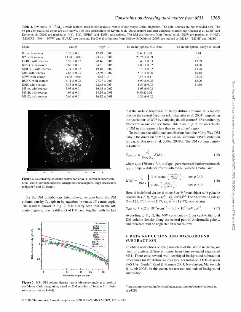
Figure 1. Selected regions in the central part of M31 (shown in linear scale).

Small circles correspond to excluded point source regions, large circles have

radius of 5 and 13 arcmin.

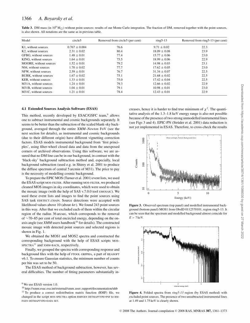
For the DM distributions listed above, we also build the DM

column density Sdm (given by equation 4) versus off-centre angle.

The result is shown in Fig. 2. It is clearly seen that, in the off-

centre regions, there is still a lot of DM, and, together with the fact

0.1

1

10

13 60 1 5 25

DM

co

lum

n d

en

sit

y (

g/c

m2)

Off-center angle, arcmin

K2GFBGKING

MOOREN04

NFWBURK

KERM31AM31BM31C

Figure 2. M31 DM column density versus off-centre angle as a result of

our Monte Carlo integration, based on DM profiles of Section 3.1. (Point

sources are not excluded).

that the surface brightness of X-ray diffuse emission falls rapidly

outside the central 5 arcmin (cf. Takahashi et al. 2004), improving

the restrictions of W06 by analysing the off-centre 5–13 arcmin ring.

Moreover, as one can see from Table 3 and Fig. 2, the uncertainty

of DM in this region is less than in the circle5 region.

To estimate the additional contribution from the Milky Way DM

halo in the direction of M31, we use an isothermal DM distribution

(as e.g. in Boyarsky et al. 2006c, 2007b). The DM column density

is equal to

SMW,DM = v2h

8πrcG NK (φ), (15)

where vh =170 km s−1, rc =4 kpc – parameters of isothermal model,

r� = 8 kpc – distance from Earth to the Galactic Centre, and

K (φ) = rc

R(φ)

⎧⎨⎩

π

2+ arctan

(r� cos φ

R(φ)

), cos φ � 0,

arctan

(R(φ)

r� cos φ

), cos φ < 0.

(16)

Here, φ is defined via cos φ = cos l cos b for an object with galactic

coordinates (b, l), R(φ) = (r2c + r2� sin2φ)1/2. For Andromeda galaxy

(l = 121.◦17, b = −21.◦57, i.e. φ = 118.◦77), one obtains

SMW,DM ≈ 6.2 × 10−3g cm−2 = 3.5 × 1027 keV cm−2. (17)

According to Fig. 2, the MW contributes <5 per cent to the total

DM column density along the central part of Andromeda galaxy,

and therefore will be neglected in what follows.

4 DATA R E D U C T I O N A N D BAC K G RO U N DS U B T R AC T I O N

To obtain restrictions on the parameters of the sterile neutrino, we

need to analyse diffuse emission from faint extended regions of

M31. There exist several well-developed background subtraction

procedures for the diffuse sources (see, for instance, XMM–NewtonSAS User Guide,8 Read & Ponman 2003; Nevalainen, Markevitch

& Lumb 2005). In this paper, we use two methods of background

subtraction.

8 http://xmm.esac.esa.int/external/xmm user support/documentation/sas

usg/USG


Dow


ic.oup.com/m



Table 3. DM mass (in 109 M�) without point sources: results of our Monte Carlo integration. The fraction of DM, removed together with the point sources,

is also shown. All notations are the same as in previous table.

Model circle5 Removed from circle5 (per cent) ring5-13 Removed from ring5-13 (per cent)

K1, without sources 0.767 ± 0.004 76.6 9.71 ± 0.02 22.3

K2, without sources 2.31 ± 0.02 80.4 18.09 ± 0.08 23.9

GFBG, without sources 1.48 ± 0.01 77.4 15.77 ± 0.06 23.0

KING, without sources 1.64 ± 0.01 75.5 18.99 ± 0.06 22.9

MOORE, without sources 1.52 ± 0.01 79.2 14.98 ± 0.03 23.1

N04, without sources 1.70 ± 0.02 77.7 17.62 ± 0.05 23.0

NFW, without sources 2.59 ± 0.01 76.7 31.34 ± 0.07 22.5

BURK, without sources 1.67 ± 0.02 75.1 21.68 ± 0.02 22.5

KER, without sources 1.33 ± 0.01 75.0 17.42 ± 0.04 22.5

M31A, without sources 1.24 ± 0.01 79.3 12.66 ± 0.02 22.9

M31B, without sources 1.04 ± 0.01 79.1 10.98 ± 0.01 23.0

M31C, without sources 1.21 ± 0.01 78.4 12.43 ± 0.01 22.9

4.1 Extended Sources Analysis Software (ESAS)

This method, recently developed by ESAC/GSFC team,9 allows

one to subtract instrumental and cosmic backgrounds separately. It

seems to be better than the subtraction of the scaled blank-sky back-

ground, averaged through the entire XMM–Newton FoV (see the

next section for details), as instrumental and cosmic backgrounds

(due to their different origin) have different vignetting correction

factors. ESAS models instrumental background from ‘first princi-

ples’, using filter-wheel closed data and data from the unexposed

corners of archived observations. Using this software, we are as-

sured that no DM line can be in our background, in contrast with the

‘black-sky’ background subtraction method and, especially, local

background subtraction (used e.g. in Shirey et al. 2001 to produce

the diffuse spectrum of central 5 arcmin of M31). The price to pay

is the necessity of modelling cosmic background.

To prepare the EPIC MOS (Turner et al. 2001) event lists, we used

the ESAS script MOS-FILTER. After running MOS-FILTER, we produced

cleaned MOS images in sky coordinates, which were used to obtain

the mosaic image (with the help of SAS v.7.0.0 tool EMOSAIC). We

used these event lists and images to find the point sources using

SAS task EDETECT CHAIN. Source detections were accepted with

likelihood values above 10 (about 4σ ). We found 243 point sources

in this way. After that we excluded each of them within the circular

region of the radius 36 arcsec, which corresponds to the removal

of ∼70–85 per cent of total encircled energy, depending on the on-

axis angle (see XMM users handbook10 for details). The constructed

mosaic image with detected point sources and selected regions is

shown in Fig. 1.

We obtained the MOS1 and MOS2 spectra and constructed the

corresponding background with the help of ESAS scripts MOS-

SPECTRA11 and XMM-BACK, respectively.

Finally, we grouped the spectra with corresponding response and

background files with the help of FTOOL GRPPHA, a part of HEASOFT

v6.1. To ensure Gaussian statistics, the minimum number of counts

per bin was set to be 50.

The ESAS method of background subtraction, however, has sev-

eral difficulties. The number of fitting parameters substantially in-

9 We use ESAS version 1.0.10 http://xmm.esac.esa.int/external/xmm user support/documentation/uhb11 To produce a correct redistribution matrix function (RMF) file, we

changed in the script MOS-SPECTRA option RMFGEN DETMAPTYPE=PSF to RM-

FGEN DETMAPTYPE=DATA SET.

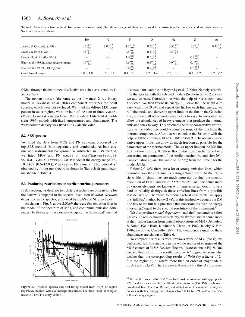
creases, hence it is harder to find true minimum of χ2. The quanti-

tative analysis of the 1.3–1.8 keV energy range is also not possible

because of the presence of two strong unmodelled instrumental lines

(see Figs 3 and 4). EPIC-PN (Struder et al. 2001) data reduction is

not yet implemented in ESAS. Therefore, to cross-check the results

0 5 10

10

100

1000

Counts

Energy (keV)

Observed (high), Particle Background (low)

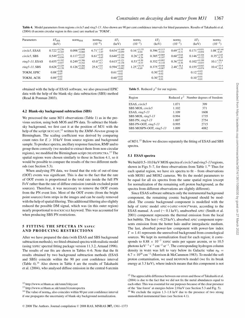
Figure 3. Observed spectrum (top panel) and modelled instrumental back-

ground (bottom panel) MOS1 from ObsID 0112570101, region ring5-13. It

can be seen that the spectrum and modelled background almost coincide for

E > 7 keV.

1 2 5

10

–4

10

–3

0.0

10.1

1

norm

aliz

ed c

ounts

/sec/k

eV

channel energy (keV)

Figure 4. Folded spectra from ring5-13 region (by ESAS method) with

excluded point sources. The presence of two unsubtracted instrumental lines

at 1.49 and 1.75 keV is clearly shown.


Dow


ic.oup.com/m



Table 4. Model parameters from regions circle5 and ring5-13. Also shown are 90 per cent confidence intervals for fitted parameters. Results of Takahashi et al.

(2004) (6 arcmin circular region in this case) are marked as ‘TOKM’.

Parameters kTdisk normdisk normbb kT1 norm1 kT2 norm2 kT3 norm3

(keV) (10−6) (keV) (10−3) (keV) (10−3) (keV) (10−3)

circle5, ESAS 0.722+0.236−0.103 0.098+0.098

−0.060 6.71+1.07−1.07 0.634+0.169

−0.059 0.16+11.55−0.04 0.396+0.113

−0.141 0.69+0.75−0.31 0.171+0.031

−0.054 1.08+63.44−0.45

circle5, SBS 0.549+0.171−0.030 0.117+0.116

−0.047 8.61+0.92−0.65 0.640+0.144

−0.184 0.26+1.09−0.26 0.385+0.069

−0.107 0.60+0.64−0.60 0.146+0.104

−0.122 0.35+2.65−0.35

ring5-13, ESAS 0.655+0.192−0.037 0.249+0.386

−0.162 43.0+4.5−9.3 0.615+0.121

−0.138 0.53+0.50−0.53 0.352+0.092

−0.118 0.36+0.63−0.36 0.102+0.199

−0.033 10.1+38.6−7.7

ring5-13, SBS 0.628+0.229−0.139 0.126+0.266

−0.092 25.6+4.0−3.2 0.594+0.160

−0.082 1.25+34.19−0.69 0.375+0.040

−0.087 2.48+38.4−1.93 0.155+0.043

−0.074 10.4+55.9−10.4

TOKM, EPIC 0.88+0.08−0.07 0.61+0.03

−0.02 0.30+0.03−0.02 0.12+0.03

−0.02

TOKM, ACIS 0.89+0.02−0.01 0.60+0.03

−0.02 0.30+0.01−0.01 0.10+0.01

−0.01

obtained with the help of ESAS software, we also processed EPIC

data with the help of the blank-sky data subtraction (SBS) method

(Read & Ponman 2003).

4.2 Blank-sky background subtraction (SBS)

We processed the same M31 observations (Table 1) as in the pre-

vious section, using both MOS and PN data. To subtract the blank-

sky background, we first cast it at the position of M31 with the

help of the script SKYCAST,12 written by the XMM–Newton group in

Birmingham. The scaling coefficient was derived by comparing

count rates for E � 10 keV from source regions and background

sample. To produce spectra, ancillary response function, RMF and to

group them correctly (we needed to extract them from non-circular

regions), we modified the Birmingham script CREATESPECTRA.13 The

spatial regions were chosen similarly to those in Section 4.1, so it

would be possible to compare the results of the two different meth-

ods (see Section 5.3).

When analysing PN data, we found that the role of out-of-time

(OOT) events was significant. This is due to the fact that the rate

of OOT events is proportional to the total rate inside the full PN

FoV rather than the rate of diffuse emission (outside excluded point

sources). Therefore, it was necessary to remove the OOT events

from the PN event lists. Most of the OOT events (from the bright

point sources) form strips in the images and can be easily removed

with the help of spatial filtering. This additional filtering also slightly

reduced the possible DM signal, which was (in this outer region)

nearly proportional to BACKSCALE keyword. This was accounted for

when producing SBS PN restrictions.

5 F I T T I N G T H E S P E C T R A I N X S P E C

A N D P RO D U C I N G R E S T R I C T I O N S

After we have prepared the data (with ESAS and SBS background

subtraction methods), we fitted obtained spectra with realistic model

(using XSPEC spectral fitting package version 11.3.2, Arnaud 1996).

The results of our fits are shown in Tables 4–6. Note that the fit

results obtained by two background subtraction methods (ESAS

and SBS) coincide within the 90 per cent confidence interval

(Table 4).14 Also shown in Table 4 are the results of Takahashi

et al. (2004), who analysed diffuse emission in the central 6 arcmin

12 http://www.sr.bham.ac.uk/xmm3/skycast13 http://www.sr.bham.ac.uk/xmm3/createspectra14 The value of normbb also coincides within 90 per cent confidence interval

if one propagates the uncertainty of blank-sky background normalization.

Table 5. Reduced χ2 for our regions.

Region Reduced χ2 Number degrees of freedom

ESAS, circle5 1.071 399

SBS MOS, circle5 1.102 371

ESAS, ring5-13 1.109 1608

SBS MOS, ring5-13 0.994 1735

SBS PN, ring5-13 1.007 2754

SBS PN-OOT, ring5-13 0.995 2715

SBS MOSPN-OOT, ring5-13 1.009 4082

of M31.15 Below we discuss separately the fitting of ESAS and SBS

spectra.

5.1 ESAS spectra

We build 0.5–10.0 keV MOS spectra of circle5 and ring5-13 regions,

shown in Figs 5–7, for three observations from Table 1.16 Thus for

each spatial region, we have six spectra to fit – from observations

with MOS1 and MOS2 cameras. We fix the model parameters to

be equal for all six spectra from the same spatial region (except

for normalization of the remaining soft proton background, as the

spectra from different observations are slightly different).

Since ESAS software subtracts only the instrumental background

component, the remaining cosmic background should be mod-

elled. The cosmic background component is modelled with the

help of XSPEC model APEC+(APEC+POW)*WABS, according to the

ESAS manual. A cool (∼ 0.1 keV), unabsorbed APEC (Smith et al.

2001) component represents the thermal emission from the local

hot bubble. The hot (∼0.25 keV), absorbed APEC component repre-

sents emission from the hotter halo and/or intergalactic medium.

The last, absorbed power-law component with power-law index

� = 1.41 represents the unresolved background from cosmological

sources. We kept its normalization fixed for each region; it corre-

sponds to 8.88 × 10−7XSPEC units per square arcmin, or to 10.5

photons keV−1 s−1 cm−2 sr−1. The corresponding hydrogen column

density in WABS was left to vary below its Galactic value nH =6.7 × 1020 cm−2 (Morrison & McCammon 1983). To model the soft

proton contamination, we used BKNPOW/B model (we fix its break

energy at 3.3 keV), where index/B means that this component is not

15 The appreciable difference between our errors and those of Takahashi et al.

(2004) is due to the fact that we did not fix the metal abundances equal to

each other. This was essential for our purposes because of the clear presence

of the ‘line forest’ at energies below 2.0 keV (see Section 5.3 and Fig. 5).16 We exclude the region 1.3–1.8 keV due to the presence of two strong

unmodelled instrumental lines (see Section 4.1).


Dow


ic.oup.com/m



Table 6. Abundances from optical observations (in solar units). Our allowed range of abundances, used for construction the model-dependent restriction (see

Section 5.3), is also shown.

He C N O Ne S Ar

Jacoby & Ciardullo (1999) 1.3+0.3−0.3 1.0+0.7

−0.4 1.1+1.0−0.6 0.3+0.2

−0.1 0.3+0.2−0.1 1.5+1.2

−0.7 0.3+0.2−0.1

Jacoby & Ford (1986) 1.3+0.4−0.3 – 0.5+0.3

−0.2 0.4+0.1−0.1 0.5+0.2

−0.2 – –

Dennefeld & Kunth (1981) – 0.2 1.0+0.2−0.2 0.3+0.1

−0.1 – 0.8+0.5−0.5 –

Blair et al. (1982), supernova remnants 1.6+0.3−0.3 – 0.6+0.3

−0.3 0.4+0.1−0.1 0.9+0.1

−0.1 0.4+0.1−0.1 –

Blair et al. (1982), H II regions – – 0.4+0.3−0.3 0.9+0.5

−0.5 – 0.8+0.5−0.5 –

Our allowed range 1.0. . .1.9 0.2. . .1.7 0.1. . .2.1 0.2. . .1.4 0.2. . .1.0 0.3. . .2.7 0.2. . .0.5

folded through the instrumental effective area (in XSPEC versions 11

and earlier).

The DISKBB+BBODY (the same as the low-mass X-ray binary

model in Takahashi et al. 2004) component describes the point

sources, which were not excluded. We fitted the diffuse M31 com-

ponent in outer regions with the help of the sum of three VMEKAL

(Mewe, Lemen & van den Oord 1986; Liedahl, Osterheld & Gold-

stein 1995) models with fixed temperatures and abundances. The

WABS column density was fixed at its Galactic value.

5.2 SBS spectra

We fitted the data from MOS and PN cameras, processed us-

ing SBS method (both separately and combined). As both cos-

mic and instrumental background is subtracted in SBS method,

we fitted MOS and PN spectra on WABS*(DISKBB+BBODY+VMEKAL+VMEKAL+VMEKAL) XSPEC model at the energy range 0.6–

10.0 keV (0.6–12.0 keV in case of PN camera). The reduced χ2

obtained by fitting our spectra is shown in Table 5; fit parameters

are shown in Table 4.

5.3 Producing restrictions on sterile neutrino parameters

In this section, we describe two different techniques of searching for

the narrow (compared to the spectral resolution of XMM–Newton)

decay line in the spectra, processed by ESAS and SBS methods.

As shown in Fig. 5, above 2.0 keV there are few emission lines in

the model of the spectrum of M31, and continuum emission dom-

inates. In this case, it is possible to apply the ‘statistical’ method

1 100.5 2 5

10

–6

10

–5

10

–4

10

–3

0.0

1

keV

/cm

2 s

keV


unfolded spectrum

Figure 5. Unfolded spectra and best-fitting model from ring5-13 region

(by ESAS method) with excluded point sources. The ‘line forest’ at energies

lower 2.0 keV is clearly visible.

discussed, for example, in Boyarsky et al. (2006c). Namely, after fit-

ting the spectra with the selected models (Sections 5.1–5.2 above),

we add an extra Gaussian line with the help of XSPEC command

ADDCOMP. We then freeze its energy Eγ , leave the line width σ to

vary within 0–10 eV, and repeat the fit. For each line energy, we

refit the model and derive an upper limit on the flux in the Gaussian

line, allowing all other model parameters to vary. In particular, we

allow the abundances of heavy elements that produce the thermal

emission lines to vary. This produces the most conservative restric-

tions as the added line could account for some of the flux from the

thermal components. After that we calculate the 3σ error with the

help of XSPEC command ERROR 〈LINE NORM〉 9.0. To obtain conser-

vative upper limits, we allow as much freedom as possible for the

parameters of the thermal model. The 3σ upper limit on the DM line

flux is shown in Fig. 8. These flux restrictions can be turned into

constraints on parameters of the sterile neutrino [ms and sin2(2θ )],

using equation (6) and the value of the Mfovdm from the Table 3 for the

model M31B.

Below 2.0 keV, there are a lot of strong emission lines, which

dominate over the continuum, creating a ‘line forest’. As the intrin-

sic widths of these lines are much more narrow than the spectral

resolution of EPIC cameras of XMM–Newton, and the abundances

of various elements are known with large uncertainties, it is very

hard to reliably distinguish these emission lines from a possible

DM decay line. Therefore, to produce robust constraints, we apply

the ‘full flux’ method below 2 keV. In this method, we equate the DM

line flux to the full flux plus three flux uncertainties over the energy

interval �E equal to the spectral resolution of the instrument.17

We also produce model-dependent ‘statistical’ constraints below

2.0 keV. To reduce model uncertainty, we fix most metal abundances

at their values known from optical observations of M31 (Dennefeld

& Kunth 1981; Blair, Kirshner & Chevalier 1982; Jacoby & Ford

1986; Jacoby & Ciardullo 1999). The confidence ranges of these

abundances are shown in Table 6.

To compare our results with previous work of M31 (W06), we

performed full flux analysis in the whole region of energies of the

MOS camera of XMM–Newton. The results are shown in Fig. 9. One

can see that our full flux results from circle5 region are somewhat

weaker than the corresponding results of W06 (by a factor of 2–

3 in the region ms ∼ 4 keV; more than an order of magnitude at

ms � 2 and 12 keV). There are several reasons for this. As discussed

17 To find the proper value of �E, we fold thin Gaussian line with appropriate

RMF and then evaluate full width at half-maximum (FWHM) of obtained

broadened line. The FWHM �E, calculated in such a manner, slowly in-

creases with line energy and changes from 0.18 to 0.21 keV in the 0.5–

2.0 keV energy region.


Dow


ic.oup.com/m



10.5 2 5

10

–4

10

–3

0.0

10.1

1

norm

aliz

ed c

ounts

/sec/k

eV


Figure 6. Folded MOS1 spectra from circle5 region, ObsID 0112570401,

with (top panel) and without (bottom panel) point sources.

10

–4

10

–3

0.0

10

.1

no

rma

lize

d c

ou

nts

/se

c/k

eV

10.5 2 5

–4

–2

02

4

χ


Figure 7. Folded spectra and best-fitting model from circle5 region with

excluded point sources.

in Section 3.1, we use an ∼8 times lower estimate for the DM

mass within the FoV, because we use the more recent and more

conservative DM profile of Widrow & Dubinski (2005) and compute

the amount of DM by explicit integration over the FoV with removed

point sources. At the same time, comparing our diffuse spectrum

(Figs 6 and 7) with fig. 1 in W06, we see that the intensity of our

diffuse spectrum is ∼2–3 times lower (due to the ∼4 times larger

number of point sources removed). Therefore, one would expect a

factor of 2–3 difference between our results (as indeed is seen at

ms ∼ 4 keV).

An additional discrepancy at low energies is due to the differ-

ent choice of the energy bin intervals. In W06, the energy bin

interval was chosen according to the empirical formula �E =Eγ /30 = ms/60, while we have determined it using the XMM–Newton response matrices (as described in footnote 17 above). The

difference is most prominent at low energies: for example at E ∼1 keV, we obtain �E ≈ 0.2 keV, which is ∼6 times bigger than the

value, used by W06. Therefore, at small energies we would expect

constraints about an order of magnitude lower than those of W06,

as Fig. 9 indeed demonstrates.

The other important effect, seen in Fig. 9, is the high-energy

behaviour. Our restrictions remain nearly constant for ms � 12 keV

(Eγ � 6 keV), in contrast to the steeply decreasing results of W06.

This is due to the fact that W06 used an energy-averaged count

rate to flux conversion factor (i.e. the telescope effective area): see

section 4 of W06. However, the effective area of the XMM–Newton

MOS cameras declines sharply with energy, essentially going to

zero at 9–10 keV.18 Therefore, after a proper conversion, a constant

count rate at high energies, assumed by W06 would correspond to a

sharply rising physical flux in photons/(s cm2) which is, of course,

incorrect. We performed a full data analysis, taking into account the

dependence of the effective area on the energy and our constraints

weaken sharply at high energies. This effect is well known and

present in many papers that perform spectral analysis of XMM–Newton or Chandra data.

Our final constraints are shown in Fig. 10. At masses ms � 4 keV

(energies Eγ � 2 keV), we use the results of statistical constraints

from the ring5-13 region. To produce the final restriction, we choose,

for each value of ms, the minimal value of sin2 (2θ ). For ms < 4 keV

(Eγ < 2 keV), we plot both the model independent (full flux) and

the model-dependent constraints. The restrictions of Boyarsky et al.

(2007b) and W06 are shown for comparison.

The high-energy behaviour of our final statistical constraints dif-

fers from that of in Fig. 9. There are several reasons for this. First, in

Fig. 9 we showed the full flux restrictions from the MOS camera (to

compare our results with those of W06), while in Fig. 10 we used

the combined constraints from both MOS and PN cameras. The PN

camera has a wider energy range: its effective area decreases only

above E ≈ 10 keV,19 which explains the weakening of constraints

on Fig. 10 for ms � 20 keV. The ‘peak’ at ms ≈ 16–18 keV is due to

the presence of strong Cu instrumental lines in the PN background

spectrum (Struder et al. 2001, see also Fig. 8). This region has, thus,

higher errors, which weaken the constraints. Finally, we used sev-

eral jointly fitted spectra (up to 9 in MOSPN–OOT data set) in our

‘statistical’ method, as opposed to the restrictions in Fig. 9 where

we used only one spectrum. The combination of several spectra

improves the bounds as statistical errors decrease.

6 R E S U LT S A N D C O N C L U S I O N S

Using available XMM–Newton data on the central region of the

Andromeda galaxy (M31), we obtained new restrictions on sterile

neutrino DM parameters. We analysed various DM distributions for

the central part of M31, and obtained a conservative estimate of

the DM mass inside the central 13 arcmin, using the model M31B

of Widrow & Dubinski (2005). This DM distribution turned out

to be the most conservative among those which studied the DM

distribution in the inner part of M31.20

We found that exclusion of numerous point sources from the

central part significantly improves our limits, therefore we have also

calculated the DM mass in such ‘cheesed’ regions with the help of

Monte Carlo integration.

As the surface brightness is low in the selected regions, the

choice of the background subtraction method is important. We pro-

cessed XMM–Newton data from these regions with the help of two

18 For PN camera, this happens at ∼12 keV (cf. Fig. 8).19 XMM–Newton Users Handbook, Section 3.2.2.1, http://xmm.esac.esa.int/

external/xmm user support/documentation/uhb 2.5.20 We would like to note, however, that in the work Kerins (2004), a number

of ‘extreme’ (i.e. maximizing contributions of disc, spheroid or halo) models

are considered. Some of these models would reduce an estimated DM signal

from the inner 13 arcmin (and correspondingly our limits) by a factor of ∼2.

We chose to use the family of models, shown in Fig. 2, as they qualitatively

agree with each other and do not contain any ‘extreme’ assumptions. How-

ever, below, in deriving a model-dependent upper limit of the mass of the

DM particle, we will introduce an additional penalty factor, to account for

this and other possible systematic uncertainties.


Dow


ic.oup.com/m



1e-07

1e-06

1e-05

1e-04

0.001

10 2 4 8

Flu

x [

ph

oto

ns

/cm

2 s

ec

]

E, keV

Stat. method, circle5, ESASStat. method, ring5-13, ESAS

1e-06

1e-05

1e-04

0.001

12 2 4 8

Flu

x [

ph

oto

ns

/cm

2 s

ec

]

E, keV

ESASSBS, MOS

SBS, PN-OOTSBS, MOSPN-OOT

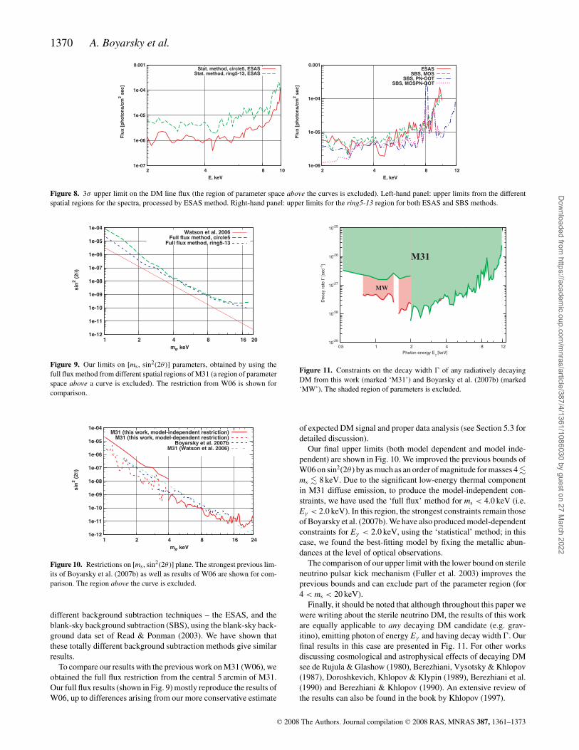
Figure 8. 3σ upper limit on the DM line flux (the region of parameter space above the curves is excluded). Left-hand panel: upper limits from the different

spatial regions for the spectra, processed by ESAS method. Right-hand panel: upper limits for the ring5-13 region for both ESAS and SBS methods.

1e-12

1e-11

1e-10

1e-09

1e-08

1e-07

1e-06

1e-05

1e-04

1 20 2 4 8 16

sin

2 (

2θ)

ms, keV

Watson et al. 2006Full flux method, circle5

Full flux method, ring5-13

Figure 9. Our limits on [ms, sin2(2θ )] parameters, obtained by using the

full flux method from different spatial regions of M31 (a region of parameter

space above a curve is excluded). The restriction from W06 is shown for

comparison.

1e-12

1e-11

1e-10

1e-09

1e-08

1e-07

1e-06

1e-05

1e-04

24 1 2 4 8 16

sin

2 (

2θ)

ms, keV

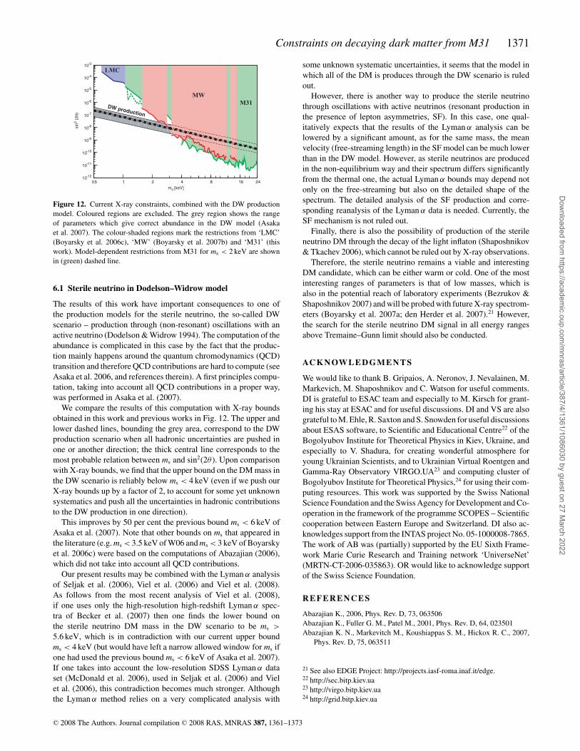
M31 (this work, model-independent restriction)M31 (this work, model-dependent restriction)

Boyarsky et al. 2007bM31 (Watson et al. 2006)

Figure 10. Restrictions on [ms, sin2(2θ )] plane. The strongest previous lim-

its of Boyarsky et al. (2007b) as well as results of W06 are shown for com-

parison. The region above the curve is excluded.

different background subtraction techniques – the ESAS, and the

blank-sky background subtraction (SBS), using the blank-sky back-

ground data set of Read & Ponman (2003). We have shown that

these totally different background subtraction methods give similar

results.

To compare our results with the previous work on M31 (W06), we

obtained the full flux restriction from the central 5 arcmin of M31.

Our full flux results (shown in Fig. 9) mostly reproduce the results of

W06, up to differences arising from our more conservative estimate

10-29

10-28

10-27

10-26

10-25

0.5 12 1 2 4 8

De

ca

y r

ate

Γ [

se

c-1

]

Photon energy Eγ [keV]

M31

MW

Figure 11. Constraints on the decay width � of any radiatively decaying

DM from this work (marked ‘M31’) and Boyarsky et al. (2007b) (marked

‘MW’). The shaded region of parameters is excluded.

of expected DM signal and proper data analysis (see Section 5.3 for

detailed discussion).

Our final upper limits (both model dependent and model inde-

pendent) are shown in Fig. 10. We improved the previous bounds of

W06 on sin2(2θ ) by as much as an order of magnitude for masses 4 �ms � 8 keV. Due to the significant low-energy thermal component

in M31 diffuse emission, to produce the model-independent con-

straints, we have used the ‘full flux’ method for ms < 4.0 keV (i.e.

Eγ < 2.0 keV). In this region, the strongest constraints remain those

of Boyarsky et al. (2007b). We have also produced model-dependent

constraints for Eγ < 2.0 keV, using the ‘statistical’ method; in this

case, we found the best-fitting model by fixing the metallic abun-

dances at the level of optical observations.

The comparison of our upper limit with the lower bound on sterile

neutrino pulsar kick mechanism (Fuller et al. 2003) improves the

previous bounds and can exclude part of the parameter region (for

4 < ms < 20 keV).

Finally, it should be noted that although throughout this paper we

were writing about the sterile neutrino DM, the results of this work

are equally applicable to any decaying DM candidate (e.g. grav-

itino), emitting photon of energy Eγ and having decay width �. Our

final results in this case are presented in Fig. 11. For other works

discussing cosmological and astrophysical effects of decaying DM

see de Rujula & Glashow (1980), Berezhiani, Vysotsky & Khlopov

(1987), Doroshkevich, Khlopov & Klypin (1989), Berezhiani et al.

(1990) and Berezhiani & Khlopov (1990). An extensive review of

the results can also be found in the book by Khlopov (1997).


Dow


ic.oup.com/m



10-12

10-11

10-10

10-9

10-8

10-7

10-6

10-5

10-4

10-3

0.5 24 1 2 4 8 16

sin

2 (

2θ)

ms [keV]

DW production

LMC

MWM31

Figure 12. Current X-ray constraints, combined with the DW production

model. Coloured regions are excluded. The grey region shows the range

of parameters which give correct abundance in the DW model (Asaka

et al. 2007). The colour-shaded regions mark the restrictions from ‘LMC’

(Boyarsky et al. 2006c), ‘MW’ (Boyarsky et al. 2007b) and ‘M31’ (this

work). Model-dependent restrictions from M31 for ms < 2 keV are shown

in (green) dashed line.

6.1 Sterile neutrino in Dodelson–Widrow model

The results of this work have important consequences to one of

the production models for the sterile neutrino, the so-called DW

scenario – production through (non-resonant) oscillations with an

active neutrino (Dodelson & Widrow 1994). The computation of the

abundance is complicated in this case by the fact that the produc-

tion mainly happens around the quantum chromodynamics (QCD)

transition and therefore QCD contributions are hard to compute (see

Asaka et al. 2006, and references therein). A first principles compu-

tation, taking into account all QCD contributions in a proper way,

was performed in Asaka et al. (2007).

We compare the results of this computation with X-ray bounds

obtained in this work and previous works in Fig. 12. The upper and

lower dashed lines, bounding the grey area, correspond to the DW

production scenario when all hadronic uncertainties are pushed in

one or another direction; the thick central line corresponds to the

most probable relation between ms and sin2(2θ ). Upon comparison

with X-ray bounds, we find that the upper bound on the DM mass in

the DW scenario is reliably below ms < 4 keV (even if we push our

X-ray bounds up by a factor of 2, to account for some yet unknown

systematics and push all the uncertainties in hadronic contributions

to the DW production in one direction).

This improves by 50 per cent the previous bound ms < 6 keV of

Asaka et al. (2007). Note that other bounds on ms that appeared in

the literature (e.g. ms < 3.5 keV of W06 and ms < 3 keV of Boyarsky

et al. 2006c) were based on the computations of Abazajian (2006),

which did not take into account all QCD contributions.

Our present results may be combined with the Lyman α analysis

of Seljak et al. (2006), Viel et al. (2006) and Viel et al. (2008).

As follows from the most recent analysis of Viel et al. (2008),

if one uses only the high-resolution high-redshift Lyman α spec-

tra of Becker et al. (2007) then one finds the lower bound on

the sterile neutrino DM mass in the DW scenario to be ms >

5.6 keV, which is in contradiction with our current upper bound

ms < 4 keV (but would have left a narrow allowed window for ms if

one had used the previous bound ms < 6 keV of Asaka et al. 2007).

If one takes into account the low-resolution SDSS Lyman α data

set (McDonald et al. 2006), used in Seljak et al. (2006) and Viel

et al. (2006), this contradiction becomes much stronger. Although

the Lyman α method relies on a very complicated analysis with

some unknown systematic uncertainties, it seems that the model in

which all of the DM is produces through the DW scenario is ruled

out.

However, there is another way to produce the sterile neutrino

through oscillations with active neutrinos (resonant production in

the presence of lepton asymmetries, SF). In this case, one qual-

itatively expects that the results of the Lyman α analysis can be

lowered by a significant amount, as for the same mass, the mean

velocity (free-streaming length) in the SF model can be much lower

than in the DW model. However, as sterile neutrinos are produced

in the non-equilibrium way and their spectrum differs significantly

from the thermal one, the actual Lyman α bounds may depend not

only on the free-streaming but also on the detailed shape of the

spectrum. The detailed analysis of the SF production and corre-

sponding reanalysis of the Lyman α data is needed. Currently, the

SF mechanism is not ruled out.

Finally, there is also the possibility of production of the sterile

neutrino DM through the decay of the light inflaton (Shaposhnikov

& Tkachev 2006), which cannot be ruled out by X-ray observations.

Therefore, the sterile neutrino remains a viable and interesting

DM candidate, which can be either warm or cold. One of the most

interesting ranges of parameters is that of low masses, which is

also in the potential reach of laboratory experiments (Bezrukov &

Shaposhnikov 2007) and will be probed with future X-ray spectrom-

eters (Boyarsky et al. 2007a; den Herder et al. 2007).21 However,

the search for the sterile neutrino DM signal in all energy ranges

above Tremaine–Gunn limit should also be conducted.

AC K N OW L E D G M E N T S

We would like to thank B. Gripaios, A. Neronov, J. Nevalainen, M.

Markevich, M. Shaposhnikov and C. Watson for useful comments.

DI is grateful to ESAC team and especially to M. Kirsch for grant-

ing his stay at ESAC and for useful discussions. DI and VS are also

grateful to M. Ehle, R. Saxton and S. Snowden for useful discussions

about ESAS software, to Scientific and Educational Centre22 of the

Bogolyubov Institute for Theoretical Physics in Kiev, Ukraine, and

especially to V. Shadura, for creating wonderful atmosphere for

young Ukrainian Scientists, and to Ukrainian Virtual Roentgen and

Gamma-Ray Observatory VIRGO.UA23 and computing cluster of

Bogolyubov Institute for Theoretical Physics,24 for using their com-

puting resources. This work was supported by the Swiss National

Science Foundation and the Swiss Agency for Development and Co-

operation in the framework of the programme SCOPES – Scientific

cooperation between Eastern Europe and Switzerland. DI also ac-

knowledges support from the INTAS project No. 05-1000008-7865.

The work of AB was (partially) supported by the EU Sixth Frame-

work Marie Curie Research and Training network ‘UniverseNet’

(MRTN-CT-2006-035863). OR would like to acknowledge support

of the Swiss Science Foundation.

R E F E R E N C E S

Abazajian K., 2006, Phys. Rev. D, 73, 063506

Abazajian K., Fuller G. M., Patel M., 2001, Phys. Rev. D, 64, 023501

Abazajian K. N., Markevitch M., Koushiappas S. M., Hickox R. C., 2007,

Phys. Rev. D, 75, 063511

21 See also EDGE Project: http://projects.iasf-roma.inaf.it/edge.22 http://sec.bitp.kiev.ua23 http://virgo.bitp.kiev.ua24 http://grid.bitp.kiev.ua


Dow


ic.oup.com/m



Alcock C. et al., 2000, ApJ, 541, 270

Arnaud K. A., 1996, in Jacoby G. H., Barnes J., eds, ASP Conf. Ser. Vol.

101, Astronomical Data Analysis Software and Systems V. Astron. Soc.

Pac., San Francisco, p. 17

Asaka T., Shaposhnikov M., 2005, Phys. Lett. B, 620, 17

Asaka T., Blanchet S., Shaposhnikov M., 2005, Phys. Lett. B, 631, 151

Asaka T., Laine M., Shaposhnikov M., 2006, J. High Energy Phys., 06, 053

Asaka T., Laine M., Shaposhnikov M., 2007, J. High Energy Phys., 01, 091

Avila-Reese V., Colın P., Valenzuela O., D’Onghia E., Firmani C., 2001,

ApJ, 559, 516

Baltz E. A., Murayama H., 2003, J. High Energy Phys., 5, 67

Barger V. D., Phillips R. J. N., Sarkar S., 1995, Phys. Lett. B, 352, 365

Becker G. D., Rauch M., Sargent W. L. W., 2007, ApJ, 662, 72

Berezhiani Z. G., Khlopov M. Y., 1990, Sov. J. Nucl. Phys., 52, 60

Berezhiani Z. G., Vysotsky M. I., Khlopov M. Y., 1987, Sov. J. Nucl. Phys.,

45, 1065

Berezhiani Z. G., Vysotsky M. I., Yurov V. P., Doroshkevich A. G., Khlopov

M. Y., 1990, Sov. J. Nucl. Phys., 51, 1020

Bezrukov F., Shaposhnikov M., 2007, Phys. Rev. D, 75, 053005

Biermann P. L., Kusenko A., 2006, Phys. Rev. Lett., 96, 091301

Bisnovatyi-Kogan G. S., 1980, AZh, 57, 899

Blair W. P., Kirshner R. P., Chevalier R. A., 1982, ApJ, 254, 50

Bode P., Ostriker J. P., Turok N., 2001, ApJ, 556, 93

Bond J. R., Szalay A. S., 1983, ApJ, 274, 443

Bond J. R., Efstathiou G., Silk J., 1980, Phys. Rev. Lett., 45, 1980

Boyarsky A., Neronov A., Ruchayskiy O., Shaposhnikov M., 2006a,

MNRAS, 370, 213

Boyarsky A., Neronov A., Ruchayskiy O., Shaposhnikov M., 2006b, Phys.

Rev. D, 74, 103506

Boyarsky A., Neronov A., Ruchayskiy O., Shaposhnikov M., Tkachev I.,

2006c, Phys. Rev. Lett., 97, 261302

Boyarsky A., den Herder J. W., Neronov A., Ruchayskiy O., 2007a, As-

tropart. Phys., 28, 303

Boyarsky A., Nevalainen J., Ruchayskiy O., 2007b, A&A, 471, 51

Boyarsky A., Ruchayskiy O., Markevitch M., 2008, ApJ, 673, 752

Burkert A., 1995, ApJ, 447, L25

Carignan C., Chemin L., Huchtmeier W. K., Lockman F. J., 2006, ApJ, 641,

L109

Cembranos J. A. R., Feng J. L., Rajaraman A., Smith B. T., Takayama F.,

2006, preprint (hep-ph/0603067)

Dalcanton J. J., Hogan C. J., 2001, ApJ, 561, 35

Dar A., 1995, ApJ, 449, 550

de Rujula A., Glashow S. L., 1980, Phys. Rev. Lett., 45, 942

den Herder J. W. et al., 2007, in O’Dell S.L., Pareschi G., eds, Proc. SPIE

Vol. 6688, Optics for EUV, X-Ray and Gamma-Ray Astronomy III.

SPIE, Bellingham, p. 4

Dennefeld M., Kunth D., 1981, AJ, 86, 989

Diemand J., Kuhlen M., Madau P., 2007, ApJ, 657, 262

Dodelson S., Widrow L. M., 1994, Phys. Rev. Lett., 72, 17

Dolgov A. D., Hansen S. H., 2002, Astropart. Phys., 16, 339

Doroshkevich A. G., Khlopov M. I., Klypin A. A., 1989, MNRAS, 239,

923

Doroshkevich A. G., Khlopov M. I., Sunyaev R. A., Szalay A. S., Zeldovich

I. B., 1981, Ann. New York Acad. Sci., 375, 32

Einasto J. et al., 1974, Tartu Astrofuus Obser. Teated, 48, 3

Fogli G. L., Lisi E., Marrone A., Palazzo A., Rotunno A. M., 2006, Prog.

Part. Nucl. Phys., 57, 71

Fuller G. M., Kusenko A., Mocioiu I., Pascoli S., 2003, Phys. Rev. D, 68,

103002

Gates E. I., Gyuk G., Turner M. S., 1995, ApJ, 449, L123

Geehan J. J., Fardal M. A., Babul A., Guhathakurta P., 2006, MNRAS, 366,

996

Ghigna S., Moore B., Governato F., Lake G., Quinn T., Stadel J., 2000, ApJ,

544, 616

Gilmore G., 2007, preprint (astro-ph/0703370)

Gilmore G., Wilkinson M. I., Wyse R. F. G., Kleyna J. T., Koch A., Evans

N. W., Grebel E. K., 2007, ApJ, 663, 948

Giunti C., 2007, Nucl. Phys. Proc. Suppl., 169, 309

Goerdt T., Moore B., Read J. I., Stadel J., Zemp M., 2006, MNRAS, 368,

1073

Hidaka J., Fuller G. M., 2006, Phys. Rev. D, 74, 125015

Hidaka J., Fuller G. M., 2007, Phys. Rev. D, 76, 083516

Hui L., Gnedin N. Y., Zhang Y., 1997, ApJ, 486, 599

Jacoby G. H., Ford H. C., 1986, ApJ, 304, 490

Jacoby G. H., Ciardullo R., 1999, ApJ, 515, 169

Jansen F. et al., 2001, A&A, 365, L1

Kerins E., 2004, MNRAS, 347, 1033

Kerins E. et al., 2001, MNRAS, 323, 13

Khlopov M. Y., 1997, Cosmoparticle Physics. World Scientific Press, Sin-

gapore

King I., 1962, AJ, 67, 471

Kleyna J. T., Wilkinson M. I., Gilmore G., Evans N. W., 2003a, ApJ, 588,

L21

Kleyna J. T., Wilkinson M. I., Gilmore G., Evans N. W., 2003b, ApJ, 589,

L59

Klypin A., Kravtsov A. V., Valenzuela O., Prada F., 1999, ApJ, 522, 82

Klypin A., Zhao H., Somerville R. S., 2002, ApJ, 573, 597

Koposov S. et al., 2007, ApJ, 669, 337

Kusenko A., 2006, Phys. Rev. Lett., 97, 241301

Lasserre T. et al., 2000, A&A, 355, L39

Liedahl D. A., Osterheld A. L., Goldstein W. H., 1995, ApJ, 438, L115

McDonald P. et al., 2006, ApJS, 163, 80

Mewe R., Lemen J. R., van den Oord G. H. J., 1986, A&AS, 65, 511

Miranda M., Maccio A. V., 2007, MNRAS, 382, 1225

Moore B., Quinn T., Governato F., Stadel J., Lake G., 1999, MNRAS, 310,

1147

Morrison R., McCammon D., 1983, ApJ, 270, 119

Navarro J. F., Frenk C. S., White S. D. M., 1997, ApJ, 490, 493

Navarro J. F. et al., 2004, MNRAS, 349, 1039

Nevalainen J., Markevitch M., Lumb D., 2005, ApJ, 629, 172

Pal P. B., Wolfenstein L., 1982, Phys. Rev. D, 25, 766

Palazzo A., Cumberbatch D., Slosar A., Silk J., 2007, Phys. Rev. D, 76,

103511

Peebles P. J. E., 1980, The Large-Scale Structure of the Universe. Princeton

Univ. Press, Princeton, NJ, p. 435

Peebles P. J. E., 1984, Sci, 224, 1385

Penarrubia J., McConnachie A., Navarro J. F., 2008, ApJ, 672, 904

Read A. M., Ponman T. J., 2003, A&A, 409, 395

Riemer-Sørensen S., Hansen S. H., Pedersen K., 2006, ApJ, 644, L33

Ruchayskiy O., 2007, in Kleinert H., Jantzen R., Ruffini R., eds, Proc.

11th Marcel Grossmann Meeting on General Relativity, preprint

(arXiv:0704.3215)

Sanchez-Salcedo F. J., Reyes-Iturbide J., Hernandez X., 2006, MNRAS,

370, 1829

Seljak U., Makarov A., McDonald P., Trac H., 2006, Phys. Rev. Lett., 97,

191303

Seto O., Yamaguchi M., 2007, Phys. Rev. D, 75, 123506

Shaposhnikov M., Tkachev I., 2006, Phys. Lett. B, 639, 414

Shi X.-d., Fuller G. M., 1999, Phys. Rev. Lett., 82, 2832 (SF)

Shirey R. et al., 2001, A&A, 365, L195

Simon J. D., Geha M., 2007, ApJ, 670, 313

Smith R. K., Brickhouse N. S., Liedahl D. A., Raymond J. C., 2001, ApJ,

556, L91

Sommer-Larsen J., Dolgov A., 2001, ApJ, 551, 608

Stanek K. Z., Garnavich P. M., 1998, ApJ, 503, L131

Stasielak J., Biermann P. L., Kusenko A., 2007, ApJ, 654, 290

Strigari L. E., Bullock J. S., Kaplinghat M., Diemand J., Kuhlen M., Madau

P., 2007, ApJ, 669, 676

Struder L. et al., 2001, A&A, 365, L18

Strumia A., Vissani F., 2006, preprint (hep-ph/0606054)

Takahashi H., Okada Y., Kokubun M., Makishima K., 2004, ApJ, 615,

242

Tegmark M. et al., 2004, Phys. Rev., D, 69, 103501

Tempel E., Tamm A., Tenjes P., 2007, preprint (arXiv:0707.4374)

Tremaine S., Gunn J. E., 1979, Phys. Rev. Lett., 42, 407

Turner M. J. L. et al., 2001, A&A, 365, L27


Dow


ic.oup.com/m



Viel M., Lesgourgues J., Haehnelt M. G., Matarrese S., Riotto A., 2006,

Phys. Rev. Lett., 97, 071301

Viel M., Becker G. D., Bolton J. S., Haehnelt M. G., Rauch M., Sargent W.

L. W., 2008, Phys. Rev. Lett., 100, 041304

Watson C. R., Beacom J. F., Yuksel H., Walker T. P., 2006, Phys. Rev. D,

74, 033009 (W06)

White S. D. M., Frenk C. S., Davis M., 1983, ApJ, 274, L1

Widrow L. M., Dubinski, J. 2005, ApJ, 631, 838

Wu X., 2007, preprint (astro-ph/0702233)

Zel’dovich Y. B., 1970, A&A, 5, 84

This paper has been typeset from a TEX/LATEX file prepared by the author.


Dow


ic.oup.com/m


constraints on decaying dark matter from xmm–newton

Documents