Conditions for zero duality gap in convex programming

Jonathan M. Borwein∗, Regina S. Burachik†, and Liangjin Yao‡

April 14, revision, 2013

Abstract

We introduce and study a new dual condition which characterizes zero duality gapin nonsmooth convex optimization. We prove that our condition is less restrictive thanall existing constraint qualifications, including the closed epigraph condition. Our dualcondition was inspired by, and is less restrictive than, the so-called Bertsekas’ conditionfor monotropic programming problems. We give several corollaries of our result andspecial cases as applications. We pay special attention to the polyhedral and sublinearcases, and their implications in convex optimization.

2010 Mathematics Subject Classification:Primary 49J52, 48N15; Secondary 90C25, 90C30, 90C46

Keywords: Bertsekas Constraint Qualification, Fenchel conjugate, Fenchel duality theorem,normal cone operator, inf-convolution, ε−subdifferential operator, subdifferential operator,zero duality gap.

1 Introduction

Duality theory establishes an interplay between an optimization problem, called the primal,and another optimization problem, called the dual. A main target of this approach is the

∗CARMA, University of Newcastle, Newcastle, New South Wales 2308, Australia. E-mail:jonathan.borwein@newcastle.edu.au. Laureate Professor at the University of Newcastle and Distin-guished Professor at King Abdul-Aziz University, Jeddah.†School of Mathematics and Statistics, University of South Australia, Mawson Lakes, SA 5095, Australia.

E-mail: regina.burachik@unisa.edu.au.‡CARMA, University of Newcastle, Newcastle, New South Wales 2308, Australia. E-mail:

liangjin.yao@newcastle.edu.au.

1

establishment of the so-called zero duality gap, which means that the optimal values of primaland dual problems coincide. Not all convex problems enjoy the zero duality gap property,and this has motivated the quest for assumptions on the primal problem which ensure zeroduality gap (see [29] and references therein).

Recently Bertsekas considered such an assumption for a specific convex optimization prob-lem, called the extended monotropic programming problem, the origin of which goes back toRockafellar (see [24, 25]). Following Bot and Csetnek [6], we study this problem in the fol-lowing setting. Let {Xi}mi=1 be separated locally convex spaces and let fi : Xi → ]−∞,+∞]be proper lower semicontinuous and convex for every i ∈ {1, 2, . . . ,m}. Consider the mini-mization problem

(P ) p := inf

(m∑i=1

fi(xi)

)subject to (x1, . . . , xm) ∈ S,

where S ⊆ X1 × X2 × · · ·Xm is a linear closed subspace. The dual problem is given asfollows:

(D) d := sup

(m∑i=1

−f ∗i (x∗i )

)subject to (x∗1, . . . , x

∗m) ∈ S⊥.

We note that formulation (P ) includes any general convex optimization problem. Indeed, forX a separated locally convex space, and f : X → ]−∞,+∞] a proper lower semicontinuousand convex function, consider the problem

(CP ) inf f(x) subject tox ∈ C,

where C is a closed and convex set. Problem (CP ) can be reformulated as

inf {f(x1) + ιC(x2)} subject to (x1, x2) ∈ S = {(y1, y2) ∈ X ×X : y1 = y2},

where ιC is the indicator function of C.

Denote by v(P ) and v(D) the optimal values of (P ) and (D), respectively. In the finitedimensional setting, Bertsekas proved in [3, Proposition 4.1] that a zero duality gap holdsfor problems (P ) and (D) (i.e., p = v(P ) = v(D) = d) under the following condition:

NS(x) +(∂εf1(x1), . . . , ∂εfm(xm)

)is closed

for every ε > 0, (x1, . . . , xm) ∈ S and xi ∈ dom fi, ∀i ∈ {1, 2, . . . ,m},

where the sets ∂εfi(xi) are the epsilon-subdifferentials of the fi at xi (see (8) for the defini-tion). In [6, Theorem 3.2], Bot and Csetnek extended this result to the setting of separatedlocally convex spaces.

2

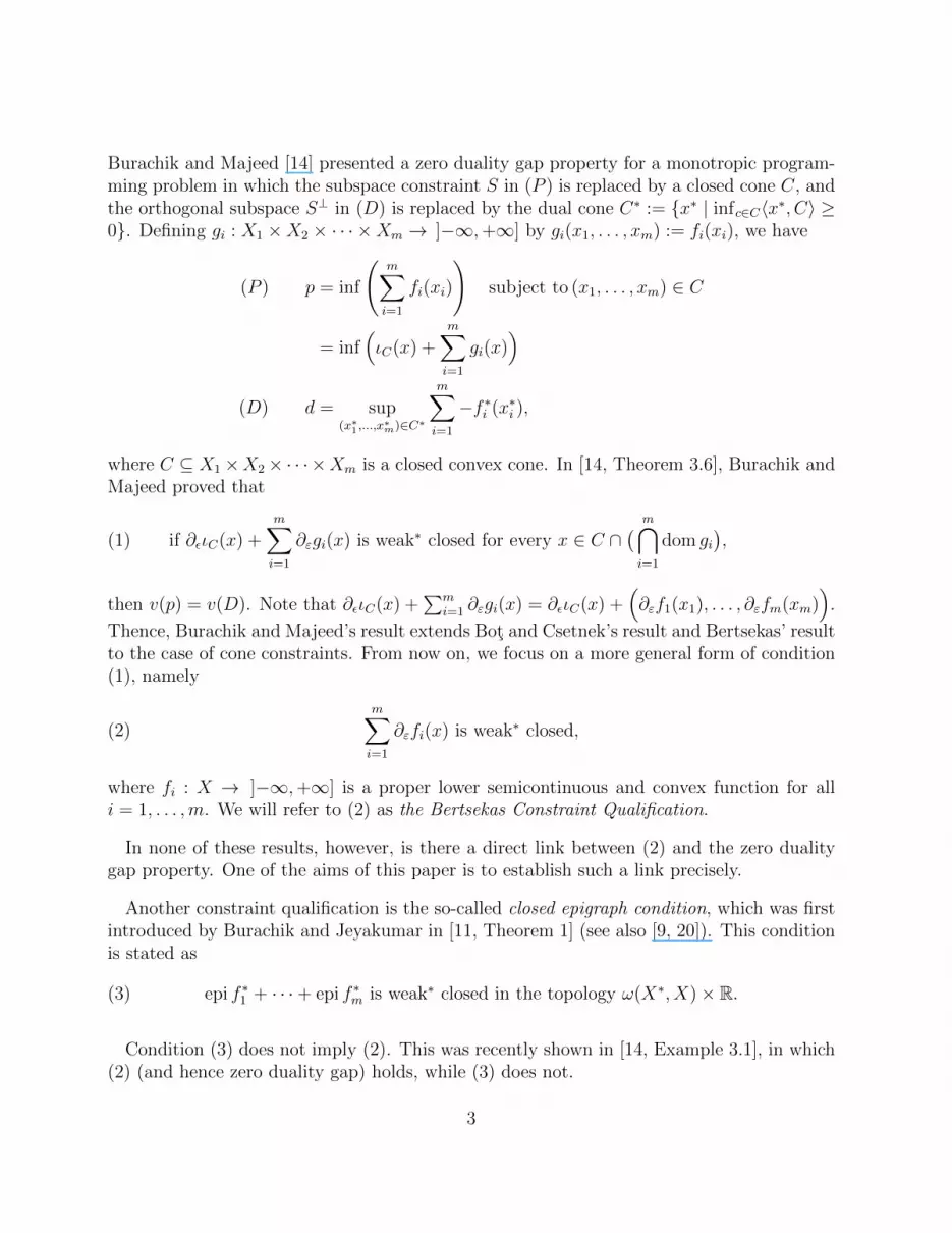
Burachik and Majeed [14] presented a zero duality gap property for a monotropic program-ming problem in which the subspace constraint S in (P ) is replaced by a closed cone C, andthe orthogonal subspace S⊥ in (D) is replaced by the dual cone C∗ := {x∗ | infc∈C〈x∗, C〉 ≥0}. Defining gi : X1 ×X2 × · · · ×Xm → ]−∞,+∞] by gi(x1, . . . , xm) := fi(xi), we have

(P ) p = inf

(m∑i=1

fi(xi)

)subject to (x1, . . . , xm) ∈ C

= inf(ιC(x) +

m∑i=1

gi(x))

(D) d = sup(x∗1,...,x

∗m)∈C∗

m∑i=1

−f ∗i (x∗i ),

where C ⊆ X1×X2× · · · ×Xm is a closed convex cone. In [14, Theorem 3.6], Burachik andMajeed proved that

(1) if ∂ειC(x) +m∑i=1

∂εgi(x) is weak∗ closed for every x ∈ C ∩( m⋂i=1

dom gi),

then v(p) = v(D). Note that ∂ειC(x) +∑m

i=1 ∂εgi(x) = ∂ειC(x) +(∂εf1(x1), . . . , ∂εfm(xm)

).

Thence, Burachik and Majeed’s result extends Bot and Csetnek’s result and Bertsekas’ resultto the case of cone constraints. From now on, we focus on a more general form of condition(1), namely

(2)m∑i=1

∂εfi(x) is weak∗ closed,

where fi : X → ]−∞,+∞] is a proper lower semicontinuous and convex function for alli = 1, . . . ,m. We will refer to (2) as the Bertsekas Constraint Qualification.

In none of these results, however, is there a direct link between (2) and the zero dualitygap property. One of the aims of this paper is to establish such a link precisely.

Another constraint qualification is the so-called closed epigraph condition, which was firstintroduced by Burachik and Jeyakumar in [11, Theorem 1] (see also [9, 20]). This conditionis stated as

(3) epi f ∗1 + · · ·+ epi f ∗m is weak∗ closed in the topology ω(X∗, X)× R.

Condition (3) does not imply (2). This was recently shown in [14, Example 3.1], in which(2) (and hence zero duality gap) holds, while (3) does not.

3

We recall from [19, Proposition 6.7.3] the following characterization of the zero dualitygap property for (P ) and (D), which uses the infimal convolution (see (9) for its definition)of the conjugate functions f ∗i .

(P ) p = inf

(m∑i=1

fi(x)

)= −

( m∑i=1

fi)∗

(0)

(D) d = − (f ∗1� · · ·�f ∗m) (0).

Hence, zero duality gap is tantamount to the equality( m∑i=1

fi)∗

(0) =(f ∗1� · · ·�f ∗m

)(0).

In our main result (Theorem 3.2 below), we introduce a new closedness property, statedas follows. There exists K > 0 such for every x ∈

⋂mi=1 dom fi and every ε > 0,

(4)

[m∑i=1

∂εfi(x)

]w*

⊆m∑i=1

∂Kεfi(x).

Theorem 3.2 below proves that this property is equivalent to

(5)( m∑i=1

fi)∗

(x∗) =(f ∗1� · · ·�f ∗m

)(x∗), for all x∗ ∈ X∗.

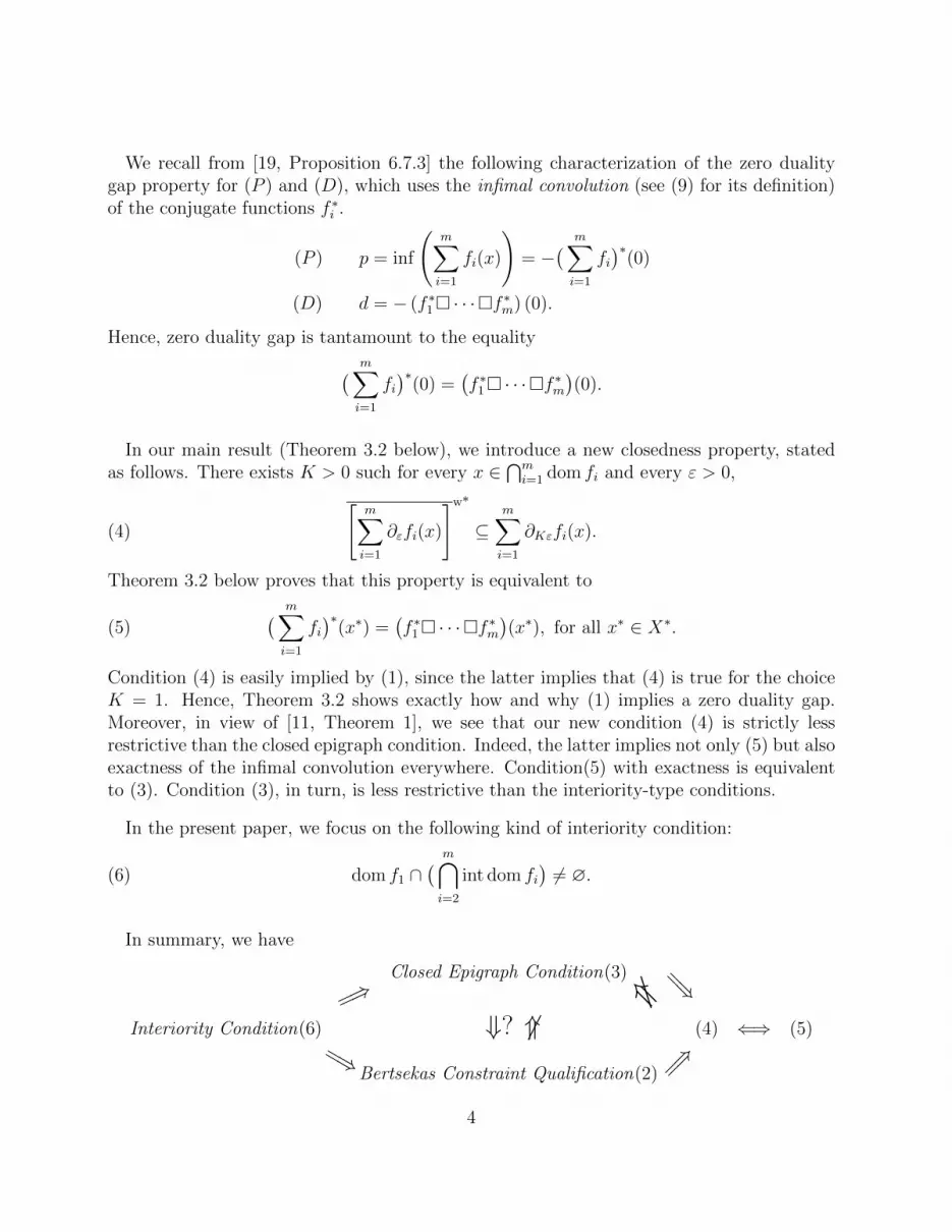
Condition (4) is easily implied by (1), since the latter implies that (4) is true for the choiceK = 1. Hence, Theorem 3.2 shows exactly how and why (1) implies a zero duality gap.Moreover, in view of [11, Theorem 1], we see that our new condition (4) is strictly lessrestrictive than the closed epigraph condition. Indeed, the latter implies not only (5) but alsoexactness of the infimal convolution everywhere. Condition(5) with exactness is equivalentto (3). Condition (3), in turn, is less restrictive than the interiority-type conditions.

In the present paper, we focus on the following kind of interiority condition:

(6) dom f1 ∩( m⋂i=2

int dom fi)6= ∅.

In summary, we have

Closed Epigraph Condition(3) 6⇓ =⇒=⇒

Interiority Condition(6) ⇓? 6⇑ (4) ⇐⇒ (5)=⇒

Bertsekas Constraint Qualification(2) =⇒

4

Example 3.1 in [14] allows us to assert that the Bertsekas Constraint Qualification is not morerestrictive than the Closed Epigraph Condition. This example also shows that our condition(4) does not imply the closed epigraph condition. It is still an open question whether a moreprecise relationship can be established between the closed epigraph condition and BertsekasConstraint Qualification. The arrow linking (6) to (3) has been established by Zalinescuin [30, 31]. All other arrows are, as far as we know, new, and are established by us inthis paper. Some clarification is in order regarding the arrow from (6) to the BertsekasConstraint Qualification(2). It is clear that for every x0 ∈ dom f1 ∩

(⋂mi=2 int dom fi

), the

set∑m

i=1 ∂εfi(x0) is weak∗ closed. Indeed, this is true because the latter set is the sumof a weak∗ compact set and a weak∗ closed set. Our Lemma 4.2 establishes that, underassumption (6), the set

∑mi=1 ∂εfi(x) is weak∗ closed for every point x ∈

(⋂mi=1 dom fi

).

A well-known result, which is not easily found in the literature, is the equivalence between(3) and the equality (5) with exactness of the infimal convolution everywehere in X∗. Forconvenience and possible future use, we have included the proof of this equivalence in thepresent paper (see Proposition 3.11).

The layout of our paper is as follows. The next section contains the necessary preliminarymaterial. Section 3 contains our main result, and gives its relation with the BertsekasConstraint Qualification (2), with the closed epigraph condition (3), and with the interiorityconditions (6). Still in this section we establish stronger results for the important specialcase in which all fis are sublinear. We finish this section by showing that our closednesscondition allows for a simplification of the well-known Hiriart-Urruty and Phelps formula forthe subdifferential of the sum of convex functions. In Section 4 we show that (generalized)interiority conditions imply (2), as well as (3). We also provide some additional consequencesof Corollary 4.3, including various forms of Rockafellar’s Fenchel duality result. At the endof Section 4 we establish stronger results for the case involving polyhedral functions. Weend the paper with some conclusions and open questions.

2 Preliminaries

Let I be a directed set with a partial order �. A subset J of I is said to be terminal if thereexists j0 ∈ I such that every successor k � j0 verifies k ∈ J . We say that a net {sα}α∈I ⊆ Ris eventually bounded if there exists a terminal set J and R > 0 such that |sα| ≤ R for everyα ∈ J .

We assume throughout that X is a separated (i.e., Hausdorff) locally convex topologicalvector space and X∗ is its continuous dual endowed with the weak∗ topology ω(X∗, X).Given a subset C of X, intC is the interior of C. We next recall standard notions fromconvex analysis, which can be found, e.g., in [2, 5, 10, 21, 23, 26, 31]. For the set D ⊆ X∗,

5

Dw*

is the weak∗ closure of D. The indicator function of C, written as ιC , is defined atx ∈ X by

ιC(x) :=

{0, if x ∈ C;

+∞, otherwise.(7)

The normal cone operator of C at x is defined byNC(x) :={x∗ ∈ X∗ | supc∈C〈c− x, x∗〉 ≤ 0

},

if x ∈ C; and NC(x) := ∅, if x /∈ C. If S ⊆ X is a subspace, we define S⊥ by S⊥ := {z∗ ∈X∗ | 〈z∗, s〉 = 0, ∀s ∈ S}. Let f : X → [−∞,+∞]. Then dom f := f−1 [−∞,+∞[ is thedomain (or effective domain) of f , and f ∗ : X∗ → [−∞,+∞] : x∗ 7→ supx∈X{〈x, x∗〉−f(x)}is the Fenchel conjugate of f . The epigraph of f is epi f :=

{(x, r) ∈ X × R | f(x) ≤ r

}.

The lower semicontinuous hull of f is denoted by f . We say f is proper if dom f 6= ∅and f > −∞. Given a function f , the subdifferential of f is the point-to-set mapping∂f : X ⇒ X∗ defined by

∂f(x) :=

{{x∗ ∈ X∗ | (∀y ∈ X) 〈y − x, x∗〉+ f(x) ≤ f(y)} if f(x) ∈ R;

∅ otherwise.

Given ε ≥ 0, the ε−subdifferential of f is the point-to-set mapping ∂εf : X ⇒ X∗ definedby

(8) ∂εf(x) :=

{{x∗ ∈ X∗ | (∀y ∈ X) 〈y − x, x∗〉+ f(x) ≤ f(y) + ε} if f(x) ∈ R;

∅ otherwise.

Thus, if f is not proper, then ∂εf(x) = ∅ for every ε ≥ 0 and x ∈ X. Note also that if f isconvex and there exists x0 ∈ X such that f(x0) = −∞, then f(x) = −∞,∀x ∈ dom f (see[13, Proposition 2.4] or [16, page 867]).

Let f : X → ]−∞,+∞]. We say f is a sublinear function if f(x + y) ≤ f(x) + f(y),f(0) = 0, and f(tx) = tf(x) for every x, y ∈ dom f and t ≥ 0.

Let Z be a separated locally convex space and let m ∈ N. For a family of functionsψ1, . . . , ψm such that ψi : Z → [−∞,+∞] for all i = 1, . . . ,m, we define its infimal convolu-tion as the function (ψ1� · · ·�ψm) : Z → [−∞,+∞] as

(9)(ψ1� · · ·�ψm

)z = inf∑m

i=1 zi=z

{ψ(z1) + · · ·+ ψm(zm)

}.

We denote by ⇁w* the weak∗ convergence of nets in X∗.

6

3 Our main results

The following formula will be important in the proof of our main result.

Fact 3.1 (See [31, Corollary 2.6.7] or [6, Theorem 3.1].) Let f, g : X → ]−∞,+∞] beproper lower semicontinuous and convex. Then for every x ∈ X and ε ≥ 0,

∂ε(f + g)(x) =⋂η>0

[ ⋃ε1≥0,ε2≥0, ε1+ε2=ε+η

(∂ε1f(x) + ∂ε2g(x)

)]w*

.

We now come to our main result. The proof in part follows that of [6, Theorem 3.2].

Theorem 3.2 Let m ∈ N, and fi : X → ]−∞,+∞] be proper convex with⋂mi=1 dom fi 6= ∅,

where i ∈ {1, 2, . . . ,m}. Suppose that fi = fi on⋂mi=1 dom fi. Then the following four

conditions are equivalent.

(i) There exists K > 0 such that for every x ∈⋂mi=1 dom fi, and every ε > 0,[

m∑i=1

∂εfi(x)

]w*

⊆m∑i=1

∂Kεfi(x).

(ii) (∑m

i=1 fi)∗

= f ∗1� · · ·�f ∗m in X∗.

(iii) f ∗1� · · ·�f ∗m is weak∗ lower semicontinuous.

(iv) For every x ∈ X and ε ≥ 0,

∂ε(f1 + · · ·+ fm)(x) =⋂η>0

⋃εi≥0,

∑mi=1 εi=ε+η

(∂ε1f1(x) + · · ·+ ∂εmfm(x)

) .Proof. First we show that our basic assumptions imply that fi is proper for every i ∈{1, 2, . . . ,m}. Let i ∈ {1, 2, . . . ,m}.

Since ∅ 6=(⋂m

j=1 dom fj)⊆(⋂m

j=1 dom fj), then

⋂mj=1 dom fj 6= ∅. Let x0 ∈

⋂mi=j dom fj.

Suppose to the contrary that fi is not proper and thus there exists y0 ∈ X such thatfi(y0) = −∞. Then by [13, Proposition 2.4], fi(x0) = −∞. By the assumption, fi(x0) =fi(x0) > −∞, which is a contradiction. Hence fi is proper.

7

(i)⇒(ii): Let x∗ ∈ X∗. Clearly, we have (f ∗1� · · ·�f ∗m) (x∗) ≥ (∑m

i=1 fi)∗

(x∗). It sufficesto show that (

m∑i=1

fi

)∗(x∗) ≥ (f ∗1� · · ·�f ∗m) (x∗).(10)

First we show that

m∑i=1

fi(y) ≥m∑i=1

fi(y), ∀y ∈ X.(11)

Indeed, let y ∈ X. If y 6∈⋂mi=1 dom fi. Clearly, (11) holds. Now assume that y ∈

⋂mi=1 dom fi.

By our assumption fi(y) = fi(y), we conclude that (11) holds. Combining both cases, weconclude that (11) holds everywhere.

Since∑m

i=1 fi ≤∑m

i=1 fi, (11) implies that

m∑i=1

fi =m∑i=1

fi.(12)

Taking the lower semicontinuous hull in the equality above, we have

m∑i=1

fi =m∑i=1

fi = f1 + · · ·+ fm.(13)

Clearly, if (∑m

i=1 fi)∗(x∗) = +∞, then (10) holds. Now assume that (

∑mi=1 fi)

∗(x∗) < +∞.Then we have (

∑mi=1 fi)

∗(x∗) ∈ R and thus x∗ ∈ dom(∑m

i=1 fi)∗. Since (

∑mi=1 fi)

∗ is lowersemicontinuous, given ε > 0, there exists x ∈ X such that x ∈ ∂ε(

∑mi=1 fi)

∗(x∗). Then

(m∑i=1

fi)∗(x∗) + (

m∑i=1

fi)(x) = (m∑i=1

fi)∗(x∗) + (

m∑i=1

fi)∗∗(x) ≤ 〈x, x∗〉+ ε.

By (13), we have

(m∑i=1

fi)∗(x∗) + (

m∑i=1

fi)(x) = (m∑i=1

fi)∗(x∗) + (

m∑i=1

fi)(x) ≤ 〈x, x∗〉+ ε.

Hence

x∗ ∈ ∂ε(m∑i=1

fi)(x) and x∗ ∈ ∂ε(m∑i=1

fi)(x).(14)

8

Next, we claim that there exists K > 0 such that

x∗ ∈m∑i=1

∂Kmεfi(x).(15)

Set f := f1, g := (∑m

i=2 fi), and η = ε in Fact 3.1, and use (14) to write

x∗ ∈ ∂ε(m∑i=1

fi)(x)⇒ x∗ ∈

[∂2εf1(x) + ∂2ε(

m∑i=2

fi)(x)

]w*

.

We repeat the same idea with f := f2, g := (∑m

i=3 fi) in Fact 3.1, and continue iterativelyto obtain

⇒ x∗ ∈

∂2εf1(x) + ∂3εf2(x) + ∂3ε(m∑i=3

fi)(x)

w*w*

⇒ x∗ ∈

[∂2εf1(x) + ∂3εf2(x) + ∂3ε(

m∑i=3

fi)(x)

]w*

· · ·

⇒ x∗ ∈[∂2εf1(x) + ∂3εf2(x) + · · ·+ ∂mεfm(x)

]w*

⇒ x∗ ∈ [∂2εf1(x) + ∂3εf2(x) + · · ·+ ∂mεfm(x)]w*

(by (14) and fi(x) = fi(x),∀i)

⇒ x∗ ∈ [∂mεf1(x) + ∂mεf2(x) + · · ·+ ∂mεfm(x)]w*.

By assumption (i), the last inclusion implies that there exists K > 0 such that

x∗ ∈ ∂Kmεf1(x) + ∂Kmεf2(x) + · · ·+ ∂Kmεfm(x)

Hence (15) holds. Thus, there exists y∗i ∈ ∂Kmεfi(x) such that x∗ =∑m

i=1 y∗i and

f ∗i (y∗i ) + fi(x) ≤ 〈x, y∗i 〉+Kmε, ∀i ∈ {1, 2, . . . ,m}.

Thus,

(f ∗1� · · ·�f ∗m)(x∗) ≤m∑i=1

f ∗i (y∗i ) ≤ −m∑i=1

fi(x) + 〈x, x∗〉+Km2ε

≤ (m∑i=1

fi)∗(x∗) +Km2ε.

9

Letting ε −→ 0 in the above inequality, we have

(f ∗1� · · ·�f ∗m) (x∗) ≤

(m∑i=1

fi

)∗(x∗).

Hence (10) holds and so (m∑i=1

fi

)∗= f ∗1� · · ·�f ∗m.(16)

(ii)⇒(iii): This clearly follows from the lower semicontinuity of (∑m

i=1 fi)∗.

(iii)⇒(i): Let x ∈⋂mi=1 dom fi and ε > 0, and x∗ ∈ [

∑mi=1 ∂εfi(x)]

w*. Then for each

i = 1, . . . ,m there exists a net (x∗i,α)α∈I in ∂εfi(x) such that

m∑i=1

x∗i,α⇁w* x∗.(17)

We have

fi(x) + f ∗i (x∗i,α) ≤ 〈x, x∗i,α〉+ ε, ∀i ∈ {1, 2, . . . ,m} ∀α ∈ I.(18)

Thus

m∑i=1

fi(x) + (f ∗1� · · ·�f ∗m)(m∑i=1

x∗i,α) ≤m∑i=1

fi(x) +m∑i=1

f ∗i (x∗i,α) ≤ 〈x,m∑i=1

x∗i,α〉+mε, ∀α ∈ I.

(19)

Since f ∗1� · · ·�f ∗m is weak∗ lower semicontinuous, it follows from (19) and (17) that

m∑i=1

fi(x) + (f ∗1� · · ·�f ∗m)(x∗) ≤ 〈x, x∗〉+mε.(20)

There exists y∗i ∈ X∗ such that∑m

i=1 y∗i = x∗ and

∑mi=1 f

∗i (y∗i ) ≤ (f ∗1� · · ·�f ∗m)(x∗) + ε.

Then by (20),

m∑i=1

fi(x) +m∑i=1

f ∗i (y∗i ) ≤ 〈x, x∗〉+ (m+ 1)ε.

Thus, we have

y∗i ∈ ∂(m+1)εfi(x), ∀i ∈ {1, 2, . . . ,m}.

10

Hence

x∗ =m∑i=1

y∗i ∈m∑i=1

∂(m+1)εfi(x),

and the statement in (i) holds for K := (m+ 1).

(ii)⇒(iv): Let x ∈ X and ε ≥ 0.

We have

⋂η>0

⋃εi≥0,

∑mi=1 εi=ε+η

(∂ε1f1(x) + · · ·+ ∂εmfm(x)

)⊆⋂η>0

⋃εi≥0,

∑mi=1 εi=ε+η

∂∑mi εi(f1 + · · ·+ fm)(x)

=⋂η>0

∂ε+η(f1 + · · ·+ fm)(x)

= ∂ε(f1 + · · ·+ fm)(x).

Now we show the other inclusion:

∂ε(f1 + · · ·+ fm)(x) ⊆(⋂η>0

⋃εi≥0,

∑mi=1 εi=ε+η

(∂ε1f1(x) + · · ·+ ∂εmfm(x)

)).(21)

Let x∗ ∈ ∂ε(f1 + · · ·+ fm)(x). Then we have∑m

i=1 fi(x) + (∑fi)∗(x∗) ≤ 〈x, x∗〉+ ε. By (ii),

we have

m∑i=1

fi(x) +(f ∗1� · · ·�f ∗m

)(x∗) ≤ 〈x, x∗〉+ ε.(22)

Let η > 0. Then there exists y∗i ∈ X∗ such that∑m

i=1 y∗i = x∗ and

∑mi=1 f

∗i (y∗i ) ≤(

f ∗1� · · ·�f ∗m)

(x∗) + η. Then by (22),

m∑i=1

fi(x) +m∑i=1

f ∗i (y∗i ) ≤ 〈x, x∗〉+ ε+ η.(23)

Set γi := fi(x) + f ∗i (y∗i )− 〈x, y∗i 〉. Then γi ≥ 0 and y∗i ∈ ∂γifi(x). By (23),

〈x, x∗〉+m∑i=1

γi =m∑i=1

[〈x, y∗i 〉+ γi] ≤ 〈x, x∗〉+ ε+ η.(24)

11

Hence∑m

i=1 γi ≤ ε + η. Set ε1 := ε + η −∑m

i=2 γi and εi := γi for every i = {2, 3, . . . ,m}.Then ε1 ≥ γ1 and we have

x∗ =m∑i=1

y∗i ∈m∑i=1

∂εifi(x).

Hence x∗ ∈⋃εi≥0,

∑mi=1 εi=ε+η

(∂εifi(x) + · · ·+ ∂εmfm(x)

)and therefore (21) holds.

(iv)⇒(i): Let x ∈⋂mi=1 dom fi, ε > 0, and x∗ ∈ [

∑mi=1 ∂εfi(x)]

w*. Then for each i =

1, . . . ,m there exists a net (x∗i,α)α∈I in ∂εfi(x) such that

m∑i=1

x∗i,α⇁w* x∗,(25)

and this implies that

m∑i=1

x∗i,α ∈(⋂η>0

⋃εi≥0,

∑mi=1 εi=mε+η

(∂ε1f1(x) + · · ·+ ∂εmfm(x)

)).(26)

Assumption (iv) yields∑m

i=1 x∗i,α ∈ ∂mε(f1 + · · · + fm)(x). Since ∂mε(f1 + · · · + fm)(x) is

weak∗ closed, (25) shows that x∗ ∈ ∂mε(f1 + · · · + fm)(x). Using (iv) again for η = ε, we

conclude that x∗ ∈(∂(m+1)εfi(x) + · · ·+ ∂(m+1)εfm(x)

).

Therefore, statement (i) holds for K := m+ 1. �

Remark 3.3 (a) We point out that the proof of Theorem 3.2(i) actually shows that K =m+ 1, and this constant is independent of the functions f1, . . . , fm.

(b) Part (i) implies (ii) of Theorem 3.2 generalizes [3, Proposition 4.1], [6, Theorem 3.2]by Bot and Csetnek, and [14, Theorem 3.6] by Burachik and Majeed.

(c) A result similar to Theorem 3.2(iii)⇔(iv) has been established in [7, Corollary 3.9] byBot and Grad.

An immediate corollary follows:

Corollary 3.4 Let f, g : X → ]−∞,+∞] be proper convex with dom f ∩ dom g 6= ∅.Suppose that f = f and g = g on dom f ∩ dom g. Suppose also that for every x ∈ dom f ∩dom g and ε > 0,

∂εf(x) + ∂εg(x) is weak∗ closed.

Then (f + g)∗ = f ∗�g∗ in X∗. Consequently, inf(f + g) = supx∗∈X∗{−f ∗(x∗)− g∗(−x∗)}.

12

Note that, for a linear subspace S ⊆ X, we have ∂ειS = S⊥. Taking this into account wederive the Bertsekas Constraint Qualification result from Theorem 3.2.

Corollary 3.5 (Bertsekas) (See [3, Proposition 4.1].) Let m ∈ N and suppose that Xi isa finite dimensional space, and let fi : Xi → ]−∞,+∞] be proper lower semicontinuous andconvex, where i ∈ {1, 2, . . . ,m}. Let S be a linear subspace of X1 × X2 × · · · × Xm withS ∩

(⋂mi=1 dom fi

)6= ∅. Define gi : X1 ×X2 × · · · ×Xm → ]−∞,+∞] by gi(x1, . . . , xm) :=

fi(xi). Assume that for every x ∈ S ∩(⋂m

i=1 dom fi)

and for every ε > 0 we have that

S⊥ +m∑i=1

∂εgi(x) is closed.

Then v(P ) = infx∈S{∑m

i=1 fi(x)} = supx∗∈S⊥{−∑m

i=1 f∗i (x∗)} = v(D).

The following example which is due to [14, Example 3.1] and [9, Example, page 2798],shows that the infimal convolution in Corollary 3.4 is not always achieved (exact).

Example 3.6 Let X = R2, and f := ιC , g := ιD, where C := {(x, y) ∈ R2 | 2x + y2 ≤ 0}and D := {(x, y) ∈ R2 | x ≥ 0}. Then f and g are proper lower semicontinuous and convexwith dom f ∩ dom g = {(0, 0)}. For every ε > 0, ∂εf(0, 0) + ∂εg(0, 0) is closed. Hence(f + g)∗ = f ∗�g∗. But f ∗�g∗ is not exact everywhere and ∂(f + g)(0) 6= ∂f(0) + ∂g(0).Consequently, epi f ∗ + epi g∗ is not closed in the topology ω(X∗, X)× R.

Proof. Clearly, f and g are proper lower semicontinuous convex. Let ε > 0. Then by [14,Example 3.1]

∂εf(0, 0) =⋃u≥0

(u×

[−√

2εu,√

2εu] )

and ∂εg(0, 0) = ]−∞, 0]× {0}.(27)

Thus, ∂εf(0, 0)+∂εg(0, 0) = R2 and then ∂εf(0, 0)+∂εg(0, 0) is closed. Corollary 3.4 impliesthat (f + g)∗ = f ∗�g∗. [9, Example, page 2798] shows that (f ∗�g∗) is not exact at (1, 1)and ∂(f + g)(0) 6= ∂f(0) + ∂g(0). By [11, 9], epi f ∗ + epi g∗ is not closed in the topologyω(X∗, X)× R. �

The following result is classical, we state and prove it here for more convenient and clearfuture use.

Lemma 3.7 (Hiriart-Urruty) Let m ∈ N, and fi : X → ]−∞,+∞] be proper convexwith

⋂mi=1 dom fi 6= ∅, where i ∈ {1, 2, . . . ,m}. Assume that (

∑mi=1 fi)

∗ = f ∗1� · · ·�f ∗m inX∗ and the infimal convolution is exact (attained) everywhere. Then

∂(f1 + f2 + · · ·+ fm) = ∂f1 + · · ·+ ∂fm.

13

Proof. Let x ∈ X. We always have ∂(f1 + f2 + · · ·+ fm)(x) ⊇ ∂f1(x) + · · ·+ ∂fm(x). So itsuffices to show that

∂(f1 + f2 + · · ·+ fm)(x) ⊆ ∂f1(x) + · · ·+ ∂fm(x).(28)

Let w∗ ∈ ∂(f1 + f2 + · · ·+ fm)(x). Then

(f1 + f2 + · · ·+ fm)(x) + (f1 + f2 + · · ·+ fm)∗(w∗) = 〈x,w∗〉.

By the assumption, there exists w∗i ∈ X∗ such that∑m

i=1 w∗i = w∗ and

f1(x) + f2(x) + · · ·+ fm(x) + f ∗1 (w∗1) + · · ·+ f ∗m(w∗m) = 〈x,w∗1 + · · ·+ w∗m〉.

Hence

w∗i ∈ ∂fi(wi), ∀i ∈ {1, 2, . . . ,m}.

Thus

w∗ =m∑i=1

w∗i ∈m∑i=1

∂fi(wi),

and (28) holds. �

A less immediate corollary is:

Corollary 3.8 (See [8, Theorem 3.5.8].) Let m ∈ N, and fi : X → ]−∞,+∞] be properconvex with

⋂mi=1 dom fi 6= ∅, where i ∈ {1, 2, . . . ,m}. Suppose that fi = fi on

⋂mi=1 dom fi.

Assume that epi f ∗1 + · · ·+ epi f ∗m is closed in the topology ω(X∗, X)× R.

Then (∑m

i=1 fi)∗ = f ∗1� · · ·�f ∗m in X∗ and the infimal convolution is exact (attained)

everywhere. In consequence, we also have

∂(f1 + f2 + · · ·+ fm) = ∂f1 + · · ·+ ∂fm.

Proof. Let x ∈⋂mi=1 dom fi, x

∗ ∈ [∑m

i=1 ∂εfi(x)]w*

and ε > 0. We will show that

x∗ ∈m∑i=1

∂mεfi(x).(29)

The assumption on x∗ implies that for each i = 1, . . . ,m there exists (x∗i,α)α∈I in ∂εfi(x) suchthat

m∑i=1

x∗i,α⇁w* x∗.(30)

14

We have

f ∗i (x∗i,α) ≤ −fi(x) + 〈x, x∗i,α〉+ ε, ∀i ∈ {1, 2, . . . ,m} ∀α ∈ I.(31)

Thus (x∗i,α,−fi(x) + 〈x, x∗i,α〉+ ε) ∈ epi f ∗i ,∀i and hence

( m∑i=1

x∗i,α,−m∑i=1

fi(x) + 〈x,m∑i=1

x∗i,α〉+mε)∈ epi f ∗1 + · · ·+ epi f ∗m.(32)

Now epi f ∗1 + · · · + epi f ∗m is closed in the topology ω(X∗, X) × R. Thus, by (30) and (32),we have (

x∗,−m∑i=1

fi(x) + 〈x, x∗〉+mε)∈ epi f ∗1 + · · ·+ epi f ∗m.(33)

Consequently, there exists y∗i ∈ X∗ and ti ≥ 0 such that

x∗ =m∑i=1

y∗i(34)

−m∑i=1

fi(x) + 〈x, x∗〉+mε =m∑i=1

(f ∗(y∗i ) + ti).

Hence

−m∑i=1

fi(x) + 〈x, x∗〉+mε ≥m∑i=1

f ∗(y∗i ).(35)

Then we have

y∗i ∈ ∂mεfi(x), ∀i ∈ {1, 2, . . . ,m}.

Thus by (34),

x∗ ∈m∑i=1

∂mεfi(x).

Hence (29) holds. Applying Theorem 3.2, part (i) implies (ii), we have

(m∑i=1

fi)∗ = f ∗1� · · ·�f ∗m.(36)

Let z∗ ∈ X∗. Next we will show that (f ∗1� · · ·�f ∗m)(z∗) is achieved. If z∗ /∈ dom(∑m

i=1 fi)∗,

then (f ∗1� · · ·�f ∗m)(x∗) = +∞ by (36) and hence (f ∗1� · · ·�f ∗m)(z∗) is achieved.

15

Now suppose that z∗ ∈ dom(∑m

i=1 fi)∗ and then (

∑mi=1 fi)

∗(z∗) ∈ R. By (36), there exists(z∗i,n)n∈N such that

∑mi=1 z

∗i,n = z∗ and

(m∑i=1

fi)∗(z∗) ≤ f ∗1 (z∗1,n) + f ∗2 (z∗2,n) + · · ·+ f ∗m(z∗m,n) ≤ (

m∑i=1

fi)∗(z∗) +

1

n.

Then we have

f ∗1 (z∗1,n) + f ∗2 (z∗2,n) + · · ·+ f ∗m(z∗m,n) −→ (m∑i=1

fi)∗(z∗).(37)

Since(z∗,∑m

i=1 f∗i (z∗i,n)

)=(∑m

i=1 z∗i,n,∑m

i=1 f∗i (z∗i,n)

)∈ epi f ∗1 + · · ·+epi f ∗m and epi f ∗1 + · · ·+

epi f ∗m is closed in the topology ω(X∗, X)× R, (37) implies that

(z∗, (

m∑i=1

fi)∗(z∗)

)∈ epi f ∗1 + · · ·+ epi f ∗m.

Thus, there exists v∗i ∈ X∗ such that∑m

i=1 v∗i = z∗ and

(m∑i=1

fi)∗(z∗) ≥

m∑i=1

f ∗i (v∗i ) ≥ (f ∗1� · · ·�f ∗m)(z∗).(38)

Since (∑m

i=1 fi)∗(z∗) = (f ∗1� · · ·�f ∗m)(z∗) by (36), it follows from (38) that (

∑mi=1 fi)

∗(z∗) =∑mi=1 f

∗i (v∗i ). Hence (f ∗1� · · ·�f ∗m)(z∗) is achieved.

The applying Lemma 3.7, we have ∂(f1 + f2 + · · ·+ fm) = ∂f1 + · · ·+ ∂fm. �

When there are precisely two functions this reduces to:

Corollary 3.9 (Bot and Wanka) (See [9, Theorem 3.2].) Let f, g : X → ]−∞,+∞] beproper lower semicontinuous and convex with dom f∩dom g 6= ∅. Assume that epi f ∗+epi g∗

is closed in the topology ω(X∗, X) × R. Then (f + g)∗ = f ∗�g∗ in X∗ and the infimalconvolution is exact everywhere. In consequence, ∂(f + g) = ∂f + ∂g.

Proof. Directly apply Corollary 3.8. �

Remark 3.10 In the setting of Banach space, Corollary 3.9 was first established by Burachikand Jeyakumar [11]. Example 3.6 shows that the equality (f+g)∗ = f ∗�g∗ is not a sufficientcondition for epi f ∗ + epi g∗ to be closed.

The following result, stating the equivalence between the closed epigraph condition andcondition (ii) in Theorem 3.2 with exactness, is well known but hard to track down.

16

Proposition 3.11 Let m ∈ N, and fi : X → ]−∞,+∞] be proper lower semicontinuousand convex with

⋂mi=1 dom fi 6= ∅, where i ∈ {1, 2, . . . ,m}. Then epi f ∗1 + · · · + epi f ∗m is

closed in the topology ω(X∗, X)× R if and only if (∑m

i=1 fi)∗ = f ∗1� · · ·�f ∗m in X∗ and the

infimal convolution is exact.

Proof. ⇒: This follows directly from Corollary 3.10.

⇐: Assume now that (∑m

i=1 fi)∗ = f ∗1� · · ·�f ∗m in X∗ and the infimal convolution is

always exact. Note that this assumption implies that the function f ∗1� · · ·�f ∗m is lowersemicontinuous in X∗. Let (w∗, r) ∈ X∗ ×R be in the closure of epi f ∗1 + · · ·+ epi f ∗m in thetopology ω(X∗, X)× R. We will show that (w∗, r) ∈ epi f ∗1 + · · · + epi f ∗m. The assumptionon (w∗, r) implies that there exist (x∗i,α)α∈I in dom f ∗i and (ri,α)α∈I in R such that

w∗α :=m∑i=1

x∗i,α⇁w*w∗, f ∗i (x∗i,α) ≤ ri,α , ∀ i, α and

m∑i=1

ri,α −→ r.(39)

Then (f ∗1� · · ·�f ∗m

)(w∗α) ≤

m∑i=1

f ∗i (x∗i,α) ≤m∑i=1

ri,α.(40)

Our assumption implies that f ∗1� · · ·�f ∗m is lower semicontinuous, hence by taking limits in(40) and using (39) we obtain (

f ∗1� · · ·�f ∗m)

(w∗) ≤ r.(41)

By assumption,(f ∗1� · · ·�f ∗m

)(w∗) is exact. Therefore there exists w∗i such that w∗ =∑m

i=1w∗i and

(f ∗1� · · ·�f ∗m

)(w∗) =

∑mi=1 f

∗i (w∗i ). The latter fact and (41) show that

(w∗, r) ∈ epi f ∗1 + · · ·+ epi f ∗m. �

We next dualize Corollary 3.8.

Corollary 3.12 (Dual conjugacy) Suppose that X is a reflexive Banach space. Let m ∈N, and fi : X → ]−∞,+∞] be proper lower semicontinuous and convex with

⋂mi=1 dom f ∗i 6=

∅, where i ∈ {1, 2, . . . ,m}. Assume that epi fi + · · · + epi fm is closed in the weak topologyω(X,X∗)× R.

Then (∑m

i=1 f∗i )∗ = f1� · · ·�fm in X and the infimal convolution is exact (attained) ev-

erywhere. In consequence, we also have

∂(f ∗1 + f ∗2 + · · ·+ f ∗m) = ∂f ∗1 + · · ·+ ∂f ∗m.

17

Proof. Apply Corollary 3.8 to the functions f ∗i . �

In a Banach space we can add a general interiority condition for closure.

Remark 3.13 (Transversality) Suppose that X is a Banach space, and let f, g be definedas in Corollary 3.9. If

⋃λ>0 λ [dom f − dom g] is a closed subspace, then the Attouch-Brezis

theorem implies that epi f ∗ + epi g∗ is closed in the topology ω(X∗, X) × R [1, 27, 9, 11].This result works also in a locally convex Frechet space [4].

The following result shows that sublinearity rules out the pathology of Example 3.6 inTheorem 3.2(i).

Corollary 3.14 (Sublinear functions) Let m ∈ N, and fi : X → ]−∞,+∞] be propersublinear, where i ∈ {1, 2, . . . ,m}. Suppose that fi = fi on

⋂mi=1 dom fi. Then the following

eight conditions are equivalent.

(i) There exists K > 0 such that for every x ∈⋂mi=1 dom fi, and every ε > 0,[

m∑i=1

∂εfi(x)

]w*

⊆m∑i=1

∂Kεfi(x).

(ii)∑m

i=1 ∂fi(0) is weak∗ closed.

(iii) (∑m

i=1 fi)∗

= f ∗1� · · ·�f ∗m in X∗.

(iv) f ∗1� · · ·�f ∗m is weak∗ lower semicontinuous.

(v) For every x ∈ X and ε ≥ 0,

∂ε(f1 + · · ·+ fm)(x) =⋂η>0

⋃εi≥0,

∑mi=1 εi=ε+η

(∂ε1f1(x) + · · ·+ ∂εmfm(x)

) .(vi) epi f ∗1 + · · ·+ epi f ∗m is closed in the topology ω(X∗, X)× R.

(vii) (∑m

i=1 fi)∗ = f ∗1� · · ·�f ∗m in X∗ and the infimal convolution is exact (attained) every-

where it is finite.

(viii)∂(f1 + f2 + · · ·+ fm) = ∂f1 + · · ·+ ∂fm.

18

Proof. We first show that (i)⇔(ii)⇔(iii)⇔(iv)⇔(v). By Theorem 3.2, it suffices to showthat (i)⇔(ii).

(i)⇒(ii): Let x∗ ∈ [∑m

i=1 ∂fi(0)]w*

. Then x∗ ∈ [∑m

i=1 ∂1fi(0)]w*

. By (i), there exists K > 0such that x∗ ∈

∑mi=1 ∂Kfi(0). [31, Theorem 2.4.14(iii)] shows that x∗ ∈

∑mi=1 ∂fi(0). Hence∑m

i=1 ∂fi(0) is weak∗ closed.

(ii)⇒(i): Let x ∈⋂mi=1 dom fi and ε > 0, and x∗ ∈ [

∑mi=1 ∂εfi(x)]

w*. Then there exists a

net (x∗i,α)α∈I in ∂εfi(x) such that

m∑i=1

x∗i,α⇁w* x∗.(42)

Then by [31, Theorem 2.4.14(iii)], we have

x∗i,α ∈ ∂fi(0) and fi(x) ≤ 〈x, x∗i,α〉+ ε, ∀i ∈ {1, 2, . . . ,m} ∀α ∈ I.(43)

Hence

m∑i=1

x∗i,α ∈m∑i=1

∂fi(0) andm∑i=1

fi(x) ≤ 〈x,m∑i=1

x∗i,α〉+mε, ∀α ∈ I.(44)

Thus, by (42) and (44),

x∗ ∈

[m∑i=1

∂fi(0)

]w*

andm∑i=1

fi(x) ≤ 〈x, x∗〉+mε.(45)

Since∑m

i=1 ∂fi(0) is weak∗ closed, by (45), x∗ ∈∑m

i=1 ∂fi(0). Then there exists y∗i ∈ ∂fi(0)such that

x∗ =m∑i=1

y∗i .(46)

By (45) and [31, Theorem 2.4.14(i)], we have

m∑i=1

(fi(x) + f ∗i (y∗i )

)=

m∑i=1

(fi(x) + ι∂fi(0)(y

∗i ))≤ 〈x, x∗〉+mε

Hence

y∗i ∈ ∂mεfi(x), ∀i ∈ {1, 2, . . . ,m}.

Then by (46), x∗ ∈∑m

i=1 ∂mεfi(x). Setting K := m, we obtain (i).

19

Hence (i)⇔(ii)⇔(iii) ⇔(iv)⇔(v).

(ii)⇔(vi): By [31, Theorem 2.4.14(i)], we have

epi f ∗1 + · · ·+ epi f ∗m =(∂f1(0) + · · ·+ ∂fm(0)

)× {r | r ≥ 0}.

The rest is now clear.

(vi)⇒(vii): Apply Corollary 3.8.

(vii)⇒(viii): Apply Lemma 3.7 directly.

(viii)⇒(ii): Since∑m

i=1 ∂fi(0) = ∂(f1 + f2 + · · ·+ fm)(0), we conclude that∑m

i=1 ∂fi(0) isweak∗ closed �

Remark 3.15 By applying Corollary 3.14 to a single sublinear function, we conclude thatf = f and is lower semicontinuous everywhere (see (13)). By [31, Theorem 2.4.14], thisimplies existence of subdifferentials at 0 (as indeed can also be deduced from Corollary3.14).

Corollary 3.16 (Burachik, Jeyakumar and Wu) (See [12, Corollary 3.3].) Supposethat X is a Banach space. Let f, g : X → ]−∞,+∞] be proper lower semicontinuousand sublinear. Then the following are equivalent.

(i) epi f ∗ + epi g∗ is closed in the topology ω(X∗, X)× R.

(ii) (f + g)∗ = f ∗�g∗ in X∗ and the infimal convolution is exact (attained) everywhere.

(iii) ∂(f + g) = ∂f + ∂g.

Proof. Apply Corollary 3.14 directly. �

We end this section with a corollary of our main result involving the subdifferential of thesum of convex functions. We recall that a formula known to hold in general, without anyconstraint qualification, has been given by Hiriart-Urruty and Phelps in [18, Theorem 2.1](see also [15, Corollary 5.1] and [17, Theorem 3.1]) and is as follows.

(47) ∂(f1 + · · ·+ fm)(x) =⋂η>0

[∂ηf1(x) + · · ·+ ∂ηfm(x)]w*.

Several constraint qualifications have been given in the literature to obtain simpler expres-sions for the right hand side in (47). As we mentioned before, the closed epigraph conditionallows one to conclude the subdifferential sum formula, so both the intersection symbol and

20

the closure operator become superfluous under this constraint qualification. Hence it is validto ask whether our closedness condition in Theorem 3.2(i) allows us to simplify the righthand side in (47). The following corollary shows that this is indeed the case, and we are ableto remove the weak∗ closure from (47).

Corollary 3.17 Let m ∈ N, and fi : X → ]−∞,+∞] be proper convex with⋂mi=1 dom fi 6=

∅, where i ∈ {1, 2, . . . ,m}. Suppose that fi = fi on⋂mi=1 dom fi. Assuming any of the

assumptions (i)-(iv) in Theorem 3.2, the following equality holds for every x ∈ X,

∂(f1 + · · ·+ fm)(x) =⋂η>0

[∂ηf1(x) + · · ·+ ∂ηfm(x)] .

Proof. By Theorem 3.2(iv), we have

∂(f1 + · · ·+ fm)(x) =⋂η>0

⋃εi≥0,

∑mi=1 εi=η

(∂ε1f1(x) + · · ·+ ∂εmfm(x)

)⊆⋂η>0

( m∑i=1

∂ηfi(x))⊆⋂η>0

(∂mη(

m∑i=1

fi)(x))

= ∂(m∑i=1

fi)(x).

Hence ∂(f1 + · · ·+ fm)(x) =⋂η>0 [∂ηf1(x) + · · ·+ ∂ηfm(x)]. �

Without the constraint qualification in Theorem 3.2, Corollary 3.17 need not hold, asshown in the following example. We denote by span{C} the closed linear subspace spannedby a set C.

Example 3.18 Let N := {0, 1, 2, . . .}. Suppose that H is an infinite-dimensional Hilbertspace and let (en)n∈N be an orthonormal sequence in H. Set

C := span{e2n}n∈N and D := span{cos(θn)e2n + sin(θn)e2n+1}n∈N,

where (θn)n∈N is a sequence in]0, π

2

]such that

∑n∈N sin2(θn) < +∞. Define f, g : H →

]−∞,+∞] by

f := ιC⊥ and g := ιD⊥ .(48)

Then f and g are proper lower semicontinuous and convex, and constraint qualifications inTheorem 3.2 fail. Moreover,

∂(f + g)(x) 6=⋂η>0

[∂ηf(x) + ∂ηg(x)] , ∀x ∈ dom f ∩ dom g.

21

Proof. Since C,D are closed linear subspaces, f and g are proper lower semicontinuousand convex. Let x ∈ dom f ∩ dom g and η > 0. Then we have ∂ηf(x) = C⊥⊥ = C and∂ηg(x) = D⊥⊥ = D and thus ∂ηf(x) + ∂ηg(x) = C +D. Hence⋂

η>0

[∂ηf(x) + ∂ηg(x)] = C +D.(49)

Then by [2, Example 3.34],⋂η>0 [∂ηf(x) + ∂ηg(x)] is not norm closed and hence⋂

η>0 [∂ηf(x) + ∂ηg(x)] is not weak∗ closed by [2, Theorem 3.32]. However, ∂(f + g)(x)is weak∗ closed. Hence ∂(f + g)(x) 6=

⋂η>0 [∂ηf(x) + ∂ηg(x)].

Note that ∂ηf(x) + ∂ηg(x)w*

= C +Dw* * C + D = ∂εf(x) + ∂εg(x), ∀ε > 0. Hence the

constraint qualification in Theorem 3.2(i) fails. �

4 Further consequences of our main result

In this section, we will recapture various forms of Rockafellar’s Fenchel duality theorem.

Lemma 4.1 (Interiority) Let m ∈ N, and εi ≥ 0 and let fi : X → ]−∞,+∞] be properconvex, where i ∈ {1, 2, . . . ,m}. Assume that there exists x0 ∈

(⋂mi=1 dom fi

)such that fi

is continuous at x0 for every i ∈ {2, 3, . . . ,m}. Then for every x ∈(⋂m

i=1 dom fi), the set∑m

i=1 ∂εifi(x) is weak∗ closed. Moreover, for every z ∈(⋂m

i=1 dom fi), the set

∑mi=1 ∂εifi(z)

is weak∗ closed.

Proof. We can and do suppose that x0 = 0. Then there exist a neighbourhood V of 0 andK > max{0, f1(0)} such that V = −V (see [28, Theorem 1.14(a)]) and

V ⊆ dom fi and supy∈V

fi(y) ≤ supy∈V

fi(y) ≤ K, ∀i ∈ {2, 3, . . . ,m}.(50)

Let x ∈⋂mi=1 dom fi, x

∗ ∈ [∑m

i=1 ∂εifi(x)]w*

. We will show that

x∗ ∈m∑i=1

∂εifi(x).(51)

Our assumption on x∗ implies that for every i = 1, . . . ,m there exists a net (x∗i,α)α∈I in∂εifi(x) such that

m∑i=1

x∗i,α⇁w* x∗.(52)

22

We have

f ∗i (x∗i,α) ≤ −fi(x) + 〈x, x∗i,α〉+ εi, ∀i ∈ {1, 2, . . . ,m} ∀α ∈ I(53)

Now we claim that{ m∑i=2

sup |〈x∗i,α, V 〉|}α∈I =

{ m∑i=2

sup〈x∗i,α, V 〉}α∈I is eventually bounded.(54)

In other words, we will find a terminal set J ⊆ I and R > 0 such that∑m

i=2 sup〈x∗i,α, V 〉 ≤ Rfor all α ∈ J . Fix i ∈ {2, . . . ,m}. By (53), we have

− fi(x) + 〈x, x∗i,α〉+ εi ≥ supy∈V{〈x∗i,α, y〉 − fi(y)} ≥ sup

y∈V{〈x∗i,α, y〉 −K} (by (50))

= sup〈x∗i,α, V 〉 −K.(55)

Then we have

−m∑i=2

fi(x) + 〈x,m∑i=2

x∗i,α〉+m∑i=2

εi ≥m∑i=2

sup〈x∗i,α, V 〉 − (m− 1)K, ∀α ∈ I.(56)

Since 0 ∈ dom f1 and , f ∗1 (x∗1,α) ≥ −f1(0) ≥ −K. Then by (53),

− f1(x) + 〈x, x∗1,α〉+ ε1 ≥ −K, ∀α ∈ I.(57)

Combining (56) and (57)

−m∑i=1

fi(x) + 〈x,m∑i=1

x∗i,α〉+m∑i=1

εi ≥m∑i=2

sup〈x∗i,α, V 〉 −mK, ∀α ∈ I.

Then by (52),

−m∑i=1

fi(x) + 〈x, x∗〉+m∑i=1

εi ≥ lim supα∈I

m∑i=2

sup〈x∗i,α, V 〉 −mK.(58)

Hence (54) holds.

Then by (54) and the Banach-Alaoglu Theorem (see [28, Theorem 3.15] or [31, Theo-rem 1.1.10]), there exists a weak* convergent subnet (x∗i,γ)γ∈Γ of (x∗i,α)α∈I such that

x∗i,γ⇁w* x∗i,∞ ∈ X∗, i ∈ {2, . . . ,m}.(59)

Since ∂εifi(x) is weak∗ closed by [31, Theorem 2.4.2], then

x∗i,∞ ∈ ∂εifi(x), ∀i ∈ {2, . . . ,m}.(60)

23

Then by (52),

x∗ −m∑i=2

x∗i,∞ ∈ ∂ε1f1(x).(61)

Combining the above two equations, we have

x∗ ∈m∑i=1

∂εifi(x).

Hence∑m

i=1 ∂εifi(x) is weak∗ closed.

Similarly, the set∑m

i=1 ∂εifi(z) is weak∗ closed for every z ∈(⋂m

i=1 dom fi). �

Lemma 4.2 Suppose that X is a Banach space. Let m ∈ N, and εi ≥ 0 and fi : X →]−∞,+∞] be proper lower semicontinuous and convex, where i ∈ {1, 2, . . . ,m}. Assumethat

dom f1 ∩( m⋂i=2

int dom fi)6= ∅.

Then for every x ∈⋂mi=1 dom fi, the set

∑mi=1 ∂εifi(x) is weak∗ closed.

Proof. By [21, Proposition 3.3], we conclude that fi is continuous for i ∈ {2, . . . ,m}. Applynow Lemma 4.1 directly. �

The following results recapture various known exactness results as consequences of ourmain results.

Corollary 4.3 (See [8, Theorem 3.5.8].) Let m ∈ N, and εi ≥ 0 and fi : X → ]−∞,+∞]be proper convex, where i ∈ {1, 2, . . . ,m}. Assume that there exists x0 ∈

(⋂mi=1 dom fi

)such

that fi is continuous at x0 for every i ∈ {2, 3, . . . ,m}. Then (∑m

i=1 fi)∗ = f ∗1� · · ·�f ∗m in

X∗ and the infimal convolution is exact everywhere. Furthermore, ∂(f1 + f2 + · · · + fm) =∂f1 + · · ·+ ∂fm.

Proof. By [16, Lemma 15],

f1 + f2 . . .+ fm = f1 + f2 . . .+ fm = . . . = f1 + f2 + · · ·+ fm.(62)

By the assumption, we have x0 ∈ dom f1 ∩(⋂m

i=2 int dom fi)

and fi is proper for everyi ∈ {2, 3, . . . ,m} by [31, Theorem 2.3.4(ii)].

We consider two cases.

Case 1 : f1 is proper.

24

By (62), Lemma 4.1 and Theorem 3.2 (applied to fi), we have

(m∑i=1

fi)∗ =

( m∑i=1

fi

)∗= (

m∑i=1

fi)∗ = f1

∗� · · ·�fm

∗= f ∗1� · · ·�f ∗m.(63)

Let x∗ ∈ X∗. Next we will show that (f ∗1� · · ·�f ∗m)(x∗) is achieved. This is clear when x∗ /∈dom(

∑mi=1 fi)

∗ by (63). Now suppose that x∗ ∈ dom(∑m

i=1 fi)∗ and then (

∑mi=1 fi)

∗(x∗) ∈ R.By (63), there exists (x∗i,n)n∈N such that

∑mi=1 x

∗i,n = x∗ and

f ∗1 (x∗1,n) + f ∗2 (x∗2,n) + · · ·+ f ∗m(x∗m,n) ≤ (m∑i=1

fi)∗(x∗) +

1

2n.(64)

Since x∗ ∈ dom(∑m

i=1 fi)∗, there exists x ∈ X such that x ∈ ∂ 1

2n(∑m

i=1 fi)∗(x∗). Then by

(62),

(m∑i=1

fi)∗(x∗) + (

m∑i=1

fi)(x) = (m∑i=1

fi)∗(x∗) +

( m∑i=1

fi)(x) = (

m∑i=1

fi)∗(x∗) + (

m∑i=1

fi)∗∗(x)

≤ 〈x, x∗〉+1

2n.

Then by (64),

f ∗1 (x∗1,n) + f ∗2 (x∗2,n) + · · ·+ f ∗m(x∗m,n) + (m∑i=1

fi)(x) ≤ 〈x, x∗〉+1

n.

Hence

x∗i,n ∈ ∂ 1nfi(x), ∀i ∈ {1, 2, . . . ,m},∀n ∈ N.(65)

By the assumptions, there exist a neighbourhood V of 0 and K > max{0, f1(0)} such thatV = −V (see [28, Theorem 1.14(a)]) and

V ⊆ dom fi and sup fi(V ) ≤ sup fi(V ) ≤ K, ∀i ∈ {2, 3, . . . ,m}.

As in the proof of Lemma 4.1,(∑m

i=2 sup |〈x∗i,n, V 〉|)n∈N is bounded and then there exists a

weak* convergent subnet (x∗i,γ)γ∈Γ of (x∗i,n)n∈N such that

x∗i,γ⇁w* x∗i,∞ ∈ X∗, i ∈ {2, . . . ,m}

x∗1,γ⇁w* x∗ −

m∑i=2

x∗i,∞ ∈ X∗.(66)

25

Combining (66) and taking the limit along the subnets in (64), we have

f ∗1 (x∗ −m∑i=2

x∗i,∞) + f ∗2 (x∗2,∞) + · · ·+ f ∗m(x∗m,∞) ≤ (m∑i=1

fi)∗(x∗).(67)

By (63) again and (67),

f ∗1 (x∗ −m∑i=2

x∗i,∞) + f ∗2 (x∗2,∞) + · · ·+ f ∗m(x∗m,∞) = (f ∗1� · · ·�f ∗m)(x∗).

Hence f ∗1� · · ·�f ∗m is achieved at x∗.

By Lemma 3.7, we have ∂(f1 + f2 + · · ·+ fm) = ∂f1 + · · ·+ ∂fm

Case 2 : f1 is not proper.

Since x0 ∈ dom f1, we have there exists y0 ∈ X such that f1(y0) = −∞ and thus f1(x) =−∞ for every x ∈ dom f1 by [13, Proposition 2.4]. Thus by (62),

(f1 + f2 . . .+ fm)(x0) = f1(x0) + f2(x0) + · · ·+ fm(x0) = −∞(68)

since fi is proper for every ∈ {2, 3, . . . ,m} and x0 ∈ dom f1 ∩(⋂m

i=2 int dom fi).

We also have f ∗1 = +∞ and then

f ∗1� · · ·�f ∗m = +∞.(69)

Then by (68), we have

(m∑i=1

fi)∗ =

( m∑i=1

fi

)∗= +∞ = f ∗1� · · ·�f ∗m.

Hence f ∗1� · · ·�f ∗m is exact everywhere.

Apply Lemma 3.7 directly to obtain that ∂(f1 + f2 + · · ·+ fm) = ∂f1 + · · ·+ ∂fm.

Combining the above two cases, the result holds. �

Corollary 4.4 Suppose that X is a Banach space. Let m ∈ N, and fi : X → ]−∞,+∞]be proper lower semicontinuous and convex with dom f1 ∩

(⋂mi=2 int dom fi

)6= ∅, where

i ∈ {1, 2, . . . ,m}. Then (∑m

i=1 fi)∗ = f ∗1� · · ·�f ∗m in X∗ and the infimal convolution is

exact everywhere. Furthermore, ∂(f1 + f2 + · · ·+ fm) = ∂f1 + · · ·+ ∂fm.

Proof. By [21, Proposition 3.3], fi is continuous on int dom fi for i ∈ {2, . . . ,m}. Then applyCorollary 4.3 directly. �

26

Corollary 4.5 (Rockafellar) (See [5, Theorem 4.1.19] [22, Theorem 3], or [31, Theo-rem 2.8.7(iii)].) Let f, g : X → ]−∞,+∞] be proper convex. Assume that there existsx0 ∈ dom f ∩ dom g such that f is continuous at x0. Then (f + g)∗ = f ∗�g∗ in X∗ and theinfimal convolution is exact everywhere. Furthermore, ∂(f + g) = ∂f + ∂g.

Proof. Apply Corollary 4.3 directly. �

A polyhedral set is a subset of a Banach space defined as a finite intersection of halfspaces.A function f : X → ]−∞,+∞] is said to be polyhedrally convex if epi f is a polyhedral set.

Corollary 4.6 Let m, k, d ∈ N and suppose that X = Rd, let fi : X → ]−∞,+∞] be apolyhedrally convex function for i ∈ {1, 2, . . . , k}. Let fj : X → ]−∞,+∞] be proper convexfor every j ∈ {k + 1, k + 2, . . . ,m}. Assume that there exists x0 ∈

⋂mi=1 dom fi such that fi

is continuous at x0 for every i ∈ {k + 1, k + 2, . . . ,m}.

Then (∑m

i=1 fi)∗ = f ∗1� · · ·�f ∗m in X∗ and the infimal convolution is exact everywhere.

Furthermore, ∂(f1 + f2 + · · ·+ fm) = ∂f1 + · · ·+ ∂fm.

Proof. Set g1 :=∑k

i=1 fi and g2 :=∑m

i=k+1 fi. By [23, Corollary 19.1.2], fi is lower semicon-tinuous for every i ∈ {1, 2, . . . , k}, so is g1. By Corollary 4.5, (g1 + g2)∗ = g∗1�g

∗2 with the

exact infimal convolution and ∂(g1 + g2) = ∂g1 + ∂g2.

Let i ∈ {1, 2, . . . , k}. By [23, Theorem 19.2], f ∗i is a polyhedrally convex function. Hencef ∗1� · · ·�f ∗m is polyhedrally convex by [23, Corollary 19.3.4] and hence

∑mi=1 epi f ∗i is closed

by [31, Theorem 2.1.3(ix)] and [23, Theorem 19.1]. Then applying Corollary 3.8, we haveg∗1 = f ∗1� · · ·�f ∗k with the infimal convolution is exact everywhere. Using now Lemma 3.7we obtain ∂g1 = ∂(f1 + f2 + · · ·+ fk) = ∂f1 + · · ·+ ∂fk.

By Corollary 4.3, we have g∗2 = f ∗k+1� · · ·�f ∗m with exact infimal convolution, and ∂g2 =∂(fk+1 + fk+2 + · · ·+ fm) = ∂fk+1 + · · ·+ ∂fm.

Combining the above results, we have (∑m

i=1 fi)∗ = (g1 + g2)∗ = f ∗1� · · ·�f ∗m with exact

infimal convolution, and ∂(f1 + f2 + · · ·+ fm) = ∂f1 + · · ·+ ∂fm. �

5 Conclusion

We have introduced a new dual condition for zero duality gap in convex programming. Wehave proved that our condition is less restrictive than all other conditions in the literature,and relate it with (a) Bertsekas constraint qualification, (b) the closed epigraph condition,and (c) the interiority conditions. We use our closedness condition to simplify the well-known

27

expression for the subdifferential of the sum of convex functions. Our study has motivatedthe following open questions.

(i) Does the Closed Epigraph Condition imply Bertsekas Constraint Qualification?

(ii) Are the conditions of Theorem 3.2 strictly more restrictive than Bertsekas ConstraintQualification?

(iii) How do these results extend when, instead of the sum of convex functions, the objectiveof the primal problem has the form f+g◦A, where f, g convex and A a linear operator?

Acknowledgments. The authors thank the anonymous referee for his/her pertinent andconstructive comments. The authors are grateful to Dr. Erno Robert Csetnek for pointingout to us some important references. Jonathan Borwein and Liangjin Yao were partiallysupported by the Australian Research Council. The third author thanks the School ofMathematics and Statistics of University of South Australia for the support of a visit toAdelaide, which started this research.

References

[1] H. Attouch and H. Brezis, “Duality for the sum of convex functions in general Ba-nach spaces”, Aspects of Mathematics and its Applications, J. A. Barroso, ed., ElsevierScience Publishers, pp. 125–133, 1986.

[2] H.H. Bauschke and P.L. Combettes, Convex Analysis and Monotone Operator Theoryin Hilbert Spaces, Springer, 2011.

[3] D.P. Bertsekas, “Extended monotropic programming and duality”, Lab. for Informationand Decision Systems Report LIDS-2692, MIT; http://web.mit.edu/dimitrib/www/Extended_Mono.pdf, February 2010.

[4] J.M. Borwein, “Adjoint process duality,” Mathematics of Operations Research, vol. 8,pp. 403–434, 1983.

[5] J.M. Borwein and J.D. Vanderwerff, Convex Functions, Cambridge University Press,2010.

[6] R.I. Bot and E.R. Csetnek, “On a zero duality gap result in extended monotropicprogramming”, Journal of Optimization Theory and Applications, vol. 147, pp. 473–482, 2010.

28

[7] R.I. Bot and S.-M. Grad, “Lower semicontinuous type regularity conditions for subdif-ferential calculus”, Optimization Methods and Software, vol. 25, pp 37–48, 2010.

[8] R.I. Bot, S.-M. Grad, and G. Wanka, Duality in Vector Optimization, Springer, 2009.

[9] R.I. Bot and G. Wanka, “A weaker regularity condition for subdifferential calculusand Fenchel duality in infinite dimensional spaces”, Nonlinear Anal., vol. 64 (2006),pp. 2787–2804, 2006.

[10] R.S. Burachik and A.N. Iusem, Set-Valued Mappings and Enlargements of MonotoneOperators, Springer, vol 8, 2008.

[11] R.S. Burachik and V. Jeyakumar, “A new geometric condition for Fenchels duality ininfinite dimensional spaces”, Math. Programming, vol. 104, pp. 229–233, 2005.

[12] R.S. Burachik, V. Jeyakumar, and Z.-Y. Wu, “Necessary and sufficient conditions forstable conjugate duality”, Nonlinear Analysis: Theory Methods Appl., vol. 64, pp. 1998–2006, 2006.

[13] I. Ekeland and R. Temam, Convex analysis and variational problems, Society for In-dustrial and Applied Mathematics (SIAM), Philadelphia, 1999.

[14] R.S. Burachik and S.N. Majeed, “Strong duality for generalized monotropic program-ming in infinite Dimensions”, Journal of Mathematical Analysis and Applications,vol. 400, pp. 541–557, 2013.

[15] S. P. Fitzpatrick, and S. Simons, “The Conjugates, Compositions and Marginals ofConvex Functions”, Journal of Convex Analysis, vol. 8(2), pp. 423–446, 2001.

[16] A. Hantoutey, M.A. Lopez, and C. Zalinescu, “Subdiferential calculus rules in convexanalysis: A unifying approach via pointwise supremum functions”, SIAM Journal onOptimization, vol. 19, pp. 863–882, 2008.

[17] J.-B. Hiriart-Urruty, M. Moussaoui, A. Seeger, and M. Volle, “Subdifferential calculuswithout qualification conditions, using approximate subdifferentials: a survey”, Nonlin-ear Anal., vol. 24, pp. 1727–1754, 1995.

[18] J.-B. Hiriart-Urruty and R.R. Phelps, “Subdifferential Calculus Using ε-Subdifferentials”, Journal of Functional Analysis vol. 118, pp. 154–166, 1993.

[19] P. J. Laurent, Approximation et optimisation, Hermann, Paris, 1972.

[20] G. Li and K.F. Ng, “On extension of Fenchel duality and its application”, SIAM Journalon Optimization, vol. 19, pp. 1489–1509, 2008.

29

[21] R.R. Phelps, Convex Functions, Monotone Operators and Differentiability, 2nd Edition,Springer-Verlag, 1993.

[22] R.T. Rockafellar, “Extension of Fenchel’s duality theorem for convex functions”, DukeMathematical Journal, vol. 33, pp. 81–89, 1966.

[23] R.T. Rockafellar, Convex Analysis, Princeton Univ. Press, Princeton, 1970.

[24] R.T. Rockafellar, “Monotropic programming: descent algorithms and duality”, Nonlin-ear Programming, vol. 4, pp. 327–366, Academic Press, San Diego, 19981

[25] R.T. Rockafellar, Network Flows and Monotropic Optimization, Wiley, New York, 1984.

[26] R.T. Rockafellar and R.J-B Wets, Variational Analysis, 3rd Printing, Springer-Verlag,2009.

[27] B. Rodrigues and S. Simons, “Conjugate functions and subdifferentials in non-normedsituations for operators with complete graphs”, Nonlinear Anal: Theory Methods Appl.,vol. 12, pp. 1069–1078, 1998.

[28] R. Rudin, Functional Analysis, Second Edition, McGraw-Hill, 1991.

[29] P. Tseng “Some convex programs without a duality gap”, Mathematical Progamming,Ser. B, pp. 553-578, 2009.

[30] C. Zalinescu, “A comparison of constraint qualifications in infinite-dimensional convexprogramming revisited”, Australian Mathematical Society. Journal. Series B. AppliedMathematics, vol. 40, pp. 353–378, 1999.

[31] C. Zalinescu, Convex Analysis in General Vector Spaces, World Scientific Publishing,2002.

30