i

CONCEPTUAL COST ESTIMATING OF

URBAN RAILWAY SYSTEM PROJECTS

A THESIS SUBMITTED TO THE GRADUATE SCHOOL OF NATURAL AND APPLIED SCIENCES

OF MIDDLE EAST TECHNICAL UNIVERSITY

BY

MEHMET BAHADIR ÖNTEPELİ

IN PARTIAL FULFILLMENT OF THE REQUIREMENTS FOR

THE DEGREE OF MASTER OF SCIENCE IN

CIVIL ENGINEERING

JUNE 2005

ii

Approval of the Graduate School of Natural and Applied Sciences

____________________ Prof. Dr. Canan Özgen

Director

I certify that this thesis satisfies all the requirements as a thesis for the degree of Master of Science.

______________________ Prof. Dr. Erdal Çokça

Head of Department

This is to certify that we have read this thesis and that in our opinion it is fully adequate, in scope and quality, as a thesis for the degree of Master of Science.

______________________________

Asst. Prof. Dr. Rifat Sönmez

Supervisor

Examining Committee Members

Prof. Dr. Talat Birgönül (METU, CE) _____________________

Asst. Prof. Dr. Rifat Sönmez (METU, CE) _____________________

Asst. Prof. Dr. İrem Dikmen Toker (METU, CE) _____________________

Asst. Prof. Dr. Murat Gündüz (METU, CE) _____________________

Ziya Kerim Erkan, M.S. (AKTÜRK) _____________________

iii

I hereby declare that all information in this document has been obtained

and presented in accordance with academic rules and ethical conduct. I also

declare that, as required by this rules and conduct, I have fully cited and

referenced all material and results that are not original to this work.

Name, Last name : Mehmet Bahadır Öntepeli Signature :

iv

ABSTRACT

CONCEPTUAL COST ESTIMATING OF

URBAN RAILWAY SYSTEM PROJECTS

ÖNTEPELİ, Mehmet Bahadır

M.S. Department of Civil Engineering

Supervisor: Asst. Prof. Dr. Rifat SÖNMEZ

June 2005, 81 pages

Conceptual cost estimates play a crucial role on initial project decisions although

scope is not finalized and very limited design information is available during

early project stages. At these stages, cost estimates are needed by the owner,

contractor, designer or the lending organization for several purposes including;

determination of feasibility of a project, financial evaluation of a number of

alternative projects or establishment of an initial budget. Conceptual cost

estimates are not expected to be precise, since project scope is not finalized and

very limited design information is available during the pre-design stages of a

project. However; a quick, inexpensive and reasonably accurate estimate is

needed based on the available information. In this study, conceptual cost

estimating models will be developed for urban railway systems using data of

projects from Turkey. The accuracy of the models and advantages of the study

will be discussed.

Key Words: Conceptual Cost Estimation, Regression Analysis, Urban Railway

Systems, Cost Modeling.

v

ÖZ

KENTSEL RAYLI SİSTEM PROJELERİNİN

DETAYLI MÜHENDİSLİK ÖNCESİ

MALİYETLERİNİN TAHMİN EDİLMESİ

ÖNTEPELİ, Mehmet Bahadır

Yüksek Lisans, İnşaat Mühendisliği Bölümü

Tez Yöneticisi: Yrd. Doç. Dr. Rifat SÖNMEZ

Haziran 2005, 81 sayfa

Detaylı mühendislik öncesi maliyet tahminleri, projenin erken dönemlerinde çok

kısıtlı dizayn bilgisinin mevcut olması ve proje kapsamının henüz son halini

almamış olması sebebiyle söz konusu proje için başlangıç kararlarının

alınmasında önemli rol oynamaktadır. Projenin bu dönemlerinde projenin

fizibilitesinin saptanması, birkaç alternatif projenin finansal değerlendirilmesinin

yapılması veya ön bütçenin oluşturulması gibi birçok sebepten dolayı işveren,

müteahhit, tasarımcı veya finansman sağlayıcı kuruluş tarafından maliyet

tahminlerine ihtiyaç duyulmaktadır. Detaylı mühendislik öncesi maliyet

tahminlerinin kesin olması beklenmemektedir, çünkü projenin dizayn öncesi

dönemlerinde proje kapsamı son şeklini almamıştır ve bu dönemlerde çok kısıtlı

dizayn bilgileri mevcuttur. Bununla birlikte mevcut bilgilerin ışığında çabuk,

pahalı olmayan ve kabul edilebilir bir maliyet tahminine ihtiyaç duyulmaktadır.

Bu çalışma kapsamında Türkiye’de yer alan projelerin verileri kullanılarak

kentsel raylı sistemler için detaylı mühendislik öncesi maliyet tahmini modelleri

vi

geliştirilecektir. Bu modellerin doğruluğu ve çalışmanın avantajları ayrıca ele

alınacaktır.

Anahtar Sözcükler: Detaylı Mühendislik Öncesi Maliyet Tahmini, Regresyon

Analizi, Kentsel Raylı Sistemler, Maliyet Modellemesi.

vii

ACKNOWLEDGMENTS

I would like to express my gratitude to and sincerely appreciate Dr. Rifat

Sönmez for his vast amounts of guidance and encouragement throughout this

journey. He contributed considerable time and effort to keeping this work

focused and on going. His unlimited assistance and insights have proved

invaluable throughout the duration of this research.

I would like to express my appreciation for the companies that assisted with this

work. A special thanks goes to Güriş Construction and Engineering Company for

providing the majority of the data for this study. I wish to thank to Macit Sancar

and Bahadır Aksan for their assistance with the compilation of the data from

other companies. And a special thanks goes to Kerim Erkan, Nilsoy Sözer, Asım

Musluoğlu, Barış Nazlım, Yener Aydın, Cüneyt Karacasu and Beliz Özorhon for

their contributions to shaping this research.

Perhaps the greatest resources a graduate student can have are friends and

colleagues. I would like to mention especially Serhan Kahraman for his positive

approach and considerable aids that have made this study reach its objectives. I

should thank to all my friends, who have believed in me in the way to achieve

this study, for their sincere and continuous love.

Finally, my deepest gratitude and most sincere appreciation are for my family.

To my parents, my father Yılmaz Öntepeli and my mother Safiye Öntepeli who

never left me alone, for their unconditional love and support over the many

years, without them none of this would have been possible. I owe everything to

these two very special people.

viii

TO MY PARENTS,

ix

TABLE OF CONTENTS

PLAGIARISM.................................................................................................... iii

ABSTRACT........................................................................................................ iv

ÖZ ......................................................................................................................... v

ACKNOWLEDGMENTS ................................................................................ vii

DEDICATION.................................................................................................. viii

TABLE OF CONTENTS................................................................................... ix

LIST OF TABLES ............................................................................................ xii

LIST OF FIGURES ......................................................................................... xiii

LIST OF ABBREVIATIONS........................................................................... xv

CHAPTERS

1. INTRODUCTION ................................................................................. 1

2. LITERATURE REVIEW ..................................................................... 5

3. GENERAL INFORMATION ABOUT METRO AND

LR SYSTEMS .......................................................................................... 11

3.1 Introduction................................................................................... 11

3.2 Metro Systems ............................................................................... 11

3.2.1 Definitions ............................................................................... 11

3.2.2 History of Metro Systems ....................................................... 14

3.3 Light Rail (LR) .............................................................................. 15

3.3.1 Definitions ............................................................................... 15

3.3.2 Attempting to define "Light Rail" ........................................... 18

3.3.3 History..................................................................................... 19

3.3.4 Advantages of Light Rail ........................................................ 20

3.4 Metro and LR Systems in Europe ............................................... 20

3.4.1 Metro Systems in Europe ........................................................ 21

3.4.1.1 Overview.......................................................................... 21

x

3.4.1.2 Existing Systems .............................................................. 22

3.4.1.3 Growth of Metro systems in Europe ................................ 22

3.4.2 LR Systems In Europe............................................................. 24

3.4.2.1 Overview.......................................................................... 24

3.4.2.2 Existing Systems .............................................................. 24

3.4.2.3 Growth of LRT systems in Europe................................... 25

3.4.3 Conclusions of ERRAC’s Research ........................................ 25

4. CHARACTERISTICS OF METRO AND LR SYSTEMS.............. 28

4.1 Introduction................................................................................... 28

4.2 Tunnels........................................................................................... 28

4.3 Construction Methods for Tunneling.......................................... 29

4.3.1 Cut-and-cover.......................................................................... 30

4.3.2 Boring...................................................................................... 31

4.3.2.1 Boring Tunnels by Tunnel Boring Machine (TBM)......... 33

4.3.2.2 New Austrian Tunneling Method..................................... 35

4.3.3 Drilling & Blasting (DB)......................................................... 39

4.4 Depressed-Open Sections ............................................................. 39

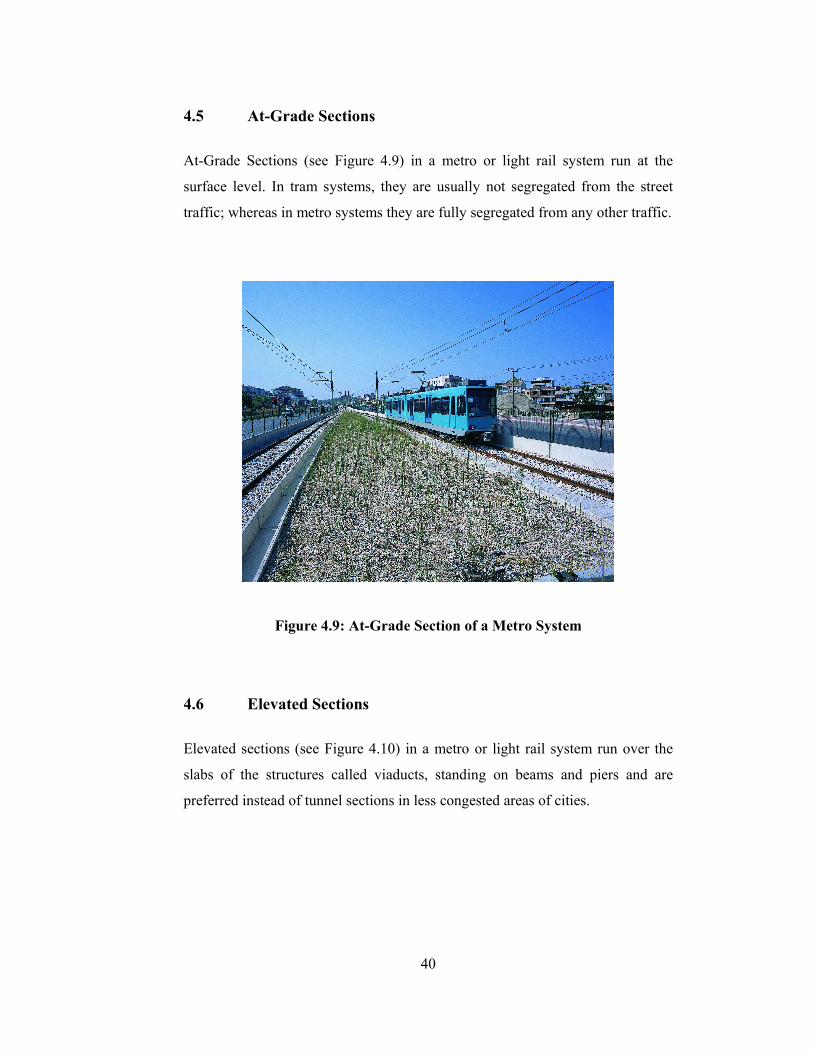
4.5 At-Grade Sections ......................................................................... 40

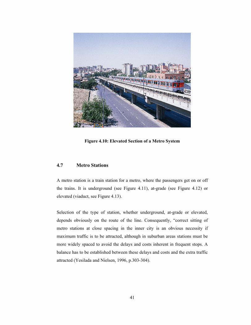
4.6 Elevated Sections........................................................................... 40

4.7 Metro Stations ............................................................................... 41

4.8 Trackwork ..................................................................................... 43

4.9 Complementary Works of Metro and Light Rail Systems........ 45

4.9.1 Depot Area and Maintenance Building ................................... 45

4.9.2 Administration Building.......................................................... 46

4.10 Conclusions .................................................................................. 46

5. METHODOLOGY AND DATA ANALYSIS....................................48

5.1 Introduction................................................................................... 48

5.2 Data Collection .............................................................................. 49

5.3 Data Identification ........................................................................ 50

5.4 Independent variables................................................................... 52

5.4.1 Dummy (Categorical) variables .............................................. 52

xi

5.4.1.1 Dummy variables for Complementary Station Works ..... 53

5.4.1.2 Dummy variables for Trackwork..................................... 54

5.4.1.3 Dummy variables for Main Complementary Works ........ 55

5.4.1.4 Dummy variable for the Type of Contract....................... 55

5.4.1.5 Dummy variable for the Financing Method .................... 56

5.4.2 Continuous variables ............................................................... 59

5.5 Dependent Variable ...................................................................... 61

5.6 Regression Analysis....................................................................... 64

5.7 Stepwise Regression Process ........................................................ 65

5.7.1 Descriptions............................................................................. 65

5.7.2 Initial RM and First Step of Regression Process..................... 66

5.7.3 Second Step of Regression Process......................................... 70

5.8 Validation of the model RM1.5.................................................... 73

5.8.1 Prediction Performance Evaluation......................................... 73

5.8.2 Model Results.......................................................................... 74

6. CONCLUSIONS AND RECOMMENDATIONS ............................ 77

REFERENCES.................................................................................................. 79

xii

LIST OF TABLES

TABLES

Table 3.1 Overview of Metro Systems in Europe………………... 21

Table 3.2 Existing Metro Systems by group of countries.……….. 23

Table 3.3 Overview of LR systems in Europe…………………… 24

Table 3.4 Existing LR systems by group of countries………….... 26

Table 3.5 Growth Potential of Metro and LR Systems in Europe... 26

Table 3.6 Monetary Evaluation of the Market for Metro and LR Systems in Europe…………………………..…………. 27

Table 5.1 List of projects...……………………………………...... 51

Table 5.2 List of Dummy Variables and Corresponding Values… 57

Table 5.3 List of Continuous Variables and Corresponding Values………………………………………………….. 62

Table 5.4 Regression Models of First Step………………………. 69

Table 5.5 P values for regression model RM1.5…………………. 69

Table 5.6 Regression Models of Second Step……………………. 72

Table 5.7 Prediction performance of the model RM1.5………….. 74

Table 5.8 Regression coefficients for the regression model RM1.5………………………………………………….. 75

Table 5.9 AACE International Cost Estimation Classifications (18R-97………………………………………………… 76

Table 5.10 CII Cost Estimate Definitions (CII SD-6)……………... 76

xiii

LIST OF FIGURES

FIGURES

Figure 3.1 A view from a metro system.…………………................... 13

Figure 3.2 A view from a light rail system ………………………....... 16

Figure 3.3 Overhead wires to power a light rail system……………… 17

Figure 4.1 Inside view of a circular tunnel…………………………… 29

Figure 4.2 Construction of a cut-and-cover tunnel…………………… 30

Figure 4.3 Rectangular concrete box for a cut-and-cover tunnel…….. 32

Figure 4.4 A view of a TBM being dismantled after the tunnel excavation…………………………………………………. 33

Figure 4.5 One-shield TBM…………………....................................... 35

Figure 4.6 Cutting wheel of a TBM…………………………………... 36

Figure 4.7 Tunnel Boring by NATM………………………………..... 38

Figure 4.8 Depressed-Open Section of a Metro System……………… 39

Figure 4.9 At-Grade Section of a Metro System……………………... 40

Figure 4.10 Elevated Section of a Metro System……………………… 41

Figure 4.11 Underground Station of a Metro System………………….. 42

Figure 4.12 At-Grade Station of a Metro System……………………… 42

Figure 4.13 Elevated (Viaduct) Station of a Metro System……………. 43

Figure 4.14 Trackwork for the Main Line……………………………... 44

Figure 4.15 Trackwork for the Depot Area……………………………. 44

Figure 4.16 Depot Area………………………………………………... 45

Figure 4.17 Maintenance Building…………………………………….. 46

xiv

Figure 4.18 Administration Building…………………………………... 47

xv

LIST OF ABBREVIATIONS

AACE Association for Advancement of Cost Engineering

ATC Automatic Train Control

CEEC Central and Eastern European Countries

CII Construction Industry Institute

DB Drilling and Blasting

DEM Deutsche Mark

DLLT Dictionary on Labor Law Talk

ERRAC European Rail Research Advisory Council

EU European Union

EUR Euro

LR Light Rail

LRT Light Rail Transit

MAPE Mean Absolute Percent Error

NATM New Australian Tunneling Method

NN Neural Network

RM Regression Model

TBM Tunnel Boring Machine

TL Turkish Lira

UITP International Union of Public Transport

US United States

USD United States Dollar

1

CHAPTER I

INTRODUCTION

As it strives to be more competitive on a world scale, early cost estimation gains

significant importance over the judgment of the future of a capital project in its

conceptual stage, when very limited design information is available. The initial

project decisions are concluded mainly according to the results of these early

cost estimations. As such, use of conceptual cost models, developed by means of

the existing historical information, enable more realistic expectations and

constitute a comparably more dependable basis for the initial business decisions,

including asset development strategies and screening of potential projects.

One of the main factors, perhaps the most important one, affecting the decision

about the future of capital projects at the conceptual phase is to achieve reliable

cost estimation. The owner, lending organization, contractor or the designer need

this cost estimation at the very early stages of the project for several purposes,

including but not limited to the determination of the feasibility project, financial

evaluation of a number of alternatives and establishment of the initial budget.

However, usually very limited design information is available for a project, yet

the scope is not finalized at the conceptual phase. In such a situation, a quick,

inexpensive and reliable technique is necessary in order to obtain a cost estimate

with a reasonable accuracy. Ability to do so is enhanced by conceptual cost

estimation techniques.

As can be derived from its name, conceptual cost estimation is the use of several

techniques to facilitate the estimation of the cost of a project in its conceptual

2

phase. The overall objective of this study is to drive a cost model to assist in the

cost estimation of urban railway system projects (regarding only the civil scope,

excluding electromechanical works and rolling stock), using the very limited

design information available at the very early stages. The data to be used for the

modeling process were collected from actual projects of several Turkish

contractors through a survey method. People at different positions from these

companies were contacted to obtain the required data, which actually consisted

of several parameters corresponding to the main characteristics (both technical

and contractual) of the projects under examination, and their contract prices,

referred as the costs of the projects in this research. Then, parametric modeling

was used to identify the variability in the cost caused by some specific

parameters. There were two limitations to such modeling study; the parameters

used in the modeling process were selected among the ones which would be

available at the feasibility stage of the projects; on the other side, the size of the

data set was limited with the number of projects of which data could be compiled

from the contractors.

In conceptual cost estimation of construction projects, parametric modeling

provides a useful prototype. Referring to the theory of parametric modeling, one

can use it to identify the relationship between the independent variables and the

dependent variable. Basically, this type of modeling quantifies how much the

dependent variable is influenced or explained by the independent variables. In

order to quantify this relation, regression analysis, simulation and neural network

(NN) models are among the techniques used for cost estimation at the early

project phases. Simulation is mainly used for probabilistic estimation where data

of independent variables are not available. NN models usually require larger data

sets which were not available in this study. Therefore, regression analysis was

used for the cost modeling of urban railway system projects in this study.

Many studies regarding conceptual cost estimation have been performed and

several techniques have been suggested. Kouskoulas and Koehn (1974)

3

attempted conceptual cost modeling by deriving a single cost estimation function

that applied to several classes of buildings and defined cost in terms of several

other measurable variables. Karshenas (1984) examined historical data of

multistory steel-framed office buildings to develop a conceptual cost model with

regression analysis. Hegazy and Ayed (1998) mentioned the advantages of using

neural networks (NN) in parametric cost modeling and performed a cost model

for highway projects using NNs. Sönmez (2004) performed a study to construct a

model for the conceptual cost estimate for building projects, using a combination

of the methods of regression analysis and NN models.

This research was designed to facilitate reliable cost estimation, and so improve

ability for initial project decisions concerning urban railway system projects,

covering metro and light rail (LR) systems. It is intended to develop a model

which municipalities, lending organizations and contractors in Turkey can

benefit from during the feasibility stage.

This study is structured as an introductory chapter, four main chapters and a

summary chapter.

• Chapter One – Introduction – The introduction lays the framework and

the purpose of the research that is detailed and developed in the following

chapters. The goal of the research is articulated and the objectives

through which the goal will be attained are presented.

• Chapter Two – Literature Review – A review of literature has been

performed to establish the current body of knowledge pertaining to

conceptual cost modeling and the related techniques.

• Chapter Three – General Information about Metro and LR Systems –

Background information regarding metro and LR systems is provided and

4

the results of a research conducted to give a magnitude of market share

for the urban railway systems in Europe market are presented.

• Chapter Four – Main Characteristics of Metro and LR Systems – This

chapter presents and describes the main characteristics of metro and LR

systems and the related terminology, to provide the reader with a better

understanding of the subject and the relevant parameters.

• Chapter Five – Methodology and Data Analysis – Data compiled for the

research purposes and the statistical results obtained during the modeling

process are presented. The methodology used is described, a model is

selected as the final cost model and its accuracy is calculated.

• Chapter Six – Conclusions and Recommendations – This chapter

provides a comprehensive review of whether the objectives have been

achieved and clear statements regarding the future use of the developed

model.

5

CHAPTER II

LITERATURE REVIEW

This chapter intends to present the review of the available literature regarding the

concept of conceptual cost estimation and is presented to establish the current

body of knowledge pertaining to the analysis of the collected data. The literature

review yielded that conceptual cost estimation had an important place in

developing initial project decisions and several techniques have been suggested

to explain the variations in the project cost by using several parameters.

The study by Hollmann and Dysert (1989) discusses the establishment of a

conceptual cost estimating department in a large organization, presenting an

example of why and to what extent such an organization may require the

conceptual cost estimates. The studies by Kouskoulas and Koehn (1974),

Karshenas (1984), Hegazy and Ayed (1998), Sönmez (2004) investigate the

development of conceptual cost models for different types of construction

projects.

Hollmann and Dysert (1989) examined the conceptual estimating system

developed by the Eastman Kodak Project Management Division in the Kodak

Part Site in Rochester, NY. Several requirements, such as needs of quick

estimates supported by good documentation and needs to evaluate multiple

project options or project cost sensitivity to design changes, were identified for

the purpose of establishment of Conceptual Estimating Department within

Kodak, which would evaluate several project alternatives and establish initial

budgets and plans. The department would provide conceptual and semi-detailed

6

estimates, and thus, development of specialized estimating data, systems and

techniques were required. The developed systems for conceptual cost estimating

provided successful results within the organization, measured by the growth of

department in two years to staff of 17 estimators with annual estimated projects

averaging about $50 million per staff member. Actually, although it had not been

fully measured giving the length of capital cycles when the study was conducted,

the real success would be measured by comparing the project performance

against the budgets and plans originally developed by the Conceptual Estimating

Department, being its main purpose of establishment. However, early feedback

signed that the results would be positive at the time when the research was

conducted.

Kouskoulas and Koehn (1974) attempted conceptual cost modeling by deriving a

single cost estimation function that applied to several classes of buildings and

defined cost in terms of several other measurable variables. They used location,

time of construction, building height, building type, quality and building

technology as the independent variables to develop a linear cost equation, which

was also called as the predesign estimation function. The model was developed

by using the historical building costs and the resulting linear equation, with the

availability of the six above-mentioned parameters, could calculate the square-

foot cost for a building. In addition, the derived function was evaluated by a

residual analysis to check the accuracy of the predictions. By this way, one could

easily comment with the qualifications on the probability that the difference of

the estimated cost from the actual cost would be within a certain percentage of

the actual cost. However, the function was not validated by a technique such as

cross validation, which would provide more information about the prediction

performance of the model.

Karshenas (1984) examined historical data of multistory steel-framed office

buildings to develop a conceptual cost model with regression analysis. Karshenas

argued that since the type of the building had an important effect on the

7

construction cost, different types of buildings should be investigated separately.

Thus, only the data related to the multistory steel-framed office buildings was

studied. For the purpose of the study, the data published by Engineering News

Record was analyzed. However, different from the study performed by

Kouskoulas and Koehn, Karshenas used nonlinear parameters in terms of typical

floor area and building height to explain the variations in the cost. The necessity

of including nonlinear parameters in the cost model was clear by examining the

plotted observed costs, which all led to curves, on a grid space. On the other

hand, several types of mathematical functions could fit the data. Karshenas used

regression analysis, or the method of least squares in other words, to select the

type of function that best fitted the cost data. The accuracy of the predictions was

checked by a residual analysis, likewise the study of Kouskoulas and Koehn.

Furthermore, the ability of the model to explain the variations in the cost was

measured by investigating the coefficient of determination, called as R2. This

measure of closeness of fit gave a percentage of the variations explained by the

developed regression equation. In addition to the residual analysis, Karshenas

also compared published costs and the predicted costs to investigate the accuracy

of the predictions. Karshenas, on the other hand along with Kouskoulas and

Koehn, argued that the cost equations must have been updated periodically by

new data sets. However, the model developed by Karshenas was not, either,

validated by a technique such as cross validation.

Hegazy and Ayed (1998) mentioned the advantages of using NNs in parametric

cost modeling and performed a cost model for highway projects using NNs.

They preferred NNs for the modeling of their data due to their argument

regarding the inherent limitations of regression-based techniques in the

development of parametric cost models. They pointed out that regression-based

techniques required a defined mathematical form for the cost function that best

fitted the available historical data and these techniques were unsuitable to

account for the large number of variables present in a construction project and

the numerous interactions among them. In terms of using non linear parameters

8

in the modeling process, their study was similar to that of Karshenas, who used

nonlinear parameters determined by regression technique to explain the

variations in the cost. However, Hegazy and Ayed preferred to use NN

technique, both to investigate the shape of interactions between the parameters

leading to the use of non linear parameters and to drive the cost model.

Hegazy and Ayed (1998) used the data of 14 projects for training and 4 projects

(total of 18 observations) for testing the developed NN models. In order to

optimize the NN performance, three approaches, as back-propagation training,

simplex optimization and genetic algorithms, were used to train the NNs

developed by the ten input variables. At the end of the model development, the

results were examined by comparing the errors for the three approaches and it

was concluded that the networks of the simplex optimization and back-

propagation training were most suited to the study, where the simplex

optimization produced the optimum NN. As an addition to the findings of the

study, excel macros were developed to encode the optimum model in a user-

friendly software to facilitate the user input of cost-related parameters for new

projects and, accordingly, predict their budget costs.

Sönmez (2004) performed a study to construct a model for the conceptual cost

estimate for building projects, using a combination of the methods of regression

analysis, simulation and NN models. The advantages of simultaneous use of

regression analysis and NNs for conceptual cost estimating were discussed and a

cost model for continuing care retirement projects (CCRC) was developed with a

pragmatic approach using a mix of these tools. A CCRC was defined to be an

organization established to provide housing and services, including health care,

to people of retirement age, generally consisting of residential, health center and

commons buildings, and sometimes a structured parking. Data for 30 CCRC

projects built by a contractor in the United States were compiled and

construction time (year) and location, total building area, combined percent area

of health center and commons, area per unit, number of floors and percent area

9

of structured parking, and the total project costs were used for the modeling

purposes.

Sönmez considered parsimonious models in the study, which produce generally

better forecasts. A parsimonious model was defined as the model fitting to the

data adequately without using any unnecessary parameters. Therefore, it was

crucial to eliminate the insignificant variables from the model for a better

prediction performance. A backward elimination method was used and the

variables that were not contributing to the model were eliminated one at a time at

each step of the regression process. The determination about the variables to be

eliminated was based on two regression statistics, significance level (P value,

giving an indication of the significance of the variables included in the model)

and coefficient of determination (R2, giving a measure of the variability

explained in the model).

The first regression model (RM) was performed using all the variables available

and the variable corresponding to the coefficient with the highest P value for

each model was eliminated one at a time. A final RM was achieved with a

reasonable closeness of fit, at a significant level of the variables. NN models

were developed to investigate the possible existence of significant nonlinear or

interaction relations between the variables. The variables in the final RM were

trained by two NNs with different hidden units.

The final RM and the NN models were then compared in terms of closeness of

fit and prediction performance, on the basis of MSE (Mean Squared Error) and

MAPE (Mean Absolute Percent Error) values. Linear regression model, which

provided a better prediction performance, was selected as the final model to be

used for future forecast purposes. Furthermore, prediction intervals were also

constructed using probabilistic techniques to quantify the level of uncertainties

existing in the conceptual stage of a project. Sönmez also performed a case study

to illustrate the use of the developed cost model.

10

NNs have seen an explosion of interest over the last few years due to their

capability of modeling extremely complex functions and ease of use. NNs learn

by example and have evolved based on an artificial intelligence offering an

alternative approach for cost modeling. NNs are commonly used for difficult

tasks involving intuitive judgment or requiring the detection of data patterns that

elude conventional analytic techniques (Hegazy and Ayed, 1998). NNs were not

used in this research, mainly due to the limited number of observations (project

data) available. A NN trained with such a large set of variables could result with

the over-fitting problem, which could lead to models with worse prediction

performances. Sönmez (2004) notes that the advantage of RMs lies in their

generally parsimonious use of parameters compared to NNs. The principle of

parsimony is important because, in practice, parsimonious models generally

produce better forecasts (Pankratz, 1983, p.81-82). Also in the same study, linear

regression models were found sufficient in terms of representing the relations

between dependent and independent variables for conceptual cost modeling. That

is why linear regression models were preferred in this study.

11

CHAPTER III

GENERAL INFORMATION ABOUT

METRO AND LR SYSTEMS

3.1 Introduction

This chapter covers some background information about the metro and LR

systems, pointing out the main differences between them, as the projects used for

the purpose of this study may be classified into these two groups. Consequently,

this chapter also presents the results of the studies regarding metro and LR

systems performed by the European Rail Research Advisory Council (ERRAC),

concerning the worldwide association of urban and regional passenger transport

operators, their authorities and suppliers in the 35 European countries. The

purpose of including the results of such a research in this study lies under the

idea to raise further awareness of the reader on the paramount importance of the

subject regarding conceptual cost estimation of urban railway systems, by

featuring the indicative figures.

3.2 Metro Systems

3.2.1 Definitions

“A Metro can be defined as a form of mass transit public transport system

employing trains. In many cases, at least a portion of the rails are placed in

tunnels dug beneath the surface of a city in which case the system may be called

the Underground or the subway. However, one definition of a true metro system

12

can be made as an urban, electric mass transit system, which is totally

independent from other traffic, with high service frequency.” [Dictionary on

Labor Law Talk (DLLT), http://encyclopedia.laborlawtalk.com/Metro, last

access June 9, 2005]

“Another possible definition of a metro may be an urban passenger railway with

stations at frequent intervals to provide convenient and rapid transport over

relatively short distances within a city and its environs (Yesilada and Nielsen,

1996, p.303).” This definition states that a metro system is an urban railway

system and is designed to transport passengers within a city; not to provide

transportation between cities. “The term metro best generalizes various names

used to call the same type of transit system as Underground, Subway, U-bahn or

Rapid Transit; where it is thought that the said term is derived from Paris or

London’s first system, the Metropolitan Railway (Yesilada and Nielsen, 1996,

p.303)”.

International Union of Public Transport (UITP) defines metro as “a tracked,

electrically driven local means of transport, which has an integral, continuous

track bed of its own (large underground or elevated sections)”. ERRAC (2004)

notes that this results in a high degree of freedom for the choice of vehicle width

and length, and thus a large carrying capacity (above 30,000 passengers per hour

per direction – pphpd). “Intervals between stations would be typically more than

1 km, and because the alignment does not have to follow existing streets, curve

radii and section gradient can be more generously dimensioned and permits for

an overall higher commercial speed (ERRAC, 2004)”.

This large carrying capacity indicates the main difference between the metro and

LR systems. As such, ERRAC states that metro systems require, therefore,

heavier investment than LR, and can be implemented only in large cities where

demand justifies the capital cost. On the other hand, one of the most important

characteristics of a metro system is noted as “the ability to transport rapidly large

13

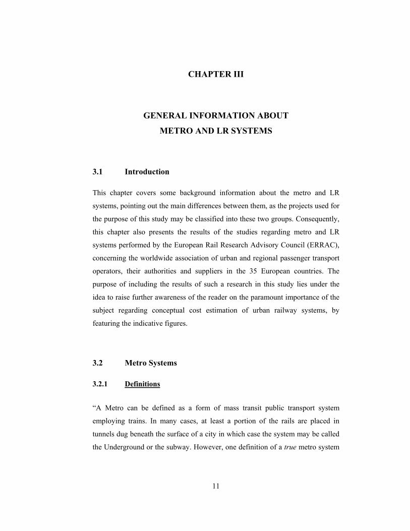
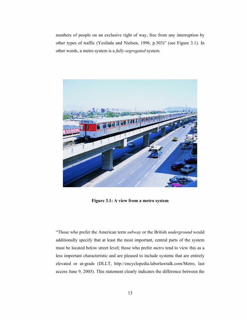
numbers of people on an exclusive right of way, free from any interruption by

other types of traffic (Yesilada and Nielsen, 1996, p.303)” (see Figure 3.1). In

other words, a metro system is a fully-segregated system.

Figure 3.1: A view from a metro system

“Those who prefer the American term subway or the British underground would

additionally specify that at least the most important, central parts of the system

must be located below street level; those who prefer metro tend to view this as a

less important characteristic and are pleased to include systems that are entirely

elevated or at-grade (DLLT, http://encyclopedia.laborlawtalk.com/Metro, last

access June 9, 2005). This statement clearly indicates the difference between the

14

use of terms of subway, underground and metro. In this study the term metro was

used wherever necessary, since the projects under examination for the research

purposes include systems consisting of elevated, at-grade and underground

sections together. “The varieties of the system are many but almost all the metro

systems have, in common, tunneling for at least some sections of their city routes

(Yesilada and Nielsen, 1996, p.10)”. The metro systems to be analyzed in this

research, in parallel with this statement, have tunnel sections built for some

sections along their routes.

“The volume of passengers a metro train can carry is often quite high, and a

metro system is often viewed as the backbone of a large city's public

transportation system (DLLT, http://encyclopedia.laborlawtalk.com/Metro, last

access June 9, 2005)”. Broadly classifying the public transportation systems for a

large city as bus transit system and rapid transit system (referring to metro); it

could be stated that the public transportation system stands on the metro system,

where any disruption in the metro system might lead to the fall of the overall

structure.

3.2.2 History of Metro Systems

The Metropolitan Railway in London, opened in 1863, is the first real

underground line in the sense discussed in this study, where the rolling stock

consisted of steam locomotives designed to condense their exhaust steam in the

tunnels (Wikipedia, http://en.wikipedia.org/wiki/Metro, last access June 9,

2005). This line was followed by many extensions and the Metropolitan

eventually became an important part of the London Underground system.

“Before the end of 19th century, in addition to London, lines were constructed in

Glasgow (1896), Budapest (1897), Boston (1897) and Vienna (1898). After

London, the next major system was the Paris Metro, whose first line was opened

15

in 1902 (Yesilada and Nielsen, 1996, p.10)”. “The full name of the Paris Metro

was the Chemin de Fer Métropolitain, a direct translation of London's

Metropolitan Railway. The name was shortened to métro in French, and this

word was borrowed by many other languages (Wikipedia, http://en.wikipedia.-

org/wiki/Metro, last access June 9, 2005)”.

3.3 Light Rail (LR)

3.3.1 Definitions

“Light rail (LR) is a particular class of urban and suburban passenger railway

that utilizes equipment and infrastructure that is typically less massive than that

used for metro systems and heavy railways (DLLT, http://encyclopedia.-

laborlawtalk.com/Light_rail, last access June 9, 2005)”. As such, the main

difference between LR and metro systems is drawn as the mass of the utilized

equipment and infrastructure. The heavier mass of the equipment and

infrastructure is used, the higher the cost of the system results; where one can

broadly compare the cost of metro and LR systems.

UITP defines LR as “a tracked, electrically driven local means of transport,

which can be developed step by step from a modern tramway to a means of

transport running in tunnels or above ground level. Every development stage can

be a final stage in itself. It should, however, permit further development to the

next higher stage.” ERRAC (2004) notes that this broad definition encompasses

a wide array of situations, from conventional tramway, to tram-train solutions.

“LR systems are thus flexible and expandable. It is not absolutely necessary to

have an independent bed track over the whole route; however, the highest degree

of segregation from private traffic should be aimed for (ERRAC, 2004)”. In this

aspect, one of the differences between metro and LR systems can be stated as the

16

concept of segregation. As previously mentioned, metro systems are fully-

segregated systems. In other words, metro systems operate fully independent

from the other traffic. However, LR systems can not be classified as fully-

segregated systems, and they are usually semi-segregated systems, although, as

noted in the above statement, highest degree of segregation from private traffic

should be aimed for the development of such.

“LR systems can be developed from traditional tramway systems or planned and

built as entirely new systems. The former option being likely to happen in many

central and eastern European cities, and the latter option mostly in Western

European countries (ERRAC, 2004)”. This is the general approach of the

European countries regarding the construction and development of LR systems.

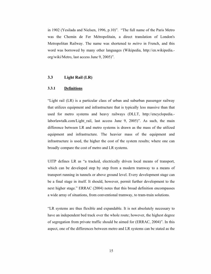
Figure 3.2: A view from a light rail system

17

The term light rail is derived from the British English term light railway long

used to distinguish tram operations from steam railway lines, as well as from its

usually lighter infrastructure (see Figure 3.2) (DLLT, http://encyclopedia.labor-

lawtalk.com/Light_rail, last access June 9, 2005).

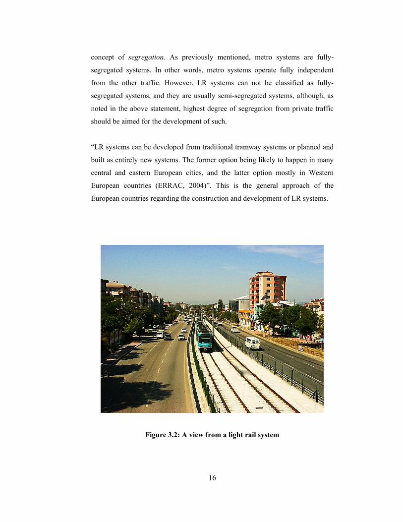
LR systems are almost universally operated by electricity delivered through

overhead lines (see Figure 3.3). However, third-rail systems have been coming

into practice where the trains use a standard third rail for electrical power

(DLLT, http://encyclopedia.laborlawtalk.com/Light_rail, last access June 9,

2005).

Figure 3.3: Overhead wires to power a light rail system

18

3.3.2 Attempting to define "Light Rail"

As mentioned in the section describing the metro systems, metro systems are

considered to be "heavy rail" in comparison. Regarding the number of

passengers carried within a comparable time period or per vehicle, the main

difference between the LR and metro systems is drawn as the passenger carrying

capacity and the systems designed with less passenger capacity are considered to

be “lighter”, which results in the naming of these systems as “Light Rail”

systems. Speed of the vehicles may be another aspect in the classification of such

systems. “Monorails are also considered to be a separate technology. LR systems

can handle steeper inclines than heavy rail, and curves sharp enough to fit within

street intersections (though this is hardly true for all light-rail lines). They are

typically built in urban areas, providing frequent service with small, light trains

or single cars (DLLT, http://encyclopedia.laborlawtalk.com/Light_rail, last

access June 9, 2005)”.

The most difficult distinction to draw is that between LR and streetcar or tram

systems, where 2 projects out of 13 of which data were compiled for this study

were tram systems; the others being either metro or LR. There is a significant

amount of overlap between the technologies, and it is common to classify

streetcars/trams as a subtype of LR rather than as a distinct type of

transportation. The following two general versions are noted by DLLT:

• “The traditional type, where the tracks and trains run along the streets and

share space with road traffic. Stops tend to be very frequent, but little effort

is made to set up special stations. Because space is shared, the tracks are

usually visually unobtrusive.

• A more modern variation, where the trains tend to run along their own

right-of-way and are often separated from road traffic. Stops are generally

less frequent, and the vehicles are often boarded from a platform. Tracks

19

are highly visible, and in some cases significant effort is expended to keep

traffic away through the use of special signaling and even grade crossings

with gate arms.”

(DLLT, http://encyclopedia.laborlawtalk.com/Light_rail, last access June

9, 2005)

As the purpose of the study is to drive a model for the conceptual cost estimation

of metro and LR systems (where trams could be considered as a sub-type of such

systems), it is better to point out that there is a significant difference in cost

between these different classes of LR transit (LR and tram). DLLT describes that

the traditional style, which also can be called as the tram system, is often less

expensive by a factor of two or more. Despite the increased cost, the more

modern variation (which can be considered as "heavier" than old streetcar

systems, even though it is called "LR") is the dominant form of urban rail

development in the US.

3.3.3 History

“The origin of the tramway can be traced back to the plateways used in mines

and quarries to ease the passage of horse-drawn wagons, but the first street

tramway in a city was the New York and Harlem line of 1832, coining the

American term still used today, street railway. Remarkably the world's second

horse tramway, in New Orleans (1835), is still in use for electric cars today, after

over 150 years of continuous service (Taplin, 1998)”.

On the other hand, Taplin (1998) notes that the tramway to Europe was brought

by American promoters for Paris in 1853 and Birkenhead in England in 1860,

followed by London in 1861 and Copenhagen in 1863.

20

3.3.4 Advantages of Light Rail

After pointing out the differences between LR and metro systems, one may ask

for the advantages of LR over the heavier systems. Taplin (1998) notes that the

LR demonstrates its flexibility by its ability to operate in a wide range of built

environments. “It can act as a tramway in the street, though if its advantages over

the bus are to be maximized, unsegregated street track should be kept to the

minimum needed to pass particular pinch points. Within the street environment it

can be segregated by white lines, low kerbs, and side or central reservation

(Taplin, 1998)”.

However, the main advantage to prefer a LR system is that it is generally cheaper

to build than heavy rail, since the infrastructure does not need to be as

substantial, and tunnels are generally not required as is the case with most metro

systems. Moreover, the ability to handle sharp curves and steep gradients can

reduce the amount of work required (DLLT, http://encyclopedia.labor-

lawtalk.com/Light_rail, last access June 9, 2005).

Concerning the issue of safety, in an emergency, LR trains are easier to evacuate

than those of heavier systems.

3.4 Metro and LR Systems in Europe

The European Rail Research Advisory Council (ERRAC) set-up in September

2002, delivered some specific analysis on urban railway systems in Europe in

April 2004 based on the studies performed by International Union of Public

Transport (UITP), the worldwide association of urban and regional passenger

transport operators, their authorities and suppliers. The studies were made of two

parts and covered the Metro and LR Systems in 35 European countries.

21

The research, based on the findings of the analysis performed by ERRAC,

provide indicative figures for the stunning market share of the urban railway

sector in Europe. The data and results of this research, limited to the boundaries,

are presented in the following pages, in order to raise further awareness of the

importance of conceptual cost estimation for urban railway systems, especially

among decision-makers and those with responsibilities in research.

3.4.1 Metro Systems in Europe

3.4.1.1 Overview

ERRAC gives a total number of 36 systems in Europe, 27 within the EU-15, 3

within the new member states that joined to EU in May 2004 and 6 within the

countries beyond the EU-25 (including Norway and Switzerland but also

candidate countries for EU membership such as Bulgaria, Romania and Turkey

as par of the second enlargement wave). This group of countries, however

heterogeneous it may seem, has been constituted by the research group in order

to simplify and ensure a better understanding of results.

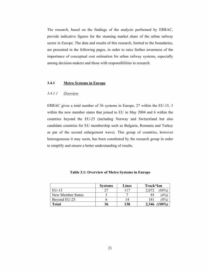
Table 3.1: Overview of Metro Systems in Europe

Systems Lines Track*km EU-15 27 117 2,072 (88%)

New Member States 3 7 93 (4%)

Beyond EU-25 6 14 181 (8%)

Total 36 138 2,346 (100%)

22

3.4.1.2 Existing Systems

Table 3.1 shows that among the 36 metro systems (138 lines), 75% of systems

(27), 85% of lines (117) and 88% of track*km (2,072) are in operation within the

EU-15 (Marginally, some systems have single track sections, or sections with

over 2 tracks, but in this research performed by ERRAC, 1 track*km is to be

understood as 1 km of double track.). The first wave of the Eastern enlargement

in 2004 is said to have brought another 3 systems (7 lines and 93 km) into the

EU. Another 6 systems are said to be found in countries that remained outside

the borders of the enlarged EU after 2004 (14 lines and 181 km).

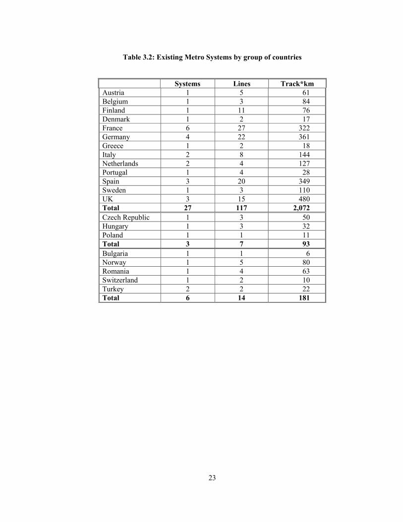
The results of the exploration have also revealed that few cities in Central and

Eastern European Countries (CEEC) invested in metro systems. These cities are

said to have, instead, expanded their tramway systems. Table 3.2 summarizes the

distribution of existing metro systems in Europe by group of countries.

3.4.1.3 Growth of Metro systems in Europe

New lines can mean either cities introducing a metro system for the first time or

additional lines being built next to existing ones. The findings of the research

performed by ERRAC state that, in 20 cities (of which 14 are in the EU-15), new

lines are being built or existing lines are being extended, which is an increase of

55% of existing systems (of which 52% of these systems are in the EU-15). This

represents 135.3 km, of which nearly 112 km are in the EU-15. On the other

hand, the study also indicates that in a further 33 cities, 503.9 km of new lines or

extensions are planned.

23

Table 3.2: Existing Metro Systems by group of countries

Systems Lines Track*km Austria 1 5 61 Belgium 1 3 84 Finland 1 11 76 Denmark 1 2 17 France 6 27 322 Germany 4 22 361 Greece 1 2 18 Italy 2 8 144 Netherlands 2 4 127 Portugal 1 4 28 Spain 3 20 349 Sweden 1 3 110 UK 3 15 480 Total 27 117 2,072 Czech Republic 1 3 50 Hungary 1 3 32 Poland 1 1 11 Total 3 7 93 Bulgaria 1 1 6 Norway 1 5 80 Romania 1 4 63 Switzerland 1 2 10 Turkey 2 2 22 Total 6 14 181

24

3.4.2 LR Systems In Europe

3.4.2.1 Overview

ERRAC gives a total number of 170 systems represented in this LRT overview

in Europe, 107 within the current EU-15, 30 within the new Member States that

joined the EU in May 2004 and 33 within the countries beyond the EU-25

(including Norway, Switzerland but also candidate countries for the EU

membership such as Bulgaria, Romania and Turkey, or the 2nd enlargement

wave, as well as Western Balkan countries). This group of countries has been

constituted in order to simplify and ensure a better understanding of results, in

the same way followed for the metro systems.

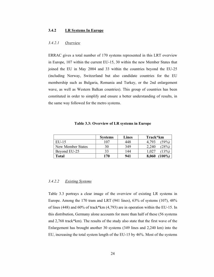
Table 3.3: Overview of LR systems in Europe

Systems Lines Track*km EU-15 107 448 4,793 (59%)

New Member States 30 349 2,240 (28%)

Beyond EU-25 33 144 1,027 (13%)

Total 170 941 8,060 (100%)

3.4.2.2 Existing Systems

Table 3.3 portrays a clear image of the overview of existing LR systems in

Europe. Among the 170 tram and LRT (941 lines), 63% of systems (107), 48%

of lines (448) and 60% of track*km (4,793) are in operation within the EU-15. In

this distribution, Germany alone accounts for more than half of these (56 systems

and 2,768 track*km). The results of the study also state that the first wave of the

Enlargement has brought another 30 systems (349 lines and 2,240 km) into the

EU, increasing the total system length of the EU-15 by 46%. Most of the systems

25

are in operation in Poland, the Czech Republic and Hungary. Another 31 systems

can be found in countries that remained outside the borders of the enlarged EU

after 2004 (144 lines and 1,027 km). The study points out to the plans for

extensions of the existing, as well as for several new systems, in well-off and

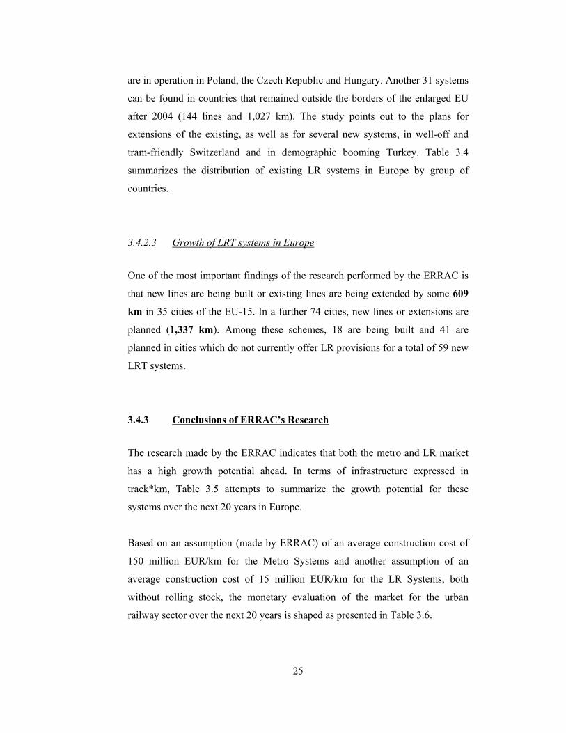
tram-friendly Switzerland and in demographic booming Turkey. Table 3.4

summarizes the distribution of existing LR systems in Europe by group of

countries.

3.4.2.3 Growth of LRT systems in Europe

One of the most important findings of the research performed by the ERRAC is

that new lines are being built or existing lines are being extended by some 609

km in 35 cities of the EU-15. In a further 74 cities, new lines or extensions are

planned (1,337 km). Among these schemes, 18 are being built and 41 are

planned in cities which do not currently offer LR provisions for a total of 59 new

LRT systems.

3.4.3 Conclusions of ERRAC’s Research

The research made by the ERRAC indicates that both the metro and LR market

has a high growth potential ahead. In terms of infrastructure expressed in

track*km, Table 3.5 attempts to summarize the growth potential for these

systems over the next 20 years in Europe.

Based on an assumption (made by ERRAC) of an average construction cost of

150 million EUR/km for the Metro Systems and another assumption of an

average construction cost of 15 million EUR/km for the LR Systems, both

without rolling stock, the monetary evaluation of the market for the urban

railway sector over the next 20 years is shaped as presented in Table 3.6.

26

Table 3.4: Existing LR systems by group of countries

Systems Lines Track*km Austria 6 47 313 Belgium 5 33 332 Finland 1 11 76 France 11 20 202 Germany 56 231 2,768 Greece 0 0 0 Ireland 0 0 0 Italy 7 37 209 Luxembourg 0 0 0 Netherlands 5 34 280 Portugal 2 6 65 Spain 4 5 206 Sweden 3 14 186 UK 7 10 156 Total 107 448 4,793 Czech Republic 7 71 333 Estonia 1 4 39 Hungary 1 34 188 Latvia 1 8 167 Poland 14 204 1,445 Slovakia 3 28 68 Total 30 349 2,240 Bosnia and Herzegovina 1 2 16 Bulgaria 1 16 208 Croatia 2 15 57 Norway 2 9 47 Romania 14 69 461 Switzerland 7 26 112 Turkey 5 6 66 Serbia and Montenegro 1 11 60 Total 33 144 1,027

Table 3.5: Growth Potential of Metro and LR Systems in Europe

Track*km in Construction Track*km Planned Metro Systems 135.3 503.9 LR Systems 609.0 1,337.0

27

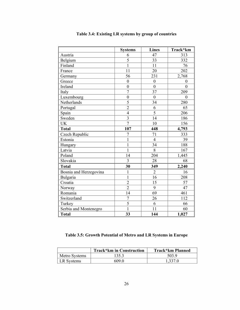
Table 3.6: Monetary Evaluation of the Market for

Metro and LR Systems in Europe

Lines in Construction Planned Lines Metro Systems over EUR 20 billion over EUR 75 billion LR Systems over EUR 9.5 billion over EUR 22 billion Total over EUR 29.5 billion over EUR 97 billion Grand Total over EUR 126.5 billion

Table 3.6 presents significant figures regarding the monetary evaluation of the

market for metro and LR systems in Europe, reaching to a range of EUR125

billion over the next 20 years.

This stunning market share certainly will help to convince the railway

community to benefit from the conceptual cost estimation techniques developed

for the urban railway sector, being the main focus of this study. Obviously, this

modeling study will contribute to the initial project decisions needed by the

owners, contractors, designer and lending organizations for the metro and LR

systems located in Turkey, for several purposes including determination of the

feasibility of the system, financial evaluation of a number of alternative systems

and establishment of an initial budget.

28

CHAPTER IV

MAIN CHARACTERISTICS OF METRO AND LR SYSTEMS

4.1 Introduction

This chapter presents information about the main characteristics of a metro and

LR system, with the particular structures included, and the terminology used to

define these particular structures and sections of such systems. These particular

structures and sections along the line of a metro or LR system project will

correspond to the majority of the independent variables to be used for regression

analysis in the next chapter. The purpose of this chapter is to provide the

particular information related to such systems before the data analysis, with

illustrative figures where necessary, to create a media for the reader where a

clear image of the data collected for the projects could be visualized.

4.2 Tunnels

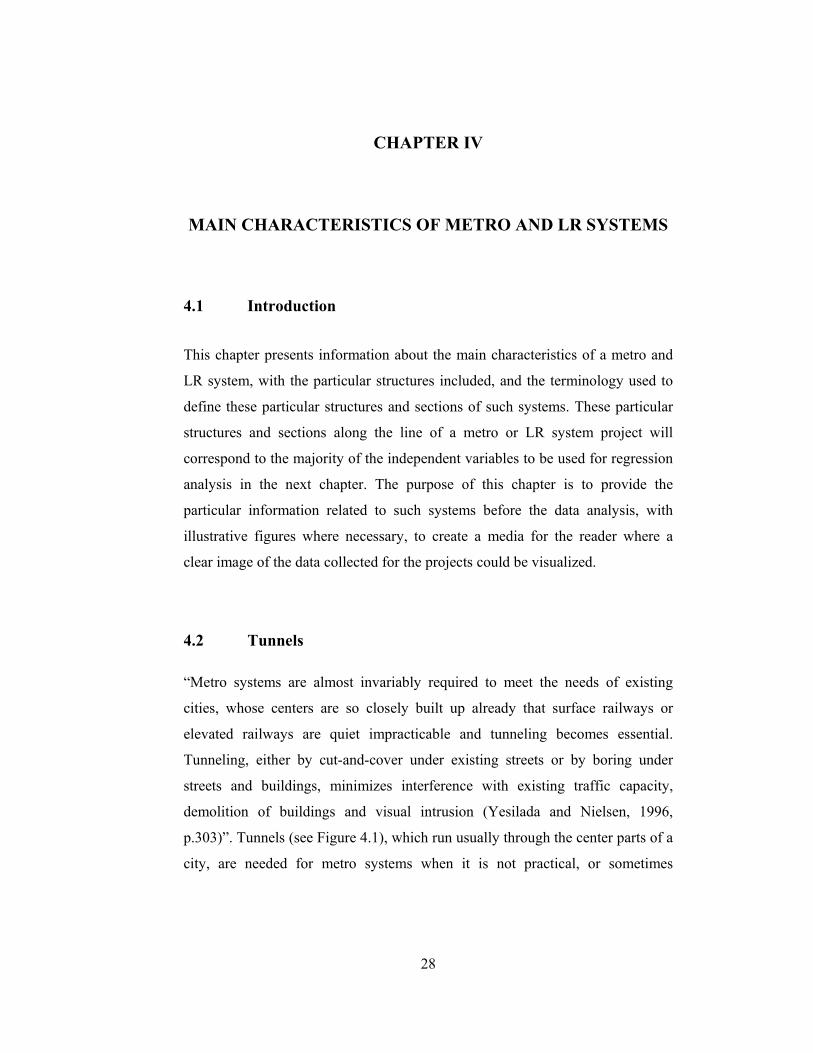
“Metro systems are almost invariably required to meet the needs of existing

cities, whose centers are so closely built up already that surface railways or

elevated railways are quiet impracticable and tunneling becomes essential.

Tunneling, either by cut-and-cover under existing streets or by boring under

streets and buildings, minimizes interference with existing traffic capacity,

demolition of buildings and visual intrusion (Yesilada and Nielsen, 1996,

p.303)”. Tunnels (see Figure 4.1), which run usually through the center parts of a

city, are needed for metro systems when it is not practical, or sometimes

29

impossible, to construct elevated or at-grade systems along the route. Besides,

tunneling also provides the protection of the existing aesthetics.

Figure 4.1: Inside view of a circular tunnel

The cost difference between the tunnel sections and the others, including at-

grade and elevated, of a metro system is significant due to the construction

difficulties and so developed methods. “The construction of a tunnel, in other

words an underground, is an expensive project, often carried out over a number

of years. Tunneling costs are necessarily high and thus, it is usual to tunnel only

in congested areas and under high ground (Yesilada and Nielsen, 1996, p.303)”.

4.3 Construction Methods for Tunneling

Tunnels are dug in various types of ground, from soft clays to hard rocks.

Depending on the type of soil, a method of excavation is selected. Several modes

of tunneling exist and are introduced in the following pages.

30

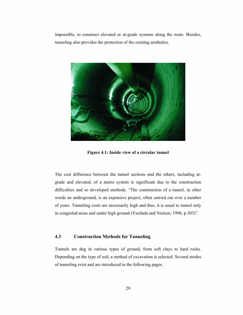
4.3.1 Cut-and-cover

“In dealing with shape, size and structure, there are substantial differences

according to whether construction is bored tunnel or cut-and-cover (depressed-

enclosed). The choice of method is a complex matter, but cut-and-cover is likely

to be preferred where it is possible to follow a shallow subsurface route without

unacceptable disruption of streets and services, while deeper tunneling is

progressively more necessary in heavily congested city areas (Yesilada and

Nielsen, 1996, p.15)”.

Figure 4.2: Construction of a cut-and-cover tunnel

Figure 4.2 presents a view from the initial phases of construction of a cut-and-

cover tunnel running below a street within the inner parts of a city. The

construction method of a cut-and-cover tunnel can be summarized as follows:

31

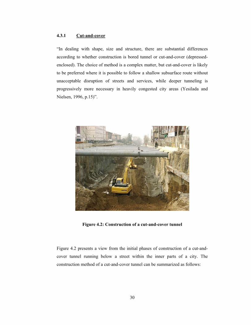
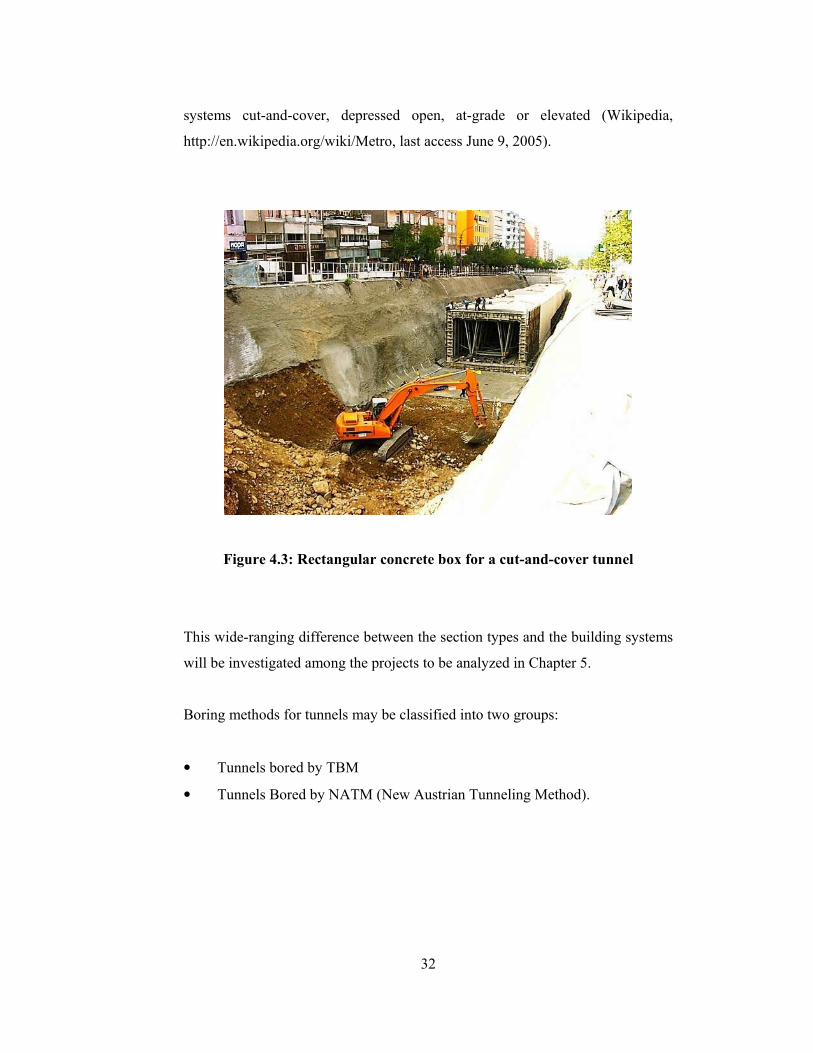
“In cut-and-cover method of tunneling, the city streets are excavated and a tunnel

structure strong enough to support the road above is built at the trench, which is

then filled in and the roadway rebuilt. Twin tracks are usually accommodated in

a rectangular concrete box with a central wall or line of columns (see Figure 4.3).

However, sometimes it might be compulsory to construct two separate box

structures, each including a single track, slightly far away from each other. These

are typically made of concrete, usually with structural columns of steel; in the

oldest systems, brick and cast iron were used, however. This method often

involves extensive relocation of the utilities commonly buried not far below city

streets, particularly power and telephone wiring, water and gas mains, and

sewers (Wikipedia, http://en.wikipedia.org/wiki/Metro, last access June 9, 2005).

This mandatory “utility relocation” works usually raises the most

disadvantageous side of cut-and-cover tunneling method.

In this study, most of the projects to be analyzed include significant lengths of

tunnel sections executed by cut-and cover method along their routes.

4.3.2 Boring

Another possible way of tunneling is boring, and is preferred usually when cut-

and-cover method is not practical. A vertical shaft is constructed and the tunnels

are dug horizontally from there. This method almost avoids any disturbance to

existing streets, buildings and utilities and this fact draws the most essential side

of boring method to be preferred instead of cut-and-cover tunneling. However,

this time, problems with ground water are more likely, and tunneling through

native bedrock may require blasting. The confined space in the tunnel also limits

the machinery that can be used, but specialized tunnel-boring machines (TBMs)

are fortunately now available to overcome this challenge. One disadvantage with

this, however, is that the cost of bored-tunneling is much higher than building

32

systems cut-and-cover, depressed open, at-grade or elevated (Wikipedia,

http://en.wikipedia.org/wiki/Metro, last access June 9, 2005).

Figure 4.3: Rectangular concrete box for a cut-and-cover tunnel

This wide-ranging difference between the section types and the building systems

will be investigated among the projects to be analyzed in Chapter 5.

Boring methods for tunnels may be classified into two groups:

• Tunnels bored by TBM

• Tunnels Bored by NATM (New Austrian Tunneling Method).

33

4.3.2.1 Boring Tunnels by Tunnel Boring Machine (TBM)

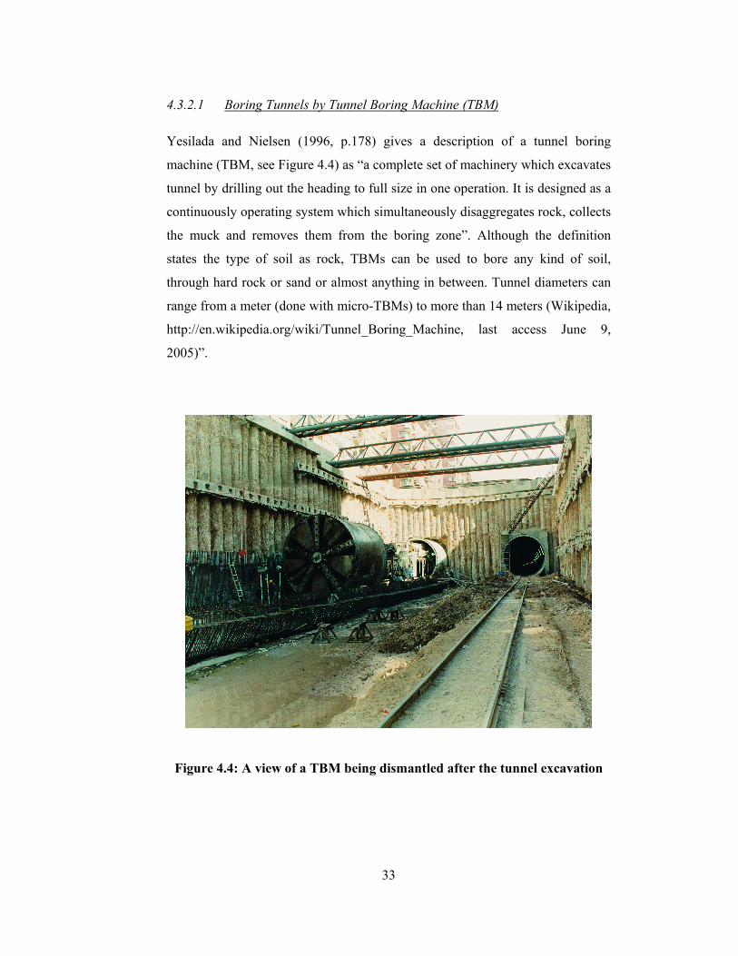
Yesilada and Nielsen (1996, p.178) gives a description of a tunnel boring

machine (TBM, see Figure 4.4) as “a complete set of machinery which excavates

tunnel by drilling out the heading to full size in one operation. It is designed as a

continuously operating system which simultaneously disaggregates rock, collects

the muck and removes them from the boring zone”. Although the definition

states the type of soil as rock, TBMs can be used to bore any kind of soil,

through hard rock or sand or almost anything in between. Tunnel diameters can

range from a meter (done with micro-TBMs) to more than 14 meters (Wikipedia,

http://en.wikipedia.org/wiki/Tunnel_Boring_Machine, last access June 9,

2005)”.

Figure 4.4: A view of a TBM being dismantled after the tunnel excavation

34

The key disadvantage for the use of TBMs is cost. Manufacturing of TBMs are

expensive, yet it is difficult to transport them to the site. Besides, TBMs require

significant infrastructure, which consist of multiple systems installed behind the

machinery itself inside the tunnel and plants installed in the shaft zone. On the

other hand, TBMs are generally manufactured on the basis of a project-oriented

design (Yesilada and Nielsen, 1996, p.180). Thus, TBMs are manufactured

specifically for the concerned project and rarely suit with the conditions of any

following project, with respect to soil conditions and diameter. This is one of the

significant factors that cause the high cost of using TBM for tunnel construction.

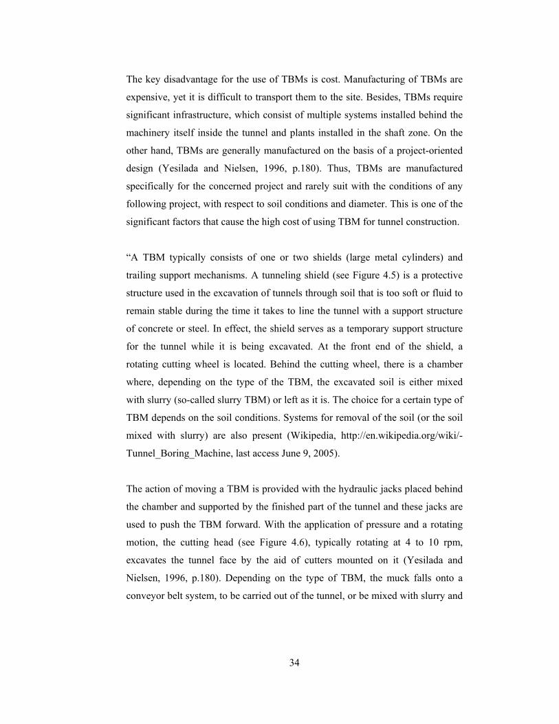
“A TBM typically consists of one or two shields (large metal cylinders) and

trailing support mechanisms. A tunneling shield (see Figure 4.5) is a protective

structure used in the excavation of tunnels through soil that is too soft or fluid to

remain stable during the time it takes to line the tunnel with a support structure

of concrete or steel. In effect, the shield serves as a temporary support structure

for the tunnel while it is being excavated. At the front end of the shield, a

rotating cutting wheel is located. Behind the cutting wheel, there is a chamber

where, depending on the type of the TBM, the excavated soil is either mixed

with slurry (so-called slurry TBM) or left as it is. The choice for a certain type of

TBM depends on the soil conditions. Systems for removal of the soil (or the soil

mixed with slurry) are also present (Wikipedia, http://en.wikipedia.org/wiki/-

Tunnel_Boring_Machine, last access June 9, 2005).

The action of moving a TBM is provided with the hydraulic jacks placed behind

the chamber and supported by the finished part of the tunnel and these jacks are

used to push the TBM forward. With the application of pressure and a rotating

motion, the cutting head (see Figure 4.6), typically rotating at 4 to 10 rpm,

excavates the tunnel face by the aid of cutters mounted on it (Yesilada and

Nielsen, 1996, p.180). Depending on the type of TBM, the muck falls onto a

conveyor belt system, to be carried out of the tunnel, or be mixed with slurry and

35

pumped back to the tunnel entrance (Wikipedia, http://en.wikipedia.-

org/wiki/Tunnel_Boring_Machine, last access June 9, 2005)”.

Figure 4.5: One-shield TBM

Most of the projects compiled for this study include significant lengths of tunnel

sections executed by TBM-Boring method along their routes.

4.3.2.2 New Austrian Tunneling Method

When digging soft clays, as well as in unstable rock, the New Austrian

Tunneling method (NATM) is used (Wikipedia, http://en.wikipedia.org/wiki/-

Tunnel#Construction, last access June 9, 2005). Yesilada and Nielsen (1996,

p.248) states the following principle on which NATM is based: “it is desirable to

36

take the utmost advantage of the capacity of the rock to support itself, by

carefully and deliberately controlling the forces in the readjustment process

which takes place in the surrounding rock after a cavity has been made, and to

adapt the chosen support accordingly.”

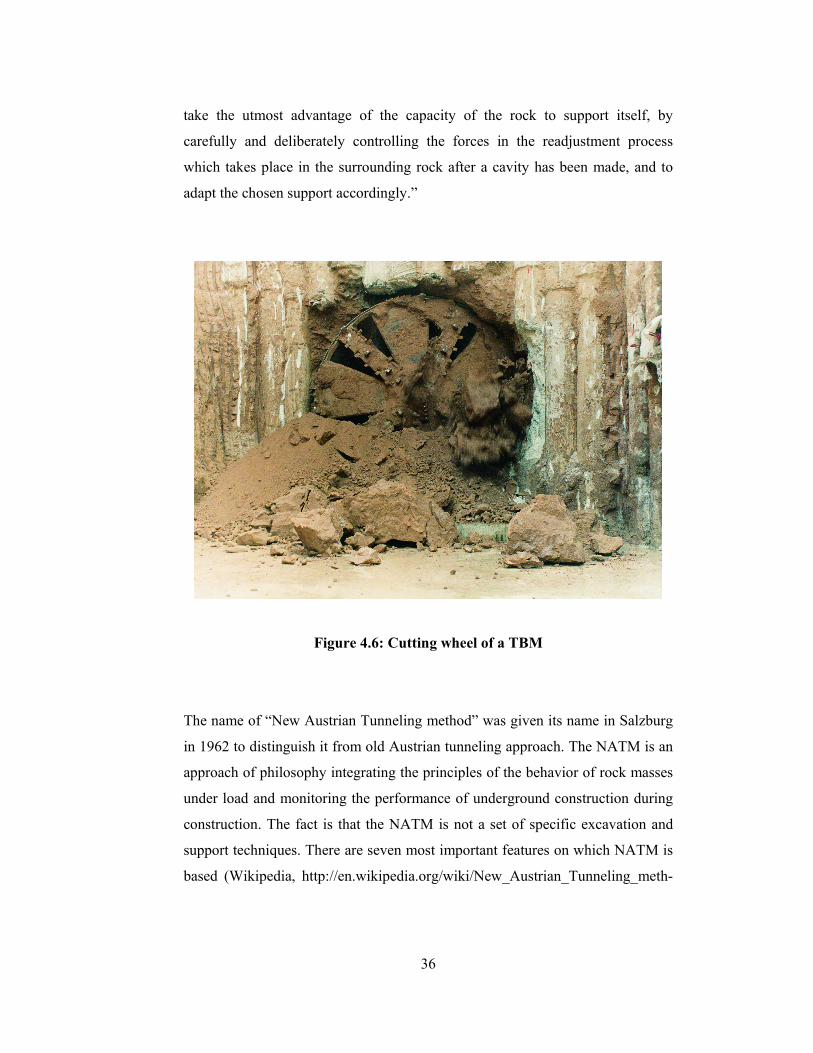
Figure 4.6: Cutting wheel of a TBM

The name of “New Austrian Tunneling method” was given its name in Salzburg

in 1962 to distinguish it from old Austrian tunneling approach. The NATM is an

approach of philosophy integrating the principles of the behavior of rock masses

under load and monitoring the performance of underground construction during

construction. The fact is that the NATM is not a set of specific excavation and

support techniques. There are seven most important features on which NATM is

based (Wikipedia, http://en.wikipedia.org/wiki/New_Austrian_Tunneling_meth-

37

od, last access June 9, 2005):

i) Mobilization of the strength of rock mass - The method relies on the

inherent strength of the surrounding rock mass being conserved as the main

component of tunnel support. Primary support is directed to enable rock

support itself.

ii) Shotcrete Protection - Loosening and excessive rock deformation must be

minimized. This is achieved by applying thin layer of shotcrete

immediately after face advance.

iii) Measurements - Every deformation of excavation must be measured.

NATM requires installation of sophisticated measurement instrumentation.

It is embedded in lining, ground, and boreholes.

iv) Flexible support - The primary lining is thin and reflects recent strata

conditions. Used is rather active than passive support and strengthening is

not by thicker concrete lining but by a flexible combination of rock bolts,

wire mesh and steel ribs.

v) Closing of invert - Important is quickly closing of invert and create load-

bearing ring. It is crucial in soft grounded tunnels where no section of

tunnel should be left open even temporarily.

vi) Contractual arrangements - Since the NATM is based on monitoring

measurements, changes in support and construction method are possible.

This is possible only if the contractual system enables those changes.

vii) Rock mass classification determines support measures - There are main

rock classes for tunnels and corresponding support. These serve as the

guidelines for tunnel reinforcement.

38

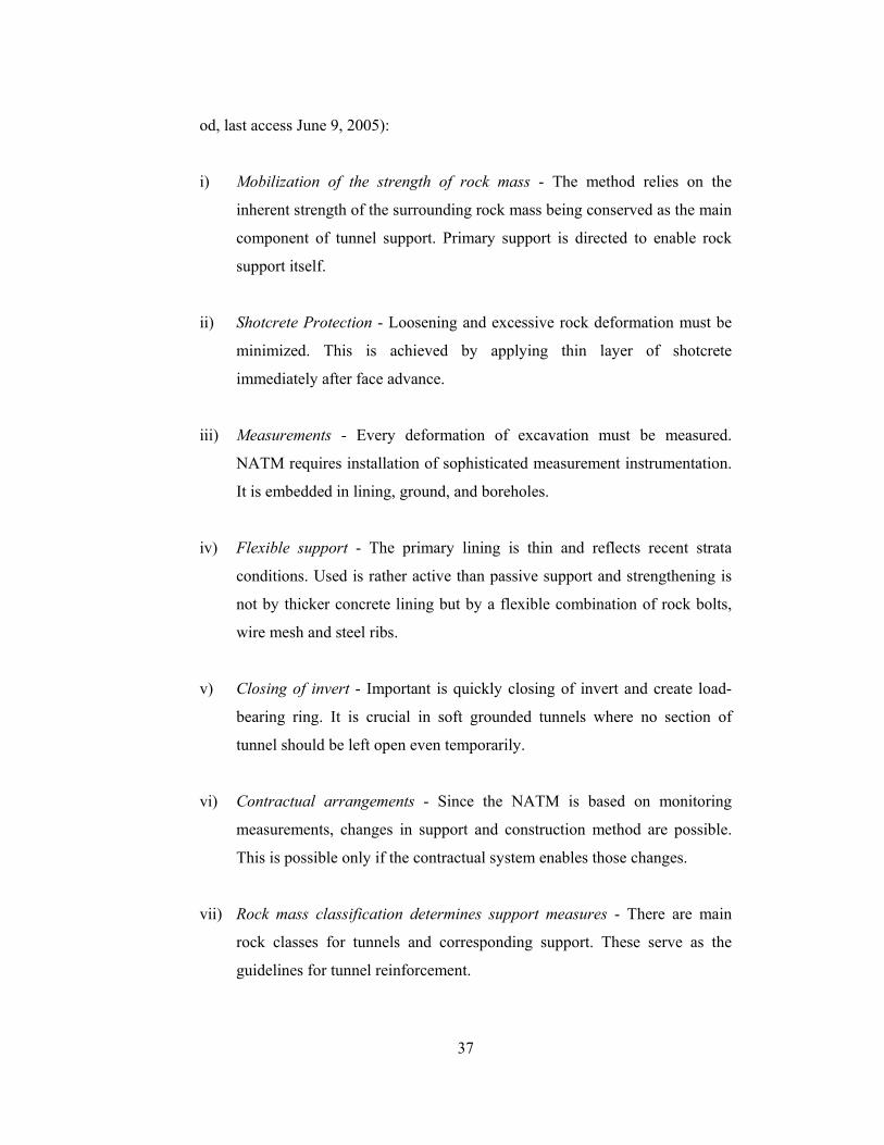
Figure 4.7: Tunnel Boring by NATM

Yesilada and Nielsen (1996, p.248-249) note that generally two methods of

support are performed, first being a flexible outer arch or protective support

designed to stabilize the structure accordingly. This kind of support consists of a

systematically anchored rock arch with surface protection mostly by shotcrete,

possibly reinforced by additional ribs and closed by an invert. A sophisticated

measuring system enables to control the behavior of the protective support and

the surrounding rock during the readjustment process. On the other hand, the

other method of support is an inner arch consisting of concrete. This kind of

support is not carried out before the outer arch has reached equilibrium. The

purpose is to establish or increase the safety factors as required (see Figure 4.7).

Most of the projects to be analyzed for the purpose of this research include

considerable lengths of tunnel sections executed by NATM.

39

4.3.3 Drilling & Blasting (DB)

Another possible method of excavation is the DB Technique, applied for solid

rocks, with the use of explosive materials. However, for the tunnels to be

executed in dense urban areas, this method is almost not preferred. Yet the

projects to be analyzed in this study do not include any tunnel section executed

by this technique. Thus, details of this method will not be discussed further.

Various combinations of these methods are also possible and practiced usually

within a single project.

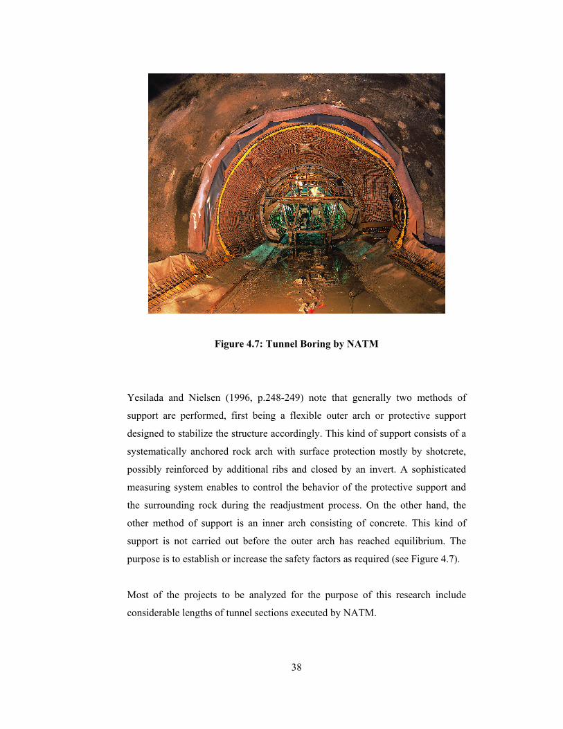
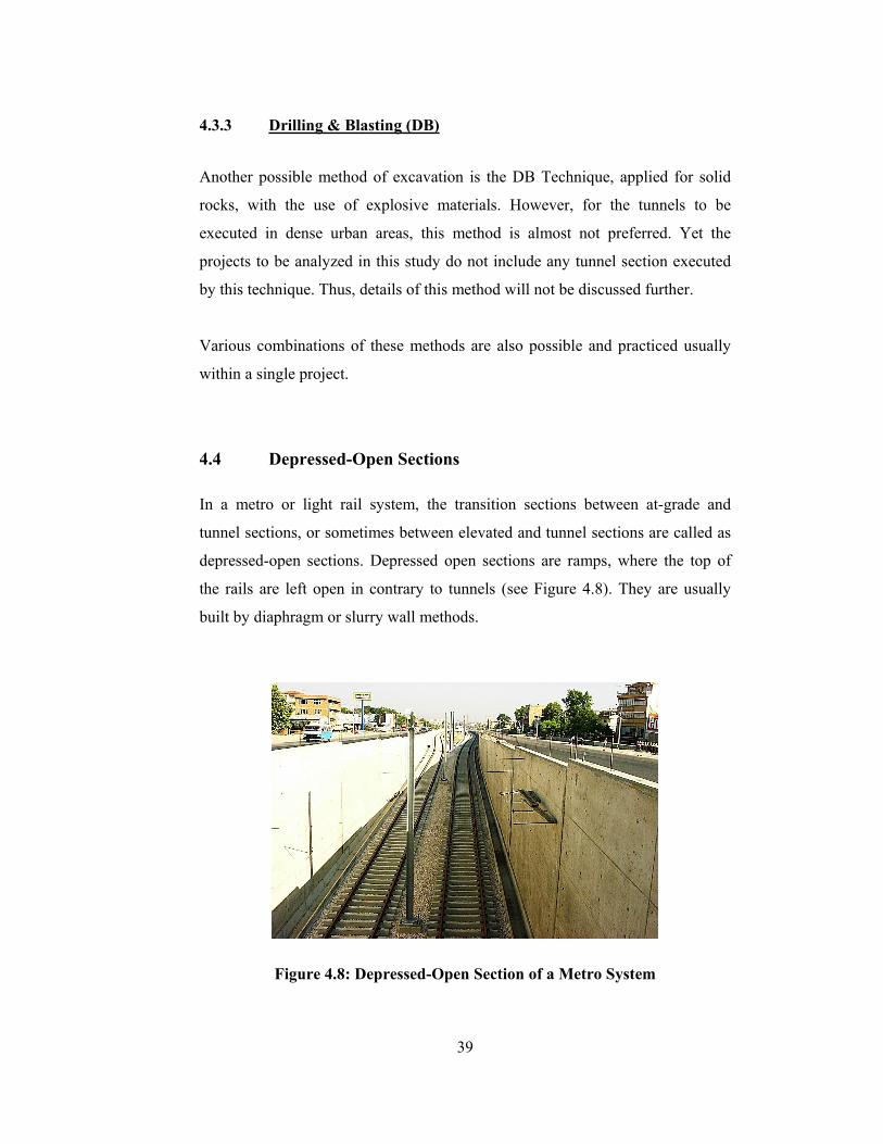
4.4 Depressed-Open Sections

In a metro or light rail system, the transition sections between at-grade and

tunnel sections, or sometimes between elevated and tunnel sections are called as

depressed-open sections. Depressed open sections are ramps, where the top of

the rails are left open in contrary to tunnels (see Figure 4.8). They are usually

built by diaphragm or slurry wall methods.

Figure 4.8: Depressed-Open Section of a Metro System

40

4.5 At-Grade Sections

At-Grade Sections (see Figure 4.9) in a metro or light rail system run at the

surface level. In tram systems, they are usually not segregated from the street

traffic; whereas in metro systems they are fully segregated from any other traffic.

Figure 4.9: At-Grade Section of a Metro System

4.6 Elevated Sections

Elevated sections (see Figure 4.10) in a metro or light rail system run over the

slabs of the structures called viaducts, standing on beams and piers and are

preferred instead of tunnel sections in less congested areas of cities.

41

Figure 4.10: Elevated Section of a Metro System

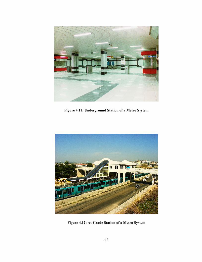
4.7 Metro Stations

A metro station is a train station for a metro, where the passengers get on or off

the trains. It is underground (see Figure 4.11), at-grade (see Figure 4.12) or

elevated (viaduct, see Figure 4.13).

Selection of the type of station, whether underground, at-grade or elevated,

depends obviously on the route of the line. Consequently, “correct sitting of

metro stations at close spacing in the inner city is an obvious necessity if

maximum traffic is to be attracted, although in suburban areas stations must be

more widely spaced to avoid the delays and costs inherent in frequent stops. A

balance has to be established between these delays and costs and the extra traffic

attracted (Yesilada and Nielsen, 1996, p.303-304).

42

Figure 4.11: Underground Station of a Metro System

Figure 4.12: At-Grade Station of a Metro System

43

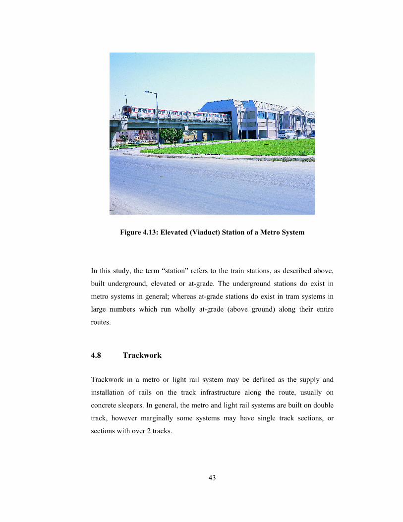
Figure 4.13: Elevated (Viaduct) Station of a Metro System

In this study, the term “station” refers to the train stations, as described above,

built underground, elevated or at-grade. The underground stations do exist in

metro systems in general; whereas at-grade stations do exist in tram systems in

large numbers which run wholly at-grade (above ground) along their entire

routes.

4.8 Trackwork

Trackwork in a metro or light rail system may be defined as the supply and

installation of rails on the track infrastructure along the route, usually on

concrete sleepers. In general, the metro and light rail systems are built on double

track, however marginally some systems may have single track sections, or

sections with over 2 tracks.

44

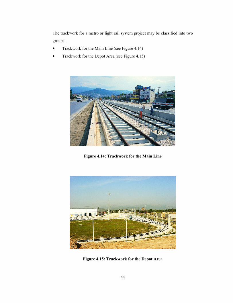
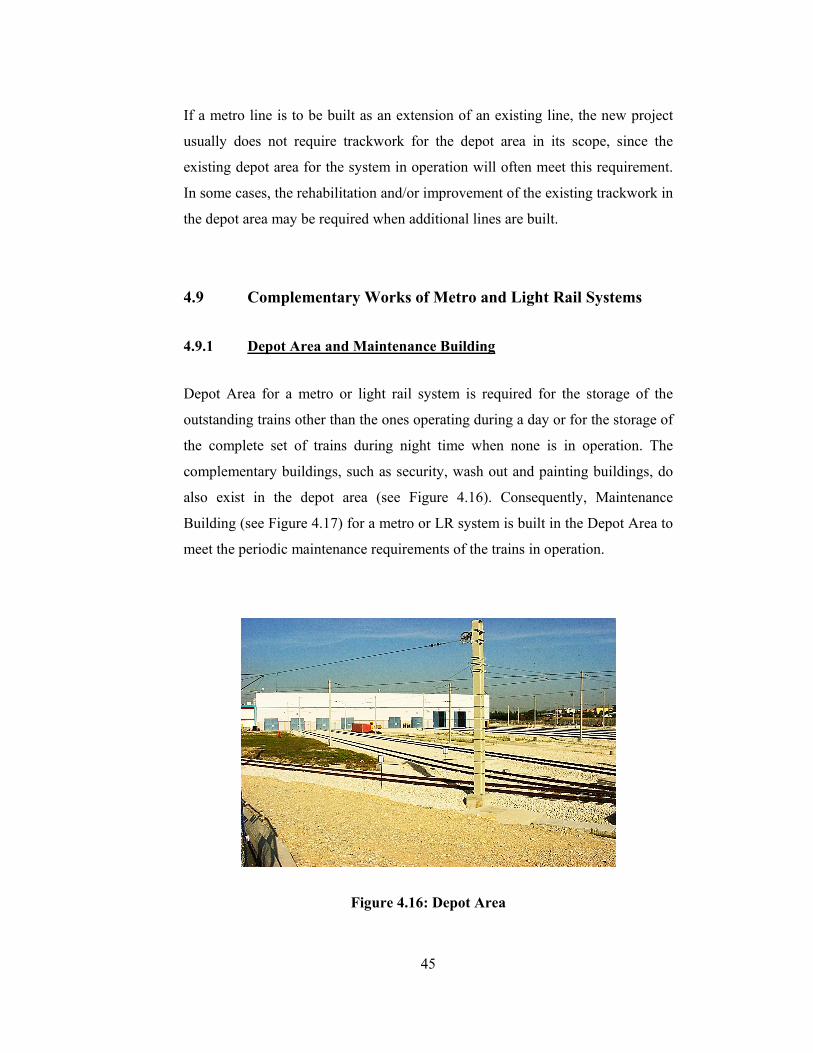
The trackwork for a metro or light rail system project may be classified into two

groups:

• Trackwork for the Main Line (see Figure 4.14)

• Trackwork for the Depot Area (see Figure 4.15)

Figure 4.14: Trackwork for the Main Line

Figure 4.15: Trackwork for the Depot Area

45

If a metro line is to be built as an extension of an existing line, the new project

usually does not require trackwork for the depot area in its scope, since the

existing depot area for the system in operation will often meet this requirement.

In some cases, the rehabilitation and/or improvement of the existing trackwork in

the depot area may be required when additional lines are built.

4.9 Complementary Works of Metro and Light Rail Systems

4.9.1 Depot Area and Maintenance Building

Depot Area for a metro or light rail system is required for the storage of the

outstanding trains other than the ones operating during a day or for the storage of

the complete set of trains during night time when none is in operation. The

complementary buildings, such as security, wash out and painting buildings, do

also exist in the depot area (see Figure 4.16). Consequently, Maintenance

Building (see Figure 4.17) for a metro or LR system is built in the Depot Area to

meet the periodic maintenance requirements of the trains in operation.

Figure 4.16: Depot Area

46

Figure 4.17: Maintenance Building

4.9.2 Administration Building

The Administration Building is built for the purpose of operation, management

and control of the overall metro or LR system, usually in the Depot Area.

Besides the management of the system, signalization, communication and

security systems are all controlled from this building (see Figure 4.18).

4.10 Conclusions

This chapter has provided the reader the background information about the

sections and particular structures included in a typical metro or LR system.

Tunneling, which may be defined as the most notable part of construction of a

metro or light rail system, has been discussed in a detailed manner especially

regarding the construction methods which result in significant cost differences

and thus which shall be given special attention before a cost model is established

47

for such systems. These descriptions will be useful for understanding of the data

collected and the variables analyzed in Chapter 5.

Figure 4.18: Administration Building

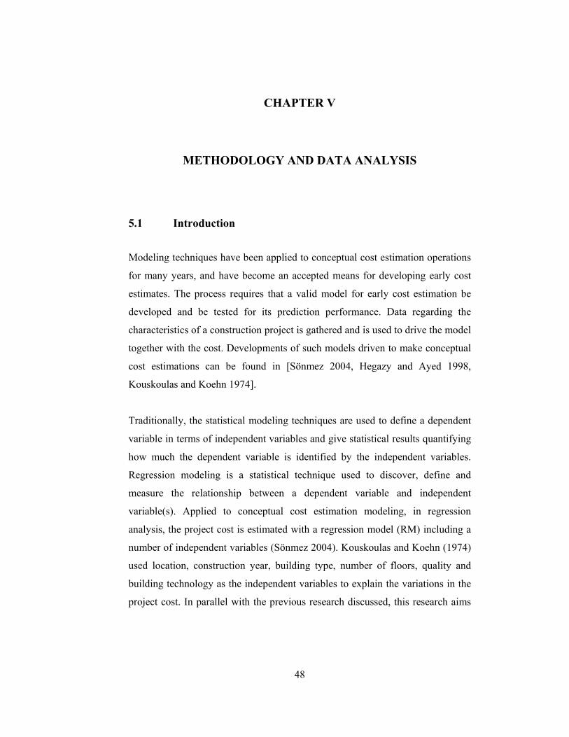
48

CHAPTER V

METHODOLOGY AND DATA ANALYSIS

5.1 Introduction

Modeling techniques have been applied to conceptual cost estimation operations

for many years, and have become an accepted means for developing early cost

estimates. The process requires that a valid model for early cost estimation be

developed and be tested for its prediction performance. Data regarding the

characteristics of a construction project is gathered and is used to drive the model

together with the cost. Developments of such models driven to make conceptual

cost estimations can be found in [Sönmez 2004, Hegazy and Ayed 1998,

Kouskoulas and Koehn 1974].

Traditionally, the statistical modeling techniques are used to define a dependent

variable in terms of independent variables and give statistical results quantifying

how much the dependent variable is identified by the independent variables.

Regression modeling is a statistical technique used to discover, define and

measure the relationship between a dependent variable and independent

variable(s). Applied to conceptual cost estimation modeling, in regression

analysis, the project cost is estimated with a regression model (RM) including a

number of independent variables (Sönmez 2004). Kouskoulas and Koehn (1974)

used location, construction year, building type, number of floors, quality and

building technology as the independent variables to explain the variations in the

project cost. In parallel with the previous research discussed, this research aims

49

to explain the relationship between the characteristics of an urban railway system

and its infrastructure cost by use of regression analysis.

This chapter will investigate how models can be constructed for conceptual cost

estimation of urban railway systems, regarding their infrastructures. Steps of the

regression analysis developed particular to this study will be discussed and the

statistical results achieved within the regression process will be presented to

define the validity of the developed models.

5.2 Data Collection

The data about the urban railway systems, consisting of main characteristics,

contractual characteristics and contract prices, were obtained through

conversations with the contractors and e-mail correspondences, together with a

detailed survey among the web conducted to confirm the compiled information

received from the contractors whenever possible.

In the beginning, a target project list was produced by making a short survey

throughout the urban railway system sector in Turkey and the opportunities were

discussed how and how much detailed information could be obtained about the

projects in the target list. The information to be collected regarding the projects

in the target list referred to the parameters which might have affect on the overall

contract prices of the projects, referred as the costs of the projects. Hence, based

on the suggestions of the experts working in the field of urban railway systems,

parameters were defined and listed.

The next step was to contact with the contractors in the target project list to

collect data of the defined parameters for each project. Wherever possible, an

archive of a contractor was explored and the required information were pulled

out.

50

Examining the parameters necessary to construct such a cost estimation model,

one can easily envision that it is easier to collect information about the technical

and contractual characteristics of the projects, rather than to do the same for their

costs. This is due to the fact that the contractors, in general, tend to be reluctant

to furnish information about the cost of the projects, since the subject

information is usually deemed to be confidential to each contractor. However,

such a difficulty could be overcome for most of the projects in the target list and

the contract prices of the civil scope for the majority of the projects could be

achieved. Cost of civil scope (infrastructure cost) for a project mentioned

anywhere in this study refer to the contract price for only the civil scope of that

railway system project, without the scope of rolling stock and the electro-

mechanical works related to the operation of the trains such as signalization,

communication, public address system, passenger announcement system, ATC,

etc.

The data for this study were compiled from 13 rail system projects, belonging to

the time frame 1986-2005 in terms of their contract dates. The projects were

located in Turkey. Table 5.1 lists the projects of which data were used for the

purpose of this study.

In Table 5.1, M1 to M8 represents 8 metro projects, L1 to L3 represents 3 light

rail transit (LRT) system projects, whereas T1 and T2 represents 2 tram projects.

5.3 Data Identification

The data was successfully collected for the majority of the projects in the target

list. Special attention was given to the fact that the collected costs would be the

ones regarding only the civil scope of the projects. For the prices in foreign

currencies, the buying exchange rate of Central Bank of Turkey at the contract

date of each project was used to convert that contract price to TL.

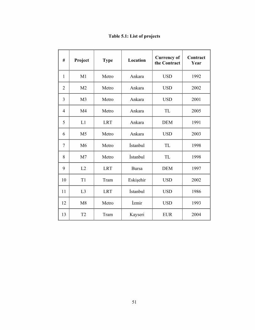
51

Table 5.1: List of projects

# Project Type Location Currency of the Contract

Contract Year

1 M1 Metro Ankara USD 1992

2 M2 Metro Ankara USD 2002

3 M3 Metro Ankara USD 2001

4 M4 Metro Ankara TL 2005

5 L1 LRT Ankara DEM 1991

6 M5 Metro Ankara USD 2003

7 M6 Metro İstanbul TL 1998

8 M7 Metro İstanbul TL 1998

9 L2 LRT Bursa DEM 1997

10 T1 Tram Eskişehir USD 2002

11 L3 LRT İstanbul USD 1986

12 M8 Metro İzmir USD 1993

13 T2 Tram Kayseri EUR 2004

52

Hence, the contract prices were converted into a single currency to make any

comparison possible before the regression analysis.

The next step with the costs was to select a method to reflect the impact of

inflation to the same, since the contract years of the projects were differing.

Here, the cost index published by the Ministry of Public Works and Settlement

was used to describe the variability caused by the time factor and to escalate the

contract prices for year 2005. It was thought that method of escalating the

contract prices by the use of this cost index would be one of the most accurate

techniques which could be performed and would be in parallel with the real

conditions of the construction sector in Turkey, since this cost index is calculated

based upon the Turkish construction market and all the projects were located in

Turkey.

5.4 Independent variables

The cost of rail system projects are affected by numerous variables. The

independent variables in this study were classified into two groups:

i. Dummy (Categorical) variables

ii. Continuous variables

5.4.1 Dummy (Categorical) variables

A dummy variable in a regression analysis is the variable which takes the value

of either 0 or 1. For this study, dummy variables were used to identify the

differences between the scope of the projects and the contractual conditions, by

classifying them into groups.

53

5.4.1.1 Dummy variables for Complementary Station Works

The dummy variables assigned for complementary station works indicated

whether or not the subject complementary works were included under the scope

of the subject project. When such scope was included, the dummy variable was

assigned 1; whereas if not included, it was assigned 0 (zero).

The complementary works for the stations could be summarized under 3 groups,

as:

i. Finishing Works of Stations

ii. Electrical & Plumbing Works of Stations

iii. Elevators & Escalators for Stations

The following parameters were identified to illustrate the coverage of the scope

for some works relevant to the stations (underground, at-grade or elevated), each

being either 0 or 1, in the regression analysis:

i. FWS (Finishing Works of Stations)

Some projects did not include the finishing works for stations in their scope, and

thus in their contract price. This parameter was defined to represent the inclusion

or exclusion of the finishing works of stations under the scope of each contract.

ii. EPS (Electrical & Plumbing Works of Stations)

Like the finishing works for stations, some projects did not include the electrical

and plumbing works for stations in their scope, and thus in their contract price.

This parameter was defined to represent the inclusion of the electrical and

plumbing works of stations under the scope of each contract.

54

iii. EES (Elevators & Escalators for Stations)

This parameter was defined to represent the inclusion of the works of supply and

installation of elevators and escalators for the stations under the scope of each

contract, since some projects did not cover these works within their scopes.

5.4.1.2 Dummy variables for Trackwork

The trackwork for a railway system could be summarized under 2 groups for the

projects of which data was to be analyzed, as explained in Chapter 4:

i. Trackwork for mainline

ii. Trackwork for depot area

The following parameters were identified to illustrate the coverage of trackwork

for mainline or depot area within the scope, each being either 0 or 1 before in the

regression analysis:

i. TWM (Trackwork Mainline - Supply & Installation)

Some projects were contracted excluding the trackwork for the mainline from the

scope. This parameter was defined to represent the inclusion of the supply and

installation of rail (trackwork) for the main line of the project under the scope of

the contract.

ii. TWD (Trackwork Depot Area - Supply & Installation)

Some projects were to be built as an extension to the existing lines and did not

require trackwork for the depot area, as explained in Chapter 4. This parameter

was defined to represent the inclusion of the supply and installation of rail

(trackwork) for the depot area of the project under the scope of the contract.

55

5.4.1.3 Dummy variables for Main Complementary Works

The dummy variables assigned for the main complementary works indicated

whether or not the subject main complementary works, as described in Chapter

4, were included under the scope of the subject project. When such a scope was

included, the dummy variable was assigned 1; whereas if not included, it was

assigned 0 (zero).

The main complementary works for the projects could be summarized under 2

groups:

i. Construction of Depot Area & Maintenance Building

ii. Construction of Administration Building

The following parameters were identified to illustrate the coverage of the scope

for these works, each being either 0 or 1 in the regression analysis:

i. DMC (Construction of Depot Area & Maintenance Building)

This parameter was defined to represent the inclusion of the construction of

depot area and the maintenance building under the scope of the contract.

ii. ABC (Construction of Administration Building)

This parameter was defined to represent the inclusion of the construction of an

administration building under the scope of the contract.

5.4.1.4 Dummy variable for the Type of Contract

Types of contract for the projects were in 2 groups:

i. Lump sum based contracts

ii. Unit Price based contracts

56

The following parameter was identified to illustrate the type of contract for the

projects, being either 0 or 1 in the regression analysis:

i. LS (Contract Type - Lump Sum)

This parameter represented whether or not the contract for the project is lump

sum based. When assigned 1, it meant that the contract for that project was lump

sum based; whereas when assigned 0 (zero), the contract was a unit price based

contract.

5.4.1.5 Dummy variable for the Financing Method

The financing for the projects could be summarized in two groups:

i. Financing by credit

ii. Financing by self resources

The following parameter was identified to illustrate the financing method for the

projects, being either 0 or 1 in the regression analysis:

i. CR (Financing by Credit)

This parameter was assigned 1 for a project if it was financed by credit; whereas

financing by the self resources of the owner resulted with 0 (zero) assignment of

this parameter for that project.

The dummy variables and the corresponding values for each project are given in

Table 5.2.

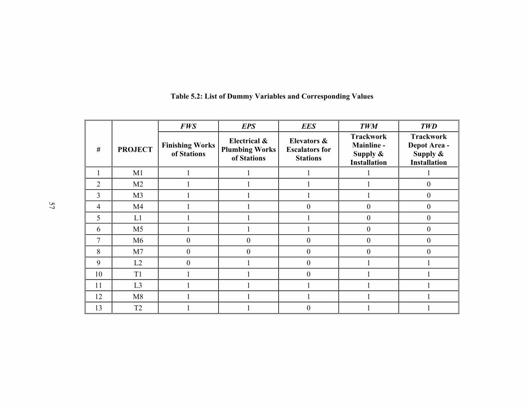
57

Table 5.2: List of Dummy Variables and Corresponding Values

FWS EPS EES TWM TWD

# PROJECT Finishing Works

of Stations

Electrical & Plumbing Works

of Stations

Elevators & Escalators for

Stations

Trackwork Mainline - Supply & Installation

Trackwork Depot Area - Supply & Installation

1 M1 1 1 1 1 1

2 M2 1 1 1 1 0

3 M3 1 1 1 1 0

4 M4 1 1 0 0 0

5 L1 1 1 1 0 0

6 M5 1 1 1 0 0

7 M6 0 0 0 0 0

8 M7 0 0 0 0 0

9 L2 0 1 0 1 1

10 T1 1 1 0 1 1

11 L3 1 1 1 1 1

12 M8 1 1 1 1 1

13 T2 1 1 0 1 1

57

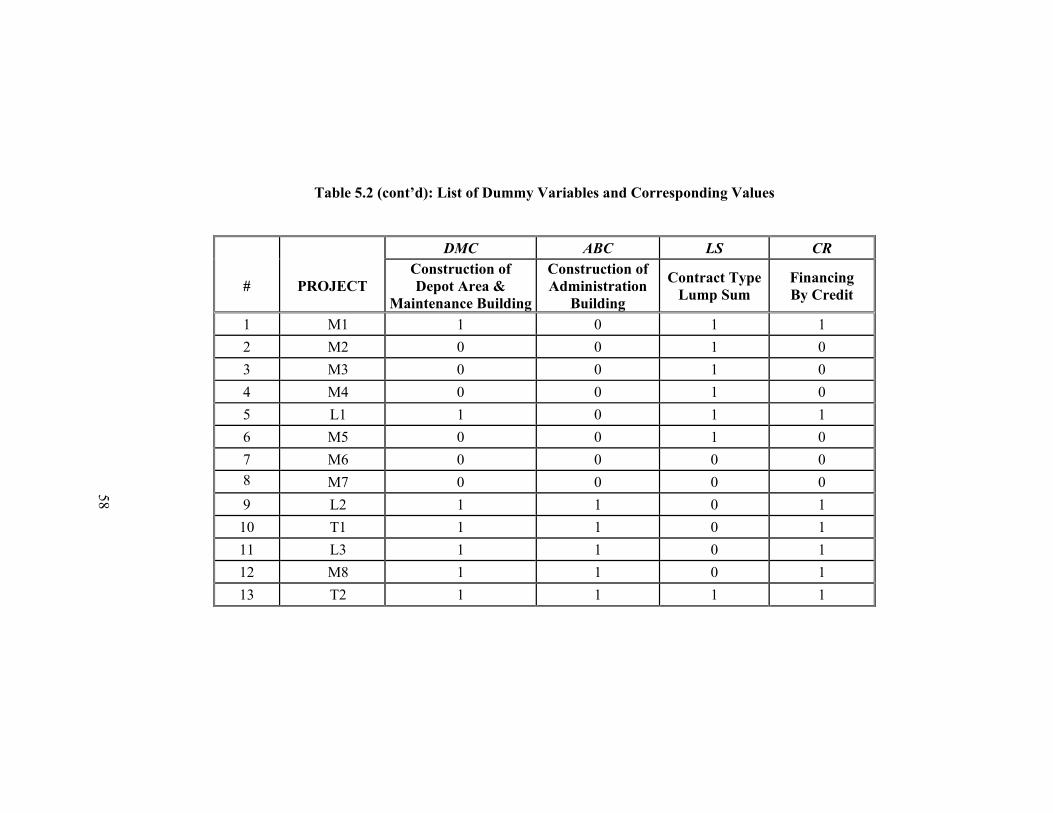
58

Table 5.2 (cont’d): List of Dummy Variables and Corresponding Values

DMC ABC LS CR

# PROJECT Construction of Depot Area &

Maintenance Building

Construction of Administration

Building

Contract Type Lump Sum

Financing By Credit

1 M1 1 0 1 1

2 M2 0 0 1 0

3 M3 0 0 1 0

4 M4 0 0 1 0

5 L1 1 0 1 1

6 M5 0 0 1 0

7 M6 0 0 0 0

8 M7 0 0 0 0

9 L2 1 1 0 1

10 T1 1 1 0 1

11 L3 1 1 0 1

12 M8 1 1 0 1

13 T2 1 1 1 1

58

59

It is better to emphasize here that the projects were not classified as metro and

LR systems. In other words, dummy variables for this type of classification were

not used. This is mainly due to the fact that there is not a significant difference

between the metro and LR system projects included in this study and listed in

Table 5.1, in terms of design and construction methods applied. The projects

listed in Table 5.1 are classified as metro and LR systems mainly with respect to

their passenger carrying capacities, which result in longer trains and fleets for

metro systems due to the larger passenger carrying capacities. This leads to the

fact that the platform of a station in a metro system shall be longer than that of a

station in a LR system. However, this is not a significant parameter affecting the

cost of the overall system. Besides these, the building systems like tunneling and

viaducts, which cost necessarily higher when compared to the other particular

building systems and structures in a railway system, are common for both metro

and LR systems considered for the analysis purposes of this study. Hence, using

dummy variables to distinguish and represent the projects as metro and LR

systems in the regression analysis would not be true and thus, such parameters

were avoided.

5.4.2 Continuous variables

On the other hand, the main characteristics of the projects of which data to be

analyzed were to correspond to the continuous variables, as the remaining part of

the independent variables. The following parameters were identified to represent

the main characteristics of the projects in the regression analysis, such as lengths

of tunnel sections, number of underground/at-grade/viaduct stations and the

other particular sections and structures included in a project as explained in detail

in Chapter 4:

60

i. UGS (Number of Underground Stations)

This parameter was defined to represent the number of underground stations

included in the project.

ii. AGS (Number of At-Grade Stations)

This parameter was defined to represent the number of at-grade stations included

in the project.

iii. VS (Number of Viaduct Stations)

This parameter was defined to represent the number of viaduct (elevated)

stations included in the project.

iv. LL (Length of Line – Km)

This parameter was defined to represent the total length of main line for the

project.

v. PBNT (TBM-Bored and/or NATM Tunnel %)

This parameter was defined to represent the percentage of total length of tunnel

sections executed by TBM Boring and/or NATM over the total length of main

line (LL).

The lengths of tunnel sections in a project executed by TBM Boring and NATM

were added up for the calculation purpose of this parameter when combinations

of both methods were available in the same contract. This was, in fact, due to the

fact that the costs of tunneling by either TBM Boring or NATM were close to

each other.

vi. PCCT (Cut-Cover Tunnel %)

This parameter was defined to represent the percentage of total length of tunnel

sections executed by Cut-and-Cover method over the total length of main line

(LL).

61

vii. PDO (Depressed Open Section %)

This parameter was defined to represent the percentage of total length of

depressed-open sections (ramps) over the total length of main line (LL).

viii. PAG (At-Grade Section %)

This parameter was defined to represent the percentage of total length of at-

grade sections over the total length of main line (LL).

ix. PES (Elevated Section %)

This parameter was defined to represent the percentage of total length of

elevated sections over the total length of main line (LL).

x. CI (Cost Index)

This parameter was used to escalate the contract prices of the projects for year

2005. Once it was used for escalation, it was not considered again for the

purposes of regression analysis.

Table 5.3 presents the continuous variables and their corresponding values for

each project.

5.5 Dependent Variable

The dependent variable to be used for the regression analysis was the escalated

unit cost of the projects, symbolized as UCP (TL/Km). The unit costs of the

projects were calculated through dividing the escalated total contract price for

the civil scope by the total length of main line (LL). Consequently, one should

take care of the fact that all metro, light rail and tram systems considered for this

research were double-track lines and “1 km” in this study refers to 1 km of

double-track line. However, for simplicity, unit costs of the projects in this report

were represented by UCP in “TL/Km” instead of “TL /double-track*Km”.

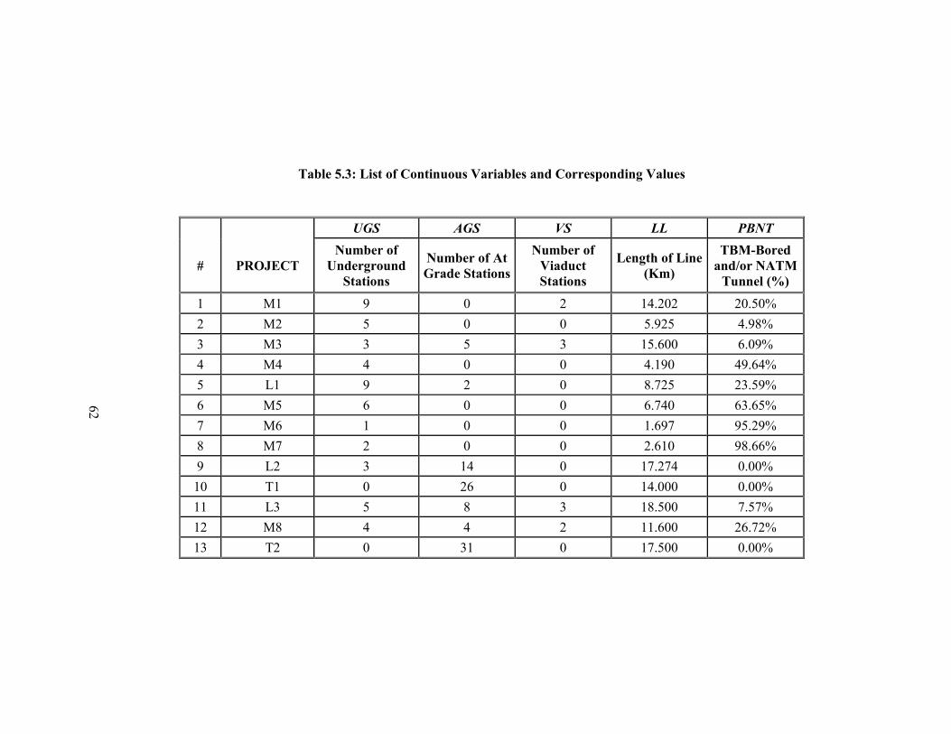
62

Table 5.3: List of Continuous Variables and Corresponding Values

UGS AGS VS LL PBNT

# PROJECT Number of

Underground Stations

Number of At Grade Stations

Number of Viaduct Stations

Length of Line (Km)

TBM-Bored and/or NATM Tunnel (%)

1 M1 9 0 2 14.202 20.50%

2 M2 5 0 0 5.925 4.98%

3 M3 3 5 3 15.600 6.09%

4 M4 4 0 0 4.190 49.64%

5 L1 9 2 0 8.725 23.59%

6 M5 6 0 0 6.740 63.65%

7 M6 1 0 0 1.697 95.29%

8 M7 2 0 0 2.610 98.66%

9 L2 3 14 0 17.274 0.00%

10 T1 0 26 0 14.000 0.00%

11 L3 5 8 3 18.500 7.57%

12 M8 4 4 2 11.600 26.72%

13 T2 0 31 0 17.500 0.00%

62

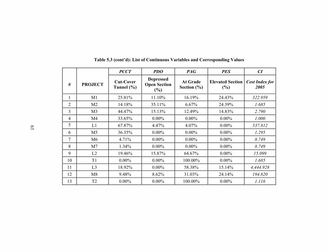
63

Table 5.3 (cont’d): List of Continuous Variables and Corresponding Values

PCCT PDO PAG PES CI

# PROJECT Cut-Cover Tunnel (%)

Depressed Open Section

(%)

At Grade Section (%)

Elevated Section (%)

Cost Index for

2005

1 M1 25.81% 11.10% 16.19% 24.43% 322.959

2 M2 14.18% 35.11% 6.67% 24.39% 1.685

3 M3 44.47% 15.13% 12.49% 14.83% 2.790

4 M4 33.65% 0.00% 0.00% 0.00% 1.000

5 L1 67.87% 4.47% 4.07% 0.00% 537.812

6 M5 36.35% 0.00% 0.00% 0.00% 1.295

7 M6 4.71% 0.00% 0.00% 0.00% 8.749

8 M7 1.34% 0.00% 0.00% 0.00% 8.749

9 L2 19.46% 15.87% 64.67% 0.00% 15.099

10 T1 0.00% 0.00% 100.00% 0.00% 1.685

11 L3 18.92% 0.00% 58.38% 15.14% 4,444.928

12 M8 9.48% 8.62% 31.03% 24.14% 194.820

13 T2 0.00% 0.00% 100.00% 0.00% 1.116

63

64

On the other hand, cost of civil scope for a project mentioned anywhere in this

study refer to the contract price regarding only the civil scope of that railway

system project. It should also be emphasized that the escalated costs of civil

scope of each project for year 2005 were used, after conversion to TL for the

foreign currency contract prices.

The set of independent variables to be analyzed for regression were large when

compared to the number of observations (projects available for regression

analysis). Using the escalated unit cost, UCP (TL/Km), as the dependent variable

for the regression analysis, the independent variables LL, as well as the cost

index CI, were eliminated from the set of independent variables.

5.6 Regression Analysis

Regression models provide the user a powerful tool, allowing predictions of

future events using data of past events. Ostwald (2001, p.146-148) states that in

regression, on the basis of sample data, the value of a dependent variable y is to

be found corresponding to a given value of a variable x. This is determined from

a least-squares equation that fits the sample data. The resulting curve is called a

regression curve of y on x, because y is determined from a corresponding value

of x. If the variable x is time, then the data show the values of y at various times,

and the equation is known as a time series. A regression line or a curve y on x or

the response function on time is frequently called a trend line and is used for

prediction and forecasting. Thus, regression refers to average relationship

between variables.

“The notion of fitting a curve to a set of sufficient points is essentially the

problem of finding the parameters of the curve. The best-known method is that

of least squares (regression). Since the desired curve or equation is to be used for

estimating or prediction purposes, the curve or equation should be so modeled as

65

to make the errors of estimation small. An error of estimation means the

difference between an observed value and the corresponding fitted curve value

for the specific value of x. It will not do require that the sum of these differences

or errors to be as small as possible. It is a requirement that the sum of absolute

value of the errors be as small as possible. However, sums of absolute values are

not convenient mathematically. The difficulty is avoided by requiring that the

sum of the squares of the errors be minimized. If this procedure is followed, the

values of parameters give what is known as the best curve in the sense of least-

squares difference (Ostwald, 2001, p.146-148)”.

In its simplest form, linear regression analysis involves finding the best straight

line relationship to explain how the variation in an outcome (or dependent)

variable depends on the variation in a predictor (or independent or explanatory

variable). In this study, linear regression analysis was performed using the

available data. As the number of projects was limited to 13 and previous

conceptual cost modeling studies indicated that linear regression models were

sufficient (Sönmez 2004), only linear models were used.

The regression analysis was performed with the help of the analysis toolpak of

Microsoft Excel for the data about the 13 projects. A total of 18 independent

variables were available; where 9 being dummy (categorical) variables and 9

being the continuous variables (CI is not considered again), to be used for

regression analysis.

5.7 Stepwise Regression Process

5.7.1 Descriptions

The regression analysis can not be performed if the total number of independent

variables is greater than number of observations due to the number of degrees of

66

freedom for residuals below 0 (zero). Therefore, regression analysis could not be

performed with the entire set of independent variables including 18 parameters,

due to the inadequate number of observations (projects) being 13.

The inadequate number of observations made it compulsory to apply stepwise

regression method by using both backward and forward elimination techniques

to achieve RMs including significant parameters. Regression models including

significant variables were to be achieved throughout the following iterations and

each was to be tested for its prediction performance afterwards.

By using a stepwise regression process, the independent variables were

considered one at a time. The one that explained a significant variation in the

dependent variable would be added to the model at each step. The process would

stop when the addition of an extra variable made no significant improvement in

the amount of variation explained.

Based on the experience of which parameters might significantly affect the cost

of the projects, the initial RM was formed by selecting a few independent

variables from the entire set.

5.7.2 Initial RM and First Step of Regression Process

The purpose of the establishment of the initial RM was to identify a set of factors

that might have an affect on the cost of the projects. Based on the experience

gained from the previous cost studies, 6 parameters were selected for the initial

RM as TWM, UGS, PBNT, PES, PAG and PCCT. The basis for selection of these

parameters for the initial RM lies behind the expectation that these parameters

would have significant contribution to the cost. The cost of trackwork for the

mainline of a rail system project, including both supply and installation of rails,

is expected to cover a significant amount of the total cost of an urban railway

67

system. The variable number of underground stations (UGS) is selected since an

underground station costs considerably higher, in general, when compared to

either an at-grade station or a viaduct station. Nevertheless, tunneling by TBM

and NATM is one of the work items having necessarily high costs when

compared to other sections or particular structures in an urban railway system,

even the total cost depends upon the total length of this kind of section. Thinking

that length of elevated sections (PES), length of at-grade sections (PAG) and

length of cut-and-cover sections (PCCT) in a railway system might also have

significant contribution over the cost, the variables PES, PAG and PCCT

representing the share of these sections along the routes of the corresponding

projects were also included in the initial RM.

The first regression analysis was performed with the independent variables

TWM, UGS, PBNT, PES, PAG and PCCT and the dependent variable UCP

representing the unit cost of a project. The first RM (RM1.1) included the 6

parameters mentioned above and was in the following form:

CCTPAGPESPPBNTGSUWMT 654321O βββββββUCP ++++++= [1]

in which UCP is the escalated unit contract price (TL/Km); TWM is the dummy

variable representing the inclusion of trackwork for the mainline covering supply

and installation of rails; UGS is the number of underground stations, PBNT is the

percent tunnel section by TBM-Boring and/or NATM; PES is the percent

elevated section; PAG is the percent at-grade section; PCCT is the percent tunnel

section by Cut-and-Cover method; and ß0, ß1, …, ß6 are the regression

coefficients. Data from the 13 projects were used to determinate the regression

coefficients and statistics.

In this study, parsimonious models were considered for the regression modeling.

A parsimonious model can be defined as a model that fits the data adequately

without using any unnecessary parameters. The principle of parsimony is

68

important, because in general, parsimonious models generally produce better

forecasts (Pankratz, 1983, p.81-82). To achieve parsimonious models, a

backward elimination method was used for the initial RM. According to this

technique, variables that were not contributing to the model were eliminated one

at a time. The regression statistic, significance level (P value, which gives an

indication of the significance of the variables included in the model) was used

for determination of variables to be eliminated. In general, the variables

corresponding to the coefficients with P values close to or less than 0.10 are

considered to have significant contribution to the model. As such, in this study,

variables corresponding to the coefficients with P values close to or less than

0.10 will be considered to be significant.

The Table 5.4 presents P values of the coefficients, together with the coefficient

of determination (R2) which gives a measure of the variability explained by the

model, for the regression models RM1.1 to RM1.5. Table 5.4 also indicates the

variable corresponding to the coefficient with the highest P value for each RM

obtained during the backward elimination.

The P value 0.920 for the regression coefficient corresponding to the variable

percent tunnel section executed by Cut-and-Cover method (PCCT) for the model

RM1.1 indicates that this variable probably does not have a significant

contribution to the model. Thus, this variable was dropped from the model and

RM1.2 was driven with the remaining 5 parameters.

In model RM1.2, the coefficient for the variable number of underground stations

(UGS) had the highest P value as 0.689 and was dropped from the model. In the

model RM1.3, the coefficient for the variable percent at-grade section PAG had a

P value of 0.233 being the highest among the others. Dropping the variable PAG

and a new regression analysis resulted in the model RM1.4, including the

variable trackwork for main line (TWM) with the highest P value as 0.226. This

variable was then dropped from the model to obtain RM1.5.

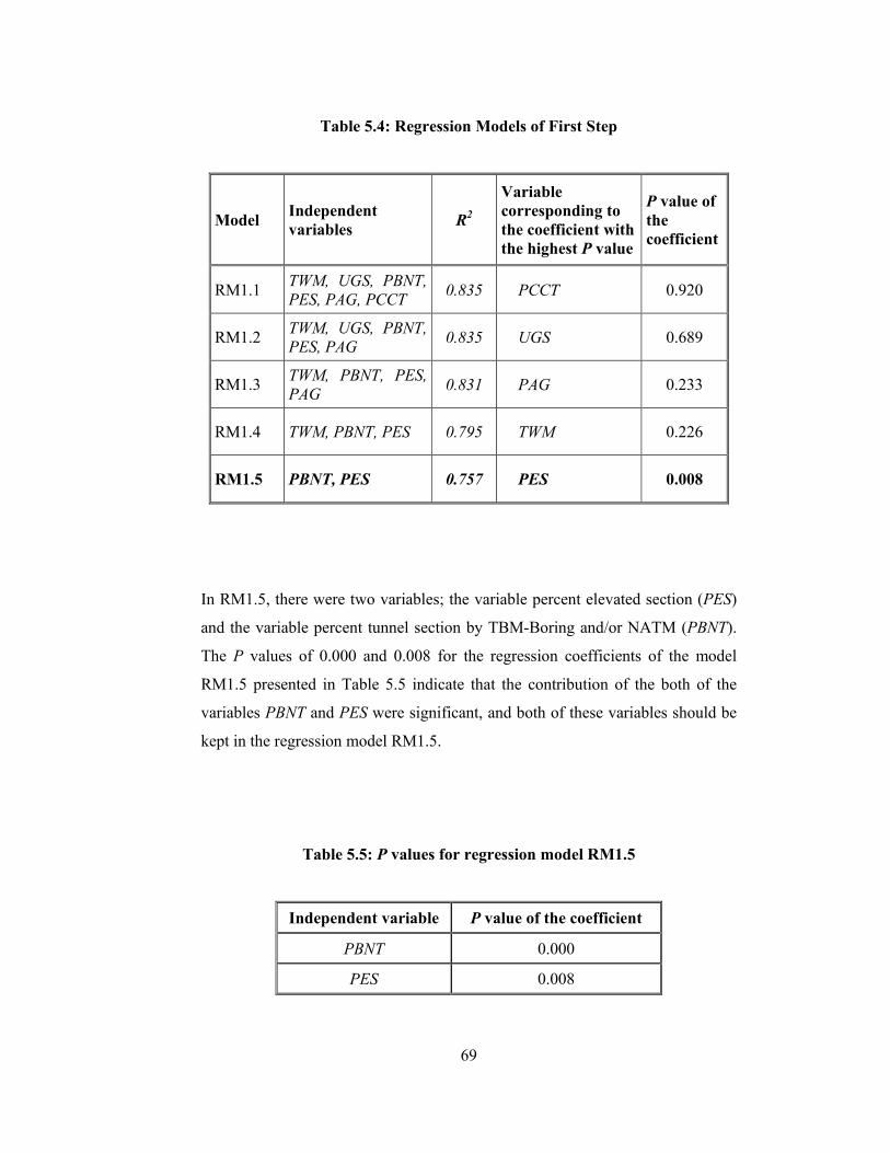
69

Table 5.4: Regression Models of First Step

Model Independent variables

R2

Variable corresponding to the coefficient with the highest P value

P value of the coefficient

RM1.1 TWM, UGS, PBNT,

PES, PAG, PCCT 0.835 PCCT 0.920

RM1.2 TWM, UGS, PBNT,

PES, PAG 0.835 UGS 0.689

RM1.3 TWM, PBNT, PES,

PAG 0.831 PAG 0.233

RM1.4 TWM, PBNT, PES 0.795 TWM 0.226

RM1.5 PBNT, PES 0.757 PES 0.008

In RM1.5, there were two variables; the variable percent elevated section (PES)

and the variable percent tunnel section by TBM-Boring and/or NATM (PBNT).

The P values of 0.000 and 0.008 for the regression coefficients of the model

RM1.5 presented in Table 5.5 indicate that the contribution of the both of the

variables PBNT and PES were significant, and both of these variables should be

kept in the regression model RM1.5.

Table 5.5: P values for regression model RM1.5

Independent variable P value of the coefficient

PBNT 0.000

PES 0.008

70

In addition to all of these, the R2 value of 0.757 for RM1.5 indicates that this

model accounts for 75.7% of the variation in the dependent variable being the

unit cost. In other words, the model RM1.5 explains the 75.7% of the variation in

the dependent variable by the independent variables.

RM1.5 included variables at a significant level and was determined to be the

base model for the second step. However, the outstanding variables, which were

not included in the initial model, should be tested by introducing new regression

models to measure their significance over the dependent variable. This was done

by adding the outstanding variables one at a time to the model RM1.5 and

performing regression analysis for each model. This process would be repeated

with subsequent iterations if a new RM with variables at a significant level could

be found at the end of the second step, in addition to RM1.5.

5.7.3 Second Step of Regression Process

The RMs in the second step included 3 independent variables, 2 being those of

the RM1.5, as PBNT and PES. As mentioned previously, the RMs in this step

were formed by adding the 12 outstanding independent variables one at a time

to RM1.5 and regression analysis was performed for each of the new RMs. For

example, to obtain RM2.1, the variable finishing works (FWS) was added to the

independent variable set of RM1.5 and the new set of independent variables

included the variables PBNT, PES and FWS for RM2.1.

The variable length of mainline (LL) was included in this step for regression,

although it was used before for the calculation purposes of unit cost (UCP) being

the dependent variable. The reason to include the variable LL again in stepwise

regression process laid behind the expectation that the unit cost of a project could

decrease with the increasing length of main line, due to the decrease in the

contribution of the fixed costs included in a project to the unit cost.

71

The other RMs were also obtained by the same technique and regression analysis

was performed for each of the models. The regression statistics achieved as a

result of the regression analyses in this step are presented in Table 5.6.

The results of the regression analyses performed for the models RM2.1 to

RM2.12 indicated that none of the 12 outstanding variables had significant

contribution to the RMs developed, including the regression coefficients with P

values ranging between 0.326 and 0.890, where the variable number of at-grade

stations (AGS) with the coefficient corresponding to the lowest P value of this

range as 0.326 could even not be considered to have significant contribution to

the model RM2.9. The iterations were stopped here since a variable

corresponding to a coefficient having significant contribution to the produced

models could not be found.

Among the RMs achieved up to this level (RM1.1 to RM1.5 and RM2.1 to

RM2.12), only the regression model RM1.5 included significant variables, which

were PBNT and PES corresponding to the coefficients with P values as 0.000

and 0.008 as presented in Table 5.5. Thus, this model was validated by a

technique called as cross validation, and its prediction performance was

evaluated.

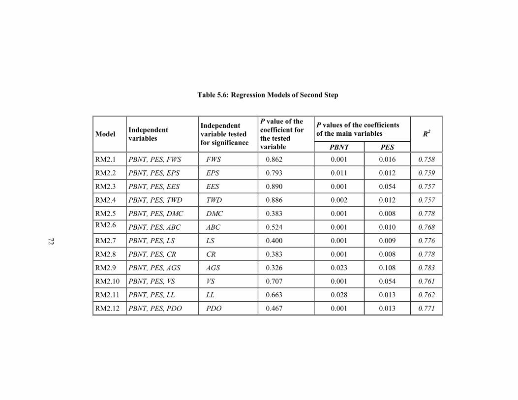
72

Table 5.6: Regression Models of Second Step

P values of the coefficients of the main variables Model

Independent variables

Independent variable tested for significance

P value of the coefficient for the tested variable PBNT PES

R2

RM2.1 PBNT, PES, FWS FWS 0.862 0.001 0.016 0.758

RM2.2 PBNT, PES, EPS EPS 0.793 0.011 0.012 0.759

RM2.3 PBNT, PES, EES EES 0.890 0.001 0.054 0.757

RM2.4 PBNT, PES, TWD TWD 0.886 0.002 0.012 0.757

RM2.5 PBNT, PES, DMC DMC 0.383 0.001 0.008 0.778

RM2.6 PBNT, PES, ABC ABC 0.524 0.001 0.010 0.768

RM2.7 PBNT, PES, LS LS 0.400 0.001 0.009 0.776

RM2.8 PBNT, PES, CR CR 0.383 0.001 0.008 0.778

RM2.9 PBNT, PES, AGS AGS 0.326 0.023 0.108 0.783

RM2.10 PBNT, PES, VS VS 0.707 0.001 0.054 0.761

RM2.11 PBNT, PES, LL LL 0.663 0.028 0.013 0.762

RM2.12 PBNT, PES, PDO PDO 0.467 0.001 0.013 0.771

72

73

5.8 Validation of the model RM1.5

5.8.1 Prediction Performance Evaluation

The model RM1.5, obtained as a result of stepwise regression process, was tested

in terms of prediction performance. For this purpose, mean absolute percent

error (MAPE) was used as an error measure and was calculated as follows:

100xpredicted

predictedactual1MAPE

1∑

=

−

=

n

i i

ii

n [2]

in which i is the project number; actual is the actual cost of the project in

TL/Km; and predicted is the predicted cost of the project in TL/Km. The

procedure used to evaluate prediction performance (Sönmez, 2004) can be

summarized in the following steps:

1. Two projects were selected randomly as the first test sample and a new

data set was formed. The new data set included data of all of the

remaining projects, but not the data of the two projects which were

selected as the test sample.

2. Model parameters for the RM were calculated with the new data set by

regression analysis.

3. The RM with the new parameters was used to predict the unit cost of the

projects which were selected as the test sample.

4. Steps 1-3 were repeated for the remaining test samples (Totally six test

samples were used, five including two projects and the last one including

three projects).

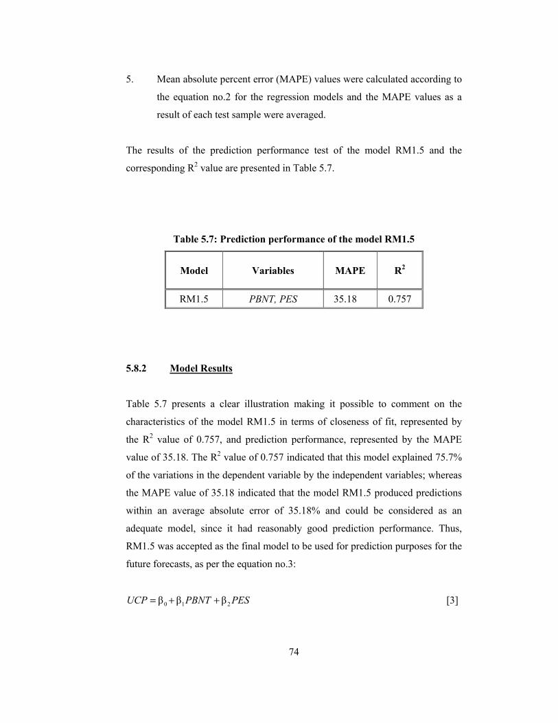
74

5. Mean absolute percent error (MAPE) values were calculated according to

the equation no.2 for the regression models and the MAPE values as a

result of each test sample were averaged.

The results of the prediction performance test of the model RM1.5 and the

corresponding R2 value are presented in Table 5.7.

Table 5.7: Prediction performance of the model RM1.5

Model Variables MAPE R2

RM1.5 PBNT, PES 35.18 0.757

5.8.2 Model Results

Table 5.7 presents a clear illustration making it possible to comment on the

characteristics of the model RM1.5 in terms of closeness of fit, represented by

the R2 value of 0.757, and prediction performance, represented by the MAPE

value of 35.18. The R2 value of 0.757 indicated that this model explained 75.7%

of the variations in the dependent variable by the independent variables; whereas

the MAPE value of 35.18 indicated that the model RM1.5 produced predictions

within an average absolute error of 35.18% and could be considered as an

adequate model, since it had reasonably good prediction performance. Thus,

RM1.5 was accepted as the final model to be used for prediction purposes for the

future forecasts, as per the equation no.3:

ESPPBNTUCP 210 βββ ++= [3]

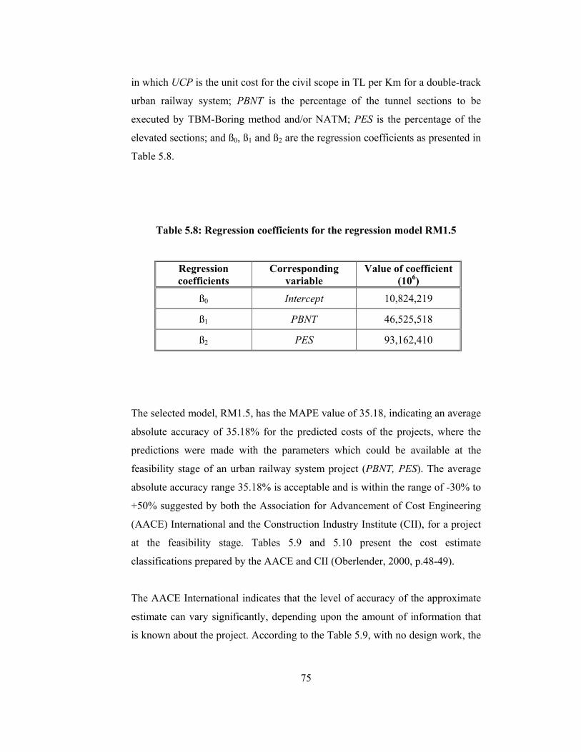
75

in which UCP is the unit cost for the civil scope in TL per Km for a double-track

urban railway system; PBNT is the percentage of the tunnel sections to be

executed by TBM-Boring method and/or NATM; PES is the percentage of the

elevated sections; and ß0, ß1 and ß2 are the regression coefficients as presented in

Table 5.8.

Table 5.8: Regression coefficients for the regression model RM1.5

Regression coefficients

Corresponding variable

Value of coefficient (106)

ß0 Intercept 10,824,219

ß1 PBNT 46,525,518

ß2 PES 93,162,410

The selected model, RM1.5, has the MAPE value of 35.18, indicating an average

absolute accuracy of 35.18% for the predicted costs of the projects, where the

predictions were made with the parameters which could be available at the

feasibility stage of an urban railway system project (PBNT, PES). The average

absolute accuracy range 35.18% is acceptable and is within the range of -30% to

+50% suggested by both the Association for Advancement of Cost Engineering

(AACE) International and the Construction Industry Institute (CII), for a project

at the feasibility stage. Tables 5.9 and 5.10 present the cost estimate

classifications prepared by the AACE and CII (Oberlender, 2000, p.48-49).

The AACE International indicates that the level of accuracy of the approximate

estimate can vary significantly, depending upon the amount of information that

is known about the project. According to the Table 5.9, with no design work, the

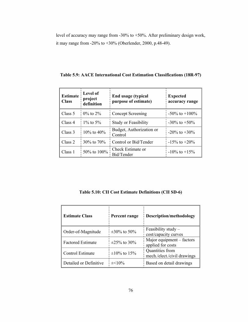
76

level of accuracy may range from -30% to +50%. After preliminary design work,

it may range from -20% to +30% (Oberlender, 2000, p.48-49).

Table 5.9: AACE International Cost Estimation Classifications (18R-97)

Estimate Class

Level of project definition

End usage (typical purpose of estimate)

Expected accuracy range

Class 5 0% to 2% Concept Screening -50% to +100%

Class 4 1% to 5% Study or Feasibility -30% to +50%

Class 3 10% to 40% Budget, Authorization or Control

-20% to +30%

Class 2 30% to 70% Control or Bid/Tender -15% to +20%

Class 1 50% to 100% Check Estimate or Bid/Tender

-10% to +15%

Table 5.10: CII Cost Estimate Definitions (CII SD-6)

Estimate Class Percent range Description/methodology

Order-of-Magnitude ±30% to 50% Feasibility study – cost/capacity curves

Factored Estimate ±25% to 30% Major equipment – factors applied for costs

Control Estimate ±10% to 15% Quantities from mech./elect./civil drawings

Detailed or Definitive ±<10% Based on detail drawings

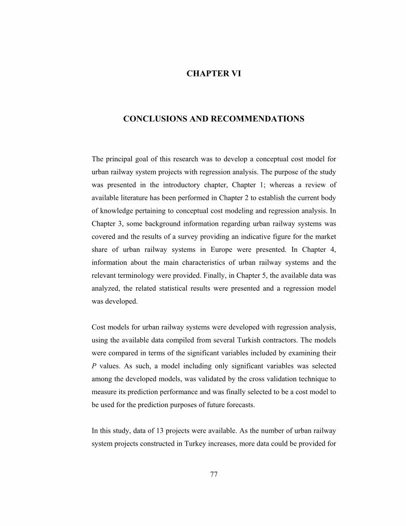
77

CHAPTER VI

CONCLUSIONS AND RECOMMENDATIONS

The principal goal of this research was to develop a conceptual cost model for

urban railway system projects with regression analysis. The purpose of the study

was presented in the introductory chapter, Chapter 1; whereas a review of

available literature has been performed in Chapter 2 to establish the current body

of knowledge pertaining to conceptual cost modeling and regression analysis. In

Chapter 3, some background information regarding urban railway systems was

covered and the results of a survey providing an indicative figure for the market

share of urban railway systems in Europe were presented. In Chapter 4,

information about the main characteristics of urban railway systems and the

relevant terminology were provided. Finally, in Chapter 5, the available data was

analyzed, the related statistical results were presented and a regression model

was developed.

Cost models for urban railway systems were developed with regression analysis,

using the available data compiled from several Turkish contractors. The models

were compared in terms of the significant variables included by examining their

P values. As such, a model including only significant variables was selected

among the developed models, was validated by the cross validation technique to

measure its prediction performance and was finally selected to be a cost model to

be used for the prediction purposes of future forecasts.

In this study, data of 13 projects were available. As the number of urban railway

system projects constructed in Turkey increases, more data could be provided for

78

conceptual cost estimation purposes. With more data available, some factors that

were not found significant in this study could be investigated in detail with the

additional information and new conceptual cost models could be formed. This

study provides a methodology for conceptual cost estimation of urban railway

system projects.

The final RM can be used to improve estimation of costs in the early stages of

urban railway system projects in Turkey. Authorities, sponsoring organizations,

engineering teams and perhaps the contractors could benefit from the results of

this study. More accurate early estimates will hopefully lead to more realistic

expectations and better execution strategies.

79

REFERENCES

Cresswell, J.W., 1994. Research Design – Qualitative & Quantitative Approaches, Vol. 1, SAGE Publications, US.

Dictionary on Labor Law Talk, Last Updated 2005. “Light Rail”, http://encyclopedia.laborlawtalk.com/Light_rail, Last accessed June 9, 2005.

Dictionary on Labor Law Talk, Last Updated 2005. “Metro”, http://encyclopedia.laborlawtalk.com/Metro, Last accessed June 9, 2005.

ERRAC, The European Rail Research Advisory Council, April 2004. Light Rail and Metro Systems in Europe – Current market, perspectives and research implication, Brussels.

Hegazy, T., and Ayed, A., 1998. “Neural network model for parametric cost estimation of highway projects”, Journal of Construction Engineering and Management, 124(3): 210-218.

Hollmann, J.K., and Dysert, L., 1989. “Development of conceptual estimating support systems at Kodak”, AACE Transactions.

Karshenas, S., 1984. “Predesign cost estimating method for multistory buildings”, Journal of Construction Engineering and Management, 110(1): 79-86.

Kouskoulas, V., and Koehn, E., 1974. “Predesign cost-estimation function for buildings”, Journal of the Construction Division, ASCE, 110(CO4): 589-604.

Oberlender, G.D., 1993. Project Management for Engineering and Construction, International Edition 2000 (Second Edition), McGraw-Hill Higher International Editions, Civil Engineering Series, Singapore.

Oberlender, G.D., and Trost, S.M.., 2001. “Predicting accuracy of early cost estimates based on estimate quality”, Journal of Construction Engineering and

80

Management, Vol. 127, No. 3, May/June, 2001. ASCE, ISSN 0733-9634/01/0003-0173-0182. Paper No. 22225.

Ostwald, P.F., 2001. Construction Cost Analysis and Estimating, Prentice Hall International Series In Civil Engineering and Engineering Mechanics, New Jersey.

Pankratz, A., 1983. Forecasting with univariate Box-Jenkins models, John Wiley and Sons, New York.

Sönmez, R., 2004. “Conceptual cost estimation of building projects with regression analysis and neural networks”, Canadian Journal of Civil Engineering, 31: 677-683.

Sönmez, R., and Rowings, J.E. 1998. “Construction labor productivity modeling with neural networks”, Journal of Construction Engineering and Management, 124(6): 498-504.

Taplin, M.R., 1998. “The History of Tramways and Evolution of Light Rail”, LRTA (Light Rail Transit Association).

Trost, S.M.., and Oberlender, G.D., 2003. “Predicting accuracy of early cost estimates using factor analysis and multivariate regression”, Journal of Construction Engineering and Management, Vol. 129, No. 2, April 1, 2003. ASCE, ISSN 0733-9364/2003/2-198-204.

Wikipedia The Free Encyclopedia, Last Updated April 11, 2005. “Tunnel Boring Machine”, http://en.wikipedia.org/wiki/Tunnel_Boring_Machine, Last accessed June 9, 2005.

Wikipedia The Free Encyclopedia, Last Updated June 6, 2005. “Rapid Transit”, http://en.wikipedia.org/wiki/Metro, Last accessed June 9, 2005.

Wikipedia The Free Encyclopedia, Last Updated May 20, 2005. “New Austrian Tunnelling Method”, http://en.wikipedia.org/wiki/New_Austrian_Tunneling_-method, Last accessed June 9, 2005.

Wikipedia The Free Encyclopedia, Last Updated May 30, 2005. “Tunnel”, http://en.wikipedia.org/wiki/Tunnel#Construction, Last accessed June 9, 2005.

81

Wilmot, C.G., and Cheng, G.., 2003. “Estimating future highway construction costs”, Journal of Construction Engineering and Management, Vol. 129, No. 3, June 1, 2003. ASCE, ISSN 0733-9364/2003/3-272-279.

Yesilada, E., and Nielsen, Y., 1996 METU Fall. Railway and Metro Tunnels - CE 439 Lecture Notes, Ankara.