computer abstractions and technology
TRANSCRIPT

Computer Abstractions and Technology 1.1 Introduction 3 1.2 Seven Great Ideas in Computer
Architecture 10 1.3 Below Your Program 13 1.4 Under the Covers 16 1.5 Technologies for Building Processors and
Memory 24
Civilization advances by extending the number of important operations which we can perform without thinking about them. Alfred North Whitehead, An Introduction to Mathematics , 1911
1
1.6 Performance 28 1.7 The Power Wall 40 1.8 The Sea Change: The Switch from Uniprocessors to
Multiprocessors 43 1.9 Real Stuff: Benchmarking the Intel Core i7 46 1.10 Going Faster: Matrix Multiply in Python 49 1.11 Fallacies and Pitfalls 50 1.12 Concluding Remarks 53 1.13 Historical Perspective and Further Reading 55 1.14 Self-Study 55 1.15 Exercises 59
1.1 Introduction
Welcome to this book! We’re delighted to have this opportunity to convey the excitement of the world of computer systems. Th is is not a dry and dreary fi eld, where progress is glacial and where new ideas atrophy from neglect. No! Computers are the product of the incredibly vibrant information technology industry, all aspects of which are responsible for almost 10% of the gross national product of the United States, and whose economy has become dependent in part on the rapid improvements in information technology. Th is unusual industry embraces innovation at a breathtaking rate. In the last 40 years, there have been a number of new computers whose introduction appeared to revolutionize the computing industry; these revolutions were cut short only because someone else built an even better computer.
Th is race to innovate has led to unprecedented progress since the inception of electronic computing in the late 1940s. Had the transportation industry kept pace with the computer industry, for example, today we could travel from New York to London in a second for a penny. Take just a moment to contemplate how such an improvement would change society—living in Tahiti while working in San Francisco, going to Moscow for an evening at the Bolshoi Ballet—and you can appreciate the implications of such a change.
1.1 Introduction 5
Classes of Computing Applications and Their Characteristics Although a common set of hardware technologies (see Sections 1.4 and 1.5 ) is used in computers ranging from smart home appliances to cell phones to the largest supercomputers, these diff erent applications have diff erent design requirements and employ the core hardware technologies in diff erent ways. Broadly speaking, computers are used in three diff erent classes of applications.
Personal computers (PCs) in the form of laptops are possibly the best known form of computing, which readers of this book have likely used extensively. Personal computers emphasize delivery of good performance to single users at low cost and usually execute third-party soft ware. Th is class of computing drove the evolution of many computing technologies, which is only about 40 years old!
Servers are the modern form of what were once much larger computers, and are usually accessed only via a network. Servers are oriented to carrying large workloads, which may consist of either single complex applications—usually a scientifi c or engineering application—or handling many small jobs, such as would occur in building a large web server. Th ese applications are usually based on soft ware from another source (such as a database or simulation system), but are oft en modifi ed or customized for a particular function. Servers are built from the same basic technology as desktop computers, but provide for greater computing, storage, and input/output capacity. In general, servers also place a greater emphasis on dependability, since a crash is usually more costly than it would be on a single-user PC.
Servers span the widest range in cost and capability. At the low end, a server may be little more than a desktop computer without a screen or keyboard and cost a thousand dollars. Th ese low-end servers are typically used for fi le storage, small business applications, or simple web serving (see Section 6.11). At the other extreme are supercomputers , which at the present consist of hundreds of thousands of processors and many terabytes of memory, and cost tens to hundreds of millions of dollars. Supercomputers are usually used for high-end scientifi c and engineering calculations, such as weather forecasting, oil exploration, protein structure determination, and other large-scale problems. Although such supercomputers represent the peak of computing capability, they represent a relatively small fraction of the servers and a relatively small fraction of the overall computer market in terms of total revenue.
Embedded computers are the largest class of computers and span the widest range of applications and performance. Embedded computers include the microprocessors found in your car, the computers in a television set, and the networks of processors that control a modern airplane or cargo ship. A popular term today is Internet of Th ings (IoT), which suggests many small devices that all communicate wirelessly over the Internet. Embedded computing systems are designed to run one application or one set of related applications that are normally integrated with the hardware and delivered as a single system; thus, despite the large number of embedded computers, most users never really see that they are using a computer!
personal computer (PC) A computer designed for use by an individual, usually incorporating a graphics display, a keyboard, and a mouse.
server A computer used for running larger programs for multiple users, oft en simultaneously, and typically accessed only via a network.
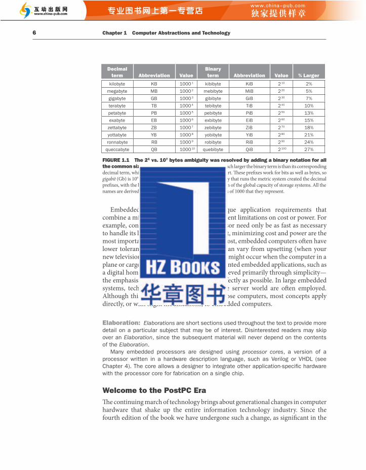
terabyte (TB) Originally 1,099,511,627,776 (2 40 ) bytes, although communications and secondary storage systems developers started using the term to mean 1,000,000,000,000 (10 12 ) bytes. To reduce confusion, we now use the term tebibyte (TiB) for 2 40 bytes, defi ning terabyte (TB) to mean 10 12 bytes. Figure 1.1 shows the full range of decimal and binary values and names.
supercomputer A class of computers with the highest performance and cost; they are confi gured as servers and typically cost tens to hundreds of millions of dollars.
embedded computer A computer inside another device used for running one predetermined application or collection of soft ware.
4 Chapter 1 Computer Abstractions and Technology
Computers have led to a third revolution for civilization, with the information revolution taking its place alongside the agricultural and the industrial revolutions. Th e resulting multiplication of humankind’s intellectual strength and reach naturally has aff ected our everyday lives profoundly and changed the ways in which the search for new knowledge is carried out. Th ere is now a new vein of scientifi c investigation, with computational scientists joining theoretical and experimental scientists in the exploration of new frontiers in astronomy, biology, chemistry, and physics, among others.
Th e computer revolution continues. Each time the cost of computing improves by another factor of 10, the opportunities for computers multiply. Applications that were economically infeasible suddenly become practical. In the recent past, the following applications were “computer science fi ction.”
■ Computers in automobiles: Until microprocessors improved dramatically in price and performance in the early 1980s, computer control of cars was ludicrous. Today, computers reduce pollution, improve fuel effi ciency via engine controls, and increase safety through nearly automated driving and air bag infl ation to protect occupants in a crash.
■ Cell phones: Who would have dreamed that advances in computer systems would lead to more than half of the planet having mobile phones, allowing person-to-person communication to almost anyone anywhere in the world?
■ Human genome project: Th e cost of computer equipment to map and analyze human DNA sequences was hundreds of millions of dollars. It’s unlikely that anyone would have considered this project had the computer costs been 10 to 100 times higher, as they would have been 15 to 25 years earlier. Moreover, costs continue to drop; you will soon be able to acquire your own genome, allowing medical care to be tailored to you.
■ World Wide Web: Not in existence at the time of the fi rst edition of this book, the web has transformed our society. For many, the web has replaced libraries and newspapers.
■ Search engines: As the content of the web grew in size and in value, fi nding relevant information became increasingly important. Today, many people rely on search engines for such a large part of their lives that it would be a hardship to go without them.
Clearly, advances in this technology now aff ect almost every aspect of our society. Hardware advances have allowed programmers to create wonderfully useful soft ware, which explains why computers are omnipresent. Today’s science fi ction suggests tomorrow’s killer applications: already on their way are glasses that augment reality, the cashless society, and cars that can drive themselves.
1.1 Introduction 5
Classes of Computing Applications and Their Characteristics Although a common set of hardware technologies (see Sections 1.4 and 1.5 ) is used in computers ranging from smart home appliances to cell phones to the largest supercomputers, these diff erent applications have diff erent design requirements and employ the core hardware technologies in diff erent ways. Broadly speaking, computers are used in three diff erent classes of applications.
Personal computers (PCs) in the form of laptops are possibly the best known form of computing, which readers of this book have likely used extensively. Personal computers emphasize delivery of good performance to single users at low cost and usually execute third-party soft ware. Th is class of computing drove the evolution of many computing technologies, which is only about 40 years old!
Servers are the modern form of what were once much larger computers, and are usually accessed only via a network. Servers are oriented to carrying large workloads, which may consist of either single complex applications—usually a scientifi c or engineering application—or handling many small jobs, such as would occur in building a large web server. Th ese applications are usually based on soft ware from another source (such as a database or simulation system), but are oft en modifi ed or customized for a particular function. Servers are built from the same basic technology as desktop computers, but provide for greater computing, storage, and input/output capacity. In general, servers also place a greater emphasis on dependability, since a crash is usually more costly than it would be on a single-user PC.
Servers span the widest range in cost and capability. At the low end, a server may be little more than a desktop computer without a screen or keyboard and cost a thousand dollars. Th ese low-end servers are typically used for fi le storage, small business applications, or simple web serving (see Section 6.11). At the other extreme are supercomputers , which at the present consist of hundreds of thousands of processors and many terabytes of memory, and cost tens to hundreds of millions of dollars. Supercomputers are usually used for high-end scientifi c and engineering calculations, such as weather forecasting, oil exploration, protein structure determination, and other large-scale problems. Although such supercomputers represent the peak of computing capability, they represent a relatively small fraction of the servers and a relatively small fraction of the overall computer market in terms of total revenue.
Embedded computers are the largest class of computers and span the widest range of applications and performance. Embedded computers include the microprocessors found in your car, the computers in a television set, and the networks of processors that control a modern airplane or cargo ship. A popular term today is Internet of Th ings (IoT), which suggests many small devices that all communicate wirelessly over the Internet. Embedded computing systems are designed to run one application or one set of related applications that are normally integrated with the hardware and delivered as a single system; thus, despite the large number of embedded computers, most users never really see that they are using a computer!
personal computer (PC) A computer designed for use by an individual, usually incorporating a graphics display, a keyboard, and a mouse.
server A computer used for running larger programs for multiple users, oft en simultaneously, and typically accessed only via a network.
terabyte (TB) Originally 1,099,511,627,776 (2 40 ) bytes, although communications and secondary storage systems developers started using the term to mean 1,000,000,000,000 (10 12 ) bytes. To reduce confusion, we now use the term tebibyte (TiB) for 2 40 bytes, defi ning terabyte (TB) to mean 10 12 bytes. Figure 1.1 shows the full range of decimal and binary values and names.
supercomputer A class of computers with the highest performance and cost; they are confi gured as servers and typically cost tens to hundreds of millions of dollars.
embedded computer A computer inside another device used for running one predetermined application or collection of soft ware.
4 Chapter 1 Computer Abstractions and Technology
Computers have led to a third revolution for civilization, with the information revolution taking its place alongside the agricultural and the industrial revolutions. Th e resulting multiplication of humankind’s intellectual strength and reach naturally has aff ected our everyday lives profoundly and changed the ways in which the search for new knowledge is carried out. Th ere is now a new vein of scientifi c investigation, with computational scientists joining theoretical and experimental scientists in the exploration of new frontiers in astronomy, biology, chemistry, and physics, among others.
Th e computer revolution continues. Each time the cost of computing improves by another factor of 10, the opportunities for computers multiply. Applications that were economically infeasible suddenly become practical. In the recent past, the following applications were “computer science fi ction.”
■ Computers in automobiles: Until microprocessors improved dramatically in price and performance in the early 1980s, computer control of cars was ludicrous. Today, computers reduce pollution, improve fuel effi ciency via engine controls, and increase safety through nearly automated driving and air bag infl ation to protect occupants in a crash.
■ Cell phones: Who would have dreamed that advances in computer systems would lead to more than half of the planet having mobile phones, allowing person-to-person communication to almost anyone anywhere in the world?
■ Human genome project: Th e cost of computer equipment to map and analyze human DNA sequences was hundreds of millions of dollars. It’s unlikely that anyone would have considered this project had the computer costs been 10 to 100 times higher, as they would have been 15 to 25 years earlier. Moreover, costs continue to drop; you will soon be able to acquire your own genome, allowing medical care to be tailored to you.
■ World Wide Web: Not in existence at the time of the fi rst edition of this book, the web has transformed our society. For many, the web has replaced libraries and newspapers.
■ Search engines: As the content of the web grew in size and in value, fi nding relevant information became increasingly important. Today, many people rely on search engines for such a large part of their lives that it would be a hardship to go without them.
Clearly, advances in this technology now aff ect almost every aspect of our society. Hardware advances have allowed programmers to create wonderfully useful soft ware, which explains why computers are omnipresent. Today’s science fi ction suggests tomorrow’s killer applications: already on their way are glasses that augment reality, the cashless society, and cars that can drive themselves.
1.1 Introduction 7
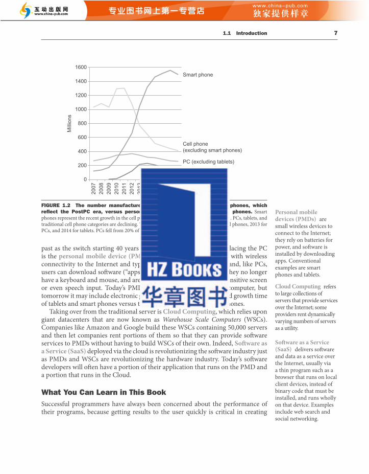
past as the switch starting 40 years ago to personal computers. Replacing the PC is the personal mobile device (PMD) . PMDs are battery operated with wireless connectivity to the Internet and typically cost hundreds of dollars, and, like PCs, users can download soft ware (“apps”) to run on them. Unlike PCs, they no longer have a keyboard and mouse, and are more likely to rely on a touch-sensitive screen or even speech input. Today’s PMD is a smart phone or a tablet computer, but tomorrow it may include electronic glasses. Figure 1.2 shows the rapid growth time of tablets and smart phones versus that of PCs and traditional cell phones.
Taking over from the traditional server is Cloud Computing , which relies upon giant datacenters that are now known as Warehouse Scale Computers (WSCs). Companies like Amazon and Google build these WSCs containing 50,000 servers and then let companies rent portions of them so that they can provide soft ware services to PMDs without having to build WSCs of their own. Indeed, Soft ware as a Service (SaaS) deployed via the cloud is revolutionizing the soft ware industry just as PMDs and WSCs are revolutionizing the hardware industry. Today’s soft ware developers will oft en have a portion of their application that runs on the PMD and a portion that runs in the Cloud.
What You Can Learn in This Book Successful programmers have always been concerned about the performance of their programs, because getting results to the user quickly is critical in creating
0
200
400
600
800
1000
1200
1400
1600
2007
2008
2009
2010
2011
2012
2013
2014
2015
2016
2017
2018
Mill
ions
Cell phone(excluding smart phones)
PC (excluding tablets)
Smart phone
Tablet
FIGURE 1.2 The number manufactured per year of tablets and smart phones, which refl ect the PostPC era, versus personal computers and traditional cell phones. Smart phones represent the recent growth in the cell phone industry, and they passed PCs in 2011. PCs, tablets, and traditional cell phone categories are declining. Th e peak volume years text are 2011 for cell phones, 2013 for PCs, and 2014 for tablets. PCs fell from 20% of total units shipped in 2007 to 10% in 2018.
Personal mobile devices (PMDs) are small wireless devices to connect to the Internet; they rely on batteries for power, and soft ware is installed by downloading apps. Conventional examples are smart phones and tablets.
Soft ware as a Service (SaaS) delivers soft ware and data as a service over the Internet, usually via a thin program such as a browser that runs on local client devices, instead of binary code that must be installed, and runs wholly on that device. Examples include web search and social networking.
Cloud Computing refers to large collections of servers that provide services over the Internet; some providers rent dynamically varying numbers of servers as a utility.
6 Chapter 1 Computer Abstractions and Technology
Embedded applications oft en have unique application requirements that combine a minimum performance with stringent limitations on cost or power. For example, consider a music player: the processor need only be as fast as necessary to handle its limited function, and beyond that, minimizing cost and power are the most important objectives. Despite their low cost, embedded computers oft en have lower tolerance for failure, since the results can vary from upsetting (when your new television crashes) to devastating (such as might occur when the computer in a plane or cargo ship crashes). In consumer-oriented embedded applications, such as a digital home appliance, dependability is achieved primarily through simplicity—the emphasis is on doing one function as perfectly as possible. In large embedded systems, techniques of redundancy from the server world are oft en employed. Although this book focuses on general-purpose computers, most concepts apply directly, or with slight modifi cations, to embedded computers.
Elaboration : Elaborations are short sections used throughout the text to provide more detail on a particular subject that may be of interest. Disinterested readers may skip over an Elaboration , since the subsequent material will never depend on the contents of the Elaboration .
Many embedded processors are designed using processor cores , a version of a processor written in a hardware description language, such as Verilog or VHDL (see Chapter 4). The core allows a designer to integrate other application-specifi c hardware with the processor core for fabrication on a single chip.
Welcome to the PostPC Era Th e continuing march of technology brings about generational changes in computer hardware that shake up the entire information technology industry. Since the fourth edition of the book we have undergone such a change, as signifi cant in the
Decimal term Abbreviation Value
Binary term Abbreviation Value % Larger
kilobyte KB 1000 1 kibibyte KiB 210 2%megabyte MB 1000 2 mebibyte MiB 220 5%gigabyte GB 1000 3 gibibyte GiB 230 7%terabyte TB 1000 4 tebibyte TiB 240 10%petabyte PB 1000 5 pebibyte PiB 250 13%exabyte EB 1000 6 exbibyte EiB 260 15%
zettabyte ZB 1000 7 zebibyte ZiB 270 18%yottabyte YB 1000 8 yobibyte YiB 280 21%ronnabyte RB 1000 9 robibyte RiB 290 24%
queccabyte QB 1000 10 quebibyte QiB 2100 27%
FIGURE 1.1 The 2 X vs. 10 Y bytes ambiguity was resolved by adding a binary notation for all the common size terms. In the last column we note how much larger the binary term is than its corresponding decimal term, which is compounded as we head down the chart. Th ese prefi xes work for bits as well as bytes, so gigabit (Gb) is 10 9 bits while gibibits (Gib) is 2 30 bits. Th e society that runs the metric system created the decimal prefi xes, with the last two proposed only in 2019 in anticipation of the global capacity of storage systems. All the names are derived from the entymology in Latin of the powers of 1000 that they represent.
1.1 Introduction 7
past as the switch starting 40 years ago to personal computers. Replacing the PC is the personal mobile device (PMD) . PMDs are battery operated with wireless connectivity to the Internet and typically cost hundreds of dollars, and, like PCs, users can download soft ware (“apps”) to run on them. Unlike PCs, they no longer have a keyboard and mouse, and are more likely to rely on a touch-sensitive screen or even speech input. Today’s PMD is a smart phone or a tablet computer, but tomorrow it may include electronic glasses. Figure 1.2 shows the rapid growth time of tablets and smart phones versus that of PCs and traditional cell phones.
Taking over from the traditional server is Cloud Computing , which relies upon giant datacenters that are now known as Warehouse Scale Computers (WSCs). Companies like Amazon and Google build these WSCs containing 50,000 servers and then let companies rent portions of them so that they can provide soft ware services to PMDs without having to build WSCs of their own. Indeed, Soft ware as a Service (SaaS) deployed via the cloud is revolutionizing the soft ware industry just as PMDs and WSCs are revolutionizing the hardware industry. Today’s soft ware developers will oft en have a portion of their application that runs on the PMD and a portion that runs in the Cloud.
What You Can Learn in This Book Successful programmers have always been concerned about the performance of their programs, because getting results to the user quickly is critical in creating
0
200
400
600
800
1000
1200
1400
1600
2007
2008
2009
2010
2011
2012
2013
2014
2015
2016
2017
2018
Mill
ions
Cell phone(excluding smart phones)
PC (excluding tablets)
Smart phone
Tablet
FIGURE 1.2 The number manufactured per year of tablets and smart phones, which refl ect the PostPC era, versus personal computers and traditional cell phones. Smart phones represent the recent growth in the cell phone industry, and they passed PCs in 2011. PCs, tablets, and traditional cell phone categories are declining. Th e peak volume years text are 2011 for cell phones, 2013 for PCs, and 2014 for tablets. PCs fell from 20% of total units shipped in 2007 to 10% in 2018.
Personal mobile devices (PMDs) are small wireless devices to connect to the Internet; they rely on batteries for power, and soft ware is installed by downloading apps. Conventional examples are smart phones and tablets.
Soft ware as a Service (SaaS) delivers soft ware and data as a service over the Internet, usually via a thin program such as a browser that runs on local client devices, instead of binary code that must be installed, and runs wholly on that device. Examples include web search and social networking.
Cloud Computing refers to large collections of servers that provide services over the Internet; some providers rent dynamically varying numbers of servers as a utility.
6 Chapter 1 Computer Abstractions and Technology
Embedded applications oft en have unique application requirements that combine a minimum performance with stringent limitations on cost or power. For example, consider a music player: the processor need only be as fast as necessary to handle its limited function, and beyond that, minimizing cost and power are the most important objectives. Despite their low cost, embedded computers oft en have lower tolerance for failure, since the results can vary from upsetting (when your new television crashes) to devastating (such as might occur when the computer in a plane or cargo ship crashes). In consumer-oriented embedded applications, such as a digital home appliance, dependability is achieved primarily through simplicity—the emphasis is on doing one function as perfectly as possible. In large embedded systems, techniques of redundancy from the server world are oft en employed. Although this book focuses on general-purpose computers, most concepts apply directly, or with slight modifi cations, to embedded computers.
Elaboration : Elaborations are short sections used throughout the text to provide more detail on a particular subject that may be of interest. Disinterested readers may skip over an Elaboration , since the subsequent material will never depend on the contents of the Elaboration .
Many embedded processors are designed using processor cores , a version of a processor written in a hardware description language, such as Verilog or VHDL (see Chapter 4). The core allows a designer to integrate other application-specifi c hardware with the processor core for fabrication on a single chip.
Welcome to the PostPC Era Th e continuing march of technology brings about generational changes in computer hardware that shake up the entire information technology industry. Since the fourth edition of the book we have undergone such a change, as signifi cant in the
Decimal term Abbreviation Value
Binary term Abbreviation Value % Larger
kilobyte KB 1000 1 kibibyte KiB 210 2%megabyte MB 1000 2 mebibyte MiB 220 5%gigabyte GB 1000 3 gibibyte GiB 230 7%terabyte TB 1000 4 tebibyte TiB 240 10%petabyte PB 1000 5 pebibyte PiB 250 13%exabyte EB 1000 6 exbibyte EiB 260 15%
zettabyte ZB 1000 7 zebibyte ZiB 270 18%yottabyte YB 1000 8 yobibyte YiB 280 21%ronnabyte RB 1000 9 robibyte RiB 290 24%
queccabyte QB 1000 10 quebibyte QiB 2100 27%
FIGURE 1.1 The 2 X vs. 10 Y bytes ambiguity was resolved by adding a binary notation for all the common size terms. In the last column we note how much larger the binary term is than its corresponding decimal term, which is compounded as we head down the chart. Th ese prefi xes work for bits as well as bytes, so gigabit (Gb) is 10 9 bits while gibibits (Gib) is 2 30 bits. Th e society that runs the metric system created the decimal prefi xes, with the last two proposed only in 2019 in anticipation of the global capacity of storage systems. All the names are derived from the entymology in Latin of the powers of 1000 that they represent.
1.1 Introduction 9
Without understanding the answers to these questions, improving the performance of your program on a modern computer or evaluating what features might make one computer better than another for a particular application will be a complex process of trial and error, rather than a scientifi c procedure driven by insight and analysis.
Th is fi rst chapter lays the foundation for the rest of the book. It introduces the basic ideas and defi nitions, places the major components of soft ware and hardware in perspective, shows how to evaluate performance and energy, introduces integrated circuits (the technology that fuels the computer revolution), and explains the shift to multicores.
In this chapter and later ones, you will likely see many new words, or words that you may have heard but are not sure what they mean. Don’t panic! Yes, there is a lot of special terminology used in describing modern computers, but the terminology actually helps, since it enables us to describe precisely a function or capability. In addition, computer designers (including your authors) love using acronyms , which are easy to understand once you know what the letters stand for! To help you remember and locate terms, we have included a highlighted defi nition of every term in the margins the fi rst time it appears in the text. Aft er a short time of working with the terminology, you will be fl uent, and your friends will be impressed as you correctly use acronyms such as BIOS, CPU, DIMM, DRAM, PCIe, SATA, and many others.
To reinforce how the soft ware and hardware systems used to run a program will aff ect performance, we use a special section, Understanding Program Performance , throughout the book to summarize important insights into program performance. Th e fi rst one appears below.
Th e performance of a program depends on a combination of the eff ectiveness of the algorithms used in the program, the soft ware systems used to create and translate the program into machine instructions, and the eff ectiveness of the computer in executing those instructions, which may include input/output (I/O) operations. Th is table summarizes how the hardware and soft ware aff ect performance.
Hardware or software component How this component affects performance
Where is this topic covered?
Algorithm Determines both the number of source-level statements and the number of I/O operations executed
Other books!
Programming language, compiler, and architecture
Determines the number of computer instructions for each source-level statement
Chapters 2 and 3
Processor and memory system
Determines how fast instructions can be executed Chapters 4, 5, and 6
I/O system (hardware and operating system)
Determines how fast I/O operations may be executed
Chapters 4, 5, and 6
acronym A word constructed by taking the initial letters of a string of words. For example: RAM is an acronym for Random Access Memory, and CPU is an acronym for Central Processing Unit.
Understanding Program Performance
8 Chapter 1 Computer Abstractions and Technology
successful soft ware. In the 1960s and 1970s, a primary constraint on computer performance was the size of the computer’s memory. Th us, programmers oft en followed a simple credo: minimize memory space to make programs fast. In the last two decades, advances in computer design and memory technology have greatly reduced the importance of small memory size in most applications other than those in embedded computing systems.
Programmers interested in performance now need to understand the issues that have replaced the simple memory model of the 1960s: the parallel nature of processors and the hierarchical nature of memories. Moreover, as we explain in Section 1.7 , today’s programmers need to worry about energy effi ciency of their programs running either on the PMD or in the Cloud, which also requires understanding what is below your code. Programmers who seek to build competitive versions of soft ware will therefore need to increase their knowledge of computer organization.
We are honored to have the opportunity to explain what’s inside this revolutionary machine, unraveling the soft ware below your program and the hardware under the covers of your computer. By the time you complete this book, we believe you will be able to answer the following questions:
■ How are programs written in a high-level language, such as C or Java, translated into the language of the hardware, and how does the hardware execute the resulting program? Comprehending these concepts forms the basis of understanding the aspects of both the hardware and soft ware that aff ect program performance.
■ What is the interface between the soft ware and the hardware, and how does soft ware instruct the hardware to perform needed functions? Th ese concepts are vital to understanding how to write many kinds of soft ware.
■ What determines the performance of a program, and how can a programmer improve the performance? As we will see, this depends on the original program, the soft ware translation of that program into the computer’s language, and the eff ectiveness of the hardware in executing the program.
■ What techniques can be used by hardware designers to improve performance? Th is book will introduce the basic concepts of modern computer design. Th e interested reader will fi nd much more material on this topic in our advanced book, Computer Architecture: A Quantitative Approach .
■ What techniques can be used by hardware designers to improve energy effi ciency? What can the programmer do to help or hinder energy effi ciency?
■ What are the reasons for and the consequences of the switch from sequential processing to parallel processing? Th is book gives the motivation, describes the current hardware mechanisms to support parallelism, and surveys the new generation of “multicore” microprocessors (see Chapter 6).
■ Since the fi rst commercial computer in 1951, what great ideas did computer architects come up with that lay the foundation of modern computing?
multicore microprocessor A microprocessor containing multiple processors (“cores”) in a single integrated circuit.
1.2 Eight Great Ideas in Computer Architecture 11
representation; lower-level details are hidden to off er a simpler model at higher levels. We’ll use the abstract painting icon to represent this second great idea.
Make the Common Case Fast Making the common case fast will tend to enhance performance better than optimizing the rare case. Ironically, the common case is oft en simpler than the rare case and hence is oft en easier to enhance. Th is common sense advice implies that you know what the common case is, which is only possible with careful experimentation and measurement (see Section 1.6 ). We use a sports car as the icon for making the common case fast, as the most common trip has one or two passengers, and it’s surely easier to make a fast sports car than a fast minivan!
Performance via Parallelism Since the dawn of computing, computer architects have off ered designs that get more performance by performing operations in parallel. We’ll see many examples of parallelism in this book. We use multiple jet engines of a plane as our icon for parallel performance .
Performance via Pipelining A particular pattern of parallelism is so prevalent in computer architecture that it merits its own name: pipelining . For example, before fi re engines, a “bucket brigade” would respond to a fi re, which many cowboy movies show in response to a dastardly act by the villain. Th e townsfolk form a human chain to carry a water source to fi re, as they could much more quickly move buckets up the chain instead of individuals running back and forth. Our pipeline icon is a sequence of pipes, with each section representing one stage of the pipeline.
Performance via Prediction Following the saying that it can be better to ask for forgiveness than to ask for permission, the next great idea is prediction . In some cases it can be faster on average to guess and start working rather than wait until you know for sure, assuming that the mechanism to recover from a misprediction is not too expensive and your prediction is relatively accurate. We use the fortune-teller’s crystal ball as our prediction icon.
Hierarchy of Memories Programmers want memory to be fast, large, and cheap, as memory speed oft en shapes performance, capacity limits the size of problems that can be solved, and the cost of memory today is oft en the majority of computer cost. Architects have found that they can address these confl icting demands with a hierarchy of memories , with
10 Chapter 1 Computer Abstractions and Technology
Check Yourself sections are designed to help readers assess whether they comprehend the major concepts introduced in a chapter and understand the implications of those concepts. Some Check Yourself questions have simple answers; others are for discussion among a group. Answers to the specifi c questions can be found at the end of the chapter. Check Yourself questions appear only at the end of a section, making it easy to skip them if you are sure you understand the material.
1. Th e number of embedded processors sold every year greatly outnumbers the number of PC and even PostPC processors. Can you confi rm or deny this insight based on your own experience? Try to count the number of embedded processors in your home. How does it compare with the number of conventional computers in your home?
2. As mentioned earlier, both the soft ware and hardware aff ect the performance of a program. Can you think of examples where each of the following is the right place to look for a performance bottleneck?
■ Th e algorithm chosen ■ Th e programming language or compiler ■ Th e operating system ■ Th e processor ■ Th e I/O system and devices
1.2 Seven Great Ideas in Computer Architecture
We now introduce seven great ideas that computer architects have been invented in the last 60 years of computer design. Th ese ideas are so powerful they have lasted long aft er the fi rst computer that used them, with newer architects demonstrating their admiration by imitating their predecessors. Th ese great ideas are themes that we will weave through this and subsequent chapters as examples arise. To point out their infl uence, in this section we introduce icons and highlighted terms that represent the great ideas and we use them to identify the nearly 100 sections of the book that feature use of the great ideas.
Use Abstraction to Simplify Design Both computer architects and programmers had to invent techniques to make themselves more productive, for otherwise design time would lengthen as dramatically as resources grew. A major productivity technique for hardware and soft ware is to use abstractions to represent the design at diff erent levels of
Check Yourself

1.2 Eight Great Ideas in Computer Architecture 11
representation; lower-level details are hidden to off er a simpler model at higher levels. We’ll use the abstract painting icon to represent this second great idea.
Make the Common Case Fast Making the common case fast will tend to enhance performance better than optimizing the rare case. Ironically, the common case is oft en simpler than the rare case and hence is oft en easier to enhance. Th is common sense advice implies that you know what the common case is, which is only possible with careful experimentation and measurement (see Section 1.6 ). We use a sports car as the icon for making the common case fast, as the most common trip has one or two passengers, and it’s surely easier to make a fast sports car than a fast minivan!
Performance via Parallelism Since the dawn of computing, computer architects have off ered designs that get more performance by performing operations in parallel. We’ll see many examples of parallelism in this book. We use multiple jet engines of a plane as our icon for parallel performance .
Performance via Pipelining A particular pattern of parallelism is so prevalent in computer architecture that it merits its own name: pipelining . For example, before fi re engines, a “bucket brigade” would respond to a fi re, which many cowboy movies show in response to a dastardly act by the villain. Th e townsfolk form a human chain to carry a water source to fi re, as they could much more quickly move buckets up the chain instead of individuals running back and forth. Our pipeline icon is a sequence of pipes, with each section representing one stage of the pipeline.
Performance via Prediction Following the saying that it can be better to ask for forgiveness than to ask for permission, the next great idea is prediction . In some cases it can be faster on average to guess and start working rather than wait until you know for sure, assuming that the mechanism to recover from a misprediction is not too expensive and your prediction is relatively accurate. We use the fortune-teller’s crystal ball as our prediction icon.
Hierarchy of Memories Programmers want memory to be fast, large, and cheap, as memory speed oft en shapes performance, capacity limits the size of problems that can be solved, and the cost of memory today is oft en the majority of computer cost. Architects have found that they can address these confl icting demands with a hierarchy of memories , with
10 Chapter 1 Computer Abstractions and Technology
Check Yourself sections are designed to help readers assess whether they comprehend the major concepts introduced in a chapter and understand the implications of those concepts. Some Check Yourself questions have simple answers; others are for discussion among a group. Answers to the specifi c questions can be found at the end of the chapter. Check Yourself questions appear only at the end of a section, making it easy to skip them if you are sure you understand the material.
1. Th e number of embedded processors sold every year greatly outnumbers the number of PC and even PostPC processors. Can you confi rm or deny this insight based on your own experience? Try to count the number of embedded processors in your home. How does it compare with the number of conventional computers in your home?
2. As mentioned earlier, both the soft ware and hardware aff ect the performance of a program. Can you think of examples where each of the following is the right place to look for a performance bottleneck?
■ Th e algorithm chosen ■ Th e programming language or compiler ■ Th e operating system ■ Th e processor ■ Th e I/O system and devices
1.2 Seven Great Ideas in Computer Architecture
We now introduce seven great ideas that computer architects have been invented in the last 60 years of computer design. Th ese ideas are so powerful they have lasted long aft er the fi rst computer that used them, with newer architects demonstrating their admiration by imitating their predecessors. Th ese great ideas are themes that we will weave through this and subsequent chapters as examples arise. To point out their infl uence, in this section we introduce icons and highlighted terms that represent the great ideas and we use them to identify the nearly 100 sections of the book that feature use of the great ideas.
Use Abstraction to Simplify Design Both computer architects and programmers had to invent techniques to make themselves more productive, for otherwise design time would lengthen as dramatically as resources grew. A major productivity technique for hardware and soft ware is to use abstractions to represent the design at diff erent levels of
Check Yourself
1.3 Below Your Program 13
1.3 Below Your Program
A typical application, such as a word processor or a large database system, may consist of millions of lines of code and rely on sophisticated soft ware libraries that implement complex functions in support of the application. As we will see, the hardware in a computer can only execute extremely simple low-level instructions. To go from a complex application to the simple instructions involves several layers of soft ware that interpret or translate high-level operations into simple computer instructions, an example of the great idea of abstraction .
Figure 1.3 shows that these layers of soft ware are organized primarily in a hierarchical fashion, with applications being the outermost ring and a variety of systems soft ware sitting between the hardware and applications soft ware.
Th ere are many types of systems soft ware, but two types of systems soft ware are central to every computer system today: an operating system and a compiler. An operating system interfaces between a user’s program and the hardware and provides a variety of services and supervisory functions. Among the most important functions are:
■ Handling basic input and output operations
■ Allocating storage and memory
■ Providing for protected sharing of the computer among multiple applications using it simultaneously.
Examples of operating systems in use today are Linux, iOS, Android, and Windows.
In Paris they simply stared when I spoke to them in French; I never did succeed in making those idiots understand their own language. Mark Twain, Th e Innocents Abroad , 1869
systems soft ware Soft ware that provides services that are commonly useful, including operating systems, compilers, loaders, and assemblers.
operating system Supervising program that manages the resources of a computer for the benefi t of the programs that run on that computer.
Applications software
Systems software
Hardware
FIGURE 1.3 A simplifi ed view of hardware and software as hierarchical layers, shown as concentric circles with hardware in the center and applications software outermost. In complex applications, there are oft en multiple layers of application soft ware as well. For example, a database system may run on top of the systems soft ware hosting an application, which in turn runs on top of the database.
12 Chapter 1 Computer Abstractions and Technology
the fastest, smallest, and most expensive memory per bit at the top of the hierarchy and the slowest, largest, and cheapest per bit at the bottom. As we shall see in Chapter 5, caches give the programmer the illusion that main memory is nearly as fast as the top of the hierarchy and nearly as big and cheap as the bottom of the hierarchy. We use a layered triangle icon to represent the memory hierarchy. Th e shape indicates speed, cost, and size: the closer to the top, the faster and more expensive per bit the memory; the wider the base of the layer, the bigger the memory.
Dependability via Redundancy Computers not only need to be fast; they need to be dependable. Since any physical device can fail, we make systems dependable by including redundant components that can take over when a failure occurs and to help detect failures. We use the tractor-trailer as our icon, since the dual tires on each side of its rear axles allow the truck to continue driving even when one tire fails. (Presumably, the truck driver heads immediately to a repair facility so the fl at tire can be fi xed, thereby restoring redundancy!)
In the prior edition , we listed an eighth great idea, which was “Designing for Moore’s Law.” Gordon Moore, one of the founders of Intel, made a remarkable prediction in 1965: integrated circuit resources would double every year. A decade later he amended his prediction to doubling every 2 years.
His prediction was accurate, and for 50 years, Moore’s Law shaped computer architecture. As computer designs can take years, the resources available per chip (“transistors”; see page 24) could easily double or triple between the start and fi nish of the project. Like a skeet shooter, computer architects had to anticipate where the technology would be when the design fi nishes rather than design for when it starts.
Alas, no exponential growth can last forever, and Moore’s Law is no longer accurate. Th e slowing of Moore’s Law is shocking for computer designers who have long leveraged it. Some do not want to believe it is over, despite the substantial evidence to the contrary. Part of the reason is confusion between saying that Moore’s prediction of the biannual doubling rate is now incorrect and claiming that semiconductors will no longer improve. Semiconductor technology will continue to improve, but more slowly than in the past. Starting with this edition, we will discuss the implications of the slowing of Moore’s Law, especially in Chapter 6.
Elaboration: During the heydays of Moore’s Law, the cost per chip resource would drop with each new technology generation. In the latest technologies, the cost per resource may be fl at or even rising with each new generation, due to the cost of the new equipment, the elaborate processes invented to make chips work at these fi ner feature sizes, and the reduction of the number of companies who are investing in these new technologies to push the state-of-the-art. Less competition naturally leads to higher prices.

1.3 Below Your Program 15
Th e recognition that a program could be written to translate a more powerful language into computer instructions was one of the great breakthroughs in the early days of computing. Programmers today owe their productivity—and their sanity—to the creation of high-level programming languages and compilers that translate programs in such languages into instructions. Figure 1.4 shows the relationships among these programs and languages, which are more examples of the power of abstraction .
high-level programming language A portable language such as C, C+ +, Java, or Visual Basic that is composed of words and algebraic notation that can be translated by a compiler into assembly language.
swap(int v[], int k){int temp; temp = v[k]; v[k] = v[k+1]; v[k+1] = temp;}
swap: multi $2, $5,4 add $2, $4,$2 lw $15, 0($2) lw $16, 4($2) sw $16, 0($2) sw $15, 4($2) jr $31
00000000101000100000000100011000000000001000001000010000001000011000110111100010000000000000000010001110000100100000000000000100101011100001001000000000000000001010110111100010000000000000010000000011111000000000000000001000
Assembler
Compiler
Binary machinelanguageprogram(for MIPS)
Assemblylanguageprogram(for MIPS)
High-levellanguageprogram(in C)
FIGURE 1.4 C program compiled into assembly language and then assembled into binary machine language. Although the translation from high-level language to binary machine language is shown in two steps, some compilers cut out the middleman and produce binary machine language directly. Th ese languages and this program are examined in more detail in Chapter 2.
14 Chapter 1 Computer Abstractions and Technology
Compilers perform another vital function: the translation of a program written in a high-level language, such as C, C+ +, Java, or Visual Basic into instructions that the hardware can execute. Given the sophistication of modern programming languages and the simplicity of the instructions executed by the hardware, the translation from a high-level language program to hardware instructions is complex. We give a brief overview of the process here and then go into more depth in Chapter 2 and in Appendix A .
From a High-Level Language to the Language of Hardware To actually speak to electronic hardware, you need to send electrical signals. Th e easiest signals for computers to understand are on and off , and so the computer alphabet is just two letters. Just as the 26 letters of the English alphabet do not limit how much can be written, the two letters of the computer alphabet do not limit what computers can do. Th e two symbols for these two letters are the numbers 0 and 1, and we commonly think of the computer language as numbers in base 2, or binary numbers . We refer to each “letter” as a binary digit or bit . Computers are slaves to our commands, which are called instructions . Instructions, which are just collections of bits that the computer understands and obeys, can be thought of as numbers. For example, the bits
1000110010100000
tell one computer to add two numbers. Chapter 2 explains why we use numbers for instructions and data; we don’t want to steal that chapter’s thunder, but using numbers for both instructions and data is a foundation of computing.
Th e fi rst programmers communicated to computers in binary numbers, but this was so tedious that they quickly invented new notations that were closer to the way humans think. At fi rst, these notations were translated to binary by hand, but this process was still tiresome. Using the computer to help program the computer, the pioneers invented programs to translate from symbolic notation to binary. Th e fi rst of these programs was named an assembler . Th is program translates a symbolic version of an instruction into the binary version. For example, the programmer would write
add A,B
and the assembler would translate this notation into
1000110010100000
Th is instruction tells the computer to add the two numbers A and B . Th e name coined for this symbolic language, still used today, is assembly language . In contrast, the binary language that the machine understands is the machine language .
Although a tremendous improvement, assembly language is still far from the notations a scientist might like to use to simulate fl uid fl ow or that an accountant might use to balance the books. Assembly language requires the programmer to write one line for every instruction that the computer will follow, forcing the programmer to think like the computer.
compiler A program that translates high-level language statements into assembly language statements.
binary digit Also called a bit . One of the two numbers in base 2 (0 or 1) that are the components of information.
instruction A command that computer hardware understands and obeys.
assembler A program that translates a symbolic version of instructions into the binary version.
assembly language A symbolic representation of machine instructions.
machine language A binary representation of machine instructions.
1.4 Under the Covers 17
computer, and output is the result of computation sent to the user. Some devices, such as wireless networks, provide both input and output to the computer.
Chapters 5 and 6 describe input/output (I/O) devices in more detail, but let’s take an introductory tour through the computer hardware, starting with the external I/O devices.
The BIG Picture
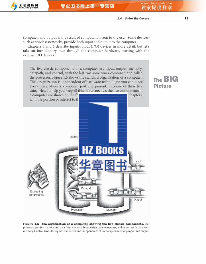
Th e fi ve classic components of a computer are input, output, memory, datapath, and control, with the last two sometimes combined and called the processor. Figure 1.5 shows the standard organization of a computer. Th is organization is independent of hardware technology: you can place every piece of every computer, past and present, into one of these fi ve categories. To help you keep all this in perspective, the fi ve components of a computer are shown on the front page of each of the following chapters, with the portion of interest to that chapter highlighted.
FIGURE 1.5 The organization of a computer, showing the fi ve classic components. Th e processor gets instructions and data from memory. Input writes data to memory, and output reads data from memory. Control sends the signals that determine the operations of the datapath, memory, input, and output.
16 Chapter 1 Computer Abstractions and Technology
A compiler enables a programmer to write this high-level language expression:
A + B
Th e compiler would compile it into this assembly language statement:
add A,B
As shown above, the assembler would translate this statement into the binary instructions that tell the computer to add the two numbers A and B .
High-level programming languages off er several important benefi ts. First, they allow the programmer to think in a more natural language, using English words and algebraic notation, resulting in programs that look much more like text than like tables of cryptic symbols (see Figure 1.4 ). Moreover, they allow languages to be designed according to their intended use. Hence, Fortran was designed for scientifi c computation, Cobol for business data processing, Lisp for symbol manipulation, and so on. Th ere are also domain-specifi c languages for even narrower groups of users, such as those interested in machine learning, for example.
Th e second advantage of programming languages is improved programmer productivity. One of the few areas of widespread agreement in soft ware development is that it takes less time to develop programs when they are written in languages that require fewer lines to express an idea. Conciseness is a clear advantage of high-level languages over assembly language.
Th e fi nal advantage is that programming languages allow programs to be independent of the computer on which they were developed, since compilers and assemblers can translate high-level language programs to the binary instructions of any computer. Th ese three advantages are so strong that today little programming is done in assembly language.
1.4 Under the Covers
Now that we have looked below your program to uncover the underlying soft ware, let’s open the covers of your computer to learn about the underlying hardware. Th e underlying hardware in any computer performs the same basic functions: inputting data, outputting data, processing data, and storing data. How these functions are performed is the primary topic of this book, and subsequent chapters deal with diff erent parts of these four tasks.
When we come to an important point in this book, a point so important that we hope you will remember it forever, we emphasize it by identifying it as a Big Picture item. We have about a dozen Big Pictures in this book, the fi rst being the fi ve components of a computer that perform the tasks of inputting, outputting, processing, and storing data.
Two key components of computers are input devices , such as the microphone, and output devices , such as the speaker. As the names suggest, input feeds the
input device A mechanism through which the computer is fed information, such as a keyboard.
output device A mechanism that conveys the result of a computation to a user, such as a display, or to another computer.
1.4 Under the Covers 17
computer, and output is the result of computation sent to the user. Some devices, such as wireless networks, provide both input and output to the computer.
Chapters 5 and 6 describe input/output (I/O) devices in more detail, but let’s take an introductory tour through the computer hardware, starting with the external I/O devices.
The BIG Picture
Th e fi ve classic components of a computer are input, output, memory, datapath, and control, with the last two sometimes combined and called the processor. Figure 1.5 shows the standard organization of a computer. Th is organization is independent of hardware technology: you can place every piece of every computer, past and present, into one of these fi ve categories. To help you keep all this in perspective, the fi ve components of a computer are shown on the front page of each of the following chapters, with the portion of interest to that chapter highlighted.
FIGURE 1.5 The organization of a computer, showing the fi ve classic components. Th e processor gets instructions and data from memory. Input writes data to memory, and output reads data from memory. Control sends the signals that determine the operations of the datapath, memory, input, and output.
16 Chapter 1 Computer Abstractions and Technology
A compiler enables a programmer to write this high-level language expression:
A + B
Th e compiler would compile it into this assembly language statement:
add A,B
As shown above, the assembler would translate this statement into the binary instructions that tell the computer to add the two numbers A and B .
High-level programming languages off er several important benefi ts. First, they allow the programmer to think in a more natural language, using English words and algebraic notation, resulting in programs that look much more like text than like tables of cryptic symbols (see Figure 1.4 ). Moreover, they allow languages to be designed according to their intended use. Hence, Fortran was designed for scientifi c computation, Cobol for business data processing, Lisp for symbol manipulation, and so on. Th ere are also domain-specifi c languages for even narrower groups of users, such as those interested in machine learning, for example.
Th e second advantage of programming languages is improved programmer productivity. One of the few areas of widespread agreement in soft ware development is that it takes less time to develop programs when they are written in languages that require fewer lines to express an idea. Conciseness is a clear advantage of high-level languages over assembly language.
Th e fi nal advantage is that programming languages allow programs to be independent of the computer on which they were developed, since compilers and assemblers can translate high-level language programs to the binary instructions of any computer. Th ese three advantages are so strong that today little programming is done in assembly language.
1.4 Under the Covers
Now that we have looked below your program to uncover the underlying soft ware, let’s open the covers of your computer to learn about the underlying hardware. Th e underlying hardware in any computer performs the same basic functions: inputting data, outputting data, processing data, and storing data. How these functions are performed is the primary topic of this book, and subsequent chapters deal with diff erent parts of these four tasks.
When we come to an important point in this book, a point so important that we hope you will remember it forever, we emphasize it by identifying it as a Big Picture item. We have about a dozen Big Pictures in this book, the fi rst being the fi ve components of a computer that perform the tasks of inputting, outputting, processing, and storing data.
Two key components of computers are input devices , such as the microphone, and output devices , such as the speaker. As the names suggest, input feeds the
input device A mechanism through which the computer is fed information, such as a keyboard.
output device A mechanism that conveys the result of a computation to a user, such as a display, or to another computer.

1.4 Under the Covers 19
Touchscreen While PCs also use LCD displays, the tablets and smartphones of the PostPC era have replaced the keyboard and mouse with touch sensitive displays, which has the wonderful user interface advantage of users pointing directly what they are interested in rather than indirectly with a mouse.
While there are a variety of ways to implement a touch screen, many tablets today use capacitive sensing. Since people are electrical conductors, if an insulator like glass is covered with a transparent conductor, touching distorts the electrostatic fi eld of the screen, which results in a change in capacitance. Th is technology can allow multiple touches simultaneously, which allows gestures that can lead to attractive user interfaces.
Opening the Box Figure 1.7 shows the contents of the Apple iPhone Xs Max smart phone. Unsurprisingly, of the fi ve classic components of the computer, I/O dominates this device. Th e list of I/O devices includes a capacitive multitouch LCD display, front-facing camera, rear-facing camera, microphone, headphone jack, speakers, accelerometer, gyroscope, Wi-Fi network, and Bluetooth network. Th e datapath, control, and memory are a tiny portion of the components.
Th e small rectangles in Figure 1.8 contain the devices that drive our advancing technology, called integrated circuits and nicknamed chips . Th e A12 package seen in the middle of in Figure 1.8 contains two large ARM processors and four little ARM processors that operate with a clock rate of 2.5 GHz. Th e processor is the active part of the computer, following the instructions of a program to the letter. It adds numbers, tests numbers, signals I/O devices to activate, and so on. Occasionally, people call the processor the CPU , for the more bureaucratic-sounding central processor unit .
Descending even lower into the hardware, Figure 1.9 reveals details of a microprocessor. Th e processor logically comprises two main components: datapath and control, the respective brawn and brain of the processor. Th e datapath performs the arithmetic operations, and control tells the datapath, memory, and I/O devices what to do according to the wishes of the instructions of the program. Chapter 4 explains the datapath and control for a higher performance design.
Th e iPhone Xs Max package in Figure 1.8 also includes a memory chip with 32 gibibits or 2 GiB of capacity. Th e memory is where the programs are kept when they are running; it also contains the data needed by the running programs. Th e memory is a DRAM chip. DRAM stands for dynamic random access memory . DRAMs are used together to contain the instructions and data of a program. In contrast to sequential access memories, such as magnetic tapes, the RAM portion of the term DRAM means that memory accesses take basically the same amount of time no matter what portion of the memory is read.
integrated circuit Also called a chip. A device combining dozens to millions of transistors.
central processor unit (CPU) Also called processor. Th e active part of the computer, which contains the datapath and control and which adds numbers, tests numbers, signals I/O devices to activate, and so on.
datapath Th e component of the processor that performs arithmetic operations
control Th e component of the processor that commands the datapath, memory, and I/O devices according to the instructions of the program.
memory Th e storage area in which programs are kept when they are running and that contains the data needed by the running programs.
dynamic random access memory (DRAM) Memory built as an integrated circuit; it provides random access to any location. Access times are 50 nanoseconds and cost per gigabyte in 2020 was $3 to $6.
18 Chapter 1 Computer Abstractions and Technology
Through the Looking Glass Th e most fascinating I/O device is probably the graphics display. Most personal mobile devices use liquid crystal displays (LCDs) to get a thin, low-power display. Th e LCD is not the source of light; instead, it controls the transmission of light. A typical LCD includes rod-shaped molecules in a liquid that form a twisting helix that bends light entering the display, from either a light source behind the display or less oft en from refl ected light. Th e rods straighten out when a current is applied and no longer bend the light. Since the liquid crystal material is between two screens polarized at 90 degrees, the light cannot pass through unless it is bent. Today, most LCD displays use an active matrix that has a tiny transistor switch at each pixel to precisely control current and make sharper images. A red-green-blue mask associated with each dot on the display determines the intensity of the three-color components in the fi nal image; in a color active matrix LCD, there are three transistor switches at each point.
Th e image is composed of a matrix of picture elements, or pixels , which can be represented as a matrix of bits, called a bit map . Depending on the size of the screen and the resolution, the display matrix in a typical tablet ranges in size from 1024 𝖷𝖷 768 to 2048 𝖷𝖷 1536. A color display might use 8 bits for each of the three colors (red, blue, and green), for 24 bits per pixel, permitting millions of diff erent colors to be displayed.
Th e computer hardware support for graphics consists mainly of a raster refresh buff er , or frame buff er , to store the bit map. Th e image to be represented onscreen is stored in the frame buff er, and the bit pattern per pixel is read out to the graphics display at the refresh rate. Figure 1.6 shows a frame buff er with a simplifi ed design of just 4 bits per pixel.
Th e goal of the bit map is to faithfully represent what is on the screen. Th e challenges in graphics systems arise because the human eye is very good at detecting even subtle changes on the screen.
liquid crystal display A display technology using a thin layer of liquid polymers that can be used to transmit or block light according to whether a charge is applied.
active matrix display A liquid crystal display using a transistor to control the transmission of light at each individual pixel.
pixel Th e smallest individual picture element. Screens are composed of hundreds of thousands to millions of pixels, organized in a matrix.
X0 X1
Y0
Frame buffer
Raster scan CRT display
0011
1101
Y1
X0 X1
Y0
Y1
FIGURE 1.6 Each coordinate in the frame buffer on the left determines the shade of the corresponding coordinate for the raster scan CRT display on the right. Pixel (X 0 , Y 0 ) contains the bit pattern 0011, which is a lighter shade on the screen than the bit pattern 1101 in pixel (X 1 , Y 1 ).
Th rough computer displays I have landed an airplane on the deck of a moving carrier, observed a nuclear particle hit a potential well, fl own in a rocket at nearly the speed of light and watched a computer reveal its innermost workings. Ivan Sutherland, the “father” of computer graphics, Scientifi c American , 1984
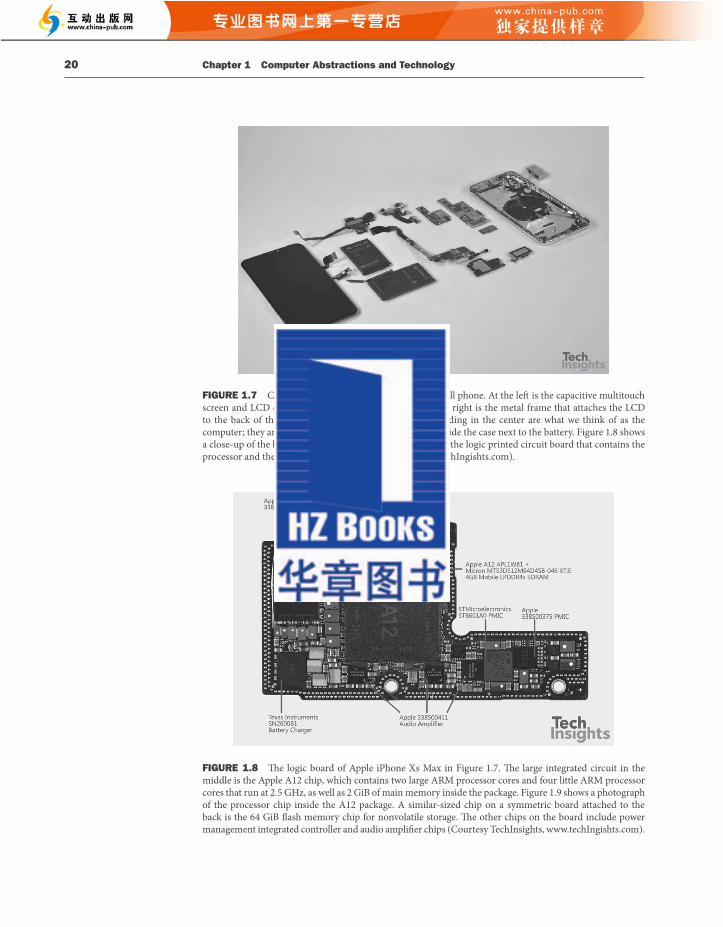
1.4 Under the Covers 21
Descending into the depths of any component of the hardware reveals insights into the computer. Inside the processor is another type of memory—cache memory. Cache memory consists of a small, fast memory that acts as a buff er for the DRAM memory. (Th e nontechnical defi nition of cache is a safe place for hiding things.) Cache is built using a diff erent memory technology, static random access memory (SRAM) . SRAM is faster but less dense, and hence more expensive, than DRAM (see Chapter 5 ). SRAM and DRAM are two layers of the memory hierarchy .
static random access memory (SRAM) Also memory built as an integrated circuit, but faster and less dense than DRAM.
FIGURE 1.9 Th e processor integrated circuit inside the A12 package. Th e size of chip is 8.4 by 9.91 mm, and it was manufactured originally in a 7-nm process (see Section 1.5). It has two identical ARM big processors or cores in the lower middle of the chip, four small cores on the lower right of the chip, a graphical processor unit (GPU) on the far right (see Section 6.6), and a domain-specifi c accelerator for neural networks (see Section 6.7), called the NPU, on the far left . In the middle are second-level cache memories (L2) for the big and small cores (see Chapter 5). At the top and bottom of the chip are interfaces to main memory (DDR DRAM) (Courtesy TechInsights, www.techinsights.com , and AnandTech, www.anandtech.com ).
cache memory A small, fast memory that acts as a buff er for a slower, larger memory.
20 Chapter 1 Computer Abstractions and Technology
FIGURE 1.7 Components of the Apple iPhone Xs Max cell phone. At the left is the capacitive multitouch screen and LCD display. Next to it is the battery. To the far right is the metal frame that attaches the LCD to the back of the iPhone. Th e small components surrounding in the center are what we think of as the computer; they are not simple rectangles to fi t compactly inside the case next to the battery. Figure 1.8 shows a close-up of the board to the left of the metal case, which is the logic printed circuit board that contains the processor and the memory (Courtesy TechInsights, www.techIngishts.com ).
FIGURE 1.8 Th e logic board of Apple iPhone Xs Max in Figure 1.7 . Th e large integrated circuit in the middle is the Apple A12 chip, which contains two large ARM processor cores and four little ARM processor cores that run at 2.5 GHz, as well as 2 GiB of main memory inside the package. Figure 1.9 shows a photograph of the processor chip inside the A12 package. A similar-sized chip on a symmetric board attached to the back is the 64 GiB fl ash memory chip for nonvolatile storage. Th e other chips on the board include power management integrated controller and audio amplifi er chips (Courtesy TechInsights, www.techIngishts.com ).
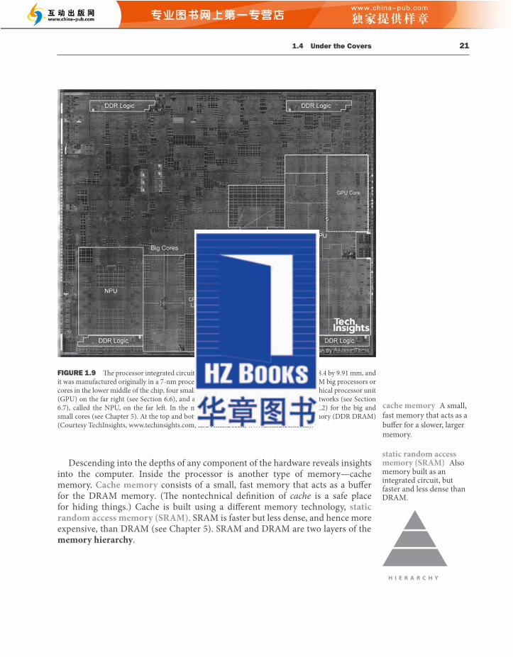
1.4 Under the Covers 23
the former, and secondary memory for the latter. Secondary memory forms the next lower layer of the memory hierarchy . DRAMs have dominated main memory since 1975, but magnetic disks dominated secondary memory starting even earlier. Because of their size and form factor, personal Mobile Devices use fl ash memory , a nonvolatile semiconductor memory, instead of disks. Figure 1.8 shows the chip containing the 64 GiB fl ash memory of the iPhone Xs. While slower than DRAM, it is much cheaper than DRAM in addition to being nonvolatile. Although costing more per bit than disks, it is smaller, it comes in much smaller capacities, it is more rugged, and it is more power effi cient than disks. Hence, fl ash memory is the standard secondary memory for PMDs. Alas, unlike disks and DRAM, fl ash memory bits wear out aft er 100,000 to 1,000,000 writes. Th us, fi le systems must keep track of the number of writes and have a strategy to avoid wearing out storage, such as by moving popular data. Chapter 5 describes disks and fl ash memory in more detail.
Communicating with Other Computers We’ve explained how we can input, compute, display, and save data, but there is still one missing item found in today’s computers: computer networks. Just as the processor shown in Figure 1.5 is connected to memory and I/O devices, networks interconnect whole computers, allowing computer users to extend the power of computing by including communication. Networks have become so popular that they are the backbone of current computer systems; a new personal mobile device or server without a network interface would be ridiculed. Networked computers have several major advantages:
■ Communication : Information is exchanged between computers at high speeds.
■ Resource sharing : Rather than each computer having its own I/O devices, computers on the network can share I/O devices.
■ Nonlocal access : By connecting computers over long distances, users need not be near the computer they are using.
Networks vary in length and performance, with the cost of communication increasing according to both the speed of communication and the distance that information travels. Perhaps the most popular type of network is Ethernet . It can be up to a kilometer long and transfer at up to 100 gigabits per second. Its length and speed make Ethernet useful to connect computers on the same fl oor of a building; hence, it is an example of what is generically called a local area network . Local area networks are interconnected with switches that can also provide routing services and security. Wide area networks cross continents and are the backbone of the Internet, which supports the web. Th ey are typically based on optical fi bers and are leased from telecommunication companies.
Networks have changed the face of computing in the last 40 years, both by becoming much more ubiquitous and by making dramatic increases in performance.
main memory Also called primary memory . Memory used to hold programs while they are running; typically consists of DRAM in today’s computers.
secondary memory Nonvolatile memory used to store programs and data between runs; typically consists of fl ash memory in PMDs and magnetic disks in servers.
magnetic disk Also called hard disk . A form of nonvolatile secondary memory composed of rotating platters coated with a magnetic recording material. Because they are rotating mechanical devices, access times are about 5 to 20 milliseconds and cost per gigabyte in 2020 was $0.01 to $0.02.
fl ash memory A nonvolatile semi-conductor memory. It is cheaper and slower than DRAM but more expensive per bit and faster than magnetic disks. Access times are about 5 to 50 microseconds and cost per gigabyte in 2020 was $0.06 to $0.12. local area network (LAN) A network designed to carry data within a geographically confi ned area, typically within a single building. wide area network (WAN) A network extended over hundreds of kilometers that can span a continent.
22 Chapter 1 Computer Abstractions and Technology
As mentioned above, one of the great ideas to improve design is abstraction. One of the most important abstractions is the interface between the hardware and the lowest-level soft ware. Soft ware communicates to hardware via a vocabulary. Th e words of the vocabulary are called instructions, and the vocabulary itself is called the instruction set architecture , or simply architecture , of a computer. Th e instruction set architecture includes anything programmers need to know to make a binary machine language program work correctly, including instructions, I/O devices, and so on. Typically, the operating system will encapsulate the details of doing I/O, allocating memory, and other low-level system functions so that application programmers do not need to worry about such details. Th e combination of the basic instruction set and the operating system interface provided for application programmers is called the application binary interface (ABI) .
An instruction set architecture allows computer designers to talk about functions independently from the hardware that performs them. For example, we can talk about the functions of a digital clock (keeping time, displaying the time, setting the alarm) independently from the clock hardware (quartz crystal, LED displays, plastic buttons). Computer designers distinguish architecture from an implementation of an architecture along the same lines: an implementation is hardware that obeys the architecture abstraction. Th ese ideas bring us to another Big Picture.
instruction set architecture Also called architecture . An abstract interface between the hardware and the lowest-level soft ware that encompasses all the information necessary to write a machine language program that will run correctly, including instructions, registers, memory access, I/O, and so on.
application binary interface (ABI) Th e user portion of the instruction set plus the operating system interfaces used by application programmers. It defi nes a standard for binary portability across computers.
Both hardware and soft ware consist of hierarchical layers using abstraction, with each lower layer hiding details from the level above. One key interface between the levels of abstraction is the instruction set architecture —the interface between the hardware and low-level soft ware. Th is abstract interface enables many implementations of varying cost and performance to run identical soft ware.
The BIGPicture
A Safe Place for Data Th us far, we have seen how to input data, compute using the data, and display data. If we were to lose power to the computer, however, everything would be lost because the memory inside the computer is volatile —that is, when it loses power, it forgets. In contrast, a DVD disk doesn’t forget the movie when you turn off the power to the DVD player, and is thus a nonvolatile memory technology.
To distinguish between the volatile memory used to hold data and programs while they are running and this nonvolatile memory used to store data and programs between runs, the term main memory or primary memory is used for
implementation Hardware that obeys the architecture abstraction.
volatile memory Storage, such as DRAM, that retains data only if it is receiving power.
nonvolatile memory A form of memory that retains data even in the absence of a power source and that is used to store programs between runs. A DVD disk is nonvolatile.
1.5 Technologies for Building Processors and Memory 25
Year Technology used in computers Relative performance/unit cost
1951 Vacuum tube 11965 351975 Integrated circuit
Very large-scale integrated circuitUltra large-scale integrated circuit
Transistor900
1995 2,400,0002020 500,000,000,000
FIGURE 1.10 Relative performance per unit cost of technologies used in computers over time. Source: Computer Museum, Boston, with 2020 extrapolated by the authors. See Section 1.13 .
1,000,000
10,000,000
100,000,000
1976 1978 1980 1982 1984 1986
Year of introduction
1988 1990 1992 1994 1996 1998 2000 2002 2004 2006 2008 2010 2012
Kib
ibit
capa
city
16K
64K
256K
1M
4M
16M64M
128M256M 512M
1G 2G4G
100,000
10,000
1000
100
102014 2016 2018 2020
8G16G
FIGURE 1.11 Growth of capacity per DRAM chip over time. Th e y -axis is measured in kibibits (2 10 bits). Th e DRAM industry quadrupled capacity almost every three years, a 60% increase per year, for 20 years. In recent years, the rate has slowed down and is somewhat closer to doubling every three years. With the slowing of Moore’s Law and diffi culties in reliable manufacturing of smaller DRAM cells given the challenging aspect ratios of their three-dimensional structure.
the growth rate of the number of transistors per chip. To describe the tremendous increase in the number of transistors from hundreds to millions, the adjective very large scale is added to the term, creating the abbreviation VLSI , for very large-scale integrated circuit .
Th is rate of increasing integration has been remarkably stable. Figure 1.11 shows the growth in DRAM capacity since 1977. For decades, the industry has consistently quadrupled capacity every 3 years, resulting in an increase in excess of 16,000 times! Figure 1.11 also shows the slowdown due to the slowing of Moore’s Law; quadrupuling capacity has taken 6 years recently.
To understand how manufacture integrated circuits, we start at the beginning. Th e manufacture of a chip begins with silicon , a substance found in sand. Because silicon does not conduct electricity well, it is called a semiconductor . With a special chemical process, it is possible to add materials to silicon that allow tiny areas to transform into one of three devices:
■ Excellent conductors of electricity (using either microscopic copper or aluminum wire)
■ Excellent insulators from electricity (like plastic sheathing or glass)
■ Areas that can conduct or insulate under special conditions (as a switch)
very large-scale integrated (VLSI) circuit A device containing hundreds of thousands to millions of transistors.
silicon A natural element that is a semiconductor.
semiconductor A substance that does not conduct electricity well.
24 Chapter 1 Computer Abstractions and Technology
In the 1970s, very few individuals had access to electronic mail, the Internet and web did not exist, and physically mailing magnetic tapes was the primary way to transfer large amounts of data between two locations. Local area networks were almost nonexistent, and the few existing wide area networks had limited capacity and restricted access.
As networking technology improved, it became much cheaper and had a much higher capacity. For example, the fi rst standardized local area network technology, developed about 40 years ago, was a version of Ethernet that had a maximum capacity (also called bandwidth) of 10 million bits per second, typically shared by tens of, if not a hundred, computers. Today, local area network technology off ers a capacity of from 1 to 100 gigabits per second, usually shared by at most a few computers. Optical communications technology has allowed similar growth in the capacity of wide area networks, from hundreds of kilobits to gigabits and from hundreds of computers connected to a worldwide network to millions of computers connected. Th is combination of dramatic rise in deployment of networking combined with increases in capacity have made network technology central to the information revolution of the last 30 years.
For the last 15 years another innovation in networking is reshaping the way computers communicate. Wireless technology is widespread, which enabled the PostPC Era. Th e ability to make a radio in the same low-cost semiconductor technology (CMOS) used for memory and microprocessors enabled a signifi cant improvement in price, leading to an explosion in deployment. Currently available wireless technologies, called by the IEEE standard name 802.11ac, allow for transmission rates from 1 to 1300 million bits per second. Wireless technology is quite a bit diff erent from wire-based networks, since all users in an immediate area share the airwaves.
■ Semiconductor DRAM memory, fl ash memory, and disk storage diff er signifi cantly. For each technology, list its volatility, approximate relative access time, and approximate relative cost compared to DRAM.
1.5 Technologies for Building Processors and Memory
Processors and memory have improved at an incredible rate, because computer designers have long embraced the latest in electronic technology to try to win the race to design a better computer. Figure 1.10 shows the technologies that have been used over time, with an estimate of the relative performance per unit cost for each technology. Since this technology shapes what computers will be able to do and how quickly they will evolve, we believe all computer professionals should be familiar with the basics of integrated circuits.
A transistor is simply an on/off switch controlled by electricity. Th e integrated circuit (IC) combined dozens to hundreds of transistors into a single chip. When Gordon Moore predicted the continuous doubling of resources, he was predicting
Check Yourself
transistor An on/off switch controlled by an electric signal.

1.5 Technologies for Building Processors and Memory 27
yield of a process, which is defi ned as the percentage of good dies from the total number of dies on the wafer.
Th e cost of an integrated circuit rises quickly as the die size increases, due both to the lower yield and the smaller number of dies that fi t on a wafer. To reduce the cost, using the next generation process shrinks a large die as it uses smaller sizes for both transistors and wires. Th is improves the yield and the die count per wafer. A 7-nanometer (nm) process was state-of-the-art in 2020, which means essentially that the smallest feature size on the die is 7 nm.
Once you’ve found good dies, they are connected to the input/output pins of a package, using a process called bonding . Th ese packaged parts are tested a fi nal time, since mistakes can occur in packaging, and then they are shipped to customers.
While we have talked about the cost of chips, there is a diff erence between cost and price. Companies charge as much as the market will bear to maximize the
yield Th e percentage of good dies from the total number of dies on the wafer.
FIGURE 1.13 A 12-inch (300-mm) wafer this 10nm wafer contains 10th Gen Intel® Core™ processors, code-named “Ice Lake” (Courtesy Intel). Th e number of dies on this 300-mm (12-inch) wafer at 100% yield is 506. According to AnandTech, 1 each Ice Lake die is 11.4 by 10.7 mm. Th e several dozen partially rounded chips at the boundaries of the wafer are useless; they are included because it is easier to create the masks used to pattern the silicon. Th is die uses a 10-nm technology, which means that the smallest features are approximately 10 nm in size, although they are typically somewhat smaller than the actual feature size, which refers to the size of the transistors as “drawn” versus the fi nal manufactured size.
1Ian Cutress, “I Ran Off with Intel’s Tiger Lake Wafer. Who Wants a Die Shot?” January 13, 2020, https://www.anandtech.com/show/15380/i-ran-off -with-intels-tiger-lake-wafer-who-wants-a-die-shot
26 Chapter 1 Computer Abstractions and Technology
Transistors fall in the last category. A VLSI circuit, then, is just billions of combinations of conductors, insulators, and switches manufactured in a single small package.
Th e manufacturing process for integrated circuits is critical to the cost of the chips and hence important to computer designers. Figure 1.12 shows that process. Th e process starts with a silicon crystal ingot , which looks like a giant sausage. Today, ingots are 8–12 inches in diameter and about 12–24 inches long. An ingot is fi nely sliced into wafers no more than 0.1 inches thick. Th ese wafers then go through a series of processing steps, during which patterns of chemicals are placed on each wafer, creating the transistors, conductors, and insulators discussed earlier. Today’s integrated circuits contain only one layer of transistors but may have from two to eight levels of metal conductor, separated by layers of insulators.
silicon crystal ingot A rod composed of a silicon crystal that is between 8 and 12 inches in diameter and about 12 to 24 inches long.
wafer A slice from a silicon ingot no more than 0.1 inches thick, used to create chips.
Slicer
Dicer
20 to 40processing steps
Bond die topackage
Silicon ingot
Wafertester
Parttester
Ship tocustomers
Tested dies Testedwafer
Blankwafers
Packaged dies
Patterned wafers
Tested packaged dies
FIGURE 1.12 The chip manufacturing process. Aft er being sliced from the silicon ingot, blank wafers are put through 20 to 40 steps to create patterned wafers (see Figure 1.13 ). Th ese patterned wafers are then tested with a wafer tester, and a map of the good parts is made. Th en, the wafers are diced into dies (see Figure 1.9 ). In this fi gure, one wafer produced 20 dies, of which 17 passed testing. (X means the die is bad.) Th e yield of good dies in this case was 17/20, or 85%. Th ese good dies are then bonded into packages and tested one more time before shipping the packaged parts to customers. One bad packaged part was found in this fi nal test.
A single microscopic fl aw in the wafer itself or in one of the dozens of patterning steps can result in that area of the wafer failing. Th ese defects , as they are called, make it virtually impossible to manufacture a perfect wafer. Th e simplest way to cope with imperfection is to place many independent components on a single wafer. Th e patterned wafer is then chopped up, or diced, into these components, called dies and more informally known as chips . Figure 1.13 shows a photograph of a wafer containing microprocessors before they have been diced; earlier, Figure 1.9 shows an individual microprocessor die.
Dicing enables you to discard only those dies that were unlucky enough to contain the fl aws, rather than the whole wafer. Th is concept is quantifi ed by the
defect A microscopic fl aw in a wafer or in patterning steps that can result in the failure of the die containing that defect.
die Th e individual rectangular sections that are cut from a wafer, more informally known as chips .
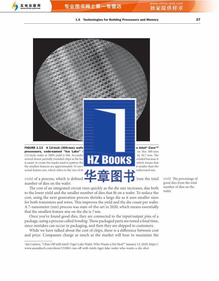
1.6 Performance 29
improvement techniques employed by hardware designers, have made performance assessment much more diffi cult.
When trying to choose among diff erent computers, performance is an important attribute. Accurately measuring and comparing diff erent computers is critical to purchasers and therefore to designers. Th e people selling computers know this as well. Oft en, salespeople would like you to see their computer in the best possible light, whether or not this light accurately refl ects the needs of the purchaser’s application. Hence, understanding how best to measure performance and the limitations of performance measurements is important in selecting a computer.
Th e rest of this section describes diff erent ways in which performance can be determined; then, we describe the metrics for measuring performance from the viewpoint of both a computer user and a designer. We also look at how these metrics are related and present the classical processor performance equation, which we will use throughout the text.
Defi ning Performance When we say one computer has better performance than another, what do we mean? Although this question might seem simple, an analogy with passenger airplanes shows how subtle the question of performance can be. Figure 1.14 lists some typical passenger airplanes, together with their cruising speed, range, and capacity. If we wanted to know which of the planes in this table had the best performance, we would fi rst need to defi ne performance. For example, considering diff erent measures of performance, we see that the plane with the highest cruising speed was the Concorde (retired from service in 2003), the plane with the longest range is the Boeing 777-200LR, and the plane with the largest capacity is the Airbus A380-800.
Let’s suppose we defi ne performance in terms of speed. Th is still leaves two possible defi nitions. You could defi ne the fastest plane as the one with the highest cruising speed, taking a single passenger from one point to another in the least time. If you were interested in transporting 500 passengers from one point to another, however, the Airbus A380-800 would clearly be the fastest, as the last column of the fi gure shows. Similarly, we can defi ne computer performance in several diff erent ways.
If you were running a program on two diff erent desktop computers, you’d say that the faster one is the desktop computer that gets the job done fi rst. If you were running a datacenter that had several servers running jobs submitted by many users, you’d say that the faster computer was the one that completed the most
response time Also called execution time . Th e total time required for the computer to complete a task, including disk accesses, memory accesses, I/O activities, operating system overhead, CPU execution time, and so on.
AirplanePassenger capacity
Cruising range (miles)
Cruising speed (m.p.h.)
Passenger throughput (passengers × m.p.h.)
Boeing 737 240 3000 0564 135,360BAC/Sud Concorde 132
301853
4000 01350 178,200Boeing 777-200LR 9395 554 166,761Airbus A380-800 8477 0587 500,711
FIGURE 1.14 The capacity, range, and speed for a number of commercial airplanes. Th e last column shows the rate at which the airplane transports passengers, which is the capacity times the cruising speed (ignoring range and takeoff and landing times).
28 Chapter 1 Computer Abstractions and Technology
return on their investment, which must cover costs like a company’s research and development (R&D), marketing, sales, manufacturing equipment maintenance, building rental, cost of fi nancing, pretax profi ts, and taxes. Margins can be higher on unique chips that come from only one company, like microprocessors, versus chips that are commodities supplied by several companies, like DRAMs. Th e price fl uctuates based on the ratio of supply and demand, and it is easy for multiple companies to build more chips than the market demands.
Elaboration : The cost of an integrated circuit can be expressed in three simple equations:
The fi rst equation is straightforward to derive. The second is an approximation, since it does not subtract the area near the border of the round wafer that cannot accommodate the rectangular dies (see Figure 1.13 ). The fi nal equation is based on empirical observations of yields at integrated circuit factories, with the exponent related to the number of critical processing steps.
Hence, depending on the defect rate and the size of the die and wafer, costs are generally not linear in the die area.
A key factor in determining the cost of an integrated circuit is volume. Which of the following are reasons why a chip made in high volume should cost less?
1. With high volumes, the manufacturing process can be tuned to a particular design, increasing the yield.
2. It is less work to design a high-volume part than a low-volume part.
3. Th e masks used to make the chip are expensive, so the cost per chip is lower for higher volumes.
4. Engineering development costs are high and largely independent of volume; thus, the development cost per die is lower with high-volume parts.
5. High-volume parts usually have smaller die sizes than low-volume parts and therefore have higher yield per wafer.
1.6 Performance
Assessing the performance of computers can be quite challenging. Th e scale and intricacy of modern soft ware systems, together with the wide range of performance
Cost per die Cost per waferDies per wafer yield
Dies per wafer Wafer areaDie area
YieldDefects per area Die area))n
11( (
Check Yourself
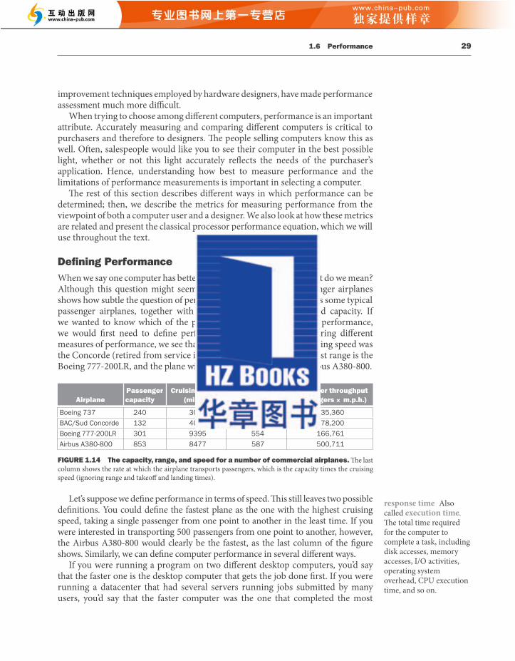
1.6 Performance 31
In discussing a computer design, we oft en want to relate the performance of two diff erent computers quantitatively. We will use the phrase “X is n times faster than Y”—or equivalently “X is n times as fast as Y”—to mean
PerformancePerformance
X
Y= n
If X is n times as fast as Y, then the execution time on Y is n times as long as it is on X:
PerformancePerformance
Execution timeExecution time
X
Y
Y
X� � n
Relative Performance
If computer A runs a program in 10 seconds and computer B runs the same program in 15 seconds, how much faster is A than B?
We know that A is n times as fast as B if
PerformancePerformance
Execution timeExecution time
A
B
B
A� � n
Th us the performance ratio is
1510
1 5� .
and A is therefore 1.5 times as fast as B.
In the above example, we could also say that computer B is 1.5 times slower than computer A, since
PerformancePerformance
A
B� 1 5.
means that
Performance PerformanceAB1 5.
�
EXAMPLE
ANSWER
30 Chapter 1 Computer Abstractions and Technology
jobs during a day. As an individual computer user, you are interested in reducing response time —the time between the start and completion of a task—also referred to as execution time . Datacenter managers are oft en interested in increasing throughput or bandwidth —the total amount of work done in a given time. Hence, in most cases, we will need diff erent performance metrics as well as diff erent sets of applications to benchmark personal mobile devices, which are more focused on response time, versus servers, which are more focused on throughput.
Throughput and Response Time
Do the following changes to a computer system increase throughput, decrease response time, or both?
1. Replacing the processor in a computer with a faster version
2. Adding additional processors to a system that uses multiple processors for separate tasks—for example, searching the web
Decreasing response time almost always improves throughput. Hence, in case 1, both response time and throughput are improved. In case 2, no one task gets work done faster, so only throughput increases.
If, however, the demand for processing in the second case was almost as large as the throughput, the system might force requests to queue up. In this case, increasing the throughput could also improve response time, since it would reduce the waiting time in the queue. Th us, in many real computer systems, changing either execution time or throughput oft en aff ects the other.
In discussing the performance of computers, we will be primarily concerned with response time for the fi rst few chapters. To maximize performance, we want to minimize response time or execution time for some task. Th us, we can relate performance and execution time for a computer X:
PerformanceExecution timeX
X�
1
Th is means that for two computers X and Y, if the performance of X is greater than the performance of Y, we have
Performance Performance
Execution time Execution time
X Y
X Y
�
�1 1
EExecution time Execution timeY X�
Th at is, the execution time on Y is longer than that on X, if X is faster than Y.
throughput Also called bandwidth . Another measure of performance, it is the number of tasks completed per unit time.
EXAMPLE
ANSWER
1.6 Performance 33
some application environments, the user may care about throughput, response time, or a complex combination of the two (e.g., maximum throughput with a worst-case response time). To improve the performance of a program, one must have a clear defi nition of what performance metric matters and then proceed to look for performance bottlenecks by measuring program execution and looking for the likely bottlenecks. In the following chapters, we will describe how to search for bottlenecks and improve performance in various parts of the system.
Although as computer users we care about time, when we examine the details of a computer it’s convenient to think about performance in other metrics. In particular, computer designers may want to think about a computer by using a measure that relates to how fast the hardware can perform basic functions. Almost all computers are constructed using a clock that determines when events take place in the hardware. Th ese discrete time intervals are called clock cycles (or ticks , clock ticks , clock periods , clocks , cycles ). Designers refer to the length of a clock period both as the time for a complete clock cycle (e.g., 250 picoseconds, or 250 ps) and as the clock rate (e.g., 4 gigahertz, or 4 GHz), which is the inverse of the clock period. In the next subsection, we will formalize the relationship between the clock cycles of the hardware designer and the seconds of the computer user.
1. Suppose we know that an application that uses both personal mobile devices and the Cloud is limited by network performance. For the following changes, state whether only the throughput improves, both response time and throughput improve, or neither improves.
a. An extra network channel is added between the PMD and the Cloud, increasing the total network throughput and reducing the delay to obtain network access (since there are now two channels).
b. Th e networking soft ware is improved, thereby reducing the network communication delay, but not increasing throughput.
c. More memory is added to the computer.
2. Computer C’s performance is 4 times as fast as the performance of computer B, which runs a given application in 28 seconds. How long will computer C take to run that application?
CPU Performance and Its Factors Users and designers oft en examine performance using diff erent metrics. If we could relate these diff erent metrics, we could determine the eff ect of a design change on the performance as experienced by the user. Since we are confi ning ourselves to CPU performance at this point, the bottom-line performance measure is CPU
clock cycle Also called tick , clock tick , clock period , clock , or cycle . Th e time for one clock period, usually of the processor clock, which runs at a constant rate.
clock period Th e length of each clock cycle.
Check Yourself
32 Chapter 1 Computer Abstractions and Technology
For simplicity, we will normally use the terminology as fast as when we try to compare computers quantitatively. Because performance and execution time are reciprocals, increasing performance requires decreasing execution time. To avoid the potential confusion between the terms increasing and decreasing , we usually say “improve performance” or “improve execution time” when we mean “increase performance” and “decrease execution time.”
Measuring Performance Time is the measure of computer performance: the computer that performs the same amount of work in the least time is the fastest. Program execution time is measured in seconds per program. However, time can be defi ned in diff erent ways, depending on what we count. Th e most straightforward defi nition of time is called wall clock time , response time , or elapsed time . Th ese terms mean the total time to complete a task, including disk accesses, memory accesses, input/output (I/O) activities, operating system overhead—everything.
Computers are oft en shared, however, and a processor may work on several programs simultaneously. In such cases, the system may try to optimize throughput rather than attempt to minimize the elapsed time for one program. Hence, we might want to distinguish between the elapsed time and the time over which the processor is working on our behalf. CPU execution time or simply CPU time , which recognizes this distinction, is the time the CPU spends computing for this task and does not include time spent waiting for I/O or running other programs. (Remember, though, that the response time experienced by the user will be the elapsed time of the program, not the CPU time.) CPU time can be further divided into the CPU time spent in the program, called user CPU time , and the CPU time spent in the operating system performing tasks on behalf of the program, called system CPU time . Diff erentiating between system and user CPU time is diffi cult to do accurately, because it is oft en hard to assign responsibility for operating system activities to one user program rather than another and because of the functionality diff erences among operating systems.
For consistency, we maintain a distinction between performance based on elapsed time and that based on CPU execution time. We will use the term system performance to refer to elapsed time on an unloaded system and CPU performance to refer to user CPU time. We will focus on CPU performance in this chapter, although our discussions of how to summarize performance can be applied to either elapsed time or CPU time measurements.
Diff erent applications are sensitive to diff erent aspects of the performance of a computer system. Many applications, especially those running on servers, depend as much on I/O performance, which, in turn, relies on both hardware and soft ware. Total elapsed time measured by a wall clock is the measurement of interest. In
CPU execution time Also called CPU time . Th e actual time the CPU spends computing for a specifi c task.
user CPU time Th e CPU time spent in a program itself.
system CPU time Th e CPU time spent in the operating system performing tasks on behalf of the program.
Understanding Program
Performance
1.6 Performance 35
CPU time for B can be found using this equation:
CPU time CPU clock cyclesClock rateB
A
B
1 2.
61 2 20 109
secondscycles
Clock rateB
.
Clock rate cycles seconds
cyclessecoB
1 2 20 106
0 2 20 109 9. .nnd
cyclessecond
GHz4 10 49
To run the program in 6 seconds, B must have twice the clock rate of A.
Instruction Performance Th e performance equations above did not include any reference to the number of instructions needed for the program. However, since the compiler clearly generated instructions to execute, and the computer had to execute the instructions to run the program, the execution time must depend on the number of instructions in a program. One way to think about execution time is that it equals the number of instructions executed multiplied by the average time per instruction. Th erefore, the number of clock cycles required for a program can be written as
CPU clock cycles Instructions for a program Average clock ccyclesper instruction
Th e term clock cycles per instruction , which is the average number of clock cycles each instruction takes to execute, is oft en abbreviated as CPI . Since diff erent instructions may take diff erent amounts of time depending on what they do, CPI is an average of all the instructions executed in the program. CPI provides one way of comparing two diff erent implementations of the same instruction set architecture, since the number of instructions executed for a program will, of course, be the same.
Using the Performance Equation Suppose we have two implementations of the same instruction set architecture. Computer A has a clock cycle time of 250 ps and a CPI of 2.0 for some program, and computer B has a clock cycle time of 500 ps and a CPI of 1.2 for the same program. Which computer is faster for this program and by how much?
clock cycles per instruction (CPI) Average number of clock cycles per instruction for a program or program fragment.
EXAMPLE
34 Chapter 1 Computer Abstractions and Technology
execution time. A simple formula relates the most basic metrics (clock cycles and clock cycle time) to CPU time:
CPU execution time
for a programCPU clock cycles
for a progrram Clock cycle time
Alternatively, because clock rate and clock cycle time are inverses,
CPU execution timefor a program
CPU clock cycles for a pro�
ggramClock rate
Th is formula makes it clear that the hardware designer can improve performance by reducing the number of clock cycles required for a program or the length of the clock cycle. As we will see in later chapters, the designer oft en faces a trade-off between the number of clock cycles needed for a program and the length of each cycle. Many techniques that decrease the number of clock cycles may also increase the clock cycle time.
Improving Performance
Our favorite program runs in 10 seconds on computer A, which has a 2 GHz clock. We are trying to help a computer designer build a computer, B, which will run this program in 6 seconds. Th e designer has determined that a substantial increase in the clock rate is possible, but this increase will aff ect the rest of the CPU design, causing computer B to require 1.2 times as many clock cycles as computer A for this program. What clock rate should we tell the designer to target?
Let’s fi rst fi nd the number of clock cycles required for the program on A:
CPU time CPU clock cyclesClock rateA
A
A�
102 109
seconds CPU clock cyclescycles
second
A
CPU clock cycles seconds cyclessecond
cycleA 10 2 10 20 109 9 ss
EXAMPLE
ANSWER

1.6 Performance 37
Comparing Code Segments
A compiler designer is trying to decide between two code sequences for a particular computer. Th e hardware designers have supplied the following facts:
CPI for each instruction class
A B C
CPI 1 2 3
For a particular high-level language statement, the compiler writer is considering two code sequences that require the following instruction counts:
Instruction counts for each instruction class
Code sequence A B C
1 2 1 2
2 4 1 1
Which code sequence executes the most instructions? Which will be faster? What is the CPI for each sequence?
Sequence 1 executes 2 + 1 + 2 = 5 instructions. Sequence 2 executes 4 + 1 + 1 = 6 instructions. Th erefore, sequence 1 executes fewer instructions.
We can use the equation for CPU clock cycles based on instruction count and CPI to fi nd the total number of clock cycles for each sequence:
CPU clock cycles CPI C( )i i
i
n
=∑
1
Th is yields
CPU clock cycles cycles1 2 1 1 2 2 3 2 2 6 10( ) ( ) ( )
CPU clock cycles cycles2 4 1 1 2 1 3 4 2 3 9( ) ( ) ( ) So code sequence 2 is faster, even though it executes one extra instruction. Since code sequence 2 takes fewer overall clock cycles but has more instructions, it must have a lower CPI. Th e CPI values can be computed by
CPI CPU clock cyclesInstruction count
CPI CPU clock cycles
�
�111
1
22
105
2 0Instruction count
CPI CPU clock cyclesInstruct
� �
�
.
iion count2
96
1 5� � .
EXAMPLE
ANSWER
36 Chapter 1 Computer Abstractions and Technology
We know that each computer executes the same number of instructions for the program; let’s call this number I . First, fi nd the number of processor clock cycles for each computer:
CPU clock cyclesCPU clock cycles
A
B
II
2 01 2
..
Now we can compute the CPU time for each computer:
CPU time CPU clock cycles Clock cycle timeps
A A
I 2 0 250 5. 000 I ps
Likewise, for B:
CPU time ps psB I I1 2 500 600.
Clearly, computer A is faster. Th e amount faster is given by the ratio of the execution times:
CPU performance
CPU performanceExecution timeExecution
A
B
Bttime
pspsA
600500
1 2II
.
We can conclude that computer A is 1.2 times as fast as computer B for this program.
The Classic CPU Performance Equation We can now write this basic performance equation in terms of instruction count (the number of instructions executed by the program), CPI, and clock cycle time:
CPU times Instruction count CPI Clock cycle time
or, since the clock rate is the inverse of clock cycle time:
CPU times Instruction count CPIClock rate
Th ese formulas are particularly useful because they separate the three key factors that aff ect performance. We can use these formulas to compare two diff erent implementations or to evaluate a design alternative if we know its impact on these three parameters.
ANSWER
instruction count Th e number of instructions executed by the program.
1.6 Performance 39
Th e above example shows the danger of using only one factor (instruction count) to assess performance. When comparing two computers, you must look at all three components, which combine to form execution time. If some of the factors are identical, like the clock rate in the above example, performance can be determined by comparing all the nonidentical factors. Since CPI varies by instruction mix , both instruction count and CPI must be compared, even if clock rates are identical. Several exercises at the end of this chapter ask you to evaluate a series of computer and compiler enhancements that aff ect clock rate, CPI, and instruction count. In Section 1.13 , we’ll examine a common performance measurement that does not incorporate all the terms and can thus be misleading.
Th e performance of a program depends on the algorithm, the language, the compiler, the architecture, and the actual hardware. Th e following table summarizes how these components aff ect the factors in the CPU performance equation.
Hardware or software component Affects what? How?
Algorithm Instruction count, possibly CPI
The algorithm determines the number of source program instructions executed and hence the number of processor instructions executed. The algorithm may also affect the CPI, by favoring slower or faster instructions. For example, if the algorithm uses more divides, it will tend to have a higher CPI.
Programming language
Instruction count, CPI
The programming language certainly affects the instruction count, since statements in the language are translated to processor instructions, which determine instruction count. The language may also affect the CPI because of its features; for example, a language with heavy support for data abstraction (e.g., Java) will require indirect calls, which will use higher CPI instructions.
Compiler Instruction count, CPI
The effi ciency of the compiler affects both the instruction count and average cycles per instruction, since the compiler determines the translation of the source language instructions into computer instructions. The compiler’s role can be very complex and affect the CPI in complicated ways.
Instruction set architecture
Instruction count, clock rate, CPI
The instruction set architecture affects all three aspects of CPU performance, since it affects the instructions needed for a function, the cost in cycles of each instruction, and the overall clock rate of the processor.
Elaboration : Although you might expect that the minimum CPI is 1.0, as we’ll see in Chapter 4 , some processors fetch and execute multiple instructions per clock cycle. To refl ect that approach, some designers invert CPI to talk about IPC , or instructions per clock cycle . If a processor executes on average 2 instructions per clock cycle, then it has an IPC of 2 and hence a CPI of 0.5.
instruction mix A measure of the dynamic frequency of instructions across one or many programs.
Understanding Program Performance
38 Chapter 1 Computer Abstractions and Technology
How can we determine the value of these factors in the performance equation? We can measure the CPU execution time by running the program, and the clock cycle time is usually published as part of the documentation for a computer. Th e instruction count and CPI can be more diffi cult to obtain. Of course, if we know the clock rate and CPU execution time, we need only one of the instruction count or the CPI to determine the other.
We can measure the instruction count by using soft ware tools that profi le the execution or by using a simulator of the architecture. Alternatively, we can use hardware counters, which are included in most processors, to record a variety of measurements, including the number of instructions executed, the average CPI, and oft en, the sources of performance loss. Since the instruction count depends on the architecture, but not on the exact implementation, we can measure the instruction count without knowing all the details of the implementation. Th e CPI, however, depends on a wide variety of design details in the computer, including both the memory system and the processor structure (as we will see in Chapter 4 and Chapter 5 ), as well as on the mix of instruction types executed in an application. Th us, CPI varies by application, as well as among implementations with the same instruction set.
The BIG Picture
Figure 1.15 shows the basic measurements at diff erent levels in the computer and what is being measured in each case. We can see how these factors are combined to yield execution time measured in seconds per program:
Time Seconds/Program InstructionsProgram
Clock cyclesInstruuction
SecondsClock cycle
Always bear in mind that the only complete and reliable measure of computer performance is time. For example, changing the instruction set to lower the instruction count may lead to an organization with a slower clock cycle time or higher CPI that off sets the improvement in instruction count. Similarly, because CPI depends on type of instructions executed, the code that executes the fewest number of instructions may not be the fastest.
Components of performance Units of measure
CPU execution time for a program Seconds for the program
Instruction count Instructions executed for the program
Clock cycles per instruction (CPI) Average number of clock cycles per instruction
Clock cycle time Seconds per clock cycle
FIGURE 1.15 The basic components of performance and how each is measured.
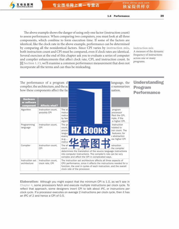

1.7 The Power Wall 41
Although power provides a limit to what we can cool, in the PostPC Era the really critical resource is energy. Battery life can trump performance in the personal mobile device, and the architects of warehouse scale computers try to reduce the costs of powering and cooling 50,000 servers as the costs are high at this scale. Just as measuring time in seconds is a safer measure of program performance than a rate like MIPS (see Section 1.11 ), the energy metric joules is a better measure than a power rate like watts, which is just joules/second.
Th e dominant technology for integrated circuits is called CMOS (complementary metal oxide semiconductor). For CMOS, the primary source of energy consumption is so-called dynamic energy—that is, energy that is consumed when transistors switch states from 0 to 1 and vice versa. Th e dynamic energy depends on the capacitive loading of each transistor and the voltage applied:
Energy Capacitive load Voltage∝ � 2 Th is equation is the energy of a pulse during the logic transition of 0 → 1 → 0 or 1 → 0 → 1. Th e energy of a single transition is then
Energy Capacitive load Voltage∝ 1 2 2/ � �
Th e power required per transistor is just the product of energy of a transition and the frequency of transitions:
Power Capacitive load Voltage Frequency switched∝ 1 2 2/ � � �
Frequency switched is a function of the clock rate. Th e capacitive load per transistor is a function of both the number of transistors connected to an output (called the fanout ) and the technology, which determines the capacitance of both wires and transistors.
With regard to Figure 1.16 , how could clock rates grow by a factor of 1000 while power grew by only a factor of 30? Energy and thus power can be reduced by lowering the voltage, which occurred with each new generation of technology, and power is a function of the voltage squared. Typically, the voltage was reduced about 15% per generation. In 20 years, voltages have gone from 5 V to 1 V, which is why the increase in power is only 30 times.
Relative Power
Suppose we developed a new, simpler processor that has 85% of the capacitive load of the more complex older processor. Further, assume that it has adjustable voltage so that it can reduce voltage 15% compared to processor B, which results in a 15% shrink in frequency. What is the impact on dynamic power?
EXAMPLE
40 Chapter 1 Computer Abstractions and Technology
Elaboration : Although clock cycle time has traditionally been fi xed, to save energy or temporarily boost performance, today’s processors can vary their clock rates, so we would need to use the average clock rate for a program. For example, the Intel Core i7 will temporarily increase clock rate by about 10% until the chip gets too warm. Intel calls this Turbo mode .
A given application written in Java runs 15 seconds on a desktop processor. A new Java compiler is released that requires only 0.6 as many instructions as the old compiler. Unfortunately, it increases the CPI by 1.1. How fast can we expect the application to run using this new compiler? Pick the right answer from the three choices below:
a. 15 0 6
1 18 2.
.. sec
b. 15 𝖷𝖷 0.6 𝖷𝖷 1.1 = 9.9 sec
c. 1 5 1 1
0 627 5. .
.. sec
1.7 The Power Wall
Figure 1.16 shows the increase in clock rate and power of nine generations of Intel microprocessors over 36 years. Both clock rate and power increased rapidly for decades, and then fl attened or dropped off recently. Th e reason they grew together is that they are correlated, and the reason for their recent slowing is that we have run into the practical power limit for cooling commodity microprocessors.
Check Yourself
2667 3300 3500
12.5 16
2000
20066
25
3600
75.395
8784
29.110.14.94.13.3
103
1
10
100
1000
10,000
8028
6(1
982)
8038
6(1
985)
8048
6(1
989)
Pen
tium
(199
3)
Pen
tium
Pro
(199
7)
Pen
tium
4W
illam
ette
(200
1)
Pen
tium
4P
resc
ott (
2004
)
Cor
e 2
Ken
tsfie
ld (2
007)
Clo
ck R
ate
(MH
z)
0
20
40
60
80
100
120
Pow
er (w
atts
)
Clock Rate
Power
Cor
e i5
Cla
rkda
le (2
010)
Cor
e i5
Has
wel
l (20
13)
3500 3600
Cor
e i5
Sky
lake
(201
6)
Cor
e i5
Cof
fee
Lake
(201
8)
91 95
FIGURE 1.16 Clock rate and Power for Intel x86 microprocessors over nine generations and 36 years. Th e Pentium 4 made a dramatic jump in clock rate and power but less so in performance. Th e Prescott thermal problems led to the abandonment of the Pentium 4 line. Th e Core 2 line reverts to a simpler pipeline with lower clock rates and multiple processors per chip. Th e Core i5 pipelines follow in its footsteps.
1.8 The Sea Change: The Switch from Uniprocessors to Multiprocessors 43
1.8 The Sea Change: The Switch from Uniprocessors to Multiprocessors
Th e power limit has forced a dramatic change in the design of microprocessors. Figure 1.17 shows the improvement in response time of programs for desktop microprocessors over time. Since 2002, the rate has slowed from a factor of 1.5 per year to a factor of only 1.03 per year.
Rather than continuing to decrease the response time of a single program running on the single processor, as of 2006 all desktop and server companies are shipping microprocessors with multiple processors per chip, where the benefi t is oft en more on throughput than on response time. To reduce confusion between the words processor and microprocessor, companies refer to processors as “cores,” and such microprocessors are generically called multicore microprocessors. Hence, a “quadcore” microprocessor is a chip that contains four processors or four cores.
In the past, programmers could rely on innovations in hardware, architecture, and compilers to double performance of their programs every 18 months without having to change a line of code. Today, for programmers to get signifi cant improvement in response time, they need to rewrite their programs to take advantage of multiple processors. Moreover, to get the historic benefi t of running faster on new microprocessors, programmers will have to continue to improve performance of their code as the number of cores increases.
To reinforce how the soft ware and hardware systems work hand in hand, we use a special section, Hardware/Soft ware Interface , throughout the book, with the fi rst one appearing below. Th ese elements summarize important insights at this critical interface .
Parallelism has always been critical to performance in computing, but it was oft en hidden. Chapter 4 will explain pipelining , an elegant technique that runs programs faster by overlapping the execution of instructions. Pipelining is one example of instruction-level parallelism , where the parallel nature of the hardware is abstracted away so the programmer and compiler can think of the hardware as executing instructions sequentially.
Forcing programmers to be aware of the parallel hardware and to explicitly rewrite their programs to be parallel had been the “third rail” of computer architecture, for companies in the past that depended on such a change in behavior failed (see Section 6.16 ). From this historical perspective, it’s startling that the whole IT industry bet its future that programmers will successfully switch to explicitly parallel programming.
Hardware/Software Interface
Up to now, most soft ware has been like music written for a solo performer; with the current generation of chips we’re getting a little experience with duets and quartets and other small ensembles; but scoring a work for large orchestra and chorus is a diff erent kind of challenge. Brian Hayes, Computing in a Parallel Universe, 2007.
42 Chapter 1 Computer Abstractions and Technology
PowerPower
Capacitive load Voltage Frequenew
old
0 85 0 85 2. . nncy switchedCapacitive load Voltage Frequency switc
0 852
.hhed
Th us the power ratio is
0 85 0 524. .�
Hence, the new processor uses about half the power of the old processor.
Th e problem today is that further lowering of the voltage appears to make the transistors too leaky, like water faucets that cannot be completely shut off . Even today about 40% of the power consumption in server chips is due to leakage. If transistors started leaking more, the whole process could become unwieldy.
To try to address the power problem, designers have already attached large devices to increase cooling, and they turn off parts of the chip that are not used in a given clock cycle. Although there are many more expensive ways to cool chips and thereby raise their power to, say, 300 watts, these techniques are generally too expensive for personal computers and even servers, not to mention personal mobile devices.
Since computer designers slammed into a power wall, they needed a new way forward. Th ey chose a diff erent path from the way they designed microprocessors for their fi rst 30 years.
Elaboration : Although dynamic energy is the primary source of energy consumption in CMOS, static energy consumption occurs because of leakage current that fl ows even when a transistor is off. In servers, leakage is typically responsible for 40% of the energy consumption. Thus, increasing the number of transistors increases power dissipation, even if the transistors are always off. A variety of design techniques and technology innovations are being deployed to control leakage, but it’s hard to lower voltage further.
Elaboration : Power is a challenge for integrated circuits for two reasons. First, power must be brought in and distributed around the chip; modern microprocessors use hundreds of pins just for power and ground! Similarly, multiple levels of chip interconnect are used solely for power and ground distribution to portions of the chip. Second, power is dissipated as heat and must be removed. Server chips can burn more than 100 watts, and cooling the chip and the surrounding system is a major expense in Warehouse Scale Computers (see Chapter 6 ).
ANSWER
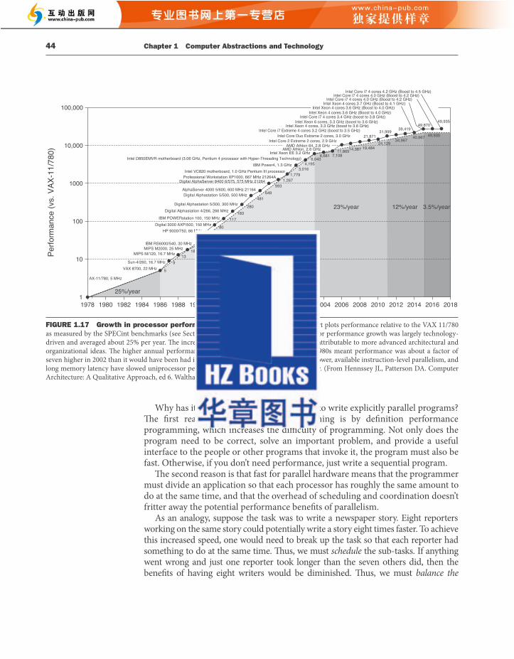
1.8 The Sea Change: The Switch from Uniprocessors to Multiprocessors 45
load evenly to get the desired speedup. Another danger would be if reporters had to spend a lot of time talking to each other to write their sections. You would also fall short if one part of the story, such as the conclusion, couldn’t be written until all of the other parts were completed. Th us, care must be taken to reduce communication and synchronization overhead . For both this analogy and parallel programming, the challenges include scheduling, load balancing, time for synchronization, and overhead for communication between the parties. As you might guess, the challenge is stiff er with more reporters for a newspaper story and more processors for parallel programming.
To refl ect this sea change in the industry, the next fi ve chapters in this edition of the book each have a section on the implications of the parallel revolution to that chapter:
■ Chapter 2 , Section 2.11 : Parallelism and Instructions: Synchronization . Usually independent parallel tasks need to coordinate at times, such as to say when they have completed their work. Th is chapter explains the instructions used by multicore processors to synchronize tasks.
■ Chapter 3 , Section 3.6 : Parallelism and Computer Arithmetic: Subword Parallelism . Perhaps the simplest form of parallelism to build involves computing on elements in parallel, such as when multiplying two vectors. Subword parallelism relies on wider arithmetic units that can operate on many operands simultaneously.
■ Chapter 4 , Section 4.11 : Parallelism via Instructions . Given the diffi culty of explicitly parallel programming, tremendous eff ort was invested in the 1990s in having the hardware and the compiler uncover implicit parallelism, initially via pipelining . Th is chapter describes some of these aggressive techniques, including fetching and executing multiple instructions simultaneously and guessing on the outcomes of decisions, and executing instructions speculatively using prediction .
■ Chapter 5 , Section 5.10 : Parallelism and Memory Hierarchies: Cache Coherence . One way to lower the cost of communication is to have all processors use the same address space, so that any processor can read or write any data. Given that all processors today use caches to keep a temporary copy of the data in faster memory near the processor, it’s easy to imagine that parallel programming would be even more diffi cult if the caches associated with each processor had inconsistent values of the shared data. Th is chapter describes the mechanisms that keep the data in all caches consistent.
■ Chapter 5 , Section 5.11 : Parallelism and Memory Hierarchy: Redundant Arrays of Inexpensive Disks . Th is section describes how using many disks in conjunction can off er much higher throughput, which was the original inspiration of Redundant Arrays of Inexpensive Disks (RAID). Th e real popularity of RAID proved to be to the much greater dependability off ered by including a modest number of redundant disks. Th e section explains the diff erences in performance, cost, and dependability between the diff erent RAID levels.
44 Chapter 1 Computer Abstractions and Technology
Why has it been so hard for programmers to write explicitly parallel programs? Th e fi rst reason is that parallel programming is by defi nition performance programming, which increases the diffi culty of programming. Not only does the program need to be correct, solve an important problem, and provide a useful interface to the people or other programs that invoke it, the program must also be fast. Otherwise, if you don’t need performance, just write a sequential program.
Th e second reason is that fast for parallel hardware means that the programmer must divide an application so that each processor has roughly the same amount to do at the same time, and that the overhead of scheduling and coordination doesn’t fritter away the potential performance benefi ts of parallelism.
As an analogy, suppose the task was to write a newspaper story. Eight reporters working on the same story could potentially write a story eight times faster. To achieve this increased speed, one would need to break up the task so that each reporter had something to do at the same time. Th us, we must schedule the sub-tasks. If anything went wrong and just one reporter took longer than the seven others did, then the benefi ts of having eight writers would be diminished. Th us, we must balance the
1
5
913
1824
51
80
117183
280
481649
9931,267
1,7793,016
4,1956,043
6,681 7,10811,86514,387 19,484
21,87124,129
31,999
34,967
39,419
40,967
49,935
49,935
49,870
1
10
100
1000
10,000
100,000
1978 1980 1982 1984 1986 1988 1990 1992 1994 1996 1998 2000 2002 2004 2006 2008 2010 2012 2014 2016 2018
Perfo
rman
ce (v
s. V
AX-1
1/78
0)
25%/year
52%/year
23%/year 12%/year 3.5%/year IBM POWERstation 100, 150 MHz
Digital Alphastation 4/266, 266 MHzDigital Alphastation 5/300, 300 MHz
Digital Alphastation 5/500, 500 MHz AlphaServer 4000 5/600, 600 MHz 21164
Digital AlphaServer 8400 6/575, 575 MHz 21264Professional Workstation XP1000, 667 MHz 21264AIntel VC820 motherboard, 1.0 GHz Pentium III processor
IBM Power4, 1.3 GHz
Intel Xeon EE 3.2 GHz AMD Athlon, 2.6 GHz
Intel Core 2 Extreme 2 cores, 2.9 GHz Intel Core Duo Extreme 2 cores, 3.0 GHz
Intel Core i7 Extreme 4 cores 3.2 GHz (boost to 3.5 GHz)
Intel Core i7 4 cores 3.4 GHz (boost to 3.8 GHz)Intel Xeon 4 cores 3.6 GHz (Boost to 4.0 GHz)
Intel Xeon 4 cores 3.6 GHz (Boost to 4.0 GHz)Intel Xeon 4 cores 3.7 GHz (Boost to 4.1 GHz)
Intel Core i7 4 cores 4.0 GHz (Boost to 4.2 GHz)Intel Core i7 4 cores 4.0 GHz (Boost to 4.2 GHz)
Intel Core i7 4 cores 4.2 GHz (Boost to 4.5 GHz)
Intel Xeon 4 cores, 3.3 GHz (boost to 3.6 GHz) Intel Xeon 6 cores, 3.3 GHz (boost to 3.6 GHz)
Intel D850EMVR motherboard (3.06 GHz, Pentium 4 processor with Hyper-Threading Technology)
AMD Athlon 64, 2.8 GHz
Digital 3000 AXP/500, 150 MHzHP 9000/750, 66 MHz
IBM RS6000/540, 30 MHzMIPS M2000, 25 MHz
MIPS M/120, 16.7 MHz
Sun-4/260, 16.7 MHzVAX 8700, 22 MHz
AX-11/780, 5 MHz
FIGURE 1.17 Growth in processor performance since the mid-1980s. Th is chart plots performance relative to the VAX 11/780 as measured by the SPECint benchmarks (see Section 1.11 ). Prior to the mid-1980s, processor performance growth was largely technology-driven and averaged about 25% per year. Th e increase in growth to about 52% since then is attributable to more advanced architectural and organizational ideas. Th e higher annual performance improvement of 52% since the mid-1980s meant performance was about a factor of seven higher in 2002 than it would have been had it stayed at 25%. Since 2002, the limits of power, available instruction-level parallelism, and long memory latency have slowed uniprocessor performance recently, to about 3.5% per year. (From Hennssey JL, Patterson DA. Computer Architecture: A Qualitative Approach, ed 6. Waltham, MA: Elsevier, 2017.)
1.9 Real Stuff: Benchmarking the Intel Core i7 47
focusing on processor performance (now called SPEC89), which has evolved through fi ve generations. Th e latest is SPEC CPU2017, which consists of a set of 10 integer benchmarks (SPECspeed 2017 Integer) and 13 fl oating-point benchmarks (SPECspeed 2017 Floating Point). Th e integer benchmarks vary from part of a C compiler to a chess program to a quantum computer simulation. Th e fl oating-point benchmarks include structured grid codes for fi nite element modeling, particle method codes for molecular dynamics, and sparse linear algebra codes for fl uid dynamics.
Figure 1.18 describes the SPEC integer benchmarks and their execution time on the Intel Core i7 and shows the factors that explain execution time: instruction count, CPI, and clock cycle time. Note that CPI varies by more than a factor of 4.
To simplify the marketing of computers, SPEC decided to report a single number to summarize all 10 integer benchmarks. Dividing the execution time of a reference processor by the execution time of the measured computer normalizes the execution time measurements; this normalization yields a measure, called the SPECratio, which has the advantage that bigger numeric results indicate faster performance. Th at is, the SPECratio is the inverse of execution time. A SPECspeed 2017 summary measurement is obtained by taking the geometric mean of the SPECratios.
Elaboration : When comparing two computers using SPECratios, use the geometric mean so that it gives the same relative answer no matter what computer is used to normalize the results. If we averaged the normalized execution time values with an arithmetic mean, the results would vary depending on the computer we choose as the reference.
Description NameInstructionCount x 109 CPI
Clock cycle time(seconds x 10–9)
ExecutionT ime
(seconds)
ReferenceT ime
(seconds ) SPECratio
Perl interpreter perlbench 2684 0.42 0.556 627 1774 2.83
GNU C compiler gcc 2322 0.67 0.556 863 3976 4.61
Route planning mcf 1786 1.22 0.556 1215 4721 3.89Discrete Event simulation - computer network omnetpp 1107 0.82 0.556 507 1630 3.21XML to HTML conversion via XSLT xalancbmk 1314 0.75 0.556 549 1417 2.58
Video compression x264 4488 0.32 0.556 813 1763 2.17Artificial Intelligence: alpha-beta tree search (Chess) deepsjeng 2216 0.57 0.556 698 1432 2.05Artificial Intelligence: Monte Carlo tree search (Go) leela 2236 0.79 0.556 987 1703 1.73Artificial Intelligence: recursivesolution generator (Sudoku) exchange2 6683 0.46 0.556 1718 2939 1.71General data compression xz 8533 1.32 0.556 6290 6182 0.98Geometric mean 2.36
FIGURE 1.18 SPECspeed 2017 Integer benchmarks running on a 1.8 GHz Intel Xeon E5-2650L. As the equation on page 35 explains, execution time is the product of the three factors in this table: instruction count in billions, clocks per instruction (CPI), and clock cycle time in nanoseconds. SPECratio is simply the reference time, which is supplied by SPEC, divided by the measured execution time. Th e single number quoted as SPECspeed 2017 Integer is the geometric mean of the SPECratios. SPECspeed 2017 has multiple input fi les for perlbench, gcc, x264, and xz. For this fi gure, execution time and total clock cycles are the sum running times of these programs for all inputs.
46 Chapter 1 Computer Abstractions and Technology
In addition to these sections, there is a full chapter on parallel processing. Chapter 6 goes into more detail on the challenges of parallel programming; presents the two contrasting approaches to communication of shared addressing and explicit message passing; describes a restricted model of parallelism that is easier to program; discusses the diffi culty of benchmarking parallel processors; introduces a new simple performance model for multicore microprocessors; and, fi nally, describes and evaluates four examples of multicore microprocessors using this model.
As mentioned above, Chapters 3 to 6 use matrix vector multiply as a running example to show how each type of parallelism can signifi cantly increase performance.
Appendix C describes an increasingly popular hardware component that is included with desktop computers, the graphics processing unit (GPU). Invented to accelerate graphics, GPUs are becoming programming platforms in their own right. As you might expect, given these times, GPUs rely on parallelism.
Appendix C describes the NVIDIA GPU and highlights parts of its parallel programming environment.
1.9 Real Stuff: Benchmarking the Intel Core i7
Each chapter has a section entitled “Real Stuff ” that ties the concepts in the book with a computer you may use every day. Th ese sections cover the technology underlying modern computers. For this fi rst “Real Stuff ” section, we look at how integrated circuits are manufactured and how performance and power are measured, with the Intel Core i7 as the example.
SPEC CPU Benchmark A computer user who runs the same programs day in and day out would be the perfect candidate to evaluate a new computer. Th e set of programs run would form a workload . To evaluate two computer systems, a user would simply compare the execution time of the workload on the two computers. Most users, however, are not in this situation. Instead, they must rely on other methods that measure the performance of a candidate computer, hoping that the methods will refl ect how well the computer will perform with the user’s workload. Th is alternative is usually followed by evaluating the computer using a set of benchmarks —programs specifi cally chosen to measure performance. Th e benchmarks form a workload that the user hopes will predict the performance of the actual workload. As we noted above, to make the common case fast , you fi rst need to know accurately which case is common, so benchmarks play a critical role in computer architecture.
SPEC ( System Performance Evaluation Cooperative ) is an eff ort funded and supported by a number of computer vendors to create standard sets of benchmarks for modern computer systems. In 1989, SPEC originally created a benchmark set
I thought [computers] would be a universally applicable idea, like a book is. But I didn’t think it would develop as fast as it did, because I didn’t envision we’d be able to get as many parts on a chip as we fi nally got. Th e transistor came along unexpectedly. It all happened much faster than we expected. J. Presper Eckert, coinventor of ENIAC, speaking in 1991
workload A set of programs run on a computer that is either the actual collection of applications run by a user or constructed from real programs to approximate such a mix. A typical workload specifi es both the programs and the relative frequencies.
benchmark A program selected for use in comparing computer performance.
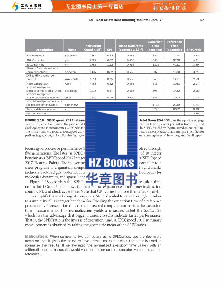
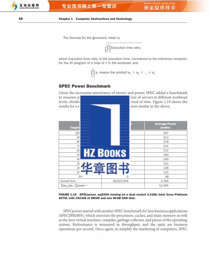
1.10 Going Faster: Matrix Multiply in Python 49
boils these numbers down to a single number, called “overall ssj_ops per watt.” Th e formula for this single summarizing metric is
overall ssj_ops per watt ssj_ops power��
ii
i0
10
∑⎛
⎝⎜⎜⎜⎜
⎞
⎠⎟⎟⎟⎟⎟ ii�0
10
∑⎛
⎝⎜⎜⎜⎜
⎞
⎠⎟⎟⎟⎟⎟
where ssj_ops i is performance at each 10% increment and power i is power consumed at each performance level.
1.10 Going Faster: Matrix Multiply in Python
To demonstrate the impact of the ideas in this book, every chapter has a “Going Faster” section that improves the performance of a program that multiplies a matrix times a vector. We start with this Python program:
for i in xrange(n): for j in xrange(n):
for k in xrange(n): C[i][j] += A[i][k] * B[k][j]
We are using the n1-standard-96 server in Google Cloud Engine, which has two Intel Skylake Xeon chips, and each chip has 24 processors or cores and running Python version 3.1. If the matrices are 960 𝖷𝖷𝖷 960, it takes about 5 minutes to run using Python 2.7. Since fl oating point computations go up with the cube of the matrix dimension, it would take almost 6 hours to run if the matrices were 4096 𝖷𝖷𝖷 4096. While it is quick to write the matrix multiply in Python, who wants to wait that long to get the answer?
In Chapter 2 , we are converting the Python version of matrix multiply to a C version, which increases performance by a factor of 200. Th e C programming abstraction is much closer to the hardware than Python is, which is why we use it as the programming example in this book. Closing the abstraction gap also makes it much faster than Python [Leiserson, 2020 ].
● In the category of data level parallelism, in Chapter 3 , we use subword parallelism via C intrinsics to increase performance by a factor of about 8.
● In the category of instruction level parallelism, in Chapter 4 , we use loop unrolling to exploit multiple instruction issue and out-of-order execution hardware to increase performance by another factor of about 2.
● In the category of memory hierarchy optimization, in Chapter 5 , we use cache blocking to increase performance on large matrices by another factor of about 1.5.
● In the category of thread level parallelism, in Chapter 6, we use parallel for loops in OpenMP to exploit multicore hardware to increase performance by another factor of 12–17.
48 Chapter 1 Computer Abstractions and Technology
The formula for the geometric mean is
Execution time ratioii
nn
�1∏
where Execution time ratio i is the execution time, normalized to the reference computer,
for the i th program of a total of n in the workload, and
a a a ai ni
n
means the product 1 21
…∏
SPEC Power Benchmark Given the increasing importance of energy and power, SPEC added a benchmark to measure power. It reports power consumption of servers at diff erent workload levels, divided into 10% increments, over a period of time. Figure 1.19 shows the results for a server using Intel Nehalem processors similar to the above.
Target Load %Performance
(ssj_ops)Average Power
(watts)
100% 4,864,136 347 90% 4,389,196 312 80% 3,905,724 278 70% 3,418,737 241 60% 2,925,811 212 50% 2,439,017 183 40% 1,951,394 160 30% 1,461,411 141 20% 974,045 128 10% 485,973 115 0% 0 48 Overall Sum 26,815,444 2,165 ∑ssj_ops / ∑power = 12,385
FIGURE 1.19 SPECpower_ssj2008 running on a dual socket 2.2 GHz Intel Xeon Platinum 8276L with 192 GiB of DRAM and one 80 GB SSD disk.
SPECpower started with another SPEC benchmark for Java business applications (SPECJBB2005), which exercises the processors, caches, and main memory as well as the Java virtual machine, compiler, garbage collector, and pieces of the operating system. Performance is measured in throughput, and the units are business operations per second. Once again, to simplify the marketing of computers, SPEC
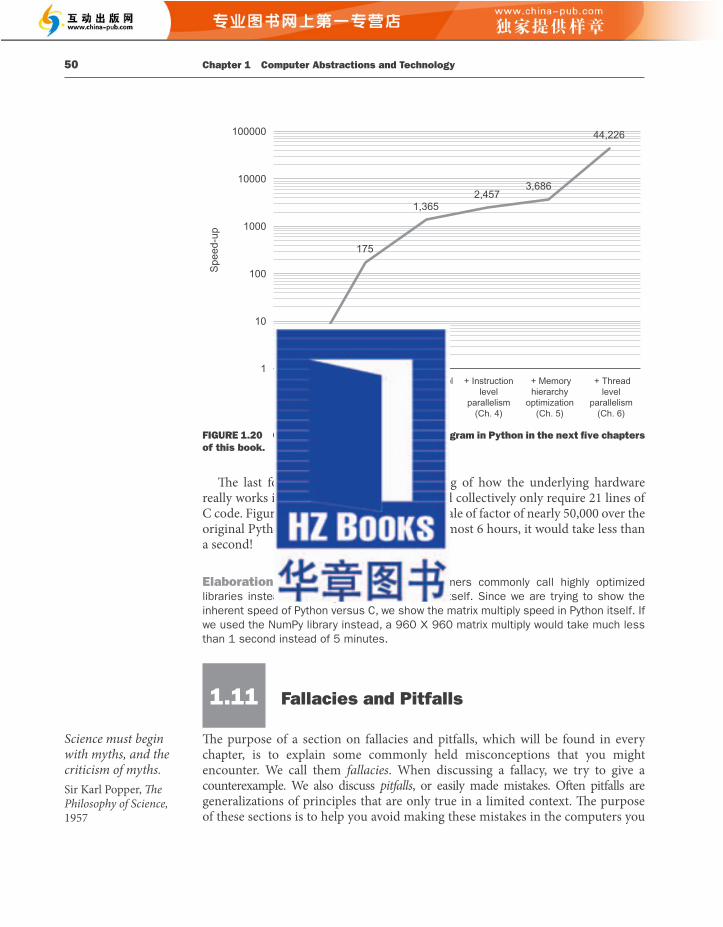
1.11 Fallacies and Pitfalls 51
may design or use. Cost/performance fallacies and pitfalls have ensnared many a computer architect, including us. Accordingly, this section suff ers no shortage of relevant examples. We start with a pitfall that traps many designers and reveals an important relationship in computer design.
Pitfall : Expecting the improvement of one aspect of a computer to increase overall performance by an amount proportional to the size of the improvement.
Th e great idea of making the common case fast has a demoralizing corollary that has plagued designers of both hardware and soft ware. It reminds us that the opportunity for improvement is aff ected by how much time the event consumes.
A simple design problem illustrates it well. Suppose a program runs in 100 seconds on a computer, with multiply operations responsible for 80 seconds of this time. How much do I have to improve the speed of multiplication if I want my program to run fi ve times faster?
Th e execution time of the program aft er making the improvement is given by the following simple equation known as Amdahl’s Law :
Execution time after improvement
Execution time affected byy improvementAmount of improvement
Execution time unaffectted
For this problem:
Execution time after improvement seconds secon80 100 80n
( dds)
Since we want the performance to be fi ve times faster, the new execution time should be 20 seconds, giving
20 80 20
0 80
seconds seconds seconds
secondsn
n
Th at is, there is no amount by which we can enhance-multiply to achieve a fi vefold increase in performance, if multiply accounts for only 80% of the workload. Th e performance enhancement possible with a given improvement is limited by the amount that the improved feature is used. In everyday life this concept also yields what we call the law of diminishing returns.
We can use Amdahl’s Law to estimate performance improvements when we know the time consumed for some function and its potential speedup. Amdahl’s Law, together with the CPU performance equation, is a handy tool for evaluating potential enhancements. Amdahl’s Law is explored in more detail in the exercises.
Amdahl’s Law is also used to argue for practical limits to the number of parallel processors. We examine this argument in the Fallacies and Pitfalls section of Chapter 6 .
Amdahl’s Law A rule stating that the performance enhancement possible with a given improvement is limited by the amount that the improved feature is used. It is a quantitative version of the law of diminishing returns.
50 Chapter 1 Computer Abstractions and Technology
Th e last four steps leverage understanding of how the underlying hardware really works in a modern microprocessor, and collectively only require 21 lines of C code. Figure 1.20 shows speedup on a log scale of factor of nearly 50,000 over the original Python version. Instead of waiting almost 6 hours, it would take less than a second!
Elaboration: To accelerate Python, programmers commonly call highly optimized libraries instead of writing the code in Python itself. Since we are trying to show the inherent speed of Python versus C, we show the matrix multiply speed in Python itself. If we used the NumPy library instead, a 960 𝖷𝖷𝖷 960 matrix multiply would take much less than 1 second instead of 5 minutes.
1.11 Fallacies and Pitfalls
Th e purpose of a section on fallacies and pitfalls, which will be found in every chapter, is to explain some commonly held misconceptions that you might encounter. We call them fallacies . When discussing a fallacy, we try to give acounterexample. We also discuss pitfalls , or easily made mistakes. Oft en pitfalls are generalizations of principles that are only true in a limited context. Th e purpose of these sections is to help you avoid making these mistakes in the computers you
Science must begin with myths, and the criticism of myths. Sir Karl Popper, Th e Philosophy of Science, 1957
FIGURE 1.20 Optimizations of matrix multiply program in Python in the next fi ve chapters of this book.
1
175
1,3652,457
3,686
44,226
1
10
100
1000
10000
100000
Python(Ch. 1)
translate to C(Ch. 2)
+ Data LevelParallelism
(Ch. 3)
+ Instructionlevel
parallelism(Ch. 4)
+ Memoryhierarchy
optimization(Ch. 5)
+ Threadlevel
parallelism(Ch. 6)
Spe
ed-u
p

1.12 Concluding Remarks 53
cannot have a single MIPS rating. For example, by substituting for execution time, we see the relationship between MIPS, clock rate, and CPI:
MIPS Instruction countInstruction count CPI
Clock rate106
CClock rateCPI 106
Th e CPI varied by a factor of 4 for SPECspeed 2017 Integer on an Intel Xeon computer in Figure 1.18 , so MIPS does as well. Finally, and most importantly, if a new program executes more instructions but each instruction is faster, MIPS can vary independently from performance!
Consider the following performance measurements for a program:
Measurement Computer A Computer B
Instruction count 10 billion 8 billion
Clock rate 4 GHz 4 GHz
CPI 1.0 1.1
a. Which computer has the higher MIPS rating?
b. Which computer is faster?
1.12 Concluding Remarks
Although it is diffi cult to predict exactly what level of cost/performance computers will have in the future, it’s a safe bet that they will be much better than they are today. To participate in these advances, computer designers and programmers must understand a wider variety of issues.
Both hardware and soft ware designers construct computer systems in hierarchical layers, with each lower layer hiding details from the level above. Th is great idea of abstraction is fundamental to understanding today’s computer systems, but it does not mean that designers can limit themselves to knowing a single abstraction. Perhaps the most important example of abstraction is the interface between hardware and low-level soft ware, called the instruction set architecture . Maintaining the instruction set architecture as a constant enables many implementations of that architecture—presumably varying in cost and performance—to run identical soft ware. On the downside, the architecture may preclude introducing innovations that require the interface to change.
Check Yourself
Where … the ENIAC is equipped with 18,000 vacuum tubes and weighs 30 tons, computers in the future may have 1,000 vacuum tubes and perhaps weigh just 1½ tons. Popular Mechanics , March 1949
52 Chapter 1 Computer Abstractions and Technology
Fallacy : Computers at low utilization use little power. Power effi ciency matters at low utilizations because server workloads vary. Utilization of servers in Google’s warehouse scale computer, for example, is between 10% and 50% most of the time and at 100% less than 1% of the time. Even given fi ve years to learn how to run the SPECpower benchmark well, the specially confi gured computer with the best results in 2020 still uses 33% of the peak power at 10% of the load the same as in 2012 for the last edition. Systems in the fi eld that are not confi gured for the SPECpower benchmark are surely worse.
Since servers’ workloads vary but use a large fraction of peak power, Luiz Barroso and Urs Hölzle [2007] argue that we should redesign hardware to achieve “energy-proportional computing.” If future servers used, say, 10% of peak power at 10% workload, we could reduce the electricity bill of datacenters and become good corporate citizens in an era of increasing concern about CO 2 emissions.
Fallacy : Designing for performance and designing for energy effi ciency are unrelated goals.
Since energy is power over time, it is oft en the case that hardware or soft ware optimizations that take less time save energy overall even if the optimization takes a bit more energy when it is used. One reason is that all of the rest of the computer is consuming energy while the program is running, so even if the optimized portion uses a little more energy, the reduced time can save the energy of the whole system.
Pitfall : Using a subset of the performance equation as a performance metric. We have already warned about the danger of predicting performance based on simply one of clock rate, instruction count, or CPI. Another common mistake is to use only two of the three factors to compare performance. Although using two of the three factors may be valid in a limited context, the concept is also easily misused. Indeed, nearly all proposed alternatives to the use of time as the performance metric have led eventually to misleading claims, distorted results, or incorrect interpretations.
One alternative to time is MIPS (million instructions per second) . For a given program, MIPS is simply
MIPS Instruction count
Execution time 106
Since MIPS is an instruction execution rate, MIPS specifi es performance inversely to execution time; faster computers have a higher MIPS rating. Th e good news about MIPS is that it is easy to understand, and faster computers mean bigger MIPS, which matches intuition.
Th ere are three problems with using MIPS as a measure for comparing computers. First, MIPS specifi es the instruction execution rate but does not take into account the capabilities of the instructions. We cannot compare computers with diff erent instruction sets using MIPS, since the instruction counts will certainly diff er. Second, MIPS varies between programs on the same computer; thus, a computer
million instructions per second (MIPS) A measurement of program execution speed based on the number of millions of instructions. MIPS is computed as the instruction count divided by the product of the execution time and 10 6 .

1.14 Self-Study 55
■ Memory: Chapter 5
■ Input: Chapters 5 and 6
■ Output: Chapters 5 and 6
As mentioned above, Chapter 4 describes how processors exploit implicit parallelism, Chapter 6 describes the explicitly parallel multicore microprocessors that are at the heart of the parallel revolution, and Appendix C describes the highly parallel graphics processor chip. Chapter 5 describes how a memory hierarchy exploits locality. Chapter 2 describes instruction sets—the interface between compilers and the computer—and emphasizes the role of compilers and programming languages in using the features of the instruction set. Appendix A provides a reference for the instruction set of Chapter 2. Chapter 3 describes how computers handle arithmetic data. Appendix B introduces logic design.
1.13 Historical Perspective and Further Reading
For each chapter in the text, a section devoted to a historical perspective can be found online on a site that accompanies this book. We may trace the development of an idea through a series of computers or describe some important projects, and we provide references in case you are interested in probing further.
Th e historical perspective for this chapter provides a background for some of the key ideas presented in this opening chapter. Its purpose is to give you the human story behind the technological advances and to place achievements in their historical context. By understanding the past, you may be better able to understand the forces that will shape computing in the future. Each Historical Perspective section online ends with suggestions for further reading, which are also collected separately online under the section “ Further Reading .” Th e rest of Section 1.13 is found online.
1.14 Self-Study
Starting with the sixth edition, we are adding a section in every chapter with some hopefully thought-provoking exercises along with their solutions to help readers check to see if they’re following the material.
Mapping great ideas in architecture to the real world. Find the best match of the seven great ideas from computer architecture to these real-world examples:
1. Reducing time to do laundry by washing the next load while drying the last load
2. Hiding a spare key in case you lose your front door key
1.13
An active fi eld of science is like an immense anthill; the individual almost vanishes into the mass of minds tumbling over each other, carrying information from place to place, passing it around at the speed of light. Lewis Th omas, “Natural Science,” in Th e Lives of a Cell , 1974
54 Chapter 1 Computer Abstractions and Technology
Th ere is a reliable method of determining and reporting performance by using the execution time of real programs as the metric. Th is execution time is related to other important measurements we can make by the following equation:
SecondsProgram
InstructionsProgram
Clock cyclesInstruction
SecondsClock cycle
We will use this equation and its constituent factors many times. Remember, though, that individually the factors do not determine performance: only the product, which equals execution time, is a reliable measure of performance.
Th e key hardware technology for modern processors is silicon. While silicon fuels the advance of hardware, new ideas in the organization of computers have improved price/performance. Two of the key ideas are exploiting parallelism in the program, typically today via multiple processors, and exploiting locality of accesses to a memory hierarchy , typically via caches.
Energy effi ciency has replaced die area as the most critical resource of microprocessor design. Conserving power while trying to increase performance has forced the hardware industry to switch to multicore microprocessors, thereby forcing the soft ware industry to switch to programming parallel hardware. Parallelism is now required for performance.
Computer designs have always been measured by cost and performance, as well as other important factors such as energy, dependability, cost of ownership, and scalability. Although this chapter has focused on cost, performance, and energy, the best designs will strike the appropriate balance for a given market among all the factors.
Road Map for This Book At the bottom of these abstractions are the fi ve classic components of a computer: datapath, control, memory, input, and output (refer to Figure 1.5 ). Th ese fi ve components also serve as the framework for the rest of the chapters in this book:
■ Datapath: Chapter 3 , Chapter 4, Chapter 6, and Appendix C
■ Control: Chapter 4, Chapter 6, and Appendix C
Execution time is the only valid and unimpeachable measure of performance. Many other metrics have been proposed and found wanting. Sometimes these metrics are fl awed from the start by not refl ecting execution time; other times a metric that is valid in a limited context is extended and used beyond that context or without the additional clarifi cation needed to make it valid.
The BIG Picture

1.14 Self-Study 57
3. Why do you think price per gigabyte fl uctuates over 3- to 5-year periods? Is it be related to the chip cost formulas on page 28 or to other forces in the marketplace?
Answers to Self-Study Mapping great ideas in architecture to the real world:
1. Performance via pipelining
2. Dependability via redundancy (although you could argue it is also a use of performance via parallelism)
3. Performance via prediction
4. Make the common case fast
5. Hierarchy of memories
6. Performance via parallelism (although you could argue it is also a use of dependability via redundancy)
7. Use abstraction to simplify design
Fastest Computer
1. Th e clock rates are the inverse of the clock cycle time. P1 = 1/(0.33 𝖷𝖷 10 −9 seconds) = 3 GHz; P2 = 1/(0.40 𝖷𝖷 10 −9 seconds) = 2.5 GHz; P3 = 1/(0.25 𝖷𝖷 10 −9 seconds) = 4 GHz. P3 has the highest clock rate.
FIGURE 1.21 Price of memory per gigabyte between 1975 and 2020. (Source: https://jcmit.net/memoryprice.htm)
$1
$10
$100
$1,000
$10,000
$1,00,000
$10,00,000
$1,00,00,000
$10,00,00,000
1975 1980 1985 1990 1995 2000 2005 2010 2015 2020
DR
AM
Mem
ory
Pric
e ($
/Gig
abyt
e)
Price of DRAM Memory over Time
56 Chapter 1 Computer Abstractions and Technology
3. Checking the weather forecast for cities you would drive through when deciding which route to take on a long winter trip
4. Express checkout lanes in grocery stores for 10 items or less
5. Th e local branch of a large city library system
6. Automobile powered by an electric motor on all four wheels
7. Optional self-driving automobile mode that requires purchase of self-parking and navigation options
How do you measure fastest? Consider three diff erent processors P1, P2, and P3 executing the same instruction set. P1 has a clock cycle time of 0.33 ns and a CPI of 1.5; P2 has a clock cycle time of 0.40 ns and a CPI of 1.0; P3 has clock cycle time of 0.25 ns and a CPI of 2.2.
1. Which has the highest clock rate? What is it?
2. Which is the fastest computer? If answer is diff erent from above , explain why. Which is the slowest?
3. How do the answers to (1) and (2) refl ect the importance of benchmarks?
Amdahl’s Law and brotherhood. Amdahl’s Law is basically the Law of Diminishing Returns, which applies to investments as well as computer architecture. Here is an example that helps explain the law —Your brother has joined a start-up and is trying to convince you to invest some of your savings, since, he claims, “it’s a sure thing!”
1. You decide to invest 10% of your savings. What must be the return on your investment in the start-up to double your overall wealth, assuming the start-up was your only investment?
2. Assuming the start-up investment delivers the return you calculated in (1), how much of your savings would you have to invest to realize 90% of start-up’s increase ? How about 95%?
3. How do the results relate to Amdahl’s observation about computers? What does it say about brotherhood?
DRAM price versus cost. Figure 1.21 plots the price of DRAM chips from 1975 to 2020, while Figure 1.11 shows capacity per DRAM chip over the same period. Th ey show a 1,000,000-fold increase in capacity (16 Kbit to 16 Gbit) and a 25,000,000-fold reduction in price per gigabyte ($100 million to $4). Note that the price per GiB fl uctuates up and down over time, while capacity per chip has a smooth growth curve.
1. Can you see evidence of the slowing of Moore’s Law in Figure 1.21 ?
2. Why might price improve by a factor of 25 higher than the improvement in capacity per chip? What might be other reasons than the increasing chip capacity?
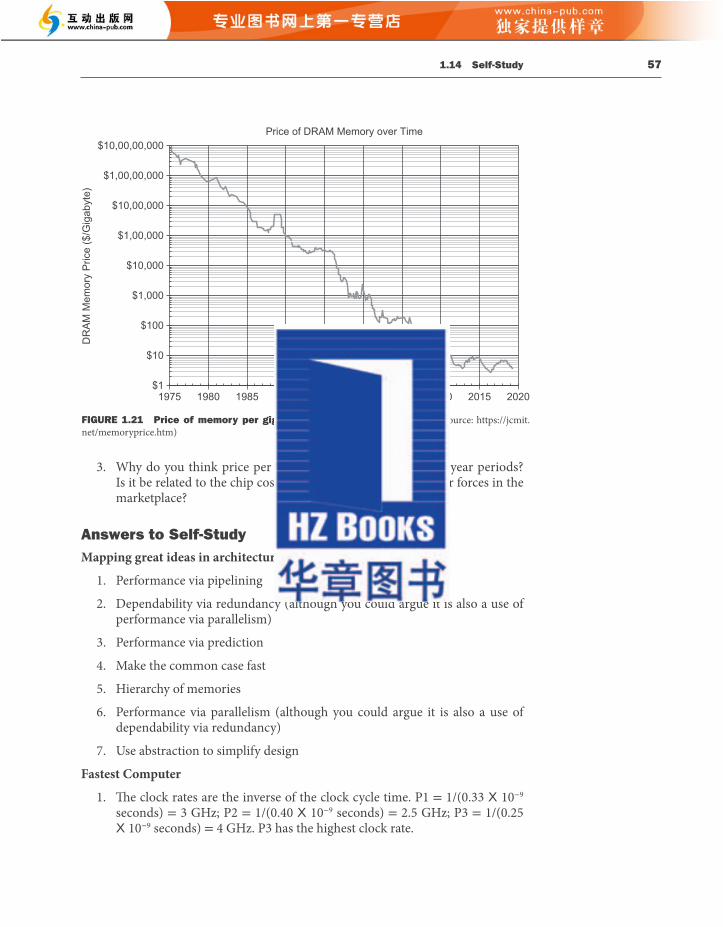
1.15 Exercises 59
can result in, say, a factor-of-2 reduction in cost. Th ere were also innovations in packaging of the chips that can lower costs and thus prices over this long time period.
3. DRAMs are commodity parts, as there are multiple companies manufacturing similar products, and thus they are subject to market pressures and fl uctuating prices. Prices go up when demand exceeds supply and they fall when vice versa. Th e industry has a history of periods when DRAMs are very profi table, so they build more manufacturing lines, until there is an oversupply and prices drop, and so they cut back new manufacturing lines.
1.15 Exercises
Th e relative time ratings of exercises are shown in square brackets aft er each exercise number. On average, an exercise rated [10] will take you twice as long as one rated [5]. Sections of the text that should be read before attempting an exercise will be given in angled brackets; for example, <§1.4> means you should have read Section 1.4 , Under the Covers, to help you solve this exercise.
1.1 [2] <§1.1> List and describe three types of computers.
1.2 [5] <§1.2> Th e seven great ideas in computer architecture are similar to ideas from other fi elds. Match the seven ideas from computer architecture, “Use Abstraction to Simplify Design”, “Make the Common Case Fast”, “Performance via Parallelism”, “Performance via Pipelining”, “Performance via Prediction” “Hierarchy of Memories”, and “Dependability via Redundancy” to the following ideas from other fi elds:
a. Assembly lines in automobile manufacturing
b. Suspension bridge cables
c. Aircraft and marine navigation systems that incorporate wind information
d. Express elevators in buildings e. Library reserve desk f. Increasing the gate area on a CMOS transistor to decrease its switching time g. Building self-driving cars whose control systems partially rely on existing sensor systems already installed into the base vehicle, such as lane departure systems and smart cruise control systems
1.3 [2] <§1.3> Describe the steps that transform a program written in a high-level language such as C into a representation that is directly executed by a computer processor.
58 Chapter 1 Computer Abstractions and Technology
2. Since they all have the same instruction set architecture, their programs all have the same instruction count, so we can measure performance as the product of average clock cycles per instruction (CPI) times clock cycle time, which is also the average time of an instruction:
a. P1 = 1.5 𝖷𝖷 0.33 ns = 0.495 ns.
(You could also calculate average instruction time using CPI/clock rate, or 1.5/3.0 GHz = 0.495 ns)
b. P2 = 1.0 𝖷𝖷 0.40 ns = 0.400 ns (or 1.0/2.5 GHz = 0.400 ns)
c. P3 = 2.2 𝖷𝖷 0.25 ns = 0.550 ns (or 1.0/4.0 GHz = 0.550 ns)
P2 is the fastest and P3 is the slowest. Despite having the highest clock rate, on average, P3 takes so many more clock cycles that it loses the benefi t of a higher clock rate.
3. Th e CPI calculation was based on running some benchmarks. If they are representative of real workloads, these answers to these questions are correct. If the benchmarks are unrealistic, they may not . Th e diff erence between things easy to advertise, like clock rate versus actual performance, highlights the importance of developing good benchmarks.
Brotherhood and Amdahl’s Law
1. 11𝖷𝖷 return on investment to double your savings: 90% 𝖷𝖷 1 + 10% 𝖷𝖷 11 = 2.0.
2. You must invest 89% of your wealth to get 90% of the full return. 90% of 11𝖷𝖷 = 9.9𝖷𝖷 and 11% 𝖷𝖷 1 + 89% 𝖷𝖷 11 = 9.9. You must invest 94.5% of wealth to get 95% return. 95% of 11𝖷𝖷 = 10.45𝖷𝖷 and 5.5% 𝖷𝖷 1 + 94.5% 𝖷𝖷 11 = 10.45.
3. Just as the part you do not invest limits the return on investment even for high returns for a successful start-up, the part of the computer that you do not accelerate limits the benefi ts of acceleration, no matter how much faster you make that improved piece. Th e amount you invest will be infl uenced by your faith in your brother’s judgment, especially since 90% of all start-ups do not succeed!
Price Versus Cost of Memory
1. Although the prices fl uctuate, it does look like pricing is fl attening out since 2013, which is consistent with the slowing of Moore’s Law. For example, DRAM was $4/GB in 2013 and 2016 as well as in 2019. Th ere is no other such long period as fl at in the past.
2. Neither fi gure mentions the volume of DRAM chips, which can explain why price improves more than capacity per chip. Th ere are typically manufacturing learning curves where every factor-of-10 increase in volume
1.15 Exercises 61
1.7 [20] <§1.6> Consider two diff erent implementations of the same instruction set architecture. Th e instructions can be divided into four classes according to their CPI (class A, B, C, and D). P1 with a clock rate of 2.5 GHz and CPIs of 1, 2, 3, and 3, and P2 with a clock rate of 3 GHz and CPIs of 2, 2, 2, and 2.
Given a program with a dynamic instruction count of 1.0E6 instructions divided into classes as follows: 10% class A, 20% class B, 50% class C, and 20% class D, which is faster: P1 or P2?
a. What is the global CPI for each implementation?
b. Find the clock cycles required in both cases.
1.8 [15] <§1.6> Compilers can have a profound impact on the performance of an application. Assume that for a program, compiler A results in a dynamic instruction count of 1.0E9 and has an execution time of 1.1 s, while compiler B results in a dynamic instruction count of 1.2E9 and an execution time of 1.5 s.
a. Find the average CPI for each program given that the processor has a clock cycle time of 1 ns.
b. Assume the compiled programs run on two diff erent processors. If the execution times on the two processors are the same, how much faster is the clock of the processor running compiler A’s code versus the clock of the processor running compiler B’s code?
c. A new compiler is developed that uses only 6.0E8 instructions and has an average CPI of 1.1. What is the speedup of using this new compiler versus using compiler A or B on the original processor?
1.9 Th e Pentium 4 Prescott processor, released in 2004, had a clock rate of 3.6 GHz and voltage of 1.25 V. Assume that, on average, it consumed 10 W of static power and 90 W of dynamic power.
Th e Core i5 Ivy Bridge, released in 2012, had a clock rate of 3.4 GHz and voltage of 0.9 V. Assume that, on average, it consumed 30 W of static power and 40 W of dynamic power.
1.9.1 [5] <§1.7> For each processor fi nd the average capacitive loads.
1.9.2 [5] <§1.7> Find the percentage of the total dissipated power comprised by static power and the ratio of static power to dynamic power for each technology.
1.9.3 [15] <§1.7> If the total dissipated power is to be reduced by 10%, how much should the voltage be reduced to maintain the same leakage current? Note: power is defi ned as the product of voltage and current.
60 Chapter 1 Computer Abstractions and Technology
1.4 [2] <§1.4> Assume a color display using 8 bits for each of the primary colors (red, green, blue) per pixel and a frame size of 1280 𝖷𝖷 1024. a. What is the minimum size in bytes of the frame buff er to store a frame? b. How long would it take, at a minimum, for the frame to be sent over a 100 Mbit/s network?
1.5 [4] <§1.6> Consider three diff erent processors P1, P2, and P3 executing the same instruction set. P1 has a 3 GHz clock rate and a CPI of 1.5. P2 has a 2.5 GHz clock rate and a CPI of 1.0. P3 has a 4.0 GHz clock rate and has a CPI of 2.2. a. Which processor has the highest performance expressed in instructions per second? b. If the processors each execute a program in 10 seconds, fi nd the number of cycles and the number of instructions. c. We are trying to reduce the execution time by 30% but this leads to an increase of 20% in the CPI. What clock rate should we have to get this time reduction?
1.6 [5] Consider the table given next, which tracks several performance indicators for Intel desktop processors since 2010.
Th e “Tech” column shows the minimum feature size of each processor’s fabrication process. Assume that the die size has remained relatively constant and the number of transistors that comprise each processor scales at (1/ t ) 2 , where t = the minimum feature size.
For each performance indicator, calculate the average rate of improvement from 2010 to 2019, as well as the number of years required to double each at that corresponding rate.
Desktop processor Year Tech
Max. clock speed (GHz)
Integer IPC/core Cores
Max. DRAM
Bandwidth (GB/s)
SP fl oating point
(Gfl op/s)
L3 cache (MiB)
Westmere 2010 32 3.33 4 2 17.1 107 4
i7-620
Ivy Bridge 2013 22 3.90 6 4 25.6 250 8
i7-3770K
Broadwell 2015 14 4.20 8 4 34.1 269 8
i7-6700K
Kaby Lake 2017 14 4.50 8 4 38.4 288 8
i7-7700K
Coffee Lake 2019 14 4.90 8 8 42.7 627 12
i7-9700K
Imp./year __% __% __% __% __% __% __%
Doubles every __years __years __years __years __years __years __years
1.15 Exercises 63
1.12.4 [5] <§§1.6, 1.9> Find the increase in CPU time if the number of instructions of the benchmark is increased by 10% and the CPI is increased by 5%.
1.12.5 [5] <§§1.6, 1.9> Find the change in the SPECratio for this change.
1.12.6 [10] <§1.6> Suppose that we are developing a new version of the AMD Barcelona processor with a 4 GHz clock rate. We have added some additional instructions to the instruction set in such a way that the number of instructions has been reduced by 15%. Th e execution time is reduced to 700 s and the new SPECratio is 13.7. Find the new CPI.
1.12.7 [10] <§1.6> Th is CPI value is larger than obtained in 1.11.1 as the clock rate was increased from 3 GHz to 4 GHz. Determine whether the increase in the CPI is similar to that of the clock rate. If they are dissimilar, why?
1.12.8 [5] <§1.6> By how much has the CPU time been reduced? 1.12.9 [10] <§1.6> For a second benchmark, libquantum, assume an execution time of 960 ns, CPI of 1.61, and clock rate of 3 GHz. If the execution time is reduced by an additional 10% without aff ecting to the CPI and with a clock rate of 4 GHz, determine the number of instructions. 1.12.10 [10] <§1.6> Determine the clock rate required to give a further 10% reduction in CPU time while maintaining the number of instructions and with the CPI unchanged. 1.12.11 [10] <§1.6> Determine the clock rate if the CPI is reduced by 15% and the CPU time by 20% while the number of instructions is unchanged.
1.13 Section 1.11 cites as a pitfall the utilization of a subset of the performance equation as a performance metric. To illustrate this, consider the following two processors. P1 has a clock rate of 4 GHz, average CPI of 0.9, and requires the execution of 5.0E9 instructions. P2 has a clock rate of 3 GHz, an average CPI of 0.75, and requires the execution of 1.0E9 instructions. 1.13.1 [5] <§§1.6, 1.11> One usual fallacy is to consider the computer with the largest clock rate as having the largest performance. Check if this is true for P1 and P2. 1.13.2 [10] <§§1.6, 1.11> Another fallacy is to consider that the processor executing the largest number of instructions will need a larger CPU time. Considering that processor P1 is executing a sequence of 1.0E9 instructions and that the CPI of processors P1 and P2 do not change, determine the number of instructions that P2 can execute in the same time that P1 needs to execute 1.0E9 instructions. 1.13.3 [10] <§§1.6, 1.11> A common fallacy is to use MIPS (millions of instructions per second) to compare the performance of two diff erent processors, and consider that the processor with the largest MIPS has the largest performance. Check if this is true for P1 and P2.
62 Chapter 1 Computer Abstractions and Technology
1.10 Assume for arithmetic, load/store, and branch instructions, a processor has CPIs of 1, 12, and 5, respectively. Also assume that on a single processor a program requires the execution of 2.56E9 arithmetic instructions, 1.28E9 load/store instructions, and 256 million branch instructions. Assume that each processor has a 2 GHz clock frequency.
Assume that, as the program is parallelized to run over multiple cores, the number of arithmetic and load/store instructions per processor is divided by 0.7 x p (where p is the number of processors) but the number of branch instructions per processor remains the same.
1.10.1 [5] <§1.7> Find the total execution time for this program on 1, 2, 4, and 8 processors, and show the relative speedup of the 2, 4, and 8 processor result relative to the single processor result.
1.10.2 [10] <§§1.6, 1.8> If the CPI of the arithmetic instructions was doubled, what would the impact be on the execution time of the program on 1, 2, 4, or 8 processors?
1.10.3 [10] <§§1.6, 1.8> To what should the CPI of load/store instructions be reduced in order for a single processor to match the performance of four processors using the original CPI values?
1.11 Assume a 15 cm diameter wafer has a cost of 12, contains 84 dies, and has 0.020 defects/cm 2 . Assume a 20 cm diameter wafer has a cost of 15, contains 100 dies, and has 0.031 defects/cm 2 .
1.11.1 [10] <§1.5> Find the yield for both wafers.
1.11.2 [5] <§1.5> Find the cost per die for both wafers.
1.11.3 [5] <§1.5> If the number of dies per wafer is increased by 10% and the defects per area unit increases by 15%, fi nd the die area and yield.
1.11.4 [5] <§1.5> Assume a fabrication process improves the yield from 0.92 to 0.95. Find the defects per area unit for each version of the technology given a die area of 200 mm 2 .
1.12 Th e results of the SPEC CPU2006 bzip2 benchmark running on an AMD Barcelona has an instruction count of 2.389E12, an execution time of 750 s, and a reference time of 9650 s.
1.12.1 [5] <§§1.6, 1.9> Find the CPI if the clock cycle time is 0.333 ns.
1.12.2 [5] <§1.9> Find the SPECratio.
1.12.3 [5] <§§1.6, 1.9> Find the increase in CPU time if the number of instructions of the benchmark is increased by 10% without aff ecting the CPI.
1.15 Exercises 65
time for 2, 4, 8, 16, 32, 64, and 128 processors. For each case, list the corresponding speedup relative to a single processor and the ratio between actual speedup versus ideal speedup (speedup if there was no overhead).
§1.1, page 10: Discussion questions: many answers are acceptable. §1.4, page 24: DRAM memory: volatile, short access time of 50 to 70 nanoseconds, and cost per GB is $5 to $10. Disk memory: nonvolatile, access times are 100,000 to 400,000 times slower than DRAM, and cost per GB is 100 times cheaper than DRAM. Flash memory: nonvolatile, access times are 100 to 1000 times slower than DRAM, and cost per GB is 7 to 10 times cheaper than DRAM. §1.5, page 28: 1, 3, and 4 are valid reasons. Answer 5 can be generally true because high volume can make the extra investment to reduce die size by, say, 10% a good economic decision, but it doesn’t have to be true. §1.6, page 33: 1. a: both, b: latency, c: neither. 7 seconds. §1.6, page 40: b. §1.11, page 53: a. Computer A has the higher MIPS rating. b. Computer B is faster.
Answers to Check Yourself
64 Chapter 1 Computer Abstractions and Technology
1.13.4 [10] <§1.11> Another common performance fi gure is MFLOPS (millions of fl oating-point operations per second), defi ned as
but this fi gure has the same problems as MIPS. Assume that 40% of the instructions executed on both P1 and P2 are fl oating-point instructions. Find the MFLOPS fi gures for the processors.
1.14 Another pitfall cited in Section 1.11 is expecting to improve the overall performance of a computer by improving only one aspect of the computer. Consider a computer running a program that requires 250 s, with 70 s spent executing FP instructions, 85 s executed L/S instructions, and 40 s spent executing branch instructions. 1.14.1 [5] <§1.11> By how much is the total time reduced if the time for FP operations is reduced by 20%?
1.14.2 [5] <§1.11> By how much is the time for INT operations reduced if the total time is reduced by 20%?
1.14.3 [5] <§1.11> Can the total time can be reduced by 20% by reducing only the time for branch instructions?
1.15 Assume a program requires the execution of 50 𝖷𝖷 10 6 FP instructions, 110 𝖷𝖷 10 6 INT instructions, 80 𝖷𝖷 10 6 L/S instructions, and 16 𝖷𝖷 10 6 branch instructions. Th e CPI for each type of instruction is 1, 1, 4, and 2, respectively. Assume that the processor has a 2 GHz clock rate.
1.15.1 [10] <§1.11> By how much must we improve the CPI of FP instructions if we want the program to run two times faster?
1.15.2 [10] <§1.11> By how much must we improve the CPI of L/S instructions if we want the program to run two times faster?
1.15.3 [5] <§1.11> By how much is the execution time of the program improved if the CPI of INT and FP instructions is reduced by 40% and the CPI of L/S and Branch is reduced by 30%?
1.16 [5] <§1.8> When a program is adapted to run on multiple processors in a multiprocessor system, the execution time on each processor is comprised of computing time and the overhead time required for locked critical sections and/or to send data from one processor to another.
Assume a program requires t = 100 s of execution time on one processor. When run p processors, each processor requires t/p s, as well as an additional 4 s of overhead, irrespective of the number of processors. Compute the per-processor execution
MFLOPS No FP operations execution time 1E6. / ( )

2
Instructions: Language of the Computer 2.1 Introduction 68 2.2 Operations of the Computer Hardware 69 2.3 Operands of the Computer Hardware 72 2.4 Signed and Unsigned Numbers 79 2.5 Representing Instructions in the
Computer 86 2.6 Logical Operations 93 2.7 Instructions for Making Decisions 96 2.8 Supporting Procedures in Computer
Hardware 102
I speak Spanish to God, Italian to women, French to men, and German to my horse. Charles V, Holy Roman Emperor (1500–1558)
2.9 Communicating with People 112 2.10 MIPS Addressing for 32-Bit Immediates and Addresses 118 2.11 Parallelism and Instructions: Synchronization 127 2.12 Translating and Starting a Program 129 2.13 A C Sort Example to Put It All Together 138 2.14 Arrays versus Pointers 147 2.15 Advanced Material: Compiling C and Interpreting Java 151 2.16 Real Stuff: ARMv7 (32-bit) Instructions 151 2.17 Real Stuff: ARMv8 (64-bit) Instructions 155 2.18 Real Stuff: RISC-V Instructions 156 2.19 Real Stuff: x86 Instructions 157 2.20 Going Faster: Matrix Multiply in C 166 2.21 Fallacies and Pitfalls 167 2.22 Concluding Remarks 169 2.23 Historical Perspective and Further Reading 172 2.24 Self Study 172 2.25 Exercises 175
The Five Classic Components of a Computer
2.2 Operations of the Computer Hardware 69
Th e “simplicity of the equipment” is as valuable a consideration for today’s computers as it was for those of the 1940s. Th e goal of this chapter is to teach an instruction set that follows this advice, showing both how it is represented in hardware and the relationship between high-level programming languages and this more primitive one. Our examples are in the C programming language; Section 2.15 shows how these would change for an object-oriented language like Java.
By learning how to represent instructions, you will also discover the secret of computing: the stored-program concept . Moreover, you will exercise your “foreign language” skills by writing programs in the language of the computer and running them on the simulator that comes with this book. You will also see the impact of programming languages and compiler optimization on performance. We conclude with a look at the historical evolution of instruction sets and an overview of other computer dialects.
We reveal our fi rst instruction set a piece at a time, giving the rationale along with the computer structures. Th is top-down, step-by-step tutorial weaves the components with their explanations, making the computer’s language more palatable. Figure 2.1 gives a sneak preview of the instruction set covered in this chapter.
2.2 Operations of the Computer Hardware
Every computer must be able to perform arithmetic. Th e MIPS assembly language notation
add a, b, c
instructs a computer to add the two variables b and c and to put their sum in a . Th is notation is rigid in that each MIPS arithmetic instruction performs only
one operation and must always have exactly three variables. For example, suppose we want to place the sum of four variables b , c , d , and e into variable a . (In this section we are being deliberately vague about what a “variable” is; in the next section we’ll explain in detail.)
Th e following sequence of instructions adds the four variables:
stored-program concept Th e idea that instructions and data of many types can be stored in memory as numbers, leading to the stored program computer.
Th ere must certainly be instructions for performing the fundamental arithmetic operations. Burks, Goldstine, and von Neumann, 1946
Th us, it takes three instructions to sum the four variables. Th e words to the right of the sharp symbol ( # ) on each line above are comments
for the human reader, and the computer ignores them. Note that unlike other programming languages, each line of this language can contain at most one
68 Chapter 2 Instructions: Language of the Computer
2.1 Introduction
To command a computer’s hardware, you must speak its language. Th e words of a computer’s language are called instructions , and its vocabulary is called an instruction set . In this chapter, you will see the instruction set of a real computer, both in the form written by people and in the form read by the computer. We introduce instructions in a top-down fashion. Starting from a notation that looks like a restricted programming language, we refi ne it step-by-step until you see the real language of a real computer. Chapter 3 continues our downward descent, unveiling the hardware for arithmetic and the representation of fl oating-point numbers.
You might think that the languages of computers would be as diverse as those of people, but in reality computer languages are quite similar, more like regional dialects than like independent languages. Hence, once you learn one, it is easy to pick up others.
Th e chosen instruction set comes from MIPS Technologies, and is an elegant example of the instruction sets designed since the 1980s. To demostrate how easy it is to pick up other instruction sets, we will take a quick look at three other popular instruction sets.
1. ARMv7 is similar to MIPS. More than 100 billion chips with ARM processors will be manufactured between 2017 and 2020, making it the most popular instruction set in the world.
2. Th e second example is the Intel x86, which powers both the PC and the cloud of the PostPC Era.
3. Th e third example is ARMv8, which extends the address size of the ARMv7 from 32 bits to 64 bits. Ironically, as we shall see, this 2013 instruction set is closer to MIPS than it is to ARMv7.
Th is similarity of instruction sets occurs because all computers are constructed from hardware technologies based on similar underlying principles and because there are a few basic operations that all computers must provide. Moreover, computer designers have a common goal: to fi nd a language that makes it easy to build the hardware and the compiler while maximizing performance and minimizing cost and energy. Th is goal is time honored; the following quote was written before you could buy a computer, and it is as true today as it was in 1946:
instruction set Th e vocabulary of commands understood by a given architecture.
It is easy to see by formal-logical methods that there exist certain [instruction sets] that are in abstract adequate to control and cause the execution of any sequence of operations. … Th e really decisive considerations from the present point of view, in selecting an [instruction set], are more of a practical nature: simplicity of the equipment demanded by the [instruction set], and the clarity of its application to the actually important problems together with the speed of its handling of those problems.
Burks, Goldstine, and von Neumann, 1946
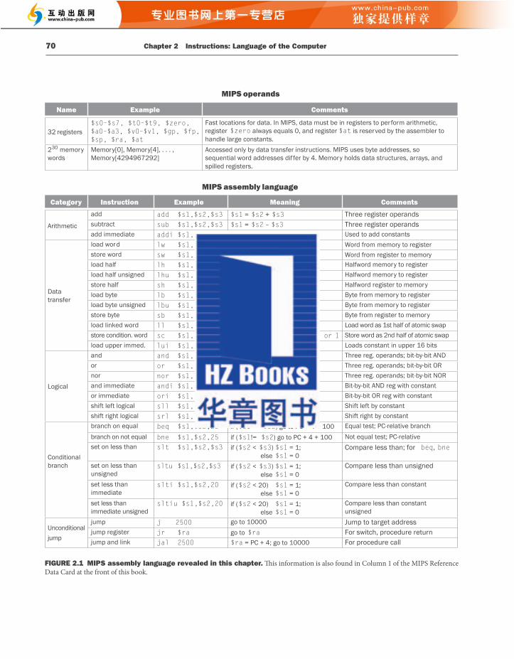
2.2 Operations of the Computer Hardware 71
EXAMPLE
EXAMPLE
instruction. Another diff erence from C is that comments always terminate at the end of a line.
Th e natural number of operands for an operation like addition is three: the two numbers being added together and a place to put the sum. Requiring every instruction to have exactly three operands, no more and no less, conforms to the philosophy of keeping the hardware simple: hardware for a variable number of operands is more complicated than hardware for a fi xed number. Th is situation illustrates the fi rst of three underlying principles of hardware design:
Design Principle 1: Simplicity favors regularity. We can now show, in the two examples that follow, the relationship of programs
written in higher-level programming languages to programs in this more primitive notation.
Compiling Two C Assignment Statements into MIPS
Th is segment of a C program contains the fi ve variables a , b , c , d , and e . Since Java evolved from C, this example and the next few work for either high-level programming language:
a = b + c; d = a – e;
Th e translation from C to MIPS assembly language instructions is performed by the compiler . Show the MIPS code produced by a compiler.
A MIPS instruction operates on two source operands and places the result in one destination operand. Hence, the two simple statements above compile directly into these two MIPS assembly language instructions:
add a, b, c sub d, a, e
Compiling a Complex C Assignment into MIPS
A somewhat complex statement contains the fi ve variables f , g , h , i , and j :
f = (g + h) – (i + j);
What might a C compiler produce?
ANSWER
70 Chapter 2 Instructions: Language of the Computer
MIPS operands
Name Example Comments
32 registers$s0–$s7, $t0–$t9, $zero, $a0–$a3, $v0–$v1, $gp, $fp, $sp, $ra, $at
Fast locations for data. In MIPS, data must be in registers to perform arithmetic, register $zero always equals 0, and register $at is reserved by the assembler to handle large constants.
230 memory words
Memory[0], Memory[4], . . . , Memory[4294967292]
Accessed only by data transfer instructions. MIPS uses byte addresses, so sequential word addresses differ by 4. Memory holds data structures, arrays, and spilled registers.
MIPS assembly language
Category Instruction Example Meaning Comments
Arithmetic
add add $s1,$s2,$s3 $s1 = $s2 + $s3 Three register operandssubtract sub $s1,$s2,$s3 $s1 = $s2 – $s3 Three register operandsadd immediate addi $s1,$s2,20 $s1 = $s2 + 20 Used to add constants
Data transfer
load word lw $s1,20($s2) $s1 = Memory[$s2 + 20] Word from memory to registerstore word sw $s1,20($s2) Memory[$s2 + 20] = $s1 Word from register to memoryload half lh $s1,20($s2) $s1 = Memory[$s2 + 20] Halfword memory to registerload half unsigned lhu $s1,20($s2) $s1 = Memory[$s2 + 20] Halfword memory to registerstore half sh $s1,20($s2) Memory[$s2 + 20] = $s1 Halfword register to memoryload byte lb $s1,20($s2) $s1 = Memory[$s2 + 20] Byte from memory to registerload byte unsigned lbu $s1,20($s2) $s1 = Memory[$s2 + 20] Byte from memory to registerstore byte sb $s1,20($s2) Memory[$s2 + 20] = $s1 Byte from register to memoryload linked word ll $s1,20($s2) $s1 = Memory[$s2 + 20] Load word as 1st half of atomic swap store condition. word sc $s1,20($s2) Memory[$s2+20]=$s1;$s1=0 or 1 Store word as 2nd half of atomic swap load upper immed. lui $s1,20 $s1
$s1$s1$s1$s1$s1$s1$s1
= 20 * 2 16 Loads constant in upper 16 bits
Logical
and and $s1,$s2,$s3 = $s2 & $s3 Three reg. operands; bit-by-bit ANDor or $s1,$s2,$s3 = $s2 | $s3 Three reg. operands; bit-by-bit ORnor nor $s1,$s2,$s3 = ~ ($s2 | $s3) Three reg. operands; bit-by-bit NORand immediate andi $s1,$s2,20 = $s2 & 20 Bit-by-bit AND reg with constantor immediate ori $s1,$s2,20 = $s2 | 20 Bit-by-bit OR reg with constantshift left logical sll $s1,$s2,10 = $s2 << 10 Shift left by constantshift right logical srl $s1,$s2,10 = $s2 >> 10 Shift right by constant
Conditional branch
branch on equal beq $s1,$s2,25 if ($s1 == $s2) go to PC + 4 + 100 Equal test; PC-relative branchbranch on not equal bne $s1,$s2,25 if ($s1!= $s2) go to PC + 4 + 100 Not equal test; PC-relative set on less than slt $s1,$s2,$s3 if ($s2 < $s3) $s1 = 1;
else $s1 = 0Compare less than; for beq, bne
set on less than unsigned
sltu if ($s2 < $s3) $s1 = 1; else $s1 = 0
Compare less than unsigned
set less than immediate
slti $s1,$s2,20 if ($s2 < 20) $s1 = 1; else $s1 = 0
Compare less than constant
set less than immediate unsigned
sltiu $s1,$s2,20 if ($s2 < 20) $s1 = 1; else $s1 = 0
Compare less than constant unsigned
Unconditional jump
jump j 2500 go to 10000 Jump to target addressjump register jr $ra go to $ra For switch, procedure returnjump and link jal 2500 $ra = PC + 4; go to 10000 For procedure call
$s1,$s2,$s3
FIGURE 2.1 MIPS assembly language revealed in this chapter. Th is information is also found in Column 1 of the MIPS Reference Data Card at the front of this book.

2.3 Operands of the Computer Hardware 73
One major diff erence between the variables of a programming language and registers is the limited number of registers, typically 32 on current computers, like MIPS. (See Section 2.23 for the history of the number of registers.) Th us, continuing in our top-down, stepwise evolution of the symbolic representation of the MIPS language, in this section we have added the restriction that the three operands of MIPS arithmetic instructions must each be chosen from one of the 32 32-bit registers.
Th e reason for the limit of 32 registers may be found in the second of our three underlying design principles of hardware technology:
Design Principle 2: Smaller is faster. A very large number of registers may increase the clock cycle time simply because it takes electronic signals longer when they must travel farther.
Guidelines such as “smaller is faster” are not absolutes; 31 registers may not be faster than 32. Yet, the truth behind such observations causes computer designers to take them seriously. In this case, the designer must balance the craving of programs for more registers with the designer’s desire to keep the clock cycle fast. Another reason for not using more than 32 is the number of bits it would take in the instruction format, as Section 2.5 demonstrates.
Chapter 4 shows the central role that registers play in hardware construction; as we shall see in this chapter, eff ective use of registers is critical to program performance.
Although we could simply write instructions using numbers for registers, from 0 to 31, the MIPS convention is to use two-character names following a dollar sign to represent a register. Section 2.8 will explain the reasons behind these names. For now, we will use $s0, $s1, … for registers that correspond to variables in C and Java programs and $t0, $t1, … for temporary registers needed to compile the program into MIPS instructions.
Compiling a C Assignment Using Registers
It is the compiler’s job to associate program variables with registers. Take, for instance, the assignment statement from our earlier example:
f=(g + h) – (i + j);
Th e variables f , g , h , i , and j are assigned to the registers $s0 , $s1 , $s2 , $s3 , and $s4 , respectively. What is the compiled MIPS code?
EXAMPLE
72 Chapter 2 Instructions: Language of the Computer
Elaboration : To increase portability, Java was originally envisioned as relying on a software interpreter. The instruction set of this interpreter is called Java bytecodes (see Section 2.15 ), which is quite different from the MIPS instruction set. To get performance close to the equivalent C program, Java systems today typically compile Java bytecodes into the native instruction sets like MIPS. Because this compilation is normally done much later than for C programs, such Java compilers are often called Just In Time (JIT) compilers. Section 2.12 shows how JITs are used later than C compilers in the start-up process, and Section 2.13 shows the performance consequences of compiling versus interpreting Java programs.
ANSWER Th e compiler must break this statement into several assembly instructions, since only one operation is performed per MIPS instruction. Th e fi rst MIPS instruction calculates the sum of g and h . We must place the result somewhere, so the compiler creates a temporary variable, called t0 :
add t0,g,h # temporary variable t0 contains g + h
Although the next operation is subtract, we need to calculate the sum of i and j before we can subtract. Th us, the second instruction places the sum of i and j in another temporary variable created by the compiler, called t1 :
add t1,i,j # temporary variable t1 contains i + j
Finally, the subtract instruction subtracts the second sum from the fi rst and places the diff erence in the variable f , completing the compiled code:
sub f,t0,t1 # f gets t0 – t1, which is (g + h) – (i + j)
For a given function, which programming language likely takes the most lines of code? Put the three representations below in order.
1. Java
2. C
3. MIPS assembly language
Check Yourself
2.3 Operands of the Computer Hardware
Unlike programs in high-level languages, the operands of arithmetic instructions are restricted; they must be from a limited number of special locations built directly in hardware called registers . Registers are primitives used in hardware design that are also visible to the programmer when the computer is completed, so you can think of registers as the bricks of computer construction. Th e size of a register in the MIPS architecture is 32 bits; groups of 32 bits occur so frequently that they are given the name word in the MIPS architecture.
word Th e natural unit of access in a computer, usually a group of 32 bits; corresponds to the size of a register in the MIPS architecture.
2.3 Operands of the Computer Hardware 75
Hardware/Software Interface
EXAMPLE
ANSWER
Compiling an Assignment When an Operand Is in Memory
Let’s assume that A is an array of 100 words and that the compiler has associated the variables g and h with the registers $s1 and $s2 as before. Let’s also assume that the starting address, or base address, of the array is in $s3 . Compile this C assignment statement:
g = h + A[8];
Although there is a single operation in this assignment statement, one of the operands is in memory, so we must fi rst transfer A[8] to a register. Th e address of this array element is the sum of the base of the array A , found in register $s3 , plus the number to select element 8. Th e data should be placed in a temporary register for use in the next instruction. Based on Figure 2.2 , the fi rst compiled instruction is
lw $t0,8($s3) # Temporary reg $t0 gets A[8]
(On the next page we’ll make a slight adjustment to this instruction, but we’ll use this simplifi ed version for now.) Th e following instruction can operate on the value in $t0 (which equals A[8] ) since it is in a register. Th e instruction must add h (contained in ($2 ) to A[8] (contained in $t0) and put the sum in the register corresponding to g (associated with $s1 ):
add $s1,$s2,$t0 # g = h + A[8]
Th e constant in a data transfer instruction (8) is called the off set, and the register added to form the address ( $s3 ) is called the base register .
In addition to associating variables with registers, the compiler allocates data structures like arrays and structures to locations in memory. Th e compiler can then place the proper starting address into the data transfer instructions.
Since 8-bit bytes are useful in many programs, virtually all architectures today address individual bytes. Th erefore, the address of a word matches the address of one of the 4 bytes within the word, and addresses of sequential words diff er by 4. For example, Figure 2.3 shows the actual MIPS addresses for the words in Figure 2.2 ; the byte address of the third word is 8.
In MIPS, words must start at addresses that are multiples of 4. Th is requirement is called an alignment restriction , and many architectures have it. ( Chapter 4 suggests why alignment leads to faster data transfers.)
alignment restriction A requirement that data be aligned in memory on natural boundaries.
74 Chapter 2 Instructions: Language of the Computer
ANSWER
data transfer instruction A command that moves data between memory and registers.
address A value used to delineate the location of a specifi c data element within a memory array.
Processor Memory
Address Data
1
101
10
100
0
1
2
3
FIGURE 2.2 Memory addresses and contents of memory at those locations. If these elements were words, these addresses would be incorrect, since MIPS actually uses byte addressing, with each word representing four bytes. Figure 2.3 shows the memory addressing for sequential word addresses.
Th e data transfer instruction that copies data from memory to a register is traditionally called load . Th e format of the load instruction is the name of the operation followed by the register to be loaded, then a constant and register used to access memory. Th e sum of the constant portion of the instruction and the contents of the second register forms the memory address. Th e actual MIPS name for this instruction is lw, standing for load word .
Th e compiled program is very similar to the prior example, except we replace the variables with the register names mentioned above plus two temporary registers, $t0 and $t1 , which correspond to the temporary variables above:
Memory Operands Programming languages have simple variables that contain single data elements, as in these examples, but they also have more complex data structures—arrays and structures. Th ese complex data structures can contain many more data elements than there are registers in a computer. How can a computer represent and access such large structures?
Recall the fi ve components of a computer introduced in Chapter 1 and repeated on page 67. Th e processor can keep only a small amount of data in registers, but computer memory contains billions of data elements. Hence, data structures (arrays and structures) are kept in memory.
As explained above, arithmetic operations occur only on registers in MIPS instructions; thus, MIPS must include instructions that transfer data between memory and registers. Such instructions are called data transfer instructions . To access a word in memory, the instruction must supply the memory address . Memory is just a large, single-dimensional array, with the address acting as the index to that array, starting at 0. For example, in Figure 2.2 , the address of the third data element is 2, and the value of Memory[2] is 10.

2.3 Operands of the Computer Hardware 77
Compiling Using Load and Store
Assume variable h is associated with register $s2 and the base address of the array A is in $s3 . What is the MIPS assembly code for the C assignment statement below?
A[12] = h + A[8];
Although there is a single operation in the C statement, now two of the operands are in memory, so we need even more MIPS instructions. Th e fi rst two instructions are the same as the prior example, except this time we use the proper off set of 32 for byte addressing in the load word instruction to select A[8] , and the add instruction places the sum in $t0 :
lw $t0,32($s3) # Temporary reg $t0 gets A[8] add $t0,$s2,$t0 # Temporary reg $t0 gets h + A[8]
Th e fi nal instruction stores the sum into A[12] , using 48 (4 × 12) as the off set and register $s3 as the base register.
sw $t0,48($s3) # Stores h + A[8] back into A[12]
Load word and store word are the instructions that copy words between memory and registers in the MIPS architecture. Other brands of computers use other instructions along with load and store to transfer data. An architecture with such alternatives is the Intel x86, described in Section 2.19 .
Many programs have more variables than computers have registers. Consequently, the compiler tries to keep the most frequently used variables in registers and places the rest in memory, using loads and stores to move variables between registers and memory. Th e process of putting less commonly used variables (or those needed later) into memory is called spilling registers.
Th e hardware principle relating size and speed suggests that memory must be slower than registers, since there are fewer registers. Th is is indeed the case; data accesses are faster if data is in registers instead of memory.
Moreover, data is more useful when in a register. A MIPS arithmetic instruction can read two registers, operate on them, and write the result. A MIPS data transfer instruction only reads one operand or writes one operand, without operating on it.
Th us, registers take less time to access and have higher throughput than memory, making data in registers both faster to access and simpler to use. Accessing registers also uses less energy than accessing memory. To achieve highest performance and conserve energy, an instruction set architecture must have a suffi cient number of registers, and compilers must use registers effi ciently.
Hardware/Software Interface
EXAMPLE
ANSWER
76 Chapter 2 Instructions: Language of the Computer
Computers divide into those that use the address of the left most or “big end” byte as the word address versus those that use the rightmost or “little end” byte. MIPS is in the big-endian camp. Since the order matters only if you access the identical data both as a word and as four bytes, few need to be aware of the endianess. (Appendix A shows the two options to number bytes in a word.)
Byte addressing also aff ects the array index. To get the proper byte address in the code above, the off set to be added to the base register $s3 must be 4 × 8, or 32, so that the load address will select A[8] and not A[8/4] . (See the related pitfall on page 168 of Section 2.21 .)
Th e instruction complementary to load is traditionally called store; it copies data from a register to memory. Th e format of a store is similar to that of a load: the name of the operation, followed by the register to be stored, then off set to select the array element, and fi nally the base register. Once again, the MIPS address is specifi ed in part by a constant and in part by the contents of a register. Th e actual MIPS name is sw , standing for store word .
As the addresses in loads and stores are binary numbers, we can see why the DRAM for main memory comes in binary sizes rather than in decimal sizes. Th at is, in gebibytes (2 30 ) or tebibytes (2 40 ), not in gigabytes (10 9 ) or terabytes (10 12 ); see Figure 1.1.
Processor Memory
Byte Address Data
1
101
10
100
0
4
8
12
FIGURE 2.3 Actual MIPS memory addresses and contents of memory for those words. Th e changed addresses are highlighted to contrast with Figure 2.2. Since MIPS addresses each byte, word addresses are multiples of 4: there are 4 bytes in a word.
Hardware/Software Interface
2.4 Signed and Unsigned Numbers 79
Elaboration : The MIPS offset plus base register addressing is an excellent match to structures as well as arrays, since the register can point to the beginning of the structure and the offset can select the desired element. We’ll see such an example in Section 2.13 .
Elaboration : The register in the data transfer instructions was originally invented to hold an index of an array with the offset used for the starting address of an array. Thus, the base register is also called the index register . Today’s memories are much larger and the software model of data allocation is more sophisticated, so the base address of the array is normally passed in a register since it won’t fi t in the offset, as we shall see.
Elaboration : Since MIPS supports negative constants, there is no need for subtract immediate in MIPS.
2.4 Signed and Unsigned Numbers
First, let’s quickly review how a computer represents numbers. Because people have 10 fi ngers, we are taught to think in base 10, but numbers may be represented in any base. For example, 123 base 10 = 1111011 base 2.
Numbers are kept in computer hardware as a series of high and low electronic signals, and so they are considered base 2 numbers. (Just as base 10 numbers are called decimal numbers, base 2 numbers are called binary numbers.)
A single digit of a binary number is thus the “atom” of computing, since all information is composed of binary digits or bits . Th is fundamental building block can be one of two values, which can be thought of as several alternatives: high or low, on or off , true or false, or 1 or 0.
Generalizing the point, in any number base, the value of i th digit d is
d i� Base
where i starts at 0 and increases from right to left . Th is representation leads to an obvious way to number the bits in the word: simply use the power of the base for that bit. We subscript decimal numbers with ten and binary numbers with two . For example,
1011 two
represents
binary digit Also called binary bit . One of the two numbers in base 2, 0 or 1, that are the components of information.
78 Chapter 2 Instructions: Language of the Computer
Constant or Immediate Operands Many times a program will use a constant in an operation—for example, incrementing an index to point to the next element of an array. In fact, more than half of the MIPS arithmetic instructions have a constant as an operand when running the SPEC CPU2006 benchmarks.
Using only the instructions we have seen so far, we would have to load a constant from memory to use one. (Th e constants would have been placed in memory when the program was loaded.) For example, to add the constant 4 to register $s3 , we could use the code
lw $t0, AddrConstant4($s1) # $t0 = constant 4 add $s3,$s3,$t0 # $s3 = $s3 + $t0 ($t0 == 4)
assuming that $s1 + AddrConstant4 is the memory address of the constant 4. An alternative that avoids the load instruction is to off er versions of the arithmetic
instructions in which one operand is a constant. Th is quick add instruction with one constant operand is called add immediate or addi . To add 4 to register $s3 , we just write
addi $s3,$s3,4 # $s3 = $s3 + 4
Constant operands occur frequently, and by including constants inside arithmetic instructions, operations are much faster and use less energy than if constants were loaded from memory.
Th e constant zero has another role, which is to simplify the instruction set by off ering useful variations. For example, the move operation is just an add instruction where one operand is zero. Hence, MIPS dedicates a register $zero to be hard-wired to the value zero. (As you might expect, it is register number 0.) Using frequency to justify the inclusions of constants is another example of the great idea of making the common case fast .
Given the importance of registers, what is the rate of increase in the number of registers in a chip over time?
1. Very fast: Th ey increased as fast as Moore’s law, which predicted doubling the number of transistors on a chip every 24 months.
2. Very slow: Since programs are usually distributed in the language of the computer, there is inertia in instruction set architecture, and so the number of registers increases only as fast as new instruction sets become viable.
Check Yourself
Elaboration : Although the MIPS registers in this book are 32 bits wide, there is a 64-bit version of the MIPS instruction set with 32 64-bit registers. To keep them straight, they are offi cially called MIPS-32 and MIPS-64. In this chapter, we use a subset of MIPS-32. Appendix E shows the differences between MIPS-32 and MIPS-64. Sections 2.16 and 2.17 show the much more dramatic difference between the 32-bit address ARMv7 and its 64-bit successor, ARMv8.

2.4 Signed and Unsigned Numbers 81
It’s up to the programming language, the operating system, and the program to determine what to do if overfl ow occurs.
Computer programs calculate both positive and negative numbers, so we need a representation that distinguishes the positive from the negative. Th e most obvious solution is to add a separate sign, which conveniently can be represented in a single bit; the name for this representation is sign and magnitude .
Alas, sign and magnitude representation has several shortcomings. First, it’s not obvious where to put the sign bit. To the right? To the left ? Early computers tried both. Second, adders for sign and magnitude may need an extra step to set the sign because we can’t know in advance what the proper sign will be. Finally, a separate sign bit means that sign and magnitude has both a positive and a negative zero, which can lead to problems for inattentive programmers. As a result of these shortcomings, sign and magnitude representation was soon abandoned.
In the search for a more attractive alternative, the question arose as to what would be the result for unsigned numbers if we tried to subtract a large number from a small one. Th e answer is that it would try to borrow from a string of leading 0s, so the result would have a string of leading 1s.
Given that there was no obvious better alternative, the fi nal solution was to pick the representation that made the hardware simple: leading 0s mean positive, and leading 1s mean negative. Th is convention for representing signed binary numbers is called two’s complement representation (an Elaboration on page 85 explains this unusual name):
Th e positive half of the numbers, from 0 to 2,147,483,647 ten (2 31 −1), use the same representation as before. Th e following bit pattern (1000 … 0000 two ) represents the most negative number −2,147,483,648 ten (−2 31 ). It is followed by a declining set of negative numbers: −2,147,483,647 ten (1000 … 0001 two ) down to −1 ten (1111 … 1111 two ).
Two’s complement does have one negative number, −2,147,483,648 ten , that has no corresponding positive number. Such imbalance was also a worry to the inattentive programmer, but sign and magnitude had problems for both the programmer and the hardware designer. Consequently, every computer today uses two’s complement binary representations for signed numbers.
80 Chapter 2 Instructions: Language of the Computer
We number the bits 0, 1, 2, 3, . . . from right to left in a word. Th e drawing below shows the numbering of bits within a MIPS word and the placement of the number 1011 two :
Since words are drawn vertically as well as horizontally, left most and rightmost may be unclear. Hence, the phrase least signifi cant bit is used to refer to the right-most bit (bit 0 above) and most signifi cant bit to the left most bit (bit 31).
Th e MIPS word is 32 bits long, so it can represent 2 32 diff erent 32-bit patterns. It is natural to let these combinations represent the numbers from 0 to 2 32 −1 (4,294,967,295 ten ):
Th at is, 32-bit binary numbers can be represented in terms of the bit value times a power of 2 (here xi means the i th bit of x ):
( ) ( ) ( ) ( ) ( )x x x x x31 2 30 2 29 2 1 2 0 231 30 29 1 0… For reasons we will shortly see, these positive numbers are called unsigned numbers.
Base 2 is not natural to human beings; we have 10 fi ngers and so fi nd base 10 natural. Why didn’t computers use decimal? In fact, the fi rst commercial computer did off er decimal arithmetic. Th e problem was that the computer still used on and off signals, so a decimal digit was simply represented by several binary digits. Decimal proved so ineffi cient that subsequent computers reverted to all binary, converting to base 10 only for the relatively infrequent input/output events.
Keep in mind that the binary bit patterns above are simply representatives of numbers. Numbers really have an infi nite number of digits, with almost all being 0 except for a few of the rightmost digits. We just don’t normally show leading 0s.
Hardware can be designed to add, subtract, multiply, and divide these binary bit patterns. If the number that is the proper result of such operations cannot be represented by these rightmost hardware bits, overfl ow is said to have occurred.
least signifi cant bit Th e rightmost bit in a MIPS word.
most signifi cant bit Th e left most bit in a MIPS word.
Hardware/Software Interface
Overfl ow When the results of an operation are larger than can be represented in a register.
2.4 Signed and Unsigned Numbers 83
Unlike the numbers discussed above, memory addresses naturally start at 0 and continue to the largest address. Put another way, negative addresses make no sense. Th us, programs want to deal sometimes with numbers that can be positive or negative and sometimes with numbers that can be only positive. Some programming languages refl ect this distinction. C, for example, names the former integers (declared as int in the program) and the latter unsigned integers ( unsigned int ). Some C style guides even recommend declaring the former as signed int to keep the distinction clear.
Let’s examine two useful shortcuts when working with two’s complement numbers. Th e fi rst shortcut is a quick way to negate a two’s complement binary number. Simply invert every 0 to 1 and every 1 to 0, then add one to the result. Th is shortcut is based on the observation that the sum of a number and its inverted representation must be 111 … 111 two , which represents −1. Since x x 1 , therefore x x 1 0 or x x1 − . (We use the notation x to mean invert every bit in x from 0 to 1 and vice versa.)
Negation Shortcut
Negate 2 ten , and then check the result by negating −2 ten .
2 ten =0000 0000 0000 0000 0000 0000 0000 0010 two
Negating this number by inverting the bits and adding one,
Going the other direction,
1111 1111 1111 1111 1111 1111 1111 1110 two
is fi rst inverted and then incremented:
Hardware/Software Interface
EXAMPLE
ANSWER
82 Chapter 2 Instructions: Language of the Computer
Two’s complement representation has the advantage that all negative numbers have a 1 in the most signifi cant bit. Hardware needs to test only this bit to see if a number is positive or negative (with the number 0 considered positive). Th is bit is oft en called the sign bit . By recognizing the role of the sign bit, we can represent positive and negative 32-bit numbers in terms of the bit value times a power of 2:
( ) ( ) ( ) ( ) ( )x x x x x31 2 30 2 29 2 1 2 0 231 30 29 1 0+ …
Th e sign bit is multiplied by −2 31 , and the rest of the bits are then multiplied by positive versions of their respective base values.
Binary to Decimal Conversion
What is the decimal value of this 32-bit two’s complement number?
1111 1111 1111 1111 1111 1111 1111 1100 two
Substituting the number’s bit values into the formula above:
( ) ( ) ( ) ( ) ( ) ( )1 2 1 2 1 2 1 2 0 2 0 2
2 2 2
31 30 29 2 1 0
31 30…
229 22 0 02 147 483 648 2 147 483 6444
…, , , , , ,te tn enten
We’ll see a shortcut to simplify conversion from negative to positive soon.
Just as an operation on unsigned numbers can overfl ow the capacity of hardware to represent the result, so can an operation on two’s complement numbers. Overfl ow occurs when the left most retained bit of the binary bit pattern is not the same as the infi nite number of digits to the left (the sign bit is incorrect): a 0 on the left of the bit pattern when the number is negative or a 1 when the number is positive.
Signed versus unsigned applies to loads as well as to arithmetic. Th e function of a signed load is to copy the sign repeatedly to fi ll the rest of the register—called sign extension —but its purpose is to place a correct representation of the number within that register. Unsigned loads simply fi ll with 0 s to the left of the data, since the number represented by the bit pattern is unsigned.
When loading a 32-bit word into a 32-bit register, the point is moot; signed and unsigned loads are identical. MIPS does off er two fl avors of byte loads: load byte ( lb ) treats the byte as a signed number and thus sign-extends to fi ll the 24 left -most bits of the register, while load byte unsigned ( lbu ) works with unsigned integers. Since C programs almost always use bytes to represent characters rather than consider bytes as very short signed integers, lbu is used practically exclusively for byte loads.
EXAMPLE
ANSWER
Hardware/Software Interface
2.4 Signed and Unsigned Numbers 85
Summary Th e main point of this section is that we need to represent both positive and negative integers within a computer word, and although there are pros and cons to any option, the unanimous choice since 1965 has been two’s complement.
What is the decimal value of this 64-bit two’s complement number?
What is the decimal value if it is instead a 64-bit unsigned number?
A fi nal notation, which we will look at when we discuss fl oating point in Chapter 3 , is to represent the most negative value by 00 … 000 two and the most positive value by 11 … 11 two , with 0 typically having the value 10 … 00 two . This is called a biased notation , since it biases the number such that the number plus the bias has a non-negative representation.
Elaboration : For signed decimal numbers, we used “−” to represent negative because there are no limits to the size of a decimal number. Given a fi xed word size, binary and hexadecimal (see Figure 2.4 ) bit strings can encode the sign; hence we do not normally use “+” or “−” with binary or hexadecimal notation.
Check Yourself
Elaboration : Two’s complement gets its name from the rule that the unsigned sum of an n -bit number and its n-bit negative is 2 n ; hence, the negation or complement of a number x is 2 n − x , or its “two’s complement.”
A third alternative representation to two’s complement and sign and magnitude is called one’s complement . The negative of a one’s complement is found by inverting each bit, from 0 to 1 and from 1 to 0, or x . This relation helps explain its name since the complement of x is 2 n − × −1. It was also an attempt to be a better solution than sign and magnitude, and several early scientifi c computers did use the notation. This representation is similar to two’s complement except that it also has two 0s: 00 … 00 two is positive 0 and 11 … 11 two is negative 0. The most negative number, 10 … 000 two , represents −2,147,483,647 ten , and so the positives and negatives are balanced. One’s complement adders did need an extra step to subtract a number, and hence two’s complement dominates today.
one’s complement A notation that represents the most negative value by 10 … 000 two and the most positive value by 01 … 11 two , leaving an equal number of negatives and positives but ending up with two zeros, one positive (00 … 00 two ) and one negative (11 … 11 two ). Th e term is also used to mean the inversion of every bit in a pattern: 0 to 1 and 1 to 0.
biased notation A notation that represents the most negative value by 00 … 000 two and the most positive value by 11 … 11 two , with 0 typically having the value 10 … 00 two , thereby biasing the number such that the number plus the bias has a nonnegative representation.
84 Chapter 2 Instructions: Language of the Computer
Our next shortcut tells us how to convert a binary number represented in n bits to a number represented with more than n bits. For example, the immediate fi eld in the load, store, branch, add, and set on less than instructions contains a two’s complement 16-bit number, representing −32,768 ten (−2 15 ) to 32,767 ten (2 15 −1). To add the immediate fi eld to a 32-bit register, the computer must convert that 16-bit number to its 32-bit equivalent. Th e shortcut is to take the most signifi cant bit from the smaller quantity—the sign bit—and replicate it to fi ll the new bits of the larger quantity. Th e old nonsign bits are simply copied into the right portion of the new word. Th is shortcut is called sign extension .
Sign Extension Shortcut
Convert 16-bit binary versions of 2 ten and −2 ten to 32-bit binary numbers.
Th e 16-bit binary version of the number 2 is
0000 0000 0000 0010 two =2 ten
It is converted to a 32-bit number by making 16 copies of the value in the most signifi cant bit (0) and placing that in the left -hand half of the word. Th e right half gets the old value:
0000 0000 0000 0000 0000 0000 0000 0010 two = 2 ten
Let’s negate the 16-bit version of 2 using the earlier shortcut. Th us,
0000 0000 0000 0010 two
becomes
Creating a 32-bit version of the negative number means copying the sign bit 16 times and placing it on the left :
1111 1111 1111 1111 1111 1111 1111 1110 two = –2 ten
Th is trick works because positive two’s complement numbers really have an infi nite number of 0s on the left and negative two’s complement numbers have an infi nite number of 1s. Th e binary bit pattern representing a number hides leading bits to fi t the width of the hardware; sign extension simply restores some of them.
EXAMPLE
ANSWER
2.5 Representing Instructions in the Computer 87
Th is layout of the instruction is called the instruction format . As you can see from counting the number of bits, this MIPS instruction takes exactly 32 bits—the same size as a data word. In keeping with our design principle that simplicity favors regularity, all MIPS instructions are 32 bits long.
To distinguish it from assembly language, we call the numeric version of instructions machine language and a sequence of such instructions machine code .
It would appear that you would now be reading and writing long, tedious strings of binary numbers. We avoid that tedium by using a higher base than binary that converts easily into binary. Since almost all computer data sizes are multiples of 4, hexadecimal (base 16) numbers are popular. Since base 16 is a power of 2, we can trivially convert by replacing each group of four binary digits by a single hexadecimal digit, and vice versa. Figure 2.4 converts between hexadecimal and binary.
instruction format A form of representation of an instruction composed of fi elds of binary numbers.
machine language Binary representation used for communication within a computer system.
hexadecimal Numbers in base 16.
Hexadecimal Binary Hexadecimal Binary Hexadecimal Binary Hexadecimal Binary
0hex 0000two 4hex 0100two 8hex 1000two chex 1100two
1hex 0001two 5hex 0101two 9hex 1001two dhex 1101two
2hex 0010two 6hex 0110two ahex 1010two ehex 1110two
3hex 0011two 7hex 0111two bhex 1011two fhex 1111two
FIGURE 2.4 The hexadecimal-binary conversion table. Just replace one hexadecimal digit by the corresponding four binary digits, and vice versa. If the length of the binary number is not a multiple of 4, go from right to left .
Because we frequently deal with diff erent number bases, to avoid confusion we will subscript decimal numbers with ten , binary numbers with two , and hexadecimal numbers with hex . (If there is no subscript, the default is base 10.) By the way, C and Java use the notation 0x nnnn for hexadecimal numbers.
Binary to Hexadecimal and Back
Convert the following hexadecimal and binary numbers into the other base:
eca8 6420 hex
0001 0011 0101 0111 1001 1011 1101 1111 two
EXAMPLE
86 Chapter 2 Instructions: Language of the Computer
2.5 Representing Instructions in the Computer
We are now ready to explain the diff erence between the way humans instruct computers and the way computers see instructions.
Instructions are kept in the computer as a series of high and low electronic signals and may be represented as numbers. In fact, each piece of an instruction can be considered as an individual number, and placing these numbers side by side forms the instruction.
Since registers are referred to by almost all instructions, there must be a convention to map register names into numbers. In MIPS assembly language, registers $s0 to $s7 map onto registers 16 to 23, and registers $t0 to $t7 map onto registers 8 to 15. Hence, $s0 means register 16, $s1 means register 17, $s2 means register 18,…, $t0 means register 8, $t1 means register 9, and so on. We’ll describe the convention for the rest of the 32 registers in the following sections.
Translating a MIPS Assembly Instruction into a Machine Instruction
Let’s do the next step in the refi nement of the MIPS language as an example. We’ll show the real MIPS language version of the instruction represented symbolically as
add $t0,$s1,$s2
fi rst as a combination of decimal numbers and then of binary numbers.
Th e decimal representation is
Each of these segments of an instruction is called a fi eld . Th e fi rst and last
fi elds (containing 0 and 32 in this case) in combination tell the MIPS computer that this instruction performs addition. Th e second fi eld gives the number of the register that is the fi rst source operand of the addition operation (17= $s1 ), and the third fi eld gives the other source operand for the addition (18= $s2 ). Th e fourth fi eld contains the number of the register that is to receive the sum (8= $t0 ). Th e fi ft h fi eld is unused in this instruction, so it is set to 0. Th us, this instruction adds register $s1 to register $s2 and places the sum in register $t0 .
Th is instruction can also be represented as fi elds of binary numbers as opposed to decimal:
EXAMPLE
ANSWER
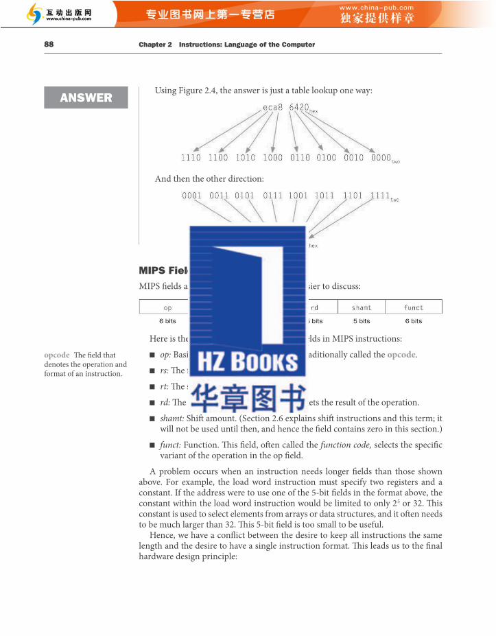
2.5 Representing Instructions in the Computer 89
Design Principle 3: Good design demands good compromises. Th e compromise chosen by the MIPS designers is to keep all instructions the
same length, thereby requiring diff erent kinds of instruction formats for diff erent kinds of instructions. For example, the format above is called R-type (for register) or R-format . A second type of instruction format is called I-type (for immediate) or I-format and is used by the immediate and data transfer instructions. Th e fi elds of I-format are
Th e 16-bit address means a load word instruction can load any word within
a region of ±2 15 or 32,768 bytes (±2 13 or 8192 words) of the address in the base register rs. Similarly, add immediate is limited to constants no larger than ±2 15 . We see that more than 32 registers would be diffi cult in this format, as the rs and rt fi elds would each need another bit, making it harder to fi t everything in one word.
Let’s look at the load word instruction from page 77:
lw $t0,32($s3) # Temporary reg $t0 gets A[8]
Here, 19 (for $s3 ) is placed in the rs fi eld, 8 (for $t0 ) is placed in the rt fi eld, and 32 is placed in the address fi eld. Note that the meaning of the rt fi eld has changed for this instruction: in a load word instruction, the rt fi eld specifi es the destination register, which receives the result of the load.
Although multiple formats complicate the hardware, we can reduce the complexity by keeping the formats similar. For example, the fi rst three fi elds of the R-type and I-type formats are the same size and have the same names; the length of the fourth fi eld in I-type is equal to the sum of the lengths of the last three fi elds of R-type.
In case you were wondering, the formats are distinguished by the values in the fi rst fi eld: each format is assigned a distinct set of values in the fi rst fi eld (op) so that the hardware knows whether to treat the last half of the instruction as three fi elds (R-type) or as a single fi eld (I-type). Figure 2.5 shows the numbers used in each fi eld for the MIPS instructions covered so far.
Instruction Format op rs rt rd shamt funct address
add R 0 reg reg reg 0 32ten n.a.
sub (subtract) R 0 reg reg reg 0 34ten n.a.
add immediate I 8ten reg reg n.a. n.a. n.a. constant
lw (load word) I 35ten reg reg n.a. n.a. n.a. address
sw (store word) I 43ten reg reg n.a. n.a. n.a. address
FIGURE 2.5 MIPS instruction encoding. In the table above, “reg” means a register number between 0 and 31, “address” means a 16-bit address, and “n.a.” (not applicable) means this fi eld does not appear in this format. Note that add and sub instructions have the same value in the op fi eld; the hardware uses the funct fi eld to decide the variant of the operation: add (32) or subtract (34).
88 Chapter 2 Instructions: Language of the Computer
Using Figure 2.4 , the answer is just a table lookup one way:
And then the other direction:
MIPS Fields MIPS fi elds are given names to make them easier to discuss:
Here is the meaning of each name of the fi elds in MIPS instructions:
■ op: Basic operation of the instruction, traditionally called the opcode .
■ rs: Th e fi rst register source operand.
■ rt: Th e second register source operand.
■ rd: Th e register destination operand. It gets the result of the operation.
■ shamt: Shift amount. ( Section 2.6 explains shift instructions and this term; it will not be used until then, and hence the fi eld contains zero in this section.)
■ funct: Function. Th is fi eld, oft en called the function code, selects the specifi c variant of the operation in the op fi eld.
A problem occurs when an instruction needs longer fi elds than those shown above. For example, the load word instruction must specify two registers and a constant. If the address were to use one of the 5-bit fi elds in the format above, the constant within the load word instruction would be limited to only 2 5 or 32. Th is constant is used to select elements from arrays or data structures, and it oft en needs to be much larger than 32. Th is 5-bit fi eld is too small to be useful.
Hence, we have a confl ict between the desire to keep all instructions the same length and the desire to have a single instruction format. Th is leads us to the fi nal hardware design principle:
opcode Th e fi eld that denotes the operation and format of an instruction.
ANSWER
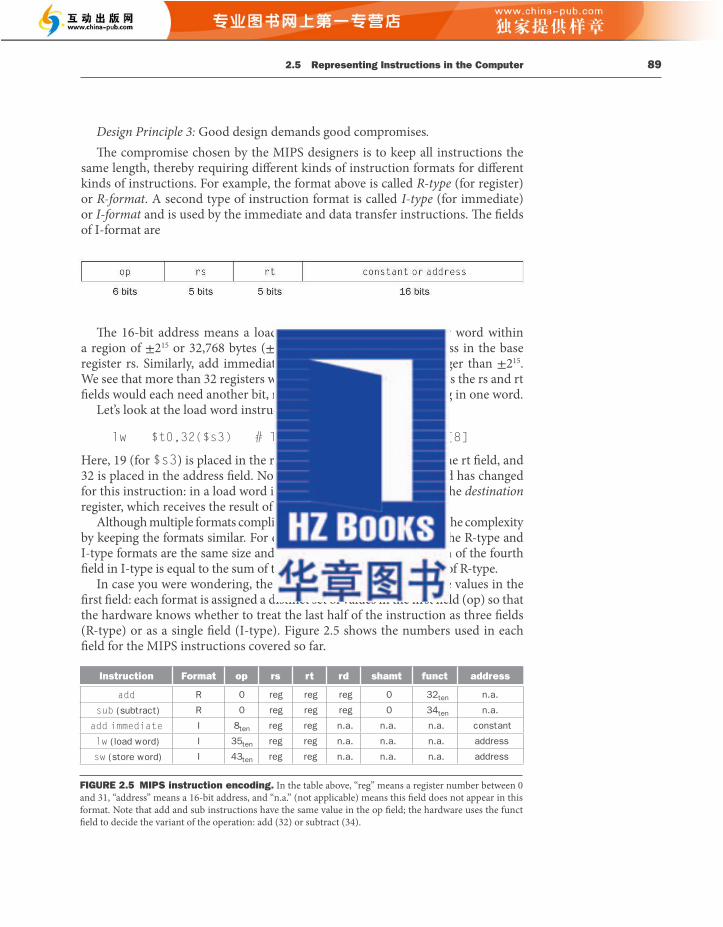
2.5 Representing Instructions in the Computer 89
Design Principle 3: Good design demands good compromises. Th e compromise chosen by the MIPS designers is to keep all instructions the
same length, thereby requiring diff erent kinds of instruction formats for diff erent kinds of instructions. For example, the format above is called R-type (for register) or R-format . A second type of instruction format is called I-type (for immediate) or I-format and is used by the immediate and data transfer instructions. Th e fi elds of I-format are
Th e 16-bit address means a load word instruction can load any word within
a region of ±2 15 or 32,768 bytes (±2 13 or 8192 words) of the address in the base register rs. Similarly, add immediate is limited to constants no larger than ±2 15 . We see that more than 32 registers would be diffi cult in this format, as the rs and rt fi elds would each need another bit, making it harder to fi t everything in one word.
Let’s look at the load word instruction from page 77:
lw $t0,32($s3) # Temporary reg $t0 gets A[8]
Here, 19 (for $s3 ) is placed in the rs fi eld, 8 (for $t0 ) is placed in the rt fi eld, and 32 is placed in the address fi eld. Note that the meaning of the rt fi eld has changed for this instruction: in a load word instruction, the rt fi eld specifi es the destination register, which receives the result of the load.
Although multiple formats complicate the hardware, we can reduce the complexity by keeping the formats similar. For example, the fi rst three fi elds of the R-type and I-type formats are the same size and have the same names; the length of the fourth fi eld in I-type is equal to the sum of the lengths of the last three fi elds of R-type.
In case you were wondering, the formats are distinguished by the values in the fi rst fi eld: each format is assigned a distinct set of values in the fi rst fi eld (op) so that the hardware knows whether to treat the last half of the instruction as three fi elds (R-type) or as a single fi eld (I-type). Figure 2.5 shows the numbers used in each fi eld for the MIPS instructions covered so far.
Instruction Format op rs rt rd shamt funct address
add R 0 reg reg reg 0 32ten n.a.
sub (subtract) R 0 reg reg reg 0 34ten n.a.
add immediate I 8ten reg reg n.a. n.a. n.a. constant
lw (load word) I 35ten reg reg n.a. n.a. n.a. address
sw (store word) I 43ten reg reg n.a. n.a. n.a. address
FIGURE 2.5 MIPS instruction encoding. In the table above, “reg” means a register number between 0 and 31, “address” means a 16-bit address, and “n.a.” (not applicable) means this fi eld does not appear in this format. Note that add and sub instructions have the same value in the op fi eld; the hardware uses the funct fi eld to decide the variant of the operation: add (32) or subtract (34).
88 Chapter 2 Instructions: Language of the Computer
Using Figure 2.4 , the answer is just a table lookup one way:
And then the other direction:
MIPS Fields MIPS fi elds are given names to make them easier to discuss:
Here is the meaning of each name of the fi elds in MIPS instructions:
■ op: Basic operation of the instruction, traditionally called the opcode .
■ rs: Th e fi rst register source operand.
■ rt: Th e second register source operand.
■ rd: Th e register destination operand. It gets the result of the operation.
■ shamt: Shift amount. ( Section 2.6 explains shift instructions and this term; it will not be used until then, and hence the fi eld contains zero in this section.)
■ funct: Function. Th is fi eld, oft en called the function code, selects the specifi c variant of the operation in the op fi eld.
A problem occurs when an instruction needs longer fi elds than those shown above. For example, the load word instruction must specify two registers and a constant. If the address were to use one of the 5-bit fi elds in the format above, the constant within the load word instruction would be limited to only 2 5 or 32. Th is constant is used to select elements from arrays or data structures, and it oft en needs to be much larger than 32. Th is 5-bit fi eld is too small to be useful.
Hence, we have a confl ict between the desire to keep all instructions the same length and the desire to have a single instruction format. Th is leads us to the fi nal hardware design principle:
opcode Th e fi eld that denotes the operation and format of an instruction.
ANSWER
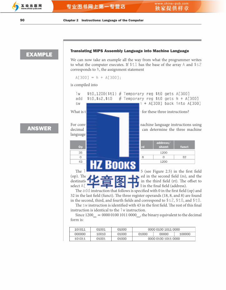
2.5 Representing Instructions in the Computer 91
Note the similarity of the binary representations of the fi rst and last instructions. Th e only diff erence is in the third bit from the left , which is highlighted here.
Th e desire to keep all instructions the same size is in confl ict with the desire to have as many registers as possible. Any increase in the number of registers uses up at least one more bit in every register fi eld of the instruction format. Given these constraints and the design princple that smaller is faster, most instruction sets today have 16 or 32 general purpose registers.
Figure 2.6 summarizes the portions of MIPS machine language described in this section. As we shall see in Chapter 4 , the similarity of the binary representations of related instructions simplifi es hardware design. Th ese similarities are another example of regularity in the MIPS architecture.
Hardware/Software Interface
MIPS machine language
Name Format Example Comments
add R 0 18 19 17 0 32 add $s1,$s2,$s3sub R 0 18 19 17 0 34 sub $s1,$s2,$s3addi I 8 18 17 100 addi $s1,$s2,100lw I 35 18 17 100 lw $s1,100($s2)sw I 43 18 17 100 sw $s1,100($s2)Field size 6 bits 5 bits 5 bits 5 bits 5 bits 6 bits All MIPS instructions are 32 bits long
R-format R op rs rt rd shamt funct Arithmetic instruction format
I-format I op rs rt address Data transfer format
FIGURE 2.6 MIPS architecture revealed through Section 2.5 . Th e two MIPS instruction formats so far are R and I. Th e fi rst 16 bits are the same: both contain an op fi eld, giving the base operation; an rs fi eld, giving one of the sources; and the rt fi eld, which specifi es the other source operand, except for load word, where it specifi es the destination register. R-format divides the last 16 bits into an rd fi eld, specifying the destination register; the shamt fi eld, which Section 2.6 explains; and the funct fi eld, which specifi es the specifi c operation of R-format instructions. I-format combines the last 16 bits into a single address fi eld.
90 Chapter 2 Instructions: Language of the Computer
Translating MIPS Assembly Language into Machine Language
We can now take an example all the way from what the programmer writes to what the computer executes. If $t1 has the base of the array A and $s2 corresponds to h , the assignment statement
A[300] = h + A[300];
is compiled into
What is the MIPS machine language code for these three instructions?
For convenience, let’s fi rst represent the machine language instructions using decimal numbers. From Figure 2.5 , we can determine the three machine language instructions:
Th e lw instruction is identifi ed by 35 (see Figure 2.5 ) in the fi rst fi eld
(op). Th e base register 9 ( $t1 ) is specifi ed in the second fi eld (rs), and the destination register 8 ( $t0 ) is specifi ed in the third fi eld (rt). Th e off set to select A[300] (1200 = 300 × 4) is found in the fi nal fi eld (address).
Th e add instruction that follows is specifi ed with 0 in the fi rst fi eld (op) and 32 in the last fi eld (funct). Th e three register operands (18, 8, and 8) are found in the second, third, and fourth fi elds and correspond to $s2 , $t0 , and $t0 .
Th e sw instruction is identifi ed with 43 in the fi rst fi eld. Th e rest of this fi nal instruction is identical to the lw instruction.
Since 1200 ten = 0000 0100 1011 0000 two , the binary equivalent to the decimal form is:
EXAMPLE
ANSWER
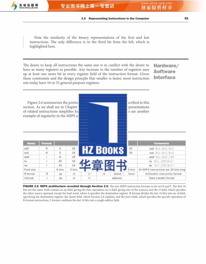
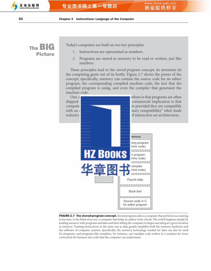
2.6 Logical Operations 93
What MIPS instruction does this represent? Choose from one of the four options below.
1. sub $t0, $t1, $t2
2. add $t2, $t0, $t1
3. sub $t2, $t1, $t0
4. sub $t2, $t0, $t1
If a person is age 40 ten , what is their age in hexidecimal?
2.6 Logical Operations
Although the fi rst computers operated on full words, it soon became clear that it was useful to operate on fi elds of bits within a word or even on individual bits. Examining characters within a word, each of which is stored as 8 bits, is one example of such an operation (see Section 2.9 ). It follows that operations were added to programming languages and instruction set architectures to simplify, among other things, the packing and unpacking of bits into words. Th ese instructions are called logical operations. Figure 2.8 shows logical operations in C, Java, and MIPS.
Check Yourself
“Contrariwise,” continued Tweedledee, “if it was so, it might be; and if it were so, it would be; but as it isn’t, it ain’t. Th at’s logic.” Lewis Carroll, Alice’s Adventures in Wonderland , 1865
Logical operations C operators Java operators MIPS instructions
Shift left << << sllShift right >> >>> srl
Bit-by-bit AND & & and, andiBit-by-bit OR | | or, oriBit-by-bit NOT ~ ~ nor
FIGURE 2.8 C and Java logical operators and their corresponding MIPS instructions. MIPS implements NOT using a NOR with one operand being zero.
Th e fi rst class of such operations is called shift s . Th ey move all the bits in a word to the left or right, fi lling the emptied bits with 0 s. For example, if register $s0 contained
0000 0000 0000 0000 0000 0000 0000 1001 two = 9 ten
and the instruction to shift left by 4 was executed, the new value would be:
0000 0000 0000 0000 0000 0000 1001 0000 two = 144 ten
92 Chapter 2 Instructions: Language of the Computer
Today’s computers are built on two key principles:
1. Instructions are represented as numbers.
2. Programs are stored in memory to be read or written, just like numbers.
Th ese principles lead to the stored-program concept; its invention let the computing genie out of its bottle. Figure 2.7 shows the power of the concept; specifi cally, memory can contain the source code for an editor program, the corresponding compiled machine code, the text that the compiled program is using, and even the compiler that generated the machine code.
One consequence of instructions as numbers is that programs are oft en shipped as fi les of binary numbers. Th e commercial implication is that computers can inherit ready-made soft ware provided they are compatible with an existing instruction set. Such “binary compatibility” oft en leads industry to align around a small number of instruction set architectures.
The BIG Picture
Memory
Accounting program(machine code)
Processor
Editor program(machine code)
C compiler(machine code)
Payroll data
Book text
Source code in Cfor editor program
FIGURE 2.7 The stored-program concept. Stored programs allow a computer that performs accounting to become, in the blink of an eye, a computer that helps an author write a book. Th e switch happens simply by loading memory with programs and data and then telling the computer to begin executing at a given location in memory. Treating instructions in the same way as data greatly simplifi es both the memory hardware and the soft ware of computer systems. Specifi cally, the memory technology needed for data can also be used for programs, and programs like compilers, for instance, can translate code written in a notation far more convenient for humans into code that the computer can understand.
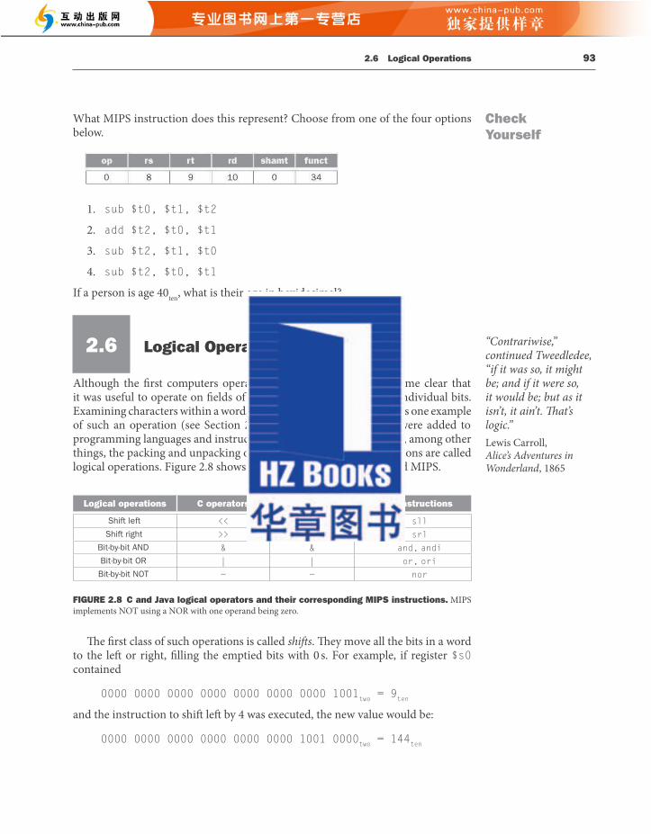
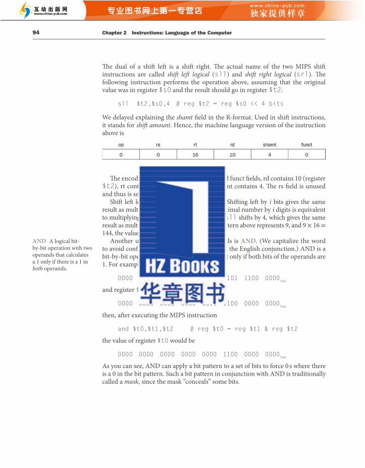
2.6 Logical Operations 95
To place a value into one of these seas of 0s, there is the dual to AND, called OR . It is a bit-by-bit operation that places a 1 in the result if either operand bit is a 1. To elaborate, if the registers $t1 and $t2 are unchanged from the preceding example, the result of the MIPS instruction
or $t0,$t1,$t2 # reg $t0 = reg $t1 | reg $t2
is this value in register $t0 :
0000 0000 0000 0000 0011 1101 1100 0000 two
Th e fi nal logical operation is a contrarian. NOT takes one operand and places a 1 in the result if one operand bit is a 0, and vice versa. Using our prior notation, it calculates x .
In keeping with the three-operand format, the designers of MIPS decided to include the instruction NOR (NOT OR) instead of NOT. If one operand is zero, then it is equivalent to NOT: A NOR 0 = NOT (A OR 0)=NOT (A).
If the register $t1 is unchanged from the preceding example and register $t3 has the value 0, the result of the MIPS instruction
nor $t0,$t1,$t3 # reg $t0 = ~ (reg $t1 | reg $t3)
is this value in register $t0 :
1111 1111 1111 1111 1100 0011 1111 1111 two
Figure 2.8 above shows the relationship between the C and Java operators and the MIPS instructions. Constants are useful in AND and OR logical operations as well as in arithmetic operations, so MIPS also provides the instructions and immediate ( andi ) and or immediate ( ori ). Constants are rare for NOR, since its main use is to invert the bits of a single operand; thus, the MIPS instruction set architecture has no immediate version.
Elaboration : The full MIPS instruction set also includes exclusive or (XOR), which sets the bit to 1 when two corresponding bits differ, and to 0 when they are the same. C allows bit fi elds or fi elds to be defi ned within words, both allowing objects to be packed within a word and to match an externally enforced interface such as an I/O device. All fi elds must fi t within a single word. Fields are unsigned integers that can be as short as 1 bit. C compilers insert and extract fi elds using logical instructions in MIPS: and , or , sll , and srl .
OR A logical bit-by-bit operation with two operands that calculates a 1 if there is a 1 in either operand.
Check Yourself
NOR A logical bit-by-bit operation with two operands that calculates the NOT of the OR of the two operands. Th at is, it calculates a 1 only if there is a 0 in both operands.
NOT A logical bit-by-bit operation with one operand that inverts the bits; that is, it replaces every 1 with a 0, and every 0 with a 1.
Elaboration : Logical AND immediate and logical OR immediate put 0s into the upper 16 bits to form a 32-bit constant, unlike add immediate, which does sign extension.
Which operations can isolate a fi eld in a word?
1. AND
2. A shift left followed by a shift right
94 Chapter 2 Instructions: Language of the Computer
Th e dual of a shift left is a shift right. Th e actual name of the two MIPS shift instructions are called shift left logical ( sll ) and shift right logical ( srl ). Th e following instruction performs the operation above, assuming that the original value was in register $s0 and the result should go in register $t2 :
sll $t2,$s0,4 # reg $t2 = reg $s0 << 4 bits
We delayed explaining the shamt fi eld in the R-format. Used in shift instructions, it stands for shift amount . Hence, the machine language version of the instruction above is
Th e encoding of sll is 0 in both the op and funct fi elds, rd contains 10 (register
$t2 ), rt contains 16 (register $s0 ), and shamt contains 4. Th e rs fi eld is unused and thus is set to 0.
Shift left logical provides a bonus benefi t. Shift ing left by i bits gives the same result as multiplying by 2 i , just as shift ing a decimal number by i digits is equivalent to multiplying by 10 i . For example, the above sll shift s by 4, which gives the same result as multiplying by 2 4 or 16. Th e fi rst bit pattern above represents 9, and 9 × 16 = 144, the value of the second bit pattern.
Another useful operation that isolates fi elds is AND . (We capitalize the word to avoid confusion between the operation and the English conjunction.) AND is a bit-by-bit operation that leaves a 1 in the result only if both bits of the operands are 1. For example, if register $t2 contains
0000 0000 0000 0000 0000 1101 1100 0000 two
and register $t1 contains
0000 0000 0000 0000 0011 1100 0000 0000 two
then, aft er executing the MIPS instruction
and $t0,$t1,$t2 # reg $t0 = reg $t1 & reg $t2
the value of register $t0 would be
0000 0000 0000 0000 0000 1100 0000 0000 two
As you can see, AND can apply a bit pattern to a set of bits to force 0 s where there is a 0 in the bit pattern. Such a bit pattern in conjunction with AND is traditionally called a mask , since the mask “conceals” some bits.
AND A logical bit-by-bit operation with two operands that calculates a 1 only if there is a 1 in both operands.
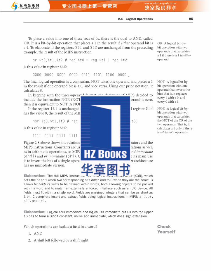
2.7 Instructions for Making Decisions 97
Th e next assignment statement performs a single operation, and if all the operands are allocated to registers, it is just one instruction:
add $s0,$s1,$s2 # f = g + h (skipped if i ≠ j)
We now need to go to the end of the if statement. Th is example introduces another kind of branch, oft en called an unconditional branch . Th is instruction says that the processor always follows the branch. To distinguish between conditional and unconditional branches, the MIPS name for this type of instruction is jump , abbreviated as j (the label Exit is defi ned below).
j Exit # go to Exit
Th e assignment statement in the else portion of the if statement can again be compiled into a single instruction. We just need to append the label Else to this instruction. We also show the label Exit that is aft er this instruction, showing the end of the if-then-else compiled code:
Else:sub $s0,$s1,$s2 # f = g – h (skipped if i = j) Exit:
Notice that the assembler relieves the compiler and the assembly language programmer from the tedium of calculating addresses for branches, just as it does for calculating data addresses for loads and stores (see Section 2.12 ).
conditional branch An instruction that requires the comparison of two values and that allows for a subsequent transfer of control to a new address in the program based on the outcome of the comparison.
f = g + h f = g – h
i = j i ��ji = = j?
Else:
Exit:
FIGURE 2.9 Illustration of the options in the if statement above. Th e left box corresponds to the then part of the if statement, and the right box corresponds to the else part.
96 Chapter 2 Instructions: Language of the Computer
2.7 Instructions for Making Decisions
What distinguishes a computer from a simple calculator is its ability to make decisions. Based on the input data and the values created during computation, diff erent instructions execute. Decision making is commonly represented in programming languages using the if statement, sometimes combined with go to statements and labels. MIPS assembly language includes two decision-making instructions, similar to an if statement with a go to . Th e fi rst instruction is
beq register1, register2, L1
Th is instruction means go to the statement labeled L1 if the value in register1 equals the value in register2 . Th e mnemonic beq stands for branch if equal . Th e second instruction is
bne register1, register2, L1
It means go to the statement labeled L1 if the value in register1 does not equal the value in register2 . Th e mnemonic bne stands for branch if not equal . Th ese two instructions are traditionally called conditional branches .
Compiling if-then-else into Conditional Branches
In the following code segment, f , g , h , i , and j are variables. If the fi ve variables f through j correspond to the fi ve registers $s0 through $s4 , what is the compiled MIPS code for this C if statement?
if (i == j) f = g + h; else f = g –h;
Figure 2.9 is a fl owchart of what the MIPS code should do. Th e fi rst expression compares for equality, so it would seem that we would want the branch if registers are equal instruction ( beq ). In general, the code will be more effi cient if we test for the opposite condition to branch over the code that performs the subsequent then part of the if (the label Else is defi ned below) and so we use the branch if registers are not equal instruction ( bne ):
bne $s3,$s4,Else # go to Else if i ≠ j
Th e utility of an automatic computer lies in the possibility of using a given sequence of instructions repeatedly, the number of times it is iterated being dependent upon the results of the computation.…Th is choice can be made to depend upon the sign of a number (zero being reckoned as plus for machine purposes). Consequently, we introduce an [instruction] (the conditional transfer [instruction]) which will, depending on the sign of a given number, cause the proper one of two routines to be executed. Burks, Goldstine, and von Neumann, 1946
EXAMPLE
ANSWER
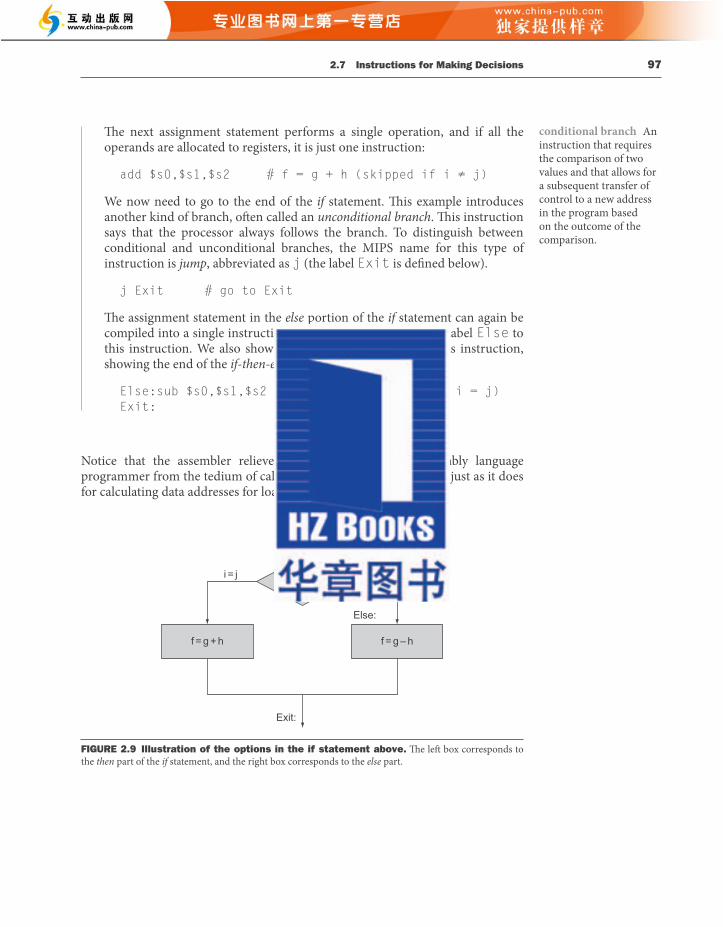
2.7 Instructions for Making Decisions 99
Th e next instruction adds 1 to i :
addi $s3,$s3,1 # i = i + 1
Th e end of the loop branches back to the while test at the top of the loop. We just add the Exit label aft er it, and we’re done:
j Loop # go to Loop Exit:
(See the exercises for an optimization of this sequence.)
Such sequences of instructions that end in a branch are so fundamental to compiling that they are given their own buzzword: a basic block is a sequence of instructions without branches, except possibly at the end, and without branch targets or branch labels, except possibly at the beginning. One of the fi rst early phases of compilation is breaking the program into basic blocks.
Th e test for equality or inequality is probably the most popular test, but sometimes it is useful to see if a variable is less than another variable. For example, a for loop may want to test to see if the index variable is less than 0. Such comparisons are accomplished in MIPS assembly language with an instruction that compares two registers and sets a third register to 1 if the fi rst is less than the second; otherwise, it is set to 0. Th e MIPS instruction is called s et on less than, or slt . For example,
slt $t0, $s3, $s4 # $t0 = 1 if $s3 < $s4
means that register $t0 is set to 1 if the value in register $s3 is less than the value in register $s4 ; otherwise, register $t0 is set to 0.
Constant operands are popular in comparisons, so there is an immediate version of the set on less than instruction. To test if register $s2 is less than the constant 10, we can just write
slti $t0,$s2,10 # $t0 = 1 if $s2 < 10
MIPS compilers use the slt , slti , beq , bne , and the fi xed value of 0 (always available by reading register $zero ) to create all relative conditions: equal, not equal, less than, less than or equal, greater than, greater than or equal.
basic block A sequence of instructions without branches (except possibly at the end) and without branch targets or branch labels (except possibly at the beginning).
Hardware/Software Interface
Hardware/Software Interface
98 Chapter 2 Instructions: Language of the Computer
Compilers frequently create branches and labels where they do not appear in the programming language. Avoiding the burden of writing explicit labels and branches is one benefi t of writing in high-level programming languages and is a reason coding is faster at that level.
Loops Decisions are important both for choosing between two alternatives—found in if statements—and for iterating a computation—found in loops. Th e same assembly instructions are the building blocks for both cases.
Compiling a while Loop in C
Here is a traditional loop in C:
while (save[i] == k) i += 1;
Assume that i and k correspond to registers $s3 and $s5 and the base of the array save is in $s6 . What is the MIPS assembly code corresponding to this C segment?
Th e fi rst step is to load save[i] into a temporary register. Before we can load save[i] into a temporary register, we need to have its address. Before we can add i to the base of array save to form the address, we must multiply the index i by 4 due to byte addressing. Fortunately, we can use shift left logical, since shift ing left by 2 bits multiplies by 2 2 or 4 (see page 94 in the prior section). We need to add the label Loop to it so that we can branch back to that instruction at the end of the loop:
Loop: sll $t1,$s3,2 # Temp reg $t1 = i * 4
To get the address of save[i] , we need to add $t1 and the base of save in $s6 :
add $t1,$t1,$s6 # $t1 = address of save[i]
Now we can use that address to load save[i] into a temporary register:
lw $t0,0($t1) # Temp reg $t0 = save[i]
Th e next instruction performs the loop test, exiting if save[i] ≠ k :
bne $t0,$s5, Exit # go to Exit if save[i] ≠ k
AU3
Hardware/Software Interface
EXAMPLE
ANSWER
2.7 Instructions for Making Decisions 101
Treating signed numbers as if they were unsigned gives us a low cost way of checking if 0≤ x< y, which matches the index out-of-bounds check for arrays. Th e key is that negative integers in two’s complement notation look like large numbers in unsigned notation; that is, the most signifi cant bit is a sign bit in the former notation but a large part of the number in the latter. Th us, an unsigned comparison of x<y also checks if x is negative as well as if x is less than y .
Bounds Check Shortcut
Use this shortcut to reduce an index-out-of-bounds check: jump to IndexOutOfBounds if $s1 ≥ $t2 or if $s1 is negative.
Th e checking code just uses sltu to do both checks:
sltu $t0,$s1,$t2 # $t0 = 0 if $s1>=length or $s1<0 beq $t0,$zero,IndexOutOfBounds #if bad, goto Error
Case/Switch Statement Most programming languages have a case or switch statement that allows the programmer to select one of many alternatives depending on a single value. Th e simplest way to implement switch is via a sequence of conditional tests, turning the switch statement into a chain of if-then-else statements.
Sometimes the alternatives may be more effi ciently encoded as a table of addresses of alternative instruction sequences, called a jump address table or jump table , and the program needs only to index into the table and then jump to the appropriate sequence. Th e jump table is then just an array of words containing addresses that correspond to labels in the code. Th e program loads the appropriate entry from the jump table into a register. It then needs to jump using the address in the register. To support such situations, computers like MIPS include a jump register instruction ( jr ), meaning an unconditional jump to the address specifi ed in a register. Th en it jumps to the proper address using this instruction. We’ll see an even more popular use of jr in the next section.
EXAMPLE
ANSWER
jump address table Also called jump table . A table of addresses of alternative instruction sequences.
100 Chapter 2 Instructions: Language of the Computer
Heeding von Neumann et al’s warning about the simplicity of the “equipment,” the MIPS architecture doesn’t include branch on less than because it is too complicated; either it would stretch the clock cycle time or it would take extra clock cycles per instruction. Two faster instructions are more useful.
Comparison instructions must deal with the dichotomy between signed and unsigned numbers. Sometimes a bit pattern with a 1 in the most signifi cant bit represents a negative number and, of course, is less than any positive number, which must have a 0 in the most signifi cant bit. With unsigned integers, on the other hand, a 1 in the most signifi cant bit represents a number that is larger than any that begins with a 0. (We’ll soon take advantage of this dual meaning of the most signifi cant bit to reduce the cost of the array bounds checking.)
MIPS off ers two versions of the set on less than comparison to handle these alternatives. Set on less than ( slt ) and set on less than immediate ( slti ) work with signed integers. Unsigned integers are compared using set on less than unsigned ( sltu ) and set on less than immediate unsigned ( sltiu ).
Signed versus Unsigned Comparison
Suppose register $s0 has the binary number
1111 1111 1111 1111 1111 1111 1111 1111 two
and that register $s1 has the binary number
0000 0000 0000 0000 0000 0000 0000 0001 two
What are the values of registers $t0 and $t1 aft er these two instructions?
slt $t0, $s0, $s1 # signed comparison sltu $t1, $s0, $s1 # unsigned comparison
Th e value in register $s0 represents −1 ten if it is an integer and 4,294,967,295 ten if it is an unsigned integer. Th e value in register $s1 represents 1 ten in either case. Th en register $t0 has the value 1, since −1 ten <1 ten , and register $t1 has the value 0, because 4,294,967,295 ten >1 ten .
Hardware/Software Interface
ANSWER
EXAMPLE

2.8 Supporting Procedures in Computer Hardware 103
You can think of a procedure like a spy who leaves with a secret plan, acquires resources, performs the task, covers his or her tracks, and then returns to the point of origin with the desired result. Nothing else should be perturbed once the mission is complete. Moreover, a spy operates on only a “need to know” basis, so the spy can’t make assumptions about his employer.
Similarly, in the execution of a procedure, the program must follow these six steps:
1. Put parameters in a place where the procedure can access them.
2. Transfer control to the procedure.
3. Acquire the storage resources needed for the procedure.
4. Perform the desired task.
5. Put the result value in a place where the calling program can access it.
6. Return control to the point of origin, since a procedure can be called from several points in a program.
As mentioned above, registers are the fastest place to hold data in a computer, so we want to use them as much as possible. MIPS soft ware follows the following convention for procedure calling in allocating its 32 registers:
■ $a0–$a3 : four argument registers in which to pass parameters
■ $v0–$v1 : two value registers in which to return values
■ $ra : one return address register to return to the point of origin
In addition to allocating these registers, MIPS assembly language includes an instruction just for the procedures: it jumps to an address and simultaneously saves the address of the following instruction in register $ra . Th e jump-and-link instruction ( jal ) is simply written
jal ProcedureAddress
Th e link portion of the name means that an address or link is formed that points to the calling site to allow the procedure to return to the proper address. Th is “link,” stored in register $ra (register 31), is called the return address . Th e return address is needed because the same procedure could be called from several parts of the program.
To support such situations, computers like MIPS use jump register instruction ( jr ), introduced above to help with case statements, meaning an unconditional jump to the address specifi ed in a register:
jr $ra
jump-and-link instruction An instruction that jumps to an address and simultaneously saves the address of the following instruction in a register ( $ra in MIPS).
return address A link to the calling site that allows a procedure to return to the proper address; in MIPS it is stored in register $ra .
102 Chapter 2 Instructions: Language of the Computer
Although there are many statements for decisions and loops in programming languages like C and Java, the bedrock statement that implements them at the instruction set level is the conditional branch.
I. C has many statements for decisions and loops, while MIPS has few. Which of the following do or do not explain this imbalance? Why?
1. More decision statements make code easier to read and understand. 2. Fewer decision statements simplify the task of the underlying layer that is
responsible for execution. 3. More decision statements mean fewer lines of code, which generally
reduces coding time. 4. More decision statements mean fewer lines of code, which generally
results in the execution of fewer operations.
II. Why does C provide two sets of operators for AND (& and &&) and two sets of operators for OR (| and ||), while MIPS doesn’t?
1. Logical operations AND and OR implement & and |, while conditional branches implement && and ||.
2. Th e previous statement has it backwards: && and || correspond to logical operations, while & and | map to conditional branches.
3. Th ey are redundant and mean the same thing: && and || are simply inherited from the programming language B, the predecessor of C.
2.8 Supporting Procedures in Computer Hardware
A procedure or function is one tool programmers use to structure programs, both to make them easier to understand and to allow code to be reused. Procedures allow the programmer to concentrate on just one portion of the task at a time; parameters act as an interface between the procedure and the rest of the program and data, since they can pass values and return results. We describe the equivalent to procedures in Java in Section 2.15 , but Java needs everything from a computer that C needs. Procedures are one way to implement abstraction in soft ware.
Hardware/Software Interface
Check Yourself
Elaboration : If you have heard about delayed branches , covered in Chapter 4 , don’t worry: the MIPS assembler makes them invisible to the assembly language programmer.
procedure A stored subroutine that performs a specifi c task based on the parameters with which it is provided.
2.8 Supporting Procedures in Computer Hardware 105
Th e parameter variables g , h , i , and j correspond to the argument registers $a0 , $a1 , $a2 , and $a3 , and f corresponds to $s0 . Th e compiled program starts with the label of the procedure:
leaf_example:
Th e next step is to save the registers used by the procedure. Th e C assignment statement in the procedure body is identical to the example on page 74, which uses two temporary registers. Th us, we need to save three registers: $s0 , $t0 , and $t1 . We “push” the old values onto the stack by creating space for three words (12 bytes) on the stack and then store them:
Figure 2.10 shows the stack before, during, and aft er the procedure call. Th e next three statements correspond to the body of the procedure, which
follows the example on page 74:
To return the value of f, we copy it into a return value register:
add $v0,$s0,$zero # returns f ($v0 = $s0 + 0)
Before returning, we restore the three old values of the registers we saved by “popping” them from the stack:
Th e procedure ends with a jump register using the return address:
jr $ra # jump back to calling routine
In the previous example, we used temporary registers and assumed their old values must be saved and restored. To avoid saving and restoring a register whose value is never used, which might happen with a temporary register, MIPS soft ware separates 18 of the registers into two groups:
■ $t0–$t9 : temporary registers that are not preserved by the callee (called procedure) on a procedure call
■ $s0–$s7 : saved registers that must be preserved on a procedure call (if used, the callee saves and restores them)
ANSWER
104 Chapter 2 Instructions: Language of the Computer
Th e jump register instruction jumps to the address stored in register $ra —which is just what we want. Th us, the calling program, or caller , puts the parameter values in $a0–$a3 and uses jal X to jump to procedure X (sometimes named the callee ). Th e callee then performs the calculations, places the results in $v0 and $v1 , and returns control to the caller using jr $ra .
Implicit in the stored-program idea is the need to have a register to hold the address of the current instruction being executed. For historical reasons, this register is almost always called the program counter , abbreviated PC in the MIPS architecture, although a more sensible name would have been instruction address register . Th e jal instruction actually saves PC + 4 in register $ra to link to the following instruction to set up the procedure return.
Using More Registers Suppose a compiler needs more registers for a procedure than the four argument and two return value registers. Since we must cover our tracks aft er our mission is complete, any registers needed by the caller must be restored to the values that they contained before the procedure was invoked. Th is situation is an example in which we need to spill registers to memory, as mentioned in the Hardware/Soft ware Interface section above.
Th e ideal data structure for spilling registers is a stack —a last-in-fi rst-out queue. A stack needs a pointer to the most recently allocated address in the stack to show where the next procedure should place the registers to be spilled or where old register values are found. Th e stack pointer is adjusted by one word for each register that is saved or restored. MIPS soft ware reserves register 29 for the stack pointer, giving it the obvious name $sp . Stacks are so popular that they have their own buzzwords for transferring data to and from the stack: placing data onto the stack is called a push , and removing data from the stack is called a pop .
By historical precedent, stacks “grow” from higher addresses to lower addresses. Th is convention means that you push values onto the stack by subtracting from the stack pointer. Adding to the stack pointer shrinks the stack, thereby popping values off the stack.
Compiling a C Procedure That Doesn’t Call Another Procedure
Let’s turn the example on page 73 from Section 2.2 into a C procedure:
What is the compiled MIPS assembly code?
caller Th e program that instigates a procedure and provides the necessary parameter values.
callee A procedure that executes a series of stored instructions based on parameters provided by the caller and then returns control to the caller.
program counter (PC) Th e register containing the address of the instruction in the program being executed.
stack A data structure for spilling registers organized as a last-in-fi rst-out queue.
stack pointer A value denoting the most recently allocated address in a stack that shows where registers should be spilled or where old register values can be found. In MIPS, it is register $sp .
push Add element to stack.
pop Remove element from stack.
EXAMPLE

2.8 Supporting Procedures in Computer Hardware 107
Compiling a Recursive C Procedure, Showing Nested Procedure Linking
Let’s tackle a recursive procedure that calculates factorial:
What is the MIPS assembly code?
Th e parameter variable n corresponds to the argument register $a0 . Th e compiled program starts with the label of the procedure and then saves two registers on the stack, the return address and $a0 :
Th e fi rst time fact is called, sw saves an address in the program that called fact . Th e next two instructions test whether n is less than 1, going to L1 if n ≥ 1.
slti $t0,$a0,1 # test for n<1 beq $t0,$zero,L1 # if n >= 1, go to L1
If n is less than 1, fact returns 1 by putting 1 into a value register: it adds 1 to 0 and places that sum in $v0 . It then pops the two saved values off the stack and jumps to the return address:
Before popping two items off the stack, we could have loaded $a0 and $ra . Since $a0 and $ra don’t change when n is less than 1, we skip those instructions.
If n is not less than 1, the argument n is decremented and then fact is called again with the decremented value:
L1: addi $a0,$a0,–1 # n >= 1: argument gets (n – 1) jal fact # call fact with (n – 1)
EXAMPLE
ANSWER
106 Chapter 2 Instructions: Language of the Computer
Th is simple convention reduces register spilling. In the example above, since the caller does not expect registers $t0 and $t1 to be preserved across a procedure call, we can drop two stores and two loads from the code. We still must save and restore $s0 , since the callee must assume that the caller needs its value.
Nested Procedures Procedures that do not call others are called leaf procedures. Life would be simple if all procedures were leaf procedures, but they aren’t. Just as a spy might employ other spies as part of a mission, who in turn might use even more spies, so do procedures invoke other procedures. Moreover, recursive procedures even invoke “clones” of themselves. Just as we need to be careful when using registers in procedures, more care must also be taken when invoking nonleaf procedures.
For example, suppose that the main program calls procedure A with an argument of 3, by placing the value 3 into register $a0 and then using jal A. Th en suppose that procedure A calls procedure B via jal B with an argument of 7, also placed in $a0 . Since A hasn’t fi nished its task yet, there is a confl ict over the use of register $a0 . Similarly, there is a confl ict over the return address in register $ra , since it now has the return address for B. Unless we take steps to prevent the problem, this confl ict will eliminate procedure A’s ability to return to its caller.
One solution is to push all the other registers that must be preserved onto the stack, just as we did with the saved registers. Th e caller pushes any argument registers ( $a0–$a3 ) or temporary registers ( $t0–$t9 ) that are needed aft er the call. Th e callee pushes the return address register $ra and any saved registers ( $s0–$s7 ) used by the callee. Th e stack pointer $sp is adjusted to account for the number of registers placed on the stack. Upon the return, the registers are restored from memory and the stack pointer is readjusted.
High address
Low address
Contents of register $t1
Contents of register $t0
Contents of register $s0
$sp
$sp
$sp
(a) (b) (c)
FIGURE 2.10 The values of the stack pointer and the stack (a) before, (b) during, and (c) after the procedure call. Th e stack pointer always points to the “top” of the stack, or the last word in the stack in this drawing.
2.8 Supporting Procedures in Computer Hardware 109
itself preserved by the callee adding exactly the same amount that was subtracted from it; and the other registers are preserved by saving them on the stack (if they are used) and restoring them from there.
Allocating Space for New Data on the Stack Th e fi nal complexity is that the stack is also used to store variables that are local to the procedure but do not fi t in registers, such as local arrays or structures. Th e segment of the stack containing a procedure’s saved registers and local variables is called a procedure frame or activation record . Figure 2.12 shows the state of the stack before, during, and aft er the procedure call.
Some MIPS soft ware uses a frame pointer ( $fp ) to point to the fi rst word of the frame of a procedure. A stack pointer might change during the procedure, and so references to a local variable in memory might have diff erent off sets depending on where they are in the procedure, making the procedure harder to understand. Alternatively, a frame pointer off ers a stable base register within a procedure for local memory-references. Note that an activation record appears on the stack whether or not an explicit frame pointer is used. We’ve been avoiding using $fp by avoiding changes to $sp within a procedure: in our examples, the stack is adjusted only on entry and exit of the procedure.
procedure frame Also called activation record . Th e segment of the stack containing a procedure’s saved registers and local variables.
frame pointer A value denoting the location of the saved registers and local variables for a given procedure.
High address
Low address(a) (b) (c)
Saved argumentregisters (if any)
$sp
$sp
$sp
$fp
$fp
$fp
Saved return address
Saved savedregisters (if any)
Local arrays andstructures (if any)
FIGURE 2.12 Illustration of the stack allocation (a) before, (b) during, and (c) after the procedure call. Th e frame pointer ( $fp ) points to the fi rst word of the frame, oft en a saved argument register, and the stack pointer ($ sp ) points to the top of the stack. Th e stack is adjusted to make room for all the saved registers and any memory-resident local variables. Since the stack pointer may change during program execution, it’s easier for programmers to reference variables via the stable frame pointer, although it could be done just with the stack pointer and a little address arithmetic. If there are no local variables on the stack within a procedure, the compiler will save time by not setting and restoring the frame pointer. When a frame pointer is used, it is initialized using the address in $sp on a call, and $sp is restored using $fp . Th is information is also found in Column 4 of the MIPS Reference Data Card at the front of this book.
108 Chapter 2 Instructions: Language of the Computer
Th e next instruction is where fact returns. Now the old return address and old argument are restored, along with the stack pointer:
Next, the value register $v0 gets the product of old argument $a0 and the current value of the value register. We assume a multiply instruction is available, even though it is not covered until Chapter 3 :
mul $v0,$a0,$v0 # return n * fact (n – 1)
Finally, fact jumps again to the return address:
jr $ra # return to the caller
A C variable is generally a location in storage, and its interpretation depends both on its type and storage class . Examples include integers and characters (see Section 2.9 ). C has two storage classes: automatic and static . Automatic variables are local to a procedure and are discarded when the procedure exits. Static variables exist across exits from and entries to procedures. C variables declared outside all procedures are considered static, as are any variables declared using the keyword static . Th e rest are automatic. To simplify access to static data, MIPS soft ware reserves another register, called the global pointer , or $gp .
Figure 2.11 summarizes what is preserved across a procedure call. Note that several schemes preserve the stack, guaranteeing that the caller will get the same data back on a load from the stack as it stored onto the stack. Th e stack above $sp is preserved simply by making sure the callee does not write above $sp ; $sp is
Hardware/Software Interface
global pointer Th e register that is reserved to point to the static area.
Saved registers: $s0–$s7 Temporary registers: $t0–$t9
Stack pointer register: $sp Argument registers: $a0–$a3
Return address register: $ra Return value registers: $v0–$v1
Stack above the stack pointer Stack below the stack pointer
Preserved Not preserved
FIGURE 2.11 What is and what is not preserved across a procedure call. If the soft ware relies on the frame pointer register or on the global pointer register, discussed in the following subsections, they are also preserved.
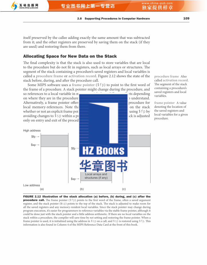
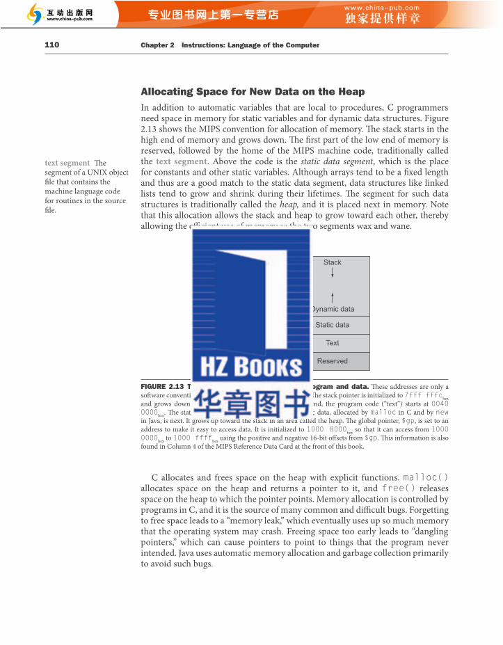
2.8 Supporting Procedures in Computer Hardware 111
Figure 2.14 summarizes the register conventions for the MIPS assembly language. Th is convention is another example of making the common case fast: most procedures can be satisfi ed with up to 4 arguments, 2 registers for a return value, 8 saved registers and 10 temporary registers without ever going to memory.
Name Register number UsagePreserved on
call?
$zero 0 The constant value 0 n.a.
$v0–$v1 2–3 Values for results and expression evaluation no
$a0–$a3 4–7 Arguments no
$t0–$t7 onseiraropmeT51–8
$s0–$s7 seydevaS32–61
$t8–$t9 onseiraropmeteroM52–42
$gp seyretnioplabolG82
$sp seyretniopkcatS92
$fp seyretniopemarF03
$ra seysserddanruteR13
FIGURE 2.14 MIPS register conventions. Register 1, called $at , is reserved for the assembler (see Section 2.12 ), and registers 26–27, called $k0–$k1 , are reserved for the operating system. Th is information is also found in Column 2 of the MIPS Reference Data Card at the front of this book.
Elaboration : What if there are more than four parameters? The MIPS convention is to place the extra parameters on the stack just above the frame pointer. The procedure then expects the fi rst four parameters to be in registers $a0 through $a3 and the rest in memory, addressable via the frame pointer.
As mentioned in the caption of Figure 2.12 , the frame pointer is convenient because all references to variables in the stack within a procedure will have the same offset. The frame pointer is not necessary, however. The GNU MIPS C compiler uses a frame pointer, but the C compiler from MIPS does not; it treats register 30 as another save register ( $s8 ).
Elaboration : Some recursive procedures can be implemented iteratively without using recursion. Iteration can signifi cantly improve performance by removing the overhead associated with procedure calls. For example, consider a procedure used to accumulate a sum:
Consider the procedure call sum(3,0) . This will result in recursive calls to sum(2,3) , sum(1,5) , and sum(0,6) , and then the result 6 will be returned four
110 Chapter 2 Instructions: Language of the Computer
Allocating Space for New Data on the Heap In addition to automatic variables that are local to procedures, C programmers need space in memory for static variables and for dynamic data structures. Figure 2.13 shows the MIPS convention for allocation of memory. Th e stack starts in the high end of memory and grows down. Th e fi rst part of the low end of memory is reserved, followed by the home of the MIPS machine code, traditionally called the text segment . Above the code is the static data segment , which is the place for constants and other static variables. Although arrays tend to be a fi xed length and thus are a good match to the static data segment, data structures like linked lists tend to grow and shrink during their lifetimes. Th e segment for such data structures is traditionally called the heap, and it is placed next in memory. Note that this allocation allows the stack and heap to grow toward each other, thereby allowing the effi cient use of memory as the two segments wax and wane.
text segment Th e segment of a UNIX object fi le that contains the machine language code for routines in the source fi le.
Stack
Dynamic data
Static data
Text
Reserved
$sp 7fff fffchex
$gp 1000 8000hex1000 0000hex
pc 0040 0000hex
0
FIGURE 2.13 The MIPS memory allocation for program and data. Th ese addresses are only a soft ware convention, and not part of the MIPS architecture. Th e stack pointer is initialized to 7fff fffc hex and grows down toward the data segment. At the other end, the program code (“text”) starts at 0040 0000 hex . Th e static data starts at 1000 0000 hex . Dynamic data, allocated by malloc in C and by new in Java, is next. It grows up toward the stack in an area called the heap. Th e global pointer, $gp , is set to an address to make it easy to access data. It is initialized to 1000 8000 hex so that it can access from 1000 0000 hex to 1000 ffff hex using the positive and negative 16-bit off sets from $gp . Th is information is also found in Column 4 of the MIPS Reference Data Card at the front of this book.
C allocates and frees space on the heap with explicit functions. malloc() allocates space on the heap and returns a pointer to it, and free() releases space on the heap to which the pointer points. Memory allocation is controlled by programs in C, and it is the source of many common and diffi cult bugs. Forgetting to free space leads to a “memory leak,” which eventually uses up so much memory that the operating system may crash. Freeing space too early leads to “dangling pointers,” which can cause pointers to point to things that the program never intended. Java uses automatic memory allocation and garbage collection primarily to avoid such bugs.
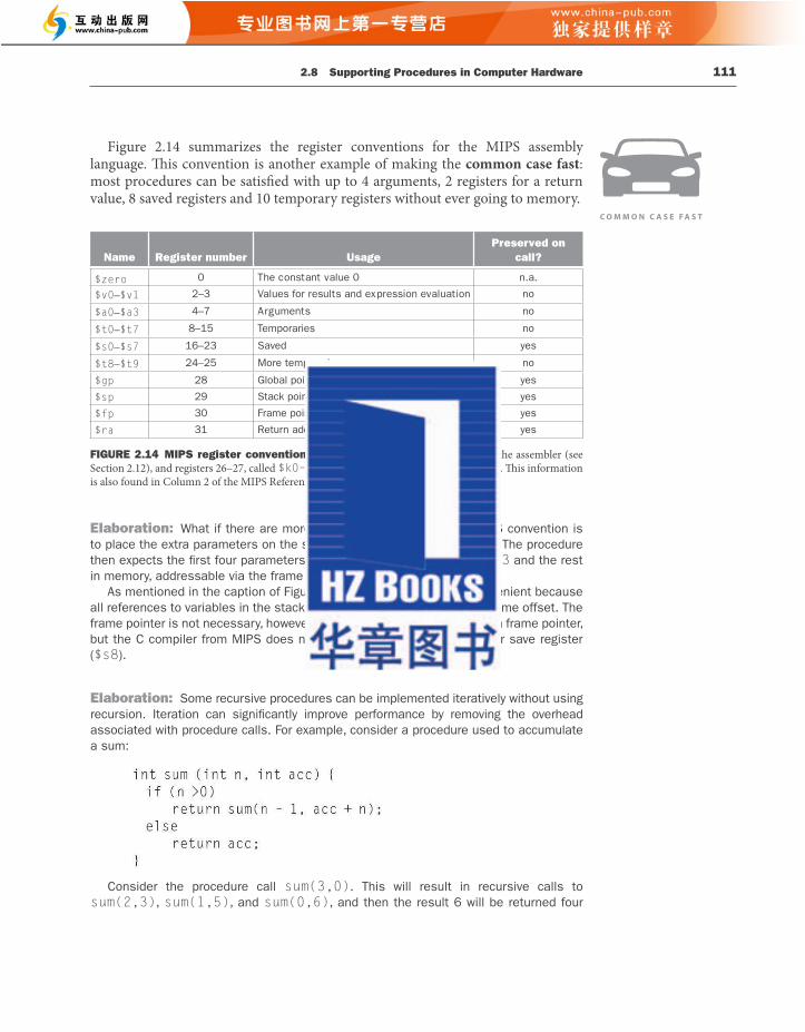
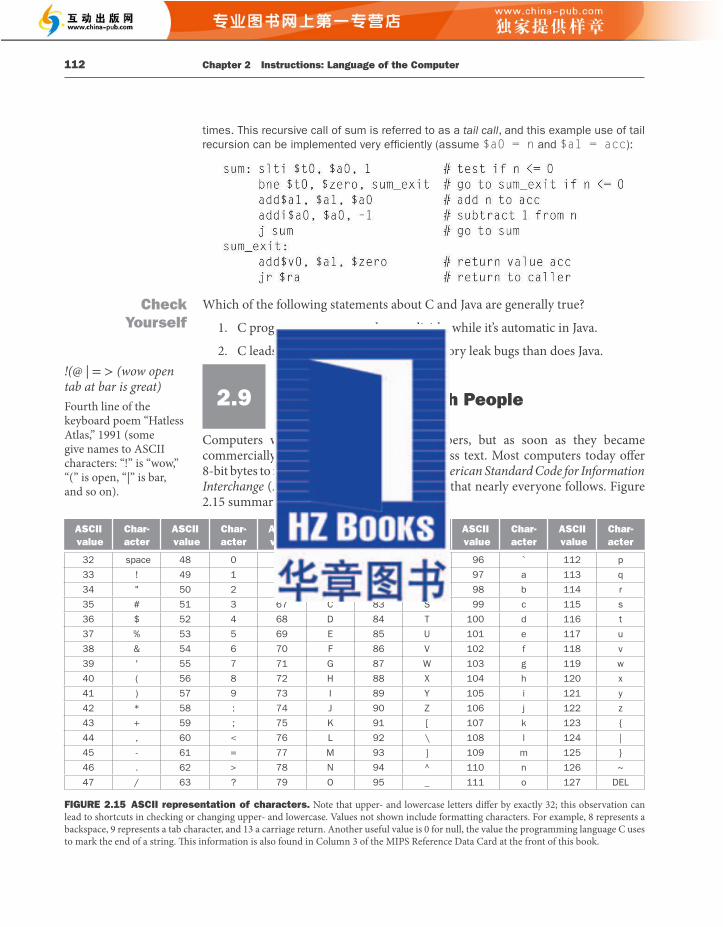
2.9 Communicating with People 113
ASCII versus Binary Numbers
We could represent numbers as strings of ASCII digits instead of as integers. How much does storage increase if the number 1 billion is represented in ASCII versus a 32-bit integer?
One billion is 1,000,000,000, so it would take 10 ASCII digits, each 8 bits long. Th us the storage expansion would be (10 × 8)/32 or 2.5. Beyond the expansion in storage, the hardware to add, subtract, multiply, and divide such decimal numbers is diffi cult and would consume more energy. Such diffi culties explain why computing professionals are raised to believe that binary is natural and that the occasional decimal computer is bizarre.
A series of instructions can extract a byte from a word, so load word and store word are suffi cient for transferring bytes as well as words. Because of the popularity of text in some programs, however, MIPS provides instructions to move bytes. Load byte ( lb ) loads a byte from memory, placing it in the rightmost 8 bits of a register. Store byte ( sb ) takes a byte from the rightmost 8 bits of a register and writes it to memory. Th us, we copy a byte with the sequence
lb $t0,0($sp) # Read byte from source sb $t0,0($gp) # Write byte to destination
Characters are normally combined into strings, which have a variable number of characters. Th ere are three choices for representing a string: (1) the fi rst position of the string is reserved to give the length of a string, (2) an accompanying variable has the length of the string (as in a structure), or (3) the last position of a string is indicated by a character used to mark the end of a string. C uses the third choice, terminating a string with a byte whose value is 0 (named null in ASCII). Th us, the string “Cal” is represented in C by the following 4 bytes, shown as decimal numbers: 67, 97, 108, 0. (As we shall see, Java uses the fi rst option.)
Compiling a String Copy Procedure, Showing How to Use C Strings
Th e procedure strcpy copies string y to string x using the null byte termination convention of C:
EXAMPLE
ANSWER
EXAMPLE
112 Chapter 2 Instructions: Language of the Computer
Which of the following statements about C and Java are generally true?
1. C programmers manage data explicitly, while it’s automatic in Java.
2. C leads to more pointer bugs and memory leak bugs than does Java.
2.9 Communicating with People
Computers were invented to crunch numbers, but as soon as they became commercially viable they were used to process text. Most computers today off er 8-bit bytes to represent characters, with the American Standard Code for Information Interchange (ASCII) being the representation that nearly everyone follows. Figure 2.15 summarizes ASCII.
times. This recursive call of sum is referred to as a tail call , and this example use of tail recursion can be implemented very effi ciently (assume $a0 = n and $a1 = acc ):
Check Yourself
!(@ | = > (wow open tab at bar is great) Fourth line of the keyboard poem “Hatless Atlas,” 1991 (some give names to ASCII characters: “!” is “wow,” “(” is open, “|” is bar, and so on).
ASCII value
Char-acter
ASCII value
Char-acter
ASCII value
Char-acter
ASCII value
Char-acter
ASCII value
Char-acter
ASCII value
Char-acter
096 ` 112 p
33 ! 49 097 a 113 q
34 " 50 098 b 114 r
35 # 51 3 6 099 c 115 s
36 $ 52
32 space 48 0 64 @ 80 P
1 65 A 81 Q
2 66 B 82 R
7 C 83 S
4 68 D 84 T 100 d 116 t
37 % 53 5 69 E 85 U 101 e 117 u
38 & 54 6 70 F 86 V 102 f 118 v
39 ' 55 7 71 G 87 W 103 g 119 w
40 ( 56 8 72 H 88 X 104 h 120 x
41 ) 57 9 73 I 89 Y 105 i 121 y
42 * 58 : 74 J 90 Z 106 j 122 z
43 + 59 ; 75 K 91 [ 107 k 123 {
44 , 60 < 76 L 92 \ 108 l 124 |
45 - 61 = 77 M 93 ] 109 m 125 }
46 . 62 > 78 N 94 ^ 110 n 126 ~
47 / 63 ? 79 O 95 _ 111 o 127 DEL
FIGURE 2.15 ASCII representation of characters. Note that upper- and lowercase letters diff er by exactly 32; this observation can lead to shortcuts in checking or changing upper- and lowercase. Values not shown include formatting characters. For example, 8 represents a backspace, 9 represents a tab character, and 13 a carriage return. Another useful value is 0 for null, the value the programming language C uses to mark the end of a string. Th is information is also found in Column 3 of the MIPS Reference Data Card at the front of this book.

2.9 Communicating with People 115
String copies usually use pointers instead of arrays in C to avoid the operations on i in the code above. See Section 2.14 for an explanation of arrays versus pointers.
Since the procedure strcpy above is a leaf procedure, the compiler could
allocate i to a temporary register and avoid saving and restoring $s0 . Hence, instead of thinking of the $t registers as being just for temporaries, we can think of them as registers that the callee should use whenever convenient. When a compiler fi nds a leaf procedure, it exhausts all temporary registers before using registers it must save.
Characters and Strings in Java Unicode is a universal encoding of the alphabets of most human languages. Figure 2.16 gives a list of Unicode alphabets; there are almost as many alphabets in Unicode as there are useful symbols in ASCII. To be more inclusive, Java uses Unicode for characters. By default, it uses 16 bits to represent a character.
Th e MIPS instruction set has explicit instructions to load and store such 16-bit quantities, called halfwords . Load half ( lh ) loads a halfword from memory, placing it in the rightmost 16 bits of a register. Like load byte, load half ( lh ) treats the halfword as a signed number and thus sign-extends to fi ll the 16 left most bits of the register, while load halfword unsigned ( lhu ) works with unsigned integers. Th us, lhu is the more popular of the two just as lbu is more popular than lb . Store half ( sh ) takes a halfword from the rightmost 16 bits of a register and writes it to memory. We copy a halfword with the sequence
lhu $t0,0($sp) # Read halfword (16 bits) from source sh $t0,0($gp) # Write halfword (16 bits) to destination
Strings are a standard Java class with special built-in support and predefi ned methods for concatenation, comparison, and conversion. Unlike C, Java includes a word that gives the length of the string, similar to Java arrays.
Elaboration : MIPS software tries to keep the stack aligned to word addresses, allowing the program to always use lw and sw (which must be aligned) to access the stack. This convention means that a char variable allocated on the stack occupies 4 bytes, even though it needs less. However, a C string variable or an array of bytes will pack 4 bytes per word, and a Java string variable or array of shorts packs 2 halfwords per word.
114 Chapter 2 Instructions: Language of the Computer
What is the MIPS assembly code?
Below is the basic MIPS assembly code segment. Assume that base addresses for arrays x and y are found in $a0 and $a1 , while i is in $s0 . strcpy adjusts the stack pointer and then saves the saved register $s0 on the stack.
To initialize i to 0, the next instruction sets $s0 to 0 by adding 0 to 0 and placing that sum in $s0 :
add $s0,$zero,$zero # i = 0 + 0
Th is is the beginning of the loop. Th e address of y[i] is fi rst formed by adding i to y[] :
L1: add $t1,$s0,$a1 # address of y[i] in $t1
Note that we don’t have to multiply i by 4 since y is an array of bytes and not of words, as in prior examples.
Load byte ( lb ) sign extends the byte while load byte unsigned ( lbu ) zero extends it.
To load the character in y[i] , we use lbu , which puts the character into $t2 :
lbu $t2, 0($t1) # $t2 = y[i]
A similar address calculation puts the address of x[i] in $t3 , and then the character in $t2 is stored at that address.
add $t3,$s0,$a0 # address of x[i] in $t3 sb $t2, 0($t3) # x[i] = y[i]
Next, we exit the loop if the character was 0. Th at is, we exit if it is the last character of the string:
beq $t2,$zero,L2 # if y[i] == 0, go to L2
If not, we increment i and loop back:
addi $s0, $s0,1 # i = i + 1 j L1 # go to L1
If we don’t loop back, it was the last character of the string; we restore $s0 and the stack pointer, and then return.
ANSWER
2.9 Communicating with People 117
The BIG Picture
Newcomers to computing are surprised that the type of the data is not encoded inside the data, but instead in the program that operates on that data.
To illustrate, we give an example from natural languages. What does the word “won” mean? You cannot answer that question without knowing the context, specifi cally the language that it is supposed to be in. Here are four alternatives:
4. In Russian, it is an adjective that means stinks .
the 32-bit pattern
01100010 01100001 01010000 00000000
could represent the following:
1. 1,650,544,640 if the program treats it as an unsigned integer.
2. +1,650,544,640 if the program treats it as a signed integer.
3. “baP” if the program treats it as a null-terminated ASCII string.
4. Th e color dark blue if the program treats the bit pattern as a mixture of the four base colors cyan, magenta, yellow, and black of the Pantone color-matching system.
Th e Big Picture on page 92 reminds us that instructions are also represented as numbers, so the bit pattern could represent the MIPS machine language instruction
011000 10011 00001 01010 00000 000000
which corresponds to the assembly language instruction multiply (see Chapter 3 ):
mult $t2, $s3, $at
If you accidentally give a word-processing program an image, it will try to interpret it as text, and you will see bizarre images on the screen; you will run into similar issues if you give text data to a graphics display program. Th is unrestricted behavior of a stored program computer is why fi le systems have a naming convention of the suffi x giving the type of the fi le (for example, .jpg, .pdf, .txt) to enable the program check for mismatches by fi le name to reduce such embarrassing scenarios.
2. In Korean, it is a noun that is the monetary unit of Korea. Repub
A binary number can also represent several types of data. For example,
of 3. In Polish, it is an adjective that means nice smelling .
ic
1. In English, it is the verb that is the past tense of win.
l
116 Chapter 2 Instructions: Language of the Computer
I. Which of the following statements about characters and strings in C and Java are true?
1. A string in C takes about half the memory as the same string in Java.
2. Strings are just an informal name for single-dimension arrays of characters in C and Java.
3. Strings in C and Java use null (0) to mark the end of a string.
4. Operations on strings, like length, are faster in C than in Java.
II. Which type of variable that can contain 1,000,000,000 ten takes the most memory space?
1. int in C
2. string in C
3. string in Java
Check Yourself
Latin Malayalam Tagbanwa General Punctuation
Greek Sinhala Khmer Spacing Modifier Letters
Cyrillic Thai Mongolian Currency Symbols
Armenian Lao Limbu Combining Diacritical Marks
Hebrew Tibetan Tai Le Combining Marks for Symbols
Arabic Myanmar Kangxi Radicals Superscripts and Subscripts
Syriac Georgian Hiragana Number Forms
Thaana Hangul Jamo Katakana Mathematical Operators
Devanagari Ethiopic Bopomofo Mathematical Alphanumeric Symbols
Bengali Cherokee Kanbun Braille Patterns
Gurmukhi Unified Canadian Aboriginal Syllabic
Shavian Optical Character Recognition
Gujarati Ogham Osmanya Byzantine Musical Symbols
Oriya Runic Cypriot Syllabary Musical Symbols
Tamil Tagalog Tai Xuan Jing Symbols Arrows
Telugu Hanunoo Yijing Hexagram Symbols Box Drawing
Kannada Buhid Aegean Numbers Geometric Shapes
FIGURE 2.16 Example alphabets in Unicode. Unicode version 4.0 has more than 160 “blocks,” which is their name for a collection of symbols. Each block is a multiple of 16. For example, Greek starts at 0370 hex , and Cyrillic at 0400 hex . Th e fi rst three columns show 48 blocks that correspond to human languages in roughly Unicode numerical order. Th e last column has 16 blocks that are multilingual and are not in order. A 16-bit encoding, called UTF-16, is the default. A variable-length encoding, called UTF-8, keeps the ASCII subset as eight bits and uses 16 or 32 bits for the other characters. UTF-32 uses 32 bits per character. New Unicode versions are released every June, with version 13.0 in 2020. Versions 9.0 to 13.0 added various Emojis, while earlier versions added new language blocks and hieroglyphs. Th e total is almost 150,000 characters. To learn more, see www.unicode.org .
Elaboration : Refl ecting the international nature of the web, most web pages today use Unicode instead of ASCII.
2.10 MIPS Addressing for 32-bit Immediates and Addresses 119
Either the compiler or the assembler must break large constants into pieces and then reassemble them into a register. As you might expect, the immediate fi eld’s size restriction may be a problem for memory addresses in loads and stores as well as for constants in immediate instructions. If this job falls to the assembler, as it does for MIPS soft ware, then the assembler must have a temporary register available in which to create the long values. Th is need is a reason for the register $at , (assembler temporary), which is reserved for the assembler.
Hence, the symbolic representation of the MIPS machine language is no longer limited by the hardware, but by whatever the creator of an assembler chooses to include (see Section 2.12 ). We stick close to the hardware to explain the architecture of the computer, noting when we use the enhanced language of the assembler that is not found in the processor.
Addressing in Branches and Jumps Th e MIPS jump instructions have the simplest addressing. Th ey use the fi nal MIPS instruction format, called the J-type , which consists of 6 bits for the operation fi eld and the rest of the bits for the address fi eld. Th us,
j 10000 # go to location 10000
could be assembled into this format (it’s actually a bit more complicated, as we will see):
where the value of the jump opcode is 2 and the jump address is 10000 .
Unlike the jump instruction, the conditional branch instruction must specify two operands in addition to the branch address. Th us,
bne $s0,$s1,Exit # go to Exit if $s0 ≠ $s1
is assembled into this instruction, leaving only 16 bits for the branch address:
Hardware/Software Interface
Elaboration : Creating 32-bit constants needs care. The instruction addi copies the left-most bit of the 16-bit immediate fi eld of the instruction into the upper 16 bits of a word. Logical or immediate from Section 2.6 loads 0s into the upper 16 bits and hence is used by the assembler in conjunction with lui to create 32-bit constants.
118 Chapter 2 Instructions: Language of the Computer
2.10 MIPS Addressing for 32-bit Immediates and Addresses
Although keeping all MIPS instructions 32 bits long simplifi es the hardware, there are times where it would be convenient to have a 32-bit constant or 32-bit address. Th is section starts with the general solution for large constants, and then shows the optimizations for instruction addresses used in branches and jumps.
32-Bit Immediate Operands Although constants are frequently short and fi t into the 16-bit fi eld, sometimes they are bigger. Th e MIPS instruction set includes the instruction load upper immediate ( lui ) specifi cally to set the upper 16 bits of a constant in a register, allowing a subsequent instruction to specify the lower 16 bits of the constant. Figure 2.17 shows the operation of lui .
Loading a 32-Bit Constant
What is the MIPS assembly code to load this 32-bit constant into register $s0 ?
0000 0000 0011 1101 0000 1001 0000 0000
First, we would load the upper 16 bits, which is 61 in decimal, using lui :
lui $s0, 61 # 61 decimal = 0000 0000 0011 1101 binary
Th e value of register $s0 aft erward is
0000 0000 0011 1101 0000 0000 0000 0000
Th e next step is to insert the lower 16 bits, whose decimal value is 2304:
ori $s0, $s0, 2304 # 2304 decimal = 0000 1001 0000 0000
Th e fi nal value in register $s0 is the desired value:
0000 0000 0011 1101 0000 1001 0000 0000
EXAMPLE
ANSWER
The machine language version of lui $t0, 255
Contents of register $t0 after executing lui $t0, 255:
001111 00000 01000 0000 0000 1111 1111
0000 0000 1111 1111 0000 0000 0000 0000
# $t0 is register 8:
FIGURE 2.17 The effect of the lui instruction. Th e instruction lui transfers the 16-bit immediate constant fi eld value into the left most 16 bits of the register, fi lling the lower 16 bits with 0s.
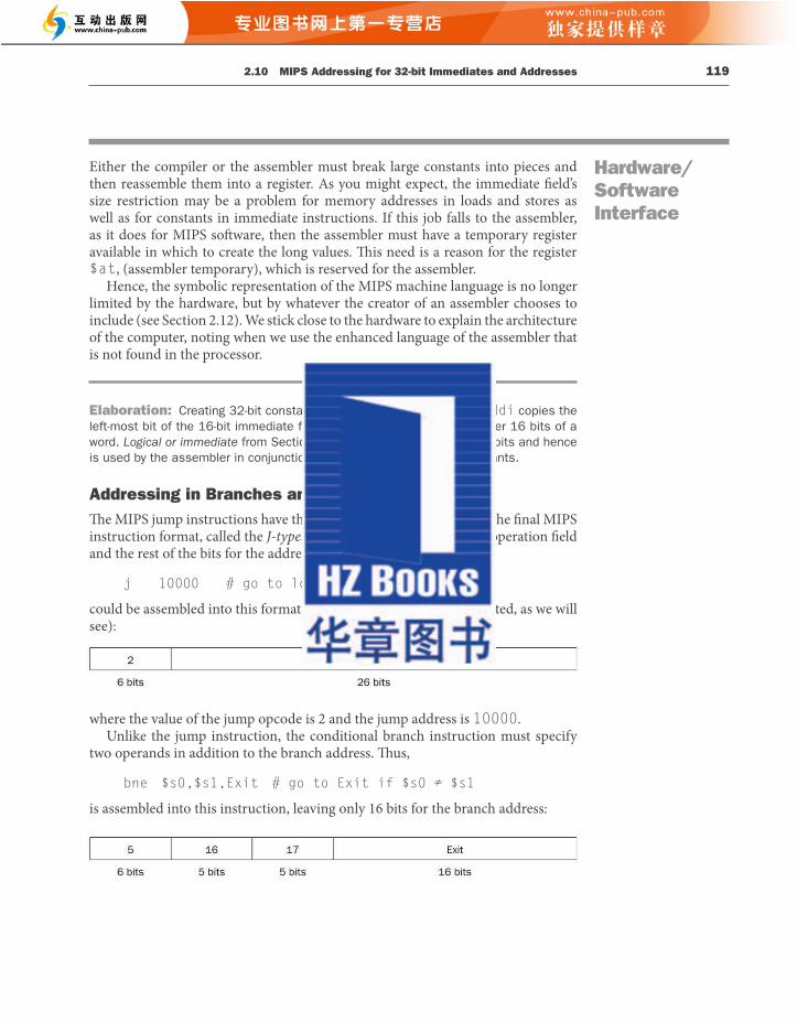

2.10 MIPS Addressing for 32-bit Immediates and Addresses 121
Showing Branch Offset in Machine Language
Th e while loop on pages 98–99 was compiled into this MIPS assembler code:
If we assume we place the loop starting at location 80000 in memory, what is the MIPS machine code for this loop?
Th e assembled instructions and their addresses are:
Th e assembled instructions and their addresses are:
Remember that MIPS instructions have byte addresses, so addresses of sequential words diff er by 4, the number of bytes in a word. Th e bne instruction on the fourth line adds 2 words or 8 bytes to the address of the following instruction (80016), specifying the branch destination relative to that following instruction (8 + 80016) instead of relative to the branch instruction (12 + 80012) or using the full destination address (80024). Th e jump instruction on the last line does use the full address (20000 × 4 = 80000), corresponding to the label Loop .
EXAMPLE
ANSWER
120 Chapter 2 Instructions: Language of the Computer
If addresses of the program had to fi t in this 16-bit fi eld, it would mean that no program could be bigger than 2 16 , which is far too small to be a realistic option today. An alternative would be to specify a register that would always be added to the branch address, so that a branch instruction would calculate the following:
Program counter Register Branch address
Th is sum allows the program to be as large as 2 32 and still be able to use conditional branches, solving the branch address size problem. Th en the question is, which register?
Th e answer comes from seeing how conditional branches are used. Conditional branches are found in loops and in if statements, so they tend to branch to a nearby instruction. For example, about half of all conditional branches in SPEC benchmarks go to locations less than 16 instructions away. Since the program counter (PC) contains the address of the current instruction, we can branch within ±2 15 words of the current instruction if we use the PC as the register to be added to the address. Almost all loops and if statements are much smaller than 2 16 words, so the PC is the ideal choice.
Th is form of branch addressing is called PC-relative addressing . As we shall see in Chapter 4 , it is convenient for the hardware to increment the PC early to point to the next instruction. Hence, the MIPS address is actually relative to the address of the following instruction (PC + 4) as opposed to the current instruction (PC). It is yet another example of making the common case fast , which in this case is addressing nearby instructions.
Like most recent computers, MIPS uses PC-relative addressing for all conditional branches, because the destination of these instructions is likely to be close to the branch. On the other hand, jump-and-link instructions invoke procedures that have no reason to be near the call, so they normally use other forms of addressing. Hence, the MIPS architecture off ers long addresses for procedure calls by using the J-type format for both jump and jump-and-link instructions.
Since all MIPS instructions are 4 bytes long, MIPS stretches the distance of the branch by having PC-relative addressing refer to the number of words to the next instruction instead of the number of bytes. Th us, the 16-bit fi eld can branch four times as far by interpreting the fi eld as a relative word address rather than as a relative byte address. Similarly, the 26-bit fi eld in jump instructions is also a word address, meaning that it represents a 28-bit byte address.
PC-relative addressing An addressing regime in which the address is the sum of the program counter (PC) and a constant in the instruction.
Elaboration : Since the PC is 32 bits, 4 bits must come from somewhere else for jumps. The MIPS jump instruction replaces only the lower 28 bits of the PC, leaving the upper 4 bits of the PC unchanged. The loader and linker ( Section 2.12 ) must be careful to avoid placing a program across an address boundary of 256 MB (64 million instructions); otherwise, a jump must be replaced by a jump register instruction preceded by other instructions to load the full 32-bit address into a register.
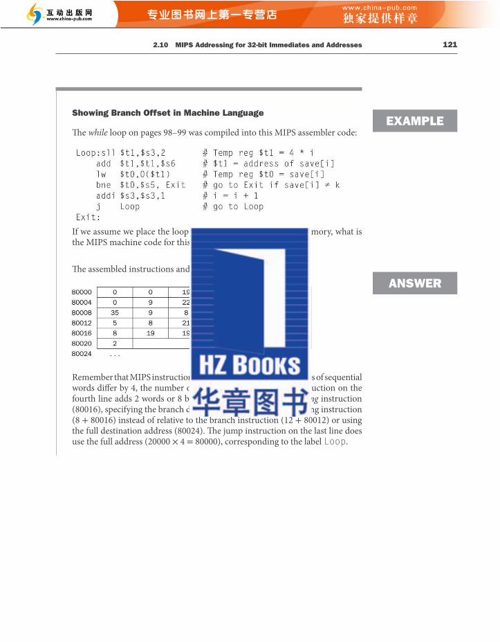
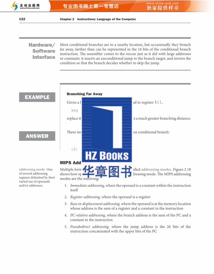
2.10 MIPS Addressing for 32-bit Immediates and Addresses 123
Although we show MIPS as having 32-bit addresses, nearly all microprocessors (including MIPS) have 64-bit address extensions (see Appendix E ). Th ese extensions were in response to the needs of soft ware for larger programs. Th e process of instruction set extension allows architectures to expand in such a way that is able to move soft ware compatibly upward to the next generation of architecture.
Hardware/Software Interface
1. Immediate addressing
2. Register addressing
3. Base addressing
4. PC-relative addressing
5. Pseudodirect addressing
Immediateop rs rt
op rs rt . . . functrd
Register
Registers
op rs rt Address
Word
Memory
+Register HalfwordByte
op rs rt Address
Word
Memory
+PC
op
Word
Memory
PC
Address
FIGURE 2.18 Illustration of the fi ve MIPS addressing modes. Th e operands are shaded in color. Th e operand of mode 3 is in memory, whereas the operand for mode 2 is a register. Note that versions of load and store access bytes, halfwords, or words. For mode 1, the operand is 16 bits of the instruction itself. Modes 4 and 5 address instructions in memory, with mode 4 adding a 16-bit address shift ed left 2 bits to the PC and mode 5 concatenating a 26-bit address shift ed left 2 bits with the 4 upper bits of the PC. Note that a single operation can use more than one addressing mode. Add, for example, uses both immediate (addi) and register (add) addressing.
122 Chapter 2 Instructions: Language of the Computer
Most conditional branches are to a nearby location, but occasionally they branch far away, farther than can be represented in the 16 bits of the conditional branch instruction. Th e assembler comes to the rescue just as it did with large addresses or constants: it inserts an unconditional jump to the branch target, and inverts the condition so that the branch decides whether to skip the jump.
Branching Far Away
Given a branch on register $s0 being equal to register $s1 ,
beq $s0, $s1, L1
replace it by a pair of instructions that off ers a much greater branching distance.
Th ese instructions replace the short-address conditional branch:
bne $s0, $s1, L2 j L1 L2:
MIPS Addressing Mode Summary Multiple forms of addressing are generically called addressing modes . Figure 2.18 shows how operands are identifi ed for each addressing mode. Th e MIPS addressing modes are the following:
1. Immediate addressing, where the operand is a constant within the instruction itself
2. Register addressing, where the operand is a register
3. Base or displacement addressing, where the operand is at the memory location whose address is the sum of a register and a constant in the instruction
4. PC-relative addressing, where the branch address is the sum of the PC and a constant in the instruction
5. Pseudodirect addressing, where the jump address is the 26 bits of the instruction concatenated with the upper bits of the PC
Hardware/Software Interface
EXAMPLE
ANSWER
addressing mode One of several addressing regimes delimited by their varied use of operands and/or addresses.
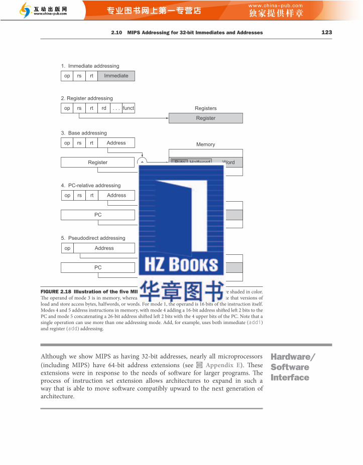

2.10 MIPS Addressing for 32-bit Immediates and Addresses 125
op(31:26)
28–26
31–290(000) R-format Bltz/gez jump jump & link branch eq branch
neblez bgtz
1(001) addimmediate
addiu set lessthan imm.
set lessthan imm. unsigned
andi ori xori load upperimmediate
2(010) TLB FlPt
3(011)
4(100) load byte load half lwl load word load byte unsigned
loadhalfunsigned
lwr
5(101) store byte store half swl store word swr
6(110) load linked word
lwc1
7(111) store cond. word
swc1
op(31:26)=010000 (TLB), rs(25:21)
23–21
25–240(00) mfc0 cfc0 mtc0 ctc01(01)2(10)3(11)
op(31:26)=000000 (R-format), funct(5:0)
2–05–3
0(000) 1(001) 2(010) 3(011) 4(100) 5(101) 6(110) 7(111)
0(000) 1(001) 2(010) 3(011) 4(100) 5(101) 6(110) 7(111)
0(000) 1(001) 2(010) 3(011) 4(100) 5(101) 6(110) 7(111)
0(000) shift leftlogical
shift rightlogical
sra sllv srlv srav
1(001) jump register jalr syscall break
2(010) mfhi mthi mfl o mtlo3(011) mult multu div divu4(100) add addu subtract subu and or xor not or (nor)5(101) set l.t. set l.t.
unsigned6(110)
7(111)
FIGURE 2.19 MIPS instruction encoding. Th is notation gives the value of a fi eld by row and by column. For example, the top portion of the fi gure shows load word in row number 4 (100 two for bits 31–29 of the instruction) and column number 3 (011 two for bits 28–26 of the instruction), so the corresponding value of the op fi eld (bits 31–26) is 100011 two . An underlined name means the fi eld is used elsewhere. For example, R-format in row 0 and column 0 (op = 000000 two ) is defi ned in the bottom part of the fi gure. Hence, subtract in row 4 and column 2 of the bottom section means that the funct fi eld (bits 5–0) of the instruction is 100010 two and the op fi eld (bits 31–26) is 000000 two . Th e floating point value in row 2, column 1 is defi ned in Figure 3.18 in Chapter 3 . Bltz/gez is the opcode for four instructions found in Appendix A: bltz , bgez , bltzal , and bgezal . Th is chapter describes instructions given in full name using color, while Chapter 3 describes instructions given in mnemonics using color. Appendix A covers all instructions.
124 Chapter 2 Instructions: Language of the Computer
Decoding Machine Language Sometimes you are forced to reverse-engineer machine language to create the original assembly language. One example is when looking at “core dump.” Figure 2.19 shows the MIPS encoding of the fi elds for the MIPS machine language. Th is fi gure helps when translating by hand between assembly language and machine language.
Decoding Machine Code
What is the assembly language statement corresponding to this machine instruction?
00af8020hex
Th e fi rst step in converting hexadecimal to binary is to fi nd the op fi elds:
(Bits: 31 28 26 5 2 0) 0000 0000 1010 1111 1000 0000 0010 0000
We look at the op fi eld to determine the operation. Referring to Figure 2.19 , when bits 31–29 are 000 and bits 28–26 are 000, it is an R-format instruction. Let’s reformat the binary instruction into R-format fi elds, listed in Figure 2.20 :
op rs rt rd shamt funct 000000 00101 01111 10000 00000 100000
Th e bottom portion of Figure 2.19 determines the operation of an R-format instruction. In this case, bits 5–3 are 100 and bits 2–0 are 000, which means this binary pattern represents an add instruction.
We decode the rest of the instruction by looking at the fi eld values. Th e decimal values are 5 for the rs fi eld, 15 for rt, and 16 for rd (shamt is unused). Figure 2.14 shows that these numbers represent registers $a1 , $t7 , and $s0 . Now we can reveal the assembly instruction:
add $s0,$a1,$t7
EXAMPLE
ANSWER
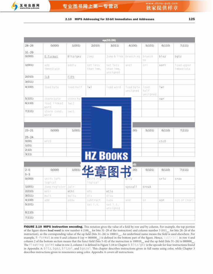
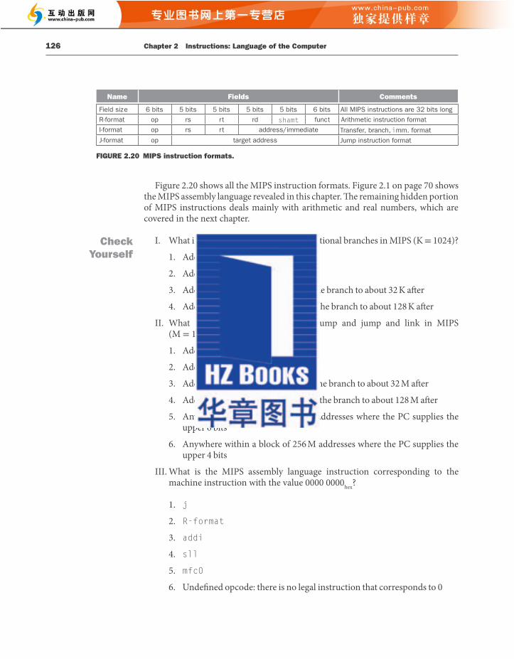
2.11 Parallelism and Instructions: Synchronization 127
2.11 Parallelism and Instructions: Synchronization
Parallel execution is easier when tasks are independent, but oft en they need to cooperate. Cooperation usually means some tasks are writing new values that others must read. To know when a task is fi nished writing so that it is safe for another to read, the tasks need to synchronize. If they don’t synchronize, there is a danger of a data race , where the results of the program can change depending on how events happen to occur.
For example, recall the analogy of the eight reporters writing a story on page 44 of Chapter 1 . Suppose one reporter needs to read all the prior sections before writing a conclusion. Hence, he or she must know when the other reporters have fi nished their sections, so that there is no danger of sections being changed aft erwards. Th at is, they had better synchronize the writing and reading of each section so that the conclusion will be consistent with what is printed in the prior sections.
In computing, synchronization mechanisms are typically built with user-level soft ware routines that rely on hardware-supplied synchronization instructions. In this section, we focus on the implementation of lock and unlock synchronization operations. Lock and unlock can be used straightforwardly to create regions where only a single processor can operate, called a mutual exclusion , as well as to implement more complex synchronization mechanisms.
Th e critical ability we require to implement synchronization in a multiprocessor is a set of hardware primitives with the ability to atomically read and modify a memory location. Th at is, nothing else can interpose itself between the read and the write of the memory location. Without such a capability, the cost of building basic synchronization primitives will be high and will increase unreasonably as the processor count increases.
Th ere are a number of alternative formulations of the basic hardware primitives, all of which provide the ability to atomically read and modify a location, together with some way to tell if the read and write were performed atomically. In general, architects do not expect users to employ the basic hardware primitives, but instead expect that the primitives will be used by system programmers to build a synchronization library, a process that is oft en complex and tricky.
Let’s start with one such hardware primitive and show how it can be used to build a basic synchronization primitive. One typical operation for building synchronization operations is the atomic exchange or atomic swap , which inter-changes a value in a register for a value in memory.
To see how to use this to build a basic synchronization primitive, assume that we want to build a simple lock where the value 0 is used to indicate that the lock is free and 1 is used to indicate that the lock is unavailable. A processor tries to set the lock by doing an exchange of 1, which is in a register, with the memory address corresponding to the lock. Th e value returned from the exchange instruction is 1 (unavailable) if some other processor had already claimed access, and 0 (free)
data race Two memory accesses form a data race if they are from diff erent threads to same location, at least one is a write, and they occur one aft er another.
126 Chapter 2 Instructions: Language of the Computer
Figure 2.20 shows all the MIPS instruction formats. Figure 2.1 on page 70 shows the MIPS assembly language revealed in this chapter. Th e remaining hidden portion of MIPS instructions deals mainly with arithmetic and real numbers, which are covered in the next chapter.
I. What is the range of addresses for conditional branches in MIPS (K = 1024)?
1. Addresses between 0 and 64 K−1
2. Addresses between 0 and 256 K−1
3. Addresses up to about 32 K before the branch to about 32 K aft er
4. Addresses up to about 128 K before the branch to about 128 K aft er
II. What is the range of addresses for jump and jump and link in MIPS (M = 1024 K)?
1. Addresses between 0 and 64 M−1
2. Addresses between 0 and 256 M−1
3. Addresses up to about 32 M before the branch to about 32 M aft er
4. Addresses up to about 128 M before the branch to about 128 M aft er
5. Anywhere within a block of 64 M addresses where the PC supplies the upper 6 bits
6. Anywhere within a block of 256 M addresses where the PC supplies the upper 4 bits
III. What is the MIPS assembly language instruction corresponding to the machine instruction with the value 0000 0000 hex ?
1. j
2. R-format
3. addi
4. sll
5. mfc0
6. Undefi ned opcode: there is no legal instruction that corresponds to 0
Name Fields Comments
Field size 6 bits 5 bits 5 bits 5 bits 5 bits 6 bits All MIPS instructions are 32 bits long
R-format op rs rt rd shamt funct Arithmetic instruction format
I-format op rs rt address/immediate Transfer, branch,imm. format
Jump instruction formatsserddategratpotamrof-J
FIGURE 2.20 MIPS instruction formats.
Check Yourself

2.12 Translating and Starting a Program 129
When do you use primitives like load linked and store conditional?
1. When cooperating threads of a parallel program need to synchronize to get proper behavior for reading and writing shared data
2. When cooperating processes on a uniprocessor need to synchronize for reading and writing shared data
2.12 Translating and Starting a Program
Th is section describes the four steps in transforming a C program in a fi le in nonvolatile storage into a program running on a computer. Figure 2.21 shows the translation hierarchy. Some systems combine these steps to reduce translation time, but these are the logical four phases that programs go through. Th is section follows this translation hierarchy.
Compiler Th e compiler transforms the C program into an assembly language program , a symbolic form of what the machine understands. High-level language programs take many fewer lines of code than assembly language, so programmer productivity is much higher.
In 1975, many operating systems and assemblers were written in assembly language because memories were small and compilers were ineffi cient. Th e million-fold increase in memory capacity per single DRAM chip has reduced program size concerns, and optimizing compilers today can produce assembly language programs nearly as good as an assembly language expert, and sometimes even better for large programs.
Elaboration: An advantage of the load linked/store conditional mechanism is that it can be used to build other synchronization primitives, such as atomic compare and swap or atomic fetch-and-increment , which are used in some parallel programming models. These involve more instructions between the ll and the sc , but not too many.
Since the store conditional will fail after either another attempted store to the load linked address or any exception, care must be taken in choosing which instructions are inserted between the two instructions. In particular, only register-register instructions can safely be permitted; otherwise, it is possible to create deadlock situations where the processor can never complete the sc because of repeated page faults. In addition, the number of instructions between the load linked and the store conditional should be small to minimize the probability that either an unrelated event or a competing processor causes the store conditional to fail frequently.
Check Yourself
assembly language A symbolic language that can be translated into binary machine language.
128 Chapter 2 Instructions: Language of the Computer
otherwise. In the latter case, the value is also changed to 1 (unavailable), preventing any competing exchange in another processor from also retrieving a 0 (free).
For example, consider two processors that each try to do the exchange simultaneously: this race is broken, since exactly one of the processors will perform the exchange fi rst, returning 0 (free), and the second processor will return 1 (unavailable) when it does the exchange. Th e key to using the exchange primitive to implement synchronization is that the operation is atomic: the exchange is indivisible, and two simultaneous exchanges will be ordered by the hardware. It is impossible for two processors trying to set the synchronization variable in this manner to both think they have simultaneously set the variable.
Implementing a single atomic memory operation introduces some challenges in the design of the processor, since it requires both a memory read and a write in a single, uninterruptible instruction.
An alternative is to have a pair of instructions in which the second instruction returns a value showing whether the pair of instructions was executed as if the pair were atomic. Th e pair of instructions is eff ectively atomic if it appears as if all other operations executed by any processor occurred before or aft er the pair. Th us, when an instruction pair is eff ectively atomic, no other processor can change the value between the instruction pair.
In MIPS this pair of instructions includes a special load called a load linked and a special store called a store conditional . Th ese instructions are used in sequence: if the contents of the memory location specifi ed by the load linked are changed before the store conditional to the same address occurs, then the store conditional fails. Th e store conditional is defi ned to both store the value of a (presumably diff erent) register in memory and to change the value of that register to a 1 if it succeeds and to a 0 if it fails. Since the load linked returns the initial value, and the store conditional returns 1 only if it succeeds, the following sequence implements an atomic exchange on the memory location specifi ed by the contents of $s1 :
Any time a processor intervenes and modifi es the value in memory between the ll and sc instructions, the sc returns 0 in $t0 , causing the code sequence to try again. At the end of this sequence, the contents of $s4 and the memory location specifi ed by $s1 have been atomically exchanged.
Elaboration : Although it was presented for multiprocessor synchronization, atomic exchange is also useful for the operating system in dealing with multiple processes in a single processor. To make sure nothing interferes in a single processor, the store conditional also fails if the processor does a context switch between the two instructions (see Chapter 5 ).
HZB
OO
K-2
021-
11-1
7

2.12 Translating and Starting a Program 131
Th e assembler converts this assembly language instruction into the machine language equivalent of the following instruction:
add $t0,$zero,$t1 # register $t0 gets 0 + register $t1
Th e MIPS assembler also converts blt (branch on less than) into the two instructions slt and bne mentioned in the example on page 101. Other examples include bgt , bge , and ble . It also converts branches to faraway locations into a branch and jump. As mentioned above, the MIPS assembler allows 32-bit constants to be loaded into a register despite the 16-bit limit of the immediate instructions.
In summary, pseudoinstructions give MIPS a richer set of assembly language instructions than those implemented by the hardware. Th e only cost is reserving one register, $at , for use by the assembler. If you are going to write assembly programs, use pseudoinstructions to simplify your task. To understand the MIPS architecture and be sure to get best performance, however, study the real MIPS instructions found in Figures 2.1 and 2.19 .
Assemblers will also accept numbers in a variety of bases. In addition to binary and decimal, they usually accept a base that is more succinct than binary yet converts easily to a bit pattern. MIPS assemblers use hexadecimal.
Such features are convenient, but the primary task of an assembler is assembly into machine code. Th e assembler turns the assembly language program into an object fi le , which is a combination of machine language instructions, data, and information needed to place instructions properly in memory.
To produce the binary version of each instruction in the assembly language program, the assembler must determine the addresses corresponding to all labels. Assemblers keep track of labels used in branches and data transfer instructions in a symbol table . As you might expect, the table contains pairs of symbols and addresses.
Th e object fi le for UNIX systems typically contains six distinct pieces:
■ Th e object fi le header describes the size and position of the other pieces of the object fi le.
■ Th e text segment contains the machine language code.
■ Th e static data segment contains data allocated for the life of the program. (UNIX allows programs to use both static data, which is allocated throughout the program, and dynamic data , which can grow or shrink as needed by the program. See Figure 2.13 .)
■ Th e relocation information identifi es instructions and data words that depend on absolute addresses when the program is loaded into memory.
■ Th e symbol table contains the remaining labels that are not defi ned, such as external references.
symbol table A table that matches names of labels to the addresses of the memory words that instructions occupy.
130 Chapter 2 Instructions: Language of the Computer
Assembler Since assembly language is an interface to higher-level soft ware, the assembler can also treat common variations of machine language instructions as if they were instructions in their own right. Th e hardware need not implement these instructions; however, their appearance in assembly language simplifi es translation and programming. Such instructions are called pseudoinstructions .
As mentioned above, the MIPS hardware makes sure that register $zero always has the value 0. Th at is, whenever register $zero is used, it supplies a 0, and the programmer cannot change the value of register $zero . Register $zero is used to create the assembly language instruction that copies the contents of one register to another. Th us the MIPS assembler accepts this instruction even though it is not found in the MIPS architecture:
move $t0,$t1 # register $t0 gets register $t1
Loader
C program
Compiler
Assembly language program
Assembler
Object: Machine language module Object: Library routine (machine language)
Linker
Memory
Executable: Machine language program
FIGURE 2.21 A translation hierarchy for C. A high-level language program is fi rst compiled into an assembly language program and then assembled into an object module in machine language. Th e linker combines multiple modules with library routines to resolve all references. Th e loader then places the machine code into the proper memory locations for execution by the processor. To speed up the translation process, some steps are skipped or combined. Some compilers produce object modules directly, and some systems use linking loaders that perform the last two steps. To identify the type of fi le, UNIX follows a suffi x convention for fi les: C source fi les are named x.c , assembly fi les are x.s , object fi les are named x.o , statically linked library routines are x.a , dynamically linked library routes are x.so , and executable fi les by default are called a.out . MS-DOS uses the suffi xes .C , .ASM , .OBJ , .LIB , .DLL , and .EXE to the same eff ect.
pseudoinstruction A common variation of assembly language instructions oft en treated as if it were an instruction in its own right.
2.12 Translating and Starting a Program 133
Linking Object Files
Link the two object fi les below. Show updated addresses of the fi rst few instructions of the completed executable fi le. We show the instructions in assembly language just to make the example understandable; in reality, the instructions would be numbers.
Note that in the object fi les we have highlighted the addresses and symbols that must be updated in the link process: the instructions that refer to the addresses of procedures A and B and the instructions that refer to the addresses of data words X and Y .
EXAMPLE
132 Chapter 2 Instructions: Language of the Computer
■ Th e debugging information contains a concise description of how the modules were compiled so that a debugger can associate machine instructions with C source fi les and make data structures readable.
Th e next subsection shows how to attach such routines that have already been assembled, such as library routines.
Linker What we have presented so far suggests that a single change to one line of one procedure requires compiling and assembling the whole program. Complete retranslation is a terrible waste of computing resources. Th is repetition is particularly wasteful for standard library routines, because programmers would be compiling and assembling routines that by defi nition almost never change. An alternative is to compile and assemble each procedure independently, so that a change to one line would require compiling and assembling only one procedure. Th is alternative requires a new systems program, called a link editor or linker , which takes all the independently assembled machine language programs and “stitches” them together.
Th ere are three steps for the linker:
1. Place code and data modules symbolically in memory.
2. Determine the addresses of data and instruction labels.
3. Patch both the internal and external references.
Th e linker uses the relocation information and symbol table in each object module to resolve all undefi ned labels. Such references occur in branch instructions, jump instructions, and data addresses, so the job of this program is much like that of an editor: it fi nds the old addresses and replaces them with the new addresses. Editing is the origin of the name “link editor,” or linker for short. Th e reason a linker is useful is that it is much faster to patch code than it is to recompile and reassemble.
If all external references are resolved, the linker next determines the memory locations each module will occupy. Recall that Figure 2.13 on page 110 shows the MIPS convention for allocation of program and data to memory. Since the fi les were assembled in isolation, the assembler could not know where a module’s instructions and data would be placed relative to other modules. When the linker places a module in memory, all absolute references—that is, memory addresses that are not relative to a register—must be relocated to refl ect its true location.
Th e linker produces an executable fi le that can be run on a computer. Typically, this fi le has the same format as an object fi le, except that it contains no unresolved references. It is possible to have partially linked fi les, such as library routines, that still have unresolved addresses and hence result in object fi les.
linker Also called link editor . A systems program that combines independently assembled machine language programs and resolves all undefi ned labels into an executable fi le.
executable fi le A functional program in the format of an object fi le that contains no unresolved references. It can contain symbol tables and debugging information. A “stripped executable” does not contain that information. Relocation information may be included for the loader.
2.12 Translating and Starting a Program 135
Loader Now that the executable fi le is on disk, the operating system reads it to memory and starts it. Th e loader follows these steps in UNIX systems:
1. Reads the executable fi le header to determine size of the text and data segments.
2. Creates an address space large enough for the text and data.
3. Copies the instructions and data from the executable fi le into memory.
4. Copies the parameters (if any) to the main program onto the stack.
5. Initializes the machine registers and sets the stack pointer to the fi rst free location.
6. Jumps to a start-up routine that copies the parameters into the argument registers and calls the main routine of the program. When the main routine returns, the start-up routine terminates the program with an exit system call.
Section A.3 and A.4 in Appendix B describe linkers and loaders in more detail.
Dynamically Linked Libraries Th e fi rst part of this section describes the traditional approach to linking libraries before the program is run. Although this static approach is the fastest way to call library routines, it has a few disadvantages:
■ Th e library routines become part of the executable code. If a new version of the library is released that fi xes bugs or supports new hardware devices, the statically linked program keeps using the old version.
■ It loads all routines in the library that are called anywhere in the executable, even if those calls are not executed. Th e library can be large relative to the program; for example, the standard C library is 2.5 MB.
Th ese disadvantages lead to dynamically linked libraries (DLLs) , where the library routines are not linked and loaded until the program is run. Both the program and library routines keep extra information on the location of nonlocal procedures and their names. In the initial version of DLLs, the loader ran a dynamic linker, using the extra information in the fi le to fi nd the appropriate libraries and to update all external references.
Elaboration : Recall that MIPS instructions are word aligned, so jal drops the right two bits to increase the instruction’s address range. Thus, it use 26 bits to create a 28-bit byte address. Hence, the actual address in the lower 26 bits of the jal instructions in this example are 10 0000 hex rather than 40 0000 hex and 10 0040 hex, versus 40 0100 hex .
loader A systems program that places an object program in main memory so that it is ready to execute.
“Virtually every problem in computer science can be solved by another level of indirection.” David Wheeler
dynamically linked libraries (DLLs) Library routines that are linked to a program during execution.
134 Chapter 2 Instructions: Language of the Computer
Procedure A needs to fi nd the address for the variable labeled X to put in the load instruction and to fi nd the address of procedure B to place in the jal instruction. Procedure B needs the address of the variable labeled Y for the store instruction and the address of procedure A for its jal instruction.
From Figure 2.13 on page 110, we know that the text segment starts at address 40 0000 hex and the data segment at 1000 0000 hex . Th e text of procedure A is placed at the fi rst address and its data at the second. Th e object fi le header for procedure A says that its text is 100 hex bytes and its data is 20 hex bytes, so the starting address for procedure B text is 40 0100 hex , and its data starts at 1000 0020 hex .
Now the linker updates the address fi elds of the instructions. It uses the instruction type fi eld to know the format of the address to be edited. We have two types here:
1. Th e jal s are easy because they use pseudodirect addressing. Th e jal at address 40 0004 hex gets 40 0100 hex (the address of procedure B ) in its address fi eld, and the jal at 40 0104 hex gets 40 0000 hex (the address of procedure A ) in its address fi eld.
2. Th e load and store addresses are harder because they are relative to a base register. Th is example uses the global pointer as the base register. Figure 2.13 shows that $ gp is initialized to 1000 8000 hex . To get the address 1000 0000 hex (the address of word X ), we place 8000 hex in the address fi eld of lw at address 40 0000 hex . Th e address fi eld of lw is sign extended, so 8000 hex becomes FFFF 8000 hex , or – 32768 two . Similarly, we place 7980 hex in the address fi eld of sw at address 40 0100 hex to get the address 1000 0020 hex (the address of word Y ).
ANSWER

2.12 Translating and Starting a Program 137
identify the desired library routine and then jumps to the dynamic linker/loader. Th e linker/loader fi nds the desired routine, remaps it, and changes the address in the indirect jump location to point to that routine. It then jumps to it. When the routine completes, it returns to the original calling site. Th ereaft er, the call to the library routine jumps indirectly to the routine without the extra hops.
In summary, DLLs require extra space for the information needed for dynamic linking, but do not require that whole libraries be copied or linked. Th ey pay a good deal of overhead the fi rst time a routine is called, but only a single indirect jump thereaft er. Note that the return from the library pays no extra overhead. Microsoft ’s Windows relies extensively on dynamically linked libraries, and it is also the default when executing programs on UNIX systems today.
Starting a Java Program Th e discussion above captures the traditional model of executing a program, where the emphasis is on fast execution time for a program targeted to a specifi c instruction set architecture, or even a specifi c implementation of that architecture. Indeed, it is possible to execute Java programs just like C. Java was invented with a diff erent set of goals, however. One was to run safely on any computer, even if it might slow execution time.
Figure 2.23 shows the typical translation and execution steps for Java. Rather than compile to the assembly language of a target computer, Java is compiled fi rst to instructions that are easy to interpret: the Java bytecode instruction set (see Section 2.15 ). Th is instruction set is designed to be close to the Java language so that this compilation step is trivial. Virtually no optimizations are performed. Like the C compiler, the Java compiler checks the types of data and produces the proper operation for each type. Java programs are distributed in the binary version of these bytecodes.
A soft ware interpreter, called a Java Virtual Machine (JVM) , can execute Java bytecodes. An interpreter is a program that simulates an instruction set architecture.
Java bytecode Instruction from an instruction set designed to interpret Java programs.
Java Virtual Machine (JVM) Th e program that interprets Java bytecodes.
Java program
Compiler
Class files (Java bytecodes)
Java Virtual Machine
Compiled Java methods (machine language)
Java library routines (machine language)
Just In Timecompiler
FIGURE 2.23 A translation hierarchy for Java. A Java program is fi rst compiled into a binary version of Java bytecodes, with all addresses defi ned by the compiler. Th e Java program is now ready to run on the interpreter, called the Java Virtual Machine (JVM). Th e JVM links to desired methods in the Java library while the program is running. To achieve greater performance, the JVM can invoke the JIT compiler, which selectively compiles methods into the native machine language of the machine on which it is running.
136 Chapter 2 Instructions: Language of the Computer
Th e downside of the initial version of DLLs was that it still linked all routines of the library that might be called, versus only those that are called during the running of the program. Th is observation led to the lazy procedure linkage version of DLLs, where each routine is linked only aft er it is called.
Like many innovations in our fi eld, this trick relies on a level of indirection. Figure 2.22 shows the technique. It starts with the nonlocal routines calling a set of dummy routines at the end of the program, with one entry per nonlocal routine. Th ese dummy entries each contain an indirect jump.
Th e fi rst time the library routine is called, the program calls the dummy entry and follows the indirect jump. It points to code that puts a number in a register to
Text
jal
(a) First call to DLL routine (b) Subsequent calls to DLL routine
lwjr
...
...
Data
Text
li IDj
...
...
Text
Data/Text
Dynamic linker/loaderRemap DLL routine
j...
DLL routine
jr...
Text
jal
lwjr
...
...
Data
DLL routine
jr...
Text
FIGURE 2.22 Dynamically linked library via lazy procedure linkage. (a) Steps for the fi rst time a call is made to the DLL routine. (b) Th e steps to fi nd the routine, remap it, and link it are skipped on subsequent calls. As we will see in Chapter 5 , the operating system may avoid copying the desired routine by remapping it using virtual memory management.
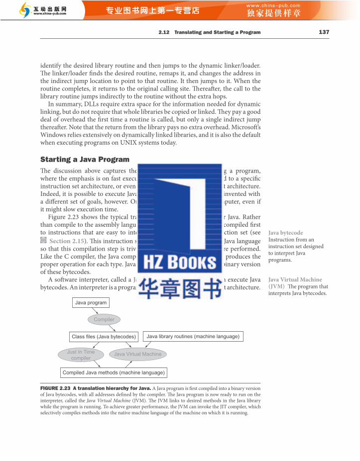
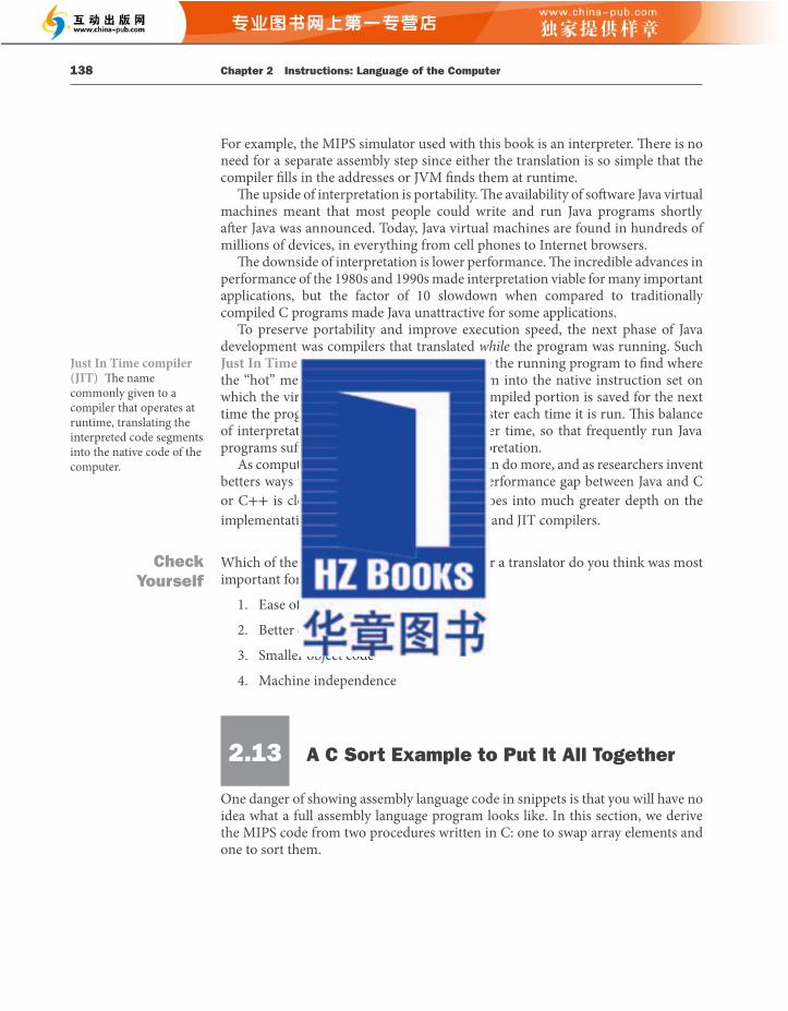
2.13 A C Sort Example to Put It All Together 139
The Procedure swap Let’s start with the code for the procedure swap in Figure 2.24 . Th is procedure simply swaps two locations in memory. When translating from C to assembly language by hand, we follow these general steps:
1. Allocate registers to program variables.
2. Produce code for the body of the procedure.
3. Preserve registers across the procedure invocation.
Th is section describes the swap procedure in these three pieces, concluding by putting all the pieces together.
Register Allocation for swap As mentioned on page 103, the MIPS convention on parameter passing is to use registers $a0 , $a1 , $a2 , and $a3 . Since swap has just two parameters, v and k , they will be found in registers $a0 and $a1 . Th e only other variable is temp , which we associate with register $t0 since swap is a leaf procedure (see page 106). Th is register allocation corresponds to the variable declarations in the fi rst part of the swap procedure in Figure 2.24 .
Code for the Body of the Procedure swap Th e remaining lines of C code in swap are
temp = v[k]; v[k] = v[k+1]; v[k+1] = temp;
Recall that the memory address for MIPS refers to the byte address, and so words are really 4 bytes apart. Hence we need to multiply the index k by 4 before adding it to the address. Forgetting that sequential word addresses diff er by 4 instead
void swap(int v[], int k) { int temp; temp = v[k]; v[k] = v[k+1]; v[k+1] = temp;
}
FIGURE 2.24 A C procedure that swaps two locations in memory. Th is subsection uses this procedure in a sorting example.
138 Chapter 2 Instructions: Language of the Computer
For example, the MIPS simulator used with this book is an interpreter. Th ere is no need for a separate assembly step since either the translation is so simple that the compiler fi lls in the addresses or JVM fi nds them at runtime.
Th e upside of interpretation is portability. Th e availability of soft ware Java virtual machines meant that most people could write and run Java programs shortly aft er Java was announced. Today, Java virtual machines are found in hundreds of millions of devices, in everything from cell phones to Internet browsers.
Th e downside of interpretation is lower performance. Th e incredible advances in performance of the 1980s and 1990s made interpretation viable for many important applications, but the factor of 10 slowdown when compared to traditionally compiled C programs made Java unattractive for some applications.
To preserve portability and improve execution speed, the next phase of Java development was compilers that translated while the program was running. Such Just In Time compilers (JIT) typically profi le the running program to fi nd where the “hot” methods are and then compile them into the native instruction set on which the virtual machine is running. Th e compiled portion is saved for the next time the program is run, so that it can run faster each time it is run. Th is balance of interpretation and compilation evolves over time, so that frequently run Java programs suff er little of the overhead of interpretation.
As computers get faster so that compilers can do more, and as researchers invent betters ways to compile Java on the fl y, the performance gap between Java and C or C++ is closing. Section 2.15 online goes into much greater depth on the implementation of Java, Java bytecodes, JVM, and JIT compilers.
Which of the advantages of an interpreter over a translator do you think was most important for the designers of Java?
1. Ease of writing an interpreter
2. Better error messages
3. Smaller object code
4. Machine independence
2.13 A C Sort Example to Put It All Together
One danger of showing assembly language code in snippets is that you will have no idea what a full assembly language program looks like. In this section, we derive the MIPS code from two procedures written in C: one to swap array elements and one to sort them.
Just In Time compiler (JIT) Th e name commonly given to a compiler that operates at runtime, translating the interpreted code segments into the native code of the computer.
Check Yourself
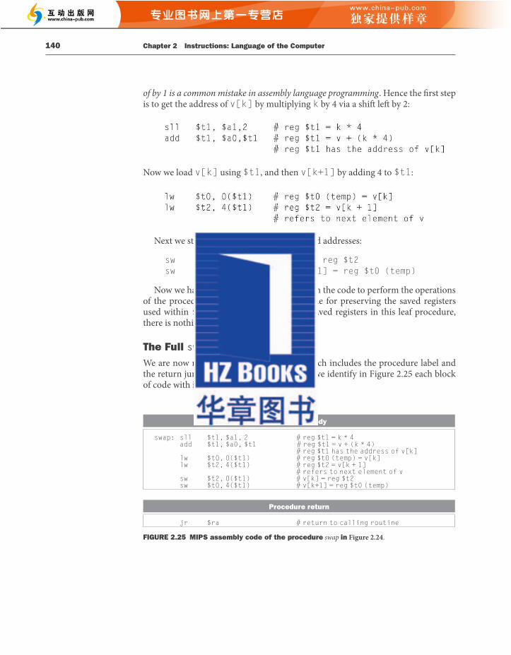
2.13 A C Sort Example to Put It All Together 141
The Procedure sort To ensure that you appreciate the rigor of programming in assembly language, we’ll try a second, longer example. In this case, we’ll build a routine that calls the swap procedure. Th is program sorts an array of integers, using bubble or exchange sort, which is one of the simplest if not the fastest sorts. Figure 2.26 shows the C version of the program. Once again, we present this procedure in several steps, concluding with the full procedure.
void sort (int v[], int n){ int i, j; for (i = 0; i < n; i += 1) { for (j = i – 1; j >= 0 && v[j] > v[j + 1]; j+=1) { swap(v,j); } }}
FIGURE 2.26 A C procedure that performs a sort on the array v .
Register Allocation for sort Th e two parameters of the procedure sort , v and n , are in the parameter registers $a0 and $a1 , and we assign register $s0 to i and register $s1 to j .
Code for the Body of the Procedure sort Th e procedure body consists of two nested for loops and a call to swap that includes parameters. Let’s unwrap the code from the outside to the middle.
Th e fi rst translation step is the fi rst for loop:
for (i = 0; i <n; i += 1) {
Recall that the C for statement has three parts: initialization, loop test, and iteration increment. It takes just one instruction to initialize i to 0, the fi rst part of the for statement:
move $s0, $zero # i = 0
(Remember that move is a pseudoinstruction provided by the assembler for the convenience of the assembly language programmer; see page 130.) It also takes just one instruction to increment i , the last part of the for statement:
addi $s0, $s0, 1 # i += 1
140 Chapter 2 Instructions: Language of the Computer
of by 1 is a common mistake in assembly language programming . Hence the fi rst step is to get the address of v[k] by multiplying k by 4 via a shift left by 2:
Now we load v[k] using $t1 , and then v[k+1] by adding 4 to $t1 :
Next we store $t0 and $t2 to the swapped addresses:
sw $t2, 0($t1) # v[k] = reg $t2 sw $t0, 4($t1) # v[k + 1] = reg $t0 (temp)
Now we have allocated registers and written the code to perform the operations of the procedure. What is missing is the code for preserving the saved registers used within swap . Since we are not using saved registers in this leaf procedure, there is nothing to preserve.
The Full swap Procedure We are now ready for the whole routine, which includes the procedure label and the return jump. To make it easier to follow, we identify in Figure 2.25 each block of code with its purpose in the procedure.
Procedure body
swap: sll $t1, $a1, 2 # reg $t1 = k * 4 add $t1, $a0, $t1 # reg $t1 = v + (k * 4)
# reg $t1 has the address of v[k] lw $t0, 0($t1) # reg $t0 (temp) = v[k] lw $t2, 4($t1) # reg $t2 = v[k + 1]
# refers to next element of v sw $t2, 0($t1) # v[k] = reg $t2 sw $t0, 4($t1) # v[k+1] = reg $t0 (temp)
Procedure return
jr $ra # return to calling routine
FIGURE 2.25 MIPS assembly code of the procedure swap in Figure 2.24 .
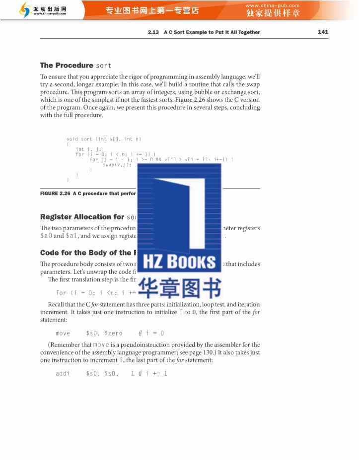

2.13 A C Sort Example to Put It All Together 143
Th e second test exits if v[j] >v[j + 1] is not true, or exits if v[j] ≤ v[j + 1] . First we create the address by multiplying j by 4 (since we need a byte address) and add it to the base address of v :
sll $t1, $s1, 2 # reg $t1 = j * 4 add $t2, $a0, $t1 # reg $t2 = v + (j * 4)
Now we load v[j] :
lw $t3, 0($t2) # reg $t3 = v[j]
Since we know that the second element is just the following word, we add 4 to the address in register $t2 to get v[j + 1] :
lw $t4, 4($t2) # reg $t4 = v[j + 1]
Th e test of v[j] ≤ v[j + 1] is the same as v[j + 1] ≥ v[j] , so the two instructions of the exit test are
slt $t0, $t4, $t3 # reg $t0 = 0 if $t4 ≥ $t3 beq $t0, $zero, exit2 # go to exit2 if $t4 ≥ $t3
Th e bottom of the loop jumps back to the inner loop test:
j for2tst # jump to test of inner loop
Combining the pieces, the skeleton of the second for loop looks like this:
The Procedure Call in sort Th e next step is the body of the second for loop:
swap(v,j);
Calling swap is easy enough:
jal swap
142 Chapter 2 Instructions: Language of the Computer
Th e loop should be exited if i < n is not true or, said another way, should be exited if i ≥ n . Th e set on less than instruction sets register $t0 to 1 if $s0 < $a1 and to 0 otherwise. Since we want to test if $s0 ≥ $a1 , we branch if register $t0 is 0. Th is test takes two instructions:
for1tst:slt $t0, $s0, $a1 # reg $t0 = 0 if $s0 ≥ $a1 (i ≥ n) beq $t0, $zero,exit1 # go to exit1 if $s0 ≥ $a1 (i ≥ n)
Th e bottom of the loop just jumps back to the loop test:
j for1tst # jump to test of outer loop exit1:
Th e skeleton code of the fi rst for loop is then
Voila! (Th e exercises explore writing faster code for similar loops.) Th e second for loop looks like this in C:
for (j = i –1; j >= 0 && v[j]>v[j + 1]; j –= 1) {
Th e initialization portion of this loop is again one instruction:
addi $s1, $s0, –1 # j = i – 1
Th e decrement of j at the end of the loop is also one instruction:
addi $s1, $s1, –1 # j –= 1
Th e loop test has two parts. We exit the loop if either condition fails, so the fi rst test must exit the loop if it fails ( j <0):
for2tst: slti $t0, $s1, 0 # reg $t0 = 1 if $s1 < 0 (j < 0) bne $t0, $zero, exit2 # go to exit2 if $s1 < 0 (j < 0)
Th is branch will skip over the second condition test. If it doesn’t skip, j ≥ 0.
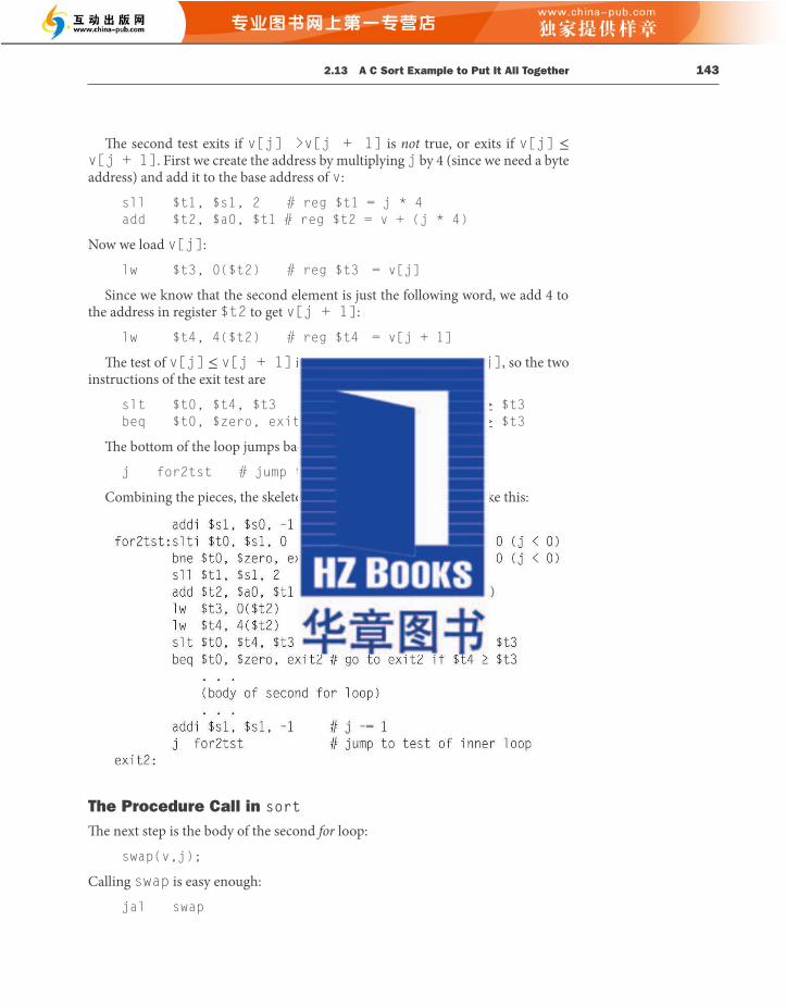
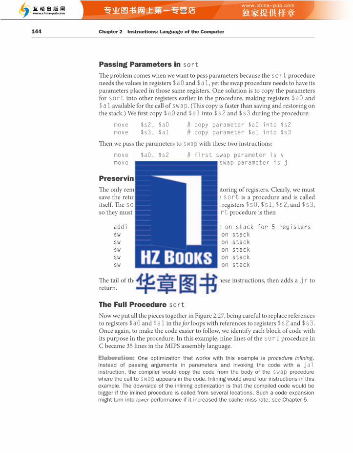
2.13 A C Sort Example to Put It All Together 145
Saving registers
sort: addi $sp,$sp, –20 # make room on stack for 5 registers sw $ra, 16($sp) # save $ra on stack sw $s3,12($sp) # save $s3 on stack sw $s2, 8($sp) # save $s2 on stack sw $s1, 4($sp) # save $s1 on stack sw $s0, 0($sp) # save $s0 on stack
Procedure body
Move parameters move $s2, $a0 #copy parameter $a0 into $s2 (save $a0) move $s3, $a1 #copy parameter $a1 into $s3 (save $a1)
Outer loop move $s0, $zero # i = 0for1tst:slt $t0, $s0,$s3 # reg$t0=0if$s0Š$s3(iŠn) beq $t0, $zero, exit1 # go to exit1 if $s0 Š $s3 (i Š n)
Inner loop
addi $s1, $s0, –1 # j = i – 1for2tst:slti $t0, $s1,0 # reg$t0=1if$s1<0(j<0) bne $t0, $zero, exit2 # go to exit2 if $s1 < 0 (j < 0) sll $t1, $s1, 2 # reg $t1 = j * 4 add $t2, $s2, $t1 # reg $t2 = v + (j * 4) lw $t3, 0($t2) # reg $t3 = v[j] lw $t4, 4($t2) # reg $t4 = v[j + 1] slt $t0, $t4, $t3 # reg $t0 = 0 if $t4 Š $t3 beq $t0, $zero, exit2 # go to exit2 if $t4 Š $t3
Pass parametersand call
move $a0, $s2 # 1st parameter of swap is v (old $a0) move $a1, $s1 # 2nd parameter of swap is j jal swap # swap code shown in Figure 2.25
Inner loop addi $s1, $s1, –1 # j –= 1 j for2tst # jump to test of inner loop
Outer loop exit2: addi $s0, $s0, 1 # i += 1 j for1tst # jump to test of outer loop
Restoring registers
exit1: lw $s0, 0($sp) # restore $s0 from stack lw $s1, 4($sp) # restore $s1 from stack lw $s2, 8($sp) # restore $s2 from stack lw $s3,12($sp) # restore $s3 from stack lw $ra,16($sp) # restore $ra from stack addi $sp,$sp, 20 # restore stack pointer
Procedure return
jr $ra # return to calling routine
FIGURE 2.27 MIPS assembly version of procedure sort in Figure 2.26 .
144 Chapter 2 Instructions: Language of the Computer
Passing Parameters in sort Th e problem comes when we want to pass parameters because the sort procedure needs the values in registers $a0 and $a1 , yet the swap procedure needs to have its parameters placed in those same registers. One solution is to copy the parameters for sort into other registers earlier in the procedure, making registers $a0 and $a1 available for the call of swap . (Th is copy is faster than saving and restoring on the stack.) We fi rst copy $a0 and $a1 into $s2 and $s3 during the procedure:
move $s2, $a0 # copy parameter $a0 into $s2 move $s3, $a1 # copy parameter $a1 into $s3
Th en we pass the parameters to swap with these two instructions:
move $a0, $s2 # first swap parameter is v move $a1, $s1 # second swap parameter is j
Preserving Registers in sort Th e only remaining code is the saving and restoring of registers. Clearly, we must save the return address in register $ra , since sort is a procedure and is called itself. Th e sort procedure also uses the saved registers $s0 , $s1 , $s2 , and $s3 , so they must be saved. Th e prologue of the sort procedure is then
Th e tail of the procedure simply reverses all these instructions, then adds a jr to return.
The Full Procedure sort Now we put all the pieces together in Figure 2.27 , being careful to replace references to registers $a0 and $a1 in the for loops with references to registers $s2 and $s3 . Once again, to make the code easier to follow, we identify each block of code with its purpose in the procedure. In this example, nine lines of the sort procedure in C became 35 lines in the MIPS assembly language.
Elaboration : One optimization that works with this example is procedure inlining . Instead of passing arguments in parameters and invoking the code with a jal instruction, the compiler would copy the code from the body of the swap procedure where the call to swap appears in the code. Inlining would avoid four instructions in this example. The downside of the inlining optimization is that the compiled code would be bigger if the inlined procedure is called from several locations. Such a code expansion might turn into lower performance if it increased the cache miss rate; see Chapter 5 .
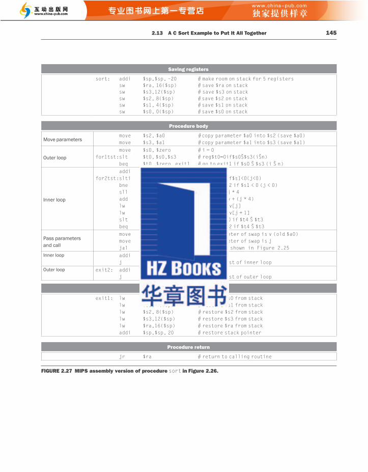
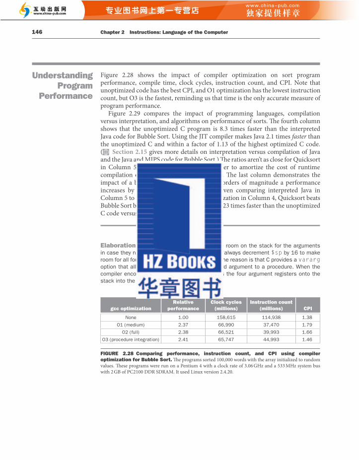
2.14 Arrays versus Pointers 147
2.14 Arrays versus Pointers
A challenge for any new C programmer is understanding pointers. Comparing assembly code that uses arrays and array indices to the assembly code that uses pointers off ers insights about pointers. Th is section shows C and MIPS assembly versions of two procedures to clear a sequence of words in memory: one using array indices and one using pointers. Figure 2.30 shows the two C procedures.
Th e purpose of this section is to show how pointers map into MIPS instructions, and not to endorse a dated programming style. We’ll see the impact of modern compiler optimization on these two procedures at the end of the section.
Array Version of Clear Let’s start with the array version, clear1 , focusing on the body of the loop and ignoring the procedure linkage code. We assume that the two parameters array and size are found in the registers $a0 and $a1 , and that i is allocated to register $t0 .
Th e initialization of i , the fi rst part of the for loop, is straightforward:
move $t0,$zero # i = 0 (register $t0 = 0)
To set array[i] to 0 we must fi rst get its address. Start by multiplying i by 4 to get the byte address:
loop1: sll $t1,$t0,2 # $t1 = i * 4
Since the starting address of the array is in a register, we must add it to the index to get the address of array[i] using an add instruction:
add $t2,$a0,$t1 # $t2 = address of array[i]
Language Execution method OptimizationBubble Sort relative
performanceQuicksort relative
performanceSpeedup Quicksort
vs. Bubble Sort
C Compiler None 1.00 1.00 2468
Compiler O1 2.37 1.50 1562
Compiler O2 2.38 1.50 1555
Compiler O3 2.41 1.91 1955
Java Interpreter – 0.12 0.05 1050
JIT compiler – 2.13 0.29 338
FIGURE 2.29 Performance of two sort algorithms in C and Java using interpretation and optimizing compilers relative to unoptimized C version. Th e last column shows the advantage in performance of Quicksort over Bubble Sort for each language and execution option. Th ese programs were run on the same system as Figure 2.28 . Th e JVM is Sun version 1.3.1, and the JIT is Sun Hotspot version 1.3.1.
146 Chapter 2 Instructions: Language of the Computer
Figure 2.28 shows the impact of compiler optimization on sort program performance, compile time, clock cycles, instruction count, and CPI. Note that unoptimized code has the best CPI, and O1 optimization has the lowest instruction count, but O3 is the fastest, reminding us that time is the only accurate measure of program performance.
Figure 2.29 compares the impact of programming languages, compilation versus interpretation, and algorithms on performance of sorts. Th e fourth column shows that the unoptimized C program is 8.3 times faster than the interpreted Java code for Bubble Sort. Using the JIT compiler makes Java 2.1 times faster than the unoptimized C and within a factor of 1.13 of the highest optimized C code.( Section 2.15 gives more details on interpretation versus compilation of Java and the Java and MIPS code for Bubble Sort.) Th e ratios aren’t as close for Quicksort in Column 5, presumably because it is harder to amortize the cost of runtime compilation over the shorter execution time. Th e last column demonstrates the impact of a better algorithm, off ering three orders of magnitude a performance increases by when sorting 100,000 items. Even comparing interpreted Java in Column 5 to the C compiler at highest optimization in Column 4, Quicksort beats Bubble Sort by a factor of 50 (0.05 × 2468, or 123 times faster than the unoptimized C code versus 2.41 times faster).
Understanding Program
Performance
Elaboration : The MIPS compilers always save room on the stack for the arguments in case they need to be stored, so in reality they always decrement $sp by 16 to make room for all four argument registers (16 bytes). One reason is that C provides a vararg option that allows a pointer to pick, say, the third argument to a procedure. When the compiler encounters the rare vararg , it copies the four argument registers onto the stack into the four reserved locations.
gcc optimizationRelative
performanceClock cycles
(millions)Instruction count
(millions) CPI
None 1.00 158,615 114,938 1.38
O1 (medium) 2.37 66,990 37,470 1.79
O2 (full) 2.38 66,521 39,993 1.66
O3 (procedure integration) 2.41 65,747 44,993 1.46
FIGURE 2.28 Comparing performance, instruction count, and CPI using compiler optimization for Bubble Sort. Th e programs sorted 100,000 words with the array initialized to random values. Th ese programs were run on a Pentium 4 with a clock rate of 3.06 GHz and a 533 MHz system bus with 2 GB of PC2100 DDR SDRAM. It used Linux version 2.4.20.
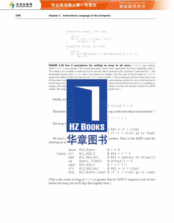
2.14 Arrays versus Pointers 149
Pointer Version of Clear Th e second procedure that uses pointers allocates the two parameters array and size to the registers $a0 and $a1 and allocates p to register $t0 . Th e code for the second procedure starts with assigning the pointer p to the address of the fi rst element of the array:
move $t0,$a0 # p = address of array[0]
Th e next code is the body of the for loop, which simply stores 0 into p :
loop2: sw $zero,0($t0) # Memory[p] = 0
Th is instruction implements the body of the loop, so the next code is the iteration increment, which changes p to point to the next word:
addi $t0,$t0,4 # p = p + 4
Incrementing a pointer by 1 means moving the pointer to the next sequential object in C. Since p is a pointer to integers, each of which uses 4 bytes, the compiler increments p by 4.
Th e loop test is next. Th e fi rst step is calculating the address of the last element of array . Start with multiplying size by 4 to get its byte address:
sll $t1,$a1,2 # $t1 = size * 4
and then we add the product to the starting address of the array to get the address of the fi rst word aft er the array:
add $t2,$a0,$t1 # $t2 = address of array[size]
Th e loop test is simply to see if p is less than the last element of array :
slt $t3,$t0,$t2 # $t3 = (p<&array[size]) bne $t3,$zero,loop2 # if (p<&array[size]) go to loop2
With all the pieces completed, we can show a pointer version of the code to zero an array:
As in the fi rst example, this code assumes size is greater than 0.
148 Chapter 2 Instructions: Language of the Computer
Finally, we can store 0 in that address:
sw $zero, 0($t2) # array[i] = 0
Th is instruction is the end of the body of the loop, so the next step is to increment i :
addi $t0,$t0,1 # i = i + 1
Th e loop test checks if i is less than size:
We have now seen all the pieces of the procedure. Here is the MIPS code for clearing an array using indices:
(Th is code works as long as size is greater than 0; ANSI C requires a test of size before the loop, but we’ll skip that legality here.)
clear1(int array[], int size){ int i; for (i = 0; i < size; i += 1) array[i] = 0;}clear2(int *array, int size){ int *p; for (p = &array[0]; p < &array[size]; p = p + 1) *p = 0;}
FIGURE 2.30 Two C procedures for setting an array to all zeros. Clear1 uses indices, while clear2 uses pointers. Th e second procedure needs some explanation for those unfamiliar with C. Th e address of a variable is indicated by &, and the object pointed to by a pointer is indicated by *. Th e declarations declare that array and p are pointers to integers. Th e fi rst part of the for loop in clear2 assigns the address of the fi rst element of array to the pointer p . Th e second part of the for loop tests to see if the pointer is pointing beyond the last element of array . Incrementing a pointer by one, in the last part of the for loop, means moving the pointer to the next sequential object of its declared size. Since p is a pointer to integers, the compiler will generate MIPS instructions to increment p by four, the number of bytes in a MIPS integer. Th e assignment in the loop places 0 in the object pointed to by p .
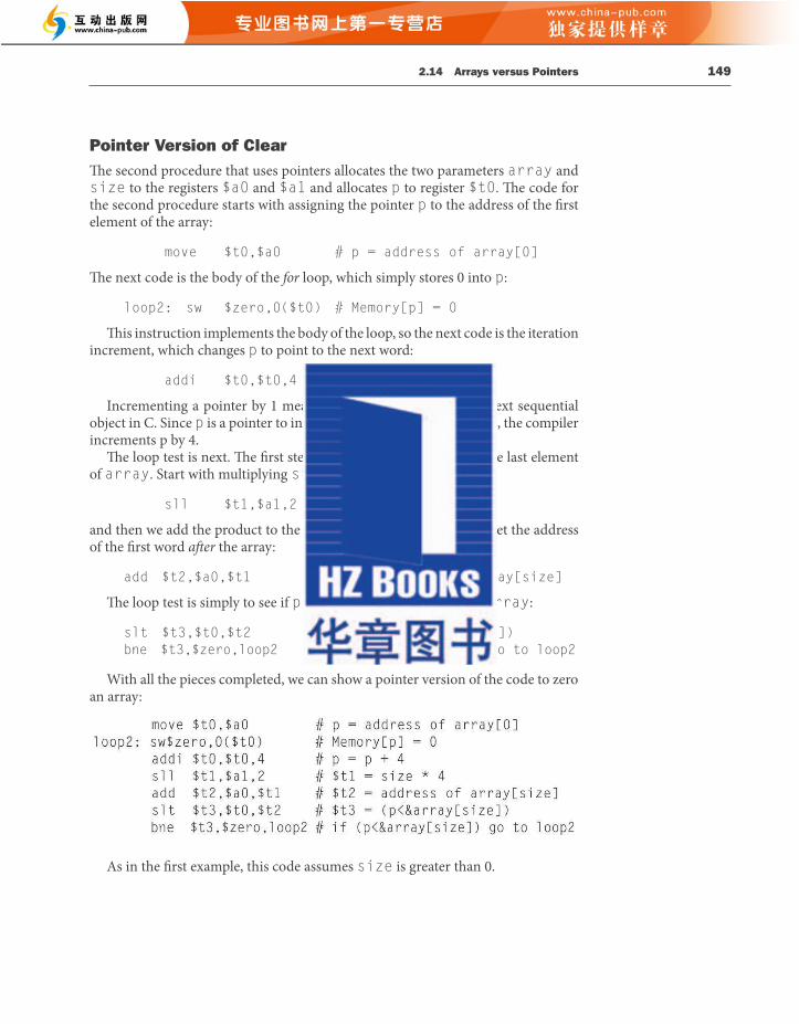
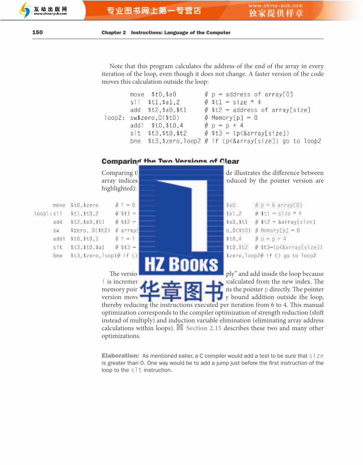
2.16 Real Stuff: ARMv7 (32-bit) Instructions 151
People used to be taught to use pointers in C to get greater effi ciency than that available with arrays: “Use pointers, even if you can’t understand the code.” Modern optimizing compilers can produce code for the array version that is just as good. Most programmers today prefer that the compiler do the heavy lift ing.
2.15 Advanced Material: Compiling C and Interpreting Java
Th is section gives a brief overview of how the C compiler works and how Java is executed. Because the compiler will signifi cantly aff ect the performance of a computer, understanding compiler technology today is critical to understanding performance. Keep in mind that the subject of compiler construction is usually taught in a one- or two-semester course, so our introduction will necessarily only touch on the basics.
Th e second part of this section is for readers interested in seeing how an objected oriented language like Java executes on a MIPS architecture. It shows the Java byte-codes used for interpretation and the MIPS code for the Java version of some of the C segments in prior sections, including Bubble Sort. It covers both the Java Virtual Machine and JIT compilers.
Th e rest of Section 2.15 can be found online.
2.16 Real Stuff: ARMv7 (32-bit) Instructions
ARM is the most popular instruction set architecture for embedded devices, with more than 100 billion devices through 2016. Standing originally for the Acorn RISC Machine, later changed to Advanced RISC Machine, ARM came out the same year as MIPS and followed similar philosophies. Figure 2.31 lists the similarities. Th e principle diff erence is that MIPS has more registers and ARM has more addressing modes.
Th ere is a similar core of instruction sets for arithmetic-logical and data transfer instructions for MIPS and ARM, as Figure 2.32 shows.
Addressing Modes Figure 2.33 shows the data addressing modes supported by ARM. Unlike MIPS, ARM does not reserve a register to contain 0. Although MIPS has just three simple data addressing modes (see Figure 2.18 ), ARM has nine, including fairly complex calculations. For example, ARM has an addressing mode that can shift one register by any amount, add it to the other registers to form the address, and then update one register with this new address.
Understanding Program Performance
object oriented language A programming language that is oriented around objects rather than actions, or data versus logic.
2.15
150 Chapter 2 Instructions: Language of the Computer
Note that this program calculates the address of the end of the array in every iteration of the loop, even though it does not change. A faster version of the code moves this calculation outside the loop:
Comparing the Two Versions of Clear Comparing the two code sequences side by side illustrates the diff erence between array indices and pointers (the changes introduced by the pointer version are highlighted):
Th e version on the left must have the “multiply” and add inside the loop because i is incremented and each address must be recalculated from the new index. Th e memory pointer version on the right increments the pointer p directly. Th e pointer version moves the scaling shift and the array bound addition outside the loop, thereby reducing the instructions executed per iteration from 6 to 4. Th is manual optimization corresponds to the compiler optimization of strength reduction (shift instead of multiply) and induction variable elimination (eliminating array address calculations within loops). Section 2.15 describes these two and many other optimizations.
Elaboration : As mentioned ealier, a C compiler would add a test to be sure that size is greater than 0. One way would be to add a jump just before the fi rst instruction of the loop to the slt instruction.
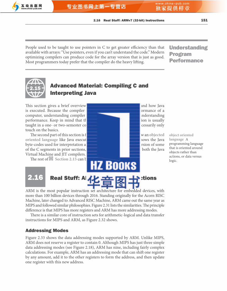
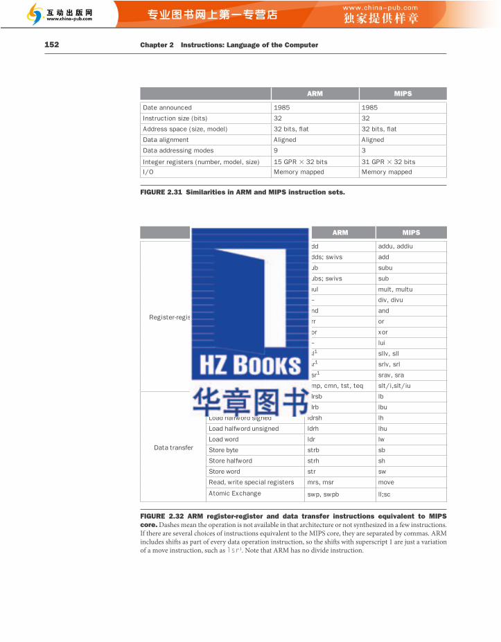
2.16 Real Stuff: ARMv7 (32-bit) Instructions 153
Addressing mode ARM MIPS
Register operand XX
Immediate operand XX
Register + offset (displacement or based) XX
Register + register (indexed) —X
Register + scaled register (scaled) —X
Register + offset and update register —X
Register + register and update register —X
Autoincrement, autodecrement —X
PC-relative data —X
FIGURE 2.33 Summary of data addressing modes. ARM has separate register indirect and register + off set addressing modes, rather than just putting 0 in the off set of the latter mode. To get greater addressing range, ARM shift s the off set left 1 or 2 bits if the data size is halfword or word.
Compare and Conditional Branch MIPS uses the contents of registers to evaluate conditional branches. ARM uses the traditional four condition code bits stored in the program status word: negative, zero, carry, and overfl ow . Th ey can be set on any arithmetic or logical instruction; unlike earlier architectures, this setting is optional on each instruction. An explicit option leads to fewer problems in a pipelined implementation (see Chapter 4). ARM uses conditional branches to test condition codes to determine all possible unsigned and signed relations.
CMP subtracts one operand from the other and the diff erence sets the condition codes. Compare negative (CMN) adds one operand to the other, and the sum sets the condition codes. TST performs logical AND on the two operands to set all condition codes but overfl ow, while TEQ uses exclusive OR to set the fi rst three condition codes.
One unusual feature of ARM is that every instruction has the option of executing conditionally, depending on the condition codes. Every instruction starts with a 4-bit fi eld that determines whether it will act as a no operation instruction (nop) or as a real instruction, depending on the condition codes. Hence, conditional branches are properly considered as conditionally executing the unconditional branch instruction. Conditional execution allows avoiding a branch to jump over a single instruction. It takes less code space and time to simply conditionally execute one instruction.
Figure 2.34 shows the instruction formats for ARM and MIPS. Th e principal diff erences are the 4-bit conditional execution fi eld in every instruction and the smaller register fi eld, because ARM has half the number of registers.
Unique Features of ARM Figure 2.35 shows a few arithmetic-logical instructions not found in MIPS. Since it does not have a dedicated register for 0, it has separate opcodes to perform
152 Chapter 2 Instructions: Language of the Computer
ARM MIPS
Date announced 1985 1985
Instruction size (bits) 32 32
Address space (size, model) 32 bits, fl at 32 bits, fl at
Data alignment Aligned Aligned
Data addressing modes 9 3
Integer registers (number, model, size) 15 GPR � 32 bits 31 GPR � 32 bits I/O Memory mapped Memory mapped
FIGURE 2.31 Similarities in ARM and MIPS instruction sets.
Register-register
ddA
buS
luM
iviD
dnA
rO
roX
oC
Data transferaoL
rotS
rotS
Instruction name ARM MIPS
add
Add (trap if overfl ow) adds; swivs add
addu, addiu
subtcart
Subtract (trap if overfl ow) subs; swivs sub
subu
mult, multumulylpit
div, divu—ed
andand
ororr
xoreor
Load high part register — lui
Shift left logical lsl1 sllv, sll
Shift right logical lsr1 srlv, srl
Shift right arithmetic asr1 srav, sra
slt/i,slt/iucmp, cmn, tst, teqerapm
Load byte signed ldrsb lb
Load byte unsigned ldrb lbu
Load halfword signed ldrsh lh
Load halfword unsigned ldrh lhu
lwldrdrowd
sbstrbetybe
Store halfword strh sh
swstrdrowe
Read, write special registers mrs, msr move
Atomic Exchange swp, swpb ll;sc
FIGURE 2.32 ARM register-register and data transfer instructions equivalent to MIPS core. Dashes mean the operation is not available in that architecture or not synthesized in a few instructions. If there are several choices of instructions equivalent to the MIPS core, they are separated by commas. ARM includes shift s as part of every data operation instruction, so the shift s with superscript 1 are just a variation of a move instruction, such as lsr 1 . Note that ARM has no divide instruction.
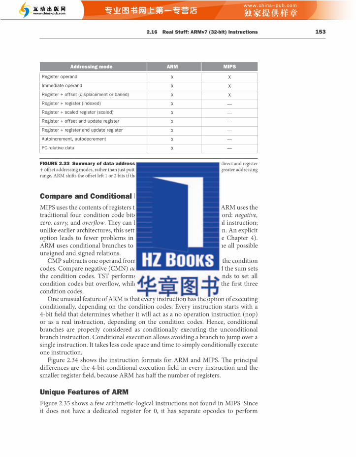
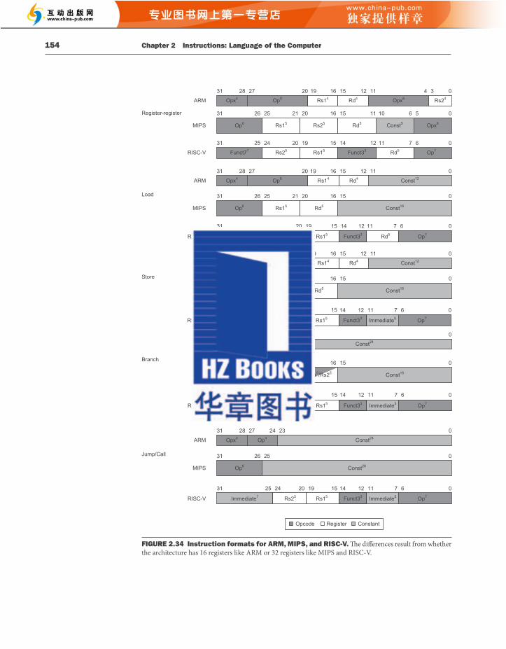
2.17 Real Stuff: ARMv8 (64-bit) Instructions 155
some operations that MIPS can do with $zero . In addition, ARM has support for multiword arithmetic.
ARM’s 12-bit immediate fi eld has a novel interpretation. Th e eight least-signifi cant bits are zero-extended to a 32-bit value, then rotated right the number of bits specifi ed in the fi rst four bits of the fi eld multiplied by two. One advantage is that this scheme can represent all powers of two in a 32-bit word. Whether this split actually catches more immediates than a simple 12-bit fi eld would be an interesting study.
Operand shift ing is not limited to immediates. Th e second register of all arithmetic and logical processing operations has the option of being shift ed before being operated on. Th e shift options are shift left logical, shift right logical, shift right arithmetic, and rotate right.
ARM also has instructions to save groups of registers, called block loads and stores . Under control of a 16-bit mask within the instructions, any of the 16 registers can be loaded or stored into memory in a single instruction. Th ese instructions can save and restore registers on procedure entry and return. Th ese instructions can also be used for block memory copy, and they also reduce code size on procedure entry and exit.
2.17 Real Stuff: ARMv8 (64-bit) Instructions
Of the many potential problems in an instruction set, the one that is almost impossible to overcome is having too small a memory address. While the x86 was successfully extended fi rst to 32-bit addresses and then later to 64-bit addresses, many of its brethren were left behind. For example, the 16-bit address MOStek 6502 powered the Apple II, but even given this headstart with the fi rst commercially successful personal computer, its lack of address bits condemned it to the dustbin of history.
Name Defi nition ARM MIPS
Load immediate Rd = Imm mov addi $0,
Not Rd = ~(Rs1) mvn nor $0,
Move Rd = Rs1 mov or $0,
Rotate right Rd = Rs i >> iRd0. . . i–1 = Rs31–i. . . 31
ror
And not Rd = Rs1 & ~(Rs2) bic
Reverse subtract Rd = Rs2 – Rs1 rsb, rsc
Support for multiword integer add
CarryOut, Rd = Rd + Rs1 + OldCarryOut
adcs —
Support for multiword integer sub
CarryOut, Rd = Rd – Rs1 + OldCarryOut
sbcs —
FIGURE 2.35 ARM arithmetic/logical instructions not found in MIPS.
154 Chapter 2 Instructions: Language of the Computer
Register ConstantOpcode
ARM
Register-register
Opx4
31 28 27
28 27
28 27
28 27
19 16 15
16 15
16 15
16 15
16 15
1112 4 3 0
Op8 Rs14 Rd4 Rs24Opx8
Load
ARM Opx4
31 1112 0
Op8 Rs14 Rd4 Const12
Branch
ARM
Jump/Call
Opx4
31 2324 0
Op4 Const24
ARM Opx4
31 2324 0
Op4 Const24
MIPS
31 2526
20
21 20
2526 21 20
21 20
1920
11 10 6 5 0
Const5Rs15 Rs25 Rd5 Opx6Op6
MIPS
31 0
Const16Rs15 Rd5Op6
MIPS
31 2526
2526
0
Rs15 Opx5/Rs25 Const16Op6
31 0
Op6MIPS Const26
15 14
RISC-V
31 2425 20 19 12 11 7 6 0
Rd5Rs25 Rs15 Funct33 Op7Funct77
15 14
RISC-V
31 20 19 12 11 7 6 0
Rd5Rs15 Funct33 Op7Immediate12
28 27 16 15
16 15Store
ARM Opx4
31 1112 0
Op8 Rs14 Rd4 Const12
2526 21 20
1920
MIPS
31 0
Const16Rs15 Rd5Op6
20 19
RISC-V
31 25 24 15 14 12 11 0
Immediate5Rs15 Funct33 Op7Immediate7 Rs25
7 6
20 19
RISC-V
31 25 24 15 14 12 11 0
Immediate5Rs15 Funct33 Op7Immediate7 Rs25
7 6
RISC- IV mmediate5Rs15 Funct33 Op7Immediate7 Rs25
20 1931 25 24 15 14 12 11 07 6
FIGURE 2.34 Instruction formats for ARM, MIPS, and RISC-V. Th e diff erences result from whether the architecture has 16 registers like ARM or 32 registers like MIPS and RISC-V.
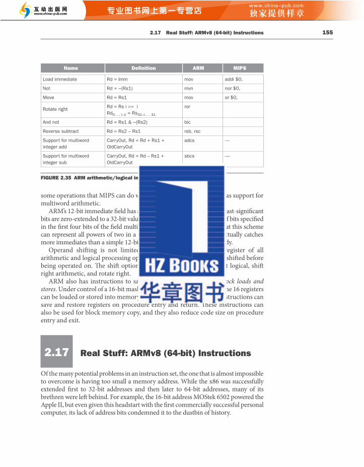
2.19 Real Stuff: x86 Instructions 157
■ Th e only way to access memory is via load and store instructions on both architectures.
■ Unlike some architectures, there are no instructions that can load or store many registers in MIPS or RISC-V.
■ Both have instructions that branch if a register is equal to zero and branch if a register is not equal to zero.
■ Both sets of addressing modes work for all data sizes.
One of the main diff erences between MIPS and RISC-V is for conditional branches other than equal or not equal. Although RISC-V simply provides branch instructions to compare two registers, MIPS relies on a comparison instruction that sets a register to 0 or 1 depending on whether the comparison is true. Programmers then follow that comparison instruction with a branch on equal to or not equal to zero depending on the desired outcome of the comparison. Keeping with its minimalist philosophy, MIPS only performs less than comparisons, leaving it up to the programmer to switch order of operands or to switch the condition being tested by the branch to get all the desired outcomes.
2.19 Real Stuff: x86 Instructions
Designers of instruction sets sometimes provide more powerful operations than those found in ARM, MIPS, and RISC-V. Th e goal is generally to reduce the number of instructions executed by a program. Th e danger is that this reduction can occur at the cost of simplicity, increasing the time a program takes to execute because the instructions are slower. Th is slowness may be the result of a slower clock cycle time or of requiring more clock cycles than a simpler sequence.
Th e path toward operation complexity is thus fraught with peril. Section 2.21 demonstrates the pitfalls of complexity.
Evolution of the Intel x86 ARM and MIPS were the vision of single small groups in 1985; the pieces of these architectures fi t nicely together, and the whole architecture can be described succinctly. Such is not the case for the x86; it is the product of several independent groups who evolved the architecture over 40 years, adding new features to the original instruction set as someone might add clothing to a packed bag. Here are important x86 milestones.
■ 1978 : Th e Intel 8086 architecture was announced as an assembly language–compatible extension of the then successful Intel 8080, an 8-bit microprocessor. Th e 8086 is a 16-bit architecture, with all internal registers 16 bits wide. Unlike MIPS, the registers have dedicated uses, and hence the 8086 is not considered a general-purpose register architecture.
Beauty is altogether in the eye of the beholder. Margaret Wolfe Hungerford, Molly Bawn , 1877
general-purpose register (GPR) A register that can be used for addresses or for data with virtually any instruction.
156 Chapter 2 Instructions: Language of the Computer
ARM architects could see the writing on the wall of their 32-bit address computer, and began design of the 64-bit address version of ARM in 2007. It was revealed in 2013. Rather than some minor cosmetic changes to make all the registers 64 bits wide, which is basically what happened to the x86, ARM did a complete overhaul. Th e good news is that if you know MIPS it will be easier to pick up ARMv8, as the 64-bit version is called.
First, as compared to MIPS, ARM dropped virtually all of the unusual features of the prior ARM architecture, referred to as ARM v7:
■ Th ere is no conditional execution fi eld, as there was in nearly every instruction in v7.
■ Th e immediate fi eld is simply a 12 bit constant, rather than essentially an input to a function that produces a constant as in v7.
■ Th ey dropped Load Multiple and Store Multiple instructions.
■ Th e PC is no longer one of the registers, which resulted in unexpected branches if you wrote to it.
Second, ARM added missing features that are useful in MIPS
■ V8 has 32 general-purpose registers, which compiler writers surely love. Like MIPS, one register is hardwired to 0, although in load and store instructions it instead refers to the stack pointer.
■ Its addressing modes work for all word sizes in ARMv8, which was not the case in ARMv7.
■ It includes a divide instruction, which was omitted from ARMv7.
■ It adds the equivalent of MIPS branch if equal and branch if not equal.
As the philosophy of the v8 instruction set is much closer to MIPS than it is to v7, our conclusion is that the main similarity between ARMv7 and ARMv8 is the name.
2.18 Real Stuff: RISC-V Instructions
Th e instruction set most similar to MIPS also originated in academia. Th e good news is that if you know MIPS, it will be very easy to pick up RISC-V. However, RISC-V is an open architecture that is controlled by RISC-V International and not a proprietary architecture that is owned by a company like ARM, MIPS, or x86. MIPS and RISC-V share the same design philosophy, despite MIPS being 25 years more senior than RISC-V. Both also have 32-bit address versions and 64-bit address versions. To show their similarity, Figure 2.34 compares instruction formats for ARM, MIPS, and RISC-V. Here are the common features between RISC-V and MIPS:
■ All instructions are 32 bit wide for both architectures.
■ Both have 32 general-purpose registers, with one register being hardwired to 0.
2.19 Real Stuff: x86 Instructions 159
space from 32 to 64 bits. Similar to the transition from a 16- to 32-bit address space in 1985 with the 80386, AMD64 widens all registers to 64 bits. It also increases the number of registers to 16 and increases the number of 128-bit SSE registers to 16. Th e primary ISA change comes from adding a new mode called long mode that redefi nes the execution of all x86 instructions with 64-bit addresses and data. To address the larger number of registers, it adds a new prefi x to instructions. Depending how you count, long mode also adds four to ten new instructions and drops 27 old ones. PC-relative data addressing is another extension. AMD64 still has a mode that is identical to x86 ( legacy mode ) plus a mode that restricts user programs to x86 but allows operating systems to use AMD64 ( compatibility mode ). Th ese modes allowed a more graceful transition to 64-bit addressing than the HP/Intel IA-64 architecture.
■ 2004 : Intel capitulates and embraces AMD64, relabeling it Extended Memory 64 Technology (EM64T). Th e major diff erence is that Intel added a 128-bit atomic compare and swap instruction, which probably should have been included in AMD64. At the same time, Intel announced another generation of media extensions. SSE3 adds 13 instructions to support complex arithmetic, graphics operations on arrays of structures, video encoding, fl oating-point conversion, and thread synchronization (see Section 2.11 ). AMD added SSE3 in subsequent chips and the missing atomic swap instruction to AMD64 to maintain binary compatibility with Intel.
■ 2006 : Intel announces 54 new instructions as part of the SSE4 instruction set extensions. Th ese extensions perform tweaks like sum of absolute diff erences, dot products for arrays of structures, sign or zero extension of narrow data to wider sizes, population count, and so on. Th ey also added support for virtual machines (see Chapter 5 ).
■ 2007 : AMD announces 170 instructions as part of SSE5, including 46 instructions of the base instruction set that adds three operand instructions like MIPS.
■ 2011 : Intel ships the Advanced Vector Extension that expands the SSE register width from 128 to 256 bits, thereby redefi ning about 250 instructions and adding 128 new instructions.
■ 2015 : Intel ships AVX-512, which widens the registers and operations from 256 to 512 bits, and once again redefi nes hundreds of instructions as well as adds many more.
Th is history illustrates the impact of the “golden handcuff s” of compatibility on the x86, as the existing soft ware base at each step was too important to jeopardize with signifi cant architectural changes.
Whatever the artistic failures of the x86, keep in mind that this instruction set largely drove the PC generation of computers and still dominates the cloud portion of the PostPC Era. Manufacturing 250 M x86 chips per year may seem small compared to billions of ARMv7 chips, but many companies would love to control such a market since the chips are much more expensive. Nevertheless, this checkered ancestry has led to an architecture that is diffi cult to explain and impossible to love.
158 Chapter 2 Instructions: Language of the Computer
■ 1980 : Th e Intel 8087 fl oating-point coprocessor is announced. Th is archi-tecture extends the 8086 with about 60 fl oating-point instructions. Instead of using registers, it relies on a stack (see Section 2.23 and Section 3.7).
■ 1982 : Th e 80286 extended the 8086 architecture by increasing the address space to 24 bits, by creating an elaborate memory-mapping and protection model (see Chapter 5 ), and by adding a few instructions to round out the instruction set and to manipulate the protection model.
■ 1985 : Th e 80386 extended the 80286 architecture to 32 bits. In addition to a 32-bit architecture with 32-bit registers and a 32-bit address space, the 80386 added new addressing modes and additional operations. Th e added instructions make the 80386 nearly a general-purpose register machine. Th e 80386 also added paging support in addition to segmented addressing (see Chapter 5 ). Like the 80286, the 80386 has a mode to execute 8086 programs without change.
■ 1989–95 : Th e subsequent 80486 in 1989, Pentium in 1992, and Pentium Pro in 1995 were aimed at higher performance, with only four instructions added to the user-visible instruction set: three to help with multiprocessing ( Chapter 6 ) and a conditional move instruction.
■ 1997 : Aft er the Pentium and Pentium Pro were shipping, Intel announced that it would expand the Pentium and the Pentium Pro architectures with MMX (Multi Media Extensions). Th is new set of 57 instructions uses the fl oating-point stack to accelerate multimedia and communication applications. MMX instructions typically operate on multiple short data elements at a time, in the tradition of single instruction, multiple data (SIMD) architectures (see Chapter 6 ). Pentium II did not introduce any new instructions.
■ 1999 : Intel added another 70 instructions, labeled SSE ( Streaming SIMD Extensions ) as part of Pentium III. Th e primary changes were to add eight separate registers, double their width to 128 bits, and add a single precision fl oating-point data type. Hence, four 32-bit fl oating-point operations can be performed in parallel. To improve memory performance, SSE includes cache prefetch instructions plus streaming store instructions that bypass the caches and write directly to memory ( see Chapter 5 ).
■ 2001 : Intel added yet another 144 instructions, this time labeled SSE2. Th e new data type is double precision arithmetic, which allows pairs of 64-bit fl oating-point operations in parallel. Almost all of these 144 instructions are versions of existing MMX and SSE instructions that operate on 64 bits of data in parallel. Not only does this change enable more multimedia operations, it gives the compiler a diff erent target for fl oating-point operations than the unique stack architecture. Compilers can choose to use the eight SSE registers as fl oating-point registers like those found in other computers. Th is change boosted the fl oating-point performance of the Pentium 4, the fi rst microprocessor to include SSE2 instructions.
■ 2003 : A company other than Intel enhanced the x86 architecture this time. AMD announced a set of architectural extensions to increase the address
2.19 Real Stuff: x86 Instructions 161
GPR 0
GPR 1
GPR 2
GPR 3
GPR 4
GPR 5
GPR 6
GPR 7
Code segment pointer
Stack segment pointer (top of stack)
Data segment pointer 0
Data segment pointer 1
Data segment pointer 2
Data segment pointer 3
Instruction pointer (PC)
Condition codes
Use031
Name
EAX
ECX
EDX
EBX
ESP
EBP
ESI
EDI
CS
SS
DS
ES
FS
GS
EIP
EFLAGS
FIGURE 2.36 The 80386 register set. Starting with the 80386, the top eight registers were extended to 32 bits and could also be used as general-purpose registers.
Source/destination operand type Second source operand
Register Register
Register Immediate
Register Memory
Memory Register
Memory Immediate
FIGURE 2.37 Instruction types for the arithmetic, logical, and data transfer instructions. Th e x86 allows the combinations shown. Th e only restriction is the absence of a memory-memory mode. Immediates may be 8, 16, or 32 bits in length; a register is any one of the 14 major registers in Figure 2.36 (not EIP or EFLAGS).
160 Chapter 2 Instructions: Language of the Computer
Brace yourself for what you are about to see! Do not try to read this section with the care you would need to write x86 programs; the goal instead is to give you familiarity with the strengths and weaknesses of the world’s most popular desktop architecture.
Rather than show the entire 16-bit, 32-bit, and 64-bit instruction set, in this section we concentrate on the 32-bit subset that originated with the 80386. We start our explanation with the registers and addressing modes, move on to the integer operations, and conclude with an examination of instruction encoding.
x86 Registers and Data Addressing Modes Th e registers of the 80386 show the evolution of the instruction set ( Figure 2.36 ). Th e 80386 extended all 16-bit registers (except the segment registers) to 32 bits, prefi xing an E to their name to indicate the 32-bit version. We’ll refer to them generically as GPRs ( general-purpose registers ). Th e 80386 contains only eight GPRs. Th is means MIPS programs can use four times as many and ARMv7 twice as many.
Figure 2.37 shows the arithmetic, logical, and data transfer instructions are two-operand instructions. Th ere are two important diff erences here. Th e x86 arithmetic and logical instructions must have one operand act as both a source and a destination; ARMv7 and MIPS allow separate registers for source and destination. Th is restriction puts more pressure on the limited registers, since one source register must be modifi ed. Th e second important diff erence is that one of the operands can be in memory. Th us, virtually any instruction may have one operand in memory, unlike ARMv7 and MIPS.
Data memory-addressing modes, described in detail below, off er two sizes of addresses within the instruction. Th ese so-called displacements can be 8 bits or 32 bits.
Although a memory operand can use any addressing mode, there are restrictions on which registers can be used in a mode. Figure 2.38 shows the x86 addressing modes and which GPRs cannot be used with each mode, as well as how to get the same eff ect using MIPS instructions.
x86 Integer Operations Th e 8086 provides support for both 8-bit ( byte ) and 16-bit ( word ) data types. Th e 80386 adds 32-bit addresses and data ( double words ) in the x86. (AMD64 adds 64-bit addresses and data, called quad words ; we’ll stick to the 80386 in this section.) Th e data type distinctions apply to register operations as well as memory accesses.
Almost every operation works on both 8-bit data and on one longer data size. Th at size is determined by the mode and is either 16 bits or 32 bits.
Clearly, some programs want to operate on data of all three sizes, so the 80386 architects provided a convenient way to specify each version without expanding code size signifi cantly. Th ey decided that either 16-bit or 32-bit data dominates most programs, and so it made sense to be able to set a default large size. Th is default data size is set by a bit in the code segment register. To override the default data size, an 8-bit prefi x is attached to the instruction to tell the machine to use the other large size for this instruction.
Th e prefi x solution was borrowed from the 8086, which allows multiple prefi xes to modify instruction behavior. Th e three original prefi xes override the default
2.19 Real Stuff: x86 Instructions 163
Instruction Function
je name if equal(condition code) {EIP=name};EIP–128 <= name < EIP+128
jmp name EIP=name
call name SP=SP–4; M[SP]=EIP+5; EIP=name;
movw EBX,[EDI+45] EBX=M[EDI+45]
push ESI SP=SP–4; M[SP]=ESI
pop EDI EDI=M[SP]; SP=SP+4
add EAX,#6765 EAX= EAX+6765
test EDX,#42 Set condition code (fl ags) with EDX and 42
movsl M[EDI]=M[ESI];EDI=EDI+4; ESI=ESI+4
FIGURE 2.39 Some typical x86 instructions and their functions. A list of frequent operations appears in Figure 2.40 . Th e CALL saves the EIP of the next instruction on the stack. (EIP is the Intel PC.)
Instruction Meaning
Control Conditional and unconditional branches
jnz, jz Jump if condition to EIP + 8-bit offset; JNE (forJNZ), JE (for JZ) are alternative names
jmp Unconditional jump—8-bit or 16-bit offset
call Subroutine call—16-bit offset; return address pushed onto stack
ret Pops return address from stack and jumps to it
loop Loop branch—decrement ECX; jump to EIP + 8-bit displacement if ECX ≠ 0 Data transfer Move data between registers or between register and memory
move Move between two registers or between register and memory
push, pop Push source operand on stack; pop operand from stack top to a register
les Load ES and one of the GPRs from memory
Arithmetic, logical Arithmetic and logical operations using the data registers and memory
add, sub Add source to destination; subtract source from destination; register-memory format
cmp Compare source and destination; register-memory format
shl, shr, rcr Shift left; shift logical right; rotate right with carry condition code as fi ll
cbw Convert byte in eight rightmost bits of EAX to 16-bit word in right of EAX
test Logical AND of source and destination sets condition codes
inc, dec Increment destination, decrement destination
or, xor Logical OR; exclusive OR; register-memory format
String Move between string operands; length given by a repeat prefi x
movs Copies from string source to destination by incrementing ESI and EDI; may be repeated
lods Loads a byte, word, or doubleword of a string into the EAX register
FIGURE 2.40 Some typical operations on the x86. Many operations use register-memory format, where either the source or the destination may be memory and the other may be a register or immediate operand.
162 Chapter 2 Instructions: Language of the Computer
segment register, lock the bus to support synchronization (see Section 2.11 ), or repeat the following instruction until the register ECX counts down to 0. Th is last prefi x was intended to be paired with a byte move instruction to move a variable number of bytes. Th e 80386 also added a prefi x to override the default address size.
Th e x86 integer operations can be divided into four major classes:
1. Data movement instructions, including move, push, and pop
2. Arithmetic and logic instructions, including test, integer, and decimal arithmetic operations
3. Control fl ow, including conditional branches, unconditional jumps, calls, and returns
4. String instructions, including string move and string compare
Th e fi rst two categories are unremarkable, except that the arithmetic and logic instruction operations allow the destination to be either a register or a memory location. Figure 2.39 shows some typical x86 instructions and their functions.
Conditional branches on the x86 are based on condition codes or fl ags , like ARMv7. Condition codes are set as a side eff ect of an operation; most are used to compare the value of a result to 0. Branches then test the condition codes. PC-relative branch addresses must be specifi ed in the number of bytes, since unlike ARMv7 and MIPS, 80386 instructions are not all 4 bytes in length.
String instructions are part of the 8080 ancestry of the x86 and are not commonly executed in most programs. Th ey are oft en slower than equivalent soft ware routines (see the fallacy on page 167).
Figure 2.40 lists some of the integer x86 instructions. Many of the instructions are available in both byte and word formats.
Mode DescriptionRegister
restrictions MIPS equivalent
Register indirect Address is in a register. Not ESP or EBP lw $s0,0($s1)
Based mode with 8- or 32-bit displacement
Address is contents of base register plus displacement.
Not ESP lw $s0,100($s1) # <= 16-bit # displacement
Base plus scaled index The address isBase + (2Scale x Index)
where Scale has the value 0, 1, 2, or 3.
Base: any GPRIndex: not ESP
mul $t0,$s2,4add $t0,$t0,$s1lw $s0,0($t0)
Base plus scaled index with8- or 32-bit displacement
The address isBase + (2Scale x Index) + displacement
where Scale has the value 0, 1, 2, or 3.
Base: any GPRIndex: not ESP
mul $t0,$s2,4add $t0,$t0,$s1lw $s0,100($t0) #<=16-bit
# displacement
FIGURE 2.38 x86 32-bit addressing modes with register restrictions and the equivalent MIPS code. Th e Base plus Scaled Index addressing mode, not found in ARM or MIPS, is included to avoid the multiplies by 4 (scale factor of 2) to turn an index in a register into a byte address (see Figures 2.25 and 2.27 ). A scale factor of 1 is used for 16-bit data, and a scale factor of 3 for 64-bit data. A scale factor of 0 means the address is not scaled. If the displacement is longer than 16 bits in the second or fourth modes, then the MIPS equivalent mode would need two more instructions: a lui to load the upper 16 bits of the displacement and an add to sum the upper address with the base register $s1 . (Intel gives two diff erent names to what is called Based addressing mode—Based and Indexed—but they are essentially identical and we combine them here.)
2.19 Real Stuff: x86 Instructions 165
reg w = 0 w = 1 r/m mod = 0 mod = 1 mod = 2 mod = 3
16b 32b 16b 32b 16b 32b 16b 32b
0 AL AX EAX 0 addr=BX+SI =EAX same same same same same
1 CL CX ECX 1 addr=BX+DI =ECX addr as addr as addr as addr as as
2 DL DX EDX 2 addr=BP+SI =EDX mod=0 mod=0 mod=0 mod=0 reg
3 BL BX EBX 3 addr=BP+SI =EBX + disp8 + disp8 + disp16 + disp32 fi eld
4 AH SP ESP 4 addr=SI =(sib) SI+disp8 (sib)+disp8 SI+disp8 (sib)+disp32 “
5 CH BP EBP 5 addr=DI =disp32 DI+disp8 EBP+disp8 DI+disp16 EBP+disp32 “
6 DH SI ESI 6 addr=disp16 =ESI BP+disp8 ESI+disp8 BP+disp16 ESI+disp32 “
7 BH DI EDI 7 addr=BX =EDI BX+disp8 EDI+disp8 BX+disp16 EDI+disp32 “
FIGURE 2.42 The encoding of the fi rst address specifi er of the x86: mod, reg, r/m. Th e fi rst four columns show the encoding of the 3-bit reg fi eld, which depends on the w bit from the opcode and whether the machine is in 16-bit mode (8086) or 32-bit mode (80386). Th e remaining columns explain the mod and r/m fi elds. Th e meaning of the 3-bit r/m fi eld depends on the value in the 2-bit mod fi eld and the address size. Basically, the registers used in the address calculation are listed in the sixth and seventh columns, under mod = 0, with mod = 1 adding an 8-bit displacement and mod = 2 adding a 16-bit or 32-bit displacement, depending on the address mode. Th e exceptions are 1) r/m = 6 when mod = 1 or mod = 2 in 16-bit mode selects BP plus the displacement; 2) r/m = 5 when mod = 1 or mod = 2 in 32-bit mode selects EBP plus displacement; and 3) r/m = 4 in 32-bit mode when mod does not equal 3, where (sib) means use the scaled index mode shown in Figure 2.38 . When mod = 3, the r/m fi eld indicates a register, using the same encoding as the reg fi eld combined with the w bit.
immediate.” Other instructions use a “postbyte” or extra opcode byte, labeled “mod, reg, r/m,” which contains the addressing mode information. Th is postbyte is used for many of the instructions that address memory. Th e base plus scaled index mode uses a second postbyte, labeled “sc, index, base.”
Figure 2.42 shows the encoding of the two postbyte address specifi ers for both 16-bit and 32-bit mode. Unfortunately, to understand fully which registers and which addressing modes are available, you need to see the encoding of all addressing modes and sometimes even the encoding of the instructions.
x86 Conclusion Intel had a 16-bit microprocessor two years before its competitors’ more elegant architectures, such as the Motorola 68000, and this head start led to the selection of the 8086 as the CPU for the IBM PC. Intel engineers generally acknowledge that the x86 is more diffi cult to build than computers like ARMv7 and MIPS, but the large market meant in the PC Era that AMD and Intel could aff ord more resources to help overcome the added complexity. What the x86 lacks in style, it made up for in market size, making it beautiful from the right perspective.
Its saving grace is that the most frequently used x86 architectural components are not too diffi cult to implement, as AMD and Intel have demonstrated by rapidly improving performance of integer programs since 1978. To get that performance, compilers must avoid the portions of the architecture that are hard to implement fast.
In the PostPC Era, however, despite considerable architectural and manufacturing expertise, x86 has not yet been competitive in the personal mobile device.
164 Chapter 2 Instructions: Language of the Computer
a. JE EIP + displacement
b. CALL
c. MOV EBX, [EDI + 45]
d. PUSH ESI
e. ADD EAX, #6765
f. TEST EDX, #42
ImmediatePostbyteTEST
ADD
PUSH
MOV
CALL
JE
w
w ImmediateReg
Reg
wd Displacementr/mPostbyte
Offset
DisplacementCondi-tion
4 4 8
8 32
6 81 1 8
5 3
4 323 1
7 321 8
FIGURE 2.41 Typical x86 instruction formats. Figure 2.42 shows the encoding of the postbyte. Many instructions contain the 1-bit fi eld w, which says whether the operation is a byte or a double word. Th e d fi eld in MOV is used in instructions that may move to or from memory and shows the direction of the move. Th e ADD instruction requires 32 bits for the immediate fi eld, because in 32-bit mode, the immediates are either 8 bits or 32 bits. Th e immediate fi eld in the TEST is 32 bits long because there is no 8-bit immediate for test in 32-bit mode. Overall, instructions may vary from 1 to 15 bytes in length. Th e long length comes from extra 1-byte prefi xes, having both a 4-byte immediate and a 4-byte displacement address, using an opcode of 2 bytes, and using the scaled index mode specifi er, which adds another byte.
x86 Instruction Encoding Saving the worst for last, the encoding of instructions in the 80386 is complex, with many diff erent instruction formats. Instructions for the 80386 may vary from 1 byte, when there are no operands, up to 15 bytes.
Figure 2.41 shows the instruction format for several of the example instructions in Figure 2.39 . Th e opcode byte usually contains a bit saying whether the operand is 8 bits or 32 bits. For some instructions, the opcode may include the addressing mode and the register; this is true in many instructions that have the form “register = register op
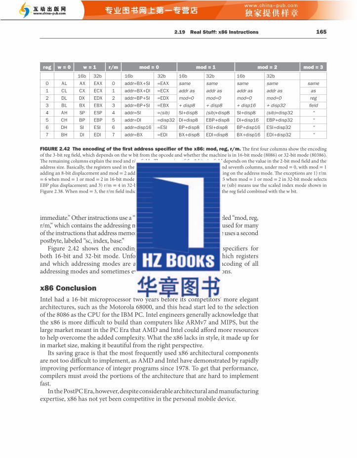

2.21 Fallacies and Pitfalls 167
1. vmovsd (%r10),%xmm0 # Load 1 element of C into %xmm0
2. mov %rsi,%rcx # register %rcx = %rsi
3. xor %eax,%eax # register %eax = 0
4. vmovsd (%rcx),%xmm1 # Load 1 element of B into %xmm1
5. add %r9,%rcx # register %rcx = %rcx + %r9
6. vmulsd (%r8,%rax,8),%xmm1,%xmm1 # Multiply %xmm1, element of A
7. add $0x1,%rax # register %rax = %rax + 1
8. cmp %eax,%edi # compare %eax to %edi
9. vaddsd %xmm1,%xmm0,%xmm0 # Add %xmm1, %xmm0
10. jg 30 <dgemm+0x30> # jump if %eax > %edi
11. add $0x1,%r11 # register %r11 = %r11 + 1
12. vmovsd %xmm0,(%r10) # Store %xmm0 into C element
FIGURE 2.44 Th e x86 assembly language for the body of the nested loops generated by compiling the unoptimized C code in Figure 2.43 using gcc with − O3 optimization fl ags.
–O0 (fastest compile time) –O1 –O2 –O3 (fastest run time)
77 208 212 212
FIGURE 2.45 Performance over the Python program on page 49 for the C program in Figure 2.43 as we increase the level of optimization of the GCC C compiler, with − O0 doing no code size or performance optimization, thereby improving compile time and − O3 being most aggressive for run time and code size. In this case, − O2 and − O3 produce the same x86 code. Most programmers use − O2 as the default compiler fl ag. GCC also off ers a − Os optimization option, which aims at smallest code size.
2.21 Fallacies and Pitfalls
Part of the power of the Intel x86 is the prefi xes that can modify the execution of the following instruction. One prefi x can repeat the following instruction until a counter counts down to 0. Th us, to move data in memory, it would seem that the natural instruction sequence is to use move with the repeat prefi x to perform 32-bit memory-to-memory moves.
An alternative method, which uses the standard instructions found in all computers, is to load the data into the registers and then store the registers back to memory. Th is second version of this program, with the code replicated to reduce loop overhead, copies at about 1.5 times faster. A third version, which uses the
Fallacy : More powerful instructions mean higher performance.
166 Chapter 2 Instructions: Language of the Computer
2.20 Going Faster: Matrix Multiply in C
We start by rewriting the Python program from Section 1.10. Figure 2.43 shows a version of a matrix–matrix multiply written in C. Th is program is commonly called DGEMM , which stands for Double precision GEneral Matrix Multiply. Because we are passing the matrix dimension as the parameter n , this version of DGEMM uses single dimensional versions of matrices C , A , and B and address arithmetic to get better performance instead of using the more intuitive two-dimensional arrays that we saw in Python. Th e comments in the fi gure remind us of this more intuitive notation. Figure 2.44 shows the x 86 assembly language output for the inner loop of Figure 2.43 . Th e fi ve fl oating-point instructions start with a v and include sd in the name, which stands for scalar double precision.
Figure 2.45 shows the performance of the C program as were vary the optimization parameter as compared to the Python program. Even the unoptimized C program is dramatically faster. As we increase optimization levels, it gets even faster; the cost is longer compile time. Th e reasons for the speed-up are fundamentally using a compiler instead of an interpreter and because the type declarations of C allow the compiler to produce much more effi cient code.
1. void dgemm (int n, double* A, double* B, double* C)
2. {
3. for (int i = 0; i < n; ++i)
4. for (int j = 0; j < n; ++j)
5. {
6. double cij = C[i+j*n]; /* cij = C[i][j] */
7. for( int k = 0; k < n; k++ )
8. cij += A[i+k*n] * B[k+j*n]; /* cij += A[i][k]*B[k][j] */
9. C[i+j*n] = cij; /* C[i][j] = cij */
10. }
11. }
FIGURE 2.43 C version of a double precision matrix multiply, widely known as DGEMM for Double-precision GEneral Matrix Multiply (GEMM).
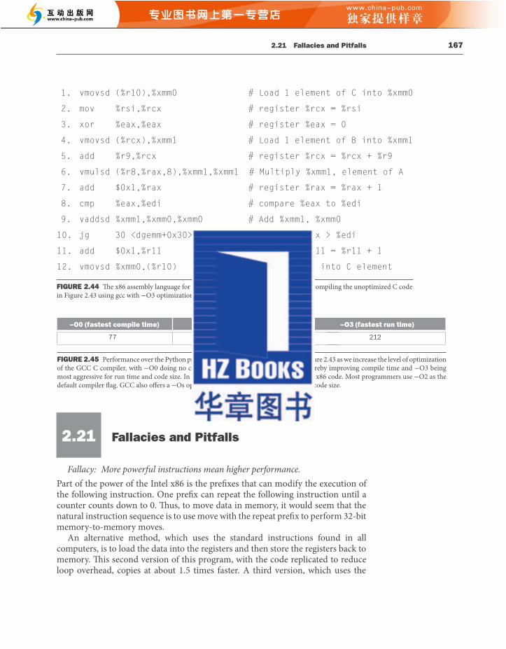

2.22 Concluding Remarks 169
A common mistake in dealing with pointers is to pass a result from a procedure that includes a pointer to an array that is local to that procedure. Following the stack discipline in Figure 2.12 , the memory that contains the local array will be reused as soon as the procedure returns. Pointers to automatic variables can lead to chaos.
2.22 Concluding Remarks
Th e two principles of the stored-program computer are the use of instructions that are indistinguishable from numbers and the use of alterable memory for programs. Th ese principles allow a single machine to aid environmental scientists, fi nancial advisers, and novelists in their specialties. Th e selection of a set of instructions that the machine can understand demands a delicate balance among the number of instructions needed to execute a program, the number of clock cycles needed by an instruction, and the speed of the clock. As illustrated in this chapter, three design principles guide the authors of instruction sets in making that delicate balance:
1. Simplicity favors regularity. Regularity motivates many features of the MIPS instruction set: keeping all instructions a single size, always requiring three register operands in arithmetic instructions, and keeping the register fi elds in the same place in each instruction format.
Less is more. Robert Browning, Andrea del Sarto , 1855
0
100
200
300
400
500
600
700
800
900
1000
1100
1200
1300
1400
1500
1978
1980
1982
1984
1986
1988
1990
1992
1994
1996
1998
2000
2002
2004
2006
2008
2010
2012
2014
2016
2018
Year
Num
ber
of In
stru
ctio
ns
FIGURE 2.46 Growth of x86 instruction set over time. While there is clear technical value to some of these extensions, this rapid change also increases the diffi culty for other companies to try to build compatible processors.
168 Chapter 2 Instructions: Language of the Computer
larger fl oating-point registers instead of the integer registers of the x86, copies at about 2.0 times faster than the complex move instruction.
At one time compilers for programming languages produced naïve instruction sequences; the increasing sophistication of compilers means the gap between compiled code and code produced by hand is closing fast. In fact, to compete with current compilers, the assembly language programmer needs to understand the concepts in Chapters 4 and 5 thoroughly (processor pipelining and memory hierarchy).
Th is battle between compilers and assembly language coders is one situation in which humans are losing ground. For example, C off ers the programmer a chance to give a hint to the compiler about which variables to keep in registers versus spilled to memory. When compilers were poor at register allocation, such hints were vital to performance. In fact, some old C text-books spent a fair amount of time giving examples that eff ectively use register hints. Today’s C compilers generally ignore such hints, because the compiler does a better job at allocation than the programmer does.
Even if writing by hand resulted in faster code, the dangers of writing in assembly language are the longer time spent coding and debugging, the loss in portability, and the diffi culty of maintaining such code. One of the few widely accepted axioms of soft ware engineering is that coding takes longer if you write more lines, and it clearly takes many more lines to write a program in assembly language than in C or Java. Moreover, once it is coded, the next danger is that it will become a popular program. Such programs always live longer than expected, meaning that someone will have to update the code over several years and make it work with new releases of operating systems and new models of machines. Writing in higher-level language instead of assembly language not only allows future compilers to tailor the code to future machines, it also makes the soft ware easier to maintain and allows the program to run on more instruction set architectures.
While backwards binary compatibility is sacrosanct, Figure 2.46 shows that the x86 architecture has grown dramatically. Th e average is more than one instruction per month over its 40-year lifetime!
Many an assembly language programmer has toiled over errors made by assuming that the address of the next word can be found by incrementing the address in a register by one instead of by the word size in bytes. Forewarned is forearmed!
Fallacy : Write in assembly language to obtain the highest performance.
Fallacy : Th e importance of commercial binary compatibility means successful instruction sets don’t change.
Pitfall : Forgetting that sequential word addresses in machines with byte addressing do not diff er by one.
Pitfall : Using a pointer to an automatic variable outside its defi ning procedure.

2.22 Concluding Remarks 171
MIPS instructions Name Format Pseudo MIPS Name Format
add add R move move Rsubtract sub R multiply mult Radd immediate addi I multiply immediate multi Iload word lw I load immediate li Istore word sw I branch less than blt Iload half lh I branch less than
or equal ble Iload half unsigned lhu Istore half sh I branch greater than bgt Iload byte lb I branch greater than
or equal bge Iload byte unsigned lbu Istore byte sb Iload linked ll Istore conditional sc Iload upper immediate lui Iand and Ror or Rnor nor Rand immediate andi Ior immediate ori Ishift left logical sll Rshift right logical srl Rbranch on equal beq Ibranch on not equal bne Iset less than slt Rset less than immediate slti Iset less than immediate unsigned
sltiu I
jump j Jjump register jr Rjump and link jal J
FIGURE 2.47 The MIPS instruction set covered so far, with the real MIPS instructions on the left and the pseudoinstructions on the right. Appendix A (Section A.10) describes the full MIPS architecture. Figure 2.1 shows more details of the MIPS architecture revealed in this chapter. Th e information given here is also found in Columns 1 and 2 of the MIPS Reference Data Card at the front of the book.
170 Chapter 2 Instructions: Language of the Computer
2. Smaller is faster. Th e desire for speed is the reason that MIPS has 32 registers rather than many more.
3. Good design demands good compromises. One MIPS example was the compromise between providing for larger addresses and constants in instructions and keeping all instructions the same length.
Another big idea in this chapter is that numbers have no inherent type. A given bit pattern can represent an integer number, or a string, or a color, or even an instruction. It is the program that determines the type of the data.
We also saw the great idea of making the common case fast applied to instruction sets as well as computer architecture. Examples of making the common MIPS case fast include PC-relative addressing for conditional branches and immediate addressing for larger constant operands.
Above this machine level is assembly language, a language that humans can read. Th e assembler translates it into the binary numbers that machines can understand, and it even “extends” the instruction set by creating symbolic instructions that aren’t in the hardware. For instance, constants or addresses that are too big are broken into properly sized pieces, common variations of instructions are given their own name, and so on. Figure 2.47 lists the MIPS instructions we have covered so far, both real and pseudoinstructions. Hiding details from the higher level is another example of the great idea of abstraction .
Each category of MIPS instructions is associated with constructs that appear in programming languages:
■ Arithmetic instructions correspond to the operations found in assignment statements.
■ Transfer instructions are most likely to occur when dealing with data structures like arrays or structures.
■ Conditional branches are used in if statements and in loops.
■ Unconditional jumps are used in procedure calls and returns and for case/switch statements.
Th ese instructions are not born equal; the popularity of the few dominates the many. For example, Figure 2.48 shows the popularity of each class of instructions for SPEC CPU2006. Th e varying popularity of instructions plays an important role in the chapters about datapath, control, and pipelining.
Aft er we explain computer arithmetic in Chapter 3 , we reveal the rest of the MIPS instruction set architecture.
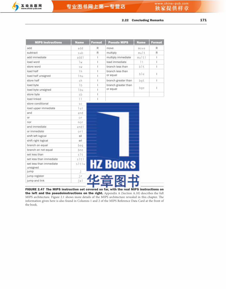
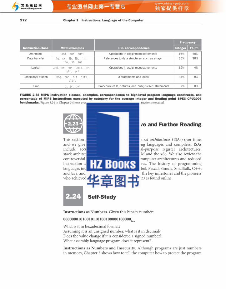
2.24 Self-Study 173
from being modifi ed by labeling a portion of the address space as read-only. Clever attackers exploit bugs in C programs to nevertheless insert their own code during program execution despite that program being protected.
Here is a simple string copy program that copies what the user types into a local variable on the stack.
#include <string.h> void copyinput (char *input) {
char copy[10]; strcpy(copy, input); // no bounds checking in strcpy
} int main (int argc, char **argv) {
copyinput(argv[1]); return 0;
}
What happens if the user writes much more than 10 characters as input? What could be the consequence to program execution? How could this let an attacker take over program execution?
While being faster . Here is the MIPS code for the C while loop from pages 98–99:
Loop: sll $t1,$s3,2 # Temp reg $t1 = i * 4 add $t1,$t1,$s6 # $t1 = address of save[i] lw $t0,0($t1) # Temp reg $t0 = save[i] bne $t0,$s5, Exit # go to Exit if save[i] ≠ k addi $s3,$s3,1 # i = i + 1 j Loop # go to Loop
Exit:
Assume the loop typically executes 10 times. Make the loop faster by executing on average one branch instruction per loop rather than both one jump instruction and one branch instruction.
Th e Anti-Compiler . Here is a portion of MIPS assembly language with comments for the fi rst fi ve instructions.
sll $t0, $s0, 2 # $t0 = f * 4 add $t0, $s6, $t0 # $t0 = &A[f] sll $t1, $s1, 2 # $t1 = g * 4 add $t1, $s7, $t1 # $t1 = &B[g] lw $s0, 0($t0) # f = A[f] addi $t2, $t0, 4 # lw $t0, 0($t2) # add $t0, $t0, $s0 # sw $t0, 0($t1) #
172 Chapter 2 Instructions: Language of the Computer
Historical Perspective and Further Reading
Th is section surveys the history of instruction set architectures (ISAs) over time, and we give a short history of programming languages and compilers. ISAs include accumulator architectures, general-purpose register architectures, stack architectures, and a brief history of ARM and the x86. We also review the controversial subjects of high-level-language computer architectures and reduced instruction set computer (RISC) architectures. Th e history of programming languages includes Fortran, Lisp, Algol, C, Cobol, Pascal, Simula, Smalltalk, C++, and Java, and the history of compilers includes the key milestones and the pioneers who achieved them. Th e rest of Section 2.23 is found online.
2.24 Self-Study
Instructions as Numbers. Given this binary number:
00000001010010110100100000100000 two
What is it in hexadecimal format? Assuming it is an unsigned number, what is it in decimal? Does the value change if it is considered a signed number? What assembly language program does it represent?
Instructions as Numbers and Insecurity . Although programs are just numbers in memory, Chapter 5 shows how to tell the computer how to protect the program
Instruction class MIPS examples HLL correspondence
Frequency
Integer Ft. pt.
Arithmetic add, sub, addi Operations in assignment statementsData transfer lw, sw, lb, lbu, lh,
lhu, sb, lui
Logical and, or, nor, andi, ori,sll, srl
0perations in assignment statements
Conditional branch beq, bne, slt, slti, sltiu
If statements and loops
Jump j, jr, jal Procedure calls, r eturns, and case/switch statements
16%35%
12%
34%
2%
48%36%
4%
8%
0%
References to data structures, such as arrays
FIGURE 2.48 MIPS instruction classes, examples, correspondence to high-level program language constructs, and percentage of MIPS instructions executed by category for the average integer and fl oating point SPEC CPU2006 benchmarks. Figure 3.24 in Chapter 3 shows average percentage of the individual MIPS instructions executed.
2.23

2.25 Exercises 175
Th e Anti-Compiler .
sll $t0, $s0, 2 # $t0 = f * 4 add $t0, $s6, $t0 # $t0 = &A[f] sll $t1, $s1, 2 # $t1 = g * 4 add $t1, $s7, $t1 # $t1 = &B[g] lw $s0, 0($t0) # f = A[f] addi $t2, $t0, 4 # $t2=$t0+4 => $t2 points to A[f+1] now lw $t0, 0($t2) # $t0 = A[f+1] add $t0, $t0, $s0 # $t0 = $t0 + $s0 => $t0 is now A[f]+A[f+1] sw $t0, 0($t1) # store the result into B[g]
2.25 Exercises
Appendix A describes the MIPS simulator, which is helpful for these exercises. Although the simulator accepts pseudoinstructions, try not to use pseudoinstructions for any exercises that ask you to produce MIPS code. Your goal should be to learn the real MIPS instruction set, and if you are asked to count instructions, your count should refl ect the actual instructions that will be executed and not the pseudoinstructions.
Th ere are some cases where pseudoinstructions must be used (for example, the la instruction when an actual value is not known at assembly time). In many cases, they are quite convenient and result in more readable code (for example, the li and move instructions). If you choose to use pseudoinstructions for these reasons, please add a sentence or two to your solution stating which pseudoinstructions you have used and why.
2.1 [5] <§2.2> For the following C statement, what is the corresponding MIPS assembly code? Assume that the C variables f, g, and h, have already been placed in registers $s0, $s1, and $s2, respectively. Use a minimal number of MIPS assembly instructions.
f = g + (h – 5);
2.2 [5] <§2.2> Write a single C statement that corresponds to the two MIPS assembly instructions below.
add f, g, h
add f, i, f
174 Chapter 2 Instructions: Language of the Computer
Assume that the variables f , g , h , i , and j are assigned to registers $s0 , $s1 , $s2 , $s3 , and $s4 , respectively. Assume that the base address of the arrays A and B are in registers $s6 and $s7 , respectively. Complete the comments for the last four instructions.
Self-Study Answers Instructions as Numbers .
Binary: 00000001010010110100100000100000 two
Hexadecimal: 014B4820 hex
Decimal: 21710880 ten Since the leading bit is a 0, it is the same decimal value whether signed or unsigned integer.
Assembly language:
add t1, t2, t3
Machine language:
Instructions as Numbers and Insecurity . Th e local variable copy can safely copy user input up to nine characters followed by the null character that terminates a string. Anything longer will overwrite other values on the stack. As the stack grows down, the values below the stack include stack frames from earlier procedure calls, which include return addresses. A careful attacker can not only insert code onto the stack but can overwrite return addresses in the stack so that the program could eventually use the attacker’s return address to start executing code placed on the stack aft er some procedures returned.
While being faster. Th e trick is to invert the conditional branch and have it jump to the top of the loop rather than having it skip the jump at the bottom of the loop. To match the semantics of the while loop, the code must fi rst check to see if save[i] == k before incrementing i .
sll $t1,$s3,2 # Temp reg $t1 = i * 4 add $t1,$t1,$s6 # $t1 = address of save[i] lw $t0,0($t1) # Temp reg $t0 = save[i] bne $t0,$s5, Exit # go to Exit if save[i] ≠ k
Loop: addi $s3,$s3,1 # i = i + 1 sll $t1,$s3,2 # Temp reg $t1 = i * 4 add $t1,$t1,$s6 # $t1 = address of save[i] lw $t0,0($t1) # Temp reg $t0 = save[i] beq $t0,$s5, Loop # go to Loop if save[i] = k
Exit:
31 2625 2120 1615 1110 65 0
SPECIAL000000
t201010
t301011
t101001
000000
ADD100000
6 5 5 5 5 6
2.25 Exercises 177
addi $t0, $s6, 4 add $t1, $s6, $0 sw $t1, 0($t0) lw $t0, 0($t0) add $s0, $t1, $t0
2.9 [20] <§§2.3, 2.5> For each MIPS instruction in Exercise 2.8, show the value of the opcode (op), source register (rs) and funct fi eld, and destination register (rd) fi elds. For the I-type instructions, show the value of the immediate fi eld, and for the R-type instructions, show the value of the second source register (rt).
2.10 Assume that registers $s0 and $s1 hold the values 0x8000000000000000 and 0xD000000000000000 , respectively.
2.10.1 [5] <§2.4> What is the value of $t0 for the following assembly code?
add $t0, $s0, $s1
2.10.2 [5] <§2.4> Is the result in $t0 the desired result, or has there been overfl ow?
2.10.3 [5] <§2.4> For the contents of registers $s0 and $s1 as specifi ed above, what is the value of $t0 for the following assembly code?
sub $t0, $s0, $s1
2.10.4 [5] <§2.4>Is the result in $t0 the desired result, or has there been overfl ow?
2.10.5 [5] <§2.4> For the contents of registers $s0 and $s1 as specifi ed above, what is the value of $t0 for the following assembly code?
add $t0, $s0, $s1
add $t0, $t0, $s0
2.10.6 [5] <§2.4> Is the result in $t0 the desired result, or has there been overfl ow?
2.11 Assume that $s0 holds the value 128 ten .
2.11.1 [5] <§2.4> For the instruction add $t0 , $s0 , $s1 , what is the range(s) of values for $s1 that would result in overfl ow?
176 Chapter 2 Instructions: Language of the Computer
2.3 [5] <§§2.2, 2.3> For the following C statement, write the corresponding MIPS assembly code. Assume that the variables f , g , h , i , and j are assigned to registers $s0 , $s1 , $s2 , $s3 , and $s4 , respectively. Assume that the base address of the arrays A and B are in registers $s6 and $s7 , respectively.
B[8] = A[i–j];
2.4 [5] <§§2.2, 2.3> For the MIPS assembly instructions above, what is the corresponding C statement? Assume that the variables f , g , h , i , and j are assigned to registers $s0 , $s1 , $s2 , $s3 , and $s4 , respectively. Assume that the base address of the arrays A and B are in registers $s6 and $s7, respectively.
2.5 [5] <§2.3> Show how the value 0xabcdef12 would be arranged in memory of a little-endian and a big-endian machine. Assume the data are stored starting at address 0 and that the word size is 4 bytes.
2.6 [5] <§2.4> Translate 0xabcdef12 into decimal.
2.7 [5] <§§2.2, 2.3> Translate the following C code to MIPS. Assume that the variables f , g , h , i , and j are assigned to registers $s0 , $s1 , $s2 , $s3 , and $s4 , respectively. Assume that the base address of the arrays A and B are in registers $s6 and $s7 , respectively. Assume that the elements of the arrays A and B are 8-byte words:
B[8] = A[i] + A[j];
2.8 [10] <§§2.2, 2.3> Translate the following MIPS code to C. Assume that the variables f , g , h , i , and j are assigned to registers $s0 , $s1 , $s2 , $s3 , and $s4 , respectively. Assume that the base address of the arrays A and B are in registers $s6 and $s7 , respectively.

2.25 Exercises 179
2.17.1 [5] <§2.6> For the register values shown above, what is the value of $t2 for the following sequence of instructions?
sll $t2, $t0, 44 or $t2, $t2, $t1
2.17.2 [5] <§2.6> For the register values shown above, what is the value of $t2 for the following sequence of instructions?
sll $t2, $t0, 4 andi $t2, $t2, –1
2.17.3 [5] <§2.6> For the register values shown above, what is the value of $t2 for the following sequence of instructions?
srl $t2, $t0, 3 andi $t2, $t2, 0xFFEF
2.18 [10] <§2.6> Find the shortest sequence of MIPS instructions that extracts bits 16 down to 11 from register $t0 and uses the value of this fi eld to replace bits 31 down to 26 in register $t1 without changing the other bits of registers $t0 and $t1 (Be sure to test your code using $t0 = 0 and $t1 = 0xffffffffffffffff . Doing so may reveal a common oversight.).
2.19 [5] <§2.6> Provide a minimal set of MIPS instructions that may be used to implement the following pseudoinstruction:
not $t1, $t2 // bit-wise invert
2.20 [5] <§2.6> For the following C statement, write a minimal sequence of MIPS assembly instructions that does the identical operation. Assume $t0 = A and $s0 is the base address of C.
A = C[0] << 4;
2.21 [5] <§2.7> Assume $t0 holds the value 0x010100000 . What is the value of $t2 aft er the following instructions?
slt $t2, $0, $t0 bne $t2, $0, ELSE j DONE ELSE: addi $t2, $t2, 2 DONE:
178 Chapter 2 Instructions: Language of the Computer
2.11.2 [5] <§2.4> For the instruction sub $t0 , $s0 , $s1 , what is the range(s) of values for $s1 that would result in overfl ow?
2.11.3 [5] <§2.4> For the instruction sub $t0 , $s1 , $s0 , what is the range(s) of values for $s1 that would result in overfl ow?
2.12 [5] <§§2.4, 2.5>
Provide the type and assembly language instruction for the following binary value: 0000 0010 0001 0000 1000 0000 0010 0000 two . Hint: Figure 2.20 may be helpful.
2.13 [5] <§§2.4, 2.5> Provide the type and hexadecimal representation of following instruction: sw $t1, 32($t2)
2.14 [5] <§2.5> Provide the type, assembly language instruction, and binary representation of instruction described by the following MIPS fi elds:
op=0, rs=3, rt=2, rd=3, shamt=0, funct=34
2.15 [5] <§2.5> Provide the type, assembly language instruction, and binary representation of instruction described by the following MIPS fi elds:
op=0x23, rs=1, rt=2, const=0x4
2.16 [5] <§2.5> Assume that we would like to expand the MIPS register fi le to 128 registers and expand the instruction set to contain four times as many instructions.
2.16.1 [5] <§2.5> How would this aff ect the size of each of the bit fi elds in the R-type instructions?
2.16.2 [5] <§2.5> How would this aff ect the size of each of the bit fi elds in the I-type instructions?
2.16.3 [5] <§§2.5, 2.10> How could each of two propose changes decrease the size of an MIPS assembly program? On the other hand, how could the proposed change increase the size of an MIPS assembly program?
2.17 Assume the following register contents:
$t0=0xAAAAAAAA, $t1=0x12345678
2.25 Exercises 181
2.25 [10] <§2.7> Translate the following C code to MIPS assembly code. Use a minimum number of instructions. Assume that the values of a , b , i , and j are in registers $s0 , $s1 , $t0 , and $t1 , respectively. Also, assume that register $s2 holds the base address of the array D.
for(i=0; i<a; i++) for(j=0; j<b; j++) D[4*j] = i + j;
2.26 [5] <§2.7> How many MIPS instructions does it take to implement the C code from Exercise 2.25? If the variables a and b are initialized to 10 and 1 and all elements of D are initially 0, what is the total number of MIPS instructions that is executed to complete the loop?
2.27 [5] <§2.7> Translate the following loop into C. Assume that the C-level integer i is held in register $t1 , $s2 holds the C-level integer called result , and $s0 holds the base address of the integer MemArray .
addi $t1, $0, 0 LOOP: lw $s1, 0($s0) add $s2, $s2, $s1 addi $s0, $s0, 4 addi $t1, $t1, 1 slti $t2, $t1, 100 bne $t2, $s0, LOOP
2.28 [10] <§2.7> Rewrite the loop from Exercise 2.27 reduce the number of MIPS instructions executed. Hint: Notice that variable i is used only for loop control.
2.29 [30] <§2.8> Implement the following C code in MIPS assembly. Hint: Remember that the stack pointer must remain aligned on a multiple of 16.
2.30 [20] <§2.8> For each function call, show the contents of the stack aft er the function call is made. Assume the stack pointer is originally at address 0x7ffffffc , and follow the register conventions as specifi ed in Figure 2.11.
180 Chapter 2 Instructions: Language of the Computer
2.22 Suppose the program counter (PC) is set to 0x20000000 .
2.22.1 [5] < §2.10> What range of addresses can be reached using the MIPS jump-and-link (jai) instruction? (In other words, what is the set of possible values for the PC aft er the jump instruction executes?)
2.22.2 [5] < §2.10> What range of addresses can be reached using the MIPS branch if equal (beq) instruction? (In other words, what is the set of possible values for the PC aft er the branch instruction executes?)
2.23 Consider a proposed new instruction named rpt . Th is instruction combines a loop’s condition check and counter decrement into a single instruction. For example, rpt $s0 , loop would do the following:
if (x29 > 0) { x29 = x29 − 1; goto loop
}
2.23.1 [5] <§2.7, 2.10> If this instruction were to be implemented in the MIPS instruction set, what is the most appropriate instruction format?
2.23.2 [5] <§2.7> What is the shortest sequence of MIPS instructions that performs the same operation?
2.24 Consider the following MIPS loop:
LOOP: slt $t2, $0, $t1 beq $t2, $0, DONE subi $t1, $t1, 1 addi $s2, $s2, 2 j LOOP DONE:
2.24.1 [5] <§2.7> Assume that the register $t1 is initialized to the value 10. What is the value in register $s0 assuming the $s0 is initially zero?
2.24.2 [5] <§2.7> For each of the loops above, write the equivalent C code routine. Assume that the registers $s1 , $s2 , $t1 , and $t2 are integers A , B , i , and temp , respectively.
2.24.3 [5] <§2.7> For the loops written in MIPS assembly above, assume that the register $t1 is initialized to the value N. How many MIPS instructions are executed?
2.25 Exercises 183
2.36 [5] <§2.10> Write the MIPS assembly code that creates the 32-bit constant ll/sc and stores that value to register $t1 .
2.37 [10] < §2.11> Write the MIPS assembly code to implement the following C code as an atomic “set max” operation using the lI/sc instructions. Here, the argument shvar contains the address of a shared variable, which should be replaced by x if x is greater than the value it points to:
void setmax(int* shvar, int x) { // Begin critical section if (x > *shvar)
*shvar = x; // End critical section}
}
2.38 [5] <§2.11> Using your code from Exercise 2.37 as an example, explain what happens when two processors begin to execute this critical section at the same time, assuming that each processor executes exactly one instruction per cycle.
2.39 Assume for a given processor the CPI of arithmetic instructions is 1, the CPI of load/store instructions is 10, and the CPI of branch instructions is 3. Assume a program has the following instruction breakdowns: 500 million arithmetic instructions, 300 million load/store instructions, 100 million branch instructions.
2.39.1 [5] <§§1.6, 2.13> Suppose that new, more powerful arithmetic instructions are added to the instruction set. On average, through the use of these more powerful arithmetic instructions, we can reduce the number of arithmetic instructions needed to execute a program by 25%, and the cost of increasing the clock cycle time by only 10%. Is this a good design choice? Why?
2.39.2 [5] <§§1.6, 2.13> Suppose that we fi nd a way to double the performance of arithmetic instructions. What is the overall speedup of our machine? What if we fi nd a way to improve the performance of arithmetic instructions by 10 times?
2.40 Assume that for a given program 70% of the executed instructions are arithmetic, 10% are load/store, and 20% are branch.
2.40.1 [5] <§2.21> Given the instruction mix and the assumption that an arithmetic instruction requires 2 cycles, a load/store instruction takes 6 cycles, and a branch instruction takes 3 cycles, fi nd the average CPI.
2.40.2 [5] <§§1.6, 2.13> For a 25% improvement in performance, how many cycles, on average, may an arithmetic instruction take if load/store and branch instructions are not improved at all?
182 Chapter 2 Instructions: Language of the Computer
2.31 [20] <§2.8> Translate function f into MIPS assembly language. If you need to use registers $t0 through $t7 , use the lower-numbered registers fi rst. Assume the function declaration for func is “ int f(int a, int b) ;”. Th e code for function f is as follows:
int f(int a, int b, int c, int d){
return func(func(a,b),c + d);
}
2.32 [5] <§2.8> Can we use the tail-call optimization in this function? If no, explain why not. If yes, what is the diff erence in the number of executed instructions in f with and without the optimization?
2.33 [5] <§2.8> Right before your function f from Exercise 2.31 returns, what do we know about contents of registers $t5 , $s3 , $ra , and $sp ? Keep in mind that we know what the entire function f looks like, but for function func we only know its declaration.
2.34 [30] <§2.9> Write a program in MIPS assembly language to convert an ASCII number string containing positive and negative integer decimal strings, to an integer. Your program should expect register $a0 to hold the address of a null-terminated string containing some combination of the digits 0 through 9. Your program should compute the integer value equivalent to this string of digits, then place the number in register $v0 . If a non-digit character appears anywhere in the string, your program should stop with the value −1 in register $v0 . For example, if register $t0 points to a sequence of three bytes 50 ten , 52 ten , 0 ten (the null-terminated string “24”), then when the program stops, register $v0 should contain the value 24 ten . Th e RISC-V mul instruction takes two registers as input. Th ere is no “muli” instruction. Th us, just store the constant 10 in a register.
2.35 [5] <§2.9> For the following code:
lbu $t0, 0($t1)
sw $t0, 0($t2)
Assume that the register $t1 contains the address 0x10000000 and the data at address is 0x11223344 .
2.35.1 [5] < §2.3, 2.9> What value is stored in 0x10000004 on a big-endian machine?
2.35.2 [5] < §2.3, 2.9> What value is stored in 0x10000004 on a little-endian machine?
184 Chapter 2 Instructions: Language of the Computer
2.40.3 [5] <§§1.6, 2.13> For a 50% improvement in performance, how many cycles, on average, may an arithmetic instruction take if load/store and branch instructions are not improved at all?
2.41 [10] < §2.21> Suppose the MIPS ISA included a scaled off set addressing mode similar to the × 86 one described in Section 2.19 (Figure 2.35). Describe how you would use scaled off set loads to further reduce the number of assembly instructions needed to carry out the function given in Exercise 2.4.
2.42 [10] < §2.21> Suppose the MIPS ISA included a scaled off set addressing mode similar to the × 86 one described in Section 2.19 (Figure 2.35). Describe how you would use scaled off set loads to further reduce the number of assembly instructions needed to implement the C code given in Exercise 2.7.
§2.2, page 72: MIPS, C, Java §2.3, page 78: 2) Very slow §2.4, page 85: First question: 2) −8 ten . Second question: 4) 18,446, 744,073,709,551,608 ten . §2.5, page 93: First question: 4) sub $t2, $t0, $t1 . Second question: 28 hex . §2.6, page 95: Both. AND with a mask pattern of 1 s will leaves 0 s everywhere but the desired fi eld. Shift ing left by the right amount removes the bits from the left of the fi eld. Shift ing right by the appropriate amount puts the fi eld into the right-most bits of the word, with 0 s in the rest of the word. Note that AND leaves the fi eld where it was originally, and the shift pair moves the fi eld into the rightmost part of the word. §2.7, page 102: I. All are true. II. 1). §2.8, page 112: Both are true. §2.9, page 116: I. 1) II. 3) §2.10, page 126: I. 4) +−128 K. II. 6) a block of 256 M. III. 4) sll §2.11, page 129: Both are true. §2.12, page 138: 4) Machine independence.
Answers to Check Yourself