computational methods in developing quantitative structureactivity relationships (qsar): a review

Combinatorial Chemistry & High Throughput Screening, 2006, 9, 213-228 213

1386-2073/06 $50.00+.00 © 2006 Bentham Science Publishers Ltd.

Computational Methods in Developing Quantitative Structure-ActivityRelationships (QSAR): A Review

Arkadiusz Z. Dudek*,a

, Tomasz Arodzb and Jorge Gálvez

c

aUniversity of Minnesota Medical School, Minneapolis, MN 55455, USA

bInstitute of Computer Science, AGH University of Science and Technology, al. Mickiewicza 30, 30-059 Kraków, Poland

cUnit of Drug Design and Molecular Connectivity Research, University of Valencia, 46100 Burjassot, Valencia, Spain

Abstract: Virtual filtering and screening of combinatorial libraries have recently gained attention as methods

complementing the high-throughput screening and combinatorial chemistry. These chemoinformatic techniques rely

heavily on quantitative structure-activity relationship (QSAR) analysis, a field with established methodology and

successful history. In this review, we discuss the computational methods for building QSAR models. We start with

outlining their usefulness in high-throughput screening and identifying the general scheme of a QSAR model. Following,

we focus on the methodologies in constructing three main components of QSAR model, namely the methods for

describing the molecular structure of compounds, for selection of informative descriptors and for activity prediction. We

present both the well-established methods as well as techniques recently introduced into the QSAR domain.

Keywords: QSAR, molecular descriptors, feature selection, machine learning.

1. INTRODUCTION

High throughput screening (HTS) has been a majorrecent technological improvement in drug discoverypipeline. In conjunction with combinatorial chemistry, itallows for synthesis and rapid activity assessment of vastnumber of small-molecule compounds [1, 2]. As theexperience with these technologies matured, the focus hasshifted from sifting through large, diverse moleculecollections to more rationally designed libraries [3].

With this need for knowledge-guided screening ofcompounds, the virtual filtering and screening have beenrecognized as techniques complementary to high-throughputscreening [4, 5]. To much extent, these techniques rely onquantitative structure-activity relationship (QSAR) analysis,which is in constant advancement since the works of Hansch[6] in early 1960s. The QSAR methodology focuses onfinding a model, which allows for correlating the activity tostructure within a family of compounds. Such models can beused to increase the effectiveness of HTS in several ways [7,8].

QSAR studies can reduce the costly failures of drugcandidates in clinical trials by filtering the combinatoriallibraries. Virtual filtering can eliminate compounds withpredicted toxic of poor pharmacokinetic properties [9, 10]early in the pipeline. It also allows for narrowing the libraryto drug-like or lead-like compounds [11] and eliminating thefrequent-hitters, i.e., compounds that show unspecificactivity in several assays and rarely result in leads [12].Including such considerations at an early stage results inmultidimensional optimization, with high activity as anessential but not only goal [8].

*Address correspondence to this author at the University of Minnesota,

Division of Hematology, Oncology and Transplantation, 420 Delaware St.

SE, MMC 480, Minneapolis, MN 55455, USA; Tel: +1 612 624-0123; Fax:

+1 612 625-6919; E-mail: [email protected]

Considering activity optimization, building target-specific structure-activity models based on identified hits canguide HTS by rapidly screening the library for mostpromising candidates. Such focused screening can reduce thenumber of experiments and allow for use of more complex,low throughput assays [7]. Interpretation of created modelsgives insight into the chemical space in proximity of the hitcompound. Feedback loops of high-throughput and virtualscreening, resulting in sequential screening approach [13],allow therefore for more rational progress towards highquality lead compounds. Later in the drug discoverypipeline, accurate QSAR models constructed on the basis ofthe lead series can assist in optimizing the lead [14].

The importance and difficulty of the above-describedtasks facing QSAR models has inspired manychemoinformatics researchers to borrow from recentdevelopments in various fields, including patternrecognition, molecular modeling, machine learning andartificial intelligence. This results in large family ofconceptually different methods being used for creatingQSARs. The purpose of this review is to guide the readerthrough the diversity of the techniques and algorithms fordeveloping successful QSAR models.

1.1. General Scheme of a QSAR Study

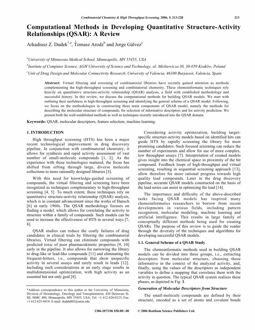
The chemoinformatic methods used in building QSARmodels can be divided into three groups, i.e., extractingdescriptors from molecular structure, choosing thoseinformative in the context of the analyzed activity, and,finally, using the values of the descriptors as independentvariables to define a mapping that correlates them with theactivity in question. The typical QSAR system realizes thesephases, as depicted in Fig. 1.

Generation of Molecular Descriptors from Structure

The small-molecule compounds are defined by theirstructure, encoded as a set of atoms and covalent bonds

'

214 Combinatorial Chemistry & High Throughput Screening, 2006, Vol. 9, No. 3 Dudek et al.

between them. However, the structure cannot be directlyused for creating structure-activity mappings for reasonsstemming from chemistry and computer science.

First, the chemical structures do not usually contain in anexplicit form the information that relates to activity. Thisinformation has to be extracted from the structure. Variousrationally designed molecular descriptors accentuatedifferent chemical properties implicit in the structure of themolecule. Only those properties may correlate more directlywith the activity. Such properties range fromphysicochemical and quantum-chemical to geometrical andtopological features.

The second, more technical reason, which guides the useand development of molecular descriptors, stems from theparadigm of feature space prevailing in statistical dataanalysis. Most methods employed to predict the activityrequire as input numerical vectors of features of uniformlength for all molecules. Chemical structures of compoundsare diverse in size and nature and as such do not fit into thismodel directly. To circumvent this obstacle, moleculardescriptors convert the structure to the form of well-definedsets of numerical values.

Selection of Relevant Molecular Descriptors

Many applications are capable of generating hundreds orthousands of different molecular descriptors. Typically, onlysome of them are significantly correlated with the activity.Furthermore, many of the descriptors are intercorrelated.This has negative effects on several aspects of QSARanalysis. Some statistical methods require that the number ofcompounds is significantly greater than the number ofdescriptors. Using large descriptor sets would require largedatasets. Other methods, while capable of handling datasetswith large descriptors to compounds ratios, nonethelesssuffer from loss of accuracy, especially for compoundsunseen during the preparation of the model. Large number ofdescriptors also affects interpretability of the final model. Totackle these problems, a wide range of methods for

automated narrowing of the set of descriptors to the mostinformative ones is used in QSAR analysis.

Mapping the Descriptors to Activity

Once the relevant molecular descriptors are computedand selected, the final task of creating a function betweentheir values and the analyzed activity can be carried out. Thevalue quantifying the activity is expressed as a function ofthe values of the descriptors. The most accurate mappingfunction from some wide family of functions, is usuallyfitted based on the information available in the training set,i.e., compounds for which the activity is known. A widerange of mapping function families can be used, includinglinear or non-linear ones, and many methods for carrying outthe training to obtain the optimal function can be employed.

1.2. Organization of the Review

In the following sections of this review, we discuss eachof the three groups of methods in more detail. We start withvarious types of molecular descriptors in section 2. Next, insection 3 we focus on automatic methods for choosing themost predictive descriptors from a large initial set. Then, insection 4 we describe the linear and non-linear mappingtechniques used for expressing the activity or property as afunction of the values of selected descriptors. For eachtechnique, we provide an overview of the method followedby examples of its applications in QSAR analysis.

2. MOLECULAR DESCRIPTORS

Molecular descriptors map the structure of the compoundinto a set of numerical or binary values representing variousmolecular properties that are deemed to be important forexplaining activity. Two broad families of descriptors can bedistinguished, based on the dependence on the informationabout 3D orientation and conformation of the molecule.

2.1. 2D QSAR Descriptors

The broad family of descriptors used in the 2D-QSARapproach share a common property of being independentfrom the 3D orientation of the compound. These descriptors

Fig. (1). Main stages of a QSAR study. The molecular structure is encoded using numerical descriptors. The set of descriptors is pruned to

select the most informative ones. The activity is derived as a function of the selected descriptors.

Computational Methods in Developing QSAR Combinatorial Chemistry & High Throughput Screening, 2006, Vol. 9, No. 3 215

range from simple measures of entities constituting themolecule, through its topological and geometrical propertiesto computed electrostatic and quantum-chemical descriptorsor advanced fragment-counting methods.

Constitutional Descriptors

Constitutional descriptors capture properties of themolecule that are related to elements constituting itsstructure. These descriptors are fast and easy to compute.Examples of constitutional descriptors include molecularweight, total number of atoms in the molecule and numbersof atoms of different identity. Also, a number of propertiesrelating to bonds are used, including total numbers of single,double, triple or aromatic type bonds, as well as number ofaromatic rings.

Electrostatic and Quantum-Chemical Descriptors

Electrostatic descriptors capture information onelectronic nature of the molecule. These include descriptorscontaining information on atomic net and partial charges[15]. Descriptors for highest negative and positive chargesare also informative, as well as molecular polarizability [16].Partial negatively or positively charged solvent-accessibleatomic surface areas have also been used as informativeelectrostatic descriptors for modeling intermolecularhydrogen bonding [17]. Energies of highest occupied andlowest unoccupied molecular orbital form useful quantum-

chemical descriptors [18], as do the derivative quantitiessuch as absolute hardness [19].

Topological Descriptors

The topological descriptors treat the structure of thecompound as a graph, with atoms as vertices and covalentbonds as edges. Based on this approach, many indicesquantifying molecular connectivity were defined, startingwith Wiener index [20], which counts the total number ofbonds in shortest paths between all pairs of non-hydrogenatoms. Other topological descriptors include Randic indices

x [21], defined as sum of geometric averages of edge degreesof atoms within paths of given lengths, Balaban's J index[22] and Shultz index [23].

Information about valence electrons can be included intopological descriptors, e.g. Kier and Hall indices x

v _ [24] or

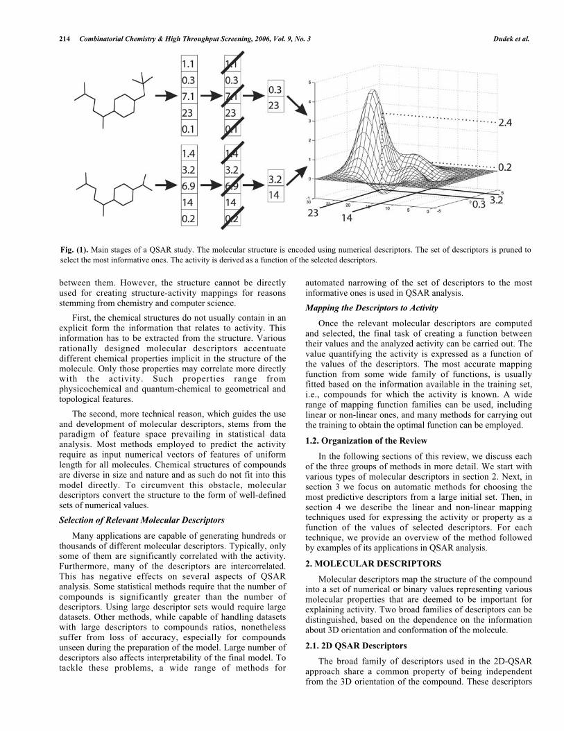
Gálvez topological charge indices [25]. The first ones usegeometric averages of valence connectivities along paths.The latter measure topological valences of atoms and netcharges transfer between pair of atoms separated by a givennumber of bonds. To exemplify the derivation of topologicalindices, in Fig. 2 we show the calculation of Gálvez indicesfor atom distance of a single bond.

Descriptors combining connectivity information withother properties are also available, e.g. BCUT [26-28]descriptors, which take form of eigenvalues of atom

Fig. (2). Example of the Galvez first-order topological charge indices G1 and J1 for isopentane. The matrix product Mij of atom adjacency

matrix and topological distance matrix defined as inverse squares of inter-atom distances, is used to define the charge terms CTij as Mij - Mji.

The Gk indices are defined as the algebraic sum of absolute values of the charge terms for pairs of atoms separated by k bonds. The Jk indices

result from normalization of Gk by the number of bonds in the molecule.


connectivity matrix with atom charge, polarizability or H-bond potential values on diagonal and additional terms offdiagonal. Similarly, the Topological Sub-StructuralMolecular Design (TOSS-MODE/TOPS-MODE) [29, 30]rely on spectral moments of bond adjacency matrix amendedwith information on for e.g. bond polarizability. The atom-type electrotopological (E-state) indices [31, 32] useelectronic and topological organization to define the intrinsicatom state and the perturbations of this state induced byother atoms. This information is gathered individually for awide range of atom-types to form a set of indices.

Geometrical Descriptors

Geometrical descriptors rely on spatial arrangement ofatoms constituting the molecule. These descriptors includeinformation on molecular surface obtained from atomic vander Waals areas and their overlap [33]. Molecular volumemay be obtained from atomic van der Waals volumes [34].Principal moments of inertia and gravitational indices [35]also capture information on spatial arrangement of the atomsin molecule. Shadow areas, obtain by projection of themolecule to its two principal axes are also used [36].Another geometrical descriptor is the total solvent-accessiblesurface area [37, 38].

Fragment-Based Descriptors and Molecular Fingerprints

The family of descriptors relying on substructural motifsis often used, especially for rapid screening of very largedatabases. The BCI fingerprints [39] are derived as bitsdescribing the presence or absence in the molecule of certainfragments, including atoms with their nearest neighborhoods,atom pairs and sequences, or ring-based fragments. A similarapproach is present in the basic set of 166 MDL Keys [40].However, other variants of the MDL Keys are also available,including extended sets of keys or compact sets. The latterare results of dedicated pruning strategies [41] or eliminationmethods, e.g. the Fast Random Elimination ofDescriptors/Substructure Keys (FRED/SKEYS) [42].Recently introduced Hologram QSAR (HQSAR) [43]approach is based on counting the number of occurrences ofcertain substructural paths of functional groups. For eachgroup, cyclic redundancy code is calculated, which serves asa hashing function [44] for partitioning the substructuralmotifs into bins of hash table. The numbers of elements inthe bins form a hologram.

The Daylight fingerprints [45] are a natural extension ofthe fragment-based descriptors by eliminating the reliance onpre-defined list of sub-structure motifs. The fingerprint foreach molecule is a string of bits. However, a structural motifin the molecule does not correspond to a single bit, but leads,through a hashing function, to a pattern of bits that are addedto the fingerprint with a logical "or" operation. The bits indifferent patterns may overlap, due to the large number ofpossible patterns and a finite length of a bit string. Thus, thefact that a bit or several bits are set in the fingerprint cannotbe interpreted as a proof of pattern's presence. However, ifone of the bits corresponding to a given pattern is not set,this guarantees that the pattern is not present in the molecule.This allows for rapid filtering of molecules that do notpossess certain structural motifs. The patterns are generated

individually for each molecule, and describe atoms with theirneighborhoods and paths of up to 7 bonds. Other approachesthan hashed fingerprints are also proposed to circumvent theproblem of a pre-defined substructure library, e.g. algorithmfor optimal discovery of frequent structural fragmentsrelevant to given activity [46].

2.2. 3D QSAR Descriptors

The 3D-QSAR methodology is much morecomputationally complex than 2D-QSAR approach. Ingeneral, it involves several steps to obtain numericaldescriptors of the compound structure. First, theconformation of the compound has to be determined eitherfrom experimental data or molecular mechanics and thenrefined by minimizing the energy [47, 48]. Next, theconformers in dataset have to be uniformly aligned in space.Finally, the space with immersed conformer is probedcomputationally for various descriptors. Some methodsindependent of the compound alignment have also beendeveloped.

2.2.1. Alignment-Dependent 3D QSAR Descriptors

The group of methods that require molecule alignmentprior to the calculation of descriptors is strongly dependenton the information on the receptor for the modeled ligand. Incase where such data is available, the alignment can beguided by studying the receptor-ligand complexes.Otherwise, purely computational methods for superimposingthe structures in space have to be used [49, 50]. Thesemethods rely e.g. on atom-atom or substructure-substructuremapping.

Comparative Molecular Field Analysis

The Comparative Molecular Field Analysis (CoMFA)[51] uses electrostatic (Coulombic) and steric (van derWaals) energy fields defined by the inspected compound.The aligned molecule is placed in a 3D grid. In each point ofthe grid lattice a probe atom with unit charge is placed andthe potentials (Coulomb and Lennard-Jones) of the energyfields are computed. Then, they serve as descriptors infurther analysis, typically using partial least squaresregression. This analysis allows for identifying structureregions positively and negatively related to the activity inquestion.

Comparative Molecular Similarity Indices Analysis

The Comparative Molecular Similarity Indices(CoMSIA) [52] is similar to CoMFA in the aspect of atomprobing throughout the regular grid lattice in which themolecules are immersed. The similarity between probe atomand the analyzed molecule are calculated. Compared toCoMFA, CoMSIA uses a different potential function,namely the Gaussian-type function. Steric, electrostatic, andhydrophobic properties are then calculated, hence the probeatom has unit hydrophobicity as additional property. The useof Gaussian-type potential function instead of Lennard-Jonesand Coulombic functions allows for accurate information ingrid points located within the molecule. In CoMFA,unacceptably large values are obtained in these points due tothe nature of the potential functions and arbitrary cut-offsthat have to be applied.


2.2.2. Alignment-Independent 3D QSAR Descriptors

Another group of 3D descriptors are those invariant tomolecule rotation and translation in space. Thus, nosuperposition of compounds is required.

Comparative Molecular Moment Analysis

The Comparative Molecular Moment Analysis(CoMMA) [53] uses second-order moments of the massdistribution and charge distributions. The moments relate tocenter of the mass and center of the dipole. The CoMMAdescriptors include principal moments of inertia, magnitudesof dipole moment and principal quadrupole moment.Furthermore, descriptors relating charge to massdistributions are defined, i.e., magnitudes of projections ofdipole upon principal moments of inertia and displacementbetween center of mass and center of dipole.

Weighted Holistic Invariant Molecular Descriptors

The Weighted Holistic Invariant Molecular (WHIM) [54,55] and Molecular Surface WHIM [56] descriptors providethe invariant information by employing the principalcomponent analysis (PCA) on the centered co-ordinates ofthe atoms constituting the molecule. This transforms themolecule into the space that captures the most variance. Inthis space, several statistics are calculated and serve asdirectional descriptors, including variance, proportions,symmetry and kurtosis. By combining the directionaldescriptors, non-directional descriptors are also defined. Thecontribution of each atom can be weighted by a chemicalproperty, leading to different principal components capturingvariance within the given property. The atoms can beweighted by mass, van der Waals volume, atomicelectronegativity, atomic polarizability, electrotopologicalindex of Kier and Hall and molecular electrostatic potential.

VolSurf

The VolSurf [57, 58] approach is based on probing thegrid around the molecule with specific probes, for e.g.hydrophobic interactions or hydrogen bond acceptor ordonor groups. The resulting lattice boxes are used tocompute the descriptors relying on volumes or surfaces of3D contours, defined by the same value of the probe-molecule interaction energy. By using various probes andcut-off values for the energy, different molecular propertiescan be quantified. These include e.g. molecular volume andsurface, and hydrophobic and hydrophilic regions.Derivative quantities, e.g. molecular globularity or factorsrelating the surface of hydrophobic or hydrophilic regions tosurface of the whole molecule can also be computed. Inaddition, various geometry-based descriptors are alsoavailable, including energy minima distances or amphiphilicmoments.

Grid-Independent Descriptors

The Grid-Independent Descriptors (GRIND) [59] havebeen devised to overcome the problems with interpretabilitycommon in alignment-independent descriptors. Similarly toVolSurf, it utilizes probing of the grid with specific probes.The regions showing the most favorable energies ofinteraction are selected, provided that the distances betweenthe regions are large. Next, the probe-based energies areencoded in a way independent of the molecule's

arrangement. To this end, the distances between the nodes inthe grid are discretized into a set of bins. For each distancebin, the nodes with the highest product of energies are storedand the value of the product serves as the numericaldescriptor. In addition, the stored information on the positionof the nodes can be used to track down the exact regions ofthe molecule relating to the given property. To extend themolecular information captured by the descriptors, theproduct of node energies may include not only energiesrelating to the same probe, but also from two different probetypes.

2.3. The 2D- Versus 3D-QSAR Approach

It is generally assumed that 3D approaches are superiorto 2D in drug design. Yet, studies show such an assumptionmay not always hold. For example, the results ofconventional CoMFA may often be non-reproducible due todependence of the outputs' quality on the orientation of therigidly aligned molecules on user's terminal [60, 61]. Suchalignment problems are typical in 3D approaches and eventhough some solutions have been proposed, the unambiguous3D alignment of structurally diverse molecules still remainsa difficult task.

Moreover, the distinction between 2D- and 3D-QSARapproaches is not a crisp one, especially when alignment-independent descriptors are considered. This can be observedwhen comparing the BCUT with the WHIM descriptors.Both employ a similar algebraic method, i.e., solving aneigenproblem for a matrix describing the compound - theconnectivity matrix in case of BCUT descriptors andcovariance matrix of 3D co-ordinates in case of WHIM.

There is also a deeper connection between 3D-QSAR andone of 2D methods, the topological approach. It stems fromthe fact that the geometry of a compound in many casesdepends on its topology. An elegant example was providedby Estrada et al., who demonstrated that the dihedral anglesof biphenyl as a function of the substituents attached to it canbe predicted by topological indices [62]. Along the sameline, a supposedly typically 3D property, chirality, has beenpredicted using chiral topological indices [63], constructedby introducing an adequate weight into the topologicalmatrix for the chiral carbons.

3. AUTOMATIC SELECTION OF RELEVANTMOLECULAR DESCRIPTORS

Automatic methods for selecting the best descriptors, orfeatures, to be used in construction of the QSAR model fallinto two categories [64]. In the wrapper approach, the qualityof descriptor subsets is obtained from constructing andevaluating a series of QSAR models. In filtering, no model isbuild, and features are evaluated using some other criteria.

3.1. Filtering Methods

These techniques are applied independently of themapping method used. They are executed prior to themapping, to reduce the number of descriptors followingsome objective criteria, e.g. inter-descriptor correlation.

Correlation-Based Methods

Pearson's correlation coefficients may serve as apreliminary filter for discarding intercorrelated descriptors.


This can be done by e.g. creating clusters of descriptorshaving correlation coefficients higher than certain thresholdand retaining only one, randomly chosen member of eachcluster [65]. Another procedure involves estimatingcorrelations between pair of descriptors and, if it exceeds athreshold, randomly discarding one of the descriptors [66].The choice of the ordering in which pairs are evaluated maylead to significantly different results. One popular method isto first rank the descriptors by using some criterion, and theniteratively browse the set starting from pairs containing thehighest-ranking features.

One such ranking may be the correlation ranking, basedon correlation coefficient between activity and descriptors.However, correlation ranking is usually used in conjunctionwith principal component analysis [67, 68]. Methods usingmeasures of correlation between activity and descriptorsother than Pearson's have been used, notably the pair-correlation method [69-71].

Methods Based on Information Theory

Information content of the descriptor is defined in termsof entropy of descriptor treated as a random variable. Basedon this notion, various measures relating the informationshared between two descriptors or between descriptor andthe activity can be defined. An example of such measure,used in descriptor selection for QSAR, is the mutualinformation.

The mutual information, sometimes referred to asinformation gain, quantifies the reduction of uncertainty, orinformation content, of activity variable by knowing thedescriptor values. It is used in QSAR to rank the descriptors[72, 73].

The application of information-theoretic criteria isstraightforward when both the descriptors and activity valuesare categorical. In case of continuous numerical variables,some discretization schemes have to be applied toapproximate the variables. Thus, such criteria are usuallyused with binary descriptors, such as ones describing 3Dproperties of molecules used in thrombin dataset inKnowledge Discovery in Databases 2001 Cup.

Statistical Criteria

The Fisher's ratio, i.e., ratio of the between class varianceto the within-class variance, can be used to rank thedescriptors [74]. Next, the correlation between pairs offeatures is used, as described before, to reduce the set ofdescriptors.

Another method used in assessing the quality of adescriptor is based on the Kolmogorov-Smirnov [75]statistics. As applied to descriptor selection in QSAR [76], itis a fast method not relying on the knowledge of theunderlying distribution and not requiring the conversion ofvariables descriptors into categorical values. For two classesof activity to be predicted, the method measures the maximalabsolute distance between cumulative distribution functionsof the descriptor for individual activity classes.

3.2. Wrapper Methods

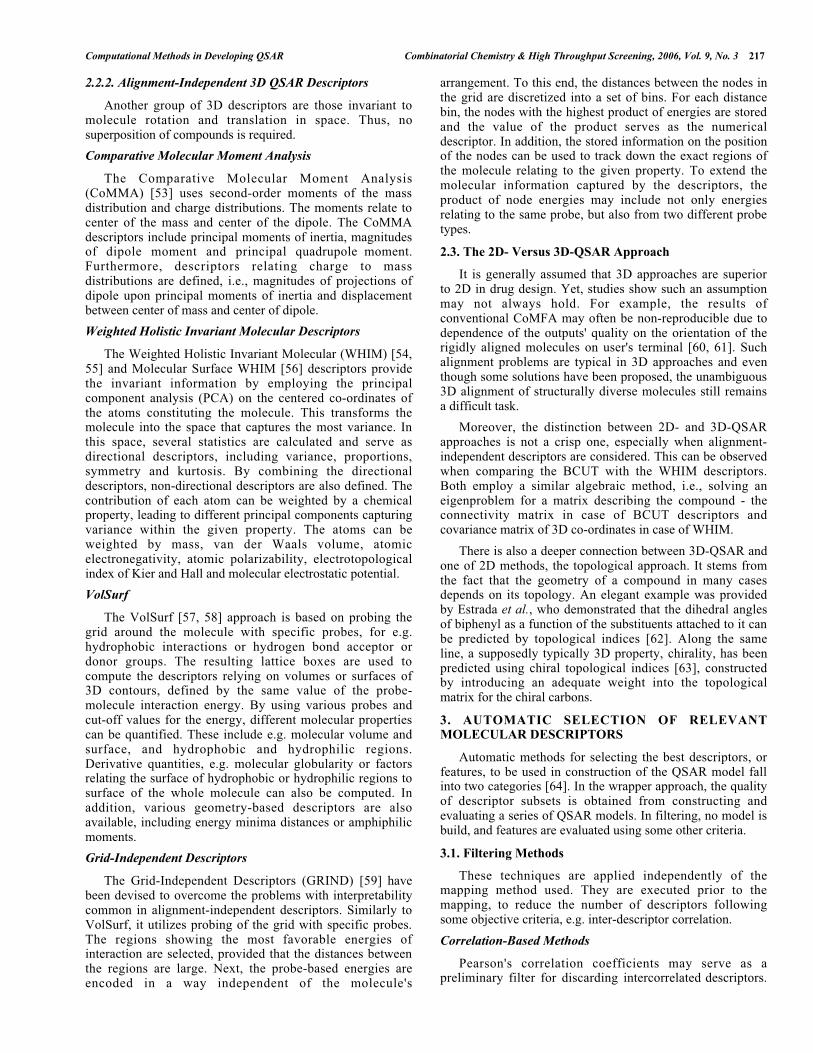
These techniques operate in conjunction with a mappingalgorithm [77]. The choice of best subset of descriptors isguided by the error of the mapping algorithm for a given

subset, measured e.g. with cross-validation. The schematicillustration of wrapper methods is given in Fig. 3.

Fig. (3). Generic scheme for wrapper descriptor selection methods.

Iteratively, various configurations of selected and discarded

descriptors are evaluated by creating a descriptors-to-activity

mapping and assessing its prediction accuracy. The final descriptors

are those yielding the highest accuracy for a given family of

mapping functions.

Genetic Algorithm

The Genetic Algorithms (GA) [78] are efficient methodsfor function minimization. In descriptor selection context,the prediction error of the model built upon a set of featuresis optimized [79, 80]. The genetic algorithm mimics thenatural evolution by modeling a dynamic population ofsolutions. The members of the population, referred to aschromosomes, encode the selected features. The encodingusually takes form of bit strings with bits corresponding toselected features set and others cleared. Each chromosomeleads to a model built using the encoded features. By usingthe training data, the error of the model is quantified andserves as a fitness function. During the course of evolution,the chromosomes are subjected to crossover and mutation.By allowing survival and reproduction of the fittestchromosomes, the algorithm effectively minimizes the errorfunction in subsequent generations.

The success of GA depends on several factors. Theparameters steering the crossover, mutation and survival ofchromosomes should be carefully chosen to allow thepopulation to explore the solution space and to prevent earlyconvergence to homogeneous population occupying a localminimum. The choice of initial population is also importantin genetic feature selection. To address this issue, e.g. amethod based on Shannon's entropy combined with graphanalysis can be used [81].


Genetic Algorithms have been used in feature selectionfor QSAR with a range of mapping methods, e.g. ArtificialNeural Networks [66, 82, 83], k-Nearest Neighbor method[84] and Random Forest [66].

Simulated Annealing

Simulated Annealing (SA) [85] is another stochasticmethod for function optimization employed in QSAR [66,86, 87]. As in the evolutionary approach, the functionminimized represents the error of the model built using thesubset of descriptors. The SA algorithm operates iterativelyby finding a new subset of descriptors by altering thecurrent-best one, e.g. by exchanging some percentage of thefeatures. Next, SA evaluates prediction error of the newsubset and makes the choice whether to adopt the newsolution as the current optimal solution. This decisiondepends on whether the new solution leads to lower errorthan the current one. If so, the new solution is used.However, in other case, the solution is not automaticallydiscarded. With a given probability, based on the Boltzmanndistribution, the worse solution can replace the current, betterone.

Replacing the solution with a worse one allows the SAmethod to escape from local minima of the error function,i.e., solutions that cannot be made better without traversingthrough less-fitted feature subsets. The power of SA methodstems from altering the temperature term in the Boltzmanndistribution. At an early stage, when the solution is not yethighly optimized and mostly prone to encounter localminima, the temperature is high. During the course ofalgorithm, the temperature is lowered and acceptance ofworse solutions is less likely. Thus, even if the obtainedminimum is not global, it is nonetheless usually of highquality.

Sequential Feature Forward Selection

While genetic algorithm and simulating annealing rely onguided random process of exploring the space of featuresubsets, Forward Feature Selection [88] operates in adeterministic manner. It implements a greedy searchthroughout the feature subsets. As a first step, a singlefeature that leads to best prediction is selected. Next,sequentially, each feature is individually added to the currentsubset and the errors of resulting models are quantified. Thefeature that is the best in reducing the error is incorporatedinto the subset. Thus, in each step a single best feature isadded, resulting in a sequence of nested subsets of features.The procedure stops when a specified number of features isselected. More elaborate stopping conditions are alsoproposed, e.g. based on incorporating an artificial randomfeature [89]. When this feature is to be selected as the onethat improves the best quality of the model, the procedure isstopped. The drawback of forward selection is that if severalfeatures collectively are good predictors but alone each is apoor prediction, none of the features may be chosen. Therecursive feature forward selection has been used in severalQSAR studies [65, 81, 90, 91].

Sequential Backward Feature Elimination

The Backward Feature Elimination [88] is anotherexample of a greedy, sequential method that yields nestedsubsets of features. In contrast to forward selection, the full

set of features is used as a starting point. Next, in each step,all subsets of features resulting from removal of a singlefeature are analyzed for the prediction error. The feature thatleads to a model with highest error is removed from thecurrent subset. The procedure stops when the given numberof features are dropped.

Backward elimination is slower than forward selection,yet often leads to better results. Recently, a significantlyfaster variant of backward elimination, the Recursive FeatureElimination [92] method has been proposed for SupportVector Machines (SVM). In this method, the feature to beremoved is chosen based on a single execution of thelearning method using all features remaining in the giveniteration. The SVM allows for ranking the features accordingto their contribution to the result. Thus, the least contributingfeature can be dropped to form a new, narrowed subset offeatures. There is no need to train SVMs for each subset asin original feature elimination method. Variants of backwardfeature elimination method have been used in numerousQSAR studies [93-97].

3.3. Hybrid Methods

In addition to the purely filter- or wrapper-baseddescriptor selection procedures, QSAR studies utilize thefusion of the two approaches. A rapid objective method isused as a preliminary filter to narrow the feature set. Next,one of the more accurate but slower subjective method isemployed. As an example of such a combination oftechniques, the correlation-based test significantly reducingthe number of features followed by genetic algorithm orsimulated annealing can be used [66]. A similar procedure,which uses a greedy sequential feature forward selection isalso in use [65].

The feature selection can also be implicit in somemapping methods. For example, the Decision Tree (seesection 4.2.4) utilizes only a subset of features in thedecision process, if a single or only a few descriptors aretested at each node and the overall number of featuresexceeds the number of those used in the nodes. Similarly,ensembles of decision stumps (see section 4.2.6) also operateon reduced number of descriptors if the number of membersin ensemble is smaller than the number of features.

4. MAPPING THE MOLECULAR STRUCTURE TOACTIVITY

Given the selected descriptors, the final step in buildingthe QSAR model is to derive the mapping between theactivity and the values of the features. Simple, yet usefulmethods model the activity as a linear function of thedescriptors. Other, non-linear, methods extend this approachto more complex relations.

Another important division of the mapping methods isbased on the nature of the activity variable. In case ofpredicting a continuous value a regression problem isencountered. When only some categories of classes of theactivity need to be predicted, e.g. partitioning compoundsinto active and inactive, the classification problem occurs. Inregression, the dependent variable is modeled as a functionof the descriptors, as noted above. In classificationframework, the resulting model is defined by a decision


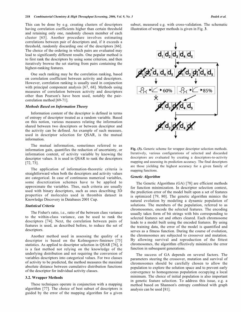
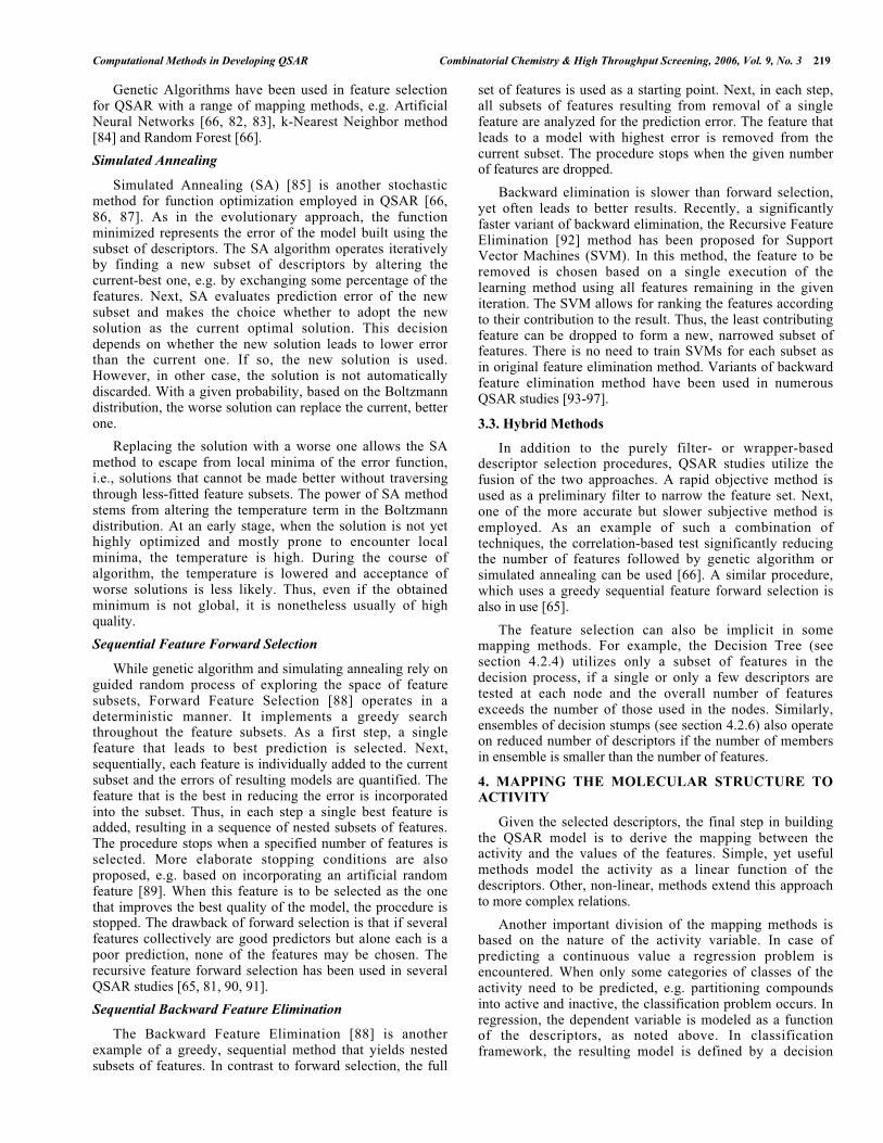
boundary, separating the classes in the descriptor space. Theapproaches to QSAR mapping are depicted in Fig. 4.

4.1. Linear Models

Linear models have been the basis of QSAR analysissince it's beginning. They predict the activity as a linearfunction of molecular descriptors. In general, linear modelsare easily interpretable and sufficiently accurate for smalldatasets of similar compounds, especially when thedescriptors are carefully selected for a given activity.

4.1.1. Multiple Linear Regression

Multiple Linear Regression (MLR) models the activity tobe predicted as a linear function of all descriptors. Based onthe examples from the training set, the coefficients of thefunction are estimated. These free parameters are chosen tominimize the squares of the errors between the predicted andthe actual activity. The main restriction of MLR analysis isthe case of large descriptors-to-compounds ratio ormulticollinear descriptors in general. This makes theproblem ill-conditioned and makes the results unstable.Multiple linear regression is among the most widely usedmapping methods in QSAR in last decades. It has beenemployed in conjunction with genetic description selectionfor modeling GABAA receptor binding, antimalaric activity,HIV-1 protease inhibition and glycogen phosphorylaseinhibition [98], exhibiting lower cross-validation error thanpartial least squares, both using 4D-QSAR fingerprints.MLR has been applied to models in predictive toxicology[99, 100], Caco-2 permeability [101] and aqueous solubility[102]. In prediction of physicochemical properties [91, 96]and of COX-2 inhibition [103], MLR proved significantlyworse than non-linear support vector machine, yetcomparable or only slightly inferior to RBF neural network.However, in studies of logP [104], it proved worse than othermodels, including multi-layer perceptron and Decision Tree.

4.1.2. Partial Least Squares

Partial Least Squares (PLS) [105-107] linear regression isa method suitable for overcoming the problems in MLRrelated to multicollinear or over-abundant descriptors. Thetechnique assumes that despite the large number ofdescriptors the modeled process is governed by a relativelysmall number of latent independent variables. The PLS triesto indirectly obtain knowledge on the latent variables bydecomposing the input matrix of descriptors into twocomponents, the scores and the loadings. The scores are

orthogonal and, while being able to capture the descriptorinformation, allow also for good prediction of the activity.

The estimation of score vectors is done iteratively. Thefirst one is derived using the first eigenvector of the activity-descriptor combined variance-covariance matrix. Next, thedescriptor matrix is deflated by subtracting the informationexplained by the first score vector. The resulting matrix isused in the derivation of the second score vector, whichfollowed by consecutive deflation, closes the iteration loop.In each iteration step, the coefficient relating the score vectorto the activity is also determined.

PLS has been used successfully with 3D QSAR andHQSAR, e.g. in a study of nicotinic acetylocholine receptorsbinding modeling [108] and estrogen receptor binding [109].It has also been used in a study [110] involving severaldataset, including blood-brain barrier permeability, toxicity,P-glycoprotein transport, multidrug resistance reversal,CDK-2 antagonism, COX-2 inhibition, dopamine bindingand log D, showing results better than decision trees in mostcases, but usually worse than most recent techniques,ensembles and SVM. PLS regression has been tested inprediction of COX-2 inhibition [84], but showed loweraccuracy than neural network and decision tree. However, ina study of solubility prediction [111], PLS outperformed aneural network. Studies report PLS-based models in meltingpoint and logP prediction [112]. Finally, PLS models forBBB permeability [113, 114], mutagenicity, toxicity, tumorgrowth inhibition and anti-HIV activity [115] and aqueoussolubility [112, 113] have been created.

4.1.3. Linear Discriminant Analysis

Linear Discriminant Analysis (LDA) [116] is aclassification method that creates a linear transformation ofthe original feature space into a space, which maximizes theinterclass separability and minimizes the within-classvariance. The procedure operates by solving a generalizedeigenvalue problem based on the between-class and within-class covariance matrices. Thus, the number of features hasto be significantly smaller than the number of observationsto avoid ill-conditioning of the eigenvalue problem.Executing principal component analysis to reduce thedimension of the input data may be employed prior toapplying LDA to overcome this problem.

LDA has been used to create QSAR models e.g. forprediction of model validity for new compounds [117],where it fared better than PLS, but worse than non-linearneural network. However, in blood-brain barrier

Fig. (4). Approaches to QSAR mapping: a) linear regression with activity as a function of two descriptors, d1 and d2, b) binary classification

with linear decision boundary between classes of active (+) and inactive (-) compounds, c) non-linear regression, d) non-linear binary

classification.


permeability prediction [114], LDA exhibited loweraccuracy than PLS-based method. In predicting antibacterialactivity [118, 119], it performed worse than neural network.LDA was also used to predict drug likeness [120], showingresults slightly better than linear programming machine, amethod similar to linear SVM. However, it yielded resultsworse than non-linear SVM and bagging ensembles. Inecotoxicity prediction [121], LDA performed better thanother linear methods and k-NN, but inferior to decision trees.

4.2. Non-Linear Models

Non-linear models extend the structure-activityrelationships to non-linear functions of input descriptors.Such models may become more accurate, especially for largeand diverse datasets. However, usually, they are harder tointerpret. Complex, non-linear models may also fall prey tooverfitting [122], i.e., low generalization to compoundsunseen during training.

4.2.1. Bayes Classifier

The Bayes Classifier stems from the Bayes rule relatingthe posterior probability of a class to its overall probability,the probability of the observations and the likelihood of aclass with respect to observed variables. In Bayes rule, theclass minimizing the posterior probability is chosen as theprediction result. However, in real problems, the likelihoodsare not known and have to be estimated. Yet, given a finitenumber of training examples, such estimation is not trivial.One method to approach this problem is to make anassumption of independence of likelihoods of class withrespect to different descriptors. This leads to the NaiveBayes Classifier (NBC). For typical datasets, the estimationof likelihoods with respect to single variables is feasible. Thedrawback of this method is that independence assumptionusually does not hold.

An extensive study using Naive Bayes Classifier incomparison with other methods was conducted [110] usingnumerous endpoints, including COX-2, CDK-2, BBB,dopamine, logD, P-glycoprotein, toxicity and multidrugresistance reversal. In most cases NBC was inferior to othermethods, however it outperformed PLS for BBB and CDK-2, k-NN for P-glycoprotein and COX-2, and decision treesfor BBB and P-glycoprotein. In thrombin binding [72], NBCyielded worse results than SVM. However, NBC has beenshown useful in modeling the inhibition of the HIV-1protease [123].

4.2.2. The k-Nearest Neighbor Method

The k-Nearest Neighbor (k-NN) [124] is a simpledecision scheme that requires practically no training and isasymptotically optimal, i.e., with increase in training dataconverges to the optimal prediction error. For a givencompound in the descriptor space, the method analyzes its knearest neighboring compounds from the training set andpredicts the activity class that is most highly representedamong these neighbors. The k-NN scheme is sensitive to thechoice of metric and to the number of training compoundsavailable. Also, the number of neighbors analyzed can beoptimized to yield best results.

The k-nearest neighbors scheme have been used e.g. forpredicting COX-2 inhibition [84], where it showed accuracy

higher than PLS and similar to neural network.Anticonvulsant activity, dopamine D1 antagonists andaquatic toxicity have also been modeled using this method[86]. In a study on P-glycoprotein transport activity [94], k-NN performed comparably to decision tree, but worse thanneural network and SVM. In ecotoxicity QSAR [121], k-NNwas better than some linear methods, but inferior todiscriminant analysis and decision trees.

4.2.3. Artificial Neural Networks

Artificial Neural Networks (ANN) [125] are biologically-inspired prediction methods based on the architecture of anetwork of neurons. A wide range of specific models basedon this paradigm have been analyzed in literature, withperceptron-based and radial-basis function-based onesprevailing. These two methods both fall into the category offeed-forward networks, in which, during the prediction, theinformation flows only in direction from the inputdescriptors, through a set of layers, to the output of thenetwork.

Multi-Layer Perceptron

The Multi-Layer Perceptron (MLP) model consists of alayered network of interconnected perceptrons, i.e., simplemodels of a neuron [126]. Each perceptron is capable ofmaking a linear combination of its input values and, bymeans of a certain transfer function, produce a binary orcontinuous output. A noteworthy fact is that each input ofthe perceptron has an adaptive weight specifying theimportance of the input. In training of a single perceptron,the inputs of the perceptron are formed by the moleculardescriptors, while the output should predict the activity ofthe compound. To achieve this goal, the perceptron is trainedby adjusting the weights, to produce a linear combination ofthe descriptors that optimally predicts the activity. Theadjusting process relies on the feedback from comparing thepredicted with the expected output. That is, the error in theprediction is propagated to the weights of the descriptors,altering them in the direction that counters the error.

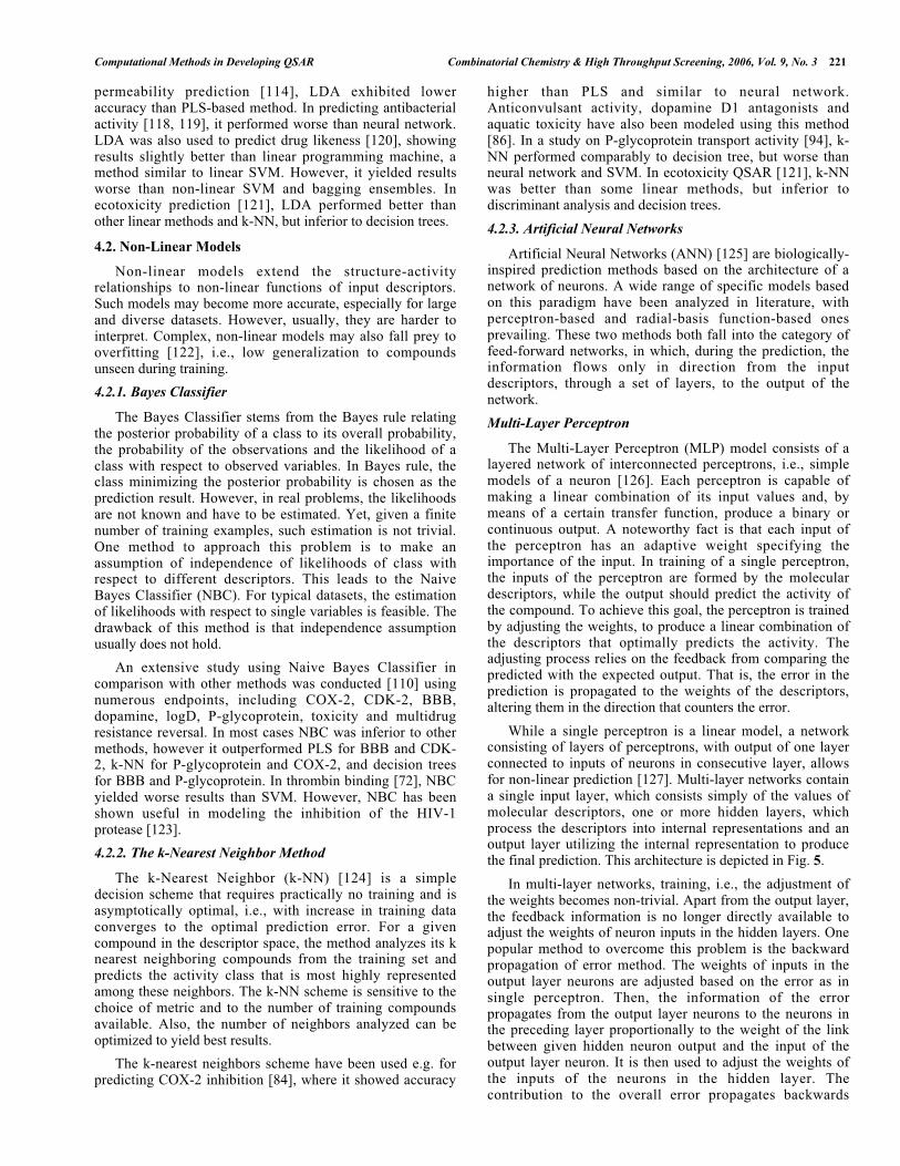
While a single perceptron is a linear model, a networkconsisting of layers of perceptrons, with output of one layerconnected to inputs of neurons in consecutive layer, allowsfor non-linear prediction [127]. Multi-layer networks containa single input layer, which consists simply of the values ofmolecular descriptors, one or more hidden layers, whichprocess the descriptors into internal representations and anoutput layer utilizing the internal representation to producethe final prediction. This architecture is depicted in Fig. 5.

In multi-layer networks, training, i.e., the adjustment ofthe weights becomes non-trivial. Apart from the output layer,the feedback information is no longer directly available toadjust the weights of neuron inputs in the hidden layers. Onepopular method to overcome this problem is the backwardpropagation of error method. The weights of inputs in theoutput layer neurons are adjusted based on the error as insingle perceptron. Then, the information of the errorpropagates from the output layer neurons to the neurons inthe preceding layer proportionally to the weight of the linkbetween given hidden neuron output and the input of theoutput layer neuron. It is then used to adjust the weights ofthe inputs of the neurons in the hidden layer. Thecontribution to the overall error propagates backwards


through all hidden layers until the weights of the first hiddenlayer are adjusted.

Fig. (5). Multi-Layer Perceptron neural network with two hidden

layers, single output neuron and four descriptors as input. Each

neuron realizes an inner product of weights wij with its input,

extended with a bias term. A binary step transfer function is used in

each neuron following the calculation of the inner product.

In general, any given function can be approximated usingneural network that is sufficiently large, both in terms ofnumber of layers and number of neurons in a layer [128].However, a big network can overfit if given a finite trainingset. Thus, the choice of the number of layers and neurons isessential in constructing the networks. Usually, networksconsisting of only one hidden layer are used. Another aspectimportant in the construction of the neural network is thechoice of the exact form of the training rule, i.e., the functionrelating the update of weights with the error of prediction.The most popular is the delta rule, the weight change isproportional to the difference of predicted and expectedoutput and to the input value. The proportionality constantdetermines the learning rate, i.e., the magnitude of steps usedin adjusting the weights. Too large learning rates mayprevent the convergence of the training to the minimal error,while too small rates increase the computational overhead.Variable, decreasing with time learning rate may also beused. The next choice in constructing the MLP is theselection of the neuron transfer function, i.e., the functionrelating the product of input and weights vectors with theoutput. Typically, a sigmoid function is used. Finally, theinitial values of weights of the links between neurons have tobe set. General consensus is that small-magnitude randomnumbers should be used.

The MLP neural networks has shown their usefulness ina wide range of QSAR applications, where linear modelsoften fail. In a human intestinal absorption study [83], MLPoutperformed the MLR model. However, single MLPnetworks have been shown inferior to ensembles of suchnetworks in prediction of antifilarial activity, GABAA

receptor binding and inhibition of dihydrofolate reductase[129]. In an antibacterial activity study [118], MLPperformed better than LDA. This type of networks has alsobeen applied to prediction of logP [104], faring better thanlinear regression and comparable to decision trees. Modelingof HIV reverse transcriptase inhibitors and E. colidihydrofolate reductase inhibitors [130] constructed withMLP were better than those relying on MLR or PLS. MLPhas also been employed to predict carcinogenic activity [82],

aquatic toxicity [131], antimalarial activity and bindingaffinities to platelet derived growth factor receptor [132].

Radial-Basis Function Neural Networks

The Radial-basis Function (RBF) [133] neural networksconsist of input layer, a single hidden layer and an outputlayer. Contrary to MLP-ANNs, the neurons in hidden layerdo not compute their output based on the product of theweights and the input values. Each hidden layer neuron isdefined by its center, i.e., a point in the feature space ofdescriptors. The output of the neuron is calculated as thefunction of the distance between the input compound in thedescriptor space and the point constituting the neuron.Typically, the Gaussian function is used, although inprincipal, some other function of the distance may beapplied. The output neuron is of perceptron type, having theoutput as a transfer function of the product of output valuesof RBF neurons and their weights.

Several parameters are adjusted during the training of theRBF network. A number of RBF neurons has to be createdand their centers and scaling of distance, i.e., widths,defined. In case of Gaussian function, these parameterscorrespond to the mean and standard deviation, respectively.The simplest approach is to create as many neurons as thecompounds in the training set and set the centers to thecoordinates of the given examples. Clustering of the trainingset into a number of groups, by e.g. k-means method, andusing the group centers and widths can be used alternatively.The orthogonal least squares [134] method can also beemployed. This procedure selects a subset of trainingexamples to be used as centers, by sequentially addingexamples, which best contribute to the explanation ofvariance of the activity to be predicted. Once all RBFneurons have been trained, the weights of the connectionbetween them and the output neuron have to be established.This can be done by analytical procedure.

The RBF-ANNs have been used in prediction of COX-2inhibition [103], yielding error lower than MLR but higherthan SVM. In prediction of physicochemical properties, suchas O-H bond dissociation energy in substituted phenols [91]and capillary electrophoresis absolute mobilities [96] RBF-ANNs showed accuracy worse than non-linear SVM, butsometimes better than linear SVM.

4.2.4. Decision Trees

Decision Trees (DT) [135, 136] differ from moststatistical-based classification and regression algorithms bytheir connection to logic-based and expert systems. In fact,each classification tree can be translated into a set ofpredictive rules in Boolean logic.

The DT classification model consists of a tree-likestructure consisting of nodes and links. Nodes are linkedhierarchically, with several child nodes branching from acommon parent node. A node with no children nodes iscalled a leaf. Typically, in each node, a test using a singledescriptor is made. Based on the result of the test, thealgorithm is directed to one of the child nodes branchingfrom the parent. In the child node, another test is performedand further traversal of the tree towards the leafs is carriedout. The final decision is based on the activity classassociated with the leaf. Thus, the whole decision process is


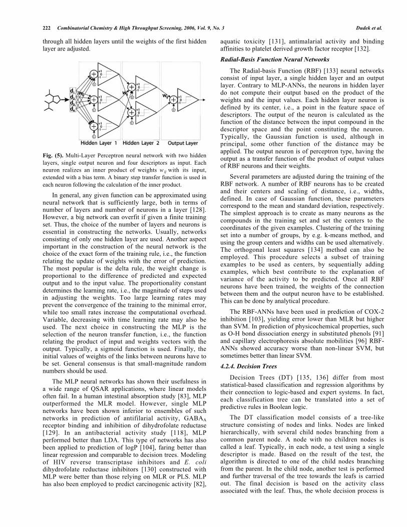
based on the series of simple tests, with results guiding thepath from the root of the tree to a leaf, as depicted in Fig. 6.

Fig. (6). Classification using decision tree based on three molecular

descriptors. The traversal of the tree on the path from the root to a

leaf node defining the final decision leads through a set of simple

tests using the values of molecular descriptors.

The training of the model consists of incrementaladdition of nodes. The process starts with choosing the testfor the root node. A test that optimally separates thecompounds into the appropriate activity classes is chosen. Ifsuch a test perfectly discriminates the classes, no furthernodes are necessary. However, in most cases, a single test isnot sufficient. A group of compounds corresponding to oneoutcome of the test contains examples from different activityclasses. Thus, iterative procedure is utilized, starting withroot node as a current node.

At each step, a current node is examined for meeting thecriteria of being a leaf. A node may become a leaf ifcompounds directed to it by the traversal from the root fallinto a single activity category or at least one category formsa clear majority. Otherwise, if the compounds are distributedbetween several classes, the optimal discriminating criterionis selected. The results of discrimination form child nodeslinked to the current node. Since the decision in the currentnode introduces new discriminatory information, the subsetsof compounds on the child nodes are more homogeneouslycorresponding to single classes. Thus, after several nodesplitting operations, the leafs can be created. Upon creationof child nodes, they are added to the list of nodes waiting tobe assessed and a first node from such a list is chosen as anext current node for evaluation. One should note, that testscarried out in nodes at the same level of the tree may bedifferent in the different branches of the tree, following thedifferent class distribution at the nodes.

There are several considerations in the development ofdecision trees. First, the method for choosing the test to beperformed on the node is necessary. As the test usuallyinvolves values of a single descriptor, the descriptor rankingcriteria outlined in section 3.1 may be employed. Once thedescriptor is chosen, the decision rule must be introduced,e.g. a threshold that separates the compounds from twoactivity classes.

The DT method may lead to overfitting on the trainingset if the tree is allowed to grow until the nodes consistpurely of one class. Thus, early stopping is used once thenodes are sufficiently pure. Moreover, pruning of theconstructed tree [137], i.e., removal of some overspecializedleafs may be introduced to increase the generalizationcapabilities of the tree [136].

In general, DT methods usually offer suboptimal errorrates compared to other non-linear methods, in particular,due to the reliance on single feature in each node.Nonetheless, they are popular in QSAR domain for their easeof interpretability. The tree effectively combines the trainingprocess with descriptor selection, limiting the complexity ofthe model to be analyzed. Furthermore, since several leafs inthe tree may correspond to a single activity class, they allowfor inspection of different paths leading to the same activity.

The decision trees also handle regression problems [138].This is done by associating each leaf with a numerical valueinstead of the categorical class. Furthermore, the criteria ofsplitting the node to form child nodes are based on thevariance of the compounds in that node.

Decision Trees have been tested in a study [110] on awide range of targets, including COX-2 inhibition, blood-brain barrier permeability, toxicity, multidrug resistancereversal, CDK-2 antagonist activity, dopamine bindingaffinity, logD and binding to an unspecified channel protein.It performed worse than support vector machines andensembles of decision trees, but often better than PLS ornaive bayes classifier. In a logP study [104], it showedresults comparable to MLP-ANNs and better than MLR. In astudy concerning P-glycoprotein transport activity [94], DTwas worse than both SVM and neural networks, but betterthan k-NN method. In various datasets related to ecotoxicity[121], decision trees usually achieved lower error than LDAor k-NN methods. Other studies employing decision trees,including anti-HIV activity [139], toxicity [140] and oralabsorption [141] have been conducted.

4.2.5. Support Vector Machines

The Support Vector Machines (SVM) [142-144] form agroup of methods stemming from the structural riskminimization principle, with the linear support vectorclassifier as its most basic member. The SVC aims atcreating a decision hyperplane that maximizes the margin,i.e., the distance from the hyperplane to the nearest examplesfrom each of the classes. This allows for formulating theclassifier training as a constrained optimization problem.Importantly, the objective function is unimodal, contrary toe.g. neural networks, and thus can be optimized effectivelyto global optimum.

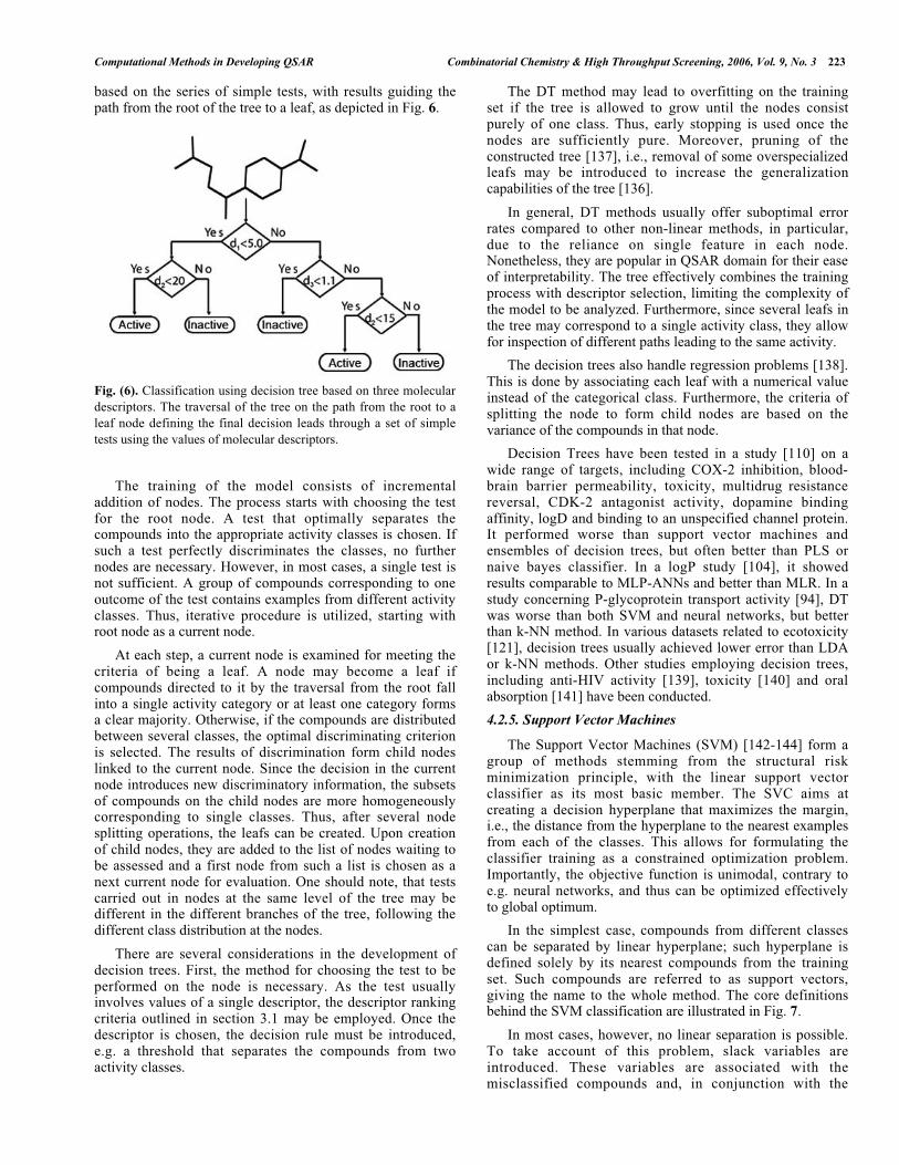
In the simplest case, compounds from different classescan be separated by linear hyperplane; such hyperplane isdefined solely by its nearest compounds from the trainingset. Such compounds are referred to as support vectors,giving the name to the whole method. The core definitionsbehind the SVM classification are illustrated in Fig. 7.

In most cases, however, no linear separation is possible.To take account of this problem, slack variables areintroduced. These variables are associated with themisclassified compounds and, in conjunction with the


margin, are subject to optimization. Thus, even though theerroneous classification cannot be avoided, it is penalized.Since the misclassification of compounds strongly influencesthe decision hyperplane, the misclassified compounds alsobecome support vectors.

Fig. (7). Support vectors and margins in linearly separable (a) and

non-separable (b) problems. In non-separable case, negative

margins are encountered and their magnitude is subject to

optimization along with the magnitude of the positive margins.

The SVC can be easily transformed into a non-linearclassifier by employing the kernel function [144, 145]. Thekernel function introduces an implicit mapping from theoriginal descriptor space to a high- or infinite-dimensionalspace. The linear hyperplane in the kernel space may behighly non-linear in the original space. Thus, by training alinear classifier in the kernel space a classifier, which is non-linear with respect to descriptor space, is obtained. Thestrength of the kernel function stems from the fact, that whileposition of compounds in the kernel space may not beexplicitly computed, the dot product can be obtained easily.As the algorithm for SVC uses the compound descriptorsonly within their dot products, this allows for computation ofthe decision boundary in the kernel space. One of two kernelfunctions are typically used, the polynomial kernel or theradial-basis function kernel.

The SVC method has been shown to exhibit lowovertraining and thus allows for good generalization to thepreviously unseen compounds. It is also relatively robustwhen only a small number of examples of each class isavailable. The SVM methods have been extended intoSupport Vector Regression (SVR) [146] to handle theregression problems. By using methods similar to SVC, e.g.the slack variables and the kernel functions, accurate non-linear mapping between the activity and the descriptors canbe found. However, contrary to typical regression methods,the predicted values are penalized only if their absolute errorexceeds certain user-specified threshold, and thus theregression model is not optimal in terms of the least-squareerror.

The SVM method has been shown to exhibit lowprediction error in QSAR [147]. Studies of P-glycoproteinsubstrates used SVMs [93, 94], with results more accuratethan neural networks, decision trees and k-NN. A studyfocused on prediction of drug likeness [120], have shownlower prediction error for SVM than for bagging ensemblesand for linear methods. In a study involving COX-2inhibition and aquatic toxicity [103], SVM outperformedMLR and RBF neural networks. An extensive study using

support vector machines among other machine learningmethods was conducted [110] using a wide range ofendpoints. In this study, SVM was usually better than k-NN,decision trees and linear methods, but slightly inferior toboosting and random forest ensembles.

SVMs have also been tested with ADME properties,including modeling of human intestinal absorption [81, 93],binding affinities to human serum albumin [95] andcytochrome P450 inhibition [65]. Studies focused onhemostatic factors have employed support vector machines,e.g. modeling thrombin binding [72] and factor Xa binding[76]. Adverse drug effects, such as carcinogenic potency[148] and Torsade de Pointes [93] were analyzed using theSVM method.

Properties such as O-H bond dissociation energy insubstituted phenols [91] and capillary electrophoresisabsolute mobilities [96] have been also studied usingSupport Vector Machines, which exhibited higher accuracythan linear regression and RBF neural networks. Otherproperties predicted with SVM include heat capacity [97]and capacity factor (logk) of peptides in high-performanceliquid chromatography [149].

4.2.6. Ensemble Methods

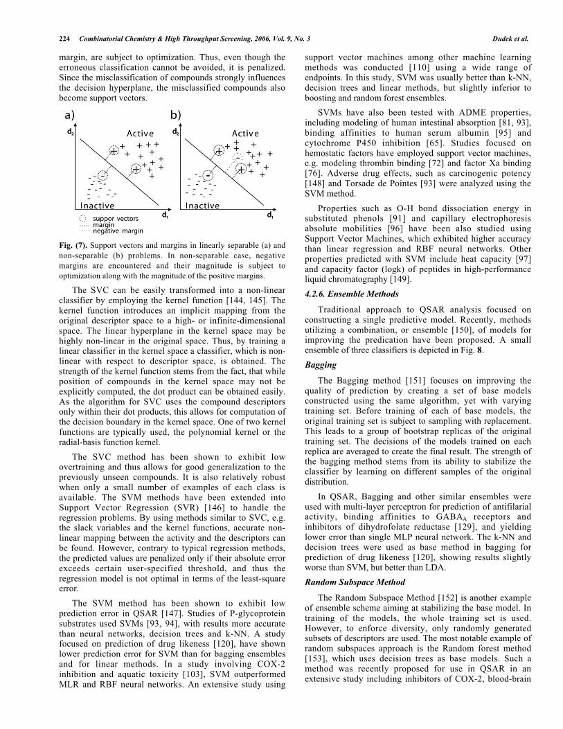
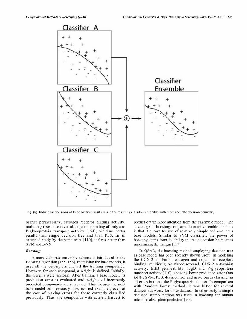
Traditional approach to QSAR analysis focused onconstructing a single predictive model. Recently, methodsutilizing a combination, or ensemble [150], of models forimproving the predication have been proposed. A smallensemble of three classifiers is depicted in Fig. 8.

Bagging

The Bagging method [151] focuses on improving thequality of prediction by creating a set of base modelsconstructed using the same algorithm, yet with varyingtraining set. Before training of each of base models, theoriginal training set is subject to sampling with replacement.This leads to a group of bootstrap replicas of the originaltraining set. The decisions of the models trained on eachreplica are averaged to create the final result. The strength ofthe bagging method stems from its ability to stabilize theclassifier by learning on different samples of the originaldistribution.

In QSAR, Bagging and other similar ensembles wereused with multi-layer perceptron for prediction of antifilarialactivity, binding affinities to GABAA receptors andinhibitors of dihydrofolate reductase [129], and yieldinglower error than single MLP neural network. The k-NN anddecision trees were used as base method in bagging forprediction of drug likeness [120], showing results slightlyworse than SVM, but better than LDA.

Random Subspace Method

The Random Subspace Method [152] is another exampleof ensemble scheme aiming at stabilizing the base model. Intraining of the models, the whole training set is used.However, to enforce diversity, only randomly generatedsubsets of descriptors are used. The most notable example ofrandom subspaces approach is the Random forest method[153], which uses decision trees as base models. Such amethod was recently proposed for use in QSAR in anextensive study including inhibitors of COX-2, blood-brain


barrier permeability, estrogen receptor binding activity,multidrug resistance reversal, dopamine binding affinity andP-glycoprotein transport activity [154], yielding betterresults than single decision tree and than PLS. In anextended study by the same team [110], it fares better thanSVM and k-NN.

Boosting

A more elaborate ensemble scheme is introduced in theBoosting algorithm [155, 156]. In training the base models, ituses all the descriptors and all the training compounds.However, for each compound, a weight is defined. Initially,the weights were uniform. After training a base model, itsprediction error is evaluated and weights of incorrectlypredicted compounds are increased. This focuses the nextbase model on previously misclassified examples, even atthe cost of making errors for those correctly classifiedpreviously. Thus, the compounds with activity hardest to

predict obtain more attention from the ensemble model. Theadvantage of boosting compared to other ensemble methodsis that it allows for use of relatively simple and erroneousbase models. Similar to SVM classifier, the power ofboosting stems from its ability to create decision boundariesmaximizing the margin [157].

In QSAR, the boosting method employing decision treeas base model has been recently shown useful in modelingthe COX-2 inhibition, estrogen and dopamine receptorsbinding, multidrug resistance reversal, CDK-2 antagonistactivity, BBB permeability, logD and P-glycoproteintransport activity [110], showing lower prediction error thank-NN, SVM, PLS, decision tree and naive bayes classifier inall cases but one, the P-glycoprotein dataset. In comparisonwith Random Forest method, it was better for severaldatasets but worse for other datasets. In other study, a simpledecision stump method was used in boosting for humanintestinal absorption prediction [90].

Fig. (8). Individual decisions of three binary classifiers and the resulting classifier ensemble with more accurate decision boundary.


5. CONCLUDING REMARKS

The chemoinformatic methods underlying QSARanalysis are in constant advancement. Well-establishedtechniques continue to be used, providing successful resultsespecially in small, homogeneous datasets consisting ofcompounds relating to a single mode of action. Thesetechniques include linear methods such as partial leastsquares. Classical non-linear methods, e.g. artificial neuralnetworks, also remain popular. However, the need for rapid,accurate assessment of large set of compounds is shifting theattention to novel techniques from pattern recognition andmachine learning fields.

Two such methods, both relying on the concept ofmargin maximization, have recently gained attention fromthe QSAR community. These are the support vectormachines and ensemble techniques. Recent studies haveshown that both yield small prediction error in numerousQSAR applications. Given the complexity of these methods,one may be tempted to treat them as black boxes. Yet, asrecently shown, only careful model selection and tuningallows for optimal prediction accuracy [120]. Thus, adoptionof novel methods should be preceded by extensive studies.Moreover, within the machine learning and patternrecognition fields, the interpretability of the model is usuallynot of utmost importance. Thus, the process of adoptingemerging techniques from these fields may requiresubstantial effort to develop methods for interpreting thecreated models.

A similar situation can be encountered in preparing themolecular descriptors to be used. The number of differentdescriptors reaches thousand in some leading commercialtools. Having at hand powerful methods for automaticallyselecting the informative features, one may be tempted toleave the descriptor selection process entirely to algorithmictechniques. While this may lead to high accuracy of themodel, often the chosen descriptors may not give clearinsight into the structure-activity relationship.

Throughout the review, we have focused on predictingthe activity or property given the values of the descriptors fora compound. The inverse problem of finding compoundswith desired activity and properties has also attractedattention. Such an inverse-QSAR formulation directlyfocuses on the goal of drug design, i.e., discovery of activecompounds with good pharmacokinetic and other properties.Authors such as Kvasnicka [158] and Lewis [14] havepublished some algorithms in this direction. Significantinsight has also been given by Kier and Hall [159] andZefirov [160]. Galvez and co-workers [161] have shown thattopological indices are particularly suited to this aim. Thereason is that whereas the conventional physical andgeometrical descriptors are structure-related, topologicalindices are just an algebraic description of the structureitself. Thus, one can go backward and forward betweenstructure and property, predicting properties for moleculesand vice versa.

Since the methods for solving the inverse problem are notyet widely adopted, the creation of QSAR models remainsthe main task in computer-aided drug discovery. In general,the adoption of novel, more accurate QSAR modelingtechniques does not reduce the responsibility of the

investigator. On the contrary, the more complex andoptimized is the model, the more caution it requires duringits application. Combined with the increased complexity ofthe inspected datasets, this makes the QSAR analysis achallenging endeavor.

REFERENCES

[1] Bleicher, K.H.; Boehm, H.-J.; Mueller, K.; Alanine, A.I. Nat. Rev.

Drug Discov., 2003, 2, 369-378.[2] Gershell, L.J.; Atkins, J.H. Nat. Rev. Drug Discov., 2003, 2, 321-

327.[3] Goodnow, R.; Guba, W.; Haap, W. Comb. Chem. High Throughput

Screen., 2003, 6, 649-660.[4] Shoichet, B.K. Nature, 2004, 432, 862-865.

[5] Stahura, F.L.; Bajorath, J. Comb. Chem. High Throughput Screen.,2004, 7, 259-269.

[6] Hansch, C.; Fujita, T. J. Am. Chem. Soc., 1964, 86, 1616-1626.[7] Bajorath, J. Nat. Rev. Drug Discov., 2002, 1, 882-894.

[8] Pirard, B. Comb. Chem. High Throughput Screen., 2004, 7, 271-280.

[9] Hodgson, J. Nat. Biotechnol., 2001, 19, 722-726.[10] van de Waterbeemd, H.; Gifford, E. Nat. Rev. Drug Discov., 2003,

2, 192-204.[11] Proudfoot, J.R. Bioorg. Med. Chem. Lett., 2002, 12, 1647-1650.

[12] Roche, O.; Schneider, P.; Zuegge, J.; Guba, W.; Kansy, M.;Alanine, A.; Bleicher, K.; Danel, F.; Gutknecht, E.M.; Rogers-

Evans, M.; Neidhart, W.; Stalder, H.; Dillon, M.; Sjogren, E.;Fotouhi, N.; Gillepsie, P.; Goodnow, R.; Harris, W.; Jones, P.;

Taniguchi, M.; Tsujii, S.; von der Saal, W.; Zimmermann, G.;Schneider, G. J. Med. Chem., 2002, 45, 137-142.

[13] Rusinko, A.; Young, S.S.; Drewry, D.H.; Gerritz, S.W. Comb.Chem. High Throughput Screen., 2002, 5, 125-133.

[14] Lewis, R.A. J. Med. Chem., 2005, 48, 1638-1648.[15] Mulliken, R.S. J. Phys. Chem., 1955, 23, 1833-1840.

[16] Cammarata, A. J. Med. Chem., 1967, 10, 525-552.[17] Stanton, D.T.; Egolf, L.M.; Jurs, P.C.; Hicks, M.G. J. Chem. Info.

Comput. Sci., 1992, 32, 306-316.[18] Klopman, G. J. Am. Chem. Soc., 1968, 90, 223-234.

[19] Zhou, Z.; Parr, R.G. J. Am. Chem. Soc., 1990, 112, 5720-5724.[20] Wiener, H. J. Am. Chem. Soc., 1947, 69, 17-20.

[21] Randic, M. J. Am. Chem. Soc., 1975, 97, 6609-6615.[22] Balaban, A.T. Chem. Phys. Lett., 1982, 89, 399-404.

[23] Schultz, H.P. J. Chem. Inf. Comput. Sci., 1989, 29, 227-222.[24] Kier, L.B.; Hall, L.H. J. Pharm. Sci., 1981, 70, 583-589.

[25] Galvez, J.; Garcia, R.; Salabert, M.T.; Soler, R. J. Chem. Inf.Comput. Sci., 1994, 34, 520-552.

[26] Pearlman, R.S.; Smith, K. Perspect. Drug Discov. Des., 1998, 9-11,339-353.

[27] Stanton, D.T. J. Chem. Inf. Comput. Sci., 1999, 39, 11-20.[28] Burden, F. J. Chem. Inf. Comput. Sci., 1989, 29, 225-227.

[29] Estrada, E. J. Chem. Info. Comput. Sci., 1996, 36, 844-849.[30] Estrada, E.; Uriarte, E. SAR QSAR Environ. Res., 2001, 12, 309-

324.[31] Hall, L.H.; Kier, L.B. Quant. Struct.-Act. Relat., 1991, 10, 43-48.

[32] Hall, L.H.; Kier, L.B. J. Chem. Inf. Comput. Sci., 2000, 30, 784-791.

[33] Labute, P. J. Mol. Graph. Model., 2000, 18, 464-477.[34] Higo, J.; Go, N. J. Comput. Chem., 1989, 10, 376-379.

[35] Katritzky, A.R.; Mu, L.; Lobanov, V.S.; Karelson, M. J. Phys.Chem., 1996, 100, 10400-10407.

[36] Rohrbaugh, R.H.; Jurs, P.C. Anal. Chim. Acta, 1987, 199, 99-109.[37] Pearlman, R.S. In: Physical Chemical Properties of Drugs ;

Yalkowsky, S.H.; Sinkula, A.A.; Valvani, S.C., Eds.; MarcelDekker: New York, 1988.

[38] Weiser, J.; Weiser, A.A.; Shenkin, P.S.; Still, W.C. J. Comp.Chem., 1998, 19, 797-808.

[39] Barnard, J.M.; Downs, G.M. J. Chem. Inf. Comput. Sci., 1997, 37,141-142.

[40] http://www.mdl.com/.[41] Durant, J.L.; Leland, B.A.; Henry, D.R.; Nourse, J.G. J. Chem.

Info. Comput. Sci., 2002, 42, 1273-1280.[42] Waller, C.L.; Bradley, M.P. J. Chem. Info. Comput. Sci., 1999, 39,

345-355.[43] Winkler, D.; Burden, F.R. Quant. Struct.-Act. Relat., 1998, 17,

224-231.


[44] Maurer, W.D.; Lewis, T.G. ACM Comput. Surv., 1975, 7, 5-19.

[45] http://www.daylight.com/.[46] Deshpande, M.; Kuramochi, M.; Wale, N.; Karypis, G. IEEE

Trans. on Knowledge and Data Eng., 2005, 17, 1036-1050.[47] Guner, O.F. Curr. Top. Med. Chem., 2002, 2, 1321-1332.

[48] Akamatsu, M. Curr. Top. Med. Chem., 2002, 2, 1381-1394.[49] Lemmen, C.; Lengauer, T. J. Comput.-Aided Mol. Des., 2000, 14,

215-232.[50] Dove, S.; Buschauer, A. Quant. Struct.-Act. Relat., 1999, 18, 329-

341.[51] Cramer, R.D.; Patterson, D.E.; Bunce, J.D. J. Am. Chem. Soc.,

1988, 110, 5959-5967.[52] Klebe, G.; Abraham, U.; Mietzner, T. J. Med. Chem., 1994, 37,

4130-4146.[53] Silverman, B.D.; Platt, D.E. J. Med. Chem., 1996, 39, 2129-2140.

[54] Todeschini, R.; Lasagni, M.; Marengo, E. J. Chemom., 1994, 8,263-272.

[55] Todeschini, R.; Gramatica, P. Perspect. Drug Discov. Des., 1998,

9-11, 355-380.

[56] Bravi, G.; Gancia, E.; Mascagni, P.; Pegna, M.; Todeschini, R.;Zaliani, A. J. Comput.-Aided Mol. Des., 1997, 11, 79-92.

[57] Cruciani, G.; Crivori, P.; Carrupt, P.-A.; Testa, B. J. Mol. Struct.:THEOCHEM., 2000, 503, 17-30.

[58] Crivori, P.; Cruciani, G.; Carrupt, P.-A.; Testa, B. J. Med. Chem.,2000, 43, 2204-2216.

[59] Pastor, M.; Cruciani, G.; McLay, I.; Pickett, S.; Clementi, S. J.Med. Chem., 2000, 43, 3233-3243.

[60] Cho, S.J.; Tropsha, A. J. Med. Chem., 1995, 38, 1060-1066.[61] Cho, S.J.; Tropsha, A.; Suffness, M.; Cheng, Y.C.; Lee, K.H. J.

Med. Chem., 1996, 39, 1383-1395.[62] Estrada, E.; Molina, E.; Perdomo-Lopez, J. J. Chem. Inf. Comput.

Sci., 2001, 41, 1015-1021.[63] de Julian-Ortiz, J.V.; de Gregorio Alapont, C.; Rios-Santamarina,

I., Garcia-Domenech, R.; Galvez, J. J. Mol. Graphics Modell.,1998, 16, 14-18.

[64] Guyon, I.; Elisseeff, A. J. Mach. Learn. Res., 2003, 3, 1157-1182.[65] Merkwirth, C.; Mauser, H.; Schulz-Gasch, T.; Roche, O.; Stahl,

M.; Lengauer, T. J. Chem. Inf. Comput. Sci., 2004, 44, 1971-1978.[66] Guha, R.; Jurs, P.C. J. Chem. Inf. Comput. Sci., 2004, 44, 2179-

2189.[67] Gallegos, A.; Girone, X. J. Chem. Inf. Comput. Sci., 2004, 44, 321-

326.[68] Verdu-Andres, J.; Massart, D.L. Appl. Spectrosc., 1998, 52, 1425-

1434.[69] Farkas, O.; Heberger, K. J. Chem. Inf. Model., 2005, 45, 339-346.

[70] Heberger, K.; Rajko, R. J. Chemom., 2002, 16, 436-443.[71] Rajko, R.; Heberger, K. Chemom. Intell. Lab. Syst., 2001, 57, 1-14.

[72] Liu, Y. J. Chem. Inf. Comput. Sci., 2004, 44, 1823-1828.[73] Venkatraman, V.; Dalby, A.R.; Yang, Z.R. J. Chem. Inf. Comput.

Sci., 2004, 44, 1686-1692.[74] Lin, T.-H.; Li, H.-T.; Tsai, K.-C. J. Chem. Inf. Comput. Sci., 2004,

44, 76-87.[75] Massey, F. J. J. Amer. Statistical Assoc., 1951, 46, 68-78.

[76] Byvatov, E.; Schneider, G. J. Chem. Inf. Comput. Sci., 2004, 44,993-999.

[77] Kohavi, R.; John, G. Artiff. Intell., 1997, 97, 273-324.[78] Michalewicz, Z. Genetic algorithms + data structures = evolution

programs (3rd ed.); Springer-Verlag: London, UK, 1996.[79] Siedlecki, W.; Sklansky, J. Int. J. Pattern Recog. Artiff. Intell.,

1988, 2, 197-220.[80] Siedlecki, W.; Sklansky, J. Pat. Rec. Lett., 1989, 10, 335-347.

[81] Wegner, J. K.; Frohlich, H.; Zell, A. J. Chem. Inf. Comput. Sci.,2004, 44, 921-930.

[82] Hemmateenejad, B.; Safarpour, M.A.; Miri, R.; Nesari, N. J. Chem.Inf. Model., 2005, 45, 190-199.

[83] Wessel, M.D.; Jurs, P.C.; Tolan, J.W.; Muskal, S.M. J. Chem. Inf.Comput. Sci., 1998, 38, 726-735.

[84] Baurin, N.; Mozziconacci, J.-C.; Arnoult, E.; Chavatte, P.; Marot,C.; Morin-Allory, L. J. Chem. Inf. Comput. Sci., 2004, 44, 276-285.

[85] Kirkpatrick, S.; C.D. Gelatt, J.; Vecchi, M.P. In Readings incomputer vision: issues, problems, principles, and paradigms ;

Morgan Kaufmann Publishers Inc.: San Francisco, CA, USA, 1987.[86] Itskowitz, P.; Tropsha, A. J. Chem. Inf. Model., 2005, 45, 777-785.

[87] Sutter, J.M.; Dixon, S.L.; Jurs, P.C. J. Chem. Info. Comput. Sci.,1995, 35, 77-84.

[88] Kittler, J. Pattern Recognition and Signal Processing, 1978, E29,

41-60[89] Bi, J.; Bennet, K.; Embrechts, M.; Breneman, C.; Song, M. J.

Mach. Learn. Res., 2003, 3, 1229-1243.[90] Wegner, J.K.; Frohlich, H.; Zell, A. J. Chem. Inf. Comput. Sci.,

2004, 44, 931-939.[91] Xue, C.X.; Zhang, R.S.; Liu, H.X.; Yao, X.J.; Liu, M.C.; Hu, Z.D.;

Fan, B.T. J. Chem. Inf. Comput. Sci., 2004, 44, 669-677.[92] Guyon, I.; Weston, J.; Barnhill, S.; Vapnik, V. Mach. Learn., 2002,

46, 389-422.[93] Xue, Y.; Li, Z.R.; Yap, C.W.; Sun, L.Z.; Chen, X.; Chen, Y.Z. J.

Chem. Inf. Comput. Sci., 2004, 44, 1630-1638.[94] Xue, Y.; Yap, C.W.; Sun, L.Z.; Cao, Z.W.; Wang, J.F.; Chen, Y.Z.

J. Chem. Inf. Comput. Sci., 2004, 44, 1497-1505.[95] Xue, C.X.; Zhang, R.S.; Liu, H.X.; Yao, X.J.; Liu, M.C.; Hu, Z.D.;

Fan, B.T. J. Chem. Inf. Comput. Sci., 2004, 44, 1693-1700.[96] Xue, C.X.; Zhang, R.S.; Liu, M.C.; Hu, Z.D.; Fan, B.T. J. Chem.

Inf. Comput. Sci., 2004, 44, 950-957.[97] Xue, C.X.; Zhang, R.S.; Liu, H.X.; Liu, M.C.; Hu, Z.D.; Fan, B.T.

J. Chem. Inf. Comput. Sci., 2004, 44, 1267-1274.[98] Senese, C.L.; Duca, J.; Pan, D.; Hopfinger, A.J.; Tseng, Y.J. J.

Chem. Inf. Comput. Sci., 2004, 44, 1526-1539.[99] Trohalaki, S.; Pachter, R.; Geiss, K.; Frazier, J. J. Chem. Inf.

Comput. Sci., 2004, 44, 1186-1192.[100] Roy, K.; Ghosh, G. J. Chem. Inf. Comput. Sci., 2004, 44, 559-567.

[101] Hou, T.J.; Zhang, W.; Xia, K.; Qiao, X.B.; Xu, X.J. J. Chem. Inf.Comput. Sci., 2004, 44, 1585-1600.

[102] Hou, T.J.; Xia, K.; Zhang, W.; Xu, X.J. J. Chem. Inf. Comput. Sci.,2004, 44, 266-275.

[103] Yao, X.J.; Panaye, A.; Doucet, J.P.; Zhang, R.S.; Chen, H.F.; Liu,M.C.; Hu, Z.D.; Fan, B.T. J. Chem. Inf. Comput. Sci., 2004, 44,

1257-1266.[104] Tino, P.; Nabney, I.T.; Williams, B.S.; Losel, J.; Sun, Y. J. Chem.

Inf. Comput. Sci., 2004, 44, 1647-1653.[105] Wold, S.; Ruhe, A.; Wold, H.; Dunn, W. SIAM J. Sci. Stat.

Comput., 1984, 5, 735-743.[106] Wold, S.; Sjostrom, M.; Eriksson, L. Chemom. Intell. Lab. Syst.,

2001, 58, 109-130.[107] Phatak, A.; de Jong, S. J. Chemom., 1997, 11, 311-338.

[108] Zhang, H.; Li, H.; Liu, C. J. Chem. Inf. Model., 2005, 45, 440-448.[109] Waller, C.L. J. Chem. Inf. Comput. Sci., 2004, 44, 758-765.

[110] Svetnik, V.; Wang, T.; Tong, C.; Liaw, A.; Sheridan, R.P.; Song,Q. J. Chem. Inf. Model., 2005, 45, 786-799.

[111] Clark, M. J. Chem. Inf. Model., 2005, 45, 30-38.[112] Catana, C.; Gao, H.; Orrenius, C.; Stouten, P.F.W. J. Chem. Inf.

Model., 2005, 45, 170-176.[113] Sun, H. J. Chem. Inf. Comput. Sci., 2004, 44, 748-757.

[114] Adenot, M.; Lahana, R. J. Chem. Inf. Comput. Sci., 2004, 44, 239-248.

[115] Feng, J.; Lurati, L.; Ouyang, H.; Robinson, T.; Wang, Y.; Yuan, S.;Young, S.S. J. Chem. Inf. Comput. Sci., 2003, 43, 1463-1470.

[116] Fisher, R. Ann. Eugen., 1936, 7, 179-188.[117] Guha, R.; Jurs, P.C. J. Chem. Inf. Model., 2005, 45, 65-73.

[118] Murcia-Soler, M.; Perez-Gimenez, F.; Garcia-March, F.J.;Salabert-Salvador, T.; Diaz-Villanueva, W.; Castro-Bleda, M.J.;

Villanueva-Pareja, A. J. Chem. Inf. Comput. Sci., 2004, 44, 1031-1041.

[119] Molina, E.; Diaz, H.G.; Gonzalez, M.P.; Rodriguez, E.; Uriarte, E.J. Chem. Inf. Comput. Sci., 2004, 44, 515-521.

[120] Mueller, K.-R.; Raetsch, G.; Sonnenburg, S.; Mika, S.; Grimm, M.;Heinrich, N. J. Chem. Inf. Model., 2005, 45, 249-253.

[121] Mazzatorta, P.; Benfenati, E.; Lorenzini, P.; Vighi, M. J. Chem. Inf.Comput. Sci., 2004, 44, 105-112.

[122] Hawkins, D.M. J. Chem. Inf. Comput. Sci., 2004, 44, 1-12.[123] Klon, A.E.; Glick, M.; Davies, J.W. J. Chem. Inf. Comput. Sci.,

2004, 44, 2216-2224.[124] Cover, T.; Hart, P. IEEE Trans. Inform. Theory, 67, 13, 21-27.

[125] Jain, A.; Mao, J.; Mohiuddin, K. Computer ,1996, 29, 31-44.[126] Rosenblatt, F. Psychol. Rev., 1958, 65, 386-408.

[127] Gallant, S. IEEE Trans. Neural Networks, 1990, 1, 179-191.[128] Hornik, K.; Stinchcombe, M.; White, H. Neural Networks, 1989, 2,

359-366.[129] Agrafiotis, D.K.; Cedeno, W.; Lobanov, V.S. J. Chem. Inf.

Comput. Sci., 2002, 42, 903-911.[130] Chiu, T.-L.; So, S.-S. J. Chem. Inf. Comput. Sci., 2004, 44, 154-

160.


[131] Gini, G.; Craciun, M.V.; Konig, C. J. Chem. Inf. Comput. Sci.,

2004, 44, 1897-1902.[132] Guha, R.; Jurs, P.C. J. Chem. Inf. Model., 2005, 45, 800-806.

[133] Mulgrew, B. IEEE Sig. Proc. Mag., 1996, 13, 50-65.[134] Chen, S.; Cowan, C.F.N.; Grant, P.M. IEEE Trans. Neural

Networks, 1991, 2, 302-309.[135] Quinlan, J.R. Mach. Learn., 1986, 1, 81-106.

[136] Gelfand, S.; Ravishankar, C.; Delp, E. IEEE Trans. Pattern Anal.Mach. Intell., 1991, 13, 163-174.

[137] Mingers, J. Mach. Learn., 1989, 4, 227-243.[138] Breiman, L.; Friedman, J.; Olshen, R.; Stone, C. Classification and

regression trees; Wadsworth: California, 1984.[139] Daszykowski, M.; Walczak, B.; Xu, Q.-S.; Daeyaert, F.; de Jonge,

M.R.; Heeres, J.; Koymans, L.M.H.; Lewi, P.J.; Vinkers, H.M.;Janssen, P.A.; Massart, D.L. J. Chem. Inf. Comput. Sci., 2004, 44,

716-26.[140] DeLisle, R.K.; Dixon, S.L. J. Chem. Inf. Comput. Sci., 2004, 44,

862-870.[141] Bai, J.P.F.; Utis, A.; Crippen, G.; He, H.-D.; Fischer, V.; Tullman,

R.; Yin, H.-Q.; Hsu, C.-P.; Jiang, L.; Hwang, K.-K. J. Chem. Inf.Comput. Sci., 2004, 44, 2061-209.

[142] Cortes, C.; Vapnik, V. Mach. Learn., 1995, 20, 273-297[143] Vapnik, V. The Nature of Statistical Learning Theory; Springer

Verlag: New York, 1995.[144] Burges, C. Data Min. Knowl. Discov., 1998, 2, 121-167

[145] Boser, B.E.; Guyon, I.M.; Vapnik, V.N. In COLT '92: Proceedingsof the fifth annual workshop on Computational learning theory ;

ACM Press: New York, NY, USA, 1992.

[146] Smola, A.; Schoelkopf, B. Stat. Comput., 2004, 14, 199-222.

[147] Burbidge, R.; Trotter, M.; Buxton, B.F.; Holden, S.B. Comput.Chem., 2001, 26, 5-14.

[148] Helma, C.; Cramer, T.; Kramer, S.; Raedt, L. D. J. Chem. Inf.Comput. Sci., 2004, 44, 1402-1411.

[149] Liu, H.X.; Xue, C.X.; Zhang, R.S.; Yao, X.J.; Liu, M.C.; Hu, Z.D.;Fan, B.T. J. Chem. Inf. Comput. Sci., 2004, 44, 1979-1986.

[150] Meir, R.; Raetsch, G. Lecture Notes in Computer Sci., 2003, 2600,118-183.

[151] Breiman, L. Mach. Learn., 1996, 24, 123-140.[152] Ho, T.K. IEEE Trans. Pat. Anal. Mach. Intell., 1998, 20, 832-844.

[153] Breiman, L. Mach. Learn., 2001, 45, 5-32.[154] Svetnik, V.; Liaw, A.; Tong, C.; Culberson, C.; Sheridan, R.P.;

Feuston, B.P. J. Chem. Inf. Comput. Sci., 2003, 43, 1947-1958.[155] Freund, Y.; Schapire, R. J. Comp. Sys. Sci., 1997, 55, 119-139.

[156] Freund, Y.; Schapire, R. J. Japanese Soc. for Artificial Intelligence,1999, 14, 771-780.

[157] Schapire, R. E.; Freund, Y.; Bartlett, P.; Lee, W. S. The Annals ofStatistics 1998, 26, 1651-1686.

[158] Kvasnicka, V.; Pospichal, J. J. Chem. Inf. Comput. Sci., 1996, 36,516-526.

[159] Kier, L.B.; Hall, L.H. Quant. Struct.-Act. Relat., 1993, 12, 383-388.[160] Skvortsova, M.; Baskin, I.; Slovokhotova, O.; Palyulin, P.; Zefirov,

N. J. Chem. Inf. Comput. Sci., 1993, 33, 630-634.[161] Galvez, J.; Garcia-Domenech, R.; Bernal, J.M.; Garcia-March, F. J.

An. Real Acad. Farm., 1991, 57, 533-546.

Received: November 1, 2005 Revised: November 15, 2005 Accepted: December 14, 2005

computational methods in developing quantitative structureactivity relationships (qsar): a review

Documents