Comparison between Discrete Wavelet Transform and Dual-Tree Complex wavelet Transform in Video Sequences Using Wavelet-Domain

Rasha Orban Mahmoud

Nile Institute of Commerce & Computer

Technology, Mansoura, Egypt

r_orban2007@yahoo.com

Mohamed T. Faheem, Amany Sarhan

Computers and Automatic Control Dept.,

Faculty of Engineering, Tanta University, Egypt

m_t_fahem@yahoo.com,

amany_m_sarhan@yahoo.com

Abstract

There has been a lot of research work dedicated

towards image denoising compared to those of video

denoising due its complexity. However, with the wide

spread of video usage in many fields of our lives, it

becomes very important to develop new techniques for

video denoising. The previous research in spatial video

denoising was based on two of the famous techniques in

the image denoising named 2-D Discrete Wavelet

Transform (2D DWT) and 2-D Dual-tree Complex

Wavelet Transform (2D DTCWT), which surpass the

available image denoising techniques. In this paper, we

introduce a comparative study of applying both Discrete

Wavelet Transform and Dual-tree Complex Wavelet

Transform techniques to the spatial video denoising. The

main goal of this study is to exploit the advantages and

disadvantages of using these techniques so as to

determine the proper application of both.

KeyWords: - Video denoising, 2D wavelet, dual-tree

complex, wavelet transform.

1. Introduction

With the maturity of digital video capturing devices

and broadband transmission networks, numerous

applications have been emerging including:

teleconferencing, remote surveillance, multimedia

services and digital television [15]. There has been a large

amount of research in the area of image and video

processing. Included in many image and video processing

algorithms such as compression, enhancement, and target

recognition are preprocessing functions for noise removal.

Noise removal is one of the most common and important

processing steps in many image and video systems [13,

15].

Video sequences are often corrupted by noise, e.g.,

due to bad reception of television pictures. Some noise

sources are located in a camera and become active during

image acquisition under bad lightning conditions. Other

noise sources are due to transmission over analogue

channels. In most cases the noise is white Gaussian noise

[4].

Considerable amount of research was dedicated to the

subject of image denoising over the past several decades,

and many different mathematical tools have been

proposed. Various established denoising methods using

variable coefficient linear filters [9, 10], adaptive

nonlinear filters [8], discrete cosine transform (DCT)-

based solutions [7], etc., have been introduced to the

literature.

For many natural signals, the wavelet transform is a

more effective tool than the Fourier transform. The

wavelet transform provides a multi-resolution

representation using a set of analyzing functions that are

dilations and translations of a few functions (wavelets)

[2].

The wavelet transform comes in several forms. The

critically-sampled form of the wavelet transform provides

the most compact representation; however, it has several

limitations. For example, it lacks the shift-invariance

property, and in multiple dimensions it does a poor job of

distinguishing orientations, which is important in image

processing. For these reasons, it turns out that for some

applications improvements can be obtained by using an

expansive wavelet transform in place of a critically-

sampled one. An expansive transform is one that converts

an N-point signal into M coefficients with M > N. There

are several kinds of expansive DWTs; here we describe

and provide an implementation of the dual-tree complex

discrete wavelet transform [14].

Recently, many wavelet-based image denoising

approaches have been proposed with impressive results

[2, 8, 14]. Two famous techniques in wavelet family are

DWT and CWT [4]. The DTCWT overcomes the

limitations of wavelet transform mentioned above; it is

nearly shift-invariant and is oriented in 2D. The 2D

DTCWT produces six subbands at each scale, each of

INFOS2008, March 27-29, 2008 Cairo-Egypt

© 2008 Faculty of Computers & Information-Cairo University

MM-20

which is strongly oriented at distinct angles [5].

However, until recently, the removal of noise in

video signals has not been studied seriously. Because the

success of the wavelet transform over other mathematical

tools in denoising images, some researchers believe that

wavelets may be successful in the removal of noise in

video signals as well. It is interesting to note that although

there have been many papers addressing wavelet-based

image denoising; comparatively few have addressed

wavelet based video denoising [13, 15].

Spatial video denoising methods treats the video as a

sequence of still images representing scenes in motion;

denoising each frame separately. Such methods are close

to image noise reduction and have been applied to wide

range of applications [6].

In this paper we introduce a detailed comparison

between the application of the two famous types of

wavelet transform namely, DWT and DTCWT to spatial

video denoising. Through this work we investigate the

potentials and disadvantages of using these techniques in

order to help in choosing the proper of them in a certain

application.

This paper is organized as follows. Firstly, this paper

presents the basics of image denoising and some of the

available image denoising technique (sec. 2), followed by

the comparison criteria and strategy (sec.3). Finally, the

experimental results and analysis are given (sec. 4).

2. Image Denoising Techniques Based On Wavelet Transform

Many different noise removal techniques have been

applied to images, but the wavelet transform has been

viewed by many as the preferred technique for noise

removal [2, 7, 14]. Rather than a complete transformation

into the frequency domain, as in DCT or FFT (Fast

Fourier Transform), the wavelet transform produces

coefficient values which represent both time and

frequency information. The hybrid spatial-frequency

representation of the wavelet coefficients allows for

analysis based on both spatial position and spatial

frequency content. The hybrid analysis of the wavelet

transform is excellent in facilitating image denoising

algorithms.

2.1 2-D Discrete Wavelet Transform

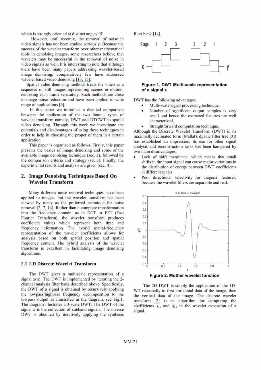
The DWT gives a multiscale representation of a

signal x(n). The DWT is implemented by iterating the 2-

channel analysis filter bank described above. Specifically,

the DWT of a signal is obtained by recursively applying

the lowpass/highpass frequency decomposition to the

lowpass output as illustrated in the diagram, see Fig.1.

The diagram illustrates a 3-scale DWT. The DWT of the

signal x is the collection of subband signals. The inverse

DWT is obtained by iteratively applying the synthesis

filter bank [14].

Figure 1. DWT Multi-scale representation of a signal x

DWT has the following advantages: Multi-scale signal processing technique. Number of significant output samples is very

small and hence the extracted features are well

characterized. Straightforward computation technique.

Although the Discrete Wavelet Transform (DWT) in its

maximally decimated form (Mallat's dyadic filter tree [3])

has established an impression, its use for other signal

analysis and reconstruction tasks has been hampered by

two main disadvantages: Lack of shift invariance, which means that small

shifts in the input signal can cause major variations in

the distribution of energy between DWT coefficients

at different scales. Poor directional selectivity for diagonal features,

because the wavelet filters are separable and real.

Figure 2. Mother wavelet function

The 2D DWT is simply the application of the 1D-

WT repeatedly to first horizontal data of the image, then

the vertical data of the image. The discrete wavelet

transform [2] is an algorithm for computing the

coefficients sj,k and dj,k in the wavelet expansion of a

signal.

MM-21

k k k k

kkkjkjkjkjkjkj xwdxwdxwdxsxf ,1,1,1,1,,,, ...(1)

where j is the number of multiresolution components (or

scales), and k ranges from 1 to the number of coefficients

in the specified component. ф is the scaling function and

the w is the wavelet function through dilation and

translation as follows

kxwxwandkxx jj

kj

jj

kj 2222 2

,2

, (2)

The scaling ф(x) function is the solution of the dilation

equation k

kkxcx 22 (3)

where the coefficients ck must satisfy the following

conditions [3]:

Unit vector: k

k.c 1

2

Double-shift: k

mkk,c.c 0

2m =1,2,…, p-1.

Approximation of order p:

m=0,1,…, p-1.

Where p =(number of coefficients)/2.

While, the wavelet function w(x) can be derived from the

corresponding scaling function by taking difference. For

the four-coefficient scaling function, the wavelet equation

is expressed as

k

k kndnw 22 (4)

where .1 12

12

kp

kp

k cd

More precisely, the expansion in (1) for any arbitrary

signal f(x) may take the form

kxwakxaxf j

k,jkk j

k

2

0

(5)

where the coefficients are given by

dxkxwxfaanddxkxxfa j

kjk 2. ,

This wavelet series expansion decomposes f(x) into an

infinite summation of wavelets at different scales. For

computing the coefficients ak and aj,k in (5) when f(x) is

sampled over some certain interval, the discrete wavelet

transform is employed.

To use the wavelet transform for image processing we

must implement a 2D version of the analysis and

synthesis filter banks. Fig. 3 shows 2-Channel Perfect

Reconstruction Filter Bank.

Figure 3. 2-Channel Perfect Reconstruction Filter Bank

2.2. 2-D Dual Tree Complex WT (2D DTCWT)

It has been noted that, for some applications of the

discrete wavelet transform, improvements can be obtained

by using an expansive wavelet transform in place of a

critically-sampled one. An expansive transform is one that

converts an N-point signal into M coefficients with M >

N. There are several kinds of expansive DWTs; here we

describe the dual-tree complex discrete wavelet transform

[6].

The DTCWT of a signal x is implemented using two

critically-sampled DWTs in parallel on the same data, as

shown in Fig. 4. The transform is 2-times expansive

because for an N-point signal it gives 2N DWT

coefficients. If the filters in the upper and lower DWTs

are the same, then no advantage is gained. However, if the

filters are designed is a specific way, then the subband

signals of the upper DWT can be interpreted as the real

part of a complex wavelet transform, and subband signals

of the lower DWT can be interpreted as the imaginary

part. Equivalently, for specially designed sets of filters,

the wavelet associated with the upper DWT can be an

approximate Hilbert transform of the wavelet associated

with the lower DWT.

Figure 4. The Dual-Tree complex DWT of a signal x

af1

af2

sf1

sf2

x(n) y(n)

c(n)

d(n)

h0(n)

h1(n)

g0(n)

g1(n)

h0(n)

h1(n)

h0(n)

h1(n)

g0(n)

g1(n)

g0(n)

g1(n)

2

2

2

2

2

2

2

2

2

2

2

2

x

k

k

mkck ,01

MM-22

When designed in this way, the dual-tree complex

DWT is nearly shift-invariant, in contrast with the

critically-sampled DWT. Moreover, the dual-tree

complex DWT can be used to implement 2D wavelet

transforms where each wavelet is oriented, which is

especially useful for image processing. (For the 2D DWT,

recall that one of the three wavelets does not have a

dominant orientation.) The DTCWT outperforms the

critically-sampled DWT for applications like image

denoising and enhancement.

One of the advantages of the DTCWT is that it can be

used to implement 2D wavelet transforms that are more

selective with respect to orientation than is the 2D DWT

[14].

Let w2 represent the parent of w1 (w2 is the wavelet

coefficient at the same spatial position as w1, but at the

next coarser scale) [4]. Then:

y = w + n

where w = (w1,w2), y = (y1,y2) and n = (n1,n2). The

noise values n1, n2 are zero-mean Gaussian with variance

sigma () [12, 13]. Based on the empirical histograms, the

following non-Gaussian bivariate equation was used [12]

2

2

2

12

3exp.

2

3wwwp w (6)

With this equation, w1 and w2 are uncorrelated, but

not independent [13]. The MAP estimator of w1 yields the

following bivariate shrinkage function [1], [5].

12

2

2

1

22

2

2

1

1 .

3

ˆ yyy

yy

w

n

(7)

In general, the DTCWT has the following properties: Approximate shift invariance; Good directional selectivity in 2-dimentions (also

true for higher dimensionality m-D); Perfect reconstruction (PR) using short linear-phase

filters; Limited redundancy, independent of the number of

scales, 2m:1 for m-D; Efficient order-N computation- only twice the simple

DWT for 1-D (2m times for m-D).

3. Video Denoising Techniques

Image sequence denoising (or video denoising) is the

process of removing noise from a video signal. Video

denoising methods are divided into:

1-Spatial video denoising methods, when only one

frame is used for noise suppression. Such methods

are close to image noise reduction. For the problem

of image sequence denoising in spatial domain,

Selesnick and Li in [12] demonstrated the

improvement gained by using both the 2D DTCWT

and 3D DTCWT in spatial video denoising. For

frames containing fast motion, the dual-tree 2-D

transform can give a superior result. This is because

for fast motion it is more difficult to exploit the

temporal correlation of pixel values [12].

2- Temporal video denoising methods, where only

temporal information is used. In order to denoise the

video sequence in temporal domain they used

temporal only filtering. The amount of the temporal

filtering is reduced when the motion confidence is

relatively high (to avoid motion blur), and increased

in case of low motion confidence, in order to filter as

much as possible in the temporal direction [15].

3- Spatio-Temporal video denoising methods uses

combination of spatial and temporal denoising.

Zlokolica final algorithm [15] performs motion-detail

adaptive averaging of the wavelet coefficients, based

on the spatio-temporal wavelet coefficient

distribution. It is generally agreed that in the case of

low and medium noise levels, which are important in

most real video applications, spatio-temporal filtering

performs better than temporal only filtering.

4. Comparison Criteria

In this work, we analyze the usage of two of the

famous wavelet transform image denoising techniques in

the spatial video denoising namely; 2D DWT and 2D

DTCWT. Both techniques were developed originally for

image denoising and have been used in spatial video

denoising. However, there has not been any analysis of

their performance or a comparison between them yet. So,

in this work we intend to introduce such a comparison

study to facilitate the choice between them in the different

applications.

We will work on the spatial domain where we split

the video stream into a number of frames (images). Then

for each of these frames we apply the 2D DWT or the 2D

DTCWT technique for denoising. We believe that even if

the DTCWT denoising technique worked well on the

image scale denoising, it may have to be studied closely

to ensure its effectiveness on video denoising. We will

concentrate on the spatial denoising in this work hoping

to extend it to both temporal and spatio-temporal

domains.

Validation of the performance of both techniques

was done by comparing their resultant video criteria and

this was made on both gray-scale and colored test movies.

The comparison between the two techniques will be based

on the PSNR and time consumed during denoising

process.

PSNR (Peak Signal to Noise Ratio) is the most

commonly used objective quality metric. It is a statistical

measure of error, used to determine the quality of

compressed images, mathematically equivalent to the

mean squared error (MSE). This is the most commonly

used metric of image quality used in the image and video

compression literature. The PSNR is usually quoted in

MM-23

decibels, a logarithmic scale. The PSNR has a limited,

approximate relationship with the perceived errors noticed

by the human visual system.

As a rough rule of thumb, an image with a PSNR of

25 dB (decibels) is usually pretty poor. Anything below

25 dB is usually unacceptable. Perceived quality usually

improves from 25 dB to about 30 dB. Above around 30

dB images look pretty good and are often

indistinguishable from the uncompressed original image.

The human visual system appears to have sensitivity

thresholds. This can be rigorously demonstrated in

controlled experiments using sinusoidal gratings against

black backgrounds. Because of this thresholding, once

the PSNR exceeds some value, the errors become

undetectable to human viewers. Hence an image with a

PSNR of 35 dB may look the same as an image with a

PSNR of 40 dB.

Conversely, the human visual system seems to have

a saturation effect as well. Once the image quality falls

below a certain level, the image simply looks bad. An

image with a PSNR of 15 dB and an image with a PSNR

of 10 dB may look equally bad to a viewer. Typically by

this point the image appears quite poor.

For a video sequence of K frames each having N×M

pixels with m-bit depth, the Mean Square Error (MSE) is

calculated as [11]:

N

n

M

m

jixjixMN

MSE1 1

2

),(),(1 (8)

where ),( jix is the original frame and ),( jix

is the

restored frame of ),( ji location.

The PSNR is calculated as:

)(log.10

2

MSE

mPSNR (9)

where m = 255.

We also computed the time required to perform the

denoising process. Our motivation is to select the most

suitable denoising technique for certain applications such

as video conference on the Internet.

5. Experimental Results

We used the ‘grayscale Akiyo‘ image sequence (gray

levels from 0 to 255), which we corrupted with three

different values of Gaussian noise with σ = 5, σ = 10 and σ = 20 to investigate the performance of the two techniques under different values of noise. Then, we

applied the 2D DWT and the 2D DTCWT to each frame

of the video. The test video consists of 50 frames.

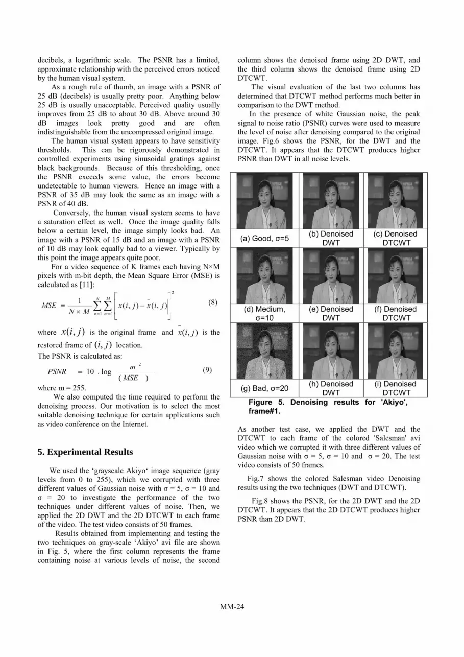
Results obtained from implementing and testing the

two techniques on gray-scale ‘Akiyo’ avi file are shown

in Fig. 5, where the first column represents the frame

containing noise at various levels of noise, the second

column shows the denoised frame using 2D DWT, and

the third column shows the denoised frame using 2D

DTCWT.

The visual evaluation of the last two columns has

determined that DTCWT method performs much better in

comparison to the DWT method.

In the presence of white Gaussian noise, the peak

signal to noise ratio (PSNR) curves were used to measure

the level of noise after denoising compared to the original

image. Fig.6 shows the PSNR, for the DWT and the

DTCWT. It appears that the DTCWT produces higher

PSNR than DWT in all noise levels.

(a) Good, σ=5 (b) Denoised DWT

(c) DenoisedDTCWT

(d) Medium, σ=10

(e) Denoised DWT

(f) Denoised DTCWT

(g) Bad, σ=20 (h) Denoised DWT

(i) Denoised DTCWT

Figure 5. Denoising results for 'Akiyo', frame#1.

As another test case, we applied the DWT and the

DTCWT to each frame of the colored 'Salesman' avi

video which we corrupted it with three different values of

Gaussian noise with σ = 5, σ = 10 and σ = 20. The test video consists of 50 frames.

Fig.7 shows the colored Salesman video Denoising

results using the two techniques (DWT and DTCWT).

Fig.8 shows the PSNR, for the 2D DWT and the 2D

DTCWT. It appears that the 2D DTCWT produces higher

PSNR than 2D DWT.

MM-24

(a) Good, σ =5

(b) Medium, σ =10

(c) Bad, σ =20

Figure 6. PSNR curves for 'Akiyo'.

Table1 summarizes all results obtained from

previous tests. From Table 1 we have the following

remarks:

1- The DTCWT consumes more time than DWT

(approximately 6 times) in the denoising operation

of both the grey scale and colored videos that is

due to the high computations it takes.

2- The DTCWT gives better average PSNR results

than the DWT (the increment in PSNR reaches

1dB in some cases) in both the grey scale and

colored videos denoising.

3- At high levels of noise, the performance of

DTCWT is better than DWT as it gives better

PSNR.

4- Denoising colored video takes more time than gray

ones in both DTCWT and DWT.

5- Both DTCWT and DWT give higher PSNR in gray

than in colored video.

(a) Good, σ =5(b) Denoised

DWT(c) Denoised

DTCWT

(d) Medium, σ =10

(e) Denoised DWT

(f) Denoised DTCWT

(g) Bad, σ =20(h) Denoised

DWT(i) Denoised

DTCWT

Figure 7. Denoising results for Colored Salesman, frame#1.

This leads us to the conclusion that we recommend

using DTCWT on bad quality videos only to enhance its

performance while using the DWT on the low noise

videos. We also recommend using DWT for video

conferencing as it will take mush less time than DTCWT.

As a possible future work, if the noise level on the

frame can be measured before choosing the denoising

technique, it would be possible to dynamically switch

between the two techniques easily to obtain faster and

more efficient results. We thus encourage the introduction

of new techniques through which the denoising system

can measure the noise level on the frame it is handling

before making the decision about the determination of the

denoising technique to be used.

Noised

DWT DTCWT

Noised

DWT DTCWT

Noised

DWT DTCWT

MM-25

(a) Good, σ =5

(b) Medium, σ =10

(c) Bad, σ =20

Figure 8. PSNR curves for 'Salesman'.

6. Conclusion

In this work we were concerned with the

comparison of the application of the most famous

techniques in the image denoising to the spatial video

denoising. This concern was driven by the idea of

exploring the true differences and potentials of both in

order to guide us through the choice process of which one

to use in a given applications.

Through the comparison results, we found that using

DTCWT will give better PSNR results and better visual

appearance especially at high levels of noise. However, it

has the disadvantage of consuming time which makes it

not suitable for the applications where time is important.

While using the DWT technique will consume less time

producing less efficient videos especially at the high

levels of noise.

References

[1] A. Alin, and K. Ercan, "Image Denoising Using Bivariate-

Stable Distributions in the Complex Wavelet Domain",

Signals and Images Laboratory, Istituto di Scienza e

Tecnologie dell’Informazione “A. Faedo”, Area della

Ricerca CNR di Pisa, Italy, 2004.

[2] I. Daubechies, "Ten Lectures on Wavelets", Rutgers

University and AT&T Bell Labaratories, USA, 1992.

[3] I. Daubechies, Daubechies, I., “Wavelets”, Philadelphia:

S.I.A.M., 1992.

[4] R. Gomathi and S. Selvakumaran, " A Bivariate Shrinkage

Function For Complex Dual Tree Dwt Based Image

Denoising ", Proceedings of the 6th WSEAS International

Conference on Wavelet Analysis & Multirate Systems,

Bucharest, Romania, October 16-18, 2006.

[5] A. Hyvarinen, P. Hoyer, and E. Oja, " Image denoising by

sparse code shrinkage", Intelligent Signal Processing, IEEE

Press, 2001.

[6] S. Kalpana, and B. Alan, "New Vistas in Image and Video

Quality Assessment", The Laboratory for Image and Video

Engineering (LIVE), The University of Texas at Austin,

USA, 2007.

[7] S. D. Kim, S. K. Jang, M. J. Kim, and J. B. Ra, “Efficient

block-based coding of noise images by combining pre-

filtering and DCT,” in Proc. IEEE Int. Symp. Circuits Syst.,

vol. 4, 1999, pp. 37–40.

[8] M. Meguro, A. Taguchi, and N. Hamada, “Data-dependent

weighted median filtering with robust motion information

PSNR of Denoised Sequence (dB) Elapsed Time using Denoising Algorithms (msec.)PSNR of Noisy

SequenceUsing 2DWT Using 2D CWT Using 2DWT Using 2D CWT

Video Squence

Noise value (dB)

min max Mean min max mean min max mean Min max mean min max mean

5 34.1 34.2 34.1 41.1 41.2 41.1 41.5 41.7 41.6 0.7 0.7 0.7 2.7 3.5 2.9

10 28.1 28.2 28.1 37.2 37.4 37.2 37.8 38.0 37.9 0.7 0.8 0.7 2.8 2.9 2.9Akiyo20 22.1 22.1 22.1 33.8 34.0 33.8 34.5 34.7 34.6 0.8 0.9 0.8 3.0 3.1 3.0

5 34.1 34.2 34.2 36.0 36.1 36.0 37.1 37.4 37.3 1.8 2.0 1.8 8.3 9.7 8.4

10 28.1 28.1 28.1 32.2 33.4 32.3 33.3 33.6 33.4 1.9 2.3 1.9 8.4 8.8 8.5Colored

Salesman20 22.1 22.1 22.1 29.0 29.6 29.0 30.3 30.6 30.4 1.8 2.2 1.8 8.4 9.0 8.5

Table 1. Summary of results obtained from previous tests.

Noised

DWT DTCWT

Noised

DWT DTCWT

Noised

DWT DTCWT

MM-26

for image sequence restoration,” IEICE Trans.

Fundamentals, vol. 2, pp. 424–428, 2001.

[9] O. Ojo and T. Kwaaitaal-Spassova, “An algorithm for

integrated noise reduction and sharpness enhancement,”

IEEE Trans. Consum. Electron., vol. 46, pp. 474–480, May

2000.

[10] P. Rieder and G. Scheffler, “New concepts on denoising

and sharpening of video signals,” IEEE Trans. Consum.

Electron., vol. 47, no. 8, pp. 666–671, Aug. 2001.

[11] C. Sang-Gyu, B. Zoran, M. Dragorad, L. Jungsik, and H.

Jae-Jeong, "Image Quality Evaluation: JPEG 2000 Versus

Intra-only H.264/AVC High Profile", Facta Universitatis

(NIˇS), Elec. vol. 20, no. 1, pp. 71-83, 2007.

[12] I.W. Selesnick, K. Y. Li, " Video denoising using 2D and

3D dual-tree complex wavelet transforms ", Proceedings of

SPIE , Vol. 5207, pp. 607-618, Nov 2003.

[13] L. Sendur, I.W. Selesnick, "A Bivariate Shrinkage

Function For Wavelet-Based Denoising", Electrical

Engineering, Polytechnic University, Metrotech Center,

Brooklyn, NY 11201, 2001.

[14] L. Sendur, I.W. Selesnick, "Bivariate shrinkage functions

for wavelet-based denoising exploiting interscale

dependency", IEEE Transactions on Signal Processing,

50(11), pp. 2744-2756, Nov 2002.

[15] V. Zlokolica, "Advanced Nonlinear Methods for Video

Denoising", Ph.D. Thesis, Faculty of Engineering, Ghent

University, Germany, 2006.

MM-27