comparing object alignment algorithms with appearance variation: forward-additive vs...

Comparing Object Alignment Algorithms with AppearanceVariation: Forward-Additive vs Inverse-Composition

Patrick Lucey#,1, Simon Lucey*,2, Mark Cox#,3, Sridha Sridharan#,4, and Jeff Cohn*,5# Speech, Audio, Image and Video Technology Laboratory, Queensland University ofTechnology, Brisbane, QLD, 4000, Australia* Robotics Institute, Carnegie Mellon University, Pittsburgh, PA, 15213, USA

AbstractA common problem that affects object alignment algorithms is when they have to deal withobjects with unseen intra-class appearance variation. Several variants based on gradient-decentalgorithms, such as the Lucas-Kanade (or forward-additive) and inverse-compositional algorithms,have been proposed to deal with this issue by solving for both alignment and appearancesimultaneously. In [1], Baker and Matthews showed that without appearance variation, theinverse-compositional (IC) algorithm was theoretically and empirically equivalent to the forward-additive (FA) algorithm, whilst achieving significant improvement in computational efficiency.With appearance variation, it would be intuitive that a similar benefit of the IC algorithm would beexperienced over the FA counterpart. However, to date no such comparison has been performed.In this paper we remedy this situation by performing such a comparison. In this comparison weshow that the two algorithms are not equivalent due to the inclusion of the appearance variationparameters. Through a number of experiments on the MultiPIE face database, we show that wecan gain greater refinement using the FA algorithm due to it being a truer solution than the ICapproach.

I. IntroductionThe accurate alignment of images is essential to almost all tasks in computer vision. Lucasand Kanade [2] devised an algorithm to image alignment using a gradient-descent approach,which worked on the basis of iteratively minimising the squared difference between atemplate and input image. Since then, the Lucas-Kanade algorithm has become one of themost widely used techniques in computer vision. However, an inherent problem with theLucas-Kanade algorithm is the computational cost associated with the calculating thegradients of the input image at each iteration. In the seminal work of Baker and Matthews[1], they alleviated this overhead by swapping the role of template and input image, thusallowing for significant savings in computation by pre-computing the gradients from thetemplate. In this overview paper, Baker and Matthews theoretically and empirically showedthat their implementation, which they called the inverse-compositional (IC) algorithm, wasequivalent to the Lucas-Kanade (or otherwise known as the forward-additive (FA))algorithm. This result was important as the IC algorithm provided an efficient framework inwhich tasks like object alignment and tracking could be performed in real-time [3].

[email protected]@[email protected]@[email protected]

NIH Public AccessAuthor ManuscriptIEEE Workshop Multimed Signal Proc. Author manuscript; available in PMC 2010 August 4.

Published in final edited form as:IEEE Workshop Multimed Signal Proc. 2008 October 8; 2008: 337–342. doi:10.1109/MMSP.2008.4665100.

NIH

-PA Author Manuscript

NIH


NIH


https://www.researchgate.net/publication/2900541_Active_appearance_models_revisited_IJCV_602_135-164?el=1_x_8&enrichId=rgreq-2323fa336a20138c58bf6fca55f56415-XXX&enrichSource=Y292ZXJQYWdlOzIyMTI3NDAyOTtBUzo5ODg4Njk5NTY3NzE5MkAxNDAwNTg3OTA1NDcx

https://www.researchgate.net/publication/228083880_An_Iterative_Image_Registration_Technique_with_an_Application_toStereo_Vision?el=1_x_8&enrichId=rgreq-2323fa336a20138c58bf6fca55f56415-XXX&enrichSource=Y292ZXJQYWdlOzIyMTI3NDAyOTtBUzo5ODg4Njk5NTY3NzE5MkAxNDAwNTg3OTA1NDcx

https://www.researchgate.net/publication/2374956_Equivalence_and_Efficiency_of_Image_Alignment_Algorithms?el=1_x_8&enrichId=rgreq-2323fa336a20138c58bf6fca55f56415-XXX&enrichSource=Y292ZXJQYWdlOzIyMTI3NDAyOTtBUzo5ODg4Njk5NTY3NzE5MkAxNDAwNTg3OTA1NDcx

A problem with gradient-descent approaches such as the FA and IC algorithms, are that theyhave poor generalisation properties when they have to deal with previously unseen intra-class object variation [4]. This is due to the assumption that the template appears within theinput image which is problematic. For example for aligning faces (see Figure 1), if we learna template face from an ensemble of training face images and try to align it to an unseenface, there is a very high probability that the template face and input face will be misaligned.This is because of the discrepancy between the appearance of the template face and the inputface image.

In an attempt overcome this inherent mismatch, Black and Jephson [5] proposed analgorithm that incorporated the appearance variation in the template through an ensemble ofknown appearance variation images (which were learnt from a stack of images) andunknown appearance parameters. In this work, Black and Jephson utilised the FAframework. Baker et al. [6] employed a similar strategy, however they employed the ICalgorithm. They called this the simultaneous algorithm, as it solved for both alignment andappearance at the same time using the IC framework.

As noted previously, it was shown in [1] that the IC algorithm was much morecomputationally efficient than the FA approach, whilst achieving the same alignmentperformance. As such, it would be intuitive that the simultaneous IC algorithm would enjoythe same performance and efficiency improvement over the simultaneous FA algorithm.However, no such comparison has been made. In an attempt to remedy this situation, in thispaper we focus on providing a comparison between these two algorithms. From thiscomparison, we will show that these assumptions are not valid as the appearance variationparameters are included into different terms for both approaches, thus resulting in differentsolutions. The appearance parameters also diminish the advantage in efficiency as no pre-computation can take place1.

In this paper, we show that the simultaneous FA algorithm provides a truer solution than thesimultaneous IC algorithm as it does not include any second order terms. As a result, weshow by using the simultaneous FA approach, we can get finer alignment compared to thesimultaneous IC algorithm. Hence, our specific contributions stemming from this paper are:

• We implement a simultaneous FA approach to image alignment to alleviate theproblem of linear appearance variation and compare it to the IC counterpart(Section 3). No such comparison has been done before.

• Mathematically, we show that the simultaneous FA and simultaneous IC algorithmsare intrinsically different. From this we show that the simultaneous FA is a truersolution than the simultaneous IC approach (Section 3).

• In our experiments we show that the simultaneous FA algorithm achieves greaterrefinement than the simultaneous IC algorithm with an initial pixel error of 5 RMSfor the affine warp (Section 4).

1It is worth noting that the simultaneous IC framework does allow for the “project-out” algorithm [6] which is a very computationallyefficient algorithm. However, this algorithm suffers from poor alignment when the appearance variation is large due to simplifyingassumptions. As we are interested in the performance, the “project-out” algorithm was not considered in this paper.

Lucey et al.

IEEE Workshop Multimed Signal Proc. Author manuscript; available in PMC 2010 August 4.

NIH


NIH


NIH


https://www.researchgate.net/publication/2913929_Lucas-Kanade_20_Years_on_A_Unifying_Framework?el=1_x_8&enrichId=rgreq-2323fa336a20138c58bf6fca55f56415-XXX&enrichSource=Y292ZXJQYWdlOzIyMTI3NDAyOTtBUzo5ODg4Njk5NTY3NzE5MkAxNDAwNTg3OTA1NDcx

https://www.researchgate.net/publication/2352288_EigenTracking_Robust_Matching_and_Tracking_of_Articulated_Objects_Using_a_View-Based_Representation?el=1_x_8&enrichId=rgreq-2323fa336a20138c58bf6fca55f56415-XXX&enrichSource=Y292ZXJQYWdlOzIyMTI3NDAyOTtBUzo5ODg4Njk5NTY3NzE5MkAxNDAwNTg3OTA1NDcx

https://www.researchgate.net/publication/222421026_Generic_vs_Person_Specific_Active_Appearance_Models?el=1_x_8&enrichId=rgreq-2323fa336a20138c58bf6fca55f56415-XXX&enrichSource=Y292ZXJQYWdlOzIyMTI3NDAyOTtBUzo5ODg4Njk5NTY3NzE5MkAxNDAwNTg3OTA1NDcx


II. Background: Image Alignment AlgorithmsA. Forward-Additive Algorithm

The standard Lucas-Kanade or forward-additive (FA) alignment algorithm attempts to findthe parametric warp p that minimises the sum of the squared error between the templateimage T and the input imageY 2, such that

(1)

where the vector is a concatenation of individual pixel 2D coordinates xwithin the template image T. One can map the image positions z to a set of new positions z′,

(2)

based on the warp parameters p. The warp function is canonically translation (x; p) = x +p, but (x; p) has been extended to numerous other types of warps such as affine [5,3] andpiece-wise affine [8]. In this paper we focus on the affine warp, which consists of n = 6parameters such that p = [p0, …, p5]T. Minimising Equation (1) is a nonlinear optimisationtask, so to optimise it we assume that a current estimate of p is known and then iterativelysolve for increments to the parameters Δp, where p ← p + Δp. As such, we minimise thefollowing expression

(3)

with respect to Δp. It is worth noting that from here on we shall refer to T( (z; 0)) as T(z)because (z; 0) is the identity warp as (z; 0) = z. Before we can minimise Equation (3),we need to linearise Y ( (z; p + Δp)). We can do this via the Taylor series expansion whichyields

(4)

From this we can denote the steepest-decent images as

(5)

and the error image as

2For convenience we employ the notation that ||a−b||2 = (a−b)T(a−b), where a and b are column vectors

Lucey et al.


NIH


NIH


NIH




(6)

Therefore, substituting in the steepest-decent and error images back into Equation (4), theminimisation with respect to Δp gives

(7)

Setting Equation (7) to equal zero and solving for Δp yields

(8)

where the Hessian matrix

(9)

We iteratively solve for Δp and then update p ← p + Δp until convergence or a maximumnumber of iterations is met. This non-linear optimisation process is called Gauss-Newtonoptimisation [7], but other least-square variants such as Newton and Levenberg-Marquardtoptimisations can be used [7].

B. Inverse-Composition AlgorithmAs pointed out by Baker et al. [7], there is a huge computational cost associated with the FAalgorithm as the Hessian matrix in Equation (9) needs to be calculated every iteration. Toovercome this problem, Baker et al. [7] found a way of switching the roles of the templateand the input image, by compositionally inverting the warp parameters. By doing this, itallows the Hessian to be calculated from the constant template image, which which allows itto be precomputed, resulting in considerable computational savings. This is called theinverse-compositional (IC) algorithm and as mentioned, it is implemented by essentiallyinverse-composing the warp update, i.e. (z; p) ← ( (z; Δp)−1; p). Thus, instead ofminimising Equation (4), we attempt to minimise

(10)

By employing a similar process to the FA algorithm, we can obtain the Δp which minimisesthe expression. Updating our current estimate of the warp parameters p is done byevaluating (z; p) ← ( (z; Δp)−1; p). So for the IC algorithm,

(11)

where the Hessian matrix is

Lucey et al.


NIH


NIH


NIH


(12)

and the steepest-decent images3 are

(13)

and the error image is

(14)

In [7], the FA and IC algorithms are shown to obtain the same image alignmentperformance. We also show this to be the case in the experiments presented in Section 5.However, this is not the case when appearance variation is included. We investigate this inthe next section.

III. Simultaneous AlgorithmsA. Simultaneous IC Algorithm

The image alignment algorithms described in the previous section both assume that thetemplate appears in the input image. However, as noted back in Fig. 1, this assumption islikely to cause misalignment due to the appearance variation between the template and theinput image. To counteract this, Baker et al. [6] included this linear appearance variationwithin the framework of the IC algorithm. They achieved this by incorporating the

appearance variation within the template by letting , where Ai, i = 1,…, m is a set of known appearance variation images and λi, i = 1, …, m is a set of unknownappearance parameters [6]. The set of known appearance variation images Ai, i = 1, …, m,were usually computed by applying principal component analysis (PCA) to a set of trainingimages and keeping the eigenvectors which correspond to the top 95% of the energy.Therefore, by including the appearance variation we want to minimise

(15)

simultaneously with respect to Δp and Δλ = (Δλ1, …, λm)T, and then updating the warp (z;p) ← ( (z; Δp)−1; p) and the appearance parameters λ ← λ + Δλ. The appearanceparameters are just additively updated as composition has no meaning for them [6]. As theexpression in Equation 15 is non-linear, we need to linearise it by performing a first orderTaylor expansion on T( (z; Δp)) and Ai( (z; Δp)). This yields

3It is worth noting that when we are finding the Jacobian matrix as the Jacobian is found as

Lucey et al.


NIH


NIH


NIH





(16)

For this expansion, we can see that the last term is a second-orderterm which makes solving for Δp and Δλ prohibitive (see Appendix A for details). As suchthis term is neglected which addressed later on in the next subsection. For the IC algorithm,neglecting this term simplifies the expression to:

(17)

From this we can determine the (n + m) × N dimensional steepest-descent images as

(18)

where q = [p, λ]T and Δq = [Δp, Δλ]T, and where q is the associated n + m dimensionalcolumn vector. The error image can then be computed as

(19)

The change in the warp parameters p and λ can therefore be found by solving for the Δqwhich minimises

(20)

with respect to Δq, which results in

(21)


(22)

Lucey et al.


NIH


NIH


NIH


It should be noted that in the simultaneous IC algorithm, in addition to it being anapproximation, the computational benefit of the inverse-composition is lost as the Hessianmatrix has to be recomputed every iteration as the appearance parameters are included in thesteepest-decent image calculation.

B. Simultaneous FA AlgorithmIncorporating the appearance variation within the FA algorithm is performed in the samemanner as the IC algorithm, where we include the appearance variation in the template. Thischanges the original FA minimisation equation in (4) to

(23)

As we can see from the above equation, we only have to linearise one term and not two likefor the simultaneous IC scenario. Linearising this equation gives us

(24)

which results in no second-order terms, which was the case in the simultaneous ICalgorithm. Solving this equation by minimising with respect to Δq, gives us

(25)


(26)

and the steepest-decent images are

(27)

The error image is described by Equation (19). In the simultaneous FA algorithm, we updateboth the warp parameters p and appearance parameters λ additively (i.e. p ← p + Δp and λ← λ + Δλ). Like the other algorithms, we continue this iterative process until convergence orthe maximum number of iterations is met. In the next section we show in our experimentsthat even though the original FA and IC algorithms yield the same alignment performance,the same can not be said for the simultaneous algorithms due to the appearance variables.

Lucey et al.


NIH


NIH


NIH


IV. ExperimentsAll experiments in this paper were conducted on the frontal portion of the MultiPIE facedatabase [8]. A total of 1128 images were employed in this subset of the database takenacross 141 subjects. Face images varied substantially in expression (see Fig. 2 for examples)making detection and alignment quite challenging. This data set was separated into subjectindependent training and testing sets with 560 and 568 images in each set respectively. Inour experiments we assume that all warped images are referenced as an 80 × 80 image. Weobtained the poor initial alignment by synthetically adding affine noise to the ground-truthcoordinates of the face (located at the eyes and nose). We randomly generated affine warps

(z; p) in the following manner. We used the top left corner (0, 0), the top right corner (79,0) and the center bottom pixel (39, 79). We then perturbed these points with a vectorgenerated from white Gaussian noise. The magnitude of this perturbation was controlled togive a desired root mean squared (RMS) pixel error (PE) from the ground-truth coordinates.During learning, the initially misaligned images were defined to have between 5–10 RMS-PE. This range of perturbation was chosen as it approximately reflected the range ofalignment error error seen when employing the freely available OpenCV [?] face detector(see Fig. 1 for examples of this perturbation). In all experiments we conducted in this paperour warped training and testing examples are assumed to have zero bias and unit gain.

To gauge what affect solving both for alignment and appearance has on the alignmentperformance on unseen faces, we compared the simultaneous FA and IC algorithms to justthe normal FA and IC algorithms (no appearance variation). To do this we used analignment convergence curve (ACC) for 5, 7.5 and 10 RMS-PE. These curves are shown inFigures 3, 4 and 5 respectively. These curves have a threshold distance in RMS-PE on the x-axis and the probability of trials that achieved convergence (i.e., final alignment RMS-PEbelow the threshold) on the y-axis. A perfect alignment algorithm would receive an ACCthat has 1 (or 100%) convergence for all threshold values.

Across all these results, it should first be noted that for the various initial perturbations, boththe FA and IC algorithms without appearance variation achieve the same alignmentperformance (Figures 3(a), 4(a) and 5(a)). This backs up the results by Baker et al. in [7].However, the interesting results come when the appearance variation parameters areincluded. Specifically in Fig. 3(b) where adding the appearance variation sees both the FAand IC algorithms improve in alignment convergence over Fig. 3(a), with the simultaneousFA outperforming the IC counterpart by quite a margin (~ 8%). A major reason for this isthat due to the simultaneous FA algorithm being a truer solution than the simultaneous ICalgorithm (Section III(b)), this results in greater refinement.

In Fig. 4(b), it can be seen that including the appearance variation does improve thealignment convergence over the normal FA and IC algorithms (Fig. 4(a)) as well. However,both the simultaneous FA and IC algorithms achieve approximately the same performance,which is different from the results in Fig. 3(b). A possible explanation of this maybe thateven though the simultaneous FA algorithm may provide greater alignment as seen in Fig.3(b), the fact that the initial error is farther away (~ 7.5 pixels) may mean that thisimprovement is somewhat diminished as sometimes the algorithm may get caught in localminima. It appears that due formulation of the simultaneous IC algorithm including theappearance variation in the steepest-decent images (compare Equations (18) to (27)), moreof a blurring effect occurs within this process, making it less prone of to getting caught inlocal minima. The trade-off with this though is that closer refinement is difficult to achieve,as seen in Fig. 3(b).

Lucey et al.


NIH


NIH


NIH


This above hypothesis is somewhat reinforced by the results in Fig. 5(b) with an initial errorof 10 RMS-PE. For this experiment, only the simultaneous IC algorithm achieved aimprovement in alignment convergence using the appearance variation parameters, with thesimultaneous FA algorithm achieving the same as the original FA algorithm. We believe thisto be caused again by the algorithm getting caught in local minima. Again, a possibleexplanation of the simultaneous IC algorithm being superior for when the initial error islarge, is that due to it including the appearance variation in the steepest-decent images, it cancircumvent this problem.

V. ConclusionIn this paper we presented a comparison between the simultaneous FA and IC algorithms,which has not been done before. In this comparison we showed that these two algorithmswere not equivalent theoretically due to the inclusion of the appearance variation parametersinto the template image. As the role of the template is switched between the FA and ICalgorithms, this resulting in the simultaneous IC algorithm containing second-order terms,which had to be omitted. This switching of roles also affected the calculation of the steepest-decent images for both algorithms, with the simultaneous IC algorithm having both thegradients of the template and appearance images within them compared to just the templatefor the simultaneous FA algorithm. Due to this we found through our experiments on theMultiPIE database that the simultaneous FA algorithm performance significantly betterwhen the initial alignment error was low (~ 5 RMS-PE) as the gradients were much finer,while the simultaneous IC gradients were much coarser. This can also account for the resultswhen the initial error was larger, with the results of the simultaneous FA algorithmdiminishing as it is more likely to get caught in local minima with the finer gradients.Conversely, with the coarser gradients in the simultaneous IC algorithm, the alignmentperformance improved.

References1. Baker, S.; Matthews, I. Equivalence and efficiency of image alignment algorithms. Proceedings of

the International Conference on Computer Vision and Pattern Recognition; Kauai Island, HI, USA.2001. p. 1090-1097.

2. Lucas, B.; Kanade, T. An iterative image registration technique with an application to stereo vision.Proceedings of the International Joint Conference on Artificial Intelligence; 1981. p. 674-679.

3. Matthews I, Baker S. Active appearance models revisited. International Journal of Computer Vision2004;60(2):135–164.

4. Gross R, Baker S, Matthews I. Generic vs. person specific active appearance models. Image andVision Computing 2005;23(11):1080–1093.

5. Black M, Jepson A. Eigentracking: Robust matching and tracking of articulated objects using aview-based representation. International Journal of Computer Vision 1998;36(2):101–130.

6. Baker, S.; Gross, R.; Matthews, I. Lucas-Kanade 20 years on: A unifying framework: Part 3.Carnegie Mellon University, Robotics Institute; Nov. Tech. Rep. CMU-RI-TR-03-35

7. Baker, S.; Matthews, I. Lucas-Kanade 20 years on: A unifying framework: Part 1. Carnegie MellonUniversity, Robotics Institute; Jul. Tech. Rep. CMU-RI-TR-02-16

8. Gross, R.; Baker, S.; Kanade, T. The CMU multiple pose, illumination and expression (MultiPIE)database. Carnegie Mellon University, Robotics Institute; 2004. Tech. Rep. CMU-RI-TR-07-08

VI. Appendix ASection III illustrates the derivation of the Simultaneous Inverse Composition Algorithm forimage alignment including appearance variation. The derivation presented involvesneglecting a second order term in order to make a solution possible. Here, we expand what

Lucey et al.


NIH


NIH


NIH














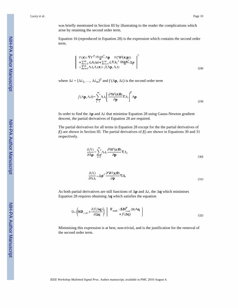
was briefly mentioned in Section III by illustrating to the reader the complications whicharise by retaining the second order term.

Equation 16 (reproduced in Equation 28) is the expression which contains the second orderterm.

(28)

where Δλ = [Δλ1, …, Δλm]T and f (Δp, Δλ) is the second order term

(29)

In order to find the Δp and Δλ that minimise Equation 28 using Gauss-Newton gradientdescent, the partial derivatives of Equation 28 are required.

The partial derivatives for all terms in Equation 28 except for the the partial derivatives off() are shown in Section III. The partial derivatives of f() are shown in Equations 30 and 31respectively.

(30)

(31)

As both partial derivatives are still functions of Δp and Δλ, the Δq which minimisesEquation 28 requires obtaining Δq which satisfies the equation

(32)

Minimising this expression is at best, non-trivial, and is the justification for the removal ofthe second order term.

Lucey et al.


NIH


NIH


NIH


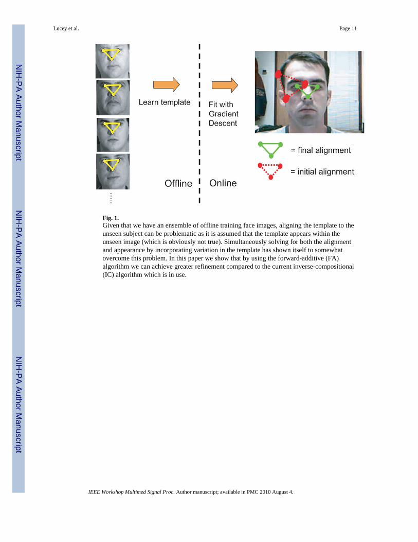
Fig. 1.Given that we have an ensemble of offline training face images, aligning the template to theunseen subject can be problematic as it is assumed that the template appears within theunseen image (which is obviously not true). Simultaneously solving for both the alignmentand appearance by incorporating variation in the template has shown itself to somewhatovercome this problem. In this paper we show that by using the forward-additive (FA)algorithm we can achieve greater refinement compared to the current inverse-compositional(IC) algorithm which is in use.

Lucey et al.


NIH


NIH


NIH


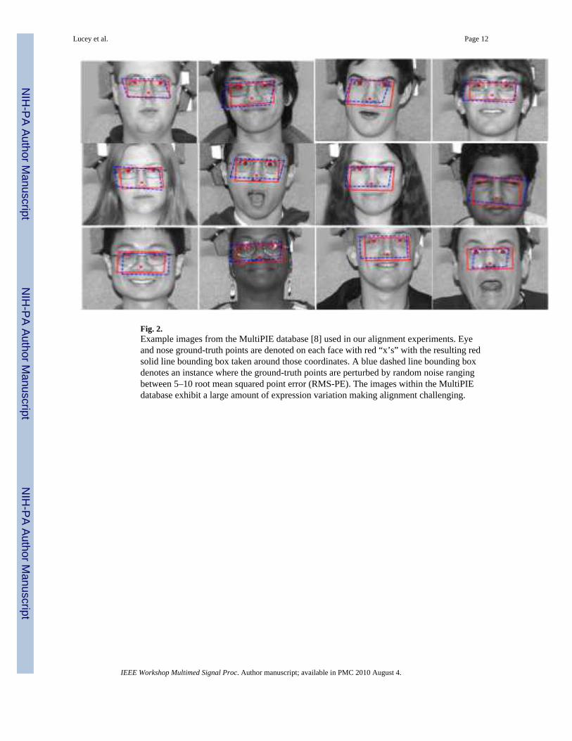
Fig. 2.Example images from the MultiPIE database [8] used in our alignment experiments. Eyeand nose ground-truth points are denoted on each face with red “x’s” with the resulting redsolid line bounding box taken around those coordinates. A blue dashed line bounding boxdenotes an instance where the ground-truth points are perturbed by random noise rangingbetween 5–10 root mean squared point error (RMS-PE). The images within the MultiPIEdatabase exhibit a large amount of expression variation making alignment challenging.

Lucey et al.


NIH


NIH


NIH


Fig. 3.Alignment results showing the difference between the FA and IC algorithms without (a) andwith (b) appearance variation included in the template with a RMS-PE of 5.

Lucey et al.


NIH


NIH


NIH


Fig. 4.Alignment results showing the difference between the FA and IC algorithms without (a) andwith (b) appearance variation included in the template with a RMS-PE of 7.5.

Lucey et al.


NIH


NIH


NIH


Fig. 5.Alignment results showing the difference between the FA and IC algorithms without (a) andwith (b) appearance variation included in the template with a RMS-PE of 10.

Lucey et al.


NIH


NIH


NIH


comparing object alignment algorithms with appearance variation: forward-additive vs...

Documents