communication complexity of correlated equilibrium with
TRANSCRIPT

Communication Complexity of CorrelatedEquilibrium with Small SupportAnat Ganor1
Tel Aviv University, Tel Aviv, [email protected]
Karthik C. S.2
Weizmann Institute of Science, Rehovot, [email protected]
AbstractWe define a two-player N × N game called the 2-cycle game, that has a unique pure Nashequilibrium which is also the only correlated equilibrium of the game. In this game, every 1/poly(N)-approximate correlated equilibrium is concentrated on the pure Nash equilibrium. We showthat the randomized communication complexity of finding any 1/poly(N)-approximate correlatedequilibrium of the game is Ω(N). For small approximation values, our lower bound answers anopen question of Babichenko and Rubinstein (STOC 2017).
2012 ACM Subject Classification Theory of computation → Communication complexity, The-ory of computation → Exact and approximate computation of equilibria
Keywords and phrases Correlated equilibrium, Nash equilibrium, Communication complexity
Digital Object Identifier 10.4230/LIPIcs.APPROX-RANDOM.2018.12
Acknowledgements We thank Yakov Babichenko, Moni Naor, Noam Nisan, Aviad Rubinstein,Amir Shpilka and Eylon Yogev for very helpful conversations and the anonymous reviewers fortheir valuable feedback on earlier versions of this manuscript.
1 Introduction
If there is intelligent life on other planets, in a majority of them, theywould have discovered correlated equilibrium before Nash equilibrium.
Roger Myerson
One of the most famous solution concepts in game theory is Nash equilibrium [28].Roughly speaking, a Nash equilibrium is a set of mixed strategies, one per player, fromwhich no player has an incentive to deviate. A well-studied computational problem inalgorithmic game theory is that of finding a Nash equilibrium of a (non-cooperative) game.Since finding a Nash equilibrium is considered hard (in particular, it is a PPAD-completeproblem), researchers studied the problem of finding an approximate Nash equilibrium,where intuitively, no player can benefit much by deviating from his mixed strategy. Thecomplexity of finding an approximate Nash equilibrium has been studied in several modelsof computation, including computational complexity, query complexity and communication
1 The research leading to these results has received funding from the Israel Science Foundation (grantnumber 552/16) and the I-CORE Program of the planning and budgeting committee and The IsraelScience Foundation (grant number 4/11).
2 This work was supported by Irit Dinur’s ERC-CoG grant 772839 and ISF-UGC grant 1399/14.
© Anat Ganor and Karthik C. S.;licensed under Creative Commons License CC-BY
Approximation, Randomization, and Combinatorial Optimization. Algorithms and Techniques(APPROX/RANDOM 2018).Editors: Eric Blais, Klaus Jansen, José D. P. Rolim, and David Steurer; Article No. 12; pp. 12:1–12:16
Leibniz International Proceedings in InformaticsSchloss Dagstuhl – Leibniz-Zentrum für Informatik, Dagstuhl Publishing, Germany

12:2 Communication Complexity of Correlated Equilibrium with Small Support
complexity. For surveys on algorithmic game theory in general and equilibria in particularsee for example [29, 32, 13, 34].
When the players reach an equilibrium they learn to predict correctly the actions of theother players. To better understand how players might learn the actions and payoffs of otherplayers, there is an extensive study of learning dynamics and their convergence to equilibria,see for example [22, 37, 19]. One natural class of dynamics in which approximate equilibriaconcepts are studied is that of uncoupled dynamics [17, 18], where each player knows his ownutilities and not those of the other players. The rate of convergence of uncoupled dynamicsto an approximate equilibrium is closely related to the communication complexity of findingthe approximate equilibrium [8].
Communication complexity is a central model in complexity theory that has been extens-ively studied. In the two-player randomized model of Yao [36], each player gets an input andtheir goal is to solve a communication task that depends on both inputs. The players can useboth common and private random coins and are allowed to err with some small probability.The communication complexity of a protocol is the total number of bits communicated bythe two players. The communication complexity of a communication task is the minimumnumber of bits that the players need to communicate in order to solve the task with highprobability, where the minimum is taken over all protocols. For surveys on communicationcomplexity see for example [25, 26, 33].
An important generalization of Nash equilibrium is correlated equilibrium [1, 2]. Whereasin a Nash equilibrium the players choose their strategies independently, in a correlatedequilibrium the players can coordinate their decisions, choosing a joint strategy. There aretwo notions of correlated equilibrium which we call correlated equilibrium (CE) and rulecorrelated equilibrium (RCE)3. In a CE no player can benefit from replacing one action withanother, whereas in a RCE no player can benefit from simultaneously replacing every actionwith another action (using a switching rule). While the above two notions are equivalent,approximate CE and approximate RCE are not equivalent, but are closely related.
The communication task of finding an approximate (rule) correlated equilibrium is asfollows. The actions sets and the approximation value are known to both players. Eachplayer gets a utility function that specify her payoffs for every pair of actions (given as atruth table). At the end of the communication both players should know the same correlatedmixed strategy which is an approximate (rule) correlated equilibrium.
In the multi-party setting, [16, 30, 21] showed protocols for finding an exact CE of N -playerbinary action games with poly(N) bits of communication (note that the input size per playeris 2N ). In the two-player setting, every N ×N game has a trivial 1/N-approximate CE (theuniform distribution over all pairs of actions, which can be found with zero communication).However, there is no trivial approximate RCE, even for constant approximation values.Babichenko and Rubinstein [6] raised the following questions:
Does a polylog(N) communication protocol for finding an approximate RCE oftwo-player N ×N games exist? Is there a poly(N) communication complexitylower bound?
1.1 Our Main ResultWe show a communication complexity lower bound for finding a 1/poly(N)-approximate CE ofa two-player N ×N game that we call the 2-cycle game. Since every approximate RCE is anapproximate CE, the same lower bound holds for RCE.
3 In most literature, both notions of correlated equilibrium are referred to by the same name. In thispaper, we choose to distinguish between them.

A. Ganor and Karthik C. S. 12:3
I Theorem 1. Let n ≥ 3 be an odd integer, let N = 2n and ε ≤ 14N3 . Then, every randomized
communication protocol for finding an ε-approximate correlated equilibrium of the 2-cycleN ×N game, with error probability at most 1
3 , has communication complexity at least Ω(N).
As far as we know, there were no communication complexity lower bounds for (exact)CE or RCE of two-player games prior to this work. Note that Theorem 1 implies a lowerbound of Ω(N) on the number of queries to the utility functions, for any randomized queryalgorithm that finds a 1/poly(N)-approximate CE (or RCE) of the 2-cycle N ×N game, withprobability at least 2/3.
After the first version of this paper was published online two similar results were proved.Babichenko [4] showed that any 1/poly(N)-approximate RCE in the generalized matching-pennies game reveals the entire input of one of the players, thus proved the same lowerbound as in Theorem 1. Ko and Schvartzman [24] independently showed that for anyΩ(1/N) < ε < 1/10, the communication complexity of finding an ε-approximate RCE isΩ(ε−1/2 logN). In our opinion, the main difference between our lower bound and the aboveresults is that their games have no approximate RCE with succinct representation, while ourgame has a unique pure Nash equilibrium (which is also a RCE with one pair of actions in itssupport). We will elaborate on the importance of proving lower bounds for equilibria withsuccinct representations later in this section.
It remains a very interesting open problem to determine the communication complexity offinding a constant-approximate RCE of two-player games. Currently, there is an exponentialgap between the best known lower and upper bounds on the communication complexity offinding a constant-approximate RCE of two-player N ×N games, where the best known lowerbound is logarithmic in N [24].
In a recent breakthrough, Babichenko and Rubinstein [6] proved the first non-triviallower bound on the randomized communication complexity of finding an approximate Nashequilibrium. More precisely, they proved a lower bound of Ω (Nε0) on the randomizedcommunication complexity of finding an ε-approximate Nash equilibrium of a two-player N ×N game, for every ε ≤ ε0, where ε0 is some small constant. Theorem 1 implies a randomizedcommunication complexity lower bound of Ω(N) for finding a 1/poly(N)-approximate Nashequilibrium of the 2-cycle game4. This is a slightly stronger lower bound but for muchsmaller approximation values. Our proof is more simple and straightforward, as it does notgo through several intermediate problems.
The 2-cycle game is a very simple game, in the sense that it is a win-lose, sparse game,in which each player has a unique best response to every action. For the class of win-lose,sparse games, our lower bound is tight up to logarithmic factors, as a player can send hisentire utility matrix using O(N logN) bits of communication. However, our lower bounddoes not hold for much larger approximation values, since there are examples of approximateequilibria of the 2-cycle game for larger approximation values, that can be found with smallamount of communication (see Appendix A for details).
Correlated Equilibrium with Succinct RepresentationIn the communication model, for a problem to be meaningful, we would like the output sizeto be much smaller than the number of bits needed to solve it. Specifically, for the problemof finding an approximate RCE (or CE) in N ×N games, we would like the output to have a
4 We are able to improve the approximation parameter from 1/4N3 in Theorem 1 above to 1/16N2 in thecase of approximate Nash equilibrium.
APPROX/RANDOM 2018

12:4 Communication Complexity of Correlated Equilibrium with Small Support
succinct representation of size polylog(N) bits. A natural notion of succinct representationis the support size of an equilibrium, thus we could define the communication problemassociated with finding a RCE to be finding an approximate RCE of polylog(N) support size.
For 1/poly(N) approximation values, there are two-player N ×N games for which everyapproximate RCE is of poly(N) support size. In contrast, Babichenko, Barman and Peretz[5] showed that every two-player game has a constant-approximate RCE of support sizeO (logN). Therefore, finding an approximate RCE of polylog(N) support size is a totalsearch problem (i.e., a solution always exists) for constant approximation values5, but is nottotal for 1/poly(N) approximation values.
As a step before understanding the total problem of finding a constant-approximate RCE,we consider promise problems, where we are guaranteed to have a RCE with a small support.Our lower bound for finding an approximate RCE implies that even for games in which weare promised to have a RCE with a small support, finding an approximate RCE remains hard.
1.2 Sampling from a Correlated EquilibriumWe introduce another natural communication task in the context of joint strategies, which isthe task of sampling from a CE. Intuitively, in the task of sampling from a CE (or RCE)6,the players are required to output each pair of actions with probability that is close tothe probability of this pair of actions under some CE. More formally, at the end of thecommunication, each player outputs a single action, such that the distribution of the protocolon pairs of actions is close (say, ∆-close in `1 distance, for some small ∆) to some jointdistribution which is a CE of the game. The above problem was suggested by Moni Naor [27].
The problem of finding a CE in the communication model requires that both playersknow at the end of the communication the entire joint strategy, which might be large.We believe that the easier task of sampling from a CE is interesting in real-life scenarios,since by sampling from an equilibrium of the game the players can act according to thatequilibrium. Sampling communication tasks were studied in many different variants indifferent contexts, such as compression of randomized protocols, simulation of randomizedprotocols, agreement distillation, sketching algorithms, approximation algorithms based onrounding linear programming relaxations, the study of parallel repetition and cryptography.
When a game has a CE with a small support size, by sampling from this equilibrium theplayers can recover (learn) the equilibrium with high probability. However, it might be thecase that the game has an approximate RCE with a large support from which sampling iseasy, while finding (even approximately) the entire joint strategy is hard. In particular, apoly-logarithmic number of samples might not be enough to recover the equilibrium. Forexample, if one of the players knows a CE of the game, she can sample a pair of actionsaccording to the equilibrium and send the other player his action. However, if the equilibriumshe knows has no succinct representation, communicating it might be hard.
The 2-cycle game has a unique exact CE which is the pure Nash equilibrium of thegame, and every 1/poly(N)-approximate CE of the game is concentrated on the pure Nashequilibrium. Thus, by sampling a pair of actions from a 1/poly(N)-approximate CE, the playerscan recover the pure Nash equilibrium with high probability. That is, not only finding a1/poly(N)-approximate CE of the game is hard, but sampling from such an equilibrium is alsohard. Since every approximate RCE is an approximate CE, the following lower bound holdsalso for RCE.
5 In fact, [5] showed that the problem is total for 1/polylog(N) approximation values.6 This problem can be naturally extended to sampling from an approximate correlated equilibrium.
A. Ganor and Karthik C. S. 12:5
I Theorem 2. Let n ≥ 3 be an odd integer, let N = 2n, ∆ ∈ [0, 2/3) and ε ≤ 1/4N3(2/3−∆).Let µ be an ε-approximate correlated equilibrium of the 2-cycle N ×N game. Then, everyrandomized communication protocol for sampling from a distribution that is ∆-close in `1distance to µ, with error probability at most 1
3 , has communication complexity at least Ω(N).
It remains a very interesting open problem to determine the communication complexityof sampling from a constant-approximate RCE of two-player games.
1.3 Proof OverviewIn the 2-cycle N × N game, the utility functions are constructed from two subsets of [n]where n = N/2. The two subsets have exactly one element in common. Each player is givenone of these subsets and computes a directed graph. The two graphs have a common vertexset of size N . The actions of each player are the N vertices. In each graph, every vertexhas a unique out-neighbor. Intuitively, each player wants to play the unique out-neighbor(according to his graph) of the vertex played by the other player.
The construction of the utility functions of the 2-cycle game was inspired by ideas of[35] of constructing utility functions from inputs to the fixed-point problem, that is, fromcontinuous functions on a compact convex space. We construct the utility functions in thesame way, but from discrete functions, i.e., the unique out-neighbor functions in directedgraphs.
To understand how the equilibria of the game look like, we examine the union of the twographs. An element in the intersection of the subsets creates a directed 2-cycle in the unionof the two graphs, with one edge from each graph. Given the two vertices of this 2-cycle,one can recover the index of the element in the intersection of the subsets. The game hasa unique (exact) equilibrium which is the two vertices of the 2-cycle (that is, a pure Nashequilibrium). Since it is hard to find the element in the intersection of the subsets, findingan equilibrium of the game is also hard.
The heart of the proof is to show that every 1/poly(N)-approximate equilibrium is concen-trated on the pure Nash equilibrium. For ease of presentation, we focus on the special caseof approximate Nash equilibria. Let (a∗, b∗) be a 1/poly(N)-approximate Nash equilibrium ofthe game. We say that a function f : [N ]→ [0, 1] is concentrated on i ∈ [N ] if f(i) > f(j)for every j ∈ [N ] \ i. We show that a∗, b∗ are concentrated on u∗ and v∗ respectively,where (u∗, v∗) is the pure Nash equilibrium of the game. Hence given (a∗, b∗), the playerscan recover the pure Nash equilibrium of the game with no communication. Intuitively, forany vertex v, a∗(v) cannot be large unless one of its neighbors (in the graph of player A) haslarge probability according to b∗. Similarly, b∗(v) cannot be large unless one of v’s neighbors(in the graph of player B) has large probability according to a∗. We use this property tobound a∗ and b∗ on all the vertices other than u∗ and v∗ respectively, one by one, movingalong alternating edges from the two graphs.
It is interesting to see what happens when the construction of the game is used on twosubsets that do not intersect. In this case, the union of the graphs has no 2-cycle and the gamehas no pure Nash equilibrium. The game has a unique exact Nash equilibrium (a∗, b∗), wherea∗ is uniform on half of the vertices that correspond to one subset and b∗ is uniform on halfof the vertices that correspond to the other subset. We note that this is not an equilibriumof the game when the subsets do intersect. For the actual 2-cycle game, constructed fromintersecting subsets, we show that every 1/poly(N)-approximate equilibrium reveals the pureNash equilibrium of the game. Thus changing a single bit in the representation of the subsetsaffects every 1/poly(N)-approximate equilibrium of the game. On a more technical note, we
APPROX/RANDOM 2018

12:6 Communication Complexity of Correlated Equilibrium with Small Support
bound a∗ and b∗ on all vertices other than the ones in the 2-cycle, one by one, starting with avertex v such that all incoming edges to v are from vertices with small probability accordingto b∗. Such a vertex does not exist if there is no element in the intersection of the subsets.
1.4 Related WorksWe overview previous works related to the computation of correlated equilibria of two-playerN ×N games.
Computational complexity
An exact correlated equilibrium can be computed for two-player games in polynomial timeby a linear program [20]. Additionally, the decision version of finding correlated equilibriawith particular properties have also been considered in literature (for examples see [12, 7]).
Query complexity
Fearnley et al. [10] showed a deterministic query algorithm that finds a 1/2-approximate Nashequilibrium by making O(N) queries and Fearnley and Savani [11] showed a randomizedquery algorithm that finds a 0.382-approximate Nash equilibrium by making O(N logN)queries. For coarse correlated equilibrium, Goldberg and Roth [15] provided a randomizedquery algorithm that finds a constant approximate coarse correlated equilibrium by makingO(N logN) queries.
Communication complexity
Goldberg and Pastink [14] showed a communication protocol that finds a 0.438-approximateNash equilibrium by exchanging polylog(N) bits of communication, and Czumaj et al. [9]showed a communication protocol that finds a 0.382-approximate Nash equilibrium withsimilar communication.
2 Preliminaries
2.1 General NotationFor n ∈ N, we denote by [n] the set 0, 1, . . . , n− 1. For two bit strings x, y ∈ 0, 1∗, letxy be the concatenation of x and y. For a bit string x ∈ 0, 1n and an index i ∈ [n], xi isthe ith + 1 bit in x and x is the negated bit string, that is xi is the negation of xi. For afunction µ : Ω→ [0, 1], where Ω is some finite set, and a subset S ⊆ Ω, let
µ(S) =∑z∈S
µ(z).
Define µ(∅) = 0 and maxz∈∅ µ(z) = 0. For u ∈ Ω we say that µ is concentrated on u if
µ(u) > µ(v) ∀ v ∈ Ω \ u.
For a function µ : U × V → [0, 1], where U ,V are some finite sets, a subset S ⊆ U and v ∈ V ,let
µ(S, v) =∑u∈S
µ(u, v).
Similarly, for a subset S ⊆ V and u ∈ U let µ(u, S) =∑v∈S µ(u, v). Define µ(∅, v) =
µ(u, ∅) = 0.
A. Ganor and Karthik C. S. 12:7
2.2 Approximate Correlated EquilibriumA win-lose, finite game for two players A and B is given by two utility functions uA : U ×V →0, 1 and uB : U × V → 0, 1, where U and V are finite sets of actions. We say that thegame is an N × N game, where N = max|U|, |V|. A mixed strategy for player A is adistribution over U and a mixed strategy for player B is a distribution over V. A mixedstrategy is called pure if it has only one action in its support. A correlated mixed strategy isa distribution over U × V. A switching rule for player A is a mapping from U to U and aswitching rule for player B is a mapping from V to V.
I Definition 3 (Approximate Correlated Equilibrium). Let ε ∈ [0, 1). An ε-approximatecorrelated equilibrium of a two-player game is a correlated mixed strategy µ such that thefollowing two conditions hold:1. For all actions u, u′ ∈ U ,∑
v∈Vµ(u, v) · (uA(u′, v)− uA(u, v)) ≤ ε.
2. For all actions v, v′ ∈ V,∑u∈U
µ(u, v) · (uB(u, v′)− uB(u, v)) ≤ ε.
I Definition 4 (Approximate Rule Correlated Equilibrium). Let ε ∈ [0, 1). An ε-approximaterule correlated equilibrium of a two-player game is a correlated mixed strategy µ such thatthe following two conditions hold:1. For every switching rule f for player A,
E(u,v)∼µ [uA(f(u), v)− uA(u, v)] ≤ ε.
2. For every switching rule f for player B,
E(u,v)∼µ [uB(u, f(v))− uB(u, v)] ≤ ε.
When the approximation value is zero the two notions above coincide. In general, everyapproximate rule correlated equilibrium is an approximate correlated equilibrium.
I Proposition 5. Fix an N action two-player game and let ε ∈ [0, 1). Then, every ε-approximate rule correlated equilibrium of the game is an ε-approximate correlated equilibriumof the game. In the other direction, every ε-approximate correlated equilibrium of the gameis an (ε ·N)-approximate rule correlated equilibrium of the game.
The communication task of finding an ε-approximate (rule) correlated equilibrium isas follows. Consider a win-lose, finite game for two players A and B, given by two utilityfunctions uA : U × V → 0, 1 and uB : U × V → 0, 1.Inputs: The actions sets U ,V and the approximation value ε are known to both players.Player A gets the utility function uA and player B gets the utility function uB . The utilityfunctions are given as truth tables of size |U| × |V| each.At the end of the communication: Both players know the same correlated mixedstrategy µ over U × V, such that µ is an ε-approximate (rule) correlated equilibrium.I Remark. Note that the communication complexity of a communication protocol for findingan ε-approximate (rule) correlated equilibrium is the total number of bits exchanged betweenthe two players, which might be smaller than the number of bits required to describe thecorrelated mixed strategy µ to an observer with no prior information.
APPROX/RANDOM 2018
12:8 Communication Complexity of Correlated Equilibrium with Small Support
(0,1)
(0,0)
(1,1)
(1,0)
(2,1)
(2,0)
(3,1)
(3,0)
(4,1)
(4,0)
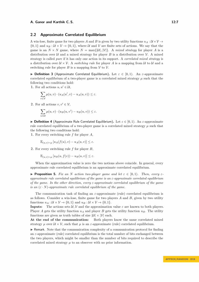
Figure 1 The graph GA built from the 5 bit string 11001. The thick edges are the edges goingback (of the form ((i, 0), (i− 1, xi−1))).
3 The 2-Cycle Game
Let n ≥ 3 be an odd integer. The 2-cycle game is a win-lose, N ×N game, where N = 2n. Itis constructed from two n-bit strings x, y ∈ 0, 1n for which there exists exactly one indexi ∈ [n], such that xi > yi. Throughout the paper, all operations (adding and subtracting)are done modulo n.
The graphs
Given a string x ∈ 0, 1n, player A computes the graph GA on the set of vertices V =[n]× 0, 1 with the following set of directed edges (an edge (u, v) is directed from u into v):
EA =
((i, 1), (i+ 1, xi+1)) : i ∈ [n]
∪
((i, 0), (i+ 1, xi+1)) : i ∈ [n], xi = 0
∪
((i, 0), (i− 1, xi−1)) : i ∈ [n], xi = 1.
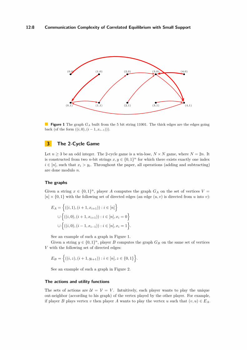
See an example of such a graph in Figure 1.Given a string y ∈ 0, 1n, player B computes the graph GB on the same set of vertices
V with the following set of directed edges:
EB =
((i, z), (i+ 1, yi+1)) : i ∈ [n], z ∈ 0, 1.
See an example of such a graph in Figure 2.
The actions and utility functions
The sets of actions are U = V = V . Intuitively, each player wants to play the uniqueout-neighbor (according to his graph) of the vertex played by the other player. For example,if player B plays vertex v then player A wants to play the vertex u such that (v, u) ∈ EA.
A. Ganor and Karthik C. S. 12:9
(0,1)
(0,0)
(1,1)
(1,0)
(2,1)
(2,0)
(3,1)
(3,0)
(4,1)
(4,0)
Figure 2 The graph GB built from the 5 bit string 10011.
Formally, the utility function uA : V 2 → 0, 1 of player A is defined for every pair of actions(u, v) ∈ V 2 as
uA(u, v) =
1 if (v, u) ∈ EA0 otherwise
.
The utility function uB : V 2 → 0, 1 of player B is defined for every pair of actions(u, v) ∈ V 2 as
uB(u, v) =
1 if (u, v) ∈ EB0 otherwise
.
Notations and basic properties
For two vertices u, v ∈ V , (u, v) is a 2-cycle if (v, u) ∈ EA and (u, v) ∈ EB. For a vertexu ∈ V , define
NA(u) = v ∈ V : (v, u) ∈ EANB(u) = v ∈ V : (v, u) ∈ EB.
That is, NA(u) is the set of incoming neighbors to u in EA, and NB(u) is the set of incomingneighbors to u in EB. Let dA(u) = |NA(u)| and dB(u) = |NB(u)|. For a subset S ⊆ V ,define
NA(S) = ∪v∈SNA(v)NB(S) = ∪v∈SNB(v).
Edges in EA of the form ((i, 0), (i− 1, xi−1)) for i ∈ [n] are called back-edges. Let x, y be thestrings from which the game was constructed. Note that uA determines x, and uB determinesy. For an index i ∈ [n] we say that i is disputed if xi > yi. Otherwise, we say that i isundisputed. Define i∗ to be the unique disputed index. We denote the following key vertices:
u∗ = (i∗ − 1, xi∗−1)v∗ = (i∗, 0) = (i∗, yi∗).
APPROX/RANDOM 2018

12:10 Communication Complexity of Correlated Equilibrium with Small Support
(0,1)
(0,0)
(1,1)
(1,0)
(2,1)
(2,0)
(3,1)
(3,0)
(4,1)
(4,0)
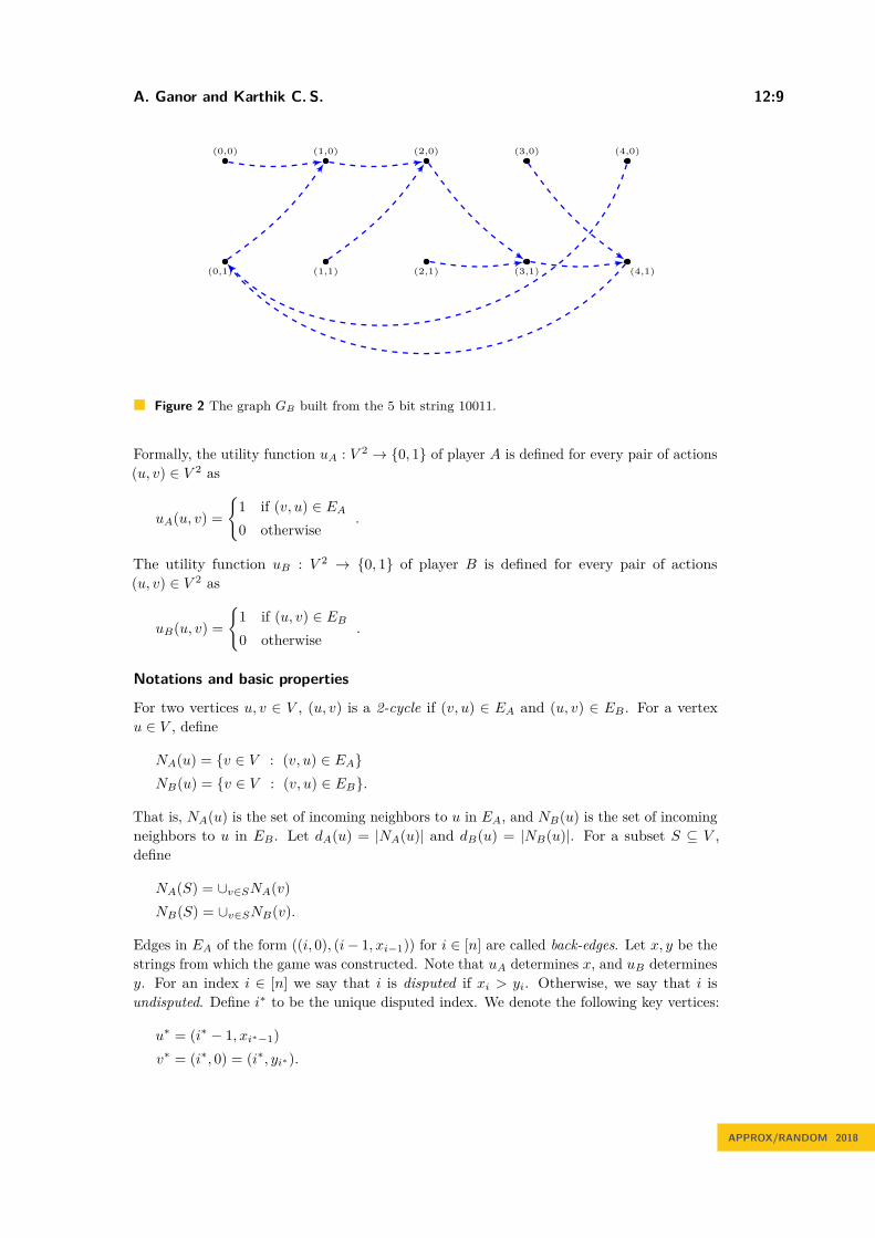
Figure 3 The 2-cycle in the union of the graphs GA from Figure 1 and GB from Figure 2.
To simplify notations, for a function f taking inputs from the set V and a vertex v = (i, z) ∈ V ,we write f(i, z) instead of f((i, z)).
The following are some useful, basic properties of the 2-cycle game.
I Proposition 6 (Out-degree). For every v ∈ V , there exists exactly one u ∈ V suchthat uA(u, v) = 1. Similarly, for every u ∈ V , there exists exactly one v ∈ V such thatuB(u, v) = 1.
I Proposition 7 (Max in-degree). For every v ∈ V , it holds that dA(v) ≤ 3 and dB(v) ≤ 2.
To understand how the equilibria of the game look like, we will examine the union of thegraphs GA and GB . The union of the graphs contains a unique 2-cycle, with one edge fromGA and one from GB . We will see that this 2-cycle corresponds to a pure Nash equilibriumof the game. The 2-cycle in the union of the graphs GA from Figure 1 and GB from Figure 2appears in Figure 3.
I Proposition 8 (A 2-cycle). Let (v, u) ∈ EA be a back-edge. If v 6= v∗ then dB(v) = 0.Otherwise, u = u∗ and (u∗, v∗) is a 2-cycle.
Proof. Let u = (i, zA) ∈ V , for some zA ∈ 0, 1 and assume there exits v = (i+ 1, zB) ∈NA(u), for some zB ∈ 0, 1. By the definition of EA,
zA = xi, xi+1 = 1 and zB = 0.
If v 6= v∗, then yi+1 = 1 and by the definition of EB, dB(v) = 0. Otherwise v = v∗ andxi∗ > yi∗ . Since v = v∗ it holds that u = u∗. Since xi∗ > yi∗ it holds that yi+1 = 0 and bythe definition of EB , (u, v) ∈ EB . J
3.1 Pure Nash EquilibriumBy Claim 9 below, the 2-cycle game has a unique pure Nash equilibrium. Together withProposition 8, the pure Nash equilibrium of the game corresponds to the 2-cycle in the unionof the two graphs.

A. Ganor and Karthik C. S. 12:11
I Claim 9. The 2-cycle game has exactly one pure Nash equilibrium (u∗, v∗).
Proof. By Proposition 8, (u∗, v∗) is a 2-cycle. That is, uA(u∗, v∗) = 1 and uB(u∗, v∗) = 1.Since the maximum payoff for either player for any pair of actions is at most 1, it is easy tosee that (u∗, v∗) is a pure Nash equilibrium of the game.
Let u, v ∈ V such that u 6= u∗ or v 6= v∗. Let a′ be the mixed strategy for player A inwhich she always plays u, and b′ be the mixed strategy for player B in which he alwaysplays v. By Proposition 8, either (v, u) /∈ EA or (u, v) /∈ EB. By proposition 6, there existu′, v′ ∈ V such that (v, u′) ∈ EA and (u, v′) ∈ EB. If (v, u) /∈ EA then let a be the mixedstrategy for player A in which she always plays u′. We get that
Eu′′∼a,v′′∼b′ [uA(u′′, v′′)] = uA(u′, v) = 1 and Eu′′∼a′,v′′∼b′ [uA(u′′, v′′)] = uA(u, v) = 0.
Otherwise (u, v) /∈ EB, then let b be the mixed strategy for player B in which he alwaysplays v′. We get that
Eu′′∼a′,v′′∼b[uB(u′′, v′′)] = uB(u, v′) = 1 and Eu′′∼a′,v′′∼b′ [uB(u′′, v′′)] = uB(u, v) = 0.
Therefore, (u, v) is not a pure Nash equilibrium. J
The following theorem states that finding the pure Nash equilibrium (equivalently, the2-cycle) of the 2-cycle game is hard. The proof is by a reduction from the following searchvariant of unique set disjointness: Player A gets a bit string x ∈ 0, 1n and player B gets abit string y ∈ 0, 1n. They are promised that there exists exactly one index i∗ ∈ [n] suchthat xi∗ > yi∗ . Their goal is to find the index i∗. It is well known that the randomizedcommunication complexity of solving this problem with constant error probability is Ω(n)[3, 23, 31]. This problem is called the universal monotone relation. For more details on theuniversal monotone relation and its connection to unique set disjointness see [25]. Note thata lower bound for finding a pure Nash equilibrium of a different game is already known dueto [8].
I Theorem 10. Every randomized communication protocol for finding the pure Nash equi-librium of the 2-cycle N × N game, with error probability at most 1
3 , has communicationcomplexity at least Ω(N).
Proof. Let x, y ∈ 0, 1n be the inputs to the search variant of unique set disjointnessdescribed above. Consider the 2-cycle N ×N game which is constructed from these inputs,given by the utility functions uA, uB. Assume towards a contradiction that there exists acommunication protocol π for finding the pure Nash equilibrium of the 2-cycle game witherror probability at most 1/3 and communication complexity o(N). The players run π onuA, uB and with probability at least 2/3, at the end of the communication, player A knows uand player B knows v, such that (u, v) is the pure Nash equilibrium of the game. By Claim 9,u = u∗ and v = v∗. Given u∗, v∗ to the players A and B respectively, both players know theindex i∗, which is a contradiction. J
4 From Approximate Equilibrium to the Pure Nash
In this section we prove Theorem 1. Let n ≥ 3 be an odd integer, let N = 2n and ε ≤ 1/4N3.Let µ be an ε-approximate correlated equilibrium of the 2-cycle N ×N game, and let x, y bethe strings from which the game was constructed. Recall that the pure Nash equilibriumof the game is denoted (u∗, v∗), where u∗ = (i∗ − 1, xi∗−1) and v∗ = (i∗, 0) = (i∗, yi∗)
APPROX/RANDOM 2018

12:12 Communication Complexity of Correlated Equilibrium with Small Support
(see Claim 9). The following theorem implies that µ is concentrated on (u∗, v∗), that isµ(u∗, v∗) > µ(u, v) for every u, v ∈ V such that u 6= u∗ or v 6= v∗. Therefore given µ, theplayers know the pure Nash equilibrium with no communication, and Theorem 1 followsfrom Theorem 10.
I Theorem 11. µ(u, v) ≤ (3N + 1)ε < 1/N2 for every u, v ∈ V such that u 6= u∗ or v 6= v∗.
Next we prove Theorem 11. Let u, v ∈ V and denote a(u) = µ(u,NA(u)), b(v) =µ(NB(v), v). By Proposition 6, there exists v′ ∈ V such that u ∈ NB(v′), therefore
µ(u, v) ≤ µ(NB(v′), v) ≤ b(v) + ε, (1)
where the second step follows from the definition of approximate correlated equilibrium (seeDefinition 3). Similarly it holds that µ(u, v) ≤ a(u) + ε. For every i ∈ [n], it holds thatNA(i, xi) = ∅ and NB(i, yi) = ∅, therefore a(i, xi) = b(i, yi) = 0. We will bound a(i, xi) forevery i ∈ [n] \ i∗ − 1 and b(i, yi) for every i ∈ [n] \ i∗.
I Claim 12. For every i ∈ [n] \ i∗ − 1, if (i, yi−1) ∈ NA(i, xi) then
a(i, xi) ≤ b(i− 1, yi−1) + 3ε,
otherwise, a(i, xi) ≤ 3ε. For every i ∈ [n] \ i∗,
b(i, yi) ≤ a(i− 1, xi−1) + 2ε.
Proof. Let i ∈ [n] \ i∗ − 1. By Equation (1), for every v ∈ V it holds that µ((i, xi), v) ≤b(v) + ε. Summing for every v ∈ NA(i, xi) we get that a(i, xi) ≤ b(NA(i, xi)) + 3ε, where webounded the right-hand side using a bound on the maximum in-degree, see Proposition 7.If there exists a back-edge (v, (i, xi)) ∈ EA than by Proposition 8, dB(v) = 0 (that isNB(v) = ∅), and b(v) = 0. Therefore back-edges do not contribute to the bound on a(i, xi).It remains to consider edges from (i− 1, yi−1) and (i− 1, yi−1). If (i, yi−1) ∈ NA(i, xi) then
a(i, xi) ≤ b(i− 1, yi−1) + b(i− 1, yi−1) + 3ε = b(i− 1, yi−1) + 3ε,
otherwise, a(i, xi) ≤ b(i− 1, yi−1) + 3ε = 3ε. Similarly for every i ∈ [n] \ i∗,
b(i, yi) ≤ a(NB(i, yi)) + 2ε= a(i− 1, xi−1) + a(i− 1, xi−1) + 2ε= a(i− 1, xi−1) + 2ε. J
Using Claim 12 we can bound a(i, xi) for every i ∈ [n] \ i∗ − 1 and b(i, yi) for everyi ∈ [n] \ i∗ as follows. Let δ = 3ε. We start with (i∗ + 1, xi∗+1). Since xi∗ = 1 and yi∗ = 0,it holds that (i∗, yi∗) /∈ NA(i∗ + 1, xi∗+1). Therefore by Claim 12,
a(i∗ + 1, xi∗+1) ≤ δ.
Once we bound a(v) (or b(v)) for some vertex v, we can apply Claim 12 again to bound thevalue of b (respectively a) on a neighbor of v. We get that
b(i∗ + 2, yi∗+2) ≤ a(i∗ + 1, xi∗+1) + δ ≤ 2δ,
then
a(i∗ + 3, xi∗+3) ≤ b(i∗ + 2, yi∗+2) + δ ≤ 3δ
A. Ganor and Karthik C. S. 12:13
and so on. After we apply Claim 12 n times, since n is odd, we get that a(i∗, xi∗) ≤ nδ. Weapply Claim 12 (n− 2) more times, until get that
b(i∗ − 2, yi∗−2) ≤ nδ + (n− 2)δ ≤ 2nδ.
This concludes the proof as we showed that every a(i, xi) for i ∈ [n] \ i∗ − 1 and everyb(i, yi) for i ∈ [n] \ i∗ is at most 2nδ = 3Nε.
4.1 Sampling from a Correlated EquilibriumTheorem 2 immediately follows from the fact that the correlated equilibria are concentratedon the pure Nash equilibrium: Let n ≥ 3 be an odd integer, let N = 2n, ∆ ∈ [0, 2/3)and ε ≤ 1/4N3(2/3 −∆). Let µ be an ε-approximate correlated equilibrium of the 2-cycleN ×N game, and let x, y be the strings from which the game was constructed. Recall thatthe pure Nash equilibrium of the game is denoted (u∗, v∗), where u∗ = (i∗ − 1, xi∗−1) andv∗ = (i∗, 0) = (i∗, yi∗) (see Claim 9). By Theorem 11 above, µ(u, v) ≤ (3N + 1)ε for everyu, v ∈ V such that u 6= u∗ or v 6= v∗. Thus,
µ(u∗, v∗) ≥ 1− (N2 − 1)(3N + 1)ε > 1− 4N3ε ≥ 13 + ∆.
If the players can sample from a distribution that is ∆-close in `1 distance to µ, using o(N)communication bits, then they can find (u∗, v∗) after O(1) attempts with high probability,using o(N) communication bits, in contradiction to Theorem 10.
References1 Robert Aumann. Subjectivity and correlation in randomized strategies. Journal of Math-
ematical Economics, 1(1):67–96, 1974.2 Robert Aumann. Correlated equilibrium as an expression of bayesian rationality. Econo-
metrica, 55(1):1–18, 1987.3 László Babai, Peter Frankl, and Janos Simon. Complexity classes in communication com-
plexity theory (preliminary version). In FOCS, pages 337–347, 1986.4 Yakov Babichenko. private communication, 2017.5 Yakov Babichenko, Siddharth Barman, and Ron Peretz. Empirical distribution of equi-
librium play and its testing application. Math. Oper. Res., 42(1):15–29, 2017. doi:10.1287/moor.2016.0794.
6 Yakov Babichenko and Aviad Rubinstein. Communication complexity of approximate Nashequilibria. In Proceedings of the 49th Annual ACM SIGACT Symposium on Theory ofComputing, STOC 2017, Montreal, QC, Canada, June 19-23, 2017, pages 878–889, 2017.
7 Siddharth Barman and Katrina Ligett. Finding any nontrivial coarse correlated equi-librium is hard. In Proceedings of the Sixteenth ACM Conference on Economics andComputation, EC ’15, Portland, OR, USA, June 15-19, 2015, pages 815–816, 2015.doi:10.1145/2764468.2764497.
8 Vincent Conitzer and Tuomas Sandholm. Communication complexity as a lower boundfor learning in games. In Machine Learning, Proceedings of the Twenty-first InternationalConference (ICML 2004), Banff, Alberta, Canada, July 4-8, 2004, 2004. doi:10.1145/1015330.1015351.
9 Artur Czumaj, Argyrios Deligkas, Michail Fasoulakis, John Fearnley, Marcin Jurdz-inski, and Rahul Savani. Distributed methods for computing approximate equilib-ria. In Web and Internet Economics - 12th International Conference, WINE 2016,Montreal, Canada, December 11-14, 2016, Proceedings, pages 15–28, 2016. doi:10.1007/978-3-662-54110-4_2.
APPROX/RANDOM 2018

12:14 Communication Complexity of Correlated Equilibrium with Small Support
10 John Fearnley, Martin Gairing, Paul W. Goldberg, and Rahul Savani. Learning equilibriaof games via payoff queries. Journal of Machine Learning Research, 16:1305–1344, 2015.URL: http://dl.acm.org/citation.cfm?id=2886792.
11 John Fearnley and Rahul Savani. Finding approximate Nash equilibria of bimatrix gamesvia payoff queries. ACM Trans. Economics and Comput., 4(4):25:1–25:19, 2016. doi:10.1145/2956579.
12 Itzhak Gilboa and Eitan Zemel. Nash and correlated equilibria: Some complexity consid-erations. Games and Economic Behavior, 1(1):80–93, 1989. doi:10.1016/0899-8256(89)90006-7.
13 Paul Goldberg. Surveys in Combinatorics 2011. London Mathematical Society LectureNote Series, 2011.
14 Paul W. Goldberg and Arnoud Pastink. On the communication complexity of approximateNash equilibria. Games and Economic Behavior, 85:19–31, 2014. doi:10.1016/j.geb.2014.01.009.
15 Paul W. Goldberg and Aaron Roth. Bounds for the query complexity of approximateequilibria. In ACM Conference on Economics and Computation, EC ’14, Stanford , CA,USA, June 8-12, 2014, pages 639–656, 2014. doi:10.1145/2600057.2602845.
16 Sergiu Hart and Yishay Mansour. How long to equilibrium? the communication complexityof uncoupled equilibrium procedures. Games and Economic Behavior, 69(1):107–126, 2010.doi:10.1016/j.geb.2007.12.002.
17 Sergiu Hart and Andreu Mas-Colell. Uncoupled dynamics do not lead to Nash equilibrium.American Economic Review, 93(5):1830–1836, 2003.
18 Sergiu Hart and Andreu Mas-Colell. Stochastic uncoupled dynamics and Nash equilibrium.Games and Economic Behavior, 57(2):286–303, 2006.
19 Sergiu Hart and Andreu Mas-Colell. Simple Adaptive Strategies:From Regret-Matching toUncoupled Dynamics. World Scientific Publishing Co. Pte. Ltd., 2013.
20 Sergiu Hart and David Schmeidler. Existence of correlated equilibria. Math. Oper. Res.,14(1):18–25, 1989. doi:10.1287/moor.14.1.18.
21 Albert Xin Jiang and Kevin Leyton-Brown. Polynomial-time computation of exact cor-related equilibrium in compact games. Games and Economic Behavior, 91:347–359, 2015.doi:10.1016/j.geb.2013.02.002.
22 Ehud Kalai and Ehud Lehrer. Rational learning leads to nash equilibrium. Econometrica,61(5):1019–45, 1993.
23 Bala Kalyanasundaram and Georg Schnitger. The probabilistic communication complexityof set intersection. SIAM J. Discrete Math., 5(4):545–557, 1992.
24 Young Kun Ko and Ariel Schvartzman. Bounds for the communication complexity oftwo-player approximate correlated equilibria. Electronic Colloquium on ComputationalComplexity (ECCC), 24:71, 2017. URL: https://eccc.weizmann.ac.il/report/2017/071.
25 Eyal Kushilevitz and Noam Nisan. Communication Complexity. Cambridge UniversityPress, New York, NY, USA, 1997.
26 Troy Lee and Adi Shraibman. Lower bounds in communication complexity. Foundationsand Trends in Theoretical Computer Science, 3(4):263–398, 2009.
27 Moni Naor. private communication, 2017.28 J.F. Nash. Non-cooperative games. Annals of Mathematics, 54(2):286–295, 1951.29 Noam Nisan, Tim Roughgarden, Eva Tardos, and Vijay V Vazirani. Algorithmic Game
Theory. Cambridge University Press, New York, NY, USA, 2007.30 Christos H. Papadimitriou and Tim Roughgarden. Computing correlated equilibria in
multi-player games. J. ACM, 55(3):14:1–14:29, 2008. doi:10.1145/1379759.1379762.
A. Ganor and Karthik C. S. 12:15
31 Alexander A. Razborov. On the distributional complexity of disjointness. Theor. Comput.Sci., 106(2):385–390, 1992.
32 Tim Roughgarden. Computing equilibria: a computational complexity perspective. Eco-nomic Theory, 42(1):193–236, 2010. doi:10.1007/s00199-009-0448-y.
33 Tim Roughgarden. Communication complexity (for algorithm designers). Foundations andTrends in Theoretical Computer Science, 11(3-4):217–404, 2016. doi:10.1561/0400000076.
34 Tim Roughgarden. Twenty Lectures on Algorithmic Game Theory. Cambridge UniversityPress, 2016.
35 Tim Roughgarden and Omri Weinstein. On the communication complexity of approximatefixed points. In IEEE 57th Annual Symposium on Foundations of Computer Science, FOCS2016, 9-11 October 2016, Hyatt Regency, New Brunswick, New Jersey, USA, pages 229–238,2016. doi:10.1109/FOCS.2016.32.
36 Andrew Chi-Chih Yao. Some complexity questions related to distributive computing (pre-liminary report). In Proceedings of the 11h Annual ACM Symposium on Theory of Com-puting, April 30 - May 2, 1979, Atlanta, Georgia, USA, pages 209–213, 1979.
37 H. Peyton Young. H. peyton young, , strategic learning and its limits (2004) oxford univ.press 165 pages. Games and Economic Behavior, 63(1):417–420, 2004.
A Trivial Approximate Equilibria of The 2-Cycle Game
In this section, we provide trivial approximate correlated equilibrium of the 2-cycle gamefrom which it is not possible to recover the disputed index.
Let us suppose that for all i ∈[n2 + 3
], we have xi = yi = 0.
We define a joint distribution µ as follows
µ((i, zA), (j, zB)) =
16αn2 if zA, zB = 0 and n
4 + 4 ≤ i, j ≤ n2 + 2,
16αn2 if zA, zB = 0, n4 + 2 ≤ j ≤ n
2 + 2 and i = n4 + 3,
16αn2 if zA, zB = 0, n4 + 2 ≤ i ≤ n
2 + 2 and j = n4 + 3,
16αn2 − 64α·(n/4−i+3)
n3 if zA, zB = 0, 2 ≤ i, j ≤ n4 + 2 and i− j = 1,
16αn2 − 64α·(n/4−j+3)
n3 if zA, zB = 0, 2 ≤ i, j ≤ n4 + 2 and j − i = 1,
0 otherwise,
where α is some normalizing constant less than 2 such that∑
(u,v)∈V 2 µ(u, v) = 1.Let ε = 64α/n3. For every action u = (i, zA) of Alice such that zA 6= 0, we have that
µ(u, v) = 0 for all v ∈ V . Similarly for every action v = (j, zB) of Bob such that zB 6= 0,we have that µ(u, v) = 0 for all u ∈ V . Also, for every action u = (i, zA) of Alice such thati ∈ n/2 + 3, . . . , n ∪ 1, we have that µ(u, v) = 0 for all v ∈ V . And, similarly for everyaction v = (j, zB) of Bob such that j ∈ n/2 + 3, . . . , n ∪ 1, we have that µ(u, v) = 0 forall u ∈ V . Since µ is symmetric7, it follows that in order to show that µ is an ε-approximatecorrelated equilibrium we only need to consider a vertex u = (i, 0) when i ∈
[n2 + 2
].
First, we consider when i ≤ n4 + 2. Let u′ ∈ V . We have∑
v∈Vµ(u, v) · (uA(u′, v)− uA(u, v)) = µ(u,NA(u′))− µ(u,NA(u))
= µ(u,NA(u′))− 16αn2 + 64α · (n/4− i+ 3)
n3 .
7 i.e., µ(u, v) = µ(v, u) for all u, v ∈ V .
APPROX/RANDOM 2018

12:16 Communication Complexity of Correlated Equilibrium with Small Support
Now if v = (j, zB) ∈ NA(u′) and |j − i| 6= 1 then, we have µ(u, v) = 0. Thus, we assumej − i = 1, as we suppose u 6= u′. Then, we have
µ(u,NA(u′)) ≤ 16αn2 −
64α · (n/4− i− 1 + 3)n3
= 16αn2 −
64α · (n/4− i+ 3)n3 + 64α
n3 .
This implies,∑v∈V
µ(u, v) · (uA(u′, v)− uA(u, v)) ≤ 64αn3 = ε.
Next, we consider when n4 + 4 ≤ i ≤ n
2 + 2. Let u′ ∈ V . We have∑v∈V
µ(u, v) · (uA(u′, v)− uA(u, v)) = µ(u,NA(u′))− µ(u,NA(u))
= µ(u,NA(u′))− 16αn2 .
Now if v = (j, zB) ∈ NA(u′) and j ≥ n2 + 3 then, we have µ(u, v) = 0. Also if j ≤ n
4 + 2 then,we have µ(u, v) = 0. Thus, we assume j ∈ [n/4 + 3, n/4 + 2] and β = 0. Then, we have
µ(u,NA(u′)) ≤ 16αn2 .
This implies,∑v∈V
µ(u, v) · (uA(u′, v)− uA(u, v)) ≤ 0.
Finally, we consider when i = n4 + 3. Let u′ = (i′, z′A) ∈ V . We have∑
v∈Vµ(u, v) · (uA(u′, v)− uA(u, v)) = µ(u,NA(u′))− 16α
n2 + 64αn3 .
Now if v = (j, zB) ∈ NA(u′) and j ≥ n2 + 3 then, we have µ(u, v) = 0. Also if j ≤ n
4 + 2and |j − i| 6= 1 then, we have µ(u, v) = 0. Since u 6= u′ we have that j ∈ [n/4 + 3, n/4 + 2]and β = 0. Then we have
µ(u,NA(u′)) ≤ 16αn2 .
This implies,∑v∈V
µ(u, v) · (uA(u′, v)− uA(u, v)) ≤ 64αn3 = ε.
Thus, µ is an ε-approximate correlated equilibrium and an (ε · N)-approximate rulecorrelated equilibrium.