combining precursory patterns and probabilistic forecast models using differential probability gains
TRANSCRIPT

Combining precursory patterns and probabilistic forecast models using differential probability gains
P. Shebalin1,2, C. Narteau2, J. D. Zechar3 and M. Holschneider4
1 International Institute of Earthquake Prediction Theory and Mathematical Geophysics, Moscow,
[email protected] Institut de Physique du Globe de Paris,
[email protected] Swiss Seismological Service, ETH Zurich,
[email protected] Institutes of Applied and Industrial Mathematics,

Earthquake prediction – earthquake forecastingalarms – expected rates
Alarm (TIP)
In an area (space, time, or time-space)
A Probability of a large earthquake is increased.
Such a probability usually is not estimated.
Seismicity rate models
In each bin of a time-space-magnitude gridExpected rates of earthquakes are estimated
RELM/CSEP
Technically, alarms may be defined on a time-space-magnitude grid (by 0 and 1 or using more detailed “alarm function”).
Vice versa, rate-based models may be converted to alarms using thresholgs (Kossobokov, 2006)

Examples
Alarms
М8, КН (periods of alarms in a given spatial objects)
Ms, NSE, RTP, EAST, PI (time-space alarms)
Maps of earthquake-prone areas (space alarms)
In principle, any color map Any precursors that are
numerically formalized Time-dependent maps
Rates
All RELM/CSEP models Models of smoothed seismicity
(RI and others) Maps of seismic hazard Time-dependent maps of seismic
hazard
General difference – absence/presence of probabilistic estimates

Evaluation
Alarms
False alarms/failure-to-predict trade-off (error diagram)
n(A) – rate of failures to predict at a given threshold for A
(A) – fraction of time-space of alarms, measured in rates of the reference model (null hypothesis)
Loss functions: Min (max(n(A),(A)) (Molchan) 1-n-Molchan) G=(1-n)/(Aki)
Rates
The goal of the evaluation is to estimate how “close” is the model to the observed seismicity.
Likelihood:L(t)=(-(x,t)+(x,t)log((x,t))-log((x,t)!),
(x,t)-expected rate(x,t)-observed number of events
Likelihood-based estimates suppose independence.Error diagram gives conditional estimates (given a target earthquake has occurred).

Different schools
Alarms
As a rule, Phenomenological approach Lithosphere – a non-linear
dynamic system “Holistic” approach in
methodology (Keilis-Borok, four paradigms)
Pattern recognition methods used to detect precursory phenomena and to combine precursors
Rates
As a rule, “Physical” approach Trend analysis Use of statistical methods
(Bayes theorem, likelihood)
Integration of the two approaches may occur fruitful.The hope is not only in combining alarm-based and rate-based models, but also in forming “a common language”, summing of efforts.

Differential probability gain
А – alarm function x – expected rate x – total rate
(A0)=1/ xx(A0) x(A0) – fraction of the alarm
time (A(x,t)≥A0) in bin x. G(A0)=(1-(A0))/(A0) – Aki's
probability gain g(A0)={(A0+A)-(A0)}/{(A0)-
(A0+A)} – differential probability gain
0.0
0.2
0.4
0.6
0.8
1.0
mis
s ra
te, ν
(A) 0
0.0 0.2 0.4 0.6 0.8 1.0

Conversion of an alarm-based model to a rate-based model
new(x,t)=g(A(x,t)) ref(x),
where ref(x) – reference time-independent model of rates,new(x,t) – resulting model,g(A(x,t)) – differential probability gains of the alarm-based
model relative to the reference model
Property of unbiasedness: new= ref
l

Example: EAST → EAST_Rg(AEAST)
0.0
0.2
0.4
0.6
0.8
1.0
mis
s ra
te, ν
0.0 0.2 0.4 0.6 0.8 1.0
τRI
0
5
10
gRI E a1875 targets of 3.95 ≤M4.45
0.0
0.2
0.4
0.6
0.8
1.0
mis
s ra
te, ν
0.0 0.2 0.4 0.6 0.8 1.0
τRI
0
5
10
gRI E a113 targets of 5.95 ≤M
0
4
8
0.0 0.2 0.4 0.6 0.8 1.0
τRI
gRI
E a1 29 targets of 5.45 ≤M5.95
0
4
8
0.0 0.2 0.4 0.6 0.8 1.0
τRI
gRI
E a1 87 targets of 4.95 ≤M5.45
0
4
8
0.0 0.2 0.4 0.6 0.8 1.0
τRI
gRI
Ea1
280 targets of 4.45 ≤M4.95

EAST → EAST_RInput maps: EAST (January-March 2011) and RI

EAST → EAST_ROutput EAST_R maps (January-March 2011): M>=4 and M>=6
-124° -122° -120° -118° -116° -114°
32°
34°
36°
38°
40°
42°
I
II
III
0
1
2-log(τ)λE (M≥4)a1
EASTR - RI0 -
0.1 -
0.05 -
0.04 -0.03 -0.01 -
0.005 -0.002 -

What are the reasons to combine precursors and seismicity models using differential probability gains?
“Strong” precursors do not exist. Direct combining of precursors easily causes over-fitting in a learning period.
Many precursors are significantly dependent. In combining one should avoid a duplication of the common effect.
A “predictive power” of a precursor is well reflected by the error diagram and thus by differential probability gains.
Independence is not required for an error diagram

Combining precursors with time-dependent rate-based seismicity models
new(x,t)=g(A(x,t)) ref(x,t),
where ref(x,t) – reference time-dependent model of rates,new(x,t) – resulting model,g(A(x,t)) – differential probability gains of the alarm-based model relative to
the reference model
The only difference with the case of time-independent reference model is definition of : =A{x,t)>Ao ref(x,t) / ref(x,t)
Property of unbiasedness is also valid
g(A(x,t)) may be constructed for any formalized precursors, for any color maps
By converting rate-based models to alarm-based ones (Kossobokov, 2006) differential probability gain combining may be applied to rate-based models too.
l
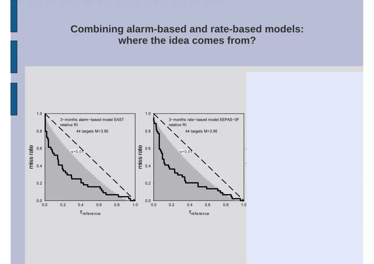
Combining alarm-based and rate-based models: where the idea comes from?
l
0.0
0.2
0.4
0.6
0.8
1.0
mis
s ra
te
0.0 0.2 0.4 0.6 0.8 1.0
τre ference
3−months alarm−based model EASTrelative RI
44 targets M>3.95
α=0.01
0.0
0.2
0.4
0.6
0.8
1.0
mis
s ra
te
0.0 0.2 0.4 0.6 0.8 1.0
τre ference
3−months rate−based model EEPAS−0Frelative RI
44 targets M>3.95
α=0.01
0.0
0.2
0.4
0.6
0.8
1.0
mis
s ra
te
0.0 0.2 0.4 0.6 0.8 1.0
τre ference
3−months alarm−based model EASTrelative 3−months rate−based model EEPAS−0F
44 targets M>3.95
α=0.01

Example: EAST*EEPASResult for testing period 1.7.2009-1.1.2012
Black EAST*EEPAS, blue EEPAS, red EAST

Example: EAST*EEPASComparison with convex combination ½ EAST_R+½ EEPAS
Black EAST*EEPAS, magenta (½ EAST_R+½ EEPAS)

Example: EAST*EEPASComparison with convex combination ½ EAST_R+½ EEPAS
1.7.2009-1.1.2012:Black EAST*EEPAS, magenta (½ EAST_R+½ EEPAS)

Example: EAST*EEPASIs a model spoiled by multiple combining with noisy
precursors?
We add a pure noise 10 times (alarm function A given by random number generator)
0123
g(A)
0.0 0.2 0.4 0.6 0.8 1.0
A
iteration 100123
g(A
) iteration 90123
g(A
) iteration 80123
g(A)
iteration 70123
g(A
) iteration 60123
g(A
) iteration 50123
g(A
) iteration 40123
g(A
) iteration 30123
g(A)
iteration 20123
g(A
) iteration 1
0.0
0.2
0.4
0.6
0.8
1.0
mis
s ra
te, ν
0.0 0.2 0.4 0.6 0.8 1.0
τRI
19 targets of M ≥5

Other examples: maps
Maps of quaternary faults in California(http://geohazards.cr.usgs.gov/cfusion/qfault)
0.0
0.2
0.4
0.6
0.8
1.0
0.0 0.2 0.4 0.6 0.8 1.0
13 targets of M≥6
n