cmsc 471 artificial intelligence search - umbc
TRANSCRIPT

CMSC 471Artificial Intelligence
Search
Frank Ferraro – [email protected]
Some material adopted from notes
by Charles R. Dyer, University of
Wisconsin-Madison
Many slides courtesy Tim Finin
“AI can be summarized in two approaches: search,
and averaging.”
My own undergrad AI
professor

Today’s topics• Goal-based agents
• Representing states and actions
• Example problems
• Generic state-space search algorithm
• Specific algorithms– Breadth-first search– Depth-first search– Uniform cost search– Depth-first iterative deepening
• Example problems revisited
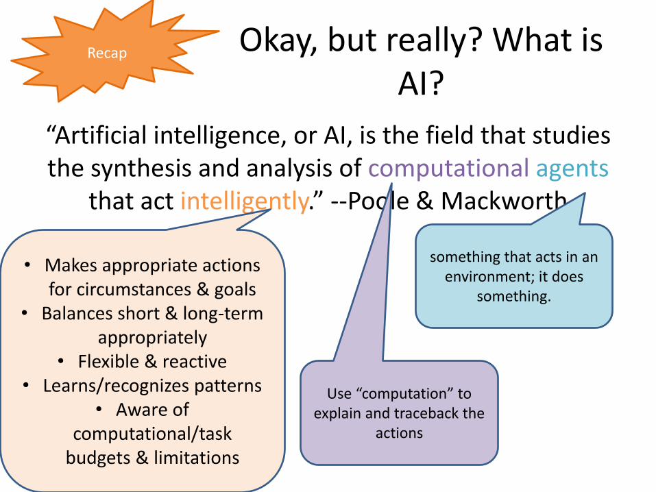
Okay, but really? What is AI?
“Artificial intelligence, or AI, is the field that studies the synthesis and analysis of computational agents
that act intelligently.” --Poole & Mackworth
• Makes appropriate actions for circumstances & goals
• Balances short & long-term appropriately
• Flexible & reactive• Learns/recognizes patterns
• Aware of computational/task
budgets & limitations
something that acts in an environment; it does
something.
Use “computation” to explain and traceback the
actions
Recap
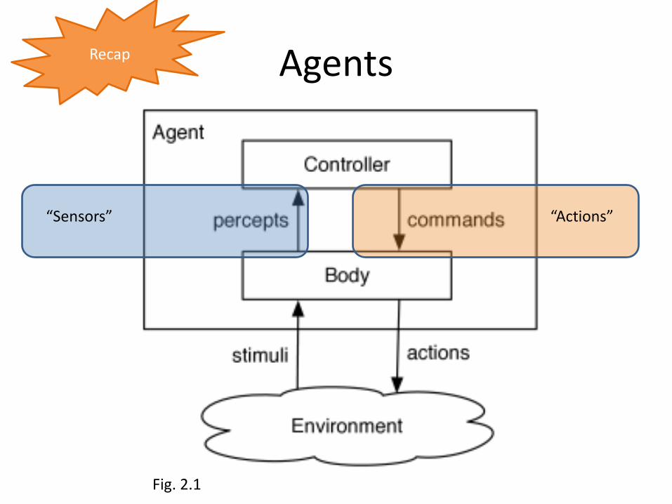
Agents
Fig. 2.1
“Sensors” “Actions”
Recap

(0) Table-driven agents
Use percept sequence/action table to find next
action. Implemented by a lookup table
(1) Simple reflex agents
Based on condition-action rules, stateless devices
with no memory of past world states
(2) Agents with memory
represent states and keep track of past world states
(3) Agents with goals
Have a state and goal information describing desirable
situations; can take future events into consideration
(4) Utility-based agents
base decisions on utility theory in order to act rationally
simple
complex
Courtesy Tim Finin
Recap
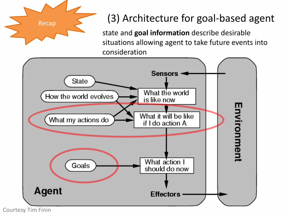
(3) Architecture for goal-based agent state and goal information describe desirable situations allowing agent to take future events into consideration
Courtesy Tim Finin
Recap
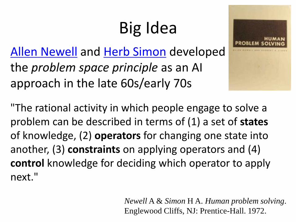
Big IdeaAllen Newell and Herb Simon developedthe problem space principle as an AIapproach in the late 60s/early 70s
"The rational activity in which people engage to solve a problem can be described in terms of (1) a set of statesof knowledge, (2) operators for changing one state into another, (3) constraints on applying operators and (4) control knowledge for deciding which operator to apply next."
Newell A & Simon H A. Human problem solving.
Englewood Cliffs, NJ: Prentice-Hall. 1972.
We’ll achieve this by formulating an appropriate
graph and then applying graph search algorithms to it
Remember: Graphs
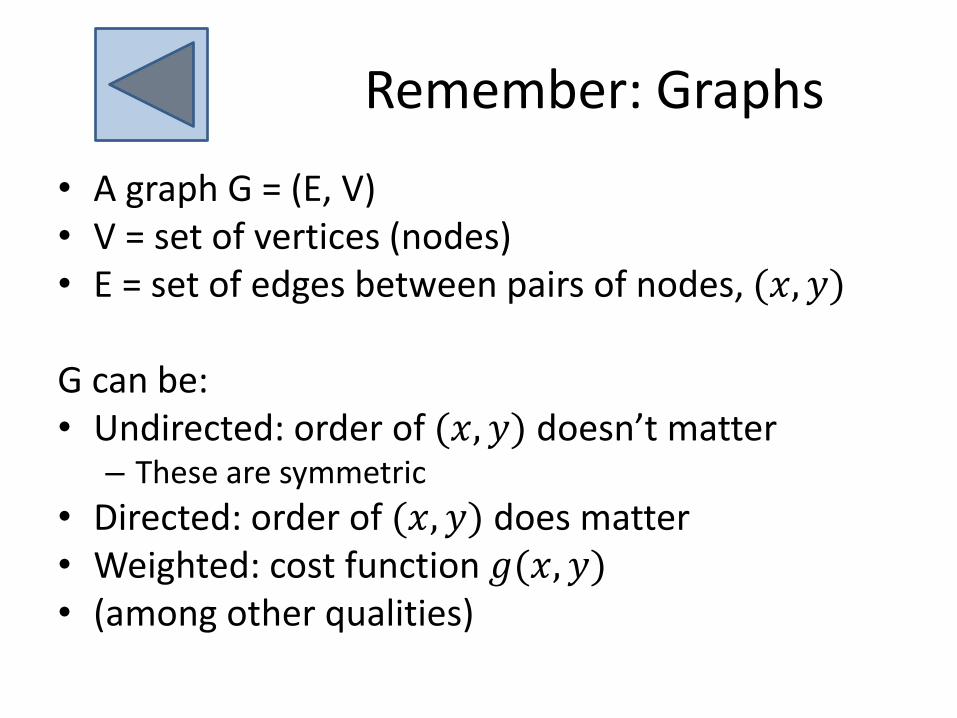
• A graph G = (E, V)• V = set of vertices (nodes)• E = set of edges between pairs of nodes, (𝑥, 𝑦)
G can be:• Undirected: order of (𝑥, 𝑦) doesn’t matter
– These are symmetric
• Directed: order of (𝑥, 𝑦) does matter• Weighted: cost function 𝑔(𝑥, 𝑦)• (among other qualities)

Remember: Graphs
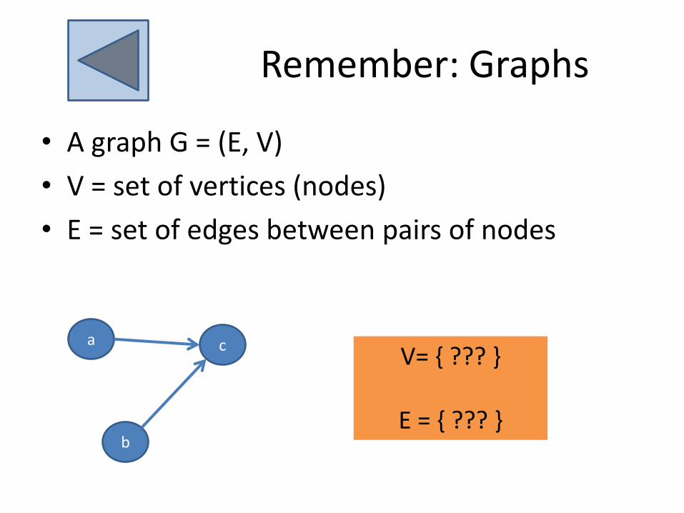
• A graph G = (E, V)
• V = set of vertices (nodes)
• E = set of edges between pairs of nodes
a
b
cV= { ??? }
E = { ??? }

Remember: Graphs
• A graph G = (E, V)
• V = set of vertices (nodes)
• E = set of edges between pairs of nodes
a
b
cV= { a, b, c }
E = { (a, c), (b, c) }
undirected
Remember: Graphs
• A graph G = (E, V)
• V = set of vertices (nodes)
• E = set of edges between pairs of nodes
a
b
cV= { ??? }
E = { ??? }
Remember: Graphs
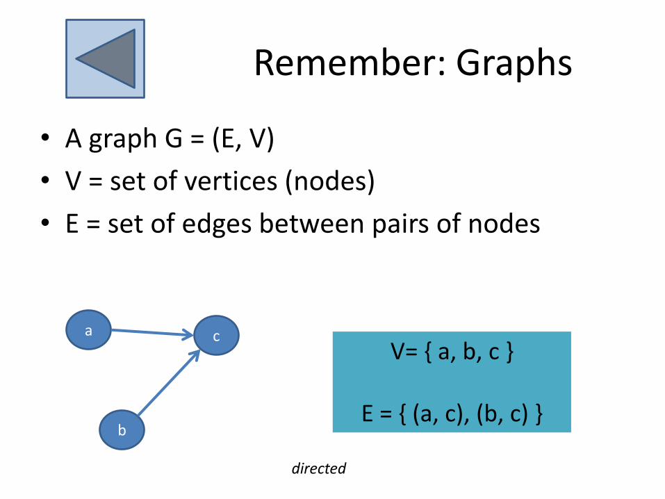
• A graph G = (E, V)
• V = set of vertices (nodes)
• E = set of edges between pairs of nodes
V= { a, b, c }
E = { (a, c), (b, c) }
a
b
c
directed

Remember: Graphs
• A graph G = (E, V)
• V = set of vertices (nodes)
• E = set of edges between pairs of nodes
V= { a, b, c }
E = { (a, c), (c, b) }
a
b
c
directed

Remember: Graphs
• A graph G = (E, V)
• V = set of vertices (nodes)
• E = set of edges between pairs of nodes
a
b
cV= { ??? }
E = { ??? }
g = ???
4
5
1

Remember: Graphs
• A graph G = (E, V)
• V = set of vertices (nodes)
• E = set of edges between pairs of nodes
a
b
c
V= { a, b, c }
E = { (a,c), (b, c), (c, b) }
g = {(a, c): 4, (b, c): 5, (c, b): 1}
4
5
1
weighted, directed

Some Key Terms: States, Goal, and Solution
State: a representation of the current world/environment (as needed for the agent)
Initial State: The state the agent/problem starts in
Goal State: The desired state
Solution: a sequence of actions that operate sequentially on states and allow the agent to
achieve its goal

Example: 8-Puzzle
Given an initial configuration of 8 numbered tiles on a 3x3 board, move the tiles to produce a desired goal configuration

Building goal-based agentsWe must answer the following questions–How do we represent the state of the “world”?
–What is the goal and how can we recognize it?
–What are the possible actions?
–What relevant information do we encode to describe states, actions and their effects and thereby solve the problem?
initial state goal state

Representing states
• State of an 8-puzzle?

Representing states
• State of an 8-puzzle?
• A 3x3 array of integer in {0..8}
• No integer appears twice
• 0 represents the empty space
• In Python, we might implement this using a nine-character string: “540681732”
• And write functions to map the 2D coordinates to an index

What’s the goal to be achieved?
• Describe situation we want to achieve, a set of properties that we want to hold, etc.
• Defining a goal test function that when applied to a state returns True or False
• For our problem:def isGoal(state):
return state == “123405678”
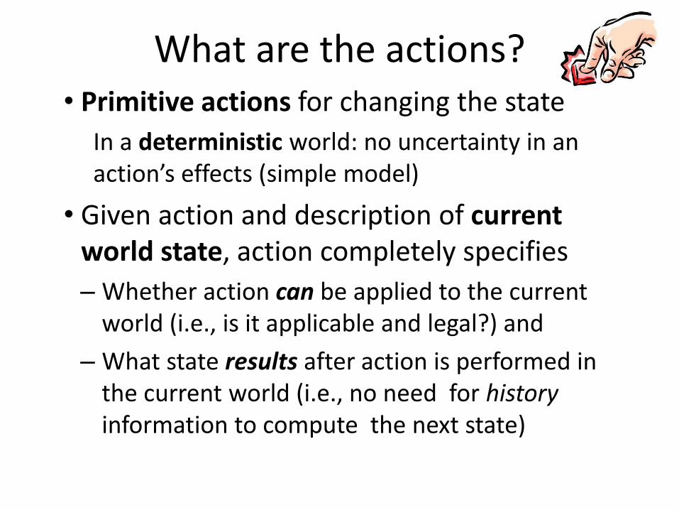
What are the actions?• Primitive actions for changing the state
In a deterministic world: no uncertainty in an action’s effects (simple model)
• Given action and description of current world state, action completely specifies
– Whether action can be applied to the current world (i.e., is it applicable and legal?) and
– What state results after action is performed in the current world (i.e., no need for history information to compute the next state)

Representing actions
• Actions ideally considered as discrete eventsthat occur at an instant of time
• Example, in a planning context
– If state:inClass and perform action:goHome, then next state is state:atHome
– There’s no time where you’re neither in class nor at home (i.e., in the state of “going home”)

Representing actions
• Actions for 8-puzzle?
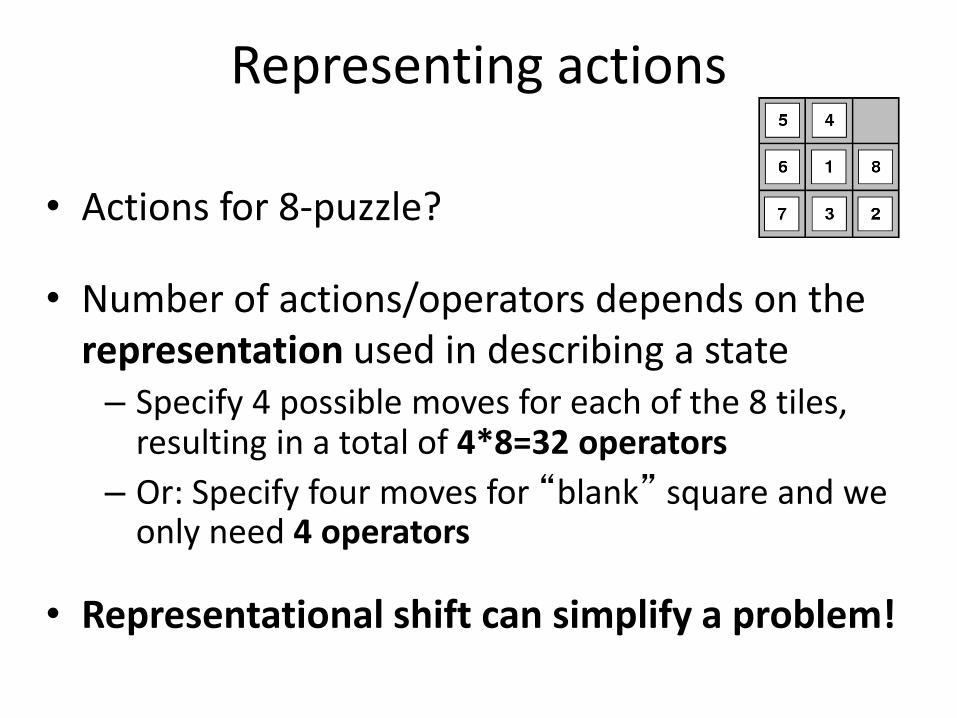
Representing actions
• Actions for 8-puzzle?
• Number of actions/operators depends on the representation used in describing a state– Specify 4 possible moves for each of the 8 tiles,
resulting in a total of 4*8=32 operators
– Or: Specify four moves for “blank” square and we only need 4 operators
• Representational shift can simplify a problem!

Representing states
• Size of a problem usually described in terms of possible number of states
– Tic-Tac-Toe has about 39 states (19,683≈2*104)
– Checkers has about 1040 states
– Rubik’s Cube has about 1019 states
– Chess has about 10120 states in a typical game
– Go has 2*10170
– Theorem provers may deal with an infinite space
• State space size ≈ solution difficulty

Representing states
• Our estimates were loose upper bounds
• How many possible, legal states does tic-tac-toe really have?
• Simple upper bound: nine board cells, each of which can be empty, O or X, so 39
• Only 593 states after eliminating
– impossible states
– Rotations and reflectionsX
X
X X
Some example problems
• Toy problems and micro-worlds
–8-Puzzle
–Missionaries and Cannibals
–Cryptarithmetic
–8-Queens Puzzle
–Remove 5 Sticks
–Water Jug Problem
• Real-world problems

Example: The 8-Queens Puzzle
Place eight queens on a chessboard such that no queen attacks any other
We can generalize the problem to a NxN chessboard
What are the states, goal test, actions?

Some more real-world problems
• Route finding
• Touring (traveling salesman)
• Logistics
• VLSI layout
• Robot navigation
• Theorem proving
• Learning
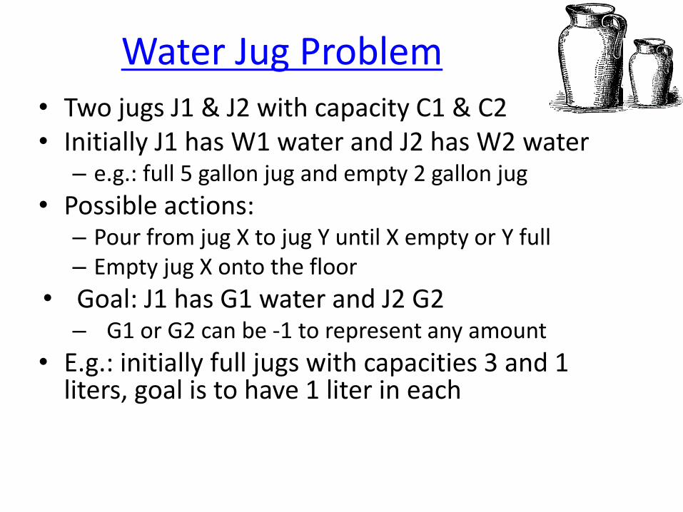
Water Jug Problem• Two jugs J1 & J2 with capacity C1 & C2• Initially J1 has W1 water and J2 has W2 water
– e.g.: full 5 gallon jug and empty 2 gallon jug
• Possible actions: – Pour from jug X to jug Y until X empty or Y full– Empty jug X onto the floor
• Goal: J1 has G1 water and J2 G2– G1 or G2 can be -1 to represent any amount
• E.g.: initially full jugs with capacities 3 and 1 liters, goal is to have 1 liter in each
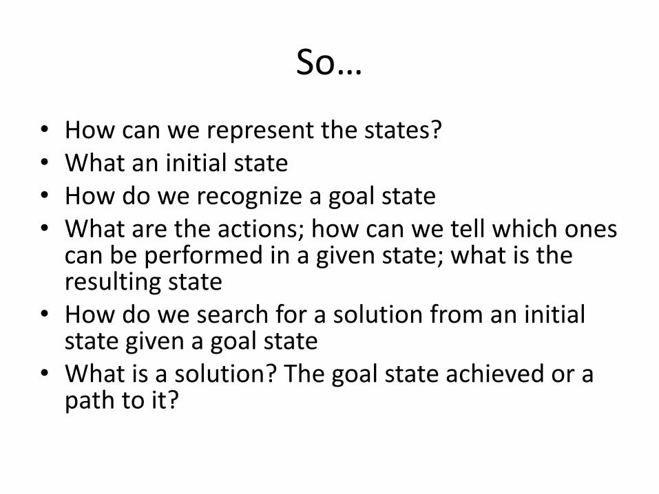
So…
• How can we represent the states?• What an initial state• How do we recognize a goal state• What are the actions; how can we tell which ones
can be performed in a given state; what is the resulting state
• How do we search for a solution from an initial state given a goal state
• What is a solution? The goal state achieved or a path to it?

Search in a state space• Basic idea:
–Create representation of initial state
–Try all possible actions & connect states that result
–Recursively apply process to the new states until we find a solution or dead ends
• We need to keep track of the connections between states and might use a
–Tree data structure or
–Graph data structure
• A graph structure is best in general…
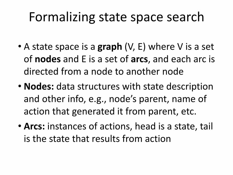
Formalizing state space search
• A state space is a graph (V, E) where V is a set of nodes and E is a set of arcs, and each arc is directed from a node to another node
• Nodes: data structures with state description and other info, e.g., node’s parent, name of action that generated it from parent, etc.
• Arcs: instances of actions, head is a state, tail is the state that results from action

Formalizing search in a state space• Each arc has fixed, positive cost associated
with it corresponding to the action cost– Simple case: all costs are 1
• Each node has a set of successor nodescorresponding to all legal actions that can be applied at node’s state– Expanding a node = generating its successor nodes and
adding them and their associated arcs to the graph
• One or more nodes are marked as start nodes
• A goal test predicate is applied to a state to determine if its associated node is a goal node
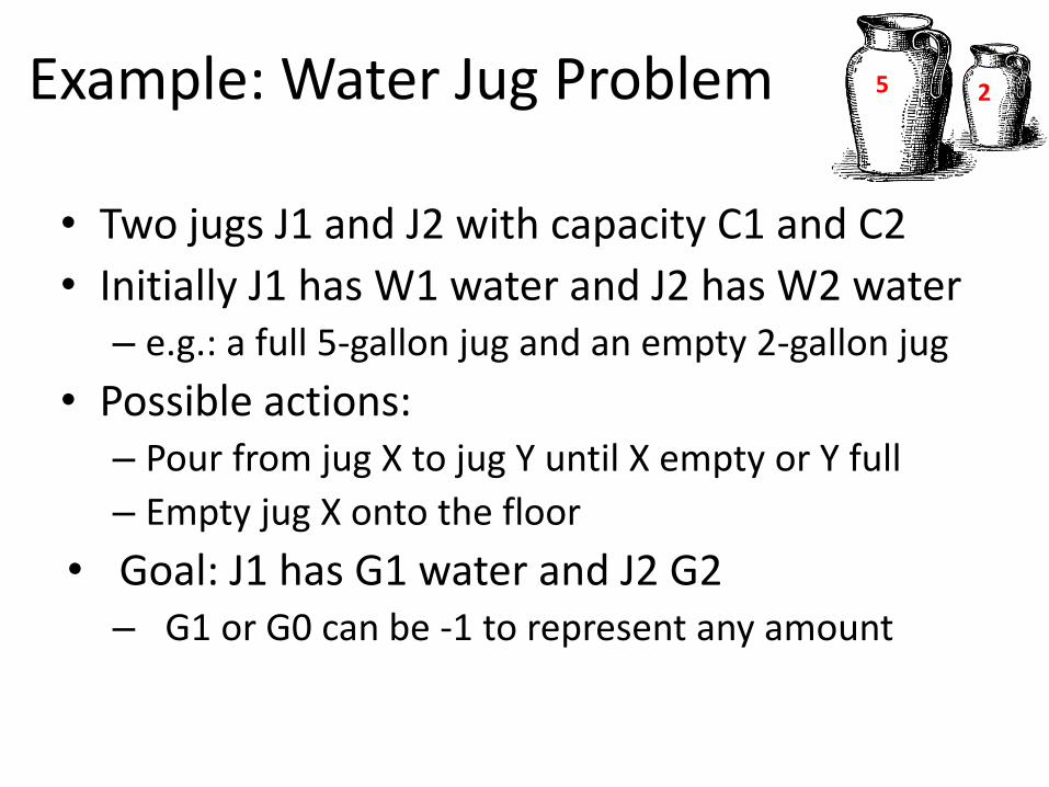
Example: Water Jug Problem
• Two jugs J1 and J2 with capacity C1 and C2
• Initially J1 has W1 water and J2 has W2 water– e.g.: a full 5-gallon jug and an empty 2-gallon jug
• Possible actions: – Pour from jug X to jug Y until X empty or Y full
– Empty jug X onto the floor
• Goal: J1 has G1 water and J2 G2– G1 or G0 can be -1 to represent any amount
5 2

Example: Water Jug Problem
Given full 5-gal. jug and empty 2-gal. jug, fill 2-gal jug with one gallon
• State representation?
–General state?
–Initial state?
–Goal state?
• Possible actions?–Condition?
–Resulting state?
Name Cond. Transition Effect
Empty5 (x,y)→(0,y)Empty 5G
jug
Empty2 (x,y)→(x,0)Empty 2G
jug
2to5 x ≤ 3 (x,2)→(x+2,0)Pour 2G into
5G
5to2 x ≥ 2 (x,0)→(x-2,2)Pour 5G into
2G
5to2part y < 2 (1,y)→(0,y+1)Pour partial
5G into 2G
Action table
5 2

Example: Water Jug Problem
Given full 5-gal. jug and empty 2-gal. jug, fill 2-gal jug with one gallon•State = (x,y), where x is water in jug 1; y is water in jug 2
• Initial State = (5,0)
•Goal State = (-1,1), where -1 means any amount
Name Cond. Transition Effect
dump1 x>0 (x,y)→(0,y) Empty Jug 1
dump2 y>0 (x,y)→(x,0) Empty Jug 2
pour_1_2x>0 &
y<C2
(x,y)→(x-D,y+D)
D = min(x,C2-y)
Pour from Jug
1 to Jug 2
pour_2_1y>0 &
X<C1
(x,y)→(x+D,y-D)
D = min(y,C1-x)
Pour from Jug
2 to Jug 1
Action table
5 2

Formalizing search
• Solution: sequence of actions associated with a path from a start node to a goal node
• Solution cost: sum of the arc costs on the solution path
– If all arcs have same (unit) cost, then solution cost is length of solution (number of steps)
–Algorithms generally require that arc costs cannot be negative (why?)
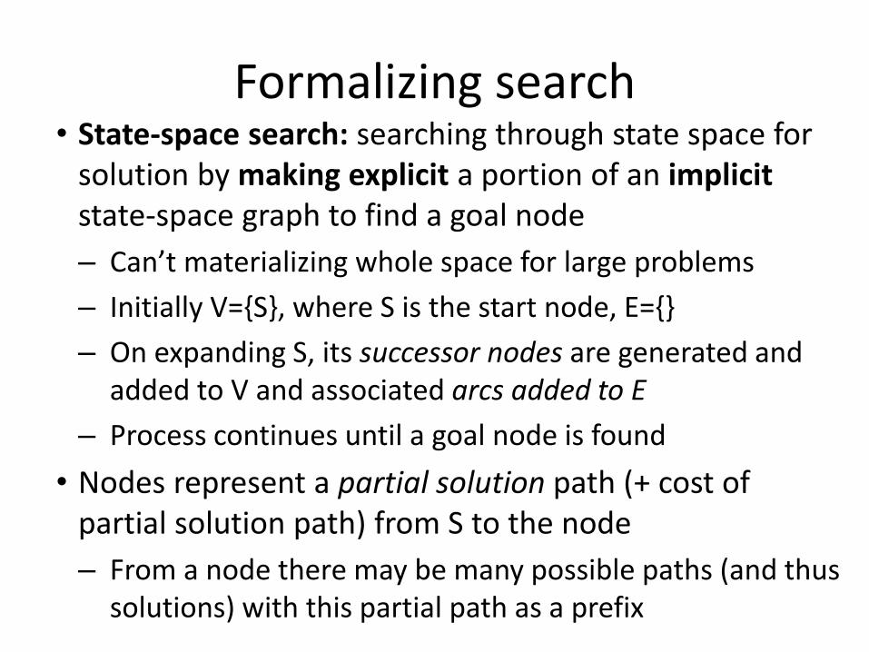
Formalizing search• State-space search: searching through state space for
solution by making explicit a portion of an implicitstate-space graph to find a goal node
– Can’t materializing whole space for large problems
– Initially V={S}, where S is the start node, E={}
– On expanding S, its successor nodes are generated and added to V and associated arcs added to E
– Process continues until a goal node is found
• Nodes represent a partial solution path (+ cost of partial solution path) from S to the node
– From a node there may be many possible paths (and thus solutions) with this partial path as a prefix
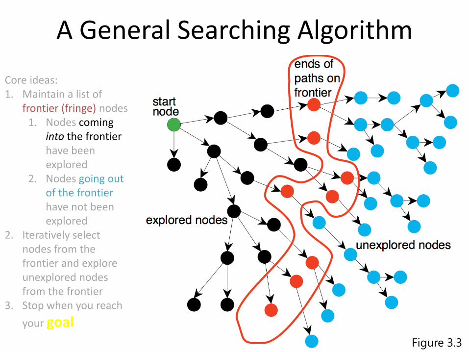
A General Searching Algorithm
Core ideas:1. Maintain a list of
frontier (fringe) nodes1. Nodes coming
into the frontierhave been explored
2. Nodes going out of the frontierhave not been explored
2. Iteratively select nodes from the frontier and explore unexplored nodes from the frontier
3. Stop when you reach
your goal
Figure 3.3
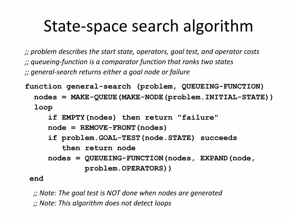
State-space search algorithm
;; problem describes the start state, operators, goal test, and operator costs
;; queueing-function is a comparator function that ranks two states
;; general-search returns either a goal node or failure
function general-search (problem, QUEUEING-FUNCTION)
nodes = MAKE-QUEUE(MAKE-NODE(problem.INITIAL-STATE))
loop
if EMPTY(nodes) then return "failure"
node = REMOVE-FRONT(nodes)
if problem.GOAL-TEST(node.STATE) succeeds
then return node
nodes = QUEUEING-FUNCTION(nodes, EXPAND(node,
problem.OPERATORS))
end
;; Note: The goal test is NOT done when nodes are generated
;; Note: This algorithm does not detect loops

Key procedures to be defined
• EXPAND
– Generate a node’s successor nodes, adding them to the graph if not already there
• GOAL-TEST
– Test if state satisfies all goal conditions
•QUEUEING-FUNCTION
– Maintain ranked list of nodes that are candidates for expansion
– Changing definition of the QUEUEING-FUNCTION leads to different search strategies

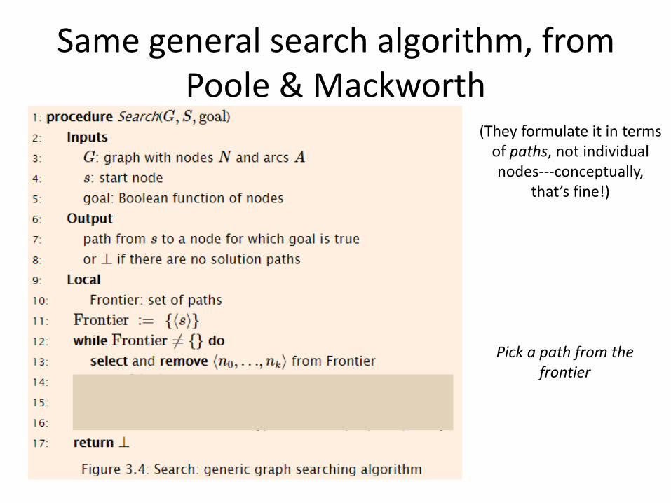
Same general search algorithm, from Poole & Mackworth
(They formulate it in terms of paths, not individual nodes---conceptually,
that’s fine!)

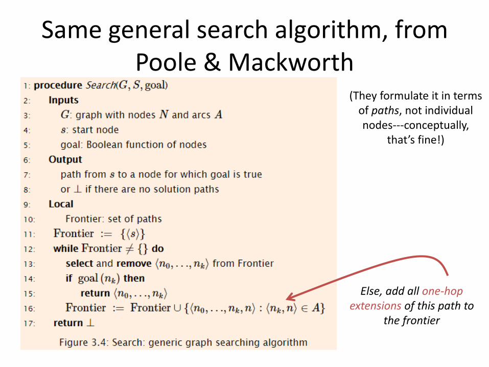
Same general search algorithm, from Poole & Mackworth
(They formulate it in terms of paths, not individual nodes---conceptually,
that’s fine!)
Initialize the frontier
Same general search algorithm, from Poole & Mackworth
(They formulate it in terms of paths, not individual nodes---conceptually,
that’s fine!)
Pick a path from the frontier

Same general search algorithm, from Poole & Mackworth
(They formulate it in terms of paths, not individual nodes---conceptually,
that’s fine!)
If the end state in the path achieves our goal, return
the path
Same general search algorithm, from Poole & Mackworth
(They formulate it in terms of paths, not individual nodes---conceptually,
that’s fine!)
Else, add all one-hop extensions of this path to
the frontier
What does “search” look like for a
particular problem?

1 2 3
4 5
7 8 6
1 2 3
4 5
7 8 6
1 3
4 2 5
7 8 6
1 2
4 5 3
7 8 6
1 2 3
4 5 6
7 8
1 2 3
4 5
7 8 6
1 2 3
4 8 5
7 6
1 2 3
4 8 5
7 6
1 2 3
4 8 5
7 6
1 2
4 8 3
7 6 5
1 2 3
4 8
7 6 5
goal
start

1 2 3
4 5
7 8 6
1 2 3
4 5
7 8 6
1 3
4 2 5
7 8 6
1 2
4 5 3
7 8 6
1 2 3
4 5 6
7 8
1 2 3
4 5
7 8 6
1 2 3
4 8 5
7 6
1 2 3
4 8 5
7 6
1 2 3
4 8 5
7 6
1 2
4 8 3
7 6 5
1 2 3
4 8
7 6 5
goal
start
Expanding a node on the fringe(taking a certain action)

1 2 3
4 5
7 8 6
1 2 3
4 5
7 8 6
1 3
4 2 5
7 8 6
1 2
4 5 3
7 8 6
1 2 3
4 5 6
7 8
1 2 3
4 5
7 8 6
1 2 3
4 8 5
7 6
1 2 3
4 8 5
7 6
1 2 3
4 8 5
7 6
1 2
4 8 3
7 6 5
1 2 3
4 8
7 6 5
goal
start
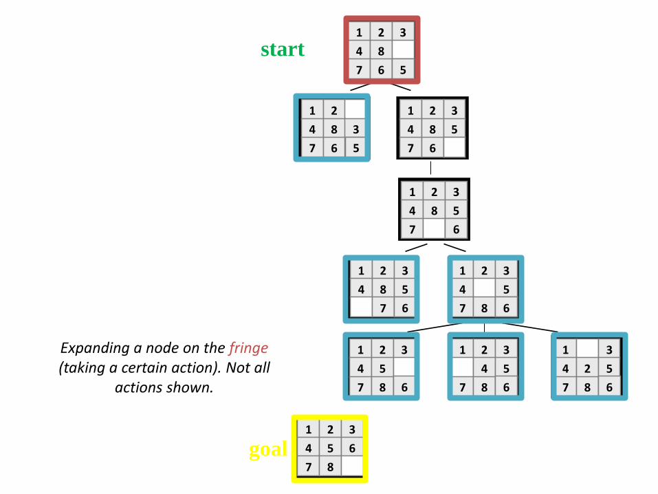
Expanding a node on the fringe(taking a certain action). Not all
actions shown.

1 2 3
4 5
7 8 6
1 2 3
4 5
7 8 6
1 3
4 2 5
7 8 6
1 2
4 5 3
7 8 6
1 2 3
4 5 6
7 8
1 2 3
4 5
7 8 6
1 2 3
4 8 5
7 6
1 2 3
4 8 5
7 6
1 2 3
4 8 5
7 6
1 2
4 8 3
7 6 5
1 2 3
4 8
7 6 5
goal
start
Expanding a node on the fringe(taking a certain action). Not all
actions shown.
1 2 3
4 5
7 8 6
1 2 3
4 5
7 8 6
1 3
4 2 5
7 8 6
1 2
4 5 3
7 8 6
1 2 3
4 5 6
7 8
1 2 3
4 5
7 8 6
1 2 3
4 8 5
7 6
1 2 3
4 8 5
7 6
1 2 3
4 8 5
7 6
1 2
4 8 3
7 6 5
1 2 3
4 8
7 6 5
goal
start
Expanding a node on the fringe(taking a certain action). Not all
actions shown.

1 2 3
4 5
7 8 6
1 2 3
4 5
7 8 6
1 3
4 2 5
7 8 6
1 2
4 5 3
7 8 6
1 2 3
4 5 6
7 8
1 2 3
4 5
7 8 6
1 2 3
4 8 5
7 6
1 2 3
4 8 5
7 6
1 2 3
4 8 5
7 6
1 2
4 8 3
7 6 5
1 2 3
4 8
7 6 5
goal
start
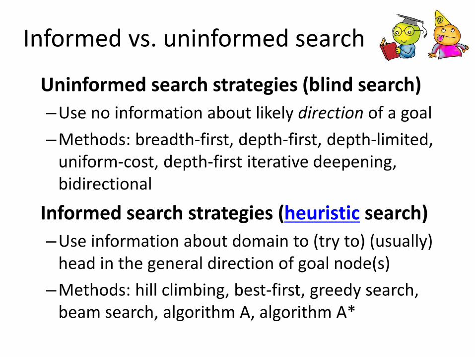
Informed vs. uninformed search
Uninformed search strategies (blind search)
–Use no information about likely direction of a goal
–Methods: breadth-first, depth-first, depth-limited, uniform-cost, depth-first iterative deepening, bidirectional
Informed search strategies (heuristic search)
–Use information about domain to (try to) (usually) head in the general direction of goal node(s)
–Methods: hill climbing, best-first, greedy search, beam search, algorithm A, algorithm A*

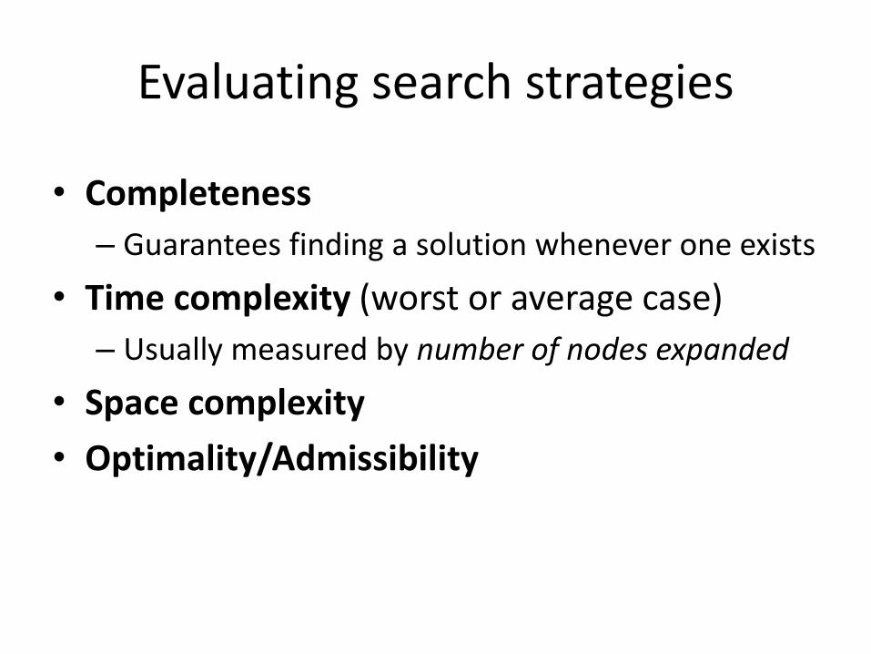
Evaluating search strategies
• Completeness
– Guarantees finding a solution whenever one exists
• Time complexity (worst or average case)
• Space complexity
• Optimality/Admissibility
Evaluating search strategies
• Completeness
– Guarantees finding a solution whenever one exists
• Time complexity (worst or average case)
– Usually measured by number of nodes expanded
• Space complexity
• Optimality/Admissibility

Evaluating search strategies
• Completeness
– Guarantees finding a solution whenever one exists
• Time complexity (worst or average case)
– Usually measured by number of nodes expanded
• Space complexity
– Usually measured by maximum size of graph/treeduring the search
• Optimality/Admissibility
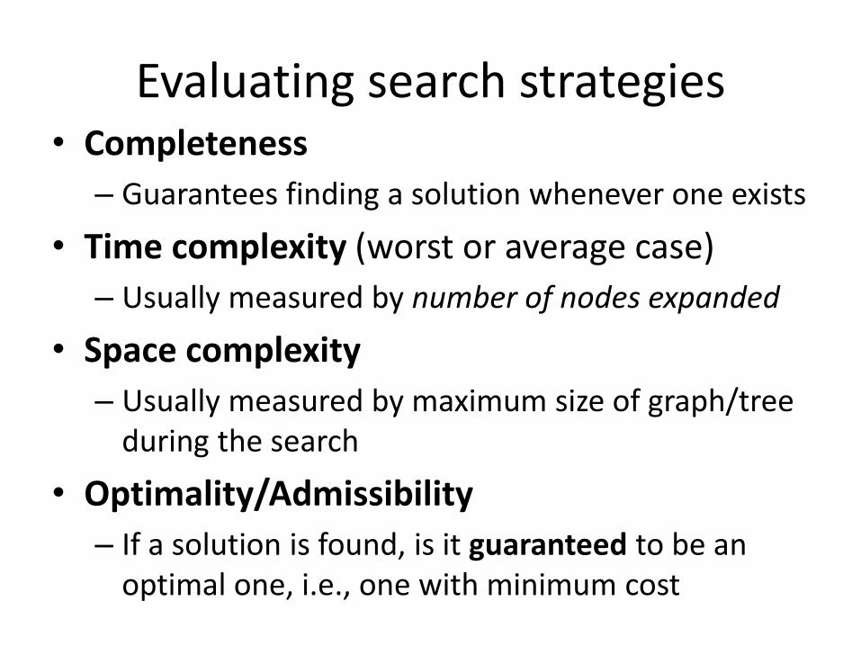
Evaluating search strategies• Completeness
– Guarantees finding a solution whenever one exists
• Time complexity (worst or average case)
– Usually measured by number of nodes expanded
• Space complexity
– Usually measured by maximum size of graph/treeduring the search
• Optimality/Admissibility
– If a solution is found, is it guaranteed to be an optimal one, i.e., one with minimum cost
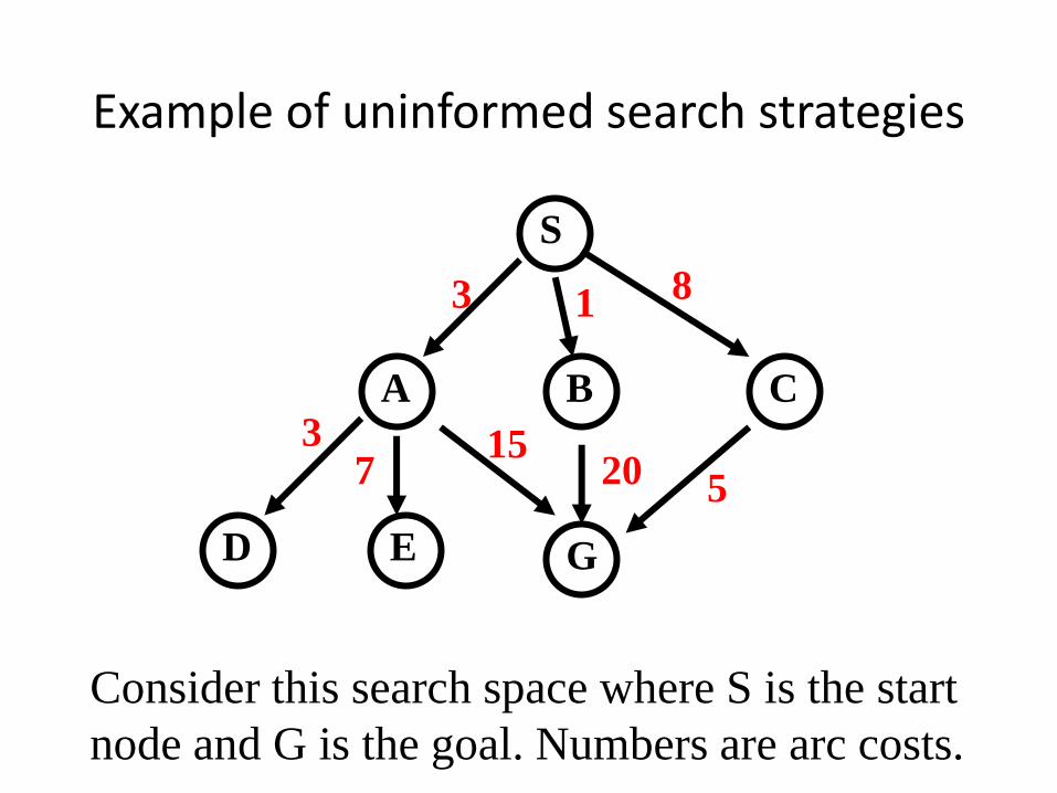
Example of uninformed search strategies
S
CBA
D GE
3 1 8
1520 5
37
Consider this search space where S is the start
node and G is the goal. Numbers are arc costs.

Classic uninformed search methods
• The four classic uninformed search methods
–Breadth first search (BFS)
–Depth first search (DFS)
–Uniform cost search (generalization of BFS)
– Iterative deepening (blend of DFS and BFS)
• To which we can add another technique
–Bi-directional search (hack on BFS)

Breadth-First Search
• Enqueue nodes in FIFO (first-in, first-out) order
• Complete
• Optimal (i.e., admissible) finds shorted path, which is optimal if all operators have same cost
• Q? Time & space complexity
• Q? Potential issues

Breadth-First Search
• Enqueue nodes in FIFO (first-in, first-out) order
• Complete
• Optimal (i.e., admissible) finds shorted path, which is optimal if all operators have same cost
• Exponential time and space complexity, O(bd), where d is depth of solution; b is branching factor (i.e., # of children)
• Q? Potential issues
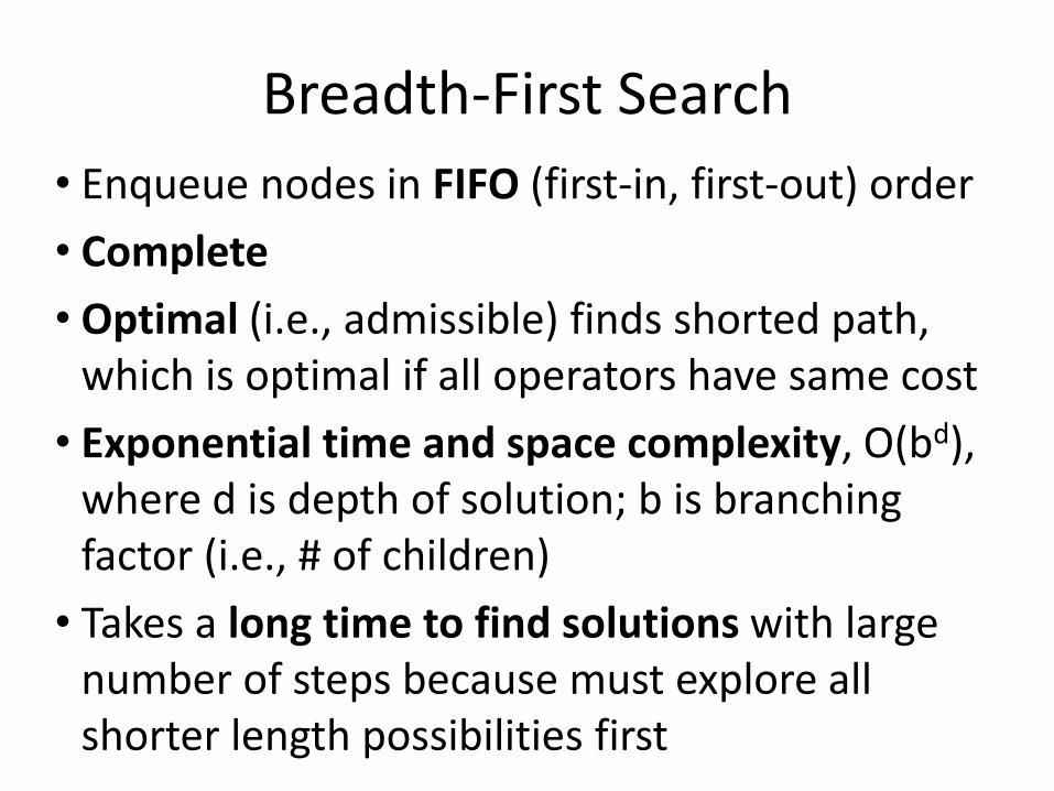
Breadth-First Search
• Enqueue nodes in FIFO (first-in, first-out) order
• Complete
• Optimal (i.e., admissible) finds shorted path, which is optimal if all operators have same cost
• Exponential time and space complexity, O(bd), where d is depth of solution; b is branching factor (i.e., # of children)
• Takes a long time to find solutions with large number of steps because must explore all shorter length possibilities first

Breadth-First Search
Expanded node Nodes list (aka Fringe)
{ S0 }
S0 { A3 B1 C8 }
A3 { B1 C8 D6 E10 G18 }
B1 { C8 D6 E10 G18 G21 }
C8 { D6 E10 G18 G21 G13 }
D6 { E10 G18 G21 G13 }
E10 { G18 G21 G13 }
G18 { G21 G13 }
Note: we typically don’t check for goal until we expand nodeSolution path found is S A G , cost 18Number of nodes expanded (including goal node) = 7
Notation
G18
G is node; 18 is cost of shortest
known path from
start node S
weighted arcs

Breadth-First Search
Long time to find solutions with many steps: we must look at all shorter length possibilities first
• Complete search tree of depth d where nodes have b children has 1 + b + b2 + ... + bd = (b(d+1) - 1)/(b-1) nodes = 0(bd)
• Tree of depth 12 with branching 10 has more than a trillion nodes
• If BFS expands 1000 nodes/sec and nodes uses 100 bytes, then it may take 35 years to run and uses 111 terabytes of memory!

Depth-First (DFS)• Enqueue nodes on nodes in LIFO (last-in, first-out)
order, i.e., use stack data structure to order nodes
• May not terminate w/o depth bound, i.e., ending search below fixed depth D (depth-limited search)
• Not complete (with or w/o cycle detection, with or w/o a cutoff depth)
• Exponential time, O(bd), but linear space, O(bd)
• Can find long solutions quickly if lucky (and short solutions slowly if unlucky!)
• On reaching deadend, can only back up one level at a time even if problem occurs because of a bad choice at top of tree

Depth-First Search
Expanded node Nodes list
{ S0 }
S0 { A3 B1 C8 }
A3 { D6 E10 G18 B1 C8 }
D6 { E10 G18 B1 C8 }
E10 { G18 B1 C8 }
G18 { B1 C8 }
Solution path found is S A G, cost 18
Number of nodes expanded (including goal node) = 5

Uniform-Cost Search (UCS)• Enqueue nodes by path cost. i.e., let g(n) = cost of
path from start to current node n. Sort nodes by increasing value of g(n).
• Also called Dijkstra’s Algorithm, similar to Branch and Bound Algorithm from operations research
• Complete (*)
• Optimal/Admissible (*)
Depends on goal test being applied when node is removed from nodes list, not when its parent node is expanded & node first generated
• Exponential time and space complexity, O(bd)
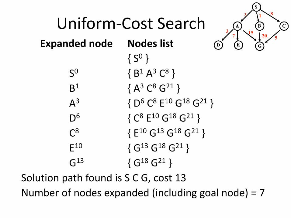
Uniform-Cost Search Expanded node Nodes list
{ S0 }
S0 { B1 A3 C8 }
B1 { A3 C8 G21 }
A3 { D6 C8 E10 G18 G21 }
D6 { C8 E10 G18 G21 }
C8 { E10 G13 G18 G21 }
E10 { G13 G18 G21 }
G13 { G18 G21 }
Solution path found is S C G, cost 13
Number of nodes expanded (including goal node) = 7

Depth-First Iterative Deepening (DFID)• Do DFS to depth 0, then (if no solution) DFS to
depth 1, etc.
• Usually used with a tree search
• Complete
• Optimal/Admissible if all operators have unit cost, else finds shortest solution (like BFS)
• Time complexity a bit worse than BFS or DFSNodes near top of search tree generated many times, but since almost all nodes are near tree bottom, worst case time complexity still exponential, O(bd)
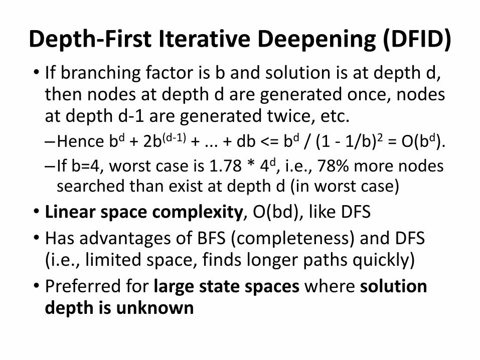
• If branching factor is b and solution is at depth d, then nodes at depth d are generated once, nodes at depth d-1 are generated twice, etc. –Hence bd + 2b(d-1) + ... + db <= bd / (1 - 1/b)2 = O(bd).
– If b=4, worst case is 1.78 * 4d, i.e., 78% more nodes searched than exist at depth d (in worst case)
• Linear space complexity, O(bd), like DFS
• Has advantages of BFS (completeness) and DFS (i.e., limited space, finds longer paths quickly)
• Preferred for large state spaces where solution depth is unknown
Depth-First Iterative Deepening (DFID)
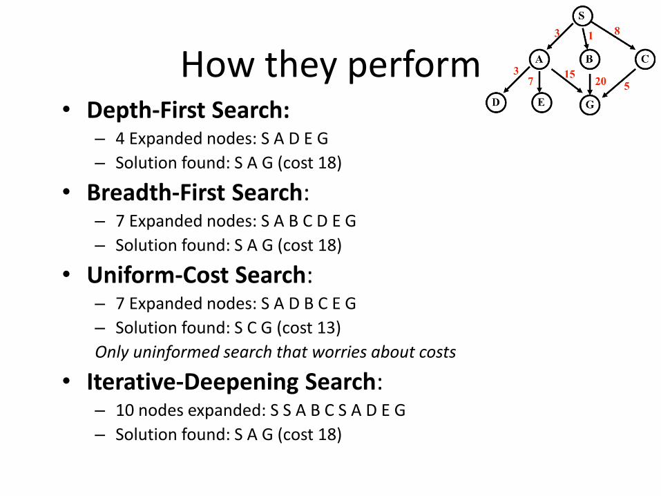
How they perform• Depth-First Search:
– 4 Expanded nodes: S A D E G
– Solution found: S A G (cost 18)
• Breadth-First Search: – 7 Expanded nodes: S A B C D E G
– Solution found: S A G (cost 18)
• Uniform-Cost Search: – 7 Expanded nodes: S A D B C E G
– Solution found: S C G (cost 13)
Only uninformed search that worries about costs
• Iterative-Deepening Search: – 10 nodes expanded: S S A B C S A D E G
– Solution found: S A G (cost 18)

Searching Backward from Goal
• Usually a successor function is reversible
– i.e., can generate a node’s predecessors in graph
• If we know a single goal (rather than a goal’s properties), we could search backward to the initial state
• It might be more efficient
– Depends on whether the graph fans in or out
Bi-directional search
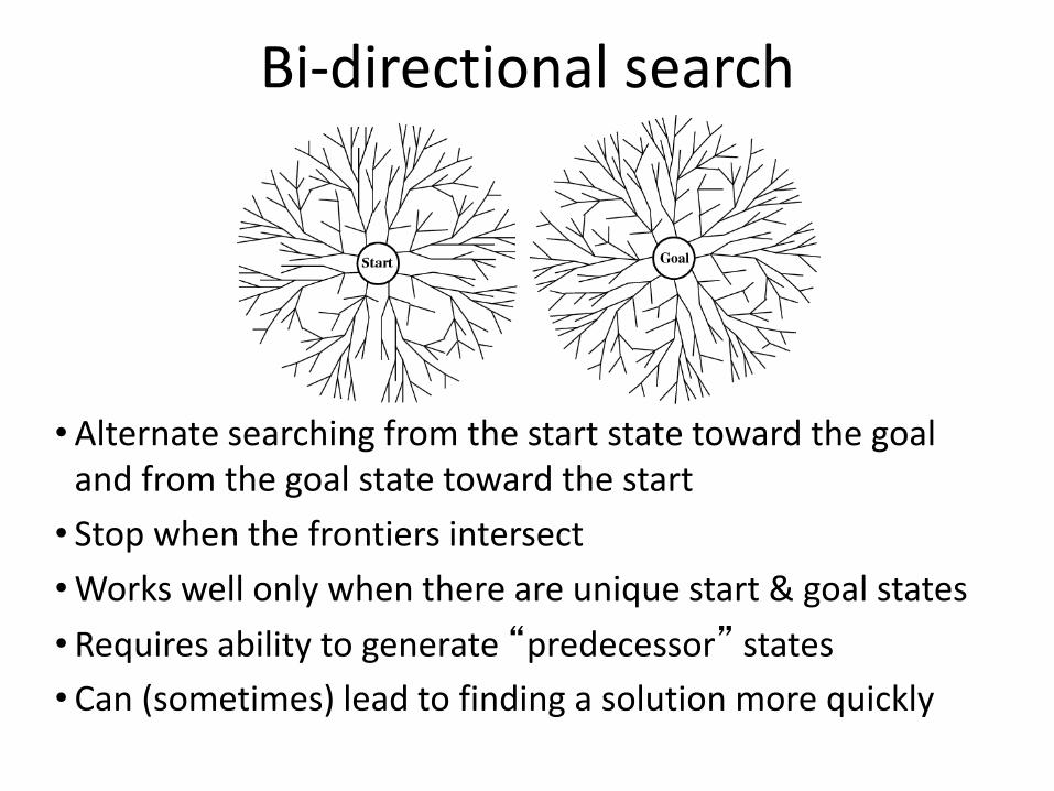
•Alternate searching from the start state toward the goal and from the goal state toward the start
• Stop when the frontiers intersect
•Works well only when there are unique start & goal states
• Requires ability to generate “predecessor” states
• Can (sometimes) lead to finding a solution more quickly

Comparing Search Strategies
Informed (Heuristic) Search
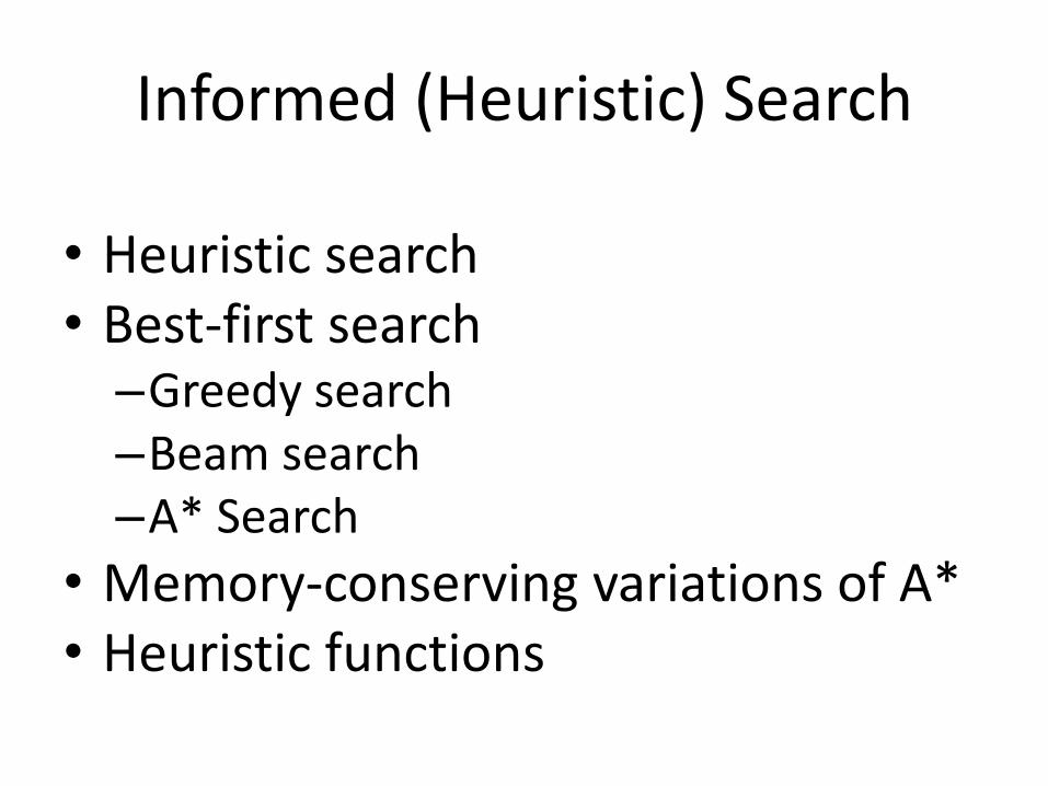
• Heuristic search• Best-first search–Greedy search–Beam search–A* Search
• Memory-conserving variations of A*• Heuristic functions

Big idea: heuristicMerriam-Webster's Online Dictionary
Heuristic (pron. \hyu-’ris-tik\): adj. [from Greek heuriskein to discover] involving or serving as an aid to learning, discovery, or problem-solving by experimental and especially trial-and-error methods
The Free On-line Dictionary of Computing (15Feb98)
heuristic 1. <programming> A rule of thumb, simplification or educated guess that reduces or limits the search for solutions in domains that are difficult and poorly understood. Unlike algorithms, heuristics do not guarantee feasible solutions and are often used with no theoretical guarantee. 2. <algorithm> approximation algorithm.
From WordNet (r) 1.6
heuristic adj 1: (CS) relating to or using a heuristic rule 2: of or relating to a general formulation that serves to guide investigation [ant: algorithmic] n : a commonsense rule (or set of rules) intended to increase the probability of solving some problem [syn: heuristic rule, heuristic program]
Heuristics, More Formally
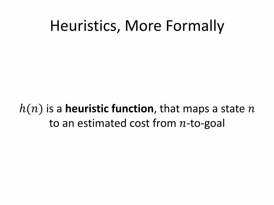
ℎ(𝑛) is a heuristic function, that maps a state 𝑛to an estimated cost from 𝑛-to-goal
Heuristics, More Formally
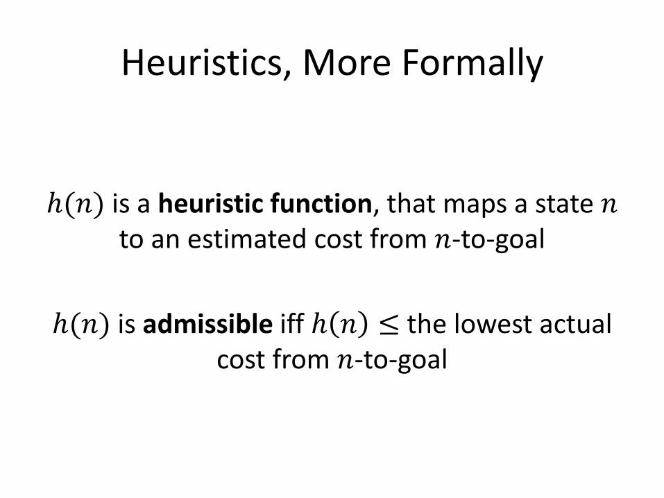
ℎ(𝑛) is a heuristic function, that maps a state 𝑛to an estimated cost from 𝑛-to-goal
ℎ(𝑛) is admissible iff ℎ 𝑛 ≤ the lowest actual cost from 𝑛-to-goal
Heuristics, More Formally
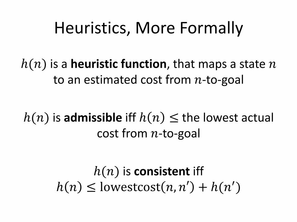
ℎ(𝑛) is a heuristic function, that maps a state 𝑛to an estimated cost from 𝑛-to-goal
ℎ(𝑛) is admissible iff ℎ 𝑛 ≤ the lowest actual cost from 𝑛-to-goal
ℎ(𝑛) is consistent iffℎ 𝑛 ≤ lowestcost 𝑛, 𝑛′ + ℎ(𝑛′)

Informed methods add domain-specific information
• Select best path along which to continue searching
• h(n): estimates goodness of node n
• h(n) = estimated cost (or distance) of minimal cost path from n to a goal state.
• Based on domain-specific information and computable from current state description that estimates how close we are to a goal

Heuristics• All domain knowledge used in search is encoded
in the heuristic function, h(<node>)
• Examples:–8-puzzle: number of tiles out of place –8-puzzle: sum of distances each tile is from its goal–Missionaries & Cannibals: # people on starting river
bank
• In general– ℎ 𝑛 ≥ 0 for all nodes n – ℎ(𝑛) = 0 implies that n is a goal node – ℎ 𝑛 = ∞ implies n is a dead-end that can’t lead to
goal
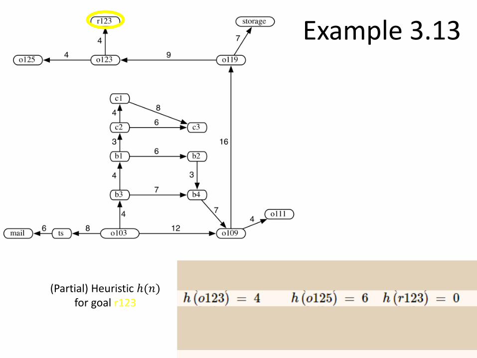
Example 3.13
(Partial) Heuristic ℎ(𝑛)for goal r123

Example 3.13
Heuristic ℎ(𝑛) for goal r123
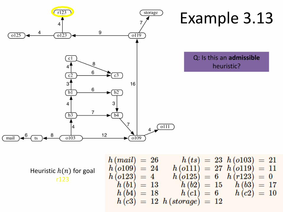
Example 3.13
Heuristic ℎ(𝑛) for goal r123
Q: Is this an admissibleheuristic?

Example 3.13
Heuristic ℎ(𝑛) for goal r123
Q: Is this an admissibleheuristic?
Q: Is it an accurate heuristic?

Heuristics for 8-puzzle
The number of
misplaced tiles
(not including
the blank)
1 2 3
4 5 6
7 8
1 2 3
4 5 6
7 8
In this case, only “8” is misplaced, so heuristic
function evaluates to 1
In other words, the heuristic says that it thinks a
solution may be available in just 1 more move
Goal
State
Current
State
1 2 3
4 5 6
7 8
1 2 3
4 5 6
7 8
N N N
N N N
N Y

Heuristics for 8-puzzle
Manhattan
Distance (not
including the
blank)
• The 3, 8 and 1 tiles are misplaced (by 2, 3,
and 3 steps) so the heuristic function
evaluates to 8
• Heuristic says that it thinks a solution may
be available in just 8 more moves.
• The misplaced heuristic’s value is 3
3 2 8
4 5 6
7 1
1 2 3
4 5 6
7 8
Goal
State
Current
State
3 3
8
8
1
1
2 spaces
3 spaces
3 spaces
Total 8
5
6 4
3
4 2
1 3 3
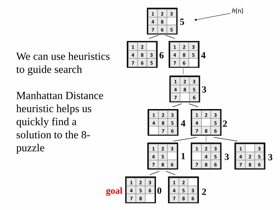
0 2
We can use heuristics
to guide search
Manhattan Distance
heuristic helps us
quickly find a
solution to the 8-
puzzle
h(n)
1 2 3
4 5
7 8 6
1 2 3
4 5
7 8 6
1 3
4 2 5
7 8 6
1 2
4 5 3
7 8 6
1 2 3
4 5 6
7 8
1 2 3
4 5
7 8 6
1 2 3
4 8 5
7 6
1 2 3
4 8 5
7 6
1 2 3
4 8 5
7 6
1 2
4 8 3
7 6 5
1 2 3
4 8
7 6 5
goal

Best-first search
• Search algorithm that improves depth-first search by expanding most promising node chosen according to heuristic rule
• Order nodes on nodes list by increasing value of an evaluation function, f(n), incorporating domain-specific information
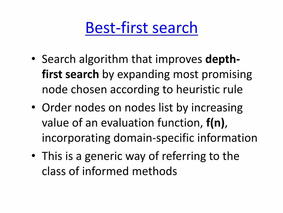
Best-first search
• Search algorithm that improves depth-first search by expanding most promising node chosen according to heuristic rule
• Order nodes on nodes list by increasing value of an evaluation function, f(n), incorporating domain-specific information
• This is a generic way of referring to the class of informed methods

Greedy best first search• A greedy algorithm makes locally optimal choices in hope of
finding a global optimum
• Uses evaluation function f(n) = h(n), sorting nodes by increasing values of f
• Selects node to expand appearing closest to goal (i.e., node with smallest f value)
• Not complete
• Not admissible, as in example– Assume arc costs = 1, greedy search finds goal g, with solution cost
of 5
–Optimal solution is path to goal with cost 3

Greedy best first search example
• Proof of non-admissibility– Assume arc costs = 1, greedy
search finds goal g, with solution cost of 5
– Optimal solution is path to goal with cost 3
a
hb
c
d
e
g
i
g2
h=2
h=1
h=1
h=1
h=0
h=4
h=1
h=0

Beam search• Use evaluation function f(n), but maximum size
of the nodes list is k, a fixed constant
• Only keep k best nodes as candidates for expansion, discard rest
• k is the beam width
• More space efficient than greedy search, but may discard nodes on a solution path
• As k increases, approaches best first search
• Complete?
• Admissible?

Beam search• Use evaluation function f(n), but maximum size
of the nodes list is k, a fixed constant
• Only keep k best nodes as candidates for expansion, discard rest
• k is the beam width
• More space efficient than greedy search, but may discard nodes on a solution path
• As k increases, approaches best first search
• Not complete
• Not admissible
We’ve got to be able to do better, right?
Let’s think about car trips…
A* Search
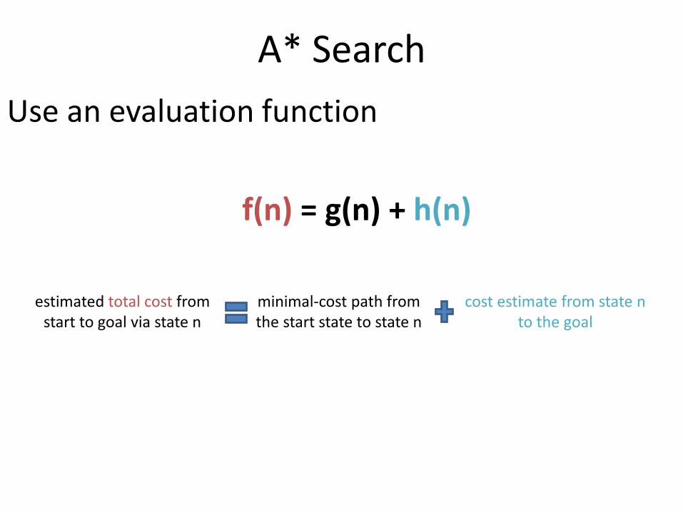
Use an evaluation function
f(n) = g(n) + h(n)
minimal-cost path from the start state to state n
cost estimate from state n to the goal
estimated total cost from start to goal via state n
A* Search
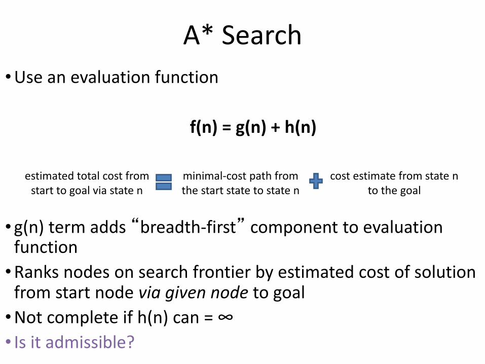
•Use an evaluation function
f(n) = g(n) + h(n)
•g(n) term adds “breadth-first” component to evaluation function
•Ranks nodes on search frontier by estimated cost of solution from start node via given node to goal
•Not complete if h(n) can = ∞
• Is it admissible?
minimal-cost path from the start state to state n
cost estimate from state n to the goal
estimated total cost from start to goal via state n

A*
• Pronounced “a star”
• h is admissible when h(n) <= h*(n) holds
–h*(n) = true cost of minimal cost path from n to a goal
• Using an admissible heuristic guarantees that 1st solution found will be an optimal one
• A* is complete whenever branching factor is finite and every action has fixed, positive cost
• A* is admissible
Hart, P. E.; Nilsson, N. J.; Raphael, B. (1968). "A Formal Basis for the Heuristic Determination of
Minimum Cost Paths". IEEE Transactions on Systems Science and Cybernetics SSC4 4 (2): 100–107.

Implementing A*
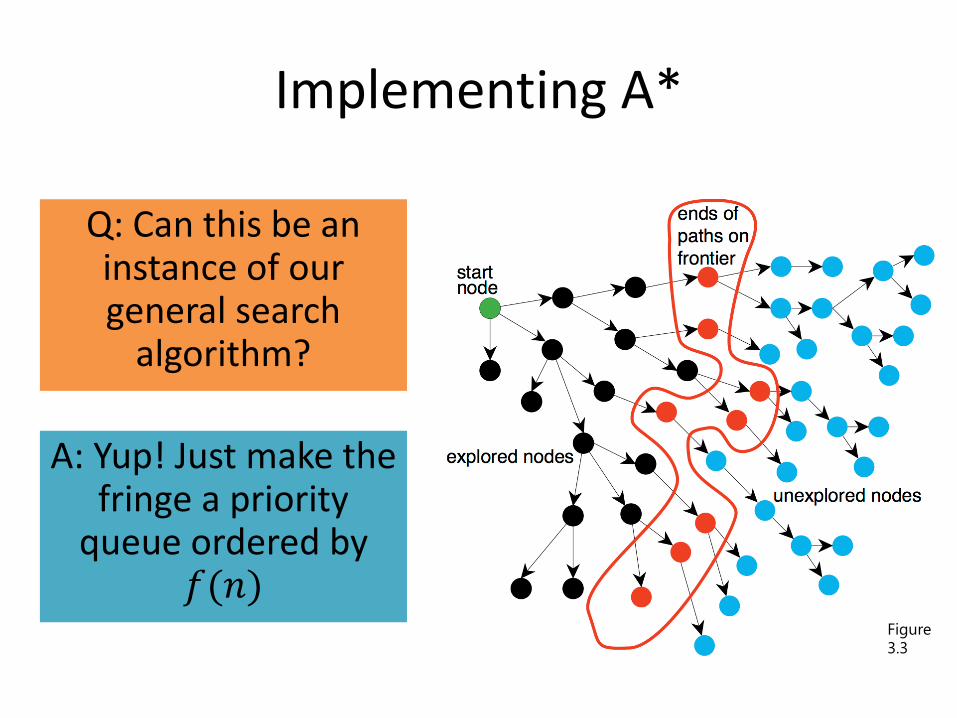
Q: Can this be an instance of our general search
algorithm?
Figure 3.3
Implementing A*
Q: Can this be an instance of our general search
algorithm?
Figure 3.3
A: Yup! Just make the fringe a priority
queue ordered by 𝑓(𝑛)
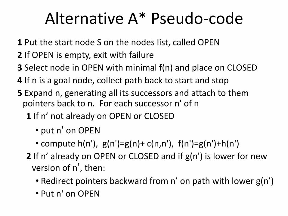
Alternative A* Pseudo-code1 Put the start node S on the nodes list, called OPEN
2 If OPEN is empty, exit with failure
3 Select node in OPEN with minimal f(n) and place on CLOSED
4 If n is a goal node, collect path back to start and stop
5 Expand n, generating all its successors and attach to them pointers back to n. For each successor n' of n
1 If n’ not already on OPEN or CLOSED
• put n' on OPEN
• compute h(n'), g(n')=g(n)+ c(n,n'), f(n')=g(n')+h(n')
2 If n’ already on OPEN or CLOSED and if g(n') is lower for new version of n', then:
• Redirect pointers backward from n’ on path with lower g(n’)
• Put n' on OPEN
Observations on A*• Perfect heuristic: If h(n) = h*(n) for all n, only nodes on an
optimal solution path expanded; no extra work is done
Observations on A*• Perfect heuristic: If h(n) = h*(n) for all n, only nodes on an
optimal solution path expanded; no extra work is done
• Null heuristic: If h(n) = 0 for all n, then it is an admissible heuristic and A* acts like uniform-cost search
Observations on A*• Perfect heuristic: If h(n) = h*(n) for all n, only nodes on an
optimal solution path expanded; no extra work is done
• Null heuristic: If h(n) = 0 for all n, then it is an admissible heuristic and A* acts like uniform-cost search
• Better heuristic: If h1(n) < h2(n) <= h*(n) for all non-goal nodes, then h2 is a better heuristic than h1
– If A1* uses h1, and A2* uses h2, then every node expanded by A2* is also expanded by A1*
i.e., A1 expands at least as many nodes as A2*
–We say that A2* is better informed than A1*
• The closer h to h*, the fewer extra nodes expanded

Example search space
S
CBA
D GE

Example search space
S
CBA
D GE
start state
goal state
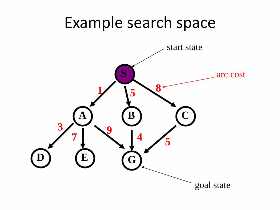
Example search space
S
CBA
D GE
start state
1 5 8
94 5
37
arc cost
goal state
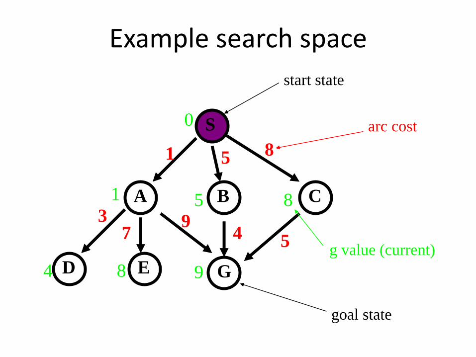
Example search space
S
CBA
D GE
start state
1 5 8
94 5
37
arc cost
goal state
0
1 85
4 8 9
g value (current)

Example search space
S
CBA
D GE
1 5 8
94 5
37
8
84 3
0
start state
goal state
arc cost
h value
0
1
4 8 9
85
g value (current)

Example search space
S
CBA
D GE
1 5 8
94 5
37
8
84 3
0
start state
goal state
arc cost
h value
parent pointer
(current)0
1
4 8 9
85
g value (current)
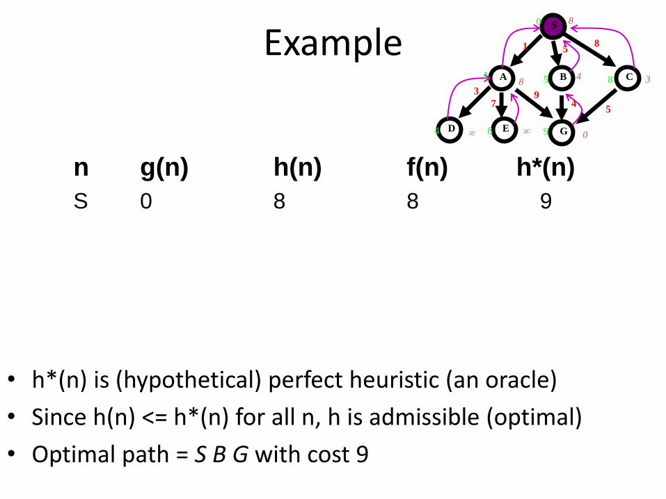
Example
n g(n) h(n) f(n) h*(n)
S 0 8 8 9
• h*(n) is (hypothetical) perfect heuristic (an oracle)
• Since h(n) <= h*(n) for all n, h is admissible (optimal)
• Optimal path = S B G with cost 9
S
CBA
D GE
1 58
94
5
3
7
8
84 3
0
0
1
4 8 9
85

Example
n g(n) h(n) f(n) h*(n)S 0 8 8 9
A 1 8 9 9
B 5 4 9 4
C 8 3 11 5
D 4 inf inf inf
E 8 inf inf inf
G 9 0 9 0
• h*(n) is (hypothetical) perfect heuristic (an oracle)
• Since h(n) <= h*(n) for all n, h is admissible (optimal)
• Optimal path = S B G with cost 9
S
CBA
D GE
1 58
94
5
3
7
8
84 3
0
0
1
4 8 9
85
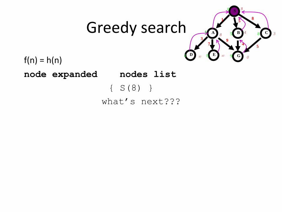
Greedy search
f(n) = h(n)
node expanded nodes list
{ S(8) }
what’s next???
S
CBA
D GE
1 58
94
5
3
7
8
84 3
0
0
1
4 8 9
85

Greedy search
f(n) = h(n)
node expanded nodes list
{ S(8) }
S { C(3) B(4) A(8) }
C { G(0) B(4) A(8) }
G { B(4) A(8) }
• Solution path found is S C G, 3 nodes expanded.
• See how fast the search is!! But it is NOT optimal.
S
CBA
D GE
1 58
94
5
3
7
8
84 3
0
0
1
4 8 9
85

A* searchf(n) = g(n) + h(n)
node exp. nodes list
{ S(8) }
What’s next?
S
CBA
D GE
1 58
94
5
3
7
8
84 3
0
0
1
4 8 9
85

A* searchf(n) = g(n) + h(n)
node exp. nodes list
{ S(8) }
S { A(9) B(9) C(11) }
What’s next?
S
CBA
D GE
1 58
94
5
3
7
8
84 3
0
0
1
4 8 9
85

A* searchf(n) = g(n) + h(n)
node exp. nodes list
{ S(8) }
S { A(9) B(9) C(11) }
A { B(9) G(10) C(11) D(inf) E(inf) }
What’s next?
S
CBA
D GE
1 58
94
5
3
7
8
84 3
0
0
1
4 8 9
85

A* searchf(n) = g(n) + h(n)
node exp. nodes list
{ S(8) }
S { A(9) B(9) C(11) }
A { B(9) G(10) C(11) D(inf) E(inf) }
B { G(9) G(10) C(11) D(inf) E(inf) }
What’s next?
S
CBA
D GE
1 58
94
5
3
7
8
84 3
0
0
1
4 8 9
85
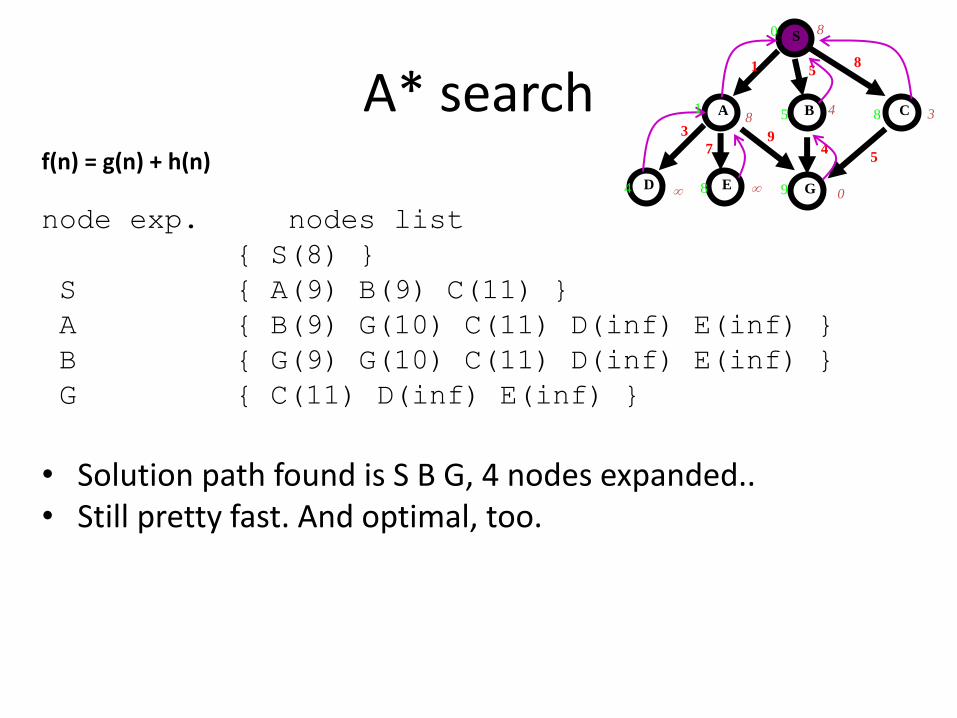
A* searchf(n) = g(n) + h(n)
node exp. nodes list
{ S(8) }
S { A(9) B(9) C(11) }
A { B(9) G(10) C(11) D(inf) E(inf) }
B { G(9) G(10) C(11) D(inf) E(inf) }
G { C(11) D(inf) E(inf) }
• Solution path found is S B G, 4 nodes expanded.. • Still pretty fast. And optimal, too.
S
CBA
D GE
1 58
94
5
3
7
8
84 3
0
0
1
4 8 9
85

Proof of the optimality of A*• Assume that A* has selected G2, a goal state
with a suboptimal solution, i.e., g(G2) > f*
• Proof by contradiction shows it’s impossible

Proof of the optimality of A*• Assume that A* has selected G2, a goal state
with a suboptimal solution, i.e., g(G2) > f*
• Proof by contradiction shows it’s impossible–Choose a node n on an optimal path to G
–Because h(n) is admissible, f* >= f(n)
– If we choose G2 instead of n for expansion, thenf(n) >= f(G2)
–This implies f* >= f(G2)
–G2 is a goal state: h(G2) = 0, f(G2) = g(G2).
–Therefore f* >= g(G2)
–Contradiction

Dealing with hard problems• For large problems, A* may require too much
space
• Variations conserve memory: IDA* and SMA*
• IDA*, iterative deepening A*, uses successive iteration with growing limits on f, e.g.
– A* but don’t consider a node n where f(n) >10
– A* but don’t consider a node n where f(n) >20
– A* but don’t consider a node n where f(n) >30, ...
• SMA* -- Simplified Memory-Bounded A*
– Uses queue of restricted size to limit memory use
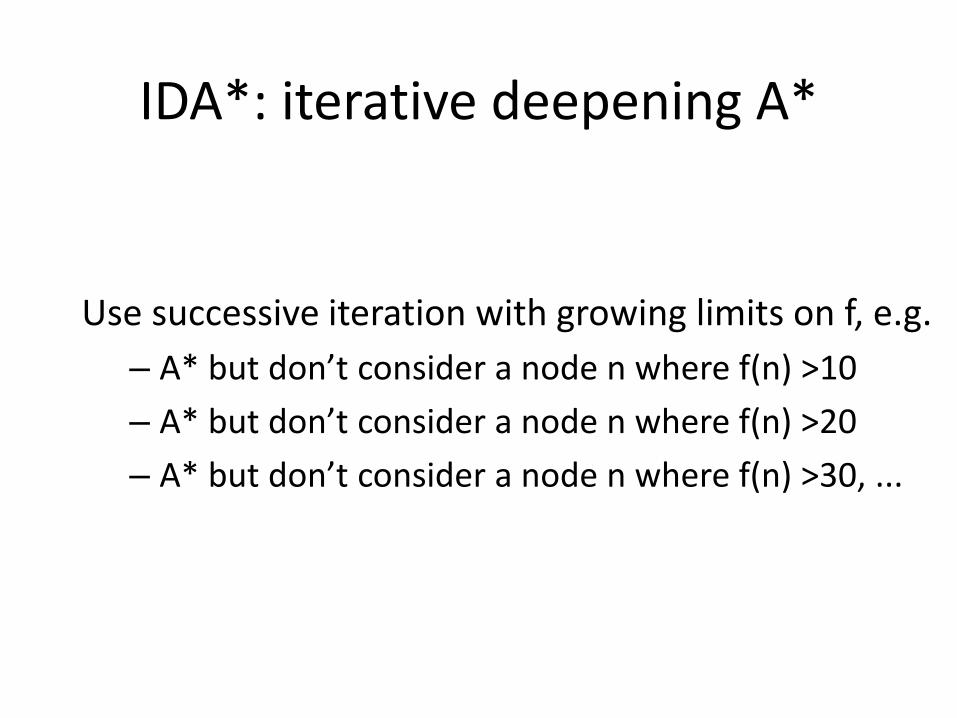
IDA*: iterative deepening A*
Use successive iteration with growing limits on f, e.g.
– A* but don’t consider a node n where f(n) >10
– A* but don’t consider a node n where f(n) >20
– A* but don’t consider a node n where f(n) >30, ...
SMA*: Simplified Memory-Bounded A*
Uses queue of restricted size to limit memory use

How to find good heuristicsSome options (mix-and-match):
• If h1(n) < h2(n) <= h*(n) for all n, h2 is better than (dominates) h1
• Relaxing problem: remove constraints for easier problem; use its solution cost as heuristic function
• Max of two admissible heuristics is a Combining heuristics: admissible heuristic, and it’s better!
• Use statistical estimates to compute h; may lose admissibility
• Identify good features, then use machine learning to find heuristic function; also may lose admissibility
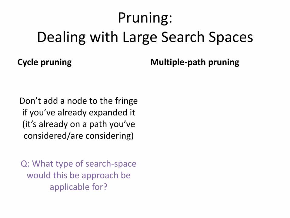
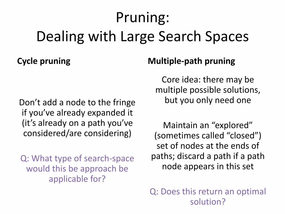
Pruning: Dealing with Large Search Spaces
Cycle pruning
Don’t add a node to the fringe if you’ve already expanded it (it’s already on a path you’ve considered/are considering)
Q: What type of search-space would this be approach be
applicable for?
Multiple-path pruning
Pruning: Dealing with Large Search Spaces
Cycle pruning
Don’t add a node to the fringe if you’ve already expanded it (it’s already on a path you’ve considered/are considering)
Q: What type of search-space would this be approach be
applicable for?
Multiple-path pruning
Core idea: there may be multiple possible solutions,
but you only need one
Maintain an “explored” (sometimes called “closed”) set of nodes at the ends of
paths; discard a path if a path node appears in this set
Q: Does this return an optimal solution?

Optimality with Multiple-Path Pruning
Some options to find the optimal solution (pulled from Ch 3.7.2)
• Make sure that the first path found to any node is a lowest-cost path to that node, then prune all subsequent paths found to that node. OR

Optimality with Multiple-Path Pruning
Some options to find the optimal solution (pulled from Ch 3.7.2)
• Make sure that the first path found to any node is a lowest-cost path to that node, then prune all subsequent paths found to that node. OR
• If the search algorithm finds a lower-cost path to a node than one already found, it could remove all paths that used the higher-cost path to the node. OR

Optimality with Multiple-Path Pruning
Some options to find the optimal solution (pulled from Ch 3.7.2)• Make sure that the first path found to any node is a lowest-
cost path to that node, then prune all subsequent paths found to that node. OR
• If the search algorithm finds a lower-cost path to a node than one already found, it could remove all paths that used the higher-cost path to the node. OR
• Whenever the search finds a lower-cost path to a node than a path to that node already found, it could incorporate a new initial section on the paths that have extended the initial path.
A* and Multiple-Path Pruning
If ℎ 𝑛 is consistent, A* with multiple-path pruning will find an optimal solution
Core Idea: Why?

A* and Multiple-Path Pruning
If ℎ 𝑛 is consistent, A* with multiple-path pruning will find an optimal solution
Core Idea: Why? (proof by contradiction: seeProposition 3.2 in Ch 3.7.2)
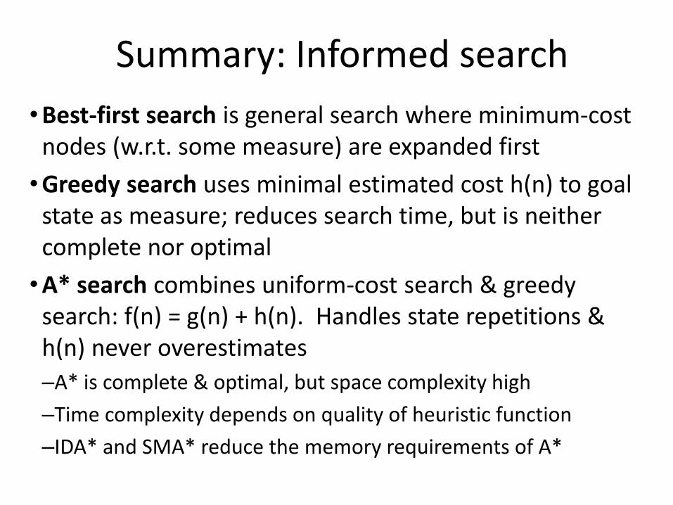
Summary: Informed search
•Best-first search is general search where minimum-cost nodes (w.r.t. some measure) are expanded first
•Greedy search uses minimal estimated cost h(n) to goal state as measure; reduces search time, but is neither complete nor optimal
•A* search combines uniform-cost search & greedy search: f(n) = g(n) + h(n). Handles state repetitions & h(n) never overestimates
–A* is complete & optimal, but space complexity high
–Time complexity depends on quality of heuristic function
–IDA* and SMA* reduce the memory requirements of A*
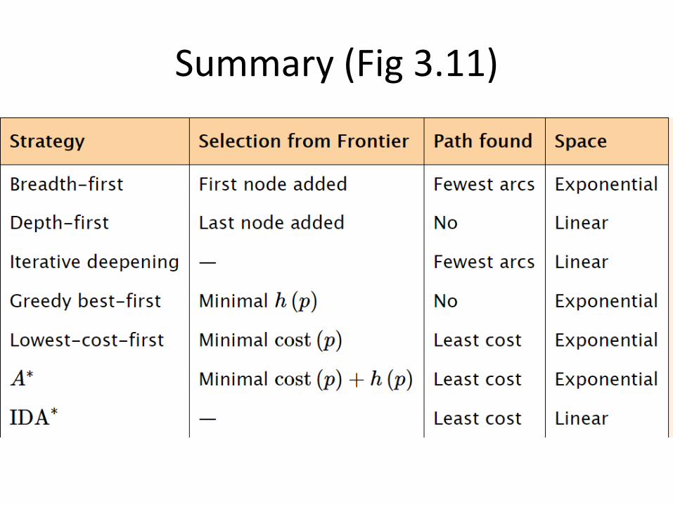
Summary (Fig 3.11)