Tellus (2008), 60B, 82–97 C© 2007 The AuthorsJournal compilation C© 2007 Blackwell Munksgaard

Printed in Singapore. All rights reservedT E L L U S

Climatic response to anthropogenic sulphate aerosolsversus well-mixed greenhouse gases from 1850

to 2000 AD in CLIMBER-2

By EVA BAUER 1∗, VLADIMIR PETOUKHOV 1, ANDREY GANOPOLSKI 1 and

ALEXEY V. ELISEEV 2, 1Potsdam Institute for Climate Impact Research, PO Box, 60 12 03, D-14412Potsdam, Germany; 2A.M. Obukhov Institute of Atmospheric Physics RAS, Moscow, Russia

(Manuscript received 3 April 2007; in final form 6 August 2007)

ABSTRACT

The Earth system model CLIMBER-2 is extended by a scheme for calculating the climatic response to anthropogenic

sulphur dioxide emissions. The scheme calculates the direct radiative forcing, the first indirect cloud albedo effect, and

the second indirect cloud lifetime effect induced by geographically resolved sulphate aerosol burden. The simulated

anthropogenic sulphate aerosol burden in the year 2000 amounts to 0.47 TgS. The best guesses for the radiative forcing

due to the direct effect are −0.4 W m−2 and for the decrease in short-wave radiation due to all aerosol effects −0.8

W m−2. The simulated global warming by 1 K from 1850 to 2000 caused by anthropogenic greenhouse gases reduces to

0.6 K when the sulphate aerosol effects are included. The model’s hydrological sensitivity of 4%/K is decreased by the

second indirect effect to 0.8%/K. The quality of the geographically distributed climatic response to the historic emissions

of sulphur dioxide and greenhouse gases makes the extended model relevant to computational efficient investigations

of future climate change scenarios.

1. Introduction

In the last century, the atmospheric concentrations of greenhouse

gases and aerosols from anthropogenic activity increased con-

siderably, thus causing a growing concern about their impact

on the climate system. Noteworthy are the growing concentra-

tions of greenhouse gases such as carbon dioxide (CO2), methane

(CH4), nitrous oxide (N2O) and the chlorofluorocarbons CFC-11

and CFC-12 and the changes in the tropospheric distribution of

sulphate aerosols. Investigations with different climate models,

ranging from simple models with a coarse resolution to sophisti-

cated general circulation models (GCMs), show that the anthro-

pogenically induced climate changes in recent decades clearly

distinguish from natural climate changes (see IPCC, 2001, and

references therein). Natural climate changes in the last millen-

nium before 1850 AD were largely caused by solar variability

and volcanic activity, but after 1850 AD the climate system is

increasingly influenced by anthropogenic activity (e.g. Crowley,

2000).

Sulphate aerosols cause a tendency of cooling due to their

direct and indirect effects exerted on the solar radiative fluxes

∗Corresponding author.

e-mail: eva.bauer@pik-potsdam.de

DOI: 10.1111/j.1600-0889.2007.00318.x

(e.g. Charlson et al., 1992; Chuang et al., 1997). Hence, the sul-

phate aerosol effects can partly compensate the enhanced global

warming generated by the long-wave absorption of the anthro-

pogenic greenhouse gases. In some regions, the temperature

rise from anthropogenic greenhouse gases may possibly even

be overcompensated by the aerosol cooling effect. The imbal-

ance between the temperature changes from the sulphate aerosol

forcing and greenhouse gas forcing is a subject of intense stud-

ies with the use of three-dimensional (3-D) atmospheric models

(Kiehl and Briegleb, 1993; Taylor and Penner, 1994; Kiehl et al.,

2000; Quaas et al., 2004) and coupled atmosphere-ocean models

(Haywood et al., 1997; Roeckner et al., 1999; Johns et al., 2003;

Harvey, 2004). In climate change simulations, the greenhouse

gases released from fossil fuel burning and industrial activity are

considered to be well mixed in the atmosphere, and global and

annual mean gas concentrations can be used. The simulation of

climate changes due to anthropogenic sulphur dioxide emissions,

however, has to account for the inhomogeneous space–time dis-

tribution of sulphate aerosols. The differences in the patterns are

related to the different lifetimes, that is, up to centuries for the

greenhouse gases and a few days for the sulphate aerosols due

to their relatively fast deposition rate.

Results from climate change simulations are often difficult

to compare. One reason is that model studies span different

time periods and therefore deal with different concentrations of

82 Tellus 60B (2008), 1

CLIMATIC RESPONSE TO ANTHROPOGENIC EMISSIONS OF SULPHUR AND GREENHOUSE GASES 83

greenhouse gases and sulphate aerosols. The simulations also

differ in the description of the sulphate aerosol distribution.

Either the sulphate aerosol burden is prescribed (Kiehl and

Briegleb, 1993; Haywood et al., 1997; Quaas et al., 2004) or a

sulphur cycle model is used (Taylor and Penner, 1994; Roeckner

et al., 1999; Kiehl et al., 2000; Johns et al., 2003). Finally, some

studies consider only the direct sulphate aerosol effect, while oth-

ers explore the direct effect together with the first indirect effect

or together with the indirect effects on clouds. Nonetheless, sim-

ulation studies provide useful information on expected ranges of

the aerosol radiative forcing and induced climate changes. The

general finding is that the sulphate aerosols produce a stronger

cooling in the Northern Hemisphere (NH) than in the Southern

Hemisphere (SH), and a stronger cooling during northern sum-

mer than during northern winter (e.g. Feichter et al., 1997; Kiehl

et al., 2000; Ming et al., 2005).

Yet, there are still open questions about implications related

to the space–time inhomogeneity of the cooling from sulphate

aerosols and the warming from greenhouse gases. In particular,

the basic reasons for the well-marked seasonality in the indicated

effects, and the role different climatic feedbacks play in the spa-

tial inhomogeneity of the response to the forcing by aerosols

and greenhouse gases are not fully understood. In this paper,

we aim at highlighting some aspects of the problem with the

use of CLIMBER-2 (Petoukhov et al., 2000; Ganopolski et al.,

2001), which is an Earth system model of intermediate complex-

ity (EMIC). We also demonstrate the robustness of our results by

comparison with analogous results from more complex general

circulation models.

CLIMBER-2 consists of interactively coupled modules for the

atmosphere, the ocean and the vegetation. The atmospheric grid

has a resolution of 10◦ in latitude and about 51◦ in longitude.

The atmospheric circulation is calculated in 10 layers and the

radiative long-wave fluxes are computed on 16 levels. The inte-

gration time step is 1 d using the daily and latitudinal resolved

insolation and solar zenith angle. The ocean consists of the zonal

mean basins of the Atlantic, the Indian and the Pacific Oceans

which are coupled through the Southern Ocean. The oceanic cir-

culation is calculated with a meridional resolution of 2.5◦ and in

20 layers with vertically increasing thickness, using a 5-d time

step. In the land surface scheme, fractions of the major vegeta-

tion types, that is, grass and forest, are determined for each grid

cell on a yearly time step. The relatively low resolution and the

parameterization of the fast (synoptic) atmospheric dynamics al-

lows for running the model over millennial time periods and for

integrated modelling purposes within a practical time frame.

CLIMBER-2 simulations of the modern climate (Petoukhov

et al., 2000; Ganopolski et al., 2001), the climate of the last glacial

maximum (Ganopolski et al., 1998a), and the climate changes

during the Holocene (Ganopolski et al., 1998b; Claussen et al.,

1999; Brovkin et al., 2002) agree on large-scales with observa-

tions and GCM simulations within error bounds. CLIMBER-2

was also applied for analysing the climate changes of the last

millennium (Bauer et al., 2003; Bauer and Claussen, 2006) and

of future warming scenarios (Rahmstorf and Ganopolski, 1999).

The climate sensitivity of CLIMBER-2 derived from equilib-

rium experiments with CO2 concentrations of 280 and 560 ppm

is 2.6 K. This value is centred in the range from 1.75 to 3.6 K

obtained in the EMIC Intercomparison Project (Petoukhov et al.,

2005) and the uncertainty range of the climate sensitivity is 1.2–

4.3 K (Schneider von Deimling et al., 2006).

So far, the sulphate aerosol effects from space–time varying

anthropogenic sulphur dioxide emissions were not investigated

with CLIMBER-2. To overcome this shortcoming, we propose

an upgrade of the CLIMBER-2 model to calculate the direct as

well as the first and second indirect sulphate aerosol effects of

anthropogenic sulphate aerosol burdens. The direct effect due

to backscattering of solar radiation is calculated in line with the

concept of Charlson et al. (1991). The calculation of the first

indirect effect, that is, the cloud albedo effect, and the second

indirect effect, that is, the cloud lifetime effect, are based on a re-

lation between the concentrations of cloud droplets and aerosol

particles (Jones et al., 1994). The climatic response to the sul-

phate aerosol effects is studied in a series of transient simulations

using the anthropogenic sulphur dioxide emission data over the

period 1850–2000 AD by Lefohn et al. (1999) and Smith et al.

(2001). The aerosol-driven simulations are complemented by in-

cluding the growing greenhouse gas concentrations. We apply in

CLIMBER-2 the so-called equivalent CO2 (eqCO2) concentra-

tion which is the CO2 concentration increased by the equivalent

CO2 contributions from the trace gases CH4, N2O, CFC-11 and

CFC-12 (Myhre et al., 1998). Thus the CO2 concentration which

grows from 284.5 to 368.2 ppm over 1850–2000, leads to an

increasing eqCO2 concentration from 287.3 to 431.4 ppm over

the 150 yr. In the present study, the anthropogenic effects from

aerosols other than sulphate, ozone and land use and the natural

effects from solar and volcanic activity are not considered.

The analysis of the CLIMBER-2 simulations focuses on the

large-scale regional and seasonal responses of the climate to

the sulphate aerosol forcing and the greenhouse gas forcing. The

next Section 2 describes the transformation of the anthropogenic

sulphur dioxide emission data into the atmospheric mass burden

of sulphate aerosols and introduces the physical-based schemes

for the calculation of the direct and the indirect sulphate aerosol

effects. Section 3 analyses the radiative forcing caused by the

anthropogenic sulphate aerosol burden and the induced climatic

changes from combining the forcing by sulphate aerosols and

greenhouse gases. Conclusions are drawn in the final Section 4.

2. Sulphur data and basic sulphateaerosol effects

2.1. Calculation of sulphate aerosol burden

The global emissions of sulphur dioxide (SO2) from fossil fuel

combustion and industrial processes have increased from about

Tellus 60B (2008), 1

84 E. BAUER ET AL.

1850 1900 1950 20000

10

20

30

40

50

60

70

80

su

lph

ur

em

issio

n (

Tg

S/y

r)

year AD

0

0.1

0.2

0.3

0.4

0.5world

NH

SH

su

lph

ate

lo

ad

ing

(T

gS

)

Fig. 1. Time series of anthropogenic sulphur dioxide emissions in

TgS yr−1 and sulphate aerosol loading in TgS for the world, the NH

and the SH over 1850–2000.

1.2 TgS yr−1 in 1850 to 68 TgS yr−1 in 2000 AD (Tg = 1012 g).

Over the years, the source strength of the global SO2 emission

and the region of maximum SO2 emission changed considerably.

In 1989, a maximum in the global source strength of 72 TgS yr−1

occurred.

Here, we use the annual inventories of the country-based an-

thropogenic emission data by Lefohn et al. (1999) for the period

1850–1990 and by Smith et al. (2001) for the period 1980–2000.

The two time series of emission patterns are spliced to obtain a

series of annual emission patterns from 1850 to 2000. Fig. 1 dis-

plays the time series of the globally aggregated SO2 emissions

in TgS yr−1 together with the partitions for the NH and the SH.

The NH emissions are seen to be roughly eight times as large as

the SH emissions.

For the subsequent simulations, the country-based anthro-

pogenic SO2 emissions are distributed among the atmospheric

grid cells of CLIMBER-2 under the condition of mass conser-

vation. The SO2 emissions are transformed to atmospheric mass

burdens of sulphate aerosols under the assumption that the coarse

resolution of the model grid and the short lifetimes of the aerosols

justify the neglect of advective and diffusive processes. Thus the

column burden B of sulphate aerosols per grid box area is

B = Eτa cm/A, (1)

where E is the mass of sulphur emitted per unit time to a grid

box, A is the surface area of the grid box, and τa is the effective

lifetime of sulphate aerosols. The column burden B is expressed

in terms of sulphate aerosol mass [g(SO4) m−2] by using the

mass conversion factor cm = 3, which accounts for the trifold

molecular weight of SO2−4 compared to the molecular weight of

S. We prescribe an effective lifetime, τa = 2.5 d. The value of τa

incorporates the loss of the precursor gas deposited to the ground

and the atmospheric turnover time of sulphate aerosols. Aerosol

cycle models yield for sulphate aerosols a mean turnover time of

4.12 d and an estimate of the precursor gas loss of 38% (Textor

et al., 2006). These values lead to an effective lifetime of 2.6 d

which is close to the corresponding value of 2.7 d given in IPCC

(2001). We implicitly assume that the SO2 oxidation and depo-

sition processes are constant throughout the year.

The global sulphate aerosol loading in TgS (Fig. 1) obtained

from the anthropogenic SO2 emissions (eq. 1) agree with the sul-

phate burdens computed with a sulphur cycle model over 1850–

2000 by Boucher and Pham (2002). The global mean anthro-

pogenic emission of 68 TgS yr−1 in the year 2000 corresponds

to a global sulphate aerosol loading of 0.47 TgS. This loading

compares also well with the anthropogenic part of the sulphate

aerosol loading in Stier et al. (2005) which amounts to 60%

of the total sulphate loading of 0.8 TgS in 2000. The anthro-

pogenic sulphate aerosol loading of 0.47 TgS corresponds to

1.41 Tg(SO4) and to a global mean column burden per area of

BG = 2.8 mg(SO4) m−2. Again, the value of BG = 2.8 mg(SO4)

m−2 is well in the range of the anthropogenic sulphate burdens

given in (table 6.4 IPCC, 2001) which extends from 1.14 to

4 mg m−2, and is in the range obtained by the AeroCom initia-

tive (Schulz et al., 2006).

In practice, the actual column burden from anthropogenic

sources in a grid box can exceed the global mean column bur-

den by an order of magnitude. The patterns of the anthropogenic

sulphate aerosol burden evolve with the industrial development,

as seen by the drift of the maximum sulphate aerosol burden

from Europe in 1989 to Southeast Asia in 2000 (Fig. 2). The

temporally changing patterns of the sulphate aerosols are of rel-

ative importance in the calculation of the sulphate aerosol effects

since the induced radiative effects depend not only on the aerosol

concentration but also on the ambient climate system properties,

such as surface albedo, insolation and cloudiness.

latitu

de

a

−180 −120 −60 0 60 120 180

−50

0

0

50

1

11

21

31

41

longitude

b

−180 −120 −60 0 60 120 180

−50

50

1

11

21

31

41

Fig. 2. Geographical distribution of sulphate aerosol mass burden B

[mg(SO4) m−2] aggregated on CLIMBER-2 grid shown for (a) 1989

and (b) 2000.

Tellus 60B (2008), 1

CLIMATIC RESPONSE TO ANTHROPOGENIC EMISSIONS OF SULPHUR AND GREENHOUSE GASES 85

2.2. Direct sulphate aerosol effect

Anthropogenic sulphate aerosols in the atmosphere induce a

negative radiative forcing (direct effect, DE) because sulphate

aerosol particles scatter short-wave radiation essentially with

no absorption. The upscattering of the insolation by sulphate

aerosols is related to an increase in the global and annual mean

planetary albedo, ap , of the Earth–atmosphere system. (We use ·to indicate global and annual averaging.) An increase in the plan-

etary albedo by �ap corresponds to a decrease in insolation by

�F = −(S0/4)�ap , where S0 is the solar constant. In the con-

text of radiative forcing, sulphate aerosols from anthropogenic

emissions can be treated as an optically thin layer (aerosol optical

thickness δa � 1) located in the near-surface troposphere. In that

case, the global and annual mean of the radiative forcing at the

top of the atmosphere (TOA) from the direct effect of sulphate

aerosols with no absorption is assessed to a first approximation

(Charlson et al., 1991, 1992)

�FR = − S0

2Ti

2(1 − Ac) (1 − as)2 β δa, (2)

where Ti , Ac, as, β and δa are global and annual mean values

of, respectively, transmittance for the solar radiation in the at-

mosphere above the aerosol layer, cloud fraction, albedo of the

Earth’s surface, fraction of the insolation scattered upward by

sulphate aerosols and their scattering optical thickness. Thus the

direct radiative forcing due to a sulphate aerosol layer increases

with increasing δa and Ti , and with decreasing Ac and as . The

scattering optical thickness δa in eq. (2) can be estimated by

the product of the mass scattering coefficient σ and the column

burden B of the sulphate mass (Charlson et al., 1991)

δa = σ B. (3)

According to eq. (3), the global and annual mean sulphate

aerosol optical thickness in 2000 is δa = 0.01 when using for

B the anthropogenic burden BG = 2.8 mg(SO4) m−2 and a

mass scattering efficiency σ = 3.5 m2 g−1 which is the central

value in the uncertainty range for polluted continental aerosols

at wavelength 0.55 μm (IPCC, 2001, Table 5.10a). The value

of δa = 0.01 lies close to optical depths determined for sulphate

aerosols in 2000 relative to 1750 by the AeroCom initiative.

The optical depth range for the total sulphate aerosol loading is

0.015–0.051 (Kinne et al., 2006) and the optical depth range for

anthropogenic sulphate aerosols is 0.006–0.042 (Schulz et al.,

2006).

Typical values for eq. (2) are Ti = 0.76 (Charlson et al., 1992),

β = 0.23 (IPCC, 2001, table 5.10a), S0 = 1365 W m−2 and from

a CLIMBER-2 simulation for present climate conditions (see

Section 3.2), as = 0.155 and Ac = 0.65. Inserting the above val-

ues in eq. (2) yields �FR = −0.23 W m−2. However, �FR based

on eq. (2) represents a rough approximation as, for instance, the

contribution from the cloudy atmosphere is neglected and differ-

ing shares from the inhomogeneous spatial distribution of sul-

phate aerosols and ambient climate conditions are ignored (e.g.

Boucher et al., 1998). Actually, the local direct radiative forcing

of the sulphate aerosols can differ substantially from the global

mean because of space–time variations in solar radiation, so-

lar zenith angle, scattering optical thickness of aerosols, albedo

of the Earth’s surface and cloudiness. 3-D atmospheric models

(see IPCC, 2001, table 6.4) yield for the direct radiative forcing

due to anthropogenic sulphate aerosols values between −0.28

and −0.82 W m−2 and the AeroCom initiative presents values

between −0.19 and −0.96 W m−2 (Schulz et al., 2006).

The short-wave scheme of CLIMBER-2 computes the atmo-

spheric transmittance of the solar radiation as a function of wa-

ter vapour, carbon dioxide, liquid cloud water and background

aerosol content using the solar radiation and the solar zenith angle

on a daily time step for each grid cell (Petoukhov et al., 2000). We

adopt the approach of Charlson et al. (1991) to compute regional

and seasonal resolved climate changes from the anthropogenic

sulphur emissions. This implies for the computation of the local

DE the introduction of the combined surface–aerosol albedo

asa = aa + T 2a as

[1 + aaas + (aaas)2 + · · · ], (4)

where as and aa denote the local values, respectively, of the

albedo of the Earth’s surface and the albedo of the near-surface

sulphate aerosol layer while Ta = 1 − aa is the transmittance of

the sulphate aerosol layer on the assumption that the short-wave

radiation is not absorbed by sulphate aerosols. The combined

albedo asa in eq. (4) describes multiple reflections between the

aerosol layer and the surface which is expressed by

asa = aa + T 2a as

1 − aaas. (5)

The combined albedo asa substitutes for the surface albedo

as of each grid cell in the short-wave radiation scheme of the

upgraded CLIMBER-2 model. Eq. (5) reveals that asa increases

with aa , and that asa reduces to the surface albedo as when the

aerosol burden vanishes. For a given aa the lower as is, the larger

is the difference asa − as . This implies a larger cooling for sul-

phate aerosols above dark surfaces than for sulphate aerosols

above bright surfaces. Following Charlson et al. (1991), the

aerosol albedo is

aa = β δa sec θ, (6)

where δa is given by eq. (3), but with local sulphate aerosol

burden B and local mass scattering coefficient σ in the right

side of eq. (3), β is the local upscatter fraction of the insolation,

and sec θ is the secant of the local solar zenith angle θ . Eq. (6)

applies for the direct solar radiation in clear sky conditions, and

in cloudy conditions θ is replaced by the effective zenith angle

θe with characteristic value sec θe = 1.66 (Liou, 1992).

The local sulphate aerosol mass scattering efficiency σ and

upscatter fraction β depend on the microphysical properties

of particle size distribution, aerosol composition, and relative

Tellus 60B (2008), 1

86 E. BAUER ET AL.

Table 1. Parameters for calculation of sulphate aerosol effects and

effective parameter values used in the presented simulations

Parameter Effective value

Lifetime of aerosols τa = 2.5 d

Aerosol scale height Ha = 1500 m

Upscatter fraction β = 0.23

Scattering efficiency σ = 3.5 m2 g−1

Natural CCN number conc. Nnata = 75 × 106 m−3

Aerosol radiusa ra = 0.15 μm

aSimulation results of indirect sulphate aerosol effects are also

presented for ra = 0.1 μm.

humidity (RH) (Chylek and Wong, 1995; Nemesure et al., 1995;

Pilinis et al., 1995; Boucher et al., 1998). The dependence of β

on the solar zenith angle and the aerosol phase function of light

scattering is implicitly included by an average over the solar

zenith angle. Sulphate aerosol particles which reside in the size

range of the accumulation mode (particle radii between 0.05 and

1 μm) are hygroscopic and their size grows with increasing RH

(Li et al., 2001; Takemura et al., 2005; Randriamiarisoa et al.,

2006). For solar wavelengths, an increase in the particle radius

is accompanied, on the one hand, with an increase in σ , and on

the other hand, with a decrease in β. The range of uncertainty in

the radiative forcing due to changes in σ and β with changes in

RH and particle size can be estimated based on the uncertainty

ranges for σ from 2.3 to 4.7 m2 g−1 and for β from 0.17 to 0.29

(IPCC, 2001, table 5.10a). Hence, from eqs (2) and (3) a lower

value of the direct radiative forcing �FR , representative for dry

aerosol particles, can be estimated using σd = 2.3 m2 g−1 and

βd = 0.29, while an upper value of �FR , representative for wet

aerosol particles, can be estimated using σw = 4.7 m2 g−1 and

βw = 0.17. The use of σw and βw leads practically to the same

�FR as estimated with the central values of σ and β, while �FR

becomes only 20% smaller when using σd and βd . For that rea-

son, we utilise in the following calculation of the local DE the

central values for σ and β (Table 1) which are appropriate for

usual ambient humidity.

2.3. Indirect sulphate aerosol effects

Sulphate aerosols affect the microphysical properties of clouds

which can be expressed in terms of changes in the cloud optical

thickness (first indirect effect, FIE) and changes in the lifetime

of clouds (second indirect effect, SIE). The emission of sulphur

involves an increase in the number of sulphate aerosol particles

in clouds and thus an increase in the number of cloud conden-

sation nuclei (CCN). The consequence of seeding a cloud with

CCN is a decrease in the effective radius of the cloud droplets. A

common assumption is that the decrease in the droplet radius is a

process during which the liquid-water content of the clouds and

the geometric thickness of the clouds hardly change (Twomey,

1974). Thus, FIE can be described to a first approximation by an

increase in the cloud optical thickness. In addition, the decrease

in the effective radius of the cloud droplets causes a decrease in

the rate of autoconversion (Albrecht, 1989). In consequence, the

formation of precipitation is inhibited, which prolongs the cloud

lifetime. Thus, SIE can be described by an increased character-

istic time of the rain drop formation. This leads to an increase in

the cloud fraction, provided the other cloud processes as well as

the advective and turbulent motions are retained.

A simulation of the indirect effects is accompanied with large

uncertainties due to a still incomplete understanding of the con-

tributing processes. Based on the current knowledge, a reason-

able way to account for FIE and SIE due to sulphate aerosol

burdens in CLIMBER-2 is to modify the optical thickness of

clouds, and the characteristic turnover time of the precipitable

liquid water of clouds, respectively. To modify these parameters

in dependence of the sulphate aerosol burden, we use a sim-

ple scheme to transform the sulphate mass burden into a number

concentration of sulphate aerosol particles which is further trans-

formed into a number concentration of cloud droplets.

The determination of FIE is based on the definition of the

short-wave optical thickness δc of liquid-water clouds

δc = 3 w0 Hc

2 ρw rc, (7)

where w0 is the cloud liquid-water content (kg m−3), Hc is the

cloud geometric thickness, ρw is the water density, and rc is the

effective radius of cloud droplets (e.g. Liou, 2002). The determi-

nation of rc depends mainly on w0 and the number concentration

of cloud droplets Nc

rc =(

3 w0

4π ρw κ Nc

)1/3

, (8)

where κ = 0.67 in continental air masses and κ = 0.8 in maritime

air masses (Jones et al., 1994; Martin et al., 1994). Based on the

assumption that w0 and Hc remain unchanged when clouds are

seeded with CCN, eqs (7) and (8) show that δc is proportional to

the third root of the cloud droplet number concentration

δc(Nc) ∝ (Nc)1/3. (9)

In turn, Nc depends on the CCN number concentration, Na , at

the cloud base

Nc(Na) = Nc,0 [1 − exp{−αc Na}], (10)

where the empirical coefficients are Nc,0 = 375 × 106 m−3 and

αc = 2.5 × 10−9 m3 (Jones et al., 1994). Alternative relationships

for Nc(Na) as discussed in Jones et al. (2001) are found to cause

relatively small differences in the present coarse scale applica-

tions. The CCN number concentration Na consists of the natural

CCN concentration Nnata and the anthropogenic sulphate aerosol

concentration Nanta at the cloud base. Combining eqs (9) and (10)

Tellus 60B (2008), 1

CLIMATIC RESPONSE TO ANTHROPOGENIC EMISSIONS OF SULPHUR AND GREENHOUSE GASES 87

shows that the emission of anthropogenic sulphate aerosols re-

sults in a modified cloud optical thickness

δc(Na) = δc

(N nat

a

)[ fmod]1/3, (11)

where δc(Nnata ) is the cloud optical thickness computed in

CLIMBER-2 using a background concentration Nnata of natural

CCN and f mod is given by

fmod = 1 − exp{−αc Na}1 − exp

{−αc N nata

} . (12)

Since natural CCN consist mainly of sulphate aerosol particles,

we consider Nnata to represent a background concentration of

natural sulphate aerosols. A mean value of Nnata = 75 × 106 m−3

was determined for pre-industrial times at the cloud base by

Jones et al. (1994). The value of Nnata is difficult to assess but

the value is compatible with the approximate minimum aerosol

number concentration of 100 × 106 m−3 at the surface (Kiehl

et al., 2000) and of 80 × 106 m−3 below marine clouds (Twohy

et al., 2005).

The anthropogenic sulphate aerosol concentration at the

cloud base Nanta can be determined by assuming that the sul-

phate aerosol number concentration decreases exponentially

with height. Thus, Na consisting of anthropogenic and natural

sulphate aerosols at the cloud base is

Na = N anta (0) exp{−Hst/Ha} + N nat

a , (13)

where Nanta (0) is the anthropogenic sulphate aerosol number

concentration at the surface, Ha is the aerosol scale height, and

Hst is the effective height of the cloud base. We prescribe Ha =1500 m analogous to the scale height of the specific humidity

in CLIMBER-2, while Hst is a prognostic variable in the cloud

scheme (Petoukhov et al., 2000). The value of Nanta (0) follows

directly from

N anta (0) = Lant

a /Ha, (14)

where Lanta is the column-integrated anthropogenic aerosol num-

ber burden (m−2). The value of Lanta can be inferred from the

column-integrated sulphate aerosol mass burden B

Lanta = B

ρa 4/3 π r 3a

, (15)

where ρa = 1.769 × 106 g m−3 is the density of sulphate aerosols

and ra is the effective radius of sulphate aerosol particles.

Under the ideal assumption that all climate variables are

retained, eqs (12)–(15) yield f mod = 1.21, by use of BG =2.8 mg(SO4) m−2, Hst = 4000 m, ra = 0.1 μm, and the above

empirical values for Nnata , αc and Ha . According to eq. (11) this

implies an increase of the global mean cloud optical thickness

by about 6%. We note that the sulphate aerosol radius increases

with relative humidity in the atmosphere (see discussion in Sec-

tion 2.2). Considering of the aerosol size distribution in polluted

regions, ra of sulphate aerosols ranges typically between 0.1 and

0.2 μm (Randriamiarisoa et al., 2006). Repeating the above cal-

culation of f mod using a 50% larger effective radius, that is, ra =0.15 μm, leads to f mod = 1.09 which implies an increase of δc by

2% only.

The determination of SIE is based on a theoretical relationship

for the precipitation rate (Petoukhov, 1991; Liou, 1992). With the

conventional assumption that the precipitation rate P in stratus

and cumulus clouds depends primarily on the autoconversion

process from small to large cloud droplets, P increases with

cloud thickness and decreases with the number concentration of

cloud droplets

P ∝ (Hc)m+n/3 (Nc)−n/3, (16)

where m ≈ 1 and n ≈ 3. If we again assume that Hc remains

constant when seeding clouds with sulphate aerosols, eq. (16)

reduces to

P ∝ (Nc)−1. (17)

Thus the modified precipitation rate due to seeding clouds

with anthropogenic sulphate aerosols can be described by

P(Na) = P(N nat

a

)/ fmod, (18)

where P(Nnata ) is the precipitation rate calculated in accord with

the scheme of the hydrological cycle under a background con-

centration of natural aerosols and f mod is defined by eq. (12).

According to eq. (8) and under the same assumptions as before,

SIE would yield a reduced global mean precipitation of 9–21%

by use of BG = 2.8 mg(SO4) m−2. We note that the actual pre-

cipitation change is computed consistently with the distributions

of temperature and specific humidity.

2.4. Transient simulations

The modifications in the short-wave radiation scheme and in the

cloud and precipitation scheme of CLIMBER-2 are tested in a

series of simulations using the space–time varying sulphur emis-

sions over 1850–2000 AD. The initial condition of all transient

simulations is the equilibrium state of the CLIMBER-2 model

driven with the eqCO2 concentration corresponding to the initial

year 1850, that is, Cc = 287.3 ppm. The sulphate aerosol effects

in this study are computed with the use of the effective parameter

values (Table 1). Different simulations are conducted to account

for the three aerosol effects separately or in combination, which

is indicated in the name of simulation A by three lower indices

(Table 2). The first, second and third lower indices at A corre-

spond to the aerosol effects, respectively, DE, FIE and SIE. The

lower index is 1 if the corresponding effect is accounted for, and

0 if it is not.

The simulations are divided in two subsets with (i) fixed green-

house gas concentration (Cc) and (ii) growing greenhouse gas

concentrations (Ce). The first subset of simulations is conducted

to test the sensitivity of the radiative effects to the effective

paramter values. The radiative effects due to the indirect aerosol

Tellus 60B (2008), 1

88 E. BAUER ET AL.

Table 2. Notation of transient simulations over 1850–2000 AD with

different combinations of direct effect (DE), first indirect effect (FIE),

and second indirect effect (SIE) using two different effective radii ra ,

under constant or growing greenhouse gas concentrations

Simulation Greenhouse Aerosol effect ra

gas conc. DE FIE SIE (μm)

A100Cc const. 1 0 0 a

Ar110Cc const. 1 1 0 0.10

Ar111Cc const. 1 1 1 0.10

A110Cc const. 1 1 0 0.15

A111Cc const. 1 1 1 0.15

A100Ce grow. 1 0 0 a

A110Ce grow. 1 1 0 0.15

A111Ce grow. 1 1 1 0.15

Ce grow. 0 0 0 –

aThe direct aerosol effect is only implicitly influenced by ra (see

discussion in Section 2.2).

forcing of FIE and SIE are found to be very sensitive to the

effective radius of the sulphate aerosols (Section 2.3). This is

demonstrated by displaying the radiative effects obtained for

two values, ra = 0.10 and 0.15 μm. The usage of ra = 0.1 μm

is marked in the name A by the upper index r (Table 2). The

second subset of simulations serves to study the interplay of the

effects from the sulphate aerosol and the greenhouse gas forc-

ing. Finally, the simulation Ce is performed with growing eqCO2

concentration and without aerosol effects to compare individual

climatic responses.

3. Results

3.1. Radiative forcing from sulphate aerosol burdenin 2000

The short-wave radiative forcing of sulphate aerosols is calcu-

lated via the instantaneous change in the short-wave radiation

at TOA due to seeding sulphate aerosols into the lower tropo-

sphere while holding the surface and tropospheric temperatures

and the other climate variables fixed. Thus the global and annual

mean radiative forcing due to the direct sulphate aerosol effect

is comparable with �FR in eq. (2). (Henceforth, we omit · for

global and annual means.) Also, the short-wave radiative forcing

of FIE through changing the cloud optical thickness can be cal-

culated by holding all other climate variables fixed. In contrast,

the radiative forcing attributed to SIE represents an approximate

value since a change in the cloud lifetime involves changes in

cloud fraction and atmospheric temperature.

Table 3 shows the global and hemispheric short-wave radiative

forcing caused by the anthropogenic sulphur dioxide emissions

in 2000. In the global and annual mean, the radiative forcing of

the direct effect is �FR = −0.41 W m−2 which is in the range of

Table 3. Shortwave radiative forcing �FR due to combinations of

sulphate aerosol effects for the anthropogenic sulphur emission in 2000

given as global, NH and SH means using two different effective radii ra

of sulphate aerosols and eqCO2 concentration of 1850

Simulation �FR �FNHR �FSH

R�FNH

R�FSH

Rra

(W m−2) (W m−2) (W m−2) (μm)

A100Cc −0.41 −0.71 −0.10 7.1 –

Ar010Cc −1.03 −1.70 −0.37 4.6 0.10

Ar001Cc −1.15a −1.66a −0.63a 2.6 0.10

Ar110Cc −1.42 −2.37 −0.47 5.1 0.10

Ar111Cc −1.44a −2.41a −0.48a 5.1 0.10

A010Cc −0.42 −0.71 −0.12 5.9 0.15

A001Cc −0.48a −0.73a −0.23a 3.2 0.15

A110Cc −0.81 −1.41 −0.22 6.4 0.15

A111Cc −0.81a −1.40a −0.22a 6.3 0.15

aRadiative forcing of SIE is an approximate value from the change in

short-wave radiation at TOA since climate variables are not kept fixed.

the direct radiative forcing given in IPCC (2001), and in the range

from −0.16 to −0.58 W m−2 given in Schulz et al. (2006). In

2000, the ratio of the anthropogenic burden of sulphate aerosols

from NH and SH is 8.1, and the ratio of the direct radiative forcing

in NH and SH is �FNHR /�FSH

R = 7.1 in simulation A100Cc. This

ratio of the hemispheric radiative forcing is at the upper edge of

the range of values compiled by the IPCC (2001). Ratios of the

hemispheric radiative forcing from simulations including FIE

and SIE tend to become smaller than the ratio from including

only DE.

The annual mean pattern of the direct radiative forcing resem-

bles the pattern of sulphate aerosol burden (compare Figs. 3a and

2b). Nevertheless, the aerosol burden, which is constant over the

year, involves a seasonally changing direct radiative forcing due

to the seasonal changes in insolation, surface albedo and cloudi-

ness. Hence, the radiative forcing which is concentrated over

the areas of main sulphur dioxide emissions in North America,

Europe and Southeast Asia is about twice as strong in the boreal

summer months (JJA, Fig. 3c) than in the boreal winter months

(DJF, Fig. 3b).

3.2. Climatic responses to sulphate aerosol burdenover 1850–2000

The responses of the climate variables to the year-to-year vary-

ing sulphur dioxide emissions (Section 2.1), which modify the

combined surface–aerosol albedo (Section 2.2), the cloud opti-

cal thickness and the turnover time of cloud water (Section 2.3)

are displayed as global and annual means in Fig. 4. The sulphate

aerosol albedo aa (eq. 6) grows uniformly in all simulations up

to about 0.005 (Fig. 4a). In 2000, the relative increase in surface

albedo as with respect to as of 1850 is 0.5, 1.3 and 2.4% obtained

in the simulations A100Cc, A110Cc and A111Cc, respectively

Tellus 60B (2008), 1

CLIMATIC RESPONSE TO ANTHROPOGENIC EMISSIONS OF SULPHUR AND GREENHOUSE GASES 89

latitu

de

a

−180 −120 −60 0 60 120 180

−50

−50

0

50

latitu

de

b

−180 −120 −60 0 60 120 180

0

50

longitude

latitu

de

c

−180 −120 −60 0 60 120 180

−50

0

50

−7.7

−6.2

−4.7

−3.2

−1.7

−0.2

−7.7

−6.2

−4.7

−3.2

−1.7

−0.2

−7.7

−6.2

−4.7

−3.2

−1.7

−0.2

Fig. 3. Horizontal distribution of the direct radiative forcing �FR

(W m−2) due to sulphate aerosol burden in 2000 (see Fig. 2b) shown

for (a) annual mean, (b) DJF and (c) JJA from simulation A100Cc .

(Fig. 4b). The increase in as is connected with an increase of

the sea ice area and the snow coverage. The combined surface–

aerosol albedo asa (eq. 5) shows in 2000, relative to 1850, in-

creases of 2.3, 3.1 and 4.1% in the simulations A100Cc, A110Cc

and A111Cc, respectively (Fig. 4c).

Increases in as and asa involve increases in the planetary albedo

(Fig. 4d) whereby the absorbed insolation at TOA, F = S0(1 −ap)/4, decreases (Fig. 4e). The change in the absorbed insola-

tion consists primarily of the aerosol-induced direct radiative

forcing and is amplified by radiative contributions from induced

increases in surface albedo and cloud albedo. For instance in sim-

ulation A100Cc, the direct radiative forcing is �FR = −0.41 W

m−2 while the decrease in insolation is �F = −0.52 W m−2 as

a result of positive feedback processes. The climatic response,

which incorporates the feedback processes, is characterised by

a decrease in surface air temperature (Fig. 4f), an increase in

cloud fraction (Fig. 4g) and a decrease in precipitation rate

(Fig. 4h). The cooling through DE in simulation A100Cc involves

a relatively small increase in cloud fraction (0.1%) and a rela-

tively small decrease in precipitation rate (−0.8%). In simulation

A110Cc, DE and FIE produce also small relative changes in cloud

fraction (0.2%) and precipitation rate (−1.3%), but in simulation

A111Cc, all aerosol effects together involve significant changes in

cloud fraction (0.8%) and precipitation rate (−3.2%). The cool-

ing associated with SIE is a minor implication of the increase in

cloud lifetime.

3.3. Climatic responses to sulphate aerosolsand greenhouse gases

3.3.1. Global and hemispheric means. The individual sulphate

aerosol effects lead at the end of the 150 year-long simulations

to cooler global temperatures by −0.17, − 0.18 and −0.07 K

in the simulations A100Cc, A010Cc and A001Cc, respectively. TheeqCO2-driven simulation Ce leads to a warming of the global tem-

perature by 1.0 K. The eqCO2-induced global warming declines

successively through the activation of the sulphate aerosol effects

in the simulations A100Ce (0.84 K), A110Ce (0.68 K) and A111Ce

(0.59 K). The sum of the individual temperature changes is seen

to agree closely with the temperature response to all effects in

simulation A111Ce (Table 4).

The aerosol-induced cooling is always larger in NH than in

SH with the ratio �T N H /�TSH ≈ 2.5, irrespective of the ac-

tivated aerosol effect. The eqCO2-induced warming is larger in

NH (1.16 K) than in SH (0.84 K). Although the aerosol-induced

cooling is larger in NH than in SH, in the simulation A100Ce

the NH warming (0.91 K) exceeds the SH warming (0.76 K).

Only the activation of FIE and SIE in A110Ce and A111Ce leads

to less warming in NH than in SH. The apparent linearity in

the temperature response to different types of forcing can also

be seen for the hemispheric temperatures. However, the ratio

�TNH/�TSH in A100Cc (Table 4) is at least a factor two smaller

than the corresponding ratio of the direct radiative forcing

(Table 3) indicating that the hemispheric response to the different

direct radiative forcing in NH and SH is partially compensated by

internal processes. These processes comprise interhemispheric

exchanges of sensible and latent heat due to the Hadley cell cir-

culation and the macroturbulence associated with synoptic scale

eddies/waves (Peixoto and Oort, 1992) and also exchanges by

the oceanic transport; although the latter two contributions are

less important than the Hadley cell circulation.

The global and annual mean precipitation changes are seen

to be correlated with the temperature changes (Table 4). The

cooling in the aerosol-driven simulations is accompanied with

less precipitation reaching up to −3.4% in simulation A111Cc.

The warming in simulation Ce is associated with an increased

precipitation rate (4%), and the dominance of the eqCO2-induced

warming over the aerosol-induced cooling leads to an increased

precipitation rate (0.5%) in the simulation A111Ce. However, the

NH decrease in the precipitation rate (−1%) in simulation A111Ce

shows that the aerosol-induced precipitation decrease overcom-

pensates the eqCO2-induced precipitation increase.

The correlation between precipitation rate and temperature

can be expressed by the hydrological sensitivity. The simulations

accounting for DE, FIE or the eqCO2 concentration yield �P/

�T ≈ 4%/K (Table 4). That value agrees closely with 3.9%/K

in Feichter et al. (2004) from the aerosol-driven simulation but

Tellus 60B (2008), 1

90 E. BAUER ET AL.

1850 1900 1950 20000

0.005

0.01

a

a

a (

)

1850 1900 1950 2000233

234

235

236

e

F (

W/m

2)

1850 1900 1950 20000.152

0.154

0.156

0.158

0.16

0.162

b

as (

)

1850 1900 1950 2000

13.6

13.8

14

f T

(d

eg

.C)

1850 1900 1950 20000.152

0.154

0.156

0.158

0.16

0.162

c

as

a (

)

1850 1900 1950 20000.645

0.65

0.655

g

Ac (

)

1850 1900 1950 20000.308

0.31

0.312

0.314

0.316

0.318

d

year AD

ap (

)

1850 1900 1950 20002.6

2.65

2.7

2.75

h

year AD

h h

P (

mm

/d)

Fig. 4. Time series over 1850–2000 from

simulations (see Table 2) A100Cc (dotted),

A110Cc (dashed) and A111Cc (continuous)

showing global and annual means of (a)

aerosol albedo aa , (b) surface albedo as , (c)

combined surface–aerosol albedo asa , (d)

planetary albedo ap , (e) absorbed short-wave

radiation at TOA F (W m−2), (f) surface air

temperature T (◦C), (g) cloud fraction Ac and

(h) precipitation rate P (mm d−1). Thin

straight lines mark initial value in 1850.

Table 4. Changes in surface air temperature �T in K and precipitation

rate �P in % in 2000 relative to 1850 as global, NH and SH means.

The precipitation changes are normalised by the precipitation rate in

1850 of 2.72, 2.67 and 2.78 mm d−1 for the global, NH and SH mean,

respectively

Simulation �T �TNH �TSH �P �PNH �PSH �P�T

(K) (K) (K) (%) (%) (%) (%/K)

A100Cc −0.17 −0.25 −0.10 −0.7 −1.1 −0.3 4.0

A010Cc −0.18 −0.26 −0.11 −0.7 −1.0 −0.4 3.7

A001Cc −0.07 −0.10 −0.04 −2.1 −3.5 −0.7 a

A110Cc −0.35 −0.52 −0.19 −1.4 −2.1 −0.7 3.9

A111Cc −0.43 −0.62 −0.23 −3.4 −5.5 −1.4 8.0

A100Ce 0.84 0.91 0.76 3.3 3.7 2.9 3.9

A010Ce 0.84 0.91 0.77 3.3 3.8 2.9 3.9

A001Ce 0.94 1.05 0.82 1.8 1.2 2.5 1.9

A110Ce 0.68 0.66 0.70 2.6 2.7 2.6 3.8

A111Ce 0.59 0.53 0.65 0.5 −1.0 1.9 0.8

Ce 1.00 1.16 0.84 4.0 4.9 3.2 4.0

aThe determination of �P/�T from simulation with SIE has little

meaning as SIE involves a change in P while the change in T is minor.

overestimates the value of 1.5%/K in Feichter et al. (2004) from

the greenhouse-gas simulation. We note, however, that the study

by Feichter et al. (2004) includes additional aerosol effects from

black carbon and particulate organic matter which precludes a

further analysis of the differences in the hydrological sensitivity.

3.3.2. Zonal means for winter and summer. The seasonal re-

sponses of climate system variables to the spatially varying sul-

phate aerosol burden and the homogeneous eqCO2 concentration

are exhibited by zonal mean changes for DJF (Fig. 5) and JJA

(Fig. 6). The changes are calculated by subtracting zonal means

of 1850 from zonal means of 2000 and the relative changes are

given with respect to the zonal mean of 1850. The zonal mean

changes are shown from simulations A111Cc, Ce and A111Ce.

The regionally limited sulphate aerosol burden (Figs. 5a and

6a) causes a global cooling in A111Cc, which exceeds 1 K north of

60◦N in DJF (Fig. 5b) and also at 40–70◦N in JJA (Fig. 6b). TheeqCO2-induced warming overcompensates the aerosol-induced

cooling, and A111Ce yields a warming of more than 1 K north of

70◦N during DJF, and a larger warming in SH than in NH during

JJA. The precipitation rate reduces globally in A111Cc through the

Tellus 60B (2008), 1

CLIMATIC RESPONSE TO ANTHROPOGENIC EMISSIONS OF SULPHUR AND GREENHOUSE GASES 91

−50 0 500

5

10

B (

mg

(SO

4)/

m2)

a

−50 0 50−2

0

2

Δ T

(K

)

b

−50 0 50

−10

0

10

20

30

c

Δ P

(%

)

latitude

−50 0 50−5

0

5

d

Δ a

p (

%)

−50 0 50

−10

0

10 e

Δ a

s (

%)

−50 0 50−5

0

5

f

Δ A

c (

%)

latitude

Fig. 5. Zonal means for DJF from

simulations A111Cc (dashed), Ce (dotted) and

A111Ce (continuous). Panels show (a) mass

burden of sulphate aerosols B [mg(SO4)

m−2] in year 2000 and (b) surface air

temperature change �T (K) in 2000 relative

to 1850, and panels (c)–(f) show relative

changes from 1850 to 2000 by normalisation

with mean of 1850 for (c) precipitation �P(%), (d) planetary albedo �ap (%), (e)

surface albedo �as (%) and (f) cloud

fraction �Ac (%).

−50 0 500

5

10

B (

mg

(SO

4)/

m2)

a

−50 0 50−2

0

2

Δ T

(K

)

b

−50 0 50−30

−20

−10

0

10

c

Δ P

(%

)

latitude

−50 0 50−5

0

5

d

Δ a

p (

%)

−50 0 50

−10

0

10 eΔ

as (

%)

−50 0 50−5

0

5

f

Δ A

c (

%)

latitudeFig. 6. As Fig. 5 but for JJA; note different

range of relative precipitation change in (c).

aerosol effects. During DJF, the relative change in precipitation

rate is about −10% at 20–30◦N and north of 80◦N (Fig. 5c), and

reaches about −20% at 20–40◦N in JJA (Fig. 6c). The eqCO2-

induced change in precipitation is positive everywhere. In total,

the simulation A111Ce yields latitudinally varying rain changes.

These zonal mean changes are positive in SH and in the tropical

latitudes, negative in the northern subtropical and mid latitudes,

and again positive in the high northern latitudes in both seasons.

The planetary albedo in simulation A111Cc is seen to increase

by more than 4% in the latitudes of main sulphate aerosol bur-

den in both seasons (Figs. 5d and 6d). The increase in the plane-

tary albedo outweighs the relatively small decrease in planetary

albedo connected with the eqCO2 forcing. In contrast, the sur-

face albedo changes mainly in latitudes with snow and ice cover

(Figs. 5e and 6e). The relative changes in as in A111Cc approach

9% at 50–60◦N during DJF and 6% north of 60◦N during JJA.

The changes in as in simulation Ce are about −10% at 60–70◦S

and north of 70◦N. Thus in A111Ce, as decreases around Antarc-

tica up to 8% during DJF and JJA because the eqCO2-induced

warming effect overcompensates the aerosol-induced cooling ef-

fect, while as varies in NH between ±5% in both seasons. The

relative changes in cloud fraction show latitudinal variations of

inverse sign from the aerosol forcing and the eqCO2 forcing in

both seasons (Figs. 5f and 6f). The total effect on cloud fraction

Tellus 60B (2008), 1

92 E. BAUER ET AL.

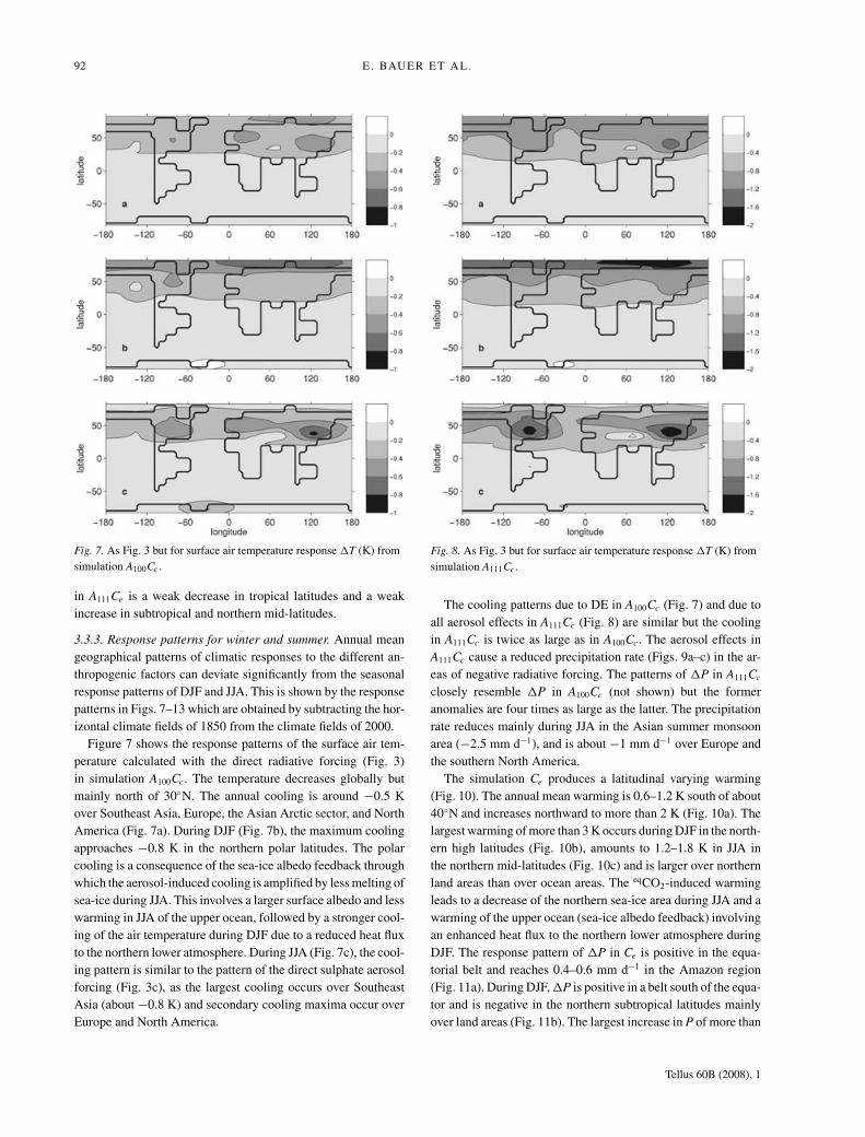
Fig. 7. As Fig. 3 but for surface air temperature response �T (K) from

simulation A100Cc .

in A111Ce is a weak decrease in tropical latitudes and a weak

increase in subtropical and northern mid-latitudes.

3.3.3. Response patterns for winter and summer. Annual mean

geographical patterns of climatic responses to the different an-

thropogenic factors can deviate significantly from the seasonal

response patterns of DJF and JJA. This is shown by the response

patterns in Figs. 7–13 which are obtained by subtracting the hor-

izontal climate fields of 1850 from the climate fields of 2000.

Figure 7 shows the response patterns of the surface air tem-

perature calculated with the direct radiative forcing (Fig. 3)

in simulation A100Cc. The temperature decreases globally but

mainly north of 30◦N. The annual cooling is around −0.5 K

over Southeast Asia, Europe, the Asian Arctic sector, and North

America (Fig. 7a). During DJF (Fig. 7b), the maximum cooling

approaches −0.8 K in the northern polar latitudes. The polar

cooling is a consequence of the sea-ice albedo feedback through

which the aerosol-induced cooling is amplified by less melting of

sea-ice during JJA. This involves a larger surface albedo and less

warming in JJA of the upper ocean, followed by a stronger cool-

ing of the air temperature during DJF due to a reduced heat flux

to the northern lower atmosphere. During JJA (Fig. 7c), the cool-

ing pattern is similar to the pattern of the direct sulphate aerosol

forcing (Fig. 3c), as the largest cooling occurs over Southeast

Asia (about −0.8 K) and secondary cooling maxima occur over

Europe and North America.

Fig. 8. As Fig. 3 but for surface air temperature response �T (K) from

simulation A111Cc .

The cooling patterns due to DE in A100Cc (Fig. 7) and due to

all aerosol effects in A111Cc (Fig. 8) are similar but the cooling

in A111Cc is twice as large as in A100Cc. The aerosol effects in

A111Cc cause a reduced precipitation rate (Figs. 9a–c) in the ar-

eas of negative radiative forcing. The patterns of �P in A111Cc

closely resemble �P in A100Cc (not shown) but the former

anomalies are four times as large as the latter. The precipitation

rate reduces mainly during JJA in the Asian summer monsoon

area (−2.5 mm d−1), and is about −1 mm d−1 over Europe and

the southern North America.

The simulation Ce produces a latitudinal varying warming

(Fig. 10). The annual mean warming is 0.6–1.2 K south of about

40◦N and increases northward to more than 2 K (Fig. 10a). The

largest warming of more than 3 K occurs during DJF in the north-

ern high latitudes (Fig. 10b), amounts to 1.2–1.8 K in JJA in

the northern mid-latitudes (Fig. 10c) and is larger over northern

land areas than over ocean areas. The eqCO2-induced warming

leads to a decrease of the northern sea-ice area during JJA and a

warming of the upper ocean (sea-ice albedo feedback) involving

an enhanced heat flux to the northern lower atmosphere during

DJF. The response pattern of �P in Ce is positive in the equa-

torial belt and reaches 0.4–0.6 mm d−1 in the Amazon region

(Fig. 11a). During DJF, �P is positive in a belt south of the equa-

tor and is negative in the northern subtropical latitudes mainly

over land areas (Fig. 11b). The largest increase in P of more than

Tellus 60B (2008), 1

CLIMATIC RESPONSE TO ANTHROPOGENIC EMISSIONS OF SULPHUR AND GREENHOUSE GASES 93

latitu

de

a

−180 −120 −60 0 60 120 180

−50

0

50

−2.75

−2.25

−1.75

−1.25

−0.75

−0.25

0.25

latitu

de

b

−180 −120 −60 0 60 120 180

−50

0

50

−2.75

−2.25

−1.75

−1.25

−0.75

−0.25

0.25

longitude

latitu

de

c

−180 −120 −60 0 60 120 180

−50

0

50

−2.75

−2.25

−1.75

−1.25

−0.75

−0.25

0.25

Fig. 9. As Fig. 3 but for precipitation response �P (mm d−1) from

simulation A111Cc .

0.6 mm d−1 occurs during the Asian summer monsoon (Fig. 11c).

Secondary maxima in �P are seen in the Sahel zone, the Amazon

area and in the southern North America during JJA.

The response to all effects in simulation A111Ce changes signif-

icantly from 1989 with maximum sulphur emissions to 2000 with

maximum eqCO2 concentration. In 1989, the annual mean eqCO2-

induced warming is about balanced by the aerosol-induced cool-

ing over southern North America, North Atlantic and Southeast

Asia while the temperature over Europe cools between −0.2

and −0.6 K (not shown). In 2000, the eqCO2-induced warming

prevails globally over the aerosol-induced cooling (Fig. 12a).

During DJF in 1989, the warming in the northern polar region

approaches 1 K, while in 2000 the DJF warming exceeds 1.4

K (Fig. 12b). During JJA in 2000, the aerosol-induced cooling

outweighs the eqCO2-induced warming only over North America

and Southeast Asia (Fig. 12c), while the eqCO2-induced warm-

ing dominates in central Asia and in the SH, where the warming

reaches 1–1.4 K around Antarctica.

The annual pattern of �P in 2000 (Fig. 13a) shows negative

anomalies between −0.25 and −1.3 mm d−1 over the three major

areas of sulphate aerosol burden, and positive anomalies above

0.25 mm d−1 over the Amazon area and the tropical western

Pacific. During DJF, �P lies within ±0.75 mm d−1 (Fig. 13b)

and lies between −2.75 and 0.75 mm d−1 during JJA (Fig. 13c).

The effects of the sulphate aerosols and the eqCO2 concentration

Fig. 10. As Fig. 3 but for surface air temperature response �T (K) from

simulation Ce .

impose changes of inverse sign on the Asian summer monsoon

whereby the inhomogeneous sulphate aerosol burden leads to a

bimodal distribution with less rainfall (−2.5 mm d−1) in South-

east Asia and more rainfall (0.5 mm d−1) over India.

3.4. Simulated and observed temperature changesover 1850–2000

The annual mean temperature changes in response to the direct

and indirect sulphate aerosol effects from anthropogenic emis-

sions are relevant for reproducing observed temperature changes

with climate models. Fig. 14 shows the temperature anomalies

over 1850–2000 from observed data as global, NH and SH means

(Brohan et al., 2006). The observed temperature anomalies with

respect to the mean over 1850–1880 are compared with the sim-

ulated temperature responses in the simulations A111Cc, Ce and

A111Ce. The simulated warming due to the growing eqCO2 con-

centration overestimates the observed warming in the last cen-

tury while the temperature increase in the simulation A111Ce with

sulphate aerosol and greenhouse gas effects leads to a consider-

ably improved reproduction of the observed centennial warming

trend.

The interannual and interdecadal variations are not resolved

by the simulation since the contributions from volcanic and solar

Tellus 60B (2008), 1

94 E. BAUER ET AL.

Fig. 11. As Fig. 3 but for precipitation response �P (mm d−1) from

simulation Ce .

activity and the interannual variability are ignored. Furthermore,

the El Nino-Southern Oscillation and other intradecadal and in-

terdecadal varying modes are not reproduced. The short-term

variations in the observed temperature series exceed the inter-

hemispheric differences largely which makes a more detailed

analysis of hemispheric temperature changes difficult. Nonethe-

less, the seasonal temperature anomalies in simulation A111Ce

reveal a larger NH warming during DJF (0.61 K) than during

JJA (0.42 K) which is in line with the temperature reconstruc-

tions over 1861–2000 by Jones et al. (2003).

4. Conclusions

In the time interval 1850–2000 AD, the global climate changes

are influenced by anthropogenic activity largely as a result of the

progressive emissions of greenhouse gases and sulphur dioxide

from fossil fuel burning. As a step toward improving the simu-

lation of the past climate changes with the Earth system model

CLIMBER-2, a physical based scheme for sulphate aerosol ef-

fects is presented with the goal to obtain a computational efficient

climate system model suitable for investigations into future cli-

mate policy strategies. The computational efficiency is obtained

by ignoring chemical and dynamical processes of the sulphur

cycle which can be justified by the short lifetime of sulphate

aerosols and the coarse spatial grid of the model. The proposed

Fig. 12. As Fig. 3 but for surface air temperature response �T (K) from

simulation A111Ce .

scheme concentrates on the calculation of the climatic impact in-

duced by sulphate aerosols and neglects the influences of other

aerosol components such as carbonaceous aerosols, mineral dust

and sea salt.

The scheme is capable to account for localized emission

data of sulphur dioxide and determines distributions of sulphate

aerosol burdens by assuming an effective lifetime of sulphur

aerosols. The sulphate aerosol effects are calculated in a phys-

ically consistent manner with the short-wave radiation scheme

in CLIMBER-2. The calculation utilises a few effective param-

eters describing the physical and optical properties of sulphate

aerosols (aerosol particle radius, scattering efficiency and up-

scatter fraction) and geophysical characteristics (atmospheric

sulphate aerosol lifetime, scale height and natural aerosol con-

centration) in close relationship to measurements, theoretical

Mie calculations and numerical GCM simulations. Each param-

eter has a range of uncertainty which can be attributed to aerosol

composition, size distribution, relative humidity and wavelength.

The values of the effective parameters are chosen from the cen-

tres of the uncertainty ranges related to the wavelength of 0.55

μm and to the usual ambient relative humidity. Simulations con-

ducted with the described parameters show that the climatic re-

sponses compare reasonably well with analogous results from

GCM simulations.

Tellus 60B (2008), 1

CLIMATIC RESPONSE TO ANTHROPOGENIC EMISSIONS OF SULPHUR AND GREENHOUSE GASES 95

latitu

de

a

−180 −120 −60 0 60 120 180

−50

0

50

−2.75

−2.25

−1.75

−1.25

−0.75

−0.25

0.25

latitu

de

b

−180 −120 −60 0 60 120 180

−50

0

50

−2.75

−2.25

−1.75

−1.25

−0.75

−0.25

0.25

longitude

latitu

de

c

−180 −120 −60 0 60 120 180

−50

0

50

−2.75

−2.25

−1.75

−1.25

−0.75

−0.25

0.25

Fig. 13. As Fig. 3 but for precipitation response �P (mm d−1) from

simulation A111Ce .

The calculated loading of anthropogenic sulphate aerosols

over 1850–2000 agrees with the global mean loading in Boucher

and Pham (2002) who used a sulphur cycle model and historical

trends in emission data on a per country basis. In 2000, the

anthropogenic sulphate aerosol loading reaches 0.47 TgS. The

1850 1900 1950 2000

−0.6

−0.4

−0.2

0

0.2

0.4

0.6

0.8

1

1.2

T (

K)

a

year AD1850 1900 1950 2000

−0.6

−0.4

−0.2

0

0.2

0.4

0.6

0.8

1

1.2

b

year AD1850 1900 1950 2000

−0.6

−0.4

−0.2

0

0.2

0.4

0.6

0.8

1

1.2

c

year AD

Fig. 14. Changes in annual surface air

temperature (K) over 1850–2000 averaged

for (a) globe, (b) NH and (c) SH from

simulations A111Cc (dotted), Ce (dashed) and

A111Ce (continuous) in comparison to

HadCRUT3 data (dash–dotted).

resulting best guess for the short-wave radiative forcing due to

the direct sulphate aerosol effect is −0.4 W m−2 which is com-

patible with results in IPCC (2001) and Schulz et al. (2006). The

best guess for the change in the short-wave radiation at TOA

due to all sulphate aerosol effects is −0.8 W m−2. This radiative

effect including the direct, the first and second indirect effects

can only be compared with model simulations and appears com-

parable with results in Lohmann and Lesins (2002). The global

temperature rise over 1850–2000 simulated with the growingeqCO2 concentration and the sulphate aerosol loading amounts

to 0.6 K. This agrees with observational data (e.g. Brohan et al.,

2006) showing that the natural climate variability is considerably

influenced through effects from anthropogenic activity. Further-

more, the sulphate aerosol effects influence the hydrological cy-

cle. The simulation which includes the second indirect effect

suggests a decrease of the global hydrological sensitivity from

4 to 0.8%/K which is in line with findings by Feichter et al.

(2004).

The regional and seasonal varying temperature response in-

duced by the sulphate aerosol effects and greenhouse gases can

differ significantly from the global and annual mean response.

The sulphate aerosol effects involve a larger cooling in NH than

in SH and the NH cooling is larger in JJA than in DJF. The differ-

ence in the seasonal temperature response is largely connected

with the seasonal cycle of the insolation leading to the larger

cooling in the northern mid-latitudes during JJA than during

DJF. Since we apply in the model annual sulphate aerosol bur-

dens, the indicated decrease in the seasonal temperature contrast

represents rather a lower estimate. A larger decrease in the sea-

sonal temperature contrast can be expected because chemistry-

transport model simulations show higher sulphate aerosol bur-

dens during JJA than during DJF due to the more effective

Tellus 60B (2008), 1

96 E. BAUER ET AL.

oxidation of sulphur dioxide to sulphate aerosols in summer

(Myhre et al., 2004). The cooling induced by the sulphate aerosol

effects is enhanced in the model by the positive sea-ice albedo

feedback which affects mainly the high northern latitudes. The

simulated temperature response to the sulphate aerosol effects

together with the greenhouse gas forcing agrees reasonably well

with GCM simulations and observations on seasonal and large

regional scales, which makes the CLIMBER-2 model a useful

tool for investigating climate changes connected with future an-

thropogenic emission scenarios.

5. Acknowledgments

The authors thank Hermann Held and Elmar Kriegler for pro-

cessing the aerosol emission data. Fortunat Joos kindly provided

the data of greenhouse gas concentrations. Discussions with Jo-

hann Feichter and the ENIGMA group are greatly appreciated.

EB acknowledges support partly by DFG grant CL/178 3-2 and

VW grant II/78470. AE was partly funded by the Russian Presi-

dent grant 4166.2006.5 and by the Russian Foundation for Basic

Research (project 07-05-00273). The authors are also thankful

to the valuable comments of two anonymous reviewers.

References

Albrecht, B. A. 1989. Aerosols, cloud microphysics, and fractional

cloudiness. Science 245, 1227–1230.

Bauer, E., Claussen, M., Brovkin, V. and Huenerbein, A. 2003. Assessing

climate forcings of the Earth system for the past millennium. Geophys.Res. Lett. 30, 1276, doi:10.1029/2002GL016639.

Bauer, E. and Claussen, M. 2006. Analyzing seasonal temperature trends

in forced climate simulations of the past millennium. Geophys. Res.Lett. 33, L02702, doi:10.1029/2005GL024593.

Boucher, O., Schwartz, S. E., Ackerman, T. P., Anderson, T. L.,

Bergstrom, B. and co-authors. 1998. Intercomparison of models rep-

resenting direct shortwave radiative forcing by sulfate aerosols. J.Geophys. Res. 103, 16979–16998.

Boucher, O. and Pham, M. 2002. History of sulfate aerosol radiative

forcings. Geophys. Res. Lett. 29, 1308, 10.1029/2001GL014048.

Brohan, P., Kennedy, J. J., Harris, I., Tett, S. F. B. and Jones, P. D. 2006.

Uncertainty estimates in regional and global observed temperature

changes: a new data set from 1850. J. Geophys. Res. 111, D12106,

doi:10.1029/2005JD006548.

Brovkin, V., Bendtsen, J., Claussen, M., Ganopolski, A., Kubatzki, C.

and co-authors. 2002. Carbon cycle, vegetation and climate dynamics

in the Holocene: experiments with the CLIMBER-2 model. GlobalBiogeochem. Cycles 16, 1139, doi:10.1029/2001GB001662.

Charlson, R. J., Langner, J., Rodhe, H., Leovy, C. B. and Warren, S.

G. 1991. Perturbation of the northern hemisphere radiative balance

by backscattering from anthropogenic sulfate aerosols. Tellus 43AB,

152–163.

Charlson, R. J., Schwartz, S. E., Hales, J. M., Cess, R. D., Coackley, J.

A. and co-authors. 1992. Climate forcing by anthropogenic aerosols.

Science 255, 423–430.

Chuang, C. C., Penner, J. E., Taylor, K. E., Grossman, A. S. and Walton,

J. J. 1997. An assessment of the radiative effects of anthropogenic

sulfate. J. Geophys. Res. 102, 3761–3778.

Chylek, P. and Wong, J. 1995. Effect of absorbing aerosols on global

radiation budget. Geophys. Res. Lett. 22, 929–931.

Claussen, M., Kubatzki, C., Brovkin, V., Ganopolski, A., Hoelzmann,

P. and co-authors. 1999. Simulation of an abrupt change in Saharan

vegetation at the end of the mid-Holocene. Geophys. Res. Lett. 24,

2037–2040.

Crowley, T. J. 2000. Causes of climate change over the past 1000 years.

Science 289, 270–277.

Feichter, J., Lohmann, U. and Schult, I. 1997. The atmospheric sulfur

cycle in ECHAM-4 and its impact on the shortwave radiation. Clim.Dyn. 13, 235–246.

Feichter, J., Roeckner, E., Lohmann, U. and Liepert, B. 2004. Nonlinear

aspects of the climate response to greenhouse gas and aerosol forcing.

J. Climate 17, 2384–2398.

Ganopolski, A., Rahmstorf, S., Petoukhov, V. and Claussen, M. 1998a.

Simulation of modern and glacial climates with a coupled model of

intermediate complexity. Nature 391, 351–356.

Ganopolski, A., Kubatzki, C., Claussen, M., Brovkin, V. and Petoukhov,

V. 1998b. The influence of vegetation-atmosphere-ocean interaction

on climate during the mid-Holocene. Science 280, 1916–1919.

Ganopolski, A., Petoukhov, V. K., Rahmstorf, S., Brovkin, V., Claussen,

M. and co-authors. 2001. CLIMBER-2: a climate system model of

intermediate complexity. Part II: sensitivity experiments. Clim. Dyn.17, 735–751.

Harvey, L. D. D. 2004. Characterizing the annual-mean climatic ef-

fect of anthropogenic CO2 and aerosol emissions in eight coupled

atmosphere-ocean GCMs. Clim. Dynamics 23, 569–599.

Haywood, J. M., Stouffer, R. J., Wetherald, R. T., Manabe, S. and

Ramaswamy, V. 1997. Transient response of a coupled model to esti-

mated changes in greenhouse gas and sulfate concentrations. Geophys.Res. Lett. 24, 1335–1338.

IPCC, 2001. Climate change 2001: the scientific basis. In: Contributionof Working Group I to the Third Assessment Report of the Intergov-ernmental Panel on Climate Change, (eds J. T. Houghton, Y. Ding, D.

J. Griggs, M. Noguer, P. J. van der Linden and co-editors). Cambridge

University Press, Cambridge, United Kingdom and New York, NY,

USA, 881 pp.

Johns, T. C., Gregory, J. M., Ingram, W. J., Johnson, C. E., Jones, A. and

co-authors. 2003. Anthropogenic climate change for 1860 to 2100

simulated with the HadCM3 model under updated emissions scenar-

ios. Clim. Dyn. 20, 583–612.

Jones, A., Roberts, D. L. and Slingo, A. 1994. A climate model study of

indirect radiative forcing by anthropogenic sulphate aerosols. Nature370, 450–453.

Jones, A., Roberts, D. L., Woodage, M. J. and Johnson, C. E. 2001.

Indirect sulphate aerosol forcing in a climate model with interactive

sulphur cycle. J. Geophys. Res. 106, 20293–20310.

Jones, P. D., Briffa, K. R. and Osborn, T. J. 2003. Changes in the North-

ern Hemisphere annual cycle: implications for paleoclimatology? J.Geophys. Res. 108, 4588, doi:10.1029/2003JD003695.

Kiehl, J. T. and Briegleb, B. P. 1993. The relative roles of sulfate aerosols

and greenhouse gases in climate forcing. Science 260, 311–314.

Kiehl, J. T., Schneider, T. L., Rasch, P. J., Barth, M. C. and Wong, J.

2000. Radiative forcing due to sulfate aerosols from simulations with

Tellus 60B (2008), 1

CLIMATIC RESPONSE TO ANTHROPOGENIC EMISSIONS OF SULPHUR AND GREENHOUSE GASES 97

the National Center for Atmospheric Research Community Climate

Model, Version3. J. Geophys. Res. 105, 1441–1457.

Kinne, S., Schulz, M., Textor, C., Guibert, S., Balkanski, Y. and co-

authors 2006. An AeroCom initial assessment - optical properties in

aerosol component modules of global models. Atmos. Chem. Phys. 6,

1815–1834.

Lefohn, A. S., Husar, J. D. and Husar, R. B. 1999. Estimating historical

anthropogenic global sulfur emission patterns for the period 1850–

1990. Atmos. Environ. 33, 3435–3444.

Li, J., Wong, J. G. D., Dobbie, J. S. and Chylek, P. 2001. Parameterization

of the optical properties of sulfate aerosols. J. Atmos. Sciences 58,

193–209.

Liou, K. N. 1992. Radiation and cloud processes in the atmosphere:

theory, observation, and modeling. Oxford Monographs on Geologyand Geophysics 20, Oxford Univ. Press, New York, 487 pp.

Liou, K. N. 2002. An introduction to atmospheric radiation. InternationalGeophysics Series 84, 2nd Edition. Academic Press, Amsterdam, 577

pp.

Lohmann, U. and Lesins, G. 2002. Stronger constraints on the anthro-

pogenic indirect aerosol effect. Science 298, 1012–1015.

Martin, G. M., Johnson, D. W. and Spice, A. 1994. The measurement and

parameterization of effective radius of droplets in warm stratocumulus

clouds. J. Atmos. Sci. 51, 1823–1842.

Ming, Y., Ramaswamy, V., Ginoux, P. A., Horowitz, L. W. and Rus-

sell, L. M. 2005. Geophysical Fluid Dynamics Laboratory gen-

eral circulation model investigation of the indirect radiative effects

of anthropogenic sulfate aerosol. J. Geophys. Res. 110, D22206,

doi:10.1029/2005JD006161.

Myhre, G., Highwood E. J., Shine K. P. and Stordal, F. 1998. New esti-

mates of radiative forcing due to well mixed greenhouse gases. Geo-phys. Res. Lett. 25, 2715–2718.

Myhre, G., Stordal, F., Berglen, T. F., Sundet, J. K. and Isaksen, I. S. A.

2004. Uncertainties in the radiative forcing due to sulfate aerosols. J.Atmos. Sci. 61, 485–498.

Nemesure, S., Wagener, R. and Schwartz, S. E. 1995. Direct shortwave

forcing of climate by the anthropogenic sulfate aerosol: sensitivity

to particle size, composition, and relative humidity. J. Geophys. Res.100, 26105–26116.

Peixoto, J. P. and Oort, A. H. 1992. Physics of Climate, Springer Verlag,

New York, 520 pp.

Petoukhov, V. 1991. Dynamical–statistical modelling of large-scale cli-matic processes. Dr. Sci. thesis, Leningrad Hydrometeorological In-

stitute, St.Petersburg, 431 p. [in Russian].

Petoukhov, V., Ganopolski, A., Brovkin, V., Claussen, M., Eliseev, A.

and co-authors. 2000. CLIMBER-2: a climate system model of in-

termediate complexity. Part I: model description and performance for

present climate. Clim. Dyn. 16, 1–17.

Petoukhov, V., Claussen, M., Berger, A., Crucifix, M., Eby, M. and

co-authors. 2005. EMIC Intercomparison Project (EMIP-CO2): com-

parative analysis of EMIC simulations of climate, and of equilibrium

and transient responses to atmospheric CO2 doubling. Clim. Dyn. 25,

363–385, doi:10.1007/s00382-005-0042-3.

Pilinis, C., Pandis, S. N. and Seinfeld, J. H. 1995. Sensitivity of direct cli-

mate forcing by atmospheric aerosols to aerosol size and composition.

J. Geophys. Res. 100, 18739–18754.

Quaas, J., Boucher, O., Dufresne, J.-L. and Le Treut, H. 2004. Impacts of

greenhouse gases and aerosol direct and indirect effects on clouds and

radiation in atmospheric GCM simulations of the 1930–1989 period.

Clim. Dyn. 23, 779–789.

Rahmstorf, S. and Ganopolski, A. 1999. Long-term global warming sce-

narios computed with an efficient coupled climate model. ClimaticChange 43, 353–367.

Randriamiarisoa, H., Chazette, P., Couvert, P., Sanak, J. and Megie, G.

2006. Relative humidity impact on aerosol parameters in a Paris sub-

urban area. Atmos. Chem. Phys. 6, 1389–1407.

Roeckner, E., Bengtsson, L., Feichter, J. Lelieveld, J. and Rodhe,

H. 1999. Transient climate change simulations with a coupled

Atmosphere-Ocean GCM including the tropospheric sulfur cycle. J.Climate 12, 3004–3032.

Rotstayn, L. D. and Lohmann, U. 2002. Simulation of the tropospheric

sulfur cycle in a global model with a physically based cloud scheme.

J. Geophys. Res. 107, 4592, doi:10.1029/2002JD002128.

Schneider von Deimling, T., Held, H., Ganopolski, A. and Rahmstorf,

S. 2006. Climate sensitivity estimated from ensemble simulations of

glacial climate. Clim. Dyn. 27, 149–163, doi:10.1007/s00382-006-

0126-8.

Schulz, M., Textor, C., Kinne, S., Balkanski, Y., Bauer, S. and co-authors.

2006. Radiative forcing by aerosols as derived from the AeroCom

present-day and pre-industrial simulations. Atmos. Chem. Phys. 6,

5225–5246.

Smith, S. J., Pitcher, H. and Wigley, T. M. L. 2001. Global and regional

anthropogenic sulfur dioxide emissions. Global Planet. Change 29,

99–119.

Stier, P., Feichter, J., Kinne, S., Kloster, S., Vignati, E. and co-authors.

2005. The aerosol-climate model ECHAM5-HAM. Atmos. Chem.Phys. 5, 1125–1156.

Takemura, T., Nozawa, T., Emori, S., Nakajima, T. Y. and Nakajima, T.

2005. Simulation of climate response to aerosol direct and indirect

effects with aerosol transport-radiation model. J. Geophys. Res. 110,

D02202, doi:10.1029/2004JD005029.

Taylor, K. E. and Penner, J. E. 1994. Response of the climate sys-

tem to atmospheric aerosols and greenhouse gases. Nature 369, 734–

737.

Textor, C., Schulz, M., Guibert, S., Kinne, S., Balkanski, Y. and

co-authors. 2006. Analysis and quantification of the diversities of

aerosol life cycles within AeroCom. Atmos. Chem. Phys. 6, 1777–

1813.

Twohy, C. H., Petters, M. D., Snider, R. J., Stevens, B., Tahnk,

W. and co-authors. 2005. Evaluation of the aerosol indirect ef-

fect in marine stratocumulus clouds: droplet number, size, liquid

water path, and radiative impact. J. Geophys. Res. 110, D08203,

doi:10.1029/2004JD005116.

Twomey, S. A. 1974. Pollution and the planetary albedo. Atmos. Environ.8, 1251–1256.

Tellus 60B (2008), 1