claude e. boyd an introduction third edition - agroportal

Claude E. Boyd

Water QualityAn Introduction

Third Edition

Water Quality

Claude E. Boyd

Water QualityAn Introduction

Third Edition

Claude E. BoydSchool of Fisheries, Aquaculture and Aquatic SciencesAuburn UniversityAuburn, AL, USA

ISBN 978-3-030-23334-1 ISBN 978-3-030-23335-8 (eBook)https://doi.org/10.1007/978-3-030-23335-8

# Springer Nature Switzerland AG 2000, 2015, 2020This work is subject to copyright. All rights are reserved by the Publisher, whether the whole or partof the material is concerned, specifically the rights of translation, reprinting, reuse of illustrations,recitation, broadcasting, reproduction on microfilms or in any other physical way, and transmission orinformation storage and retrieval, electronic adaptation, computer software, or by similar or dissimilarmethodology now known or hereafter developed.The use of general descriptive names, registered names, trademarks, service marks, etc. in thispublication does not imply, even in the absence of a specific statement, that such names are exemptfrom the relevant protective laws and regulations and therefore free for general use.The publisher, the authors, and the editors are safe to assume that the advice and information in this bookare believed to be true and accurate at the date of publication. Neither the publisher nor the authors or theeditors give a warranty, express or implied, with respect to the material contained herein or for any errorsor omissions that may have been made. The publisher remains neutral with regard to jurisdictional claimsin published maps and institutional affiliations.

This Springer imprint is published by the registered company Springer Nature Switzerland AGThe registered company address is: Gewerbestrasse 11, 6330 Cham, Switzerland

https://doi.org/10.1007/978-3-030-23335-8

Preface

Water is commonplace; two-thirds of the earth is covered by the ocean, and nearly4% of the global land mass is inundated permanently with water. Water exists in thehydrosphere in a continuous cycle—it is evaporated from the surface of the earth butsubsequently condenses in the atmosphere and returns as liquid water. Life in allforms depends on water, and fortunately the earth is not going to run out of water;there is as much as there ever was or is ever going to be.

Despite the rosy scenario expressed above, water can be and often is in shortsupply, a trend that will intensify as global population increases. This results becauseall places on the earth’s land mass are not equally watered. Some places are wellwatered, others have little water, and water may be deficient in well-wateredlocations during droughts. The quality of water also varies from place to place andtime to time. Most of the earth’s water is too saline for most human uses, andpollution from anthropogenic sources has degraded the quality of much freshwaterand lessened its usefulness. Evaporation is a water purification process, but salts andpollutants left behind when water evaporates remain to contaminate the returningrainwater.

As the human population has grown, the necessity for producing goods andservices necessary or desired by the population has increased, resulting in greaterwater use and water pollution. Water quality has increased in importance, becausethe quantity of water often cannot be assessed independently of its quality. Waterquality is a critical consideration in domestic, agricultural, and industrial watersupply, fisheries and aquaculture production, aquatic recreation, and the health ofecosystems. Professionals in many disciplines should understand the factorscontrolling concentrations of water quality variables as well as the effects of waterquality on ecosystems and humans. Efficient management of water resourcesrequires the application of knowledge about water quality.

Water quality is a complex subject, and unfortunately, the teaching of thisimportant topic is not well organized. In many colleges and universities, waterquality instruction is given mainly in certain engineering curricula. The classesemphasize specific aspects of water quality management and tend to focus on thetreatment of water for municipal and domestic use and on the methods of improvingeffluent quality to lessen pollution loads to natural water bodies. Such classestypically have prerequisites that prohibit students from other disciplines from

v

enrolling in them. Specific aspects of water quality are taught in certain courses inthe curricula of agriculture, forestry, fisheries and aquaculture, biology, chemistry,physics, geology, environmental science, nutrition, and science education. But, thecoverage of water quality in such courses does not provide an understanding of waterquality as a whole.

When I began teaching water quality in the College of Agriculture at AuburnUniversity in 1971, available texts on water quality, limnology, and water chemistrywere unsuitable for the class. These books were either too descriptive to be mean-ingful or too complicated to be understood by most students. Students who needtraining in water quality often have a limited background in physics and chemistry.As a result, the background for each facet of water quality should be provided usingonly first year college-level chemistry, physics, and algebra. The book WaterQuality: An Introduction was based on lectures for the class. This book is slantedtoward physical and chemical aspects of water quality, but it includes discussions ofinteractions among physical and chemical variables and biological components inwater bodies. Because the chemistry is presented at a basic level, some calculations,explanations, and solutions to problems are approximate. Nevertheless, simplifica-tion allows students to grasp salient points with relatively little “weeping, wailing,and gnashing of the teeth.” Hopefully, this third edition of Water Quality: AnIntroduction is an improvement over previous editions.

The preparation of this book would not have been impossible without theexcellent assistance of June Burns in typing the manuscript and proofing the tables,references, and examples.

Auburn, AL, USA Claude E. Boyd

vi Preface

Introduction

The universe consists of space, time, and matter behaving in obedience to verycomplex physical, chemical, and mathematical rules which are incompletely under-stood or not understood at all by humans. We know most about the earth, and it is avery special place, the only body in the universe known to support living thingsincluding what we vainly refer to as intelligent life. One of the main reasons thatearth is favorable for life is the presence of liquid water in abundance. The earth hasabundant liquid water because of its special features (viz., proper temperature andatmospheric pressure at its surface) and the physical characteristics of water resultingfrom hydrogen bonding among its molecules.

Water is essential for life and is a major component of living things. Bacteria andother microorganisms usually contain about 90–95% water; herbaceous plants are80–90% water; woody plants are usually 50–70% water. Humans are abouttwo-thirds water, and most other terrestrial animals contain a similar proportion.Aquatic animals usually are about three-fourths water. Water is important physio-logically. It plays an essential role in temperature control of organisms. It is aninternal solvent for gases, minerals, organic nutrients, and metabolic wastes.Substances move among cells and within the bodies of organisms via fluidscomprised mostly of water. Water is a reactant in biochemical reactions, the turgidityof cells depends upon water, and water is essential in excretory functions.

Water plays a major role in shaping the earth’s surface through the processes ofdissolution, erosion, and deposition. Large water bodies exert considerable controlover air temperature of surrounding land masses. Coastal areas may have coolerclimates than expected because of cold ocean current offshore and vice versa. Thedistribution of vegetation over the earth’s surface is controlled more by the avail-ability of water than by any other factor. Well-watered areas have abundant vegeta-tion, while vegetation is scarce in arid regions. Water is important ecologically for itis the medium in which many organisms live.

Water is essential for the production of nearly all goods and services, but it iscritical for the production of food and fiber through agriculture, processing ofagricultural crops, and domestic purposes, such as food preparation, washingclothes, and sanitation.

Early human settlements developed in areas with dependable supplies of waterfrom lakes or streams. Humans gradually learned to tap underground water supplies,

vii

store and convey water, and irrigate crops. This permitted humans to spread intopreviously dry and uninhabitable areas, and even today, population growth in an areadepends upon water availability.

Water bodies afford a convenient means of transportation. Much of the world’scommerce depends upon maritime shipping that allows relatively inexpensive trans-port of raw materials and industrial products among continents and countries. Inlandwaterways also are important in both international and domestic shipping. Forexample, in the United States, huge amounts of cargo are moved along routes suchas the Mississippi and Ohio Rivers and the Tennessee-Tombigbee waterway.

Water bodies are important for recreational activities such as sportfishing, swim-ming, and boating, and they are of great aesthetic appeal to people who reflect onnature. Water bodies have become an essential aspect of landscape architecture.Water has much symbolic significance in nearly all regions and especially in theJudeo-Christian faiths.

Water Quality

At the same time, that humans were learning to exert a degree of control over thequantity of water available to them, they found different waters to vary in qualities,such as warmth, color, taste, odor, etc. They noted how these qualities influenced thesuitability of water for certain purposes. Salty water was not suitable for human andlivestock consumption or irrigation. Clear water was superior over turbid water fordomestic use. Some waters caused illness or even death when consumed by humansor livestock. The concepts of water quantity and water quality were developedsimultaneously, but throughout most of human history, there were few ways forevaluating water quality beyond sensory perception and observations of its effectson living things and water uses.

Any physical, chemical, or biological property of water that effects naturalecological systems or influences water use by humans is a water quality variable.There are literally hundreds of water quality variables, but for a particular water use,only a few variables usually are of interest. Water quality standards have beendeveloped to serve as guidelines for selecting water supplies for various uses andfor protecting water bodies from pollution. The quality of drinking water is a healthconsideration. Drinking water must not have excessive concentrations of minerals, itmust be free of toxins, and it must not contain disease organisms. People prefer theirdrinking water to be clear and without bad odor or taste. Water quality standards alsoare established for bathing and recreational waters and for waters in which shellfishare cultured or captured. Diseases can be spread through contact with watercontaminated with pathogens. Oysters and some other shellfish can accumulatepathogens or toxic compounds from water, making these organisms dangerous forhuman consumption. Water for livestock does not have to be of human drinkingwater quality, but it must not cause sickness or death in animals. Excessiveconcentrations of minerals in irrigation water have adverse osmotic effects on plants,

viii Introduction

and irrigation water also must be free of phytotoxic substances. Water for industryalso must be of adequate quality for the purposes for which it is used. Extremelyhigh-quality water may be needed for some processes, and even boiler feed watermust not contain excessive suspended solids or a high concentration of carbonatehardness. Solids can settle in plumbing systems, and calcium carbonate can precipi-tate to form scale. Acidic waters and saline waters can cause severe corrosion ofmetal objects with which they come in contact.

Water quality effects the survival and growth of plants and animals in aquaticecosystems. Water often deteriorates in quality as a result of human use, and much ofthe water used for domestic, industrial, or agricultural purposes is discharged intonatural water bodies. In most countries, attempts are made to maintain the quality ofnatural waters within limits suitable for fish and other aquatic life. Water qualitystandards may be recommended for natural bodies of water, and effluents must beshown to comply with specific water quality standards to prevent pollution andadverse effects on the flora and fauna.

Aquaculture, the farming of aquatic plants and animals, now supplies nearly halfof the world’s fisheries production for human consumption, because capture fisherieshave been exploited to their sustainable limit. Water quality is a particularly criticalissue in cultivation of aquatic organisms.

Factors Controlling Water Quality

Pure water is rarely found in nature. Rainwater contains dissolved gases and traces ofmineral and organic substances originating from dust, combustion products, andother substances in the atmosphere. When raindrops fall on the land, their impactdislodges soil particles, and flowing water erodes and suspends soil particles. Wateralso dissolves minerals and organic matter from the soil and underlying formations.There is a continuous exchange of gases between water and air, and when waterstands in contact with sediment in the bottoms of water bodies, there is an exchangeof substances until equilibrium is reached. Biological activity in the aquatic environ-ment has a tremendous effect upon pH and concentrations of dissolved gases,nutrients, and organic matter. Natural bodies of water tend toward an equilibriumstate with regard to water quality that depends upon climatic, hydrologic, geologic,and biologic factors.

Human activities strongly influence water quality, and they can upset the naturalstatus quo. The most common human influence for many years was the introductionof disease organisms via disposal of human wastes into water supplies. Water-bornediseases were until the past century a leading cause of sickness and death throughoutthe world. The problems of water-borne diseases have been reduced through theapplication of better waste management and public health practices in mostcountries. Water-borne diseases are still an issue, but the growing population andincreasing agricultural and industrial effort necessary to support mankind aredischarging contaminants into surface waters and groundwaters at an increasingand alarming rate. Contaminants include suspended soil particles from erosion that

Introduction ix

cause turbidity and sedimentation in water bodies and inputs of plant nutrients, toxicmetals, pesticides, industrial chemicals, and heated water from cooling of industrialprocesses. Water bodies have a natural capacity to assimilate contaminants, and thiscapacity is one of the services provided by aquatic ecosystems. However, if the inputof contaminants exceeds the assimilative capacity of a water body, there will beecological damage and loss of ecological services.

Purpose of Book

Water quality is a key issue in water supply, wastewater treatment, industry,agriculture, aquaculture, aquatic ecology, human and animal health, and manyother areas. The practitioners of many different occupations need information onwater quality. The principles of water quality are presented in specialized classesdealing with environmental sciences and engineering, but many students in otherfields who need to be taught the principles of water quality do not receive thistraining. The purpose of this book is to present the basic aspects of water quality withemphasis on physical, chemical, and biological factors controlling the quality ofsurface freshwaters. There also will be brief discussions of groundwater and marinewater quality as well as water pollution, water treatment, and water quality standards.The influence of water quality on the aesthetic and recreational value of water bodieswill also be discussed.

It is impossible to provide a meaningful discussion of water quality withoutconsiderable use of chemistry and physics. Many water quality books are availablein which the level of chemistry and physics is far above the ability of the averagereaders to understand. In this book, I have attempted to use only first-year, college-level chemistry and physics in a very basic way. Most of the discussion hopefullywill be understandable even to the readers with only rudimentary formal training inchemistry and physics.

x Introduction

Contents

1 Physical Properties of Water . . . . . . . . . . . . . . . . . . . . . . . . . . . . . . 1

2 Solar Radiation and Water Temperature . . . . . . . . . . . . . . . . . . . . 21

3 An Overview of Hydrology and Water Supply . . . . . . . . . . . . . . . . 41

4 Solubility and Chemical Equilibrium . . . . . . . . . . . . . . . . . . . . . . . 65

5 Dissolved Solids . . . . . . . . . . . . . . . . . . . . . . . . . . . . . . . . . . . . . . . . 83

6 Suspended Solids, Color, Turbidity, and Light . . . . . . . . . . . . . . . . 119

7 Dissolved Oxygen and Other Gases . . . . . . . . . . . . . . . . . . . . . . . . . 135

8 Redox Potential . . . . . . . . . . . . . . . . . . . . . . . . . . . . . . . . . . . . . . . . 163

9 Carbon Dioxide, pH, and Alkalinity . . . . . . . . . . . . . . . . . . . . . . . . 177

10 Total Hardness . . . . . . . . . . . . . . . . . . . . . . . . . . . . . . . . . . . . . . . . 205

11 Acidity . . . . . . . . . . . . . . . . . . . . . . . . . . . . . . . . . . . . . . . . . . . . . . 215

12 Microorganisms and Water Quality . . . . . . . . . . . . . . . . . . . . . . . . 233

13 Nitrogen . . . . . . . . . . . . . . . . . . . . . . . . . . . . . . . . . . . . . . . . . . . . . 269

14 Phosphorus . . . . . . . . . . . . . . . . . . . . . . . . . . . . . . . . . . . . . . . . . . . 291

15 Eutrophication . . . . . . . . . . . . . . . . . . . . . . . . . . . . . . . . . . . . . . . . 311

16 Sulfur . . . . . . . . . . . . . . . . . . . . . . . . . . . . . . . . . . . . . . . . . . . . . . . 323

17 Micronutrients and Other Trace Elements . . . . . . . . . . . . . . . . . . . 335

18 Water Quality Protection . . . . . . . . . . . . . . . . . . . . . . . . . . . . . . . . 379

Appendix: Some Fundamental Principles and Calculations . . . . . . . . . . 411

Index . . . . . . . . . . . . . . . . . . . . . . . . . . . . . . . . . . . . . . . . . . . . . . . . . . . 427

Physical Properties of Water 1

AbstractThe water molecule is electrostatically charged with a negative site on one sideand two positive sites on the other. Attractions between oppositely-charged siteson adjacent water molecules are stronger than typical van der Waals attractionsamong molecules and are called hydrogen bonds. The molecules in solid (ice) andin liquid water exhibit stronger mutual attractions than do the molecules of othersubstances of similar molecular weight. This results in water having maximumdensity at 3.98 �C, high specific heat, elevated freezing and boiling points, highlatent heats for phase changes, remarkable cohesive and adhesive tendenciesresulting in strong surface tension and capillary action, and a high dielectricconstant. Light also penetrates readily into water and is strongly absorbed. Thepressure of water at a given depth is a combination of atmospheric pressure andthe weight of the water column above that depth (hydrostatic pressure). Waterrefracts light making underwater objects appear to be at lesser depth. The physicalproperties of water are of intrinsic interest, but they also are critical factors ingeology, hydrology, ecology, physiology and nutrition, water use, engineering,and water quality measurement.

Introduction

Pure liquid water is colorless, tasteless, and odorless and consists solely of H2Omolecules. The International Union of Pure and Applied Chemistry (IUPAC) namefor water is oxidane. It also is sometimes called dihydrogen oxide or dihydrogenmonoxide. The water molecule is small with a molecular weight of 18.015 g/mol, butwater molecules are not as simple as their low molecular weight suggests. A watermolecule is negatively charged on one end and positively charged on the other. Theseparation of charges results in water molecules having properties very differentfrom those of other compounds of similar molecular weight. These differences

# Springer Nature Switzerland AG 2020C. E. Boyd, Water Quality, https://doi.org/10.1007/978-3-030-23335-8_1

1

http://crossmark.crossref.org/dialog/?doi=10.1007/978-3-030-23335-8_1&domain=pdf

include elevated freezing and boiling points, large latent heat requirements forchanges between solid and liquid phases and between liquid and vapor phases,temperature dependent density, a large capacity to hold heat, and excellent solventaction. These unique physical properties of water allow it to abound on the earth’ssurface and influence many of its uses.

Water is a remarkable substance that has much to do with the uniqueness of theearth. Without it there would be no life on this planet. As the twentieth centuryAmerican philosopher Loren Eiseley put it, “there is magic on this planet, it iscontained in water.”

Structure of Water Molecule

Water is formed by the unions of two hydrogen atoms with one oxygen atom. Lawsof thermodynamics dictate that substances spontaneously change towards their moststable states possible under existing conditions. A stable atom has two electrons in itsinnermost electron shell and at least eight electrons in its outermost electron shell.Atoms of nonmetals such as oxygen and hydrogen can come together to shareelectrons with other atoms to fill their outermost electron shell in a process calledcovalent bonding. The water molecule is the result of two hydrogen atoms eachsharing one electron with oxygen and forming two covalent bonds (Fig. 1.1). Thisarrangement allows the oxygen atom to obtain two electrons to fill its outermostelectron shell, while each hydrogen atom gains one electron to fill its outer and onlyelectron shell.

Atoms and molecules often are said to be electrically neutral to distinguish themfrom ions that are charged, but in reality, molecules seldom are completely neutral.Electrons of a molecule are constantly in motion and they may concentrate in one ormore particular areas of a molecule. When this happens, the negative chargeimparted by electrons is not completely balanced by the positive charges of nearbynuclei of the molecule’s atoms. This results in oppositely-charged sites or poles, andmolecules with such sites are said to be dipolar. Covalent bonds in molecules alsomay create dipoles. In a polar covalent bond, the electrons are unequally distributedbetween the atoms participating in the covalent bond resulting in a slight negativecharge for the more electronegative atom and a slight positive charge on the lesselectronegative atom. This separation of charge causes a permanent dipole momentin which the atom on one side of the bond has a positive charge and vice versa.Charges on molecules are electrostatic charges, i.e., they are at rest creating anelectric field rather than current flow.

Completely non-polar covalent bonds occur when two atoms of the same kindbond together (H2, N2, O2, etc.), but bonds in other compounds in which thedifference in electronegativity of atoms is not great also are considered non-polar.Charges associated with polar covalent bonds also may be cancelled by each other insymmetrical molecules. The carbon dioxide molecule is symmetrical and it does nothave a molecular dipole in spite of its two polar O-C bonds.

2 1 Physical Properties of Water

The electrostatic charges created on molecules by differences in electron densityare weaker than ionic charges in which each electron lost or gained by an atombecoming an ion is assigned a unit charge, i.e., the charge on the monovalent sodiumion (Na+) is +1 and the divalent sulfate ion (SO4

2�) has a charge of �2. Todistinguish small electrostatic charges associated with unequal electron density inmolecules from ionic charges, they often are written as δ+ or δ� instead of +1 or�1(or greater) unit charges.

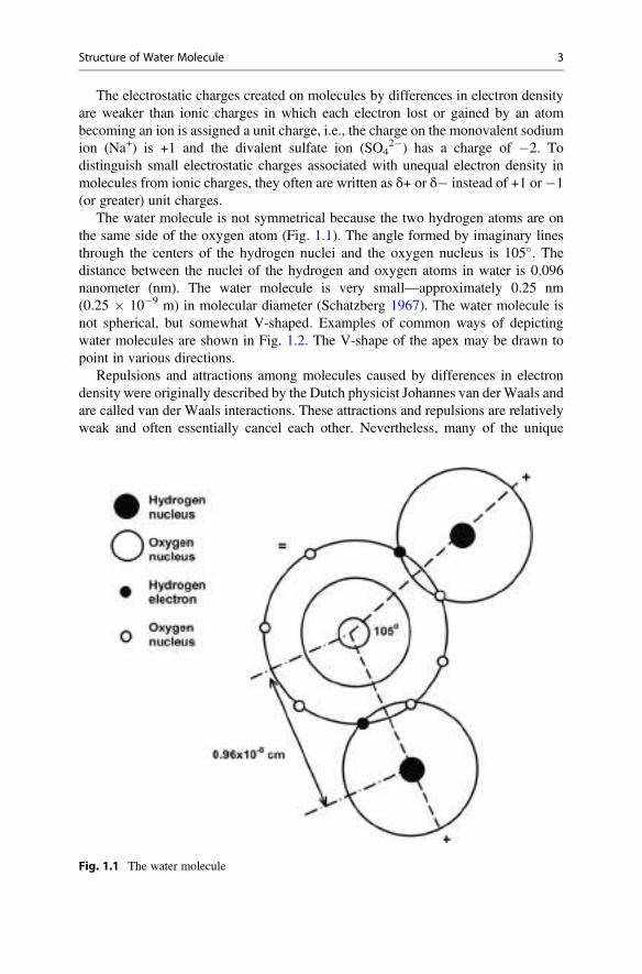
The water molecule is not symmetrical because the two hydrogen atoms are onthe same side of the oxygen atom (Fig. 1.1). The angle formed by imaginary linesthrough the centers of the hydrogen nuclei and the oxygen nucleus is 105�. Thedistance between the nuclei of the hydrogen and oxygen atoms in water is 0.096nanometer (nm). The water molecule is very small—approximately 0.25 nm(0.25 � 10�9 m) in molecular diameter (Schatzberg 1967). The water molecule isnot spherical, but somewhat V-shaped. Examples of common ways of depictingwater molecules are shown in Fig. 1.2. The V-shape of the apex may be drawn topoint in various directions.

Repulsions and attractions among molecules caused by differences in electrondensity were originally described by the Dutch physicist Johannes van der Waals andare called van der Waals interactions. These attractions and repulsions are relativelyweak and often essentially cancel each other. Nevertheless, many of the unique

Fig. 1.1 The water molecule

Structure of Water Molecule 3

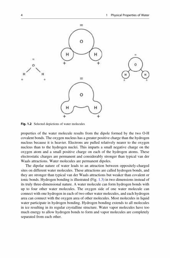
properties of the water molecule results from the dipole formed by the two O-Hcovalent bonds. The oxygen nucleus has a greater positive charge than the hydrogennucleus because it is heavier. Electrons are pulled relatively nearer to the oxygennucleus than to the hydrogen nuclei. This imparts a small negative charge on theoxygen atom and a small positive charge on each of the hydrogen atoms. Theseelectrostatic charges are permanent and considerably stronger than typical van derWaals attractions. Water molecules are permanent dipoles.

The dipolar nature of water leads to an attraction between oppositely-chargedsites on different water molecules. These attractions are called hydrogen bonds, andthey are stronger than typical van der Waals attractions but weaker than covalent orionic bonds. Hydrogen bonding is illustrated (Fig. 1.3) in two dimensions instead ofits truly three-dimensional nature. A water molecule can form hydrogen bonds withup to four other water molecules. The oxygen side of one water molecule canconnect with one hydrogen in each of two other water molecules, and each hydrogenarea can connect with the oxygen area of other molecules. Most molecules in liquidwater participate in hydrogen bonding. Hydrogen bonding extends to all moleculesin ice resulting in its regular crystalline structure. Water vapor molecules have toomuch energy to allow hydrogen bonds to form and vapor molecules are completelyseparated from each other.

Fig. 1.2 Selected depictions of water molecules


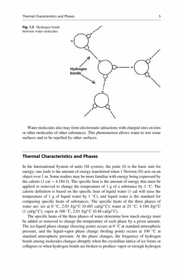
Water molecules also may form electrostatic attractions with charged sites on ionsor other molecules of other substances. This phenomenon allows water to wet somesurfaces and to be repelled by other surfaces.

Thermal Characteristics and Phases

In the International System of units (SI system), the joule (J) is the basic unit forenergy; one joule is the amount of energy transferred when 1 Newton (N) acts on anobject over 1 m. Some readers may be more familiar with energy being expressed bythe calorie (1 cal ¼ 4.184 J). The specific heat is the amount of energy that must beapplied or removed to change the temperature of 1 g of a substance by 1 �C. Thecalorie definition is based on the specific heat of liquid water (1 cal will raise thetemperature of 1 g of liquid water by 1 �C), and liquid water is the standard forcomparing specific heats of substances. The specific heats of the three phases ofwater are: ice at 0 �C, 2.03 J/g/�C (0.485 cal/g/�C); water at 25 �C, 4.184 J/g/�C(1 cal/g/�C); vapor at 100 �C, 2.01 J/g/�C (0.48 cal/g/�C).

The specific heats of the three phases of water determine how much energy mustbe added or removed to change the temperature of each phase by a given amount.The ice-liquid phase change (freezing point) occurs at 0 �C at standard atmosphericpressure, and the liquid-vapor phase change (boiling point) occurs at 100 �C atstandard atmospheric pressure. At the phase changes, the frequency of hydrogenbonds among molecules changes abruptly when the crystalline lattice of ice forms orcollapses or when hydrogen bonds are broken to produce vapor or enough hydrogen

Fig. 1.3 Hydrogen bondsbetween water molecules

Thermal Characteristics and Phases 5

bonds are formed to result in condensate of vapor to liquid water. There-arrangement of hydrogen bonds at phase changes requires a large input orremoval of energy that does not cause a temperature change. The amounts of energychange necessary to cause phase changes are called the latent heat (or enthalpy) offusion for freezing and the latent heat (or enthalpy) of vaporization for boiling.Enthalpy is a term referring to the internal energy of a substance. For water, the heatof fusion is 334 J/g (80 cal/g) and the heat of vaporization is 2260 J/g (540 cal/g).

Conversion of 1 g ice at�10 �C to water vapor at 100 �C requires an energy inputof 20.1 J (2.010 J/g/�C � 1 g � 10 �C) to raise the temperature to 0 �C, and 334 Jmore are required to convert 1 g of ice at 0 �C to liquid water at 0 �C. Raising thetemperature of 1 g liquid water to its boiling pointy requires 418.4 J (4.184 J/g/�

C � 1 g) of energy, and to boil it requires an additional 2260 J/g. Reversing theprocess described above would require removal of the same amount of energy.

Ice also can change from a solid to a vapor without passing through the liquidphase. This is the reason wet clothes suspended on a line outdoors in freezingweather may become dry. The process is called sublimation, and the latent heat ofsublimation is 3012 J/g (720 cal/g). Water vapor also can change from vapor to icewithout going through the liquid phase. This process is known as deposition forwhich the latent heat also is 3012 J/g.

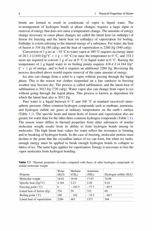
Pure water is a liquid between 0 �C and 100 �C at standard (sea-level) atmo-spheric pressure. Other common hydrogen compounds such as methane, ammonia,and hydrogen sulfide are gases at ordinary temperatures on the earth’s surface(Table 1.1). The specific heats and latent heats of fusion and vaporization also aregreater for water than for the other three common hydrogen compounds (Table 1.1).The reason water differs in thermal properties from other substances of similarmolecular weight results from its ability to form hydrogen bonds among itsmolecules. The high latent heat values for water reflect the resistance to formingand to breaking of hydrogen bonds. In the case of freezing, molecular motion mustdecline to the point that the crystalline lattice of ice can form, but when ice melts,enough energy must be applied to break enough hydrogen bonds to collapse tolattice of ice. The same logic applies for vaporization. Energy is necessary to free thevapor molecules from hydrogen bonding.

Table 1.1 Thermal properties of water compared with those of other hydrogen compounds ofsimilar molecular weight

PropertyWater(H2O)

Methane(CH4)

Ammonia(NH3) Hydrogen sulfide (H2S)

Molecular weight 18.02 16.04 17.03 34.08

Specific heat (J/g/�C) 4.184 2.23 2.20 0.24

Freezing point (�C) 0 �182.5 �77.7 �85.5

Latent heat of fusion (J/g) 334 59 332 68

Boiling point (�C) 100 �162 �33.3 �60.7

Latent heat of vaporization 2260 481 1371 548


The large specific heat and latent heat requirements necessary to cause phasechanges in water bodies has considerable climatic, environmental, and physiologicalsignificance. Large water bodies store heat and affect the surrounding climate. Heatloss caused by evaporation of perspiration from our skin is critical to bodilytemperature control. As air masses rise the cooling rate decreases when the tempera-ture falls low enough to allow water vapor to condense.

Vapor Pressure

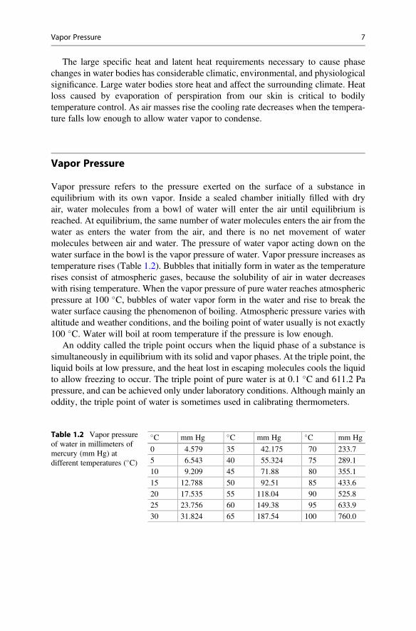
Vapor pressure refers to the pressure exerted on the surface of a substance inequilibrium with its own vapor. Inside a sealed chamber initially filled with dryair, water molecules from a bowl of water will enter the air until equilibrium isreached. At equilibrium, the same number of water molecules enters the air from thewater as enters the water from the air, and there is no net movement of watermolecules between air and water. The pressure of water vapor acting down on thewater surface in the bowl is the vapor pressure of water. Vapor pressure increases astemperature rises (Table 1.2). Bubbles that initially form in water as the temperaturerises consist of atmospheric gases, because the solubility of air in water decreaseswith rising temperature. When the vapor pressure of pure water reaches atmosphericpressure at 100 �C, bubbles of water vapor form in the water and rise to break thewater surface causing the phenomenon of boiling. Atmospheric pressure varies withaltitude and weather conditions, and the boiling point of water usually is not exactly100 �C. Water will boil at room temperature if the pressure is low enough.

An oddity called the triple point occurs when the liquid phase of a substance issimultaneously in equilibrium with its solid and vapor phases. At the triple point, theliquid boils at low pressure, and the heat lost in escaping molecules cools the liquidto allow freezing to occur. The triple point of pure water is at 0.1 �C and 611.2 Papressure, and can be achieved only under laboratory conditions. Although mainly anoddity, the triple point of water is sometimes used in calibrating thermometers.

Table 1.2 Vapor pressureof water in millimeters ofmercury (mm Hg) atdifferent temperatures (�C)

�C mm Hg �C mm Hg �C mm Hg

0 4.579 35 42.175 70 233.7

5 6.543 40 55.324 75 289.1

10 9.209 45 71.88 80 355.1

15 12.788 50 92.51 85 433.6

20 17.535 55 118.04 90 525.8

25 23.756 60 149.38 95 633.9

30 31.824 65 187.54 100 760.0

Vapor Pressure 7

Density

Molecules of ice are arranged in a regular lattice through hydrogen bonding. Theregular spacing of molecules in ice creates voids absent in liquid water wheremolecules are closer together. Ice is less dense than liquid water (0.917 g/cm3 versus1 g/cm3) allowing it to float.

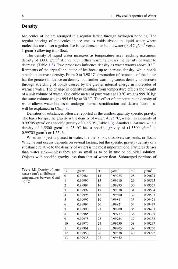
The density of liquid water increases as temperature rises reaching maximumdensity of 1.000 g/cm3 at 3.98 �C. Further warming causes the density of water todecrease (Table 1.3). Two processes influence density as water warms above 0 �C.Remnants of the crystalline lattice of ice break up to increase density, while bondsstretch to decrease density. From 0 to 3.98 �C, destruction of remnants of the latticehas the greatest influence on density, but further warming causes density to decreasethrough stretching of bonds caused by the greater internal energy in molecules ofwarmer water. The change in density resulting from temperature effects the weightof a unit volume of water. One cubic meter of pure water at 10 �C weighs 999.70 kg;the same volume weighs 995.65 kg at 30 �C. The effect of temperature on density ofwater allows water bodies to undergo thermal stratification and destratification aswill be explained in Chap. 3.

Densities of substances often are reported as the unitless quantity specific gravity.The basis for specific gravity is the density of water. At 25 �C, water has a density of0.99705 g/cm3 or a specific gravity of 0.99705 (Table 1.3). Another substance with adensity of 1.5500 g/cm3 at 25 �C has a specific gravity of (1.5500 g/cm3 �0.99705 g/cm3) or 1.5546.

When an object is placed in water, it either sinks, dissolves, suspends, or floats.Which event occurs depends on several factors, but the specific gravity (density of asubstance relative to the density of water) is the most important one. Particles denserthan water sink—unless they are so small as to be in true or colloidal solution.Objects with specific gravity less than that of water float. Submerged portions of

Table 1.3 Density of purewater (g/m3) at differenttemperatures between 0 and40 �C

�C g/cm3 �C g/cm3 �C g/cm3

0 0.99984 14 0.99925 28 0.99624

1 0.99990 15 0.99910 29 0.99595

2 0.99994 16 0.99895 30 0.99565

3 0.99997 17 0.99878 31 0.99534

4 0.99998 18 0.99860 32 0.99503

5 0.99997 19 0.99841 33 0.99471

6 0.99994 20 0.99821 34 0.99437

7 0.99990 21 0.99800 35 0.99403

8 0.99985 22 0.99777 36 0.99309

9 9.99978 23 0.99754 37 0.99333

10 0.99970 24 0.99730 38 0.99297

11 0.99961 25 0.99705 39 0.99260

12 0.99950 26 0.99678 40 0.99222

13 0.99938 27 0.99652


floating objects and dissolved or suspended particles displace a volume of waterequal to their own volumes. For example, a 10-cm3 marble placed in a glass of watersinks displacing 10-cm3 of water to cause the water level in the glass to increaseslightly. However, the volume of water displaced is unrelated to the density of thesubmerged object—two, 10-cm3 marbles of different densities would displace equalamounts of water.

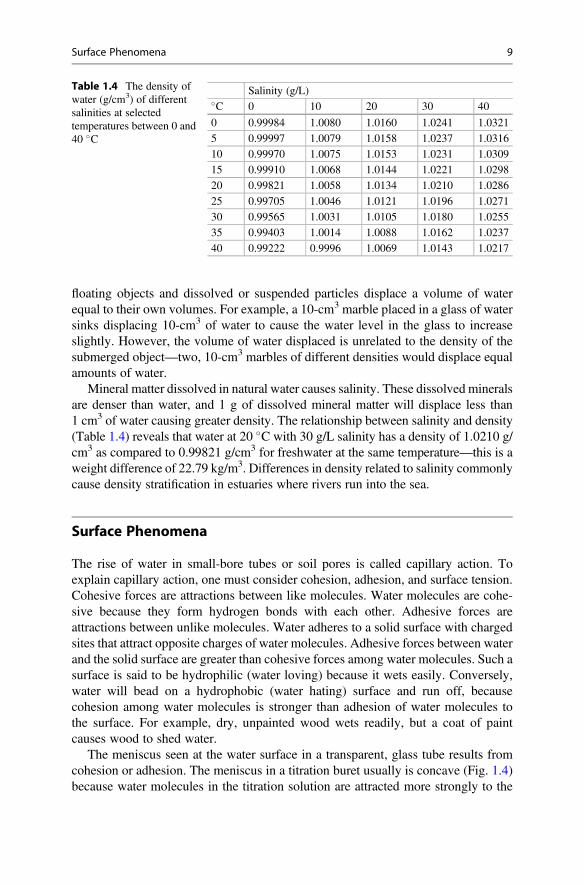
Mineral matter dissolved in natural water causes salinity. These dissolved mineralsare denser than water, and 1 g of dissolved mineral matter will displace less than1 cm3 of water causing greater density. The relationship between salinity and density(Table 1.4) reveals that water at 20 �C with 30 g/L salinity has a density of 1.0210 g/cm3 as compared to 0.99821 g/cm3 for freshwater at the same temperature—this is aweight difference of 22.79 kg/m3. Differences in density related to salinity commonlycause density stratification in estuaries where rivers run into the sea.

Surface Phenomena

The rise of water in small-bore tubes or soil pores is called capillary action. Toexplain capillary action, one must consider cohesion, adhesion, and surface tension.Cohesive forces are attractions between like molecules. Water molecules are cohe-sive because they form hydrogen bonds with each other. Adhesive forces areattractions between unlike molecules. Water adheres to a solid surface with chargedsites that attract opposite charges of water molecules. Adhesive forces between waterand the solid surface are greater than cohesive forces among water molecules. Such asurface is said to be hydrophilic (water loving) because it wets easily. Conversely,water will bead on a hydrophobic (water hating) surface and run off, becausecohesion among water molecules is stronger than adhesion of water molecules tothe surface. For example, dry, unpainted wood wets readily, but a coat of paintcauses wood to shed water.

The meniscus seen at the water surface in a transparent, glass tube results fromcohesion or adhesion. The meniscus in a titration buret usually is concave (Fig. 1.4)because water molecules in the titration solution are attracted more strongly to the

Table 1.4 The density ofwater (g/cm3) of differentsalinities at selectedtemperatures between 0 and40 �C

Salinity (g/L)�C 0 10 20 30 40

0 0.99984 1.0080 1.0160 1.0241 1.0321

5 0.99997 1.0079 1.0158 1.0237 1.0316

10 0.99970 1.0075 1.0153 1.0231 1.0309

15 0.99910 1.0068 1.0144 1.0221 1.0298

20 0.99821 1.0058 1.0134 1.0210 1.0286

25 0.99705 1.0046 1.0121 1.0196 1.0271

30 0.99565 1.0031 1.0105 1.0180 1.0255

35 0.99403 1.0014 1.0088 1.0162 1.0237

40 0.99222 0.9996 1.0069 1.0143 1.0217

Surface Phenomena 9

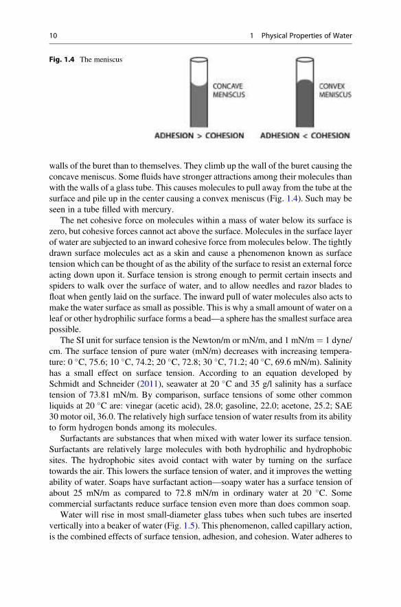
walls of the buret than to themselves. They climb up the wall of the buret causing theconcave meniscus. Some fluids have stronger attractions among their molecules thanwith the walls of a glass tube. This causes molecules to pull away from the tube at thesurface and pile up in the center causing a convex meniscus (Fig. 1.4). Such may beseen in a tube filled with mercury.

The net cohesive force on molecules within a mass of water below its surface iszero, but cohesive forces cannot act above the surface. Molecules in the surface layerof water are subjected to an inward cohesive force from molecules below. The tightlydrawn surface molecules act as a skin and cause a phenomenon known as surfacetension which can be thought of as the ability of the surface to resist an external forceacting down upon it. Surface tension is strong enough to permit certain insects andspiders to walk over the surface of water, and to allow needles and razor blades tofloat when gently laid on the surface. The inward pull of water molecules also acts tomake the water surface as small as possible. This is why a small amount of water on aleaf or other hydrophilic surface forms a bead—a sphere has the smallest surface areapossible.

The SI unit for surface tension is the Newton/m or mN/m, and 1 mN/m ¼ 1 dyne/cm. The surface tension of pure water (mN/m) decreases with increasing tempera-ture: 0 �C, 75.6; 10 �C, 74.2; 20 �C, 72.8; 30 �C, 71.2; 40 �C, 69.6 mN/m). Salinityhas a small effect on surface tension. According to an equation developed bySchmidt and Schneider (2011), seawater at 20 �C and 35 g/l salinity has a surfacetension of 73.81 mN/m. By comparison, surface tensions of some other commonliquids at 20 �C are: vinegar (acetic acid), 28.0; gasoline, 22.0; acetone, 25.2; SAE30 motor oil, 36.0. The relatively high surface tension of water results from its abilityto form hydrogen bonds among its molecules.

Surfactants are substances that when mixed with water lower its surface tension.Surfactants are relatively large molecules with both hydrophilic and hydrophobicsites. The hydrophobic sites avoid contact with water by turning on the surfacetowards the air. This lowers the surface tension of water, and it improves the wettingability of water. Soaps have surfactant action—soapy water has a surface tension ofabout 25 mN/m as compared to 72.8 mN/m in ordinary water at 20 �C. Somecommercial surfactants reduce surface tension even more than does common soap.

Water will rise in most small-diameter glass tubes when such tubes are insertedvertically into a beaker of water (Fig. 1.5). This phenomenon, called capillary action,is the combined effects of surface tension, adhesion, and cohesion. Water adheres to

Fig. 1.4 The meniscus


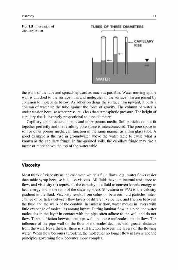
the walls of the tube and spreads upward as much as possible. Water moving up thewall is attached to the surface film, and molecules in the surface film are joined bycohesion to molecules below. As adhesion drags the surface film upward, it pulls acolumn of water up the tube against the force of gravity. The column of water isunder tension because water pressure is less than atmospheric pressure. The height ofcapillary rise is inversely proportional to tube diameter.

Capillary action occurs in soils and other porous media. Soil particles do not fittogether perfectly and the resulting pore space is interconnected. The pore space insoil or other porous media can function in the same manner as a thin glass tube. Agood example is the rise in groundwater above the water table to cause what isknown as the capillary fringe. In fine-grained soils, the capillary fringe may rise ameter or more above the top of the water table.

Viscosity

Most think of viscosity as the ease with which a fluid flows, e.g., water flows easierthan table syrup because it is less viscous. All fluids have an internal resistance toflow, and viscosity (η) represents the capacity of a fluid to convert kinetic energy toheat energy and is the ratio of the shearing stress (force/area or F/A) to the velocitygradient in the fluid. Viscosity results from cohesion between fluid particles, inter-change of particles between flow layers of different velocities, and friction betweenthe fluid and the walls of the conduit. In laminar flow, water moves in layers withlittle exchange of molecules among layers. During laminar flow in a pipe, the watermolecules in the layer in contact with the pipe often adhere to the wall and do notflow. There is friction between the pipe wall and those molecules that do flow. Theinfluence of the pipe wall on the flow of molecules declines with greater distancefrom the wall. Nevertheless, there is still friction between the layers of the flowingwater. When flow becomes turbulent, the molecules no longer flow in layers and theprinciples governing flow becomes more complex.

Fig. 1.5 Illustration ofcapillary action

Viscosity 11

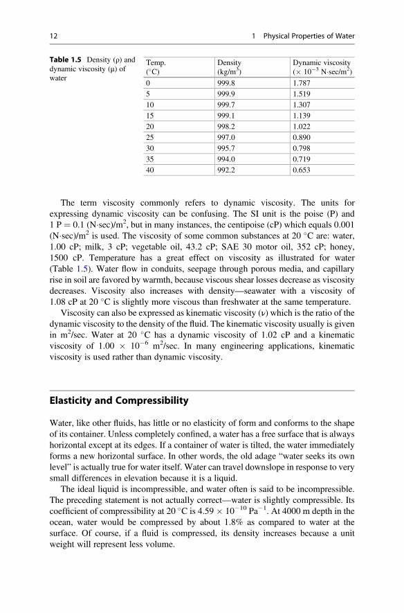
The term viscosity commonly refers to dynamic viscosity. The units forexpressing dynamic viscosity can be confusing. The SI unit is the poise (P) and1 P ¼ 0.1 (N�sec)/m2, but in many instances, the centipoise (cP) which equals 0.001(N�sec)/m2 is used. The viscosity of some common substances at 20 �C are: water,1.00 cP; milk, 3 cP; vegetable oil, 43.2 cP; SAE 30 motor oil, 352 cP; honey,1500 cP. Temperature has a great effect on viscosity as illustrated for water(Table 1.5). Water flow in conduits, seepage through porous media, and capillaryrise in soil are favored by warmth, because viscous shear losses decrease as viscositydecreases. Viscosity also increases with density—seawater with a viscosity of1.08 cP at 20 �C is slightly more viscous than freshwater at the same temperature.

Viscosity can also be expressed as kinematic viscosity (ν) which is the ratio of thedynamic viscosity to the density of the fluid. The kinematic viscosity usually is givenin m2/sec. Water at 20 �C has a dynamic viscosity of 1.02 cP and a kinematicviscosity of 1.00 � 10�6 m2/sec. In many engineering applications, kinematicviscosity is used rather than dynamic viscosity.

Elasticity and Compressibility

Water, like other fluids, has little or no elasticity of form and conforms to the shapeof its container. Unless completely confined, a water has a free surface that is alwayshorizontal except at its edges. If a container of water is tilted, the water immediatelyforms a new horizontal surface. In other words, the old adage “water seeks its ownlevel” is actually true for water itself. Water can travel downslope in response to verysmall differences in elevation because it is a liquid.

The ideal liquid is incompressible, and water often is said to be incompressible.The preceding statement is not actually correct—water is slightly compressible. Itscoefficient of compressibility at 20 �C is 4.59 � 10�10 Pa�1. At 4000 m depth in theocean, water would be compressed by about 1.8% as compared to water at thesurface. Of course, if a fluid is compressed, its density increases because a unitweight will represent less volume.

Table 1.5 Density (ρ) anddynamic viscosity (μ) ofwater

Temp.(�C)

Density(kg/m3)

Dynamic viscosity(� 10�3 N�sec/m2)

0 999.8 1.787

5 999.9 1.519

10 999.7 1.307

15 999.1 1.139

20 998.2 1.022

25 997.0 0.890

30 995.7 0.798

35 994.0 0.719

40 992.2 0.653


Water Pressure

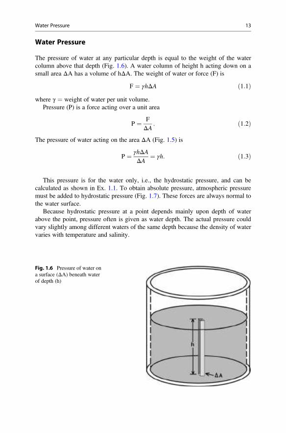
The pressure of water at any particular depth is equal to the weight of the watercolumn above that depth (Fig. 1.6). A water column of height h acting down on asmall area ΔA has a volume of hΔA. The weight of water or force (F) is

F ¼ γhΔA ð1:1Þwhere γ ¼ weight of water per unit volume.

Pressure (P) is a force acting over a unit area

P ¼ FΔA

: ð1:2Þ

The pressure of water acting on the area ΔA (Fig. 1.5) is

P ¼ γhΔAΔA

¼ γh: ð1:3Þ

This pressure is for the water only, i.e., the hydrostatic pressure, and can becalculated as shown in Ex. 1.1. To obtain absolute pressure, atmospheric pressuremust be added to hydrostatic pressure (Fig. 1.7). These forces are always normal tothe water surface.

Because hydrostatic pressure at a point depends mainly upon depth of waterabove the point, pressure often is given as water depth. The actual pressure couldvary slightly among different waters of the same depth because the density of watervaries with temperature and salinity.

Fig. 1.6 Pressure of water ona surface (ΔA) beneath waterof depth (h)

Water Pressure 13

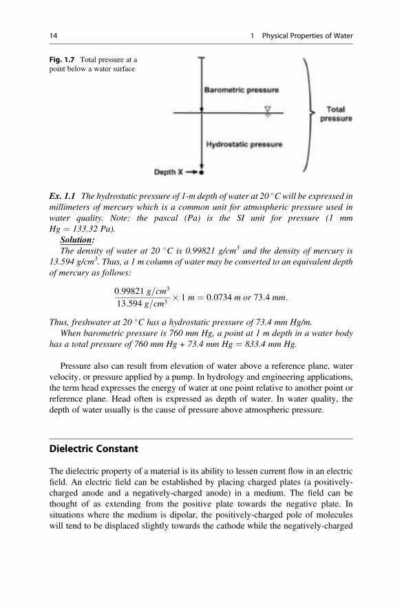
Ex. 1.1 The hydrostatic pressure of 1-m depth of water at 20 �C will be expressed inmillimeters of mercury which is a common unit for atmospheric pressure used inwater quality. Note: the pascal (Pa) is the SI unit for pressure (1 mmHg ¼ 133.32 Pa).

Solution:The density of water at 20 �C is 0.99821 g/cm3 and the density of mercury is

13.594 g/cm3. Thus, a 1 m column of water may be converted to an equivalent depthof mercury as follows:

0:99821 g=cm3

13:594 g=cm3� 1 m ¼ 0:0734 m or 73:4 mm:

Thus, freshwater at 20 �C has a hydrostatic pressure of 73.4 mm Hg/m.When barometric pressure is 760 mm Hg, a point at 1 m depth in a water body

has a total pressure of 760 mm Hg + 73.4 mm Hg ¼ 833.4 mm Hg.

Pressure also can result from elevation of water above a reference plane, watervelocity, or pressure applied by a pump. In hydrology and engineering applications,the term head expresses the energy of water at one point relative to another point orreference plane. Head often is expressed as depth of water. In water quality, thedepth of water usually is the cause of pressure above atmospheric pressure.

Dielectric Constant

The dielectric property of a material is its ability to lessen current flow in an electricfield. An electric field can be established by placing charged plates (a positively-charged anode and a negatively-charged anode) in a medium. The field can bethought of as extending from the positive plate towards the negative plate. Insituations where the medium is dipolar, the positively-charged pole of moleculeswill tend to be displaced slightly towards the cathode while the negatively-charged

Fig. 1.7 Total pressure at apoint below a water surface


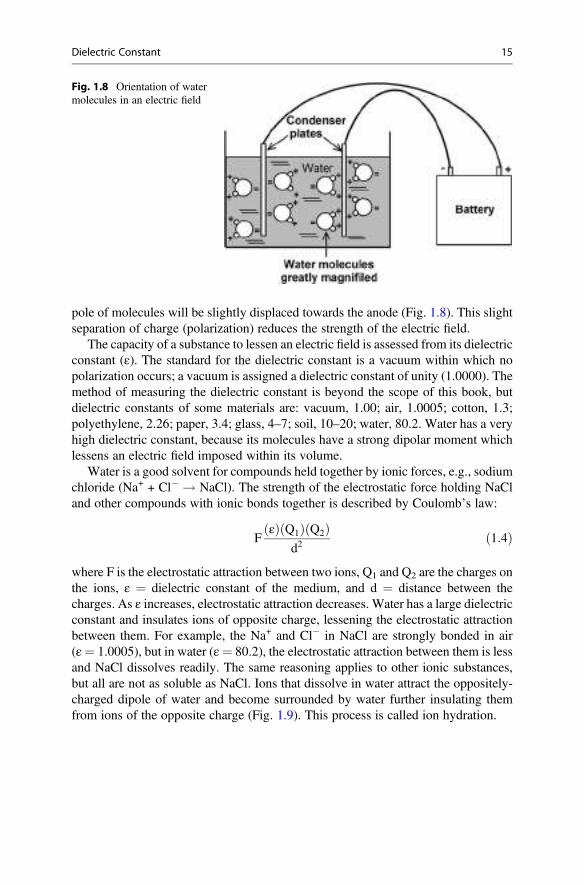
pole of molecules will be slightly displaced towards the anode (Fig. 1.8). This slightseparation of charge (polarization) reduces the strength of the electric field.

The capacity of a substance to lessen an electric field is assessed from its dielectricconstant (ε). The standard for the dielectric constant is a vacuum within which nopolarization occurs; a vacuum is assigned a dielectric constant of unity (1.0000). Themethod of measuring the dielectric constant is beyond the scope of this book, butdielectric constants of some materials are: vacuum, 1.00; air, 1.0005; cotton, 1.3;polyethylene, 2.26; paper, 3.4; glass, 4–7; soil, 10–20; water, 80.2. Water has a veryhigh dielectric constant, because its molecules have a strong dipolar moment whichlessens an electric field imposed within its volume.

Water is a good solvent for compounds held together by ionic forces, e.g., sodiumchloride (Na+ + Cl� ! NaCl). The strength of the electrostatic force holding NaCland other compounds with ionic bonds together is described by Coulomb’s law:

Fεð Þ Q1ð Þ Q2ð Þ

d2ð1:4Þ

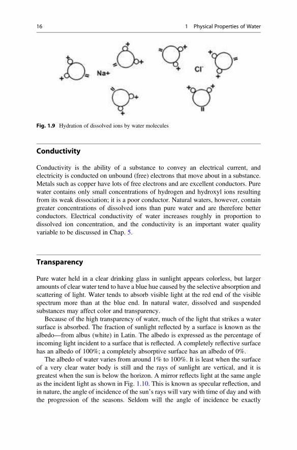
where F is the electrostatic attraction between two ions, Q1 and Q2 are the charges onthe ions, ε ¼ dielectric constant of the medium, and d ¼ distance between thecharges. As ε increases, electrostatic attraction decreases. Water has a large dielectricconstant and insulates ions of opposite charge, lessening the electrostatic attractionbetween them. For example, the Na+ and Cl� in NaCl are strongly bonded in air(ε¼ 1.0005), but in water (ε¼ 80.2), the electrostatic attraction between them is lessand NaCl dissolves readily. The same reasoning applies to other ionic substances,but all are not as soluble as NaCl. Ions that dissolve in water attract the oppositely-charged dipole of water and become surrounded by water further insulating themfrom ions of the opposite charge (Fig. 1.9). This process is called ion hydration.

Fig. 1.8 Orientation of watermolecules in an electric field

Dielectric Constant 15

Conductivity

Conductivity is the ability of a substance to convey an electrical current, andelectricity is conducted on unbound (free) electrons that move about in a substance.Metals such as copper have lots of free electrons and are excellent conductors. Purewater contains only small concentrations of hydrogen and hydroxyl ions resultingfrom its weak dissociation; it is a poor conductor. Natural waters, however, containgreater concentrations of dissolved ions than pure water and are therefore betterconductors. Electrical conductivity of water increases roughly in proportion todissolved ion concentration, and the conductivity is an important water qualityvariable to be discussed in Chap. 5.

Transparency

Pure water held in a clear drinking glass in sunlight appears colorless, but largeramounts of clear water tend to have a blue hue caused by the selective absorption andscattering of light. Water tends to absorb visible light at the red end of the visiblespectrum more than at the blue end. In natural water, dissolved and suspendedsubstances may affect color and transparency.

Because of the high transparency of water, much of the light that strikes a watersurface is absorbed. The fraction of sunlight reflected by a surface is known as thealbedo—from albus (white) in Latin. The albedo is expressed as the percentage ofincoming light incident to a surface that is reflected. A completely reflective surfacehas an albedo of 100%; a completely absorptive surface has an albedo of 0%.

The albedo of water varies from around 1% to 100%. It is least when the surfaceof a very clear water body is still and the rays of sunlight are vertical, and it isgreatest when the sun is below the horizon. A mirror reflects light at the same angleas the incident light as shown in Fig. 1.10. This is known as specular reflection, andin nature, the angle of incidence of the sun’s rays will vary with time of day and withthe progression of the seasons. Seldom will the angle of incidence be exactly

Fig. 1.9 Hydration of dissolved ions by water molecules


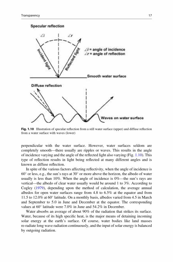
perpendicular with the water surface. However, water surfaces seldom arecompletely smooth—there usually are ripples or waves. This results in the angleof incidence varying and the angle of the reflected light also varying (Fig. 1.10). Thistype of reflection results in light being reflected at many different angles and isknown as diffuse reflection.

In spite of the various factors affecting reflectivity, when the angle of incidence is60� or less, e.g., the sun’s rays at 30� or more above the horizon, the albedo of waterusually is less than 10%. When the angle of incidence is 0%—the sun’s rays arevertical—the albedo of clear water usually would be around 1 to 3%. According toCogley (1979), depending upon the method of calculation, the average annualalbedos for open water surfaces range from 4.8 to 6.5% at the equator and from11.5 to 12.0% at 60� latitude. On a monthly basis, albedos varied from 4.5 in Marchand September to 5.0 in June and December at the equator. The correspondingvalues at 60� latitude were 7.0% in June and 54.2% in December.

Water absorbs an average of about 90% of the radiation that strikes its surface.Water, because of its high specific heat, is the major means of detaining incomingsolar energy at the earth’s surface. Of course, water bodies like land massesre-radiate long wave radiation continuously, and the input of solar energy is balancedby outgoing radiation.

Fig. 1.10 Illustration of specular reflection from a still water surface (upper) and diffuse reflectionfrom a water surface with waves (lower)

Transparency 17

The light that penetrates the water surface is absorbed and scattered as it passesthrough the water column. This phenomenon has many implications in the study ofwater quality, and will be discussed several places in this book—especially inChap. 6.

Refractive Index

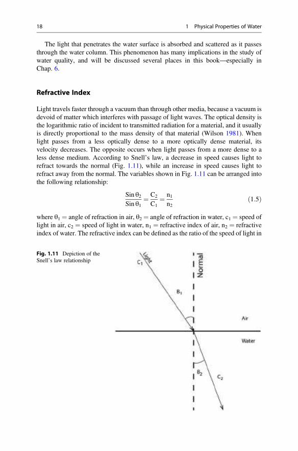
Light travels faster through a vacuum than through other media, because a vacuum isdevoid of matter which interferes with passage of light waves. The optical density isthe logarithmic ratio of incident to transmitted radiation for a material, and it usuallyis directly proportional to the mass density of that material (Wilson 1981). Whenlight passes from a less optically dense to a more optically dense material, itsvelocity decreases. The opposite occurs when light passes from a more dense to aless dense medium. According to Snell’s law, a decrease in speed causes light torefract towards the normal (Fig. 1.11), while an increase in speed causes light torefract away from the normal. The variables shown in Fig. 1.11 can be arranged intothe following relationship:

Sin θ2Sin θ1

¼ C2

C1¼ n1

n2ð1:5Þ

where θ1 ¼ angle of refraction in air, θ2 ¼ angle of refraction in water, c1 ¼ speed oflight in air, c2 ¼ speed of light in water, n1 ¼ refractive index of air, n2 ¼ refractiveindex of water. The refractive index can be defined as the ratio of the speed of light in

Fig. 1.11 Depiction of theSnell’s law relationship


a vacuum to the speed of light in another medium. The refractive index of water hastraditionally been reported as 1.33300 (Baxter et al. 1911). However, the refractiveindex varies with the wavelength of measurement, increases with greater salinity andpressure, and decreases with greater temperature (Segelstein 1981).

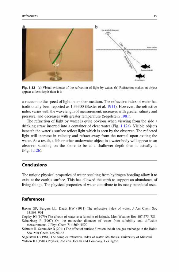
The refraction of light by water is quite obvious when viewing from the side adrinking straw inserted into a container of clear water (Fig. 1.12a). Visible objectsbeneath the water’s surface reflect light which is seen by the observer. The reflectedlight will increase in velocity and refract away from the normal upon exiting thewater. As a result, a fish or other underwater object in a water body will appear to anobserver standing on the shore to be at a shallower depth than it actually is(Fig. 1.12b).

Conclusions

The unique physical properties of water resulting from hydrogen bonding allow it toexist at the earth’s surface. This has allowed the earth to support an abundance ofliving things. The physical properties of water contribute to its many beneficial uses.

References

Baxter GP, Burgess LL, Daudt HW (1911) The refractive index of water. J Am Chem Soc33:893–901

Cogley JG (1979) The albedo of water as a function of latitude. Mon Weather Rev 107:775–781Schatzberg P (1967) On the molecular diameter of water from solubility and diffusion

measurements. J Phys Chem 71:4569–4570Schmidt R, Schneider B (2011) The effect of surface films on the air-sea gas exchange in the Baltic

Sea. Mar Chem 126:56–62Segelstein D (1981) The complex refractive index of water. MS thesis. University of MissouriWilson JD (1981) Physics, 2nd edn. Health and Company, Lexington

Fig. 1.12 (a) Visual evidence of the refraction of light by water. (b) Refraction makes an objectappear at less depth than it is

References 19

Solar Radiation and Water Temperature 2

AbstractTemperature is a measure of the heat content of an object which results from theenergy content of that object. The main source of energy in ecological systems issolar radiation. The earth’s energy budget is essentially balanced with the incom-ing solar radiation being balanced by the reflection of solar radiation and there-radiation of energy absorbed by the earth as longwave radiation. The tempera-ture of natural water bodies vary in response to diurnal and seasonal changes insolar radiation. The penetration of light into water bodies which regulates thedepth to which photosynthesis occurs is strongly influenced by water clarity.Solar radiation heats the surface layers of water in lakes, reservoirs, and pondsmore quickly than it warms deeper water. Water bodies often experience thermalstratification in which warmer, lighter water of the surface layer does mix withcooler, heavier deeper water. Warmth also favors greater rates of most chemicaland physical process, and respiration of organisms increases with greater temper-ature within the temperature tolerance range of organisms.

Introduction

Temperature has a major influence on rates of physical, chemical, and biologicalprocesses. Temperature effects molecular motion, which, in turn influences physicalproperties of matter, abiotic and biotic reactions, and activities of organisms. Eachbiological species has a specific range of temperature within which it can survive anda narrower temperature range within which it functions most efficiently and does notsuffer thermal stress. Rates of physical and chemical reactions influenceconcentrations of dissolved and suspended matter in water. Suspended particlesand some colored organic compounds in water lessen light penetration and reduceaquatic plant growth which is the source of nutrition for animals and most non-photosynthetic microorganisms. The influence of temperature on activities of aquaticorganisms result in water quality fluctuations.


21


Physical, chemical, and biological aspects of water quality are highly interrelated,and water temperature effects water quality. Water temperature depends mainlyupon the amount of solar radiation received by water bodies, but it is generallyconsidered a basic water quality variable because of its many effects. The purpose ofthis chapter is to explain relationships among energy, heat, and temperature, discusssolar radiation, and describe the major effects of temperature in water bodies.

Energy, Heat, and Temperature

Electrons, atoms, and molecules are in constant motion. Electrons are classicallydepicted by the Bohr model as moving around the nucleus of an atom in well-definedlayers of orbitals with each orbital containing a fixed number of electrons. Althoughthis depiction is extremely useful, modern quantum mechanics holds that electronsmove very fast and act as if in a cloud revolving about the nucleus of an atom. Theexact location of an electron at any given moment is not predictable. Electrons arenegatively charged and repel each other, but their density around the nucleus isseldom uniform.

The bonds between atoms in a molecule vibrate. A molecule with two atomsvibrates when its atoms move closer together and then further apart. Molecules withthree or more atoms—water has three atoms—can vibrate in more than one way. Thetwo H-O bonds in water can go back and forth like a yo-yo in a symmetrical or in anon-symmetrical pattern, and two H-O bonds may bend towards each other and thenaway. The bonds, including hydrogen bonds in water, also tend to stretch astemperature increases. The rate that atoms and molecules vibrate and stretch isrelated to temperature. All molecular motion is said to cease (it actually becomesminimal) at a temperature of�273.15 �C on the Celsius scale or 0�Kelvin (K) on theabsolute temperature scale, and molecular vibrations increase with increasing tem-perature. The temperature per se does not cause the vibrations; the energy content ofatoms and molecules is responsible for the vibrations. Temperature is merely ameasure of the energy content of something, or in everyday terms, how hot orhow cold something is. The temperature results from the response of the temperaturesensor to the activity level of molecules in a substance according to a scale rangingfrom cold to hot.

Energy is a complex concept difficult to explain in a few words. It is universallyrecognized as what is required to warm something or to do work, and its definitionrelates to doing work on or transferring heat to an object. The science of thermody-namics is the study of relationships among heat, work, temperature, and energy.There are three main laws of thermodynamics, and the first law often is stated as“energy cannot be created or destroyed, but it can be changed between heat andwork. The total energy content of the universe remains constant according to time’sarrow.” The expression time’s arrow (passing of time) implies that energy, likematter, had a beginning. It was created at some time in the past, but it has not beencreated since. This is one of many examples of the overlaps of physics, philosophy,and theology.

22 2 Solar Radiation and Water Temperature

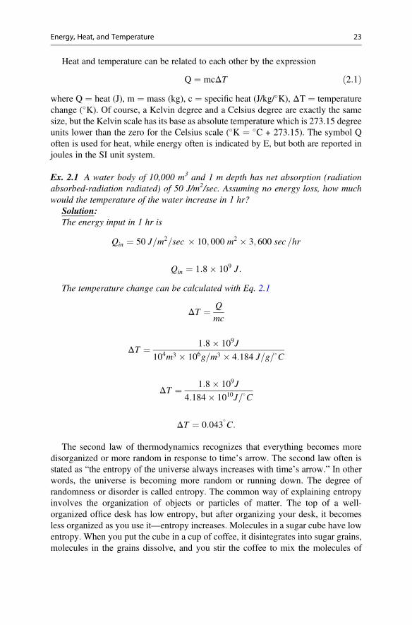
Heat and temperature can be related to each other by the expression

Q ¼ mcΔT ð2:1Þwhere Q ¼ heat (J), m ¼ mass (kg), c ¼ specific heat (J/kg/�K), ΔT ¼ temperaturechange (�K). Of course, a Kelvin degree and a Celsius degree are exactly the samesize, but the Kelvin scale has its base as absolute temperature which is 273.15 degreeunits lower than the zero for the Celsius scale (�K ¼ �C + 273.15). The symbol Qoften is used for heat, while energy often is indicated by E, but both are reported injoules in the SI unit system.

Ex. 2.1 A water body of 10,000 m3 and 1 m depth has net absorption (radiationabsorbed-radiation radiated) of 50 J/m2/sec. Assuming no energy loss, how muchwould the temperature of the water increase in 1 hr?

Solution:The energy input in 1 hr is

Qin ¼ 50 J=m2=sec � 10; 000 m2 � 3; 600 sec =hr

Qin ¼ 1:8� 109 J:

The temperature change can be calculated with Eq. 2.1

ΔT ¼ Q

mc

ΔT ¼ 1:8� 109J

104m3 � 106g=m3 � 4:184 J=g=�C

ΔT ¼ 1:8� 109J

4:184� 1010J=�C

ΔT ¼ 0:043�C:

The second law of thermodynamics recognizes that everything becomes moredisorganized or more random in response to time’s arrow. The second law often isstated as “the entropy of the universe always increases with time’s arrow.” In otherwords, the universe is becoming more random or running down. The degree ofrandomness or disorder is called entropy. The common way of explaining entropyinvolves the organization of objects or particles of matter. The top of a well-organized office desk has low entropy, but after organizing your desk, it becomesless organized as you use it—entropy increases. Molecules in a sugar cube have lowentropy. When you put the cube in a cup of coffee, it disintegrates into sugar grains,molecules in the grains dissolve, and you stir the coffee to mix the molecules of

Energy, Heat, and Temperature 23

sugar homogeneously. Entropy increases from cube to grains to heterogeneouscoffee-sugar mixture to homogeneous coffee-sugar solution. This simple view ofentropy is not useful in mathematic computations of energy relationships. It did,however, inspire the Scot-Irish physicist William Thompson (better known as LordKelvin) to say “we have (from the second law of thermodynamics) the soberscientific certainty that the heavens and earth shall wax old as doth a garment.”

Entropy can also be defined as the energy change which occurs when energy istransferred between two objects at constant temperature. There are several equationsfor entropy, but a simple one is

ΔS ¼ QT

ð2:2Þ

where ΔS ¼ entropy change (J/�K), Q ¼ heat transferred (J), T ¼ temperature (�K).The second law requires energy to flow by conduction from a hotter object to acooler object until both objects are at the same temperature. Some heat will be lost tothe surroundings and not available to do the work of raising the temperature of thesecond object. Entropy is the amount of energy not available for doing work. Closedsystems move towards a state of equilibrium in which entropy is maximum. Entropychange in a closed system cannot decrease (be negative).

The third law acknowledges that entropy is related to temperature and establishesa zero point for entropy. This law usually is expressed as “the entropy of a perfectcrystal of a substance is zero at absolute zero (�K or � 273.15 �C).” In the entropyequation (Eq. 2.2), temperature must be in degrees absolute.

There is a fourth law (often called the zeroth law) indicating the rather obviousfact that “two thermodynamic systems each in thermal equilibrium with a third, arein thermal equilibrium with each other.” This law is usually not of much importancein water temperature discussions.

Solar Radiation

The source of energy (and light) for earth is the sun. The sun consists mainly ofhydrogen gas (73.46%) and helium gas (24.58%). The sun emits energy produced bynuclear fusion (mainly by the proton-proton chain) occurring in its core. At the hightemperature (possibly 15 million �C) and enormous pressure (possibly 250 billionatmospheres) in the sun’s core, hydrogen gas (H2) is converted to electrons andnaked hydrogen ions or protons (H1). The electrons and protons are moving rapidly,and when two protons smash together, they form a deuterium nucleus (H2) with therelease of a positron (β+) and a neutrino (ν):

H1 þ H1 ! H2 þ βþ þ v: ð2:3ÞWhen a deuterium nucleus collides with a proton, a helium-three nucleus (H3) resultswith the release of a gamma ray (γ):


H2 þ H1 ¼ H3 þ γ: ð2:4ÞTwo H3 nuclei collide to make a helium-four (He4) nucleus and two protons arereleased.

H3 þ H3 ! He4 þ 2H1: ð2:5ÞThe mass of H4 is slightly less than the mass of the four protons (H1) that combinedto make it. This slight loss of mass resulted from mass being converted to energy inthe form of gamma rays.

The relationship of mass to energy is explained by Einstein’s equation

E ¼ mc2 ð2:6Þwhere E ¼ energy (J), m ¼ mass (kg), c ¼ speed of light (299,792,458 m/sec or�3 � 108 m/sec). The base unit for the joule is kg�m2/sec2 or Newton�meter (N�m).Using Eq. 2.6, it can be seen that if 1 kg of mass is converted completely to energy,8.99 � 1016 J of energy would result. The sun creates about 3.9 � 1026 J of energyevery second by converting an estimated 600 � 106 t of hydrogen to 596 � 106 t ofhelium (www.astronomy.ohio-state.edu/~ryden/ast162_1/notes2.html). To put thisin some kind of perspective, the daily energy consumption by the global activities ofhumans was only around 1018 J in 2018 (https://www.eia.gov/outlooks/aeo/). Ofcourse, the earth only receives about 0.0000002% of the total amount of solar energyemitted into space by the sun.

Energy released in the sun’s core as gamma rays by the proton-proton chainreaction slowly migrates through the plasma of the sun to its surface. The tempera-ture declines from millions of degrees Celsius in the sun’s core to about 5500 �C atits surface. As the gamma rays move through the plasma, they are absorbed andreradiated at lower frequencies, and the lower frequencies are likewise absorbed andreradiated at even lower frequencies.

Electromagnetic radiation from the sun (sunlight) can, according to quantummechanics, be thought of as consisting of massless particles traveling in waves ofdifferent frequencies. The energy content of electromagnetic waves increases withdecreasing wavelength. The wavelength (λ) is the distance between the crests of anelectromagnetic wave. Short gamma rays have the most energy, while long radiowaves have the least. A wave transports momentum through its motion, and thismotion carries energy even though the particles of energy called photons of whichlight consists of no mass. This can be visualized as one flipping the end of a rope tocause the rope to move as a wave to the other end. The wave could cause a personholding the other end of the rope to experience a tug even though the rope carried nomatter. The fact that a wave can carry energy results in an energy transfer when thewave strikes another substance.

Objects absorb electromagnetic radiation but they simultaneously emit electro-magnetic radiation. Objects with temperatures above absolute zero emit radiationbecause electric charges on their surfaces are accelerated by thermal agitation. The

Solar Radiation 25

http://www.astronomy.ohio.state.edu/-ryden/ast162_1/notes2.html

https://www.eia.gov/outlooks/aeo/

wavelength of radiation is equal to the speed of light (c) divided by the frequency(f) or λ ¼ c/f. The frequency of the radiation increases with the energy content ofwaves, e.g., gamma rays have more energy than visible light. The electric charges onobjects are accelerated at different rates, and a spectrum of radiation is emitted.

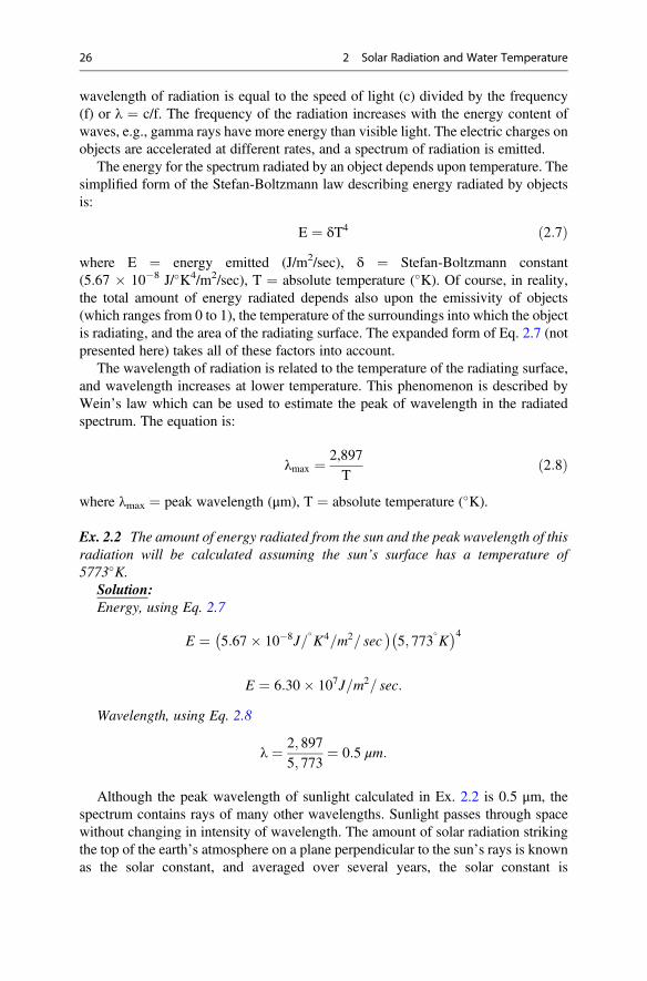
The energy for the spectrum radiated by an object depends upon temperature. Thesimplified form of the Stefan-Boltzmann law describing energy radiated by objectsis:

E ¼ δT4 ð2:7Þwhere E ¼ energy emitted (J/m2/sec), δ ¼ Stefan-Boltzmann constant(5.67 � 10�8 J/�K4/m2/sec), T ¼ absolute temperature (�K). Of course, in reality,the total amount of energy radiated depends also upon the emissivity of objects(which ranges from 0 to 1), the temperature of the surroundings into which the objectis radiating, and the area of the radiating surface. The expanded form of Eq. 2.7 (notpresented here) takes all of these factors into account.

The wavelength of radiation is related to the temperature of the radiating surface,and wavelength increases at lower temperature. This phenomenon is described byWein’s law which can be used to estimate the peak of wavelength in the radiatedspectrum. The equation is:

λmax ¼ 2,897T

ð2:8Þ

where λmax ¼ peak wavelength (μm), T ¼ absolute temperature (�K).

Ex. 2.2 The amount of energy radiated from the sun and the peak wavelength of thisradiation will be calculated assuming the sun’s surface has a temperature of5773�K.

Solution:Energy, using Eq. 2.7

E ¼ 5:67� 10�8J=�K4=m2= sec

� �5; 773

�K

� �4

E ¼ 6:30� 107J=m2= sec:

Wavelength, using Eq. 2.8

λ ¼ 2; 8975; 773

¼ 0:5 μm:

Although the peak wavelength of sunlight calculated in Ex. 2.2 is 0.5 μm, thespectrum contains rays of many other wavelengths. Sunlight passes through spacewithout changing in intensity of wavelength. The amount of solar radiation strikingthe top of the earth’s atmosphere on a plane perpendicular to the sun’s rays is knownas the solar constant, and averaged over several years, the solar constant is


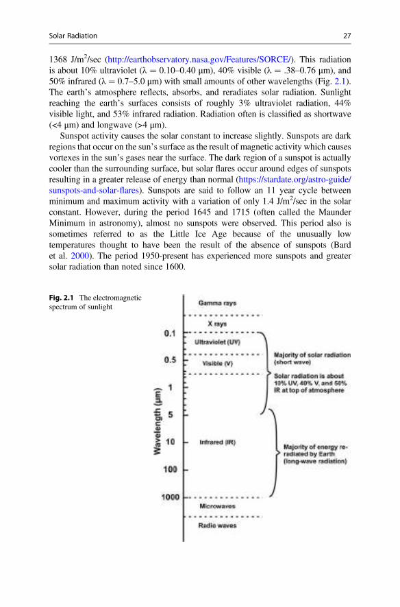
1368 J/m2/sec (http://earthobservatory.nasa.gov/Features/SORCE/). This radiationis about 10% ultraviolet (λ ¼ 0.10–0.40 μm), 40% visible (λ ¼ .38–0.76 μm), and50% infrared (λ ¼ 0.7–5.0 μm) with small amounts of other wavelengths (Fig. 2.1).The earth’s atmosphere reflects, absorbs, and reradiates solar radiation. Sunlightreaching the earth’s surfaces consists of roughly 3% ultraviolet radiation, 44%visible light, and 53% infrared radiation. Radiation often is classified as shortwave(<4 μm) and longwave (>4 μm).

Sunspot activity causes the solar constant to increase slightly. Sunspots are darkregions that occur on the sun’s surface as the result of magnetic activity which causesvortexes in the sun’s gases near the surface. The dark region of a sunspot is actuallycooler than the surrounding surface, but solar flares occur around edges of sunspotsresulting in a greater release of energy than normal (https://stardate.org/astro-guide/sunspots-and-solar-flares). Sunspots are said to follow an 11 year cycle betweenminimum and maximum activity with a variation of only 1.4 J/m2/sec in the solarconstant. However, during the period 1645 and 1715 (often called the MaunderMinimum in astronomy), almost no sunspots were observed. This period also issometimes referred to as the Little Ice Age because of the unusually lowtemperatures thought to have been the result of the absence of sunspots (Bardet al. 2000). The period 1950-present has experienced more sunspots and greatersolar radiation than noted since 1600.

Fig. 2.1 The electromagneticspectrum of sunlight

Solar Radiation 27

http://earthobservatory.nasa.gov/Features/SORCE/

https://stardate.org/astro-guide/sunspots-and-solar-flares

https://stardate.org/astro-guide/sunspots-and-solar-flares

Earth’s Energy Budget

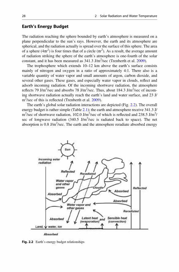
The radiation reaching the sphere bounded by earth’s atmosphere is measured on aplane perpendicular to the sun’s rays. However, the earth and its atmosphere arespherical, and the radiation actually is spread over the surface of this sphere. The areaof a sphere (4πr2) is four times that of a circle (πr2). As a result, the average amountof radiation striking the sphere of the earth’s atmosphere is one-fourth of the solarconstant, and it has been measured as 341.3 J/m2/sec (Trenberth et al. 2009).

The trophosphere which extends 10–12 km above the earth’s surface consistsmainly of nitrogen and oxygen in a ratio of approximately 4:1. There also is avariable quantity of water vapor and small amounts of argon, carbon dioxide, andseveral other gases. These gases, and especially water vapor in clouds, reflect andadsorb incoming radiation. Of the incoming shortwave radiation, the atmospherereflects 79 J/m2/sec and absorbs 78 J/m2/sec. Thus, about 184.3 J/m2/sec of incom-ing shortwave radiation actually reach the earth’s land and water surface, and 23 J/m2/sec of this is reflected (Trenberth et al. 2009).

The earth’s global solar radiation interactions are depicted (Fig. 2.2). The overallenergy budget is rather simple (Table 2.1); the earth and atmosphere receive 341.3 J/m2/sec of shortwave radiation, 102.0 J/m2/sec of which is reflected and 238.5 J/m2/sec of longwave radiation (340.5 J/m2/sec is radiated back to space). The netabsorption is 0.8 J/m2/sec. The earth and the atmosphere reradiate absorbed energy

Fig. 2.2 Earth’s energy budget relationships


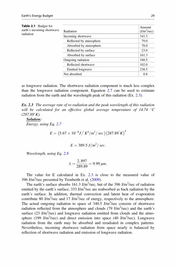
as longwave radiation. The shortwave radiation component is much less complexthan the longwave radiation component. Equation 2.7 can be used to estimateradiation from the earth and the wavelength peak of this radiation (Ex. 2.3).

Ex. 2.3 The average rate of re-radiation and the peak wavelength of this radiationwill be calculated for an effective global average temperature of 14.74 �C(287.89�K).

Solution:Energy, using Eq. 2.7

E ¼ 5:67� 10�8J=�K4=m2= sec

� �287:89

�K

� �4

E ¼ 389:5 J=m2= sec:

Wavelength, using Eq. 2.8

λ ¼ 2; 897289:89

¼ 9:99 μm:

The value for E calculated in Ex. 2.3 is close to the measured value of396 J/m2/sec presented by Trenberth et al. (2009).

The earth’s surface absorbs 161.3 J/m2/sec, but of the 396 J/m2/sec of radiationemitted by the earth’s surface, 333 J/m2/sec are reabsorbed as back radiation by theearth’s surface. In addition, thermal convection and latent heat of evaporationcontribute 80 J/m2/sec and 17 J/m2/sec of energy, respectively to the atmosphere.The actual outgoing radiation to space of 340.5 J/m2/sec consists of shortwaveradiation reflected from the atmosphere and clouds (79 J/m2/sec) and the earth’ssurface (23 J/m2/sec) and longwave radiation emitted from clouds and the atmo-sphere (199 J/m2/sec) and direct emission into space (40 J/m2/sec). Longwaveradiation from the earth may be absorbed and reradiated in complex patterns.Nevertheless, incoming shortwave radiation from space nearly is balanced byreflection of shortwave radiation and emission of longwave radiation.

Table 2.1 Budget forearth’s incoming shortwaveradiation

RadiationAmount(J/m2/sec)

Incoming shortwave 341.3

Reflected by atmosphere 79.0

Absorbed by atmosphere 78.0

Reflected by surface 23.0

Absorbed by surface 161.3

Outgoing radiation 340.5

Reflected shortwave 102.0

Emitted longwave 238.5

Net absorbed 0.8

Earth’s Energy Budget 29

The ocean and other water bodies absorb and hold a considerable amount ofenergy. According to Kirchhoff’s law, there is a direct relationship between absorp-tivity (a) and emissivity (e), a� e, and good absorbers are good radiators. The albedoof water is low (usually no more than 5–10%), and its emissivity is 0.96 on a scale of0–1.0. The earth’s land surface has an average emissivity around 0.5.

Greenhouse Effect

Nitrogen, oxygen, and argon in the atmosphere do not impede escape of longwaveradiation into space. Water vapor, carbon dioxide, methane, nitrous oxide, and a fewother gases absorb longwave radiation slowing its passage into space and increasingthe heat content of the atmosphere. This process is known as the greenhouse effect ofthe earth’s atmosphere; the gases responsible for this effect are called greenhousegases. The common observation that nights are often warmer when there is cloudcover than when the sky is clear provides tangible evidence of the greenhouse effect.The greenhouse effect warms the earth, and without it, the earth would average about30 �C cooler. Life on earth, as we know it, depends upon the natural greenhouseeffect of the atmosphere.

The concentration of carbon dioxide in the atmosphere was around 280 ppm atthe beginning of the industrial revolution (�1750). The increased use of fossil fuelsfor energy since the 1750s has progressively increased atmospheric carbon dioxideconcentration. Carbon dioxide concentration has been monitored continuously in theair at Mauna Loa Observatory in Hawaii since the late 1950s. The concentration was320 ppm in 1960, and the average for June 2018 was 411 ppm (https://www.co2.earth). Concentrations of other greenhouse gases also have increased because of airpollution. Greater greenhouse gas concentrations are thought to be the major factorcausing global warming. The annual global temperature has increased about 0.07 �C/decade since 1880, but since 1970, the increase rate averaged 0.17 �C/decade.

Light Penetration in Water

A major influence of solar radiation in aquatic ecology is the necessity of light forphotosynthesis. Light for photosynthesis is almost entirely within the visible rangeof the electromagnetic spectrum, but the visible spectrum represents only 44% of theelectromagnetic input to earth from the sun. Infrared radiation accounts for 53% ofthe remaining electromagnetic input. Most of the solar radiation entering waterbodies is in the visible or infrared range. The focus here will be on the absorptionof light energy by water, and effects of light on photosynthesis is deferred toChap. 10. Most of the absorption of light by water is within the 0.38–4 μmwavelength range. Although Fig. 2.3 indicates strong absorption in the0.01–0.1 μm range, relatively little of the sun’s electromagnetic input falls withinthis range.


https://www.co2.earth

https://www.co2.earth

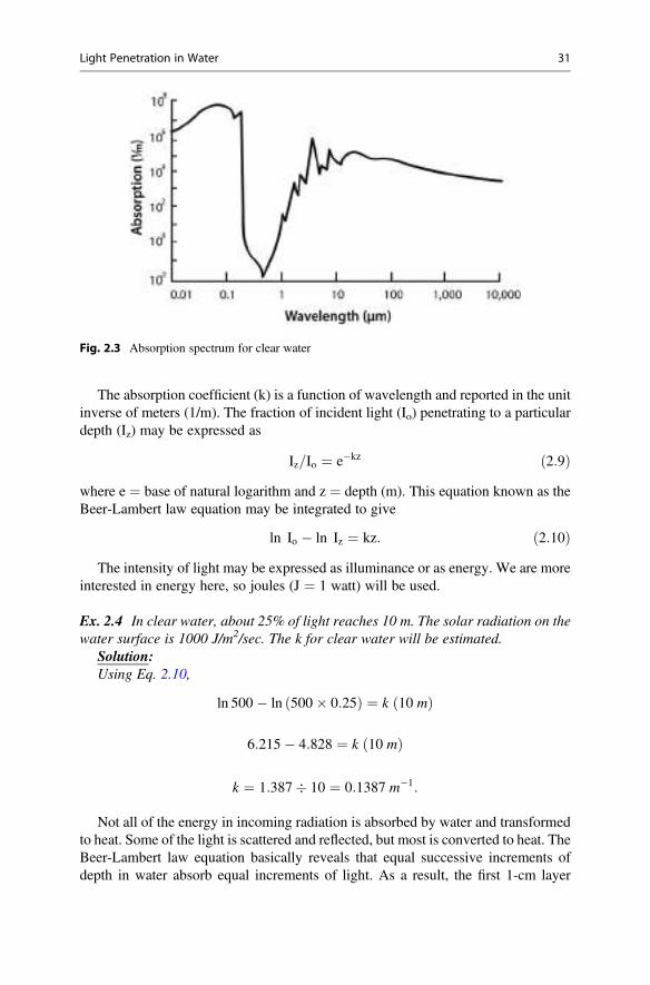
The absorption coefficient (k) is a function of wavelength and reported in the unitinverse of meters (1/m). The fraction of incident light (Io) penetrating to a particulardepth (Iz) may be expressed as

Iz=Io ¼ e�kz ð2:9Þwhere e ¼ base of natural logarithm and z ¼ depth (m). This equation known as theBeer-Lambert law equation may be integrated to give

ln Io � ln Iz ¼ kz: ð2:10ÞThe intensity of light may be expressed as illuminance or as energy. We are more

interested in energy here, so joules (J ¼ 1 watt) will be used.

Ex. 2.4 In clear water, about 25% of light reaches 10 m. The solar radiation on thewater surface is 1000 J/m2/sec. The k for clear water will be estimated.

Solution:Using Eq. 2.10,

ln 500� ln 500� 0:25ð Þ ¼ k 10 mð Þ

6:215� 4:828 ¼ k 10 mð Þ

k ¼ 1:387� 10 ¼ 0:1387 m�1:

Not all of the energy in incoming radiation is absorbed by water and transformedto heat. Some of the light is scattered and reflected, but most is converted to heat. TheBeer-Lambert law equation basically reveals that equal successive increments ofdepth in water absorb equal increments of light. As a result, the first 1-cm layer

Fig. 2.3 Absorption spectrum for clear water

Light Penetration in Water 31

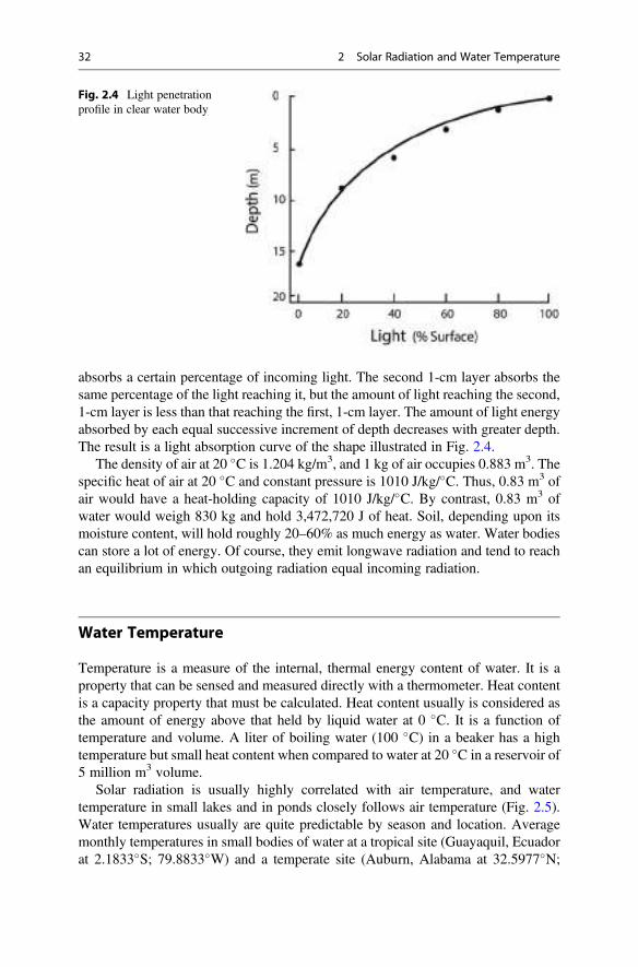
absorbs a certain percentage of incoming light. The second 1-cm layer absorbs thesame percentage of the light reaching it, but the amount of light reaching the second,1-cm layer is less than that reaching the first, 1-cm layer. The amount of light energyabsorbed by each equal successive increment of depth decreases with greater depth.The result is a light absorption curve of the shape illustrated in Fig. 2.4.

The density of air at 20 �C is 1.204 kg/m3, and 1 kg of air occupies 0.883 m3. Thespecific heat of air at 20 �C and constant pressure is 1010 J/kg/�C. Thus, 0.83 m3 ofair would have a heat-holding capacity of 1010 J/kg/�C. By contrast, 0.83 m3 ofwater would weigh 830 kg and hold 3,472,720 J of heat. Soil, depending upon itsmoisture content, will hold roughly 20–60% as much energy as water. Water bodiescan store a lot of energy. Of course, they emit longwave radiation and tend to reachan equilibrium in which outgoing radiation equal incoming radiation.

Water Temperature

Temperature is a measure of the internal, thermal energy content of water. It is aproperty that can be sensed and measured directly with a thermometer. Heat contentis a capacity property that must be calculated. Heat content usually is considered asthe amount of energy above that held by liquid water at 0 �C. It is a function oftemperature and volume. A liter of boiling water (100 �C) in a beaker has a hightemperature but small heat content when compared to water at 20 �C in a reservoir of5 million m3 volume.

Solar radiation is usually highly correlated with air temperature, and watertemperature in small lakes and in ponds closely follows air temperature (Fig. 2.5).Water temperatures usually are quite predictable by season and location. Averagemonthly temperatures in small bodies of water at a tropical site (Guayaquil, Ecuadorat 2.1833�S; 79.8833�W) and a temperate site (Auburn, Alabama at 32.5977�N;

Fig. 2.4 Light penetrationprofile in clear water body


85.4808�W) are provided in Fig. 2.6. Water temperatures at Auburn, Alabama, in thetemperate zone change markedly with season, but water temperatures also vary to alesser extent with season even in the tropics. Air temperature in Ecuador is higherduring the warmer wet season (January through May) than during the cooler dryseason. This difference in air temperature between seasons also is reflected in watertemperatures. Air temperatures at a given locality may deviate from normal for aparticular period causing deviation in water temperatures.

Because water can store much heat, larger bodies of water require time to warmup in the spring and to cool down in the autumn. Therefore, the temperature of largereservoirs and lakes tend to lag air temperatures. The heat budgets of lakes obviously

Fig. 2.5 Upper: Plot of daily air and water temperatures in a small pond. Lower: Regressionbetween daily air and water temperatures in a small pond (Source: Prapaiwong and Boyd 2012)

Water Temperature 33

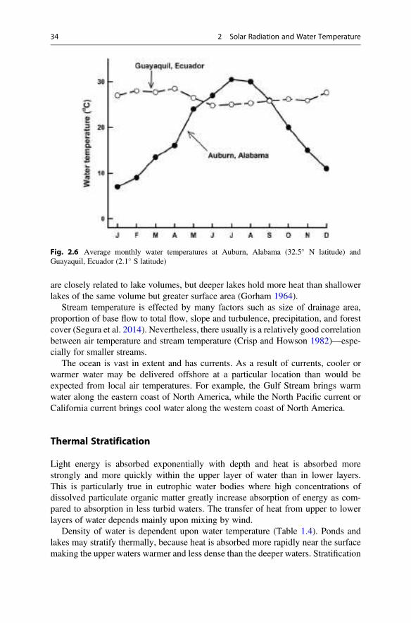
are closely related to lake volumes, but deeper lakes hold more heat than shallowerlakes of the same volume but greater surface area (Gorham 1964).

Stream temperature is effected by many factors such as size of drainage area,proportion of base flow to total flow, slope and turbulence, precipitation, and forestcover (Segura et al. 2014). Nevertheless, there usually is a relatively good correlationbetween air temperature and stream temperature (Crisp and Howson 1982)—espe-cially for smaller streams.

The ocean is vast in extent and has currents. As a result of currents, cooler orwarmer water may be delivered offshore at a particular location than would beexpected from local air temperatures. For example, the Gulf Stream brings warmwater along the eastern coast of North America, while the North Pacific current orCalifornia current brings cool water along the western coast of North America.

Thermal Stratification

Light energy is absorbed exponentially with depth and heat is absorbed morestrongly and more quickly within the upper layer of water than in lower layers.This is particularly true in eutrophic water bodies where high concentrations ofdissolved particulate organic matter greatly increase absorption of energy as com-pared to absorption in less turbid waters. The transfer of heat from upper to lowerlayers of water depends mainly upon mixing by wind.

Density of water is dependent upon water temperature (Table 1.4). Ponds andlakes may stratify thermally, because heat is absorbed more rapidly near the surfacemaking the upper waters warmer and less dense than the deeper waters. Stratification

Fig. 2.6 Average monthly water temperatures at Auburn, Alabama (32.5� N latitude) andGuayaquil, Ecuador (2.1� S latitude)


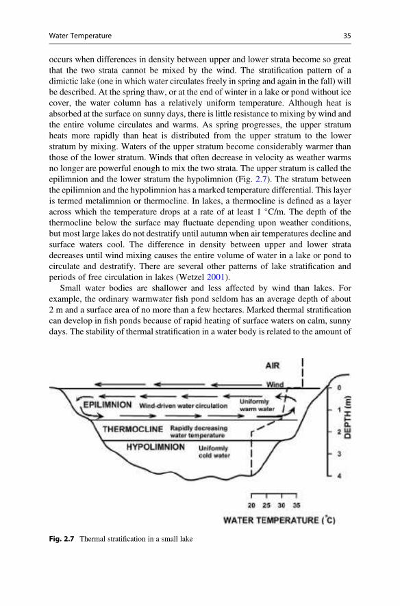
occurs when differences in density between upper and lower strata become so greatthat the two strata cannot be mixed by the wind. The stratification pattern of adimictic lake (one in which water circulates freely in spring and again in the fall) willbe described. At the spring thaw, or at the end of winter in a lake or pond without icecover, the water column has a relatively uniform temperature. Although heat isabsorbed at the surface on sunny days, there is little resistance to mixing by wind andthe entire volume circulates and warms. As spring progresses, the upper stratumheats more rapidly than heat is distributed from the upper stratum to the lowerstratum by mixing. Waters of the upper stratum become considerably warmer thanthose of the lower stratum. Winds that often decrease in velocity as weather warmsno longer are powerful enough to mix the two strata. The upper stratum is called theepilimnion and the lower stratum the hypolimnion (Fig. 2.7). The stratum betweenthe epilimnion and the hypolimnion has a marked temperature differential. This layeris termed metalimnion or thermocline. In lakes, a thermocline is defined as a layeracross which the temperature drops at a rate of at least 1 �C/m. The depth of thethermocline below the surface may fluctuate depending upon weather conditions,but most large lakes do not destratify until autumn when air temperatures decline andsurface waters cool. The difference in density between upper and lower stratadecreases until wind mixing causes the entire volume of water in a lake or pond tocirculate and destratify. There are several other patterns of lake stratification andperiods of free circulation in lakes (Wetzel 2001).

Small water bodies are shallower and less affected by wind than lakes. Forexample, the ordinary warmwater fish pond seldom has an average depth of about2 m and a surface area of no more than a few hectares. Marked thermal stratificationcan develop in fish ponds because of rapid heating of surface waters on calm, sunnydays. The stability of thermal stratification in a water body is related to the amount of

Fig. 2.7 Thermal stratification in a small lake


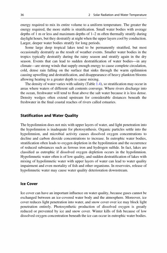
energy required to mix its entire volume to a uniform temperature. The greater theenergy required, the more stable is stratification. Small water bodies with averagedepths of 1 m or less and maximum depths of 1–2 m often thermally stratify duringdaylight hours, but they destratify at night when the upper layers cool by conduction.Larger, deeper water bodies stratify for long periods.

Some large deep tropical lakes tend to be permanently stratified, but mostoccasionally destratify as the result of weather events. Smaller water bodies in thetropics typically destratify during the rainy season and stratify again in the dryseason. Events that can lead to sudden destratification of water bodies—in anyclimate—are strong winds that supply enough energy to cause complete circulation,cold, dense rain falling on the surface that sinks through the warm epilimnioncausing upwelling and destratification, and disappearance of heavy plankton bloomsallowing heating to a greater depth to cause mixing.

The density of water varies with salinity (Table 1.4), so stratification may occur inareas where waters of different salt contents converge. Where rivers discharge intothe ocean, freshwater will tend to float above the salt water because it is less dense.Density wedges often extend upstream for considerable distances beneath thefreshwater in the final coastal reaches of rivers called estuaries.

Statification and Water Quality

The hypolimnion does not mix with upper layers of water, and light penetration intothe hypolimnion is inadequate for photosynthesis. Organic particles settle into thehypolimnion, and microbial activity causes dissolved oxygen concentrations todecline and carbon dioxide concentrations to increase. In eutrophic water bodies,stratification often leads to oxygen depletion in the hypolimnion and the occurrenceof reduced substances such as ferrous iron and hydrogen sulfide. In fact, lakes areclassified as eutrophic if dissolved oxygen depletion occurs in the hypolimnion.Hypolimnetic water often is of low quality, and sudden destratification of lakes withmixing of hypolimnetic water with upper layers of water can lead to water qualityimpairment and even mortality of fish and other organisms. In reservoirs, release ofhypolimnetic water may cause water quality deterioration downstream.

Ice Cover

Ice cover can have an important influence on water quality, because gases cannot beexchanged between an ice-covered water body and the atmosphere. Moreover, icecover reduces light penetration into water, and snow cover over ice may block lightpenetration entirely. Photosynthetic production of dissolved oxygen is greatlyreduced or prevented by ice and snow cover. Winter kills of fish because of lowdissolved oxygen concentration beneath the ice can occur in eutrophic water bodies.


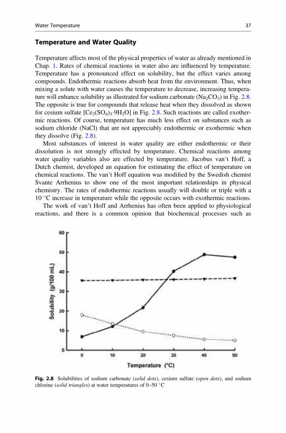
Temperature and Water Quality

Temperature affects most of the physical properties of water as already mentioned inChap. 1. Rates of chemical reactions in water also are influenced by temperature.Temperature has a pronounced effect on solubility, but the effect varies amongcompounds. Endothermic reactions absorb heat from the environment. Thus, whenmixing a solute with water causes the temperature to decrease, increasing tempera-ture will enhance solubility as illustrated for sodium carbonate (Na2CO3) in Fig. 2.8.The opposite is true for compounds that release heat when they dissolved as shownfor cesium sulfate [Ce2(SO4)3�9H2O] in Fig. 2.8. Such reactions are called exother-mic reactions. Of course, temperature has much less effect on substances such assodium chloride (NaCl) that are not appreciably endothermic or exothermic whenthey dissolve (Fig. 2.8).

Most substances of interest in water quality are either endothermic or theirdissolution is not strongly effected by temperature. Chemical reactions amongwater quality variables also are effected by temperature. Jacobus van’t Hoff, aDutch chemist, developed an equation for estimating the effect of temperature onchemical reactions. The van’t Hoff equation was modified by the Swedish chemistSvante Arrhenius to show one of the most important relationships in physicalchemistry. The rates of endothermic reactions usually will double or triple with a10 �C increase in temperature while the opposite occurs with exothermic reactions.

The work of van’t Hoff and Arrhenius has often been applied to physiologicalreactions, and there is a common opinion that biochemical processes such as

Fig. 2.8 Solubilities of sodium carbonate (solid dots), cesium sulfate (open dots), and sodiumchlorine (solid triangles) at water temperatures of 0–50 �C


respiration or growth will double with a 10 �C increase in temperature (within therange of tolerance of the organism). However, this is not always a reliable “rule ofthumb.” The temperature coefficient (Q10) may be calculated to determine the actualrate of change in a biological process when temperature changes by 10 �C. The Q10

equation is:

Q10 ¼ R2 � R1ð Þ10�c= T2�T1ð Þ ð2:11Þ

where R1 and R2 are rates for the process at temperatures T1 and T2 (�C). The Q10 ofbiological processes may range from <1.0 to >4.0 (Kruse et al. 2011; Peck andMoyano 2016).

Ex. 2.5 Fish respire at 200 mg O2/kg body weight/hr at 22 �C and at 350 mg O2/kg/hr at 28 �C. The Q10 will be calculated.

Solution:Using Eq. 2.11,

Q10 ¼ 350� 200 mg=kg=hrð Þ10�=28�22 ¼ 1:75ð Þ1:67 ¼ 2:55:

Temperature effects all biological processes in aquatic ecosystems, and rates ofgrowth of all species tend to increase with warmth. However, temperatures that aretoo high or too low will adversely influence living things. Each species has itsparticular temperature range within which it may exist within ecosystems. Aquaticanimals often are classified as coldwater, warmwater, and tropical species.Coldwater species will not tolerate temperatures above 20–25 �C. Warmwaterspecies will usually not reproduce at temperatures below 20 �C or grow attemperatures below 10–15 �C, but they will survive much lower wintertemperatures. Tropical species will die at temperatures of 10–20 �C, and most donot grow well at temperatures below 25 �C.

Temperature ranges given above are very general, and each species, whethercoldwater, warmwater, or tropical has its characteristic temperature requirements.The temperature effects on a tropical species of fish is illustrated in Fig. 2.9. There isa low temperature below which fish die, at slightly higher temperature, fish live, butthey do not grow or grow very slowly. Above a certain temperature, growth willincrease rapidly with increasing temperature until the optimum temperature isreached. As temperature rises beyond the optimum temperature, growth will slow,cease, and fish will die if the increase continues. The relationship in Fig. 2.9 isslightly different for warmwater or coldwater species which are not likely to die as aresult of low temperature in natural or aquaculture waters.

The growth pattern shown in Fig. 2.9 is for animals held in the laboratory underhighly controlled conditions. In natural water bodies, water temperature will fluctu-ate according to daily and seasonal patterns and weather patterns may result indeviations from normal trends. However, a species will do best in an environmentwhere the water temperature remains within a non-stressful range.


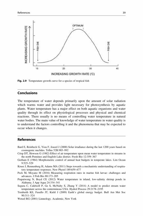
Conclusions

The temperature of water depends primarily upon the amount of solar radiationwhich warms water and provides light necessary for photosynthesis by aquaticplants. Water temperature has a major effect on both aquatic organisms and waterquality through its effect on physiological processes and physical and chemicalreactions. There usually is no means of controlling water temperature in naturalwater bodies. The main value of knowledge of water temperature in water quality isto understand the factors controlling it and the phenomena that may be expected tooccur when it changes.

References

Bard E, Reinbeck G, Yiou F, Jouzel J (2000) Solar irradiance during the last 1200 years based oncosmogenic nuclides. Tellus 52B:985–992

Crisp DT, Howson G (1982) Effect of air temperature upon mean water temperature in streams inthe north Pennines and English Lake district. Fresh Bio 12:359–367

Gorham E (1964) Morphometric control of annual heat budgets in temperate lakes. Lim Ocean9:525–529

Kruse J, Rennenberg H, Adams MA (2011) Steps towards a mechanistic understanding of respira-tory temperature responses. New Phytol 189:659–677

Peck M, Moyano M (2016) Measuring respiration rates in marine fish larvae: challenges andadvances. J Fish Bio 88:173–205

Prapaiwong N, Boyd CE (2012) Water temperature in inland, low-salinity shrimp ponds inAlabama. J App Aqua 24:334–341

Segura C, Caldwell P, Ge S, McNulty S, Zhang Y (2014) A model to predict stream watertemperature across the conterminous USA. Hydrol Process 29:2178–2195

Trenberth KE, Fasullo JT, Kiehl J (2009) Earth’s global energy budget. Bull Am Met Soc90:311–324

Wetzel RG (2001) Limnology. Academic, New York

Fig. 2.9 Temperature growth curve for a species of tropical fish

References 39

An Overview of Hydrology and WaterSupply 3

AbstractThe familiar water cycle is driven by solar radiation, and water is continuallytransformed back and forth between water vapor and liquid water. In the process,water passes through several distinct compartments of the hydrosphere to includeatmospheric moisture, precipitation, runoff, groundwater, standing water bodies,flowing streams, and ocean. Water budgets for water bodies allow concentrationsof water quality variables to be used with inflow, outflow, and storage changes toestimate quantities of water quality variables that are contained in and passthrough water bodies.

Introduction

Rainwater contains low concentrations of dissolved matter, but as water passesthrough the different compartments of the hydrologic cycle, it becomes moreconcentrated with dissolved matter in the order rainwater < overland flow < streamflow < groundwater < ocean water. A knowledge of how water moves through thehydrologic cycle allows one to appreciate why these changes occur. Water qualityusually cannot be separated entirely from water quantity. One reason for this is thatthe amounts of nutrients entering water bodies from their watersheds depend uponboth nutrient concentrations in inflows from watersheds and the amounts of inflows.Information on water quantity is needed when assessing water quality, and thestudent of water quality should learn the basic principles related to water quantity.

This chapter provides a brief discussion of the hydrologic cycle, the basic types ofwater bodies, and simple methods of water quantity measurement.


41


The Earth’s Water

The hydrosphere consists of the earth’s gaseous, liquid, and solid water and iscomprised of several compartments to include the ocean, freshwater lakes andponds, streams, wetlands, soil moisture, water vapor, etc. (Table 3.1). The oceanhas a volume of around 1.3 billion km3 and comprises 97.4% of the earth’s water.The remaining water—about 36 million km3

— is contained in several freshwatercompartments of the hydrosphere. The largest proportion of the earth’s freshwater isbound in ice, occurs as deep groundwater, or is flood-stage stream flow, none ofwhich can often be put to a beneficial use. The amount of freshwater available forhuman use at any particular time is shallow groundwater, water in lakes, non-flood-stage flow of rivers and small streams, and manmade reservoirs that capture and storeriver flow. Much of the available freshwater is either not accessible or not sustainablefor human use.

The amount of water occurring at a given time in a compartment of the hydro-sphere is not directly related to the amount of water available from that compartmentfor ecological or human use. The reason of this discrepancy relates to the renewal(turnover) time of water in a particular compartment of the hydrosphere (Table 3.1).The volume of water in the atmosphere is around 14,400 km3 at any particular time,but the renewal time of water vapor in the atmosphere is only 9 days. If all watervapor could be instantly removed from the atmosphere, it would be replaced in9 days. Water in the atmosphere can be recycled 1,500,000 times during the 37,000-year renewal time of the ocean. The amount of water cycling through the atmospherein 37,000 years is 21,600,000,000 km3 or about 16 times the volume of the ocean.Rainfall and other forms of precipitation directly or indirectly sustain the othercomponents of the hydrosphere.

Table 3.1 Volumes of ocean water and different compartments of freshwater

CompartmentVolume(km3)

Proportion of total(%)

Renewaltime

Oceans 1,348,000,000 97.40 37,000 yr

Freshwater

Polar ice, icebergs, and glaciers 27,818,000 2.01 16,000 yr

Groundwater (800 to 4000 m depth) 4,447,000 0.32 –

Groundwater (to 800 m depth) 3,551,000 0.26 300 yr

Lakes 126,000 0.009 1–100 yr

Soil moisture 61,100 0.004 280 d

Atmosphere (water vapor) 14,400 0.001 9 d

Rivers 1070 0.00008 12–20 d

Plants, animals, humans 1070 0.00008 –

Hydrated minerals 360 0.00002 –

Total freshwater (36,020,000) (2.60) –

Renewal times are provided for selected compartments. (Baumgartner and Reichel 1975; Wetzel2001)

42 3 An Overview of Hydrology and Water Supply

Precipitation on the earth’s land masses totals about 110,000 km3 annually.Evapotranspiration from the land returns about 70,000 km3 water to the atmosphereeach year, and the rest—an estimated 40,000 km3 becomes runoff and flows into theocean (Baumgartner and Reichel 1975). Of course, if the ocean is included, evapo-transpiration from land plus evaporation from the ocean must equal to precipitationonto the entire earth’s surface.

Runoff consists of overland (storm) flow and base flow of groundwater intostreams. Removing groundwater for water supply potentially can cause a decreasein base flow from streams, and groundwater use often is not considered sustainable.About 30% of global runoff or 12,000 km3 is stream base flow, and another6000 km3 is captured in impoundments (Table 3.2). Most authorities believe about70% of runoff is spatially available for extraction for human use, and the annualsupply of water for human use is around 12,600 km3.

The water footprint is defined as the total amount of water used for a particularpurpose. Water footprints can be calculated for individuals, countries, the world, andfor specific goods and services. The average water footprint for humans was anestimated 1385 m3/cap/year (Hoekstra and Mekonnen 2012); water footprints incubic meters per capita annually for several countries were: China, 1071;South Africa, 1255; France, 1786; Brazil, 2027; United States, 2842. Waterfootprints usually include rainwater that evaporates from agricultural fields. Thiswater is called “green” water, but it would have evaporated whether or not it hadfallen on cropland.

The global water footprint for agriculture given by Hoekstra and Mekonnen(2012) was 8363 km3/year while global industrial and domestic footprints werearound 400 km3/year and 324 km3/year, respectively. The total global water foot-print is 9087 km3/year, but this includes 6684 km3/year of “green” water used inagriculture. A more reasonable estimate of water use is to combine water forirrigation of 3200 km3/year (Wisser et al. 2008), animal water supply (46 km3/year), industrial (400 km3/year), and domestic purposes (324 km3/year)—a total of3970 km3/year.

When compared to the amount of runoff that is renewable and accessible tohumans, the total amount of water available for human use appears quite adequatefor the future if green water is omitted. This unfortunately is not the case because ofseveral reasons. Water is not uniformly distributed with population (Table 3.3), andmany countries or areas of countries with rapidly growing populations have a naturalscarcity of water. Water supply varies from year to year with respect to weather

Table 3.2 Renewable, accessible water for humankind

Hydrologic item Volume (km3/yr)

Rainfall onto land masses 110,000

Evapotranspiration from land masses 70,000

Renewable water: Total stream flow 40,000

Available water: Base stream flow (12,000 km3/yr) and reservoirs(6000 km3/yr)

18,000

Accessible water: About 70% of available 12,600

The Earth’s Water 43

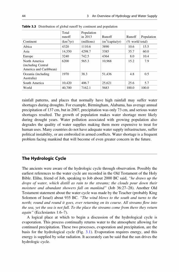
rainfall patterns, and places that normally have high rainfall may suffer watershortages during droughts. For example, Birmingham, Alabama, has average annualprecipitation of 137 cm, but in 2007, precipitation was only 73 cm, and serious watershortages resulted. The growth of population makes water shortage more likelyduring drought years. Water pollution associated with growing population alsodegrades the quality of water supplies making them more expensive to treat forhuman uses. Many countries do not have adequate water supply infrastructure, sufferpolitical instability, or are embroiled in armed conflicts. Water shortage is a frequentproblem facing mankind that will become of even greater concern in the future.

The Hydrologic Cycle

The ancients were aware of the hydrologic cycle through observation. Possibly theearliest references to the water cycle are recorded in the Old Testament of the HolyBible. Elihu, friend of Job, speaking to Job about 2000 BC said, “he draws up thedrops of water, which distill as rain to the streams; the clouds pour down theirmoisture and abundant showers fall on mankind” (Job 36:27–28). Another OldTestament statement about the water cycle was made by the Teacher (probably KingSolomon of Israel) about 935 BC. “The wind blows to the south and turns to thenorth; round and round it goes, ever returning on its course. All streams flow intothe sea, yet the sea is not full. To the place the streams come from there they returnagain” (Ecclesiastes 1:6–7).

A logical place at which to begin a discussion of the hydrological cycle isevaporation. This process continually returns water to the atmosphere allowing forcontinued precipitation. These two processes, evaporation and precipitation, are thebasis for the hydrological cycle (Fig. 3.1). Evaporation requires energy, and thisenergy is supplied by solar radiation. It accurately can be said that the sun drives thehydrologic cycle.

Table 3.3 Distribution of global runoff by continent and population

Totalrunoff

Populationin 2013 Runoff Runoff Population

Continent (km3/yr) (millions) (m3/capita/yr) (% world total)

Africa 4320 1110.6 3890 10.6 15.5

Asia 14,550 4298.7 3385 35.7 60.0

Europe 3240 742.5 4364 8.0 10.4

North America(including CentralAmerica and Caribbean)

6200 565.3 10,968 15.2 7.9

Oceania (includingAustralia)

1970 38.3 51,436 4.8 0.5

South America 10,420 406.7 25,621 25.6 5.7

World 40,700 7162.1 5683 100.0 100.0


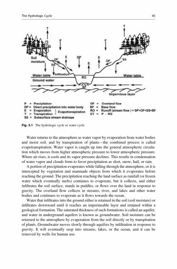
Water returns to the atmosphere as water vapor by evaporation from water bodiesand moist soil, and by transpiration of plants—the combined process is calledevapotranspiration. Water vapor is caught up into the general atmospheric circula-tion which moves from higher atmospheric pressure to lower atmospheric pressure.Where air rises, it cools and its vapor pressure declines. This results in condensationof water vapor and clouds form to favor precipitation as sleet, snow, hail, or rain.

A portion of precipitation evaporates while falling through the atmosphere, or it isintercepted by vegetation and manmade objects from which it evaporates beforereaching the ground. The precipitation reaching the land surface as rainfall (or frozenwater which eventually melts) continues to evaporate, but it collects, and eitherinfiltrates the soil surface, stands in puddles, or flows over the land in response togravity. The overland flow collects in streams, river, and lakes and other waterbodies and continues to evaporate as it flows towards the ocean.

Water that infiltrates into the ground either is retained in the soil (soil moisture) orinfiltrates downward until it reaches an impermeable layer and retained within ageological formation. The saturated thickness of such formations is called an aquifer,and water in underground aquifers is known as groundwater. Soil moisture can bereturned to the atmosphere by evaporation from the soil directly or by transpirationof plants. Groundwater moves slowly through aquifers by infiltration in response togravity. It will eventually seep into streams, lakes, or the ocean, and it can beremoved by wells for human use.

Fig. 3.1 The hydrologic cycle or water cycle

The Hydrologic Cycle 45

Evaporation

The capacity of air to hold water vapor depends on its temperature (Table 1.2). Themaximum amount of moisture that air can hold at a given temperature is its satura-tion vapor pressure. If unsaturated air is brought in contact with a water surface,molecules of water bounce from the water surface into the air until vapor pressure inair equals the pressure of water molecules escaping the surface. While watermolecules continue to move back and forth across the surface, there is no netmovement in either direction. The driving force for evaporation is the vapor pressuredeficit (VPD)

VPD ¼ es � ea ð3:1Þwhere es ¼ saturation vapor pressure and ea ¼ actual vapor pressure. The greater thevapor pressure deficit, the greater is the potential for evaporation.

Energy is required to raise the temperature of a mass of water to 100 �C andadditional heat must be added to cause boiling and vaporization. Some may havedifficulty reconciling this fact with the observation that water evaporates attemperatures below 100 �C. Molecules in a mass of water are in constant motion,and molecular motion increases with greater temperature. However, molecules in amass of water of a given temperature are moving at different speeds. The faster-moving molecules contain more thermal energy than do the slower-movingmolecules, and some of the fastest-moving molecules escape the surface to evapo-rate. Nearly all evaporation occurring in nature occurs at temperatures far below theboiling point of water. Nevertheless, greater temperature favors evaporation,because more molecules gain sufficient energy to escape the water surface. Somereaders may recognize the explanation above as an extension of Maxwell’s “demonconcept” (Klein 1970). James Maxwell, an early Scottish physicist of thermody-namic fame, envisioned a demon capable of allowing only the fast-movingmolecules in air to enter a room and thereby raising the temperature in the room.

Relative humidity is a measure of the percentage saturation of air with watervapor. It is an indicator of how much more moisture can evaporate into a given massof air. It is calculated as follows:

RH ¼ eaes

� 100 ð3:2Þ

where RH ¼ relative humidity (%), ea ¼ actual vapor pressure, and es ¼ saturationvapor pressure. Relative humidity usually is measured with a sling hygrometer (alsocalled a sling psychrometer) which consists of a wet bulb and a dry bulb thermome-ter that can be rapidly rotated in the air. Evaporation causes the wet bulb temperatureto decline to a lower temperature than measured by the dry bulb thermometer unlessthe air is saturated with water vapor (100% RH) and both thermometers read thesame temperature. The ratio of the wet to dry bulb temperatures is used to determinerelative humidity. The moisture content of air also may be expressed by the dewpoint or the temperature at which a parcel of air would begin to condense water


vapor. The higher the dew point, the more moisture there is in the air. Saturationvapor pressure (Table 1.2) increases with warmth, so warm air has the capacity tohold more water vapor than does cool air. Evaporation rate obviously is favored bylow relative humidity.

Wind velocity accelerates evaporation, because air movement usually replaceshumid air with drier air. When there is no air movement over a water surface,evaporation quickly saturates the layer of air above the water surface and evapora-tion ceases or diminishes greatly. The influence of wind on evaporation is especiallypronounced in windy, arid regions where air normally contains little moisture.

Dissolved salts decrease the vapor pressure of water. The evaporation rate underthe same conditions is about 5% greater from freshwater than from ocean water.Dissolved salt concentrations do not vary enough among freshwater bodies toinfluence evaporation rates appreciably. Turbid waters heat faster than clear waters,and as a result, greater turbidity, and especially turbidity caused by phytoplankton,tends to enhance evaporation (Idso and Foster 1974). Changes in atmosphericpressure effect evaporation slightly.

Temperature usually has the greatest influence on evaporation, and the air andwater temperatures at a locality are closely related to the amount of incoming solarradiation. The temperature difference between air and water affects evaporation. Acold water surface cannot generate a high vapor pressure, and cold air does not holdmuch water vapor. Cold air over cold water, cold air over warm water, and warm airover cold water are not as favorable for evaporation as is warm air over warm water.Evaporation rates tend to increase from cooler regions to warmer regions. Relativehumidity must be considered, because cold, dry air may take on more moisture thanwarm, moist air if the moisture-holding capacity of the warm air has already beenpartially or completely filled.

Evaporation occurs from lakes and streams, but most terrestrial evaporation isfrom the leaves of plants by a process called transpiration. The combined water lossby evaporation and transpiration is given the name evapotranspiration. Unlikeevaporation from the surface of a water body, evapotranspiration of terrestrialecosystems often is limited by a lack of moisture.

Measurement of Evaporation

The water balance in a water body is complex. Water is removed from water bodiesthrough evaporation, transpiration, seepage, consumptive use, and outflow, andwater also flows into water bodies by runoff or through precipitation. The changein depth over a period of time in a water body does not result solely from evapora-tion, and the change in moisture content of soil over time is not the sole result oftranspiration by plants and evaporation from the soil surface. Water in soil mayinfiltrate downward and precipitation delivers water to the soil.

One way of determining the potential for evaporation from water bodies is tomeasure evaporation from the surface of an otherwise “water-tight” container. Threetypes of evaporation instruments were recommended by the World Meteorological

Measurement of Evaporation 47

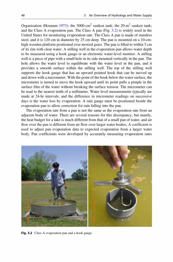
Organization (Hounam 1973): the 3000-cm2 sunken tank; the 20-m2 sunken tank;and the Class A evaporation pan. The Class A pan (Fig. 3.2) is widely used in theUnited States for monitoring evaporation rate. The Class A pan is made of stainlesssteel, and it is 120 cm in diameter by 25 cm deep. The pan is mounted on a 10-cm-high wooden platform positioned over mowed grass. The pan is filled to within 5 cmof its rim with clear water. A stilling well in the evaporation pan allows water depthto be measured using a hook gauge or an electronic water-level monitor. A stillingwell is a piece of pipe with a small hole in its side mounted vertically in the pan. Thehole allows the water level to equilibrate with the water level in the pan, and itprovides a smooth surface within the stilling well. The top of the stilling wellsupports the hook gauge that has an upward pointed hook that can be moved upand down with a micrometer. With the point of the hook below the water surface, themicrometer is turned to move the hook upward until its point pulls a pimple in thesurface film of the water without breaking the surface tension. The micrometer canbe read to the nearest tenth of a millimeter. Water level measurements typically aremade at 24-hr intervals, and the difference in micrometer readings on successivedays is the water loss by evaporation. A rain gauge must be positioned beside theevaporation pan to allow correction for rain falling into the pan.

The evaporation rate from a pan is not the same as the evaporation rate from anadjacent body of water. There are several reasons for this discrepancy, but mainly,the heat budget for a lake is much different from that of a small pan of water, and airflow over the pan is different from air flow over larger water bodies. A coefficient isused to adjust pan evaporation data to expected evaporation from a larger waterbody. Pan coefficients were developed by accurately measuring evaporation rates

Fig. 3.2 Class A evaporation pan and a hook gauge


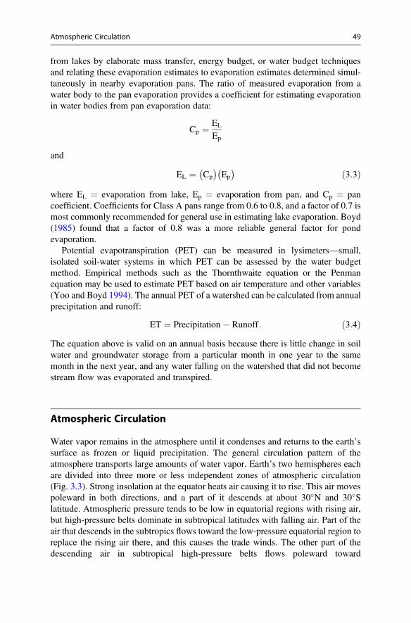
from lakes by elaborate mass transfer, energy budget, or water budget techniquesand relating these evaporation estimates to evaporation estimates determined simul-taneously in nearby evaporation pans. The ratio of measured evaporation from awater body to the pan evaporation provides a coefficient for estimating evaporationin water bodies from pan evaporation data:

Cp ¼ EL

Ep

and

EL ¼ Cp� �

Ep� � ð3:3Þ

where EL ¼ evaporation from lake, Ep ¼ evaporation from pan, and Cp ¼ pancoefficient. Coefficients for Class A pans range from 0.6 to 0.8, and a factor of 0.7 ismost commonly recommended for general use in estimating lake evaporation. Boyd(1985) found that a factor of 0.8 was a more reliable general factor for pondevaporation.

Potential evapotranspiration (PET) can be measured in lysimeters—small,isolated soil-water systems in which PET can be assessed by the water budgetmethod. Empirical methods such as the Thornthwaite equation or the Penmanequation may be used to estimate PET based on air temperature and other variables(Yoo and Boyd 1994). The annual PET of a watershed can be calculated from annualprecipitation and runoff:

ET ¼ Precipitation� Runoff: ð3:4ÞThe equation above is valid on an annual basis because there is little change in soilwater and groundwater storage from a particular month in one year to the samemonth in the next year, and any water falling on the watershed that did not becomestream flow was evaporated and transpired.

Atmospheric Circulation

Water vapor remains in the atmosphere until it condenses and returns to the earth’ssurface as frozen or liquid precipitation. The general circulation pattern of theatmosphere transports large amounts of water vapor. Earth’s two hemispheres eachare divided into three more or less independent zones of atmospheric circulation(Fig. 3.3). Strong insolation at the equator heats air causing it to rise. This air movespoleward in both directions, and a part of it descends at about 30�N and 30�Slatitude. Atmospheric pressure tends to be low in equatorial regions with rising air,but high-pressure belts dominate in subtropical latitudes with falling air. Part of theair that descends in the subtropics flows toward the low-pressure equatorial region toreplace the rising air there, and this causes the trade winds. The other part of thedescending air in subtropical high-pressure belts flows poleward toward

Atmospheric Circulation 49

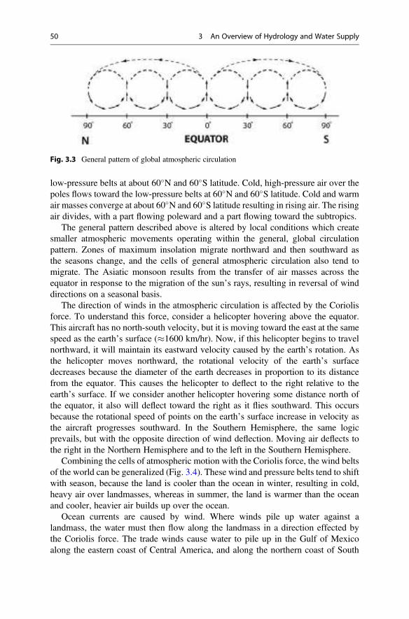
low-pressure belts at about 60�N and 60�S latitude. Cold, high-pressure air over thepoles flows toward the low-pressure belts at 60�N and 60�S latitude. Cold and warmair masses converge at about 60�N and 60�S latitude resulting in rising air. The risingair divides, with a part flowing poleward and a part flowing toward the subtropics.

The general pattern described above is altered by local conditions which createsmaller atmospheric movements operating within the general, global circulationpattern. Zones of maximum insolation migrate northward and then southward asthe seasons change, and the cells of general atmospheric circulation also tend tomigrate. The Asiatic monsoon results from the transfer of air masses across theequator in response to the migration of the sun’s rays, resulting in reversal of winddirections on a seasonal basis.

The direction of winds in the atmospheric circulation is affected by the Coriolisforce. To understand this force, consider a helicopter hovering above the equator.This aircraft has no north-south velocity, but it is moving toward the east at the samespeed as the earth’s surface (�1600 km/hr). Now, if this helicopter begins to travelnorthward, it will maintain its eastward velocity caused by the earth’s rotation. Asthe helicopter moves northward, the rotational velocity of the earth’s surfacedecreases because the diameter of the earth decreases in proportion to its distancefrom the equator. This causes the helicopter to deflect to the right relative to theearth’s surface. If we consider another helicopter hovering some distance north ofthe equator, it also will deflect toward the right as it flies southward. This occursbecause the rotational speed of points on the earth’s surface increase in velocity asthe aircraft progresses southward. In the Southern Hemisphere, the same logicprevails, but with the opposite direction of wind deflection. Moving air deflects tothe right in the Northern Hemisphere and to the left in the Southern Hemisphere.

Combining the cells of atmospheric motion with the Coriolis force, the wind beltsof the world can be generalized (Fig. 3.4). These wind and pressure belts tend to shiftwith season, because the land is cooler than the ocean in winter, resulting in cold,heavy air over landmasses, whereas in summer, the land is warmer than the oceanand cooler, heavier air builds up over the ocean.

Ocean currents are caused by wind. Where winds pile up water against alandmass, the water must then flow along the landmass in a direction effected bythe Coriolis force. The trade winds cause water to pile up in the Gulf of Mexicoalong the eastern coast of Central America, and along the northern coast of South

Fig. 3.3 General pattern of global atmospheric circulation


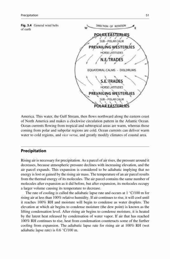
America. This water, the Gulf Stream, then flows northward along the eastern coastof North America and makes a clockwise circulation pattern in the Atlantic Ocean.Ocean currents flowing from tropical and subtropical areas are warm, whereas thosecoming from polar and subpolar regions are cold. Ocean currents can deliver warmwater to cold regions, and vice versa, and greatly modify climates of coastal area.

Precipitation

Rising air is necessary for precipitation. As a parcel of air rises, the pressure around itdecreases, because atmospheric pressure declines with increasing elevation, and theair parcel expands. This expansion is considered to be adiabatic implying that noenergy is lost or gained by the rising air mass. The temperature of an air parcel resultsfrom the thermal energy of its molecules. The air parcel contains the same number ofmolecules after expansion as it did before, but after expansion, its molecules occupya larger volume causing its temperature to decrease.

The rate of cooling is called the adiabatic lapse rate and occurs at 1 �C/100 m forrising air at less than 100% relative humidity. If air continues to rise, it will cool untilit reaches 100% RH and moisture will begin to condense as water droplets. Theelevation at which air begins to condense moisture (the dew point) is known as thelifting condensation level. After rising air begins to condense moisture, it is heatedby the latent heat released by condensation of water vapor. If air that has reached100% RH continues to rise, heat from condensation counteracts some of the furthercooling from expansion. The adiabatic lapse rate for rising air at 100% RH (wetadiabatic lapse rate) is 0.6 �C/100 m.

Fig. 3.4 General wind beltsof earth

Precipitation 51

Clouds form when air begins to condense moisture and the moisture collects onhygroscopic particles of dust, salts, and acids to form tiny water droplets or iceparticles. Droplets grow because they bump together and coalesce when air temper-ature is above freezing. At freezing temperatures, both super-cooled water and icecrystals exist in clouds. The vapor pressure of super-cooled water is greater than thatof ice, and ice particles grow at the expense of water droplets because of their lowervapor pressure. Precipitation occurs when water droplets or ice particles grow toolarge to remain suspended by air turbulence. The size of droplets or particles at theinitiation of precipitation depends on the degree of turbulence. In the tops of somethunderheads, turbulence and freezing temperature can lead to ice particles severalcentimeters in diameter known as hail. Precipitation may begin its descent as sleet,snow, or hail, but it may melt while falling through warm air. Sometimes iceparticles may be so large that they reach the ground as hail even in summer.

The major factors causing air to rise are flow over elevated topography, warm airmasses rising above heavier, cold air masses, and convectional heating of air masses.The basic rules for the amounts of precipitation at different locations are summarizedas follows:

• Precipitation is normally greater where air tends to rise than where air tendsto fall.

• Amounts of precipitation generally decrease with increasing latitude.• The amount of precipitation usually declines from the coast to the interior of a

large land mass.• A warm ocean offshore favors high precipitation while a cold ocean favors low

precipitation.

Amounts of annual precipitation vary greatly with location; some arid regionsreceive <5 cm/year and some humid regions have >200 cm/year. The world averageannual precipitation on the land masses is around 70 cm/year. Precipitation totalsvary greatly from year to year, and at a given location some months typically havegreater precipitation than others.

Measurement of Precipitation

The amount of precipitation is determined by capturing precipitation in a con-tainer—melting it if it is frozen—and measuring water depth. The standard USNational Weather Service rain gauge (Fig. 3.5) consists of a brass bucket or overflowcan into which a brass collector tube is placed. A removable, brass collector funnel ismounted on top of the overflow can to direct water into the collector tube. The raingauge is mounted in a support attached to a wooden or concrete base. Rain isconcentrated 10 times in the collector tube, because the area of the collector funnelis 10 times the area of the collector tube. Concentration of the rainfall facilitatesmeasurement with a calibrated dipstick on which the wetted distance indicatesrainfall depth. If rainfall exceeds the capacity of the collector tube, it overflows


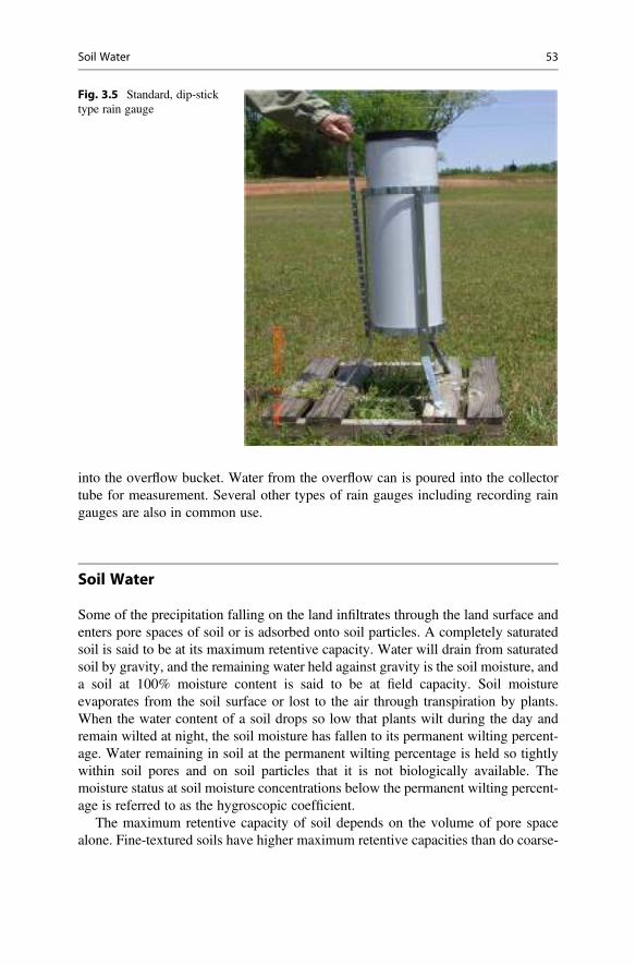
into the overflow bucket. Water from the overflow can is poured into the collectortube for measurement. Several other types of rain gauges including recording raingauges are also in common use.

Soil Water

Some of the precipitation falling on the land infiltrates through the land surface andenters pore spaces of soil or is adsorbed onto soil particles. A completely saturatedsoil is said to be at its maximum retentive capacity. Water will drain from saturatedsoil by gravity, and the remaining water held against gravity is the soil moisture, anda soil at 100% moisture content is said to be at field capacity. Soil moistureevaporates from the soil surface or lost to the air through transpiration by plants.When the water content of a soil drops so low that plants wilt during the day andremain wilted at night, the soil moisture has fallen to its permanent wilting percent-age. Water remaining in soil at the permanent wilting percentage is held so tightlywithin soil pores and on soil particles that it is not biologically available. Themoisture status at soil moisture concentrations below the permanent wilting percent-age is referred to as the hygroscopic coefficient.

The maximum retentive capacity of soil depends on the volume of pore spacealone. Fine-textured soils have higher maximum retentive capacities than do coarse-

Fig. 3.5 Standard, dip-sticktype rain gauge

Soil Water 53

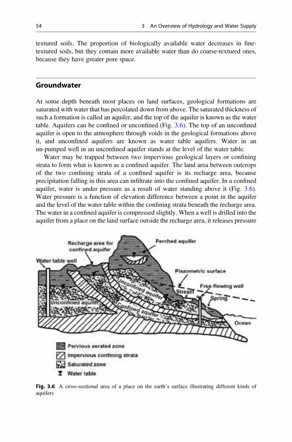
textured soils. The proportion of biologically available water decreases in fine-textured soils, but they contain more available water than do coarse-textured ones,because they have greater pore space.

Groundwater

At some depth beneath most places on land surfaces, geological formations aresaturated with water that has percolated down from above. The saturated thickness ofsuch a formation is called an aquifer, and the top of the aquifer is known as the watertable. Aquifers can be confined or unconfined (Fig. 3.6). The top of an unconfinedaquifer is open to the atmosphere through voids in the geological formations aboveit, and unconfined aquifers are known as water table aquifers. Water in anun-pumped well in an unconfined aquifer stands at the level of the water table.

Water may be trapped between two impervious geological layers or confiningstrata to form what is known as a confined aquifer. The land area between outcropsof the two confining strata of a confined aquifer is its recharge area, becauseprecipitation falling in this area can infiltrate into the confined aquifer. In a confinedaquifer, water is under pressure as a result of water standing above it (Fig. 3.6).Water pressure is a function of elevation difference between a point in the aquiferand the level of the water table within the confining strata beneath the recharge area.The water in a confined aquifer is compressed slightly. When a well is drilled into theaquifer from a place on the land surface outside the recharge area, it releases pressure

Fig. 3.6 A cross-sectional area of a place on the earth’s surface illustrating different kinds ofaquifers


on the aquifer allowing water in the aquifer to expand. This is a case where the slightcompressibility of water plays an important role. The water level in a well casingdrilled into a confined aquifer will usually rise above the top of the aquifer andsometimes reach the land surface.

The level at which water stands in an unpumped well in a confined aquifer is thepiezometric level. Piezometric levels mapped over the entire aquifer form a piezo-metric surface. Water rises above the land surface from a well drilled into a confinedaquifer when the piezometric level is above the land surface. Confined aquifers oftenare called artesian aquifers, and free-flowing wells frequently are said to exhibitartesian flow. The piezometric surface slopes downward, and water in a well drilledinto the aquifer does not rise to the same elevation as that of the water table in therecharge area between the two confining layers (Fig. 3.6). This results primarily fromreduction in hydraulic head caused by friction as water infiltrates through the aquifer.A well drilled from the recharge area into a confined aquifer will behave like a watertable well.

As can be seen in Fig. 3.6, more than one water table may occur beneath aparticular place on the land surface. Small perched aquifers are common on hillswhere water stands above a small hardpan or impervious layer. Water may leak froman artesian aquifer into aquifers above or below. One or more artesian aquifers mayoccur below the same point, or artesian aquifers may be absent.

Water in aquifers moves in response to decreasing hydraulic head. Groundwatermay seep into streams where stream bottoms cut below the water table—this iscalled base flow. Aquifers may also flow onto the earth’s surface from springs, orseep into the ocean.

Ocean water may seep into aquifers, and the salt water will interface withfreshwater. The position of the interface depends on the hydraulic head of freshwaterrelative to salt water. As the hydraulic head of an aquifer decreases because ofexcessive pumping, salt water moves further into the aquifer. Salt water intrusion inwells of coastal regions can result in salinization of groundwater. This phenomenonusually results from over-pumping by wells resulting in a decrease in the water tableelevation in coastal areas.

Aquifers vary greatly in size and depth beneath the land. Some water tableaquifers may be only 2–3-m thick and a few hectares in extent. Others may bemany meters thick and cover hundreds or thousands of square kilometers. Artesianaquifers normally are rather large, at least 5–10-m thick, a few kilometers wide, andseveral kilometers long. Recharge areas may be many kilometers away from aparticular well drilled into an artesian aquifer. The depth of aquifers below theland varies from a few to several hundred meters. For obvious reasons, good aquifersnearer the ground surface are more useful for wells. The water table is not level buttends to follow the surface terrain, being higher in recharge areas in hills than indischarge areas in valleys. The vertical distance from the land surface to the watertable is often less under valleys than under hills. Water table depth also changes inresponse to rainfall; it declines during prolonged periods of dry weather and risesfollowing heavy rains.

Groundwater 55

Runoff and Streams

Runoff from watersheds or catchments consisting of multiple watersheds formsstreams that convey both storm flow (overland flow) and subsurface inflow. Over-land flow is the portion of the precipitation that flows over the land surface and entersstreams. Overland flow begins after the capacity of watershed surfaces to detainwater by absorption or in depressions has been filled, and the rate of rainfall exceedsthe rate of infiltration of water on the surface into the soil. Features of the watershed,duration and intensity of rainfall, season, and climate influence the amount of runoffgenerated by a watershed. Factors favoring large amounts of overland flow areintense rainfall, prolonged rainfall, impervious soil, frozen or moist soil, low airtemperature, high proportion of paved surface, steep slope, little surface storagecapacity on land surface, sparse vegetative cover, soils with a low moisture-holdingcapacity, and a shallow water table. Overland flow moves downslope in response togravity, it erodes the soil creating channels for water flow and ultimately forms achannel that becomes an intermittent or permanent stream.

An ephemeral stream only flows after rains and does not have a well-definedchannel. An intermittent stream flows only during the wet season and after heavyrains but usually creates a channel. A perennial stream normally flows year-roundand has a well-defined channel. Perennial streams receive groundwater inflow whentheir bottoms are below the water table and this base flow sustains stream flow in dryweather.

Streams in an area form a drainage pattern discernable on a topographic map. Atree-shaped pattern, called a dendritic pattern, forms where the land erodes uniformlyand streams randomly branch and advance upslope. Where faulting is prevalent,streams follow the faults to form a rectangular pattern. Where the land surface isfolded or is a broad, gently sloping plain, streams form a trellis or lattice pattern.

A stream without tributaries is a first-order stream, and its basin is a first-orderbasin. Two, first-order streams combine to form a second-order stream. A streamwith a second-order branch is a third-order stream, and so on. The stream system thatcontributes to the discharge at a specified point in a higher-order stream is called adrainage network. The number of streams decreases and stream length increases asstream order increases (Leopold 1974, 1997).

Stream discharge is the amount of water flowing through the stream’s crosssection in a given time and at a particular place. A stream hydrograph is a plot ofdischarge versus time. The hydrograph in Fig. 3.7 shows the discharge of a smallstream before, during, and after a storm. During dry weather, the hydrographrepresents only groundwater intrusion into the stream (base flow). During the initialphase of a rainstorm, only rain falling directly into the channel (channel precipita-tion) contributes to the hydrograph. Channel precipitation seldom is great enough tocause an appreciable increase in discharge. During a fairly large rain, streamdischarge rises sharply as storm flow enters causing the rising limb of thehydrograph. Peak discharge is reached, the crest segment of the hydrograph occursand then declines forming the falling limb of the hydrograph. Subsurface stormdrainage—water flowing downslope through the soil pores—often is blocked from


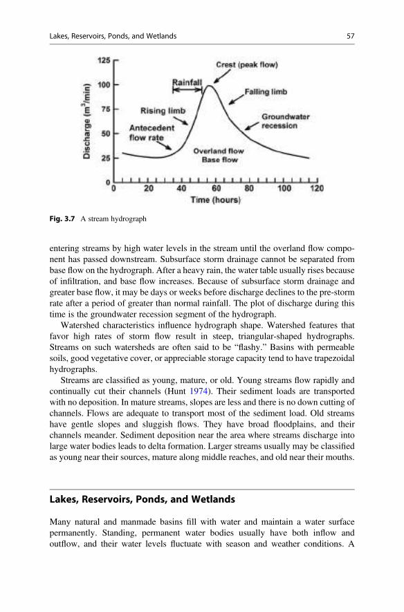
entering streams by high water levels in the stream until the overland flow compo-nent has passed downstream. Subsurface storm drainage cannot be separated frombase flow on the hydrograph. After a heavy rain, the water table usually rises becauseof infiltration, and base flow increases. Because of subsurface storm drainage andgreater base flow, it may be days or weeks before discharge declines to the pre-stormrate after a period of greater than normal rainfall. The plot of discharge during thistime is the groundwater recession segment of the hydrograph.

Watershed characteristics influence hydrograph shape. Watershed features thatfavor high rates of storm flow result in steep, triangular-shaped hydrographs.Streams on such watersheds are often said to be “flashy.” Basins with permeablesoils, good vegetative cover, or appreciable storage capacity tend to have trapezoidalhydrographs.

Streams are classified as young, mature, or old. Young streams flow rapidly andcontinually cut their channels (Hunt 1974). Their sediment loads are transportedwith no deposition. In mature streams, slopes are less and there is no down cutting ofchannels. Flows are adequate to transport most of the sediment load. Old streamshave gentle slopes and sluggish flows. They have broad floodplains, and theirchannels meander. Sediment deposition near the area where streams discharge intolarge water bodies leads to delta formation. Larger streams usually may be classifiedas young near their sources, mature along middle reaches, and old near their mouths.

Lakes, Reservoirs, Ponds, and Wetlands

Many natural and manmade basins fill with water and maintain a water surfacepermanently. Standing, permanent water bodies usually have both inflow andoutflow, and their water levels fluctuate with season and weather conditions. A

Fig. 3.7 A stream hydrograph

Lakes, Reservoirs, Ponds, and Wetlands 57

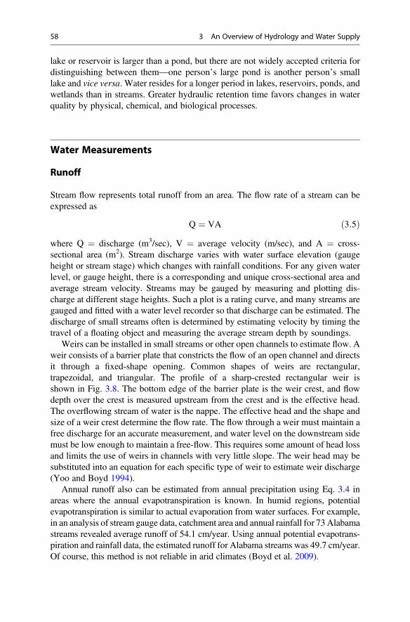
lake or reservoir is larger than a pond, but there are not widely accepted criteria fordistinguishing between them—one person’s large pond is another person’s smalllake and vice versa. Water resides for a longer period in lakes, reservoirs, ponds, andwetlands than in streams. Greater hydraulic retention time favors changes in waterquality by physical, chemical, and biological processes.

Water Measurements

Runoff

Stream flow represents total runoff from an area. The flow rate of a stream can beexpressed as

Q ¼ VA ð3:5Þwhere Q ¼ discharge (m3/sec), V ¼ average velocity (m/sec), and A ¼ cross-sectional area (m2). Stream discharge varies with water surface elevation (gaugeheight or stream stage) which changes with rainfall conditions. For any given waterlevel, or gauge height, there is a corresponding and unique cross-sectional area andaverage stream velocity. Streams may be gauged by measuring and plotting dis-charge at different stage heights. Such a plot is a rating curve, and many streams aregauged and fitted with a water level recorder so that discharge can be estimated. Thedischarge of small streams often is determined by estimating velocity by timing thetravel of a floating object and measuring the average stream depth by soundings.

Weirs can be installed in small streams or other open channels to estimate flow. Aweir consists of a barrier plate that constricts the flow of an open channel and directsit through a fixed-shape opening. Common shapes of weirs are rectangular,trapezoidal, and triangular. The profile of a sharp-crested rectangular weir isshown in Fig. 3.8. The bottom edge of the barrier plate is the weir crest, and flowdepth over the crest is measured upstream from the crest and is the effective head.The overflowing stream of water is the nappe. The effective head and the shape andsize of a weir crest determine the flow rate. The flow through a weir must maintain afree discharge for an accurate measurement, and water level on the downstream sidemust be low enough to maintain a free-flow. This requires some amount of head lossand limits the use of weirs in channels with very little slope. The weir head may besubstituted into an equation for each specific type of weir to estimate weir discharge(Yoo and Boyd 1994).

Annual runoff also can be estimated from annual precipitation using Eq. 3.4 inareas where the annual evapotranspiration is known. In humid regions, potentialevapotranspiration is similar to actual evaporation from water surfaces. For example,in an analysis of stream gauge data, catchment area and annual rainfall for 73 Alabamastreams revealed average runoff of 54.1 cm/year. Using annual potential evapotrans-piration and rainfall data, the estimated runoff for Alabama streams was 49.7 cm/year.Of course, this method is not reliable in arid climates (Boyd et al. 2009).


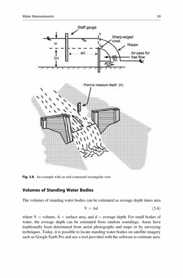
Volumes of Standing Water Bodies

The volumes of standing water bodies can be estimated as average depth times area

V ¼ Ad ð3:6Þwhere V ¼ volume, A ¼ surface area, and d ¼ average depth. For small bodies ofwater, the average depth can be estimated from random soundings. Areas havetraditionally been determined from aerial photographs and maps or by surveyingtechniques. Today, it is possible to locate standing water bodies on satellite imagerysuch as Google Earth Pro and use a tool provided with the software to estimate area.

Fig. 3.8 An example with an end-contracted rectangular weir

Water Measurements 59

Water Budgets and Mass Balance

Water budgets often are made for the purposes of describing the hydrology ofcatchments or watersheds, natural water bodies, or water supply systems. Waterbudgets can be made by the general hydrologic equation

Inflow ¼ Outflow� Change in storage: ð3:7ÞThis equation appears simple, but it often becomes complex when expanded to takeinto account all inflows and outflows. For example, the expanded equation for asmall lake made by damming a watershed might be

RainfallþSeepage inþ Runoff ¼ Evaporationþ Seepage outþ OverflowðþConsumptive useÞ � Change in storage:

ð3:8ÞIn Eq. 3.8, rainfall and change in storage can be measured easily. Evaporation can beestimated by applying a coefficient to Class A pan evaporation data. A weir or otherflow measuring device would need to be installed in the pond to obtain overflowvalues. Runoff would have to be estimated by a procedure that takes into accountrainfall amount and runoff-producing characteristics of the watershed. Consumptiveuse measurements could be made, but one would have to know the activities thatwithdraw water and quantify them. Seepage in and seepage out probably could notbe measured independently, but if all other terms in Eq. 3.8 were known, net seepagecould be estimated by difference.

The hydrologic equation allows the estimation of net seepage in a small pond asshown in Ex. 3.1.

Ex. 3.1 A small pond has a water level of 3.61 m on day 1, and after 5 days, thewater level is 3.50 m. There is no rainfall or consumptive water use over the 5-dayperiod, and Class A pan evaporation is 6.0 cm. Net seepage will be estimated.

Solution:

Pond evaporation ¼ Class A pan evaporation� 0:8

Pond evaporation ¼ 6 cm� 0:8 ¼ 4:8 cm:

The water budget equation is

Inflow ¼ Outflow � Δ Storage:

There was no inflow, outflows were seepage and evaporation, and storagechange was 3.61 m – 3.50 m ¼ 0.11 m or 11 cm. The seepage was outward—lostfrom the pond. Thus,


0:0 cm ¼ seepageþ 4:8 cmð Þ � 11 cm

Seepageþ 4:8 cmð Þ � 11 cm ¼ 0

Seepageþ 4:8 cm ¼ 11 cm

Seepage ¼ 11� 4:8 cm ¼ 6:2 cm ¼ 1:24 cm=dð Þ:

In studies of water quality, it often is necessary to calculate the amounts ofsubstances contained in inputs, outputs, transport, or storage for specific masses ofwater. For example, it may be desired to calculate the amount of total suspendedsolids transported by a stream or the amount of phosphorus retained within awetland. The hydrologic equation (Eq. 3.7) can be modified to make mass balancecalculations of dissolved substances:

Inputs volume� concentrationð Þ ¼ Outputs volume� concentrationð Þ� Storage volume� concentrationð Þ: ð3:9Þ

Ex. 3.2 The discharge of streams average 35 cm/year in an area. The streamflowing from a watershed in this area has an average total nitrogen concentrationof 2 mg/L. The annual nitrogen loss per hectare will be estimated.

Solution:

Runoff volume ¼ 0:35 m=yr � 10; 000 m2=ha ¼ 3; 500 m3=ha=yr

Nitrogen loss ¼ 3; 500 m3=ha=yr � 2 g N=m3

¼ 7; 000 g N=ha=yr or 7 kg N=ha=yr:

Ex. 3.3 A plastic lined pond (2000 m3) in an arid region is filled and supplied withcity water containing 500 mg/L TDS. Over a year, 1000 m3 of water must be addedto the pond to replace evaporation. What would be the approximate concentration ofTDS after 3 years?

Solution:Quantities of dissolved solids added to the pond are

Filling 2; 000 m3 � 500 g=m3 ¼ 1; 000; 000 g

Maintenance 1; 000 m3=yr � 3 yr � 500 g=m3 ¼ 1; 500; 000 g

Water Measurements 61

Total ¼ 2; 500; 000 g

Volume after 3 years is still 2; 000 m3:

Concentration of TDS after 3 yr ¼ 2; 500; 000 g

2; 000 m3¼ 1; 250 mg=L:

Estimates of volumes, flow rates, or both frequently are needed in water qualitystudies. Most water quantity variables are more difficult to measure than are theconcentrations of water quality variables.

Oceans and Estuaries

Most of the world’s water is contained in the ocean. The ocean system is much largerthan all other water bodies combined and contains salt water instead of freshwater.Water movements in the ocean are complex because of the large expanses of openwater, great depths, wind driven currents, coriolis effect, tides, and other factors, butpredictable and well-defined currents exist.

Estuaries are the entrances of streams into the ocean. Estuaries contain brackishwater because the inflow of freshwater from streams dilutes ocean water. Because oftidal influence there are continuous changes in salinity at any given location in anestuary. When the tide recedes, the freshwater influence will extend farther into theestuary than when the tide advances. Salt or brackishwater is heavier than freshwaterand a salt water wedge often extends into rivers beneath their freshwater flow. Thiscan result in stratification of salinity at any given point in an estuary. Inflow offreshwater from streams increases after heavy rains and reduces the salinity ofestuaries. Estuaries with poor connection to the ocean may become hypersaline inarid areas or during the dry season. The tide flushes estuaries, and the combination offreshwater inflow, size of the connection with the ocean, and tidal amplitudedetermines the water retention time in estuaries. Water quality in estuaries is highlydependent upon water residence time. Many estuaries are greatly influenced byhuman activities, and pollution problems are much more likely in estuaries wherewater exchange with the ocean is incomplete and slow.

Conclusions

The world’s water is partitioned into several components, but nearly all of it iscontained in the ocean, ice formations, or deep groundwater that is either not suitableor accessible for most human uses. The water available for human use is mainly aportion of the water continually moving through the hydrologic cycle. The threemost important components of the hydrologic cycle effecting the human water


supply are precipitation, evapotranspiration, and runoff. A basic knowledge of thefactors affecting the quantity of water available at a particular place and time isuseful to those studying water quality. The quality of water is highly dependent uponthe rates at which dissolved and suspended substances enter and exit water bodiesvia inflow and outflow.

References

Baumgartner A, Reichel E (1975) The world water balance. Elsevier, AmsterdamBoyd CE (1985) Pond evaporation. Trans Am Fish Soc 114:299–303Boyd CE, Soongsawang S, Shell EW, Fowler S (2009) Small impoundment complexes as a

possible method to increase water supply in Alabama. In: Proceedings 2009 Georgia waterresources conference, April 27–29. University of Georgia, Athens

Hoekstra AY, Mekonnen MM (2012) The water footprint of humanity. Proc Nat Acad Sci109:3232–3237

Hounam CE (1973) Comparisons between pan and lake evaporation. Technical Note 126, WorldMeteorological Organization, Geneva

Hunt CB (1974) Natural regions of the United States and Canada. WH Freeman, San FranciscoIdso SB, Foster JM (1974) Light and temperature relations in a small desert pond as influenced by

phytoplanktonic density variations. Water Res Res 10:129–132Klein MJ (1970) Maxwell, his demon and the second law of thermodynamics. Am Sci 58:84–97Leopold LB (1974) Water a primer. WH Freeman, San FranciscoLeopold LB (1997) Water, rivers, and creeks. University Science Books, SausalitoWetzel RG (2001) Limnology, 3rd edn. Academic, New YorkWisser D, Frolking S, Douglas EM, Fekete BM, Vöoösmarty CJ, Schumann AH (2008) Global

irrigation water demand: variability and uncertainties arising from agricultural and climate datasets. Geophys Res Let 35(24):L24408. https://doi.org/10.1029/2008GL035296

Yoo KH, Boyd CE (1994) Hydrology and water supply for pond aquaculture. Chapman and Hall,New York

References 63

https://doi.org/10.1029/2008GL035296

Solubility and Chemical Equilibrium 4

AbstractSolubility, chemical equilibrium, and equilibrium constants are closely related toGibbs free energy of reaction. Electrostatic interactions among ions decrease theactivities of ions, and these interactions increase with greater ionic strength. As aresult, for precise calculations related to solubility and equilibrium, ionicactivities instead of measured molar concentrations must be used. For practicalillustrations of principles, molar concentrations will be used in this book.

Introduction

A solution consists of a liquid called the solvent into which another substance thesolute is uniformly mixed. Natural waters are solutions comprised of various solutes.These solutes may be solids, liquids, or gases, but in water quality, solids and gasesare the most important solutes. The principles regulating the dissolution of gases andsolids differ, and only the solubility of solids will be considered here. The majorcomponent of dissolved solids in natural waters is mineral matter resulting from thedissolution of minerals in surface soils and underground geological formations.Minerals have different solubilities, and their solubilities are also effected by tem-perature, pH, oxidation-reduction potential, presence of other dissolved substances,and the principles of chemical equilibrium.

Dissolutions

A simple dissolution occurs when a solute separates into individual molecules asillustrated below for table sugar (sucrose):


65


C12H22O11 sð Þ !Water C12H22O11 aqð Þ: ð4:1ÞIn Eq. 4.1, (s) designates a solid and (aq) indicates the molecule is dissolved inwater. A (g) beside a molecule indicates that it is in gaseous form. As it usually isimplicit which forms are present, the designations are introduced here but seldomused elsewhere in this book. The sucrose molecules are in crystalline form; dissolu-tion results in sucrose molecules in water. The sugar crystal is not held togetherstrongly, and it has hydroxyl groups in which the bond between hydrogen andoxygen gives a slight negative charge to oxygen and a slight positive charge tohydrogen. Water is dipolar and attracted to the charges forcing the sucrosemolecules from the crystal and holding them in aqueous solution. This type ofsolution is a purely physical process.

Dissolution may result from dissociation of a substance into its ions. This is thecommon way in which salts dissolve. Gypsum is an ionically bound salt that ishydrated with the formula CaSO4�2H2O. When put in water, the hydrating water isimmediately lost into the solvent, and the salt dissolves as follows:

CaSO4 sð Þ Ð Ca2þ aqð Þ þ SO2�4 aqð Þ: ð4:2Þ

Water molecules, being dipolar, arrange themselves around the ions insulating andpreventing recombination of the ions. This type of dissociation also is basically aphysical process.

Chemical weathering is a chemical dissolution caused by reactions of water andminerals in the earth’s crust. Carbon dioxide reacts with limestone to dissolve it asillustrated in the following equation in which calcium carbonate represents limestone

CaCO3 sð Þ þ CO2 aqð Þ þ H2O Ð Ca2þ aqð Þ þ 2HCO�3 aqð Þ: ð4:3Þ

Carbon dioxide also accelerates dissolution of feldspars common in soils and othergeological formations. There are many other reactions causing chemical weathering,and nearly all of these reactions are equilibrium reactions in which only a smallportion of the mineral form dissolves.

Most compounds whether inorganic or organic have a degree of water solubility;but water, because it is polar, is particularly effective in dissolving polar solutes.Hence, the old adage—“like dissolves like.” Nevertheless, two polar compounds(ionically-bound compounds) can have drastically different solubilities in water; thewater solubility at 25 �C of sodium chloride is 357 g/L while that of silver chlorideis only 1.8 mg/L. Compounds of large molecular weight (large molecules) tend tobe less soluble than compounds consisting of smaller molecules, because it is moredifficult for water molecules to surround larger molecules. The chemical composi-tion of inorganic compounds is especially important in governing solubility. Thishas resulted in general guidelines of solubility (Table 4.1) which have even beenused as the lyrics of “The Solubility Song” many renditions of which have beenposted online.

66 4 Solubility and Chemical Equilibrium

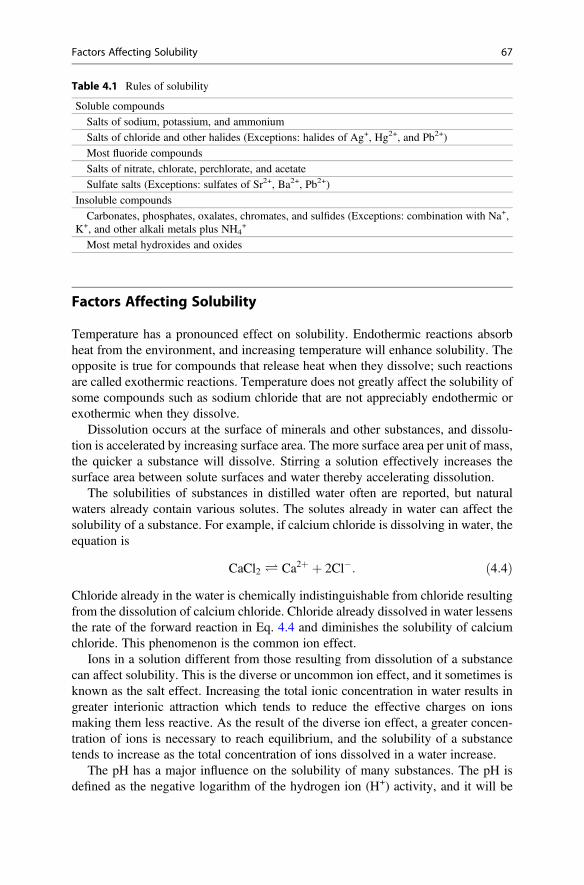
Factors Affecting Solubility

Temperature has a pronounced effect on solubility. Endothermic reactions absorbheat from the environment, and increasing temperature will enhance solubility. Theopposite is true for compounds that release heat when they dissolve; such reactionsare called exothermic reactions. Temperature does not greatly affect the solubility ofsome compounds such as sodium chloride that are not appreciably endothermic orexothermic when they dissolve.

Dissolution occurs at the surface of minerals and other substances, and dissolu-tion is accelerated by increasing surface area. The more surface area per unit of mass,the quicker a substance will dissolve. Stirring a solution effectively increases thesurface area between solute surfaces and water thereby accelerating dissolution.

The solubilities of substances in distilled water often are reported, but naturalwaters already contain various solutes. The solutes already in water can affect thesolubility of a substance. For example, if calcium chloride is dissolving in water, theequation is

CaCl2 Ð Ca2þ þ 2Cl�: ð4:4ÞChloride already in the water is chemically indistinguishable from chloride resultingfrom the dissolution of calcium chloride. Chloride already dissolved in water lessensthe rate of the forward reaction in Eq. 4.4 and diminishes the solubility of calciumchloride. This phenomenon is the common ion effect.

Ions in a solution different from those resulting from dissolution of a substancecan affect solubility. This is the diverse or uncommon ion effect, and it sometimes isknown as the salt effect. Increasing the total ionic concentration in water results ingreater interionic attraction which tends to reduce the effective charges on ionsmaking them less reactive. As the result of the diverse ion effect, a greater concen-tration of ions is necessary to reach equilibrium, and the solubility of a substancetends to increase as the total concentration of ions dissolved in a water increase.

The pH has a major influence on the solubility of many substances. The pH isdefined as the negative logarithm of the hydrogen ion (H+) activity, and it will be

Table 4.1 Rules of solubility

Soluble compounds

Salts of sodium, potassium, and ammonium

Salts of chloride and other halides (Exceptions: halides of Ag+, Hg2+, and Pb2+)

Most fluoride compounds

Salts of nitrate, chlorate, perchlorate, and acetate

Sulfate salts (Exceptions: sulfates of Sr2+, Ba2+, Pb2+)

Insoluble compounds

Carbonates, phosphates, oxalates, chromates, and sulfides (Exceptions: combination with Na+,K+, and other alkali metals plus NH4

+

Most metal hydroxides and oxides

Factors Affecting Solubility 67

discussed in detail later (Chaps. 9 and 11). For present purposes, it will be enough tostate that pH 7 is neutral, and water is acidic at lower pH, because there is a greaterconcentration of hydrogen ion than of hydroxyl ion. At higher pH than 7, water isbasic because hydroxyl ion concentration exceeds that of hydrogen ion. An exampleof the influence of pH on dissolution of a compound is the reaction of ferrichydroxide [Fe(OH)3] in acidic water:

Fe OHð Þ3 þ 3Hþ Ð Fe3þ þ 3H2O: ð4:5ÞIncreasing H+ concentration favors the reaction towards the right (forward reaction)in Eq. 4.5.

Low redox potential also increases the solubility of many substances; insolubleferric iron compounds tend to dissolve at low redox potential when ferric iron (Fe3+)is reduced to more soluble ferrous iron (Fe2+). Low dissolved oxygen concentrationis associated with low redox potential (see Chap. 8). Pressure seldom has aninfluence on the solubility of solids in natural waters, but pressure has a tremendouseffect on gas solubility (see Chap. 7).

Chemical Equilibrium

More of a substance added to the substance’s saturated solution will settle to thebottom of the container—no more will dissolve. The saturated solution of a com-pound results from an equilibrium between the solid compound and the dissolvedions, e.g., in a calcium sulfate solution in pure water, there will be an equilibriumamong CaSO4, Ca

2+, and SO42�.

The equilibrium state achieved in a saturated solution conforms to the Law ofMass Action—also known as Le Chatelier’s Principle or as the Equilibrium Law.This principle holds that if a chemical reaction is at equilibrium and conditions ofconcentration, temperature, volume, or pressure are changed, the reaction will adjustitself to restore the original equilibrium. This idea often is expressed in a generalmanner as follows:

aAþ bB Ð cCþ dD: ð4:6ÞThis equation shows that reactants A and B combine in specific proportions to formproducts C and D also in specific proportions. There is a back reaction, however, inwhich C and D combine to form A and B. At equilibrium, the forward and reversereactions are occurring at equal rates and there is no change in concentrations ofreactants and products. At equilibrium, a mathematical relationship exists betweenthe concentrations of the substances on each side of the equation and the equilibriumconstant (K)

Cð Þc Dð ÞdAð Þa Bð Þb ¼ K ð4:7Þ


where the concentrations ideally should be expressed as molar activities. Thedifference in molar activities and molar concentrations will be explained later inthis chapter; but for our purposes, it will be adequate to use molar concentrations.The equilibrium constant K sometimes is replaced by its negative logarithm, pK(K¼ 10�9 and pK¼ 9), but K will be used in this book in all but one instance whichis related to pH buffering.

Until equilibrium is reached, the left-hand side of Eq. 4.7 is called the reactionquotient (Q), but when equilibrium is attained, Q ¼ K. Once equilibrium occurs,addition or removal of any one of the reactants (A and B) or products (C and D) inEq. 4.6 will disrupt the equilibrium. The reactants and products will undergorearrangement in concentrations establishing a new equilibrium in which Q ¼ K.The reactants and products in reactions such as illustrated in Eq. 4.6 will always reactin a manner to reduce stress in the reaction and maintain a state of equilibrium asdepicted in Eq. 4.7.

Some reactions tend to progress almost entirely to the right and there will be verylittle or none of the reactants remaining. When a strong acid such as hydrochloricacid is placed in water, it dissociates almost entirely into H+ and Cl� with little HClremaining. Treatment of calcium carbonate with excess hydrochloric acid results inall of the CaCO3 being converted to Ca2+, CO2, and H2O.

The K values for reactions that progress to completion are much larger than thosefor reaction in which a mixture of products and reactions remain resulting in anequilibrium. The smaller the value of the equilibrium constant the greater will be theconcentration of the reactants relative to the concentrations of the products.

Relationship of Chemical Equilibrium to Thermodynamics

The force causing a chemical reaction to proceed is the difference in the energy of itsproducts relative to the energy of its reactants. A reaction will progress in thedirection of lower energy, and at equilibrium the energy of products equals theenergy of the reactants. In Eq. 4.6, when A and B are brought together, they contain acertain amount of energy. They react to form C and D, and the energy of the “left-hand side” of the equation declines as C and D are formed on the “right-hand side.”When the energy on both sides of the equation is equal, a state of equilibrium exists.

In terms of the laws of thermodynamics, the first law states that the amount ofenergy in the universe is constant, i.e., energy can neither be created nor destroyed. Itcan, however, be transformed back and forth between heat and work. In a system,heat can be used to do work, and work can be changed to heat, but at eachtransformation, some heat will be lost from the system and no longer useful fordoing work in the system.

In a chemical reaction within a fixed volume, the output of heat equals the changein internal energy when reactants form products. This output of heat is known as thechange in enthalpy (enthalpy is a measure of the internal heat content of a substance),and it is symbolized as ΔH. Thus, ΔH reaction ¼ H products – H reactants. In anexothermic reaction, ΔH will have a negative sign because the enthalpy of thereactants is greater than the enthalpy of the products and heat is released to the

Relationship of Chemical Equilibrium to Thermodynamics 69

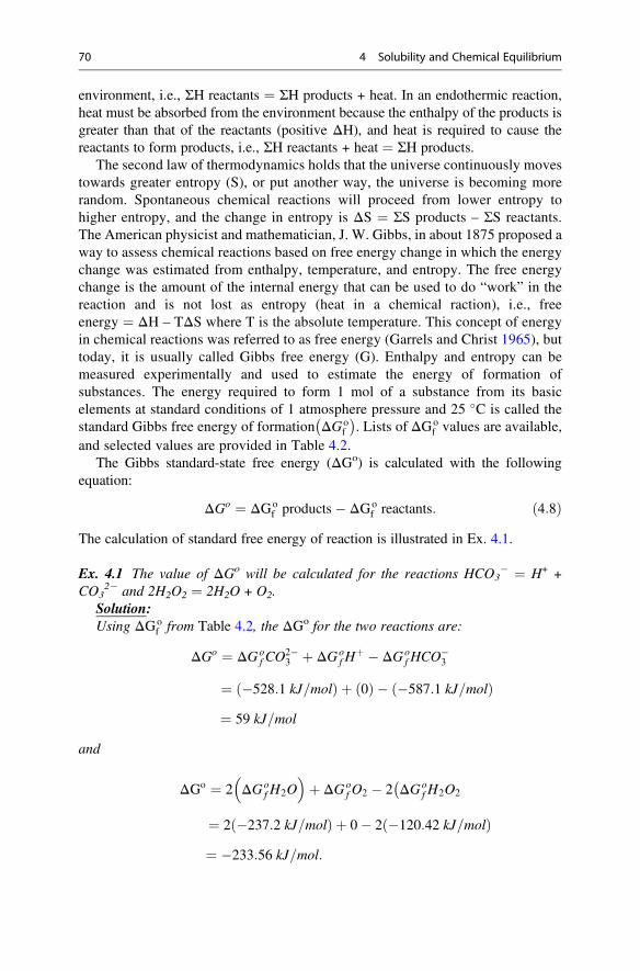
environment, i.e., ΣH reactants ¼ ΣH products + heat. In an endothermic reaction,heat must be absorbed from the environment because the enthalpy of the products isgreater than that of the reactants (positive ΔH), and heat is required to cause thereactants to form products, i.e., ΣH reactants + heat ¼ ΣH products.

The second law of thermodynamics holds that the universe continuously movestowards greater entropy (S), or put another way, the universe is becoming morerandom. Spontaneous chemical reactions will proceed from lower entropy tohigher entropy, and the change in entropy is ΔS ¼ ΣS products – ΣS reactants.The American physicist and mathematician, J. W. Gibbs, in about 1875 proposed away to assess chemical reactions based on free energy change in which the energychange was estimated from enthalpy, temperature, and entropy. The free energychange is the amount of the internal energy that can be used to do “work” in thereaction and is not lost as entropy (heat in a chemical raction), i.e., freeenergy ¼ ΔH – TΔS where T is the absolute temperature. This concept of energyin chemical reactions was referred to as free energy (Garrels and Christ 1965), buttoday, it is usually called Gibbs free energy (G). Enthalpy and entropy can bemeasured experimentally and used to estimate the energy of formation ofsubstances. The energy required to form 1 mol of a substance from its basicelements at standard conditions of 1 atmosphere pressure and 25 �C is called thestandard Gibbs free energy of formation ΔGo

f

� �. Lists of ΔGo

f values are available,and selected values are provided in Table 4.2.

The Gibbs standard-state free energy (ΔGo) is calculated with the followingequation:

ΔGo ¼ ΔGof products� ΔGo

f reactants: ð4:8ÞThe calculation of standard free energy of reaction is illustrated in Ex. 4.1.

Ex. 4.1 The value of ΔGo will be calculated for the reactions HCO3� ¼ H+ +

CO32� and 2H2O2 ¼ 2H2O + O2.

Solution:Using ΔGo

f from Table 4.2, the ΔGo for the two reactions are:

ΔGo ¼ ΔGof CO

2�3 þ ΔGo

f Hþ � ΔGo

f HCO�3

¼ �528:1 kJ=molð Þ þ 0ð Þ � �587:1 kJ=molð Þ¼ 59 kJ=mol

and

ΔGo ¼ 2 ΔGof H2O

� �þ ΔGo

f O2 � 2�ΔGo

f H2O2

¼ 2 �237:2 kJ=molð Þ þ 0� 2 �120:42 kJ=molð Þ¼ �233:56 kJ=mol:


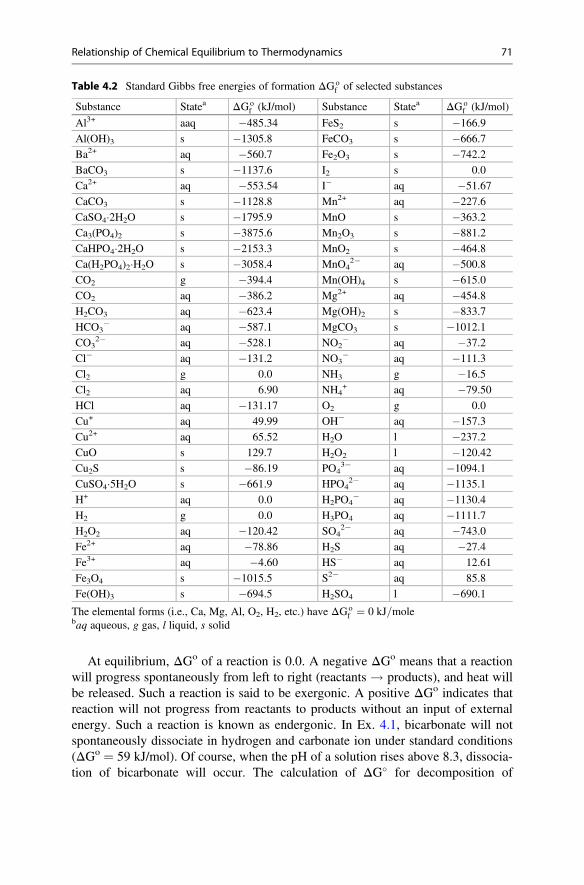
At equilibrium, ΔGo of a reaction is 0.0. A negative ΔGo means that a reactionwill progress spontaneously from left to right (reactants ! products), and heat willbe released. Such a reaction is said to be exergonic. A positive ΔGo indicates thatreaction will not progress from reactants to products without an input of externalenergy. Such a reaction is known as endergonic. In Ex. 4.1, bicarbonate will notspontaneously dissociate in hydrogen and carbonate ion under standard conditions(ΔGo ¼ 59 kJ/mol). Of course, when the pH of a solution rises above 8.3, dissocia-tion of bicarbonate will occur. The calculation of ΔG� for decomposition of

Table 4.2 Standard Gibbs free energies of formation ΔGof of selected substances

Substance Statea ΔGof (kJ/mol) Substance Statea ΔGo

f (kJ/mol)

Al3+ aaq �485.34 FeS2 s �166.9

Al(OH)3 s �1305.8 FeCO3 s �666.7

Ba2+ aq �560.7 Fe2O3 s �742.2

BaCO3 s �1137.6 I2 s 0.0

Ca2+ aq �553.54 I� aq �51.67

CaCO3 s �1128.8 Mn2+ aq �227.6

CaSO4�2H2O s �1795.9 MnO s �363.2

Ca3(PO4)2 s �3875.6 Mn2O3 s �881.2

CaHPO4�2H2O s �2153.3 MnO2 s �464.8

Ca(H2PO4)2�H2O s �3058.4 MnO42� aq �500.8

CO2 g �394.4 Mn(OH)4 s �615.0

CO2 aq �386.2 Mg2+ aq �454.8

H2CO3 aq �623.4 Mg(OH)2 s �833.7

HCO3� aq �587.1 MgCO3 s �1012.1

CO32� aq �528.1 NO2

� aq �37.2

Cl� aq �131.2 NO3� aq �111.3

Cl2 g 0.0 NH3 g �16.5

Cl2 aq 6.90 NH4+ aq �79.50

HCl aq �131.17 O2 g 0.0

Cu+ aq 49.99 OH� aq �157.3

Cu2+ aq 65.52 H2O l �237.2

CuO s 129.7 H2O2 l �120.42

Cu2S s �86.19 PO43� aq �1094.1

CuSO4�5H2O s �661.9 HPO42� aq �1135.1

H+ aq 0.0 H2PO4� aq �1130.4

H2 g 0.0 H3PO4 aq �1111.7

H2O2 aq �120.42 SO42� aq �743.0

Fe2+ aq �78.86 H2S aq �27.4

Fe3+ aq �4.60 HS� aq 12.61

Fe3O4 s �1015.5 S2� aq 85.8

Fe(OH)3 s �694.5 H2SO4 l �690.1

The elemental forms (i.e., Ca, Mg, Al, O2, H2, etc.) have ΔGof ¼ 0 kJ=mole

baq aqueous, g gas, l liquid, s solid


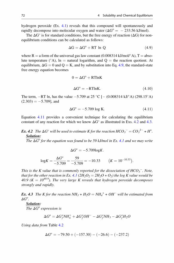
hydrogen peroxide (Ex. 4.1) reveals that this compound will spontaneously andrapidly decompose into molecular oxygen and water (ΔGo ¼ � 233.56 kJ/mol).

The ΔG� is for standard conditions, but the free energy of reaction (ΔG) for non-equilibrium conditions can be calculated as follows:

ΔG ¼ ΔGo þ RT ln Q ð4:9Þwhere R¼ a form of the universal gas law constant (0.008314 kJ/mol/�A), T¼ abso-lute temperature (�A), ln ¼ natural logarithm, and Q ¼ the reaction quotient. Atequilibrium, ΔG ¼ 0 and Q ¼ K, and by substitution into Eq. 4.9, the standard-statefree energy equation becomes

0 ¼ ΔGo þ RTlnK

ΔGo ¼ �RTlnK: ð4:10ÞThe term, �RT ln, has the value �5.709 at 25 �C [� (0.008314 kJ/�A) (298.15�A)(2.303) ¼ �5.709], and

ΔGo ¼ �5:709 log K: ð4:11ÞEquation 4.11 provides a convenient technique for calculating the equilibriumconstant of any reaction for which we know ΔG� as illustrated in Exs. 4.2 and 4.3.

Ex. 4.2 The ΔG� will be used to estimate K for the reaction HCO3� ¼ CO3

2� + H+.Solution:The ΔGo for the equation was found to be 59 kJ/mol in Ex. 4.1 and we may write

ΔGo ¼ �5:709logK:

logK ¼ ΔGo

�5:709¼ 59

�5:709¼ �10:33 K ¼ 10�10:33

� �:

This is the K value that is commonly reported for the dissociation of HCO3�. Note,

that for the other reaction in Ex. 4.1 (2H2O2¼ 2H2O + O2) the log K value would be40.9 (K ¼ 1040.9). The very large K reveals that hydrogen peroxide decomposesstrongly and rapidly.

Ex. 4.3 The K for the reaction NH3 + H2O ¼ NH4+ + OH� will be estimated from

ΔGo.Solution:The ΔGo expression is

ΔGo ¼ ΔGof NH

þ4 þ ΔGo

f OH� � ΔGo

f NH3 � ΔGof H2O

Using data from Table 4.2

ΔGo ¼ �79:50þ �157:30ð Þ � �26:6ð Þ � �237:2ð Þ


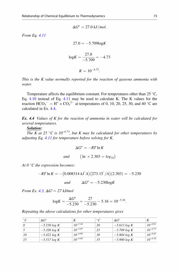
ΔGo ¼ 27:0 kJ=mol:

From Eq. 4.11

27:0 ¼ �5:709logK

logK ¼ 27:0�5:709

¼ �4:73

K ¼ 10�4:73:

This is the K value normally reported for the reaction of gaseous ammonia withwater.

Temperature affects the equilibrium constant. For temperatures other than 25 �C,Eq. 4.10 instead of Eq. 4.11 may be used to calculate K. The K values for thereaction HCO3

� ¼ H+ + CO32� at temperatures of 0, 10, 20, 25, 30, and 40 �C are

calculated in Ex. 4.4.

Ex. 4.4 Values of K for the reaction of ammonia in water will be calculated forseveral temperatures.

Solution:The K at 25 �C is 10–4.73, but K may be calculated for other temperatures by

adjusting Eq. 4.11 for temperature before solving for K.

ΔGo ¼ �RT lnK

and�ln � 2:303 ¼ log10

�

At 0 �C the expression becomes:

�RT lnK ¼ � 0:008314 kJ�A

� �273:15

�=A

� �2:303ð Þ ¼ �5:230

and ΔGo ¼ �5:230logK

From Ex. 4.3, ΔG�¼ 27 kJ/mol

logK ¼ ΔGo

�5:230¼ 27

�5:230� 5:16 ¼ 10�5:16:

Repeating the above calculations for other temperatures gives

�C ΔG� K �C ΔG� K

0 �5.230 log K 10–5.16 20 �5.613 log K 10–4.81

5 �5.326 log K 10–5.07 25 �5.709 log K 10–4.73

10 �5.422 log K 10–4.98 30 �5.804 log K 10–4.65

15 �5.517 log K 10–4.89 35 �5.900 log K 10–4.58


Solubility Product

The concept of equilibrium applies to all kinds of chemical reactions, but thesolubility product is a special form of Le Chatelier’s principle that may begeneralized as

AB Ð Aþ B: ð4:12ÞThe concept assumes that there is a large excess of solid phase AB so that the amountthat dissolves does not influence its concentration, i.e., the solid phase may beconsidered unity. This allows the equilibrium constant—also called the solubilityproduct constant (Ksp)—to be expressed as simply the product of the molarconcentrations of A and B in the solution state

Bð Þ Að Þ ¼ Ksp: ð4:13ÞIn a case of a more complex molecules we could have

A2B3 Ð 2Aþ 3B: ð4:14ÞIn this case, the expression for the solubility product constant is

Að Þ2 Bð Þ3 ¼ Ksp: ð4:15ÞSelected Ksp values for compounds of interest in water quality given in Table 4.3

do not include those for common compounds that are highly water soluble anddissolve completely under most conditions. Solid compounds may occur in morethan one form. Variation in crystalline structure, and degree of hydration in particu-lar, may influence solubility. An amorphous mineral—one that has not formed thetypical crystalline structure of the particular compound—has a different solubilitythan the crystalline form. It is not uncommon to find somewhat different solubilityproduct constants and solubility data for different forms of the same compound.

The solubility of a compound is not always presented as a simple dissolution inwater. Consider the dissolution of gibbsite [Al(OH)3]:

Al OHð Þ3 Ð Al3þ þ 3OH� K ¼ 10�33: ð4:16ÞThis dissolution also may be presented as

Al OHð Þ3 þ 3Hþ ¼ Al3þ þ 3H2O K ¼ 109: ð4:17ÞEither way, the concentration of aluminum ion at equilibrium is the same for a givenpH: (Al3+) ¼ 10�6 M at pH 5 by both Eqs. 4.16 and 4.17.

Some examples showing how to estimate the concentrations of substances inwater from chemical reactions and equilibrium constants are provided in Exs. 4.5,4.6, and 4.7.


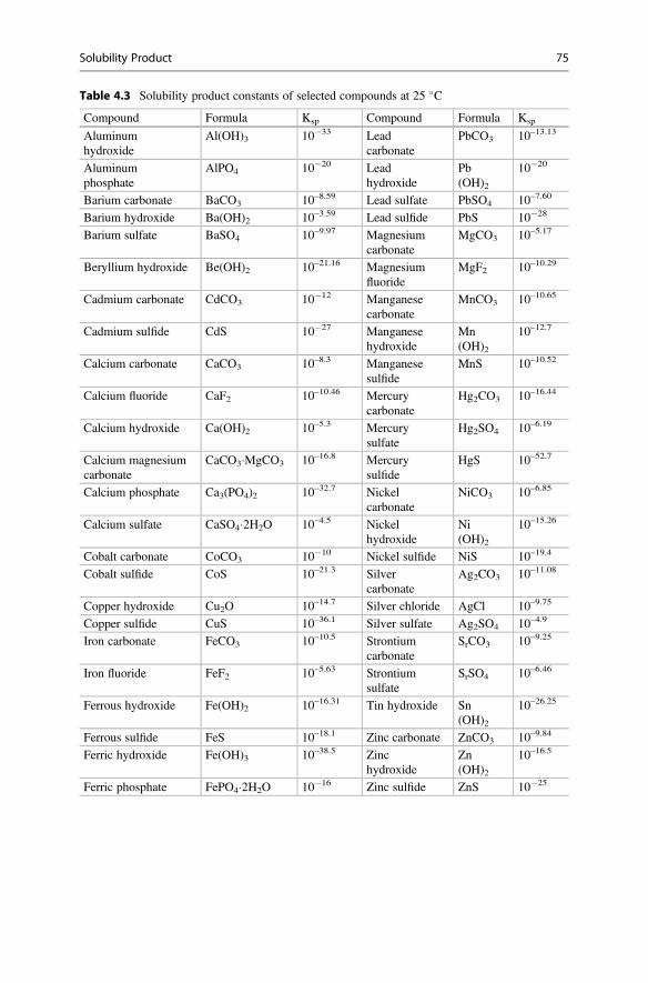
Table 4.3 Solubility product constants of selected compounds at 25 �C

Compound Formula Ksp Compound Formula Ksp

Aluminumhydroxide

Al(OH)3 10�33 Leadcarbonate

PbCO3 10–13.13

Aluminumphosphate

AlPO4 10�20 Leadhydroxide

Pb(OH)2

10�20

Barium carbonate BaCO3 10–8.59 Lead sulfate PbSO4 10–7.60

Barium hydroxide Ba(OH)2 10–3.59 Lead sulfide PbS 10�28

Barium sulfate BaSO4 10–9.97 Magnesiumcarbonate

MgCO3 10–5.17

Beryllium hydroxide Be(OH)2 10–21.16 Magnesiumfluoride

MgF2 10–10.29

Cadmium carbonate CdCO3 10�12 Manganesecarbonate

MnCO3 10–10.65

Cadmium sulfide CdS 10�27 Manganesehydroxide

Mn(OH)2

10–12.7

Calcium carbonate CaCO3 10–8.3 Manganesesulfide

MnS 10–10.52

Calcium fluoride CaF2 10–10.46 Mercurycarbonate

Hg2CO3 10–16.44

Calcium hydroxide Ca(OH)2 10–5.3 Mercurysulfate

Hg2SO4 10–6.19

Calcium magnesiumcarbonate

CaCO3�MgCO3 10–16.8 Mercurysulfide

HgS 10–52.7

Calcium phosphate Ca3(PO4)2 10–32.7 Nickelcarbonate

NiCO3 10–6.85

Calcium sulfate CaSO4�2H2O 10–4.5 Nickelhydroxide

Ni(OH)2

10–15.26

Cobalt carbonate CoCO3 10�10 Nickel sulfide NiS 10–19.4

Cobalt sulfide CoS 10–21.3 Silvercarbonate

Ag2CO3 10–11.08

Copper hydroxide Cu2O 10–14.7 Silver chloride AgCl 10–9.75

Copper sulfide CuS 10–36.1 Silver sulfate Ag2SO4 10–4.9

Iron carbonate FeCO3 10–10.5 Strontiumcarbonate

SrCO3 10–9.25

Iron fluoride FeF2 10–5.63 Strontiumsulfate

SrSO4 10–6.46

Ferrous hydroxide Fe(OH)2 10–16.31 Tin hydroxide Sn(OH)2

10–26.25

Ferrous sulfide FeS 10–18.1 Zinc carbonate ZnCO3 10–9.84

Ferric hydroxide Fe(OH)3 10–38.5 Zinchydroxide

Zn(OH)2

10–16.5

Ferric phosphate FePO4�2H2O 10�16 Zinc sulfide ZnS 10�25

Solubility Product 75

Ex. 4.5 Concentrations of Ca2+ and SO42� will be calculated for a saturated

solution of gypsum (CaSO4�2H2O) in distilled water.Solution:The dissolution equation is

CaSO4 ∙ 2H2O Ð Ca2þ þ SO2�4 þ 2H2O

and from Table 4.3, K is 10–4.5.Because gypsum and water both can be assigned a value of unity, the solubility

product expression becomes

Ca2þ� �

SO2�4

� � ¼ 10�4:5:

Each gypsum molecule dissolves into one calcium and one sulfate ion; hence,(Ca2+) ¼ (SO4

2�) at equilibrium. This allows us to let x ¼ (Ca2+) ¼ (SO42�), and

xð Þ xð Þ ¼ 10�4:5

x ¼ 10�2:25 M:

This molar concentration is equal to 225 mg/L Ca2+ and 540 mg/L sulfate.

Ex. 4.6 The common ion effect will be illustrated by estimating the calciumconcentration that could occur in water containing 1000 mg/L (10–1.98 M) sulfate.

Solution:

Ca2þ� �

SO2�4

� � ¼ Ksp

Ca2þ� � ¼ Ksp

SO4ð Þ

Ca2þ� � ¼ 10�4:5

10�1:98 ¼ 10�2:52 M:

This is a calcium ion concentration of 121 mg/L as compared to 225 mg/L of calciumpossible when gypsum dissolves in distilled water (Ex. 4.4).

Ex. 4.7 The solubility of calcium fluoride (CaF2) will be calculated.Solution:From Table 4.3, the Ksp for CaF2 is 10

–10.46, and the reaction is

CaF2 ¼ Ca2þ þ 2F�:

The solubility product expression is


Ca2þ� �

F�ð Þ2 ¼ 10�10:46:

Letting (Ca2+) ¼ X and (F�) ¼ 2X,

Xð Þ 2Xð Þ2 ¼ 10�10:46

4X3 ¼ 10�10:46 ¼ 3:47� 10�11

X3 ¼ 8:68� 10�12 ¼ 10�11:06

X ¼ 10�3:7M ¼ 0:0002 M:

Thus, (Ca2+) ¼ 0.0002 M (8.0 mg/L) and (F�) ¼ 0.0002 M � 2 ¼ 0.0004 M(7.6 mg/L).

Electrostatic Interactions

Electrostatic interactions among ions in solutions usually cause ions to react to alesser degree than expected from measured molar concentrations, e.g., the reactingconcentration is less than the measured concentration. The ratio of the reactingconcentration:measured concentration is called the activity coefficient. For dilutesolutions, such as most natural waters, the activity coefficient of a single ion may becalculated with the Debye-Hückel equation

logγi ¼ � Að Þ Zið Þ2 Ið Þ1=21þ Bð Þ aið Þ Ið Þ1=2

ð4:18Þ

where γi ¼ the activity coefficient for the ion i, A and B are dimensionless constantsfor standard atmospheric pressure and different water temperatures (Table 4.4),Zi ¼ the valence of ion i, ai ¼ the effective size of ion i (Table 4.5), and I ¼ theionic strength. In Eq. 4.18, the 10�8 of ai in the denominator is cancelled by the 10�8

of B in the numerator. Thus, the ai and B values usually are substituted into theequation without their power of 10 factors.

The ionic strength of a solution may be calculated as

I ¼Xn

i

Mið Þ Zið Þ22

þ . . .þ Mnð Þ Znð Þ22

ð4:19Þ

where M ¼ the measured concentration of individual ions.The activity of an ion is

Electrostatic Interactions 77

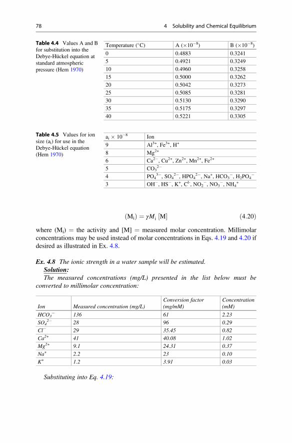
Mið Þ ¼ γMi M½ � ð4:20Þwhere (Mi) ¼ the activity and [M] ¼ measured molar concentration. Millimolarconcentrations may be used instead of molar concentrations in Eqs. 4.19 and 4.20 ifdesired as illustrated in Ex. 4.8.

Ex. 4.8 The ionic strength in a water sample will be estimated.Solution:The measured concentrations (mg/L) presented in the list below must be

converted to millimolar concentration:

Ion Measured concentration (mg/L)Conversion factor(mg/mM)

Concentration(mM)

HCO3� 136 61 2.23

SO42� 28 96 0.29

Cl� 29 35.45 0.82

Ca2+ 41 40.08 1.02

Mg2+ 9.1 24.31 0.37

Na+ 2.2 23 0.10

K+ 1.2 3.91 0.03

Substituting into Eq. 4.19:

Table 4.4 Values A and Bfor substitution into theDebye-Hückel equation atstandard atmosphericpressure (Hem 1970)

Temperature (�C) A (�10�8) B (�10�8)

0 0.4883 0.3241

5 0.4921 0.3249

10 0.4960 0.3258

15 0.5000 0.3262

20 0.5042 0.3273

25 0.5085 0.3281

30 0.5130 0.3290

35 0.5175 0.3297

40 0.5221 0.3305

Table 4.5 Values for ionsize (ai) for use in theDebye-Hückel equation(Hem 1970)

ai � 10�8 Ion

9 Al3+, Fe3+, H+

8 Mg2+

6 Ca2�, Cu2+, Zn2+, Mn2+, Fe2+

5 CO32�

4 PO43�, SO4

2�, HPO42�, Na+, HCO3

�, H2PO4�

3 OH�, HS�, K+, Cl-, NO2�, NO3

�, NH4+


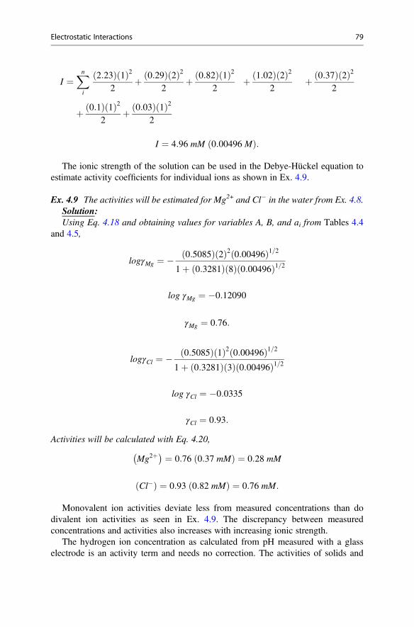
I ¼Xn

i

2:23ð Þ 1ð Þ22

þ 0:29ð Þ 2ð Þ22

þ 0:82ð Þ 1ð Þ22

þ 1:02ð Þ 2ð Þ22

þ 0:37ð Þ 2ð Þ22

þ 0:1ð Þ 1ð Þ22

þ 0:03ð Þ 1ð Þ22

I ¼ 4:96 mM 0:00496 Mð Þ:

The ionic strength of the solution can be used in the Debye-Hückel equation toestimate activity coefficients for individual ions as shown in Ex. 4.9.

Ex. 4.9 The activities will be estimated for Mg2+ and Cl� in the water from Ex. 4.8.Solution:Using Eq. 4.18 and obtaining values for variables A, B, and ai from Tables 4.4

and 4.5,

logγMg ¼ � 0:5085ð Þ 2ð Þ2 0:00496ð Þ1=21þ 0:3281ð Þ 8ð Þ 0:00496ð Þ1=2

log γMg ¼ �0:12090

γMg ¼ 0:76:

logγCl ¼ � 0:5085ð Þ 1ð Þ2 0:00496ð Þ1=21þ 0:3281ð Þ 3ð Þ 0:00496ð Þ1=2

log γCl ¼ �0:0335

γCl ¼ 0:93:

Activities will be calculated with Eq. 4.20,

Mg2þ� � ¼ 0:76 0:37 mMð Þ ¼ 0:28 mM

Cl�ð Þ ¼ 0:93 0:82 mMð Þ ¼ 0:76 mM:

Monovalent ion activities deviate less from measured concentrations than dodivalent ion activities as seen in Ex. 4.9. The discrepancy between measuredconcentrations and activities also increases with increasing ionic strength.

The hydrogen ion concentration as calculated from pH measured with a glasselectrode is an activity term and needs no correction. The activities of solids and

Electrostatic Interactions 79

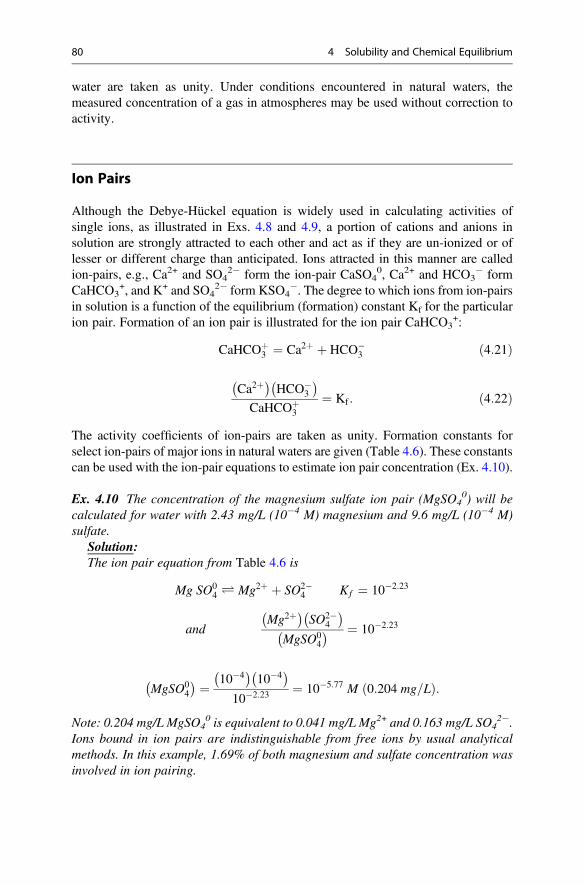
water are taken as unity. Under conditions encountered in natural waters, themeasured concentration of a gas in atmospheres may be used without correction toactivity.

Ion Pairs

Although the Debye-Hückel equation is widely used in calculating activities ofsingle ions, as illustrated in Exs. 4.8 and 4.9, a portion of cations and anions insolution are strongly attracted to each other and act as if they are un-ionized or oflesser or different charge than anticipated. Ions attracted in this manner are calledion-pairs, e.g., Ca2+ and SO4

2� form the ion-pair CaSO40, Ca2+ and HCO3

� formCaHCO3

+, and K+ and SO42� form KSO4

�. The degree to which ions from ion-pairsin solution is a function of the equilibrium (formation) constant Kf for the particularion pair. Formation of an ion pair is illustrated for the ion pair CaHCO3

+:

CaHCOþ3 ¼ Ca2þ þ HCO�

3 ð4:21Þ

Ca2þ� �

HCO�3

� �

CaHCOþ3

¼ Kf : ð4:22Þ

The activity coefficients of ion-pairs are taken as unity. Formation constants forselect ion-pairs of major ions in natural waters are given (Table 4.6). These constantscan be used with the ion-pair equations to estimate ion pair concentration (Ex. 4.10).

Ex. 4.10 The concentration of the magnesium sulfate ion pair (MgSO40) will be

calculated for water with 2.43 mg/L (10�4 M) magnesium and 9.6 mg/L (10�4 M)sulfate.

Solution:The ion pair equation from Table 4.6 is

Mg SO04 Ð Mg2þ þ SO2�

4 Kf ¼ 10�2:23

andMg2þ� �

SO2�4

� �

MgSO04

� � ¼ 10�2:23

MgSO04

� � ¼ 10�4� �

10�4� �

10�2:23 ¼ 10�5:77 M 0:204 mg=Lð Þ:

Note: 0.204 mg/L MgSO40 is equivalent to 0.041 mg/L Mg2+ and 0.163 mg/L SO4

2�.Ions bound in ion pairs are indistinguishable from free ions by usual analyticalmethods. In this example, 1.69% of both magnesium and sulfate concentration wasinvolved in ion pairing.


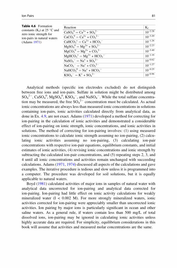
Analytical methods (specific ion electrodes excluded) do not distinguishbetween free ions and ion-pairs. Sulfate in solution might be distributed amongSO4

2�, CaSO40, MgSO4

0, KSO4�, and NaSO4

�. While the total sulfate concentra-tion may be measured, the free SO4

2� concentration must be calculated. As actualionic concentrations are always less than measured ionic concentrations in solutionscontaining ion-pairs, ionic activities calculated directly from analytical data, asdone in Ex. 4.9, are not exact. Adams (1971) developed a method for correcting forion-pairing in the calculation of ionic activities and demonstrated a considerableeffect of ion-pairing on ionic strength, ionic concentrations, and ionic activities insolutions. The method of correcting for ion-pairing involves: (1) using measuredionic concentrations to calculate ionic strength assuming no ion-pairing, (2) calcu-lating ionic activities assuming no ion-pairing, (3) calculating ion-pairconcentrations with respective ion-pair equations, equilibrium constants, and initialestimates of ionic activities, (4) revising ionic concentrations and ionic strength bysubtracting the calculated ion-pair concentrations, and (5) repeating steps 2, 3, and4 until all ionic concentrations and activities remain unchanged with succeedingcalculations. Adams (1971, 1974) discussed all aspects of the calculations and gaveexamples. The iterative procedure is tedious and slow unless it is programmed intoa computer. The procedure was developed for soil solutions, but it is equallyapplicable to natural waters.

Boyd (1981) calculated activities of major ions in samples of natural water withanalytical data uncorrected for ion-pairing and analytical data corrected forion-pairing. Ion-pairing had little effect on ionic activity calculations for weaklymineralized water (I < 0.002 M). For more strongly mineralized waters, ionicactivities corrected for ion-pairing were appreciably smaller than uncorrected ionicactivities. Ion pairing by major ions is particularly significant in ocean and othersaline waters. As a general rule, if waters contain less than 500 mg/L of totaldissolved ions, ion-pairing may be ignored in calculating ionic activities unlesshighly accurate data are required. For simplicity, equilibrium considerations in thisbook will assume that activities and measured molar concentrations are the same.

Table 4.6 Formationconstants (Kf) at 25 �C andzero ionic strength forion-pairs in natural waters(Adams 1971)

Reaction Kf

CaSO40 ¼ Ca2+ + SO4

2� 10–2.28

CaCO30 ¼ Ca2+ + CO3

2� 10–3.20

CaHCO3+ ¼ Ca2+ + HCO3

� 10–1.26

MgSO40 ¼ Mg2+ + SO4

2� 10–2.23

MgCO30 ¼ Mg2+ + CO3

2� 10–3.40

MgHCO3+ ¼ Mg2+ + HCO3

� 10–1.16

NaSO4� ¼ Na+ + SO4

2� 10–0.62

NaCO3� ¼ Na+ + CO3

2� 10–1.27

NaHCO30 ¼ Na+ + HCO3

� 10–0.25

KSO4� ¼ K+ + SO4

2� 10–0.96

Ion Pairs 81

Conclusions

Concentrations of water quality variables typically are measured rather than calcu-lated. Nevertheless, knowledge of the principles of solubility and use of solubilityproducts and equilibrium constants to calculate anticipated concentrations can behelpful in explaining observed concentrations and predicting changes in waterquality. The concept of chemical equilibrium also can be especially useful inpredicting changes in concentrations of water quality variables that may resultfrom addition of substances to water by natural or anthropogenic processes.

References

Adams F (1971) Ionic concentrations and activities in soil solutions. Soil Sci Soc Am Proc35:420–426

Adams F (1974) Soil solution. In: Carson WE (ed) The plant root and its environment. UniversityPress of Virginia, Charlottesville, pp 441–481

Boyd CE (1981) Effects of ion-pairing on calculations of ionic activities of major ions in freshwater.Hydrobio 80:91–93

Garrels RM, Christ CL (1965) Solutions, minerals, and equilibria. Harper and Row, New YorkHem JD (1970) Study and interpretation of the chemical characteristics of natural water. Water-

supply paper 1473, United States Geological Survey, United States Government Printing Office.Washington.


Dissolved Solids 5

AbstractThe total dissolved solids (TDS) concentration in freshwater is determined bypassing water through a 2-μm filter, evaporating the filtrate to dryness, andreporting the weight of the solids remaining after evaporation in milligrams perliter. Salinity and electrical conductivity usually are used to assess theconcentrations of ions in seawater, and electrical conductivity also may beused to determine the extent of mineralization of freshwater. The TDSconcentrations in natural freshwaters typically range from about 20 to1000 mg/L, and the solids consist mainly of bicarbonate (and carbonate at pHabove 8.3), chloride, sulfate, calcium, magnesium, potassium, sodium, andsilicate. The concentration of TDS in inland waters is controlled mainly bygeological and climatic factors. The most weakly mineralized waters are foundin areas with high-rainfall and heavily leached or poorly developed soils. Themost strongly mineralized waters usually occur in arid regions. Examples of TDSconcentrations in different regions are presented, and reasons for differences inTDS concentrations among regions and sources of water are discussed. Althoughthe major dissolved inorganic substances in natural water are essential for life,minor dissolved constituents in water often have the greatest effect on aquaticorganisms. The main effect of TDS concentration on animals and plants usuallyis related to osmotic pressure that increases with greater TDS concentration. Theaverage TDS concentration in seawater is about 35,000 mg/L. Aquatic speciesare adapted to specific TDS ranges, and outside this range osmoregulatorydifficulty occurs. Excessive TDS concentration also can make water unsuitablefor domestic use, irrigation, and various other purposes. Desalination is increas-ingly used to increase water supply in arid regions. Bottled water has becomevery popular as a source of drinking water.


83


Introduction

Natural waters contain both gases and solids in solution. Solids differ from gases inthat they remain as a residue when water evaporates. Solids originate mainly fromdissolution of minerals and suspension of mineral and organic particles from soilsand other geological formations, living aquatic microorganisms, and decayingremains of organisms. The portion of these solids in solution is called the dissolvedsolids. Chemists usually consider dissolved particles to be �0.5–1 μm in diameter,but the method for determining dissolved solids in waters typically relies on a 2.0-μm filter to separate dissolved from suspended solids (Eaton et al. 2005).

Most of the weight of dissolved solids results from inorganic particles, and waterswith large dissolved solids concentrations often are said to be highly mineralized.Concentrations of dissolved solids in natural waters vary from 1–2 mg/L to over100,000 mg/L. Waters in regions with acidic, weathered soils and geologicalformations of dissolution-resistant rocks may contain <50 mg/L of dissolved solids.Waters from areas with limestone deposits or calcareous soils may have200–400 mg/L of dissolved solids, while in arid regions concentrations above1000 mg/L are common. The ocean averages 34,500 mg/L dissolved solids, butclosed-basin lakes (water flows in but not out) like the Dead Sea and the Great SaltLake may contain over 250,000 mg/L.

Freshwater usually is considered to contain no more than 1000 mg/L of dissolvedsolids, and some inland waters are saline. Drinking water ideally should not exceed500 mg/L of dissolved solids, but in some areas higher concentrations cannot beavoided.

The atmosphere contains particles of solids resulting from evaporation of sprayfrom waves, dust, and combustion by-products. As a result, raindrops acquire smallamounts of dissolved solids from the atmosphere. When rainwater reaches the earth,it contacts vegetation, soil and other geological formations and dissolves additionalmineral and organic matter. Dissolved mineral matter consists largely of calcium,magnesium, sodium, potassium, chloride, sulfate, bicarbonate, and carbonate. Mostnatural waters also have a significant concentration of undissociated silicic acid.Hutchinson (1957) defined freshwaters as “dilute solutions of alkaline earth andalkali bicarbonate, carbonate, sulfate, and chloride with a quantity of silica.” Seawa-ter is essentially a sodium chloride solution containing sulfates and bicarbonates ofpotassium, calcium, and sodium. Both freshwater and seawater also contain smallconcentrations of other dissolved inorganic substances. The most important arehydrogen and hydroxyl ions, nitrate, ammonium, phosphate, borate, iron, manga-nese, zinc, copper, cobalt, and molybdenum. Hydrogen and hydroxyl ions determinepH and the others are nutrients. Natural waters also contain minor concentrations ofother elements that are not nutrients. Minor elements, both nutrients andnon-nutrients, may be toxic at elevated concentrations.

The degree of mineralization of inland water is highly variable from place to placeand depends upon the solubility of minerals, length of time and conditions of contactof water with minerals, and concentration of substances through evaporation. Whileocean water is rather similar in mineral content worldwide, water in estuaries can

84 5 Dissolved Solids

vary greatly in degree of mineralization. A direct way of assessing the mineralizationof water is to measure the concentrations of the individual inorganic constituents. Alarge effort is required to make a total analysis of water, and it is more common tomeasure the total concentration of dissolved substances in water in a single analysis.In freshwater, this is possible by the total dissolved solids (TDS) analysis (Eatonet al. 2005). In seawater, the degree of mineralization is usually assessed by chlorideconcentration, salinity, or specific conductance. Mineralization of freshwater also isoften assessed by specific conductance.

Soluble organic compounds reach water through the decay of dead plant andanimal matter and by the excretion of organic matter by aquatic organisms.Thousands of organic compounds occur in water, and dissolved organic compoundsusually are measured collectively for convenience. Dissolved organic matterconcentrations are highest in waters that have had contact with organic residues orin which phytoplankton abound.

Dissolved Solids Measurement

Total Dissolved Solids

The method for determining the TDS concentration begins with filtration of a watersample through a filter with 2-μm or smaller openings. A measured volume of thefiltrate is evaporated in a tared (weighed) evaporating dish, the dish and residue arecooled in a desiccator and weighed to constant weight (Fig. 5.1, Left; Ex. 5.1). Theresidue left upon evaporation is mainly from dissolved inorganic matter, but avariable portion is dissolved organic matter. This method does not give exact results,because carbon dioxide is lost from bicarbonate when calcium carbonate precipitatesduring evaporation:

Ca2þ þ 2HCO�3 !

ΔCaCO3 # þH2O " þCO2 " : ð5:1Þ

The weight loss of solids during evaporation is about 38% of the portion of the TDSconcentration resulting from calcium and bicarbonate. This is because molar weightsof Ca2+ and 2HCO3

� sum to 162.08 g and the molar weights of the volatilized CO2

and H2O sum to 62 g; thus, (62� 162.08)� 100¼ 38%. A small amount of organicmatter also may be lost by volatilization. Nevertheless, TDS concentration is indica-tive of the degree of mineralization of freshwaters. The TDS procedure does notwork well for saline waters, because the large residue of hygroscopic salts absorbsmoisture from the air making accurate weighing difficult.

Ex. 5.1 A 100-mL water sample that passed a 2-μm filter is dried at 105 �C in a5.2000-g dish. The dish and residue weigh 5.2100 g. The TDS concentration will beestimated.

Dissolved Solids Measurement 85

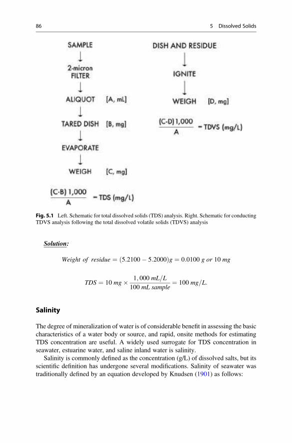
Solution:

Weight of residue ¼ 5:2100� 5:2000ð Þg ¼ 0:0100 g or 10 mg

TDS ¼ 10 mg� 1; 000 mL=L

100 mL sample¼ 100 mg=L:

Salinity

The degree of mineralization of water is of considerable benefit in assessing the basiccharacteristics of a water body or source, and rapid, onsite methods for estimatingTDS concentration are useful. A widely used surrogate for TDS concentration inseawater, estuarine water, and saline inland water is salinity.

Salinity is commonly defined as the concentration (g/L) of dissolved salts, but itsscientific definition has undergone several modifications. Salinity of seawater wastraditionally defined by an equation developed by Knudsen (1901) as follows:

Fig. 5.1 Left. Schematic for total dissolved solids (TDS) analysis. Right. Schematic for conductingTDVS analysis following the total dissolved volatile solids (TDVS) analysis


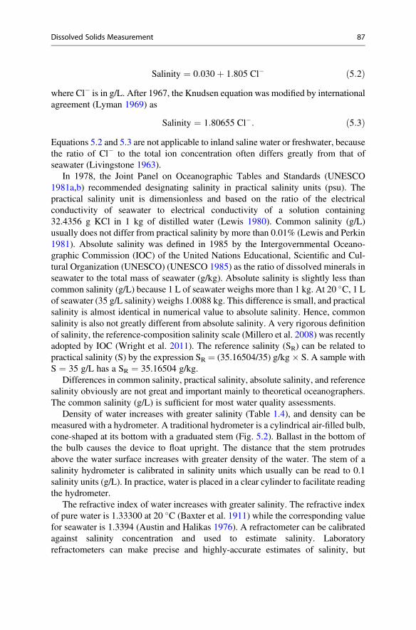
Salinity ¼ 0:030þ 1:805 Cl� ð5:2Þwhere Cl� is in g/L. After 1967, the Knudsen equation was modified by internationalagreement (Lyman 1969) as

Salinity ¼ 1:80655 Cl�: ð5:3ÞEquations 5.2 and 5.3 are not applicable to inland saline water or freshwater, becausethe ratio of Cl� to the total ion concentration often differs greatly from that ofseawater (Livingstone 1963).

In 1978, the Joint Panel on Oceanographic Tables and Standards (UNESCO1981a,b) recommended designating salinity in practical salinity units (psu). Thepractical salinity unit is dimensionless and based on the ratio of the electricalconductivity of seawater to electrical conductivity of a solution containing32.4356 g KCl in 1 kg of distilled water (Lewis 1980). Common salinity (g/L)usually does not differ from practical salinity by more than 0.01% (Lewis and Perkin1981). Absolute salinity was defined in 1985 by the Intergovernmental Oceano-graphic Commission (IOC) of the United Nations Educational, Scientific and Cul-tural Organization (UNESCO) (UNESCO 1985) as the ratio of dissolved minerals inseawater to the total mass of seawater (g/kg). Absolute salinity is slightly less thancommon salinity (g/L) because 1 L of seawater weighs more than 1 kg. At 20 �C, 1 Lof seawater (35 g/L salinity) weighs 1.0088 kg. This difference is small, and practicalsalinity is almost identical in numerical value to absolute salinity. Hence, commonsalinity is also not greatly different from absolute salinity. A very rigorous definitionof salinity, the reference-composition salinity scale (Millero et al. 2008) was recentlyadopted by IOC (Wright et al. 2011). The reference salinity (SR) can be related topractical salinity (S) by the expression SR ¼ (35.16504/35) g/kg � S. A sample withS ¼ 35 g/L has a SR ¼ 35.16504 g/kg.

Differences in common salinity, practical salinity, absolute salinity, and referencesalinity obviously are not great and important mainly to theoretical oceanographers.The common salinity (g/L) is sufficient for most water quality assessments.

Density of water increases with greater salinity (Table 1.4), and density can bemeasured with a hydrometer. A traditional hydrometer is a cylindrical air-filled bulb,cone-shaped at its bottom with a graduated stem (Fig. 5.2). Ballast in the bottom ofthe bulb causes the device to float upright. The distance that the stem protrudesabove the water surface increases with greater density of the water. The stem of asalinity hydrometer is calibrated in salinity units which usually can be read to 0.1salinity units (g/L). In practice, water is placed in a clear cylinder to facilitate readingthe hydrometer.

The refractive index of water increases with greater salinity. The refractive indexof pure water is 1.33300 at 20 �C (Baxter et al. 1911) while the corresponding valuefor seawater is 1.3394 (Austin and Halikas 1976). A refractometer can be calibratedagainst salinity concentration and used to estimate salinity. Laboratoryrefractometers can make precise and highly-accurate estimates of salinity, but


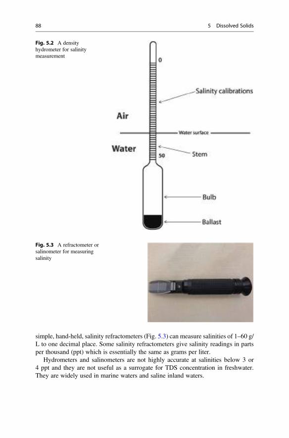
simple, hand-held, salinity refractometers (Fig. 5.3) can measure salinities of 1–60 g/L to one decimal place. Some salinity refractometers give salinity readings in partsper thousand (ppt) which is essentially the same as grams per liter.

Hydrometers and salinometers are not highly accurate at salinities below 3 or4 ppt and they are not useful as a surrogate for TDS concentration in freshwater.They are widely used in marine waters and saline inland waters.

Fig. 5.2 A densityhydrometer for salinitymeasurement

Fig. 5.3 A refractometer orsalinometer for measuringsalinity


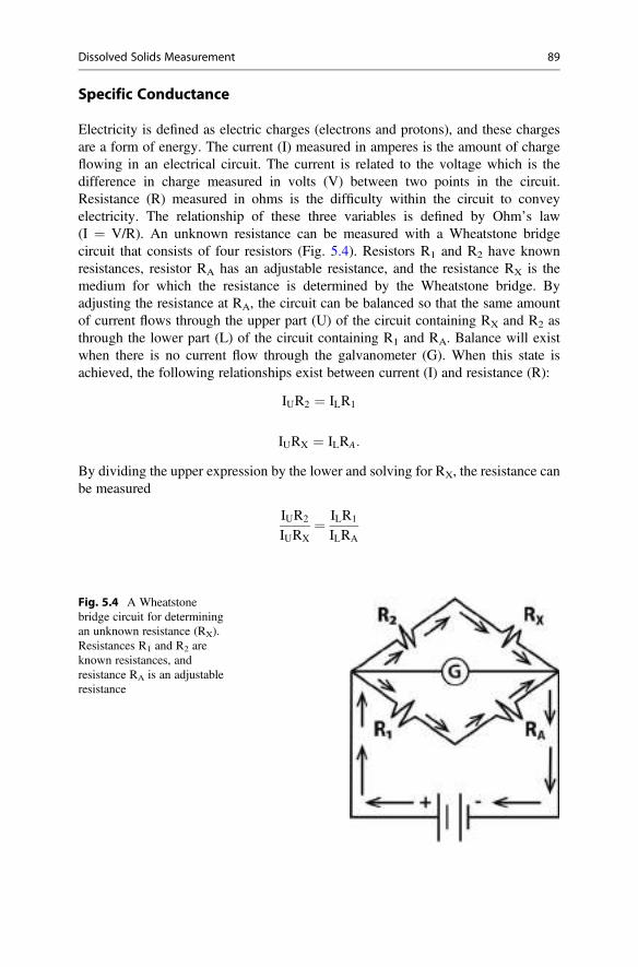
Specific Conductance

Electricity is defined as electric charges (electrons and protons), and these chargesare a form of energy. The current (I) measured in amperes is the amount of chargeflowing in an electrical circuit. The current is related to the voltage which is thedifference in charge measured in volts (V) between two points in the circuit.Resistance (R) measured in ohms is the difficulty within the circuit to conveyelectricity. The relationship of these three variables is defined by Ohm’s law(I ¼ V/R). An unknown resistance can be measured with a Wheatstone bridgecircuit that consists of four resistors (Fig. 5.4). Resistors R1 and R2 have knownresistances, resistor RA has an adjustable resistance, and the resistance RX is themedium for which the resistance is determined by the Wheatstone bridge. Byadjusting the resistance at RA, the circuit can be balanced so that the same amountof current flows through the upper part (U) of the circuit containing RX and R2 asthrough the lower part (L) of the circuit containing R1 and RA. Balance will existwhen there is no current flow through the galvanometer (G). When this state isachieved, the following relationships exist between current (I) and resistance (R):

IUR2 ¼ ILR1

IURX ¼ ILRA:

By dividing the upper expression by the lower and solving for RX, the resistance canbe measured

IUR2

IURX¼ ILR1

ILRA

Fig. 5.4 A Wheatstonebridge circuit for determiningan unknown resistance (RX).Resistances R1 and R2 areknown resistances, andresistance RA is an adjustableresistance


RX ¼ R2RA

R1: ð5:4Þ

Conductance is the reciprocal of resistance, and the principle of the Wheatstonebridge circuit can be used to measure the conductivity of water. Resistance andconductance depend upon the dimensions of the conductor, and the terms resistivityand conductivity are used to describe the resistance of unit length and cross-sectionalarea of the conductor

R ¼ ρLA

or ρ ¼ RAL

ð5:5Þ

where L ¼ length, A ¼ cross-sectional area, and ρ ¼ specific resistance of theconductor. With the dimensions of the conductor in centimeters, R will be inohm/cm and ρ in ohm�cm. In SI units, R will be in siemens/cm (S/cm) and ρ insiemens�cm (S�cm). Because k is the reciprocal of resistance,

k ¼ 1ρ: ð5:6Þ

The unit for k is reciprocal ohm�cm (1/ohm�cm) which usually is referred to asmho/cm—mho is ohm spelled backwards.

The resistivities (and conductivities) of different materials vary greatly. Metalssuch as copper used as wires in electrical circuits conduct electricity via freeelectrons that can move around, because they are not attached to cations of themetal. The resistance (R) is greater for an equal length of small diameter wire thanfor a larger diameter wire, but resistivity (ρ) is equal for both because ρ is a propertyof the metal and R is the product of ρmultiplied by (L/A). The same reasoning can beapplied to conductance (K) and k (conductivity).

Pure water is not a good conductor of electricity, because electrical current inliquids is conducted by dissolved ions, but as the concentration of ions in waterincreases, its electrical conductivity (EC) increases. The measurement of electricalconductivity is usually an excellent indicator of the degree of mineralization ofwater.

The electrical conductivity of water is the conductance afforded by a cubic massof water with edges of 1 cm. As a result of the specificity of the determination,electrical conductivity sometimes is referred to as specific conductance. The stan-dard for electrical conductivity is 0.0100 N KCl solution which has a specificconductance of 0.001413 mho/cm at 25 �C. To avoid small decimal numbers,specific conductance is customarily reported in micromhos per centimeter, or inthe case of 0.0100 N KCl, 1413 μmho/cm. The unit, μmho/cm, is replaced by itsequivalent microsiemens per centimeter (μS/cm) in the International System (SI) ofUnits. The SI units can be easily confused, because conductivity meters may allowthe display to be selected as siemens/m (S/m), millisiemens/m (mS/m), millisiemens/cm (mS/cm), microsiemens/cm (μS/cm) or other combinations of conductance and


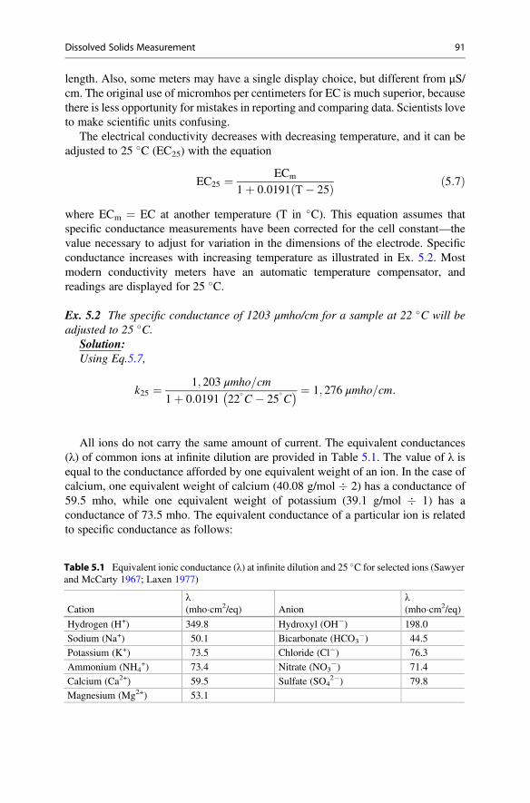
length. Also, some meters may have a single display choice, but different from μS/cm. The original use of micromhos per centimeters for EC is much superior, becausethere is less opportunity for mistakes in reporting and comparing data. Scientists loveto make scientific units confusing.

The electrical conductivity decreases with decreasing temperature, and it can beadjusted to 25 �C (EC25) with the equation

EC25 ¼ ECm

1þ 0:0191 T� 25ð Þ ð5:7Þ

where ECm ¼ EC at another temperature (T in �C). This equation assumes thatspecific conductance measurements have been corrected for the cell constant—thevalue necessary to adjust for variation in the dimensions of the electrode. Specificconductance increases with increasing temperature as illustrated in Ex. 5.2. Mostmodern conductivity meters have an automatic temperature compensator, andreadings are displayed for 25 �C.

Ex. 5.2 The specific conductance of 1203 μmho/cm for a sample at 22 �C will beadjusted to 25 �C.

Solution:Using Eq.5.7,

k25 ¼ 1; 203 μmho=cm

1þ 0:0191 22�C � 25

�C

� � ¼ 1; 276 μmho=cm:

All ions do not carry the same amount of current. The equivalent conductances(λ) of common ions at infinite dilution are provided in Table 5.1. The value of λ isequal to the conductance afforded by one equivalent weight of an ion. In the case ofcalcium, one equivalent weight of calcium (40.08 g/mol � 2) has a conductance of59.5 mho, while one equivalent weight of potassium (39.1 g/mol � 1) has aconductance of 73.5 mho. The equivalent conductance of a particular ion is relatedto specific conductance as follows:

Table 5.1 Equivalent ionic conductance (λ) at infinite dilution and 25 �C for selected ions (Sawyerand McCarty 1967; Laxen 1977)

Cationλ(mho�cm2/eq) Anion

λ(mho�cm2/eq)

Hydrogen (H+) 349.8 Hydroxyl (OH�) 198.0

Sodium (Na+) 50.1 Bicarbonate (HCO3�) 44.5

Potassium (K+) 73.5 Chloride (Cl�) 76.3

Ammonium (NH4+) 73.4 Nitrate (NO3

�) 71.4

Calcium (Ca2+) 59.5 Sulfate (SO42�) 79.8

Magnesium (Mg2+) 53.1


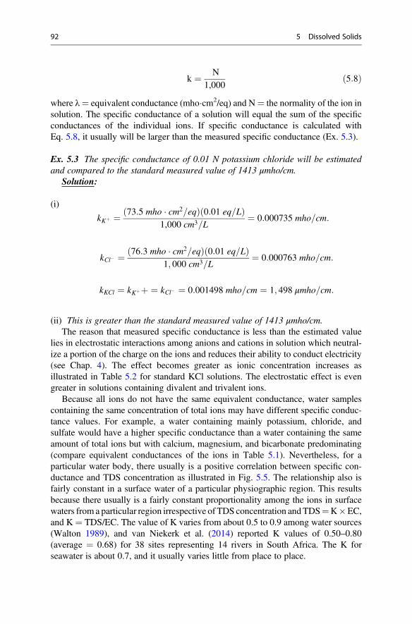
k ¼ N1,000

ð5:8Þ

where λ¼ equivalent conductance (mho�cm2/eq) and N¼ the normality of the ion insolution. The specific conductance of a solution will equal the sum of the specificconductances of the individual ions. If specific conductance is calculated withEq. 5.8, it usually will be larger than the measured specific conductance (Ex. 5.3).

Ex. 5.3 The specific conductance of 0.01 N potassium chloride will be estimatedand compared to the standard measured value of 1413 μmho/cm.

Solution:

(i)

kKþ ¼ 73:5 mho � cm2=eqð Þ 0:01 eq=Lð Þ1,000 cm3=L

¼ 0:000735 mho=cm:

kCl� ¼ 76:3 mho � cm2=eqð Þ 0:01 eq=Lð Þ1; 000 cm3=L

¼ 0:000763 mho=cm:

kKCl ¼ kKþþ ¼ kCl� ¼ 0:001498 mho=cm ¼ 1; 498 μmho=cm:

(ii) This is greater than the standard measured value of 1413 μmho/cm.The reason that measured specific conductance is less than the estimated value

lies in electrostatic interactions among anions and cations in solution which neutral-ize a portion of the charge on the ions and reduces their ability to conduct electricity(see Chap. 4). The effect becomes greater as ionic concentration increases asillustrated in Table 5.2 for standard KCl solutions. The electrostatic effect is evengreater in solutions containing divalent and trivalent ions.

Because all ions do not have the same equivalent conductance, water samplescontaining the same concentration of total ions may have different specific conduc-tance values. For example, a water containing mainly potassium, chloride, andsulfate would have a higher specific conductance than a water containing the sameamount of total ions but with calcium, magnesium, and bicarbonate predominating(compare equivalent conductances of the ions in Table 5.1). Nevertheless, for aparticular water body, there usually is a positive correlation between specific con-ductance and TDS concentration as illustrated in Fig. 5.5. The relationship also isfairly constant in a surface water of a particular physiographic region. This resultsbecause there usually is a fairly constant proportionality among the ions in surfacewaters from a particular region irrespective of TDS concentration andTDS¼K�EC,and K ¼ TDS/EC. The value of K varies from about 0.5 to 0.9 among water sources(Walton 1989), and van Niekerk et al. (2014) reported K values of 0.50–0.80(average ¼ 0.68) for 38 sites representing 14 rivers in South Africa. The K forseawater is about 0.7, and it usually varies little from place to place.


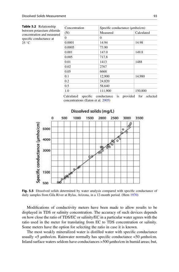
Modifications of conductivity meters have been made to allow results to bedisplayed in TDS or salinity concentration. The accuracy of such devices dependson how close the ratio of TDS/EC or salinity/EC in a particular water agrees with theratio used in the meter for translating from EC to TDS concentration or salinity.Some meters have the option for selecting the ratio in case it is known.

The most weakly mineralized water is distilled water with specific conductanceusually <5 μmho/cm. Rainwater normally has specific conductance <50 μmho/cm.Inland surface waters seldom have conductances >500 μmho/cm in humid areas; but,

Table 5.2 Relationshipbetween potassium chlorideconcentration and measuredspecific conductance at25 �C

Concentration Specific conductance (μmho/cm)

(N) Measured Calculated

0 0

0.0001 14.94 14.98

0.0005 73.90

0.001 147.0 149.8

0.005 717.8

0.01 1413 1488

0.02 2767

0.05 6668

0.1 12,900 14,980

0.2 24,820

0.5 58,640

1.0 111,900 150,800

Calculated specific conductance is provided for selectedconcentrations (Eaton et al. 2005)

Fig. 5.5 Dissolved solids determined by water analysis compared with specific conductance ofdaily samples from Gila River at Bylas, Arizona, in a 12-month period. (Hem 1970)


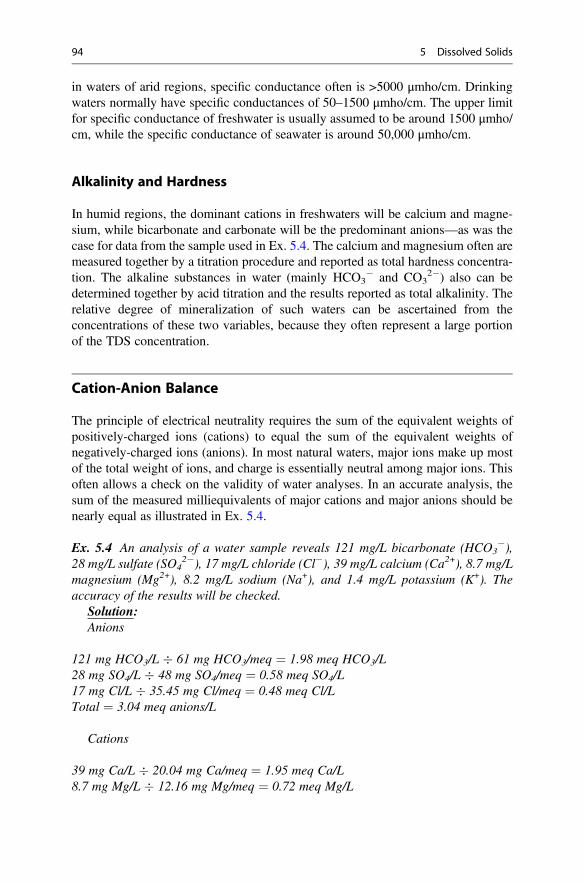
in waters of arid regions, specific conductance often is >5000 μmho/cm. Drinkingwaters normally have specific conductances of 50–1500 μmho/cm. The upper limitfor specific conductance of freshwater is usually assumed to be around 1500 μmho/cm, while the specific conductance of seawater is around 50,000 μmho/cm.

Alkalinity and Hardness

In humid regions, the dominant cations in freshwaters will be calcium and magne-sium, while bicarbonate and carbonate will be the predominant anions—as was thecase for data from the sample used in Ex. 5.4. The calcium and magnesium often aremeasured together by a titration procedure and reported as total hardness concentra-tion. The alkaline substances in water (mainly HCO3

� and CO32�) also can be

determined together by acid titration and the results reported as total alkalinity. Therelative degree of mineralization of such waters can be ascertained from theconcentrations of these two variables, because they often represent a large portionof the TDS concentration.

Cation-Anion Balance

The principle of electrical neutrality requires the sum of the equivalent weights ofpositively-charged ions (cations) to equal the sum of the equivalent weights ofnegatively-charged ions (anions). In most natural waters, major ions make up mostof the total weight of ions, and charge is essentially neutral among major ions. Thisoften allows a check on the validity of water analyses. In an accurate analysis, thesum of the measured milliequivalents of major cations and major anions should benearly equal as illustrated in Ex. 5.4.

Ex. 5.4 An analysis of a water sample reveals 121 mg/L bicarbonate (HCO3�),

28 mg/L sulfate (SO42�), 17 mg/L chloride (Cl�), 39 mg/L calcium (Ca2+), 8.7 mg/L

magnesium (Mg2+), 8.2 mg/L sodium (Na+), and 1.4 mg/L potassium (K+). Theaccuracy of the results will be checked.

Solution:Anions

121 mg HCO3/L � 61 mg HCO3/meq ¼ 1.98 meq HCO3/L28 mg SO4/L � 48 mg SO4/meq ¼ 0.58 meq SO4/L17 mg Cl/L � 35.45 mg Cl/meq ¼ 0.48 meq Cl/LTotal ¼ 3.04 meq anions/L

Cations

39 mg Ca/L � 20.04 mg Ca/meq ¼ 1.95 meq Ca/L8.7 mg Mg/L � 12.16 mg Mg/meq ¼ 0.72 meq Mg/L


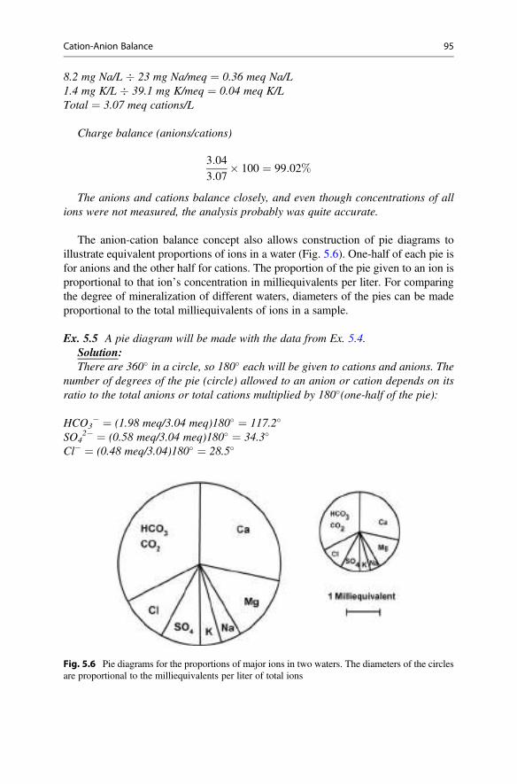
8.2 mg Na/L � 23 mg Na/meq ¼ 0.36 meq Na/L1.4 mg K/L � 39.1 mg K/meq ¼ 0.04 meq K/LTotal ¼ 3.07 meq cations/L

Charge balance (anions/cations)

3:043:07

� 100 ¼ 99:02%

The anions and cations balance closely, and even though concentrations of allions were not measured, the analysis probably was quite accurate.

The anion-cation balance concept also allows construction of pie diagrams toillustrate equivalent proportions of ions in a water (Fig. 5.6). One-half of each pie isfor anions and the other half for cations. The proportion of the pie given to an ion isproportional to that ion’s concentration in milliequivalents per liter. For comparingthe degree of mineralization of different waters, diameters of the pies can be madeproportional to the total milliequivalents of ions in a sample.

Ex. 5.5 A pie diagram will be made with the data from Ex. 5.4.Solution:There are 360� in a circle, so 180� each will be given to cations and anions. The

number of degrees of the pie (circle) allowed to an anion or cation depends on itsratio to the total anions or total cations multiplied by 180�(one-half of the pie):

HCO3� ¼ (1.98 meq/3.04 meq)180� ¼ 117.2�

SO42� ¼ (0.58 meq/3.04 meq)180� ¼ 34.3�

Cl� ¼ (0.48 meq/3.04)180� ¼ 28.5�

Fig. 5.6 Pie diagrams for the proportions of major ions in two waters. The diameters of the circlesare proportional to the milliequivalents per liter of total ions

Cation-Anion Balance 95

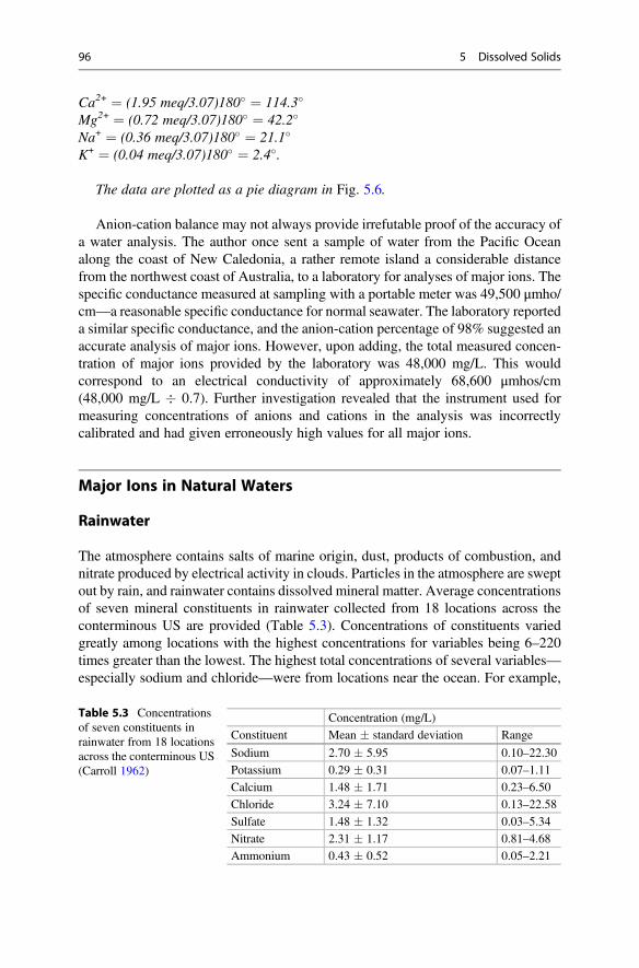
Ca2+ ¼ (1.95 meq/3.07)180� ¼ 114.3�

Mg2+ ¼ (0.72 meq/3.07)180� ¼ 42.2�

Na+ ¼ (0.36 meq/3.07)180� ¼ 21.1�

K+ ¼ (0.04 meq/3.07)180� ¼ 2.4�.

The data are plotted as a pie diagram in Fig. 5.6.

Anion-cation balance may not always provide irrefutable proof of the accuracy ofa water analysis. The author once sent a sample of water from the Pacific Oceanalong the coast of New Caledonia, a rather remote island a considerable distancefrom the northwest coast of Australia, to a laboratory for analyses of major ions. Thespecific conductance measured at sampling with a portable meter was 49,500 μmho/cm—a reasonable specific conductance for normal seawater. The laboratory reporteda similar specific conductance, and the anion-cation percentage of 98% suggested anaccurate analysis of major ions. However, upon adding, the total measured concen-tration of major ions provided by the laboratory was 48,000 mg/L. This wouldcorrespond to an electrical conductivity of approximately 68,600 μmhos/cm(48,000 mg/L � 0.7). Further investigation revealed that the instrument used formeasuring concentrations of anions and cations in the analysis was incorrectlycalibrated and had given erroneously high values for all major ions.

Major Ions in Natural Waters

Rainwater

The atmosphere contains salts of marine origin, dust, products of combustion, andnitrate produced by electrical activity in clouds. Particles in the atmosphere are sweptout by rain, and rainwater contains dissolved mineral matter. Average concentrationsof seven mineral constituents in rainwater collected from 18 locations across theconterminous US are provided (Table 5.3). Concentrations of constituents variedgreatly among locations with the highest concentrations for variables being 6–220times greater than the lowest. The highest total concentrations of several variables—especially sodium and chloride—were from locations near the ocean. For example,

Table 5.3 Concentrationsof seven constituents inrainwater from 18 locationsacross the conterminous US(Carroll 1962)

Concentration (mg/L)

Constituent Mean � standard deviation Range

Sodium 2.70 � 5.95 0.10–22.30

Potassium 0.29 � 0.31 0.07–1.11

Calcium 1.48 � 1.71 0.23–6.50

Chloride 3.24 � 7.10 0.13–22.58

Sulfate 1.48 � 1.32 0.03–5.34

Nitrate 2.31 � 1.17 0.81–4.68

Ammonium 0.43 � 0.52 0.05–2.21


sodium concentration at coastal locations of Brownsville, Texas and Tacoma,Washington was 22.3 and 14.5 mg/L, respectively, while at inland sites of Columbia,Missouri and Ely, Nevada, the respective values were 0.33 and 0.69 mg/L. Theaverage specific conductance of US rainfall calculated from ion concentrationsreported in Table 5.3 and assuming a pH of 6 was 25.7 μmhos/cm.

Average concentrations of the six major ions in rainwater over the entire UnitedStates were lower than concentrations of these ions typically found in inland surfacewaters. Ammonium and especially nitrate, however, were of higher average concen-tration than often found in surface waters—including the ocean. Rainfall in highlypopulated and industrialized regions may have particularly high sulfateconcentrations because of contamination of the atmosphere with sulfur dioxidefrom combustion of fossil fuels.

Rainfall at a location varies in composition from storm to storm because ofdifferences in origins of air masses and the duration of rainfall events. Initial rainfalltends to be more concentrated in impurities than rainfall occurring later in a stormevent, because the initial rainfall tends to sweep the majority of particles from theatmosphere.

Inland Waters

Inland surface waters consist of runoff from watersheds (overland runoff), streams,lakes, reservoirs, ponds, and swamps. Overland runoff has brief contact with soil,but this provides the first opportunity for increasing its mineral content above that ofrainwater. Streams carry overland flow and groundwater seepage (base flow).Groundwater usually is more concentrated in mineral matter than overland flow,because it has resided for months to years within geological formations. Groundwa-ter often is depleted of dissolved oxygen and charged with carbon dioxide as a resultof infiltration through the soil. Carbon dioxide lowers the pH of water, and manyminerals are more soluble at low pH and low oxygen content (low redox potential).The presence of carbon dioxide will increase the capacity of water to dissolvelimestone, calcium, silicate, feldspars, and some other minerals. Moreover, streamwater has contact with soil and geological material in the streambed. These factorscontribute to higher concentrations of mineral matter in stream water than inoverland flow, but stream water may be less concentrated in minerals than ground-water. Streams often flow into standing water bodies where the residence time isgreater than in streams. This provides longer contact of water with bottom soils andgreater opportunity for dissolution of minerals.

Each mineral has a given solubility depending on temperature, pH,concentrations of carbon dioxide and dissolved oxygen, and redox potential of thewater with which it has contact. If contact is long enough, minerals will dissolveuntil equilibrium is reached between the concentrations of dissolved ions and thesolid phase minerals (Li et al. 2012). In humid climates where there has beenextensive weathering, soils may be highly leached and contain only small quantitiesof soluble minerals. In areas where there are abundant outcrops of rocks and

Major Ions in Natural Waters 97

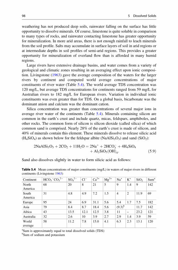
weathering has not produced deep soils, rainwater falling on the surface has littleopportunity to dissolve minerals. Of course, limestone is quite soluble in comparisonto many types of rocks, and rainwater contacting limestone has greater opportunityfor mineralization. In more arid areas, there is not enough rainfall to leach mineralsfrom the soil profile. Salts may accumulate in surface layers of soil in arid regions orat intermediate depths in soil profiles of semi-arid regions. This provides a greateropportunity for mineralization of overland flow than is afforded in many humidregions.

Large rivers have extensive drainage basins, and water comes from a variety ofgeological and climatic zones resulting in an averaging effect upon ionic composi-tion. Livingstone (1963) gave the average composition of the waters for the largerrivers by continent and computed world average concentrations of majorconstituents of river water (Table 5.4). The world average TDS concentration was120 mg/L, but average TDS concentrations for continents ranged from 59 mg/L forAustralian rivers to 182 mg/L for European rivers. Variation in individual ionicconstituents was even greater than for TDS. On a global basis, bicarbonate was thedominant anion and calcium was the dominant cation.

Silica concentration was greater than concentrations of several major ions inaverage river water of the continents (Table 5.4). Minerals containing silicon arecommon in the earth’s crust and include quartz, micas, feldspars, amphiboles, andother rocks. The common form of silicon is silicon dioxide (called silica) of whichcommon sand is comprised. Nearly 28% of the earth’s crust is made of silicon, and40% of minerals contain this element. These minerals dissolve to release silicic acid(H4SiO4) as shown below for the feldspar albite (NaAlSi3O3) and sand (SiO2):

2NaAlSi3O3 þ 2CO2 þ 11H2O ¼ 2Naþ þ 2HCO�3 þ 4H4SiO4

þ Al2SiO5 OHð Þ4: ð5:9ÞSand also dissolves slightly in water to form silicic acid as follows:

Table 5.4 Mean concentrations of major constituents (mg/L) in waters of major rivers in differentcontinents (Livingstone 1963)

Continent HCO3�CO3

2� SO42� Cl� Ca2+ Mg2+ Na+ K+ SiO2 Suma

NorthAmerica

68 20 8 21 5 9 1.4 9 142

SouthAmerica

31 4.8 4.9 7.2 1.5 4 2 11.9 69

Europe 95 24 6.9 31.1 5.6 5.4 1.7 7.5 182

Asia 79 8.4 8.7 18.4 5.6 (9.3)b 11.7 142

Africa 43 13.5 12.1 12.5 3.8 11 – 23.2 121

Australia 32 2.6 10 3.9 2.7 2.9 1.4 3.9 59

Worldaverage

58 11.2 7.8 15.0 4.1 6.3 2.3 13.1 120

aSum is approximately equal to total dissolved solids (TDS)bSum of sodium and potassium


SiO2 þ 2H2O ¼ H4SiO4: ð5:10ÞSilicic acid dissociates as shown below:

H4SiO4 ¼ Hþ þ H3SiO�4 K ¼ 10�9:46 ð5:11Þ

H3SiO�4 ¼ Hþ þ H2SiO

2�4 K ¼ 10�12:56: ð5:12Þ

The ratio of the parent silicic acid to ionized H3SiO�4 is dependent upon pH or more

specifically the hydrogen ion concentration:

H3SiO�4

� �

H4SiO4ð Þ ¼ 10�9:46

Hþð Þ : ð5:13Þ

Dissociation of silicic acid is favored by elevated pH. The pH must be 9.46 beforethe ratio has a value of 1.0. The pH of surface waters usually is below 9, andundissociated silicic acid predominates.

Small streams have small drainage basins and concentrations of ionic constituentsin their waters reflect geological and climatic conditions within a limited area. Forexample, streams near Auburn, Alabama (USA) usually have <100 mg/L TDS, butthere is one stream draining from an area where there is limestone that has a TDSconcentration around 200 mg/L. The ionic composition of water from small streamsin a region is much more variable than is the composition of waters of larger rivers inthe region which have more diverse conditions within their larger drainage basins.Concentrations of major mineral constituents in some relatively small rivers(Table 5.5) illustrate this variation. The Moser River of Nova Scotia has very dilutewater because it flows through an area where the geological formations consist ofhard, highly insoluble rocks and soils are not highly developed or fertile. TheEtowah River in Georgia has fairly dilute water, because it flows through areaswhere weathering and leaching of soils has been extensive because of high rainfalland temperature. But, the Etowah River is more highly mineralized than the MoserRiver. The Withlacoochee River in Florida also flows through an area with weath-ered and highly leached soils, but there are limestone formations in its drainagebasin. Dissolution of limestone results in a higher degree of mineralization of thewater than in either the Moser or Etowah Rivers. The Republican River in Kansas isin an area of relatively low rainfall and soils are deep and fertile. The water is morehighly mineralized than stream waters in regions of greater rainfall where soils areeither poorly developed or highly leached. The Pecos River in New Mexico flowsthrough an arid region, and its waters are highly mineralized as compared to the otherfour rivers. Sulfate, chloride, and sodium are greatly enriched in the Pecos River.This results from the high concentrations of soluble salts that accumulate in soils asthe result of the rate of evaporation exceeding that of rainfall in arid regions.Limestone (calcium and magnesium carbonates) is not as soluble as the sulfateand chloride salts of alkali and alkaline earth elements found in soils of arid regions.


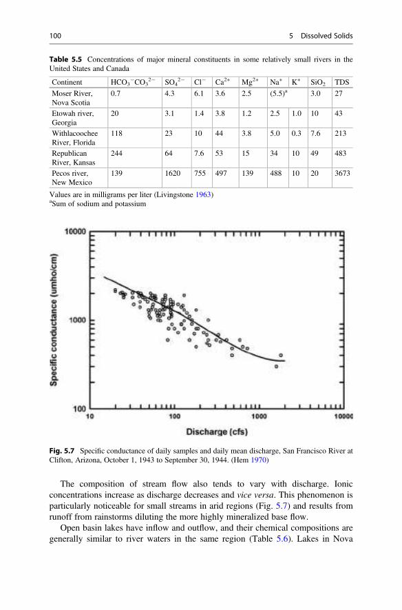
The composition of stream flow also tends to vary with discharge. Ionicconcentrations increase as discharge decreases and vice versa. This phenomenon isparticularly noticeable for small streams in arid regions (Fig. 5.7) and results fromrunoff from rainstorms diluting the more highly mineralized base flow.

Open basin lakes have inflow and outflow, and their chemical compositions aregenerally similar to river waters in the same region (Table 5.6). Lakes in Nova

Table 5.5 Concentrations of major mineral constituents in some relatively small rivers in theUnited States and Canada

Continent HCO3�CO3

2� SO42� Cl� Ca2+ Mg2+ Na+ K+ SiO2 TDS

Moser River,Nova Scotia

0.7 4.3 6.1 3.6 2.5 (5.5)a 3.0 27

Etowah river,Georgia

20 3.1 1.4 3.8 1.2 2.5 1.0 10 43

WithlacoocheeRiver, Florida

118 23 10 44 3.8 5.0 0.3 7.6 213

RepublicanRiver, Kansas

244 64 7.6 53 15 34 10 49 483

Pecos river,New Mexico

139 1620 755 497 139 488 10 20 3673

Values are in milligrams per liter (Livingstone 1963)aSum of sodium and potassium

Fig. 5.7 Specific conductance of daily samples and daily mean discharge, San Francisco River atClifton, Arizona, October 1, 1943 to September 30, 1944. (Hem 1970)


Table

5.6

Con

centratio

nsof

major

mineralconstituentsin

someselected

lakes(Livingstone

1963)

Lake

HCO3� C

O32�

SO42�

Cl�

Ca2

+Mg2

+Na+

K+

TDS

Average

ofnine

lakesin

Nov

aScotia

2.7

5.4

5.2

2.3

0.5

3.2

0.6

20

LakeOgletree,Aub

urn,

Alabamaa

25.6

3.2

1.2

3.1

1.7

2.6

1.4

46

LakeOkeecho

bee,Florida

136

2829

419.1

2.2

1.2

277

LakeBalmorheahak,T

exas

159

555

560

380.1

(642

)b19

70

LittleBorax

Lake,California

8166

1090

58

2433

9073

113

,600

DeadSea

240

540

208,02

015

,800

41,960

34,940

7560

315,04

0

Valuesarein

milligramsperliter

a From

C.E

.Boy

d,un

publisheddata

bSum

ofsodium

andpo

tassium


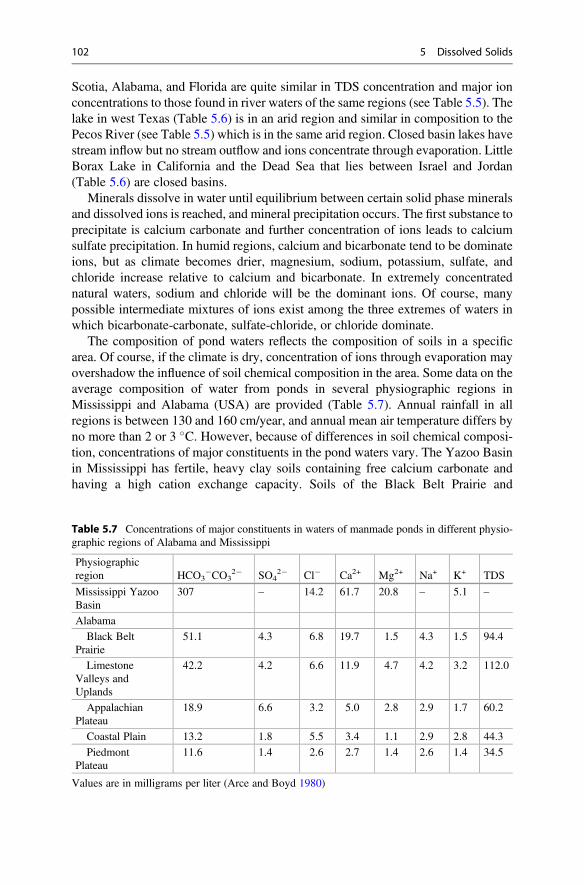
Scotia, Alabama, and Florida are quite similar in TDS concentration and major ionconcentrations to those found in river waters of the same regions (see Table 5.5). Thelake in west Texas (Table 5.6) is in an arid region and similar in composition to thePecos River (see Table 5.5) which is in the same arid region. Closed basin lakes havestream inflow but no stream outflow and ions concentrate through evaporation. LittleBorax Lake in California and the Dead Sea that lies between Israel and Jordan(Table 5.6) are closed basins.

Minerals dissolve in water until equilibrium between certain solid phase mineralsand dissolved ions is reached, and mineral precipitation occurs. The first substance toprecipitate is calcium carbonate and further concentration of ions leads to calciumsulfate precipitation. In humid regions, calcium and bicarbonate tend to be dominateions, but as climate becomes drier, magnesium, sodium, potassium, sulfate, andchloride increase relative to calcium and bicarbonate. In extremely concentratednatural waters, sodium and chloride will be the dominant ions. Of course, manypossible intermediate mixtures of ions exist among the three extremes of waters inwhich bicarbonate-carbonate, sulfate-chloride, or chloride dominate.

The composition of pond waters reflects the composition of soils in a specificarea. Of course, if the climate is dry, concentration of ions through evaporation mayovershadow the influence of soil chemical composition in the area. Some data on theaverage composition of water from ponds in several physiographic regions inMississippi and Alabama (USA) are provided (Table 5.7). Annual rainfall in allregions is between 130 and 160 cm/year, and annual mean air temperature differs byno more than 2 or 3 �C. However, because of differences in soil chemical composi-tion, concentrations of major constituents in the pond waters vary. The Yazoo Basinin Mississippi has fertile, heavy clay soils containing free calcium carbonate andhaving a high cation exchange capacity. Soils of the Black Belt Prairie and

Table 5.7 Concentrations of major constituents in waters of manmade ponds in different physio-graphic regions of Alabama and Mississippi

Physiographicregion HCO3

�CO32� SO4

2� Cl� Ca2+ Mg2+ Na+ K+ TDS

Mississippi YazooBasin

307 – 14.2 61.7 20.8 – 5.1 –

Alabama

Black BeltPrairie

51.1 4.3 6.8 19.7 1.5 4.3 1.5 94.4

LimestoneValleys andUplands

42.2 4.2 6.6 11.9 4.7 4.2 3.2 112.0

AppalachianPlateau

18.9 6.6 3.2 5.0 2.8 2.9 1.7 60.2

Coastal Plain 13.2 1.8 5.5 3.4 1.1 2.9 2.8 44.3

PiedmontPlateau

11.6 1.4 2.6 2.7 1.4 2.6 1.4 34.5

Values are in milligrams per liter (Arce and Boyd 1980)


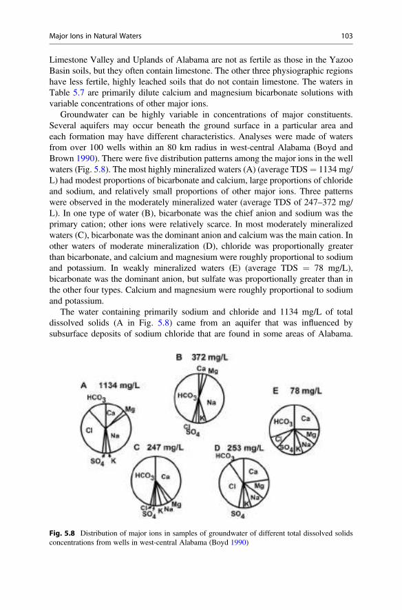
Limestone Valley and Uplands of Alabama are not as fertile as those in the YazooBasin soils, but they often contain limestone. The other three physiographic regionshave less fertile, highly leached soils that do not contain limestone. The waters inTable 5.7 are primarily dilute calcium and magnesium bicarbonate solutions withvariable concentrations of other major ions.

Groundwater can be highly variable in concentrations of major constituents.Several aquifers may occur beneath the ground surface in a particular area andeach formation may have different characteristics. Analyses were made of watersfrom over 100 wells within an 80 km radius in west-central Alabama (Boyd andBrown 1990). There were five distribution patterns among the major ions in the wellwaters (Fig. 5.8). The most highly mineralized waters (A) (average TDS¼ 1134 mg/L) had modest proportions of bicarbonate and calcium, large proportions of chlorideand sodium, and relatively small proportions of other major ions. Three patternswere observed in the moderately mineralized water (average TDS of 247–372 mg/L). In one type of water (B), bicarbonate was the chief anion and sodium was theprimary cation; other ions were relatively scarce. In most moderately mineralizedwaters (C), bicarbonate was the dominant anion and calcium was the main cation. Inother waters of moderate mineralization (D), chloride was proportionally greaterthan bicarbonate, and calcium and magnesium were roughly proportional to sodiumand potassium. In weakly mineralized waters (E) (average TDS ¼ 78 mg/L),bicarbonate was the dominant anion, but sulfate was proportionally greater than inthe other four types. Calcium and magnesium were roughly proportional to sodiumand potassium.

The water containing primarily sodium and chloride and 1134 mg/L of totaldissolved solids (A in Fig. 5.8) came from an aquifer that was influenced bysubsurface deposits of sodium chloride that are found in some areas of Alabama.

Fig. 5.8 Distribution of major ions in samples of groundwater of different total dissolved solidsconcentrations from wells in west-central Alabama (Boyd 1990)


The water containing primarily bicarbonate and sodium (B) was the result of aninteresting phenomenon sometimes found on coastal plains and known as naturalsoftening of groundwater (Hem 1970). Groundwater high in bicarbonate and sodiumconcentrations occurs in areas where surface formations contain limestone andunderlying aquifers have solids which have adsorbed an abundance of sodium.The aquifers contain sodium because they were filled with seawater during an earliergeological time. Seawater was replaced by freshwater as uplifting of the coastal plainoccurred. Rainwater infiltrating downward is charged with carbon dioxide anddissolves limestone to increase concentrations of bicarbonate, calcium, and magne-sium. Upon reaching the aquifers, calcium in the infiltrating water is exchanged forsodium in aquifer solids resulting in a dilute sodium bicarbonate solution.

Coastal and Ocean Water

The ocean is essentially saturated with dissolved inorganic substances and is more orless at equilibrium with respect to these substances. The ocean is quite similar inchemical composition worldwide (Table 5.8). The variation in composition is likelyquite similar to that observed for salinity. For example, the northern Pacific Oceanhas areas where salinity is 31–33 ppt, while some areas in the Atlantic Ocean havesalinities of 36–37 ppt. The Mediterranean and Red Seas have areas with salinityabove 38 ppt (World Ocean Atlas 2018) (https://www.nodc.noaa.gov/OC5/woa18/woa18data.html).

Ocean waters and river waters mix together in estuaries. Because most riverwaters are much more dilute in ions than ocean waters, ionic proportions in estuarinewaters generally reflect those of ocean waters. The salinity of estuarine water at agiven location in an estuary may vary greatly with water depth, time of day, andfreshwater inflow. In coastal reaches of rivers, a density wedge of salt water mayoccur in the bottoms of rivers causing depth stratification of salinity. Tidal actioncauses changes in salinity by causing salt water to flow into and out of estuaries.

Table 5.8 The averagecomposition of major ionsin seawater (Goldberg1963)

Constituent mg/L

Cl� 19,000

Na+ 10,500

SO42� 2700 (900 mg S/L)

Mg2+ 1350

Ca2+ 400

K+ 380

HCO3� 142 (28 mg C/L)

Br� 65

Sr2+ 8

SiO2 3 (as Si)

B(OH)3, B(OH)4� 4.6 (as B)

F� 1.3


https://www.nodc.noaa.gov/OC5/woa18/woa18data.html

https://www.nodc.noaa.gov/OC5/woa18/woa18data.html

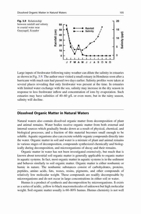
Large inputs of freshwater following rainy weather can dilute the salinity in estuariesas shown in Fig. 5.9. The author once visited a small estuary in Honduras soon after ahurricane with much rain had passed two days earlier. Salinity profiles were taken atseveral places revealing that only freshwater was present at the time. In estuarieswith limited water exchange with the sea, salinity may increase in the dry season inresponse to less freshwater inflow and concentration of ions by evaporation. Suchestuaries may have salinities of 40–60 g/L or even more, but in the rainy season,salinity will decline.

Dissolved Organic Matter in Natural Waters

Natural waters also contain dissolved organic matter from decomposition of plantand animal remains. Water bodies receive organic matter from both external andinternal sources which gradually breaks down as a result of physical, chemical, andbiological processes, and a fraction of this material becomes small enough to besoluble. Aquatic organisms also can excrete soluble organic compounds directly intothe water. Organic matter in soil and water is a mixture of plant and animal remainsin various stages of decomposition, compounds synthesized chemically and biolog-ically during decomposition, and microorganisms of decay and their remains.

Organic matter in water has not been investigated extensively, but much that isknown about terrestrial soil organic matter is generally applicable to organic matterin aquatic systems. In fact, most organic matter in aquatic systems is in the sedimentand behaves similarly to soil organic matter. Organic matter is either nonhumic orhumic in nature. The nonhumic substances consist of carbohydrates, proteins,peptides, amino acids, fats, waxes, resins, pigments, and other compounds ofrelatively low molecular weight. These compounds are readily decomposable bymicroorganisms and do not occur in large concentrations in either soil or water.

Humus is a product of synthesis and decomposition by microorganisms. It existsas a series of acidic, yellow to black macromolecules of unknown but high molecularweight. Soil organic matter usually is 60–80% humus. Humus chemistry is not well

Fig. 5.9 Relationshipbetween rainfall and salinityin coastal water nearGuayaquil, Ecuador

Dissolved Organic Matter in Natural Waters 105

understood, but it consists of a heterogeneous mixture of molecules that formpolymers. Molecular weights of polymers in humus range from several hundred tomore than 300,000 g/mole. One hypothesis holds that in humus formation,polyphenols derived from lignin and other compounds synthesized bymicroorganisms polymerize along or with amino compounds to form polymers ofvariable molecular weights with functional acidic groups. Humus often is consideredto be composed of three classes of compounds: humic acids, fulvic acids, and humin.Fulvic acids have higher oxygen contents, lower carbon contents, lower molecularweights, and higher degrees of acidity than humic acids. Fulvic acids are yellowish,whereas humic acids are dark brown or black. The properties of humin are poorlydefined. Humin differs from fulvic and humic acids by being insoluble in alkali.Humic substances decompose very slowly and they accumulate in soil. Humin is notwater soluble, but humic acids are soluble in water at pH > 1.0 and fulvic acids aresoluble at all pHs (Steelink 2002). Because of their solubility, humic and fulvic acidsare found in natural waters and especially in those that receive inflow from forestedareas or contain large populations of higher aquatic plants. Some of the most highlyhumic water bodies in areas with peat bogs (Druvietis et al. 2010). These authorsreported that such lakes in Latvia had Secchi disk visibilities as low as 0.4 m as aresult of humic substances.

Most relatively clear waters will have less than 10 mg/L dissolved organic matter,but nutrient enriched waters with abundant phytoplankton often have considerablymore dissolved organic matter. Highest concentrations are found in waters stainedwith humic substances such as those of bog lakes and swamps. Dissolved organicmatter causes color (usually the color of coffee or tea) and restricts light penetration.Organic compounds chelate metals and increase the concentrations of trace metalsthat can occur in water. Some polluted waters receive exceptionally high inputs oforganic matter in effluents.

One way of determining dissolved organic matter concentration [often called thetotal dissolved volatile solids (TDVS) concentration] is to ignite the residue from theTDS analysis at 450–500 �C to burn off the organic matter. The weight loss is thedissolved organic matter or TDVS. The determinations of TDS and TDVS often arecombined into the single methodology outlined in Fig. 5.1, Right. The inorganicfraction of the TSS often is called the total dissolved fixed solids (TDFS), because itis not lost during ignition, and TDFS ¼ TDS – TDVS.

Ex. 5.6 The dish and dry residue from the TDS analysis that weighed 5.2100 g (Ex.5.1) are ignited, and after cooling, the dish and residue weigh 5.2080 g. The TDVSconcentration will be estimated.

Solution:

TDVS ¼ 5:2100� 5:2080ð Þ g� 1; 000 mg=g� 1; 000 mL=L

100 mL sample

TDVS ¼ 20 mg/L.


The dissolved organic matter concentration may be estimated using a carbonanalyzer that combusts the organic matter and measures the amount of carbondioxide released. Such an instrument is expensive; a cheaper way is by sulfuricacid-potassium dichromate digestion. In this procedure, a sample of water filtered toremove the suspended particles is treated with concentrated sulfuric acid (H2SO4)and excess, standard potassium dichromate (K2Cr2O7). It is then held at boilingtemperature for 2 hours in a reflux apparatus. Certain other reagents are sometimesadded as catalysts or to act as inhibitors of chloride of other interfering substances(Eaton et al. 2005). The organic matter is oxidized by the Cr2O2�

7 ion

2Cr2O2�7 þ 3 organic C0 þ 16Hþ ¼ 4Cr3þ þ 3CO2 þ 8H2O: ð5:14Þ

The amount of dichromate remaining at the end of the digestion is determined byback-titration with standard ferrous ammonium sulfate (FeNH4SO4). Themilliequivalents ofCr2O2�

7 consumed in the reaction are equal to the milliequivalentsof dissolved organic carbon in the sample as illustrated in Ex. 5.7.

Ex. 5.7 Estimation of dissolved organic carbon concentration by dichromatedigestion.

Situation: A 20-mL water sample that passed a 2-μm filter is treated withconcentrated H2SO4, 10.00 mL of 0.025 N K2Cr2O7, and refluxed at boilingtemperature for 2 hours. The digestate requires 4.15 mL 0.025 N FeNH4SO4

(FAS) for reducing the remaining Cr2O2�7 . The blank titration requires 9.85 mL of

the FAS solution.Solution:The unconsumed K2Cr2O7 is estimated:

Blank 0:025 meq=mLð Þ 9:85 mL FASð Þ ¼ 0:246 meq

Sample 0:025 meq=mLð Þ 4:15 mL FASð Þ ¼ 0:104 meq:

The amounts of K2Cr2O7 consumed are:

Blank 0:025 meq=Lð Þ 10:00 mL K2Cr2O7ð Þ½ � 0:246 meq ¼ 0:004 meq

Sample 0:025 meq=Lð Þ 10:00 mL K2Cr2O7ð Þ½ � 0:104 meq ¼ 0:146 meq:

Organic matter in the sample equaled the amount of K2Cr2O7 consumed or(0.146–0.004) meq ¼ 0.142 meq. The equivalent weight of organic carbon in thereaction depicted in Eq. 5.14 can be determined from the observation that threecarbon atoms with valence of 0 lost four electrons each to obtain a valence of 4+ incarbon dioxide. The equivalent weight of carbon in the reaction is obtained bydividing the atomic weight of carbon (12) by the number of electrons transferred percarbon atom (4).

Thus, the amount of dissolved organic carbon in 20 mL of the water sample was

Dissolved Organic Matter in Natural Waters 107

0:142 meq K2Cr2O7 � 3 mg C=meq ¼ 0:426 mg,C in the 20� mL sample or 21:3 mg C=L:

Dissolved Solids and Colligative Properties

Vapor Pressure

The colligative properties of solutions are physical changes caused by the solute thatdepends on the amount of solute but not on the type of solute. These changes includedecreased vapor pressure, decreased freezing point, increased boiling point, andincreased osmotic pressure with greater solute concentration. The TDS concentra-tion effects the colligative properties of water.

The French chemist, François Raoult, discovered in the late eighteenth centurythat at the same temperature the vapor pressure of a solution is less than the vaporpressure of its pure solvent. This phenomenon, known as Raoult’s law, is expressedas

Psol ¼ XPo ð5:15Þwhere Psol ¼ vapor pressure of the solution, X ¼ mole fraction of pure solvent[moles solvent/(moles of solute + moles of solvent)], and Po ¼ the vapor pressure ofpure solvent.

The phenomenon results because solute molecules occupy space among thesolvent molecules. The solution surface does not consist totally of solvent molecules,and the rate of diffusion of the solvent molecules into the air above the solution willbe less than it would be for the pure solvent exposed to air. As the solute concentra-tion increases, vapor pressure decreases.

Freezing and Boiling Points

Water boils when its vapor pressure equals atmospheric pressure. A solute reducesthe vapor pressure of water, and to effect boiling, the solution must be raised to ahigher temperature than would pure water (see Ex. 5.8).

At the freezing point, the movements of water molecules slow enough to allowhydrogen bonding to arrange the solid crystalline lattice of ice. Of course, watermolecules are continuously exchanged between the solid and liquid phases of water,but at the freezing point, there is no net exchange of molecules between the twophases. Just as solute molecules occupy space at the water surface and lessen the rateat which water molecules enter the air (lower the vapor pressure), solute moleculesoccupy space in liquid water. But, solute molecules do not enter the crystallinestructure of ice. The overall effect is that the presence of solutes in water slows therate at which water molecules enter the solid phase. This results in a decrease in the


temperature at which molecular movement becomes slow enough to allow equilib-rium in exchange of water molecules between solid and liquid phases, i.e., it resultsin freezing point depression (see Ex. 5.8).

The effect of the solute results from the solute particles, and some substancesdissolve into ions rather than molecules. Thus, 1 mole of salt (NaCl) gives 2 moles ofparticles (1 mol of Na+ and 1 mol of Cl�). Sugar (sucrose) dissolves as molecules,and 1 mole of sugar gives 1 mole of particles. The phenomenon is the basis for thevan’t Hoff factor which is used to adjust ionic concentrations to particleconcentrations.

The equations for estimating freezing point depression and boiling point elevationare

ΔT fp ¼ ið Þ Kfp� �

mð Þ ð5:16Þ

ΔTbp ¼ ið Þ Kbp� �

mð Þ ð5:17Þwhere ΔTfp and ΔTbp ¼ the changes in freezing and boiling points (�C), respec-tively; I ¼ van’t Hoff factor; Kfp and Kbp ¼ proportionality constants for freezingand boiling point changes, respectively; and m ¼ molality of the solution (m ¼ gsolute/g solution). Typical values for Kfp and Kbp for water are 1.86 �C/m and0.512 �C/m, respectively.

Ex. 5.8 The vapor pressure, depression of freezing point, and elevation of boilingpoint in a 1-m aqueous salt solution will be estimated for 20 �C and standardpressure.

Solution:The 1 m KCl solution consists of 74.55 g (1 mole) KCl and 1000 g water (55.56

moles). The van’t Hoff factor is 2 (KCl ¼ K+ + Cl�). The mole fraction, X ¼ (55.56moles) � (2 moles + 55.56 moles) ¼ 0.965. Using Eq. 5.15 and Po from Table 1.2,vapor pressure of the solution is:

Psol ¼ 0:965ð Þ 17:535 mmð Þ ¼ 16:92 mm:

The freezing point reduction is calculated with Eq. 5.16

ΔT fp ¼ 2ð Þ 1:86�C=m

� �1 mð Þ ¼ 3:72

�C:

The elevation of the boiling point is obtained with Eq. 5.17

ΔTbp ¼ 2ð Þ 0:512�C=m

� �1 mð Þ ¼ 1:02

�C:

While Ex. 5.8 shows substantial changes in freezing and boiling points of a 1 mKCl solution, this solution is quite concentrated in TDS concentration as comparedto freshwater. Freshwater freezes and boils at about the same temperature as purewater, but the TDS concentration of seawater and some inland saline waters is greatenough to have a significant effect on boiling and freezing points. Seawater typicallyfreezes at �1.9 �C and boils at around 100.6 �C.

Dissolved Solids and Colligative Properties 109

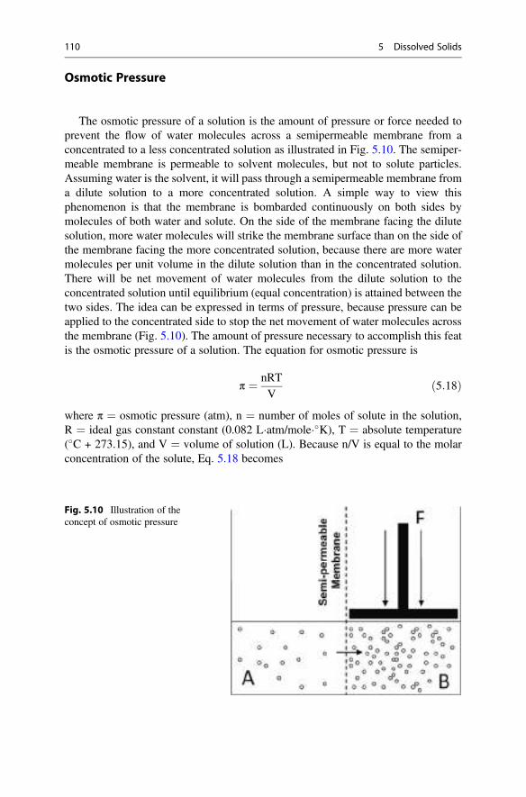
Osmotic Pressure

The osmotic pressure of a solution is the amount of pressure or force needed toprevent the flow of water molecules across a semipermeable membrane from aconcentrated to a less concentrated solution as illustrated in Fig. 5.10. The semiper-meable membrane is permeable to solvent molecules, but not to solute particles.Assuming water is the solvent, it will pass through a semipermeable membrane froma dilute solution to a more concentrated solution. A simple way to view thisphenomenon is that the membrane is bombarded continuously on both sides bymolecules of both water and solute. On the side of the membrane facing the dilutesolution, more water molecules will strike the membrane surface than on the side ofthe membrane facing the more concentrated solution, because there are more watermolecules per unit volume in the dilute solution than in the concentrated solution.There will be net movement of water molecules from the dilute solution to theconcentrated solution until equilibrium (equal concentration) is attained between thetwo sides. The idea can be expressed in terms of pressure, because pressure can beapplied to the concentrated side to stop the net movement of water molecules acrossthe membrane (Fig. 5.10). The amount of pressure necessary to accomplish this featis the osmotic pressure of a solution. The equation for osmotic pressure is

π ¼ nRTV

ð5:18Þ

where π ¼ osmotic pressure (atm), n ¼ number of moles of solute in the solution,R ¼ ideal gas constant constant (0.082 L�atm/mole��K), T ¼ absolute temperature(�C + 273.15), and V ¼ volume of solution (L). Because n/V is equal to the molarconcentration of the solute, Eq. 5.18 becomes

Fig. 5.10 Illustration of theconcept of osmotic pressure


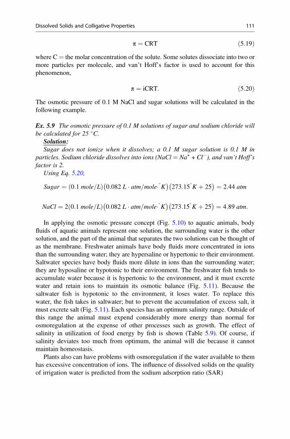
π ¼ CRT ð5:19Þwhere C¼ the molar concentration of the solute. Some solutes dissociate into two ormore particles per molecule, and van’t Hoff’s factor is used to account for thisphenomenon,

π ¼ iCRT: ð5:20ÞThe osmotic pressure of 0.1 M NaCl and sugar solutions will be calculated in thefollowing example.

Ex. 5.9 The osmotic pressure of 0.1 M solutions of sugar and sodium chloride willbe calculated for 25 �C.

Solution:Sugar does not ionize when it dissolves; a 0.1 M sugar solution is 0.1 M in

particles. Sodium chloride dissolves into ions (NaCl ¼ Na+ + Cl�), and van’t Hoff’sfactor is 2.

Using Eq. 5.20,

Sugar ¼ 0:1 mole=Lð Þ 0:082 L � atm=mole��K� �273:15

�K þ 25

� � ¼ 2:44 atm

NaCl ¼ 2 0:1 mole=Lð Þ 0:082 L � atm=mole��K� �273:15

�K þ 25

� � ¼ 4:89 atm:

In applying the osmotic pressure concept (Fig. 5.10) to aquatic animals, bodyfluids of aquatic animals represent one solution, the surrounding water is the othersolution, and the part of the animal that separates the two solutions can be thought ofas the membrane. Freshwater animals have body fluids more concentrated in ionsthan the surrounding water; they are hypersaline or hypertonic to their environment.Saltwater species have body fluids more dilute in ions than the surrounding water;they are hyposaline or hypotonic to their environment. The freshwater fish tends toaccumulate water because it is hypertonic to the environment, and it must excretewater and retain ions to maintain its osmotic balance (Fig. 5.11). Because thesaltwater fish is hypotonic to the environment, it loses water. To replace thiswater, the fish takes in saltwater; but to prevent the accumulation of excess salt, itmust excrete salt (Fig. 5.11). Each species has an optimum salinity range. Outside ofthis range the animal must expend considerably more energy than normal forosmoregulation at the expense of other processes such as growth. The effect ofsalinity in utilization of food energy by fish is shown (Table 5.9). Of course, ifsalinity deviates too much from optimum, the animal will die because it cannotmaintain homeostasis.

Plants also can have problems with osmoregulation if the water available to themhas excessive concentration of ions. The influence of dissolved solids on the qualityof irrigation water is predicted from the sodium adsorption ratio (SAR)

Dissolved Solids and Colligative Properties 111

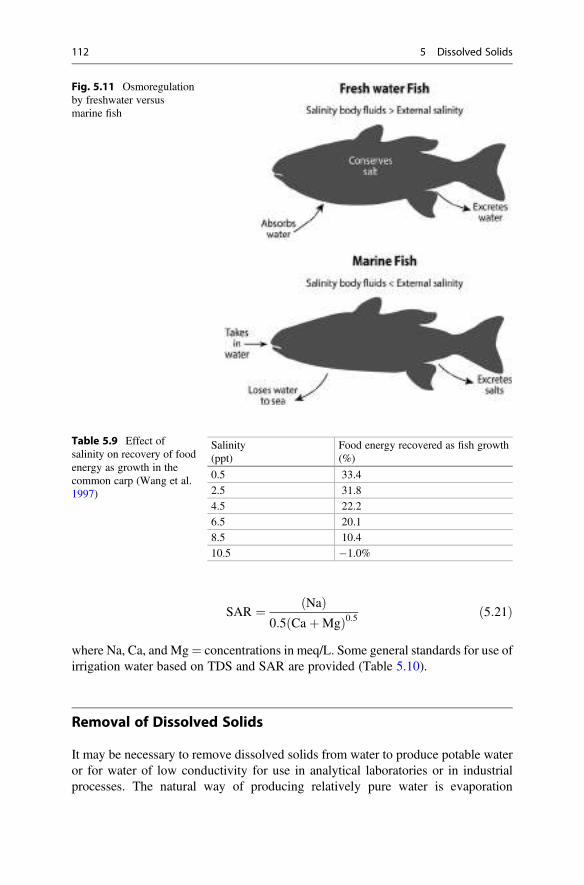
SAR ¼ Nað Þ0:5 CaþMgð Þ0:5 ð5:21Þ

where Na, Ca, and Mg¼ concentrations in meq/L. Some general standards for use ofirrigation water based on TDS and SAR are provided (Table 5.10).

Removal of Dissolved Solids

It may be necessary to remove dissolved solids from water to produce potable wateror for water of low conductivity for use in analytical laboratories or in industrialprocesses. The natural way of producing relatively pure water is evaporation

Fig. 5.11 Osmoregulationby freshwater versusmarine fish

Table 5.9 Effect ofsalinity on recovery of foodenergy as growth in thecommon carp (Wang et al.1997)

Salinity(ppt)

Food energy recovered as fish growth(%)

0.5 33.4

2.5 31.8

4.5 22.2

6.5 20.1

8.5 10.4

10.5 �1.0%


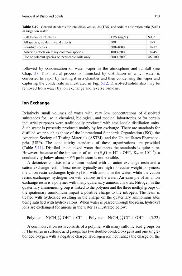
followed by condensation of water vapor in the atmosphere and rainfall (seeChap. 3). This natural process is mimicked by distillation in which water isconverted to vapor by heating it in a chamber and then condensing the vapor andcapturing the condensate as illustrated in Fig. 5.12. Dissolved solids also may beremoved from water by ion exchange and reverse osmosis.

Ion Exchange

Relatively small volumes of water with very low concentrations of dissolvedsubstances for use in chemical, biological, and medical laboratories or for certainindustrial purposes were traditionally produced with small-scale distillation units.Such water is presently produced mainly by ion exchange. There are standards fordistilled water such as those of the International Standards Organization (ISO), theAmerican Society of Testing Materials (ASTM), and the United States Pharmaco-peia (USP). The conductivity standards of these organizations are provided(Table 5.11). Distilled or deionized water that meets the standards is quite pure.However, because of the ionization of water (H2O ¼ H+ + OH�, Kw ¼ 10�14), aconductivity below about 0.055 μmhos/cm is not possible.

A deionizer consists of a column packed with an anion exchange resin and acation exchange resin. These resins typically are high molecular weight polymers;the anion resin exchanges hydroxyl ion with anions in the water, while the cationresins exchanges hydrogen ion with cations in the water. An example of an anionexchange resin is a polymer with many quaternary ammonium sites. Nitrogen in thequaternary ammonium group is linked to the polymer and the three methyl groups ofthe quaternary ammonium impart a positive charge to the nitrogen. The resin istreated with hydroxide resulting in the charge on the quaternary ammonium sitesbeing satisfied with hydroxyl ions. When water is passed through the resin, hydroxylions are exchanged for anions in the water as illustrated below:

Polymer � N CH3ð Þþ3 OH� þ Cl� ! Polymer � N CH3ð Þþ3 Cl� þ OH�: ð5:22ÞA common cation resin consists of a polymer with many sulfonic acid groups on

it. The sulfur in sulfonic acid groups has two double-bonded oxygens and one single-bonded oxygen with a negative charge. Hydrogen ion neutralizes the charge on the

Table 5.10 General standards for total dissolved solids (TDS) and sodium adsorption ratio (SAR)in irrigation water

Salt tolerance of plants TDS (mg/L) SAR

All species, no detrimental effects 500 2–7

Sensitive species 500–1000 8–17

Adverse effects on many common species 1000–2000 18–45

Use on tolerant species on permeable soils only 2000–5000 46–100

Removal of Dissolved Solids 113

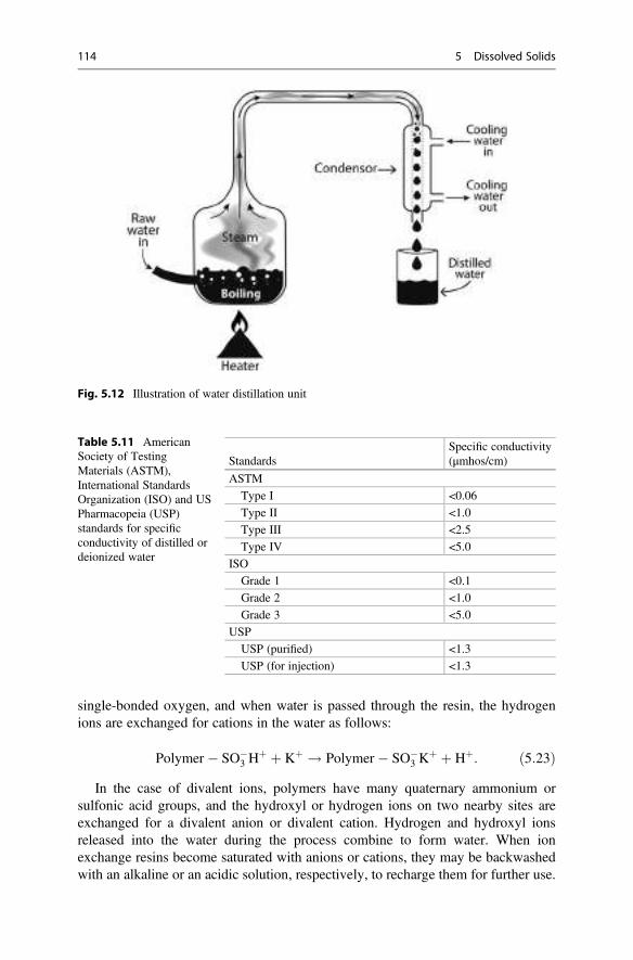
single-bonded oxygen, and when water is passed through the resin, the hydrogenions are exchanged for cations in the water as follows:

Polymer � SO�3 H

þ þ Kþ ! Polymer � SO�3 K

þ þ Hþ: ð5:23ÞIn the case of divalent ions, polymers have many quaternary ammonium or

sulfonic acid groups, and the hydroxyl or hydrogen ions on two nearby sites areexchanged for a divalent anion or divalent cation. Hydrogen and hydroxyl ionsreleased into the water during the process combine to form water. When ionexchange resins become saturated with anions or cations, they may be backwashedwith an alkaline or an acidic solution, respectively, to recharge them for further use.

Table 5.11 AmericanSociety of TestingMaterials (ASTM),International StandardsOrganization (ISO) and USPharmacopeia (USP)standards for specificconductivity of distilled ordeionized water

StandardsSpecific conductivity(μmhos/cm)

ASTM

Type I <0.06

Type II <1.0

Type III <2.5

Type IV <5.0

ISO

Grade 1 <0.1

Grade 2 <1.0

Grade 3 <5.0

USP

USP (purified) <1.3

USP (for injection) <1.3

Fig. 5.12 Illustration of water distillation unit


Dissolved organic matter that is charged—usually it will bear a negative charge—can be removed by ion exchange. Activated carbon filtration can be used to removedissolved organic carbon that is not charged. Activated carbon is highly porouscharcoal with a huge surface area—up to 2000 m2/g. Water can be passed through acolumn of activated carbon and the charcoal will adsorb many dissolved organicsubstances from water.

Desalination

In many respects, the entire human race suffers from the problem of the AncientMariner who shot the albatross resulting in a curse on him and his sailing ship:“water, water everywhere, nor any drop to drink” (The Rime of the Ancient Marinerby Samuel Taylor Coleridge). The ocean holds an immense quantity of water, but itis not suitable for most human purposes because of its high salinity. Desalination ofocean water is promoted as a means of increasing the supply of freshwater for humanuse. There are several processes for desalination, but most desalination plants rely oneither distillation or reverse osmosis. Multistage flash distillation allows heat recov-ered from condensing steam in the first stage vaporization of water to be used tovaporize water in the second stage, and the process is repeated for several stagesmaking the overall process more energy efficient. In reverse osmosis, pressure isused to force water through membranes that exclude the dissolved solids.

According to the International Desalination Association (idadesal.org), as of June2015, there were 18,246 desalination plants in over 150 countries that producedabout 86.8 million m3/day (32 km3/year) and supplied water for about 300 millionpeople.

Desalination occurs naturally when water freezes in the ocean, because dissolvedions are not included in the structure of ice and displaced into the liquid phase.Icebergs and glaciers represent relatively pure water, and it has been proposed thatthese masses of frozen freshwater could be towed to coastal cities as a freshwatersource. This idea has yet to be brought to fruition.

Bottled Water

Bottled water production has become a huge global industry. Municipal watersystems produce water similar in microbiological and chemical quality to bottledwater, but the public has taken a liking to bottled water. An estimated 400 billionliters (0.4 km3) worth $US 240 billion were consumed globally in 2017 (https://www.statista.com/statistics/387255/global-bottle-water-consumption/).

Water for bottling can be taken from springs, wells, or municipal water supplies,but most is purified by distillation, deionization, or reverse osmosis. Fluorine may beadded to bottled water, and most brands have been subjected to microbial puritytests. The chemical composition of bottled water varies among types and brands, and

Bottled Water 115

http://idadesal.org

https://www.statista.com/statistics/387255/global-bottle-water-consumption/

https://www.statista.com/statistics/387255/global-bottle-water-consumption/

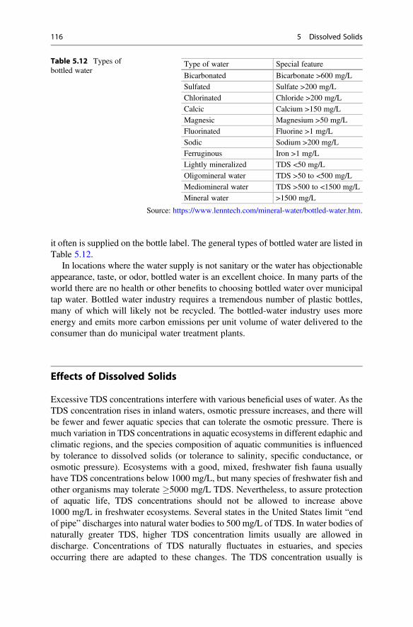
it often is supplied on the bottle label. The general types of bottled water are listed inTable 5.12.

In locations where the water supply is not sanitary or the water has objectionableappearance, taste, or odor, bottled water is an excellent choice. In many parts of theworld there are no health or other benefits to choosing bottled water over municipaltap water. Bottled water industry requires a tremendous number of plastic bottles,many of which will likely not be recycled. The bottled-water industry uses moreenergy and emits more carbon emissions per unit volume of water delivered to theconsumer than do municipal water treatment plants.

Effects of Dissolved Solids

Excessive TDS concentrations interfere with various beneficial uses of water. As theTDS concentration rises in inland waters, osmotic pressure increases, and there willbe fewer and fewer aquatic species that can tolerate the osmotic pressure. There ismuch variation in TDS concentrations in aquatic ecosystems in different edaphic andclimatic regions, and the species composition of aquatic communities is influencedby tolerance to dissolved solids (or tolerance to salinity, specific conductance, orosmotic pressure). Ecosystems with a good, mixed, freshwater fish fauna usuallyhave TDS concentrations below 1000 mg/L, but many species of freshwater fish andother organisms may tolerate �5000 mg/L TDS. Nevertheless, to assure protectionof aquatic life, TDS concentrations should not be allowed to increase above1000 mg/L in freshwater ecosystems. Several states in the United States limit “endof pipe” discharges into natural water bodies to 500 mg/L of TDS. In water bodies ofnaturally greater TDS, higher TDS concentration limits usually are allowed indischarge. Concentrations of TDS naturally fluctuates in estuaries, and speciesoccurring there are adapted to these changes. The TDS concentration usually is

Table 5.12 Types ofbottled water

Type of water Special feature

Bicarbonated Bicarbonate >600 mg/L

Sulfated Sulfate >200 mg/L

Chlorinated Chloride >200 mg/L

Calcic Calcium >150 mg/L

Magnesic Magnesium >50 mg/L

Fluorinated Fluorine >1 mg/L

Sodic Sodium >200 mg/L

Ferruginous Iron >1 mg/L

Lightly mineralized TDS <50 mg/L

Oligomineral water TDS >50 to <500 mg/L

Mediomineral water TDS >500 to <1500 mg/L

Mineral water >1500 mg/L

Source: https://www.lenntech.com/mineral-water/bottled-water.htm.


https://www.lenntech.com/mineral-water/bottled-water.htm

not an issue in effluents discharged directly into the ocean—an exception is reverseosmosis seawater desalination plants that discharge water much more concentratedthan ocean water in salts.

The main physiological influence to humans of high TDS concentration is alaxative effect caused by sodium and magnesium sulfates. Sodium also has adverseeffects on individuals with high blood pressure and cardiac disease and pregnantwomen with toxemia. Normally, an upper limit for chlorides and sulfates of 250 mg/L each is suggested. Excessive solids also impart a bad taste to water, and this taste iscaused primarily by chloride. Problems with encrustations and corrosion of plumb-ing fixtures also occur when waters have excessive TDS concentration. If possible,public water supplies should not have TDS concentration above 500 mg/L, but somemay have up to 1000 mg/L or more. Livestock water can contain up to 3000 mg/Ltotal dissolved solids without normally causing adverse effects on animals.

Conclusions

The total dissolved solids concentration is one of the most important variables forassessing the suitability of inland water for domestic, agricultural and industrialwater sources. Specific conductance is probably the most versatile method forassessing concentrations of dissolved solids in freshwater and salinity is the mostwidely used indicator of dissolved solids in estuarine and ocean water. Dissolvedsolids concentration may negatively affect organisms, because if the concentration isoutside the acceptable range, osmoregulatory problems occur. Desalination hasbecome a significant source of freshwater in many arid countries located along thecoast. Bottled drinking water has become a huge industry in many countries includ-ing those with a safe supply of municipal water.

References

Arce RG, Boyd CE (1980) Water chemistry of Alabama ponds. Bulletin 522, Alabama AgriculturalExperiment Station, Auburn University

Austin RW, Halikas G (1976) The index of refraction of seawater. US Department of CommerceTechnical Information Series AD-A024800, Washington

Baxter GP, Burgess LL, Daudt HW (1911) The refractive index of water. J Am Chem Soc33:893–901

Boyd CE (1990) Water quality in ponds for aquaculture. Alabama Agricultural Experiment Station,Auburn University

Boyd CE, Brown SW (1990) Quality of water from wells in the major catfish farming area ofAlabama. In: Tave D (ed) Proceedings 50th Anniversary Symposium Department of Fisheriesand Allied Aquacultures, Auburn University

References 117

Carroll D (1962) Rainwater as a chemical agent of geologic processes—a review. Water-supplypaper 1535-G, United States Geological Survey, United States Government Printing Office,Washington.

Druvietis I, Springe G, Briende A, Kokorite I, Parele E (2010) A comparative assessment of the bogaquatic environment of the Ramsar site of Teici Nature Reserve and North Vidzeme BiosphereReserve, Latvia. In: Klavins M (ed) Mires and Peats. University of Latvia Press, Salaspils,Latvia

Eaton AD, Clesceri LS, Rice EW, Greenburg AE (eds) (2005) Standard methods for the examina-tion of water and wastewater, 21st edn. American Public Health Association, Washington

Goldberg ED (1963) Chemistry—the oceans as a chemical system. In: Hill MN (ed) Composition ofsea water, comparative and descriptive oceanography, Vol. II. The sea. Interscience Publishers,New York, pp 3–25

Hem JD (1970) Study and interpretation of the chemical characteristics of natural water. Water-supply paper 1473, United States Geological Survey, United States. Government PrintingOffice, Washington

Hutchinson GE (1957) A treatise on limnology, vol 1, geography, physics, and chemistry. Wiley,New York

Knudsen M (1901) Hydrographical tables. G. E. C. Gad, CopenhagenLaxen DPH (1977) A specific conductance method for quality control in water analysis. Water Res

11:91–94Lewis EL (1980) The practical salinity scale 1978 and its antecedents. J Ocean Eng 5:3–8Lewis EL, Perkin RG (1981) The practical salinity scale 1978: conversion of existing data. Deep-

Sea Res 28:307–328Li L, Dong S, Tian X, Boyd CE (2012) Equilibrium concentrations of major cations and total

alkalinity in laboratory soil-water systems. J App Aqua 25:50–65Livingstone DA (1963) Chemical composition of rivers and lakes. Professional Paper 440-G,

United States Geological Survey, United States Government Printing Office, WashingtonLyman J (1969) Redefinition of salinity and chlorinity. Lim and Ocean 14:28–29Millero FJ, Rainer F, Wright DG, McDougall TJ (2008) The composition of standard seawater and

the definition of the reference-composition salinity scale. Deep-Sea Res 55:50–72Sawyer CN, McCarty PL (1967) Chemistry for sanitary engineers. McGraw-Hill, New YorkSteelink C (2002) Investigating humic acids in soil. Anal Chem 74:326–333UNESCO (1981a) The practical salinity scale 1978 and the international equation of state of

seawater 1980. UNESCO Technical Papers in Mar Sci 36, ParisUNESCO (1981b) Background papers and supporting data on the practical salinity scale 1978.

UNESCO Technical Papers in Mar Sci 37, ParisUNESCO (1985) The international system of units (SI) in oceanography. UNESCO Technical

Papers in Mar Sci 45, Parisvan Niekerk H, Silberbauer MJ, Maluleke M (2014) Geographical differences in the relationship

between total dissolved solids and electrical conductivity in South African rivers. WaterSouth Africa 40:133–137

Walton NRG (1989) Electrical conductivity and total dissolved solids—what is their preciserelationship? Desal 72:275–292

Wang J-O, Liu H, Po H, Fan L (1997) Influence of salinity on food consumption, growth, andenergy conversion efficiency of common carp (Cyprinus Carpio) fingerling. Aqua 148:115–124

Wright DG, Pawlowicz R, McDougall TJ, Feistel R, Marion GM (2011) Absolute salinity, “densitysalinity,” and the reference-composition salinity scale: present and future use in the seawaterstandard TEOS-10. Ocean Sci 7:1–26


Suspended Solids, Color, Turbidity,and Light 6

AbstractNatural waters contain suspended particulates that increase turbidity, impartapparent color, and interfere with light penetration. These particles originatefrom erosion, vegetative debris from watersheds, and microorganisms producedin water bodies. Suspended particles vary from colloids that remain suspendedindefinitely to larger silt and sand particles held in suspension by turbulence.Settling velocities of particles in still water are estimated by the Stoke’s lawequation and depend mainly on particle diameter and density—large, denseparticles settle the fastest. Organic particles settle slowly because of their lowdensity, but planktonic organisms also have adaptions that lessen settling veloc-ity. Solar radiation of all wavelengths is quenched quickly—about 50% isreflected or converted to heat within the first meter. Within the visible spectrum,clear water absorbs red and orange light most strongly followed by violet, and byyellow, green, and blue, but suspended particles in water tend to absorb allwavelengths. Sedimentation of suspended solids can result in gradual “fillingin” of water bodies and destruction of benthic organisms. Turbidity and color inwater bodies lower photosynthesis rates and reduce productivity. Clear water ismore pleasing to the eye, preferred for recreational water uses, and greatlyfavored for drinking purposes. Erosion control, sedimentation, chemical coagu-lation, and filtration techniques are used in color and turbidity control.

Introduction

Natural waters contain particles not in true solution but held in temporary orpermanent suspension against the force of gravity. These particles are calledsuspended solids, but many speak of them as particulate matter. Strictly speakingthe latter term should not be used, because all particles, dissolved or suspended, arematter. Larger suspended particles continuously settle in relation to their density andsize, but turbulence may prevent or slow their settling rate. Suspended particles


119


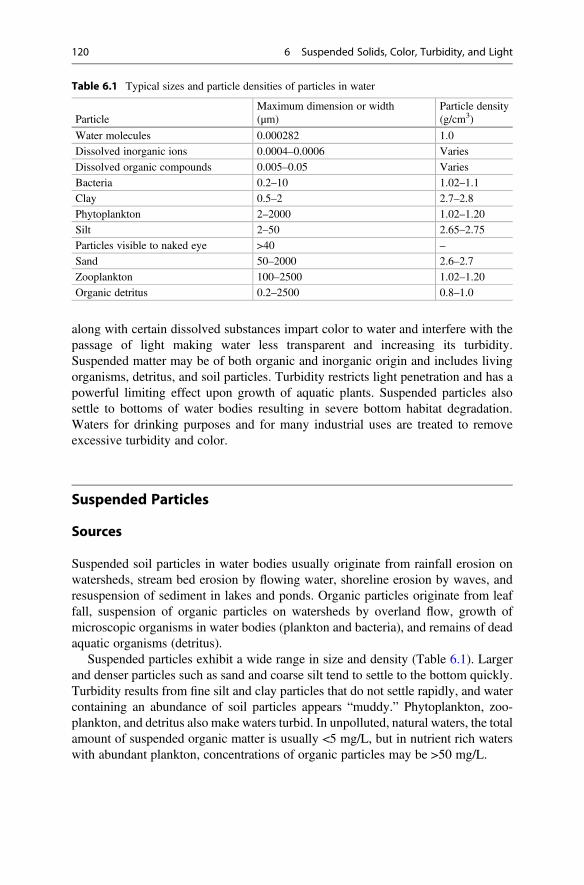
along with certain dissolved substances impart color to water and interfere with thepassage of light making water less transparent and increasing its turbidity.Suspended matter may be of both organic and inorganic origin and includes livingorganisms, detritus, and soil particles. Turbidity restricts light penetration and has apowerful limiting effect upon growth of aquatic plants. Suspended particles alsosettle to bottoms of water bodies resulting in severe bottom habitat degradation.Waters for drinking purposes and for many industrial uses are treated to removeexcessive turbidity and color.

Suspended Particles

Sources

Suspended soil particles in water bodies usually originate from rainfall erosion onwatersheds, stream bed erosion by flowing water, shoreline erosion by waves, andresuspension of sediment in lakes and ponds. Organic particles originate from leaffall, suspension of organic particles on watersheds by overland flow, growth ofmicroscopic organisms in water bodies (plankton and bacteria), and remains of deadaquatic organisms (detritus).

Suspended particles exhibit a wide range in size and density (Table 6.1). Largerand denser particles such as sand and coarse silt tend to settle to the bottom quickly.Turbidity results from fine silt and clay particles that do not settle rapidly, and watercontaining an abundance of soil particles appears “muddy.” Phytoplankton, zoo-plankton, and detritus also make waters turbid. In unpolluted, natural waters, the totalamount of suspended organic matter is usually <5 mg/L, but in nutrient rich waterswith abundant plankton, concentrations of organic particles may be >50 mg/L.

Table 6.1 Typical sizes and particle densities of particles in water

ParticleMaximum dimension or width(μm)

Particle density(g/cm3)

Water molecules 0.000282 1.0

Dissolved inorganic ions 0.0004–0.0006 Varies

Dissolved organic compounds 0.005–0.05 Varies

Bacteria 0.2–10 1.02–1.1

Clay 0.5–2 2.7–2.8

Phytoplankton 2–2000 1.02–1.20

Silt 2–50 2.65–2.75

Particles visible to naked eye >40 –

Sand 50–2000 2.6–2.7

Zooplankton 100–2500 1.02–1.20

Organic detritus 0.2–2500 0.8–1.0

120 6 Suspended Solids, Color, Turbidity, and Light

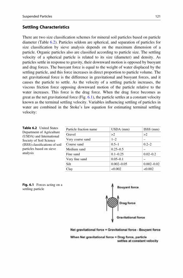
Settling Characteristics

There are two size classification schemes for mineral soil particles based on particlediameter (Table 6.2). Particles seldom are spherical, and separation of particles forsize classification by sieve analysis depends on the maximum dimension of aparticle. Organic particles also are classified according to particle size. The settlingvelocity of a spherical particle is related to its size (diameter) and density. Asparticles settle in response to gravity, their downward motion is opposed by buoyantand drag forces. The buoyant force is equal to the weight of water displaced by thesettling particle, and this force increases in direct proportion to particle volume. Thenet gravitational force is the difference in gravitational and buoyant forces, and itcauses the particle to settle. As the velocity of a settling particle increases, theviscous friction force opposing downward motion of the particle relative to thewater increases. This force is the drag force. When the drag force becomes asgreat as the net gravitational force (Fig. 6.1), the particle settles at a constant velocityknown as the terminal settling velocity. Variables influencing settling of particles inwater are combined in the Stoke’s law equation for estimating terminal settlingvelocity:

Table 6.2 United StatesDepartment of Agriculture(USDA) and InternationalSociety of Soil Science(ISSS) classifications of soilparticles based on sieveanalysis

Particle fraction name USDA (mm) ISSS (mm)

Gravel >2 >2

Very coarse sand 1–2 –

Course sand 0.5–1 0.2–2

Medium sand 0.25–0.5 –

Fine sand 0.1–0.25 0.02–0.2

Very fine sand 0.05–0.1 –

Silt 0.002–0.05 0.002–0.02

Clay <0.002 <0.002

Fig. 6.1 Forces acting on asettling particle

Suspended Particles 121

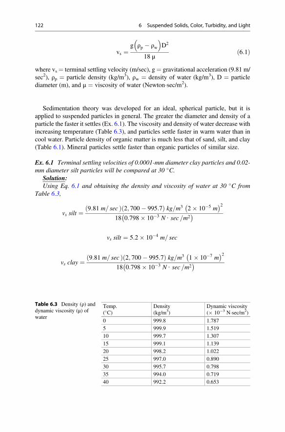
vs ¼g ρp � ρw� �

D2

18 μð6:1Þ

where vs¼ terminal settling velocity (m/sec), g¼ gravitational acceleration (9.81 m/sec2), ρp ¼ particle density (kg/m3), ρw ¼ density of water (kg/m3), D ¼ particlediameter (m), and μ ¼ viscosity of water (Newton�sec/m2).

Sedimentation theory was developed for an ideal, spherical particle, but it isapplied to suspended particles in general. The greater the diameter and density of aparticle the faster it settles (Ex. 6.1). The viscosity and density of water decrease withincreasing temperature (Table 6.3), and particles settle faster in warm water than incool water. Particle density of organic matter is much less that of sand, silt, and clay(Table 6.1). Mineral particles settle faster than organic particles of similar size.

Ex. 6.1 Terminal settling velocities of 0.0001-mm diameter clay particles and 0.02-mm diameter silt particles will be compared at 30 �C.

Solution:Using Eq. 6.1 and obtaining the density and viscosity of water at 30 �C from

Table 6.3,

vs silt ¼9:81 m= secð Þ 2; 700� 995:7ð Þ kg=m3 2� 10�5 m

� �218 0:798� 10�3 N ∙ sec =m2

� �

vs silt ¼ 5:2� 10�4 m= sec

vs clay ¼9:81 m= secð Þ 2; 700� 995:7ð Þ kg=m3 1� 10�7 m

� �218 0:798� 10�3 N ∙ sec =m2

� �

Table 6.3 Density (ρ) anddynamic viscosity (μ) ofwater

Temp.(�C)

Density(kg/m3)

Dynamic viscosity(� 10�3 N�sec/m2)

0 999.8 1.787

5 999.9 1.519

10 999.7 1.307

15 999.1 1.139

20 998.2 1.022

25 997.0 0.890

30 995.7 0.798

35 994.0 0.719

40 992.2 0.653


vs clay ¼ 1:16� 10�8 m= sec :

Silt particles, because of their greater diameter, sink much faster than clayparticles.

Bacterial cells seldom sink, because most have densities less than water. Phyto-plankton cells are quite small, but many of them still tend to sink. Many species haveadaptations to reduce or prevent settling such as gas vacuoles to increase buoyancyor projections to increase drag force. Some species have flagella, cilia, or othermethods of motility to avoid sinking. These adaptations are known as form resis-tance, a concept expressed as the rate at which a particle sinks as compared to the ratethat a sphere of equal density would sink (Padisák et al. 2003). For planktonic algae,form resistance factors range from 0.476 to 2.008. The larger the value of formresistance, the slower plankton settle. Stokes law equation usually is not applicableto the settling rate of microorganisms. In natural waters, turbulence also plays acritical role in particle settling. Turbulent conditions may keep a particle in suspen-sion much longer than would be expected from calculations made with the generalform of the Stokes law equation.

Colloids

Colloidal particles range in size from 0.001 to 1 μm. Although larger than mostmolecules, colloidal particles are so small that they remain in water even though theyare not in true solution. Colloidal particles have several properties that are differentfrom those of dissolved molecules and suspended particles. A narrow beam of lightpasses through a true solution, and its path cannot be observed. In a colloidalsuspension, the path of the light is visible because colloids are large enough toscatter light. This effect of light scattering by colloids is known as the Tyndall effectin honor of the British physicist, John Tyndall, who first described it. In a colloidalsuspension viewed under a dark field microscope, colloidal particles appear as brightpoints that move irregularly against a dark background. Random movement ofcolloidal particles results from their bombardment by molecules of water. Randommotion of colloidal particles is called Brownian movement. Colloidal particlescannot be removed from water by filtration unless special filters with very smallapertures are used. Colloidal particles have a tremendous surface area relative tovolume, and this imparts to them a large surface adsorptive capacity. Most colloidscarry either net positive or net negative charges, but all colloids of the same typehave the same charge and repel each other. Colloidal clay particles (<200 μm) foundin natural waters are negatively charged. Neutralization of the charge on colloidsallows dispersed particles to come together, and they aggregate and precipitate fromsolution. At municipal water supply plants, suspended, negatively-charged clayparticles often are precipitated from water by adding aluminum ion to neutralizethe charge on their surfaces.

Suspended Particles 123

Color

Large bodies of water often appear blue because their surfaces reflect the color of thesky. The true color of natural water results from the unabsorbed light rays remainingfrom sunlight after it has passed into the water. Because water absorbs light morestrongly at the red end of the visible spectrum than at the blue end, blue and blue-green light is scattered back and visible. This gives clear waters a blue hue, butdissolved and suspended particles also absorb light and influence color. True color inwater includes color resulting from the water itself and substances dissolved in it.

Phytoplankton blooms color water various shades of green, blue-green, yellow,brown, red, and even black. Suspended mineral particles also can differ greatly incolor (various shades of black, red, yellow, gray, and white). Tannins and ligninsusually impart a yellow-brown, tea-like appearance to water, but when theirconcentrations are high the water may appear black. Well water may contain tracesof suspended iron and manganese oxides that are yellowish or black in color,respectively. Color disappears from waters following the removal of suspendedparticles is called apparent color, while the true color remains.

Turbidity, Light, and Photosynthesis

The upper, illuminated layer of a water body in which plants grow is called thephotic zone—the bottom of this layer is usually considered to receive 1% of incidentlight. The photic zone in the open ocean is about 200 m thick. Freshwater lakes rangein nutrient status from oligotrophic (nutrient poor with scant plant growth) toeutrophic (nutrient rich with much plant growth). The thickness of the photic zonebased on lake trophic status is: ultraoligotrophic, 50–100 m; oligotrophic, 5–50 m;mesotrophic, 2–5 m; eutrophic, <2 m (Wetzel 2001). Lakes with turbidity fromsuspended soil particles or tannins and lignins may be of low productivity yet have aphotic zone as shallow as that of a eutrophic water body. The photic zone in smallwater bodies such as fish ponds may extend to the bottom if waters do not have aplankton bloom.

Light penetration in water was discussed in Chap. 2 in relation to energy, heat,and temperature, but the degree of brightness of visible light also is of importance.The original unit for visible light was candlepower, and 1 candlepower was equal tothe light produced by a particular type and size of candle (standard candle). The basicunit used today is the candela (cd) defined in SI units is a luminous intensity equal to1/60 of the luminous intensity per square centimeter of a blackbody radiating at2046�K. In addition, 1 cd also is equivalent to 1/683 W/steradian (sr). A steradian isthe solid geometry equivalent of the radian. One radian isolates a segment of thecircumference of a circle equal to its radius, while a steradian isolates an area on thesurface of sphere equal to πr2. A circle has 2π radians so the area associated with1 radian is 1/2π or�16% of the area of a circle. The surface area of a sphere is 4πr2, asphere is 4π steradian, and 1 radian is 1/4π or �8% of the surface area of a sphere.


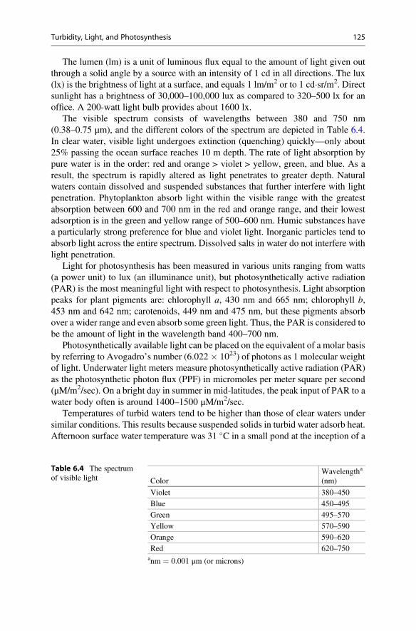
The lumen (lm) is a unit of luminous flux equal to the amount of light given outthrough a solid angle by a source with an intensity of 1 cd in all directions. The lux(lx) is the brightness of light at a surface, and equals 1 lm/m2 or to 1 cd�sr/m2. Directsunlight has a brightness of 30,000–100,000 lux as compared to 320–500 lx for anoffice. A 200-watt light bulb provides about 1600 lx.

The visible spectrum consists of wavelengths between 380 and 750 nm(0.38–0.75 μm), and the different colors of the spectrum are depicted in Table 6.4.In clear water, visible light undergoes extinction (quenching) quickly—only about25% passing the ocean surface reaches 10 m depth. The rate of light absorption bypure water is in the order: red and orange > violet > yellow, green, and blue. As aresult, the spectrum is rapidly altered as light penetrates to greater depth. Naturalwaters contain dissolved and suspended substances that further interfere with lightpenetration. Phytoplankton absorb light within the visible range with the greatestabsorption between 600 and 700 nm in the red and orange range, and their lowestadsorption is in the green and yellow range of 500–600 nm. Humic substances havea particularly strong preference for blue and violet light. Inorganic particles tend toabsorb light across the entire spectrum. Dissolved salts in water do not interfere withlight penetration.

Light for photosynthesis has been measured in various units ranging from watts(a power unit) to lux (an illuminance unit), but photosynthetically active radiation(PAR) is the most meaningful light with respect to photosynthesis. Light absorptionpeaks for plant pigments are: chlorophyll a, 430 nm and 665 nm; chlorophyll b,453 nm and 642 nm; carotenoids, 449 nm and 475 nm, but these pigments absorbover a wider range and even absorb some green light. Thus, the PAR is considered tobe the amount of light in the wavelength band 400–700 nm.

Photosynthetically available light can be placed on the equivalent of a molar basisby referring to Avogadro’s number (6.022 � 1023) of photons as 1 molecular weightof light. Underwater light meters measure photosynthetically active radiation (PAR)as the photosynthetic photon flux (PPF) in micromoles per meter square per second(μM/m2/sec). On a bright day in summer in mid-latitudes, the peak input of PAR to awater body often is around 1400–1500 μM/m2/sec.

Temperatures of turbid waters tend to be higher than those of clear waters undersimilar conditions. This results because suspended solids in turbid water adsorb heat.Afternoon surface water temperature was 31 �C in a small pond at the inception of a

Table 6.4 The spectrumof visible light Color

Wavelengtha

(nm)

Violet 380–450

Blue 450–495

Green 495–570

Yellow 570–590

Orange 590–620

Red 620–750anm ¼ 0.001 μm (or microns)

Turbidity, Light, and Photosynthesis 125

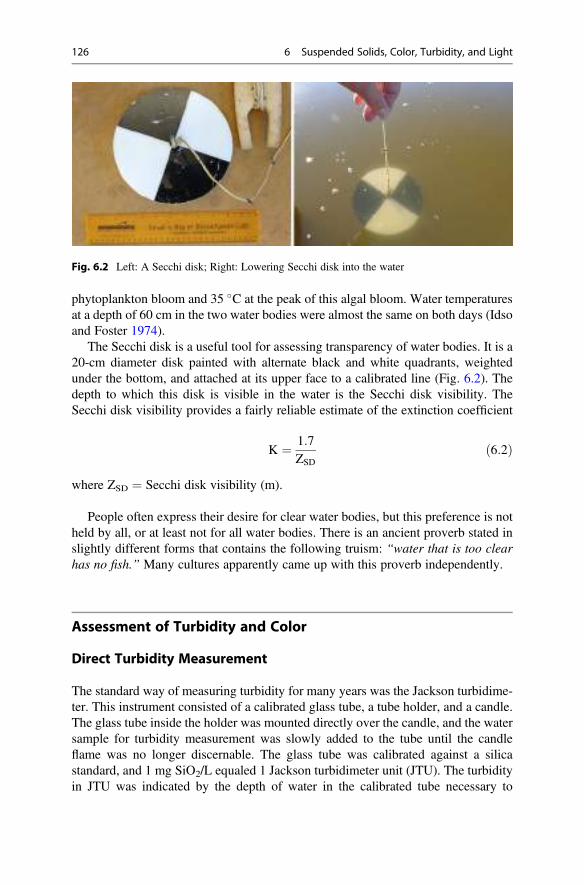
phytoplankton bloom and 35 �C at the peak of this algal bloom. Water temperaturesat a depth of 60 cm in the two water bodies were almost the same on both days (Idsoand Foster 1974).

The Secchi disk is a useful tool for assessing transparency of water bodies. It is a20-cm diameter disk painted with alternate black and white quadrants, weightedunder the bottom, and attached at its upper face to a calibrated line (Fig. 6.2). Thedepth to which this disk is visible in the water is the Secchi disk visibility. TheSecchi disk visibility provides a fairly reliable estimate of the extinction coefficient

K ¼ 1:7ZSD

ð6:2Þ

where ZSD ¼ Secchi disk visibility (m).

People often express their desire for clear water bodies, but this preference is notheld by all, or at least not for all water bodies. There is an ancient proverb stated inslightly different forms that contains the following truism: “water that is too clearhas no fish.” Many cultures apparently came up with this proverb independently.

Assessment of Turbidity and Color

Direct Turbidity Measurement

The standard way of measuring turbidity for many years was the Jackson turbidime-ter. This instrument consisted of a calibrated glass tube, a tube holder, and a candle.The glass tube inside the holder was mounted directly over the candle, and the watersample for turbidity measurement was slowly added to the tube until the candleflame was no longer discernable. The glass tube was calibrated against a silicastandard, and 1 mg SiO2/L equaled 1 Jackson turbidimeter unit (JTU). The turbidityin JTU was indicated by the depth of water in the calibrated tube necessary to

Fig. 6.2 Left: A Secchi disk; Right: Lowering Secchi disk into the water


obscure the candle flame. The Jackson turbidimeter would not read turbidities lessthan 25 JTU, and it has been replaced by turbidity meters that employ the principlesof nephelometry.

A nephelometer is an instrument in which a beam of light is passed through awater sample and the amount of light scattered at 90� to the light beam is measured.The amount of scattered light increases with greater turbidity. The standard forcalibrating a nephelometer for turbidity analysis is a suspension of formazin madeby combining 5.0 mL volumes of a hydrazine sulfate solution (1 g/100 mL) and asolution of hexamethylenetetramine (10 g/100 mL) and diluting to 100 mL withdistilled water. This solution has a turbidity of 400 nephelometer turbidity units(NTU), and it can be further diluted to calibrate the nephelometer (Eaton et al. 2005).Most natural waters have turbidities <50 NTU, but values can range from <1 NTU to>1000 NTU. There is no direct relationship in natural waters between turbiditymeasurements made by nephelometry or by the Jackson turbidimeter.

A standard spectrophotometer also can be used to measure turbidity (Kitchneret al. 2017) by comparing absorbance at 750 nm with a standard curve prepared fromformazin. The results are reported as formazin attenuation units (FAU), and there isgood agreement between FAU units and FTU units measured by nephelometry.

Suspended Solids

The total suspended solids (TSS) concentration is determined by filtering a samplethrough a tared glass fiber filter, the filter and residue are dried at 102 �C, and theweight gain of the filter is caused by the suspended solids retained on it (Fig. 6.3).The suspended organic matter concentration can be determined by igniting theresidue from the TSS analysis. The loss of weight upon ignition is equal to theorganic component of the residue. This fraction of the TSS concentration is calledthe total volatile suspended solids (TVSS). Example 6.2 illustrates the calculationsof TSS and TVSS analyses. Of course, filtered and unfiltered portions of a watersample can be evaporated to dryness in tared dishes, and the difference in weights ofresidues in the two dishes is the TSS concentration (see Fig. 5.1).

Ex. 6.2 Calculation of TSS and TVSS concentrations.Solution:A 100-mL water sample is passed through a glass fiber filter weighing 1.25000 g.

Upon drying, the filter weighs 1.25305 g. The TSS concentration will be estimated.

TSS ¼ 1:25305� 1:25000ð Þg 103 mg=g� �

1; 000 mL=Lð Þ100 mL

¼ 30:5 mg=L:

The glass fiber filter and residue from TSS analysis weighed 1.25211 g after itwas ignited at 550 �C. The TVSS concentration will be calculated.

Assessment of Turbidity and Color 127

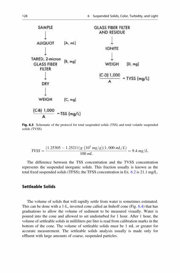
TVSS ¼ 1:25305� 1:25211ð Þg 103 mg=g� �

1; 000 mL=Lð Þ100 mL

¼ 9:4 mg=L:

The difference between the TSS concentration and the TVSS concentrationrepresents the suspended inorganic solids. This fraction usually is known as thetotal fixed suspended solids (TFSS); the TFSS concentration in Ex. 6.2 is 21.1 mg/L.

Settleable Solids

The volume of solids that will rapidly settle from water is sometimes estimated.This can be done with a 1-L, inverted cone called an Imhoff cone (Fig. 6.4) that hasgraduations to allow the volume of sediment to be measured visually. Water ispoured into the cone and allowed to set undisturbed for 1 hour. After 1 hour, thevolume of settleable solids in milliliters per liter is read from calibration marks in thebottom of the cone. The volume of settleable solids must be 1 mL or greater foraccurate measurement. The settleable solids analysis usually is made only foreffluent with large amounts of coarse, suspended particles.

Fig. 6.3 Schematic of the protocol for total suspended solids (TSS) and total volatile suspendedsolids (TVSS)


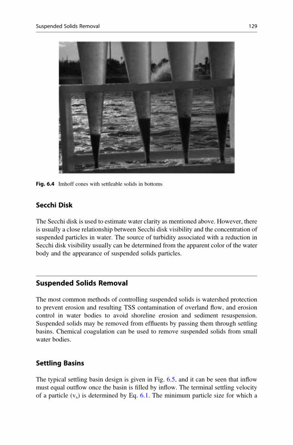
Secchi Disk

The Secchi disk is used to estimate water clarity as mentioned above. However, thereis usually a close relationship between Secchi disk visibility and the concentration ofsuspended particles in water. The source of turbidity associated with a reduction inSecchi disk visibility usually can be determined from the apparent color of the waterbody and the appearance of suspended solids particles.

Suspended Solids Removal

The most common methods of controlling suspended solids is watershed protectionto prevent erosion and resulting TSS contamination of overland flow, and erosioncontrol in water bodies to avoid shoreline erosion and sediment resuspension.Suspended solids may be removed from effluents by passing them through settlingbasins. Chemical coagulation can be used to remove suspended solids from smallwater bodies.

Settling Basins

The typical settling basin design is given in Fig. 6.5, and it can be seen that inflowmust equal outflow once the basin is filled by inflow. The terminal settling velocityof a particle (vs) is determined by Eq. 6.1. The minimum particle size for which a

Fig. 6.4 Imhoff cones with settleable solids in bottoms

Suspended Solids Removal 129

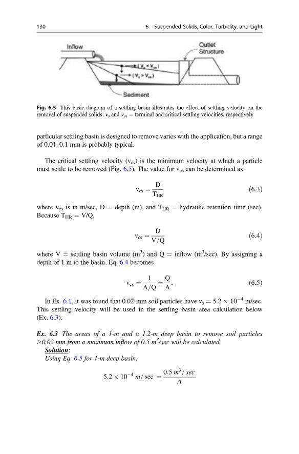
particular settling basin is designed to remove varies with the application, but a rangeof 0.01–0.1 mm is probably typical.

The critical settling velocity (vcs) is the minimum velocity at which a particlemust settle to be removed (Fig. 6.5). The value for vcs can be determined as

vcs ¼ DTHR

ð6:3Þ

where vcs is in m/sec, D ¼ depth (m), and THR ¼ hydraulic retention time (sec).Because THR ¼ V/Q,

vcs ¼ DV=Q

ð6:4Þ

where V ¼ settling basin volume (m3) and Q ¼ inflow (m3/sec). By assigning adepth of 1 m to the basin, Eq. 6.4 becomes

vcs ¼ 1A=Q

¼ QA: ð6:5Þ

In Ex. 6.1, it was found that 0.02-mm soil particles have vs ¼ 5.2 � 10�4 m/sec.This settling velocity will be used in the settling basin area calculation below(Ex. 6.3).

Ex. 6.3 The areas of a 1-m and a 1.2-m deep basin to remove soil particles�0.02 mm from a maximum inflow of 0.5 m3/sec will be calculated.

Solution:Using Eq. 6.5 for 1-m deep basin,

5:2� 10�4 m= sec ¼ 0:5 m3= sec

A

Fig. 6.5 This basic diagram of a settling basin illustrates the effect of settling velocity on theremoval of suspended solids; νs and νcs ¼ terminal and critical settling velocities, respectively


A ¼ 962 m2:

The 1.2-m deep basin could be smaller by a fraction of 1/1.2 (0.83). Its areawould be 798 m2.

Settling basins fill with sediment over time, and they normally are built 1.5 ormore times larger than the minimum area. Of course, basins also can be cleaned ofsediment periodically in order to maintain the design THR.

Chemical Coagulants

The most common chemical coagulant for removing suspended solids from water isaluminum sulfate (Al2SO4�14H2O) commonly called alum. Suspended clay particleshave negative charges and mutually repel. By increasing the cation concentration inwater, the charges on clay particles will be neutralized allowing them to flocculateinto clumps heavy enough to settle. The effectiveness of cations in coagulating clayparticles increases with greater valence, and the trivalent aluminum ion often is used.Treatment rates are determined by evaluating a series of alum concentrations insmall containers of the turbid water. Normally, 15–30 mg/L of alum are necessary toremove turbidity.

Alum treatment must be done with caution, because aluminum has an acidicreaction in water.

Al2 SO4ð Þ314H2O ¼ 2Al3þ þ 3SO2�4 þ 14H2O ð6:6Þ

2Al3þ þ 6H2O ¼ 2Al OHð Þ3 þ 6Hþ: ð6:7ÞEach milligram of alum will produce enough acidity to neutralize about 0.5 mg/Lalkalinity (expressed as equivalent CaCO3)

3CaCO3 þ 6Hþ ! 3Ca2þ þ 3H2Oþ 3CO2: ð6:8ÞAlkalinity can be increased by treating with lime before the alum treatment isapplied. Alum is widely used for clearing water of turbidity, but ferric sulfate andother iron and aluminum compounds also have been applied for this purpose.

Water quality criteria usually have some reference to TSS concentration, turbid-ity, and color. In order to protect aquatic ecosystems, TSS, turbidity, and colorshould not change by more than 10% of the seasonal mean concentration, or thecompensation point for photosynthetic activity should not be reduced by more than10%. Water quality criteria for effluents may contain limits for TSS, and an upperlimit of 25 mg/L usually will provide a good level of protection against excessiveturbidity and sedimentation in aquatic ecosystems, and fair protection may beachieved by a limit of 50 mg/L. Some effluent discharge permits may prohibit aturbidity plume.

Suspended Solids Removal 131

The maximum allowable turbidity concentration for municipal water supplyusually is about 5 NTU with a requirement for 95% of samples to have less than1 NTU. Turbidity usually is removed by chemical coagulation and sedimentation orby filtration. Such treatment will remove coarse and colloidal particles, but it will notremove true color of dissolved matter. High-dose chlorination sometimes willremove tannic substances, but it may be necessary to resort to activated carbonfilters, anion exchange, or potassium permanganate treatment.

Color

Although many associate clear water with high purity and turbid water with contam-ination, clear water could contain harmful microorganisms, and the possibility forcontamination with pathogens should always be considered in potable water. Tur-bidity and color in water is an important aesthetic issue. Water users want cleardrinking water, and do not desire that their fabrics be stained during washing or thatsinks, tubs, showers, and glassware be stained by exposure to water with a highdegree of color. While there are no mandated standards for color, the recommendedallowable limit is 15 color units.

The usual method of measuring color in water is relatively primitive in compari-son with methods for determining concentrations of other variables. It relies uponcomparison of natural water color to a series of standard color solutions in clear tubes(Nessler tubes) of 17.5 cm or 20 cm in height and with volumes of 50 or 100 mL,respectively. A solution containing 500 color units is prepared by dissolving 1.246 gpotassium chloroplatinate and 1.00 g cobaltous chloride with 100 mL nitric acid anddiluting to 1000 mL with distilled water (Eaton et al. 2005). Standards containingfrom 0 (distilled water) to 70 color units are prepared and placed in Nessler tubes.The water sample is filtered and placed in a Nessler tube and a color unit is assignedto the sample after comparison with the standards. The water sample may be dilutedwith distilled water if necessary to assign a color reading to a highly colored sample.A spectrophotometric color method is available; it reveals the hue of the color butnot the intensity (Eaton et al. 2005).

Conclusions

Suspended matter in water can result in high turbidity and excessive sedimentation.Sedimentation in water bodies makes affected areas shallower, and it may destroybenthic organisms and fish eggs. Turbidity seldom has direct toxic or mechanicaleffects on fish and other aquatic organisms, but it restricts light penetration andlessens productivity of water bodies. Turbidity and color in public water supplies isundesirable because consumers want clear water. Turbidity in water also detractsfrom its value for recreational purposes and makes it less aesthetically pleasing.


References

Eaton AD, Clesceri LS, Rice EW, Greenburg AE (eds) (2005) Standard methods for the examina-tion of water and wastewater. American Public Health Association, Washington

Idso SB, Foster JM (1974) Light and temperature relations in a small desert pond as influenced byphytoplanktonic density variations. Water Resources Res 10:129–132

Kitchner GB, Wainwright J, Parsons AJ (2017) A review of the principles of turbidity measure-ment. Prog Phys Geo 41:620–642

Padisák J, Soróczki-Printér E, Rezner Z (2003) Sinking properties of some phytoplankton shapesand the relation of form resistance to morphological diversity of plankton—an experimentalstudy. Hydrobio 500:243–257

Wetzel RG (2001) Limnology, 3rd edn. Academic, San Diego

References 133

Dissolved Oxygen and Other Gases 7

AbstractConcentrations of dissolved oxygen and other dissolved atmospheric gases atsaturation in water vary with the partial pressures and solubilities of the gases, andthe temperature and salinity of the water. Concentrations of dissolved oxygen andother dissolved gases at saturation decrease with greater elevation (lower baro-metric pressure), higher salinity, and rising temperature. Their concentrations inwater may be expressed in milligrams per liter, but it also can be reported inmilliliters per liter, percentage saturation, oxygen tension, or other units. The rateof diffusion of dissolved oxygen and other gases into water bodies is related tovarious factors, but the most important is the concentration of each gas alreadypresent in the water, the area of contact between the air and water, and the amountof turbulence in the water. Gases enter water from the air until saturationconcentrations are reached, but if saturation concentrations in the water are inexcess of concentration, gases diffuse into the air. Dissolved oxygen is of utmostimportance in water quality, because it is essential for aerobic respiration.Absorption of oxygen by fish and other aquatic animals is controlled by thepressure of oxygen in the water rather than the dissolved oxygen concentration inmilligrams per liter. Low oxygen pressure can stress or even kill aquaticorganisms. Excessive dissolved gas (including oxygen) concentrations in watercan lead to gas bubble trauma in fish and other aquatic animals.

Introduction

Aerobic organisms, whether they live on land or in water, must have oxygen or theywill suffocate. Almost everyone also knows that while water (H2O) is mainly madeof oxygen (88.89%), aquatic animals cannot utilize the oxygen from watermolecules; they require molecular oxygen (O2) that is dissolved in water. A fish ina lake with water depleted of dissolved oxygen is literally suffocating in a lake ofoxygen.


135


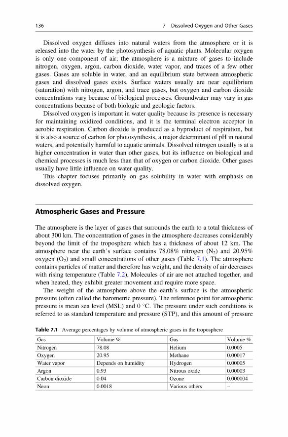
Dissolved oxygen diffuses into natural waters from the atmosphere or it isreleased into the water by the photosynthesis of aquatic plants. Molecular oxygenis only one component of air; the atmosphere is a mixture of gases to includenitrogen, oxygen, argon, carbon dioxide, water vapor, and traces of a few othergases. Gases are soluble in water, and an equilibrium state between atmosphericgases and dissolved gases exists. Surface waters usually are near equilibrium(saturation) with nitrogen, argon, and trace gases, but oxygen and carbon dioxideconcentrations vary because of biological processes. Groundwater may vary in gasconcentrations because of both biologic and geologic factors.

Dissolved oxygen is important in water quality because its presence is necessaryfor maintaining oxidized conditions, and it is the terminal electron acceptor inaerobic respiration. Carbon dioxide is produced as a byproduct of respiration, butit is also a source of carbon for photosynthesis, a major determinant of pH in naturalwaters, and potentially harmful to aquatic animals. Dissolved nitrogen usually is at ahigher concentration in water than other gases, but its influence on biological andchemical processes is much less than that of oxygen or carbon dioxide. Other gasesusually have little influence on water quality.

This chapter focuses primarily on gas solubility in water with emphasis ondissolved oxygen.

Atmospheric Gases and Pressure

The atmosphere is the layer of gases that surrounds the earth to a total thickness ofabout 300 km. The concentration of gases in the atmosphere decreases considerablybeyond the limit of the troposphere which has a thickness of about 12 km. Theatmosphere near the earth’s surface contains 78.08% nitrogen (N2) and 20.95%oxygen (O2) and small concentrations of other gases (Table 7.1). The atmospherecontains particles of matter and therefore has weight, and the density of air decreaseswith rising temperature (Table 7.2), Molecules of air are not attached together, andwhen heated, they exhibit greater movement and require more space.

The weight of the atmosphere above the earth’s surface is the atmosphericpressure (often called the barometric pressure). The reference point for atmosphericpressure is mean sea level (MSL) and 0 �C. The pressure under such conditions isreferred to as standard temperature and pressure (STP), and this amount of pressure

Table 7.1 Average percentages by volume of atmospheric gases in the troposphere

Gas Volume % Gas Volume %

Nitrogen 78.08 Helium 0.0005

Oxygen 20.95 Methane 0.00017

Water vapor Depends on humidity Hydrogen 0.00005

Argon 0.93 Nitrous oxide 0.00003

Carbon dioxide 0.04 Ozone 0.000004

Neon 0.0018 Various others –

136 7 Dissolved Oxygen and Other Gases

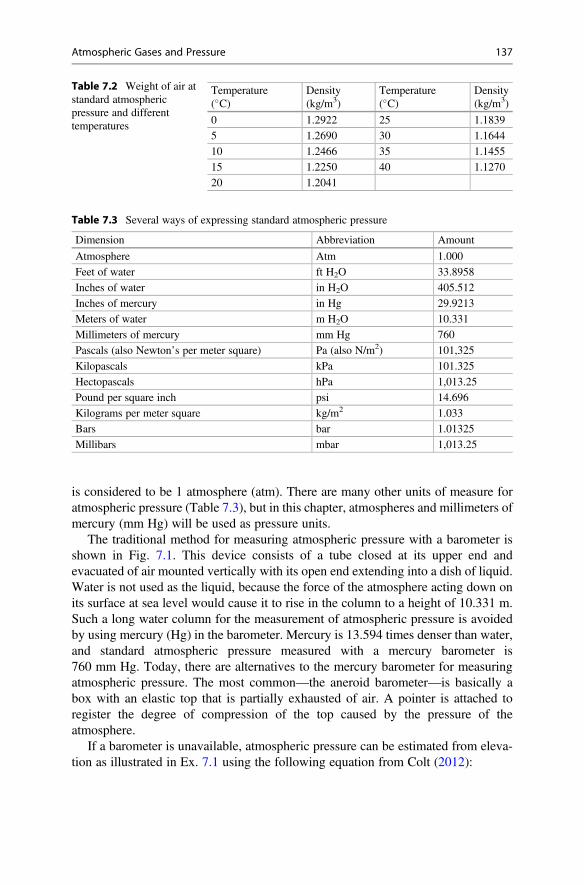
is considered to be 1 atmosphere (atm). There are many other units of measure foratmospheric pressure (Table 7.3), but in this chapter, atmospheres and millimeters ofmercury (mm Hg) will be used as pressure units.

The traditional method for measuring atmospheric pressure with a barometer isshown in Fig. 7.1. This device consists of a tube closed at its upper end andevacuated of air mounted vertically with its open end extending into a dish of liquid.Water is not used as the liquid, because the force of the atmosphere acting down onits surface at sea level would cause it to rise in the column to a height of 10.331 m.Such a long water column for the measurement of atmospheric pressure is avoidedby using mercury (Hg) in the barometer. Mercury is 13.594 times denser than water,and standard atmospheric pressure measured with a mercury barometer is760 mm Hg. Today, there are alternatives to the mercury barometer for measuringatmospheric pressure. The most common—the aneroid barometer—is basically abox with an elastic top that is partially exhausted of air. A pointer is attached toregister the degree of compression of the top caused by the pressure of theatmosphere.

If a barometer is unavailable, atmospheric pressure can be estimated from eleva-tion as illustrated in Ex. 7.1 using the following equation from Colt (2012):

Table 7.2 Weight of air atstandard atmosphericpressure and differenttemperatures

Temperature(�C)

Density(kg/m3)

Temperature(�C)

Density(kg/m3)

0 1.2922 25 1.1839

5 1.2690 30 1.1644

10 1.2466 35 1.1455

15 1.2250 40 1.1270

20 1.2041

Table 7.3 Several ways of expressing standard atmospheric pressure

Dimension Abbreviation Amount

Atmosphere Atm 1.000

Feet of water ft H2O 33.8958

Inches of water in H2O 405.512

Inches of mercury in Hg 29.9213

Meters of water m H2O 10.331

Millimeters of mercury mm Hg 760

Pascals (also Newton’s per meter square) Pa (also N/m2) 101,325

Kilopascals kPa 101.325

Hectopascals hPa 1,013.25

Pound per square inch psi 14.696

Kilograms per meter square kg/m2 1.033

Bars bar 1.01325

Millibars mbar 1,013.25

Atmospheric Gases and Pressure 137

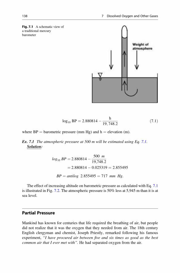
log10 BP ¼ 2:880814� h19; 748:2

ð7:1Þ

where BP ¼ barometric pressure (mm Hg) and h ¼ elevation (m).

Ex. 7.1 The atmospheric pressure at 500 m will be estimated using Eq. 7.1.Solution:

log10 BP ¼ 2:880814 � 500 m

19,748:2

¼ 2:880814 � 0:025319 ¼ 2:855495

BP ¼ antilog 2:855495 ¼ 717 mm Hg:

The effect of increasing altitude on barometric pressure as calculated with Eq. 7.1is illustrated in Fig. 7.2. The atmospheric pressure is 50% less at 5,945 m than it is atsea level.

Partial Pressure

Mankind has known for centuries that life required the breathing of air, but peopledid not realize that it was the oxygen that they needed from air. The 18th centuryEnglish clergyman and chemist, Joseph Priestly, remarked following his famousexperiment, “I have procured air between five and six times as good as the bestcommon air that I ever met with”. He had separated oxygen from the air.

Fig. 7.1 A schematic view ofa traditional mercurybarometer


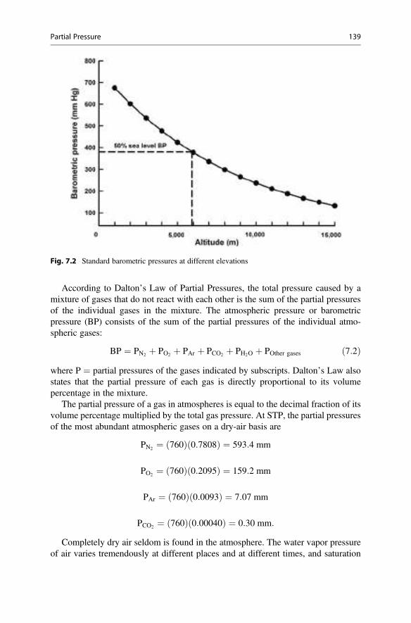
According to Dalton’s Law of Partial Pressures, the total pressure caused by amixture of gases that do not react with each other is the sum of the partial pressuresof the individual gases in the mixture. The atmospheric pressure or barometricpressure (BP) consists of the sum of the partial pressures of the individual atmo-spheric gases:

BP ¼ PN2 þ PO2 þ PAr þ PCO2 þ PH2O þ POther gases ð7:2Þwhere P ¼ partial pressures of the gases indicated by subscripts. Dalton’s Law alsostates that the partial pressure of each gas is directly proportional to its volumepercentage in the mixture.

The partial pressure of a gas in atmospheres is equal to the decimal fraction of itsvolume percentage multiplied by the total gas pressure. At STP, the partial pressuresof the most abundant atmospheric gases on a dry-air basis are

PN2 ¼ 760ð Þ 0:7808ð Þ ¼ 593:4 mm

PO2 ¼ 760ð Þ 0:2095ð Þ ¼ 159:2 mm

PAr ¼ 760ð Þ 0:0093ð Þ ¼ 7:07 mm

PCO2 ¼ 760ð Þ 0:00040ð Þ ¼ 0:30 mm:

Completely dry air seldom is found in the atmosphere. The water vapor pressureof air varies tremendously at different places and at different times, and saturation

Fig. 7.2 Standard barometric pressures at different elevations

Partial Pressure 139

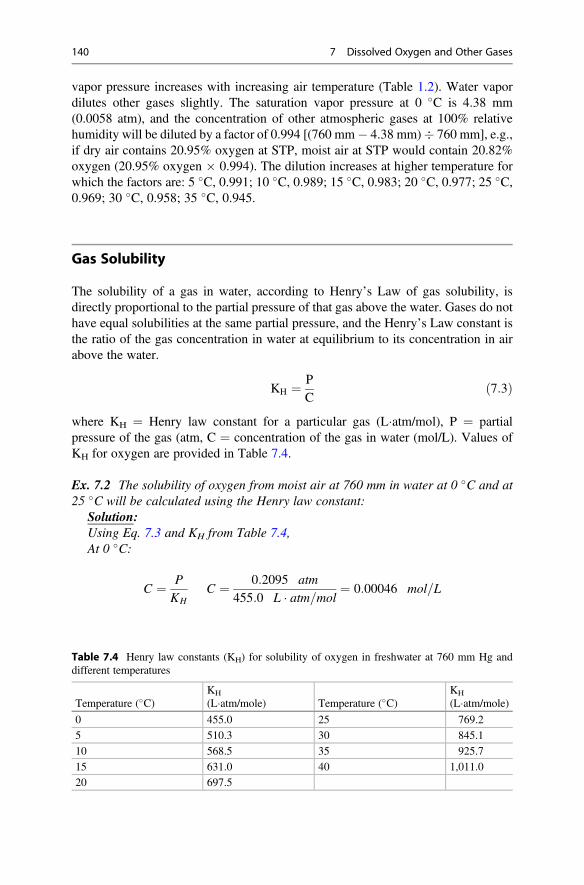
vapor pressure increases with increasing air temperature (Table 1.2). Water vapordilutes other gases slightly. The saturation vapor pressure at 0 �C is 4.38 mm(0.0058 atm), and the concentration of other atmospheric gases at 100% relativehumidity will be diluted by a factor of 0.994 [(760 mm� 4.38 mm)� 760 mm], e.g.,if dry air contains 20.95% oxygen at STP, moist air at STP would contain 20.82%oxygen (20.95% oxygen � 0.994). The dilution increases at higher temperature forwhich the factors are: 5 �C, 0.991; 10 �C, 0.989; 15 �C, 0.983; 20 �C, 0.977; 25 �C,0.969; 30 �C, 0.958; 35 �C, 0.945.

Gas Solubility

The solubility of a gas in water, according to Henry’s Law of gas solubility, isdirectly proportional to the partial pressure of that gas above the water. Gases do nothave equal solubilities at the same partial pressure, and the Henry’s Law constant isthe ratio of the gas concentration in water at equilibrium to its concentration in airabove the water.

KH ¼ PC

ð7:3Þ

where KH ¼ Henry law constant for a particular gas (L�atm/mol), P ¼ partialpressure of the gas (atm, C ¼ concentration of the gas in water (mol/L). Values ofKH for oxygen are provided in Table 7.4.

Ex. 7.2 The solubility of oxygen from moist air at 760 mm in water at 0 �C and at25 �C will be calculated using the Henry law constant:

Solution:Using Eq. 7.3 and KH from Table 7.4,At 0 �C:

C ¼ P

KHC ¼ 0:2095 atm

455:0 L � atm=mol ¼ 0:00046 mol=L

Table 7.4 Henry law constants (KH) for solubility of oxygen in freshwater at 760 mm Hg anddifferent temperatures

Temperature (�C)KH

(L�atm/mole) Temperature (�C)KH

(L�atm/mole)

0 455.0 25 769.2

5 510.3 30 845.1

10 568.5 35 925.7

15 631.0 40 1,011.0

20 697.5


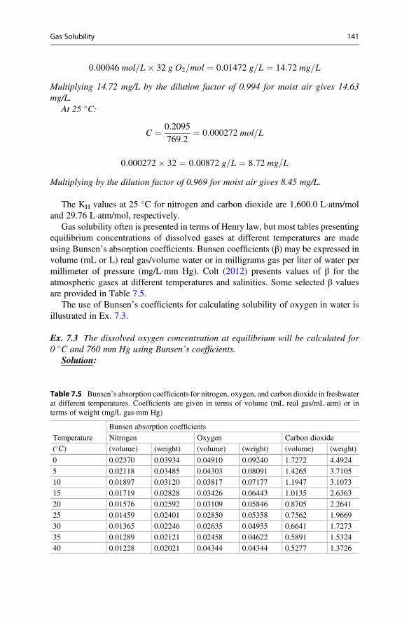
0:00046 mol=L� 32 g O2=mol ¼ 0:01472 g=L ¼ 14:72 mg=L

Multiplying 14.72 mg/L by the dilution factor of 0.994 for moist air gives 14.63mg/L.

At 25 �C:

C ¼ 0:2095769:2

¼ 0:000272 mol=L

0:000272� 32 ¼ 0:00872 g=L ¼ 8:72 mg=L

Multiplying by the dilution factor of 0.969 for moist air gives 8.45 mg/L.

The KH values at 25 �C for nitrogen and carbon dioxide are 1,600.0 L�atm/moland 29.76 L�atm/mol, respectively.

Gas solubility often is presented in terms of Henry law, but most tables presentingequilibrium concentrations of dissolved gases at different temperatures are madeusing Bunsen’s absorption coefficients. Bunsen coefficients (β) may be expressed involume (mL or L) real gas/volume water or in milligrams gas per liter of water permillimeter of pressure (mg/L�mm Hg). Colt (2012) presents values of β for theatmospheric gases at different temperatures and salinities. Some selected β valuesare provided in Table 7.5.

The use of Bunsen’s coefficients for calculating solubility of oxygen in water isillustrated in Ex. 7.3.

Ex. 7.3 The dissolved oxygen concentration at equilibrium will be calculated for0 �C and 760 mm Hg using Bunsen’s coefficients.

Solution:

Table 7.5 Bunsen’s absorption coefficients for nitrogen, oxygen, and carbon dioxide in freshwaterat different temperatures. Coefficients are given in terms of volume (mL real gas/mL�atm) or interms of weight (mg/L gas�mm Hg)

Temperature

Bunsen absorption coefficients

Nitrogen Oxygen Carbon dioxide

(�C) (volume) (weight) (volume) (weight) (volume) (weight)

0 0.02370 0.03934 0.04910 0.09240 1.7272 4.4924

5 0.02118 0.03485 0.04303 0.08091 1.4265 3.7105

10 0.01897 0.03120 0.03817 0.07177 1.1947 3.1073

15 0.01719 0.02828 0.03426 0.06443 1.0135 2.6363

20 0.01576 0.02592 0.03109 0.05846 0.8705 2.2641

25 0.01459 0.02401 0.02850 0.05358 0.7562 1.9669

30 0.01365 0.02246 0.02635 0.04955 0.6641 1.7273

35 0.01289 0.02121 0.02458 0.04622 0.5891 1.5324

40 0.01228 0.02021 0.04344 0.04344 0.5277 1.3726

Gas Solubility 141

Using volume/volume coefficients for a real gas (Table 7.5)

1. According to Avogadro’s law relating volume to mass of a gas, 1 mole oxygenweighs 31.999 g and occupies 22.4 L at STP. Thus, the density of oxygen at STP is

32 g O2=mol

22:4 L=mol¼ 1:4285 g=L ¼ 1:4285 mg=mL:

2. The Bunsen’s coefficient at 0 �C is 0.04910 mL/mL. Multiplying by density gives

0:04910 mL=mL� 1:4285 mg=mL ¼ 0:07014 mg O2=mL or 70:14 mg O2=L:

3. The calculation in step 2 is for pure oxygen, but the atmosphere is 20.95%oxygen. Thus, the concentration of oxygen in water would be

70:14 mg=L� 0:2095 ¼ 14:694 mg=L:

4. The concentration from step 3 is for dry air. Previously the dilution factor of0.994 was calculated for 0�C, and the saturation concentration from moist air is

14:694� 0:994 ¼ 14:61 mg=L:

The calculation is much easier using the weight over volume version of the Bunsen’scoefficient (Table 7.5). The value of β simply has to be multiplied by the partialpressure of oxygen in the air. From Table 7.5, β ¼ 0.09240 mg/L�mm Hg, and asshown earlier at STP, the partial pressure of oxygen is 159.2 mm.

0:09240 mg=L ∙mm Hgð Þ 159:2 mm Hgð Þ ¼ 14:71 mg=L:

Adjusting with the dilution factor of 0.994 for moist air, we get 14.62 mg/L.

The same approach illustrated in Ex. 7.3 can be used to calculate solubilities ofnitrogen, argon, and carbon dioxide. The resulting solubilities of these three gases atSTP are 23.05 mg/L for nitrogen, 1.32 mg/L for carbon dioxide, and 0.89 mg/L forargon. Nitrogen has the greatest concentration in water despite being the leastsoluble, because it comprises a much greater volume percentage of the atmospherethan do other gases.

Colt (1984) reported the Bunsen coefficients for atmospheric gases in water ofdifferent temperatures and salinities. However, he also calculated the atmosphericgases from moist air in water for the normal temperature and salinity ranges encoun-tered in water quality efforts. The solubilities of oxygen, nitrogen, and carbon dioxideat selected temperatures and salinities are provided in Tables 7.6, 7.7, and 7.8,


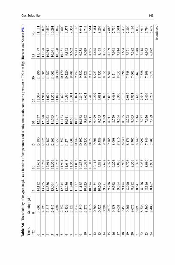
Table

7.6

The

solubilityof

oxyg

en(m

g/L)as

afunctio

nof

temperatureandsalin

ity(m

oistair,barometricpressure¼

760mm

Hg)

(BensonandKrause19

84)

Tem

p.Salinity

(g/L)

(�C)

05

1015

2025

3035

40

014

.602

14.112

13.638

13.180

12.737

12.309

11.896

11.497

11.111

114

.198

13.725

13.268

12.825

12.398

11.984

11.585

11.198

10.825

213

.813

13.356

12.914

12.487

12.073

11.674

11.287

10.913

10.552

313

.445

13.004

12.576

12.163

11.763

11.376

11.003

10.641

10.291

413

.094

12.667

12.253

11.853

11.467

11.092

10.730

10.380

10.042

512

.757

12.344

11.944

11.557

11.183

10.820

10.470

10.131

9.80

2

612

.436

12.036

11.648

11.274

10.911

10.560

10.220

9.89

29.57

3

712

.127

11.740

11.365

11.002

10.651

10.311

9.98

19.66

29.35

4

811

.832

11.457

11.093

10.742

10.401

10.071

9.75

29.44

39.14

3

911

.549

11.185

10.833

10.492

10.162

9.84

29.53

29.23

28.94

1

1011

.277

10.925

10.583

10.252

9.93

29.62

19.32

19.02

98.74

7

1111

.016

10.674

10.343

10.022

9.71

19.41

09.11

88.83

58.56

1

1210

.766

10.434

10.113

9.80

19.49

99.20

78.92

38.64

88.38

1

1310

.525

10.203

9.89

19.58

99.29

59.01

18.73

58.46

88.20

9

1410

.294

9.98

19.67

89.38

49.09

98.82

38.55

58.29

58.04

3

1510

.072

9.76

89.47

39.18

88.91

18.64

28.38

18.12

97.88

3

169.85

89.56

29.27

68.99

88.72

98.46

88.21

47.96

87.73

0

179.65

19.36

49.08

68.81

68.55

48.30

08.05

37.81

47.58

1

189.45

39.17

48.90

38.64

08.38

58.13

87.89

87.66

47.43

8

199.26

18.99

08.72

68.47

18.22

27.98

27.74

87.52

17.30

0

209.07

78.81

28.55

68.30

78.06

57.83

17.60

37.38

27.16

7

218.89

88.64

18.39

28.14

97.91

47.68

57.46

37.24

87.03

8

228.72

68.47

68.23

37.99

77.76

77.54

57.32

87.11

86.91

4

238.56

08.31

68.08

07.84

97.62

67.40

97.19

86.99

36.79

4

248.40

08.16

27.93

17.70

77.48

97.27

77.07

26.87

26.67

7

(con

tinued)

Gas Solubility 143

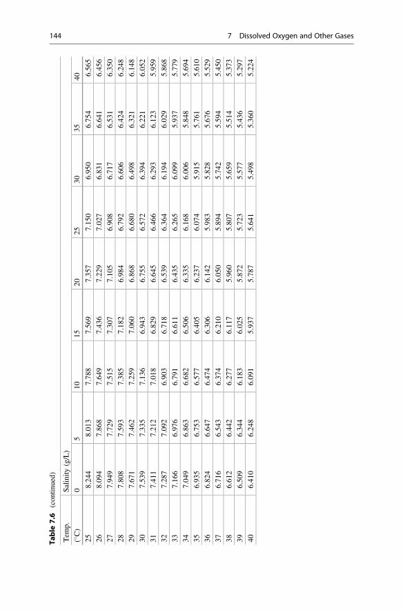
Table

7.6

(con

tinued)

Tem

p.Salinity

(g/L)

(�C)

05

1015

2025

3035

40

258.24

48.01

37.78

87.56

97.35

77.15

06.95

06.75

46.56

5

268.09

47.86

87.64

97.43

67.22

97.02

76.83

16.64

16.45

6

277.94

97.72

97.51

57.30

77.10

56.90

86.71

76.53

16.35

0

287.80

87.59

37.38

57.18

26.98

46.79

26.60

66.42

46.24

8

297.67

17.46

27.25

97.06

06.86

86.68

06.49

86.32

16.14

8

307.53

97.33

57.13

66.94

36.75

56.57

26.39

46.22

16.05

2

317.41

17.21

27.01

86.82

96.64

56.46

66.29

36.12

35.95

9

327.28

77.09

26.90

36.71

86.53

96.36

46.19

46.02

95.86

8

337.16

66.97

66.79

16.61

16.43

56.26

56.09

95.93

75.77

9

347.04

96.86

36.68

26.50

66.33

56.16

86.00

65.84

85.69

4

356.93

56.75

36.57

76.40

56.23

76.07

45.91

55.76

15.61

0

366.82

46.64

76.47

46.30

66.14

25.98

35.82

85.67

65.52

9

376.71

66.54

36.37

46.21

06.05

05.89

45.74

25.59

45.45

0

386.61

26.44

26.27

76.11

75.96

05.80

75.65

95.51

45.37

3

396.50

96.34

46.18

36.02

55.87

25.72

35.57

75.43

65.29

7

406.41

06.24

86.09

15.93

75.78

75.64

15.49

85.36

05.22

4


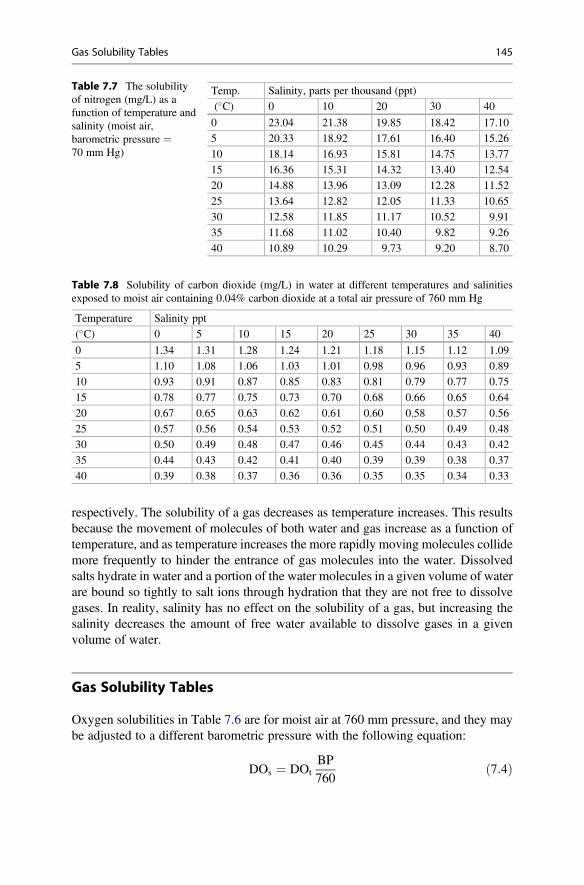
respectively. The solubility of a gas decreases as temperature increases. This resultsbecause the movement of molecules of both water and gas increase as a function oftemperature, and as temperature increases the more rapidly moving molecules collidemore frequently to hinder the entrance of gas molecules into the water. Dissolvedsalts hydrate in water and a portion of the water molecules in a given volume of waterare bound so tightly to salt ions through hydration that they are not free to dissolvegases. In reality, salinity has no effect on the solubility of a gas, but increasing thesalinity decreases the amount of free water available to dissolve gases in a givenvolume of water.

Gas Solubility Tables

Oxygen solubilities in Table 7.6 are for moist air at 760 mm pressure, and they maybe adjusted to a different barometric pressure with the following equation:

DOs ¼ DOtBP760

ð7:4Þ

Table 7.7 The solubilityof nitrogen (mg/L) as afunction of temperature andsalinity (moist air,barometric pressure ¼70 mm Hg)

Temp. Salinity, parts per thousand (ppt)

(�C) 0 10 20 30 40

0 23.04 21.38 19.85 18.42 17.10

5 20.33 18.92 17.61 16.40 15.26

10 18.14 16.93 15.81 14.75 13.77

15 16.36 15.31 14.32 13.40 12.54

20 14.88 13.96 13.09 12.28 11.52

25 13.64 12.82 12.05 11.33 10.65

30 12.58 11.85 11.17 10.52 9.91

35 11.68 11.02 10.40 9.82 9.26

40 10.89 10.29 9.73 9.20 8.70

Table 7.8 Solubility of carbon dioxide (mg/L) in water at different temperatures and salinitiesexposed to moist air containing 0.04% carbon dioxide at a total air pressure of 760 mm Hg

Temperature Salinity ppt

(�C) 0 5 10 15 20 25 30 35 40

0 1.34 1.31 1.28 1.24 1.21 1.18 1.15 1.12 1.09

5 1.10 1.08 1.06 1.03 1.01 0.98 0.96 0.93 0.89

10 0.93 0.91 0.87 0.85 0.83 0.81 0.79 0.77 0.75

15 0.78 0.77 0.75 0.73 0.70 0.68 0.66 0.65 0.64

20 0.67 0.65 0.63 0.62 0.61 0.60 0.58 0.57 0.56

25 0.57 0.56 0.54 0.53 0.52 0.51 0.50 0.49 0.48

30 0.50 0.49 0.48 0.47 0.46 0.45 0.44 0.43 0.42

35 0.44 0.43 0.42 0.41 0.40 0.39 0.39 0.38 0.37

40 0.39 0.38 0.37 0.36 0.36 0.35 0.35 0.34 0.33

Gas Solubility Tables 145

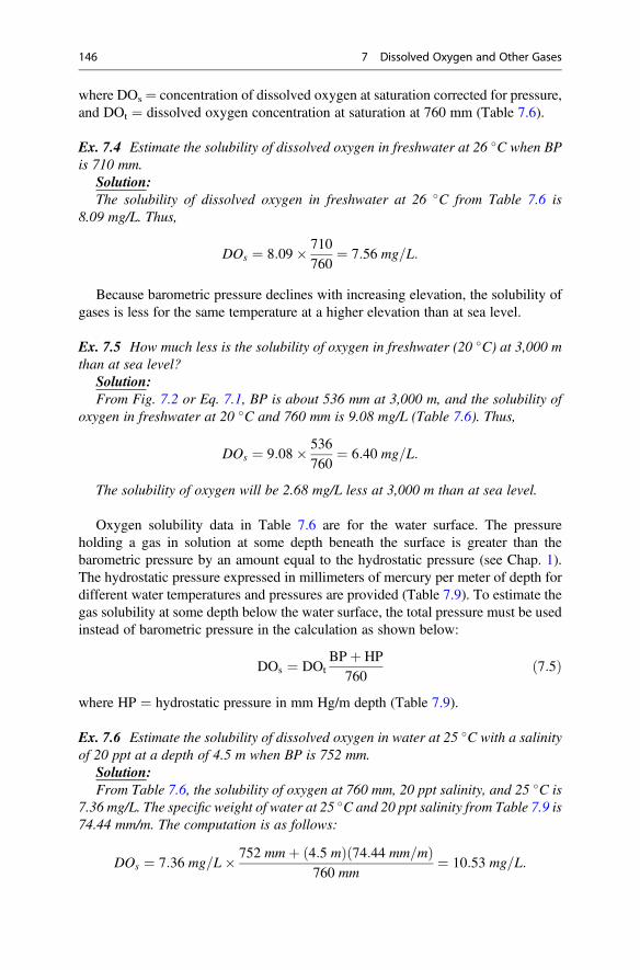
where DOs ¼ concentration of dissolved oxygen at saturation corrected for pressure,and DOt ¼ dissolved oxygen concentration at saturation at 760 mm (Table 7.6).

Ex. 7.4 Estimate the solubility of dissolved oxygen in freshwater at 26 �C when BPis 710 mm.

Solution:The solubility of dissolved oxygen in freshwater at 26 �C from Table 7.6 is

8.09 mg/L. Thus,

DOs ¼ 8:09� 710760

¼ 7:56 mg=L:

Because barometric pressure declines with increasing elevation, the solubility ofgases is less for the same temperature at a higher elevation than at sea level.

Ex. 7.5 How much less is the solubility of oxygen in freshwater (20 �C) at 3,000 mthan at sea level?

Solution:From Fig. 7.2 or Eq. 7.1, BP is about 536 mm at 3,000 m, and the solubility of

oxygen in freshwater at 20 �C and 760 mm is 9.08 mg/L (Table 7.6). Thus,

DOs ¼ 9:08� 536760

¼ 6:40 mg=L:

The solubility of oxygen will be 2.68 mg/L less at 3,000 m than at sea level.

Oxygen solubility data in Table 7.6 are for the water surface. The pressureholding a gas in solution at some depth beneath the surface is greater than thebarometric pressure by an amount equal to the hydrostatic pressure (see Chap. 1).The hydrostatic pressure expressed in millimeters of mercury per meter of depth fordifferent water temperatures and pressures are provided (Table 7.9). To estimate thegas solubility at some depth below the water surface, the total pressure must be usedinstead of barometric pressure in the calculation as shown below:

DOs ¼ DOtBPþ HP

760ð7:5Þ

where HP ¼ hydrostatic pressure in mm Hg/m depth (Table 7.9).

Ex. 7.6 Estimate the solubility of dissolved oxygen in water at 25 �C with a salinityof 20 ppt at a depth of 4.5 m when BP is 752 mm.

Solution:From Table 7.6, the solubility of oxygen at 760 mm, 20 ppt salinity, and 25 �C is

7.36 mg/L. The specific weight of water at 25 �C and 20 ppt salinity from Table 7.9 is74.44 mm/m. The computation is as follows:

DOs ¼ 7:36 mg=L� 752 mmþ 4:5 mð Þ 74:44 mm=mð Þ760 mm

¼ 10:53 mg=L:


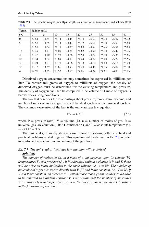
Dissolved oxygen concentrations may sometimes be expressed in milliliters perliter. To convert milligrams of oxygen to milliliters of oxygen, the density ofdissolved oxygen must be determined for the existing temperature and pressure.The density of oxygen can then be computed if the volume of 1 mole of oxygen isknown for existing conditions.

The law that describes the relationships about pressure, temperature, volume, andnumber of moles of an ideal gas is called the ideal gas law or the universal gas law.The common expression of the law is the universal gas law equation

PV ¼ nRT ð7:6Þwhere P ¼ pressure (atm), V ¼ volume (L), n ¼ number of moles of gas, R ¼universal gas law equation (0.082 L�atm/mol��K), and T¼ absolute temperature (�A¼ 273.15 + �C).

The universal gas law equation is a useful tool for solving both theoretical andpractical problems related to gases. This equation will be derived in Ex. 7.7 in orderto reinforce the readers’ understanding of the gas laws.

Ex. 7.7 The universal or ideal gas law equation will be derived.Solution:The number of molecules (n) in a mass of a gas depends upon its volume (V),

temperature (T), and pressure (P). If P is doubled without a change in V and T, therewill be twice as many molecules in the same volume, i.e., n ¼ kP. The number ofmolecules of a gas also varies directly with V if T and P are constant, i.e., V ¼ kP. IfV and P are constant, an increase in T will increase P and gas molecules would haveto be removed to maintain constant V. This reveals that the number of moleculesvaries inversely with temperature, i.e., n ¼ 1/T. We can summarize the relationshipsin the following expression:

Table 7.9 The specific weight (mm Hg/m depth) as a function of temperature and salinity (Colt1984)

Temp. Salinity (g/L)

(�C) 0 5 10 15 20 25 30 35 40

0 73.54 73.84 74.14 74.44 74.73 75.03 75.33 75.62 75.92

5 73.55 73.85 74.14 74.43 74.72 75.01 75.30 75.59 75.88

10 73.53 73.82 74.11 74.39 74.68 74.97 75.25 75.54 75.83

15 73.49 73.77 74.05 74.34 74.62 74.90 75.18 75.47 75.75

20 73.42 73.70 73.98 74.26 74.54 74.82 75.10 75.38 75.66

25 73.34 73.62 73.89 74.17 74.44 74.72 75.00 75.27 75.55

30 73.24 73.51 73.78 74.06 74.33 74.60 74.88 75.15 75.43

35 73.12 73.39 73.66 73.93 74.20 74.48 74.75 75.02 75.30

40 72.98 73.25 73.52 73.79 74.06 74.34 74.61 74.88 75.15

Gas Solubility Tables 147

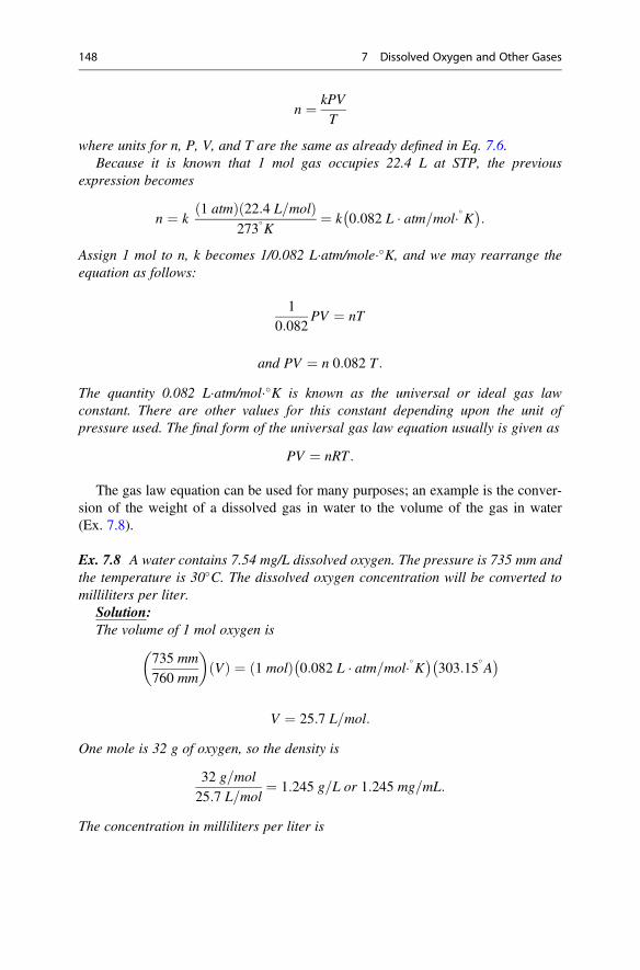
n ¼ kPV

T

where units for n, P, V, and T are the same as already defined in Eq. 7.6.Because it is known that 1 mol gas occupies 22.4 L at STP, the previous

expression becomes

n ¼ k1 atmð Þ 22:4 L=molð Þ

273�K

¼ k 0:082 L � atm=mol��K� �:

Assign 1 mol to n, k becomes 1/0.082 L�atm/mole��K, and we may rearrange theequation as follows:

10:082

PV ¼ nT

and PV ¼ n 0:082 T :

The quantity 0.082 L�atm/mol��K is known as the universal or ideal gas lawconstant. There are other values for this constant depending upon the unit ofpressure used. The final form of the universal gas law equation usually is given as

PV ¼ nRT :

The gas law equation can be used for many purposes; an example is the conver-sion of the weight of a dissolved gas in water to the volume of the gas in water(Ex. 7.8).

Ex. 7.8 A water contains 7.54 mg/L dissolved oxygen. The pressure is 735 mm andthe temperature is 30�C. The dissolved oxygen concentration will be converted tomilliliters per liter.

Solution:The volume of 1 mol oxygen is

735 mm

760 mm

� �Vð Þ ¼ 1 molð Þ 0:082 L � atm=mol��K� �

303:15�A

� �

V ¼ 25:7 L=mol:

One mole is 32 g of oxygen, so the density is

32 g=mol

25:7 L=mol¼ 1:245 g=L or 1:245 mg=mL:

The concentration in milliliters per liter is


7:54 mg=L

1:245 mg=mL¼ 6:06 mL=L:

Percentage Saturation and Oxygen Tension

Awater may contain more or less dissolved oxygen than the saturation concentrationfor existing conditions because of biological activity. The percentage saturation ofwater with dissolved oxygen is calculated as follows:

PS ¼ DOm

DOs� 100 ð7:7Þ

where PS ¼ percentage saturation and DOm ¼ the measured concentration ofdissolved oxygen (mg/L). A calculation of PS is made in Ex. 7.9.

Ex. 7.9 Calculate the percentage saturation at the surface of a freshwater bodycontaining 10.08 mg/L dissolved oxygen when the water temperature is 28�C andBP is 732 mm.

Solution:The concentration of dissolved oxygen at saturation is

DOs ¼ 7:81 mg=L� 732760

¼ 7:52 mg=L:

The percentage saturation is

PS ¼ 10:087:52

� 100 ¼ 134%:

Suppose the following morning, the body of water in Ex. 7.9 contained only4.5 mg/L dissolved oxygen and the temperature and barometric pressure were 24 �Cand 740 mm, respectively. The percentage saturation would now be only 55%.

Fish and other aquatic organisms that breathe with gills respond to the pressure ofdissolved oxygen in the water rather than to its concentration. Physiologists oftenrefer to the pressure of dissolved oxygen as the oxygen tension. The tension ofdissolved oxygen refers to the pressure of oxygen in the atmosphere required to holdan observed concentration of dissolved oxygen in the water. The partial pressure ofoxygen in air is 159.2 mm at STP. To estimate oxygen tension, the partial pressure ofoxygen in the atmosphere is multiplied by the factor DOm/DOs—oxygen tension isclosely linked to percentage saturation.

Percentage Saturation and Oxygen Tension 149

Ex. 7.10 Estimate the oxygen tension in water with 10 ppt salinity and 24 �C wheredissolved oxygen is 9.24 mg/L and BP is 760 mm.

Solution:The concentration at saturation is 7.93 mg/L. Thus,

Oxygen tension ¼ 9:24 mg=L

7:93 mg=L� 159:2 mm ¼ 185:5 mm:

Waters saturated with dissolved oxygen and at different temperatures will havethe same oxygen tension. A freshwater at 20 �C with 9.08 mg/L dissolved oxygenhas the same oxygen tension as a freshwater at 10 �C with 11.28 mg/L dissolvedoxygen. This results because the factor DOm/DOs is unity for both. Aquaticorganisms would be exposed to the same oxygen pressure (tension) even thoughthe oxygen concentration would be greater for the cooler water. It also is significantto note that when water holding a certain concentration of a gas warms without lossof gas to the air, the gas tension and the percentage saturation increase. If a waterholding 6.35 mg/L dissolved oxygen at 760 mm and 18 �C warms to 23 �C at thesame atmospheric pressure and without loss of oxygen, the value for oxygen tensionincreases from 107 mm to 118 mm and saturation increases from 67% to 74%.

The DP

There are various reasons why waters become supersaturated with gases. Coldrainwater and snow melt become supersaturated with gases when they percolatedownward to the water table and warm. In warm weather, water from wells orsprings often will be cooler than ambient temperature at ground level, and supersat-urated with gas. When water falls over a high dam, air bubbles may be entrained. Thewater will plunge to a considerable depth beneath the surface in the pool behind thedam into which it falls. The resulting increase in hydrostatic pressure raises thedissolved oxygen concentration at saturation, and when the water ascends and flowsinto shallower areas, it will be supersaturated with gases (Boyd and Tucker 2014).

Air leaks in or improper submergence of the intakes of pumps can result in gassupersaturation. Air bubbles can be sucked into the water, and as a result of thepressure increase caused by the pump, discharge will be supersaturated with gases(air). Aquatic plants often cause gas supersaturation by releasing copious amounts ofdissolved oxygen during photosynthesis.

The difference between the total gas pressure (TGP) and the total pressure at agiven depth is called ΔP. At the water surface, ΔP can be expressed as

ΔP ¼ TGP� BP: ð7:8ÞThe total gas pressure can be determined from the partial pressures (tensions) of theindividual gases in water


ΔP ¼ PO2 þ PN2 þ PAr þ PCO2ð Þ � BP: ð7:9ÞFor practical purposes, PAr and PCO2 can be omitted from Eq. 7.9, but the analysis fordissolved nitrogen concentration is difficult. A relatively inexpensive instrumentknown as a saturometer may be used to measure ΔP directly.

Some of the ΔP is offset by hydrostatic pressure at depths below the watersurface. The actual ΔP to which aquatic animals are exposed is called the uncom-pensated ΔP:

ΔPuncomp: ¼ ΔP� HP: ð7:10ÞValues for the hydrostatic pressure (HP) for different depths and salinities can befound in Table 7.9.

Gases dissolve in the blood of fish, shrimp, and other aquatic animals and reachequilibrium with external conditions. If water is supersaturated with gases, the bloodof animals living in the water also becomes saturated. The blood of an aquatic animalat equilibrium with dissolved gases at a particular temperature will become super-saturated with gases if the animal moves to warmer water. If supersaturating gasesare not rapidly lost to the surrounding water through the gills, gas bubbles can formin the blood.

The occurrence of gas bubbles in the blood causes gas bubble trauma—oftencalled gas bubble disease. Gas bubble trauma leads to stress and mortality. Eggs mayfloat to the surface, larvae and fry may exhibit hyperinflation of the swim bladder,cranial swelling, swollen gill lamellae, and other abnormalities. A common symp-tom of gas bubble trauma in juvenile and adult fish is gas bubbles in the blood thatare visible in surface tissues on the head, in the mouth, and in fin rays. The eyes ofaffected fish also may protrude.

Aquatic animals exposed to ΔP values of 25 to 75 mm Hg on a continuous basismay present symptoms of gas bubble trauma, and some of the affected animals maydie if exposure is prolonged for several days. Acute gas bubble trauma may lead to50–100% mortality at greater ΔP.

Gas bubble trauma is most common in shallow water or in organisms that cannotescape the surface water by sounding. At greater depths, the hydrostatic pressureincreases the equilibrium concentration of gases in water and thereby lowers the ΔP(Ex. 7.11)

Ex. 7.11 Calculation of reduction in ΔP with depth.Situation:A freshwater water body has a temperature of 28 �C, and a ΔP of 115 mm Hg at

the surface. The water is thoroughly mixed and gas concentrations and temperatureare the same at all depths. The uncompensated ΔP will be estimated for 1.5 m depth.

Solution:Using Eq. 7.10 and obtaining the hydrostatic pressure per meter of water depth

(by extrapolation between 25 � and 30 �C) from Table 7.9, the uncompensated ΔPwill be calculated.

The DP 151

ΔPuncomp: ¼ 115 mm� 73:28 mm=m� 1:5 mð Þ ¼ 5:1 mm:

Supersaturation of surface waters with dissolved oxygen during afternoons is acommon occurrence. This condition usually does not cause harm to aquatic animalsbecause the period of supersaturation is limited to a few hours in the afternoon andearly evening, the dissolved oxygen concentration decreases with depth, and mostanimals can go to greater depth (sound) where the combination of lower dissolvedconcentration and greater hydrostatic pressure lessens ΔP.

Gas Transfer

Most of the information on gas transfer between air and water has been developedfor oxygen, but principles presented for oxygen are applicable to other gases. Innatural waters, dissolved oxygen concentrations are constantly changing because ofbiological, physical, and chemical processes. The air above water has a constantpercentage of oxygen, even though the partial pressure of oxygen in air may varybecause of differences in atmospheric pressure. When water is at equilibrium withatmospheric oxygen, there is no net transfer of oxygen between air and water.Transfer of oxygen from air to water will occur when water is undersaturated withdissolved oxygen, and oxygen will diffuse from the water to the air when water issupersaturated with oxygen. The driving force causing net transfer of oxygenbetween air and water is the difference in oxygen tension. Once equilibrium isreached, oxygen tension in the air and in the water are the same and net transferceases. The oxygen deficit or oxygen surplus may be expressed as

D ¼ DOs � DOm ð7:11Þ

S ¼ DOm � DOs ð7:12Þwhere D ¼ oxygen deficit (mg/L), S ¼ oxygen surplus (mg/L), DOs ¼ solubility ofoxygen in water at saturation under existing conditions (mg/L), and DOm ¼measured concentration of dissolved oxygen (mg/L).

Oxygen enters or leaves a body of water at the air-water interface. For the thinfilm of water in contact with air, the greater D or S, the faster oxygen will enter orleave the film. For undisturbed water, the net transfer of oxygen will depend upon thevalue of D or S, the area of the air-water interface, the temperature, and time ofcontact. Even when D or S is great, the rate of net transfer is slow because the surfacefilm quickly reaches equilibrium and further net transfer requires oxygen to diffusefrom the film to the greater body of water, or from the greater body of water to thefilm. Natural waters are never completely quiescent, and the rate of oxygen transferincreases with greater turbulence.


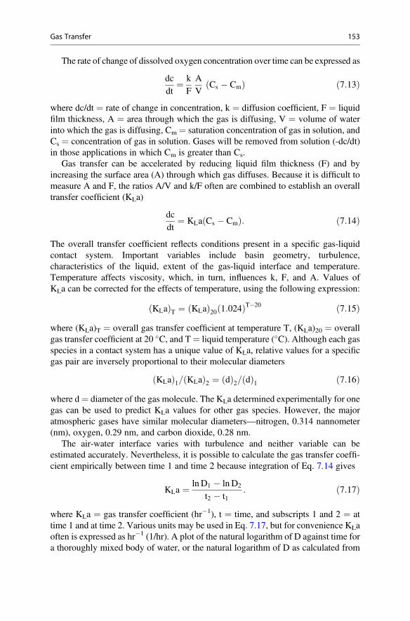
The rate of change of dissolved oxygen concentration over time can be expressed as

dcdt

¼ kFAV

Cs � Cmð Þ ð7:13Þ

where dc/dt ¼ rate of change in concentration, k ¼ diffusion coefficient, F ¼ liquidfilm thickness, A ¼ area through which the gas is diffusing, V ¼ volume of waterinto which the gas is diffusing, Cm ¼ saturation concentration of gas in solution, andCs ¼ concentration of gas in solution. Gases will be removed from solution (-dc/dt)in those applications in which Cm is greater than Cs.

Gas transfer can be accelerated by reducing liquid film thickness (F) and byincreasing the surface area (A) through which gas diffuses. Because it is difficult tomeasure A and F, the ratios A/V and k/F often are combined to establish an overalltransfer coefficient (KLa)

dcdt

¼ KLa Cs � Cmð Þ: ð7:14Þ

The overall transfer coefficient reflects conditions present in a specific gas-liquidcontact system. Important variables include basin geometry, turbulence,characteristics of the liquid, extent of the gas-liquid interface and temperature.Temperature affects viscosity, which, in turn, influences k, F, and A. Values ofKLa can be corrected for the effects of temperature, using the following expression:

KLað ÞT ¼ KLað Þ20 1:024ð ÞT�20 ð7:15Þwhere (KLa)T ¼ overall gas transfer coefficient at temperature T, (KLa)20 ¼ overallgas transfer coefficient at 20 �C, and T¼ liquid temperature (�C). Although each gasspecies in a contact system has a unique value of KLa, relative values for a specificgas pair are inversely proportional to their molecular diameters

KLað Þ1= KLað Þ2 ¼ dð Þ2= dð Þ1 ð7:16Þwhere d¼ diameter of the gas molecule. The KLa determined experimentally for onegas can be used to predict KLa values for other gas species. However, the majoratmospheric gases have similar molecular diameters—nitrogen, 0.314 nannometer(nm), oxygen, 0.29 nm, and carbon dioxide, 0.28 nm.

The air-water interface varies with turbulence and neither variable can beestimated accurately. Nevertheless, it is possible to calculate the gas transfer coeffi-cient empirically between time 1 and time 2 because integration of Eq. 7.14 gives

KLa ¼ ln D1 � ln D2

t2 � t1: ð7:17Þ

where KLa ¼ gas transfer coefficient (hr�1), t ¼ time, and subscripts 1 and 2 ¼ attime 1 and at time 2. Various units may be used in Eq. 7.17, but for convenience KLaoften is expressed as hr�1 (1/hr). A plot of the natural logarithm of D against time fora thoroughly mixed body of water, or the natural logarithm of D as calculated from

Gas Transfer 153

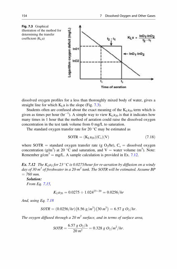
dissolved oxygen profiles for a less than thoroughly mixed body of water, gives astraight line for which KLa is the slope (Fig. 7.3).

Students often are confused about the exact meaning of the KLa20 term which isgiven as times per hour (hr�1). A simple way to view KLa20 is that it indicates howmany times in 1 hour that the method of aeration could raise the dissolved oxygenconcentration in the test tank volume from 0 mg/L to saturation.

The standard oxygen transfer rate for 20 �C may be estimated as

SOTR ¼ KLa20ð Þ Csð Þ Vð Þ ð7:18Þwhere SOTR ¼ standard oxygen transfer rate (g O2/hr), Cs ¼ dissolved oxygenconcentration (g/m3) at 20 �C and saturation, and V ¼ water volume (m3). Note:Remember g/cm3 ¼ mg/L. A sample calculation is provided in Ex. 7.12.

Ex. 7.12 The KLaT for 23 �C is 0.0275/hour for re-aeration by diffusion on a windyday of 30 m3 of freshwater in a 20-m2 tank. The SOTR will be estimated. Assume BP¼ 760 mm.

Solution:From Eq. 7.15,

KLa20 ¼ 0:0275� 1:02423�20 ¼ 0:0256=hr

And, using Eq. 7.18

SOTR ¼ 0:0256=hrð Þ 8:56 g=m3� �

30 m3� � ¼ 6:57 g O2=hr:

The oxygen diffused through a 20 m2 surface, and in terms of surface area,

SOTR ¼ 6:57 g O2=h

20 m2¼ 0:328 g O2=m

2=hr:

Fig. 7.3 Graphicalillustration of the method fordetermining the transfercoefficient (KLa)


The methodology for determining oxygen transfer rate described above often isused to determine the SOTR of mechanical aerators used in wastewater treatment(American Society of Civil Engineers 1992). Dividing the SOTR by the powerapplied to the aeration device provides an estimate of the standard aeration efficiencyof the aerator.

Measurements of SOTR in laboratory tanks range from 0.01 to 0.10 g oxygen/m2

per hour in still water to as high as 1.0 g oxygen/m2 per hour in turbulent water.Accurate measurement of SOTR is difficult in natural waters because biologicalprocesses add or remove oxygen during the period of measurement, and circulationpatterns are difficult to assess. Schroeder (1975) reported SOTR values of 0.01 to0.05 g oxygen/m2 per hour for each 0.2 atm (152 mm) saturation deficit. Welch(1968) measured SOTR values of 0.1 to 0.5 g oxygen/m2 per hour at 100% departurefrom saturation for a pond. The highest SOTR values were for windy days.

Gas exchange with the air is particularly rapid when waves break forming whitecaps. In small lakes and ponds, water surfaces are usually rather calm and oxygentransfer is impeded by lack of disturbance of the water surface. The followingequation (Boyd and Teichert-Coddington 1992) can be used to relate wind speedto rate of wind aeration in small ponds:

WRR ¼ 0:153X� 0:127ð Þ Cs � Cm

9:08

� �1:024T�20� � ð7:19Þ

where WRR ¼ wind re-aeration rate (g O2/m2 per hour) and X ¼ wind speed 3 m

above the water surface (m/sec).

Ex. 7.13 The wind re-aeration rate for a wind speed of 3 m/sec and the oxygenadded to a pond by diffusion during the night (12 hours) will be estimated for a 1.5 mdeep pond at 25 �C when the barometric pressure is 760 mm Hg and dissolvedoxygen concentration averages 5 mg/L during the night.

Solution:

(i) By substitution of data on oxygen concentrations and wind speed into Eq. 7.19,we get

(ii) WRR ¼ 0:153ð Þ 3 m= secð Þ � 0:127½ � 8:24� 5:009:08

� �1:024ð Þ5

WRR ¼ 0:133 g O2=m2=hr:

(iii) There is 1.5 m3 water beneath 1 m2 of surface, so

0:133 g O2=m2=hr

1:5 m3=m2¼ 0:089 g O2=m

3=hr

Gas Transfer 155

or 0:089 mg O2=L=hr:

In 12 hours, the amount of dissolved oxygen entering the pond by diffusion from theair would be

0:089 g O2=m3=hr � 12 hr ¼ 1:07 mg=L:

Stream Re-aeration

Several equations for estimating stream re-aeration rate have been proposed. Onesuch equation (O’Connor and Dobbins 1958) that was developed for streams withwater velocities between 0.15 and 0.5 m/sec and average depths between 0.3 and 9 mfollows:

ks ¼ 3:93ν0:5H�1:5 ð7:20Þwhere ks ¼ stream re-aeration coefficient (day�1), ν ¼ velocity (m/sec), and H ¼average depth (m). The ks can be adjusted for temperature and oxygen deficit in thestream by the equation

k0s ¼ ksCs � Cm

Cs

� �1:024T�20 ð7:21Þ

where k0s ¼ adjusted ks. The daily oxygen input from diffusion from the atmospherecan be estimated using Eq. 7.18 in which the volume term (V) is taken as stream flowpast a given point in cubic meters per day.

Stream re-aeration coefficients are lowest for sluggish rivers—usually beingbelow 0.35 day�1 (0.35/day). Large rivers with moderate to normal velocities havestream re-aeration coefficients between 0.35 and 0.7 day�1, while swift flowingrivers may have re-aeration constants of 1.0 or slightly greater. The higher rates ofre-aeration are for streams with rapids and waterfalls.

Concentrations of Dissolved Oxygen

Diffusion of oxygen from air to water and vice versa causes dissolved oxygenconcentrations in natural waters to tend towards equilibrium—but, they seldom areat equilibrium. This results because biological activity changes dissolved oxygenconcentrations faster than diffusion can produce equilibrium for existing conditions.The biological processes that influence dissolved oxygen concentrations are photo-synthesis by green plants and respiration by all aquatic organisms. During daylight,photosynthesis usually occurs more rapidly than does respiration, and dissolvedoxygen concentration increases. Afternoon dissolved oxygen concentration willtypically be above saturation in waters with healthy plant communities. At night,


photosynthesis stops, but respiration continues to use oxygen and causes dissolvedoxygen concentration to decline to less than saturation. Dissolved oxygen concen-tration also tends to decline with increasing water depth because there is lessillumination in deeper waters.

Oxygen and Carbon Dioxide in Respiration

Absorption of oxygen is a greater challenge to aquatic animals than to terrestrialanimals. At 25 �C and standard atmospheric pressure, the volume of molecularoxygen in freshwater at saturation is 6.29 mL/L, while in the atmosphere (20.95%oxygen) the volume of oxygen at the same temperature and pressure is about 209.5mL/L (Ex. 7.14). Air in this instance contains 33 times greater volume of oxygenthan occurs in oxygen-saturated surface water. The absorption of equal amounts ofoxygen by an aquatic animal and a terrestrial animal requires the aquatic animal topump a much larger volume of water across the gills than the land animal needs tobreathe. Assuming the fish in Ex. 7.14 could extract all of the dissolved oxygen fromwater, it would have to pump 24.3 L of water per hour to satisfy its respiratory needfor molecular oxygen. The same amount of oxygen is contained in 0.73 L of air.Neither the fish nor the land animal can remove all of the molecular oxygen fromwater or air, respectively, but Ex. 7.14 illustrates why oxygen availability is ofgreater concern in aquatic environments than in terrestrial ones.

Ex. 7.14 The volume of water that must be pumped across the gills of a fish ascompared to the amount of air breathed by a land animal to supply the same amountof oxygen for respiration will be calculated.

Solution:The volumes of oxygen in freshwater and in air at 25 �C and 1 atm pressure are:

Volume of 1 mol of oxygen is

PV ¼ nRT

V ¼ 1 molð Þ 0:082 L � atm=mol�A� �298:15

�A

� �

V ¼ 24:45 L=mol:

Density of oxygen at 25 �C and 1 atm is

32 g=mol

24:45 L=mol¼ 1:309 g=L or mg=mLð Þ:

Freshwater at 25 �C and 1 atm holds 8.24 mg/L dissolved oxygen at saturation(Table 7.6), which on a volume of oxygen basis is

Oxygen and Carbon Dioxide in Respiration 157

8:24 mg=L

1:309 mg=mL¼ 6:29 mL=L:

Suppose a 1-kg fish uses 200 mg O2/hour, for which the required volume of water tocontain this much oxygen is

200 mg O2=hr � 1:309 mg O2=mL ¼ 152:8 mL O2=hr

and

152:8 mL O2=hr

6:29 mL O2=L¼ 24:3 L water=hr:

Air contains 20.95% oxygen on volume basis, and like oxygen, 1 mol of air at 25 �Cand 1 atm occupies 24.45 L.

Volume of oxygen in 1 mol air (25 �C, 1 atm) is

24:45 L=mol� 0:2095 ¼ 5:122 L:

Weight of 5.122 L of oxygen is

5:122 L� 1:309 g O2=L ¼ 6:70 g O2:

Weight/volume concentration of oxygen in air is

6:70 g O2

24:45 L¼ 0:274 g O2=L air ¼ 274 mg O2=L air:

Volume air to provide 200 mg O2 is

200 mg O2

274 mg O2¼ 0:73 L:

The fish must pump 24.3 L of water to expose the gills to the same amount of oxygenas the land animal would breathe into its lungs in 0.73 L of air.

When oxygen is removed from water, it must be replaced by diffusion from theair or by release of oxygen from photosynthesis, both of which are relatively slowprocesses. Air movement usually replaces very quickly the oxygen removed by landanimals during respiration. Humans can congregate in large numbers to viewoutdoor sights or events with no danger of suffocation. The usual recommendedstanding capacity for humans at outdoor events is 3-5 individuals/m2. This is ahuman biomass of 200-400 kg/m2, and much greater than the standing crops ofaquatic animals found in natural water bodies.

The concentration of atmospheric oxygen seldom changes in the air surroundingterrestrial ecosystems. In water bodies, there is typically a daily oscillation ofdissolved oxygen concentration with lowest levels at night and highest levels indaytime. Many other events, e.g., cloudy weather, plankton density, wind velocity,


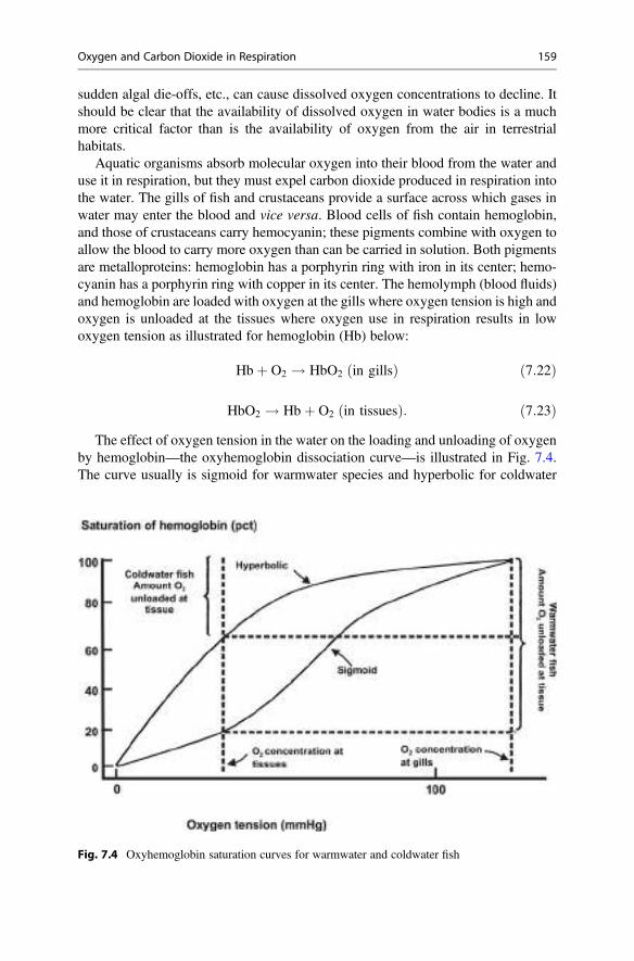
sudden algal die-offs, etc., can cause dissolved oxygen concentrations to decline. Itshould be clear that the availability of dissolved oxygen in water bodies is a muchmore critical factor than is the availability of oxygen from the air in terrestrialhabitats.

Aquatic organisms absorb molecular oxygen into their blood from the water anduse it in respiration, but they must expel carbon dioxide produced in respiration intothe water. The gills of fish and crustaceans provide a surface across which gases inwater may enter the blood and vice versa. Blood cells of fish contain hemoglobin,and those of crustaceans carry hemocyanin; these pigments combine with oxygen toallow the blood to carry more oxygen than can be carried in solution. Both pigmentsare metalloproteins: hemoglobin has a porphyrin ring with iron in its center; hemo-cyanin has a porphyrin ring with copper in its center. The hemolymph (blood fluids)and hemoglobin are loaded with oxygen at the gills where oxygen tension is high andoxygen is unloaded at the tissues where oxygen use in respiration results in lowoxygen tension as illustrated for hemoglobin (Hb) below:

Hbþ O2 ! HbO2 in gillsð Þ ð7:22Þ

HbO2 ! Hbþ O2 in tissuesð Þ: ð7:23ÞThe effect of oxygen tension in the water on the loading and unloading of oxygen

by hemoglobin—the oxyhemoglobin dissociation curve—is illustrated in Fig. 7.4.The curve usually is sigmoid for warmwater species and hyperbolic for coldwater

Fig. 7.4 Oxyhemoglobin saturation curves for warmwater and coldwater fish


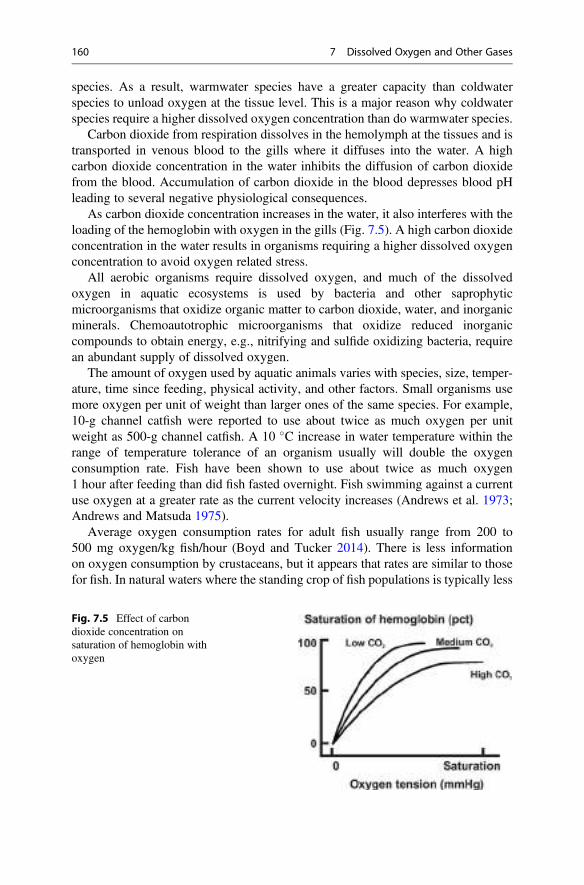
species. As a result, warmwater species have a greater capacity than coldwaterspecies to unload oxygen at the tissue level. This is a major reason why coldwaterspecies require a higher dissolved oxygen concentration than do warmwater species.

Carbon dioxide from respiration dissolves in the hemolymph at the tissues and istransported in venous blood to the gills where it diffuses into the water. A highcarbon dioxide concentration in the water inhibits the diffusion of carbon dioxidefrom the blood. Accumulation of carbon dioxide in the blood depresses blood pHleading to several negative physiological consequences.

As carbon dioxide concentration increases in the water, it also interferes with theloading of the hemoglobin with oxygen in the gills (Fig. 7.5). A high carbon dioxideconcentration in the water results in organisms requiring a higher dissolved oxygenconcentration to avoid oxygen related stress.

All aerobic organisms require dissolved oxygen, and much of the dissolvedoxygen in aquatic ecosystems is used by bacteria and other saprophyticmicroorganisms that oxidize organic matter to carbon dioxide, water, and inorganicminerals. Chemoautotrophic microorganisms that oxidize reduced inorganiccompounds to obtain energy, e.g., nitrifying and sulfide oxidizing bacteria, requirean abundant supply of dissolved oxygen.

The amount of oxygen used by aquatic animals varies with species, size, temper-ature, time since feeding, physical activity, and other factors. Small organisms usemore oxygen per unit of weight than larger ones of the same species. For example,10-g channel catfish were reported to use about twice as much oxygen per unitweight as 500-g channel catfish. A 10 �C increase in water temperature within therange of temperature tolerance of an organism usually will double the oxygenconsumption rate. Fish have been shown to use about twice as much oxygen1 hour after feeding than did fish fasted overnight. Fish swimming against a currentuse oxygen at a greater rate as the current velocity increases (Andrews et al. 1973;Andrews and Matsuda 1975).

Average oxygen consumption rates for adult fish usually range from 200 to500 mg oxygen/kg fish/hour (Boyd and Tucker 2014). There is less informationon oxygen consumption by crustaceans, but it appears that rates are similar to thosefor fish. In natural waters where the standing crop of fish populations is typically less

Fig. 7.5 Effect of carbondioxide concentration onsaturation of hemoglobin withoxygen


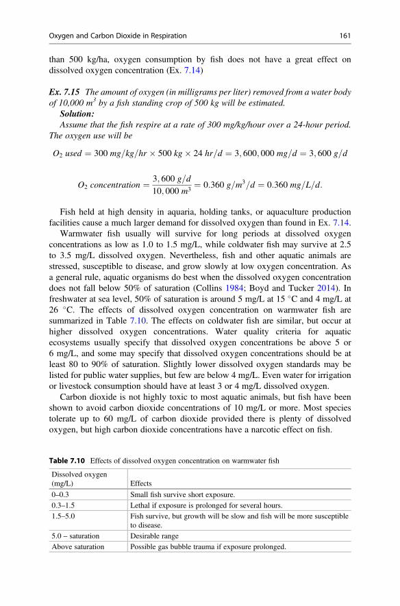
than 500 kg/ha, oxygen consumption by fish does not have a great effect ondissolved oxygen concentration (Ex. 7.14)

Ex. 7.15 The amount of oxygen (in milligrams per liter) removed from a water bodyof 10,000 m3 by a fish standing crop of 500 kg will be estimated.

Solution:Assume that the fish respire at a rate of 300 mg/kg/hour over a 24-hour period.

The oxygen use will be

O2 used ¼ 300 mg=kg=hr � 500 kg� 24 hr=d ¼ 3; 600; 000 mg=d ¼ 3; 600 g=d

O2 concentration ¼ 3; 600 g=d

10; 000 m3¼ 0:360 g=m3=d ¼ 0:360 mg=L=d:

Fish held at high density in aquaria, holding tanks, or aquaculture productionfacilities cause a much larger demand for dissolved oxygen than found in Ex. 7.14.

Warmwater fish usually will survive for long periods at dissolved oxygenconcentrations as low as 1.0 to 1.5 mg/L, while coldwater fish may survive at 2.5to 3.5 mg/L dissolved oxygen. Nevertheless, fish and other aquatic animals arestressed, susceptible to disease, and grow slowly at low oxygen concentration. Asa general rule, aquatic organisms do best when the dissolved oxygen concentrationdoes not fall below 50% of saturation (Collins 1984; Boyd and Tucker 2014). Infreshwater at sea level, 50% of saturation is around 5 mg/L at 15 �C and 4 mg/L at26 �C. The effects of dissolved oxygen concentration on warmwater fish aresummarized in Table 7.10. The effects on coldwater fish are similar, but occur athigher dissolved oxygen concentrations. Water quality criteria for aquaticecosystems usually specify that dissolved oxygen concentrations be above 5 or6 mg/L, and some may specify that dissolved oxygen concentrations should be atleast 80 to 90% of saturation. Slightly lower dissolved oxygen standards may belisted for public water supplies, but few are below 4 mg/L. Even water for irrigationor livestock consumption should have at least 3 or 4 mg/L dissolved oxygen.

Carbon dioxide is not highly toxic to most aquatic animals, but fish have beenshown to avoid carbon dioxide concentrations of 10 mg/L or more. Most speciestolerate up to 60 mg/L of carbon dioxide provided there is plenty of dissolvedoxygen, but high carbon dioxide concentrations have a narcotic effect on fish.

Table 7.10 Effects of dissolved oxygen concentration on warmwater fish

Dissolved oxygen(mg/L) Effects

0–0.3 Small fish survive short exposure.

0.3–1.5 Lethal if exposure is prolonged for several hours.

1.5–5.0 Fish survive, but growth will be slow and fish will be more susceptibleto disease.

5.0 – saturation Desirable range

Above saturation Possible gas bubble trauma if exposure prolonged.


Conclusions

Dissolved oxygen is the most important water quality variable in aquaticecosystems. Molecular oxygen is the electron acceptor in aerobic metabolism, andall aerobic organisms must have an adequate supply of dissolved oxygen. Whendissolved oxygen concentrations are low or dissolved oxygen is absent, decomposi-tion of organic matter by anaerobic microorganisms releases reduced substancessuch as ammonia, nitrite, ferrous iron, hydrogen sulfide, and dissolved organiccompounds into the water. In the absence of adequate dissolved oxygen, aerobicmicroorganisms do not function efficiently in oxidizing these reduced substances.The combination of low dissolved oxygen concentration and high concentrations ofcertain reduce, toxic metabolites cause drastic, negative impacts on the structure andfunction of aquatic ecosystems. “Clean water” species disappear and only thoseorganisms that can tolerate highly polluted conditions thrive. Such ecosystems are oflow biodiversity, unstable, and greatly impaired for most beneficial uses.

References

American Society of Civil Engineers (1992) Measurement of oxygen transfer in clean water, 2ndedn. ANSI/ASCE 2-91,. American Society of Civil Engineers, New York

Andrews JW, Matsuda Y (1975) The influence of various culture conditions on the oxygenconsumption of channel catfish. Trans Am Fish Soc 104:322–327

Andrews JW, Murai T, Gibbons G (1973) The influence of dissolved oxygen on the growth ofchannel catfish. Trans Am Fish Soc 102:835–838

Benson BB, Krause D (1984) The concentration and isotopic fractionation of oxygen dissolved infreshwater and seawater in equilibrium with the atmosphere. Lim Ocean 29:620–632

Boyd CE, Teichert-Coddington D (1992) Relationship between wind speed and reaeration in smallaquaculture ponds. Aqua Eng 11:121–131

Boyd CE, Tucker CS (2014) Handbook for aquaculture water quality. Craftmaster Printers, AuburnCollins G (1984) Fish growth and lethality versus dissolved oxygen. In: Proceedings specialty

conference on environmental engineering, ASCE, Los Angeles, June 25–27, 1984, pp 750–755Colt J (1984) Computation of dissolved gas concentrations in water as functions of temperature,

salinity, and pressure, Special Publication 14. American Fisheries Society, BethesdaColt J (2012) Dissolved gas concentration in water. Elsevier, New YorkO’Connor DJ, Dobbins WE (1958) Mechanism of reaeration in natural streams. Trans Am Soc Civ

Eng 123:641–666Schroeder GL (1975) Nighttime material balance for oxygen in fish ponds receiving organic wastes.

Bamidgeh 27:65–74Welch HE (1968) Use of modified diurnal curves for the measurement of metabolism in standing

water. Lim Ocean 13:679–687


Redox Potential 8

AbstractElectrons are lost when a substance is oxidized and gained when a substance isreduced. Oxidations and reductions occur in couplets—known as half-cells—inwhich one substance, the oxidizing agent, accepts electrons from another sub-stance, the reducing agent. The oxidizing agent is reduced and the reducing agentis oxidized. The flow of electrons between two half-cells can be measured as anelectromotive force (in volts). The hydrogen half-cell (H2 ! 2H+ + 2e�) has anelectrical potential of 0.0 volt at 25 �C, 1 atm H2 and 1 M H+; it is said to have astandard electrode potential (E0) of 0.0 volt. The flow of electrons to or from thehydrogen half-cell is the reference for determining E0 values of other half-cells.The greater a positive E0, the more oxidized a half-cell with respective to thehydrogen electrode; the opposite is true for a negative E0. The redox potential(E or Eh) for non-standard conditions is measured with a calomel electrode orcalculated with the Nernst equation. Water with measureable dissolved oxygenhas Eh ¼ 0.50 volt, and at oxygen saturation, Eh ¼ 0.56 volt. The redox potentialindicates whether given substances may exist in a particular environment andexplains the sequence of reactions that occur as dissolved oxygen concentrationdeclines in water bodies and sediments. The redox potential has many practicalapplications in analytical chemistry and industry, but it is not frequently measuredin water quality investigations.

Introduction

The oxidation-reduction (redox) potential is a measurement of the direction andamount of electron transfer that occurs in oxidation-reduction reactions. The redoxpotential indicates whether a substance is a reducing agent and donates electrons toanother substance or an oxidizing agent and accepts electrons from another sub-stance. It also provides an indication of the relative oxidizing and reducing strengthsof reactants.


163


In a redox reaction, electrons donated (lost) by the reducing agent must beaccepted (gained) by the oxidizing agent. A redox reaction can be thought of ashaving two parts: electrons are released by the reducing agent; electrons released bythe reducing agent are accepted by the oxidizing agent. The flow of electronsbetween the two parts of the reaction can be measured as an electrical current—theredox potential.

Hydrogen (H2) is the base for comparing the relative oxidizing or reducing powerof a substance. Hydrogen is assigned a redox potential of zero at standard conditions(1.0 MH+; 1 atm pressure; 25 �C). Other substances can be compared to hydrogen,and their redox potentials can be compared to each other. Concentrations ofsubstances, pH, and temperature influence redox potential, but redox can be adjustedfor differences in these variables. Redox potential may be used to determine theendpoints of chemical reactions, predict whether or not two substances will reactwhen brought together, ascertain if certain substances are likely to be present in theaquatic environment, and other purposes.

Oxidation-Reduction

Principles of the law of mass action, Gibbs free energy change of reaction, and theequilibrium constant can be applied to oxidation-reduction reactions. The drivingforce for oxidation-reduction reactions can be expressed in terms of a measurableelectrical current. Consider the oxidation-reduction reaction

I2 þ H2 ¼ 2Hþ þ 2I�: ð8:1ÞIodine is reduced to iodide, and hydrogen gas is oxidized to hydrogen ion. Thereaction can be divided into two parts, each called a half-cell, one showing the loss ofelectrons (e�) resulting in oxidation and one showing the gain of electrons causingreduction:

H2 ¼ 2Hþ þ 2e� ð8:2Þ

I2 þ 2e� ¼ 2I�: ð8:3ÞThe standard Gibbs free energy of reaction (ΔGo) expressions for Eqs. 8.2 and 8.3,respectively, are:

ΔGo ¼ 2ΔG0f H

þ þ 2ΔG0f e

� � ΔG0f H2

ΔGo ¼ 2ΔG0f I

� � ΔG0f I2 � 2ΔG0

f e�:

TheΔGof e

� term cancels during addition of the right-hand sides of these expressions,and the sum is

164 8 Redox Potential

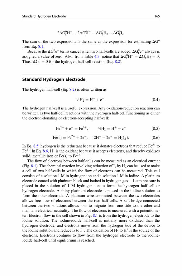
2ΔG0f H

þ þ 2ΔG0f I

� � ΔG0f H2 � ΔG0

f I2:

The sum of the two expressions is the same as the expression for estimating ΔGo

from Eq. 8.1.Because theΔG0

f e� terms cancel when two half-cells are added,ΔG0

f e� always is

assigned a value of zero. Also, from Table 4.3, notice that ΔG0f H

þ ¼ ΔG0f H2 ¼ 0:

Thus, ΔGo ¼ 0 for the hydrogen half-cell reaction (Eq. 8.2).

Standard Hydrogen Electrode

The hydrogen half-cell (Eq. 8.2) is often written as

½H2 ¼ Hþ þ e�: ð8:4ÞThe hydrogen half-cell is a useful expression. Any oxidation-reduction reaction canbe written as two half-cell reactions with the hydrogen half-cell functioning as eitherthe electron-donating or electron-accepting half-cell:

Fe3þ þ e� ¼ Fe2þ, ½H2 ¼ Hþ þ e� ð8:5Þ

Fe sð Þ ¼ Fe2þ þ 2e�, 2Hþ þ 2e� ¼ H2 gð Þ: ð8:6ÞIn Eq. 8.5, hydrogen is the reductant because it donates electrons that reduce Fe3+ toFe2+. In Eq. 8.6, H+ is the oxidant because it accepts electrons, and thereby oxidizessolid, metallic iron or Fe(s) to Fe2+.

The flow of electrons between half-cells can be measured as an electrical current(Fig. 8.1). The chemical reaction involving reduction of I2 by H2 can be used to makea cell of two half-cells in which the flow of electrons can be measured. This cellconsists of a solution 1 M in hydrogen ion and a solution 1 M in iodine. A platinumelectrode coated with platinum black and bathed in hydrogen gas at 1 atm pressure isplaced in the solution of 1 M hydrogen ion to form the hydrogen half-cell orhydrogen electrode. A shiny platinum electrode is placed in the iodine solution toform the other electrode. A platinum wire connected between the two electrodesallows free flow of electrons between the two half-cells. A salt bridge connectedbetween the two solutions allows ions to migrate from one side to the other andmaintain electrical neutrality. The flow of electrons is measured with a potentiome-ter. Electron flow in the cell shown in Fig. 8.1 is from the hydrogen electrode to theiodine solution. The iodine-iodide half-cell is initially more oxidized than thehydrogen electrode, and electrons move from the hydrogen side of the device tothe iodine solution and reduce I2 to I

�. The oxidation of H2 to H+ is the source of the

electrons. Electrons continue to flow from the hydrogen electrode to the iodine-iodide half-cell until equilibrium is reached.

Standard Hydrogen Electrode 165

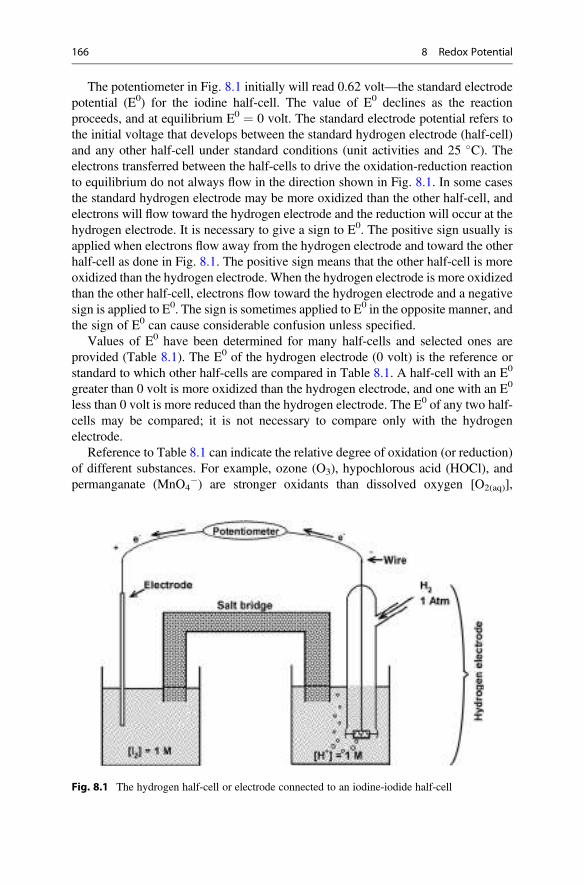
The potentiometer in Fig. 8.1 initially will read 0.62 volt—the standard electrodepotential (E0) for the iodine half-cell. The value of E0 declines as the reactionproceeds, and at equilibrium E0 ¼ 0 volt. The standard electrode potential refers tothe initial voltage that develops between the standard hydrogen electrode (half-cell)and any other half-cell under standard conditions (unit activities and 25 �C). Theelectrons transferred between the half-cells to drive the oxidation-reduction reactionto equilibrium do not always flow in the direction shown in Fig. 8.1. In some casesthe standard hydrogen electrode may be more oxidized than the other half-cell, andelectrons will flow toward the hydrogen electrode and the reduction will occur at thehydrogen electrode. It is necessary to give a sign to E0. The positive sign usually isapplied when electrons flow away from the hydrogen electrode and toward the otherhalf-cell as done in Fig. 8.1. The positive sign means that the other half-cell is moreoxidized than the hydrogen electrode. When the hydrogen electrode is more oxidizedthan the other half-cell, electrons flow toward the hydrogen electrode and a negativesign is applied to E0. The sign is sometimes applied to E0 in the opposite manner, andthe sign of E0 can cause considerable confusion unless specified.

Values of E0 have been determined for many half-cells and selected ones areprovided (Table 8.1). The E0 of the hydrogen electrode (0 volt) is the reference orstandard to which other half-cells are compared in Table 8.1. A half-cell with an E0

greater than 0 volt is more oxidized than the hydrogen electrode, and one with an E0

less than 0 volt is more reduced than the hydrogen electrode. The E0 of any two half-cells may be compared; it is not necessary to compare only with the hydrogenelectrode.

Reference to Table 8.1 can indicate the relative degree of oxidation (or reduction)of different substances. For example, ozone (O3), hypochlorous acid (HOCl), andpermanganate (MnO4

�) are stronger oxidants than dissolved oxygen [O2(aq)],

Fig. 8.1 The hydrogen half-cell or electrode connected to an iodine-iodide half-cell


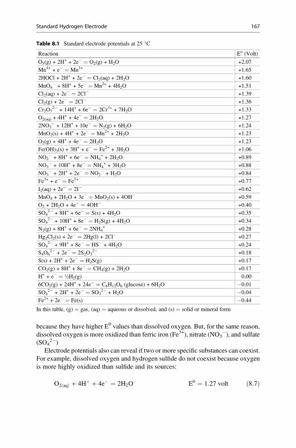
because they have higher E0 values than dissolved oxygen. But, for the same reason,dissolved oxygen is more oxidized than ferric iron (Fe3+), nitrate (NO3

�), and sulfate(SO4

2�)Electrode potentials also can reveal if two or more specific substances can coexist.

For example, dissolved oxygen and hydrogen sulfide do not coexist because oxygenis more highly oxidized than sulfide and its sources:

O2 aqð Þ þ 4Hþ þ 4e� ¼ 2H2O E0 ¼ 1:27 volt ð8:7Þ

Table 8.1 Standard electrode potentials at 25 �C

Reaction Eo (Volt)

O3(g) + 2H+ + 2e� ¼ O2(g) + H2O +2.07

Mn4+ + e� ¼ Mn3+ +1.65

2HOCl + 2H+ + 2e� ¼ Cl2(aq) + 2H2O +1.60

MnO4� + 8H+ + 5e� ¼ Mn2+ + 4H2O +1.51

Cl2(aq) + 2e� ¼ 2Cl� +1.39

Cl2(g) + 2e� ¼ 2Cl� +1.36

Cr2O72� + 14H+ + 6e� ¼ 2Cr3+ + 7H2O +1.33

O2(aq) + 4H+ + 4e� ¼ 2H2O +1.27

2NO3� + 12H+ + 10e� ¼ N2(g) + 6H2O +1.24

MnO2(s) + 4H+ + 2e� ¼ Mn2+ + 2H2O +1.23

O2(g) + 4H+ + 4e� ¼ 2H2O +1.23

Fe(OH)3(s) + 3H+ + e� ¼ Fe2+ + 3H2O +1.06

NO2� + 8H+ + 6e� ¼ NH4

+ + 2H2O +0.89

NO3� + 10H+ + 8e� ¼ NH4

+ + 3H2O +0.88

NO3� + 2H+ + 2e� ¼ NO2

� + H2O +0.84

Fe3+ + e� ¼ Fe2+ +0.77

I2(aq) + 2e� ¼ 2I� +0.62

MnO4 + 2H2O + 3e� ¼ MnO2(s) + 4OH� +0.59

O2 + 2H2O + 4e� ¼ 4OH� +0.40

SO42� + 8H+ + 6e� ¼ S(s) + 4H2O +0.35

SO42� + 10H+ + 8e� ¼ H2S(g) + 4H2O +0.34

N2(g) + 8H+ + 6e� ¼ 2NH4+ +0.28

Hg2Cl2(s) + 2e� ¼ 2Hg(l) + 2Cl� +0.27

SO42� + 9H+ + 8e� ¼ HS� + 4H2O +0.24

S4O62� + 2e� ¼ 2S2O3

2� +0.18

S(s) + 2H+ + 2e� ¼ H2S(g) +0.17

CO2(g) + 8H+ + 8e� ¼ CH4(g) + 2H2O +0.17

H+ + e� ¼ ½H2(g) 0.00

6CO2(g) + 24H+ + 24e� ¼ C6H12O6 (glucose) + 6H2O �0.01

SO42� + 2H+ + 2e� ¼ SO3

2� + H2O �0.04

Fe2+ + 2e� ¼ Fe(s) �0.44

In this table, (g) ¼ gas, (aq) ¼ aqueous or dissolved, and (s) ¼ solid or mineral form

Standard Hydrogen Electrode 167

SO2�4 þ 10Hþ þ 8e� ¼ H2S gð Þ þ 4H2O E0 ¼ 0:34 volt ð8:8Þ

S sð Þ þ 2Hþ þ 2e� ¼ H2S gð Þ E0 ¼ 0:17 volt: ð8:9ÞIf dissolved oxygen is present, hydrogen sulfide will be oxidized to sulfate. There aremany other examples pertinent to water quality considerations. One is the occurrenceof ferrous iron (Fe2+) in water

Fe3þ þ e� ¼ Fe2þ E0 ¼ 0:77: ð8:10ÞIf the water contains dissolved oxygen (E0 ¼ 1.27 volt), the redox potential will betoo high for Fe2+ to exist and only ferric iron (Fe3+) can be present. Another exampleis nitrite—it seldom exists in appreciable concentration in aerobic water because itsredox potential is less than that of dissolved oxygen.

Cell Voltage and Free-Energy Change

The relationship between voltage in cell reactions and the standard Gibbs free energyof reaction may be determined by the equation

ΔGo ¼ �nFE0 ð8:11Þwhere ΔGo ¼ Gibbs standard free energy of reaction (kJ/mol), n ¼ number ofelectrons transferred in the cell reaction, F ¼ Faraday constant (96.485 kJ/volt-gramequivalent), and E0 ¼ voltage of the reaction in which all substances are at unitactivity. The n and F values are multiplied by the voltage to convert the voltage to anenergy equivalent. It follows that

ΔG ¼ �nFE ð8:12Þwhere ΔG and E are for non-standard conditions.

Ex. 8.1 The measured E0 for the reaction in Eq. 8.1 is 0.62 volt (Table 8.1). It willbe shown that Eq. 8.11 gives the same value of ΔGo as calculated by Eq. 4.8 usingtabular values of ΔG0

f :

Solution:From Eq. 8.11, ΔGo is

ΔGo ¼ � 2� 0:62 volt � 96:48 kJ=volt-gram equivalentð Þ ¼ �119:6 kJ:

The ΔGo may be calculated from ΔG0f values with Eq. 4.8 as follows:

ΔGo ¼ 2ΔG0f H

þ þ 2ΔG0f I

� � ΔG0f I2 � ΔG0

f H2:

Using ΔG0f values from Table 4.3 gives


https://doi.org/10.1007/978-3-030-23335-8_4#Equ8

https://doi.org/10.1007/978-3-030-23335-8_4#Equ8

ΔGo ¼ 2 0ð Þ þ 2 �51:56ð Þ � 16:43ð Þ � 0 ¼ �119:6 kJ:

Thus, ΔGo is the same whether calculated from the standard Gibbs free energy ofreaction or from the standard electrode potential (Table 8.1).

Notice also, that the value of ΔGo can be used in Eq. 8.11 to calculate Eo:

ΔGo ¼ �nFEo

�119:6 kJ ¼ � 2ð Þ 96:485 kJ=volt-gram equivalentð Þ Eoð Þ

Eo ¼ 119:6 kJ

192:97 kJ=volt-gram equivalent

Eo ¼ 0:62 volt:

It was shown in Chap. 4 that the following equation may be used to estimate thefree energy of reaction during a reaction until equilibrium is reached andΔG¼ 0 andQ ¼ K:

ΔG ¼ ΔGo þ RT lnQ ð8:13Þwhere R ¼ a form of the universal gas law (also called the ideal gas law) equationconstant (0.008314 kJ/mol/�A) [�A ¼ absolute temperature (273.15 + �C)], andln ¼ natural logarithm, and Q ¼ the reaction quotient.

Substituting Eqs. 8.11 and 8.12 into Eq. 8.13 gives.�nFe ¼ � nFE0 + RTlnQ, and by dividing through by –nF we get

E ¼ E0 � RTnF

lnQ: ð8:14Þ

Because R ¼ 0.008314 kJ/mol��A; T ¼ 25 �C + 273.15�; F ¼ 96.48 kJ/volt�gramequivalent, and 2.303 converts from natural logarithms to common (base 10)logarithms, Eq. 8.14 can be written as

E ¼ E0 � 0:0592n

logQ: ð8:15Þ

Equations 8.14 and 8.15 are both forms of the Nernst equation; Eq. 8.15 is for 25 �Cand Eq. 8.14 is for other temperatures. Just as with ΔG, when equilibrium is reachedE ¼ 0.0 volt and Q ¼ K. The electrode potential E is the redox potential; it often isreferred to as Eh.

Cell Voltage and Free-Energy Change 169

Ex. 8.2 The redox potential will be calculated using the Nernst equation for waterat 25 �C with pH ¼ 7 and a dissolved oxygen concentration of 8 mg/L.

Solution:

8 mg=L O2

32; 000 mg=mol¼ 10�3:60 M

Hþð Þ ¼ 10�7 M at pH 7:

The appropriate reaction is

O2 aqð Þ þ 4Hþ þ 4e� ¼ 2H2O

for which E0 ¼ 1.27 volt (Table 8.1)

Eh ¼ E0 � 0:0592n

logQ

where

logQ ¼ 1

O2ð Þ Hþð Þ4H2O is taken as unityð Þ:

so

Eh ¼ 1:27� 0:05924

log1

10�3:6� �

10�28� �

¼ 1:27� 0:05924

log1

10�31:6� �

¼ 1:27� 0:0148ð Þ 31:6ð Þ ¼ 0:802 volt:

The pH has an effect on the redox potential, and Eh is often adjusted to its value atpH 7. To adjust Eh to pH 7, subtract 0.0592 volt for each pH unit below neutralityand add 0.0592 volt for each pH unit above neutrality. The origin of this correctionfactor is shown in Ex. 8.3. Many researchers adjust Eh values to pH 7 and report theredox potential using the symbol E7 instead of Eh.

Ex. 8.3 What is the Eh at pH 5, 6, 7, 8, and 9 for the reaction


when dissolved oxygen is 8 mg/L (10�3.60M) and water temperature is 25 �C?.


Solution:The method of calculating Eh for the reaction was shown in Ex. 8.2:

Eh ¼ 1:27� 0:05924

log1

10�3:6� �

Hþð Þ4:

(H+) ¼ 10�5, 10�6, 10�7, 10�8, and 10�9 M for pH 5, 6. 7, 8, and 9, respectively.Substituting into the preceding equation gives Eh values as follows: pH 5, 0.921 volt;pH 6, 0.862 volt; pH 7, 0.802 volt; pH 8, 0.743 volt; pH 9, 0.684 volt. Notice that Eh

decreases by 0.059 volt for each unit increase in pH.

It can be seen from Eq. 8.14 that a change in temperature also causes Eh tochange. However, Ex. 8.4 shows that the change caused by temperature (0.0016volt/�C) is much less than caused by pH change. A pH change of 1 unit causes a pHto change about three-fold greater than does a 10 �C temperature change (compareEx. 8.3 and Ex. 8.4). The factor 0.0016 volt/�C can be used to adjust Eh or E7 to thestandard temperature of 25 �C. This adjustment usually is not necessary, becausemodern redox instruments usually have a temperature compensator.

Ex. 8.4 What is the Eh at different temperatures for the reaction


at 8 mg/L dissolved oxygen and pH 7 for which log Q ¼ 31.6?Solution:At 0 �C, the Eh is:

Eh ¼ E� �

�0:008314 kJ=mol

��273:15

�A�

4ð Þ 96:48 kJ volt-gram equivð Þ � 2:303� 31:6

Eh ¼ 0:842 volt:

Repeating the calculation for 0 �C for other temperatures gives:

°C Eh ΔEh/degree0 0.842

0.01610 0.826

0.01620 0.810

0.01530 0.795

0.01640 0.779

Cell Voltage and Free-Energy Change 171

Practical Measurement of Redox Potential

Although the hydrogen electrode is a standard half-cell against which other half-cellsare commonly compared, it is not used as the reference electrode in practical redoxpotential measurement. The most common reference electrode for redox measure-ment is the calomel (Hg2Cl2) electrode

Hg2Cl2 þ 2e� ¼ 2Hgþ þ 2Cl�: ð8:16ÞA KCl-saturated calomel electrode has E0 ¼ 0.242 volt at 25 �C. Standard electrodepotentials for the popular KCl-saturated calomel electrode are 0.242 volt less thantabulated E0 values of standard electrode potentials for the hydrogen electrode asshown in Ex. 8.5.

Ex. 8.5Eo values from Table 8.1 will be adjusted to indicate potentials that would beobtained with a KCl-saturated calomel electrode.

1ð Þ O2 aqð Þ þ 4Hþ þ 4e� ¼ 2H2O E0 ¼ 1:27 volt

2ð Þ Fe3þ þ e� ¼ Fe2þ E0 ¼ 0:77 volt

3ð Þ NO�3 þ 2Hþ þ 2e� ¼ NO�

2 þ H2O E0 ¼ 0:84 volt:

Solution:

Half-cell E0 Correction Factor Calomel potential (volt)

(1) 1.27 ̶ 0.242 ¼ 1.028

(2) 0.77 ̶ 0.242 ¼ 0.528

(3) 0.84 ̶ 0.242 ¼ 0.598

As will be seen in other chapters, the redox potential is a useful concept inexplaining many chemical and biological phenomena related to water quality.However, the practical use of redox potential in natural ecosystems is fraught withdifficulty. In natural waters and sediments, redox potential is governed by dissolvedoxygen concentration. Although oxygen is used up as it oxidizes reduced substancesin the water, oxygen is continually replaced by diffusion of oxygen from theatmosphere or by oxygen produced in photosynthesis, and the redox potentialusually remains fairly constant.

Measurement of redox potential is especially difficult in sediment. The redoxpotential often changes drastically across a few millimeters of sediment depth. Theredox probe is rather large—about the size of a ballpoint pen—making it impossibleto determine the precise depth in the sediment to which a redox reading applies. The


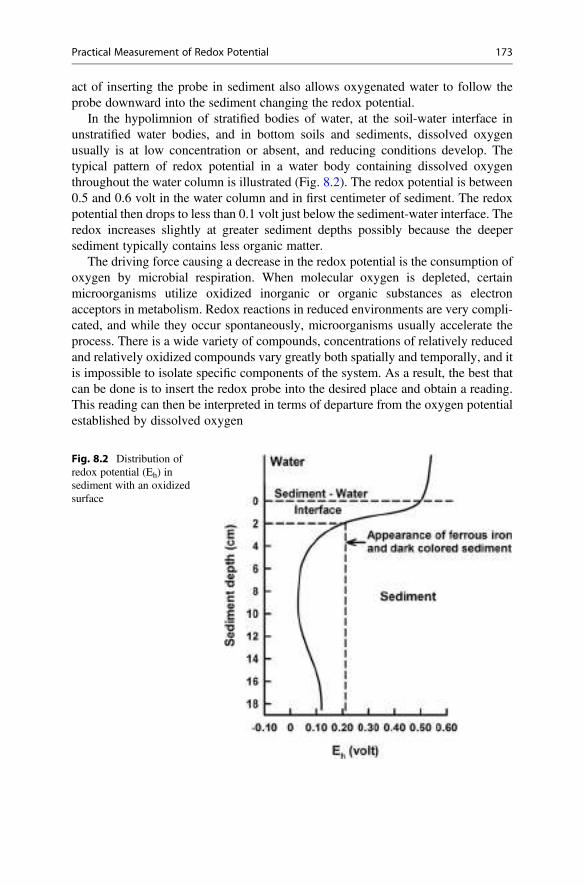
act of inserting the probe in sediment also allows oxygenated water to follow theprobe downward into the sediment changing the redox potential.

In the hypolimnion of stratified bodies of water, at the soil-water interface inunstratified water bodies, and in bottom soils and sediments, dissolved oxygenusually is at low concentration or absent, and reducing conditions develop. Thetypical pattern of redox potential in a water body containing dissolved oxygenthroughout the water column is illustrated (Fig. 8.2). The redox potential is between0.5 and 0.6 volt in the water column and in first centimeter of sediment. The redoxpotential then drops to less than 0.1 volt just below the sediment-water interface. Theredox increases slightly at greater sediment depths possibly because the deepersediment typically contains less organic matter.

The driving force causing a decrease in the redox potential is the consumption ofoxygen by microbial respiration. When molecular oxygen is depleted, certainmicroorganisms utilize oxidized inorganic or organic substances as electronacceptors in metabolism. Redox reactions in reduced environments are very compli-cated, and while they occur spontaneously, microorganisms usually accelerate theprocess. There is a wide variety of compounds, concentrations of relatively reducedand relatively oxidized compounds vary greatly both spatially and temporally, and itis impossible to isolate specific components of the system. As a result, the best thatcan be done is to insert the redox probe into the desired place and obtain a reading.This reading can then be interpreted in terms of departure from the oxygen potentialestablished by dissolved oxygen

Fig. 8.2 Distribution ofredox potential (Eh) insediment with an oxidizedsurface

Practical Measurement of Redox Potential 173

O2 aqð Þ þ 4Hþ þ 4e� ¼ 2H2O: ð8:17ÞAt 25 �C and pH 7, the oxygen potential in well-oxygenated water should be about0.802 volt (802 millivolts) against a standard hydrogen electrode (see Ex. 8.2). Theoxygen potential of well-oxygenated surface water is about 0.560 volt (560 millivolt)when measured with a KCl-saturated calomel electrode. Redox potential drops inanaerobic waters or soils, and values below �0.250 volt have been observed inhypolimnetic waters and in sediments.

Commercially available devices for measuring redox potential do not all providethe same reading for the redox potential of well-oxygenated water or for a sample ofreduced water or sediment. This makes it difficult to interpret redox potentialsmeasured in natural waters and sediments. Nevertheless, a decrease in the redoxpotential below values obtained in oxygen-saturated water with a particular instru-ment indicates that reducing conditions are developing, and the reducing ability ofthe environment increases as the redox potential drops. Care must be taken not tointroduce air or oxygenated water into the medium where redox potential is to bemeasured.

The presence of dissolved oxygen in water—even at low concentration—tends tostabilize the redox potential (Ex. 8.6). Thus, the oxygen potential (Eq. 8.17) is thestandard for comparing redox potential among different places in a water body andits sediment.

Ex. 8.6 The Eh of water at 25 �C and pH 7 will be calculated for dissolved oxygenconcentrations of 1, 2, 4, and 8 mg/L.

Solution:The molar concentration of dissolved oxygen can be computed by dividing

milligrams per liter values by 32,000 mg O2/mol:1 mg/L ¼ 10–4.5 M; 2 mg/L ¼ 10–4.2 M; 4 mg/L ¼ 10–3.9 M; 8 mg/L ¼ 10–3.6 M. Use the molar concentrationsof dissolved oxygen and a hydrogen ion concentration of 10�7 M (pH 7) to solve theexpression

Eh ¼ 1:27� 0:05924

log1

O2ð Þ Hþð Þ4:

Eh values are as follows: 1 mg/L ¼ 0.789 volt; 2 mg/L ¼ 0.793 volt; 4 mg/L ¼ 0.798 volt; 8 mg/L ¼ 0.802 volt. The corresponding readings for a calomelelectrode are 1 mg/L ¼ 0.547 volt; 2 mg/L ¼ 0.551 volt; 4 mg/L¼ 0.556 volt; 8 mg/L ¼ 0.560 volt.

It can be seen from Ex. 8.6 that an amount of dissolved oxygen as low as 1 mg/Lwill maintain Eh near 0.8 volt (near 0.56 volt for a calomel electrode). Naturalsystems do not become strongly reducing until dissolved oxygen is entirely depleted.


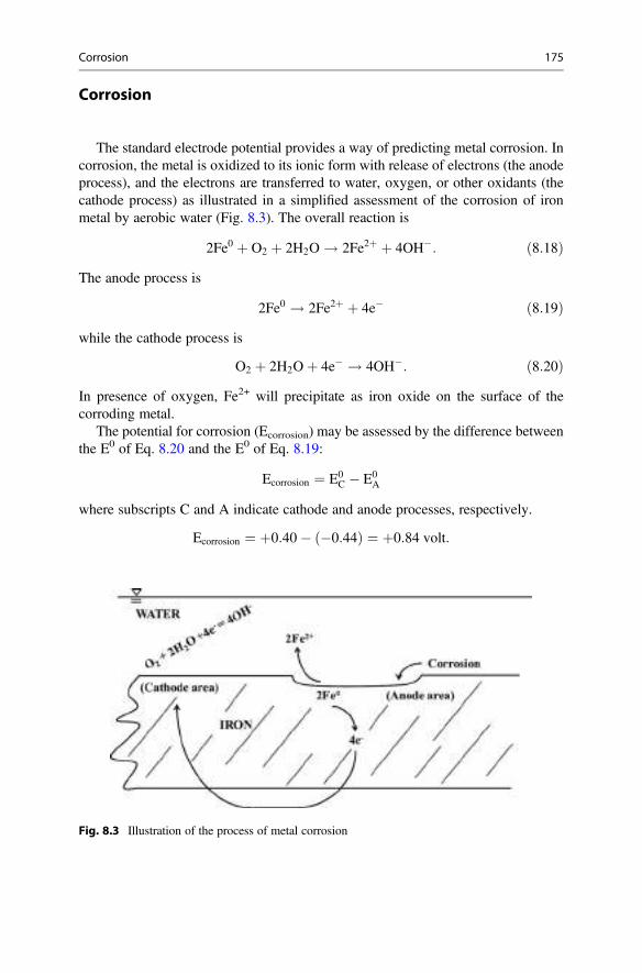
Corrosion

The standard electrode potential provides a way of predicting metal corrosion. Incorrosion, the metal is oxidized to its ionic form with release of electrons (the anodeprocess), and the electrons are transferred to water, oxygen, or other oxidants (thecathode process) as illustrated in a simplified assessment of the corrosion of ironmetal by aerobic water (Fig. 8.3). The overall reaction is

2Fe0 þ O2 þ 2H2O ! 2Fe2þ þ 4OH�: ð8:18ÞThe anode process is

2Fe0 ! 2Fe2þ þ 4e� ð8:19Þwhile the cathode process is

O2 þ 2H2Oþ 4e� ! 4OH�: ð8:20ÞIn presence of oxygen, Fe2+ will precipitate as iron oxide on the surface of thecorroding metal.

The potential for corrosion (Ecorrosion) may be assessed by the difference betweenthe E0 of Eq. 8.20 and the E0 of Eq. 8.19:

Ecorrosion ¼ E0C � E0

A

where subscripts C and A indicate cathode and anode processes, respectively.

Ecorrosion ¼ þ0:40� �0:44ð Þ ¼ þ0:84 volt:

Fig. 8.3 Illustration of the process of metal corrosion

Corrosion 175

The positive value for Ecorrosion indicates that the reaction is possible and thatcorrosion will occur under the specific conditions. Of course, this simple approachdoes not indicate the degree of corrosion that may be expected.

The corrosive potential of water is increased by lower pH, and highconcentrations of dissolved oxygen, carbon dioxide, and dissolved solids. Acidicwaters have more hydrogen ion to facilitate the cathode reaction, oxygen reacts withhydrogen gas at the cathode speeding up the reaction, carbon dioxide reduces pH,and higher dissolved solids concentration increases electrical conductivity. Bacteriaaction and presence of oxidants such as nitrate or chlorine also can acceleratecorrosion.

A common way of reducing corrosion of methods is to put a corrosion resistantcoating on the metal to protect it from contact with the environment, e.g., zinc or tincoating on steel, resins, plastics, paints, or greases. Another way is to reduce thecorrosiveness of the environment, e.g., removal of dissolved oxygen from water.There also are electrochemical means of lessening corrosion that will not bediscussed.

Conclusions

The redox potential is directly related to dissolved oxygen concentration. Whenthere is dissolved oxygen at concentrations above 1 or 2 mg/L, the redox potentialwill be high. The main value of the redox potential in aquatic ecology is forexplaining how oxidations and reductions occur in sediment-water systems. Theredox potential is difficult to measure, so it is not generally a useful variable in waterquality criteria for aquatic ecosystems. Of course, concepts from electrochemistrydiscussed above in relation to the redox potential are the basis for understanding andcontrolling corrosion of metal structures and devices so essential to human society.Redox potential also has far-reaching importance in analytical chemistry and manyindustrial processes.


Carbon Dioxide, pH, and Alkalinity 9

AbstractThe pH or negative logarithm of the hydrogen ion concentration is a mastervariable in water quality because the hydrogen ion influences many reactions.Because dissolved carbon dioxide is acidic, rainwater that is saturated with thisgas is naturally acidic—usually about pH 5.6. Limestone, calcium silicate, andfeldspars in soils and other geological formations dissolve through the action ofcarbon dioxide to increase the concentration of bicarbonate in water and raise thepH. The total concentration of titratable bases—usually bicarbonate and carbon-ate—expressed in milligrams per liter of calcium carbonate is the total alkalinity.Total alkalinity typically is less than 50 mg/L in waters of humid areas withhighly leached soils, but it is greater where soils are more fertile, limestoneformations are present, or the climate is arid. Alkalinity increases the availabilityof inorganic carbon for photosynthesis in waters of low to moderate pH. Waterbodies with moderate to high alkalinity are well-buffered against wide dailyswings in pH resulting from net removal of carbon dioxide by photosynthesisduring daytime and return of carbon dioxide to the water by respiratory process atnight when there is no photosynthesis. The optimum pH range for most aquaticorganisms is 6.5–8.5, and the acid and alkaline death points are around pH 4 andpH 11, respectively. Fish and other aquatic animals avoid high carbon dioxideconcentration, but 20 mg/L or more can be tolerated if there is plenty of dissolvedoxygen. The optimum alkalinity for aquatic life is between 50 and 150 mg/L.

Introduction

The pH is a master variable in water quality because many reactions are pHdependent. Normal waters contain both acids and bases and biological processestend to increase either acidity or basicity. The interactions among these opposingacidic and basic substances and processes determine pH. Carbon dioxide is particu-larly influential in regulating the pH of natural water. This dissolved gas is acidic,


177


and its concentration is in continual flux, because it is removed from water by aquaticplants for use in photosynthesis and released to the water by respiration of aquaticorganisms. The alkalinity of water results primarily from bicarbonate and carbonateions derived from the reaction of aqueous carbon dioxide with limestone and certainother minerals.

Alkalinity plays an important role in aquatic biology by increasing the availabilityof inorganic carbon for plants. It also tends to buffer water against excessive pHchange. A basic knowledge of the relationships among pH, carbon dioxide, andalkalinity is essential to an understanding of water quality.

pH

The Concept

The hydrogen ion (H+) is a naked nucleus, a proton with a high charge density. Aproton cannot exist in water, because it is attracted to the negatively-charged side ofwater molecules creating an ion pair known as the hydronium ion (H3O

+). Thedissociation of water can be written as H2O + H2O ¼ H3O

+ + OH�, but forsimplicity H3O

+ is replaced by H+ and the dissociation of water expressed as

H2O ¼ Hþ þ OH�: ð9:1ÞThe pH is an index of the hydrogen ion concentration (H+), and it is based on themass action expression of Eq. 8.1

Hþð Þ OH�ð ÞH2Oð Þ ¼ Kw: ð9:2Þ

The equilibrium constant (K) for water is usually written as Kw. Water dissociatesonly slightly and can be considered unity in Eq. 9.2 giving

Hþð Þ OH�ð Þ ¼ Kw: ð9:3ÞWater dissociates into equal numbers of hydrogen and hydroxyl (OH�) ions;hydrogen ion can be substituted into Eq. 9.3 to obtain

Hþð Þ Hþð Þ ¼ Kw:

The hydrogen ion concentration is the square root of Kw

Hþð Þ ¼ffiffiffiffiffiffiffiffiKw:

pð9:4Þ

Of course, the hydroxyl ion concentration is related to hydrogen ion concentration

178 9 Carbon Dioxide, pH, and Alkalinity

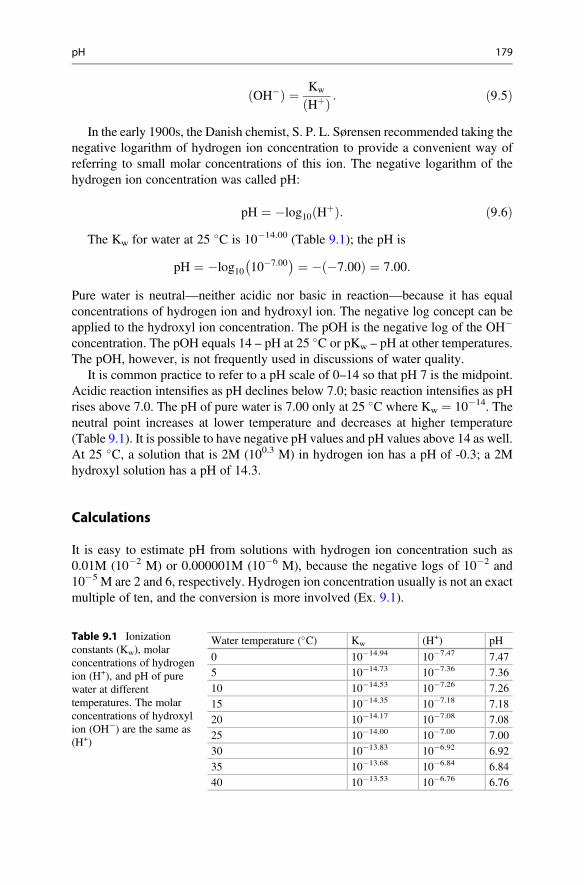
https://doi.org/10.1007/978-3-030-23335-8_8#Equ1

OH�ð Þ ¼ Kw

Hþð Þ : ð9:5Þ

In the early 1900s, the Danish chemist, S. P. L. Sørensen recommended taking thenegative logarithm of hydrogen ion concentration to provide a convenient way ofreferring to small molar concentrations of this ion. The negative logarithm of thehydrogen ion concentration was called pH:

pH ¼ �log10 Hþð Þ: ð9:6ÞThe Kw for water at 25 �C is 10�14.00 (Table 9.1); the pH is

pH ¼ �log10 10�7:00� � ¼ � �7:00ð Þ ¼ 7:00:

Pure water is neutral—neither acidic nor basic in reaction—because it has equalconcentrations of hydrogen ion and hydroxyl ion. The negative log concept can beapplied to the hydroxyl ion concentration. The pOH is the negative log of the OH�

concentration. The pOH equals 14 – pH at 25 �C or pKw – pH at other temperatures.The pOH, however, is not frequently used in discussions of water quality.

It is common practice to refer to a pH scale of 0–14 so that pH 7 is the midpoint.Acidic reaction intensifies as pH declines below 7.0; basic reaction intensifies as pHrises above 7.0. The pH of pure water is 7.00 only at 25 �C where Kw ¼ 10�14. Theneutral point increases at lower temperature and decreases at higher temperature(Table 9.1). It is possible to have negative pH values and pH values above 14 as well.At 25 �C, a solution that is 2M (100.3 M) in hydrogen ion has a pH of -0.3; a 2Mhydroxyl solution has a pH of 14.3.

Calculations

It is easy to estimate pH from solutions with hydrogen ion concentration such as0.01M (10�2 M) or 0.000001M (10�6 M), because the negative logs of 10�2 and10�5 M are 2 and 6, respectively. Hydrogen ion concentration usually is not an exactmultiple of ten, and the conversion is more involved (Ex. 9.1).

Table 9.1 Ionizationconstants (Kw), molarconcentrations of hydrogenion (H+), and pH of purewater at differenttemperatures. The molarconcentrations of hydroxylion (OH�) are the same as(H+)

Water temperature (�C) Kw (H+) pH

0 10�14.94 10�7.47 7.47

5 10�14.73 10�7.36 7.36

10 10�14.53 10�7.26 7.26

15 10�14.35 10�7.18 7.18

20 10�14.17 10�7.08 7.08

25 10�14.00 10�7.00 7.00

30 10�13.83 10�6.92 6.92

35 10�13.68 10�6.84 6.84

40 10�13.53 10�6.76 6.76

pH 179

Ex. 9.1 The pH of water 0.002M in hydrogen ion concentration will be calculated.Solution:

0:002M ¼ 2� 10�3 M

pH ¼ �log10 Hþð Þ ¼ � log102þ log1010�3

� � ¼ � 0:301þ �3ð Þ½ � ¼ 2:70:

The pH scale is logarithmic; a solution of pH 6 has a ten times greater hydrogenion concentration than does a water of pH 7. This brings us to the question of how toaverage pH values. The pH of a solution made by mixing 1 L each of solutions withpH 2, 4, and 6 is not 4; it is 2.47 as illustrated in Ex. 9.2.

Ex. 9.2 The pH resulting from mixing 1-L each of solutions with pH values of 2, 4,and 6 will be calculated.

Solution:

pH mol H+ in 1.0 L2 0.014 0.00016 0.000001Sum 0.010101 mol H+ in 3.0 L

Average ¼ 0:010101 mol Hþ

3 L¼ 3:37� 10�3 mol Hþ=L

pH ¼ �log10 3:37� 10�3� � ¼ � 0:53þ �3ð Þ½ � ¼ 2:47:

Averaging pH directly would give an erroneous pH of 4.0.

The illustration of pH averaging (Ex. 9.2) appears to be mathematically correctand totally obvious. However, while the method is obligatory for calculating theresulting average pH of mixing solutions of different pH, the method is incorrect inmost water quality applications (Boyd et al. 2011). The averaging of hydrogen ionconcentration will not provide the correct average pH, because buffers present innatural waters have a greater effect on final pH than does dilution alone. When datasets are transformed to hydrogen ion to estimate average pH, extreme pH values willdistort the average pH. Values of pH conform more closely to a normal distributionthan do hydrogen ion concentrations, making pH values more acceptable for use instatistical analyses. Electrochemical measurements of pH and many biologicalresponses to hydrogen ion concentration are described by the Nernst equation thatstates that the measured or observed response is linearly related to 10-fold changes inhydrogen ion concentration. Moreover, and possibly most important, is that in mostapplications, the relationships between pH and other variables are reported as theobserved effect of measured pH—not H+ concentration—on the response of theother variables. The use of direct pH averaging is definitely correct in most waterquality applications, so please be confident in yourself when rebuked for doing so.


pH of Natural Waters

The technique for measuring pH with a glass electrode was commercialized 1936,and the measurement of environmental pH is common. There have been millions ofpH measurements in all kinds of natural waters, and values as low as 1 and as high as13 have been reported.

Waters in humid areas with highly leached soils tend to have lower pH thanwaters in areas with limestone formations or those in semi-arid or arid regions. But,most natural waters have pH within the 6 to 9 range.

Waters that have high concentrations of humic substances tend to have a low pHbecause of acidic groups on the humic molecules as illustrated by the equation belowin which R represents the organic (humic) moiety:

RCOOH ¼ RCOO� þ Hþ: ð9:7ÞFor example, waters in rivers flowing from South American jungles may have pHvalues of 4–4.5. Low pH from organic acids is not as harmful to aquatic organisms aslow pH caused by strong, mineral acids. Moreover, species living in rivers flowingfrom jungle areas are more tolerant to low pH than organisms in other waters.

Carbon Dioxide

The atmosphere contains an average carbon dioxide concentration of roughly0.040%, and raindrops become saturated with carbon dioxide while falling to theground. The equilibrium concentrations of carbon dioxide in water of differenttemperatures and salinity were provided in Table 7.8.

Dissolved carbon dioxide reacts with water forming carbonic acid (H2CO3)

CO2 þ H2O Ð H2CO3 K ¼ 10�2:75: ð9:8ÞCarbonic acid is a diprotic acid

H2CO3 Ð Hþ þ HCO�3 K1 ¼ 10�3:6 ð9:9Þ

HCO�3 Ð Hþ þ CO2�

3 K2 ¼ 10�10:33: ð9:10ÞThe second dissociation may be ignored here, because, as explained later, it is notsignificant at pH less than 8.3.

Only a small fraction of dissolved carbon dioxide reacts with water. UsingEq. 9.8, it can be seen that the ratio (H2CO3):(CO2) will be 0.00178:1:

Carbon Dioxide 181

H2CO3ð ÞCO2ð Þ ¼ 10�2:75 ¼ 0:00178:

The carbonic acid concentration at equilibrium will be only 0.18% of the carbondioxide concentration. Although carbonic acid is a strong acid, little of it is present inwater at equilibrium with atmospheric carbon dioxide. Moreover, common analyti-cal procedures cannot distinguish carbonic acid from carbon dioxide.

A dilemma is avoided by considering the analytical carbon dioxide as a weak acidand deriving an apparent reaction and equilibrium constant for the acidic reaction ofcarbon dioxide in water. Multiplication of the equilibrium expressions of Eqs. 9.8and 9.9 gives

H2CO3ð ÞCO2ð Þ � HCO�

3

� �Hþð Þ

H2CO3ð Þ ¼ 10�2:75 � 10�3:6

HCO�3

� �Hþð Þ

CO2ð Þ ¼ 10�6:35:

The apparent equilibrium expression derived above typically is used to explain thereaction of carbon dioxide with water as given below:

CO2 þ H2O Ð Hþ þ HCO�3 K ¼ 10�6:35: ð9:11Þ

In Chap. 4, it was illustrated that the K for any reaction can be estimated fromΔGo using Eq. 4.11. The K for Eq. 9.11 estimated from ΔGo is 10�6.356

—essentiallythe same value derived above by combining Eqs. 9.8 and 9.9 through multiplication.

The pH of rainwater not contaminated with acids stronger than carbon dioxide isaround 5.6, and carbon dioxide normally will not lower the pH of water below 4.5.The two points will be illustrated in Exs. 9.3 and 9.4.

Ex. 9.3 The pH of rainwater saturated with carbon dioxide at 25 �C will beestimated.

Solution:From Table 7.8, the carbon dioxide concentration in rainwater is 0.57 mg/L

(10�4.89M). Using Eq. 9.11,

Hþð Þ HCO�3

� �CO2ð Þ ¼ 10�6:35

but Hþð Þ ¼ HCO�3

� �


https://doi.org/10.1007/978-3-030-23335-8_4#Equ11

and Hþð Þ2 ¼ 10�6:35� �

CO2ð Þ:

Thus, Hþð Þ2 ¼ 10�6:35� �

10�4:89� � ¼ 10�11:24

Hþð Þ ¼ 10�5:62

pH ¼ 5:62:

Rainwater with a lower pH contains an acid stronger than carbon dioxide asdiscussed in Chap. 10.

Ex. 9.4 Water from a well contains 100 mg/L (10�2.64 M ) carbon dioxide. The pHwill be determined using Eq. 9.11.

Solution:As shown above in Ex. 9.3,

Hþð Þ2 ¼ 10�6:35� �

10�2:64� �

CO2ð Þ:For a water with 10�2.64 M CO2, we have (H

+)2 ¼ (10�6.35)(10�2.64) ¼ 10�9.99,

Hþð Þ ¼ 10�4:50

pH ¼ 4:5:

Although carbon dioxide concentrations up to 650 mg/L have been reported innatural water bodies (Stone et al. 2018), few natural waters contain more than100 mg/L of carbon dioxide. It follows that a pH below 4.5 suggests that a watercontains a stronger acid than carbon dioxide. In surface waters, the most commonstrong acid is sulfuric acid that originates from deposits of iron pyrite that may beexposed to the air and oxidize resulting in sulfuric acid (see Chap. 11). Rainwatermay contain sulfuric and other strong acids as a result of air pollution.

Natural waters may contain more carbon dioxide than suggested by equilibriumconcentrations provided in Table 7.8. This is because most waters contain morebicarbonate than that resulting from the reaction of carbon dioxide and water(Eq. 9.11). There is an equilibrium among H+, HCO3

�, and CO2, and at a giventemperature and pH, as the HCO3

� concentration increases, the water can hold moreCO2 at equilibrium. For example, the equilibrium CO2 concentrations at 25 �C andpH 7 in water with 61 mg/L (10�3 M) HCO3

� would be 9.85, but it would be27.8 mg/L in water with 122 mg/L (10�2.55 M) HCO3

�. In pure water, the equilib-rium concentration at 25 �C is 0.57 mg/L (Table 7.8).

Carbon Dioxide 183

Total Alkalinity

The total alkalinity of water is defined as the total concentration of titratable basesexpressed as calcium carbonate (CaCO3). Calcium carbonate is the basis forexpressing alkalinity, because it is commonly added to increase the pH and alkalinityof acidic water. Calcium carbonate also is the substance that precipitates from somewaters when they are boiled as will be discussed in Chap. 10.

Examination of Eq. 9.11 reveals that bicarbonate results from the reaction ofcarbon dioxide with water. At equilibrium with atmospheric carbon dioxide, theconcentrations of H+ and HCO3

� in unpolluted rainwater or other relatively purewater are both 10�5.62 M (Ex. 9.3). This molar concentration of HCO3

� is equal to0.144 mg/L. The ratio of equivalent weights of CaCO3 to HCO3

� is 50/61, and thetotal alkalinity concentration would be 0.118 mg/L as CaCO3. At a carbon dioxideconcentration of 100 mg/L (Ex. 9.4) the total alkalinity in pure water would be only1.58 mg/L as CaCO3. Such low concentrations are essentially undetectable analyti-cally, and carbon dioxide is not a direct source of alkalinity. Moreover, (H+) ¼(HCO3

�) in pure water, and the acidity of the water (see Chap. 11) would be thesame as the alkalinity.

Carbon dioxide increases the dissolution of limestone and certain other mineralsin soils and other geological formations imparting bicarbonate (and carbonate) tonatural waters. Concentrations of total alkalinity usually range between 5 and300 mg/L in freshwaters. Although alkalinity often results almost entirely frombicarbonate and carbonate, some waters—especially polluted ones—contain appre-ciable amounts of hydroxide, ammonia, phosphate, borate, or other bases thatcontribute alkalinity. The reactions of selected bases in neutralizing acidity areillustrated below:

OH� þ Hþ Ð H2O

CO2�3 þ Hþ Ð HCO�

3

HCO�3 þ Hþ Ð CO2 þ H2O

NH3 þ Hþ Ð NHþ4

PO3�4 þ Hþ ¼ HPO�

4

HPO�4 þ Hþ Ð H2PO

�4

H2BO�4 þ Hþ Ð H3BO4

H3SiO�4 þ Hþ Ð H4SiO4


RCOO� þ Hþ Ð RCOOH:

Bicarbonate and carbonate usually comprise most of the alkalinity in natural waters,but in some cases, other ions may contribute significantly to alkalinity. For example,Snoeyink and Jenkins (1980) presented an example from a major water supply to theBay Area in California that originates in the Sierra Nevada Mountains where rockformations are rich in silicate minerals. The water has 20 mg/L alkalinity of which4 mg/L is the result of silicic acid.

Alkalinity sometimes is described by the expression

Alkalinity ¼ HCO�3

� �þ 2 CO2�3

� �þ OH�ð Þ � Hþð Þ ð9:12Þwhere the ions are entered in moles/L.

Ex. 9.5 The alkalinity of a water sample with pH ¼ 9 (H+ ¼ 10�9 M; OH� ¼ 10�5

M) that contains 61 mg/L HCO3� (10�3 m) and 30 mg/L CO3

2� (5� 10�4 M) will becalculated.

Solution:

Alkalinity¼ 10�3 M HCO�3

� �þ 2 5� 10�4 M CO2�3

� �þ 10�5 M OH�� 10�9 M Hþ� �¼ 0:001M þ 0:001M þ 0:00001Mð Þ � 0:000000001Mð Þ¼ 0:00201M:

It would require 0.00201 M of H+ to neutralize 0.00201 M alkalinity, and molarityand normality are the same for H+.

Alkalinity is expressed as equivalent CaCO3 and it takes 2 mol H+ to neutralize1 mol of CaCO3, e.g., CaCO3 + 2H+ ¼ Ca2+ + CO2 + H2O (1 mol CaCO3 ¼2 equivalents CaCO3).

And, 0.00201 eq H+� 50.04 g CaCO3/eq¼ 0.10058 g/L (100.58 mg/L) alkalinityas CaCO3.

Measurement of Alkalinity

The expression (Eq. 9.12) illustrates the concept of alkalinity, but it does not providea practical way of estimating the alkalinity of natural waters. Total alkalinity isdetermined by titration of a water sample with standard sulfuric or hydrochloric acid(Eaton et al. 2005). The measurement traditionally was done by titration with0.020 N acid to the methyl orange endpoint—the color of methyl orange changesfrom yellow to faint orange at pH 4.4. However, the pH in the water sample at theend of the titration is influenced by the amount of carbon dioxide produced in thereaction between acid and bicarbonate (HCO3

� + H+! CO2 + H2O), and samples ofhigher alkalinity will be at a lower pH when bicarbonate has been neutralized thanwill samples of lower alkalinity.

Total Alkalinity 185

In the situation where all of the alkalinity in a sample is from bicarbonate, themaximum amount of carbon dioxide will be liberated per milligram per liter ofalkalinity during titration. Assuming total alkalinity concentrations of 30, 150, and500 mg/L and using the ratio 2HCO3

�:CaCO3 (122:100), the carbon dioxide at thetitration endpoint (assuming no loss by diffusion to the air) would be 36.6, 183, and610 mg/L or 10�3.08, 10�4.36, and 10�4.10 M, respectively. With Eq. 9.11, it can beshown the potential pH at the endpoint would be 4.72, 4.36, and 4.10, for 30, 150,and 500 mg/L total alkalinity respectively. Of course, some carbon dioxide is lost tothe air during titration. Taras et al. (1971) recommended the following endpoint pHsfor different alkalinities: <30 mg/L, 5.1; 30–500 mg/L, 4.8; >500 mg/L, 4.5. Eatonet al. (2005) revised these recommendations to pHs of 4.9, 4.6, and 4.3 at alkalinitiesof 30, 150, 500 mg/L, respectively—roughly 0.2 pH units more than potential pHscalculated above.

Mixed bromocresol green-methyl red indicator can be used to detect pH 5.1 and4.8, while methyl orange can be used to signal pH 4.5, but many analysts prefer touse a pH electrode to detect the endpoint. For routine titrations, pH 4.5 often is usedas the endpoint for samples of all concentrations of total alkalinity.

The measurement and calculation of total alkalinity are illustrated in Ex. 9.6.

Ex. 9.6 A 100-mL water sample is titrated with 0.0210 N sulfuric acid to anendpoint of pH 4.5. The titration consumes 18.75 mL of sulfuric acid. The totalalkalinity will be calculated.

Solution:The milliequivalent quantity of alkalinity or CaCO3 equals the milliequivalent

amount of acid used in the titration:

18:75 mLð Þ 0:0210 Nð Þ ¼ 0:394 meq CaCO3: Note : N ¼ meq=mLð ÞThe weight of equivalent CaCO3 is

0:394 meqð Þ 50:04 mg CaCO3=meqð Þ ¼ 19:72 mg CaCO3:

To convert to milligrams per liter,

19:72 mg CaCO3 � 1000 mL=L

100 mL sample¼ 197:2 mg=L:

In water samples with pH <8.3, the alkalinity is typically considered to be frombicarbonate alone. Samples with a pH >8.3 usually contain both carbonate andbicarbonate, but if the pH is especially high, bicarbonate may be absent. Suchsamples may contain carbonate only, carbonate and hydroxide, or hydroxide only.Phenolphthalein indicator is pink above pH 8.3 and colorless at lower pH and maybe used in samples with pH >8.3 to separate the total alkalinity titration into twosteps: determination of the volume of acid needed to decrease pH to 8.3 andcontinuation of the titration to pH 4.5 (or other selected endpoint) to determine thetotal volume of acid needed to neutralize all base in the sample. The first step


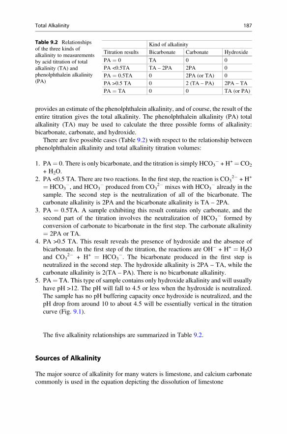
provides an estimate of the phenolphthalein alkalinity, and of course, the result of theentire titration gives the total alkalinity. The phenolphthalein alkalinity (PA) totalalkalinity (TA) may be used to calculate the three possible forms of alkalinity:bicarbonate, carbonate, and hydroxide.

There are five possible cases (Table 9.2) with respect to the relationship betweenphenolphthalein alkalinity and total alkalinity titration volumes:

1. PA¼ 0. There is only bicarbonate, and the titration is simply HCO3� + H+¼ CO2

+ H2O.2. PA <0.5 TA. There are two reactions. In the first step, the reaction is CO3

2� + H+

¼ HCO3�, and HCO3

� produced from CO32� mixes with HCO3

� already in thesample. The second step is the neutralization of all of the bicarbonate. Thecarbonate alkalinity is 2PA and the bicarbonate alkalinity is TA – 2PA.

3. PA ¼ 0.5TA. A sample exhibiting this result contains only carbonate, and thesecond part of the titration involves the neutralization of HCO3

� formed byconversion of carbonate to bicarbonate in the first step. The carbonate alkalinity¼ 2PA or TA.

4. PA >0.5 TA. This result reveals the presence of hydroxide and the absence ofbicarbonate. In the first step of the titration, the reactions are OH� + H+ ¼ H2Oand CO3

2� + H+ ¼ HCO3�. The bicarbonate produced in the first step is

neutralized in the second step. The hydroxide alkalinity is 2PA – TA, while thecarbonate alkalinity is 2(TA – PA). There is no bicarbonate alkalinity.

5. PA¼ TA. This type of sample contains only hydroxide alkalinity and will usuallyhave pH >12. The pH will fall to 4.5 or less when the hydroxide is neutralized.The sample has no pH buffering capacity once hydroxide is neutralized, and thepH drop from around 10 to about 4.5 will be essentially vertical in the titrationcurve (Fig. 9.1).

The five alkalinity relationships are summarized in Table 9.2.

Sources of Alkalinity

The major source of alkalinity for many waters is limestone, and calcium carbonatecommonly is used in the equation depicting the dissolution of limestone

Table 9.2 Relationshipsof the three kinds ofalkalinity to measurementsby acid titration of totalalkalinity (TA) andphenolphthalein alkalinity(PA)

Kind of alkalinity

Titration results Bicarbonate Carbonate Hydroxide

PA ¼ 0 TA 0 0

PA <0.5TA TA – 2PA 2PA 0

PA ¼ 0.5TA 0 2PA (or TA) 0

PA >0.5 TA 0 2 (TA – PA) 2PA – TA

PA ¼ TA 0 0 TA (or PA)


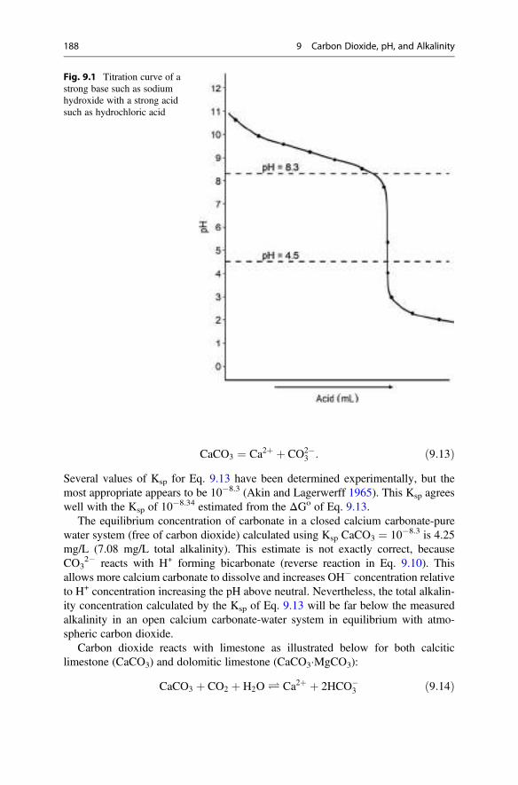
CaCO3 ¼ Ca2þ þ CO2�3 : ð9:13Þ

Several values of Ksp for Eq. 9.13 have been determined experimentally, but themost appropriate appears to be 10�8.3 (Akin and Lagerwerff 1965). This Ksp agreeswell with the Ksp of 10

�8.34 estimated from the ΔGo of Eq. 9.13.The equilibrium concentration of carbonate in a closed calcium carbonate-pure

water system (free of carbon dioxide) calculated using Ksp CaCO3 ¼ 10�8.3 is 4.25mg/L (7.08 mg/L total alkalinity). This estimate is not exactly correct, becauseCO3

2� reacts with H+ forming bicarbonate (reverse reaction in Eq. 9.10). Thisallows more calcium carbonate to dissolve and increases OH� concentration relativeto H+ concentration increasing the pH above neutral. Nevertheless, the total alkalin-ity concentration calculated by the Ksp of Eq. 9.13 will be far below the measuredalkalinity in an open calcium carbonate-water system in equilibrium with atmo-spheric carbon dioxide.

Carbon dioxide reacts with limestone as illustrated below for both calciticlimestone (CaCO3) and dolomitic limestone (CaCO3�MgCO3):

CaCO3 þ CO2 þ H2O Ð Ca2þ þ 2HCO�3 ð9:14Þ

Fig. 9.1 Titration curve of astrong base such as sodiumhydroxide with a strong acidsuch as hydrochloric acid


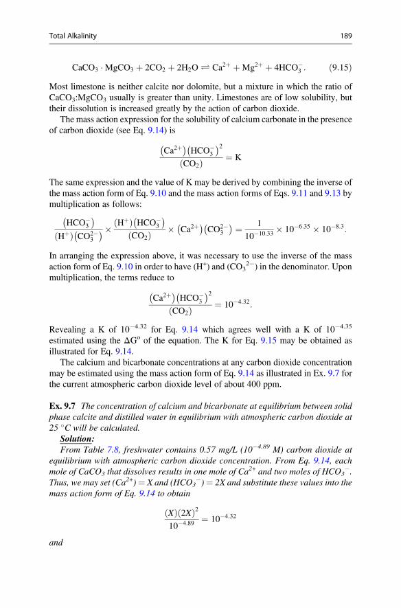
CaCO3 �MgCO3 þ 2CO2 þ 2H2O Ð Ca2þ þMg2þ þ 4HCO�3 : ð9:15Þ

Most limestone is neither calcite nor dolomite, but a mixture in which the ratio ofCaCO3:MgCO3 usually is greater than unity. Limestones are of low solubility, buttheir dissolution is increased greatly by the action of carbon dioxide.

The mass action expression for the solubility of calcium carbonate in the presenceof carbon dioxide (see Eq. 9.14) is

Ca2þ� �

HCO�3

� �2CO2ð Þ ¼ K

The same expression and the value of K may be derived by combining the inverse ofthe mass action form of Eq. 9.10 and the mass action forms of Eqs. 9.11 and 9.13 bymultiplication as follows:

HCO�3

� �Hþð Þ CO2�

3

� �� Hþð Þ HCO�3

� �CO2ð Þ � Ca2þ

� �CO2�

3

� � ¼ 1

10�10:33 � 10�6:35 � 10�8:3:

In arranging the expression above, it was necessary to use the inverse of the massaction form of Eq. 9.10 in order to have (H+) and (CO3

2�) in the denominator. Uponmultiplication, the terms reduce to

Ca2þ� �

HCO�3

� �2CO2ð Þ ¼ 10�4:32:

Revealing a K of 10�4.32 for Eq. 9.14 which agrees well with a K of 10�4.35

estimated using the ΔGo of the equation. The K for Eq. 9.15 may be obtained asillustrated for Eq. 9.14.

The calcium and bicarbonate concentrations at any carbon dioxide concentrationmay be estimated using the mass action form of Eq. 9.14 as illustrated in Ex. 9.7 forthe current atmospheric carbon dioxide level of about 400 ppm.

Ex. 9.7 The concentration of calcium and bicarbonate at equilibrium between solidphase calcite and distilled water in equilibrium with atmospheric carbon dioxide at25 �C will be calculated.

Solution:From Table 7.8, freshwater contains 0.57 mg/L (10�4.89 M) carbon dioxide at

equilibrium with atmospheric carbon dioxide concentration. From Eq. 9.14, eachmole of CaCO3 that dissolves results in one mole of Ca

2+ and two moles of HCO3�.

Thus, we may set (Ca2+)¼ X and (HCO3�)¼ 2X and substitute these values into the

mass action form of Eq. 9.14 to obtain

Xð Þ 2Xð Þ210�4:89 ¼ 10�4:32

and


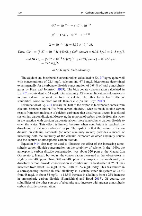
4X3 ¼ 10�9:21 ¼ 6:17� 10�10

X3 ¼ 1:54� 10�10 ¼ 10�9:81

X ¼ 10�3:27 M ¼ 5:37� 10�4 M:

Thus, Ca2þ ¼ 5:37� 10�4 M� �

40:08 g Ca2þ=mole� � ¼ 0:0215g=L ¼ 21:5 mg=L

and HCO�3 ¼ 5:37� 10�4 M

� �2ð Þ 61 g HCO�

3 =mole� � ¼ 0:0655 g=L

¼ 65:5 mg=L

or 53:6 mg=L total alkalinity:

The calcium and bicarbonate concentrations calculated in Ex. 9.7 agree quite wellwith concentrations of 22.4 mg/L calcium and 67.1 mg/L bicarbonate determinedexperimentally for a carbonate dioxide concentration of 0.04% of total atmosphericgases by Frear and Johnston (1929). The bicarbonate concentration calculated inEx. 9.7 is equivalent to 54 mg/L total alkalinity. Of course, limestone seldom existsas pure calcium carbonate in form of calcite. The other forms have differentsolubilities, some are more soluble than calcite (Sá and Boyd 2017).

Examination of Eq. 9.14 reveals that half of the carbon in bicarbonate comes fromcalcium carbonate and half is from carbon dioxide. Twice as much soluble carbonresults from each molecule of calcium carbonate that dissolves as occurs in a closedsystem (no carbon dioxide). Moreover, the removal of carbon dioxide from the waterin the reaction with calcium carbonate allows more atmospheric carbon dioxide toenter the water. This effect is limited, because when equilibrium is reached, thedissolution of calcium carbonate stops. The upshot is that the action of carbondioxide on calcium carbonate (or other alkalinity source) provides a means ofincreasing both the solubility of the calcium carbonate or other alkalinity sourceand the capture of atmospheric carbon dioxide.

Equation 9.14 also may be used to illustrate the effect of the increasing atmo-spheric carbon dioxide concentration on the solubility of calcite. In the 1960s, theatmospheric carbon dioxide concentration was about 320 ppm at the Mauna LoaObservatory, Hawaii, but today, the concentration measured at that observatory isslightly over 400 ppm. Using 320 and 400 ppm of atmospheric carbon dioxide, thedissolved carbon dioxide concentration at equilibrium in freshwater at 25 �C hasincreased from about 0.42 mg/L in the 1960s to 0.57 mg/L today. This has resulted ina corresponding increase in total alkalinity in a calcite-water-air system at 25 �Cfrom 48 mg/L to about 54 mg/L—a 12.5% increase in alkalinity from a 25% increasein atmospheric carbon dioxide (Somridhivej and Boyd 2017). Of course, thesolubilities of the other sources of alkalinity also increase with greater atmosphericcarbon dioxide concentration.


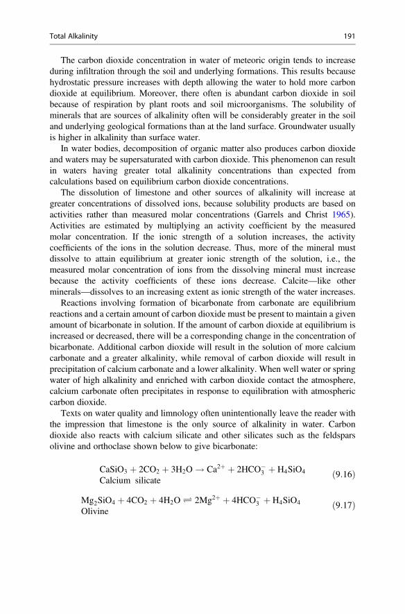
The carbon dioxide concentration in water of meteoric origin tends to increaseduring infiltration through the soil and underlying formations. This results becausehydrostatic pressure increases with depth allowing the water to hold more carbondioxide at equilibrium. Moreover, there often is abundant carbon dioxide in soilbecause of respiration by plant roots and soil microorganisms. The solubility ofminerals that are sources of alkalinity often will be considerably greater in the soiland underlying geological formations than at the land surface. Groundwater usuallyis higher in alkalinity than surface water.

In water bodies, decomposition of organic matter also produces carbon dioxideand waters may be supersaturated with carbon dioxide. This phenomenon can resultin waters having greater total alkalinity concentrations than expected fromcalculations based on equilibrium carbon dioxide concentrations.

The dissolution of limestone and other sources of alkalinity will increase atgreater concentrations of dissolved ions, because solubility products are based onactivities rather than measured molar concentrations (Garrels and Christ 1965).Activities are estimated by multiplying an activity coefficient by the measuredmolar concentration. If the ionic strength of a solution increases, the activitycoefficients of the ions in the solution decrease. Thus, more of the mineral mustdissolve to attain equilibrium at greater ionic strength of the solution, i.e., themeasured molar concentration of ions from the dissolving mineral must increasebecause the activity coefficients of these ions decrease. Calcite—like otherminerals—dissolves to an increasing extent as ionic strength of the water increases.

Reactions involving formation of bicarbonate from carbonate are equilibriumreactions and a certain amount of carbon dioxide must be present to maintain a givenamount of bicarbonate in solution. If the amount of carbon dioxide at equilibrium isincreased or decreased, there will be a corresponding change in the concentration ofbicarbonate. Additional carbon dioxide will result in the solution of more calciumcarbonate and a greater alkalinity, while removal of carbon dioxide will result inprecipitation of calcium carbonate and a lower alkalinity. When well water or springwater of high alkalinity and enriched with carbon dioxide contact the atmosphere,calcium carbonate often precipitates in response to equilibration with atmosphericcarbon dioxide.

Texts on water quality and limnology often unintentionally leave the reader withthe impression that limestone is the only source of alkalinity in water. Carbondioxide also reacts with calcium silicate and other silicates such as the feldsparsolivine and orthoclase shown below to give bicarbonate:

CaSiO3 þ 2CO2 þ 3H2O ! Ca2þ þ 2HCO�3 þ H4SiO4

Calcium silicateð9:16Þ

Mg2SiO4 þ 4CO2 þ 4H2O Ð 2Mg2þ þ 4HCO�3 þ H4SiO4

Olivineð9:17Þ


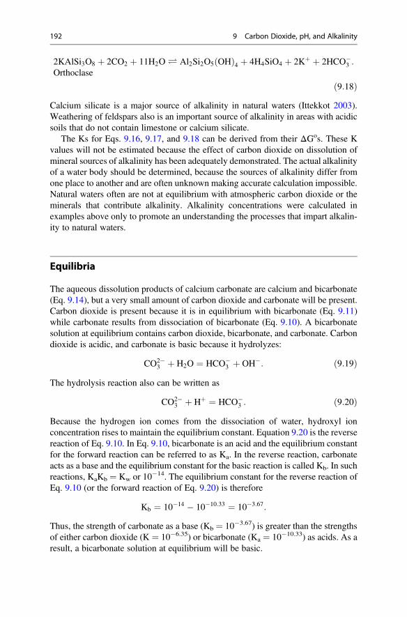
2KAlSi3O8 þ 2CO2 þ 11H2O Ð Al2Si2O5 OHð Þ4 þ 4H4SiO4 þ 2Kþ þ 2HCO�3 :

Orthoclase

ð9:18ÞCalcium silicate is a major source of alkalinity in natural waters (Ittekkot 2003).Weathering of feldspars also is an important source of alkalinity in areas with acidicsoils that do not contain limestone or calcium silicate.

The Ks for Eqs. 9.16, 9.17, and 9.18 can be derived from their ΔGos. These Kvalues will not be estimated because the effect of carbon dioxide on dissolution ofmineral sources of alkalinity has been adequately demonstrated. The actual alkalinityof a water body should be determined, because the sources of alkalinity differ fromone place to another and are often unknown making accurate calculation impossible.Natural waters often are not at equilibrium with atmospheric carbon dioxide or theminerals that contribute alkalinity. Alkalinity concentrations were calculated inexamples above only to promote an understanding the processes that impart alkalin-ity to natural waters.

Equilibria

The aqueous dissolution products of calcium carbonate are calcium and bicarbonate(Eq. 9.14), but a very small amount of carbon dioxide and carbonate will be present.Carbon dioxide is present because it is in equilibrium with bicarbonate (Eq. 9.11)while carbonate results from dissociation of bicarbonate (Eq. 9.10). A bicarbonatesolution at equilibrium contains carbon dioxide, bicarbonate, and carbonate. Carbondioxide is acidic, and carbonate is basic because it hydrolyzes:

CO2�3 þ H2O ¼ HCO�

3 þ OH�: ð9:19ÞThe hydrolysis reaction also can be written as

CO2�3 þ Hþ ¼ HCO�

3 : ð9:20ÞBecause the hydrogen ion comes from the dissociation of water, hydroxyl ionconcentration rises to maintain the equilibrium constant. Equation 9.20 is the reversereaction of Eq. 9.10. In Eq. 9.10, bicarbonate is an acid and the equilibrium constantfor the forward reaction can be referred to as Ka. In the reverse reaction, carbonateacts as a base and the equilibrium constant for the basic reaction is called Kb. In suchreactions, KaKb ¼ Kw or 10�14. The equilibrium constant for the reverse reaction ofEq. 9.10 (or the forward reaction of Eq. 9.20) is therefore

Kb ¼ 10�14 � 10�10:33 ¼ 10�3:67:

Thus, the strength of carbonate as a base (Kb ¼ 10�3.67) is greater than the strengthsof either carbon dioxide (K ¼ 10�6.35) or bicarbonate (Ka ¼ 10�10.33) as acids. As aresult, a bicarbonate solution at equilibrium will be basic.


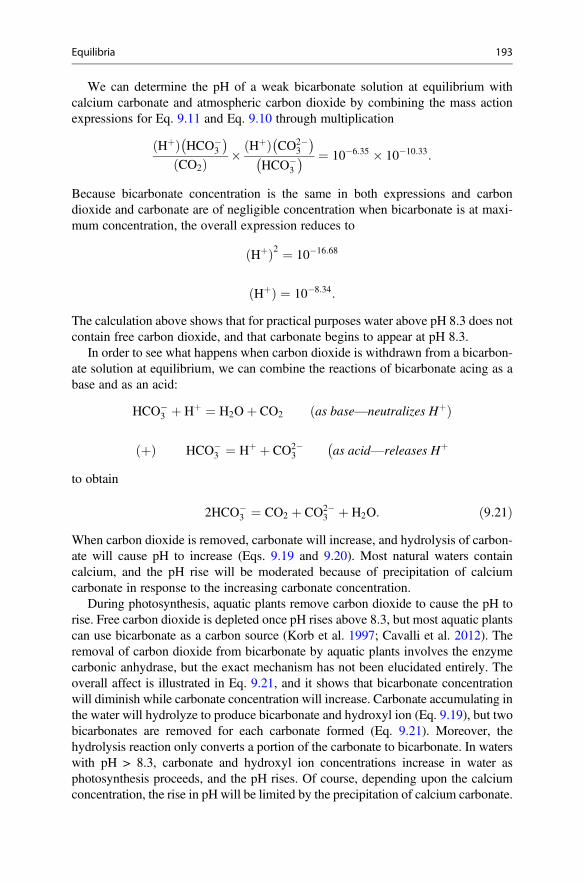
We can determine the pH of a weak bicarbonate solution at equilibrium withcalcium carbonate and atmospheric carbon dioxide by combining the mass actionexpressions for Eq. 9.11 and Eq. 9.10 through multiplication

Hþð Þ HCO�3

� �CO2ð Þ � Hþð Þ CO2�

3

� �HCO�

3

� � ¼ 10�6:35 � 10�10:33:

Because bicarbonate concentration is the same in both expressions and carbondioxide and carbonate are of negligible concentration when bicarbonate is at maxi-mum concentration, the overall expression reduces to

Hþð Þ2 ¼ 10�16:68

Hþð Þ ¼ 10�8:34:

The calculation above shows that for practical purposes water above pH 8.3 does notcontain free carbon dioxide, and that carbonate begins to appear at pH 8.3.

In order to see what happens when carbon dioxide is withdrawn from a bicarbon-ate solution at equilibrium, we can combine the reactions of bicarbonate acing as abase and as an acid:

HCO�3 þ Hþ ¼ H2Oþ CO2 as base—neutralizes Hþð Þ

þð Þ HCO�3 ¼ Hþ þ CO2�

3

�as acid—releases Hþ

to obtain

2HCO�3 ¼ CO2 þ CO2�

3 þ H2O: ð9:21ÞWhen carbon dioxide is removed, carbonate will increase, and hydrolysis of carbon-ate will cause pH to increase (Eqs. 9.19 and 9.20). Most natural waters containcalcium, and the pH rise will be moderated because of precipitation of calciumcarbonate in response to the increasing carbonate concentration.

During photosynthesis, aquatic plants remove carbon dioxide to cause the pH torise. Free carbon dioxide is depleted once pH rises above 8.3, but most aquatic plantscan use bicarbonate as a carbon source (Korb et al. 1997; Cavalli et al. 2012). Theremoval of carbon dioxide from bicarbonate by aquatic plants involves the enzymecarbonic anhydrase, but the exact mechanism has not been elucidated entirely. Theoverall affect is illustrated in Eq. 9.21, and it shows that bicarbonate concentrationwill diminish while carbonate concentration will increase. Carbonate accumulating inthe water will hydrolyze to produce bicarbonate and hydroxyl ion (Eq. 9.19), but twobicarbonates are removed for each carbonate formed (Eq. 9.21). Moreover, thehydrolysis reaction only converts a portion of the carbonate to bicarbonate. In waterswith pH > 8.3, carbonate and hydroxyl ion concentrations increase in water asphotosynthesis proceeds, and the pH rises. Of course, depending upon the calciumconcentration, the rise in pH will be limited by the precipitation of calcium carbonate.

Equilibria 193

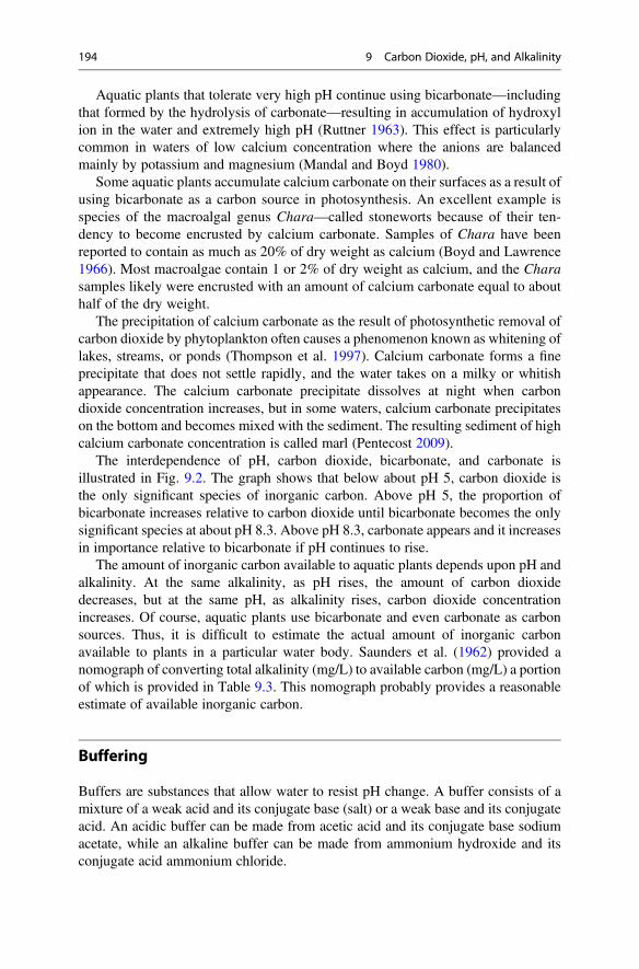
Aquatic plants that tolerate very high pH continue using bicarbonate—includingthat formed by the hydrolysis of carbonate—resulting in accumulation of hydroxylion in the water and extremely high pH (Ruttner 1963). This effect is particularlycommon in waters of low calcium concentration where the anions are balancedmainly by potassium and magnesium (Mandal and Boyd 1980).

Some aquatic plants accumulate calcium carbonate on their surfaces as a result ofusing bicarbonate as a carbon source in photosynthesis. An excellent example isspecies of the macroalgal genus Chara—called stoneworts because of their ten-dency to become encrusted by calcium carbonate. Samples of Chara have beenreported to contain as much as 20% of dry weight as calcium (Boyd and Lawrence1966). Most macroalgae contain 1 or 2% of dry weight as calcium, and the Charasamples likely were encrusted with an amount of calcium carbonate equal to abouthalf of the dry weight.

The precipitation of calcium carbonate as the result of photosynthetic removal ofcarbon dioxide by phytoplankton often causes a phenomenon known as whitening oflakes, streams, or ponds (Thompson et al. 1997). Calcium carbonate forms a fineprecipitate that does not settle rapidly, and the water takes on a milky or whitishappearance. The calcium carbonate precipitate dissolves at night when carbondioxide concentration increases, but in some waters, calcium carbonate precipitateson the bottom and becomes mixed with the sediment. The resulting sediment of highcalcium carbonate concentration is called marl (Pentecost 2009).

The interdependence of pH, carbon dioxide, bicarbonate, and carbonate isillustrated in Fig. 9.2. The graph shows that below about pH 5, carbon dioxide isthe only significant species of inorganic carbon. Above pH 5, the proportion ofbicarbonate increases relative to carbon dioxide until bicarbonate becomes the onlysignificant species at about pH 8.3. Above pH 8.3, carbonate appears and it increasesin importance relative to bicarbonate if pH continues to rise.

The amount of inorganic carbon available to aquatic plants depends upon pH andalkalinity. At the same alkalinity, as pH rises, the amount of carbon dioxidedecreases, but at the same pH, as alkalinity rises, carbon dioxide concentrationincreases. Of course, aquatic plants use bicarbonate and even carbonate as carbonsources. Thus, it is difficult to estimate the actual amount of inorganic carbonavailable to plants in a particular water body. Saunders et al. (1962) provided anomograph of converting total alkalinity (mg/L) to available carbon (mg/L) a portionof which is provided in Table 9.3. This nomograph probably provides a reasonableestimate of available inorganic carbon.

Buffering

Buffers are substances that allow water to resist pH change. A buffer consists of amixture of a weak acid and its conjugate base (salt) or a weak base and its conjugateacid. An acidic buffer can be made from acetic acid and its conjugate base sodiumacetate, while an alkaline buffer can be made from ammonium hydroxide and itsconjugate acid ammonium chloride.


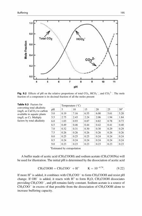
A buffer made of acetic acid (CH3COOH) and sodium acetate (CH3COONa) willbe used for illustration. The initial pH is determined by the dissociation of acetic acid

CH3COOH ¼ CH3COO� þ Hþ K ¼ 10�4:74: ð9:22Þ

If more H+ is added, it combines with CH3COO� to form CH3COOH and resist pH

change. If OH� is added, it reacts with H+ to form H2O, CH3COOH dissociatesproviding CH3COO

�, and pH remains fairly constant. Sodium acetate is a source ofCH3COO

� in excess of that possible from the dissociation of CH3COOH alone toincrease buffering capacity.

Fig. 9.2 Effects of pH on the relative proportions of total CO2, HCO3�, and CO3

2�. The molefraction of a component is its decimal fraction of all the moles present

Table 9.3 Factors forconverting total alkalinity(mg/L as CaCO3) to carbonavailable to aquatic plants(mg/L as C). Multiplyfactors by total alkalinity

Temperature (�C)pH 5 10 15 20 25 30a

5.0 8.19 7.16 6.55 6.00 5.61 5.20

5.5 2.75 2.43 2.24 2.06 1.94 1.84

6.0 1.03 0.93 0.87 0.82 0.78 0.73

6.5 0.49 0.46 0.44 0.42 0.41 0.40

7.0 0.32 0.31 0.30 0.30 0.29 0.29

7.5 0.26 0.26 0.26 0.26 0.26 0.26

8.0 0.25 0.25 0.25 0.24 0.24 0.24

8.5 0.24 0.24 0.24 0.24 0.24 0.24

9.0 0.23 0.23 0.23 0.23 0.23 0.23aEstimated by extrapolation

Buffering 195

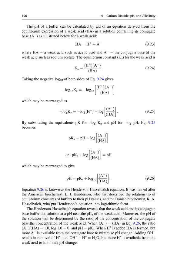
The pH of a buffer can be calculated by aid of an equation derived from theequilibrium expression of a weak acid (HA) in a solution containing its conjugatebase (A�) as illustrated below for a weak acid:

HA ¼ Hþ þ A� ð9:23Þwhere HA ¼ a weak acid such as acetic acid and A� ¼ the conjugate base of theweak acid such as sodium acetate. The equilibrium constant (Ka) for the weak acid is

Ka ¼ Hþð Þ A�ð ÞHAð Þ : ð9:24Þ

Taking the negative log10 of both sides of Eq. 9.24 gives

�log10Ka ¼ �log10Hþð Þ A�ð ÞHAð Þ

� �

which may be rearranged as

�logKa ¼ �log Hþð Þ � logA�ð ÞHAð Þ

� �: ð9:25Þ

By substituting the equivalents pK for –log Ka and pH for –log pH, Eq. 9.25becomes

pKa ¼ pH� logA�ð ÞHAð Þ

� �

or pKa þ logA�ð ÞHAð Þ

� �¼ pH

which may be rearranged to give

pH ¼ pKa þ log10A�ð ÞHAð Þ

� �: ð9:26Þ

Equation 9.26 is known as the Henderson-Hasselbalch equation. It was named afterthe American biochemist, L. J. Henderson, who first described the relationship ofequilibrium constants of buffers to their pH values, and the Danish biochemist, K. A.Hasselbalch, who put Henderson’s equation into logarithmic form.

The Henderson-Hasselbalch equation reveals that the weak acid and its conjugatebase buffer the solution at a pH near the pKa of the weak acid. Moreover, the pH ofthe solution will be determined by the ratio of the concentration of the conjugatebase:the concentration of the weak acid. When (A�) ¼ (HA) in Eq. 9.26, the ratio(A�)/(HA) ¼ 1.0, log 1.0 ¼ 0, and pH ¼ pKa. When H+ is added HA is formed, butmore A� is available from the conjugate base to minimize pH change. Adding OH�

results in removal of H+, i.e., OH� + H+ ¼ H2O, but more H+ is available from theweak acid to minimize pH change.


The pH of a buffer changes as H+ or OH� is added, but the changes are relativelysmall as shown in Ex. 9.8 for addition of OH� to a buffer.

Ex. 9.8 The pH change in a buffer (pKa ¼ 7.0) that is 0.1 M in HA and A� will becalculated for the addition of 0.01 mol/L and 0.05 mol/L of OH�.

Solution:For simplicity, it will be assumed that there is no change in buffer volume as a

result of the OH� addition. The addition of 0.01 mol/L OH� will reduce (AH) to0.09 M and increase (A�) to 0.11 M, while the 0.05 mole/L increase in OH� willresult in concentrations of 0.15 M A� and 0.05 M AH.

The pH values will be0.01 mol/L OH� added:

pH ¼ 7:0þ log0:110:09

� �

pH ¼ 7:0þ log1:222 ¼ 7:0þ 0:087 ¼ 7:09:

0.05 mole/L OH� added:

pH ¼ 7:0þ log0:150:05

� �

pH ¼ 7:0þ log3 ¼ 7:0þ 0:48 ¼ 7:48:

It can be seen from Ex. 9.8 that the addition of hydroxyl ion changed the pH of thebuffer. However, the increase in pH was much less than would have occurred had thesame quantity of OH� been added to pure water at pH 7 as illustrated in Ex. 9.9.

Ex. 9.9 The effect of OH� additions of 0.01 mol/L and 0.05 mol/L on the pH of purewater initially at pH 7 will be calculated.

Solution:0.01 mol/L OH� added:

10�7 OH� þ 10�2 mol=L OH� ¼ 0:0000001 M þ 0:01 M � 10�2 M

pOH ¼ �log 10�2� � ¼ �log �2

� � ¼ 2

pH ¼ 14� 2 ¼ 12:

0.05 mol/L OH� added:

10�7 OH� þ 0:05 mol=L OH� ¼ 10�1:30 M OH�

Buffering 197

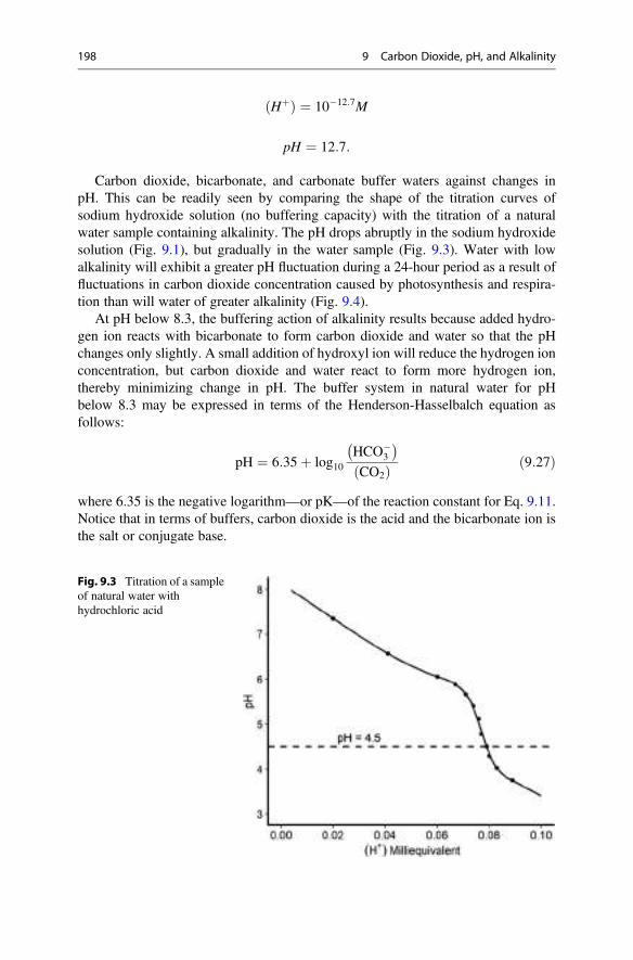
Hþð Þ ¼ 10�12:7M

pH ¼ 12:7:

Carbon dioxide, bicarbonate, and carbonate buffer waters against changes inpH. This can be readily seen by comparing the shape of the titration curves ofsodium hydroxide solution (no buffering capacity) with the titration of a naturalwater sample containing alkalinity. The pH drops abruptly in the sodium hydroxidesolution (Fig. 9.1), but gradually in the water sample (Fig. 9.3). Water with lowalkalinity will exhibit a greater pH fluctuation during a 24-hour period as a result offluctuations in carbon dioxide concentration caused by photosynthesis and respira-tion than will water of greater alkalinity (Fig. 9.4).

At pH below 8.3, the buffering action of alkalinity results because added hydro-gen ion reacts with bicarbonate to form carbon dioxide and water so that the pHchanges only slightly. A small addition of hydroxyl ion will reduce the hydrogen ionconcentration, but carbon dioxide and water react to form more hydrogen ion,thereby minimizing change in pH. The buffer system in natural water for pHbelow 8.3 may be expressed in terms of the Henderson-Hasselbalch equation asfollows:

pH ¼ 6:35þ log10HCO�

3

� �CO2ð Þ ð9:27Þ

where 6.35 is the negative logarithm—or pK—of the reaction constant for Eq. 9.11.Notice that in terms of buffers, carbon dioxide is the acid and the bicarbonate ion isthe salt or conjugate base.

Fig. 9.3 Titration of a sampleof natural water withhydrochloric acid


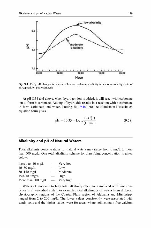
At pH 8.34 and above, when hydrogen ion is added, it will react with carbonateion to form bicarbonate. Adding of hydroxide results in a reaction with bicarbonateto form carbonate and water. Putting Eq. 9.10 into the Henderson-Hasselbalchequation form gives

pH ¼ 10:33þ log10CO2�

3

� �HCO�

3

� � ð9:28Þ

Alkalinity and pH of Natural Waters

Total alkalinity concentrations for natural waters may range from 0 mg/L to morethan 500 mg/L. One total alkalinity scheme for classifying concentration is givenbelow:

Less than 10 mg/L — Very low10–50 mg/L — Low50–150 mg/L — Moderate150–300 mg/L — HighMore than 300 mg/L — Very high

Waters of moderate to high total alkalinity often are associated with limestonedeposits in watershed soils. For example, total alkalinities of waters from differentphysiographic regions of the Coastal Plain region of Alabama and Mississippiranged from 2 to 200 mg/L. The lower values consistently were associated withsandy soils and the higher values were for areas where soils contain free calcium

Fig. 9.4 Daily pH changes in waters of low or moderate alkalinity in response to a high rate ofphytoplankton photosynthesis

Alkalinity and pH of Natural Waters 199

carbonate (Boyd and Walley 1975). Livingstone (1963) did not present alkalinitydata in his survey of the chemical composition of the world’s rivers and lakes, but hisbicarbonate data allow inference about alkalinity. Livingstone’s data suggest thatareas with weakly-developed or highly-leached soils have very low or low alkalinity,humid regions with abundant limestone in watershed soils have moderate alkalinity,and areas with semi-arid or arid climate have moderate to high alkalinity waters.Seawater has an average total alkalinity of 116 mg/L. Alkalinity is very high inclosed basin lakes. Waters from places with organic soils tend to have very low orlow alkalinity.

The alkalinity of water is closely related to pH. In general, pH tends to increase asalkalinity increases. Waters that do not contain measurable alkalinity have pH valuesbelow 5, those with very low or low alkalinity tend to have pH values between 5 and7, pH usually is between 7 and 8.5 in moderate and high alkalinity waters, and watersof very high alkalinity may have pH of 9 or more. The average pH of the ocean isabout 8.1. The influence of photosynthesis on pH is greater in low alkalinity watersbecause of their low buffering capacity. In waters of very low to moderate alkalinity,a dense phytoplankton bloom may cause afternoon pH to rise above 9. At night, pHwill usually decline to a much lower value in such waters.

Along coastal plains in several countries including the United States, there areareas where water percolates through calcium carbonates deposit and accumulatesmoderate to high concentrations of calcium and bicarbonate. This water then entersan aquifer that contains a lot of sodium from having been saturated with seawater inthe geological past. Calcium in the water recharging the aquifer is exchanged forsodium in the geological matrix of the formation. The water removed from theaquifer in wells will be high in alkalinity and sodium, but low in calcium. Hem(1970) referred to this process as natural softening of groundwater. When such wateris used to fill fish ponds, an extremely high pH that may be toxic to fish can resultfrom the effects of photosynthesis (Mandal and Boyd 1980).

Importance of Alkalinity System

pH

The pH of water is important in aquatic ecosystems, because it affects aquatic life.Gill tissue is the primary target organ in fish affected by excessively low pH. Whenfish are exposed to low pH, the amount of mucus on gill surfaces increases. Excessmucus interferes with the exchange of respiratory gases and ions across the gill.Therefore, failure in blood acid-base balance resulting in respiratory stress anddecreasing blood concentrations of sodium chloride which cause osmotic distur-bance are the dominant physiologic symptoms of acid stress. Of course, at low pH,aluminum ion concentration increases in water, and sometimes, toxic effects ofaluminum may occur in addition to pH effects.

Gill damage in fish also can occur in alkaline solutions (high pH). Mucus cells atthe base of the gill filaments become hypertrophic and the gill epithelium separates


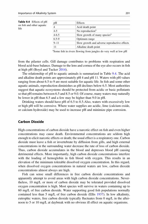
from the pilaster cells. Gill damage contributes to problems with respiration andblood acid-base balance. Damage to the lens and cornea of the eye also occurs in fishat high pH (Boyd and Tucker 2014).

The relationship of pH to aquatic animals is summarized in Table 9.4. The acidand alkaline death points are approximately pH 4 and pH 11. Waters with pH valuesranging from about 6.5 to 9 are most suitable for aquatic life. In fish and some otheraquatic animals, reproduction diminishes as pH declines below 6.5. Most authoritiessuggest that aquatic ecosystems should be protected from acidic or basic pollutantsso that pH remains between 6.5 and 8.5 or 9.0. Of course, many waters may naturallybe lower in pH than 6.5 and a few may be higher than 9.0 in pH.

Drinking waters should have pH of 6.5 to 8.5.Also, waters with excessively lowor high pH will be corrosive. Where water supplies are acidic, lime (calcium oxide,or calcium hydroxide) may be used to increase pH and minimize pipe corrosion.

Carbon Dioxide

High concentrations of carbon dioxide have a narcotic effect on fish and even higherconcentrations may cause death. Environmental concentrations are seldom highenough to elicit narcotic effects or death; the usual effect is a respiratory one. Carbondioxide must leave a fish or invertebrate by diffusion from gills, and high externalconcentrations in the surrounding water decrease the rate of loss of carbon dioxide.Thus, carbon dioxide accumulates in the blood and depresses blood pH causingdetrimental effects. More importantly, high carbon dioxide concentrations interferewith the loading of hemoglobin in fish blood with oxygen. This results in anelevation of the minimum tolerable dissolved oxygen concentration. In this regard,when dissolved oxygen concentrations in natural waters are low, carbon dioxideconcentrations almost always are high.

Fish can sense small differences in free carbon dioxide concentrations andapparently attempt to avoid areas with high carbon dioxide concentrations. Never-theless, 10 mg/L or more of carbon dioxide may be tolerated provided dissolvedoxygen concentration is high. Most species will survive in waters containing up to60 mg/L of free carbon dioxide. Water supporting good fish populations normallycontained less than 5 mg/L of free carbon dioxide (Ellis 1937). In low alkalinity,eutrophic waters, free carbon dioxide typically fluctuates from 0 mg/L in the after-noon to 5 or 10 mg/L at daybreak with no obvious ill effect on aquatic organisms.

Table 9.4 Effects of pHon fish and other aquaticlife

pH Effects

4 Acid death point

4-5 No reproductiona

4-6.5 Slow growth of many speciesa

6.5-9 Optimum range

9–11 Slow growth and adverse reproductive effects

11 Alkaline death pointaSome fish in rivers flowing from jungles do very well at low pH

Importance of Alkalinity System 201

Carbon dioxide is necessary in photosynthesis, but its concentration is closelyrelated to pH and total alkalinity. At the same pH, a water with a greater alkalinitywill contain more available carbon for photosynthesis than a water with lesseralkalinity. But, at the same alkalinity, the availability of free carbon dioxide (gaseousform) will decrease as pH increases.

Alkalinity

The alkalinity of water is an important variable as productivity is related to alkalinitybecause of the relationship between alkalinity and carbon availability. Waters withtotal alkalinity values of 0 to 50 mg/L usually are less productive than those withtotal alkalinity concentrations of 50 to 200 mg/L (Moyle 1946). Productivity tends todecrease at higher alkalinities. Liming sometimes may be used to increase thealkalinity of water.

Alkalinity has a great influence on the use of water. Waters with a high carbonatehardness (high alkalinity and high hardness) will be problematic in causing depositswhen heated. Total alkalinities up to 400–500 mg/L are permissible in public watersupplies.

Conclusions

The relationships among carbon dioxide, bicarbonate, and carbonate concentrationscontrol the pH of most natural waters. Carbon dioxide has an acidic reaction inwater. Plants normally remove more carbon dioxide from water than is returned byrespiration during daylight, and pH rises. Carbon dioxide becomes depleted at pH8.3, but many aquatic plants can use bicarbonate as an inorganic carbon source forphotosynthesis. Plants use one-half of the carbon in bicarbonate, and the other half isexcreted into the water as carbonate. The carbonate hydrolyzes causing pH tocontinue rising. Photosynthesis stops at night and carbon dioxide from respirationresults in a decline in pH.

Dissolution of limestone, calcium silicate, and feldspars is the source of alkalinityin natural waters, and dissolved carbon dioxide enhances the solubilities of theseminerals. Alkalinity usually consists primarily of bicarbonate which is in equilibriumwith carbon dioxide and hydrogen ion. Alkalinity is a reserve of inorganic carbon,and the CO2-HCO3

�-CO32� system acts to buffers water. The buffering capacity

increases with greater alkalinity.


References

Akin GW, Lagerwerff JV (1965) Calcium carbonate equilibria in aqueous solution open to the air.I. The solubility of calcite in relation to ionic strength. Geochimica et Cosmochimica29:343–352

Boyd CE, Lawrence JM (1966) The mineral composition of several freshwater algae. Proc AnnConf SE Assoc Game Fish Comm 20:413–424

Boyd CE, Tucker CS (2014) Handbook for aquaculture water quality. Craftmaster Printers, AuburnBoyd CE, Walley WW (1975) Total alkalinity and hardness of surface waters in Alabama and

Mississippi. Bulletin 465, Alabama Agricultural Experiment Station, Auburn University.Boyd CE, Tucker CS, Viriyatum R (2011) Interpretation of pH, acidity and alkalinity in aquaculture

and fisheries. N Am J Aqua 73:403–408Cavalli G, Riis T, Baattrup-Pedersen A (2012) Bicarbonate use in three aquatic plants. Aqua Bot

98:57–60Eaton AD, Clesceri LS, Rice EW, Greenburg AE (eds) (2005) Standard methods for the examina-

tion of water and wastewater. American Public Health Association, Washington, DCEllis MM (1937) Detection and measurement of stream pollution. U.S. Bur Fish Bull 22:367–437Frear CL, Johnston J (1929) The solubility of calcium carbonate (calcite) in certain aqueous

solutions at 25 �C. J Am Chem Soc 51:2082–2093Garrels RM, Christ CL (1965) Solutions, minerals, and equilibria. Freeman, Cooper, and Company,

San FranciscoHem JD (1970) Study and interpretation of the chemical characteristics of natural water. Water-

Supply Paper 1473, United States Geological Survey, United States Government PrintingOffice, Washington, DC.

Ittekkot V (2003) A new story from the Ol’ Man River. Science 301:56–58Korb RE, Saville PJ, Johnston AM, Raven JA (1997) Sources of inorganic carbon for photosynthe-

sis by three species of marine diatom. J Phycol 33:433–440Livingstone DA (1963) Chemical composition of rivers and lakes. Professional Paper 440-G,

United States Government Printing Office, Washington, DC.Mandal BK, Boyd CE (1980) The reduction of pH in water of high total alkalinity and low total

hardness. Prog Fish-Cult 42:183–185Moyle JB (1946) Some indices of lake productivity. Trans Am Fish Soc 76:322–334Pentecost A (2009) The marl lakes of the British Isles. Freshwater Rev 2:167–197Ruttner F (1963) Fundamentals of limnology. University of Toronto Press, TorontoSá MVC, Boyd CE (2017) Variability in the solubility of agricultural limestone from different

sources and its pertinenece for aquaculture. Aqua Res 48:4,292–4,299Saunders GW, Trama FB, Bachmann RW (1962) Evaluation of a modified C-14 technique for

shipboard estimation of photosynthesis in large lakes. Publication No. 8, Great Lakes researchDivision, University of Michigan, Ann Arbor.

Snoeyink VL, Jenkins D (1980) Water chemistry. John wiley and Sons, New YorkSomridhivej B, Boyd CE (2017) likely effects of the increasing alkalinity of inland waters on

aquaculture. J World Aqua Soc 48:496–502Stone DM, Young KL, Mattes WP, Cantrell MA (2018) Abiotic controls of invasive nonnative

fishes in the Little Colorado River, Arizona. Am Midl Nat 180:119–142Taras MJ, Greenberg AE, Hoak RD, Rand MC (1971) Standard methods for the examination of

water and wastewater, 13th edn. American Public Health Association, Washington, DCThompson JB, Schultzepam S, Beveridge TJ, DesMarais DJ (1997) Whiting events: biogenic origin

due to the photosynthetic activity of cyanobacterial picoplankton. Lim Ocean 42:133–141

References 203

Total Hardness 10

AbstractThe total hardness of water results from divalent cations—mainly from calciumand magnesium—expressed as equivalent calcium carbonate. The total hardnessequivalence of 1 mg/L calcium is 2.5 mg/L, while 1 mg/L magnesium equates to4.12 mg/L. Hardness and alkalinity often are similar in concentration in waters ofhumid regions, but hardness frequently exceeds alkalinity in waters of aridregions. Hardness generally is less important than alkalinity as a biological factor,but it is quite important in water supply and use. High concentrations of calciumand magnesium in water containing appreciable alkalinity lead to scale formationwhen the water is heated or its pH increases. This leads to clogging of water pipesand scale accumulation in boilers and on heat exchangers. The Langelier Satura-tion Index often is used to determine if water has potential to cause scaling.Divalent ions also precipitate soap increasing soap use for domestic purposes andin commercial laundries. The traditional method for softening water is to precipi-tate calcium as calcium carbonate and magnesium as magnesium hydroxide bythe lime-soda ash process. Water also may be softened by passing it through acation exchange medium such as zeolite.

Introduction

The rather strange designations of waters as soft or hard apparently originated fromthe observation that waters from some sources imparted deposits in pipes and invessels in which they were boiled. Waters which caused the deposits were calledhard as opposed to soft waters that did not produce such deposits. Hard waters alsoleave spots on drinking glasses, plumbing fixtures, and other objects after drying.Moreover, hard waters do not produce copious lather with soap, a failure resultingfrom precipitation of soap by minerals in the water and formation of the familiarbathtub ring.


205


The degree of hardness in water obviously is important to water use. Hard waterscan clog pipes, form scales in boilers, waste soap, and cause unwanted spots andstains on various fixtures and household items. Hardness also is closely related toalkalinity and the amount of hardness and the ratio of hardness to alkalinityinfluences other water quality variables and biological processes in natural waters.

This chapter describes hardness, its measurements, and its effect on water qualityand water use.

Definition and Sources

Total hardness is defined as the total concentration of divalent cations in waterexpressed as equivalent calcium carbonate. If a water contains 10 mg/L calcium,the resulting hardness is 25 mg/L as CaCO3, because calcium has an atomic weightof 40 as opposed to a molecular weight of 100 for calcium carbonate. The ratio100/40 multiplied by calcium concentration gives hardness as equivalent calciumcarbonate.

The divalent cations—calcium, magnesium, strontium, ferrous iron, and manga-nous manganese—cause hardness in water. Surface waters usually are oxygenatedand will not contain divalent iron or manganese. Few inland waters contain morethan 1 or 2 mg/L of strontium, and calcium and magnesium are the major sources ofhardness in nearly all surface waters including the ocean. Groundwaters usually areanaerobic and contain reduced iron and manganese (Fe2+ and Mn2+) which contrib-ute hardness, but hardness from iron and manganese is lost when these two ionsprecipitate when water removed from aquifers becomes oxygenated.

As with alkalinity, the dissolution of limestone, calcium silicate, and feldspars is asource of hardness. As discussed in Chap. 9, carbon dioxide in rainwater acceleratesthe dissolution of limestone, calcium silicate, and feldspars, and this capacityincreases as water infiltrates downward dissolving carbon dioxide released by rootand microbial respiration. Some aquifers are actually contained in undergroundlimestone formations, and groundwater from such aquifers usually has high hard-ness. The acquisition of hardness (calcium and magnesium) by the dissolution ofdolomitic limestone, calcium silicate, and feldspars is illustrated in Eqs. 9.14, 9.15,9.16, 9.17, and 9.18. In addition, when gypsum (CaSO4�2H2O) and certain magne-sium salts common in soils of arid regions dissolve, they impart calcium andmagnesium to the water. In arid regions, ions in water are concentrated by evapora-tion increasing hardness.

Because hardness often is derived from the dissolution of limestone or calciumsilicate, concentrations of calcium and magnesium are nearly equal in chemicalequivalence to concentrations of bicarbonate and carbonate in many natural waters.However, in areas with acidic soils, neutralization of alkalinity may result in greaterhardness than alkalinity. In arid regions, concentration of ions by evaporation causesprecipitation of alkalinity as calcium carbonate causing alkalinity to decline relativeto hardness. Alkalinity, which also is expressed as calcium carbonate equivalent,sometimes exceeds hardness in groundwaters that have been naturally softened (seeChap. 9).

206 10 Total Hardness

Determination of Hardness

As mentioned above, hardness is reported as its calcium carbonate equivalent, andeach milligram per liter of calcium is equal to 2.5 mg/L of hardness as calciumcarbonate. Similar calculations reveal that the hardness factors are 4.12 for magne-sium, 1.82 for manganese, 1.79 for iron, and 1.14 for strontium. If the ioniccomposition of a water is known, the total hardness may be calculated from theconcentrations of divalent ions as illustrated in the next example.

Ex. 10.1 A water sample contains 50 mg/L of calcium, 5 mg/L of magnesium, and0.5 mg/L of strontium. The total hardness will be calculated.

Solution:50 mg Ca2+/L � 2.50 ¼ 125 mg/L of CaCO3.5 mg Mg2+/L � 4.12 ¼ 20.6 mg/L of CaCO3.0.5 Mg Sr2+/L � 1.14 ¼ 0.57 Mg/L of CaCO3.Total hardness ¼ (125 + 20.6 + 0.57) ¼ 146.17 mg/L as CaCO3.

Rather than calculating hardness from divalent cation concentrations, it is morecommon to measure the concentration of total hardness by titration of samples withthe chelating agent ethylenediaminetetraacetic acid (EDTA) as described by Eatonet al. (2005). This titrating agent forms stable complexes with divalent cations asillustrated for calcium:

Ca2þ þ EDTA ¼ Ca � EDTA: ð10:1ÞEach molecule of EDTA complexes one divalent metal ion, and the endpoint isdetected with the indicator eriochrome black T. The indicator combines with a smallamount of calcium in the sample and holds it rather tightly creating a wine-red color.When all Ca2+ in the water sample has been chelated, the EDTA strips the Ca2+ fromthe indicator and the solution turns blue. The endpoint is very sharp and distinct.Each mole of EDTA equals 1 mol of CaCO3 equivalence. Example 10.2 shows thecalculation of hardness from EDTA titration.

Ex. 10.2 Titration of a 100-mL water sample requires 12.55 mL of 0.0095 M EDTAsolution. The total hardness will be calculated.

Solution:Each mole of EDTA equals one mole of CaCO3, and

12:55 mLð Þ 0:0095 Mð Þ ¼ 0:119 mM CaCO3

0:119 mMð Þ 100:08 mgCaCO3

mM

� �¼ 11:91 mg CaCO3

Determination of Hardness 207

11:91mg CaCO3 � 1;000mL=L100mL

¼ 119mg=L total hardness as equivalent CaCO3:

The steps in the solution shown in Ex. 10.2 can be combined into an equation forestimating hardness from EDTA titration:

Total hardness mg=L CaCO3ð Þ ¼ Mð Þ Vð Þ 100; 080ð ÞS

ð10:2Þ

where M¼molarity of EDTA, V¼ volume of EDTA (mL), and S¼ sample volume(mL).

Hardness Concentrations

The hardness of inland waters may be around 5 to 75 mg/L in humid areas withhighly-leached, acidic soil, 150 to 300 mg/L in humid areas with calcareous soil, and1000 mg/L or more in arid regions. Average ocean water contains about 1350 mg/Lmagnesium, 400 mg/L calcium, and 8 mg/L strontium (Table 5.8); its calculatedhardness is about 6571 mg/L. Hardness of water for water supply purposes often isclassified as follows:

Less than 50 mg/L — Soft50–150 mg/L — Moderately hard150–300 mg/L — HardMore than 300 mg/L — Very Hard

This is similar to the classification given in Chap. 9 for total alkalinity.

Problems with Hardness

Common soap, sodium stearate, dissolves into stearate ions and sodium ions, but inhard water, stearate ions are precipitated as calcium stearate

2C17H35COO� þ Ca2þ ! C17H35COOð Þ2Ca # : ð10:3Þ

As a result, lather formation is limited, and the calcium stearate precipitates. Thiswastes soap and is particularly troublesome in commercial laundries. It also can bedifficult to remove the precipitate from household items washed in hard water.

A scale often forms in containers in which hard waters are boiled. This is causedby loss of carbon dioxide to the air by boiling and the precipitation of calciumcarbonate


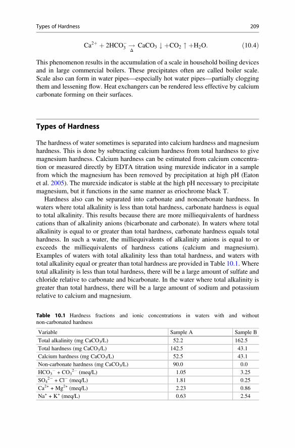
Ca2þ þ 2HCO�3 !

ΔCaCO3 # þCO2 " þH2O: ð10:4Þ

This phenomenon results in the accumulation of a scale in household boiling devicesand in large commercial boilers. These precipitates often are called boiler scale.Scale also can form in water pipes—especially hot water pipes—partially cloggingthem and lessening flow. Heat exchangers can be rendered less effective by calciumcarbonate forming on their surfaces.

Types of Hardness

The hardness of water sometimes is separated into calcium hardness and magnesiumhardness. This is done by subtracting calcium hardness from total hardness to givemagnesium hardness. Calcium hardness can be estimated from calcium concentra-tion or measured directly by EDTA titration using murexide indicator in a samplefrom which the magnesium has been removed by precipitation at high pH (Eatonet al. 2005). The murexide indicator is stable at the high pH necessary to precipitatemagnesium, but it functions in the same manner as eriochrome black T.

Hardness also can be separated into carbonate and noncarbonate hardness. Inwaters where total alkalinity is less than total hardness, carbonate hardness is equalto total alkalinity. This results because there are more milliequivalents of hardnesscations than of alkalinity anions (bicarbonate and carbonate). In waters where totalalkalinity is equal to or greater than total hardness, carbonate hardness equals totalhardness. In such a water, the milliequivalents of alkalinity anions is equal to orexceeds the milliequivalents of hardness cations (calcium and magnesium).Examples of waters with total alkalinity less than total hardness, and waters withtotal alkalinity equal or greater than total hardness are provided in Table 10.1. Wheretotal alkalinity is less than total hardness, there will be a large amount of sulfate andchloride relative to carbonate and bicarbonate. In the water where total alkalinity isgreater than total hardness, there will be a large amount of sodium and potassiumrelative to calcium and magnesium.

Table 10.1 Hardness fractions and ionic concentrations in waters with and withoutnon-carbonated hardness

Variable Sample A Sample B

Total alkalinity (mg CaCO3/L) 52.2 162.5

Total hardness (mg CaCO3/L) 142.5 43.1

Calcium hardness (mg CaCO3/L) 52.5 43.1

Non-carbonate hardness (mg CaCO3/L) 90.0 0.0

HCO3� + CO3

2� (meq/L) 1.05 3.25

SO42� + Cl� (meq/L) 1.81 0.25

Ca2+ + Mg2+ (meq/L) 2.23 0.86

Na+ + K+ (meq/L) 0.63 2.54

Types of Hardness 209

If a water containing carbonate hardness is heated, carbon dioxide is driven offand calcium carbonate, magnesium carbonate or both precipitate as was shown forcalcium carbonate precipitation in Eq. 10.4. Sulfate, chloride, sodium, and potas-sium are not precipitated by boiling, but the carbonate hardness can be removed fromwater by precipitation following boiling for a sufficient time. Because it can beremoved by heating, carbonate hardness is called temporary hardness. Of course,boiling will not remove all of the hardness or alkalinity from a water with nononcarbonate hardness because calcium and magnesium carbonates have a degreeof solubility.

Carbonate hardness is responsible for boiler scale. Hardness remaining in waterafter boiling is the permanent hardness. Because bicarbonate and carbonate precipi-tate with part of the calcium and magnesium during boiling, the permanent hardnessalso is known as noncarbonate hardness, and

Noncarbonate hardness ¼ total hardness� carbonate hardness: ð10:5Þ

Biological Significance of Hardness

The biological productivity of natural freshwaters increases with greater hardness upto a concentration of 150–200 mg/L (Moyle 1946, 1956). Hardness per se has lessbiological significance than does alkalinity. Productivity depends upon the availabil-ity of carbon dioxide, nitrogen, phosphorus, and other nutrients, a suitable pH range,and many other factors. As a rule, alkalinity tends to increase along with concentra-tion of other dissolved ions where watershed soils are fertile but not highly acidic.Hardness and alkalinity often increase in proportion to each other, and in manywaters of humid regions, they may be roughly equal. Nevertheless, for analyticalreasons, it was easier in the past to measure total hardness than to determine totalalkalinity. Hardness became a common index of productivity. Today, there is noreason to follow this tradition, and indices of productivity in aquatic ecosystemsshould be based on total alkalinity or other variables.

Water Softening

Two methods have traditionally been used for softening water—the lime-soda ashprocess and the zeolite process (Sawyer and McCarty 1978) . The lime-soda ashprocedure involves treating water with calcium hydroxide (lime) to remove calciumcarbonate and to convert magnesium bicarbonate to magnesium carbonate as shownin the following reactions:

Ca OHð Þ2 þ CO2 ¼ CaCO3 # þH2O ð10:6Þ


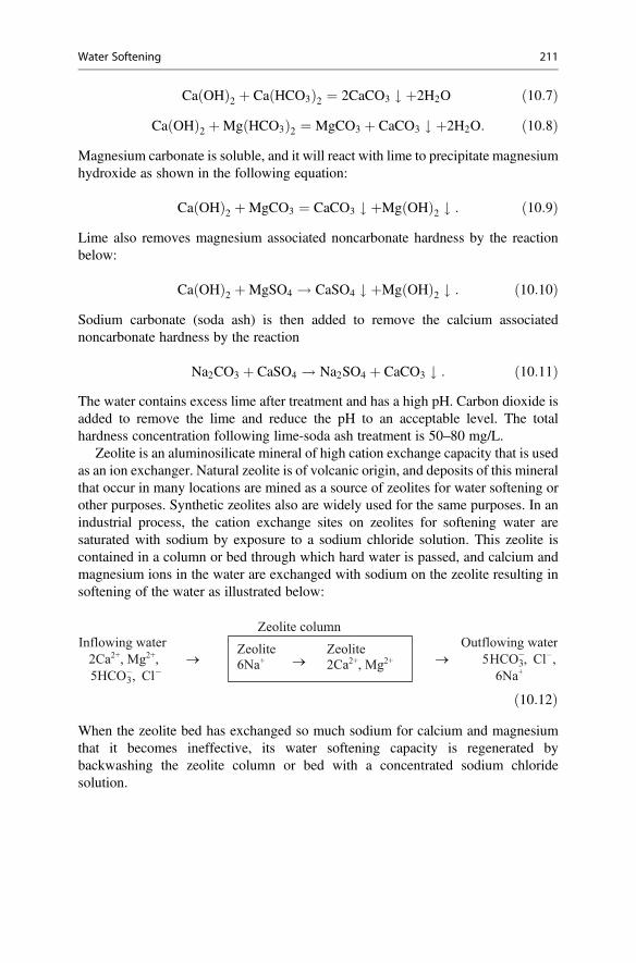
Ca OHð Þ2 þ Ca HCO3ð Þ2 ¼ 2CaCO3 # þ2H2O ð10:7ÞCa OHð Þ2 þMg HCO3ð Þ2 ¼ MgCO3 þ CaCO3 # þ2H2O: ð10:8Þ

Magnesium carbonate is soluble, and it will react with lime to precipitate magnesiumhydroxide as shown in the following equation:

Ca OHð Þ2 þMgCO3 ¼ CaCO3 # þMg OHð Þ2 # : ð10:9ÞLime also removes magnesium associated noncarbonate hardness by the reactionbelow:

Ca OHð Þ2 þMgSO4 ! CaSO4 # þMg OHð Þ2 # : ð10:10ÞSodium carbonate (soda ash) is then added to remove the calcium associatednoncarbonate hardness by the reaction

Na2CO3 þ CaSO4 ! Na2SO4 þ CaCO3 # : ð10:11ÞThe water contains excess lime after treatment and has a high pH. Carbon dioxide isadded to remove the lime and reduce the pH to an acceptable level. The totalhardness concentration following lime-soda ash treatment is 50–80 mg/L.

Zeolite is an aluminosilicate mineral of high cation exchange capacity that is usedas an ion exchanger. Natural zeolite is of volcanic origin, and deposits of this mineralthat occur in many locations are mined as a source of zeolites for water softening orother purposes. Synthetic zeolites also are widely used for the same purposes. In anindustrial process, the cation exchange sites on zeolites for softening water aresaturated with sodium by exposure to a sodium chloride solution. This zeolite iscontained in a column or bed through which hard water is passed, and calcium andmagnesium ions in the water are exchanged with sodium on the zeolite resulting insoftening of the water as illustrated below:

Zeolite columnInflowing water Outflowing water

2Ca2+, Mg2+, → → 5HCO3−, Cl−,

5HCO3−, Cl− 6Na+

Zeolite Zeolite6Na+ 2Ca2+, Mg2+→

ð10:12ÞWhen the zeolite bed has exchanged so much sodium for calcium and magnesiumthat it becomes ineffective, its water softening capacity is regenerated bybackwashing the zeolite column or bed with a concentrated sodium chloridesolution.

Water Softening 211

Calcium Carbonate Saturation

The degree of calcium carbonate saturation of water affects the likelihood of calciumcarbonate precipitation or scaling by a water during use. Several indices of scalingpotential have been formulated, and one of the most popular is the LangelierSaturation Index (Langelier 1936). The full explanation of this index is beyond thescope of this book but the equation is

LSI ¼ pH� pHsat ð10:13Þwhere LSI ¼ Langelier Saturation Index; pH ¼ pH of water; pHsat ¼ pH at calciumcarbonate saturation of the water.

pHsat ¼ 9:3þ Aþ Bð Þ � Cþ Dð Þ ð10:14Þwhere A ¼ (log TDS – 1)/10, B ¼ [�13.12 � log (�C + 273)] + 34.55, C ¼ log(Ca2+ � 2.5) – 0.4, and D ¼ log (alkalinity as CaCO3).

For waters with TDS concentration < 500 mg/L, a simplified equation (Gebbie2000) may be used for pHsat:

pHsat ¼ 11:5� log Ca2þ� �� log Alkalinityð Þ: ð10:15Þ

At LSI¼ 0, the water is saturated with calcium carbonate. Waters with a negativeLSI are undersaturated with calcium carbonate and potentially corrosive (seeChap. 8), because the precipitation of calcium carbonate over a surface protects itfrom corrosion. When the LSI is positive, the water is not corrosive, but it can causescaling that can be problematic. Calculation of the LSI is illustrated in Ex. 10.3.

Ex. 10.3 Calculation of the Langelier Saturation Index for a water at 20 �C withpH 7.7, 20 mg/L Ca2+, 75 mg/L total alkalinity, and 375 mg/L total dissolved solids.

Solution:The pHsat value is calculated with Eq. 10.14.A ¼ (log 375–1)/10 ¼ 0.16.B ¼ [�13.12 � log (20 + 273)] + 34.55 ¼ 2.18.C ¼ log (20 � 2.5) – 0.4 ¼ 1.30.D ¼ log (75) ¼ 1.88

pHsat ¼ 9:3þ 0:16þ 2:18ð Þ � 1:30þ 1:88ð Þ ¼ 8:46:

The LSI is computed using Eq. 10.13

LSI ¼ 7:7� 8:46 ¼ �0:76:

The simplified Gebbie equation (Eq. 10.15) can be used instead of Eq. 10.14 becauseTDS is < 500 mg/L. The result is


pHsat ¼ 11:5� log20� log75 ¼ 8:32

and

LSI ¼ 7:7� 8:32 ¼ �0:62:

The calculation by either procedure suggests that the water would be corrosive, butit would not cause scaling.

Suppose that the water referred to in Ex. 10.3 is in a lake that develops a denseplankton bloom in summer and pH rises to 8.6 and the water temperature increases to28 �C. The LSI would be +0.29 by the Langelier method for estimating pHsat

(Eq. 10.14) and +0.28 by the Gebbie (2000) shortcut method for estimating pHsat

(Eq. 10.15). At the higher pH and water temperature, the water would have potentialto cause scaling, particularly in the afternoon when pH is high because of photosyn-thesis as discussed in Chap. 9.

Conclusions

Hardness is an important factor regarding the use of water for many purposes.Hardness of water is manifest most commonly by the amount of soap needed toproduce suds. Hardness might be called the soap-wasting property of water, becauseno suds will be produced in a hard water until the minerals causing the hardness havebeen removed from the water by combining with the soap. The material that isremoved by the soap is evident as an insoluble scum—familiar ring on the bathtub—that forms during bathing in some waters.

Waters with a hardness of less than 50 mg/L are considered soft. A hardness of50–150 mg/L is not objectionable for most purposes, but the amount of soap neededincreases with hardness. Laundries or other industries using large quantities of soapgenerally find it profitable to lower hardness concentrations to about 50 mg/L. Waterhaving 100–150 mg/L hardness will deposit considerable scale in steam boilers.Hardness of more than 150 mg/L is decidedly noticeable. At levels of 200–300 mg/Lor higher, it is common practice to soften water for household uses. Where municipalwater supplies are softened, the hardness is reduced to about 85 mg/L. Furthersoftening of a whole public water supply is not considered economical.

Where scale forms when water is heated, calcium carbonate scale deposits first,because it is more insoluble than magnesium carbonate. In the absence of carbondioxide, water will carry only about 14 mg/L calcium carbonate in solution. Underthe same conditions, the solubility of magnesium carbonate is more than five timesas great, or about 80 mg/L.

Conclusions 213

References

Eaton AD, Clesceri LS, Rice EW, Greenburg AE (eds) (2005) Standard methods for the examina-tion of water and wastewater. American Public Health Association, Washington

Gebbie P (2000) Water stability—what does it mean and how do you measure it? In: Proceedings of63rd Annual Water Industry Engineers and Operators Conference, Warrnambool, pp 50–58.(http://wioa.org.au/conference_papers/2000/pdf/paper7.pdf).

Langelier WF (1936) The analytical control of anti-corrosion water treatment. J Am Water WorksAssoc 28:1500–1521

Moyle JB (1946) Some indices of lake productivity. Trans Am Fish Soc 76:322–334Moyle JB (1956) Relationships between the chemistry of Minnesota surface waters and wildlife

management. J Wildlife Man 20:303–320Sawyer CN, McCarty PL (1978) Chemistry for environmental engineering. McGraw-Hill,

New York


http://wioa.org.au/conference_papers/2000/pdf/paper7.pdf

Acidity 11

AbstractAcidity in water bodies with pH of about 4 up to 8.3 is caused by carbon dioxideand dissolved humic substances. Waters with pH <4.0 usually contain sulfuricacid or possibly another strong acid, but they still contain carbon dioxide andpossibly humic compounds. Low pH is associated with low productivity andbiodiversity. Acidity is measured by titration with standard sodium hydroxide andreported in milligrams per liter of calcium carbonate. Low pH and elevatedacidity result naturally from oxidation of sulfides in soil or sediment. Oxidationof pyritic material exposed by mining and oxidation of sulfur and nitrogencompounds released into the atmosphere by combustion of fuels also are sourcesof acidity to surface waters. The increasing solubility of carbon dioxide as a resultof higher atmospheric carbon dioxide concentration does not have a large effecton pH of rainfall and freshwater bodies. However, it is causing ocean acidificationand interfering with biological calcium carbonate precipitation by calcifyingorganisms. Liming materials typically are used to counteract acidity.

Introduction

Freshwater bodies usually have pHs between 6 and 9, but some have lower pHs thatrestrict the type and abundance of biota. Acidic waters can be put into three verygeneral classes: low alkalinity and early morning pHs of 5–6; no alkalinity and pHsof 4–5; highly acidic with pH <4. Carbon dioxide is the main source of acidity inwaters with low but measurable alkalinity. In waters with pH between 4 and 5 thereis no alkalinity, and carbon dioxide and humic substances contribute to acidity.Humic substances have been reported to depress pH slightly below 4, but mostwaters with pH <4 contain an acid stronger than either carbon dioxide or humiccompounds. Carbon dioxide and usually humic substances also will be present inwater of pH <4. The most common cause of pH <4.0 in natural waters is the presenceof a strong acid (often sulfuric acid) of natural or anthropogenic origin.


215


Acidity is not commonly measured in water quality investigations, but somewaters are impacted by low pH and measurements of acidity are necessary forassessing water quality conditions. This chapter explains the concept of acidity, itsmeasurement, its effects, and its mitigation.

The Concept of Acidity in Water

The pH is an index of the hydrogen ion concentration in water, but hydrogen ionconcentration and pH are not the same as acidity. The acidity of water is defined byEaton et al. (2005) as a capacity factor; the amount of strong base necessary toneutralize the hydrogen ion concentration in a given volume of water. In otherwords, acidity can be described as the total concentration of titratable acids inwater. By this description, acidity can be considered the opposite of alkalinity,because alkalinity is the total concentration of titratable bases in water. This descrip-tion could be taken to imply that acidity is negative alkalinity—not a bad analogy inmany respects. The concept of acidity is perplexing, because most natural waterscontain both acidity and alkalinity. This results because carbon dioxide is an acid,and is present in water at pH <8.3, while water contains bicarbonate as its mainsource of alkalinity in waters with pH >5.6. The practical endpoint pH for alkalinitytitrations is lower than 5.6 as the result of accumulation of carbon dioxide producedin the titration vessel by reaction of acid with bicarbonate (see Chap. 9).

The concept of water with pH between 5.6 and 8.3 containing both acidity andalkalinity seems to contrast with the usual concept that pH <7 is an acidic conditionand pH >7 is an alkaline condition. Actually both concepts are true; a water with pHbetween 5.6 and 7 is acidic, but it contains alkaline substances, while a water ofpH 7–8.3 is alkaline, but it contains acidic substances.

Acidity in most natural waters is caused by carbon dioxide which acts as a weakacid, and humic substances which also are weak acids. Carbon dioxide concentrationis normally not high enough to depress pH below 4.5; humic substances may depresspH as low as 3.7 or 3.8. Waters of lower pH contain strong acids. A water samplewith pH�4.5 usually is said to contain only carbon dioxide acidity. A water with pH<4.5 is considered to contain an acid stronger than carbon dioxide, but it alsocontains acidity from carbon dioxide. Waters may have only carbon dioxide acidity,but most waters also have acidity from humic substances.

A weak acid does not dissociate appreciably and acids with Ka > 10�2 often aredesignated to be weak acids. The reader should note that Ka 10

�2 is greater than Ka

of 10�3. A strong acid has a greater Ka and is assumed to dissociate completely(Table 11.1). The Ka usually is not reported for a strong acid, because it is a largevalue. The pH of a 0.01 M solution of acetic acid is 3.39 as compared to 2.0 for0.01 M hydrochloric acid (a strong acid). The ratio, acetate ion to undissociatedacetic acid, in a 0.01 M solution of acetic acid is:

216 11 Acidity

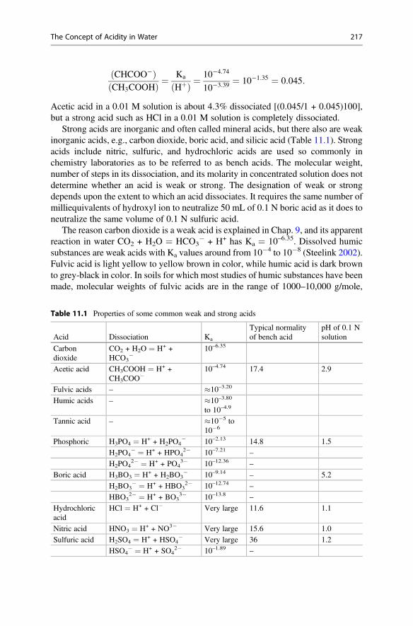
CHCOO�ð ÞCH3COOHð Þ ¼

Ka

Hþð Þ ¼10�4:74

10�3:39 ¼ 10�1:35 ¼ 0:045:

Acetic acid in a 0.01 M solution is about 4.3% dissociated [(0.045/1 + 0.045)100],but a strong acid such as HCl in a 0.01 M solution is completely dissociated.

Strong acids are inorganic and often called mineral acids, but there also are weakinorganic acids, e.g., carbon dioxide, boric acid, and silicic acid (Table 11.1). Strongacids include nitric, sulfuric, and hydrochloric acids are used so commonly inchemistry laboratories as to be referred to as bench acids. The molecular weight,number of steps in its dissociation, and its molarity in concentrated solution does notdetermine whether an acid is weak or strong. The designation of weak or strongdepends upon the extent to which an acid dissociates. It requires the same number ofmilliequivalents of hydroxyl ion to neutralize 50 mL of 0.1 N boric acid as it does toneutralize the same volume of 0.1 N sulfuric acid.

The reason carbon dioxide is a weak acid is explained in Chap. 9, and its apparentreaction in water CO2 + H2O ¼ HCO3

� + H+ has Ka ¼ 10–6.35. Dissolved humicsubstances are weak acids with Ka values around from 10�4 to 10�8 (Steelink 2002).Fulvic acid is light yellow to yellow brown in color, while humic acid is dark brownto grey-black in color. In soils for which most studies of humic substances have beenmade, molecular weights of fulvic acids are in the range of 1000–10,000 g/mole,

Table 11.1 Properties of some common weak and strong acids

Acid Dissociation Ka

Typical normalityof bench acid

pH of 0.1 Nsolution

Carbondioxide

CO2 + H2O ¼ H+ +HCO3

�10–6.35

Acetic acid CH3COOH ¼ H+ +CH3COO

�10–4.74 17.4 2.9

Fulvic acids – �10–3.20

Humic acids – �10–3.80

to 10–4.9

Tannic acid – �10�5 to10�6

Phosphoric H3PO4 ¼ H+ + H2PO4� 10–2.13 14.8 1.5

H2PO4� ¼ H+ + HPO4

2� 10–7.21 –

H2PO42� ¼ H+ + PO4

3� 10–12.36 –

Boric acid H3BO3 ¼ H+ + H2BO3� 10–9.14 – 5.2

H2BO3� ¼ H+ + HBO3

2� 10–12.74 –

HBO32� ¼ H+ + BO3

3� 10–13.8 –

Hydrochloricacid

HCl ¼ H+ + Cl� Very large 11.6 1.1

Nitric acid HNO3 ¼ H+ + NO3� Very large 15.6 1.0

Sulfuric acid H2SO4 ¼ H+ + HSO4� Very large 36 1.2

HSO4� ¼ H+ + SO4

2� 10–1.89 –

The Concept of Acidity in Water 217

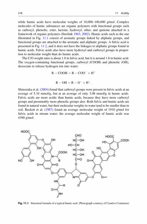
while humic acids have molecular weights of 10,000–100,000 g/mol. Complexmolecules of humic substances are organic polymers with functional groups suchas carboxyl, phenolic, ester, lactone, hydroxyl, ether, and quinone attached to aframework of organic polymers (Steelink 1963, 2002). Humic acids such as the oneillustrated in Fig. 11.1 consist of aromatic groups linked by aliphatic groups, andfunctional groups are attached to the aromatic and aliphatic groups. A fulvic acid ispresented in Fig. 11.2, and it does not have the linkages to aliphatic groups found inhumic acids. Fulvic acids also have more hydroxyl and carboxyl groups in propor-tion to molecular weight than do humic acids.

The C/O weight ratio is about 1.0 in fulvic acid, but it is around 1.8 in humic acid.The oxygen-containing functional groups, carboxyl (COOH) and phenolic (OH),dissociate to release hydrogen ion into water:

R� COOH ¼ R� COO� þ Hþ

R� OH ¼ R� O� þ Hþ:

Shinozuka et al. (2004) found that carboxyl groups were present in fulvic acids at anaverage of 5.34 mmol/g, but at an average of only 3.08 mmol/g in humic acids.Fulvic acids are more acidic than humic acids, because they have more carboxylgroups and presumably more phenolic groups also. Both fulvic and humic acids arefound in natural water, but their molecular weights in water tend to be smaller than insoil. Beckett et al. (1987) found an average molecular weight of 1910 g/mol forfulvic acids in stream water; the average molecular weight of humic acids was4390 g/mol.

Fig. 11.1 Structural formula of a typical humic acid. (Photograph courtesy of Creative Commons)

218 11 Acidity

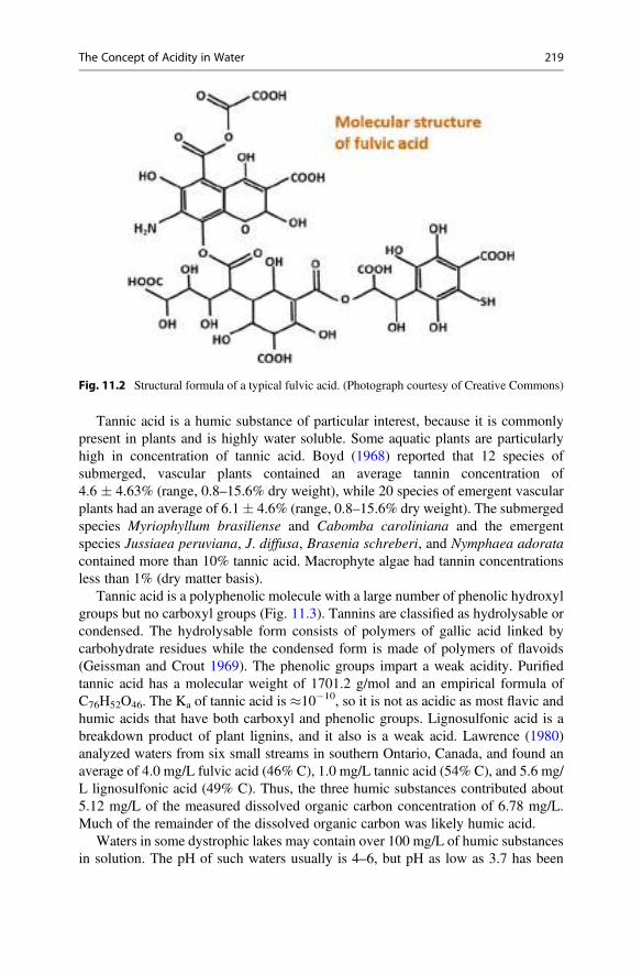
Tannic acid is a humic substance of particular interest, because it is commonlypresent in plants and is highly water soluble. Some aquatic plants are particularlyhigh in concentration of tannic acid. Boyd (1968) reported that 12 species ofsubmerged, vascular plants contained an average tannin concentration of4.6 � 4.63% (range, 0.8–15.6% dry weight), while 20 species of emergent vascularplants had an average of 6.1� 4.6% (range, 0.8–15.6% dry weight). The submergedspecies Myriophyllum brasiliense and Cabomba caroliniana and the emergentspecies Jussiaea peruviana, J. diffusa, Brasenia schreberi, and Nymphaea adoratacontained more than 10% tannic acid. Macrophyte algae had tannin concentrationsless than 1% (dry matter basis).

Tannic acid is a polyphenolic molecule with a large number of phenolic hydroxylgroups but no carboxyl groups (Fig. 11.3). Tannins are classified as hydrolysable orcondensed. The hydrolysable form consists of polymers of gallic acid linked bycarbohydrate residues while the condensed form is made of polymers of flavoids(Geissman and Crout 1969). The phenolic groups impart a weak acidity. Purifiedtannic acid has a molecular weight of 1701.2 g/mol and an empirical formula ofC76H52O46. The Ka of tannic acid is �10�10, so it is not as acidic as most flavic andhumic acids that have both carboxyl and phenolic groups. Lignosulfonic acid is abreakdown product of plant lignins, and it also is a weak acid. Lawrence (1980)analyzed waters from six small streams in southern Ontario, Canada, and found anaverage of 4.0 mg/L fulvic acid (46% C), 1.0 mg/L tannic acid (54% C), and 5.6 mg/L lignosulfonic acid (49% C). Thus, the three humic substances contributed about5.12 mg/L of the measured dissolved organic carbon concentration of 6.78 mg/L.Much of the remainder of the dissolved organic carbon was likely humic acid.

Waters in some dystrophic lakes may contain over 100 mg/L of humic substancesin solution. The pH of such waters usually is 4–6, but pH as low as 3.7 has been

Fig. 11.2 Structural formula of a typical fulvic acid. (Photograph courtesy of Creative Commons)

The Concept of Acidity in Water 219

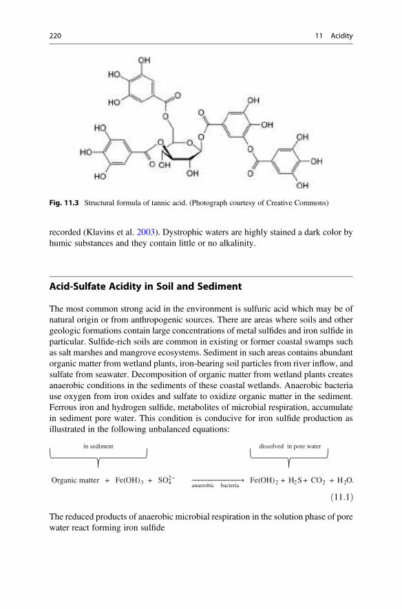
recorded (Klavins et al. 2003). Dystrophic waters are highly stained a dark color byhumic substances and they contain little or no alkalinity.

Acid-Sulfate Acidity in Soil and Sediment

The most common strong acid in the environment is sulfuric acid which may be ofnatural origin or from anthropogenic sources. There are areas where soils and othergeologic formations contain large concentrations of metal sulfides and iron sulfide inparticular. Sulfide-rich soils are common in existing or former coastal swamps suchas salt marshes and mangrove ecosystems. Sediment in such areas contains abundantorganic matter from wetland plants, iron-bearing soil particles from river inflow, andsulfate from seawater. Decomposition of organic matter from wetland plants createsanaerobic conditions in the sediments of these coastal wetlands. Anaerobic bacteriause oxygen from iron oxides and sulfate to oxidize organic matter in the sediment.Ferrous iron and hydrogen sulfide, metabolites of microbial respiration, accumulatein sediment pore water. This condition is conducive for iron sulfide production asillustrated in the following unbalanced equations:

Organic matter + Fe(OH)3 + SO42−

anaerobic bacteriaFe(OH)2 + H2S + CO2 + H2O.

in sediment dissolved in pore water

ð11:1ÞThe reduced products of anaerobic microbial respiration in the solution phase of porewater react forming iron sulfide

Fig. 11.3 Structural formula of tannic acid. (Photograph courtesy of Creative Commons)

220 11 Acidity

Fe OHð Þ2 þ H2S ! FeSþ 2H2O: ð11:2ÞFerrous sulfide is readily transformed to iron pyrite (FeS2) in the presence of

hydrogen sulfide that may be abundant in anaerobic environments (Rickard andLuther 1997). The reaction is:

FeSþ H2S ! FeS2 þ H2 " : ð11:3ÞNotice that in Eq. 11.3, sulfur in FeS2 should have a valence of �1, a valence notusually assigned to sulfur. Schippers (2004) and Borda (2006) assigned a valence of�1 to S in iron pyrite, but the�1 valence causes a dilemma with others (Nesbitt et al.1998). Those who do not agree with a �1 valence for sulfur solve this dilemma byreferring to the S2 in FeS2 as the persulfide ion with a valence of �2.

Some soils in coastal areas of South Carolina in the southern United States werereported to contain up to 5.5% sulfide-sulfur (Fleming and Alexander 1961). Coastalareas with soil high in sulfide-sulfur concentration are common in Indonesia, thePhilippines, Thailand, Malaysia, Australia, and many other countries. Metal sulfidesalso form in marine sediment not associated with wetlands or warm climates. Thefirst description of acid-sulfate soils was made in the eighteenth century for certainsoils in the Netherlands by Carl Linneaus, the Swedish botanist of plant and animaltaxonomy fame (Fanning 2006).

In addition to iron sulfide, copper sulfide (CuS), zinc sulfide (ZnS), manganoussulfide (MnS), and other metal sulfides form in anaerobic environments (Rickard andLuther 2006). Iron pyrite and other metal sulfides are common constituents of coaland some other mineral deposits. Mining often exposes overburden of high sulfide-sulfur content and creates spoil piles that contain sulfide-sulfur.

Soils containing sulfur concentrations of 0.75% or more are classified as potentialacid-sulfate soils (Soil Survey Staff 1994). While soils containing metal sulfides areanaerobic, these compounds are insoluble and have little influence on soil acidity.When potential acid-sulfate (PAS) soils are exposed to the air or oxygenated water,oxidation occurs and sulfuric acid is produced. Potential acid-sulfate soils are thencalled active acid-sulfate soils. The rate of oxidation of sulfide is much greater insoils exposed to the atmosphere than in sediment exposed to oxygenated water. Theoxidation of iron pyrite is a complex reaction occurring in several ways dependingupon conditions in pyritic sediment or PAS soil (Chandra and Gerson 2011).According to Sorensen et al. (1980) iron pyrite reacts with oxygen to produce ferroussulfate and sulfuric acid. Presence of sulfuric acid allows further oxidation of ferroussulfate to ferric sulfate. The presence of ferric sulfate also permits oxidation of ironpyrite to sulfuric acid. These reactions are shown below:

FeS2 þ H2Oþ 3:5 O2 ! FeSO4 þ H2SO4 ð11:4Þ

2FeSO4 þ 0:5 O2 þ H2SO4 ! Fe2 SO4ð Þ3 þ H2O ð11:5Þ

Acid-Sulfate Acidity in Soil and Sediment 221

FeS2 þ 7Fe2 SO4ð Þ3 þ 8H2O ! 15FeSO4 þ 8H2SO4: ð11:6ÞFerric sulfate plays an important role in pyrite oxidation, and the production of ferricsulfate from ferrous sulfate is greatly accelerated by activity of bacteria of the genusThiobacillus, and under acidic conditions, oxidation of pyrite by ferric sulfate israpid.

Ferric sulfate can hydrolyze with formation of sulfuric acid according to thefollowing reactions:

Fe2 SO4ð Þ3 þ 6H2O ! 2Fe OHð Þ3 þ 3H2SO4 ð11:7Þ

Fe2 SO4ð Þ3 þ 2H2O ! 2Fe OHð ÞSO4 þ H2SO4: ð11:8ÞFerric sulfate also can react with iron pyrite to form elemental sulfur and the sulfurmay be oxidized to sulfuric acid by microorganisms

Fe2 SO4ð Þ3 þ FeS2 ! 3FeSO4 þ 2S ð11:9Þ

Sþ 1:5 O2 þ H2O ! H2SO4: ð11:10ÞFerric hydroxide can react with bases, such as potassium, in acid sulfate soils to

form jarosite, a basic iron sulfate

3Fe OHð Þ3 þ 2SO2�4 þ Kþ þ 3Hþ ! KFe3 SO4ð Þ2 OHð Þ6 � 2H2Oþ H2O: ð11:11Þ

Jarosite is relatively stable, but in older acid-sulfate soils where acidity has beenneutralized, jarosite tends to hydrolyze as follows:

KFe3 SO4ð Þ2 OHð Þ6 � 2H2Oþ 3H2O ! 3Fe OHð Þ3 þ Kþ þ 2SO2�4

þ 3Hþ þ 2H2O: ð11:12ÞThere are several purely chemical oxidations and microbially mediated

oxidations of reduced sulfur compounds that cause acidity in sediment. The impor-tant point is that all of these reactions ultimately lead to the release of sulfuric acid.All of the reactions are summarized by the reaction of oxygen with sulfur(Eq. 11.10). An example of the calculation of the potential acidity of a potentialacid sulfate soil is provided in Ex. 11.1.

Ex. 11.1 The potential acidity of an aquatic soil (bulk density ¼ 1.15 kg/m3)containing 5.5% sulfide-sulfur will be calculated.

Solution: The approximate answer can be obtained using Eq. 11.10. The poten-tial acid is reported as equivalent calcium carbonate. The stoichiometricrelationships are:

Sþ 1:5 O2 þ H2O ! H2SO4

222 11 Acidity

CaCO3 þ H2SO4 ! Ca2þ þ CO2 þ SO4 þ H2O:

It follows that

S ! H2SO4 ! CaCO3

and 1 kg of soil with 5.5% S would contain 0.055 kg S. The stoichiometric ratio is:

0:055 kgS32

¼X

CaCO3

100

X ¼ 0:17 kg CaCO3=kg soil:

One hectare of this soil to a depth of 15 cm would weigh10,000 m2 � 0.15 m � 1150 kg/m3 ¼ 1,725,000 kg. The amount of potential acidwould be equal to

1; 725; 000 kg=ha� 0:17 kg CaCO3=kg soil¼ 293; 250 kg CaCO3=ha or 293:2 t=ha:

Sulfuric acid dissolves aluminum, manganese, zinc, copper, and other metalsfrom soil, and runoff from acid-sulfate soils and mine spoils is highly acidic andusually contains potentially toxic metallic ions. The potential for acid production inan acid-sulfate soil depends largely upon the amount and particle size of the ironpyrite, the presence or absence of exchangeable bases and carbonate within thepyrite-bearing material, the exchange of oxygen and solutes with the soil, and theabundance of Thiobacillus. Because the exchange of oxygen and solutes and theabundance of Thiobacillus are restricted with depth, the acid-sulfate conditionusually is a surface soil phenomenon.

Waterlogging of acid-sulfate soils restricts the availability of oxygen, and sulfuricacid production ceases when soil becomes anaerobic. Sulfate is reduced to sulfideunder anaerobic conditions by bacteria of the genus Desulfovibrio. In natural waters,the sediment-water interface usually is aerobic, and sulfuric acid production occurs,but at a much slower rate than when sediment is exposed to air.

Oxidation of pyrite in spoil piles from mine excavations results in sulfuric acidthat may enter streams in runoff and reduce pH. Seepage from underground minesalso may be acidic. Surface coal mining was a major source of acid drainage tostreams in the past, because the overburden above coal deposits was stripped off andpiled on the land surface. The last overburden removed from above the coalformation was contaminated with particles of coal that contained sulfide sulfur.This contaminated material tended to end up on top of the spoil pile promotingcontact with atmospheric oxygen and oxidation of sulfide to sulfuric acid. The acidremoved from mine spoils by rainwater and runoff flowed into streams causingacidification. Acidic water also may seep or be pumped from mines to causeacidification of receiving waters.

Acid-Sulfate Acidity in Soil and Sediment 223

The modern procedure at surface mining operations is to separate the overburdenthat is contaminated with coal and stockpile it separately from the other overburden.Once the coal deposit has been mined, the contaminated overburden is placed backinto the mined area and covered with the stockpiled nonacidic overburden. Limingof spoil material and development of grass cover on it also lessens the problem withacid drainage. Most countries have regulations regarding treatment of mine effluent,and in some cases, effluents or streams are treated with limestone to neutralizeacidity.

Acidic, Atmospheric Deposition

Rainwater naturally has a pH of about 5.6 because it becomes saturated with carbondioxide while falling through the atmosphere. The carbon dioxide concentration ofthe atmosphere is increasing, but this has little effect on the pH of rain. A pH <5.6 inrainfall usually results from atmospheric pollution with sulfur and nitrogen gases.The acidic rain problems have arisen because of combustion of fuels, and it is mostsevere in urbanized and industrial areas and in the direction of the prevailing windfrom these areas. Rainfall in eastern Canada and the northeastern United States wasreported to have an annual, average pH of 4.2–4.4 and rain from individual stormshad lower pH (Haines 1981).

Hydrogen sulfide and other sulfides emitted with sulfur dioxide are oxidized tosulfur dioxide in the atmosphere. In the gaseous phase of the atmosphere, sulfurdioxide and nitrogen oxides (NOx) form strong acids as illustrated in the sequence ofreactions given below:

2H2Sþ 3O2 ! 2H2Oþ 2SO2

SO2 þ OH� ! HOSO2 hydroxysulfonyl radicalð Þ

HOSO2 þ O2 ! HO�2 þ SO3 sulfur trioxideð Þ

SO3 þ H2O ! H2SO4

NO2 þ OH� ! HNO3

or NOx þ xOH� ! HNOx:

In cloud droplets, sulfur dioxide reacts in a slightly different manner:

SO2 ! H2O ¼ SO2 ∙H2O

224 11 Acidity

SO2 ∙H2O ! Hþ þ HSO�3 bisulfite ionð Þ

HSO�3 $ Hþ þ SO2�

3

SO2�3 þ H2O $ H2SO4:

Combustion of fossil fuels is the main source of acid-forming substances in theatmosphere. All sectors that burn fuel contribute such emissions roughly in propor-tion to energy use. The emissions not only include hydrogen sulfide, sulfur dioxide,and nitrogen oxides, they also contain particulate material that can continue tooxidize and produce acidity. Wet precipitation (rainfall, snow, dew, etc.) and dryfall out of particles can deliver acidity to the earth’s surface. Burning of crop residuesafter harvest and other agricultural wastes often cause much smoke and haze at timesin developing countries. These emissions, however, contribute only about 0.1% ofsulfur emissions (Smith et al. 2011).

It is interesting to note that global sulfur dioxide emissions had been increasingrapidly, but they declined following an effort beginning in the 1970s in developedcountries to remove sulfur from emissions. Since the early 2000s, global sulfuremissions are rapidly increasing again as the industrial sector and economy of China,India, and a few other countries have expanded in the absence of effective airpollution regulations.

The rising carbon dioxide concentration in the atmosphere is an important factorrelated to acidification of rainfall or surface freshwater bodies. Increased atmo-spheric carbon dioxide does, however, influence oceanic carbon dioxide concentra-tion, pH, and calcium carbonate saturation level. As the atmospheric carbon dioxideincreases, the solubility of carbon dioxide in the ocean increases. Greater carbondioxide concentration reduces ocean pH slightly despite the buffering capacity of themoderate alkalinity of the ocean. Caldeira and Wickett (2003) reported that theaverage pH of the ocean has fallen by 0.1 pH units since the beginning of theindustrial revolution (mid 1700s). The USEPA (https://www.epa.gov/climate-indicators/climate-change-indicators-ocean-acidity) present data for ocean pH nearBermuda and Hawaii between 1987 and 2015. The pH decreases were 8.12 to 8.06and 8.12 to 8.07, respectively. The average decrease has been about 0.002 pH unitsper year, and the trajectory of the decline has been essentially constant since 1987.Some authors such as Feely et al. (2004) predict ocean pH will drop by another0.3–0.4 unit by 2100.

Reduction in ocean pH favors the dissolution of aragonite and calcite by reducingthe pH below that of calcium carbonate saturation. Aragonite and calcite comprisethe shells of calcifying marine organisms, and thinner shells will negatively affectsurvival and growth of these organisms (Orr et al. 2005). The effect on oceanecology could be enormous.

Acidic, Atmospheric Deposition 225

https://www.epa.gov/climate-indicators/climate-change-indicators-ocean-acidity

https://www.epa.gov/climate-indicators/climate-change-indicators-ocean-acidity

Measurement of Acidity

The simplest procedure for measuring acidity is to titrate a water sample from itsinitial pH to pH 8.3 with standard sodium hydroxide solution. A 0.010 N sodiumhydroxide solution is often used, but other normalities may be used where necessaryto obtain suitable titration volumes (buret readings). The amount of base needed toraise the pH to the methyl orange endpoint (or to pH 4.5 as measured with a pHmeter) is recorded, and the titration is continued to pH 8.3 (phenolphthalein end-point) in instances where carbon dioxide acidity is of interest.

The titration of acidity is illustrated in Ex. 11.2.

Ex. 11.2 A 100-mL water sample of pH 3.1 is titrated with 0.022 N NaOH topH 4.5, and then the titration is continued to pH 8.3. The volume of acid to titrate topH 4.5 is 3.11 mL, and the total acid used in the titration is 3.89 mL. The total acidityand mineral acidity will be estimated.

Solution: The same approach used for alkalinity calculation (Ex. 9.5) can beused here because results will again be reported as equivalent CaCO3. The totalacidity as milliequivalent CaCO3 equals the milliequivalents of base used in theentire titration:

3:89 mLð Þ 0:022 Nð Þ ¼ 0:0856 meq NaOH ¼ meq acidity ¼ meq CaCO3:

The weight equivalent CaCO3 in the sample is

0:0856 meq CaCO3ð Þ 50:04 mg CaCO3=meqð Þ ¼ 4:28 mg CaCO3:

To convert milligrams of CaCO3 in the sample to milligrams per liter of CaCO3 inthe sample,

4:28 mg CaCO3ð Þ 1; 000 mL=L

100 mL

� �¼ 42:8 mg=L CaCO3:

The same procedure is repeated for the volume of base used for titration to pH 4.5 toobtain the mineral acidity. The result is 34.2 mg/L CaCO3.

The sample had 42.8 mg/L total acidity and 34.2 mg/L mineral acidity. Thedifference of 8.6 mg/L represents acidity of carbon dioxide in the sample.

Acidic waters may contain measurable concentrations of metal ions that mayreact with hydroxide during titration as shown below:

Fe3þ þ 3OH� ! Fe OHð Þ3: ð11:13ÞThis results in an overestimation of acidity. The discrepancy can be prevented by thehot peroxide treatment method (Eaton et al. 2005). In the hot peroxide method, thesample pH is reduced below 4.0 (if necessary) by adding 5.00-mL increments of0.02 N sulfuric acid. Five drops of 30% hydrogen peroxide (H2O2) are added, andthe sample is boiled for 5 min. After cooling to room temperature, the sample is

226 11 Acidity

https://doi.org/10.1007/978-3-030-23335-8_9#FPar5

titrated with standard sodium hydroxide to pH 3.7, 4.5, or 8.3 as desired. Hot sulfuricacid-hydrogen peroxide treatment removes the potentially interfering substances,and the titration volume must be corrected for the added acidity. This is done bysubtracting the product (mL H2SO4 � N H2SO4) from the product (mL NaOH �N NaOH).

The equations for calculating acidity based on the pH selected for the endpointare:

Without hot peroxide pretreatment,

Acidity mg CaCO3=Lð Þ ¼ Nbð Þ Vbð Þ 50ð Þ 1; 000ð ÞS

ð11:14Þ

where Nb ¼ normality NaOH (meq/mL), Vb ¼ volume NaOH used (mL), 50 ¼ mgCaCO3/meq, 1000 ¼ mL/L, and S ¼ sample volume (mL).

With hot peroxide pretreatment

Acidity mg CaCO3=Lð Þ ¼ Nb � Vbð Þ � Na � Vað Þ½ � 50ð Þ 1; 000ð ÞS

ð11:15Þ

where Na ¼ normality H2SO4 (meq/mL) and Va ¼ volume H2SO4 (mL).

Effects of Acidity

Water bodies with high concentrations of humic substances typically have lowproductivity as the result of low pH, low nutrient concentrations, and restrictedlight penetration. Such waters also will have relatively low biodiversity. There havebeen studies suggesting that decomposition products (presumably humic substances)of barley straw in natural waters act as algicides (Everall and Lees 1996). However,there is no evidence that low primary productivity and biodiversity in humically-stained waters is a direct toxic effect.

The most serious effects of acidity on species diversity and productivity usuallyare observed at pH < 5. The phenomenon of acid rain provides an excellent example.Lakes in some areas of Canada and the northeastern United States declined in pH by1–2 units between 1950 and 1980 (Haines 1981; Cowling 1982). Aquatic organismshave been affected at all trophic levels; species abundance, productivity, and speciesdiversity has been reduced. Fish have suffered acute mortality, reduced growth,reproductive failures, skeletal deformities, and increased accumulations of heavymetals (Haines 1981).

There is a well-known exception to the preceding paragraph. Rivers flowing fromtropical rainforests usually have pH 4–5 and high concentrations of humicsubstances, but they usually have diverse and flourishing fish communities. Thesefish possibly are adapted to low pH, but there is evidence that low pH from humicand fulvic acids is less harmful to fish than is low pH from mineral acids (Hollandet al. 2015). Organic matter decomposition does not progress rapidly at lowpH. Greater acidity favors fungi over bacteria, and fungi are not as effective in

Effects of Acidity 227

decomposing organic matter as are bacteria. In standing waters in poorly-drainedareas, shallow and marginal areas usually are infested by species of aquaticmacrophytes and reed-swamp plants. These plants have a low nitrogen concentra-tion, a high fiber content, and they decompose slowly resulting in a large residue oforganic matter. Peat bogs and organic soils are common in regions with highly acidicsoils and water.

Humic substances have a low mammalian toxicity, and no direct toxicityproblems are incurred from elevated concentrations of these substances in watersfor swimming, bathing, or domestic water supply (de Melo et al. 2016). Of course,people desire clear water for these purposes, and clear water usually is preferred inbodies of water used for landscape enhancement (Smith et al. 1995; Nassar and Li2004). High concentrations of humic substances in municipal water supplies also areproblematic, because these substances react with free chlorine residuals to producetrihalomethane, a suspected carcinogen (Rathbun 1996). Removal of humicsubstances from water supplies is difficult. The most common method is chemicalflocculation, but it does not reduce concentration by more than 40–60%. Othermethods include membrane filtration, adsorption of activated carbon, and ozoneoxidation.

Mitigation of Acidity

Limestone, lime, and other alkaline materials have been used to neutralize acidity forimproving crop growth in agriculture since at least the thirteenth century (Johnson2010). The effect of increasing pH on water quality in bog lakes was demonstrated inan early study by Hasler et al. (1951). In Cather Lake in Wisconsin, liming improvedconditions for fish production by increasing pH from 5.6 to 7.1–7.5, alkalinity from3.0 to 15–19 mg/L, and Secchi disk visibility from 2.0 m to 4.3–5.7 m. Conditionsfor fish production were greatly improved. The use of liming materials also is acommon practice in sportfish ponds and aquaculture ponds (Boyd 2017).

The most common agent for neutralizing acidity in water bodies is agriculturallimestone made by pulverizing limestone. This liming material usually has an acidneutralizing value of 90–100% CaCO3 equivalent. Two other common limingmaterials are burnt lime (calcium oxide or a mixture of calcium and magnesiumoxides) and hydrated lime (calcium hydroxide or a mixture of calcium and magne-sium hydroxides). Burnt lime is made by burning limestone in a furnace, and theresulting chemical reaction is illustrated using calcium carbonate as the limestonesource

CaCO3 !Δ

CaOþ CO2 " : ð11:16Þ

Hydrated lime is made by treating burnt lime with water

228 11 Acidity

CaOþ H2O ! Ca OHð Þ2: ð11:17ÞBurnt lime usually has an acid neutralizing value of 160–180% CaCO3 equivalent,while for hydrated lime the value is about 130–140% CaCO3 equivalent.

Sodium bicarbonate and sodium hydroxide also can be used to neutralize acid,but they tend to be more expensive than limestone products. The acid neutralizingvalues of sodium bicarbonate and sodium hydroxide are around 60% and 125%CaCO3 equivalent, respectively.

The neutralization of acidity in a water body appears simple at first consideration.A water body containing 10,000 m3 with an acidity of 100 mg/L of CaCO3 wouldrequire 1000 kg of liming material (expressed as equivalent CaCO3) to neutralize itsacidity (10,000 m3 � 100 mg CaCO3/L of acidity � 10�3 kg/g ¼ 1000 kg CaCO3).This amount of liming material would only neutralize the acidity in the water.Additional liming material would be required to raise the alkalinity of the water.For example, to raise the alkalinity to 50 mg/L would require another 500 kg ofCaCO3 equivalent.

Effective liming cannot be achieved as illustrated in the preceding paragraph. Inan acidic water body, the sediment contains acidity, and this acidity must beneutralized or it will remove alkalinity from the water. Soil acidity is more difficultto measure than is the acidity of water. The lime requirement of sediment can bemeasured by procedures modified from agricultural soil testing methods (Han et al.2014; Boyd 2017).

Acidic effluents are treated with liming materials to neutralize acidity and preventdamage to organisms in receiving water bodies. Acidic water is corrosive to waterpipes and other plumbing fixtures. Thus, liming of acidic water before distributionprotects the delivery system from corrosion.

Conclusions

The productivity and biodiversity of water bodies decrease as pH declines, and mostwaters with little or no alkalinity (pH <5.5) are considered dystrophic. The exceptionis waters from tropical jungles in which the acidity is primarily from humicsubstances. The lowest pHs are found in surface waters that contain sulfuric acidfrom oxidation of iron pyrite in soils, from acidic mine drainage, or from acidicrainfall. Acidity can be measured by titration with standard sodium hydroxide.Liming materials (limestone, burnt lime, and hydrated lime) often are applied tomitigate acidity.

Conclusions 229

References

Beckett R, Jue Z, Giddings JC (1987) Determination of molecular weight distributions of fulvic andhumic acids using flow field-flow fractionation. Environ Sci Tech 21:289–295

Borda MJ (2006) Pyrite. In: Lai R (ed) Encyclopedia of soil science. Taylor & Francis, New York,pp 1385–1387

Boyd CE (1968) Freshwater plants: a potential source of protein. Econ Bot 22:359–368Boyd CE (2017) Use of agricultural limestone and lime in aquaculture. CAB Rev 12(015). http://

cabi.org/cabreviewsCaldeira K, Wickett ME (2003) Anthropogenic carbon and ocean pH. Nature 425:365Chandra AP, Gerson AR (2011) Pyrite (FeS2) oxidation: a sub-micron synchrotron investigation of

the initial steps. Geochim Cosmochim Acta 75:6239–6254Cowling EB (1982) Acid precipitation in historical perspective. Environ Sci Tech 16:110–123de Melo BA, Motta FL, Santana MH (2016) Humic acids: structural properties and multiple

functionalities for novel technological developments. Mater Sci Eng C 62:967–974Eaton AD, Clesceri LS, Rice EW, Greenburg AE (eds) (2005) Standard methods for the examina-

tion of water and wastewater. American Public Health Association, Washington, DCEverall NC, Lees DR (1996) The use of barley-straw to control general and blue-green algal growth

in a Derbyshire reservoir. Water Res 30:269–276Fanning DS (2006) Acid sulfate soils. In: Lai R (ed) Encyclopedia of soil science. Taylor & Francis,

New York, pp 11–13Feely RA, Sabine CL, Lee K, Berelson W, Kleypas J, Fabry VJ, Millero FJ (2004) Impact of

anthropogenic CO2 on the CaCO3 system in the ocean. Science 305:363–366Fleming JF, Alexander LT (1961) Sulfur acidity in South Carolina tidal marsh soils. Soil Sci Soc

Am Proc 25:94–95Geissman TA, Crout DHG (1969) Organcic chemistry of secondary plant metabolism. Freeman,

San FranciscoHaines TA (1981) Acid precipitation and its consequences for aquatic ecosystems: a review. Trans

Am Fish Soc 110:669–707Han Y, Boyd CE, Viriyatum R (2014) A bicarbonate method for lime requirement to neutralize

exchangeable acidity of pond bottom soils. Aqua 434:282–287Hasler AD, Brynildson OM, Helm WT (1951) Improving conditions for fish in brown-water bog

lakes by alkalization. J Wildl Manag 15:347–352Holland A, Duivenvoorden LJ, Kinnear SHW (2015) Effect of key water quality variables on

macroinvertebrate and fish communities within naturally acidic wallum streams. Mar FreshwRes 66:50–59

Johnson DS (2010) Liming and agriculture in the Central Pennines. BAR Publishing, OxfordKlavins M, Rodinov V, Druvietis I (2003) Aquatic chemistry and humic substances in bog lakes in

Latvia. Boreal Environ Res 8:113–123Lawrence J (1980) Semi-quantitative determination of fulvic acid, tannin and lignin in natural

waters. Water Res 14:373–377Nassar JL, Li M (2004) Landscape mirror: the attractiveness of reflecting water. Landsc Urban Plan

66:233–238Nesbitt HW, Bancroft GM, Pratt AR, Scaini MJ (1998) Sulfur and iron surface states on fractured

pyrite surfaces. Am Min 83:1067–1076Orr JC, Fabry VJ, Aumont O, Bopp L, Doney SC, Feely RA, Gnanadesikan A, Gruber N, Ishida A,

Joos F, Key RM, Lindsay K, Maier-Reimer E, Matear R, Monfray P, Mouchet A, Najjar RG,Plattner G, Rodgers KB, Sabine CL, Sarmiento JL, Schlitzer R, Slater RD, Totterdell IJ,Weirig M, Yamanaka Y, Yool A (2005) Anthropogenic ocean acidification over the twenty-first century and its impact on calcifying organisms. Nature 437:681–686

Rathbun RE (1996) Disinfection byproduct yields from the chlorination of natural waters. ArchEnviron Contam Toxicol 31:420–425

230 11 Acidity

http://cabi.org/cabreviews

http://cabi.org/cabreviews

Rickard D, Luther GW III (1997) Kinetics of pyrite formation by the H2S oxidation of iron(II) monosulfide in aqueous solutions between 25 and 125C: the mechanisms. GeochimCosmochim Acta 61:135–147

Rickard D, Luther GW III (2006) Metal sulfide complexes and clusters. Rev Mineral Geochem61:421–504

Schippers A (2004) Biogeochemistry of metal sulfide oxidation in mining environments, sediments,and soils. In: Amend JP, Edwards KJ, Lyons TW (eds) Sulfur biogeochemistry: past andpresent, Special Paper 379. Geological Society of America, Washington, DC, pp 49–62

Shinozuka T, Shibata M, Yamaguchi T (2004) Molecular weight characterization of humicsubstances by MALDI-TOF-MS. J Mass Spectrom Soc Jpn 52:29–32

Smith DG, Croker GF, McFarlane K (1995) Human perception of water appearance. 1. Clarity andcolor for bathing and aesthetics. N Z J Mar Fresh Res 29:29–43

Smith SJ, van Aardenne J, Kilmont Z, Andres RJ, Volke A, Arias SD (2011) Anthropogenic sulfurdioxide emissions: 1850-2005. Atmos Chem Phys 11:1101–1116

Soil Survey Staff (1994) Keys to soil taxonomy, 6th edn. United States Department of Agriculture,Soil Conservation Service, Washington, DC

Sorensen DL, Knieb WA, Porcella DB, Richardson BZ (1980) Determining the lime requirementfor the blackbird mine spoil. J Environ Qual 9:162–166

Steelink C (1963) What is humic acid? Proc Cal Assoc Chem Teach 7:379–384Steelink C (2002) Investigating humic acids in soils. Anal Chem 74:327–333

References 231

Microorganisms and Water Quality 12

AbstractPhytoplankton and bacteria have a greater effect on water quality than do otheraquatic microorganisms. Phytoplankton are the main primary producers whilebacteria are responsible for the majority of organic matter decomposition andnutrient recycling. An overview of microbial growth, photosynthesis, and respi-ration is provided, and methods for measuring primary production and respirationin water bodies are discussed. The combined physiological activities of producerand decomposer organisms in water bodies cause pH and dissolved oxygenconcentration to increase and carbon dioxide concentration to decrease in day-time, while the opposite occurs during nighttime. In unstratified water bodies,aerobic conditions usually exist in the water column and at the sediment-waterinterface. Nevertheless, sediment typically is anaerobic at depths greater than afew centimeters in oligotrophic water bodies or greater than a few millimeters ineutrophic water bodies. In anaerobic sediment (or water), the metabolic activity ofchemotrophic bacteria is important in decomposing organic compounds resultingfrom fermentation. Although chemotrophic bacteria are beneficial in assuringmore complete decomposition of organic matter, toxic metabolic wastes—partic-ularly nitrite and hydrogen sulfide—produced by these microorganisms can enterthe water column. Blue-green algae—often called cyanobacteria—tend to domi-nate phytoplankton communities in eutrophic waters. Blue-green algae can causesurface scums and shallow thermal stratification, be toxic to other algae andaquatic animals, or produce taste and odor problems in public water supplies.

Introduction

Aquatic ecosystems are inhabited by many types of microorganisms to includealgae, bacteria, fungi, protozoa, rotifers, bryozoa, and arthropods. Algae are theprimary producers, and bacteria and fungi are the decomposers. Microscopic animalsfeed on microscopic plants and animals and their remains; they serve to link between


233


primary producers and larger animals in the food web of aquatic ecosystems. All ofthese organisms are important ecologically, but microscopic algae suspended in thewater column (phytoplankton) and bacteria suspended in the water column andliving in the sediment have a greater impact on water quality than do othermicroorganisms. Phytoplankton produce large amounts of organic matter throughphotosynthesis and release prodigious quantities of oxygen into water during theprocess. Bacteria decompose organic matter to release (recycle) inorganic nutrients.Respiration by bacteria and respiration and photosynthesis by phytoplankton have apronounced effect on pH and concentrations of carbon dioxide and dissolved oxygenin water. Certain bacteria and other microscopic organisms are pathogenic, and somespecies of algae can impart bad tastes and odors to water as well as to the flesh of fishand other aquatic food animals.

Although phytoplankton and bacteria are the focus of this chapter, larger aquaticplants that are rooted in the bottoms and edges of water bodies also will be discussedas they are sometimes the dominant plants in aquatic habitats. Moreover, all con-sumer organisms participate in the process of organic matter degradation andnutrient recycling through their use of organic matter for food.

Bacteria

A main distinguishing feature between bacteria and other single-celledmicroorganisms is that the nuclei of bacterial cells are not enclosed in a mem-brane—they are known as prokaryotic organisms as opposed to eukaryoticorganisms in which the nucleus is bound by a membrane. Bacteria may be eitherunicellular or filamentous, and their cells usually are spherical or cylindrical (rods).They may live free in water, attached to surfaces, in sediment, and within other livingorganisms. A few types are capable of locomotion. Some bacteria are pathogenic toplants, animals, or humans.

The food source for most bacteria is dead organic matter, while a few kinds ofbacteria are capable of synthesizing organic matter. These two groups of bacteria areknown as heterotrophic and autotrophic bacteria, respectively. Obligate aerobicbacteria cannot live without oxygen, obligate anaerobic bacteria cannot exist inenvironments with oxygen, and facultative anaerobic bacteria can do well with orwithout oxygen. Some species that can function without molecular oxygen obtainoxygen from nitrate, sulfate, carbon dioxide, or other inorganic compounds.

The major ecological role of most bacteria is to decompose organic matter andrecycle its essential inorganic components, e.g., carbon dioxide, water, ammonia,phosphate, sulfate, and other minerals. Some bacteria can have a major influence oncertain species in a water body by causing disease. There also are some bacteria andviruses that can cause illness in humans who drink water in which these organismsoccur.

234 12 Microorganisms and Water Quality

Physiology

Nutrients have three functions in growth and metabolism. They are raw materials forelaboration of biochemical compounds of which organisms are made. Carbon andnitrogen contained in organic nutrients are used in making protein, carbohydrate, fat,and other components of microbial cells. Nutrients supply energy for growth andchemical reactions. Organic nutrients are oxidized in respiration, and the energyreleased is used to drive chemical reactions that synthesize biochemical compoundsnecessary for growth and maintenance. Nutrients also serve as electron and hydro-gen acceptors in respiration. The terminal electron and hydrogen acceptor for aerobicrespiration is molecular oxygen. An organic metabolite or inorganic substancereplaces oxygen as electron or hydrogen acceptor in anaerobic respiration.

Growth

Water and sediment contain species of microorganisms capable of decomposingalmost any organic substance. Some substances decompose faster than others, butfew organic compounds completely resist decay by microorganisms. Microbialactivity is slow where organic matter is scarce, but actively growingmicroorganisms, resting spores, and other propagules are present almost every-where. An increase in organic matter provides substrate for microbial growth, andthe number of microorganisms increases. As a general rule, the bacteria necessary todegrade organic matter are present in nature. It is usually not necessary to addbacteria. If decomposition is slow, it is because environmental conditions do notfavor rapid microbial action or the organic substrate is resistant to decay.

Bacteria reproduce by binary fission. One cell divides into two cells, and the newcells continue to divide. The time between cell divisions is called the generation timeor doubling time. The number of bacterial cells present after a given time (Nt) can becomputed from the initial number of cells (No) and the number of generations (n)

Nt ¼ No � 2n: ð12:1ÞMicroorganisms with a short generation time increase their numbers quickly

(Ex. 12.1).

Ex. 12.1 Organic matter is added to a water containing 103 bacterial cells permilliliter. These bacteria can double every 4 hours. The number of bacterial cellsafter 36 hours will be estimated.

Solution:The number of generations that will occur in 36 hours is

n ¼ 36 hr

4 hr=generation¼ 9:

The number of cells after 36 hours can be calculated with Eq. 12.1.

Bacteria 235

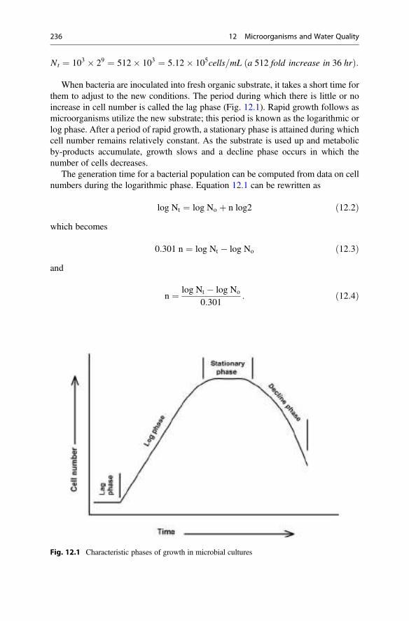
Nt ¼ 103 � 29 ¼ 512� 103 ¼ 5:12� 105cells=mL a 512 fold increase in 36 hrð Þ:

When bacteria are inoculated into fresh organic substrate, it takes a short time forthem to adjust to the new conditions. The period during which there is little or noincrease in cell number is called the lag phase (Fig. 12.1). Rapid growth follows asmicroorganisms utilize the new substrate; this period is known as the logarithmic orlog phase. After a period of rapid growth, a stationary phase is attained during whichcell number remains relatively constant. As the substrate is used up and metabolicby-products accumulate, growth slows and a decline phase occurs in which thenumber of cells decreases.

The generation time for a bacterial population can be computed from data on cellnumbers during the logarithmic phase. Equation 12.1 can be rewritten as

log Nt ¼ log No þ n log2 ð12:2Þwhich becomes

0:301 n ¼ log Nt � log No ð12:3Þand

n ¼ log Nt � log No

0:301: ð12:4Þ

Fig. 12.1 Characteristic phases of growth in microbial cultures


The generation time (g) is computed from the time interval (t) over which a givennumber of generations (n) occurred

g ¼ tnor n ¼ t

g: ð12:5Þ

Substituting tg for n in Eq. 12.4 gives

g ¼ 0:301 tlogNt � logNo

: ð12:6Þ

The utility of Eq. 12.6 is illustrated in Ex. 12.2.

Ex. 12.2 A bacterial culture increases from 104 cells/mL to 108 cells/mL in12 hours. The generation time will be calculated using Eq. 12.6.

Solution:

g ¼ 0:301 12ð Þ8� 4

¼ 0:903 hr ¼ 54 min:

The generation time of bacteria differs among species, and for a given species,generation time varies with temperature, substrate availability, and other environ-mental factors. When bacteria are growing rapidly, they also are quicklydecomposing substrate. For example, in a water where microorganisms are growinglogarithmically, the rate of evolution of carbon dioxide increases logarithmically.

Aerobic Respiration

Aerobic respiration is a major topic in books on plant and animal physiology,metabolic process, and general biochemistry. Nevertheless, a brief overview of themajor features of aerobic respiration will be provided. The reader should note thataerobic respiration is much the same for all organisms, and it involves oxidation oforganic compounds to carbon dioxide and water. The purpose of respiration is torelease energy from organic compounds and store it in high-energy phosphate bondsof adenosine triphosphate (ATP)

Adenosine diphosphate ADPð Þ þ PO4 þ energy Ð ATP: ð12:7ÞEnergy stored in ATP can be used to drive chemical reactions in cells. When energyis released from ATP, ADP is regenerated and used again.

In aerobic carbohydrate metabolism, a glucose molecule passes through glycoly-sis and the citric acid cycle (also called the Krebs cycle or the tricarboxylic acidcycle) before being completely oxidized to carbon dioxide. Glycolysis is a series ofordered reactions catalyzed by numerous enzymes—not indicated in the equationsbelow—that transform one glucose molecule to two pyruvate molecules

Bacteria 237

C6H12O6 ! 2C3H4O3 þ 4Hþ: ð12:8ÞTwo moles of ATP are formed per mole of glucose in glycolysis, but no carbondioxide is released. As a result, glycolysis does not require oxygen.

In aerobic respiration, pyruvate molecules from glycolysis react with coenzyme A(CoA) and nicotinamide adenine dinucleotide (NAD+) forming acetyl CoAmolecules

Pyruvateþ CoAþ 2NADþ Ð Acetyl CoAþ 2NADHþ 2Hþ þ CO2: ð12:9ÞThe formation of acetyl CoA from pyruvate is an oxidative decarboxylation in whichtwo H+ ions, 2 electrons, and one CO2 molecule are removed from each molecule ofpyruvate—a total of four hydrogen ions and two carbon dioxide molecules permolecule of the original glucose entering glycolysis. Acetyl CoA formation linksglycolysis to the citric acid cycle. Although glycolysis does not use oxygen, acetylCoA production and the citric acid cycle require oxygen.

The first step in the citric acid cycle is the reaction of acetyl CoA and oxaloaceticacid to form citric acid. In succeeding reactions—also catalyzed by enzymes—aseries of transformations of organic acids occur with release of eight H+ ions and twoCO2 molecules for each molecule of citric acid entering the cycle. This accounts forthe oxidation of the six organic carbon atoms present in one glucose molecule. Onemolecule of oxaloacetic acid also is regenerated in the cycle (recycled) and it canreact again with acetyl CoA.

Hydrogen ions produced through oxidation of glucose in glycolysis and the citricacid cycle reduce the enzymes NAD, NADP (nicotinamide adenine dinucleotidephosphate), and FAD (flavin adenine dinucleotide). A representative reaction whereH+ is released in the citric acid cycle is

C6H8O7 ! C6H6O7 þ 2Hþ

Isocitric acidð Þ Oxalosuccinic acidð Þand

NADPþ þ 2Hþ Ð NADPHþ Hþ: ð12:10ÞEnzymes of the citric acid cycle are brought in contact with the electron transport

system where they are reoxidized. Energy released in these oxidations is used forATP synthesis, and the regenerated NAD, NADP, and FAD are used again ashydrogen acceptors. Reoxidation of enzymes is accomplished by a series of cyto-chrome enzymes that pass electrons from one cytochrome compound to another. Inthe electron transport system, ADP combines with inorganic phosphate to form ATPand H+ ions combine with molecular oxygen to form water.

A total of 38 ATP molecules can be formed from 1 mole of glucose in aerobicrespiration (glycolysis and citric acid cycle). The ATP molecules contain approxi-mately one-third of the theoretical energy released during glucose oxidation. Energy


not used to form ATP is lost as heat. In aerobic respiration, 1 mole of glucoseconsumes 6 moles of oxygen and releases 6 moles of CO2 and water. This stoichi-ometry is illustrated in the summary equation for respiration

C6H12O6 þ 6O2 ! 6CO2 þ 6H2Oþ energy: ð12:11ÞThis equation usually is an adequate summary of the overall results of respiration inall types of aerobic organisms—microscopic or macroscopic and plant, animal,bacterial, or fungal.

Oxygen Stoichiometry in Aerobic Respiration

Organic matter contains a wide array of organic compounds, most of which are morecomplex than glucose. Bacteria excrete extracellular enzymes that break complexorganic matter down into particles small enough to be absorbed. These fragments arebroken down further inside the bacterial cell by enzymatic action until they are smallenough to be used in glycolysis. These fragments pass through the respiratoryreactions in the same way as glucose fragments.

The ratio of moles carbon dioxide produced to moles oxygen consumed is therespiratory quotient (RQ)

RQ ¼ CO2

O2: ð12:12Þ

Reference to Eq. 12.11 reveals that in the oxidation of glucose, six oxygenmolecules are consumed and six carbon dioxide molecules are released, i.e.,RQ ¼ 1.0. Other classes of organic matter do not contain the same ratio of carbonto oxygen to hydrogen as carbohydrate (Table 12.1), and RQmay be lesser or greaterthan 1.0. For example, consider the oxidation of a fat

C57H104O6 þ 80O2 ! 57CO2 þ 52H2O: ð12:13ÞThe respiratory quotient for the above reaction is 57CO2/80O2 or 0.71. Organiccompounds more highly oxidized (more oxygen relative to carbon) thancarbohydrates will have a respiratory quotient greater than 1.0, and more reducedcompounds such as fat and protein will have a respiratory quotient less than 1.0. Itfollows that the more reduced an organic substance, the more oxygen that is requiredto oxidize a unit quantity (Ex. 12.3).

Table 12.1 Carbon, hydrogen, and oxygen content of three major classes of organic compounds

% C % H % O

Carbohydrate 40 6.7 53.3

Protein 53 7 22

Fatty acids 77.2 11.4 11.4

Bacteria 239

https://doi.org/10.1007/978-3-030-23335-8_12#Equ11

Ex. 12.3 Calculate the amount of oxygen required to completely oxidize the organiccarbon in 1 g each of carbohydrate, protein, and fat.

Solution:Assume that carbon concentrations are carbohydrate, 40%; protein, 53%; fat,

77.2% (Table 10.1). One gram of mass represents 0.4 g C, 0.53 g C, and 0.772 g Cfor carbohydrate, protein, and fat, respectively. The stoichiometry for convertingorganic carbon to CO2 is

C þ O2 ! CO2:

The appropriate ratio for computing oxygen consumption is

g C

12¼ O2 used

32

O2 used ¼ 32 g Cð Þ12

O2 carbohydrate ¼ 32ð Þ 0:4ð Þ12

¼ 1:07 g

O2 protein ¼ 32ð Þ 0:53ð Þ12

¼ 1:41 g

O2 fat ¼ 32ð Þ 0:772ð Þ12

¼ 2:06 g:

Based on the relationship between the degree of reduction of organic compoundsand their oxygen requirement for decomposition, one can see that there is not adirect proportionality between the weight of organic matter and of oxygen requiredfor its decomposition. There is, however, a direct proportionality between thepercentage carbon in organic matter and the amount of oxygen necessary tocompletely decompose it. Of course, some complex organic matter is more resistantto decay than simple carbohydrates, and for this reason, the rate of decompositionof organic matter is not always related to carbon concentration. There also is a directrelationship between the amount of organic carbon in a compound and the amountof energy released by its oxidation. The specific heats of combustion of food groupsare: carbohydrate, 4.1 kcal/g; protein, 5.65 kcal/g; fat, 9.4 kcal/g. Metabolizableenergy is the important factor in nutrition, and the carbohydrates and protein areconsidered to have 4 kcal/g while fat has 9 kcal/g of metabolizable energy(Jumpertz et al. 2013).

Anaerobic Respiration

Under anaerobic conditions, certain kinds of bacteria, yeast, and fungi, continue torespire, but in the absence of molecular oxygen, terminal electron acceptors foranaerobic respiration are organic or inorganic compounds. Carbon dioxide may be


produced in anaerobic respiration, but other end products include alcohol, formate,lactate, propionate, acetate, methane, other organic compounds, gaseous nitrogen,ferrous iron, manganous manganese, and sulfide.

Fermentation is a common type of anaerobic respiration. Organisms capable offermentation hydrolyze complex organic compounds to simpler ones that can beused in a process identical to glycolysis to produce pyruvate. In fermentation,pyruvate cannot be oxidized to carbon dioxide and water with molecular oxygenserving as the terminal electron and hydrogen acceptor. Hydrogen ions removedfrom organic matter during pyruvate formation are transferred via nicotinamideadenine dinucleotide to an intermediary product of metabolism.

Ethanol production from glucose has traditionally been used in general biologytextbooks as an example of fermentation. In this process, glucose is converted topyruvate, and four ATP molecules result from each molecule of glucose. Hydrogenions removed from pyruvate are transferred to acetaldehyde with the release ofcarbon dioxide. The summary equations are as follows:

C6H12O6 ! 2C3H4O3 þ 4Hþ

Glucoseð Þ Pyruvateð Þ ð12:14Þ

2C3H4O3 ! 2C2H4O þ 2CO2

Acetaldehydeð Þ ð12:15Þ

2C2H4Oþ 4Hþ ! 2CH3CH2OH:Ethanolð Þ ð12:16Þ

In addition to producing carbon dioxide, fermentation also may yield hydrogen gas(H2). The hydrogen gas apparently is formed when NADH is oxidized at lowhydrogen pressure with liberation of hydrogen gas as follows:

NADHþ Hþ ! NADþ þ H2: ð12:17ÞEthanol is only one of many organic compounds that can be produced by

fermentation. For example, some microorganisms convert glucose to lactic acid

C6H12O6 ! 2C3H4O3 þ 4Hþ

Glucoseð Þð12:18Þ

2C3H4O3 þ 4Hþ ! 2C3H6O3:Lactic acidð Þ ð12:19Þ

In lactic acid production, carbon dioxide is not released as it is in ethanol production(Eqs. 12.15 and 12.16).

Fermentation does not oxidize organic matter completely. In ethanol productiononly one-third of the organic carbon in glucose is converted to carbon dioxide, andno carbon dioxide is produced in the fermentation of glucose to lactic acid. As aresult, carbon dioxide and organic products accumulate in zones where fermentation

Bacteria 241

is occurring. Fortunately, the end products of fermentation can be oxidized bymicroorganisms capable of using inorganic substances instead of molecular oxygenas electron acceptors. If decomposition stopped with fermentation, the environmentwould soon be very acidic and contain a lot of intermediate, organic decompositionproducts.

Bacteria that use nitrate as an electron acceptor can hydrolyze complexcompounds and oxidize the hydrolytic products to carbon dioxide. Nitrate is reducedto nitrite, ammonia, nitrogen gas, or nitrous oxide. In the zone where nitrate-reducing bacteria occur, a part of the organic carbon is oxidized completely tocarbon dioxide and a portion is converted to organic fermentation products.

The iron- and manganese-reducing bacteria utilize oxidized iron and manganesecompounds as oxidants in the same manner as nitrate-reducing bacteria use nitrate.They absorb organic fermentation products and oxidize them to carbon dioxide.Ferrous iron (Fe2+) and manganous manganese (Mn2+) are released as by-productsof respiration.

Sulfate-reducing bacteria and methane-producing bacteria cannot hydrolyze com-plex organic substances or decompose simple carbohydrates and amino acidsoriginating from hydrolytic activity by other bacteria. They utilize short-chainfatty acids and simple alcohols produced by fermentation as organic carbon sources.Sulfate-reducing bacteria use sulfate as an oxygen source to oxidize fermentationproducts to carbon dioxide. Sulfide is released as a by-product.

Fermentation products also can be utilized by bacteria that produce methane. Inthe most common method of methane formation, a simple organic molecule isfermented and carbon dioxide is utilized as the electron (hydrogen) acceptor asshown below:

CH3COOHþ 2H2O ! 2CO2 þ 8Hþ ð12:20Þ8Hþ þ CO2 ! CH4 þ 2H2O: ð12:21Þ

Subtraction of the two reactions gives

CH3COOH ! CH4 þ CO2: ð12:22ÞSome bacteria also can use carbon dioxide as an oxidant to convert hydrogen gasproduced in fermentation to methane

4H2 þ CO2 ! CH4 þ 2H2O: ð12:23ÞMethane production is an important process because the hydrogen that accumulatesfrom fermentation must be disposed of or it will inhibit the fermentation process.

The presence of alternative electron acceptors such as nitrate, ferric iron, sulfate,and other oxidized inorganic compounds in water or sediment favor anaerobicdecomposition. Complete decomposition of organic matter in aquatic environmentsrequires both aerobic and anaerobic organisms. The anaerobic organisms are espe-cially important in sediment, because organic matter tends to settle to the bottom of


water bodies, and anaerobic conditions typically occur a few centimeters ormillimeters below the sediment-water interface. In eutrophic waters, the hypolim-nion will become anaerobic during thermal stratification.

Complete decomposition of a given organic matter residue takes a long time. Theeasily-decomposed compounds are oxidized within a few days to months. As theydecompose, bacteria die and also decompose. Slowly decomposing organic matter issynthesized into complex organic matter that decomposes even more slowly (a fewyears) and the remains of this material takes many years to decompose. Hundreds ofyears may be required to completely decompose an organic residue to its basicinorganic elements.

Environmental Effects on Bacterial Growth

Major factors affecting growth and respiration of bacteria are temperature, oxygensupply, moisture availability, pH, mineral nutrients, and composition and availabil-ity of organic substrates. Temperature effect on growth is illustrated in Fig. 12.2.Growth is limited by low temperature, there is a narrow optimal temperature range,temperature can be too high for good growth, and temperature can reach the thermaldeath point of the decomposers.

According to van Hoff’s law, the rate of many chemical reactions doubles or tripleswith a 10 �C increase in temperature. Most physiological processes are chemicalreactions and comply closely to van Hoff’s law. The factor of increase in reaction ratethat typically is about 2 or 3 for a 10 �C increase in temperature usually is called theQ10. At suboptimal temperature, an increase of 10 �C normally doubles respirationand growth. Decomposition rate of organic matter also will double if the temperatureis increased by 10 �C. Most bacteria in natural waters and sediment probably growbest at 30–35 �C, and decomposition rate slows at greater temperatures.

A continuous supply of oxygen is needed to support aerobic bacterial activity, butfacultative and anaerobic bacteria continue to decompose organic matter underanaerobic conditions. Leachable and easily hydrolysable compounds in freshorganic matter decompose equally fast under either aerobic or anaerobic conditions,but anaerobic decomposition of structural remains (complex macromolecules) ofliving things is slower than aerobic decomposition (Kristensen et al. 1995).

Moisture is abundant in aquatic habitats, so aquatic decomposition is not ham-pered by lack of moisture. Bacteria thrive at pH 7 to 8, and decomposition is morerapid in neutral or slightly alkaline environments than in acidic ones. Bacteria musthave inorganic nutrients such as sulfate, phosphate, calcium, potassium, etc., butthese nutrients normally can be obtained from the substrate even if they are present inwater at low concentration.

The nature of the organic substrate is particularly important. The protoplasmiccomponents of organic matter can be decomposed more rapidly than the structural(cell wall) fraction. Fibrous remains of reeds or other large aquatic plants decomposeslower than residues from dead phytoplankton. Organic residues with a large amountof nitrogen usually decompose faster than those with less nitrogen because bacteria

Bacteria 243

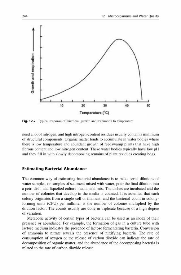
need a lot of nitrogen, and high nitrogen-content residues usually contain a minimumof structural components. Organic matter tends to accumulate in water bodies wherethere is low temperature and abundant growth of reedswamp plants that have highfibrous content and low nitrogen content. These water bodies typically have low pHand they fill in with slowly decomposing remains of plant residues creating bogs.

Estimating Bacterial Abundance

The common way of estimating bacterial abundance is to make serial dilutions ofwater samples, or samples of sediment mixed with water, pour the final dilution intoa petri dish, add liquefied culture media, and mix. The dishes are incubated and thenumber of colonies that develop in the media is counted. It is assumed that eachcolony originates from a single cell or filament, and the bacterial count in colony-forming units (CFU) per milliliter is the number of colonies multiplied by thedilution factor. The counts usually are done in triplicate because of a high degreeof variation.

Metabolic activity of certain types of bacteria can be used as an index of theirpresence or abundance. For example, the formation of gas in a culture tube withlactose medium indicates the presence of lactose fermentating bacteria. Conversionof ammonia to nitrate reveals the presence of nitrifying bacteria. The rate ofconsumption of oxygen or the release of carbon dioxide can indicate the rate ofdecomposition of organic matter, and the abundance of the decomposing bacteria isrelated to the rate of carbon dioxide release.

Fig. 12.2 Typical response of microbial growth and respiration to temperature


Sediment Respiration

Decomposition occurs in both water and sediment, and the main effect on waterquality of aerobic respiration is to remove dissolved oxygen and release carbondioxide, ammonia, and other mineral substances. The flocculent layer of sedimentjust above the sediment-water interface and the upper few centimeters or millimetersof sediment contain a large amount of fresh, readily decomposable organic matter.Microbial activity in aquatic ecosystems usually is greatest in the flocculent layerand upper sediment layer. Uptake of oxygen results from respiration in the flocculentlayer, and from respiration and chemical oxidation of reduced metabolites in thesediment. Sediment respiration rates as great as 20–30 g O2/m

2 per day have beenmeasured, but rates usually are 5 g O2/m

2 per day or less. The removal of dissolvedoxygen for use in sediment respiration is illustrated in Ex. 12.4.

Ex. 12.4 The loss of dissolved oxygen from the water will be estimated for sedimentrespiration of 2 g O2/m

2/day in a 3-m deep body of water.Solution:The water column above a 1 m2 area of sediment will contain 3 m3 of water.

Remembering that 1 mg/L is the same as 1 g/m3,

2 g O2=m2

3 m3 water=m2¼ 0:67 g=m3 or 0:67 mg=L:

Oxygen in sediment pore water or in the water column also may be consumed bypurely chemical reaction without biological influence as illustrated in the followingequations:

2Fe2þ þ 0:5O2 þ 2H2O ! Fe2O3 þ 4Hþ ð12:24Þ

Mn2þ þ 0:5O2 þ H2O ! MnO2 þ 2Hþ ð12:25Þ

H2Sþ 2O2 ! SO2�4 þ 2Hþ: ð12:26Þ

Some bacteria also can mediate reactions in which reduced metabolites are oxidized,and they also consume oxygen in the process. It is difficult to separate oxygenconsumption by respiration from oxygen consumption in chemical oxidation, andsediment oxygen uptake measurements usually indicate the combined uptake byboth processes.

Oxidation of metabolites is important, because the deeper sediment is anaerobic,and the reduced metabolites of anaerobic respiration can diffuse upward or be mixedupward by bioturbation. Upon entering the aerobic zone of the sediment, the reducedmetabolites may be oxidized chemically or through microbial activity. In the casewhere sediment is anaerobic to the sediment-water interface, the reduced metabolitesenter the water column, and some of them are toxic. Chemical and biologicaloxidation of these metabolites is important in preventing toxic conditions fromdeveloping in the water column.

Sediment Respiration 245

Organic matter decomposition controls the redox potential in water and sediment.As long as dissolved oxygen is plentiful, only aerobic decomposition occurs.However, when dissolved oxygen concentration falls to 1 or 2 mg/L, certain bacteriabegin to use oxygen from nitrate. As nitrate is used up, the redox potential declines,and when nitrate is depleted, the bacteria begin to use oxidized forms of iron andmanganese in respiration. Redox continues to fall until sulfate and finally carbondioxide become oxygen sources. Because the utilization of oxidized inorganiccompounds is sequential, the different bacterial reductions occur sequentially intime or occur in different layers of sediment. For example, when a body of waterstratifies thermally, it no longer obtains dissolved oxygen from the illuminatedepilimnion in which photosynthesis occurs. Organic matter settles into the hypolim-nion, and dissolved oxygen and redox potential decline as aerobic bacteria decom-pose organic matter. Simply put, once dissolved oxygen is depleted, nitrate supportsrespiration; when nitrate is gone, iron and manganese compounds become oxidantsin respiration; sulfate and finally carbon dioxide serve as oxidants as redox falls.

Sediment becomes depleted of oxygen quicker than water, because dissolvedoxygen cannot move downward rapidly in the pore water. Oxygen availabilitydeclines with sediment depth, and this results in zonation of the different processes(Fig. 12.3). This zonation will develop in sediment in bodies of water that are notchemically stratified, but in most unstratified bodies of water, the thin surface layerof the sediment remains aerobic as shown in Fig. 12.3. If organic matter inputs arehigh, the entire sediment mass, including its surface, may become highly reduced inboth stratified and unstratified water bodies. The vertical profile of redox potential inan unstratified lake and its sediment is illustrated in Fig. 12.3.

The results of anaerobic microbial respiration is the occurrence of reducedinorganic compounds to include nitrite, ferrous iron, manganous manganese, sulfide,and methane and many reduced organic compounds in waters of the hypolimnion oflakes, ponds, and other water bodies. When these reduced substances diffuse or aremixed into waters containing dissolved oxygen, they will be oxidized. If the inputrate of reduced substances into aerobic water exceeds the oxidation rate, an equilib-rium concentration of reduced substances may persist.

Some bacteria can oxidize ammonia to nitrate and thereby lower ammoniaconcentrations in water. This process will be discussed in Chap. 13.

Phytoplankton

The aquatic flora is very diverse and includes many thousand species. These includeplanktonic algae (phytoplankton) that are microscopic and suspended in the water,macrophytic algae that live on the bottom or form mats in the water, fungi which lackchlorophyll and are decomposers rather than producers like other plants, liverwortsand mosses that lack flowers and water conducting tissues characteristic of moreadvanced plants, and vascular plants that have water-conducting tissues throughouttheir bodies. Phytoplankton, macrophytic algae, and vascular plants usually are


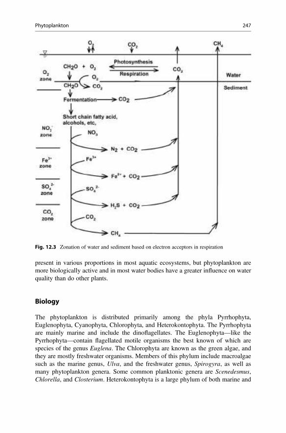
present in various proportions in most aquatic ecosystems, but phytoplankton aremore biologically active and in most water bodies have a greater influence on waterquality than do other plants.

Biology

The phytoplankton is distributed primarily among the phyla Pyrrhophyta,Euglenophyta, Cyanophyta, Chlorophyta, and Heterokontophyta. The Pyrrhophytaare mainly marine and include the dinoflagellates. The Euglenophyta—like thePyrrhophyta—contain flagellated motile organisms the best known of which arespecies of the genus Euglena. The Chlorophyta are known as the green algae, andthey are mostly freshwater organisms. Members of this phylum include macroalgaesuch as the marine genus, Ulva, and the freshwater genus, Spirogyra, as well asmany phytoplankton genera. Some common planktonic genera are Scenedesmus,Chlorella, and Closterium. Heterokontophyta is a large phylum of both marine and

Fig. 12.3 Zonation of water and sediment based on electron acceptors in respiration

Phytoplankton 247

freshwater algae that includes the yellow-green algae (Xanthophyceae), golden algae(Chrysophyceae), brown algae (Phaeophyceae), and diatoms (Bacillariophyceae).The Cyanophyta are the blue-green algae. However, this group of algae is prokary-otic like bacteria, and taxonomic authorities consider blue-green algae to becyanobacteria. But, in this book these organisms will be referred to as blue-greenalgae. A more complete discussion of phytoplankton systematics is beyond thescope of this text, but there are many books and websites from which moreinformation can be obtained.

Blue-green algae can have particularly large effects on water quality. They tend tobe abundant in nutrient enriched waters, and many species of planktonic blue-greenalgae are considered undesirable. They form scums on the water surface, they aresubject to sudden population crashes, a few species may be toxic to other aquaticorganisms, and some species excrete odorous compounds into the water. Theseodorous compounds may cause a bad odor and taste in drinking water or impartbad flavor to fish and other aquatic food animals.

Phytoplankton requires sunlight for growth, so actively-growing phytoplanktonare found only in illuminated water where there is more than about 1% of incidentlight. The density of phytoplankton is slightly greater than that of water, so they tendto sink from the photic zone (illuminated surface stratum), but all species haveadaptations such as small size, irregular morphology often with projecting surfaces,gas vacuoles, or means of motility to reduce their sinking rate and permit them toremain suspended even in waters of low turbulence. Nearly all waters containphytoplankton, and waters with abundant nutrients will contain enough phytoplank-ton to cause turbidity and discoloration. Waters discolored by phytoplankton are saidto have phytoplankton blooms and appear green, blue-green, red, yellow, brown,black, gray, or various other colors.

Reproduction in phytoplankton usually is by binary fission as described above forbacteria. The life span of phytoplankton is short, individual cells probably survivefor no more than 1 or 2 weeks. As dead cells settle, they quickly rupture and theprotoplasmic contents spill into the water. Natural waters usually contain muchorganic detritus originating from dead phytoplankton.

Most species of phytoplankton disperse readily. The atmosphere contains sporesand vegetative bodies of many species. If a flask of sterile nutrient solution is openedto the atmosphere, algal communities will soon develop. Wading birds often spreadphytoplankton from one body of water to another. This results because phytoplank-ton propagules stick to their external surfaces, and viable algal spores and vegetativebodies pass through their digestive tracts. Species of phytoplankton that colonize ahabitat depend upon the suitability of the habitat into which their propaguleshappened to enter.

Suppose that a tank of nutrient-enriched water containing no algae is exposedoutdoors. Species of phytoplankton in the air will fall into the tank, and the speciesentering would be primarily the result of chance. However, the species that persist inthe tank will depend upon environmental conditions. Moreover, once thephytoplankters begin to grow they will go through a succession until a climaxphytoplankton community is attained. This community eventually will make theenvironment unsuitable for its growth and crash (see Fig. 12.1), or the season may


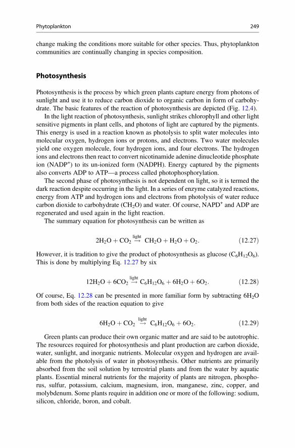
change making the conditions more suitable for other species. Thus, phytoplanktoncommunities are continually changing in species composition.

Photosynthesis

Photosynthesis is the process by which green plants capture energy from photons ofsunlight and use it to reduce carbon dioxide to organic carbon in form of carbohy-drate. The basic features of the reaction of photosynthesis are depicted (Fig. 12.4).

In the light reaction of photosynthesis, sunlight strikes chlorophyll and other lightsensitive pigments in plant cells, and photons of light are captured by the pigments.This energy is used in a reaction known as photolysis to split water molecules intomolecular oxygen, hydrogen ions or protons, and electrons. Two water moleculesyield one oxygen molecule, four hydrogen ions, and four electrons. The hydrogenions and electrons then react to convert nicotinamide adenine dinucleotide phosphateion (NADP+) to its un-ionized form (NADPH). Energy captured by the pigmentsalso converts ADP to ATP—a process called photophosphorylation.

The second phase of photosynthesis is not dependent on light, so it is termed thedark reaction despite occurring in the light. In a series of enzyme catalyzed reactions,energy from ATP and hydrogen ions and electrons from photolysis of water reducecarbon dioxide to carbohydrate (CH2O) and water. Of course, NAPD+ and ADP areregenerated and used again in the light reaction.

The summary equation for photosynthesis can be written as

2H2Oþ CO2 !light CH2Oþ H2Oþ O2: ð12:27ÞHowever, it is tradition to give the product of photosynthesis as glucose (C6H12O6).This is done by multiplying Eq. 12.27 by six

12H2Oþ 6CO2 !light C6H12O6 þ 6H2Oþ 6O2: ð12:28ÞOf course, Eq. 12.28 can be presented in more familiar form by subtracting 6H2Ofrom both sides of the reaction equation to give

6H2Oþ CO2 !light C6H12O6 þ 6O2: ð12:29ÞGreen plants can produce their own organic matter and are said to be autotrophic.

The resources required for photosynthesis and plant production are carbon dioxide,water, sunlight, and inorganic nutrients. Molecular oxygen and hydrogen are avail-able from the photolysis of water in photosynthesis. Other nutrients are primarilyabsorbed from the soil solution by terrestrial plants and from the water by aquaticplants. Essential mineral nutrients for the majority of plants are nitrogen, phospho-rus, sulfur, potassium, calcium, magnesium, iron, manganese, zinc, copper, andmolybdenum. Some plants require in addition one or more of the following: sodium,silicon, chloride, boron, and cobalt.

Phytoplankton 249

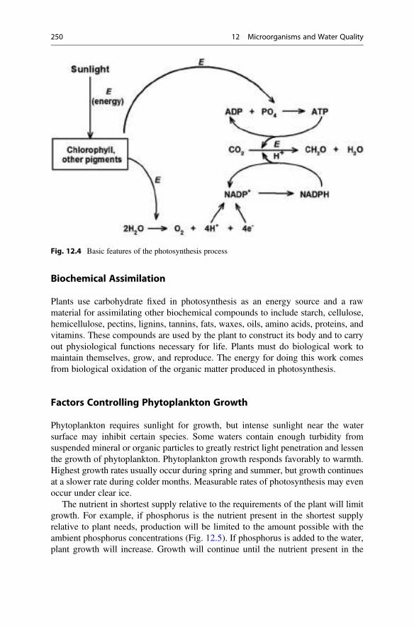
Biochemical Assimilation

Plants use carbohydrate fixed in photosynthesis as an energy source and a rawmaterial for assimilating other biochemical compounds to include starch, cellulose,hemicellulose, pectins, lignins, tannins, fats, waxes, oils, amino acids, proteins, andvitamins. These compounds are used by the plant to construct its body and to carryout physiological functions necessary for life. Plants must do biological work tomaintain themselves, grow, and reproduce. The energy for doing this work comesfrom biological oxidation of the organic matter produced in photosynthesis.

Factors Controlling Phytoplankton Growth

Phytoplankton requires sunlight for growth, but intense sunlight near the watersurface may inhibit certain species. Some waters contain enough turbidity fromsuspended mineral or organic particles to greatly restrict light penetration and lessenthe growth of phytoplankton. Phytoplankton growth responds favorably to warmth.Highest growth rates usually occur during spring and summer, but growth continuesat a slower rate during colder months. Measurable rates of photosynthesis may evenoccur under clear ice.

The nutrient in shortest supply relative to the requirements of the plant will limitgrowth. For example, if phosphorus is the nutrient present in the shortest supplyrelative to plant needs, production will be limited to the amount possible with theambient phosphorus concentrations (Fig. 12.5). If phosphorus is added to the water,plant growth will increase. Growth will continue until the nutrient present in the

Fig. 12.4 Basic features of the photosynthesis process


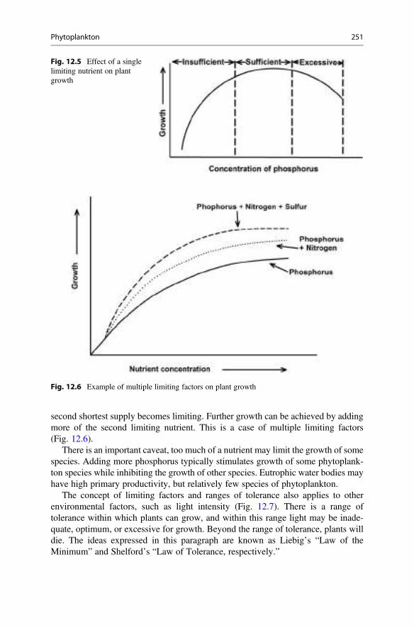
second shortest supply becomes limiting. Further growth can be achieved by addingmore of the second limiting nutrient. This is a case of multiple limiting factors(Fig. 12.6).

There is an important caveat, too much of a nutrient may limit the growth of somespecies. Adding more phosphorus typically stimulates growth of some phytoplank-ton species while inhibiting the growth of other species. Eutrophic water bodies mayhave high primary productivity, but relatively few species of phytoplankton.

The concept of limiting factors and ranges of tolerance also applies to otherenvironmental factors, such as light intensity (Fig. 12.7). There is a range oftolerance within which plants can grow, and within this range light may be inade-quate, optimum, or excessive for growth. Beyond the range of tolerance, plants willdie. The ideas expressed in this paragraph are known as Liebig’s “Law of theMinimum” and Shelford’s “Law of Tolerance, respectively.”

Fig. 12.5 Effect of a singlelimiting nutrient on plantgrowth

Fig. 12.6 Example of multiple limiting factors on plant growth

Phytoplankton 251

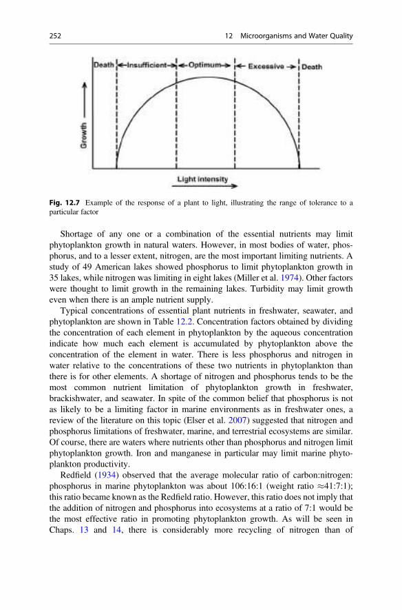
Shortage of any one or a combination of the essential nutrients may limitphytoplankton growth in natural waters. However, in most bodies of water, phos-phorus, and to a lesser extent, nitrogen, are the most important limiting nutrients. Astudy of 49 American lakes showed phosphorus to limit phytoplankton growth in35 lakes, while nitrogen was limiting in eight lakes (Miller et al. 1974). Other factorswere thought to limit growth in the remaining lakes. Turbidity may limit growtheven when there is an ample nutrient supply.

Typical concentrations of essential plant nutrients in freshwater, seawater, andphytoplankton are shown in Table 12.2. Concentration factors obtained by dividingthe concentration of each element in phytoplankton by the aqueous concentrationindicate how much each element is accumulated by phytoplankton above theconcentration of the element in water. There is less phosphorus and nitrogen inwater relative to the concentrations of these two nutrients in phytoplankton thanthere is for other elements. A shortage of nitrogen and phosphorus tends to be themost common nutrient limitation of phytoplankton growth in freshwater,brackishwater, and seawater. In spite of the common belief that phosphorus is notas likely to be a limiting factor in marine environments as in freshwater ones, areview of the literature on this topic (Elser et al. 2007) suggested that nitrogen andphosphorus limitations of freshwater, marine, and terrestrial ecosystems are similar.Of course, there are waters where nutrients other than phosphorus and nitrogen limitphytoplankton growth. Iron and manganese in particular may limit marine phyto-plankton productivity.

Redfield (1934) observed that the average molecular ratio of carbon:nitrogen:phosphorus in marine phytoplankton was about 106:16:1 (weight ratio �41:7:1);this ratio became known as the Redfield ratio. However, this ratio does not imply thatthe addition of nitrogen and phosphorus into ecosystems at a ratio of 7:1 would bethe most effective ratio in promoting phytoplankton growth. As will be seen inChaps. 13 and 14, there is considerably more recycling of nitrogen than of

Fig. 12.7 Example of the response of a plant to light, illustrating the range of tolerance to aparticular factor


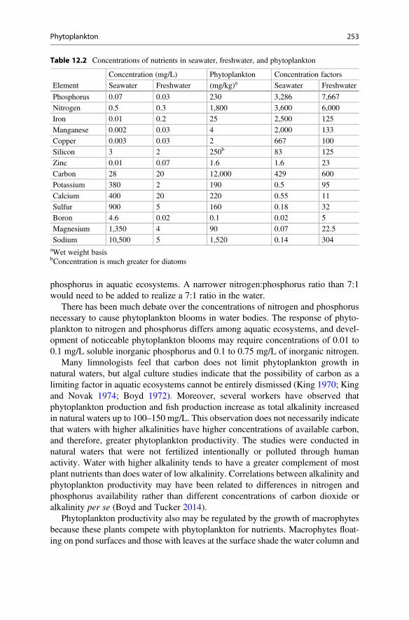
phosphorus in aquatic ecosystems. A narrower nitrogen:phosphorus ratio than 7:1would need to be added to realize a 7:1 ratio in the water.

There has been much debate over the concentrations of nitrogen and phosphorusnecessary to cause phytoplankton blooms in water bodies. The response of phyto-plankton to nitrogen and phosphorus differs among aquatic ecosystems, and devel-opment of noticeable phytoplankton blooms may require concentrations of 0.01 to0.1 mg/L soluble inorganic phosphorus and 0.1 to 0.75 mg/L of inorganic nitrogen.

Many limnologists feel that carbon does not limit phytoplankton growth innatural waters, but algal culture studies indicate that the possibility of carbon as alimiting factor in aquatic ecosystems cannot be entirely dismissed (King 1970; Kingand Novak 1974; Boyd 1972). Moreover, several workers have observed thatphytoplankton production and fish production increase as total alkalinity increasedin natural waters up to 100–150 mg/L. This observation does not necessarily indicatethat waters with higher alkalinities have higher concentrations of available carbon,and therefore, greater phytoplankton productivity. The studies were conducted innatural waters that were not fertilized intentionally or polluted through humanactivity. Water with higher alkalinity tends to have a greater complement of mostplant nutrients than does water of low alkalinity. Correlations between alkalinity andphytoplankton productivity may have been related to differences in nitrogen andphosphorus availability rather than different concentrations of carbon dioxide oralkalinity per se (Boyd and Tucker 2014).

Phytoplankton productivity also may be regulated by the growth of macrophytesbecause these plants compete with phytoplankton for nutrients. Macrophytes float-ing on pond surfaces and those with leaves at the surface shade the water column and

Table 12.2 Concentrations of nutrients in seawater, freshwater, and phytoplankton

Element

Concentration (mg/L) Phytoplankton Concentration factors

Seawater Freshwater (mg/kg)a Seawater Freshwater

Phosphorus 0.07 0.03 230 3,286 7,667

Nitrogen 0.5 0.3 1,800 3,600 6,000

Iron 0.01 0.2 25 2,500 125

Manganese 0.002 0.03 4 2,000 133

Copper 0.003 0.03 2 667 100

Silicon 3 2 250b 83 125

Zinc 0.01 0.07 1.6 1.6 23

Carbon 28 20 12,000 429 600

Potassium 380 2 190 0.5 95

Calcium 400 20 220 0.55 11

Sulfur 900 5 160 0.18 32

Boron 4.6 0.02 0.1 0.02 5

Magnesium 1,350 4 90 0.07 22.5

Sodium 10,500 5 1,520 0.14 304aWet weight basisbConcentration is much greater for diatoms

Phytoplankton 253

greatly restrict phytoplankton growth. Certain macrophytes also excrete substancesknown as allelopaths that are toxic to phytoplankton. Regardless of the reasons,additions of nutrients to water bodies containing extensive macrophyte communitiesoften do not cause phytoplankton blooms; rather, they stimulate further macrophytegrowth.

Estimating Phytoplankton Abundance

The number of individuals (single cells, filaments, or colonies) per milliliter or literof water may be determined directly by microscopic examination. Different specieshave characteristic sizes, and the volume of phytoplankton cells per unit of waterprovides a better estimate of biomass than does enumeration of phytoplanktonabundance. However, it is exceedingly difficult to measure the volume of phyto-plankton in a sample. A formula must be concocted for estimating the value of eachspecies present and multiplied by the number of that species per unit volume ofwater.

Indirect methods of assessing phytoplankton abundance are popular. Chlorophylla determination on particulate matter removed from a water sample by filtrationprovides an index of phytoplankton abundance. Because particulate organic matteroften consists mostly of phytoplankton, this variable is indicative of phytoplanktonabundance in many waters. Suitable techniques for separating phytoplankton fromother particulate matter are not available, so results must be assessed with caution.The Secchi disk visibility decreases with increasing plankton abundance, and inmany bodies of water, the Secchi disk visibility can be a useful measure of phyto-plankton abundance. Of course, one must consider how much of the turbidityappears to be from other sources when assessing plankton abundance with aSecchi disk.

Effects of Phytoplankton on Water Quality

The most profound effects of phytoplankton activity on water quality are changes inpH and concentrations of dissolved oxygen and carbon dioxide. Photosynthesisusually dominates over respiration during daylight in a water body, while theopposite occurs at night. In other words, there is a net increase in dissolved oxygenand a net decrease in carbon dioxide during the day and vice versa at night. Changesin carbon dioxide concentration affect pH. The pH increases when carbon dioxidedecreases. Daily changes in carbon dioxide, dissolved oxygen, and pH are illustratedin Fig. 12.8. The magnitude of daily fluctuations in concentrations of the threevariables will tend to increase as phytoplankton abundance increases.

Light availability decreases with depth, so the rate of phytoplankton photosyn-thesis will tend to decrease with depth. In the afternoon, dissolved oxygen and pHwill tend to be higher in surface water than in deeper water while the opposite will betrue for carbon dioxide.


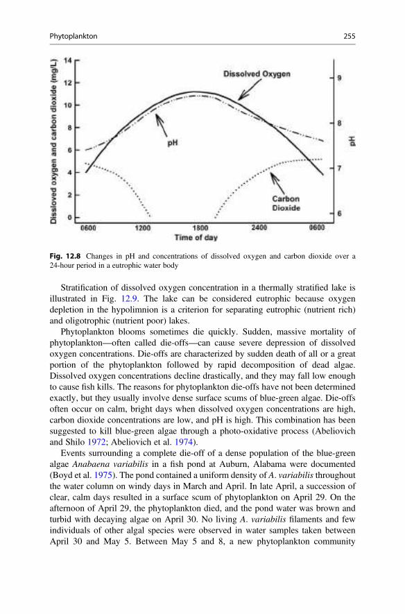
Stratification of dissolved oxygen concentration in a thermally stratified lake isillustrated in Fig. 12.9. The lake can be considered eutrophic because oxygendepletion in the hypolimnion is a criterion for separating eutrophic (nutrient rich)and oligotrophic (nutrient poor) lakes.

Phytoplankton blooms sometimes die quickly. Sudden, massive mortality ofphytoplankton—often called die-offs—can cause severe depression of dissolvedoxygen concentrations. Die-offs are characterized by sudden death of all or a greatportion of the phytoplankton followed by rapid decomposition of dead algae.Dissolved oxygen concentrations decline drastically, and they may fall low enoughto cause fish kills. The reasons for phytoplankton die-offs have not been determinedexactly, but they usually involve dense surface scums of blue-green algae. Die-offsoften occur on calm, bright days when dissolved oxygen concentrations are high,carbon dioxide concentrations are low, and pH is high. This combination has beensuggested to kill blue-green algae through a photo-oxidative process (Abeliovichand Shilo 1972; Abeliovich et al. 1974).

Events surrounding a complete die-off of a dense population of the blue-greenalgae Anabaena variabilis in a fish pond at Auburn, Alabama were documented(Boyd et al. 1975). The pond contained a uniform density of A. variabilis throughoutthe water column on windy days in March and April. In late April, a succession ofclear, calm days resulted in a surface scum of phytoplankton on April 29. On theafternoon of April 29, the phytoplankton died, and the pond water was brown andturbid with decaying algae on April 30. No living A. variabilis filaments and fewindividuals of other algal species were observed in water samples taken betweenApril 30 and May 5. Between May 5 and 8, a new phytoplankton community

Fig. 12.8 Changes in pH and concentrations of dissolved oxygen and carbon dioxide over a24-hour period in a eutrophic water body

Phytoplankton 255

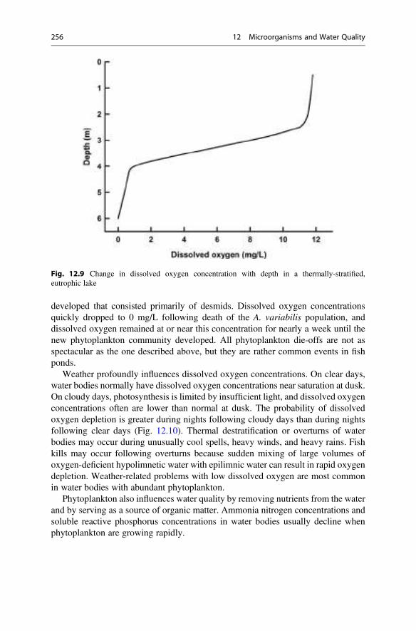
developed that consisted primarily of desmids. Dissolved oxygen concentrationsquickly dropped to 0 mg/L following death of the A. variabilis population, anddissolved oxygen remained at or near this concentration for nearly a week until thenew phytoplankton community developed. All phytoplankton die-offs are not asspectacular as the one described above, but they are rather common events in fishponds.

Weather profoundly influences dissolved oxygen concentrations. On clear days,water bodies normally have dissolved oxygen concentrations near saturation at dusk.On cloudy days, photosynthesis is limited by insufficient light, and dissolved oxygenconcentrations often are lower than normal at dusk. The probability of dissolvedoxygen depletion is greater during nights following cloudy days than during nightsfollowing clear days (Fig. 12.10). Thermal destratification or overturns of waterbodies may occur during unusually cool spells, heavy winds, and heavy rains. Fishkills may occur following overturns because sudden mixing of large volumes ofoxygen-deficient hypolimnetic water with epilimnic water can result in rapid oxygendepletion. Weather-related problems with low dissolved oxygen are most commonin water bodies with abundant phytoplankton.

Phytoplankton also influences water quality by removing nutrients from the waterand by serving as a source of organic matter. Ammonia nitrogen concentrations andsoluble reactive phosphorus concentrations in water bodies usually decline whenphytoplankton are growing rapidly.

Fig. 12.9 Change in dissolved oxygen concentration with depth in a thermally-stratified,eutrophic lake


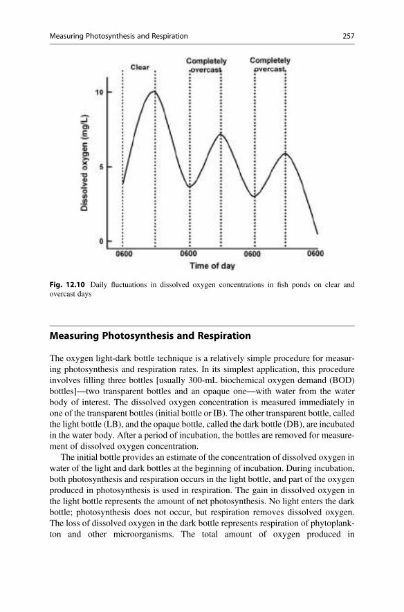
Measuring Photosynthesis and Respiration

The oxygen light-dark bottle technique is a relatively simple procedure for measur-ing photosynthesis and respiration rates. In its simplest application, this procedureinvolves filling three bottles [usually 300-mL biochemical oxygen demand (BOD)bottles]—two transparent bottles and an opaque one—with water from the waterbody of interest. The dissolved oxygen concentration is measured immediately inone of the transparent bottles (initial bottle or IB). The other transparent bottle, calledthe light bottle (LB), and the opaque bottle, called the dark bottle (DB), are incubatedin the water body. After a period of incubation, the bottles are removed for measure-ment of dissolved oxygen concentration.

The initial bottle provides an estimate of the concentration of dissolved oxygen inwater of the light and dark bottles at the beginning of incubation. During incubation,both photosynthesis and respiration occurs in the light bottle, and part of the oxygenproduced in photosynthesis is used in respiration. The gain in dissolved oxygen inthe light bottle represents the amount of net photosynthesis. No light enters the darkbottle; photosynthesis does not occur, but respiration removes dissolved oxygen.The loss of dissolved oxygen in the dark bottle represents respiration of phytoplank-ton and other microorganisms. The total amount of oxygen produced in

Fig. 12.10 Daily fluctuations in dissolved oxygen concentrations in fish ponds on clear andovercast days

Measuring Photosynthesis and Respiration 257

photosynthesis (gross photosynthesis) is the sum of dissolved oxygen produced innet photosynthesis and used in respiration.

If the objective is to determine the influence of depth on photosynthesis andrespiration or to obtain average rates of photosynthesis and respiration in the watercolumn, bottles must be filled with water from several depths and then incubated atthose same depths. This arrangement is necessary because light penetrationdecreases with depth and photosynthesis rates are sensitive to light intensity. Bothtemperature and the abundance of planktonic organisms also differ with depth andinfluence photosynthesis and respiration.

Light intensity varies during the day and influences photosynthetic rate. A24-hour incubation would be ideal, but sedimentation of organisms within bottles,depletion of dissolved oxygen in the dark bottle, or supersaturation of dissolvedoxygen in the light bottle can alter respiration and photosynthesis rates. These “bottleeffects” make it necessary to restrict incubation to a few hours. Incubations fromdawn (provided the initial dissolved oxygen is high enough to sustain respiration inthe dark bottle) until noon are more feasible than incubations from noon until dusk,because at noon waters are already high in dissolved oxygen concentration. If bottlesare incubated at dawn and removed at noon, the incubation period will representone-half of a photoperiod. Another alternative is to incubate the bottles during aspecific time interval and measure solar radiation during the incubation interval andfor the entire photoperiod. The fraction of the daily radiation occurring during theincubation period can be determined by dividing radiation during the incubationperiod by total radiation for the day. The total amount of photosynthesis is assumedto equal the amount during the incubation period times the ratio of total dailyradiation to radiation received during incubation.

It is possible to calculate three variables, net photosynthesis (NP), gross photo-synthesis (GP), and water column respiration (R) from light-dark bottle data. Ofcourse, net photosynthesis will be underestimated because organisms other thanphytoplankton contribute to respiration and detract from net photosynthesis.Equations for these calculations follow:

NP ¼ LB� IB ð12:30ÞR ¼ IB� DB ð12:31ÞGP ¼ NPþ R ð12:32Þ

or GP ¼ LB� DB: ð12:33ÞAll variables are reported in milligrams per liter of dissolved oxygen. Where bottlesare incubated at different depths, results can be averaged to obtain values for thewater column. Results can be adjusted to a 24-hour basis by considering the length ofthe incubation period and the amount of radiation during the incubation period. Thecomputations are illustrated in Ex. 12.5.


Ex. 12.5 The following data are the averages for results of light-dark bottleincubations at 0.1, 0.5, 1.0, and 1.5 m in a 1.75-m deep column of water.

IB ¼ 4.02 mg/LLB ¼ 6.75 mg/LDB ¼ 2.98 mg/LIncubation period ¼ dawn to noon (6.5 hours)

NP, GP, and R will be calculated for a 24-hour day.Solution:For the incubation period,

NP ¼ 6:75� 4:02 ¼ 2:73 mg=L

R ¼ 4:02� 2:98 ¼ 1:04 mg=L

GP ¼ 6:75� 2:98 ¼ 3:77 mg=L:

Assuming a clear day, the values may be doubled to provide totals for the photope-riod. Respiration will continue throughout the 11-hour period of darkness, sonighttime respiration will be only 11/13 of daytime values. Nighttime respirationmust be subtracted from daytime NP in order to estimate 24-hour NP.

Photosynthesis and respiration rates may be expressed on an areal basis (usuallysquare meter). This is done by multiplying the average values for NP, GP, and R inthe entire water column by water depth. Values for NP, GP, and R also can beexpressed in terms of carbon. In the general expressions for respiration and photo-synthesis, one mole of oxygen can be equated to one mole of carbon dioxide orcarbon. The ratio of the atomic weight of carbon (C) to the molecular weight ofoxygen (O2), 12/32 or 0.375, can be used to convert oxygen concentrations to carbonconcentrations.

The Compensation Depth

Photosynthesis rate decreases with increasing depth because of diminishing light. Inmost water bodies there will be a depth at which oxygen produced by photosynthesiswill be equal to oxygen used in respiration. At this depth—called the compensationdepth or point—net photosynthesis will be zero. At depths less than the compensa-tion depth, more dissolved oxygen will be produced by phytoplankton than used inrespiration by microorganisms in the water column. At depths greater than thecompensation depth, more dissolved oxygen will be used in respiration than pro-duced by photosynthesis.

In a stratified body of water, the compensation depth usually corresponds to thethermocline, and no oxygen is produced in the hypolimnion. Because of

The Compensation Depth 259

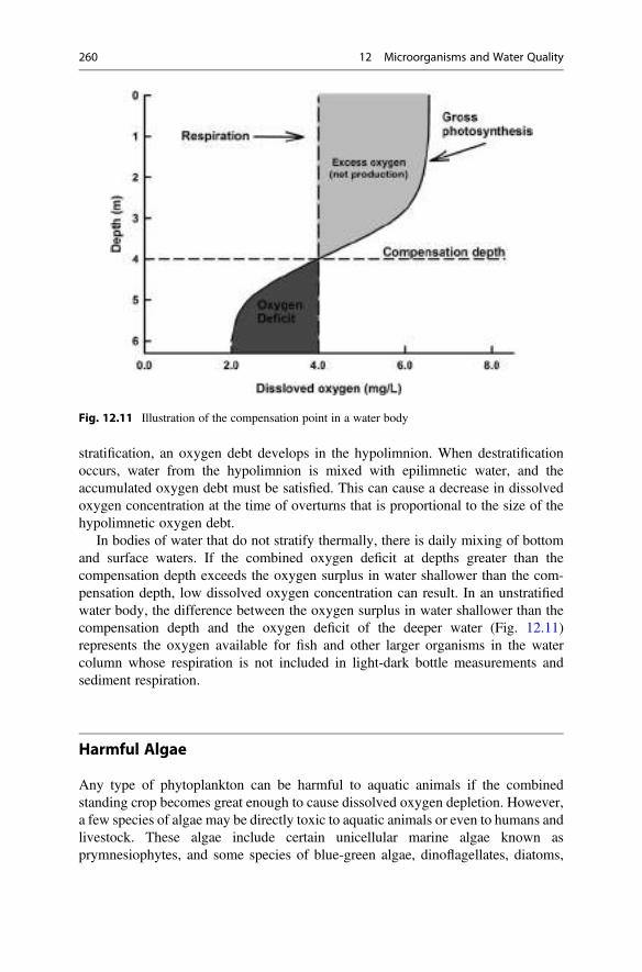
stratification, an oxygen debt develops in the hypolimnion. When destratificationoccurs, water from the hypolimnion is mixed with epilimnetic water, and theaccumulated oxygen debt must be satisfied. This can cause a decrease in dissolvedoxygen concentration at the time of overturns that is proportional to the size of thehypolimnetic oxygen debt.

In bodies of water that do not stratify thermally, there is daily mixing of bottomand surface waters. If the combined oxygen deficit at depths greater than thecompensation depth exceeds the oxygen surplus in water shallower than the com-pensation depth, low dissolved oxygen concentration can result. In an unstratifiedwater body, the difference between the oxygen surplus in water shallower than thecompensation depth and the oxygen deficit of the deeper water (Fig. 12.11)represents the oxygen available for fish and other larger organisms in the watercolumn whose respiration is not included in light-dark bottle measurements andsediment respiration.

Harmful Algae

Any type of phytoplankton can be harmful to aquatic animals if the combinedstanding crop becomes great enough to cause dissolved oxygen depletion. However,a few species of algae may be directly toxic to aquatic animals or even to humans andlivestock. These algae include certain unicellular marine algae known asprymnesiophytes, and some species of blue-green algae, dinoflagellates, diatoms,

Fig. 12.11 Illustration of the compensation point in a water body


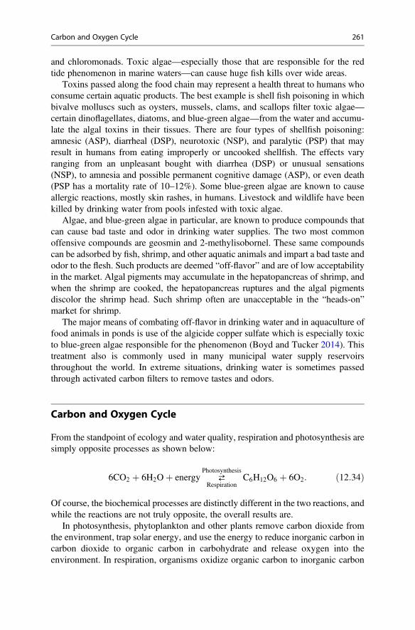
and chloromonads. Toxic algae—especially those that are responsible for the redtide phenomenon in marine waters—can cause huge fish kills over wide areas.

Toxins passed along the food chain may represent a health threat to humans whoconsume certain aquatic products. The best example is shell fish poisoning in whichbivalve molluscs such as oysters, mussels, clams, and scallops filter toxic algae—certain dinoflagellates, diatoms, and blue-green algae—from the water and accumu-late the algal toxins in their tissues. There are four types of shellfish poisoning:amnesic (ASP), diarrheal (DSP), neurotoxic (NSP), and paralytic (PSP) that mayresult in humans from eating improperly or uncooked shellfish. The effects varyranging from an unpleasant bought with diarrhea (DSP) or unusual sensations(NSP), to amnesia and possible permanent cognitive damage (ASP), or even death(PSP has a mortality rate of 10–12%). Some blue-green algae are known to causeallergic reactions, mostly skin rashes, in humans. Livestock and wildlife have beenkilled by drinking water from pools infested with toxic algae.

Algae, and blue-green algae in particular, are known to produce compounds thatcan cause bad taste and odor in drinking water supplies. The two most commonoffensive compounds are geosmin and 2-methylisobornel. These same compoundscan be adsorbed by fish, shrimp, and other aquatic animals and impart a bad taste andodor to the flesh. Such products are deemed “off-flavor” and are of low acceptabilityin the market. Algal pigments may accumulate in the hepatopancreas of shrimp, andwhen the shrimp are cooked, the hepatopancreas ruptures and the algal pigmentsdiscolor the shrimp head. Such shrimp often are unacceptable in the “heads-on”market for shrimp.

The major means of combating off-flavor in drinking water and in aquaculture offood animals in ponds is use of the algicide copper sulfate which is especially toxicto blue-green algae responsible for the phenomenon (Boyd and Tucker 2014). Thistreatment also is commonly used in many municipal water supply reservoirsthroughout the world. In extreme situations, drinking water is sometimes passedthrough activated carbon filters to remove tastes and odors.

Carbon and Oxygen Cycle

From the standpoint of ecology and water quality, respiration and photosynthesis aresimply opposite processes as shown below:

6CO2 þ 6H2Oþ energy ⇄Photosynthesis

RespirationC6H12O6 þ 6O2: ð12:34Þ

Of course, the biochemical processes are distinctly different in the two reactions, andwhile the reactions are not truly opposite, the overall results are.

In photosynthesis, phytoplankton and other plants remove carbon dioxide fromthe environment, trap solar energy, and use the energy to reduce inorganic carbon incarbon dioxide to organic carbon in carbohydrate and release oxygen into theenvironment. In respiration, organisms oxidize organic carbon to inorganic carbon

Carbon and Oxygen Cycle 261

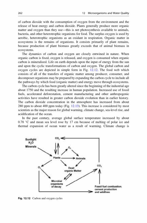
of carbon dioxide with the consumption of oxygen from the environment and therelease of heat energy and carbon dioxide. Plants generally produce more organicmatter and oxygen than they use—this is net photosynthesis available to animals,bacteria, and other heterotrophic organisms for food. The surplus oxygen is used byaerobic, heterotrophic organisms as an oxidant in respiration. Organic matter inecosystems is the remains of organisms. It consists primarily of plant remains,because production of plant biomass greatly exceeds that of animal biomass inecosystems.

The dynamics of carbon and oxygen are closely entwined in nature. Whenorganic carbon is fixed, oxygen is released, and oxygen is consumed when organiccarbon is mineralized. Life on earth depends upon the input of energy from the sunand upon the cyclic transformations of carbon and oxygen. The global carbon andoxygen cycles are depicted in simple form in Fig. 12.12. The food web whichconsists of all of the transfers of organic matter among producer, consumer, anddecomposer organisms may be prepared by expanding the carbon cycle to include allthe pathways by which food (organic matter) and energy move through ecosystems.

The carbon cycle has been greatly altered since the beginning of the industrial ageabout 1750 and the resulting increase in human population. Increased use of fossilfuels, accelerated deforestation, cement manufacturing and other anthropogenicactivities have resulted in greater carbon dioxide evolution than in earlier history.The carbon dioxide concentration in the atmosphere has increased from about280 ppm to about 400 ppm today (Fig. 12.13). This increase is considered by mostscientists as the major reason for global warming, climate change, sea-level rise, andacidification of the ocean.

In the past century, average global surface temperature increased by about0.78 �C and mean sea level rose by 17 cm because of melting of polar ice andthermal expansion of ocean water as a result of warming. Climate change is

Fig. 12.12 Carbon and oxygen cycles


occurring resulting in more extreme weather. The extreme weather index maintainedby the US National Oceanographic and Atmospheric Administration fluctuated butshowed no clear pattern of increase from 1920 to 1970, but since, this index hasexhibited an upward trend. Average ocean pH declined from 8.12 in 1988 to 8.09 in2008, and it is resulting in thinner calcium carbonate shells on many marineinvertebrates. The changes are expected to accelerate during the remainder of thetwenty-first century (Boyd and McNevin 2015).

Human Pathogens and Chlorination

Water supplies for human use may be contaminated with pathogens. Some of themost serious waterborne infections such as typhoid fever, dysentery, and cholera arenot common in developed countries, but waterborne diseases are still of majorsignificance in the developing world. Organisms responsible for waterborne diseasesinclude viruses, bacteria, protozoans, mites, and worms.

Waters that are contaminated with human pathogens usually are alsocontaminated by human fecal material. Coliform bacteria are used to identify watersthat may have received human wastes, and water containing significant numbers ofcoliforms is a health hazard because of the possibility of waterborne diseases.

Coliform organisms are aerobic and facultative anaerobic, gram-negative,nonspore-forming, rod-shaped bacteria that ferment lactose with gas formationwithin 48 hours at 35 �C. Some of these organisms can be found in soil and onvegetation, but fecal coliforms Escherichia coli usually originate from feces ofwarm-blooded animals. The ratio of fecal coliforms to fecal streptococci is some-times used to differentiate waters contaminated with human fecal coliforms from

Fig. 12.13 Annual estimates of global, anthropogenic carbon dioxide emissions at 10-yearintervals (dots) (1850–2030) and changes in atmospheric carbon dioxide concentrations measuredat Mauna Loa, Hawaii from 1958 to 2012 (circles). (Boyd and McNevin 2014)

Human Pathogens and Chlorination 263

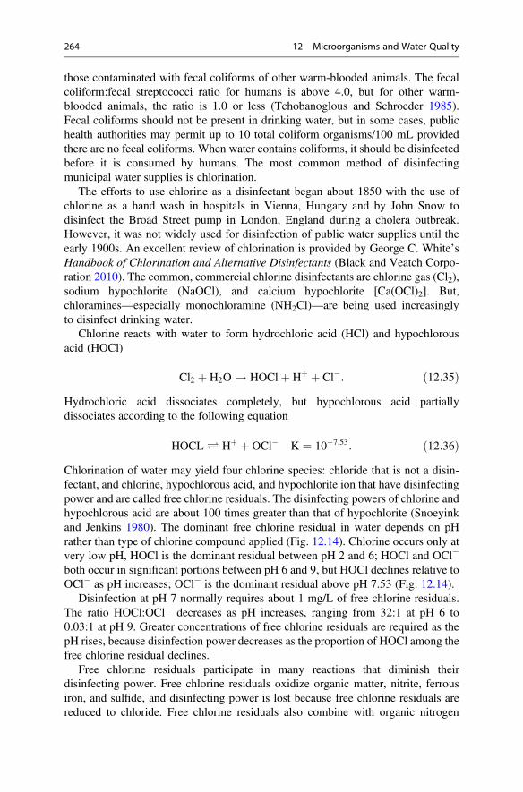
those contaminated with fecal coliforms of other warm-blooded animals. The fecalcoliform:fecal streptococci ratio for humans is above 4.0, but for other warm-blooded animals, the ratio is 1.0 or less (Tchobanoglous and Schroeder 1985).Fecal coliforms should not be present in drinking water, but in some cases, publichealth authorities may permit up to 10 total coliform organisms/100 mL providedthere are no fecal coliforms. When water contains coliforms, it should be disinfectedbefore it is consumed by humans. The most common method of disinfectingmunicipal water supplies is chlorination.

The efforts to use chlorine as a disinfectant began about 1850 with the use ofchlorine as a hand wash in hospitals in Vienna, Hungary and by John Snow todisinfect the Broad Street pump in London, England during a cholera outbreak.However, it was not widely used for disinfection of public water supplies until theearly 1900s. An excellent review of chlorination is provided by George C. White’sHandbook of Chlorination and Alternative Disinfectants (Black and Veatch Corpo-ration 2010). The common, commercial chlorine disinfectants are chlorine gas (Cl2),sodium hypochlorite (NaOCl), and calcium hypochlorite [Ca(OCl)2]. But,chloramines—especially monochloramine (NH2Cl)—are being used increasinglyto disinfect drinking water.

Chlorine reacts with water to form hydrochloric acid (HCl) and hypochlorousacid (HOCl)

Cl2 þ H2O ! HOClþ Hþ þ Cl�: ð12:35ÞHydrochloric acid dissociates completely, but hypochlorous acid partiallydissociates according to the following equation

HOCL Ð Hþ þ OCl� K ¼ 10�7:53: ð12:36ÞChlorination of water may yield four chlorine species: chloride that is not a disin-fectant, and chlorine, hypochlorous acid, and hypochlorite ion that have disinfectingpower and are called free chlorine residuals. The disinfecting powers of chlorine andhypochlorous acid are about 100 times greater than that of hypochlorite (Snoeyinkand Jenkins 1980). The dominant free chlorine residual in water depends on pHrather than type of chlorine compound applied (Fig. 12.14). Chlorine occurs only atvery low pH, HOCl is the dominant residual between pH 2 and 6; HOCl and OCl�

both occur in significant portions between pH 6 and 9, but HOCl declines relative toOCl� as pH increases; OCl� is the dominant residual above pH 7.53 (Fig. 12.14).

Disinfection at pH 7 normally requires about 1 mg/L of free chlorine residuals.The ratio HOCl:OCl� decreases as pH increases, ranging from 32:1 at pH 6 to0.03:1 at pH 9. Greater concentrations of free chlorine residuals are required as thepH rises, because disinfection power decreases as the proportion of HOCl among thefree chlorine residual declines.

Free chlorine residuals participate in many reactions that diminish theirdisinfecting power. Free chlorine residuals oxidize organic matter, nitrite, ferrousiron, and sulfide, and disinfecting power is lost because free chlorine residuals arereduced to chloride. Free chlorine residuals also combine with organic nitrogen


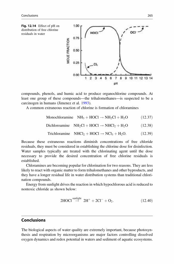
compounds, phenols, and humic acid to produce organochlorine compounds. Atleast one group of these compounds—the trihalomethanes—is suspected to be acarcinogen in humans (Jimenez et al. 1993).

A common extraneous reaction of chlorine is formation of chloramines

Monochloramine NH3 þ HOCl ! NH2Clþ H2O ð12:37ÞDichloroamine NH2Clþ HOCl ! NHCl2 þ H2O ð12:38ÞTrichloramine NHCl2 þ HOCl ! NCl3 þ H2O: ð12:39Þ

Because these extraneous reactions diminish concentrations of free chlorideresiduals, they must be considered in establishing the chlorine dose for disinfection.Water samples typically are treated with the chlorinating agent until the dosenecessary to provide the desired concentration of free chlorine residuals isestablished.

Chloramines are becoming popular for chlorination for two reasons. They are lesslikely to react with organic matter to form trihalomethanes and other byproducts, andthey have a longer residual life in water distribution systems than traditional chlori-nation compounds.

Energy from sunlight drives the reaction in which hypochlorous acid is reduced tonontoxic chloride as shown below:

2HOCl !sunlight2Hþ þ 2Cl� þ O2: ð12:40Þ

Conclusions

The biological aspects of water quality are extremely important, because photosyn-thesis and respiration by microorganisms are major factors controlling dissolvedoxygen dynamics and redox potential in waters and sediment of aquatic ecosystems.

Fig. 12.14 Effect of pH ondistribution of free chlorineresiduals in water

Conclusions 265

Dissolved oxygen concentration is probably the most important variable related tothe overall well-being of aquatic ecosystems. In highly eutrophic ecosystems,excessive phytoplankton production results in high concentrations of organic matter,wide daily fluctuations in dissolved oxygen concentrations, and low redox potentialat the sediment-water interface. Low dissolved oxygen concentration is stressful toaquatic species, and only those species most tolerant to low dissolved oxygenconcentrations can prosper in eutrophic water bodies. Usually, species diversityand stability decline in eutrophic ecosystems in spite of the high level of primaryproductivity.

Techniques relying on the presence, absence, or relative abundance of indicatorspecies have been developed for assessing the trophic status of ecosystems and toindicate relative degrees of pollution in aquatic ecosystems. However, theseprocedures are difficult and time consuming. A less tedious technique for assessingthe trophic status of water bodies is measurement of primary productivity. Wetzel(1975) ranked lake trophic status according to the average net primary productivityas follows: ultra-oligotrophic, <50 mg C/m2/day; oligotrophic, 50–300 mg C/m2/day; mesotrophic, 250–1000 mg C/m2/day; eutrophic, >1000 mg C/m2/day.

Simpler measures of trophic status also can be used. For example, the depletion ofdissolved oxygen in the hypolimnion of a water body during stratification indicateseutrophic conditions. The clarity of water as determined by Secchi disk visibility inwaters where plankton is the main source of turbidity can indicate trophic status.Oligotrophic bodies of water may have Secchi disk visibilities of 4 or 5 m or morewhile Secchi disk visibility is less than 1.0 m in highly eutrophic waters. Of course,Secchi disk visibility is not a good index of productivity where light penetration isrestricted by suspended soil particles or humic substances. Chlorophylla concentrations are not difficult to measure, and they provide a good index ofphytoplankton abundance and trophic status of ponds, lakes, reservoirs, and coastalwaters. The relationship between chlorophyll a concentration and the trophic statusof lakes and reservoirs is provided (Table 12.3).

Microorganisms in water bodies also can have a great influence on human andanimal health. Better sanitary conditions to prevent the contamination of public

Table 12.3 Relationship between chlorophyll a concentrations and conditions in reservoirs andlakes

Chlorophyll a (μg/L)

ConditionsAnnualmean

Annualmaximum

<2 <5 Oligotrophic, aesthetically pleasing, very low phytoplankton levels

2–5 5–15 Mesotrophic, some algal turbidity, reduced aesthetic appeal, oxygendepletion not likely

5–15 15–40 Mesotrophic, obvious algal turbidity, reduced aesthetic appeal,oxygen depletion likely

>15 >40 Eutrophic, high levels of phytoplankton growth, significantlyreduced aesthetic appeal, serious oxygen depletion in bottom waters,reduction in other uses


water supplies with human wastes and methods for disinfecting drinking water havebeen major milestones in the continuing effort to improve public health. Of course,many diseases of fish and wildlife also can be spread by water.

The presence of excessive algae discolors water and creates surface scums thatdetract from aesthetic value, and turbidity created by planktonic algae restrictsunderwater visibility and makes waters less desirable for swimming and otherwater sports. Bad tastes and odors are imparted to drinking waters by some phyto-plankton species that occur in public water supplies. The same algal compounds thatcause bad tastes and odors in drinking water can be absorbed by fish and otheraquatic organisms. Absorption of algal compounds taints the flesh of aquatic foodanimals and makes them less desirable to the consumer or even harmful to the healthof the consumer. Shellfish poisoning is caused by an algal toxins and can lead tovarious painful symptoms or even death in humans.

References

Abeliovich A, Shilo M (1972) Photo-oxidative death in blue-green algae. J Bacteriol 11:682–689Abelivoich A, Kellenberg D, Shilo M (1974) Effects of photo-oxidative conditions on levels of

superoxide dismutase in Anacystis nidulans. Photochem Photobiol 19:379–382Black and Veatch Corporation (2010) White’s Handbook of chlorination and alternative

disinfectants, 5th edn. Wiley, HobokenBoyd CE (1972) Sources of CO2 for nuisance blooms of algae. Weed Sci 20:492–497Boyd CE, McNevin AA (2015) Aquaculture, resource use, and the environment. Wiley-Blackwell,

HobokenBoyd CE, Tucker CS (2014) Handbook for aquaculture water quality. Craftmaster Printers, AuburnBoyd CE, Prather EE, Parks RW (1975) Sudden mortality of a massive phytoplankton bloom. Weed

Sci 23:61–67Elser JJ, Bracken M, Cleland EE et al (2007) Global analysis of nitrogen and phosphorus limitation

of primary producers in freshwater, marine and terrestrial ecosystems. Ecol Lett 10:1135–1142Jimenez MCS, Dominguez AP, Silverio JMC (1993) Reaction kinetics of humic acid with sodium

hypochlorite. Water Res 27:815–820Jumpertz R, Venti CA, Le DS, Michaels J, Parrington S, Krakoff J, Votruba S (2013) Food label

accuracy of common snack foods. Obesity 21:164–169King DL (1970) The role of carbon in eutrophication. J Water Pollut Control Fed 42:2035–2051King DL, Novak JT (1974) The kinetics of inorganic carbon-limited algal growth. J Water Pollut

Control Fed 46:1812–1816Kristensen E, Ahmed SI, Devol AH (1995) Aerobic and anaerobic decomposition of organic matter

in marine sediment: which is fastest? Limnol Oceanogr 40:1430–1437Miller WE, Maloney TE, Greene JC (1974) Algal productivity in 49 lake waters as determined by

algal assays. Water Res 8:667–679Redfield AC (1934) On the proportions of organic deviations in sea water and their relation to the

composition of plankton. In: Daniel RJ (ed) James Johnstone memorial volume. UniversityPress of Liverpool, Liverpool, pp 177–192

Snoeyink VL, Jenkins D (1980) Water chemistry. Wiley, New YorkTchobanoglous G, Schroeder ED (1985) Water quality: characteristics, modeling, modification.

Adison-Wesley, ReadingWetzel RG (1975) Limnology. WB Saunders, Philadelphia

References 267

Nitrogen 13

AbstractThe atmosphere is a vast storehouse of nitrogen—it consists of 78% by volume ofthis gas. Atmospheric nitrogen is converted by electrical activity to nitrate(NO3

�) that reaches the earth’s surface in rainfall. Atmospheric nitrogen alsocan be fixed as organic nitrogen by bacteria and blue-green algae, and it can bereduced to ammonia (NH3) by industrial nitrogen fixation. Plants use ammonium(NH4

+) or nitrate as nutrients for making protein that is passed through the foodweb. Elevated concentrations of ammonium and nitrate contribute to eutrophica-tion of water bodies. Because it has several valence states, nitrogen undergoesoxidations and reductions most of which are biologically mediated. Nitrogen inorganic matter is converted to ammonia (and ammonium) by decomposition.Organic matter with high nitrogen content typically decomposes quickly withrelease of appreciable ammonia nitrogen (NH3 + NH4

+). In aerobic zones,nitrifying bacteria oxidize ammonia nitrogen to nitrate, while in anaerobiczones, nitrate is reduced to nitrogen gas by denitrifying bacteria. Ammonia andammonium exist in a temperature and pH dependent equilibrium—the proportionof NH3 increases with greater temperature and pH. Elevated concentrations ofun-ionized ammonia can be toxic to aquatic organisms. Nitrite sometimes reacheshigh concentrations even in aerobic water and is potentially toxic to aquaticanimals.

Introduction

Nitrogen gas (N2) comprises 78.08% by volume of the atmosphere. Protein, anessential constituent of living things, contains an average of 16% nitrogen. Proteinconsists of amino acids, which are made by plants using ammonium (NH4

+) ornitrate (NO3

�) as sources of nitrogen and by certain microorganisms capable ofconverting nitrogen gas to ammonia. Animals and many saprophyticmicroorganisms do not have the ability to synthesize certain amino acids from


269


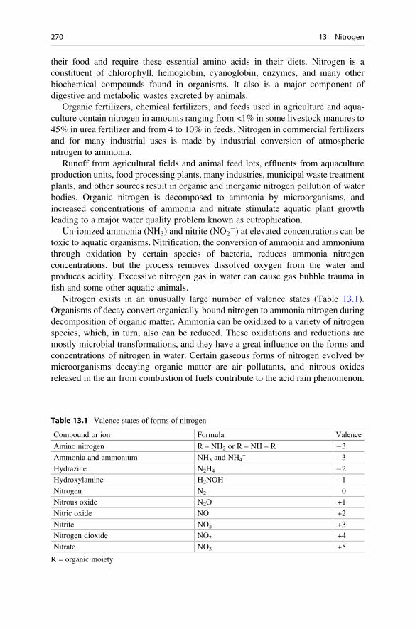
their food and require these essential amino acids in their diets. Nitrogen is aconstituent of chlorophyll, hemoglobin, cyanoglobin, enzymes, and many otherbiochemical compounds found in organisms. It also is a major component ofdigestive and metabolic wastes excreted by animals.

Organic fertilizers, chemical fertilizers, and feeds used in agriculture and aqua-culture contain nitrogen in amounts ranging from <1% in some livestock manures to45% in urea fertilizer and from 4 to 10% in feeds. Nitrogen in commercial fertilizersand for many industrial uses is made by industrial conversion of atmosphericnitrogen to ammonia.

Runoff from agricultural fields and animal feed lots, effluents from aquacultureproduction units, food processing plants, many industries, municipal waste treatmentplants, and other sources result in organic and inorganic nitrogen pollution of waterbodies. Organic nitrogen is decomposed to ammonia by microorganisms, andincreased concentrations of ammonia and nitrate stimulate aquatic plant growthleading to a major water quality problem known as eutrophication.

Un-ionized ammonia (NH3) and nitrite (NO2�) at elevated concentrations can be

toxic to aquatic organisms. Nitrification, the conversion of ammonia and ammoniumthrough oxidation by certain species of bacteria, reduces ammonia nitrogenconcentrations, but the process removes dissolved oxygen from the water andproduces acidity. Excessive nitrogen gas in water can cause gas bubble trauma infish and some other aquatic animals.

Nitrogen exists in an unusually large number of valence states (Table 13.1).Organisms of decay convert organically-bound nitrogen to ammonia nitrogen duringdecomposition of organic matter. Ammonia can be oxidized to a variety of nitrogenspecies, which, in turn, also can be reduced. These oxidations and reductions aremostly microbial transformations, and they have a great influence on the forms andconcentrations of nitrogen in water. Certain gaseous forms of nitrogen evolved bymicroorganisms decaying organic matter are air pollutants, and nitrous oxidesreleased in the air from combustion of fuels contribute to the acid rain phenomenon.

Table 13.1 Valence states of forms of nitrogen

Compound or ion Formula Valence

Amino nitrogen R – NH2 or R – NH – R �3

Ammonia and ammonium NH3 and NH4+ �3

Hydrazine N2H4 �2

Hydroxylamine H2NOH �1

Nitrogen N2 0

Nitrous oxide N2O +1

Nitric oxide NO +2

Nitrite NO2� +3

Nitrogen dioxide NO2 +4

Nitrate NO3� +5

R = organic moiety

270 13 Nitrogen

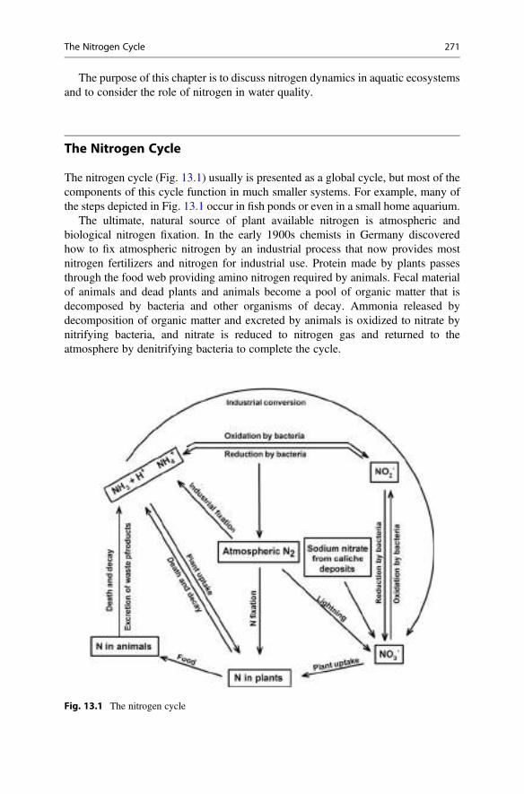
The purpose of this chapter is to discuss nitrogen dynamics in aquatic ecosystemsand to consider the role of nitrogen in water quality.

The Nitrogen Cycle

The nitrogen cycle (Fig. 13.1) usually is presented as a global cycle, but most of thecomponents of this cycle function in much smaller systems. For example, many ofthe steps depicted in Fig. 13.1 occur in fish ponds or even in a small home aquarium.

The ultimate, natural source of plant available nitrogen is atmospheric andbiological nitrogen fixation. In the early 1900s chemists in Germany discoveredhow to fix atmospheric nitrogen by an industrial process that now provides mostnitrogen fertilizers and nitrogen for industrial use. Protein made by plants passesthrough the food web providing amino nitrogen required by animals. Fecal materialof animals and dead plants and animals become a pool of organic matter that isdecomposed by bacteria and other organisms of decay. Ammonia released bydecomposition of organic matter and excreted by animals is oxidized to nitrate bynitrifying bacteria, and nitrate is reduced to nitrogen gas and returned to theatmosphere by denitrifying bacteria to complete the cycle.

Fig. 13.1 The nitrogen cycle

The Nitrogen Cycle 271

Most of the earth’s nitrogen is in the atmosphere, and in organic matter (includingfossil fuels and living biomass). A small quantity is present in deposits of a sodiumnitrate bearing mineral—called caliche—found in the Atacama Desert of Chile and afew other arid places. Most nitrogen transformations are biologically mediated, andgaseous forms of nitrogen can freely exchange between air and water.

Nitrogen Transformations

Atmospheric Fixation by Lightning

Nitrogen gas in the atmosphere must be transformed to ammonia nitrogen or nitrateto be useful to plants. Lightning can result in oxidation of nitrogen gas to nitric acid.This process occurs when heat from lightning breaks the triple bond betweennitrogen atoms allowing them to react with molecular oxygen in the atmosphereforming nitric oxide

N2 þ O2 ! 2NO: ð13:1ÞNitric oxide is then oxidized to nitrite

2NOþ O2 ! 2NO�2 : ð13:2Þ

Though other reactions may occur, the most common way of expressing the conver-sion of nitrite to nitric acid in the atmosphere is

4NO�2 þ 2H2Oþ O2 ! 4HNO3: ð13:3Þ

Nitric acid is washed from the atmosphere by rainfall. Fixation by lightning is animportant source of plant available nitrogen in high rainfall regions—especially inthose where there is frequent lightning during storms. Nitrogen oxides (NOx)entering the atmosphere from combustion of fossil fuels and wildfires also isoxidized to nitric acid and comes down in rainfall.

Nitrate concentration in rainwater from 18 stations across the conterminousUnited States averaged 2.31 mg/L (as NO3

�) with a range of 0.48–5.34 mg/L(Carroll 1962). The atmosphere also contains ammonia from various terrestrialsources, and rainwater from the 18 stations mentioned above had an averageammonia concentration of 0.43 mg/L (as NH4

+) with a range of 0.05–2.11 mg/L.The average annual rainfall for the stations was 875 mm. Thus, the input of nitrogenin form of nitrate and ammonium in rainfall was about 7.5 kg N/ha/yr.

272 13 Nitrogen

Biological Fixation

Nitrogen gas is soluble in water; its concentration at equilibrium for differenttemperatures and salinities are found in Table 7.7. Nitrogen gas is not highlyreactive, but certain species of blue-green algae and bacteria are able to absorbmolecular nitrogen from water, transform it to ammonia, and combine ammonia withintermediate carbohydrate compounds to make amino acids. The summary for thereaction producing ammonia nitrogen is

N2 þ 8Hþ þ 8e� þ 16ATP Ð 2NH�4 þ 16 ADPþ 16 PO2�

4 : ð13:4ÞThe reaction is catalyzed by two enzymes both of which require iron and one ofwhich contains molybdenum as cofactors. Ammonia produced by biological fixationis used to synthesize amino acids that are combined into protein. The processrequires metabolic energy, but the process per se does not require molecular oxygen,and can occur in either aerobic or anaerobic environments.

Nitrogen fixation rates in aquatic ecosystems usually are in the range of 1–10 kg/ha per year, but larger rates have been observed. The greatest rates of nitrogenfixation in aquatic environments have been observed in wetlands where certain treesand shrubs have nitrogen-fixing bacteria associated with their roots. Large amountsof nitrogen also may be fixed by blue-green algae in rice paddies and aquacultureponds.

Blue-green algae capable of fixing nitrogen have heterocysts; these large, thick-walled, spherical cells found in filaments of Nostoc, Anabaena, Gloeocapsa, and afew other genera are the site of nitrogen fixation. The ability of some blue-greenalgae to fix nitrogen gives them a nutrient availability advantage over other algaewhen nitrate and ammonium concentrations are low; however, nitrogen fixation byphytoplanktic blue-green algae tends to decline as nitrate and ammonia nitrogenconcentrations increase. This results because it is more energy efficient for thesemicroorganisms to use nutrients already present than to reduce N2. There also tendsto be a decrease in nitrogen fixation in water bodies as the ratio of total N:total P inwater increases. At a total N:total P ratio of 13 or more, nitrogen fixation stops(Findlay et al. 1994). This suggests that adding phosphorus to waters will increasethe rate of nitrogen fixation.

Industrial Fixation

Industrial nitrogen fixation is accomplished by the Haber-Bosch process. Theprocess involves bringing hydrogen gas made from natural gas or petroleum andatmospheric nitrogen together at high pressure (15–25 M Pa) and temperature(300–550 �C) in the presence of a catalyst (K2O, CaO, SiO2, or Al2O3). Onemolecule of N2 reacts with three molecules of H2 to form two molecules of NH3.Ammonia can be used directly or oxidized to nitrate by an industrial process. Mostnitrogen for making fertilizers and for use in other industrial applications is from the

Nitrogen Transformations 273

Haber-Bosch process. The importance of this process to mankind was expressedbeautifully by the Serbian-American engineer, physicist, and inventor Nikola Teslawho said “the earth is bountiful, and where her bounty fails, nitrogen drawn fromthe air will refertilize her womb.”

Plant Uptake of Nitrate and Ammonium

Ammonia, ammonium, nitrite, and nitrate nitrogen are said to be combined forms ofnitrogen, and plants can absorb combined nitrogen from the water. Most speciesapparently prefer to use ammonium, because it is energetically less demanding to doso. Nitrate nitrogen must be reduced to ammonia nitrogen by the nitrate reductasepathway before it can be used for amino acid synthesis

NO3 ! NO2 ! NH3: ð13:5ÞBiological nitrate reduction requires the nitrate reductase enzyme, molybdenum as acofactor, and metabolic energy from ATP. The ammonia from Eq. 13.5 is thenreacted with intermediates of carbohydrate metabolism to produce amino acids:

Carbohydratesþ NH3 ! amino acids: ð13:6ÞMost phytoplankton species contain from 5 to 10% of their dry weights as protein

nitrogen. In phytoplankton without the capacity to fix nitrogen, protein is madeentirely from combined nitrogen absorbed from the water. The result can be aconsiderable reduction in combined nitrogen concentration as illustrated in Ex. 13.1.

Ex. 13.1 Net productivity of phytoplankton in a 2-m deep body of water is 2 gcarbon/m2/day. Assuming the phytoplankton contain 50% carbon and 8% nitrogen(dry weight), daily nitrogen removal from the water will be estimated.

Solution:

2 g C=m2=d � 0:50 g C=g dry wt ¼ 4 g dry wt=m2=d

4 g dry wt=m2=d � 0:08 g N=g dry wt ¼ 0:32 g N=m2=d

This amount is equivalent to 3.2 kg N/ha/d.Phytoplankton removed nitrogen from the water at a rate of 0.16 mg N/L/d

0:32 g N=m2=d � 2 m3=m2 ¼ 0:16 g N=m3 or 0:16 mg=L:

Phytoplankton uptake is a major factor affecting combined nitrogenconcentrations in water bodies. Aquatic macrophyte communities also may containlarge amounts of nitrogen (Ex. 13.2). Stands of macrophytes can remove nitrogen

274 13 Nitrogen

from the water and hold it in their biomass throughout the growing season, andthereby reduce the availability of nitrogen to phytoplankton.

Ex. 13.2 A lake of 100 ha in area and 3 m in average depth has 10 ha of rootedaquatic plants along its shallow edges. Assuming the dry matter standing crop ofmacrophytes is 800 g/m2 containing 2% nitrogen, the amount of nitrogen in macro-phyte biomass will be estimated.

Solution:

800 g=m2 � 10; 000 m2=ha� 10 ha� 0:02 g N=g dry wt ¼ 1; 600; 000 g N:

Assuming the plants absorbed the nitrogen from lake water, the concentration ofnitrogen in macrophyte biomass equals a concentration of 0.53 mg/L of combinednitrogen

1; 600; 000 g N

100 ha� 3 m� 10; 000 m2=ha¼ 0:53 g N=m3 or 0:53 mg=L:

Phytoplankton and other plants may be consumed by animals or they may die andbecome organic matter that is decomposed by microorganisms. When animals eatplants, at least 10 units of plant dry weight usually are necessary to produce 1 unit ofdry animal biomass and the ratio is often greater and especially for fibrous plants oflow nitrogen content. The nitrogen in plant material consumed by animals and notconverted to nitrogen in biomass is excreted in feces or other metabolic wastes(Ex. 13.3).

Ex. 13.3 Suppose the conversion of phytoplankton to tissue of animals consuming itis at a 15:1 ratio, the plants contain 6% nitrogen, and the animals are 11% nitrogen.The waste nitrogen excreted during the production of 1000 g of animal biomass willbe calculated.

Solution:The dry matter conversion ratio is 15:1, and it will require 15,000 g of plants to

yield 1000 g of animal biomass. The nitrogen budget is

Plant nitrogen 15,000 g� 0:06 g N=g ¼ 900 g N

Animal nitrogen 1,000 g� 0:11 g N=g ¼ 110 g N

Waste nitrogen 900� 110ð Þ g N ¼ 790 g N:

The waste will be excreted as organic nitrogen in feces and most aquatic animalsexcrete ammonia as a metabolic waste. Of course, when animals die, their bodiesbecome organic matter to be decomposed by bacteria with excretion of ammonia.


Mineralization of Organic Nitrogen

Much of the knowledge of microbial decomposition of organic matter comes fromthe literature about the fate of organic residues applied to agricultural fields andpastures. The decomposition of different kinds of organic matter occurs at differentrates: carbohydrates and protein decompose mostly within 1 year, the non-humicsubstances in 1–5 years, and the humic fraction decomposed very slowly overcenturies. When bacteria and fungi decompose organic matter, part of the nitrogenin organic matter is converted to organic nitrogen in microbial biomass, someremains in undecomposed organic matter, and the remainder is released(mineralized) to the environment mainly in the form of ammonia.

Hoorman and Islam (2010) provided information for the annual decomposition oforganic residues added to cropland. By converting the information to carbon con-centration, it can be shown that the addition of around 35 g C in organic residuecould result in about 19 g carbon in CO2, 3 g carbon in bacterial biomass, 2 g carbonin undecomposed non-humic matter, and 11 g carbon in undecomposed humicmatter. The ratio of carbon in living microbial biomass to carbon metabolized toCO2 would be 3/16 or 0.16. This ratio is called the microbial growth efficiency(MGE), and Six et al. (2006) reviewed the literature on MGE and found valuesranging from 0.14 to 0.77 for soils and from 0.01 to 0.70 for aquatic ecosystems. Theaverage for aquatic ecosystems was 0.32. In aquaculture, experience with carbohy-drate additions to remove ammonia by incorporating it in microbial protein in bioflocculture systems suggest that the MGE for bacteria utilizing raw sugar or molasses isaround 0.5 (Hargreaves 2013). However, for more complex residues, the MGE islikely around 0.2–0.3, and much of the residue does not decompose in a single year.

The rate of decomposition of an organic residue depends upon its compositionand especially its carbon:nitrogen (C/N) ratio. Bacteria usually are about 10%nitrogen and 50% carbon (5:1 C/N ratio). Fungi also contain around 50% carbon,but only about 5% nitrogen. Fungi typically have greater MGE than do bacteria.Microorganisms must have adequate nitrogen for biomass synthesis in order todecompose organic matter quickly. If there is not enough nitrogen, microorganismsmust die and their nitrogen recycled to allow decomposition to progress. Residueswith a small (narrow) C/N ratio typically decompose faster with a great mineraliza-tion of nitrogen in the environment than will residues with a greater (wider) C/Nratio. A residue with a wide C/N ratio will tend to lead to withdrawal of combinednitrogen from the environment (nitrogen immobilization) for use by bacteria and theaccumulation of undecomposed organic matter in the environment.

By assuming a given residue is entirely decomposable in a few weeks or monthsleaving only living bacteria, carbon dioxide, and basic elements (a rare situation innature), the importance of the C/N ratio of a residue will be illustrated in Ex. 13.4.

Ex. 13.4 The amount of nitrogen mineralized by bacteria with a MGE of 0.25 incompletely decomposing 1000 g (dry wt) of substrate containing 42% organiccarbon and 4% nitrogen will be determined.

276 13 Nitrogen

Solution:Substrate C: 1,000 g � 0.42 ¼ 420 g CSubstrate N: 1,000 g � 0.04 ¼ 40 g NBacterial biomass produced:

420 g C � 0:25 g bacterial C=g substrate C ¼ 105 g bacterial C

105 g bacterial C � 0:5 g C=g dry bacteria ¼ 210 g bacteria

Bacterial nitrogen: 210 g bacteria � 0.1 g N/g bacteria ¼ 21 g bacterial N.Nitrogen mineralized: 40 g substrate N � 21 g bacterial N ¼ 19 g N released to

environment.

Using the same methods illustrated in Ex. 13.4, 21.1 g of nitrogen would bemineralized by fungi with a MGE of 45% and containing 5% nitrogen.

Organic matter in natural ecosystems normally contains 40 to 50% carbon on adry matter basis. Nitrogen content is more variable ranging from less than 0.4 to 10%or more. As the nitrogen percentage in organic matter increases, there tends to be anincrease in the rate of decomposition and in the proportion of organic nitrogenmineralized. This results because a high nitrogen content is associated with organicmatter that contains less decay-resistant structural compounds and more easilydegradable proteinaceous material. A high nitrogen content also assures that thereis more than enough nitrogen to sustain the microbial biomass that develops duringdecay.

In a substrate with less nitrogen than needed to effect its complete and rapiddecomposition by microorganisms, one or both of two phenomena occur duringdecomposition: (1) decomposition is slow and microorganisms must die so that theirnitrogen can be mineralized and used again to decompose substrate; (2) ammonianitrogen and nitrate in the environment can be removed (immobilized) and used bymicroorganisms to decompose the nitrogen-deficient residue. Where nitrogen isavailable for immobilization, decomposition of low-nitrogen content residues oftenis greatly accelerated.

The influence of the C:N ratio on nitrogen balance during decomposition can beillustrated by solving the nitrogen budget (see Ex. 13.4 for procedure) for two readilydecomposable residues, one with 42% carbon and 2% N and a second with 42%carbon and 0.4% N, decomposed by bacteria with a MGE of 0.2. Decomposition of1000 g of the first residue would mineralize 3.2 g nitrogen—the second, 1000-gresidue with 0.4% nitrogen contains only 4 g nitrogen. This is 14.8 g less nitrogenthan needed by the bacteria decomposing the residue.

The relationship of nitrogen concentration in organic matter to decompositionrate is illustrated in Fig. 13.2. The oxygen consumption rate of decomposition ofaquatic plant residues increased as the nitrogen concentration of these residuesincreased (C/N ratios declined). The rate of oxygen consumption also droppedquickly in residues and after 5 days were essentially equal in residues of high and


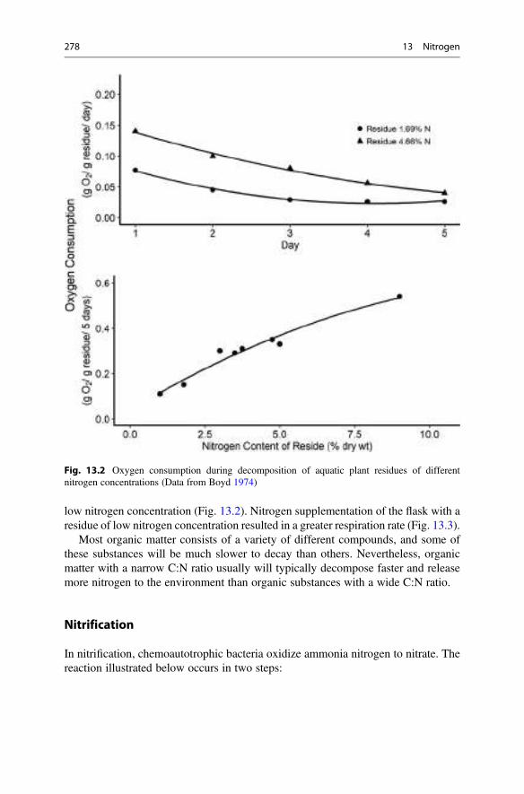
low nitrogen concentration (Fig. 13.2). Nitrogen supplementation of the flask with aresidue of low nitrogen concentration resulted in a greater respiration rate (Fig. 13.3).

Most organic matter consists of a variety of different compounds, and some ofthese substances will be much slower to decay than others. Nevertheless, organicmatter with a narrow C:N ratio usually will typically decompose faster and releasemore nitrogen to the environment than organic substances with a wide C:N ratio.

Nitrification

In nitrification, chemoautotrophic bacteria oxidize ammonia nitrogen to nitrate. Thereaction illustrated below occurs in two steps:

Fig. 13.2 Oxygen consumption during decomposition of aquatic plant residues of differentnitrogen concentrations (Data from Boyd 1974)

278 13 Nitrogen

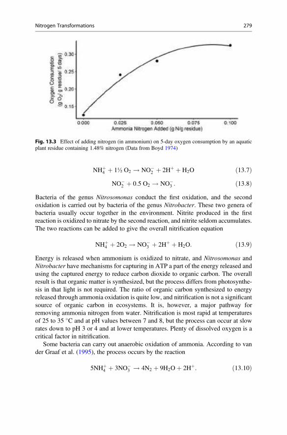
NHþ4 þ 1½ O2 ! NO�

2 þ 2Hþ þ H2O ð13:7ÞNO�

2 þ 0:5 O2 ! NO�3 : ð13:8Þ

Bacteria of the genus Nitrosomonas conduct the first oxidation, and the secondoxidation is carried out by bacteria of the genus Nitrobacter. These two genera ofbacteria usually occur together in the environment. Nitrite produced in the firstreaction is oxidized to nitrate by the second reaction, and nitrite seldom accumulates.The two reactions can be added to give the overall nitrification equation

NHþ4 þ 2O2 ! NO�

3 þ 2Hþ þ H2O: ð13:9ÞEnergy is released when ammonium is oxidized to nitrate, and Nitrosomonas andNitrobacter have mechanisms for capturing in ATP a part of the energy released andusing the captured energy to reduce carbon dioxide to organic carbon. The overallresult is that organic matter is synthesized, but the process differs from photosynthe-sis in that light is not required. The ratio of organic carbon synthesized to energyreleased through ammonia oxidation is quite low, and nitrification is not a significantsource of organic carbon in ecosystems. It is, however, a major pathway forremoving ammonia nitrogen from water. Nitrification is most rapid at temperaturesof 25 to 35 �C and at pH values between 7 and 8, but the process can occur at slowrates down to pH 3 or 4 and at lower temperatures. Plenty of dissolved oxygen is acritical factor in nitrification.

Some bacteria can carry out anaerobic oxidation of ammonia. According to vander Graaf et al. (1995), the process occurs by the reaction

5NHþ4 þ 3NO�

3 ! 4N2 þ 9H2Oþ 2Hþ: ð13:10Þ

Fig. 13.3 Effect of adding nitrogen (in ammonium) on 5-day oxygen consumption by an aquaticplant residue containing 1.48% nitrogen (Data from Boyd 1974)


Nitrate is the oxygen source for oxidation of ammonium to nitrogen gas. Thisreaction could just as aptly be called denitrification because nitrate also is reducedto nitrogen gas.

Nitrification by both aerobic and anaerobic processes produces hydrogen ion, sothe nitrification process contributes to acidity. Aerobic nitrification also requires anabundant supply of molecular oxygen and contributes greatly to oxygen demand inwaters receiving high inputs of ammonia nitrogen. The oxygen demand and acidityof aerobic nitrification is illustrated in the next example.

Ex. 13.5 The amount of dissolved oxygen consumed and the amount of acidityproduced (in terms of alkalinity loss) in the biological oxidation of 1 mg/L ammonianitrogen (NH4-N) in aerobic nitrification will be estimated.

Solution:From Eq. 13.9, one mole of nitrogen consumes two moles of molecular oxygen

and produces two moles of hydrogen ions. Thus,

(i)1 mg=L x

N ¼ 2O2

14 64

x ¼ 4:57 mg=L of dissolved oxygen consumed per 1 mg=L of NHþ4 -N:

(ii) Two moles of hydrogen ions react with one mole of calcium carbonate (alkalin-ity is expressed as CaCO3)

CaCO3 þ 2Hþ ¼ Ca2þ þ CO2 þ H2O

and

1 mg=L xN ¼ 2Hþ ¼ CaCO3

14 100

x ¼ 7:14 mg=L of total alkalinity neutralized per 1 mg=L of NHþ4 -N:

In Ex. 13.5 above, 1 mg/L NH4-N means that there is 1 mg/L of nitrogen in NH4+

from (NH4+-N). To convert 1 mg/L NH4

+-N to milligrams per liter of NH4+, multiply

1 mg/L NH4+-N by NH4

+/N or 18/14 to get 1.29 mg/L. The NH4+ concentration can

be converted to NH4+-N concentration by dividing it by 18/14.

Rates of nitrification differ greatly among waters and over time in the same bodyof water. They tend to be much greater in summer than in winter, and they increasewhen ammonia nitrogen concentration increases. An abundant supply of dissolvedoxygen is necessary for rapid nitrification. Nitrification can occur both in the water

280 13 Nitrogen

column and in aerobic sediment. Gross (1999) found that nitrification produced anaverage of 240 mg NO3-N/m

2/day and 260 mg NO3-N/m2/day in the water column

and sediment, respectively, of shallow, eutrophic ponds. However, Hargreaves(1995) reported that nitrification in the aerobic layers of sediment could be severaltimes greater than in the water column.

Denitrification

Under anaerobic conditions, some bacteria use oxygen from nitrate as a substrate formolecular oxygen to oxidize organic matter (respire). One equation for denitrifica-tion is

6NO�3 þ 5CH3OH ! 5CO2 þ 3N2 þ 7H2Oþ 6OH�: ð13:11Þ

Methanol is the carbon source for denitrification in Eq. 13.11, and methanol is thecarbon source frequently used in the denitrification process at sewage treatmentplants. In nature many types of organic matter can be used by denitrifying bacteria.The process is called denitrification because nitrate nitrogen is converted to nitrogengas and lost from the ecosystem by diffusion into the atmosphere. Denitrificationyields one mole of hydroxyl ion for each mole of nitrate reduced, and therebyincreases the alkalinity of water.

Nitrification and denitrification can be thought of as coupled, because nitrateproduced in nitrification can be denitrified. Only one-half of the alkalinity losscaused by nitrification is restored when nitrification and denitrification are perfectlycoupled. This is because each mole of nitrogen oxidized in nitrification releases twomoles of hydrogen ions, while each mole of nitrogen denitrified releases only onemole of hydroxyl ion. The potential acidity of nitrification is 7.14 mg/L equivalentCaCO3 while the potential alkalinity of denitrification is 3.57 mg/L equivalentCaCO3.

Denitrification does not always lead to formation of N2. It can end with nitrite

NO�3 þ 2Hþ ! NO�

2 þ H2O: ð13:12ÞAmmonia can be an end product when nitrate is reduced to nitrite followed byconversion of nitrite to hyponitrite (H2N2O2) and hyponitrite to hydroxylamine(H2NOH)

2NO�2 þ 5Hþ ! H2N2O2 þ H2Oþ OH� ð13:13ÞH2N2O2 þ 4Hþ ! 2H2NOH ð13:14Þ

H2NOHþ 2Hþ ! NH3 þ H2O: ð13:15ÞAnother pathway results in formation of nitrous oxide as follows:


H2N2O2 ! N2Oþ H2O: ð13:16ÞHowever, N2 formation is the most common pathway in denitrification.

Denitrification rates can be very high in aquatic ecosystems where nitrate isabundant and there is a readily available source of organic matter. The denitrificationrate during the period June to October in small, eutrophic ponds at Auburn,Alabama, in which fish were fed a high-protein content ration ranged from 0 to60 mg N/m2/day (average ¼ 38 mg N/m2/day). On an annual basis, the average rateis equivalent to 139 kg N/ha (Gross 1999). Nitrogen inputs to most aquaticecosystems are not great enough to support such large amounts of denitrificationas seen in aquaculture ponds with daily additions of high-protein-content feeds.

Nitrite may sometimes accumulate in water to concentrations of 1 mg/L or more.When this phenomenon occurs, there may be toxicity to fish and other aquaticanimals. Nitrite accumulation can result when the first step in nitrification(Eq. 13.7) proceeds faster than the second step. It also can result from nitriteproduction in anaerobic sediment as shown in Eq. 13.16 with subsequent diffusionof nitrite into the water column.

Ammonia-Ammonium Equilibrium

Ammonia nitrogen exists in water as ammonia (NH3) and ammonium ion (NH4+).

The un-ionized form is a gas, and it is potentially toxic to fish and other aquatic life atrelatively low concentration. Ammonium is not appreciably toxic. Ammoniahydrolyses to ammonium in aqueous solution, and the two forms exist in a pH andtemperature dependent equilibrium

NH3 þ H2O ¼ NHþ4 þ OH� Kb ¼ 10�4:75: ð13:17Þ

The hydrolysis may alternatively be expressed as

NHþ4 ¼ NH3 þ Hþ: ð13:18Þ

Analytical procedures for ammonia nitrogen (including both ion sensing and gassensing electrodes) measure total ammonia nitrogen (TAN) and the NH3 concentra-tion must be calculated by aid of pH and water temperature (Zhou and Boyd 2016).Ammonia acts as a base in Eq. 13.17, but ammonium is an acid in Eq. 13.18.Because KaKb ¼ Kw ¼ 10�14 (at 25 �C), Ka ¼ 10�14/Kb, and Ka for Eq. 13.18 is10–9.25. The Ka and Kb values given above are for 25 �C, but values of Ka and Kb forother temperatures obtained from Bates and Pinching (1949) are presented(Table 13.2) along with Kw values for different temperatures. The ratio of NH3-Nto NH4-N can be calculated most conveniently using Eq. 13.18 as follows:

282 13 Nitrogen

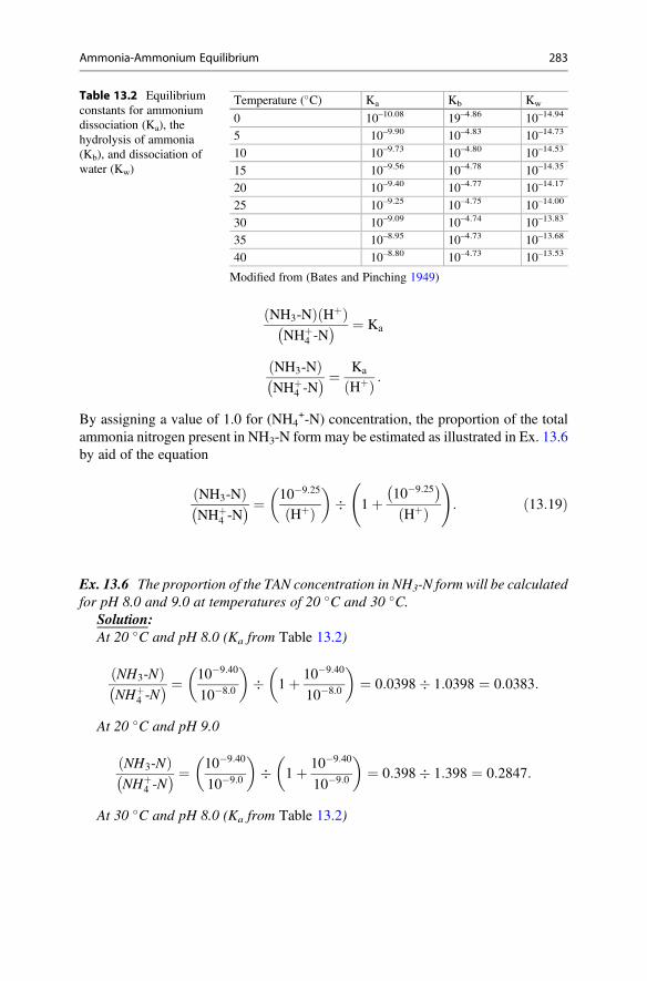
NH3-Nð Þ Hþð ÞNHþ

4 -N� � ¼ Ka

NH3-Nð ÞNHþ

4 -N� � ¼ Ka

Hþð Þ :

By assigning a value of 1.0 for (NH4+-N) concentration, the proportion of the total

ammonia nitrogen present in NH3-N form may be estimated as illustrated in Ex. 13.6by aid of the equation

NH3-Nð ÞNHþ

4 -N� � ¼ 10�9:25

Hþð Þ� �

� 1þ 10�9:25� �

Hþð Þ

!

: ð13:19Þ

Ex. 13.6 The proportion of the TAN concentration in NH3-N form will be calculatedfor pH 8.0 and 9.0 at temperatures of 20 �C and 30 �C.

Solution:At 20 �C and pH 8.0 (Ka from Table 13.2)

NH3-Nð ÞNHþ

4 -N� � ¼ 10�9:40

10�8:0

� �� 1þ 10�9:40

10�8:0

� �¼ 0:0398� 1:0398 ¼ 0:0383:

At 20 �C and pH 9.0

NH3-Nð ÞNHþ

4 -N� � ¼ 10�9:40

10�9:0

� �� 1þ 10�9:40

10�9:0

� �¼ 0:398� 1:398 ¼ 0:2847:

At 30 �C and pH 8.0 (Ka from Table 13.2)

Table 13.2 Equilibriumconstants for ammoniumdissociation (Ka), thehydrolysis of ammonia(Kb), and dissociation ofwater (Kw)

Temperature (�C) Ka Kb Kw

0 10–10.08 19–4.86 10–14.94

5 10–9.90 10–4.83 10–14.73

10 10–9.73 10–4.80 10–14.53

15 10–9.56 10–4.78 10–14.35

20 10–9.40 10–4.77 10–14.17

25 10–9.25 10–4.75 10–14.00

30 10–9.09 10–4.74 10–13.83

35 10–8.95 10–4.73 10–13.68

40 10–8.80 10–4.73 10–13.53

Modified from (Bates and Pinching 1949)

Ammonia-Ammonium Equilibrium 283

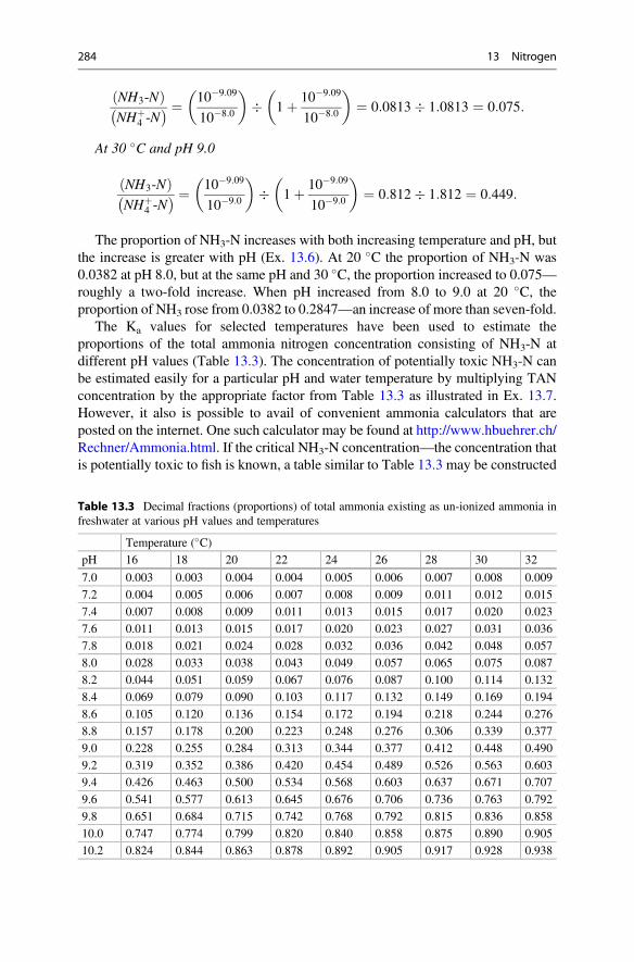
NH3-Nð ÞNHþ

4 -N� � ¼ 10�9:09

10�8:0

� �� 1þ 10�9:09

10�8:0

� �¼ 0:0813� 1:0813 ¼ 0:075:

At 30 �C and pH 9.0

NH3-Nð ÞNHþ

4 -N� � ¼ 10�9:09

10�9:0

� �� 1þ 10�9:09

10�9:0

� �¼ 0:812� 1:812 ¼ 0:449:

The proportion of NH3-N increases with both increasing temperature and pH, butthe increase is greater with pH (Ex. 13.6). At 20 �C the proportion of NH3-N was0.0382 at pH 8.0, but at the same pH and 30 �C, the proportion increased to 0.075—roughly a two-fold increase. When pH increased from 8.0 to 9.0 at 20 �C, theproportion of NH3 rose from 0.0382 to 0.2847—an increase of more than seven-fold.

The Ka values for selected temperatures have been used to estimate theproportions of the total ammonia nitrogen concentration consisting of NH3-N atdifferent pH values (Table 13.3). The concentration of potentially toxic NH3-N canbe estimated easily for a particular pH and water temperature by multiplying TANconcentration by the appropriate factor from Table 13.3 as illustrated in Ex. 13.7.However, it also is possible to avail of convenient ammonia calculators that areposted on the internet. One such calculator may be found at http://www.hbuehrer.ch/Rechner/Ammonia.html. If the critical NH3-N concentration—the concentration thatis potentially toxic to fish is known, a table similar to Table 13.3 may be constructed

Table 13.3 Decimal fractions (proportions) of total ammonia existing as un-ionized ammonia infreshwater at various pH values and temperatures

Temperature (�C)pH 16 18 20 22 24 26 28 30 32

7.0 0.003 0.003 0.004 0.004 0.005 0.006 0.007 0.008 0.009

7.2 0.004 0.005 0.006 0.007 0.008 0.009 0.011 0.012 0.015

7.4 0.007 0.008 0.009 0.011 0.013 0.015 0.017 0.020 0.023

7.6 0.011 0.013 0.015 0.017 0.020 0.023 0.027 0.031 0.036

7.8 0.018 0.021 0.024 0.028 0.032 0.036 0.042 0.048 0.057

8.0 0.028 0.033 0.038 0.043 0.049 0.057 0.065 0.075 0.087

8.2 0.044 0.051 0.059 0.067 0.076 0.087 0.100 0.114 0.132

8.4 0.069 0.079 0.090 0.103 0.117 0.132 0.149 0.169 0.194

8.6 0.105 0.120 0.136 0.154 0.172 0.194 0.218 0.244 0.276

8.8 0.157 0.178 0.200 0.223 0.248 0.276 0.306 0.339 0.377

9.0 0.228 0.255 0.284 0.313 0.344 0.377 0.412 0.448 0.490

9.2 0.319 0.352 0.386 0.420 0.454 0.489 0.526 0.563 0.603

9.4 0.426 0.463 0.500 0.534 0.568 0.603 0.637 0.671 0.707

9.6 0.541 0.577 0.613 0.645 0.676 0.706 0.736 0.763 0.792

9.8 0.651 0.684 0.715 0.742 0.768 0.792 0.815 0.836 0.858

10.0 0.747 0.774 0.799 0.820 0.840 0.858 0.875 0.890 0.905

10.2 0.824 0.844 0.863 0.878 0.892 0.905 0.917 0.928 0.938

284 13 Nitrogen

http://www.hbuehrer.ch/Rechner/Ammonia.html

http://www.hbuehrer.ch/Rechner/Ammonia.html

in which the table entries represent the maximum acceptable total ammonia nitrogenconcentrations. For instance, if the critical concentration is 0.10 mg/L NH3-N, atpH 8 and 25 �C, the total ammonia nitrogen concentration should not exceed1.92 mg/L (0.1 mg/L � 0.052).

Factors for estimating the NH3 concentration from the TAN concentration(Table 13.3) are for freshwater. Increasing ionic strength (greater salinity) lessensthe proportion of NH3 to TAN, and Spotte and Adams (1983) devised a series oftables of NH4

+-N/NH3-N ratios for estimating NH3 concentration from the TANconcentration at different pH values, water temperatures, and salinities. Thedifferences among salinities are rather small. For example, at pH 8.2 and 25 �C,the factor to be multiplied by TAN concentration to obtain NH3-N concentrationsare: 5 ppt, 0.078; 10 ppt, 0.077; 15 ppt, 0.075; 20 ppt, 0.072; 25 ppt, 0.070; 30 ppt,0.068; 35 ppt, 0.065. The factor for freshwater extrapolated from Table 13.3 is0.082. There also are online ammonia calculators that include salinity as a factor,e.g., (https://pentairaes.com/amonia-calculator).

Ex. 13.7 A water sample contains 1 mg/L TAN. The concentration of NH3-N will beestimated at 30 �C for pH 7, 8, 9, and 10.

Solution:From Table 13.3, the proportions of un-ionized ammonia at 30 �C are 0.008,

0.075, 0.448, and 0.890 in order of increasing pH. Thus,pH 7:

1 mg/L � 0.008 ¼ 0.008 mg NH3-N/LpH 8:

1 mg/L � 0.075 ¼ 0.075 mg NH3-N/LpH 9:

1 mg/L � 0.448 ¼ 0.448 mg NH3-N/LpH 10:

1 mg/L � 0.890 ¼ 0.890 mg NH3-N/L.

Ammonia Diffusion

The potential for diffusion of ammonia from the surface of a water body into the airobviously will be greatest when pH is high. Weiler (1979) reported ammoniadiffusion losses up to 10 kg N/ha per day when wind velocity, pH, and totalammonia nitrogen concentrations were high. In most waters, the ammonia nitrogenconcentration will not be great enough to support such large ammonia diffusionrates. Gross et al. (1999) reported diffusion losses of 9 to 71 mg N/m2/day from smallponds with 0.05 to 5.0 mg/L of total ammonia nitrogen, afternoon pH values of 8.3to 9.0, and water temperature of 21 to 29 �C. The effect of ammonia diffusion to theatmosphere on the total ammonia concentration in water is illustrated (Ex. 13.8).

Ammonia Diffusion 285

https://pentairaes.com/amonia-calculator

Ex. 13.8 The reduction in ammonia nitrogen concentration that could result bydiffusion of ammonia at a rate 10 mg NH3-N/m

2/day will be calculated for a 1-hawater body that has an average depth of 2 m.

Solution:

10 mg NH3-N=m2=d

2m3=m2¼ 5 mg NH3-N=m

3=d ¼ 0:005 mg NH3 � N=L=d:

The decrease in ammonia nitrogen concentration is small for 1 day, but over a year,the total loss of nitrogen could be substantial. If the loss rate used above is expandedfor 1 year, the nitrogen loss would be

10 mg NH3-N=m2=d � 365 d=yr ¼ 3:65 g=m2:

This is 36.5 kg N/ha per year.

Nitrogen Inputs and Outputs

Aquatic ecosystems have various inputs and outputs of nitrogen. The main inputs arerainfall, inflowing water containing nitrogen from natural sources and pollution,nitrogen added intentionally (as in aquaculture), and nitrogen fixation. The outputsare outflowing water, harvest of aquatic products, intentional withdrawal of water,seepage, diffusion of ammonia into the atmosphere, and denitrification. The relativeimportance of each gain and loss varies greatly from one body of water to another.

Nitrogen is stored in aquatic ecosystems primarily as organic matter in bottomsediments, but smaller amounts occur in the water as nitrogen gas, nitrate, nitrite,ammonia, and nitrogen in dissolved and particulate organic matter. Dissolvednitrogen gas often is the major form of nitrogen in water bodies (Table 7.7), but itis largely inert and seldom of water quality significance. When nitrogen in organicmatter is mineralized, it is subject to the various processes and transformationsdescribed above, and it can be lost from the ecosystem. However, there is a tendencyfor recycling of nitrogen in aquatic ecosystems, and in most, an equilibrium amonginputs, outputs, and stored nitrogen is reached. Pollution can quickly disrupt thisequilibrium and cause higher nitrogen concentrations in the water and sediment.

Concentrations of Nitrogen in Water and Sediment

Dissolved nitrogen gas is not as biologically active as dissolved oxygen, and itsconcentrations usually remain near saturation. Ammonia nitrogen and nitrate nitro-gen concentrations each normally are less than 0.25 mg/L in unpolluted waters. Theymay be above 1 mg/L in polluted waters, and in highly polluted watersconcentrations of 5 to 10 mg/L are not uncommon. Nitrite nitrogen is seldom present

286 13 Nitrogen

at concentrations above 0.05 mg/L in oxygenated water, but it may reachconcentrations of several milligrams per liter in polluted waters with low dissolvedoxygen concentration.

The concentration of ammonia and nitrate nitrogen necessary to cause phyto-plankton blooms in natural waters is difficult to ascertain, because many otherfactors also influence phytoplankton productivity. Concentrations of 0.1–0.75 mg/L of combined nitrogen in freshwater and even lower concentrations in brackish andmarine waters have caused phytoplankton blooms. Limitation of combined nitrogenconcentrations and loads is an important tool in eutrophication control.

The usual procedure is to determine total organic nitrogen rather thanconcentrations of specific organic nitrogen compounds. Measurements of totalorganic nitrogen include dissolved and particulate organic nitrogen, and they usuallyare below 1 or 2 mg/L in relatively unpolluted natural waters. Effluents and pollutedwaters may have much higher concentrations of total organic nitrogen. Domesticsewage has an average total nitrogen concentration around 40 mg/L (Tchobanoglousand Schroeder 1985).

Concentrations of nitrogen also are highly variable in sediment. As a general rule,organic matter is about 5% nitrogen, and sediments in aquatic ecosystems usuallycontain 1 to 10% organic matter which corresponds to around 0.05 to 0.5% nitrogen.

Ammonia Toxicity

Ammonia is the major nitrogenous excretory product of aquatic animals, and likeother excretory products, is toxic if it cannot be excreted. A high concentration ofammonia in the water makes it more difficult for organisms to excrete ammonia. As aresult the concentration of ammonia in the blood of fish and other aquatic animalsincreases with greater environmental ammonia concentration.

Although the mechanism of ammonia toxicity has not been elucidated entirely, anumber of physiological and histological effects of high ammonia concentration inthe blood and tissues of fish have been identified as follows: elevation of blood pH;disruption of enzyme systems and membrane stability; increased water uptake;increased oxygen consumption; gill damage; histological lesions in various internalorgans.

The concentration of ammonia in most water bodies fluctuates daily because theproportion of ammonia to total ammonia nitrogen varies with pH and temperature(Table 13.3). Most data on ammonia toxicity were based on exposure to constantammonia concentration, and less is known about the effects of fluctuating ammoniaconcentrations than about exposure to a constant concentration on aquatic animals.In water bodies, pH and temperature tend to increase in daytime to a peak in theafternoon and decline at night to their lowest near dawn. Hargreaves and Kucuk(2001) exposed three common species of fish used in aquaculture to daily fluctuatingconcentrations of NH3 typical in magnitude to those occurring in ponds. The effects

Ammonia Toxicity 287

of ammonia were observed at greater concentrations than was expected from theresults of toxicity tests conducted at constant temperature, pH and NH3

concentration.The potential for toxicity at a given ammonia nitrogen concentration depends on

several factors in addition to pH and temperature. Toxicity increases with decreasingdissolved oxygen concentration, but this effect often is negated by high carbondioxide concentration which decreases ammonia toxicity. There is evidence thatammonia toxicity decreases with increasing concentrations of salinity and calcium.Fish also tend to increase their tolerance for ammonia when acclimated to graduallyincreasing ammonia concentrations over several weeks or months.

Most ammonia toxicity data come from LC50 tests on fish—the LC50 is theconcentration required to kill 50% of the animals exposed. The 96-hour LC50concentrations for un-ionized ammonia nitrogen to various species of fish rangefrom about 0.3 to 3.0 mg/L (Ruffier et al. 1981; Hargreaves and Kucuk 2001).Coldwater species usually are more susceptible to ammonia than warmwater species.Un-ionized ammonia should not cause lethal or sublethal effects at concentrationsbelow 0.005 to 0.01 mg/L for coldwater species or below 0.01 to 0.05 mg/L forwarmwater species. Corresponding concentrations of total ammonia nitrogendepend upon pH and temperature. The concentrations of ammonia nitrogen neces-sary to give 0.05 mg/L un-ionized ammonia nitrogen at selected pH values and 26 �Care as follows: pH 7, 8.33 mg/L; pH 8, 0.88 mg/L; pH 9, 0.13 mg/L. Ammoniatoxicity obviously is of greater concern in waters where the pH is well above neutralthan in neutral or acidic waters. The main effect of ammonia on aquatic life probablyis stress rather than mortality. Several studies have shown that ammoniaconcentrations well below lethal concentrations lead to poor appetite, slow growth,and greater susceptibility to disease.

Nitrite Toxicity

Nitrite is absorbed from the water by fish and other organisms. In the blood of fish,nitrite reacts with hemoglobin to form methemoglobin. Methemoglobin does notcombine with oxygen, and high nitrite concentrations in water can result in afunctional anemia known as methemoglobinemia. Blood that contains significantmethemoglobin is brown, so the common name for nitrite toxicity in fish is “brownblood disease.” Nitrite also can bind hemocyanin, the oxygen binding pigment incrustacean blood, to lower the ability of their blood to transport oxygen.

Nitrite is transported across the gill by lamellar chloride cells. These same cellsapparently transport chloride and they cannot distinguish between nitrite and chlo-ride. The rate of nitrite absorption declines, at least in freshwater fish, as theconcentration of chloride increases relative to nitrite. In freshwater, a chloride tonitrite ratio of 6 to 10:1 will prevent methemoglobinemia at nitrite concentrations upto at least 5 or 10 mg/L. In brackishwater, high concentrations of calcium and chloridetend to minimize problems of nitrite toxicity in fish (Crawford and Allen 1977).

288 13 Nitrogen

Because the toxic effects of nitrite are worsened by low dissolved oxygenconcentration and also depend upon chloride, calcium, and salinity concentrations,it is virtually impossible to make recommendations on lethal, sublethal, and safeconcentrations. The 96-hour LC50 values (as nitrite) are in the range of 0.66 to200 mg/L for freshwater fish and crustaceans and 40 to 4000 mg/L for brackishwaterand marine species. Safe concentrations would likely be about 0.05 times the96-hour LC50 concentration for a species.

Nitrogen and Gas Bubble Trauma

Because nitrogen is the most abundant atmospheric gas, it is the major gas in watersupersaturated with air. As discussed in Chap. 7, nitrogen usually is the primary gascontributing to gas bubble trauma in aquatic animals exposed to gas supersaturatedwater. Common reasons for air supersaturation are sudden warming of water andwater entraining air when it falls over high dams into streams below. Air leaks on thesuction sides of pumps also can cause air supersaturation of discharge water.

Atmospheric Pollution by Nitrogen Compounds

Nitrous oxide that can be produced by denitrification in anaerobic environments isnot generally considered a water quality issue, because it diffuses from water bodiesinto the atmosphere. However, nitrous oxide is one of the greenhouse gases that canincrease the heat retaining capacity of the atmosphere to cause global warming. Theglobal warming potential of nitrous oxide is about 300 times greater than that ofcarbon dioxide (the standard for greenhouse global warming potential).

Nitrogen dioxide (NO2) and related nitrogen oxides—often referred to collec-tively as NOx—are produced by combustion of fossil fuels and by wildfires. In theatmosphere, nitrogen oxides are oxidized to nitric acid and contribute to the acid rainphenomenon.

Conclusions

Plant growth often increases in response to increased nitrogen concentrations,because a shortage of available nitrogen is a limiting factor in many aquaticecosystems. Nitrogen is used as a fertilizer in agriculture and aquaculture, butaddition of nitrogen to most water bodies is considered to be nutrient pollution,because it contributes to dense phytoplankton blooms—causes eutrophication.Excessive concentrations of ammonia, nitrite, and dinitrogen gas (N2) can be toxicto aquatic organisms. In addition, nitrous oxide is a greenhouse gas and nitrogenoxides contribute to acidity in rainfall.

Conclusions 289

References

Bates RG, Pinching GD (1949) Acid dissociation constant of ammonium ion at 0� to 50�C, and thebase strength of ammonia. J Res Nat Bur Stan 42:419–420

Boyd CE (1974) The utilization of nitrogen from decomposition of organic matter by cultures ofScenedesumes dimorphus. Arch fur Hydro 73:361–368

Carroll D (1962) Rainwater as a chemical agent of geologic processes—a review. United Statesgeological survey water-supply paper 1535 G, United States. Government Printing Office,Washington, DC

Crawford RE, Allen GH (1977) Seawater inhibition of nitrite toxicity to Chinook salmon. Trans AmFish Soc 106:105–109

Findlay DL, Hecky RE, Hendzel LL, Stainton MP, Regehr GW (1994) Relationship betweenN2-fixation and heterocyst abundance and its relevance to the nitrogen budget of lake 227.Can J Fish Aqua Sci 51:2,254–2,266

Gross A (1999) Nitrogen cycling in aquaculture ponds. Dissertation, Auburn University, AlabamaGross A, Boyd CE, Wood CW (1999) Ammonia volatilization from freshwater fish ponds. J Env

Qual 28:793–797Hargreaves JA (1995) Nitrogen biochemistry of aquaculture pond sediments. Dissertation,

Louisiana State University, Baton RougeHargreaves JA (2013) Biofloc production systems for aquaculture. Publication 4503, Southern

Regional Aquaculture Center, StonevilleHargreaves JA, Kucuk S (2001) Effects of diel un-ionized ammonia fluctuation on juvenile striped

bass, channel catfish, and blue tilapia. Aqua 195:163–181Hoorman JJ, Islam R (2010) Understanding soil microbes and nutrient recycling. Fact sheet

SAG-16-10, The Ohio State University Extension, ColumbusRuffier PJ, Boyle WC, Kleinschmidt J (1981) Short-term acute bioassays to evaluate ammonia

toxicity and effluent standards. J Water Poll Con Fed 53:367–377Six J, Frey SD, Thiet RK, Batten KM (2006) Bacterial and fungal contributions to carbon

sequestration in agroecosystems. Soil Sci Soc Am J 70:555–569Spotte S, Adams G (1983) Estimation of the allowable upper limit of ammonia in saline water. Mar

Ecol Prog Ser 10:207–210Tchobanoglous G, Schroeder ED (1985) Water quality. Addison-Wesley, Menlo Parkvan der Graaf AA, Mulder A, de Bruijin P, Jetten MSM, Robertson LA, Kuenen JG (1995)

Anaerobic oxidation of ammonium is a biologically mediated process. App Env Microb61:1246–1251

Weiler RR (1979) Rate of loss of ammonia from water to the atmosphere. J Fish Res Bd Canada36:685–689

Zhou L, Boyd CE (2016) Comparison of Nessler, phenate, salicylate and ion selective electrodeprocedures for determination of total ammonia nitrogen in aquaculture. Aqua 450:187–193

290 13 Nitrogen

Phosphorus 14

AbstractPhosphorus usually is the most important nutrient limiting phytoplankton pro-ductivity in both aquatic and terrestrial ecosystems. Phosphorus occurs naturallyin most geological formations and soils in varying amounts and forms; the mainsource of agricultural and industrial phosphate is deposits of the mineral apatite—known as rock phosphate. Municipal and agricultural pollution is a major sourceof phosphorus to many water bodies. Most dissolved inorganic phosphorus inaquatic ecosystems is an ionization product of orthophosphoric acid (H3PO4). Atthe pH of most water bodies, HPO4

2� and H2PO4� are the forms of dissolved

phosphate. Despite its biological significance, the dynamics of phosphorus inecosystems are dominated by chemical processes. Phosphate is removed fromwater by reactions with aluminum, and to a lesser extent, with iron in sediment. Inalkaline environments, phosphate is precipitated as calcium phosphate. Alumi-num, iron and calcium phosphates are only slightly soluble, and sediments act assinks for phosphorus. Concentrations of inorganic phosphorus in water bodiesseldom exceed 0.1 mg/L, and total phosphorus concentration rarely is greater than0.5 mg/L. In anaerobic zones, the solubility of iron phosphates increases; sedi-ment pore water and hypolimnetic water of eutrophic lakes may have phosphateconcentrations above 1 mg/L. Phosphorus is not toxic at elevated concentration,but along with nitrogen, it can lead to eutrophication.

Introduction

Phosphorus usually is in short supply in the environment relative to plant needsmaking it a key factor regulating primary productivity of natural and agriculturalecosystems. Phosphorus is the most important nutrient controlling plant growth inmany water bodies, and phosphorus pollution of natural waters is considered aprimary cause of eutrophication. Phosphorus is absorbed strongly by bottom sedi-ment where it is bound in iron, aluminum, and calcium phosphate compounds and


291


adsorbed onto iron and aluminum oxides and hydroxides. Solubilities of the mineralforms of phosphorus are regulated by pH, and there are comparatively few situationsin nature in which phosphorus minerals are highly soluble. The phosphorus inorganic matter is mineralized, but when it is, it usually will be adsorbed by sedimentunless it is quickly absorbed by plants or bacteria. Because sediments tend to be asink for phosphorus, high rates of plant growth in aquatic ecosystems require acontinuous input of phosphorus.

Phosphorus is absorbed from environmental solutions by plants and supplied toanimals and microorganisms of decay mainly through food webs. The storage formof phosphorus in plant tissues is phytic acid, a saturated cyclic acid with the formulaC6H18O24P6—a six carbon ring with a phosphate radical (H2PO4

�) attached to eachcarbon. This compound is particularly abundant in bran and cereal grains. Phyticacid is not readily digestible by non-ruminant animals, but the enzyme phytaseproduced in the rumen by microorganisms allows ruminant animals to digest phyticacid. Most animals get their phosphorus from other phosphorus compounds in theirdiets rather than from phytic acid, but, microorganisms of decay can degrade phyticacid to release phosphate.

Phosphorus is a key nutrient with many functions in all living things. It iscontained in deoxyribonucleic acid (DNA) that contains the genetic code(or genome) to instruct organisms how to grow, maintain themselves, and reproduce.Phosphorus also is a component of ribonucleic acid (RNA) that provides theinformation needed for protein synthesis, i.e., DNA is responsible for RNA produc-tion which in turn controls protein synthesis. Phosphorus is a component of adeno-sine diphosphate (ADP) and adenosine triphosphate (ATP) responsible for energytransfer, storage, and use at the cellular level. Phosphorus is a component of manyother biochemical compounds such as phospholipids important in cellularmembranes. Moreover, calcium phosphate is the major constituent of bone andteeth of vertebrates.

Over the past two centuries there has been much debate over phosphorus as“brain food.” To this debate, Mark Twain, the famous American author and humoristonce added, “Agassiz does recommend authors to eat fish, because the phosphorusin it makes brains. But, I cannot help you to a decision about the amount you need toeat. Perhaps a couple of whales would be enough.” The modern view is that foodshigh in phosphorus concentration may help mental concentration.

Phosphorus has several valence states ranging from �3 to +5, but most phospho-rus in nature has a valence state of +5. In contrast with nitrogen and sulfur, oxidationand reduction reactions mediated by chemotropic bacteria are not an importantfeature of its cycle. Microbial decomposition is an important factor by releasingphosphorus from organic matter, but despite its tremendous biological importance,the phosphorus cycle is largely chemical rather than biological.

This chapter will discuss the sources and reactions of phosphorus in aquaticecosystems and consider the importance of phosphorus in water quality.

292 14 Phosphorus

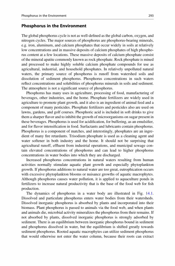
Phosphorus in the Environment

The global phosphorus cycle is not as well-defined as the global carbon, oxygen, andnitrogen cycles. The major sources of phosphorus are phosphorus-bearing minerals,e.g. iron, aluminum, and calcium phosphates that occur widely in soils at relativelylow concentrations and in massive deposits of calcium phosphates of high phospho-rus content at a few locations. These massive deposits of calcium phosphate consistof the mineral apatite commonly known as rock phosphate. Rock phosphate is minedand processed to make highly soluble calcium phosphate compounds for use asagricultural, industrial, and household phosphates. In relatively unpolluted naturalwaters, the primary source of phosphorus is runoff from watershed soils anddissolution of sediment phosphorus. Phosphorus concentrations in such watersreflect concentrations and solubilities of phosphorus minerals in soils and sediment.The atmosphere is not a significant source of phosphorus.

Phosphorus has many uses in agriculture, processing of food, manufacturing ofbeverages, other industries, and the home. Phosphate fertilizers are widely used inagriculture to promote plant growth, and it also is an ingredient of animal feed and acomponent of many pesticides. Phosphate fertilizers and pesticides also are used onlawns, gardens, and golf courses. Phosphoric acid is included in soft drinks to givethem a sharper flavor and to inhibit the growth of microorganisms on sugar present inthese beverages. Phosphorus is used for acidification, for buffering, as an emulsifier,and for flavor intensification in food. Surfactants and lubricants contain phosphorus.Phosphorus is a component of matches, and interestingly, phosphates are an ingre-dient of many fire retardants. Trisodium phosphate is used as a cleaning agent andwater softener in both industry and the home. It should not be surprising thatagricultural runoff, effluent from industrial operations, and municipal sewage con-tain elevated concentrations of phosphorus and can lead to higher phosphorusconcentrations in water bodies into which they are discharged.

Increased phosphorus concentrations in natural waters resulting from humanactivities normally stimulate aquatic plant growth and especially phytoplanktongrowth. If phosphorus additions to natural water are too great, eutrophication occurswith excessive phytoplankton blooms or nuisance growths of aquatic macrophytes.Although phosphorus causes water pollution, it is applied to aquaculture ponds infertilizers to increase natural productivity that is the base of the food web for fishproduction.

The dynamics of phosphorus in a water body are illustrated in Fig. 14.1.Dissolved and particulate phosphorus enters water bodies from their watersheds.Dissolved inorganic phosphorus is absorbed by plants and incorporated into theirbiomass. Plant phosphorus is passed to animals via the food web, and when plantsand animals die, microbial activity mineralizes the phosphorus from their remains. Ifnot absorbed by plants, dissolved inorganic phosphorus is strongly adsorbed bysediment. There is an equilibrium between inorganic phosphorus bound in sedimentand phosphorus dissolved in water, but the equilibrium is shifted greatly towardssediment phosphorus. Rooted aquatic macrophytes can utilize sediment phosphorusthat would otherwise not enter the water column, because their roots can extract

Phosphorus in the Environment 293

phosphorus dissolved in sediment pore water. Phosphorus is lost from aquaticecosystems in outflowing water, intentional withdrawal of water for human use,and harvest of aquatic products. The sediments of water bodies tend to be phospho-rus sinks, and they tend to increase in phosphorus content over time. In unpollutednatural waters, there is an equilibrium among phosphorus inputs, outputs, andstorage, and additions of phosphorus through water pollution disrupt thisequilibrium.

Phosphorus Chemistry

Phosphorus interactions in water bodies (Fig. 14.1) involve biological processes, butthe concentrations of phosphorus in water are controlled by chemical principles ofdissolution, equilibrium, precipitation, and adsorption. These processes influence themass balance of phosphorus which consists of inflow, outflow, storage, and concen-tration in the water. It is necessary to explain the basic features of phosphoruschemistry in water bodies.

Dissociation of Orthophosphoric Acid

Inorganic phosphorus in soils, sediment, and water usually occurs as an ionizationproduct of orthophosphoric acid (H3PO4) that dissociates as follows:

H3PO4 ¼ Hþ þ H2PO�4 K1 ¼ 10�2:13 ð14:1Þ

H2PO�4 ¼ Hþ þ HPO2�

4 K2 ¼ 10�7:21 ð14:2Þ

Fig. 14.1 A qualitative model of the phosphorus cycle in an aquatic ecosystem

294 14 Phosphorus

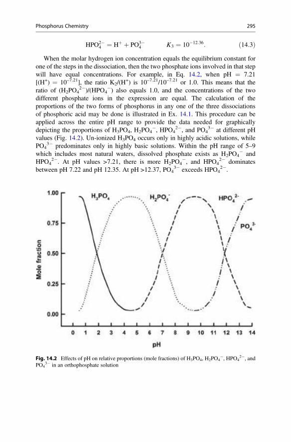
HPO2�4 ¼ Hþ þ PO3�

4 K3 ¼ 10�12:36: ð14:3ÞWhen the molar hydrogen ion concentration equals the equilibrium constant for

one of the steps in the dissociation, then the two phosphate ions involved in that stepwill have equal concentrations. For example, in Eq. 14.2, when pH ¼ 7.21[(H+) ¼ 10–7.21], the ratio K2/(H

+) is 10–7.21/10–7.21 or 1.0. This means that theratio of (H2PO4

2�)/(HPO4�) also equals 1.0, and the concentrations of the two

different phosphate ions in the expression are equal. The calculation of theproportions of the two forms of phosphorus in any one of the three dissociationsof phosphoric acid may be done is illustrated in Ex. 14.1. This procedure can beapplied across the entire pH range to provide the data needed for graphicallydepicting the proportions of H3PO4, H2PO4

�, HPO42�, and PO4

3� at different pHvalues (Fig. 14.2). Un-ionized H3PO4 occurs only in highly acidic solutions, whilePO4

3� predominates only in highly basic solutions. Within the pH range of 5–9which includes most natural waters, dissolved phosphate exists as H2PO4

� andHPO4

2�. At pH values >7.21, there is more H2PO4�, and HPO4

2� dominatesbetween pH 7.22 and pH 12.35. At pH >12.37, PO4

3� exceeds HPO42�.

Fig. 14.2 Effects of pH on relative proportions (mole fractions) of H3PO4, H2PO4�, HPO4

2�, andPO4

3� in an orthophosphate solution

Phosphorus Chemistry 295

Ex. 14.1 The percentages of H2PO�4 and HPO2�

4 at pH 6 will be estimated.Solution:The mass action expression for Eq. 14.2 allows an expression for the ratio of

HPO2�4 to H2PO�

4 ,

Hþð Þ HPO2�4

� �

H2PO�4

� � ¼ 10�7:21

HPO2�4

� �

H2PO�4

� � ¼ 10�7:21

Hþð Þ

and

HPO2�4

� �

H2PO�4

� � ¼ 10�7:21

10�6 ¼ 10�1:21 ¼ 0:062:

There will be the equivalent of 1 part of H2PO4� and 0.062 part of HPO4

2� at pH6. The percentage of HPO4

2� will be

0:0621þ 0:062

� 100 ¼ 5:83%

and 100%� 5:83% ¼ 94:17% H2PO�4 :

Polyphosphate compounds have a greater proportion of phosphorus than found inorthophosphate. For example, the orthophosphate ion PO4

3� is 25% phosphorus, butpolyphosphate ions such as PO3

�, P2O74�, and P4O13

6� contain 40%, 36%, and38% phosphorus, respectively. The parent form of polyphosphate can be considereda compound such as sodium hexametaphosphate [(NaPO3)6] or polyphosphoric acid(H6P4O13). Polyphosphates have many industrial uses and they may be used asfertilizer, and as a result be contained in effluents. Polyphosphates also occurnaturally in certain bacteria, plants, and lower animals (Harold 1966). Whenintroduced into water, polyphosphate soon hydrolyzes to orthophosphate asillustrated below for a single unit of NaPO3 from (NaPO3)6:

NaPO3 þ H2O ! Naþ þ H2PO�4 : ð14:4Þ

Phosphorus-Sediment Reactions

Inorganic phosphorus reacts with iron and aluminum in acidic sediments or waters toform slightly soluble compounds. The aluminum and iron phosphate compoundsvariscite (AlPO4�2H2O) and strengite (FePO4�2H2O) will be used as representativecompounds. The dissolution of these compounds is pH-dependent

296 14 Phosphorus

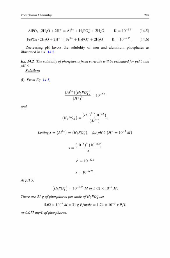
AlPO4 � 2H2Oþ 2Hþ ¼ Al3þ þ H2PO�4 þ 2H2O K ¼ 10�2:5 ð14:5Þ

FePO4 � 2H2Oþ 2Hþ ¼ Fe3þ þ H2PO�4 þ 2H2O K ¼ 10�6:85: ð14:6Þ

Decreasing pH favors the solubility of iron and aluminum phosphates asillustrated in Ex. 14.2.

Ex. 14.2 The solubility of phosphorus from variscite will be estimated for pH 5 andpH 6.

Solution:

(i) From Eq. 14.5,

Al3þ� �

H2PO�4

� �

Hþð Þ2¼ 10�2:5

and

H2PO�4

� � ¼ Hþð Þ2 10�2:5� �

Al3þ� � :

Letting x ¼ Al3þ� � ¼ H2PO

�4

� �, for pH 5 Hþ ¼ 10�5 M

� �

x ¼ 10�5� �2

10�2:5� �

x

x2 ¼ 10�12:5

x ¼ 10�6:25:

At pH 5,

H2PO�4

� � ¼ 10�6:25 M or 5:62� 10�7 M:

There are 31 g of phosphorus per mole of H2PO�4 , so

5:62� 10�7 M � 31 g P=mole ¼ 1:74� 10�5 g P=L

or 0.017 mg/L of phosphorus.


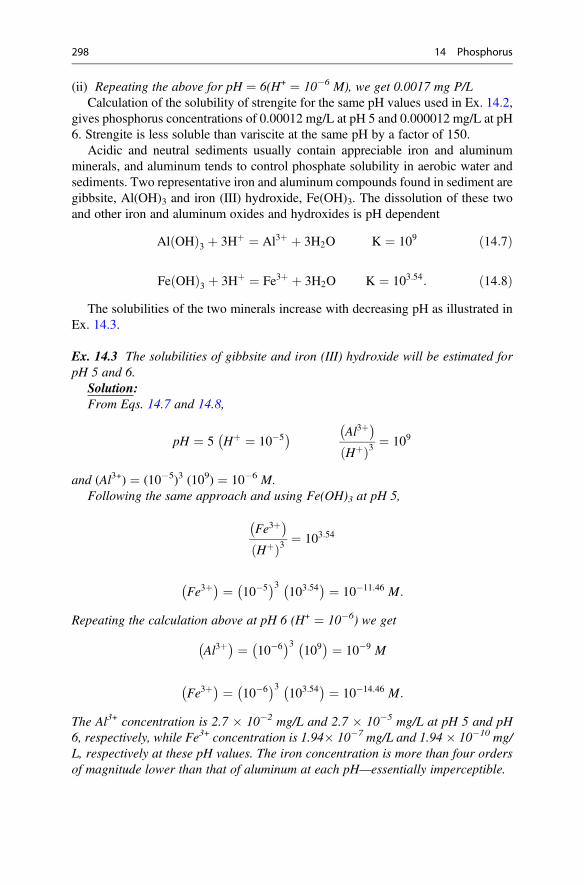
(ii) Repeating the above for pH ¼ 6(H+ ¼ 10�6 M), we get 0.0017 mg P/LCalculation of the solubility of strengite for the same pH values used in Ex. 14.2,

gives phosphorus concentrations of 0.00012 mg/L at pH 5 and 0.000012 mg/L at pH6. Strengite is less soluble than variscite at the same pH by a factor of 150.

Acidic and neutral sediments usually contain appreciable iron and aluminumminerals, and aluminum tends to control phosphate solubility in aerobic water andsediments. Two representative iron and aluminum compounds found in sediment aregibbsite, Al(OH)3 and iron (III) hydroxide, Fe(OH)3. The dissolution of these twoand other iron and aluminum oxides and hydroxides is pH dependent

Al OHð Þ3 þ 3Hþ ¼ Al3þ þ 3H2O K ¼ 109 ð14:7Þ

Fe OHð Þ3 þ 3Hþ ¼ Fe3þ þ 3H2O K ¼ 103:54: ð14:8ÞThe solubilities of the two minerals increase with decreasing pH as illustrated in

Ex. 14.3.

Ex. 14.3 The solubilities of gibbsite and iron (III) hydroxide will be estimated forpH 5 and 6.

Solution:From Eqs. 14.7 and 14.8,

pH ¼ 5 Hþ ¼ 10�5� � Al3þ

� �

Hþð Þ3¼ 109

and (Al3+) ¼ (10�5)3 (109) ¼ 10�6 M.Following the same approach and using Fe(OH)3 at pH 5,

Fe3þ� �

Hþð Þ3¼ 103:54

Fe3þ� � ¼ 10�5

� �3103:54� � ¼ 10�11:46 M:

Repeating the calculation above at pH 6 (H+ ¼ 10�6) we get

Al3þ� � ¼ 10�6

� �3109� � ¼ 10�9 M

Fe3þ� � ¼ 10�6

� �3103:54� � ¼ 10�14:46 M:

The Al3+ concentration is 2.7 � 10�2 mg/L and 2.7 � 10�5 mg/L at pH 5 and pH6, respectively, while Fe3+ concentration is 1.94� 10�7 mg/L and 1.94 � 10�10 mg/L, respectively at these pH values. The iron concentration is more than four ordersof magnitude lower than that of aluminum at each pH—essentially imperceptible.

298 14 Phosphorus

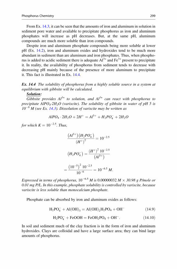
From Ex. 14.3, it can be seen that the amounts of iron and aluminum in solution insediment pore water and available to precipitate phosphorus as iron and aluminumphosphates will increase as pH decreases. But, at the same pH, aluminumcompounds are much more soluble than iron compounds.

Despite iron and aluminum phosphate compounds being more soluble at lowerpH (Ex. 14.2), iron and aluminum oxides and hydroxides tend to be much moreabundant in sediment than are aluminum and iron phosphates. Thus, when phospho-rus is added to acidic sediment there is adequate Al3+ and Fe3+ present to precipitateit. In reality, the availability of phosphorus from sediment tends to decrease withdecreasing pH mainly because of the presence of more aluminum to precipitateit. This fact is illustrated in Ex. 14.4.

Ex. 14.4 The solubility of phosphorus from a highly soluble source in a system atequilibrium with gibbsite will be calculated.

Solution:Gibbsite provides Al3+ to solution, and Al3+ can react with phosphorus to

precipitate AlPO4�2H2O (variscite). The solubility of gibbsite in water of pH 5 is10�6 M (see Ex. 14.3). Dissolution of variscite may be written as

AlPO4 � 2H2Oþ 2Hþ ¼ Al3þ þ H2PO�4 þ 2H2O

for which K ¼ 10�2.5. Thus,

Al3þ� �

H2PO�4

� �

Hþð Þ2¼ 10�2:5

H2PO�4

� � ¼ Hþð Þ2 10�2:5

Al3þ� �

¼ 10�5� �2

10�2:5

10�6 ¼ 10�6:5 M:

Expressed in terms of phosphorus, 10�6.5 M is 0.00000032 M � 30.98 g P/mole or0.01 mg P/L. In this example, phosphate solubility is controlled by variscite, becausevariscite is less soluble than monocalcium phosphate.

Phosphate can be absorbed by iron and aluminum oxides as follows:

H2PO�4 þ Al OHð Þ3 ¼ Al OHð Þ2H2PO4 þ OH� ð14:9Þ

H2PO�4 þ FeOOH ¼ FeOH2PO4 þ OH�: ð14:10Þ

In soil and sediment much of the clay fraction is in the form of iron and aluminumhydroxides. Clays are colloidal and have a large surface area; they can bind largeamounts of phosphorus.


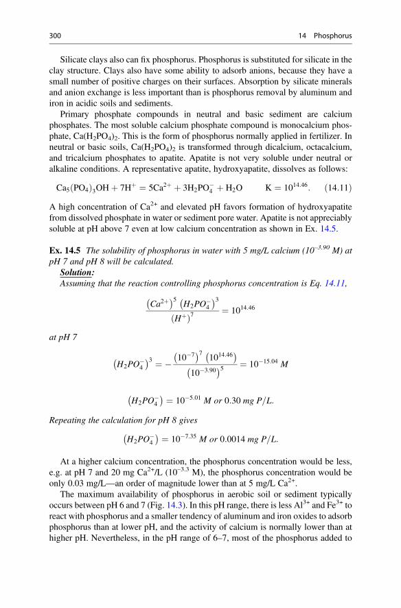
Silicate clays also can fix phosphorus. Phosphorus is substituted for silicate in theclay structure. Clays also have some ability to adsorb anions, because they have asmall number of positive charges on their surfaces. Absorption by silicate mineralsand anion exchange is less important than is phosphorus removal by aluminum andiron in acidic soils and sediments.

Primary phosphate compounds in neutral and basic sediment are calciumphosphates. The most soluble calcium phosphate compound is monocalcium phos-phate, Ca(H2PO4)2. This is the form of phosphorus normally applied in fertilizer. Inneutral or basic soils, Ca(H2PO4)2 is transformed through dicalcium, octacalcium,and tricalcium phosphates to apatite. Apatite is not very soluble under neutral oralkaline conditions. A representative apatite, hydroxyapatite, dissolves as follows:

Ca5 PO4ð Þ3OHþ 7Hþ ¼ 5Ca2þ þ 3H2PO�4 þ H2O K ¼ 1014:46: ð14:11Þ

A high concentration of Ca2+ and elevated pH favors formation of hydroxyapatitefrom dissolved phosphate in water or sediment pore water. Apatite is not appreciablysoluble at pH above 7 even at low calcium concentration as shown in Ex. 14.5.

Ex. 14.5 The solubility of phosphorus in water with 5 mg/L calcium (10–3.90 M) atpH 7 and pH 8 will be calculated.

Solution:Assuming that the reaction controlling phosphorus concentration is Eq. 14.11,

Ca2þ� �5

H2PO�4

� �3

Hþð Þ7 ¼ 1014:46

at pH 7

H2PO�4

� �3 ¼ � 10�7� �7

1014:46� �

10�3:90� �5 ¼ 10�15:04 M

H2PO�4

� � ¼ 10�5:01 M or 0:30 mg P=L:

Repeating the calculation for pH 8 gives

H2PO�4

� � ¼ 10�7:35 M or 0:0014 mg P=L:

At a higher calcium concentration, the phosphorus concentration would be less,e.g. at pH 7 and 20 mg Ca2+/L (10–3.3 M), the phosphorus concentration would beonly 0.03 mg/L—an order of magnitude lower than at 5 mg/L Ca2+.

The maximum availability of phosphorus in aerobic soil or sediment typicallyoccurs between pH 6 and 7 (Fig. 14.3). In this pH range, there is less Al3+ and Fe3+ toreact with phosphorus and a smaller tendency of aluminum and iron oxides to adsorbphosphorus than at lower pH, and the activity of calcium is normally lower than athigher pH. Nevertheless, in the pH range of 6–7, most of the phosphorus added to

300 14 Phosphorus

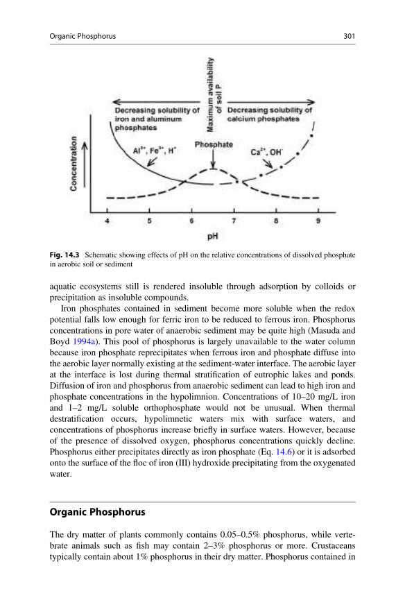
aquatic ecosystems still is rendered insoluble through adsorption by colloids orprecipitation as insoluble compounds.

Iron phosphates contained in sediment become more soluble when the redoxpotential falls low enough for ferric iron to be reduced to ferrous iron. Phosphorusconcentrations in pore water of anaerobic sediment may be quite high (Masuda andBoyd 1994a). This pool of phosphorus is largely unavailable to the water columnbecause iron phosphate reprecipitates when ferrous iron and phosphate diffuse intothe aerobic layer normally existing at the sediment-water interface. The aerobic layerat the interface is lost during thermal stratification of eutrophic lakes and ponds.Diffusion of iron and phosphorus from anaerobic sediment can lead to high iron andphosphate concentrations in the hypolimnion. Concentrations of 10–20 mg/L ironand 1–2 mg/L soluble orthophosphate would not be unusual. When thermaldestratification occurs, hypolimnetic waters mix with surface waters, andconcentrations of phosphorus increase briefly in surface waters. However, becauseof the presence of dissolved oxygen, phosphorus concentrations quickly decline.Phosphorus either precipitates directly as iron phosphate (Eq. 14.6) or it is adsorbedonto the surface of the floc of iron (III) hydroxide precipitating from the oxygenatedwater.

Organic Phosphorus

The dry matter of plants commonly contains 0.05–0.5% phosphorus, while verte-brate animals such as fish may contain 2–3% phosphorus or more. Crustaceanstypically contain about 1% phosphorus in their dry matter. Phosphorus contained in

Fig. 14.3 Schematic showing effects of pH on the relative concentrations of dissolved phosphatein aerobic soil or sediment

Organic Phosphorus 301

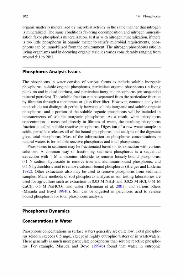
organic matter is mineralized by microbial activity in the same manner that nitrogenis mineralized. The same conditions favoring decomposition and nitrogen minerali-zation favor phosphorus mineralization. Just as with nitrogen mineralization, if thereis too little phosphorus in organic matter to satisfy microbial requirements, phos-phorus can be immobilized from the environment. The nitrogen:phosphorus ratio inliving organisms and in decaying organic residues varies considerably ranging fromaround 5:1 to 20:1.

Phosphorus Analysis Issues

The phosphorus in water consists of various forms to include soluble inorganicphosphorus, soluble organic phosphorus, particulate organic phosphorus (in livingplankton and in dead detritus), and particulate inorganic phosphorus (on suspendedmineral particles). The soluble fraction can be separated from the particulate fractionby filtration through a membrane or glass fiber filter. However, common analyticalmethods do not distinguish perfectly between soluble inorganic and soluble organicphosphorus, and a portion of the soluble organic phosphorus will be included inmeasurements of soluble inorganic phosphorus. As a result, when phosphorusconcentration is measured directly in filtrates of water, the resulting phosphorusfraction is called soluble reactive phosphorus. Digestion of a raw water sample inacidic persulfate releases all of the bound phosphorus, and analysis of the digestategives total phosphorus. Most of the information on phosphorus concentrations innatural waters is for soluble reactive phosphorus and total phosphorus.

Phosphorus in sediment may be fractionated based on its extraction with varioussolutions. A common way of fractioning sediment phosphorus is a sequentialextraction with 1 M ammonium chloride to remove loosely-bound phosphorus,0.1 N sodium hydroxide to remove iron and aluminum-bound phosphorus, and0.5 N hydrochloric acid to remove calcium-bound phosphorus (Hieltjes and Liklema1982). Other extractants also may be used to remove phosphorus from sedimentsamples. Many methods of soil phosphorus analysis in soil testing laboratories areused for agriculture such as extraction in 0.03 M NH4F and 0.025 M HCl, 0.61 MCaCl2, 0.5 M NaHCO3, and water (Kleinman et al. 2001), and various others(Masuda and Boyd 1994b). Soil can be digested in perchloric acid to releasebound phosphorus for total phosphorus analysis.

Phosphorus Dynamics

Concentrations in Water

Phosphorus concentrations in surface waters generally are quite low. Total phospho-rus seldom exceeds 0.5 mg/L except in highly eutrophic waters or in wastewaters.There generally is much more particulate phosphorus than soluble reactive phospho-rus. For example, Masuda and Boyd (1994b) found that water in eutrophic

302 14 Phosphorus

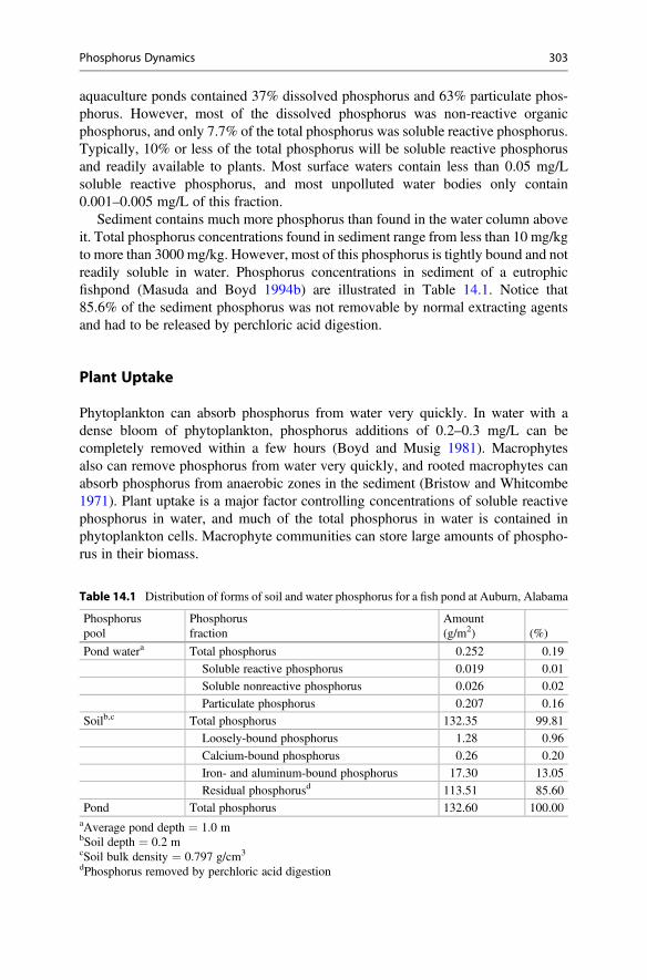
aquaculture ponds contained 37% dissolved phosphorus and 63% particulate phos-phorus. However, most of the dissolved phosphorus was non-reactive organicphosphorus, and only 7.7% of the total phosphorus was soluble reactive phosphorus.Typically, 10% or less of the total phosphorus will be soluble reactive phosphorusand readily available to plants. Most surface waters contain less than 0.05 mg/Lsoluble reactive phosphorus, and most unpolluted water bodies only contain0.001–0.005 mg/L of this fraction.

Sediment contains much more phosphorus than found in the water column aboveit. Total phosphorus concentrations found in sediment range from less than 10 mg/kgto more than 3000 mg/kg. However, most of this phosphorus is tightly bound and notreadily soluble in water. Phosphorus concentrations in sediment of a eutrophicfishpond (Masuda and Boyd 1994b) are illustrated in Table 14.1. Notice that85.6% of the sediment phosphorus was not removable by normal extracting agentsand had to be released by perchloric acid digestion.

Plant Uptake

Phytoplankton can absorb phosphorus from water very quickly. In water with adense bloom of phytoplankton, phosphorus additions of 0.2–0.3 mg/L can becompletely removed within a few hours (Boyd and Musig 1981). Macrophytesalso can remove phosphorus from water very quickly, and rooted macrophytes canabsorb phosphorus from anaerobic zones in the sediment (Bristow and Whitcombe1971). Plant uptake is a major factor controlling concentrations of soluble reactivephosphorus in water, and much of the total phosphorus in water is contained inphytoplankton cells. Macrophyte communities can store large amounts of phospho-rus in their biomass.

Table 14.1 Distribution of forms of soil and water phosphorus for a fish pond at Auburn, Alabama

Phosphoruspool

Phosphorusfraction

Amount(g/m2) (%)

Pond watera Total phosphorus 0.252 0.19

Soluble reactive phosphorus 0.019 0.01

Soluble nonreactive phosphorus 0.026 0.02

Particulate phosphorus 0.207 0.16

Soilb,c Total phosphorus 132.35 99.81

Loosely-bound phosphorus 1.28 0.96

Calcium-bound phosphorus 0.26 0.20

Iron- and aluminum-bound phosphorus 17.30 13.05

Residual phosphorusd 113.51 85.60

Pond Total phosphorus 132.60 100.00aAverage pond depth ¼ 1.0 mbSoil depth ¼ 0.2 mcSoil bulk density ¼ 0.797 g/cm3

dPhosphorus removed by perchloric acid digestion

Phosphorus Dynamics 303

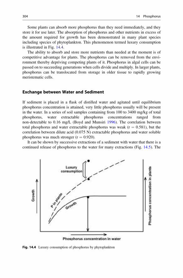
Some plants can absorb more phosphorus than they need immediately, and theystore it for use later. The absorption of phosphorus and other nutrients in excess ofthe amount required for growth has been demonstrated in many plant speciesincluding species of phytoplankton. This phenomenon termed luxury consumptionis illustrated in Fig. 14.4.

The ability to absorb and store more nutrients than needed at the moment is ofcompetitive advantage for plants. The phosphorus can be removed from the envi-ronment thereby depriving competing plants of it. Phosphorus in algal cells can bepassed on to succeeding generations when cells divide and multiply. In larger plants,phosphorus can be translocated from storage in older tissue to rapidly growingmeristematic cells.

Exchange between Water and Sediment

If sediment is placed in a flask of distilled water and agitated until equilibriumphosphorus concentration is attained, very little phosphorus usually will be presentin the water. In a series of soil samples containing from 100 to 3400 mg/kg of totalphosphorus, water extractable phosphorus concentrations ranged fromnon-detectable to 0.16 mg/L (Boyd and Munsiri 1996). The correlation betweentotal phosphorus and water extractable phosphorus was weak (r ¼ 0.581), but thecorrelation between dilute acid (0.075 N) extractable phosphorus and water solublephosphorus was much stronger (r ¼ 0.920).

It can be shown by successive extractions of a sediment with water that there is acontinued release of phosphorus to the water for many extractions (Fig. 14.5). The

Fig. 14.4 Luxury consumption of phosphorus by phytoplankton

304 14 Phosphorus

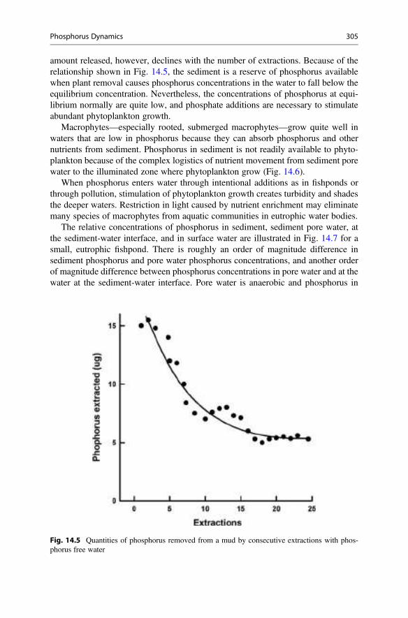
amount released, however, declines with the number of extractions. Because of therelationship shown in Fig. 14.5, the sediment is a reserve of phosphorus availablewhen plant removal causes phosphorus concentrations in the water to fall below theequilibrium concentration. Nevertheless, the concentrations of phosphorus at equi-librium normally are quite low, and phosphate additions are necessary to stimulateabundant phytoplankton growth.

Macrophytes—especially rooted, submerged macrophytes—grow quite well inwaters that are low in phosphorus because they can absorb phosphorus and othernutrients from sediment. Phosphorus in sediment is not readily available to phyto-plankton because of the complex logistics of nutrient movement from sediment porewater to the illuminated zone where phytoplankton grow (Fig. 14.6).

When phosphorus enters water through intentional additions as in fishponds orthrough pollution, stimulation of phytoplankton growth creates turbidity and shadesthe deeper waters. Restriction in light caused by nutrient enrichment may eliminatemany species of macrophytes from aquatic communities in eutrophic water bodies.

The relative concentrations of phosphorus in sediment, sediment pore water, atthe sediment-water interface, and in surface water are illustrated in Fig. 14.7 for asmall, eutrophic fishpond. There is roughly an order of magnitude difference insediment phosphorus and pore water phosphorus concentrations, and another orderof magnitude difference between phosphorus concentrations in pore water and at thewater at the sediment-water interface. Pore water is anaerobic and phosphorus in

Fig. 14.5 Quantities of phosphorus removed from a mud by consecutive extractions with phos-phorus free water


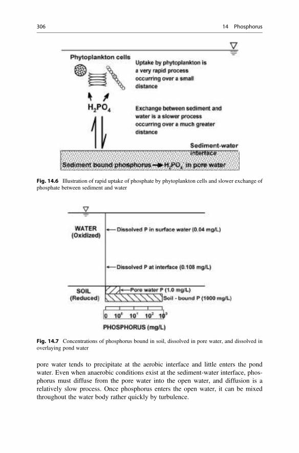
pore water tends to precipitate at the aerobic interface and little enters the pondwater. Even when anaerobic conditions exist at the sediment-water interface, phos-phorus must diffuse from the pore water into the open water, and diffusion is arelatively slow process. Once phosphorus enters the open water, it can be mixedthroughout the water body rather quickly by turbulence.

Fig. 14.6 Illustration of rapid uptake of phosphate by phytoplankton cells and slower exchange ofphosphate between sediment and water

Fig. 14.7 Concentrations of phosphorus bound in soil, dissolved in pore water, and dissolved inoverlaying pond water

306 14 Phosphorus

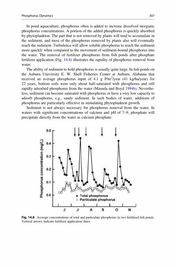
In pond aquaculture, phosphorus often is added to increase dissolved inorganicphosphorus concentrations. A portion of the added phosphorus is quickly absorbedby phytoplankton. The part that is not removed by plants will tend to accumulate inthe sediment, and most of the phosphorus removed by plants also will eventuallyreach the sediment. Turbulence will allow soluble phosphorus to reach the sedimentmore quickly when compared to the movement of sediment-bound phosphorus intothe water. The removal of fertilizer phosphorus from fish ponds after phosphatefertilizer application (Fig. 14.8) illustrates the rapidity of phosphorus removal fromwater.

The ability of sediment to hold phosphorus is usually quite large. In fish ponds onthe Auburn University E. W. Shell Fisheries Center at Auburn, Alabama thatreceived an average phosphorus input of 4.1 g P/m2/year (41 kg/ha/year) for22 years, bottom soils were only about half-saturated with phosphorus and stillrapidly adsorbed phosphorus from the water (Masuda and Boyd 1994b). Neverthe-less, sediment can become saturated with phosphorus or have a very low capacity toadsorb phosphorus, e.g., sandy sediment. In such bodies of water, additions ofphosphorus are particularly effective in stimulating phytoplankton growth.

Sediment is not always necessary for phosphorus removal from the water. Inwaters with significant concentrations of calcium and pH of 7–9, phosphate willprecipitate directly from the water as calcium phosphate.

Fig. 14.8 Average concentrations of total and particulate phosphorus in two fertilized fish ponds.Vertical arrows indicate fertilizer application dates


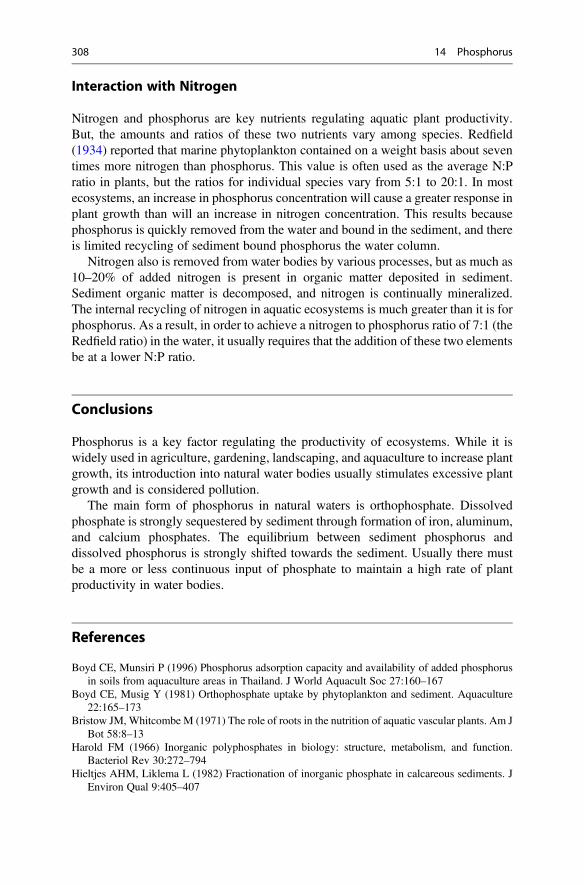
Interaction with Nitrogen

Nitrogen and phosphorus are key nutrients regulating aquatic plant productivity.But, the amounts and ratios of these two nutrients vary among species. Redfield(1934) reported that marine phytoplankton contained on a weight basis about seventimes more nitrogen than phosphorus. This value is often used as the average N:Pratio in plants, but the ratios for individual species vary from 5:1 to 20:1. In mostecosystems, an increase in phosphorus concentration will cause a greater response inplant growth than will an increase in nitrogen concentration. This results becausephosphorus is quickly removed from the water and bound in the sediment, and thereis limited recycling of sediment bound phosphorus the water column.

Nitrogen also is removed from water bodies by various processes, but as much as10–20% of added nitrogen is present in organic matter deposited in sediment.Sediment organic matter is decomposed, and nitrogen is continually mineralized.The internal recycling of nitrogen in aquatic ecosystems is much greater than it is forphosphorus. As a result, in order to achieve a nitrogen to phosphorus ratio of 7:1 (theRedfield ratio) in the water, it usually requires that the addition of these two elementsbe at a lower N:P ratio.

Conclusions

Phosphorus is a key factor regulating the productivity of ecosystems. While it iswidely used in agriculture, gardening, landscaping, and aquaculture to increase plantgrowth, its introduction into natural water bodies usually stimulates excessive plantgrowth and is considered pollution.

The main form of phosphorus in natural waters is orthophosphate. Dissolvedphosphate is strongly sequestered by sediment through formation of iron, aluminum,and calcium phosphates. The equilibrium between sediment phosphorus anddissolved phosphorus is strongly shifted towards the sediment. Usually there mustbe a more or less continuous input of phosphate to maintain a high rate of plantproductivity in water bodies.

References

Boyd CE, Munsiri P (1996) Phosphorus adsorption capacity and availability of added phosphorusin soils from aquaculture areas in Thailand. J World Aquacult Soc 27:160–167

Boyd CE, Musig Y (1981) Orthophosphate uptake by phytoplankton and sediment. Aquaculture22:165–173

Bristow JM, Whitcombe M (1971) The role of roots in the nutrition of aquatic vascular plants. Am JBot 58:8–13

Harold FM (1966) Inorganic polyphosphates in biology: structure, metabolism, and function.Bacteriol Rev 30:272–794

Hieltjes AHM, Liklema L (1982) Fractionation of inorganic phosphate in calcareous sediments. JEnviron Qual 9:405–407

308 14 Phosphorus

Kleinman PJA, Sharpley AN, Gartley K, Jarrell WM, Kuo S, Menon RG, Myers R, Reddy KR,Skogley EO (2001) Interlaboratory comparisons of soil phosphorus extracted by various soil testmethods. Commun Soil Sci Plant Anal 32:2325–2345

Masuda K, Boyd CE (1994a) Chemistry of sediment pore water in aquaculture ponds built onclayey, Ultisols at Auburn, Alabama. J World Aquacult Soc 25:396–404

Masuda K, Boyd CE (1994b) Phosphorus fractions in soil and water of aquaculture ponds built onclayey, Ultisols at Auburn, Alabama. J World Aquacult Soc 25:379–395

Redfield AC (1934) On the proportions of organic deviations in sea water and their relation to thecomposition of plankton. In: Daniel RJ (ed) James johnstone memorial volume. UniversityPress of Liverpool, Liverpool

References 309

Eutrophication 15

AbstractThe term eutrophication refers to a water body changing over time from nutrient-poor to nutrient-rich status. More nutrients cause increased aquatic plant growththat negatively influences water quality and especially dissolved oxygen avail-ability. The result is a decrease in species diversity and an increase in the biomassof a few and usually less desirable species. The changes caused by eutrophicationoften are gradual and not noticed until there is a sudden shift (tipping point) to amore eutrophic status. The two nutrients responsible for eutrophication arenitrogen and phosphorus contained in nearly all effluents. Much effort is devotedto removing these nutrients by water treatment and watershed managementpractices. Sometimes, chemical coagulants may be added to water bodies toprecipitate phosphorus, and chemicals such as copper sulfate applied as algicides.Although most popular discussions of eutrophication apply to lakes, streams alsomay suffer eutrophication.

Introduction

Kociolek and Stoermer (2009) state that oligotrophy means poor food or low level ofnutrients as compared to eutrophy which suggests good food or high level ofnutrients. Water bodies vary in availability of nutrients, and there exists a continuumof water bodies ranging from those that are very nutrient deficient to those withextremely abundant supplies of nutrients. This continuum extends fromultraoligotrophy through oligotrophy, mesotrophy (moderate food and nutrients),eutrophy, to ultraeutrophy. The earliest use of this continuum for categorizingnutrient states was probably about 1920, and it is still a fundamental concept ofecology and particularly in aquatic sciences. Oligotrophic water bodies with acidicwaters stained by high concentrations of dissolved humic substances are a specialcase known as dystrophy.


311


The addition of nutrients to oligotrophic water bodies from natural or anthropo-genic sources will make them more nutrient rich and less oligotrophic. While waterbodies may naturally become more eutrophic over time, in the past 100 years,nutrient pollution from anthropogenic sources has greatly increased nutrient avail-ability in many water bodies throughout the world. This has been a disturbingphenomenon, because it has encouraged plant growth (especially phytoplanktongrowth) in water bodies resulting in undesirable changes such as low dissolvedoxygen concentration and reduction in biodiversity. The artificial enrichment ofwater bodies with nutrients has become known as eutrophication or more preciselycultural eutrophication.

The word eutrophication is defined in the Merriam-Webster Dictionary as “theprocess by which a water body becomes enriched in dissolved nutrients (such asphosphates) that stimulate the growth of plant life usually resulting in the depletionof dissolved oxygen.” The term was said to have been first used with the abovemeaning in 1946 (https://www.merriam-webster.com/dictionary/eutrophication),but it has no doubt been used many millions of times since. The dictionary definitionabove refers only to phosphorus, but nitrogen is almost or equally as important ineutrophication as is phosphorus, and both are causes of eutrophication. The referenceto “usually resulting in depletion of dissolved oxygen” also is not exactly accurate.Many eutrophic water bodies simply have lower dissolved oxygen concentrationthan less eutrophic ones, but if the process of eutrophication is allowed to progress,dissolved oxygen depletion will eventually become a common phenomenon.

Eutrophication has already been discussed briefly in several chapters and espe-cially in the three preceding ones. Nevertheless, eutrophication is such a commonconcern in society and the focus of so many environmental protection efforts thatfurther discussion is desirable.

The Eutrophication Process

Eutrophication of water bodies occurs naturally because nutrients and sedimentaccumulate as the result of erosion on catchments. Sediment decreases the volumeof a water body, and as the volume becomes less, the store of nutrients in thesediment increases nutrient concentration in the water column. Sedimentation alsoresults in shallow edges where rooted aquatic plants can thrive. A water body fills inand becomes more nutrient enriched as it ages. The edges become shallowerallowing shrubs and trees to grow and over many years—usually centuries—thewater body may fill in completely and becomes terrestrial habitat.

Cultural eutrophication greatly accelerates natural eutrophication or aging ofwater bodies. Human activities, particularly agriculture and deforestation oncatchments expose the land surface allowing greater erosion and delivery ofsuspended solids to water bodies. These solids settle, and water bodies fill in muchfaster than through natural processes. Agricultural runoff contains nitrogen, phos-phorus, and other nutrients applied to crops as fertilizer. Runoff from suburbanlawns, parks, golf courses, and similar areas also contain nutrients from fertilizers

312 15 Eutrophication

https://www.merriam-webster.com/dictionary/eutrophication

and other sources. Municipalities and industries discharge effluents containingnutrients into water bodies, and septic tanks seep into ground water which mayenter water bodies. The overall effect is that anthropogenic activities on watershedscause water bodies to fill in faster with sediment and supply nutrients for abundantaquatic plant growth. Rooted aquatic plants fill the water column of shallow waterareas, floating aquatic plants may completely cover smaller water bodies, andphytoplankton may become extremely abundant in open water areas. The overabun-dance of vegetation completely changes the physical and chemical environment, andthere is a trend towards lower dissolved oxygen concentrations and even periods ofoxygen depletion. These changes lead to a decrease in biological diversity with theexclusion of many ecologically-sensitive species. Biomass will be greater in eutro-phic waters than in oligotrophic ones, but there will be fewer species and lessbiological stability in eutrophic waters. The phytoplankton community becomesdominated with blue-green algae, and fish communities decrease in species abun-dance with only a few coarse species dominating. Such water bodies often are said tobe dead, but this is by no means true. Eutrophic water bodies are very much alive, butthe life consists mainly of a few less desirable species and biodiversity and ecologi-cal stability decline. Eutrophic waters also are impaired for many human uses.

Nitrogen, Phosphorus, and Eutrophication

The trophic state of a water body can be established by several methods. Thetraditional opinion held that eutrophic lakes have hypolimnetic dissolved oxygendepletion during thermal stratification while oligotrophic ones do not. This is notalways a reliable indicator of eutrophication in shallow water bodies that do notstratify thermally, and it does not allow classification as to degree of oligotrophy oreutrophy. The modern way of classifying trophic status of water bodies relies onmeasurements of total nitrogen, total phosphorus, and chlorophyll a concentrations,primary productivity, abundance of blue-green algae, and Secchi disk visibility.Indices of trophic status based on a combination of the preceding factors alsoare used.

There is no general agreement on the concentration ranges of the variablesmentioned above that should be expected in water bodies of different trophic states.Water bodies vary in most chemical and physical features, and this variation mayaffect concentrations or levels of the indicator variables. Nevertheless, some typicalvalues of the key variables in oligotrophic, mesotrophic, and eutrophic water bodiesare presented (Table 15.1). Ultraoligotrophy and ultraeutrophy are not included inTable 15.1, but water bodies with extremely small or large values for the variablesmay be classified accordingly.

The author believes that there are three main factors affecting the concentrationsof nutrients necessary to initiate phytoplankton blooms. Turbidity interferes withlight penetration. In water bodies turbid with suspended clay particles or dissolvedhumic substances, high concentrations of nitrogen and phosphorus may not causephytoplankton blooms because of light limitation of photosynthesis. The hydraulic

Nitrogen, Phosphorus, and Eutrophication 313

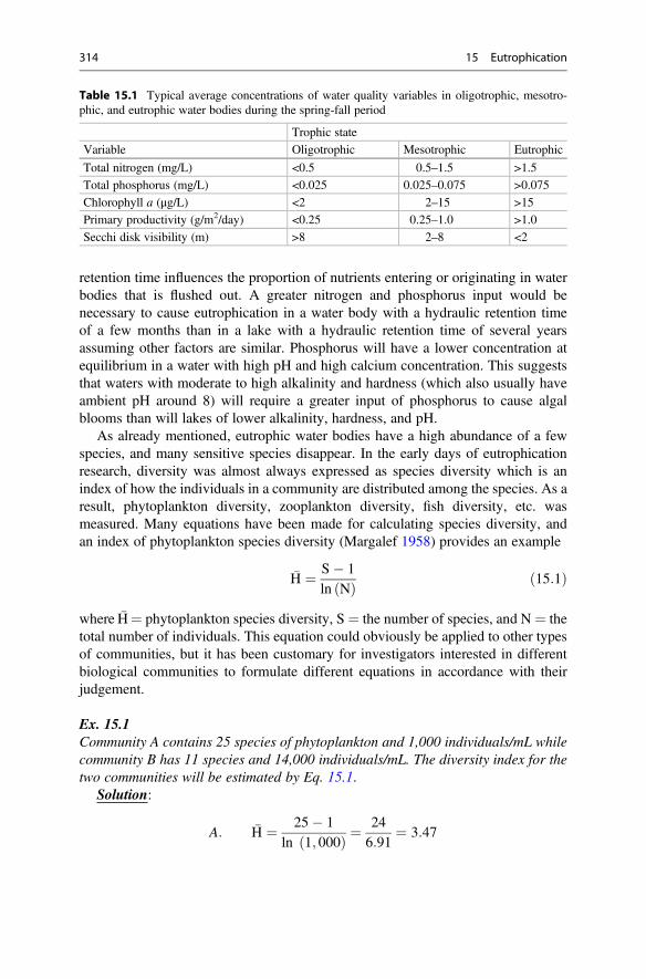
retention time influences the proportion of nutrients entering or originating in waterbodies that is flushed out. A greater nitrogen and phosphorus input would benecessary to cause eutrophication in a water body with a hydraulic retention timeof a few months than in a lake with a hydraulic retention time of several yearsassuming other factors are similar. Phosphorus will have a lower concentration atequilibrium in a water with high pH and high calcium concentration. This suggeststhat waters with moderate to high alkalinity and hardness (which also usually haveambient pH around 8) will require a greater input of phosphorus to cause algalblooms than will lakes of lower alkalinity, hardness, and pH.

As already mentioned, eutrophic water bodies have a high abundance of a fewspecies, and many sensitive species disappear. In the early days of eutrophicationresearch, diversity was almost always expressed as species diversity which is anindex of how the individuals in a community are distributed among the species. As aresult, phytoplankton diversity, zooplankton diversity, fish diversity, etc. wasmeasured. Many equations have been made for calculating species diversity, andan index of phytoplankton species diversity (Margalef 1958) provides an example

�H ¼ S� 1ln Nð Þ ð15:1Þ

where �H¼ phytoplankton species diversity, S ¼ the number of species, and N ¼ thetotal number of individuals. This equation could obviously be applied to other typesof communities, but it has been customary for investigators interested in differentbiological communities to formulate different equations in accordance with theirjudgement.

Ex. 15.1Community A contains 25 species of phytoplankton and 1,000 individuals/mL whilecommunity B has 11 species and 14,000 individuals/mL. The diversity index for thetwo communities will be estimated by Eq. 15.1.

Solution:

A: �H ¼ 25� 1ln 1; 000ð Þ ¼

246:91

¼ 3:47

Table 15.1 Typical average concentrations of water quality variables in oligotrophic, mesotro-phic, and eutrophic water bodies during the spring-fall period

Trophic state

Variable Oligotrophic Mesotrophic Eutrophic

Total nitrogen (mg/L) <0.5 0.5–1.5 >1.5

Total phosphorus (mg/L) <0.025 0.025–0.075 >0.075

Chlorophyll a (μg/L) <2 2–15 >15

Primary productivity (g/m2/day) <0.25 0.25–1.0 >1.0

Secchi disk visibility (m) >8 2–8 <2


B: �H ¼ 11� 1ln 14; 000ð Þ ¼

109:55

¼ 1:05:

A greater value of �H implies a higher biodiversity, i.e., community A has a greaterphytoplankton species diversity than does community B.

A community with more species relative to the total number of individuals hashigher diversity than a community with fewer species relative to the number ofindividuals. As a rule, the greater the species diversity, the more stable an ecosystemis considered to be (Odum 1971). The logic for this supposition is that if a speciesdisappears from a diverse community, there will be a greater likelihood that anotherspecies can fulfill the function of the species that disappeared than there would be ina less diverse community. Eutrophic aquatic ecosystems tend to be less stable thanoligotrophic ones. This lack of stability may be reflected in sudden shifts in theabundance of species and also in sudden changes in dissolved oxygen concentrationsand other water quality variables.

The modern concept of diversity has been expanded to include the diversity ofecosystems, communities, and habitats. Ecosystems have unique geological,edaphic, hydrologic, and climatic regimes that affect the types and abundance ofspecies living in them. An aquatic ecosystem is much different from a terrestrialecosystem, but a nutrient-poor aquatic ecosystem also differs greatly from a nutrient-rich one. Moreover, the species in an ecosystem all have genetic diversity, and theinteraction of ecosystem diversity and genetic diversity results in gradual changes inthe characteristics of organisms over time. The new concept of biodiversity is sobroad that it is almost impossible to find a suitable, single index of biodiversity. As aresult, it is still popular to enumerate species and count the number of individuals ofeach species in samples of the major types of communities as a way of assessing thebiodiversity status.

Most unpolluted water bodies typically contain no more than 0.05 mg/L of totalphosphorus and 0.75 mg/L of total nitrogen. An increase in the inputs of nitrogenand phosphorus may or may not cause an algal bloom to develop and the visibility ina lake to decrease. A water body is able to assimilate a certain quantity of nutrientswith relative little change in primary productivity and water quality. However, if theinputs continue, ambient concentrations of phosphorus and combined nitrogen willincrease and changes in primary productivity and water quality will becomeapparent.

The processes of a water body changing from oligotrophic to mesotrophic or frommesotrophic to eutrophic is gradual and the change is not easily detected visually orfrom water quality measurements and phytoplankton abundance. Nitrogen andphosphorus concentrations, phytoplankton abundance, species of plankton, waterclarity, and dissolved oxygen concentrations naturally vary over spans of days orweeks and longer-term trends of change often are obscured by the short-termvariation.

Nitrogen, Phosphorus, and Eutrophication 315

The phenomenon of an ecological system changing rapidly from one state toanother state is often referred to as the tipping point in ecology and especially indiscussions of eutrophication in water bodies. There have been hundreds of studiesof the tipping point in ecological systems and of techniques for predicting when itwill occur. These models usually include many factors, and they are not particularlyaccurate. A recent model for safe-guarding plant pollinators (Jiang et al. 2018) isbased on comparatively fewer factors, and the concept upon which it is based likelyhas wider application. The topic of predicting tipping points is beyond the scope ofthis book, but the existence of tipping points in aquatic systems is important inassessing eutrophication. It makes changes in eutrophication status very difficult todetect from nitrogen and phosphorus concentrations and phytoplankton abundance.Levels of these variables may have been increasing gradually for decades with littleobserved effect, but at some time, the water body may suddenly begin to have densephytoplankton blooms.

Lake Eutrophication

The eutrophication process has been studied in many lakes. The pattern is usually thedevelopment of dense phytoplankton blooms, often dominated by one or morespecies of blue-green algae, shallow thermal stratification, wide daily dissolvedoxygen fluctuations in the epilimnion, and dissolved oxygen depletion in the hypo-limnion. Other water quality changes are wider daily fluctuations in carbon dioxideconcentration and pH, and of course, greater concentrations of combined nitrogen,total nitrogen, soluble reactive phosphorus, and total phosphorus.

The bigger concern relates to the changes in aquatic communities of eutropicwaters. It has already been mentioned that a few species and sometimes a singlespecies of blue-green algae will dominate the phytoplankton of eutrophic lakes.Genera such as Anacystis, Aphanizomenon, Anabaena, and Oscillatoria are com-monly abundant in eutrophic situations. Species of these genera are particularlyharmful, because they often form unsightly surface scums, produce obnoxiousodors, cause taste and odors where lakes or reservoirs are used for water supply,and they may even be toxic to animals and humans. Algal scums also undergomassive die-offs that can have serious impacts on fish populations by causingdissolved oxygen depletion. Of course, even under normal situations dissolvedoxygen depletion may occur in the late night and early morning in surface waterof eutrophic reservoirs and lakes.

Underwater species of aquatic plants can only grow where light penetration isadequate to support photosynthesis. As phytoplankton abundance increases in lakes,submersed macrophyte species tend to disappear other than from very shallow water.This can be illustrated by the fact that fertilization to produce phytoplankton bloomsis frequently recommended as a submerged macrophyte control method in fish ponds.

The food web in lakes and other aquatic habitats is complex and involves themovement of nutrients (organic matter) from the primary producers to the finalconsumers which usually are fish. There are many pathways by which organic


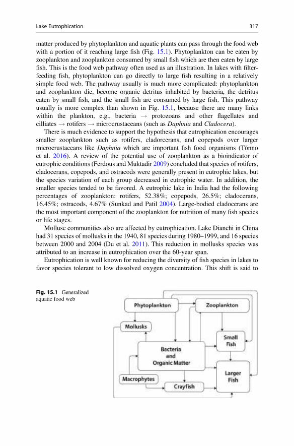
matter produced by phytoplankton and aquatic plants can pass through the food webwith a portion of it reaching large fish (Fig. 15.1). Phytoplankton can be eaten byzooplankton and zooplankton consumed by small fish which are then eaten by largefish. This is the food web pathway often used as an illustration. In lakes with filter-feeding fish, phytoplankton can go directly to large fish resulting in a relativelysimple food web. The pathway usually is much more complicated: phytoplanktonand zooplankton die, become organic detritus inhabited by bacteria, the detrituseaten by small fish, and the small fish are consumed by large fish. This pathwayusually is more complex than shown in Fig. 15.1, because there are many linkswithin the plankton, e.g., bacteria ! protozoans and other flagellates andcilliates ! rotifers ! microcrustaceans (such as Daphnia and Cladocera).

There is much evidence to support the hypothesis that eutrophication encouragessmaller zooplankton such as rotifers, cladorcerans, and copepods over largermicrocrustaceans like Daphnia which are important fish food organisms (Tõnnoet al. 2016). A review of the potential use of zooplankton as a bioindicator ofeutrophic conditions (Ferdous and Muktadir 2009) concluded that species of rotifers,cladocerans, copepods, and ostracods were generally present in eutrophic lakes, butthe species variation of each group decreased in eutrophic water. In addition, thesmaller species tended to be favored. A eutrophic lake in India had the followingpercentages of zooplankton: rotifers, 52.38%; copepods, 26.5%; cladocerans,16.45%; ostracods, 4.67% (Sunkad and Patil 2004). Large-bodied cladocerans arethe most important component of the zooplankton for nutrition of many fish speciesor life stages.

Mollusc communities also are affected by eutrophication. Lake Dianchi in Chinahad 31 species of mollusks in the 1940, 81 species during 1980–1999, and 16 speciesbetween 2000 and 2004 (Du et al. 2011). This reduction in mollusks species wasattributed to an increase in eutrophication over the 60-year span.

Eutrophication is well known for reducing the diversity of fish species in lakes tofavor species tolerant to low dissolved oxygen concentration. This shift is said to

Fig. 15.1 Generalizedaquatic food web

Lake Eutrophication 317

favor “coarse” species, because the species popular for sport fishing commonlybecome less abundant and sometimes disappear from the fish fauna. Kautz (1980)analyzed fish populations and trophic status in 22 lakes in Florida (USA). Total fishbiomass was low in oligotrophic lakes, increased to a maximum in mesotrophic andeutrophic lakes, and was near maximum in hypereutrophic lakes. Species diversitywas highest in mesotrophic lakes, but it decreased markedly in eutrophic andhypertrophic lakes. This reveals that a shrift from oligotrophy to mesotrophy maynot reduce fish species numbers, but a shift to eutrophy will lessen the numbers offish species.

Stream Eutrophication

Butcher (1947) states that a stream almost inevitably becomes more eutrophic as itflows downstream and receives nutrient inputs from its watershed. Phytoplanktonblooms do not develop in rapidly flowing water, but submerged macrophytes or matforming, filamentous macroalgae may grow well. Thièbaut and Muller (1998)reported that eutrophic streams in a mountainous region of France had a lowdiversity of submerged vascular plants because of overgrowth by filamentousalgae. According to Dodds (2006), many natural streams become net heterotrophicsystems (photosynthetic oxygen production < dissolved oxygen consumption inrespiration). This situation may not cause extremely low dissolved oxygen concen-tration in reaches of eutrophic streams where reaeration replenishes the dissolvedoxygen rapidly, but in stagnant reaches with low rates of reaeration, dissolvedoxygen concentrations may become critically low. Large inputs of organic wasteto streams also may cause dissolved oxygen depletion near effluent outfalls, but thestream reaerates as it passes downstream and dissolved oxygen concentration mayrecover and ammonia concentration decline as a result of nitrification. This topic isdiscussed in greater detail in Chap. 18.

The permissible organic waste input to streams often is estimated from streamaeration rate and the biological oxygen demand (BOD) of the wastewater input. Thisis possible because the rate that the stream reaerates can be used to estimate the dailyBOD load to the stream that may be allowed without the stream dissolved oxygenconcentration falling below a specified minimum level.

Climate Change and Eutrophication

The term global warming has largely been replaced by the concept of climatechange, because some places may become cooler and others warmer even thoughthe average global temperature is tending to increase. Rising temperature is the mainconsideration related to eutrophication. A study by Feuchtmayr et al. (2009) revealedthat increasing water temperature resulted in greater dissolved phosphateconcentrations, increased plant biomass, and reduced fish biomass. High nitrogeninput and warming reduced the number of plant species. Warming also seemed to


favor increased macrophyte growth more than it enhanced phytoplankton growth.The results suggested that large surface to volume ratios (shallow lakes and streams)would be more susceptible to adverse effects of global warming than would deeperwater bodies with lower surface to volume ratios.

Kaushal et al. (2013) reported that the rising atmospheric carbon dioxide concen-tration was increasing limestone solubility and causing stream alkalinity to increase.They suggested that greater alkalinity in streams may increase the availability ofinorganic carbon for photosynthesis in water bodies to accelerate eutrophication.They also suggested that high stream pH would make high ammonia nitrogenconcentrations more problematic by increasing the proportion of potentially toxicNH3 relative to NH4

+.

Eutrophication and Water Use

Dense algal blooms cause water quality deterioration ultimately reducing biodiver-sity and leading to water bodies inhabited mainly by coarse fish species. Eutrophi-cation has a serious impact on the usefulness of water bodies for sport fishing and forthe capture of species of fish acceptable in the market. Dense algal blooms also makewaters turbid and less desirable for swimming and other kinds of recreational wateruse. Taste and odor in municipal water supplies result in many consumer complaints.Water with algal blooms also are unsightly and less appealing to those who enjoyviewing lakes and streams.

The problem of algal toxicity has already been discussed in Chap. 12, and algaltoxicity usually is not widespread other than in the case of shellfish poisoning inhumans. Nevertheless, blue-green algae blooms can lead to medical problemsranging from rashes to death in some instances of shellfish poisoning. Livestockalso have died from drinking water containing toxic algae.

Blue-green algae and other dense algal blooms increase the cost of water treat-ment. The removal of taste and odor problems sometimes cannot be resolved withoutpassing water through activated carbon filters.

Eutrophication Control

Eutrophication control typically focuses on the removal of nitrogen and phosphorusfrom effluents. The major inputs of these two nutrients are municipal wastewater,runoff from agricultural and urban areas, certain industrial effluents, and in someregions, commercial aquaculture. Effluents contain nitrogen and phosphorus areeither point-source that are discharged through a pipe or other conduit or non-point-source that are in the form of runoff which is either too voluminous or toodiffuse to subject to standard, point-source wastewater treatment.

The phosphorus concentration in point-source effluents usually can be reduced by80–90% by one of the following chemical treatments: lime [Ca(OH)2] to precipitatehydroxyapatite [Ca10(PO4)6�6H2O]; alum [Al2(SO4)3�14H2O] to precipitate

Eutrophication Control 319

aluminum phosphate (AlPO4); compounds such as ferric chloride [Fe(Cl)3] toprecipitate ferric phosphate (FePO4). The precipitates of phosphorus and othersettled solids are removed as sludge, and the wastewater is aerated. There also is abiological phosphorus removal procedure in which phosphorus is incorporated intomicrobial biomass and these organisms removed in a clarifier as sludge. By use ofthese methods, 90–95% of phosphorus can be removed.

Nitrification and denitrification are used to remove combined nitrogen from pointsource effluents. Much of the particulate organic nitrogen is removed by sedimenta-tion in a clarifier along with other total solids, and the water is then aeratedthoroughly for long enough to convert most of the ammonia nitrogen to nitratethrough biological nitrification. The water is then put into an anaerobic digester and acarbon source such as methanol is added to allow denitrification. Around 85–90% ofthe total nitrogen in wastewater can be removed through sedimentation, nitrification,and denitrification.

Nitrogen and phosphorus concentrations are reduced in non-point-source effluentby use of management practices of many types depending upon effluent sources. Inagriculture, the management practices are those that lessen nitrogen and phosphorusinputs in fertilizers and minimize their loss in runoff. Particular attention is given tomaintaining vegetative cover and other erosion measures, installing sedimentremoval sills in ditches, and many others. Runoff from concentrated animal rearingfacilities is directed in retention ponds and stored for land application.

Practices vary depending upon the activity or industry producing the non-point-source discharge of which agriculture is the major source. Of course, suburbanlawns, golf courses, and other fertilized land are also significant sources of nitrogenand phosphorus in runoff.

In lakes and other static water bodies, phosphorus removal can be effected bychemical coagulation—usually aluminum sulfate (Huser et al. 2011). This treatmentcan be quite effective in lowering phosphorus concentrations for several years tolessen phytoplankton abundance. Biological control methods such as phosphorus(and nitrogen) removal in aquatic plants, filter-feeding fish, and mollusks have beenpromoted with varying degrees of success. Copper sulfate often is used to lessen theabundance of phytoplankton in water bodies for water supply and recreation use.

Schindler et al. (2008) did a long-term study that revealed phosphorus to be theprimary limiting nutrient in some Canadian lakes—a fact already known for manyyears in pond aquaculture (Swingle 1947; Mortimer 1954; Hickling 1962; Hepher1962). Because of the importance of phosphorus in freshwater, there is a tendency ineutrophication control to focus primarily on reducing phosphorus inputs. The studyby Schindler et al. (2008) was done in Canada, and there have been reports ofnitrogen-limited lakes and reservoirs in other places. Conley et al. (2009) warnedthat focusing on phosphorus control in freshwater will increase the nitrogen input toestuaries in which nitrogen is often a limiting factor for phytoplankton growth, andthey cited some specific instances of this phenomenon. Conversely, if nitrogen is thefocus of eutrophication control, low nitrogen concentrations in presence of elevatedphosphorus concentrations will stimulate nitrogen fixation. In some lakes, especiallyshallow ones, phosphorus may be available from sediment in sufficient quantities to


cause phytoplankton blooms. Both nitrogen inputs from anthropogenic activities andnitrogen fixation can trigger phytoplankton blooms. Phosphorus removal from waterentering such lakes would not control eutrophication because of nitrogen fixation.The sensitivity of nitrogen fixation rate to the N/P to nitrogen fixation was consid-ered in Chap. 13.

The upshot of the nitrogen versus phosphorus control issue can be summarized asfollows: both can be limiting; all lakes are not the same with respect to nitrogen andphosphorus requirements; relying only on phosphorus control increases downstreamnitrogen loads. While both nitrogen and phosphorus generally should be controlled,in specific situations, control of one over the other may be preferable. Most point-source effluent treatment removes both nitrogen and phosphorus relatively well. Themajor cause of eutrophication is non-point-source effluent, and agriculture is themain source of such effluent.

Conclusions

Eutrophication is probably the most troublesome aspect of water pollution. It causesincreased phytoplankton growth and a reduction in dissolved oxygen availabilityleading to a reduction in species diversity in which species that tolerate lowdissolved oxygen concentration are favored. Many of these species are undesirablefor both efficient ecological function and water use by humans. Eutrophicationcontrol consists mainly of techniques for removing nitrogen and phosphorus frompoint-source effluents by treatment and application of management practices toreduce inputs of nitrogen and phosphorus to water bodies in runoff.

References

Butcher RW (1947) Studies in the ecology of rivers: VIII. The algae of organically enriched waters.J Ecol 35:186–191

Conley DJ, Paerl HW, Howarth RW, Boesch DF, Seitzinger SP, Havens KE, Lancelot C, LikensGE (2009) Controlling eutrophication: nitrogen and phosphorus. Science 323:1014–1015

Dodds WK (2006) Eutrophication and trophic state in rivers and streams. Limnol Oceanogr51:671–680

Du LN, Li Y, Chen X, Yang JX (2011) Effect of eutrophication on molluscan communitycomposition in Lake Dianchi (China, Yunnan). Limnol Ecol Manage InlandWaters 41:213–219

Ferdous Z, Muktadir AKM (2009) A review: potentiality of zooplankton as bioindicator. Am J ApplSci 6:1815–1819

Feuchtmayr H, Moran R, Hatton K, Conner L, Heyes T, Moss B, Harvey I, Atkinson D (2009)Global warming and eutrophication: effects on water chemistry and autotrophic communities inexperimental hypertrophic shallow lake mesocosms. J Appl Ecol 46:713–723

Hepher B (1962) Ten years of research in pond fertilization in Israel, II. The effect of fertilization onfish yields. Bamidgeh 14:29–48

Hickling CF (1962) Fish culture. Faber and Faber, LondonHuser B, Brezonik P, Newman R (2011) Effects of alum treatment on water quality and sediment in

the Minneapolis chain of lakes, Minnesota, USA. Lake Reservoir Manage 27:220–228

References 321

Jiang J, Huang ZG, Seager TP, Lin W, Grebogi C, Hastings A, Lai YC (2018) Predicting tippingpoints in mutualistic networks through dimension reduction. Proc Natl Acad Sci USA115:39–47

Kaushal SS, Likens GE, Utz RM, Pace ML, Grese M, Yepsen M (2013) Increased river alkaliniza-tion in the Eastern U.S. Environ Sci Technol 47:10302–10311

Kautz RS (1980) Effects of eutrophication on the fish communities of Florida lakes. Proc Ann ConfSE Assoc Fish Wildlife Agencies 34:67–80

Kociolek JP, Stoermer EF (2009) Oligotrophy: the forgotten end of an ecological spectrum. ActaBot Croatica 68:465–472

Margalef R (1958) Temporal succession and spatial heterogeneity in phytoplankton. In: Buzzati-Traverso AA (ed) Perspectives in marine biology. University of California Press, Berkeley, pp323–349

Mortimer CH (1954) Fertilizers in fish ponds. Publication 5. Her Majesty’s Stationery Office,London

Odum EP (1971) Fundamentals of ecology. 3rd edn. W. B. Saunders Company, PhiladelphiaSchindler DW, Hecky RE, Findlay DL, Stainton MP, Parker BR, Paterson MJ, Beaty KG, Lyng M,

Kasian SEM (2008) Eutrophication of lakes cannot be controlled by reducing nitrogen input:results of a 37-year whole-ecosystem experiment. Proc Natl Acad Sci USA 105:1254–1258

Sunkad BN, Patil HS (2004) Water quality assessment of Fort Lake of Belgaum (Karnataka) withspecial reference to zooplankton. J Environ Biol 25:99–102

Swingle HS (1947) Experiments on pond fertilization. Alabama Agricultural Experiment StationBulletin 264. Auburn University, Auburn

Thièbaut G, Muller S (1998) The impact of eutrophication on aquatic diversity in weaklymineralized streams in the Northern Vosges Mountains (NE France). Biodivers Conserv7:1051–1068

Tõnno I, Agasild H, Kõiv T, Freiberg R, Nõges P, Nõges T (2016) Algal diet of small-bodiedcrustacean zooplankton in a cyanobacteria-dominated eutrophic lake. PLoS One 11:e0154526.https://doi.org/10.1371/journal.pone.0154526


https://doi.org/10.1371/journal.pone.0154526

Sulfur 16

AbstractSulfur is a nutrient for plants and animals; hydrogen sulfide is an odorous, toxicmaterial; and sulfur dioxide is an air pollutant responsible for acid rain. Plantsprimarily use sulfate as a sulfur source, and sulfur containing amino acids inplants are important to animal nutrition. Sulfur compounds undergo oxidationsand reductions in the environment. The most famous sulfur oxidizing bacteria areof the genus Thiobacillus that oxidize elemental sulfur, sulfides, and otherreduced sulfur compounds releasing sulfuric acid into the environment—acidsulfate soils and acidic mine drainage result from sulfur oxidation. Bacteria of thegenus Desulfovibrio use certain sulfur compounds as electron and hydrogenacceptors in respiration allowing them to decompose organic matter in anaerobicenvironments. Ferrous iron and other metals may react with sulfide in anaerobicsediments to form metallic sulfides, e.g., iron sulfide (iron pyrite). If suchsediment later is exposed to oxygen, sulfides will be oxidized resulting in sulfuricacid production. Sulfide in anaerobic zones sometimes diffuses or is mixed intooverlaying aerobic water at a rate exceeding the oxidation rate of sulfide—toxicity to aquatic animals can result. Sulfide toxicity is favored by low pH,because un-ionized hydrogen sulfide (H2S) is the toxic form. Elevated sulfateconcentration and the presence of sulfide degrades the quality of drinking water.

Introduction

Sulfur is a major element of geochemistry, making up around 3% of the earth’s totalmass, but its abundance is only about 0.04% of the earth’s crust. It occurs in theearth’s crust as deposits of elemental sulfur, sulfate salts such as gypsum (calciumsulfate), epsomite (magnesium sulfate), varite (barium sulfate), and in metamorphicand igneous rock. Weathering delivers about 60 million tonnes of sulfur to the oceaneach year. The sulfur concentration is about 1% in crude oil and 0.5–5.0% in coaland lignite. Sulfur occurs in soil mainly as sulfate salts, sulfate in the soil solution,


323


and sulfur in soil organic matter. Sulfate is the major form of sulfur in the ocean andfreshwater bodies. Freshwater contains a small percentage of the earth’s sulfur, butthe ocean is 0.09% sulfur by weight and sulfur in sulfate makes up 2.7% of the totaldissolved solids in ocean water. Natural water contains only about 7% of the sulfurfound in the earth’s solid crust (Hem 1985).

Sulfur is widely used in industry as a reactant and component of products, and it iscontained in fuels. The nineteenth century German chemist Justus von Liebigrecognized the importance of sulfur when he declared: “you may fairly judge thecommercial prosperity of a country from the amount of sulfuric acid it consumes.”But, the modern day American environmental activist Denis Hayes is quoted assaying “there was almost a universal acceptance of unhealthy conditions. Sulfurdioxide in smokestacks were the price, or smell, of prosperity.”

Sulfur dioxide results mainly from combustion of fuels and volcanic eruptions,and the atmosphere contains a small percentage (usually less than 10 ppb) of sulfurdioxide. For example, the annual, ambient sulfur dioxide concentrations in differentregions of Canada ranged from 1 to 3 ppb in 2014 (https://www.ec.gc.ca/indicateurs-indicators/default.asp?lang¼En&n¼307CCE5B-1&pedisable-true). Hydrogen sul-fide enters the atmosphere from microbial decay (especially in marshes), and it isoxidized to sulfur dioxide.

Sulfur is an essential nutrient for plants, animals, and bacteria, but unlike nitrogenand phosphorus, sulfur seldom limits primary productivity. Sulfur is a component oftwo essential amino acids (cysteine and methionine) and other organic compounds,the best-known of which are the vitamins biotin and thiamine, and iron-sulfurclusters called ferredoxins. Ferredoxins function in the transfer of electrons invarious biochemical reactions.

Sulfur, like nitrogen, commonly occurs in the environment in several oxidationstates (valences), and bacteria oxidize and reduce sulfur compounds. Oxidations andreductions of sulfur also may occur by chemical reactions not involving biologicalactivity. Sulfate is the form of sulfur used most commonly by plants, but some plantscan fix atmospheric sulfur by a method analogous to nitrogen fixation. As shown inChap. 11, sulfur oxidations often produce sulfuric acid. Oxidation of sulfur dioxideemitted into the atmosphere by combustion of fossil fuels is the main cause of theacid rain phenomenon. Sulfide oxidation is responsible for acid mine drainage, andoxidation of sulfur or sulfide in soil can cause extreme acidity. Of course, certainanaerobic bacteria can reduce sulfate and other oxidized forms of sulfur to sulfides.

There is a global sulfur cycle, and most aspects of this natural cycle operate inaquatic ecosystems. Sulfate influences biological activity by acting as a nutrient, butsulfide can be toxic to aquatic organisms. The purpose of this chapter is to discusssulfur chemistry and its influence on water quality.

324 16 Sulfur

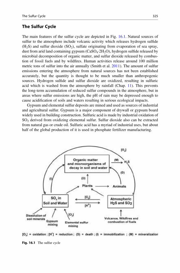
https://www.ec.gc.ca/indicateurs-indicators/default.asp?lang=En&n=307CCE5B-1&pedisable-true




The Sulfur Cycle

The main features of the sulfur cycle are depicted in Fig. 16.1. Natural sources ofsulfur to the atmosphere include volcanic activity which releases hydrogen sulfide(H2S) and sulfur dioxide (SO2), sulfate originating from evaporation of sea spray,dust from arid land containing gypsum (CaSO4�2H2O), hydrogen sulfide released bymicrobial decomposition of organic matter, and sulfur dioxide released by combus-tion of fossil fuels and by wildfires. Human activities release around 100 millionmetric tons of sulfur into the air annually (Smith et al. 2011). The amount of sulfuremissions entering the atmosphere from natural sources has not been establishedaccurately, but the quantity is thought to be much smaller than anthropogenicsources. Hydrogen sulfide and sulfur dioxide are oxidized, resulting in sulfuricacid which is washed from the atmosphere by rainfall (Chap. 11). This preventsthe long-term accumulation of reduced sulfur compounds in the atmosphere, but inareas where sulfur emissions are high, the pH of rain may be depressed enough tocause acidification of soils and waters resulting in serious ecological impacts.

Gypsum and elemental sulfur deposits are mined and used as sources of industrialand agricultural sulfur. Gypsum is a major component of drywall or gypsum boardwidely used in building construction. Sulfuric acid is made by industrial oxidation ofSO2 derived from oxidizing elemental sulfur. Sulfur dioxide also can be extractedfrom natural gas or crude oil. Sulfuric acid has a myriad of industrial uses, but abouthalf of the global production of it is used in phosphate fertilizer manufacturing.

Fig. 16.1 The sulfur cycle

The Sulfur Cycle 325

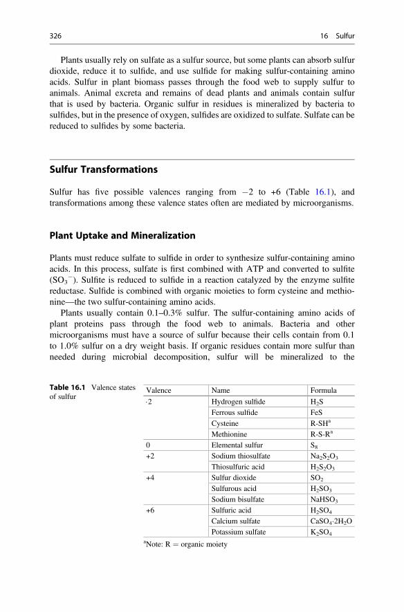
Plants usually rely on sulfate as a sulfur source, but some plants can absorb sulfurdioxide, reduce it to sulfide, and use sulfide for making sulfur-containing aminoacids. Sulfur in plant biomass passes through the food web to supply sulfur toanimals. Animal excreta and remains of dead plants and animals contain sulfurthat is used by bacteria. Organic sulfur in residues is mineralized by bacteria tosulfides, but in the presence of oxygen, sulfides are oxidized to sulfate. Sulfate can bereduced to sulfides by some bacteria.

Sulfur Transformations

Sulfur has five possible valences ranging from �2 to +6 (Table 16.1), andtransformations among these valence states often are mediated by microorganisms.

Plant Uptake and Mineralization

Plants must reduce sulfate to sulfide in order to synthesize sulfur-containing aminoacids. In this process, sulfate is first combined with ATP and converted to sulfite(SO3

�). Sulfite is reduced to sulfide in a reaction catalyzed by the enzyme sulfitereductase. Sulfide is combined with organic moieties to form cysteine and methio-nine—the two sulfur-containing amino acids.

Plants usually contain 0.1–0.3% sulfur. The sulfur-containing amino acids ofplant proteins pass through the food web to animals. Bacteria and othermicroorganisms must have a source of sulfur because their cells contain from 0.1to 1.0% sulfur on a dry weight basis. If organic residues contain more sulfur thanneeded during microbial decomposition, sulfur will be mineralized to the

Table 16.1 Valence statesof sulfur

Valence Name Formula

×2 Hydrogen sulfide H2S

Ferrous sulfide FeS

Cysteine R-SHa

Methionine R-S-Ra

0 Elemental sulfur S8+2 Sodium thiosulfate Na2S2O3

Thiosulfuric acid H2S2O3

+4 Sulfur dioxide SO2

Sulfurous acid H2SO3

Sodium bisulfate NaHSO3

+6 Sulfuric acid H2SO4

Calcium sulfate CaSO4�2H2O

Potassium sulfate K2SO4

aNote: R ¼ organic moiety

326 16 Sulfur

environment (Ex. 16.1). Sulfur will be immobilized from the environment ininstances where residues contain less sulfur than needed for microbialdecomposition.

Ex. 16.1 Suppose that a residue containing 0.3% sulfur and 45% carbon (dryweight basis) is completely decomposed by bacteria. It will be assumed that thereis adequate nitrogen and other elements present to meet microbial needs. Thebacteria have a carbon assimilation efficiency to 20% and contain 0.15% S. Thesulfur mineralized from 1000 g of residue will be estimated.

Solution:The carbon and sulfur contents of 1000 g residue are

1; 000� 0:45 ¼ 450 g carbon

1; 000� 0:003 ¼ 3 g sulfur:

The bacterial biomass will be

450 g C � 0:2 ¼ 90 g bacterial carbon

90 g bacteria C � 0.5 ¼ 180 g bacterial biomass.The sulfur in bacterial biomass is

180 g bacteria� 0:0015 ¼ 0:27 g sulfur:

The residue contains 2.73 g more sulfur than needed for its decomposition, andthis sulfur will be mineralized.

The C:N ratio is of more importance than the C:S ratio in controlling the rate oforganic matter decomposition in nearly all situations.

Oxidations

Most sulfur oxidations can proceed by purely chemical processes, but biologicalintervention often speeds up sulfur oxidation. Bacteria that oxidize inorganic sulfurusually are obligate or facultative autotrophs. They use the energy obtained fromoxidizing sulfur to convert carbon dioxide to organic carbon in their cells. Thisprocess is analogous to nitrification and results in organic matter synthesis. How-ever, like in nitrification, carbon fixation by sulfur-oxidizing bacteria is not highlyenergy efficient. The amount of organic matter produced globally by sulfur oxidizingbacteria is miniscule in comparison to the quantity produced through photosynthesis.

The best-known sulfur-oxidizing bacteria are species of Thiobacillus, a genus ofgram-negative rod-shaped bacteria of the hetaproteabacteria. Some representativereactions carried out by these microorganisms are

Sulfur Transformations 327

Na2S2O3 þ 2O2 þ H2O ! 2NaHSO4 ð16:1Þ

5Na2S2O3 þ 4O2 þ H2O ! 5Na2SO4 þ H2SO4 þ 4S ð16:2Þ

Sþ 1½ O2 þ H2O ! H2SO4: ð16:3ÞIn each of these reactions, energy is released and a small portion of the energy iscaptured (by converting ADP to ATP) and used to reduce carbon dioxide tocarbohydrate.

Nitrate also can be an oxygen source for sulfur oxidation as shown below:

5Sþ 6KNO3 þ 2H2O ! K2SO4 þ 4KHSO4 þ 3N2: ð16:4ÞIn the reaction depicted by Eq. 16.4, oxygen is removed from nitrate and used tooxidize sulfur to sulfate. The process may be called sulfur oxidation, but it also isdenitrification, because nitrogen gas is released.

Green and purple sulfur bacteria also can oxidize sulfur. These bacteria are highlyunusual in that they are anaerobic photoautotrophs. The green sulfur bacteria includeChlorobium and several other genera of the family Chlorobiaceae, while the purplesulfur bacteria are of the family Chromatiaceae that includes Thiospirillum andseveral other genera. The colored, green and purple sulfur bacteria use light andenergy from oxidizing sulfide to reduce carbon dioxide to carbohydrate (CH2O)according to the following reactions:

CO2 þ 2H2S !light

CH2Oþ 2Sþ H2O ð16:5Þ

2CO2 þ H2Sþ 2H2O !light

2CH2Oþ H2SO4: ð16:6Þ

Both light and anaerobic conditions are necessary for colored, photosynthetic sulfurbacteria, so their presence is greatly restricted in nature. Colored sulfur bacteria areparticularly troublesome by growing on the inside tops of sewer pipes near manholecovers where light is available. The result is corrosion of the upper inner surface ofthe pipe near the manhole cover by sulfuric acid produced by the bacteria.

Reductions

Sulfur reductions occur in anaerobic environments, and sulfur-reducing bacteria useoxygen from sulfate or other oxidized sulfur compounds as electron and hydrogenacceptors in respiration. The process is similar in this regard to denitrification. Thepredominant sulfur-reducing bacteria are species of gram-negative bacteria of thegenus Desulfovibrio, which commonly occur in sediment or waterlogged soil thathas a high concentration of organic matter. Some typical reactions are

328 16 Sulfur

SO2�4 þ 8Hþ ! S2� þ 4H2O ð16:7Þ

SO2�3 þ 6Hþ ! S2� þ 3H2O ð16:8Þ

S2O2�3 þ 8Hþ ! 2SH� þ 3H2O: ð16:9Þ

The source of electrons, hydrogen, and energy for the reactions depicted inEqs. 16.7, 16.8, and 16.9 are carbohydrates, organic acids, and alcohols. A repre-sentative complete reaction is

2CH3CHOHCOONaþMgSO4 ! H2Sþ 2CH3COONa þ CO2

þMgCO3 þ H2O: ð16:10Þ

Hydrogen Sulfide

The preceding equations for sulfur reductions showed sulfate and other oxidizedforms of sulfur being converted to S2�, HS�, or H2S. These are all forms of sulfide-sulfur, and they also are dissociation products of the diprotic acid, hydrogen sulfide(H2S). Hydrogen sulfide dissociates as follows:

H2S ¼ HS� þ Hþ K1 ¼ 10�7:01 ð16:11Þ

HS� ¼ S2� þ Hþ K2 ¼ 10�13:89: ð16:12ÞDepending on pH, the dominant sulfide species resulting from reduction of sulfurcompounds by bacteria will be H2S, HS

�, or S2� (Fig. 16.2). Un-ionized hydrogensulfide dominates in acidic environments, but in alkaline situations, S2� will be themain form.

With respect to water quality, sulfides typically are produced in sediment or in thehypolimnion of stratified lakes. When sulfide enters the aerobic water column abovethe sediment or is mixed into aerobic water at thermal overturn, the sulfide isoxidized rather quickly. Only oxygen-depleted water will contain appreciable levelsof sulfide.

Highly anaerobic environments contain both ferrous iron and sulfide, and ferroussulfide precipitates. Sulfides also react forming metal sulfides. Reference toTable 4.3 shows that metal sulfides have small solubility product constants. Marinesediment is a particularly favorable environment for the formation of metal sulfides,because the high sulfate content of the pore water favors sulfide production.

The mass action expression for Eq. 16.11 will be used to estimate the proportionof sulfide in un-ionized form at a particular pH in the following example.

Hydrogen Sulfide 329

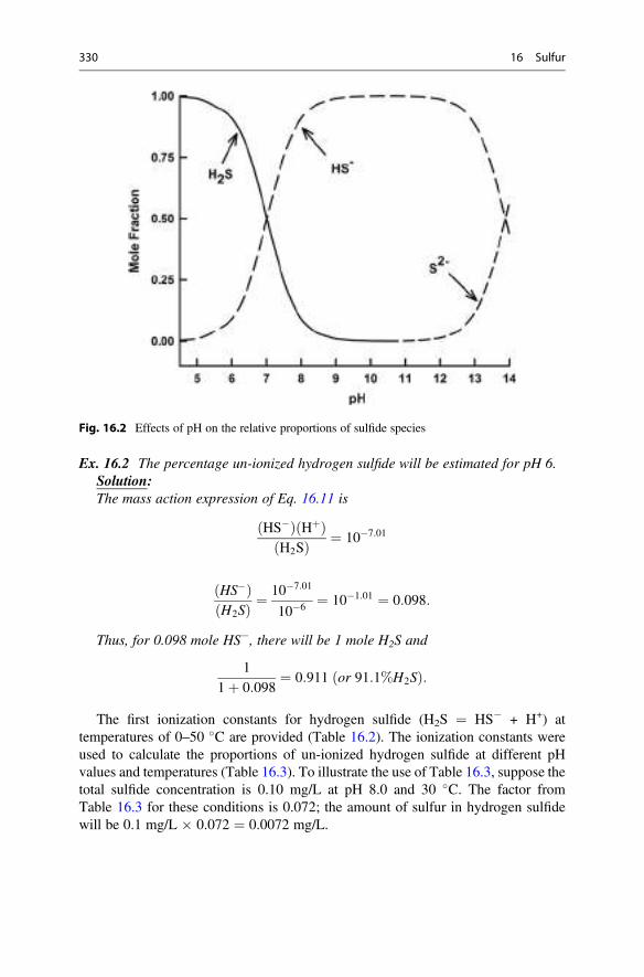
Ex. 16.2 The percentage un-ionized hydrogen sulfide will be estimated for pH 6.Solution:The mass action expression of Eq. 16.11 is

HS�ð Þ Hþð ÞH2Sð Þ ¼ 10�7:01

HS�ð ÞH2Sð Þ ¼

10�7:01

10�6 ¼ 10�1:01 ¼ 0:098:

Thus, for 0.098 mole HS�, there will be 1 mole H2S and

11þ 0:098

¼ 0:911 or 91:1%H2Sð Þ:

The first ionization constants for hydrogen sulfide (H2S ¼ HS� + H+) attemperatures of 0–50 �C are provided (Table 16.2). The ionization constants wereused to calculate the proportions of un-ionized hydrogen sulfide at different pHvalues and temperatures (Table 16.3). To illustrate the use of Table 16.3, suppose thetotal sulfide concentration is 0.10 mg/L at pH 8.0 and 30 �C. The factor fromTable 16.3 for these conditions is 0.072; the amount of sulfur in hydrogen sulfidewill be 0.1 mg/L � 0.072 ¼ 0.0072 mg/L.

Fig. 16.2 Effects of pH on the relative proportions of sulfide species

330 16 Sulfur

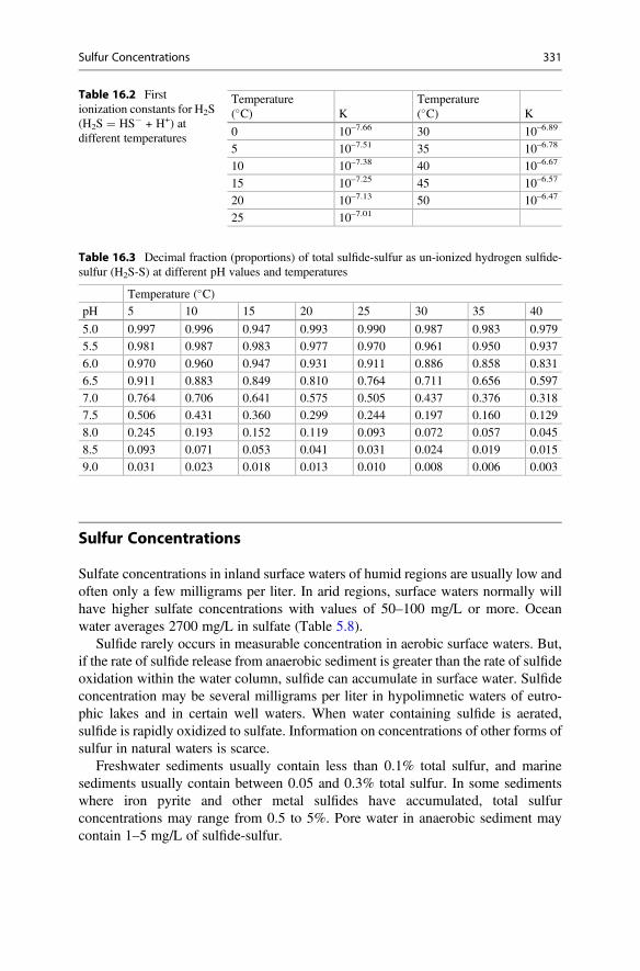
Sulfur Concentrations

Sulfate concentrations in inland surface waters of humid regions are usually low andoften only a few milligrams per liter. In arid regions, surface waters normally willhave higher sulfate concentrations with values of 50–100 mg/L or more. Oceanwater averages 2700 mg/L in sulfate (Table 5.8).

Sulfide rarely occurs in measurable concentration in aerobic surface waters. But,if the rate of sulfide release from anaerobic sediment is greater than the rate of sulfideoxidation within the water column, sulfide can accumulate in surface water. Sulfideconcentration may be several milligrams per liter in hypolimnetic waters of eutro-phic lakes and in certain well waters. When water containing sulfide is aerated,sulfide is rapidly oxidized to sulfate. Information on concentrations of other forms ofsulfur in natural waters is scarce.

Freshwater sediments usually contain less than 0.1% total sulfur, and marinesediments usually contain between 0.05 and 0.3% total sulfur. In some sedimentswhere iron pyrite and other metal sulfides have accumulated, total sulfurconcentrations may range from 0.5 to 5%. Pore water in anaerobic sediment maycontain 1–5 mg/L of sulfide-sulfur.

Table 16.2 Firstionization constants for H2S(H2S ¼ HS� + H+) atdifferent temperatures

Temperature(�C) K

Temperature(�C) K

0 10–7.66 30 10–6.89

5 10–7.51 35 10–6.78

10 10–7.38 40 10–6.67

15 10–7.25 45 10–6.57

20 10–7.13 50 10–6.47

25 10–7.01

Table 16.3 Decimal fraction (proportions) of total sulfide-sulfur as un-ionized hydrogen sulfide-sulfur (H2S-S) at different pH values and temperatures

Temperature (�C)pH 5 10 15 20 25 30 35 40

5.0 0.997 0.996 0.947 0.993 0.990 0.987 0.983 0.979

5.5 0.981 0.987 0.983 0.977 0.970 0.961 0.950 0.937

6.0 0.970 0.960 0.947 0.931 0.911 0.886 0.858 0.831

6.5 0.911 0.883 0.849 0.810 0.764 0.711 0.656 0.597

7.0 0.764 0.706 0.641 0.575 0.505 0.437 0.376 0.318

7.5 0.506 0.431 0.360 0.299 0.244 0.197 0.160 0.129

8.0 0.245 0.193 0.152 0.119 0.093 0.072 0.057 0.045

8.5 0.093 0.071 0.053 0.041 0.031 0.024 0.019 0.015

9.0 0.031 0.023 0.018 0.013 0.010 0.008 0.006 0.003

Sulfur Concentrations 331

Effects of Sulfur

Sulfide oxidizes quickly in aerobic environments where fish are found. But, undersome conditions, sulfide may be delivered into oxygenated zones at rates exceedingthe rates at which it can be oxidized. This phenomenon can result in toxicconcentrations of sulfide.

Sulfide in the un-ionized form (H2S) is highly toxic to fish and other aquaticanimals, but the two, ionized species (HS� and S2�) have little toxicity. The 96-hourLC50 of hydrogen sulfide to freshwater fish ranged from 4.2 to 34.8 μg/L (Gray et al.2002), but marine species apparently are somewhat less sensitive to hydrogensulfide—96-hour LC50s are 2–10 times greater than for freshwater fish (Bagarinaoand Lantin-Olaguer 1999; Gopakumar and Kuttyamma 1996). Most authoritiessuggest that no more than 0.002 mg/L of sulfide should be present in natural watersand any detectable concentration is undesirable. Hydrogen sulfide toxicity toorganisms results from several effects. Hydrogen sulfide inhibits the reoxidation ofcytochrome a3 by molecular oxygen, because it blocks the electron transport systemand stops oxidative respiration. Blood lactate concentration also increases andanaerobic glycolysis is favored over aerobic respiration. The overall toxic effect ishypoxia, and low dissolved oxygen concentrations enhance sulfide toxicity (Boydand Tucker 2014). As already mentioned, hydrogen sulfide is rarely detectable inenvironments containing dissolved oxygen, and it seldom is an important toxicityfactor other than in polluted aquatic ecosystems.

The most common concern over sulfur concentration relates to drinking waterquality. Sulfate in drinking water can impart a bitter taste. Depending upon theirsensitivity, people notice the bitter taste at sulfate concentrations of 250–1000 mg/L.Water containing elevated sulfate concentration also can act as a laxative to peoplenot used to drinking it. The highest quality drinking water will not contain more than50 mg/L sulfate, but most authorities indicate that up to 250 mg/L is acceptable fordrinking water supplies. In addition, high sulfate concentration in water interfereswith chlorination.

Hydrogen sulfide can be a contaminant in well water. Although it is not toxic tohumans at concentrations normally encountered, most people can detect a bad odorat sulfide concentrations of 0.1–0.5 mg/L. At sulfide concentrations up to 1 mg/L theodor often is described as musty, but higher concentrations cause the typical “rottenegg” odor of hydrogen sulfide. In addition to the odor, elevated hydrogen sulfideconcentrations are highly corrosive to water pipes and fixtures. Methods for remov-ing hydrogen sulfide from drinking water include activated carbon filtration, aera-tion, and oxidation with chlorine or potassium permanganate.

Atmospheric emissions of sulfur dioxide caused by combustion of fossil fuels arethe major cause of acid rain. Since the 1970s, many countries have worked to reducesulfur dioxide emissions by requiring sulfur dioxide removal devices in vehicles, onsmokestacks, etc. Although considerable control of sulfur dioxide emissions wasachieved and global emission declined for several years, sulfur dioxide emissions arenow increasing because of increased fossil fuel use by countries with rapidlydeveloping economies such as China and India (Boyd and McNevin 2015).

332 16 Sulfur

Conclusions

Sulfate concentration in most surface waters is adequate to support plant growth, andit is not a common limiting factor or a cause of eutrophication. Hydrogen sulfide isproduced in anaerobic zones, and it may diffuse or mix into aerobic zones faster thanit is oxidized leading to toxicity to fish and other aquatic life. Excessive sulfateconcentration and the presence of sulfides may be a concern in drinking waterquality. Excessive acidity and low pH in water bodies usually is a result of sulfuricacid from natural sources or pollution.

References

Bagarinao T, Lantin-Olaguer I (1999) The sulfide tolerance of milkfish and tilapia in relation to fishkills in farms and natural waters in the Philippines. Hydrobio 382:137–150

Boyd CE, McNevin AA (2015) Aquaculture, resource use, and the environment. Wiley Blackwell,Hoboken

Boyd CE, Tucker CS (2014) Handbook for aquaculture water quality. Craftmaster Printers, AuburnGopakumar G, Kuttyamma VJ (1996) Effect of hydrogen sulphide on two species of penaeid

prawns Penaeus indicus (H. Milne Edwards) and Metapenaeus dobsoni (Miers). Env Con Tox57:824–828

Gray JS, Wu RS, Or YY (2002) Effects of hypoxia and organic enrichment on the coastal marineenvironment. Mar Ecol Prog Ser 238:249–279

Hem JD (1985) Study and interpretation of the chemical characteristics of natural water. WaterSupply Paper 2254, United States Geological Survey, United States Government PrintingOffice, Washington

Smith SJ, van Aardenne J, Kilmont Z, Andres RJ, Volke A, Arias SD (2011) Anthropogenic sulfurdioxide emissions: 1850�2005. Atmos Chem Phy 11:1101–1116

References 333

Micronutrients and Other Trace Elements 17

AbstractThe solubilities of most minerals from which trace metals in natural watersoriginate are favored by low pH. The concentration of the free ion of a dissolvedtrace element usually is much lower than is the total concentration of the traceelement. This results from ion pair associations between the free trace ion andmajor ions, complex ion formation, hydrolysis of metal ions, and chelation ofmetal ions. Several trace elements—zinc, copper, iron, manganese, boron, fluo-rine, iodine, selenium, cadmium, cobalt, and molybdenum—are essential toplants, animals or both. A few other trace elements are suspected, but notunequivocally proven to be essential. There are some reports of low micronutrientconcentrations limiting the productivity of water bodies; but primary productivityin most water bodies apparently is not limited by a shortage of micronutrients.Trace elements—including the ones that are nutrients—may be toxic at highconcentration to aquatic organisms. Excessive concentrations of several tracemetals in drinking water also can be harmful to human health. Instances oftrace element toxicity in aquatic animals and humans usually have resultedfrom anthropogenic pollution. Nevertheless, excessive concentrations of tracemetals in drinking water sometimes occur naturally—an example is the presenceof chronically-toxic concentrations of arsenic in groundwater that serves as thewater supply for several million people in a few provinces of Bangladesh andadjoining India.

Introduction

Ninety-four of the 118 elements of the periodic table occur in nature and can bepresent in water at some concentration. The usual concentration range of differentelements varies greatly. In a complete analysis of freshwater, some elements will beat concentrations of 10–100 mg/L, while others will be present at less than 0.1 mg/L.Even wider ranges in concentration of elements are found in seawater. Dissolved


335


elements in natural waters often are divided into one of two categories. Elementswith concentrations above 1 mg/L usually are called major elements and those atlower concentration are known as trace elements (Gaillardet et al. 2003). Sometimes,elements of the lowest concentrations may be referred to as ultra trace elements.

Iron, manganese, zinc, copper, and a few other trace elements essential to aquaticorganisms are called micronutrients or trace nutrients. Phosphate, nitrate, andammonia nitrogen discussed earlier also are usually present in water atconcentrations <1 mg/L, but they are not considered micronutrients, because theyare required in large amounts by organisms. Concentrations of iron and sometimesother micronutrients may be low enough to limit productivity in some freshwaterbodies (Goldman 1972; Hyenstrand et al. 2000; Vrede and Tranvik 2006) and in theocean (Nadis 1998). Excessive concentrations of both micronutrients andnon-essential trace elements can be toxic to organisms including humans whodrink water with high concentrations of certain trace elements. Higher than normalconcentrations of trace elements often result from pollution, but elevatedconcentrations occasionally are natural phenomena.

The purpose of this chapter is to discuss both micronutrients and non-essentialtrace elements. The focus will be on sources, chemistry, concentrations, and effectsof trace elements in water bodies.

Chemical Control of Trace Element Concentrations

The solubility of trace elements in water is a complex topic and depends uponparticular combinations of factors (Hem 1985; McBride 1989; Deverel et al. 2012).A source of an element obviously is necessary, and the main sources are minerals inthe watershed, in the bottom of the water body, and in some instances, pollution. Amajor controlling factor in mineral solubility is the solubility product (Ksp). The Ksp

effects the degree of dissolution of a mineral, but equally as important, ifconcentrations of certain ions in water exceed the Ksp of some mineral, precipitationof that mineral will occur. The common ion principle is particularly important incausing precipitation.

Some Ksp values (at 25 �C) of interest in water quality are provided (Table 17.1).The solubility reactions are in the form aAbB(s) ¼ aA(aq) + bB(aq). Solubilityproducts are useful for calculating the probable water solubility of compounds, andtabular values of Ksp apply to solubilities of compounds in distilled water at 25 �C.The Ksp of a compound may have been measured; but, more likely, it was calculatedfrom the standard Gibbs free energy (ΔG�) of the chemical species involved fromtheir standard states by use of Eq. 4.11 and illustrated in the example below.

336 17 Micronutrients and Other Trace Elements

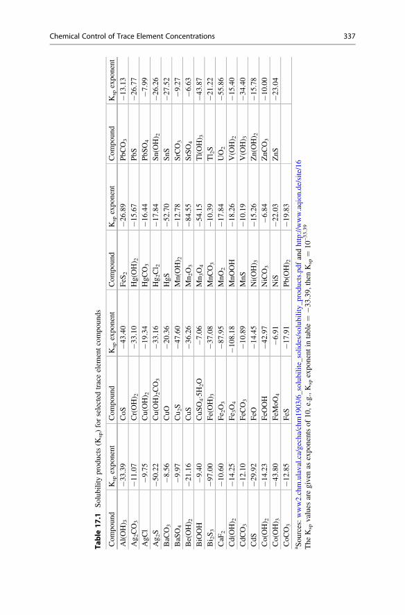
https://doi.org/10.1007/978-3-030-23335-8_4#Equ11

Table

17.1

Solub

ility

prod

ucts(K

sp)forselected

traceelem

entcom

poun

ds

Com

poun

dKspexpo

nent

Com

poun

dKspexpo

nent

Com

poun

dKspexpo

nent

Com

poun

dKspexpo

nent

Al(OH) 3

�33.39

CoS

�43.40

FeS

2�2

6.89

PbC

O3

�13.13

Ag 2CO3

�11.07

Cr(OH) 2

�33.10

Hg(OH) 2

�15.67

PbS

�26.77

AgC

l�9

.75

Cu(OH) 2

�19.34

HgC

O3

�16.44

PbS

O4

�7.99

Ag 2S

�50.22

Cu(OH) 2CO3

�33.16

Hg 2Cl 2

�17.84

Sn(OH) 2

�26.26

BaC

O3

�8.56

CuO

�20.36

HgS

�52.70

SnS

�27.52

BaSO4

�9.97

Cu 2S

�47.60

Mn(OH) 2

�12.78

SrCO3

�9.27

Be(OH) 2

�21.16

CuS

�36.26

Mn 2O3

�84.55

SrSO4

�6.63

BiOOH

�9.40

CuS

O4�5H

2O

�7.06

Mn 3O4

�54.15

Tl(OH) 3

�43.87

Bi 2S3

�97.00

Fe(OH) 3

�37.08

MnC

O3

�10.39

Tl 2S

�21.22

CaF

2�1

0.60

Fe 2O3

�87.95

MnO

2�1

7.84

UO2

�55.86

Cd(OH) 2

�14.25

Fe 3O4

�108

.18

MnO

OH

�18.26

V(O

H) 2

�15.40

CdC

O3

�12.10

FeC

O3

�10.89

MnS

�10.19

V(O

H) 3

�34.40

CdS

�29.92

FeO

�14.45

Ni(OH) 3

�15.26

Zn(OH) 2

�15.78

Co(OH) 2

�14.23

FeO

OH

�42.97

NiCO3

�6.84

ZnC

O3

�10.00

Co(OH) 3

�43.80

FeM

oO4

�6.91

NiS

�22.03

ZnS

�23.04

CoC

O3

�12.85

FeS

�17.91

Pb(OH) 2

�19.83

a Sou

rces:www2.chm.ulaval.ca/gecha/chm19

03/6_solub

ilite_solides/solub

ility_p

rodu

cts.pd

fandhttp://www.aqion

.de/site/16

The

Kspvalues

aregivenas

expo

nentsof

10,e.g.,Kspexpo

nent

intable¼

�33.39

,thenKsp¼

10–33.39

Chemical Control of Trace Element Concentrations 337

http://www2.chm.ulaval.ca/gecha/chm1903/6_solubilite_solides/solubility_products.pdf

http://www.aqion.de/site/16

Ex. 17.1 Calculation of Ksp of Cu2S.Solution:

Cu2S ¼ 2Cuþ þ S2�

ΔG� ¼ 2ΔGo

f Cuþð Þ þ ΔGof S2�� ΔGo

f Cu2Sð Þ

ΔG� ¼ 2 49:99 kJ=molð Þ þ 85:8 kJ=mol� �86:19 kJ=molð Þ

ΔG� ¼ 271:97 kJ=mol

ΔG� ¼ �5:709logK

logK ¼ ΔG�

�5:709¼ 271:97

�5:709¼ �47:64

K ¼ 10�47:64

Ksp ¼ 2:28� 10�48 or 10�47:64

The Ksp from Table 17.1 also is 10–47.64.

Values of Ksp reported in different tables may vary slightly. They can be obtainedfor temperatures other than 25 �C using their relationship to standard Gibbs freeenergy. The Ksp values in tables do not give correct concentrations for compoundswhose solubilities are influenced by pH, carbon dioxide concentration, or redoxpotential. To illustrate the effect of pH on solubility, consider tenorite (CuO;Ksp ¼ 10�20) that reacts in water to form Cu2+ and 2OH�. The equilibriumconcentration of Cu2+ using the Ksp of tenorite is only 10

–8.5 M (0.2 μg/L). However,CuO reacts with H+ to produce Cu2+ and water for which K ¼ 107.35. The solubilityof copper oxide reacting at lower pH will be calculated in the following example.

Ex. 17.2 Copper solubility from CuO at pH 5 and 25 �C will be calculated.Solution:

CuOþ 2Hþ ¼ Cu2þ þ H2O

Cu2þð ÞHþð Þ2

¼ 107:35

Cu2þ� � ¼ 10�5

� �2107:35� � ¼ 10�2:65 M or 2:24 mM

Cu2þ� � ¼ 2:24 mM Cu2þ � 63:54 mg Cu2þ=m mol ¼ 142 mg=L Cu2þ

The effects of temperature and pH can be demonstrated by repeating the calcula-tion in Ex. 17.2 for different temperatures and pH values. In order to accomplish this,the equation relating standard Gibbs free energy to the equilibrium constant at any


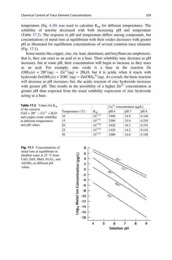
temperature (Eq. 4.10) was used to calculate Ksp for different temperatures. Thesolubility of tenorite decreased with both increasing pH and temperature(Table 17.2). The response to pH and temperature differs among compounds, butconcentrations of metal ions at equilibrium with their oxides decreases with greaterpH as illustrated for equilibrium concentrations of several common trace elements(Fig. 17.1).

Some metals like copper, zinc, tin, lead, aluminum, and beryllium are amphoteric;that is, they can react as an acid or as a base. Their solubility may decrease as pHincreases, but at some pH, their concentration will begin to increase as they reactas an acid. For example, zinc oxide is a base in the reaction Zn(OH)2(s) + 2H+(aq) ¼ Zn2+(aq) + 2H2O, but it is acidic when it reacts withhydroxide Zn(OH)2(s) + 2OH�(aq) ¼ Zn(OH)4

4+(aq). As a result, the basic reactionwill decrease as pH increases; but, the acidic reaction of zinc hydroxide increaseswith greater pH. This results in the possibility of a higher Zn2+ concentration atgreater pH than expected from the usual solubility expression of zinc hydroxideacting as a base.

Table 17.2 Values for Ksp

of the reactionCuO + 2H+ ¼ Cu2+ + H2Oand copper oxide solubilityat different temperaturesand pH values

Temperature (�C) Ksp

Cu2+ concentration (μg/L)pH 6 pH 7 pH 8

10 107.74 3490 34.9 0.349

15 107.61 2590 25.9 0.259

20 107.48 1920 19.2 0.192

25 107.35 1420 14.2 0.142

30 107.23 1080 10.8 0.108

Fig. 17.1 Concentrations ofmetal ions at equilibrium indistilled water at 25 �C fromCuO, ZnO, MnO, Fe2O3, andAl(OH)3 at different pHvalues


https://doi.org/10.1007/978-3-030-23335-8_4#Equ10

The redox potential increases in presence of dissolved oxygen and it greatlyinfluences the solubility of compounds of iron and several other elements. Thesolubility of ferrous iron from ferrous molybdate in pure water will be calculatedfrom Ksp (Table 17.1) in Ex. 17.3.

Ex. 17.3 The solubility of ferrous iron (Fe2+) from ferrous molybdate (FeMoO4)will be calculated.

Solution:The mass action form of the reaction (Table 17.1) is

Fe2þ� �

MoO2�4

� � ¼ 10�6:91

Letting X ¼ Fe2þ� � ¼ MoO2�

4

� �

X2 ¼ 10�6:91; X ¼ 10�3:455 or 3:51� 10�4 M Fe2þ and MoO2�4

In terms of Fe2+

3:51� 10�4 M � 55:84 g Fe2þ=gmw ¼ 0:0195 g=L Fe2þ or 20 mg=L Fe2þ:

The calculation of iron concentration in Ex. 17.3 is not the final result inoxygenated water, because Fe2+ oxidizes and precipitates as ferric hydroxide:

Fe2þ þ O2 þ H2O ¼ Fe OHð Þ3 # þHþ ð17:1ÞFerric hydroxide [Fe(OH)3] is quite insoluble at pH above 5.

Fe OHð Þ3 þ 3Hþ ¼ Fe3þ þ 3H2O K ¼ 103:54 ð17:2ÞAt pH 7, the concentration of Fe3+ is only 10–17.46 M—undetectable analytically.

Low redox potential in sediment increases the solubility of ferric hydroxidebecause ferric iron (Fe3+) is oxidized to soluble ferrous iron (Fe2+). Anaerobicbacteria in sediment produce sulfide (S2�) which reacts with ferrous iron and afew other metal ions to form insoluble metal sulfides, e.g., FeS and FeS2. Thesemetal sulfides precipitate in anaerobic sediment and do not enter the water column(Guo et al. 1997).

Despite the low solubility of Fe3+ and other trace metals, there will be detectableconcentrations of trace metals in water bodies. This results from metal ions reactingwith major ions, water, dissolved organic matter, ammonia, and cyanide to formsoluble associations.

Carbon dioxide can increase the solubility of carbonates above that expected fromKsp values. The Ksp for BaCO3 ¼ Ba + CO3

2� is 10–8.56, and from ΔG�, the reactionBaCO3 + CO2 + H2O ¼ Ba2+ + 2HCO3

� has a K ¼ 10–3.11. Calculations using thetwo equilibrium constants reveal that reaction of carbon dioxide increases the Ba2+

concentration at equilibrium by 2.3 mg/L.


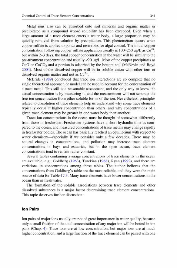
Metal ions also can be absorbed onto soil minerals and organic matter orprecipitated as a compound whose solubility has been exceeded. Even when alarge amount of a trace element enters a water body, a large proportion may bequickly removed from solution by precipitation. This phenomenon occurs whencopper sulfate is applied to ponds and reservoirs for algal control. The initial copperconcentration following copper sulfate application usually is 100–250 μg/L as Cu2+,but within 2–3 days, the total copper concentration in the water will be similar to thepre-treatment concentration and usually <20 μg/L. Most of the copper precipitates asCuO or CuCO3 and a portion is adsorbed by the bottom soil (McNevin and Boyd2004). Most of the dissolved copper will be in soluble union with other ions ordissolved organic matter and not as Cu2+.

McBride (1989) concluded that trace ion interactions are so complex that nosingle theoretical approach or model can be used to account for the concentration ofa trace metal. This still is a reasonable assessment, and the only way to know theactual concentration is by measuring it, and the measurement will not separate thefree ion concentration from other soluble forms of the ion. Nevertheless, principlesrelated to dissolution of trace elements help us understand why some trace elementstypically occur at higher concentration than others, and why concentrations of agiven trace element may be greater in one water body than another.

Trace ion concentrations in the ocean must be thought of somewhat differentlyfrom those in freshwater. Freshwater systems have a short hydraulic time as com-pared to the ocean, and measured concentrations of trace metals may change rapidlyin freshwater bodies. The ocean has basically reached an equilibrium with respect towater chemistry—especially if we consider only a few decades. There may benatural changes in concentrations, and pollution may increase trace elementconcentrations in bays and estuaries, but in the open ocean, trace elementconcentrations tend to remain rather constant.

Several tables containing average concentrations of trace elements in the oceanare available, e.g., Goldberg (1963), Turekian (1968), Ryan (1992), and there arevariations in concentrations among these tables. The author believes that theconcentrations from Goldberg’s table are the most reliable, and they were the mainsource of data for Table 17.3. Many trace elements have lower concentrations in theocean than in freshwater.

The formation of the soluble associations between trace elements and otherdissolved substances is a major factor determining trace element concentrations.This topic deserves further discussion.

Ion Pairs

Ion pairs of major ions usually are not of great importance in water quality, becauseonly a small fraction of the total concentration of any major ion will be bound in ionpairs (Chap. 4). Trace ions are at low concentration, but major ions are at muchhigher concentration, and a large fraction of the trace element can be paired with one


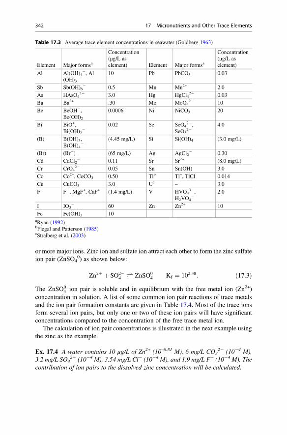
or more major ions. Zinc ion and sulfate ion attract each other to form the zinc sulfateion pair (ZnSO4

0) as shown below:

Zn2þ þ SO2�4 Ð ZnSO0

4 Kf ¼ 102:38: ð17:3ÞThe ZnSO0

4 ion pair is soluble and in equilibrium with the free metal ion (Zn2+)concentration in solution. A list of some common ion pair reactions of trace metalsand the ion pair formation constants are given in Table 17.4. Most of the trace ionsform several ion pairs, but only one or two of these ion pairs will have significantconcentrations compared to the concentration of the free trace metal ion.

The calculation of ion pair concentrations is illustrated in the next example usingthe zinc as the example.

Ex. 17.4 A water contains 10 μg/L of Zn2+ (10–6.81 M), 6 mg/L CO32� (10�4 M),

3.2 mg/L SO42� (10�4 M), 3.54 mg/L Cl� (10�4 M), and 1.9 mg/L F� (10�4 M). The

contribution of ion pairs to the dissolved zinc concentration will be calculated.

Table 17.3 Average trace element concentrations in seawater (Goldberg 1963)

Element Major formsa

Concentration(μg/L aselement) Element Major formsa

Concentration(μg/L aselement)

Al Al(OH)4�, Al

(OH)310 Pb PbCO3 0.03

Sb Sb(OH)6� 0.5 Mn Mn2+ 2.0

As HAsO42� 3.0 Hg HgCl4

2� 0.03

Ba Ba2+ .30 Mo MoO42� 10

Be BeOH�,Be(OH)2

0.0006 Ni NiCO3 20

Bi BiO+,Bi(OH)2

�0.02 Se SeO4

2�,SeO3

2�4.0

(B) B(OH)3,B(OH)4

�(4.45 mg/L) Si Si(OH)4 (3.0 mg/L)

(Br) (Br�) (65 mg/L) Ag AgCl2� 0.30

Cd CdCl2� 0.11 Sr Sr2+ (8.0 mg/L)

Cr CrO42� 0.05 Sn Sn(OH) 3.0

Co Co2+, CoCO3 0.50 Tlb Tl+, TlCl 0.014

Cu CuCO3 3.0 Uc– 3.0

F F�, MgF+, CaF+ (1.4 mg/L) V HVO43�,

H2VO4�

2.0

I IO3� 60 Zn Zn2+ 10

Fe Fe(OH)3 10aRyan (1992)bFlegal and Patterson (1985)cStralberg et al. (2003)


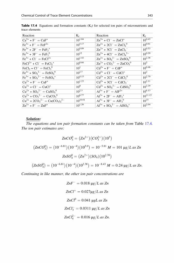
Solution:The equations and ion pair formation constants can be taken from Table 17.4.

The ion pair estimates are:

ZnCO03 ¼ Zn2þ

� �CO2þ

3

� �105� �

ZnCO03

� � ¼ 10�6:81� �

10�4� �

105:0� � ¼ 10�5:81 M ¼ 101 μg=L as Zn

ZnSO04 ¼ Zn2þ

� �SO4ð Þ 102:38

� �

ZnSO04

� � ¼ 10�6:81� �

10�4� �

102:38� � ¼ 10�8:43 M ¼ 0:24 μg=L as Zn:

Continuing in like manner, the other ion pair concentrations are

ZnF� ¼ 0:018 μg=L as Zn

ZnClþ ¼ 0:027μg=L as Zn

ZnCl0 ¼ 0:041 μgL as Zn

ZnCl�3 ¼ 0:0311 μg=L as Zn

ZnCl2�4 ¼ 0:016 μg=L as Zn:

Table 17.4 Equations and formation constants (Kf) for selected ion pairs of micronutrients andtrace elements

Reaction Kf Reaction Kf

Ca2+ + F� ¼ CaF+ 101.04 Zn2+ + Cl� ¼ ZnCl+ 100.43

Fe3+ + F� ¼ FeF2+ 105.17 Zn2+ + 2Cl� ¼ ZnCl20 100.61

Fe3+ + 2F� ¼ FeF2+ 109.09 Zn2+ + 3Cl� ¼ ZnCl3

� 100.53

Fe3+ + 3F� ¼ FeF30 1012 Zn2+ + 4Cl� ¼ ZnCl4

2� 100.20

Fe3+ + Cl� ¼ FeCl2+ 101.42 Zn2+ + SO42� ¼ ZnSO4

0 102.38

FeCl2+ + Cl� ¼ FeCl2+ 100.66 Zn2+ + CO3

2� ¼ ZnCO30 105

FeCl2 + Cl� ¼ FeCl30 101 Cd2+ + F� ¼ CdF+ 100.46

Fe2+ + SO42� ¼ FeSO4

0 102.7 Cd2+ + Cl� ¼ CdCl+ 102

Fe3+ + SO42� ¼ FeSO4

+ 104.15 Cd2+ + 2Cl� ¼ CdCl20 102.70

Cu2+ + F� ¼ CuF+ 101.23 Cd2+ + 3Cl� ¼ CdCl3� 102.11

Cu2+ + Cl� ¼ CuCl+ 100 Cd2+ + SO42� ¼ CdSO4

0 102.29

Cu2+ + SO42� ¼ CuSO4

0 102.3 Al3+ + F� ¼ AlF2+ 106.13

Cu2+ + CO32� ¼ CuCO3

0 106.77 Al3+ + 2F� ¼ AlF2+ 1011.15

Cu2+ + 2CO32� ¼ Cu(CO3)2

2� 1010.01 Al3+ + 3F� ¼ AlF30 1015

Zn2+ + F� ¼ ZnF+ 101.26 Al3+ + SO42� ¼ AlSO4

+ 102.04


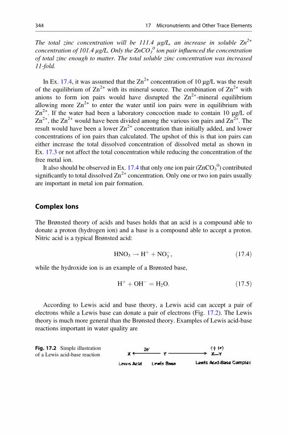
The total zinc concentration will be 111.4 μg/L, an increase in soluble Zn2+

concentration of 101.4 μg/L. Only the ZnCO30 ion pair influenced the concentration

of total zinc enough to matter. The total soluble zinc concentration was increased11-fold.

In Ex. 17.4, it was assumed that the Zn2+ concentration of 10 μg/L was the resultof the equilibrium of Zn2+ with its mineral source. The combination of Zn2+ withanions to form ion pairs would have disrupted the Zn2+-mineral equilibriumallowing more Zn2+ to enter the water until ion pairs were in equilibrium withZn2+. If the water had been a laboratory concoction made to contain 10 μg/L ofZn2+, the Zn2+ would have been divided among the various ion pairs and Zn2+. Theresult would have been a lower Zn2+ concentration than initially added, and lowerconcentrations of ion pairs than calculated. The upshot of this is that ion pairs caneither increase the total dissolved concentration of dissolved metal as shown inEx. 17.3 or not affect the total concentration while reducing the concentration of thefree metal ion.

It also should be observed in Ex. 17.4 that only one ion pair (ZnCO30) contributed

significantly to total dissolved Zn2+ concentration. Only one or two ion pairs usuallyare important in metal ion pair formation.

Complex Ions

The Brønsted theory of acids and bases holds that an acid is a compound able todonate a proton (hydrogen ion) and a base is a compound able to accept a proton.Nitric acid is a typical Brønsted acid:

HNO3 ! Hþ þ NO�3 , ð17:4Þ

while the hydroxide ion is an example of a Brønsted base,

Hþ þ OH� ¼ H2O: ð17:5Þ

According to Lewis acid and base theory, a Lewis acid can accept a pair ofelectrons while a Lewis base can donate a pair of electrons (Fig. 17.2). The Lewistheory is much more general than the Brønsted theory. Examples of Lewis acid-basereactions important in water quality are

Fig. 17.2 Simple illustrationof a Lewis acid-base reaction


Cu2þ þ 4NH3 ¼ Cu NH3ð Þ2þ4 ð17:6Þ

Fe2þ þ 6CN� ¼ Fe CNð Þ3�6 ð17:7Þ

PbCl2 þ 2Cl� ¼ PbCl2�4 ð17:8ÞAgþ þ 2NH3 ¼ Ag NH3ð Þ2: ð17:9Þ

Lewis acid-base reactions occur in natural waters, and they are important in waterswith high concentrations of ammonia, cyanide, and certain other pollutants.Reactions in Eqs. 17.6, 17.7, 17.8, and 17.9 reveal that potentially toxic traceelements can be put into solution by reaction with other ions according to Lewisacid-base theory.

Hydrolysis of Metal Ions

Hydrolysis also involves the Lewis acid-base concept, and metal ions hydrolyze inwater causing an acid reaction and formation of a soluble, metal-hydroxide complexor hydrolysis product as illustrated for the cupric ion (Cu2+):

Cu2þ þ H2O ¼ CuOHþ þ Hþ: ð17:10ÞThe hydrolysis may alternatively be written as:

Cu2þ þ OH� ¼ CuOHþ: ð17:11ÞIn both representations, H+ and OH� are related to the dissociation of water(H2O ¼ H+ + OH�) and H+ increases relative to OH� causing pH to decrease.

The mass action expression of Eq. 17.11 multiplied by the mass action form of thereaction for dissociation of water gives the mass action form of Eq. 17.10:

CuOHþð ÞCu2þð Þ OH�ð Þ � Hþð Þ OH�ð Þ ¼ CuOH�ð Þ Hþð Þ

Cu2þð Þ :

This exercise confirms that the two reactions have the same relationship to water andhydrogen ion concentration (or pH)—they are simply two ways of expressing thesame reaction.

The amphoteric property of trace metals deserves some further comment. Anotherway of writing the reactions of zinc oxide to illustrate its amphoterism is:

ZnOþ HCl ¼ Zn2þ þ Cl� þ H2O ð17:12Þand


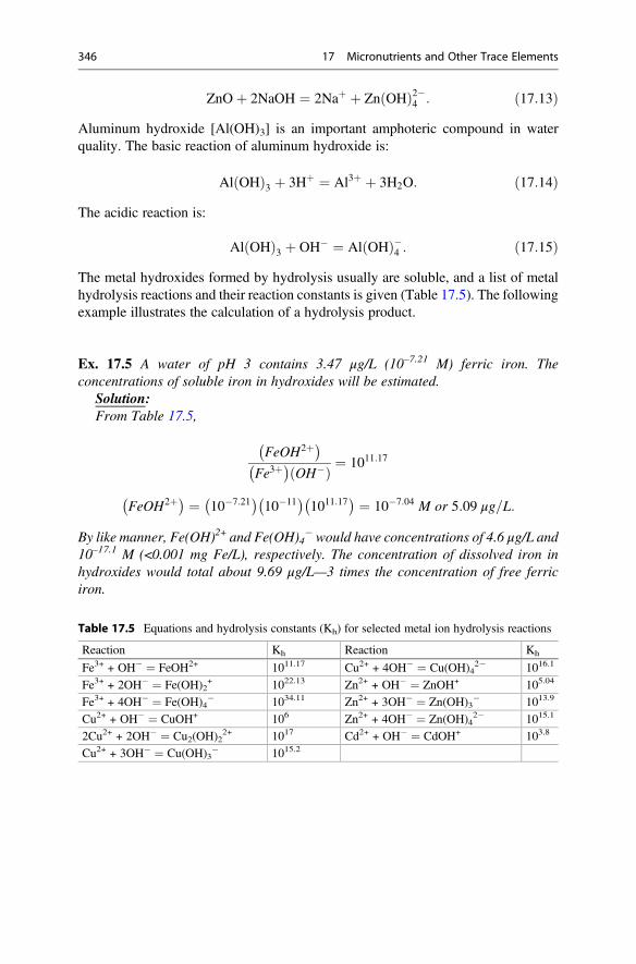
ZnOþ 2NaOH ¼ 2Naþ þ Zn OHð Þ2�4 : ð17:13ÞAluminum hydroxide [Al(OH)3] is an important amphoteric compound in waterquality. The basic reaction of aluminum hydroxide is:

Al OHð Þ3 þ 3Hþ ¼ Al3þ þ 3H2O: ð17:14ÞThe acidic reaction is:

Al OHð Þ3 þ OH� ¼ Al OHð Þ�4 : ð17:15ÞThe metal hydroxides formed by hydrolysis usually are soluble, and a list of metalhydrolysis reactions and their reaction constants is given (Table 17.5). The followingexample illustrates the calculation of a hydrolysis product.

Ex. 17.5 A water of pH 3 contains 3.47 μg/L (10–7.21 M) ferric iron. Theconcentrations of soluble iron in hydroxides will be estimated.

Solution:From Table 17.5,

FeOH2þ� �

Fe3þ� �

OH�ð Þ ¼ 1011:17

FeOH2þ� � ¼ 10�7:21� �

10�11� �

1011:17� � ¼ 10�7:04 M or 5:09 μg=L:

By like manner, Fe(OH)2+ and Fe(OH)4� would have concentrations of 4.6 μg/L and

10–17.1 M (<0.001 mg Fe/L), respectively. The concentration of dissolved iron inhydroxides would total about 9.69 μg/L—3 times the concentration of free ferriciron.

Table 17.5 Equations and hydrolysis constants (Kh) for selected metal ion hydrolysis reactions

Reaction Kh Reaction Kh

Fe3+ + OH� ¼ FeOH2+ 1011.17 Cu2+ + 4OH� ¼ Cu(OH)42� 1016.1

Fe3+ + 2OH� ¼ Fe(OH)2+ 1022.13 Zn2+ + OH� ¼ ZnOH+ 105.04

Fe3+ + 4OH� ¼ Fe(OH)4� 1034.11 Zn2+ + 3OH� ¼ Zn(OH)3

� 1013.9

Cu2+ + OH� ¼ CuOH+ 106 Zn2+ + 4OH� ¼ Zn(OH)42� 1015.1

2Cu2+ + 2OH� ¼ Cu2(OH)22+ 1017 Cd2+ + OH� ¼ CdOH+ 103.8

Cu2+ + 3OH� ¼ Cu(OH)3� 1015.2


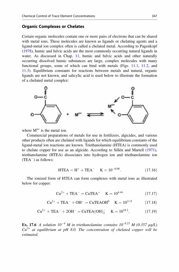
Organic Complexes or Chelates

Certain organic molecules contain one or more pairs of electrons that can be sharedwith metal ions. These molecules are known as ligands or chelating agents and aligand-metal ion complex often is called a chelated metal. According to Pagenkopf(1978), humic and fulvic acids are the most commonly occurring natural ligands inwater. As discussed in Chap. 11, humic and fulvic acids and other naturallyoccurring dissolved humic substances are large, complex molecules with manyfunctional groups, some of which can bind with metals (Figs. 11.1, 11.2, and11.3). Equilibrium constants for reactions between metals and natural, organicligands are not known, and salicylic acid is used below to illustrate the formationof a chelated metal complex:

where Mn+ is the metal ion.Commercial preparations of metals for use in fertilizers, algicides, and various

other products often are chelated with ligands for which equilibrium constants of theligand-metal ion reactions are known. Triethanolamine (HTEA) is commonly usedto chelate copper for use as an algicide. According to Sillén and Martell (1971),triethanolamine (HTEA) dissociates into hydrogen ion and triethanolamine ion(TEA�) as follows:

HTEA ¼ Hþ þ TEA� K ¼ 10�8:08: ð17:16ÞThe ionized form of HTEA can form complexes with metal ions as illustrated

below for copper:

Cu2þ þ TEA� ¼ CuTEAþ K ¼ 104:44 ð17:17Þ

Cu2þ þ TEA� þ OH� ¼ CuTEAOH0 K ¼ 1011:9 ð17:18Þ

Cu2þ þ TEA� þ 2OH� ¼ CuTEA OHð Þ�2 K ¼ 1018:2: ð17:19Þ

Ex. 17.6 A solution 10�4 M in triethanolamine contains 10–8.25 M (0.357 μg/L)Cu2+ at equilibrium at pH 8.0. The concentration of chelated copper will beestimated.


Solution:The triethanolamine concentration is given, so the TEA� concentration available

to chelate copper will be computed. From Eq. 17.16,

Hþð Þ TEA�ð ÞHTEAð Þ ¼ 10�8:08

TEA�ð ÞHTEAð Þ ¼

10�8:08

10�8 ¼ 10�0:08 ¼ 0:83

%TEA� ¼ 0:831:83

� 100 ¼ 45:4%:

The HTEA concentration is 0.0001 M, and TEA� ¼ (0.0001)(0.454) ¼ 0.0000454 M ¼ 10–4.34 M.

Equations 17.17, 17.18, and 17.19 allow computations of concentrations oftriethanolamine-chelated copper complexes:

Cu2þ þ TEA� ¼ CuTEAþ

CuTEAþð Þ ¼ Cu2þ� �

TEA�ð Þ K ¼ 10�8:35� �

10�4:34� �

104:44� �

¼ 10�8:25 M 0:357 μg Cu2þ=L� �

:

Following the same procedure, the copper concentrations in CuTEAOH0 andCuTEA(OH)2

� are 10�6 M (63.6 μg/L) and 10–6.49 M (20.6 μg/L), respectively.The total concentration of chelated copper is 84.6 μg/L or two orders of magnitudegreater than the Cu2+ concentration.

Role of Metal Hydroxides, Ion Pairs, and Chelates in Solubility

Equilibrium concentrations of free trace metal ions in natural water bodies are loweven where the controlling minerals occur in abundance. Free metal ions are inequilibrium with their controlling minerals, but they also are in equilibrium with ionpairs and inorganic and organic complexes as illustrated in Fig. 17.3 for copper ion.The presence of dissolved copper associations does not alter the concentration ofCu2+ at equilibrium with CuO. The dissolved associations usually result in moredissolved copper than would be expected from the Ksp calculation for CuO, and thesame situation is true for other metals. At pH 7, the equilibrium concentration of Fe3+

is calculated from the Ksp of one of the ferric iron minerals listed in Table 17.1 isundetectable by analytical methods, but the dissolved iron concentrations in naturalwaters are usually 100–500 μg/L. Waters that contain large amounts of humicsubstances may have higher total dissolved iron concentrations.


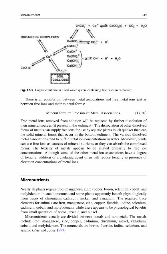
There is an equilibrium between metal associations and free metal ions just asbetween free ions and their mineral forms:

Mineral form Ð Free ion Ð Metal Associations: ð17:20ÞFree metal ions removed from solution will be replaced by further dissolution oftheir mineral sources (if present in the sediment). The dissociation of other dissolvedforms of metals can supply free ions for use by aquatic plants much quicker than canthe solid mineral forms that occur in the bottom sediment. The various dissolvedmetal associations tend to buffer metal ion concentrations in water. Moreover, plantscan use free ions as sources of mineral nutrients or they can absorb the complexedforms. The toxicity of metals appears to be related primarily to free ionconcentrations. Although some of the other metal ion associations have a degreeof toxicity, addition of a chelating agent often will reduce toxicity in presence ofelevation concentrations of metal ions.

Micronutrients

Nearly all plants require iron, manganese, zinc, copper, boron, selenium, cobalt, andmolybdenum in small amounts, and some plants apparently benefit physiologicallyfrom traces of chromium, cadmium, nickel, and vanadium. The required traceelements for animals are iron, manganese, zinc, copper, fluoride, iodine, selenium,cadmium, cobalt, and molybdenum, while there appears to be physiological benefitsfrom small quantities of boron, arsenic, and nickel.

Micronutrients usually are divided between metals and nonmetals. The metalsinclude iron, manganese, zinc, copper, cadmium, chromium, nickel, vanadium,cobalt, and molybdenum. The nonmetals are boron, fluoride, iodine, selenium, andarsenic (Pais and Jones 1997).

Fig. 17.3 Copper equilibria in a soil-water system containing free calcium carbonate

Micronutrients 349

Iron (Fe)

The two main iron ores are hematite (F2O3) and magnetite (Fe3O4). Of course, ironoccurs in other oxides, hydroxides, sulfides, sulfates, arsenates, and carbonates. Ironoxides and hydroxides are abundant in soil.

Many enzymes such as peroxidases, catalases, and cytochrome oxidases impor-tant in cellular energy transformations contain iron. Iron proteins (ferredoxins) areinvolved in phytophosphorylation in photosynthesis. Hemoglobin in the blood ofanimals contains an iron porphyrin ring.

Iron concentrations seldom are great enough to be harmful to aquatic life.Nevertheless, it precipitates in water and the resulting floc can be harmful in fishhatcheries by settling on eggs and by occluding the gills of fish. Precipitates of ironon other biological surfaces also can be harmful.

The solubility of iron compounds under aerobic conditions is controlled mainlyby pH, and except at very low pH, the oxides and hydroxides found in soil are of lowsolubilities. But, iron is abundant in nature and dissolved ion associations increaseiron concentrations, and freshwaters contain 250 μg/L to 1000 μg/L and even morein water heavily stained by humic substances. Polluted acidic waters can have veryhigh iron concentrations. Ocean water has an average of 10 μg/L of iron mostly inthe form of Fe(OH)3.

Iron has been shown to limit phytoplankton productivity in freshwater bodies(Hyenstrand et al. 2000; Vrede and Tranvik 2006) and in the ocean (Nadis 1998).There have been suggested that fertilization of the ocean with iron could increase itsproductivity and thereby increase both global fish supply and counteract globalwarming through carbon sequestration.

Respiration in sediment uses dissolved oxygen from the pore water faster thanoxygen enters by diffusion and infiltration. This leads to anaerobic conditions otherthan in the layer near the sediment-water interface. Ferric iron and other oxidizedsubstances in anaerobic sediment act as oxidizing agents by accepting electrons:

Fe3þ þ e� ¼ Fe2þ: ð17:21ÞSome types of bacteria under anaerobic conditions can use ferric iron as a substitutefor molecular oxygen as an acceptor of electrons and hydrogen ions resulting fromrespiration. The general process of iron reduction by bacteria is illustrated below:

Organic matter ! fragments such as CH3COOH ð17:22ÞCH3COOHþ 6H2O ! 2CO2 þ 8Hþ ð17:23Þ

8Fe OHð Þ3 þ 8Hþ ! 8Fe OHð Þ2 þ 8H2O ð17:24Þ

Fe OHð Þ2 ¼ Fe2þ þ 2OH�: ð17:25ÞAnaerobic respiration increases the Fe2+ concentration in sediment pore water andoxygen-depleted hypolimnetic water. Ferrous iron concentrations begin to increase


at redox potentials of 0.2–0.3 volt. Concentrations up to 5–10 mg/L of ferrous ironare common, and concentrations several times this have been measured in bottomsoil of fertilized fish ponds.

Water from some wells may contain high concentrations of iron because of lowredox potential in aquifers. Ferric hydroxide tends to control iron concentration inshallow aquifers where redox potential usually is comparatively high, andconcentrations of ferrous iron usually will be low (Hem 1985). Deep wells oftendraw water from aquifers where there is a low redox potential and ironconcentrations may be controlled by iron sulfide,

FeS2 ¼ Fe2þ þ 2S2� K ¼ 10�26: ð17:26ÞGroundwater usually contains sulfate, and sulfate-reducing bacteria reduce sulfate tosulfide in respiration. Ferrous iron also is present from anaerobic respiration, andiron precipitates as insoluble ferrous sulfide. Waters from deep aquifers usuallycontain very little iron, but they may yield waters high in sulfide concentration. Inaquifers of intermediate depth, redox potential is intermediate between that ofshallow and deep aquifers. Ferrous carbonate (siderite) tends to be the mineralcontrolling iron concentration in aquifers of intermediate depth:

FeCO3 þ Hþ ¼ Fe2þ þ HCO�3 K ¼ 10�0:3: ð17:27Þ

Very high concentrations of iron (up to 100 mg/L or more) may occur in waters fromaquifers where siderite is the iron-controlling mineral.

Organic matter decomposition in waterlogged soil and in sediment causes lowredox potential and high concentrations of ferrous iron often result. The pH usuallywill be between 6 and 6.5 in such situations (Ex. 17.7).

Ex. 17.7 The pH will be estimated for a sediment in which the pore water contains20 mg/L (10–3.47 M) Fe2+ and 61 mg/L (10�3 M) HCO3

�.Solution:From Eq. 17.27,

Fe2þ� �

HCO�3

� �Hþð Þ ¼ 10�0:3

Hþð Þ ¼ Fe2þ� �

HCO�3

� �

10�0:3 ¼ 10�3:47� �

10�3� �

10�0:3 ¼ 10�6:17

pH ¼ 6:17:

When water containing ferrous iron contacts oxygen, precipitation of ironcompounds occur as illustrated below:

4Fe HCO3ð Þ2 þ 2H2Oþ O2 ¼ 4Fe OHð Þ3 # þ8CO2: ð17:28Þ

Micronutrients 351

Ferric hydroxide precipitation from water following oxygenation can stain plumbingfixtures and kitchen utensils, and clothes laundered in such water may be perma-nently stained.

Iron bacteria such as Leptothrix ochracea and Spirophyllum ferrugineum obtainenergy for the synthesis of organic compounds (chemoautotrophy) from oxidation offerrous salts as follows:

4FeCO3 þ O2 þ 6H2O ¼ 4Fe OHð Þ3 # þ4CO2: ð17:29ÞThese bacteria tend to form slimy mats known as ochre where waters containing ahigh concentration of iron flow or seep onto the land surface and absorbs oxygenfrom the air.

Manganese (Mn)

The principal ore of manganese is manganese dioxide (MnO2). There are otheroxides and hydroxides of manganese, and a great many other manganese compoundsin nature. Soils usually contain manganese at a much lower concentration than atwhich iron is present.

Manganese is a nutrient, because it is a constituent of enzymes or acts as anenzyme activator. This element is particularly important in the action of antioxidants,and catalyzes the photolysis reaction that releases oxygen in photosynthesis. Man-ganese, like iron, seldom causes toxicity, but elevated concentrations of manganesehave been reported to be toxic to benthic invertebrates (Pinsino et al. 2012). Also,like iron, manganese can precipitate in water having various mechanical effects onorganisms. It also can stain plumbing fixtures and cause laundry stains.

The factors governing the solubility of manganese are similar to those discussedfor iron under both aerobic and anaerobic conditions. The concentration of Mn2+ inwater is usually very low, and it occurs mainly in combination with other dissolvedsubstances. Manganese concentrations usually are considerably lower than those ofiron, because of its lower abundance than iron in nature. Maximum concentrations ofmanganese typically will be below 100 μg/L in unpolluted natural waters. Theaverage manganese concentration in the ocean is given as 2 μg/L.

Copper (Cu)

The main ore of copper is an iron-copper sulfide (CuFeS2) known as chalcopyrite,and it also is present in other sulfide deposits, sandstones, and shales. Copper ispresent in soil mainly as copper adsorbed on clay and organic matter.

Copper is a cofactor in many metalloenzymes including those that catalyze RNAand DNA synthesis, melanin production, electron transfers in respiration, collagenand elastin formation. Plants require copper for chlorophyll synthesis, root metabo-lism, and lignification.


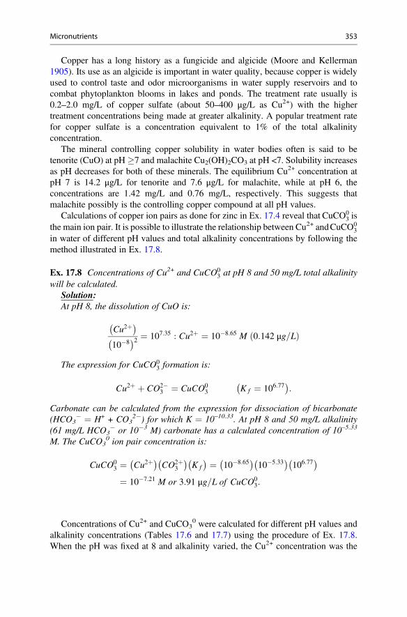
Copper has a long history as a fungicide and algicide (Moore and Kellerman1905). Its use as an algicide is important in water quality, because copper is widelyused to control taste and odor microorganisms in water supply reservoirs and tocombat phytoplankton blooms in lakes and ponds. The treatment rate usually is0.2–2.0 mg/L of copper sulfate (about 50–400 μg/L as Cu2+) with the highertreatment concentrations being made at greater alkalinity. A popular treatment ratefor copper sulfate is a concentration equivalent to 1% of the total alkalinityconcentration.

The mineral controlling copper solubility in water bodies often is said to betenorite (CuO) at pH�7 and malachite Cu2(OH)2CO3 at pH <7. Solubility increasesas pH decreases for both of these minerals. The equilibrium Cu2+ concentration atpH 7 is 14.2 μg/L for tenorite and 7.6 μg/L for malachite, while at pH 6, theconcentrations are 1.42 mg/L and 0.76 mg/L, respectively. This suggests thatmalachite possibly is the controlling copper compound at all pH values.

Calculations of copper ion pairs as done for zinc in Ex. 17.4 reveal that CuCO03 is

the main ion pair. It is possible to illustrate the relationship between Cu2+ andCuCO03

in water of different pH values and total alkalinity concentrations by following themethod illustrated in Ex. 17.8.

Ex. 17.8 Concentrations of Cu2+ and CuCO03 at pH 8 and 50 mg/L total alkalinity

will be calculated.Solution:At pH 8, the dissolution of CuO is:

Cu2þ� �

10�8� �2 ¼ 107:35 : Cu2þ ¼ 10�8:65 M 0:142 μg=Lð Þ

The expression for CuCO03 formation is:

Cu2þ þ CO2�3 ¼ CuCO0

3 K f ¼ 106:77� �

:

Carbonate can be calculated from the expression for dissociation of bicarbonate(HCO3

� ¼ H+ + CO32�) for which K ¼ 10–10.33. At pH 8 and 50 mg/L alkalinity

(61 mg/L HCO3� or 10�3 M) carbonate has a calculated concentration of 10–5.33

M. The CuCO30 ion pair concentration is:

CuCO03 ¼ Cu2þ

� �CO2þ

3

� �K f

� � ¼ 10�8:65� �

10�5:33� �

106:77� �

¼ 10�7:21 M or 3:91 μg=L of CuCO03:

Concentrations of Cu2+ and CuCO30 were calculated for different pH values and

alkalinity concentrations (Tables 17.6 and 17.7) using the procedure of Ex. 17.8.When the pH was fixed at 8 and alkalinity varied, the Cu2+ concentration was the

Micronutrients 353

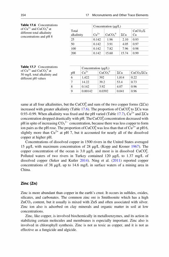
same at all four alkalinities, but the CuCO03 and sum of the two copper forms (ΣCu)

increased with greater alkalinity (Table 17.6). The proportion of CuCO03 to ΣCu was

0.93–0.99. When alkalinity was fixed and the pH varied (Table 17.7), Cu2+ and ΣCuconcentration dropped drastically with pH. TheCuCO0

3 concentration decreased withpH in spite of increasing CO3

2� concentration, because there was less copper to formion pairs as the pH rose. The proportion ofCuCO0

3 was less than that of Cu2+ at pH 6,

slightly more than Cu2+ at pH 7, but it accounted for nearly all of the dissolvedcopper at higher pH.

Concentrations of dissolved copper in 1500 rivers in the United States averaged15 μg/L with maximum concentration of 28 μg/L (Kopp and Kroner 1967). Thecopper concentration of the ocean is 3.0 μg/L and most is in dissolved CuCO0

3.Polluted waters of two rivers in Turkey contained 120 μg/L to 1.37 mg/L ofdissolved copper (Seker and Kutler 2014). Ning et al. (2011) reported copperconcentrations of 38 μg/L up to 14.6 mg/L in surface waters of a mining area inChina.

Zinc (Zn)

Zinc is more abundant than copper in the earth’s crust. It occurs in sulfides, oxides,silicates, and carbonates. The common zinc ore is Smithsonite which has a highZnCO3 content, but it usually is mixed with ZnS and often associated with silver.Zinc ion also is adsorbed on clay minerals and organic matter in soil at lowconcentrations.

Zinc, like copper, is involved biochemically in metalloenzymes, and its action instabilizing certain molecules and membranes is especially important. Zinc also isinvolved in chlorophyll synthesis. Zinc is not as toxic as copper, and it is not aseffective as a fungicide and algicide.

Table 17.7 Concentrationsof Cu2+ and CuCO3

0 at50 mg/L total alkalinity anddifferent pH values

pH

Concentration (μg/L)Cu2+ CuCO3

0 ΣCu CuCO3/ΣCu6 1,422 392 1,814 0.22

7 14.22 39.2 53.4 0.73

8 0.142 3.92 4.07 0.96

9 0.00142 0.0392 0.041 0.96

Table 17.6 Concentrationsof Cu2+ and CuCO3

0 atdifferent total alkalinityconcentrations and pH 8

Totalalkalinity

Concentration (μg/L)

Cu2+ CuCO30 ΣCu

CuCO3/ΣCu

25 0.142 1.96 2.10 0.93

50 0.142 3.91 4.05 0.97

100 0.142 7.82 7.96 0.98

200 0.142 15.60 15.74 0.99


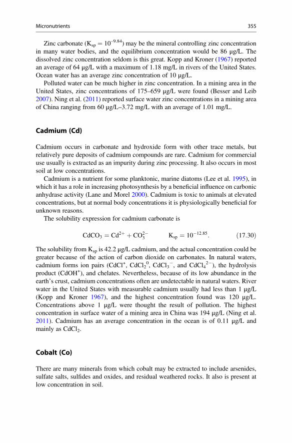
Zinc carbonate (Ksp ¼ 10–9.84) may be the mineral controlling zinc concentrationin many water bodies, and the equilibrium concentration would be 86 μg/L. Thedissolved zinc concentration seldom is this great. Kopp and Kroner (1967) reportedan average of 64 μg/L with a maximum of 1.18 mg/L in rivers of the United States.Ocean water has an average zinc concentration of 10 μg/L.

Polluted water can be much higher in zinc concentration. In a mining area in theUnited States, zinc concentrations of 175–659 μg/L were found (Besser and Leib2007). Ning et al. (2011) reported surface water zinc concentrations in a mining areaof China ranging from 60 μg/L–3.72 mg/L with an average of 1.01 mg/L.

Cadmium (Cd)

Cadmium occurs in carbonate and hydroxide form with other trace metals, butrelatively pure deposits of cadmium compounds are rare. Cadmium for commercialuse usually is extracted as an impurity during zinc processing. It also occurs in mostsoil at low concentrations.

Cadmium is a nutrient for some planktonic, marine diatoms (Lee et al. 1995), inwhich it has a role in increasing photosynthesis by a beneficial influence on carbonicanhydrase activity (Lane and Morel 2000). Cadmium is toxic to animals at elevatedconcentrations, but at normal body concentrations it is physiologically beneficial forunknown reasons.

The solubility expression for cadmium carbonate is

CdCO3 ¼ Cd2þ þ CO2�3 Ksp ¼ 10�12:85: ð17:30Þ

The solubility from Ksp is 42.2 μg/L cadmium, and the actual concentration could begreater because of the action of carbon dioxide on carbonates. In natural waters,cadmium forms ion pairs (CdCl+, CdCl2

0, CdCl3�, and CdCl4

2�), the hydrolysisproduct (CdOH+), and chelates. Nevertheless, because of its low abundance in theearth’s crust, cadmium concentrations often are undetectable in natural waters. Riverwater in the United States with measurable cadmium usually had less than 1 μg/L(Kopp and Kroner 1967), and the highest concentration found was 120 μg/L.Concentrations above 1 μg/L were thought the result of pollution. The highestconcentration in surface water of a mining area in China was 194 μg/L (Ning et al.2011). Cadmium has an average concentration in the ocean is of 0.11 μg/L andmainly as CdCl2.

Cobalt (Co)

There are many minerals from which cobalt may be extracted to include arsenides,sulfate salts, sulfides and oxides, and residual weathered rocks. It also is present atlow concentration in soil.

Micronutrients 355

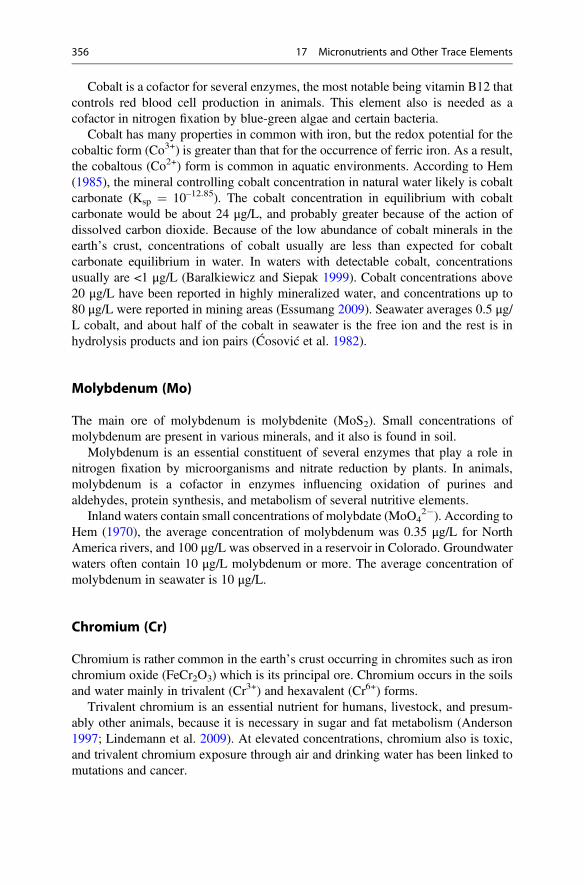
Cobalt is a cofactor for several enzymes, the most notable being vitamin B12 thatcontrols red blood cell production in animals. This element also is needed as acofactor in nitrogen fixation by blue-green algae and certain bacteria.

Cobalt has many properties in common with iron, but the redox potential for thecobaltic form (Co3+) is greater than that for the occurrence of ferric iron. As a result,the cobaltous (Co2+) form is common in aquatic environments. According to Hem(1985), the mineral controlling cobalt concentration in natural water likely is cobaltcarbonate (Ksp ¼ 10–12.85). The cobalt concentration in equilibrium with cobaltcarbonate would be about 24 μg/L, and probably greater because of the action ofdissolved carbon dioxide. Because of the low abundance of cobalt minerals in theearth’s crust, concentrations of cobalt usually are less than expected for cobaltcarbonate equilibrium in water. In waters with detectable cobalt, concentrationsusually are <1 μg/L (Baralkiewicz and Siepak 1999). Cobalt concentrations above20 μg/L have been reported in highly mineralized water, and concentrations up to80 μg/L were reported in mining areas (Essumang 2009). Seawater averages 0.5 μg/L cobalt, and about half of the cobalt in seawater is the free ion and the rest is inhydrolysis products and ion pairs (Ćosović et al. 1982).

Molybdenum (Mo)

The main ore of molybdenum is molybdenite (MoS2). Small concentrations ofmolybdenum are present in various minerals, and it also is found in soil.

Molybdenum is an essential constituent of several enzymes that play a role innitrogen fixation by microorganisms and nitrate reduction by plants. In animals,molybdenum is a cofactor in enzymes influencing oxidation of purines andaldehydes, protein synthesis, and metabolism of several nutritive elements.

Inland waters contain small concentrations of molybdate (MoO42�). According to

Hem (1970), the average concentration of molybdenum was 0.35 μg/L for NorthAmerica rivers, and 100 μg/L was observed in a reservoir in Colorado. Groundwaterwaters often contain 10 μg/L molybdenum or more. The average concentration ofmolybdenum in seawater is 10 μg/L.

Chromium (Cr)

Chromium is rather common in the earth’s crust occurring in chromites such as ironchromium oxide (FeCr2O3) which is its principal ore. Chromium occurs in the soilsand water mainly in trivalent (Cr3+) and hexavalent (Cr6+) forms.

Trivalent chromium is an essential nutrient for humans, livestock, and presum-ably other animals, because it is necessary in sugar and fat metabolism (Anderson1997; Lindemann et al. 2009). At elevated concentrations, chromium also is toxic,and trivalent chromium exposure through air and drinking water has been linked tomutations and cancer.


Concentrations of chromium in rivers of the United States ranged from belowdetection to 112 μg/L with an average of 9.7 μg/L for water in which it could bedetected. Samples with particularly elevated concentrations were polluted withindustrial effluents. Chromium concentrations up to 60 μg/L were reported inwells in arid areas of southern California (Izbicki et al. 2008), and Ning et al.(2011) found a maximum surface water concentration of 75 μg/L in a mining areain China. There is an average of 0.05 μg/L of chromium in the ocean.

Vanadium (V)

Vanadium sulfide (VS4) and carnotite K2(UO2)2(VO4)2�3H2O are the main ores ofthis element, but it also is extracted from Venezuelan crude oil. It is present in soils atvery low concentration.

Vanadium has been identified as an essential element for the green algaeScenedesmus obliquus (Arnon and Wessel 1953), and for some marine macroalgae(Fries 1982). However, it is apparently not essential for higher plants or for animals.

Vanadium concentration is inland waters usually are very low. In some arid areaswith rocks of elevated vanadium concentration, river water may contain over 1 mg/Lof vanadium (Livingstone 1963). The ocean contains about 2 μg/L of vanadium.

Nickel (Ni)

Nickel occurs in nature as oxides, sulfides, and silicates. The geochemistry of nickelis similar to that of iron.

Nickel is a cofactor at very low concentration in certain metalloenzyme functions.It has been recognized for several decades as an essential nutrient (Spears 1984).These studies have demonstrated that if nickel is absent in the diet, organisms do notgrow as well as when it is present in small amounts.

The ionic form of nickel in water is Ni2+, and it forms soluble hydroxides. Nickelcarbonate may be considered the controlling mineral:

NiCO3 ¼ Ni2þ þ CO3�2 Ksp ¼ 10�8:2: ð17:31Þ

Based on Ksp, a concentration of 4.66 mg/L would be possible at equilibrium, butsuch a high concentrations is not found in surface waters. Rivers in the United Statescontained up to 56 μg/L of nickel (Koop and Kroner 1967), and in another study,Durum and Haffty (1961) reported 10 μg/L as the average for North American rivers.Khan et al. (2011) reported 650 μg/L of nickel in the Shah Alum River inAfghanistan. Ocean water contains around 2 μg/L nickel mostly as NiCO3.

Micronutrients 357

Boron (B)

Boron is a metalloid having properties of both metals and nonmetals. Boron occursin relatively insoluble aluminosilicate minerals into which it substituted for siliconand aluminum. It also occurs in arid areas as borax (Na2B4O7�10H2O), ulexite(NaCaB5O9�8H2O) and other borate minerals which are mined to make boronproducts (Kochkodan et al. 2015). Its geochemical cycle is much like that ofchloride.

Plants require small amounts of boron, and there have been suggestions thatboron may be essential in animals. Boric acid forms bonds with molecules of pectinsin plant cell walls and glycolipids in bacterial cell walls to make the cell walls morestable. High boron concentrations in irrigation water are toxic to plants.

Boron behaves as a Lewis acid (Kochkodan et al. 2015) for which the firstdissociation is:

B OHð Þ3 þ H2O ¼ B OH4ð Þ� þ Hþ K ¼ 10�9:24: ð17:32ÞAt pH below 9.24, undissociated boric acid comprises more than 50% of the totaldissolved boron. For example, at pH 8, only 5% of boric acid is dissociated. Theother two dissociations with K values of 10–12.74 and 10–13.80, respectively, areseldom of water quality interest. Traditionally, boric acid was considered to dissoci-ate as a Brønsted acid and its dissociation often is still written as follows:

H3BO3 ¼ Hþ þ H2BO�3 K ¼ 10�9:24: ð17:33Þ

Boron concentration in freshwater bodies in the southeastern US seldom exceeds100 μg/L (Boyd and Walley 1972). A more extensive survey of 1546 river and lakesamples throughout the United States gave an average boron concentration of100 μg/L with a maximum of 5 mg/L (Kopp and Kroner 1970). Much greaterconcentrations can be found in saline inland waters of arid regions; concentrationsabove 100 mg/L were reported (Livingstone 1963). Boron occurs in the ocean as B(OH)3 and B(OH)4�, and its concentration averages about 4.5 mg/L.

Fluoride (F)

Fluoride, like chlorine, bromine, and iodine, is a highly electronegative element ofthe halogen group. Calcium fluoride (CaF2) is a common fluoride bearing mineral,and fluoride also is contained in apatite and some other common minerals. Fluoridecompounds are less abundant in the earth’s crust and of lower solubility than arechloride compounds. As a result, most fluoride in the earth’s crust is bound in rockswhile the sea is a huge reservoir of dissolved chloride.

Fluoride is a nutrient at optimal levels, because it is important to the integrity ofbone and teeth in humans and other animals. According to Palmer and Gilbert (2012),fluoridation of municipal water supplies for the prevention of dental cavities is likely


the most effective public dental health measure in existence. However, highconcentrations of fluoride in drinking water can cause bone disease and mottling oftooth enamel. The current recommended upper limit for fluoride in drinking water foravoiding health effects is 4 mg/L, and no negative cosmetic effects on teeth have beenreported for fluoride concentrations less than 2 mg/L. TheWorld Health Organization(WHO) suggested an upper limit of 1.5 mg/L for fluoride concentrations in drinkingwater (https://www.who.int/water_sanitation_health/dwq/chemicals/fluoride.pdf). Inthe United States, the recommended fluoride concentration in drinking water was0.7–1.2 mg/L for many years, but the maximum concentration limit was reduced to0.7 mg/L in 2015 (https://www.medicalnewstoday.com/articles/154164.php). Thereis a segment of society opposing fluoridation of drinking water, but the availableevidence does not support this concern.

The solubility of calcium fluoride may be expressed as follows:

CaF2 ¼ Ca2þ þ 2F� K ¼ 10�10:60: ð17:34ÞThe concentration of fluoride based on Ksp from calcium fluoride is 125 μg/L. Itforms ion pairs with the major cations and with many metals in water, and this wouldincrease concentration above that of the fluoride ion. Most freshwaters contain lessthan 100 μg/L of fluoride. Puntoriero et al. (2014) reported fluoride concentrationsranging from 0.15 μg/L to 1.37 mg/L in lakes of different continents. Ocean watertypically contains around 1.4 mg/L of fluoride present as F�, MgF+, and CaF+.

Iodine (I2)

Iodine is present as iodide (I�) and in combination with other elements in the earth’scrust. Iodide is obtained commercially by extracting it from natural brines or brinesfrom oil wells. Iodine (I2) also is extracted from seaweed.

Iodine is important for proper function of the thyroid gland in producing thyroidhormones needed for normal growth, development, and metabolism in humans andother vertebrates. In areas of the world where soils and waters are deficient in iodine,those who rely heavily on local sources of food may develop iodine-deficiencydisorders—the most famous of which is enlargement of the thyroid gland (goiter)producing a prominent swelling of the neck. The diet is an important source ofiodine, and in the past when foods were produced locally, the incidence of goiter washigh in areas where soils and crops produced in them were low in iodide. Dietaryiodine supplements such as iodized salt were and still are a preventive measure forgoiter. Since at least the 1960s, most people in developed countries obtain food frommany different places, and dietary iodine deficiency has become less common.

Being a halogen, iodide’s chemistry is similar to that of chloride and fluoride.According to Hem (1985), rainwater typically contains 1–3 μg/L of iodine, whilethe range for river water is 3–42 μg/L. The British Geological Survey (2000)reported that potable groundwater typically contained 1–70 μg/L iodide withextreme values up to 400 μg/L. Seawater has an average iodine concentration of60 μg/L mainly as IO3

�.

Micronutrients 359

https://www.who.int/water_sanitation_health/dwq/chemicals/fluoride.pdf

https://www.medicalnewstoday.com/articles/154164.php

Selenium (Se)

Selenium occurs in the earth’s crust mainly as elemental selenium, ferric selenite,and calcium selenite. The chemistry of selenium is similar to that of sulfur, but it ismuch less common than sulfur. The ion, SeO3

2� is the most stable form of seleniumin water.

Selenium is a component of the amino acids selenocysteine andselenomethionine. It also is a cofactor for certain peroxidases and reductases.Selenium accumulates in the food chain, and in spite of being an essential elementfor aquatic animals, selenium pollution can have serious consequences on aquaticecosystems (Hamilton 2004). Those who drink water of high selenium concentrationover many years may experience hair and fingernail loss, numbness in extremities,and circulation problems.

Selenium concentrations in groundwater and surface water seldom exceed 1 μg/L(Hem 1985), but concentrations of 0.06–400 μg/L have been reported. There is onereport of 6 mg/L of selenium in groundwater (World Health Organization 2011). Theaverage concentration of selenium in ocean water is 4 μg/L.

Arsenic (As)

Arsenic occurs in minerals such as arsenopyrite (AsFeS), realgar (AsS), and orpi-ment (As2S3) from which it is released by weathering as arsenate. Small percentagesof arsenate have substituted for phosphate in apatite (rock phosphate). Arseniccompounds tend to be of low solubility, and they are seldom abundant in soils orbottom sediments. The chemistry of arsenic and phosphorus is similar. Arsenic isstrongly absorbed on clay minerals and increases in solubility when redox potentialis low. Even the dissociation constants for the three step ionization of arsenic acid(H3AsO4) and orthophosphoric acid (H3PO4) are similar. Compare Eqs. 17.35,17.36, and 17.37 with Eqs. 14.1, 14.2, and 14.3).

H3AsO4 ¼ Hþ þ H2AsO�4 K ¼ 10�2:2 ð17:35Þ

H2AsO�4 ¼ Hþ þ HAsO2�

4 K ¼ 10�7 ð17:36Þ

HAsO2�4 ¼ Hþ þ AsO3�

4 K ¼ 10�11:5:: ð17:37ÞThe different arsenate ions also react similarly to phosphate ions, and arsenatecannot be distinguished from phosphate in the usual methods for determiningphosphate concentration.

Arsenic is considered a micronutrient because it apparently is a factor in methio-nine metabolism by certain animals (Uthus 1992). Arsenic is important in medicalhistory because it was once used to treat sleeping sickness and syphilis. It is still usedin treatment of acute promyelocytic leukemia.


https://doi.org/10.1007/978-3-030-23335-8_14#Equ1

https://doi.org/10.1007/978-3-030-23335-8_14#Equ2

https://doi.org/10.1007/978-3-030-23335-8_14#Equ3

Arsenic is most famous as a murder weapon. Arsenic trioxide is colorless,tasteless, and virtually impossible to detect in food and drink, and it becameknown as the “poison of kings.” Of course, it has been used for murder in all levelsof society. Arsenicals also are used as insecticides, fungicides, and woodpreservatives. The United States Army even has a chemical weapon that is anarsenical (Firth 2013).

Arsenate is the main form of arsenic in water, and the concentration range for itssoluble inorganic form is similar to phosphorus. Of course, arsenic is notaccumulated in plankton and detritus to the extent that phosphorus is. Accordingto Kopp (1969), arsenic concentrations in river water in the United States rangedfrom 5 to 336 μg/L with an average of 64 μg/L. Arsenic concentrations as high as187 μg/L were found in surface waters of a mining area in China (Ning et al. 2011).On average, ocean water contains 3 μg/L of arsenic.

Natural arsenic contamination of groundwater is a serious problem in a fewregions of the world. The most highly publicized incidence is in the lower GangesRiver basin in nine districts of West Bengal, India and 42 districts in Bangladeshwhere arsenic levels in drinking water exceed the World Health Organizationmaximum permissible limit of 50 μg/L (Chowdhury et al. 2000). In Bangladesh,about 21 million people use well waters with more than 50 μg/L arsenic, and somewell waters have over 1 mg/L. Arsenic poisoning symptoms include lesions, kerato-sis, conjunctival congestion, edema of feet, and liver and spleen enlargement. Inadvanced cases, cancers affecting lungs, uterus, bladder, and genitourinary tractoften are seen. According to Chowdhury et al. (2000), of 11,180 people examinedwho had been drinking water with over 50 μg/L of arsenic, about 25% had arsenicalskin lesions. An estimated 100 million people are at risk of arsenic poisoning inWestBengal and Bangladesh.

Elevated concentrations of arsenic in public water supplies increase cancer risk,and many countries have been imposing stricter arsenic standards for drinkingwaters. In the United States, the standard was 50 μg/L for many years, but in2006, it was reduced to 10 μg/L. Of course, many municipal water supplies havenot yet complied with the new standard.

Nonessential Trace Elements

Nonessential elements are of concern in water quality mainly because, likemicronutrients, they can be toxic to aquatic organisms at elevated concentrations.Trace elements also can be toxic through drinking water for humans, livestock, andother animals.

Aluminum (Al)

Aluminum is present in many silicate rocks and in deposits of aluminum oxides andhydroxides, and only oxygen and silicon exceed aluminum in abundance in theearth’s crust. Deposits of bauxite, a mixture of gibbsite [Al(OH)3] and boehmite

Nonessential Trace Elements 361

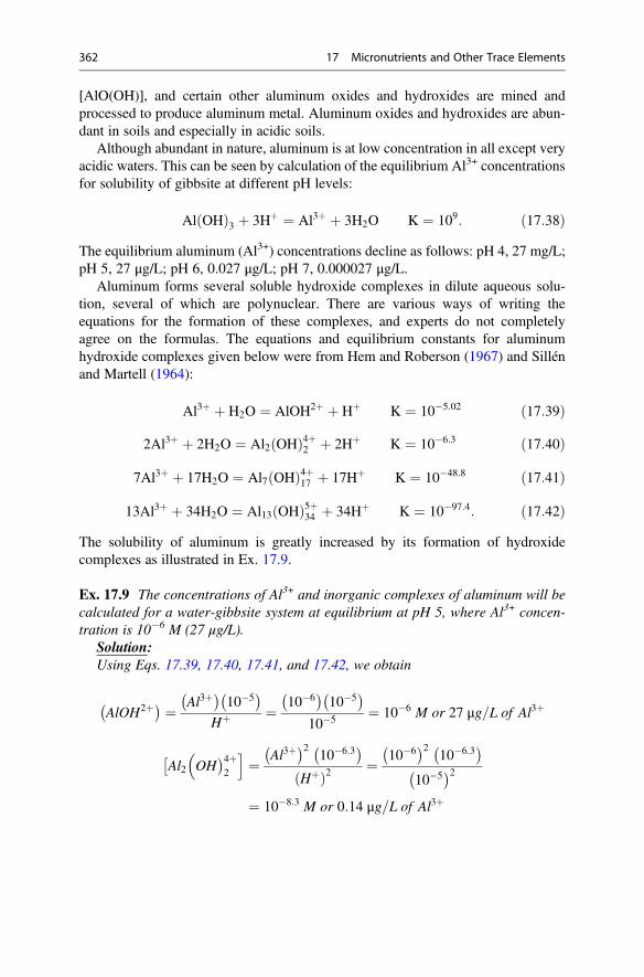
[AlO(OH)], and certain other aluminum oxides and hydroxides are mined andprocessed to produce aluminum metal. Aluminum oxides and hydroxides are abun-dant in soils and especially in acidic soils.

Although abundant in nature, aluminum is at low concentration in all except veryacidic waters. This can be seen by calculation of the equilibrium Al3+ concentrationsfor solubility of gibbsite at different pH levels:

Al OHð Þ3 þ 3Hþ ¼ Al3þ þ 3H2O K ¼ 109: ð17:38ÞThe equilibrium aluminum (Al3+) concentrations decline as follows: pH 4, 27 mg/L;pH 5, 27 μg/L; pH 6, 0.027 μg/L; pH 7, 0.000027 μg/L.

Aluminum forms several soluble hydroxide complexes in dilute aqueous solu-tion, several of which are polynuclear. There are various ways of writing theequations for the formation of these complexes, and experts do not completelyagree on the formulas. The equations and equilibrium constants for aluminumhydroxide complexes given below were from Hem and Roberson (1967) and Sillénand Martell (1964):

Al3þ þ H2O ¼ AlOH2þ þ Hþ K ¼ 10�5:02 ð17:39Þ

2Al3þ þ 2H2O ¼ Al2 OHð Þ4þ2 þ 2Hþ K ¼ 10�6:3 ð17:40Þ

7Al3þ þ 17H2O ¼ Al7 OHð Þ4þ17 þ 17Hþ K ¼ 10�48:8 ð17:41Þ

13Al3þ þ 34H2O ¼ Al13 OHð Þ5þ34 þ 34Hþ K ¼ 10�97:4: ð17:42ÞThe solubility of aluminum is greatly increased by its formation of hydroxidecomplexes as illustrated in Ex. 17.9.

Ex. 17.9 The concentrations of Al3+ and inorganic complexes of aluminum will becalculated for a water-gibbsite system at equilibrium at pH 5, where Al3+ concen-tration is 10�6 M (27 μg/L).

Solution:Using Eqs. 17.39, 17.40, 17.41, and 17.42, we obtain

AlOH2þ� � ¼ Al3þ� �

10�5� �

Hþ ¼ 10�6� �

10�5� �

10�5 ¼ 10�6 M or 27 μg=L of Al3þ

�Al2 OH

�4þ2

� i¼ Al3þ

� �210�6:3� �

Hþð Þ2¼ 10�6

� �210�6:3� �

10�5� �2

¼ 10�8:3 M or 0:14 μg=L of Al3þ


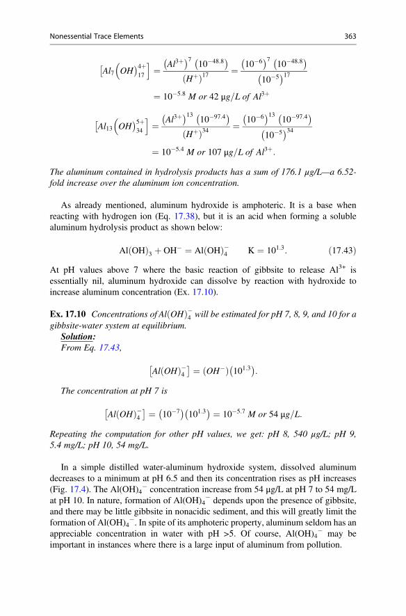
�Al7 OH

�4þ17

� i¼ Al3þ

� �710�48:8� �

Hþð Þ17¼ 10�6

� �710�48:8� �

10�5� �17

¼ 10�5:8 M or 42 μg=L of Al3þ

�Al13 OH

�5þ34

� i¼ Al3þ

� �1310�97:4� �

Hþð Þ34¼ 10�6

� �1310�97:4� �

10�5� �34

¼ 10�5:4 M or 107 μg=L of Al3þ:

The aluminum contained in hydrolysis products has a sum of 176.1 μg/L—a 6.52-fold increase over the aluminum ion concentration.

As already mentioned, aluminum hydroxide is amphoteric. It is a base whenreacting with hydrogen ion (Eq. 17.38), but it is an acid when forming a solublealuminum hydrolysis product as shown below:

Al OHð Þ3 þ OH� ¼ Al OHð Þ�4 K ¼ 101:3: ð17:43ÞAt pH values above 7 where the basic reaction of gibbsite to release Al3+ isessentially nil, aluminum hydroxide can dissolve by reaction with hydroxide toincrease aluminum concentration (Ex. 17.10).

Ex. 17.10 Concentrations of Al OHð Þ�4 will be estimated for pH 7, 8, 9, and 10 for agibbsite-water system at equilibrium.

Solution:From Eq. 17.43,

Al OHð Þ�4� � ¼ OH�ð Þ 101:3

� �:

The concentration at pH 7 is

Al OHð Þ�4� � ¼ 10�7

� �101:3� � ¼ 10�5:7 M or 54 μg=L:

Repeating the computation for other pH values, we get: pH 8, 540 μg/L; pH 9,5.4 mg/L; pH 10, 54 mg/L.

In a simple distilled water-aluminum hydroxide system, dissolved aluminumdecreases to a minimum at pH 6.5 and then its concentration rises as pH increases(Fig. 17.4). The Al(OH)4

� concentration increase from 54 μg/L at pH 7 to 54 mg/Lat pH 10. In nature, formation of Al(OH)4

� depends upon the presence of gibbsite,and there may be little gibbsite in nonacidic sediment, and this will greatly limit theformation of Al(OH)4

�. In spite of its amphoteric property, aluminum seldom has anappreciable concentration in water with pH >5. Of course, Al(OH)4

� may beimportant in instances where there is a large input of aluminum from pollution.


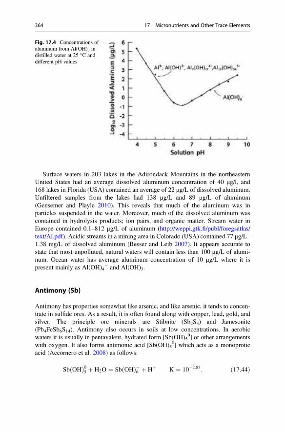
Surface waters in 203 lakes in the Adirondack Mountains in the northeasternUnited States had an average dissolved aluminum concentration of 40 μg/l, and168 lakes in Florida (USA) contained an average of 22 μg/L of dissolved aluminum.Unfiltered samples from the lakes had 138 μg/L and 89 μg/L of aluminum(Gensemer and Playle 2010). This reveals that much of the aluminum was inparticles suspended in the water. Moreover, much of the dissolved aluminum wascontained in hydrolysis products; ion pairs, and organic matter. Stream water inEurope contained 0.1–812 μg/L of aluminum (http://weppi.gtk.fi/publ/foregsatlas/text/Al.pdf). Acidic streams in a mining area in Colorado (USA) contained 77 μg/L–1.38 mg/L of dissolved aluminum (Besser and Leib 2007). It appears accurate tostate that most unpolluted, natural waters will contain less than 100 μg/L of alumi-num. Ocean water has average aluminum concentration of 10 μg/L where it ispresent mainly as Al(OH)4

� and Al(OH)3.

Antimony (Sb)

Antimony has properties somewhat like arsenic, and like arsenic, it tends to concen-trate in sulfide ores. As a result, it is often found along with copper, lead, gold, andsilver. The principle ore minerals are Stibnite (Sb2S3) and Jamesonite(Pb4FeSb6S14). Antimony also occurs in soils at low concentrations. In aerobicwaters it is usually in pentavalent, hydrated form [Sb(OH)5

0] or other arrangementswith oxygen. It also forms antimonic acid [Sb(OH)5

0] which acts as a monoproticacid (Accornero et al. 2008) as follows:

Sb OHð Þ05 þ H2O ¼ Sb OHð Þ�6 þ Hþ K ¼ 10�2:85: ð17:44Þ

Fig. 17.4 Concentrations ofaluminum from Al(OH)3 indistilled water at 25 �C anddifferent pH values


http://weppi.gtk.fi/publ/foregsatlas/text/Al.pdf

http://weppi.gtk.fi/publ/foregsatlas/text/Al.pdf

Most natural waters have antimony concentrations <1 μg/L, but in mining areasconcentrations may be 100 times or more greater, while ocean water averages0.33–0.5 μg/L antimony.

Barium (Ba)

Barium occurs in the earth’s crust as barite (BaSO4) and witherite (BaCO3). Thesolubilities of these compounds can be expressed as

BaSO4 ¼ Ba2þ þ SO2�4 K ¼ 10�9:97 ð17:45Þ

BaCO3 ¼ Ba2þ þ CO2�3 K ¼ 10�8:56: ð17:46Þ

Based on calculations using Ksp, barite and witherite are rather insoluble, andequilibrium Ba2+ concentrations would be 5.47 mg/L and 5.34 mg/L, respectively.Witherite solubility is increased by the action of carbon dioxide. Depending uponsulfate and carbonate concentrations in natural waters, rather large amounts of Ba2+

and its hydrolysis product BaOH+ could exist in equilibrium with barium sulfate orbarium carbonate.

Barium concentrations in natural waters are generally far below equilibriumconcentrations. Surface waters and public water supplies in the United States hadaverage barium concentrations of 43 μg/L and 45 μg/L, respectively (Durum andHaffty 1961; Koop and Kroner 1967), but concentrations up to 3 mg/L were found.Seawater contains an average of 30 μg/L barium.

Beryllium (Be)

Beryllium occurs in geological formations as silicates and hydroxyl silicates. Its oresinclude beryl, penakite, Bertrandite, and several others which contain 6–45% BeOdepending upon the ore. Beryllium also is found in soil at very low concentration.

Beryllium hydroxide [Be(OH)2] is very insoluble in water (Ksp ¼ 10–21.84), butberyllium oxide (BeO) will dissolve when exposed to acid. Because beryllium is rareand its minerals are not highly soluble, concentrations in natural waters are low.River waters in the United States contained 0.01–112 μg/L of beryllium with anaverage of 9.7 μg/L (Kopp 1969). Korečková-Sysalová (1997) reported that beryl-lium concentrations usually were 0.01–1 μg/L in the Czech Republic. However,higher concentrations may result from pollution. Seawater has an average of 0.05 μg/L of beryllium.


Bismuth (Bi)

The most common bismuth ores are bismuthinite (Bi2S3) and bismite (B2O3). Thiselement also occurs in some other minerals and in soils at low concentration. TheBi2S3 form is highly insoluble (Ksp ¼ 10�97), but the oxide form will dissolve inpresence of acid:

Bi2CO3 þ 6Hþ ¼ 2Bi3þ þ 3H2O: ð17:47ÞBismuth concentrations in natural waters are poorly documented. The ionic form

is Bi3+, and its concentration range has been given from undetectable to 0.26 μg/L inmining areas (http://weppi.gtk.fi/publ/foregsatlas/text/Bi.pdf). The average bismuthconcentration of the ocean is given as 0.02 μg/L.

A review of bismuth concentrations in surface water (Filella 2010) includedinland water concentrations of 1–250 μg/L and seawater concentrations of0.02–0.04 μg/L. The conclusion of the review was that the existing data on dissolvedbismuth concentration in surface waters are unreliable because of analyticallimitations.

Bromine (Br)

Bromine occurs in soils and waters mostly as bromide (Br�). The main commercialsources of bromide are oil well brines and Dead Sea brine from which it is extracted(Wisniak 2002).

Bromide is not highly toxic, but it can form trihalomethanes by reaction withdissolved organic matter (Magazinovic et al. 2004). Because it can formtrihalomethanes, bromide has been considered a potential risk in drinking water.Of course, bromine (Br2) is highly toxic and has been used to disinfect drinkingwater as an alternative to chlorine.

Magazinovic et al. (2004) summarized bromide concentrations reported in inlandsurface waters: 6–170 μg/L (USA); 9–760 mg/L (Germany); 24–200 μg/L (France);30–70 μg/L (UK, Spain, and France); 4–76 μg/L (Sweden); 2.0 mg/L (Israel); 30 μg/L-4.3 mg/L (Australia). The higher concentrations were in arid areas, e.g., Israel andsome places in Australia. Bromide is a major constituent of seawater at an averageconcentration of 65–80 mg/L.

Cyanide (CN)

Cyanide is not a trace element. Rather, it is a trace compound containing one or morecarbon atoms triple bonded to nitrogen (-C � N), and it occurs naturally in manyplants including food plants (Jones 1998). Hydrogen cyanide and cyanides are usedin plastic and dye production, occur in exhaust from fuel combustion, and are widelyused in gold and silver mining and in metallurgical processes. Cyanide ions enter


http://weppi.gtk.fi/publ/foregsatlas/text/Bi.pdf

natural waters mainly in wastewater. Cyanide is highly toxic to all forms of life. It isa rapidly acting poison which mainly interferes with cellular respiration.

The forms of cyanide that enters water include Fe4[Fe(CN6)]3, Na4Fe(CN)6, K4Fe(CN)6, NaCN and KCN. The more complex compounds break down into Fe(CN)6

3�

and Fe(CN)64�, and all forms ultimately result in CN� (Jaszczak et al. 2017). The

CN� ion can be associated with hydrocyanic acid:

HCN ¼ Hþ þ CN� K ¼ 10�9:31: ð17:48ÞAt pH 9.31 and less, most of the cyanide will be in HCN. Cyanide reacts with tracemetals according to the Lewis acid-base theory forming both strong solublecomplexes Fe(CN)6

4�, Au(CN)2�, Co(CN)64�, and Ni(CN)4

2�, and weak solublecomplexes, CdCN�, Ag(CN)2

�, Cu(CN)32�, and Zn(CN)4

2� (Jaszczak et al. 2017).Concentrations of cyanide in surface water ranged from 0.77 to 5.11 μg/L, drinkingwater contained 0.6 μg/L or less, and wastewater varied from 0.04 to 1.2 μg/L inelectroplating waste to 540 mg/L in waste from gold extraction (Jaszczak et al.2017).

Lead (Pb)

Lead occurs in several minerals as sulfides, sulfates, and carbonates. The principalores of lead are galena (PbS), cerussite (PbCO3), and anglesite (PbSO4). It alsoenters the environment through pollution. Soils usually have low concentrationsof lead.

Because of the common use of lead and its harmful effects, it has been the focusof considerable environmental and public health concerns. Lead is toxic to plantsand animals, and humans may take in lead through contact and in drinking water. Itaccumulates in the body, and excessive exposure can have several effects, the mostserious being adverse effects on the nervous system and retarded mental develop-ment in children.

The equilibrium concentration for PbSO4 and PbCO3 in water are 32.8 mg/L and82 μg/L, respectively. Most other lead compounds are less soluble. Lead concentra-tion in rivers of the world were 1–10 μg/L (Livingstone 1963), and Kopp and Kroner(1967) found a maximum lead concentration of 140 μg/L in rivers of the UnitedStates. Hard rock mining and ore processing are major sources of lead pollution.Ning et al. (2011) reported an average concentration of 69 μg/L (range ¼ 1.8–434μg/L) in surface waters of a mining area in China. Average concentration of lead inthe ocean is given as 4 μg/L; it is mostly as the PbCO3 ion pair.

Mercury (Hg)

Mercury is of low abundance in geological formations, but it is found in manyminerals and is contained in coal. The common ore is cinnabar (HgS).


Mercury compounds are not appreciably soluble as illustrated with the followingKsp values: Hg2Cl2, 10–25.4; HgS, 10–51.8; HgCO3, 10–16.4. Total mercuryconcentrations for baseline streams not receiving mercury pollution in Alaska(USA) were 0.001 μg/L total mercury and 0.0004 μg/L methyl mercury. Theseconcentrations increased 2,000–300,000 times for total mercury and 6–350 timesfor methyl mercury in mercury mining areas (Wentz et al. 2014). In mercury miningareas in Texas (USA), 1.1–9.7 μg/L total mercury and 0.03–0.61 μg/L of methylmercury were measured (Gary et al. 2015). Ning et al. (2011) also found highconcentrations of total mercury in surface waters of a mining area in China. Theaverage concentration was 61 μg/L with a range of 0.01–827 μg/L. Ocean water hasan average mercury concentration of 0.03–0.15 μg/L.

There are several sources of mercury pollution in addition to mercury mining.These include goldmining, combustion of coal, production of nonferrous metals, andcement production. Mercury can enter water bodies in effluents or from atmosphericdeposition (https://www.epa.gov/international-cooperation/mercury-emissions-global-context).

Goldmining—especially small-scale and artisanal goldmining—is the greatestglobal source of mercury contamination. Liquid mercury is mixed with the crushedore in a 1:20 weight ratio to form a mercury-gold concentrate. The concentrate andexcess mercury are removed, but the extracted ore which still contains some mercuryis released into the environment. Additional mercury is used to further concentratethe mercury-gold amalgam, and the amalgam is heated in the open to distill themercury and isolate the gold. Mercury enters the environment during extraction ofthe ore, the concentration step, and during vaporization of the mercury from theamalgam. This practice is widespread, but particularly in several South American,Asian, and African countries accounting for about 1400 t of mercury pollution andaround 40% of global mercury pollution (Esdaile and Chalker 2018).

Silver (Ag)

Silver is rather rare geologically, but it occasionally is found at greater abundance indeposits of argentite (Ag2S) and chlorargyrite (AgCl). Much silver also is obtainedalong with lead from the lead ore galena for which the formula often is written as(Pb, Ag, Sb, Cu)S. This formula is not exact, because the proportions of the fourmetals vary among different sources of galena. Most silver compounds are insolublewith Ksp values of 10

�10 to 10�50, but a few like silver sulfate (Ksp¼ 10�5) are moresoluble.

The solubility of silver oxide (Ag2O) is so low as to prevent high concentrationsof silver at high pH, and chloride concentration is usually adequate to precipitatesilver at low pH and avoid high concentrations. This can be seen from the equationsbelow:

High pH : Agþ þ 2OH� ¼ Ag2O # ð17:49Þ


https://www.epa.gov/international-cooperation/mercury-emissions-global-context

https://www.epa.gov/international-cooperation/mercury-emissions-global-context

Low pH : Agþ þ 2Cl� ¼ AgCl # : ð17:50ÞMonovalent silver (Ag+) is the common form in water. The mean silver concentra-tion of rivers in the United States was 0.09 μg/L (Durum and Haffty 1961). Flegalet al. (1997) reported that surface water subjected to pollution may contain up to0.3 μg/L or more. Ocean water contains about 0.05 μg/L silver.

Strontium (Sr)

The main ores of strontium are celestite (SrSO4) and strontite (SrCO3). Strontiumalso occurs in various minerals, and limestone usually contains about 0.1% ofstrontium carbonate.

Strontium carbonate is sometimes found in lake sediment. Using this compoundas the controlling mineral, the equilibrium concentration would be about 2.2 mg/Laccording to Ksp. Such high concentrations in inland waters have only been reportedin a few arid areas, and the strontium concentration averaged 60 μg/L in NorthAmerican rivers (Hem 1970). The ocean has an average strontium concentration of8 mg/L.

Thallium (Tl)

Thallium is found in several minerals such as Crookesite [Cu7(Tl,Mg)Se4],Hutchinsonite (Tl,Pb)2As5S9], and in iron pyrite. For commercial purposes, itusually is recovered from byproducts of lead and zinc refining. It is contained incoal and enters the air in gaseous emissions, but elevated environmentalconcentrations usually result from ore processing. Thallium is highly toxic toanimals and humans.

Thallium exists in water primarily as Tl+, but it forms hydrolysis products andother soluble combined forms. Thallium oxide is rather insoluble and is probably thecontrolling mineral. Concentrations in surface waters were reported to average0.01–1 μg/L in uncontaminated surface water and up to 96 μg/L in surface waterof mining regions (Frattini 2005). Thallium concentrations in rivers of Polandranged from 5 to 17 μg/L, a lake in Macedonia contained 0.5 μg/L, and contaminatedsites of the Huron and Raisin rivers in Michigan (USA) contained 21 μg/L and2.62 mg/L, respectively, according to a review by Karbowska (2016). The averagethallium concentration in ocean water is around 0.014 μg/L.

Tin (Sn)

The main ores mined for tin extraction are cassiterite which is a high tin oxide(SnO2) content and tin sulfides such as teallite (PbSnS2). Tin occurs in many otherminerals in low concentrations, and most soils contain 2–3 mg/kg of tin (Howe andWatts 2003).


Tin is not considered by most authorities to be an essential nutrient. Nevertheless,many health advocates claim that tin supports hair growth and enhances reflexes.Deficiency symptoms such as certain types of baldness and less hemoglobin synthe-sis have been claimed.

Tin is not highly soluble, but it is often at detectable concentrations in water. Tinoccurs in natural waters as Sn2+ and Sn4+, with the Sn2+ form favored by lowdissolved oxygen concentration. Quadrivalent tin hydrolyzes and precipitates asSn(OH)4, but divalent tin forms soluble hydroxides [SnOH+, Sn(OH)2

0, Sn(OH3)

�, Sn2(OH)22+, and Sn(OH)4

2+]. Livingstone (1963) reported that some riverscontained up to 100 μg/L of tin, but most rivers contained <2.5 μg/L. Howe andWatts (2003) reported the following: rivers in Maine (USA) had an average tinconcentration 0f 0.03 μg/L; Canadian rivers had tin concentrations of 1–37 μg/L; ariver in Turkey usually contained 0.004 μg/L tin, but near its mouth, pollutionincreased the tin concentration to 0.7 μg/L; Lake Michigan (USA) contained0.08–0.5 μg/L tin. Ocean water contains on average 3 μg/L tin.

Uranium (U)

Uranium is most commonly associated with nuclear fuels and weapons. There areseveral types of uranium deposits that provide its ores to include uraninite(UO2 + UO3), Brannerite [U(TiFe)2O2], and Carnotite (K2O�2U2O3�V2O5�3H2O).It also is found in rock phosphate and a few other minerals. Uranium is the heaviest,natural element that occurs in abundance; its atomic weight is 238. Natural uraniumhas three major isotypes: 238U, 235U, 234U, and 238U is most abundant (99.28%). Theisotopes are unstable and emit gamma particles eventually decaying into lead.Uranium exists in several valence states, and the hexavalent form UO2

2+ is themost stable in water (https://periodic.lanl.gov/926shtml).

Uranium was once used as a coloring agent in ceramic glazes and glass, but thishas been discontinued because of its potential harmful radiation. It now is usedmainly as a nuclear fuel and in nuclear weapons. It is highly toxic both chemicallyand radiologically.

Uranium is leached from geological formations and soils and pollution from oreprocessing. The chemistry of uranium in aqueous solution, unlike most other traceelements, has been thoroughly investigated because of its importance in nuclearapplications and its chemical and radiological hazards (Thoenen and Hummel 2007).Uranium forms many complexes, but in water, soluble hydroxides and carbonatesare predominant, e.g., UO2(OH)2

+, UO2(CO3)22�, UO2(CO3)3

4�, and UO2(CO3)(OH)3

�. The worldwide average for uranium in natural waters is about 0.5 μg/L(range ¼ 0.02–6 μg/L), but extreme values in excess of 20 μg/L have resulted frompollution (IRSN 2012). Examples of extreme uranium concentrations are 61.3 μg/Lin a lake and 57.8 μg/L in a river in Russia reported by Shiraishi et al. (1994).Seawater contains around 3 μg/L uranium.


https://periodic.lanl.gov/926shtml

Toxicity of Trace Elements

The toxicity of trace elements in aquatic ecosystems is a major concern. The pH hasa great effect on solubility of trace elements. The form of the trace metal in water(free ions versus ion pairs, hydrolysis products or chelated ions) has a great influenceon toxicity. Trace metals enter fish mainly through the gills. Calcium and magne-sium ions—the sources of hardness in water—interfere with the transport of tracemetals across the gill and into the blood of aquatic animals. Trace elements aretransported across the gills by an active carrier mechanism, and a high abundance ofcalcium (and presumably magnesium) in the water compete for absorption sites onthe carrier mechanism lessening the amount of trace metal that can enter the fish. Asa result, a higher concentration of a trace metal is necessary to cause toxicity in hardwater than in soft water (Howarth and Sprague 1978).

One approach to estimating safe concentrations of trace elements (and othertoxins) is development of the criterion maximum concentration (CMC) and thecriterion continuous concentration (CCC) which are based on models made fromexisting toxicity data (Mu et al. 2014). The CMC and CCC values accepted areconservative, because they are based on the values for the most sensitive species inthe database. Another method for metals is the Biotic Ligand Model (BLM) whichpredicts effects in waters of different chemical concentrations. The BLMincorporates 10 water quality variables: temperature, pH, dissolved organic carbon,calcium, magnesium, sodium, potassium, sulfate, chloride, and alkalinity to estimatethe safe concentration (USEPA 2007). A list of the CMC and CCC concentrationsfor trace metals are given in Table 17.8.

Possible Health Effects of Trace Elements

Standards for concentrations of trace elements in drinking water are provided inTable 17.9. The World Health Organization and governments in most countries havedeveloped recommended limits on concentrations of trace elements in drinkingwater. These limits are based upon the accumulation of experience in the publichealth aspects of water supply, observed effects of trace elements on animals inlaboratory studies, and epidemiological studies relating exposure to differentconcentrations of trace elements in drinking water to health problems.

Possible Health Effects of Trace Elements 371

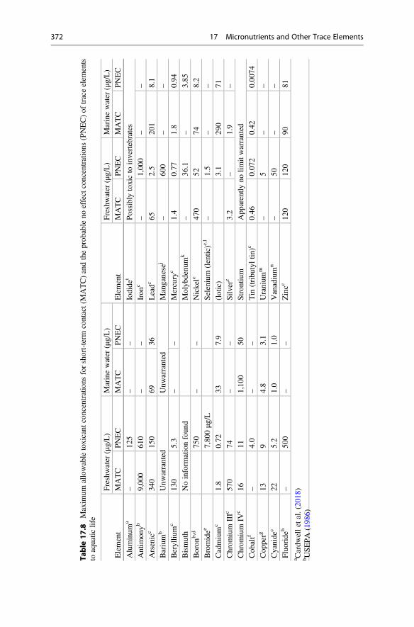
Table

17.8

Maxim

umallowabletoxicant

concentrations

forshort-term

contact(MATC)andtheprob

ableno

effectconcentrations

(PNEC)of

traceelem

ents

toaquatic

life

Element

Freshwater

(μg/L)

Marinewater

(μg/L)

Element

Freshwater

(μg/L)

Marinewater

(μg/L)

MATC

PNEC

MATC

PNEC

MATC

PNEC

MATC

PNEC

Aluminum

a–

125

––

Iodide

iPossiblytoxicto

invertebrates

Antim

onyb

9,00

061

0–

–Iron

c–

1,00

0–

–

Arsenicc

340

150

6936

Leadc

652.5

201

8.1

Barium

bUnw

arranted

Unw

arranted

Manganese

j–

600

––

Berylliu

mc

130

5.3

––

Mercury

c1.4

0.77

1.8

0.94

Bismuth

Noinform

ationfoun

dMolyb

denu

mk

–36

.1–

3.85

Boron

b,d

750

––

Nickelc

470

5274

8.2

Bromidee

7,80

0μg

/LSelenium

(lentic)c,l

–1.5

––

Cadmium

c1.8

0.72

337.9

(lotic)

3.1

290

71

Chrom

ium

IIIc

570

74–

–Silv

erc

3.2

–1.9

–

Chrom

ium

IVc

1611

1,10

050

Stron

tium

App

arently

nolim

itwarranted

Cob

altf

–4.0

––

Tin

(tribu

tyltin

)c0.46

0.07

20.42

0.00

74

Cop

perg

139

4.8

3.1

Uranium

m–

5–

–

Cyanide

c22

5.2

1.0

1.0

Vanadium

n–

50–

–

Fluorideh

–50

0–

–Zincc

120

120

9081

a Cardw

elletal.(20

18)

bUSEPA

(198

6)


c USEPA(201

8)thesearetheUSEPAcriterion

maxim

umconcentration(CMC)andcriterion

continuo

usconcentration(CCC)recommendatio

ns(http

s://w

ww.

epa.go

v/wqc/national-recommended-water-quality-criteria-aquatic-life-criteria-table)

dBoron

standard

ison

lyrelatedto

water

useforirrigatio

ne Cantonetal.(19

83)

f Nagpal(200

4)gUSEPA

(200

4)hCam

argo

(200

3)i Laverochetal.(19

95)

j Reimer

(198

8)kHeijerick

andCarey

(201

7)l USEPA(201

6)mShepp

ardetal.(20

05)

nSchifferandKarsten

(201

7)

Possible Health Effects of Trace Elements 373

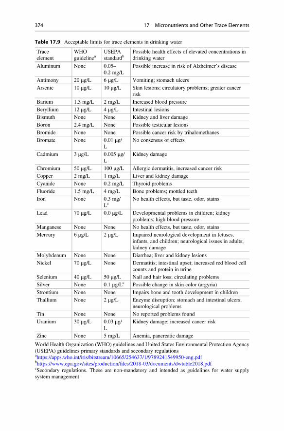
https://www.epa.gov/wqc/national-recommended-water-quality-criteria-aquatic-life-criteria-table

https://www.epa.gov/wqc/national-recommended-water-quality-criteria-aquatic-life-criteria-table

Table 17.9 Acceptable limits for trace elements in drinking water

Traceelement

WHOguidelinea

USEPAstandardb

Possible health effects of elevated concentrations indrinking water

Aluminum None 0.05–0.2 mg/L

Possible increase in risk of Alzheimer’s disease

Antimony 20 μg/L 6 μg/L Vomiting; stomach ulcers

Arsenic 10 μg/L 10 μg/L Skin lesions; circulatory problems; greater cancerrisk

Barium 1.3 mg/L 2 mg/L Increased blood pressure

Beryllium 12 μg/L 4 μg/L Intestinal lesions

Bismuth None None Kidney and liver damage

Boron 2.4 mg/L None Possible testicular lesions

Bromide None None Possible cancer risk by trihalomethanes

Bromate None 0.01 μg/L

No consensus of effects

Cadmium 3 μg/L 0.005 μg/L

Kidney damage

Chromium 50 μg/L 100 μg/L Allergic dermatitis, increased cancer risk

Copper 2 mg/L 1 mg/L Liver and kidney damage

Cyanide None 0.2 mg/L Thyroid problems

Fluoride 1.5 mg/L 4 mg/L Bone problems; mottled teeth

Iron None 0.3 mg/Lc

No health effects, but taste, odor, stains

Lead 70 μg/L 0.0 μg/L Developmental problems in children; kidneyproblems; high blood pressure

Manganese None None No health effects, but taste, odor, stains

Mercury 6 μg/L 2 μg/L Impaired neurological development in fetuses,infants, and children; neurological issues in adults;kidney damage

Molybdenum None None Diarrhea; liver and kidney lesions

Nickel 70 μg/L None Dermatitis; intestinal upset; increased red blood cellcounts and protein in urine

Selenium 40 μg/L 50 μg/L Nail and hair loss; circulating problems

Silver None 0.1 μg/Lc Possible change in skin color (argyria)

Strontium None None Impairs bone and tooth development in children

Thallium None 2 μg/L Enzyme disruption; stomach and intestinal ulcers;neurological problems

Tin None None No reported problems found

Uranium 30 μg/L 0.03 μg/L

Kidney damage; increased cancer risk

Zinc None 5 mg/L Anemia, pancreatic damage

World Health Organization (WHO) guidelines and United States Environmental Protection Agency(USEPA) guidelines primary standards and secondary regulationsahttps://apps.who.int/iris/bitstream/10665/254637/1/9789241549950-eng.pdfbhttps://www.epa.gov/sites/production/files/2018-03/documents/dwtable2018.pdfcSecondary regulations. These are non-mandatory and intended as guidelines for water supplysystem management


https://apps.who.int/iris/bitstream/10665/254637/1/9789241549950-eng.pdf

https://www.epa.gov/sites/production/files/2018%E2%80%9303/documents/dwtable2018.pdf

References

Accornero M, Marini L, Lelli M (2008) The dissociation constant of antimonic acid at 10-40�C. JSolution Chem 37:785–800

Anderson RA (1997) Chromium as an essential nutrient for humans. Regul Toxicol Pharmacol26:535–541

Arnon DI, Wessel G (1953) Vanadium as an essential element in green plants. Nature172:1039–1040

Baralkiewicz D, Siepak J (1999) Chromium, nickel, and cobalt in environmental samples andexisting legal norms. Pol J Environ Stud 8:201–208

Besser JM, Leib KJ (2007) Toxicity of metals in water and sediment to aquatic biota. In: Church SE,von Guerard P, Finger SE (eds) Integrated investigations of environmental effects of historicalmining in the Animas River Watershed, San Juan County, Colorado. U.S. Geological Survey,Washington, p. 839–849

Boyd CE, Walley WW (1972) Studies of the biogeochemistry of boron. I. Concentrations in surfacewaters, rainfall, and aquatic plants. Am Midl Nat 88(1):1–14

British Geological Survey (2000) Iodine. Water quality fact sheet, LondonCamargo JA (2003) Fluoride toxicity to aquatic organisms: a review. Chemosphere 50:251–264Canton JH, Webster PW, Mathijssen-Speikman EA (1983) Study on the toxicity of sodium bromide

to different freshwater organisms. Food Chem Toxicol 21:369–378Cardwell AS, Adams WJ, Gensemer RW, Nordheim E, Santore RC, Ryan AC, Stubblefield WA

(2018) Chronic toxicity of aluminum, at pH 6, to freshwater organisms: empirical data for thedevelopment of international regulatory standards/criteria. Environ Toxicol Chem 37:36–48

Chowdhury UK, Biswas BK, Chowdhury TR, Samanta G, Mandal BK, Basu GC, Cahnda CR,Lodh D, Saha KC, Murkherfee SK, Roy S, Kalir S, Quamruzzaman Q, Chakraborti D (2000)Groundwater arsenic contamination in Bangladesh and West Bengal, India. Environ HealthPerspect 108:393–397

Ćosović B, Degobbis D, Bilinski H, Branica M (1982) Inorganic cobalt species in seawater.Geochim Cosmochim Acta 46:151–158

Deverel SJ, Goldberg S, Fujii R (2012) Chemistry of trace elements in soils and groundwater. In:Wallender WW, Tanji KK (eds) ASCE manual and reports on Engineering practice No71 Agricultural salinity assessment and management, 2nd edn. ASCE, Reston, pp 89–137

Durum WH, Haffty J (1961) Occurrence of minor elements in water. United States GeologicalSurvey Circular 445, United States Government Printing Office, Washington

Esdaile LJ, Chalker JM (2018) The mercury problem in artisanal and small-scale gold mining.Chem Eur J 24:6905–6916

Essumang DK (2009) Levels of cobalt and silver in water sources in a mining area in Ghana. Int JBiol Chem Sci 3:1437–1444

Filella M (2010) How reliable are environmental data on “orphan elements?” The case of bismuthconcentrations in surface waters. J Environ Monit 12:90–109

Firth J (2013) Arsenic—the ‘poison of kings’ and the ‘saviour of syphilis’. J Mil Vet Health21:11–17

Flegal AR, Patterson CC (1985) Concentrations of thallium in seawater. Mar Chem 15:327–331Flegal AR, Rivera-Durarte SA, Sanudo-Wilhelmy SA (1997) Silver contamination in aquatic

environments. Rev Environ Contam Toxicol 148:139–162Frattini P (2005) Thallium properties and behaviour—a literature study. Geological survey of

Finland. http://tupa.gtk.fi/raportti/arkisto/s41_0000_2005_2.pdfFries L (1982) Vanadium an essential element for some marine macroalgae. Planta 154:393–396Gaillardet J, Viers J, Duprèe B (2003) Trace elements in river waters. In: Turekian K, Holland H

(eds) Treatise on geochemistry. Elsevier, Amsterdam, pp 5–9Gary JE, Theodorakos PM, Fey DL, Krabbenhoft DP (2015) Mercury concentrations and distribu-

tion in soil, water, mine waste leachates, and air in and around mercury mines in the Big Bendregion, Texas, USA. Environ Geochem Health 37:35–48

References 375

http://tupa.gtk.fi/raportti/arkisto/s41_0000_2005_2.pdf

Gensemer RW, Playle RC (2010) The bioavailability and toxicity of aluminum in aquaticenvironments. Crit Rev Environ Sci Tech 29:315–450

Goldberg ED (1963) The oceans as a chemical system. In: Hill MN (ed) Composition of sea water,comparative and descriptive oceanography, Vol II. The sea. Wiley, New York

Goldman CR (1972) The role of minor nutrients in limiting the productivity of aquatic ecosystems.In Likens GE (ed) Nutrients and eutrophication: the limiting-nutrients controversy. Lim OceanSpec Sym 1:21–33

Guo T, Delaune RD, Patrick WH (1997) The effect of sediment redox chemistry on solubility/chemically active forms of selected metals in bottom sediment receiving produced waterdischarge. Spill Sci Tech Bull 4:165–175

Hamilton SJ (2004) Review of selenium toxicity in the aquatic food chain. Sci Total Environ326:1–31

Heijerick DG, Carey S (2017) The toxicity of molybdate to freshwater and marine organisms. III.Generating additional chronic toxicity data for the refinement of safe environmental exposureconcentrations in the US and Europe. Sci Total Environ 609:420–428

Hem JD (1970) Study and interpretation of the chemical characteristics of natural water. Water-supply paper 1473, United States Geological Survey, United States Government Printing Office,Washington

Hem JD (1985) Study and interpretation of the chemical characteristics of natural water. Water-supply paper 2254, United States Geological Survey, United States Government Printing Office,Washington

Hem JD, Roberson CE (1967) Form and stability of aluminum hydroxide complexes in dilutesolution. Water-supply paper 1827-A, United States Geological Survey, United States Govern-ment Printing Office, Washington

Howarth RS, Sprague JB (1978) Copper lethality to rainbow trout in waters of various hardness andpH. Water Res 12:455–462

Howe P, Watts P (2003) Tin and inorganic tin compounds. Concise International ChemicalAssessment Document 65, World Health Organization, Geneva

Hyenstrand P, Rydin E, Gunnerhed M (2000) Response of pelagic cyanobacteria to ironadditions—enclosure experiments from Lake Erken. J Plankton Res 22:1113–1126

IRSN (Institut de Radioprotection et de Sûretè Nuclèaire) (2012) Natural uranium in the environ-ment. https://www.irsn.fr/EN/Research/publications-documentation/radionuclides-sheets/environment/Pages/Natural-uranium-environment.aspx

Izbicki JA, Ball JW, Bullen TD, Sutley SJ (2008) Chromium, chromium isotopes and selected traceelements, western Mojave Desert, USA. Appl Geochem 23:1325–1352

Jaszczak E, Palkowska Z, Narkowicz S, Namieśnik J (2017) Cyanides in the environment—analysis—problems—challenges. Environ Sci Pollut Res 24:15929–15948

Jones DA (1998) Why are so many plant foods cyanogenic? Phytochemistry 47:155–162Karbowska B (2016) Presence of thallium in the environment: sources of contaminations, distribu-

tion, and monitoring methods. Environ Monit Assess 188:640Khan T, Mohammad S, Khan B, Khan H (2011) Investigating the levels of heavy metals in surface

water of Shah Alam River (a tributary of River Kabul, Khyber Pakhtunkhwa). Asian J Earth Sci44:71–79

Kochkodan V, Darwish NB, Hilal N (2015) The chemistry of boron in water. In: Kabay N, Hilal N,Bryak M (eds) Boron separation processes. Elsevier, The Netherlands, pp 35–62

Kopp JF (1969) The occurrence of trace elements in water. In: Hemphill DD (ed) Proceedings of theThird Annual Conference on Trace Substances in Environmental Health. University ofMissouri, Columbia, pp 59–79

Kopp JF, Kroner RC (1967) Trace metals in waters of the United States. A five year summary oftrace metals in rivers and lakes of the United States (October 1, 1962 to September 30, 1967).United States Department of the Interior, Federal Water Pollution Control Administration,Cincinnati


https://www.irsn.fr/EN/Research/publications-documentation/radionuclides-sheets/environment/Pages/Natural-uranium-environment.aspx

https://www.irsn.fr/EN/Research/publications-documentation/radionuclides-sheets/environment/Pages/Natural-uranium-environment.aspx

Kopp JF, Kroner RC (1970) Trace metals in waters of the United States. Report PB-215680. FederalWater Pollution Control Administration, Cincinnati

Korečková-Sysalová J (1997) Determination of beryllium in natural waters using atomic absorptionspectrometry with tantalum-coated graphite tube. Int J Environ Anal Chem 68:397–404

Lane TW, Morel FMM (2000) A biological function for cadmium in marine diatoms. Proc NatlAcad Sci 97:4627–4631

Laveroch MJ, Stephenson M, Macdonald CR (1995) Toxicity of iodine, iodide, and iodate toDaphnia magna and rainbow trout (Oncorhynchus mykiss). Arch Environ Con Toxicol 29(3):344–350

Lee JG, Roberts SB, Morel FMM (1995) Cadmium: a nutrient for the marine diatom Thelassiosiraweissflogii. Limnol Oceanogr 40:1056–1063

Lindemann MD, Cho JH, Wang MQ (2009) Chromium—an essential mineral. Rev Colom de CienPec 22:339–445

Livingstone DA (1963) Chemical composition of rivers and lakes. Professional Paper 440-G,United States Geological Survey, United States Government Printing Office, Washington

Magazinovic RS, Nicholson BC, Mulcahy DE, Davey DE (2004) Bromide levels in natural waters:its relationship to chloride and total dissolved solids and the implications for water treatment.Chemosphere 57:329–335

McBride MB (1989) Reactions controlling heavy metal solubility in soils. In: Stewart BA(ed) Advances in soil science. Springer, New York, pp 1–56

McNevin AA, Boyd CE (2004) Copper concentrations in channel catfish, Ictalurus punctatus,ponds treated with copper sulfate. J World Aquacult Soc 35:16–24

Moore GT, Kellerman KF (1905) Copper as an algicide and disinfectant in water supplies. Bull BurInd 76:19–55

Mu Y, Wu F, Chen C, Liu Y, Zhao X, Liao H, Giesy JP (2014) Predicting criteria continuousexposure concentrations of 34 metals or metalloids by use of quantitative ion character-activityrelationships-species sensitivity distributions (QICAR-SSD) model. Environ Pollut 188:50–55

Nadis S (1998) Fertilizing the sea. Sci Am 177:33Nagpal NK (2004) Technical report-water quality guidelines for cobalt. Ministry of Water, Land,

and Air Protection, VictoriaNing L, Liyuan Y, Jirui D, Xugui P (2011) Heavy metal pollution in surface water of Linglong gold

mining area, China. Procedia Environ Sci 10:914–917Pagenkopf GK (1978) Introduction to natural water chemistry. Marcel Dekker, Inc., New YorkPais I, Jones JB Jr (1997) The handbook of trace elements. Saint Lucie Press, Boca RatonPalmer CA, Gilbert JA (2012) Position of the Academy of Nutrition and Dietetics: the impact of

fluoride on health. J Acad Nutr Diet 112:1443–1453Pinsino A, Matranga V, Roccheri MC (2012) Manganese: a new emerging contaminant in the

environment. In: Srivastava J (ed) Environmental contamination. InTech Europe, Rijeka, pp17–36

Puntoriero ML, Volpedo AJ, Fernandez-Cirelli A (2014) Arsenic, fluoride, and vanadium in surfacewater (Chasicó Lake, Argentina). Front Environ Sci 2:1–5

Reimer PS (1988) Environmental effects of manganese and proposed freshwater guidelines toprotect aquatic life in British Columbia. Thesis, University of British Columbia

Ryan D (1992) Minor elements in seawater. In: Millero FJ (ed) Chemical oceanography. CRCPress, Boca Raton, pp 89–119

Schiffer S, Karsten L (2017) Estimation of vanadium water quality benchmarks for protection ofaquatic life with reference to the Athabasca Oil Sands region using species sensitivitydistributions. Environ Toxicol Chem 36:3034–3044

Seker S, Kutler B (2014) Determination of copper (Cu) levels for rivers in Tunceli, Turkey. WorldEnviron 4:168–171

Sheppard SC, Sheppard NI, Gallerand MO, Sanipelli B (2005) Deviation of ecotoxicity thresholdsfor uranium. J Environ Radioact 79:55–83

References 377

Sillén LG, Martell AE (1964) Stability constants for metal-ion complexes. Special Publication17, Chemical Society, London

Sillén LG, Martell AE (1971) Stability constants of metal-ion complexes. Special Publication25, Chemical Society, London

Shiraishi K, Igarashi Y, Yamamoto M, Nakajima T, Los IP, Zelensky AV, Buzinny MZ (1994)Concentrations of thorium and uranium in freshwater samples collected in the former USSR. JRadioanal Nucl Chem 185:157–165

Spears JW (1984) Nickel as a “newer trace element” in the nutrition of domestic animals. J AnimSci 59:823–835

Stralberg E, Varskog ATS, Raaum A, Varskog P (2003) Naturally occurring radio-nuclides in themarine environment—an overview by current knowledge with emphasis on the North Sea area.Norse Decom AS, Kjeller, Norway

Thoenen T, Hummel (2007) The PSI/Nogra chemical thermodynamic database (Update of theNagra/PSI TDB 01/01: data selection for uranium. Paul Scherrer Institute

Turekian KK (1968) Oceans. Prentice-Hall, Englewood CliffsUSEPA (1986) Quality criteria for water. EPA 440/S-86-001. USEPA Office of Water, WashingtonUSEPA (2004) National recommended water quality criteria. USEPA Office of Water, WashingtonUSEPA (2007) Aquatic life ambient freshwater quality criteria: copper, EPA 822-R-07-001. http://

www.epa.gov/waterscience/criteria/copper/index.htmUSEPA (2016) Aquatic life ambient water quality criterion for selenium—freshwater. USEPA

Office of Water, WashingtonUSEPA (2018) Aquatic life criteria and methods for toxics. https://www.epa.gov/wqc/aquatic-life-

criteria-and-methods-toxicsUthus EO (1992) Evidence for arsenic essentiality. Environ Geochem Health 14:55–58Vrede T, Tranvik LJ (2006) Ion constraints on planktonic primary production in oligotrophic lakes.

Ecosystems 9:1094–1105Wentz DA, Brigham ME, Chasar LC, Lutz MA, Krabbenholf DP (2014) Mercury in the nation’s

steams—levels, trends, and implications. Circular 1395, US Geological Survey, WashingtonWisniak J (2002) The history of bromine from discovery to commodity. Indian J Chem Technol

9:262–271World Health Organization (2011) Selenium in drinking water. WHO/HSE/WSH/10.01/14


http://www.epa.gov/waterscience/criteria/copper/index.htm

http://www.epa.gov/waterscience/criteria/copper/index.htm

https://www.epa.gov/wqc/aquatic-life-criteria-and-methods-toxics

https://www.epa.gov/wqc/aquatic-life-criteria-and-methods-toxics

Water Quality Protection 18

AbstractImpaired water quality can result from natural causes, but the most common causeis anthropogenic pollution. Soil erosion leads to turbidity and sedimentation inwater bodies. Organic wastes impart a high oxygen demand often culminating inlow dissolved oxygen concentrations and nitrogen and phosphorus in effluentscause eutrophication. Pesticides, synthetic organic chemicals and heavy metalsfrom industry, and pharmaceutical compounds and their degradation products canbe toxic to aquatic animals or have other adverse effects on them. Toxins indrinking water can lead to several serious illnesses to include cancer in humans.Water bodies also may be contaminated with biological agents that cause aquaticanimal and human diseases. Elevated sulfur dioxide and carbon dioxideconcentrations in the atmosphere as a result of air pollution can influence waterquality. Wetland destruction must be considered in a discussion of water pollu-tion, because functional wetlands are important for natural water purification.Water quality regulations are important for avoiding conflicts among water users,minimizing public health risks of certain chemical and biological pollutants,protecting the environment, and preventing conditions that lessen the recreationaland aesthetic value of water bodies. Most countries have developed water qualityregulations with which effluents must comply. These permits typically havelimits on concentrations of pollutants in effluents, and many times, there arelimits on quantities of pollutants that may be discharged. There is a growingtendency to develop total maximum daily pollutant loads (TMDL) that specifythe total quantities of selected pollutants that can be discharged into a stream orother water body by all permit holders. Standards with which municipal watersupply operations must comply also have been developed to protect drinkingwater quality and protect public health.


379


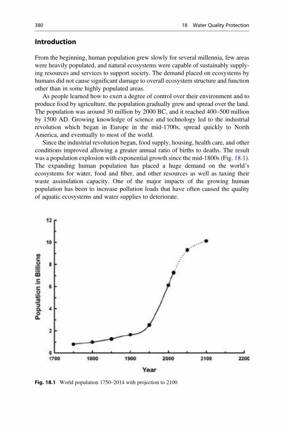
Introduction

From the beginning, human population grew slowly for several millennia, few areaswere heavily populated, and natural ecosystems were capable of sustainably supply-ing resources and services to support society. The demand placed on ecosystems byhumans did not cause significant damage to overall ecosystem structure and functionother than in some highly populated areas.

As people learned how to exert a degree of control over their environment and toproduce food by agriculture, the population gradually grew and spread over the land.The population was around 30 million by 2000 BC, and it reached 400–500 millionby 1500 AD. Growing knowledge of science and technology led to the industrialrevolution which began in Europe in the mid-1700s, spread quickly to NorthAmerica, and eventually to most of the world.

Since the industrial revolution began, food supply, housing, health care, and otherconditions improved allowing a greater annual ratio of births to deaths. The resultwas a population explosion with exponential growth since the mid-1800s (Fig. 18.1).The expanding human population has placed a huge demand on the world’secosystems for water, food and fiber, and other resources as well as taxing theirwaste assimilation capacity. One of the major impacts of the growing humanpopulation has been to increase pollution loads that have often caused the qualityof aquatic ecosystems and water supplies to deteriorate.

Fig. 18.1 World population 1750–2014 with projection to 2100

380 18 Water Quality Protection

The major sources of pollution and their effects on natural aquatic ecosystems andwater use by humans will be discussed in this chapter.

Types of Water Pollution

Discharges that cause water pollution are separated into two broad categories: pointsources and nonpoint sources. Well-defined effluent streams discharged in both wetand dry weather via pipes, channels, or other conduits are point sources. Commonpoint sources of pollution are industrial operations and municipal wastewater treat-ment plants. Urban and suburban runoff from streets, parking lots, lawns, etc., entersstorm sewers, ditches, and similar conduits that discharge untreated into waterbodies. Runoff from farmland, construction sites, etc., also enters water bodies byoverland flow and atmospheric deposition falls directly into water bodies. Stormsewer flow, overland runoff, and atmospheric deposition are nonpoint sourcedischarges.

There are several types of pollutants. Organic waste impose an oxygen demandwhen microorganisms decompose it. Organic matter is a major contaminant indomestic and municipal wastewater, animal feedlot effluents, and discharges fromfood processing and paper manufacturing.

Turbidity from suspended solids is unsightly and interferes with light penetrationand aquatic plant growth. Solids that settle from water create sediment deposits thatmay suffocate benthic organisms. Sediment also reduces water depth, and shallowwater favors growth of rooted aquatic macrophytes. The oxygen demand of sedimentwith a high organic matter content can cause anaerobic conditions in shallow areas.Suspended solids in municipal, industrial, and feedlot effluents tend to be highlyorganic, while effluents from agricultural land, logging operations, constructionsites, and surface mining have a high proportion of inorganic, suspended solids.

Nutrient pollution results primarily from nitrogen and phosphorus in runoff andeffluents. Municipal wastewater and other effluents with high concentrations oforganic matter also tend to have large concentrations of nitrogen and phosphorus.Runoff from residential lawns and from cropland and pastureland also containelevated concentrations of nitrogen and phosphorus from fertilizers and contributesto eutrophication.

Chemicals used for domestic, industrial, and agricultural purposes find their wayinto water bodies from normal operations or in leaks from storage depots or seepagefrom waste disposal sites. Toxic substances may be directly harmful to aquatic life orthey may cause toxicity through bioconcentration and be toxic to organisms in thefood chain. Bioconcentration also presents a potential food safety hazard forconsumers of aquatic products. Toxins also can be present in domestic drinkingwater or in waters used for agricultural purposes.

Runoff from surface mining and seepage from underground mines are wellknown sources of acidification in natural waters. Combustion of fossil fuelscontaminates the air with sulfur dioxide, nitrous oxide, and other compounds thatoxidize to form mineral acids. Rainfall in heavily populated or industrialized areas is

Types of Water Pollution 381

a major source of acidification. Nitrification also can be a significant source ofacidity in surface waters. On the other hand, some effluents may be alkaline andcause an excessive pH in receiving waters.

Many natural waters contain residues and degradation products of pharmaceuticalchemicals. Pharmaceuticals often enter water by home disposal of unwanted medi-cine and other health products into the sewer system. Some are actually toxic toaquatic life, while others act more subtly by having negative physiological or geneticeffects upon prolonged exposure. Pharmaceutical residues also can enter the watersupply for humans.

Contamination of waters with disease organisms of human origin is still a majorconcern in many developing nations. If human fecal material enters water, the risk ofdisease spread through drinking water is greatly increased.

Many industrial processes generate waste heat that may be disposed of by transferto water. Heated effluents may raise temperatures in streams or other water bodies tocause serious ecological perturbations. Desalination of seawater necessary to sup-plement water supply in some countries also causes pollution. The discharge waterfrom reverse osmosis plants is of higher salinity than coastal waters. Distillationplants discharge thermally polluted cooling water, and metals from heat exchangersenter the cooling water.

Accidents may result in spills of potentially toxic chemicals or other substances.A highway or rail accident can result in a cargo being inadvertently spilled into awatercourse, or a ship accident can spill crude oil or other substances into the oceanor into coastal and inland waters. The most famous cases of crude oil pollutionprobably are the Exxon Valdez oil spill that occurred when an Exxon tanker struck areef in Prince William Sound, Alaska in 1989, and the BP Deepwater Horizon oilspill that resulted from an accident on an off-shore oil drilling platform in the Gulf ofMexico in 2010.

Water quality can be impaired through natural processes without human inter-vention. In some coastal areas, soils contain iron pyrite that oxidizes in dry weatherto produce sulfuric acid which leaches in rainy weather to cause acidification ofsurface water. Some groundwaters may be unfit for domestic or other uses becauseof high iron or manganese concentrations. The inhabitants of areas in Bangladeshand India are at risk of poisoning by naturally-occurring arsenic in groundwater (seeChap. 17). Salinization has made freshwaters in some areas too salty for domesticand agricultural purposes.

Considerable attention is given to amounts of suspended solids, biochemicaloxygen demand, nitrogen, phosphorus, and dissolved metals in effluents. In theUnited States, about 50% of the total point source amounts of these five pollutantsare from the 10 industries listed in Table 18.1. However, point source pollutioncontributes less than 0.2% of total suspended solids, 5% of phosphorus, 10% ofnitrogen, and 20% of oxygen demand. Nonpoint source discharges are the mostserious pollution threats to water bodies. Agriculture contributes more than 50% ofnonpoint source pollution.


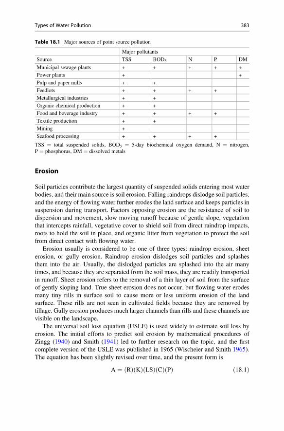
Erosion

Soil particles contribute the largest quantity of suspended solids entering most waterbodies, and their main source is soil erosion. Falling raindrops dislodge soil particles,and the energy of flowing water further erodes the land surface and keeps particles insuspension during transport. Factors opposing erosion are the resistance of soil todispersion and movement, slow moving runoff because of gentle slope, vegetationthat intercepts rainfall, vegetative cover to shield soil from direct raindrop impacts,roots to hold the soil in place, and organic litter from vegetation to protect the soilfrom direct contact with flowing water.

Erosion usually is considered to be one of three types: raindrop erosion, sheeterosion, or gully erosion. Raindrop erosion dislodges soil particles and splashesthem into the air. Usually, the dislodged particles are splashed into the air manytimes, and because they are separated from the soil mass, they are readily transportedin runoff. Sheet erosion refers to the removal of a thin layer of soil from the surfaceof gently sloping land. True sheet erosion does not occur, but flowing water erodesmany tiny rills in surface soil to cause more or less uniform erosion of the landsurface. These rills are not seen in cultivated fields because they are removed bytillage. Gully erosion produces much larger channels than rills and these channels arevisible on the landscape.

The universal soil loss equation (USLE) is used widely to estimate soil loss byerosion. The initial efforts to predict soil erosion by mathematical procedures ofZingg (1940) and Smith (1941) led to further research on the topic, and the firstcomplete version of the USLE was published in 1965 (Wischeier and Smith 1965).The equation has been slightly revised over time, and the present form is

A ¼ Rð Þ Kð Þ LSð Þ Cð Þ Pð Þ ð18:1Þ

Table 18.1 Major sources of point source pollution

Major pollutants

Source TSS BOD5 N P DM

Municipal sewage plants + + + + +

Power plants + +

Pulp and paper mills + +

Feedlots + + + +

Metallurgical industries + +

Organic chemical production + +

Food and beverage industry + + + +

Textile production + +

Mining +

Seafood processing + + + +

TSS ¼ total suspended solids, BOD5 ¼ 5-day biochemical oxygen demand, N ¼ nitrogen,P ¼ phosphorus, DM ¼ dissolved metals


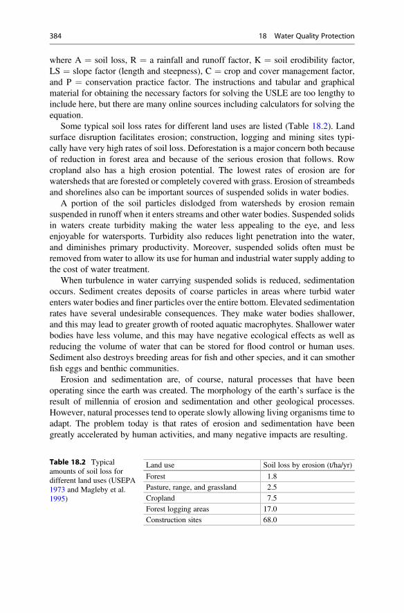
where A ¼ soil loss, R ¼ a rainfall and runoff factor, K ¼ soil erodibility factor,LS ¼ slope factor (length and steepness), C ¼ crop and cover management factor,and P ¼ conservation practice factor. The instructions and tabular and graphicalmaterial for obtaining the necessary factors for solving the USLE are too lengthy toinclude here, but there are many online sources including calculators for solving theequation.

Some typical soil loss rates for different land uses are listed (Table 18.2). Landsurface disruption facilitates erosion; construction, logging and mining sites typi-cally have very high rates of soil loss. Deforestation is a major concern both becauseof reduction in forest area and because of the serious erosion that follows. Rowcropland also has a high erosion potential. The lowest rates of erosion are forwatersheds that are forested or completely covered with grass. Erosion of streambedsand shorelines also can be important sources of suspended solids in water bodies.

A portion of the soil particles dislodged from watersheds by erosion remainsuspended in runoff when it enters streams and other water bodies. Suspended solidsin waters create turbidity making the water less appealing to the eye, and lessenjoyable for watersports. Turbidity also reduces light penetration into the water,and diminishes primary productivity. Moreover, suspended solids often must beremoved from water to allow its use for human and industrial water supply adding tothe cost of water treatment.

When turbulence in water carrying suspended solids is reduced, sedimentationoccurs. Sediment creates deposits of coarse particles in areas where turbid waterenters water bodies and finer particles over the entire bottom. Elevated sedimentationrates have several undesirable consequences. They make water bodies shallower,and this may lead to greater growth of rooted aquatic macrophytes. Shallower waterbodies have less volume, and this may have negative ecological effects as well asreducing the volume of water that can be stored for flood control or human uses.Sediment also destroys breeding areas for fish and other species, and it can smotherfish eggs and benthic communities.

Erosion and sedimentation are, of course, natural processes that have beenoperating since the earth was created. The morphology of the earth’s surface is theresult of millennia of erosion and sedimentation and other geological processes.However, natural processes tend to operate slowly allowing living organisms time toadapt. The problem today is that rates of erosion and sedimentation have beengreatly accelerated by human activities, and many negative impacts are resulting.

Table 18.2 Typicalamounts of soil loss fordifferent land uses (USEPA1973 and Magleby et al.1995)

Land use Soil loss by erosion (t/ha/yr)

Forest 1.8

Pasture, range, and grassland 2.5

Cropland 7.5

Forest logging areas 17.0

Construction sites 68.0


Biological Oxygen Demand

Bacteria and other saprophytes in aquatic ecosystems remove dissolved oxygen foruse in decomposing organic matter. The effect of addition of organic matter inpollutants on dissolved oxygen concentration depends upon the capacity of awater body to assimilate organic matter relative to the amount of organic matterintroduced. A given organic matter load might not influence dissolved oxygenconcentrations in a large body of water, but the same load might cause oxygendepletion in a smaller body of water. A rapidly flowing stream reaerates more rapidlythan a sluggish stream of the same cross-sectional area, and therefore can assimilatea greater organic matter input than a sluggish stream. The oxygen demand ofwastewater is usually estimated as the biochemical oxygen demand (BOD).

The standard 5-day BOD (BOD5) determination provides an estimate of thepollutional strength of wastewaters (Eaton et al. 2005). In the BOD procedure, analiquot of wastewater is typically diluted with inorganic nutrient solution and abacterial seed added. The inorganic nutrients and bacterial seed are necessary toprevent a shortage of bacteria and inorganic nutrients that might result from dilution.Because of the possibility of oxygen demand from the bacterial seed, a blankconsisting of the same quantity of bacterial seed used in the sample is introducedinto nutrient solution and carried through the same incubation as the sample.Samples are incubated in the dark to prevent photosynthetic oxygen production.The incubation is continued in the dark for 5 days at 20 �C. At the beginning and endof incubation, the dissolved oxygen concentration is measured in blank and sampleto permit estimation of BOD5 as illustrated in Ex. 18.1.

Ex. 18.1 In a BOD5 analysis, the sample is diluted 20 times. The initial dissolvedoxygen concentration is 9.01 mg/L in sample and blank. After 5 days of incubation,the dissolved oxygen concentration is 8.80 mg/L in the blank and 4.25 mg/L in thesample. The BOD will be calculated.

Solution:The oxygen loss caused by the bacterial seed is the blank BOD,

Blank BOD ¼ Initial DO� Blank DO

or 9:01� 8:80ð Þmg=L ¼ 0:21 mg=L:

The oxygen consumption by the sample is

Initial DO� Final DOð Þ � Blank BOD

or 9:01� 4:25ð Þ � 0:21 ¼ 4:55 mg=L:

The sample BOD is the oxygen consumption by the sample multiplied by acorrection factor equal to the number of times the sample was diluted—20 timesin this case.


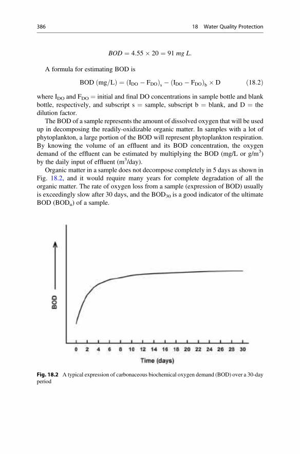
BOD ¼ 4:55� 20 ¼ 91 mg L:

A formula for estimating BOD is

BOD mg=Lð Þ ¼ IDO � FDOð Þs � IDO � FDOð Þb � D ð18:2Þwhere IDO and FDO ¼ initial and final DO concentrations in sample bottle and blankbottle, respectively, and subscript s ¼ sample, subscript b ¼ blank, and D ¼ thedilution factor.

The BOD of a sample represents the amount of dissolved oxygen that will be usedup in decomposing the readily-oxidizable organic matter. In samples with a lot ofphytoplankton, a large portion of the BOD will represent phytoplankton respiration.By knowing the volume of an effluent and its BOD concentration, the oxygendemand of the effluent can be estimated by multiplying the BOD (mg/L or g/m3)by the daily input of effluent (m3/day).

Organic matter in a sample does not decompose completely in 5 days as shown inFig. 18.2, and it would require many years for complete degradation of all theorganic matter. The rate of oxygen loss from a sample (expression of BOD) usuallyis exceedingly slow after 30 days, and the BOD30 is a good indicator of the ultimateBOD (BODu) of a sample.

Fig. 18.2 A typical expression of carbonaceous biochemical oxygen demand (BOD) over a 30-dayperiod


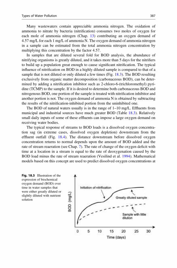
Many wastewaters contain appreciable ammonia nitrogen. The oxidation ofammonia to nitrate by bacteria (nitrification) consumes two moles of oxygen foreach mole of ammonia nitrogen (Chap. 13) contributing an oxygen demand of4.57 mg/L for each 1 mg/L of ammonia N. The oxygen demand of ammonia nitrogenin a sample can be estimated from the total ammonia nitrogen concentration bymultiplying this concentration by the factor 4.57.

In samples that are diluted several fold for BOD analysis, the abundance ofnitrifying organisms is greatly diluted, and it takes more than 5 days for the nitrifiersto build up a population great enough to cause significant nitrification. The typicalinfluence of nitrification on BOD in a highly diluted sample is compared to that of asample that is not diluted or only diluted a few times (Fig. 18.3). The BOD resultingexclusively from organic matter decomposition (carbonaceous BOD), can be deter-mined by adding a nitrification inhibitor such as 2-chloro-6-(trichloromethyl) pyri-dine (TCMP) to the sample. If it is desired to determine both carbonaceous BOD andnitrogenous BOD, one portion of the sample is treated with nitrification inhibitor andanother portion is not. The oxygen demand of ammonia N is obtained by subtractingthe results of the nitrification-inhibited portion from the uninhibited one.

The BOD of natural waters usually is in the range of 1–10 mg/L. Effluents frommunicipal and industrial sources have much greater BOD (Table 18.3). Relativelysmall daily inputs of some of these effluents can impose a large oxygen demand onreceiving water bodies.

The typical response of streams to BOD loads is a dissolved oxygen concentra-tion sag (in extreme cases, dissolved oxygen depletion) downstream from theeffluent outfall (Fig. 18.4). The distance downstream before dissolved oxygenconcentration returns to normal depends upon the amount of BOD added and therate of stream reaeration (see Chap. 7). The rate of change of the oxygen deficit withtime at a location in a stream is equal to the rate of deoxygenation caused by theBOD load minus the rate of stream reaeration (Vesilind et al. 1994). Mathematicalmodels based on this concept are used to predict dissolved oxygen concentrations at

Fig. 18.3 Illustration of theexpression of biochemicaloxygen demand (BOD) overtime in water samples thatwere either greatly diluted orslightly diluted with nutrientsolution


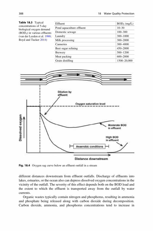
different distances downstream from effluent outfalls. Discharge of effluents intolakes, estuaries, or the ocean also can depress dissolved oxygen concentrations in thevicinity of the outfall. The severity of this effect depends both on the BOD load andthe extent to which the effluent is transported away from the outfall by watercurrents.

Organic wastes typically contain nitrogen and phosphorus, resulting in ammoniaand phosphate being released along with carbon dioxide during decomposition.Carbon dioxide, ammonia, and phosphorus concentrations tend to increase in

Table 18.3 Typicalconcentrations of 5-daybiological oxygen demand(BOD5) in various effluents(van der Leeden et al. 1990;Boyd and Tucker 2014)

Effluent BOD5 (mg/L)

Pond aquaculture effluent 10–30

Domestic sewage 100–300

Laundry 300–1000

Milk processing 300–2000

Canneries 300–4000

Beet sugar refining 450–2000

Brewery 500–1200

Meat packing 600–2000

Grain distilling 1500–20,000

Fig. 18.4 Oxygen sag curve below an effluent outfall in a stream


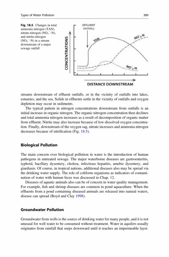
streams downstream of effluent outfalls, or in the vicinity of outfalls into lakes,estuaries, and the sea. Solids in effluents settle in the vicinity of outfalls and oxygendepletion may occur in sediments.

The typical pattern in nitrogen concentrations downstream from outfalls is aninitial increase in organic nitrogen. The organic nitrogen concentration then declinesand total ammonia nitrogen increases as a result of decomposition of organic matterfrom effluent. Nitrite may also increase because of low dissolved oxygen concentra-tion. Finally, downstream of the oxygen sag, nitrate increases and ammonia nitrogendecreases because of nitrification (Fig. 18.5).

Biological Pollution

The main concern over biological pollution in water is the introduction of humanpathogens in untreated sewage. The major waterborne diseases are gastroenteritis,typhoid, bacillary dysentery, cholera, infectious hepatitis, amebic dysentery, andgiardiasis. Of course, in tropical nations, additional diseases also may be spread viathe drinking water supply. The role of coliform organisms as indicators of contami-nation of water with human feces was discussed in Chap. 12.

Diseases of aquatic animals also can be of concern in water quality management.For example, fish and shrimp diseases are common in pond aquaculture. When theeffluents from a pond containing diseased animals are released into natural waters,disease can spread (Boyd and Clay 1998).

Groundwater Pollution

Groundwater from wells is the source of drinking water for many people, and it is notunusual for well water to be consumed without treatment. Water in aquifers usuallyoriginates from rainfall that seeps downward until it reaches an impermeable layer.

Fig. 18.5 Changes in totalammonia nitrogen (TAN),nitrate-nitrogen (NO3

�-N),and nitrite-nitrogen(NO2

�-N) in a streamdownstream of a majorsewage outfall


Groundwater may accumulate pollutants, because wastes are sometimes disposed inor on the soil. Manure of farm animals is disposed by application as fertilizer to fieldsand pastures, sewage is used for irrigation in some parts of the world, septic tanksseep into the soil, waste is buried in landfills, and waste is sometimes put into dumpson the land surface. Tanks that hold fuel and other chemicals may be buried in theground or placed on the land surface, and leakage or spillage is not uncommon.Pesticides are applied to fields, and a portion reaches the soil surface and movedownward with infiltrating water.

In spite of the many opportunities for contamination, groundwater is protectedfrom pollution to a large extent by the natural purifying action of the soil, soilmicroorganisms, and geological formations with which it comes in contact. The soilis composed of a mixture of particles of sand, silt, clay, and organic matter, and theunderlying geological formations also contain layers of sand, silt, clay, gravel, andlimestone and other fractured rocks. Water infiltrates slowly and bacteria in the soildecompose some of the dissolved organic material. Bacteria can even degrade oralter the molecular structure of agricultural and industrial chemicals to make themless toxic or render them harmless. More importantly, the soil and underlyinggeological formations act as a porous medium to filter harmful bacteria and othersmall particles from the infiltrating water. Clay, in particular, has a great ability toadsorb substances from infiltrating water. Bollenbach (1975) summarized data onthe movement of bacterial and chemical pollution in infiltrating water. Coliformbacteria moved through the first 1.5 m at the same rate as the water, and a few movedabout 5 m in 3 days. After 2 months, a few coliforms had seeped to a depth of 10 m.Chemical pollution, however, was found to move 3 m in 4 days and to ultimatelyseep to a depth of 30 m. Some studies in more permeable soil showed greater rates ofmovement of bacteria and pollutants, but the medium through which water mustseep to reach the permanently saturated groundwater zone is highly effective infiltering out particles such as bacteria and in adsorbing chemicals.

Wells themselves provide a conduit between the land surface and aquifers thatcan result in pollution of groundwater. A sanitary seal should be placed between thewell casing and the borehole to prevent water from flowing downward through thisspace. Dug wells are still used in some parts of the world, and means for preventingsurface runoff from entering these wells after rains should be provided. Abandonedwells should be sealed for human safety and to prevent them from being conduits forgroundwater contamination.

In spite of the purification of water by natural process as it seeps downward,groundwater in many aquifers is contaminated with bacteria and chemicals. This isparticularly true in areas where wastes have been disposed in the soil or on itssurface, and pollutants have infiltrated into shallow aquifers.

Toxins and Human Risk Assessment

Many chemicals used by agriculture, industry, and households can be toxic tohumans and other organisms. There is a large number of potentially toxic chemicalsto include petroleum products, inorganic substances (ammonia and heavy metals),


pesticides and other agricultural chemicals, industrial chemicals, andpharmaceuticals. Evaluation of the toxicity of waterborne toxins to aquaticorganisms is difficult, because the toxicity of a substance depends upon its concen-tration, its degradation rate, and environmental conditions. Mortality may be rapid(acute) if a high concentration of the toxin is introduced or slow (chronic) if a lowerconcentration is maintained in the water. The lowest concentration at which mortal-ity can be detected is the threshold toxic concentration. The threshold concentrationalso may be defined as the lowest concentration necessary to elicit some responseother than death. Responses may include failure to reproduce, lesions, aberrantphysiological activity, susceptibility to disease, or behavioral changes. The exposuretime necessary for a toxin to produce some undesirable effect on organismsdecreases with increasing concentration.

Organisms usually must absorb a certain amount of a toxin before the thresholdbody burden necessary to produce a toxic effect occurs. The total body burden at aparticular instant for a toxin is described by the following equation:

TBB ¼ DIþ Rð Þ � DL ð18:3Þwhere TBB ¼ total body burden, DI¼ daily intake of toxin, R¼ residual of toxin inbody before exposure, and DL ¼ daily loss of toxin from body by metabolism orexcretion. Toxicity occurs when the body burden reaches the threshold level. If thetoxin disappears from the water, organisms will eliminate the toxin, but the rate ofloss usually declines as the total body burden decreases.

Bioaccumulation occurs when an organism accumulates a toxin in specific organsor tissues. Many pesticides are fat-soluble and tend to accumulate in fatty tissues.The term bioconcentration is used to describe the phenomenon in which a toxicsubstance accumulates at greater and greater concentrations as it passes through thefood chain. A toxin introduced into water may be bioaccumulated by plankton. Fisheating the plankton may store this toxin in their fat and have higher body burdensthan did the plankton. Birds feeding on the fish may further concentrate the toxinuntil a toxic body burden is reached. Bioaccumulation and bioconcentration of toxicsubstances by aquatic food organisms is also a human food safety concern.

Toxicity may increase as a result of synergism of two toxic compounds. Toxicitynormally increases with increasing water temperature. In the case of metals, the freeion usually is the most toxic form, and the toxicity of a metal will be less in waterwith high concentrations of humic substances that complex metals than in clearwater. Other water quality factors such as pH, alkalinity, hardness, and dissolvedoxygen concentration can affect the toxicity of substances.

Toxicity tests are not conducted on human subjects, and humans are seldomexposed to a high enough concentration of a particular toxin in water to elicit animmediate response of lesions, sickness, or death. Still, over a long time, exposure topollutants in water can adversely influence an individual’s health. The USEPA hasdeveloped a system of evaluating human risk from pollutants that is used indeveloping drinking water quality standards that are protective of human health.


A lengthy discussion of the epidemiological techniques for assigning humanhealth risks to pollutants is beyond the scope of this book, but a brief illustrationof the general procedure is in order. The USEPA uses the concept of unit risk. Forpollutants in water, a unit risk is the risk incurred by exposure to 10�9 g/L of thesubstance. A unit lifetime risk is the risk associated with exposure to 10�9 g/L of thepollutant for 70 years. In the case of carcinogens in water, the risk is given in terms oflatent cancer fatalities. Such data must be obtained from complex epidemiologicalstudies that have been done for various compounds, and it is presented as the numberof latent cancer fatalities (LCF) per 100,000 people.

The unit annual risk (UAR) for a compound is

UAR ¼ LCF=yr

10�9 g=Lð18:5Þ

or unit lifetime risk (ULR)

ULR ¼ LCF

10�9 g=L� �

70 yrð Þ : ð18:6Þ

The ULR of a hypothetical compound is calculated in Ex. 18.2.

Ex. 18.2 A community has been drinking water for 10 years that contains 10�7 g/Lof a compound known to be a carcinogen with a LCF of 0.2/100,000. The risk ofthese people developing cancer will be estimated using Eq. 18.6.

Solution:

ULR ¼ 10�7 g=L� �

0:2 LCFð Þ 10 yrð Þ100; 000ð Þ 10�9 g=L

� �70 yrð Þ ¼ 2:86� 10�5 LCF:

About three cancer deaths per 100,000 people could be expected as a result of thecommunity drinking the water for 10 years. Of course, individuals in the communitymay also develop cancer from other causes beside drinking water contaminated withthe carcinogen.

Toxicity Tests and Their Interpretation

Toxicity tests are important tools of aquatic toxicology for determining effects,including death, of different concentrations of toxins. Threshold concentrations fordifferent responses can be estimated, and the influence of exposure time and waterquality conditions on toxicity can be evaluated. Toxicity tests often are important inestablishing safe concentrations of pollutants for natural waters. Some species aremore sensitive than others, and the overall risk of waterborne toxins to ecosystems isextremely difficult to establish with certainty.

In acute toxicity tests, aquatic organisms are exposed for specific time periods to aconcentration range of a toxicant under carefully controlled and standardized


conditions in the laboratory. The mortality at each concentration is determined, andthe resulting data are helpful in assessing toxicity under field conditions. Toxicitystudies may be conducted as static tests in which water with toxicant is placed inchambers and organisms introduced. There may or may not be water or toxicantrenewal during the exposure period. The duration of static tests seldom exceed96 hours and sometimes is shorter. Toxicity studies also may be conducted asflow-through trials in which fresh toxicant solution is continuously flushed throughthe test chambers. Animals may be fed in flow-through tests, and animals may beexposed to a toxicant for weeks or months. There are many sources of informationon toxicity test methodology; an excellent one is the Standard Methods for theExamination of Water and Wastewater (Eaton et al. 2005).

The most common way of analyzing results of acute toxicity tests is to calculatethe percentage survival (or mortality) at each test concentration, and plot percentagesurvival on the ordinate against toxicant concentrations on the abscissa. Semi-logpaper is normally used for preparing the graph of concentration versus mortalitybecause the relationship is logarithmic. The concentration of toxicant that caused50% mortality can be estimated from the graph by direct interpolation or by aid ofregression analysis. The concentration of the toxicant necessary to kill 50% of thetest animals during the time that organisms were exposed to the toxicant (exposuretime) is called the lethal concentration 50 (LC50). The exposure time of animals totoxicants usually is specified by placing the number of hours of exposure beforeLC50, e.g., 24-hr LC50, 48 hr-LC50, or 96-hr LC50. The graphical estimation of theLC50 from the results of a toxicity test is illustrated (Fig. 18.6).

In addition to providing the LC50, toxicity testing can reveal the lowest concen-tration of a substance that causes toxicity or the highest concentration that causes notoxicity. Sometimes tests may be conducted in which the endpoint is some responseother than toxicity. For example, in long-term tests, the concentration that inhibitsreproduction could be measured, the concentration that produces a particular lesion,or the concentration that elicits a particular physiological or behavioral change mightbe ascertained.

In many instances the only toxicity data for a substance will be the short-termLC50 for one or possibly a few species at a single temperature and a specific waterquality regime. Lists of 96-hr LC50 concentrations of selected inorganic elements,pesticides, and industrial chemicals for freshwater fish (Tables 18.4, 18.5, and 18.6)reveal the wide ranges in toxicity of these classes of substances.

The LC50s for acute mortality (exposures up to 96 hours) will be larger thanLC50s for chronic mortality (longer exposure). A plot of LC50 versus exposure timefor a given toxicant will show a curvilinear decline in LC50 until the LC50 becomesasymptotic to the abscissa (Fig. 18.7). The asymptotic LC50 is the toxicant concen-tration above which the LC50 does not decline with greater exposure time.

The concentration of potential toxicants in water bodies should be below theconcentration that has adverse effects on growth and reproduction. Information onminimum lethal concentrations and no-effect levels can be obtained from full- orpartial-life-cycle tests that are more difficult and expensive to conduct than are short-term tests.

Toxicity Tests and Their Interpretation 393

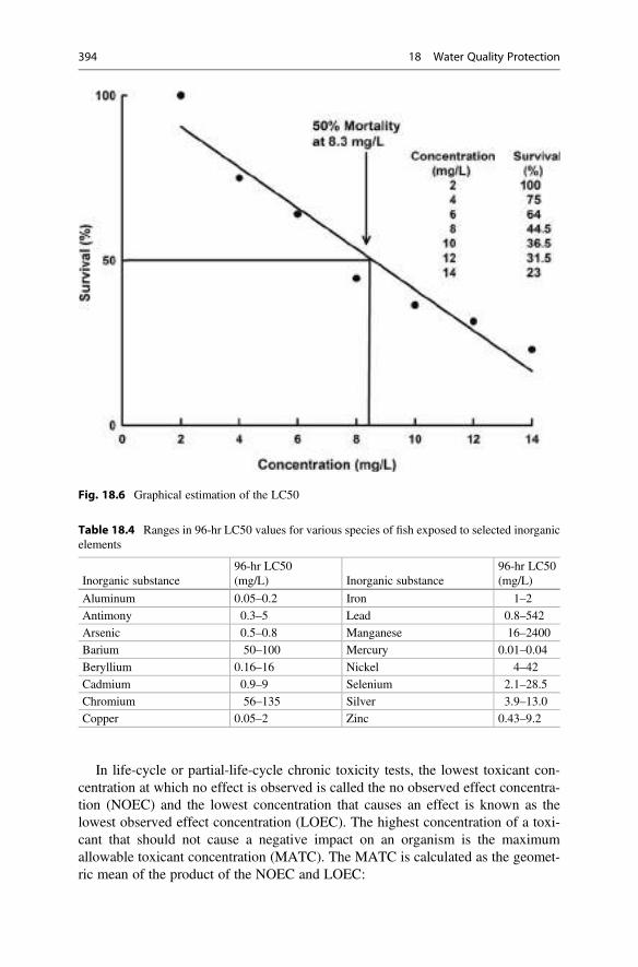
In life-cycle or partial-life-cycle chronic toxicity tests, the lowest toxicant con-centration at which no effect is observed is called the no observed effect concentra-tion (NOEC) and the lowest concentration that causes an effect is known as thelowest observed effect concentration (LOEC). The highest concentration of a toxi-cant that should not cause a negative impact on an organism is the maximumallowable toxicant concentration (MATC). The MATC is calculated as the geomet-ric mean of the product of the NOEC and LOEC:

Fig. 18.6 Graphical estimation of the LC50

Table 18.4 Ranges in 96-hr LC50 values for various species of fish exposed to selected inorganicelements

Inorganic substance96-hr LC50(mg/L) Inorganic substance

96-hr LC50(mg/L)

Aluminum 0.05–0.2 Iron 1–2

Antimony 0.3–5 Lead 0.8–542

Arsenic 0.5–0.8 Manganese 16–2400

Barium 50–100 Mercury 0.01–0.04

Beryllium 0.16–16 Nickel 4–42

Cadmium 0.9–9 Selenium 2.1–28.5

Chromium 56–135 Silver 3.9–13.0

Copper 0.05–2 Zinc 0.43–9.2


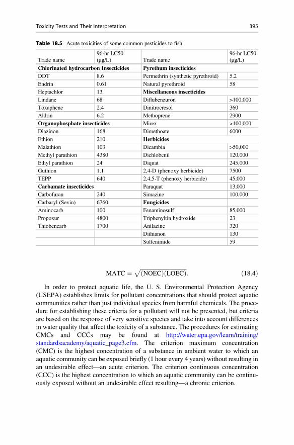
MATC ¼ffiffiffiffiffiffiffiffiffiffiffiffiffiffiffiffiffiffiffiffiffiffiffiffiffiffiffiffiffiffiffiffiffiNOECð Þ LOECð Þ

p: ð18:4Þ

In order to protect aquatic life, the U. S. Environmental Protection Agency(USEPA) establishes limits for pollutant concentrations that should protect aquaticcommunities rather than just individual species from harmful chemicals. The proce-dure for establishing these criteria for a pollutant will not be presented, but criteriaare based on the response of very sensitive species and take into account differencesin water quality that affect the toxicity of a substance. The procedures for estimatingCMCs and CCCs may be found at http://water.epa.gov/learn/training/standardsacademy/aquatic_page3.cfm. The criterion maximum concentration(CMC) is the highest concentration of a substance in ambient water to which anaquatic community can be exposed briefly (1 hour every 4 years) without resulting inan undesirable effect—an acute criterion. The criterion continuous concentration(CCC) is the highest concentration to which an aquatic community can be continu-ously exposed without an undesirable effect resulting—a chronic criterion.

Table 18.5 Acute toxicities of some common pesticides to fish

Trade name96-hr LC50(μg/L) Trade name

96-hr LC50(μg/L)

Chlorinated hydrocarbon Insecticides Pyrethum insecticidesDDT 8.6 Permethrin (synthetic pyrethroid) 5.2

Endrin 0.61 Natural pyrethroid 58

Heptachlor 13 Miscellaneous insecticidesLindane 68 Diflubenzuron >100,000

Toxaphene 2.4 Dinitrocresol 360

Aldrin 6.2 Methoprene 2900

Organophosphate insecticides Mirex >100,000

Diazinon 168 Dimethoate 6000

Ethion 210 HerbicidesMalathion 103 Dicambia >50,000

Methyl parathion 4380 Dichlobenil 120,000

Ethyl parathion 24 Diquat 245,000

Guthion 1.1 2,4-D (phenoxy herbicide) 7500

TEPP 640 2,4,5-T (phenoxy herbicide) 45,000

Carbamate insecticides Paraquat 13,000

Carbofuran 240 Simazine 100,000

Carbaryl (Sevin) 6760 FungicidesAminocarb 100 Fenaminosulf 85,000

Propoxur 4800 Triphenyltin hydroxide 23

Thiobencarb 1700 Anilazine 320

Dithianon 130

Sulfenimide 59

Toxicity Tests and Their Interpretation 395

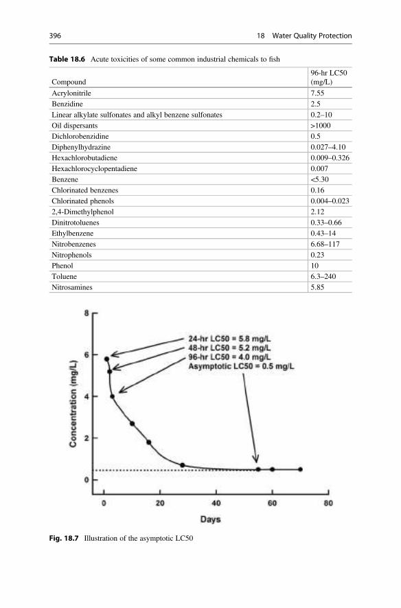
http://water.epa.gov/learn/training/standardsacademy/aquatic_page3.cfm

http://water.epa.gov/learn/training/standardsacademy/aquatic_page3.cfm

Table 18.6 Acute toxicities of some common industrial chemicals to fish

Compound96-hr LC50(mg/L)

Acrylonitrile 7.55

Benzidine 2.5

Linear alkylate sulfonates and alkyl benzene sulfonates 0.2–10

Oil dispersants >1000

Dichlorobenzidine 0.5

Diphenylhydrazine 0.027–4.10

Hexachlorobutadiene 0.009–0.326

Hexachlorocyclopentadiene 0.007

Benzene <5.30

Chlorinated benzenes 0.16

Chlorinated phenols 0.004–0.023

2,4-Dimethylphenol 2.12

Dinitrotoluenes 0.33–0.66

Ethylbenzene 0.43–14

Nitrobenzenes 6.68–117

Nitrophenols 0.23

Phenol 10

Toluene 6.3–240

Nitrosamines 5.85

Fig. 18.7 Illustration of the asymptotic LC50


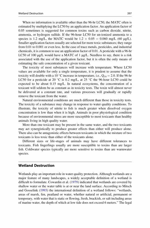
When no information is available other than the 96-hr LC50, the MATC often isestimated by multiplying the LC50 by an application factor. An application factor of0.05 sometimes is suggested for common toxins such as carbon dioxide, nitrite,ammonia, or hydrogen sulfide. If the 96-hour LC50 for un-ionized ammonia to aspecies is 1.2 mg/L, the MATC would be 1.2 � 0.05 ¼ 0.060 mg/L (60 μg/L).Smaller application factors usually are selected for more toxic substances; they rangefrom 0.01 to 0.001 or even less. In the case of trace metals, pesticides, and industrialchemicals, it is common to use an application factor of 0.01. A pesticide with a 96-hrLC50 of 100 μg/L would have a MATC of 1 μg/L. Needless to say, there is a riskassociated with the use of the application factor, but it is often the only means ofestimating the safe concentration of a given toxicant.

The toxicity of most substances will increase with temperature. Where LC50values are available for only a single temperature, it is prudent to assume that thetoxicity will double with a 10 �C increase in temperature, i.e., Q10 ¼ 2.0. If the 96-hrLC50 for a pesticide at 20 �C is 0.2 mg/L, at 25 �C the 96-hour LC50 could beexpected to be about 0.15 mg/L. In natural ecosystems, the concentration of atoxicant will seldom be as constant as in toxicity tests. The toxin will almost neverbe delivered at a constant rate, and various processes will gradually or rapidlyremove the toxicant from the water.

Natural environmental conditions are much different than those in toxicity tests.The toxicity of a substance may change in response to water quality conditions. Toillustrate, the toxicity of nitrite to fish is much greater when dissolved oxygenconcentration is low than when it is high. Animals in poor physiological conditionbecause of environmental stress are more susceptible to most toxicants than healthyanimals living in high quality water.

More than one toxicant may be present in the same water, and the two toxicantsmay act synergistically to produce greater effects than either will produce alone.There also can be antagonistic effects between toxicants in which the mixture of twotoxicants is less toxic than either of the toxicants alone.

Different sizes or life-stages of animals may have different tolerances totoxicants. Fish fingerlings usually are more susceptible to toxins than are largerfish. Coldwater species typically are more sensitive to toxins than are warmwaterspecies.

Wetland Destruction

Wetlands play an important role in water quality protection. Although wetlands are amajor feature of many landscapes, a widely acceptable definition of a wetland isdifficult to formulate. Cowardin et al. (1979) indicated that wetlands are covered byshallow water or the water table is at or near the land surface. According to Mitschand Gosselink (1993) the international definition of a wetland follows: “wetlands,areas of marsh, fen, peatland or water, whether natural or artificial, permanent ortemporary, with water that is static or flowing, fresh, brackish, or salt including areasof marine water, the depth of which at low tide does not exceed 6 meters.” The legal

Wetland Destruction 397

definition of a wetland in the United States is as follows: “the term wetlands meansthose areas that are inundated or saturated by surface or groundwater at a frequencyand duration sufficient to support, and that under normal circumstances do support, aprevalence of vegetation typically adapted for life in saturated soil conditions.Wetlands generally include swamps, marshes, bogs, and similar areas.”

As an analogy to emphasize the role of wetlands in purifying water, Mitsch andGosselink (1993) called wetlands “the kidneys of the landscape,” but wetlands alsoprovide many other ecological services. Wetlands are highly productive ecosystems.They are nurseries and feeding grounds for aquatic animals, waterfowl, and otherbird life. They also are important habitats for amphibians and some reptiles.Wetlands act as sediment and nutrient traps and provide flood protection. Riparianvegetation is a buffer zone that filters runoff and reduces the input of suspendedsolids and nutrients into streams. Riparian vegetation also helps control bankerosion. Coastal mangrove forests and other marine wetlands provide a similarfiltration system at mouths and deltas of rivers, and mangroves reduce wave andstorm damage to the coastline.

The major cause of freshwater wetland loss is conversion of wetlands to agricul-tural land. It is estimated that 26,000,000 ha of farmland in the United States wereobtained by draining wetlands (Dahl 1990). Over half of the original mangrovewetlands that occur in coastal areas of the world have been destroyed or converted toother uses (Massaut 1999). Coastal pond aquaculture was a major driver of man-grove loss between 1970 and 2000, but its role in mangrove loss is declining greatlybecause of better regulations. Wetlands are today protected by law in the UnitedStates and many other countries, and their conversion to agricultural land, aquacul-tural ponds, and municipal and industrial areas has greatly declined. However, insome parts of the world, wetland destruction continues.

Water Quality Regulations and Pollution Control

The usefulness of water declines as water quality deteriorates, and high quality wateris in greater demand and has more value than low quality water. The concepts ofwater quality and water quantity developed simultaneously during human history,but until recently, few quantitative means of assessing water quality were available.Because of the importance of water in human affairs and the relative scarcity ofwater in many regions, conflicts over water use rights and water quality have oftenoccurred. Water rights issues historically focused on water quantity and especiallyon the quantity of surface water. Disputes over water rights have been settled bysundry methods, but mainly warfare, feuds, court decisions, and mutual agreements.

In the United States and most developed nations, water rights disputes havetraditionally been settled through legal actions based on the principles of commonlaw. In common law, court rulings are based on precedents set in previous courtcases of similar nature, or if there is no precedent, the court must make a decision thatwill become precedent. According to Vesilind et al. (1994), common law hasprovided a reasonable way to deal with surface water disputes through the theories


of riparian doctrine, prior appropriations doctrine, the principle of reasonable use,and the concept of prescriptive rights. Riparian doctrine holds that ownership of theland beneath or adjoining a body of surface water includes the right to use this water.Prior appropriations take the approach that water use rights are based on a “first-come, first-serve basis” and land ownership does not necessarily grant control overthe use of the water associated with the land. The principle of reasonable use statesthat the riparian owner is entitled to make reasonable use of the water, but the courtmay take into account the needs of others downstream. The concept of prescriptiverights basically allows the upstream user to abuse water quantity and water qualityprovided the downstream riparian owner does not use the water. Thus, by lack ofuse, the downstream owner gives up his water rights.

Doctrines, principles, and concepts of water rights used in common law do notprovide clear guidance about issues related to water quality. Of course, if a wateruser impairs the quality of water that another party has a right to use, the injuredparty may initiate a court case to seek relief. It takes years to set precedents, andcurrent issues often are settled by ancient precedents. This does not allow good useof new technology and knowledge, and it does not provide adequate protection ofenvironmental quality and public health. Modern governments establish rules orregulations related to water quality and water pollution abatement through govern-mental mandates known as statutory laws. Statutory laws about water quality allow agovernment to exert a degree of control over the quality of waters within itsboundaries, minimize disputes over water quality, protect aquatic ecosystems, andguard public health.

In the United States, federal legislation known as the Clean Water Act was passedin 1965 to provide a uniform series of procedures to deal with water pollution. TheUS Environmental Protection Agency (USEPA) has the responsibility for enforcingthe regulations and laws mandated by the Clean Water Act, but the day to dayenforcement of the Clean Water Act has been relegated mainly to the individualstates. The Clean Water Act applies to governmental facilities, municipalities,industries, and private individuals. Implementation and enforcement of the CleanWater Act is obviously a tremendous task, and it has yet to be applied to all activitiesthat affect water quality in the United States. Implementation and enforcement of theact are continuing, and water quality in the United States has improved greatly and iscontinuing to improve as a result. Most countries have a system of water qualitylegislation, but in developing nations, water quality legislation often is either poorlystructured or not adequately implemented and enforced.

Effluent Discharge Permits

The initial step in water pollution control is to require a permit for discharge ofpollutants from a point source into natural waters. The Clean Water Act in the UnitedStates requires a National Pollutant Discharge Elimination System (NPDES) permitfor every pollutant discharge. The holder of a NPDES permit has the right todischarge effluents containing specified concentrations or amounts of pollutants at

Water Quality Regulations and Pollution Control 399

a given point usually for a 5-year period. The NPDES does not apply to storm runoff,discharges into water treatment systems, and some other waters. Individual statesand municipalities must establish regulations for discharges not covered by NPDES.

Pollution discharge permits typically contain effluent limitations, monitoringrequirements, and reporting schedules. They also may contain other features suchas use of best management practices (BMPs) to prevent or reduce the release ofpollutants or to clean up spills. Permits also specify conditions related to operation oftreatment systems, record keeping, inspection and entry, etc. In addition to effluentdischarge permits, legally enforceable standards are imposed on drinking waterquality in most countries.

Effluent Limitations

The reason for limits on the discharge of pollutants into natural waters is to avoidwater quality degradation. Prohibiting discharge is rarely a possibility, because manyactivities that cause water pollution are essential for society. Complete removal ofpollutants by treatment of effluents before final discharge usually is bothtechnologically and economically impossible. As a compromise, regulatory agenciesusually try to achieve a balance in water quality permits to allow an activity tocontinue but with limits on pollutants in effluents that are technologically achiev-able, affordable, and protective of water quality.

Use Classification for Water Bodies

The task of assigning effluent limitations in effluent permits can be facilitated as it isin the United States by classifying streams and other water bodies according to theiranticipated maximum beneficial use such as public drinking water supplies, propa-gation of fish and wildlife, recreational activities, industrial and agricultural watersources, navigation, and others. Each water use requires a certain level of waterquality. Water bodies can be classified into use categories and each use categoryassigned water quality standards. A stream classified for agricultural and industrialuse will have lower water quality standards than a stream designated for fish andwildlife. Stream classification force water users to limit or treat discharges to preventstreams from violating their water quality standards. Use classification also can beapplied to other types of water bodies and water sources.

A stream classification system usually has both quantitative and qualitativestandards as illustrated in Table 18.7. The US Clean Water Act requires that eachstate develop a stream classification system with criteria and standards for each usecategory. The standards developed by each state must attain the Clean Water Act’sgoal of fishable, swimmable water wherever possible and should prevent furtherstream degradation.

Most streams already were receiving pollution and degraded below their pristinecondition before the initiation of stream classification, but stream classification and


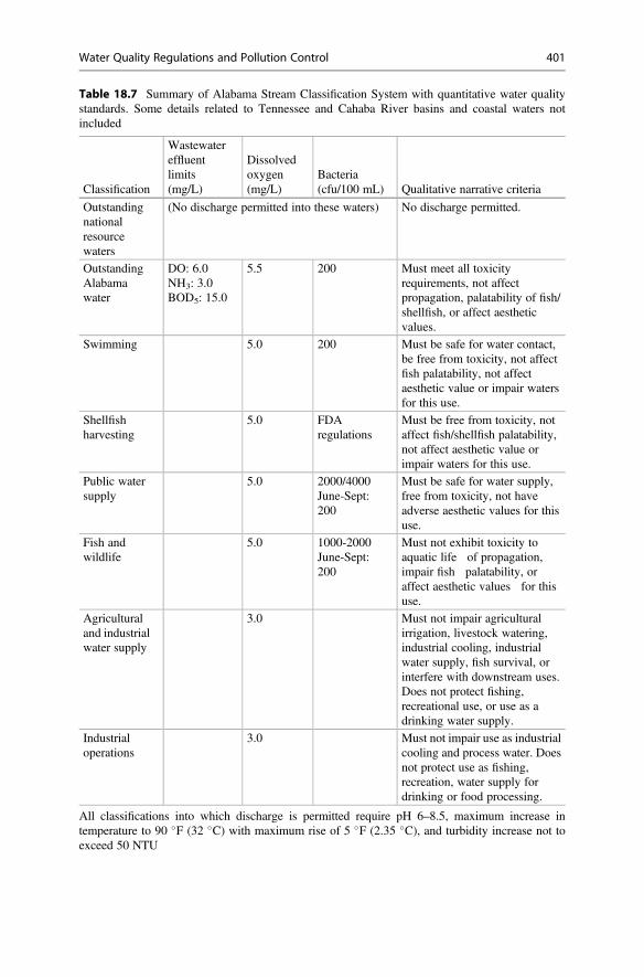
Table 18.7 Summary of Alabama Stream Classification System with quantitative water qualitystandards. Some details related to Tennessee and Cahaba River basins and coastal waters notincluded

Classification

Wastewatereffluentlimits(mg/L)

Dissolvedoxygen(mg/L)

Bacteria(cfu/100 mL) Qualitative narrative criteria

Outstandingnationalresourcewaters

(No discharge permitted into these waters) No discharge permitted.

OutstandingAlabamawater

DO: 6.0NH3: 3.0BOD5: 15.0

5.5 200 Must meet all toxicityrequirements, not affectpropagation, palatability of fish/shellfish, or affect aestheticvalues.

Swimming 5.0 200 Must be safe for water contact,be free from toxicity, not affectfish palatability, not affectaesthetic value or impair watersfor this use.

Shellfishharvesting

5.0 FDAregulations

Must be free from toxicity, notaffect fish/shellfish palatability,not affect aesthetic value orimpair waters for this use.

Public watersupply

5.0 2000/4000June-Sept:200

Must be safe for water supply,free from toxicity, not haveadverse aesthetic values for thisuse.

Fish andwildlife

5.0 1000-2000June-Sept:200

Must not exhibit toxicity toaquatic life of propagation,impair fish palatability, oraffect aesthetic values for thisuse.

Agriculturaland industrialwater supply

3.0 Must not impair agriculturalirrigation, livestock watering,industrial cooling, industrialwater supply, fish survival, orinterfere with downstream uses.Does not protect fishing,recreational use, or use as adrinking water supply.

Industrialoperations

3.0 Must not impair use as industrialcooling and process water. Doesnot protect use as fishing,recreation, water supply fordrinking or food processing.

All classifications into which discharge is permitted require pH 6–8.5, maximum increase intemperature to 90 �F (32 �C) with maximum rise of 5 �F (2.35 �C), and turbidity increase not toexceed 50 NTU

Water Quality Regulations and Pollution Control 401

effluent standards can prevent water quality in a stream or a reach of a stream fromdegrading further and may cause water quality to improve. The system can be usedto force improvements in surface water quality by giving streams a higher classifi-cation or disallowing the lowest classification.

Stream classification can fail to provide the intended benefits of protecting publichealth and the aquatic environment for several reasons. The stream standards maynot be adequate to protect water quality, or the effluent standards may not be strictenough to prevent waste from causing the receiving water to violate its standard.Moreover, there are many cases where standards simply are not enforced.

The way in which governments foster economic development also can affectwater quality protection. Two general approaches are used in setting water qualitystandards: (1) stipulation and (2) a policy of minimum degradation of water quality.Where the major goal of a government is to encourage economic development,subsidies can be stipulated to industry. One possible subsidy to industry is to classifysteams according to low standards. From an environmental standpoint, it would bebetter for governments to subsidize wastewater treatment rather than to lower streamclassification or relax discharge standards (Tchobanoglous and Schroeder 1985).

Water Quality Standards

Once streams have been classified, the major focus is on limiting pollutant levels ineffluents to assure water quality in the receiving stream does not violate the standardsof its use classification. The writer of an effluent permit has the responsibility toprotect the environment while not unduly penalizing municipalities, industries, orother users. The criteria and standards in effluent permits are selected based onexperience, technical attainability, economic attainability, bioassays and other tests,ability to reliably measure the criteria, evidence of public health effects, educatedguess or judgment, mathematical models, and legal enforceability (Tchobanoglousand Schroeder 1985). Considerable experience has been accumulated in settingwater quality standards, and many water quality guidelines have been published,e.g., guidelines for drinking water, for protection of aquatic ecosystems, for irriga-tion water, for livestock watering, and for recreational waters. Nevertheless, thepermit writer must decide upon the safe limits of pollutants in effluents in order toachieve the goals of the guidelines. Permits must be renewed at intervals, andobvious flaws in permits may be negotiated between the permit holder and thepermitting agency. No permit is perfect, but discharge permits with water qualitycriteria and standards are important for protecting water quality.

Concentration Based Standards

The simplest standards in effluent permits have criteria regarding permissibleconcentrations of selected water quality variables. Examples of concentration-based criteria in a water quality standard for an effluent follow:


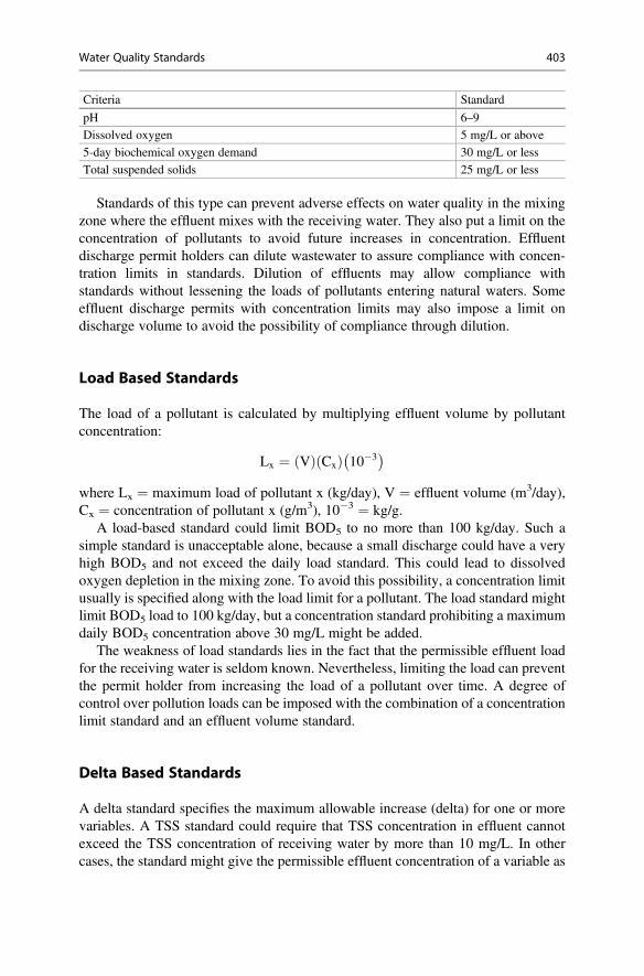
Criteria Standard

pH 6–9

Dissolved oxygen 5 mg/L or above

5-day biochemical oxygen demand 30 mg/L or less

Total suspended solids 25 mg/L or less

Standards of this type can prevent adverse effects on water quality in the mixingzone where the effluent mixes with the receiving water. They also put a limit on theconcentration of pollutants to avoid future increases in concentration. Effluentdischarge permit holders can dilute wastewater to assure compliance with concen-tration limits in standards. Dilution of effluents may allow compliance withstandards without lessening the loads of pollutants entering natural waters. Someeffluent discharge permits with concentration limits may also impose a limit ondischarge volume to avoid the possibility of compliance through dilution.

Load Based Standards

The load of a pollutant is calculated by multiplying effluent volume by pollutantconcentration:

Lx ¼ Vð Þ Cxð Þ 10�3� �

where Lx ¼ maximum load of pollutant x (kg/day), V ¼ effluent volume (m3/day),Cx ¼ concentration of pollutant x (g/m3), 10�3 ¼ kg/g.

A load-based standard could limit BOD5 to no more than 100 kg/day. Such asimple standard is unacceptable alone, because a small discharge could have a veryhigh BOD5 and not exceed the daily load standard. This could lead to dissolvedoxygen depletion in the mixing zone. To avoid this possibility, a concentration limitusually is specified along with the load limit for a pollutant. The load standard mightlimit BOD5 load to 100 kg/day, but a concentration standard prohibiting a maximumdaily BOD5 concentration above 30 mg/L might be added.

The weakness of load standards lies in the fact that the permissible effluent loadfor the receiving water is seldom known. Nevertheless, limiting the load can preventthe permit holder from increasing the load of a pollutant over time. A degree ofcontrol over pollution loads can be imposed with the combination of a concentrationlimit standard and an effluent volume standard.

Delta Based Standards

A delta standard specifies the maximum allowable increase (delta) for one or morevariables. A TSS standard could require that TSS concentration in effluent cannotexceed the TSS concentration of receiving water by more than 10 mg/L. In othercases, the standard might give the permissible effluent concentration of a variable as

Water Quality Standards 403

an increase above the expected seasonal average (ambient) concentration of thereceiving water, e.g., the turbidity of the discharge must not exceed the ambientturbidity by more than 10 NTU. The delta standard differs from a concentration limitstandard by including a relationship to the quality of the receiving water.

Total Maximum Daily Loads

The shortcomings of effluent standards discussed above have led the United Statesand some other countries to establish total maximum daily loads (TMDLs) forpriority pollutants in receiving waters. This approach consists of calculating themaximum amount of a pollutant from all sources (natural or anthropogenic) that canbe allowed without causing a water body to violate its classification standards. Insome situations, the TMDL of a pollutant must be allocated among the differentsources of the pollutant. Suppose a stream reach has a TMDL for phosphorus of500 kg/day, several industries discharge into the stream reach, and natural sources ofphosphorus are 100 kg/day. The maximum amount of phosphorus permissible ineffluents is 400 kg/day, but this amount normally would not be allowed in order tohave a safety factor. A safety factor of 1.5 would lower the TMDL of this example to267 kg/day. This load would have to be allocated among the different industries, andin some cases, the current load of a pollutant might already exceed the TMDLleading to stricter limits in permits. Use of TMDLs allows industries to trade inpollution loads. If an industry does not need its entire assigned TMDL for apollutant, it could sell the unneeded portion of its TMDL allocation to anotherindustry that cannot meet its TMDL for the particular pollutant.

Toxic Chemical Standards

Water pollution control agencies often publish lists of acceptable concentrations ofpollutants that may be used as guidelines for establishing limits in permits. It isdifficult to establish standards for toxic chemicals, and metals in particular, ineffluent permits because their toxicities vary with water quality conditions. Toavoid this problem, toxicity-based limitations may be established through effluenttoxicity testing. The toxicity tests are conducted by exposing certain species ofaquatic organisms to the effluent in question. A permit may require that toxicitytesting be done to prove that the effluent is not acutely toxic to organisms in thereceiving water body at the time of its discharge.

Biological Standards

Discharge permits often contain standards for coliform organisms that can beindicators of fecal pollution and certain other microorganisms of human healthconcern. There is a growing tendency to include biological standards based on


biocriteria associated with the flora and fauna of the receiving water body.Biocriteria may be used to supplement the traditional water quality criteria andstandards or used as an alternative where traditional methods have not been effec-tive. Development of biocriteria requires a reference condition (minimal impact) foreach use classification, measurement of community structure and function in refer-ence to water quality to establish biocriteria, and a protocol for determining ifcommunity structure and function has been impaired. Biocriteria are much moredifficult to assess than chemical and physical criteria and standards.

Waste Treatment and Best Management Practices

Pollution control involves technological, political, legislative, regulatory, enforce-ment, business, ethical educational, and other issues. Most governments have devel-oped regulations of point source effluents to impose concentration limits, load limits,or both. Treatment of point source pollution allows compliance with the standards inthe discharge regulations. Activities that discharge nonpoint source pollution aretypically required to operate in a manner that minimizes pollution, and inspectionsare made by the appropriate authority to verify that pollution is being controlled.

Point source effluent can be directed through treatment facilities to lessenconcentrations and loads of pollutants. Some treatment techniques in common useare filtration and sedimentation to remove solids, activated sludge basins withaeration to rapidly oxidize organic matter, precipitation of phosphorus with ferrouschloride, aerobic reactors for nitrification, anaerobic reactors for denitrification,air-stripping of ammonia, outdoor wastewater stabilization ponds, neutralization,and precipitation of metals by chemical treatment or pH manipulation. Removal ofcertain substances from industrial effluents may require development of specifictreatment technologies. Some effluents that contain biological pollutants must bedisinfected—often by chlorination—before final discharge.

Nonpoint source effluents are not confined in a conduit, and conventional treat-ment techniques cannot generally be applied. The most common means of reducingnonpoint source pollution is through the use of practices that lessen the amounts ofpollutants entering runoff. Such practices are called best management practices(BMPs). Sometimes BMPs and qualitative standards also are included in standardsfor point source discharges.

Agriculture is the largest single source of nonpoint pollution, and BMPs havelong been used for controlling agricultural pollution. There are three classes ofagricultural BMPs: erosion control, nutrient management, and integrated pest man-agement. Some examples of erosion control BMPs in agriculture are cover crops,no-till farming, conservation tillage, grass-lined ditches, terraces in fields on slopingland, etc. Storm water runoff management in municipalities also may consist of asystem of BMPs, and BMPs are used to lessen pollution from logging, construction,and mining operations.


Monitoring and Enforcement of Discharge Permits

Many times it is not possible for effluent discharge permit holders to complyimmediately with the conditions of the permit, and a schedule for compliance maybe specified. Most governments depend largely upon self-monitoring to documentcompliance with permit standards. The permit will specify minimum monitoringrequirements including frequency of sampling, type of sample, variables to beanalyzed, and reporting schedule. Permits normally require the permit holder toimmediately report when discharges are not in compliance.

Enforcement of water discharge permits normally involves administrativeactions, because the permit holder must report compliance or noncompliance withthe permit on a scheduled basis. In theory, the permit holder should realize whencompliance is not being achieved and work to correct the problem. In the UnitedStates, federal and state enforcement of the Clean Water Act can be in the form ofadministrative actions or judicial actions. The administrative actions may take manyforms depending upon the type of violation. An order to comply may be issued alongwith a compliance schedule. For serious violations, the administrative order mayinclude a fine or other penalty. Failure to comply with administrative orders can leadto criminal prosecution. Both civil and criminal judicial enforcement is possible ifadministrative orders do not solve problems related to permits. The penaltiesresulting from judicial enforcement are more severe than those resulting fromadministrative orders.

Parties who feel that they have been injured by water discharges may bring civillawsuits against permit holders if the government is not “diligently prosecuting” theviolation (Gallagher and Miller 1996). The form of enforcement of water dischargepermits will vary greatly among nations.

Drinking Water Standards

Many countries, individual states or provinces, and international agencies have madestandards for drinking water quality. The current National Drinking WaterRegulations for the United States may be found at (https://www.epa.gov/sites/production/files/2018-03/documents/dwtable2018.pdf). These standards come fromthe Office of Groundwater and Drinking Water of the USEPA, and the primarystandards are legally enforceable standards that apply to public water systems. Thepurpose of these primary standards is to protect drinking water quality by limitingthe levels of specific contaminants that can adversely affect public health and areknown or anticipated to occur in public water supply systems. The SecondaryDrinking Water Regulations for the United States are non-enforceable guidelinesregulating contaminants that may cause cosmetic effects such as skin or toothdiscoloration and aesthetic effects such as taste, odor, or color in drinking water.


https://www.epa.gov/sites/production/files/2018-03/documents/dwtable2018.pdf

https://www.epa.gov/sites/production/files/2018-03/documents/dwtable2018.pdf

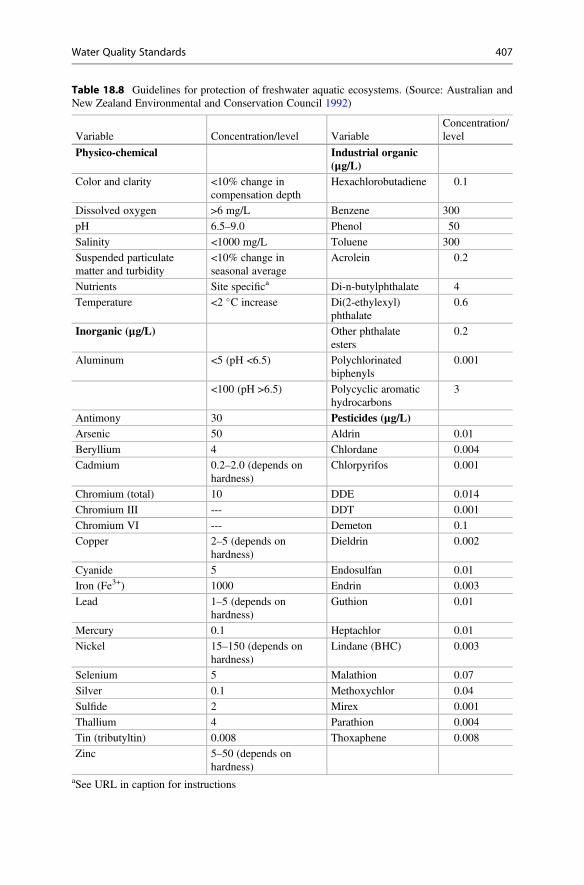
Table 18.8 Guidelines for protection of freshwater aquatic ecosystems. (Source: Australian andNew Zealand Environmental and Conservation Council 1992)

Variable Concentration/level VariableConcentration/level

Physico-chemical Industrial organic(μg/L)

Color and clarity <10% change incompensation depth

Hexachlorobutadiene 0.1

Dissolved oxygen >6 mg/L Benzene 300

pH 6.5–9.0 Phenol 50

Salinity <1000 mg/L Toluene 300

Suspended particulatematter and turbidity

<10% change inseasonal average

Acrolein 0.2

Nutrients Site specifica Di-n-butylphthalate 4

Temperature <2 �C increase Di(2-ethylexyl)phthalate

0.6

Inorganic (μg/L) Other phthalateesters

0.2

Aluminum <5 (pH <6.5) Polychlorinatedbiphenyls

0.001

<100 (pH >6.5) Polycyclic aromatichydrocarbons

3

Antimony 30 Pesticides (μg/L)Arsenic 50 Aldrin 0.01

Beryllium 4 Chlordane 0.004

Cadmium 0.2–2.0 (depends onhardness)

Chlorpyrifos 0.001

Chromium (total) 10 DDE 0.014

Chromium III --- DDT 0.001

Chromium VI --- Demeton 0.1

Copper 2–5 (depends onhardness)

Dieldrin 0.002

Cyanide 5 Endosulfan 0.01

Iron (Fe3+) 1000 Endrin 0.003

Lead 1–5 (depends onhardness)

Guthion 0.01

Mercury 0.1 Heptachlor 0.01

Nickel 15–150 (depends onhardness)

Lindane (BHC) 0.003

Selenium 5 Malathion 0.07

Silver 0.1 Methoxychlor 0.04

Sulfide 2 Mirex 0.001

Thallium 4 Parathion 0.004

Tin (tributyltin) 0.008 Thoxaphene 0.008

Zinc 5–50 (depends onhardness)

aSee URL in caption for instructions


Water Quality Guidelines

There are many lists of guidelines or criteria for public water supplies, fish andwildlife, agriculture, recreation and aesthetics, and industry. Guidelinesrecommended for protection of aquatic ecosystems in Australia, and New Zealandare provided in Table 18.8. Such guidelines usually are not legally enforceable, butthey show acceptable concentrations and may be the basis for criteria in legallyenforceable effluent permits.

Water quality guidelines for agriculture can help farmers to protect their crops andlivestock from damage by poor quality water. Guidelines for industrial waters maybe very important in assuring adequate water quality for various processes.

Conclusions

Humans must use water for many purposes, and water quality often is impairedthrough use. The demand for water is increasing because of the rapidly growinghuman population, and water quality deterioration has become a serious issue inmany countries. Measures to conserve both the quantity and quality of water must beimposed or the world will face serious water shortages in the future. Some countrieshave developed rather elaborate systems of water quality regulations for maintainingor improving the quality of their waters. Other countries have done little to protectwater quality, and serious water quality problems are occurring. It is urgent for allcountries to develop water quality regulations and to enforce them seriously. It isequally important to educate the public about the importance of protecting ourlimited and fragile water supplies for future use.

References

Australian and New Zealand Environment and Conservation Council (1992) Australian waterquality guidelines for fresh and marine waters. Australian and New Zealand Environment andConservation Council, Canberra

Bollenbach WM Jr (1975) Ground water and wells. Johnson Division, UOP Inc, Saint PaulBoyd CE, Clay J (1998) Shrimp aquaculture and the environment. Sci Am 278:42–49Boyd CE, Tucker CS (2014) Handbook for aquaculture water quality. Craftmaster Printers, AuburnCowardin LM, Carter V, Golet FC, LaRoe ET (1979) Classification of wetlands and deepwater

habitats of the United States. Publication FWS/OBS-79/31, United States Fish and WildlifeService, Washington

Dahl TE (1990) Wetlands losses in the United States, 1780s to 1980s. United States Department ofthe Interior, Fish and Wildlife Service, Washington

Eaton AD, Clesceri LS, Greenburg AE (eds) (2005) Standard methods for the examination of waterand wastewater. American Public Health Association, Washington

Gallagher LM, Miller LA (1996) Clean water handbook. Government Institutes, Inc., RockvilleMagleby R, Sandretto C, Crosswaite W, Osborn CT (1995) Soil erosion and conservation in the

United States. An overview. USDA Economic Research Service Report AIB-178, WashingtonMassaut L (1999) Mangrove management and shrimp aquaculture. Department of Fisheries and

Allied Aquacultures, Auburn University, Alabama


Mitsch WJ, Gosselink JG (1993) Wetlands. Van Nostrand Reinhold, New YorkSmith DD (1941) Interpretation of soil conservation data for field use. Ag Eng 21:59–64Tchobanoglous G, Schroeder ED (1985) Water quality: characteristics, modeling, modification.

Adison-Wesley Publishing Company, ReadingUSEPA (1973) Methods for identifying and evaluating the nature and extent of nonpoint sources of

pollution. EPA 430/9-73-014, Washingtonvan der Leeden F, Troise FL, Todd DK (1990) The water encyclopedia. Lewis Publishers, Inc.,

ChelseaVesilind PA, Peirce JJ, Weiner RF (1994) Environmental engineering. Butterworth-Heinemann,

BostonWischeier WH, Smith DD (1965) Predicting rainfall erosion losses from cropland east of the Rocky

Mountains. Agricultural Handbook 282, United States Department of Agriculture, Beltsville,Maryland

Zingg AW (1940) Degree and length of land slope as it affects soil loss in runoff. Ag Eng22:173–175

References 409

Appendix: Some Fundamental Principlesand Calculations

Introduction

This appendix provides some very basic principles of chemistry and some informa-tion on calculating concentration of substances in solution. Much more detailedinformation is available in a general inorganic chemistry textbook.

Elements, Atoms, Molecules, and Compounds

Elements are the basic substances of which more complex substances are composed.Anything that has mass (or weight) and occupies space is matter made up ofchemical elements such as silicon, aluminum, iron, oxygen, sulfur, copper, etc.Substances more complex than atoms of a single element consist of molecules. Amolecule is the smallest entity of a substance that has all the properties of thatsubstance.

Elements are classified broadly as metals, nonmetals, or metalloids. Metals have ametallic luster, are malleable (but often hard), and can conduct electricity and heat.Some examples are iron, zinc, copper, silver, and gold. Nonmetals lack metallicluster, they are not malleable (but tend to be brittle), some are gases, and they doconduct heat and electricity. Metalloids have one or more properties of both metalsand nonmetals. Because metalloids can both insulate and conduct heat and electric-ity, they are known as semiconductors. The best examples of metalloids are boronand silicon, but there are several others.

There also are less inclusive groupings of elements than metals, nonmetals, andmetalloids. Alkali metals such as sodium and potassium are highly reactive and havean ionic valence of +1. Alkaline earth metals include calcium, magnesium, and otherelements that are moderately reactive and have an ionic valence of +2. Halogensillustrated by chlorine and iodine are highly reactive nonmetals, and they have anionic valence of �1. This group is unique in that its members can exist in solid,liquid, and gaseous form at temperatures and pressures found on the earth’s surface.Because of their toxicity, halogens often are used as disinfectants. Noble gases suchas helium, argon, and neon are unreactive except under very special conditions. In allthere are 18 groups and subgroups of elements. Most elements are included in the

# Springer Nature Switzerland AG 2020C. E. Boyd, Water Quality, https://doi.org/10.1007/978-3-030-23335-8

411

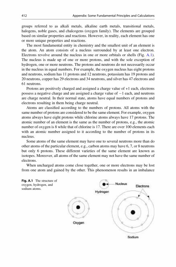
https://doi.org/10.1007/978-3-030-23335-8

groups referred to as alkali metals, alkaline earth metals, transitional metals,halogens, noble gases, and chalcogens (oxygen family). The elements are groupedbased on similar properties and reactions. However, in reality, each element has oneor more unique properties and reactions.

The most fundamental entity in chemistry and the smallest unit of an element isthe atom. An atom consists of a nucleus surrounded by at least one electron.Electrons revolve around the nucleus in one or more orbitals or shells (Fig. A.1).The nucleus is made up of one or more protons, and with the sole exception ofhydrogen, one or more neutrons. The protons and neutrons do not necessarily occurin the nucleus in equal numbers. For example, the oxygen nucleus has eight protonsand neutrons, sodium has 11 protons and 12 neutrons, potassium has 19 protons and20 neutrons, copper has 29 electrons and 34 neutrons, and silver has 47 electrons and61 neutrons.

Protons are positively charged and assigned a charge value of +1 each, electronspossess a negative charge and are assigned a charge value of �1 each, and neutronsare charge neutral. In their normal state, atoms have equal numbers of protons andelectrons resulting in them being charge neutral.

Atoms are classified according to the numbers of protons. All atoms with thesame number of protons are considered to be the same element. For example, oxygenatoms always have eight protons while chlorine atoms always have 17 protons. Theatomic number of an element is the same as the number of protons, e.g., the atomicnumber of oxygen is 8 while that of chlorine is 17. There are over 100 elements eachwith an atomic number assigned to it according to the number of protons in itsnucleus.

Some atoms of the same element may have one to several neutrons more than doother atoms of the particular element, e.g., carbon atoms may have 6, 7, or 8 neutronsbut only 6 protons. These different varieties of the same element are known asisotopes. Moreover, all atoms of the same element may not have the same number ofelectrons.

When uncharged atoms come close together, one or more electrons may be lostfrom one atom and gained by the other. This phenomenon results in an imbalance

Fig. A.1 The structure ofoxygen, hydrogen, andsodium atoms.

412 Appendix: Some Fundamental Principles and Calculations

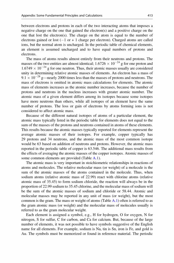
between electrons and protons in each of the two interacting atoms that imposes anegative charge on the one that gained the electron(s) and a positive charge on theone that lost the electron(s). The charge on the atom is equal to the number ofelectrons gained or lost (�1 or + 1 charge per electron). Charged atoms are calledions, but the normal atom is uncharged. In the periodic table of chemical elements,an element is assumed uncharged and to have equal numbers of protons andelectrons.

The mass of atoms results almost entirely from their neutrons and protons. Themasses of the two entities are almost identical; 1.6726 � 10�24 g for one proton and1.6749 � 10�24 g for one neutron. Thus, their atomic masses usually are consideredunity in determining relative atomic masses of elements. An electron has a mass of9.1� 10�28 g—nearly 2000 times less than the masses of protons and neutrons. Themass of electrons is omitted in atomic mass calculations for elements. The atomicmass of elements increases as the atomic number increases, because the number ofprotons and neutrons in the nucleus increases with greater atomic number. Theatomic mass of a given element differs among its isotopes because some isotopeshave more neutrons than others, while all isotopes of an element have the samenumber of protons. The loss or gain of electrons by atoms forming ions is notconsidered to affect atomic mass.

Because of the different natural isotopes of atoms of a particular element, theatomic mass typically listed in the periodic table for elements does not equal to thesum of the masses of the protons and neutrons contained in atoms of these elements.This results because the atomic masses typically reported for elements represent theaverage atomic masses of their isotopes. For example, copper typically has29 protons and 34 neutrons, and the atomic mass of the most common isotopewould be 63 based on addition of neutrons and protons. However, the atomic massreported in the periodic table of copper is 63.546. The additional mass results fromthe effects of averaging the atomic masses of the copper isotopes. Atomic masses ofsome common elements are provided (Table A.1).

The atomic mass is very important in stoichiometric relationships in reactions ofatoms and molecules. The relative molecular mass (or weight) of a molecule is thesum of the atomic masses of the atoms contained in the molecule. Thus, whensodium atoms (relative atomic mass of 22.99) react with chlorine atoms (relativeatomic mass of 35.45) to form sodium chloride, the reaction will always be in theproportion of 22.99 sodium to 35.45 chlorine, and the molecular mass of sodium willbe the sum of the atomic masses of sodium and chloride or 58.44. Atomic andmolecular masses may be reported in any unit of mass (or weight), but the mostcommon is the gram. The mass or weight of atoms (Table A.1) often is referred to asthe gram atomic mass (or weight) and the molecular mass of molecules usually isreferred to as the gram molecular weight.

Each element is assigned a symbol, e.g., H for hydrogen, O for oxygen, N fornitrogen, S for sulfur, C for carbon, and Ca for calcium. But, because of the largenumber of elements, it was not possible to have symbols suggestive of the Englishname for all elements. For example, sodium is Na, tin is Sn, iron is Fe, and gold isAu. The symbols must be memorized or found in reference material. The periodic

Appendix: Some Fundamental Principles and Calculations 413

table of the elements is a convenient listing of the elements in a way that elementswith similar chemical properties are grouped together. The periodic table ispresented in various formats, but most presentations include, at minimum, eachelement’s symbol, atomic number, and relative atomic mass and indicate the groupof elements to which it belongs.

The maximum number of electrons that can occur in a shell of an atom usually is2n2 where n is the number of the shell starting at the shell nearest the nucleus, i.e.,two electrons in the first shell, eight in the second shell, etc. Elements with a largeatomic number have several shells and some shells may not contain the maximumnumber of electrons. Chemical reactions among atoms involve only the electrons inthe outermost shell of atoms.

The laws of thermodynamics dictate that substances spontaneously changetowards their most stable states possible under existing conditions. To be stable,an atom needs two electrons in the inner shell, and at least eight electrons in itsoutermost shell. Chemical combinations (reactions) occur so that atoms gain or loseelectrons to attain stable outer shells.

Nonmetals tend to have outer shells nearly full of electrons. For example, chlorinehas seven electrons in its outer shell. If it gains one electron, it will have a stable

Table A.1 Selected atomic weights

Element Symbol Atomic weight Element Symbol Atomic weight

Aluminum Al 26.9815 Magnesium Mg 24.305

Antimony Sb 121.76 Manganese Mn 54.905

Arsenic As 74.9216 Mercury Hg 200.59

Barium Ba 137.327 Molybdenum Mo 95.94

Beryllium Be 9.0122 Nickel Ni 58.6934

Bismuth Bi 208.9804 Nitrogen N 14.0067

Boron B 10.811 Oxygen O 15.9994

Bromine Br 79.904 Phosphorus P 30.9738

Cadmium Cd 112.411 Platinum Pt 195.078

Calcium Ca 40.078 Potassium K 39.0983

Carbon C 12.0107 Selenium Se 78.96

Chlorine Cl 35.453 Silicon Si 28.0855

Chromium Cr 51.996 Silver Ag 107.8682

Cobalt Co 58.9332 Sodium Na 22.9897

Copper Cu 63.546 Strontium Sr 87.62

Fluorine F 18.9984 Sulfur S 32.065

Gold Au 196.9665 Thallium Tl 204.3833

Helium He 4.0026 Tin Sn 118.71

Hydrogen H 1.0079 Tungsten W 183.84

Iodine I 126.9045 Uranium U 238.0289

Iron Fe 55.845 Vanadium V 50.9415

Lead Pb 207.19 Zinc Zn 65.39

Lithium Li 6.941


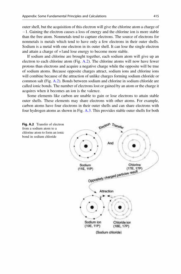
outer shell, but the acquisition of this electron will give the chlorine atom a charge of�1. Gaining the electron causes a loss of energy and the chlorine ion is more stablethan the free atom. Nonmetals tend to capture electrons. The source of electrons fornonmetals is metals which tend to have only a few electrons in their outer shells.Sodium is a metal with one electron in its outer shell. It can lose the single electronand attain a charge of +1and lose energy to become more stable.

If sodium and chlorine are brought together, each sodium atom will give up anelectron to each chlorine atom (Fig. A.2). The chlorine atoms will now have fewerprotons than electrons and acquire a negative charge while the opposite will be trueof sodium atoms. Because opposite charges attract, sodium ions and chlorine ionswill combine because of the attraction of unlike charges forming sodium chloride orcommon salt (Fig. A.2). Bonds between sodium and chlorine in sodium chloride arecalled ionic bonds. The number of electrons lost or gained by an atom or the charge itacquires when it becomes an ion is the valence.

Some elements like carbon are unable to gain or lose electrons to attain stableouter shells. These elements may share electrons with other atoms. For example,carbon atoms have four electrons in their outer shells and can share electrons withfour hydrogen atoms as shown in Fig. A.3. This provides stable outer shells for both

Fig. A.2 Transfer of electronfrom a sodium atom to achlorine atom to form an ionicbond in sodium chloride


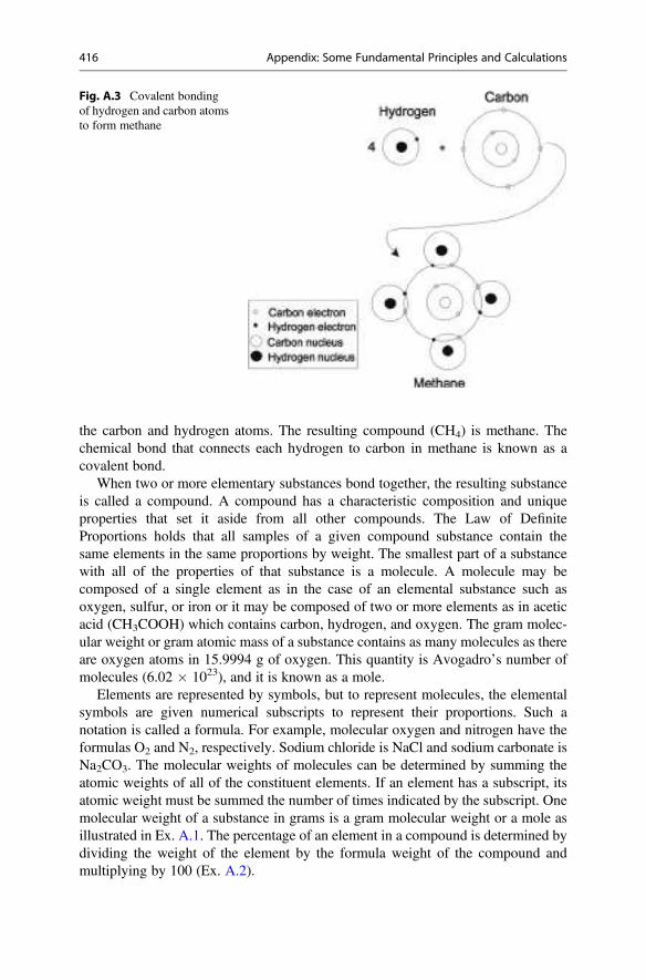
the carbon and hydrogen atoms. The resulting compound (CH4) is methane. Thechemical bond that connects each hydrogen to carbon in methane is known as acovalent bond.

When two or more elementary substances bond together, the resulting substanceis called a compound. A compound has a characteristic composition and uniqueproperties that set it aside from all other compounds. The Law of DefiniteProportions holds that all samples of a given compound substance contain thesame elements in the same proportions by weight. The smallest part of a substancewith all of the properties of that substance is a molecule. A molecule may becomposed of a single element as in the case of an elemental substance such asoxygen, sulfur, or iron or it may be composed of two or more elements as in aceticacid (CH3COOH) which contains carbon, hydrogen, and oxygen. The gram molec-ular weight or gram atomic mass of a substance contains as many molecules as thereare oxygen atoms in 15.9994 g of oxygen. This quantity is Avogadro’s number ofmolecules (6.02 � 1023), and it is known as a mole.

Elements are represented by symbols, but to represent molecules, the elementalsymbols are given numerical subscripts to represent their proportions. Such anotation is called a formula. For example, molecular oxygen and nitrogen have theformulas O2 and N2, respectively. Sodium chloride is NaCl and sodium carbonate isNa2CO3. The molecular weights of molecules can be determined by summing theatomic weights of all of the constituent elements. If an element has a subscript, itsatomic weight must be summed the number of times indicated by the subscript. Onemolecular weight of a substance in grams is a gram molecular weight or a mole asillustrated in Ex. A.1. The percentage of an element in a compound is determined bydividing the weight of the element by the formula weight of the compound andmultiplying by 100 (Ex. A.2).

Fig. A.3 Covalent bondingof hydrogen and carbon atomsto form methane


Ex. A.1 The molecular weights of O2 and CaCO3 will be calculated from theirformulas.

Solution:

O2: The atomic weight of O is 15.9994 (Table A.1), but it usually is rounded to16, thus 16 � 2 ¼ 32 g/mole.

CaCO3: The atomic weights of Ca, C, and O are 40.08, 12.01, and 16, respectively(Table A.1), thus 40.08 + 12.01 + 3(16) ¼ 100.09 g/mole.

The percentage composition of substances can be estimated from their formulasbecause of the Law of Definite Proportions.

Ex. A.2 The percentage Cu in CuSO4�5H2O will be calculated.Solution:From Table A.1, the atomic weights of Cu, S, O, and H are 63.55, 32.06, 16.00

and 1.01, respectively. Thus, the molecular weight of CuSO4�5H2O is63.55 + 32.06 + 9(16) + 10(1.01) ¼ 249.7 g. The percentage Cu is

Cu

CuSO4 � 5H2O� 100 or

63:55249:71

� 100 ¼ 25:4%:

Some compounds dissociate into ions in water, e.g. sodium nitrate (NaNO3)dissociates into Na+ and NO3

�. The ionic weight of a complex ion such as nitrateis calculated in the same manner as for the molecular weight of a compound. Ofcourse, the weight of Na+ is the same as the atomic weight of sodium.

Definition of a Solution

A solution consists of a solvent and a solute. A solvent is defined as the medium inwhich another substance—the solute—dissolves. In an aqueous sodium chlorinesolution, water is the solvent and sodium chloride is the solute. Miscibility refers to asolute and solvent mixing in all proportions to form a homogenous mixture orsolution. A true solution is by definition a homogenous mixture of two or morecomponents that cannot be separated into their individual ionic or molecularcomponents. Most solutes are only partially miscible in water. If a soluble compoundsuch as sodium chloride is mixed with water in progressively increasing amounts,the concentration of the solute will reach a constant level. Such a solution is said tobe saturated, and the amount of the sodium chloride held in solution is the solubilityof sodium chloride in water at the particular temperature. Any more sodium chlorideadded to the saturated solution will settle to the bottom without dissolving.

Solubilities of chemical compounds often are reported as grams of solute in100 mL of solution. Chemists generally consider substances that will dissolve to


the extent of 0.1 g/100 mL in water as soluble. A general list of classes of solublecompounds follows:

• nitrates• bromides, chlorides, and iodides—except those of lead, silver, and mercury• sulfates—except those of calcium, strontium, lead, and barium• carbonates and phosphates of sodium, potassium, and ammonium• sulfides of alkali and alkaline earth metals and ammonium.

Much of this book is devoted to a discussion of factors controlling concentrationsof dissolved matter in natural waters. This dissolved matter in water includesinorganic ions and compounds, organic compounds, and atmospheric gases, andmuch of water quality depends upon the concentrations of solutes in water.

Methods of Expressing Solute Strength

The solubility of a solute in a saturated solution or its concentration in an unsaturatedsolution may be expressed in several ways—the most common of which will bedescribed.

Molarity

In a molar solution, the solute strength is expressed in moles of solute per liter, e.g., a1 molar (1 M) solution contains 1 mole of solute in 1 L of solution. In other words, a1 M solution of NaCl consists of 1 mole (58.44 g NaCl) in 1 liter. Note: this is not thesame as putting 1 mole of NaCl in 1 L of solvent. It is 1 mole of NaCl contained in1 L of solution. The NaCl is dissolved in the solvent and the solution diluted to 1 lwith additional solvent. Calculations for a molar solution are shown in Ex. A.3.

Ex. A.3 How much Na2CO3 must be dissolved and diluted to 1 L to give a 0.25 Msolution?

Solution:The molecular weight of Na2CO3 is.2 Na ¼ 22.99 g/mol � 2 ¼ 45.98 g1 C ¼ 12.01 g/mol � 1 ¼ 12.01 g

3O ¼ 16 g/mol � 3 ¼ 48:0g105:99g

105:99 g=mole� 0:25 mol=L ¼ 26:5 g=L:

Thus, 26.5 g Na2CO3 diluted to 1 L in distilled water gives 0.25 M Na2CO3.


Molality

Not to be confused with a 1 molar solution, a 1 molal solution contains 1 molecularweight of a solute in 1 kg of solvent. The unit of molality is moles of solute perkilogram of solvent, and it is abbreviated as m or m.

Ex. A.4 The preparation of a 0.3 m KCl solution is illustrated.Solution:The molecular weight of KCl is.K ¼ 39.1 g/molCl ¼ 35.45 g/molKCl ¼ 74.55 g/mol

74:55 g=mol� 0:3 mol=kg ¼ 22:36 g KCl=kg solvent:

Thus, to make the 0.3 m KCl solution weigh 22.36 kg KCl and dissolve it in 1 kg ofdistilled water (or other solvent).

Formality

There also is a formal concentration which is calculated as the number of moles of asubstance in a liter of solution. The formal solution is denoted by the symbol F andrepresents the formula weights of solute per liter of solution. The formal solution isseldom used in water quality.

Normality

Because reactions occur on an equivalent weight basis, it is often more convenient toexpress concentration in equivalents per liter instead of moles per liter. A solutioncontaining 1 gram equivalent weight of solute per liter is a 1 normal (1 N) solution.In cases where the equivalent weight and formula weight of a compound are equal, a1 M solution and a 1 N solution have identical concentrations of solute. This is thecase with HCl and NaCl, but with H2SO4 or Na2SO4, a 1 M solution would be a 2 Nsolution.

The following rules may be used to compute equivalent weights of mostreactants: (1) the equivalent weight of acids and bases equal their molecular (for-mula) weights divided by their number of reactive hydrogen or hydroxyl ions; (2) theequivalent weights of salts equal their molecular weights divided by the product ofthe number and valence of either cation component (positively charged ion) or anioncomponent (negatively charged ion); (3) the equivalent weights of oxidizing andreducing agents may be determined by dividing their molecular weights by thenumber of electrons transferred per molecular weight in oxidation-reductionreactions.


Oxidation-reduction reactions usually are more troublesome to students thanother types of reactions. An example of an oxidation reduction reaction is providedbelow in which manganese sulfate reacts with molecular oxygen:

2MnSO4 þ 4NaOH þ O2 ! 2MnO2 þ 2Na2SO4 þ 2H2O ðA:1ÞManganese in MnSO4 has a valence of +2 and sulfate has a valence of �2. Inmanganese dioxide the valance of manganese is +4 (notice each of the two oxygenshave a valence of �2 making a total valence of �4 for oxygen). Manganese wasoxidized, because its valence increased. Molecular oxygen with valence of 0 wasreduced to a valence of �2 in manganese dioxide. Each molecule of manganesesulfate (the reducing agent) lost two electrons which were gained by oxygen (theoxidizing agent). The equivalent weight of magnesium sulfate in this reaction is itsformula weight divided by two.

Additional examples illustrating calculations of equivalent weights andnormalities of acids, bases, and salts are provided in Exs. A.5, A.6, and A.7.

Ex. A.5 What is the equivalent weight of sodium carbonate when it reacts withhydrochloric acid?

Solution:The reaction is: Na2CO3 + 2HCl ¼ 2NaCl + CO2 + H2O.One sodium carbonate molecule reacts with two hydrochloric acid molecules.

Thus, the equivalent weight of sodium carbonate is

Na2CO3

2¼ 106

2¼ 53 g:

Ex. A.6 What are the equivalent weights of sulfuric acid (H2SO4), nitric acid(HNO3), and aluminum hydroxide [Al(OH)3]?

Solution:

(i) Sulfuric acid has two available hydrogen ions

H2SO4 ! 2Hþ þ SO2�4 :

Thus, the equivalent weight is

H2SO4

2¼ 98

2¼ 49 g:

(ii) Nitric acid has one available hydrogen ion

HNO3 ! Hþ þ NO�3 :

The equivalent weight is


HNO3

1¼ 63

1¼ 63 g:

(iii) Aluminum hydroxide has three available hydroxide ions

Al OHð Þ3 ¼ Al3þ þ 3OH�:

The equivalent weight is

Al OHð Þ33

¼ 77:983

¼ 25:99 g:

Ex. A.7 How much Na2CO3 must be dissolved and diluted to 1 L to give a 0.05 Nsolution?

Solution:

Na2CO3 ! 2Naþ þ CO2�3 :

The formula weight must be divided by 2 because 2Naþ ¼ 2, or because CO2�3

¼ �2:The sign difference (2Na+¼ +2 andCO2�3 ¼ -2) with respect to valence) does

not matter in calculating equivalent weight.

106 g Na2CO3=mole

2¼ 53 g=equiv:

53 g=equiv: � 0:05 equiv:=L ¼ 2:65 g=L:

In expressing solute strength for dilute solutions, it is convenient to usemilligrams instead of grams. Thus, we have millimoles (mmol), millimolar (mM),millimoles/L (mmol/L that is the same as mM), milliequivalents (meq), andmilliequivalents/liter (meq/L). A 0.001 M solution is a 1 mM solution.

Weight per Unit Volume

In water quality, concentrations often are expressed in weight of a substance per liter.The usual procedure is to report milligrams of a substance per liter (Ex. A.8).

Ex. A.8 What is the concentration of K in a solution that is 0.1 N with respect toKNO3?

Solution:

KNO3 ¼ 101:1 g=equiv:


101:1 g=equiv: � 0:1 equiv:=L ¼ 10:11g=L:

The amount of K in 10.11 g of KNO3 is

39:1101:1

� 10:11 g=L ¼ 3:9 g=L:

3:9 g=L� 1; 000 mg=g ¼ 3; 900 mg=L:

The unit, milligrams per liter, is equivalent to the unit, parts per million (ppm) asshown in Ex. A.9; it is common in water quality to use parts per million (ppm)interchangeably with milligrams per liter.

Ex. A.9 It will be demonstrated that 1 mg/L ¼ 1 ppm for aqueous solutions.Solution:

1 mg

1 L¼ 1 mg

1 kg¼ 1 mg

1; 000 g¼ 1 mg

1; 000; 000 mg¼ 1 ppm:

It also is common in water quality to express concentration of minor constituentsin micrograms per liter (μg/L); and, of course, 1 μg/L ¼ 0.001 mg/L. To convertmilligrams per liter to micrograms per liter, simply move the decimal place to theright three places, e.g., 0.05 mg/L¼ 50 μg/L, and vice versa. Sometimes microgramsper liter will be expressed as parts per billion (ppb). The rationale for this is easilyseen if the calculation in Ex. A.9 is begun with 1 μg/L and we get 1 μg/1,000,000,000 μg.

It also is convenient to express the strength of more concentrated solutions inparts per thousand or ppt (Ex. A.10). One part per thousand is equal to 1 g/L becausethere are 1000 g in 1 L. It also is equal to 1000 mg/L. An alternative way ofindicating concentration in parts per thousand is the symbol ‰.

Ex. A.10 Express the concentration of sodium chloride in a 0.1 M solution as partsper thousand and milligrams per liter.

Solution:

0:1 M � 58:45 g NaCl=mole ¼ 5:845 g=L:

The salinity is 5.845 ppt that is equal to 5845 mg/L.

It is easy to convert water quality data in milligrams per liter to molar or normalconcentrations (Ex. A.11).


Ex. A.11 Molarity and normality of 100 mg/L calcium will be calculated.Solution:

(i)100 mg=L

40:08 mg Ca=mmol¼ 2:495 mmol=L or 0:0025 M:

(ii) Calcium is divalent, so

100 mg=L

20:04 mg=meq¼ 4:99 meq=L or 0:005 N:

Concentrations of solutions often are in milligrams per liter with no regard formolarity of normality as shown in Ex. A.12.

Ex. A.12 How much magnesium sulfate (MgSO4�7H2O) must be dissolved andmade to 1000 mL final volume and to provide a magnesium concentration of100 mg/L?

Solution:

x 100 mg=LMgSO4 ∙ 7H2O ¼ Mg

mw ¼ 246:31 g mw ¼ 24:31 g

rearranging,

x ¼ 24; 63124:31

¼ 1; 013:2 mg=L of MgSO4 � 7H2O:

Weight Relationships in Reactions

Stoichiometry is the area of chemistry that considers weight relationships amongreactants and products in chemical reactions. The equations for reactions allowweights of reactants and products to be calculated. The reaction of sodium hydroxideto neutralize hydrochloric acid is NaOH + HCl ¼ NaCl + H2O. Each mole of HClrequires 1 mol of NaOH for neutralization. Thus 40.00 g NaOH reacts with 36.46 gof HCl to yield 58.44 g NaCl and 18.02 g H2O. The weight on each side of theequation remains the same before and after a reaction that goes to completion (therewere 76.46 g of reactants and 76.46 g of products in this instance). Calculationsusually are more complex than for hydrochloric acid and sodium hydroxide asillustrated in Ex. A.13.


Ex. A.13 The amount of calcium carbonate necessary to neutralize the acidity for100 kg of aluminum chloride will be calculated.

Solution:Al(Cl)3 dissolves releasing Al3+

Al Clð Þ3 ¼ Al3þ þ 3Cl�

Al3+ hydrolyzes producing hydrogen ion (H+) which is a source of acidity:

Al3þ þ 3H2O ¼ Al OHð Þ3 # þ3Hþ:

Hydrogen ion is neutralized by calcium carbonate (CaCO3):

3Hþ þ 1:5 CaCO3 ¼ 1:5 Ca2þ þ 1:5 CO2 þ 1:5 H2O:

Weight of Al in 100 kg of AlCl3 is

100 kg XAlCl3 ¼ Al3þ

133:34 g=mol 26:98 g=at:wt:þ 3Cl�

Al3+ ¼ 20.23 kg Al3+.Weight of CaCO3 needed to neutralize the acidity is.Al3+ ¼ 3H+; therefore, Al3+ ¼ 1.5 CaCO3.

20:23 kg XAl3þ ¼ 1:5 CaCO3

26:98 g=at:wt: 150 g

X ¼ 112.5 kg CaCO3.

Two more examples will be provided.

Ex. A.14 The amount of carbon dioxide required to produce 100 kg organic matterin photosynthesis will be determined.

Solution:The photosynthesis equation is

6CO2 þ 6H2O ¼ C6H12O6 þ 6O2:

The relationship of CO2 to carbon in organic matter is CO2 ¼ CH2O.and

X 100 kgCO2 ¼ CH2O44 g=mol 30 g=mol

CO2 ¼ 146.7 kg.


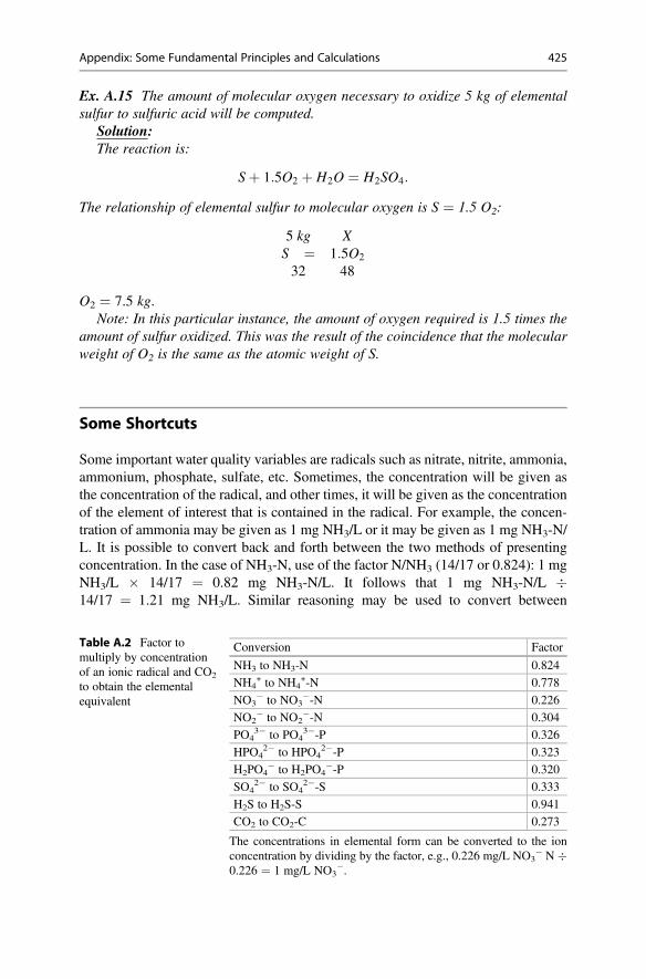
Ex. A.15 The amount of molecular oxygen necessary to oxidize 5 kg of elementalsulfur to sulfuric acid will be computed.

Solution:The reaction is:

Sþ 1:5O2 þ H2O ¼ H2SO4:

The relationship of elemental sulfur to molecular oxygen is S ¼ 1.5 O2:

5 kg XS ¼ 1:5O2

32 48

O2 ¼ 7.5 kg.Note: In this particular instance, the amount of oxygen required is 1.5 times the

amount of sulfur oxidized. This was the result of the coincidence that the molecularweight of O2 is the same as the atomic weight of S.

Some Shortcuts

Some important water quality variables are radicals such as nitrate, nitrite, ammonia,ammonium, phosphate, sulfate, etc. Sometimes, the concentration will be given asthe concentration of the radical, and other times, it will be given as the concentrationof the element of interest that is contained in the radical. For example, the concen-tration of ammonia may be given as 1 mg NH3/L or it may be given as 1 mg NH3-N/L. It is possible to convert back and forth between the two methods of presentingconcentration. In the case of NH3-N, use of the factor N/NH3 (14/17 or 0.824): 1 mgNH3/L � 14/17 ¼ 0.82 mg NH3-N/L. It follows that 1 mg NH3-N/L �14/17 ¼ 1.21 mg NH3/L. Similar reasoning may be used to convert between

Table A.2 Factor tomultiply by concentrationof an ionic radical and CO2

to obtain the elementalequivalent

Conversion Factor

NH3 to NH3-N 0.824

NH4+ to NH4

+-N 0.778

NO3� to NO3

�-N 0.226

NO2� to NO2

�-N 0.304

PO43� to PO4

3�-P 0.326

HPO42� to HPO4

2�-P 0.323

H2PO4� to H2PO4

�-P 0.320

SO42� to SO4

2�-S 0.333

H2S to H2S-S 0.941

CO2 to CO2-C 0.273

The concentrations in elemental form can be converted to the ionconcentration by dividing by the factor, e.g., 0.226 mg/L NO3

� N �0.226 ¼ 1 mg/L NO3

�.


NO3� and NO3-N, NO2

� and NO2�-N, SO4

2� and SO42�-S, etc. Some conversion

factors are given in Table A.2.It also is useful to note that the dimensions for molarity and normality are moles

per liter and equivalents per liter, respectively. Thus, multiplying molarity ornormality by volume in liters gives moles and equivalents, respectively. The samelogic applies for multiplying millimoles or milliequivalents per milliliter by volumein milliliters.

In some calculations, the quantity of a dissolved substance in a particular volumemay be sought. It is helpful to remember that 1 mg/L is the same as 1 g/m3, becausethere are 1000 L in a cubic meter. Likewise, 1 μg/L is the same as 1 mg/m3 for thesame reason.


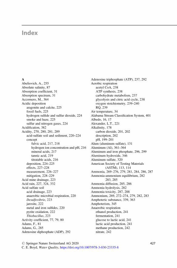
Index

AAbeliovich, A., 255Absolute salinity, 87Absorption coefficient, 31Absorption spectrum, 31Accornero, M., 364Acidic deposition

aragonite and calcite, 225fossil fuels, 225hydrogen sulfide and sulfur dioxide, 224smoke and haze, 225sulfur and nitrogen gases, 224

Acidification, 382Acidity, 270, 280, 281, 289

acid-sulfate soil and sediment, 220–224concept

fulvic acid, 217, 218hydrogen ion concentration and pH, 216mineral acids, 217tannic acid, 219titratable acids, 216

deposition, 224–225effects, 227–228measurement, 226–227mitigation, 228–229

Acid mine drainage, 223Acid rain, 227, 324, 332Acid sulfate soil

acid drainage, 223anaerobic microbial respiration, 220Desulfovibrio, 223jarosite, 222metal and iron sulfides, 220pyrite oxidation, 222Thiobacillus, 223

Activity coefficient, 77, 79, 80Adams, F., 81Adams, G., 285Adenosine diphosphate (ADP), 292

Adenosine triphosphate (ATP), 237, 292Aerobic respiration

acetyl CoA, 238ATP synthesis, 238carbohydrate metabolism, 237glycolysis and citric acid cycle, 238oxygen stoichiometry, 239–240RQ, 239

Air temperature, 34Alabama Stream Classification System, 401Albedo, 16, 17Alexander, L.T., 221Alkalinity, 178

carbon dioxide, 201, 202description, 202pH, 199–201

Alum (aluminum sulfate), 131Aluminum (Al), 361–364Aluminum and iron phosphate, 296, 299Aluminum hydroxide, 346Aluminum sulfate, 320American Society of Testing Materials

(ASTM), 113, 114Ammonia, 269–276, 279, 281, 284, 286, 287Ammonia-ammonium equilibrium, 282

283, 285Ammonia diffusion, 285, 286Ammonia hydrolysis, 282Ammonia toxicity, 287, 288Ammonium, 269, 272–274, 279, 282, 283Amphoteric substance, 339, 363Amphoterism, 345Anaerobic respiration

ethanol production, 241fermentation, 241glucose to lactic acid, 241lactic acid production, 241methane production, 242nitrate, 242

# Springer Nature Switzerland AG 2020C. E. Boyd, Water Quality, https://doi.org/10.1007/978-3-030-23335-8

427

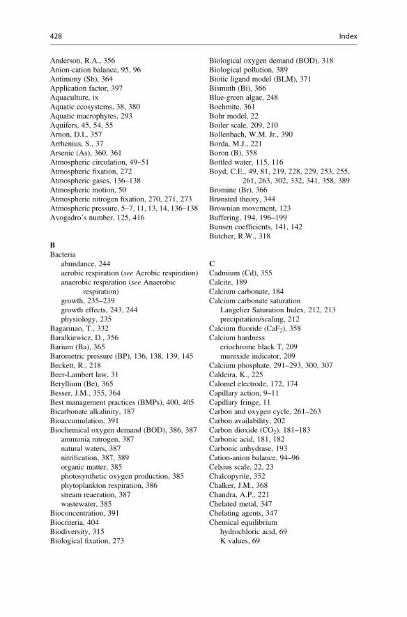
https://doi.org/10.1007/978-3-030-23335-8

Anderson, R.A., 356Anion-cation balance, 95, 96Antimony (Sb), 364Application factor, 397Aquaculture, ixAquatic ecosystems, 38, 380Aquatic macrophytes, 293Aquifers, 45, 54, 55Arnon, D.I., 357Arrhenius, S., 37Arsenic (As), 360, 361Atmospheric circulation, 49–51Atmospheric fixation, 272Atmospheric gases, 136–138Atmospheric motion, 50Atmospheric nitrogen fixation, 270, 271, 273Atmospheric pressure, 5–7, 11, 13, 14, 136–138Avogadro’s number, 125, 416

BBacteria

abundance, 244aerobic respiration (see Aerobic respiration)anaerobic respiration (see Anaerobic

respiration)growth, 235–239growth effects, 243, 244physiology, 235

Bagarinao, T., 332Baralkiewicz, D., 356Barium (Ba), 365Barometric pressure (BP), 136, 138, 139, 145Beckett, R., 218Beer-Lambert law, 31Beryllium (Be), 365Besser, J.M., 355, 364Best management practices (BMPs), 400, 405Bicarbonate alkalinity, 187Bioaccumulation, 391Biochemical oxygen demand (BOD), 386, 387

ammonia nitrogen, 387natural waters, 387nitrification, 387, 389organic matter, 385photosynthetic oxygen production, 385phytoplankton respiration, 386stream reaeration, 387wastewater, 385

Bioconcentration, 391Biocriteria, 404Biodiversity, 315Biological fixation, 273

Biological oxygen demand (BOD), 318Biological pollution, 389Biotic ligand model (BLM), 371Bismuth (Bi), 366Blue-green algae, 248Boehmite, 361Bohr model, 22Boiler scale, 209, 210Bollenbach, W.M. Jr., 390Borda, M.J., 221Boron (B), 358Bottled water, 115, 116Boyd, C.E., 49, 81, 219, 228, 229, 253, 255,

261, 263, 302, 332, 341, 358, 389Bromine (Br), 366Brønsted theory, 344Brownian movement, 123Buffering, 194, 196–199Bunsen coefficients, 141, 142Butcher, R.W., 318

CCadmium (Cd), 355Calcite, 189Calcium carbonate, 184Calcium carbonate saturation

Langelier Saturation Index, 212, 213precipitation/scaling, 212

Calcium fluoride (CaF2), 358Calcium hardness

eriochrome black T, 209murexide indicator, 209

Calcium phosphate, 291–293, 300, 307Caldeira, K., 225Calomel electrode, 172, 174Capillary action, 9–11Capillary fringe, 11Carbon and oxygen cycle, 261–263Carbon availability, 202Carbon dioxide (CO2), 181–183Carbonic acid, 181, 182Carbonic anhydrase, 193Cation-anion balance, 94–96Celsius scale, 22, 23Chalcopyrite, 352Chalker, J.M., 368Chandra, A.P., 221Chelated metal, 347Chelating agents, 347Chemical equilibrium

hydrochloric acid, 69K values, 69

428 Index

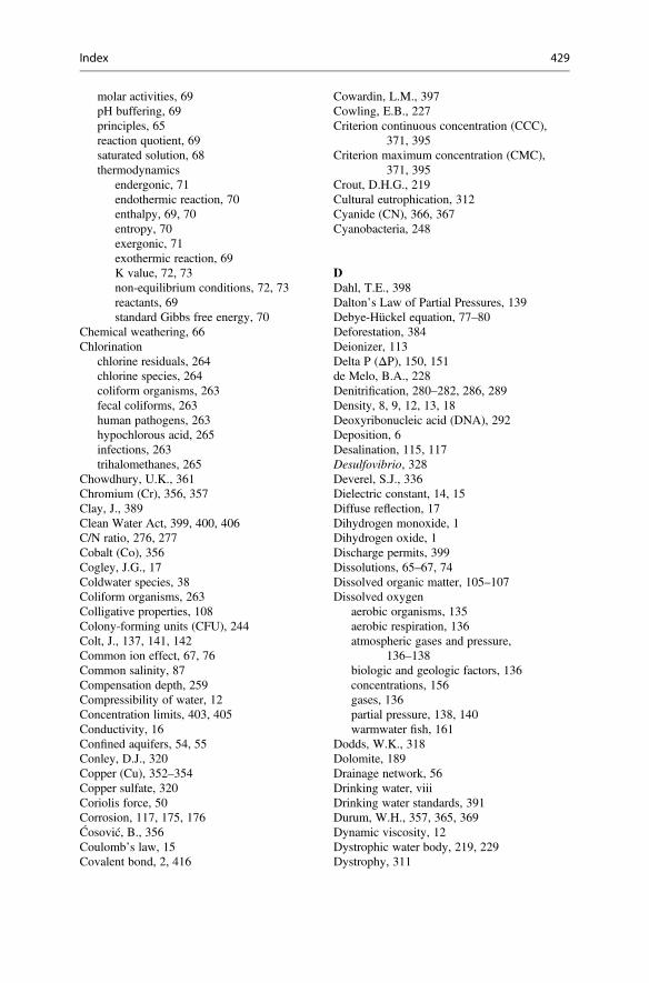
molar activities, 69pH buffering, 69principles, 65reaction quotient, 69saturated solution, 68thermodynamics

endergonic, 71endothermic reaction, 70enthalpy, 69, 70entropy, 70exergonic, 71exothermic reaction, 69K value, 72, 73non-equilibrium conditions, 72, 73reactants, 69standard Gibbs free energy, 70

Chemical weathering, 66Chlorination

chlorine residuals, 264chlorine species, 264coliform organisms, 263fecal coliforms, 263human pathogens, 263hypochlorous acid, 265infections, 263trihalomethanes, 265

Chowdhury, U.K., 361Chromium (Cr), 356, 357Clay, J., 389Clean Water Act, 399, 400, 406C/N ratio, 276, 277Cobalt (Co), 356Cogley, J.G., 17Coldwater species, 38Coliform organisms, 263Colligative properties, 108Colony-forming units (CFU), 244Colt, J., 137, 141, 142Common ion effect, 67, 76Common salinity, 87Compensation depth, 259Compressibility of water, 12Concentration limits, 403, 405Conductivity, 16Confined aquifers, 54, 55Conley, D.J., 320Copper (Cu), 352–354Copper sulfate, 320Coriolis force, 50Corrosion, 117, 175, 176Ćosović, B., 356Coulomb’s law, 15Covalent bond, 2, 416

Cowardin, L.M., 397Cowling, E.B., 227Criterion continuous concentration (CCC),

371, 395Criterion maximum concentration (CMC),

371, 395Crout, D.H.G., 219Cultural eutrophication, 312Cyanide (CN), 366, 367Cyanobacteria, 248

DDahl, T.E., 398Dalton’s Law of Partial Pressures, 139Debye-Hückel equation, 77–80Deforestation, 384Deionizer, 113Delta P (ΔP), 150, 151de Melo, B.A., 228Denitrification, 280–282, 286, 289Density, 8, 9, 12, 13, 18Deoxyribonucleic acid (DNA), 292Deposition, 6Desalination, 115, 117Desulfovibrio, 328Deverel, S.J., 336Dielectric constant, 14, 15Diffuse reflection, 17Dihydrogen monoxide, 1Dihydrogen oxide, 1Discharge permits, 399Dissolutions, 65–67, 74Dissolved organic matter, 105–107Dissolved oxygen

aerobic organisms, 135aerobic respiration, 136atmospheric gases and pressure,

136–138biologic and geologic factors, 136concentrations, 156gases, 136partial pressure, 138, 140warmwater fish, 161

Dodds, W.K., 318Dolomite, 189Drainage network, 56Drinking water, viiiDrinking water standards, 391Durum, W.H., 357, 365, 369Dynamic viscosity, 12Dystrophic water body, 219, 229Dystrophy, 311

Index 429

EEarth’s water

freshwater, 42hydrosphere, 42precipitation, 43runoff, 43water cycling, 42water footprint, 43water shortages, 44

Eaton, A.D., 186, 207, 209, 216, 226,385, 393

Economic development, 402Effluent standards, 400, 404Einstein’s equation, 25Eisely, L., 2Electrical conductivity (EC), 90, 91Electrical neutrality, 94Electricity, 89Electromagnetic radiation, 25Electromagnetic spectrum, 27, 30Electron shell, 2Electrostatic interactions, 77–80Elements

alkaline earth metals, 411atomic mass, 413atoms, 412classification, 411formula, 416ions, 413isotopes, 413metalloids, 411molecules, 411noble gases, 411nonmetals, 411, 414nucleus, 412protons, 412sodium and chlorine, 415symbol, 413

Elser, J.J., 252Endothermic reactions, 37Energy, 22, 25, 46Enthalpy, 6, 69, 70Entropy, 23, 24, 70Epilimnion, 35, 36Equilibria, 192–194Equilibrium constant, 68, 69, 72–74, 81,

82, 164Equilibrium Law, 68Equivalent conductances (λ), 91, 92Equivalent ionic conductance, 91Eriochrome black T, 207, 209Erosion, 129

factors, 383

gully, 383land surface disruption, 384raindrop, 383sedimentation, 384sheet, 383soil, 383turbidity, 384USLE, 383

Esdaile, J.L., 368Essumang, D.K., 356Estuaries, 36, 62Ethylenediaminetetraacetic acid (EDTA),

207, 208Etowah River, 99Eutrophication, 291, 293

anthropogenic activities, 313aquatic ecosystems, 315biological communities, 314climate change, 318, 319control, 319–321definition, 312diversity, 315ecologically-sensitive species, 313ecological system, 316lakes, 316–318nitrogen and phosphorus, 313, 315, 321physical and chemical environment, 313phytoplankton species diversity, 314runoff, 312sedimentation, 312stream, 318unpolluted water bodies, 315variables, 313water bodies, 312water pollution, 321water usage, 319

Eutrophy, 311, 313Evaporation, 48, 60

dissolved salt concentrations, 47energy, 44, 46measurement, 47–49molecules, 46phytoplankton, 47relative humidity, 46, 47saturation vapor pressure, 47VPD, 46wind velocity, 47

Evaporation pan, 48, 49Evapotranspiration, 43, 45Everall, N.C., 227Exothermic reactions, 37Extinction coefficient, 126

430 Index

FFanning, D.S., 221Faraday constant, 168Feely, R.A., 225Fermentation, 241, 242Ferredoxins, 324Feuchtmayr, H., 318Filella, M., 366Firth, J., 361Flegal, A.R., 369Fleming, J.F., 221Flocculation, 131Fluoride (F), 358, 359Food web, 292, 316, 317Formality, 419Formazin attenuation units (FAU), 127Frattini, P., 369Frear, C.L., 190Free energy of reaction, 70, 72Freshwater, 42Freshwater aquatic ecosystems, 407Fries, L., 357Fulvic acids, 218, 219

GGaillardet, J., 336Gallagher, L.M., 406Gary, J.E., 368Gas bubble trauma, 151, 270, 289Gas solubility

Bunsen’s absorption coefficients, 141Henry’s law, 140STP, 142temperatures and salinities, 142

Gas solubility tablesBP, 145, 146dissolved oxygen concentrations, 147hydrostatic pressure, 146universal gas law equation, 147

Gas transferair-water interface, 152, 153dissolved oxygen concentrations, 152, 153gas-liquid contact system, 153molecular diameters, 153oxygen deficit/surplus, 152SOTR, 154, 155WRR, 155

Gebbie, P., 212, 213Geissman, T.A., 219Gensemer, R.W., 364George, C., 264Gerson, A.R., 221

Gibbs free energy, 70, 71, 164, 168, 336Gibbsite, 298, 361, 363Gibbs, J.W., 70Gibbs standard-state free energy, 70Gilbert, J.A., 358Global atmospheric circulation, 50Global energy budget, 28Global warming, 30, 318Goldberg, E.D., 341Goldman, C.R., 336Goldmining, 368Gopakumar, G., 332Gosselink, J.G., 397Gram atomic mass, 413Gram molecular weight, 413Gray, J.S., 332Green and purple sulfur bacteria, 328Greenhouse effect, 30Greenhouse gases, 30Gross, A., 281, 285Groundwater, 45, 54, 55, 97Groundwater pollution, 389, 390Gully erosion, 383Guo, T., 340Gypsum, 66, 325

HHaber-Bosch process, 273Haffty, J., 357, 365, 369Haines, T.A., 224, 227Halogens, 411Hamilton, S.J., 360Han, Y., 229Hardness and biological productivity, 210Hardness categories

calcium and magnesium hardness, 209carbonate and noncarbonate hardness, 209

Hargreaves, J.A., 287Hasler, A.D., 228Hasselbalch, K.A., 196Hayes, D., 324Heat, 23Hem, J.D., 200, 324, 336, 351, 356, 359,

360, 362, 369Hemoglobin, 159, 160, 350Henderson-Hasselbalch equation, 196, 198, 199Henry’s law, 140Hoekstra, A.Y., 43Holland, A., 227Hoorman, J.J., 276Howarth, R.S., 371Howe, P., 369

Index 431

Humankind, 43Human population, 380Humic acids, 218, 219Humic substances, 106, 125, 181

fulvic acid, 217humic acid, 219mineral acids, 227organic polymers, 218toxic effect, 227toxicity, 228

Hutchinson, G.E., 84Hydrogen (H2), 164Hydrogen bonds, 4–6, 9, 10, 22Hydrogen sulfide (H2S), 329, 330Hydrologic cycle, 41, 44, 45, 62Hydrologic equation, 60Hydrolysis, 345, 346Hydrolysis of carbonate, 193, 194Hydrometers, 87, 88Hydronium ion (H3O

+), 178Hydrosphere, 42Hydrostatic pressure (HP), 146, 150–152Hydroxide alkalinity, 187Hydroxyapatite, 300Hyenstrand, P., 336, 350Hygroscopic coefficient, 53Hypolimnion, 35, 36, 173

IIce, 6, 8Ice cover, 36Ideal gas law, 147, 169Imhoff cone, 128, 129Immobilization of nitrogen, 276Industrial fixation, 273Industrial revolution, 380Inorganic phosphorus, 293, 294, 296, 302Intergovernmental Oceanographic

Commission (IOC), 87International Desalination Association, 115International Society of Soil Science (ISSS), 121International Standards Organization

(ISO), 113, 114International System of Units (SI units), 5, 90International Union of Pure and Applied

Chemistry (IUPAC), 1Iodine (I2), 359Ion activities

divalent, 79monovalent, 79

Ion hydration, 15Ionic strength, 77–79, 81

Ion pairs, 80, 81, 341, 342, 344, 348Iron (Fe), 350–352Iron pyrite, 331Islam, R., 276Isotopes, 412Izbicki, J.A., 357

JJackson turbidimeter unit (JTU), 126Jaszczak, E., 367Jenkins, D., 185, 264Jimenez, M.C.S., 265Johnson, D.S., 228Johnston, J., 190Jones, D.A., 366Jones, J.B. Jr., 349Jumpertz, R., 240

KKarbowska, B., 369Kaushal, S.S., 319Kautz, R.S., 318Kellerman, K.F., 353Kelvin scale, 23Khan, T., 357King, D.J., 253Kirchhoff’s law, 30Klavins, M., 220Knudsen equation, 87Knudsen, M., 86Kochkodan, V., 358Kociolek, J.P., 311Kopp, J.F., 354, 355, 358, 361, 365, 367Korečková-Sysalová, J., 365Krebs cycle, 237Kristensen, E., 243Kroner, R.C., 354, 355, 357, 358, 365, 367Kucuk, S., 287Kutler, B., 354Kuttyamma, V.J., 332

LLakes, 58Lane, T.W., 355Langelier Saturation Index, 212Langelier, W.F., 212, 213Lantin-Olaguer, I., 332Latent cancer fatalities (LCF), 392Latent heat, 6, 7Law of Definite Proportions, 416, 417

432 Index

Law of mass action, 68, 164Lawrence, J., 219Laws of thermodynamics, 2, 22, 23, 69, 70, 414LC50 tests, 288, 289Lead (Pb), 367Le Chatelier’s principle, 68, 74Lee, J.G., 355Lees, D.R., 227Leib, K.J., 355, 364Lethal concentration 50 (LC50), 393,

394, 396, 397Lewis acid and base theory, 344Lewis acid-base reaction, 344Liebig’s law, 251Ligands, 347Light and dark reactions, 249Light-dark bottle technique, 257Light penetration in water, 30–32, 124Lignins, 124Lignosulfonic acid, 219Li, M., 228Lime-soda ash process, 210, 211Lindemann, M.D., 356Livingstone, D.A., 98, 200, 357, 358, 367, 370Load limits, 403, 405Longwave radiation, 29Lowest observed effect concentration

(LOEC), 394Luther III, G.W., 221Luxury consumption, 304Lysimeters, 49

MMacrophytes, 303, 305Magazinovic, R.S., 366Magnesium hardness, 209Manganese (Mn), 352Martell, A.E., 347, 362Massaut, L., 398Mass balance, 61Masuda, K., 302Maunder Minimum in astronomy, 27Maximum allowable toxicant concentrations

(MATC), 372, 394, 397Maxwell, J., 46Maxwell’s demon concept, 46McBride, M.B., 336, 341McCarty, P.L., 210McNevin, A.A., 263, 332, 341Mean sea level (MSL), 136Mekonnen, M.M., 43Meniscus, 9, 10

Mercury (Hg), 367, 368Mesotrophy, 311Metalimnion, 35Metalloids, 411Methane production, 242Methyl mercury, 368Microbial decomposition, 292Microbial growth efficiency (MGE), 276Micronutrients, 336

arsenic, 360, 361boron, 358cadmium, 355chromium, 356, 357cobalt, 356copper, 352–354fluoride, 358, 359iodine, 359iron, 350–352manganese, 352molybdenum, 356nickel, 357selenium, 360and trace elements, 343vanadium, 357zinc, 354, 355

Microorganismsbacteria (see Bacteria)phytoplankton (see Phytoplankton)

Miller, L.A., 406Miller, W.E., 252Mineralization of nitrogen, 276, 277Miscibility, 417Mitsch, W.J., 397Molality, 419Molarity, 418, 426Molecular oxygen, 136, 162Molybdenum (Mo), 356Monocalcium phosphate, 299, 300Moore, G.T., 353Morel, F.M.M., 355Moser River, 99Moyle, J.B., 210Muller, S., 318Murexide indicator, 209Mu, Y., 371

NNadis, S., 336, 350Nassar, L.J., 228National Pollutant Discharge Elimination

System (NPDES), 399Natural ecosystems, 380

Index 433

Natural softening of groundwater, 104Natural waters, 65, 81

coastal and ocean water, 104, 105dissolved organic matter, 105–107inland waters

aquifers, 103carbon dioxide, 97geological and climatic zones, 98groundwater, 97, 103hydrogen ion concentration, 99ionic constituents, 98, 99limestone, 98, 99mineral precipitation, 102minerals, 97physiographic regions, 103pond waters, 102runoff, 97silica concentration, 98streams, 97

rainwater, 96, 97Nephelometer, 127Nephelometer turbidity units (NTU), 127Nephelometry, 127Nernst equation, 169, 170, 180Nesbitt, H.W., 221Nickel (Ni), 357Ning, L., 354, 355, 357, 361, 367, 368Nitrate reduction in plants, 274Nitrification, 270, 278–280, 382Nitrite toxicity, 288Nitrobacter, 279Nitrogen, 270, 286, 287Nitrogen compounds, 289Nitrogen cycle, 271Nitrogen dioxide (NO2), 289Nitrogen fixation, 271, 273, 286Nitrosomonas, 279Nonessential trace elements

aluminum, 361–364antimony, 364barium, 365beryllium, 365bismuth, 366bromine, 366cyanide, 366, 367lead, 367mercury, 367, 368silver, 368, 369strontium, 369thallium, 369tin, 369uranium, 370

Non-photosynthetic microorganisms, 21

No observed effect concentration (NOEC), 394Normality, 419, 420, 426Novak, J.T., 253Nutrient pollution, 381Nutrients

alkalinity and phytoplanktonproductivity, 253

growth and metabolism, 235inorganic, 243multiple limiting, 251phytoplankton growth, 252single limiting, 251turbidity and discoloration, 248

OOcean currents, 50Oceans, 42, 62Ocean water, 104Ohm’s law, 89Oligotrophy, 311, 313Organic phosphorus, 301–303Orr, J.C., 225Orthophosphoric acid, 294Osmoregulation, 112Osmotic pressure, 110–112Oxidation-reduction (redox) potential

aquatic ecology, 176cell voltage and free-energy change,

168–171corrosion, 175, 176electron transfer, 163half-cell reactions, 165hydrogen, 164iodine, 164measurable electrical current, 164measurement, 172–174oxidizing agent, 164standard hydrogen electrode, 165–168

Oxygen consumption, 160Oxygen potential, 173, 174Oxygen solubilities, 145Oxygen tension, 149, 150, 152, 159Oxyhemoglobin, 159Oysters, viii

PPagenkopf, G.K., 347Pais, I., 349Palmer, C.A., 358Partial pressure, 139, 140, 149, 152Pecos River, 99

434 Index

Penman equation, 49Percentage saturation, 149, 150pH

acidity/basicity, 177alkalinity, 178averaging, 180calculations, 179, 180concept, 178, 179natural waters, 181on fish, 201rainwater, 182, 183

Phenolphthalein alkalinity (PA), 187Phosphate fertilizers, 293, 307Phosphorus

analysis issues, 302brain food, 292concentrations in water, 302, 303ecosystems, 308environment, 293, 294fertilized fish ponds, 307natural and agricultural ecosystems, 291nitrogen, 308organic, 301organic matter, 292orthophosphate, 308orthophosphoric acid, 294–296pH, 295, 301phospholipids, 292phytic acid, 292plant uptake, 303, 304protein synthesis, 292qualitative model, 294sediment reactions, 296, 298–301valence states, 292water and sediment, 304, 305, 307

Phosphorus removal, 320, 321Photic zone, 124Photosynthesis, 249, 250Photosynthesis and respiration rates,

measurement, 257–259Photosynthetically active radiation (PAR), 125Photosynthetic photon flux (PPF), 125Phytic acid, 292Phytoplankton

abundancechlorophyll a determination, 254Secchi disk visibility, 254

biochemical assimilation, 250biology, 247–248harmful algae, 260, 261photosynthesis, 249

Phytoplankton die-offs, 255, 256Piezometric levels, 55

Pinsino, A., 352Polarization, 15Pollutants, 381Pollution, viii, ixPollution control

effluent discharge permits, 399effluent limitations, 400water bodies, 400, 402

Polyphosphate, 296Ponds, 58Pore water, 294, 299, 301, 305, 306Potential acid-sulfate (PAS), 221Potential evapotranspiration (PET), 49Practical salinity, 87Practical salinity units (psu), 87Precipitation, 45, 49

adiabatic lapse rate, 51air rising, 51hail, 52hygroscopic particles, 52measurement, 52rules, 52water droplets/ice particles, 52

Probable no effect concentrations (PNEC), 372Proton-proton chain, 24, 25Puntoriero, M.L., 359Pure water, ix

QQ10 equation, 38

RRaindrop erosion, 383Rainfall, 42, 45, 52, 55, 56, 58, 60Rain gauges, 48, 53Rainwater, ix, 41, 96, 97Raoult, F., 108Raoult’s law, 108Rathbun, R.E., 228Redfield, A.C., 252, 308Redfield ratio, 252, 308Reference salinity, 87Reflectivity, 17Refractive index, 18, 19, 87Refractometer, 87, 88Relative humidity (RH), 46, 47Republican River, 99Reservoirs, 58Resistivity, 90Respiration

absorption, 157

Index 435

Respiration (cont.)air movement, 158aquatic ecosystems, 162aquatic environments, 157aquatic organisms, 159carbon dioxide, 160, 161chemoautotrophic microorganisms, 160metalloproteins, 159oxygen, 160terrestrial ecosystems, 158warmwater fish, 161weight/volume concentration, 158

Respiratory quotient (RQ), 239Ribonucleic acid (RNA), 292Rickard, D., 221Roberson, C.E., 362Runoff, 43, 44, 49, 56, 60Ryan, D., 341

SSalinity, 9, 10, 13, 86–88, 112Salinometers, 88Salt effect, 67Saturometer, 151Saunders, G.W., 194Sawyer, C.N., 210Schindler, D.W., 320Schippers, A., 221Schmidt, R., 10Schneider, B., 10Schroeder, E.D., 264, 402Schroeder, G.L., 155Seawater, 84, 104Secchi disk, 126, 129Sedimentation, 122, 384Sediment phosphorus, 293, 302, 303, 305, 308Sediment redox, 172, 173Sediment respiration

aerobic respiration, 245aquatic ecosystems, 245decomposition, 246oxidation, 245zonation, 246, 247

Seepage, 60Seker, S., 354Selenium (Se), 360Semiconductors, 411Sheet erosion, 383Shelford’s law, 251Shellfish poisoning, 261, 267Shilo, M., 255Shinozuka, T., 218

Shiraishi, K., 370Shortwave radiation, 29Siepak, J., 356Silicate, 97Silicate clays, 300Silicic acid, 99Sillén, J.G., 347, 362Silver (Ag), 368, 369Six, J., 276Sling psychrometer, 46Smith, D.D., 383Smith, D.J., 228Smith, S.J., 225, 325Snell’s law, 18Snoeyink, V.L., 185, 264Sodium adsorption ratio (SAR), 111, 113Sodium stearate, 208Soil erosion, 383Soil loss, 384Soil water, 53, 54Soil-water system, 349Solar constant, 26–28Solar radiation, 32, 39, 47

deuterium nucleus, 24electromagnetic waves, 25nuclear fusion, 24photons, 25proton-proton chain, 25shortwave and longwave, 27sunspots, 27wavelength, 26

Solubilityendothermic reactions, 67exothermic reactions, 67inorganic/organic compounds, 66ion effect, 67low redox potential, 68pH, 67products, 74, 75rules, 67soluble compounds, 418substances, 67temperature, 67

Solubility product (Ksp), 336Soluble reactive phosphorus, 302, 303Solutes, 65Solvent, 65, 417Sorensen, D.L., 221Sørensen, S.P.L., 179Spears, J.W., 357Specular reflection, 16, 17Spotte, S., 285Sprague, J.B., 371

436 Index

Standard electrode potential, 166, 167,172, 175

Standard oxygen transfer rate (SOTR), 154Standard temperature and pressure (STP), 136Steelink, C., 217Stefan-Boltzmann law, 26Stoermer, E.F., 311Stoichiometry, 423Stoke’s law equation, 121, 123Stream re-aeration, 156Streams

channel precipitation, 56classification system, 400dendritic pattern, 56discharge, 56ephemeral, 56first-order, 56hydrograph, 56, 57intermittent, 56order, 56perennial, 56second-order, 56sediment deposition, 57subsurface storm drainage, 56watershed characteristics, 57

Stream temperature, 34Strontium (Sr), 369Sublimation, 6Sulfate, 324Sulfide oxidation, 324Sulfur, 221–224

amino acids, 324concentrations, 331cycle, 325, 326effects, 332fuels and volcanic eruptions, 324geochemistry, 323oxidation states, 324transformations

oxidations, 327, 328plant uptake and mineralization,

326, 327reductions, 328, 329

valence states, 326Sulfur dioxide, 224, 225Sunspots, 27Surface tension, 9, 10Suspended particles

colloids, 123color, 124settling characteristics, 121–123sources, 120

Suspended solids, 119

TTannic acid, 219, 220Tannins, 124Taras, M.J., 186Tchobanoglous, G., 264, 402Temperature, 21, 23, 38Terminal settling velocity, 121, 122, 129Thallium (Tl), 369Thermal destratification, 8Thermal stratification, 8, 34–36, 313Thermal stress, 21Thermocline, 35Thièbaut, G., 318Thiobacillus, 327Thoenen, T., 370Thompson, W., 24Thornthwaite equation, 49Tin (Sn), 369Total alkalinity (TA), 94, 187, 195

bicarbonate and carbonate, 184, 185carbon dioxide, 184definition, 184expression, 185measurement, 185–187pH, 199, 200sources

calcite, 191calcium and bicarbonate, 190calcium carbonate, 188, 191calcium silicate, 192carbon dioxide, 190, 191limestone, 187, 188, 191mass action, 189organic matter, 191weathering of feldspars, 192

Total ammonia nitrogen (TAN), 389Total body burden (TBB), 391Total dissolved fixed solids (TDFS), 106Total dissolved solids (TDS)

alkalinity and hardness, 94analysis, 86aquatic ecosystems, 116atmosphere, 84bottled water, 115, 116degree of mineralization, 84desalination, 115end of pipe discharges, 116estuaries, 116evaporation, 85freezing and boiling points, 108, 109freshwaters, 84geological formations, 84inorganic particles, 84

Index 437

Total dissolved solids (TDS) (cont.)ion exchange, 113, 115laxative effect, 117organic compounds, 85osmotic pressure, 110–112salinity, 86–88seawater, 84specific conductance

EC, 90, 91electricity, 89electrostatic interactions, 92ions, 91resistivities, 90salinity, 93SI units, 90surface waters, 92

vapor pressure, 108Total dissolved volatile solids (TDVS), 106Total fixed suspended solids (TFSS), 128Total gas pressure (TGP), 139, 150Total hardness

biological productivity, 210boiler scale, 209, 210calcium carbonate saturation, 212–213calcium hardness, 209concentrations, 208definition, 206EDTA, 207, 208eriochrome black T, 209limestone/calcium silicate, 206magnesium carbonate, 213magnesium hardness, 209permanent/noncarbonate hardness, 210problems, 208, 209soap precipitation, 205soap-wasting property, 213sodium stearate, 208sources, 206temporary/carbonate hardness, 210water softening, 210–211

Total maximum daily loads (TMDLs), 404Total suspended solids (TSS), 127, 128Total volatile suspended solids (TVSS),

127, 128Toxic algae, 261Toxicity tests, 391, 393, 394, 397, 404

aquatic organisms, 392aquatic toxicology, 392LC50, 393, 397MATC, 394, 397threshold concentrations, 392

Trace elementsanaerobic bacteria, 340

carbon dioxide, 340complex ions, 344, 345copper sulfate, 341description, 336drinking water, 374ferric hydroxide, 340freshwater systems, 341health effects, 371ion pairs, 341, 342, 344, 348ion principle, 336metal ion hydrolysis, 345, 346metals, 339mineral nutrients, 349organic complexes/chelates, 347pH, 338redox potential, 340seawater, 342solubility, 336temperatures, 338toxicity, 371

Trace metals, 341, 342, 345, 355, 371Trace nutrients, 336Transparency, 16–18Transpiration, 47Tranvik, L.J., 336, 350Trenberth, K.E., 29Triethanolamine (HTEA), 347Triple point, 7Trisodium phosphate, 293Trophosphere, 28Tropic status of lakes, 266Tropical species, 38Troposphere, 136Tucker, C.S., 253, 261, 332Turbidity, 120

chemical coagulant, 131, 132color, 132measurement, 126, 127Secchi disk, 129settleable solids, 128settling basin, 129–131suspended solids, 127, 128suspended solids removal, 129

Turekian, K.K., 3412-Chloro-6-(trichloromethyl) pyridine

(TCMP), 387Tyndall effect, 123Tyndall, J., 123

UUltraeutrophy, 313Ultraoligotrophy, 313

438 Index

Ultra trace elements, 336Unit annual risk (UAR), 392Unit lifetime risk (ULR), 392United Nations Educational, Scientific

and Cultural Organization(UNESCO), 87

United States Department of Agriculture(USDA), 121

United States Pharmacopeia (USP), 113, 114Universal gas law, 147, 148, 169Universal soil loss equation (USLE), 383Uranium (U), 370U. S. Environmental Protection Agency

(USEPA), 395, 399US National Oceanographic and Atmospheric

Administration, 263Uthus, E.O., 360

VVanadium (V), 357van der Graaf, A.A., 279van der Waals interactions, 3, 4van der Waals, J., 3van Hoff’s law, 243van Niekerk, H., 92van’t Hoff equation, 37van’t Hoff factor, 109van’t Hoff, J., 37Vapor pressure, 7Vapor pressure deficit (VPD), 46Vesilind, P.A., 387, 398Viscosity, 11, 12Visible light, 125Vrede, T., 336, 350

WWalley, W.W., 358Warmwater species, 38Water

agricultural crops, viiavailability, viiibacteria, viibiochemical reactions, viidissolution, erosion and deposition, viiearly human settlements, viimicroorganisms, viiorganisms, viitransportation, viii

Water bodies, viii, 400Waterborne diseases, ix, 389Water budgets, 49, 60

Water cycle, 45Water distillation unit, 114Water footprint, 43Water measurements

mass balance, 61runoff, 58seepage, 60volumes of standing water bodies, 59water budgets, 60

Water moleculeadhesive forces, 9capillary action, 9–11cohesive forces, 9, 10compressibility, 12conductivity, 16density, 8, 9dielectric constant, 14, 15dissolved ions, 16elasticity, 12electric field, 15meniscus, 10pressure, 13, 14refraction of light, 19refractive index, 18, 19SI unit, 10structure

covalent bonds, 2electrons, 2electrostatic charges, 3hydrogen and oxygen atoms, 2, 3hydrogen bonding, 4laws of thermodynamics, 2repulsions and attractions, 3

surface tension, 10surfactants, 10temperature, 5–10, 12thermal characteristics and phases, 5–7thermal properties, 6transparency, 16, 18vapor pressure, 7viscosity, 11, 12

Water pollution, 44acidification, 382bioconcentration, 381biological, 389BOD (see Biological oxygen demand

(BOD))erosion, 383, 384fossil fuels, 381groundwater, 389, 390heated effluents, 382nonpoint sources, 381nutrient pollution, 381

Index 439

Water pollution (cont.)organic wastes, 381pharmaceuticals, 382point sources, 381, 383runoff, 381salinization, 382sediment, 381toxic chemicals/substances, 382toxicity, 381toxins and human risk assessment, 390–392turbidity, 381

Water pressure, 11, 13, 14, 54Water quality

acidic and saline waters, ixaquatic ecosystems, ixcontaminants, ixecological services, xecological systems, viiiguidelines, 402minerals, viiipathogens and chlorination, 263–265phytoplankton

Anabaena variabilis, 255die-offs, 255, 256nutrients, 256oxygen concentration, 256, 257photosynthesis, 254thermal destratification or overturns, 256

phytotoxic substances, viiiprinciples, xsalty water, viiisensory perception and observations, viii

Water quality standards, viii, ixbiological, 404concentration based standards, 402delta based standards, 403discharge permits, 406drinking water, 406guidelines, 408local based standards, 403TMDLs, 404toxic chemical, 404waste treatment and BMPs, 405

Water quantityhuman affairs, 398prescriptive rights, 399

riparian doctrine, 399Water softening

lime-soda ash process and zeoliteprocess, 210, 211

magnesium hydroxide, 211Water supply

groundwater, 43infrastructure, 44weather rainfall patterns, 43

Water surface, 14Water table, 54Water temperature, 34, 39

heat content, 32ice cover, 36statification, 36temperate zone change, 33thermal stratification, 34–36water quality, 36–38

Water vapor, 4, 6, 7Watts, P., 369Wavelength, 25, 26, 29–31Weight per unit volume, 421, 422Weight relationships, 423Weiler, R.R., 285Wein’s law, 26Welch, H.E., 155Wentz, D.A., 368Wessel, G., 357Wetland destruction, 397, 398Wetlands, 58Wetzel, R.G., 266Wheatstone bridge circuit, 89, 90Whitening of water bodies, 194Wickett, M.E., 225Wind re-aeration rate (WRR), 155Wischeier, W.H., 383Wisniak, J., 366Withlacoochee River, 99World Health Organization (WHO), 359, 371World Meteorological Organization, 47

ZZeolite process, 210, 211Zinc (Zn), 354, 355Zingg, A.W., 383

440 Index

claude e. boyd an introduction third edition - agroportal

Documents