chptr 4 antenna dipole yagi2015
TRANSCRIPT
Antenna
Chapter 4

2
Chapter OutlinesChapter 4 Antenna
Fundamental Parameters of Antennas Electrically Short Antennas Dipole Antennas Monopole Antennas Antenna Arrays Helical Antennas Yagi Uda Array Antennas Antennas for Wireless Communications

3
IntroductionWires passing an alternating current emit or radiate EM energy. The shape and size of the current carrying structure determine how much energy is radiated, direction of propagation and how well the radiation is captured.
Henceforth, the structure to efficiently radiate in a preferred direction is called transmitting antenna, while the other side which is to capture radiation from preferable direction is called receiving antenna.In most cases, the efficiency and directional nature for an antenna is the same whether its receiving or transmitting.

4
Common types of antennas:
Introduction (Cont’d..)
Fundamentals of Electromagnetics With Engineering Applications by Stuart M. WentworthCopyright © 2005 by John Wiley & Sons. All rights reserved.
Figure 8-1 (p. 389)Common single-element antennas.
5
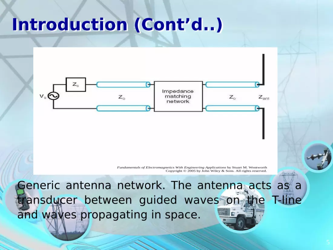
Introduction (Cont’d..)
Fundamentals of Electromagnetics With Engineering Applications by Stuart M. WentworthCopyright © 2005 by John Wiley & Sons. All rights reserved.
Generic antenna network. The antenna acts as a transducer between guided waves on the T-line and waves propagating in space.

4.1 Fundamental Parameters of AntennasTo describe the performance of an antenna, definitions of various parameters are discussed. The radiated power, beam pattern, directivity, and efficiency are all important parameters in characterizing antenna.RADIATED POWER
Suppose transmitting antenna located at the origin of spherical coordinate. From this coordinate system, there are three components of radiated field, in r, θ and φ. But, the intensities of these components vary with radial distance as 1/r, 1/r2 and 1/r3.

Fundamental Parameters of Antennas (Cont’d..)
Fundamentals of Electromagnetics With Engineering Applications by Stuart M. WentworthCopyright © 2005 by John Wiley & Sons. All rights reserved.
Figure 8-3 (p. 392) The spherical radiation pattern for an isotropic antenna.
For almost all practical applications, a receiving antenna located far enough away from the transmitter (as a point source of radiation) far field region.A distance r from the origin is generally accepted as being in the far field region if :
22Lr
L is the length of the largest dimension on the antenna element, and assumed L>λ. For smaller L, r should at least as large as λ

Fundamental Parameters of Antennas (Cont’d..)In the far field, the radiated waves resemble plane waves propagating in ar direction where time harmonic fields related by :
12010
00 EaH HaE SrSSrS
The time averaged power density vector of the wave is by Poynting Theorem,
*Re21,, SSr HEP
Where in the far field, rrPr a P ,,,,
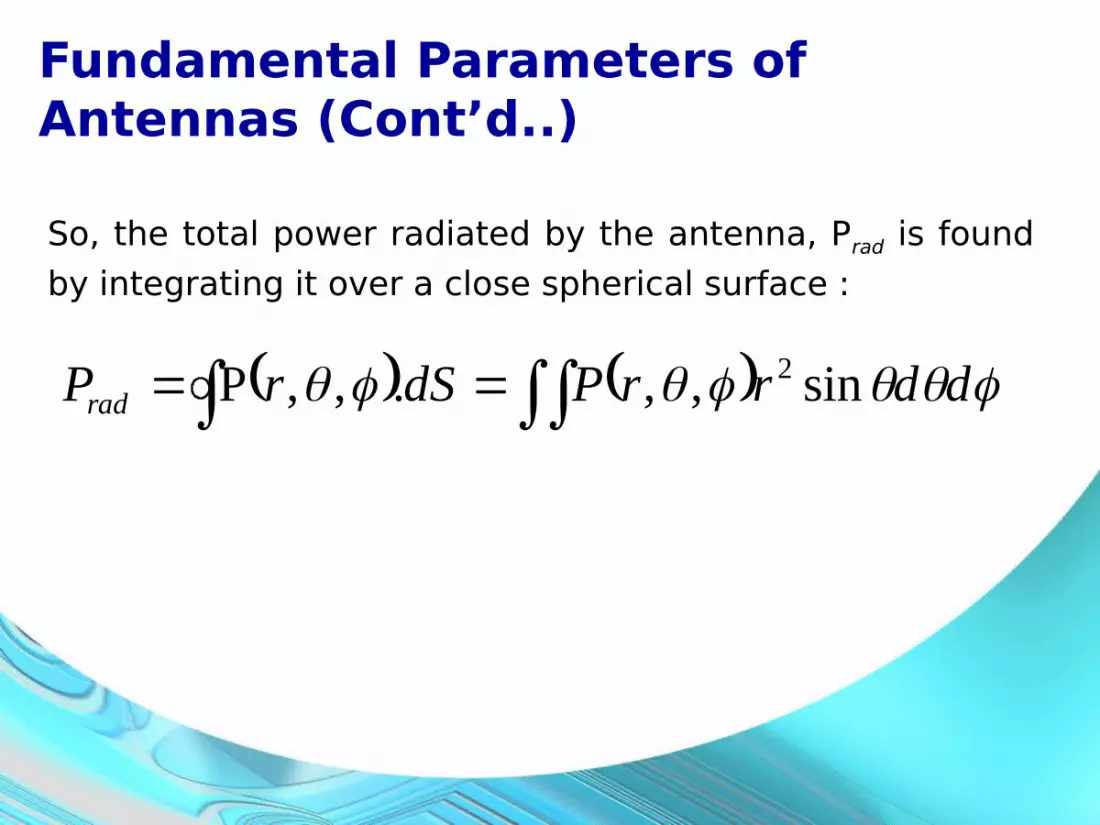
Fundamental Parameters of Antennas (Cont’d..)
So, the total power radiated by the antenna, Prad is found by integrating it over a close spherical surface :
ddrrPdSrPrad sin,,.,,P 2
10
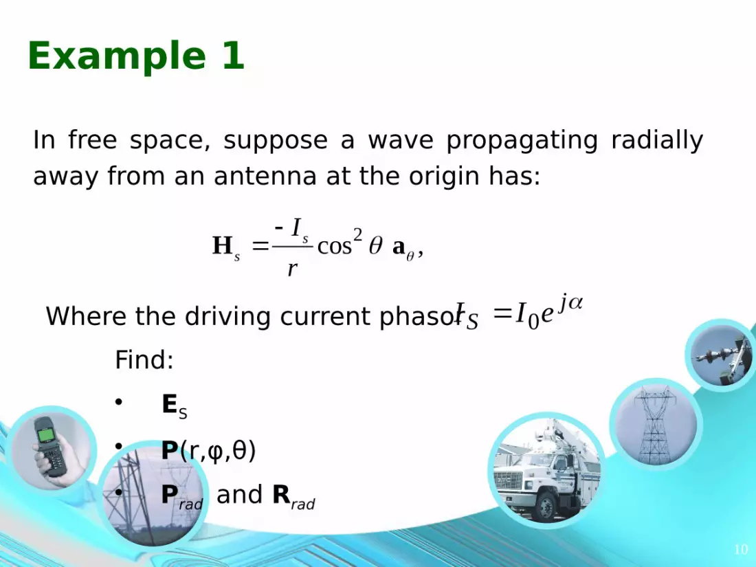
Example 1
In free space, suppose a wave propagating radially away from an antenna at the origin has:
Where the driving current phasor jS eII 0
Find:• ES
• P(r,φ,θ) • Prad and Rrad
2cos ,ss
Ir
H a
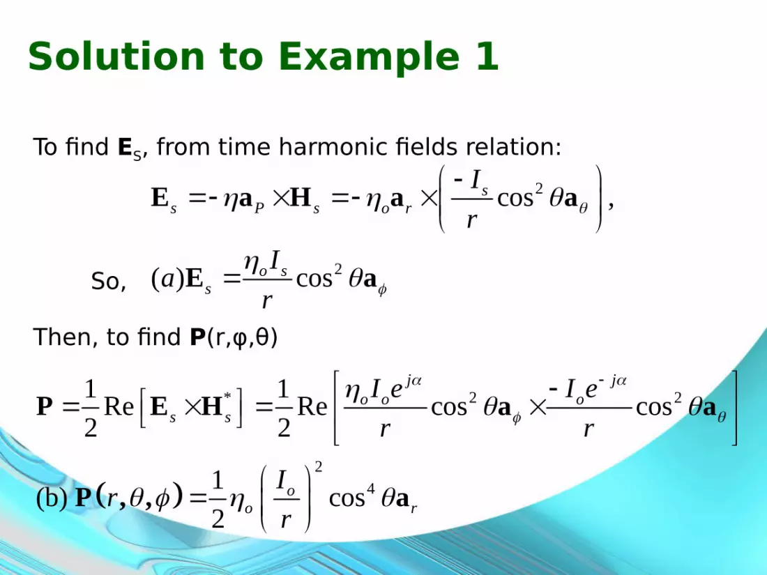
Solution to Example 1
To find ES, from time harmonic fields relation:
So,
2
2
cos ,
( ) cos
ss P s o r
o ss
Ir
Iar
E a H a a
E a
* 2 2
24
1 1Re Re cos cos2 2
1(b) cos2
j jo o o
s s
oo r
I e I er r
Ir
r
P E H a a
P , , a
Then, to find P(r,φ,θ)

Solution to Example 1 (Cont’d..)Then,
2
2
2
2 1205 961
2( ) 950
o
rad
o
rad
IR
I
c R
Solving:
200
2
00
4200
22
42
00
20
52
sincos21
sincos21
21,,
I
ddI
ddrr
I
RIdrP
rr
radrad
aa
SP
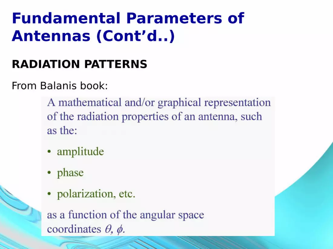
Fundamental Parameters of Antennas (Cont’d..)RADIATION PATTERNSFrom Balanis book:

Fundamental Parameters of Antennas (Cont’d..)Radiation patterns usually indicate either electric field, E intensity or power intensity. Magnetic field intensity, H has the same radiation pattern as E related by η0. The polarization or orientation of the E field vector is an important consideration in an E field plot. A transmit receive antenna pair must share same polarization for the most efficient communication.

Fundamental Parameters of Antennas (Cont’d..)
Coordinate System

Fundamental Parameters of Antennas (Cont’d..)Since the actual field intensity is not only depends on radial distance, but also on how much power delivered to antenna, we use and plot normalized function divide the field or power component with its maximum value.
E.g. the normalized power function or normalized radiation intensity :
max
,,,PrPPn

Fundamental Parameters of Antennas (Cont’d..)
1, isonP So,
In contrast with isotropic antenna, a directional antenna radiates and receives preferentially in some direction.
If the antenna radiates EM waves equally in all directions, it is termed as isotropic antenna, where the normalized power function is equal to 1.

Fundamental Parameters of Antennas (Cont’d..)
Fundamentals of Electromagnetics With Engineering Applications by Stuart M. WentworthCopyright © 2005 by John Wiley & Sons. All rights reserved.
Figure 8-4a (p. 392)General far-field antenna radiation pattern: (a) polar plot; (b) rectangular plot.
Fundamentals of Electromagnetics With Engineering Applications by Stuart M. WentworthCopyright © 2005 by John Wiley & Sons. All rights reserved.
Figure 8-4a (p. 392)General far-field antenna radiation pattern: (a) polar plot; (b) rectangular plot.
The normalized radiation patterns for a generic antenna, called polar plot. A 3D plot of radiation pattern can be difficult to generate and work with, so take slices of the pattern and generate 2D plots (rectangular plots) for all θ at φ=π/2 and φ=3π/2
Polar plot
Rectangular plot (in dB)

Fundamental Parameters of Antennas (Cont’d..)

Fundamental Parameters of Antennas (Cont’d..)
The polar plot also can be in terms of dB. Where normalized E field pattern,
max
,,,ErEEn
This will be identical to the power pattern in decibels if:
,log20, nn EdBE
whereas
,log10, nn PdBP

Fundamental Parameters of Antennas (Cont’d..)
The are some zeros and nulls in radiation pattern, indicating no radiations. These lobes shows the direction of radiation, where main or major lobe lies in the direction of maximum radiation. The other lobes divert power away from the main beam, so that good antenna design will seek to minimize the side and back lobes.Beam’s directional nature is beamwidth, or half power beamwidth or 3 dB beamwidth. It will shows the angular width of the beam measured at the half power or -3 dB points.

Fundamental Parameters of Antennas (Cont’d..)For linearly polarized antenna, performance is often described in terms of its principal E and H plane patterns.E plane : the plane containing the E field vector & the direction of max radiationH plane : the plane containing the H field vector & the direction of max radiation
For next figure, • the x-z plane (elevation plane, φ=0) is the principal E-
plane• the x-y plane (azimuthal plane; θ=π/2) is the principal H-
plane.

Fundamental Parameters of Antennas (Cont’d..)

Fundamental Parameters of Antennas (Cont’d..)
For this figure, • Infinite number of
principal E-planes (elevation plane, φ=φc).• One principal H-plane
(azimuthal plane; θ=π/2).

Fundamental Parameters of Antennas (Cont’d..)DIRECTIVITY
A measure of how well an antenna radiate most of the power fed into the main lobe. Before defining directivity, describe first the antenna’s pattern solid angle or beam solid angle.
Fundamentals of Electromagnetics With Engineering Applications by Stuart M. WentworthCopyright © 2005 by John Wiley & Sons. All rights reserved.
Figure 8-5 (p. 393)(a) An arc with length equal to a circle’s radius defines a radian. (b) An area equal to the square of a sphere’s radius defines a steradian.
An arc with length equal to a circle’s radius defines a radian.

Fundamental Parameters of Antennas (Cont’d..)
An area equal to the square of a sphere’s radius defines a steradian (sr).A differential solid angle dΩ in sr is:
ddd sin
For sphere, the solid angle is found by integrating dΩ :
sr
4sin2
0 0
dd

Fundamental Parameters of Antennas (Cont’d..)
An antenna’s solid angle Ωp:
dPnp ,
To find the normalized power’s average value taken over the entire spherical solid angle :
4
,, pn
avend
dPP

Fundamental Parameters of Antennas (Cont’d..)The directive gain D(θ,φ) of an antenna is the ratio of the normalized power in particular direction to the average normalized power :
aven
nP
PD
,
,,
The directivity Dmax is the maximum directive gain,
1,
,,
, maxmax
maxmax
naven
n PwherePP
DD
So,
pD
4
max

Fundamental Parameters of Antennas (Cont’d..)Directivity in decibels as:
maxmax log10 DdBD
Useful relation:
,,, max nPDD
Total radiated power as:
dPPrPrad ,max2
Or :prad PrP max
2
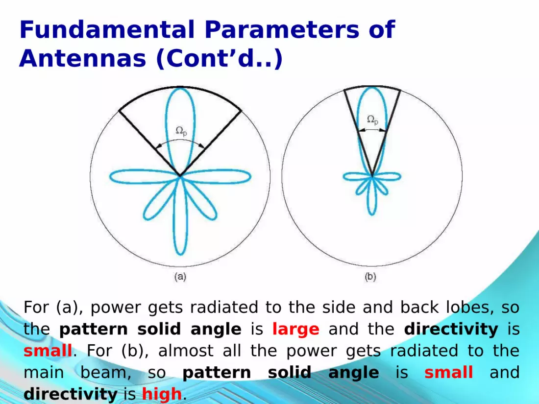
Fundamental Parameters of Antennas (Cont’d..)
For (a), power gets radiated to the side and back lobes, so the pattern solid angle is large and the directivity is small. For (b), almost all the power gets radiated to the main beam, so pattern solid angle is small and directivity is high.

31
Example 2
2 3, sin for 0 ,
0 otherwise.
sin nP
For this normalized radiation intensity,
Find the beamwidth, pattern solid angle and the directivity.

32
Solution to Example 2
The beam is pointing in the +y direction. WHY?!?!
Due to the beam having function in θ and φ, so that:
1 .2
BW BW BW
From previous equation, so that a 3dB beamwidth is at half of total power = 0.5.
1, max nP

33
Solution to Example 2 (Cont’d..)
To find BWθ, we fix φ = π/2 to get:
and then set sin2θ equal to ½. Then,
1sin, 2 nP
1 1sin 45 , so 180 45 45 90 .2
BW
To find BWφ, we fix θ = π/2 to get:
3sin1, nP

and then set sin3θ equal to ½. Then,
Solution to Example 2 (Cont’d..)
11 3sin 1 2 52.5 , so 180 52.5 52.5 75 .BW
So, 1 90 75 82.5 .
2BW
The pattern solid angle is:
2 3
3 3
0 0
sin sin sin ,
sin sin , (note limits on )
P n
P
P d d d
d d
35
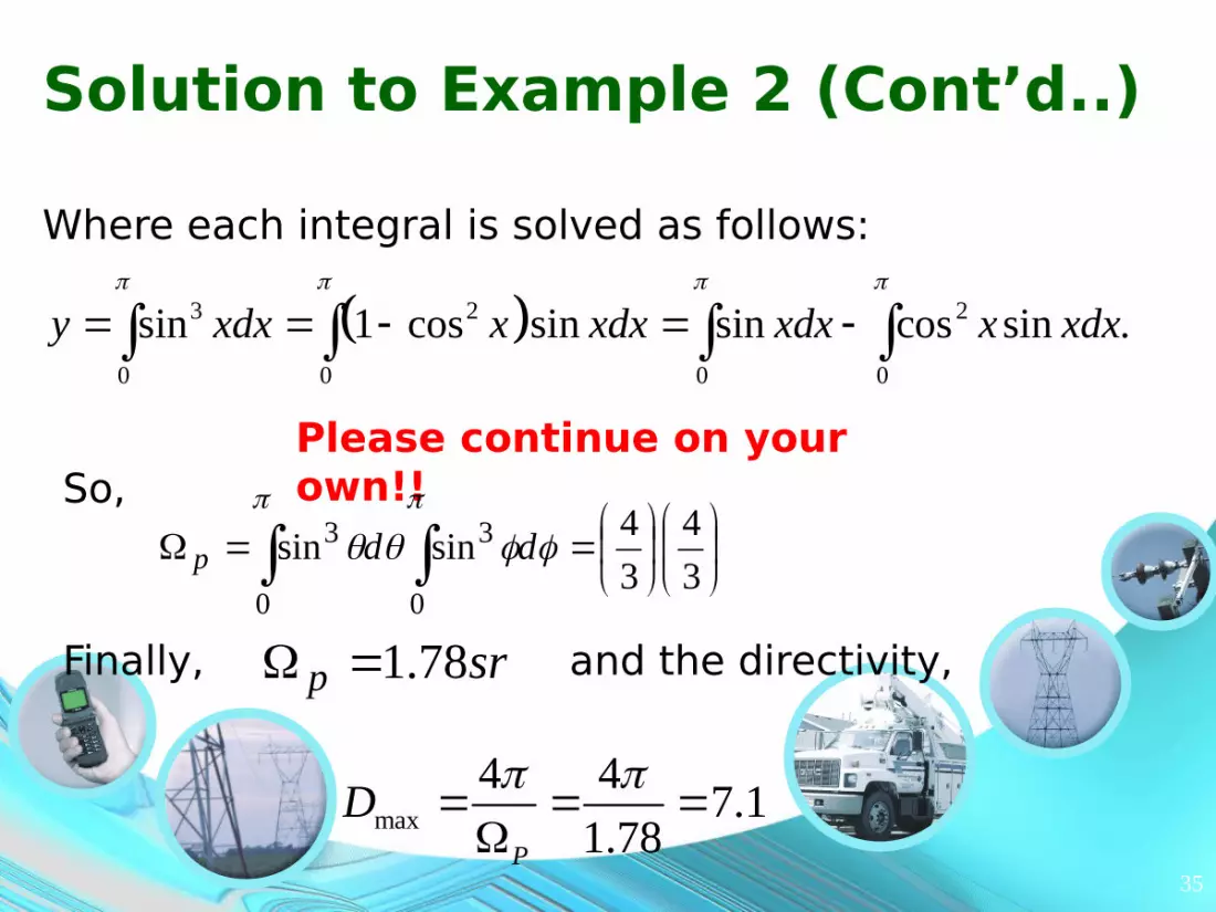
Solution to Example 2 (Cont’d..)
Where each integral is solved as follows:
3 2 2
0 0 0 0
sin 1 cos sin sin cos sin .y xdx x xdx xdx x xdx
Please continue on your own!!
3
434sinsin
0 0
33
ddp
srp 78.1Finally,
So,
max4 4 7.1
1.78P
D
and the directivity,
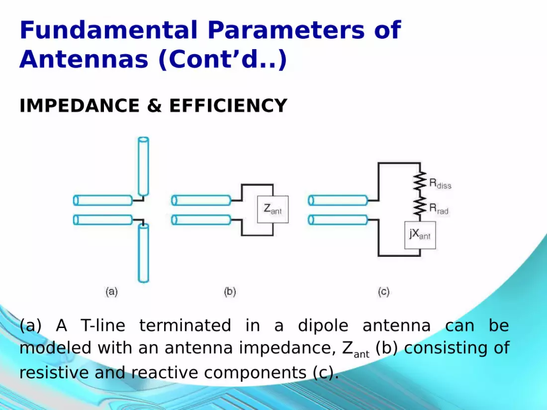
Fundamental Parameters of Antennas (Cont’d..)IMPEDANCE & EFFICIENCY
(a) A T-line terminated in a dipole antenna can be modeled with an antenna impedance, Zant (b) consisting of resistive and reactive components (c).

Fundamental Parameters of Antennas (Cont’d..)
The antenna resistance consists of radiation resistance Rrad and a dissipative resistance Rdiss that arises from ohmic losses in the metal conductor. For antenna driven by phasor current,
radrad RIP 202
1 and also dissdiss RIP 2
021
For maximum radiated power, Rrad need to be as large as possible but without being too large, for easily match with the feedline.

Fundamental Parameters of Antennas (Cont’d..)So then the antenna efficiency, e
dissrad
rad
dissrad
radRR
RPP
Pe
The power gain G(θ,φ) is likely its directive gain plus efficiency, where:
,, eDG
And the max power gain is when the directivity is max. It’s been always expressed in dBi , indicating dB with respect to an isotropic antenna.

4.2 Electrically Short Antennas
If the current distribution of a radiating element is known, it’s possible to calculate the radiated fields by a direct integration but, the integrals can be very complex.For time harmonic fields, integration is performed to find a phasor called retarded vector magnetic potential, which then followed by simple differentiation to find the H field. We will begin with a derivation of the retarded vector magnetic potential, then find the radiated fields for Hertzian dipole (infinitesimally short element with uniform current along its length). From that, we can find the fields from longer structures via integration e.g. small loop antenna.

Electrically Short Antennas (Cont’d..)Vector Magnetic Potential
In working with electric fields, and analogous term for H field is the vector magnetic potential A, often used for antenna calculations.
VE
Where in the point form of Gauss Law for magnetic fields,
0 BWith vector identity that states the div of the curl of any vector A is zero. So,
AB Then we now seek a relation between vector A and a current source.
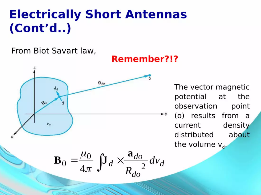
Electrically Short Antennas (Cont’d..)From Biot Savart law,
ddo
dod dv
R 20
0 4a
JB
Remember?!?
The vector magnetic potential at the observation point (o) results from a current density distributed about the volume vd.

Electrically Short Antennas (Cont’d..)
Due to long derivation and by using vector identity, we could get:
ddo
d dvR 2
000 4
JB
Then,
ddo
d dvR 2
00 4
JA
More properly,
d
do
dddd dvR
zyxzyx
20
0000,,
4,,
JA
Where the vector
potential at point o is a function of the position of current element
Refer to text book!

Electrically Short Antennas (Cont’d..)
We have yet to consider time dependence, so:
d
do
pdodddd dvR
uRtzyxtzyx
/,,,
4,,, 0
0000J
A
Where:
tjdspdodddd euRtzyx JJ /,,,
Where Jds is the retarded phasor quantity:
dojkRddddds ezyx ,,JJ k = β =
2π/λ

Electrically Short Antennas (Cont’d..)
Using this current density, the phasor form is:
ddo
dsS dv
RJ
A4
00
This is what we called as the time harmonic equation for the retarded vector magnetic potential.
In phasor notation, the vector magnetic potential is related to the magnetic flux density by :
SS 00 AB

Electrically Short Antennas (Cont’d..)
From there, we could find H in free space :
000 / SS BH
Because the radiation is propagating radially away from the source, it is then a simple matter to find E, where:
SrS 000 HaE
Finally, the time averaged power radiated is:
SSr 00Re21,, *HEP

Electrically Short Antennas (Cont’d..)Hertzian Dipole
Suppose that a short line of current, tIti cos)( 0
It’s placed along the z axis as shown.

Electrically Short Antennas (Cont’d..)
Here, the phasor current is:To maintain constant current over its entire length, imagine a pair of plates at the ends of the line that can store charge.The stored charge at the ends resembles an electric dipole, and the short line of oscillating current is then ‘Hertzian Dipole’.
js eII 0
For Is in the +az direction through a cross sectional S, the current density at the source seen by the observation point:
zjkRs
ds eSI
aJ

Electrically Short Antennas (Cont’d..)
Geometrical arrangement of an infinitesimal dipole and its associated electric field components on a spherical surface.

Electrically Short Antennas (Cont’d..)A differential volume of this element,
zjkR
sdds dzeIdv aJ
Sdzdvd So,
With assumption that the Hertzian dipole is very short, integrate to get A0S :
2/
2/
00 4
z
jkRs
S dzR
eIaA
Therefore,
z
jkRs
S ReI
aA
4
00

Electrically Short Antennas (Cont’d..)The unit vector az can be converted to its equivalent spherical coordinates, so that:
aaA sincos
40
0
r
jkRs
S ReI
It is now a relatively straightforward matter to find B0S and then,
aH sin1
40
Rjk
ReI jkR
sS
Regroup to get:
aH sin1
4 2
2
0
kRkRjekI jkR
sS

Electrically Short Antennas (Cont’d..)The second terms drops off with increasing radius much faster than the first term, where for far field condition:
211
kRkR
aH sin
40 RkeI
jjkR
sS
Therefore,
Meanwhile, the far field value of E field :
aE sin
400 RkeI
jjkR
sS
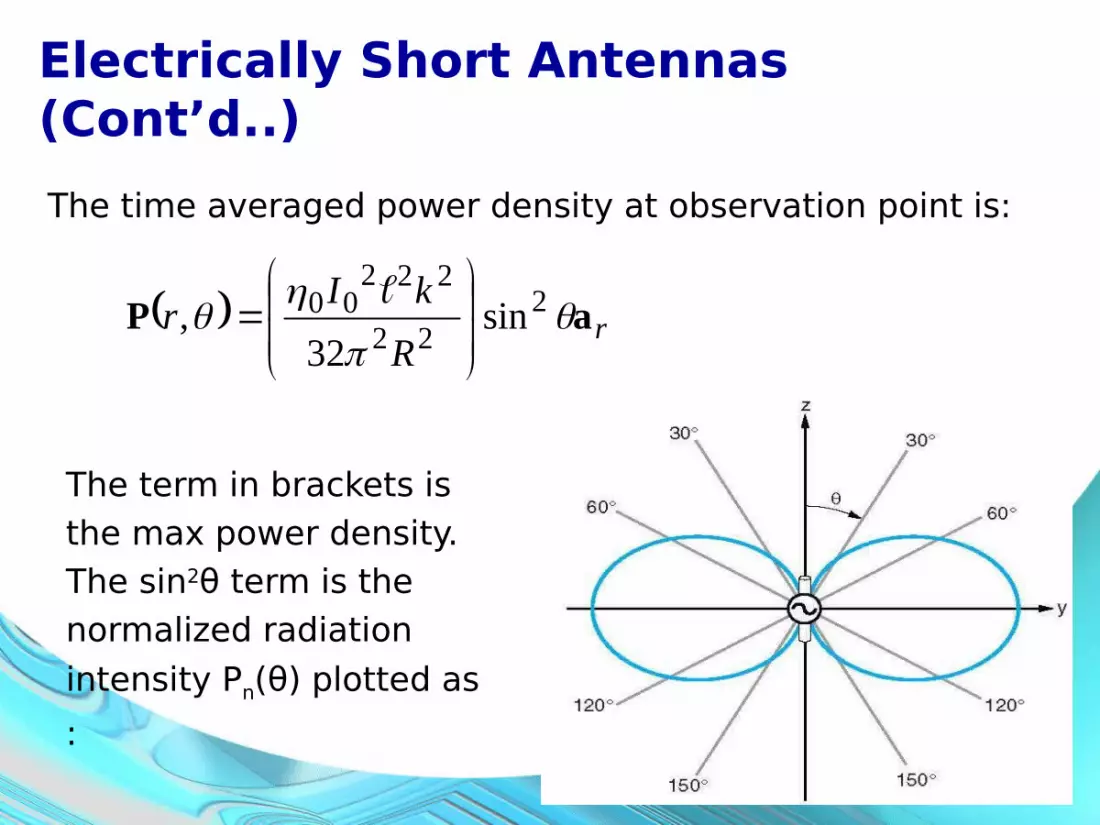
Electrically Short Antennas (Cont’d..)The time averaged power density at observation point is:
rR
kIr aP
2
22
22200 sin
32,
The term in brackets is the max power density. The sin2θ term is the normalized radiation intensity Pn(θ) plotted as :

Electrically Short Antennas (Cont’d..)The normalized radiation intensity can be used to find the pattern solid angle,
38sinsinsin 22 dddp
The directivity is then: 5.14max
pD
20
222
220
202
max2 40
32I
R
IkrPrP pprad
The total power radiated by a Hertzian dipole:

Electrically Short Antennas (Cont’d..)
Also Rrad as:2
280
radR
For Hertzian dipole, where l<<λ, Rrad will be very small and the antenna will not efficiently radiate power. Larger dipole antennas, have much higher Rrad and thus more efficient.

55
Example 3
Suppose a Hertzian dipole antenna is 1 cm long and is excited by a 10 mA amplitude current source at 100 MHz. What is the maximum power density radiated by this antenna at a 1 km distance? What is the antenna’s radiation resistance?

Solution to Example 3
8
6
3 10, 3 .100 10 1
c x m sc f mf x s
2 2 22 2 2
max 2 2 2 2 2 2
2 0.010 0.010120 0.05232 32 3 1000o oI pWP
r m
l
2 22 2 0.0180 80 8.8
3radR m l
We should calculate the wavelength,
The max. power radiated is:
The antenna radiation resistance :

Electrically Short Antennas (Cont’d..)Small Loop Antenna
A small loop of current located in the xy plane centered at the origin small loop antenna or magnetic dipole.

Electrically Short Antennas (Cont’d..)
aJ adeIdv jkRsdds
Substitute,
Giving us,
aA dR
eaI jkRs
S 40
0
Assume that a<<λ and A0s is in far field. It’s discovered that,
aA sin1
4 20
0jkRs
S ejkRR
SI
Where, and thus,2aS
aH jkRsS e
RSkI
sin4 0
00
aE jkRsS e
RSkI sin
40
0

Electrically Short Antennas (Cont’d..)The power density vector :
rR
kSIr aP
2
220
2220
20
2sin
32,
Where,
220
2220
20
2
max32 R
kSIP
Since the normalized power function is the same as Hertzian dipole, Ωp=8π/3, Dmax = 1.5

Electrically Short Antennas (Cont’d..)
2
2
20
30
34
SIPrad
Calculation of Prad and Rrad yields
2
24320
SRrad
The fields for the small loop antenna is similar to Hertzian dipole. It’s the dual of Hertzian (electric) dipole magnetic dipole.
The equations also valid for multi turn loop, as long as the loop small compared to wavelength. For N circular loop, S=Nπa2 and for square coil N loops, with each side length b, S=Nb2
Try this!!
4.3 Dipole Antennas
Dipole Antennas
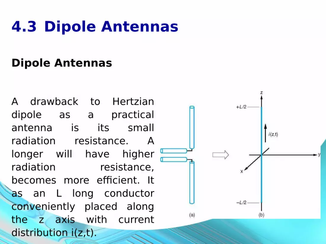
A drawback to Hertzian dipole as a practical antenna is its small radiation resistance. A longer will have higher radiation resistance, becomes more efficient. It as an L long conductor conveniently placed along the z axis with current distribution i(z,t).

Assume sinusoidal current distribution on each arm, where the antenna is center-fed and the current vanishes at the end points. The distribution:
tzItzi s cos)(,
Where,
02/
2sin
2/02
sin)(
0
0
zLzLkeI
LzzLkeIzI
j
j
s
Division of the L long dipole into a series of infinitesimal Hertzian dipoles !!
Dipole Antennas (Cont’d..)

For simplicity, assume phase term =0, and make use of current distribution term with magnetic field equation for a Hertzian dipole to get :
2/
0
0
2/
00 'sin
2sin'sin
2sin
4
L jkR
L
jkR
S dzzL
kR
edzz
Lk
RekI
j aH
Dipole Antennas (Cont’d..)

For far field, the vectors r and R appear to be parallel, so that θ’=θ and R=r, where:
coscos jkzjkrzrjkjkR eeee
After pulling the components that don’t change with z, use table of integrals and with application to Euler’s identity,
aaH
sin2
coscos2
cos
20
00
kLkL
reI
jHjkr
SS
Dipole Antennas (Cont’d..)

The vector E0S is then easily found from :
a HaE SSrS H00000
Where, the pattern function is given by:
2
sin2
coscos2
cos
kLkL
F
The time averaged power radiated is:
rFr
Ir a P
2
2015
,
Dipole Antennas (Cont’d..)

Therefore, the normalized power function is:
max
FFPn
And the max time averaged power density is then :
max2
20
max15
Fr
IP
It’s not generally equivalent to the normalized power function since F(θ) can be greater than one.
Dipole Antennas (Cont’d..)

Dipole Antennas (Cont’d..)

3D and 2D amplitude patterns for a thin dipole of l=1.25λ
Dipole Antennas (Cont’d..)

Half Wave Dipole Antennas
Because of its convenient radiation resistance, and because it’s a smallest resonant dipole antenna, the half wavelength dipole antenna merits special attention.With kL/2 = π/2,
rr
Ir a P
2
2
2
20
sin
cos2
cos15
,
With the F(θ) is 1, the maximum power density is: 2
2015
,r
Ir
P
Dipole Antennas (Cont’d..)

Therefore, the normalized power density is:
2
2
cos
cos2
cos
nP
The current distribution and normalized radiation pattern for a half wave dipole antenna.
Dipole Antennas (Cont’d..)

Dipole Antennas (Cont’d..)

For half wave dipole…658.7 p and with L = λ/2 Try
this!!We can then find the directivity as :
640.14max
pD
Which is slightly higher than the directivity of Hertzian dipole, the radiation resistance is given by:
pradrad PrRIP max22
021
Leads to: 2.7330
pradR
Dipole Antennas (Cont’d..)

This radiation resistance much higher than of Hertzian dipole, where it radiates more efficiently easier to construct an impedance matching network for this antenna impedance.This antenna impedance also contains a reactive components, Xant, where for a λ/2 dipole antenna it is equal to 42.5Ω . Therefore, total impedance by neglecting Rdiss. 5.422.73 jZant
For impedance matching, need to make reactance zero (in resonant condition). So, it can be achieved by making the antenna slightly shorter (reduced in length until reactance vanishes).
Dipole Antennas (Cont’d..)

74
Example 4
Find the efficiency and maximum power gain of a λ/2 dipole antenna constructed with AWG#20 (0.406 mm radius) copper wire operating at 1.0 GHz.
Compare your result with a 3 mm length dipole antenna (Hertzian Dipole) if the center of this antenna is driven with a 1.0 GHz sinusoidal current.

Solution to Example 4
We first find the skin depth of copper at 1.0 GHz,
mfcu
6
7790
1009.2108.5104101
11
This is much smaller than the wire radius, so the wire area over which current is conducted by:
291033.52 maS cu
At 1 GHz, the wavelength is 0.3m and the λ/2 is 0.15m long. The ohmic resistance is then:
485.01S
Rdiss

Solution to Example 4 (Cont’d..)Since the radiation resistance for half wave dipole is 73.2Ω, we have :
99.0485.02.73
2.73
e
A gain of:
63.1640.199.0maxmax eDG
Meanwhile for Hertzian Dipole, the ohmic resistance of the small dipole is :
mS
Rdiss 7.91

Solution to Example 4 (Cont’d..)To find the radiation resistance, with value of wavelength is 0.3m, thus :
m
mm
Rrad 793.0
10380
32
Therefore, its efficiency and gain:
89.07.979
79
mm
me 34.15.189.0maxmax eDG
Thus, the half wave dipole is clearly more efficient with a higher gain than the short dipole.

Consider the construction of half wave dipole for an AM radio station broadcasting at 1 MHz. At this f, the wavelength is 300m long and the half wave dipole antenna must be 150m tall.We can cut this in half, by employing image theory to build a quarter wave monopole antenna that is only 75m tall!!
4.4 Monopole Antennas

Monopole Antennas (Cont’d..)
Consider pair of charges, +Q and –Q (as electric dipole), where the dashed line shows the location of zero potential surface. If we slide a conductive plane over the zero potential surface, the field lines in the upper half plane are unchanged.

Note that the charge can be in any distribution (point charge, line charge, surface or volume charge) and the image charge is a mirror image of opposite polarity.A monopole antenna is excited by a current source at its base. By image theory, the current in the image will be the same with the current in actual monopole. The pair of monopole resembles a dipole antenna.A monopole antenna placed over a conductive plane and half the length of a corresponding dipole antenna will have identical field patterns in the upper half plane.
Monopole Antennas (Cont’d..)

For the upper half plane (00< θ<900), the time averaged power, max power density and normalized power density for the quarter wave monopole is the same with half wave dipole. But the pattern solid angle is different.
Monopole Antennas (Cont’d..)

Since the normalized power density is zero for (900< θ<1800), the pattern solid angle:
dPnp
Integrate over all space will be half value of Ωp for half wave dipole. So, for quarter wave monopole,
28.34829.3 max
p
p D
See that the radiation resistance is halved, and the antenna impedance :
6.3630
pradR
25.216.36 jZant
Monopole Antennas (Cont’d..)
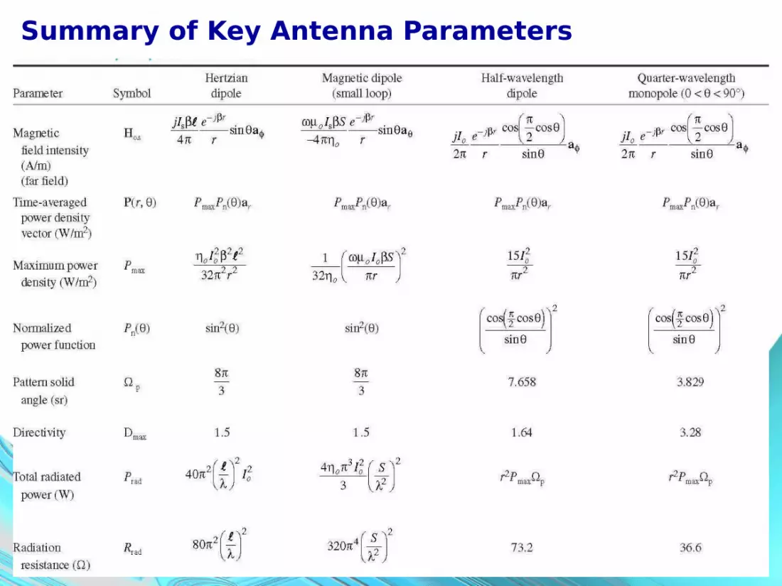
Summary of Key Antenna Parameters

4.5 Antenna ArraysThe antennas we have studied so far have all been omnidirectional – no variation in φ. A properly spaced collection of antennas, can have significant variation in φ leading to dramatic improvements in directivity.
A Ka-Band Array Antenna

Antenna Arrays (Cont’d..)An antenna array can be designed to give a particular shape of radiating pattern. Control of the phase and current driving each array element along with spacing of array elements can provide beam steering capability. For simplification: All antenna elements are identical The current amplitude is the same feeding each
element. The radiation pattern lies only in xy plane, θ=π/2 The radiation pattern then can be controlled by: controlling the spacing between elements or controlling the phase of current driving for each element

Antenna Arrays (Cont’d..)For simple example, consider a pair of dipole antennas driven in phase current source and separated by λ/2 on the x axis. Assume each antenna radiates
independently, at far field point P, the fields from 2 antennas will be 180 out-of-phase, owing to extra λ/2 distance travel by the wave from the farthest antenna fields cancel in this direction. At point Q, the fields in phase and adds. The E field is then twice from single dipole, fourfold increase in power broadside array max radiation is directed broadside to axis of elements.

Antenna Arrays (Cont’d..)
Modify with driving the pair of dipoles with current sources 180 out of phase. Then along x axis will be in phase and along y axis will be out of phase, as shown by the resulting beam pattern endfire array max radiation is directed at the ends of axis containing array elements.

Antenna Arrays (Cont’d..)
Pair of Hertzian Dipoles
Recall that the far field value of E field from Hertzian dipole at origin,
aE sin
400 RkeI
jjkR
sS
But confining our discussion to the xy plane where θ = π/2,
aE
RkeI
jjkR
sS 400

Antenna Arrays (Cont’d..)
Consider a pair of z oriented Hertzian dipole, with distance d, where the total field is the vector sum of the fields for both dipoles and the magnitude of currents the same but a phase shift between them.
aaEEE
2
20
1
1020100 44
21
RkeI
jR
keIj
jkRs
jkRs
SStotS
Where, jss eIIII 0201

Antenna Arrays (Cont’d..)Assumption,
2121 RrR
And,

Antenna Arrays (Cont’d..)Where geometrically we could get,
cos2
cos2 21
drRdrR
Thus, the total E field becomes:
aE
2cos
22cos
22000 4
dkjdkjj
jkR
totS eeeR
keIj
With Euler’s identity, the total E field at far field observation point from two element Hertzian dipole array becomes :
aE
2cos
2cos2
420
00dke
RkeI
jjjkR
totS

Antenna Arrays (Cont’d..)To find radiated power,
r
rtotSSS
dkR
kI
Er
a
aHEP
2cos
2cos4
32
21Re
21,
2,
222
22200
200
*
It can be written as:
rarrayunit FFr a P
,
2,
Antenna Arrays (Cont’d..)
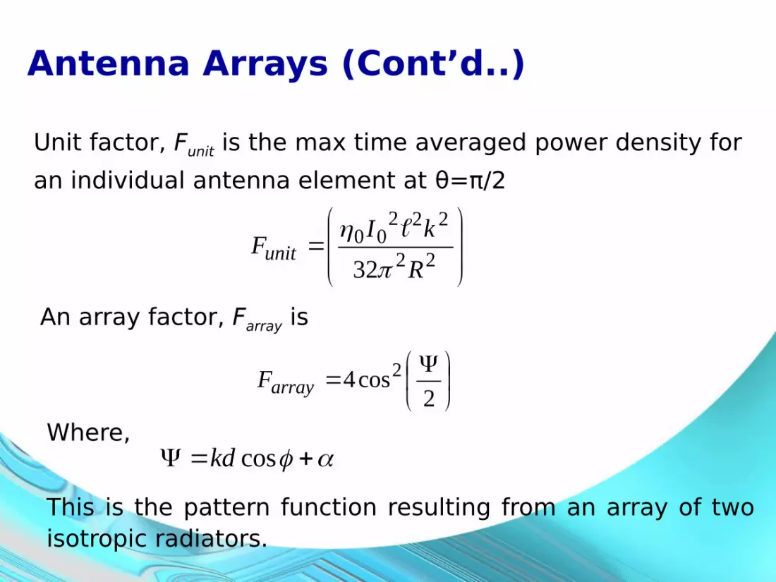
Unit factor, Funit is the max time averaged power density for an individual antenna element at θ=π/2
22
22200
32 R
kIFunit
An array factor, Farray is
2cos4 2
arrayF
Where, coskd
This is the pattern function resulting from an array of two isotropic radiators.

94
Example 5
The λ/2 long antennas are driven in phase and are λ/2 apart. Find: the far field radiation
pattern for a pair of half wave dipole shown.
the maximum power density 1 km away from the array if each antenna is driven by a 1mA amplitude current source at 100 MHz.

Solution to Example 5At 100 MHz, λ = 3m, so that 1 km away is definitely in far field. For a half wave dipole, we have :
rrr
IrPr a aP
2
2
2
20
sin
cos2
cos15
,,
The unit factor can be found by evaluating above at θ = π/2 ,
2
2015
r
IFunit

Solution to Example 5 (Cont’d..)The array factor, with d = λ/2 and =0 (due to antennas are driven at the same phase) :
cos
2cos4 2
arrayF
For the array, we now have :
cos
2cos
60,
2, 2
2
20
r
IFFr rarrayunit a P
The normalized power function is:
cos2
cos,
2,
,2
,,
22
maxrP
rP
nP

Solution to Example 5 (Cont’d..)This can be plotted as :
But how to plot?!?!?!
The maximum radiated power density at 1000m is :
22
23
2
20
max 191000
106060
m
pW
r
IP
Use MATLAB!!

Antenna Arrays (Cont’d..)
N - Element Linear Arrays
The procedure of two-element array can be extended for an arbitrary number of array elements, by simplifying assumptions : The array is linear antenna elements are evenly spaced,
d along a line. The array is uniform each antenna element driven by
same magnitude current source, constant phase difference, between adjacent elements.

Antenna Arrays (Cont’d..)
10
2030201 ,....,, Nj
sNj
sj
ss eIIeIIeIIII

Antenna Arrays (Cont’d..)
The far field electric field intensity :
rNjjj
jkR
totS eeeR
keIj aE
120
00 ...14
Where, coskd
Manipulate this series to get:
2sin
2sin
2
2 N
FarrayWith the max value as :
2max
NFarray

Antenna Arrays (Cont’d..)
So then the normalized power pattern for these elements is :
2sin
2sin
12
2
2max
N
NF
FP
array
arrayn

102
Example 6
Five antenna elements spaced λ/4 apart with progressive phase steps 300. The antennas are assumed to be linear array of z oriented dipoles on the x axis. Find: the normalized radiation pattern in xy plane the plot of the radiation pattern.

Solution to Example 6
To find the array factor, first need to find psi, Ψ:
6cos
218030cos
42
cos
kd
Inserting this ratio to array factor,
12cos
4sin
125cos
45sin
2sin
2sin
2
2
2
2
N
Farray 252max
NFarray

Solution to Example 6 (Cont’d..)The normalized radiation pattern is :
12cos
4sin
125cos
45sin
251
2
2
nP
But how to plot?!?!?!
Use MATLAB!!
The plot is :

Antenna Arrays (Cont’d..)
Parasitic Arrays
Not all the elements in array need be directly driven by current source. A parasitic array typically one driven element and several parasitic elements, the best known parasitic array is Yagi-Uda antenna.
Antenna Arrays (Cont’d..)
On one side of the driven element is reflector length and spacing are chosen to cancel most of the radiation in that direction, as well as to enhance the direction to forward or main beam direction.
Several directors (four to six) focus the main beam in the forward direction high gain and easy to construct.
Parasitic elements tend to pull down the Rrad of the driven element. E.g. Rrad of dipole would drop from 73Ω to 20Ω when used as the driven element in Yagi-Uda antenna.But higher Rrad is more efficient, so use half wavelength folded dipole antenna (four times Rrad of half-wave dipole!)
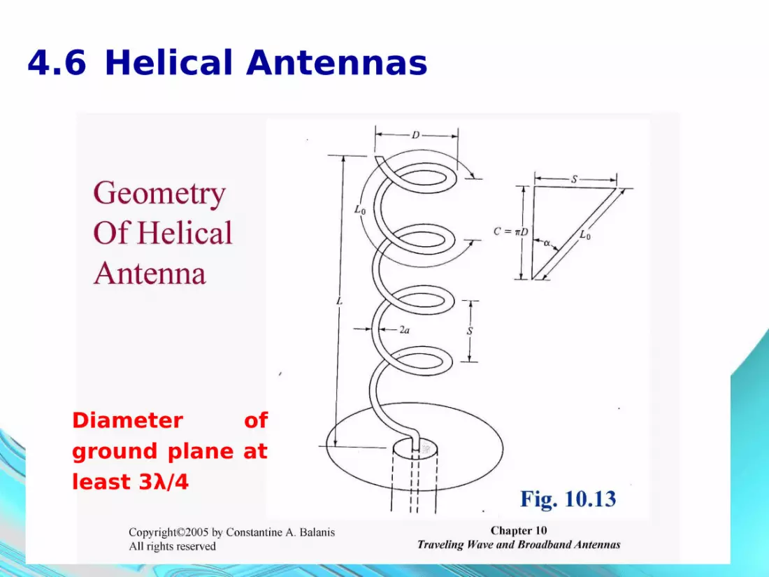
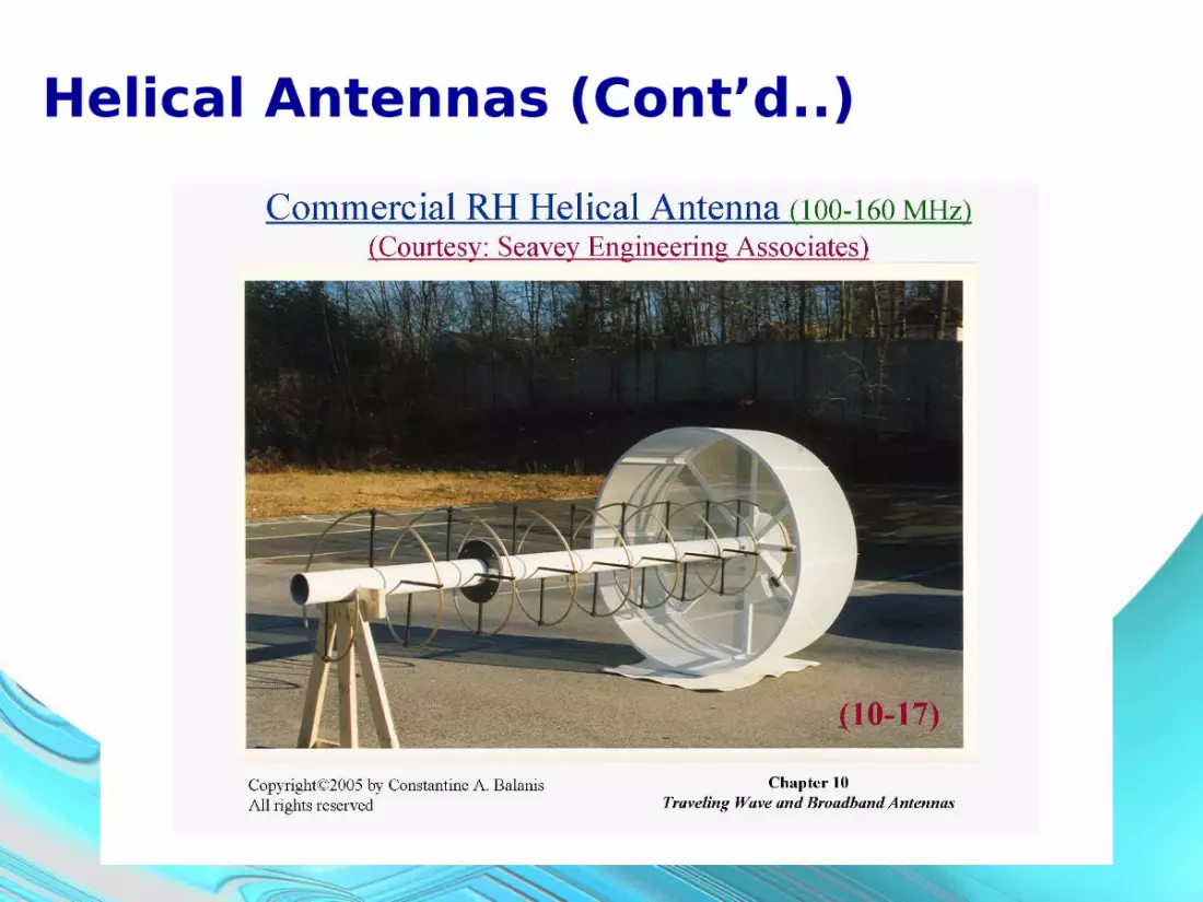
4.6 Helical Antennas
Diameter of ground plane at least 3λ/4

Helical Antennas (Cont’d..)
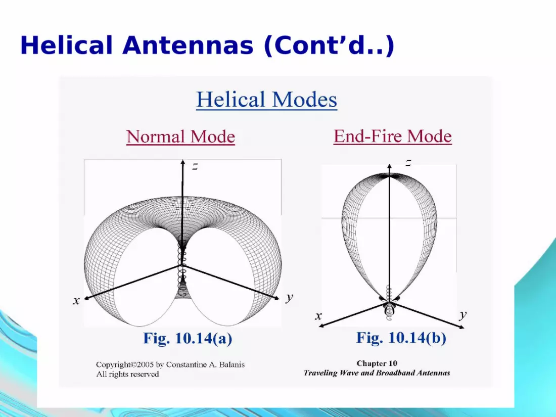
Helical Antennas (Cont’d..)

Helical Antennas (Cont’d..)Important Parameters

Helical Antennas (Cont’d..)

Helical Antennas (Cont’d..)
For this special case,
The radiated field is circularly polarized in all directions other than θ = 00

Helical Antennas (Cont’d..)
Parameters for End Fire mode

Helical Antennas (Cont’d..)

Helical Antennas (Cont’d..)Feed Design for Helical Antennas

Helical Antennas (Cont’d..)
Helical Antennas (Cont’d..)

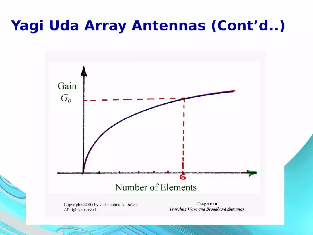
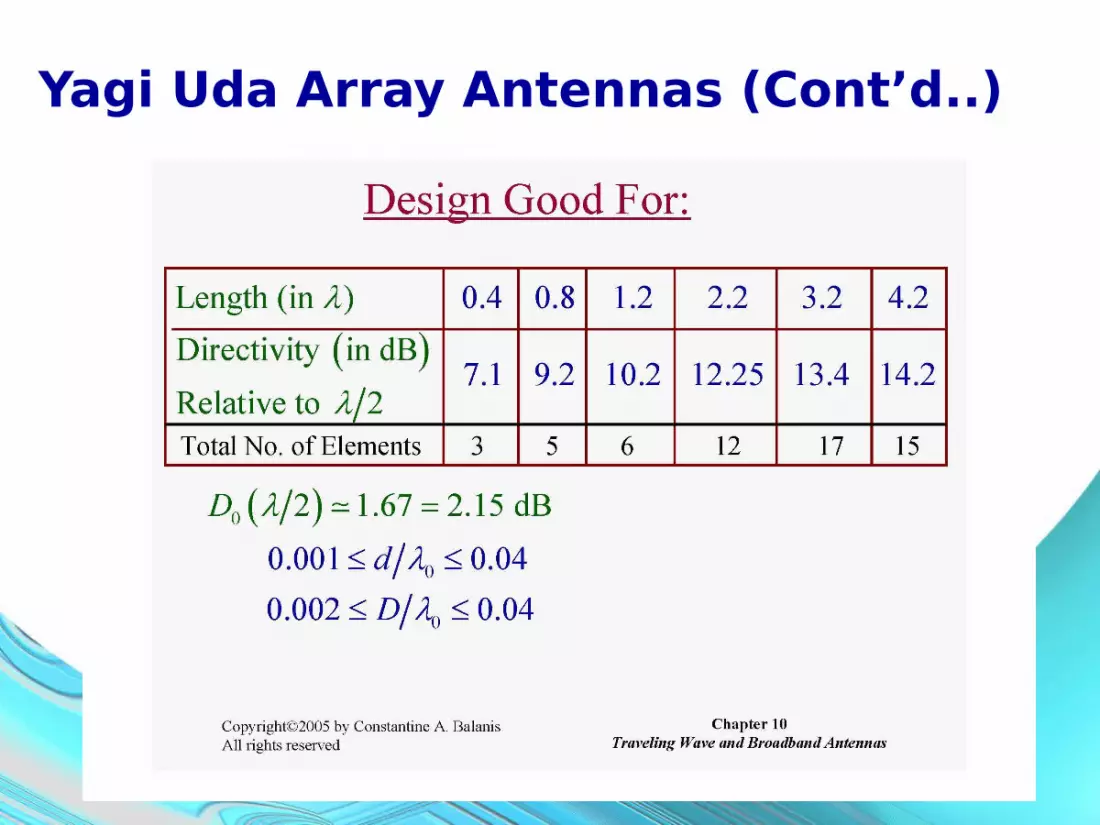
4.7 Yagi Uda Array Antennas

Yagi Uda Array Antennas (Cont’d..)

Yagi Uda Array Antennas (Cont’d..)
Yagi Uda Array Antennas (Cont’d..)
Yagi Uda Array Antennas (Cont’d..)

Yagi Uda Array Antennas (Cont’d..)

124
Example 7
With above parameters, design a Yagi Uda Array antenna by finding the element spacing, lengths and total array length.
Given
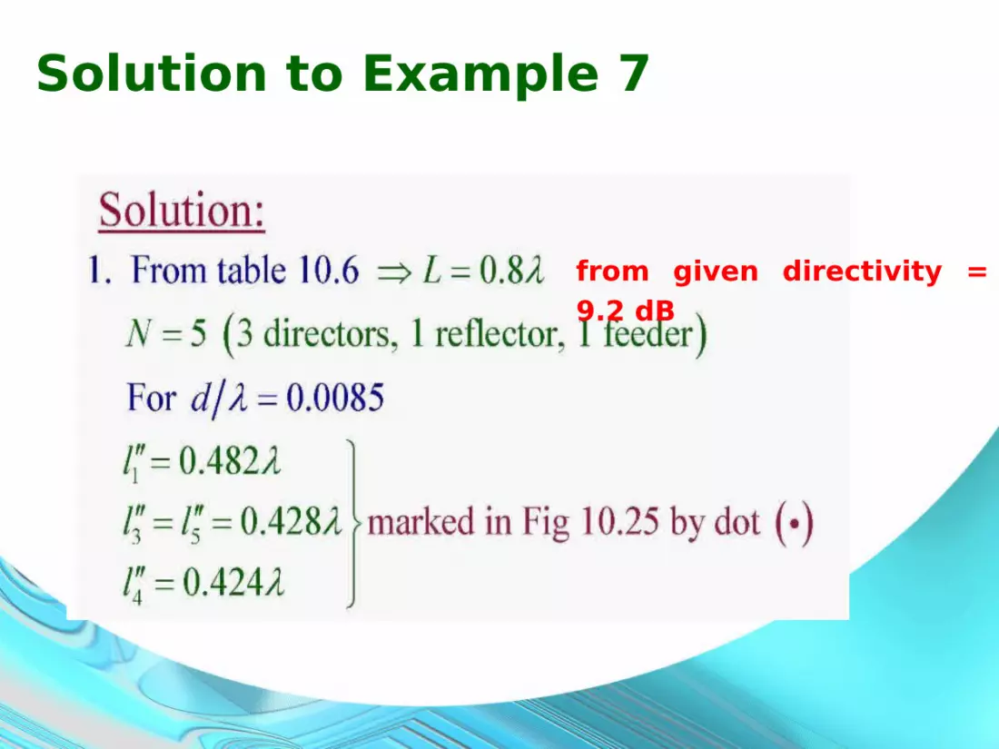
Solution to Example 7
from given directivity = 9.2 dB

Solution to Example 7(Cont’d..)

Solution to Example 7(Cont’d..)
Therefore,Total array length: 0.8 λThe spacing between directors: 0.2 λThe reflector spacing: 0.2 λThe actual elements length:
L3 = L5 : 0.447λ
L4 : 0.443λ
L1 : 0.490λ

128
Solution to Example 7(Cont’d..)

129
Fig 10.25
Solution to Example 7(Cont’d..)Design Curves to Determine Element Lengths
X
.

130
Fig 10.26
Solution to Example 7(Cont’d..)

Yagi Uda Array Antennas (Cont’d..)

4.8 Antennas for Wireless CommunicationsParabolic Reflectors
Parabolic dish antenna
Parabolic reflector antenna

Antennas for Wireless Communications (Cont’d..)
Cassegrain reflector antenna
All of these parabolic reflectors operates based on the geometric optics principle that a point source of radiation placed at the focal point of parabolic reflector will radiate the energy incident on the dish in a narrow and collimated beam.For high efficient, the dish must be significantly larger
than the radiation wavelength, and has a directive feed.

Antennas for Wireless Communications (Cont’d..)Patch Antennas
Other shapes such as circles, triangles and annular rings also been used. It can be excited by an edge or probe fed, where its location is chosen for impedance match between cable and antenna.

Antennas for Wireless Communications (Cont’d..)Folded Dipole Antennas
A pair of half-wavelength dipole elements are joined at the ends and fed from the center of one of the pair. If the two sections are close together (d on the order of λ/64), the impedance will be four times greater than the regular λ/2 dipole antenna. The directivity is the same but the bandwidth is significantly broader.

AntennaEnd