choice of routes in congested traffic networks: experimental tests of the braess paradox
TRANSCRIPT

Choice of Routes in Congested Traffic Networks:
Experimental Tests of the Braess Paradox
Amnon Rapoport
University of Arizona
Tamar Kugler University of Arizona
Subhasish Dugar
University of Arizona
Eyran Gisches University of Arizona
July 6, 2005
Keywords: Braess Paradox, congested traffic networks, choice of routes, experimental study Please address all Correspondence to: Amnon Rapoport Department of Management and Policy 405 McClelland Hall University of Arizona Tucson, AZ 85721 Email: [email protected] Phone: 520-621-9325 Fax: 520-621-4171

2
Abstract
The Braess paradox (Braess, 1968) consists of showing that, in equilibrium, adding a new link
that connects two routes running between a common origin and common destination may raise
the travel cost for each network user. We report the results of two experiments designed to study
whether the paradox is behaviorally realized in two simulated traffic networks that differ from
each other in their topology. Implementing a within-subjects design, both experiments include
finite populations of paid participants in a computer-controlled setup who independently and
repeatedly choose travel routes in one of two types of traffic networks, one without the added
links and the other with the added links, to minimize their travel costs. Our results reject the
hypothesis that the paradox is of marginal value and its force, if at all evident, diminishes with
experience. Rather, they strongly support the alternative hypothesis that with experience in
traversing the traffic network players converge to choosing the Pareto deficient equilibrium
routes despite sustaining a sharp decline in their earnings.

3
1. Introduction
Transportation and communication networks are among the best examples of frequently used
physical networks in which vertices (nodes) correspond to locations in space and edges (links) to
connections between them. They provide the infrastructure for humans to conduct much of their
social and economic activities (Nagurney, 2000). It would seem rather natural to believe that
increasing the capacity of an existing network or adding one or more new edges to traffic or
communication networks with fixed capacity would definitely not worsen and probably improve
efficiency. Braess (1968) has shattered this deeply entrenched belief by demonstrating that,
paradoxically, adding a link that connects two alternative routes in parallel running between a
common origin and common destination may raise the total travel cost of all the network users.
This phenomenon, subsequently labeled the Braess Paradox (BP), has stimulated a rapidly
growing body of research in transportation science, computer science, and applied probability.
Researchers have attempted to classify networks in which the addition of a single link could
degrade network performance (Frank, 1981; Steinberg & Zangwill, 1983), discovered new
paradoxes (Arnott, De Palma, & Lindsey, 1993; Cohen & Kelly, 1990; Dafermos & Nagurney,
1984; Fisk, 1979; Hagstrom & Abrams, 2001; Pas & Principio, 1997; Smith, 1978; Steinberg &
Stone, 1988), proved that detecting the BP is algorithmically hard (Roughgarden, 2001), and
quantified the degree of degradation in network performance due to unregulated traffic
(Kousoupias & Papadimitriu, 1999; Roughgarden & Tardos, 2002).
Steinberg and Zangwill concluded an early analysis of the BP with the claim that “under
reasonable assumptions, Braess’ Paradox is not a curious anomaly but in fact might occur quite
frequently (1983, p. 317).” However, no direct empirical evidence has been forthcoming to
buttress this claim. In a postscript of his exposition of the BP more than 35 years ago, Murchland
(1970) remarked that Knödel had noted that major road investments in the center of the city of

4
Stuttgart had failed to yield the benefits expected. This briefly mentioned case is the only
example subsequently cited by Kelly (1991), Roughgarden and Tardos (2002), and others.
Analyzing network data from the city of Winnipeg, Fisk and Pallottino (1981) used a variety of
statistical tests to determine if manifestations of the BP could be found on a localized section of
the road network; they reported positive albeit rather weak evidence. The New York Times also
hinted at the counterintuitive consequences of road closures in an article with a provocative title
that appeared on Christmas Day, 1990: “What if they closed 42nd street and nobody noticed?”
This mostly anecdotal and very sketchy evidence is clearly insufficient to counter arguments
about the importance and relevance of the BP to real transportation and communication
problems. A claim can be made that the BP is no more than a theoretical curiosity, that it is too
simple to model real-life traffic and communication networks, and that examples closer to the
complexity of real life would prevent those kinds of paradoxes from being realized. Another
argument is directed not so much against the realism of the model but against the assumed
behavior of the network users. In formulating the BP, network users are viewed as independent
“selfish” agents participating in a noncooperative game, where each agent wishes to choose a
path from a common origin to a common destination that minimizes her travel cost. The
decisions of the agents constitute Nash equilibrium if no agent has an incentive to unilaterally
change her path. The paradox is based on an equilibrium analysis of a weighted traffic network
both before and after one or more edges are added to it. But real network users, it may be
claimed, may quickly learn to avoid traversing the new edges—and thereby depart from
equilibrium play—in an attempt to escape the adverse effects of the BP. The Prisoner’s Dilemma
game is the most well known example of Nash equilibria that, in general, do not optimize social
welfare. Just as agents participating in the finitely iterated two-person Prisoner’s Dilemma game
may learn to play dominated strategies in an attempt to maximize joint payoff, network users

5
who play for considerably higher stakes may be expected to learn avoiding the BP by choosing
dominated routes in the network.
As empirical evidence about the occurrence of the BP is very difficult to come by, the
approach that we pursue in the present study is to simulate simple traffic networks that are
susceptible to the BP in the laboratory, have subjects choose routes in these simulated traffic
networks before and after one or more edges are added to them, and find out whether systematic
and replicable patterns of behavior emerge. If they do, it is of significant interest to determine
whether they support the intuition that the BP is of marginal value and its force, if at all evident,
diminishes with experience or, alternatively, that they support the equilibrium analysis that
underlies the BP.
Rooted in the methodology of experimental economics, this approach is not common in
transportation research. We are familiar with only four experimental studies of traffic congestion.
The first is an experiment by Schneider and Weimann (2004) that was designed to test a simple
model of bottleneck congestion on a single route in a rush-hour situation. The model was
originally proposed by Arnott, De Palma, and Lindsey (1990, 1993). The second is an
experimental study by Gabuthy, Neveu, and Boement (2004), who generalized the analysis of
Arnott et al. (1990) to traffic networks with a single origin and single destination connected by
two routes. The experimental evidence is mixed; Schneider and Weimann report evidence in
support of equilibrium departure time in their first but not second experiment, whereas Gabuthy
et al. report no support. The third study is due to Selten et al. (2004), who conducted laboratory
experiments of a day-by-day route choice game with two parallel roads but no crossroad. Unlike
the two studies by Gabuthy et al. and Schneider et al., the experiment by Selten et al. is not
concerned with endogenous departure time but with route choice. They report aggregate road
choices that are accounted for quite well by the Nash equilibrium predictions and large

6
fluctuations around the mean choice frequencies that do not seem to diminish after an unusually
large number of rounds of play. In a fourth study, Helbing (2004) repeated these experiments
with more iterations, and further tested additional experimental conditions in an attempt to better
understand the reasons for the fairly large fluctuations around the mean choice frequencies. None
of these studies is concerned with the counterintuitive implication of the BP that is the main
focus of the present study.
The rest of the paper is organized as follows. Section 2 introduces terminology and illustrates
the BP in a network with the simplest possible form (called the Minimal Critical Network by
Penchina, 1997). Section 3 reports the results of an experiment designed to examine route choice
in the iterated Minimal Critical Network game. Section 4 extends the investigation to a
topologically richer network with three routes and a symmetric cost structure. The paradox in
this much more complex network is created by adding two new links connecting the three
original routes. Section 5 concludes.
2. The Braess Paradox
Notation and Terminology
We consider road networks with a common origin O and common destination D that are
modeled as a directed graph G=(V, E) with vertex (node) set V, edge (link) set E, and a set
K⊆V×V of origin-destination (OD) pairs. We consider a finite, commonly known, and relatively
small number of users, n, in contrast to the more common case discussed in the transportation
literature that assumes infinitely many users. The traffic in the road network is described by the
number fij of cars (users) moving along the edge (i,j) from vertex i to vertex j. The cost for each
user of traversing from i to j along the link (i,j) when the flow on this link is fij is denoted by
cij(fij). Travel costs are typically measured by time spent in travel or by gasoline consumed. It is
assumed that the cost of traveling on edge (i,j) at a given level of traffic is the same for all the

7
users traversing this edge. Total travel cost is the sum of the edge costs over all edges in the
travel route (also called path) from O to D.
Each of the n users is assumed to independently seek a path that minimizes her total travel
cost. In equilibrium, the n users are distributed over one or more routes so that a unilateral
change of path by any one user would raise the total travel cost for that user, given that all other
n-1 users do not change their routes. In both experiments, we consider road networks with linear
costs, where for each edge (i,j)∈E, cij=aijfij+bij for some aij, bij>0. The fixed component bij can be
interpreted as the minimum time to traverse edge (i,j) with no traffic, whereas the variable
component aij corresponds to the effect of congestion. Linear edge costs were chosen because
they are most easily explained to the subjects in traffic network experiments. Moreover, the BP
was originally stated in terms of linear costs (Braess, 1968; Murchland, 1970), and many
subsequent papers have primarily focused on the linear case. Citing Walters (1971), Steinberg
and Zangwill remark that empirical evidence in transportation networks supports the linear cost
approximation.
The original game (hereafter called the basic game) presented by Braess included a simple
network with four vertices, four edges, and an anti-symmetric (Penchina, 1997) arrangement of
the edges (Fig. 1a). One path consisted of an edge with a high fixed cost and low congestion cost
starting at the origin followed by an edge with no fixed cost and high congestion cost. On the
second path, the edges had identical costs to those of the first, but were arranged in a reverse
order. In the augmented game (Fig. 1b), these edges were connected by a transversal edge
(crossroad, bridge) of low fixed cost and low congestion cost connecting the end of the edge with
no fixed cost in one path to the beginning of the edge with no fixed cost in the other path (edge
(A,B) in Fig. 1b).
--Insert Fig. 1 about here—

8
Minimal Critical Network
Penchina argues that the essence of the BP comes from six qualitative properties. The first
three are necessary and sufficient for the BP to occur.
1. The network G must have both fixed and variable user costs.
2. The two paths in the basic network must have an opposite order of appearance of the
edges dominated by fixed vs. variable costs.
3. The fixed cost on the bridge in the augmented network must be smaller than the
difference in fixed costs between the edges dominated by fixed costs and those
dominated by variable costs.
Three additional properties were proposed to simplify the analysis:
4. Zero user cost on the bridge.
5. The two congested edges have identical linear variable user cost functions and zero fixed
cost.
6. The two uncongested edges have identical fixed user cost functions and zero variable
cost.
Networks satisfying these properties are called Minimal Critical Networks (Penchina, 1997). The
one we study experimentally is Section 3 (Figs. 1a and 1b) has the cost functions: cOA=10fOA,
cBD=10fBD, cAD=cOB=210, and cAB=0. It is easy to verify hat this cost structure satisfies all six
properties above.
To illustrate the BP, assume the cost structure in Fig. 1 with n=18. Consider first the basic
network in Fig. 1a. There are 620,48!9!9!18 = pure-strategy equilibria with 9 users traversing route
(O-A-D) and 9 others traversing route (O-B-D). The cost for each user is 210+10×9=300. There
is also a symmetric mixed-strategy equilibrium where each path is chosen with probability 0.5.

9
Because of the randomization, the associated cost of travel increases from 300 to 305. Consider
next the augmented network in Fig. 1b. It has a unique pure-strategy equilibrium where all 18
users traverse the path (O-A-B-D) for total individual travel cost of 360. The counterintuitive
feature of this example is that the improvement of the network by adding a new cost-free link
(bridge) causes every user to be worse off by 20 percent of the original travel cost. Commenting
on this counterintuitive effect, Cohen writes, “Adam Smith’s Invisible hand leads everyone
astray (1988, p. 583).”
Even a stronger effect in this network is obtained with n=20. In equilibrium, 10 users traverse
route (O-A-D) and 10 others route (O-B-D) for a total individual travel cost of 310. When the
cost-free edge (A,B) is added (Fig. 1b), in equilibrium all 20 users traverse the route (O-A-B-D)
for total individual travel cost of 400, an increase of approximately 29 percent. The BP may
obtain with certain values of n but not with others. For the cost parameters displayed in Fig. 1,
the paradox only holds for 14<n<40. Assuming a linear cost structure and continuum of users, so
that each user controls a negligible fraction of the overall traffic, Roughgarden and Tardos
proved that the degradation of the network performance by the lack of central authority—dubbed
the “price of anarchy” by Papadimitriu (2001)—cannot exceed 4/3 (a 33.3 percent decrease in
cost). As explained below, a major feature of our experimental design considerably enhances the
effect of the BP by subtracting the individual travel cost from a fixed endowment that assumes
the same value in both Games 1A and 1B.
3. A Two-route Symmetric Network with One Additional Edge
Experiment 1 has two major purposes. The first is to test for the occurrence of the BP in the
Minimal Critical Network. The coordination problem faced by the n=18 players in Game 1A is
far from trivial as, under pure-strategy equilibrium play, they have to coordinate on one of many
equilibria that are not Pareto rankable. Of course, rather than trying to solve this coordination

10
problem, subjects may choose to randomize their route selections with equal probabilities.
Because equilibrium play is only likely to be reached with considerable experience, Games 1A
and 1B were each iterated 40 times.
The counterintuitive feature of the BP is that the addition of a cost-free edge causes every
user to be worse off. An alternative way of viewing this paradoxical result is to start with the
augmented network in Game 1B, delete the cost-free edge (A,B), and note that, in equilibrium, all
users benefit from the degradation of the network (travel cost decreases by 16.6 percent from 360
to 300). Phenomenologically, these alternative formulations of the BP—one in terms of loss and
the other in terms of gain--may be perceived by network users quite differently. The second
purpose of Experiment 1 is to compare these two alternative “framings” of the BP.
Method
Subjects. The subjects were 108 undergraduate and graduate students at the University of
Arizona, who volunteered to participate in a computer-controlled experiment on group decision
making for payoff contingent on performance. Males and females participated in almost equal
numbers. The subjects were divided into 6 groups (sessions) of 18 members each. Three groups
participated in Condition ADD and three others in Condition DELETE (see below). A session
lasted about 90 minutes. Excluding a $5 show-up bonus, the mean payoff across the six sessions
was $20.63.
Procedure. All six sessions were conducted at a large computerized laboratory with forty
terminals located in separate cubicles. Upon arrival at the laboratory, each subject was asked to
draw a marked chip from a bag that determined her seating. Subjects were then handed written
instructions that they read at their own pace. Questions about the procedure and the traffic
network game were answered individually by the experimenter. Very few questions were asked.

11
The subjects were instructed that the experiment was about route choice in a simple simulated
traffic network.
Each session was divided into two separate parts, and specific instructions were handed to
the subjects at the beginning of each part. The instructions for Part I displayed the traffic network
in Game 1A and explained the procedure for choosing one of the two routes in this game. The
instructions for Part II displayed the traffic network in Game 1B and explained the procedure for
choosing one of the three routes in this game. Condition ADD was structured as follows. The
subjects were first handed the instructions for Part I, and then played Game 1A for forty identical
trials without being forewarned about Part II. After completing Part I, the subjects were handed a
new set of instructions for Part II, and then played Game 1B for forty additional trials. Condition
DELETE was the same with the exception that the order of presentation of Parts I and II was
reversed. The subjects were first given the instructions for Part II and played Game 1B for forty
trials. After completing Part II, they were given new instructions for Part I and played Game 1A
for forty additional trials.
The instructions for Part I graphically displayed the traffic network in Game 1A, explained
the linear cost functions, and illustrated the computation of the travel cost for links with either
variable or fixed costs. At the beginning of the trial, each subject was given an endowment of
400 travel units (points). The payoff for the trial was computed separately for each subject by
subtracting her travel cost from this fixed endowment. Denote by (fj,fk) the number of subjects
choosing routes j and k in Game 1A, respectively, where j, k∈{(O-A-D), (O-B-D)}, j≠k, and
fj+fk=n. Individual travel cost of a player choosing route j is seen to increase linearly in j from
220 for j=1 to 390 for j=18. Hence, with an endowment of 400 travel units, a subject could never
lose money in Game 1A. To choose one of the two routes—(O-A-D) or (O-B-D)—the subject
had to click on the two links of this route and then press a “confirm” button. Clicking with the

12
mouse on a link changed the link’s color on the screen to indicate the subject’s choice. The
subject was then asked to verify the choice of a route by clicking on a “Yes” button. After all the
group members independently and anonymously registered and later verified their route choices,
a new screen was displayed with the following information:
--The route chosen by the subject.
--The number of subjects choosing each of the routes.
--The subject’s payoff for the trial.
The instructions for Part II displayed the traffic network in Game 1B, explained the linear
cost functions, and illustrated the computation of the travel cost for edges with either variable,
fixed, or zero cost. Because Game 1B, unlike Game 1A, allows for negative externalities, these
were explained in detail and illustrated. For example, the subjects were instructed that fOA in Fig.
1b indicates the number of subjects choosing edge (O,A) in traveling from O to D via route (O-A-
D) and route (O-A-B-D). Similarly, subjects choosing route (O-A-B-D) and those choosing route
(O-B-D) share the edge (B,D). Similarly to Game 1A, and despite the fact that equilibrium travel
cost increases from 300 in Game 1A to 360 in Game 1B, subjects could not lose money in Game
1B.
After Part II was completed, the subjects were paid their earnings in four randomly chosen
trials from the forty trials in Part I and four additional trials randomly drawn from the forty trials
completed in Part II. The eight payoff trials were drawn publicly at the end of the session. Points
were accumulated across the eight payoff trials and then converted to money at the exchange rate
of 25 points=$1.00. Subjects were paid their earnings individually and dismissed from the
laboratory.
Main Features of the Design. Four major features of the design warrant brief discussion. First,
no communication between subjects was possible. In accordance with the assumptions

13
underlying the BP, route choices on each trial were made independently. Also in accordance with
the assumptions underlying the BP, the value of n was commonly known. Second, the
experiment was conducted under full information; at the end of each trial the subjects were
informed of the distribution of network users across all possible routes rather than only the
number of subjects who chose the same route as they did. This feature was introduced to
facilitate learning over iterations of the stage game. Third, we opted for a within- rather than
between-subject design so that the same subjects would experience the effect of adding
(Condition ADD) or deleting (Condition DELETE) the cost-free edge (A,B). This design feature
was introduced to compare the effects of the two different formulations of the BP. Fourth, and
perhaps most importantly, the same endowment of 400 travel units was given in both Games 1A
and 1B. Under pure-strategy equilibrium play by all group members, this would have resulted in
payoffs of 100 and 40 travel units per trial in Games 1A and 1B, respectively. The corresponding
payoffs under mixed-strategy equilibrium play in Game 1A are 95 and 40. One might expect—
we certainly did—differences in behavior between the two experimental conditions. If the
subjects in Condition ADD were to reach equilibrium in Game 1A, they would be expected to
resist being drawn into choosing route (O-A-B-D) in Game 1B and thereby watch their payoff
plummeting to 40 percent of their earlier earnings. In contrast, having no prior experience with
Game 1A, subjects in Condition DELETE would be expected to converge quickly to route (O-A-
B-D) in Game 1B.
Results
Under the present experimental design, where a player’s route choice on a given trial might
affect the decisions of the other n-1 players in subsequent trials, the appropriate statistical unit is
the group. With only three data points for each condition, statistical comparisons of groups
within condition are not possible. Notwithstanding this problem, which is common to large-

14
group experiments, in the rest of the analysis players (but not repeated decisions of the same
player) are assumed to be independent. In justification of this assumption, we list two reasons.
First, as n becomes larger the effect of any particular player on the population becomes
negligible. With groups of n=18 players each, treating the group as a population is not
unreasonable. Second, our experimental design does not allow for establishing reputation, as the
identity of individual subjects is not revealed. This mitigates any effect that a particular player
may have on the route choices of the other group members.
This section proceeds as follows. First, we examine session effects within each of the two
conditions. Not finding significant session differences, we combine the data across sessions.
Next, we test the implications of the BP on the aggregate level and compare the two conditions
to each other. We complete this section by discussing sequential dependencies and individual
differences.
Session Effects. The purpose of this section is to test for differences among the three sessions in
each condition. If significant differences are found, then individual sessions have to be presented
separately. If not, then the data of the three sessions can be amalgamated. For this purpose, the
following statistics were computed for each of the six sessions. In Game 1A, we first counted the
number of times (out of 40) that each subject chose route (O-A-D) (the frequency of route (O-B-
D) is obtained by subtraction). We then computed the mean and standard deviation of route (O-
A-D) choices across the members of each group (column 2 of Table 1). Since the network in
Game 1B includes three rather than two routes, we computed the mean route choices for two of
the three routes, namely, routes (O-A-D) and (O-B-D) (columns 4 and 5 of Table 1). Once again,
the mean choice frequency for route (O-A-B-D) is obtained by subtraction from 40. Define a
switch for some player i, if i chooses two different routes on trials t and t+1, t=1, 2, … , 39.
Clearly, a subject in Game 1A can only switch from one route to another, whereas in Game 1B

15
she can switch to any of the two other routes. Columns 3 and 6 of Table 1 present the means and
standard deviations of the number of switches per subject (out of 39) for Games 1A and 1B,
respectively. Using a one-way ANOVA, we tested the null hypothesis of equality of means
across the three sessions. None of the five tests—one for each statistic—rejected the null
hypothesis in Conditions ADD and DELETE.1
--Insert Table 1 about here—
In additional analyses designed to compare the three sessions to one another in terms of the
dynamics of play, we computed similar statistics for each round (rather than subject). For
example, we counted the number of subjects who chose route (O-A-D) in each round of each
session. We then computed the mean of these frequencies for each block of 10 consecutive
rounds, and compared the three sessions to one another in terms of the trend, if any, across the
four blocks. No significant difference between the three sessions in either of the two conditions
was detected. The mean number of subjects (out of 18) who chose route (O-A-D) in Game 1B in
Condition ADD decreased from 2.8 in block 1 to 0.4 in block 4 in session 1, 4.1 to 0.7 in session
2, and 3.2 to 0.6 in session 3. The corresponding means in Condition DELETE were (2.6, 0.4),
(2.6, 1.1), and (3.0, 1.1). The results for route (O-B-D) in Game 1B were practically the same.
The mean number of switches per block in Game 1B Condition ADD decreased from 2.9 in
block 1 to 0.4 in block 4 of session 1, 3.4 to 0.4 in session 2, and 3.2 to 0.5 in session 3. The
corresponding means in Condition DELETE were (3.7, 0.5), (3.0, 0.3), and (2.3, 0.9). In contrast,
block effects in mean choice of route (O-A-D) and in number of switches were minimal in Game
1 Condition ADD: mean (O-A-D) choice in Game 1A: F(2,51)=0.20, p=0.82; mean (O-A-D) choice in Game 1B: F(2,51)=1.02, p=0.37; mean (O-B-D) choice in Game 1B: F(2,51)=0.24, p=0.79; mean number of switches in Game 1A: F(2,51)=0.55, p=0.59; mean number of switches in Game 1B: F(2,51)=0.20, p=0.82. Condition DELETE: mean (O-A-D) choice in Game 1A: F(2,51)=0.00, p=1.00; mean (O-A-D) choice in Game 1B: F(2,51)=0.16, p=0.85; mean (O-B-D) choice in Game 1B: F(2,51)=0.51, p=0.60; mean number of switches in Game 1A: F(2,51)=1.29, p=0.29; mean number of switches in Game 1B: F(2,51)=0.53, p=0.59.

16
1A. Having failed to find significant differences between sessions for all the statistics reported
above, the raw data were combined across sessions.
Aggregate Route Choices. We proceed to test the implications of the BP. For each trial
separately, we counted the number of subjects who chose route (O-A-D) in Game 1A. These
frequencies were then averaged across subjects, trials, and sessions. Similar means were
computed for route (O-B-D) in Game 1A and for each of the three routes in Game 1B. Table 2
presents the means and standard deviations for each condition separately. The bottom row
presents the equilibrium predictions. The standard deviations (2.12) refer to the symmetric
mixed-strategy equilibrium where each player chooses routes (O-A-D) and (O-B-D) in Game 1A
with equal probability.
--Insert Table 2 about here—
Three observations about the statistics presented in Table 2 are in order. First, for each of the
two conditions, it is evident (columns 2 and 3) that the two paths in Game 1A were chosen
equally likely. No statistical tests are needed to support the equilibrium prediction. Second, again
for each of the two conditions, Table 2 shows that routes (O-A-D) and (O-B-D) in Game 1B were
jointly chosen, on average, on 18 percent of the trials. This observation is qualified immediately
below when we examine the mean route choices by trial. The third observation concerns the
standard deviations reported for Game 1A. These seem to be inordinately close to the theoretical
standard deviations under mixed-strategy equilibrium play. In fact, the mixed-strategy
equilibrium accounts for the aggregate route choices in Game 1A almost perfectly. Subsequent
analyses of sequential dependencies and individual differences will reject the mixed-strategy
equilibrium hypothesis on the individual level.
Turning next to the dynamics of play, Figs. 2A and 2B exhibit the mean number of subjects
choosing each of the two routes in Game 1A. To more clearly exhibit the main trend across
17
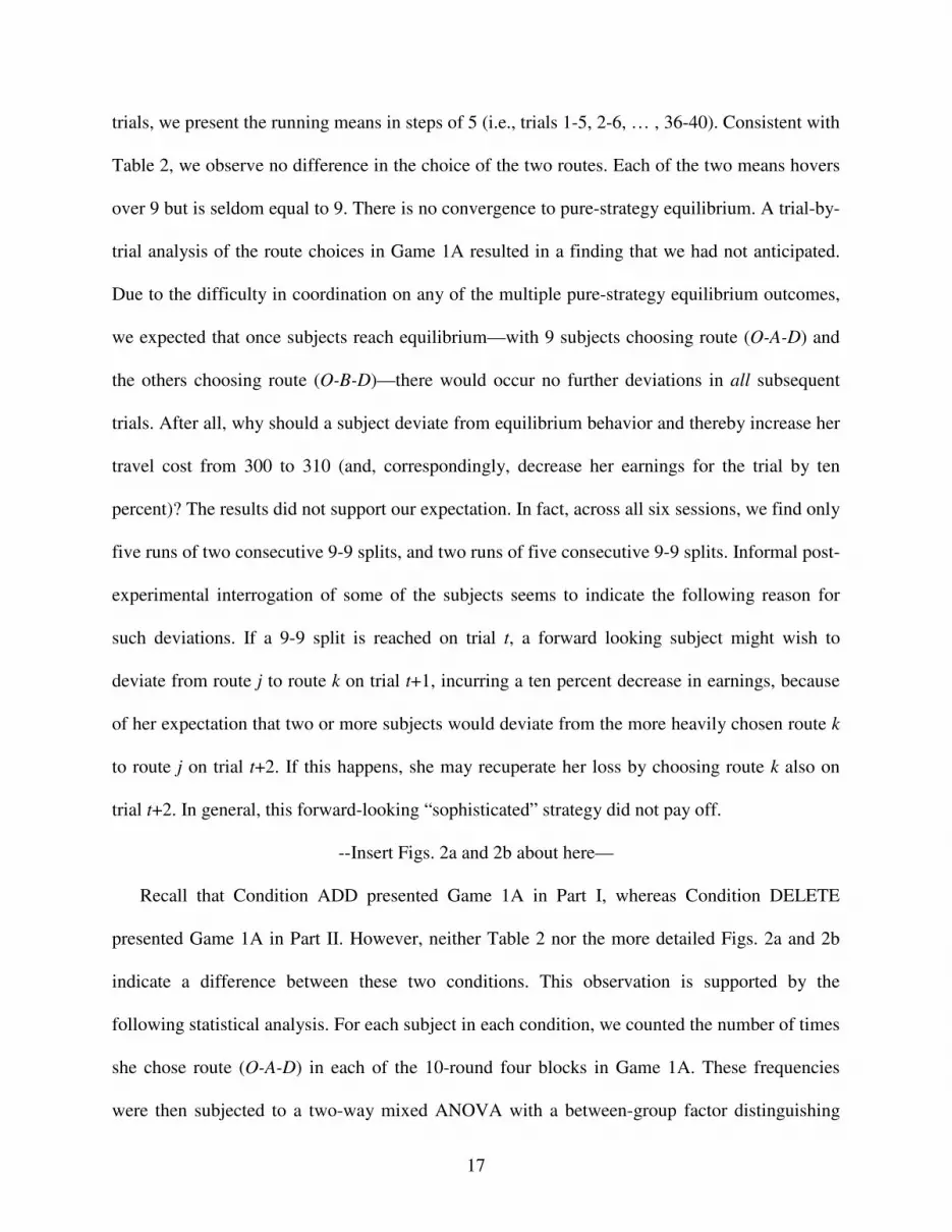
trials, we present the running means in steps of 5 (i.e., trials 1-5, 2-6, … , 36-40). Consistent with
Table 2, we observe no difference in the choice of the two routes. Each of the two means hovers
over 9 but is seldom equal to 9. There is no convergence to pure-strategy equilibrium. A trial-by-
trial analysis of the route choices in Game 1A resulted in a finding that we had not anticipated.
Due to the difficulty in coordination on any of the multiple pure-strategy equilibrium outcomes,
we expected that once subjects reach equilibrium—with 9 subjects choosing route (O-A-D) and
the others choosing route (O-B-D)—there would occur no further deviations in all subsequent
trials. After all, why should a subject deviate from equilibrium behavior and thereby increase her
travel cost from 300 to 310 (and, correspondingly, decrease her earnings for the trial by ten
percent)? The results did not support our expectation. In fact, across all six sessions, we find only
five runs of two consecutive 9-9 splits, and two runs of five consecutive 9-9 splits. Informal post-
experimental interrogation of some of the subjects seems to indicate the following reason for
such deviations. If a 9-9 split is reached on trial t, a forward looking subject might wish to
deviate from route j to route k on trial t+1, incurring a ten percent decrease in earnings, because
of her expectation that two or more subjects would deviate from the more heavily chosen route k
to route j on trial t+2. If this happens, she may recuperate her loss by choosing route k also on
trial t+2. In general, this forward-looking “sophisticated” strategy did not pay off.
--Insert Figs. 2a and 2b about here—
Recall that Condition ADD presented Game 1A in Part I, whereas Condition DELETE
presented Game 1A in Part II. However, neither Table 2 nor the more detailed Figs. 2a and 2b
indicate a difference between these two conditions. This observation is supported by the
following statistical analysis. For each subject in each condition, we counted the number of times
she chose route (O-A-D) in each of the 10-round four blocks in Game 1A. These frequencies
were then subjected to a two-way mixed ANOVA with a between-group factor distinguishing

18
between the two conditions and a within-group block factor. Neither of the two main effects due
to condition (F(1,106)=0.01, p=1.00) and block (F(3,318)=0.02, p=1.00), nor the condition by
block interaction effect (F(3,318)=0.07, p=0.94) were significant.
Turning next to Game 1B, the most critical finding of Experiment 1 is exhibited in Figs. 3a
and 3b that display the running mean number of subjects choosing each of the three routes in
Game 1B. Figure 3a shows the results for Condition ADD and Fig. 3b for Condition DELETE.
In both conditions, almost 2/3 of the subjects already chose the dominant route (O-A-B-D) during
the first five trials. With experience in traversing the traffic network in Game 1B, the frequencies
of choice of the two dominated strategies converged to zero, and the frequency of choice of route
(O-A-B-D) converged to 18. Figure 3 shows that all 40 trials were required to reach convergence.
Results not reported here show that a few subjects struggled to avoid choosing the “bridge” in
Game 1B. But with no communication possible, their signals were not heeded by the other
subjects as the attraction of the Pareto deficient equilibrium strategy proved too strong to resist.
--Insert Figs. 3a and 3b about here—
Similarly to Game 1A, we compared the route choices in Game 1B between the two
conditions. To do so, we counted for each subject the number of times she chose route (O-A-B-
D) in each block of ten trials. These frequencies were then subjected to the same two-way mixed
ANOVA. As suggested by Figs. 3a and 3b, the ANOVA yielded a significant block effect
(F(3,318)=81.96, p<0.001). With experience, route (O-A-B-D) was chosen more frequently.
However, neither the effect of condition (F(1,106)=0.01, p=0.93) nor the block by condition
interaction effect (F(3,318)=1.40, p=0.24) were significant.
Aggregate Payoffs. As before, denote by (fj,fk) the number of subjects choosing routes j and k in
Game 1A, respectively. The mean payoff in Game 1A cannot exceed 100, and it decreases in the
absolute difference ∆=fj-fk. Thus, if ∆=0 (a (9,9) split), then the mean payoff is 100. Mean

19
payoffs for (10,8), (11,7), and (12,6) splits are 98.8, 95.56, and 90, respectively. The expected
payoff under mixed-strategy play is 95 and the associated standard deviation is 7.01. The mean
payoff computed across all 54 subjects in sessions 1-3 of Condition ADD is 94.42. The
corresponding mean for Condition DELETE is 95.21. Once again, we observe that the mixed-
strategy equilibrium accounts for the mean Game 1A payoffs in both conditions extremely well.
There is no mixed-strategy equilibrium for Game 1B. If all 18 players choose route (O-A-B-
D), then each would earn 40 payoff units. Figures 4a and 4b exhibit the running mean payoff by
game for Conditions ADD and DELETE, respectively. The mean payoffs for Game 1B start
around 80 in trial 1 in each condition and slowly decrease to about 40. Consistent with all the
previous analyses that failed to detect any significant difference between the two conditions, the
null hypothesis of equality of mean payoffs (Condition ADD: 59.96, Condition DELETE: 61.19)
cannot be rejected. Taken together, our analyses suggest that the two framings of the BP in terms
of adding a cost-free edge to a two-route network (and sustaining a decrease in payoff) or
deleting the same edge from a three-route network (and sustaining an increase in payoff) have
the same effect on route choice and payoffs in both Games 1A and 1B. Consequently, the six
sessions are combined across the two conditions in subsequent analyses.
--Insert Figs. 4a and 4b about here--
Switches. Selten et al. conducted an experiment on traffic networks quite similar to Game 1A.
They studied a network with two parallel roads—a main road M and a side road S—connecting a
common origin to a common destination. The cost functions were linear: cM=6+2fM and
cS=12+2fS, and the group size was n=18. These cost functions result in multiple equilibria in
which 12 players choose road M and 6 choose road S. Subjects chose their routes independently
of one another in a stage game that was iterated 200 times. Similar to the results of Game 1A
reported above, Selten et al. reported strong support for equilibrium play on the aggregate level.

20
The mean number of subjects choosing route S in two different experimental conditions (that
differed from each other in the outcome information at the end of each trial) were 5.98 and 6.06.
Despite increasing the number of trials five-fold, they found no convergence to pure-strategy
equilibrium. Rather, they observed considerable fluctuations around the means, not unlike the
ones displayed in Figs. 2a and 2b. The standard deviations of the number of subjects choosing
route S on any given trial assumed values between 1.53 and 1.94. Helbing (2004) reported
similar results.
Neither Selten et al. nor Helbing invoked the mixed-strategy equilibrium solution to explain
these substantial fluctuations. Rather, they attributed them to the multiplicity of equilibria: “The
multiplicity of pure strategy equilibria poses a coordination problem which may be one of the
reasons for non-convergence and the persistence of fluctuations” (Selten et al., 2004 p. 4). In our
view, this may not fully explain the deviations from equilibrium once it has been reached. We
proposed above a “sophisticated” and quite likely misguided strategy where some forward-
looking players deviate from equilibrium deliberately in the hope of exploiting this deviation in
subsequent trials. Another possible reason may be grounded in the demand characteristics of the
game. Some subjects may simply not believe that they are expected to stick to the same route
once equilibrium is reached. Deliberate randomization of routes may account for the behavior of
yet another fraction of the subjects. All of these reasons interact with the opportunity cost of a
single deviation from a (9,9) split to (10,8) split that, as we reported above, reduces the
individual earnings by only 10 percent.
Figure 5 exhibits the running mean number of switches for Games 1A and 1B. The means for
each trial are computed across all the 108 subjects who participated in both conditions. As
subjects converge to choosing route (O-A-B-D) in Game 1B, the number of switches converges
to zero. Consistent with Figs. 3a and 3b, Fig. 5 shows that learning in Game 1B is slow; on

21
average, the mean frequency of switches decreases by 1 every 5 trials. Figure 5 further shows no
downtrend in the mean number of switches in Game 1A. Our results are consistent with those
reported by Selten et al. (2004, Fig. 3). Although there is a negative trend over the 200 trials in
their experiment, their figure suggests no discernible trend in the first 40 trials. The mean
number of switches in Game 1A is about 6 (Fig. 5), whereas the mixed-strategy equilibrium
predicts a mean of 9. This is the first piece of evidence that rejects the symmetric mixed-strategy
equilibrium. On the whole, subjects do switch their routes in Game 1A but not as frequently as
predicted. This finding suggests individual differences, which we explore in the next section.
--Insert Fig. 5 about here—
But first we pose the question whether it is beneficial to switch. Our answer is negative. For
each game separately, we correlated the individual frequency of switches (min=0, max=39) and
the individual payoff across all the 108 subjects. Both correlations were negative and significant:
-0.43 for Game 1A and –0.83 for Game 1B (p<0.05 in both cases). To assess the magnitude of
decrease in earnings associated with switching, we computed for each subject the mean payoff
across all the trials that were preceded by a switch and the mean payoff across all trials not
preceded by a switch. This computation yielded two means for each subject, payswitch and paynon-
switch (pays and payns for short). Subjects who switched less than four times were excluded from
this analysis. Our results show that payns>pays for 58 of the 94 subjects in Game 1A and 76 of 87
subjects in Game 1B. Both results are significant (p<0.05) by a sign test. On average, the
subjects’ mean earnings decreased by 2.86 in Game 1A and 11.72 in Game 1B after switching.
Individual Differences. The symmetric mixed-strategy equilibrium accounts for the aggregate
but not individual route choices. Figure 6 displays the frequency distribution of the number of
subjects choosing route (O-A-D) in Game 1A. Except of the two classes with a single frequency
of 0 and 40, all the other frequencies are grouped in classes of 3 (1-3, 4-6, …, 37-39). The mean

22
and variance of this grouped frequency distribution are 20.06 and 91.1, respectively. The
expected number and variance under mixed-strategy equilibrium play are 20 and 10,
respectively. The observed frequency distribution differs significantly from the theoretical
distribution in its variance but not in its mean. The hypothesis that all subjects follow the mixed-
strategy equilibrium with probability 0.5 of choosing route (O-A-D) is flatly rejected. Figure 6
shows that 6 subjects chose route (O-A-D) no more than 3 times and 11 other subjects chose it at
least 37 times. The corresponding theoretical frequencies are essentially zero.
--Insert Fig. 6 about here—
Figure 6 suggests a mixture of subject types, with a few subjects choosing the same route on
almost all 40 trials and most others mixing their route choices although not necessarily with
probability 0.5. For all the subjects who chose each of the two routes in Game 1A at least once
(101 subjects), we conducted a run test to test the considerably weaker null hypothesis that each
sequence of 40 route choices is generated by a Bernoulli process with a fixed probability p
(0<p<1) that may differ from one subject to another. This hypothesis was rejected for only 30 of
the 101 subjects. The null hypothesis of random play in Game 1A cannot be rejected for about 70
percent of the subjects. The majority of the subjects seem to be mixing their choice of routes but
not in the proportions dictated by the symmetric mixed-strategy equilibrium.
Discussion. There are three major findings. First, the symmetric mixed-strategy equilibrium
accounts for the aggregate choice data in the basic game in all six sessions extremely well.
However, there is no support for it on the individual level. Rather, most subjects do mix their
route choices but not in the proportions implied by equilibrium play. Second, in support of the
BP, when a cost-free edge is added to the basic game, players’ route choices converge to the
Pareto deficient and dominant strategy that results in a 60 percent decrease in their earnings.
Third, route choice and rate of learning are immune to alternative framings of the BP in terms of

23
adding a cost-free edge to the basic game or deleting the same edge from the augmented game.
These findings are obviously restricted to the Minimal Critical Network—the simplest traffic
network in which the BP may be realized; they may not generalize to other networks with more
routes. Experiment 2 was designed to extend the investigation of the BP to networks with a
richer topology.
4. A Three-route Symmetric Network with Two Additional Edges
Figure 7a exhibits the basic game that we have constructed for studying the BP in
Experiment 2. Game 2A consists of a network with six vertices and three routes, namely, a two-
edge route (O-A-D), another two-edge route (O-B-D), and a three-edge route (O-C-E-D). The
two routes (O-A-D) and (O-B-D) maintain the anti-symmetric arrangement of the fixed and
variable travel costs as in Game 1A. Route (O-C-E-D) has a single edge with only a fixed cost
and two additional edges each with both variable and fixed costs. With a group size of n=18,
there are multiple pure-strategy equilibria with 6 players choosing each of the three routes. The
individual travel cost under pure-strategy equilibrium is 132. There is also a symmetric mixed-
strategy equilibrium where each player chooses routes (O-A-D), (O-B-D), and (O-C-E-D) with
probability 1/3. The associated expected cost is 140.2
The augmented game in Experiment 2, Game 2B (Fig. 7b), includes two additional cost-free
edges, namely, edge (C,A) connecting nodes C and A, and edge (B,E) connecting nodes B and E.
These result in adding two new routes from the origin to the destination, namely, routes (O-C-A-
D) and (O-B-E-D) for a total of five routes. There are multiple pure-strategy equilibria in which
routes (O-A-D), (O-B-D), and (O-C-E-D) are never chosen, and each of the two new routes (O-
2 �=
− =++���
����
�=
17
0
17 140)]1(1260[)3/2()3/1(17
j
jj jj
EV .
24
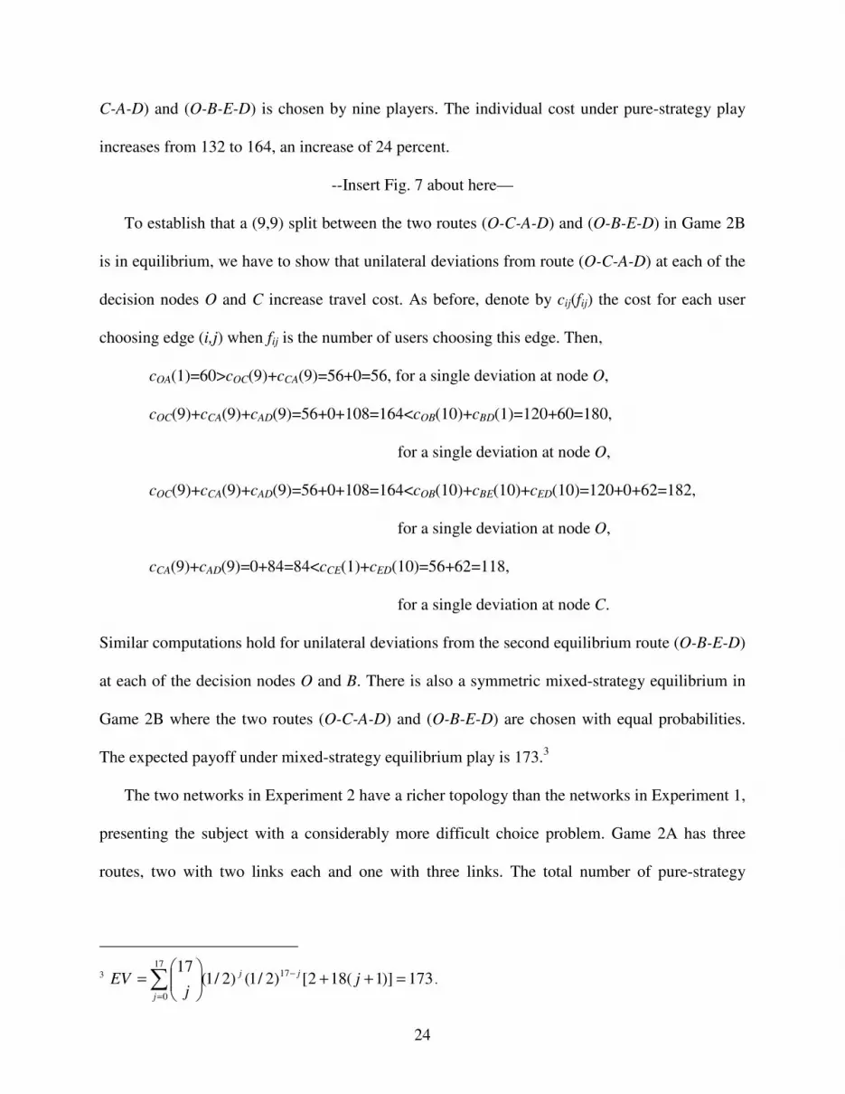
C-A-D) and (O-B-E-D) is chosen by nine players. The individual cost under pure-strategy play
increases from 132 to 164, an increase of 24 percent.
--Insert Fig. 7 about here—
To establish that a (9,9) split between the two routes (O-C-A-D) and (O-B-E-D) in Game 2B
is in equilibrium, we have to show that unilateral deviations from route (O-C-A-D) at each of the
decision nodes O and C increase travel cost. As before, denote by cij(fij) the cost for each user
choosing edge (i,j) when fij is the number of users choosing this edge. Then,
cOA(1)=60>cOC(9)+cCA(9)=56+0=56, for a single deviation at node O,
cOC(9)+cCA(9)+cAD(9)=56+0+108=164<cOB(10)+cBD(1)=120+60=180,
for a single deviation at node O,
cOC(9)+cCA(9)+cAD(9)=56+0+108=164<cOB(10)+cBE(10)+cED(10)=120+0+62=182,
for a single deviation at node O,
cCA(9)+cAD(9)=0+84=84<cCE(1)+cED(10)=56+62=118,
for a single deviation at node C.
Similar computations hold for unilateral deviations from the second equilibrium route (O-B-E-D)
at each of the decision nodes O and B. There is also a symmetric mixed-strategy equilibrium in
Game 2B where the two routes (O-C-A-D) and (O-B-E-D) are chosen with equal probabilities.
The expected payoff under mixed-strategy equilibrium play is 173.3
The two networks in Experiment 2 have a richer topology than the networks in Experiment 1,
presenting the subject with a considerably more difficult choice problem. Game 2A has three
routes, two with two links each and one with three links. The total number of pure-strategy
3 �=
− =++���
����
�=
17
0
17 173)]1(182[)2/1()2/1(17
j
jj jj
EV .

25
equilibria in Game 2A is truly astronomical: .156,153,17!6!6!6
!18 = If deviating from any given
route in Game 2A, a player has two alternative routes to choose from rather than a single
alternative route in Game 1A. In Game 2B, a player has to choose one of five routes compared to
one of three routes in Game 1B. Even if she decides not to travel on any of the three original
routes of the network in Game 2A, she still has to choose between routes (O-C-A-D) and (O-B-
E-D). Yet another important difference between Experiments 1 and 2 is that subjects could end
up with negative payoffs in Experiment 2 but not Experiment 1. With an endowment of 196
travel points in Experiment 2 (see below), if 12 or more subjects were to choose any of the three
routes in Game 2A, each of them would end up with negative payoffs. For example, if all 18
subjects were to choose the same route in Game 2A, each would lose 60 (196-256) travel points.
In contrast, with a 400 travel-point endowment in Experiment 1, no distribution of network users
across the two routes in Game 1A would have resulted in negative payoffs. Finally, Game 1B has
a single dominant strategy, which may be easy to identify, whereas Game 2B has two strategies
that jointly dominate the three routes in Game 2A. Consequently, Game 2 provides a
considerably more stringent test of the BP.
Method
Subjects. The subjects in Experiment 2 were 54 undergraduate and graduate students at the
University of Arizona. All of them volunteered to take part in a group decision making
experiment for payoff contingent on performance, and none of them had participated in
Experiment 1. Male and female subjects participated in about equal numbers. The subjects were
divided into 3 groups (sessions) of 18 members each. Because Experiment 1 yielded no
significant differences between conditions ADD and DELETE, only Condition ADD was

26
implemented with Game 2A presented in Part I of the experiment and Game 2B in Part II. A
session lasted 100-110 minutes. Excluding a $5 show-up bonus, the mean payoff was $16.
Procedure. The procedure was the same as in Condition ADD of Experiment 1 with the
following exceptions. Because we expected slower learning than in Experiment 1, the number of
trials in Games 2A and 2B was doubled from 40 to 80. The endowment for each of the 160 trials
in Games 2A and 2B was set at 196. This resulted in individual earnings under pure-strategy
equilibrium play of 196-132=64 and 196-164=32 travel units in Games 2A and 2B, respectively,
and a corresponding ratio of equilibrium payoffs of 2:1 (compared to 2.5:1 in Experiment 1). As
noted earlier, subjects could lose money in any given trial in Experiment 2, but not in
Experiment 1. The information provided to the subject at the end of each trial, the number of
payoff trials, and the conversion rate of travel units to dollars were the same as in Experiment 1.
Results
The organization of this section follows the corresponding Results section in Experiment 1.
We first test for session effects, then test for the implications of the BP on the aggregate level,
and finally conclude the section with the study of switches and individual differences.
Session Effects. We computed the following eight statistics for each of the three sessions of
Experiment 2:
• The number of times (out of 80) that each subject chose routes (O-A-D) and (O-B-D) in
Game 2A.
• The number of times (out of 80) that each subject chose routes (O-A-D), (O-B-D), (O-
C-A-D), and (O-B-E-D) in Game 2B.
• The frequency of switches (out of 79) in Games 2A and 2B.
Table 3 presents the means and standard deviations of these statistics by session and game.
Similarly to Experiment 1, we conducted separate one-way ANOVA’s on each of these statistics

27
to test the null hypothesis of equality of means across the three sessions. With the exception of a
single test (frequency of switches in Game 2A), none of tests rejected the null hypothesis.4
Similarly to Experiment 1, having failed to find significant differences between the three
sessions in 7 out of 8 tests, the raw data were combined across sessions.
--Insert Table 3 about here--
Aggregate Route Choice. For each trial separately, we counted the number of subjects (out of
18) who chose routes (O-A-D), (O-B-D), and (O-C-E-D) in Game 2A, and then averaged the
results across subjects and trials. Similar means were computed for each of the five routes in
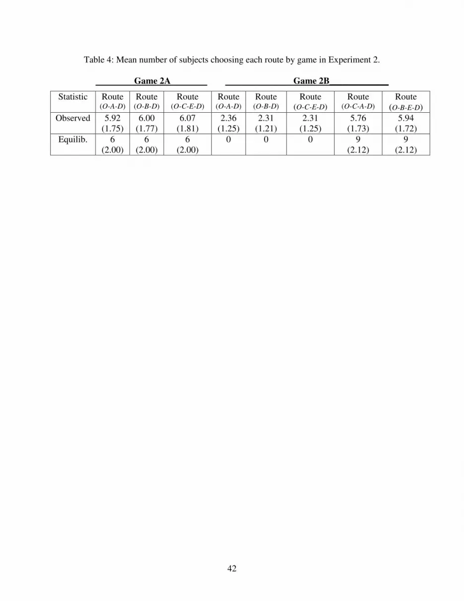
Game 2B. Table 4 (row 2) presents the means and standard deviations. The bottom row shows
the equilibrium predictions. The theoretical standard deviations in the bottom row refer to the
symmetric mixed-strategy equilibria, where a player chooses each of the three routes in Game
2A with probability 1/3, and each of the two routes (O-C-A-D) and (O-B-E-D) in Game 2B with
probability 1/2.
--Insert Table 4 about here—
The results for Game 2A basically replicate the ones for Game 1A. On the average, the three
routes were chosen equally likely (means: 5.92, 6.00, 6.07). The standard deviations point again
to considerable fluctuations across iterations. Unlike Experiment 1, the three observed standard
deviations are slightly smaller than the predicted values under mixed-strategy equilibrium play.
There are fluctuations around the mean route choices, but they are not as large as predicted.
Routes (O-A-D), (O-B-D) and (O-C-E-D) in Game 2B were jointly chosen on 39 percent of the
4 Mean (O-A-D) choice in Game 2A; F(2,51)=0.03, p=0.97; Mean (O-B-D) choice in Game 2A; F(2,51)=0.05, p=0.96; mean number of switches in Game 2A: F(2,51)=2.58, p<0.05; Mean (O-A-D) choice in Game 2B; F(2,51)=0.33, p=0.72; Mean (O-B-D) choice in Game 2B; F(2,51)=0.24, p=0.79; Mean (O-C-A-D) choice in Game 2B; F(2,51)=0.03, p=0.97; Mean (O-B-E-D) choice in Game 2B; F(2,51)=0.20, p=0.82; mean number of switches in Game 2B: F(2,51)=2.54, p=0.09.

28
trials compared to 0 percent under equilibrium play. We examine how this percentage changes
across trials in the next section.
Figures 8a and 8b display the mean number of subjects choosing each of the three routes in
Game 2A and each of the five routes in Game 2B. Once again, to better exhibit the trends across
trials, we present the running means in steps of 5 rather than the individual means for each trial.
Consider first Fig. 8a. It is evident, and perhaps unexpected, that the mean route choices in Game
2A hover around 6 from the very first trials. We observe no differences in choice frequency
among the three routes, nor discern any learning trends across the 80 trials. Also similar to Game
1A, we observe no tendency to maintain the same choices until the end of the session once a
(6,6,6) split has been obtained. Out of a total of 240 trials across the three sessions in Game 2A,
15 ended up in a (6,6,6) split, and these were evenly spaced across the sessions. However, there
was only a single run of two consecutive (6,6,6) splits, and no run of three or more (6,6,6) splits.
Pure-strategy equilibria were seldom reached and almost never maintained.
--Insert Figs. 8a and 8b around here—
Results pertaining to the major hypothesis of the present study are displayed in Fig. 8b.
Similarly to Fig. 8a, Fig. 8b plots the running means of route choice in steps of 5. The two
equilibrium routes (O-C-A-D) and (O-B-E-D) are already separated from the three non-
equilibrium routes in the first few trials. This separation increases across trials. On trial 80, the
two equilibrium routes (O-C-A-D) and (O-B-E-D) were chosen together on 77.7 percent of the
trials. Inspection of Fig. 8b shows that the subjects started choosing the two equilibrium routes
on the early trials, that learning was faster in the first 30 trials or so than in the remaining trials,
that the two equilibrium routes were chosen, on average, in roughly equal proportions, and that
the three non-equilibrium routes were also chosen in roughly equal proportions. Unlike Game 1B
(Fig. 3b), the mean route choices of the two equilibrium routes did not converge to the

29
equilibrium prediction in 80 trials, although they steadily moved in this direction. Examination
of the learning curves seems to suggest that hundreds of trials may be needed for convergence.
Switches. Figure 9 displays the running mean number of switches for Games 2A and 2B. For
both games, there is clear downtrend in the mean number of switches. For the basic game (Game
2A), the mean number of switches declines from about 9 on the first five trials or so to about 7.
For the augmented game (Game 2B), the corresponding values are 12 and 8. A player who
adheres to mixed-strategy equilibrium play in Game 2A should switch her route from one trial to
another with probability 2/3. This would result, on average, in 12 players switching their routes
on any given trial. Similarly to Experiment 1, our results show that subjects switched their routes
in Game 2A but not as frequently as predicted.
--Insert Fig. 9 about here--
Is it beneficial to switch? Similarly to Experiment 1, the results of Experiment 2 suggest that
switching does not pay off. For each subject separately, we counted the number of switches
(min=0, max=79) in Game 2A and correlated it with her payoff in Game 2A. We computed the
same correlation between number of switches and individual payoff in Game 2B. Both
correlations were negative and highly significant: -0.68 for Game 2A and -0.63 for Game 2B.
Under mixed-strategy equilibrium play, the frequencies of switches in games 2A and 2B are not
correlated. To test this implication, we computed the correlation between the individual number
of switches in Games 2A and 2B (n=54). The correlation was positive and quite high: r=0.75,
p<0.01. We conclude from this statistic that the propensity to switch seems to be unrestricted by
the topology of the network. Subjects who switch more in one network are likely to switch more
in another.
Individual Differences. In this section, we focus on individual differences in route choice and
number of switches. Turning first to route choice, Table 4 shows that the three non-equilibrium

30
routes in Game 2B were chosen together, on average, by 6.98 of the 18 subjects. Table 4 does
not tell us whether all subjects chose non-equilibrium routes in Games 2B with roughly equal
proportions or some subjects chose these routes considerably more often than others. Figure 10
answers this question by exhibiting the frequency distribution of the number of subjects choosing
non-equilibrium routes in Game 2B. It shows that 5 subjects never chose non-equilibrium routes
across all 80 trials, and a total of 17 subjects chose non-equilibrium routes no more than 10
times. In contrast, 15 subjects chose non-equilibrium routes in more than 50 percent of the trials
and 3 of these 15 subjects chose them on at least 71 trials. The individual frequencies of non-
equilibrium route choices are seen to range all the way from 0 to 80 trials, suggesting that
whatever conclusions we may draw with regard to the realization of the BP in the population
may not apply to individual players. We can only speculate about the reasons for the individual
differences in Fig. 10. They may indicate individual differences in the rate of recognizing the
equilibrium routes in Game 2B and switching from the equilibrium routes in Game 2A to the
new equilibrium routes in Game 2B. Under this interpretation, eventually all the subjects will be
choosing equilibrium routes. Alternatively, they may indicate only partly successful signaling of
more sophisticated subjects who, perceiving the payoff implications of equilibrium play in Game
2B, persist in choosing non-equilibrium routes to prevent the dramatic 50 percent decline in their
earnings.
--Insert Fig. 10 about here--
Turning next to the individual differences in the frequency of switches, Figs. 11a and 11b
display the frequency distributions of individual number of switches for Games 2A and 2B,
respectively. Once again, we observe individual differences that cover almost the entire range
from 0 to 79. We cannot tell whether the propensity to switch reflects boredom with the task,

31
exploration, attempts to change the group behavior in order to exploit non-equilibrium play on
subsequent trails, or some combination of these factors.
--Insert Figs. 11a and 11b about here—
Discussion. The results of Experiment 2 indicate that the main findings in Experiments 1
generalize with minor changes to a considerably richer topology, where players have to choose
one of three routes in the basic game and one of five routes in the augmented game. The
equilibrium solution accounts surprisingly well for the aggregate behavior of the subjects in all
three sessions of the basic game. However, there is no support for either pure- or mixed-strategy
equilibrium on the individual level. Simultaneously accounting for the considerable individual
differences in route choice and frequency of switching and the orderly and predictable aggregate
behavior remains a challenge for future research. Herding behavior, which is possible in Game
1B that includes only a single route that dominates the other two routes, is no longer possible in
Game 2B that includes two new routes that jointly dominate the three routes in the basic game
but do not dominate each other. Players’ route choice frequencies in the augmented game move
with experience in the direction of the equilibrium prediction. Convergence is not reached in 80
trials, possibly because as the structure of the network gets richer more experience is required to
achieve equilibrium. This finding suggests that equilibrium may be approached but most likely
not reached in real life traffic networks in which the number of drivers is neither fixed not
commonly known and information about route choices is not routinely provided.
5. Discussion and Conclusions
The optimal design and efficient use of traffic and communication networks are important
aspects of economically complex systems (Cohen & Jeffries, 1997; Kelly, 1991; Arnott & Small,
1994). A fundamental problem in the management of these systems is that of routing traffic to
optimize network performance. In many networks, including traffic and Internet networks, it is

32
difficult or even impossible to impose optimal routing strategies on network traffic, leaving
network users to act independently or “selfishly.” This has led researchers to model the behavior
of network users with noncooperative games and study the resulting Nash equilibria. One of the
early researchers to apply this methodology is Braess, who illustrated an apparently paradoxical
situation where adding a new link to a transportation network results in increased equilibrium
travel costs, often measured in terms of travel time, for all network users. When viewed in terms
of deleting a link from an existing network, the BP exhibits the well-known result that Nash
equilibrium needs not be Pareto optimal (e.g., the Prisoner’s Dilemma game, the Voluntary
Contribution Mechanism in public goods research, the Centipede game).
Arguments have been raised (Cohen, 1988) against the relevance of the BP to real situations.
Similar arguments have been raised, in turn, against the relevance of the Prisoner’s Dilemma and
Centipede games. According to these criticisms, the surprises in these abstract games and their
counterintuitive implications arise from the many respects in which they differ from reality
rather than from those aspects they share with reality (Cohen, 1988). In defending the study of
the finitely iterated Prisoner’s Dilemma game, Axelrod wrote: “It is the very complexity of
reality which makes the analysis of an abstract interaction so helpful as an aid to understanding”
(1984, p. 19). We contend that the same argument applies here as well, and that the experimental
analysis of the BP makes an additional contribution to the study of large group interactive
behavior that is predicted to yield Pareto deficient equilibrium outcomes.
The experimental findings reported in the present study should best be evaluated in light of
the main features of the experimental design. Two are particularly critical: the within-subject
design and the same endowment for the basic and augmented games. Both were introduced in
order to test the BP under the most stringent conditions, where the same users traverse the
network either with or without the additional links and where the addition (deletion) of one or

33
more links results in loss (gain) in the equilibrium payoff that far exceeds the 4/3 upper limit on
the “price of anarchy” for linear cost functions set by Roughgarden and Tardos (2002). Like the
two-person Prisoner’s Dilemma game, the equilibrium analysis underlying the BP shows that, for
certain parameter values (link costs, number of players), adding a new edge to a transportation
network results in increased travel costs for all network users. It does not quantify the “cost of
anarchy.” But as Rapoport and Chammah (1965) have shown in their parametric study of the
Prisoner’s Dilemma, the parameter values matter greatly for the frequency of choice of
dominated strategies.
Our experimental findings fall into three main categories. First, the equilibrium solution
accounts very accurately for the mean route choices in the two basic games in Experiments 1 and
2 (Games 1A and 2A). However (see also Selten et al., 2004), convergence to equilibrium play is
not reached as subjects continue to switch routes over iterations of the stage game resulting in
fluctuations around the means that do not diminish with experience. Our analysis of individual
results suggests a mixture of player types, some choosing the same route over almost all
iterations, some exhibiting the opposite behavior by mixing their routes although not necessarily
with the equilibrium probabilities, and some deliberately upsetting any equilibrium in pure
strategies that is temporarily reached in an attempt to exploit deviations from equilibrium on later
trials. A more detailed analysis of individual types and sequential dependencies is relegated to
future studies.
The second major finding is strong support for the equilibrium analysis underlying the BP.
When the subjects shift from playing the basic game to playing the augmented game, their choice
of routes changes dramatically in the direction of equilibrium play despite the substantial drop in
payoff associated with this change. These results are tempered by the topology of the network.
Convergence to equilibrium in the Minimal Critical Network (Experiment 1) is achieved after 40
34
trials. In contrast, route choice in the augmented game in Experiment 2 moves in the direction of
the equilibrium solution but convergence is not reached even after 80 trials. These findings
immediately suggest additional studies that manipulate the topological properties of the network
(e.g., cardinality of the sets V and E, the number and placement of the additional edges in the
augmented game, and the degree of asymmetry in edge costs) and vary the number of iterations.
The third major finding, which is restricted to the Minimal Critical Network in Experiment 1,
is that the results are not affected by the alternative framings of the BP in terms of gains or
losses. This finding would seem to suggest that the effects of gains and losses with respect to a
status quo point, so prominent in the study of individual decision behavior, might not extend to
interactive decisions in noncooperative games with Pareto deficient equilibrium outcomes. This,
too, is a topic for future research.

35
References
Arnott, R, De Palma, A., and Lindsey, R. (1990). Economics of bottleneck. Journal of Urban
Economics, 27, 111-130.
Arnott, R, De Palma, A., and Lindsey, R. (1993). A structural model of peak-period congestion:
A traffic bottleneck with elastic demand. American Economic Review, 83, 161-179.
Arnott, R. and Small, K. (1994). The economies of traffic congestion. American Scientist, 82,
446-455.
Axelrod, R. (1984). The Evolution of Cooperation. NY: Basic Books.
Braess, D. (1968). Über ein paradoxon der verkehrsplanung. Unternehmensforschung, 12, 258-
268.
Cohen, J. E. (1988). The counterintuitive in conflict and cooperation. American Scientist, 76,
577-584.
Cohen, J. E. and Jeffries, C. (1997). Congestion resulting from increased capacity in single-
server queueing networks. IEEE/ACM Transactions on Networks, 5, 305-310.
Cohen, J. E. and Kelly, F. P. (1990). A paradox of congestion in a queueing network. Journal of
Applied Probability, 27, 730-734.
Dafermos, S. C. and Nagurney, A. (1984). On some traffic equilibrium theory paradoxes.
Transportation Research, Series B, 18, 101-110.
Fisk, C. (1979). More paradoxes in the equilibrium assignment problem. Transportation
Research, Series B 13, 305-309.
Fisk, C. and Pallottino, S. (1981). Empirical evidence for equilibrium paradoxes with
implications for optimal planning strategies. Transportation Research, Series A, 15, 245-248.
Frank, M. (1981). The Braess paradox. Mathematical Programming, 20, 283-302.

36
Gabuthy, Y., Neveu, M., and Denant-Boement, L. (2004). Structural model of peaked-period
congestion: An experimental study. Working paper, Groupe d’Analyse de Théorie
Economique, Ecully, France.
Hagstrom, J. N. and Abrams, R. A. (2001). Characterizing Braess’s paradox for traffic networks.
Proceedings of the IEEE Conference on Intelligent Transportation Systems. Los Alamitos,
CA: IEEE Computer Society Press, pp. 837-842.
Helbing, D. (2004). Dynamic decision behavior and optimal guidance through information
services: Models and experiments. In M. Schreckenberg and R. Selten (Eds.), Human
Behavior and Traffic Networks. Berlin: Springer, pp. 48-95.
Kelly, F. P. (1991). Network routing. Philosophical Transactions of the Royal Society, Series A
337, 343-367.
Koutsoupias, E., and Papadimitriu, C. (1999). Worst-case equilibria. Proceedings of the 16th
Annual Symposium on Theoretical Aspects of Computing. Science Lecture Notes in
Computer Science, Vol. 1563. Berlin: Springer, pp. 404-413.
Murchland, J. D. (1970). Braess’s paradox of traffic flow. Transportation Research, 4, 391-394.
New York Times. What if they closed 42nd street and nobody noticed? NYT, Dec. 25, 1990.
Papadimitriu, C. (2001). Algorithms, games, and the internet. Proceedings of the 33rd Annual
ACM Symposium on the Theory of Computing. ACM, NY, pp. 749-753.
Pas, E. I. and Principio, S. L. (1997). Braess’ paradox: Some new insight. Transportation
Research, Series B 31, 265-276.
Penchina, C. M. (1997). Braess paradox: Maximum penalty in a minimal critical network.
Transportation Research, Series A 31, 379-388.
Rapoport, A. and Chammah, A. M. (1965). Prisoner’s Dilemma. Ann Arbor: University of
Michigan Press.

37
Roughgarden, T. (2001). Designing networks for selfish users is hard. Proceedings of the 42nd
Annual Symposium on Foundations of Computer Science. Los Alamitos, CA: IEEE
Computer Society Press, pp. 472-481.
Roughgarden, T. and Tardos, E. (2002). How bad is selfish routing? Journal of the ACM, 49,
236-259.
Schneider, K. and Weimann, J. (2004). Against all odds: Nash equilibria in road pricing
experiment. In M. Schreckenberg and R. Selten (Eds.), Human Behavior and Traffic
Networks. Berlin: Springer, pp. 153.
Selten, R. et al. (2004). Experimental investigation of day-to-day route-choice behavior and
network simulations of Autobahn traffic in North Rhine-Westphalia. In M. Schreckenberg
and R. Selten (Eds.), Human Behavior and Traffic Networks. Berlin: Springer, pp. 1-21.
Smith, M. J. (1978). In a road network, increasing delay locally can reduce delay globally.
Transportation Research, 12, 419-422.
Steinberg, R. and Stone, R. E. (1988). The prevalence of paradoxes in transportation equilibrium
problems. Transportation Science, 22, 231-241.
Steinberg, R. and Zangwill, W. I. (1983). On the prevalence of the Braess’s paradox.
Transportation Science, 17, 301-318.

38
Acknowledgement
We gratefully acknowledge financial support by a contract F49620-03-1-0377 from the
AFOSR/MURI to the University of Arizona. We also thank Ryan O. Murphy and Maya
Rosenblatt for their assistance in data collection.

39
Table 1: Mean values of summary statistics by game, session, and condition in Experiment 1.
Game 1A Game 1B
Statistic Route (O-A-D)
No. of Switches
Route (O-A-D)
Route (O-B-D)
No. of Switches
Session 1 Cond. ADD
20.06 (8.02)
12.94 (5.14)
3.22 (2.64)
2.89 (2.45)
9.94 (7.41)
Session 2 Cond. ADD
21.83 (8.87)
11.56 (5.28)
4.56 (3.76)
3.39 (1.79)
10.78 (6.3)
Session 3 Cond. ADD
20.28 (10.75)
10.89 (7.28)
3.61 (1.94)
3.28 (2.56)
9.44 (5.23)
Session 1 Cond. DELETE
20.22 (11.36)
11.33 (7.22)
3.39 (2.97)
3.67 (3.63)
9.39 (6.61)
Session 2 Cond. DELETE
20.06 (11.10)
11.72 (8.37)
4.06 (5.58)
2.72 (1.96)
8.78 (6.48)
Session 3 Cond. DELETE
20.11 (7.68)
14.78 (5.20)
4.11 (3.77)
3.28 (2.61)
11.28 (9.29)
(standard deviations in parentheses)

40
Table 2: Mean number of subjects choosing each route by game and condition in Experiment 1.
Condition
Game 1A
Routes
Game 1B
Routes
(O-A-D) (O-B-D) (O-A-D) (O-B-D) (O-A-B-D)
ADD 9.04 (2.15)
8.96 (2.15)
1.70 (1.86)
1.49 (1.68)
14.82 (2.79)
DELETE 9.08 (2.08)
8.92 (2.08)
1.75 (1.51)
1.45 (1.49)
14.82 (2.27)
Equilibrium 9 (2.12)
9 (2.12)
0 0 18
(standard deviations in parentheses)

41
Table 3: Mean values of summary statistics by game and session in Experiment 2.
Game 2A Game 2B
Statistic Route (O-A-D)
Route (O-B-D)
No. of Switches
Route (O-A-D)
Route (O-B-D)
Route (O-C-A-D)
Route (O-B-E-
D)
No. of Switches
Session 1
26.94 (17.22)
26.72 (23.51)
12.25 (11.90)
8.11 (7.40)
8.06 (11.06)
26.33 (25.35)
28.17 (26.10)
20.25 (23.92)
Session 2
26.60 (11.58)
25.61 (14.48)
19.75 (23.09)
8.89 (6.77)
9.11 (8.63)
25.83 (15.75)
27.17 (17.00)
20.00 (22.89)
Session 3
25.39 (10.47)
27.67 (21.60)
17.25 (18.39)
10.67 (6.76)
10.28 (8.80)
24.67 (20.57)
23.83 (20.22)
17.75 (18.58)
42
Table 4: Mean number of subjects choosing each route by game in Experiment 2.
Game 2A Game 2B_____________
Statistic Route (O-A-D)
Route (O-B-D)
Route (O-C-E-D)
Route (O-A-D)
Route (O-B-D)
Route (O-C-E-D)
Route (O-C-A-D)
Route (O-B-E-D)
Observed 5.92 (1.75)
6.00 (1.77)
6.07 (1.81)
2.36 (1.25)
2.31 (1.21)
2.31 (1.25)
5.76 (1.73)
5.94 (1.72)
Equilib. 6 (2.00)
6 (2.00)
6 (2.00)
0 0 0 9 (2.12)
9 (2.12)

43
List of Figures
Figure 1. Basic and augmented networks for Games 1A and 1B in Experiment 1. Figure 2. Mean number of subjects choosing each route in Game 1A: Conditions ADD and
DELETE. Figure 3. Mean number of subjects choosing each route in Game 1B: Conditions ADD and
DELETE.
Figure 4. Mean payoff by game and trial in Experiment 1: Conditions ADD and DELETE. Figure 5. Running mean number of switches by game in Experiment 1. Figure 6. Frequency distribution of number of subjects in Game 1A choosing route (O-A-D). Figure 7. Basic and augmented networks for Games 2A and 2B in Experiment 2. Figure 8. Mean number of subjects choosing each route in Games 2A and 2B. Figure 9. Running mean number of switches by game in Experiment 2. Figure 10. Frequency distribution of number of subjects in Game 2B choosing non-equilibrium
routes.
Figure 11. Frequency distribution of number of individual switches in Games 2A and 2B.

44
Figure 1. Basic and augmented networks for Games 1A and 1B in Experiment 1

Figure 2a: Mean number of subjects choosing each route in Game 1A
Condition ADD
Condition Add - Game 1A
0.00
2.00
4.00
6.00
8.00
10.00
12.00
14.00
1 3 5 7 9 11 13 15 17 19 21 23 25 27 29 31 33 35 37 39
Trial
Mea
n N
o. o
f Sub
ject
s
OAD
OBD
Figure 2b: Mean number of subjects choosing each route in Game 1A
Condition DELETE
Condition DELETE - Game 1A
0.00
2.00
4.00
6.00
8.00
10.00
12.00
14.00
1 3 5 7 9 11 13 15 17 19 21 23 25 27 29 31 33 35 37 39
Trial
Mea
n N
o. o
f Sub
ject
s
OAD
OBD
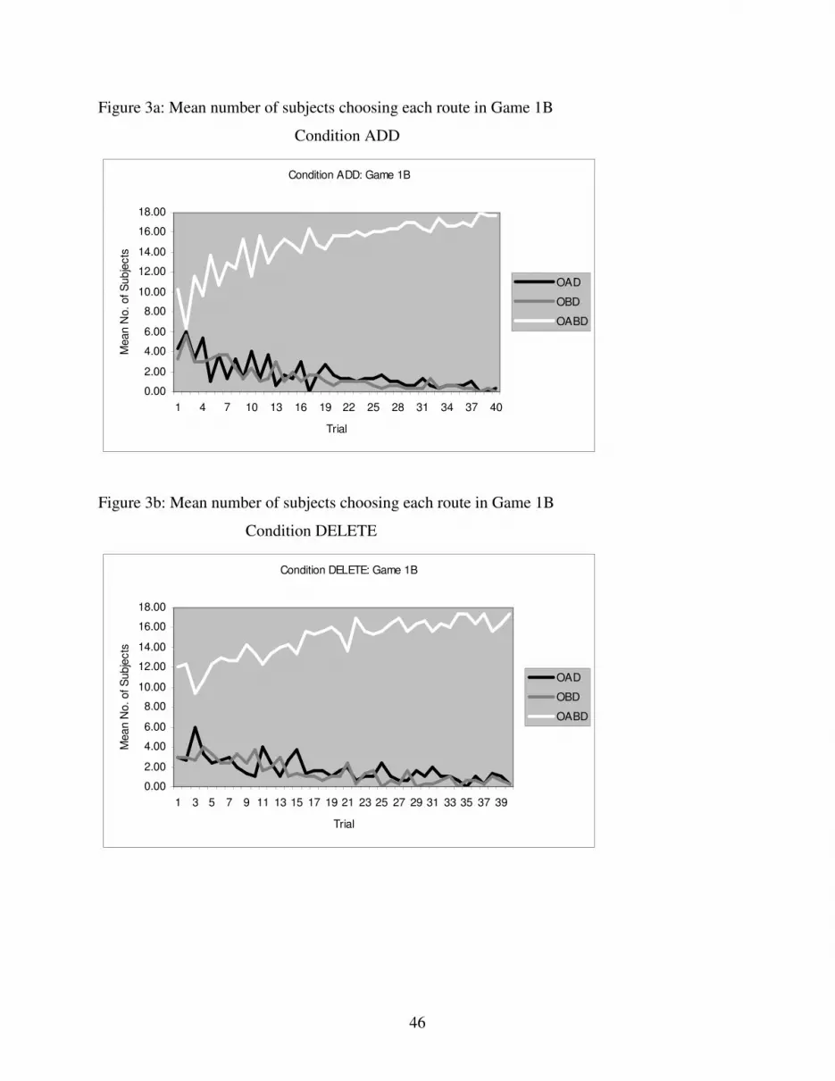
46
Figure 3a: Mean number of subjects choosing each route in Game 1B
Condition ADD
Condition ADD: Game 1B
0.00
2.00
4.00
6.00
8.00
10.00
12.00
14.00
16.00
18.00
1 4 7 10 13 16 19 22 25 28 31 34 37 40
Trial
Mea
n N
o. o
f Sub
ject
s
OAD
OBD
OABD
Figure 3b: Mean number of subjects choosing each route in Game 1B
Condition DELETE
Condition DELETE: Game 1B
0.00
2.00
4.00
6.00
8.00
10.00
12.00
14.00
16.00
18.00
1 3 5 7 9 11 13 15 17 19 21 23 25 27 29 31 33 35 37 39
Trial
Mea
n N
o. o
f Sub
ject
s
OAD
OBD
OABD

47
Figure 4a: Mean payoff by game and trial in Experiment 1: Condition ADD
Condition ADD
0.00
20.00
40.00
60.00
80.00
100.00
120.00
1 4 7 10 13 16 19 22 25 28 31 34 37 40
Trial
Mea
n pa
yoff
Game 1A
Game 1B
Figure 4b: Mean payoff by game and trial in Experiment 1: Condition DELETE
Condition DELETE
0.00
20.00
40.00
60.00
80.00
100.00
120.00
1 4 7 10 13 16 19 22 25 28 31 34 37 40
Trial
Mea
n pa
yoff
Game 1A
Game 1B

48
Figure 5: Running mean number of switches by game in Experiment 1
0
2
4
6
8
10
12
1 3 5 7 9 11 13 15 17 19 21 23 25 27 29 31 33 35 37 39
Trial
Run
ning
mea
n -
no. o
f sw
itche
s
Game 1A
Game 1B

49
Figure 6: Frequency distribution of number of subjects in Game 1A choosing route (O-A-D)
0
5
10
15
20
250
1-3
4-6
7-9
10-1
2
13-1
5
16-1
8
19-2
1
22-2
4
25-2
7
28-3
0
31-3
3
34-3
6
37-3
9 40
No. of (O-A-D) Choices
Fre
quen
cy
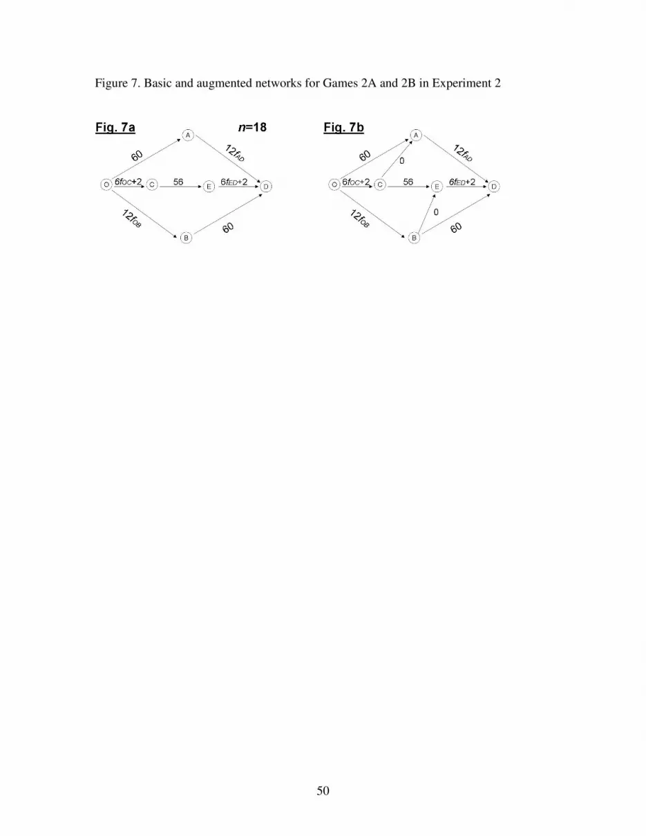
50
Figure 7. Basic and augmented networks for Games 2A and 2B in Experiment 2

51
Figure 8a. Running mean number of subjects choosing each route in Game 2A.
Game 2A
0.00
1.00
2.00
3.00
4.00
5.00
6.00
7.00
8.00
1 6 11 16 21 26 31 36 41 46 51 56 61 66 71
Trial
Run
ning
mea
n -
No.
of s
ubje
cts
OAD
OBD
OCED
Figure 8b. Running mean number of subjects choosing each route in Game 2B.
Game 2B
0.00
1.00
2.00
3.00
4.00
5.00
6.00
7.00
8.00
1 5 9 13 17 21 25 29 33 37 41 45 49 53 57 61 65 69
Trial
Run
ning
mea
n no
. of s
ubje
cts
OAD
OBD
OCED
OCAD
OBED

52
Figure 9. Running mean number of switches by game in Experiment 2
0
2
4
6
8
10
12
14
1 5 9 13 17 21 25 29 33 37 41 45 49 53 57 61 65 69 73 77
Round
No.
of s
witc
hes
Game 2a
Game 2b

53
Figure 10: Frequency distribution of number of subjects in Game 2B choosing non-equilibrium routes
0
1
2
3
4
5
6
70
1-5
6-10
11-1
5
16-2
0
21-2
5
26-3
0
31-3
5
36-4
0
41-4
5
46-5
0
51-5
5
56-6
0
61-6
5
66-7
0
71-7
5
76-8
0
No. of non-equilibrium choices
Fre
quen
cy
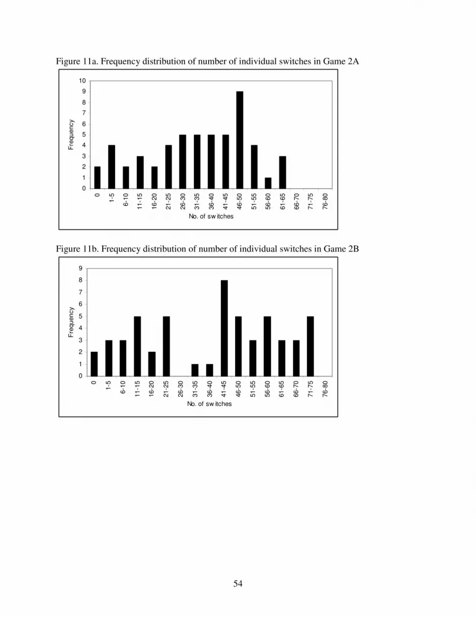
54
Figure 11a. Frequency distribution of number of individual switches in Game 2A
0
1
2
3
4
5
6
7
8
9
10
0
1-5
6-10
11-1
5
16-2
0
21-2
5
26-3
0
31-3
5
36-4
0
41-4
5
46-5
0
51-5
5
56-6
0
61-6
5
66-7
0
71-7
5
76-8
0
No. of sw itches
Fre
quen
cy
Figure 11b. Frequency distribution of number of individual switches in Game 2B
0
1
2
3
4
5
6
7
8
9
0
1-5
6-10
11-1
5
16-2
0
21-2
5
26-3
0
31-3
5
36-4
0
41-4
5
46-5
0
51-5
5
56-6
0
61-6
5
66-7
0
71-7
5
76-8
0
No. of sw itches
Fre
quen
cy