1

CHEM 3010

Introduction to

Quantum Chemistry,

Spectroscopy,

& Statistical Thermodynamics

2

Rene Fournier: Petrie 303, renef@yorku.ca,

ext 30687

prerequisite: CHEM 2011

Required Text: Physical Chemistry by Thomas

Engel and Philip Reid (Pearson Prentice Hall) 3rd

edition (2013), ISBN-10: 0-321-81200-X ISBN-13:

978-0-321-81200-1

Course web site (soon): go to www.yorku.ca/renef

and follow the CHEM 3010 link.

Lectures: LSB 105, MWF 10:30–11:20

Office hours: Petrie 303, MWF 13:00-14:00

3

Chapter 12:

From Classical to

Quantum Mechanics

4

In early 1900’s, classical physics failed to explain

• why atoms, with their electrons orbiting around

a nucleus, are stable

• why the spectrum of the H atom is discrete

• the blackbody radiation

• the photoelectric effect

• electron diffraction

A “new physics” was needed.

5

Two key concepts in quantum mechanics:

• energy quantization:

the amount of energy exchanged between molecules

and radiation (light) is a discrete variable, ie, it is

not continuous

• wave-particle duality:

light (a wave) sometimes shows particle-like pro-

perties; and “particles” (e−, p+, atoms, . . . ) so-

metimes show wave-like properties.

6

Rutherford, 1910: atoms have a positive charge

concentrated at the center (nucleus) and negative

charge (electrons, e−) spread out around it.

Classically, orbiting e− should radiate energy and

quickly spiral down to the nucleus.

How can atoms be stable ? ? ?

7

H atoms only emit light with specific (discrete)

wavelengths λ, see Fig. 12.11, p 304.

A fit to data shows that

1

λ= RH

(1

n21

− 1

n22

)

with RH = 109678 cm−1

n1 = 1, 2, 3, . . .

and n2 = n1 + 1, n1 + 2, n1 + 3, . . .

But why ?

8

Blackbody radiation

Fig. 12.1, p295

Light is emitted, re-absorbed, and re-emitted many

times: it is in thermodynamic equilibrium with

the solid.

9

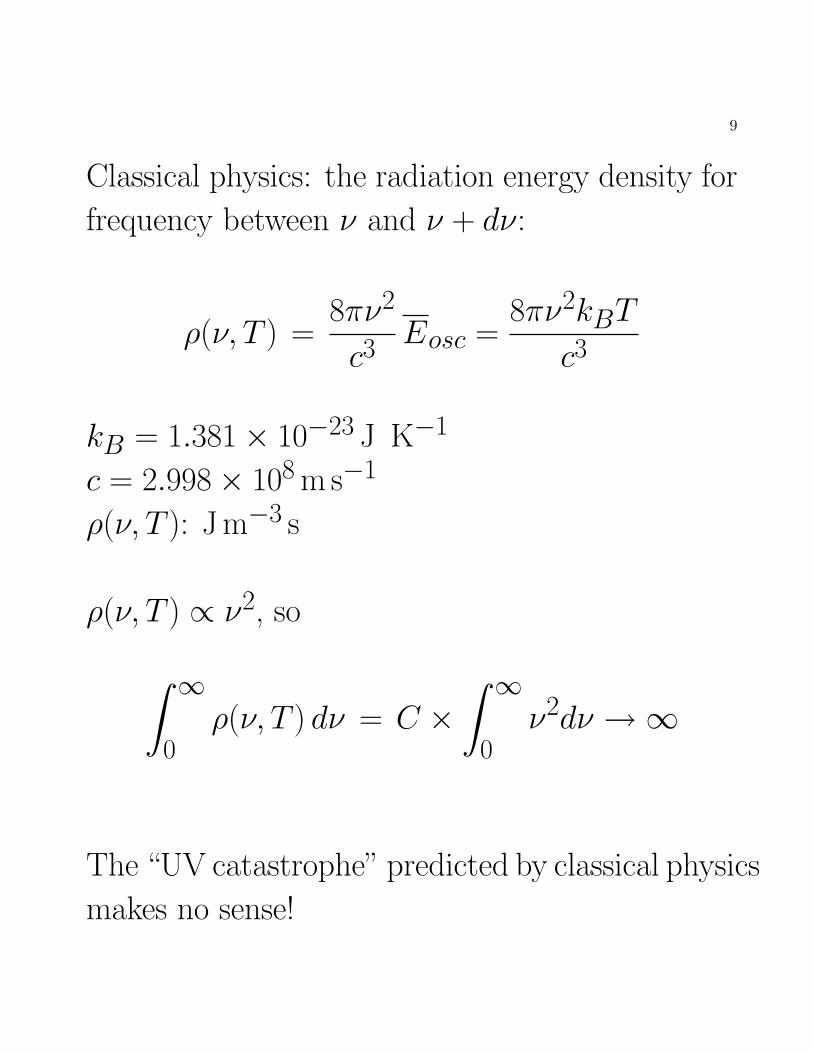
Classical physics: the radiation energy density for

frequency between ν and ν + dν:

ρ(ν, T ) =8πν2

c3Eosc =

8πν2kBT

c3

kB = 1.381× 10−23 J K−1

c = 2.998× 108 m s−1

ρ(ν, T ): J m−3 s

ρ(ν, T ) ∝ ν2, so

∫ ∞0

ρ(ν, T ) dν = C ×∫ ∞

0ν2dν →∞

The “UV catastrophe” predicted by classical physics

makes no sense!

10

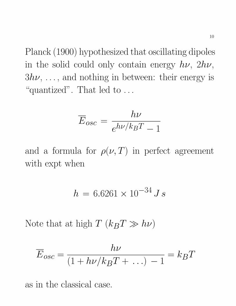
Planck (1900) hypothesized that oscillating dipoles

in the solid could only contain energy hν, 2hν,

3hν, . . . , and nothing in between: their energy is

“quantized”. That led to . . .

Eosc =hν

ehν/kBT − 1

and a formula for ρ(ν, T ) in perfect agreement

with expt when

h = 6.6261× 10−34 J s

Note that at high T (kBT � hν)

Eosc =hν

(1 + hν/kBT + . . .) − 1= kBT

as in the classical case.

11

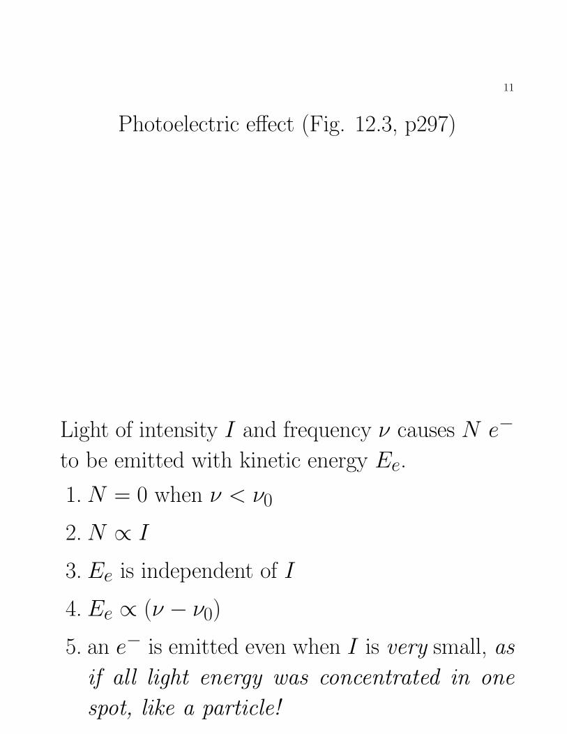
Photoelectric effect (Fig. 12.3, p297)

Light of intensity I and frequency ν causes N e−

to be emitted with kinetic energy Ee.

1. N = 0 when ν < ν0

2. N ∝ I

3. Ee is independent of I

4. Ee ∝ (ν − ν0)

5. an e− is emitted even when I is very small, as

if all light energy was concentrated in one

spot, like a particle!

12

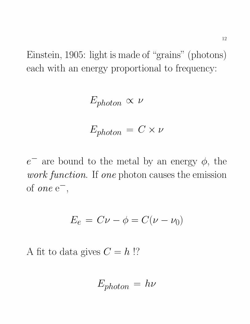
Einstein, 1905: light is made of “grains” (photons)

each with an energy proportional to frequency:

Ephoton ∝ ν

Ephoton = C × ν

e− are bound to the metal by an energy φ, the

work function. If one photon causes the emission

of one e−,

Ee = Cν − φ = C(ν − ν0)

A fit to data gives C = h !?

Ephoton = hν

13

Bohr’s H atom

1. the e− goes around the proton, with orbit cir-

cumference 2πr

2. for stable orbits Coulombic and centrifugal forces

must cancel out: e2/(4πε0r2) = mev

2/r

This gives v2 = e2/(4πε0mer)

3. the e− can jump between orbits 1 and 2 by ab-

sorbing light energy E2 − E1 = ∆E = hν

4. the angular momentum is mevr = n(h/2π)

with n = 1, 2, 3,. . .

This is not a trivial assumption!

14

m2e ×

(e2

4πε0mer

)× r2 = n2(h/2π)2

Rearranging gives the size of stable orbits, rn.

rn = n2 h2

4π2

4πε0mee2

= n2 0.5291772× 10−10m

The energy in a stable orbit, En, is the sum of

potential and kinetic energies

En =−e2

4πε0r+mev

2

2

=−e2

4πε0r+

mee2

8πε0mer

=−e2

8πε0rn

15

En = − 1

n2

mee4

8ε20h2

= − 1

n22.17987× 10−18 J

in perfect agreement with the H atom spectrum!

Furthermore,

2.17987× 10−18 J = hcRH

Same h again!?

16

DeBroglie, 1924: every object has an associated

wavelength λ

λ =h

p=

h

mv

Davisson and Germer, 1927, observed diffraction

of an e− beam off a NiO crystal.

If the beam has very few e−, we see individual e−

impacts, but the diffraction pattern is preserved.

He atoms bouncing off a Ni surface also form a

diffraction pattern.

17

e− diffraction by a double slit

A low intensity e− beam shows particle-like be-

havior.

But accumulating signals over a long time reveals

the diffraction pattern ⇒ wave-like behavior.

⇒ each e− goes through both slits at once and

“interferes with itself”. Each e− is wave-like . . .

until it hits the photographic plate.

18

Chapter 13:

The Schrodinger Equation

(S equation)

19

• Quantum mechanics (QM) is strictly “better”

(more accurate) than classical mechanics (CM)

• QM is much more complicated

• QM and CM give nearly identical results when

1. masses are big enough ( ' 100 a.m.u.)

2. dimensions are big enough (' 1000 A)

3. T is high enough

• Better: CM may be used when

(1) λ = h/p is small compared to a charac-

teristic length for the phenomenon

(2) ∆E is small compared to kBT

20

Diffraction of e− and Xe atoms

through a 1 A slit

21

Vibrations of H2 and Ar2 at T = 300 K

22

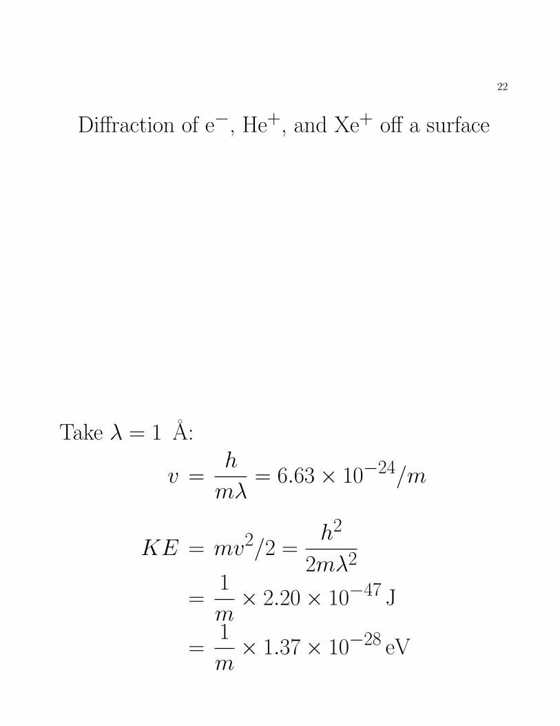
Diffraction of e−, He+, and Xe+ off a surface

Take λ = 1 A:

v =h

mλ= 6.63× 10−24/m

KE = mv2/2 =h2

2mλ2

=1

m× 2.20× 10−47 J

=1

m× 1.37× 10−28 eV

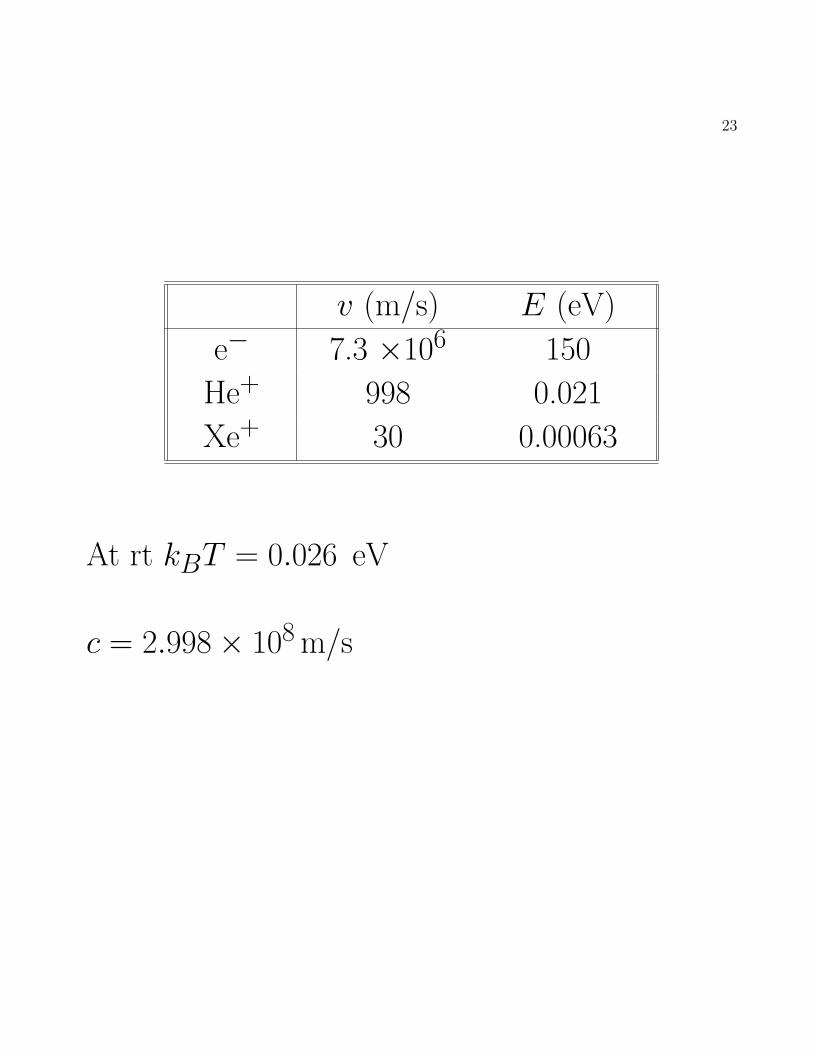
23

v (m/s) E (eV)

e− 7.3 ×106 150

He+ 998 0.021

Xe+ 30 0.00063

At rt kBT = 0.026 eV

c = 2.998× 108 m/s

24

Traveling wave:

velocity v = λν

vertical displacement ψ:

ψ(x, t) = A sin[2π(x/λ− νt)]note that

ψ(x± λ, t) = ψ(x, t)

ψ(x, t± 1/ν) = ψ(x, t)

because that adds ±2π inside [. . .] in both cases.

Let

k = 2π/λ

ω = 2πν

25

then

ψ(x, t) = A sin(kx− ωt)

but

sinx = cos(x− π/2)

and the choices for x = 0 and t = 0 are arbitrary.

So

ψ(x, t) = A cos(kx− ωt + φ)

26

Complex numbers

The imaginary number i is defined by

i2 = −1

A complex number z has a real part a and ima-

ginary part ib: z = a + ib, with a and b real.

For z = a + ib, define

z∗ = a− ib

Then

zz∗ = a2 − aib + aib− i2b2 = a2 + b2

so zz∗ is always real. We also define

Re(z) = a

Im(z) = b

27

Physical quantities (energy, position, mass, etc.)

are always real of course. But complex numbers

and functions “z” can be used as intermediate

variables to describe physical systems, and the

physical quantities can then be expressed in terms

of zz∗, Re(z), or Im(z).

28

Complex plane representation of z = a + ib:

a = r cos θ ⇒ θ = cos−1(a/r)

b = r sin θ ⇒ θ = sin−1(b/r)

r =√a2 + b2

Euler’s formula:

eiθ = cos θ + i sin θ

So z can be written as z = reiθ and

ψ(x, t) = A Re[ei(kx−ωt+φ)

]

29

Standing wave.

If you pluck a string, a mixture of λ’s coexist for a

short time, but they all interfere and destruct ex-

cept λ = 2L, λ = 2L/2, λ = 2L/3, . . .λ = 2L/n,

n = 1, 2, 3,. . . .

The “quantization” of standing waves, E = hν,

and λ = h/p, suggested that the classical diffe-

rential equation for waves may apply to particles,

with λclassical changed to h/p.

. . .

30

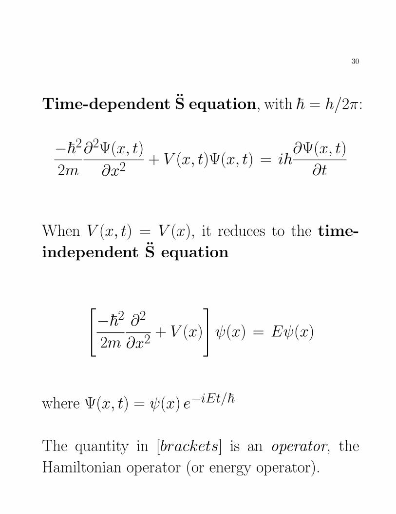
Time-dependent S equation, with ~ = h/2π:

−~2

2m

∂2Ψ(x, t)

∂x2+ V (x, t)Ψ(x, t) = i~

∂Ψ(x, t)

∂t

When V (x, t) = V (x), it reduces to the time-

independent S equation

[−~2

2m

∂2

∂x2+ V (x)

]ψ(x) = Eψ(x)

where Ψ(x, t) = ψ(x) e−iEt/~

The quantity in [brackets] is an operator, the

Hamiltonian operator (or energy operator).

31

Numbers, functions, and operators

If x and y are real numbers, a function f is a rule

(or algorithm) that inputs a number x and out-

puts another number y: y = f (x).

An operator O is an algorithm that inputs a func-

tion f and outputs another function g:

g(x) = O[f (x)]

Examples of operators: “multiply by 3”, “take the

derivative w.r.t. x”, “take the square of”, . . .

32

Note: a functional is an algorithm that inputs a

function f and outputs a number y

y = F [f (x)]

for example, “integrate f between 0 and infinity”,

or “take the minimum of f over the interval from

0 to 5”.

A transform is an algorithm that inputs a func-

tion f of variable x, and outputs a different func-

tion g of a different variable t:

g(t) = F [f (x)]

for ex., the Fourier transform (often used for time-

to-frequency mapping).

33

From the time-dependent S equation to

the time-independent S equation

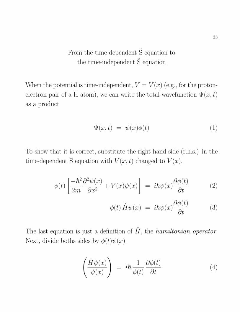
When the potential is time-independent, V = V (x) (e.g., for the proton-

electron pair of a H atom), we can write the total wavefunction Ψ(x, t)

as a product

Ψ(x, t) = ψ(x)φ(t) (1)

To show that it is correct, substitute the right-hand side (r.h.s.) in the

time-dependent S equation with V (x, t) changed to V (x).

φ(t)

[−~2

2m

∂2ψ(x)

∂x2+ V (x)ψ(x)

]= i~ψ(x)

∂φ(t)

∂t(2)

φ(t) Hψ(x) = i~ψ(x)∂φ(t)

∂t(3)

The last equation is just a definition of H , the hamiltonian operator.

Next, divide boths sides by φ(t)ψ(x).

(Hψ(x)

ψ(x)

)= i~

1

φ(t)

∂φ(t)

∂t(4)

34

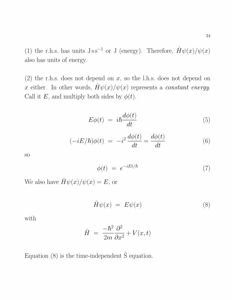
(1) the r.h.s. has units J s s−1 or J (energy). Therefore, Hψ(x)/ψ(x)

also has units of energy.

(2) the r.h.s. does not depend on x, so the l.h.s. does not depend on

x either. In other words, Hψ(x)/ψ(x) represents a constant energy.

Call it E, and multiply both sides by φ(t).

Eφ(t) = i~dφ(t)

dt(5)

(−iE/~)φ(t) = −i2 dφ(t)

dt=dφ(t)

dt(6)

so

φ(t) = e−iEt/~ (7)

We also have Hψ(x)/ψ(x) = E, or

Hψ(x) = Eψ(x) (8)

with

H =−~2

2m

∂2

∂x2+ V (x, t)

Equation (8) is the time-independent S equation.

35

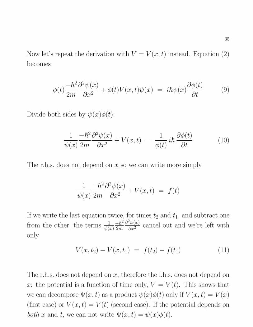
Now let’s repeat the derivation with V = V (x, t) instead. Equation (2)

becomes

φ(t)−~2

2m

∂2ψ(x)

∂x2+ φ(t)V (x, t)ψ(x) = i~ψ(x)

∂φ(t)

∂t(9)

Divide both sides by ψ(x)φ(t):

1

ψ(x)

−~2

2m

∂2ψ(x)

∂x2+ V (x, t) =

1

φ(t)i~∂φ(t)

∂t(10)

The r.h.s. does not depend on x so we can write more simply

1

ψ(x)

−~2

2m

∂2ψ(x)

∂x2+ V (x, t) = f (t)

If we write the last equation twice, for times t2 and t1, and subtract one

from the other, the terms 1ψ(x)

−~2

2m∂2ψ(x)∂x2 cancel out and we’re left with

only

V (x, t2)− V (x, t1) = f (t2)− f (t1) (11)

The r.h.s. does not depend on x, therefore the l.h.s. does not depend on

x: the potential is a function of time only, V = V (t). This shows that

we can decompose Ψ(x, t) as a product ψ(x)φ(t) only if V (x, t) = V (x)

(first case) or V (x, t) = V (t) (second case). If the potential depends on

both x and t, we can not write Ψ(x, t) = ψ(x)φ(t).

36

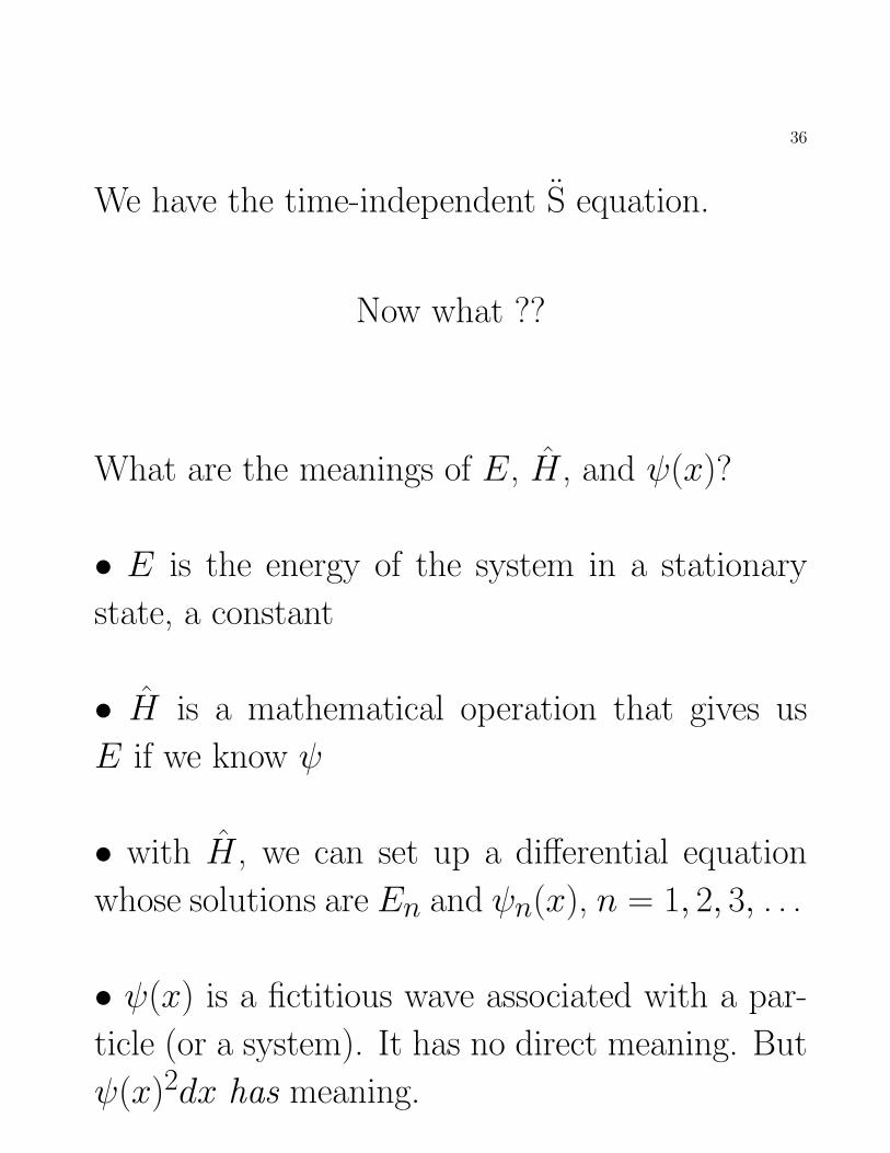
We have the time-independent S equation.

Now what ??

What are the meanings of E, H , and ψ(x)?

• E is the energy of the system in a stationary

state, a constant

• H is a mathematical operation that gives us

E if we know ψ

• with H , we can set up a differential equation

whose solutions are En and ψn(x), n = 1, 2, 3, . . .

• ψ(x) is a fictitious wave associated with a par-

ticle (or a system). It has no direct meaning. But

ψ(x)2dx has meaning.

37

Eigenvalue Equations

The time-independent S equation is

Hψ(x) = Eψ(x)

H is an operator. The S equation is an “eigen-

value equation” (EE) where E is the eigenvalue

and ψ(x) is the eigenfunction. Here’s a simpler

example of EE:

O =d

dx

Of (x) = αf (x)

The solutions to this EE: f (x) = Ceax, α = a.

38

Note that

(1) once O is known, the EE solutions (f (x), α)

can be found;

(2) for a given O, there are infinitely many

solutions;

(3) in this example, the eigenvalues a form

a continuum. However, if we force f (x) to satisfy

some boundary conditions, the eigenvalues will

form a discrete set (which is still infinite).

39

For the time-independent S equation:

1. from V (x)⇒ H

2. solve Hψ = Eψ ⇒ (En, ψn(x)), n = 1, 2, 3. . .

3. ψ(x)⇒ physical properties of stationary states

40

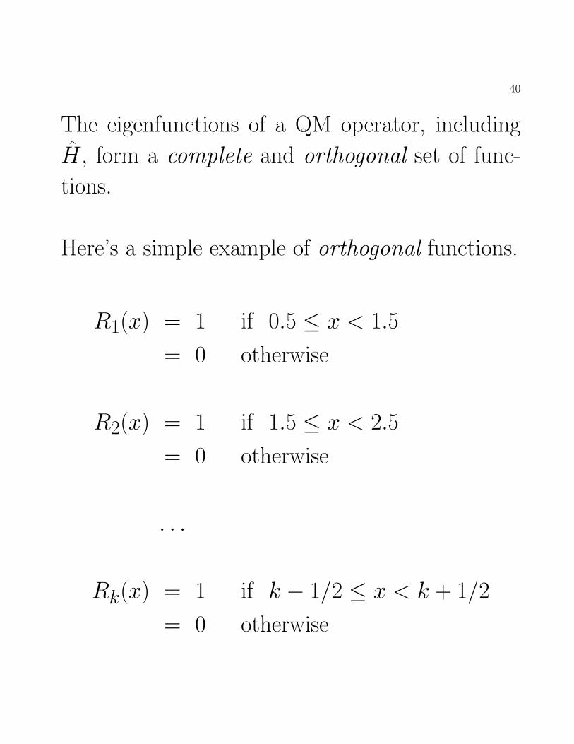
The eigenfunctions of a QM operator, including

H , form a complete and orthogonal set of func-

tions.

Here’s a simple example of orthogonal functions.

R1(x) = 1 if 0.5 ≤ x < 1.5

= 0 otherwise

R2(x) = 1 if 1.5 ≤ x < 2.5

= 0 otherwise

. . .

Rk(x) = 1 if k − 1/2 ≤ x < k + 1/2

= 0 otherwise

41

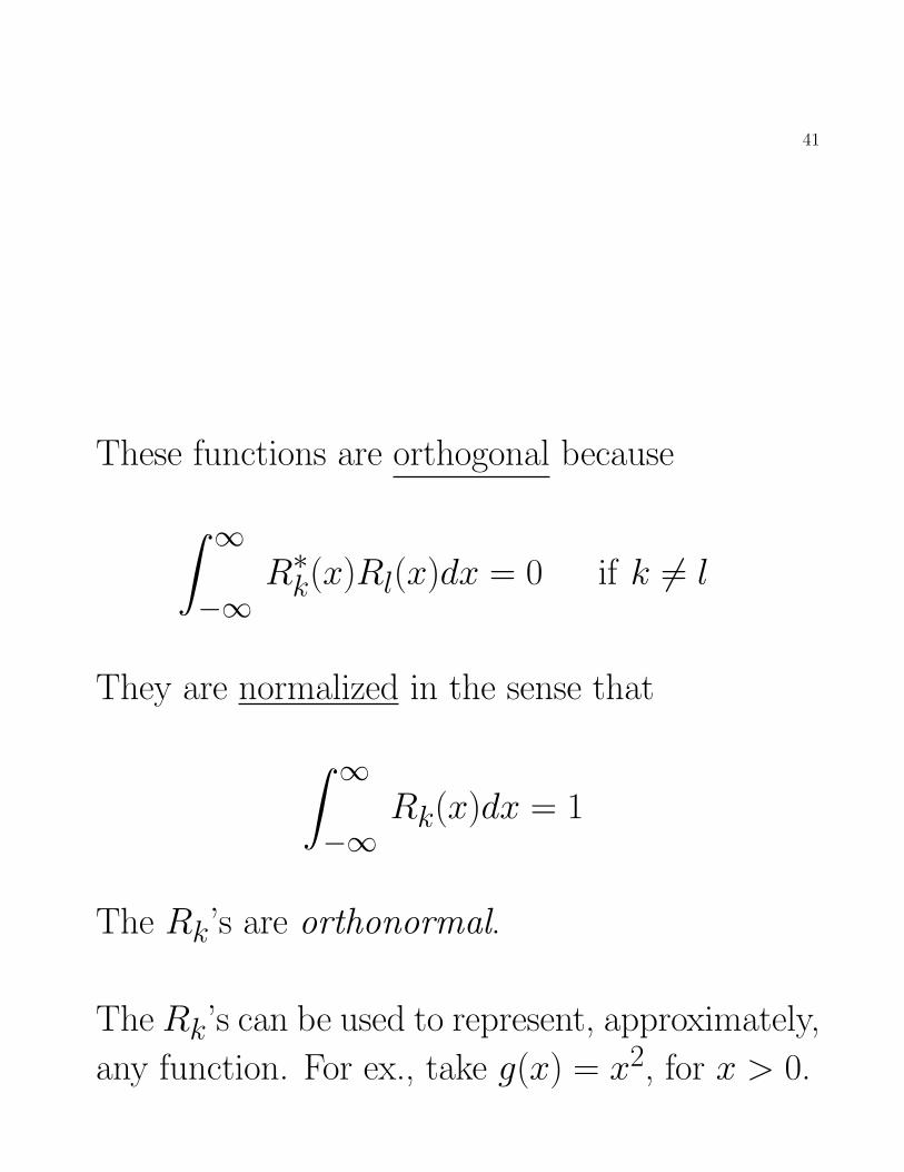
These functions are orthogonal because

∫ ∞−∞

R∗k(x)Rl(x)dx = 0 if k 6= l

They are normalized in the sense that

∫ ∞−∞

Rk(x)dx = 1

The Rk’s are orthonormal.

The Rk’s can be used to represent, approximately,

any function. For ex., take g(x) = x2, for x > 0.

42

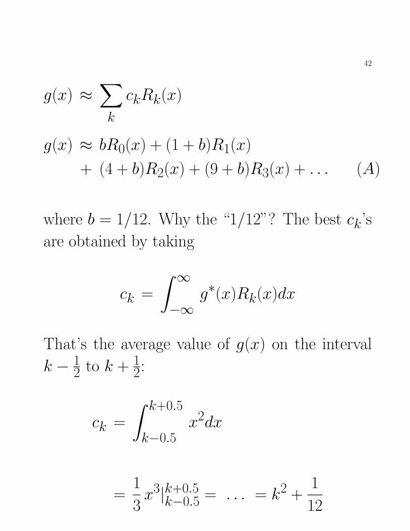
g(x) ≈∑k

ckRk(x)

g(x) ≈ bR0(x) + (1 + b)R1(x)

+ (4 + b)R2(x) + (9 + b)R3(x) + . . . (A)

where b = 1/12. Why the “1/12”? The best ck’s

are obtained by taking

ck =

∫ ∞−∞

g∗(x)Rk(x)dx

That’s the average value of g(x) on the interval

k − 12 to k + 1

2:

ck =

∫ k+0.5

k−0.5x2dx

=1

3x3|k+0.5

k−0.5 = . . . = k2 +1

12

43

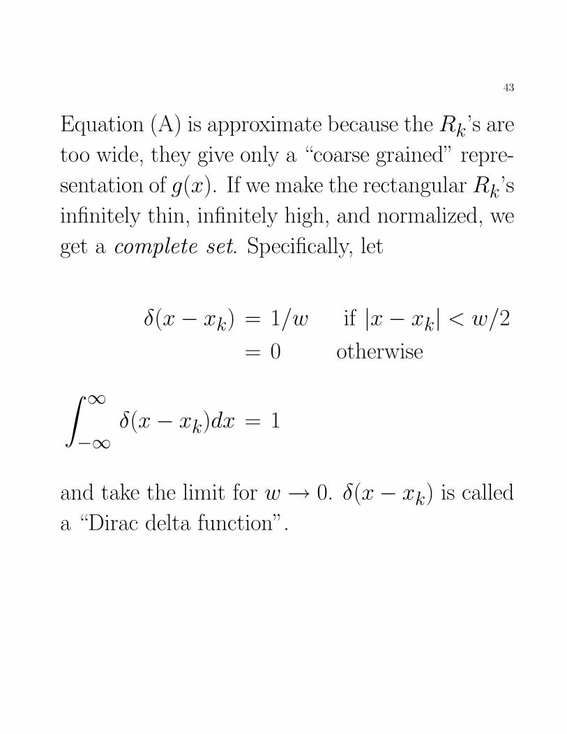
Equation (A) is approximate because the Rk’s are

too wide, they give only a “coarse grained” repre-

sentation of g(x). If we make the rectangular Rk’s

infinitely thin, infinitely high, and normalized, we

get a complete set. Specifically, let

δ(x− xk) = 1/w if |x− xk| < w/2

= 0 otherwise∫ ∞−∞

δ(x− xk)dx = 1

and take the limit for w → 0. δ(x− xk) is called

a “Dirac delta function”.

44

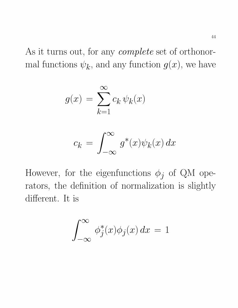
As it turns out, for any complete set of orthonor-

mal functions ψk, and any function g(x), we have

g(x) =

∞∑k=1

ck ψk(x)

ck =

∫ ∞−∞

g∗(x)ψk(x) dx

However, for the eigenfunctions φj of QM ope-

rators, the definition of normalization is slightly

different. It is

∫ ∞−∞

φ∗j(x)φj(x) dx = 1

45

The function-vector analogy

The concepts of orthogonality, normalization, and completeness are easier to

grasp for vectors. Functions can be viewed as a natural generalization of vectors.

Viewed that way, the concepts of orthogonality, normalization, and completeness

for sets of functions do not seem so strange.

First, consider vectors in two-dimensional (2D) space. The position of any point

in 2D can be given with two coordinates x and y. The arrow that goes from the

origin to that point is a vector which we represent by ~r = |x, y >. Vectors can

also be represented by columns of numbers:

~r =

(x

y

)(12)

The transpose of a vector is that same vector written as a row of numbers. The

notation for the transpose of a vector is like this:

~rT = < x, y| =(x y

)(13)

Instead of ~r, “x” and “y”, it is preferable to use “~x”, “x1”, and “x2”, because

later on we will generalize definitions to the n-dimensional case. So

~x = |x1, x2 > =

(x1

x2

)(14)

~xT = < x1, x2| =(x1 x2

)(15)

The length of a vector is |~x| = (x21 + x2

2)1/2. When |~x| = 1, we say that ~x is

normalized.

By definition, the multiplication of a vector ~x = |x1, x2 > by a number c gives

c~x = |cx1, cx2 >. Geometrically speaking, multiplying a vector by c leaves its

orientation unchanged but changes its length by a factor c.

By definition, addition of two vectors gives ~x + ~y = |x1, x2 > +|y1, y2 >=

|x1 + y1, x2 + y2 >.

46

The inner product ~xT~y of two vectors ~x and ~y is defined as the sum x1y1+x2y2.

The notation is

~xT~y = < x1, x2|y1, y2 > =(x1 x2

) (y1

y2

)= x1y1 + x2y2 (16)

Note that

~xT~y = x1y1 + x2y2 = y1x1 + y2x2 = ~yT~x

~xT~y = ~yT~x

The two basis vectors ~b1 = |1, 0 > and ~b2 = |0, 1 > are normalized and

orthogonal:

< 1, 0|1, 0 > = 1 + 0 = 1

< 0, 1|0, 1 > = 0 + 1 = 1

< 1, 0|0, 1 > = 0 + 0 = 0

Furthermore, ~b1 and ~b2 form a complete set for the representation of 2D vectors

because any vector ~v = |v1, v2 > can be written as a linear combination of ~b1 and~b2.

~v = |v1, v2 >= v1~b1 + v2~b2

Vectors ~b1 and ~b2 are just one of infinitely many possible choices of orthonormal

basis. Geometrically speaking, any two unit length vectors that make a right

angle are orthonormal. For instance, we could take s =√

2/2, and define a new

basis ~c1 = |s, s > and ~c2 = |s,−s >.

< s, s|s,−s > = s2 − s2 = 0

< s, s|s, s > = s2 + s2 = 1

< s,−s|s,−s > = s2 + s2 = 1

Any vector ~v = |v1, v2 > can be written as a linear combination in that new basis

47

with coefficients a1 and a2.

|v1, v2 > = a1|s, s > +a2|s,−s >

For an orthonormal basis there is a simple formula to find the coefficients a1 and

a2. We illustrate it with |v1, v2 > and basis { ~c1,~c2 }.

a1 = ~cT1 ~v =< s, s|v1, v2| >= sv1 + sv2

a2 = ~cT2 ~v =< s,−s|v1, v2| >= sv1 − sv2

|v1, v2 >?= a1~c1 + a2~c2

= (sv1 + sv2)|s, s > +(sv1 − sv2)|s,−s >= |s2v1, s

2v1 > +|s2v2, s2v2 > +|s2v1,−s2v1 > +| − s2v2, s

2v2 >

= |2s2v1, 2s2v2 >

= |v1, v2 >

The definitions and formulas carry over to the general case of vectors in a n-

dimensional space.

|~x| = (~xT~x)1/2 = (< x|x >)1/2

= (< x1, x2, x3, . . . , xn|x1, x2, x3, . . . , xn >)1/2

= (x21 + x2

2 + x23 + . . .+ x2

n)1/2

c~x = c|x1, x2, x3, . . . , xn >

= |cx1, cx2, cx3, . . . , cxn >

~x+ ~y = |x1 + y1, x2 + y2, x3 + y3, . . . , xn + yn >

~xT~y = < x|y >= x1y1 + x2y2 + x3y3 + . . .+ xnyn

48

and one can define a set of n orthonormal basis vectors, for instance,

~b1 = |1, 0, 0, . . . , 0 >~b2 = |0, 1, 0, . . . , 0 >~b3 = |0, 0, 1, . . . , 0 >

. . .

~bn = |0, 0, 0, . . . , 1 >

~bTi~bj = δij

where δij, Kronecker’s delta, is 1 if i = j and 0 otherwise. As before, there are

infinitely many possible choices of orthonormal basis sets. For instance, if the

“. . . ” represent a series of 0’s, we could have:

~a1 = |0.48797,−0.31553, 0.81383, . . . >

~a2 = | − 0.63085,−0.77187, 0.07900, . . . >

~a3 = |0.60324,−0.55196,−0.57571, . . . >

~a4 = |0, 0, 0, 1, . . . , 0 >. . .

~an = |0, 0, 0, . . . , 1 >

As before, we can use an orthonormal basis to represent any vector ~v.

~v =∑

j

cj~bj =∑

j

(~bTj ~v)~bj =∑

j

(~vT~bj)~bj

We can show that the formula for cj is correct:

~v =∑

j

cj~bj or ~vT =∑

j

cj~bTj

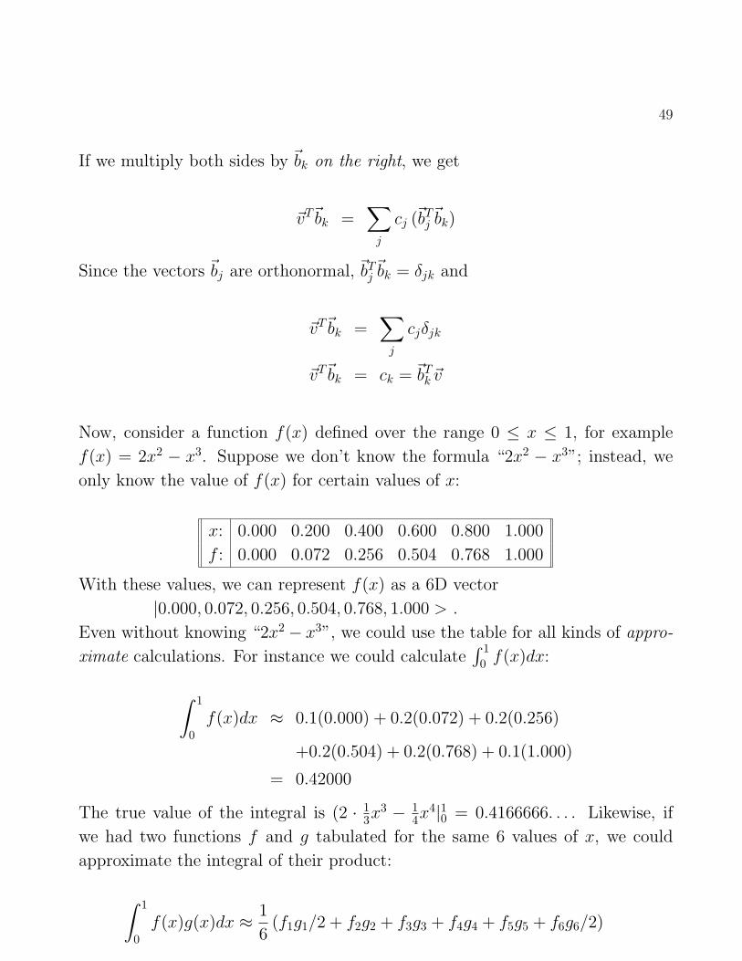
49

If we multiply both sides by ~bk on the right, we get

~vT~bk =∑

j

cj (~bTj~bk)

Since the vectors ~bj are orthonormal, ~bTj~bk = δjk and

~vT~bk =∑

j

cjδjk

~vT~bk = ck = ~bTk~v

Now, consider a function f(x) defined over the range 0 ≤ x ≤ 1, for example

f(x) = 2x2 − x3. Suppose we don’t know the formula “2x2 − x3”; instead, we

only know the value of f(x) for certain values of x:

x: 0.000 0.200 0.400 0.600 0.800 1.000

f : 0.000 0.072 0.256 0.504 0.768 1.000

With these values, we can represent f(x) as a 6D vector

|0.000, 0.072, 0.256, 0.504, 0.768, 1.000 > .

Even without knowing “2x2 − x3”, we could use the table for all kinds of appro-

ximate calculations. For instance we could calculate∫ 1

0 f(x)dx:

∫ 1

0f(x)dx ≈ 0.1(0.000) + 0.2(0.072) + 0.2(0.256)

+0.2(0.504) + 0.2(0.768) + 0.1(1.000)

= 0.42000

The true value of the integral is (2 · 13x

3 − 14x

4|10 = 0.4166666. . . . Likewise, if

we had two functions f and g tabulated for the same 6 values of x, we could

approximate the integral of their product:

∫ 1

0f(x)g(x)dx ≈ 1

6(f1g1/2 + f2g2 + f3g3 + f4g4 + f5g5 + f6g6/2)

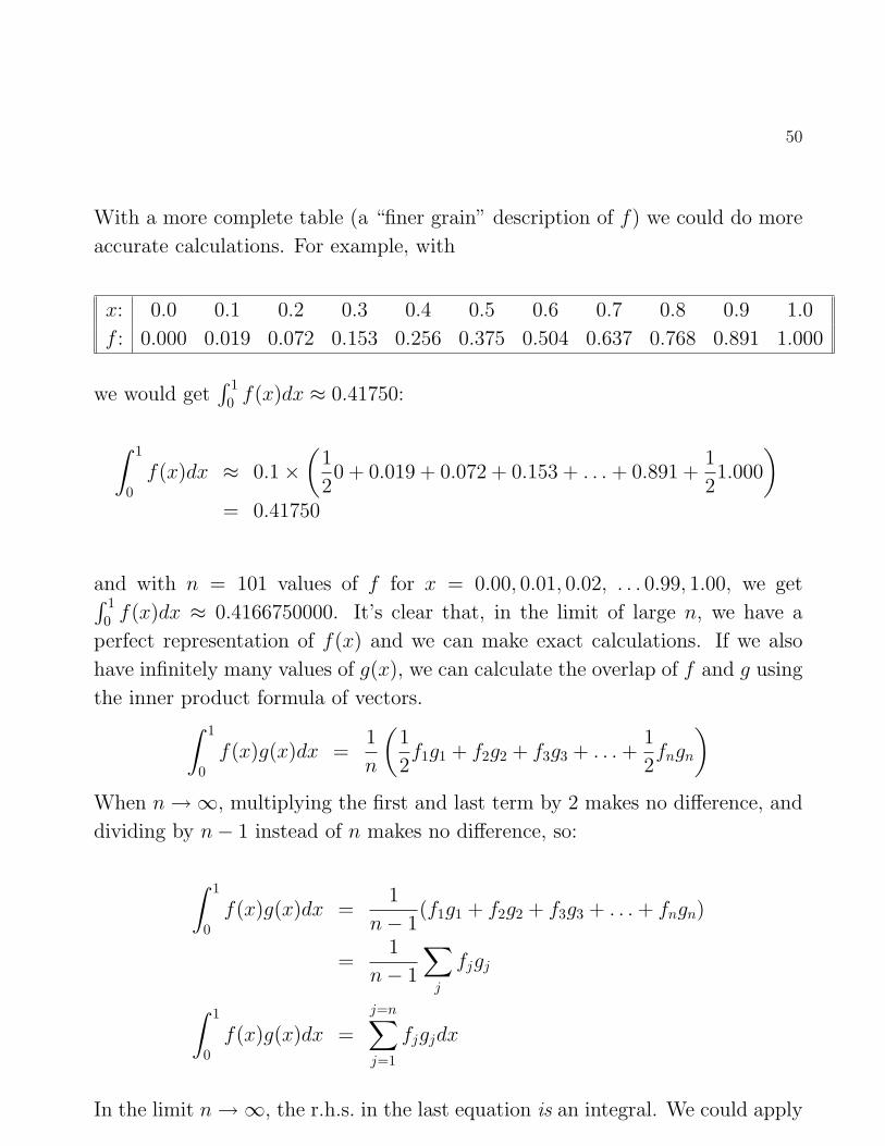
50

With a more complete table (a “finer grain” description of f) we could do more

accurate calculations. For example, with

x: 0.0 0.1 0.2 0.3 0.4 0.5 0.6 0.7 0.8 0.9 1.0

f : 0.000 0.019 0.072 0.153 0.256 0.375 0.504 0.637 0.768 0.891 1.000

we would get∫ 1

0 f(x)dx ≈ 0.41750:

∫ 1

0f(x)dx ≈ 0.1×

(1

20 + 0.019 + 0.072 + 0.153 + . . .+ 0.891 +

1

21.000

)= 0.41750

and with n = 101 values of f for x = 0.00, 0.01, 0.02, . . . 0.99, 1.00, we get∫ 10 f(x)dx ≈ 0.4166750000. It’s clear that, in the limit of large n, we have a

perfect representation of f(x) and we can make exact calculations. If we also

have infinitely many values of g(x), we can calculate the overlap of f and g using

the inner product formula of vectors.∫ 1

0f(x)g(x)dx =

1

n

(1

2f1g1 + f2g2 + f3g3 + . . .+

1

2fngn

)When n→∞, multiplying the first and last term by 2 makes no difference, and

dividing by n− 1 instead of n makes no difference, so:

∫ 1

0f(x)g(x)dx =

1

n− 1(f1g1 + f2g2 + f3g3 + . . .+ fngn)

=1

n− 1

∑j

fjgj

∫ 1

0f(x)g(x)dx =

j=n∑j=1

fjgjdx

In the limit n→∞, the r.h.s. in the last equation is an integral. We could apply

51

the same reasoning for functions defined over x = 0 to x =∞, or over x = −∞to x = ∞. The conclusion is that, conceptually, a function f(x) can be viewed

as an infinite-dimensional vector. So all the results obtained for vectors carry

over to functions. In particular, if we have a complete basis of (infinitely many)

orthonormal functions φj(x)

< φj|φk > =

∫ ∞−∞

φ∗j(x)φk(x)dx = δjk

then we can write any function f(x) as a linear combination of the φj’s

f(x) =∑

j

cjφj(x)

cj =

∫ ∞−∞

f ∗(x)φj(x)dx =

∫ ∞−∞

φ∗j(x)f(x)dx

52

Chapter 14:

The Postulates of QM

53

We will write the postulates for a single particle in

1D, with spatial coordinate “x” and time “t”, but

they are easily generalized to systems of n parti-

cles in 3D by changing

x⇒ x, y, z

dx⇒ dxdydz

x⇒ x1, y1, z1, x2, . . . , yn, zn

etc.

54

Postulate 1

The wavefunction (wf) Ψ(x, t) completely speci-

fies the state of a system. Ψ∗(x0, t)Ψ(x0, t)dx =

|Ψ(x, t)|2dx is the probability of finding the par-

ticle between x0 and x0 + dx at time t.

In CM, positions x and velocities dx/dt completely

specify the state of a system. (I assume we know

the mass and charge of every particle.)

Note 1.1. Multiplying Ψ(x, t) by eiθ does not

change Ψ∗(x0, t)Ψ(x0, t)dx. So the phase factor

(θ) is immaterial.

55

Note 1.2. Since |Ψ(x, t)|2dx is a probability, we

must have

|Ψ(x, t)|2 ≥ 0∫ ∞−∞|Ψ(x, t)|2 dx = 1

Note 1.3. Ψ(x, t) must be single-valued and smooth:

∂2Ψ/∂x2 is not infinite, or, ∂Ψ/∂x has no discon-

tinuity.

56

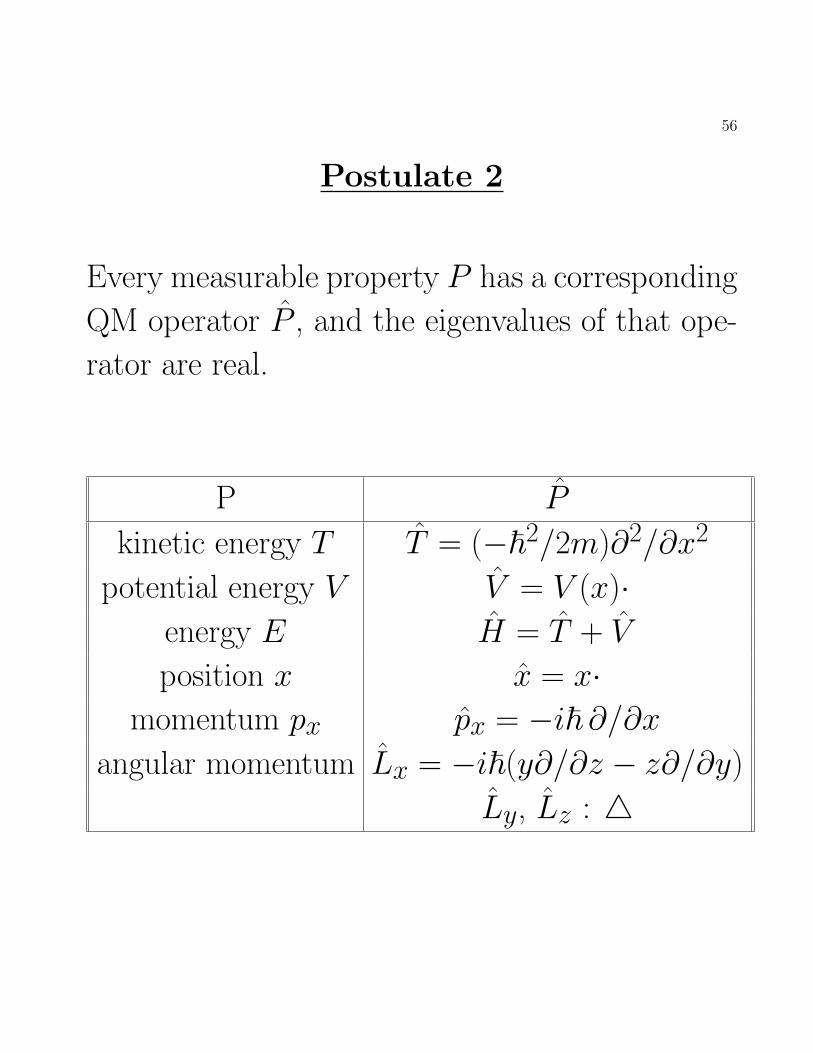
Postulate 2

Every measurable property P has a corresponding

QM operator P , and the eigenvalues of that ope-

rator are real.

P P

kinetic energy T T = (−~2/2m)∂2/∂x2

potential energy V V = V (x)·energy E H = T + V

position x x = x·momentum px px = −i~ ∂/∂x

angular momentum Lx = −i~(y∂/∂z − z∂/∂y)

Ly, Lz : 4

57

Postulate 3

If A is a QM operator and Aφj(x) = ajφj(x),

then a measurement of property “A” must yield

one of the aj’s.

Note 3.1. The aj’s may form a discrete set, or

a continuous set.

58

Postulate 4

If we prepare a very large number N of identical

systems in the same state Ψ(x, 0) at time t = 0

(Ψ is normalized) and we then measure property

“A” for each system, the average of those mea-

surements will be

Avg(a) = < a >=

∫ ∞−∞

Ψ∗(x, t) (AΨ(x, t)) dx

59

Note 4.1. If Ψ(x, t) is one of the eigenfunctions

φj(x, t) of A, then

< a > =

∫ ∞−∞

φ∗j(x, t)(Aφj(x, t)) dx

=

∫ ∞−∞

φ∗j(x, t)ajφj(x, t)) dx

= aj

∫ ∞−∞

φ∗j(x, t)φj(x, t)) dx

= aj

60

Note 4.2. The eigenfunctions of A form a com-

plete set so we can write

Ψ =∑j

cjφj

< a > =

∫ ∞−∞

∑j

c∗jφ∗j

A

∑k

ckφk

dx

=∑j

∑k

c∗jck

∫ ∞−∞

φ∗j Aφk dx

=∑j

∑k

c∗jck ak

∫ ∞−∞

φ∗jφk dx

The φj’s are orthonormal, so the integral is 0 if

j 6= k and 1 if j = k. We represent this by the

“Kronecker delta” δjk:

δjk = 1 if j = k

= 0 if j 6= k

61

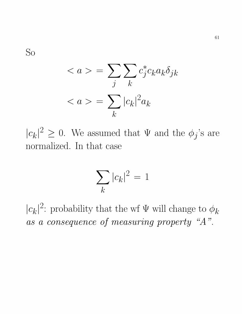
So

< a > =∑j

∑k

c∗jckakδjk

< a > =∑k

|ck|2ak

|ck|2 ≥ 0. We assumed that Ψ and the φj’s are

normalized. In that case

∑k

|ck|2 = 1

|ck|2: probability that the wf Ψ will change to φkas a consequence of measuring property “A”.

62

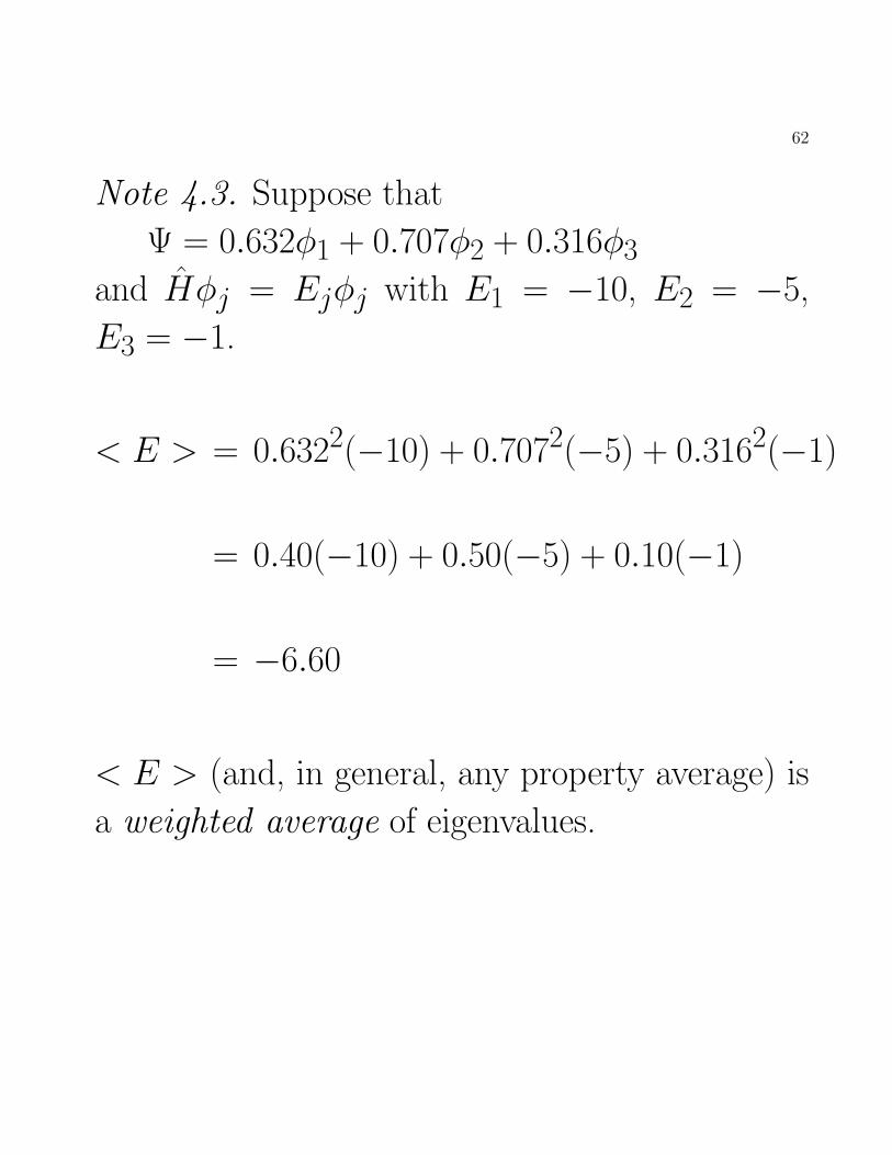
Note 4.3. Suppose that

Ψ = 0.632φ1 + 0.707φ2 + 0.316φ3

and Hφj = Ejφj with E1 = −10, E2 = −5,

E3 = −1.

< E > = 0.6322(−10) + 0.7072(−5) + 0.3162(−1)

= 0.40(−10) + 0.50(−5) + 0.10(−1)

= −6.60

< E > (and, in general, any property average) is

a weighted average of eigenvalues.

63

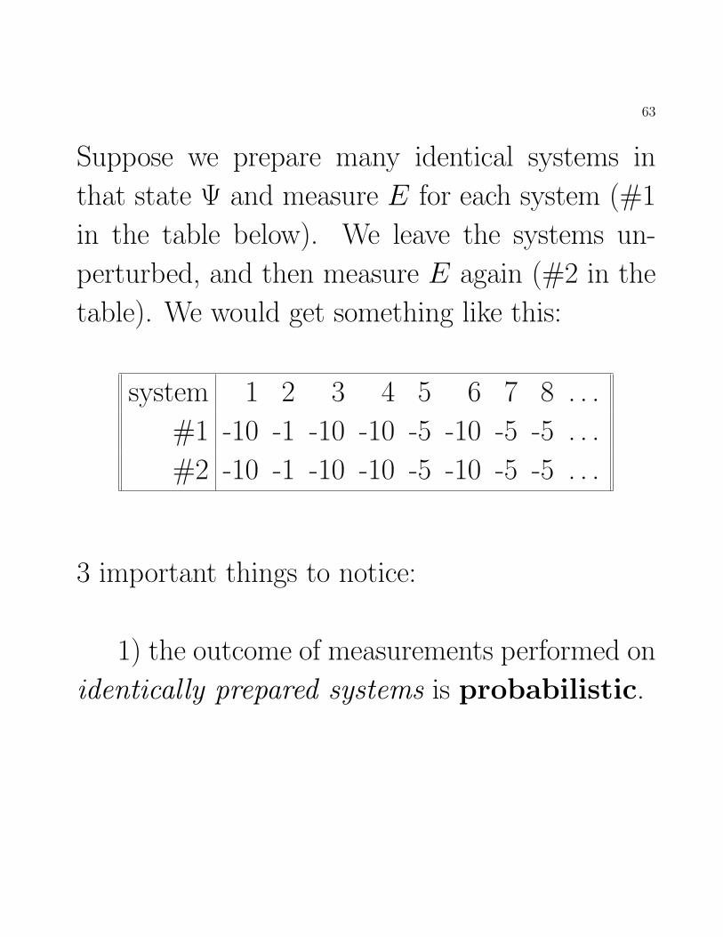
Suppose we prepare many identical systems in

that state Ψ and measure E for each system (#1

in the table below). We leave the systems un-

perturbed, and then measure E again (#2 in the

table). We would get something like this:

system 1 2 3 4 5 6 7 8 . . .

#1 -10 -1 -10 -10 -5 -10 -5 -5 . . .

#2 -10 -1 -10 -10 -5 -10 -5 -5 . . .

3 important things to notice:

1) the outcome of measurements performed on

identically prepared systems is probabilistic.

64

2) measuring property “A” of a system changes

its wf to an eigenfunction of A with eigenvalue aj(−10,−5, or −1 in our example), and aj is the

measured value. In general, measuring a pro-

perty changes the state of the system.

3) If, after the first measurement of “A”, the

system is left undisturbed, every subsequent mea-

surement of “A” will give the same aj.

65

Postulate 5

The time evolution of a system is deterministic

and given by

HΨ(x, t) = i~∂Ψ(x, t)

∂t

66

Note 5.1. Take an operator A, with eigenfunc-

tions Φj(x, t), that does not depend on time.

AΦj(x, t) = ajΦj(x, t)

We can write Φj(x, t) = φj(x)f (t) and preserve

the eigenvalue equation. To show that, substitute:

A(φj(x)f (t))?= ajφj(x)f (t)

f (t)Aφj(x) = f (t)ajφj(x)

Aφj(x) = ajφj(x)

So if A is time-independent it has time-independent

eigenfunctions φj(x).

67

Chapter 15:

QM of simple systems

68

the free particle (FP)

By definition, no force acts on a “free particle”:

F = 0. But F = −dV/dx, so V is a constant.

We are free to choose any value for that constant:

take V (x) = 0.

In CM F = md2x/dt2 = 0, so x = x0 + v0t.

The FP moves at constant speed v0 from left to

right if v0 > 0, and right to left if v0 < 0.

69

In QM we note that V is independent of t and

substitute V (x) by 0 in the time-independent S

equation.

−~2

2m

d2ψ

dx2= Eψ(x)

d2ψ

dx2=

(−2mE

~2

)ψ(x)

ψ(x) equals its own second derivative times a cons-

tant, and it is finite everywhere. So ψ(x) can be

written either as: (i) a combination of sine and

cosine; or (ii) an exponential with imaginary ar-

gument. The latter is easier, so

ψ+(x) = A+ eikx

ψ−(x) = A− e−ikx

k =√

2mE/~

70

Euler’s formula tells us that kx is the argument

of cosine and sine functions, so kx = 2πx/λ.

2π/λ = k =√

2mE/~

E =~2k2

2m

k can be any real value, so E is continuous. Since

V = 0, E is just the kinetic energy of the FP. The

CM expression is E = mv2/2. So

2π/λ =

(2mmv2

2

)1/2

/(h/2π)

1/λ = mv/h

λ = h/mv = h/p

just like the DeBroglie formula.

71

When we get ψ(x) by solving the time-independent

S equation, we can get the full wf by multiplying

ψ(x) by e−iEt/~. Define ω = E/~,

Ψ+(x, t) = A+ eikx e−iωt = A+ e

i(kx−ωt)

The r.h.s. is the equation of a traveling wave going

from left to right. Likewise, Ψ−(x, t) is a wave

traveling from right to left. Ψ+(x, t) and Ψ−(x, t)

are called plane waves. They are constant energy,

constant velocity, waves.

Ψ+(x, t) and Ψ−(x, t) can not be normalized be-

cause they do not go to zero as x → ±∞. Their

square describes a density made of infinitely many

particles: |Ψ+(x, t)|2 = A2+e−ikxeikx = A2

+. If

we setA2+ = 1/2L, then |Ψ+(x, t)|2dx = A2

+dx =

(1/2L)dx, which means that there is one particle

for every 2L units of length.

72

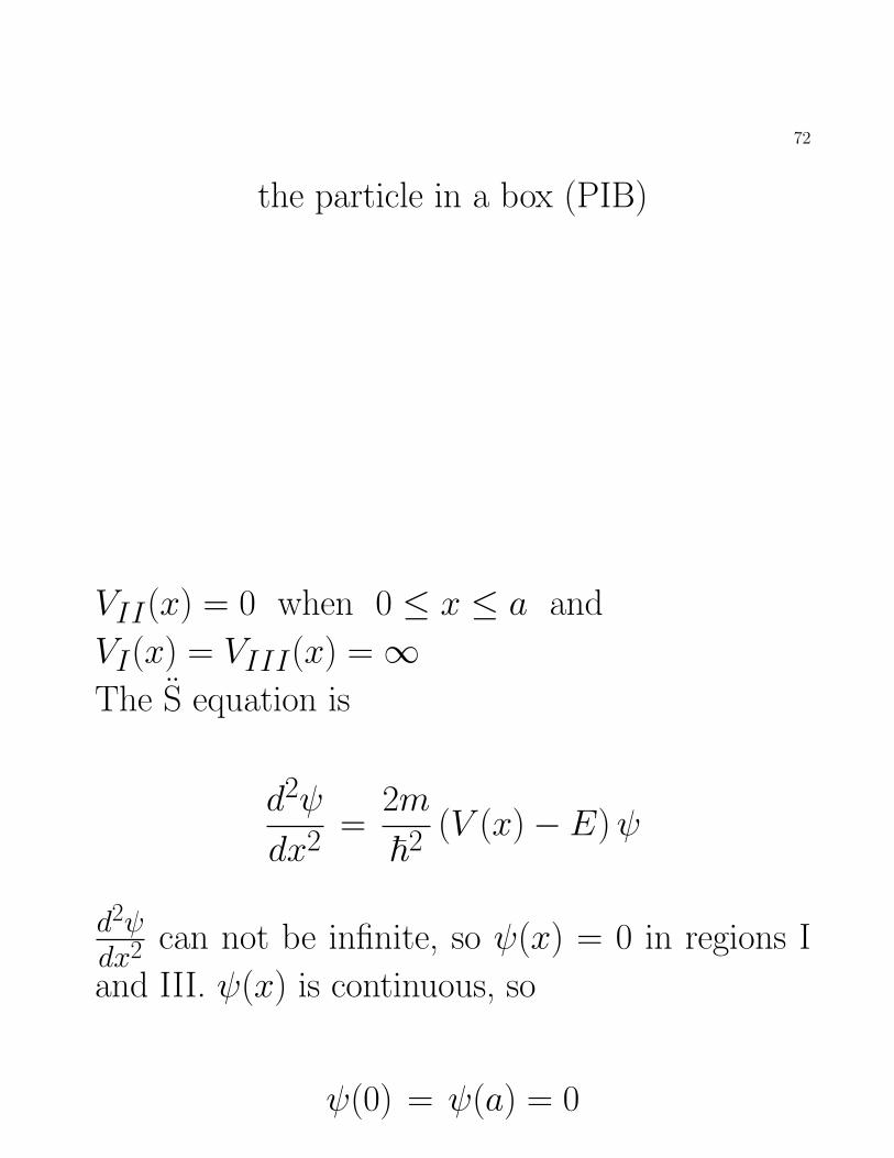
the particle in a box (PIB)

VII(x) = 0 when 0 ≤ x ≤ a and

VI(x) = VIII(x) =∞The S equation is

d2ψ

dx2=

2m

~2(V (x)− E)ψ

d2ψdx2 can not be infinite, so ψ(x) = 0 in regions I

and III. ψ(x) is continuous, so

ψ(0) = ψ(a) = 0

73

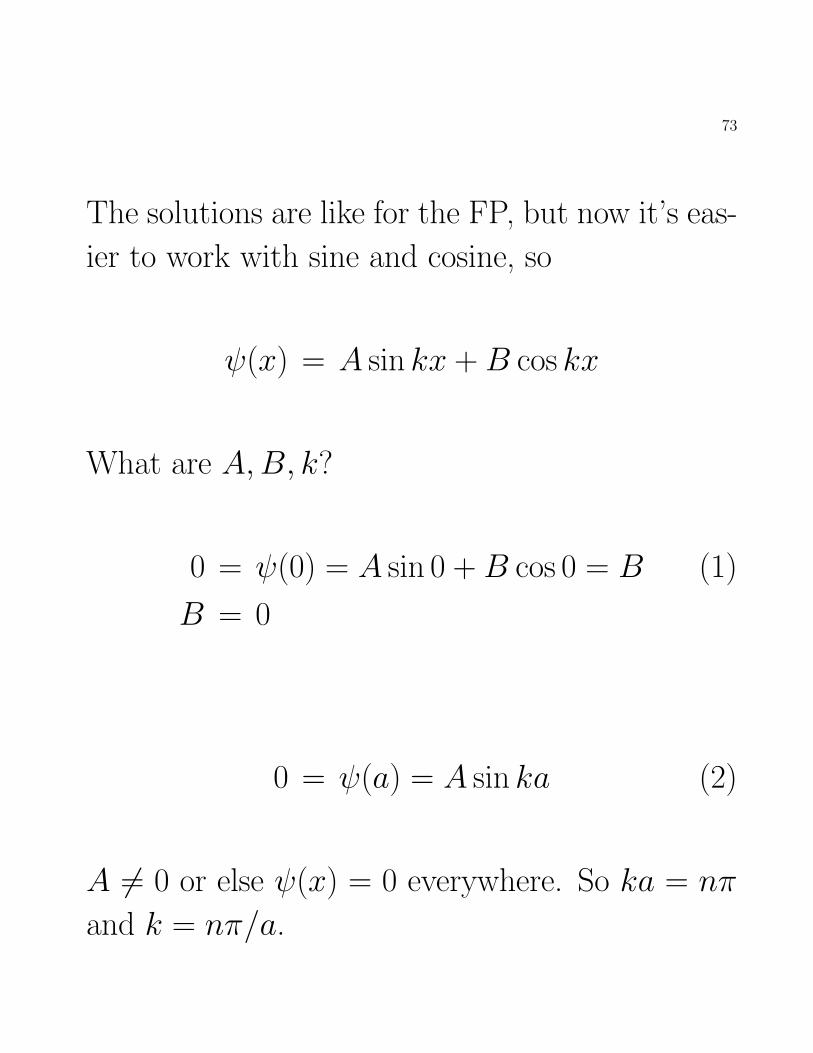
The solutions are like for the FP, but now it’s eas-

ier to work with sine and cosine, so

ψ(x) = A sin kx + B cos kx

What are A,B, k?

0 = ψ(0) = A sin 0 + B cos 0 = B (1)

B = 0

0 = ψ(a) = A sin ka (2)

A 6= 0 or else ψ(x) = 0 everywhere. So ka = nπ

and k = nπ/a.

74

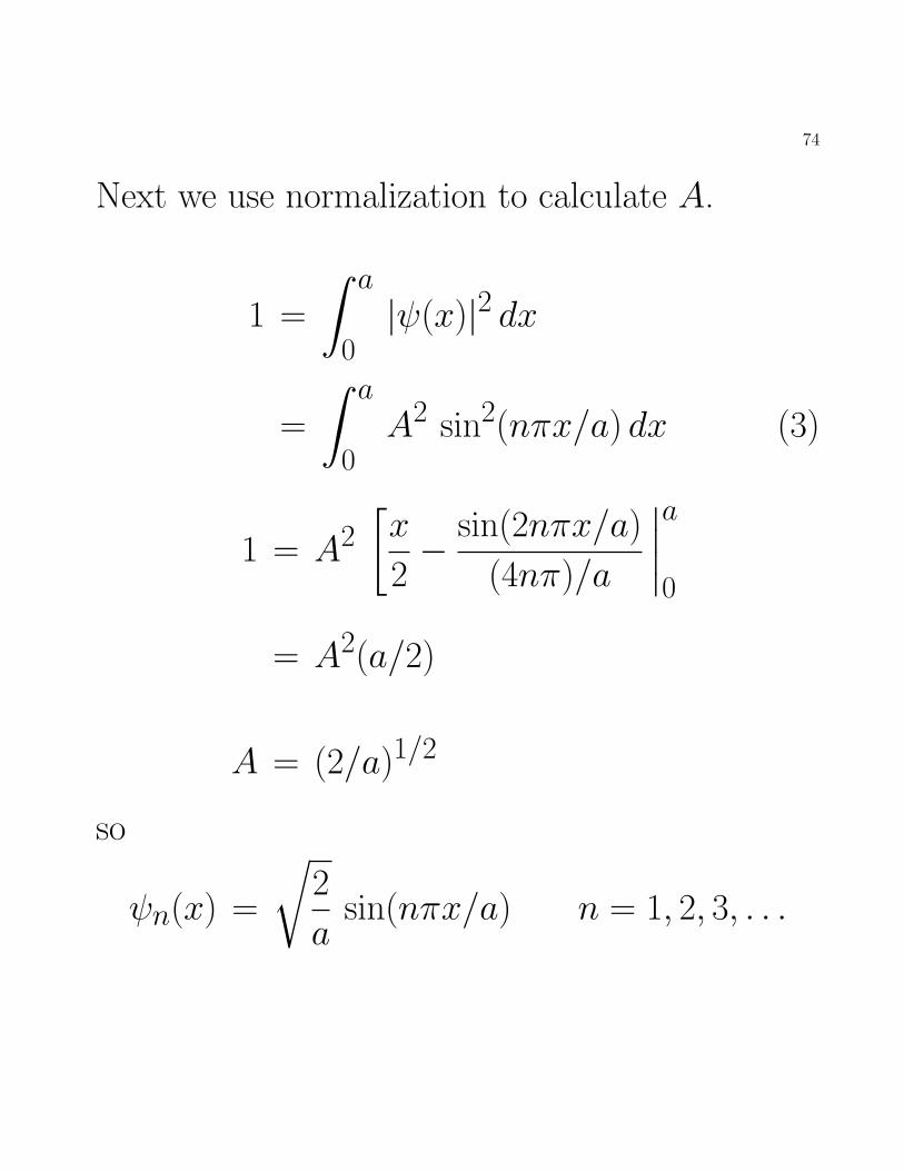
Next we use normalization to calculate A.

1 =

∫ a

0|ψ(x)|2 dx

=

∫ a

0A2 sin2(nπx/a) dx (3)

1 = A2[x

2− sin(2nπx/a)

(4nπ)/a

∣∣∣∣a0

= A2(a/2)

A = (2/a)1/2

so

ψn(x) =

√2

asin(nπx/a) n = 1, 2, 3, . . .

75

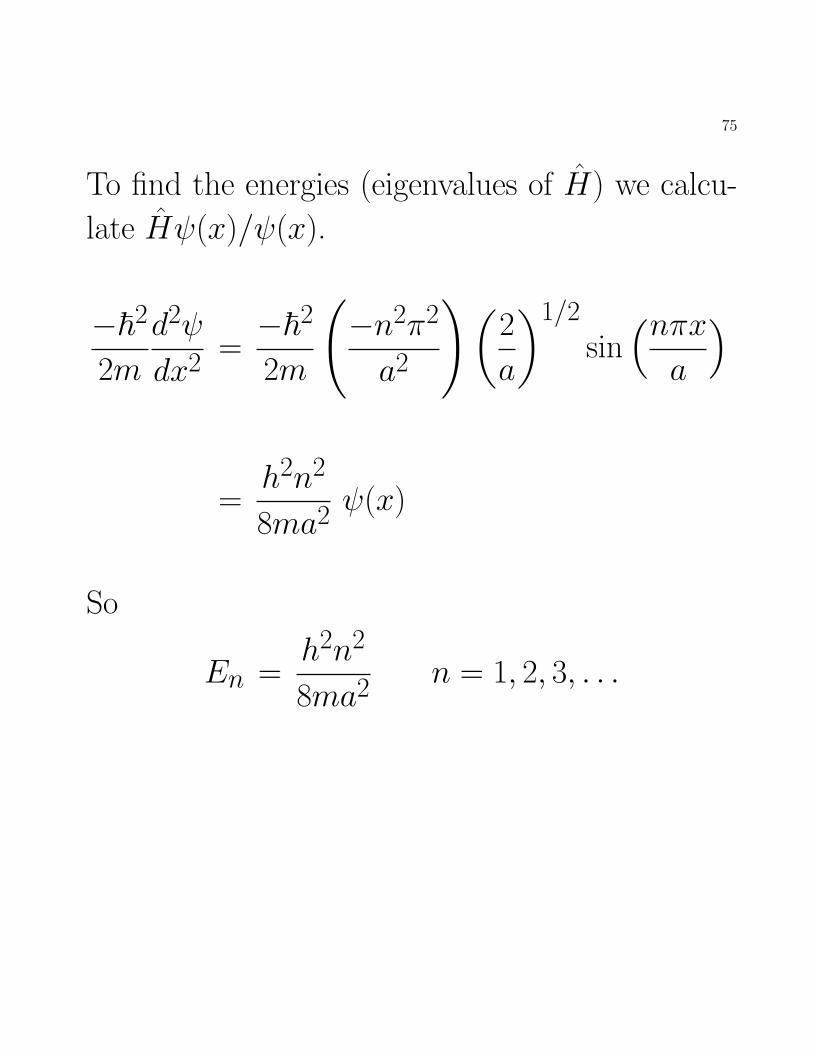
To find the energies (eigenvalues of H) we calcu-

late Hψ(x)/ψ(x).

−~2

2m

d2ψ

dx2=−~2

2m

(−n2π2

a2

)(2

a

)1/2

sin(nπxa

)

=h2n2

8ma2ψ(x)

So

En =h2n2

8ma2n = 1, 2, 3, . . .