characterizing filtered light waves corrupted by phase noise

IEEE TRANSACTIONS ON INFORMATION THEORY, VOL. 34, NO. 6, NOVEMBER 1988 1437

Characterizing Filtered Light Waves Corrupted by Phase Noise

Abstruct -The phase noise associated with single-mode semiconductor lasers must be accounted for in performance studies of lightwave communication systems. The standard phase noise model is a Brownian-motion stochastic process. Although many analyses of lightwave communication systems have been published, none, to our knowledge, has fully adhered to the standard model. The reason is that a proper characterization of a filtered lightwave signal had not been achieved. Such a characterization, along with theoretical approaches to obtaining it, is detailed here. We show, for example, how to generate probability density functions (pdf's) of the magnitude of a filtered laser tone (with special attention to the tail region) and how to analytically represent the characteristic function of the pdf in closed form in the small-phase-noise realm. With the characterization in place, the stage is now set for determining the bit-error rate performance of advanced detection techniques which seek to mitigate the phase noise impairment.

I. INTRODUCTION

A . Background

HE ADVENT of coherent optical communication T systems has focused much attention on the problem of phase noise. Indeed, in systems that use semiconductor lasers, phase noise is a very important impairment, and techniques to reduce phase noise are being studied by many investigators. The reason why phase noise is a problem in coherent systems has to do with the unavoidable filtering of the received signal that is intrinsic to the coherent detection scheme. Thus, even coherent systems relying on amplitude modulation (phase noise is obviously a problem in systems employing phase modulation) will suffer some degradation due to the presence of phase noise.

Performance limitations introduced by phase noise in coherent optical systems have been examined by many researchers [1]-[12].' To account for laser phase noise, the model for a laser tone in complex form is refined to e'(2"fcf+g(f)), where the random function e( r ) is a continuous-path Brownian motion process with zero mean and variance E [ e'( r ) ] = 2 4 r . The resulting power spectrum is

Manuscript received November 1986; revised January 1988. This paper was partially presented at the Princeton University 22nd Annual Confer- ence on Information Science and Systems, March 1988.

The authors are with AT&T Bell Laboratories, Crawford Hill Labora- tory, P.O. Box 400, Holmdel, NJ 07733.

IEEE Log Number 8824873. 'Reference [12] is especially thorough in the scope of systems treated.

Lorentzian.2 The parameter p is called the laser linewidth or the Lorentzian bandwidth. Indeed, p is the frequency spacing between the 3-dB points of the power spectral density function.

In a typical coherent optical communication system, the laser tone is modulated according to some modulation scheme (via, for example, an external electro-optic modu- lator) while, at the receiver, the signal is passed through some kind of linear filter. As noted before, this filtering operation is an integral part of coherent detection, as it is needed to reduce the shot noise introduced by the local oscillator and to achieve a good signal-to-noise ratio (SNR). The simplest possible model assumes digital modulation with rectangular pulses and a receiver filter that integrates the received signal over the pulse duration; i.e., the impulse response of the filter is itself a rectangular pulse. Despite the simplicity of this model, the probability density function of this most fundamental baseband filtering operation

l r ( T ) + A T ) ,

(1) rectangular coordinates 8 ( T ) = JOTeJg(t) dt 1

m ( T ) \ polar coordinates

is difficult to determine. Up to now, to the authors' knowledge, the determination has not been reported in the literature and analyses of communication systems with full adherence to the Brownian motion model of phase noise have not been done.

An actual communication system will, in general, use nonrectangular pulses for the modulation and a receiver filter with a nonrectangular impulse response. However, system performance is not affected in a fundamental way by such variations, so that the results obtained here characterize the performance of a general coherent system. Also, some of the techniques presented here can be easily extended to the more general case; and furthermore, this simplified model is at the heart of more complex systems which may use more sophisticated processing to improve

2Lorentzian is the descriptor favored by physicists. Probabilists and statisticians would say the power spectrum has the shape of the Cauchy density. Electrical engineers would say the shape matches that of RC- filtered white noise.

0018-9448/88/1100-1437$01.00 01988 IEEE

1438 IEEE TRANSACTIONS ON INFORMATION THEORY, VOL. 3 4 , NO. 6, NOVEMBER 1988

performance (see, for example, [13]). Since it is so basic to the analysis and design of coherent optical communications systems, it is of crucial importance to determine the probability density function (pdf) p,,, (or P , , , ~ in polar coordinates) or, equivalently, the moment generating function (mgf) Mr,s (or M,,,J. Knowledge of the density function is needed to resolve communication system performance issues. Even the usually straightforward approach of system simulation becomes prohibitive as the bit-error rate (BER) level of interest is decreased.

In this paper, we present several approaches to obtaining the aforementioned functions. In Section I1 we introduce a special simulation technique, based on the Radon-Nikodym derivative (RND) from probability theory, that achieves enhanced accuracy at very low probability levels. Through this technique, we obtain numerical results for the pdf of 1.31 that are accurate down to quantile probabilities around lop9. In Section I11 we obtain closed-form expressions for the mgf of 8 in the limit of low levels of phase noise. We note that the mgf of 1.3(T)l happens to be a function that was examined by theoretical statisticians over half a century ago [14]-[17] in a totally different context; in that literature we found an easy-to-compute expression for the corresponding pdf which agrees well with the simulation results of Section 11. We also show how Huygens' principle can be used for numerically propagating this small-phase-noise solution to obtain a solution for an arbitrary level of phase noise. In Section IV we briefly discuss how these results can be applied to the characterization of practical receivers; a comprehensive treatment is provided in [13], while [18] reports experimental results that corroborate the theoretical calculations of [13]. Finally, in Section V we comment on an alternative type of approach based on the Fokker-Planck equation and suitable for direct numerical evaluation of the pdf of 8 for arbitrary levels of phase noise.

11. EFFICIENT SIMULATION OF FILTERED LIGHT WAVES WITH PHASE NOISE

We can estimate the bivariate density P , , , ~ by computer simulation of 3 ( T ) = jEe''(')dt. We need to take care to partition [0, T ] into enough time segments to avoid accuracy problems. This evolution of O ( t ) is especially easy to generate on the computer due to the fact that O ( t ) has independent Gaussian increments.

Of course, no matter how efficiently the simulation program is written, there are limits to estimating P , , , ~ in this manner. The Radon-Nikodym theorem (RNT) provides a way to extend greatly the ability to estimate P , , , ~ in the tail. Before presenting numerical results based on the theorem, we first state it and clarify how it is applied.

A. The Radon - Nikodym Derivative (RND)

The RNT is somewhat abstract. To state this very general and useful theorem, we need a setting involving some of the most basic elements from probability theory. For a

rigorous treatment of the RND concept and a proof of the RNT the reader is referred to [19]. S e e also [20] which focuses on RNDs related to Brownian motion. In the next few paragraphs, we give a very abridged introductory version of the backdrop for the RNT.

1) Backdrop for the Radon-Nikodym Theorem: Let (52, 6,9) be a probability space. 51 is the sample space of interest and 6 are the subsets (events) within 51 for which probability can be measured, and 9 is the probability measure that assigns numbers between zero and one to events in 6.

Later, for our application, 51 will be specialized to be the space of continuous time functions vanishing at the origin, 9 will be a variant of the Brownian motion assignment of probabilities to events. (We will also be interested in discretizations of this continuous function setup.) A typical event A of interest in estimating p,+ is the subset of 52 that is mapped by /tef'(')dt into a specified region within the circle about the origin of radius T.

The assignment of probability measure 9 ( A ) to sets A in 1 can be used for bootstrapping a notion of integration in Q. For each A in d we define the indicator function of A which is denoted lA(u). The function has the value one on A and zero otherwise. Define

kA(u) d 9 = 9 ( A ) .

Very general complex-valued functions on 51 (random variables) can be approximated via limits of finite linear combinations of indicator functions. The integral of such a random variable over 52 can be defined in terms of the limits of the integrals of the approximating sums of indicator functions. A basic requirement of an integration concept is that the integral of a finite sum of integrable functions be the same as the sum of the integrals. Conse- quently, it can be shown that the integral of a random variable, when it exists, is determined by integrals of indicator functions.

Thus integration is introduced into an abstract probability space (and therefore into function space). The RNT is nothing more than the change of variables theorem in this abstract context.

2) The Radon-Nikodym Theorem: Let 9 be a second probability measure on events of d which has the property that, for each event A for which 9 ( A ) = 0, we have 9( A) = 0. Then a random variable exists, denoted d 9 / d l for which we can write

(3)

for all events B in 1. The variate d 9 / d 9 is called the RND (or the likelihood ratio) of 9 with respect to 9.

B. Examples with Specific Application to Determining the Density of 8

We start with an elementary example. Example 1: Suppose that 9 and 9 are a pair of proba-

bility measures for which there correspond density func-

FOSCHINI AND VANNUCCI: CHARACTERIZING FILTERED LIGHT WAVES 1439

tions in n-dimensional Euclidean space. Assume the density corresponding to 9 is always nonzero. The d 9 / d 3 is simply the joint density corresponding to 9 divided by the one for 2.

The next example builds on the previous one and is more interesting. It is directed at our application.

Example 2: Let be the space of continuous functions of t on the interval [0, T ] that vanish at the origin. Again, d is the standard set of events. Let be the probability measure for a Brownian motion process with mean at and variance 2 ~ p t . The phase noise process has measure Po,+ The probability measure 9a,s. corresponding to altering each phase noise path by adding a drift, f a t , with sign determined by a fair coin, is 2a,B =

The RND d9’o,,/d9a,, can be obtained by tahng the limit of quotients of finite-dimensional densities corresponding to discrete-time approximations to phase noise: The interval [0, T ] is partitioned into intervals of size ( T / N ) , and we are interested in the limit as N + 00. In forming the density quotient, the terms in the exponents that are quadratic in the sample path cancel, since Pa+-, and P-a,p share the same covariance function. The resulting RND turns out to be

+ 9- , ). a s

T h s second example is useful in estimating pm,+. If we simulate 3a,s by appropriate choice of a we can get many paths with lO(T)I much larger than would be generated with a simulation of This corresponds to much lower values for 1.3(T)l and, therefore, we can estimate the density of pm,+ in the tail region more accurately than if we simulate directly. Let A be the set of paths that map into a small rectangle of area a in the ( m , I$) plane with center coordinates (mo, Goo>. Let { Ok}f denote K simulated paths under the measure 9. Then (3) and (4) give an estimate for pm,+(mo, Go):

1A(8k) e(a~)2/477S~ K

pm3+(mo”o) aK k = l c cosh(aTB,(T)/2~/3T).

( 5 )

The more standard use of simulation to estimate pm,+(mo,Go), corresponds to the special case a = 0, where

( 5 ’ )

Then, as expected, the estimate is simply the relative number of times the outcome of the approximation to 8 fell in the rectangular “bin,” divided by the area of the bin a. Again, the estimate provided by (5) will be better than that of (5’) because many more terms in the summation are nonzero.

This simulation technique is related to the technique known as “importance sampling” in mathematical statistics [21] which has its roots in the work reported in [22] and [23]. Although [24]-[26] do not explicitly mention the

Radon-Nikodym terminology, they use essentially a scalar version of the RNT for the estimation of rare events in communication problems.

C. Numerical Results

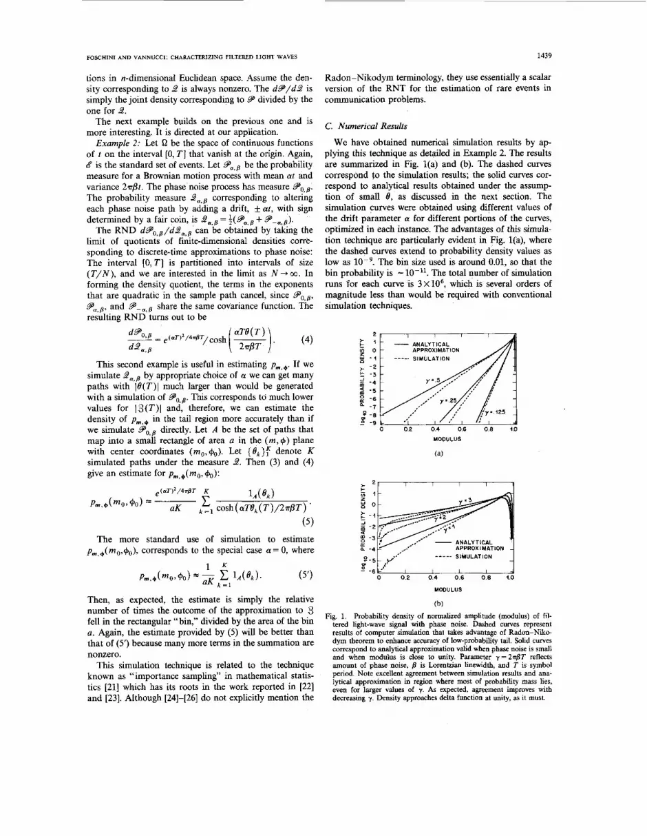
We have obtained numerical simulation results by ap- plying this technique as detailed in Example 2. The results are summarized in Fig. l(a) and (b). The dashed curves correspond to the simulation results; the solid curves correspond to analytical results obtained under the assumption of small 8, as discussed in the next section. The simulation curves were obtained using different values of the drift parameter a for different portions of the curves, optimized in each instance. The advantages of this simulation technique are particularly evident in Fig. l(a), where the dashed curves extend to probability density values as low as lop9. The bin size used is around 0.01, so that the bin probability is - lo-”. The total number of simulation runs for each curve is 3X106, which is several orders of magnitude less than would be required with conventional simulation techniques.

2

C ’ s o g - 4

> - 2 k -3 f - 4 2 - 5

$ -8

$ -6 -7

-0 -9

- ANALYTICAL - APPROXIMATION

0 0.2 0.4 0.6 0.8 1.0

t 2 P I I I I ’I

; - 1 -,____-e-- -..- 4 5 - /.. f - 2 __..*-- ..--;4 a T--.* ,,.-- I g -3 1 - ANALYTICAL

,.e’ APPROXIMATION -4 ----_ s WLAT ION : - 5 ,J’

H -6 -1. I I I I

0 0 2 0.4 0.6 0.8 1.0

MODULUS

(b) Fig. Probability density of normalized amplitude (moduluc, of fil-

t e d light-wave signal with phase noise. Dashed curves represent results of computer simulation that takes advantage of Radon-Niko- dym theorem to enhance accuracy of low-probability tail. Solid curves correspond to analytical approximation valid when phase noise is small and when modulus is close to Unity. Parameter y = 2 ~ / 3 T reflects amount of phase noise, /3 is Lorentzian linewidth, and T is symbol period. Note excellent agreement between simulation results and analytical approximation in region where most of probability mass lies, even for larger values of y. As expected, agreement improves with decreasing y. Density approaches delta function at Unity, as it must.

1440 IEEE TRANSACTIONS ON INFORMATION THEORY, VOL. 34, NO. 6 , NOVEMBER 1988

Note the excellent agreement between the simulation results and the analytical approximation over the region where most of the probability mass lies. This means that in many applications-those where the behavior far in the tail is not too important-the analytical approximation can be used in place of the actual simulation results [13].

For the purpose of computer simulation, we approximated the continuous-path Brownian process in terms of discrete random steps. The step size was progressively decreased (for each simulation run) to the point where any further decrease did not affect the results obtained. The latter results are the ones shown in the figures.

111. ANALYTICAL SOLUTION IN THE LIMIT OF SMALL PHASE NOISE, AND EXTENSIONS

A . Main Results

In this section we present, in the realm of small phase noise, the mgf of (8 ( T), (e( T)). This vector can be viewed as a three-dimensional vector since 8 ( T ) is complex. Both polar ( m ( T ) e ' @ ( T ) ) and rectangular ( r (T)+ j s ( T ) ) repre- sentations of 8 ( T ) are useful. We shall find the mgfs Mm,+,e(S, 17, S) and M,,s,e(S, v,{). Generalizing to include 8 is needed, as we shall see. The polar form is better matched to modulation processes (e.g., M m ( 5 ) = Mm,+, e((, 0,O) is of direct interest in analyzing amplitude shift keying (ASK)). The rectangular form is better suited to a couple of methods for continuing the mgf beyond the perturbation realm (Sections III-C and -D).

We use the notation sinhcx = sinhx/x, tanhcx = tanh x/x, cothcx = coth x/x to express the mgf s, and we define the parameter y 2rPT. As detailed in Appendix I, we find that, in the limit of small y , the mgf is represented as

M m , o , e ( S , q , S ) = e5Tsinhc-'/2(yTS)'/2

- exp [ (Y/2) [ (S + 1 7 a 2 t d c (YTS )'I2

+ ( q/2)2(cothc (~T5 /4 ) ' /~

so M,(O = M ~ , + , ~ ( S , O , O ) = etTsinhc-'/2(yTS)'/2

1"' ( 7 4 1

= etT fi ( k = i 1 + yST/(

where we have employed the well-known product formula for the sinh (see (A6a') in Appendix I). The mgf of the squared amplitude by itself is also of interest. It is given by

M ~ ~ ( E ) = etT2 ~ i n h c - ' / ~ ( 2 y ~ ) ' ' ~ ~

= fi ( 1 )'" (7b) k = i 1 + 2 ~ 5 T ~ / ( k r ) ~

The product representation shows that the mgf of m' ( I = 1,2) corresponds to an infinite sum of independent

gamma variates shifted to and reflected about T' ( 1 = 1,2). The location of the singularity (branch point) closest to 5 = 0 gives the tail exponent for the probability density function. Thus the decay exponent for the density of m is r 2 / y and for m2 it is r2/(2y). This predicted exponential decay for the density of m is evidenced numerically in Fig. Wa).

More generally, the bivariate mgf M,,,, +( 5 , ~ ) (obtained by setting { = 0 in (6)) can also be written as an infinite product by exploiting the identities (A6b') and (A6c'). As with (7a) and (7b), each factor turns out to be easy to invert.

The rectangular form of the three-variable mgf is somewhat more complicated than the polar form. It is

Mr,s,e(S, 17, {> = M,,,,+,e(S, VT , ~ ) * t a n h c ' / ~ (uTz)''~

. exp( -(yTS)tanhc(yTS)'/2

* ( Y/2) [ ( VT 1 (cothc ( Y Tt

- (YTS) -'> + (S/2) t d c ( YTS )1/2] 2). (8)

As already mentioned, the derivation of these mgf s appears in Appendix I. To obtain the corresponding pdf s, one can numerically calculate the inverse transforms of the expressions given in (6) and (8). However, for the simpler cases of (7a) and (7b), an expression for the associated probability distribution exists (see (A7e) and [17]). This expression was used to obtain the analytical approximation curves of Fig. l(a) and (b). In our application, the integrand is an exponential; however, the perturbation analysis that we have developed can be used in any application for which the integrand is a function (of 8 ( t ) ) with a local quadratic Maclaurin expansion.

B. Huygens' Principle for Filtered Light Waves with Phase Noise

Although the solution for small P T provided by (6), (7a), (7b), and (8) is useful in a number of applications [13], it is important to extend the result to the more general case of arbitrary BT. In this section we show how to build a general solution out of the T = O + solution.

dt for a given T which may not be small, we partition [0, TI into small equal segments of length T/n and then sum up the contributions from each segment. In carrying out this procedure, one must take care that the statistical dependencies among the different time subintervals are correctly accounted for. The technique whereby solutions "in the small" are patched to- gether to get solutions for larger T is known as Huygens' principle [27]. This is because the seventeenth-century physicist Christian Huygens applied this technique to the paradigm which involved light propagating in three-space (no filtering or phase noise).

In this subsection, the time flow of the mgf s comes into prominence. Consequently, we change our previous nota-

To characterize

EOSCHINI AND VANNUCCI: CHARACTERIZING FILTERED LIGHT WAVES 1441

tion to show explicitly dependence on the time parameter 7 > 0. Let p ( r , s; 7) denote the pdf of ( r ( T ) , ~(7)) and let p ( r , s, 8; T) denote the pdf of ( r ( T), s( T), e( 7)). We define a pair of mgf‘s

M([, T J ; 7) = d m d m e ( i r - n r ) p ( r , s; T ) drds (9)

and

(Note that m is not a trivariate mgf as we find it convenient not to transform the 8 variable.) We will also need the notation ( 5 , ~ ) ~ to convey that the vector ( [ , T J ) is rotated through an angle 8.

Write the identity

J d l T ’ ” e J o ( T ) dT = iT’neJe(T)d7

(11) e ~ [ o ( ~ ) - s ( T / n ) + e ( T / n ) l d7 . + jTZfl

LkT/n J,

Revise this identity to read

e J e ( T ) d7 = e / e ( T / n ) ( k - ’ ) T ’ n e J l e ( T + T / n ) - e ( T / n ) l d,,

+ /,”ne d7 (12)

and note that the two integrands on the right side of (12) are independent processes, when conditioned on the value of 8(T /n ) . Hence the two terms on the right side are conditionally independent random variables, and we can just multiply their conditional mgf‘s. The mgf of the second term is essentially given in (10) while that of the first term can be obtained from (9) through a rotation by the angle 8 ( T / n ) . Finally, an integration is required to remove conditionality on B(T/n) and we obtain

~ ( 5 , T J ; k ~ / n ) = lW M(( t , 77) e; ( k - 1) ~ / n ) 00

.m([,q; 6; T / H ) d e , k = 2 ,3 , - , n . (13)

Based on the results of Section III-A the asymptotic (large n ) form of the bootstrap m([, T J ; 8; T / n ) is known. In fact, upon fixing 5 and TJ the trivariate mgf M r , s , o ( & ~ , l ) as a function of 5 has the form of a Gaussian mgf. So m( ~ , T J , 8; O t ) is known in closed form.

In numerical studies one would repeat the k iteration for successively larger values of n until results stabilize. Furthermore, note that (13) is easily generalized to any filter with impulse response of length T. To generalize, simply approximate the filter response by functions that are constant on each (( k - l)T/n, k T / n ) interval.

IV. APPLICATIONS

The work presented up to this point is, essentially, a discussion of mathematical methods for evaluating the integral of (1). To appreciate the importance of that inte-

gral in communication problems, note that it is the starting point in the analysis of many types of receivers, as it represents the output of a linear filter with a rectangular impulse response. As such, the results presented here can be applied in a straightforward manner to analyze a “single filtering” receiver consisting of just a filter followed by a detector. The performance of such a receiver with on-off keying (OOK) modulation turns out to be rather poor even with relatively small amounts of phase noise [13].

A better receiver can be realized with “double filtering” and nonlinear detection. The accuracy and extensiveness of the results obtained in this paper allow a complete analysis of such a receiver, which is provided in [13]. The small-PT results derived in Section I11 are particularly useful in the analysis, as they greatly simplify the numerical calculations, while the inaccuracy introduced in the final results is found to be neghgible. The receiver turns out to have surprisingly good performance even in the presence of large amounts of phase noise, corresponding to a Lorentzian linewidth P comparable to the bit rate.

A receiver for binary differential phase-shft keying (DPSK) can be analyzed by assuming-without loss of generality-that the instantaneous phase 8( t) at the mid- point between two consecutive symbols is zero. At the output of the I F filter, the two received symbols being compared can thus be modeled as independent complex random variables defined by (1). A relevant generating function for DPSK studies is M,,,+((, TJ) = Mm,+,o([, T J , ~ ) . This function, along with M,,,(&TJ) is basic for performance analyses of amplitude- and phase-modulated signal constellations.

V. FOKKER-PLANCK METHODS

A substantially different approach to the solution con- sists of modeling the parameters of interest as a multidi- mensional Markov process. Specifically, with T being identified with the time parameter of the process, the three-dimensional stochastic process ( r ( t ) , s(t), e( t)) can be easily shown to be a Markov process.

The theory of continuous-path Markov processes is well developed [28]-[30]. In particular, the pdf p ( r , s, 8; t) can be shown to satisfy the following partial differential equation (PDE) (see Appendix 11).

a 2 a a a a e z p a r

(y/2)- -cosB-p-sin8-p=-p. a s at (14)

Equation (14) is called the Fokker-Planck (FP) equation. Since we are only interested in the joint statistics of r ( t )

and s ( t ) , it would be helpful if we could write an equivalent equation without the 8 variable. However, the two-dimensional process ( r ( t), s( t ) ) is not Markov; consequently, we cannot obtain such an equation in a straightforward manner. As detailed in Appendix 11, we can achieve the desired simplification by defining a new Markov process that is statistically identical to ( r ( t ), s ( t ) ,O( t ) ) and by an appropriate choice of initial conditions. With the approach in Appendix 11, the 8 variable

1442 IEEE TRANSACTIONS ON INFORMATION THEORY, VOL. 34, NO. 6 , NOVEMBER 1988

disappears and the resulting equation, in polar coordinates, is

a = a sin+ a COS+ a (y/2) - - cos + - p + - -p + - p = - p

a + 2 P a m m a+ m a t

(15)

l i m p ( m , + ; t ) =8 (m,+) . (16) with initial conditions

1 4 0

A numerical solution of (15) appears to be within the capabilities of present-day general-purpose PDE algorithms based on the transient tensor Galerlun approach [31]. The difficulty that might arise due to the singularity in (16) can be avoided by using the approximate solution presented in Section I11 as the initial condition.

We offer next an FP solution approach that is tailored to the dynamical structure represented by (15). Observe that, assuming arbitrary placement of an initial unit probability mass, the FP is trivial to solve numerically if we alter the left side of (15) either to omit the second derivative term or to contain only the second derivative term. This is tantamount to realizing the Markov process corresponding to (15) in terms of two simpler Markov processes, and so a numerical solution corresponding to the Trotter product [32], [33] represents an attractive option.

The FP method, as discussed here and in Appendix 11, can be generalized to handle filters with an arbitrary impulse response. In the authors' view, it is a promising method for obtaining a solution in those regimes where the simulation approach is inadequate, i.e., for very low bit error rates and high values of PT. Under the assumption of a delta-function initial density, the results in Section 111-A provide the mgfs of the exact solutions to the approximate FP equations obtained from (14) and (15) by replacing the sine and cosine coefficients with their linear and quadratic Maclaurin expansions.

VI. DISCUSSION AND CONCLUSION

We have developed three theoretical approaches that allow, for the first time, a statistical characterization of filtered lightwave signals impaired by phase noise. The special case of greatest immediacy to us requires determining the statistics of 131 for ASK and FSK studies [13]. Numerical results for this case served to illustrate both the perturbation theory method and the simulation method using the Radon-Nikodym derivative (see Fig. l(a) and (b).) The two sets of curves generated by these methods are in excellent agreement. The analytical probability curves more accurately approximate the RND curves as y = 27$T decreases.

The RND simulation method is a powerful technique. For example, other filterings of a lightwave signal with phase noise, besides a simple integrator, could be easily characterized using the RND approach. However, the method is limited to producing graphs or tables and, although it enhances the ability to simulate the tail by several orders of magnitude, it is still a computationally intensive method. (A grand total of over lo7 Brownian motion sample paths were used to generate Fig. l(a) and

(b)). In contrast, the perturbation method gives closed-form expressions in terms of elementary functions (at least for the moment generating function). The inversion of M,,,([) can be performed in terms of a Bessel function series. More generally, the mgfs of Section I11 can be inverted numerically by employing FFT algorithms.

The Fokker-Planck (FP) method has relevance in cases where the complex quantity 3, and not just its magnitude, needs to be characterized. For example, the joint pdf P , , , ~ is of interest for optical systems that employ QAM and PSK modulations; and the joint pdf P , , , ~ , ~ can be used in analyzing DPSK systems. The FP methodology represents a promising approach for obtaining accurate solutions for pm,* for arbitrary y. To obtain P,, ,~, the FP method of continuation is superior to the Huygens principle of Sec- tion 111-B in that only two space variables, rather than three, are needed. However, we recognize that FFT routines tend to be generally available, while TT'G routines may not be readily accessible to all investigators.

ACKNOWLEDGMENT

Upon learning of our early results on the problem of characterizing filtered phase noise through the RND and perturbation approaches, L. A. Shepp alerted us to [17], [21], and [36]. We also would like to thank N. L. Schryer for helpful discussions.

APPENDIX I DERIVATION OF MGF's FOR y Smu

This Appendix is concerned with deriving (6), (7a), (7b), and '

(8).

A . Notation

We record some notation that will prove convenient. For integrals, sums, and products we use the convention that I, Z, and l7, written without limits, mean f , E?, and l7y. We suppress differentials when writing integrals except for white noise integrals3 like /:tde(t).

We also need the following infinite matrices: Z identity matrix, J D diagonal matrix with hth diagonal entry (nr)- ' .

matrix with one in each entry,

Let Q be a symmetric nonnegative definite matrix { q,,,, }, ', define

llQ11*

Q112 nonnegative definite square root, IQ1

1;

trace of Q'Q, where the prime means transpose and trace means sum of the diagonal elements,

limit of the determinants of the upper left hand N X N blocks.

Let x and y be square summable infinite dimensional vectors { X n l n L ~ and {Yfl l">l9 define

(xt r> = CXf lYf l

(x, Y > N = C X f l Y n

llxIl2 = (x, x).

N

3~ excellent treatment of white noise integrals is given in 1301.


Finally, we need the odd term indicator sequence 1, =

1 ,0 ,1 ,0 ,1 ,0 ,~~~

B. Perturbation Representation of 8 for Small y

Expanding the exponential in a power series gives

We want to express 8 in terms of a normalized Brownian process so that the dependence on the parameter y is more clearly revealed. To develop such an expression, begin with the state space normalization e&) e Y-i/2e(t). The process e l ( t ) is normalized in the sense that E [ e : ( T ) ] = l (this follows from the definition of the parameter y given in Section I-A). So we write

Next normalize the time axis with T = ~ / T replacing t . Let + ( T ) =el(?) = O1(TT) so that E[+2(1)] = E[e:(T)] =l. In terms of the standardized Brownian motion process +( T ) , we have

L'e;( t ) dt = T / v ( T ) dT.

Therefore,

Neglecting terms that are o ( y ) , we have

C. Representing Variates in Term of Gaussian Sequences

To get to the crux of our analysis without encumbrance, we introduce a list of normalized canonical variates. We see from (A4a)-(A4f) that they are related by multiplicative and/or addi- tive constants to the corresponding variates shown to the right:

41f JI does not appear under an integral, then #(1) is intended

If one can find the Laplace transform of the joint density of a subset of these canonical variates, then for the corresponding subset of unnormalized variates one can immediately express the mgf. By first determining Laplace transforms, we will obtain M,,,z,+,@, Mm.+,@, and M *,*, e . To get the Laplace transforms, it is expeditious to express the normalized variates in an infinite dimensional system of uncorrelated Gaussian coordinates.

Each of the two sequences 1, fi COS m, fi cos2a7, . . . and f i s i n n ~ , fisin2a7, . . . is a complete set of orthonormal functions for square-integrable functions on [0,1]. We use this to express the listed functionals of + (A5a)-(A5d) in terms of the independent identically distributed (i.i.d.) standard (i.e., normalized) Gaussian variates { x , Afijsin nmd+)?=, .

To express /+2 - ( j+)2, use Parseval's theorem to write

and then integrate by parts to get

= (x, D'x) .

To express /+, first integrate by parts:

/+ = + - / T c i + =/( I - ci+

Next, express (1 - T ) in a Fourier sine series. The nth Fourier coefficient is

Similarly, for + = j d + to be expressed in terms of the x , , we must expand the function 1 in a Fourier sine series. The nth Fourier coefficient is

Hence, q =C(2fi/na) loxn. It remains to express /#'. This is readily accomplished since

The second term can be expressed as

so that

D. Laplace Transforms

In this section, we find the Laplace transforms related to Mm3+,e and For each of (m,&fJ) and ( r ,s , fJ ) , we first develop the transform in terms of operators on the sequence space { x,, }r-l. Then we reduce the operator form to a form involving elementary functions.

1444 IEEE TRANSACTIONS ON INFORMATION THEORY, VOL. 34, NO. 6, NOVEMBER 1988

I ) Laplace Transform Related to (m, +, 6): a) operator form: The function

is the Laplace transform of the joint of /+2 - ( /+)2, /+, and +, which are variates that are simply related to m2 (or m), +, and 8.

Using the representation developed in Appendix I-C we can write L ( 6 , 1793)

Substituting z = jw, we get other useful versions of these identities. It is also useful to record the small w asymptotes:

n(1+&j =sinhcw-l (A6a’)

1 1 (A6b’) 8

1 ~ ( ( k ~ ) ~ + w ~ ) - ~ = - ( c o t h c w - w ~ ~ ) -1/6. (A~c’)

2 Now we can express IZ+2[O21-’/’ and ilKZ+2502)-’/2all and hence L(5, 7, 6) in closed form.

c ((2k -1)’d + w2)- = -tanhc w - 1/8

First of all we employ (A6a’) to get

Let a be the vector whose nth component is f i ( q + 231,)/nn. 25 -I/’ Therefore, I I + 2 6 0 2 l - ” = ( n ( l + ~ ) ) - -

L ( 5 , 9 , 3) The norm splits into two sums, i.e.,

= lim (2?r)-N/2J-m /m 1 1 ,ll(Z + 2502) - 1/2a(1’ N + m m --m

- ( ( I + 2602) -l l2a,( I + 2 5 ~ ’ ) - ~ / ~ a ) , 2 tanhJzF

2@ ,

( q +23)’C ((2k - 1)’d + (a)’) - l = (4 + 3) ~

where we have taken advantage of the fact that all the matrices are symmetric.

Address the determination of L with the fact in mind that the multivariate Gaussian with mean -(Z+2[D2)-’a and variance-covariance matrix (1+250~)-’ must integrate to one. We get immediately’

L( 6, q , t ) = 11 + 25021-1/2 exp ( 5 II( I + 2502) -1/2al12).

Note that to interpret the matrix (Z+25O2)-’ as a variance- covariance matrix it must be positive definite. This is certainly true for values of 6 that are real and positive. Through analytic continuation, the above expression for L([,q,{) can then be extended to complex values of 6.

Each of IZ+2[O21-’/’ and ll(Z+26D2)-’/’a11’ have closed- form expression in terms of elementary functions, as we now show.

b) A closed-form expression for 4.$,7,3): To proceed, we require the following identities which can be found in [37] and [38]:

1

n( 1- &) = (sinz)/z = sincz (A6a)

For the second sum, use (A6c’) to get

q2c ( (2n4’ + (GI2) - l

= ( 72/41 c ( ( 4’ + (fl )2) -

so

The univariate marginals are

1 8 8

2 1 2 (A6c) Gaussian variates as does the joint mgf:

(A7b) 1 1

( ( 2 k - 1)’d - z’) - = -( tanz)/z=- tancz (A6b) L(O,v,O) =exp(7?/6)

E( z’ - k 2 d - l =-((cot 1 z)/z - z-2) ~ ( o , o , S ) =exp(I2/2). (‘474 For the last two marginals, we employed the small-5 asymptotes listed in (A6a’)-(A6c’). The last two marginals correspond to =-(cotcz-2-2).

’The authors learned this trick from [34] and [35]. These two studies in mathematical statistics are motivated by soil treatment experiments. See also [36] for analysis of quadratic forms involving normal random variables. The procedure to calculate the inverse of the first marginal (A7a)

FOSCHIN AND VANNUCCI: CHARACTENZING FILTERED LIGHT WAVES 1445

is given in detail in [17]. The result is expressed as 1 -L( [ ,O,O) = ime-'"P( x) dx 2

where

.(4n + l)"* exp [ - (4n + 1)2/( 16x)]

.~'/4((4n + 1)2/(16x)). (A74 The expression for the binomial coefficient is

and KIl4(x) is the modified Bessel function. P(x) is a probability distribution [17]; the corresponding probability density is the inverse of L([,O,O).

To obtain the moment generating function for the vector (m2,+ ,0) , we refer to (A4a), (A4b), and (A4d). There- fore, substitute the argument (yT26, - y1l2q, - y'/2P)6in place of ( 5 , 7,s) in the formula for L ( [ , q, 5 ) and multiply L ( y T 2 [ , - y1l2q, - Y'/~{), by eET2 to account for shift. We get

Mm2,+. B ( 5 9

The univariate Mm2(5) A M,,,z([,O,O) is of interest. It is given by

~ , , , 2 ( 0 = etT2 sinhc-'/2(2y[)'/*T. (A9) Equation (A9) is labeled (7b) in the main text. With the appropriate substitutions, (A7e) provides the corresponding probability distribution.

For the vector ( m , +, e), proceed as above except using (A4b) in place of (A4a). The corresponding mgf will be the same as (A8) with y replaced by y/2 and T replaced by T'/'.

2) Loplace Transform Related to (r, s, e): a) Operator form: The Laplace transform of the joint of the

variates 14, 4) is

L ( t , 7, S) = E [ exp ( - 6/42 - 714 - 41 The three variates are simply related to ( r , s, e). In terms of the expansions of Appendix I-C,

L( I , 11, SI = E [ exp( (x, D( I + 2.1) OX)[)

-P( - { Lax./(..)} 7)

-exP( - { C2d5xnl0/(n77)}5)].

It is notationally efficient to introduce the matrix G = Z+25D( 1 + 2 J ) B

= 4 5 D [ ( D-2/4[ + 1/2) + J ] D

and the vector b whose generic entry is - ( q +2{1,)fi/(nn). SO,

L ( [ , ~ , s ) = lim (2n)-N/2/-m jm N - w m - m

We now follow the same technique that we used earlier. We rewrite the exponent term as

( 9 Gx)N - 2( 9 .)N

= ((x-G-'b),G(x-G-'b)), - (G- ' /2b ,G-1/2b)N

where we have exploited the fact that G is a symmetric matrix. We see that for real positive

G - I = ( 4 [ ) - ' D - ' [ ( D - * / ( 4 [ ) + 1 / 2 ) + J ] -ID-' (All)

is positive definite and can be interpreted as the reciprocal variance-covariance matrix of a multivariate Gaussian. Interpret C- ' b as the Gaussian mean. Therefore,

the matrix

L ( t , q , ~ ) = IG1-'/2exp( ~ ~ ~ ~ - 1 ~ 2 ~ ~ ~ * ) . 1

b) A closed-form expression for U[, q, S): We compute 1GI- 'I2 and 11G-1/2b112 in turn. In preparation for doing so, we record a couple of properties possessed by any diagonal and nonsingular matrix A :

1 A + J I = ( I I a n n ) ( l + C a ~ ~ ) ( ~ 1 2 a )

( A - + J ) ' = A* - ( 1 + IIA 11') ' A2JA2. (A12b)

The first is an elementary exercise, and the second follows from direct verification.

For (Cl we use (A12a) and get

= n( 1 + (22/( nn,')) .( 1 + 4 2 1 ((nn)*+25) - I )

= ( s i n h G / f i ) ( 1 +22( cothJZT/@ - 1/26))

= cosh@.

so, = ~osh- ' /~(2[) ' /~.

The expression for llG-'/*b11* is more complicated. Make the identification

A - * = ( D - 2 +2[1)/(4[)

and use (A12b) and (All) to write

G - ' = (45)-'D-'[ A2 - ( l+ llA(12)-1A2.T,42] D-'

Therefore,

(b , G- lb) = (44) D - m - l b )

- [ ( 4 [ ) ( 1 + ll,411')] - ' ( b , D-'A2.TA2D-'b). (A13)


Next, we compute each of these two quadratic forms. The first

( 4 t ) ~ ' C ( n ~ a , ~ ~ ) ~ = 2 C ( v + ~ 1 0 ) ~ / ( 2 . i + ( n ~ ) ~ )

is a diagonal form

= 2( c v2/( ( fi)' + 4( n r I 2 )

+ C(1) +w2

= 2( ( ;)2( (m)2+(n42)j1

+L(21{)2tanhc@) 2 2

+ - + { tanhcfi. ( i l2 The second term in (A13) can be viewed as a quadratic form in

-&(? +231,)(4t) [ 2.i + (nn)2] -'.

(AZD-'b,JA2D-'b) =2[4Ex(?+2J10)/[2E+(nn)2]]2

the vector A2D-'b which has for its nth component

Thus

= 32P( x 1 ) / [ ( i % ) 2 + ( n 4 2 ]

+~Z{/[(+Z)~+ [(2n - 1 ) 7 r 1 2 ] ) ~

=32t2( ;[cothcfi-(2[)-']

The coefficient (1 + ~ ~ A ~ ~ 2 ) - ' also needs to be evaluated. Thus

(1 + IIA 11') -1 = [ 1 + 4 1 ~ (JZT)' + ( n 7r)'l

- '

= [1+2t(cothcfi-(2t)- ')] -' = [2.icothc@gJ -'= tanhcfi.

Consequently, we obtain the contribution to (A13) represented

- [(4[)(1+ llA1I2)] - ' (b , D-'A2JA2D-'b) by

= -(4.i)-'[email protected]

= -(2*)tanhcJZI[ 1)(cothcJZI-(2~)-') +

In summary,

-(21) tanhcfi[ 1)(cothc@-(2.i)-')

+ i'""fi]'). s

from which (8) follows easily. The marginal

1 1 ) L(0,1) 9 0 = exP y [ ( y + s)2 + f ( ;) '1

agrees with (A7d), as it must.

APPENDIX I1

A . The Basic Fokker- PIanck Equation for Filtered Light Waves with Phase Noise

It is well-known that the Brownian motion process 8 ( t ) is a continuous-path Markov process. It is evident that the three- dimensional process q( t ) = ( r ( t ) , s( t ) , e( t ) ) is also Markov. Un- der extremely general conditions a continuous-path Markov process can be entirely characterized by its first- and second-order differential dynamics [28]-[30]. Specifically, for the process at hand, the differential-mean vector can be easily found to be

#E(?) =(cos(?, sin8,O) (B1)

and the differential dispersion matrix is simply

D ( i j ) = 0 0 0 . 032) [: : 3 From these we can directly obtain the PDE:

a a a 2 a a e 2 p ar as at

(y/2)- - c o s 8 - p - s i n 8 - p = - p (B3)

where p(r , s ,B; t ) is the joint pdf for r ( t ) , s ( t ) , 8 ( t ) . This equation is known as the Fokker-Planck equation for this Markov process. Since 8 is an angle, we shall seek a solution for (B3) which is a periodic function of 8 with period 27r, and which satisfies the normalization condition

and the initial condition

limp( r , s , 8 ; t ) = 6( r , s , B ) . (B5) t - 0

The latter condition can be easily obtained from (1) by letting T-, 0.


B. Analytical Approach to Solving the FP Equation

A triple Fourier transform on ( t , r , s ) converts (B3) to a standard ordinary differential equation-a Mathieu equation.(‘ This approach has the attraction of producing a closed-form solution in terms of known functions and a triple inverse Fourier transform. However, the analysis seemed to us, after a prelimi- nary look, to be comparatively formidable. Indeed, even after extensive algebraic manipulation, the amount of computation still required to obtain numerical results for p ( r , s, 8; t ) appeared large. The approach described next was adopted to circumvent this computational complexity.

C. Suppressing the 8 Dimension in the FP Equation

In many applications, the solution to (B3) provides us with more information than we need. Often, we are only interested in the joint statistics of r ( t ) and s( t ) (or, in polar coordinates, m( t ) and + ( t ) ; we shall use polar coordinates in the rest of this section). If we could find an equation involving just these two variables, it would make a numerical solution available [31]. Unfortunately, we easily see that a simple elimination of 8 ( t ) yields a two-dimensional stochastic process ( m ( t ) , +( t ) ) that is not Markov; so that a straightfoxward derivation of an FP equation for p ( m , +; t ) is precluded.

To achieve the desired equation in two state variables, we use a definition of 3( t ) slightly different from (1) but statistically equivalent to it:

The equivalence stems from the fact that integrals do not depend on the time sense of the integrand. With the new definition, the two-dimensional stochastic process ( m ( t ) , +( t ) ) is statistically identical to the one obtained from the old definition and, of course, is still not Markov. However, the full three-dimensional process ( m ( t ) , +( t ) , e( t ) ) under the new definition is not statistically identical to what it was under the old definition, but it is still Markov.

In the introduction, we defined 8 ( t ) as a continuous-path Brownian motion, which is usually understood to start at zero so that O(0) = 0. More generally, one can assume an arbitrary starting point 8(0) = e,, which is equivalent to simply offsetting the Brownian motion by a fixed amount 8,. It is easy to see that the new definition provided by (B6) makes m ( t ) and + ( t ) independent of the value of the starting point 8,. This allows us some freedom in the choice of the initial conditions for p ( m , + , 8; t ) . In particular, we can assume that 0, is uniformly distributed in the interval [0,27~).

One immediate consequence of this choice of initial conditions is that the marginal pdf of e( t ) will remain uniform for all values of t , i.e.,

1 p ( 8 ; t ) = l m d m l n d+p(m,+,O;t)=--. (B7)

0 -71 2 n

Another somewhat subtler consequence is that m ( t ) and + ( t ) become independent of 8 ( t ) . This is because the integral in (B6) only involves increments of 8 ( t ) which, when O(0) is uniformly

[37], [39], [40] for treatments of Mathieu functions. The Feynman-Kac approach [29], [41] can also be shown to lead to a Mathieu equation.

distributed, are independent of e( t ) . As a result,

p ( m,+,8; t ) = p ( m , + ; t ) p ( e ; t ) = p ( m , + ; t)/(2n) (B8) and any terms with 8 derivatives in the FP equation will vanish.

Next, compute differential means and dispersions for m( t ) , +( t ) , e( t ) ) and compose the FP equation to obtain

a 2 a sin+ a cos+ 8

a + Z p a m m a+ m a t

l imp(m,+;t) = a ( m , + ) .

In this way the 8 variable is eliminated and we have found the PDE in two state variables that we sought.

( y/2) ~ - COS+-^ + ~ - p + - p - p , (B9)

with initial condition

1 - 0

REFERENCES

Y. Yamamoto and T. Kimura, “Coherent optical fiber transmission systems,’’ IEEE J . Quantum Electron., vol. QE-17, pp. 919-935, June 1981. T. Okoshi, K. Emma, K. Kikuchi, and R. Th. Kersten, “Computa- tion of bit-error rate of various heterodyne and coherent-type optical communication schemes,” J . Opt. Commun., vol. 2, no. 3, pp. 89-96, Sept. 1981. T. Okoshi, “Heterodyne and coherent optical fiber communications: Recent progress,” IEEE Trans. Microwave Theory Tech., vol.

F. Favre and D. Le Guen, “Effect of semiconductor laser phase noise on BER performance in an optical DPSK heterodyne-type experiment,” Electron. Lett., vol. 18, pp. 964-965, Oct. 28, 1982. S . Saito, Y . Yamamoto, and T. Kimura, “S,” and error rate evaluation for an optical FSK-heterodyne detection system using semiconductor lasers,” IEEE J . Quantum Electron., vol. QE-19, pp. 180-193, Feb. 1983. M. Shikada, M. Emura, and K. Minemura, “High-sensitivity optical PSK heterodyne differential detection simulation experiment,” presented at the 4th Int. Conf. Integrated Optics and Optical Fiber Communications, Tokyo, Japan, June 1983, paper 3OC3-4. M. Tamburrini, P. Spano, and S . Piazzolla, “Influence of semiconductor-laser phase noise on coherent optical communication systems,” Opt. Lett., vol. 8, pp. 174-176, Mar. 1983. G. Nicholson, “Probability of error for optical heterodyne DPSK system with quantum phase noise,” Electron. Lett., vol. 20, pp. 1005-1007, Nov. 22, 1984. K. Kikuch, T. Okoshi, M. Nagamatsu, and N. Henmi, “Degrada- tion of bit-error rate in coherent optical communications due to spectral spread of the transmitter and local oscillator,” J . Light- wave Techno/., vol. LT-2, no. 6, pp. 1024-1033, Dec. 1984. G. Jacobsen and I. Garret, “Error-rate floor in optical ASK heterodyne systems caused by nonzero (semiconductor) laser linewidth,” Electron. Lett., vol. 21, no. 7, pp. 268-270, Mar. 28, 1985. L. G. Kazovsky, “Impact of laser phase noise on optical heterodyne communication systems,” J . Optical Commun., vol. 7, pp. 66-78, June 1986. J. Salz, “Coherent lightwave communications,” A T&T Tech. J . , vol. 64, no. 10, pp. 2153-2209, Dec. 1985. G. J. Foschni, L. J. Greenstein, and G. Vannucci, “Noncoherent detection of coherent lightwave signals corrupted by phase noise,” IEEE Trans. Commun., vol. 36, pp. 306-314, Mar. 1988. N. V. Smirnov, “Sur la distribution de w2,” C. R. Acad. Sci. Paris, vol. 202, p. 449, 1936. -, “On the distribution of the w2 criterion,” Rec. Math. (Mat . Sbornik) ( N S ) , vol. 2, pp. 973-993, 1937. R. von Mises, “Differentiable statistical functions,” Ann. Math. Statist., vol. 18, pp. 309-343, 1947. T. W. Anderson and D. A. Darling, “Asymptotic theory of certain goodness of fit criteria based on stochastic processes,” Ann. Math. Statist., vol. 23, pp. 191-192, 1952. Y . K. Park, S. W. Granlund, C. Y. Kuo, M. Dixon, T. W. Cline, R. W. Smith, N. K. Dutta, and G. Vannucci, “Crosstalk penalty in

MTT-30, pp. 1138-1148, Aug. 1982.


a two-channel ASK heterodyne detection system with non-negligi- ble laser linewidth,” Electron. Lett., vol. 23, no. 24, pp. 1291-1293, Nov. 19, 1987. J. F. C. Kingman and S . J. Taylor, Introduction to Measure and Probability. Cambridge, England: Cambridge Univ. Press, 1966. L. A. Shepp, “ Radon-Nikodym derivatives of Gaussian measures,” Ann. Math. Statist., vol. 37, pp. 321-354, 1966. D. Siegmund, “Importance sampling in the Monte Carlo study of sequential tests,” Ann. Statist., vol. 4, no. 4, pp. 673-684, July 1976. G. Goertzel, “Quota sampling ,and importance functions,” U.S. Dept. Energy, Oak Ridge, TN, AECD-2793, 1949. G. Goertzel and M. H. Kalos, “Monte Carlo methods in transport problems,” Progr. Nucl. Energy, vol. 2, pp. 315-369, 1958. P. Balaban, “Statistical evaluation of the error rate of the fiber-guide repeater using importance sampling,” Bell Syst. Tech. J. , vol. 55, no. 6, pp. 745-766, July-Aug. 1976. M. C. Jeruchim, “Techniques for estimating the bit error rate in the simulation of digital communication systems,” IEEE J . Sel. Areas Commun., vol. SAC-2, no. 1, pp. 153-170, Jan. 1984. K. S. Shanmugam and P. Balaban, “A modified Monte-Carlo simulation technique for the evaluation of error rate in digital communication systems,” IEEE Trans. Commun., vol. COM-28,

P. L. Butzer and H. Berens, Semi-Groups of Operators and Approxi- mation. New York: Springer-Verlag, 1967. E. Wong, Stochastic Processes in Information and Dynamical Sys- rems. New York: McGraw-Hill, 1971. S . Karlin and H. M. Tavlor. A Second Course in Stochastic Pro-

pp. 1916-1924, NOV. 1980.

~ 9 1 , ,

cerses. L. Amold, Stochastic Differential Equations. New York: Wiley- Interscience, 1974. N. L. Schryer and L. Kaufman, “TTGR, a package for solving partial differential equations in two state variables,” AT&T Bell Labs. Comput. Sci. Tech. Rep. N. 135, 1985. M. Reed and B. Simon, Methodr of Modern Mathematical Physics, vol. 11. New York: Academic, 1975, p. 245. W. Press, B. Flannery, S. Teukolsky, and W. Vetterling, Numerical Recipes. New York: Cambridge Univ. Press, 1986, sec. 17.6. W. G. Cochran, “The distribution of quadratic forms in a normal system with applications to the analysis of variance,” Proc. Cam- bridge Phil. Soc., vol. 30, pt. 11, pp. 178-191, 1934. J. Wishart and M. S . Bartlett, “The generalized product moment distribution in a normal system,” Proc. Cambridge Phil. Soc., vol.

J. Hoffmann-Jorgensen, L. A. Shepp, and R. M. Dudley, “On the lower tail of Gaussian seminorms,” Ann. Probab., vol. 7, no. 2, pp.

M. Abramowitz and I. A. Stegun, Handbook of Mathematical Functions. New York: Dover, 1970. E. C. Titchmarsh, The Theory of Functions. New York: Oxford Univ. Press, 1968. E. L. Ince, Ordinary Differential Equations. New York: Dover,

E. T. Whittaker and G. N. Watson, A Course of Modern Analysis. New York: Cambridge Univ. Press, 1963, pp. 404-428. K. It0 and H. P. McKean, Diffusion Processes and their Sample Paths. New York: Academic, 1965, p. 54.

New York: Academic, 1981, ch. 15.

29, pp. 260-270, 1937.

319-342, 1979.

1956, pp. 175-178.

characterizing filtered light waves corrupted by phase noise

Documents