characterizing chemical cleaners used in removing varnish in
TRANSCRIPT
UNIVERSITY OF CALIFORNIA, MERCED
CHARACTERIZING CHEMICAL CLEANERS USED INREMOVING VARNISH IN GAS TURBINE ENGINES
by
Duval A. Johnson
A disertation submitted in partial satisfaction of the
requirements for the degree of
Doctor of Philosophy
in
Mechanical Engineering
Committee in charge:Professor Ashlie Martini, Advisor
Professor Gerardo DiazProfessor Po-Ya Abel Chuang
Dr. Zhen Zhou
c©2018 Duval A. Johnson

c©2018 Duval A. Johnson
All rights are reserved.
The disertation of Duval A. Johnson is approved:
Ashlie Martini, Advisor Date
Gerardo Diaz Date
Po-Ya Abel Chuang Date
Zhen Zhou Date
University of California, Merced
c©2018 Duval A. Johnson

This dissertation is dedicated to the people I cherish most in my life.My children have become a source of inspiration and motivation forme throughout my academic life. As a man ages, thoughts of legacyand contribution fill his mind. I submit this work as motivation forthem to achieve great things and to gain an understanding of thevaluable contributions they can make to the scientific communityand society. My wife, Xiaoli, who also obtained her Ph.D. from
Professor Ashlie Martini, is an incredible woman who supports ourfamily and fills the role of taxi, chef, tutor and so much more. My
mother was constantly available to help her grandchildren in anywayneeded. This wouldn’t have been possible without the combinedcontribution of my family. Reach for the stars and never give up.
i
CURRICULUM VITAE
EDUCATION
• B.S. in Mechanical Engineering, University of California, Merced, 2014.
WORK HISTORY
• 2018 Mechanical Engineer II and Tribologist, Jet Propulsion Laboratory, Pasadena,CA
• 2018 Teaching Assistant, Statics and Dynamics (ENGR 057), University ofCalifornia, Merced, CA
• 2017 Graduate Student Researcher, Martini Research Group, University ofCalifornia, Merced, CA
• 2016 Lecturer, Statics and Dynamics (ENGR 057), University of California,Merced, CA
• 2015 Lecturer, Statics and Dynamics (ENGR 057), University of California,Merced, CA
• 2015 Teaching Assistant, Capstone Design, University of California, Merced,CA
• 2014 Teaching Assistant, Statics and Dynamics (ENGR 057), University ofCalifornia, Merced, CA
• 2014 Undergraduate Reader, Statics and Dynamics (ENGR 057), Universityof California, Merced, CA
• 2014 Lead Transmission Specialist, AAMCO Transmissions, Merced, CA
• 1991-1018 CEO and Founder, DJ Repair and Fabrication, Merced, CA
• 1986-1988 Medical Specialist, United States Army
HONORS AND AWARDS
ii
• 2017-2018 Graduate Deans Dissertation Fellowship, University of California,Merced
• 2015-2016 Graduate Deans Dissertation Fellowship, University of California,Merced
• 2015 Bobcat Fellowship Award, University of California, Merced
• 2014-2015 School of Engineering Dean’s Travel Award, University of Califor-nia, Merced
• 2014 Outstanding Undergraduate Award, University of California, Merced
• 2013 Mechanical Engineering Graduate Fellowship Award, University of Cal-ifornia, Merced
• 2012 Graduate Division General Fellowship, University of California, Merced
PUBLICATIONS
1. Duval Johnson, Characterizing Chemical Cleaners Used in Removing Var-nish in Gas Turbine Engines, Thesis, University of California, Merced, (2018).
2. Duval Johnson, Enrique Dominguez, Elizabeth Montalvo, Zhen Zhou,Ashlie Martini, Quantifying Varnish Removal Using Chemical Flushes, Tri-bology Transactions, (2018).
3. Paul Michael, Mercy Cheekolu, Pawan Panwar, Mark Devlin, RobDavidson, Duval Johnson, Ashlie Martini, Temporary and PermanentViscosity Loss Correlated to Hydraulic System Performance, Tribology Trans-actions, (2018).
4. Duval Johnson, Simulation and Analysis of a Fractionally Controlled ActiveSuspension System Using Quarter Car Model, ASME, (2015).
iii
TABLE OF CONTENTS
CURRICULUM VITAE . . . . . . . . . . . . . . . . . . . . . . . . . . . . iiLIST OF FIGURES . . . . . . . . . . . . . . . . . . . . . . . . . . . . . . . xLIST OF TABLES . . . . . . . . . . . . . . . . . . . . . . . . . . . . . . . . xviiiACKNOWLEDGEMENTS . . . . . . . . . . . . . . . . . . . . . . . . . . xxiABSTRACT . . . . . . . . . . . . . . . . . . . . . . . . . . . . . . . . . . . xxii
Chapter
1 INTRODUCTION . . . . . . . . . . . . . . . . . . . . . . . . . . . . . . 1
1.1 Lubrication History . . . . . . . . . . . . . . . . . . . . . . . . . . . . 11.2 Lubrication Basics . . . . . . . . . . . . . . . . . . . . . . . . . . . . 4
1.2.1 Friction . . . . . . . . . . . . . . . . . . . . . . . . . . . . . . 41.2.2 Mechanisms of Wear . . . . . . . . . . . . . . . . . . . . . . . 6
1.2.2.1 Abrasive Wear . . . . . . . . . . . . . . . . . . . . . 71.2.2.2 Adhesive Wear . . . . . . . . . . . . . . . . . . . . . 91.2.2.3 Contact Fatigue . . . . . . . . . . . . . . . . . . . . 91.2.2.4 Corrosive Wear . . . . . . . . . . . . . . . . . . . . . 10
1.2.3 Surface Types . . . . . . . . . . . . . . . . . . . . . . . . . . . 101.2.4 Lubrication Regimes . . . . . . . . . . . . . . . . . . . . . . . 111.2.5 Viscosity Shear Rate Dependence . . . . . . . . . . . . . . . . 131.2.6 Viscosity Temperature Dependence . . . . . . . . . . . . . . . 141.2.7 Viscosity Pressure Dependence . . . . . . . . . . . . . . . . . 15
iv
1.2.8 Summary . . . . . . . . . . . . . . . . . . . . . . . . . . . . . 16
1.3 Lubricants . . . . . . . . . . . . . . . . . . . . . . . . . . . . . . . . . 17
1.3.1 American Petroleum Institute Base Stocks . . . . . . . . . . . 17
1.3.1.1 Group I . . . . . . . . . . . . . . . . . . . . . . . . . 171.3.1.2 Group II . . . . . . . . . . . . . . . . . . . . . . . . . 181.3.1.3 Group III . . . . . . . . . . . . . . . . . . . . . . . . 181.3.1.4 Group IV . . . . . . . . . . . . . . . . . . . . . . . . 191.3.1.5 Group V . . . . . . . . . . . . . . . . . . . . . . . . . 191.3.1.6 Group II+ and III+ . . . . . . . . . . . . . . . . . . 19
1.3.2 Base Stock Application . . . . . . . . . . . . . . . . . . . . . . 201.3.3 Crude Oil . . . . . . . . . . . . . . . . . . . . . . . . . . . . . 21
1.3.3.1 Chemical Composition . . . . . . . . . . . . . . . . . 211.3.3.2 Hydrocarbons . . . . . . . . . . . . . . . . . . . . . . 211.3.3.3 Non-Hydrocarbons . . . . . . . . . . . . . . . . . . . 23
1.3.4 Crude Refining . . . . . . . . . . . . . . . . . . . . . . . . . . 231.3.5 Synthetic Oils . . . . . . . . . . . . . . . . . . . . . . . . . . . 241.3.6 Chemical Additives . . . . . . . . . . . . . . . . . . . . . . . . 25
1.3.6.1 Antioxidants . . . . . . . . . . . . . . . . . . . . . . 26
1.3.7 Summary . . . . . . . . . . . . . . . . . . . . . . . . . . . . . 27
2 VARNISH . . . . . . . . . . . . . . . . . . . . . . . . . . . . . . . . . . . 29
2.1 Introduction . . . . . . . . . . . . . . . . . . . . . . . . . . . . . . . . 292.2 Varnish Formation . . . . . . . . . . . . . . . . . . . . . . . . . . . . 30
2.2.1 Base Oil Oxidation . . . . . . . . . . . . . . . . . . . . . . . . 312.2.2 Thermal and Compressive Base Oil Degradation . . . . . . . . 342.2.3 Electrostatic Discharge . . . . . . . . . . . . . . . . . . . . . . 36
2.3 Removing and/or Mitigating Varnish . . . . . . . . . . . . . . . . . . 36
2.3.1 Full or Partial Oil Changes . . . . . . . . . . . . . . . . . . . . 372.3.2 Electrostatic Purification . . . . . . . . . . . . . . . . . . . . . 38
v
2.3.3 Adsorption Using Filter Media . . . . . . . . . . . . . . . . . . 382.3.4 Chemical Cleaning or Flushing . . . . . . . . . . . . . . . . . 39
2.4 Summary and Motivation . . . . . . . . . . . . . . . . . . . . . . . . 39
3 EXPERIMENTAL DESIGN . . . . . . . . . . . . . . . . . . . . . . . 41
3.1 Design Introduction . . . . . . . . . . . . . . . . . . . . . . . . . . . . 413.2 Test Coupon . . . . . . . . . . . . . . . . . . . . . . . . . . . . . . . . 41
3.2.1 Artificial Varnish . . . . . . . . . . . . . . . . . . . . . . . . . 42
3.3 Design Components . . . . . . . . . . . . . . . . . . . . . . . . . . . . 44
3.3.1 Flux Over Varnish Stain . . . . . . . . . . . . . . . . . . . . . 443.3.2 Test Cell Port Geometry . . . . . . . . . . . . . . . . . . . . . 453.3.3 Pump Selection . . . . . . . . . . . . . . . . . . . . . . . . . . 463.3.4 Electric Motor and Control Selection . . . . . . . . . . . . . . 513.3.5 Motor to Pump Couplings and Mounting . . . . . . . . . . . . 533.3.6 Test Cell . . . . . . . . . . . . . . . . . . . . . . . . . . . . . . 553.3.7 Flow Meters . . . . . . . . . . . . . . . . . . . . . . . . . . . . 583.3.8 Heater . . . . . . . . . . . . . . . . . . . . . . . . . . . . . . . 583.3.9 Filter . . . . . . . . . . . . . . . . . . . . . . . . . . . . . . . . 593.3.10 Reservoir . . . . . . . . . . . . . . . . . . . . . . . . . . . . . 613.3.11 System Piping and Components . . . . . . . . . . . . . . . . . 61
3.4 Summary . . . . . . . . . . . . . . . . . . . . . . . . . . . . . . . . . 64
4 TEST METHODS AND METRICS . . . . . . . . . . . . . . . . . . . 66
4.1 Test Fluids . . . . . . . . . . . . . . . . . . . . . . . . . . . . . . . . 664.2 Test Methods . . . . . . . . . . . . . . . . . . . . . . . . . . . . . . . 674.3 Test Metrics . . . . . . . . . . . . . . . . . . . . . . . . . . . . . . . . 69
4.3.1 Mass Loss . . . . . . . . . . . . . . . . . . . . . . . . . . . . . 704.3.2 Time-lapse Photography . . . . . . . . . . . . . . . . . . . . . 71
4.3.2.1 Algorithmic Processing . . . . . . . . . . . . . . . . . 72
4.3.3 Filter . . . . . . . . . . . . . . . . . . . . . . . . . . . . . . . . 754.3.4 Viscosity . . . . . . . . . . . . . . . . . . . . . . . . . . . . . . 76
vi
4.3.5 Optically Detected Particle Counts . . . . . . . . . . . . . . . 774.3.6 Fluid Odor and De-aeration . . . . . . . . . . . . . . . . . . . 784.3.7 Mass Diffusion . . . . . . . . . . . . . . . . . . . . . . . . . . 79
4.4 Summary . . . . . . . . . . . . . . . . . . . . . . . . . . . . . . . . . 80
5 RESULTS . . . . . . . . . . . . . . . . . . . . . . . . . . . . . . . . . . . 81
5.1 Introduction . . . . . . . . . . . . . . . . . . . . . . . . . . . . . . . . 815.2 Test Method Evaluation . . . . . . . . . . . . . . . . . . . . . . . . . 815.3 Initial Testing . . . . . . . . . . . . . . . . . . . . . . . . . . . . . . . 83
5.3.1 Tests 1-2: 70◦C, 9GPM, Varnish A, Base Fluid A . . . . . . . 835.3.2 Tests 3-5: 70◦C, 0.5GPM, Varnish A, Base Fluid A . . . . . . 855.3.3 Tests 6-7: 70◦C, 0.5 and 10GPM, Varnish B, Base Fluid B . . 855.3.4 Tests 9, 10, 14 and 17-25: 70◦C, 0.5GPM, Varnish C, Base
Fluid B and 4 Cleaner Fluids . . . . . . . . . . . . . . . . . . 855.3.5 Tests 8, 11-13: 70◦C, 10GPM, Varnish C, Base Fluid B and
Cleaner Fluid J . . . . . . . . . . . . . . . . . . . . . . . . . . 875.3.6 Test 29a: 90◦C, 0.5GPM, Varnish C, Fluid H . . . . . . . . . 885.3.7 Tests 26a and 36: 90◦C, 10GPM, Varnish C, Fluid H . . . . . 885.3.8 Tests 32b and 37-63: 90◦C, 4.5GPM, Varnish C, 6 Cleaner
Fluids . . . . . . . . . . . . . . . . . . . . . . . . . . . . . . . 885.3.9 Start of Test (SOT) vs End of Test (EOT) Trend . . . . . . . 90
5.4 Varnish Aging . . . . . . . . . . . . . . . . . . . . . . . . . . . . . . . 91
5.4.1 Chemical Changes in Varnish Over Time . . . . . . . . . . . . 915.4.2 Tests 64-78: 90◦C, 4.5GPM, Varnish C, Base Fluid B and 6
Cleaner Fluids . . . . . . . . . . . . . . . . . . . . . . . . . . . 935.4.3 Tests 82-93: 90◦C, 4.5GPM, Varnish D at Various Preparation
Conditions, Base Fluid B . . . . . . . . . . . . . . . . . . . . . 94
5.5 Final Testing of 8 Fluids . . . . . . . . . . . . . . . . . . . . . . . . . 96
5.5.1 Mass Removal (%) . . . . . . . . . . . . . . . . . . . . . . . . 965.5.2 Trends and Aging . . . . . . . . . . . . . . . . . . . . . . . . . 975.5.3 Time-Lapse Photographic Results . . . . . . . . . . . . . . . . 985.5.4 Fluid Characterization Using Primary Metrics . . . . . . . . . 985.5.5 Filter . . . . . . . . . . . . . . . . . . . . . . . . . . . . . . . . 1015.5.6 Viscosity . . . . . . . . . . . . . . . . . . . . . . . . . . . . . . 104
vii
5.5.7 Optically Detected Particle Counts . . . . . . . . . . . . . . . 1065.5.8 Fluid Odor, De-aeration and Seal/O-ring Swelling . . . . . . . 107
5.6 Summary . . . . . . . . . . . . . . . . . . . . . . . . . . . . . . . . . 108
6 THEORETICAL ANALYSIS . . . . . . . . . . . . . . . . . . . . . . . 111
6.1 Introduction . . . . . . . . . . . . . . . . . . . . . . . . . . . . . . . . 111
6.1.1 Thermal Diffusion . . . . . . . . . . . . . . . . . . . . . . . . . 1126.1.2 Momentum Diffusion . . . . . . . . . . . . . . . . . . . . . . . 1146.1.3 Mass Diffusion . . . . . . . . . . . . . . . . . . . . . . . . . . 121
6.1.3.1 High Flow Results (1700 < Re < 2000) . . . . . . . . 1246.1.3.2 Low Flow Results (175 < Re < 225) . . . . . . . . . 126
6.1.4 High and Low Flow Comparison . . . . . . . . . . . . . . . . . 127
6.2 Summary . . . . . . . . . . . . . . . . . . . . . . . . . . . . . . . . . 128
7 SUMMARY AND RECOMMENDATIONS FOR FUTURERESEARCH . . . . . . . . . . . . . . . . . . . . . . . . . . . . . . . . . 130
7.1 Summary . . . . . . . . . . . . . . . . . . . . . . . . . . . . . . . . . 1307.2 Recommendations for Future Research . . . . . . . . . . . . . . . . . 131
7.2.1 Artificial Varnish . . . . . . . . . . . . . . . . . . . . . . . . . 1317.2.2 Chemical Cleaner Properties . . . . . . . . . . . . . . . . . . . 1327.2.3 Testing Parameters . . . . . . . . . . . . . . . . . . . . . . . . 1337.2.4 Photographic Data . . . . . . . . . . . . . . . . . . . . . . . . 1347.2.5 Algorithmic Improvement . . . . . . . . . . . . . . . . . . . . 1347.2.6 Improved By-Pass Control . . . . . . . . . . . . . . . . . . . . 1357.2.7 Improved Heater Control . . . . . . . . . . . . . . . . . . . . . 1357.2.8 Particle Counting . . . . . . . . . . . . . . . . . . . . . . . . . 1367.2.9 Expanded Test Conditions . . . . . . . . . . . . . . . . . . . . 1367.2.10 Quantify Smell and Strength . . . . . . . . . . . . . . . . . . . 1377.2.11 Foam Production . . . . . . . . . . . . . . . . . . . . . . . . . 137
7.3 Conclusions . . . . . . . . . . . . . . . . . . . . . . . . . . . . . . . . 137
BIBLIOGRAPHY . . . . . . . . . . . . . . . . . . . . . . . . . . . . . . . . 139
viii

APPENDIX . . . . . . . . . . . . . . . . . . . . . . . . . . . . . . . . . . . . 151
ix
LIST OF FIGURES
1.1.0.1 Egyptian drill [1] . . . . . . . . . . . . . . . . . . . . . . . . . . . 1
1.1.0.2 Two plate model . . . . . . . . . . . . . . . . . . . . . . . . . . . 2
1.2.1.1 A surface of 52100 steel, with expected roughness of Ra of 0.8µm(31.5µin) magnified 1000 times with a scanning electron microscope 6
1.2.2.1 Normalized wear rates for industrial machinery (wearvolume/distance) x (hardness/load). Figure from Reference [2] . . 7
1.2.2.2 Left: red ellipse outlining asperity contact causing two-bodyabrasion. Right: interfacial element causing three-body abrasion . 8
1.2.3.1 Left: conformal surface. Right: non-conformal surface . . . . . . . 10
1.2.4.1 Lubrication regimes . . . . . . . . . . . . . . . . . . . . . . . . . . 11
1.2.4.2 Stribeck curve . . . . . . . . . . . . . . . . . . . . . . . . . . . . . 12
1.2.5.1 Left: flow curve showing stress vs shear rate. Right: viscositycurve showing viscosity vs shear rate. . . . . . . . . . . . . . . . . 14
1.2.6.1 ASTM viscosity temperature diagram. . . . . . . . . . . . . . . . 15
1.2.7.1 Variation of viscosity with pressure: (a) Di-(2-ethylhexyl) sebacate;(b) naphthenic mineral oil at 210◦F; (c) naphthenic mineral oil at100◦F. Figure from Reference [3] . . . . . . . . . . . . . . . . . . . 16
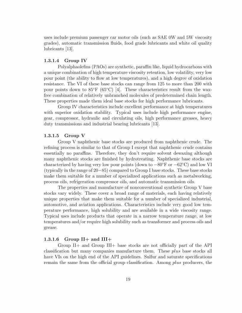
1.3.3.1 Examples of straight- and branched-chain aliphatic, alkenes,alicyclic and aromatic hydrocarbon structures. Figure fromReference [4] . . . . . . . . . . . . . . . . . . . . . . . . . . . . . . 22
x
1.3.3.2 Non-hydrocarbon examples of sulphur and nitrogen heterocyclicstructures. Figure from Reference [4] . . . . . . . . . . . . . . . . 23
2.2.0.1 Mechanisms of varnish and sludge formation. In black: base oiloxidation. In red: high temperature decomposition includingelectrostatic discharge. In blue: compressive degradation. Figurerecreated from Reference [5] . . . . . . . . . . . . . . . . . . . . . 30
2.2.0.2 From left to right: fully formulated lubricant includinghydrocarbons (yellow). Soluble impurities - low molecular weightproducts such as alcohols, ketones and carboxylic acids. Insolublesuspensions - high molecular weight products such as polymerisedor polycondensed products. Deposit formation - varnish on polarmetal surfaces and sludge forming on low flow areas. Figurerecreated from Reference [6] . . . . . . . . . . . . . . . . . . . . . 32
2.2.2.1 Left: entrained air bubble with contour lines showing decreasingvolumes due to compression ending with an oxidative carbonparticle. Right: Contour lines represented as temperature zonesdue to compression. Figure from Reference [5] . . . . . . . . . . . 35
3.2.0.1 Test coupon with dimensions. . . . . . . . . . . . . . . . . . . . . 42
3.2.1.1 Left: FTIR of artificial varnish made for testing. Right thin line:FTIR of new engine oil. Right thick line: FTIR of used engine oil.Right Figure taken from [7]. . . . . . . . . . . . . . . . . . . . . . 43
3.3.2.1 Port shape showing the length between semi-circles (l1), the widthallotted for varnish width variations (l2), the thickness allotted forvarnish height variations (t) and the radius of the semi-circles (r). 45
3.3.3.1 Reynolds numbers based on flow rate using ISO VG-46 base oil. . 46
3.3.3.2 Left: plunger pump [8]. Right: diaphragm pump [9] . . . . . . . . 47
3.3.3.3 Typical external gear pump [10]. . . . . . . . . . . . . . . . . . . . 48
3.3.3.4 Typical balanced vane pump [10]. . . . . . . . . . . . . . . . . . . 49
3.3.3.5 Typical piston pump [10]. . . . . . . . . . . . . . . . . . . . . . . 49
xi
3.3.3.6 Hydraulic pump for varnish test system. . . . . . . . . . . . . . . 51
3.3.4.1 Electric motor for varnish test system. . . . . . . . . . . . . . . . 53
3.3.4.2 VF inverter controller for varnish test system. . . . . . . . . . . . 54
3.3.5.1 Adapters and couplers for transmission of power from electricmotor to hydraulic pump. . . . . . . . . . . . . . . . . . . . . . . 54
3.3.6.1 Standard CD-61 fitting schematic. . . . . . . . . . . . . . . . . . . 55
3.3.6.2 Side view of the preliminary test cell design showing the entranceand blended section (B), the o-ring land (A) and the location ofthe test coupon. . . . . . . . . . . . . . . . . . . . . . . . . . . . . 56
3.3.6.3 Front view of the test cell lid with arrows pointing out areas foro-rings to be housed to ensure a force holding test coupon tobottom of test cell. . . . . . . . . . . . . . . . . . . . . . . . . . . 57
3.3.6.4 Test cell dimensions and specifications. . . . . . . . . . . . . . . . 57
3.3.7.1 Left: positive displacement flow meter located in the by pass lineof the test system. Right: variable area flow meter located in themain line of the test system. . . . . . . . . . . . . . . . . . . . . . 59
3.3.8.1 Heater for varnish test system with specifications. . . . . . . . . . 60
3.3.9.1 Filter for varnish test system. . . . . . . . . . . . . . . . . . . . . 60
3.3.10.1Reservoir for varnish test system with specifications. . . . . . . . . 62
3.3.11.1Re numbers based on 1-1/4 inch 316 stainless steel pipe. . . . . . 62
3.3.11.2Layout of the varnish test system to ensure minimal piping. . . . . 63
3.3.11.3Left: 2 way ball valve. Right: pressure gauge. . . . . . . . . . . . 63
3.3.11.4Left: pressure relief valve. Right: 3 way brass ball valve. . . . . . 64
xii
3.3.11.5Complete hydraulic diagram of test system: red is fluid pressure,blue is return fluid, green is suction and yellow is low pressurefluid. System symbols are given in the figures in each section. . . . 65
4.1.0.1 Cleaner fluid color for Fluids L, M, N, O, P, Q, R, S. . . . . . . . 66
4.2.0.1 (a) Wireframe CAD model of test cell showing location of couponand varnish. (b) Photo of the test cell without the polycarbonatelid. The varnish coupon prior to testing can be seen in the centerof the cell. Dimensions on both figures correspond to the scale barshown in the lower right corner of (b). . . . . . . . . . . . . . . . . 68
4.3.1.1 Percent varnish mass removed during the 120-minute tests on FluidD and E. Insets show photos of the coupons after each of the tests 70
4.3.2.1 Test cell shown with Neewer NL-660 lighting . . . . . . . . . . . . 71
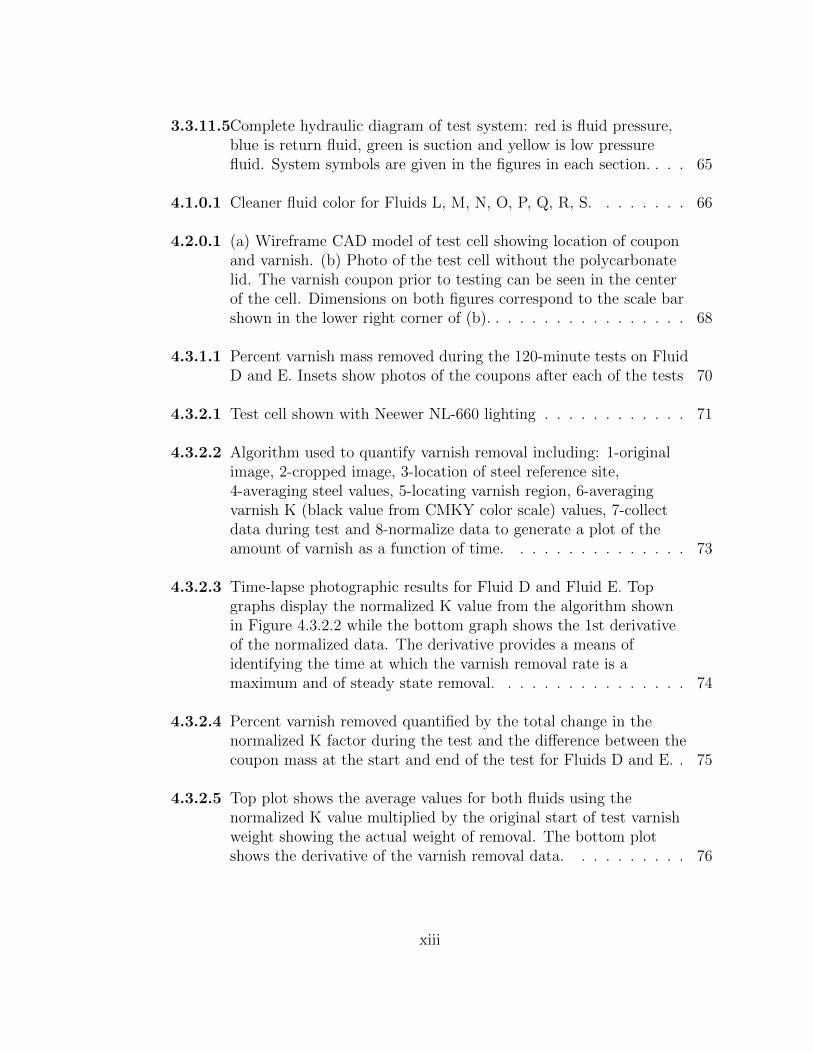
4.3.2.2 Algorithm used to quantify varnish removal including: 1-originalimage, 2-cropped image, 3-location of steel reference site,4-averaging steel values, 5-locating varnish region, 6-averagingvarnish K (black value from CMKY color scale) values, 7-collectdata during test and 8-normalize data to generate a plot of theamount of varnish as a function of time. . . . . . . . . . . . . . . 73
4.3.2.3 Time-lapse photographic results for Fluid D and Fluid E. Topgraphs display the normalized K value from the algorithm shownin Figure 4.3.2.2 while the bottom graph shows the 1st derivativeof the normalized data. The derivative provides a means ofidentifying the time at which the varnish removal rate is amaximum and of steady state removal. . . . . . . . . . . . . . . . 74
4.3.2.4 Percent varnish removed quantified by the total change in thenormalized K factor during the test and the difference between thecoupon mass at the start and end of the test for Fluids D and E. . 75
4.3.2.5 Top plot shows the average values for both fluids using thenormalized K value multiplied by the original start of test varnishweight showing the actual weight of removal. The bottom plotshows the derivative of the varnish removal data. . . . . . . . . . 76
xiii
4.3.2.6 Comparison of Fluids D and E in terms of four varnish removalperformance metrics. Upper left: maximum percent varnishremoved. Upper right: time required to achieve steady statevarnish removal. Bottom left: maximum varnish removal rate.Bottom right: time of maximum removal rate. . . . . . . . . . . . 77
4.3.3.1 Initial filter inspection performed using visual/photographicimaging. Left: filter showing a base fluid varnish trappings. Right:filter showing a cleaner fluid trappings. . . . . . . . . . . . . . . . 78
4.3.3.2 Current polypropylene filter paper used for filter inspection. Left:pretest paper with markings for fluid, coupon, test number and a1in2 area marked on its surface. Right: post test filter (Test 74)paper showing varnish removed . . . . . . . . . . . . . . . . . . . 79
5.3.1.1 Test 1 showing the movement of varnish on the coupon at 0, 10,60, and 165 minutes. The test cell lid was removed and the couponwas imaged in the test cell while covered in fluid. . . . . . . . . . 84
5.3.1.2 Test 2 showing the movement of varnish on the coupon at 0, 1, 5,and 165 minutes. The test cell lid was removed and the couponwas imaged in the test cell while covered in fluid. . . . . . . . . . 84
5.3.4.1 Tests 17-25 where three fluids K, H and Base Fluid B werecompared for varnish removal at 5, 15, 30, 60 and 110 gallons offlow with heptane being used to remove oil for weighing. . . . . . 86
5.3.4.2 Tests 17-34 where three fluids K, H and Base Fluid B werecompared for varnish removal at 110 gallons of flow with andwithout heptane wash. . . . . . . . . . . . . . . . . . . . . . . . . 87
5.3.8.1 Tests 37-63 where one base fluid and six cleaner fluids werecompared at 4.5GPM at 90◦C. The large error associated withFluid E gave cause for concern and prompted further analysis ofthis anomaly. . . . . . . . . . . . . . . . . . . . . . . . . . . . . . 89
5.3.9.1 Tests 17-34 showing the trend between the start of test (SOT)mass and the end of test (EOT) mass. . . . . . . . . . . . . . . . 90
5.4.1.1 Tests 50-54 showing a large discrepancy of % varnish removed withthe same fluid and test parameters . . . . . . . . . . . . . . . . . 91
xiv
5.4.2.1 Base Fluid B and six cleaner fluids compared at 4.5 GPM at 90◦Cover tests 37-63 and 64-78. The bottom rows show the varnish ageat the time of testing along with the test number and fluid used. . 94
5.4.3.1 Base Fluid B tested with 4 different preparation conditions at 4.5GPM, 90◦C and 120 minutes. The bottom rows show the varnishage at the time of testing along with the preparation condition. . . 95
5.5.1.1 Mass removal results for base Fluid R and 7 cleaner fluids usingVarnish D and preparation conditions P1A. . . . . . . . . . . . . . 97
5.5.3.1 Removal amounts obtained from video processing and actual massloss. The good correlation between these two measurementsenables use of the normalized K values to find the maximum rateof removal, time of maximum rate of removal and steady stateremoval. . . . . . . . . . . . . . . . . . . . . . . . . . . . . . . . . 99
5.5.3.2 Upper panels: Normalized K value multiplied by SOT for Fluids L,M, N, O, P, Q, R and S. Lower panels: 1st derivative of data inupper panel with respect to time. . . . . . . . . . . . . . . . . . . 100
5.5.4.1 Left upper: Maximum removal rates in mg/min. Right upper:Maximum removal rate time in min. Left lower: Maximum varnishremoved in %. Right lower: Maximum removal time (or steadystate) in min. . . . . . . . . . . . . . . . . . . . . . . . . . . . . . 101
5.5.4.2 Knorm average removal rate compared to actual mass averageremoval rate. Average removal rates shown for Fluids L, M, N, O,P, Q, R and S. . . . . . . . . . . . . . . . . . . . . . . . . . . . . . 102
5.5.4.3 Left: average removal rates. Right: mass percent removed. Resultsshown for Fluids L, M, N, O, P, Q, R and S. . . . . . . . . . . . . 103
5.5.5.1 Filter images for Fluids L, M, N, and O shown at standardmagnification and at 10x magnification in the insets. . . . . . . . 104
5.5.5.2 Filter images for Fluids P, Q, R and S shown at standardmagnification and at 10x magnification in the insets. . . . . . . . 104
5.5.6.1 Left: viscosity of new fluids. Right: viscosity after 2 tests. . . . . 105
xv
5.5.7.1 Left: particle counts of new fluids. Right: particle counts of thefluids after 2 tests. . . . . . . . . . . . . . . . . . . . . . . . . . . 106
5.6.0.1 Complete overview of testing metrics for each of the eight fluidstested. . . . . . . . . . . . . . . . . . . . . . . . . . . . . . . . . . 109
6.1.1.1 COMSOL simulation to verify that the test cell can be treated asbeing at one temperature. The COMSOL simulation wasperformed on a full scale model of the test cell (3.2in, x 2.5in x7in) with the port shape (from Figure 3.3.2.1) shown in the center.As the Biot number inferred, the test cell can be treated as onetemperature. The temperatures from this simulation are reportedin units of Kelvin. . . . . . . . . . . . . . . . . . . . . . . . . . . . 113
6.1.2.1 Constant radius (R) pipe flow showing a ring-shaped volumeelement, with radial thickness dr and length dx, and a parabolicvelocity profile. The ring element is shown at the top and is onlyacted upon by pressure and shear forces. . . . . . . . . . . . . . . 115
6.1.2.2 Flow simulations using the actual test cell geometry and theelliptical geometry. These results were used for calculating thevelocity of the fluid as it encounters the varnish. The black ellipseis identifying the effective area of maximum velocity for eachgeometrical shape. The slight difference in area causes differencesin the maximum velocity numbers. . . . . . . . . . . . . . . . . . 118
6.1.2.3 Flat plate boundary layer theory showing the development of alaminar boundary layer over the coupon. . . . . . . . . . . . . . . 119
6.1.2.4 The development of boundary layer over the varnish occurs 4.15µmfrom the leading edge of the varnish. . . . . . . . . . . . . . . . . 119
6.1.3.1 Left: SOT varnish volume element at t = 0. Right: The process oftesting which shows mass and convective diffusion over the varnish(t > 0). . . . . . . . . . . . . . . . . . . . . . . . . . . . . . . . . . 122
6.1.3.2 Left: Fluids O and M. Right: Fluids L, N, P, Q, R and S. Bothplots show the natural log of mass concentration plotted againstthe time of mass removal. . . . . . . . . . . . . . . . . . . . . . . 124
xvi
6.1.3.3 Left: Fluids M, O, P, Q and S. Plots show the natural log of massconcentration plotted against the time of mass removal. . . . . . . 126
6.1.4.1 Left: Fluids M, O, P, Q and S graphed in terms of flow rate andremoved varnish. . . . . . . . . . . . . . . . . . . . . . . . . . . . 128
xvii
LIST OF TABLES
1.2.1.1 Typical roughness average values of engineered surfaces finished bydifferent processes. Table from Reference [11] . . . . . . . . . . . . 5
1.3.1.1 Categories of base oils according to the API. Table fromReference [12] . . . . . . . . . . . . . . . . . . . . . . . . . . . . . 18
1.3.2.1 Base stock and additive impact on lubricant properties. Table fromReference [13] . . . . . . . . . . . . . . . . . . . . . . . . . . . . . 20
1.3.3.1 Standard component analysis of crude oil. Table fromReference [14] . . . . . . . . . . . . . . . . . . . . . . . . . . . . . 21
3.2.1.1 Composition of artificial varnish used in this work. . . . . . . . . . 43
3.2.1.2 Preparation conditions for application of varnish to coupon. . . . 44
3.3.3.1 Pump characteristics and ratings for piston, vane, and gear typesof pump [10]. . . . . . . . . . . . . . . . . . . . . . . . . . . . . . 50
3.3.4.1 Minimum nominal efficiencies according to NEMA design B. . . . 52
3.3.4.2 Finding required amperage for direct and alternating currentelectric motors. . . . . . . . . . . . . . . . . . . . . . . . . . . . . 52
3.3.4.3 Typical motor power factors for 3 phase motors. . . . . . . . . . . 52
4.3.6.1 Identifying the fluid odor (as unpleasantness), strength (inpermeation) and foam tendency (for the ability to de-aerate) forFluid D and E on a scale from 1-5. 1 is a low value for strength,smell and foam, while 5 is a high value for strength, smell andfoam. . . . . . . . . . . . . . . . . . . . . . . . . . . . . . . . . . . 79
xviii
5.4.1.1 Results for tests 50-54, where a comparison is made between alltesting parameters and mass removed to explain the difference inmass removed between tests. Neither the SOT-EOT trend or totalflow over the coupon can explain the difference. . . . . . . . . . . 92
5.4.1.2 Results for tests 50-54 showing the age of Varnish C during testing 93
5.4.2.1 Results for tests 64, 65 and 78, using the same Base Fluid B andtesting conditions, showing the varnish change over time. . . . . . 94
5.5.2.1 Varnish aging for Fluid B and R using preparation conditions P1A.Values shown in %/day. . . . . . . . . . . . . . . . . . . . . . . . . 98
5.5.7.1 Fluid mass removal shown with each ISO count recorded. Anegative value is a decrease of ISO count while a positive value isan increase of ISO count. Fluids where high mass was removedshowed an increase of ISO counts while fluids that removed lowamounts show a decrease. The filter used in this work was 5micron polypropylene paper. Fluid O had particle counts higherthan 29 for ISO 4 which could not be recorded by the counter usedin this work. . . . . . . . . . . . . . . . . . . . . . . . . . . . . . . 107
5.5.8.1 Identifying the fluid odor (as unpleasantness), strength (inpermeation) and foam tendency (for the ability to de-aerate) forFluid D and E on a scale from 1-5. 1 is a low value for strength,smell and foam, while 5 is a high value for strength, smell andfoam. . . . . . . . . . . . . . . . . . . . . . . . . . . . . . . . . . . 108
6.1.2.1 Each fluid compared for viscosity (cSt), shear forces (N) on varnishsurface and varnish removed (%). . . . . . . . . . . . . . . . . . . 120
6.1.3.1 Mass concentration at EOT for each fluid tested. The small massconcentrations allowed the boundary condition of no flux at adistance L from the coupon. . . . . . . . . . . . . . . . . . . . . . 123
6.1.3.2 Diffusion coefficient (D), kinematic viscosity (St), Schmidt number(Sc) and mass removed shown for all fluids. All tests run at4.5GPM and 90◦C. . . . . . . . . . . . . . . . . . . . . . . . . . . 125
xix
6.1.3.3 Diffusion coefficient (D), kinematic viscosity (St), Schmidt number(Sc) and mass removed shown 5 fluids. All tests run at 0.5GPMand 90◦C. . . . . . . . . . . . . . . . . . . . . . . . . . . . . . . . 127
6.1.4.1 Diffusion coefficient (D) and Schmidt number (Sc) compared forthe high (4.5GPM) and low (0.5GPM) flow results. . . . . . . . . 127
7.3.0.1 Tests 1-27a . . . . . . . . . . . . . . . . . . . . . . . . . . . . . . . 151
7.3.0.2 Tests 28-63 . . . . . . . . . . . . . . . . . . . . . . . . . . . . . . . 152
7.3.0.3 Tests 64-99 . . . . . . . . . . . . . . . . . . . . . . . . . . . . . . . 153
7.3.0.4 Tests 100 - 117 . . . . . . . . . . . . . . . . . . . . . . . . . . . . 154
xx
ACKNOWLEDGEMENTS
I would like to thank my advisor, Professor Ashlie Martini, for supporting thiswork. She was, and is, a constant and valuable resource for a wealth of informationregarding tribology. Sean Lantz, a former graduate student of Professor Martini, wasan invaluable resource as we walked the path from community college to graduateschool together. Sean is one of the most academically inclined persons I have hadthe privilege to associate with. I would like to thank research scientist Dr. ZhouZhen for all his input on this work. I would like to thank Professor Gerardo Diaz forconstantly pushing me to work problems on my own. His influence has broadenedmy understanding of thermodynamic and mass transfer principles. Professor Po-YaAbel Chuang provided valuable insight and happily shared our limited lab space.Finally, Professor Michael Modest, a heat transfer guru, taught me more aboutmath than any math professor ever. Period. Without the influence of these menand women this work would not have been possible. Thank you.
xxi
ABSTRACT
Varnish is an undesirable by-product of using hydrocarbons as lubricantsand hydraulic fluids. Oxidation of hydrocarbons is a natural process accelerated byheat, pressure, light and mechanical stressing. Varnish coats metal surfaces with athin orange carbonaceous film that reduces clearances and, in extreme cases, causesstuck hydraulic valves in large frame gas turbine engines and automotive automatictransmissions, as well as failure of journal bearings and thrust surfaces from reducedclearances and high temperatures. These effects can cost down time for equipmentcausing lost revenue and expense to address varnish related failures. One method ofremoving varnish is the use of chemical cleaning compounds that are flushed throughthe system to soften, dislodge and remove varnish using filtration. However, com-parisons of varnish removal effectiveness between cleaning compounds have not beenpossible because there is no consistent method used for evaluating varnish removaland, more generally, a poor fundamental understanding of removal mechanisms.This research included design and implementation of a varnish removal test systemcombined with a new method of characterizing cleaner fluid effectiveness. In thenewly developed method, the fluids remove artificial varnish applied to a couponwithin the test system and removal is characterized by mass loss, filter inspectionand in situ imaging of the removal process. The results are analyzed in terms ofvarnish removal mechanisms based on multiple types of diffusion. This researchallows cleaner fluids to be directly compared and provides a greater fundamentalunderstanding of varnish and varnish removal mechanisms.
xxii
Chapter 1
INTRODUCTION
1.1 Lubrication History
The history of lubrication extends well over 7 millennia [15]. The knowledgeaccumulated during this time gives us the ability to design, build, and maintainsome of the most sophisticated machines the world has ever seen. Machines thatprovide us with the ability to generate electricity, provide transportation, processmaterials, explore space, and a host of other comforts we have come to enjoy andrely on today.
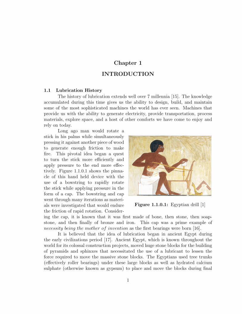
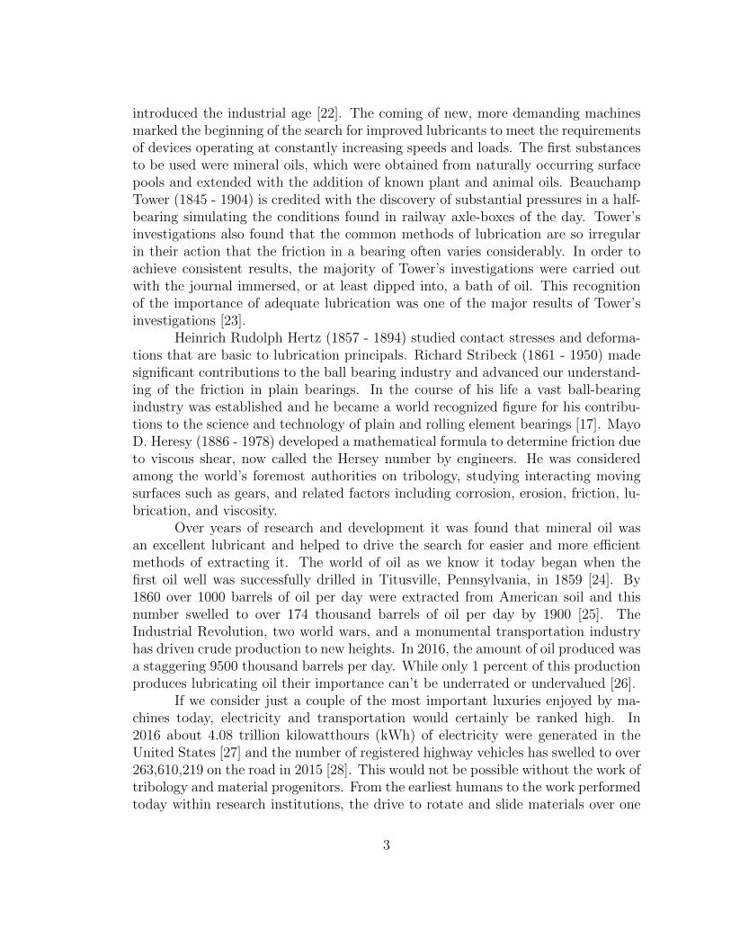
Figure 1.1.0.1: Egyptian drill [1]
Long ago man would rotate astick in his palms while simultaneouslypressing it against another piece of woodto generate enough friction to makefire. This pivotal idea began a questto turn the stick more efficiently andapply pressure to the end more effec-tively. Figure 1.1.0.1 shows the pinna-cle of this hand held device with theuse of a bowstring to rapidly rotatethe stick while applying pressure in theform of a cap. The bowstring and capwent through many iterations as materi-als were investigated that would endurethe friction of rapid rotation. Consider-ing the cap, it is known that it was first made of bone, then stone, then soap-stone, and then finally of bronze and iron. This cap was a prime example ofnecessity being the mother of invention as the first bearings were born [16].
It is believed that the idea of lubrication began in ancient Egypt duringthe early civilizations period [17]. Ancient Egypt, which is known throughout theworld for its colossal construction projects, moved huge stone blocks for the buildingof pyramids and sphinxes that necessitated the use of a lubricant to lessen theforce required to move the massive stone blocks. The Egyptians used tree trunks(effectively roller bearings) under these large blocks as well as hydrated calciumsulphate (otherwise known as gypsum) to place and move the blocks during final
1
assembly. Water is shown as a lubricant on paintings from Saqqara (circa 2400BC) and El-Bersheh (c.1880 BC) as another method to facilitate moving large stoneblocks [18].
Perhaps the most pivotal invention of all time, the wheel, set man on a pathto find methods of reducing rolling resistance and mitigating the heat that occurredon the hub of the wheel. Lubricating the wheel hub began around 2600 B.C. whensled wheels, that belonged to Ra-At-Ka (Pharo king of Egypt), used beef or ramtallow to lubricate the axle [18]. Early experimentation used oils and fats commonto the day and the Egyptians noticed that some of the more viscous liquids not onlydissipated heat but also prevented much of the heat from being generated in thefirst place [19].
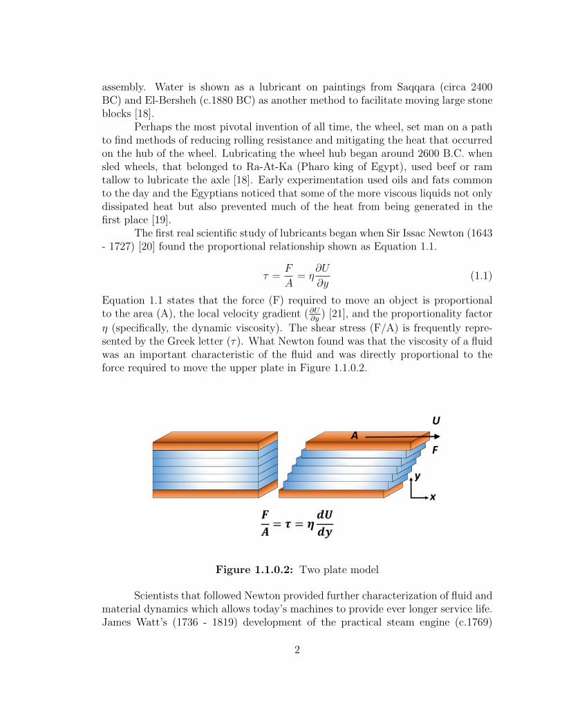
The first real scientific study of lubricants began when Sir Issac Newton (1643- 1727) [20] found the proportional relationship shown as Equation 1.1.
τ =F
A= η
∂U
∂y(1.1)
Equation 1.1 states that the force (F) required to move an object is proportionalto the area (A), the local velocity gradient (∂U
∂y) [21], and the proportionality factor
η (specifically, the dynamic viscosity). The shear stress (F/A) is frequently repre-sented by the Greek letter (τ). What Newton found was that the viscosity of a fluidwas an important characteristic of the fluid and was directly proportional to theforce required to move the upper plate in Figure 1.1.0.2.
Figure 1.1.0.2: Two plate model
Scientists that followed Newton provided further characterization of fluid andmaterial dynamics which allows today’s machines to provide ever longer service life.James Watt’s (1736 - 1819) development of the practical steam engine (c.1769)
2
introduced the industrial age [22]. The coming of new, more demanding machinesmarked the beginning of the search for improved lubricants to meet the requirementsof devices operating at constantly increasing speeds and loads. The first substancesto be used were mineral oils, which were obtained from naturally occurring surfacepools and extended with the addition of known plant and animal oils. BeauchampTower (1845 - 1904) is credited with the discovery of substantial pressures in a half-bearing simulating the conditions found in railway axle-boxes of the day. Tower’sinvestigations also found that the common methods of lubrication are so irregularin their action that the friction in a bearing often varies considerably. In order toachieve consistent results, the majority of Tower’s investigations were carried outwith the journal immersed, or at least dipped into, a bath of oil. This recognitionof the importance of adequate lubrication was one of the major results of Tower’sinvestigations [23].
Heinrich Rudolph Hertz (1857 - 1894) studied contact stresses and deforma-tions that are basic to lubrication principals. Richard Stribeck (1861 - 1950) madesignificant contributions to the ball bearing industry and advanced our understand-ing of the friction in plain bearings. In the course of his life a vast ball-bearingindustry was established and he became a world recognized figure for his contribu-tions to the science and technology of plain and rolling element bearings [17]. MayoD. Heresy (1886 - 1978) developed a mathematical formula to determine friction dueto viscous shear, now called the Hersey number by engineers. He was consideredamong the world’s foremost authorities on tribology, studying interacting movingsurfaces such as gears, and related factors including corrosion, erosion, friction, lu-brication, and viscosity.
Over years of research and development it was found that mineral oil wasan excellent lubricant and helped to drive the search for easier and more efficientmethods of extracting it. The world of oil as we know it today began when thefirst oil well was successfully drilled in Titusville, Pennsylvania, in 1859 [24]. By1860 over 1000 barrels of oil per day were extracted from American soil and thisnumber swelled to over 174 thousand barrels of oil per day by 1900 [25]. TheIndustrial Revolution, two world wars, and a monumental transportation industryhas driven crude production to new heights. In 2016, the amount of oil produced wasa staggering 9500 thousand barrels per day. While only 1 percent of this productionproduces lubricating oil their importance can’t be underrated or undervalued [26].
If we consider just a couple of the most important luxuries enjoyed by ma-chines today, electricity and transportation would certainly be ranked high. In2016 about 4.08 trillion kilowatthours (kWh) of electricity were generated in theUnited States [27] and the number of registered highway vehicles has swelled to over263,610,219 on the road in 2015 [28]. This would not be possible without the work oftribology and material progenitors. From the earliest humans to the work performedtoday within research institutions, the drive to rotate and slide materials over one
3
another ever more efficiently, with less wear, will provide the next generation withsuperior machines.
1.2 Lubrication Basics
At the heart of the typical mechanical system lies surfaces which slide or rollagainst each other. Tribology, therefore, is central to the understanding of lubricatedsystems and provides technological advances for a wide range of applications. Thescience of decreasing wear, friction and oil degradation while increasing componentlife, oil change intervals and our basic understanding of lubricated systems hasfallen to mechanical engineers, chemists, physicists and materials scientists. Whiletribology encompasses much more than the study of friction, it is central to theperformance of mechanical systems [11]
Work done in overcoming friction in bearings and gears is dissipated as heat,and by reducing friction we can achieve an increase in overall efficiency of machines.A key method of reducing friction, and often wear, is to introduce a lubricant intothe system. Additionally, due to the close proximity of the lubricating oil to thesource of friction, the lubricating oil becomes the most convenient mechanism forremoving heat from the system. This heat is transferred to the atmosphere throughradiators typically mounted with cooling fans thereby providing oil temperaturesconducive to the longevity and performance of the system. Furthermore, the lu-bricating oil provides a way to remove foreign and domestic contaminates from thesystem, through filtration, as well as coating the internal surfaces of the system withoil to minimize corrosion. Lubricating oils also serve as work mediums in hydraulicsystems by transmitting work from one form to another. Few systems have theability to provide such a wide ranging list of benefits and abilities.
1.2.1 Friction
Engineered surfaces, when viewed under magnification, are all found to pos-sess irregularities. A plethora of methods have been used to study surface topogra-phy, including electron, light and atomic force microscopy [29]. Several quantitativemeasures are used to characterize the irregularities from one surface to another. Themost commonly reported measure of surface roughness is the roughness average(Ra) and is shown as Equation 1.2.
Ra u1
N
N∑i=1
|Zi| (1.2)
where Zi is the height of the ith point and N is the number of points measuredalong the sampling length [30]. Another widely used measure of surface roughnessis the root mean squared (rms) roughness and is defined as Equation 1.3. A list oftypical Ra values are shown in Table 1.2.1.1.
4
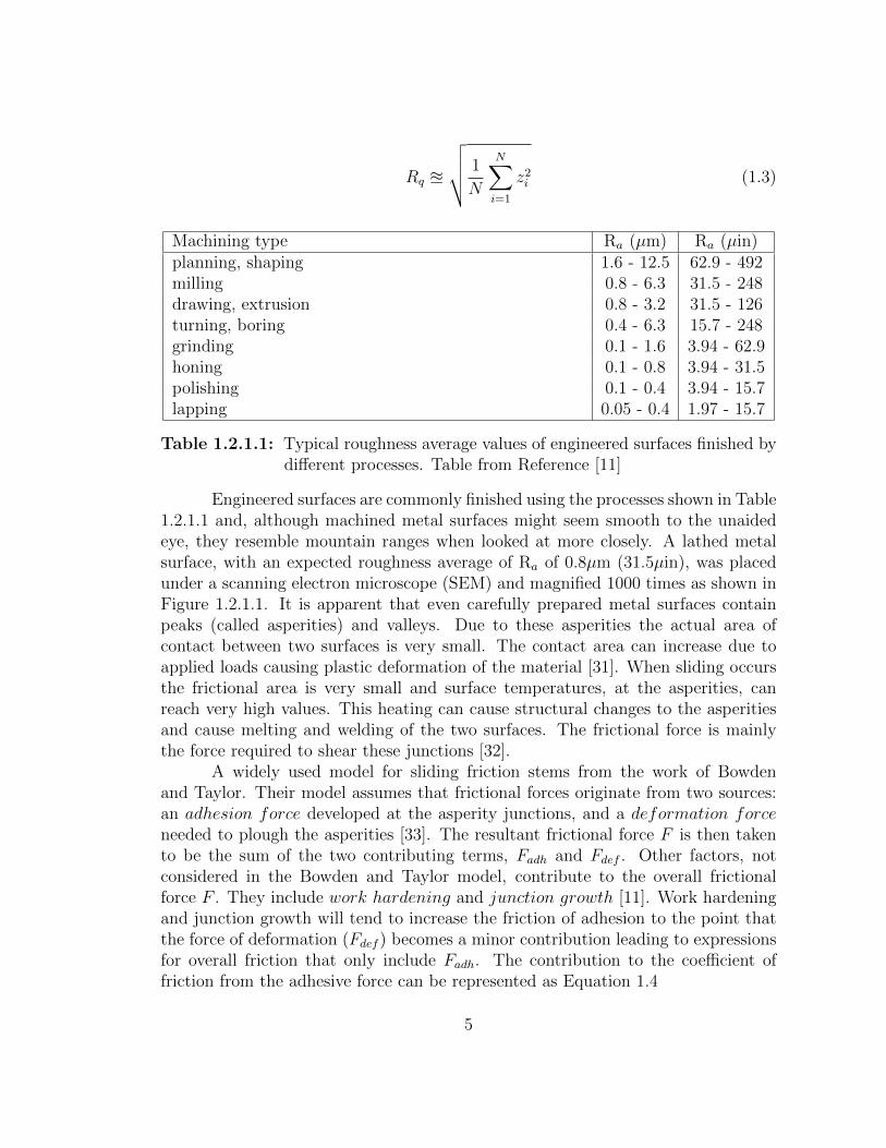
Rq u
√√√√ 1
N
N∑i=1
z2i (1.3)
Machining type Ra (µm) Ra (µin)planning, shaping 1.6 - 12.5 62.9 - 492milling 0.8 - 6.3 31.5 - 248drawing, extrusion 0.8 - 3.2 31.5 - 126turning, boring 0.4 - 6.3 15.7 - 248grinding 0.1 - 1.6 3.94 - 62.9honing 0.1 - 0.8 3.94 - 31.5polishing 0.1 - 0.4 3.94 - 15.7lapping 0.05 - 0.4 1.97 - 15.7
Table 1.2.1.1: Typical roughness average values of engineered surfaces finished bydifferent processes. Table from Reference [11]
Engineered surfaces are commonly finished using the processes shown in Table1.2.1.1 and, although machined metal surfaces might seem smooth to the unaidedeye, they resemble mountain ranges when looked at more closely. A lathed metalsurface, with an expected roughness average of Ra of 0.8µm (31.5µin), was placedunder a scanning electron microscope (SEM) and magnified 1000 times as shown inFigure 1.2.1.1. It is apparent that even carefully prepared metal surfaces containpeaks (called asperities) and valleys. Due to these asperities the actual area ofcontact between two surfaces is very small. The contact area can increase due toapplied loads causing plastic deformation of the material [31]. When sliding occursthe frictional area is very small and surface temperatures, at the asperities, canreach very high values. This heating can cause structural changes to the asperitiesand cause melting and welding of the two surfaces. The frictional force is mainlythe force required to shear these junctions [32].
A widely used model for sliding friction stems from the work of Bowdenand Taylor. Their model assumes that frictional forces originate from two sources:an adhesion force developed at the asperity junctions, and a deformation forceneeded to plough the asperities [33]. The resultant frictional force F is then takento be the sum of the two contributing terms, Fadh and Fdef . Other factors, notconsidered in the Bowden and Taylor model, contribute to the overall frictionalforce F . They include work hardening and junction growth [11]. Work hardeningand junction growth will tend to increase the friction of adhesion to the point thatthe force of deformation (Fdef ) becomes a minor contribution leading to expressionsfor overall friction that only include Fadh. The contribution to the coefficient offriction from the adhesive force can be represented as Equation 1.4
5
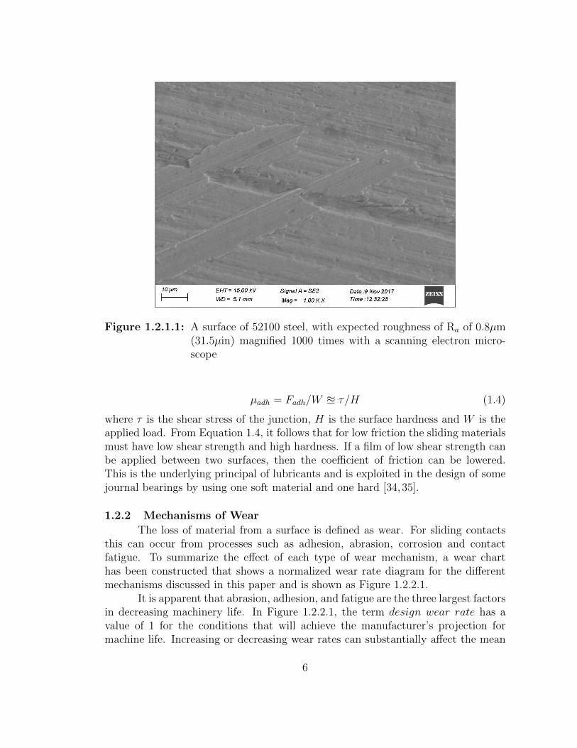
Figure 1.2.1.1: A surface of 52100 steel, with expected roughness of Ra of 0.8µm(31.5µin) magnified 1000 times with a scanning electron micro-scope
µadh = Fadh/W u τ/H (1.4)
where τ is the shear stress of the junction, H is the surface hardness and W is theapplied load. From Equation 1.4, it follows that for low friction the sliding materialsmust have low shear strength and high hardness. If a film of low shear strength canbe applied between two surfaces, then the coefficient of friction can be lowered.This is the underlying principal of lubricants and is exploited in the design of somejournal bearings by using one soft material and one hard [34,35].
1.2.2 Mechanisms of Wear
The loss of material from a surface is defined as wear. For sliding contactsthis can occur from processes such as adhesion, abrasion, corrosion and contactfatigue. To summarize the effect of each type of wear mechanism, a wear charthas been constructed that shows a normalized wear rate diagram for the differentmechanisms discussed in this paper and is shown as Figure 1.2.2.1.
It is apparent that abrasion, adhesion, and fatigue are the three largest factorsin decreasing machinery life. In Figure 1.2.2.1, the term design wear rate has avalue of 1 for the conditions that will achieve the manufacturer’s projection formachine life. Increasing or decreasing wear rates can substantially affect the mean
6
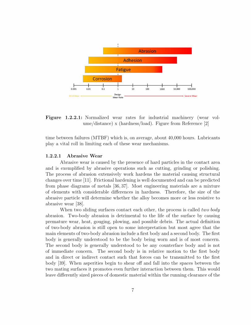
Figure 1.2.2.1: Normalized wear rates for industrial machinery (wear vol-ume/distance) x (hardness/load). Figure from Reference [2]
time between failures (MTBF) which is, on average, about 40,000 hours. Lubricantsplay a vital roll in limiting each of these wear mechanisms.
1.2.2.1 Abrasive Wear
Abrasive wear is caused by the presence of hard particles in the contact areaand is exemplified by abrasive operations such as cutting, grinding or polishing.The process of abrasion extensively work hardens the material causing structuralchanges over time [11]. Frictional hardening is well documented and can be predictedfrom phase diagrams of metals [36, 37]. Most engineering materials are a mixtureof elements with considerable differences in hardness. Therefore, the size of theabrasive particle will determine whether the alloy becomes more or less resistive toabrasive wear [38].
When two sliding surfaces contact each other, the process is called two bodyabrasion. Two-body abrasion is detrimental to the life of the surface by causingpremature wear, heat, gouging, plowing, and possible debris. The actual definitionof two-body abrasion is still open to some interpretation but most agree that themain elements of two-body abrasion include a first body and a second body. The firstbody is generally understood to be the body being worn and is of most concern.The second body is generally understood to be any counterface body and is notof immediate concern. The second body is in relative motion to the first bodyand in direct or indirect contact such that forces can be transmitted to the firstbody [39]. When asperities begin to shear off and fall into the spaces between thetwo mating surfaces it promotes even further interaction between them. This wouldleave differently sized pieces of domestic material within the running clearance of the
7
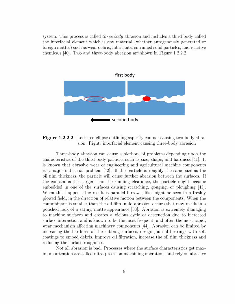
system. This process is called three body abrasion and includes a third body calledthe interfacial element which is any material (whether autogenously generated orforeign matter) such as wear debris, lubricants, entrained solid particles, and reactivechemicals [40]. Two and three-body abrasion are shown in Figure 1.2.2.2.
Figure 1.2.2.2: Left: red ellipse outlining asperity contact causing two-body abra-sion. Right: interfacial element causing three-body abrasion
Three-body abrasion can cause a plethora of problems depending upon thecharacteristics of the third body particle, such as size, shape, and hardness [41]. Itis known that abrasive wear of engineering and agricultural machine componentsis a major industrial problem [42]. If the particle is roughly the same size as theoil film thickness, the particle will cause further abrasion between the surfaces. Ifthe contaminant is larger than the running clearance, the particle might becomeembedded in one of the surfaces causing scratching, gouging, or ploughing [43].When this happens, the result is parallel furrows, like might be seen in a freshlyplowed field, in the direction of relative motion between the components. When thecontaminant is smaller than the oil film, mild abrasion occurs that may result in apolished look of a satiny, matte appearance [38]. Abrasion is extremely damagingto machine surfaces and creates a vicious cycle of destruction due to increasedsurface interaction and is known to be the most frequent, and often the most rapid,wear mechanism affecting machinery components [44]. Abrasion can be limited byincreasing the hardness of the rubbing surfaces, design journal bearings with softcoatings to embed debris, improve oil filtration, increase the oil film thickness andreducing the surface roughness.
Not all abrasion is bad. Processes where the surface characteristics get max-imum attention are called ultra-precision machining operations and rely on abrasive
8
properties. They are often used to alter surface attributes such as roughness, wavi-ness, flatness and roundness without significant material removal from the workpiece.Typical examples are the lapping and polishing of optical lenses, computer chips ormagnetic heads, honing of cylinder liners, and micro-finishing of bearing races [45].
1.2.2.2 Adhesive Wear
Adhesive wear occurs when bonding, or cold welding, occurs at the asperitytips of loaded surfaces. Thus, work hardening can occur at the bonded, or welded,tip section and be strengthened. This can cause the material to shear well below theasperity tip junction [46]. This process can cause one surface to become bonded, orwelded, to the other. It can also cause the sheared material to break off and becomean abrasive particle when the elastic energy just exceeds the surface energy [47].When sheared material comes loose a fresh surface is exposed. This surface is morereactive than the original surface and must be quickly covered with additives toprevent detrimental effects [32]. Many wear process begin as adhesive wear and endas abrasive wear because of the sheared off material [48]. Abrasive wear can belimited by metal combinations which don’t bond together easily, improving the lowshear strength of additive layers and by increasing the oil film thickness.
Adhesion is a common problem when there is a lack of lubrication suppliedto frictional surfaces. It commonly occurs when high temperatures, or pressures,cause the lubricant film to decrease enough for asperities to contact each other andspot weld together. Adhesion occurs in the mixed and boundary lubrication regimestypically due to insufficient lubrication supply, improper viscosity choice, clearanceproblems, machining issues, or incorrect assembly of equipment. Some adhesion isexpected when new components typically go through a break-in period when firstused [49].
1.2.2.3 Contact Fatigue
There are two main types of contact fatigue: surface and subsurface [50].Contact fatigue tends to predominate in rolling contacts where slip is small andcontact stresses are high. Pitting in gears and bearings, and squats in railway trackare examples of surface initiated contact fatigue cracks [51]. Plastic deformation,caused by high contact stresses, can initiate surface cracks. Material defects, suchas scratches or dents, can also initiate surface cracks [52]. Subsurface fatigue isgenerally found in rolling element bearings and gear teeth. The long term, repeated,exposure to load cycles and stress cause elastic deformation of the material. Thiselastic deformation can reach subsurface flaws and cracks in the material and begina cycle of propagation of the crack to the surface [53, 54]. This is common and isthe result of a bearing, or gear, surviving its normal life expectancy. The eventualresult is pitting and spalling of the material’s surface [55]. Fatigue damage can belimited by increasing the oil film thickness, minimizing the influence of entrained air
9
and dissolved water and with the addition of fatigue limiting additives such as zincor phosphate.
1.2.2.4 Corrosive Wear
Corrosive wear loses material by chemical reaction and can be very detri-mental to the service life of materials. For example, the acidic corrosion of cylinderliner materials caused by oil degradation and combustion components can prema-turely wear these materials [56,57]. However, if it is controlled, it can be beneficial.The formation of low shear strength boundary lubricant films such as extreme pres-sure (EP) and anti wear (AW) additives are a form of chemical corrosion [11]. Alubricated system contains many corrosive species such as oxygen, water, carbondioxide, sulphur compounds, acidic combustion products, acidic oil oxidation prod-ucts and anti wear and extreme pressure additives. Corrosive species, like thoselisted previously, have a tendency to attack metals. Normal sliding, and rolling,motions can exacerbate this chemical attack by removing protective corrosive coat-ings. This exposes fresh surface material and can increase surface temperaturescausing increased diffusion and reaction rates [58]. Corrosion can be limited byusing corrosion inhibitors, using additives that prevent adhesion, limiting corrosivespecies and neutralizing acidic species by using over based detergents.
1.2.3 Surface Types
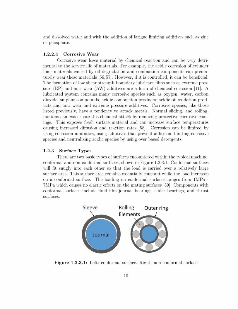
There are two basic types of surfaces encountered within the typical machine,conformal and non-conformal surfaces, shown in Figure 1.2.3.1. Conformal surfaceswill fit snugly into each other so that the load is carried over a relatively largesurface area. This surface area remains essentially constant while the load increaseson a conformal surface. The loading on conformal surfaces ranges from 1MPa -7MPa which causes no elastic effects on the mating surfaces [59]. Components withconformal surfaces include fluid film journal bearings, slider bearings, and thrustsurfaces.
Figure 1.2.3.1: Left: conformal surface. Right: non-conformal surface
10
Nonconformal surfaces do not conform to each other very well and the loadmust be carried by a very small contact area. The contact areas between noncon-formal surfaces enlarge considerably with increasing load but are still small whencompared with the contact areas between conformal surfaces. The loading on non-conformal surfaces can exceed 700MPa even at modest applied loads causing elasticdeformation of the materials such that elliptical contact areas are formed on themating surfaces [60]. Components with nonconformal surfaces include mating gearteeth, cams, followers and rolling element bearings. It is important to note that it iscommon practice in engineering to have one hard surface and one softer (sacrificial)surface with conformal surfaces and two hard surfaces with non-conformal surfaces.
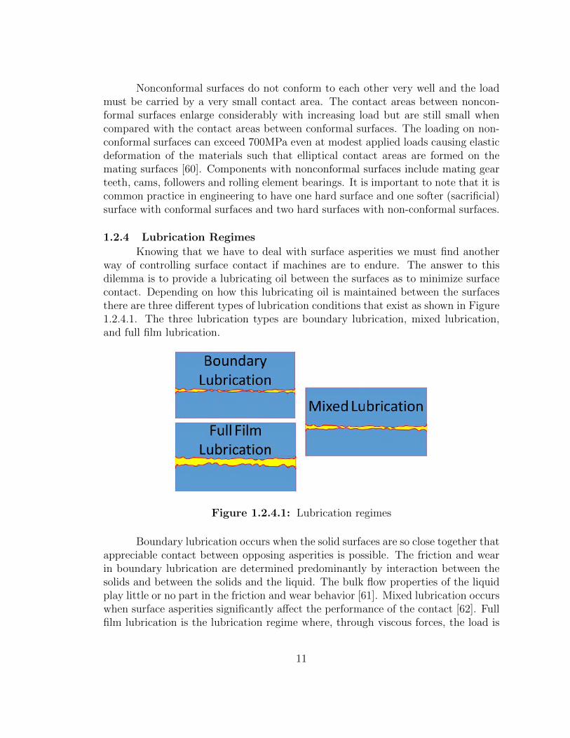
1.2.4 Lubrication Regimes
Knowing that we have to deal with surface asperities we must find anotherway of controlling surface contact if machines are to endure. The answer to thisdilemma is to provide a lubricating oil between the surfaces as to minimize surfacecontact. Depending on how this lubricating oil is maintained between the surfacesthere are three different types of lubrication conditions that exist as shown in Figure1.2.4.1. The three lubrication types are boundary lubrication, mixed lubrication,and full film lubrication.
Figure 1.2.4.1: Lubrication regimes
Boundary lubrication occurs when the solid surfaces are so close together thatappreciable contact between opposing asperities is possible. The friction and wearin boundary lubrication are determined predominantly by interaction between thesolids and between the solids and the liquid. The bulk flow properties of the liquidplay little or no part in the friction and wear behavior [61]. Mixed lubrication occurswhen surface asperities significantly affect the performance of the contact [62]. Fullfilm lubrication is the lubrication regime where, through viscous forces, the load is
11
fully supported by the lubricant between the surfaces in relative motion. Full filmlubrication consists of both hydrodynamic (conformal surfaces) and elastohydrody-namic (non-conformal surfaces) lubrication [59].
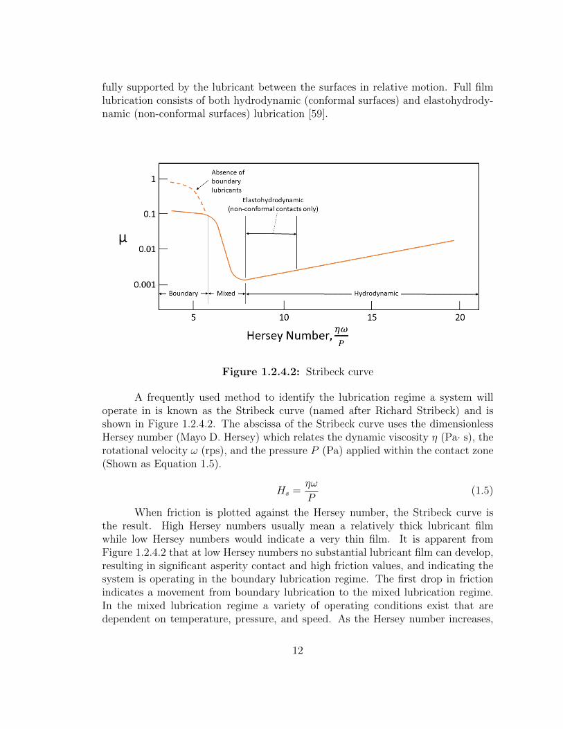
Figure 1.2.4.2: Stribeck curve
A frequently used method to identify the lubrication regime a system willoperate in is known as the Stribeck curve (named after Richard Stribeck) and isshown in Figure 1.2.4.2. The abscissa of the Stribeck curve uses the dimensionlessHersey number (Mayo D. Hersey) which relates the dynamic viscosity η (Pa· s), therotational velocity ω (rps), and the pressure P (Pa) applied within the contact zone(Shown as Equation 1.5).
Hs =ηω
P(1.5)
When friction is plotted against the Hersey number, the Stribeck curve isthe result. High Hersey numbers usually mean a relatively thick lubricant filmwhile low Hersey numbers would indicate a very thin film. It is apparent fromFigure 1.2.4.2 that at low Hersey numbers no substantial lubricant film can develop,resulting in significant asperity contact and high friction values, and indicating thesystem is operating in the boundary lubrication regime. The first drop in frictionindicates a movement from boundary lubrication to the mixed lubrication regime.In the mixed lubrication regime a variety of operating conditions exist that aredependent on temperature, pressure, and speed. As the Hersey number increases,
12
friction reaches a low point and then steadily, and slowly, increases marking thenext regime of hydrodynamic lubrication. At this point the surfaces are effectivelyseparated by the lubricant and asperity contact has negligible effect on load supportand friction [59].
While the Stribeck curve gives a method to define system lubrication regimesgiven operational parameters, it isn’t readily apparent that the Hersey number con-tains the complexities inherent in viscosity, which exhibits unique, and unexpectedbehaviors. The dynamic viscosity, which was first defined in Equation 1.1 and Fig-ure 1.1.0.2, is also contained in the numerator of the Hersey equation shown inEquation 1.5. Viscosity can be highly dependent upon the operating temperaturesof the system, the local pressures within the contact zone and upon the shear rate(γ) the fluid experiences.
1.2.5 Viscosity Shear Rate Dependence
If we look again at Figure 1.1.0.2 we can impose two conditions that allowfor accurate calculation of viscosity-related variables. The first is a no slip conditionalong the length of the plates that the fluid is in contact with and the second isthat laminar flow conditions exist within the layers of the fluid. The second variablethat can be defined from Equation 1.1, is shear rate (γ). To obtain shear rate thevelocity of the upper plate of Figure 1.1.0.2, is divided by the distance betweenthe plates giving the unit of reciprocal second. This provides a second equation fordynamic viscosity shown as Equation 1.6. The shear rate is an important parameterin defining viscosity and a substance’s flow behavior [3].
η =τ
γ(1.6)
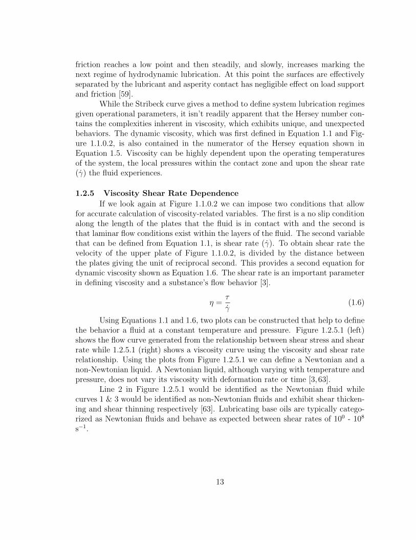
Using Equations 1.1 and 1.6, two plots can be constructed that help to definethe behavior a fluid at a constant temperature and pressure. Figure 1.2.5.1 (left)shows the flow curve generated from the relationship between shear stress and shearrate while 1.2.5.1 (right) shows a viscosity curve using the viscosity and shear raterelationship. Using the plots from Figure 1.2.5.1 we can define a Newtonian and anon-Newtonian liquid. A Newtonian liquid, although varying with temperature andpressure, does not vary its viscosity with deformation rate or time [3, 63].
Line 2 in Figure 1.2.5.1 would be identified as the Newtonian fluid whilecurves 1 & 3 would be identified as non-Newtonian fluids and exhibit shear thicken-ing and shear thinning respectively [63]. Lubricating base oils are typically catego-rized as Newtonian fluids and behave as expected between shear rates of 100 - 108
s−1.
13
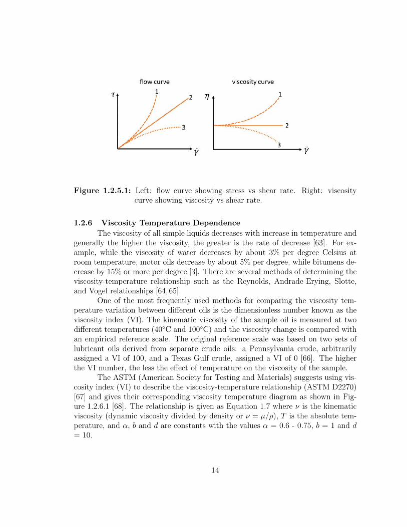
Figure 1.2.5.1: Left: flow curve showing stress vs shear rate. Right: viscositycurve showing viscosity vs shear rate.
1.2.6 Viscosity Temperature Dependence
The viscosity of all simple liquids decreases with increase in temperature andgenerally the higher the viscosity, the greater is the rate of decrease [63]. For ex-ample, while the viscosity of water decreases by about 3% per degree Celsius atroom temperature, motor oils decrease by about 5% per degree, while bitumens de-crease by 15% or more per degree [3]. There are several methods of determining theviscosity-temperature relationship such as the Reynolds, Andrade-Erying, Slotte,and Vogel relationships [64,65].
One of the most frequently used methods for comparing the viscosity tem-perature variation between different oils is the dimensionless number known as theviscosity index (VI). The kinematic viscosity of the sample oil is measured at twodifferent temperatures (40◦C and 100◦C) and the viscosity change is compared withan empirical reference scale. The original reference scale was based on two sets oflubricant oils derived from separate crude oils: a Pennsylvania crude, arbitrarilyassigned a VI of 100, and a Texas Gulf crude, assigned a VI of 0 [66]. The higherthe VI number, the less the effect of temperature on the viscosity of the sample.
The ASTM (American Society for Testing and Materials) suggests using vis-cosity index (VI) to describe the viscosity-temperature relationship (ASTM D2270)[67] and gives their corresponding viscosity temperature diagram as shown in Fig-ure 1.2.6.1 [68]. The relationship is given as Equation 1.7 where ν is the kinematicviscosity (dynamic viscosity divided by density or ν = µ/ρ), T is the absolute tem-perature, and α, b and d are constants with the values α = 0.6 - 0.75, b = 1 and d= 10.
14
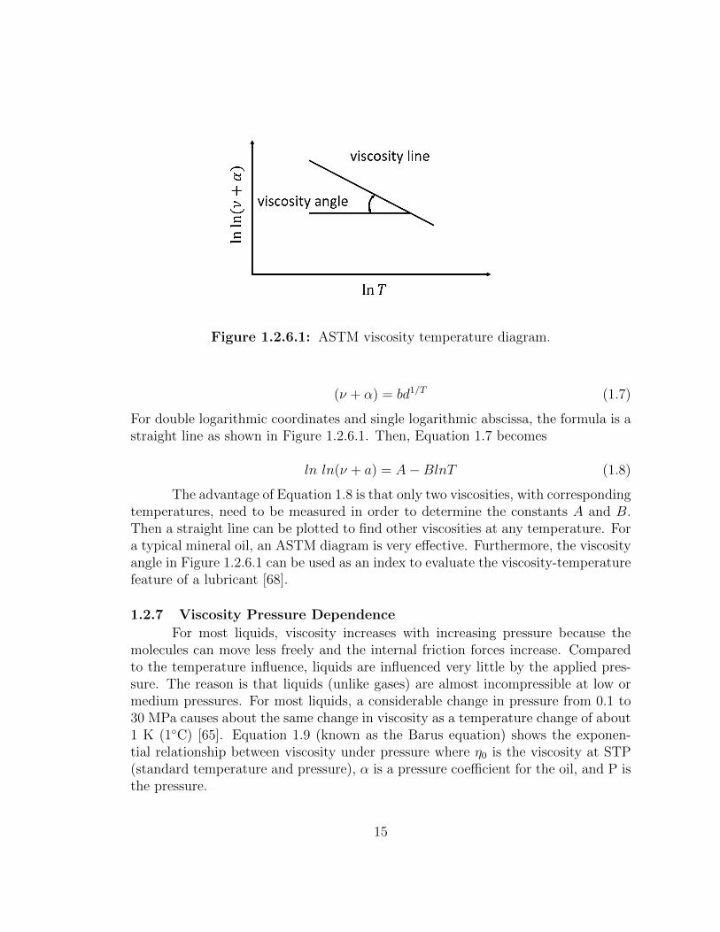
Figure 1.2.6.1: ASTM viscosity temperature diagram.
(ν + α) = bd1/T (1.7)
For double logarithmic coordinates and single logarithmic abscissa, the formula is astraight line as shown in Figure 1.2.6.1. Then, Equation 1.7 becomes
ln ln(ν + a) = A−BlnT (1.8)
The advantage of Equation 1.8 is that only two viscosities, with correspondingtemperatures, need to be measured in order to determine the constants A and B.Then a straight line can be plotted to find other viscosities at any temperature. Fora typical mineral oil, an ASTM diagram is very effective. Furthermore, the viscosityangle in Figure 1.2.6.1 can be used as an index to evaluate the viscosity-temperaturefeature of a lubricant [68].
1.2.7 Viscosity Pressure Dependence
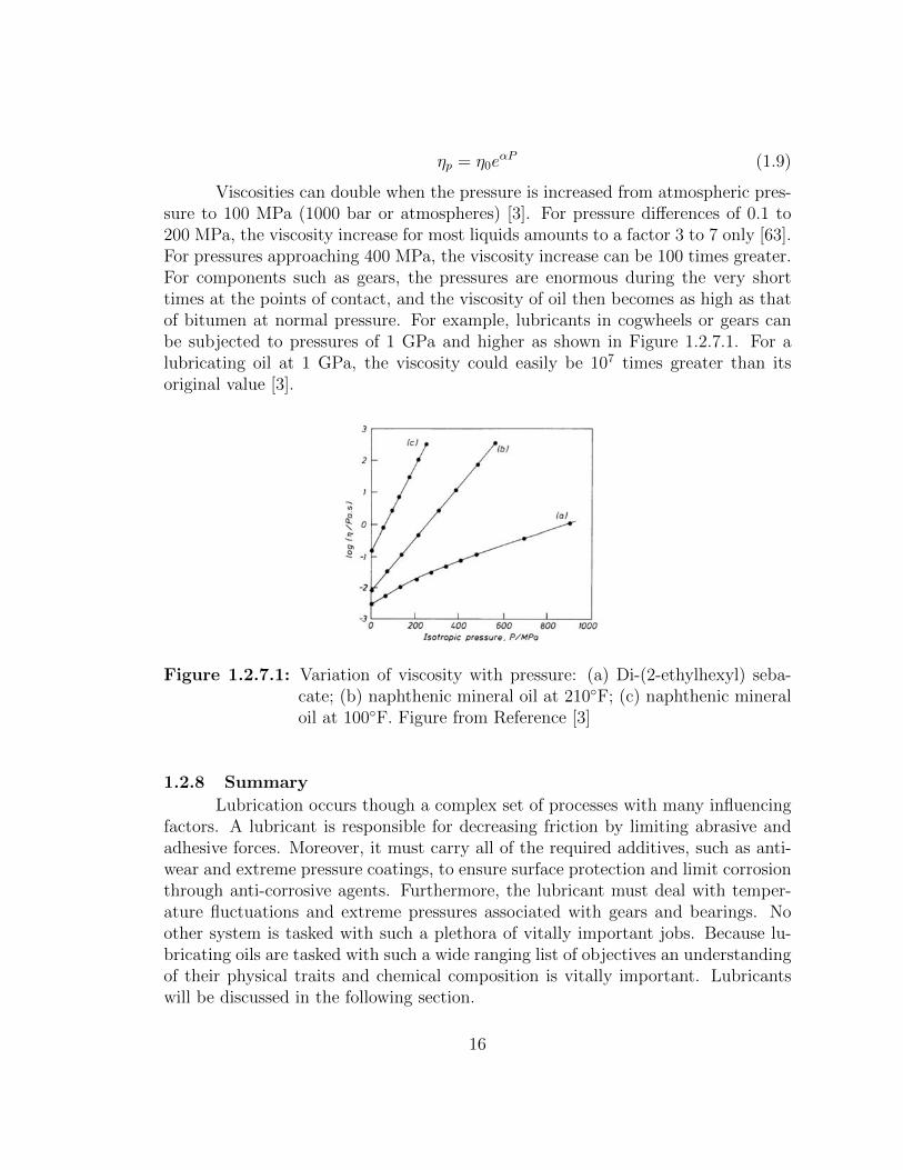
For most liquids, viscosity increases with increasing pressure because themolecules can move less freely and the internal friction forces increase. Comparedto the temperature influence, liquids are influenced very little by the applied pres-sure. The reason is that liquids (unlike gases) are almost incompressible at low ormedium pressures. For most liquids, a considerable change in pressure from 0.1 to30 MPa causes about the same change in viscosity as a temperature change of about1 K (1◦C) [65]. Equation 1.9 (known as the Barus equation) shows the exponen-tial relationship between viscosity under pressure where η0 is the viscosity at STP(standard temperature and pressure), α is a pressure coefficient for the oil, and P isthe pressure.
15
ηp = η0eαP (1.9)
Viscosities can double when the pressure is increased from atmospheric pres-sure to 100 MPa (1000 bar or atmospheres) [3]. For pressure differences of 0.1 to200 MPa, the viscosity increase for most liquids amounts to a factor 3 to 7 only [63].For pressures approaching 400 MPa, the viscosity increase can be 100 times greater.For components such as gears, the pressures are enormous during the very shorttimes at the points of contact, and the viscosity of oil then becomes as high as thatof bitumen at normal pressure. For example, lubricants in cogwheels or gears canbe subjected to pressures of 1 GPa and higher as shown in Figure 1.2.7.1. For alubricating oil at 1 GPa, the viscosity could easily be 107 times greater than itsoriginal value [3].
Figure 1.2.7.1: Variation of viscosity with pressure: (a) Di-(2-ethylhexyl) seba-cate; (b) naphthenic mineral oil at 210◦F; (c) naphthenic mineraloil at 100◦F. Figure from Reference [3]
1.2.8 Summary
Lubrication occurs though a complex set of processes with many influencingfactors. A lubricant is responsible for decreasing friction by limiting abrasive andadhesive forces. Moreover, it must carry all of the required additives, such as anti-wear and extreme pressure coatings, to ensure surface protection and limit corrosionthrough anti-corrosive agents. Furthermore, the lubricant must deal with temper-ature fluctuations and extreme pressures associated with gears and bearings. Noother system is tasked with such a plethora of vitally important jobs. Because lu-bricating oils are tasked with such a wide ranging list of objectives an understandingof their physical traits and chemical composition is vitally important. Lubricantswill be discussed in the following section.
16
1.3 Lubricants
The majority of a lubricating oil consists of a base stock that is the foundationof the lubricant. The base stock material can have different origins such as mineraloil, synthetic oil or vegetable oil. Mineral oil, which is derived from crude oil, isproduced with a wide range of characteristics depending on the refining process.Synthetic oils are produced through a synthesis process (man-made oligomers) andcome in even a wider range of chemical compositions depending on their intendedpurpose. Vegetable oils are a very small percentage of lubrications and won’t bediscussed in this work.
Base stocks can have very different physical and chemical properties and pos-sess characteristics that will determine their performance for a variety of lubricationchallenges. Mineral oils obtain these specific characteristics from the refining pro-cess. Synthetics oils have come to address characteristics that are not achievablewith mineral oils [13]. Modern lubricants are formulated from a range of base stocksand chemical additives. The base stock has several functions but its primary useis to provide the fluid layer to separate moving surfaces. Many properties of thelubricant are enhanced, or created, by the addition of special chemical additives tothe base fluid. For example, stability to oxidation and degradation in an engine oilis improved by the addition of antioxidants while extreme pressure anti-wear prop-erties, needed in gear lubrication, are created by the addition of special additives.The base stock acts as the carrier for these additives and therefore must be able tomaintain them in solution under normal working conditions [69].
1.3.1 American Petroleum Institute Base Stocks
The 20th century implemented a number of improvements in the refiningprocess used for mineral oils along with the introduction of a variety of synthet-ics. By the early 1990s, the American Petroleum Institute (API) had developed aclassification system for lubricant base stocks, as identified in API Publication 1509Annex E [12]. The definitions have evolved to the present five group standard, setin 1995, which categorize base oils for their origins (mineral or synthetic) and theirmethod/process of production as well as the range of their viscosity index and thepercentage of saturated hydrocarbons as shown in Table 1.3.1.1.
1.3.1.1 Group I
Group I base stocks are manufactured using solvent extraction techniques,solvent or catalytic de-waxing, and hydro finishing techniques [70]. The solventrefining process is a selective separation process that isolates compounds present inthe crude without the formation of new molecules.
First, to remove undesirable aromatics, polar solvents such as furfural orphenol are used to attract and remove heavy aromatics from the vacuum distillate.
17
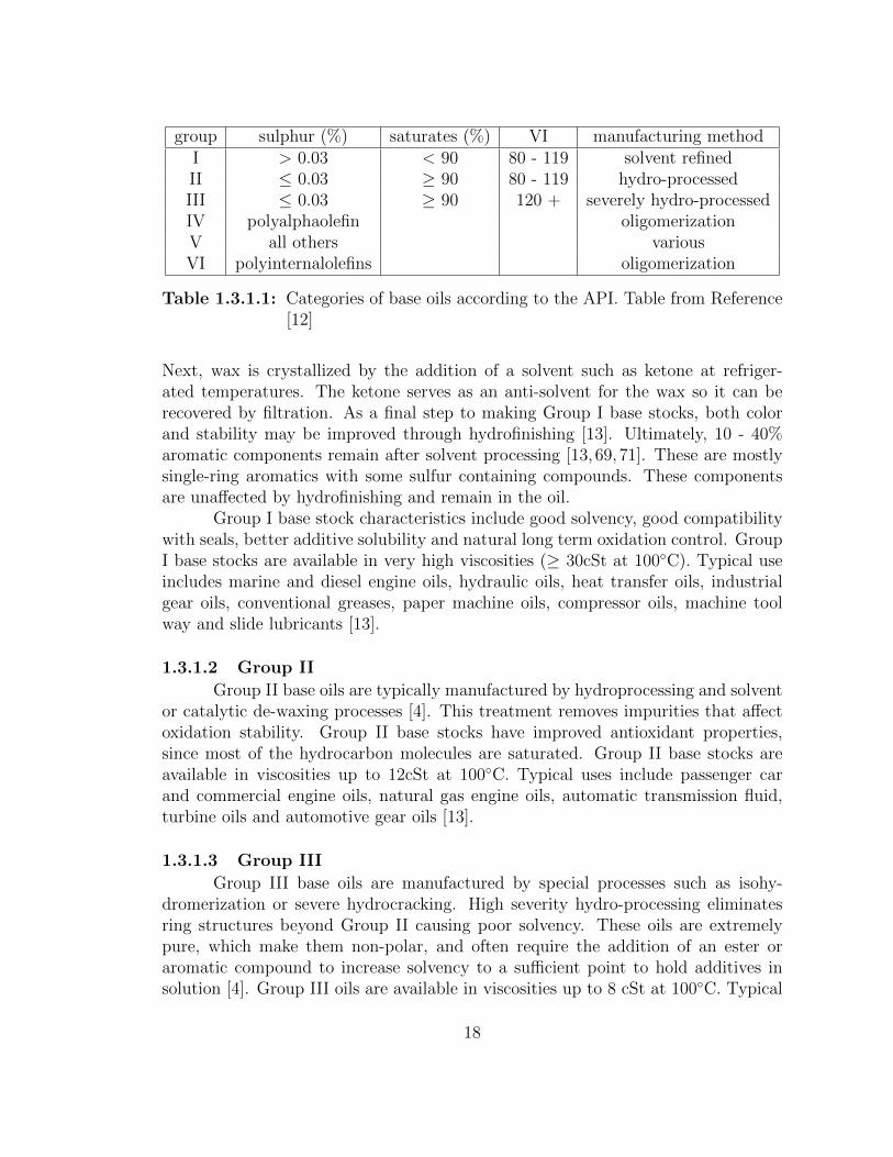
group sulphur (%) saturates (%) VI manufacturing methodI > 0.03 < 90 80 - 119 solvent refinedII ≤ 0.03 ≥ 90 80 - 119 hydro-processedIII ≤ 0.03 ≥ 90 120 + severely hydro-processedIV polyalphaolefin oligomerizationV all others variousVI polyinternalolefins oligomerization
Table 1.3.1.1: Categories of base oils according to the API. Table from Reference[12]
Next, wax is crystallized by the addition of a solvent such as ketone at refriger-ated temperatures. The ketone serves as an anti-solvent for the wax so it can berecovered by filtration. As a final step to making Group I base stocks, both colorand stability may be improved through hydrofinishing [13]. Ultimately, 10 - 40%aromatic components remain after solvent processing [13, 69, 71]. These are mostlysingle-ring aromatics with some sulfur containing compounds. These componentsare unaffected by hydrofinishing and remain in the oil.
Group I base stock characteristics include good solvency, good compatibilitywith seals, better additive solubility and natural long term oxidation control. GroupI base stocks are available in very high viscosities (≥ 30cSt at 100◦C). Typical useincludes marine and diesel engine oils, hydraulic oils, heat transfer oils, industrialgear oils, conventional greases, paper machine oils, compressor oils, machine toolway and slide lubricants [13].
1.3.1.2 Group II
Group II base oils are typically manufactured by hydroprocessing and solventor catalytic de-waxing processes [4]. This treatment removes impurities that affectoxidation stability. Group II base stocks have improved antioxidant properties,since most of the hydrocarbon molecules are saturated. Group II base stocks areavailable in viscosities up to 12cSt at 100◦C. Typical uses include passenger carand commercial engine oils, natural gas engine oils, automatic transmission fluid,turbine oils and automotive gear oils [13].
1.3.1.3 Group III
Group III base oils are manufactured by special processes such as isohy-dromerization or severe hydrocracking. High severity hydro-processing eliminatesring structures beyond Group II causing poor solvency. These oils are extremelypure, which make them non-polar, and often require the addition of an ester oraromatic compound to increase solvency to a sufficient point to hold additives insolution [4]. Group III oils are available in viscosities up to 8 cSt at 100◦C. Typical
18
uses include premium passenger car motor oils (such as SAE 0W and 5W viscositygrades), automatic transmission fluids, food grade lubricants and white oil qualitylubricants [13].
1.3.1.4 Group IV
Polyalphaolefins (PAOs) are synthetic, paraffin like, liquid hydrocarbons witha unique combination of high temperature viscosity retention, low volatility, very lowpour point (the ability to flow at low temperatures), and a high degree of oxidationresistance. The VI of these base stocks can range from 125 to more than 200 withpour points down to 85◦F (65◦C) [4]. These characteristics result from the wax-free combination of relatively unbranched molecules of predetermined chain length.These properties made them ideal base stocks for high performance lubricants.
Group IV characteristics include excellent performance at high temperatureswith superior oxidation stability. Typical uses include high performance engine,gear, compressor, hydraulic and circulating oils, high performance greases, heavyduty transmissions and industrial bearing lubricants [13].
1.3.1.5 Group V
Group V naphthenic base stocks are produced from naphthenic crude. Therefining process is similar to that of Group I except that naphthenic crude containsessentially no paraffins. Therefore, they don’t require solvent dewaxing althoughmany naphthenic stocks are finished by hydrotreating. Naphthenic base stocks arecharacterized by having very low pour points (down to −80◦F or −62◦C) and low VI(typically in the range of 20−85) compared to Group I base stocks. These base stocksmake them suitable for a number of specialized applications such as metalworking,process oils, refrigeration compressor oils, and automatic transmission oils.
The properties and manufacture of nonconventional synthetic Group V basestocks vary widely. These cover a broad range of materials, each having relativelyunique properties that make them suitable for a number of specialized industrial,automotive, and aviation applications. Characteristics include very good low tem-perature performance, high solubility and are available in a wide viscosity range.Typical uses include products that operate in a narrow temperature range, at lowtemperatures and/or require high solubility such as transformer and process oils andgrease.
1.3.1.6 Group II+ and III+
Group II+ and Group III+ base stocks are not officially part of the APIclassification but many companies manufacture them. These plus base stocks allhave VIs on the high end of the API guidelines. Sulfur and saturate specificationsremain the same from the official group classification. Among plus producers, the
19
minimum VI falls somewhere between 130 and 140. In addition to the high VIbenefit, these stocks generally have lower volatility and lower pour points. [69].
1.3.2 Base Stock Application
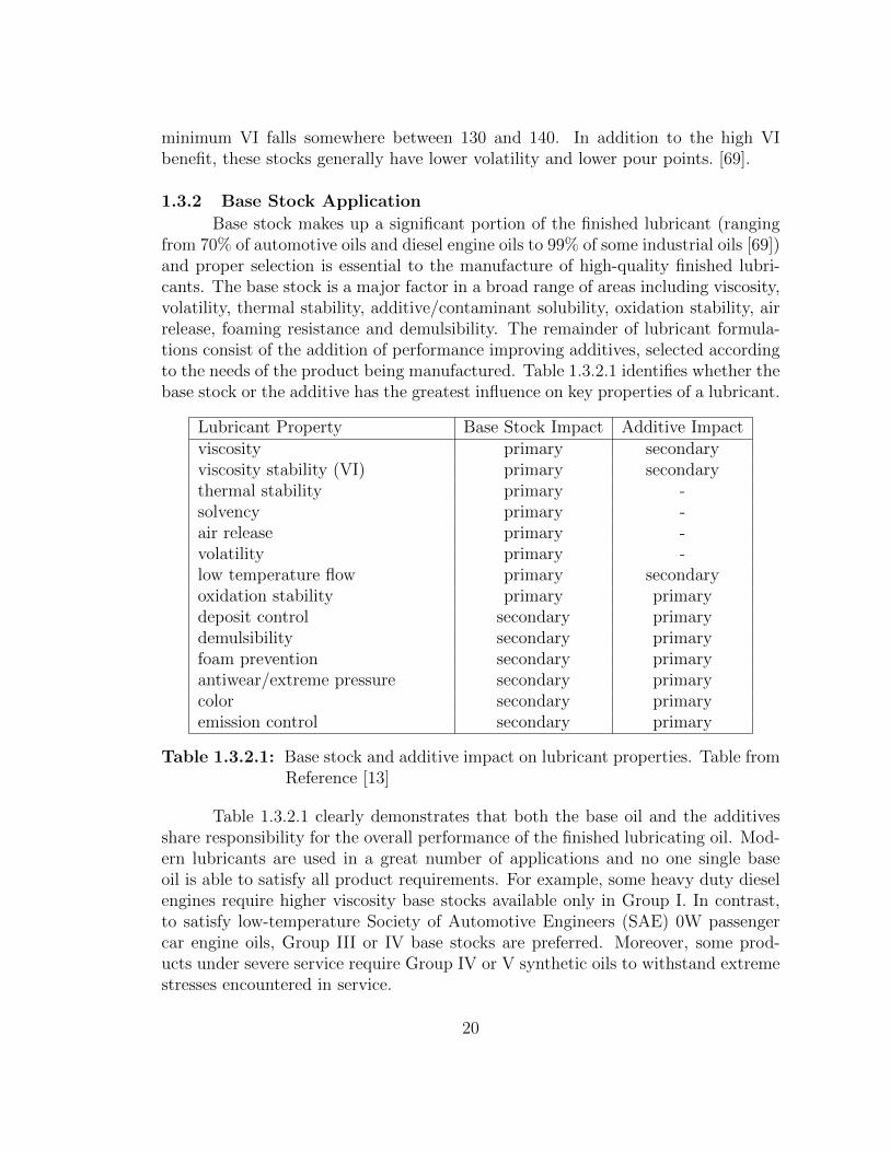
Base stock makes up a significant portion of the finished lubricant (rangingfrom 70% of automotive oils and diesel engine oils to 99% of some industrial oils [69])and proper selection is essential to the manufacture of high-quality finished lubri-cants. The base stock is a major factor in a broad range of areas including viscosity,volatility, thermal stability, additive/contaminant solubility, oxidation stability, airrelease, foaming resistance and demulsibility. The remainder of lubricant formula-tions consist of the addition of performance improving additives, selected accordingto the needs of the product being manufactured. Table 1.3.2.1 identifies whether thebase stock or the additive has the greatest influence on key properties of a lubricant.
Lubricant Property Base Stock Impact Additive Impactviscosity primary secondaryviscosity stability (VI) primary secondarythermal stability primary -solvency primary -air release primary -volatility primary -low temperature flow primary secondaryoxidation stability primary primarydeposit control secondary primarydemulsibility secondary primaryfoam prevention secondary primaryantiwear/extreme pressure secondary primarycolor secondary primaryemission control secondary primary
Table 1.3.2.1: Base stock and additive impact on lubricant properties. Table fromReference [13]
Table 1.3.2.1 clearly demonstrates that both the base oil and the additivesshare responsibility for the overall performance of the finished lubricating oil. Mod-ern lubricants are used in a great number of applications and no one single baseoil is able to satisfy all product requirements. For example, some heavy duty dieselengines require higher viscosity base stocks available only in Group I. In contrast,to satisfy low-temperature Society of Automotive Engineers (SAE) 0W passengercar engine oils, Group III or IV base stocks are preferred. Moreover, some prod-ucts under severe service require Group IV or V synthetic oils to withstand extremestresses encountered in service.
20
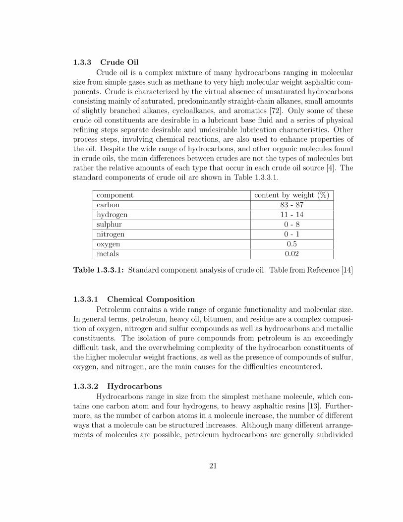
1.3.3 Crude Oil
Crude oil is a complex mixture of many hydrocarbons ranging in molecularsize from simple gases such as methane to very high molecular weight asphaltic com-ponents. Crude is characterized by the virtual absence of unsaturated hydrocarbonsconsisting mainly of saturated, predominantly straight-chain alkanes, small amountsof slightly branched alkanes, cycloalkanes, and aromatics [72]. Only some of thesecrude oil constituents are desirable in a lubricant base fluid and a series of physicalrefining steps separate desirable and undesirable lubrication characteristics. Otherprocess steps, involving chemical reactions, are also used to enhance properties ofthe oil. Despite the wide range of hydrocarbons, and other organic molecules foundin crude oils, the main differences between crudes are not the types of molecules butrather the relative amounts of each type that occur in each crude oil source [4]. Thestandard components of crude oil are shown in Table 1.3.3.1.
component content by weight (%)carbon 83 - 87hydrogen 11 - 14sulphur 0 - 8nitrogen 0 - 1oxygen 0.5metals 0.02
Table 1.3.3.1: Standard component analysis of crude oil. Table from Reference [14]
1.3.3.1 Chemical Composition
Petroleum contains a wide range of organic functionality and molecular size.In general terms, petroleum, heavy oil, bitumen, and residue are a complex composi-tion of oxygen, nitrogen and sulfur compounds as well as hydrocarbons and metallicconstituents. The isolation of pure compounds from petroleum is an exceedinglydifficult task, and the overwhelming complexity of the hydrocarbon constituents ofthe higher molecular weight fractions, as well as the presence of compounds of sulfur,oxygen, and nitrogen, are the main causes for the difficulties encountered.
1.3.3.2 Hydrocarbons
Hydrocarbons range in size from the simplest methane molecule, which con-tains one carbon atom and four hydrogens, to heavy asphaltic resins [13]. Further-more, as the number of carbon atoms in a molecule increase, the number of differentways that a molecule can be structured increases. Although many different arrange-ments of molecules are possible, petroleum hydrocarbons are generally subdivided
21
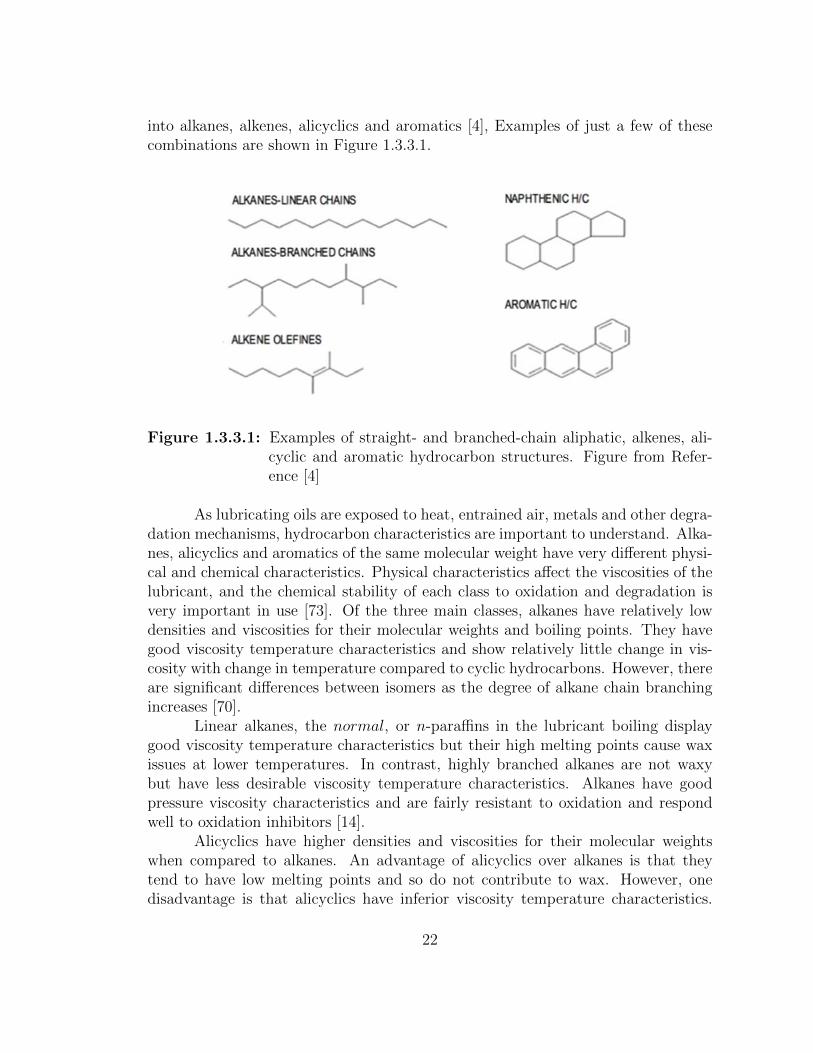
into alkanes, alkenes, alicyclics and aromatics [4], Examples of just a few of thesecombinations are shown in Figure 1.3.3.1.
Figure 1.3.3.1: Examples of straight- and branched-chain aliphatic, alkenes, ali-cyclic and aromatic hydrocarbon structures. Figure from Refer-ence [4]
As lubricating oils are exposed to heat, entrained air, metals and other degra-dation mechanisms, hydrocarbon characteristics are important to understand. Alka-nes, alicyclics and aromatics of the same molecular weight have very different physi-cal and chemical characteristics. Physical characteristics affect the viscosities of thelubricant, and the chemical stability of each class to oxidation and degradation isvery important in use [73]. Of the three main classes, alkanes have relatively lowdensities and viscosities for their molecular weights and boiling points. They havegood viscosity temperature characteristics and show relatively little change in vis-cosity with change in temperature compared to cyclic hydrocarbons. However, thereare significant differences between isomers as the degree of alkane chain branchingincreases [70].
Linear alkanes, the normal, or n-paraffins in the lubricant boiling displaygood viscosity temperature characteristics but their high melting points cause waxissues at lower temperatures. In contrast, highly branched alkanes are not waxybut have less desirable viscosity temperature characteristics. Alkanes have goodpressure viscosity characteristics and are fairly resistant to oxidation and respondwell to oxidation inhibitors [14].
Alicyclics have higher densities and viscosities for their molecular weightswhen compared to alkanes. An advantage of alicyclics over alkanes is that theytend to have low melting points and so do not contribute to wax. However, onedisadvantage is that alicyclics have inferior viscosity temperature characteristics.
22
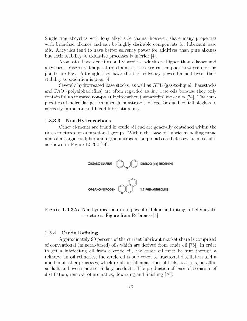
Single ring alicyclics with long alkyl side chains, however, share many propertieswith branched alkanes and can be highly desirable components for lubricant baseoils. Alicyclics tend to have better solvency power for additives than pure alkanesbut their stability to oxidative processes is inferior [4].
Aromatics have densities and viscosities which are higher than alkanes andalicyclics. Viscosity temperature characteristics are rather poor however meltingpoints are low. Although they have the best solvency power for additives, theirstability to oxidation is poor [4].
Severely hydrotreated base stocks, as well as GTL (gas-to-liquid) basestocksand PAO (polyalphaolefins) are often regarded as dry base oils because they onlycontain fully saturated non-polar hydrocarbon (isoparaffin) molecules [74]. The com-plexities of molecular performance demonstrate the need for qualified tribologists tocorrectly formulate and blend lubrication oils.
1.3.3.3 Non-Hydrocarbons
Other elements are found in crude oil and are generally contained within thering structures or as functional groups. Within the base oil lubricant boiling rangealmost all organosulphur and organonitrogen compounds are heterocyclic moleculesas shown in Figure 1.3.3.2 [14].
Figure 1.3.3.2: Non-hydrocarbon examples of sulphur and nitrogen heterocyclicstructures. Figure from Reference [4]
1.3.4 Crude Refining
Approximately 90 percent of the current lubricant market share is comprisedof conventional (mineral-based) oils which are derived from crude oil [75]. In orderto get a lubricating oil from a crude oil, the crude oil must be sent through arefinery. In oil refineries, the crude oil is subjected to fractional distillation and anumber of other processes, which result in different types of fuels, base oils, paraffin,asphalt and even some secondary products. The production of base oils consists ofdistillation, removal of aromatics, dewaxing and finishing [76]:
23
Crude oil is sent through a furnace where it is heated, partially vaporized andsent to a fractionating column. The fractionating column separates hydrocarbonsbased on their boiling and condensing points, which are a direct result of theirmolecular size [14]. As the vaporized hydrocarbons travel up the column they cooland condense. The condensation happens at different heights allowing separationbased on molecular size. The smallest of the hydrocarbons (5 to 10 carbon atoms)will rise to the very top of the column. They will be processed into products likegasoline. Condensing just before reaching the top, compounds containing 11 to 13carbon atoms will be processed into kerosene and jet fuel. Larger atoms, with 14 to25 carbon atoms in the molecular chain, are diesel and gas oils. Compounds with26 to 40 carbon atoms are a tribologists main concern. This is the material usedfor the creation of lubricating oil. At the bottom of the column, the heaviest andlargest of the hydrocarbons (40-plus carbon atoms) are taken and used in asphalticbased products [70].
Aromatics are then removed by solvent extraction to improve characteristicsof the lubricating oil. Wax is then removed by cooler temperatures and filtration [77].The return on the base oil from the distillation column of the refinery depends on theproportion of desirable components in the range of the lubricants boiling points [78].
1.3.5 Synthetic Oils
Synthetic lubricants first appeared in the early 1930s, as synthetic hydrocar-bon and ester technologies were developed at the same time in Germany and theUSA [79]. The increasing demand of lubricants to perform in expanding temperatureranges (mainly driven by the developments in the engines of the military aircrafts)will ensure continuing development of synthetic lubricant technology [80,81].
Today, synthetic lubricants are used in virtually all fields and applicationsthat require lubrication. Industries such as automotive, shipping, industry, aviationand aerospace all use synthetic oils in high temperature applications. A plurality ofbase oils has been investigated for their use as potential synthetic base oils of finallubricants, out of which the most prevalent ones are alkylated aromatics, esters,PAOs, polybutenes and silicones [4]. Below is a list of the most common syntheticoils:
• Alkylated aromatics: include dialkyl benzenes and alkyl aromatics [4]
• Esters (100% synthetic): include diesters and polyesters [82]
• Polyalphaolefins (PAO), (100% synthetic): derived from the polymerization ofan alpha-olefin [79]
• Polybutenes (PIB)
• Polyglycols (PAGs): produced by oxidation of ethylene and propylene [4]
24
• Silicones: typically contain a Si=O functional group such as PDMS [80]
1.3.6 Chemical Additives
The various base stock manufacturing processes can all produce base stocksthat have characteristics conducive to formulating finished lubricants with desirableperformance. The lubricant oil base stock is the building block to which chemi-cal additives or improvers, which enhance their physicochemical characteristics andproperties, are added. Additives give the final product properties and characteris-tics required for individual application [83]. Some additives impart new and usefulproperties to the lubricant, some enhance properties already present and some actto reduce the rate at which undesirable changes take place in the oil during itsservice life. The key to achieving good performance in finished lubricants is un-derstanding the interactions of base stocks and additives and combining them tomeet the requirements of machinery and operating conditions. Modern passengercar engines, automatic transmissions, hypoid gears, railroad and marine diesel en-gines, high speed gas and steam turbines, and industrial processing machinery, aswell as many other types of equipment would have been greatly lagging in theirdevelopment were it not for lubricant additives and the performance benefits theyprovide [70].
Additives for lubricating oils were used first during the 1920s, and their usehas continued to increase [84]. Additives, in improving the performance characteris-tics of lubricating oils, have aided significantly in the development of the transporta-tion industry and industrial machinery. Over a period of many years, oil additiveswere identified that solved a variety of engine problems: corrosion inhibition, abilityto keep particles such as soot dispersed, ability to prohibit acidic combustion prod-ucts from forming varnish on engine surfaces, and the ability to minimize wear bylaying down a chemical film on heavily loaded surfaces [80]. Furthermore, engine oilsbecame so specialized that requirements for diesel engine oils began to diverge fromrequirements for gasoline engines, since enhanced dispersive capability was neededto keep soot from clumping in the oil of diesel engines. Today, practically all typesof lubricating oils contain at least one additive, and some oils contain many differenttypes of additives. Additives can also have detrimental effects if too much is addedor there are undesirable interactions with other additives. The amount of additivesused in a finished lubricant varies from a few hundredths of a percent to 30% ormore [70]. The main chemical additives are listed below, with additional detail onantioxidants, which are the most relevant to this research, in the following section:
• Anti Foaming: chemicals that lower air droplet surface tension allowing releaseof air [85]
• Corrosion Inhibitors and Rust Preventatives: a tenacious film that preventswater from reaching the metal surface [86]
25
• Detergents: metal salts of organic acids that frequently contain excess base [84]
• Dispersants: interfere in agglomeration by associating with individual resinand soot particles [87]
• Extreme Pressure: compounds containing sulfur, phosphorus, chlorine, borate,or metals, either alone or in combination [88]
• Friction Modifiers: used for smooth transition from static to dynamic conditionas well as reduced noise, frictional heat, and startup torque [89]
• Viscosity Index (VI) Improvers: long chain, high molecular weight polymersthat function by increasing the relative viscosity of an oil more at high tem-peratures than they do at low temperatures [90]
1.3.6.1 Antioxidants
Through the natural oxidative process, or accelerated by the presence ofoxidative mechanisms, oxidative degradation occurs in the lubricating oil. As aresult of this oxidation, the oil viscosity and concentration of organic acids in theoil both increase, and varnish deposits begin to form on hot metal surfaces exposedto the oil. Varnish deposits may be further oxidized to form hard carbonaceousmaterials. The rate at which oxidation proceeds is affected by several factors. Asthe temperature increases, the rate of oxidation increases exponentially and a generalguide is that for each 10◦C (18◦F) rise in temperature, the oxidation rate will double(Arrhenius rate rule) [91]. Greater exposure to air (and the oxygen it contains), orgreater mixing with it, will also increase the rate of oxidation. Many materials, suchas metals (particularly copper and iron) and organic and mineral acids, may act ascatalysts or oxidation promoters [92].
Before the mechanisms of hydrocarbon oxidation were well known, researchersobserved that some oils provided greater resistance to oxidation than others. Thisresistance was eventually identified as naturally occurring antioxidants, which varieddepending on crude source or refining techniques. Some of these natural antioxidantswere found to contain sulfur or nitrogen bearing functional groups [4]. Therefore,certain additives that are used to impart special properties to the oil, such as sul-fur bearing chemicals, were found to provide additional antioxidant stability. Thediscovery of sulfurized additives providing oxidation stability was followed by theidentification of similar properties with phenols, which led to the development ofsulfurized phenols. Next, certain amines and metal salts of phosphorus or sulfur con-taining acids were identified as imparting oxidation stability [93]. Today, nearly alllubricants contain at least one antioxidant for stabilization and other performanceenhancing purposes. Since oxidation has been identified as the primary cause of
26
oil degradation, it is the most important aspect for lubricants that the oxidationstability be maximized.
Oxidation produces harmful species, which eventually compromise the desig-nated functionalities of a lubricant, shortens its service life, and to a more extremeextent, damages the machinery it lubricates. The internal combustion engine is anexcellent chemical reactor for catalyzing the process of oxidation with heat and en-gine metal parts acting as effective oxidation catalysts [94]. Thus, in service engineoils are probably more susceptible to oxidation than most other lubricant applica-tions. For the prevention of lubricant oxidation, antioxidants are the key additivethat protects the lubricant from oxidative degradation, allowing the fluid to meetthe requirements for use in engines and industrial applications.
Several effective antioxidant classes have been developed over the years andhave seen use in engine oils, automatic transmission fluids, gear oils, turbine oils,compressor oils, greases, hydraulic fluids, and metal working fluids. The main classesinclude oil soluble organic and organometallic antioxidants of the following types[95]:
• sulfur compounds
• sulfur-nitrogen compounds
• phosphorus compounds
• sulfur-phosphorus compounds
• aromatic amine compounds
• hindered phenolic (HP) compounds
• organo-copper compounds
• boron compounds
• other organometallic compounds
Antioxidants are formulated into modern lubricants in order to inhibit theoil oxidation mechanism and extend the lubricant life. However, these antioxidantsare gradually consumed causing the oil to increase the oxidative process.
1.3.7 Summary
Formulating a finished lubricant that meets the demands of a given system isa challenge. This challenge includes choosing a base stock based on its physical andchemical characteristics, and then selecting an additive package. Synthetics base
27
stocks are known to provide better thermal and oxidative stability, viscosity perfor-mance and friction properties. They would seem an obvious choice if it weren’t fortheir lower solubility to additives and high cost [80]. Group I, II and III offer a goodviscosity index, good solvency and lower cost. Group V offers very specific charac-teristics from the naphthenic content and are widely used for locomotive engine oils,refrigerant oils, compressor oils, transformer oils and process oils [75].
The operating envelope of the machine is important in identifying the properlubricating oil and additive package to ensure long and efficient life. There is no onelubricating oil that meets the demands for all applications so lubricating oils can betailored to meet the specific demands within a given system. Lubricating environ-ments that endure extreme pressures or temperatures can be chemically composedto provide adequate performance for these extreme environments. Additive packagesthat incorporate viscosity modifiers, foam inhibitors, extreme pressure additives, de-tergents, rust and corrosion inhibitors, antioxidants, and friction modifiers all helpto tailor the oil to a specific system.
It is important to understand that even with a healthy lubrication systemenvironmental contaminants, fuel contamination due to blow-by in internal com-bustion engines, antifreeze contamination, and additive shearing can create enginelubrication problems. Oil change intervals can greatly affect the performance of anytype of machinery and several parameters are usually tested to check the health oflubrication oil. The viscosity, acid number, additive elements, oxidation number,and other tests can help to ensure proper oil change intervals and keep machineryrunning smoothly.
The leading cause of oil degradation is oxidation. Anti-oxidants are a widelyresearched area of lubrication and every oil consists of some type of anti-oxidant ad-ditive. The result of the oxidation process is varnish and sludge. Varnish is a leadingcause of servo valve sticking in the gas turbine industry and has been a problem inthe ring-pack of the internal combustion engine. Varnish coats surfaces and robsefficiency by decreasing working clearances and clogging pumps and sumps. Thiswork directly addresses the varnish problem and the following chapter is devoted tothe detrimental effects of varnish, varnish formation and mitigating varnish.
28
Chapter 2
VARNISH
2.1 Introduction
Varnish is formed as hydrocarbon base fluids degrade through oxidation. Ox-idation is accelerated by exposure to increased temperatures, mechanical stresses,ultraviolet light, entrained air, electrostatic discharge and wear materials (metals)found in typical machines [73, 80]. Varnish is formed as soluble primary oxidationproducts, such as acids, water and alcohols, follow condensation and polymerizationreactions to form insoluble products [4]. These products are polar, causing varnishto adsorb on metal surfaces where further agglomeration thickens the varnish [96].Varnish typically has a gold-orange appearance that darkens as the thickness in-creases. However, varnish appearance can vary with factors such as base stockand additive package constituents, temperature, atmospheric content and surfacematerial [97].
Varnish deposits are one of the most detrimental by-products of hydrocar-bon oxidation [98,99]. Varnish fills the tight clearances between the valve and borein hydraulic circuits causing erratic valve operation and in some cases fully seizedvalves [98]. Varnish contributes to decreased efficiency, increased wear and corrosion,impaired oil cooler performance and inadequate hydrodynamic lubrication. Jour-nal bearings that experience varnish build up have increased shear rates, increasedoperational temperatures and, in extreme cases, bearing failure [100]. A stickinginlet guide vane valve of large frame gas turbines, such as those used in the powergeneration industry, can produce a fail to start, or shut-down event [101].
More efficient combustion processes have been achieved by increasing com-bustion temperatures [102]. This has strained the capabilities of materials andthe lubricants that separate them. For temperatures greater than 100◦C, each in-crease of 10◦C doubles the rate of oxidation, which directly contributes to the in-evitable formation of varnish and the eventual depletion of anti-oxidant compounds[11]. Internal combustion engines are well known for creating environments con-ducive to varnish formation where, in the ring pack of the piston, temperaturescan exceed 250◦C [103]. Air compressor temperatures can exceed 250◦C, causingvarnish formation which decreases the working clearances of rotor blades and robsefficiency [13]. The rapid compression of entrained air can produce temperatures inexcess of 500◦C and electrostatic discharge creates localized temperatures upwards
29
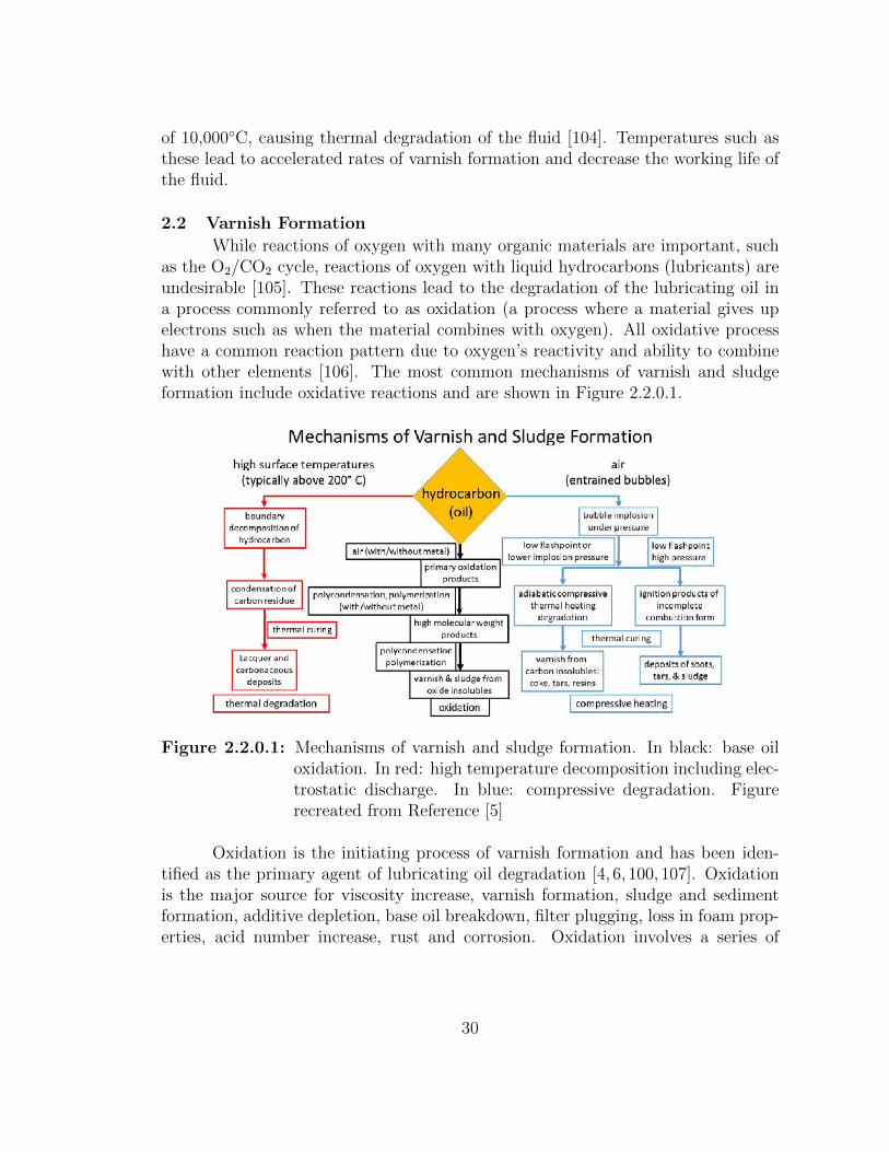
of 10,000◦C, causing thermal degradation of the fluid [104]. Temperatures such asthese lead to accelerated rates of varnish formation and decrease the working life ofthe fluid.
2.2 Varnish Formation
While reactions of oxygen with many organic materials are important, suchas the O2/CO2 cycle, reactions of oxygen with liquid hydrocarbons (lubricants) areundesirable [105]. These reactions lead to the degradation of the lubricating oil ina process commonly referred to as oxidation (a process where a material gives upelectrons such as when the material combines with oxygen). All oxidative processhave a common reaction pattern due to oxygen’s reactivity and ability to combinewith other elements [106]. The most common mechanisms of varnish and sludgeformation include oxidative reactions and are shown in Figure 2.2.0.1.
Figure 2.2.0.1: Mechanisms of varnish and sludge formation. In black: base oiloxidation. In red: high temperature decomposition including elec-trostatic discharge. In blue: compressive degradation. Figurerecreated from Reference [5]
Oxidation is the initiating process of varnish formation and has been iden-tified as the primary agent of lubricating oil degradation [4, 6, 100, 107]. Oxidationis the major source for viscosity increase, varnish formation, sludge and sedimentformation, additive depletion, base oil breakdown, filter plugging, loss in foam prop-erties, acid number increase, rust and corrosion. Oxidation involves a series of
30
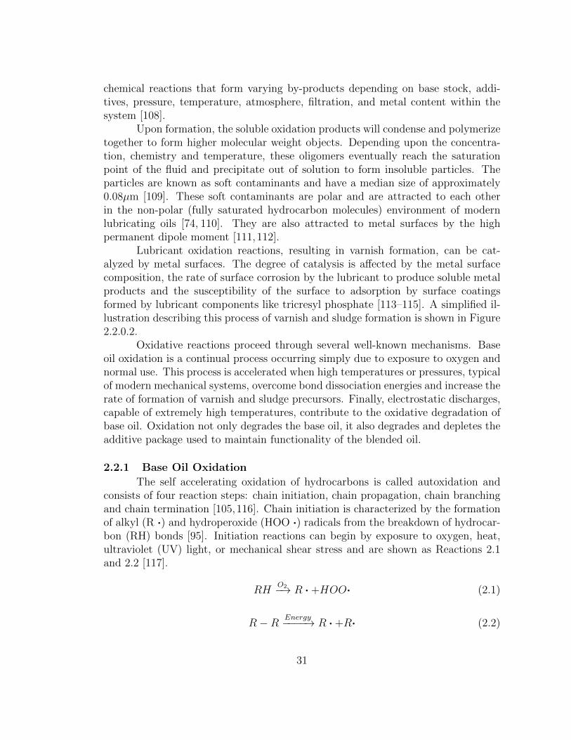
chemical reactions that form varying by-products depending on base stock, addi-tives, pressure, temperature, atmosphere, filtration, and metal content within thesystem [108].
Upon formation, the soluble oxidation products will condense and polymerizetogether to form higher molecular weight objects. Depending upon the concentra-tion, chemistry and temperature, these oligomers eventually reach the saturationpoint of the fluid and precipitate out of solution to form insoluble particles. Theparticles are known as soft contaminants and have a median size of approximately0.08µm [109]. These soft contaminants are polar and are attracted to each otherin the non-polar (fully saturated hydrocarbon molecules) environment of modernlubricating oils [74, 110]. They are also attracted to metal surfaces by the highpermanent dipole moment [111,112].
Lubricant oxidation reactions, resulting in varnish formation, can be cat-alyzed by metal surfaces. The degree of catalysis is affected by the metal surfacecomposition, the rate of surface corrosion by the lubricant to produce soluble metalproducts and the susceptibility of the surface to adsorption by surface coatingsformed by lubricant components like tricresyl phosphate [113–115]. A simplified il-lustration describing this process of varnish and sludge formation is shown in Figure2.2.0.2.
Oxidative reactions proceed through several well-known mechanisms. Baseoil oxidation is a continual process occurring simply due to exposure to oxygen andnormal use. This process is accelerated when high temperatures or pressures, typicalof modern mechanical systems, overcome bond dissociation energies and increase therate of formation of varnish and sludge precursors. Finally, electrostatic discharges,capable of extremely high temperatures, contribute to the oxidative degradation ofbase oil. Oxidation not only degrades the base oil, it also degrades and depletes theadditive package used to maintain functionality of the blended oil.
2.2.1 Base Oil Oxidation
The self accelerating oxidation of hydrocarbons is called autoxidation andconsists of four reaction steps: chain initiation, chain propagation, chain branchingand chain termination [105,116]. Chain initiation is characterized by the formationof alkyl (R ·) and hydroperoxide (HOO ·) radicals from the breakdown of hydrocar-bon (RH) bonds [95]. Initiation reactions can begin by exposure to oxygen, heat,ultraviolet (UV) light, or mechanical shear stress and are shown as Reactions 2.1and 2.2 [117].
RHO2−→ R · +HOO· (2.1)
R−R Energy−−−−→ R · +R· (2.2)
31
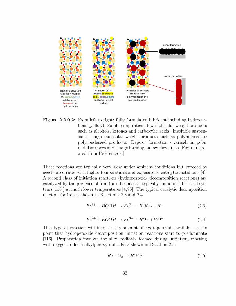
Figure 2.2.0.2: From left to right: fully formulated lubricant including hydrocar-bons (yellow). Soluble impurities - low molecular weight productssuch as alcohols, ketones and carboxylic acids. Insoluble suspen-sions - high molecular weight products such as polymerised orpolycondensed products. Deposit formation - varnish on polarmetal surfaces and sludge forming on low flow areas. Figure recre-ated from Reference [6]
These reactions are typically very slow under ambient conditions but proceed ataccelerated rates with higher temperatures and exposure to catalytic metal ions [4].A second class of initiation reactions (hydroperoxide decomposition reactions) arecatalyzed by the presence of iron (or other metals typically found in lubricated sys-tems [118]) at much lower temperatures [4,95]. The typical catalytic decompositionreaction for iron is shown as Reactions 2.3 and 2.4.
Fe3+ +ROOH → Fe2+ +ROO · +H+ (2.3)
Fe2+ +ROOH → Fe3+ +RO · +HO− (2.4)
This type of reaction will increase the amount of hydroperoxide available to thepoint that hydroperoxide decomposition initiation reactions start to predominate[116]. Propagation involves the alkyl radicals, formed during initiation, reactingwith oxygen to form alkylperoxy radicals as shown in Reaction 2.5.
R · +O2 → ROO· (2.5)
32
This reaction happens very fast, with low activation energy, and is inde-pendent of temperature [4]. The alkylperoxy radicals then abstract hydrogen fromother hydrocarbon molecules to form hydroperoxide and additional alkyl radicals asshown in Reaction 2.6.
ROO · +RH → ROOH +R· (2.6)
This reaction is slow, depending on the type of hydrocarbon, and is a rate determin-ing step for chain propagation. The new alkyl radicals can then react with oxygento form additional alkyl peroxide radicals (Reaction 2.5). This leads to an increasedrate of formation of various types of hydroperoxide, which results in a reinforcedautocatalytic degradation of hydrocarbons [4].
Low temperature (< 120◦C) chain branching either homolytically cleaves (lowconcentrations), or through bimolecular reaction (high concentrations) the varioushydroperoxides, formed during the early stages of autoxidation, to yield alkoxy andhydroxy radicals as shown in Reactions 2.7 and 2.8 [4].
ROOH → RO · +HO· (2.7)
ROOH +ROOH ←→ ROO · +RO · +H2O (2.8)
Reaction 2.7 has high activation energy and is only significant at higher temperaturesor under catalysed conditions. The resulting radicals follow a number of possiblereactions as shown below [95]:
• alkoxyl radicals abstract hydrogen from a hydrocarbon to form a molecule ofalcohol and a new alkyl radical
• hydroxyl radicals abstract hydrogen from a hydrocarbon molecule to formwater and a new alkyl radical
• secondary alkoxyl radicals may decompose to form an aldehyde
• tertiary alkoxy radicals may decompose to form a ketone
As a consequence of hydroperoxide accumulation and reaction, the concen-tration of free radicals initiating new chains increase. The lower molecular weightaldehydes and ketones generated will immediately affect the physical properties ofthe lubricant by decreasing oil viscosity, increasing oil volatility and increasing po-larity [95,116].
High temperature (> 120◦C) chain branching begins with the same radicalchain reactions as discussed under low temperature conditions with reduced selectiv-ity and increased reactions rates. At high temperature the cleavage of hydroperoxide
33
plays the most important role. Reaction 2.7, now with plenty of energy, leads to anabundance of hydroxy radicals, which non selectively abstract hydrogen atoms [4].Carboxylic acids are formed using the hydroperoxy peroxy radicals and aldehydesthat were formed earlier. Carboxylic acids can react with the alcohols (formed un-der low temperature chain branching) to form esters and when the rate of oxidationbecomes diffusion limited, ethers are formed [4]. As oxidation proceeds, acid or basecatalyzed Aldol reactions take place leading to the formation of oligomers and highmolecular weight oil soluble products (molecular weight about 2000 amu) [80, 116].When diffusion becomes limited, by the increase in oil viscosity, polycondensationand polymerization (initiated by alkoxy radicals) reactions of these high molecularweight intermediates form products which are no longer soluble in the lubricationoil. These high molecular weight products contribute to oil viscosity increase andcan eventually combine to form oil insoluble products resulting in sludge and var-nish [95].
Chain termination reactions might include limited diffusion, from increasedviscosity, that cause two alkyl radicals to combine forming a hydrocarbon moleculeor an alkyl radical combining with a alkylperoxy radical to form a peroxide [4].Termination reactions might proceed through primary and secondary peroxy radi-cals but at temperatures above 120◦C these peroxy radicals also interact in a nonterminating way to give primary and secondary alkoxy radicals [95]. These radicalsagain contribute to the formation of cleavage products. During the chain termina-tion processes, formation of carbonyl compounds and alcohols may also take placeon the peroxy radicals that contain an extractable α-hydrogen atom [116]. Termi-nation may be effected by the combination of radical species such as peroxy radicalsto yield ketones and alcohols leading to the formation of higher molecular weightcompounds.
In summary, the uncatalyzed oxidation of hydrocarbons at temperatures ofup to 120◦C leads to peroxides, alcohols, aldehydes, water and ketones [80]. Undermetal catalyzed conditions or at higher temperatures (> 120◦C), degradation leadsto a complex mixture of final products that include varnish and sludge deposits [4].
2.2.2 Thermal and Compressive Base Oil Degradation
Thermal breakdown occurs when a mechanical system’s temperature beginsto increase beyond the point of thermal stability of the base oil. When the temper-atures of a mechanical system exceed 200◦C (400◦F) thermal decomposition (crack-ing) of the base oil will occur producing lower molecular weight volatile products [70].Furthermore, thermal cracking can initiate side reactions, induce polymerization,produce gaseous by products, destroy additives, and generate insoluble by prod-ucts [80].
34
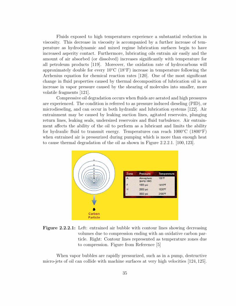
Fluids exposed to high temperatures experience a substantial reduction inviscosity. This decrease in viscosity is accompanied by a further increase of tem-perature as hydrodynamic and mixed regime lubrication surfaces begin to haveincreased asperity contact. Furthermore, lubricating oils entrain air easily and theamount of air absorbed (or dissolved) increases significantly with temperature forall petroleum products [119]. Moreover, the oxidation rate of hydrocarbons willapproximately double for every 10◦C (18◦F) increase in temperature following theArrhenius equation for chemical reaction rates [120]. One of the most significantchange in fluid properties caused by thermal decomposition of lubrication oil is anincrease in vapor pressure caused by the shearing of molecules into smaller, morevolatile fragments [121].
Compressive oil degradation occurs when fluids are aerated and high pressuresare experienced. The condition is referred to as pressure induced dieseling (PID), ormicrodieseling, and can occur in both hydraulic and lubrication systems [122]. Airentrainment may be caused by leaking suction lines, agitated reservoirs, plungingreturn lines, leaking seals, undersized reservoirs and fluid turbulence. Air entrain-ment affects the ability of the oil to perform as a lubricant and limits the abilityfor hydraulic fluid to transmit energy. Temperatures can reach 1000◦C (1800◦F)when entrained air is pressurized during pumping which is more than enough heatto cause thermal degradation of the oil as shown in Figure 2.2.2.1. [100,123].
Figure 2.2.2.1: Left: entrained air bubble with contour lines showing decreasingvolumes due to compression ending with an oxidative carbon par-ticle. Right: Contour lines represented as temperature zones dueto compression. Figure from Reference [5]
When vapor bubbles are rapidly pressurized, such as in a pump, destructivemicro-jets of oil can collide with machine surfaces at very high velocities [124,125].
35
This causes deformation of the pumping material and can lead to debris, pumpinglosses, and even failure of the pump. Furthermore, the temperature reached withPID leads to microscopic ignition (called partial combustion) of the oxygen rich oilvapors. The problem is exacerbated with low viscosity oils such as turbine oils [6].Low viscosity fluids have low flash points, which contribute to the vaporization ofthe light oil fractions that mix with air at the bubble boundaries. PID can causepressures in the area of micro-explosion to reach 5-6 times normal working pressureas well as very high temperatures. The end result is carbonized oil at the bubbleinterface leading to varnish and sludge deposits as well as increased oil degradation.
2.2.3 Electrostatic Discharge
Electrostatic charge generation occurs in fluid systems as a result of frictionbetween the fluid and system components [6]. The magnitude of charge depends onmany interrelated factors such as flow rates, composition of base oil, film thickness,surface roughness and environment [126]. Charges can occur during filtration ofhydraulic and lubricating oils as well as diesel and gasoline fuels. Electrostaticdischarge manifests itself as an audible noise (clicking sound) as charge accumulationcauses sparking internally within the system as well as charge dissipation of theelectrical charge downstream of the filter to a grounded surface [127].
Spark discharges can reach temperatures as high as 10,000 to 20,000◦C andare usually short lived, being extinguished by the fluid [128]. This can result in etch-ing of the discharged surface, possibly removing microscopic particles and leavingcarbon deposits on the surface. Voltage potentials are directly related to the fluxthrough the filter media and voltages exceeding 10 kV have been measured [128].The high temperatures experienced during electrostatic discharge cause acceleratedrates of hydrocarbon decomposition [127]. Electrostatic discharge has been shownto increase oxygen uptake (furthering oxidation) of test samples stored in light free,ambient temperature environments [104].
2.3 Removing and/or Mitigating Varnish
The first steps in minimizing hydrocarbon oxidation are implemented at re-fineries where techniques are employed to remove undesirable components that areeasily oxidized, such as unsaturated hydrocarbons, polar components and wax, fromcrude oil [4]. Synthetic oils are widely produced to combat thermal degradation byproducing molecular chains that are fully saturated, uniform and predictable duringformation. Further oxidative resistance is provided through the use of strong anti-oxidation compounds designed to work synergistically with other additives, therebyproviding superior performance and degradation resistance [70].
Unfortunately, additives can be harmful to the environment and emissionrelated controls. For example, modern catalytic converters are highly effective in re-ducing emissions, however, they are vulnerable to the deteriorating effects of sulfur,
36
phosphorus, and ash derived from engine oils and fuels [80]. Due to this, the APIhas limited the allowable concentrations of elements like sulfur and phosphorus inblended oils. Therefore, initiatives have been made to reduce the Zinc dialkyldithio-phosphates (ZDDP) content in engine oils. The current ILSAC GF-4 specificationhas limited the sulfur and phosphorus levels to a maximum of 0.7 and 0.08 wt%,respectively, and these numbers are likely to be even lower for future engine oils [129].
Varnish mitigation methods are also implemented by removing primary ox-idation products using electrostatic and adsorption methods. Electrostatic varnishmitigation takes advantage of the polar nature of varnish combined with dielec-trophoresis to remove varnish and varnish pre-cursors. Adsorption typically usesfilter media with pores small enough to retain oxidation by-products. While thesemethods are successful in removing degradation by-products, they require extendeddurations for optimal performance and that no shut down time occurs, allowing tem-peratures to be maintained in a range that allow varnish to remain in suspensionand be removed by filtration. Furthermore, caution must be used when choosingfilter media, which can inadvertently remove beneficial additive compounds fromthe fluid [130].
Varnish removal can also be performed using chemical flushing compounds.While the electrostatic and adsorption methods are re-active to the formation ofvarnish, the chemical flush is pro-active in removing varnish. Chemical flushingcomprises compounds that soften varnish, allowing it be suspended in the fluid andremoved by filter media. This process can be very fast, depending on the chemicalsused, and allows the system to remain fully functional while the cleaning processoccurs. Moreover, the removal of additive package compounds by filtration is nota concern since a full oil change will occur when the process is complete, allowingvery fine filter media to be used.
2.3.1 Full or Partial Oil Changes
The full, or partial, oil change method of varnish mitigation is a leadingpreventative measure in the transportation industry. New oil has typically notbegun the oxidation process so it should not be expected to cause new depositswhen added to the system. However, the benefit of this method is severely limitedby the quantity of varnish deposits within the system. When new oil is placed in-service it will suspend some of the varnish and sludge contaminants already presentin the system. This causes premature oxidation and saturation of the oil negatingthe benefits of a complete oil change. This is only the case when oil change intervalsare not adhered to causing an abundance of varnish and sludge in the system.
While this approach could be beneficial if the oil is maintained in a less thansaturated condition, it requires frequent testing to ensure oil condition. Moreover,oil consumers may not be sensitive to the rate of varnish accumulation in the newoil, limiting the benefit of this method. However, the approach would produce a net
37
benefit if performed periodically, as the cleanliness of the system in terms of existingvarnish deposits can be improved with time.
2.3.2 Electrostatic Purification
The electrostatic method, operating in a kidney loop mode off the maintank, subjects the fluid to an electrical field, which causes the varnish precursors tocharge and agglomerate into larger particles that are then captured by a filter mator attracted to a charged, disposable surface [120]. There are several designs basedon variants of the electrostatic charging principle to accomplish this goal.
The electrostatic type devices are reported to remove varnish precursors fromthe fluid phase, and as the fluid is cleaned up, soft varnish deposits from surfaces arere-entrained in the fluid and removed, thus resulting in the cleaning up of depositsaccumulated over a period of time [100]. Since the removal of varnish from systemcomponents is a relatively slow process, these devices are recommended to be op-erated over a long period of time or to be installed permanently. The electrostatictype devices are reported to be sensitive to elevated moisture levels in the fluid andalso to the presence of high levels of metal wear particles [131].
Electrostatic charge purification can be problematic for several reasons. Whenhydrocarbons pass by nonconductive filtration material there is the potential fordischarge within the filer and media [132]. The use of grounded filter housings andpipelines does not stop the charge generation or internal damage to the filter orother components [131]. Furthermore, mineral based oils generate positive chargeson filter media causing a negative charge to be carried downstream while syntheticoils showed just the opposite. Electrostatic charge purification is also limited to sta-tionary systems and implementation in the transportation industry is not realisticdue to cost and size constraints.
2.3.3 Adsorption Using Filter Media
The adsorption method utilizes adsorbent media with a large surface areato collect varnish and sludge. This method also requires a high void volume in thefilter media, relatively low fluid flow and in some cases an electro chemical affinityfor varnish and sludge precursors [120]. Many materials can be used as adsorbents,including compressed cellulose, cotton linters and macro-porous media such as resinbeads, Fullers earth, activated carbon and others [127].
Physisorption, also known as physical adsorption, is characterized by thephysical bonding of varnish and sludge precursors to the surface of the filter mediaat low temperatures in the absence of chemical bonds. The electronic structure ofthe adsorbate does not change upon adsorption and varnish molecules are believedto be attracted to the adsorbent through weak molecular forces such as hydrogenbonding (van der Waals forces) [120].
38
The down side to the adsorption method is the possibility of inadvertentremoval of additives from the oil as well as placement of the filter media that willdetermine the effectiveness of the system [130]. Furthermore, this type of systemmust be implemented for extended durations (> 8 weeks) and is highly dependenton the amount of varnish and sludge previously in the system [120].
2.3.4 Chemical Cleaning or Flushing
The chemical cleaning/flushing method for removing varnish utilizes cleaningchemicals that are typically circulated through the system to dislodge, dissociate, orsoften varnish and sludge from components [133]. The flushing action suspends thedeposits in the fluid which are then removed by filtration and with the fluid when itis drained from the system. This process is usually performed for several hours orseveral days, depending on the system size and the extent of the varnish build upon components [134].
Once the flush and chemical treatment is completed, the system must beflushed again with an appropriate flushing fluid (such as base stock) to remove resid-ual chemicals and to ensure no contamination finds its way into the new lubricatingoil [135]. Although this process is more intensive, it does allow for quicker removalof varnish deposits, especially in a large systems. The quick removal rates are thedefining aspect of this process. It is known to be cost effective when compared toother methods and only requires flushing when the system exhibits an abundance ofvarnish buildup. It does required close monitoring and entails lost production dueto system downtime.
2.4 Summary and Motivation
Varnish is a natural process exacerbated by heat, light, contaminants andmechanical stresses. Because varnish is an unavoidable by-product of hydrocar-bon degradation, understanding the factors that cause its formation is importantto the scientific community as well as the end user. If steps can be taken to mini-mize the formation of varnish for in-service systems, efficiencies and longevities willincrease. This is beneficial from both economic and environmental perspectives.Manufactures, as well as end users, have an obligation to provide the best possiblestewardship over in-service equipment.
The mitigation of varnish for in-service equipment is possible because of ourunderstanding of the mechanisms of varnish formation. Different types of varnishmitigation systems are available which are relevant to each type of industry. Forexample, the transportation industry’s method of mitigating varnish will be verydifferent than that used by the power generation industry. Moreover, the amountof oil in a given system, as well as whether that system is mobile or stationary, willdictate the most beneficial method of varnish mitigation. Historically, varnish hasbeen the major factor in recommended service intervals and remains so to this day.
39
This work will focus on varnish removal from gas turbine engines used inthe power generation industry using chemical cleaners. Gas turbines are stationaryunits that can hold up to 40,000 gallons of lubricating oil which makes full oilchanges a daunting task both economically and environmentally. Implementingthe use of chemical cleaners, combined with proper filtration, can extend the life ofsystem components and the lubricating oils that separate them. Therefore, properlycharacterizing the performance of chemical cleaner is of utmost importance.
The largest concern using chemical cleaners is the lack of standard meth-ods to characterize removal amounts and rates. This is in sharp contrast to themany standards that are available to characterize an oils resistance to oxidation,the precursor to varnish formation, e.g. ASTM D974 [136] or D664 [137], ASTMD2272 [138], ASTM D445 [139], ASTM D92 [140]. Testing lubricating oils beforeand during use is invaluable to the end user and, due to the fact that varnish for-mation is usually inevitable, it is also very important to quantify and standardizevarnish removal methods. Standards that consistently quantify the removal poten-tial of chemical cleaners are needed to ensure performance data will be available tothe scientific community, as well as the end user.
To address this, a test has been designed that will allow varnish removalusing chemical cleaners to be quantified. This test system has been designed toallow control of flow rates and temperatures across a flat steel sample containing anartificial varnish. This varnish is produced using common oxidative mechanisms andcharacterized to ensure the product accurately simulates varnish produced withinthe gas turbine engine. The varnish is subjected to chemical flushes at flow ratesand temperatures designed to mimic conditions within a typical gas turbine engine.Testing metrics include mass loss and time-lapse photographic data, where the latteris analyzed numerically to determine parameters including the maximum rate ofvarnish removal. The novel test method developed in this research is described indetail in the next chapter.
40
Chapter 3
EXPERIMENTAL DESIGN
3.1 Design Introduction
To characterize chemical cleaners, a test system was needed to provide anenvironment where varnish would be exposed to the simulated conditions of inservice systems. Furthermore, the test system needed to provide ease of testing,controllability, and reproducibility. To provide this, several design constraints wereconsidered when designing the varnish test system. The system needed to operateeffectively with a minimal amount of fluid, providing an efficient use of blendedchemicals. Moreover, the design required that temperature control be a paramountfeature, with the ability to ensure precise, accurate temperatures throughout testing.Furthermore, accurately controlling the flux of the test fluids through the systemwas of utmost importance, thereby allowing a broad range of testing to be donewith consistency and confidence. The design also needed to provide easy flushing ofchemicals between testing as well easily accessible locations for filling and drainingfluids.
The test system needed to deliver operational envelopes for a wide rangeof industrial, commercial and transportation environments to ensure that condi-tions within journal bearings, heat transfer units, pumping lines, thrust washersand other engineered systems could be simulated. It was imperative that the testsystem provide a safe working environment both physically and environmentally.The total tabletop area of the test system needed to be kept to a minimum to allowlocation in confined spaces. The following sections will describe the components,sub-components, further design criteria and operational envelope of the varnish testsystem.
3.2 Test Coupon
A method of supplying a varnished surface, that could be repeated with confi-dence, was needed for the varnish test system. Stamping uniformly sized, rectangu-lar metal coupons, were decided upon and varnish would be applied on the surface.A test coupon specimen, dimensioned as shown in Figure 3.2.0.1, was implemented.
The test coupon would need to slip fit into the test chamber, be held tightlyto minimize movement during testing, and allow for easy removal when coated with
41
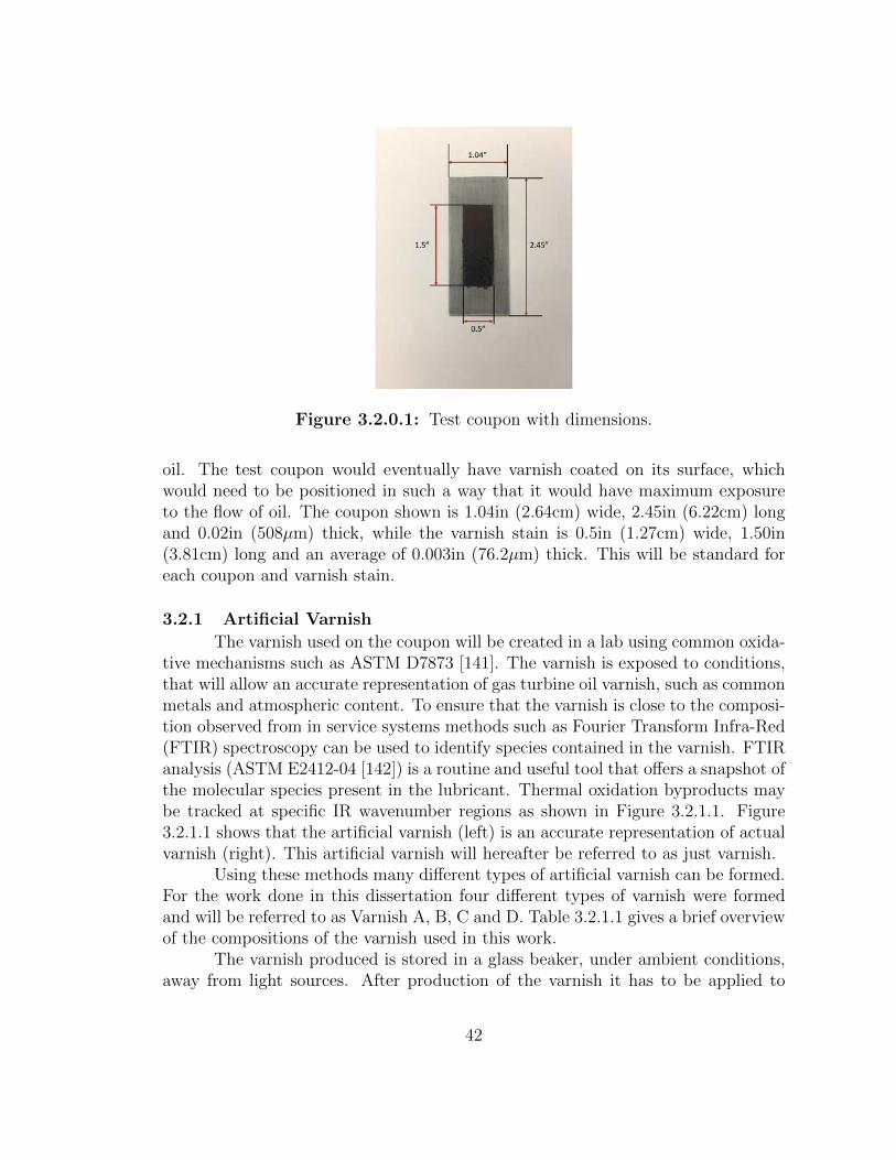
Figure 3.2.0.1: Test coupon with dimensions.
oil. The test coupon would eventually have varnish coated on its surface, whichwould need to be positioned in such a way that it would have maximum exposureto the flow of oil. The coupon shown is 1.04in (2.64cm) wide, 2.45in (6.22cm) longand 0.02in (508µm) thick, while the varnish stain is 0.5in (1.27cm) wide, 1.50in(3.81cm) long and an average of 0.003in (76.2µm) thick. This will be standard foreach coupon and varnish stain.
3.2.1 Artificial Varnish
The varnish used on the coupon will be created in a lab using common oxida-tive mechanisms such as ASTM D7873 [141]. The varnish is exposed to conditions,that will allow an accurate representation of gas turbine oil varnish, such as commonmetals and atmospheric content. To ensure that the varnish is close to the composi-tion observed from in service systems methods such as Fourier Transform Infra-Red(FTIR) spectroscopy can be used to identify species contained in the varnish. FTIRanalysis (ASTM E2412-04 [142]) is a routine and useful tool that offers a snapshot ofthe molecular species present in the lubricant. Thermal oxidation byproducts maybe tracked at specific IR wavenumber regions as shown in Figure 3.2.1.1. Figure3.2.1.1 shows that the artificial varnish (left) is an accurate representation of actualvarnish (right). This artificial varnish will hereafter be referred to as just varnish.
Using these methods many different types of artificial varnish can be formed.For the work done in this dissertation four different types of varnish were formedand will be referred to as Varnish A, B, C and D. Table 3.2.1.1 gives a brief overviewof the compositions of the varnish used in this work.
The varnish produced is stored in a glass beaker, under ambient conditions,away from light sources. After production of the varnish it has to be applied to
42
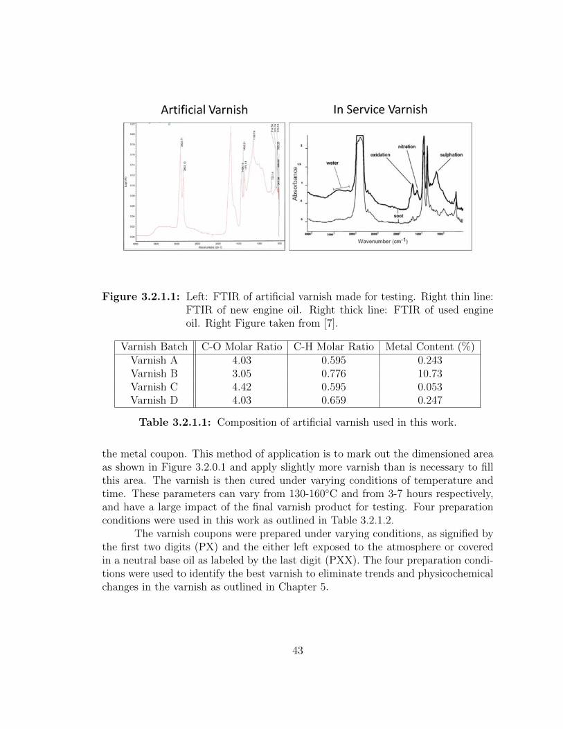
Figure 3.2.1.1: Left: FTIR of artificial varnish made for testing. Right thin line:FTIR of new engine oil. Right thick line: FTIR of used engineoil. Right Figure taken from [7].
Varnish Batch C-O Molar Ratio C-H Molar Ratio Metal Content (%)Varnish A 4.03 0.595 0.243Varnish B 3.05 0.776 10.73Varnish C 4.42 0.595 0.053Varnish D 4.03 0.659 0.247
Table 3.2.1.1: Composition of artificial varnish used in this work.
the metal coupon. This method of application is to mark out the dimensioned areaas shown in Figure 3.2.0.1 and apply slightly more varnish than is necessary to fillthis area. The varnish is then cured under varying conditions of temperature andtime. These parameters can vary from 130-160◦C and from 3-7 hours respectively,and have a large impact of the final varnish product for testing. Four preparationconditions were used in this work as outlined in Table 3.2.1.2.
The varnish coupons were prepared under varying conditions, as signified bythe first two digits (PX) and the either left exposed to the atmosphere or coveredin a neutral base oil as labeled by the last digit (PXX). The four preparation condi-tions were used to identify the best varnish to eliminate trends and physicochemicalchanges in the varnish as outlined in Chapter 5.
43
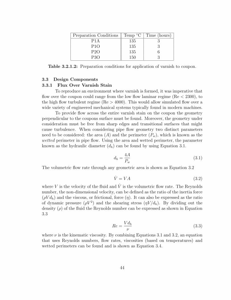
Preparation Conditions Temp ◦C Time (hours)P1A 135 3P1O 135 3P2O 135 6P3O 150 3
Table 3.2.1.2: Preparation conditions for application of varnish to coupon.
3.3 Design Components
3.3.1 Flux Over Varnish Stain
To reproduce an environment where varnish is formed, it was imperative thatflow over the coupon could range from the low flow laminar regime (Re < 2300), tothe high flow turbulent regime (Re > 4000). This would allow simulated flow over awide variety of engineered mechanical systems typically found in modern machines.
To provide flow across the entire varnish stain on the coupon the geometryperpendicular to the coupons surface must be found. Moreover, the geometry underconsideration must be free from sharp edges and transitional surfaces that mightcause turbulence. When considering pipe flow geometry two distinct parametersneed to be considered: the area (A) and the perimeter (Pw), which is known as thewetted perimeter in pipe flow. Using the area and wetted perimeter, the parameterknown as the hydraulic diameter (dh) can be found by using Equation 3.1.
dh =4A
Pw(3.1)
The volumetric flow rate through any geometric area is shown as Equation 3.2
V = V A (3.2)
where V is the velocity of the fluid and V is the volumetric flow rate. The Reynoldsnumber, the non-dimensional velocity, can be defined as the ratio of the inertia force(ρV dh) and the viscous, or frictional, force (η). It can also be expressed as the ratioof dynamic pressure (ρV 2) and the shearing stress (ηV/dh). By dividing out thedensity (ρ) of the fluid the Reynolds number can be expressed as shown in Equation3.3
Re =V dhν
(3.3)
where ν is the kinematic viscosity. By combining Equations 3.1 and 3.2, an equationthat uses Reynolds numbers, flow rates, viscosities (based on temperatures) andwetted perimeters can be found and is shown as Equation 3.4.
44
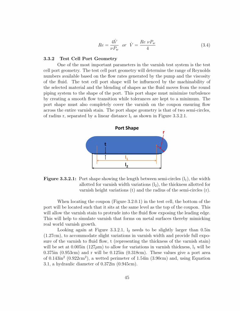
Re =4V
νPwor V =
Re νPw4
(3.4)
3.3.2 Test Cell Port Geometry
One of the most important parameters in the varnish test system is the testcell port geometry. The test cell port geometry will determine the range of Reynoldsnumbers available based on the flow rates generated by the pump and the viscosityof the fluid. The test cell port shape will be influenced by the machinability ofthe selected material and the blending of shapes as the fluid moves from the roundpiping system to the shape of the port. This port shape must minimize turbulenceby creating a smooth flow transition while tolerances are kept to a minimum. Theport shape must also completely cover the varnish on the coupon ensuring flowacross the entire varnish stain. The port shape geometry is that of two semi-circles,of radius r, separated by a linear distance l1 as shown in Figure 3.3.2.1.
Figure 3.3.2.1: Port shape showing the length between semi-circles (l1), the widthallotted for varnish width variations (l2), the thickness allotted forvarnish height variations (t) and the radius of the semi-circles (r).
When locating the coupon (Figure 3.2.0.1) in the test cell, the bottom of theport will be located such that it sits at the same level as the top of the coupon. Thiswill allow the varnish stain to protrude into the fluid flow exposing the leading edge.This will help to simulate varnish that forms on metal surfaces thereby mimickingreal world varnish growth.
Looking again at Figure 3.3.2.1, l2 needs to be slightly larger than 0.5in(1.27cm), to accommodate slight variations in varnish width and provide full expo-sure of the varnish to fluid flow, t (representing the thickness of the varnish stain)will be set at 0.005in (127µm) to allow for variations in varnish thickness, l1 will be0.375in (0.953cm) and r will be 0.125in (0.318cm). These values give a port areaof 0.143in2 (0.922cm2), a wetted perimeter of 1.54in (3.90cm) and, using Equation3.1, a hydraulic diameter of 0.372in (0.945cm).
45
3.3.3 Pump Selection
To properly size the oil pump a common oil (ISO VG-46), 46 centistokes (cSt)at 40◦C and 8.2 cSt at 100◦C, was selected to enable temperature related viscositiesto be used in flow rate calculations. Using Equation 3.4, Reynolds numbers werefound for flow rates ranging from 0 - 180 in3/s and for viscosities at 40, 70 and100◦C. The results are shown in Figure 3.3.3.1. Based on the desired operationalparameters of laminar to turbulent flow, a pump capable of 180 in3/s is required.
Figure 3.3.3.1: Reynolds numbers based on flow rate using ISO VG-46 base oil.
There are several types of pumps available to move fluid and they includepositive displacement pumps, impulse pumps, velocity pumps, gravity pumps, steampumps, and valveless pumps [143]. Because only positive displacement pumps arecapable of providing constant flow, for a given pressure, the remaining pump typeswill not be considered. A Positive Displacement Pump has an expanding cavityduring suction and a decreasing cavity during discharge providing constant geomet-ric pumping volumes for each revolution. The positive displacement pumps can bedivided into two categories of pumps: reciprocating and rotary.
Reciprocating pumps can be configured in to two main types of pumps; theplunger, and the diaphragm pump as shown in Figure 3.3.3.2. Because the operationof the reciprocating pump relies on a pulsed cycle, a constant flux across the varnishcoupon is not possible without the addition of an accumulator or multiple plungers.Likewise, diaphragm pumps operate on a similar pulsed cycle but are typically foundin dual diaphragm configurations to alleviate much of the pulsing. Due to the pulsingnature of reciprocating pumps they were not considered for use in the varnish testsystem.
Rotary pumps can be configured in many different ways including gear, lobe,vane, piston, progressive cavity pumps, peripheral pumps, and screw pumps. The
46
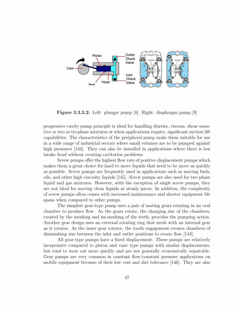
Figure 3.3.3.2: Left: plunger pump [8]. Right: diaphragm pump [9]
progressive cavity pump principle is ideal for handling slurries, viscous, shear sensi-tive or two or tri-phase mixtures or when applications require, significant suction liftcapabilities. The characteristics of the peripheral pump make them suitable for usein a wide range of industrial sectors where small volumes are to be pumped againsthigh pressures [144]. They can also be installed in applications where there is lowintake head without creating cavitation problems.
Screw pumps offer the highest flow rate of positive displacement pumps whichmakes them a great choice for hard to move liquids that need to be move as quicklyas possible. Screw pumps are frequently used in applications such as moving fuels,oils, and other high viscosity liquids [145]. Screw pumps are also used for two phaseliquid and gas mixtures. However, with the exception of single screw pumps, theyare not ideal for moving clean liquids at steady paces. In addition, the complexityof screw pumps often comes with increased maintenance and shorter equipment lifespans when compared to other pumps.
The simplest gear-type pump uses a pair of mating gears rotating in an ovalchamber to produce flow. As the gears rotate, the changing size of the chambers,created by the meshing and un-meshing of the teeth, provides the pumping action.Another gear design uses an external rotating ring that mesh with an internal gearas it rotates. As the inner gear rotates, the tooth engagement creates chambers ofdiminishing size between the inlet and outlet positions to create flow [143].
All gear-type pumps have a fixed displacement. These pumps are relativelyinexpensive compared to piston and vane type pumps with similar displacements,but tend to wear out more quickly and are not generally economically repairable.Gear pumps are very common in constant flow/constant pressure applications onmobile equipment because of their low cost and dirt tolerance [146]. They are also
47
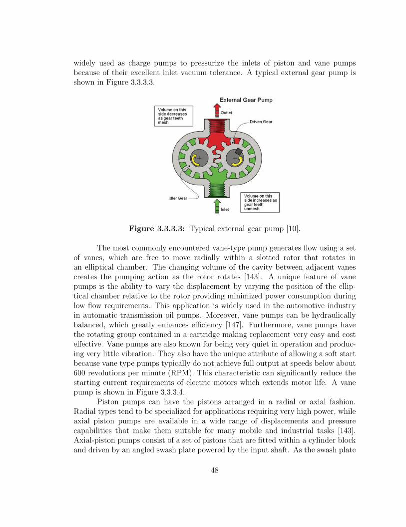
widely used as charge pumps to pressurize the inlets of piston and vane pumpsbecause of their excellent inlet vacuum tolerance. A typical external gear pump isshown in Figure 3.3.3.3.
Figure 3.3.3.3: Typical external gear pump [10].
The most commonly encountered vane-type pump generates flow using a setof vanes, which are free to move radially within a slotted rotor that rotates inan elliptical chamber. The changing volume of the cavity between adjacent vanescreates the pumping action as the rotor rotates [143]. A unique feature of vanepumps is the ability to vary the displacement by varying the position of the ellip-tical chamber relative to the rotor providing minimized power consumption duringlow flow requirements. This application is widely used in the automotive industryin automatic transmission oil pumps. Moreover, vane pumps can be hydraulicallybalanced, which greatly enhances efficiency [147]. Furthermore, vane pumps havethe rotating group contained in a cartridge making replacement very easy and costeffective. Vane pumps are also known for being very quiet in operation and produc-ing very little vibration. They also have the unique attribute of allowing a soft startbecause vane type pumps typically do not achieve full output at speeds below about600 revolutions per minute (RPM). This characteristic can significantly reduce thestarting current requirements of electric motors which extends motor life. A vanepump is shown in Figure 3.3.3.4.
Piston pumps can have the pistons arranged in a radial or axial fashion.Radial types tend to be specialized for applications requiring very high power, whileaxial piston pumps are available in a wide range of displacements and pressurecapabilities that make them suitable for many mobile and industrial tasks [143].Axial-piston pumps consist of a set of pistons that are fitted within a cylinder blockand driven by an angled swash plate powered by the input shaft. As the swash plate
48
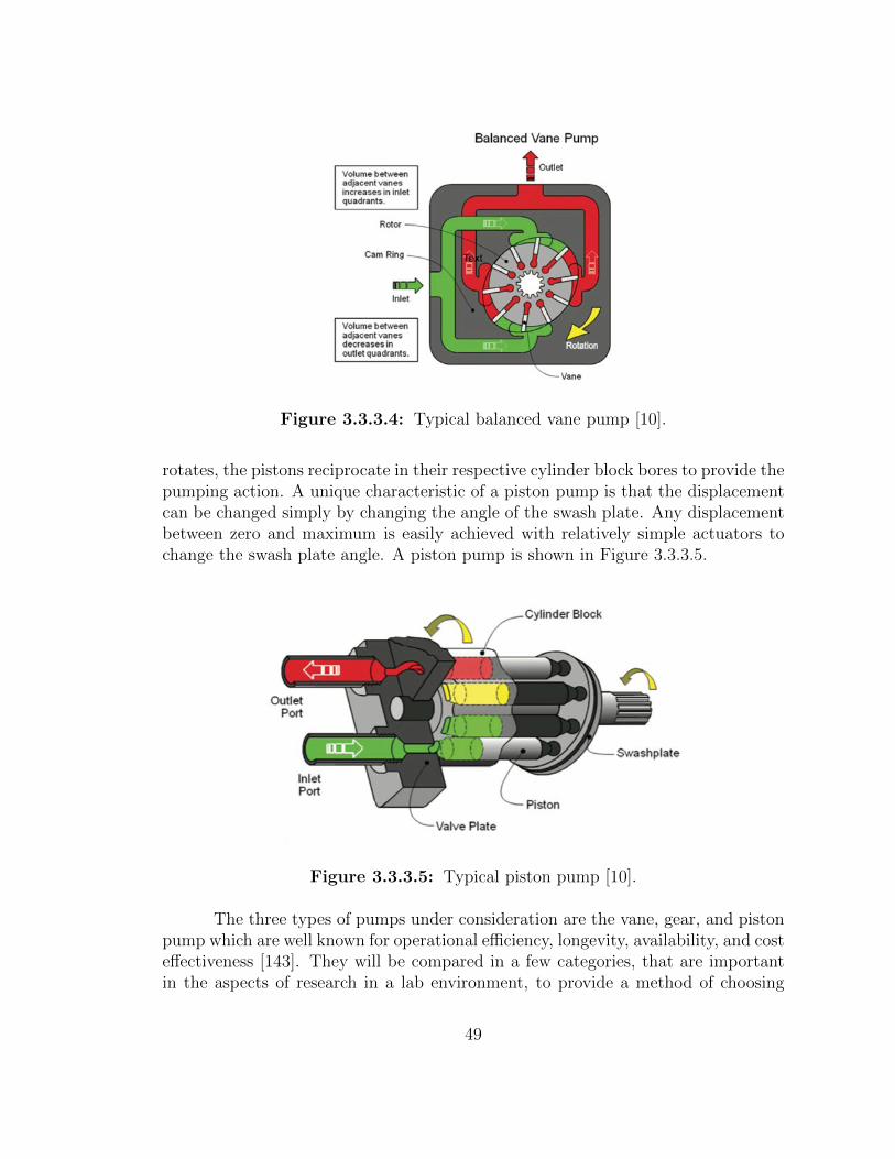
Figure 3.3.3.4: Typical balanced vane pump [10].
rotates, the pistons reciprocate in their respective cylinder block bores to provide thepumping action. A unique characteristic of a piston pump is that the displacementcan be changed simply by changing the angle of the swash plate. Any displacementbetween zero and maximum is easily achieved with relatively simple actuators tochange the swash plate angle. A piston pump is shown in Figure 3.3.3.5.
Figure 3.3.3.5: Typical piston pump [10].
The three types of pumps under consideration are the vane, gear, and pistonpump which are well known for operational efficiency, longevity, availability, and costeffectiveness [143]. They will be compared in a few categories, that are importantin the aspects of research in a lab environment, to provide a method of choosing
49
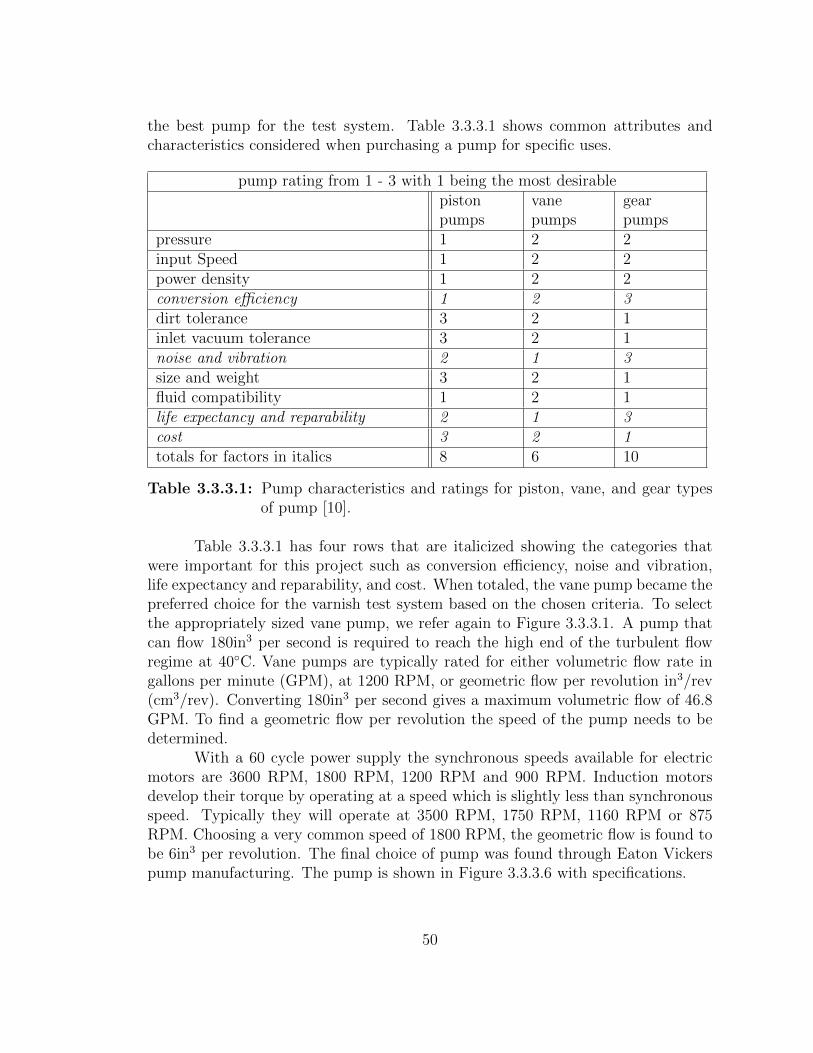
the best pump for the test system. Table 3.3.3.1 shows common attributes andcharacteristics considered when purchasing a pump for specific uses.
pump rating from 1 - 3 with 1 being the most desirablepistonpumps
vanepumps
gearpumps
pressure 1 2 2input Speed 1 2 2power density 1 2 2conversion efficiency 1 2 3dirt tolerance 3 2 1inlet vacuum tolerance 3 2 1noise and vibration 2 1 3size and weight 3 2 1fluid compatibility 1 2 1life expectancy and reparability 2 1 3cost 3 2 1totals for factors in italics 8 6 10
Table 3.3.3.1: Pump characteristics and ratings for piston, vane, and gear typesof pump [10].
Table 3.3.3.1 has four rows that are italicized showing the categories thatwere important for this project such as conversion efficiency, noise and vibration,life expectancy and reparability, and cost. When totaled, the vane pump became thepreferred choice for the varnish test system based on the chosen criteria. To selectthe appropriately sized vane pump, we refer again to Figure 3.3.3.1. A pump thatcan flow 180in3 per second is required to reach the high end of the turbulent flowregime at 40◦C. Vane pumps are typically rated for either volumetric flow rate ingallons per minute (GPM), at 1200 RPM, or geometric flow per revolution in3/rev(cm3/rev). Converting 180in3 per second gives a maximum volumetric flow of 46.8GPM. To find a geometric flow per revolution the speed of the pump needs to bedetermined.
With a 60 cycle power supply the synchronous speeds available for electricmotors are 3600 RPM, 1800 RPM, 1200 RPM and 900 RPM. Induction motorsdevelop their torque by operating at a speed which is slightly less than synchronousspeed. Typically they will operate at 3500 RPM, 1750 RPM, 1160 RPM or 875RPM. Choosing a very common speed of 1800 RPM, the geometric flow is found tobe 6in3 per revolution. The final choice of pump was found through Eaton Vickerspump manufacturing. The pump is shown in Figure 3.3.3.6 with specifications.
50
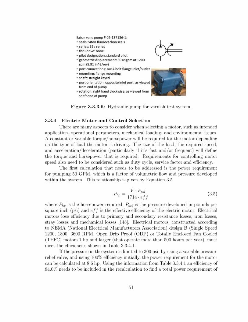
Figure 3.3.3.6: Hydraulic pump for varnish test system.
3.3.4 Electric Motor and Control Selection
There are many aspects to consider when selecting a motor, such as intendedapplication, operational parameters, mechanical loading, and environmental issues.A constant or variable torque/horsepower will be required for the motor dependingon the type of load the motor is driving. The size of the load, the required speed,and acceleration/deceleration (particularly if it’s fast and/or frequent) will definethe torque and horsepower that is required. Requirements for controlling motorspeed also need to be considered such as duty cycle, service factor and efficiency.
The first calculation that needs to be addressed is the power requirementfor pumping 50 GPM, which is a factor of volumetric flow and pressure developedwithin the system. This relationship is given by Equation 3.5
Php =V · Ppsi
1714 · eff(3.5)
where Php is the horsepower required, Ppsi is the pressure developed in pounds persquare inch (psi) and eff is the effective efficiency of the electric motor. Electricalmotors lose efficiency due to primary and secondary resistance losses, iron losses,stray losses and mechanical losses [148]. Electrical motors, constructed accordingto NEMA (National Electrical Manufacturers Association) design B (Single Speed1200, 1800, 3600 RPM, Open Drip Proof (ODP) or Totally Enclosed Fan Cooled(TEFC) motors 1 hp and larger (that operate more than 500 hours per year), mustmeet the efficiencies shown in Table 3.3.4.1.
If the pressure in the system is limited to 300 psi, by using a variable pressurerelief valve, and using 100% efficiency initially, the power requirement for the motorcan be calculated at 8.6 hp. Using the information from Table 3.3.4.1 an efficiency of84.0% needs to be included in the recalculation to find a total power requirement of
51
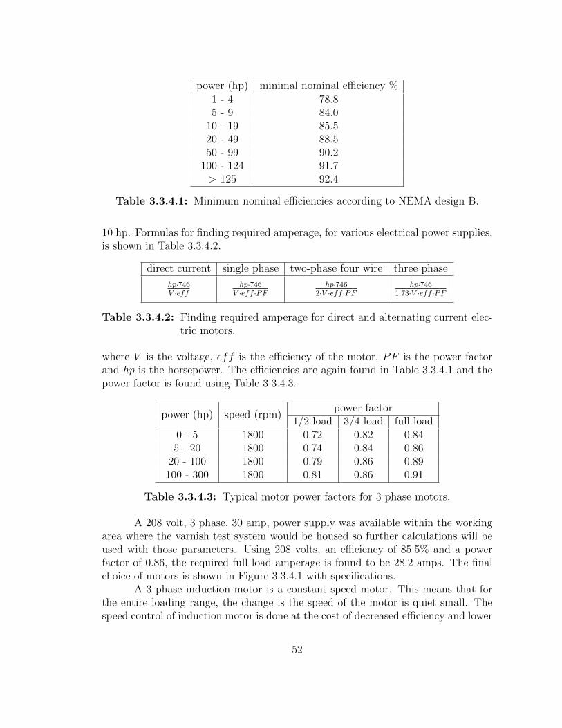
power (hp) minimal nominal efficiency %1 - 4 78.85 - 9 84.0
10 - 19 85.520 - 49 88.550 - 99 90.2
100 - 124 91.7> 125 92.4
Table 3.3.4.1: Minimum nominal efficiencies according to NEMA design B.
10 hp. Formulas for finding required amperage, for various electrical power supplies,is shown in Table 3.3.4.2.
direct current single phase two-phase four wire three phase
hp·746V ·eff
hp·746V ·eff ·PF
hp·7462·V ·eff ·PF
hp·7461.73·V ·eff ·PF
Table 3.3.4.2: Finding required amperage for direct and alternating current elec-tric motors.
where V is the voltage, eff is the efficiency of the motor, PF is the power factorand hp is the horsepower. The efficiencies are again found in Table 3.3.4.1 and thepower factor is found using Table 3.3.4.3.
power (hp) speed (rpm)power factor
1/2 load 3/4 load full load0 - 5 1800 0.72 0.82 0.845 - 20 1800 0.74 0.84 0.86
20 - 100 1800 0.79 0.86 0.89100 - 300 1800 0.81 0.86 0.91
Table 3.3.4.3: Typical motor power factors for 3 phase motors.
A 208 volt, 3 phase, 30 amp, power supply was available within the workingarea where the varnish test system would be housed so further calculations will beused with those parameters. Using 208 volts, an efficiency of 85.5% and a powerfactor of 0.86, the required full load amperage is found to be 28.2 amps. The finalchoice of motors is shown in Figure 3.3.4.1 with specifications.
A 3 phase induction motor is a constant speed motor. This means that forthe entire loading range, the change is the speed of the motor is quiet small. Thespeed control of induction motor is done at the cost of decreased efficiency and lower
52
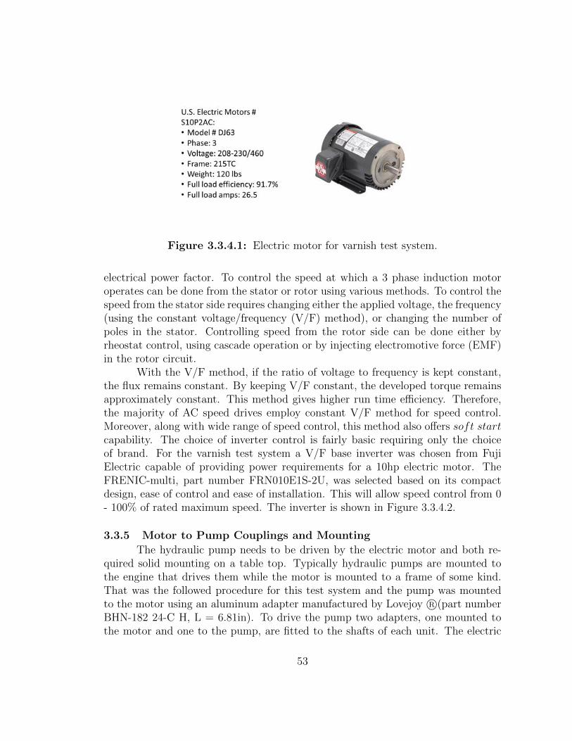
Figure 3.3.4.1: Electric motor for varnish test system.
electrical power factor. To control the speed at which a 3 phase induction motoroperates can be done from the stator or rotor using various methods. To control thespeed from the stator side requires changing either the applied voltage, the frequency(using the constant voltage/frequency (V/F) method), or changing the number ofpoles in the stator. Controlling speed from the rotor side can be done either byrheostat control, using cascade operation or by injecting electromotive force (EMF)in the rotor circuit.
With the V/F method, if the ratio of voltage to frequency is kept constant,the flux remains constant. By keeping V/F constant, the developed torque remainsapproximately constant. This method gives higher run time efficiency. Therefore,the majority of AC speed drives employ constant V/F method for speed control.Moreover, along with wide range of speed control, this method also offers soft startcapability. The choice of inverter control is fairly basic requiring only the choiceof brand. For the varnish test system a V/F base inverter was chosen from FujiElectric capable of providing power requirements for a 10hp electric motor. TheFRENIC-multi, part number FRN010E1S-2U, was selected based on its compactdesign, ease of control and ease of installation. This will allow speed control from 0- 100% of rated maximum speed. The inverter is shown in Figure 3.3.4.2.
3.3.5 Motor to Pump Couplings and Mounting
The hydraulic pump needs to be driven by the electric motor and both re-quired solid mounting on a table top. Typically hydraulic pumps are mounted tothe engine that drives them while the motor is mounted to a frame of some kind.That was the followed procedure for this test system and the pump was mountedto the motor using an aluminum adapter manufactured by Lovejoy R©(part numberBHN-182 24-C H, L = 6.81in). To drive the pump two adapters, one mounted tothe motor and one to the pump, are fitted to the shafts of each unit. The electric
53
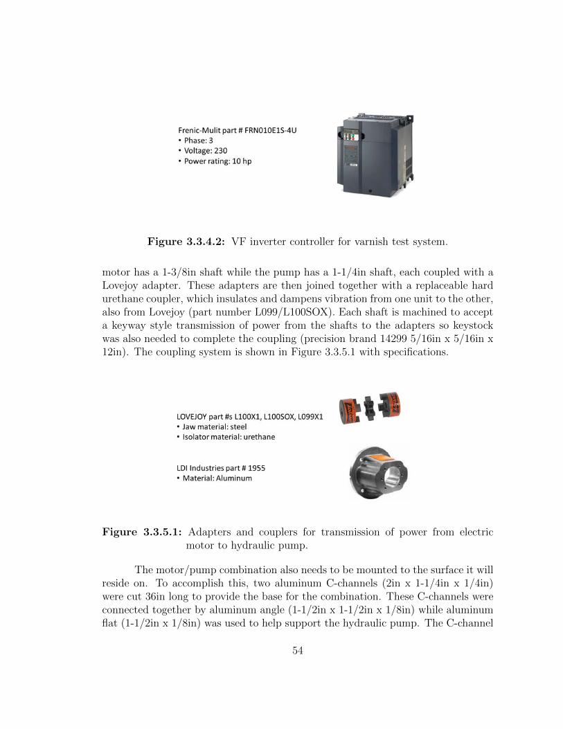
Figure 3.3.4.2: VF inverter controller for varnish test system.
motor has a 1-3/8in shaft while the pump has a 1-1/4in shaft, each coupled with aLovejoy adapter. These adapters are then joined together with a replaceable hardurethane coupler, which insulates and dampens vibration from one unit to the other,also from Lovejoy (part number L099/L100SOX). Each shaft is machined to accepta keyway style transmission of power from the shafts to the adapters so keystockwas also needed to complete the coupling (precision brand 14299 5/16in x 5/16in x12in). The coupling system is shown in Figure 3.3.5.1 with specifications.
Figure 3.3.5.1: Adapters and couplers for transmission of power from electricmotor to hydraulic pump.
The motor/pump combination also needs to be mounted to the surface it willreside on. To accomplish this, two aluminum C-channels (2in x 1-1/4in x 1/4in)were cut 36in long to provide the base for the combination. These C-channels wereconnected together by aluminum angle (1-1/2in x 1-1/2in x 1/8in) while aluminumflat (1-1/2in x 1/8in) was used to help support the hydraulic pump. The C-channel
54
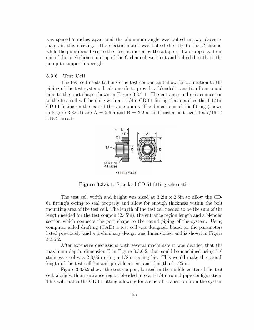
was spaced 7 inches apart and the aluminum angle was bolted in two places tomaintain this spacing. The electric motor was bolted directly to the C-channelwhile the pump was fixed to the electric motor by the adapter. Two supports, fromone of the angle braces on top of the C-channel, were cut and bolted directly to thepump to support its weight.
3.3.6 Test Cell
The test cell needs to house the test coupon and allow for connection to thepiping of the test system. It also needs to provide a blended transition from roundpipe to the port shape shown in Figure 3.3.2.1. The entrance and exit connectionto the test cell will be done with a 1-1/4in CD-61 fitting that matches the 1-1/4inCD-61 fitting on the exit of the vane pump. The dimensions of this fitting (shownin Figure 3.3.6.1) are A = 2.6in and B = 3.2in, and uses a bolt size of a 7/16-14UNC thread.
Figure 3.3.6.1: Standard CD-61 fitting schematic.
The test cell width and height was sized at 3.2in x 2.5in to allow the CD-61 fitting’s o-ring to seal properly and allow for enough thickness within the boltmounting area of the test cell. The length of the test cell needed to be the sum of thelength needed for the test coupon (2.45in), the entrance region length and a blendedsection which connects the port shape to the round piping of the system. Usingcomputer aided drafting (CAD) a test cell was designed, based on the parameterslisted previously, and a preliminary design was dimensioned and is shown in Figure3.3.6.2.
After extensive discussions with several machinists it was decided that themaximum depth, dimension B in Figure 3.3.6.2, that could be machined using 316stainless steel was 2-3/8in using a 1/8in tooling bit. This would make the overalllength of the test cell 7in and provide an entrance length of 1.25in.
Figure 3.3.6.2 shows the test coupon, located in the middle-center of the testcell, along with an entrance region blended into a 1-1/4in round pipe configuration.This will match the CD-61 fitting allowing for a smooth transition from the system
55
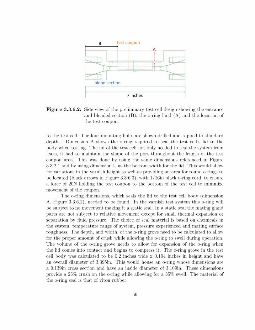
Figure 3.3.6.2: Side view of the preliminary test cell design showing the entranceand blended section (B), the o-ring land (A) and the location ofthe test coupon.
to the test cell. The four mounting bolts are shown drilled and tapped to standarddepths. Dimension A shows the o-ring required to seal the test cell’s lid to thebody when testing. The lid of the test cell not only needed to seal the system fromleaks, it had to maintain the shape of the port throughout the length of the testcoupon area. This was done by using the same dimensions referenced in Figure3.3.2.1 and by using dimension l2 as the bottom width for the lid. This would allowfor variations in the varnish height as well as providing an area for round o-rings tobe located (black arrows in Figure 3.3.6.3), with 1/16in black o-ring cord, to ensurea force of 20N holding the test coupon to the bottom of the test cell to minimizemovement of the coupon.
The o-ring dimensions, which seals the lid to the test cell body (dimensionA, Figure 3.3.6.2), needed to be found. In the varnish test system this o-ring willbe subject to no movement making it a static seal. In a static seal the mating glandparts are not subject to relative movement except for small thermal expansion orseparation by fluid pressure. The choice of seal material is based on chemicals inthe system, temperature range of system, pressure experienced and mating surfaceroughness. The depth, and width, of the o-ring grove need to be calculated to allowfor the proper amount of crush while allowing the o-ring to swell during operation.The volume of the o-ring grove needs to allow for expansion of the o-ring whenthe lid comes into contact and begins to compress it. The o-ring grove in the testcell body was calculated to be 0.2 inches wide x 0.104 inches in height and havean overall diameter of 3.395in. This would house an o-ring whose dimensions area 0.139in cross section and have an inside diameter of 3.109in. These dimensionsprovide a 25% crush on the o-ring while allowing for a 35% swell. The material ofthe o-ring seal is that of viton rubber.
56
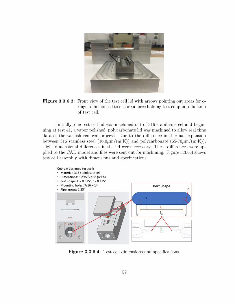
Figure 3.3.6.3: Front view of the test cell lid with arrows pointing out areas for o-rings to be housed to ensure a force holding test coupon to bottomof test cell.
Initially, one test cell lid was machined out of 316 stainless steel and begin-ning at test 41, a vapor polished, polycarbonate lid was machined to allow real timedata of the varnish removal process. Due to the difference in thermal expansionbetween 316 stainless steel (16.0µm/(m·K)) and polycarbonate (65-70µm/(m·K)),slight dimensional differences in the lid were necessary. These differences were ap-plied to the CAD model and files were sent out for machining. Figure 3.3.6.4 showstest cell assembly with dimensions and specifications.
Figure 3.3.6.4: Test cell dimensions and specifications.
57
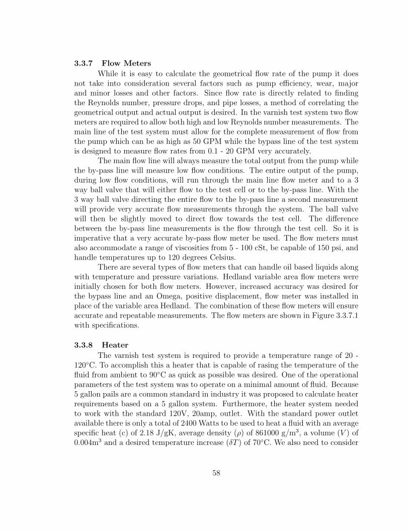
3.3.7 Flow Meters
While it is easy to calculate the geometrical flow rate of the pump it doesnot take into consideration several factors such as pump efficiency, wear, majorand minor losses and other factors. Since flow rate is directly related to findingthe Reynolds number, pressure drops, and pipe losses, a method of correlating thegeometrical output and actual output is desired. In the varnish test system two flowmeters are required to allow both high and low Reynolds number measurements. Themain line of the test system must allow for the complete measurement of flow fromthe pump which can be as high as 50 GPM while the bypass line of the test systemis designed to measure flow rates from 0.1 - 20 GPM very accurately.
The main flow line will always measure the total output from the pump whilethe by-pass line will measure low flow conditions. The entire output of the pump,during low flow conditions, will run through the main line flow meter and to a 3way ball valve that will either flow to the test cell or to the by-pass line. With the3 way ball valve directing the entire flow to the by-pass line a second measurementwill provide very accurate flow measurements through the system. The ball valvewill then be slightly moved to direct flow towards the test cell. The differencebetween the by-pass line measurements is the flow through the test cell. So it isimperative that a very accurate by-pass flow meter be used. The flow meters mustalso accommodate a range of viscosities from 5 - 100 cSt, be capable of 150 psi, andhandle temperatures up to 120 degrees Celsius.
There are several types of flow meters that can handle oil based liquids alongwith temperature and pressure variations. Hedland variable area flow meters wereinitially chosen for both flow meters. However, increased accuracy was desired forthe bypass line and an Omega, positive displacement, flow meter was installed inplace of the variable area Hedland. The combination of these flow meters will ensureaccurate and repeatable measurements. The flow meters are shown in Figure 3.3.7.1with specifications.
3.3.8 Heater
The varnish test system is required to provide a temperature range of 20 -120◦C. To accomplish this a heater that is capable of rasing the temperature of thefluid from ambient to 90◦C as quick as possible was desired. One of the operationalparameters of the test system was to operate on a minimal amount of fluid. Because5 gallon pails are a common standard in industry it was proposed to calculate heaterrequirements based on a 5 gallon system. Furthermore, the heater system neededto work with the standard 120V, 20amp, outlet. With the standard power outletavailable there is only a total of 2400 Watts to be used to heat a fluid with an averagespecific heat (c) of 2.18 J/gK, average density (ρ) of 861000 g/m3, a volume (V ) of0.004m3 and a desired temperature increase (δT ) of 70◦C. We also need to consider
58
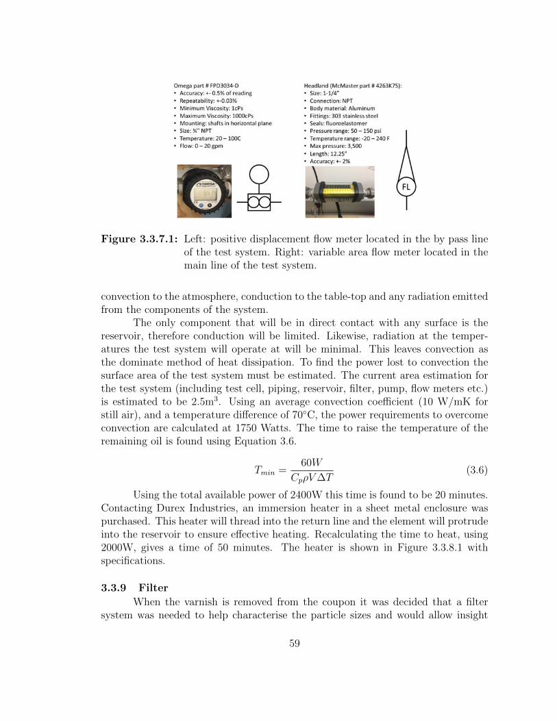
Figure 3.3.7.1: Left: positive displacement flow meter located in the by pass lineof the test system. Right: variable area flow meter located in themain line of the test system.
convection to the atmosphere, conduction to the table-top and any radiation emittedfrom the components of the system.
The only component that will be in direct contact with any surface is thereservoir, therefore conduction will be limited. Likewise, radiation at the temper-atures the test system will operate at will be minimal. This leaves convection asthe dominate method of heat dissipation. To find the power lost to convection thesurface area of the test system must be estimated. The current area estimation forthe test system (including test cell, piping, reservoir, filter, pump, flow meters etc.)is estimated to be 2.5m3. Using an average convection coefficient (10 W/mK forstill air), and a temperature difference of 70◦C, the power requirements to overcomeconvection are calculated at 1750 Watts. The time to raise the temperature of theremaining oil is found using Equation 3.6.
Tmin =60W
CpρV∆T(3.6)
Using the total available power of 2400W this time is found to be 20 minutes.Contacting Durex Industries, an immersion heater in a sheet metal enclosure waspurchased. This heater will thread into the return line and the element will protrudeinto the reservoir to ensure effective heating. Recalculating the time to heat, using2000W, gives a time of 50 minutes. The heater is shown in Figure 3.3.8.1 withspecifications.
3.3.9 Filter
When the varnish is removed from the coupon it was decided that a filtersystem was needed to help characterise the particle sizes and would allow insight
59
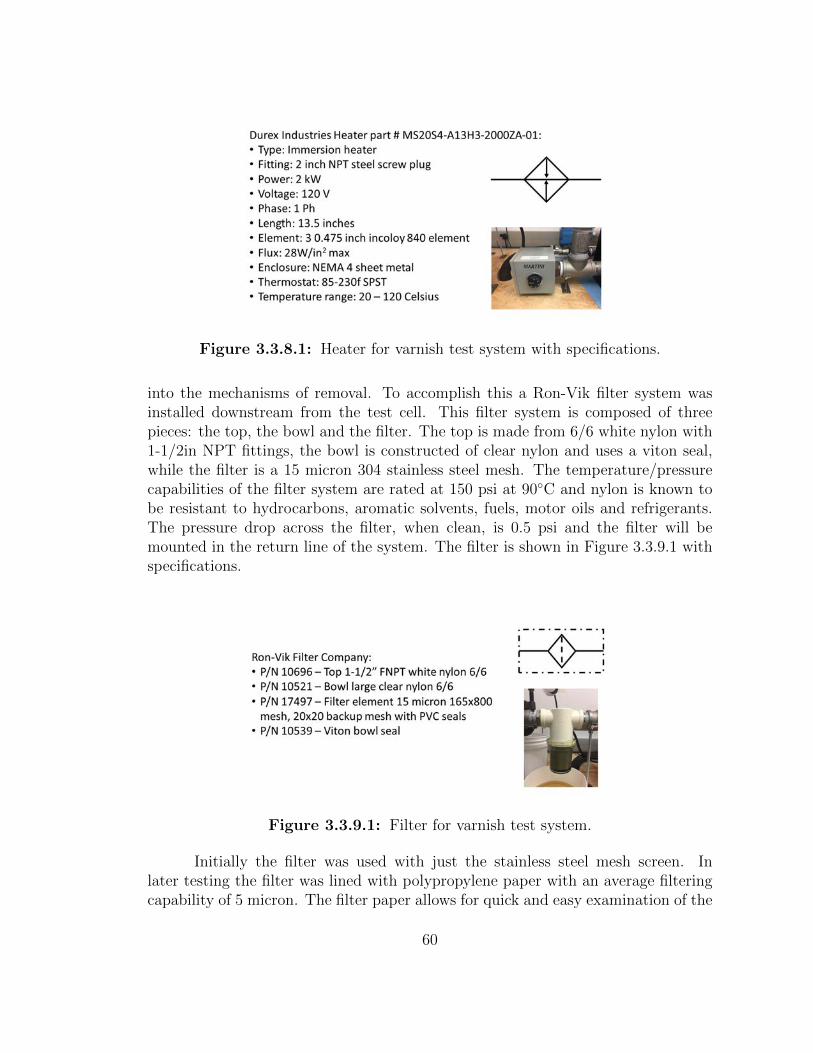
Figure 3.3.8.1: Heater for varnish test system with specifications.
into the mechanisms of removal. To accomplish this a Ron-Vik filter system wasinstalled downstream from the test cell. This filter system is composed of threepieces: the top, the bowl and the filter. The top is made from 6/6 white nylon with1-1/2in NPT fittings, the bowl is constructed of clear nylon and uses a viton seal,while the filter is a 15 micron 304 stainless steel mesh. The temperature/pressurecapabilities of the filter system are rated at 150 psi at 90◦C and nylon is known tobe resistant to hydrocarbons, aromatic solvents, fuels, motor oils and refrigerants.The pressure drop across the filter, when clean, is 0.5 psi and the filter will bemounted in the return line of the system. The filter is shown in Figure 3.3.9.1 withspecifications.
Figure 3.3.9.1: Filter for varnish test system.
Initially the filter was used with just the stainless steel mesh screen. Inlater testing the filter was lined with polypropylene paper with an average filteringcapability of 5 micron. The filter paper allows for quick and easy examination of the
60
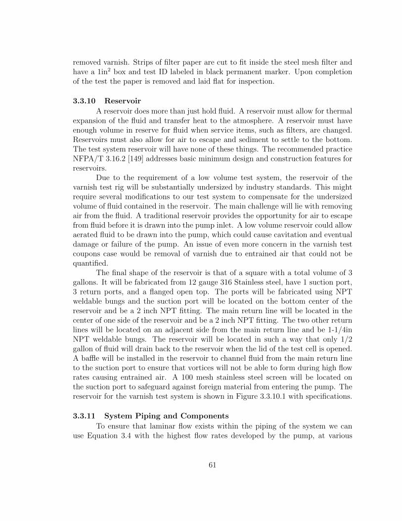
removed varnish. Strips of filter paper are cut to fit inside the steel mesh filter andhave a 1in2 box and test ID labeled in black permanent marker. Upon completionof the test the paper is removed and laid flat for inspection.
3.3.10 Reservoir
A reservoir does more than just hold fluid. A reservoir must allow for thermalexpansion of the fluid and transfer heat to the atmosphere. A reservoir must haveenough volume in reserve for fluid when service items, such as filters, are changed.Reservoirs must also allow for air to escape and sediment to settle to the bottom.The test system reservoir will have none of these things. The recommended practiceNFPA/T 3.16.2 [149] addresses basic minimum design and construction features forreservoirs.
Due to the requirement of a low volume test system, the reservoir of thevarnish test rig will be substantially undersized by industry standards. This mightrequire several modifications to our test system to compensate for the undersizedvolume of fluid contained in the reservoir. The main challenge will lie with removingair from the fluid. A traditional reservoir provides the opportunity for air to escapefrom fluid before it is drawn into the pump inlet. A low volume reservoir could allowaerated fluid to be drawn into the pump, which could cause cavitation and eventualdamage or failure of the pump. An issue of even more concern in the varnish testcoupons case would be removal of varnish due to entrained air that could not bequantified.
The final shape of the reservoir is that of a square with a total volume of 3gallons. It will be fabricated from 12 gauge 316 Stainless steel, have 1 suction port,3 return ports, and a flanged open top. The ports will be fabricated using NPTweldable bungs and the suction port will be located on the bottom center of thereservoir and be a 2 inch NPT fitting. The main return line will be located in thecenter of one side of the reservoir and be a 2 inch NPT fitting. The two other returnlines will be located on an adjacent side from the main return line and be 1-1/4inNPT weldable bungs. The reservoir will be located in such a way that only 1/2gallon of fluid will drain back to the reservoir when the lid of the test cell is opened.A baffle will be installed in the reservoir to channel fluid from the main return lineto the suction port to ensure that vortices will not be able to form during high flowrates causing entrained air. A 100 mesh stainless steel screen will be located onthe suction port to safeguard against foreign material from entering the pump. Thereservoir for the varnish test system is shown in Figure 3.3.10.1 with specifications.
3.3.11 System Piping and Components
To ensure that laminar flow exists within the piping of the system we canuse Equation 3.4 with the highest flow rates developed by the pump, at various
61
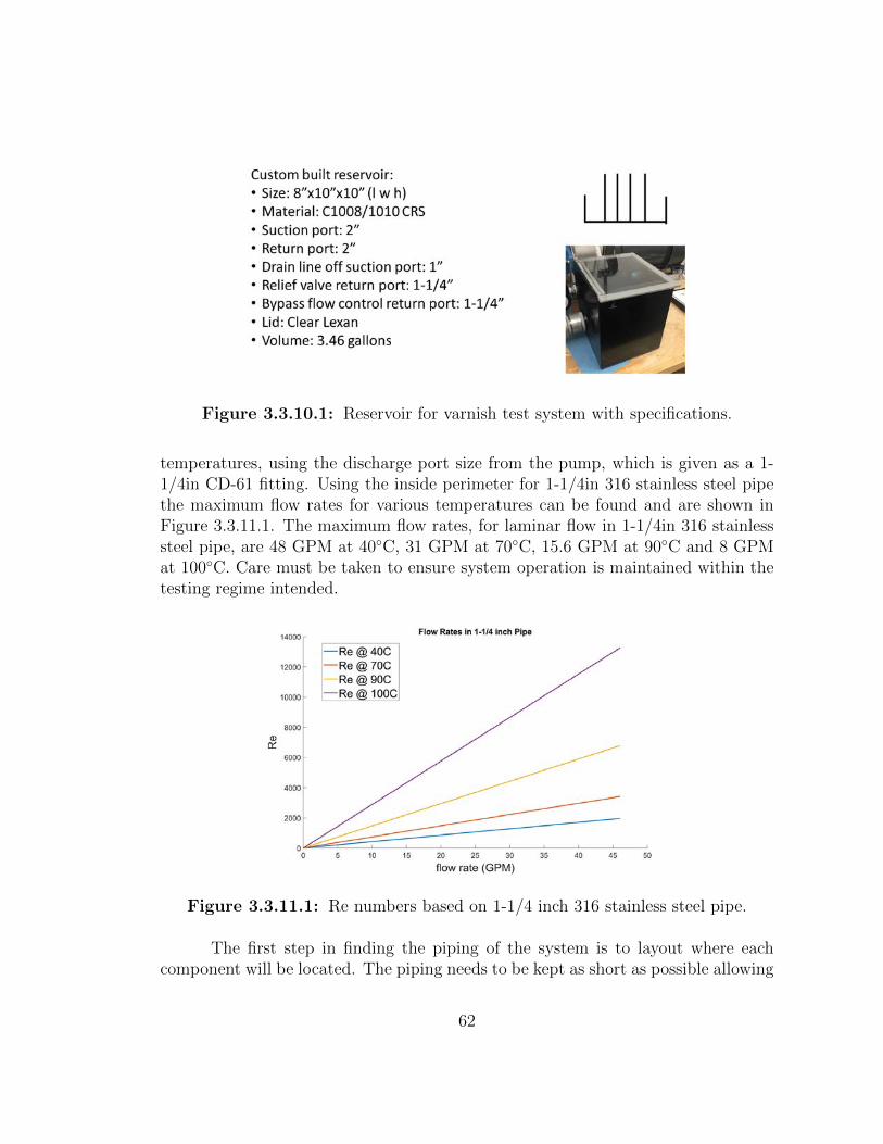
Figure 3.3.10.1: Reservoir for varnish test system with specifications.
temperatures, using the discharge port size from the pump, which is given as a 1-1/4in CD-61 fitting. Using the inside perimeter for 1-1/4in 316 stainless steel pipethe maximum flow rates for various temperatures can be found and are shown inFigure 3.3.11.1. The maximum flow rates, for laminar flow in 1-1/4in 316 stainlesssteel pipe, are 48 GPM at 40◦C, 31 GPM at 70◦C, 15.6 GPM at 90◦C and 8 GPMat 100◦C. Care must be taken to ensure system operation is maintained within thetesting regime intended.
Figure 3.3.11.1: Re numbers based on 1-1/4 inch 316 stainless steel pipe.
The first step in finding the piping of the system is to layout where eachcomponent will be located. The piping needs to be kept as short as possible allowing
62
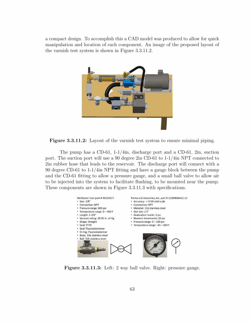
a compact design. To accomplish this a CAD model was produced to allow for quickmanipulation and location of each component. An image of the proposed layout ofthe varnish test system is shown in Figure 3.3.11.2.
Figure 3.3.11.2: Layout of the varnish test system to ensure minimal piping.
The pump has a CD-61, 1-1/4in, discharge port and a CD-61, 2in, suctionport. The suction port will use a 90 degree 2in CD-61 to 1-1/4in NPT connected to2in rubber hose that leads to the reservoir. The discharge port will connect with a90 degree CD-61 to 1-1/4in NPT fitting and have a gauge block between the pumpand the CD-61 fitting to allow a pressure gauge, and a small ball valve to allow airto be injected into the system to facilitate flushing, to be mounted near the pump.These components are shown in Figure 3.3.11.3 with specifications.
Figure 3.3.11.3: Left: 2 way ball valve. Right: pressure gauge.
63
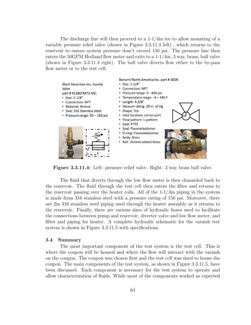
The discharge line will then proceed to a 1-1/4in tee to allow mounting of avariable pressure relief valve (shown in Figure 3.3.11.4 left) , which returns to thereservoir to ensure system pressure dose’t exceed 150 psi. The pressure line thenenters the 50GPM Hedland flow meter and exits to a 1-1/4in, 3 way, brass, ball valve(shown in Figure 3.3.11.4 right). The ball valve diverts flow either to the by-passflow meter or to the test cell.
Figure 3.3.11.4: Left: pressure relief valve. Right: 3 way brass ball valve.
The fluid that diverts through the low flow meter is then channeled back tothe reservoir. The fluid through the test cell then enters the filter and returns tothe reservoir passing over the heater coils. All of the 1-1/4in piping in the systemis made from 316 stainless steel with a pressure rating of 150 psi. Moreover, thereare 2in 316 stainless steel piping used through the heater assembly as it returns tothe reservoir. Finally, there are various sizes of hydraulic hoses used to facilitatethe connections between pump and reservoir, diverter valve and low flow meter, andfilter and piping for heater. A complete hydraulic schematic for the varnish testsystem is shown in Figure 3.3.11.5 with specifications.
3.4 Summary
The most important component of the test system is the test cell. This iswhere the coupon will be housed and where the flow will interact with the varnishon the coupon. The coupon was chosen first and the test cell was sized to house thecoupon. The main components of the test system, as shown in Figure 3.3.11.5, havebeen discussed. Each component is necessary for the test system to operate andallow characterization of fluids. While most of the components worked as expected
64
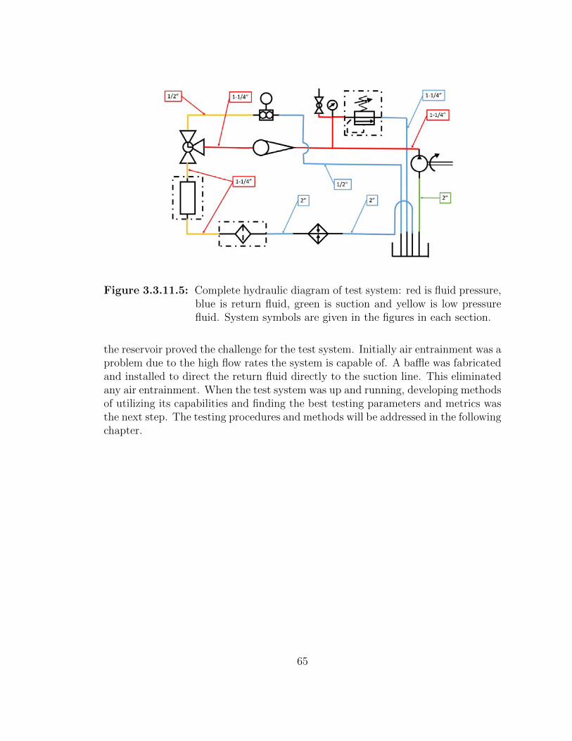
Figure 3.3.11.5: Complete hydraulic diagram of test system: red is fluid pressure,blue is return fluid, green is suction and yellow is low pressurefluid. System symbols are given in the figures in each section.
the reservoir proved the challenge for the test system. Initially air entrainment was aproblem due to the high flow rates the system is capable of. A baffle was fabricatedand installed to direct the return fluid directly to the suction line. This eliminatedany air entrainment. When the test system was up and running, developing methodsof utilizing its capabilities and finding the best testing parameters and metrics wasthe next step. The testing procedures and methods will be addressed in the followingchapter.
65
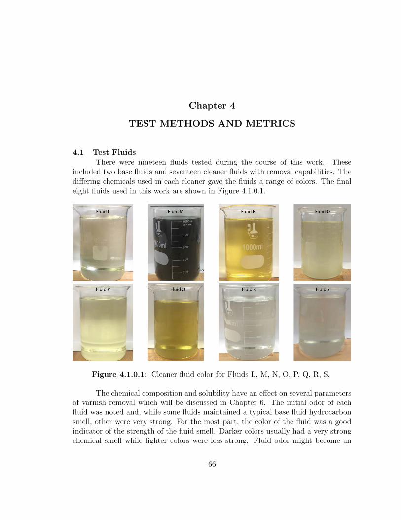
Chapter 4
TEST METHODS AND METRICS
4.1 Test Fluids
There were nineteen fluids tested during the course of this work. Theseincluded two base fluids and seventeen cleaner fluids with removal capabilities. Thediffering chemicals used in each cleaner gave the fluids a range of colors. The finaleight fluids used in this work are shown in Figure 4.1.0.1.
Figure 4.1.0.1: Cleaner fluid color for Fluids L, M, N, O, P, Q, R, S.
The chemical composition and solubility have an effect on several parametersof varnish removal which will be discussed in Chapter 6. The initial odor of eachfluid was noted and, while some fluids maintained a typical base fluid hydrocarbonsmell, other were very strong. For the most part, the color of the fluid was a goodindicator of the strength of the fluid smell. Darker colors usually had a very strongchemical smell while lighter colors were less strong. Fluid odor might become an
66
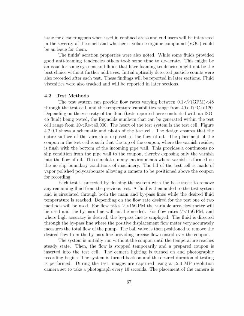
issue for cleaner agents when used in confined areas and end users will be interestedin the severity of the smell and whether it volatile organic compound (VOC) couldbe an issue for them.
The fluids’ aeration properties were also noted. While some fluids providedgood anti-foaming tendencies others took some time to de-aerate. This might bean issue for some systems and fluids that have foaming tendencies might not be thebest choice without further additives. Initial optically detected particle counts werealso recorded after each test. These findings will be reported in later sections. Fluidviscosities were also tracked and will be reported in later sections.
4.2 Test Methods
The test system can provide flow rates varying between 0.1<V (GPM)<48through the test cell, and the temperature capabilities range from 40<T(◦C)<120.Depending on the viscosity of the fluid (tests reported here conducted with an ISO-46 fluid) being tested, the Reynolds numbers that can be generated within the testcell range from 10<Re<40,000. The heart of the test system is the test cell. Figure4.2.0.1 shows a schematic and photo of the test cell. The design ensures that theentire surface of the varnish is exposed to the flow of oil. The placement of thecoupon in the test cell is such that the top of the coupon, where the varnish resides,is flush with the bottom of the incoming pipe wall. This provides a continuous noslip condition from the pipe wall to the coupon, thereby exposing only the varnishinto the flow of oil. This simulates many environments where varnish is formed onthe no slip boundary conditions of machinery. The lid of the test cell is made ofvapor polished polycarbonate allowing a camera to be positioned above the couponfor recording.
Each test is preceded by flushing the system with the base stock to removeany remaining fluid from the previous test. A fluid is then added to the test systemand is circulated through both the main and by-pass lines while the desired fluidtemperature is reached. Depending on the flow rate desired for the test one of twomethods will be used. For flow rates V >15GPM the variable area flow meter willbe used and the by-pass line will not be needed. For flow rates V <15GPM, andwhere high accuracy is desired, the by-pass line is employed. The fluid is directedthrough the by-pass line where the positive displacement flow meter very accuratelymeasures the total flow of the pump. The ball valve is then positioned to remove thedesired flow from the by-pass line providing precise flow control over the coupon.
The system is initially run without the coupon until the temperature reachessteady state. Then, the flow is stopped temporarily and a prepared coupon isinserted into the test cell. The camera lighting is turned on and photographicrecording begins. The system is turned back on and the desired duration of testingis performed. During the test, images are captured using a 12.0 MP resolutioncamera set to take a photograph every 10 seconds. The placement of the camera is
67
Figure 4.2.0.1: (a) Wireframe CAD model of test cell showing location of couponand varnish. (b) Photo of the test cell without the polycarbonatelid. The varnish coupon prior to testing can be seen in the centerof the cell. Dimensions on both figures correspond to the scale barshown in the lower right corner of (b).
fixed so that the position of the varnish is the same for all tests. Upon completionof the test, the coupon is removed from the test cell and dried in heptane to removeany oil from the sample prior to weighing. An initial post-test mass recording isdone and 24 hours later another is performed to ensure no further change occurreddue to evaporating heptane. The difference between the pre-test and post-test massis identified as mass loss, one of the metrics used to characterize varnish removal.
In the Methods Section, the test system is demonstrated with two fluids,Fluid D and Fluid E, both of which are known to have varnish removal capabilities.This will help to identify the removal metrics used in Chapter 5. All tests areconducted at a temperature of 90◦C, a flow rate of 4.5GPM and a duration of 120minutes. With a flow rate of 4.5GPM, an average velocity of 10.12 ft/s (3.08 m/s)is created within the test cell. The viscosities of the two fluids tested are 17.27and 12.82 centi-Stokes (cSt) at 90◦C, which correspond to Reynolds numbers in
68
the high laminar flow regime (ReD=1,442 and ReE=1,944). These conditions areselected to approximate lubrication conditions in a gas turbine engine, as well asother components. Two tests are run for each fluid under these conditions.
4.3 Test Metrics
The initial testing metrics were mass loss and filter inspection. The varnishmass was recorded pre and post testing to find removed mass in %. The filter wasused to help identify the type of mechanism responsible for the removal (diffusionor convection discussed later). Filter characterizations included not only the sizeof removed particles but their shape. More aggressive chemicals would dissolve thevarnish into particles smaller than 5µm and pass through the filter entirely justgiving a hint of brown on the filter. The filter will be discussed further in Section4.3.3.
These two metrics, mass loss and filter inspection, became the initial basisfor characterizing varnish removal and although these two metrics were valuable incharacterizing the chemical cleaners removal abilities further metrics such as theremoval rate were desired. A clear test cell lid was incorporated into the designprior to test 41. This allowed real time images of the varnish removal process to becaptured in situ. This allowed further metrics to be found including the removal ratethrough the entire test, the maximum removal rate, the time of maximum removalrate and the time at which no further varnish was being removed. These will bediscussed in Section 4.3.2.
At the present time there are four primary, three secondary and two tertiarymetrics. The primary metrics are used to characterize the varnish removal processand include maximum removal rate (mg/min), maximum removal rate time (min),steady state removal (min) and maximum removed varnish (%). The first threeprimary metrics are found using numerically analyzed time-lapse photography whilethe fourth is found using mass loss. The three secondary testing metrics includeanalyzing the removed particles in the filter, tracking the viscosities and identifyingthe ISO codes of the fluids. The two tertiary metrics include odor and aerationproperties.
The combination of primary, secondary and tertiary metrics allows for a verycomprehensive comparison from fluid to fluid. The primary metrics are used toquantify the varnish removal process and provide information on the capability ofeach fluid to remove the varnish. The secondary metrics are used to accuratelyidentify how the cleaner will affect the system. Analyzing the removed varnishwill provide information on the size of the varnish particles that will be circulat-ing through the system and helps to properly size the filter system for each fluid.Identifying the viscosities of the fluids initial viscosity, and tracking them throughuse, allows confidence that the proper viscosity will be used in a given system. Fur-thermore, identifying the initial cleanliness of the fluid, and tracking it through use,
69
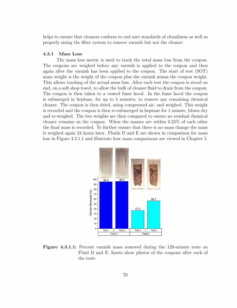
helps to ensure that cleaners conform to end user standards of cleanliness as well asproperly sizing the filter system to remove varnish but not the cleaner.
4.3.1 Mass Loss
The mass loss metric is used to track the total mass loss from the coupon.The coupons are weighed before any varnish is applied to the coupon and thenagain after the varnish has been applied to the coupon. The start of test (SOT)mass weight is the weight of the coupon plus the varnish minus the coupon weight.This allows tracking of the actual mass loss. After each test the coupon is stood onend, on a soft shop towel, to allow the bulk of cleaner fluid to drain from the coupon.The coupon is then taken to a vented fume hood. In the fume hood the couponis submerged in heptane, for up to 5 minutes, to remove any remaining chemicalcleaner. The coupon is then dried, using compressed air, and weighed. This weightis recorded and the coupon is then re-submerged in heptane for 1 minute, blown dryand re-weighed. The two weights are then compared to ensure no residual chemicalcleaner remains on the coupon. When the masses are within 0.25% of each otherthe final mass is recorded. To further ensure that there is no mass change the massis weighed again 24 hours later. Fluids D and E are shown in comparison for massloss in Figure 4.3.1.1 and illustrate how mass comparisons are viewed in Chapter 5.
Figure 4.3.1.1: Percent varnish mass removed during the 120-minute tests onFluid D and E. Insets show photos of the coupons after each ofthe tests
70
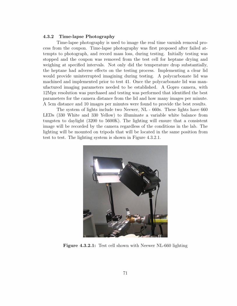
4.3.2 Time-lapse Photography
Time-lapse photography is used to image the real time varnish removal pro-cess from the coupon. Time-lapse photography was first proposed after failed at-tempts to photograph, and record mass loss, during testing. Initially testing wasstopped and the coupon was removed from the test cell for heptane drying andweighing at specified intervals. Not only did the temperature drop substantially,the heptane had adverse effects on the testing process. Implementing a clear lidwould provide uninterrupted imagining during testing. A polycarbonate lid wasmachined and implemented prior to test 41. Once the polycarbonate lid was man-ufactured imaging parameters needed to be established. A Gopro camera, with12Mpx resolution was purchased and testing was performed that identified the bestparameters for the camera distance from the lid and how many images per minute.A 5cm distance and 10 images per minutes were found to provide the best results.
The system of lights include two Neewer, NL - 660s. These lights have 660LEDs (330 White and 330 Yellow) to illuminate a variable white balance fromtungsten to daylight (3200 to 5600K). The lighting will ensure that a consistentimage will be recorded by the camera regardless of the conditions in the lab. Thelighting will be mounted on tripods that will be located in the same position fromtest to test. The lighting system is shown in Figure 4.3.2.1.
Figure 4.3.2.1: Test cell shown with Neewer NL-660 lighting
71
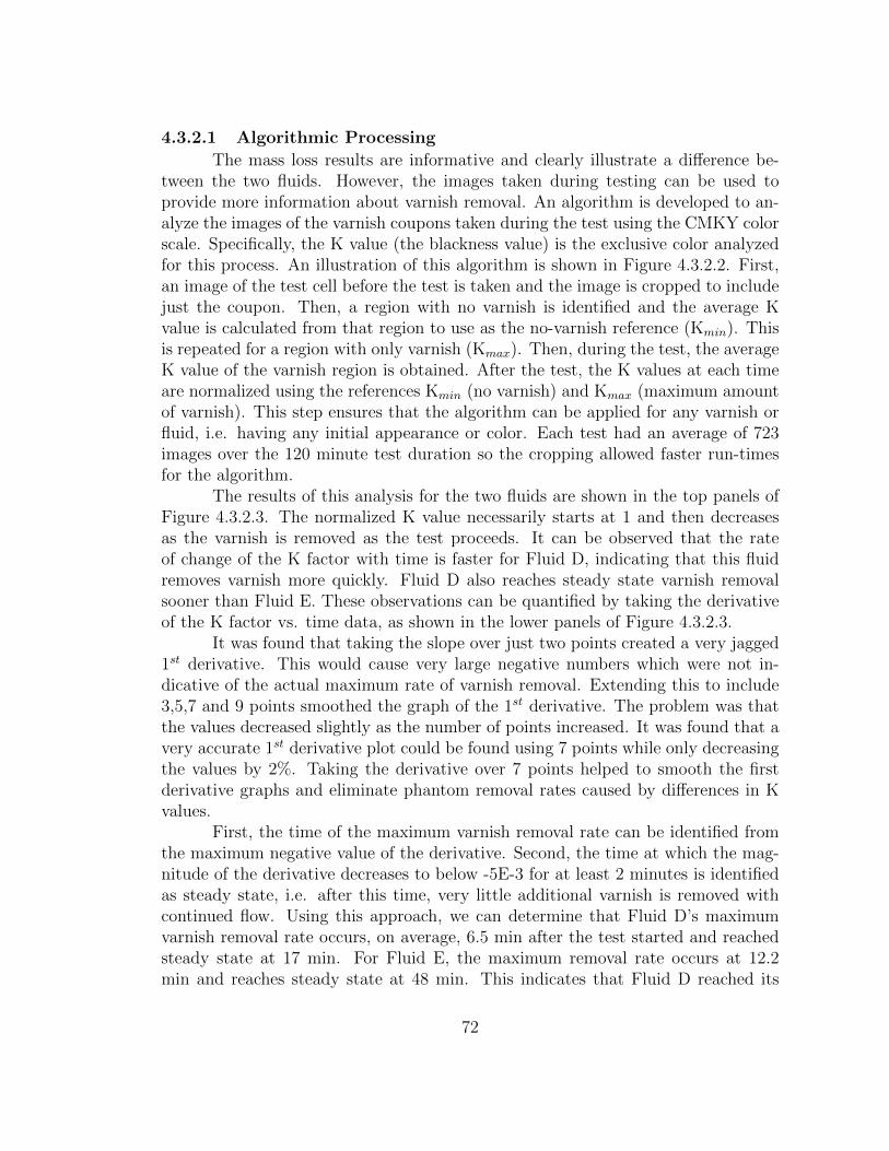
4.3.2.1 Algorithmic Processing
The mass loss results are informative and clearly illustrate a difference be-tween the two fluids. However, the images taken during testing can be used toprovide more information about varnish removal. An algorithm is developed to an-alyze the images of the varnish coupons taken during the test using the CMKY colorscale. Specifically, the K value (the blackness value) is the exclusive color analyzedfor this process. An illustration of this algorithm is shown in Figure 4.3.2.2. First,an image of the test cell before the test is taken and the image is cropped to includejust the coupon. Then, a region with no varnish is identified and the average Kvalue is calculated from that region to use as the no-varnish reference (Kmin). Thisis repeated for a region with only varnish (Kmax). Then, during the test, the averageK value of the varnish region is obtained. After the test, the K values at each timeare normalized using the references Kmin (no varnish) and Kmax (maximum amountof varnish). This step ensures that the algorithm can be applied for any varnish orfluid, i.e. having any initial appearance or color. Each test had an average of 723images over the 120 minute test duration so the cropping allowed faster run-timesfor the algorithm.
The results of this analysis for the two fluids are shown in the top panels ofFigure 4.3.2.3. The normalized K value necessarily starts at 1 and then decreasesas the varnish is removed as the test proceeds. It can be observed that the rateof change of the K factor with time is faster for Fluid D, indicating that this fluidremoves varnish more quickly. Fluid D also reaches steady state varnish removalsooner than Fluid E. These observations can be quantified by taking the derivativeof the K factor vs. time data, as shown in the lower panels of Figure 4.3.2.3.
It was found that taking the slope over just two points created a very jagged1st derivative. This would cause very large negative numbers which were not in-dicative of the actual maximum rate of varnish removal. Extending this to include3,5,7 and 9 points smoothed the graph of the 1st derivative. The problem was thatthe values decreased slightly as the number of points increased. It was found that avery accurate 1st derivative plot could be found using 7 points while only decreasingthe values by 2%. Taking the derivative over 7 points helped to smooth the firstderivative graphs and eliminate phantom removal rates caused by differences in Kvalues.
First, the time of the maximum varnish removal rate can be identified fromthe maximum negative value of the derivative. Second, the time at which the mag-nitude of the derivative decreases to below -5E-3 for at least 2 minutes is identifiedas steady state, i.e. after this time, very little additional varnish is removed withcontinued flow. Using this approach, we can determine that Fluid D’s maximumvarnish removal rate occurs, on average, 6.5 min after the test started and reachedsteady state at 17 min. For Fluid E, the maximum removal rate occurs at 12.2min and reaches steady state at 48 min. This indicates that Fluid D reached its
72
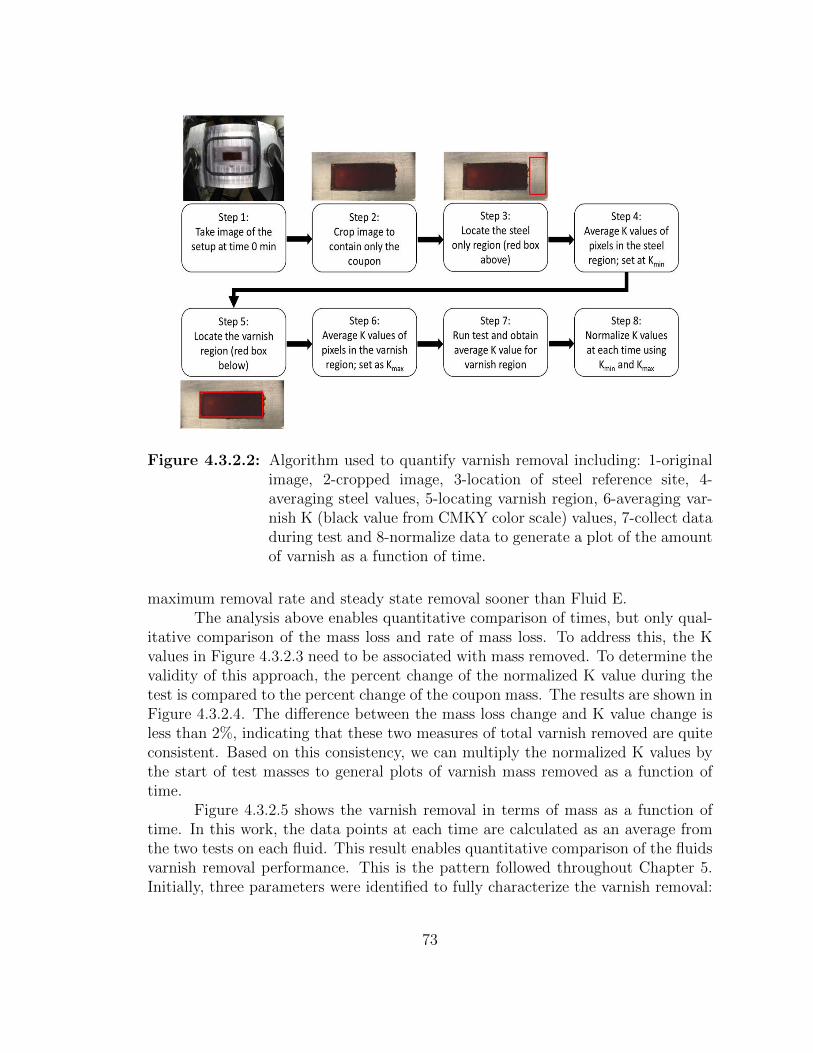
Figure 4.3.2.2: Algorithm used to quantify varnish removal including: 1-originalimage, 2-cropped image, 3-location of steel reference site, 4-averaging steel values, 5-locating varnish region, 6-averaging var-nish K (black value from CMKY color scale) values, 7-collect dataduring test and 8-normalize data to generate a plot of the amountof varnish as a function of time.
maximum removal rate and steady state removal sooner than Fluid E.The analysis above enables quantitative comparison of times, but only qual-
itative comparison of the mass loss and rate of mass loss. To address this, the Kvalues in Figure 4.3.2.3 need to be associated with mass removed. To determine thevalidity of this approach, the percent change of the normalized K value during thetest is compared to the percent change of the coupon mass. The results are shown inFigure 4.3.2.4. The difference between the mass loss change and K value change isless than 2%, indicating that these two measures of total varnish removed are quiteconsistent. Based on this consistency, we can multiply the normalized K values bythe start of test masses to general plots of varnish mass removed as a function oftime.
Figure 4.3.2.5 shows the varnish removal in terms of mass as a function oftime. In this work, the data points at each time are calculated as an average fromthe two tests on each fluid. This result enables quantitative comparison of the fluidsvarnish removal performance. This is the pattern followed throughout Chapter 5.Initially, three parameters were identified to fully characterize the varnish removal:
73
Figure 4.3.2.3: Time-lapse photographic results for Fluid D and Fluid E. Topgraphs display the normalized K value from the algorithm shownin Figure 4.3.2.2 while the bottom graph shows the 1st derivativeof the normalized data. The derivative provides a means of iden-tifying the time at which the varnish removal rate is a maximumand of steady state removal.
maximum varnish removed, time at which the maximum varnish has been removedand maximum rate of varnish removal. These three parameters have been updatedto include a fourth: the time of maximum varnish removal rate. With these fourparameters, characterizing each fluid becomes simplistic and comprehensive.
Using the four characterization parameters mentioned above, a direct com-parison between Fluid D and E can be made, as shown in Figure 4.3.2.6. In all cases,the parameters are averages from the two tests performed on each fluid. First, FluidD removed substantially more varnish from the coupon than did Fluid E (95.9% vs46.94%). The time required to reach steady state varnish removal is also shorter forFluid D than Fluid E (17 min vs 48 min). Finally, Fluid D has a much larger max-imum varnish removal rate than Fluid E (6.42 mg/min vs. 1.62 mg/min). Takentogether, the comparison of these parameters shows that Fluid D is a much moreaggressive chemical compound than Fluid E, removing twice as much varnish in halfof the time.
74
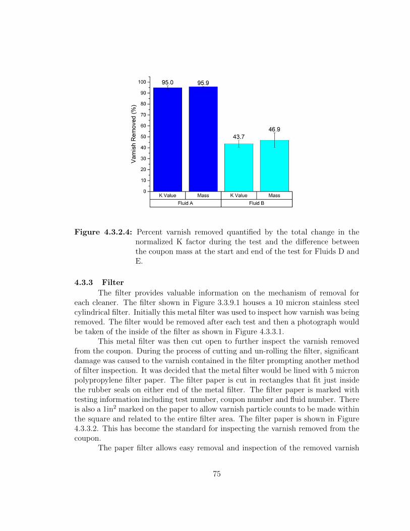
Figure 4.3.2.4: Percent varnish removed quantified by the total change in thenormalized K factor during the test and the difference betweenthe coupon mass at the start and end of the test for Fluids D andE.
4.3.3 Filter
The filter provides valuable information on the mechanism of removal foreach cleaner. The filter shown in Figure 3.3.9.1 houses a 10 micron stainless steelcylindrical filter. Initially this metal filter was used to inspect how varnish was beingremoved. The filter would be removed after each test and then a photograph wouldbe taken of the inside of the filter as shown in Figure 4.3.3.1.
This metal filter was then cut open to further inspect the varnish removedfrom the coupon. During the process of cutting and un-rolling the filter, significantdamage was caused to the varnish contained in the filter prompting another methodof filter inspection. It was decided that the metal filter would be lined with 5 micronpolypropylene filter paper. The filter paper is cut in rectangles that fit just insidethe rubber seals on either end of the metal filter. The filter paper is marked withtesting information including test number, coupon number and fluid number. Thereis also a 1in2 marked on the paper to allow varnish particle counts to be made withinthe square and related to the entire filter area. The filter paper is shown in Figure4.3.3.2. This has become the standard for inspecting the varnish removed from thecoupon.
The paper filter allows easy removal and inspection of the removed varnish
75
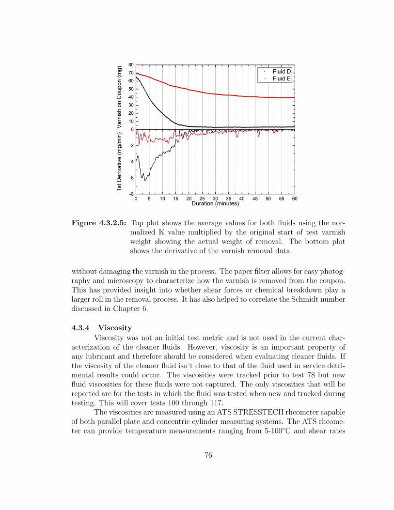
Figure 4.3.2.5: Top plot shows the average values for both fluids using the nor-malized K value multiplied by the original start of test varnishweight showing the actual weight of removal. The bottom plotshows the derivative of the varnish removal data.
without damaging the varnish in the process. The paper filter allows for easy photog-raphy and microscopy to characterize how the varnish is removed from the coupon.This has provided insight into whether shear forces or chemical breakdown play alarger roll in the removal process. It has also helped to correlate the Schmidt numberdiscussed in Chapter 6.
4.3.4 Viscosity
Viscosity was not an initial test metric and is not used in the current char-acterization of the cleaner fluids. However, viscosity is an important property ofany lubricant and therefore should be considered when evaluating cleaner fluids. Ifthe viscosity of the cleaner fluid isn’t close to that of the fluid used in service detri-mental results could occur. The viscosities were tracked prior to test 78 but newfluid viscosities for these fluids were not captured. The only viscosities that will bereported are for the tests in which the fluid was tested when new and tracked duringtesting. This will cover tests 100 through 117.
The viscosities are measured using an ATS STRESSTECH rheometer capableof both parallel plate and concentric cylinder measuring systems. The ATS rheome-ter can provide temperature measurements ranging from 5-100◦C and shear rates
76
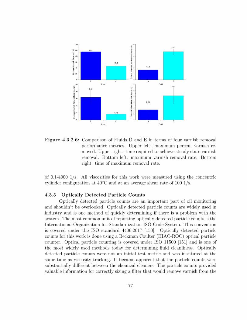
Figure 4.3.2.6: Comparison of Fluids D and E in terms of four varnish removalperformance metrics. Upper left: maximum percent varnish re-moved. Upper right: time required to achieve steady state varnishremoval. Bottom left: maximum varnish removal rate. Bottomright: time of maximum removal rate.
of 0.1-4000 1/s. All viscosities for this work were measured using the concentriccylinder configuration at 40◦C and at an average shear rate of 100 1/s.
4.3.5 Optically Detected Particle Counts
Optically detected particle counts are an important part of oil monitoringand shouldn’t be overlooked. Optically detected particle counts are widely used inindustry and is one method of quickly determining if there is a problem with thesystem. The most common unit of reporting optically detected particle counts is theInternational Organization for Standardization ISO Code System. This conventionis covered under the ISO standard 4406:2017 [150]. Optically detected particlecounts for this work is done using a Beckman Coulter (HIAC-ROC) optical particlecounter. Optical particle counting is covered under ISO 11500 [151] and is one ofthe most widely used methods today for determining fluid cleanliness. Opticallydetected particle counts were not an initial test metric and was instituted at thesame time as viscosity tracking. It became apparent that the particle counts weresubstantially different between the chemical cleaners. The particle counts providedvaluable information for correctly sizing a filter that would remove varnish from the
77
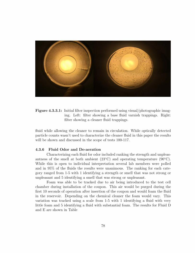
Figure 4.3.3.1: Initial filter inspection performed using visual/photographic imag-ing. Left: filter showing a base fluid varnish trappings. Right:filter showing a cleaner fluid trappings.
fluid while allowing the cleaner to remain in circulation. While optically detectedparticle counts wasn’t used to characterize the cleaner fluid in this paper the resultswill be shown and discussed in the scope of tests 100-117.
4.3.6 Fluid Odor and De-aeration
Characterizing each fluid for odor included ranking the strength and unpleas-antness of the smell at both ambient (23◦C) and operating temperature (90◦C).While this is open to individual interpretation several lab members were polledand in 95% of the fluids the results were unanimous. The ranking for each cate-gory ranged from 1-5 with 1 identifying a strength or smell that was not strong orunpleasant and 5 identifying a smell that was strong or unpleasant.
Foam was able to be tracked due to air being introduced to the test cellchamber during installation of the coupon. This air would be purged during thefirst 10 seconds of operation after insertion of the coupon and would foam the fluidin the reservoir. Depending on the chemical cleaner the foam would vary. Thisvariation was tracked using a scale from 1-5 with 1 identifying a fluid with verylittle foam and 5 identifying a fluid with substantial foam. The results for Fluid Dand E are shown in Table
78
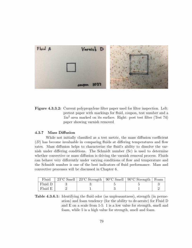
Figure 4.3.3.2: Current polypropylene filter paper used for filter inspection. Left:pretest paper with markings for fluid, coupon, test number and a1in2 area marked on its surface. Right: post test filter (Test 74)paper showing varnish removed
4.3.7 Mass Diffusion
While not initially classified as a test metric, the mass diffusion coefficient(D) has become invaluable in comparing fluids at differing temperatures and flowrates. Mass diffusion helps to characterize the fluid’s ability to dissolve the var-nish under differing conditions. The Schmidt number (Sc) is used to determinewhether convective or mass diffusion is driving the varnish removal process. Fluidscan behave very differently under varying conditions of flow and temperature andthe Schmidt number is one of the best indicators of fluid performance. Mass andconvective processes will be discussed in Chapter 6.
Fluid 23◦C Smell 23◦C Strength 90◦C Smell 90◦C Strength FoamFluid D 3 3 5 5 3Fluid E 2 1 3 1 2
Table 4.3.6.1: Identifying the fluid odor (as unpleasantness), strength (in perme-ation) and foam tendency (for the ability to de-aerate) for Fluid Dand E on a scale from 1-5. 1 is a low value for strength, smell andfoam, while 5 is a high value for strength, smell and foam.
79
4.4 Summary
The initial test metrics of mass loss and filter inspection proved inadequateto characterize the performance of the cleaner fluids. However, with introductionof the clear test lid, non-intrusive photographic data was collected that allowedvarnish removal rates to be calculated using algorithmic processing. This allowedthe majority of the current work to progress using the 4 characterization parametersdiscussed previously. With the addition of viscometry and optically detected particlecounts, further characterizations are allowed. The viscosities ensure that the fluidfalls into the range expected for in service systems. Optically detected particlecounting ensures that chemical cleaner compounds, containing large particles, won’tinadvertently cause concern by appearing as contaminated fluid. The performance ofthe fluid used in the test system, as well as the characterizations discussed previously,will be discussed in Chapter 5.
80
Chapter 5
RESULTS
5.1 Introduction
Over 140 individual varnish removal tests were run, as summarized in theAppendix. Initially, tests were designed to provide information about the testingconditions that provided consistent and high varnish mass removal amounts. Overthe course of these initial tests, it was found that not enough varnish was removed.This was addressed by changing the test conditions and varnish preparation andstorage. Then, testing metrics were expanded from just mass removal to severaltest metrics, including mass removal rates, time of maximum removal rate andwhen the removal process reached steady state. This was enabled by the additionof updated components to the test system as discussed in Chapter 3. Moreover,during these tests, unexpected phenomena occurred that prompted the investigationof varnish composition, varnish preparation conditions and varnish mass control onthe coupon. What follows is a chronological description of each test series alongwith what information was gained, how that information was used to improve thetests, which test metrics became the standard, and final results for a series of testfluids evaluated using the developed standard metrics.
5.2 Test Method Evaluation
During design and construction of the varnish test system, significant con-sideration was given to flow rate and temperature control. These two parametersprovide a method of simulating the conditions that exist for in service systems. Fur-thermore, the varnish on the surface of the coupon was exposed to the flow of oil onthe no slip boundary condition at the pipe walls. This simulated environment allowsconfidence in the varnish removal process by accurately mimicking real systems. Indoing so, it is important that conditions such as flow within journal bearings andheat transfer units can be reproduced.
Reynolds numbers for common, hydrodynamic, journal bearings were inves-tigated and found to be very low (Re = 10-100) in the laminar regime [152]. Thetransition to turbulent flow in common journal bearings is estimated to be Re =1300 using a bearing ratio (R/C) of 1000, where R is the radius of the journal andC is the oil film thickness. This provided some insight into flow numbers needed
81
to simulate common journal bearings. Flow rates in typical piping systems, suchas heat transfer systems, are designed to remain in the laminar flow regime to keepfriction as low as possible. This fact is apparent from observing the Moody Dia-gram which shows the friction factor in terms of the Reynolds number and piperoughness [153]. Flow within lubrication passages and drain-back channels are alsotypically in the laminar regime [154]. For cams and lifters, the Reynolds numbersare known to be low within the journal bearing and even lower on the cam surface.For these reasons, tests should be performed with laminar flow to reproduce theconditions in many components.
The first 45 tests were run using only mass loss and filter inspection. However,these two metrics provided no information about the rate of removal as well aswhen the varnish removal process ended. A series of tests were designed to identifyrates of removal and the steady state condition. In the following sections, the termsteady state refers to a condition where the varnish is not appreciably losing masswith additional flow. While varnish mass will continually be removed, the rate ofremoval has reach its lowest point and further testing would not help to characterizefluid performance. During these tests, the coupon was removed at specific intervalsto be weighed and imaged. This caused several problems, explained later, and theprocess was discontinued.
However, the observations prompted the use of a clear lid to enable pho-tographic imaging during testing. This allowed the varnish removal process to bephotographed in situ and the results using real time photographic imaging provedinvaluable. It was then possible to record, non-intrusively, the varnish removal pro-cess. The imaging data was combined with the mass loss data to provide ratesof removal in mg/min. The result became a primary metric for chemical cleanerperformance.
Initially, three tests were used for each fluid. This provided a means tocheck the accuracy and precision of the tests by finding the average values, standarddeviations and errors. When confidence was established in the testing process, andin the interest of time, only two tests were run for each fluid. Moreover, testswere run for extended durations to determine where steady state exists for base oilsand provide an upper time limit on testing. We expected the chemical cleaners tooutperform the base oils and remove the varnish in shorter periods of time. Thatis, the time to reach steady state for cleaner fluids was expected to be less than thetime it takes base oils reach steady state.
After each test, the filter was imaged to help understand how the varnish wasbeing removed i.e. small/large particles, flaking or rolling. Attempts were made tocut the stainless-steel filter open to allow it to lay flat for inspection and imaging.It was found that the process of cutting the metal filter and rolling it open damagedthe varnish on the filter. Much of the varnish was contained between the layers ofsteel mesh so the varnish was squeezed into different shapes as well as broken into
82
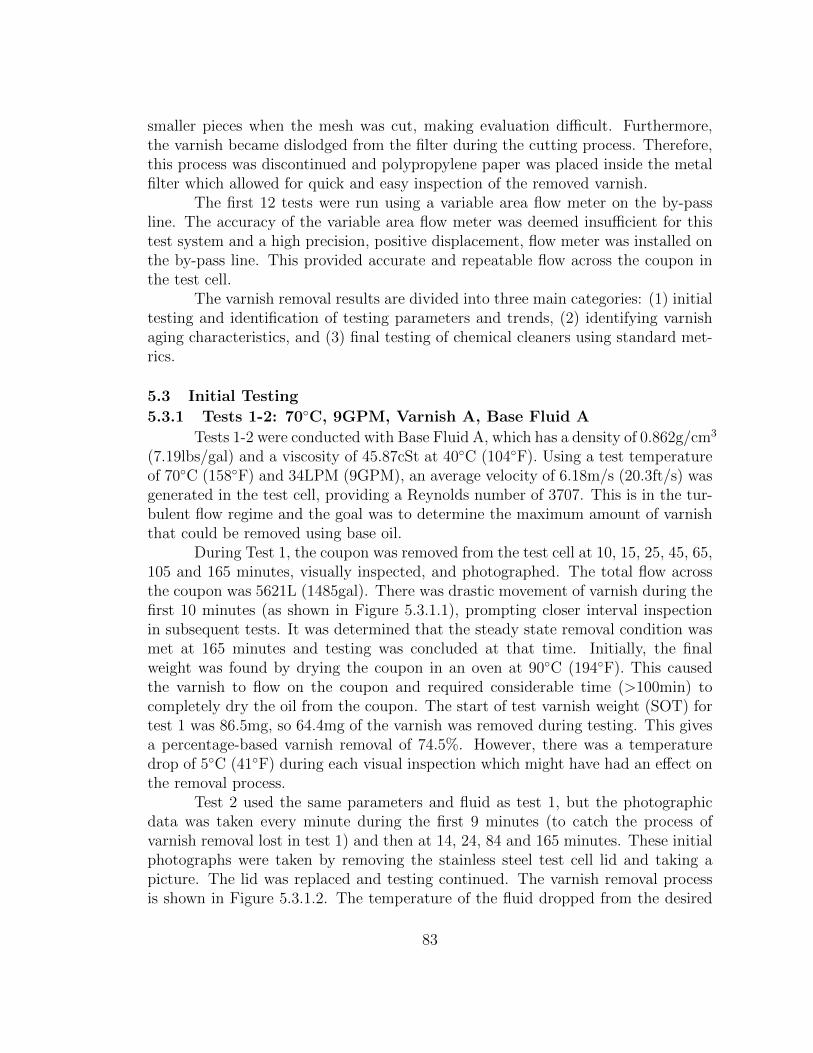
smaller pieces when the mesh was cut, making evaluation difficult. Furthermore,the varnish became dislodged from the filter during the cutting process. Therefore,this process was discontinued and polypropylene paper was placed inside the metalfilter which allowed for quick and easy inspection of the removed varnish.
The first 12 tests were run using a variable area flow meter on the by-passline. The accuracy of the variable area flow meter was deemed insufficient for thistest system and a high precision, positive displacement, flow meter was installed onthe by-pass line. This provided accurate and repeatable flow across the coupon inthe test cell.
The varnish removal results are divided into three main categories: (1) initialtesting and identification of testing parameters and trends, (2) identifying varnishaging characteristics, and (3) final testing of chemical cleaners using standard met-rics.
5.3 Initial Testing
5.3.1 Tests 1-2: 70◦C, 9GPM, Varnish A, Base Fluid A
Tests 1-2 were conducted with Base Fluid A, which has a density of 0.862g/cm3
(7.19lbs/gal) and a viscosity of 45.87cSt at 40◦C (104◦F). Using a test temperatureof 70◦C (158◦F) and 34LPM (9GPM), an average velocity of 6.18m/s (20.3ft/s) wasgenerated in the test cell, providing a Reynolds number of 3707. This is in the tur-bulent flow regime and the goal was to determine the maximum amount of varnishthat could be removed using base oil.
During Test 1, the coupon was removed from the test cell at 10, 15, 25, 45, 65,105 and 165 minutes, visually inspected, and photographed. The total flow acrossthe coupon was 5621L (1485gal). There was drastic movement of varnish during thefirst 10 minutes (as shown in Figure 5.3.1.1), prompting closer interval inspectionin subsequent tests. It was determined that the steady state removal condition wasmet at 165 minutes and testing was concluded at that time. Initially, the finalweight was found by drying the coupon in an oven at 90◦C (194◦F). This causedthe varnish to flow on the coupon and required considerable time (>100min) tocompletely dry the oil from the coupon. The start of test varnish weight (SOT) fortest 1 was 86.5mg, so 64.4mg of the varnish was removed during testing. This givesa percentage-based varnish removal of 74.5%. However, there was a temperaturedrop of 5◦C (41◦F) during each visual inspection which might have had an effect onthe removal process.
Test 2 used the same parameters and fluid as test 1, but the photographicdata was taken every minute during the first 9 minutes (to catch the process ofvarnish removal lost in test 1) and then at 14, 24, 84 and 165 minutes. These initialphotographs were taken by removing the stainless steel test cell lid and taking apicture. The lid was replaced and testing continued. The varnish removal processis shown in Figure 5.3.1.2. The temperature of the fluid dropped from the desired
83
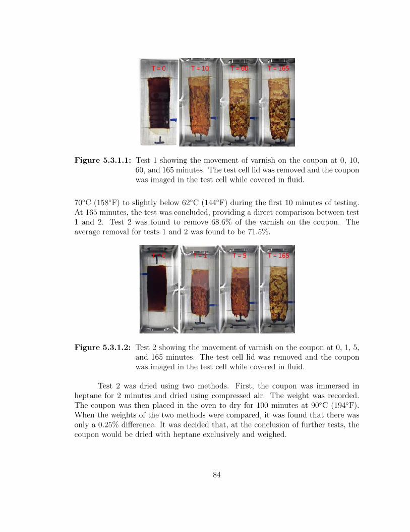
Figure 5.3.1.1: Test 1 showing the movement of varnish on the coupon at 0, 10,60, and 165 minutes. The test cell lid was removed and the couponwas imaged in the test cell while covered in fluid.
70◦C (158◦F) to slightly below 62◦C (144◦F) during the first 10 minutes of testing.At 165 minutes, the test was concluded, providing a direct comparison between test1 and 2. Test 2 was found to remove 68.6% of the varnish on the coupon. Theaverage removal for tests 1 and 2 was found to be 71.5%.
Figure 5.3.1.2: Test 2 showing the movement of varnish on the coupon at 0, 1, 5,and 165 minutes. The test cell lid was removed and the couponwas imaged in the test cell while covered in fluid.
Test 2 was dried using two methods. First, the coupon was immersed inheptane for 2 minutes and dried using compressed air. The weight was recorded.The coupon was then placed in the oven to dry for 100 minutes at 90◦C (194◦F).When the weights of the two methods were compared, it was found that there wasonly a 0.25% difference. It was decided that, at the conclusion of further tests, thecoupon would be dried with heptane exclusively and weighed.
84
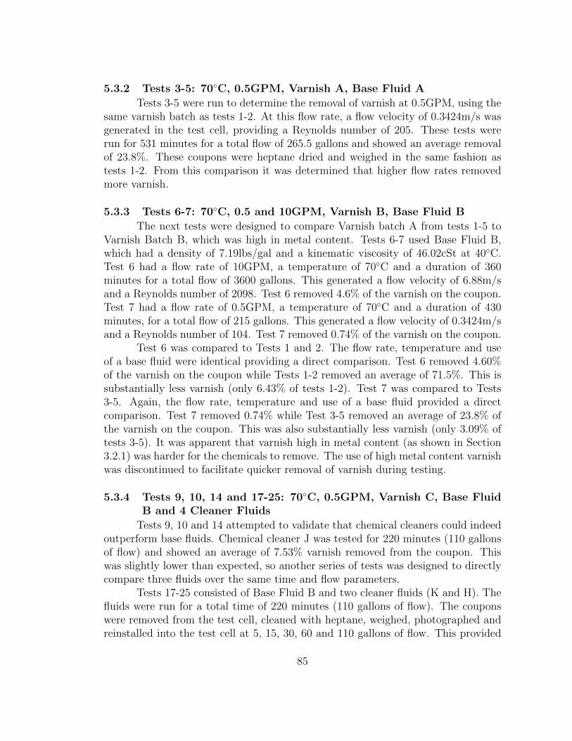
5.3.2 Tests 3-5: 70◦C, 0.5GPM, Varnish A, Base Fluid A
Tests 3-5 were run to determine the removal of varnish at 0.5GPM, using thesame varnish batch as tests 1-2. At this flow rate, a flow velocity of 0.3424m/s wasgenerated in the test cell, providing a Reynolds number of 205. These tests wererun for 531 minutes for a total flow of 265.5 gallons and showed an average removalof 23.8%. These coupons were heptane dried and weighed in the same fashion astests 1-2. From this comparison it was determined that higher flow rates removedmore varnish.
5.3.3 Tests 6-7: 70◦C, 0.5 and 10GPM, Varnish B, Base Fluid B
The next tests were designed to compare Varnish batch A from tests 1-5 toVarnish Batch B, which was high in metal content. Tests 6-7 used Base Fluid B,which had a density of 7.19lbs/gal and a kinematic viscosity of 46.02cSt at 40◦C.Test 6 had a flow rate of 10GPM, a temperature of 70◦C and a duration of 360minutes for a total flow of 3600 gallons. This generated a flow velocity of 6.88m/sand a Reynolds number of 2098. Test 6 removed 4.6% of the varnish on the coupon.Test 7 had a flow rate of 0.5GPM, a temperature of 70◦C and a duration of 430minutes, for a total flow of 215 gallons. This generated a flow velocity of 0.3424m/sand a Reynolds number of 104. Test 7 removed 0.74% of the varnish on the coupon.
Test 6 was compared to Tests 1 and 2. The flow rate, temperature and useof a base fluid were identical providing a direct comparison. Test 6 removed 4.60%of the varnish on the coupon while Tests 1-2 removed an average of 71.5%. This issubstantially less varnish (only 6.43% of tests 1-2). Test 7 was compared to Tests3-5. Again, the flow rate, temperature and use of a base fluid provided a directcomparison. Test 7 removed 0.74% while Test 3-5 removed an average of 23.8% ofthe varnish on the coupon. This was also substantially less varnish (only 3.09% oftests 3-5). It was apparent that varnish high in metal content (as shown in Section3.2.1) was harder for the chemicals to remove. The use of high metal content varnishwas discontinued to facilitate quicker removal of varnish during testing.
5.3.4 Tests 9, 10, 14 and 17-25: 70◦C, 0.5GPM, Varnish C, Base FluidB and 4 Cleaner Fluids
Tests 9, 10 and 14 attempted to validate that chemical cleaners could indeedoutperform base fluids. Chemical cleaner J was tested for 220 minutes (110 gallonsof flow) and showed an average of 7.53% varnish removed from the coupon. Thiswas slightly lower than expected, so another series of tests was designed to directlycompare three fluids over the same time and flow parameters.
Tests 17-25 consisted of Base Fluid B and two cleaner fluids (K and H). Thefluids were run for a total time of 220 minutes (110 gallons of flow). The couponswere removed from the test cell, cleaned with heptane, weighed, photographed andreinstalled into the test cell at 5, 15, 30, 60 and 110 gallons of flow. This provided
85
insight into the performance of the cleaners, on a rate of removal basis, throughoutthe duration of the test. This process was repeated for each test. The results fortests 17-25 are shown in Figure 5.3.4.1. While the removal exhibited similar trendswith increasing flow, there were large differences in the amount of varnish removedby each fluid from test-to-test. This was unexpected and further investigation wasneeded to identify the cause of the anomaly.
Figure 5.3.4.1: Tests 17-25 where three fluids K, H and Base Fluid B were com-pared for varnish removal at 5, 15, 30, 60 and 110 gallons of flowwith heptane being used to remove oil for weighing.
The observation that heptane might influence the chemistry of the varnishduring testing prompted re-testing of the three fluids from Tests 17-25, with nointerruption to weigh the coupons during testing, and only recording the final weightof varnish removed after 220 minutes (110 gallons of flow). Tests 26-34, which werenot washed with heptane, are shown in comparison to tests 17-25 in Figure 5.3.4.2.
The results showed that, indeed, the heptane had an influence on overall var-nish removal from each fluid. Fluid K showed a decrease from a heptane washed13.3% (11.30mg) removed to an unwashed 10.5% (10.42mg) removed. Fluid Hshowed an increase from a heptane washed 8.71% (5.67mg) removed to an unwashed14.5% (10.47mg) removed. Finally, Base Fluid B showed a decrease from a heptanewashed 10.5% (9.73mg) removed to an unwashed 7.94% (5.48mg) removed. Thisshows that the heptane wash affected the fluids in different ways. While heptane
86
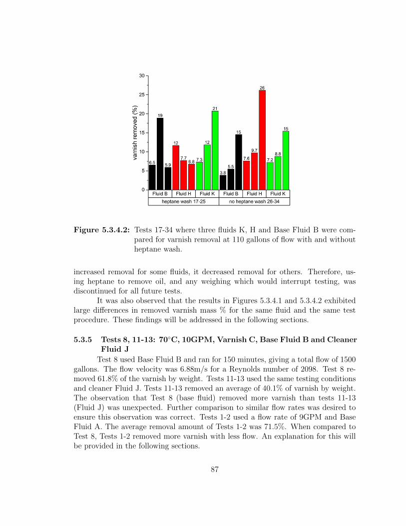
Figure 5.3.4.2: Tests 17-34 where three fluids K, H and Base Fluid B were com-pared for varnish removal at 110 gallons of flow with and withoutheptane wash.
increased removal for some fluids, it decreased removal for others. Therefore, us-ing heptane to remove oil, and any weighing which would interrupt testing, wasdiscontinued for all future tests.
It was also observed that the results in Figures 5.3.4.1 and 5.3.4.2 exhibitedlarge differences in removed varnish mass % for the same fluid and the same testprocedure. These findings will be addressed in the following sections.
5.3.5 Tests 8, 11-13: 70◦C, 10GPM, Varnish C, Base Fluid B and CleanerFluid J
Test 8 used Base Fluid B and ran for 150 minutes, giving a total flow of 1500gallons. The flow velocity was 6.88m/s for a Reynolds number of 2098. Test 8 re-moved 61.8% of the varnish by weight. Tests 11-13 used the same testing conditionsand cleaner Fluid J. Tests 11-13 removed an average of 40.1% of varnish by weight.The observation that Test 8 (base fluid) removed more varnish than tests 11-13(Fluid J) was unexpected. Further comparison to similar flow rates was desired toensure this observation was correct. Tests 1-2 used a flow rate of 9GPM and BaseFluid A. The average removal amount of Tests 1-2 was 71.5%. When compared toTest 8, Tests 1-2 removed more varnish with less flow. An explanation for this willbe provided in the following sections.
87
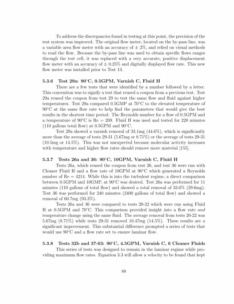
To address the discrepancies found in testing at this point, the precision of thetest system was improved. The original flow meter, located on the by-pass line, wasa variable area flow meter with an accuracy of ± 2%, and relied on visual methodsto read the flow. Because the by-pass line was used to obtain specific flows rangesthrough the test cell, it was replaced with a very accurate, positive displacementflow meter with an accuracy of ± 0.25% and digitally displayed flow rate. This newflow meter was installed prior to Test 13.
5.3.6 Test 29a: 90◦C, 0.5GPM, Varnish C, Fluid H
There are a few tests that were identified by a number followed by a letter.This convention was to signify a test that reused a coupon from a previous test. Test29a reused the coupon from test 29 to test the same flow and fluid against highertemperatures. Test 29a compared 0.5GMP at 70◦C to the elevated temperature of90◦C at the same flow rate to help find the parameters that would give the bestresults in the shortest time period. The Reynolds number for a flow of 0.5GPM anda temperature of 90◦C is Re = 209. Fluid H was used and tested for 220 minutes(110 gallons total flow) at 0.5GPM and 90◦C.
Test 29a showed a varnish removal of 33.1mg (44.6%), which is significantlymore than the average of tests 29-31 (5.67mg or 8.71%) or the average of tests 29-31(10.5mg or 14.5%). This was not unexpected because molecular activity increaseswith temperature and higher flow rates should remove more material [155].
5.3.7 Tests 26a and 36: 90◦C, 10GPM, Varnish C, Fluid H
Tests 26a, which reused the coupon from test 26, and test 36 were run withCleaner Fluid H and a flow rate of 10GPM at 90◦C which generated a Reynoldsnumber of Re = 4214. While this is into the turbulent regime, a direct comparisonbetween 0.5GPM and 10GMP, at 90◦C was desired. Test 26a was performed for 11minutes (110 gallons of total flow) and showed a total removal of 33.6% (29.6mg).Test 36 was performed for 240 minutes (2400 gallons of total flow) and showed aremoval of 60.7mg (93.3%).
Tests 26a and 36 were compared to tests 20-22 which were run using FluidH at 0.5GPM and 70◦C. This comparison provided insight into a flow rate andtemperature change using the same fluid. The average removal from tests 20-22 was5.67mg (8.71%) while tests 29-31 removed 10.47mg (14.5%). These results are asignificant improvement. This substantial difference prompted a series of tests thatwould use 90◦C and a flow rate set to ensure laminar flow.
5.3.8 Tests 32b and 37-63: 90◦C, 4.5GPM, Varnish C, 6 Cleaner Fluids
This series of tests was designed to remain in the laminar regime while pro-viding maximum flow rates. Equation 3.3 will allow a velocity to be found that kept
88
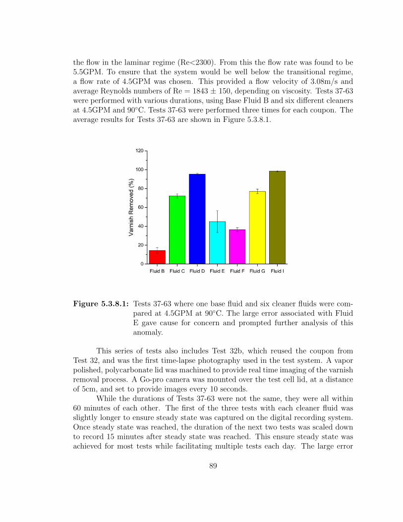
the flow in the laminar regime (Re<2300). From this the flow rate was found to be5.5GPM. To ensure that the system would be well below the transitional regime,a flow rate of 4.5GPM was chosen. This provided a flow velocity of 3.08m/s andaverage Reynolds numbers of Re = 1843 ± 150, depending on viscosity. Tests 37-63were performed with various durations, using Base Fluid B and six different cleanersat 4.5GPM and 90◦C. Tests 37-63 were performed three times for each coupon. Theaverage results for Tests 37-63 are shown in Figure 5.3.8.1.
Figure 5.3.8.1: Tests 37-63 where one base fluid and six cleaner fluids were com-pared at 4.5GPM at 90◦C. The large error associated with FluidE gave cause for concern and prompted further analysis of thisanomaly.
This series of tests also includes Test 32b, which reused the coupon fromTest 32, and was the first time-lapse photography used in the test system. A vaporpolished, polycarbonate lid was machined to provide real time imaging of the varnishremoval process. A Go-pro camera was mounted over the test cell lid, at a distanceof 5cm, and set to provide images every 10 seconds.
While the durations of Tests 37-63 were not the same, they were all within60 minutes of each other. The first of the three tests with each cleaner fluid wasslightly longer to ensure steady state was captured on the digital recording system.Once steady state was reached, the duration of the next two tests was scaled downto record 15 minutes after steady state was reached. This ensure steady state wasachieved for most tests while facilitating multiple tests each day. The large error
89
associated with Fluid E was unexpected and prompted investigation of cause. Thisdifference will be discussed in later sections.
5.3.9 Start of Test (SOT) vs End of Test (EOT) Trend
Referring back to Figure 5.3.4.1 and Figure 5.3.4.2, there are large differencesin varnish removal for the same fluid under the same conditions. When this isanalyzed in terms of varnish present at the start of test (SOT) and varnish presentat the end of test (EOT), a trend can be found. Figure 5.3.9.1 shows the effect ofinitial varnish weight (SOT) on the amount of varnish removed from the coupon(EOT).
Figure 5.3.9.1: Tests 17-34 showing the trend between the start of test (SOT)mass and the end of test (EOT) mass.
Figure 5.3.9.1 confirms that, if the varnish coupon has more varnish initially,then more varnish will be removed from the coupon. Linear fitting of the SOT-EOT results showed that this relationship was exhibited by all fluids, regardless oftesting conditions. Several attempts were made to standardize the SOT-EOT effectsobserved. This included both linearization of the data to extrapolate varnish removalamounts and finding a relationship that would describe the SOT/EOT dependence.Neither of these methods proved successful.
To limit the effects of EOT/SOT dependence on test results, it was decidedto control the SOT weight on the coupon within specific tolerances. Prior to test37, the average mass of the varnish on the coupon was 87.8mg and the standard
90
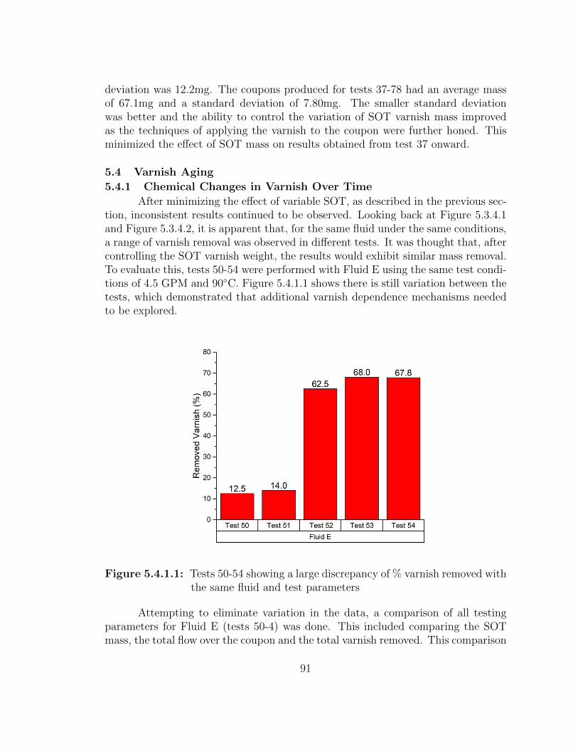
deviation was 12.2mg. The coupons produced for tests 37-78 had an average massof 67.1mg and a standard deviation of 7.80mg. The smaller standard deviationwas better and the ability to control the variation of SOT varnish mass improvedas the techniques of applying the varnish to the coupon were further honed. Thisminimized the effect of SOT mass on results obtained from test 37 onward.
5.4 Varnish Aging
5.4.1 Chemical Changes in Varnish Over Time
After minimizing the effect of variable SOT, as described in the previous sec-tion, inconsistent results continued to be observed. Looking back at Figure 5.3.4.1and Figure 5.3.4.2, it is apparent that, for the same fluid under the same conditions,a range of varnish removal was observed in different tests. It was thought that, aftercontrolling the SOT varnish weight, the results would exhibit similar mass removal.To evaluate this, tests 50-54 were performed with Fluid E using the same test condi-tions of 4.5 GPM and 90◦C. Figure 5.4.1.1 shows there is still variation between thetests, which demonstrated that additional varnish dependence mechanisms neededto be explored.
Figure 5.4.1.1: Tests 50-54 showing a large discrepancy of % varnish removed withthe same fluid and test parameters
Attempting to eliminate variation in the data, a comparison of all testingparameters for Fluid E (tests 50-4) was done. This included comparing the SOTmass, the total flow over the coupon and the total varnish removed. This comparison
91
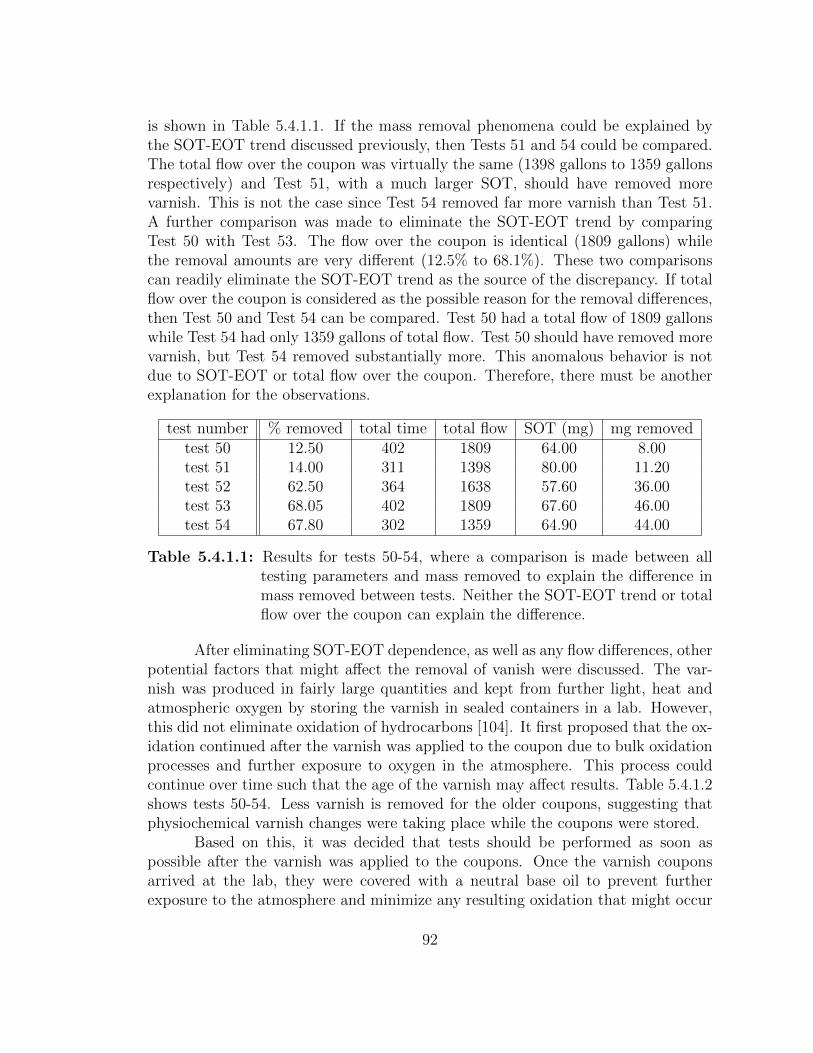
is shown in Table 5.4.1.1. If the mass removal phenomena could be explained bythe SOT-EOT trend discussed previously, then Tests 51 and 54 could be compared.The total flow over the coupon was virtually the same (1398 gallons to 1359 gallonsrespectively) and Test 51, with a much larger SOT, should have removed morevarnish. This is not the case since Test 54 removed far more varnish than Test 51.A further comparison was made to eliminate the SOT-EOT trend by comparingTest 50 with Test 53. The flow over the coupon is identical (1809 gallons) whilethe removal amounts are very different (12.5% to 68.1%). These two comparisonscan readily eliminate the SOT-EOT trend as the source of the discrepancy. If totalflow over the coupon is considered as the possible reason for the removal differences,then Test 50 and Test 54 can be compared. Test 50 had a total flow of 1809 gallonswhile Test 54 had only 1359 gallons of total flow. Test 50 should have removed morevarnish, but Test 54 removed substantially more. This anomalous behavior is notdue to SOT-EOT or total flow over the coupon. Therefore, there must be anotherexplanation for the observations.
test number % removed total time total flow SOT (mg) mg removedtest 50 12.50 402 1809 64.00 8.00test 51 14.00 311 1398 80.00 11.20test 52 62.50 364 1638 57.60 36.00test 53 68.05 402 1809 67.60 46.00test 54 67.80 302 1359 64.90 44.00
Table 5.4.1.1: Results for tests 50-54, where a comparison is made between alltesting parameters and mass removed to explain the difference inmass removed between tests. Neither the SOT-EOT trend or totalflow over the coupon can explain the difference.
After eliminating SOT-EOT dependence, as well as any flow differences, otherpotential factors that might affect the removal of vanish were discussed. The var-nish was produced in fairly large quantities and kept from further light, heat andatmospheric oxygen by storing the varnish in sealed containers in a lab. However,this did not eliminate oxidation of hydrocarbons [104]. It first proposed that the ox-idation continued after the varnish was applied to the coupon due to bulk oxidationprocesses and further exposure to oxygen in the atmosphere. This process couldcontinue over time such that the age of the varnish may affect results. Table 5.4.1.2shows tests 50-54. Less varnish is removed for the older coupons, suggesting thatphysiochemical varnish changes were taking place while the coupons were stored.
Based on this, it was decided that tests should be performed as soon aspossible after the varnish was applied to the coupons. Once the varnish couponsarrived at the lab, they were covered with a neutral base oil to prevent furtherexposure to the atmosphere and minimize any resulting oxidation that might occur
92
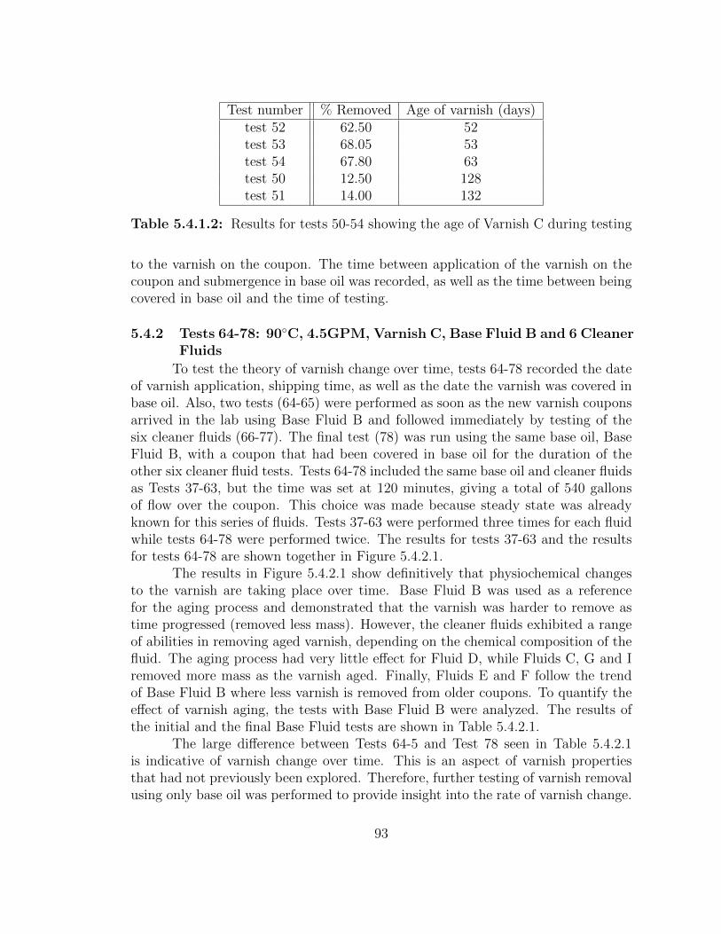
Test number % Removed Age of varnish (days)test 52 62.50 52test 53 68.05 53test 54 67.80 63test 50 12.50 128test 51 14.00 132
Table 5.4.1.2: Results for tests 50-54 showing the age of Varnish C during testing
to the varnish on the coupon. The time between application of the varnish on thecoupon and submergence in base oil was recorded, as well as the time between beingcovered in base oil and the time of testing.
5.4.2 Tests 64-78: 90◦C, 4.5GPM, Varnish C, Base Fluid B and 6 CleanerFluids
To test the theory of varnish change over time, tests 64-78 recorded the dateof varnish application, shipping time, as well as the date the varnish was covered inbase oil. Also, two tests (64-65) were performed as soon as the new varnish couponsarrived in the lab using Base Fluid B and followed immediately by testing of thesix cleaner fluids (66-77). The final test (78) was run using the same base oil, BaseFluid B, with a coupon that had been covered in base oil for the duration of theother six cleaner fluid tests. Tests 64-78 included the same base oil and cleaner fluidsas Tests 37-63, but the time was set at 120 minutes, giving a total of 540 gallonsof flow over the coupon. This choice was made because steady state was alreadyknown for this series of fluids. Tests 37-63 were performed three times for each fluidwhile tests 64-78 were performed twice. The results for tests 37-63 and the resultsfor tests 64-78 are shown together in Figure 5.4.2.1.
The results in Figure 5.4.2.1 show definitively that physiochemical changesto the varnish are taking place over time. Base Fluid B was used as a referencefor the aging process and demonstrated that the varnish was harder to remove astime progressed (removed less mass). However, the cleaner fluids exhibited a rangeof abilities in removing aged varnish, depending on the chemical composition of thefluid. The aging process had very little effect for Fluid D, while Fluids C, G and Iremoved more mass as the varnish aged. Finally, Fluids E and F follow the trendof Base Fluid B where less varnish is removed from older coupons. To quantify theeffect of varnish aging, the tests with Base Fluid B were analyzed. The results ofthe initial and the final Base Fluid tests are shown in Table 5.4.2.1.
The large difference between Tests 64-5 and Test 78 seen in Table 5.4.2.1is indicative of varnish change over time. This is an aspect of varnish propertiesthat had not previously been explored. Therefore, further testing of varnish removalusing only base oil was performed to provide insight into the rate of varnish change.
93
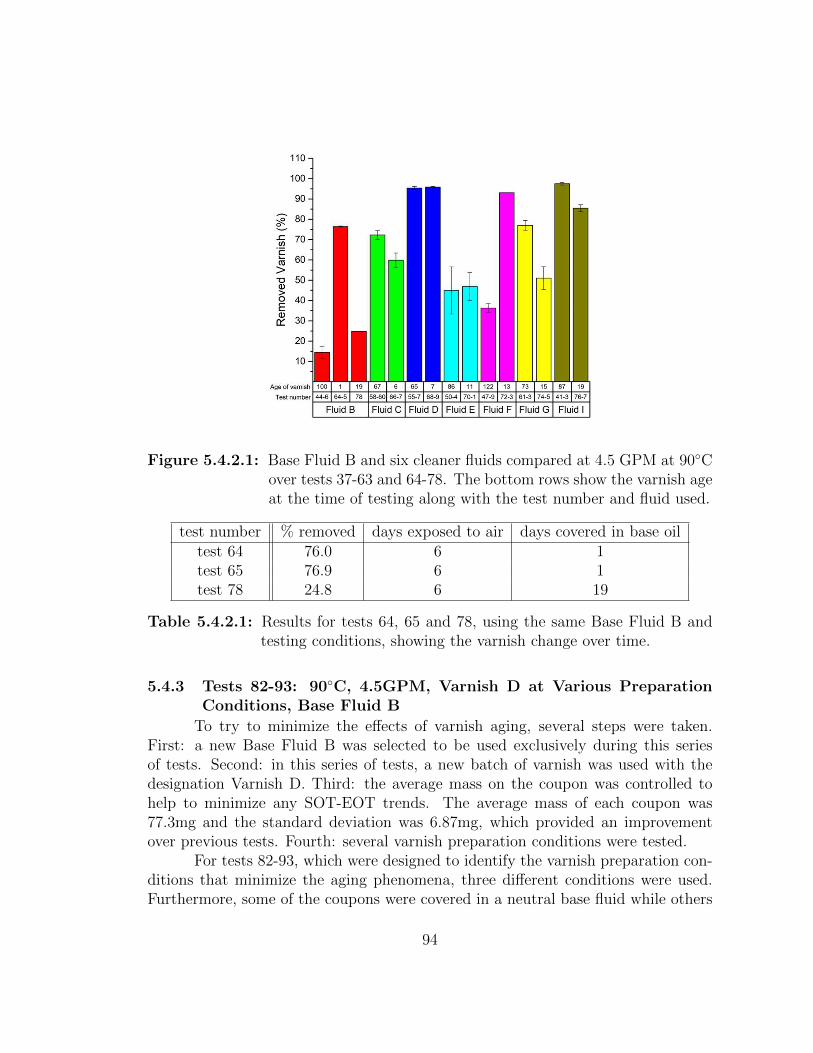
Figure 5.4.2.1: Base Fluid B and six cleaner fluids compared at 4.5 GPM at 90◦Cover tests 37-63 and 64-78. The bottom rows show the varnish ageat the time of testing along with the test number and fluid used.
test number % removed days exposed to air days covered in base oiltest 64 76.0 6 1test 65 76.9 6 1test 78 24.8 6 19
Table 5.4.2.1: Results for tests 64, 65 and 78, using the same Base Fluid B andtesting conditions, showing the varnish change over time.
5.4.3 Tests 82-93: 90◦C, 4.5GPM, Varnish D at Various PreparationConditions, Base Fluid B
To try to minimize the effects of varnish aging, several steps were taken.First: a new Base Fluid B was selected to be used exclusively during this seriesof tests. Second: in this series of tests, a new batch of varnish was used with thedesignation Varnish D. Third: the average mass on the coupon was controlled tohelp to minimize any SOT-EOT trends. The average mass of each coupon was77.3mg and the standard deviation was 6.87mg, which provided an improvementover previous tests. Fourth: several varnish preparation conditions were tested.
For tests 82-93, which were designed to identify the varnish preparation con-ditions that minimize the aging phenomena, three different conditions were used.Furthermore, some of the coupons were covered in a neutral base fluid while others
94
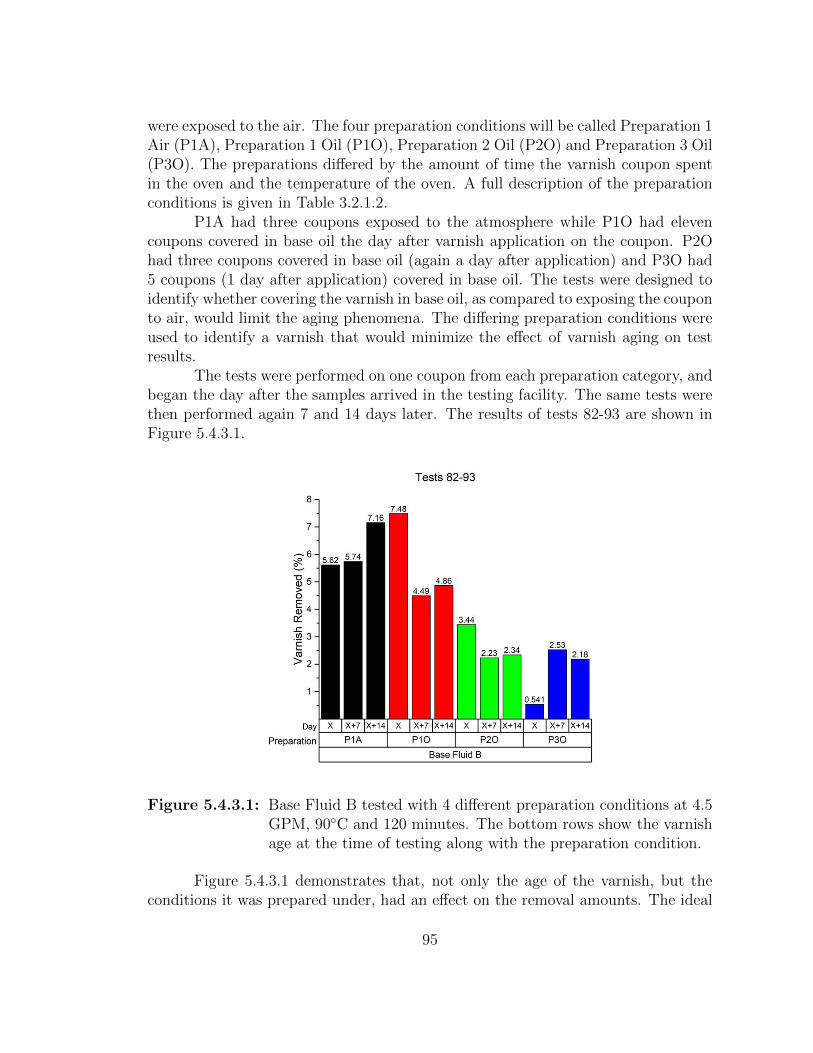
were exposed to the air. The four preparation conditions will be called Preparation 1Air (P1A), Preparation 1 Oil (P1O), Preparation 2 Oil (P2O) and Preparation 3 Oil(P3O). The preparations differed by the amount of time the varnish coupon spentin the oven and the temperature of the oven. A full description of the preparationconditions is given in Table 3.2.1.2.
P1A had three coupons exposed to the atmosphere while P1O had elevencoupons covered in base oil the day after varnish application on the coupon. P2Ohad three coupons covered in base oil (again a day after application) and P3O had5 coupons (1 day after application) covered in base oil. The tests were designed toidentify whether covering the varnish in base oil, as compared to exposing the couponto air, would limit the aging phenomena. The differing preparation conditions wereused to identify a varnish that would minimize the effect of varnish aging on testresults.
The tests were performed on one coupon from each preparation category, andbegan the day after the samples arrived in the testing facility. The same tests werethen performed again 7 and 14 days later. The results of tests 82-93 are shown inFigure 5.4.3.1.
Figure 5.4.3.1: Base Fluid B tested with 4 different preparation conditions at 4.5GPM, 90◦C and 120 minutes. The bottom rows show the varnishage at the time of testing along with the preparation condition.
Figure 5.4.3.1 demonstrates that, not only the age of the varnish, but theconditions it was prepared under, had an effect on the removal amounts. The ideal
95
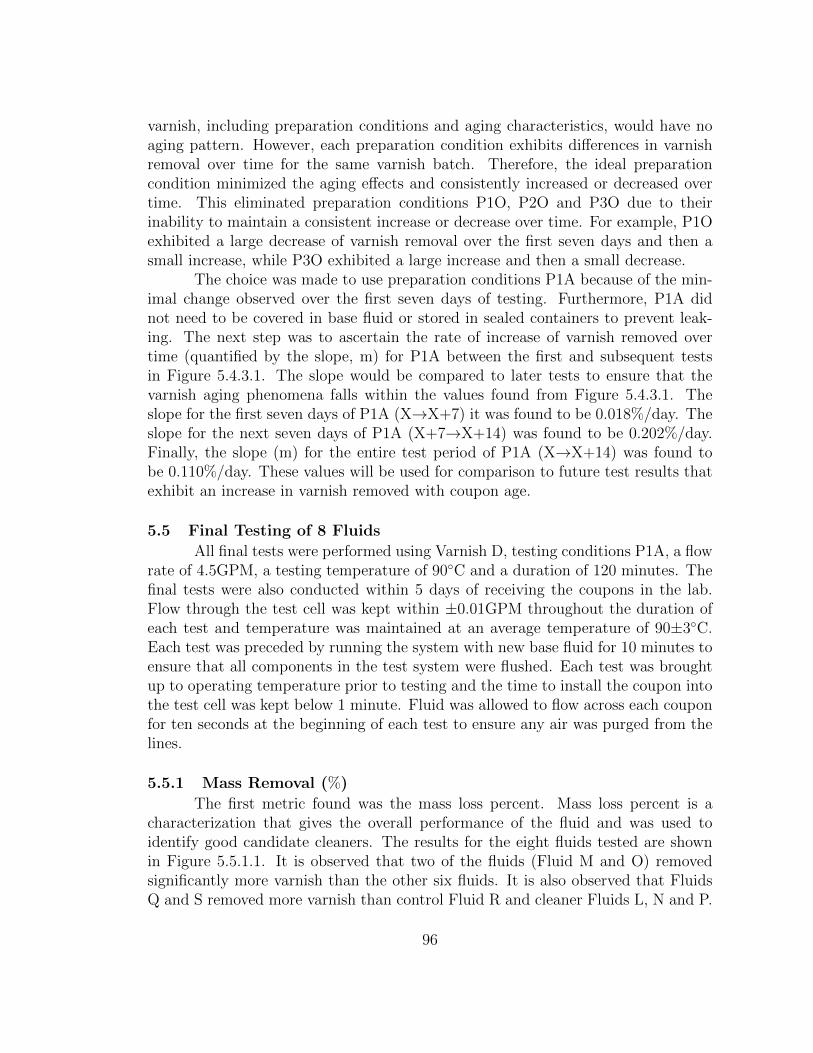
varnish, including preparation conditions and aging characteristics, would have noaging pattern. However, each preparation condition exhibits differences in varnishremoval over time for the same varnish batch. Therefore, the ideal preparationcondition minimized the aging effects and consistently increased or decreased overtime. This eliminated preparation conditions P1O, P2O and P3O due to theirinability to maintain a consistent increase or decrease over time. For example, P1Oexhibited a large decrease of varnish removal over the first seven days and then asmall increase, while P3O exhibited a large increase and then a small decrease.
The choice was made to use preparation conditions P1A because of the min-imal change observed over the first seven days of testing. Furthermore, P1A didnot need to be covered in base fluid or stored in sealed containers to prevent leak-ing. The next step was to ascertain the rate of increase of varnish removed overtime (quantified by the slope, m) for P1A between the first and subsequent testsin Figure 5.4.3.1. The slope would be compared to later tests to ensure that thevarnish aging phenomena falls within the values found from Figure 5.4.3.1. Theslope for the first seven days of P1A (X→X+7) it was found to be 0.018%/day. Theslope for the next seven days of P1A (X+7→X+14) was found to be 0.202%/day.Finally, the slope (m) for the entire test period of P1A (X→X+14) was found tobe 0.110%/day. These values will be used for comparison to future test results thatexhibit an increase in varnish removed with coupon age.
5.5 Final Testing of 8 Fluids
All final tests were performed using Varnish D, testing conditions P1A, a flowrate of 4.5GPM, a testing temperature of 90◦C and a duration of 120 minutes. Thefinal tests were also conducted within 5 days of receiving the coupons in the lab.Flow through the test cell was kept within ±0.01GPM throughout the duration ofeach test and temperature was maintained at an average temperature of 90±3◦C.Each test was preceded by running the system with new base fluid for 10 minutes toensure that all components in the test system were flushed. Each test was broughtup to operating temperature prior to testing and the time to install the coupon intothe test cell was kept below 1 minute. Fluid was allowed to flow across each couponfor ten seconds at the beginning of each test to ensure any air was purged from thelines.
5.5.1 Mass Removal (%)
The first metric found was the mass loss percent. Mass loss percent is acharacterization that gives the overall performance of the fluid and was used toidentify good candidate cleaners. The results for the eight fluids tested are shownin Figure 5.5.1.1. It is observed that two of the fluids (Fluid M and O) removedsignificantly more varnish than the other six fluids. It is also observed that FluidsQ and S removed more varnish than control Fluid R and cleaner Fluids L, N and P.
96
Therefore, Fluids Q and S might be good candidates for long term use in a system,depending on the remaining characterizations.
Figure 5.5.1.1: Mass removal results for base Fluid R and 7 cleaner fluids usingVarnish D and preparation conditions P1A.
5.5.2 Trends and Aging
Control of both the SOT/EOT trend and varnish aging is imperative toensure accurate and reliable test results. To minimize the effect of SOT/EOT, theweights of the coupons were kept within strict limits. The average SOT weight of thefinal batch of coupons was 86.6mg and the deviation was reduced to only 4.72mg.This is a drastic improvement over the prior measurements given in Section 5.3.9.
After the mass removal data was found (Figure 5.5.1.1) the results needed tobe analyzed to determine if varnish aging had an effect. Fluid R (a base fluid) wastested at the beginning and end of this test series to track any varnish aging thatmight have occurred. Fluid R, shown in Figure 5.5.1.1, was tested with varnish agedfor 6 days and then again at 18 days. The slope (m) for this time period (twelvedays) is found to be 0.048%/day. Table 5.5.2.1 summarizes the comparison betweenthe values from the previous varnish aging tests (Figure 5.4.3.1) and the currentseries of tests.
Table 5.5.2.1 shows that the slope of Fluid R fits nicely between the slopes ofFluid B. This indicates that the aging process falls in the range expected from the
97
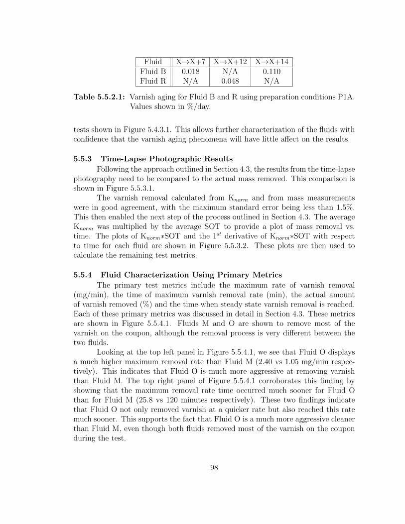
Fluid X→X+7 X→X+12 X→X+14Fluid B 0.018 N/A 0.110Fluid R N/A 0.048 N/A
Table 5.5.2.1: Varnish aging for Fluid B and R using preparation conditions P1A.Values shown in %/day.
tests shown in Figure 5.4.3.1. This allows further characterization of the fluids withconfidence that the varnish aging phenomena will have little affect on the results.
5.5.3 Time-Lapse Photographic Results
Following the approach outlined in Section 4.3, the results from the time-lapsephotography need to be compared to the actual mass removed. This comparison isshown in Figure 5.5.3.1.
The varnish removal calculated from Knorm and from mass measurementswere in good agreement, with the maximum standard error being less than 1.5%.This then enabled the next step of the process outlined in Section 4.3. The averageKnorm was multiplied by the average SOT to provide a plot of mass removal vs.time. The plots of Knorm∗SOT and the 1st derivative of Knorm∗SOT with respectto time for each fluid are shown in Figure 5.5.3.2. These plots are then used tocalculate the remaining test metrics.
5.5.4 Fluid Characterization Using Primary Metrics
The primary test metrics include the maximum rate of varnish removal(mg/min), the time of maximum varnish removal rate (min), the actual amountof varnish removed (%) and the time when steady state varnish removal is reached.Each of these primary metrics was discussed in detail in Section 4.3. These metricsare shown in Figure 5.5.4.1. Fluids M and O are shown to remove most of thevarnish on the coupon, although the removal process is very different between thetwo fluids.
Looking at the top left panel in Figure 5.5.4.1, we see that Fluid O displaysa much higher maximum removal rate than Fluid M (2.40 vs 1.05 mg/min respec-tively). This indicates that Fluid O is much more aggressive at removing varnishthan Fluid M. The top right panel of Figure 5.5.4.1 corroborates this finding byshowing that the maximum removal rate time occurred much sooner for Fluid Othan for Fluid M (25.8 vs 120 minutes respectively). These two findings indicatethat Fluid O not only removed varnish at a quicker rate but also reached this ratemuch sooner. This supports the fact that Fluid O is a much more aggressive cleanerthan Fluid M, even though both fluids removed most of the varnish on the couponduring the test.
98
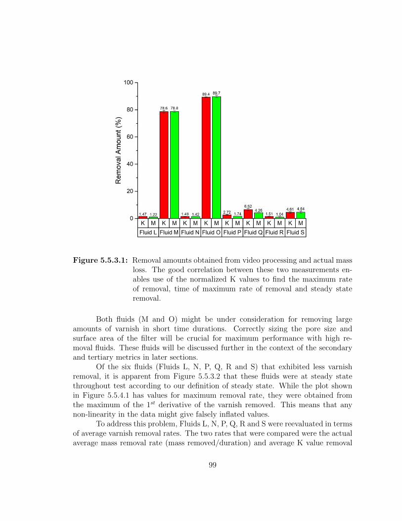
Figure 5.5.3.1: Removal amounts obtained from video processing and actual massloss. The good correlation between these two measurements en-ables use of the normalized K values to find the maximum rateof removal, time of maximum rate of removal and steady stateremoval.
Both fluids (M and O) might be under consideration for removing largeamounts of varnish in short time durations. Correctly sizing the pore size andsurface area of the filter will be crucial for maximum performance with high re-moval fluids. These fluids will be discussed further in the context of the secondaryand tertiary metrics in later sections.
Of the six fluids (Fluids L, N, P, Q, R and S) that exhibited less varnishremoval, it is apparent from Figure 5.5.3.2 that these fluids were at steady statethroughout test according to our definition of steady state. While the plot shownin Figure 5.5.4.1 has values for maximum removal rate, they were obtained fromthe maximum of the 1st derivative of the varnish removed. This means that anynon-linearity in the data might give falsely inflated values.
To address this problem, Fluids L, N, P, Q, R and S were reevaluated in termsof average varnish removal rates. The two rates that were compared were the actualaverage mass removal rate (mass removed/duration) and average K value removal
99
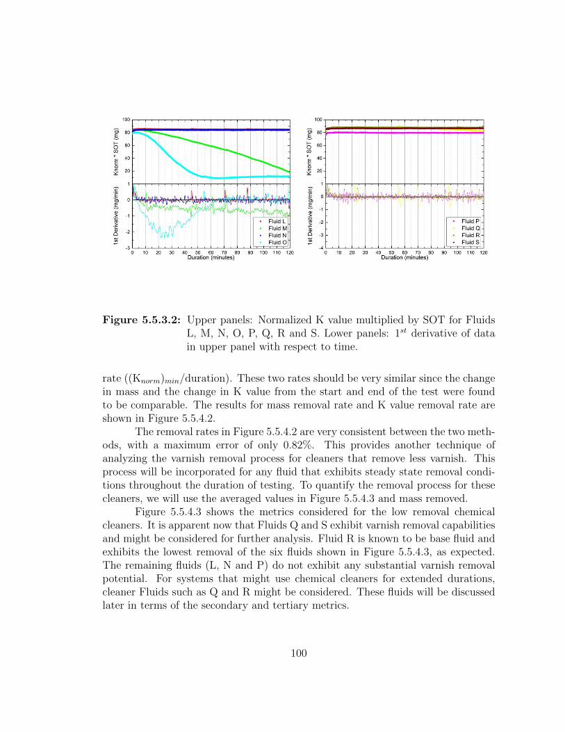
Figure 5.5.3.2: Upper panels: Normalized K value multiplied by SOT for FluidsL, M, N, O, P, Q, R and S. Lower panels: 1st derivative of datain upper panel with respect to time.
rate ((Knorm)min/duration). These two rates should be very similar since the changein mass and the change in K value from the start and end of the test were foundto be comparable. The results for mass removal rate and K value removal rate areshown in Figure 5.5.4.2.
The removal rates in Figure 5.5.4.2 are very consistent between the two meth-ods, with a maximum error of only 0.82%. This provides another technique ofanalyzing the varnish removal process for cleaners that remove less varnish. Thisprocess will be incorporated for any fluid that exhibits steady state removal condi-tions throughout the duration of testing. To quantify the removal process for thesecleaners, we will use the averaged values in Figure 5.5.4.3 and mass removed.
Figure 5.5.4.3 shows the metrics considered for the low removal chemicalcleaners. It is apparent now that Fluids Q and S exhibit varnish removal capabilitiesand might be considered for further analysis. Fluid R is known to be base fluid andexhibits the lowest removal of the six fluids shown in Figure 5.5.4.3, as expected.The remaining fluids (L, N and P) do not exhibit any substantial varnish removalpotential. For systems that might use chemical cleaners for extended durations,cleaner Fluids such as Q and R might be considered. These fluids will be discussedlater in terms of the secondary and tertiary metrics.
100
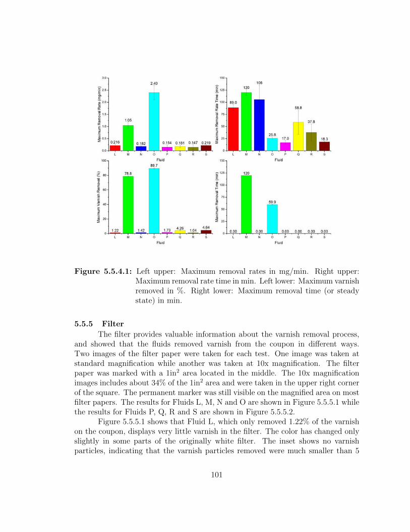
Figure 5.5.4.1: Left upper: Maximum removal rates in mg/min. Right upper:Maximum removal rate time in min. Left lower: Maximum varnishremoved in %. Right lower: Maximum removal time (or steadystate) in min.
5.5.5 Filter
The filter provides valuable information about the varnish removal process,and showed that the fluids removed varnish from the coupon in different ways.Two images of the filter paper were taken for each test. One image was taken atstandard magnification while another was taken at 10x magnification. The filterpaper was marked with a 1in2 area located in the middle. The 10x magnificationimages includes about 34% of the 1in2 area and were taken in the upper right cornerof the square. The permanent marker was still visible on the magnified area on mostfilter papers. The results for Fluids L, M, N and O are shown in Figure 5.5.5.1 whilethe results for Fluids P, Q, R and S are shown in Figure 5.5.5.2.
Figure 5.5.5.1 shows that Fluid L, which only removed 1.22% of the varnishon the coupon, displays very little varnish in the filter. The color has changed onlyslightly in some parts of the originally white filter. The inset shows no varnishparticles, indicating that the varnish particles removed were much smaller than 5
101
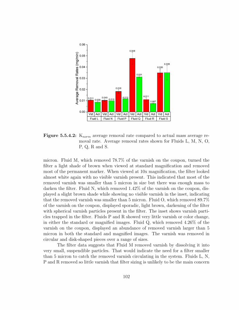
Figure 5.5.4.2: Knorm average removal rate compared to actual mass average re-moval rate. Average removal rates shown for Fluids L, M, N, O,P, Q, R and S.
micron. Fluid M, which removed 78.7% of the varnish on the coupon, turned thefilter a light shade of brown when viewed at standard magnification and removedmost of the permanent marker. When viewed at 10x magnification, the filter lookedalmost white again with no visible varnish present. This indicated that most of theremoved varnish was smaller than 5 micron in size but there was enough mass todarken the filter. Fluid N, which removed 1.42% of the varnish on the coupon, dis-played a slight brown shade while showing no visible varnish in the inset, indicatingthat the removed varnish was smaller than 5 micron. Fluid O, which removed 89.7%of the varnish on the coupon, displayed sporadic, light brown, darkening of the filterwith spherical varnish particles present in the filter. The inset shows varnish parti-cles trapped in the filter. Fluids P and R showed very little varnish or color change,in either the standard or magnified images. Fluid Q, which removed 4.26% of thevarnish on the coupon, displayed an abundance of removed varnish larger than 5micron in both the standard and magnified images. The varnish was removed incircular and disk-shaped pieces over a range of sizes.
The filter data suggests that Fluid M removed varnish by dissolving it intovery small, suspendible particles. That would indicate the need for a filter smallerthan 5 micron to catch the removed varnish circulating in the system. Fluids L, N,P and R removed so little varnish that filter sizing is unlikely to be the main concern
102
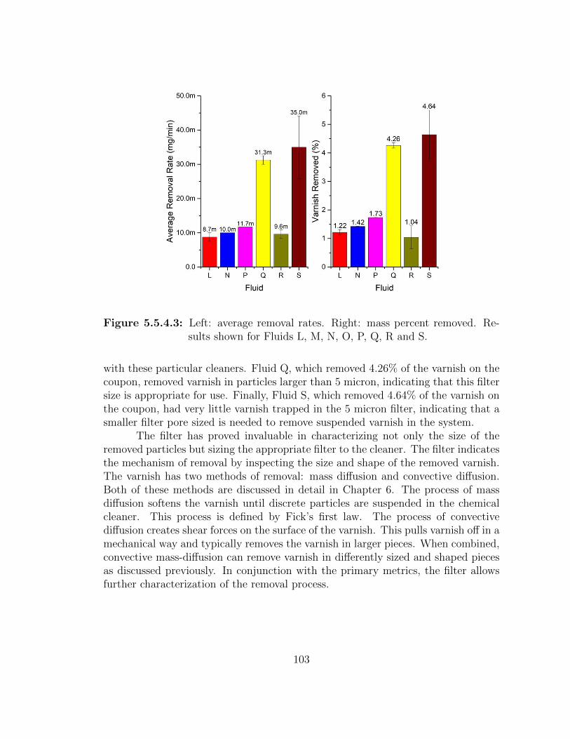
Figure 5.5.4.3: Left: average removal rates. Right: mass percent removed. Re-sults shown for Fluids L, M, N, O, P, Q, R and S.
with these particular cleaners. Fluid Q, which removed 4.26% of the varnish on thecoupon, removed varnish in particles larger than 5 micron, indicating that this filtersize is appropriate for use. Finally, Fluid S, which removed 4.64% of the varnish onthe coupon, had very little varnish trapped in the 5 micron filter, indicating that asmaller filter pore sized is needed to remove suspended varnish in the system.
The filter has proved invaluable in characterizing not only the size of theremoved particles but sizing the appropriate filter to the cleaner. The filter indicatesthe mechanism of removal by inspecting the size and shape of the removed varnish.The varnish has two methods of removal: mass diffusion and convective diffusion.Both of these methods are discussed in detail in Chapter 6. The process of massdiffusion softens the varnish until discrete particles are suspended in the chemicalcleaner. This process is defined by Fick’s first law. The process of convectivediffusion creates shear forces on the surface of the varnish. This pulls varnish off in amechanical way and typically removes the varnish in larger pieces. When combined,convective mass-diffusion can remove varnish in differently sized and shaped piecesas discussed previously. In conjunction with the primary metrics, the filter allowsfurther characterization of the removal process.
103
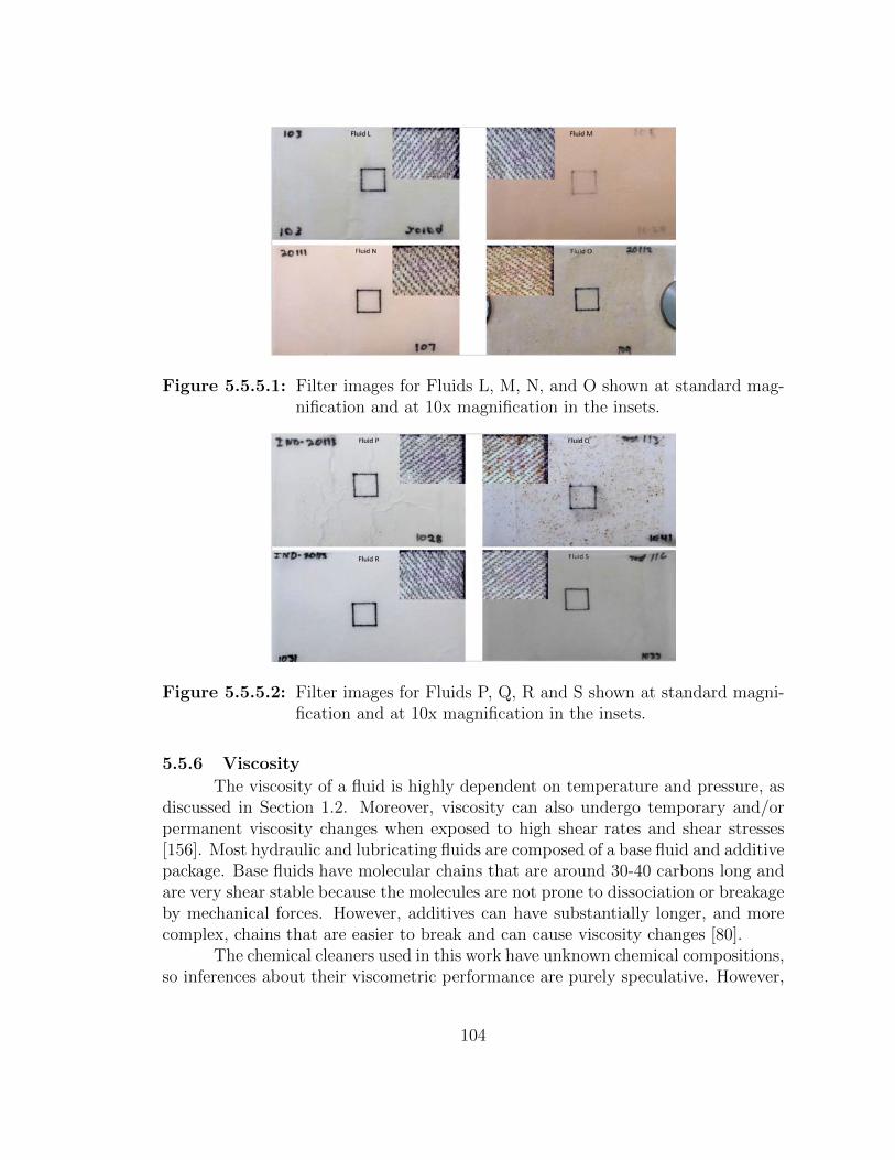
Figure 5.5.5.1: Filter images for Fluids L, M, N, and O shown at standard mag-nification and at 10x magnification in the insets.
Figure 5.5.5.2: Filter images for Fluids P, Q, R and S shown at standard magni-fication and at 10x magnification in the insets.
5.5.6 Viscosity
The viscosity of a fluid is highly dependent on temperature and pressure, asdiscussed in Section 1.2. Moreover, viscosity can also undergo temporary and/orpermanent viscosity changes when exposed to high shear rates and shear stresses[156]. Most hydraulic and lubricating fluids are composed of a base fluid and additivepackage. Base fluids have molecular chains that are around 30-40 carbons long andare very shear stable because the molecules are not prone to dissociation or breakageby mechanical forces. However, additives can have substantially longer, and morecomplex, chains that are easier to break and can cause viscosity changes [80].
The chemical cleaners used in this work have unknown chemical compositions,so inferences about their viscometric performance are purely speculative. However,
104
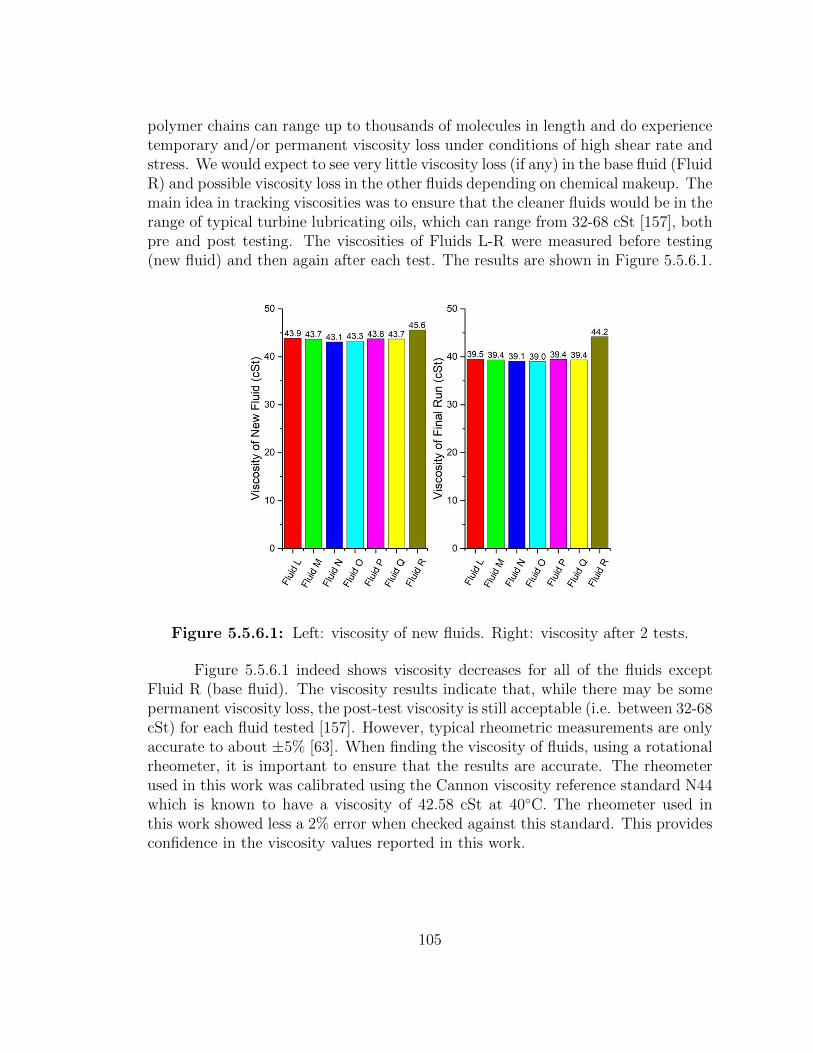
polymer chains can range up to thousands of molecules in length and do experiencetemporary and/or permanent viscosity loss under conditions of high shear rate andstress. We would expect to see very little viscosity loss (if any) in the base fluid (FluidR) and possible viscosity loss in the other fluids depending on chemical makeup. Themain idea in tracking viscosities was to ensure that the cleaner fluids would be in therange of typical turbine lubricating oils, which can range from 32-68 cSt [157], bothpre and post testing. The viscosities of Fluids L-R were measured before testing(new fluid) and then again after each test. The results are shown in Figure 5.5.6.1.
Figure 5.5.6.1: Left: viscosity of new fluids. Right: viscosity after 2 tests.
Figure 5.5.6.1 indeed shows viscosity decreases for all of the fluids exceptFluid R (base fluid). The viscosity results indicate that, while there may be somepermanent viscosity loss, the post-test viscosity is still acceptable (i.e. between 32-68cSt) for each fluid tested [157]. However, typical rheometric measurements are onlyaccurate to about ±5% [63]. When finding the viscosity of fluids, using a rotationalrheometer, it is important to ensure that the results are accurate. The rheometerused in this work was calibrated using the Cannon viscosity reference standard N44which is known to have a viscosity of 42.58 cSt at 40◦C. The rheometer used inthis work showed less a 2% error when checked against this standard. This providesconfidence in the viscosity values reported in this work.
105
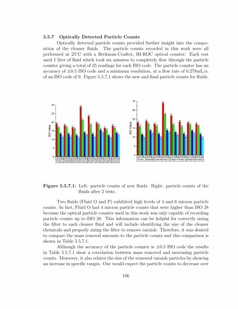
5.5.7 Optically Detected Particle Counts
Optically detected particle counts provided further insight into the compo-sition of the cleaner fluids. The particle counts recorded in this work were allperformed at 25◦C with a Beckman-Coulter, HI-ROC optical counter. Each testused 1 liter of fluid which took six minutes to completely flow through the particlecounter giving a total of 35 readings for each ISO code. The particle counter has anaccuracy of ±0.5 ISO code and a minimum resolution, at a flow rate of 0.278mL/s,of an ISO code of 9. Figure 5.5.7.1 shows the new and final particle counts for fluids.
Figure 5.5.7.1: Left: particle counts of new fluids. Right: particle counts of thefluids after 2 tests.
Two fluids (Fluid O and P) exhibited high levels of 4 and 6 micron particlecounts. In fact, Fluid O had 4 micron particle counts that were higher than ISO 28because the optical particle counter used in this work was only capable of recordingparticle counts up to ISO 28. This information can be helpful for correctly sizingthe filter to each cleaner fluid and will include identifying the size of the cleanerchemicals and properly sizing the filter to remove varnish. Therefore, it was desiredto compare the mass removal amounts to the particle counts and this comparison isshown in Table 5.5.7.1.
Although the accuracy of the particle counter is ±0.5 ISO code the resultsin Table 5.5.7.1 show a correlation between mass removed and increasing particlecounts. Moreover, it also relates the size of the removed varnish particles by showingan increase in specific ranges. One would expect the particle counts to decrease over
106
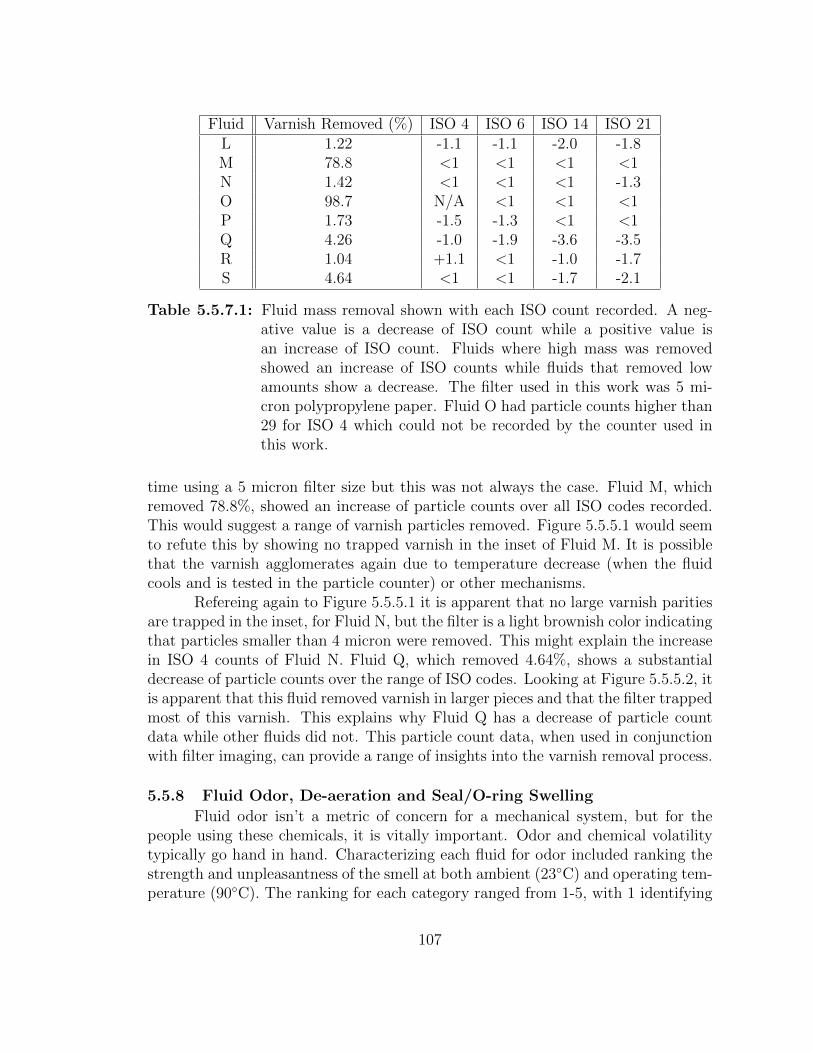
Fluid Varnish Removed (%) ISO 4 ISO 6 ISO 14 ISO 21L 1.22 -1.1 -1.1 -2.0 -1.8M 78.8 <1 <1 <1 <1N 1.42 <1 <1 <1 -1.3O 98.7 N/A <1 <1 <1P 1.73 -1.5 -1.3 <1 <1Q 4.26 -1.0 -1.9 -3.6 -3.5R 1.04 +1.1 <1 -1.0 -1.7S 4.64 <1 <1 -1.7 -2.1
Table 5.5.7.1: Fluid mass removal shown with each ISO count recorded. A neg-ative value is a decrease of ISO count while a positive value isan increase of ISO count. Fluids where high mass was removedshowed an increase of ISO counts while fluids that removed lowamounts show a decrease. The filter used in this work was 5 mi-cron polypropylene paper. Fluid O had particle counts higher than29 for ISO 4 which could not be recorded by the counter used inthis work.
time using a 5 micron filter size but this was not always the case. Fluid M, whichremoved 78.8%, showed an increase of particle counts over all ISO codes recorded.This would suggest a range of varnish particles removed. Figure 5.5.5.1 would seemto refute this by showing no trapped varnish in the inset of Fluid M. It is possiblethat the varnish agglomerates again due to temperature decrease (when the fluidcools and is tested in the particle counter) or other mechanisms.
Refereing again to Figure 5.5.5.1 it is apparent that no large varnish paritiesare trapped in the inset, for Fluid N, but the filter is a light brownish color indicatingthat particles smaller than 4 micron were removed. This might explain the increasein ISO 4 counts of Fluid N. Fluid Q, which removed 4.64%, shows a substantialdecrease of particle counts over the range of ISO codes. Looking at Figure 5.5.5.2, itis apparent that this fluid removed varnish in larger pieces and that the filter trappedmost of this varnish. This explains why Fluid Q has a decrease of particle countdata while other fluids did not. This particle count data, when used in conjunctionwith filter imaging, can provide a range of insights into the varnish removal process.
5.5.8 Fluid Odor, De-aeration and Seal/O-ring Swelling
Fluid odor isn’t a metric of concern for a mechanical system, but for thepeople using these chemicals, it is vitally important. Odor and chemical volatilitytypically go hand in hand. Characterizing each fluid for odor included ranking thestrength and unpleasantness of the smell at both ambient (23◦C) and operating tem-perature (90◦C). The ranking for each category ranged from 1-5, with 1 identifying
107
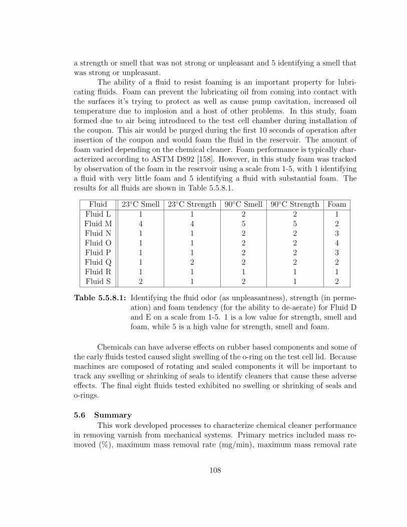
a strength or smell that was not strong or unpleasant and 5 identifying a smell thatwas strong or unpleasant.
The ability of a fluid to resist foaming is an important property for lubri-cating fluids. Foam can prevent the lubricating oil from coming into contact withthe surfaces it’s trying to protect as well as cause pump cavitation, increased oiltemperature due to implosion and a host of other problems. In this study, foamformed due to air being introduced to the test cell chamber during installation ofthe coupon. This air would be purged during the first 10 seconds of operation afterinsertion of the coupon and would foam the fluid in the reservoir. The amount offoam varied depending on the chemical cleaner. Foam performance is typically char-acterized according to ASTM D892 [158]. However, in this study foam was trackedby observation of the foam in the reservoir using a scale from 1-5, with 1 identifyinga fluid with very little foam and 5 identifying a fluid with substantial foam. Theresults for all fluids are shown in Table 5.5.8.1.
Fluid 23◦C Smell 23◦C Strength 90◦C Smell 90◦C Strength FoamFluid L 1 1 2 2 1Fluid M 4 4 5 5 2Fluid N 1 1 2 2 3Fluid O 1 1 2 2 4Fluid P 1 1 2 2 3Fluid Q 1 2 2 2 2Fluid R 1 1 1 1 1Fluid S 2 1 2 1 2
Table 5.5.8.1: Identifying the fluid odor (as unpleasantness), strength (in perme-ation) and foam tendency (for the ability to de-aerate) for Fluid Dand E on a scale from 1-5. 1 is a low value for strength, smell andfoam, while 5 is a high value for strength, smell and foam.
Chemicals can have adverse effects on rubber based components and some ofthe early fluids tested caused slight swelling of the o-ring on the test cell lid. Becausemachines are composed of rotating and sealed components it will be important totrack any swelling or shrinking of seals to identify cleaners that cause these adverseeffects. The final eight fluids tested exhibited no swelling or shrinking of seals ando-rings.
5.6 Summary
This work developed processes to characterize chemical cleaner performancein removing varnish from mechanical systems. Primary metrics included mass re-moved (%), maximum mass removal rate (mg/min), maximum mass removal rate
108
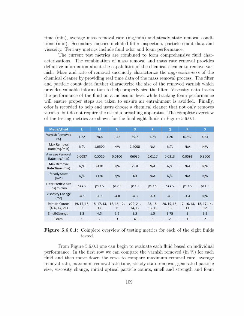
time (min), average mass removal rate (mg/min) and steady state removal condi-tions (min). Secondary metrics included filter inspection, particle count data andviscosity. Tertiary metrics include fluid odor and foam performance.
The current test metrics are combined to form comprehensive fluid char-acterizations. The combination of mass removal and mass rate removal providesdefinitive information about the capabilities of the chemical cleaner to remove var-nish. Mass and rate of removal succinctly characterize the aggressiveness of thechemical cleaner by providing real time data of the mass removal process. The filterand particle count data further characterize the size of the removed varnish whichprovides valuable information to help properly size the filter. Viscosity data tracksthe performance of the fluid on a molecular level while tracking foam performancewill ensure proper steps are taken to ensure air entrainment is avoided. Finally,odor is recorded to help end users choose a chemical cleaner that not only removesvarnish, but do not require the use of a breathing apparatus. The complete overviewof the testing metrics are shown for the final eight fluids in Figure 5.6.0.1.
Figure 5.6.0.1: Complete overview of testing metrics for each of the eight fluidstested.
From Figure 5.6.0.1 one can begin to evaluate each fluid based on individualperformance. In the first row we can compare the varnish removed (in %) for eachfluid and then move down the rows to compare maximum removal rate, averageremoval rate, maximum removal rate time, steady state removal, generated particlesize, viscosity change, initial optical particle counts, smell and strength and foam
109
production. For the end user, each of these categories will provide significant insightinto the performance of the fluid as well as expected filter requirement and workingenvironment.
Furthermore, the characterization of varnish aging will allow the scientificcommunity to understand the effects of varnish composition on chemical cleanerperformance. Moreover, the analysis of the effects of varnish preparation conditionsprovides information about how much varnish might be removed for given curingconditions in a mechanical system. Aspects of the varnish removal process that havenot previously been considered have been explored in this work.
Overall, this research provides a new approach to comprehensive characteri-zation of chemical cleaner performance. The approach has been demonstrated withrepresentative cleaner fluids which has revealed previously unexplored trends in var-nish removal. The results are therefore valuable to both the scientific communityand end users. The two main processes of removal in this work, mass and convectivediffusion, will be discussed in the following chapter and help to characterize fluidperformance.
110
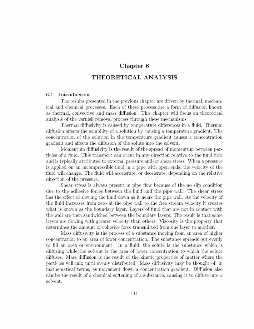
Chapter 6
THEORETICAL ANALYSIS
6.1 Introduction
The results presented in the previous chapter are driven by thermal, mechan-ical and chemical processes. Each of these process are a form of diffusion knownas thermal, convective and mass diffusion. This chapter will focus on theoreticalanalysis of the varnish removal process through these mechanisms.
Thermal diffusivity is caused by temperature differences in a fluid. Thermaldiffusion affects the solubility of a solution by causing a temperature gradient. Theconcentration of the solution in the temperature gradient causes a concentrationgradient and affects the diffusion of the solute into the solvent.
Momentum diffusivity is the result of the spread of momentum between par-ticles of a fluid. This transport can occur in any direction relative to the fluid flowand is typically attributed to external pressure and/or shear stress. When a pressureis applied on an incompressible fluid in a pipe with open ends, the velocity of thefluid will change. The fluid will accelerate, or decelerate, depending on the relativedirection of the pressure.
Shear stress is always present in pipe flow because of the no slip conditiondue to the adhesive forces between the fluid and the pipe wall. The shear stresshas the effect of slowing the fluid down as it nears the pipe wall. As the velocity ofthe fluid increases from zero at the pipe wall to the free stream velocity it createswhat is known as the boundary layer. Layers of fluid that are not in contact withthe wall are then sandwiched between the boundary layers. The result is that somelayers are flowing with greater velocity than others. Viscosity is the property thatdetermines the amount of cohesive force transmitted from one layer to another.
Mass diffusivity is the process of a substance moving from an area of higherconcentration to an area of lower concentration. The substance spreads out evenlyto fill an area or environment. In a fluid, the solute is the substance which isdiffusing while the solvent is the area of lower concentration to which the solutediffuses. Mass diffusion is the result of the kinetic properties of matter where theparticles will mix until evenly distributed. Mass diffusivity may be thought of, inmathematical terms, as movement down a concentration gradient. Diffusion alsocan be the result of a chemical softening of a substance, causing it to diffuse into asolvent.
111
In this work all three types of diffusion - mass, momentum and thermal - arepresent. The chemical cleaners cause the varnish to soften and diffuse into the fluid.The momentum diffusion causes shear stress along the surface of the varnish to pullthe softened particles off. Thermal diffusion causes a temperature gradient, whichin turn affects the solubility of the varnish in the fluid. The units for diffusivity are(length)2/(time) for all three types of diffusion.
6.1.1 Thermal Diffusion
Thermal effects on fluid behavior (such as viscosity) are well documented[159, 160]. Molecular activity increases with temperature [161] and the viscosity-temperature relationship was discussed in Chapter 1. Therefore, any thermal effectson the varnish removal process must be quantified for a complete understanding ofvarnish removal.
The heater for the test system is located in the return line near the reservoirand, while the average temperature is 90◦C, the instantaneous temperature fluctu-ated by ± 3◦C between heater cycles. The heater is trying to compensate for theheat lost from the test system through convection and radiation. Although there arethree types of heat loss (convection, radiation and conduction) the test system haslimited solid contact with its surroundings limiting conduction. Therefore, radiation(though limited at the operating temperatures of the test system) and convectionare responsible for the majority of the heat lost. The surroundings are at a nearlyconstant temperature of 23◦C while the fluid is kept near 90◦C. The equations forradiation and convection are well known and shown as Equations 6.1 and 6.2
Q = εσA(T 4pipe − T 4
envrionment) (6.1)
Q = hA(Tpipe − Tenvrionment) (6.2)
where Q (W ) is power, ε (dimensionless) is emissivity, σ (W/(m2K4)) is the Stefan-Boltzman constant, A (m2) is the area of radiation and h (W/(m2K)) is the con-vective heat transfer coefficient. To simplify the process of calculating heat transfer,the Biot number was found using Equation 6.3
Bi =Lch
k(6.3)
where Lc is a characteristic length (typically the volume of a body divided by itssurface area) and k (W/(mK)) is the thermal conductivity of the body. The Biotnumber provides a simple way of determining if the temperature inside the bodywill vary significantly in space as the body is cooled. If the Biot number is small(<<1) the body can be treated as one constant temperature. The test cell has acharacteristic length of 0.0149m, h for free convection air is typically 10(W/(m2K))
112
[162] and k for 316 stainless steel is 16.3(W/(mK)) [163]. The Biot number wasfound to be 0.009, which is much smaller than one. To confirm this result, i.e. thatthe temperature of the test cell was constant in space, a simulation was done inCOMSOL. The COMSOL simulation was performed on a full scale model of thetest cell (3.2in, x 2.5in x 7in) with the port shape (from Figure 3.3.2.1) shown inthe center. The parameters in COMSOL were prescribed as a temperature of 90◦Cfor the fluid and convective surface flux with 23◦C for ambient temperature. Theresults are shown in Figure 6.1.1.1.
Figure 6.1.1.1: COMSOL simulation to verify that the test cell can be treatedas being at one temperature. The COMSOL simulation was per-formed on a full scale model of the test cell (3.2in, x 2.5in x 7in)with the port shape (from Figure 3.3.2.1) shown in the center.As the Biot number inferred, the test cell can be treated as onetemperature. The temperatures from this simulation are reportedin units of Kelvin.
Figure 6.1.1.1 shows that the temperature variation in the test cell is verysmall (as the Biot number implied) allowing simplification of the heat transfer cal-culations by allowing the test cell to be treated as one temperature. Using Equation6.1, the power lost to radiation is found to be 28.9W and using Equation 6.2 thepower lost to convection is found to be 40.2W . The mass flow rate of the test systemcan be found using Equation 6.4.
113
m = ρV (6.4)
where the flow rate (V ) of the test system is 284e-6m3/s (4.5GPM) and the averagedensity (ρ) of the fluids is 870kg/m3 for a mass flow rate (m) of 0.247kg/s. To findthe temperature drop across the test cell, Equation 6.5 can be used.
Q = mCp(∆T ) (6.5)
where Cp is the specific heat of the fluid and ∆ T is the temperature drop acrossthe test cell which is found to be 0.14◦C. The Prandtl number, which represents theratio of momentum to heat diffusion in a fluid, is shown as Equation 6.6)
Pr =ν
α(6.6)
where α (m2/s) is the thermal diffusivity of a standard ISO-46 base fluid at 90◦C. Forthe eight fluids tested, the Prandtl number was found to be 180 ± 20. The Prandtlnumber indicates that the convection process dominates the thermal diffusion pro-cess in the varnish removal test system. The Prandtl number, combined with thevery small temperature loss through the test cell, indicates that thermal diffusionhas a negligible impact on the varnish removal process and can be neglected.
6.1.2 Momentum Diffusion
Pipe flow is commonly encountered in practice. Round pipes are typicallyused to transport fluids (due to their ability to resist hoop stresses) while rectangularshapes are used to transport gasses. When a fluid flows through a pipe, friction isgenerated. This friction is directly related to the pressure drop and/or head lossduring flow. The pressure drop is used to find the pumping power needed to pushthe fluid through the pipe (Section 3.3.4).
In pipe flow, the fluid velocity is zero at the pipe surface (known as the no-slip condition) and the maximum fluid velocity occurs at the center of the pipe.This creates a velocity profile in the fluid that is dependent upon the radial distancefrom the center of the pipe. For this reason, it is common to use an average fluidvelocity when dealing with pipe flow. The average velocity can be calculated fromthe known flow rate and the cross sectional area of the pipe as shown in Equation3.2. The relationship between the average velocity and the velocity profile can befound using the principle of mass conservation shown as Equation 6.7.
m = ρvaveAc =
∫Ac
ρu(r)dAc (6.7)
The average velocities, combined with the viscosity and a characteristic length,can be used to differentiate between three fluid flow regimes. The three regimes of
114
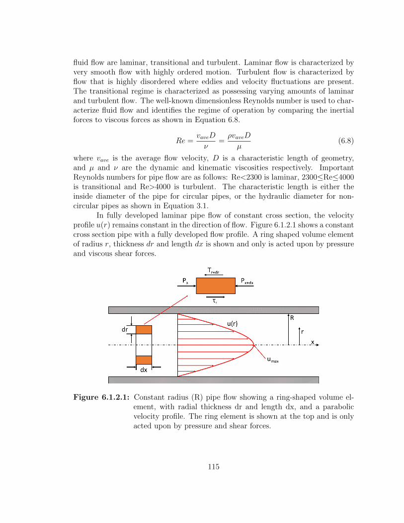
fluid flow are laminar, transitional and turbulent. Laminar flow is characterized byvery smooth flow with highly ordered motion. Turbulent flow is characterized byflow that is highly disordered where eddies and velocity fluctuations are present.The transitional regime is characterized as possessing varying amounts of laminarand turbulent flow. The well-known dimensionless Reynolds number is used to char-acterize fluid flow and identifies the regime of operation by comparing the inertialforces to viscous forces as shown in Equation 6.8.
Re =vaveD
ν=ρvaveD
µ(6.8)
where vave is the average flow velocity, D is a characteristic length of geometry,and µ and ν are the dynamic and kinematic viscosities respectively. ImportantReynolds numbers for pipe flow are as follows: Re<2300 is laminar, 2300≤Re≤4000is transitional and Re>4000 is turbulent. The characteristic length is either theinside diameter of the pipe for circular pipes, or the hydraulic diameter for non-circular pipes as shown in Equation 3.1.
In fully developed laminar pipe flow of constant cross section, the velocityprofile u(r) remains constant in the direction of flow. Figure 6.1.2.1 shows a constantcross section pipe with a fully developed flow profile. A ring shaped volume elementof radius r, thickness dr and length dx is shown and only is acted upon by pressureand viscous shear forces.
Figure 6.1.2.1: Constant radius (R) pipe flow showing a ring-shaped volume el-ement, with radial thickness dr and length dx, and a parabolicvelocity profile. The ring element is shown at the top and is onlyacted upon by pressure and shear forces.
115
To find the velocity profile, a force balance is done on the volume elementand is shown as Equation 6.9.
(2πrdrP )x − (2πrdrP )x+dx + (2πrdxτ)r − (2πrdxτ)r+dr = 0 (6.9)
Solving this equation leads to the very well-known velocity profile equationfor circular pipes under the conditions of incompressible, steady state flow. Thisequation is shown as Equation 6.10.
v(r) = 2vave
(1− r2
R2
)(6.10)
However, the test cell is not circular in shape. Although the test cell has aconstant cross section across the varnish, the shape is that of two half circles split bya rectangle as shown in Figure 3.3.2.1. Finding an analytical solution for the velocityprofile for this geometry would enable the velocity at the surface of the varnish tobe calculated. A close approximation for the actual test system port shape wasfound by using an ellipse. A velocity profile for an ellipse was calculated and thencompared to simulations of the actual port geometry in COMSOL to ensure thevelocity at the surface of the varnish was the same as obtained for the approximateellipse geometry. The continuity and Navier-Stokes equations were used to solvethis problem and are shown below:
∂xvx + ∂yvy + ∂zvz = 0 (6.11)
ρ(vx∂x + vy∂y + vz∂z)vx = −∂xpvx + η(∂2x + ∂2y + ∂2z )vx
ρ(vx∂x + vy∂y + vz∂z)vy = −∂xpvy + η(∂2x + ∂2y + ∂2z )vy (6.12)
ρ(vx∂x + vy∂y + vz∂z)vz = −∂xpvz + η(∂2x + ∂2y + ∂2z )vz
where vi is the ith component of velocity, ρ is the density, p is the pressure and η is thedynamic viscosity. These equations simplify greatly when considering steady state,incompressible pipe flow where the axis is coincident with the z-axis and vx and vyare zero. This also means that the pressure gradients ∂xp and ∂yp are zero. Thecontinuity equation from 6.11 then reduces to ∂zvz=0. When these simplificationsare made, the remaining equation describing axis-symmetric pipe flow is shown asEquation 6.13.
(∂2x + ∂2y)vz =1
η∂zp (6.13)
The equation for an ellipse is shown as Equation 6.14 and will be used inconjunction with the solution of Equation 6.13 to find the velocity profile in anelliptical cross-section.
116
x2
a2+y2
b2= 1 (6.14)
A solution of Equation 6.13 that satisfies the boundary conditions of no-slipat the wall and no shear in the center provides the velocity profile and is shown asEquation 6.15.
vz = 2vave
(1− x2
a2− y2
b2
)(6.15)
This solution is identical to Equation 6.10 with the exception of the geomet-rical term for a pipe vs an ellipse. The cross sectional area of the test cell port isknown to be 0.922cm2. The height of the port is .635cm and the overall length is1.59cm, for a length to height ratio of 2.5. Calculating the major and minor axisvalues for an ellipse that has an area of 0.922cm2 and a length-to-height ratio of 2.5,we find that a equals 0.857 and b equals 0.343.
The characteristic length for the test cell was given as 0.945cm and the cal-culated characteristic length for the ellipse is 0.935cm for an error of 1.05%. Thecharacteristic length, dh, is the hydraulic diameter and is used when calculatingthe Reynolds number. The Reynolds number for the test cell at 90◦C, when usedwith base Fluid R, is known to be 1843 and the calculated Reynolds number for theelliptical shape is 1823 for an error of 1.09%. Therefore, using an ellipse to find thevelocity of the fluid over the varnish in the test cell is acceptable.
The flow rate used in the test system was 4.5GPM (284cm3/s) which providesan average flow velocity of 3.08 m/s in the test cell. This average flow velocity isthe same for the actual system and the ellipse because the cross sectional areas arethe same. However, the velocity profiles will be slightly different and need to bechecked against the actual port shape to ensure the velocity profiles are comparable.COMSOL simulations were run using both geometric profiles and the results areshown in Figure 6.1.2.2.
The maximum flow velocity for the varnish test system is 5.31m/s while themaximum velocity for the elliptical shape is 5.86m/s, which is an error of 10.4%.The error is due to the difference in areas at the position of the maximum velocity.From Figure 6.1.2.2 it can be seen that there is a much larger area of high flow ratein the actual test cell than in the elliptical area (as shown in the black ellipticalarea). The velocity of interest is where the fluid encounters the leading edge ofthe varnish layer. To ensure that the analytical solution for the velocity profile canindeed be used to find the velocity near the surface of the varnish, the velocity ofthe COMSOL model was compared to the elliptical model at the average height ofthe varnish. To find the velocity of the fluid at the average height of the varnishlayer, Equation 6.15 was used. The velocity of interest, in the case of an ellipse,occurs where x is zero and y is the average varnish height of 124µm. This gives a
117
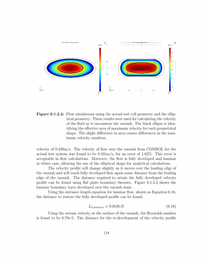
Figure 6.1.2.2: Flow simulations using the actual test cell geometry and the ellip-tical geometry. These results were used for calculating the velocityof the fluid as it encounters the varnish. The black ellipse is iden-tifying the effective area of maximum velocity for each geometricalshape. The slight difference in area causes differences in the max-imum velocity numbers.
velocity of 0.438m/s. The velocity of flow over the varnish from COMSOL for theactual test system was found to be 0.431m/s, for an error of 1.62%. This error isacceptable in flow calculations. Moreover, the flow is fully developed and laminarin either case, allowing the use of the elliptical shape for analytical calculations.
The velocity profile will change slightly as it moves over the leading edge ofthe varnish and will reach fully developed flow again some distance from the leadingedge of the varnish. The distance required to attain the fully developed velocityprofile can be found using flat plate boundary theories. Figure 6.1.2.3 shows thelaminar boundary layer developed over the varnish stain.
Using the entrance length equation for laminar flow, shown as Equation 6.16,the distance to restore the fully developed profile can be found.
Lh,laminar ' 0.05ReD (6.16)
Using the stream velocity at the surface of the varnish, the Reynolds numberis found to be 8.78e-5. The distance for the re-development of the velocity profile
118
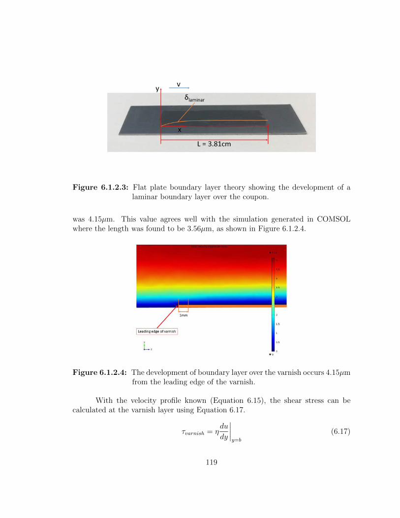
Figure 6.1.2.3: Flat plate boundary layer theory showing the development of alaminar boundary layer over the coupon.
was 4.15µm. This value agrees well with the simulation generated in COMSOLwhere the length was found to be 3.56µm, as shown in Figure 6.1.2.4.
Figure 6.1.2.4: The development of boundary layer over the varnish occurs 4.15µmfrom the leading edge of the varnish.
With the velocity profile known (Equation 6.15), the shear stress can becalculated at the varnish layer using Equation 6.17.
τvarnish = ηdu
dy
∣∣∣∣y=b
(6.17)
119
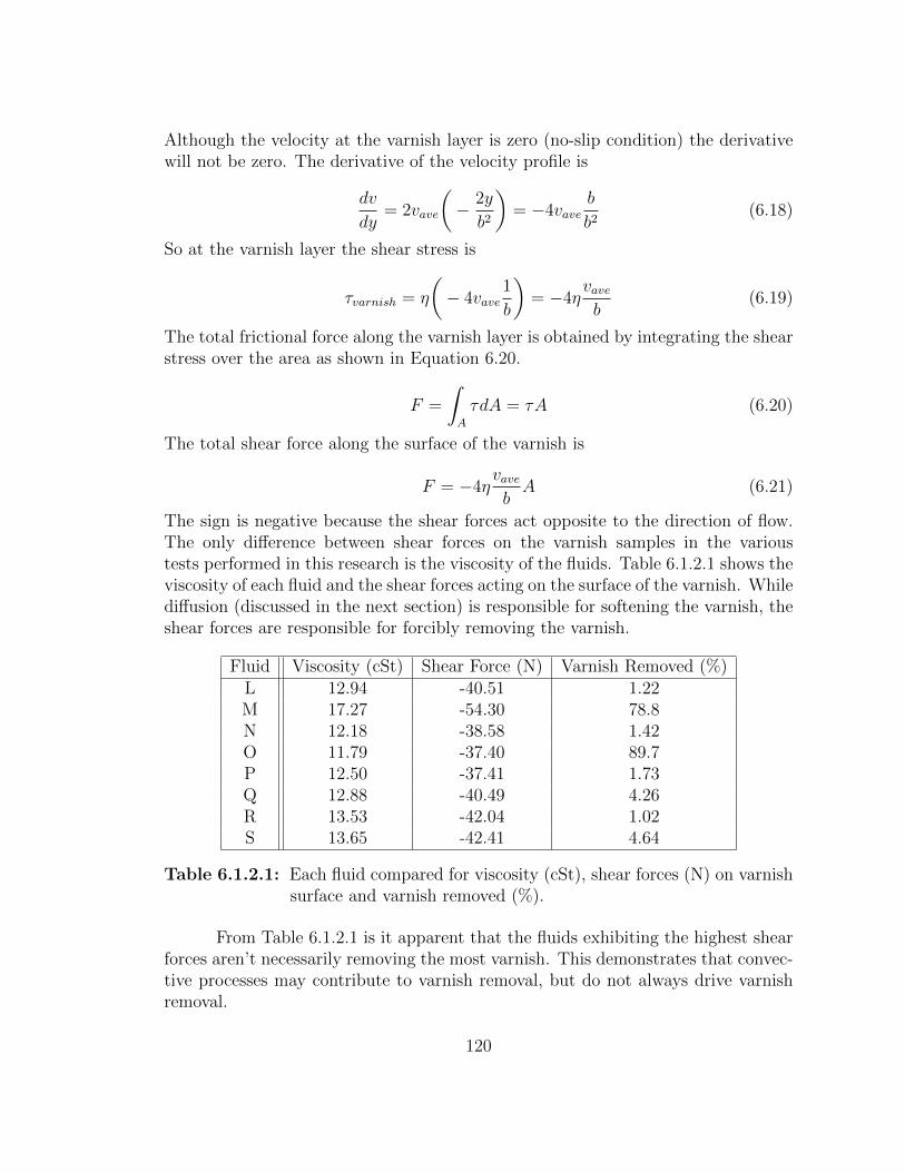
Although the velocity at the varnish layer is zero (no-slip condition) the derivativewill not be zero. The derivative of the velocity profile is
dv
dy= 2vave
(− 2y
b2
)= −4vave
b
b2(6.18)
So at the varnish layer the shear stress is
τvarnish = η
(− 4vave
1
b
)= −4η
vaveb
(6.19)
The total frictional force along the varnish layer is obtained by integrating the shearstress over the area as shown in Equation 6.20.
F =
∫A
τdA = τA (6.20)
The total shear force along the surface of the varnish is
F = −4ηvavebA (6.21)
The sign is negative because the shear forces act opposite to the direction of flow.The only difference between shear forces on the varnish samples in the varioustests performed in this research is the viscosity of the fluids. Table 6.1.2.1 shows theviscosity of each fluid and the shear forces acting on the surface of the varnish. Whilediffusion (discussed in the next section) is responsible for softening the varnish, theshear forces are responsible for forcibly removing the varnish.
Fluid Viscosity (cSt) Shear Force (N) Varnish Removed (%)L 12.94 -40.51 1.22M 17.27 -54.30 78.8N 12.18 -38.58 1.42O 11.79 -37.40 89.7P 12.50 -37.41 1.73Q 12.88 -40.49 4.26R 13.53 -42.04 1.02S 13.65 -42.41 4.64
Table 6.1.2.1: Each fluid compared for viscosity (cSt), shear forces (N) on varnishsurface and varnish removed (%).
From Table 6.1.2.1 is it apparent that the fluids exhibiting the highest shearforces aren’t necessarily removing the most varnish. This demonstrates that convec-tive processes may contribute to varnish removal, but do not always drive varnishremoval.
120
6.1.3 Mass Diffusion
Mass diffusion, in liquids, is the process whereby a solute is diffused into asolvent. A concentration gradient is established and is dependent upon the strengthof the chemical cleaner, the temperature of the fluid and, if present, convectivediffusion. In the varnish test system, the varnish (the solute) is dissolved into thecleaner fluid (the solvent). Fick’s first law (shown as Equation 6.22) relates thediffusive flux to the concentration under steady state conditions.
J = −Ddc
dx(6.22)
where J (g/(m · s)) is the diffusion flux, D (m2/s) is the diffusion coefficient, c(g/m3) is the concentration and x (m) is the position. Fick’s second law (shown asEquation 6.23), which is identical to the heat equation in one dimension, predictshow diffusion causes the concentration to change over time.
∂c
∂t= D
∂2c
∂x2(6.23)
Using Equation 6.23, combined with knowledge of the mass concentration ofthe varnish over time, the diffusion coefficient for each cleaner can be found. Figure6.1.3.1 shows the process of mass diffusion from the varnish into the chemical cleanerunder steady state convective conditions.
The first step in using Equation 6.23 is to identify the boundary conditions(BCs) and any initial (IC) condition. Figure 6.1.3.1 shows that Neumann boundaryconditions can be applied because no flux occurs at y = 0 and at y = L. Theboundary conditions are shown below
∂c(0, t)
∂y= 0
∂c(L, t)
∂y= 0
The initial conditions then need to ensure that, between y = 0 and the average var-nish height for each test (y = have), the concentration is c0 (the mass concentrationin g/cm3) and, between y = have and y = L, the concentration is 0. These initialconditions are summarized below.
c(y, 0) = c0, 0 < y ≤ have
c(y, 0) = 0, have < y ≤ L
121
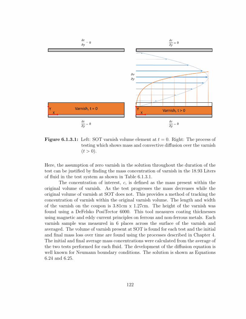
Figure 6.1.3.1: Left: SOT varnish volume element at t = 0. Right: The process oftesting which shows mass and convective diffusion over the varnish(t > 0).
Here, the assumption of zero varnish in the solution throughout the duration of thetest can be justified by finding the mass concentration of varnish in the 18.93 Litersof fluid in the test system as shown in Table 6.1.3.1.
The concentration of interest, c, is defined as the mass present within theoriginal volume of varnish. As the test progresses the mass decreases while theoriginal volume of varnish at SOT does not. This provides a method of tracking theconcentration of varnish within the original varnish volume. The length and widthof the varnish on the coupon is 3.81cm x 1.27cm. The height of the varnish wasfound using a DeFelsko PosiTector 6000. This tool measures coating thicknessesusing magnetic and eddy current principles on ferrous and non-ferrous metals. Eachvarnish sample was measured in 6 places across the surface of the varnish andaveraged. The volume of varnish present at SOT is found for each test and the initialand final mass loss over time are found using the processes described in Chapter 4.The initial and final average mass concentrations were calculated from the average ofthe two tests performed for each fluid. The development of the diffusion equation iswell known for Neumann boundary conditions. The solution is shown as Equations6.24 and 6.25.
122
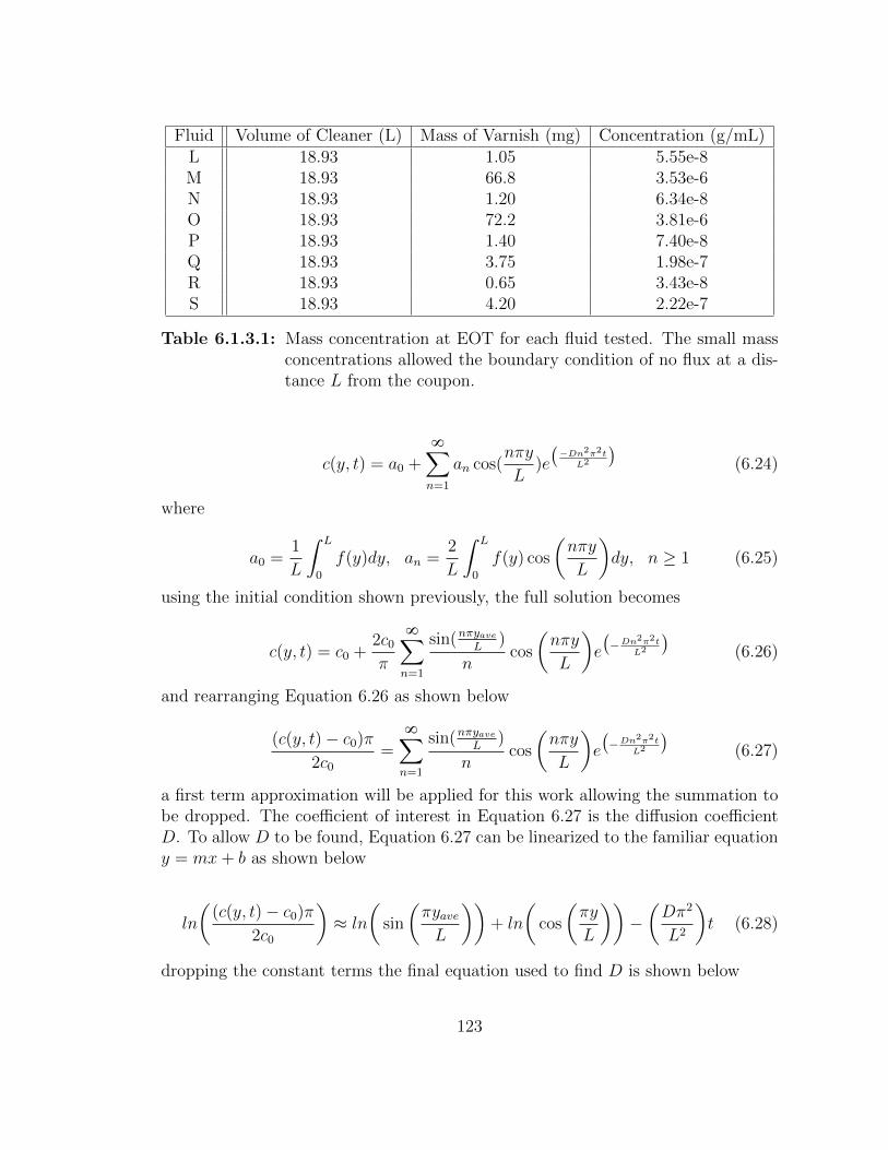
Fluid Volume of Cleaner (L) Mass of Varnish (mg) Concentration (g/mL)L 18.93 1.05 5.55e-8M 18.93 66.8 3.53e-6N 18.93 1.20 6.34e-8O 18.93 72.2 3.81e-6P 18.93 1.40 7.40e-8Q 18.93 3.75 1.98e-7R 18.93 0.65 3.43e-8S 18.93 4.20 2.22e-7
Table 6.1.3.1: Mass concentration at EOT for each fluid tested. The small massconcentrations allowed the boundary condition of no flux at a dis-tance L from the coupon.
c(y, t) = a0 +
8∑n=1
an cos(nπy
L)e
(−Dn2π2t
L2
)(6.24)
where
a0 =1
L
∫ L
0
f(y)dy, an =2
L
∫ L
0
f(y) cos
(nπy
L
)dy, n ≥ 1 (6.25)
using the initial condition shown previously, the full solution becomes
c(y, t) = c0 +2c0π
8∑n=1
sin(nπyaveL
)
ncos
(nπy
L
)e
(−Dn2π2t
L2
)(6.26)
and rearranging Equation 6.26 as shown below
(c(y, t)− c0)π2c0
=
8∑n=1
sin(nπyaveL
)
ncos
(nπy
L
)e
(−Dn2π2t
L2
)(6.27)
a first term approximation will be applied for this work allowing the summation tobe dropped. The coefficient of interest in Equation 6.27 is the diffusion coefficientD. To allow D to be found, Equation 6.27 can be linearized to the familiar equationy = mx+ b as shown below
ln
((c(y, t)− c0)π
2c0
)≈ ln
(sin
(πyaveL
))+ ln
(cos
(πy
L
))−(Dπ2
L2
)t (6.28)
dropping the constant terms the final equation used to find D is shown below
123
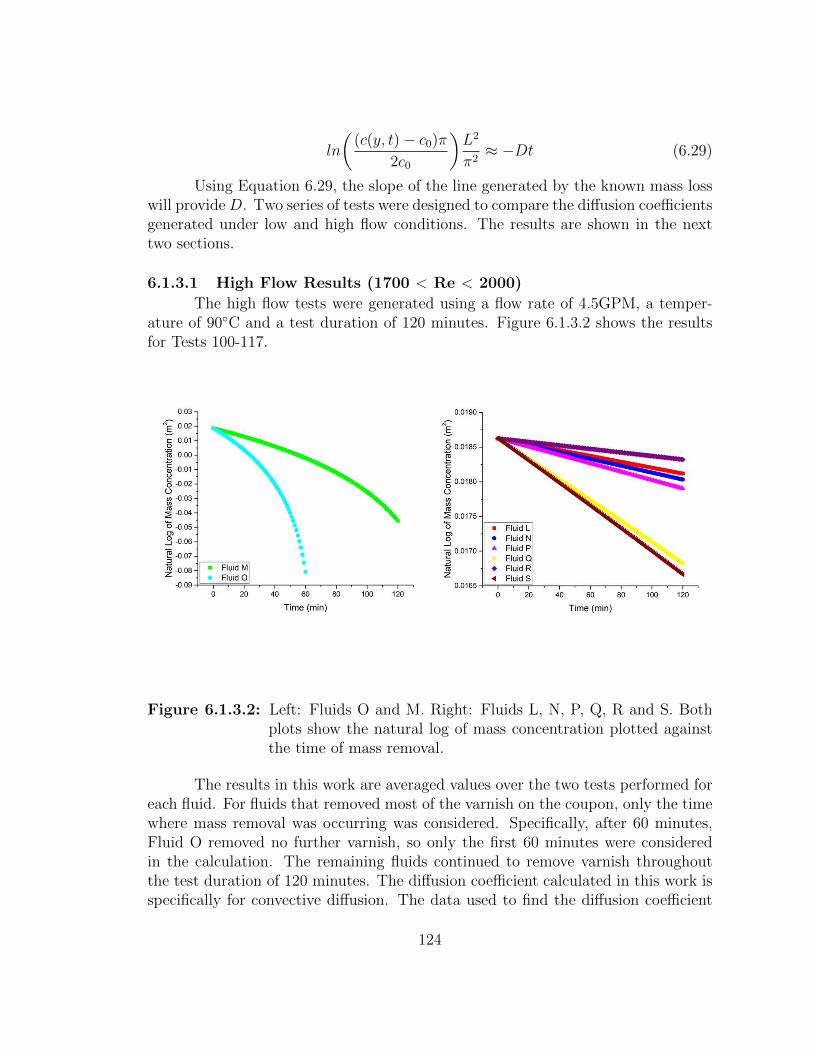
ln
((c(y, t)− c0)π
2c0
)L2
π2≈ −Dt (6.29)
Using Equation 6.29, the slope of the line generated by the known mass losswill provide D. Two series of tests were designed to compare the diffusion coefficientsgenerated under low and high flow conditions. The results are shown in the nexttwo sections.
6.1.3.1 High Flow Results (1700 < Re < 2000)
The high flow tests were generated using a flow rate of 4.5GPM, a temper-ature of 90◦C and a test duration of 120 minutes. Figure 6.1.3.2 shows the resultsfor Tests 100-117.
Figure 6.1.3.2: Left: Fluids O and M. Right: Fluids L, N, P, Q, R and S. Bothplots show the natural log of mass concentration plotted againstthe time of mass removal.
The results in this work are averaged values over the two tests performed foreach fluid. For fluids that removed most of the varnish on the coupon, only the timewhere mass removal was occurring was considered. Specifically, after 60 minutes,Fluid O removed no further varnish, so only the first 60 minutes were consideredin the calculation. The remaining fluids continued to remove varnish throughoutthe test duration of 120 minutes. The diffusion coefficient calculated in this work isspecifically for convective diffusion. The data used to find the diffusion coefficient
124
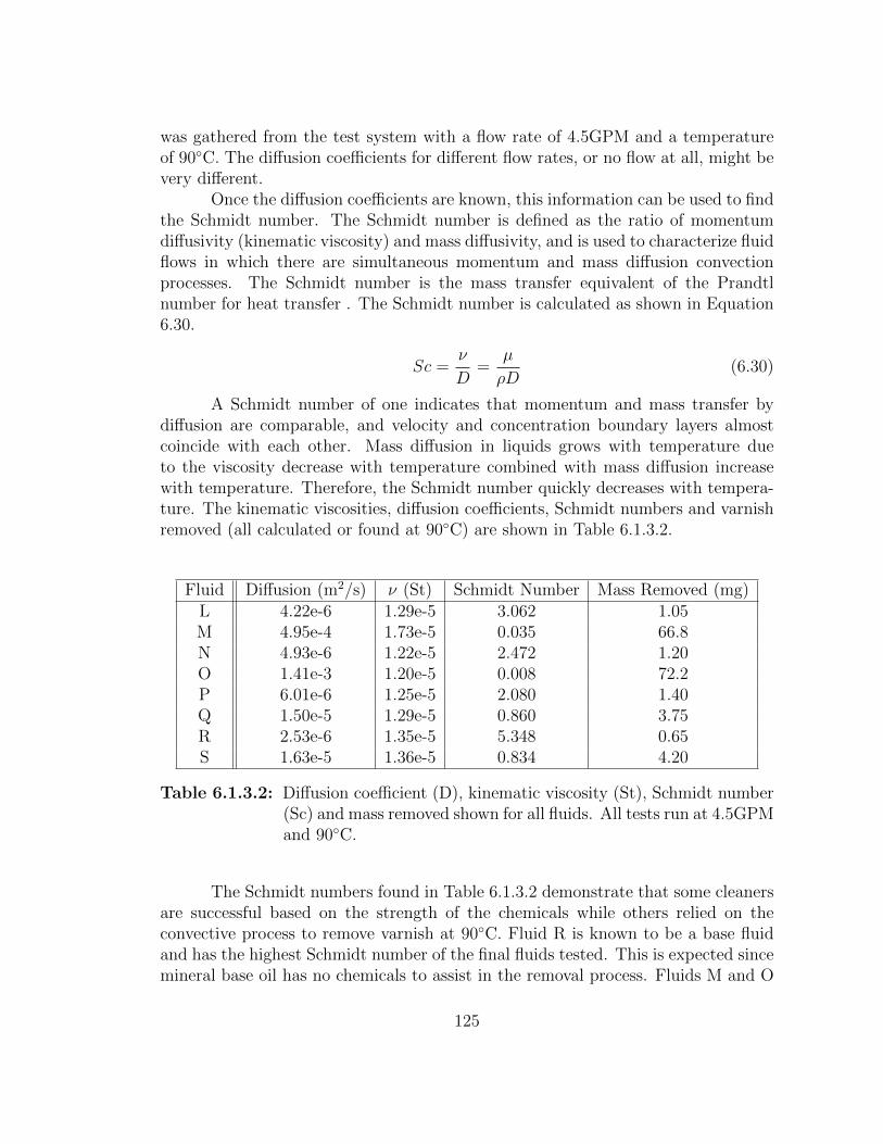
was gathered from the test system with a flow rate of 4.5GPM and a temperatureof 90◦C. The diffusion coefficients for different flow rates, or no flow at all, might bevery different.
Once the diffusion coefficients are known, this information can be used to findthe Schmidt number. The Schmidt number is defined as the ratio of momentumdiffusivity (kinematic viscosity) and mass diffusivity, and is used to characterize fluidflows in which there are simultaneous momentum and mass diffusion convectionprocesses. The Schmidt number is the mass transfer equivalent of the Prandtlnumber for heat transfer . The Schmidt number is calculated as shown in Equation6.30.
Sc =ν
D=
µ
ρD(6.30)
A Schmidt number of one indicates that momentum and mass transfer bydiffusion are comparable, and velocity and concentration boundary layers almostcoincide with each other. Mass diffusion in liquids grows with temperature dueto the viscosity decrease with temperature combined with mass diffusion increasewith temperature. Therefore, the Schmidt number quickly decreases with tempera-ture. The kinematic viscosities, diffusion coefficients, Schmidt numbers and varnishremoved (all calculated or found at 90◦C) are shown in Table 6.1.3.2.
Fluid Diffusion (m2/s) ν (St) Schmidt Number Mass Removed (mg)L 4.22e-6 1.29e-5 3.062 1.05M 4.95e-4 1.73e-5 0.035 66.8N 4.93e-6 1.22e-5 2.472 1.20O 1.41e-3 1.20e-5 0.008 72.2P 6.01e-6 1.25e-5 2.080 1.40Q 1.50e-5 1.29e-5 0.860 3.75R 2.53e-6 1.35e-5 5.348 0.65S 1.63e-5 1.36e-5 0.834 4.20
Table 6.1.3.2: Diffusion coefficient (D), kinematic viscosity (St), Schmidt number(Sc) and mass removed shown for all fluids. All tests run at 4.5GPMand 90◦C.
The Schmidt numbers found in Table 6.1.3.2 demonstrate that some cleanersare successful based on the strength of the chemicals while others relied on theconvective process to remove varnish at 90◦C. Fluid R is known to be a base fluidand has the highest Schmidt number of the final fluids tested. This is expected sincemineral base oil has no chemicals to assist in the removal process. Fluids M and O
125
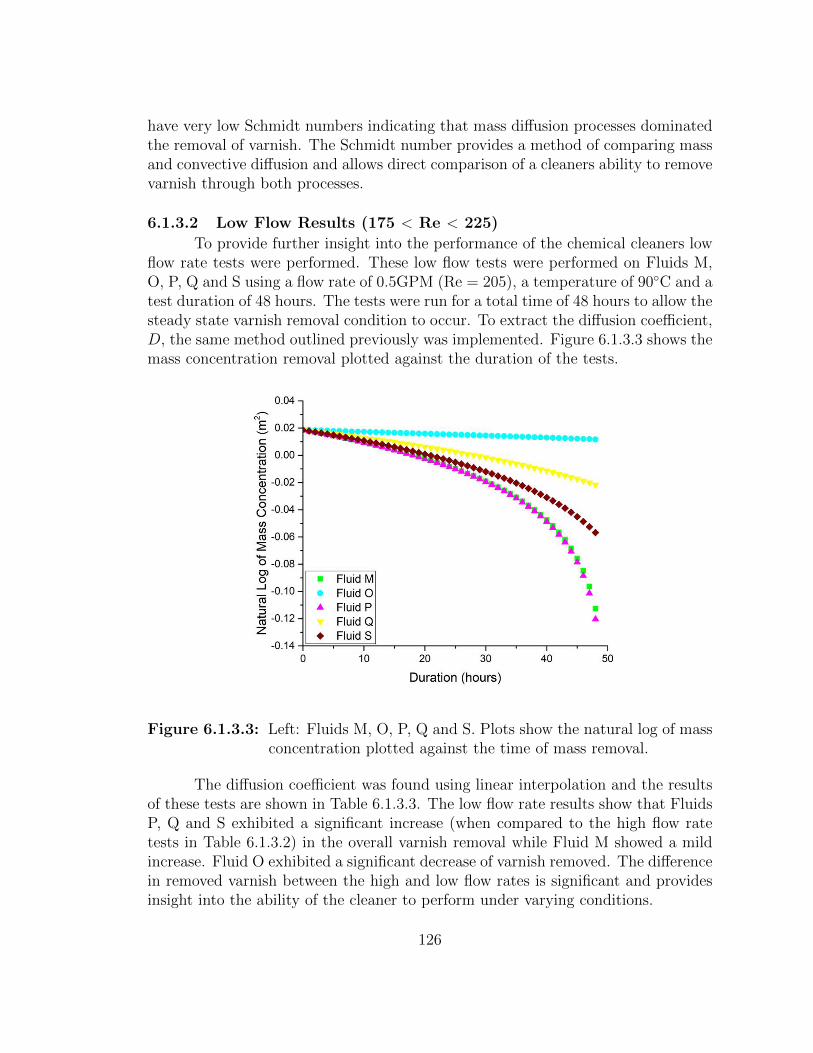
have very low Schmidt numbers indicating that mass diffusion processes dominatedthe removal of varnish. The Schmidt number provides a method of comparing massand convective diffusion and allows direct comparison of a cleaners ability to removevarnish through both processes.
6.1.3.2 Low Flow Results (175 < Re < 225)
To provide further insight into the performance of the chemical cleaners lowflow rate tests were performed. These low flow tests were performed on Fluids M,O, P, Q and S using a flow rate of 0.5GPM (Re = 205), a temperature of 90◦C and atest duration of 48 hours. The tests were run for a total time of 48 hours to allow thesteady state varnish removal condition to occur. To extract the diffusion coefficient,D, the same method outlined previously was implemented. Figure 6.1.3.3 shows themass concentration removal plotted against the duration of the tests.
Figure 6.1.3.3: Left: Fluids M, O, P, Q and S. Plots show the natural log of massconcentration plotted against the time of mass removal.
The diffusion coefficient was found using linear interpolation and the resultsof these tests are shown in Table 6.1.3.3. The low flow rate results show that FluidsP, Q and S exhibited a significant increase (when compared to the high flow ratetests in Table 6.1.3.2) in the overall varnish removal while Fluid M showed a mildincrease. Fluid O exhibited a significant decrease of varnish removed. The differencein removed varnish between the high and low flow rates is significant and providesinsight into the ability of the cleaner to perform under varying conditions.
126
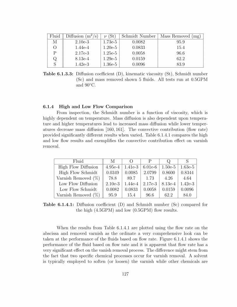
Fluid Diffusion (m2/s) ν (St) Schmidt Number Mass Removed (mg)M 2.10e-3 1.73e-5 0.0082 95.9O 1.44e-4 1.20e-5 0.0833 15.4P 2.17e-3 1.25e-5 0.0058 96.6Q 8.13e-4 1.29e-5 0.0159 62.2S 1.42e-3 1.36e-5 0.0096 83.9
Table 6.1.3.3: Diffusion coefficient (D), kinematic viscosity (St), Schmidt number(Sc) and mass removed shown 5 fluids. All tests run at 0.5GPMand 90◦C.
6.1.4 High and Low Flow Comparison
From inspection, the Schmidt number is a function of viscosity, which ishighly dependent on temperature. Mass diffusion is also dependent upon tempera-ture and higher temperatures lead to increased mass diffusion while lower temper-atures decrease mass diffusion [160, 161]. The convective contribution (flow rate)provided significantly different results when varied. Table 6.1.4.1 compares the highand low flow results and exemplifies the convective contribution effect on varnishremoval.
Fluid M O P Q SHigh Flow Diffusion 4.95e-4 1.41e-3 6.01e-6 1.50e-5 1.63e-5High Flow Schmidt 0.0349 0.0085 2.0799 0.8600 0.8344
Varnish Removed (%) 78.8 89.7 1.73 4.26 4.64Low Flow Diffusion 2.10e-3 1.44e-4 2.17e-3 8.13e-4 1.42e-3Low Flow Schmidt 0.0082 0.0833 0.0058 0.0159 0.0096
Varnish Removed (%) 95.9 15.4 96.6 62.2 84.0
Table 6.1.4.1: Diffusion coefficient (D) and Schmidt number (Sc) compared forthe high (4.5GPM) and low (0.5GPM) flow results.
When the results from Table 6.1.4.1 are plotted using the flow rate on theabscissa and removed varnish as the ordinate a very comprehensive look can betaken at the performance of the fluids based on flow rate. Figure 6.1.4.1 shows theperformance of the fluid based on flow rate and it is apparent that flow rate has avery significant effect on the vanish removal process. The difference might stem fromthe fact that two specific chemical processes occur for varnish removal. A solventis typically employed to soften (or loosen) the varnish while other chemicals are
127
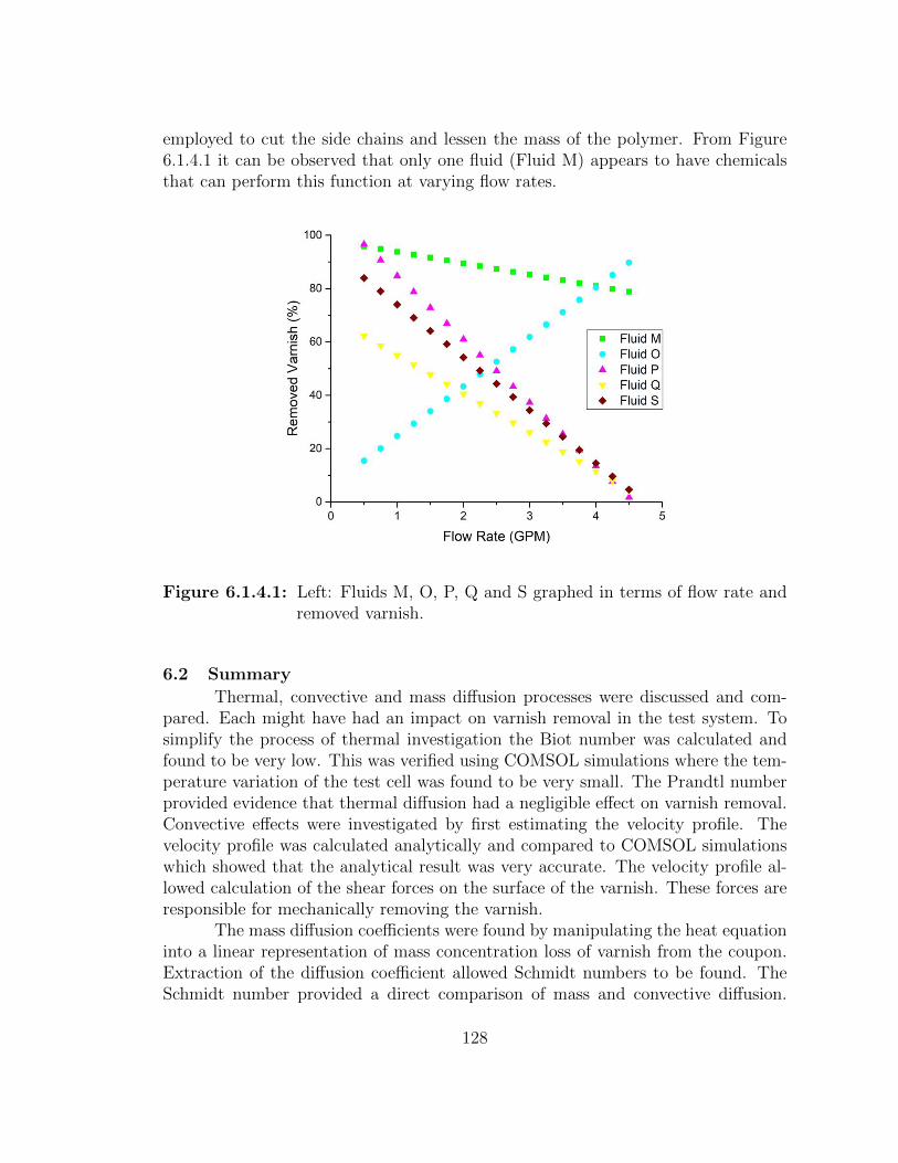
employed to cut the side chains and lessen the mass of the polymer. From Figure6.1.4.1 it can be observed that only one fluid (Fluid M) appears to have chemicalsthat can perform this function at varying flow rates.
Figure 6.1.4.1: Left: Fluids M, O, P, Q and S graphed in terms of flow rate andremoved varnish.
6.2 Summary
Thermal, convective and mass diffusion processes were discussed and com-pared. Each might have had an impact on varnish removal in the test system. Tosimplify the process of thermal investigation the Biot number was calculated andfound to be very low. This was verified using COMSOL simulations where the tem-perature variation of the test cell was found to be very small. The Prandtl numberprovided evidence that thermal diffusion had a negligible effect on varnish removal.Convective effects were investigated by first estimating the velocity profile. Thevelocity profile was calculated analytically and compared to COMSOL simulationswhich showed that the analytical result was very accurate. The velocity profile al-lowed calculation of the shear forces on the surface of the varnish. These forces areresponsible for mechanically removing the varnish.
The mass diffusion coefficients were found by manipulating the heat equationinto a linear representation of mass concentration loss of varnish from the coupon.Extraction of the diffusion coefficient allowed Schmidt numbers to be found. TheSchmidt number provided a direct comparison of mass and convective diffusion.
128
These numbers showed that some fluids relied on convection to remove varnishwhile others used powerful chemicals to loosen the varnish and allow mass diffusionto dominate. Therefore, mass and convective diffusion can be expected to be theprimary mechanisms of removing varnish.
The chemical aspect of varnish removal relies on solvents to soften the varnishand chemicals to cut the varnish polymers into shorter lengths. The mechanicalprocess removes the softened and shortened polymers by force when the shear forceson the surface of the varnish overcome the surface energy holding the polymerin place. The analysis of the combined effects of convective, mass and thermaldiffusion demonstrated here can be applied to other cases to determine varnishremoval mechanisms and provide a broad understanding of the varnish removalprocess in general.
129

Chapter 7
SUMMARY AND RECOMMENDATIONS FOR FUTURERESEARCH
7.1 Summary
The work done for this dissertation directly addressed the lack of performancedata for chemical cleaners used to flush varnish from gas turbine engines. This thesisreports the first scientific method for characterizing varnish removal performance.A varnish removal test system was designed and manufactured which facilitates theprocess of testing by using a blank steel coupon which can be covered with artificialvarnish. This coupon is easily accessed and changed between tests. The test systemcan create fluid flows from very low laminar to very high turbulent regimes. Thisallows virtually every type of system to be simulated within the test cell. Thetest system can also produce temperatures ranging from ambient (25◦C) to 120◦C,which allows temperatures common to gas turbine engine, and other mechanicalsystems, to be generated in the fluid. A filter, located downstream from the testcell, facilitates inspection of the removed varnish to characterize how the chemicalis removing the varnish. The filter allows quick and easy changing of pore size usingpolypropylene filter paper.
This test system is the first of its kind to begin the process of characterizingchemical cleaners. Initially, two parameters were used to characterize the perfor-mance of the chemical cleaners (mass loss and filter inspection). This was extendedto include four primary test metrics: rate of removal, time of maximum removalrate, steady state varnish removal and mass percent varnish removal. The combi-nation of time-lapse photography and mass removal has allowed a unique methodof quantifying varnish removal in terms of color change. This provides a real timeplot of the varnish removal process to be generated. This data can be further pro-cessed by taking the slope of the color value as a function of time to obtain a removalrate. This is the first scientific evaluation of chemical cleaners designed for removingvarnish.
Secondary test metrics include preliminary work on optical particle countingand changes in viscosity over the duration of testing. Initial optical counts wererecorded and then again after each test. This data allows insight into the varnishremoval process by identifying increases and decreases in optical particle counts.
130
This will provide invaluable information when sizing a filter to trap removed varnishfrom a system. Initial viscosities are also recorded and then again after each test.This allows insight into what the varnish is doing to the chemical cleaner duringuse. Any change in viscosity can be attributed to molecular composition and/orintroduced impurities.
Theoretical work has been performed to characterize the thermal, convectiveand mass diffusion processes. Thermal effects were found to be negligible. Con-vective and mass diffusion were found to compete in the varnish removal processat 4.5GPM and 90◦C. While the investigation into convective and mass diffusionwas only performed on the final series of tests, this information will prove invalu-able when compared to future testing. Moreover, future work needs to be done inthe area of tribological performance of chemical cleaners to round out the completecharacterization of cleaner fluids.
This work has made valuable contributions to the scientific community andhas provided important practical information for optimizing removal of varnish.The use of this test system will continue to provide data, not only for the gasturbine industry, but for the lubrication industry as a whole. Removing varnishusing chemical cleaners may become a more commonly used method if end usershave confidence in expected performance of the product, enabled by this research.
7.2 Recommendations for Future Research
7.2.1 Artificial Varnish
Varnish is a complicated substance with a multitude of compositions. Some ofthe influencing factors in varnish formation are base oil, additive package, metalliccomponents in the machine, atmospheric conditions, operational parameters andfiltration, just to name a few. Each system has a unique makeup of materials andparameters that contribute to the eventual and inevitable formation of varnish.With such a plethora of possible varnish compositions, it is imperative that theartificial varnish be given special attention.
In the scope of this work, the artificial varnish was designed to simulate var-nish formed within the gas turbine engine. Therefore, the findings reported hereare most applicable to that system. The new test method and trends reported arealso likely to be relevant to other mechanical components, but quantitative resultsfor a specific component would require testing with varnish from that component.The formation of artificial varnish is the crucial first step in being able to iden-tify the best cleaners for each specific application. Using methods, such as ASTMD7873, artificial varnish can be formed that accurately simulates the chemistry ofany desired varnish. This can be done going forward using methods such as FTIRto identify the composition, of in service varnish, and allow similar varnish to beartificially produced. Then, using methods, such as ASTM D7873, artificial varnish
131
can be formed that accurately simulates the chemistry of any desired varnish. Con-trolling the exposure to differing metals, temperatures and atmospheres needs to bedone with precision and accuracy to ensure test results are beneficial. Future workshould include the ability to produce varnish in a lab, under strictly controlled con-ditions, to enable tests directly applicable to a wide variety of mechanical systemswith confidence.
Producing the artificial varnish is just the first of many steps in providingthe best testing environment possible. Characterizing any aging effects that happenduring storage will help to ensure that test results are interpreted correctly. Applica-tion of the varnish on the coupon, including any temperature variations, duration ofbaking and controlling the mass on the coupon are just as important. This work hasdemonstrated that differing conditions of application can produce vastly differentresults which, if not characterized, can lead to inconsistent results.
The production, storage, application and testing of varnish are all critical toaccurate chemical cleaner comparison. Controlling artificial varnish production isthe first step toward achieving useful results. An application process that providesa varnish that is soft enough to be removed, but not so hard as to render chemicalcleaners powerless, should be identified. Beyond what has been done here, addi-tional work can be done to fine tune the varnish application process. Moreover,controlling the mass of varnish on the coupon, to ensure that any SOT-EOT de-pendence is removed, is of utmost importance. It is imperative that consistentlyweighted coupons are produced with a minimum of deviation. Future work shouldinclude steps to accurately simulate in-service varnish and identify the conditionsthat provide the best possible varnish for testing a wide variety of chemical cleaners.
7.2.2 Chemical Cleaner Properties
The performance of the chemical cleaners in removing varnish is not the onlyproperty of these chemicals that should be considered. Future work should includetesting the chemical cleaners for tribological performance. This includes, but is notlimited to, finding the coefficient of friction for metals sliding with a cleaner fluid aslubricant under varying loads and speeds. Having a chemical cleaner that removes100% of varnish present in a system is useless if the cleaner is not capable of actingas a lubricant when the system is operating.
It is also relevant to identify the rheological properties of chemical clean-ing agents. Journal bearings, thrust pads, pumps and servo valves are designedand built to operate effectively over a narrow range of viscosities. Altering fluidviscosities might have unintended consequences and negatively impact future ma-chine performance. Preliminary viscosity characterization (in results chapter) hasbeen performed during the scope of this work but much more needs to be done tounderstand cleaner fluid viscosity and how it varies as varnish is removed.
132
Future work on fluid cleanliness and filter sizing needs to be performed. Pre-liminary work has been performed (in results chapter) characterizing fluid cleanlinessbut further research needs to be done to identify just how much varnish can be sus-pended in a particular fluid. If these chemical cleaners are to perform their taskseffectively, an understanding of their saturation points and removed varnish particlesize should be known. This will help to find the correct filter size for each fluid.A filter sized to large (pore-size) will allow varnish to continue to circulate whilean undersized filter might remove the very compounds responsible for removal. Inthis work it has been documented that cleaners remove varnish through very dif-ferent mechanisms. Future work should include identifying candidate cleaners andsuggesting a proper filter size to assist in varnish removal.
Only chemical removing properties were truly considered in this work but alogical progression of chemical cleaner characterization will include understandingthe performance in each regime of lubrication as well as documenting any viscositychange over time. Fluid cleanliness and filter sizing should be considered as thework of varnish testing continues.
The chemical cleaners are a complex mixture of compounds that either softenor cleave the varnish. The softening of the varnish is performed by solvents thatseparate the polymeric layers of varnish and allow the shear forces to remove it. Theshortening of the varnish polymer chains is performed by scission, or bond cleavage,which break the molecular chains into smaller pieces and allows the varnish to beremoved by smaller shear forces. The filter results, shown in Figure 5.5.5.1 and5.5.5.2 demonstrate that some cleaners only soften the varnish, allowing large piecesto be removed, others break the varnish polymers into small pieces much smallerthan 5 micron.
Future investigation of the performance between the chemicals that soften thevarnish and the chemicals that cleave the varnish should be performed. The flowrate results demonstrate that some chemicals perform better at specific flow rates.The convective flow definitely impacts the performance of the chemicals chosen toperform as a solvent and as a bond cleaver. The ideal fluid will balance performanceat low and high flow rates. It is suggested that future work investigate this complexchemical relationship.
7.2.3 Testing Parameters
The current testing parameters (90C, 4.5 GPM and 1800 Re) were selectedto remove the most varnish under laminar flow conditions. While these parameterssimulate many in-service components, there are a myriad of flow rates within agiven system. For example, differing flow rates are present in journal bearings (10-100 Re), servo valves (1000-40,000 Re), pumping components (2000-50,000 Re), heatexchangers and many others. Therefore, the test system can generate very broadrange of Reynolds numbers (40<Re<40,000), a range that includes most of these
133
in-service operational conditions. However, a comprehensive investigation into flowparameters for different components needs to be performed to identify conditionsfor future testing. This will result in a more complete understanding of chemicalcleaner behavior.
7.2.4 Photographic Data
The photographic data has proven invaluable in characterizing the varnishremoval process. The ability to view, in real time, the varnish removal processhas allowed removal rates and steady state values to be found. Improvement inphotographic data can be realized in several ways. The polycarbonate lid, whileeffective, might be improved with the use of a more transparent material. There areglares and soft spots that limit the resolution of the results obtained thus far.
The lighting plays a major role in ensuring there are no shadows, glares andother detrimental factors in photography. The position of the lighting has beenadjusted to minimize these issues, but there is room for improvement. There arecamera adjustments available that have not yet been explored which could lead toimprovements in imaging. Lighting positions need to be explored that might offerimproved imaging. The lights on the current test system have two sources thatinclude bright white and yellow bulbs. The balance of the two, as well as theirintensity, should be explored.
During the scope of this work, a record has been made of camera height,lighting position and intensity. The camera has recently been upgraded and the newcamera offers many features not offered in the previous model. The combinationof camera settings, lighting positioning, intensity and color might further minimizeshadow and glare without a change of lid materials. Future work should includeoptimization of camera and lighting.
7.2.5 Algorithmic Improvement
The algorithm used in processing the time-lapse photography is relativelyquick and easy to use. Prior to test 79, the camera was attached to a flex stick thatwas clamped to one of the light stands. After test 79, a camera mount was fabricatedthat fixed the camera frame to the test cell lid. This improved the algorithmic databy allowing the same area to be cropped from test to test. However, th algorithmdoes not search intelligently for the varnish or the steel reference on the coupon andrelies on fixed coordinates to assume the position of each.
Even though the fixed position greatly reduces errors in imaging the coupon,there are still slight variations in where the varnish is located on the coupon. Thismeans that, for each test, the algorithm is divided into two sections. The first sectionfinds all the images in the folder and categorizes the information into a matrix. Thealgorithm then displays four images: the whole image captured from the camera,the cropped image that includes the varnish and steel reference spots, the cropped
134
varnish image and finally the cropped steel reference image. The images must bevisually inspected to ensure that the correct cropping dimensions are applied. Thesecond part of the algorithm then calculates the averaged, max and min K valuesand stores them in a text file for analyzing.
Upgrades to the algorithm would greatly facilitate the image analysis process.The algorithm could be upgraded to search for the boundaries of the varnish bycomparing the dark varnish K values with the lighter steel color that surroundsthe varnish. When the boundaries of the varnish are found, they can be used in allsubsequent images for varnish reference. The algorithm would then find the brighteststeel section located just to the right, or left, of the varnish coupon. Future workshould include these algorithmic upgrades to facilitate image processing.
7.2.6 Improved By-Pass Control
The by-pass line is a crucial component of the test system because it regulatesthe fluid through the test cell. Currently, the ball valve is adjusted by hand and eyeto adjust the flow over the test coupon. The ball valve has 4lb·ft of resistance andtypically it remains in position once set. This is a very simple method of settingthe flow rate through the test cell but does not guarantee that the flow will remainin this position through the test. A method of ensuring that the flow will remainconstant at a precise value would be beneficial.
The 3-way ball valve could be upgraded to a 3-way motorized electric ballvalve that receives its signal from the positive displacement flow meter. The flowmeter is capable of supplying a signal which can be read by an Arduino Board whichwill control the motorized ball valve. This would be a drastic improvement over thecurrent method of flow control and would allow for pump variations, temperaturefluctuations and movement of the manual control ball valve. Future work couldinclude upgrading the manual 3-way control valve to accurately meter the flow overthe coupon.
7.2.7 Improved Heater Control
The heater is currently controlled by a thermostat with an accuracy of ± 3◦C.This allows a temperature variation of 87 93◦C when 90◦C is desired. This workhas shown that temperatures of 20◦C can drastically affect the removal of varnishfar greater that flow variations. For example, Tests 29 and 29a used a flow rateof 0.5GPM, a duration of 220 minutes, and 70◦C and 90◦C respectively. Test 29removed 10% of the varnish on the coupon while Test 29a removed 44%. Test 30aused a flow rate of 10GPM, a duration of 11 minutes and a temperature of 70◦C.Test 30a only removed 30% of the varnish on the coupon. Each of these tests hada total flow of 110 gallons across the coupon. This demonstrates that temperaturehas a larger affect on varnish removal than flow rate. Future work should includeupgrading the temperature control system to provide greater accuracy. Durex, the
135
OEM of the current heater, makes a digital control system that can directly re-place the rheostat type thermostat currently in use. This would provide increasedconfidence in the results of the varnish removal test system.
7.2.8 Particle Counting
This test system might benefit from the addition of a particle counter, locatedin the return line pre-filter. This would give great insight to the size and distributionof particles in the fluid before and during testing. It would also help to quantifythe size of the varnish particles removed from the coupon. The varnish removalprocess is more complicated than just using chemicals to loosen the varnish. Thetotal of the forces at work to remove the varnish include thermal, convective andmass diffusion effects. The mass diffusion effects are chemically driven but rely onthe filter to keep the fluid clean. The particle counter would provide insight intocorrectly sizing the filter for candidate fluids.
7.2.9 Expanded Test Conditions
Additional testing at differing flow rates and temperatures will help to charac-terize chemical cleaners in a very comprehensive way. For the five fluids tested usingvarying flow rates, the diffusion coefficient was affected. This, in turn, changed thevalues of Schmidt numbers. There is no consistent pattern to the diffusion change,indicating that the role of convection is different for each chemical cleaner. Thisdifference in Schmidt number, when investigated, will undoubtedly provide insightinto the chemical interaction between the varnish and the cleaner. It would appearthat some cleaners need time to dwell on the surface of the varnish for the chemicalsoftening process to occur. This was exemplified by cleaners P and S, where theSchmidt numbers decrease significantly with increasing flow rate. Only cleaner Oshowed an increase of Schmidt number, indicating that shear forces play a majorrole in removing the varnish.
This preliminary investigation suggests the need for further testing of dif-fering flow rates to map the mass-convection diffusion relationship. Furthermore,varying the temperature of tests will provide new results when viewed in terms ofthe Schmidt and Prandtl numbers. There will be a point where the convective andmass diffusion coefficients are equal for varying flow rates and temperatures. Wherethese coefficients cross will determine which fluids perform better under low or highflow conditions. This will allow cleaners to be selected based on their performanceunder a broad range of conditions. While some cleaners might be selected for lowflow reservoir applications, others will provide increased varnish removal under highflow conditions. The same holds true for temperature variations.
136
7.2.10 Quantify Smell and Strength
The smell and strength of the chemical cleaner is an important characteristic.In this work, a qualitative approach was used to characterize the smell and strengthof each cleaner. This needs to be improved by using scientific methods of quanti-fying the smell and strength values. Future work should include finding methodsof quantifying these metrics that are not subject to individual interpretation. Anolfactometer combined with thermal desorption and Mass Spectrometry might offermethods of characterizing smell and strength.
7.2.11 Foam Production
The foam rating was developed using the time required to de-aerate the fluidin the reservoir. The method of characterizing foam performance should be upgradedto include ASTM methods of accurately identifying the foaming tendencies of eachchemical cleaner. Future work should include characterizing foam performance inthis manner.
7.3 Conclusions
Going forward, the system and testing approach developed in this study canbecome the standard for characterizing chemical cleaner varnish removing perfor-mance. The test system may also be modified to include varnish removal by filteradsorption or electrostatic cleaning. Finally, the system can be used to remove morethan varnish. For example, beneficial tribochemistry films (formed from additivessuch as MoDDP, DLC and ZDDP) can be tested in this system to ensure they canendure the very high Reynolds numbers experienced during turbulent flow. Further-more, air can be injected into the test system to simulate micro implosion and othercavitation-based issues over the test coupon. Moreover, virtually any hydrocarbonbase fluid can be used in the test system. If the desired substance can be attachedto the steel coupon (or any material that can be cut in the desired shape and canhandle the temperature of testing), the parameters and chemicals that best removethat substance can be found.
I hope research on characterizing varnish removal and understanding removalmechanisms continues to develop. The oxidation of hydrocarbon fluids, and the var-nish that forms, is an inevitable process that requires a chemical removal process.Therefore, this work is the starting point for standardizing chemical cleaners andprovides valuable information for the scientific community and the end user. Char-acterizing chemical cleaners using the methods developed in this work will allowgreater understanding for the varnish removal process as well as the chemical in-teractions between varnish and cleaner. A complete understanding of the complexinteractions between chemical and varnish, and the convective-mass diffusion pro-cess, will take the continued collaboration of chemists, tribologists and engineers.
137

The information generated will advance our understanding of varnish, varnish re-moval and the chemicals designed to remove varnish.
138
BIBLIOGRAPHY
[1] C. S. C. Davison, Wear prevention in early history, Wear 1 (2) (1957) 155–159.
[2] R. G. Bayer, Wear analysis for engineers, Hnb Pub., 2002.
[3] H. A. Barnes, A handbook of elementary rheology.
[4] R. M. Mortier, S. T. Orszulik, M. F. Fox, Chemistry and technology of lubri-cants, Vol. 107115, Springer, 2010.
[5] J. Fitch, Using oil analysis to control varnish and sludge, Practicing Oil Anal-ysis May.
[6] J. Fitch, S. Gebarin, Review of degradation mechanisms leading to sludge andvarnish in modern turbine oil formulations, in: Oxidation and the Testing ofTurbine Oils, ASTM International, 2008.
[7] M. Johnson, M. Spurlock, Strategic oil analysis: Estimating remaining lubri-cant life, Tribology & Lubrication Technology 66 (1) (2010) 22.
[8] AirTECH, How the pump works, [Online; accessed September 20, 2016].URL http://www.airtechpumps.eu/
[9] Mechanical Engineering Community, Diiference Between Working of Centrifu-gal pump & Reciprocating Pump, [Online; accessed September 20, 2016].URL https://mechanical-engg.com
[10] R. B. Erickson, Hydraulic pump technology and selection, Design World forEaton Corporation.
[11] I. Hutchings, P. Shipway, Tribology: friction and wear of engineering materials,Butterworth-Heinemann, 2017.
[12] American Petroleum Institute, Api base oil interchangeabiltiy guidelines forpassenger car motor oils and diesel engine oils (2017).
[13] D. M. Pirro, M. Webster, E. Daschner, Lubrication Fundamentals, Revisedand Expanded, CRC Press, 2016.
139
[14] T. R. Lynch, Process chemistry of lubricant base stocks, CRC Press, 2007.
[15] H. P. Vowles, Early evolution of power engineering, Isis 17 (2) (1932) 412–420.
[16] A. Lucas, J. Harris, Ancient Egyptian materials and industries, Courier Cor-poration, 2012.
[17] D. Dowson, The history of tribology in america, Journal of Lubrication Tech-nology 103 (3) (1981) 323–333.
[18] M. Nosonovsky, Oil as a lubricant in the ancient middle east, Tribology Online2 (2) (2007) 44–49.
[19] J. Fitch, Lubrication genesis, Machinery Lubrication 3 (2) (2004) 44–49.
[20] R. S. Westfall, Never at rest: A biography of Isaac Newton, Cambridge Uni-versity Press, 1983.
[21] Standard Terminology for Plastics: Dynamic Mechanical Properties, Stan-dard, ASTM International, West Conshohocken, PA (2013).URL https://doi.org/10.1520/D4092-07R13
[22] H. W. Dickinson, James Watt: craftsman and engineer, Cambridge UniversityPress, 2010.
[23] D. Dowson, Men of tribology, Journal of Lubrication Technology 101 (1979)1.
[24] C. J. Campbell, J. H. Laherrere, The end of cheap oil, Scientific American278 (3) (1998) 60–65.
[25] U.S. Energy Information Administration, American Field Production of CrudeOil (2016).
[26] U.S. Energy Information Administration, Refinery Yield (2016).
[27] U.S. Energy Information Administration, U.S. Energy Generation (2016).
[28] Bureau of Transportation Statistics, Number of U.S. Vehicles 2015 (2015).
[29] R. W. Carpick, M. Salmeron, Scratching the surface: fundamental investi-gations of tribology with atomic force microscopy, Chemical reviews 97 (4)(1997) 1163–1194.
[30] T. Vorburger, J. Raja, Surface finish metrology tutorial, National Inst. ofStandards and Technology, 1990.
140
[31] C. Bovington, Friction, wear and the role of additives in controlling them, in:Chemistry and technology of lubricants, Springer, 2010, pp. 77–105.
[32] H. Yoshizawa, Y. L. Chen, J. Israelachvili, Fundamental mechanisms of in-terfacial friction. 1. relation between adhesion and friction, The Journal ofPhysical Chemistry 97 (16) (1993) 4128–4140.
[33] F. P. Bowden, D. Tabor, The friction and lubrication of solids, Vol. 1, Oxforduniversity press, 2001.
[34] E. P. Becker, Trends in tribological materials and engine technology, TribologyInternational 37 (7) (2004) 569–575.
[35] E. Feyzullahoglu, N. Sakiroglu, The wear of aluminium-based journal bearingmaterials under lubrication, Materials & Design (1980-2015) 31 (5) (2010)2532–2539.
[36] J.-H. Cho, D. E. Boyce, P. R. Dawson, Modeling strain hardening and tex-ture evolution in friction stir welding of stainless steel, Materials Science andEngineering: A 398 (1) (2005) 146–163.
[37] W. Li, Y. Wang, X. Yang, Frictional hardening and softening of steel 52100during dry sliding, Tribology Letters 18 (3) (2005) 353–357.
[38] A. Misra, I. Finnie, On the size effect in abrasive and erosive wear, Wear 65 (3)(1981) 359–373.
[39] J. Gates, Two-body and three-body abrasion: a critical discussion, Wear214 (1) (1998) 139–146.
[40] E. Rabinowicz, L. Dunn, P. Russell, A study of abrasive wear under three-bodyconditions, Wear 4 (5) (1961) 345–355.
[41] H. Sin, N. Saka, N. Suh, Abrasive wear mechanisms and the grit size effect,Wear 55 (1) (1979) 163–190.
[42] G. Stachowiak, G. Stachowiak, The effects of particle characteristics on three-body abrasive wear, Wear 249 (3) (2001) 201–207.
[43] W. Yi-Ling, W. Zi-Shan, An analysis of the influence of plastic indentationon three-body abrasive wear of metals, Wear 122 (2) (1988) 123–133.
[44] R. Garvey, Wear rates impact maintenance priorities, Machinery LubricationMarch.
141
[45] I. D. Marinescu, W. B. Rowe, B. Dimitrov, I. Inaski, Tribology of abrasivemachining processes, Elsevier, 2004.
[46] J. Burwell, C. Strang, On the empirical law of adhesive wear, Journal ofApplied Physics 23 (1) (1952) 18–28.
[47] J. N. Israelachvili, Y.-L. Chen, H. Yoshizawa, Relationship between adhesionand friction forces, Journal of adhesion science and technology 8 (11) (1994)1231–1249.
[48] T. Sasada, M. Oike, N. Emori, The effect of abrasive grain size on the transi-tion between abrasive and adhesive wear, Wear 97 (3) (1984) 291–302.
[49] H. Czichos, Tribology: a systems approach to the science and technology offriction, lubrication, and wear, Vol. 1, Elsevier, 2009.
[50] W. Littmann, R. Widner, Propagation of contact fatigue from surface andsubsurface origins, Journal of Basic Engineering 88 (3) (1966) 624–635.
[51] T. Beagley, Severe wear of rolling/sliding contacts, Wear 36 (3) (1976) 317–335.
[52] A. Bower, The influence of crack face friction and trapped fluid on surfaceinitiated rolling contact fatigue cracks, Journal of Tribology 110 (4) (1988)704–711.
[53] C. Bathias, Relation between endurance limits and thresholds in the field ofgigacycle fatigue, in: Fatigue Crack Growth Thresholds, Endurance Limits,and Design, ASTM International, 2000.
[54] O. Umezawa, K. Nagai, Deformation structure and subsurface fatigue crackgeneration in austenitic steels at low temperature, Metallurgical and materialstransactions A 29 (3) (1998) 809–822.
[55] M. Hoeprich, Rolling element bearing fatigue damage propagation, ASME,Transactions, Journal of Tribology 114 (2) (1992) 328–333.
[56] M. Fazal, A. Haseeb, H. Masjuki, Biodiesel feasibility study: an evaluation ofmaterial compatibility; performance; emission and engine durability, Renew-able and Sustainable Energy Reviews 15 (2) (2011) 1314–1324.
[57] G. Frankel, Pitting corrosion of metals a review of the critical factors, Journalof the Electrochemical Society 145 (6) (1998) 2186–2198.
[58] D. J. Young, High temperature oxidation and corrosion of metals, Vol. 1,Elsevier, 2008.
142
[59] B. J. Hamrock, S. R. Schmid, B. O. Jacobson, Fundamentals of fluid filmlubrication, CRC press, 2004.
[60] B. J. Hamrock, W. J. Anderson, Rolling-element bearings.
[61] F. F. Ling, E. E. Klaus, R. Fein, Boundary lubrication. an appraisal of worldliterature.
[62] Q. J. Wang, Y.-W. Chung, Encyclopedia of tribology: With 3650 Figures and493 Tables, Springer, 2013.
[63] T. G. Mezger, The rheology handbook: for users of rotational and oscillatoryrheometers, Vincentz Network GmbH & Co KG, 2006.
[64] E. d. C. Andrade, Xli. a theory of the viscosity of liquids.part i, The Lon-don, Edinburgh, and Dublin Philosophical Magazine and Journal of Science17 (112) (1934) 497–511.
[65] C. J. A. Roelands, Correlational aspects of the viscosity-temperature-pressurerelationship of lubricating oils.
[66] E. Dean, G. Davis, et al., Viscosity variations of oils with temperature, Chem-ical and Metallurgical Engineering 36 (1929) 618.
[67] Standard Practice for Calculating Viscosity Index from Kinematic Viscosityat 40◦C and 100◦C, Standard, ASTM International, West Conshohocken, PA(2016).URL https://doi.org/10.1520/D2270-10R16
[68] S. Wen, P. Huang, Principles of tribology, John Wiley & Sons, 2012.
[69] R. Prince, Base oils from petroleum, in: Chemistry and Technology of Lubri-cants, Springer, 2010, pp. 3–33.
[70] J. G. Speight, The chemistry and technology of petroleum, CRC press, 2014.
[71] D. C. Kramer, B. K. Lok, R. R. Krug, The evolution of base oil technology,in: Turbine lubrication in the 21st century, ASTM International, 2001.
[72] G. A. Olah, G. S. Prakash, Hydrocarbon chemistry, John Wiley & Sons, 2017.
[73] S. Korcek, R. Jensen, Relation between base oil composition and oxidationstability at increased temperatures, ASLE TRANSACTIONS 19 (2) (1976)83–94.
143
[74] R. M. Zhmud, Boris, New base oils pose a challenge, Tribology & LubricationTechnology 67 (7) (2009) 34–38.
[75] J. Wright, The fundamentals of mineral base oil refining (2012).
[76] W. Dresel, et al., Lubricants and lubrication, John Wiley & Sons, 2007.
[77] A. Sequeira, Lubricant base oil and wax processing, CRC press, 1994.
[78] H. Wiener, Structural determination of paraffin boiling points, Journal of theAmerican Chemical Society 69 (1) (1947) 17–20.
[79] M. Brown, J. Fotheringham, T. Hoyes, R. Mortier, S. Orszulik, S. Randles,P. Stroud, Synthetic base fluids, in: Chemistry and Technology of Lubricants,Springer, 2010, pp. 35–74.
[80] L. R. Rudnick, R. L. Shubkin, Synthetic lubricants and high-performancefunctional fluids, revised and expanded, Crc Press, 1999.
[81] L. Moore, D. Fels, A. Seay, C. Lopez, et al., Pao-based synthetic lubricants inindustrial applications, Tribology & Lubrication Technology 59 (1) (2003) 23.
[82] D. R. Kodali, High performance ester lubricants from natural oils, Industriallubrication and tribology 54 (4) (2002) 165–170.
[83] N. S. Ahmed, A. M. Nassar, Lubricating oil additives, in: Tribology-Lubricants and Lubrication, InTech, 2011.
[84] S. Q. Rizvi, Lubricant chemistry, technology, selection, and design, ASTMInternational, Conshohocken.
[85] G. Biresaw, K. L. Mittal, Surfactants in tribology, Vol. 4, CRC Press, 2014.
[86] M. T. Costello, 17 corrosion inhibitors and rust preventatives, Lubricant Ad-ditives: Chemistry and Applications (2009) 421.
[87] R. Stone, Introduction to internal combustion engines, Palgrave Macmillan,2012.
[88] V. P. Astakhov, Tribology of Metal Cutting, Vol. 52, Elsevier, 2006.
[89] Z. Tang, S. Li, A review of recent developments of friction modifiers for liq-uid lubricants (2007–present), Current Opinion in Solid State and MaterialsScience 18 (3) (2014) 119–139.
[90] M. Smeeth, H. Spikes, S. Gunsel, Boundary film formation by viscosity indeximprovers, Tribology Transactions 39 (3) (1996) 726–734.
144
[91] S. Naidu, E. Klaus, J. Duda, Kinetic model for high-temperature oxidation oflubricants, Industrial & engineering chemistry product research and develop-ment 25 (4) (1986) 596–603.
[92] J. Lahijani, F. Lockwood, E. Klaus, The influence of metals on sludge forma-tion, ASLE Transactions 25 (1) (1982) 25–32.
[93] M. Rasberger, Oxidative degradation and stabilisation of mineral oil basedlubricants, in: Chemistry and technology of lubricants, Springer, 1997, pp.98–143.
[94] E. Dimitroff, J. Moffitt, R. Quillian, Why, what, and how: Engine varnish,Journal of Lubrication Technology 91 (3) (1969) 406–416.
[95] J. Dong, C. A. Migdal, 1 antioxidants, Lubricant Additives: Chemistry andApplications (2009) 1.
[96] A. Sasaki, Contaminants in used oils and their behavior, Journal of ASTMInternational 6 (2) (2009) 1–12.
[97] L. Chen, J. Dong, G. Chen, The study of tribo-induced deposits from a copper-containing antiwear additive, Tribology transactions 40 (2) (1997) 339–345.
[98] C. A. Migdal, A. B. Wardlow, J. L. Ameye, Oxidation and the testing ofturbine oils, ASTM, 2008.
[99] F. Rounds, Effects of hydroperoxides on wear as measured in four-ball weartests, Tribology transactions 36 (2) (1993) 297–303.
[100] B. Atherton, Discovering the root cause of varnish formation, Practicing oilanalysis 2 (2007) 22–25.
[101] N. Kumar, P. Besuner, S. Lefton, D. Agan, D. Hilleman, Power plant cyclingcosts, Tech. rep., National Renewable Energy Laboratory (NREL), Golden,CO. (2012).
[102] A. Sitton, J. Ameye, R. E. Kauffman, Residue analysis on rpvot test samplesfor single and multiple antioxidants chemistry for turbine lubricants, Journalof ASTM International 3 (6) (2006) 1–15.
[103] M. Diaby, M. Sablier, A. Le Negrate, M. El Fassi, J. Bocquet, Understandingcarbonaceous deposit formation resulting from engine oil degradation, Carbon47 (2) (2009) 355–366.
145
[104] A. Sasaki, S. Uchiyama, T. Yamamoto, Free radicals and oil auto-oxidationdue to spark discharges of static electricity, Tribology & Lubrication Technol-ogy 55 (9) (1999) 24.
[105] G. Aguilar, G. Mazzamaro, M. Rasberger, Oxidative degradation and sta-bilisation of mineral oil-based lubricants, in: Chemistry and Technology ofLubricants, Springer, 2010, pp. 107–152.
[106] M. Lazar, Free radicals in chemistry and biology, CRC press, 1989.
[107] S. Blaine, P. E. Savage, Reaction pathways in lubricant degradation. 3. reac-tion model for n-hexadecane autoxidation, Industrial & engineering chemistryresearch 31 (1) (1992) 69–75.
[108] V. F. Lvovich, M. F. Smiechowski, Impedance characterization of industriallubricants, Electrochimica acta 51 (8) (2006) 1487–1496.
[109] O. D. Livingstone, Greg, The emerging problem of lubricant varnish, Mainte-nance & Asset Management 25 (2) (2010) 38–42.
[110] Z. Pawlak, Tribochemistry of lubricating oils, Vol. 45, Elsevier, 2003.
[111] P. Antoniewicz, Surface-induced dipole moments of adsorbed atoms, PhysicalReview Letters 32 (25) (1974) 1424.
[112] W. Kohn, K.-H. Lau, Adatom dipole moments on metals and their interac-tions, Solid State Communications 18 (5) (1976) 553–555.
[113] N. Emanuel, Z. Maizus, I. Skibida, The catalytic activity of transitionmetal compounds in the liquid-phase oxidation of hydrocarbons, AngewandteChemie International Edition 8 (2) (1969) 97–107.
[114] G. V. Fuchs, H. Diamond, Oxidation characteristics of lubricating oils, Indus-trial & Engineering Chemistry 34 (8) (1942) 927–937.
[115] H. Zuidema, Oxidation of lubricating oils., Chemical reviews 38 (2) (1946)197–226.
[116] V. J. Gatto, W. E. Moehle, T. W. Cobb, E. R. Schneller, Oxidation fundamen-tals and its application to turbine oil testing, Journal of ASTM International3 (4) (2006) 1–20.
[117] J. Pospısil, Aromatic and heterocyclic amines in polymer stabilization, in:Polysoaps/Stabilizers/Nitrogen-15 NMR, Springer, 1995, pp. 87–189.
146
[118] T. Colclough, Role of additives and transition metals in lubricating oil oxida-tion, Industrial & engineering chemistry research 26 (9) (1987) 1888–1895.
[119] K. C. Ludema, Friction, wear, lubrication: a textbook in tribology, CRC press,1996.
[120] K. Farooq, Varnish removal and control in turbine lubrication systems, in:ASME 2009 Power Conference, American Society of Mechanical Engineers,2009, pp. 281–287.
[121] J. Fitch, Temperature stability of lubricants and hydraulic fluids, MachineryLubrication (2002) 22–28.
[122] N. McGuire, Tiny bubbles, Tribology & Lubrication Technology 71 (2) (2015)34.
[123] J. Wright, Microdieseling and its effects on oil, Machinery Lubrication 12(2012) 2012.
[124] R. Canavelis, Jet impact and cavitation damage, TRANS ASME–J BASICENG– 90 (3) (1968) 355–367.
[125] S. R. G. Avila, C. Song, C.-D. Ohl, Fast transient microjets induced by hemi-spherical cavitation bubbles, Journal of Fluid Mechanics 767 (2015) 31–51.
[126] T. Harvey, R. Wood, G. Denuault, H. Powrie, Investigation of electrostaticcharging mechanisms in oil lubricated tribo-contacts, Tribology International35 (9) (2002) 605–614.
[127] P. W. Huber, A. A. Sonin, Electric charging in liquid hydrocarbon filtration:A comparison of theory and experiments, Journal of Colloid and InterfaceScience 61 (1) (1977) 126–145.
[128] A. Sasaki, S. Uchiyama, T. Yamamoto, Generation of static electricity duringoil filtration, Tribology & Lubrication Technology 55 (9) (1999) 14.
[129] American Petroleum Institute, Engine Oil Licensing & Certification System(EOLCS) Categories & Documents (2017).
[130] S. Lantz, J. Zakarian, S. Deskin, A. Martini, Filtration effects on foam in-hibitors and optically detected oil cleanliness, Tribology Transactions 0 (0)(2017) 1–6.URL http://dx.doi.org/10.1080/10402004.2017.1285089
147
[131] B. Phair, L. Bensch, J. Duchowski, M. Khazan, V. Tsalyuk, Overcoming theelectrostatic discharge in hydraulic, lubricating and fuel-filtration applicationsby incorporating novel synthetic filter media, Tribology transactions 48 (3)(2005) 343–351.
[132] J. T. Leonard, H. W. Carhart, Effect of conductivity on charge generation inhydrocarbon fuels flowing through fiber glass filters, Journal of Colloid andInterface Science 32 (3) (1970) 383–394.
[133] T. L. Suratt, J. R. Holtz, Engine cleaning processes, uS Patent 5,232,513(Aug. 3 1993).
[134] M. Carmichael, J. Binatena, Internal combustion engine scrubber, uS Patent4,877,043 (Oct. 31 1989).
[135] and others, Flushing device for engine lubricating systems, uS Patent 2,454,585(Nov. 23 1948).
[136] Standard Test Method for Acid and Base Number by Color-Indicator Titra-tion, Standard, ASTM International, West Conshohocken, PA (2014).URL https://doi.org/10.1520/D0974-14E02
[137] Standard Test Method for Acid Number of Petroleum Products by Poten-tiometric Titration, Standard, ASTM International, West Conshohocken, PA(2017).URL https://doi.org/10.1520/D0664-17
[138] Standard Test Method for Oxidation Stability of Steam Turbine Oils by Ro-tating Pressure Vessel, Standard, ASTM International, West Conshohocken,PA (2014).URL https://doi.org/10.1520/D2272-14A
[139] Standard Test Method for Kinematic Viscosity of Transparent and OpaqueLiquids (and Calculation of Dynamic Viscosity), Standard, ASTM Interna-tional, West Conshohocken, PA (2017).URL https://doi.org/10.1520/D0445-17A
[140] Standard Test Method for Flash and Fire Points by Cleveland Open CupTester, Standard, ASTM International, West Conshohocken, PA (2016).URL https://doi.org/10.1520/D0092-16B
[141] Standard Test Method for Determination of Oxidation Stability and InsolublesFormation of Inhibited Turbine Oils at 120◦C Without the Inclusion of Water(Dry TOST Method), Standard, ASTM International, West Conshohocken,
148
PA (2017).URL https://doi.org/10.1520/D7873-13R17
[142] Standard Practice for Condition Monitoring of Used Lubricants by TrendAnalysis Using Fourier Transform Infrared (FT-IR) Spectrometry, Standard,ASTM International, West Conshohocken, PA (2010).URL https://doi.org/10.1520/E2412-10
[143] I. J. Karassik, J. P. Messina, P. Cooper, C. Heald, et al., Pump handbook,Vol. 3, McGraw-Hill New York, 1986.
[144] H. Cholet, Progressing cavity pumps, Editions Technip, 1997.
[145] D. Dal Porto, L. Larson, et al., Multiphase-pump field trials demonstratepractical applications for the technology, SPE Production & Facilities 12 (03)(1997) 159–164.
[146] N. D. Manring, S. B. Kasaragadda, The theoretical flow ripple of an externalgear pump, Transactions-American Society of Mechanical Engineers Journalof Dynamic Systems Measurment and Control 125 (3) (2003) 396–404.
[147] D. M. Wang, H. Ding, Y. Jiang, X. Xiang, Numerical modeling of vane oilpump with variable displacement, Tech. rep., SAE Technical Paper (2012).
[148] I. Takahashi, T. Noguchi, A new quick-response and high-efficiency con-trol strategy of an induction motor, IEEE Transactions on Industry appli-cations (5) (1986) 820–827.
[149] Hydraulics & Pneumatics, Fundamentals of hydraulic reservoirs.URL http://hydraulicspneumatics.com
[150] Hydraulic fluid power - Fluids - Method for coding the level of contaminationby solid particles, Standard, International Organization for Standardization,Geneva, Switzerland (2017).URL https://www.iso.org/standard/72618.html
[151] Hydraulic fluid power - Determination of the particulate contamination levelof a liquid sample by automatic particle counting using the light-extinctionprinciple, Standard, International Organization for Standardization, Geneva,Switzerland (2008).URL https://www.iso.org/standard/45552.html
[152] A. Harnoy, Bearing design in machinery: engineering tribology and lubrica-tion, CRC press, 2002.
149
[153] L. F. Moody, Friction factors for pipe flow, Trans. Asme 66 (1944) 671–684.
[154] J. Happel, H. Brenner, Low Reynolds number hydrodynamics: with specialapplications to particulate media, Vol. 1, Springer Science & Business Media,2012.
[155] A. Fredenslund, R. L. Jones, J. M. Prausnitz, Group-contribution estima-tion of activity coefficients in nonideal liquid mixtures, AIChE Journal 21 (6)(1975) 1086–1099.
[156] P. Michael, M. Cheekolu, P. Panwar, M. Devlin, R. Davidson, D. Johnson,A. Martini, Temporary and permanent viscosity loss correlated to hydraulicsystem performance, Tribology Transactions (just-accepted).
[157] P. P. Walsh, P. Fletcher, Gas turbine performance, John Wiley & Sons, 2004.
[158] Standard Test Method for Foaming Characteristics of Lubricating Oils, Stan-dard, ASTM International, West Conshohocken, PA (2013).URL https://doi.org/10.1520/D0892-13E01
[159] H. Eyring, Viscosity, plasticity, and diffusion as examples of absolute reactionrates, The Journal of chemical physics 4 (4) (1936) 283–291.
[160] B. Gebhart, L. Pera, The nature of vertical natural convection flows resultingfrom the combined buoyancy effects of thermal and mass diffusion, Interna-tional Journal of Heat and Mass Transfer 14 (12) (1971) 2025–2050.
[161] N. Kafoussias, E. Williams, Thermal-diffusion and diffusion-thermo effectson mixed free-forced convective and mass transfer boundary layer flow withtemperature dependent viscosity, International Journal of Engineering Science33 (9) (1995) 1369–1384.
[162] J. H. Whitelaw, Convective heat transfer, Thermopedia.
[163] AISI Type 316 Stainless Steel, annealed sheet, Tech. rep., ASM AerospaceSpecification Metals Inc., Pompano Beach, FL (2016).URL http://asm.matweb.com/search/SpecificMaterial.asp?bassnum=mq316a
150
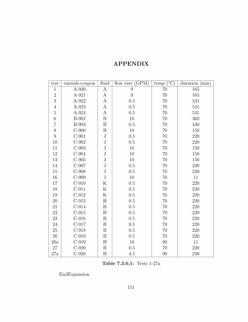
APPENDIX
test varnish-coupon fluid flow rate (GPM) temp (◦C) duration (min)1 A-920 A 9 70 1652 A-921 A 9 70 1653 A-922 A 0.5 70 5314 A-923 A 0.5 70 5315 A-924 A 0.5 70 5316 B-902 B 10 70 3607 B-903 B 0.5 70 4308 C-900 B 10 70 1509 C-901 J 0.5 70 22010 C-902 J 0.5 70 22011 C-903 J 10 70 15012 C-904 J 10 70 15013 C-905 J 10 70 15014 C-907 J 0.5 70 22015 C-908 J 0.5 70 22016 C-909 J 10 70 1117 C-910 K 0.5 70 22018 C-911 K 0.5 70 22019 C-912 K 0.5 70 22020 C-913 H 0.5 70 22021 C-914 H 0.5 70 22022 C-915 H 0.5 70 22023 C-916 B 0.5 70 22024 C-917 B 0.5 70 22025 C-918 B 0.5 70 22026 C-919 B 0.5 70 22026a C-919 H 10 90 1127 C-920 B 0.5 70 22027a C-920 H 4.5 90 240
Table 7.3.0.1: Tests 1-27a
EndExpansion
151
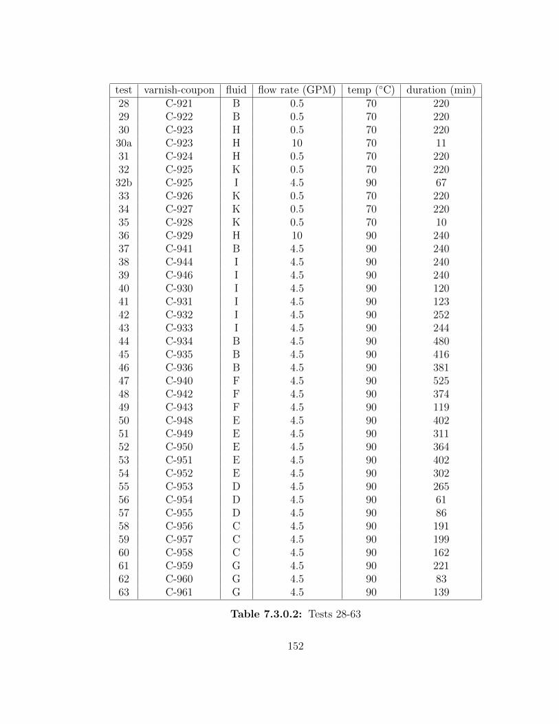
test varnish-coupon fluid flow rate (GPM) temp (◦C) duration (min)28 C-921 B 0.5 70 22029 C-922 B 0.5 70 22030 C-923 H 0.5 70 22030a C-923 H 10 70 1131 C-924 H 0.5 70 22032 C-925 K 0.5 70 22032b C-925 I 4.5 90 6733 C-926 K 0.5 70 22034 C-927 K 0.5 70 22035 C-928 K 0.5 70 1036 C-929 H 10 90 24037 C-941 B 4.5 90 24038 C-944 I 4.5 90 24039 C-946 I 4.5 90 24040 C-930 I 4.5 90 12041 C-931 I 4.5 90 12342 C-932 I 4.5 90 25243 C-933 I 4.5 90 24444 C-934 B 4.5 90 48045 C-935 B 4.5 90 41646 C-936 B 4.5 90 38147 C-940 F 4.5 90 52548 C-942 F 4.5 90 37449 C-943 F 4.5 90 11950 C-948 E 4.5 90 40251 C-949 E 4.5 90 31152 C-950 E 4.5 90 36453 C-951 E 4.5 90 40254 C-952 E 4.5 90 30255 C-953 D 4.5 90 26556 C-954 D 4.5 90 6157 C-955 D 4.5 90 8658 C-956 C 4.5 90 19159 C-957 C 4.5 90 19960 C-958 C 4.5 90 16261 C-959 G 4.5 90 22162 C-960 G 4.5 90 8363 C-961 G 4.5 90 139
Table 7.3.0.2: Tests 28-63
152
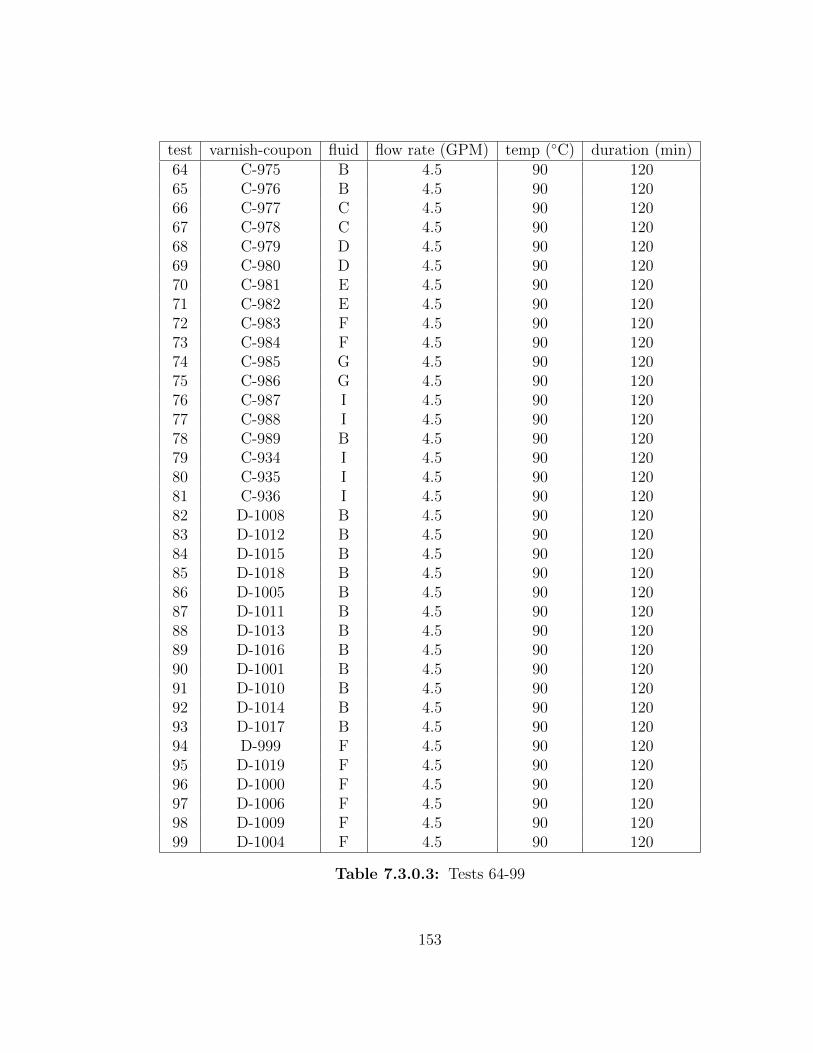
test varnish-coupon fluid flow rate (GPM) temp (◦C) duration (min)64 C-975 B 4.5 90 12065 C-976 B 4.5 90 12066 C-977 C 4.5 90 12067 C-978 C 4.5 90 12068 C-979 D 4.5 90 12069 C-980 D 4.5 90 12070 C-981 E 4.5 90 12071 C-982 E 4.5 90 12072 C-983 F 4.5 90 12073 C-984 F 4.5 90 12074 C-985 G 4.5 90 12075 C-986 G 4.5 90 12076 C-987 I 4.5 90 12077 C-988 I 4.5 90 12078 C-989 B 4.5 90 12079 C-934 I 4.5 90 12080 C-935 I 4.5 90 12081 C-936 I 4.5 90 12082 D-1008 B 4.5 90 12083 D-1012 B 4.5 90 12084 D-1015 B 4.5 90 12085 D-1018 B 4.5 90 12086 D-1005 B 4.5 90 12087 D-1011 B 4.5 90 12088 D-1013 B 4.5 90 12089 D-1016 B 4.5 90 12090 D-1001 B 4.5 90 12091 D-1010 B 4.5 90 12092 D-1014 B 4.5 90 12093 D-1017 B 4.5 90 12094 D-999 F 4.5 90 12095 D-1019 F 4.5 90 12096 D-1000 F 4.5 90 12097 D-1006 F 4.5 90 12098 D-1009 F 4.5 90 12099 D-1004 F 4.5 90 120
Table 7.3.0.3: Tests 64-99
153
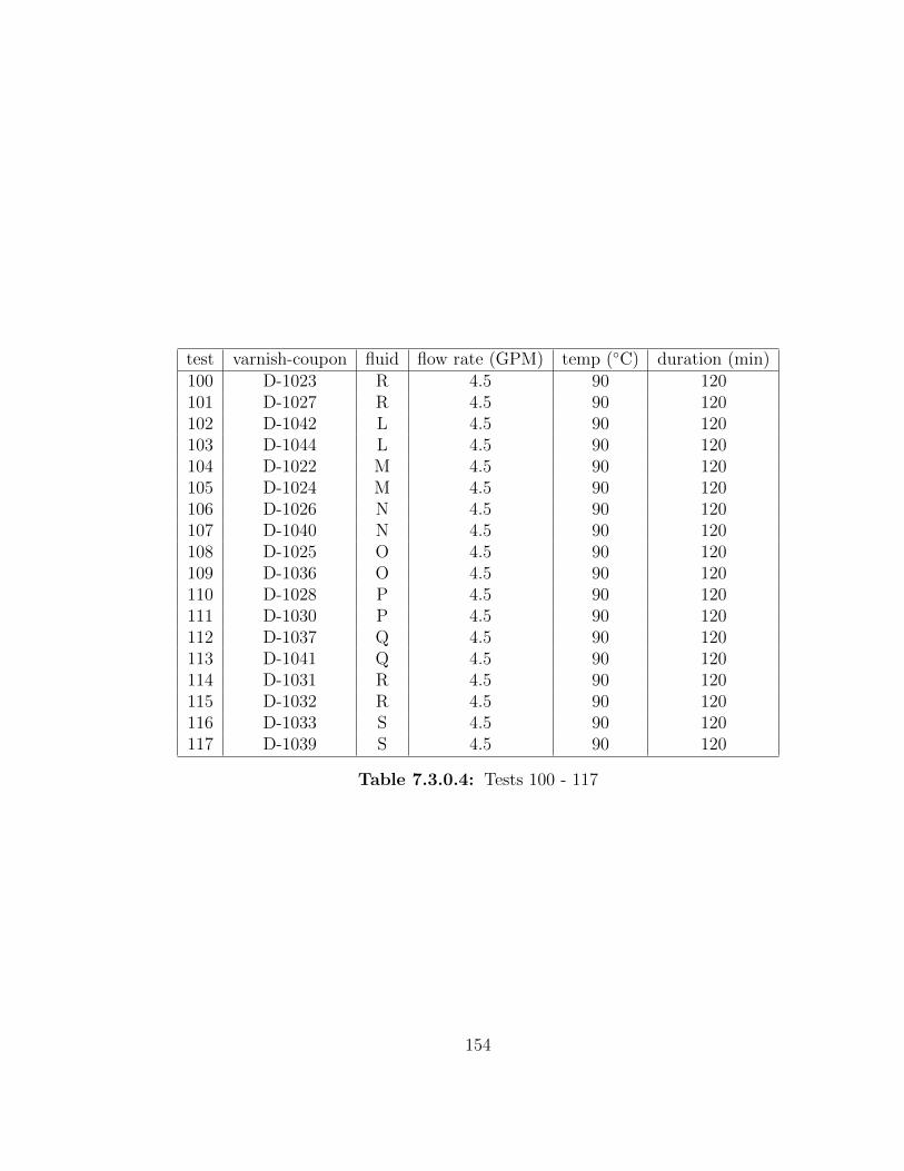
test varnish-coupon fluid flow rate (GPM) temp (◦C) duration (min)100 D-1023 R 4.5 90 120101 D-1027 R 4.5 90 120102 D-1042 L 4.5 90 120103 D-1044 L 4.5 90 120104 D-1022 M 4.5 90 120105 D-1024 M 4.5 90 120106 D-1026 N 4.5 90 120107 D-1040 N 4.5 90 120108 D-1025 O 4.5 90 120109 D-1036 O 4.5 90 120110 D-1028 P 4.5 90 120111 D-1030 P 4.5 90 120112 D-1037 Q 4.5 90 120113 D-1041 Q 4.5 90 120114 D-1031 R 4.5 90 120115 D-1032 R 4.5 90 120116 D-1033 S 4.5 90 120117 D-1039 S 4.5 90 120
Table 7.3.0.4: Tests 100 - 117
154