chapter 5 inland mineral soil wetlands - ipcc-nggip

DO NOT CITE OR QUOTE DRAFT Chapter 5 Inland Mineral Soil Wetlands

DRAFT 2013 Wetlands Supplement 5.1 Chapter 5

CHAPTER 5 1

INLAND MINERAL SOIL WETLANDS 2

3

4

Contents 5

5.1 Introduction ........................................................................................................................................... 1 6

5.1.1 Inland Mineral Soil Wetlands ....................................................................................................... 2 7

5.1.2 Guidance for Inland Mineral Soil Wetlands ................................................................................. 3 8

5.1.3 Choice of Activity Data ................................................................................................................ 4 9

5.1.4 Reporting Inland Mineral Soil Wetlands ...................................................................................... 4 10

5.2 General Methods ................................................................................................................................... 6 11

5.2.1 CO2 ............................................................................................................................................... 6 12

5.2.2 Non-CO2 Emissions from IMS Wetlands ..................................................................................... 8 13

5.3 Drainage, Creation, and Restoration of Inland Mineral Soil Wetlands ............................................... 11 14

5.3.1 Introduction ................................................................................................................................. 11 15

5.3.2 Methodological Issues ................................................................................................................ 12 16

5.4 Completeness, Time Series Consistency, Qa/Qc, and Reporting and Documentation ........................ 16 17

5.5 Future Methodological Guidance ........................................................................................................ 17 18

References ............................................................................................................................................................. 17 19

20

21

5.1 INTRODUCTION 22

This chapter provides guidance for estimating and reporting greenhouse gas emissions and removals from 23

Managed Inland Wetlands having Mineral Soils. This will be referred to as IMS wetlands (inland mineral soil 24

wetlands). 25

26

This chapter builds on the 2006 IPCC Guidelines for National Greenhouse Gas Inventories (2006 IPCC 27

Guidelines), Volume 4 chapter 2. Following the 2006 Guidelines, greenhouse gas emissions and removals can be 28

estimated in two ways: 1) Net changes in carbon stocks in the five IPCC C pools over time (used for most CO2 29

fluxes); and 2) Directly as gas flux rates to/from the atmosphere using emission factors (used for non-CO2 30

emissions and some CO2 emissions and removals). 31

32

These wetlands can occur in any of the six IPCC land classes. For example, a riverine wetland with trees may be 33

classified as a forest, while a marsh may be used for grazing and classified as grassland. The precise details of 34

this classification are specific to each country so it is not possible to say exactly how an inland wetland on 35

mineral soil may be classified. This guidance applies to all inland wetlands on mineral soils, however they are 36

Chapter 5 Inland Mineral Soil Wetlands DRAFT DO NOT CITE OR QUOTE

Chapter 5 5.2 DRAFT 2013 Wetlands Supplement

classified. The classification is important when reporting these emissions, and there is no intention to change in 37

any way how land is classified, however there may be a need to sub-divide some land types to reflect differing 38

management actions. 39

40

Inland Wetlands Having Mineral Soils meet the following two criteria: 41

1) Have Mineral Soils (i.e. not organic soils) 42

2) Do not meet the definition of Coastal Wetland 43

44

Mineral soils are those that do not fit the definition of organic soils. Organic soils are those that satisfy 45

requirements 1 & 2, or 1 & 3 below (FAO, 1998; 2006 IPCC Guidelines Vol. 4, Chap. 4 Glossary): 46

1) O horizon thickness ≥ 10 cm; a horizon of less than 20 cm must have 12% or more organic carbon 47

when mixed to a depth of 20 cm. 48

2) Soils that are never saturated for more than a few days must contain more than 20% organic C by 49

weight (i.e. about 35% organic matter). 50

3) Soils are subject to water saturation episodes and have either: 51

a. At least 12% organic carbon by weight (i.e. about 20% organic matter) if the soil has no clay; 52

or 53

b. At least 18% organic carbon by weight (i.e. about 30% organic matter) if the soil has 60% or 54

more clay; or 55

c. An intermediate, proportional amount of organic carbon for intermediate amounts of clay. 56

57

Coastal wetlands are covered in Chapter 4 of this Supplement. 58

59

Saline Inland Wetlands are a group of very specific Inland Wetlands. A review of the literature for potential 60

methods to estimate carbon stock changes and greenhouse gas fluxes was conducted for inland saline wetlands 61

(i.e. saline wetlands not covered in Chapter Four). Also known as playas, pans, salt lakes, brackish wetlands, 62

salinas, and sabkhas (generally associated with coasts), saline wetlands are important parts of arid landscapes 63

across the globe (Shaw and Bryant 2011). Carbon stocks and greenhouse gas fluxeshave been little studied in 64

inland saline wetlands. In a recent review of the literature characterizing known information on pans, playas and 65

salt lakes, carbon stocks and carbon dioxide, methane and nitrous oxide fluxes were not discussed (Shaw and 66

Bryant 2011), likely indicating little research carbon and greenhouse gas fluxes has been conducted. Because of 67

the briny nature of inland saline wetlands and their periodic flooding, saline wetlands are generally not 68

vegetated. A review of the broader literature on saline wetlands indicates that only one study has assessed soil C 69

in inland saline wetlands (Bai et al. 2007), and no studies have measured greenhouse gas fluxes or other biomass 70

categories from inland saline wetlands. The Bai et al. (2007) study was conducted in northeast China and found 71

relatively low soil carbon stocks when compared to other wetlands in China. Although only a single study, the 72

soil carbon stocks found in Bai et al. (2007) of 41-47 Mg ha-1 to 30 cm are more similar to upland soils (Table 73

2.3 in the 2006 IPCC Guidelines) than freshwater mineral wetland soils (Table 5.1). At present the lack of data 74

on inland saline wetlands does not allow for default of carbon stock changes or greenhouse gas emission factors 75

to be given. However the same methods as described here for IMS wetlands can be used with nationally 76

measured factors and applied to inland saline wetlands. Note that it is good practice for inventory compilers to 77

account for all areas of inland saline wetlands as sub-categories of the six IPCC land classes, to ensure that all 78

land is accounted. 79

80

Figure 1 in Chapter 1 shows a decision tree to orient the inventory compiler to what types of wetlands are 81

covered in this Chapter. 82

5.1.1 Inland Mineral Soil Wetlands 83

84

Mineral wetland soils are estimated to cover ~5.3% of the world’s land surface, or 7.26 x 106 km2 (Batjes, 2010). 85

The most important climate zone is boreal (2%), followed by Tropical Moist (0.67%), Cool Temperate Moist 86

(0.63%), Tropical Wet (0.61%), Polar (0.60%), and Warm Temperate Moist (0.23%) soils (Batjes, 2010). 87

Climate zones with less than 0.20% mineral wetland soils include Cool and Warm Temperate Dry, Tropical Dry, 88

and Tropical Montane. 89

90

Numerous inland wetland types have been described based on various criteria; the Ramsar Convention Wetland 91

Classification includes 24 inland wetland types alone. Wetland classification can be simplified by considering 92

broad generalizations of landform and hydroperiod (Semeniuk and Semeniuk, 1995, 1997). Inland mineral soil 93

wetlands (IMS wetlands) are found in a variety of landscape settings, including basins, channels, flats, slopes, 94

and highlands (Semeniuk and Semeniuk, 1995). It is common to find IMS wetlands adjacent to flowing waters 95



(riparian wetland) and lake and pond margins. The hydroperiod, or degree of wetness over time, of IMS 96

wetlands range from inundated (covered by water) to saturated (water is at or just below the surface) to 97

unsaturated, and from permanent to seasonal or intermittent. Hydroperiod is directly related to climate 98

(precipitation and evaporation), mechanisms of water discharge and recharge, and permeability of underlying 99

sediment. Hydroperiod can significantly impact wetland carbon and nitrogen cycling pathways and rates, and is 100

commonly altered by management activities. Therefore knowledge of wetland hydroperiod (inundated vs. un-101

inundated, permanent vs. seasonal) is useful for inventories of emissions and removals, particularly CH4. An 102

additional characteristic that is used to classify IMS wetlands is dominant vegetation community, and can 103

include trees (forested wetland), woody shrubs, and/or emergent and non-emergent vascular plants. Vegetation 104

type and productivity is important to carbon cycling, and is commonly impacted by management activities. For 105

instance, emergent vascular plants can significantly enhance CH4 production and emission from wetland 106

sediments (Whiting et al., 1991; Whiting and Chanton, 1992, 1993). 107

108

An important agricultural use of inland wetlands is rice cultivation, which is covered in the 2006 IPCC 109

Guidelines (Vol. 4, Chapter 5 – Croplands), and not addressed in this supplement. Other potentially important 110

agricultural uses of wetlands on mineral soils include lotus and mat rush cultivation, particularly in Asia (Seo et 111

al., 2010; Maruyama et al., 2004). Currently there is little available information on C stock changes or 112

greenhouse gas emissions for this type of cultivation. Further research will be required to develop methodologies 113

for these types of cultivation practices. Indirect effects of agricultural activities include agricultural runoff to 114

adjacent wetlands. Runoff would be expected to increase sedimentation rates, and may also alter greenhouse gas 115

fluxes, e.g. nitrogen-rich inputs from agricultural runoff may lead to higher N2O emissions (Bridgham et al., 116

2006). The impact of nitrogen fertilization on methane emissions is currently unclear as interactions are 117

complex, and can affect both methane production and methane consumption (Bodelier, 2011). 118

119

Grazing is an important activity in wetlands within grassland or forest landscapes (Liu et al., 2009; Oates et al., 120

2008; Wang et al., 2009). The direct effects of livestock grazing on wetlands can be selective removal of plant 121

biomass, trampling of plants, changes in below-ground biomass and soil properties, nutrient inputs, and bacterial 122

contamination from animal waste. Overgrazing can influence biomass and carbon stocks. The intensity of 123

grazing can also affect species composition and diversity. Reduction of aboveground biomass by grazing can 124

affect plant-mediated gas transport between soil and the atmosphere, which may alter greenhouse gas fluxes in 125

wetlands. Grazed wetlands and wetlands receiving run-off from adjacent livestock grazing areas, may also alter 126

N2O (and NO) emissions from wetlands. 127

128

Forest management activities on forested wetlands can vary in management intensity depending on the 129

silvicultural system. The intensity may range from selective cutting treatments to large area clearcuts. It 130

represents a loss in biomass pools and can also alter the ecologic and hydrologic conditions of the site. Possible 131

consequences of harvesting in wetlands can be changes in water table, and changes in microclimatic conditions 132

such as increased solar radiation and evapotranspiration. Some of these changes can substantially affect primary 133

production, respiration, and fluxes of CO2, CH4, and N2O. Many studies have reported temporary increases in 134

water levels after harvesting from increased interception and decreased transpiration. The increase in water level 135

may result in decreasing decomposition rates but acceleration in CH4 and N2O emissions. This point is further 136

discussed below in rewetting. Another important point is the wetland ecosystem type where harvesting takes 137

place, for example seasonally flooded riparian ecosystems are known to have more soil and biomass carbon 138

content compared to upland ecosystems. Therefore, harvesting may be expected to cause larger carbon emissions 139

in these areas compared to dryer environments. A specific accounting method for harvesting in riparian 140

ecosystems is a topic for future improvement. 141

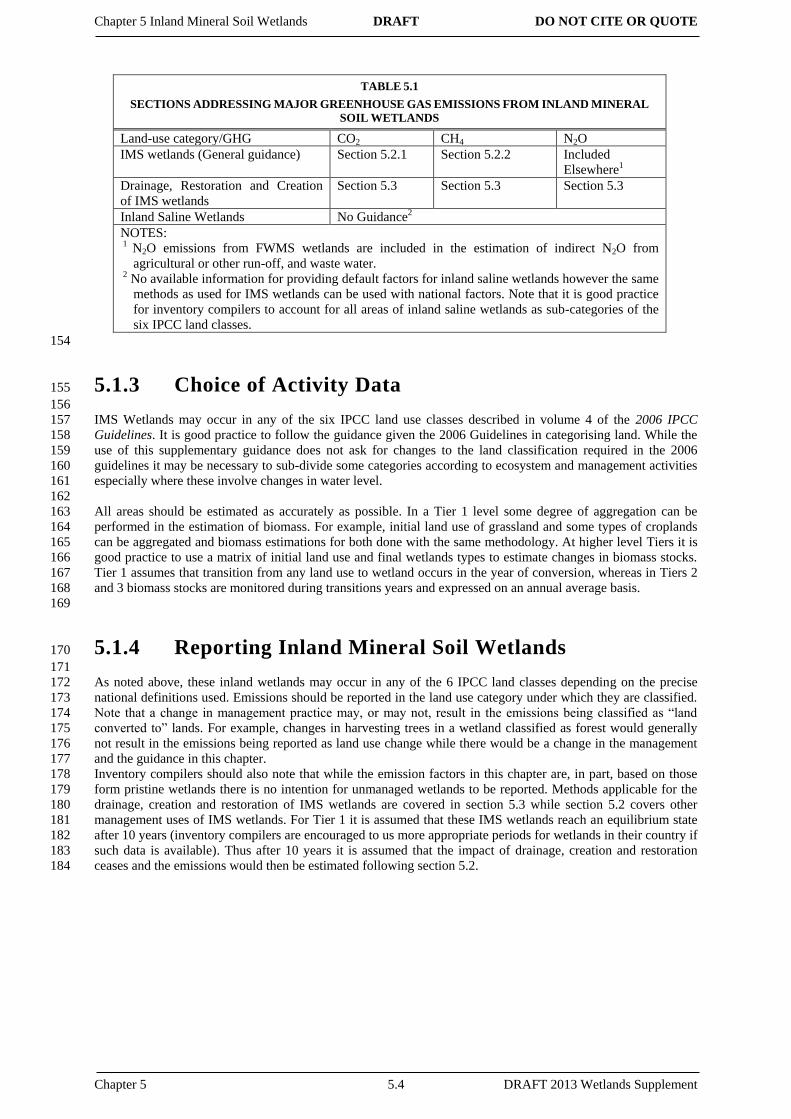
5.1.2 Guidance for Inland Mineral Soil Wetlands 142

143

In this Chapter guidance and methodologies mainly follow the 2006 IPCC Guidelines, in particular the generic 144

guidance given in Volume 4 Chapter 2. This chapter provides additional information to be used in applying the 145

methods in the 2006 IPCC Guidelines and should be read in conjunction with volume 4 of the 2006 Guidelines. 146

147

Management activities that impact CO2 and non-CO2 (CH4 and N2O) emissions include water level management 148

as well as activities that impact vegetation (such as grazing, vegetation removal, and cultivation, nutrient 149

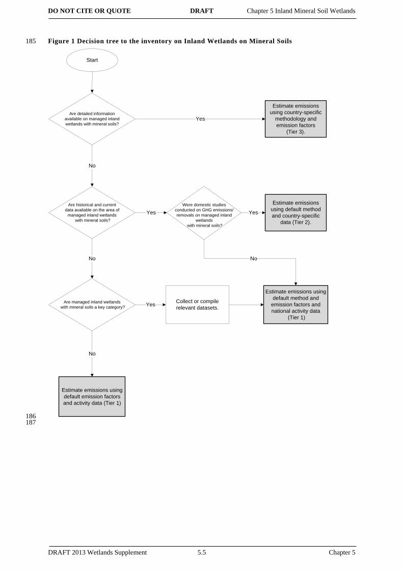
amendments). Figure 1 shows a decision tree to guide inventory compilers on which Tier approach should be 150

used to report on Inland Wetlands on Mineral Soils. Table 5.1. clarifies the scope of the assessment, and the 151

corresponding sections of this chapter. 152

153



TABLE 5.1

SECTIONS ADDRESSING MAJOR GREENHOUSE GAS EMISSIONS FROM INLAND MINERAL

SOIL WETLANDS

Land-use category/GHG CO2 CH4 N2O

IMS wetlands (General guidance) Section 5.2.1 Section 5.2.2 Included

Elsewhere1

Drainage, Restoration and Creation

of IMS wetlands

Section 5.3 Section 5.3 Section 5.3

Inland Saline Wetlands No Guidance2

NOTES: 1 N2O emissions from FWMS wetlands are included in the estimation of indirect N2O from

agricultural or other run-off, and waste water. 2 No available information for providing default factors for inland saline wetlands however the same

methods as used for IMS wetlands can be used with national factors. Note that it is good practice

for inventory compilers to account for all areas of inland saline wetlands as sub-categories of the

six IPCC land classes.

154

5.1.3 Choice of Activity Data 155

156

IMS Wetlands may occur in any of the six IPCC land use classes described in volume 4 of the 2006 IPCC 157

Guidelines. It is good practice to follow the guidance given the 2006 Guidelines in categorising land. While the 158

use of this supplementary guidance does not ask for changes to the land classification required in the 2006 159

guidelines it may be necessary to sub-divide some categories according to ecosystem and management activities 160

especially where these involve changes in water level. 161

162

All areas should be estimated as accurately as possible. In a Tier 1 level some degree of aggregation can be 163

performed in the estimation of biomass. For example, initial land use of grassland and some types of croplands 164

can be aggregated and biomass estimations for both done with the same methodology. At higher level Tiers it is 165

good practice to use a matrix of initial land use and final wetlands types to estimate changes in biomass stocks. 166

Tier 1 assumes that transition from any land use to wetland occurs in the year of conversion, whereas in Tiers 2 167

and 3 biomass stocks are monitored during transitions years and expressed on an annual average basis. 168

169

5.1.4 Reporting Inland Mineral Soil Wetlands 170

171

As noted above, these inland wetlands may occur in any of the 6 IPCC land classes depending on the precise 172

national definitions used. Emissions should be reported in the land use category under which they are classified. 173

Note that a change in management practice may, or may not, result in the emissions being classified as “land 174

converted to” lands. For example, changes in harvesting trees in a wetland classified as forest would generally 175

not result in the emissions being reported as land use change while there would be a change in the management 176

and the guidance in this chapter. 177

Inventory compilers should also note that while the emission factors in this chapter are, in part, based on those 178

form pristine wetlands there is no intention for unmanaged wetlands to be reported. Methods applicable for the 179

drainage, creation and restoration of IMS wetlands are covered in section 5.3 while section 5.2 covers other 180

management uses of IMS wetlands. For Tier 1 it is assumed that these IMS wetlands reach an equilibrium state 181

after 10 years (inventory compilers are encouraged to us more appropriate periods for wetlands in their country if 182

such data is available). Thus after 10 years it is assumed that the impact of drainage, creation and restoration 183

ceases and the emissions would then be estimated following section 5.2. 184



Figure 1 Decision tree to the inventory on Inland Wetlands on Mineral Soils 185

Start

Are detailed information

available on managed inland

wetlands with mineral soils?

Estimate emissions

using country-specific

methodology and

emission factors

(Tier 3).

Yes

Are historical and current

data available on the area of

managed inland wetlands

with mineral soils?

No

Are managed inland wetlands

with mineral soils a key category?

No

Estimate emissions using

default method and

emission factors and

national activity data

(Tier 1)

Estimate emissions

using default method

and country-specific

data (Tier 2).

Were domestic studies

conducted on GHG emissions/

removals on managed inland

wetlands

with mineral soils?

Estimate emissions using

default emission factors

and activity data (Tier 1)

No

Yes Yes

No

Collect or compile

relevant datasets.Yes

186 187



5.2 GENERAL METHODS 188

5.2.1 CO2 189

5.2.1.1 BIOMASS AND DEAD ORGANIC MATTER 190

The set of general equations to estimate the annual carbon stock changes on Managed Inland Wetlands are given 191

in Volume 4, Chapter 2 of the 2006 IPCC Guidelines. 192

193

Figure 1.2 in Chapter 1 of Volume 4 of the 2006 Guidelines shows a decision tree for the identification of 194

appropriate Tiers for the inventory of land remaining in the same land-use category. Refer also to Figure 4.2 of 195

Chapter 4 in Volume 1 of the 2006 Guidelines for assigning key categories. 196

CHOICE OF METHOD AND TIER 197

Where there is no change in management or change in land-use the Tier 1 approach assumes no change in 198

biomass, dead wood or soil carbon in these wetlands. Following a change in management practices the biomass 199

and dead organic matter will not vary significantly after 10 years (Miller and Fujii, 2010), and this land area will 200

not fall into the definition of a key category (see Figure 1.2. in Chapter 1 of Volume 4 in the 2006 Guidelines for 201

guidance on defining key categories). Where there are significant changes in management, biomass stocks can 202

change accordingly. The Tier 1 approach of no change in biomass can be used if the land is not considered to be 203

a key category, but if there is reliable data about rates of biomass change then countries should use a higher Tier 204

to estimate emissions and removals associated with changes in biomass and dead organic matter. For Tier 2 and 205

3, it is good practice to implement country-specific biomass and carbon stock inventories. If national data are not 206

available for Tier 2, countries can use globally-compiled databases (e.g. FAO) and assume that wetland 207

vegetation does not have substantially different biomass carbon densities than upland vegetation (Bridgham et 208

al., 2006). It is also good practice to use modern satellite imagery and field surveys to estimate sub-types of 209

Wetlands, as outlined in Chapter 3 of the 2006 IPCC Guidelines. Where resources are not available to obtain 210

country-specific data, wetland cover can also be derived from globally-compiled databases (e.g. WWF Global 211

Lakes and Wetlands Database – GLWD). Since several definitions exist for the classification of land as wetland 212

(Mitsch and Gosselink, 2011), it is good practice that countries explicitly describe criteria of classification. 213

214

UNCERTAINTY ASSESSMENT 215

As stated in the 2006 Guidelines, Volume 1, Chapter 3 provides information on forest biomass uncertainties 216

associated with sample-based studies. FAO (2006) provides uncertainty estimates for forest carbon factors; basic 217

wood density (10 to 40%); annual increment in managed forests of industrialized countries (6 %); growing stock 218

(industrialized countries 8%, nonindustrialized countries 30%); combined natural losses for industrialized 219

countries (15%); wood and fuelwood removals (industrialized countries 20%). The major sources of uncertainty 220

of wood density and biomass expansion factors are stand age, species composition, and structure. To reduce 221

uncertainty, countries are encouraged to develop country- or region specific biomass expansion factors and 222

BCEFs for FWMW. In case country- or regional-specific values are unavailable, the sources of default 223

parameters should be checked and their correspondence with specific conditions of a country should be 224

examined. 225

226

Uncertainty in dead organic matter pools is high relative to other carbon pools (Bradford et al. 2010). Dead 227

organic matter pools are dependent on the vegetation type (Currie and Nadelhoffer 2002), management (Scheller 228

et al. 2011), age of stand (if forested) (Sun et al. 2004), disturbance history (Tinker and Knight 2000) and the 229

presence of soil fauna (Hale et al. 2005). Errors as high as 100% are common when measuring DOM (Bradford 230

et al. 2009). For IMS wetlands it is highly unlikely that approaches other than inventory methods (Tier 2) will 231

be available to assess changes in DOM pools. Hence, good practice for inventory methods is critical for an 232

accurate assessment of DOM (see inventory discussion in Uncertainty Assessment in Soil C section – 5.2.3.5). 233

When no data on DOM are available, no change in DOM stocks can be assumed unless changes in DOM are 234

associated with a key category. 235

5.2.1.2 SOIL CARBON 236

Management practices can significantly change mineral soil wetland C stocks, especially when flow is regulated 237

and sediment deposition rates change (McCarty and Ritchie 2002; Chmura et al. 2003). Changes in water table 238

affect redox conditions in soils which affect decomposition rates and ultimately C stocks (Zdruli et al. 1995). 239

Restoration and rewetting of mineral soil wetlands can increase C stocks over time (Ballantine and Schneider 240

(2009). 241



242

CHOICE OF METHOD 243

Little information is available to conduct Tier 2 and Tier 3 soil C stock analyses for organic C in IMS wetlands. 244

For example, only two studies have assessed site specific changes in soil C pools following mineral soil wetland 245

drainage (Zdruli et al. 1995; Page and Dalal 2011). An alternative approach for Tier 1 could characterize the 246

direct soil emissions of CO2 by vegetation type, climate zone, management practices and soil type, however little 247

information is available to use a direct CO2 emission approach. Only four studies have assessed CO2 emissions 248

following a change in IMS wetlands (Danevcic et al. 2010; Fromin et al. 2010; Samaratini 2011; Sgouridis 249

2011). Similarly, only three studies have measured direct emissions of CO2 following mineral soil wetland 250

restoration (Pfeifer-Meister 2008; Gleason et al. 2009). Because of the paucity of data on both changes in soil C 251

stock and on direct CO2 emissions, a Tier 1 approach based on annual multiple inventories is described to assess 252

changes in soil C stocks for mineral soil wetlands. If data from multiple inventories is not available, changes to 253

soil C stocks in IMS wetlands is assumed to be zero at Tier 1 level of estimation. 254

255

TIER 1 256

Chapter 2 of Volume 4 of the 2006 Guidelines provides general information about mineral soil classification and 257

soil C stock estimations. The annual change in carbon stocks in mineral soils is calculated using Equation 2.25 258

(IPCC 2006, Volume 4 chapter 2). The Tier 1 approach is based on changes in soil C stocks over a finite period 259

of time, assuming (i) over time, soil organic C reaches a spatially-averaged, stable value specific to the soil, 260

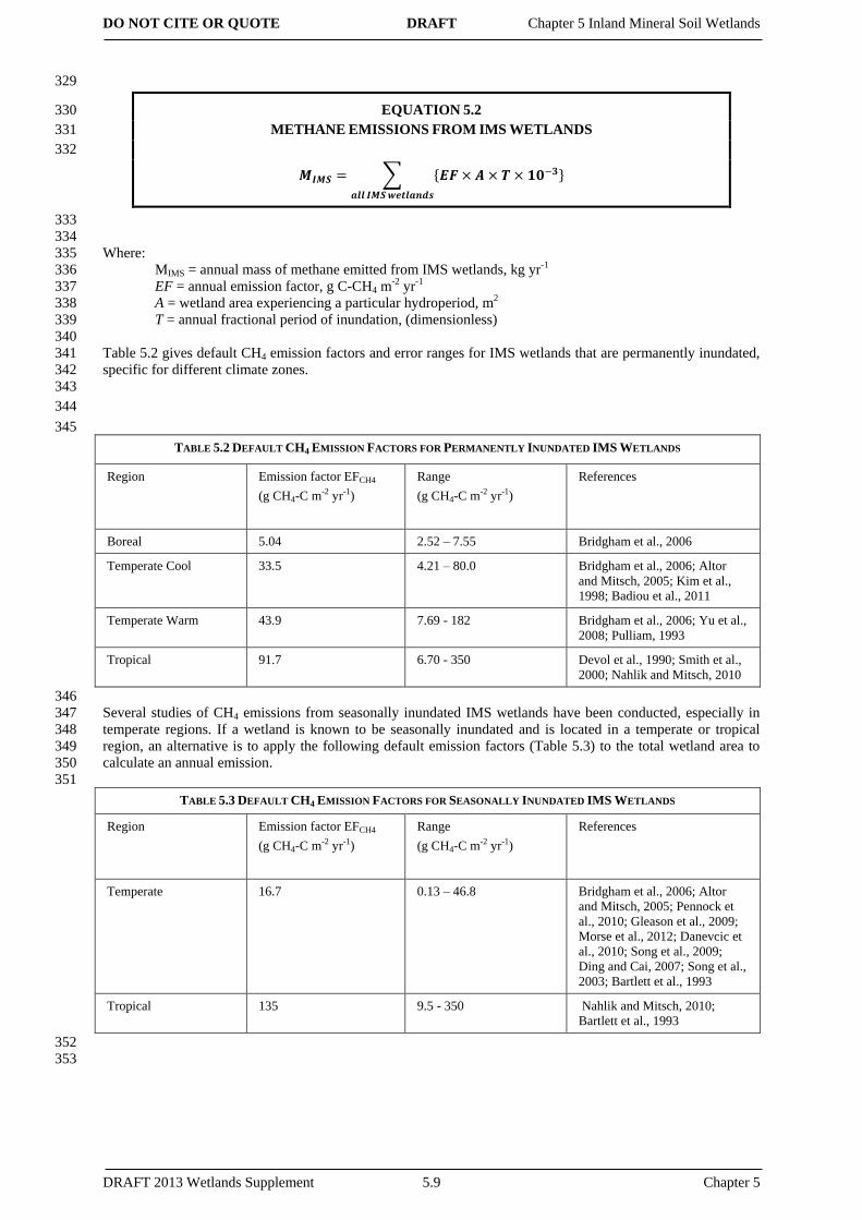
climate, land-use and management practices and (ii) soil organic C stock changes during the transition to a new 261

equilibrium SOC occurs in a linear fashion (IPCC 2006). To account for changes in SOC, countries need to 262

estimate wetland areas according to climate zones, management practices and soil types. Table 5.1 below gives 263

some updated reference soil organic carbon stocks that should be used in preference to those in the 2006 264

Guidelines in table 2.3 of volume 4, chapter 2. 265

266

267

TABLE 5.1. DEFAULT REFERENCE SOIL ORGANIC CARBON STOCKS FOR IMS WETLANDS.

IPCC (2006),

Table 2.3a

Batjes, 2011b

Region Depth Mg C

ha-1

Error Mg C ha-

1

Error

Boreal 0-30cm 146* 131 116 94

Cold temperate, dry 0-30cm 87 78

Cold temperate, moist 0-30cm 87* 78 128 55

Warm temperate, dry 0-30cm 88* 79 74 45

Warm temperate, moist 0-30cm 88* 79 135 101

Tropical, dry 0-30cm 86 77 22 11

Tropical, moist 0-30cm 86 77 68 45

Tropical, wet 0-30cm 86 77 49 27

Tropical, montane 0-30cm 86 77 82 73

aSOC stocks for mineral soils under natural vegetation presented as Tier 1 values in Table 2.3 of the IPCC

2006 Guidelines for National Greenhouse Gas Inventories, Volume 4. They are derived from soil databases

described by Jobbagy and Jackson (2000) and Bernoux et al. (2002). bThis study presents revised estimates of the IPCC 2006 SOC stocks for mineral soils under natural vegetation

based on an expanded version of the ISRIC-WISE database (Batjes, 2009) which contains 1.6 times the

number of soil profiles of the databases used in the IPCC 2006 SOC stocks estimate.

*SOC stock estimates from IPCC 2006 that were not based on expert estimates (Batjes, 2011).

268

269

For this assessment only new values of SOCref were found to support the derivation of general stock change 270

factors for IMS wetlands utilizing the second equation in 2.25 from the 2006 IPCC Guidelines. Inventory 271

compilers should use the data from the appropriate chapters of Volume 4 of the 2006 IPCC Guidelines in 272

conjunction with the data in table 5.1, above. If countries have data that can be used to derive stock change 273

factors or suitable literature values for these parameters for wetlands by climate region it is good practice to use 274

them. 275

276



TIER 2 277

For Tier 2, it is good practice to conduct soil inventories for the appropriate classification of soils, but if data are 278

not available, aggregate data (e.g. FAO) can be used for general classification. To conduct a Tier 2 approach soil 279

C stocks need to be known at two periods in time and stock changes are simply a function of the difference in C 280

stock divided by the time period (years) (Equation 5.1). 281

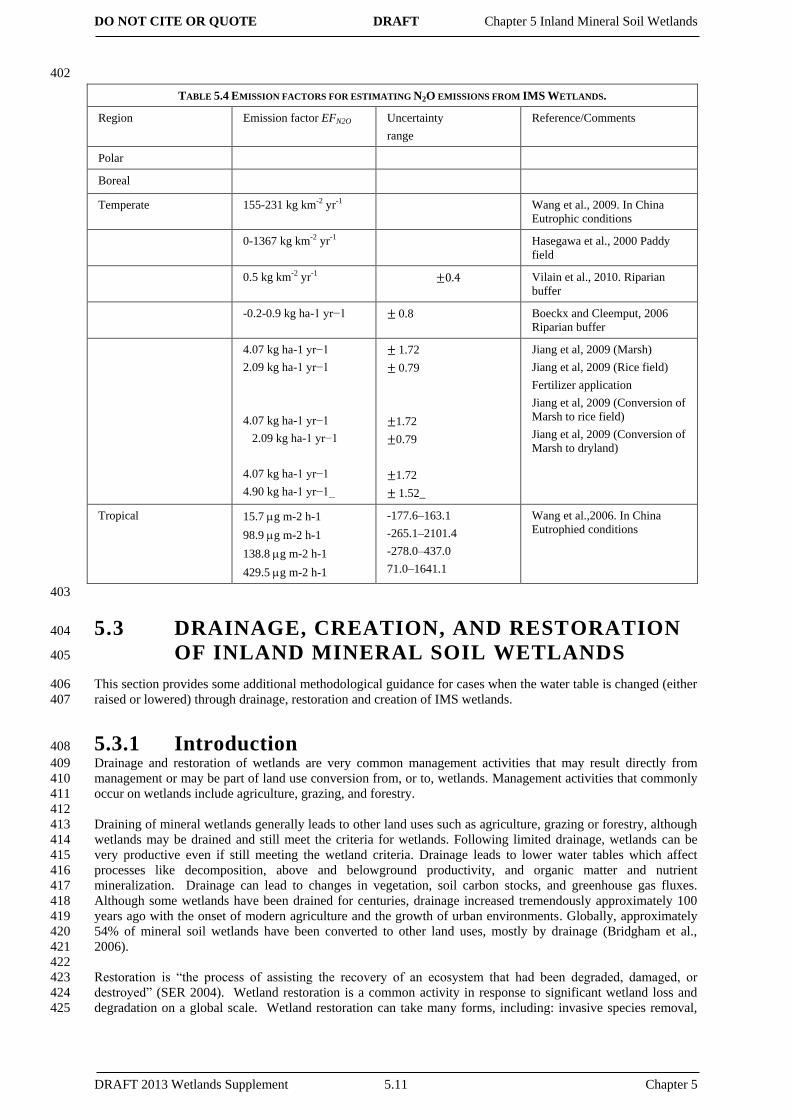
282

EQUATION 5.1 283

ANNUAL CHANGE IN ORGANIC CARBON STOCKS IN MINERAL SOILS 284

285

( )

Where: 286

ΔCMineral = annual change in carbon stocks in mineral soils, tonnes C yr-1 287

SOC0 = soil organic carbon stock in the last year of an inventory time period, tonnes C 288

SOC(0-T) = soil organic carbon stock at the beginning of the inventory time period, tonnes C 289

SOC0 and SOC(0-T) are calculated using the SOC equation in the box where the reference carbon stocks and stock 290

change factors are assigned according to the land-use and management activities and corresponding areas at each 291

of the points in time (time = 0 and time = 0-T) 292

T = number of years between inventory time periods, yr 293

294

UNCERTAINTY ASSESSMENT 295

Because of lack of data at this time, the only reliable higher Tier approach to assess C stock changes in soils for 296

IMS wetlands is through repeated inventories. The repeated inventory (stock changes) approach works well for 297

any of the disturbances and restoration activities discussed in this chapter. Inventory methods, if conducted with 298

consistent methods for measurement and analysis from year to year tend to be very accurate in assessing change 299

(Gillespie 1999). As stated in the 2006 Guidelines, the precision of an inventory is increased and confidence 300

ranges are smaller with more sampling. If plot locations are not re-locatable, if measurement methods change or 301

if lab analyses protocols are not consistent with time, uncertainty increases for inventories. 302

303

As indicated in the 2006 Guidelines, uncertainties in activity statistics may be reduced through a better national 304

system, such as developing or extending a ground-based survey with additional sample locations and/or 305

incorporating remote sensing to provide additional coverage. It is good practice to design a classification that 306

captures the majority of land-use and management activities with a sufficient sample size to minimize 307

uncertainty at the national scale. 308

5.2.2 Non-CO2 Emissions from IMS Wetlands 309

5.2.2.1 METHANE EMISSIONS FROM IMS WETLANDS 310

311

Methane is produced in soils of IMS during anaerobic decomposition of organic matter, and emitted to the 312

atmosphere after diffusion or ebullition through the water column or through plant-mediated transport. Several 313

factors have been identified as important controls on methane production and emission, including water level, 314

temperature, and vegetation community and productivity (Whiting and Chanton, 1993). Despite current 315

understanding of the processes involved in methane production and emission from wetlands, it remains difficult 316

to accurately predict methane emissions with a high degree of confidence. Studies show high spatial variability 317

in methane emissions across large areas that have similar climate, vegetation, and topography, and within small 318

areas that have microscale variation in topography (Ding et al., 2003; Saarnio et al., 2009). In addition, there are 319

very few studies of methane emissions from IMS wetlands in Europe (Saarnio et al., 2009), tropical regions 320

(Mitsch et al., 2010), and certain regions of North America (Pennock et al., 2010). Therefore, the default 321

emission factors we present necessarily have large uncertainties. 322

TIER 1 323

The basic equation to estimate CH4 emission is shown in Eq. 5.2, where wetland area subject to a particular 324

hydroperiod is multiplied by the default emission factor, and by the annual fractional period that the wetland area 325

is inundated by water, if known. This allows for the incorporation of wetland hydroperiod, which may be 326

determined by natural causes or as a consequence of management activity. If the annual fractional period of 327

inundation is unknown, then a default fraction of 1 is assumed. 328



329

EQUATION 5.2 330

METHANE EMISSIONS FROM IMS WETLANDS 331

332

∑ { }

333

334

Where: 335

MIMS = annual mass of methane emitted from IMS wetlands, kg yr-1 336

EF = annual emission factor, g C-CH4 m-2 yr-1 337

A = wetland area experiencing a particular hydroperiod, m2 338

T = annual fractional period of inundation, (dimensionless) 339

340

Table 5.2 gives default CH4 emission factors and error ranges for IMS wetlands that are permanently inundated, 341

specific for different climate zones. 342

343

344

345

TABLE 5.2 DEFAULT CH4 EMISSION FACTORS FOR PERMANENTLY INUNDATED IMS WETLANDS

Region Emission factor EFCH4

(g CH4-C m-2 yr-1)

Range

(g CH4-C m-2 yr-1)

References

Boreal 5.04 2.52 – 7.55 Bridgham et al., 2006

Temperate Cool 33.5 4.21 – 80.0 Bridgham et al., 2006; Altor

and Mitsch, 2005; Kim et al.,

1998; Badiou et al., 2011

Temperate Warm 43.9 7.69 - 182 Bridgham et al., 2006; Yu et al.,

2008; Pulliam, 1993

Tropical 91.7 6.70 - 350 Devol et al., 1990; Smith et al.,

2000; Nahlik and Mitsch, 2010

346

Several studies of CH4 emissions from seasonally inundated IMS wetlands have been conducted, especially in 347

temperate regions. If a wetland is known to be seasonally inundated and is located in a temperate or tropical 348

region, an alternative is to apply the following default emission factors (Table 5.3) to the total wetland area to 349

calculate an annual emission. 350

351

TABLE 5.3 DEFAULT CH4 EMISSION FACTORS FOR SEASONALLY INUNDATED IMS WETLANDS

Region Emission factor EFCH4

(g CH4-C m-2 yr-1)

Range

(g CH4-C m-2 yr-1)

References

Temperate 16.7 0.13 – 46.8 Bridgham et al., 2006; Altor

and Mitsch, 2005; Pennock et

al., 2010; Gleason et al., 2009;

Morse et al., 2012; Danevcic et

al., 2010; Song et al., 2009;

Ding and Cai, 2007; Song et al.,

2003; Bartlett et al., 1993

Tropical 135 9.5 - 350 Nahlik and Mitsch, 2010;

Bartlett et al., 1993

352

353



CALCULATING STEPS FOR TIER 1 354

Step 1: Determine the area of wetland experiencing a particular hydroperiod; if hydroperiod is unknown then 355

assume permanent inundation (Tinundation=1). Using equation 5.2, the appropriate EFCH4 (Table 5.2), and the 356

annual fractional period of inundation, estimate the annual CH4 emission from that area of wetland. If a wetland 357

is known to be seasonally inundated, an alternative is to apply the appropriate EFCH4 (Table 5.3), setting 358

Tinundation=1. 359

360

Step 2: Repeat Step 1 for each wetland area experiencing a particular hydroperiod. 361

362

Step 3: Sum the annual CH4 emissions from each wetland area to calculate a total annual CH4 emission from 363

IMS wetlands. 364

365

TIER 2 366

Tier 2 calculations use country-specific emission factors and parameters, to reflect regionally important wetland 367

types and hydrologic dynamics. For example if seasonally-inundated wetlands are a dominant IMS wetland type 368

of the country, it is recommended that wetland hydroperiod be determined. 369

370

TIER 3 371

Tier 3 calculations include site-specific determinations of methane emissions from dominant wetland types, or 372

may include approaches such as dynamic modeling of methane fluxes (Saarnio et al., 2009). Models based on 373

simple regressions (Christensen et al., 1996; Saarnio et al., 1997; Juutinen et al., 2003) or sophisticated process-374

based models (Walter and Heimann, 2000; Kettunen, 2003; Cui et al., 2005) can be applied to specific wetland 375

ecosystems, however these models require input data sets that may be difficult to obtain. 376

5.2.2.2 NITROUS OXIDE EMISSIONS FROM IMS WETLANDS 377

Nitrous oxide (N2O) is an important greenhouse gas.The microbial processes involved in production of N2O are 378

nitrification (nitrifier denitrification, in particular) and denitrification. Therefore, N2O emissions vary with 379

climate, soil-water conditions and management. Due to complexity of the interactions between these factors, 380

N2O shows very high spatial and temporal variations; even diurnal variations. 381

382

A wetland system can be a major N2O source or sink as a result of ecologic conditions and microbial activity. 383

The increase in anthropogenic nitrogen discharge to the natural environment may enhance the N2O flux to the 384

atmosphere. Generally, wetlands with low N availability are considered relatively minor sources of N2O (Durand 385

et al., 2010). Relatively high N2O emissions from IMS wetlands are associated with agricultural runoff (Phillips 386

and Beeri, 2008; DeSimone et al., 2010), and livestock runoff (Chen et al., 2011; Oates et al., 2008; Jackson et 387

al., 2006; Holst et al., 2007; Walker et al., 2002).In order to avoid double-counting N2O emitted from the use of 388

fertilizers, and urine and dung deposition from grazing animals, it is suggested to follow 2006 Guidelines 389

(Volume 4, Chapter 11) for estimating N2O emissions from those IMS wetlands receiving agricultural or other 390

runoff. 391

392

EQUATION 5.3 393

N2O EMISSIONS FROM IMS WETLANDS 394

395

396

Where 397

NIMS = N2O emissions form IMS wetlands, kg yr-1 398

EF = Emission Factors (see Table 5.4 for defaults) kg km-2 yr-1 399

A = Area of IMS wetlands km-2 400

401



402

TABLE 5.4 EMISSION FACTORS FOR ESTIMATING N2O EMISSIONS FROM IMS WETLANDS.

Region Emission factor EFN2O

Uncertainty

range

Reference/Comments

Polar

Boreal

Temperate 155-231 kg km-2 yr-1 Wang et al., 2009. In China

Eutrophic conditions

0-1367 kg km-2 yr-1 Hasegawa et al., 2000 Paddy

field

0.5 kg km-2 yr-1 Vilain et al., 2010. Riparian

buffer

-0.2-0.9 kg ha-1 yr−1 0.8 Boeckx and Cleemput, 2006

Riparian buffer

4.07 kg ha-1 yr−1

2.09 kg ha-1 yr−1

4.07 kg ha-1 yr−1

2.09 kg ha-1 yr−1

4.07 kg ha-1 yr−1

4.90 kg ha-1 yr−1_

1.72

0.79

1.72

0.79

1.72

1.52_

Jiang et al, 2009 (Marsh)

Jiang et al, 2009 (Rice field)

Fertilizer application

Jiang et al, 2009 (Conversion of

Marsh to rice field)

Jiang et al, 2009 (Conversion of

Marsh to dryland)

Tropical 15.7 g m-2 h-1

98.9 g m-2 h-1

138.8 g m-2 h-1

429.5 g m-2 h-1

-177.6–163.1

-265.1–2101.4

-278.0–437.0

71.0–1641.1

Wang et al.,2006. In China

Eutrophied conditions

403

5.3 DRAINAGE, CREATION, AND RESTORATION 404

OF INLAND MINERAL SOIL WETLANDS 405

This section provides some additional methodological guidance for cases when the water table is changed (either 406

raised or lowered) through drainage, restoration and creation of IMS wetlands. 407

5.3.1 Introduction 408

Drainage and restoration of wetlands are very common management activities that may result directly from 409

management or may be part of land use conversion from, or to, wetlands. Management activities that commonly 410

occur on wetlands include agriculture, grazing, and forestry. 411

412

Draining of mineral wetlands generally leads to other land uses such as agriculture, grazing or forestry, although 413

wetlands may be drained and still meet the criteria for wetlands. Following limited drainage, wetlands can be 414

very productive even if still meeting the wetland criteria. Drainage leads to lower water tables which affect 415

processes like decomposition, above and belowground productivity, and organic matter and nutrient 416

mineralization. Drainage can lead to changes in vegetation, soil carbon stocks, and greenhouse gas fluxes. 417

Although some wetlands have been drained for centuries, drainage increased tremendously approximately 100 418

years ago with the onset of modern agriculture and the growth of urban environments. Globally, approximately 419

54% of mineral soil wetlands have been converted to other land uses, mostly by drainage (Bridgham et al., 420

2006). 421

422

Restoration is “the process of assisting the recovery of an ecosystem that had been degraded, damaged, or 423

destroyed” (SER 2004). Wetland restoration is a common activity in response to significant wetland loss and 424

degradation on a global scale. Wetland restoration can take many forms, including: invasive species removal, 425



conversion of agricultural lands back to wetlands, filling or blocking ditches, reducing nutrient and sediment 426

levels, to name a few. There is large potential for increased carbon storage from restoring mineral soil wetlands. 427

For instance, Bridgham et al. (2006) estimated that mineral soil wetlands are currently losing roughly 45 Mt C 428

yr-1 of carbon sequestration potential from wetland conversion. This potential to sequester more carbon has been 429

borne out by many restoration studies (Euliss et al. 2006, Gleason et al. 2009, Ballantine and Schneider 2009, 430

Card et al. 2010, Badiou et al. 2011). Badiou et al. (2011) estimated from their study of 22 wetlands that 431

restored wetlands were accumulating 2.7 Mg C ha-1 yr-1 as soil organic carbon. Ballantine and Schneider (2009) 432

surveyed 35 restored wetlands in New York and found that 17% (6% to 23%) of the reference carbon stock had 433

accumulated over a 55 year chronosequence. Ballantine and Schneider (2009) also summarized the literature 434

and found that wetlands recovered about 50% of their reference soil carbon after 55 years, whereas plant 435

standing biomass reached reference conditions at 55 years. Time to recover soil C after wetland restoration 436

varies greatly depending upon the amount of soil C lost, soil wetness, vegetation, and hydrogeomorphic setting. 437

For instance, Card et al. (2010) estimated that it would only take 7-11 years after restoration in riparian wetlands 438

to come back to reference conditions. 439

440

Although restored wetlands tend to increase their ability to sequester carbon, restored wetlands may also increase 441

their emissions of CH4 and N2O, and so could increase their climate change impacts despite storing more carbon 442

(Bridgham et al. 2006). This is especially true for mineral wetlands, which can have relatively large CH4 443

emissions. For example, peatlands occupy 32% more land then mineral wetlands, but emit 46% less CH4 444

(Bridgham et al. 2006). Much less information exists for trace gas emissions compared to soil carbon contents in 445

restored wetlands. In general, emissions of CH4 and N2O are affected by hydroperiod, vegetation, and substrate 446

quality and quantity. A few studies in seasonal wetlands have found that restoration had little impact on either 447

CH4 or N2O emissions (Gleason et al. 2009, Pfeifer-Meister 2008). Conversely, other studies, especially in 448

restored wetlands with permanent or semi-permanent hydroperiods, were found to have increased CH4 and/or 449

N2O (Badiou et al. 2011). 450

451

Data is still sparse to document how wetland restoration affects emissions of total greenhouse gas emissions (see 452

summaries by Roulet 2000, Bridgham et al. 2006). Few studies of restoration effects on mineral wetlands have 453

been conducted. Badiou et al. (2011) measured greenhouse gas fluxes across a range of prairie potholes in 454

Canada and calculated that they would sequester approximately 3.25 Mg CO2 equivalents ha-1 yr-1, even after 455

accounting for an increase in CH4 and N2O emissions. Gleason et al. (2009) found no significant difference in 456

CO2, CH4, or N2O exchange between cropland and restored prairie pothole wetlands on cropland 16 years after 457

restoration. 458

5.3.2 Methodological Issues 459

460

The primary challenges to wetland restoration and creation are the development of wetland hydrology and the 461

establishment of vegetation (US EPA, 2003). Wetlands are restored or created for a variety of reasons, including 462

water-quality enhancement (treatment of wastewater, stormwater, acid mine drainage, agricultural runoff; 463

Hammer, 1989), flood minimization, and habitat replacement (Mitsch et al., 1998). Wetlands created for the 464

purposes of wastewater treatment are not covered in this Chapter; please refer to Chapter 6 (Constructed 465

Wetlands) in this Supplement for guidance on these types of wetlands. Flooding of land to create reservoirs is 466

covered in Chapter 7 of Volume 4 of 2006 Guidelines. 467

468

The inventory of greenhouse gas emissions requires the assessment of all 5 IPCC carbon pools as well as 469

emissions of non-CO2 gases, stratified by climatic zones and conversion types. For example, the initial raising of 470

the water table might result in death of all or part of the living biomass, with transfers to dead organic matter and 471

litter pools or decomposition and losses to the atmosphere. However, with time, original vegetation might 472

colonize the wetland, increasing living biomass pool again. Thus, changes and transfers in C pools will vary 473

according to the stage of the conversion until a new steady state is achieved. 474

475

The appropriate Tier to be used in the inventory can be decided based on Figure 1.3 of Chapter 1 of Volume 4 in 476

the 2006 Guidelines. 477

478

When a new wetland is created transfers of C among pools can be abrupt or follow different transitional stages 479

until a new steady state is achieved. For this reason, all carbon pools and exchanges among them have to be 480

accounted for in the first year of conversion and in the subsequent 9 years. The 10 year transitional stage is 481

assumed based on studies of vegetation recovery during wetland restorations but might not apply for every land 482

use change. Countries are encouraged to establish monitoring programs in representative plots of key categories 483

to determine which time frame is more appropriate. 484



5.3.2.1 BIOMASS 485

TIER 1. 486

In a Tier 1 approach changes in biomass carbon stock wetland creation are calculated using Equation 2.15 from 487

Chapter 2 of Volume 4 of the 2006 Guidelines. For simplicity, in Tier 1 it can be assumed that once the land is 488

rewetted all the vegetation will initially die and the resulting plant organic matter will decompose, with the 489

ecosystem reaching a new steady-state immediately after the conversion. Average C stock changes are calculated 490

from the difference between initial and final stocks. Default values for biomass carbon stocks for each type of 491

other land use (Forest, Grassland, Cropland) can be obtained from their respective chapters in Volume 4 of the 492

2006 Guidelines. After this transition period of 10 years the land is assumed to have reached a new equlibrium 493

state and would be reported in a “land remaining” category (e.g. forest land remaining forest land,or grassland 494

remaining grassland). 495

496

Tier 1 requires the estimation of biomass stocks in land before and after the conversion to Wetland. Although 497

rewetting will cause variable death rates depending on the type of living biomass prior to conversion, at this level 498

a simple assumption can be made that all biomass is lost and the ecosystem achieves a new steady-state in the 499

year of conversion. Hence, biomass stock after conversion is zero. Initial biomass is estimated using the methods 500

provided in the 2006 Guidelines for each type of Land cover, that is, Chapter 4 for Forest, Chapter 5 for 501

Cropland and Chapter 6 for Grassland. Annual change in biomass carbon stock is calculated using Equations 502

2.15 and 2.16 from Chapter 2 of Volume 4 of 2006 Guidelines. Since biomass after conversion is assumed to be 503

zero, ∆CCONVERSION term in equation 2.15 also equals to zero. If data is not available, countries might use 504

global biomass stocks datasets and emission/removal factors suggested in the referred respective chapters. 505

TIER 2 506

Tier 2 uses country-specific data for each climatic, ecosystem type and management practice to estimate biomass 507

changes following Land conversion to Wetland. In this case the Tier 1 assumption of a new steady-state 508

condition in the first year is replaced by the monitoring of the transitions in time of average carbon pools. 509

Equations 2.5 and 2.6 from Chapter 2 of Volume 4 of the 2006 Guidelines are used. To estimate biomass pools 510

suggested methods and respective equations are the same as those in Section 5.2.1.above. 511

512

It is good practice to implement country-specific biomass and carbon stock inventories. If national data are not 513

available for Tier 2, countries can use globally-compiled databases (e.g. FAO) and assume that wetland 514

vegetation does not have substantially different biomass carbon densities than terrestrial vegetation (Bridgham et 515

al., 2006). It is also good practice to use modern satellite imagery and field surveys to estimate sub-types of 516

Wetlands, as delineated in Chapter 3 of the 2006 IPCC Guidelines. Where resources are not available to obtain 517

country-specific data, wetland cover can also be derived from globally-compiled databases (e.g. WWF Global 518

Lakes and Wetlands Database – GLWD). Since several definitions exist for the classification of land into the 519

Wetland category (Mitsch and Gosselink, 2011), it is good practice that countries explicitly describe criteria of 520

classification. 521

522

Under a Tier 2 approach empirical data is used to evaluate the evolution in time of biomass stocks in Other Land 523

Converted to Wetland immediately after the conversion and in the following 9 years of succession. It is good 524

practice to obtain country-specific data from each previous kind of vegetation (forest, crop and grassland) under 525

each climatic region and to subsequently follow changes in biomass stocks according to management practices 526

under the Land Converted to Wetland. In biomass carbon stock changes accounted for longer periods of time, 527

results are converted to average annual values. 528

529

TIER 3 530

Tier 3 uses country and ecosystem specific data to model the evolution of biomass carbon stocks in time, from 531

the conversion year until a new steady-state is reached 532

5.3.2.2 DEAD ORGANIC MATTER 533

534

Dead Organic Matter and Litter summed constitute the Dead Organic Matter pool. These pools vary greatly 535

according to the type of initial land use (Forest, Crop, Grassland or Other Uses) and the rates of transfers from 536

other pools to the DOM pool will also be quite different depending on the velocity of the conversion and the 537

types of Other Land Use Converted to Wetland. For example, after rewetting of a forest leaves might fall and 538

decompose while trunks will remain as DOM, whereas grasses might be all decomposed in the first year of 539

conversion. If anaerobic conditions develop after complete rewetting, decomposition might slow down after the 540

initial phases of transition. 541



Because average DOM stock changes will depend on the stage of the transition from one type of land use to 542

another it is good practice to follow the transitional process until a new steady-state is reached. Estimates should 543

be expressed on an annual average basis for consistency. Given the variability of the DOM stock, there are no 544

default values for this carbon pool and is good practice that countries strive to obtain country specific data. 545

546

For simplicity Tier 1 assumes that a new steady-state is achieved in the first year of conversion while it is more 547

likely that the transition for this new state will take longer and countries are encouraged to use Tiers 2 and 3 to 548

obtain more accurate estimations. If countries choose to use Tier 1 method after the first year this land should be 549

classified as Wetland Remaining Wetland. 550

5.3.2.3 SOIL CARBON 551

552

Few studies have assessed the carbon implications of restoring and creating IMS wetlands. In general, the 553

restoration and creation of IMS wetlands leads to increases in soil C stocks over time (Badiou et al. 2011; Wolf 554

et al. 2011; Ballantine and Schneider 2009; Meyer et al. 2008; Wiggington et al. 2000). Research on C dynamics 555

in created wetlands is sparse with only a few a studies addressing C stocks in soils or greenhouse gas fluxes (Sha 556

et al. 2011; Wolf et al. 2011; Ahn and Peralta 2009). Although there are more data on C pools and fluxes from 557

wetland restoration studies, many do not report bulk density so that stocks can be calculated (e.g. Hartman et al. 558

2008), measurement systems such as eddy covariance include landscape components other than restored 559

wetlands (e.g. Herbst et al. 2011), or difficulty in interpreting numbers to make independent calculations (e.g. Lu 560

et al. 2007). The most detailed analysis of both soil c stocks and greenhouse gas fluxes in restored wetlands has 561

been conducted in the Prairie Pothole Region of Canada and the United States (Badiou et al. 2011; Card et al. 562

2010; Gleason et al. 2009; Euliss et al. 2006). 563

564

TIER 1 565

566

Tier 1 characterises the direct soil emissions of CO2 by climate zone, management practices and soil type, 567

whereas for non-CO2 emissions, Tier 1 estimates include factors of climate zone, management practices and 568

inundation regime Equation 5.4 gives the method that is applicable to CO2, CH4 and N2O. Emissions are 569

estimated by multiplying the emission rate for pristine wetlands by an adjustment factor AF. Values of F are 570

given in table 5.5. Emission rates for pristine wetlands for CH4 are given in tables 5.2 and 5.3 and for N2O in 571

table 5.4 with emission rates for CO2 listed in table 5.6, below. 572

573

EQUATION 5.4 574

SOIL EMISSIONS FROM DRAINAGE, CREATION, AND RESTORATION OF IMS WETLANDS 575

576

Where: 577

Ep,l = Emissions from Soil from management, restoration or creation of IMS wetlands, (tonnes) 578

With: 579

p = gas (CO2, CH4 or N2O) 580

l is land use type. 581

AFp,l = Adjustment Factor to account for drainage, creation and restoration for gas p and land type l, 582

(+ve = emission, -ve = removal) Table 5.5 provides default values. (dimensionless) 583

EFp = Emission Factor of pristine wetland for gas p 584

Al = area of land type l (ha) 585

586

587

Table 5.5 provides emission adjustment factors based on the data reported in the studies above. However, the 588

numbers were obtained from many different approaches, such as modelling by Li et al. (2004), gaseous fluxes 589

measurements by Page and Dalal (2011) and biomass changes measured by Ballantine and Schneider (2009). 590

Countries are encouraged to develop their own studies based on local climate and vegetation types. 591

592



TABLE 5.5. SOIL EMISSION ADJUSTMENT FACTORS DUE TO DRAINAGE OR RESTORATION OF IMS WETLANDS 593

TO BE USED IN EQUATION 5.4 (DIMENSIONLESS) (TO BE COMPLETED) 594

Region Deforestation/Drainage Restoration Source

CO2 CH4 N2O CO2 CH4 N2O

Boreal

+3 -1

+9

-1.2 +7 -7 Li et al., 2004*

-3 -0.7

to +1

+0.3

to

+10

Badiou et al, 2011+

Temperate

+1 -0.25

to -1

+0 to

+30

Page & Dalal,

2011++

0 0 0 Gleason et al., 2009#

North

America

+0.2

5

-0.4 Euliss et al. 2006†

Canada +0.2 -0.3 Euliss et al. 2006†

Humid -0.2 Mckenna, 2003**

Sub-Tropical

+2 -1 +8 -1.5 +47 -1 Li et al., 2004*

Humid -8 Craft et al., 2003††

Continental -0.6

to -

0.7

Ballantine &

Schneider, 2009‡

Global +1 Bridgham et al.,

2006***

Notes:

* Values based on a process-based model, Wetland-DNDC + Praire potholes, long-term restoration (> years) ++Melaleuca freshwater forests

# Wetland Croplands compared to Wetland Grasslands † Aquatic croplands, values computed as OC over a period of 10 years †† 1 year old restored marsh

** Woodland converted to upland grass wetland 6 years before the study ‡ Depressional wetlands with 10 to 50 years of restoration*** Estimates based on losses of wetland area only

595



TABLE 5.5. SOIL CO2 EMISSION FACTORS FOR IMS WETLANDS 596

TO BE USED IN EQUATION 5.4 (DIMENSIONLESS) (TO BE COMPLETED) 597

Region CO2 Source

Boreal

Temperate

North

America

Canada

Humid

Sub-Tropical

Humid

Continental

Global

Notes:

To be completed

598

TIER 2 AND 3 599

Little information is available to conduct Tier 2 and Tier 3 soil C stock analyses for Lands Converted to IMS 600

wetlands unless in the Prairie Pothole Region of Canada and the United States (see below). Outside of this 601

region single studies have been done in New York (Ballantine and Schneider 2009), Virginia (Wolf et al. 2011), 602

North Carolina (Morse et al. 2012), South Carolina (Wiggington et al. 2000), Florida (Schipper and Reddy 603

1994), Louisiana (Hunter et al. 2008), Ohio (Zhang and Mitsch 2007), Nebraska (Meyer et al. 2008), and Oregon 604

(Pfeifer-Meister 2008) within the United States, and in Denmark (Herbst et al. 2011) and China (Lu et al. 2007). 605

Although there are several studies listed from the east coast of the United States, the wetland types are very 606

different ranging from riparian bottomland hardwood ecosystems in South Carolina (e.g. Wiggington et al. 2000) 607

to marsh ecosystems in New York (Ballantine and Schneider 2009). 608

609

Due to the number of studies that have assessed soil C stock changes resulting from the restoration of prairie 610

pothole wetlands, a direct rate change for this Region is reasonable. Most recently Badiou et al. (2011) 611

calculated the mean soil C sequestration rate for the Canadian part of the Prairie Pothole Region to be 2.70 Mg C 612

ha-1 yr-1 which is slightly lower than the 3.05 Mg C ha-1 yr-1 found by Euliss et al. (2006) for semi-permanent 613

prairie potholes in the United States part of the Prairie Pothole Region. Based on the large number of wetlands 614

assessed in both studies, 2.7 to 3.1 Mg C ha-1 yr-1 are reasonable bounds for estimating soil C stock changes in 615

prairie pothole wetlands. For IMS wetlands other than prairie potholes, estimation of soil carbon stock changes 616

due to management activity requires a two-step approach. Stocks are first estimated in previous land use 617

according to their respective matrix of vegetation, climate and management practices and methodologies 618

described in the appropriate Chapters of Volume 4 of the 2006 Guidelines (e.g. Chapter 4 if the original land use 619

is Forest). Then stocks are estimated in the newly wetted soils employing the methods described in Section 5.2.3 620

(Soil Carbon). 621

5.4 COMPLETENESS, TIME SERIES 622

CONSISTENCY, QA/QC, AND REPORTING 623

AND DOCUMENTATION 624

625

Consistent reporting is a major issue for IMS wetlands because multiple activities or land uses may occur. In 626

addition to managed peatlands and flooded land already given in IPCC 2006, a complete carbon inventory on 627

this land use should include CO2, and non-CO2 emissions and removals from Wetlands Converted to Other land 628

uses and activities of wetland management (i.e. biomass burning, harvesting). 629



630

The countries selecting other land uses in inland mineral wetlands should not change during the whole reporting 631

period to avoid double accounting. For example, if a forested wetland has been reported as a forest it should be 632

reported as a forest during the whole series. It is suggested that flooded lands, peatlands, and coastal wetlands 633

are clearly excluded from IMS wetlands and this separation is applied consistently throughout the reporting 634

period. 635

636

It is good practice to disaggregate the type of IMS wetlands according to national circumstances and employ 637

national emission factors if possible. Carbon stocks and fluxes are highly variable for wetland type. It is also 638

good practice to apply methods that separate riparian ecosystems from upland ecosystems considering the 639

usually larger biomass stocks in riparian ecosystems. 640

641

5.5 FUTURE METHODOLOGICAL GUIDANCE 642

643

IMS wetlands are significant compartments in carbon cycle. However, accounting carbon emissions and 644

removals is challenging due to diversity in this land use. The diversity is not only caused by soil and climatic 645

conditions but also seasonality of water table. Changes in water table affect CO2 and CH4 emissions and N2O in 646

some cases considerably. Besides, mineral wetlands are reported under other land uses when they fit under the 647

definition of forest, agriculture, or grassland. 648

649

It is clear that removal of biomass in wetlands with human activities like harvesting, or grazing would affect the 650

stocks or fluxes of carbon different than upland conditions. Particular effort should be employed to differentiate 651

multiple uses in relation with wetlands (i.e. forested wetlands, wet grasslands) for future methodological 652

improvements. 653

654

References 655

Ahn, C., and R.M. Peralta. 2009. Soil bacterial community structure and physicochemical properties in 656

mitigation wetlands created in the Piedmont region of Virginia (USA). Ecological Engineering 35: 1036-657

1042. 658

Badiou, P., R. McDougal, D. Pennock, and B. Clark. 2011. Greenhouse gas emissions and carbon sequestration 659

potential in restored wetlands of the Canadian prairie pothole region. Wetlands Ecology and 660

Management 19:237-256. 661

Bai, J., B. Cui, W. Deng, Z. Yang, Q. Wang, and Q. Ding. 2007. Soil organic carbon contents 662

of two natural inland saline-alkalined wetlands in northeastern China. Journal of Soil and Water Conservation 663

62(6): 447-452. 664

Ballantine K, Schneider R. 2009. Fifty-five years of soil development in restored freshwater depressional 665

wetlands. Ecol. Appl. 19:1467ppl. 666

Batjes, N.H., 2009. Harmonized soil profile data for applications at global and continental scales: updates to the 667

WISE database. Soil Use and Management 25, 124–127. 668

Batjes, N.H., 2010. A global framework of soil organic carbon stocks under native vegetation for use with the 669

simple assessment option of the Carbon Benefits Project system. Carbon Benefits Project (CBP) and ISRIC – 670

World Soil Information, Wageningen, p. 72. http://www.isric.org/isric/webdocs/docs/ISRIC Report 2010 671

10.pdf (last accessed 26 May 2011). 672

Batjes, N.H., 2011 Soil organic carbon stocks under native vegetation – Revised estimates for use with the 673

simple assessment option of the Carbon Benefits Project system; Agriculture, Ecosystems and 674

Environment142: 365– 373. 675

Boeckx, P, Cleemput, O.V., 2006. Forgotten terrestrial sources of N-gases. International Congress Series 1293 , 676

363– 370. 677

Bradford, J., P. Weishampel, M.L. Smith, R. Kolka, R.A. Birdsey, S.V. Ollinger, and M.G. Ryan. 2009. 678

Detrital carbon pools in temperate forests: magnitude and potential for landscape-scale assessment. Canadian 679

Journal of Forest Research, 39: 802-813. 680

Bradford, J., P. Weishampel, M.L. Smith, R. Kolka, R.A. Birdsey, S.A. Ollinger, and M.G. Ryan. 2010. Carbon 681

pools and fluxes in small temperate forest landscapes: variability and implications for sampling design. 682

Forest Ecology and Management, 259: 1245-1254. 683

Bridgham, S. D., J. P. Megonigal, J. K. Keller, N. B. Bliss, and C. Trettin. 2006. The carbon balance of North 684

American wetlands. Wetlands 26:889-916. 685



Card, S. M., S. A. Quideau, and S. W. Oh. 2010. Carbon Characteristics in Restored and Reference Riparian 686

Soils. Soil Science Society of America Journal 74:1834-1843. 687

Chang, T.C., Yang, S.S., 2003. Methane emission from wetlands in Taiwan. Atmospheric Environment 37, 688

4551–4558. 689

Chen, H., Wang, M., Wu, N., Wang, Y., Zhu, D., Gao, Y., Peng, C., 2011. Nitrous oxide fluxes from the littoral 690

zone of a lake on the Qinghai-Tibetan Plateau. Environmental monitoring and assessment 182, 545-53. 691

Chmura, G. L., S. C. Anisfeld, D. R. Cahoon, and J. C. Lynch (2003), Global carbon sequestration in tidal, saline 692

wetland soils, Global Biogeochem. Cycles, 17(4), 1111, doi:10.1029/2002GB001917. 693

Classification of Wetlands and Deepwater Habitats of the United States, 1979, US Fish and Wildlife Service, 694

FWS/OBS-79-31 695

Craft, C., P. Megonigal, S. Broome, J. Stevenson, R. Freese, J. Cronell, L. Zheng and J. Saccco (2003). The pace 696

of ecosystem development of constructed Spartina Alterniflora Marshes. Ecological Applications, 697

13(5):1417-1432. 698

Currie, W. S. and K. J. Nadelhoffer. 2002. The imprint of land use history: Patterns of carbon and nitrogen in 699

downed woody debris at the Harvard Forest. Ecosystems, 5(5):446-460. 700

Danevcic, T., Mandic-Mulec, I., Stres, B., Stopar, D., and Hacin, J., 2010, Emissions of CO2, CH4 and N2O 701

from Southern European peatlands, Soil Biology & Biochemistry 42: 1437-1446. 702

DeSimone, J., Macrae, M.L., Bourbonniere, R.A., 2010. Spatial variability in surface N2O fluxes across a 703

riparian zone and relationships with soil environmental conditions and nutrient supply. Agriculture, 704

Ecosystems & Environment 138, 1-9. 705

Ding, W., Cai, Z., 2007. Methane Emission from Natural Wetlands in China: Summary of Years 1995–2004 706

Studies. Pedosphere 17(4): 475–486, 2007 707

Ding, W., Cai, Z., Tsuruta, H., Li, X., 2003, Key factors affecting spatial variation of methane emissions from 708

freshwater marshes, Chemosphere 51: 167–173. 709

Durand, P., Breuer, L., Johnes, P.J., 2010. Nitrogen processes in aquatic ecosystems. In: Sutton, M.A., Howard, 710

C.M., Erisman, J.W., Billen, G., Bleeker, A., Grennfelt, P., van Grinsven, H., Grizzetti, B. (eds) The 711

European Nitrogen Assessment - Sources, Effects and Policy Perspectives. Cambridge University Press, pp. 712

126-146. http://www.nine-esf.org/sites/nine-esf.org/files/ena_doc/ENA_pdfs/ENA_c7.pdf 713

Euliss, N. H., R. A. Gleason, A. Olness, R. L. McDougal, H. R. Murkin, R. D. Robarts, R. A. Bourbonniere, and 714

B. G. Warner. 2006. North American prairie wetlands are important nonforested land-based carbon storage 715

sites. Science of the Total Environment 361:179-188. 716

Fromin, N, Pinay, G, Montuelle, B, Landais, D, Ourcival, JM, Joffre, R, Lensi, R.2010. Impact of seasonal 717

sediment dessication and rewetting on microbial processes involved in greenhouse gas emissions. 718

Ecohydrology 3: 339-348. 719

Gillespie, A.J.R. 1999. Rationale for a national annual forest inventory program.Journal of Forestry 97(12): 16-720

20. 721

Gleason, R. A., B. A. Tangen, B. A. Browne, and N. H. Euliss, Jr. 2009. Greenhouse gas flux from cropland and 722

restored wetlands in the Prairie Pothole Region. Soil Biology & Biochemistry 41:2501-2507. 723

Gunnison, D., Chen, R.L., and Brannon, J.M., 1983, Relationship of materials in flooded soils and sediments to 724

the water quality of reservoirs – I: Oxygen consumption rates, Water Research, 17(11): 1609-1617. 725

Hale CM, Frelich LE, Reich PB, Pastor J. 2005. Effects of European earthworm invasion on soil characteristics 726

in northern hardwood forests of Minnesota.Ecosystems8:911-927. 727

Hammer, D.A.,1989, Constructed wetland for wastewater treatment – municipal, industrial and agricultural, 728

Lewis Publishers, Chelsea, Michigan, USA, ISBN: 087371184X. 729

Hartman, W.H., C.J. Richardson, R. Vilgaly, and G.L. Bruland. 2008. Environmental and anthropogenic controls 730

over bacterial communities in wetland soils. Proceeding of the National Academy of Sciences 105(46): 731

17842-17847. 732

Hasegawa, K., Hanaki, K., Tomonori, M., Hidaka, S., 2000. Nitrous oxide from the agricultural water system 733

contaminated with high nitrogen. Chemosphere - Global Change Science 2, 335-345. 734

Herbst, M., T. Friborg, R. Ringgaard, and H. Soegaard. 2011. Interpreting the variations in atmospheric methane 735

fluxes observed above a restored wetland. Agricultural and Forest Meteorology 151: 841-853. 736

Holst, J., Liu, C., Yao, Z., Brüggemann, N., Zheng, X., Han, X., Butterbach-Bahl, K., 2007. Importance of point 737

sources on regional nitrous oxide fluxes in semi-arid steppe of Inner Mongolia, China. Plant and Soil 296, 738

209-226. 739

Hunter, R.G., S.P. Faulkner, and K.A. Gibson. 2008. The importance of hydrology in restoration of bottomland 740

hardwood wetland functions. Wetlands 28: 605-615. 741

Jackson, R.D., Allen-Diaz, B., Oates, L.G., Tate, K.W., 2006. Spring-water Nitrate Increased with Removal of 742

Livestock Grazing in a California Oak Savanna. Ecosystems 9, 254-267. 743

Jiang, C., Wang, Y., Hao, Q., Song, C., 2009. Effect of land-use change on CH4 and N2O emissions from 744

freshwater marsh in Northeast China. Atmospheric Environment 43; 3305–3309 745

http://www.nine-esf.org/sites/nine-esf.org/files/ena_doc/ENA_pdfs/ENA_c7.pdf



Jobbagy, E., Jackson, R., 2000. The vertical distribution of soil organic carbon and its relation to climate and 746

vegetation. Ecological Applications 10, 423–436. 747

Jutras, S., Plamondon, A.P., Hökka, H., Begin, J., 2006. Water table changes following precommercial thinning 748

on post-harvest drained wetlands. Forest Ecology and Management, Volume 235, Issues 1–3, Pages 252-259. 749

Li, C., G. Sun, C. Trettin (2004). Modeling Impacts of management on carbon sequestration and trace gas 750

emissions in forested wetland ecosystems. Environmental Management, 33(sup. 1): S176-S186. 751

Liu, C., Holst, J., Yao, Z., Brüggemann, N., Butterbach-Bahl, K., Han, S., Han, X., Tas, B., Susenbeth, A., 752

Zheng, X., 2009. Growing season methane budget of an Inner Mongolian steppe.Atmospheric Environment 753

43, 3086-3095. 754

Lu, J., H. Wang, W. Wang, and C. Yin. 2007. Vegetation and soil properties in restored wetlands near Lake 755

Taihu, China. Hydrobiologia 581: 151-159. 756

Maruyama, A., Ohba, K., Kurose, Y., Miyamoto, T., 2004.Seasonal variation in evapotranspiration from mat 757

rush grown in paddy field. Journal of Agricultural Meteorology 60, 1-15. 758

Matthews, E. and Fung, I., 1987, Methane emission from natural wetlands: Global distribution, area, and 759

environmental characteristics of sources, Global Biogeochemical Cycles, Vol. 1(1): 61-86, 760

doi:10.1029/GB001i001p00061 761

McCarty, G.W., and J.C. Ritchie. 2002. Impact of soil movement on carbon sequestration in agricultural 762

ecosystems. Environmental Pollution, 116(3), 423-430. 763

Mckenna, J. (2003) Community metabolism during early development of a restored wetland. Wetlands, 23(1): 764

35-50. 765

Meyer, C.K., S.G. Baer, and M.R. Whiles. 2008. Ecosystem recovery across a chronosequence of restored 766

wetlands in the Platte River valley. Ecosystems 11: 193-208. 767

Miller, R.L., and R. Fujii. 2010. Plant community, primary productivity, and environmental conditions following 768

wetland re-estabilshment in the Sacramento-San Joaquin Delta, California. Wetland Ecol Manage 18:1-16, 769

DOI 10.1007/s11273-009-9143-9. 770

Mitsch, W. J., X. Wu, R. W. Nairn, P. E. Weihe, N. Wang, R. Deal, and C. E. Boucher. 1998. Creating and 771

restoring wetlands: A whole-ecosystem experiment in self-design. BioScience48:1019-1030. 772

Morse, J.L., M. Ardon, and E.S. Bernhardt. 2012. Greenhouse gas fluxes in southeastern U.S. coastal plain 773

wetlands under contrasting land uses. Ecological Applications 22(1): 264-280. 774

Moser et al., 1996 775

Oates, L.G., Jackson, Æ.R.D., Allen-diaz, B., 2008. Grazing removal decreases the magnitude of methane and 776

the variability of nitrous oxide emissions from spring-fed wetlands of a California oak savanna. Soil Biology 777

and Biochemistry 395-404. 778

Page, K.L., and R.C. Dalal. 2011. Contribution of natural and drained wetland systems to carbon stocks, CO2, 779

N2O and CH4 fluxes: an Australian perspective. Soil Research 49: 377-378. 780

Pennock, D., Yates, T., Bedard-Haughn A., Phipps, K., Farrel, R., McDougal., R., 2010. Landscape controls on 781

N2O and CH4emissions from freshwater mineral soil wetlands of the Canadian Prairie Pothole region. 782

Geoderma, Volume 155, Issues 3–4, 15; Pages 308–319. 783

Pfeifer-Meister, L. 2008.Community and ecosystem dynamics in restored and remnant 784

prairies.Dissertation.University of Oregon, Eugene, OR, USA. 785

Phillips, R., Beeri, O., 2008. The role of hydropedologic vegetation zones in greenhouse gas emissions for 786

agricultural wetland landscapes. Catena 72, 386-394. 787

Roulet, N. T. 2000. Peatlands, Carbon Storage, Greenhouse Gases, and the Kyoto Protocol: Prospects and 788

Significance for Canada. Wetlands 20:605-615. 789

Roy, V., Ruel, J.C., Plamondon, A.P., 2000.Establishment, growth and survival of natural regeneration after 790

clearcutting and drainage on forested wetlands. Forest Ecology and Management, Volume 129, Issues 1–3, 791

Pages 253-267. 792

Samaratini 2011 793

Scheller, R.M., D. Hua, P.V. Bolstad, R.A. Birdsey, and D.J. Mladenoff. 2011. The effects of forest harvest 794

intensity in combination with wind disturbance on carbon dynamics in Lake States Mesic Forests. Ecological 795

Modelling 222: 144-153. 796

Schipper, L.A., and K.R. Reddy. 1994. Methane production and emissions from four reclaimed and pristine 797

wetlands of southeastern United States. Soil Science Society of America Journal 58: 1270-1275. 798

Semeniuk, C.A. and Semeniuk, V. 1995.A geomorphic approach to global wetland classification.Vegetatio 799

118:103–124. 800

Semenuik, V., and Semenuik, C.A., 1997, A geomorphic approach to global classification for natural inland 801

wetlands and rationalization of the system used by the Ramsar Convention – a discussion, Wetlands Ecology 802

and Management 5: 145–158. 803

Sha, C., W.J. Mitsch, Ü. Mander, J. Lu, J. Batson, L. Zhang, and W. He. 2011. Methane emissions from 804

freshwater riverine wetlands. Ecological Engineering 37: 16-24. 805

http://www.sciencedirect.com/science/article/pii/S0378112706008607

http://www.sciencedirect.com/science/article/pii/S0378112706008607

http://www.sciencedirect.com/science/journal/00167061/155/3

http://www.sciencedirect.com/science/article/pii/S037811279900170X




Shaw, P.A., and R.G. Bryant. 2011. Chapter 15: Pans, Playas and Salt Lakes. In Arid Zone Geomorphology: 806

Process, Form and Change in Drylands, Third Edition, D.S.G Thomas (Ed.). John Wiley and Sons, Ltd. New 807

York, NY. pp 373-401. 808

Sun, G., McNulty, S.G., Shepard, J.P., Amatya, D.M., Riekerk, H., Comerford, N.B., Skaggs, W., Swift, L., 809

2001. Effects of timber management on the hydrology of wetland forests in the southern United States. Forest 810

Ecology and Management, Volume 143, Issues 1–3, Pages 227-236 811

Sun, O. J., Campbell, J., Law, B. E. and Wolf, V. (2004), Dynamics of carbon stocks in soils and detritus across 812

chronosequences of different forest types in the Pacific Northwest, USA. Global Change Biology, 10: 1470–813

1481. 814

Tinker, D.B., Knight, D.H., 2000. Coarse woody debris following fire and logging in Wyoming lodgepole pine 815

forests. Ecosystems 3, 4. 816

Walker, J.T., Geron, C.D., Vose, J.M., Swank, W.T., 2002. Nitrogen trace gas emissions from a riparian 817

ecosystem in southern Appalachia. Chemosphere 49, 1389-98. 818

Wang, Z.-ping, Song, Y., Gulledge, J., Yu, Q., Liu, H.-sheng, Han, X.-guo, 2009. China’s grazed temperate 819

grasslands are a net source of atmospheric methane. Atmospheric Environment 43, 2148-2153. 820

Wang, H., Wang, W., Yin, C., Wang, Y., Lu,J., 2006. Littoral zones as the “hotspots” of nitrous oxide (N2O) 821

emission in a hyper-eutrophic lake in China. Atmospheric Environment 40: 5522. 822

Whiting, G. J., Chanton, J. P., Bartlett, D. and Happell, J., 1991a.Relationships between CH4 emissions, 823

biomass, and net primary productivity in a sub-tropical grasssland. J. Geophys. Res. 96, 13,067–13,071. 824

Whiting, G. J. and Chanton, J. P. 1992.Plant-dependentCH4 emissions in a subarctic Canadian 825

fen.GlobalBiogeochem. Cycles 6, 225–231. 826

Whiting, G. J. and Chanton, J. P. 1993.Primary production control of methane emissions from wetlands. Nature 827

364, 794–795. 828

Wigginton, J.D., B.G. Lockaby, and C.C. Trettin. 2000. Soil organic matter formation and sequestration across a 829

forested floodplain chronosequence. Environmental Engineering 15: S141-S155. 830

Wolf, K.L., C. Ahn, and G.B. Noe. 2011. Development of soil properties and nitrogen cycling in created 831

wetlands. Wetlands 31: 699-712. 832

Zdruli, P., H. Eswaran, and J. Kimble. 1995. Organic carbon content and rates of sequestration in soils of 833

Albania. Soil Science Society of America journal. 59(6) p. 1684-1687. 834

Zhang, L., and W.J. Mitsch. 2007. Sediment chemistry and nutrient influx in a hydrologically restored 835

bottomland hardwood forest in Midwestern USA. River Research and Applications 23: 1026-1037. 836


chapter 5 inland mineral soil wetlands - ipcc-nggip

Documents