chapter 1. introduction - robert e. brooks

Chapter 1. Introduction “Price is what you pay. Value is what you get.” Ben Graham1 “The most important single aspect of software development is to be clear about what you are trying to build.” Bjarne Stroustrup2

Learning objectives • Understand several compelling reasons why aspiring financial analysts should learn a computer

language • Enumerate multiple arguments for selecting R as the language of choice for financial analysts • Introduce the R language • Defend the unique approach to learning R provided in this material

Introduction The purpose of this book is not to provide state-of-the-art R programming techniques. The purpose of this book is also not to provide state-of-the-art quantitative finance techniques. Financial quantitative analysts (quants) often lack the foundational understanding of quantitative finance as well as basic R programming. Many quants have studied the graduate level quantitative finance textbooks and passed various quantitative finance-type examinations. They have not, however, seen how to actually deploy these ideas in practice. Thus, I seek to fill this void by providing a launching pad where quantitative finance professionals can connect the dots between abstract theoretical finance concepts and prototype code that could be used to implement various quantitative finance ideas. The purpose here is to provide as simple approach as possible to enable financial analysts to develop prototype implementation R code of their quantitative finance ideas. The premise here is that two novices in R can solve difficulties in their work for one another better than the R master can. The objective of this book is to provide assistance for quantitative finance professionals who wish to implement their emerging quantitative finance ideas with R. Alternatively, we provide assistance for the computer programmer or mathematician who wish to understand quantitative finance applications. We focus on introducing quantitative finance with R because many of the modern quantitative finance concepts require some form of computer program to successfully implement. Computer programming is a unique, disciplined implementation of ideas. In this chapter, several reasons why financial analysts should learn a computer language are reviewed. In particular, the case will be made for R and it will be briefly introduced.

1Warren Buffett in his 2008 letter to Berkshire Hathaway shareholders attributes this quote to Ben Graham. 2Quoted in Herb Sutter and Andrei Alexandrescu, C++ Coding Standards 101 Rules, Guidelines, and Best Practices (2005), p. 55.

© 2020 Robert Brooks. All Rights Reserved. May not be scanned, copied or duplicated, or posted to a publicly accessible website, in whole or in part.

2

All the R code illustrated in this book, as well as much more, is available at http://www.robertebrooks.org/project/buildiingqfawr/.

Why a financial quantitative analyst should learn a computer language There are several reasons for a financial quantitative analyst to learn a computer language such as R. These reasons include: being better able to avoid conformity to popular black box solutions, developing a precise understanding of posited models, improving the buy versus build decision-making process, providing better solutions than are possible with spreadsheets or symbolic languages, improving model debugging, and learning to decompose complex problems into manageable components. We explore each of these reasons in more detail. Conformist versus non-conformist There are many influences in the financial quantitative analyst profession that result in entering professionals conforming to industry standards. There is a unique professional language and standardized methods of expressing yourself (for example, client presentations, accepted valuation methodologies, expected historical statistics gathered, and standardized analysis tools, such as Bloomberg®). Every analyst, however, is unique and brings to the profession a distinct perspective that may prove very valuable to her long run success. One way to preserve an analyst’s unique perspective is by developing non-standardized valuation and management tools via a computer language. Knowledge of a computer language dramatically expands the analyst’s means of expression. R allows the analyst to quickly develop innovative tools. An important contribution of analysts providing independent perspectives is the reduced likelihood of systemic events. If every analyst is performing their tasks in the same way, then the likelihood of systemic events actually increases. By equiping analyst with the power to implement independent perspectives, the global financial system becomes more robust. By analogy, the analyst is in some ways an artist. Learning to code in R is simply learning different basic paint brushstrokes. We will explore a variety of unique canvases (different applications such as valuation, static risk management, and dynamic risk management), a variety of unique paints (different solution methodologies, such as those based on geometric Brownian motion and arithmetic Brownian motion3), and paintbrushes (different ways to code in R, kept very basic here). Clear and crisp understanding of model For most applications related to quantitative finance, a computer program that is 99% correct is 100% wrong. That is, an error in implementation is likely to show itself at the very time the program is most needed to be correct. Many financial quantitative analysts do not have a clear and crisp understanding of the quantitative models and techniques they use. It is analogous to observing land contours from 30,000 feet in a plane. Although everything may look fine and smooth from a high altitude, descend to 500 feet and the land contours change dramatically. Programming leads to a more precise understanding of the ground contours of quantitative models and techniques and provides a very detailed level of understanding. For example, one way to value an interest rate swap is as a portfolio of forward rate agreements. At the highest level, an interest rate swap is simply the present value of forward rates. Plain vanilla interest rate swaps, however, widely reported is a semi-annual, 30/360 day count fixed rate and a quarterly, Actual/360 day count floating rate. The differences in payment frequency and the day counting have a significant impact on equilibrium swap rates. Thus, by learning to write a computer program, the analyst will have a much better understanding of the intricate details of actual interest rate swaps.

3Please do not panic if we illustrate a solution methodology that you or your instructor may deem heretical. You can choose not to use those paints. Often, however, the solution methodologies presented here are absent from academic writings, but have been found deeply useful by practicing quantitative finance professionals.


3

Build versus buy The decision to express quantitative finance ideas in a computer language has several advantages and disadvantages. The disadvantages include the time and energy that is required to complete the tasks. One alternative is to simply purchase computer software that provides quantitative solutions ready to be deployed. In the short run, this solution is often very attractive in that one simply pays an immodest fee and within a very short period of time, the quantitative finance models are up and running. In many cases, this is a reasonable solution. Unfortunately, one side effect of buying software solutions is that no one internal to the entity fully understands the nuances of the particular deployment. Many decisions that are made when developing software are not expressed in public documentation. Hence, purchased quantitative finance software always has an element of being a ‘black box.’ The best that the financial analyst can do using this purchased software is understand the required inputs and strive to accurately interpret the reported outputs. On the other hand, the decision to build software internally has the advantage of potentially being fully understood by the financial analysts within the firm. The software can be modified as market conditions change and improvements are made. Model maintenance becomes more of a process rather than a single static decision. Because finance is a social science4, maintaining flexibility to modify model design is very useful. Admittedly, the decision to build software internally has unique disadvantages, such as implementation errors. Thus, one significant advantage of purchasing, as opposed to constructing software, is that implementation problems are the responsibility of someone else. Computer language or spreadsheets Many financial firms rely heavily on spreadsheets for their required analytical work. Unfortunately, a common repercussion is that the only solutions posited for quantitative problems are those that can be implemented within spreadsheets. When seeking the best solution for difficult problems, one would rather have a more extensive set of solutions. The spreadsheet paradigm can limit one to the finite number of feasible solutions that are available to solve quantitative finance problems. Indeed, for large and complex problems, spreadsheet solutions can become very cumbersome and difficult to manage. With a computer language, one can easily decompose complex problems into component parts and build software solutions that are manageable. Many computer languages, such as R, are optimized for numerical calculations and as a result are fast. Finally, modules can be developed in R and other computer languages that run within spreadsheets, thus providing the best of both worlds. These modules are typically user-defined functions facilitated by dynamic-linked libraries or some other linking facility. Computer language or symbolic languages Symbolic languages provide a useful solution to many mathematical problems. Unfortunately, modules developed through symbolic languages are not portable to computer hardware that does not have the symbolic language software installed. As R is free, portability is not a problem. Most computer language compilers, such as C++, produce solutions that are portable to any computer that contains the appropriate operating system. In other words, if a quant writes a solution to a quantitative finance problem in a symbolic language and then wishes to provide it to her superiors, they would be unable to run the program on their machines unless the machine contains the symbolic language. Given that these symbolic language programs can be costly and take up a lot of memory, it can be cumbersome to have them housed on each machine within an entity.

4This assertion stems from the argument that given that individuals’ conception of the world has the capacity to affect real change in the marketplace (a phenomenon identified as ‘performativity’), and given that there naturally exists a degree of ebb and flow in societal value systems, finance should be studied as a social science rather than a physical science.


4

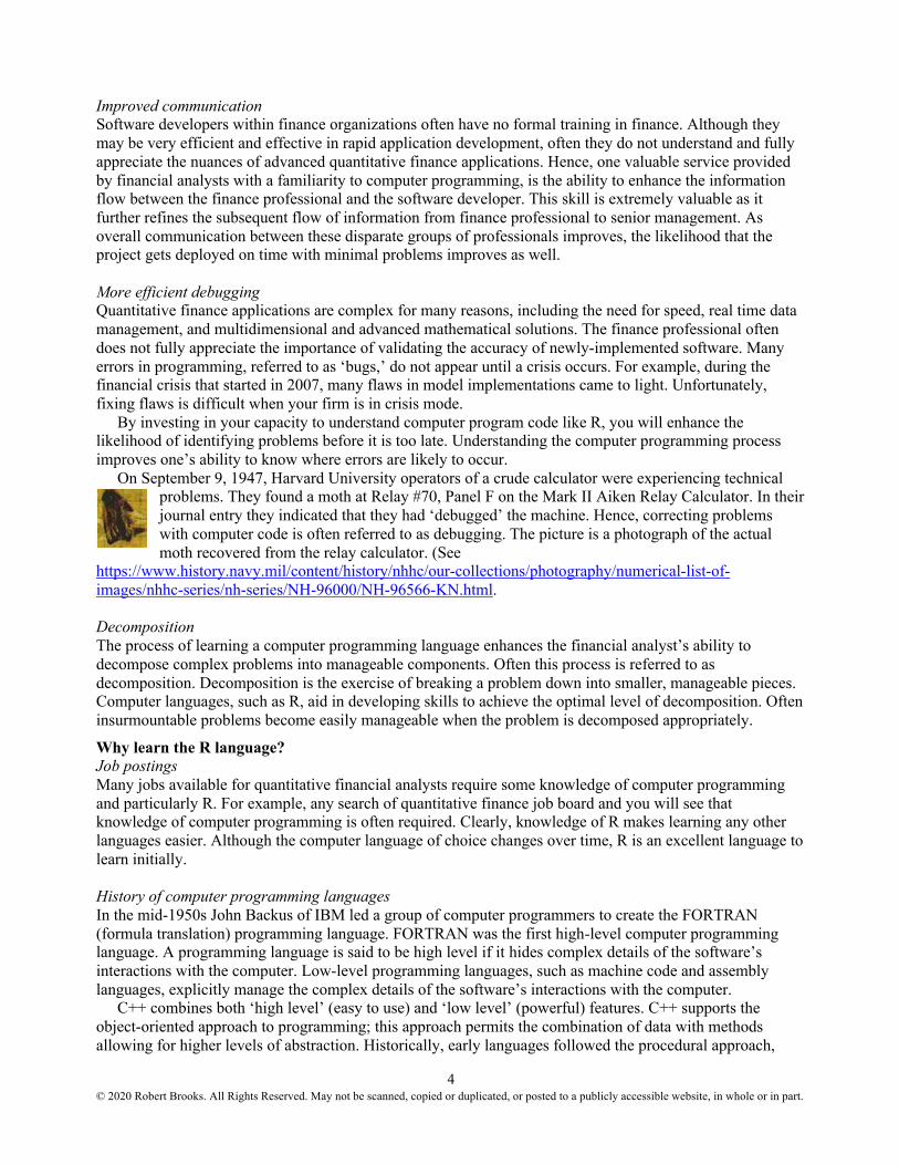
Improved communication Software developers within finance organizations often have no formal training in finance. Although they may be very efficient and effective in rapid application development, often they do not understand and fully appreciate the nuances of advanced quantitative finance applications. Hence, one valuable service provided by financial analysts with a familiarity to computer programming, is the ability to enhance the information flow between the finance professional and the software developer. This skill is extremely valuable as it further refines the subsequent flow of information from finance professional to senior management. As overall communication between these disparate groups of professionals improves, the likelihood that the project gets deployed on time with minimal problems improves as well. More efficient debugging Quantitative finance applications are complex for many reasons, including the need for speed, real time data management, and multidimensional and advanced mathematical solutions. The finance professional often does not fully appreciate the importance of validating the accuracy of newly-implemented software. Many errors in programming, referred to as ‘bugs,’ do not appear until a crisis occurs. For example, during the financial crisis that started in 2007, many flaws in model implementations came to light. Unfortunately, fixing flaws is difficult when your firm is in crisis mode. By investing in your capacity to understand computer program code like R, you will enhance the likelihood of identifying problems before it is too late. Understanding the computer programming process improves one’s ability to know where errors are likely to occur. On September 9, 1947, Harvard University operators of a crude calculator were experiencing technical

problems. They found a moth at Relay #70, Panel F on the Mark II Aiken Relay Calculator. In their journal entry they indicated that they had ‘debugged’ the machine. Hence, correcting problems with computer code is often referred to as debugging. The picture is a photograph of the actual moth recovered from the relay calculator. (See

https://www.history.navy.mil/content/history/nhhc/our-collections/photography/numerical-list-of-images/nhhc-series/nh-series/NH-96000/NH-96566-KN.html. Decomposition The process of learning a computer programming language enhances the financial analyst’s ability to decompose complex problems into manageable components. Often this process is referred to as decomposition. Decomposition is the exercise of breaking a problem down into smaller, manageable pieces. Computer languages, such as R, aid in developing skills to achieve the optimal level of decomposition. Often insurmountable problems become easily manageable when the problem is decomposed appropriately.

Why learn the R language? Job postings Many jobs available for quantitative financial analysts require some knowledge of computer programming and particularly R. For example, any search of quantitative finance job board and you will see that knowledge of computer programming is often required. Clearly, knowledge of R makes learning any other languages easier. Although the computer language of choice changes over time, R is an excellent language to learn initially. History of computer programming languages In the mid-1950s John Backus of IBM led a group of computer programmers to create the FORTRAN (formula translation) programming language. FORTRAN was the first high-level computer programming language. A programming language is said to be high level if it hides complex details of the software’s interactions with the computer. Low-level programming languages, such as machine code and assembly languages, explicitly manage the complex details of the software’s interactions with the computer. C++ combines both ‘high level’ (easy to use) and ‘low level’ (powerful) features. C++ supports the object-oriented approach to programming; this approach permits the combination of data with methods allowing for higher levels of abstraction. Historically, early languages followed the procedural approach,


5

designed as a collection of functions that manage and manipulate data. For example, the cumulative distribution function, denoted N(d), can be viewed as an object that contains data (d) and methods (solving for N()). Viewed as an object containing both the data input and the methods, N(d) can be incorporated into many different option valuation and risk management solutions. Bjarne Stroustrup developed C++ in the late 1970s as a highly optimized, object-oriented language. Hence it is very fast, a feature attractive to the finance industry. Quantitative finance problems are suitable for object-oriented programming5 as contrasted with sequential programming. Unfortunately, C++ remains difficult for many financial analysts. There have been numerous other languages that sought to simplify C++ while preserving its speed and versatility. According to Wikipedia, R was created in the early 1990s with the first version available in 1995. R was based on another programming language known as S. Rapid application development One goal of quantitative analysts is to be able to implement their solutions within an organization rapidly. Hence, it is necessary to be able to both build applications fast, as well as implement them with ease. The object-oriented approach combined with R permits rapid application development (RAD). With many well developed objects prebuilt and rigorously tested, it is relatively simple to complete the implementation of a quantitative model in a very short period of time.

File types R code is typically stored in files with the .R extension. The extension .RPROJ is a project file that aids in managing information related to a specific project. It is created in and used by RStudio. The extension .RDATA is a data file that contains readable information for use in R. The extension .RHISTORY contains information related to prior work within a particular R project.

Why learn R this way? Autonomous versus heteronomous The majority of programming books and other training materials choose to allow the learner to be autonomous when it comes to the particular version (say Mac or PC) of the given language. These materials have the advantage of being applicable to any version, so long as it complies with the existing standards established for R. For our objectives, allowing the learning to be autonomous (having freedom to act independently) versus heteronomous (subject to external standard) was a difficult choice. We chose to limit this material to a particular version (RStudio), rather than make the learning experience generic and applicable for any version. The primary motive is to allow the financial analyst to be equipped to demonstrate his or her work in an efficient way. Within a very short period of time, you will be able to create R code that is user friendly. Our primary objective, however, is not to make you a professional programmer. To this end we seek the delicate balance between keeping the concepts as simple as possible while at the same time permitting the user to develop professional solutions. For the autonomous among us, care is taken to separate the interface code (code focused on interactions with the end-user) and the implementation code (code focused on computing the solution). Because of this separation, it is easy to export the implementation code to other versions and there develop different GUI’s (Graphical User Interface). Current platform The current platform used during the production of this material is RStudio (Version 1.1.442 on a Mac).

5Object-oriented programming (OOP) with C++ is typically identified with four characteristics: encapsulation, inheritance, polymorphism, and abstraction. Object-oriented programming is addressed further in chapter 2.


6

Deliverables The main deliverables illustrated in this material are simple prototype programs. If the goal is to produce fully implementable programs in real time, then the computer source code should be refined by professional software programmers. For example, no effort is made to exhaustively error trap inputs (for example, real numbers as opposed to alphabetic characters) and test for inputs that are out of range (for example, volatility equal to zero causing a division by zero).

Sample programs: Program layout In the remainder of this book there will be references to sample programs. Depending on the version, the repository directory will have the general structure that corresponds to chapters in this book. Thus, the program illustrated below is in the folder, Ch 1 Introduction (Ch 1.1 Program Layout). To illustrate the process, we provide a simple program that runs a console application that does not do anything. The source code will be set in Courier type as follows. # 1.1 Program Layout.R # RStudio layout # This page is the File Window, multiple files open at one time # The page to the immediate right is the Environment Window, # with the Environment tab and History tab # The page below is the Console Window, give interface history # The page below to the right is the Information Window, # Files tab shows Project files (files within the Project folder), # Plots tab shows plots, # Packages show attached and some unattached packages # Help shows any requested help documentation # Program Layout help(base) # One way to get help, very cryptic library(help = "base") # Control goes to the document help("Arithmetic") # Details on arithmetic operators library(base) # This line is not necessary but is the way to include libraries # To load and attach add-on packages, either: library(stats) # Statistics package is included help(stats) # Help tab now has details on the R Stats package # Or: require(Rcpp) # Rcpp package is included ?"Rcpp" # Alternative way to have details on the R Rcpp package # R does not have a formal entry point like C++ (e.g., int main()) x = 100 # When the line above is run, you should see Values x 100 in the Environment window # and x = 100 in the Console window # The next line closes R quit()

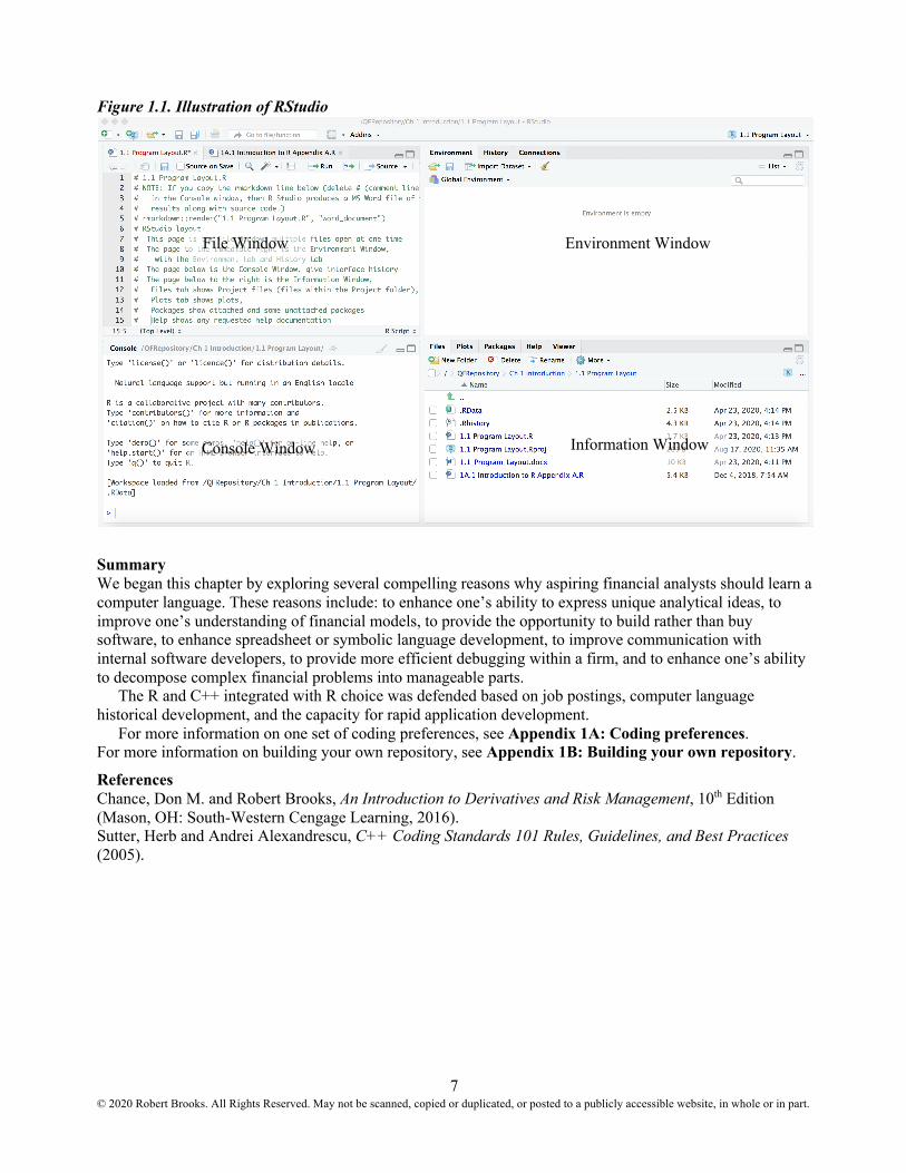
The first line is a comment line (starts with #) and is ignored when the program is implemented. Within the text, we will direct you to the location of the functioning programs provided at http://www.robertebrooks.org/project/buildiingqfawr/. Figure 1.1 illustrates what you should see when Module 1.1 is loaded into RStudio. What you see is likely a bit different depending on your operating system and RStudio version. We point out just a few items. The very top line, in faint gray, is the path along with the name of the R code file in focus within the File Window. The tab, 1.1 Program Layout.R*, is in red and the asterisk indicates changes have been made before the last time it was saved. The Environment Window is in the top right. The Environment tab will contain variables and values while the program is running. The Console Window will provide information important while the program is running. Finally, the Information Window is in the bottom right. The Files tab shows the project files and any other files contained within its folder. Plots can be found at the Plots tab. If the Information Window is too small, then the plots will fail to appear. The Packages tab is important when it is necessary to include different packages that have already been installed in the past. For example, blogdown is a package used to build websites and would appear in the Packages tab if you have ever installed it in the past. The Help tab is very useful as you begin to learn different built-in functions.


7

Figure 1.1. Illustration of RStudio

Summary We began this chapter by exploring several compelling reasons why aspiring financial analysts should learn a computer language. These reasons include: to enhance one’s ability to express unique analytical ideas, to improve one’s understanding of financial models, to provide the opportunity to build rather than buy software, to enhance spreadsheet or symbolic language development, to improve communication with internal software developers, to provide more efficient debugging within a firm, and to enhance one’s ability to decompose complex financial problems into manageable parts. The R and C++ integrated with R choice was defended based on job postings, computer language historical development, and the capacity for rapid application development. For more information on one set of coding preferences, see Appendix 1A: Coding preferences. For more information on building your own repository, see Appendix 1B: Building your own repository.

References Chance, Don M. and Robert Brooks, An Introduction to Derivatives and Risk Management, 10th Edition (Mason, OH: South-Western Cengage Learning, 2016). Sutter, Herb and Andrei Alexandrescu, C++ Coding Standards 101 Rules, Guidelines, and Best Practices (2005).

File Window Environment Window

Console Window Information Window


8

Appendix 1.A: R Coding Preferences Learning objectives

• Determine preferences related to expressing and formatting R code • Provide guidance for naming variables, methods, classes, and files

Introduction Writing R code is part mundane implementation of mathematical ideas and part free-spirited, written expressions of abstract art. The goal here is not to squelch your artistic side, but to provide a consistent framework for you to begin to express your quantitative solutions using R.

Coding preferences Accuracy and readability are vital for any successful R implementation of a quantitative finance problem. Highly readable source code that is inaccurate is nonetheless fatally flawed. It is not, however, difficult to fix readable code. It is highly recommended that you comment your code extensively so that you are able to retrace your steps as well as document what you have done in each piece of code for both debugging and reuse of code. Although accurate but illegible code will work, it cannot be easily maintained. R code presentation The first decision when expressing R code relates to spacing. It is important to keep track of how many brackets are open. It is also important to keep the number of pages printed when debugging to a minimum. Hence we recommend the following rule illustrated with the following snippet of code:

1) Indent two spaces (even for wrapped lines) after each curly bracket ({), place first curly bracket on same line, and close (}) on a new line

for (i in 1:LengthSPY){ if(i==1){ dfSPY$TotalReturn[i]=1 } else { dfSPY$TotalReturn[i] = dfSPY$TotalReturn[i-1]*(1.0 + dfSPY$DailyReturn[i]) } } PV1 = function(Maturity, Rate){ return(exp( -(Rate/100.0) * Maturity) ) } ...

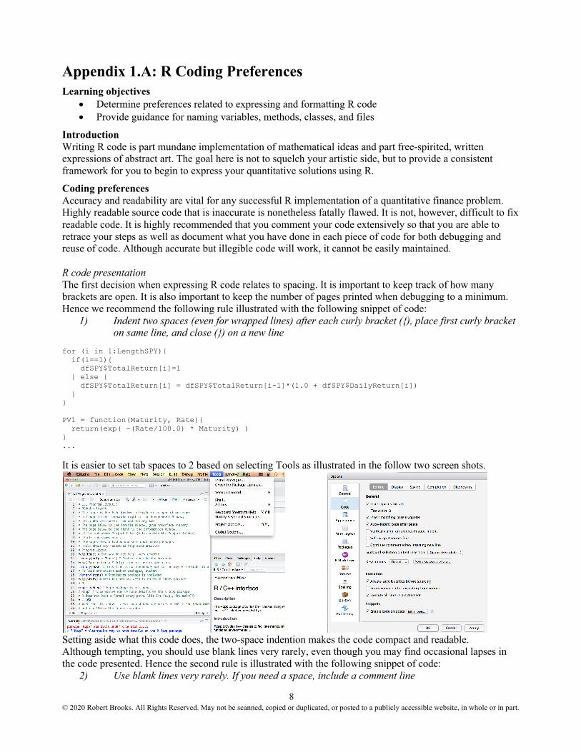
It is easier to set tab spaces to 2 based on selecting Tools as illustrated in the follow two screen shots.

Setting aside what this code does, the two-space indention makes the code compact and readable. Although tempting, you should use blank lines very rarely, even though you may find occasional lapses in the code presented. Hence the second rule is illustrated with the following snippet of code:

2) Use blank lines very rarely. If you need a space, include a comment line


9

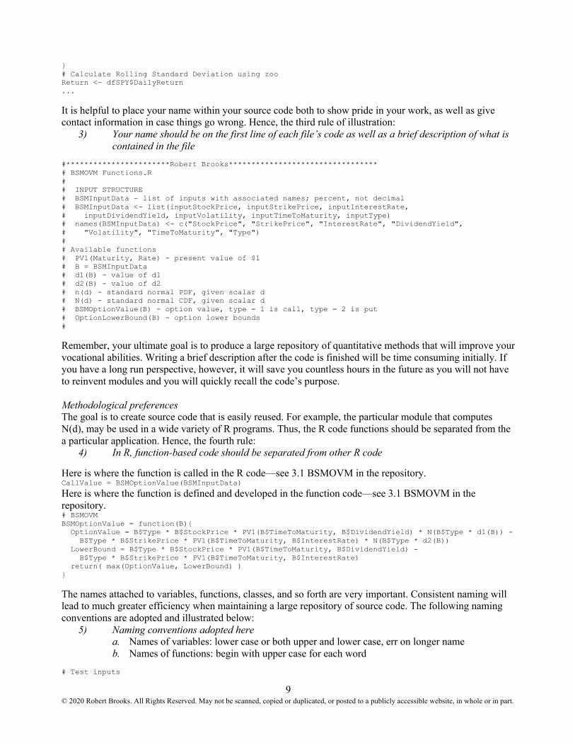
} # Calculate Rolling Standard Deviation using zoo Return <- dfSPY$DailyReturn ...

It is helpful to place your name within your source code both to show pride in your work, as well as give contact information in case things go wrong. Hence, the third rule of illustration:

3) Your name should be on the first line of each file’s code as well as a brief description of what is contained in the file

#***********************Robert Brooks********************************* # BSMOVM Functions.R # # INPUT STRUCTURE # BSMInputData - list of inputs with associated names; percent, not decimal # BSMInputData <- list(inputStockPrice, inputStrikePrice, inputInterestRate, # inputDividendYield, inputVolatility, inputTimeToMaturity, inputType) # names(BSMInputData) <- c("StockPrice", "StrikePrice", "InterestRate", "DividendYield", # "Volatility", "TimeToMaturity", "Type") # # Available functions # PV1(Maturity, Rate) - present value of $1 # B = BSMInputData # d1(B) - value of d1 # d2(B) - value of d2 # n(d) - standard normal PDF, given scalar d # N(d) - standard normal CDF, given scalar d # BSMOptionValue(B) - option value, type = 1 is call, type = 2 is put # OptionLowerBound(B) - option lower bounds #

Remember, your ultimate goal is to produce a large repository of quantitative methods that will improve your vocational abilities. Writing a brief description after the code is finished will be time consuming initially. If you have a long run perspective, however, it will save you countless hours in the future as you will not have to reinvent modules and you will quickly recall the code’s purpose. Methodological preferences The goal is to create source code that is easily reused. For example, the particular module that computes N(d), may be used in a wide variety of R programs. Thus, the R code functions should be separated from the a particular application. Hence, the fourth rule:

4) In R, function-based code should be separated from other R code

Here is where the function is called in the R code—see 3.1 BSMOVM in the repository. CallValue = BSMOptionValue(BSMInputData)

Here is where the function is defined and developed in the function code—see 3.1 BSMOVM in the repository. # BSMOVM BSMOptionValue = function(B){ OptionValue = B$Type * B$StockPrice * PV1(B$TimeToMaturity, B$DividendYield) * N(B$Type * d1(B)) - B$Type * B$StrikePrice * PV1(B$TimeToMaturity, B$InterestRate) * N(B$Type * d2(B)) LowerBound = B$Type * B$StockPrice * PV1(B$TimeToMaturity, B$DividendYield) - B$Type * B$StrikePrice * PV1(B$TimeToMaturity, B$InterestRate) return( max(OptionValue, LowerBound) ) }

The names attached to variables, functions, classes, and so forth are very important. Consistent naming will lead to much greater efficiency when maintaining a large repository of source code. The following naming conventions are adopted and illustrated below:

5) Naming conventions adopted here a. Names of variables: lower case or both upper and lower case, err on longer name b. Names of functions: begin with upper case for each word

# Test inputs


10

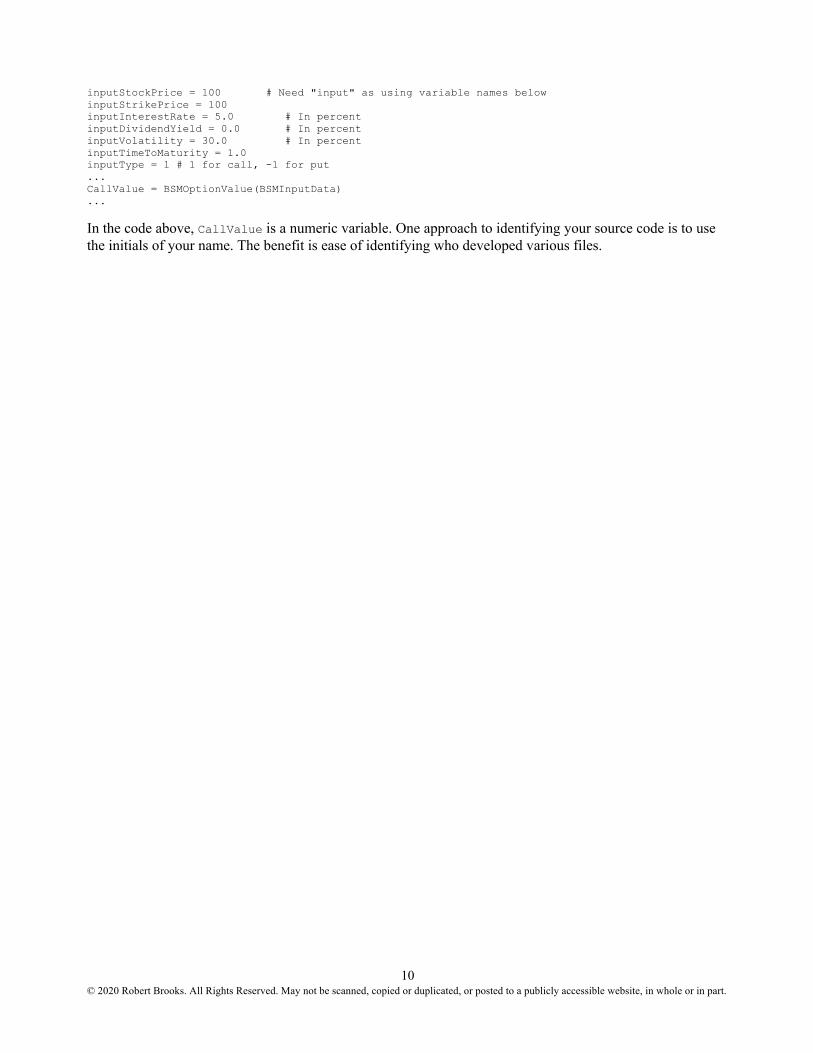
inputStockPrice = 100 # Need "input" as using variable names below inputStrikePrice = 100 inputInterestRate = 5.0 # In percent inputDividendYield = 0.0 # In percent inputVolatility = 30.0 # In percent inputTimeToMaturity = 1.0 inputType = 1 # 1 for call, -1 for put ... CallValue = BSMOptionValue(BSMInputData) ...

In the code above, CallValue is a numeric variable. One approach to identifying your source code is to use the initials of your name. The benefit is ease of identifying who developed various files.


11

Appendix 1.B: Building Your Own Code Repository Learning objectives

• Understand one approach to managing implementation code • Explain detailed steps for managing R code • Emphasize the importance of organizing your quantitative ideas when coding

Introduction The goal of this appendix is to specify one approach to managing source code. The primary goal is to maximize code reuse; ideally, you will build a module that will be used over and over again. The secondary goal is to build detailed organization in your development of quantitative ideas. Often the exercise of implementing a new idea in a computer language will result in numerous improvements to the idea itself. Coding is also much easier if you are detail oriented and very organized.

Repository We will make use of a central repository for R functions. Thus, multiple programs can access the same R functions. For example, consider the estimation function of the cumulative normal distribution (N(d)) used in many option valuation routines, as well as risk management calculations. The approximation method deployed here is accurate to about the ninth decimal place. Suppose this routine is used in 15 different programs that you have to support. If you discover a more accurate estimation method or a bug in the existing N(d) calculation without a repository, you will have to fix 15 different programs. With a repository, you fix one file. Managing subdirectories for source code (recommended when first starting) The method illustrated here is not the only one, but it is very simple. In the root directory of the operating system (or wherever you wish), create a new subdirectory. The one illustrated for this material is QFRepository.6 All R code with functions is placed in the QFRepository (and not in a subdirectory within QFRepository). For efficient R code management, all the R code for various specific purpose programs is contained in subdirectories within QFRepository. For example, all the specific purpose programs covered in this material is placed in subdirectories of the following subdirectory. C:\QFRepository

6Note that the source code provided for this book assumes the repository is located at C:\QFRepository. If it is located anywhere else, the paths must be change.


12

Chapter1.IntroductionLearningobjectivesIntroductionWhyafinancialquantitativeanalystshouldlearnacomputerlanguageConformistversusnon-conformistClearandcrispunderstandingofmodelBuildversusbuyComputerlanguageorspreadsheetsComputerlanguageorsymboliclanguagesImprovedcommunicationMoreefficientdebuggingDecomposition

WhylearntheRlanguage?JobpostingsHistoryofcomputerprogramminglanguagesRapidapplicationdevelopment

FiletypesWhylearnRthisway?AutonomousversusheteronomousCurrentplatform

DeliverablesSampleprograms:ProgramlayoutSummaryReferences

Appendix1.A:RCodingPreferencesLearningobjectivesIntroductionCodingpreferencesRcodepresentationMethodologicalpreferences

Appendix1.B:BuildingYourOwnCodeRepositoryLearningobjectivesIntroductionRepositoryManagingsubdirectoriesforsourcecode(recommendedwhenfirststarting)

chapter 1. introduction - robert e. brooks

Documents