1

Cell Breathing Techniques for Load Balancing inWireless LANs

Yigal Bejerano and Seung-Jae HanBell Laboratories, Lucent Technologies

Abstract: Maximizing the network throughput while provid-ing fairness is one of the key challenges in wireless LANs(WLANs). This goal is typically achieved when the load ofthe access points (APs) is balanced. However, recent studies onoperational WLANs have shown that AP load is often substan-tially uneven. To alleviate such imbalance of load, several loadbalancing schemes have been proposed. These schemes, essen-tially, require proprietary client software or specially-designedWLAN cards at the user computers for controlling the user-APassociation.

In this paper we present a new technique that achieves loadbalancing by reducing the cell size of congested APs, whichis conceptually similar to the so-called cell breathing methodsin cellular networks. The proposed scheme does not requireany modification at the user side neither the standard, but itonly requires the ability of dynamically changing the transmis-sion power of the AP beacon messages. Unlike existing cell-breathing methods, which utilize local optimization heuristics,we develop algorithms that guarantee to find the optimal bea-con power settings, which minimize the load of the most con-gested APs, in polynomial time. We then consider the prob-lem of network-wide min-max load balancing. We prove thatthis problem is

���-hard and cannot be easily approximated. In

spite of this, we identify a variant of the problem, termed min-max priority load balancing, and present polynomial-time al-gorithms to find optimal solutions. Extensive simulations showthat the performance of our cell-breathing methods is compara-ble with or superior to the existing association-based methods.Keywords: Wireless Local Area Networks (WLAN), IEEE802.11, Cell Breathing, Power Control, Load Balancing, Fair-ness, Combinatorial Optimization.

I. INTRODUCTION

Recent studies [1], [2] on operational IEEE 802.11 wirelessLANs (WLANs) have shown that the traffic load is often un-evenly distributed among the access points (APs). In WLANs,by default, a user scans all available channels to detect its nearbyAPs and associates itself with an AP that has the strongest re-ceived signal strength indicator (RSSI), while being oblivious tothe load of APs. As users are, typically, not evenly distributed,some APs tend to suffer from heavy load while their adjacentAPs may carry only light load. Such load imbalance amongAPs is undesirable as it hampers the network from fully utiliz-ing the network capacity and providing fair services to the users.In this paper, we present a novel load-balancing scheme that re-duces the load of congested APs by decreasing their cell size andforcing the users near the boundaries of congested cells to moveto the neighboring less-congested cells. We achieve such celldimensioning by controlling the transmission power of the APbeacon messages, which is conceptually similar to the so-calledcell breathing method in cellular networks [3], [4]. In contrast to

previous studies on cell-breathing that mostly rely on local op-timization heuristics, we present an optimal cell dimensioningalgorithm that finds deterministic min-max load balancing solu-tions. Informally, a WLAN is called min-max load balanced, ifit is impossible to reduce the load of any AP without decreasingthe load of other APs with equal or higher load. Our approachis particularly attractive in that it does not require neither userassistance or standard modification, unlike most existing pro-posals for WLAN load balancing.

A. Load Balancing via User-AP Association Control

Currently the IEEE 802.11 standard [5] does not provide anystandard method to resolve the load imbalance. To overcomethis deficiency, various load balancing schemes have been pro-posed by both the academia and the industry. Most of thesemethods commonly takes the approach of directly controllingthe user-AP association by deploying proprietary client softwareor specially-designed WLAN cards at the user computers. Forinstance, some vendors have already incorporated certain load-balancing features in their device drivers, AP firmwares, andWLAN cards [6], [7]. In these proprietary solutions, the APsbroadcast their load levels to users via modified beacon mes-sages, and each user chooses the least-loaded AP.

Several studies [8]-[14] have proposed a variety of associa-tion metrics instead of using the RSSI as the sole associationcriterion. These metrics typically take into account such fac-tors as the number of users currently associated with an AP, themean RSSI of users currently associated with an AP, and thebandwidth that a new user can get if it is associated with an AP,e.g., [8], [9]. Balachandran et al. [10] proposed to associate auser with the AP that can provide a minimal bandwidth requiredby the user. If there exist many of such APs, the one with thestrongest RSSI is selected. In [11], Velayos et al. introduced adistributed load balancing architecture where the load of an APis defined as the aggregated downlink and uplink traffic throughthe AP. In [12], Kumar et al. proposed an association selectionalgorithm which is based on the concept of proportional fair-ness to balance between throughput and fairness. Most of thesework heuristically determine only the association of newly ar-rived users. [13], [14] are exceptions. Tsai and Lien [13] pro-posed to reassociate users when the total load exceeds a cer-tain threshold or the bandwidth allocated to users drops belowa certain threshold. In [14], an on-line scheme that periodicallyoptimizes the user-AP association is proposed. This work alsoproved a strong correlation between fairness and load balancing,i.e., the fair service is obtained when the AP load is balanced.

Although the user-AP association control approach canachieve load balancing in WLANs, the requirement of deployingproprietary client software/hardware on all (or most) users raisesan acute question about its practicality. Today, WLAN usersfrequently move between different WLANs, such as hotels, air-

2

ports, shopping centers and university campuses.1 Different net-works are managed by different organizations and likely adoptdifferent load balancing mechanisms. It is unrealistic to requirethe users to have the appropriate client modules for each visit-ing network. This motivates the need for a new load-balancingscheme that does not require any proprietary client module norany modification of the standard.

B. Cell Breathing for Load Balancing

In CDMA cellular networks, the coverage and capacity of acell are inversely related with each other [15]. The increase ofthe number of active users in a cell causes the increase of thetotal interference sensed at the base station. Therefore, in con-gested cells, users need to transmit with higher power to main-tain a certain signal-to-interference ratio at the receiving basestation. As the users in a congested cell increase their transmis-sion power, they also increase their interference to the neighbor-ing cells since all cells use the same frequency band in CDMAnetworks. As a result, the overall network capacity may de-crease [3]. Furthermore, since the maximal transmission powerof the users is bounded, the users who are far from the base sta-tion may experience poor services. This so-called near-far prob-lem may result in imbalanced cell handoff boundaries for reverseand forward links, as the latter is determined by the strength ofthe pilot signal of the base stations, independent of the inter-ference [4]. In other words, the cell handoff boundary of thereverse link is tighter than that of the forward link. To over-come these problems the cell breathing approach was proposedby Togo et al.[3] and Jalali [4], independently. This approachshrinks the cell size of congested cells and balances the forwardand reverse link handoff boundaries by reducing the pilot signaltransmission power of the corresponding base stations.

Some studies have explored the benefit of combining the cell-breathing methods with other interference mitigation methods.For instance, in [16], Yang and Ephremides presented a solu-tion for the near-far problem, which is based on the combina-tion of cell-breathing and bandwidth space partitioning. Du etal.[17] proposed a distributed load balancing technique that uti-lizes a bobble oscillation algorithm. In [18], Sang et al. pro-posed a method that coordinates the packet level schedulingwith cell-breathing techniques. Generally speaking, the existingcell-breathing techniques utilize probabilistic local optimizationmethods. Therefore, they do not provide any guarantee on thequality of the solutions. Since the cells of WLANs are muchsmaller than those of cellular networks, the probabilistic localoptimization methods may not work well in WLANs, as we willdemonstrate later in the paper with a simple example. More-over, these techniques cannot be easily applied to IEEE 802.11WLANs, e.g., they require the change of scheduling algorithmsor the knowledge on the user location. This motivates the de-sign for a new cell-breathing method for WLANs which findsdeterministic global optimal solutions.

C. Min-Max Load Balancing Algorithms

In principle, our objective can be viewed as a min-max vari-ant of the unrelated parallel machine scheduling problem [19].The latter seeks for a job-machine association that minimizesthe maximal processing time of any machine, for a given set of�

In many places even free 802.11 access is offered. Recently, some cities e.g.,Philadelphia and San-Francisco, declared their intention to build a free city-wide802.11 networks.

jobs, machines, and the required running time of each job oneach machine2. Since there are extensive literature on parallelmachine scheduling problems and max-min solutions, we dis-cuss here only the most relevant ones to our study. Most of thework on min-max (or max-min) solutions address the problemof finding a fair bandwidth allocation to a set of pre-determinedroutes in a wired network [20], [21].

Selecting routes for the max-min fair bandwidth allocationis a much harder problem and has been studied in [22], [23].Megiddo [22] addressed the single-source fractional flow prob-lem and presented a polynomial time algorithm that finds an op-timal max-min fair solution. Extending this work, Kleinberg etal. [23] considered the case that a connection is routed along asingle path. In particular, their approach can be applied to loadconserving instances of the unrelated parallel machine schedul-ing problem, where each job imposes the same load on the sub-set of machines on which it can be run. They argued that acoordinate-wise constant-factor approximation cannot be foundfor this problem and presented a prefix-sum 2-approximation al-gorithm, in which for every integer ����� the sum of the first �coordinates of the calculated machine load vector sorted in in-creasing order is at most twice the sum of the first � coordinatesof the optimal min-max fractional assignment.

Another important study is the user-AP association controlscheme presented in [14]. This study can be mapped to the gen-eral unrelated parallel machine scheduling, where each job mayhave different running time on each machine. It presents a min-max load balancing algorithm that ensures a coordinate-wise -approximation ratio as compared to the optimal min-max frac-tional solution. Notice that all of these methods require a com-plete control on the job-machine association. This assumption isfeasible for the user-AP association control schemes. However,such freedom of association control is unavailable in the cell-breathing approach, which only implicitly controls the user-APassociation by adjusting the cells’ boundaries. This raises theneed for new min-max load balancing algorithms for the cell-breathing approach.

D. Our Contributions

In this paper we present a new load balancing scheme forIEEE 802.11 WLANs. The proposed scheme adjusts the size ofcells by changing the transmission power of the AP beacon mes-sages without changing the transmission power of the data traf-fic channel. While there exist similar approachs in cellular net-works, to the best of our knowledge, we are the first who appliesthe cell breathing concept to IEEE 802.11 WLANs. More im-portantly, unlike the existing cell breathing studies [3],[4],[16],[17],[18], we tackle the challenge of finding the deterministicglobal optimum instead of relying on local optimization heuris-tics. Our algorithms are not tied to a particular load definition,but support a broad range of load definitions. We treat the loadof an AP as the aggregation of the load contributions of its as-sociated users. The load contributions may be as simple as thenumber of users associated with an AP or can be more sophis-ticated to take account of factors like transmission bit rates andtraffic demands. Our scheme does not require any special assis-tance from users nor any change in the standard. It only requiresthe ability of dynamically changing the transmission power ofWhen a given job cannot be served by a specific machine, infinite running

time is assumed on that machine.

3

the AP beacon messages. Today, commercial AP products al-ready support multiple transmission power levels, so we believethis requirement can be relatively easily achieved via AP soft-ware update.

Our algorithms will be run on a network operation centerwhich collects the load and association information from theAPs via such methods as SNMP. Depending on the extent of theavailable information, we consider two knowledge models. Thefirst model assumes complete knowledge, in which the user-APassociation and the corresponding AP load are known a priorifor all possible beacon power assignments. Since such informa-tion is not readily available in current WLANs, we also considerthe second model, the limited knowledge model, in which onlyinformation on the user-AP association and AP load for the cur-rent beacon power assignment is available. The algorithms forthe complete knowledge model serve as building blocks for thealgorithms for the more practical limited knowledge model.

We present our algorithms in two steps. At first, we addressthe problem of minimizing the load of the most congested APs,whose load is called the congestion load. We present two poly-nomial time algorithms that find optimal solutions, one for thecomplete knowledge model, another for the limited knowledgemodel. These results are intriguing, because similar load bal-ancing problems, e.g., [14], are known to be strong

���-hard. It

is particularly interesting that a polynomial-time optimal algo-rithm exists for the limited knowledge model. Our algorithmsare rooted from a simple observation that as long as the cur-rent power setting ’dominates’ the optimal setting (i.e., each APhas the same or higher power level than its power level in theoptimal solution), an optimal solution can be obtained by a cer-tain sequence of power reduction operations. The algorithmsstart with the maximal power level at all APs and, iteratively,reduce the power of a selected set of APs. For the completeknowledge case, we use the concept of bottleneck set. Afterreducing the power level of all APs in the bottleneck set, theload of each AP is guaranteed to stay the same or strictly lowerthan the initial congested load before the power reduction. Thisproperty ensures monotonic convergence to the optimal solu-tion. For the limited knowledge case, we take a different ap-proach, termed optimal state recording, in which the power lev-els of the congested APs are gradually reduced until the powercannot be reduced any further, while the best solution found sofar is recorded.

Secondly, we address the problem of finding the min-maxload balanced solutions. We prove that this is a strong

���-

hard problem and there exists no good approximation algorithm.More specifically, we prove that there exists no algorithm thatguarantees any coordinate-wise approximation ratio, and the ap-proximation ratio of any prefix-sum approximation algorithm isat least �� ���������� , where � is the number of APs in the network.In spite of this, we identified a variant of this min-max prob-lem, termed min-max priority load balancing, whose optimalsolution can be calculated in polynomial-time for both knowl-edge models. Here, the AP load is defined as an ordered pairof the aggregated load contributions of its associated users anda unique AP priority. By deploying the optimal state recordingmethod, we were able to construct an algorithm that, iteratively,compute each coordinate of the min-max priority load balancedsolutions. We, later, show that our algorithms can be efficientlyembedded into adaptive on-line schemes.

Through extensive simulations, we show that the performance

of our cell-breathing methods is overall comparable with or su-perior to the existing association-control methods, irrespectiveof network load patterns. In particular, we could achieve suchperformance even with a small number of power levels. Ourmin-max priority load balancing algorithms yield near optimalresults even for the non-priority min-max problem by randomlychoosing AP priorities. Although we primarily focus on IEEE802.11 WLANs, our schemes should be applicable to otherwireless networks. Due to the space limitation, we omit someproofs.

II. THE NETWORK MODEL

We consider an IEEE 802.11 WLAN that comprises a set ofaccess points (APs), denoted by � . � ��� denotes the number ofAPs. All APs are attached to a fixed infrastructure, which con-nects them to wired networks, e.g., the Internet. Each AP has acertain transmission range and it can serve only those users thatreside in that range. Each AP is configured to use one of �����transmission power levels, denoted by �"! � �$#&% �(')' �+*-, , wherethe minimal and maximal levels are denoted by

�/.10)2435�76and

� .98;: 3<�>=, respectively. Each power level

� !is iden-

tified by its power index � and its transmission power is ?times stronger than its predecessor

�/!A@CB, where ? is defined

as ? 3ED F � .98;:HG � .10I2, i.e., ?��J� . Because

� ! 3 ?�K � !�@LB ,it follows that

� ! 35� .10)2 K�?!

for every �4#M% �N'I' �+* . Thisassumption is consistent with the transmission power level con-figurations supported by commercial AP products [6], [7]. Wedenote the transmission power of each AP O�#P� by

� 8and its

corresponding power index by Q 8 . For the sake of simplicity, weassume that the AP deployment ensures a high degree of over-laps between the range of adjacent APs. Consequently, everyuser is covered by at least one AP even when all APs are trans-mitting at the minimal power level

�R.10I2. We define the network

coverage area to be the union of the transmission ranges of allAPs in � .

We use S to denote the set of all users in the network cov-erage area and use � ST� to denote their number. We assume thatusers have a quasi-static mobility pattern. In other words, usersare free to move from place to place, but they tend to stay in thesame locations for a long period. This assumption is backed upby recent analysis of mobile user behavior [1], [2]. At any giventime, each user is associated with a single AP. Each AP peri-odically transmits beacon messages for advertising its presence.When a user enters a WLAN, the user initiates a scanning oper-ation, in which it scans all channels (i.e., listening for the bea-con messages) for identifying all APs in its reach. Then, basedon the RSSI’s of the beacon messages, the user associates itselfwith the AP that has the strongest RSSI. Whenever the channelquality deteriorates below a certain threshold, e.g., due to theuser movement, the user initiates a new scanning operation andit may associate itself with a different AP.

The RSSI that a user UV#WS senses for an AP OX#Y� is de-noted by Z\[^] 8 . It depends on the transmission power of APO ,� 8

, and the signal attenuation, which is denoted by ��[^] 8 ,i.e., Z [^] 8_3 � [^] 8 K �>8 . We consider only the signal attenuationthat results from long-term channel condition changes, such aspath-loss and slow fading. We assume that during the short pe-riod of time for executing our algorithms the signal attenuationbetween each user-AP pair does not change. As the user-APassociation depends on the RSSI’s, we can divide the networkcoverage area into � ��� disjoint cells. A cell of an AP O defines

4

the region in which AP O has the strongest RSSI. Note that thecell of an AP O is subsumed in its transmission range and it de-pends not only on the transmission power of O , but also that ofthe other APs in O ’s vicinity.

The transmission bit-rate for a user-AP pair is determined bythe Signal-to-Noise Ratio (SNR), which is the strength of thereceived signal over the accumulated strength of the other in-terfering transmissions and the background noises. Users whoare associated with the same AP may transmit with different bitrates. Each user contributes a certain amount of load on its serv-ing AP, and the load on an AP is the aggregation of the loadcontributions of its associated users. Our algorithms do not re-quire any explicit load definition and just assume that the load ofan AP O , denoted by ` 8 , is the sum of the load contributions ofits associated users. We use � 8 ] [ to denote the load contributionof a user U on an AP O . We assume that this contribution is con-stant3, so that the load of each AP O$#a� is ` 8 3cb [edAfNg � 8 ] [ ,where S 8 denotes the set of users associated with O . The APsthat experience the maximal load are called the congested APsand their load, termed congestion load, is denoted by h . OtherAPs with lower load are called non-congested APs.

Our flexible load model can accommodate many commonly-used load definitions, including the number of users associatedwith an AP as well as more advanced load definitions that maytake account of the effective transmission bit-rate or the averagetraffic demand. It can also deal with the multiplicative user loadcontributions, i.e., ` 8 3ji [edAf g � 8 ] [ , by applying kIlem to bothsides. Table I summarizes the key notations.

Symbol SemanticsnThe set of all access points (APs).oThe bottleneck set of APs.p

( q ) The set of congested APs.rThe set of fixed APs.s;tvu w Attenuation of AP x ’s signal detected by user y .zThe maximal transmission power index.{ w|u t Load contribution of user y to AP x .} w Transmission power of AP x .~ w Transmission power index of AP x , ~ w��_� ����� z�� .� tvu w Signal strength of AP x received by user y .�A network state,

�T�+��� xv� ~ w��-� .��A recorded network state.�The set of all users.� w The set of users associated with AP x .�;w The load of AP x .�The network congested load.��The congestion load of the recorded state.��The AP load vector,

�� ��� � � ��������� �v� �>� � .TABLE I

NOTATIONS.

III. THE CELL BREATHING APPROACH

In this section we present the basic concept that underlies ourapproach. We also address some practical aspects and the algo-rithmic challenges that our approach encounters. In this study,we assume the presence of a Network Operation Center (NOC).APs report to the NOC about their associated users, their loadand additional relevant information. The NOC executes our al-gorithm and configures the APs accordingly.�

In Section III we explain why we consider constant load contributions of theusers although we allow changes of the AP transmission power.

(b) AP b transmit with lower power level than APs a and c .

(a) All APs transmit with the same power level.

a b c

AP transmission range

AP cell size

a b c

AP transmission range

AP cell size

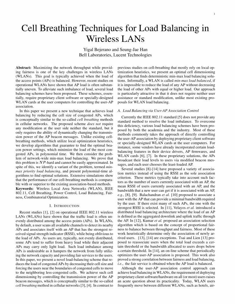
Fig. 1. Balancing the AP load by adjusting their transmission power.

A. The Concept of Cell Breathing

Our scheme reduces the load of congested APs by reducingthe size of the corresponding cells. This forces users near thecongested cells’ boundaries to shift their association to adja-cent (less-congested) APs. Such cell dimensioning can be ob-tained, for instance, by reducing the transmission power of thecongested APs, as we illustrate in Example 1.

Example 1: Consider a WLAN with three APs, O , � and � thattransmit with maximal power

� .98;:and let’s assume that they

are associated with � , � and � users, respectively, as depicted inFigure 1-(a). In this example, we define the load of an AP to bethe number of its associated users. Clearly, � has much higherload than the other two APs. Now, by reducing the transmissionpower of � , the cell size of � is also reduced and four of the usersassociated with � suffer from low signal quality. These usersinitiate scanning operations that cause them to shift to adjacentAPs. As a result, the number of users associated with the threeAPs are now � , � and � , respectively, as illustrated in Figure 1-(b), and the AP load becomes more evenly distributed.  

Reducing the transmission power of an AP affects the chan-nel quality of all of its associated users, and this effect is notlimited to those users that we intend to shift. The users who re-main associated with the considered AP also experience lowerchannel quality and may have to communicate at a lower bit ratethan before. This may result in longer transmission time of usertraffic, which effectively increases the user load contributions onthe AP, if the AP load is determined by considering not only thenumber of users but also the effective user throughput. Thus,we may end up with increasing the load of more APs rather thanreducing the load of the congested APs.

We overcome this problem by the segregation between thetransmission power of the data traffic and that of the AP bea-con messages. On one hand, the transmission bit-rate betweena user and its associated AP is determined by the quality of thedata traffic channel. Transmitting the data traffic with maximalpower4 maximizes the AP-user SNR and the bit-rate. On theother hand, each user determines its association by performinga scanning operation, in which it evaluates the quality of the bea-con messages of the APs in its vicinity. By reducing the beaconmessages’ power level of congested APs, we, practically, shrinkthe size of their cells and, consequently, discourage new userassociation. This concept of controlling the cells’ dimensionsby adapting power levels of the beacon messages is termed cellbreathing. The segregation between the power levels of the datatraffic and the beacon messages is the only modification that¡Power control of the AP data traffic can be done, separately, for reducing

inter-AP interferences. Such power allocation is beyond the scope of this paper.

5

(a) AP a and AP b have the same power level.

a b

u 1 u 2

1 2 a b

u 1 u 2

1 2

(b) AP a has lower power level than AP b, (p a =p b -1).

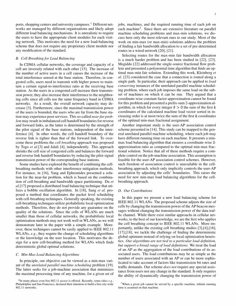
Fig. 2. Example of an execution of the greedy algorithm.

we require from APs. We believe this can be relatively easilyachieved by software update.

B. Triggering User-AP Association Changes

In the long run, the method described above balances the APload by discouraging new user association with congested APs.However, since the cell breathing method does not explicitlycontrol the user-AP association, it may not provide immediaterelief to the congested APs. It is because, once the associationdecision is made, a user stays connected with the same AP aslong as it experiences a satisfactory channel quality, regardlessof the received beacon message strength. For immediate loadreduction, we need to encourage the users in the congested cellsto invoke the scanning operations. One method is reducing thedata traffic power levels of the congested APs for a short pe-riod, which will trigger the scanning mechanism for the usersnear the boundaries of the congested cells. Another method issending ”dis-association” messages to some or all users who areassociated with the congested APs. The latter method providesthe flexibility to select particular users to change their associa-tion without affecting others. In the remainder of this paper, weassume that a proper method is used to trigger association shiftsafter the cell range of an AP is altered and limit our discussionjust to the power level of the beacon messages. That is, when wesay transmission power, we mean only the transmission powerof beacon messages.

C. Algorithmic Challenges

One may consider a greedy algorithm that, reduces the powerlevel of the congested APs until any of the congested APsreaches to the minimal power level. Note that since this algo-rithm attempts to shift users from congested APs to their neigh-bors, the set of congested APs and their load may change duringthe execution of the algorithm. As we demonstrate in Exam-ple 2, even in a very simple case, the greedy algorithm may failto find the optimal solution. Moreover, it can be shown that insome cases the final congestion load is even higher than the ini-tial congestion load.

Example 2: Consider a WLAN with two APs, denoted as Oand � , and two users U B and U£¢ . User U B can only be attached toO and it yields a load of � . User U ¢ can be attached to both APsand chooses an AP with a higher power level, while it choosesO in case of a tie. It produces load of on its associated AP. Weassume that, initially, both APs transmit with the maximal powerlevel, i.e., Q 8 3 Q£¤ 3 � , and therefore both users are associatedwith O whose load becomes � , as shown in Figure 2-(a). Tobalance the load, the greedy algorithm reduces the power levelof O and as a result U ¢ changes the association to � . Now the loadon the two APs are � and , respectively, as depicted in Figure 2-(b). At the next moment, the algorithm will reduce the power of

� , which is now the congested AP, and UL¢ will be shifted backto O . The algorithm continues to reduce the power levels of theAPs, until they both transmit with the minimal power level. Inthe final setting, the load on O will be � and � has no load, whichis obviously not the optimal solution.  

Example 2, demonstrates the need for more sophisticated al-gorithms.

IV. MINIMIZING THE CONGESTION LOAD

This section presents two algorithms for minimizing the APcongestion load, one for the complete knowledge (CK) model,another for the limited knowledge (LK) model.

A. The Problem Statement

Definition 1 (A network state) : A network state ¥ is definedas the beacon message power indices Q 8 of all the APs O$#X� ,i.e., ¥ 3 H �O§¦�Q 8 ��� ¨£O$#©�«ª¬Q 8 #�% �N'I' ��*�, . For simplicity wedenote a state by ¥ 3 H �O§¦�Q 8 �­, .A network state determines the ranges of all AP cells. Whenwe assume that the users are always associated with the APwhose beacon signal has the strongest RSSI, it also determinesthe user-AP association. Therefore, it also determines the setof congested APs, ® , and their congestion load, h . Notice thata user may change its association only when the network statechanges, which is termed a state transition. Let us now defineour objectives.

Definition 2 (AP Congestion Load Minimization) : The APcongestion load minimization problem seeks for a network statethat minimizes the AP congestion load.We address this problem in two types of networks depending onthe information available.

Definition 3 (The Complete Knowledge (CK) Model) : A net-work has complete knowledge when the available informationcomprises the signal attenuation, �H[^] 8 , and the load contribution,� 8 ] [ , for every user-AP pair, a user U�#¯S and an AP O¬#�� .A complete knowledge model is feasible when all users collectthe RSSI information from all of the nearby APs and send the in-formation to the NOC. Such a feature is suggested, for instance,in the IEEE 802.11-k proposal [24]. Unfortunately, this featureis currently not available in most existing WLANs. We use thismodel mainly as a building block of the limited knowledge so-lution.

Definition 4 (The Limited Knowledge (LK) Model) : A net-work has limited knowledge when the available informationcomprises only the set of users that are currently associated witheach AP and the load contributions, � 8 ] [ , of each user U on itsassociated AP O .In the complete knowledge model, the NOC can a priori de-termine the user-AP association in all possible states withoutactually changing the network state. This allows the NOC toperform an off-line calculation of a desired state and to directlyconfigure the APs with the corresponding power levels of thatstate. Such calculation is not possible in the limited knowledgemodel. Nevertheless, we show in the following that for bothmodels the optimal network states can be found.

B. Preliminary Observations

We present some fundamental observations that relevant toour algorithms. In particular, we study the relationship betweenthe AP power reduction and the network state transition.

6

Definition 5 (A Set °�± Power Reduction) : A set °�± power re-duction ( ° ±"² � ) causes a state transition, in which all APs in° ± reduce their power indices by one level and other APs main-tain their current power levels.

Lemma 1: For a set ° ± power reduction, the only possibleassociation changes are for the users who are associated withAPs in ° ± to shift to the APs in the set �©³´° ± . That is, there areno association changes within the set ° ± neither the set �«³P° ± .From Lemma 1 follows Corollary 1.

Corollary 1: A set power reduction of all APs does notchange the user-AP association.

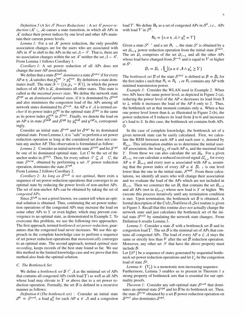
We define that a state ¥ 0)2µ0)¶ dominates a state ¥ 2e·¹¸ if for everyAP O¬#+� satisfies that Q 0I2µ0º¶8 » Q 2e·¹¸8 . By definition a state dom-inates itself. The state ¥ 3 H �O¼¦�Q 8½3 �$�;, , in which the powerindices of all APs is � , dominates all other states. This state iscalled as the maximal power state. We define the network state¥¿¾¹À ¶ as an dominated optimal state, if it is dominated by ¥ 0I2µ0º¶and also minimizes the congestion load of the APs among allnetwork states dominated by ¥ 0)2e0º¶ . An AP O¬#+� is termed an-chor if its power index QC¾ÁÀ ¶8 in the optimal state ¥1¾¹À ¶ is the sameas its power index Q 0)2e0º¶8 in ¥ 0)2e0º¶ . Finally, we denote the load onan AP O in state ¥ 0)2µ0)¶ and ¥¿¾¹À ¶ by ` 0I2µ0)¶8 and `N¾¹À ¶ O , correspond-ingly.

Consider an initial state ¥ 0I2µ0)¶ and let ¥1¾ÁÀ ¶ be its dominatedoptimal state. From Lemma 1, it is ”safe” to perform a set powerreduction operation as long at the considered set does not con-tain any anchor AP. This observation is formulated as follow:

Lemma 2: Consider an initial network state ¥ 0I2µ0)¶ and let ¥¿¾¹À ¶be one of its dominated optimal state. Let  be the set of theanchor nodes in ¥ 0I2µ0º¶ . Then, for every subset ° ±>à �ijX , thestate ¥ 2e·¹¸ , obtained by performing a set ° ± power reductionoperation, dominates the state ¥ ¾ÁÀ

¶.

From Lemma 2 follows Corollary 2.Corollary 2: As long as ¥ 0)2e0º¶ is not optimal, there exits a

sequence of set power reduction operations that converges to anoptimal state by reducing the power levels of non-anchor APs.The set of non-anchor APs can be obtained by taking the set ofcongested APs.

Since ¥¿¾¹À ¶ is not a priori known, we cannot tell when an opti-mal solution is obtained. Thus, continuing the set power reduc-tion operations of the congested APs may increase the load onsome other APs to h or even higher, which may prevent con-vergence to an optimal state, as demonstrated in Example 2. Toovercome this problem, we use the following two approaches.The first approach, termed bottleneck set power reduction, guar-antees that the congested load never increases. We use this ap-proach in the complete knowledge case to perform a sequenceof set power reduction operations that monotonically convergesto an optimal state. The second approach, termed optimal staterecording, keeps records of the best state found so far. We usethis method in the limited knowledge case and we prove that thismethod also finds the optimal solution.

C. The Bottleneck Set

We define a bottleneck set Å Ã � as the minimal set of APsthat contains all congested APs (with load h ) as well as all APswhose load may elevate to h or above due to a set power re-duction operation. Formally, the set Å is defined in a recursivemanner as follows:

Definition 6 (The bottleneck set) : Consider an initial state¥ 6 3 ¥ 0I2µ0º¶ , a load ` 68 for each AP O«#Æ� and a congestion

load h . We define Ç 6 as a set of congested APs in ¥6, i.e., APs

with load h in ¥ 6 .Ç 6 3 AO£� OT#+�VªÈ`

68 3 hT,Given a state ¥ 0�@CB and a set Ç 0�@CB , the state ¥ 0 is obtained by aset Ç 0É@LB power reduction operation from the initial state ¥ 0)2e0º¶ .The set Ç 0 comprises of the set Ç 0�@CB and all the other APswhose load have changed from ¥ 0É@LB and is equal to h or higherat ¥ 0 . Ç 0 3 Ç 0É@LB�Ê AOC� OT#+��ª�`

08 » h¬,The bottleneck set Å of the state ¥

0)2µ0)¶is defined as Å 3 Ç 0 for

the first index Ë such that Ç 0 3 Ç 0É@LB or Ç 0 contains any AP withminimal transmission power.

Example 3: Consider the WLAN used in Example 2. Whentwo APs have the same power level, as depicted in Figure 2-(a),reducing the power level of the AP O decreases its load from �to � , while it increases the load of the AP � only to . Thus,the bottleneck set at that moment contains only O . When O hasone power level lower than � , as illustrated in Figure 2-(b), thepower reduction of � reduces its load from to � and increasesO ’s load to � . In this case, the bottleneck set contains both APs. 

In the case of complete knowledge, the bottleneck set of agiven network state can be easily calculated. First, we calcu-late the RSSI between each AP O and each user U , denoted byZ [e] 8 . This information enables us to determine the initial user-AP association, the load ` 8 of each AP O , and the maximal loadh . From these we can also calculate the set Ç 6 . For a givenÇ 0É@LB , we can calculate a reduced received signal Z ±[^] 8 for everyAP O&#ÌÇ 0É@LB and every user U associated with AP O , assum-ing that the power index of every AP OÍ#4Ç 0É@LB is one levellower than the one in the initial state, ¥ 0I2µ0)¶ . From these calcu-lations, we identify all users who will change their associationand we evaluate the load of the APs which are not included inÇ 0É@LB . Then we construct the set Ç 0 that contains the set Ç 0�@CBand all APs (not in Ç 0�@CB ) whose new load is h or higher. Weexecute this process iteratively until any termination conditionis met. Upon termination, the bottleneck set Å is obtained. Aformal description of the Â�O���� ÇÎ�AϹÏ���Ð��LÐA��� Ñ/Ð�Ï routine is givenin Figure 3. Recall that this routine does not actually change thenetwork state and just calculates the bottleneck set of the ini-tial state ¥ 0I2µ0)¶ by simulating the network state changes. FromDefintion 6 results Lemma 3.

Lemma 3: Consider a state ¥ with a bottleneck set Å and itscongestion load h . The set Å is the minimal set of APs that con-tains all congested APs. The load of every AP O�#W� stays thesame or strictly less than h after the set Å reduction operation.Moreover, any other set ° ± that have the above property mustinclude Å .Let �¥"Òµ, be a sequence of states generated by sequential bottle-neck set power reduction operations and let h Ò be the congestionload of state ¥"Ò .

Lemma 4: Ah Ò , is a monotonic non-increasing sequence.Furthermore, Lemma 3 enables us to present in Theorem 1 astrong property of bottleneck sets that is essential for our opti-mality proofs.

Theorem 1: Consider any sub-optimal state ¥ 0I2µ0º¶ that domi-nates an optimal state ¥9¾ÁÀ ¶ and let Å be its bottleneck set. Then,the state ¥

2^·¹¸obtained by a set Å power reduction operation on¥ 0I2µ0)¶ also dominates ¥1¾¹À ¶ .

7

Routine Calc Bottleneck Set(�CÓ"�+��� xv� ~ Ów ��� �ÁÔ Ó � � )Ô"Õ � ��Ö //used for the termination condition.× � �

while (� Ô7Ø7Ù� Ô7Ø Õ � � and

�ÛÚ x � Ô7ØÁ� ~ ØwÝÜ �Þ� ) do× � ×eß�à//Get the simulated state

� Ø by performing set Ô7Ø Õ �//power reduction operation from state

� غá�غâ .for every AP x � Ô7Ø Õ � let ~ Øw � ~ Ówäã àfor every AP x � n ã Ô7Ø Õ � let ~ Øw � ~ Ów

// Evaluate the new user association and// compute the load on each AP in state

� Ø .� Øw � The load of AP x in state� Ø .Ô�Ø � Ô�Ø Õ �Nå � x^æ x � n´ç � Øw�è � ç � Øw�Ü � Ø Õ �w �

end whileoé� Ô7Øreturn

oend

Fig. 3. A formal description of the bottleneck set calculation routine.

Proof: Since ¥ 0)2e0º¶ is sub-optimal its congestion load is strictlyhigher than the congestion load of ¥9¾¹À ¶ . From Lemma 3 fol-lows that the set Å is the smallest set of APs that contains thecongested APs and its power reduction operation does not in-crease the load of any other AP to h or higher. Consequently,¥ 2e·�¸ is either ¥¿¾¹À ¶ or it dominates ¥1¾ÁÀ ¶ .  D. The Complete Knowledge Algorithm

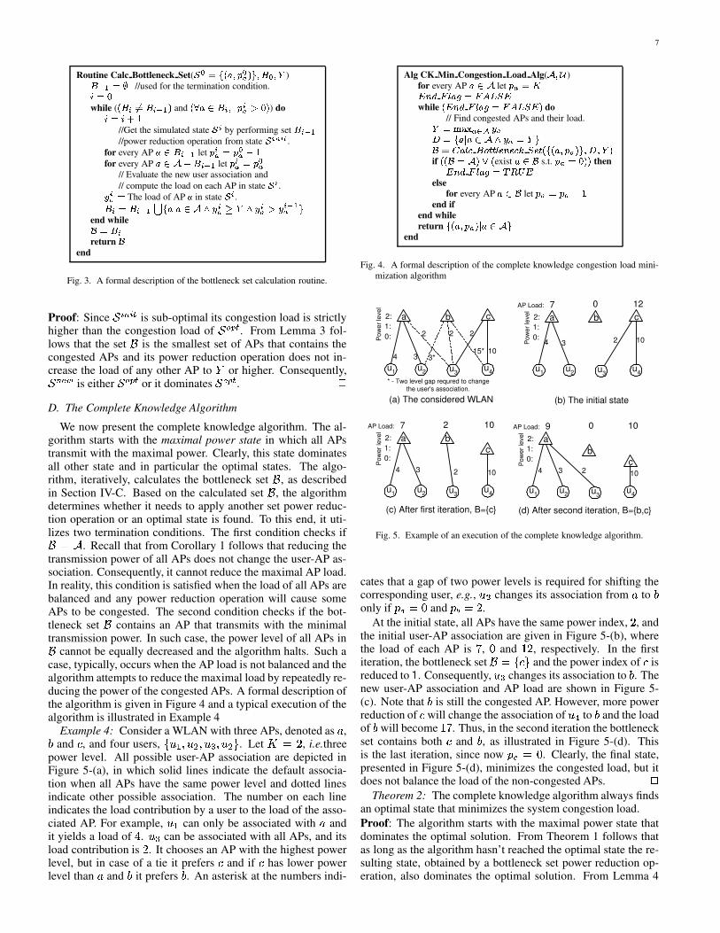
We now present the complete knowledge algorithm. The al-gorithm starts with the maximal power state in which all APstransmit with the maximal power. Clearly, this state dominatesall other state and in particular the optimal states. The algo-rithm, iteratively, calculates the bottleneck set Å , as describedin Section IV-C. Based on the calculated set Å , the algorithmdetermines whether it needs to apply another set power reduc-tion operation or an optimal state is found. To this end, it uti-lizes two termination conditions. The first condition checks ifÅ 3 � . Recall that from Corollary 1 follows that reducing thetransmission power of all APs does not change the user-AP as-sociation. Consequently, it cannot reduce the maximal AP load.In reality, this condition is satisfied when the load of all APs arebalanced and any power reduction operation will cause someAPs to be congested. The second condition checks if the bot-tleneck set Å contains an AP that transmits with the minimaltransmission power. In such case, the power level of all APs inÅ cannot be equally decreased and the algorithm halts. Such acase, typically, occurs when the AP load is not balanced and thealgorithm attempts to reduce the maximal load by repeatedly re-ducing the power of the congested APs. A formal description ofthe algorithm is given in Figure 4 and a typical execution of thealgorithm is illustrated in Example 4

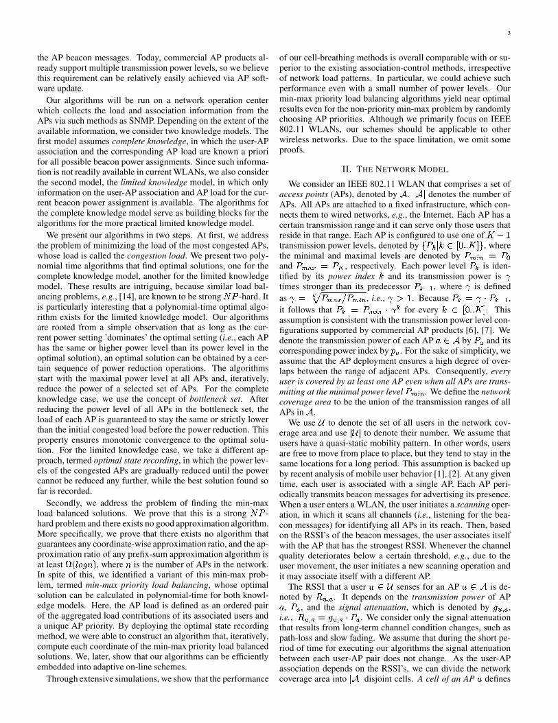
Example 4: Consider a WLAN with three APs, denoted as O ,� and � , and four users, |U B ¦�U§¢e¦êU£ëµ¦êU£¢A, . Let � 3 , i.e.threepower level. All possible user-AP association are depicted inFigure 5-(a), in which solid lines indicate the default associa-tion when all APs have the same power level and dotted linesindicate other possible association. The number on each lineindicates the load contribution by a user to the load of the asso-ciated AP. For example, U B can only be associated with O andit yields a load of � . U ë can be associated with all APs, and itsload contribution is . It chooses an AP with the highest powerlevel, but in case of a tie it prefers � and if � has lower powerlevel than O and � it prefers � . An asterisk at the numbers indi-

Alg CK Min Congestion Load Alg(n � � )

for every AP x � n let ~µw � zì"í q î { x s � î/ï>ð§ñ ìwhile

� ì/í q î { x s � î/ï7ð£ñ ì � do// Find congested APs and their load.� ��ò�óõô w�ö � �;wp ��� x^æ x � n�ç � w � � �o¯�+÷ x {)ø Ô/ùõúûú {ºü í üõø�ý ñ ü ú �É��� xµ� ~ wA��� � p � � �

if���Io¯� n �Hþ � exist x � o s.t. ~µw � �Þ��� thenì/í q î { x s �Èÿ ���>ì

elsefor every AP x � o let ~ w � ~ w ã à

end ifend whilereturn

��� xµ� ~ w�� æ x � n �end

Fig. 4. A formal description of the complete knowledge congestion load mini-mization algorithm

(a) The considered WLAN

* - Two level gap requred to change the user's association.

a b

u 1 u 2

4 3

c

u 3 u 4

Pow

er le

vel

2: 1: 0: 2 2 2

3* 10 15*

(c) After first iteration, B={c}

a b

u 1 u 2

4 3

c

u 3 u 4

Pow

er le

vel

2: 1: 0:

2 10

AP Load: 7 2 10

(d) After second iteration, B={b,c}

a b

u 1 u 2

4 3 c

u 3 u 4

Pow

er le

vel

2: 1: 0:

2 10

AP Load: 9 0 10

a b

u 1 u 2

4 3

c

u 3 u 4

Pow

er le

vel

2: 1: 0: 2 10

AP Load: 7 0 12

(b) The initial state

Fig. 5. Example of an execution of the complete knowledge algorithm.

cates that a gap of two power levels is required for shifting thecorresponding user, e.g., UC¢ changes its association from O to �only if Q 8�3 � and Q ¤ 3 .

At the initial state, all APs have the same power index, , andthe initial user-AP association are given in Figure 5-(b), wherethe load of each AP is � , � and �� , respectively. In the firstiteration, the bottleneck set Å 3 ��A, and the power index of � isreduced to � . Consequently, UCë changes its association to � . Thenew user-AP association and AP load are shown in Figure 5-(c). Note that � is still the congested AP. However, more powerreduction of � will change the association of U�� to � and the loadof � will become ��� . Thus, in the second iteration the bottleneckset contains both � and � , as illustrated in Figure 5-(d). Thisis the last iteration, since now Q�� 3 � . Clearly, the final state,presented in Figure 5-(d), minimizes the congested load, but itdoes not balance the load of the non-congested APs.  

Theorem 2: The complete knowledge algorithm always findsan optimal state that minimizes the system congestion load.Proof: The algorithm starts with the maximal power state thatdominates the optimal solution. From Theorem 1 follows thatas long as the algorithm hasn’t reached the optimal state the re-sulting state, obtained by a bottleneck set power reduction op-eration, also dominates the optimal solution. From Lemma 4

8

results that during the execution of the algorithm the conges-tion load of the WLAN never increases. So now we just haveto show that the algorithm stop with an optimal state. Since thenumber of possible set power reduction operation is limited, Thealgorithm must stop after at most ��K¹� ��� set power reduction op-erations. Now suppose that the final state is not optimal. Sincethe sequence of maximal load h Ò is non-increasing, we concludethat the algorithm must have stopped before finding an optimalstate. The algorithm stopped because Å contains an AP O withQ 8 3 � or Å 3 � . Recall that in the first case, set Å powerreduction operation cannot be done and in the second case, fromCorollary 1 results that such operation does not reduce the con-gestion load. Thus, there is a set ° ± that does not contain thebottleneck set Å and its set power reduction operation reducesthe congestion load. However, from Lemma 3 results that sucha set °�± does not exist.  

It can be shown that the computational complexity of the al-gorithm is �¯ �� K�� ��� ë K�� ST� � . Thus, from theoretical perspective,the algorithm has pseudo-polynomial running time. In practice,� is a small value like �|� , and therefore, for any practical mean,the algorithm has polynomial running time.

E. The Limited Knowledge Algorithm

We now present our limited-knowledge algorithm that findsan optimal state in the limited knowledge case. Unlike the com-plete knowledge case, we cannot calculate the bottleneck set inadvance. We overcome this obstacle by using Corollary 2. Ac-cording to it, as long as a network state is sub-optimal and itdominates an optimal solution, a sequence of set power reduc-tion operations of congested APs converges to the optimal state.This property raises the problem of determining a ”terminationcondition” when an optimal solution is found. Without the ter-mination condition, as demonstrated in Example 2, we may endup with a sub-optimal solution. To this end, we use an optimalstate recording approach that keeps record of the network statewith the lowest congestion load found so far. We define twovariables for recording. The first is ¥ that keeps the recordedstate and the second is h that keeps the congested load value ofstate ¥ , termed the recorded congestion load.

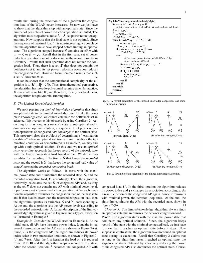
The algorithm works as follows. It starts with the maxi-mal power state and it initializes the recorded state, ¥ , and therecorded congestion load, h , accordingly. Then, the algorithm,iteratively, calculates the set ® of congested APs and, as longas the set ® does not contain any AP with minimal power level,it performs a set ® power reduction operation. After each itera-tion the algorithm evaluates the congestion load of the new stateand if that load is lower than the recorded congestion load, thenthe algorithm updates its variables, ¥ and h , correspondingly.At the end, the algorithm sets the AP power levels according tothe recorded network state. A formal description of the limited-knowledge algorithm is given in Figure 6 and a typical executionis illustrated in Example 5

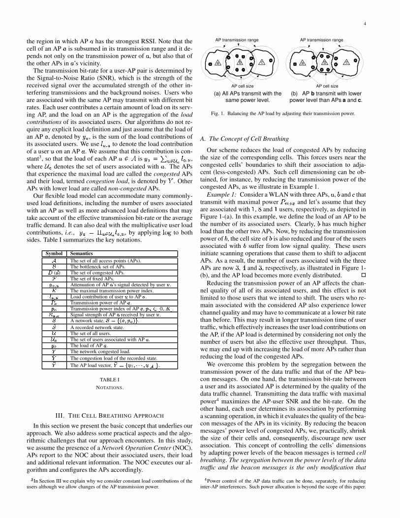
Example 5: Consider the WLAN used in Example 4. At theinitial state, all APs have the same power index, , and the initialuser-AP association and the AP load are shown in Figure 7-(a).Since, � is the congested AP, the algorithm reduces its powerindex twice in two successive iterations, as shown in Figures 7-(b) and 7-(c). After the first iteration the load on � is reducedfrom �A to ��� and the algorithm keeps a record of this state.After the second iteration, � becomes the congested AP with

Alg LK Min Congestion Load Alg(n � � )

for every AP x � n let ~µw � z// Set power indices of all APs to

zand evaluate AP load.��T�+��� xµ� ~vw ����� �Èò�óõô w�ö � �;wì"í q î { x s � î/ï>ð§ñ ì

while� ì/í q î { x s � î/ï7ð£ñ ì � do� �´ò�óõô w�ö � �;wp ��� x^æ x � n�ç �;w � � �

if (exist x � p s.t. ~ w � � ) thenì"í q î { x s �Èÿ ���>ìelse

// Decrease power indices of all APs inp

byà

// and evaluate AP load.for every AP x � p let ~ w � ~ w ã à� ��ò�óõô w�ö � �;wif� �� �� � then��¯����� xv� ~ wA����� � �

end ifend if

end whilereturn

��.

end

Fig. 6. A formal description of the limited-knowledge congestion load mini-mization algorithm

(d) After 3rd iteration, D={c}

a b

u 1 u 2

4 3 c

u 3 u 4

Pow

er le

vel

2: 1: 0:

2 10

AP Load: 9 0 10

(c) After second iteration, D={b}

a b

u 1 u 2

4 3 c

u 3 u 4

Pow

er le

vel

2: 1: 0:

2

15

AP Load: 7 17 0

(b) After first iteration, D={c}

a b

u 1 u 2

4 3

c

u 3 u 4

Pow

er le

vel

2: 1: 0:

2 10

AP Load: 7 2 10

(a) initial state, D={c}

a b

u 1 u 2

4 3

c

u 3 u 4

Pow

er le

vel

2: 1: 0:

2 10

AP Load: 7 0 12

Fig. 7. Example of an execution of the limited knowledge algorithm.

congested load ��� . In the third iteration the algorithm reducesits power index and U£ë changes its association accordingly. Asa result, � becomes the congested AP again. Since it transmitswith minimal power, the iteration loop ends. At the end, thealgorithm configures the APs with the recorded state, shown inFigure 7-(b).  

Theorem 3: The limited-knowledge algorithm always findsan optimal state that minimizes the network congestion load.Proof: The algorithm starts with the maximal power state thatdominates any optimal solution. Since, the algorithm keepsrecord of the state with the minimal congested load, we just haveto show that it reaches an optimal state before it stops. Nowsuppose in contrast that the algorithm have not found an optimalstate during its execution. Recall that Corollary 2 claims thatas long as the algorithm haven’t reached an optimal state, thesequence of states obtained by iteratively reducing the powerof the congested APs also dominates the optimal state. Conse-

9

quently, the algorithm stops with a sub-optimal state that domi-nates the optimal state. However, the algorithm halts when anycongested AP transmits with minimal power. Thus the load onthis AP cannot be reduced by further power reduction opera-tions. This implies that either the final state is optimal or it doesnot dominate an optimal state, which contradicts our assumptionthat the algorithm stopped before finding an optimal state.  

V. FINDING A MIN-MAX LOAD BALANCED STATE

The algorithms presented in Section IV minimize the networkcongestion load but they do not necessarily balance the load ofthe non-congested APs, as demonstrated in Examples 4 and 5.In this section, we consider the min-max load balancing solu-tions that not only minimize the network congestion load butalso balance the load of the non-congested APs. This objectiveis formally defined in Section V-A. Unfortunately, this problemis���

-hard and it is hard to find even an approximated solution.In spite of this, we introduce a variant of the min-max problem,termed min-max priority-load balancing problem, whose opti-mal solution can be found in polynomial time. We present ouralgorithm for this problem in Section V-B. Our solution is givenfor the limited-knowledge model, obviously, it can be used forcomplete-knowledge model as well.

A. The Problem Statement

A commonly used approach to evaluate the quality of a load-balancing method is whether it generates a min-max load bal-anced solution [14], [23]. Informally, we say that a network stateis min-max load balanced if there is no way to reduce the loadof any AP without increasing the load of another AP with sameor higher load. We define the load vector,

�h 3 |` B ¦�K|K�KÞ¦�`� �� ), ,of a state ¥ to be the � ��� -tuple consisting of the load of each APsorted in decreasing order.

Definition 7 (Min-Max Load Balanced Network State) : Afeasible network state ¥ is called min-max load balanced if itscorresponding load vector

�h 3 |` B ¦�K�K|K�¦�`� �� º, has the same orlower lexicographical value than any other load vector

�h ± 3 |` ±B ¦�K|K�KÞ¦�` ± �� , of any other feasible state ¥ ± . In other words, if�h��3 �h ± where�h is the load vector of a min-max load balanced

state, there exists an index � such that ` Ò�� ` ±Ò and for everyindex Ë � � , it follows that ` 0 3 ` ±0 .

We now show that the problem of finding a min-max loadbalanced state is

���-hard. Furthermore, we prove that even a

simpler problem, i.e., the problem of identifying the minimalset of congested APs for a known minimal congestion load, isby itself

���-hard.

Theorem 4: Consider a WLAN and let h be a known lowerbound on its congestion load that can be obtained by the cellbreathing approach. Then, identifying a network state that min-imizes the number of congested APs is

���-hard, even for in-

stances with only two power levels.Proof: For the sake of simplicity, we assume that the load gen-erated by a user on its associated AP may be zero. The problemstays NP-hard also when the load of a user is strictly positive.We prove this theorem by reducing any instance of the minimaldominating set (MDS) [26] problem to the considered state se-lection problem. Recall that the MDS problem of a given graph� �� ¦��Î� is a known

���-hard problem that seeks for the small-

est subset � ² � such that every node in �4³�� has at leastone neighbor in � . Consider a graph

� �� ¦��_� and let��� à �

be the set of nodes that contains node � and all its neighbors inthe graph

�. We construct a WLAN with � ��� users, denoted byS , and � �� APs, denoted by � , that can transmit in one of two

power level, i.e., � 3 � . For each node �P# � , we define anAP O � #�� and a user U � #ÈS . User U � can be associated withany AP O �"! such that ��±¿# �#� . If the power index of AP O � is� or all APs O � ! , � ± # � � , have power index � , then user U � isassociated with AP O � and produces load of � . Otherwise, userU � is associated with one of the other AP O � ! , � ± # �$� ³� %�(,with power level � and it does not yield any load on this AP.Note that in our construction the load of an AP may be either �or zero.

We claim that the graph� &�"¦'�_� has a dominating set of size( if and only if there is a network state such that ( APs have

load � and all other APs have load � . If the graph�

has a dom-inating set � à � of size ( , then we assign power index �to every AP O � , ��#)� and � to the other APs. Since � is adominating set, result that all users will be associated with APsO � , � #*� . Thus, the number of APs with load � is ( . Nowsuppose that there is a power level selection that yields ( APswith load � . Clearly, each user U � is associated with one AP O � ! ,� ± # �#� . Thus we just have to show that the load of this APmust be � . If U � is associated with AP O � then, by definition,the load of O � is � . Otherwise, U � is associated with an AP O � ! ,� ± # �#� ³W +�¼, . Thus, the power index of this AP must be � andconsequently also user U � ! is associated with AP O � ! . Therefore,the load of AP O � ! must be � . From the above follows that foreach set

� �at least one of the corresponding APs has load � . In

other words, the APs with load � define a dominating set of size( for the graph�

and this completes our proof.  Corollary 3: The problem of finding a min-max load bal-

anced state is���

-hard.The above proofs are based on the reduction from the minimal

dominating set (MDS) problem. Recall the MDS problem is notjust hard to calculate, it is also hard to approximate and there isno algorithm that can find an approximation ratio smaller then�£kIlem¼ õ� �È� � , for some ���&� , unless

�Æ3����[25]. By using this

reduction and the hardness property of the MDS problem, it canbe shown that our min-max load balancing problem is also hardto approximate.

Theorem 5: There exists no polynomial algorithm that canensure ? -coordinate-wise approximation solutions to our min-max load balancing problem for any ? , unless

�Í3V���.

Theorem 6: There exists no polynomial algorithm that canensure ? -prefix-sum approximation solutions to our min-maxload balancing problem for ? � � KHk)l^m�� ��� , for some �W� � ,unless

�Í3����.

In spite of the���

-hardness, we now turn to present a variantof the min-max load balancing problem that its optimal solutioncan be calculated in polynomial time. In this problem, we as-sume that each AP OW#©� has a unique priority, also termed aweight, , 8 # %º�^')'û� ��� * , that indicates the AP’s importance. Inthis study we do not address the problem of allocating priorityto the APs. In the following we give a new AP load definition,termed a priority load, for this problem.

Definition 8 (A priority load of an AP) : Consider an AP O¬#� with priority , 8 and let � 8 3 b [^dAf g � 8 ] [ be the aggregatedload of all of its associated users. The priority load of AP O ,denoted by ` 8 , is defined as the ordered pair ` 8 3 �� 8 ¦�, 8 � .

For simplicity we refer to an AP priority load by the AP load.We say that AP O has higher load than AP � if ` 8\3 �� 8 ¦-, 8 � has

10

a higher lexicographically value than `�¤ 3 ��ɤ|¦-,�¤õ� , i.e., one ofthe following two condition satisfied: (1) � 8 �V� ¤ , or (2) � 8½3 � ¤and , 8 � ,9¤ . Thus, our new objective is finding a network statethat provides a min-max priority load balanced solution.

Since there are no two APs with the same priority, results thatthere are no two AP with the same (priority) load. This ensuresthe following useful property.

Property 1: With the priority load definition, at any networkstate, the set of congested APs always contains a single AP.

B. The Min-Max Algorithm

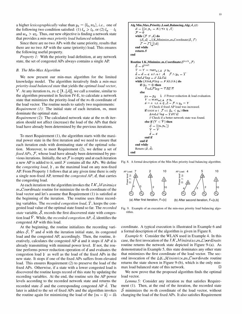
We now present our min-max algorithm for the limitedknowledge model. The algorithm iteratively finds a min-maxpriority-load balanced state that yields the optimal load vector,�h . At any iteration ( , ( #a%º�^')'û� �È� * , we call a routine, similar tothe algorithm presented in Section IV-E, to calculate a networkstate that minimizes the priority-load of the ( -th coordinate ofthe load vector. The routine needs to satisfy two requirements:Requirement (1): The initial state of each iteration, ( , mustdominate the optimal state.Requirement (2): The calculated network state at the ( -th iter-ation should not affect (increase) the load of the APs that theirload have already been determined by the previous iterations.

To meet Requirement (1), the algorithm starts with the maxi-mal power state in the first iteration and we need to ensure thateach iteration ends with dominating state of the optimal solu-tion. Moreover, to meet Requirement (2), we define a set offixed APs, . , whose load have already been determined by pre-vious iterations. Initially, the set . is empty and at each iterationa new AP is added to it, until . contains all the APs. We definethe congesting load, h , as the maximal load on any non-fixedAP. From Property 1 follows that at any given time there is onlya single non-fixed AP, termed the congested AP, / , that carriesthe congesting load.

At each iteration ( the algorithm invokes the 0ä� 1 ËÁ�CË ( Ë32HÐ( Â��v��4�/^ËÁ�LOHÏ�Ð routine for minimize the ( -th coordinate of theload vector and let’s assume that Requirement (1) is satisfied atthe beginning of the iteration. The routine uses three record-ing variables. The recorded congestion load, h , keeps the con-gested load value of the optimal state found so far. The recordedstate variable, ¥ , records the first discovered state with conges-tion load h . While, the recorded congestion AP, / , identifies thecongested AP with this load.

At the beginning, the routine initializes the recording vari-ables ¥ , h and / with the iteration initial state, its congestedload and the congested AP, accordingly. Then, the routine, it-eratively, calculates the congested AP / and it stops if AP / isalready transmitting with minimal power level. If not, the rou-tine performs power reduction operation of / and evaluates thecongestion load h as well as the load of the fixed APs in thenew state. It stops if one of the fixed APs suffers from elevatedload. This ensures Requirement (2) to preserve the load of thefixed APs. Otherwise, if a state with a lower congested load isdiscovered the routine keeps record of this state by updating therecording variables. At the end, the routine sets the AP powerlevels according to the recorded network state and returns therecorded state ¥ and the corresponding congested AP / . Thelater is added to the set of fixed APs and the algorithm invokesthe routine again for minimizing the load of the ( � �A�ä³XÏ-5

Alg Min Max Priority Load Balancing Alg(n � � )�¯�+��� xv� ~vw � z � æ Ú x � n �r ��Ö

while� r Ù� n � do�I� �Áq � � LK Minimize m Coordinate(

� � r )r � r å � q �end whilereturn

�end

Routine LK Minimize m Coordinate(� غá�غâ � r )��¯�È� Ø)á|Ø)â�� � � �´ò�óõô w�ö � Õ76 �;w�q � q � x98 � ú � x � n ã r ç �;w � �ì"í q î { x s � î/ï7ð£ñ ì

while� ì/í q î { x s � î/ï7ð£ñ ì � do

if (~;: � � ) thenì/í q î { x s ��ÿ �<�>ìelse~ : � ~ : ã à // Power reduction & load evaluation.� �Èò�óõô w|ö � Õ76 �;wq � x=8 � ú � x � n ã r ç � w � �

// Check if fixed AP load was increased.if (exist x � r s.t.

��;w �;w ) thenì/í q î { x s �Èÿ �<�>ì// Check if a better network state was found.

else if� �� �� � then��T����� xv� ~vw �-��� � ��q � q

end ifend if

end whileReturn (

��,�q ).

end

Fig. 8. A formal description of the Min-Max priority-load balancing algorithm.

(a) After first iteration, F={c} (b) After second iteration, F={c,b}

a b

u 1 u 2

4 3

c

u 3 u 4

Pow

er le

vel

2: 1: 0:

2 10

AP Load: 7 2 10

a

b

u 1 u 2

4 3

c

u 3 u 4

Pow

er le

vel

2: 1: 0:

2 10

AP Load: 4 5 10

Fig. 9. Example of an execution of the min-max priority load balancing algo-rithm.

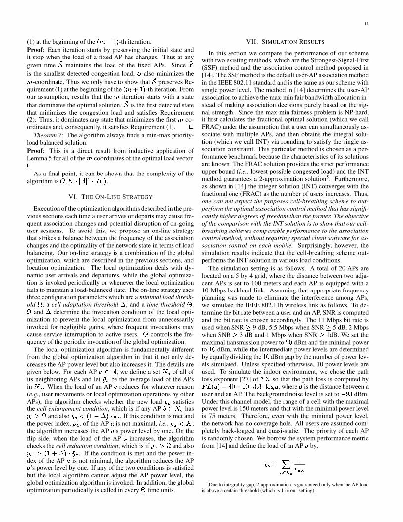
coordinate. A typical execution is illustrated in Example 6 anda formal description of the algorithm is given in Figure 8.

Example 6: Consider the WLAN used in Example 4. In thiscase, the first invocation of the 0ä� 1 ËÁ�CË ( Ë32HÐ ( Â��v��4;/^Ë-�LOHÏ�Ðroutine returns the network state depicted in Figure 9-(a). Asdemonstrated in Example 5, this state dominates any other statethat minimizes the first coordinate of the load vector. The sec-ond invocation of the 0 � 1 ËÁ�CË ( Ë>2HÐ ( Â��v��4;/eËÁ�LOHÏ�Ð routinereturns the state shown in Figure 9-(b), which is the only min-max load balanced state of this network.  

We now prove that the proposed algorithm finds the optimalload vector.

Lemma 5: Consider any iteration ( that satisfies Require-ment (1). Then, at the end of the iteration, the recorded state¥ minimizes the ( -th coordinate of the load vector, without

changing the load of the fixed APs. It also satisfies Requirement

11

(1) at the beginning of the ( ����� -th iteration.Proof: Each iteration starts by preserving the initial state andit stop when the load of a fixed AP has changes. Thus at anygiven time ¥ maintains the load of the fixed APs. Since his the smallest detected congestion load, ¥ also minimizes the( -coordinate. Thus we only have to show that ¥ preserves Re-quirement (1) at the beginning of the ( ����� -th iteration. Fromour assumption, results that the ( iteration starts with a statethat dominates the optimal solution. ¥ is the first detected statethat minimizes the congestion load and satisfies Requirement(2). Thus, it dominates any state that minimizes the first ( co-ordinates and, consequently, it satisfies Requirement (1).  

Theorem 7: The algorithm always finds a min-max priority-load balanced solution.Proof: This is a direct result from inductive application ofLemma 5 for all of the ( coordinates of the optimal load vector. 

As a final point, it can be shown that the complexity of thealgorithm is �¯ �� K^� ��� � K�� ST� � .

VI. THE ON-LINE STRATEGY

Execution of the optimization algorithms described in the pre-vious sections each time a user arrives or departs may cause fre-quent association changes and potential disruption of on-goinguser sessions. To avoid this, we propose an on-line strategythat strikes a balance between the frequency of the associationchanges and the optimality of the network state in terms of loadbalancing. Our on-line strategy is a combination of the globaloptimization, which are described in the previous sections, andlocation optimization. The local optimization deals with dy-namic user arrivals and departures, while the global optimiza-tion is invoked periodically or whenever the local optimizationfails to maintain a load-balanced state. The on-line strategy usesthree configuration parameters which are a minimal load thresh-old � , a cell adaptation threshold ? , and a time threshold @ .� and ? determine the invocation condition of the local opti-mization to prevent the local optimization from unnecessarilyinvoked for negligible gains, where frequent invocations maycause service interruption to active users. @ controls the fre-quency of the periodic invocation of the global optimization.

The local optimization algorithm is fundamentally differentfrom the global optimization algorithm in that it not only de-creases the AP power level but also increases it. The details aregiven below. For each AP OP#Y� , we define a set

� 8of all of

its neighboring APs and let A` 8 be the average load of the APsin� 8

. When the load of an AP O reduces for whatever reason(e.g., user movements or local optimization operations by otherAPs), the algorithm checks whether the new load ` 8 satisfiesthe cell enlargement condition, which is if any AP �é# � 8 has`^¤��&� and also ` 8 � ���³B?¯�RKCA` 8 . If this condition is met andthe power index, Q 8 , of the AP O is not maximal, i.e., Q 8 � � ,the algorithm increases the AP O ’s power level by one. On theflip side, when the load of the AP O increases, the algorithmchecks the cell reduction condition, which is if ` 8 �&� and also` 8 �M ê�\�D?é�9KEA` 8 . If the condition is met and the power in-dex of the AP O is not minimal, the algorithm reduces the APO ’s power level by one. If any of the two conditions is satisfiedbut the local algorithm cannot adjust the AP power level, theglobal optimization algorithm is invoked. In addition, the globaloptimization periodically is called in every @ time units.

VII. SIMULATION RESULTS

In this section we compare the performance of our schemewith two existing methods, which are the Strongest-Signal-First(SSF) method and the association control method proposed in[14]. The SSF method is the default user-AP association methodin the IEEE 802.11 standard and is the same as our scheme withsingle power level. The method in [14] determines the user-APassociation to achieve the max-min fair bandwidth allocation in-stead of making association decisions purely based on the sig-nal strength. Since the max-min fairness problem is NP-hard,it first calculates the fractional optimal solution (which we callFRAC) under the assumption that a user can simultaneously as-sociate with multiple APs, and then obtains the integral solu-tion (which we call INT) via rounding to satisfy the single as-sociation constraint. This particular method is chosen as a per-formance benchmark because the characteristics of its solutionsare known. The FRAC solution provides the strict performanceupper bound (i.e., lowest possible congested load) and the INTmethod guarantees a 2-approximation solution5. Furthermore,as shown in [14] the integer solution (INT) converges with thefractional one (FRAC) as the number of users increases. Thus,one can not expect the proposed cell-breathing scheme to out-perform the optimal association control method that has signifi-cantly higher degrees of freedom than the former. The objectiveof the comparison with the INT solution is to show that our cell-breathing achieves comparable performance to the associationcontrol method, without requiring special client software for as-sociation control on each mobile. Surprisingly, however, thesimulation results indicate that the cell-breathing scheme out-performs the INT solution in various load conditions.

The simulation setting is as follows. A total of 20 APs arelocated on a 5 by 4 grid, where the distance between two adja-cent APs is set to 100 meters and each AP is equipped with a10 Mbps backhaul link. Assuming that appropriate frequencyplanning was made to eliminate the interference among APs,we simulate the IEEE 802.11b wireless link as follows. To de-termine the bit rate between a user and an AP, SNR is computedand the bit rate is chosen accordingly. The 11 Mbps bit rate isused when SNR » 9 dB, 5.5 Mbps when SNR » 5 dB, 2 Mbpswhen SNR » 3 dB and 1 Mbps when SNR » 1dB. We set themaximal transmission power to µ� dBm and the minimal powerto �|� dBm, while the intermediate power levels are determinedby equally dividing the ��� dBm gap by the number of power lev-els simulated. Unless specified otherwise, 10 power levels areused. To simulate the indoor environment, we chose the pathloss exponent [27] of �(' � , so that the path loss is computed by� 0Ý �/H� 3 �^�1³P�|�1K��N' �1K�k)l^mF/ , where / is the distance between auser and an AP. The background noise level is set to ³HGe� dBm.Under this channel model, the range of a cell with the maximalpower level is 150 meters and that with the minimal power levelis 75 meters. Therefore, even with the minimal power level,the network has no coverage hole. All users are assumed com-pletely back-logged and quasi-static. The priority of each APis randomly chosen. We borrow the system performance metricfrom [14] and define the load of an AP O by,

` 8\3JI[^d7K g�4|[^] 8

LDue to integrality gap, 2-approximation is guaranteed only when the AP load

is above a certain threshold (which is 1 in our setting).

12

0

0.2

0.4

0.6

0.8

1

1.2

2 4 6 8 10 12 14 16 18 20

Ya

AP Index

SSFMin-Congestion

Min-MaxINT

FRAC

Fig. 10. Load comparison in networks withà �;� random users.

0

0.1

0.2

0.3

0.4

0.5

0.6

0.7

0.8

2 4 6 8 10 12 14 16 18 20

Ya

AP Index

SSFMin-Congestion

Min-MaxINT

FRAC

Fig. 11. Load comparison in networks with M � random users.

where 4 [^] 8 is the bit rate with which the user U communicateswith the AP O and N 8 is the set of users that are associated withAP O . Due to space limitation, we provide only few charts withtypical results of our simulations.

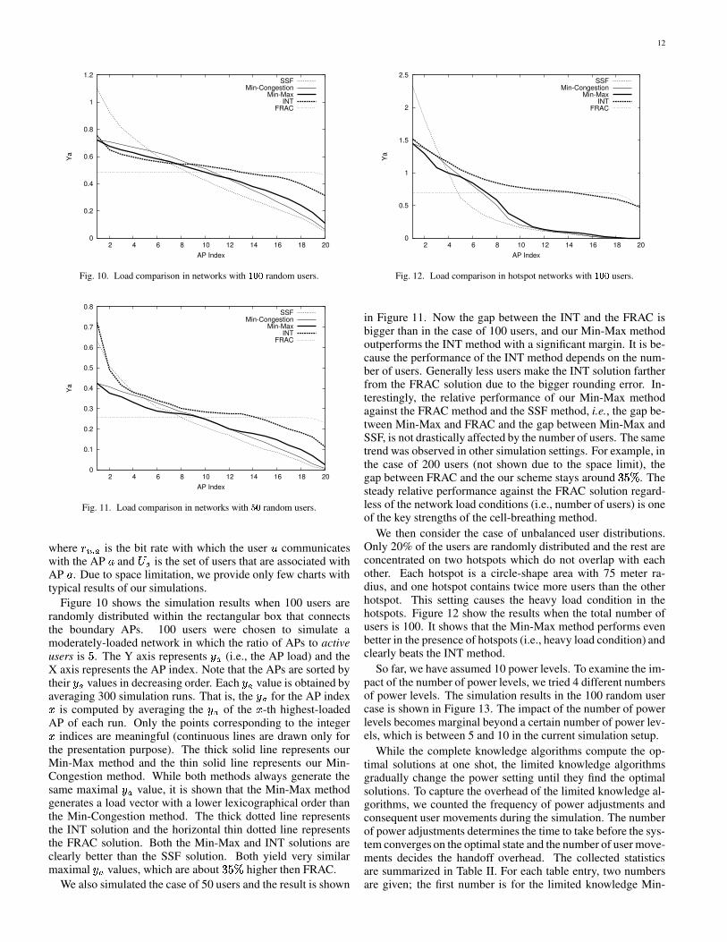
Figure 10 shows the simulation results when 100 users arerandomly distributed within the rectangular box that connectsthe boundary APs. 100 users were chosen to simulate amoderately-loaded network in which the ratio of APs to activeusers is O . The Y axis represents ` 8 (i.e., the AP load) and theX axis represents the AP index. Note that the APs are sorted bytheir ` 8 values in decreasing order. Each ` 8 value is obtained byaveraging 300 simulation runs. That is, the ` 8 for the AP indexP is computed by averaging the ` 8 of the P -th highest-loadedAP of each run. Only the points corresponding to the integerP indices are meaningful (continuous lines are drawn only forthe presentation purpose). The thick solid line represents ourMin-Max method and the thin solid line represents our Min-Congestion method. While both methods always generate thesame maximal ` 8 value, it is shown that the Min-Max methodgenerates a load vector with a lower lexicographical order thanthe Min-Congestion method. The thick dotted line representsthe INT solution and the horizontal thin dotted line representsthe FRAC solution. Both the Min-Max and INT solutions areclearly better than the SSF solution. Both yield very similarmaximal ` 8 values, which are about �QO7R higher then FRAC.

We also simulated the case of 50 users and the result is shown

0

0.5

1

1.5

2

2.5

2 4 6 8 10 12 14 16 18 20

Ya

AP Index

SSFMin-Congestion

Min-MaxINT

FRAC

Fig. 12. Load comparison in hotspot networks withà �;� users.

in Figure 11. Now the gap between the INT and the FRAC isbigger than in the case of 100 users, and our Min-Max methodoutperforms the INT method with a significant margin. It is be-cause the performance of the INT method depends on the num-ber of users. Generally less users make the INT solution fartherfrom the FRAC solution due to the bigger rounding error. In-terestingly, the relative performance of our Min-Max methodagainst the FRAC method and the SSF method, i.e., the gap be-tween Min-Max and FRAC and the gap between Min-Max andSSF, is not drastically affected by the number of users. The sametrend was observed in other simulation settings. For example, inthe case of 200 users (not shown due to the space limit), thegap between FRAC and the our scheme stays around �QO7R . Thesteady relative performance against the FRAC solution regard-less of the network load conditions (i.e., number of users) is oneof the key strengths of the cell-breathing method.

We then consider the case of unbalanced user distributions.Only 20% of the users are randomly distributed and the rest areconcentrated on two hotspots which do not overlap with eachother. Each hotspot is a circle-shape area with 75 meter ra-dius, and one hotspot contains twice more users than the otherhotspot. This setting causes the heavy load condition in thehotspots. Figure 12 show the results when the total number ofusers is 100. It shows that the Min-Max method performs evenbetter in the presence of hotspots (i.e., heavy load condition) andclearly beats the INT method.

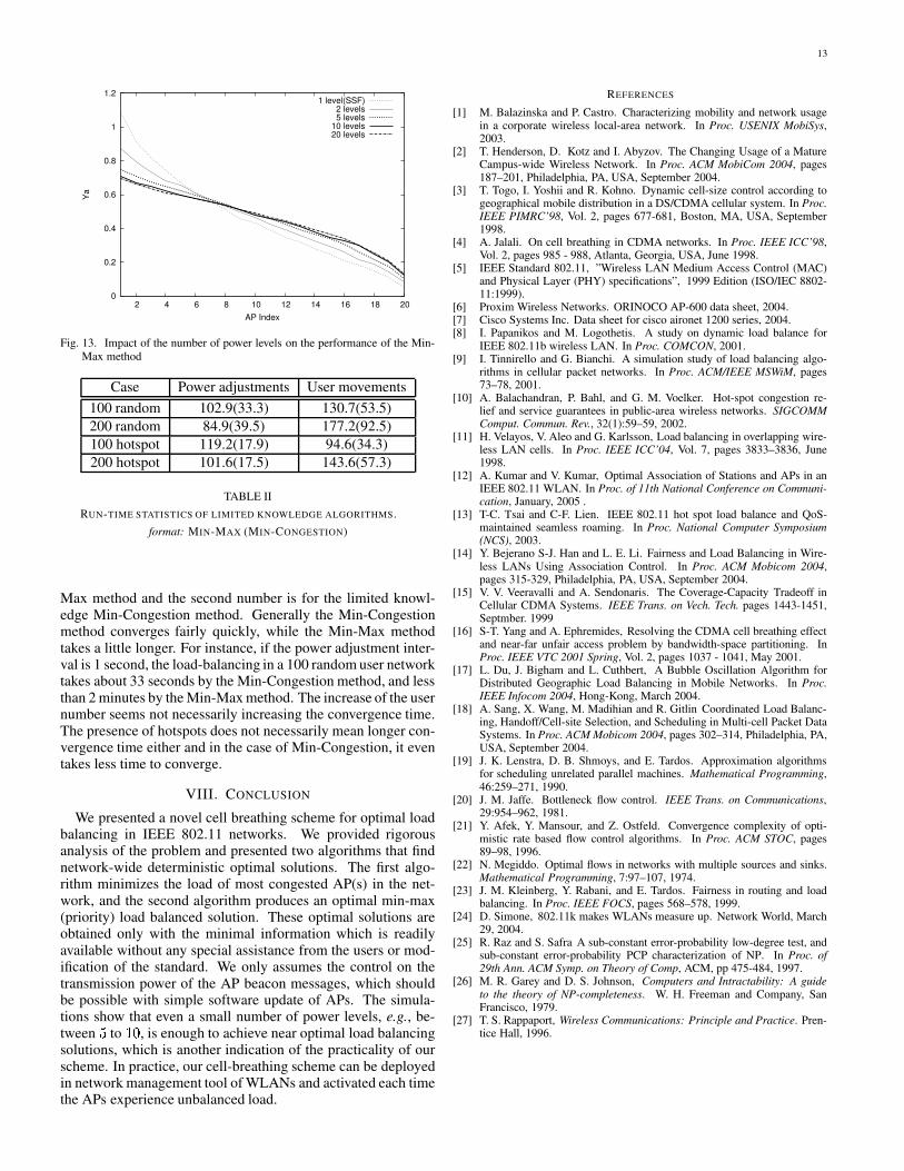
So far, we have assumed 10 power levels. To examine the im-pact of the number of power levels, we tried 4 different numbersof power levels. The simulation results in the 100 random usercase is shown in Figure 13. The impact of the number of powerlevels becomes marginal beyond a certain number of power lev-els, which is between 5 and 10 in the current simulation setup.

While the complete knowledge algorithms compute the op-timal solutions at one shot, the limited knowledge algorithmsgradually change the power setting until they find the optimalsolutions. To capture the overhead of the limited knowledge al-gorithms, we counted the frequency of power adjustments andconsequent user movements during the simulation. The numberof power adjustments determines the time to take before the sys-tem converges on the optimal state and the number of user move-ments decides the handoff overhead. The collected statisticsare summarized in Table II. For each table entry, two numbersare given; the first number is for the limited knowledge Min-

13

0

0.2

0.4

0.6

0.8

1

1.2

2 4 6 8 10 12 14 16 18 20

Ya

AP Index

1 level(SSF)2 levels5 levels

10 levels20 levels

Fig. 13. Impact of the number of power levels on the performance of the Min-Max method

Case Power adjustments User movements100 random 102.9(33.3) 130.7(53.5)200 random 84.9(39.5) 177.2(92.5)100 hotspot 119.2(17.9) 94.6(34.3)200 hotspot 101.6(17.5) 143.6(57.3)

TABLE IIRUN-TIME STATISTICS OF LIMITED KNOWLEDGE ALGORITHMS.

format: MIN-MAX (MIN-CONGESTION)

Max method and the second number is for the limited knowl-edge Min-Congestion method. Generally the Min-Congestionmethod converges fairly quickly, while the Min-Max methodtakes a little longer. For instance, if the power adjustment inter-val is 1 second, the load-balancing in a 100 random user networktakes about 33 seconds by the Min-Congestion method, and lessthan 2 minutes by the Min-Max method. The increase of the usernumber seems not necessarily increasing the convergence time.The presence of hotspots does not necessarily mean longer con-vergence time either and in the case of Min-Congestion, it eventakes less time to converge.

VIII. CONCLUSION

We presented a novel cell breathing scheme for optimal loadbalancing in IEEE 802.11 networks. We provided rigorousanalysis of the problem and presented two algorithms that findnetwork-wide deterministic optimal solutions. The first algo-rithm minimizes the load of most congested AP(s) in the net-work, and the second algorithm produces an optimal min-max(priority) load balanced solution. These optimal solutions areobtained only with the minimal information which is readilyavailable without any special assistance from the users or mod-ification of the standard. We only assumes the control on thetransmission power of the AP beacon messages, which shouldbe possible with simple software update of APs. The simula-tions show that even a small number of power levels, e.g., be-tween O to �|� , is enough to achieve near optimal load balancingsolutions, which is another indication of the practicality of ourscheme. In practice, our cell-breathing scheme can be deployedin network management tool of WLANs and activated each timethe APs experience unbalanced load.

REFERENCES

[1] M. Balazinska and P. Castro. Characterizing mobility and network usagein a corporate wireless local-area network. In Proc. USENIX MobiSys,2003.

[2] T. Henderson, D. Kotz and I. Abyzov. The Changing Usage of a MatureCampus-wide Wireless Network. In Proc. ACM MobiCom 2004, pages187–201, Philadelphia, PA, USA, September 2004.

[3] T. Togo, I. Yoshii and R. Kohno. Dynamic cell-size control according togeographical mobile distribution in a DS/CDMA cellular system. In Proc.IEEE PIMRC’98, Vol. 2, pages 677-681, Boston, MA, USA, September1998.

[4] A. Jalali. On cell breathing in CDMA networks. In Proc. IEEE ICC’98,Vol. 2, pages 985 - 988, Atlanta, Georgia, USA, June 1998.

[5] IEEE Standard 802.11, ”Wireless LAN Medium Access Control (MAC)and Physical Layer (PHY) specifications”, 1999 Edition (ISO/IEC 8802-11:1999).

[6] Proxim Wireless Networks. ORINOCO AP-600 data sheet, 2004.[7] Cisco Systems Inc. Data sheet for cisco aironet 1200 series, 2004.[8] I. Papanikos and M. Logothetis. A study on dynamic load balance for

IEEE 802.11b wireless LAN. In Proc. COMCON, 2001.[9] I. Tinnirello and G. Bianchi. A simulation study of load balancing algo-

rithms in cellular packet networks. In Proc. ACM/IEEE MSWiM, pages73–78, 2001.

[10] A. Balachandran, P. Bahl, and G. M. Voelker. Hot-spot congestion re-lief and service guarantees in public-area wireless networks. SIGCOMMComput. Commun. Rev., 32(1):59–59, 2002.

[11] H. Velayos, V. Aleo and G. Karlsson, Load balancing in overlapping wire-less LAN cells. In Proc. IEEE ICC’04, Vol. 7, pages 3833–3836, June1998.

[12] A. Kumar and V. Kumar, Optimal Association of Stations and APs in anIEEE 802.11 WLAN. In Proc. of 11th National Conference on Communi-cation, January, 2005 .

[13] T-C. Tsai and C-F. Lien. IEEE 802.11 hot spot load balance and QoS-maintained seamless roaming. In Proc. National Computer Symposium(NCS), 2003.

[14] Y. Bejerano S-J. Han and L. E. Li. Fairness and Load Balancing in Wire-less LANs Using Association Control. In Proc. ACM Mobicom 2004,pages 315-329, Philadelphia, PA, USA, September 2004.

[15] V. V. Veeravalli and A. Sendonaris. The Coverage-Capacity Tradeoff inCellular CDMA Systems. IEEE Trans. on Vech. Tech. pages 1443-1451,Septmber. 1999

[16] S-T. Yang and A. Ephremides, Resolving the CDMA cell breathing effectand near-far unfair access problem by bandwidth-space partitioning. InProc. IEEE VTC 2001 Spring, Vol. 2, pages 1037 - 1041, May 2001.

[17] L. Du, J. Bigham and L. Cuthbert, A Bubble Oscillation Algorithm forDistributed Geographic Load Balancing in Mobile Networks. In Proc.IEEE Infocom 2004, Hong-Kong, March 2004.

[18] A. Sang, X. Wang, M. Madihian and R. Gitlin Coordinated Load Balanc-ing, Handoff/Cell-site Selection, and Scheduling in Multi-cell Packet DataSystems. In Proc. ACM Mobicom 2004, pages 302–314, Philadelphia, PA,USA, September 2004.

[19] J. K. Lenstra, D. B. Shmoys, and E. Tardos. Approximation algorithmsfor scheduling unrelated parallel machines. Mathematical Programming,46:259–271, 1990.

[20] J. M. Jaffe. Bottleneck flow control. IEEE Trans. on Communications,29:954–962, 1981.

[21] Y. Afek, Y. Mansour, and Z. Ostfeld. Convergence complexity of opti-mistic rate based flow control algorithms. In Proc. ACM STOC, pages89–98, 1996.

[22] N. Megiddo. Optimal flows in networks with multiple sources and sinks.Mathematical Programming, 7:97–107, 1974.

[23] J. M. Kleinberg, Y. Rabani, and E. Tardos. Fairness in routing and loadbalancing. In Proc. IEEE FOCS, pages 568–578, 1999.

[24] D. Simone, 802.11k makes WLANs measure up. Network World, March29, 2004.

[25] R. Raz and S. Safra A sub-constant error-probability low-degree test, andsub-constant error-probability PCP characterization of NP. In Proc. of29th Ann. ACM Symp. on Theory of Comp, ACM, pp 475-484, 1997.

[26] M. R. Garey and D. S. Johnson, Computers and Intractability: A guideto the theory of NP-completeness. W. H. Freeman and Company, SanFrancisco, 1979.

[27] T. S. Rappaport, Wireless Communications: Principle and Practice. Pren-tice Hall, 1996.