Causal Assessment in Finite-LengthExtensive-Form Games∗

Jose Penalva-ZuastiUniversitat Pompeu Fabra

Michael D. Ryall†

University of Rochester, andUniversity of California, Los Angeles

September 11, 2003

∗We thank Adam Brandenburger, Colin Camerer, David M. Chickering, Eddie Dekel, BryanEllickson, Ehud Kalai, Uffe Kjærulff, David Levine, Steven Lippman, Glenn MacDonald, MarkMachina, Leslie Marx, Joseph Ostroy, Scott Page, Judea Pearl, Larry Samuelson, Joel Watson,Eduardo Zambrano, Bill Zame, participants in the MEDS, Georgetown, UCLA, and UCSD theoryworkshops, the Stanford SITE and Stonybrook theory conferences, three anonymous referees andan anonymous co-editor, for thoughtful comments. Ryall thanks the John M. Olin foundation forfinancial support.

†Correspondence should be sent to: M. D. Ryall, Economics Dept., 8283 Bunche Hall, Box951477, Los Angeles, CA. 90095; 310-825-3925; ryall@simon.rochester.edu.

1

Abstract

We consider extensive-form games in which the information structure is not known

and ask how much of that structure can be inferred from the distribution on action

profiles generated by player strategies. One game is said to observationally imitate

another when the distribution on action profiles generated by every behavior strategy

in the latter can also be generated by an appropriately chosen behavior strategy

in the former. The first part of the paper develops analytical methods for testing

observational imitation. The central idea is to relate a game’s information structure

to the conditional independencies in the distributions it generates on action profiles.

We present a new analytical device, the influence opportunity diagram of a game,

describe how such a diagram is constructed for a given finite-length extensive-form

game, and demonstrate that it provides, for a large class of economically interesting

games, a simple test for observational imitation. The second part of the paper shifts

the focus to the influence assessments of players within a game. A new equilibrium

concept, causal Nash equilibrium, is presented and compared to several other well-

known alternatives. Cases in which causal Nash equilibrium seems especially well-

suited are explored.

Keywords: causality, information structure, extensive form game, observational im-

itation, Bayesian network

2

1 Introduction

This paper focuses on the question of what can be said about situations in which

the information structure of a finite-length extensive-form game is not known. There

are two cases in which the answer to this question matters. The first is when an

individual outside the game, say a social scientist, would like to infer something about

the information structure of the game from the observed behavior of its participants.

The second is when individuals in a game are unsure of the information upon which

their opponents condition their decisions. In this latter case, beliefs about causal

structure — who influences whom — should play an important role in determining

equilibrium behavior.

We explore both cases and, specifically, analyze what can be inferred about a

game’s information structure solely from the probability distribution on action pro-

files induced by actual player strategies (which we refer to as the “empirical distri-

bution of play”). The main idea is to connect a game’s information structure, which

identifies the individual histories upon which players condition their behavior, to the

corresponding set of conditional independencies that must be observed in all of its

empirical distributions. When two games with different information structures imply

different sets of such independencies, then knowledge of the empirical distribution

provides a basis upon which to distinguish one from the other.

The first part of the paper considers information structure assessment from the

perspective of an outsider who only observes player behavior (actions, not strategies).

To this end, we introduce the notion of observational imitation. One game is said

to observationally imitate another when the empirical distribution induced by any

behavior strategy profile in the latter can also be induced by an appropriately chosen

behavior strategy profile in the former. Thus, even under infinite repetition, it is

impossible to distinguish a game from its imitators solely on the basis of the observed

behavior of its players.

Our analysis is facilitated by the introduction of a new graphical device, the

3

influence opportunity diagram of a game (hereafter, IOD). The IOD is defined con-

structively for a broad class of finite-length extensive-form games, including those

with infinite action sets. As we show, the IOD summarizes certain information about

the conditional independencies that must be observed in all empirical distributions

arising from play of the underlying game. This feature allows us to apply some re-

sults from the extensive literature on probabilistic networks in artificial intelligence

to address the issues raised above. This literature explores the use of graphs to model

uncertainty and decisions in complex domains. Since most economists are not famil-

iar with it, we have included a condensed, self-contained discussion of the relevant

results and references in Appendix A.

A basic finding is that a necessary requirement for one game to imitate another

is that their IODs imply a consistent set of conditional independencies. This require-

ment is not, in general, sufficient because differences in the specific information upon

which players condition their behavior may imply additional restrictions on empirical

distributions that are not picked up by the IOD. However, we do identify a broad

class of games, termed games of exact information, for which this condition is also

sufficient. For games of this type, we use results from the literature on probabilistic

networks and develop new ones to show that observational imitation can be identified

by simple visual comparison of the IODs of the games in question.

The second part of the paper shifts the focus to influence assessment from the

inside — that is, to games in which the players themselves are uncertain about the

information structure governing their play. If equilibrium is interpreted as the out-

come of some generic learning process (as is typical in the literature on learning in

noncooperative games), then a player’s equilibrium beliefs regarding the underlying

influence relationships should be consistent with observed behavior. This idea leads

to a new equilibrium notion, that of a causal Nash equilibrium, which imposes such

consistency on player beliefs. We demonstrate the relationship between causal Nash

equilibrium and other well-known equilibrium concepts.

4

An obvious question is whether this new equilibrium concept holds useful impli-

cations for situations of genuine economic interest. We can think of at least two

cases in which it does. The first and, perhaps most obvious, is when payoffs are sys-

tematically related to information structure. In such situations, refining beliefs with

respect to the true information structure may well lead to a better assessment of the

payoffs faced both by oneself and one’s opponents. The second case, which to our

knowledge has previously received no explicit attention, is when a player (or players)

must choose an appropriate ‘intervention’ in the activities of one or more of their op-

ponents. A player is said to have intervention ability when his or her choice of action

determines, non-trivially, the feasible actions available to others.1 Here, an accurate

assessment of the game’s influence relationships may be crucial to the success of the

interventionist. We term these intervention games and present an example of causal

Nash equilibrium applied to such a game.

The remainder of the paper is organized as follows. The next section presents

several simple examples designed to illustrate the notion of observational imitation.

Section 3 lays out the definition of a finite-length extensive-form game (which differs in

some ways from the usual setup) and defines observational imitation and observational

indistinguishability. In Section 4, we present our main results regarding the analysis

of observational imitation (from the perspective of an outside observer). Section 4.1

shows how to construct an IOD from an extensive-form game. Section 4.2 connects

information structure to observational imitation through the IOD. Section 4.3 shows

how to test whether one game observationally imitates another by visual inspection

of their respective IODs. Section 5 shifts the focus to influence uncertainty within

the game. First, we give a motivating example in which uncertainty about who

takes the role of Stackleberg leader may cause potential entrants to stay out of a

market. Section 5.2 introduces our definition of causal Nash equilibrium and makes

formal comparisons to several well-known equilibrium concepts. Section 5.3 presents

an extended example of causal Nash equilibrium applied to an intervention game.

5

We conclude in Section 6 with a more thorough discussion of related research and

potential extensions.

2 Examples and Intuition

Consider the game trees presented in Figures 1 through 3. The first, ΓA, has the

familiar structure of a standard “signalling” game. The other two are variations

involving the same players who have the same feasible actions at the time of their

moves. We wish to show that ΓA and ΓB are in an equivalence class in the sense

that any distribution on action profiles generated by (behavioral) strategies in one

can also be generated by an appropriate choice of strategies in the other. ΓC , on the

other hand, is not a member of this class.

Let A ≡ {(u, L, U) , ..., (d,R,D)} be the set of possible action profiles in eachof the three games (up to a permutation of the components). We refer to a single

profile a ∈ A as an “outcome” of play. Let θk ≡ ¡θkN , θ

kI , θ

kII

¢denote a behavior

strategy profile in Γk where θki is the strategy chosen by player i in game k. Every

behavior strategy in each of the three games implies a probability distribution mθk

on A constructed as follows, for all a ∈ A,

mθA (a) ≡ θAII (aII |aI) θAI (aI |aN) θAN (aN) ,mθB (a) ≡ θBN (aN |aI) θBI (aI |aII) θBII (aII) ,mθC (a) ≡ θCII (aII) θ

CI (aI) θ

CN (aN) .

Now, suppose ΓA is repeated a large number of times under a fixed strategy

profile θA. Assume the outcomes are recorded and reported to an outside observer

who knows that one of ΓA, ΓB, or ΓC is the game responsible for generating the data

(but not which). The question we wish to answer is whether there are any strategies

θA that would allow the outsider to correctly identify ΓA as the underlying game.

First, note that the construction of mθA immediately implies that, for all a ∈ A,

6

the following factorization holds

mθA (a) = mθA (aII |aI)mθA (aI |aN)mθA (aN) .

Of course, mθB and mθC can be factored analogously. By the definition of conditional

probability, for every θA,

mθA (a) = mθA (aII |aI)mθA (aI |aN)mθA (aN)

=mθA (aII , aI)

mθA (aI)

mθA (aI , aN )

mθA (aN)mθA (aN)

=mθA (aN , aI)

mθA (aI)

mθA (aI , aII)

mθA (aII)mθA (aII)

= mθA (aN |aI)mθA (aI |aII)mθA (aII) .

This is significant because it implies that for every behavior strategy in ΓA, one can

find a corresponding strategy in ΓB that generates exactly the same distribution onA;

given θA, simply construct θB such that, for all a ∈ A, θBN (aN |aI) ≡ mθA (aN |aI) ,and so on. Then, mθA = mθB . Therefore, the outside observer — even with very

exact information about the true distribution on outcomes implied by some behavior

strategy — can never distinguish between ΓA and ΓB.

On the other hand, it should be clear that ΓC cannot imitate all strategies from ΓA

and ΓB. Barring correlated strategies without an explicit correlating device, there are

many strategy profiles in ΓA (and, therefore, in ΓB as well) that generate distributions

over action profiles that could not possibly correspond to any strategy profile in ΓC .

For example, any θA in which player I conditions her behavior on Nature’s play

results in a mθA that cannot be duplicated by an appropriate choice of strategy in

ΓC .

3 The model

Wherever possible, capital letters (X,Z) denote sets, small letters (a, w) either ele-

ments of sets or functions, and script letters (A,F) collections of sets. Sets whose

7

members are ordered profiles are indicated by bold capitals (A,E) with small bold

(a, e) denoting typical elements. Graphs and probability spaces play a large role

in the following analysis. Standard notation and definitions are adopted wherever

possible.

3.1 Extensive-form games

We begin with a finite-length, extensive-form game of perfect recall. The game Γ has

a game tree (X,E) with nodes X and edges E. Players are indexed by N ≡ {1, ..., n}with n <∞. The terminal nodes are Z ⊂ X with typical element z. Payoffs are given

by u : Z → Rn. Attention is restricted to games in which influence opportunities

between players are fixed.2 Specifically, assume that all paths are of length t < ∞and that the player-move order is summarized by an onto function o : T → N where

T ≡ {1, ..., t} and i = o (r) means that i is the player who (always) has the rth move.3Every (xr, xr+1) ∈ E corresponds to an action available at xr. Let Xr denote the

set of all nodes associated with the rth move. For all r ∈ T, let Ar be the unionof the actions available at the nodes in Xr. Edges are labeled in such a way that

every history is unique. In particular, every z ∈ Z corresponds to a unique action

profile az = (a1z , ..., atz). The set of all action profiles is A ≡ ∪z∈Zaz. Each Ar comesequipped with a σ-algebra Ar. The σ-algebra forA is A ≡ σ ({F ∈ ×r∈TAr|F ⊂ A}).Assume all measure spaces are standard.4 We call (A,A) the outcome space. This,coupled with an appropriate probability measure, is the focal object of our analysis.

Let az 7→ v (az) ≡ u (z) translate payoffs on Z to payoffs on A.For r ∈ T, the (complete) history at r is an A-measurable function a 7→ hr (a) ≡

(a1, ..., ar−1). We use hr to denote a typical element of hr (A) and define h1 to

be a constant equal to the null history h0. For every move r, there is a bijective

relationship between hr (A) , the set of all (r − 1)-length action profiles, and Xr. Ingeneral, players do not know the full profile of actions leading up to their move. To

reflect this, Xr is partitioned into a collection of subsets called the move-r information

8

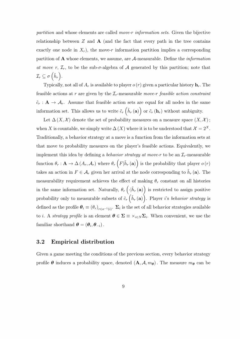
partition and whose elements are called move-r information sets. Given the bijective

relationship between Z and A (and the fact that every path in the tree contains

exactly one node in Xr), the move-r information partition implies a corresponding

partition of A whose elements, we assume, are A-measurable. Define the informationat move r, Ir, to be the sub-σ-algebra of A generated by this partition; note that

Ir ⊆ σ³hr

´.

Typically, not all of Ar is available to player o (r) given a particular history hr. The

feasible actions at r are given by the Ir-measurable move-r feasible action constraintcr : A → Ar. Assume that feasible action sets are equal for all nodes in the sameinformation set. This allows us to write cr

³hr (a)

´or cr (hr) without ambiguity.

Let ∆ (X,X ) denote the set of probability measures on a measure space (X,X ) ;whenX is countable, we simply write∆ (X) where it is to be understood that X = 2X .

Traditionally, a behavior strategy at a move is a function from the information sets at

that move to probability measures on the player’s feasible actions. Equivalently, we

implement this idea by defining a behavior strategy at move-r to be an Ir-measurablefunction θr : A→ ∆ (Ar,Ar) where θr

³F |hr (a)

´is the probability that player o (r)

takes an action in F ∈ Ar given her arrival at the node corresponding to hr (a). Themeasurability requirement achieves the effect of making θr constant on all histories

in the same information set. Naturally, θr³·|hr (a)

´is restricted to assign positive

probability only to measurable subsets of cr

³hr (a)

´. Player i’s behavior strategy is

defined as the profile θi ≡ (θr)r∈o−1(i). Σi is the set of all behavior strategies availableto i. A strategy profile is an element θ ∈ Σ ≡ ×i∈NΣi. When convenient, we use thefamiliar shorthand θ = (θi,θ−i) .

3.2 Empirical distribution

Given a game meeting the conditions of the previous section, every behavior strategy

profile θ induces a probability space, denoted (A,A,mθ) . The measure mθ can be

9

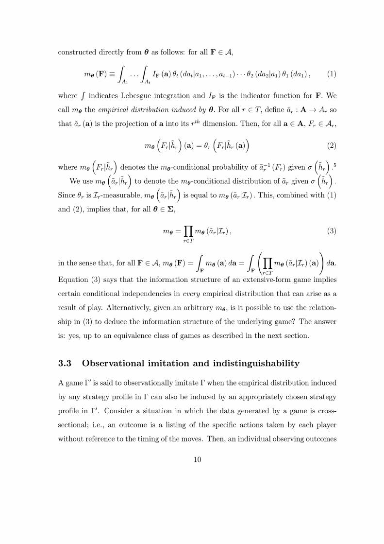
constructed directly from θ as follows: for all F ∈ A,

mθ (F) ≡ZA1

. . .

ZAt

IF (a) θt (dat|a1, . . . , at−1) · · · θ2 (da2|a1) θ1 (da1) , (1)

whereRindicates Lebesgue integration and IF is the indicator function for F. We

call mθ the empirical distribution induced by θ. For all r ∈ T, define ar : A→ Ar so

that ar (a) is the projection of a into its rth dimension. Then, for all a ∈ A, Fr ∈ Ar,

mθ

³Fr|hr

´(a) = θr

³Fr|hr (a)

´(2)

where mθ

³Fr|hr

´denotes the mθ-conditional probability of a

−1r (Fr) given σ

³hr

´.5

We use mθ

³ar|hr

´to denote the mθ-conditional distribution of ar given σ

³hr´.

Since θr is Ir-measurable, mθ

³ar|hr

´is equal to mθ (ar|Ir) . This, combined with (1)

and (2), implies that, for all θ ∈ Σ,

mθ =Yr∈Tmθ (ar|Ir) , (3)

in the sense that, for all F ∈ A, mθ (F) =

ZF

mθ (a) da =

ZF

ÃYr∈Tmθ (ar|Ir) (a)

!da.

Equation (3) says that the information structure of an extensive-form game implies

certain conditional independencies in every empirical distribution that can arise as a

result of play. Alternatively, given an arbitrary mθ, is it possible to use the relation-

ship in (3) to deduce the information structure of the underlying game? The answer

is: yes, up to an equivalence class of games as described in the next section.

3.3 Observational imitation and indistinguishability

A game Γ0 is said to observationally imitate Γ when the empirical distribution induced

by any strategy profile in Γ can also be induced by an appropriately chosen strategy

profile in Γ0. Consider a situation in which the data generated by a game is cross-

sectional; i.e., an outcome is a listing of the specific actions taken by each player

without reference to the timing of the moves. Then, an individual observing outcomes

10

generated by repeated play of θ in Γ, eventually, develops a fairly precise estimate

of mθ. However, when Γ0 observationally imitates Γ, then there is no collection of

Γ-generated data capable of ruling out Γ0 as the true underlying game.

An obvious necessary condition for observational imitation is that the games have

consistent player sets and outcome profiles. Given a permutation f : T → T, let f (a)

denote the permuted profile¡af(r)

¢r∈T and, for F ⊆ A, let f (F) be the set whose

elements are the permuted elements of F. Then, Γ0 is outcome compatible with Γ if and

only if: (1) N = N 0; (2) there exists a permutation f such that f (A) = A0; (3) for all

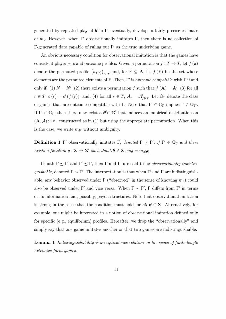
r ∈ T , o (r) = o0 (f (r)); and, (4) for all r ∈ T , Ar = A0f(r). Let OΓ denote the classof games that are outcome compatible with Γ. Note that Γ0 ∈ OΓ implies Γ ∈ OΓ0.If Γ0 ∈ OΓ, then there may exist a θ0∈ Σ0 that induces an empirical distribution on(A,A) ; i.e., constructed as in (1) but using the appropriate permutation. When thisis the case, we write mθ0 without ambiguity.

Definition 1 Γ0 observationally imitates Γ, denoted Γ ¹ Γ0, if Γ0 ∈ OΓ and thereexists a function g : Σ→ Σ0 such that ∀θ ∈ Σ, mθ = mg(θ).

If both Γ ¹ Γ0 and Γ0 ¹ Γ, then Γ and Γ0 are said to be observationally indistin-

guishable, denoted Γ ∼ Γ0. The interpretation is that when Γ0 and Γ are indistinguish-able, any behavior observed under Γ (“observed” in the sense of knowing mθ) could

also be observed under Γ0 and vice versa. When Γ ∼ Γ0, Γ differs from Γ0 in terms

of its information and, possibly, payoff structures. Note that observational imitation

is strong in the sense that the condition must hold for all θ ∈ Σ. Alternatively, forexample, one might be interested in a notion of observational imitation defined only

for specific (e.g., equilibrium) profiles. Hereafter, we drop the “observationally” and

simply say that one game imitates another or that two games are indistinguishable.

Lemma 1 Indistinguishability is an equivalence relation on the space of finite-length

extensive form games.

11

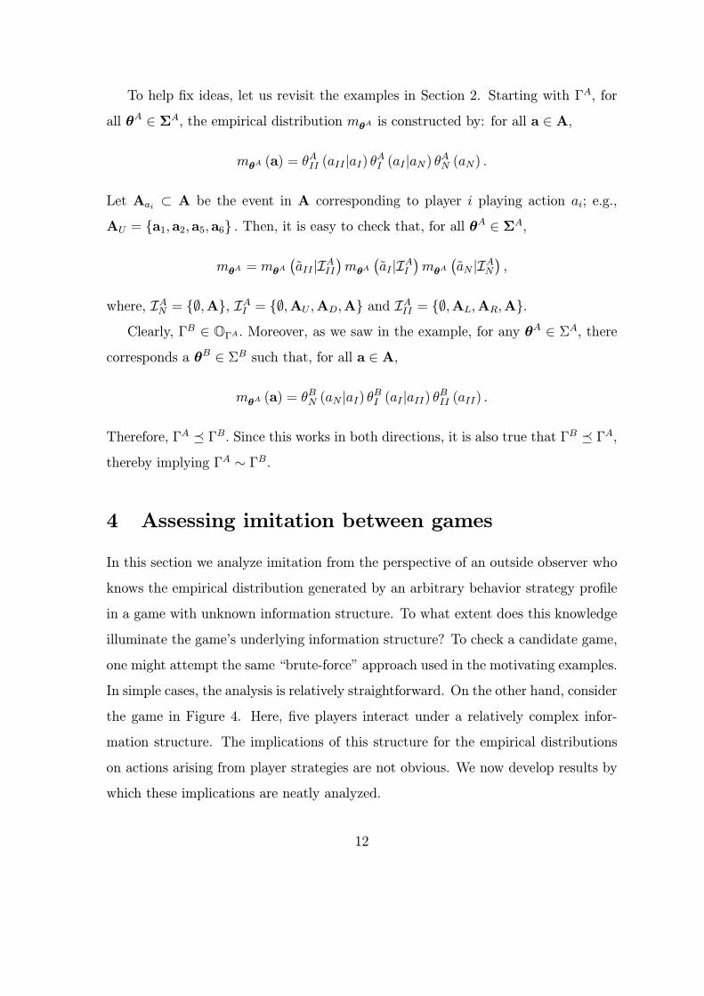
To help fix ideas, let us revisit the examples in Section 2. Starting with ΓA, for

all θA ∈ ΣA, the empirical distribution mθA is constructed by: for all a ∈ A,

mθA (a) = θAII (aII |aI) θAI (aI |aN) θAN (aN) .

Let Aai ⊂ A be the event in A corresponding to player i playing action ai; e.g.,

AU = {a1, a2,a5, a6} . Then, it is easy to check that, for all θA ∈ ΣA,

mθA = mθA¡aII |IAII

¢mθA

¡aI |IAI

¢mθA

¡aN |IAN

¢,

where, IAN = {∅,A}, IAI = {∅,AU ,AD,A} and IAII = {∅,AL,AR,A}.Clearly, ΓB ∈ OΓA. Moreover, as we saw in the example, for any θA ∈ ΣA, there

corresponds a θB ∈ ΣB such that, for all a ∈ A,

mθA (a) = θBN (aN |aI) θBI (aI |aII) θBII (aII) .

Therefore, ΓA ¹ ΓB. Since this works in both directions, it is also true that ΓB ¹ ΓA,thereby implying ΓA ∼ ΓB.

4 Assessing imitation between games

In this section we analyze imitation from the perspective of an outside observer who

knows the empirical distribution generated by an arbitrary behavior strategy profile

in a game with unknown information structure. To what extent does this knowledge

illuminate the game’s underlying information structure? To check a candidate game,

one might attempt the same “brute-force” approach used in the motivating examples.

In simple cases, the analysis is relatively straightforward. On the other hand, consider

the game in Figure 4. Here, five players interact under a relatively complex infor-

mation structure. The implications of this structure for the empirical distributions

on actions arising from player strategies are not obvious. We now develop results by

which these implications are neatly analyzed.

12

4.1 Influence opportunity diagrams

Loosely, player o (r) is said to have the opportunity to influence play at move s if

he has a choice of feasible actions available under some conceivable play of the game

that permits player o (s) to alter her behavior regardless of what her other opponents

do (i.e., opponents other than o (r)). The following definition formalizes this idea.

Definition 2 The influence opportunity diagram of Γ is a graph (T,→) such thatr → s if and only if r < s, and there exist a,a0 ∈ A satisfying each of the following

conditions: (1) hr (a) = hr (a0) ; (2) ∃F ∈Is such that h−1r+1 (a1, ..., ar) ⊂ F and a0 ∈

Fc; (3) a0s 6= as; and, (4) aj(a0)j∈{k|k>r, k→s} = aj(a)j∈{k|k>r, k→s}.

The meat of the definition is that r → s when there is some move-r history (item

1) at which player o (r) has a choice of actions that cause play at s to be at different

information sets (item 2) and to which player o (s) can respond differently (item

3). Note that item 2 implies that there are at least two distinct actions available

at r, one that guarantees the occurrence of F and another that is necessary for the

occurrence of Fc (but may not guarantee it). Influence is only an “opportunity”

since this condition is neither necessary nor sufficient for move r actions to have an

actual effect on move s behavior. For example, the player at move s may choose to

ignore the action taken at move r (e.g., when θs is constant on A). Alternatively,

the player at move r may influence play at move s indirectly through other players

(e.g., when r → q → s even though r 9 s). Item 4 is a technical condition that

rules out spurious influence due to feasible action restrictions that force the move

at s to be independent of actions taken at r given actions taken at some subset of

moves following r. Although spurious influence due to game structure is a technical

possibility, it does not arise in any games of economic interest with which we are

familiar.

Return to game ΓA in Figure 1. Here, player I observes player N and player

II observes player I, which suggests the IOD should be N → I and I → II. To

13

see that this is correct, first check N → I. In this case, II = {∅,FU ,FD,A} whereFU ≡ {a1, a2, a5,a6} . Then, (a5, a4) establish the result: (1) hN (a5) = hN (a8) = h0,(2) h−1I (h0, U) = {a1, a2, a5,a6} = FU and a4 ∈ Fc = FD, and (3) aI (a5) = (R) 6=aI (a4) = (L) . Item (4) is automatically satisfied since there are no moves between

I and II. Similarly, I → II is established by (a1,a6) . However, N 9 II since the

smallest III-measurable event containing either h−1N (U) or h−1N (D) is A.6

By identical reasoning, the IOD for the game in Figure 3 is N ← I ← II. The IOD

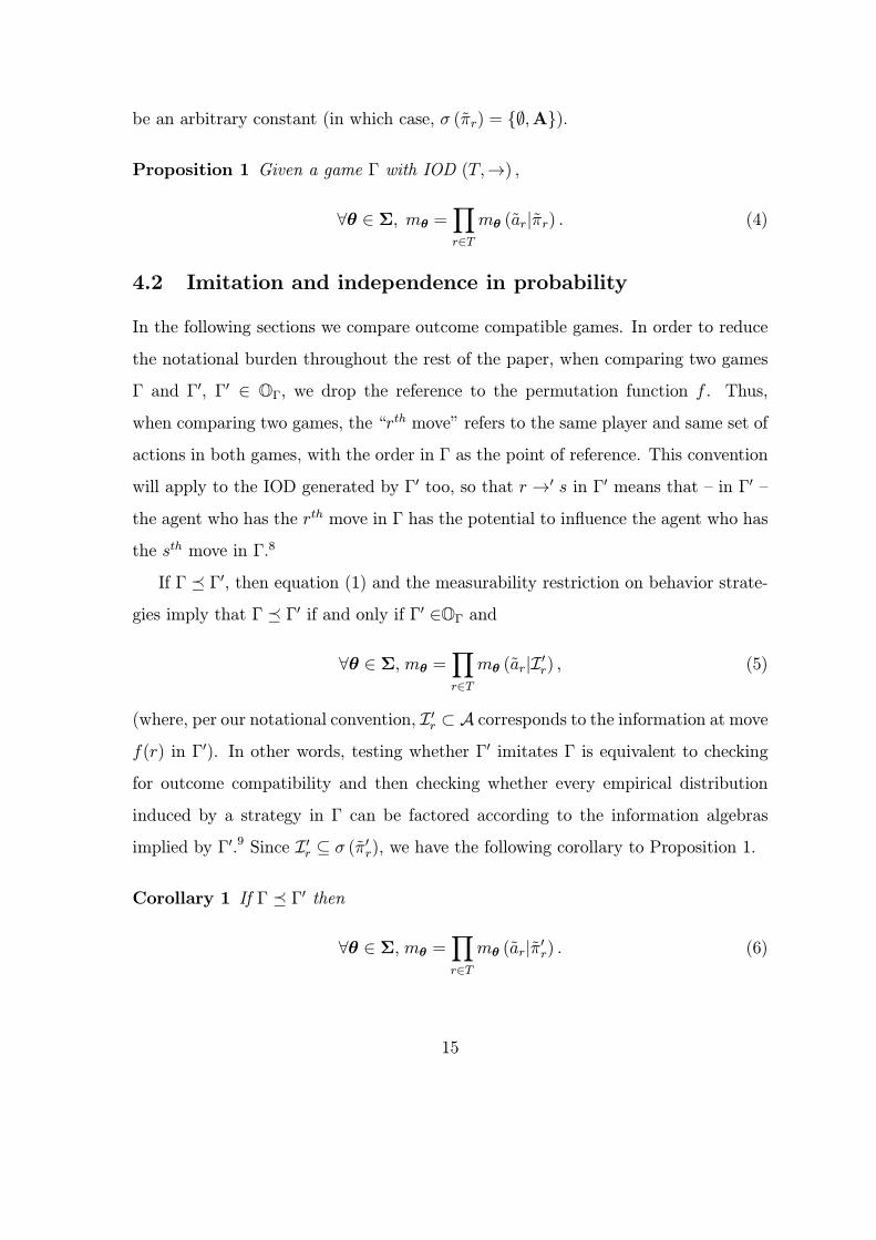
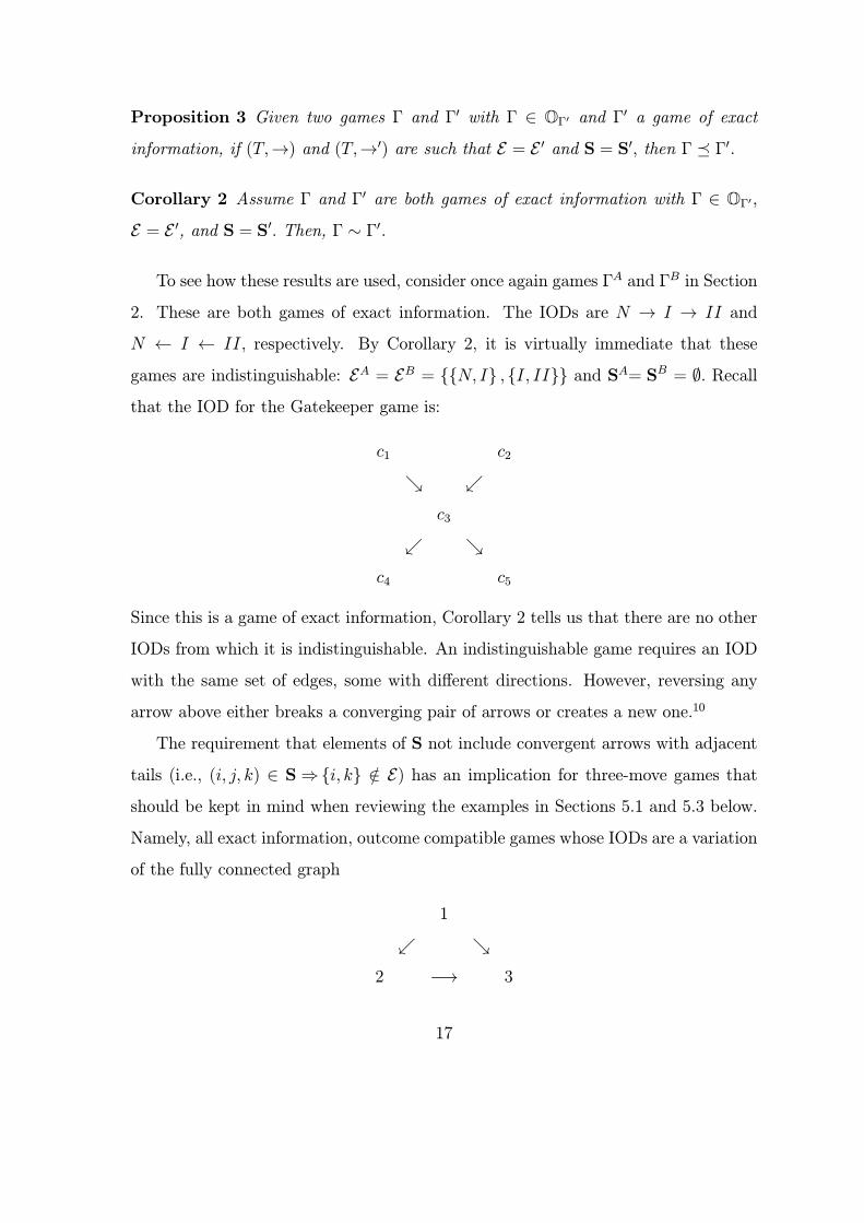
for Figure 2 is a graph with three nodes and no edges. The IOD for the Gatekeeper

game (Figure 4) is simply:

1 2

& .3

. &4 5

Player 3 is the “gatekeeper” of information flowing from players 1 and 2 to players 4

and 5.

To understand item (4) of the definition, consider Game I in Figure 5. Notice that

this game has the unusual feature that player 2’s feasible action sets are different at

every information set. Without item (4), the IOD would be 1→ 2, 2→ 3 and 1→ 3.

However, by condition (4), 1→ 3 is removed. Intuitively, the game’s structure implies

that knowing the action chosen by 1 is always irrelevant in assessing 3’s behavior when

the action taken by 2 is already known. If the feasible actions at information set 2b

are {U,D} , as in Game II, then the IOD is 1→ 2, 2→ 3 and 1→ 3.

We now demonstrate that the IOD summarizes certain conditional independen-

cies that must arise in every empirical distribution of play.7 Given (T,→) , the set ofmoves at which players may exert a direct influence upon player o (r) at move r is

{s ∈ T |s→ r} . Define πr (a) ≡ (ak)k∈{s∈T |s→r} to be the σ³hr

´-measurable projec-

tion of a into the dimensions indexed by {s ∈ T |s→ r}. If {s ∈ T |s→ r} = ∅, let πr

14

be an arbitrary constant (in which case, σ (πr) = {∅,A}).

Proposition 1 Given a game Γ with IOD (T,→) ,

∀θ ∈ Σ, mθ =Yr∈Tmθ (ar|πr) . (4)

4.2 Imitation and independence in probability

In the following sections we compare outcome compatible games. In order to reduce

the notational burden throughout the rest of the paper, when comparing two games

Γ and Γ0, Γ0 ∈ OΓ, we drop the reference to the permutation function f . Thus,when comparing two games, the “rth move” refers to the same player and same set of

actions in both games, with the order in Γ as the point of reference. This convention

will apply to the IOD generated by Γ0 too, so that r →0 s in Γ0 means that — in Γ0 —

the agent who has the rth move in Γ has the potential to influence the agent who has

the sth move in Γ.8

If Γ ¹ Γ0, then equation (1) and the measurability restriction on behavior strate-gies imply that Γ ¹ Γ0 if and only if Γ0 ∈OΓ and

∀θ ∈ Σ, mθ =Yr∈Tmθ (ar|I 0r) , (5)

(where, per our notational convention, I 0r ⊂ A corresponds to the information at movef(r) in Γ0). In other words, testing whether Γ0 imitates Γ is equivalent to checking

for outcome compatibility and then checking whether every empirical distribution

induced by a strategy in Γ can be factored according to the information algebras

implied by Γ0.9 Since I 0r ⊆ σ (π0r), we have the following corollary to Proposition 1.

Corollary 1 If Γ ¹ Γ0 then

∀θ ∈ Σ, mθ =Yr∈Tmθ (ar|π0r) . (6)

15

To see why condition (6) is only necessary (i.e., as opposed to necessary and

sufficient when Γ0 ∈OΓ), consider the two games in Figure 6. Both have the sameIOD: I → II. Moreover Γ2∈OΓ1 . Clearly, however, there are empirical distributionsthat can arise in Γ1 but not in Γ2. Indeed, Γ2 ¹ Γ1 but Γ1 ± Γ2. The issue is the

measurability distinction between conditions (5) and (6). If I2II is the informationalgebra for II in Γ2, then there are behavior strategies for II in Γ1 that are not

I2II-measurable even though every such strategy is σ¡π2II¢-measurable.

For certain types of games, Corollary 1 can be strengthened. Γ is said to be a

game of exact information if, for all r ∈ T, Ir = σ (πr) ; a game of exact information

is one in which a player observes the moves of those preceding her either perfectly

or not at all. This class contains many extensive-form games of economic interest:

all of the games in Section 2 meet this requirement as do many standard market

games such as Cournot, Stackleberg, etc. Note that games of perfect information are

games of exact information in which every player exactly observes the move of every

predecessor.

Proposition 2 Let Γ0 be a game of exact information. Then, Γ ¹ Γ0 if and only if

Γ0 ∈ OΓ and condition (6) hold.

4.3 Testing for imitation

Suppose, given a game Γ and another Γ0 of exact information, one wishes to determine

whether Γ ¹ Γ0. One might be tempted to use Proposition 2 for this purpose. How-

ever, this is not practical for complex games since condition (6) must be checked for

all strategy profiles. In this section, we develop results that permit this determination

by simple visual inspection of the games’ IODs.

For the following proposition, given an IOD (T,→) , let E be the set of edgeswithout reference to direction; i.e., {i, j} ∈ E if and only if (i→ j) or (j → i). Let S ⊂T 3 be the set of all ordered triples such that (i, j, k) ∈ S if and only if (i→ j) , (k → j)

and {i, k} /∈ E .

16

Proposition 3 Given two games Γ and Γ0 with Γ ∈ OΓ0 and Γ0 a game of exactinformation, if (T,→) and (T,→0) are such that E = E 0 and S = S0, then Γ ¹ Γ0.

Corollary 2 Assume Γ and Γ0 are both games of exact information with Γ ∈ OΓ0,E = E 0, and S = S0. Then, Γ ∼ Γ0.

To see how these results are used, consider once again games ΓA and ΓB in Section

2. These are both games of exact information. The IODs are N → I → II and

N ← I ← II, respectively. By Corollary 2, it is virtually immediate that these

games are indistinguishable: EA = EB = {{N, I} , {I, II}} and SA= SB = ∅. Recallthat the IOD for the Gatekeeper game is:

c1 c2

& .c3

. &c4 c5

Since this is a game of exact information, Corollary 2 tells us that there are no other

IODs from which it is indistinguishable. An indistinguishable game requires an IOD

with the same set of edges, some with different directions. However, reversing any

arrow above either breaks a converging pair of arrows or creates a new one.10

The requirement that elements of S not include convergent arrows with adjacent

tails (i.e., (i, j, k) ∈ S⇒ {i, k} /∈ E) has an implication for three-move games thatshould be kept in mind when reviewing the examples in Sections 5.1 and 5.3 below.

Namely, all exact information, outcome compatible games whose IODs are a variation

of the fully connected graph

1

. &2 −→ 3

17

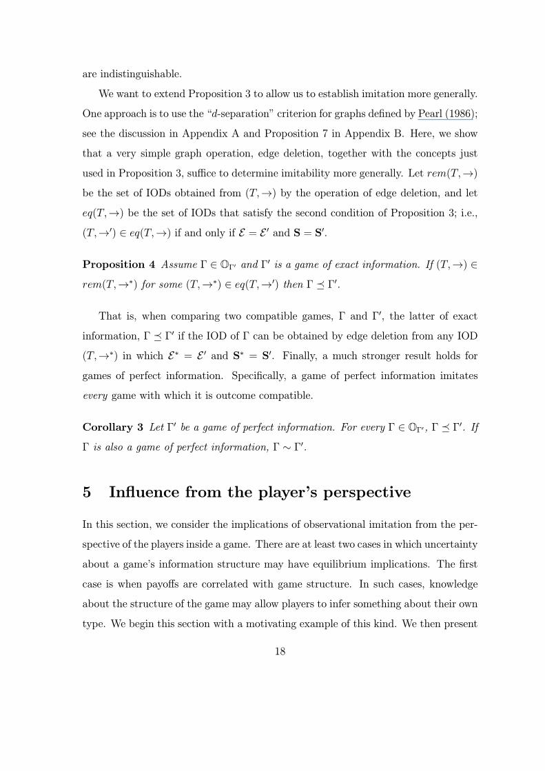
are indistinguishable.

We want to extend Proposition 3 to allow us to establish imitation more generally.

One approach is to use the “d-separation” criterion for graphs defined by Pearl (1986);

see the discussion in Appendix A and Proposition 7 in Appendix B. Here, we show

that a very simple graph operation, edge deletion, together with the concepts just

used in Proposition 3, suffice to determine imitability more generally. Let rem(T,→)be the set of IODs obtained from (T,→) by the operation of edge deletion, and leteq(T,→) be the set of IODs that satisfy the second condition of Proposition 3; i.e.,(T,→0) ∈ eq(T,→) if and only if E = E 0 and S = S0.

Proposition 4 Assume Γ ∈ OΓ0 and Γ0 is a game of exact information. If (T,→) ∈rem(T,→∗) for some (T,→∗) ∈ eq(T,→0) then Γ ¹ Γ0.

That is, when comparing two compatible games, Γ and Γ0, the latter of exact

information, Γ ¹ Γ0 if the IOD of Γ can be obtained by edge deletion from any IOD

(T,→∗) in which E∗ = E 0 and S∗ = S0. Finally, a much stronger result holds for

games of perfect information. Specifically, a game of perfect information imitates

every game with which it is outcome compatible.

Corollary 3 Let Γ0 be a game of perfect information. For every Γ ∈ OΓ0, Γ ¹ Γ0. IfΓ is also a game of perfect information, Γ ∼ Γ0.

5 Influence from the player’s perspective

In this section, we consider the implications of observational imitation from the per-

spective of the players inside a game. There are at least two cases in which uncertainty

about a game’s information structure may have equilibrium implications. The first

case is when payoffs are correlated with game structure. In such cases, knowledge

about the structure of the game may allow players to infer something about their own

type. We begin this section with a motivating example of this kind. We then present

18

a new equilibrium notion, causal Nash equilibrium, for games in which uncertainty

about who influences whom is an important factor. Finally, we close with an example

of the second case, games in which the central interest is in the ability of one player

to intervene in the activities of others. In such situations, the interventionist’s beliefs

about his influence relationships may have important behavioral implications.

5.1 Causal uncertainty as a barrier to entry

Consider a situation in which a firm must decide whether or not to enter an industry.

Assume the potential entrant is a short-term player (i.e., will play for one period

only) which, upon entry, challenges a long-term incumbent in a market game of

quantity competition. Suppose the challenger is uncertain both about the information

structure and its own marginal cost. Imagine the challenger has in its possession cross-

sectional quantity data from a long sequence of interactions in which entry occurred

(by other short-term competitors). Assume that the data indicates a noisy process

with a strong negative correlation between the quantity choices of the incumbent and

those of its competitors. Demand parameters are known, but actual cost information

is not publicly available. Entrants share a common cost.

What should the challenger do? The correlated quantity choices suggest that

someone, either the entrant or the incumbent, takes the role of Stackleberg leader.

To make things concrete, suppose the game is parameterized as follows. The market

leader and follower have constant marginal costs of cl = 2 and cf = 1, respectively.

Inverse demand is given by P ≡ 7 − ql − qf where (ql, qf ) ∈ R2+ are the quantitieschosen by the two firms. Firm production processes are prone to random shocks with

actual output for firm k given by qak ≡ qk + εk where εk ∼ (0, σ2k) is an i.i.d. randomnoise term. The Nash equilibrium expected output is ql = 2 and qf = 2. The expected

profit for the leader is vl = 2 and for the follower is vf = 4. Actual observations (i.e.,

the data available to the challenger) are generated by qal = 2+εl and qaf = 2− 1

2εl+εf .

This implies that Cov¡qal , q

af

¢< 0. The challenger knows these parameters, but not

19

the role to which it will be assigned upon entry.

Let Γ1 be the game in which the incumbent is the leader and Γ2 be the one in

which entrants lead. Assume once and for all that entrants are always Stackleberg

followers; i.e., the true game is Γ1. If the challenger enters, it pays a one-time entry

fee of 3. If it stays out, it receives a payoff of zero. In this situation, the Nash

equilibrium of the game is for the challenger to enter with a net expected payoff of 1.

The incumbent is assumed to know the truth and to play optimally in every period

(which is simply to play his part of the static Nash equilibrium in the market stage

game).

The problem with applying Nash here is highlighted by Corollary 2. The true stage

game has three moves and a fully connected IOD {(E1 → I) , (I → E2) , (E1 → E2)}where E1 is the entrant’s decision to enter or not, and I and E2 are the incumbent’s

and the entrant’s quantity choices, respectively. As we discuss on page 17, since

Stackleberg is a game of exact information, this is indistinguishable from the stage

game in which the entrant is the leader. Specifically, suppose the challenger has initial

prior µ ∈ [0, 1] that Γ1 is the true stage game. If µ ≥ 12, the subjectively rational

challenger enters, otherwise it does not. Notice that, if entry occurs, the challenger

learns the game is, indeed, Γ1 and, upon learning this, has no regrets about its

decision. On the other hand, if the firm stays out, it receives a payoff of zero (as

expected) and no sequence of additional entry data generated by future challengers

will ever reveal its mistake.

One well-known solution concept that may seem appropriate in this situation is

Bayesian Nash equilibrium (hereafter, BNE). However, BNE requires players to have

common and correct priors which, in this context, implies either that all challengers

enter or all challengers stay out. Apparently, some solution concept other than Nash

or BNE is required for the outcome suggested by the preceding example. This is the

subject to which our analysis now turns.

20

5.2 Causal Nash equilibrium

In the spirit of the literature on game theoretic learning, we wish to develop an

equilibrium concept whose interpretation is consistent with situations like the one

described above. In equilibrium, players have beliefs about the game’s true influence

relationships, they choose strategies that are optimal with respect to these beliefs

and, as play unfolds, observe nothing that refutes them. Specifically, suppose players

in some game Γ are uncertain about the game’s information structure and payoffs;

that is, everyone knows they are playing some game in OΓ. Let µi denote player i’s

initial prior regarding which of the games in OΓ is the one actually being played.

For simplicity, assume that Λi ≡ support (µi) is finite. We do not require players tohave common priors, but we do impose a minimal amount of consistency with the

underlying game: for all i ∈ N, Γ ∈ Λi.In this context, each player needs to know what she will do at any information set

that could be reached in any of the games she believes she might be playing. Recall

that the information sets at a move in Γ correspond to a partition of A. Therefore,

for all Γk ∈ Λi, let Ckr ∈ A denote the partition of A that corresponds to player o (r)’smove-r information sets in Γk. We assume that players observe their own payoffs at

the conclusion of play, which will require a consistency condition in our equilibrium

definition. Therefore, let Cki,t be the partition of A that corresponds to what player

i learns at the conclusion of play; e.g., this may equal the partition implied by vki ,

player i’s payoff in Γk.

Given µi, the set of all events that i believes could be observed during play is

Ci ≡ ∪Γk∈Λi ∪r∈{o−1(i),t} Ckr . Ci is termed i’s set of consequences under µi.Note thatCi ⊂ A and, since N may also contain a nature player, this formulation allows for the

inclusion of a rich set of environmental observables as well as partial-to-full knowlege

of competitor actions. It should also be pointed out that Γk ∈ Λi may be the extensiveform of a finitely repeated stage game. For each C ∈ Ci, there is a correspondingset of feasible actions for player i, denoted AC (the definition of OΓ ensures measure

21

consistency across games, so we suppress reference to the associated σ-algebras).

Thus, reaching an information set during play is equivalent to being told (C, AC) .

To illustrate, suppose player II from the examples in Section 2 places positive

weight on ΓA (Figure 1) and ΓB (Figure 2); so, ΛII =©ΓA,ΓB

ª. As we know,

ΓA,ΓB ∈ OΓ. Player II has one move. If the true game is ΓA, then at the time ofher move, she knows either CL ≡ {a1,a2, a3, a4} or CR ≡ {a5, a6, a7,a8} and thatshe is to choose one of {u, d} . If, on the other hand, ΓB is the true underlying game,her knowledge at the time of her move is completely unrefined; that is, she knows

C∅ ≡ A and that her feasible actions are {u, d} . Therefore, CAII = {CL,CR} andCBII = {A} . Given her uncertainty, player II must develop an action plan that allowsfor any of (CL, {u, d}) , (CR, {u, d}) ,or (C∅, {u, d}).A subjective behavior strategy for player i given µi is a function φi such that,

for all C ∈ Ci, φi (a|C) is the probability that a ∈ AC is played given i’s arrival atthe information set corresponding to C. It is easy to see that φi restricted to the

information sets of a particular game, e.g. Γk, corresponds to a unique behavior

strategy for i in that game, written φki ∈ Σki . Thus, given a game Γk, a profile ofsubjective strategies φ = (φ1, . . . ,φn) implies a probability space

¡A,A,mk

φ

¢where

mkφ is the measure induced by

¡φk1, . . . ,φ

kn

¢ ∈ Σk. When referring explicitly to thetrue game, Γ, we simply write mφ to refer to the actual measure on (A,A) inducedby φ.

For all Γk ∈ Λi, player i also makes an assessment, denoted bφk−i, of the strategiesadopted by the other players when the true game is Γk. Let Θi ≡

³bφk−i´Γk∈Λi

be the

profile summarizing i’s assessment of opponent behavior in each of these games. Given

a subjective behavior strategy φi and beliefs³µi, Θi

´, we can define the subjective

expected payoff

Ev

³φi|µi, Θi

´≡XΓk∈Λi

µi¡Γk¢ Z

A

vki (a)mkφi,bφ−i (da) .

22

For beliefs³µi, Θi

´, the best reply correspondence is

BR³µi, Θi

´≡nφi ∈ Φi|∀φ0i ∈ Φi, Ev

³φi|µi, Θi

´≥ Ev

³φ0i|µi, Θi

´o,

where Φi is the set of all subjective strategies for i (under µi). Let µ ≡ (µ1, . . . , µn)and Θ ≡

³Θ1, . . . , Θn

´denote profiles of player beliefs regarding the underlying game

and opponent behavior, respectively. Lastly, for the upcoming influence-consistency

condition, let ΞΓ denote the set of games that imitate Γ.

Definition 3 A profile φ is a causal Nash equilibrium if there exist beliefs³µ, Θ

´such that, for all i ∈ N : (1) Subjective optimization: φi ∈ BR

³µi, Θi

´; (2) Uncon-

tradicted beliefs: (i) for all B ∈ σ (Ci) ,Γk ∈ Λi, mφ (B) = mkφi,bφ−i (B) , (ii) vki = vi

mφ-a.s.; and, (3) Learned structure: Λi ⊆ ΞΓ.

The first condition says that players play best responses to their beliefs. The

second imposes consistency between a player’s expectations and the true distribution

induced on their own observables by φ. That is, a player’s expectations are correct

with respect to information sets arrived at with positive probability during the game.

Moreover, conditional expectations over own outcomes upon arriving at a particular

information set are also correct. The last requirement limits the set of games under

consideration to those that imitate Γ. The interpretation of this is that, as players

grope their way toward equilibrium during the (unmodelled) pre-equilibrium learning

phase, they discover the influence relationships implied by the structure of their game.

Finally, although a subjective strategy must provide for the possibility that player i

observes the same histories with two distinct action sets (i.e.,¡C, AkC

¢or¡C, AlC

¢with AkC 6= AlC), items (2) and (3) combined with the assumption of perfect recall

imply that this never occurs with positive probability in equilibrium.

Returning to the entry example, let φ be given by: (i) qE = 0, and (ii) qI =52if

qE = 0 and qI = 2 otherwise. Assume the challenger’s beliefs about which game is

being played is given by µE <12. Regarding the incumbent’s strategy, the challenger

23

correctly believes the incumbent produces 52when there is no entry and 2 otherwise.

The incumbent knows the game and assumes the challenger produces 2 if it enters.

Equilibrium payoffs are as expected. These strategies and beliefs constitute a causal

Nash equilibrium.

CNE places no explicit restrictions on players’ beliefs about the rationality or

payoffs of their opponents. Of course, (µi, Θi) may explicitly include such additional

restrictions. For example, a self-confirming equilibrium (SCE) in Γ is a CNE such

that, for all i ∈ N, µi (Γ) = 1. So, SCEΓ ⊆ CNEΓ where SCEΓ is the set of self-confirming equilibria associated with Γ, etc. A Nash equilibrium (NE) is an SCE

such that, for all i ∈ N, Θi = φ−i. Therefore, NEΓ ⊆ SCEΓ. A Bayesian Nash

equilibrium (BNE) is an SCE in which, for all i, j ∈ N, µi = µj and Θi = φ−i. So,

BNEΓ ⊆ SCEΓ. Summing up:

Proposition 5 For any finite-length extensive-form game Γ, NEΓ ⊆ SCEΓ ⊆ CNEΓand BNEΓ ⊆ CNEΓ.

Kalai and Lehrer (1995), hereafter KL, present the notion of a “subjective game”

and a corresponding definition of subjective Nash equilibrium (SNE). In this formu-

lation, each player chooses a best response to his “environment response function,” a

mapping from his available actions to probability distributions on the consequences

he experiences as a result of those actions. We wish to show that CNE is a refinement

of SNE. In order to make the comparison formal we must introduce some new con-

cepts and the corresponding notation. As in KL, we now restrict attention to games

with countable action sets11.

From player i’s perspective, upon reaching the information set corresponding

to C ∈ Ci, player i chooses some action aC ∈ AC and then, depending upon thetrue game and the true strategies of his opponents, observes some new consequence

C0 ∈ Ci, and so on until the conclusion of play. This process can be summarizedby an environment response function for player i, a device that summarizes his indi-

vidual decision problem. Formally, for a given game Γ and opponent strategies φ−i,

24

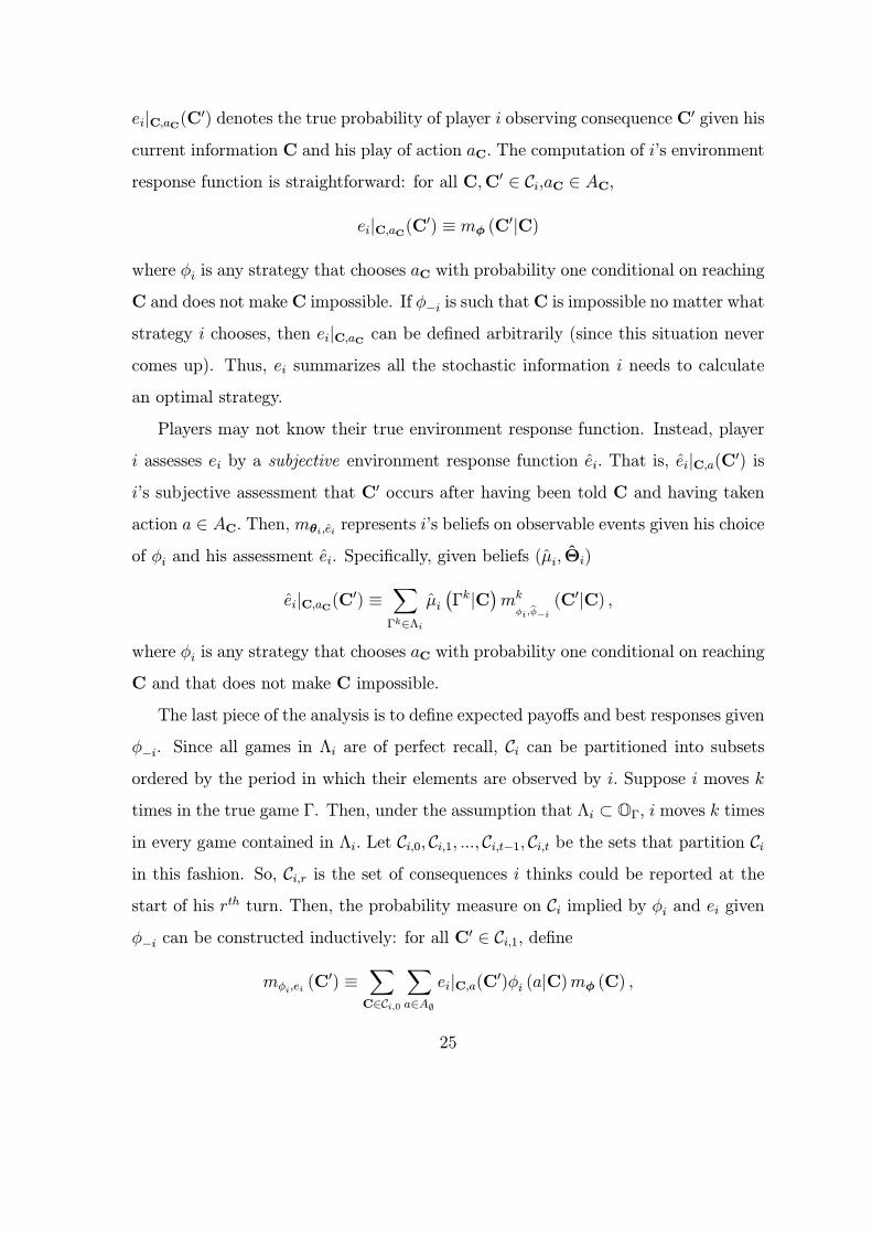
ei|C,aC(C0) denotes the true probability of player i observing consequence C0 given hiscurrent information C and his play of action aC. The computation of i’s environment

response function is straightforward: for all C,C0 ∈ Ci,aC ∈ AC,

ei|C,aC(C0) ≡ mφ (C0|C)

where φi is any strategy that chooses aC with probability one conditional on reaching

C and does not make C impossible. If φ−i is such thatC is impossible no matter what

strategy i chooses, then ei|C,aC can be defined arbitrarily (since this situation nevercomes up). Thus, ei summarizes all the stochastic information i needs to calculate

an optimal strategy.

Players may not know their true environment response function. Instead, player

i assesses ei by a subjective environment response function ei. That is, ei|C,a(C0) isi’s subjective assessment that C0 occurs after having been told C and having taken

action a ∈ AC. Then, mθi,ei represents i’s beliefs on observable events given his choice

of φi and his assessment ei. Specifically, given beliefs (µi, Θi)

ei|C,aC(C0) ≡XΓk∈Λi

µi¡Γk|C¢mk

φi,bφ−i (C

0|C) ,

where φi is any strategy that chooses aC with probability one conditional on reaching

C and that does not make C impossible.

The last piece of the analysis is to define expected payoffs and best responses given

φ−i. Since all games in Λi are of perfect recall, Ci can be partitioned into subsetsordered by the period in which their elements are observed by i. Suppose i moves k

times in the true game Γ. Then, under the assumption that Λi ⊂ OΓ, i moves k timesin every game contained in Λi. Let Ci,0, Ci,1, ..., Ci,t−1, Ci,t be the sets that partition Ciin this fashion. So, Ci,r is the set of consequences i thinks could be reported at thestart of his rth turn. Then, the probability measure on Ci implied by φi and ei givenφ−i can be constructed inductively: for all C

0 ∈ Ci,1, define

mφi,ei (C0) ≡

XC∈Ci,0

Xa∈A∅

ei|C,a(C0)φi (a|C)mφ (C) ,

25

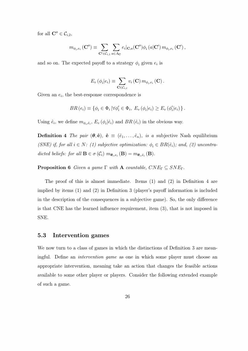
for all C00 ∈ Ci,2,

mφi,ei (C00) ≡

XC0∈Ci,1

Xa∈AC

ei|C,a(C00)φi (a|C0)mφi,ei (C0) ,

and so on. The expected payoff to a strategy φi given ei is

Ev (φi|ei) ≡XC∈Ci,t

vi (C)mφi,ei (C) .

Given an ei, the best-response correspondence is

BR (ei) ≡ {φi ∈ Φi |∀φ0i ∈ Φi, Ev (φi|ei) ≥ Ev (φ0i|ei)} .

Using ei, we define mφi,ei , Ev (φi|ei) and BR (ei) in the obvious way.

Definition 4 The pair (θ, e), e ≡ (e1, . . . , en), is a subjective Nash equilibrium

(SNE) if, for all i ∈ N : (1) subjective optimization: φi ∈ BR(ei); and, (2) uncontra-dicted beliefs: for all B ∈ σ (Ci) mθi,ei (B) = mθi,ei (B).

Proposition 6 Given a game Γ with A countable, CNEΓ ⊆ SNEΓ.

The proof of this is almost immediate. Items (1) and (2) in Definition 4 are

implied by items (1) and (2) in Definition 3 (player’s payoff information is included

in the description of the consequences in a subjective game). So, the only difference

is that CNE has the learned influence requirement, item (3), that is not imposed in

SNE.

5.3 Intervention games

We now turn to a class of games in which the distinctions of Definition 3 are mean-

ingful. Define an intervention game as one in which some player must choose an

appropriate intervention, meaning take an action that changes the feasible actions

available to some other player or players. Consider the following extended example

of such a game.

26

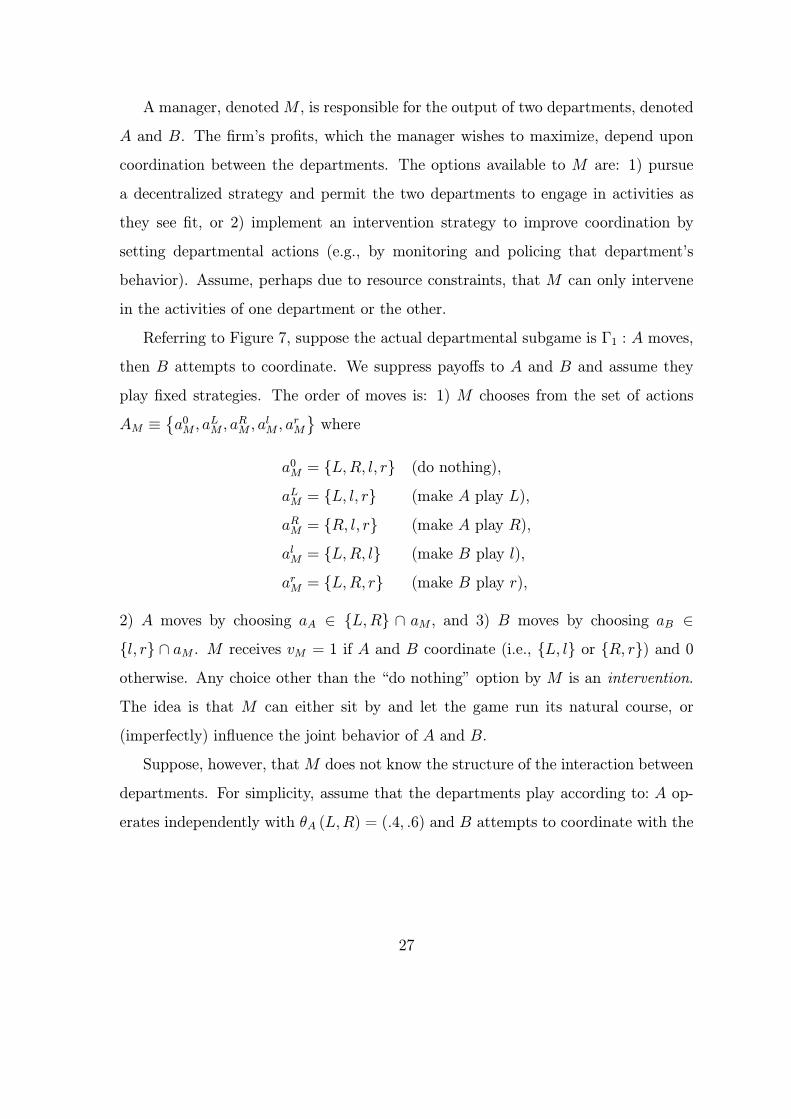
A manager, denotedM , is responsible for the output of two departments, denoted

A and B. The firm’s profits, which the manager wishes to maximize, depend upon

coordination between the departments. The options available to M are: 1) pursue

a decentralized strategy and permit the two departments to engage in activities as

they see fit, or 2) implement an intervention strategy to improve coordination by

setting departmental actions (e.g., by monitoring and policing that department’s

behavior). Assume, perhaps due to resource constraints, that M can only intervene

in the activities of one department or the other.

Referring to Figure 7, suppose the actual departmental subgame is Γ1 : A moves,

then B attempts to coordinate. We suppress payoffs to A and B and assume they

play fixed strategies. The order of moves is: 1) M chooses from the set of actions

AM ≡©a0M , a

LM , a

RM , a

lM , a

rM

ªwhere

a0M = {L,R, l, r} (do nothing),

aLM = {L, l, r} (make A play L),

aRM = {R, l, r} (make A play R),

alM = {L,R, l} (make B play l),

arM = {L,R, r} (make B play r),

2) A moves by choosing aA ∈ {L,R} ∩ aM , and 3) B moves by choosing aB ∈{l, r} ∩ aM . M receives vM = 1 if A and B coordinate (i.e., {L, l} or {R, r}) and 0otherwise. Any choice other than the “do nothing” option by M is an intervention.

The idea is that M can either sit by and let the game run its natural course, or

(imperfectly) influence the joint behavior of A and B.

Suppose, however, thatM does not know the structure of the interaction between

departments. For simplicity, assume that the departments play according to: A op-

erates independently with θA (L,R) = (.4, .6) and B attempts to coordinate with the

27

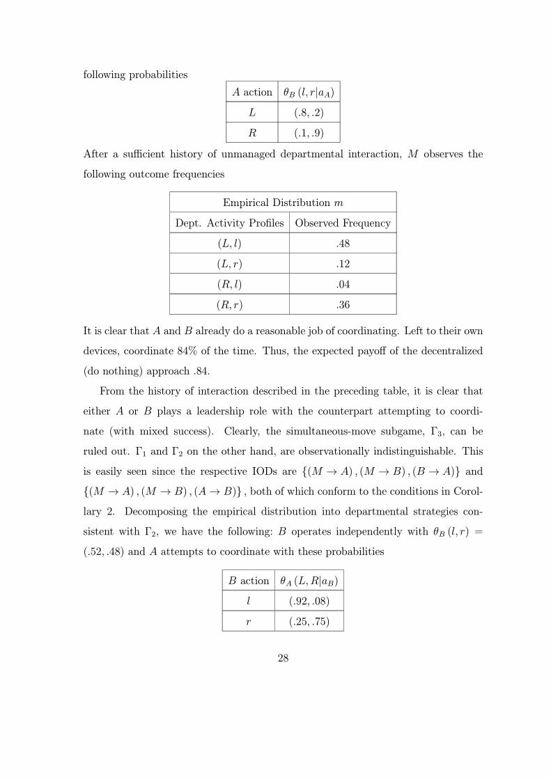
following probabilities

A action θB (l, r|aA)L (.8, .2)

R (.1, .9)

After a sufficient history of unmanaged departmental interaction, M observes the

following outcome frequencies

Empirical Distribution m

Dept. Activity Profiles Observed Frequency

(L, l) .48

(L, r) .12

(R, l) .04

(R, r) .36

It is clear that A and B already do a reasonable job of coordinating. Left to their own

devices, coordinate 84% of the time. Thus, the expected payoff of the decentralized

(do nothing) approach .84.

From the history of interaction described in the preceding table, it is clear that

either A or B plays a leadership role with the counterpart attempting to coordi-

nate (with mixed success). Clearly, the simultaneous-move subgame, Γ3, can be

ruled out. Γ1 and Γ2 on the other hand, are observationally indistinguishable. This

is easily seen since the respective IODs are {(M → A) , (M → B) , (B → A)} and{(M → A) , (M → B) , (A→ B)} , both of which conform to the conditions in Corol-lary 2. Decomposing the empirical distribution into departmental strategies con-

sistent with Γ2, we have the following: B operates independently with θB (l, r) =

(.52, .48) and A attempts to coordinate with these probabilities

B action θA (L,R|aB)l (.92, .08)

r (.25, .75)

28

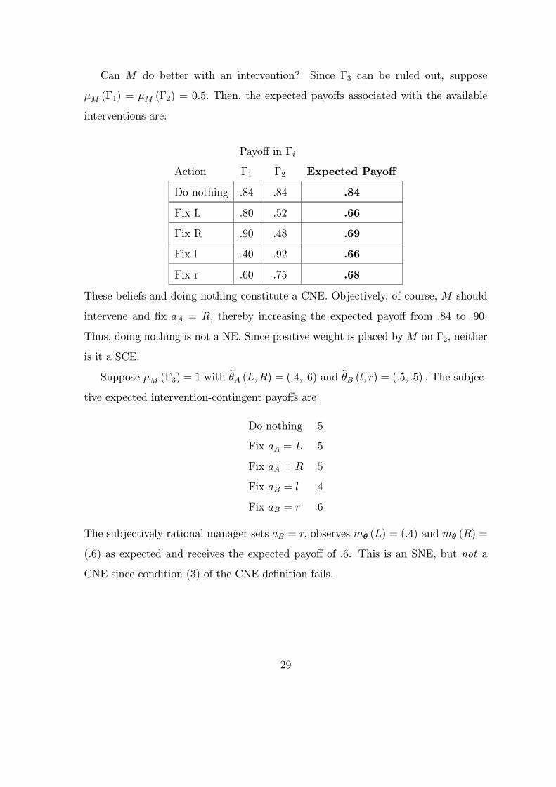
Can M do better with an intervention? Since Γ3 can be ruled out, suppose

µM (Γ1) = µM (Γ2) = 0.5. Then, the expected payoffs associated with the available

interventions are:

Payoff in Γi

Action Γ1 Γ2 Expected Payoff

Do nothing .84 .84 .84

Fix L .80 .52 .66

Fix R .90 .48 .69

Fix l .40 .92 .66

Fix r .60 .75 .68

These beliefs and doing nothing constitute a CNE. Objectively, of course, M should

intervene and fix aA = R, thereby increasing the expected payoff from .84 to .90.

Thus, doing nothing is not a NE. Since positive weight is placed by M on Γ2, neither

is it a SCE.

Suppose µM (Γ3) = 1 with θA (L,R) = (.4, .6) and θB (l, r) = (.5, .5) . The subjec-

tive expected intervention-contingent payoffs are

Do nothing .5

Fix aA = L .5

Fix aA = R .5

Fix aB = l .4

Fix aB = r .6

The subjectively rational manager sets aB = r, observes mθ (L) = (.4) and mθ (R) =

(.6) as expected and receives the expected payoff of .6. This is an SNE, but not a

CNE since condition (3) of the CNE definition fails.

29

6 Discussion

Although our definition of observational imitation is new, the idea of observation-

ally indistinguishable strategies is introduced at least as early as Kuhn (1953). Two

strategies, behavior or mixed, are equivalent if they lead to the same probability

distribution over outcomes for all strategies of one’s opponents. Kuhn demonstrates

that, in games of perfect recall, every mixed strategy is equivalent to the unique be-

havior strategy it generates and each behavior strategy is equivalent to every mixed

strategy that generates it (see Aumann, 1964, for an extension to infinite games). It

follows immediately that every extensive-form game of perfect recall is indistinguish-

able from its reduced normal form. Thus, any two games with the same reduced

normal form are indistinguishable.

We have interpreted the results in Section 4 as consistent with the inferences that

would be made by an outside observer with sufficiently informative empirical data.

One question that immediately comes to mind is whether these ideas can be extended

to construct an econometric test for game structure given cross sectional data on

player actions. For example, the maximum likelihood estimate of the information

structure for an industry might be useful in refining cost estimation in empirical

work in industrial organization (as suggested by the example in Section 5.1). This is

the subject of on-going research.

The literature contains two primary approaches to analyzing situations in which

players do not know the structure of their game. The first, and closest to ours in

spirit, is Kalai and Lehrer’s (1993, 1995) work on subjective games and their notion of

subjective equilibrium. Kalai and Lehrer show that, provided beliefs are sufficiently

close to the truth, play converges to a SNE. Moving to an infinitely repeated version

of CNE and exploring the convergence properties of noisy learning processes strikes

us as a worthwhile extension of this paper; since CNE ⊆ SNE in finitely repeated

subjective games, we conjecture that results along the lines of Kalai and Lehrer also

hold in our setting. The second approach is to encode a player’s uncertainty regarding

30

the information structure of the game into his or her type (a la Harsanyi, 1967 — 68).

When players have correct (and, therefore, common) priors, there is nothing in our

methodology that is inconsistent with the Harsanyi approach.

Several authors have proposed other equilibrium definitions whose interpretations

are consistent with the idea that equilibria arise as the result of learning.12 The

structure shared by these definitions is: 1) players have prior beliefs about certain

unknowns (i.e., competitor strategies and/or various elements of game structure),

and 2) choose strategies that are best-replies to these beliefs, which then, 3) generate

observables that do not refute the priors upon which the strategy choices were based.

CNE has the novelty that beliefs are restricted to the set of imitative games rather

than, say, the set of games capable of imitating a specific equilibrium strategy profile

(typically, a much larger set). The stronger condition is appropriate, e.g., if players

observe a wide range of behavior prior to settling down into equilibrium.

A game’s IOD is a graph that summarizes information about its empirical dis-

tributions. This idea (i.e., using graphs to encode probabilistic information) is not

new outside economics. In particular, there is a burgeoning literature in artificial

intelligence on the use of graphs to simultaneously model causal hypotheses and to

encode the conditional independence relations implied by these hypotheses. Such

graphs are called probabilistic networks. An important distinction in our work is that

the IOD is derived from the primitives of a game and not from the properties of a

single, arbitrarily-specified probability distribution. Thus, the information encoded

in an IOD holds for all empirical distributions arising from play in the underlying

game. Moreover, many of the results in the first part of the paper rely on the special

structure implied by distributions of this kind and, as mentioned earlier, may not hold

in a non-game-theoretic context (or, for example, if correlated strategies are allowed

without inclusion of a specific correlating device).

Until recently, work on probabilistic networks focused upon the decision problem

of a single individual. Thus, another aspect that separates our work from the existing

31

literature in this field is its use of these objects in the solution of game-theoretic (i.e.,

interactive) decision problems. Two other papers, one by Koller and Milch (2002)

and another by La Mura (2002) also use probabilistic networks to derive results of

interest to game theorists, though along a different line. Both of these papers develop

alternative representations for interactive decision problems (i.e., as opposed to a

game’s strategic or normal form) and argue that these representations are not only

computationally advantageous but also provide qualitative insight into the structural

interdependencies between player decisions. Our work clearly complements this line

of research.

32

A Dependency models

Here, we provide a condensed discussion of the relevant underlying theory of proba-

bilistic networks. Since most economists are unfamiliar with this literature, we wish

to: (i) give readers a sense of its theoretical content, and (ii) provide sufficient techni-

cal detail to support the development of our proofs. For those interested in pursuing

these ideas further, we suggest starting with the texts by Pearl (1988, 2000) and

Cowell et al. (1999).

Definition 5 A dependency model M over a finite set of elements T is a collection

of independence statements of the form (C ⊥ D|E) in which C,D and E are disjoint

subsets of T and which is read “C is independent of D given E.” The negation of an

independency is called a dependency.

The notion of a general dependency model was originated by Pearl and Paz (1985),

who were motivated to develop a set of axiomatic conditions on general dependency

models that would include probabilistic and graphical dependencies as special cases.

These axioms are known as the graphoid axioms.13 We are interested in graphoids,

which are defined as dependency models that are closed under the graphoid axioms.

For example, given a probability space (A,A, µ) and an associated, finite set ofrandom variables X indexed by T = {1, ..., t} with typical element xr, Mµ is the

list of conditional independencies that hold under µ. For all W ⊆ T, let xW ≡(xr)r∈W . Then, for all disjoint C,D,E ⊂ T, (C ⊥ D|E) ∈ Mµ if and only if xC is

µ-conditionally independent of xD given xE. A proof that the graphoid axioms hold

for conditional independence in all probability distributions can be found in Spohn

(1980).

Alternatively, if G is a graph whose vertices are T , then for all disjoint C,D,E ⊂ T,(C ⊥ D|E) ∈ MG if and only if E is a cutset separating C from D. Of course, in

this case, the meaning of (C ⊥ D|E) depends upon how one defines “cutset.” Theliterature on probabilistic networks contains several such definitions, depending upon

33

whether the graph is undirected, directed or some mixture of the two (i.e., a chain

graph). Since our IODs are directed, acyclic graphs (hereafter, DAGs), we proceed

with Pearl’s (1986) notion of d-separation (the d stands for “directed”).

Given a DAG G ≡ (T,→) , a path is an ordered set of nodes P ⊆ T such that,for all αr,αr+1 ∈ P, either αr → αr+1 or αr ← αr+1. A node αr ∈ P is called

head-to-head with respect to P if αr−1 → αr and αr ← αr+1 in P . A node that starts

or ends a path is not head-to-head. A path P ⊂ T is active by E ⊂ T if: (i) everyhead-to-head node is in or has a descendant in E, and (ii) every other node in P is

outside E. Otherwise, P is said to be blocked by E.

Definition 6 If G = (T,→) is a DAG and C,D and E are disjoint subsets of T,

then E is said to d-separate C from D if and only if there exists no active path by E

between a node in C and a node in D.

Examples of d-separation can be found in the Pearl references cited above. Thus,

given a DAG G we define MG such that (C ⊥ D|E) ∈MG if and only if E d-separates

C from D in G.We wish to characterize the relationship between probabilistic and graphical de-

pendency models. This is done through the general notion of an independence map

(or, I-map).

Definition 7 An I-map of a dependency model M is any model M 0 such that M 0 ⊆M.

Given a probability space (A,A, µ) and an associated, finite set of random vari-

ables X ≡ {x1, ..., xt} , the task of constructing a DAG (T,→) , T = {1, ..., t}, suchthat M(T,→) is an I-map of Mµ is straightforward (see Geiger et al., 1990, p. 514).

First, for all r ∈ T, let Ur ≡ {1, ..., r − 1} index the predecessors of xr according toT. Next, identify a minimal set of predecessors Πr ⊂ T such that ({r} ⊥ Ur\Πr|Πr)µwhere the “µ” subscript indicates probabilistic independence under µ. This results

34

in a set of t independence statements known as a recursive basis drawn from Mµ

and denoted Bµ. Now, construct (T,→) such that s → r if and only if s ∈ Πr. Theresulting graph G, a DAG, is said to be generated by Bµ and Πr = {s ∈ T |s→ r} isthe set of parents of r in G.The following theorems are from Geiger et al. (1990, Theorems 1 and 2). First,

an independence statement (C ⊥ D|E) is a semantic consequence (with respect to aclass of dependency modelsM — e.g., those that satisfy the graphoid axioms) of a set

B of such statements if (C ⊥ D|E) holds in every dependency model that satisfiesB; i.e., (C ⊥ D|E) ∈M for all M such that B ⊆M ∈M.

Theorem 1 (soundness) If M is a graphoid and B is any recursive basis drawn

from M, then the DAG generated by B is an I-map of M.

So, given (A,A, µ), the DAG G constructed in the fashion outlined above is anI-map of Mµ. That is, every independence statement implied by (T,→) under d-separation corresponds to a valid µ-conditional independency.

Theorem 2 (closure) Let D be a DAG generated by a recursive basis B. Then MD,

the dependency model generated by D, is exactly the closure of B under the graphoid

axioms.

Following Pearl (2000, pp. 16-20), two DAGs (T,→) and (T,→0) are said to

be observationally equivalent if every probability distribution that can be factored

in accordance with the recursive basis B(T,→) ≡ {({r} ⊥ Ur\Πr|Πr) |r ∈ T} can alsobe factored in accordance with B(T,→0) ≡ {({r} ⊥ U 0r\Π0r|Π0r) |r ∈ T} . The followingtheorem is from Pearl (2000, Theorem 1.2.8). It originally appears in Verma and

Pearl (1990,Theorem 1) and is generalized by Andersson et al. (1997, Theorems B.1

and 2.1).

Theorem 3 Two DAGs (T,→) and (T,→0) are observationally equivalent if and

only if E = E 0 and S = S0.

35

B Proofs

B.1 Preliminary results

We begin with four lemmas that are used later. Given a game Γ and its IOD

G ≡ (T,→). Define BΓ ≡ {({r} ⊥ Ur\Πr|Πr) |r ∈ T} to be the collection of t in-dependence statements associated with the moves in the game. Let MΓ be the clo-

sure of BΓ under the graphoid axioms. Notice that BΓ is a recursive basis drawn

from MΓ and, by construction of BΓ, G is the DAG generated by BΓ. Hence, by thesoundness theorem, G is an I-map of MΓ and by the closure theorem, MG =MΓ. By

Proposition 1, for all θ ∈ Σ, the conditional independencies in BΓ hold in mθ. Thus,

the independence statements in MΓ hold in mθ for all θ ∈ Σ; i.e., for all θ ∈ Σ,MΓ ⊆Mmθ

.

Lemma 2 Given an exact information game Γ and a probability distribution µ that

can be factored according to BΓ, there exists a strategy θ ∈ Σ such that mθ = µ,

µ-a.s.

Proof. By the premise, µ can be factored according to BΓ, so that for all r ∈ T,({r} ⊥ Ur\Πr|Πr) ∈Mµ. Thus, for all F ∈ A,

µ (F) =

ZF

Yr∈Tµ (ar|πr) (a) da.

Define, for all Fr ∈ Ar,θr³Fr|hr

´≡ µ (Fr|πr) . Because Γ is a game of exact infor-

mation, σ (πr) = Ir. Thus, the resulting profile, (θr)r∈T , is a strategy profile of Γ andmθ = µ, µ-a.s., by construction.

Lemma 3 If Γ and Γ0, Γ ∈ OΓ0, are games of exact information and Γ ∈ rem(T 0,→0)

then Γ ¹ Γ0. (Recall the definition of rem(T,→) in section 4.3.)

Proof. First, imitation is a transitive (see proof of Lemma 1 below): i.e., for

any games Γ1,Γ2 and Γ3, if Γ1 ¹ Γ2 and Γ2 ¹ Γ3, then Γ1 ¹ Γ3. Let EΓ1 ≡

36

{(a, b) |a→ b ∈ (T,→1)} denote the set of edges in (T,→1) . Define

EΓ2−Γ1 ≡ {(a, b) ∈ T × T | (a, b) ∈ EΓ2 , (a, b) /∈ EΓ1} ;

i.e., the set of edges that are in (T,→2) but not in (T,→1) .

We now continue with the proof in steps:

1. Delete one edge from Γ0. Let Γ1 ∈ OΓ0 be a game of exact information suchthat EΓ1 ⊂ EΓ0 and EΓ0−Γ1 = {(a, b)} where (a, b) ∈ EΓ0−Γ. As both Γ0 and Γ1are games of exact information, this implies that ∀r ∈ T , r 6= b, Π0r = Π1r and

that Π1b = Π0b \ {a}. Let θ1 ∈ Σ1 be an arbitrary strategy profile in Γ1. ByProposition 1,

mθ1 =Yr∈Tmθ1(ar|π1r)

= mθ1(ab|π1b)Y

r∈T\{b}mθ(ar|π0r).

Since Π1b = Π0b \ {a}, σ(π1b) ⊆ σ(π0b). Thus, mθ1(ab|π1b) = mθ(ab|π0b). Hence,condition (6) holds. By Proposition 2, Γ1 ¹ Γ0. If EΓ0−Γ = {(a, b)} , go to step4. Otherwise, let n = 2.

2. If EΓ0−Γ 6= EΓ0−Γn−1 , we proceed by deleting an additional edge. Let Γn ∈ OΓ0(and hence Γn ∈ OΓn−1) be a game of exact information such that EΓn ⊂ EΓn−1and EΓn−1−Γn = {(c, d)} where (c, d) ∈ EΓ0−Γ. By the same argument as in step1, Γn ¹ Γn−1. As, from the previous step, Γn−1 ¹ Γ0, by the transitivity of ¹(see proof of Lemma 1 below), so that Γn ¹ Γ0. If EΓ0−Γ = EΓ0−Γn go to step 4.

3. Otherwise, repeat step 2, increasing the value of n by one. Eventually, as the

set E 0 is finite and E ⊂ E 0, we will find an n such that EΓ0−Γ = EΓ0−Γn .

4. Since Γ is a game of exact information, it has the same players, action spaces

and information sets as Γn so that Σ = Σn, hence Γ ¹ Γ0.

37

Lemma 4 Let (T,→) be an IOD for some game Γ. If r, s ∈ T such that r < s andr 9 s, then Is ⊆ σ

³hs\r

´where hs\r (a) ≡ (a1, ..., ar−1, ar+1, ..., as−1).

Proof.

1. Let F0∈Is be an arbitrary element of the partition of A that generates Is.Recall, Is ⊆ σ

³hs´, so F0 = Gr−∩Gr∩Gr+ whereGr− ∈ σ

³hr´,Gr ∈ σ (ar) ,

Gr+ ∈ σ (ar+1, . . . , as−1) .

2. Let Hr+1 ≡n(hr, ar) ∈ hr+1 (A) |hr ∈ hr (A) , ar ∈ Ar

o. By the definition of

an IOD, given r, s ∈ T , r < s, if r 9 s, then for all (hr, ar) , (hr, a0r) ∈ Hr+1

we have that for all F ∈Is such that h−1r+1 (hr, ar) ⊂ F, h−1r+1 (hr, a0r) ⊂ F. Thus,for all hr ∈ hr (A) , there exist Gr+ ∈ σ (ar+1, . . . , as−1) and F ∈Is such thath−1r (hr) ∩ a−1r (cr (hr)) ∩Gr+⊂ F. But, the tree structure of the game impliesa−1r (cr (hr)) = h

−1r (hr) .

3. Taken together, items 1) and 2) imply that, for all F0∈Is there exist Gr− ∈σ³hr´and Gr+ ∈ σ (ar+1, . . . , as−1) such that

F0 = h−1r (Gr) ∩ a−1r (cr (Gr)) ∩Gr+

= h−1r (Gr) ∩Gr+.

But, this implies that F0 ∈ σ³hs\r

´. Thus, Is ⊆ σ

³hs\r

´.

Lemma 5 Every influence opportunity diagram is a DAG.

Proof. This follows by construction: the graph is defined using only directed

edges. It is acyclic because nodes are fully ranked by the order of play and directed

edges only appear from earlier moves to strictly later moves.

Finally, the following proposition implies a straightforward procedure for testing

whether Γ ¹ Γ0 where Γ is an arbitrary game and Γ0 is a game of exact information:(i) construct the IODs for each game; then, (ii) check (using d-separation) to see

38

whether the t independence statements in BΓ0 hold in (T,→) . While this resultis more general than Proposition 4, it requires an understanding of the material

presented in Appendix A and may be quite cumbersome to implement in games with

many moves.

Proposition 7 Given two games Γ and Γ0, the latter a game of exact information,

if Γ0 ∈ OΓ and BΓ0 ⊆MΓ, then Γ ¹ Γ0.

Proof. As discussed above, for all θ ∈ Σ,MΓ ⊆Mmθ. By the premise, BΓ0 ⊆MΓ.

It follows that, for all θ ∈ Σ, mθ can be factored in accordance with BΓ0 ; i.e., as in

condition (6). By Lemma 2 and Proposition 2, Γ ¹ Γ0.

B.2 Lemma 1

1. (Equivalence relation) Reflexivity: Given Γ and the identity mappings f (r) = r

and g (θ) = θ implies Γ ¹ Γ. Transitivity: Assume Γ ∼ Γ and Γ ∼ Γ0.

Suppose Γ ¹ Γ with permutation f and strategy mapping g, and Γ ¹ Γ0 with

permutation f and mapping g. Then, Γ ¹ Γ0 under f ≡ f ◦ f . and g ≡ g ◦ g.By similar reasoning, Γ0 ¹ Γ. Therefore, Γ ∼ Γ0. Symmetry: This is immediatefrom the definition.

2. ((f (A0) , f (A0))= (A,A)) This is immediate from Γ ∈ OΓ0 .

3. Let g and g be functions meeting the conditions of Γ ¹ Γ and Γ ¹ Γ, respectively.

Define g : Σ⇒ Γ as follows:

∀θ ∈ Σ, g (θ) ≡ g (θ) if θ /∈ g

³Σ´

g−1 (θ) if θ ∈ g³Σ´

Clearly, g is onto and has the desired property for θ /∈ g³Σ´. Suppose θ ∈

g³Σ´. Then, for all θ ∈g−1 (θ) ,

³A, bA, mθ

´=³A, bA, mθ

´by the definition

of g. By the equality of measurable spaces (Part II), it is also the case that

(A,A,mθ) = (A,A,mθ) .

39

B.3 Proposition 1

Given equation (3), equation (4) holds if, for all θ ∈ Σ, r ∈ T,

mθ (ar|πr) = mθ (ar|Ir) . (7)

Recall, for all F ∈ A,mθ (ar (F) |πr) is the conditional probability of a−1r (Fr) given

σ (πr) . Thus, the two conditions characterizingmθ (ar|πr) are: (i)mθ (ar|πr) is σ (πr)-measurable and (ii) for all F ∈ A, G ∈ σ (πr) ,Z

G

mθ (ar (F) |πr) (a)mθ (da) = mθ

¡a−1r (Fr) ∩G

¢.

We need to demonstrate that mθ (ar|Ir) also satisfies these conditions. For all r ∈ T,Lemma 4 implies that F ∈ Ir ⇒ F ∈ σ (ak)k∈{s∈T |s9r}c. Of course, σ (ak)k∈{s∈T |s9r}c =σ (πr) , so Ir ⊂ σ (πr). Therefore, mθ (ar|Ir) is σ (πr)-measurable. But this (and thedefinition of conditional probability) implies that, for all F ∈ A, G ∈ σ (πr) ,Z

G

mθ (ar (F) |Ir) (a)mθ (da) = mθ

¡a−1r (Fr) ∩G

¢.

B.4 Proposition 2

The necessity of (6) follows from Corollary 1. To prove sufficiency, consider an ar-

bitrary θ ∈ Σ. By the premise of the proposition, mθ can be factored according to

B(T,→0). Since Γ0 is a game of exact information, by Lemma 2, there exists a θ0 ∈ Σ0

such that mθ = mθ0 . Therefore, Γ ¹ Γ0.

B.5 Proposition 3

By Theorem 3, (T,→) and (T,→0) are observationally equivalent. Hence, for all

θ ∈ Σ, mθ can be factored in accordance with B(T,→0). By Proposition 2, Γ ¹ Γ0. Byidentical reasoning, if Γ is also a game of exact information, Γ0 ¹ Γ and, thus, Γ ∼ Γ0.

40

B.6 Proposition 4

Suppose Γ is not of exact information. Let Γ1 be the same game as Γ in all respects

except that Γ1 is of exact information. As both Γ and Γ1 admit (T,→) condition(6) holds so that by Proposition 2, Γ ¹ Γ1. Let Γ

∗, Γ∗ ∈ OΓ0, be a game of exactinformation with IOD (T,→∗). Per Corollary 2, Γ∗ ∼ Γ0. Per Lemma 3 above

Γ1 ¹ Γ∗. By the transitivity of imitation and indistinguishability (see proof of Lemma1) Γ ¹ Γ1 ¹ Γ∗ ∼ Γ.

41

C Footnotes

1. Many real-world managerial situations, for example, appear to be characterized

by this structure.

2. If our results are to be interpreted as relevant to situations in which players

learn about their ability to influence others, it seems reasonable to assume that

they do so in an environment in which such influence is a stationary aspect of

the game.

3. These conditions are less restrictive than they may at first appear since players

may make multiple moves and/or may be limited to a single, ‘null’ action at

certain information sets (see, e.g., Elmes and Reny, 1994).

4. That is, they are finite, denumerable or isomorphic with the unit interval. In

particular, this assumption implies the points in each set are measurable. The

use of this word is due to Mackey (1957).

5. Both (1) and (2) follow from a standard result in probability theory. See, e.g.,

Fristedt and Gray (1997, p. 430-31).

6. Note that N has some hope of influencing II indirectly through I. Even so, II

may choose to ignore the move of I (e.g., pick u at both information sets).

7. In what follows, keep in mind the distinction between probability measures

on (A,A) induced by a strategy profile in the underlying game versus genericelements of the much larger space∆ (A,A). Our results are critically dependentupon the structure implied by the former. In particular, correlated strategies are

not allowed without explicit correlating devices. The perfect recall assumption

implies that a player’s own behavior at different moves may be correlated.

8. To illustrate the notational convention take the Games ΓA and ΓB in Figures

1 and 2. Their IODs are N → I → II and II → I → N respectively. Strictly

42

according to the definition, both IODs are 1 → 2 → 3. Using ΓA as the

reference point, the relevant permutation is f(1) = 3, f(2) = 2 and f(3) = 1 so

that oB(f(1)) = oA(1) = N , oB(f(2)) = oA(2) = I, and oB(f(3)) = oA(3) = II.

Under our notational convention, the IOD for ΓB is 3 →B 2 →B 1, which

matches the intuitive description used in the discussion of the example: II →I → N .

9. Note that feasible action consistency is implied by Γ0 ∈OΓ.

10. This last result raised a question that was put to us by E. Dekel in correspon-

dence. Given the well-known work by Thompson (1952) and Elmes and Reny

(1994) that identify transformations on extensive form games that yield the

equivalence class of games with the same strategic form, is there a set of oper-

ations, similar to these in spirit, that yield games with equivalent IODs (in the

sense of Corollary 2)? Due to space limitations, we do not provide a formal re-

ply. Clearly, however, Corollary 2 does suggest a step-wise transformation that

will yield observationally indistinguishable extensive forms with different IODs.

The transformation, while difficult to formalize in the context of an extensive

form game, is easy to describe: it is the transformation that flips an “allowed”

arrow (per Corollary 2) in the original IOD.

11. Although KL allow for a more general set of possible consequences, we restrict

attention to those defined above, Ci

12. A few of the more important contributions include Battigalli and Guatoli’s

(1988) conjectural equilibrium, Fudenberg and Levine’s (1993) self-confirming

equilibrium and, of course, Kalai and Lehrer’s (1993, 1995) subjective equilib-

rium. For related work, see Abreu, Pearce, and Stacchetti (1990), Blume and

Easley (1992), Brandenburger and Dekel (1993), Geanakoplos (1994), Milgrom

and Roberts (1990), and Nachbar (1997). Howitt and McAfee (1992) employ a

similar idea in a macroeconomic application.

43

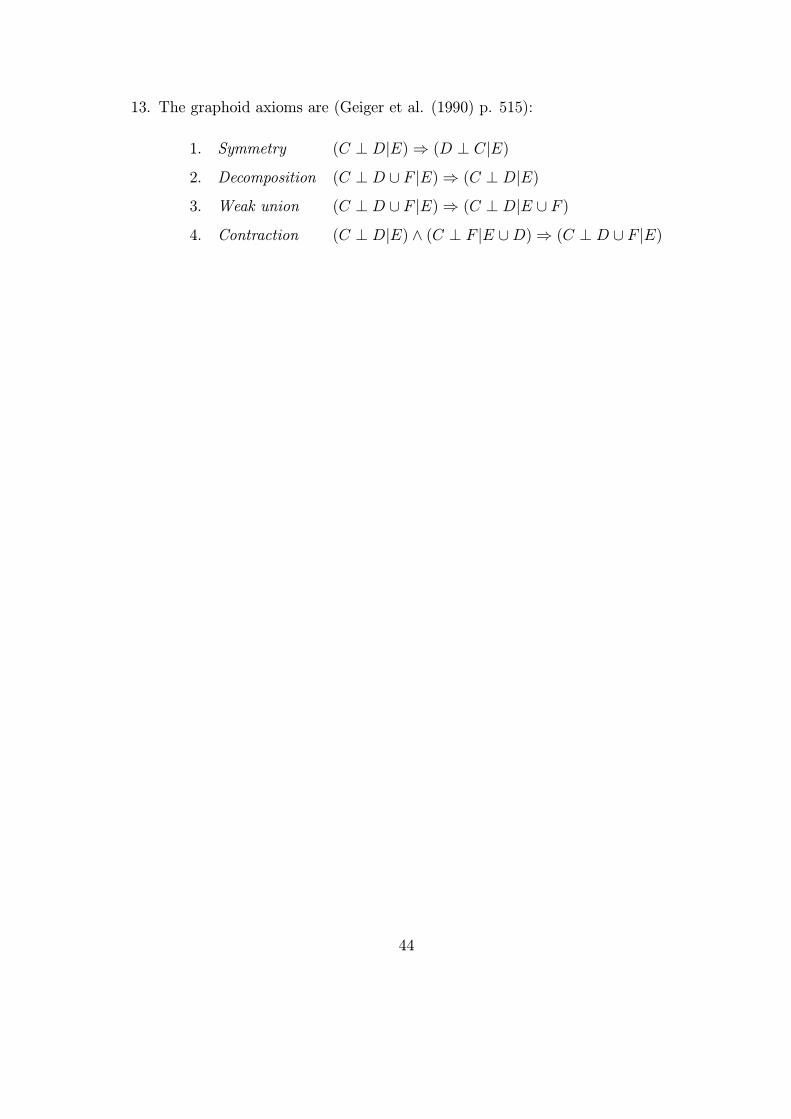
13. The graphoid axioms are (Geiger et al. (1990) p. 515):

1. Symmetry (C ⊥ D|E)⇒ (D ⊥ C|E)2. Decomposition (C ⊥ D ∪ F |E)⇒ (C ⊥ D|E)3. Weak union (C ⊥ D ∪ F |E)⇒ (C ⊥ D|E ∪ F )4. Contraction (C ⊥ D|E) ∧ (C ⊥ F |E ∪D)⇒ (C ⊥ D ∪ F |E)

44

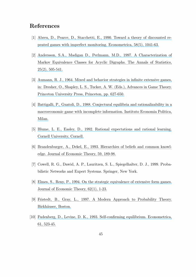
References

[1] Abreu, D., Pearce, D., Stacchetti, E., 1990. Toward a theory of discounted re-

peated games with imperfect monitoring. Econometrica, 58(5), 1041-63.

[2] Andersson, S.A., Madigan D., Perlmann, M.D., 1997. A Characterization of

Markov Equivalence Classes for Acyclic Digraphs. The Annals of Statistics,

25(2), 505-541.

[3] Aumann, R. J., 1964. Mixed and behavior strategies in infinite extensive games,

in: Dresher, O., Shapley, L. S., Tucker, A. W. (Eds.), Advances in Game Theory.

Princeton University Press, Princeton, pp. 627-650.

[4] Battigalli, P., Guatoli, D., 1988. Conjectural equilibria and rationalizability in a

macroeconomic game with incomplete information. Instituto Economia Politica,

Milan.

[5] Blume, L. E., Easley, D., 1992. Rational expectations and rational learning.

Cornell University, Cornell.

[6] Brandenburger, A., Dekel, E., 1993. Hierarchies of beliefs and common knowl-

edge. Journal of Economic Theory, 59, 189-98.

[7] Cowell, R. G., Dawid, A. P., Lauritzen, S. L., Spiegelhalter, D. J., 1999. Proba-

bilistic Networks and Expert Systems. Springer, New York.

[8] Elmes, S., Reny, P., 1994. On the strategic equivalence of extensive form games.

Journal of Economic Theory, 62(1), 1-23.

[9] Fristedt, B., Gray, L., 1997. A Modern Approach to Probability Theory.

Birkhauser, Boston.

[10] Fudenberg, D., Levine, D. K., 1993. Self-confirming equilibrium. Econometrica,

61, 523-45.

45

[11] Geanakoplos, J., 1994. Common Knowledge. Handbook of Game Theory. Else-

vier.

[12] Geiger, D., Verma, T. S., J. Pearl, J., 1990. Identifying independence in Bayesian

networks. Networks, 20, 507-34.

[13] Harsanyi, J., 1967-68. Games with incomplete information played by ‘Bayesian’

players,” Management Science, 8, Parts I-III, 159-82, 320-34, 486-502.

[14] Howitt, P., McAfee, R. P., 1992. Animal Spirits. American Economic Review,

82, 493-507.

[15] Kalai, E., Lehrer, E., 1993. Subjective equilibrium in repeated games. Econo-

metrica, 61, 1231-1240.

[16] –– 1995. Subjective games and equilibria. Games and Economic Behavior, 8,

123-63.

[17] Koller, D. Milch, B., 2002. Multi-agent influence diagrams for representing and

solving games. Seventeenth International Joint Conference on Artificial Intelli-

gence, Seattle, WA.

[18] La Mura, P., 2002. Game Networks. Unpublished manuscript.

[19] Mackey, G. W., 1957. Borel structures in groups and their duals. Trans. Amer.

Math. Soc., 85, 283-95.

[20] Milgrom, P. Roberts, J., 1990. Rationalizability, learning and equilibrium in

games with strategic complimentarities. Econometrica, 58, 1255-1277.

[21] Nachbar, J. H., 1997. Prediction, optimization and learning in repeated games.

Econometrica, 65, 275-309.

[22] Pearl, J., 1986. Fusion, propagation and structuring in belief networks. Artificial

Intelligence 29, 241-88.

46

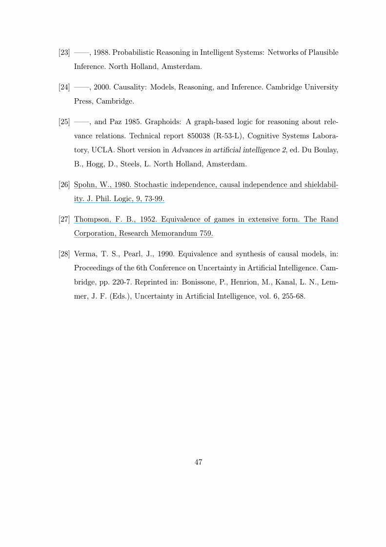
[23] ––, 1988. Probabilistic Reasoning in Intelligent Systems: Networks of Plausible

Inference. North Holland, Amsterdam.

[24] ––, 2000. Causality: Models, Reasoning, and Inference. Cambridge University

Press, Cambridge.

[25] ––, and Paz 1985. Graphoids: A graph-based logic for reasoning about rele-

vance relations. Technical report 850038 (R-53-L), Cognitive Systems Labora-

tory, UCLA. Short version in Advances in artificial intelligence 2, ed. Du Boulay,

B., Hogg, D., Steels, L. North Holland, Amsterdam.

[26] Spohn, W., 1980. Stochastic independence, causal independence and shieldabil-

ity. J. Phil. Logic, 9, 73-99.

[27] Thompson, F. B., 1952. Equivalence of games in extensive form. The Rand

Corporation, Research Memorandum 759.

[28] Verma, T. S., Pearl, J., 1990. Equivalence and synthesis of causal models, in:

Proceedings of the 6th Conference on Uncertainty in Artificial Intelligence. Cam-

bridge, pp. 220-7. Reprinted in: Bonissone, P., Henrion, M., Kanal, L. N., Lem-

mer, J. F. (Eds.), Uncertainty in Artificial Intelligence, vol. 6, 255-68.

47

D Diagrams

48

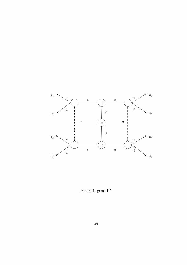
Figure 1: game ΓA

49

N II

I

I

II

U

D

L R

L R

u

d

u

d

u

d

u

d

a1

a4

a3

a2

a5

a6

a7

a8

Figure 1: game ΓA

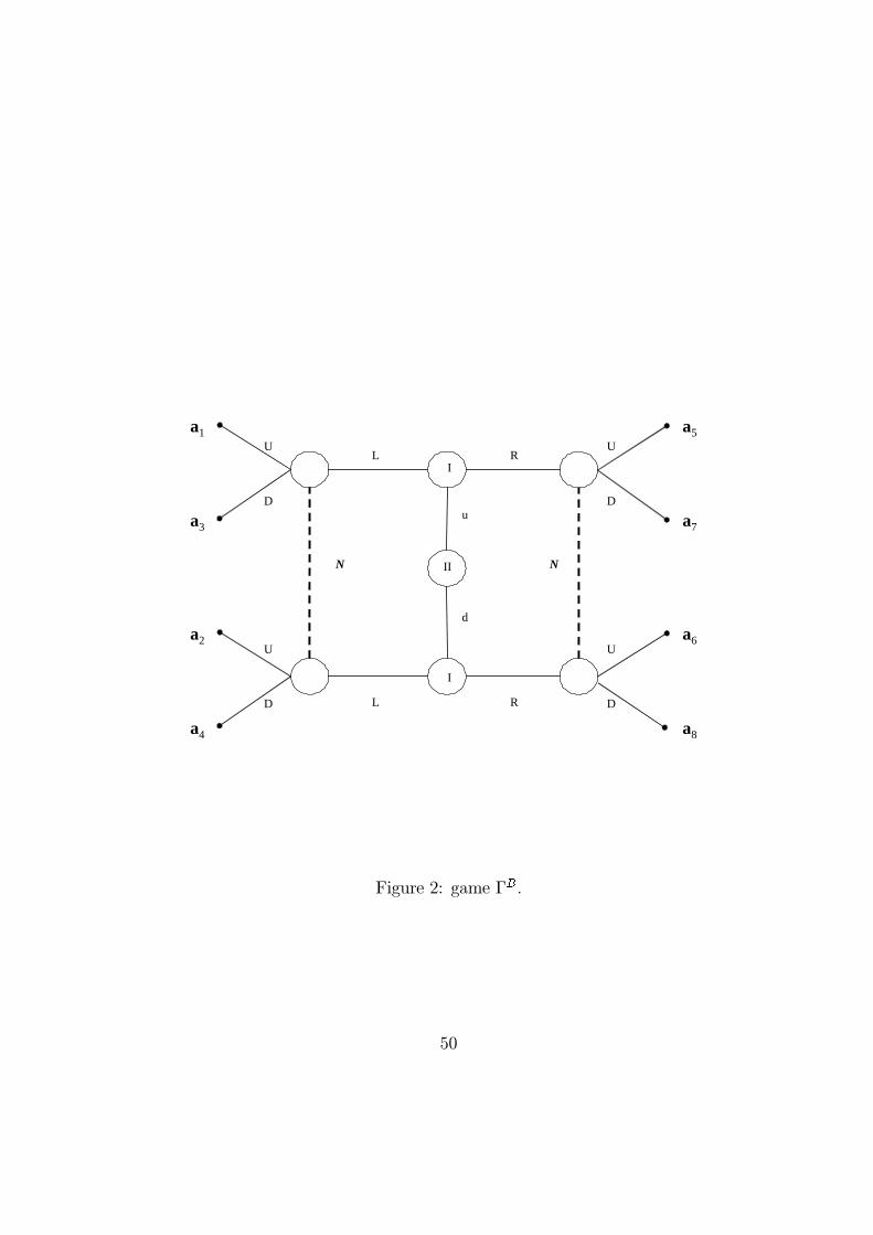
Figure 2: game ΓB.

50

II N

I

I

N

u

d

L R

L R

U

D

U

D

U

D

U

D

a1

a4

a3

a2

a5

a6

a7

a8

Figure 2: game ΓB.

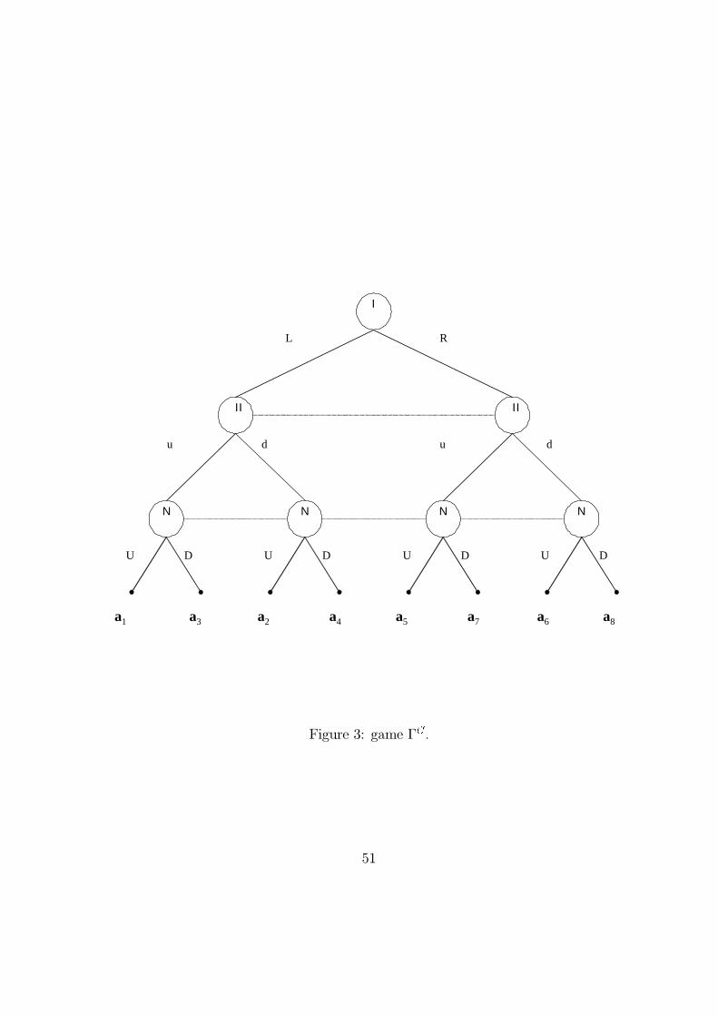
Figure 3: game ΓC .

51

L R

du

Ι

ΙΙ ΙΙ

DU

Ν

DU

Ν

du

DU

Ν

DU

Ν

a1 a4a3 a2 a5 a6a7 a8

Figure 3: game ΓC.

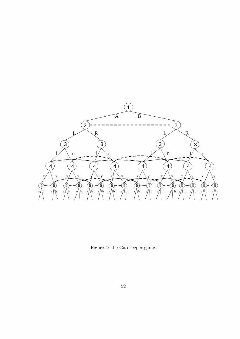
Figure 4: the Gatekeeper game.

52

A B

1

2L R

3

rl rl

3

2L R

rl

3

rl

3

yx

4 4 4 4 4 4 4 4

yx yx yx yx yx yx yx

ba

5ba

5ba

5ba

5ba

5ba

5ba

5ba

5ba

5ba

5ba

5ba

5ba

5ba

5ba

5ba

5

Figure 4: the Gatekeeper game.

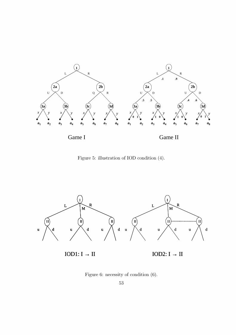
53

1

2a

L R

U D

2b

Q R

3a 3c

x y x y x y x y

3b 3d

1

2a

L R

U D

2b

U D

3a 3c

x y x y x y x y

3b 3d

a1 a2 a3 a4 a5 a6 a7 a8 a1 a2 a3 a4 a5 a6 a7 a8

Game I Game II

.1 .9

.5 .5 .4 .6

0 1 1 0 1 0 0 1

Figure 5: illustration of IOD condition (4).

IOD1: I → II IOD2: I → II

ΙΙ ΙΙ

ΙL R

du

ΙΙ

dudu

M

ΙΙ ΙΙ

ΙL R

du

ΙΙ

dudu

M

IOD1: I → II IOD2: I → II

ΙΙ ΙΙ

ΙL R

du

ΙΙ

dudu

M

ΙΙ ΙΙ

ΙL R

du

ΙΙ

dudu

M

ΙΙ ΙΙ

ΙL R

du

ΙΙ

dudu

M

Figure 6: necessity of condition (6).

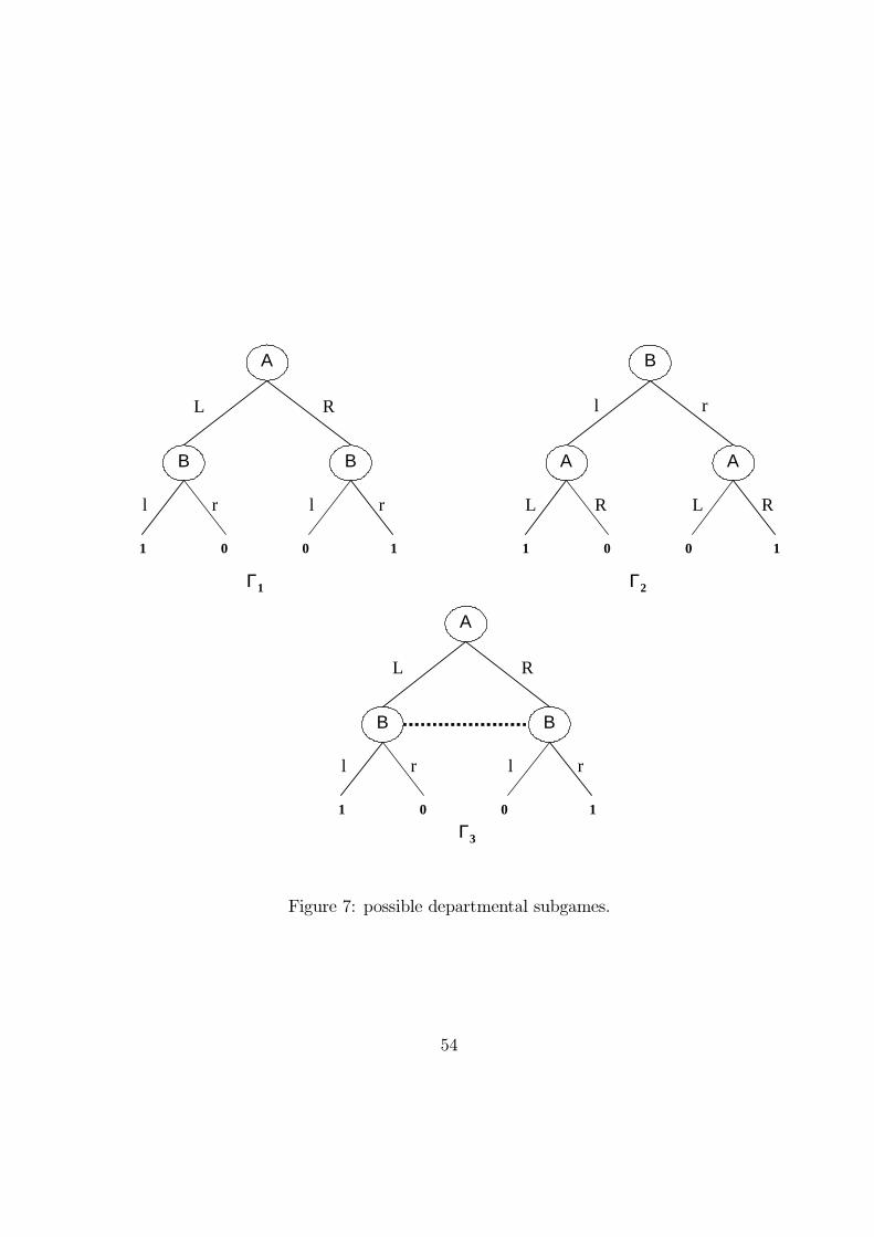
54

Β

L R

rl rl

Α

Β Β

1 0

Γ1

0 1

l r

RL RL

Β

Α Α

1 0

Γ2

0 1

L R

rl rl

Α

Β

1 0

Γ3

0 1

Figure 7: possible departmental subgames.