camcasp 5.5 alston j. misquitta and anthony j. stone university chemical laboratory, lensfield road,...
TRANSCRIPT

CamCASP 5.9
Alston J. Misquitta† and Anthony J. Stone††
†Department of Physics and Astronomy, Queen Mary, University of London, 327 Mile End Road, London E1 4NS†† University Chemical Laboratory, Lensfield Road, Cambridge CB2 1EW
March 26, 2015
Abstract
CamCASP is a suite of programs designed to calculate molecular properties (multipoles and frequency-dependent polarizabilities) in single-site and distributed form, and interaction energies between pairs of molecules,and thence to construct atom–atom potentials. The CamCASP distribution also includes the programs Pfit,Casimir, Gdma 2.2, Cluster, and Process.
Copyright c© 2007–2014 Alston J. Misquitta and Anthony J. Stone

Contents1 Introduction 1
1.1 Authors . . . . . . . . . . . . . . . . . . . . . . . . . . . . . . . . . . . . . . . . . . . . . . . 11.2 Citations . . . . . . . . . . . . . . . . . . . . . . . . . . . . . . . . . . . . . . . . . . . . . . . 1
2 What’s new? 2
3 Outline of the capabilities of CamCASP and other programs 53.1 CamCASP limits . . . . . . . . . . . . . . . . . . . . . . . . . . . . . . . . . . . . . . . . . . 7
4 Installation 74.1 Building CamCASP from source . . . . . . . . . . . . . . . . . . . . . . . . . . . . . . . . . . 9
5 Using CamCASP 105.1 Workflows . . . . . . . . . . . . . . . . . . . . . . . . . . . . . . . . . . . . . . . . . . . . . . 105.2 High-level scripts . . . . . . . . . . . . . . . . . . . . . . . . . . . . . . . . . . . . . . . . . . 105.3 The runcamcasp.py script . . . . . . . . . . . . . . . . . . . . . . . . . . . . . . . . . . . . . . 115.4 Low-level scripts . . . . . . . . . . . . . . . . . . . . . . . . . . . . . . . . . . . . . . . . . . 13
6 Data conventions 13
7 CLUSTER: Detailed specification 147.1 Prologue . . . . . . . . . . . . . . . . . . . . . . . . . . . . . . . . . . . . . . . . . . . . . . . 157.2 Molecule definitions . . . . . . . . . . . . . . . . . . . . . . . . . . . . . . . . . . . . . . . . 157.3 Geometry manipulations and other transformations . . . . . . . . . . . . . . . . . . . . . . . . 167.4 Job specification . . . . . . . . . . . . . . . . . . . . . . . . . . . . . . . . . . . . . . . . . . . 187.5 Energy . . . . . . . . . . . . . . . . . . . . . . . . . . . . . . . . . . . . . . . . . . . . . . . . 237.6 Crystal . . . . . . . . . . . . . . . . . . . . . . . . . . . . . . . . . . . . . . . . . . . . . . . . 257.7 ORIENT . . . . . . . . . . . . . . . . . . . . . . . . . . . . . . . . . . . . . . . . . . . . . . . 267.8 Finally, . . . . . . . . . . . . . . . . . . . . . . . . . . . . . . . . . . . . . . . . . . . . . . . . . 29
8 Examples 298.1 A SAPT(DFT) calculation . . . . . . . . . . . . . . . . . . . . . . . . . . . . . . . . . . . . . 298.2 An example properties calculation . . . . . . . . . . . . . . . . . . . . . . . . . . . . . . . . . 308.3 Dispersion coefficients . . . . . . . . . . . . . . . . . . . . . . . . . . . . . . . . . . . . . . . 348.4 Using CLUSTER to obtain the dimer geometry . . . . . . . . . . . . . . . . . . . . . . . . . . 36
9 CamCASP program specification 399.1 Global data . . . . . . . . . . . . . . . . . . . . . . . . . . . . . . . . . . . . . . . . . . . . . 399.2 Molecule definition . . . . . . . . . . . . . . . . . . . . . . . . . . . . . . . . . . . . . . . . . 409.3 The EDIT module: Modifying a molecular specification . . . . . . . . . . . . . . . . . . . . . . 429.4 Density-fitting . . . . . . . . . . . . . . . . . . . . . . . . . . . . . . . . . . . . . . . . . . . . 439.5 Propagator settings . . . . . . . . . . . . . . . . . . . . . . . . . . . . . . . . . . . . . . . . . 459.6 Quadrature settings . . . . . . . . . . . . . . . . . . . . . . . . . . . . . . . . . . . . . . . . . 499.7 The ISA module . . . . . . . . . . . . . . . . . . . . . . . . . . . . . . . . . . . . . . . . . . . 499.8 Multipole moments . . . . . . . . . . . . . . . . . . . . . . . . . . . . . . . . . . . . . . . . . 529.9 Display . . . . . . . . . . . . . . . . . . . . . . . . . . . . . . . . . . . . . . . . . . . . . . . 549.10 Polarizabilities . . . . . . . . . . . . . . . . . . . . . . . . . . . . . . . . . . . . . . . . . . . 559.11 Lattice . . . . . . . . . . . . . . . . . . . . . . . . . . . . . . . . . . . . . . . . . . . . . . . . 589.12 Numerical integration grid . . . . . . . . . . . . . . . . . . . . . . . . . . . . . . . . . . . . . 599.13 Electrostatic interaction . . . . . . . . . . . . . . . . . . . . . . . . . . . . . . . . . . . . . . . 609.14 First-order exchange (exchange-repulsion) . . . . . . . . . . . . . . . . . . . . . . . . . . . . . 619.15 Second-order induction energy . . . . . . . . . . . . . . . . . . . . . . . . . . . . . . . . . . . 619.16 Second-order dispersion energy . . . . . . . . . . . . . . . . . . . . . . . . . . . . . . . . . . . 649.17 Energy scan . . . . . . . . . . . . . . . . . . . . . . . . . . . . . . . . . . . . . . . . . . . . . 649.18 Overlap model . . . . . . . . . . . . . . . . . . . . . . . . . . . . . . . . . . . . . . . . . . . . 679.19 Integrals . . . . . . . . . . . . . . . . . . . . . . . . . . . . . . . . . . . . . . . . . . . . . . . 71
10 PROCESS: Syntax 73
11 CASIMIR 77

A Basis sets 79
B Dispersion coefficients: in detail 80
C Older Scripts 87C.1 High-level scripts . . . . . . . . . . . . . . . . . . . . . . . . . . . . . . . . . . . . . . . . . . 87C.2 Low-level scripts . . . . . . . . . . . . . . . . . . . . . . . . . . . . . . . . . . . . . . . . . . 87
3
1 Introduction
CamCASP is a suite of programs for the calculation of interaction energies between pairs of molecules, and molec-ular properties (multipoles and frequency-dependent polarizabilities) in single-site and distributed form. The Cam-CASP distribution also includes the programs Pfit, Casimir, Gdma 2.2, Cluster, and Process, and together theseform a package for the ab initio generation of site–site force fields between organic molecules containing up toabout 60 atoms.
1.1 Authors
The CamCASP suite of programs, which includes Pfit, Casimir, Gdma 2.2, Process, and Cluster, has been writ-ten by Alston J. Misquitta and Anthony J. Stone with important contributions from Robert Bukowski, WojciechCencek, the GAMESS(US) team and the GAUSSINT team.
1.2 Citations
This code is provided as a service to the scientific community and our only recompense, such as it is, is in citations.Therefore, if you use any results from CamCASP in your publications we request that you cite the following papers.The choice of citations would depend on the parts of the code you have used for the published results.
• SAPT(DFT) energies
A. J. Misquitta and K. Szalewicz. Intermolecular forces from asymptotically corrected density func-tional description of monomers. Chem. Phys. Lett., 357:301–306, 2002
A. J. Misquitta, B. Jeziorski, and K. Szalewicz. Dispersion energy from density-functional theorydescription of monomers. Phys. Rev. Lett., 91:33201, 2003
A. J. Misquitta and K. Szalewicz. Symmetry-adapted perturbation-theory calculations of intermolecu-lar forces employing density-functional description of monomers. J. Chem. Phys., 122:214109, 2005
A. J. Misquitta, R. Podeszwa, B. Jeziorski, and K. Szalewicz. Intermolecular potentials based onsymmetry-adapted perturbation theory with dispersion energies from time-dependent density-functionaltheory. J. Chem. Phys., 123:214103, 2005
R. Bukowski, R. Podeszwa, and K. Szalewicz. Efficient generation of the coupled Kohn–Sham dynamicsusceptibility functions and dispersion energy with density fitting. Chem. Phys. Lett., 414:111–116,2005
• WSM polarizabilities
A. J. Misquitta and A. J. Stone. Distributed polarizabilities obtained using a constrained density-fittingalgorithm. J. Chem. Phys., 124:024111, 2006
A. J. Misquitta and A. J. Stone. Accurate induction energies for small organic molecules: I. Theory.J. Chem. Theory Comput., 4:7–18, 2008a
A. J. Misquitta, A. J. Stone, and S. L. Price. Accurate induction energies for small organic molecules.2. Development and testing of distributed polarizability models against SAPT(DFT) energies. J. Chem.Theory Comput., 4:19–32, 2008a. doi: 10.1021/ct700105f
• WSM Dispersion models
A. J. Misquitta and A. J. Stone. Dispersion energies for small organic molecules: first row atoms.Molec. Phys., 106:1631 – 1643, 2008b
• SRLO polarizabilities
A. J. Misquitta and A. J. Stone. Distributed polarizabilities obtained using a constrained density-fittingalgorithm. J. Chem. Phys., 124:024111, 2006
Fazle Rob and Krzysztof Szalewicz. Asymptotic dispersion energies from distributed polarizabilities.Chem. Phys. Lett., 572:146–149, 2013
1

• GDMA multipole moments
A. J. Stone. Distributed multipole analysis: Stability for large basis sets. J. Chem. Theory Comput., 1:1128–1132, 2005
• Potentials & Overlap models
A. J. Stone and A. J. Misquitta. Atom–atom potentials from ab initio calculations. Int. Rev. Phys.Chem., 26:193–222, 2007
A. J. Misquitta, G. W. A. Welch, A. J. Stone, and S. L. Price. A first principles prediction of the crystalstructure of C6Br2ClFH2. Chem. Phys. Lett., 456:105–109, 2008b
• Charge-tranfer via regularisation
A. J. Misquitta. Charge-transfer from regularized symmetry-adapted perturbation theory. J. Chem.Theory Comput., 9:5313–5326, 2013. doi: 10.1021/ct400704a
• Iterated stockholder atom (ISA)
Alston J. Misquitta, Anthony J. Stone, and Farhang Fazeli. Distributed multipoles from a robust basis-space implementation of the iterated stockholder atoms procedure. J. Chem. Theory Comput., 2014.doi: 10.1021/ct5008444
Furthermore, if you make any changes or additions to the code and would like to share them for inclusion in futurereleases, please submit the modifications to us with suitable documentation and examples.
2 What’s new?
All changes are reported with respect to the previous version. The base version is 5.2.00.
Version 5.9.xx
• Kernel integral evaluation about 2–3 times faster.
• ISA restarts possible. Can build an ISA solution from an ISA library.
Version 5.8.23
There are only a few major changes in this version compared with the earlier release (5.7.00). These are
• The iterated stockholder atom (ISA) module, described in sec. 9.7, provides an implementation of thedensity-partitioning technique proposed by Lillestolen and Wheatley [Lillestolen and Wheatley, 2009]. Thealgorithm we have implemented in CamCASP is described in [Misquitta et al., 2014] and probably is one ofthe most stable and accurate implementations of this partitioning method currently available.
• The concept of atomic neighbourhoods is now used to make the calculation of certain types of integrals scalelinearly with system size. This concept is normally inactive, but can be activated using the EDIT moduledescribed in sec. 9.3. At present, the only module that can benefit from this feature is the ISA module.
• The DISPLAY module allows the calculation of molecular and atomic iso-density surfaces. These can bevisualised using the Orient program using suitable input files. This provides a powerful way of visualisingthe ISA atomic densities.
• The ALDA kernel used in the response calculations has been made significantly more numerically stable.Stringent tests now show that residual numerical noise arising from the numerical integration is of the order0.01 kJ mol−1.
• As always, a number of bugs have been fixed as part of this release, and, no doubt, new ones introduced.
2
Version 5.7.00
The numerical stability and accuracy of the code has been improved, and it is now considerably faster, particularlywhen calculating distributed polarizabilities. The ALDA+CHF kernel option is coded within CamCASP and nolonger requires the hessian from Dalton. This is now the default, though the ALDAX+CHF option is still available.
Most of the scripts for job submission and related tasks have been rewritten in Python. The runcamcasp.py scriptcan now be used to submit most forms of CamCASP calculation.
All CamCASP calculations can now be carried out in conjunction with the NWChem, Dalton 2013 or Gamess(US)programs.
The ‘self-repulsion plus local orthogonality’ (SRLO) density-fitting/distribution method of Rob & Szalewicz [Roband Szalewicz, 2013] is available. See the DENSITY-FITTING module description for more details.
CamCASP now uses significantly less disk space for temporary files. As a consequence, multiple CamCASP jobscan be run on the same file system without incurring a significant performance penalty.
There are various bug corrections and other minor enhancements.
Detailed changes:
• The linear-response Kohn–Sham kernel is now calculated internally using the ALDA(+CHF) approximationwith the LDA defined to contain the Slater exchange and PW91 correlation functionals. This kernel is nowthe default. As all integrals are evaluated internally, CamCASP no longer requires hessians from the DFTcode, though this option is still available. Note that the Dalton 2013 program defines the LDA with theVWN correlation functional.
• We have made significant improvements to the numerical accuracy and stability of the response calculations.In earlier versions of CamCASP the ALDAX(+CHF) kernel could result in low levels of numerical noise inthe induction and dispersion energies. This noise could be seen in weakly bound systems and could be aslarge as a few tenths of a kJ mol−1. In this version of the code this noise is at least an order of magnitudesmaller.
• The computational efficiency of the distributed polarizability module has been dramatically improved. It iscurrently a few hundred times faster.
• The SRLO method can be used to calculate distributed, non-local polarizabilities. In this method, the site-self-repulsion constraint from Misquitta & Stone [Misquitta and Stone, 2006] is combined with an additionallocalization constraint by Rob & Szalewicz [Rob and Szalewicz, 2013] to result in a density-fitting-baseddistribution scheme that results in distributed, non-local polarizabilities with very small charge-flow terms.
• The file handling module in CamCASP has been replaced by one which is significantly more robust, simplerand faster.
• We have now provided a number of additional examples.
• Many of the high-level scripts that drive the calculations have now been replaced with Python scripts. Theserequire Python 2.7 or later.
Version 5.6.00
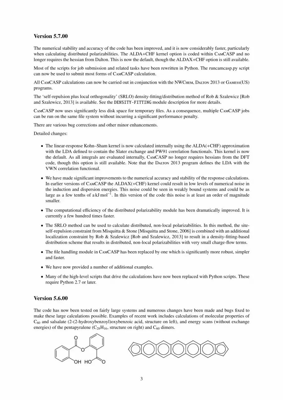
The code has now been tested on fairly large systems and numerous changes have been made and bugs fixed tomake these large calculations possible. Examples of recent work includes calculations of molecular properties ofC60 and salsalate (2-(2-hydroxybenzoyl)oxybenzoic acid, structure on left), and energy scans (without exchangeenergies) of the pentapyralene (C28H16, structure on right) and C60 dimers.
3

While such calculations are possible with this version of the code, please see the discussion on the limitations ofCamCASP in Sec. 3.1 below.
In earlier versions of CamCASP the second-order exchange-induction energy, E(2)ind,exch, was calculated by scaling
the uncoupled energy. We now calculate this energy without scaling. This is more accurate in strongly hydrogen-bonded systems. In practice, due to error cancellations in the second-order exchange-induction energy and thehigher orders (calculated via the δHF
int approach), the two approaches lead to almost the same total exchange-induction energies. Nevertheless, we do not recommend scaling any more.
A major addition to this version is the option of regularized second-order induction energies. Through regulariza-tion we can define the second-order charge-transfer energy within SAPT or SAPT(DFT). A standard SAPT(DFT)interaction energy calculation will automatically include calculation of the regularized second-order induction andexchange-induction energies.
The Cluster program now has the capacity to perform simple energy calculations with isotropic dispersion models.While Orient remains the main program for energy evaluations, Cluster provides useful tools for creating andusing dispersion models to be paired with density functionals, and allows calculations of dispersion energy andpressure contributions to crystals.
Summary of enhancements:
• Interfaces to Gamess(US) and NWChem. The interface to Dalton 2013 has been re-written and improved. Allinterfaces now use ASCII (plain text) files to store orbitals and energies and are consequently transferableacross computational platforms.
• Molecular orbital space truncations are allowed. This is handled automatically in the NWChem, Dalton2013 and Gamess(US) interfaces. Orbital-space truncations improve the stability of the SCF calculationsand subsequent CamCASP calculations. They are particularly important in large basis calculations.
• ENERGY-SCAN is now more robust. First-order energies can be calculated in a dimer-centered auxiliary basisin the scan module. The second-order energies cannot be calculated if the scan involves molecular rotations.
• Coupled second-order exchange-induction energy, E(2)ind,exch, without scaling.
• Second-order induction energies (E(2)ind,pol and E(2)
ind,exch) can be regularized using the R-SRS theory of Patkowskiet al. [2001a].
• The POLARIZABILITY module allows calculations of the point responses to a point charge perturbation. Thisis useful for visualization of polarization in the molecule using the Orient program. See §9.10.1 for details.
• Additions to Cluster to aid the construction of dispersion models (using isotropic Cn coefficients (n =
6 · · · 12)) and a variety of damping models. Dispersion energy calculations for clusters and crystals. Seesections §7.5 and §7.6.
• More basis sets added. In particular, some of the NWChem basis sets are now included.
• More examples.
Version 5.5.00
Many improvements in the code. It is no longer necessary to use Dalton to do the coupled Kohn-Sham calculation— Dalton is only needed to calculate the eigenvalues and eigenvectors. The top-level scripts have been streamlined.Most calculations can be run or set up using the runcamcasp.py script, and all data affecting the calculation itself(such as ionization potentials) are provided in the cluster file. Details:
• Kernel integrals constructed in CamCASP.
• New propagator module: implements the adiabatic local density approximation ALDA(X) in the mannerdescribed by Bukowski et al. [2005].
There are more options in this module.
The PBE/AC ALDAX route is the fastest and consumes the least memory.
4
PBE0/AC ALDAX+CHF is fast, but memory intensive.
The old ALDA propagator module can still be accessed. This delivers the highest accuracy, but is slowand requires integrals from DALTON.
• 10-fold speed-up in calculating 2 and 3-centre Coulomb integrals.
• Latest version compiles with ifort. Binary is almost twice as fast as with pgf90.
• The speed of the distribution algorithm is improved by two orders of magnitude.
• Better scripts for easier use of the code.
• Energy scan for first order energies faster by a factor of 10.
• New program: res2disp added. Source code in src/res2disp/.
Calculates dispersion energies of crystals using isotropic dispersion models.
Version 5.3.01
First-order interaction energy components can now be scanned using the ENERGY-SCAN module using auxiliarybases with either Cartesian or spherical GTOs. So can the overlap integrals. We will shortly be releasing a versionthat allows the second-order energies to be scanned using this module. We have also fixed some serious bugs inthat module that effected the exchange energies.
The Cluster program has many modifications and a new command MAKE-UNIQUE that modifies all site labels soas to make them unique. The JOIN command now accepts multiple molecule names.
The other modules that have been modified are the OVERLAP-MODEL and the integral modules.
Some of the parameters of the program have been changed to allow larger systems to be used.
Version 5.3.00
There have been many enhancements to the previous version. We have also fixed a number of serious bugs. A largenumber of basis sets have been added to the basis set library and we encourage the user to experiment with these.
3 Outline of the capabilities of CamCASP and other programs
The following types of calculation are possible with CamCASP:
• Dimer energies:The first-order electrostatic and exchange energies, E(1)
elst and E(1)exch, and the second-order dispersion and
induction energies, E(2)ind,tot and E(2)
disp,tot (including their exchange terms). All are calculated using density-fitting, and the second-order dispersion can in principle be calculated without density-fitting, though thispart of the code has not been tested in a long time. The δHF
int correction can also be calculated.
• Molecular properties:
Multipole moments: Total and distributed multipole moments can be calculated using a constraineddensity-fitting algorithm and the Gdma 2.2 code, which has been interfaced to CamCASP.
Frequency-dependent polarizabilities: Total and distributed frequency-dependent polarizabilities arecalculated using a constrained density-fitting algorithm. The Williams–Stone–Misquitta (WSM) methodcan be used to obtain the most accurate polarizability model within constraints imposed by the user.
Point-to-point polarizabilities: Responses to a frequency-dependent point-charge perturbation—calledpoint-to-point polarizabilities—can be calculated. These are needed by the Pfit program when opti-mizing the distributed polarizabilities.
5
The Orient program is needed for some aspects of the property calculations. It is distributed separately butaccess to it is provided using the same credentials as for CamCASP.
• Energy scans:Surfaces around a molecule can be defined (or supplied as a grid of points) and all dimer energies can becalculated on this surface, using a point charge (for the induction and electrostatics only) or a probe molecule.The total and distributed charge-density overlap is also scanned.
• Atom–atom potentials:Using the results of the energy scans and molecular properties, atom–atom potentials can be obtained usingthe density overlap model to model the short-range energies. The Orient program is used for some parts ofthis calculation.
• Theory levels:In all cases, calculations can be performed using either the coupled/uncoupled Kohn–Sham (CKS/UCKS) orcoupled/uncoupled Hartree–Fock propagators. In practice, the CKS propagator will be used.
• Density-fitted Integral Package:The density-fitted (DF) integral package allows the calculation of 2-electron 4-index integrals in very effi-ciently, both in computation time and memory usage. With this package, the intermediate TRAN step is nolonger needed for the Hessian calculation, thereby saving a lot of time. In principle, the Sapt2006 programcan also be run using integrals obtained from this package, but this would involve some more effort.
At present, the DF-integral package computes more than 30 kinds of integral.
The functionality of CamCASP is greatly enhanced when used with the Pfit and Orient programs. Only someof the many features of Orient—those most useful for the calculation and analysis of intermolecular forces—arelisted here.
• Pfit
Fitting of polarizability models: At present, polarizability models are not fitted from scratch, but polar-izability models from the CamCASP code can be optimised using Pfit and the point-to-point polariz-abilities from CamCASP.
Dispersion coefficients: These can be calculated by Pfit using frequency-dependent distributed polar-izabilities from CamCASP. This function is better performed by the Casimir program.
• Casimir
Dispersion coefficients: C6, C7, etc. to C12. Dispersion coefficients between pairs of identical or dis-similar molecules can be calculated by Casimir using frequency-dependent distributed polarizabilitiesfrom CamCASP that have been localized using Orient and possibly refined using Pfit. The input file forCasimir can be created with the Process program from localized frequency-dependent polarizabilities.Minor changes to the input files allow the calculation of mixed-molecule dispersion coefficients.
• Dispersion
Dispersion energies using non-local polarizabilities: This program allows two and three-body disper-sion energy calculations using frequency-dependent non-local polarizabilities such as those calculatedusing the distributed polarizability module in CamCASP. These calculations include contributions fromthe charge-flow polarizabilities.
• Orient
Local polarizabilities: The distributed polarizabilities from CamCASP include non-local contribu-tions. These can be transformed away using the localization module in Orient.
Simplification of models: The polarizability models can be modified or simplified using Orient.
Displaying energies: Energies can be displayed in 3-D using the OpenGL display module in Orient.
Calculations of asymptotic energies: Using the distributed multipoles and polarizabilities, interactionenergies can be computed in the long-range (asymptotic) approximation.
Miscellaneous programs:
6

• Process: This code is an interface code to process polarizabilities from CamCASP or (localized/modified)polarizabilities from Orient into a form Pfit can use. It also performs transformations of the polarizabilitiesand is able to write out polarizabilities in LATEX format for publications.
• Cluster: This is the program that handles the user’s input data and generates the subsidiary data files neededby other parts of the package and by the auxiliary ab initio codes. It also enables the user to conduct elemen-tary manipulations of the molecule geometry, build clusters, determine rotational and translation axes, andwrite output in a form suitable for CamCASP, Orient, and any program that can read PDB files for imaging.
An important function of Cluster is to create the input files for CamCASP, Dalton 2013 (versions 2.0 and2013), NWChem and Sapt2006 programs. All the user need do is define the dimer within Cluster, performany manipulations that might be needed, and then use the RUN-TYPE command to generate the files for thecalculation. This greatly simplifies the file generation process and removes the chance of errors in the rathercomplicated input file structure of Sapt2006, Dalton 2013 and (to a lesser extent) NWChem and CamCASP.
3.1 CamCASP limits
The following limits apply only to those parts of the calculation that require integrals of the type OVOV or OOVV.These occur in the hybrid kernels and in the second-order exchange-dispersion and exchange-induction energies.
If only the non-exchange energies are required (E(1)elst, E(2)
ind,pol and E(2)disp,pol) and the ALDAX kernel is used, the limits
are significantly higher.
Sizes assume that individual arrays that need to be stored completely in memory in the present version of the codeare limited in size to 16 GB.
• Main basis size: N = no + nv where nonv ≤ 131072Examples:
N-methylpropanamide: no = 24, therefore N ≤ 5461.
Carbamazepine: no = 62, therefore N ≤ 2114.
C60: no = 180, so N ≤ 728.
• Auxiliary basis size: M ≤ 131072. In practice the limit will be lower for computational reasons.
• Computational bottlenecks:
Hessians: Calculation of the hybrid Hessians (ALDA+CHF) is an O(n3on3
v) process. This can be reducedusing the methods recently developed by Bukowski et al. [2005]. This has been done for the ALDAXand ALDA kernels which can be calculated in O(M2nonv) effort.
2-electron 4-index integrals: These are required for the exchange energies. In particular the second-order exchange energies.
• Other limitations
Not parallelised.
While reasonably large calculations are possible with this version of the code (see the examples givenabove), bear in mind that this still is a serial code and that calculations of the second-order exchangeenergies for large systems will be difficult as they will typically require more resources and a re-programming of the relevant CamCASP modules to make better use of memory and disk resources.
4 Installation
The CamCASP package comprises several different programs, and also uses a number of third-party programs —specifically, an ab initio package for the DFT or wavefunction calculations, the SAPT symmetry-adapted pertur-bation theory package for a patch to Dalton 2013, and the Orient program. While we have interfaced CamCASPto the Dalton 2013, NWChem, Gamess(US) and (in part only) the Gaussian programs, the scripts supplied withCamCASP support Dalton 2013 and NWChem more fully than the others. Consequently, we recommend that theDalton 2013 (2.0 or 2013) or NWChem ab initio packages are used, and this is assumed below. Several scripts are
7

provided to simplify the task of setting up the various files that are needed for the calculation, and feeding themto the programs that do the work. In order for this to work successfully, a few conventions need to be followed inthe way that your computer is organised, and because of the use of third-party programs the installation procedurecannot be as fully automated as you might wish. The following instructions apply to Unix and Linux systems; theycan be followed with little change for Mac OS X and Windows systems by working from a terminal window onthe Mac or by using a Unix emulator such as Cygwin under Windows.
1. The first step is to unpack the CamCASP tarfile:tar xzvf camcasp-5.9-base.tgz
This will create a new directory camcasp-5.9 containing the architecture-independent files, except for thoseneeded for building the source. It doesn’t include the program binaries. For these, you need to download theappropriate binary package for your architecture, and unpack that:
tar xzvf camcasp-5.9-<arch>-<compiler>.tgzThis will unpack into the same directory, camcasp-5.9.
2. Next, you need to add the CamCASP bin directory to your path; for example:export PATH=/usr/local/camcasp-5.9/bin:$PATH
This can be included in your initialization file. This would probably be your .bashrc file if you use the Bashshell.
3. Install Orient and either Dalton 2013 or NWChem if you don’t already have them installed. Dalton 2.0 andDalton-2013 require slightly different input, but CamCASP can handle either.
4. You could also install the Gamess(US) program, but bear in mind that for the present, we do not include anyexamples of scripts to perform calculations with Gamess(US) and CamCASP.
5. Dalton 2013-specific: The primary need for the Sapt2006 program is the patch to Dalton 2013 2.0 included inthe distribution. This allows calculations using the ALDA/ALDA+CHF kernels with xc-kernel integrals directlyfrom Dalton 2013 and allows the Fermi–Amaldi (FA) asymptotic correction with the Tozer & Handy splicingscheme [Tozer and Handy, 1998]. The patch for Dalton 2013 needs to be applied, and Dalton 2013 recompiledif necessary. For sources for these programs seehttp://www.kjemi.uio.no/software/dalton/dalton.htmlhttp://www-stone.ch.cam.ac.uk/programs.html#Orient4http://www.physics.udel.edu/~szalewic/SAPT/SAPT.html
Dalton-2013 doesn’t require the patch, as it has the asymptotic correction already included, and CamCASP cannow handle the ALDA and ALDA+CHF kernel itself.
6. NWChem-specific: The CS00 asymptotic correction [Casida and Salahub, 2000] will be used with NWChem.Ideally an energy shift should be provided for this method; it is the sum of the (positive) ionization energyand the (negative) HOMO eigenvalue. If this is not provided an empirical relationship between the HOMOeigenvalue and the IP is used instead. Neither is as good an approximation as the asymptotic correction schemeused with Dalton 2013 (above). The CS00 scheme is similar to the GRAC scheme of Gruning et al. [2001].
7. Now you need to define some environment variables.
• CAMCASP should be set to the full pathname of the base directory for the CamCASP package.• SCRATCH should be set to the full pathname of a scratch directory that can be used for temporary files.• DALTON2013 should be set to the full pathname of the directory containing the Dalton 2013-2013
program, if installed.• DALTON2006 should be set to the full pathname of the directory containing the Dalton 2013 2.0 program,
if installed.• NWCHEM should be set to the full pathname of the directory containing the NWChem program, if installed.• SAPT should be set to the full pathname of the directory containing the Sapt2006 program, if installed.• ORIENT should be set to the full pathname of the directory containing the Orient program.
These variables can all be set in your initialization script, so that you don’t need to set them every session. Forexample:export CAMCASP=/usr/local/camcasp-5.9
You may also also need to add the Sapt2006 bin directory to your path:export PATH=$SAPT/bin:$PATH
8
8. Finally you need to set up some symbolic links (aliases) in the CamCASP bin directory to the programs thatare used by CamCASP. This only needs to be done once. To do so, run the commandmake_links.py
(after changing the PATH and setting the environment variables as explained above). The script checks that thegiven paths are correct. This script will also ask whether your system uses the PBS (Portable Batch System) orGE (Grid Engine) batch scheduling systems. If you intend to run all your calculations in the background, or viathe Linux batch command, choose ‘none’. If you use some other scheduler, you will need to modify one of thestrings header["PBS"] or header["GE"] in the bin/camcasp.py script. The header will be prefixed to yourjob script before it is submitted. In any case, ensure that the environment variable SCHEDULER is either unset orset to the scheduler you require, as appropriate.
9. Testing the installation
Once everything is set up, you can run some tests that will exercise all the programs. Go to the CamCASPsubdirectory examples and follow the instructions in the README file. There are tests for single-configurationdimer energy calculations, for properties, and for energy scans over a set of dimer configurations.
4.1 Building CamCASP from source
Executable binaries of the CamCASP, Process, Casimir, Pfit and Cluster programs are provided for PCs runningLinux and for Mac OS X. Where possible these are static binaries and don’t require additional libraries. If youneed to compile the package yourself, you will need to obtain access to the source. This is not normally available,but may be permitted on request. The Makefile supplied with the CamCASP source files will build the CamCASP,Process, Casimir, Pfit and Cluster programs. Here are some brief instructions.
The build will happen in a directory $CAMCASP/arch/compiler where arch is the machine architecture and compileris the name of the compiler chosen. The architecture and compiler must be specified, either on the make commandline:make all ARCH=arch COMPILER=compiler
by changing the beginning of the Makefile to set the default values, or by setting environment variables ARCH andCOMPILER.
The compiler flags used are set in the file $CAMCASP/arch/compiler/exe/Flags. You will have to set machine-specific flags here. The MACHINE variable provides an alternative way to select flags for different platforms, usingthe same Flags file — see the examples provided. On a Linux machine the name of the machine should be de-termined automatically, but if this doesn’t work you can specify it on the make command line. Probably the onlything that will need changing is the LIBS flag that sets the libraries to be linked to.
Architecture options are: x86-32, x86-64 and osx.
Compiler options are: pgf90, gfortran, and ifort.
• The Portland pgf90 compiler is reasonably fast, but doesn’t always keep to the standard.
• The nagfor compiler unfortunately can’t be used, as it won’t accept the very old legacy routine gaussint.F,which is still used for some integral calculations.
• The gfortran compiler is under active development, and sometimes new bugs are introduced, but it gener-ally works well, produces well optimized binaries and it’s free.
• The ifort compiler generates fast code.
We recommend either ifort or gfortran.
For other compilers, you will need to make an arch/compiler/exe directory and an arch/compiler/exe/Flagsfile.
CamCASP needs a full installation of the Lapack and Blas libraries. It is crucial that you install a fast and reliableset of libraries. We recommend the Atlas libraries combined with the Lapack libraries from Netlib.org. The Atlaslibrary contains a full Blas but by default only a partial Lapack installation that doesn’t include all the routines usedby CamCASP. To include the full Lapack library, however, it is only necessary to download the source packagefrom netlib.org and tell Atlas where it is. Instructions are provided on the Atlas webpage. It’s quite easy and won’t
9
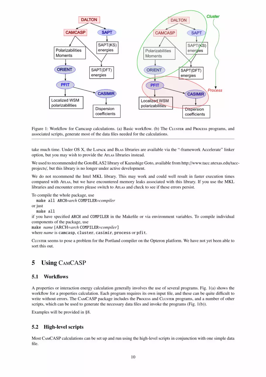
Figure 1: Workflow for Camcasp calculations. (a) Basic workflow. (b) The Cluster and Process programs, andassociated scripts, generate most of the data files needed for the calculations.
take much time. Under OS X, the Lapack and Blas libraries are available via the “-framework Accelerate” linkeroption, but you may wish to provide the Atlas libraries instead.
We used to recommended the GotoBLAS2 library of Kazushige Goto, available from http://www.tacc.utexas.edu/tacc-projects/, but this library is no longer under active development.
We do not recommend the Intel MKL library. This may work and could well result in faster execution timescompared with Atlas, but we have encountered memory leaks associated with this library. If you use the MKLlibraries and encounter errors please switch to Atlas and check to see if these errors persist.
To compile the whole package, usemake all ARCH=arch COMPILER=compiler
or justmake all
if you have specified ARCH and COMPILER in the Makefile or via environment variables. To compile individualcomponents of the package, usemake name [ARCH=arch COMPILER=compiler]where name is camcasp, cluster, casimir, process or pfit.
Cluster seems to pose a problem for the Portland compiler on the Opteron platform. We have not yet been able tosort this out.
5 Using CamCASP
5.1 Workflows
A properties or interaction energy calculation generally involves the use of several programs. Fig. 1(a) shows theworkflow for a properties calculation. Each program requires its own input file, and these can be quite difficult towrite without errors. The CamCASP package includes the Process and Cluster programs, and a number of otherscripts, which can be used to generate the necessary data files and invoke the programs (Fig. 1(b)).
Examples will be provided in §8.
5.2 High-level scripts
Most CamCASP calculations can be set up and run using the high-level scripts in conjunction with one simple datafile.
10
The following scripts are currently available. They can all be executed with the single argument --help to printbrief usage details and exit.
The older bash scripts are still available and are described in Appendix C. While these are still maintained, theywill probably be removed from subsequent distributions.
The Python scripts require python 2.7 with the argparse module installed. We have not tested thescripts with python 3.x. Since earlier versions of Python do not have the argparse module, thesescripts will not work. In this case, consider either upgrading your Python installation, or use the olderbash scripts as described in Appendix C. But bear in mind that the latter option is a stop-gap measureonly as we will eliminate these scripts in a subsequent release.
• runcamcasp.pyThis python script supersedes the runSAPT script used previously to run a complete CamCASP calculation.It can be used to carry out calculations of the following types:
properties: multipole moments, polarizabilities, etc. of single molecules.
sapt-dft: symmetry-adapted perturbation theory of dimer interaction energies, using molecularwavefunctions obtained by density functional theory.
sapt: symmetry-adapted perturbation theory using Hartree-Fock wavefunctions and perturbativecorrelation corrections.
delta-hf: calculation of the δHF estimate of higher-order induction energy terms.
supermolecule: standard supermolecule calculation of dimer energies, with counterpoise correction forBSSE.
See below for more details.
• execute.pyThis script is invoked when the job is run, and carries out the Dalton 2013 or NWChem calculations, convertsthe resulting eigenvector files into a form convenient for CamCASP, and then runs the CamCASP calculation.All of this is done in a subdirectory of the $SCRATCH directory, and the output files are copied back to thespecified job directory at the end of the calculation. Except in properties calculations, two or three DFT orHF calculations are needed, and execute.py starts them as separate processes so that they run in parallel.
• extract_saptdft.pyThe output of a SAPT(DFT) calculation can be analysed using the script extract_saptdft.py. It picksout the energy terms from the CamCASP output file and displays them in a compact form. The argumentsare directories containing SAPT(DFT) calculations, as previously set up by runcamcasp.py. Often it issufficient to run the command as extract_saptdft.py *, as the script ignores plain files and merelyissues a warning for directories that don’t contain completed SAPT(DFT) calculations.
• localize.pyUsing the polarizability files from a properties calculation, this script will generate local polarizabilities(static and dynamic). See §8.2.1 on p. 31 for details. The dynamic polarizabilities are then used to constructdispersion coefficients, if required.
• batch_sapt.pyThis is one of many batch scripts that can be used to schedule multiple calculations. Please see the bindirectory for others. batch_sapt.py can be used to perform interaction energy calculations using a templateCluster input file and a geometry file. The other batch scripts work in a similar way. It is worth testing batchscripts before using them for a real calculation.
5.3 The runcamcasp.py script
The command in its simplest form is justruncamcasp.py JOB
JOB is the name of the job, and is prefixed to files created for the job. By default it is also the name of the directorythat is created to contain the job files, but that can be changed using the --directory or -d option. You need to
11
provide one simple data file, normally JOB.clt, to define the system and specify the calculation. For details of thisfile see §7 and the example in §8.1 below.
The general form of this command isruncamcasp.py JOB optionswhere JOB is the job name — that is, the file-prefix specified in the Cluster input file. The main options are
--clt file Specify the cluster file for the job. Default is JOB.clt.
--directory or -d dir Directory for the job files. If the --restart option is used it must exist already; other-wise it is newly created. If a directory of the same name already exists, it can be deleted with all its contents,or renamed, or the job may be aborted.
--ifexists [delete | save | abort | ask] Specify what to do if the job directory already exists. Thedefault is to ask. If save is specified, the existing directory, dir, is renamed as dir_nnn, where nnn is the firstsuffix in the series 001, 002, etc., after any dir_nnn that already exists.
--restart This will start or restart the calculation in the specified directory, carrying out any Dalton 2013 orNWChem calculations that haven’t been completed, and repeating the CamCASP calculation regardless. Thisallows the calculation to be repeated with a modified CamCASP data file JOB.cks if required.
--queue or -q queue The job is to be submitted to the specified queue (see below), or run in the background if“-q bg” is specified.
--memory or -M nnnn Memory required for the job in MB.
--direct Use direct integral management.
By default, this script uses a Cluster input file with the name JOB.clt. If this is not the case, use the “--clt file”option to specify the name of the Cluster file.
This carries out the following steps, unless --restart is specified:
• Create a new directory dir for the job. By default this is called JOB, but a different directory name can begiven using the -d dir flag. If the directory already exists, you’re given the option of either deleting thatdirectory and its contents first, or renaming it as dir_nnn, where nnn is a digit string that doesn’t clash withany existing file or directory. All the files for the job will now be created in the specified directory or asubdirectory of it.
• Copy the Cluster file into the new directory, chdir into it, and run the cluster program to generate the datafiles for the SCF calculations, and the CamCASP input file JOB.cks.
• If the Dalton 2013 program is to be used, functions defined in camcasp.py are called to generate the Dalton2013 .mol and .dal input files.
Then, whether or not --restart is specified:
• Call the submit function in camcasp.py to create the script to do the calculation, and to submit the job tothe specified queue.
The main part of the calculation is carried out by the execute.py script. It begins by defining some directory names.The MAINDIR is the directory from which the job is run. The files in this directory are all copied to a scratchdirectory $SCRATCH/JOB_str, which is created if necessary, and the calculations are carried out there. where stris a unique identifier, usually the time at which the job starts. Many big files are generated in the course of thecalculation, so there needs to be plenty of space available here. At the end of the calculation, the useful output filesare copied back to $MAINDIR/OUT, and the scratch directory and its contents are deleted.
If --restart was specified, the runcamcasp.py script scans the copy of the .clt file in the job directory (notthe original one, which may have been changed or deleted) in order to assemble information about the calculation.However no files are generated, so any changes made are retained. In particular, the .cks file may be modified asrequired before restarting. In a restarted job, completed DFT or HF calculations are not repeated, but incompleteones are restarted. The CamCASP calculation itself is always repeated.
12

5.3.1 Job queues
If your machine operates a queueing system for batch jobs, the -q or --queue flag may be used to specify thequeue for the calculation. If the computer uses the PBS or GE batch queuing system, set the environment variableSCHEDULER to PBS or GE. Headers for these are defined in the camcasp.py Python module, but they may needto be changed to suit your system. The queues available will depend on your operating system. On a workstationrunning Linux, there is a batch queue, to which a series of jobs may be submitted; they will run in turn as theload on the computer permits. The queue can also be specified as “-bg”, which causes the job to be run in thebackground — convenient for small jobs. If “-q none” is specified, the files are all set up, but the calculationisn’t run immediately; instead a script submit.bash is left in the current directory, and you can execute this whenyou’re ready to run the job; for example:./submit.bash -q bg
If you regularly use a particular queue, you can set the environment variable QUEUE to that value, and that willbecome the default for the --queue option.
5.4 Low-level scripts
Some of the scripts and programs provided in the CamCASP package are low-level ones that just perform one stepin setting up the job, for example by generating further files that are needed for the calculations. If you need to dosomething unusual you may have to use the lower-level scripts directly, but for most purposes the high-level scriptswill suffice.
In all the following, JOB is the job-name, which identifies all the files belonging to the job — in particular, thecluster input file, usually called JOB.clt. Most jobs involve a large number of files, however, so it is not a goodidea to rely on the job-name to distinguish files for different jobs from each other. Recommended practice is to runevery job in its own private directory (folder).
The starting-point for all tasks is the ‘cluster’ file, conventionally given the .clt suffix, which contains informationabout the molecules involved, the basis sets to be used, and other details. Details are in §7. Once you have preparedthe input file for Cluster, called for example setup.clt, the cluster command is the first step in setting up thejob:cluster < setup.clt
(It will usually be called by a script rather than directly.) If the Dalton program is to be used, it will produce a filecalled JOB.DALtemplate, where JOB is the file prefix specified (or implied) in the Cluster data file. It will alsoproduce a number of other files — for example JOB.cks and JOB_P.data — depending on the information inthe .clt file.
The runcamcasp.py script uses a number of functions defined in the bin/camcasp.py Python module. There arefunctions to generate the full data files for Dalton calculations from the JOB.DALtemplate file and to set up theshell script that is submitted to the appropriate queue to carry out the calculation. These will usually be called fromthe runcamcasp.py script, but they could be called from a Python interactive session with the camcasp moduleloaded.
For Dalton 2013 DFT calculations using the asymptotically-corrected PBE0 functional it is necessary to specifythe molecular ionization potential in order to set up the asymptotic correction properly. The file misc/IP.txt con-tains a list of ionization potentials for some small molecules, and many others are available in the NIST ChemistryWebbook at webbook.nist.gov/chemistry/. If the IP cannot be found there or elsewhere in the literature, it is nec-essary to calculate it. The calculation requires the vertical ionization energy, i.e. the difference in energy betweenthe neutral molecule and its cation at the same geometry.
Calculations using NWChem use a different asymptotic correction scheme. This ideally uses an energy shift whichis the sum of the (positive) ionization energy and the (negative) HOMO energy for the neutral molecule, butNWChem can estimate the shift using an empirical scheme if the shift is not specified. In our experience theasymptotic correction scheme used by Dalton 2013 is more satisfactory.
6 Data conventions
General notes on the conventions used for describing the form of input files:
13

• All data values are free format. Items may usually be given in any logical order.
• Comments may be included in the file. They start with “!” (note the space) and continue to the end of theline.
• Items in square brackets are optional. (The square brackets themselves should not be included.)
• Items separated by “|” are alternatives. If a list of such items is shown in braces, one of the alternatives mustbe chosen. Often several alternative keywords are recognized; for example FREQUENCY can be replaced byFREQUENCIES or FREQ or FREQS. In most cases the allowed alternatives are shown below.
• Keywords shown here in upper-case may be given in upper, lower or mixed case.
• Some keywords are shown in lower case. They too can be given in upper, lower or mixed case. Thesekeywords are never required — they can be included in the data file to improve its human readability, buthave no other purpose. They are checked for correctness but are otherwise ignored.
• Items shown in italics should be replaced by a suitable value.
• Long lines may be broken by replacing any space between items by “+++\n”, where “” denotes space and“\n” denotes newline. This notation is also used occasionally in this manual to break lines that are too longfor the page.
• It is sometimes convenient to include data from other files:#include filenameIf such a line occurs anywhere in the input file, the contents of the specified file are read exactly as if theyhad been pasted into the data file at this point.
• For files in the CamCASP installation directory, the following command may be used:#include-camcasp path relative to CamCASPThis allows files to be specified relative to the CamCASP directory. For example, instead of specifying abasis file as#include /home/ajm/CAMCASP/basis/gamess_us/sadlej/Hyou could use#include-camcasp basis/gamess_us/sadlej/HFor this to work correctly, the CAMCASP environment variable needs to have been defined.
• The SKIP command skips execution of following lines of the input file. Normal execution resumes after anUNSKIP or ENDSKIP command.
• The FLUSH command can be used to force flushing of the standard output buffer.
7 Cluster: Detailed specification
The cluster file is normally all that is needed to define a calculation, and in essence it is very simple, although itprovides very versatile commands for manipulating the configuration of the system to be studied. It comprises foursections:
(i) Prologue
(ii) Molecule definitions
(iii) Geometry manipulations etc.
(iv) Job specification
We describe these sections in turn. See above for the conventions used to describe the commands.
14

7.1 Prologue
TITLE "title"Title for the job. Optional.
GLOBALUNITS DEG | DEGREE | DEGREES | RAD | RADIAN | RADIANS UNITS BOHR | AU | ANG | ANGSTROM | ANGSTROMS [CAMCASP path]
END
The UNITS command sets default units for lengths and angles, but they can be over-ridden locally if necessary.The CAMCASP entry specifies the full file path to the CamCASP base directory, but it will not usually be needed— if Cluster has been compiled with a modern (Fortran 2003) compiler it will read the path from the CAMCASPenvironment variable.
7.2 Molecule definitions
You can define as many molecules as you want here, and later select which of them are to be used in the actualcalculation.
MOLECULE molecule-name[UNITS BOHR | AU | ANG | ANGSTROM | ANGSTROMS ][CHARGE molecular-charge][I.P. ionization potential [eV] ][AC-SHIFT \emphasymptotic correction shift value] [ATOM-CHARGES [AUTO | USER]]
label Z key <data> [TYPE type]label Z key <data> [TYPE type]...
END
The UNITS line is only needed if the units for atom positions are different from the global units. CHARGE specifiesthe total molecular charge, default zero. I.P. specifies the ionization potential, normally in Hartree, but it can begiven in eV if the eV unit is specified. The I.P. is needed if asymptotic correction is to be applied to the exchange-correlation potential, which is recommended. If the I.P. is omitted and Dalton 2013 is used to perform the DFTcalculation, no asymptotic correction is applied. At present, no I.P. is needed to use the asymptotic correctionin NWChem as the CS00 scheme used by NWChem can estimate it, but the shift (I.P.+ HOMO energy) can besupplied.
The molecular geometry follows, one line for each atom. The label is an atom identifier, up to 8 characters in length.Z is the nuclear charge. Positions may be given in a variety of ways; see below. The site type can be optionallyspecified. It is used to impose symmetry and this information is passed to other programs. Sites can be given thesame type if they are related by a molecular symmetry operation that is a proper rotation. Sites that are related onlyby improper rotations have to be treated specially, but this situation is uncommon. The type name can be up to 8characters long.
The nuclear charges Z can be skipped in the geometry specification if ATOM-CHARGES AUTO is used. In this case,the code attempts to work out the nuclear charges from the name of the atom. Sites which are not recognised willbe assigned a zero nuclear charge.
Atom positions may be specified in any of the following ways. The default is to use Cartesian coordinates, and thiswill be the most convenient if the geometry is obtained from an ab initio geometry optimization. If the geometryis given in terms of bond lengths and bond angles the other methods may be more helpful. s1, s2 and s3 are labelsor sequence numbers of previously-defined atoms in this molecule. Negative sequence numbers can be used, andcount back from the new atom, so the most recently defined atom is −1, the previous one −2, and so on. The newatom is notionally atom 0. If names are used to identify atoms, it is best if the names are unique, but if two ormore atoms have the same name, the one most recently defined will be assumed. Dummy sites, with Z < 0, maybe included to help define the geometry. They are discarded once the molecule definition is complete.
15

• Absolute Cartesian coordinates:[AT] x y z
• Absolute polar coordinates:POLAR r θ φ
• Linear Connexion:LC s1 s2 bPlace the new atom at distance b from s1, along the extension of the line from s2 to s1.
• Planar Connexion:PC s1 s2 s3 b θPlace the new atom at distance b from s1, in the 1–2–3 plane, with bond angle 2–1–0 equal to θ, cis to s3 ifθ > 0, trans if θ < 0.
For the remaining position definitions it is useful to define a local coordinate system with origin at s1, z in thedirection from s1 to s2 and x in the 1–2–3 plane with s3 at positive x.
• General Connexion:GC s1 s2 s3 b θ φPlace the new atom at distance b from s1, with bond angle 2–1–0 equal to θ and torsion angle 3–2–1–0 equalto φ. θ and φ can be viewed as standard spherical polar angles in the local coordinate system.Alternatively, φ can be regarded as torsion angle 3–2–1–0, taken counter-clockwise looking from 2 to 1 withatom 0 cis to 3 when φ = 0. θ should be positive, but a negative value is equivalent to increasing φ by 180.
• Central ConnexionCC s1 s2 s3 b θ βθ = 2–1–0 bond angle, |β| = 3–1–0 angle. y is positive or negative in the local frame according to the sign ofβ.
• Ring ClosureRC s1 s2 s3 b b2 φThe new atom is placed at distance b from s1 and b2 from s2, and φ is the angle between the 2–0–1 planeand the 2–3–1 plane. φ is again the spherical polar angle in the local frame, so if φ = 180 the new site is inthe 2–3–1 plane, on the opposite side of the s1–s2 line from s3.
7.3 Geometry manipulations and other transformations
None of the commands in this section are required, and indeed it is common for none of them to be needed.However they do provide powerful ways to modify the geometry of the system and other details.
For example, FIND ROTATION and FIND TRANSLATION find the rotation (axis and angle) and translation neededto go from one molecular geometry, defined by nuclear coordinates, to another. This feature has proved very usefulin constructing dimers or small clusters that have the same relative positions as in the crystal.
JOIN, COPY, INVERT, ROTATE, and TRANSLATE operate on molecules and facilitate the assembly of clusters andmacro-molecules that can then be operated on as units.
The BOND command is very handy for “bonding” together molecules along a specific axis (defined using coordi-nates or sites within a molecule).
The full list of available commands is as follows.
UNIQUE-SITES [ list of molecule names]The site labels need to be unique when calculating polarizabilities and dispersion coefficients. This commandmodifies the site labels in the specified molecules to make them unique (within a given molecule). If no moleculesare specified, this command processes all the molecules currently defined.
TOL | TOLERANCE toleranceSpecifies the tolerance used in comparing geometries. Default is 10−6, which is probably too tight for most pur-poses.
16
COMPARE name of molecule 1 [and] name of molecule 2If the data for a molecule have come from different sources (e.g. X-ray diffraction and ab initio optimization) itis useful to be able to check that they describe the same geometry. This command sets up, for each molecule, adistance matrix between the atoms, and compares the two, reporting any significant differences. The atoms mustbe listed in the same order in both cases. Note that enantiomorphs will be reported as matching.
CENTRE molecule [ on | at ] [SITE] label | COM | XYZ x y z The centre of the specified molecule is defined to be at the position given. Initially the ‘centre’ is the origin ofglobal coordinates.
WRITE | PRINT molecule [[in] [ PDB | ORIENT ] [format]]With the PDB option, this writes the molecular geometry to a PDB-format file 〈molecule-name〉.pdb. Otherwise theatom names and positions are printed on standard output; if ORIENT is specified, they are in a form suitable forpasting directly into an Orient data file. See also the ORIENT option of the RUN-TYPE command, below.
FIND ROTATION[TOLERANCE tol]FROM triadTO triad
ENDFind the rotation that would take the first triad to the position of the second. Each triad is a set of three pointsspecified as Cartesian coordinates, typically the coordinates of three atoms:x1 y1 z1 x2 y2 z2 x3 y3 z3or as site labels:SITES s1 s2 s3 [in] MOLECULE | MOL molecule
The triad definition may run over more than one line if necessary. The triangles defined by the two triads must becongruent to within the tolerance specified, default 0.001.
FIND TRANS | TRANSLATION FROM positionTO position
ENDFind the translation vector from the first position to the second. Each position may be given in Cartesian coordi-nates:XYZ x y zor as a site label: SITE site | COM [ in ] MOLECULE | MOL molecule
FIND COM [ of ] moleculeFind and print out the position of the centre of mass of the specified molecule. The atom masses are assumed to bethose of the most abundant isotope.
JOIN molecule name [ and | & ] molecule name ... INTO new molecule nameCombine any number of specified molecules, at their current positions, into a single entity. This is useful forcreating a dimer or, more generally, an N-mer out of pre-defined molecules. Site types are preserved.
INVERT moleculeInvert the specified molecule w.r.t. to its centre. Note that the ‘centre’ is the origin of global coordinates if no centrehas been defined — see the CENTRE command above.
COPY moleculeA [ to ] moleculeBDefine a new molecule, initially at the same position as the original.
BOND moleculeA [ [ -> | TO ] moleculeB | XYZ ][FROM | SITES] a3 a2 a1 -> | TO b1 b2 b3 DISTANCE | LENGTH | SEPARATION distance [ ANGSTROM | ANG | BOHR ]
ENDThis moves molecule A so that sites a2, a1, b1 and b2 are collinear and arranged in that order, and so that sites a1and b1 are the specified distance apart. a3 is a third site lying off the a1–a2 axis, and b3 a third site lying off theb1–b2 axis. If molecule A is non-linear, it is rotated about the a2–a1 axis so that all six sites are coplanar, with sitesa3 and b3 cis to each other. If A is linear, then a3 is irrelevant, but at present it must still be specified and must stilllie off the a1–a2 axis. It can be specified as a position in global coordinates using the syntax XYZ x y z. MoleculeB is not moved, and indeed it need not be a molecule at all. Any or all of the B sites may be specified as cartesian
17
positions using the syntax XYZ x y z, and if ‘molecule B’ is not specified or is specified as XYZ, then all of the sitesof ‘B’ must be specified using the syntax XYZ x y z.
ROTATE moleculeRotate the specified molecule, using the rotation found by the most recent FIND ROTATION command. The rotationaxis runs through the centre of the molecule. Note that the ‘centre’ is the origin of global coordinates if no centrehas been defined — see the CENTRE command above.
ROTATE molecule BY angle [ DEGREES | RADIANS ] ABOUT nx ny nz
The axis of rotation need not be normalized. The rotation axis runs through the centre of the molecule.
PLACE molecule AT x y zPosition the specified molecule so that its centre is at (x, y, z) in global coordinates.
TRANSLATE moleculeMove the specified molecule by the vector translation found in a previous FIND TRANSLATION command.
TRANSLATE molecule BY distance [ ANGSTROM | BOHR ] ALONG x y zThe distance is assumed to be in the global units unless otherwise specified. The vector direction need not be a unitvector, but is normalized by the program.
OVERWRITEOverwrite existing files that have the same names as those generated by this run of the program.
OVERWRITE OFF | FALSE | NO Don’t overwrite existing files, but use alternative file names if files with the same names as those generated by theprogram are found to exist already. If any such file exists, the modification is applied to all files generated by thisrun. This action is the default. However it is recommended to start the calculation in a clean directory to avoid anyconfusion – a typical calculation will generate many files.
INTERPOLATE molecule1 [AND | &] molecule2 INTO new molecule name [FACTOR ξ ]Given two conformers molecule1 and molecule2 with sites in the same order, create a third molecule with a struc-ture that linearly interpolates between the two. Site coordinates in the interpolated molecule are defined by:
r = r1 + ξ(r2 − r1).
7.4 Job specification
This section specifies the input files and scripts that are to be constructed for the calculation, as well as basis-setdetails and some other options.
RUN-TYPEMOLS/MOLECULE/MOL/MOLECULES <moleculeA> [[and] <moleculeB>]FILE-PREFIX <prefix of interface files: CASE SENSITIVE>
[SAPT(DFT) | SAPT | DELTAHF | DELTA-HF | PROPERTIES | SUPERMOL | CAMCASP]SCFCODE [DALTON | GAMESS | NWCHEM ] [NO-SYMM]
METHOD <Electronic structure method | DFT>FUNCTIONAL <functional | PBE0> (applicable only for DFT)KERNEL | KERNEL-TYPE [ALDA | ALDA+CHF | CHF | ALDAX+CHF | ALDAX]
To use Hessians from DALTON use: ALDA+CHF-DALTON or ALDA-DALTONAC | ASYMPTOTIC-CORRECTION [TH | LINEAR | GRAC] [CS00 | MULTPOLE | LB94]
BASIS <basis> [of] TYPE <type of basis> [SPHERICAL | CARTESIAN]TYPE <type of basis>AUX-BASIS | AUX <auxiliary basis> [TYPE <type of aux basis>] +++
[SPHERICAL | CARTESIAN][AUX-TYPE | AUX-BASIS-TYPE <type of auxiliary basis>]ISA-AUX [SET1 | SET2 | SET3]MIDBOND/MID-BOND <name of midbond basis>/NONE +++
[and/of] TYPE WEIGHTED/COM
18
! Use these to override the default MO-file names and formatsMO-FILE-A | MO-FILE-B | MO-FILE <name of MO file for molecule> +++
[[FORMAT] ASCII | BINARY]
OPTIONS [TESTS] [ISOTROPIC-POL] [NO-3RD-ORDER] [SOLVER LU | GELSS]MEMORY <max memory> BYTES/KB/MB/GB <---default MBSITE-ORDER [OLD | DALTON2006 | NEW | DALTON2013]INTEGRAL-SWITCH <Integral switch (integer)>
CAMCASP-COMMANDSUse this block to insert User-defined commands for the CamCASP commandfile. These will be used (below the MOLECULE blocks) in lieu of thedefault commands. Useful if you wish to do something different. Usewith caution, preferably by *editing* a default CamCASP command filerather than starting from scratch.
END-CAMCASP-COMMANDS
ORIENT [file | files] [for] [DISPLAY] [ENERGY] [LOCALIZATION]PROCESS [file | files] [for] [CASIMIR] [and] [PFIT]GAUSSIAN [file]INTERFACE [file | files]RANK [LOCAL <rank>] [WSM <rank>] [NONLOCAL <rank>] +++
[HYDROGEN <rank>] [DMA <rank>] [DMA-H <rank>]SITES [file]
END
The subcommands are:
MOL | MOLS | MOLECULE | MOLECULES moleculeA [[and] moleculeB ]Specify one or two molecules involved in the calculation. Either or both may be supermolecules or clusters con-structed by joining fragments.
This command can appear any number of times. However, at present, any molecules mentioned after the first twowill be ignored.
FILE-PREFIX prefixPrefix for all the file-names to be created for this job. Default is “molA_molB” for a calculation involving moleculesmolA and molB, or “molA_basis name” for a single-molecule calculation. Note however that the prefix may bemodified, depending on the OVERWRITE setting.
SAPT(DFT) | DFT-SAPT | SAPT-DFT | SAPTDFT Perform a SAPT(DFT) calculation. Default if two molecules have been specified.
SAPTPerform a SAPT calculation. Default kernel type is set to CHF.
DELTA-HF | DELTAHF Perform a calculation of the δHF
int correction. Default kernel type is set to CHF.
PROPERTIES | PROPERTY Perform a property calculation. Default if only one molecule has been specified.
SUPERMOL | SUPERMOLECULE | SUPERMOLECULAR Perform a supermolecule calculation.
METHOD electronic structure methodThe electronic structure method to be used in the calculation. This option is needed only for a SUPERMOLECULEcalculation of the interaction energy. By default the method is set to DFT. Options are HF, MP2 and CC.
FUNCTIONAL functionalFunctional to be used in the DFT calculation of molecular orbitals. PBE0 (default) or PBE is recommended, usuallywith asymptotic correction, which is applied automatically if non-zero ionization potentials are provided in the
19
molecule definitions.
The type of functional is used to determine the fraction of exact exchange to be included. Consequently this is im-portant only for hybrid functionals. At present allowed density functionals are: PBE0 PBE HCTH HCTH147 PW91.If the functional you require is not in this list we suggest you first create the data files for one of the allowed func-tionals using the standard command (runcamcasp.py with the -q none option to stop after the files have beencreated) and then edit the CamCASP data file to set the fraction of exact exchange include the FRACTION-HFXcommand in the SET GLOBAL-DATA block.
KERNEL kernelThe recommended choice, and normally the default, for the kernel is ALDA+CHF with the PBE0 functional. Thisoption is still memory intensive and is not recommended for large jobs. If you can tolerate a small reduction inaccuracy, then we recommend the ALDA kernel with the asymptotically corrected PBE functional.
While the kernel integrals are normally calculated within CamCASP, it is also possible to use Dalton 2013 for thesecalculations, in which case more advanced kernels including gradient contructions can be used. To to calculate thekernel integrals with Dalton 2013 use ALDA-DALTON or ALDA+CHF-DALTON.
The ALDA kernel differs from ALDAX in that it includes a contribution from the LDA correlation functional (seesec. 9.5.1 for details). This could be the VWN or PW91c correlation functionals. Tests on numerous systems haveshown that the lack of correlation contribution to the kernel results in a loss in accuracy of about 1% to the dipole-dipole polarizability and 1-2% to E(2)
disp,tot. Depending on the balance of energy components, the error made in thetotal interaction energy could be larger than this.
See the CamCASP program specification (p. 45) for other possibilities. If you need to use these other options, youcan generate the CamCASP input file (suffix .cks) using the standard runcamcasp.py script with “-q none”,and modify the propagator specification before running the job.
BASIS basis [TYPE MC | MC+ | DC | DC+ ][SPHERICAL | CARTESIAN]
Specify the basis to use. Default Sadlej; other possibilities are aug-cc-pVxZ (or aVxZ) and cc-pVxZ (or VxZ),x =D, T or Q.The basis type should be specified here (the separate command BASIS-TYPE is still allowed but is not compatiblewith the scripts). Default is MC (monomer-centred), meaning that the monomer basis set has basis functions onlyon the atom sites of the monomer. In the MC+ case, the ‘monomer’ basis also has basis functions on the sites of thepartner molecule (so-called ‘far-bond’ functions) and may also include ‘mid-bond’ functions in the region betweenthe two molecules. (See the MIDBOND sub-command, below.) The DC (dimer-centred) basis has basis functions onboth molecules, and DC+ may also have mid-bond functions.
By default spherical GTOs are used in the basis set, but this can be changed using the argument CARTESIAN.
TYPE | BASIS-TYPE MC | MC+ | DC | DC+ Specify the type of basis set to be used for a dimer calculation. We do not recommend using this command as it isincompatible with the runcamcasp.py and related scripts.
MIDBOND NONE | midbond [TYPE COM | WEIGHTED ] Specify the mid-bond basis functions to be used, if any, and their position. Default for basis-types MC+ and DC+ is3s2p1d; the only other possibilities are 3s2p1d1f and NONE. COM specifies that the mid-bond functions are to beplaced at the mid-point of the line joining the centres of mass. The WEIGHTED placing is more suitable for largemolecules and is the default; this calculates the position of the midbond functions as [Akin-Ojo et al., 2003]
RMB =
∑a∈A,b∈B wab pab∑
a∈A,b∈B wab, (1)
where pab is the midpoint of the vector rab from atom a to atom b, and wab = |rab|−6. The inclusion of mid-bond
functions has been found to improve the description of the dispersion interaction [Williams et al., 1995].
AUX-BASIS auxiliary basis[TYPE MC | MC+ | DC | DC+ ] +++[SPHERICAL | CARTESIAN]
Specify the auxiliary basis to use. This command is optional. If absent, the auxiliary basis is chosen based on themain basis. The default is to use the RIMP2 auxiliary basis sets from the Turbomole program, which are specifiedin the same way as the Dunning basis sets, that is, aug-cc-pVxZ (or aVxZ) and cc-pVxZ (or VxZ), x =D, T or Q.The Sadlej basis has no optimized auxiliary basis associated with it, so the default here is the RIMP2 aug-cc-pVTZauxiliary basis. As a rule, the RIMP2 auxiliary basis sets should be used for the calculation of the second-order
20
energies.
It is also possible to specify the auxiliary basis set type as MC etc. We recommend the use of the DC or DC+ auxiliarybasis sets with MC and MC+ main basis sets, respectively. This is the default.
Other choices are Dgauss-A1-c, Dgauss-A1-x, Dgauss-A2-c, Dgauss-A2-x, and the TZVPP and SVP RI-J basesfrom the Turbomole program. We have not yet tested the other basis sets, so use them with caution.
By default Cartesian GTOs are used in the auxiliary basis set, but this can be changed using the argumentSPHERICAL.
ISA-AUX [SET1 | SET2 | SET3]Define the s-basis set for the iterated stockholder atoms (ISA) approach. If you need to use the ISA method pleaseget in touch with the authors.
MO-FILE-A | MO-FILE-B | MO-FILE <MO file name> [[FORMAT] ASCII | BINARY]Normally the names of the molecular orbital (MO) files are decided by the Cluster program. These names arebased on the molecule names. This command allows the user to specify the name and format of these MO files.
MEMORY n BYTES | KB | MB | GB The specified amount of memory will be used unless more is needed, in which case a warning will be printed.
OPTIONS [TEST | TESTS] [ISOTROPIC-POLS] [NO-3RD-ORDER] [DF-SOLVER LU | GELSS]The OPTIONS command allows the user to set various special options.
• TESTS: Use this command to create a test job. This will typically reduce the size of the run so the job finishesin a reasonable time.
• ISOTROPIC-POLS: This command will cause the Process input file to include the ISOTROPIC command,thereby limiting the WSM polarizability description to include isotropic terms only.
• NO-3RD-ORDER: Suppress the calculation of 3rd-order SAPT(DFT) energy terms when running the Sapt2006program.
• DF-SOLVER: Use this option to set the type of solver to be used to solve the density-fitting equations inCamCASP. Options are LU and GELSS. The default in CamCASP is currently LU. Use GELSS for higheraccuracies, but bear in mind that it uses considerably more resources than LU.
SITE-ORDER [OLD | DALTON2006 | NEW | DALTON2013]Specify which ordering of the sites is to be used. This is present for backward-compatibility only.
INTEGRAL-SWITCH switch valueSpecify which integral switch to use in the CamCASP code. The default is 1. This choice effects the SAPT(DFT)energy components. The choices are:
• INTEGRAL-SWITCH = 0 : Use density-fitting for the overlap and nuclear integrals. This is a low-accuracyoption, but is needed for certain types of calculations. For example, regularization requires this option.
• INTEGRAL-SWITCH = 1 : (default) Use the non-fitted forms of the overlap and nuclear integrals. This is thehigher accuracy option.
CAMCASP-COMMANDScommands go here
END-CAMCASP-COMMANDSUse this to insert user-defined commands for the CamCASP input file. These will be used (below the MOLECULEblocks) in lieu of the default commands. This is useful if you wish to do something different but do now want towrite the entire CamCASP input file by hand or wish to perform a batch of calculations. Use this with caution,preferably by editing a default CamCASP command file rather than starting from scratch.
When this block is present, Cluster will create the CamCASP file using the usual preamble and the MOLECULEspecifications, after which the commands specified within this block will be appended. Consequently the lastcommand should be FINISH to signify the normal end of the CamCASP file.
The files in directory $CAMCASP/data/camcasp-cmnds contain such blocks. For example, the file sapt-dft con-tains the camcasp comands for a standard sapt-dft calculation. It refers to molecules A and B rather than using
21
the molecule names. These are respectively the first and second molecules specified in the MOLECULES line of thejob description section of the cluster file. It isn’t necessary to change A and B to the actual names. So instead ofspecifying sapt-dft in the job description, it would be possible to specify#include-camcasp data/camcasp-cmnds/sapt-dftThere would be little point in doing this, of course, but a modified version could be filed in $CAMCASP/data/camcasp-cmndsand used in this way, or filed elsewhere and used with #include.
ORIENT [file] [for] [DISPLAY] [ENERGY] [LOCALIZATION]File suffix: .orntConstruct an input file for a later Orient calculation to localize polarizabilities. This may need a bit of editing –see §8.2 for details. ‘[file]’ is not the name of the file — it’s redundant syntax, but can be included to clarifythe function of the data line for the human reader. The file name is constructed automatically using the specifiedfile-prefix, possibly modified, and a standard suffix, ‘.ornt’ in this case.
If two or more molecules have been listed using the MOLECULE command, the Orient command file for the dimerconsisting of the first two molecules will be constructed. If only one molecule has been specified, this commandwill write out the Orient command file containing commands for localizing its polarizabilities.
Normally all you need is the ORIENT command and the types of files created is determined as described above. Thisbehaviour can be overriden using the DISPLAY ENERGY LOCALIZATION options which, if present, will generatethe appropriate files.
The energy file is generated with a number of comments and options. It will require editing and for this you mayneed to consult the Orient manual.
PROCESS [[file | files] [for] [CASIMIR] [and] [PFIT]]File suffix: .prss and _casimir.prssConstruct input files for the Process program for use in a later Pfit calculation to refine the localized polarizabilitiesand/or to create the Casimir input file for a later dispersion coefficient calculation. If no arguments are present, bothfiles are created. The Process input file with commands to create the Casimir input file are put in a file ending with_casimir.prss.
The Process input file with commands for a later Pfit calculation is written for the first in the list of molecules, butthe commands for a later Casimir calculation can use one or two molecules. If only one molecule is present in thelist, the Process input file is written out for a calculation of the dispersion coefficients between pairs of the samemolecule. If two or more molecules are present, the same is done for the first two molecules in the list.
These files may need a bit of editing – see §8.2 for details.
GAUSSIAN [file]File suffix: .comConstruct the input file for a Gaussian calculation. The Gaussian file is written for the first molecule in the list.
INTERFACE [file | files]This command writes out the CamCASP command file (‘.cks’ suffix), the *.template file, and, if needed, the_P.data file for a SAPT calculation.
If only one molecule has been specified using the MOLECULE command, only the CamCASP command file and*.template file are created, as it is assumed the interface files for a properties calculation are needed.
If two or more molecules have been specified, it is assumed that this is an interaction energy calculation usingSAPT(DFT) and all three command files are created.
RANK [NONLOCAL lNL] [LOCAL lL ] [WSM lWSM ] [HYDROGEN lH ][DMA lDMA ] [DMA-H lDMA−H ]
By default, the files produced by this module assume a polarizability and multipole moment description withrank 1 terms on the hydrogens and rank 4 terms on all other atoms. This can be changed using this command.There are many stages in the calculation of localized polarizabilities and the rank can be set for each of these,but as each stage uses the results of the previous one the rank cannot increase between stages. Also, at present,polarizabilities and multipole moments are limited to rank 4 (hexadecapole). Consequently we need to ensure that4 ≥ lNL ≥ lL ≥ lWSM ≥ lH and 4 ≥ lDMA ≥ lDMA−H. Cluster will stop with an error message if these requirementsare not satisfied.
SITES [file | files]File suffix: .sites
22
This command writes out the molecular geometry for each molecule in the list. The geometry is written in the fileprefix.sites, or in files prefix_nnn.sites if more than one molecule has been listed. The format is that used bythe Pfit program.
7.5 Energy
This module to some extent duplicates a small part of the functionality of Orient. There are a few reasons for this:(1) to read/write/alter a potential defined in Orient format, and (2) to calculate dispersion energies of clusters ofmolecules and crystals (see §7.6) using isotropic dispersion models (in this case, the anisotropy will be ignored),and hence (3) to aid the development of dispersion models to be paired with density functionals.
ENERGY...see commands below...
END
The commands that can be used in the ENERGY block are:
POTENTIALUNITS [BOHR | ANGSTROM | NM | HARTREE | KJ/MOL | KCAL/MOL | CM-1 | EV | K ]SCALE-C6 <scaling for C6>SKIP-SITES <list of sites to be skipped>NAME <name>[MOLECULE-PAIR <MolName1> <MolName2>][ISOTROPIC-ONLY]<atom name 1> <atom name 2> [rho] [alpha] [C6] [C7] [C8] [C9] [C10] [C11] [C12]
00 00 0 [<rho value> <alpha value> <C6 value> <...>]10 00 1 [<rho value> <alpha value> <C6 value> <...>]...
ENDENDThe potential is defined and modified using this block. UNITS specifies the units used for the potential parameters.SCALE-C6 scales the C6 parameters by the specified factor. This is useful when effective C6 models are needed.SKIP-SITES allows a set of sites to be removed from the potential decsription. NAME defines the name of thepotential. And MOLECULE-PAIR is used to define the pair of molecules associated with the potential.
What follows this preamble is the actual potential definition. The format used is identical to that used by Orient,so please consult the Orient manual for details of the specification. Briefly, parameters for each atom pair arespecified with a header line:<atom name 1> <atom name 2> [rho] [alpha] [C6] [C7] [C8] [C9] [C10] [C11] [C12]that starts with the atom pair labels and is followed by names of all parameters included. The order doesn’t matteras long as it is consistent with the order of the parameter values that appear on the following lines. The parametersare specified along with their angular momenta as follows:
laka lbkb j [<rho value> <alpha value> <C6 value> <...>]The pair-block is terminated with END. As many pairs can be specified as needed.
If an atom pair appears more than once the parameters in subsequent specifications are used to augment or overridethe prior sets. This is useful when the short range parameters are specified in one potential file but the long-range(dispersion) parameters are in another. Both files can be read in and concatenated into a single potential. Also, asinput units can be altered using UNITS, unit conversions are possible.
If ISOTROPIC-ONLY is specified, all anisotropy parameters will be ignored.
WRITE-POTENTIAL[SKIP-DUPLICATES | NO-SKIP-DUPLICATES ]
ENDWrites out the potential in the Orient format. The SKIP-DUPLICATES command can be used to prevent equivalentpairs from being written. Note that the pair H1 N is equivalent to N H1. This command would write only one ofthese.
Taken together with the commands in the POTENTIAL block, these provide a convenient way to manipulate the
23
potential file: discard sites, alter units, merge potentials, etc.
ANALYSETABLE [ANISO [10 | 20]]
ENDPerform an analysis of the potential model. Please see the source code to figure out what kind of analysis has beenprogrammed.
C6 | C6-MODEL | CN-MODEL | DISP-MODEL | DISPERSION-MODEL DAMPING
GRIMMEFUNCTIONAL [REVPBE | PBE | BLYP | B-P86 | TPSS | B3LYP | B97-D]DAMPING [04 | 06] [d [=] <value>]S6 [=] <value>POWER [=] <power>RADIUS-SCALING [=] <value>
ENDTANG-TOENNIES [BETA [=] <beta>]GRIMME+T-T
ENDGRIMME06 | USER-DEFSCALE-C6 [=] <multiplier>TYPES
UNITS [BOHR | ANGSTROM] [HARTREE | KJ/MOL | CM-1 | EV | KELVIN | KCAL/MOL][NAME [RADIUS] [C6] [C7]...] <---Strings<TYPE> [<radius>] [C6] [C7]... <---Values
ENDDEBUG[QUIET | VERBOSE]
ENDUse this block to define the dispersion model used for a dispersion energy calculation. There are two main sub-blocks:
• The potential blockIf a potential has already been defined using the POTENTIAL block then this potential could be used by spec-ifying USER-DEF. Else, the 2006 isotropic C6 model defined by Grimme [Grimme, 2006] can be used withthe GRIMME06 command. These two commands are mutually exclusive. Grimme specifies atomic propertiesfrom which the pair potential parameters are developed, typically using combination rules. These atomicproperties can be altered using the TYPES block. The units used in this block is specified using the UNITScommand. Next appears a header that starts with the string NAME and is followed by the list of parameterlabels as the appear in subsequent lines. You can use the TYPES block to alter atomic parameters from theGrimme 2006 values.
• DAMPINGThe following damping models can be used:
GRIMME: Either the 2004 or 2006 models. These take the form:
f G(r) = s6
11 + exp−d( r
r0− 1)
α (2)
The two models differ in the choice of the d parameter which can be set using DAMPING [04 | 06]to get the 2004/06 values, or it can be set explicitly using ... d [=] <value>. The s6 parameter isdetermined using the functional. Or it can be specified using S6 [=] <value>. The power α is 1 in theGrimme models. You can alter it using POWER [=] <power>. Finally, the atomic radii that are used todetermine r0 can be scaled using RADIUS-SCALING [=] <value>.
TANG-TOENNIES [BETA [=] <beta>]: The Tang–Toennies [Tang and Toennies, 1992] can be usedwith a specified damping parameter β. These functions take the form:
fn(βRab) = 1 − exp(−βRab)n∑
k=0
(βRab)k
k!(3)
24
GRIMME+T-T specifies that both damping functions are used.
DISPERSIONCalculate the dispersion energy between all molecules defined in the Cluster input file using the energy modeldefined.
NO-INTRADo not calculate the intra-molecular energy. In many dispersion models no distinction is made between the inter-and intra-molecular contributions. This command causes the intermolecular energy only to be calculated.
7.6 Crystal
Once an interaction energy model has been defined, the dispersion energy of a molecular crystal can be calculatedusing this module.
CRYSTAL...see commands below...
END
Allows calculations of the dispersion energy in crystals using the following commands:
CRYSTAL | CRYSTAL-CELL | CRYSTALCELL | CELLUNITS <units for length, energy, angles, pressure in the RES file>RES-FILE <file name> [READ-TITLE-LINE] [FIXED | VARIABLE CELL]CELL-FILE <file name>RADIUS [=] <radius> [Bohr | Angstrom]SHELL-TYPE [CUBIC]DEBUG[QUIET | VERBOSE]
ENDDefine the crystal cell using either a ShelX RES file or a CELL file. These formats are not defined here. Please seethe Castep manual for details. One caveat: Cluster does not know about molecular point groups. Consequently,the crystal must be specified in P1 symmetry, that is, you must specify all ions in the unit cell, and not just ions inthe asymmetric unit. Normally, Castep will write out a CELL/RES file with P1 symmetry, so you should be ableto use these files here.
The dispersion energy of the crystal is calculated using real-space summations by including shells to a specifiedradius. The radius is set using RADIUS and has a default value of 15 Å. At present, only one algorithm for con-structing shells has been provided so SHELL-TYPE must be CUBIC, which is the default. Here, the first shell is justthe unit cell. The second contains all cells with a face in contact with the first shell, and so on. Pictorially, theconstruction looks like this in 2-D:
22 1 2
2 1 0 1 22 1 22
DISPERSION MIN-SEP [=] <minimum site-site separation>EPSILON [=] <epsilon value for finite difference>[QUIET | VERBOSE]
END This calculates the dispersion energy for the crystal. The command MIN-SEP allows control of the minimumdistance between sites. Dispersion energies will not be evaluated for sites with smaller separations. The defaultvalue is 2 Å.
The code also estimates the van der Waals pressure on the cell using the method of finite differences:
PvdW =dEdisp
dV≈
Edisp(V2) − Edisp(V1)V2 − V1
, (4)
25

where, if V0 is the cell volume, V1 = (1 − ε)V0 and V2 = (1 + ε)V0. This equation scales all coordinates in the cellto calculate the pressure. The value of ε can be set using EPSILON. The default is 10−3.
7.7 ORIENT
Cluster provides functions to use the output from an Orient BASIN-HOPPING search. Orient will write out thestable structures in a *.geom file in the format:
Minimum 1, energy = -14.149952 kJ/molMoments of inertia: 1063.1800 2635.1297 2762.3835 amu bohr^2pyridine1 at 0.128741 0.029517 1.422383 rotated by 36.672 deg
about -0.209496 0.602668 -0.770002pyridine2 at -0.128471 -0.029088 8.577618 rotated by 70.480 deg
about -0.005891 0.354489 0.935042Minimum 2, energy = -15.520807 kJ/molMoments of inertia: 664.76089 4988.6802 5176.5432 amu bohr^2pyridine1 at 0.046180 -0.253926 -5.155193 rotated by 113.477 deg
about 0.937866 0.028060 0.345861pyridine2 at -0.046161 0.253801 5.154207 rotated by 79.420 deg
about 0.456964 -0.717933 -0.525125......
This module can select particular minima from this file and create dimer geometry files in the standard format(with one molecule fixed in a reference position and the other rotated. Such a file can subsequently be used in allthe CamCASP and Orient calculations possible with scripts included in this CamCASP distribution.
The syntax is as follows:
ORIENTUNITS ...[QUIET | VERBOSE]MAXCFGS = <maximum number of configurations| par_maxcfgs>CONFIG-FILE <name> [SKIP-MOMENTS] [MAXCFGS = <maximum num of configs>] +++
[OFFSET <value>] [APPEND] [NAME <name>]REORIENT [[molecule] <molecule name>]R-SCALINGS <scalings to be applied to R vectors for
molecules in configurations>WRITE [FORMAT [ORIENT [[&] GEOM]]] [ALL | CONFIG <index>] [LABELS]SORTANALYSE[CFG-LIST-INDEX <index>]DETAILSSORTSIMILARITY [ENERGY] [MOMENTS]ENERGY-SIGMA <sigma> [<units>]MOMENT-SIGMA <sigma> [<units>]SIMILARITY-CUTOFF <value in [0,1]>
END
! Subsequent calls to ANALYSE can be of the form:ANALYSE CFG-LIST-INDEX <index>
CORRELATEALL | LIST list of config-list indicesDETAILSSIMILARITY [ENERGY] [MOMENTS]ENERGY-VAR <variance> [UNITS <units>]
26
MOMENT-VAR <variance> [UNITS <units>]SIMILARITY-CUTOFF <value in [0,1]>
ENDTABULATE ALL | LIST list of config-list indices
END
UNITS ...This is the standard units specification with will typically specify length and angle units.
MAXCFGS = <maximum number of configurations| par_maxcfgs>Specify the maximum number of configurations. This should be larger than the number of minima included in the*.geom file. You should not have to specify this as it takes on a sensible default set in parameter par_maxcfgs.
CONFIG-FILE <name> [SKIP-MOMENTS] [MAXCFGS = <maximum num of configs>] +++[OFFSET <value>] [APPEND] [NAME <name>]
Specify the name of the Orient*.geom file here. The option SKIP-MOMENTS will suppress reading the momentsof inertia. And the maximum number of configurations cab be set here too using MAXCFGS. This command can beused as often to read configurations from multiple structure searches. By default each set of configurations will beplaced in a new list. The APPEND command causes configurations to be added to the previous list. In this case, toavoid a conflict of the indices of the minima, use the OFFSET command to offset the indices of the minima by thespecified value. Optionally, the configuration list can be given a name using NAME.
REORIENT [[molecule] <molecule name>]As shown in the example above, the *.geom file will usually have both molecules rotated and translated. This isa problem as the convention for all scripts included in CamCASP is to have one molecule fixed in its referenceorientation and the other translated and rotated. The REORIENT command re-orients the dimer to have the specifiedmolecule re-oriented back into its reference orientation.
R-SCALINGS <values>Having obtained the re-oriented dimer, generate a set of configurations by scaling the translation vector by thespecified values. An example set isR-SCALINGS 0.80 0.85 0.90 0.95 1.00 1.05 1.10 etc..
WRITE [FORMAT [ORIENT [[&] GEOM]]] [ALL | CONFIG <index>] [LABELS]Write out the geometries in a suitable format. FORMAT ORIENT writes out all geometries in the format used in*.geom. For the example quoted above with pyridine1 re-oriented, this would result in:
UNITS BOHR DEGREES HARTREEMinimum 1, energy = -0.005389 HARTREEMoments of inertia: 1063.180000 2635.129700 2762.383500 AMU BOHR^2
pyridine1 at 0.000000 0.000000 0.000000 rotated by0.000000 DEGREES about 1.000000 0.000000 0.000000
pyridine2 at -2.527069 -1.715543 6.475941 rotated by93.750732 DEGREES about -0.138703 0.004010 0.990326
Minimum 2, energy = -0.005912 HARTREEMoments of inertia: 664.760890 4988.680200 5176.543200 AMU BOHR^2
pyridine1 at 0.000000 0.000000 0.000000 rotated by0.000000 DEGREES about 1.000000 0.000000 0.000000
pyridine2 at 4.513912 8.832546 -2.856706 rotated by114.211262 DEGREES about -0.676391 -0.735007 -0.047549
...
...
The FORMAT GEOM for minimum 1 and the above R-SCALINGS results in the following:
Reorient pyridine1R-scalings 0.80 0.85 0.90 0.95 1.00 1.05 1.10 1.20 1.40Write Format ORIENT & GEOM Config 1
! CGF = 1! UNITS BOHR DEGREES HARTREE
1 -2.02165515 -1.37243434 5.18075303 93.75073208 -0.13870331 0.00401048 0.99032586
27

2 -2.14800859 -1.45821149 5.50455009 93.75073208 -0.13870331 0.00401048 0.990325863 -2.27436204 -1.54398863 5.82834716 93.75073208 -0.13870331 0.00401048 0.99032586
...
...
Here we have selected the first configuration using the CONFIG <index> option. By default the geometries arewritten out with integer indices; the command LABELS optionally used the scaling factors to label the geometries.
SORTSort the list of structures based on their energies.
ANALYSE[CFG-LIST-INDEX <index>]SORTSIMILARITY [ENERGY] [MOMENTS]ENERGY-VAR <variance> [<units>]MOMENT-VAR <variance> [<units>]SIMILARITY-CUTOFF <value: [0,1]>DETAILS
END
! Or the shorter form that uses the setting from! the previous call to ANALYSE:
ANALYSE CFG-LIST-INDEX <index>
Analysing more than a few structures by hand can be tedious and is prone to error. This module provides a set oftools to make structure analysis easier.
By default, the analysis is done on the last list of configurations read using CONFIG-FILE. A specific configurationlist can be selected using CFG-LIST-INDEX. Structures can be sorted based on energies using SORT. SIMILARITYtests can be performed based on the ENERGY and/or MOMENTS of intertia. As a rule of thumb, use the ENERGY crite-rion only if all structures have been obtained from the same potential energy surface. Rather than implement hardcutoffs to judge similarity Gaussian similarity probabilities are assigned based on supplied variances. Variances canbe set using the ENERGY-VAR and MOMENT-VAR commands in specifed units or current units. The only hard cutoff
used is the SIMILARITY-CUTOFF which should be between 0 and 1. Strcutures with similarity probabilities greaterthan this will be deemed similar. Normally, this sub-module will perform the analysis and write out a truncatedGEOM file that consits of unique structures only. If details of the analysis are desired use the DETAILS option. Ofuse is the similarity probability matrix printed out.
Once analysis parameters have been set using the above block, the analysis of other configuration lists can beperformed using the same settings with the following command:ANALYSE CFG-LIST-INDEX <index>
CORRELATEALL | LIST list of config-list indicesDETAILSSIMILARITY [ENERGY] [MOMENTS]ENERGY-VAR <variance> [UNITS <units>]MOMENT-VAR <variance> [UNITS <units>]SIMILARITY-CUTOFF <value in [0,1]>
END
Once a set of configurations lists has been analysed, we may want to establish correlations between the structuresin the lists. This is very tedious to do by hand and is likely to be error-prone. The CORRELATE module can be usedto establish correlations. Configuration lists can be selected using ALL for all lists, or LIST with a selection of listindices. The other commands are analogous with the ANALYSE module. As a rule, the comparison tolerances needto be loosened when attempting to make comparisons between structures found on different energy surfaces.
28
The results of the correlation will be printed out as a table of configuration indices and energies. Configura-tions in a row are deemed to be similar within the tolerances set. This table can be visualised using the scriptutilities/plot-levels.py.
TABULATE ALL | LIST list of config-list indices
Creates a table of configurations in either ALL or specific LISTs.
7.8 Finally, . . .
FINISHEnd of data.
8 Examples
8.1 A SAPT(DFT) calculation
! Cluster file for H3N...HF
! These are the global units. Can be overridden locally in some modules.Global data
Units bohr degCamcasp-path /usr/local/camcasp-5.7 ! Full path to the CAMCASP installation
! (not usually needed)End
Molecule H3NUnits bohrI.P. 0.3701! Geometry from HerzbergN 7.0 0.0000000000 0.0000000000 0.0000000000H1 1.0 1.79359084 0.0000000000 -0.69190123H2 1.0 -0.89679542 1.5532952280 -0.69190123H3 1.0 -0.89679542 -1.5532952280 -0.69190123
END
Molecule HFUnits angstromI.P. 0.5891! Geometry from HerzbergF 9.0 0.00000000 0.00000000 0.00000000H 1.0 0.00000000 0.00000000 0.9171
END
! As defined, the F of HF coincides with the N of NH3, and the H! of HF points away from N. Rotate the HF (of course we could! have placed the H on the -z axis in the first place):Rotate HF by 180 about 1.0 0.0 0.0! Now move the HF so that the N...F distance is 6 bohr:Translate HF by 6.0 bohr along 0.0 0.0 1.0
! Specify the calculationRun-Type
SAPT(DFT)Molecules H3N and HFFile-prefix H3N_HF!Basis Sadlej Type MCAux-Basis aTZ Type DC
29
!SCFcode DALTON ! These are all defaults.Functional PBE0Kernel ALDAX+CHF!Interface files ! Needed to generate the Camcasp, *.template and
! *_P.data files.End
Finish
This file creates an H3N...HF cluster. The monomer basis set will be used. The auxiliary basis is usually set bydefault, but here we have defined it explicitly. Note that even though the main basis is type MC, the auxiliary basisis set to type DC. This is the default and results in far higher accuracies than the MC basis type.
The command File-prefix allows you to specify your own file prefix. The default is to use the concatenation ofthe molecule names, which can be ugly if they’re spelt out.
We are going to run a standard SAPT(DFT) calculation, which requires a Dalton 2013 calculation to obtain wave-functions for each monomer, with and without ghost functions on the other monomer, followed by a CamCASPcalculation to obtain the induction and dispersion energies using coupled Kohn–Sham perturbation theory. All ofthis can be done using a single high-level script:runcamcasp.py H3N_HF -q smallwhere H3N_HF is the job-name, and is the same as the file prefix specified in the Cluster input file.
8.2 An example properties calculation
We start with the simple input file for Cluster. For formamide it would look like Fig. 2 on the next page. Let’s callit HCONH2.clt. The ‘!’ character starts a comment, which continues to the end of the line. Notice that the atomsmust all have different names — the properties will be different for the different H atoms, for example, and weneed to be able to tell which is which.
Now the runcamcasp.py script will set up and run the main calculation; for exampleruncamcasp.py HCONH2 -q small
This would be a properties calculation even without the Properties line, because we have only specified onemolecule. The -q flag specifies how the job is to be run, as for a SAPT(DFT) calculation; see p.13. By default,this script uses a Cluster input file with the name JOB.clt, i.e. HCONH2.clt. If this is not the case, use the“--clt cluster file” option to specify the name of the Cluster file.
The initial steps in the calculation are the same as for a dimer energy calculation, but the files created are different:
• Create a new directory for the job, as above.
• Run the cluster program to generate the necessary files. If NWChem were to be used, cluster wouldgenerate the input file directly. In the case of Dalton 2013, cluster generates a template file that is used toconstruct the Dalton 2013 .dal and .mol files. This step uses the ionization potential for formamide.
• Once the files are set up, the job submission proceeds as for a SAPT(DFT) job. The submitted job runsDalton 2013 and then the CamCASP program to calculate the properties specified in the JOB.cks file.
A note on the choice of functional: PBE0 is normally recommended, and is the default, but it is possible to useany functional provided by Dalton. Also the propagator kernel is ALDA+CHF by default, but ALDAX+CHF may bespecified for a faster calculation with a small loss in accuracy.
Now you’ve got your moments, distributed polarizabilities at 11 frequencies (static and 10 imaginary, all in a single.pol file) and point-to-point polarizability responses on a grid of 2000 points at 11 frequencies (all in a single p2pfile).
Next we’d like to localize the polarizabilities and refine them, and perhaps calculate dispersion coefficients.
30
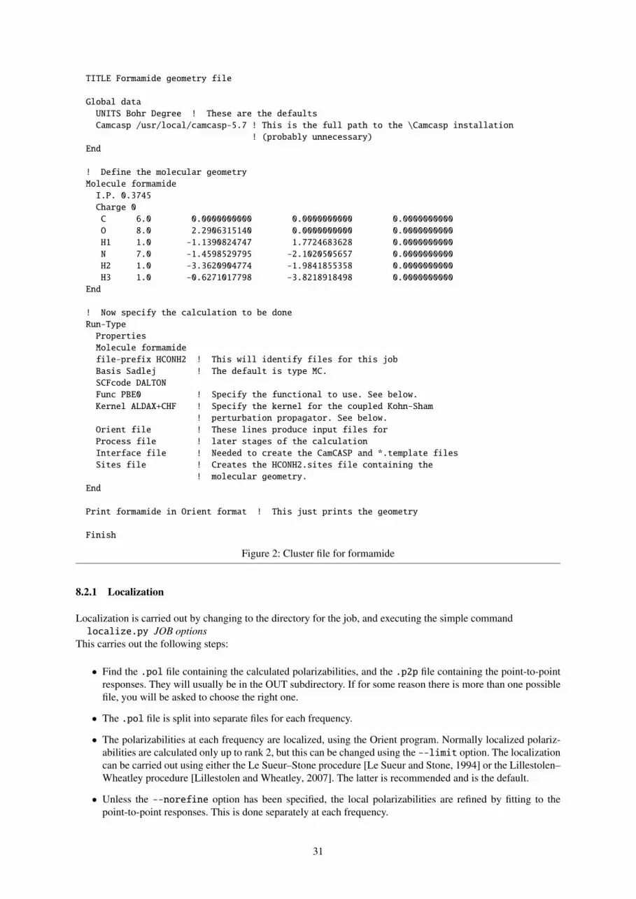
TITLE Formamide geometry file
Global dataUNITS Bohr Degree ! These are the defaultsCamcasp /usr/local/camcasp-5.7 ! This is the full path to the \Camcasp installation
! (probably unnecessary)End
! Define the molecular geometryMolecule formamide
I.P. 0.3745Charge 0C 6.0 0.0000000000 0.0000000000 0.0000000000O 8.0 2.2906315140 0.0000000000 0.0000000000H1 1.0 -1.1390824747 1.7724683628 0.0000000000N 7.0 -1.4598529795 -2.1020505657 0.0000000000H2 1.0 -3.3620904774 -1.9841855358 0.0000000000H3 1.0 -0.6271017798 -3.8218918498 0.0000000000
End
! Now specify the calculation to be doneRun-Type
PropertiesMolecule formamidefile-prefix HCONH2 ! This will identify files for this jobBasis Sadlej ! The default is type MC.SCFcode DALTONFunc PBE0 ! Specify the functional to use. See below.Kernel ALDAX+CHF ! Specify the kernel for the coupled Kohn-Sham
! perturbation propagator. See below.Orient file ! These lines produce input files forProcess file ! later stages of the calculationInterface file ! Needed to create the CamCASP and *.template filesSites file ! Creates the HCONH2.sites file containing the
! molecular geometry.End
Print formamide in Orient format ! This just prints the geometry
Finish
Figure 2: Cluster file for formamide
8.2.1 Localization
Localization is carried out by changing to the directory for the job, and executing the simple commandlocalize.py JOB options
This carries out the following steps:
• Find the .pol file containing the calculated polarizabilities, and the .p2p file containing the point-to-pointresponses. They will usually be in the OUT subdirectory. If for some reason there is more than one possiblefile, you will be asked to choose the right one.
• The .pol file is split into separate files for each frequency.
• The polarizabilities at each frequency are localized, using the Orient program. Normally localized polariz-abilities are calculated only up to rank 2, but this can be changed using the --limit option. The localizationcan be carried out using either the Le Sueur–Stone procedure [Le Sueur and Stone, 1994] or the Lillestolen–Wheatley procedure [Lillestolen and Wheatley, 2007]. The latter is recommended and is the default.
• Unless the --norefine option has been specified, the local polarizabilities are refined by fitting to thepoint-to-point responses. This is done separately at each frequency.
31
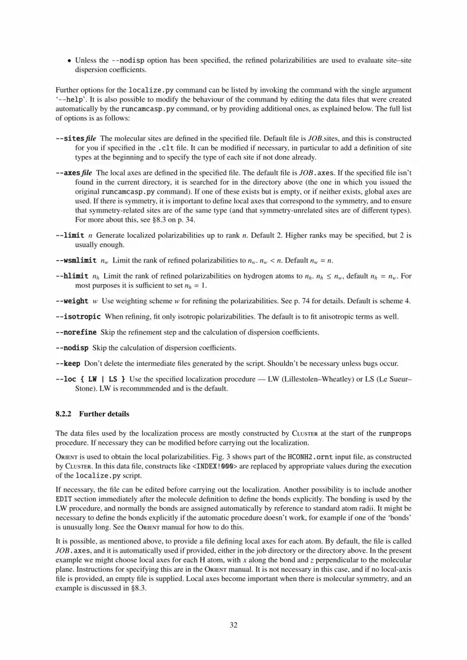
• Unless the --nodisp option has been specified, the refined polarizabilities are used to evaluate site–sitedispersion coefficients.
Further options for the localize.py command can be listed by invoking the command with the single argument‘--help’. It is also possible to modify the behaviour of the command by editing the data files that were createdautomatically by the runcamcasp.py command, or by providing additional ones, as explained below. The full listof options is as follows:
--sites file The molecular sites are defined in the specified file. Default file is JOB.sites, and this is constructedfor you if specified in the .clt file. It can be modified if necessary, in particular to add a definition of sitetypes at the beginning and to specify the type of each site if not done already.
--axes file The local axes are defined in the specified file. The default file is JOB.axes. If the specified file isn’tfound in the current directory, it is searched for in the directory above (the one in which you issued theoriginal runcamcasp.py command). If one of these exists but is empty, or if neither exists, global axes areused. If there is symmetry, it is important to define local axes that correspond to the symmetry, and to ensurethat symmetry-related sites are of the same type (and that symmetry-unrelated sites are of different types).For more about this, see §8.3 on p. 34.
--limit n Generate localized polarizabilities up to rank n. Default 2. Higher ranks may be specified, but 2 isusually enough.
--wsmlimit nw Limit the rank of refined polarizabilities to nw. nw < n. Default nw = n.
--hlimit nh Limit the rank of refined polarizabilities on hydrogen atoms to nh. nh ≤ nw, default nh = nw. Formost purposes it is sufficient to set nh = 1.
--weight w Use weighting scheme w for refining the polarizabilities. See p. 74 for details. Default is scheme 4.
--isotropic When refining, fit only isotropic polarizabilities. The default is to fit anisotropic terms as well.
--norefine Skip the refinement step and the calculation of dispersion coefficients.
--nodisp Skip the calculation of dispersion coefficients.
--keep Don’t delete the intermediate files generated by the script. Shouldn’t be necessary unless bugs occur.
--loc LW | LS Use the specified localization procedure — LW (Lillestolen–Wheatley) or LS (Le Sueur–Stone). LW is recommmended and is the default.
8.2.2 Further details
The data files used by the localization process are mostly constructed by Cluster at the start of the runpropsprocedure. If necessary they can be modified before carrying out the localization.
Orient is used to obtain the local polarizabilities. Fig. 3 shows part of the HCONH2.ornt input file, as constructedby Cluster. In this data file, constructs like <INDEX!000> are replaced by appropriate values during the executionof the localize.py script.
If necessary, the file can be edited before carrying out the localization. Another possibility is to include anotherEDIT section immediately after the molecule definition to define the bonds explicitly. The bonding is used by theLW procedure, and normally the bonds are assigned automatically by reference to standard atom radii. It might benecessary to define the bonds explicitly if the automatic procedure doesn’t work, for example if one of the ‘bonds’is unusually long. See the Orient manual for how to do this.
It is possible, as mentioned above, to provide a file defining local axes for each atom. By default, the file is calledJOB.axes, and it is automatically used if provided, either in the job directory or the directory above. In the presentexample we might choose local axes for each H atom, with x along the bond and z perpendicular to the molecularplane. Instructions for specifying this are in the Orient manual. It is not necessary in this case, and if no local-axisfile is provided, an empty file is supplied. Local axes become important when there is molecular symmetry, and anexample is discussed in §8.3.
32

Molecule formamide at 0.0 0.0 0.0! Units BOHRC 0.00000000 0.00000000 0.00000000 Type CO 2.29063151 0.00000000 0.00000000 Type OH1 -1.13908247 1.77246836 0.00000000 Type H1N -1.45985298 -2.10205057 0.00000000 Type NH2 -3.36209048 -1.98418554 0.00000000 Type H2H3 -0.62710178 -3.82189185 0.00000000 Type H3
End
Polarizabilities for formamideRead rank 4 sites +++
C O H1 N H2 H3#include HCONH2_NL4_<INDEX!000>.polLimit rank <LIMIT! 2> for +++
C O H1 N H2 H3Sum-rule test 1e-7Localize <LOC!LW> test 1e-7 Limit <LIMIT! 2> sites +++
C O H1 N H2 H3End
Edit formamide#include <AXES!axes>
End
Figure 3: Part of the Orient file for formamide
8.2.3 Refining the local polarizabilities
We have found that the localization procedure used by Orient results in local polarizabilities that are not quiteoptimum. They can be refined by using the Pfit program to reproduce the point-to-point polarizabilities. Thelocalization script does this automatically, unless the --norefine flag is specified. The necessary input files forPfit are generated automatically by Process from the HCONH2.prss input file, shown in Fig. 4. Constructions like<LIMIT! 2> are replaced by default values or by values specified on the command line.
Pfit has other important uses. The standard procedure does not impose full symmetry, though it does require sitesof the same type to have the same polarizabilities. The grid of points used for the point-to-point polarizabilitiesdoes not have any symmetry, so fitting to the values may result in polarizabilities that should be zero having smallnon-zero values. This can provide a guide to the accuracy of the fitted values, but usually it is better to obtain valuesthat have the correct symmetry. Also the standard procedure fits all possible polarizability components up to thespecified maximum rank, but a simpler model may be needed. These needs can be met by editing the polarizabilitydefinition file, JOB.pdef. This file is generated automatically if it doesn’t already exist, either in the job directoryor the one above, so the usual procedure is to carry out the localization and refinement, and check the JOB.pdefto make sure that the polarizability model is correct and suitable. If it needs to be changed, just run the localizationcommand again with the revised file in place.
The JOB.pdef file as automatically generated includes all polarizability components up to the limits specified inthe localize.py command, and the polarizabilities for sites of the same type are assumed to be identical. Thismeans that sites should not be assigned the same type unless they are related by symmetry, or they are to be treatedas equivalent. Also the axes for the symmetry-related sites must be related by proper symmetry operations (purerotations), as sites related only by improper operations may have unavoidable sign differences between some ofthe components.
Also some components may be zero as a consequence of the local site symmetry. Such components should bedeleted from the JOB.pdef file. If left, they will usually be fitted with values close to zero, but not exactly zerobecause the data grid used for the localization is not symmetric. Also including components that must be zero addsunnecessarily to the complexity of the model and may lead to numerical problems.
33
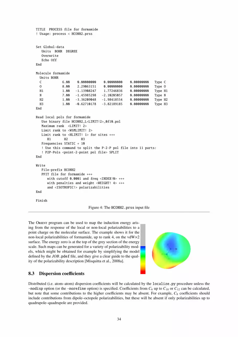
TITLE PROCESS file for formamide! Usage: process < HCONH2.prss
Set Global-dataUnits BOHR DEGREEOverwriteEcho Off
End
Molecule formamideUnits BOHRC 6.00 0.00000000 0.00000000 0.00000000 Type CO 8.00 2.29063151 0.00000000 0.00000000 Type OH1 1.00 -1.13908247 1.77246836 0.00000000 Type H1N 7.00 -1.45985298 -2.10205057 0.00000000 Type NH2 1.00 -3.36209048 -1.98418554 0.00000000 Type H2H3 1.00 -0.62710178 -3.82189185 0.00000000 Type H3
End
Read local pols for formamideUse binary file HCONH2_L<LIMIT!2>_0f10.polMaximum rank <LIMIT! 2>Limit rank to <WSMLIMIT! 2>Limit rank to <HLIMIT! 1> for sites +++
H1 H2 H3Frequencies STATIC + 10! Use this command to split the P-2-P pol file into 11 parts:! P2P-Pols <point-2-point pol file> SPLIT
End
WriteFile-prefix HCONH2PFIT file for formamide +++
with cutoff 0.0001 and freq <INDEX!0> +++with penalties and weight <WEIGHT! 4> +++and <ISOTROPIC!> polarizabilities
End
Finish
Figure 4: The HCONH2.prss input file
The Orient program can be used to map the induction energy aris-ing from the response of the local or non-local polarizabilities to apoint charge on the molecular surface. The example shows it for thenon-local polarizabilities of formamide, up to rank 4, on the vdW×2surface. The energy zero is at the top of the grey section of the energyscale. Such maps can be generated for a variety of polarizability mod-els, which might be obtained for example by simplifying the modeldefined by the JOB.pdef file, and they give a clear guide to the qual-ity of the polarizability description [Misquitta et al., 2008a].
8.3 Dispersion coefficients
Distributed (i.e. atom–atom) dispersion coefficients will be calculated by the localize.py procedure unless thenodisp option (or the norefine option) is specified. Coefficients from C6 up to C10 or C12 can be calculated,but note that some contributions to the higher coefficients may be absent. For example, C8 coefficients shouldinclude contributions from dipole–octopole polarizabilities, but these will be absent if only polarizabilities up toquadrupole–quadrupole are provided.
34
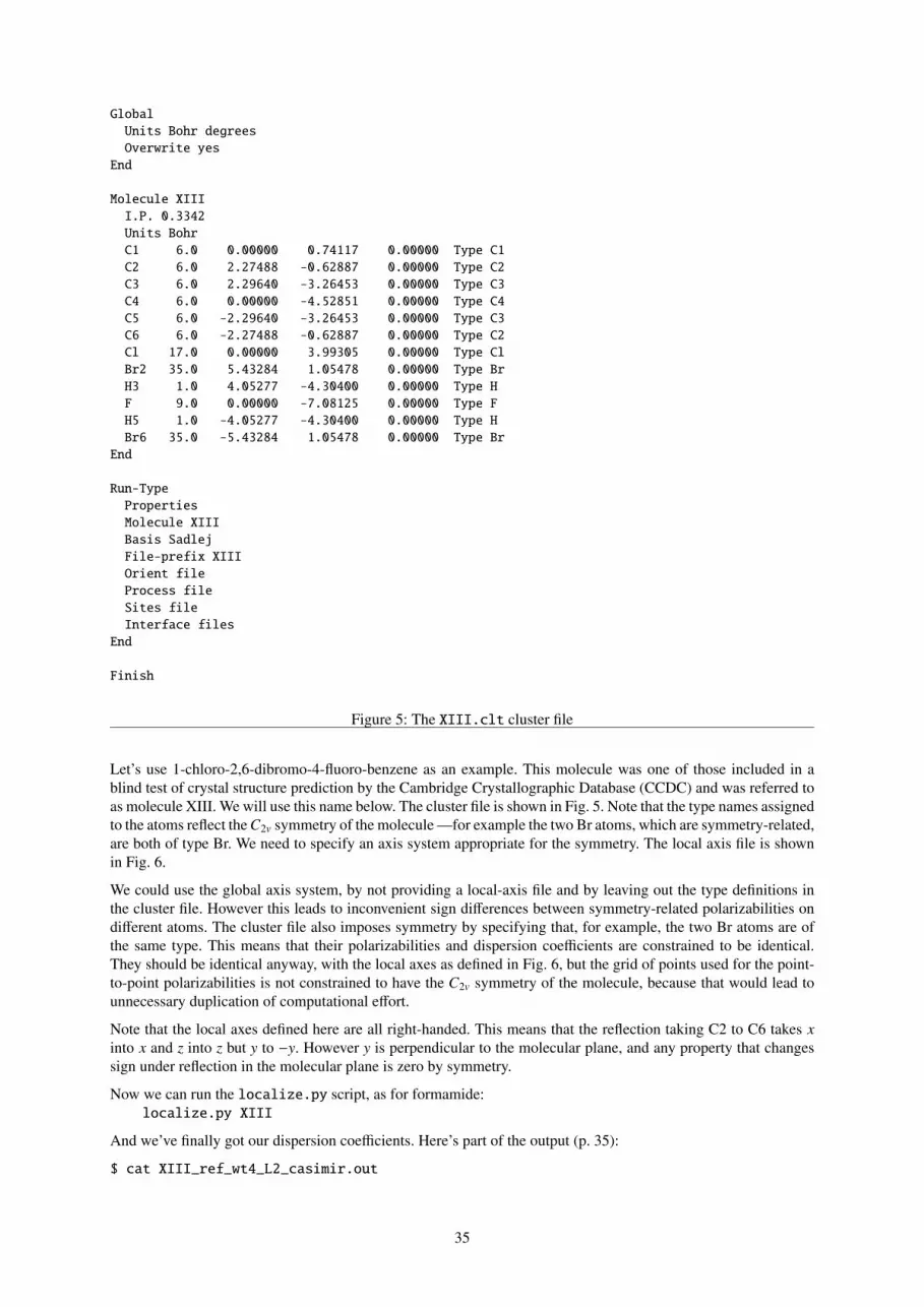
GlobalUnits Bohr degreesOverwrite yes
End
Molecule XIIII.P. 0.3342Units BohrC1 6.0 0.00000 0.74117 0.00000 Type C1C2 6.0 2.27488 -0.62887 0.00000 Type C2C3 6.0 2.29640 -3.26453 0.00000 Type C3C4 6.0 0.00000 -4.52851 0.00000 Type C4C5 6.0 -2.29640 -3.26453 0.00000 Type C3C6 6.0 -2.27488 -0.62887 0.00000 Type C2Cl 17.0 0.00000 3.99305 0.00000 Type ClBr2 35.0 5.43284 1.05478 0.00000 Type BrH3 1.0 4.05277 -4.30400 0.00000 Type HF 9.0 0.00000 -7.08125 0.00000 Type FH5 1.0 -4.05277 -4.30400 0.00000 Type HBr6 35.0 -5.43284 1.05478 0.00000 Type Br
End
Run-TypePropertiesMolecule XIIIBasis SadlejFile-prefix XIIIOrient fileProcess fileSites fileInterface files
End
Finish
Figure 5: The XIII.clt cluster file
Let’s use 1-chloro-2,6-dibromo-4-fluoro-benzene as an example. This molecule was one of those included in ablind test of crystal structure prediction by the Cambridge Crystallographic Database (CCDC) and was referred toas molecule XIII. We will use this name below. The cluster file is shown in Fig. 5. Note that the type names assignedto the atoms reflect the C2v symmetry of the molecule —for example the two Br atoms, which are symmetry-related,are both of type Br. We need to specify an axis system appropriate for the symmetry. The local axis file is shownin Fig. 6.
We could use the global axis system, by not providing a local-axis file and by leaving out the type definitions inthe cluster file. However this leads to inconvenient sign differences between symmetry-related polarizabilities ondifferent atoms. The cluster file also imposes symmetry by specifying that, for example, the two Br atoms are ofthe same type. This means that their polarizabilities and dispersion coefficients are constrained to be identical.They should be identical anyway, with the local axes as defined in Fig. 6, but the grid of points used for the point-to-point polarizabilities is not constrained to have the C2v symmetry of the molecule, because that would lead tounnecessary duplication of computational effort.
Note that the local axes defined here are all right-handed. This means that the reflection taking C2 to C6 takes xinto x and z into z but y to −y. However y is perpendicular to the molecular plane, and any property that changessign under reflection in the molecular plane is zero by symmetry.
Now we can run the localize.py script, as for formamide:localize.py XIII
And we’ve finally got our dispersion coefficients. Here’s part of the output (p. 35):
$ cat XIII_ref_wt4_L2_casimir.out
35

AxesC1 z from C1 to Cl x from C1 to C6Cl z from C1 to Cl x from C1 to C6C2 z from C2 to Br2 x from C2 to C3Br2 z from C2 to Br2 x from C2 to C3C6 z from C6 to Br6 x from C6 to C5Br6 z from C6 to Br6 x from C6 to C5C3 z from C3 to H3 x from C3 to C4H3 z from C3 to H3 x from C3 to C4C5 z from C5 to H5 x from C5 to C4H5 z from C5 to H5 x from C5 to C4C4 z from C4 to F x from C4 to C3F z from C4 to F x from C4 to C3
End
Figure 6: Local axis definitions for molecule XIII.
Title XIII ... XIIIXIIIFrequencies 0.5 10Skip 0Print nonzero
Molecule XIIISite C210 10
5.72200000 5.70700000 5.61200000 5.27400000 +++4.44000000 3.07700000 1.62100000 0.58700000 +++0.11800000 0.00600000
...
...
...Dispersion coefficients for XIII and XIII
C2 C2 C6 C7 C8 ...00 00 0 88.39684131 0.0 4820.75066614 ...00 11c 1 0.0 809.88012198 ...00 11s 1 0.0 477.13620553 ...00 20 2 -24.31832249 0.0 -3056.70651103 ............
Finish
8.4 Using Cluster to obtain the dimer geometry
The problem: We wished to study the interaction betweencarbamazepine molecules in the crystal, but this moleculewas at the time too big for the calculation to be carriedout between whole molecules. With the current version ofCamCASP this dimer is not a problem, but similar frag-ment methods are still useful in other, larger, systems. Inthis case, we modelled the close interaction using a ureafragment to represent part of one molecule and a benzenefragment for part of the other. We needed to place thefragments in the same relative geometry as in the carba-mazepine molecules. We have the CBMZ crystal geome-try from the X-ray structure.
TITLE CBMZ fragmentsUNITS Bohr Degrees
36
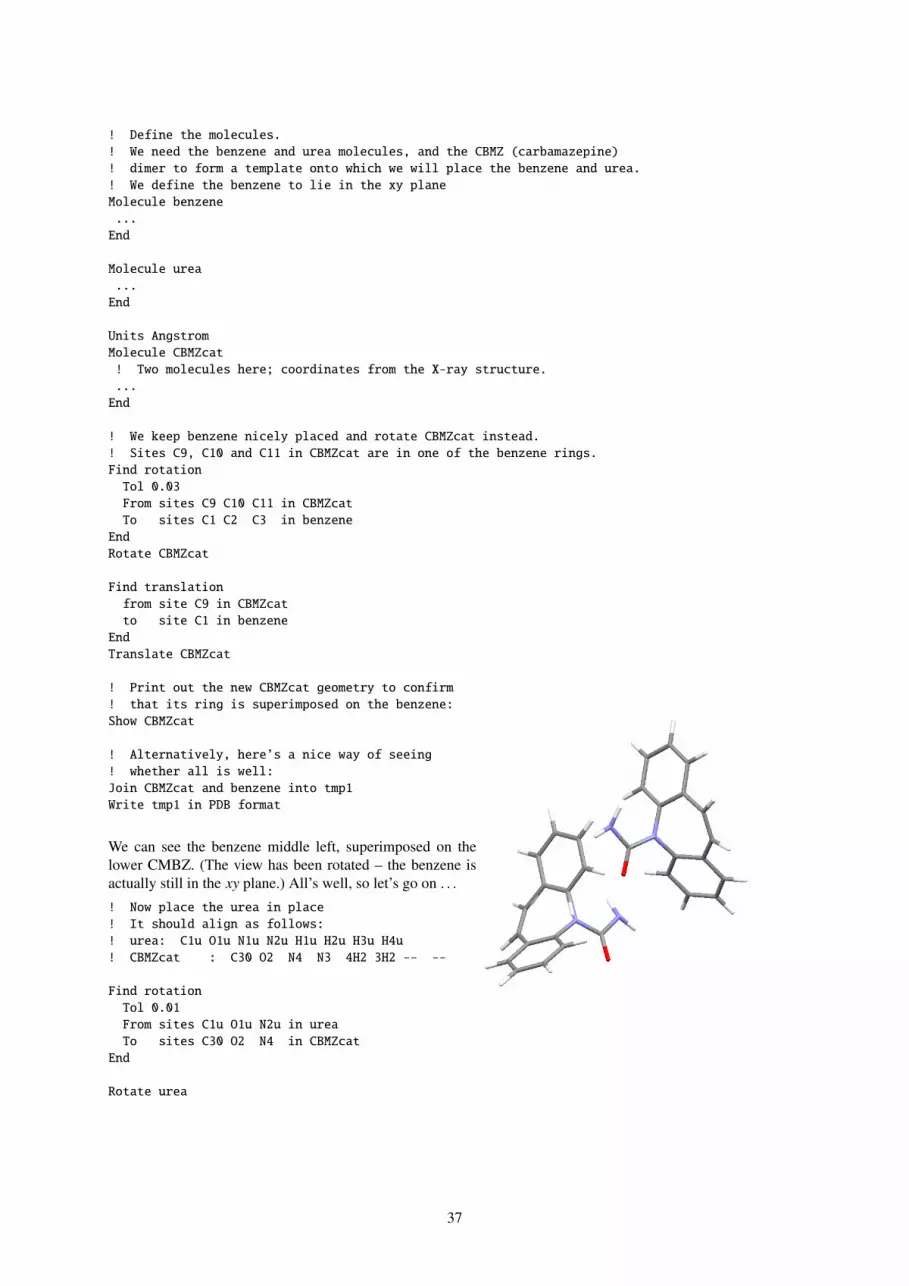
! Define the molecules.! We need the benzene and urea molecules, and the CBMZ (carbamazepine)! dimer to form a template onto which we will place the benzene and urea.! We define the benzene to lie in the xy planeMolecule benzene...End
Molecule urea...End
Units AngstromMolecule CBMZcat! Two molecules here; coordinates from the X-ray structure....End
! We keep benzene nicely placed and rotate CBMZcat instead.! Sites C9, C10 and C11 in CBMZcat are in one of the benzene rings.Find rotation
Tol 0.03From sites C9 C10 C11 in CBMZcatTo sites C1 C2 C3 in benzene
EndRotate CBMZcat
Find translationfrom site C9 in CBMZcatto site C1 in benzene
EndTranslate CBMZcat
! Print out the new CBMZcat geometry to confirm! that its ring is superimposed on the benzene:Show CBMZcat
! Alternatively, here’s a nice way of seeing! whether all is well:Join CBMZcat and benzene into tmp1Write tmp1 in PDB format
We can see the benzene middle left, superimposed on thelower CMBZ. (The view has been rotated – the benzene isactually still in the xy plane.) All’s well, so let’s go on . . .
! Now place the urea in place! It should align as follows:! urea: C1u O1u N1u N2u H1u H2u H3u H4u! CBMZcat : C30 O2 N4 N3 4H2 3H2 -- --
Find rotationTol 0.01From sites C1u O1u N2u in ureaTo sites C30 O2 N4 in CBMZcat
End
Rotate urea
37
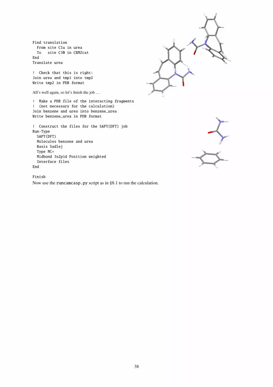
Find translationFrom site C1u in ureaTo site C30 in CBMZcat
EndTranslate urea
! Check that this is right:Join urea and tmp1 into tmp2Write tmp2 in PDB format
All’s well again, so let’s finish the job . . .
! Make a PDB file of the interacting fragments! (not necessary for the calculation)Join benzene and urea into benzene_ureaWrite benzene_urea in PDB format
! Construct the files for the SAPT(DFT) jobRun-Type
SAPT(DFT)Molecules benzene and ureaBasis SadlejType MC+Midbond 3s2p1d Position weightedInterface files
End
Finish
Now use the runcamcasp.py script as in §8.1 to run the calculation.
38
9 CamCASP program specification
Usually the input dataset for CamCASP will be generated automatically with the Cluster command, and this isusually a good starting-point in any case. Sometimes, however, it becomes necessary to modify the generated file,so full details of the program input are given here.
See §6 for general notes on syntax descriptions. In the CamCASP input, the form SET keyword is used to start ablock which just sets parameters for later use, while BEGIN keyword is used for blocks that carry out a calculation.In the latter case, the block is read to the end before the calculation is done.
The CamCASP input file begins with a title and memory declaration:
TITLE titleMEMORY memory [ BYTES | KB | MB | GB ]
The memory can be set in BYTES, KB, MB or GB.
It then continues with a series of data blocks, which are each described here in turn. In addition to the optionsmentioned, most blocks have QUIET and VERBOSE options, to reduce or increase the amount of output, and aDEBUG option, which is for development purposes and should not normally be needed.
In addition to numerical and string arguments in commands, some commands expect a switch (Boolean or logical)value, which can be YES, Y, ON, TRUE or T, which are all equivalent, or NO, N, OFF, FALSE or F. If the switch value isomitted it is assumed to be TRUE, which however may not be the default if the command is omitted altogether. Thusthe default if the ECHO command is omitted is TRUE but the default if the DEBUG command is omitted is FALSE.
9.1 Global data
SET GLOBAL | GLOBAL-DATA | DATA settings
END
SET is optional. The settings are as follows. Most of them can be over-ridden by commands in individual modules:
CAMCASP-PATH absolute path to the CamCASP installation.If set, the #include-camcasp command can be used to include files present in the CamCASP directory using onlythe relative file paths. It will usually be set automatically from the CAMCASP environment variable.
UNITS unit unit . . .where the available units areANGSTROM, ANG, BOHR or NM;HARTREE, KJ/MOL, CM-1, eV or K/KELVIN;DEG, DEGREE, DEGREES, RAD, RADIAN, or RADIANS.Defaults are BOHR, HARTREE and DEGREES. The units set in this command are used for all output. They are alsoused for input unless over-ridden by a local UNITS declaration in a module.
ECHO switchIf ON (the default) input is echoed to the output.
OVERWRITE [files] switchOVERWRITE instructs the program to overwrite any existing files with the same names as those that the programwould normally use. If OFF (the default) the names are modified, by inserting a 3-digit code just before the filesuffix. The 3-digit code may be different for different files, depending on what files are already present. The filenames are printed in the program output, but to avoid confusion it is better to carry out each run in a differentdirectory.
SCF-CODE | DFT-CODE [ DALTON | DALTON2013 | DALTON2006 | CADPAC | GAMESS(US) | NWCHEM]Specifies the SCF code to use. Default DALTON, i.e., the Dalton 2013 program. (Cadpac is unlikely to be availablefor most users.)
XC-FUNC | XC-FUNCTIONAL | FUNCTIONAL functionalSpecify the exchange-correlation functional to be used. Available functionals are PBE PW91 PBE0 HCTH HCTH407.Default PBE0.
39
C-X | FRACTION-HF | EXACT-EXCHANGE Fraction of exact-exchangeThe default fraction is set according to the chosen functional and should not need to be changed. Use this commandif the exchange-correlation functional you have used is not included above.
DEBUG switch [ MEM | MEMORY] [TIMER] [TYPES] [IO]The DEBUG option sets debugging on or off for the whole calculation. However the setting can be over-ridden forany module by a DEBUG option in that module. The MEMORY sub-option tracks memory allocation, the TIMER sub-option prints timing information for subroutine entry and exit, the TYPES sub-option prints information about theuser-defined types used in the program, and IO prints information about input and output.
Setting any of these debugging options on does not mean information will be printed out. This would be over-whelming. Rather, these options provide specific debugging information about only those modules in which theDEBUG command has been used.
9.2 Molecule definition
Each molecule needs a main basis set and an auxiliary (density-fitting) basis set. For a property calculation therewill be just one molecule; for a calculation of intermolecular interactions there will be two. The molecules areidentified by name in most modules; the names are case-sensitive. The first two molecules to be defined may alsobe referred to as A and B, and interaction energies will be calculated between these two by default.
Notes:
• Basis functions can be in SPHERICAL or CARTESIAN form and this needs to be specified.
• CamCASP can read basis sets in three formats: GAMESS (actually, GAMESS(US)), NWChem and TURBOMOLE.This is specified by the FORMAT option.
• For the main basis, the sites must be specified in the same order as was used in the CADPAC/DALTON/NWchem/GAMESS(US)runs. This is important. The site name, nuclear charge and position are followed by the basis set specification,which can be typed in or #INCLUDEd from a file. Explicit paths are needed. The site definition is terminatedby a line containing three dashes: .
• The auxiliary basis is defined in the same way, but it need not have the same number of sites, nor do theyneed to be in the same order as the main basis. They are completely independent. However, for sensibleresults you’d be better off keeping all sites.
MOLECULE name [AT x y z ] [ROTATED BY angle ABOUT nx ny nz ]optionsdatamain basis specificationauxiliary basis specification
END
The molecule is taken to be at the global origin and not rotated unless otherwise specified.
The options are:
CHARGE qThe total charge on the molecule, in units of the proton charge.
ECHO switchSwitch echoing of input data on or off. This may appear in several places to switch the echoing of particular items.
If the molecular orbitals and Hessians are not needed, use the commandSKIP MOS
Otherwise, the molecular orbitals and Hessians should have been calculated at a previous stage, and they areattached to the molecule description by the following commands: MO | MOS | MO-FILE [in] [file] file-name [ASCII | BINARY | ASCII-1 ] H1 | H1-FILE [in] [file] file-name H2 | H2-FILE [in] [file] file-nameHESSIAN-FORMAT SAPT2002 | SAPT2006H1 and H2 refer to the electric and magnetic Hessians used in the polarizability calculation. The orbitals and
40
Hessians must have been calculated for the basis set and molecular geometry defined in the BASIS blocks. If arotation is applied to the molecule the orbitals and Hessians are rotated too and need not be recalculated, but thisonly works at present if SPHERICAL basis sets are used. The HESSIAN-FORMAT command is used to specify theformat the Hessians have been written in. Use SAPT2002 or SAPT2006 depending on the patch you have used tobuild Dalton 2013. The default is SAPT2006.
The MO file is expected to be in ASCII format by default.
A special ascii format, ASCII-1 is also available. In this case the file format isMO NC(1, 1) C(1, 2) C(1, 3) . . . C(1,N)C(2, 1) C(2, 2) . . . C(N,N)ENERGY NE(1) E(2) . . .
Here C(m, i) is the coefficient of the mth atomic orbital in the ith molecular orbital, and E(i) is the energy of the ith
molecular orbital. The keywords MO and ENERGY must appear at the start of a new line, but otherwise the numbersare read in free format, separated by space or newline. N is the number of molecular orbitals.
Each basis set specification takes the form
BASIS MAIN | AUX [ CARTESIAN | SPHERICAL ][ FORMAT GAMESS | TURBOMOLE | NWCHEM ][ ECHO [ ON | OFF] ][UNITS length units]label charge x y z [TYPE site-type ][LIMIT limit]basis specification for this atom---label charge x y z[TYPE site-type ][LIMIT limit]basis specification---...
END
At present it is necessary to give the atom positions twice, once for the main basis specification and once for theauxiliary basis. This makes it possible to use different sites for the main and auxiliary basis sets. However the entiremolecule definition is normally provided automatically for you by the Cluster program.
The limit option applies to individual atoms, and takes the formLIMIT S | P | D | F | G Limit the basis to this symmetry type, i.e. omit basis functions of higher angular momentum. The basis set isusually specified by including it from a suitable file; for example:#include /usr/local/camcasp/basis/gamess_us/sadlej/C
and the LIMIT command allows just (say) the s, p and d functions from the standard basis to be used. The defaultis currently LIMIT G, as CamCASP can’t currently handle h or higher functions.
FORMAT GAMESS | TURBOMOLE The basis function definitions that follow are in the format used by Gamess(US) or Turbomole, as specified. Defaultis Gamess(US). The auxiliary basis library supplied with the CamCASP program uses basis sets in the Turbomoleprogram format. Note that the NWCHEM format is not available for this auxiliary basis set.
[ CARTESIAN | SPHERICAL ]Use Cartesian basis functions (6-component d functions) or spherical (5-component d functions). Default is Carte-sian as this results in a perceptible increase in accuracy of the density-fitting procedure. However the resultingincreased linear dependencies could cause problems in the density-fitting procedure.
UNITS A | ANG | ANGSTROM | BOHR | AU | A.U. ]Atom positions will be given in the specified unit. Only needed if this is different from the global unit.
41

9.3 The EDIT module: Modifying a molecular specification
Once defined, the molecule can be manipulated in much the same way as in the Cluster program. There is onecaveat: The commands involving a rotation will work only with main basis sets of spherical Gaussian type orbitals(GTOs). The command takes the formEDIT molecule-name
optionsEND
and the options are as follows:
TOL | TOLERANCE toleranceSpecify tolerance used in finding rotations and comparisons.
RESTORERestore the molecule to its original configuration, as set up in the MOLECULE declaration, and restore the originalmolecular orbitals.
Note that in the present version of CamCASP the Hessians are not rotated. This has consequences when anENERGY-SCAN is performed.
CENTRE [on/at] [[SITE] site | COM | XYZ x y z ] Define the molecular centre to be at the position given.If Cartesian coordinates are given, they are taken to specify a position within the molecule as originally defined,i.e. in local molecular axes which rotate and translate with it.
WRITE | PRINT | SHOW [ MO | MOS GEOM | GEOMETRY ]Print the molecular orbitals or the molecular geometry on standard output.
BOND -> | TO POINTS | XYZ | molecule SITES a3 a2 a1 -> | TO b1 b2 b3 DISTANCE | LENGTH | SEPARATION distance [ ANGSTROM | ANG | BOHR ]
END(Implemented but not fully tested.) Moves this molecule (molecule A) so that sites a2, a1, b1 and b2 are collinearand arranged in that order, and so that sites a1 and b1 are the specified distance apart. If molecule A is non-linear,a3 is a third site lying off the a1 − a2 axis, and molecules A is rotated about the a2 − a1 axis so that all six sitesare coplanar, with sites a3 and b3 cis to each other. If A is linear, then a3 is irrelevant, but at present it must stillbe specified and must still lie off the a1 − a2 axis. It can be specified as a position in global coordinates using thesyntax XYZ x y z. Sites b1, b2 and b3 may be in another molecule B, or may be specified as cartesian positions inglobal coordinates using the syntax XYZ x y z.
INVERTInvert the site positions with respect to the molecular origin. (Not yet implemented.)
ROTATE BY angle [ DEGREES | RADIANS] ABOUT nx ny nz
Rotate the molecule about an axis in the specified direction, through the molecular centre. The rotation is notcarried out until an UPDATE command is encountered.
TRANSLATE BY distance [ ANGSTROM | ANG | A | BOHR | AU ] ALONG x y zThe distance is assumed to be in the global units unless otherwise specified. The vector direction need not be aunit vector — it is normalized by the program. The translation is not carried out until an UPDATE command isencountered.
PLACE | POSITION | PUT ] [ at ] [ XYZ | POINT ] x y zPosition (translate) the molecule so that its defined centre coincides with the specified point. The translation is notcarried out until an UPDATE command is encountered.
UPDATE [MOS | ORBITALS]Carry out any translation and rotation that has been specified. Note that the rotation is about the molecular centre,which moves with the molecule, so translation and rotation commute. If ORBITALS is specified, the molecularorbitals and density matrix are rotated with the molecule.
NEIGHBOURS [TYPE [=] [ONE | ALL | OVR]] [EPS [=] <value|0.0>] [PRINT]Every atom in a molecule has a list of neighbours. By default, this list contains every other atom, but it can bechanged using this command. There are three neighbourhood types that can be defined using the TYPE option.Type ONE defines only one ‘neighbour’ for every atom: the atom itself. Type ALL is the default and defines all sites
42

as the neighbourhood. Finally, type OVR uses an overlap criterion and the value of EPS to decide which sites are tobe included in the neighbourhood. The latter is a basis and geometry-dependent criterion. We have not tested thisfeature adequately, but it seems like a reasonable choice for EPS is 0.01. The list of neighbours for every atom inthe molecule can be printed out using the PRINT option.
The reason for implementing a concept of neighbourhoods is to speed up the evaluation of integrals. UsingNEIGHBOURS TYPE = OVR EPS = 0.01we can significantly speed-up the evaluation of the numerical integrals needed for the ISA module, without asignificant reduction in the overall accuracy of the calculation. But it must be borne in mind that the largest speed-ups are obtained for linear systems.
9.4 Density-fitting
ssec:df
Significant computational gains are achieved by expanding orbital products ρi j = φiφ j as a single index expansion:
ρi j(r) ≈ ρi j(r) =∑
k
di j,kχk(r).
This is usually achieved by the minimization of the functional:
∆i j =
" [ρi j(r1) − ρi j(r1)
] 1r12
[ρi j(r2) − ρi j(r2)
]dr1dr2
In CamCASP we additionally include constraints to impose the orthonormality of ρi j:∫ρi j(r)dr = δi j,
and localization constraints that are used to obtain distributed polarizabilities [Misquitta and Stone, 2006]. Thelatter are optional and should not be used in interaction energy calculations. This gives us two types of functionalthat we minimize:
• In the first we include a term that minimizes the inter-site repulsion (the default):
ΞAi j = ∆i j − η
∑a,b,a
Eabi j + λ
(∫ρi j(r)dr − δi j
)2
.
• In the second we include a term that maximizes the site self-repulsion:
ΞBi j = ∆i j + η
∑a
Eaai j + λ
(∫ρi j(r)dr − δi j
)2
.
where
Eabi j =
" ρai j(r1)ρb
i j(r2)
r12dr1dr2.
and ρai j(r) is the (transition-)density associated with site a which is defined as
ρai j(r) =
∑k∈a
di j,kχk(r). (5)
For details and numerical results see Misquitta & Stone (2006) [Misquitta and Stone, 2006].
In addition to the above, the following constraint can be optionally included:
Ci j = γ∑
a
[∫ρa
i j(r)dr]2
. (6)
This constraint forces the (transition-)density ‘charge’ on each site to be close to zero. The larger γ is, the morestrongly this condition is enforced. This constraint should be used with the transition densities only, and eventhen with caution. When used together with a distributed polarizability calculation, this constraint has the effect ofsuppressing the charge-flow polarizabilities.
This gives us a number of choices for the density-fitting. We recommend the following in everyday usage:
43
• For energy calculations use only the orthonormality constraint, that is, either ΞAi j or ΞB
i j with η = 0.0 andλ = 1000.0.
• Do the same for total molecular properties such as the molecular density, quantities that depend on thetotal density, and total polarizabilities.
• For distributed polarizabilities perform the transition-density fitting using either ΞAi j or ΞB
i j with η =
+0.0002 and λ = 1000.0.
• For the SRLO method of Rob & Szalewicz [Rob and Szalewicz, 2013] use ΞBi j with the additional constraint
Ci j and γ = 1.0.
Many of the modules require density-fitting and while some will perform the density-fitting automati-cally if it hasn’t already been done, it is generally a good idea to perform it explicitly.
The (ortho)normality constraints are checked if PRINT...NORMALIZATION... is used. The localization constraintcan be selected using the CONSTRAINT command.
BEGIN DF | DENSITYFITTING | DENSITY-FITTINGoptionsEND
Or, to set parameters without performing the density-fitting:
SET DF | DENSITYFITTING | DENSITY-FITTINGoptionsEND
The options are:
[MOLECULE name | DIMER]Apply the fitting procedure to the specified molecule if MOLECULE is specified, or, if DIMER is specified, performthe density-fitting for the dimer consisting of the first two molecules in the input file. That is, the dimer is assumedto comprise molecules A and B. At present, there is no way to change the molecules in the dimer.
TYPE [OO] [OV | VO] [FULL | NN] [RHO] [RHO-W]Specifies the type of density-fitting to perform. OO applies density-fitting only to occupied–occupied orbital pairs,needed for the density. OV does the occupied–virtual pairs, which are needed for all second-order terms. FULL doesall pairs, and is the default.
For the dimer, only types OO and OV are available. Selecting type FULL will result in an error.
There are two special DF types:
• RHO fits the density directly.
• RHO-W is an experimental option that fits the difference of the density and (spherical) pro-atom densities.These would typically be obtained from an iterated stockholder atoms calculation. The site-charge constraintCi j can be used in this context to enforce zero site charges of the RHO-W fit. This is an experimental option.Please contact the authors if you are interested in this.
SOLVER LU [[with] ITERATIONS iterations ]| GELSS [[with] CONDITION condition-number]
Specifies the linear-equation solver to use. The LU solver is fastest but gets unstable for larger basis sets. Inprinciple the solution can be improved by iterating if the density-fitting equations are ill-conditioned, but we havenot experimented with this much and the default number of iterations is 0.
Usually the auxiliary basis set will be roughly three times the size of the main basis. But this may not be thecase if, say, you are using a Sadlej-pVTZ main basis together with a R12 aug-cc-pVTZ auxiliary basis whichcan be four to six times as large as the Sadlej main basis. In this case, the density-fitting linear equations will benear singular and LU will not result in reliable results. These equations can also be ill-conditioned for large, densesystems. For these cases we suggest the GELSS solver which uses singular value decomposition (SVD) to solvethe density-fitting equations. The effective rank of the problem is determined by the condition number set using
44
CONDITION which has a default value of 10−8. Bear in mind that GELSS requires more memory and processingresources than LU.
RESTARTRestart the density-fitting, using matrices calculated previously.
Note: Use this with care as the matrices will not be correct if the density-fitting options have changed.
ETA [=] ηη is the coefficient in front of the self-repulsion constraint term. Default = 0.0, i.e., no constraint. For distributedpolarizabilities use η = +0.0005 with the INTER-SITE constraint. We have no recommendations for the SITEself-repulsion constraint.
LAMBDA [=] λλ applies to the (ortho)normality Lagrange multiplier. Default value 1000.0.
GAMMA [=] γγ applies to the SITE self-repulsion constraint only. It is new and still being experimented with. Default value0.0. For the SRLO distribution method use γ = 1.0 together with CONSTRAINT SITE self-repulsion withη = +0.0002 and λ = 1000.0.
CONSTRAINT [type] [SITE | INTER-SITE] [repulsion | self-repulsion] [SRLO]Implement one of the two localization constraints described above. The default is the INTER-SITE constraint.
If SRLO is chosen, then the parameters for the SRLO method described by Rob & Szalewicz [Rob and Szalewicz,2013] are chosen: the SITE self-repulsion constraint is used with λ = 1000.0, η = 0.002 and γ = 1.0. Theseparameters can be altered by subsequent ETA, LAMBDA and GAMMA declarations.
TOL [=] toleranceTolerance used in DF tests. Default 0.001.
PRINT NOTHING | EVERYTHING | ALL PRINT [ONLY] REPULSION and NORMALIZATION [constraint/s] and SOLUTION Default is to perform the density-fitting tests and print the results. This is a good idea as (ortho-)normality violationsare usually indicative of problems either with the density-fitting or with an inconsistency in the molecular geometryor orbitals.
REDO-DF-ON-ROTATION [TRUE | FALSE]Repeat the density-fitting if the molecule has been rotated. The default is TRUE.
RESETParameter changes are normally saved. To reset to the default parameters, use this command.
DEBUGGING switch | EXTREME [[and] MATRIX | MATRICES switchDefault is OFF, and with debugging on, the default action is not to print the matrices. (They are large.)
[QUIET | VERBOSE ]Default is QUIET.
9.4.1 The DF-OLD and DF-FULL modules
These are earlier versions of the density-fitting code, which are still available but are not recommended for normaluse.
9.5 Propagator settings
This module is the heart of CamCASP. The propagator is used for calculations of the polarizability, inductionenergies and dispersion energies. This module is also in a state of change and this version of the CamCASPprogram contain two propagator modules. The newer module uses the method of Bukowski et al. [2005] to reducethe computational effort needed to calculate the propagators. But it is still incomplete and only some types ofpropagator can be calculated using this approach. Consequently we have still made available the older module. Wewill describe both below.
A few levels of theory can be used for constructing the propagator. These are:
45
CKS : The coupled Kohn–Sham propagator, which is the most accurate.
CHF : Coupled Hartree–Fock.
UCKS : Uncoupled Kohn–Sham.
UCHF : Uncoupled Hartree–Fock.
The CKS propagator has additional possibilities, as you can add some fraction of the CHF propagator to it. This isusually the case when a hybrid exchange-correlation functional, such as PBE0, is used. In this case you have the op-tion of constructing the propagator using the PBE kernel only, or the (faster) adiabatic local density approximation(ALDA) kernel, or part PBE/ALDA kernel and part CHF kernel.
Within linear-response Hartree–Fock/Kohn–Sham theory, the frequency-dependent density susceptibility (FDDS)function is defined as
α(r, r′|ω) =∑n,0
2ωno
(ω2no − ω
2)〈0|ρ(r)|n〉〈n|ρ(r′)|0〉, (7)
and ρ(r) is the electron density operator∑
i δ(r − ri), where i runs over the electrons in the system. The FDDSdescribes the linear response of the electron density to a frequency-dependent perturbation. Two practical ways ofevaluating the FDDS are coupled Hartree–Fock (CHF) theory and coupled Kohn–Sham (CKS) theory. Of these,the latter is in principle exact, while the former is, by definition, an approximation and will not be used in thiswork. The FDDS evaluated in both CHF and CKS theories can be written in the form
α(r, r′|ω) =∑iv,i′v′
Civ,i′v′ (ω)φi(r)φv(r)φi′ (r′)φv′ (r′), (8)
where the subscripts i and i′ (v and v′) denote occupied (virtual) molecular orbitals, Civ,i′v′ (ω) is related to thepolarization propagator, and φl is a molecular orbital. The coefficients Civ,i′v′ (ω) are conveniently written as
Civ,i′v′ (ω) = 4[(H(2)H(1) − 2ω2I)−1H(1)]
iv,i′v′ , (9)
where I is the unit matrix and the H(1) and H(2) matrices, called the electric and magnetic Hessians, respectively,are defined in CKS theory (in the adiabatic approximation [Casida, 1995, Colwell et al., 1995]) as follows:
H(1)iv,i′v′ = (ev − ei)δiv,i′v′ + 4(iv|i′v′) − ξ
[(ii′|vv′) + (iv′|i′v)
]+ 4
∫φiφvφi′φv′
δ(vxc − ξvx)δρ
d3r, (10)
andH(2)
iv,i′v′ = (ev − ei)δiv,i′v′ − ξ[(ii′|vv′) − (iv′|i′v)
], (11)
where ξ is the fraction of the Hartree-Fock exchange included in the exchange-correlation (XC) functional (ξ =
0 for a continuum functional), vx is the exchange part of vxc, and the two-electron coulomb integral (i j|kl) =
〈φi(1)φ j(1)|r−112 |φk(2)φl(2)〉. This module calculates the FDDS expansion coefficients Civ,i′v′ (ω).
The direct evaluation of these coeffcients through eq. (9) incurrs a computational cost of O(o3v3) and a memorycost of O(o2v2). This can be prohibitive and is usually not feasible for large systems. However this is not necessaryfor as shown by Misquitta et al. [2003] and by Podeszwa et al. [2006], we use the density-fitted form of the FDDSin all SAPT(DFT) calculations. In this case, for local and semi-local density functionals (for which ξ = 0.0),Hesselmann et al. [2005] have shown that the computational cost of evaluating the DF-FDDS coefficients is onlyO(ovM2) where M is the size of the auxiliary basis set. Furthermore, only O(M2) memory is used in this approach.
For the more general case when ξ , 0.0, that is, for a hybrid functional, Bukowski et al. [2005] have shown thatthe FDDS can be computed with a computational cost that scales as the fifth power of the system size. At presentwe do not have this more general method coded in CamCASP.
With this background we are now in a position to understand the way the propagator is calculated in CamCASP.The PROPAGATOR module calculates the most general form of the propagator. The syntax for this module is:
SET PROP/PROPAGATORTYPE cks/ucks/chf/uchf +++
[WITH/PLUS/AND FRACTION-CHF-KERNEL <fraction of CHF kernel>]FRACTION-CHF-KERNEL | C-X-KERNEL <fraction of CHF kernel to be included>FRACTION-CHF-FUNCTIONAL | C-X-FUNCTIONAL <fraction of HFX in functional>
46
HESSIAN/S [from] [DALTON | CADPAC | INTERNAL]DENSITY-FITTING/DF/DENSITYFITTING [T TRUE YES | NO F FALSE] +++
[WITH | WITHOUT] [CONSTRAINTS]DIRECT/DF-INTS/DF-INTEGRAL/s [integral/s]SOLVER [LU [ITERATIONS [=] <number of iterations|0> ] +++
[GELSS [CONDITION [=] <condition number>]KERNEL [ALDA/ALDAX]/[ALDA+CHF/FULL]DEBUGGING ON/OFF/EXTREME
END
These options are described in sec. 9.5.1. Use this module for linear-response calculations with hybrid densityfunctionals only. While it will also work for standard GGAs like PBE, as explained above, this module is compu-tationally expensive and is not suited for systems with more than 20 atoms.
For all non-hybrid kernels (i.e., ξ = 0.0 in eqns. (10) and (11)) use the NEW-PROP module:
SET NEW-PROPRESETPROPAGATOR-TYPE [UCKS | UCHF | CKS | ALDAX | ALDA ]FRACTION-HF-FUNCTIONAL | CX-FUNC | CX-FUNCTIONAL
<fraction of HFX in functional>FRACTION-CHF-KERNEL | CX-KERNEL <fraction of CHF in kernel>[CONSTRAINED-DF | C-DF | DF]KERNEL-INTEGRAL-PARAMETERSINFINITY-CONTROL-METHOD [ZERO | CONSTANT | FD (default)]F-MAX [=] <value| default=1000.0>RHO-EPS [=] <value| default=1e-8>FD-DELTA [=] <value| default=0.01>FD-ALPHA [=] <value| default=1.0>KERNEL-INTEGRAL-CUTOFF [=] <value|default=par_kernel_integral_cutoff>
ENDSOLVER [LU [ITERATIONS [=] <number of iterations|0> ] +++
[GELSS [CONDITION [=] <condition number>][QUIET | VERBOSE]DEBUG [ON | OFF | EXTREME]
END
These options are as follows:
RESETReset all parameters to the defaults.
PROPAGATOR-TYPE [UCKS | UCHF | CKS | ALDAX | ALDA ]Defines the type of propagator. Options are:
• ALDA: The adiabatic LDA kernel with the Slater exchange and PW91 correlation kernel. CKS is currentlysynonymous with the ALDA kernel.
• ALDAX: The adiabatic Slater exchange kernel. This would typically result in errors of about 2-3% comparedwith the ALDA kernel.
• UCKS/UCHF: The un-coupled Kohn–Sham and Hartree–Fock kernel.
FRACTION-HF-FUNCTIONAL fractionFraction of Hartree–Fock exchange. While not applicable to this module, it can be used to change settings in thePROPAGATOR module.
[CONSTRAINED-DF | C-DF | DF]Choose the type of density-fitting used in calculating the propagator. C-DF sets the density-fitting solution withconstraints and DF uses the density-fitting solution without constraints.
47

SOLVER [LU [ITERATIONS [=] <number of iterations|0> ] +++[GELSS [CONDITION [=] <condition number>]
Set the solver used for solving the propagator equations. Normally LU will suffice, but for higher accuracies useGELSS. We do not recommend iterations with the LU solver. The condition number for the GELSS solver should bearound 10−15. The default is the value of par_condition_number in parameters.F90 and is currently 10−15.
KERNEL-INTEGRAL-PARAMETERSINFINITY-CONTROL-METHOD [ZERO | CONSTANT | FD (default)]F-MAX [=] <value| default=1000.0>RHO-EPS [=] <value| default=1e-8>FD-DELTA [=] <value| default=0.01>FD-ALPHA [=] <value| default=1.0>KERNEL-INTEGRAL-CUTOFF [=] <value|default=par_kernel_integral_cutoff>
END
The kernel integrals used to define the Hessian elements are susceptible to numerical noise as the ALDA kernelcontains terms involving negative powers of the density which diverge for large-r where the density tends to zero.Three ways of controlling this divergence are provided:
• ZERO: Where the kernel integrand is greater than F-MAX, set the kernel to 0.0.
• CONSTANT: Here, where the kernel integrand is greater than F-MAX we instead set it equal to F-MAX.
• FD: Here we make the kernel integrand tend to zero smoothly using a Fermi–Dirac-type switching functionwith parameters set by FD-DELTA and FD-ALPHA. The former sets the width of the FD switching and thelatter sets the asymmetry in the switching by raising the FD function to the power specified. It seems likethis parameter should not deviate from 1.0 by much so we have set it to 1.0.
For details of how this works see dft_Sx_PW92c.F90. The defaults should normally be sufficient and should bemodified only if absolutely necessary.
9.5.1 The PROPAGATOR module
This is the older and more computationally demanding propagator module, but it is still used when the ALDA+CHFpropagator is desired.
SET PROP | PROPAGATOR settings
END
The possible settings are:
TYPE CKS | CHF | UCKS | UCHF KS is Kohn–Sham; HF is Hartree–Fock; C is coupled, UC uncoupled. Default is CKS.
FRACTION-CHF | C-X fractionFraction of exact exchange to include in the CKS. Must be in the range [0.0, 1.0]. Default 0.25.
HESSIAN | HESSIANS [from] DALTON | CADPAC ]See below. Default is DALTON.
[ DF | DENSITY-FITTING | DENSITYFITTING switch ] [ WITH | WITHOUT CONSTRAINTS]Default is OFF. Constraints will be needed if distributed polarizabilities are to be calculated.
[ DF-INTEGRALS | DF-INTS ]The 2-electron integrals for the Hessians are to be constructed using a density-fitting algorithm. If this is set, makesure you have made a call to module DF_FULL beforehand. This option is very useful for large problem sizes orwhen the TRAN code in Sapt2006 cannot be conveniently called. It will be made the default option once tests arecomplete.
KERNEL ALDA | ALDAX | ALDA+CHF | FULL Default is FULL. See below.
48
[ DEBUG | DEBUGGING] [ switch | EXTREME ]]Default is OFF. Set ON for minor debugging printout. EXTREME prints out Hessian, integrals, etc.; use with caution.
Note on Hessians: If the propagator type is CKS, the Hessians are not completely constructed within this module,and at least part needs to be read from file.
• Cadpac 6.5: The H1 and H2 Hessians are read from files h1A.data and h2A.data (or h1B.data andh2B.data). The diagonal energy term (ei − e j) is not included in these files and so must be added inter-nally.
• Dalton 2013: Only the term∫φaφiφ
′aφ′i(d(vxc−cxvx)/dρ)dr is included in the file h1A.data (or h1B.data).
The rest of H1 and all of H2 are constructed within this module. Also, when Dalton 2013 is used, thefraction of exact exchange to be included needs to be explicitly specified, or else the code will stop (seeFRACTION-CHF).
KERNEL setting: If set to ALDA or ALDAX the adiabatic local density approximation is to be used. ALDA includesthe exchange–correlation term, while ALDAX includes exchange only. It is assumed that the integral included inh1A.data (or h1B.data) uses ALDA, but possibly with cx , 0, so that the term in h1A.data is (1 − cx) ∗∫φaφiφ
′aφ′id(vx)/dρdr. (Put vxc = vx in the expression given earlier.) This is experimental and is not the default.
9.6 Quadrature settings
The quadrature procedure may need to be specified if dispersion energies or coefficients are required. Here too theentrire section may be omitted if the defaults are acceptable.
SET QUADRATURE | QUAD settings
END
The possible settings are:
TYPE type [option ]The type may be GAUSS-LEGENDRE (or GAUSSLEGENDRE or GAULEG), or GAUSS-LAGUERRE (or GAUSSLAGUERREor GAULAG). The option is relevant only for Gauss–Legendre, where it specifies the transformation between the0 < ω < ∞ range of (imaginary) frequency and the −1 < t < 1 or 0 < t < π/2 range of the Gauss–Legendrequadrature. Allowed values are:
1: use the β × (1 + t)/(1 − t) transformation.
2: use the β tan(t) transformation (not recommended).
The default is Gauss–Legendre with option 1.
BETA βSet the base frequency β (= ω0) for the Gauss–Legendre transformation. Default 0.5 Hartree.
ALPHA αValue of α for the Gauss–Laguerre transformation. Default 0.
9.7 The ISA module
The ISA (iterated stockholder atom or iterated spherical atom) method is a procedure for separating the molecularelectron density into atomic components[Lillestolen and Wheatley, 2009, Misquitta et al., 2014]. In brief, eachatom a is associated with a spherically-symmetrical weight function wa(r), and the electron density is allocatedbetween atoms in proportion to the weight function at each point:
ρa(r) = ρ(r)wa(r)∑b wb(r)
.
49
In the ISA method, the weight functions are required to satisfy
wa(r) = 〈ρa(r)〉;
where the angle brackets denote a spherical average. That is, each weight function is the spherical average of thecorresponding atom density. When both of these equations are satisfied for every atom, the sum of the weightfunctions (the promolecule density) is the best possible approximation to the electron density as a sum of sphericaldensities, and the ρa provide an exact partition of the density into atom densities that are as nearly as possiblespherical.
The equations have to be solved iteratively, and achieving convergence rapidly and reliably is difficult. See Mis-quitta et al. [2014] for details of the method. Various options are provided for adjusting the parameters of themethod to improve convergence, though the suggested values will usually be satisfactory.
The ISA data section in CamCASP takes the formBEGIN ISA
DF-TYPE [=] DOO | DOO-C | DRHO (default) | DRHO-C ISA-TYPE [DENSITY (default) | TRANSITION-DENSITY | OV]ISA-METHOD [A | B1 | B2 | DF+ISA | A+DF (default) ] [ZETA [=] ζISA (default=0.9)]W-INIT [=] ONE-GTO ALPHA0 [=] alpha0 | ALL-GTOS | DF | DRHO-C DF-PARAMETERS LAMBDA [=] λ
SOLVER LU (default) | GELSS CONDITION [=] condition-number CONVERGENCE
optionsENDTAIL-FIX
options for tail controlENDRESTART
options for restartEND
END ISA
• The DF-TYPE option specifies the density-fitting method to be used. Options are the occupied–occupiedsolution without constraints, DOO, or with constrains, DOO-C, and the analogous density expansions DRHOand DRHO-C. If a density-fitting calculation of TYPE OO has been done, then both DOO/-C and DRHO/-C willbe present.
• ISA-TYPE specifies whether the method is to be applied to the total electron density or to the occupied-virtualtransition densities. At present, only the DENSITY option is available.
• ISA-METHOD specifies the algorithm to be used. Of the options available, we recommend one of A, A+DF andDF+ISA. The A algorithm (this corresponds to functional stock(A) in [Misquitta et al., 2014]) is appropriatefor large systems, as with an appropriate definition of the atomic NEIGHBOURS (see sec. 9.3), this algorithmscales linearly with system size for sufficiently large molecules. However, the A algorithm results in a small(10−3 electrons or so) charge violation with the supplied ISA s-function basis sets. The A+DF algorithmfixes this by first converging the A algorithm, and then modifying the functional minimised to include somefraction of the density-fitting functional. This fraction is controlled using the ζISA parameter. We should have0 ≤ ζISA ≤ 1. ζISA = 0 gives just the density-fitting functional and ζISA = 1 gives just the ISA A functional.We recommend values between 0.1 and 0.9. An alternative to A+DF is the DF+ISA algorithm which uses themixed DF and ISA functional at each iteration.
• W-INIT specifies the initial guess for the weight function. The choice is not critical and this option cannormally be omitted.
• The DF-PARAMETER λ (see §9.4) should usually be set to 1000.0, and this is the default.
• The linear-equation solver is normally LU, but it may be necessary to use the GELSS method, which usessingular value decomposition.
The convergence options areCONVERGENCE-TYPE [ W (default) | RHO | CHARGE | Q ]W-DAMPING [=] ηdamp (default 0.0)
50
EPS-NORM [=] εnorm (default 1.0e−9)EPS-Q [=] εQ (default 1.0e−3)MAX-ITERATIONS [=] integer (default 120)W-MIX-FRACTION [=] real (default 0.0) [SKIP-ITERATIONS integer (default 0)]W-EPS [=] value [DECOUPLE | COUPLE (default)] +++[S-BLOCK-ONLY (default) | ALL-BLOCKS] [ACTIVATE-AT εtail (default 1.0e−5)]
TAIL-ITERATIONS [=] integer (default 30)POSITIVE-W [LAMBDA [=] λ (default 0.001)] for [MAX-ALPHA [=] α (default 0.2)] +++[AUTO (default) [with] [ACTIVATE-AT [=] eps norm (default 1.0e−5)]]
[SELF-CONSISTENT-TAIL][SKIP-DUMMY-SITES [YES (default) | NO]]
Only the important commands will be described here.
• The convergence test is based on quantities ∆a for each atom a. ∆a is the difference between the normalizedoverlap between successive iterations of the weight function for atom a, and 1. (|1−da|, in the notation of thepaper.) Convergence is usually considered to have been reached when ∆a is less than εnorm for every atom.(See Misquitta et al. [2014].) This is CONVERGENCE-TYPE W. It is the default and is recommended.
• The convergence threshold is set by EPS-NORM. The default is 10−9 which is appropriate for most systems.
• The algorithm can be forced to stop after a maximum number of iterations set by MAX-ITERATIONS. Thedefault is 120 which is usually sufficient.
• As described in [Misquitta et al., 2014], the tail region is given an additional weight by using a tail-weightednorm:
‖ f ‖tail =
∫f (r) exp(+ε|r − Ra|
2) dr, (12)
where ε is a positive number that must be less than twice the smallest exponent in the basis set so as to ensureintegrability. We apply this weight to the s-function block only (S-BLOCK-ONLY). ε is set using W-EPS. Thedefault is ε = 0.17 which is appropriate for the ISA basis sets supplied with CamCASP, but it may need tobe made smaller if more diffuse basis sets are used. This additional weight is applied only after a certaindegree of convergence has been attained; specifically, when all the ∆a are smaller than the value εtail set bythe ACTIVATE-AT option. The default is 10−5.
• If the A+DF algorithm is used, the maximum number of iterations for the combined A and DF functionalsneeds to be set. This is set using TAIL-ITERATIONS. The default is a maximum of 30 extra iterations. Theyare called ‘tail iterations’ as the prime function of these extra iterations is to tweak the atomic density tails.
• The POSITIVE-W option allows the algorithm to attempt to dynamically suppress negative coefficientsin the ISA expansion if these are associated with s-functions with exponent less than the value speci-fied by MAX-ALPHA. This is normally done automatically (AUTO) after convergence is deemed sufficient(ACTIVATE-AT). This is an experimental option that can be disabled by setting POSITIVE-W LAMBDA =0.0.
• Normally, as explained in [Misquitta et al., 2014], tail fixes are imposed during the ISA iterations. IfSELF-CONSISTENT-TAIL is present, then one additional iteration is conducted without a tail fix. In a sense,this achieves a self-consistency in the atomic density tails.
• If the auxiliary basis set contains dummy sites (sites with basis functions but no nuclear charge) then theusual algorithm may fail. The SKIP-DUMMY-SITES option allows the algorithm to skip dummy sites whendetermining the convergence criterion.
An important aspect of the method is the need to control the behaviour of the weight-function tails. They can be,and usually are, constrained to decay exponentially at long distance. The options for this procedure are:
[NO-FIX]ACTIVATE[-AT] [EPS-NORM [=] real (default 1.0e−6)] [MAX-ITER [=] integer (default 20)][FIX-DUMMY-SITES | NO-FIX-DUMMY-SITES (default)]R1-MULTIPLIER [=] real (default 1.5)R2-MULTIPLIER [=] real (default 3.5)FUNC [=] [±1 | ±2 (default = +1)][TEST]
51
FIT-TYPE [=] [1 | 2 | 3 (default)]TAG [=] string (default null)
• The NO-FIX option just suppresses the tail control. This option is not recommended; divergence will usuallyensue.
• The ACTIVATE-AT option allows the tail corrections to be applied only after convergence is deemed sufficient(EPS-NORM) or if a maximum number of iterations (MAX-ITER) is reached. This is useful in ensuring that thetail fix is consistent with the ISA solution.
• Dummy sites are usually omitted from the promolecule, and if they are included the tail-fix should normallyomitted for such sites. NO-FIX-DUMMY-SITES is the default.
• The R1-MULTIPLIER multiplies the Slater covalent radius of each atom, giving a distance from the nucleusbeyond which the weight-function tail needs to be controlled by forcing exponential decay. Larger valuesgive faster but less reliable convergence. Increasing the default to 2.0 or 2.5 may be satisfactory, particularlyfor larger atoms (or those which are electronegative).
• Some of the fitting methods used to determine the parameters in the tail-fix functions require a second radiuswhich is set by R2-MULTIPLIER.
• There are two kinds of tail function that can be used: w1(r) = A exp (−α|r − R|) and w2(r) = Arβ exp (−α|r − R|).The FUNC command chooses between these two. If negative values are set, then the tail fix is fitted but notapplied.
• There are various ways of determining the parameters in w1 and w2. FIT-TYPE controls the method used anddefaults to 3 which is the charge-conservation procedure described in [Misquitta et al., 2014]. This optiondoes not require R2-MULTIPLIER.
• The ISA atom pro-atomic data is written to file and TAG can be used to modify the file name.
After an ISA calculation, the code writes out a file containing information about the ISA shape-functions, basis set,and tail-fix for each of the atoms. Restart is possible from this kind of file. It is an ASCII file with keyword-basedfields, so the user may be able to edit it.
The RESTART commands take the form:FILE filenameITERATE YES (default) or NOTEST YES (default) or NO
• The restart file is specified with FILE. This command can appear as many times as is needed, so a restartmay involve the outputs of multiple ISA calculations. Atoms are matched first using the LABEL field, thenusing the TYPE field, and finally, if no unique match is possible using those, a match is attempted using thecoordinates in the COORDS field. If no unique match is possible, none is made. If multiple files are provided,matches are made in the order the files are listed: i.e., first file comes first.
• By default, the code assumes that iterations will be resumed after the ISA solution has been read. If noiterations are desired set ITER NO.
• Likewise, after the ISA solution has been read, a few tests will be performed. These are consistency checks.The can be disabled using TEST NO.
Output from this module comprises the weight functions, tabulated in a separate file for each atom type. TheCamCASP output also includes expressions for each weight function as an expansion in Gaussian functions. TheISA atom densities ρa are saved in the program for use in other CamCASP modules.
9.8 Multipole moments
Distributed moments can be calculated from a partition of the molecular charge density into atom densities. Werecommend the use of the ISA atom densities for this purpose, but other density partitions can be used. The Gdma2.2 program can also be used to calculate distributed multipole moments; see §9.8.2 below.
52
9.8.1 Distributed moments from atom densities
This module is used to calculate distributed moments using a partition of the electron density betwen atoms.Syntax:
BEGIN MULTIPOLES | MOMENTS | DISTMOMENTS[MOLECULE name (default is first molecule)]RANK nDF | DENSITY-FITTING [WITH | WITHOUT] [CONSTRAINTS] [TYPE [OO | RHO | RHO-W | ISA (default)]]PRINT [ONLY] TOTAL [and] DISTRIBUTED [moments/multipoles]
END
The options are:
• The MOLECULE option is only needed if more than one molecule has been defined and the required moleculeis not the first one.
• RANK: Calculate multipoles up to the rank specified. Default 2, maximum 4.
• DF | DENSITY-FITTING [WITH | WITHOUT (default)] [CONSTRAINTS][TYPE [OO | RHO (default) | RHO-W | ISA]]
Specifies which type of density to use. The ISA expansion is recommended and is the default.
For types ISA and RHO-W the expansions should be created before calling this module.
Density-fitting for other types is done by this module if it has not been done explicitly in an earlier step, butbear in mind that if the density-fitting solution with constraints has been requested, the actual values usedfor the constraints are those set in the last call to the DF module. This may not be what you expect as manycalls to to the DF module are made internally. We strongly recommend that an explicit density-fitting call bemade if constraints are needed.
• PRINT itemsDefault is to print both TOTAL and DISTRIBUTED moments.
9.8.2 Gdma 2.2 module
The Gdma 2.2 module, written by Anthony J. Stone, has been interfaced with CamCASP and can be accessed usingthe commands described below. This interface allows the densities obtained from the Dalton 2013 program to beused by Gdma 2.2, albeit with some limitations. In particular, the Pople (6-31G, etc.) basis sets are not allowed.Additionally, check-point files from the Gaussian program can still be used as before, without any limitations.
The Gdma 2.2 module is used as follows:
BEGIN GDMAoptions
END
If a check-point file from Gaussian is to be used, enter Gdma 2.2 commands as you would normally (see the GDMAmanual). If Dalton 2013 or Cadpac 6.5 is to be used, omit the FILE command which is used to specify the nameof the check-point file and use the following command instead:
BEGIN GDMA! FILE ... omit this command and use ...MOLECULE <molecule name>! Rest of GDMA commands follow as before......
END
Here’s a sample set of commands:
BEGIN GDMAMOLECULE <molecule name>
53

BohrMultipolesLimit 4Limit 1 HRadius H 0.661Punch H2O_dma_L4.punch
StartEND
For a description of the DMA method and options of the Gdma 2.2 module please see the manual, which shouldbe in the same directory as this file.
9.9 Display
It is possible to construct a display file containing a surface grid suitable for display in Orient. The possibilitiesat present are to generate an isodensity surface for the whole molecule, with values of the molecular electrostaticpotential on the surface, or to generate isodensity surfaces for individual atoms. The electrostatic potential isprovided for an atomic surface too, but is less useful since atomic surfaces may pass close to other nuclei wherethe potential becomes very high. Usually the grid will be used in Orient with a potential generated from themultipole moments of just the atom in question.
For a molecular surface, the syntax is:BEGIN DISPLAY
[MOLECULE name][MAXPOINTS Npts | MAXTRIANGLES Ntri]MOLECULAR-DENSITYSLATER-MULTIPLIER [=] Mslater (default 10.0)ISODENSITY ρ
STEP [=] step [BOHR | ANGSTROM]END
END
The MOLECULE line is not required if the display is wanted for molecule 1. The procedure initially sets up arectangular grid of points at interval step, large enough to contain spheres round each atom of radius Mslater timesthe atom’s Slater covalent radius. The electron density is evaluated at each point, and interpolated to obtain atriangulated surface grid at the specified isodensity. The electrostatic potential is then evaluated at each surfacegrid point. MAXPOINTS or MAXTRIANGLES specify the maximum size of the grid; only one of these needs to bespecified as the other is obtained from the Euler formula. In most cases the default of 100,000 triangles should beadequate.
For atomic surfaces, the procedure is similar, except that the initial grid only needs to be large enough to enclosethe individual atom sphere. The syntax is:
BEGIN DISPLAY[MOLECULE name][MAXPOINTS Npts | MAXTRIANGLES Ntri]AIM-ATOMSATOMS [=] [ALL | list of atom names]W-MIN [=] Wmin
R-MAX [=] Rmax
SLATER-MULTIPLIER [=] Mslater (default 10.0)STEP [=] step [BOHR | ANGSTROM][ANISO-ONLY]AIM-METHOD [DF | ISA ] [FUNC-EXPANSION | GRID-BASED ] [with] [RHO | RHO-C]ISODENSITY [=] ρ (default 0.001)[PREFIX file prefix]
ENDEND
Here SLATER-MULTIPLIER, R-MAX and W-MIN are alternative ways of specifying the size of the grid. R-MAXspecifies the radius of the atom sphere explicitly, and W-MIN specifies it as the distance where the weight functionfalls below the specified value. Any or all of these may be used; the radius taken is the largest of those specified.
If the display is required for some atoms only, the atom names can be specified on the ATOMS line. In this case,
54
make sure that all atoms have distinct names so the correct ones can be identified.
The file names used for the atom grids are of the form prefix_atom.grid, where atom is the name of the atom.
By default, the full atomic density (in the atom-in-a-molecule sense) is used to create the isosurface. This would in-clude the pro-atomic density and the anisotropy. The ANISO-ONLY command causes the code to use the anisotropyonly. That is, the pro-atomic (spherical) density is subtracted off.
The atomic densities can be calculated in two main ways: using a density-fitting (DF) based partitioning schemeor using the ISA scheme. These options can be set using the AIM-METHOD command which also accepts a fewqualifiers. For the ISA scheme, the partitioning can be achieved using either the atomic density expansions ina basis set (this is the FUNC-EXPANSION option), or can be achieved using the ISA shape-functions through agrid-based scheme (GRID-BASED). The former is fast as it works entirely in basis-space, but it is susceptible tosmall negative terms that can effect the quality of the small density isosurfaces. The latter is slower, but generallyyields better isosurfaces. Finally, the type of density used can be set using RHO (no constraints) or RHO-C (withconstraints). The desnity option effects the DF partitioning and the GRID-BASED ISA option.
9.10 Polarizabilities
BEGIN POLARIZABILITY | POLARISABILITYMOLECULE <name>INVERT [YES | NO]SQ_FREQ omega2_1, omega2_2,...,omega2_nSQ_FREQ omega2_n+1, omega2_n+2,...etc.QUAD <number_of_points>PROPAGATOR <prop_type> with FRACTION-CHF/C-X <fraction> [and]
HESSIAN/S [from] DALTON/CADPACSPHERICAL | CARTESIANRANK <rank>CALCULATE [ONLY] TOTAL [and] DIST/DISTRIBUTED +++
[pols/polarizabilities][and] PERTURBATIONSP2P-RESPONSE
ORIENT-LATTICE#include <Orient lattice file>
ENDPERTURBATION-LATTICEx y z [q]...
ENDFILE-PREFIX <prefix of output ORIENT grid files>FILE-SUFFIX <suffix of output ORIENT grid files>
ENDPRINT NOTHINGPRINT [ONLY] TOTAL [and] DIST/DISTRIBUTED ONLY_STATIC/STATIC
(also accepts the use of POLS/POLARIZABILITIES)PRINT [pols] [for] ORIENT [and] PFITPRINT [upto] RANK <n>CENTRE | CENTER COM/[XYZ x,y,z] [[ANG/ANGSTROM]/[BOHR]]POL-FILE pol_file_prefixPERT-FILE pert_file_prefixPFIT-FILE pfit_file_prefixPFIT-CUTOFF <pfit_cutoff>DEBUGGING ON/OFF
END
Options for the polarizability module are:
MOLECULE nameThe default molecule is A.
55
INVERT switchInvert the molecule. Inversion gives polarizabilities for the enantiomorph. The changes are trivial, involving somechanges of sign, but inversion can be used to check the sign changes.
SQ-FREQ ω21, ω2
2, . . . , ω2n
SQ-FREQ ω2n+1, ω2
n+2, . . .Specify frequencies explicitly. Several lines may be used if necessary. The values given are the squared frequen-cies, and are negative for imaginary frequencies. Default is to calculate just the static polarizability. Non-zerofrequencies are normally set in the QUADRATURE section and need not be given here, but if they are given here theyover-ride any values set previously. This command cannot be used together with QUAD (below).
QUAD number of quadrature pointsThis is the second method for setting the complex frequencies at which the polarizabilities are to be calculated.Real frequencies are not possible using this command. The quadrature points are calculated using the settings inthe QUADRATURE section. This command cannot be used together with SQ-FREQ (above).
The static polarizabilities will be calculated in addition to frequency-dependent polarizabilities calculated at thespecified number of non-zero complex frequencies.
Use this option for calculations of polarizabilities to be used by the Pfit and Casimir programs to calculate disper-sion coefficients. Ten quadrature points are enough to ensure converged dispersion coefficients.
SPHERICAL | CARTESIAN [tensor form] [ to ] [ RANK ] rankPolarizabilities are calculated up to the specified rank, in Cartesian or spherical-tensor form. 0 ≤ rank≤ 4. De-fault 2.
CALCULATE item [and] item [and] ...Specify the quantities that are to be calculated. They can be any or all ofTOTAL [pols | polarizabilities][ DIST | DISTRIBUTED ] [pols | polarizabilities]PERTURBATIONSThe last of these specifies ‘point-to-point’ polarizabilities; that is, the change in potential at a point P resultingfrom the change in charge distribution induced by a unit point charge at Q. These quantities are used to refinethe distributed polarizabilities. It is necessary in this case to define the grid of points for which point-to-pointpolarizabilities are required; this is done in the LATTICE section. Default is to calculate total and distributed polar-izabilities.
PRINT [[to] RANK n ] [ NOTHING | item [and] item ...Results are always sent to suitable files, but can also be printed on standard output if required. Any or all of thefollowing items can be specified, or NOTHING can be used to suppress this printing:
TOTAL [ pols | polarizabilities ][ DIST | DISTRIBUTED] [ pols | polarizabilities ][ONLY_STATIC | STATIC ] [ pols | polarizabilities ][polarizabilities for] ORIENT[polarizabilities for] PFIT
The default is to print results up to the maximum calculated rank both in a form suitable for Orient, and in a formsuitable for Pfit. Specifying a rank will limit the printing on standard output to that rank. This may be useful ifthe molecule has many sites and you are computing high rank polarizabilities. It does not limit the printing ofpolarizabilities in Orient format.
[ CENTRE | CENTER ] [ COM | XYZ x, y, z [ANG | ANGSTROM] | BOHR]]Take the molecular origin as specified. (Note that polarizabilities above dipole depend on the choice of origin.)The default centre is the origin of global coordinates. (This usage is deprecated. Please use the EDIT block to setthe molecule centre.)
POL_FILE pol_file_prefixPERT_FILE pert_file_prefixPFIT_FILE pfit_file_prefixIf the global OVERWRITE option is NO, output in Orient form is written to file pol_file_prefix_nnn.dat, where nnnis a 3 digit integer chosen to avoid over-writing existing files. If the global OVERWRITE option is YES, the file-nameused is pol_file_prefix.dat, whether it already exists or not. The default pol_file_prefix is pol_out.
Similarly, the perturbations (point-to-point polarizabilities) are written out in a form suitable for the Pfit pro-
56
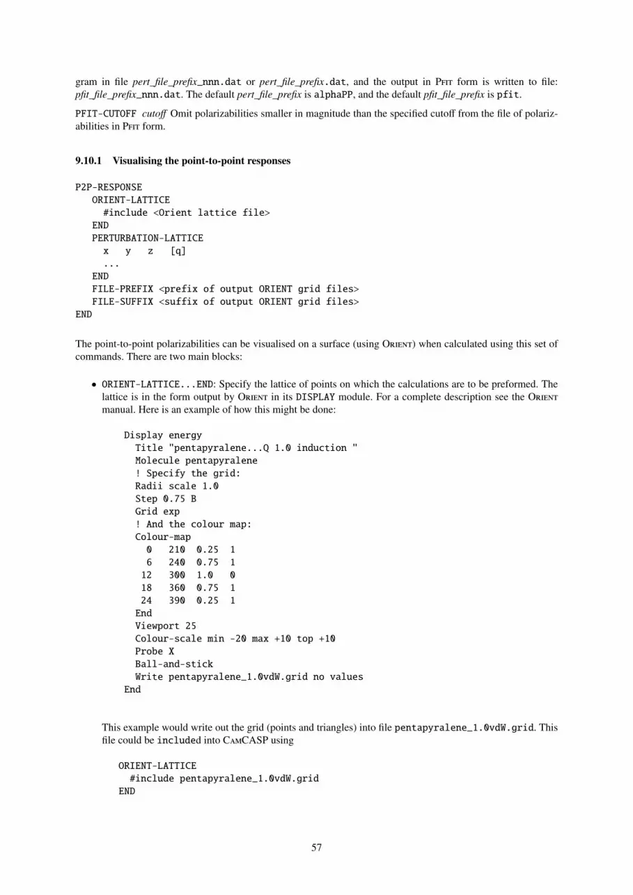
gram in file pert_file_prefix_nnn.dat or pert_file_prefix.dat, and the output in Pfit form is written to file:pfit_file_prefix_nnn.dat. The default pert_file_prefix is alphaPP, and the default pfit_file_prefix is pfit.
PFIT-CUTOFF cutoff Omit polarizabilities smaller in magnitude than the specified cutoff from the file of polariz-abilities in Pfit form.
9.10.1 Visualising the point-to-point responses
P2P-RESPONSEORIENT-LATTICE#include <Orient lattice file>
ENDPERTURBATION-LATTICEx y z [q]...
ENDFILE-PREFIX <prefix of output ORIENT grid files>FILE-SUFFIX <suffix of output ORIENT grid files>
END
The point-to-point polarizabilities can be visualised on a surface (using Orient) when calculated using this set ofcommands. There are two main blocks:
• ORIENT-LATTICE...END: Specify the lattice of points on which the calculations are to be preformed. Thelattice is in the form output by Orient in its DISPLAY module. For a complete description see the Orientmanual. Here is an example of how this might be done:
Display energyTitle "pentapyralene...Q 1.0 induction "Molecule pentapyralene! Specify the grid:Radii scale 1.0Step 0.75 BGrid exp! And the colour map:Colour-map
0 210 0.25 16 240 0.75 1
12 300 1.0 018 360 0.75 124 390 0.25 1EndViewport 25Colour-scale min -20 max +10 top +10Probe XBall-and-stickWrite pentapyralene_1.0vdW.grid no values
End
This example would write out the grid (points and triangles) into file pentapyralene_1.0vdW.grid. Thisfile could be included into CamCASP using
ORIENT-LATTICE#include pentapyralene_1.0vdW.grid
END
57

• PERTURBATION-LATTICE...END specifies the set of points at which the perturbation charges are placed. Atleast one point should be defined. The point-to-point perturbations are then calculated by placing the pointcharge perturbation at each of these points in turn, with every one of the ORIENT-LATTICE points. Each setis saved to an individual file than will contain the lattice in Orient format but will additionally include thevalue of the response. The responses can be read and displayed by Orient using a set of commands similarto those given above:
Display energyTitle "pentapyralene...Q 1.0 induction "Molecule pentapyraleneImport pentapyralene-dz-1.5vdW-1.resp with valuesColour-map0 210 0.25 16 240 0.75 112 300 1.0 018 360 0.75 124 390 0.25 1EndViewport 25Colour-scale min -0.07 max +0.07 top +0.05Probe XBall-and-stick
End
Where the file pentapyralene-dz-1.5vdW-1.resp contains the responses for perturbation point 1.
The responses from the point charge perturbation are saved in separate files. These take the formPREFIX-<number>.SUFFIX. By default, the prefix is P2Presp and suffix resp. These can be altered using thecommands FILE-PREFIX and FILE-SUFFIX.
9.11 Lattice
For point-to-point polarizabilities and energy scans it is necessary to specify the grid of points to be used. Thissection sets parameters for the grid but it is not constructed until needed.
SET LATTICECHARGE LatticeChargeUNITS [BOHR | ANGSTROM]POINTS...
END | ---RANDOM nlatSEED seedSTEP stepLOWLIM lowlimHIGHLIM highlimGRID <generate a grid using highlim and lowlim (see below)>NEWGRID icosahedron grid.SPHERE lebedev grid of radius lebrad and type nscheme.ORIGIN origin(1),origin(2),origin(3)RADIUS lebradNSCHEME nschemeDEBUG
END
The options are:
58
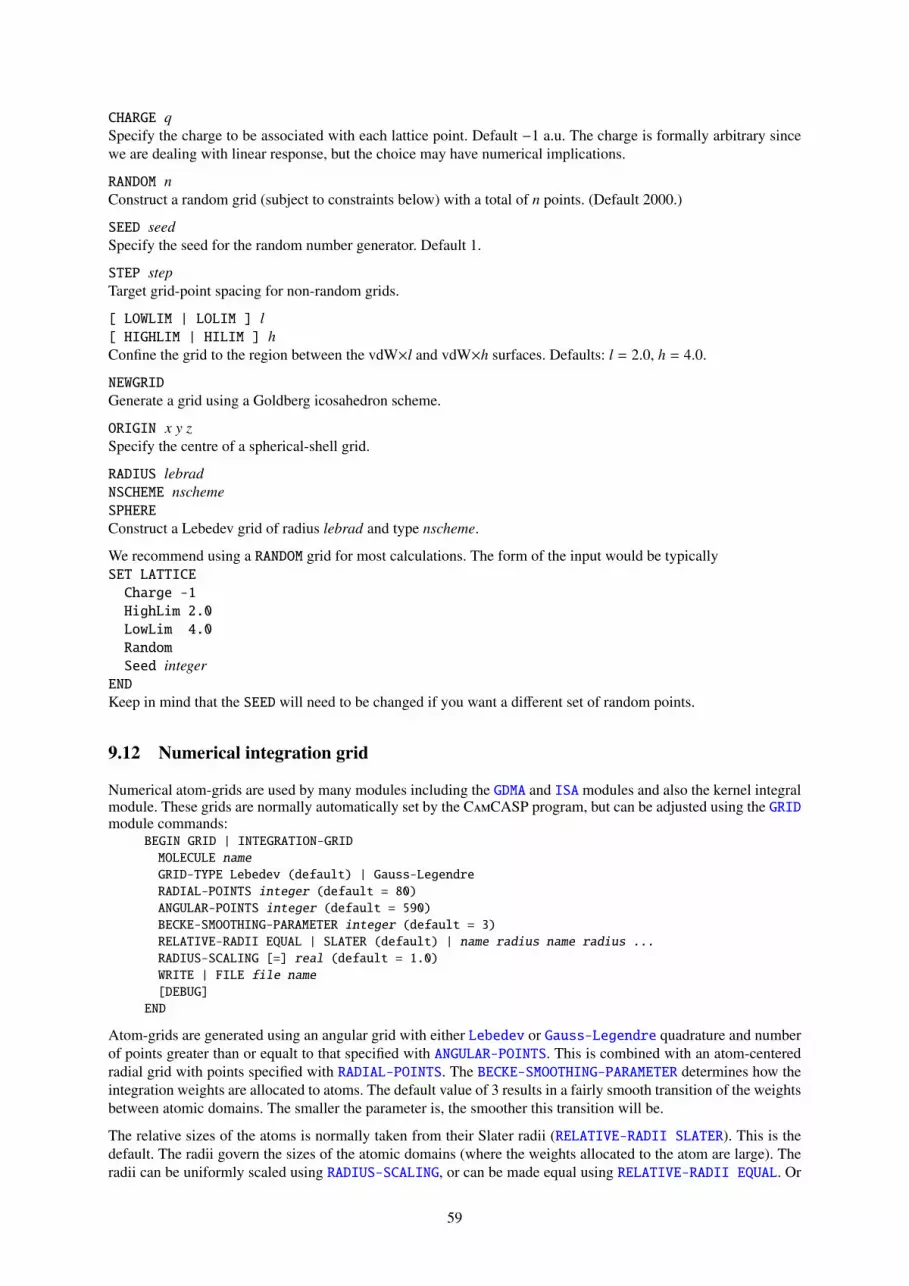
CHARGE qSpecify the charge to be associated with each lattice point. Default −1 a.u. The charge is formally arbitrary sincewe are dealing with linear response, but the choice may have numerical implications.
RANDOM nConstruct a random grid (subject to constraints below) with a total of n points. (Default 2000.)
SEED seedSpecify the seed for the random number generator. Default 1.
STEP stepTarget grid-point spacing for non-random grids.
[ LOWLIM | LOLIM ] l[ HIGHLIM | HILIM ] hConfine the grid to the region between the vdW×l and vdW×h surfaces. Defaults: l = 2.0, h = 4.0.
NEWGRIDGenerate a grid using a Goldberg icosahedron scheme.
ORIGIN x y zSpecify the centre of a spherical-shell grid.
RADIUS lebradNSCHEME nschemeSPHEREConstruct a Lebedev grid of radius lebrad and type nscheme.
We recommend using a RANDOM grid for most calculations. The form of the input would be typicallySET LATTICECharge -1HighLim 2.0LowLim 4.0RandomSeed integer
ENDKeep in mind that the SEED will need to be changed if you want a different set of random points.
9.12 Numerical integration grid
Numerical atom-grids are used by many modules including the GDMA and ISA modules and also the kernel integralmodule. These grids are normally automatically set by the CamCASP program, but can be adjusted using the GRIDmodule commands:
BEGIN GRID | INTEGRATION-GRIDMOLECULE nameGRID-TYPE Lebedev (default) | Gauss-LegendreRADIAL-POINTS integer (default = 80)ANGULAR-POINTS integer (default = 590)BECKE-SMOOTHING-PARAMETER integer (default = 3)RELATIVE-RADII EQUAL | SLATER (default) | name radius name radius ...RADIUS-SCALING [=] real (default = 1.0)WRITE | FILE file name[DEBUG]
END
Atom-grids are generated using an angular grid with either Lebedev or Gauss-Legendre quadrature and numberof points greater than or equalt to that specified with ANGULAR-POINTS. This is combined with an atom-centeredradial grid with points specified with RADIAL-POINTS. The BECKE-SMOOTHING-PARAMETER determines how theintegration weights are allocated to atoms. The default value of 3 results in a fairly smooth transition of the weightsbetween atomic domains. The smaller the parameter is, the smoother this transition will be.
The relative sizes of the atoms is normally taken from their Slater radii (RELATIVE-RADII SLATER). This is thedefault. The radii govern the sizes of the atomic domains (where the weights allocated to the atom are large). Theradii can be uniformly scaled using RADIUS-SCALING, or can be made equal using RELATIVE-RADII EQUAL. Or
59
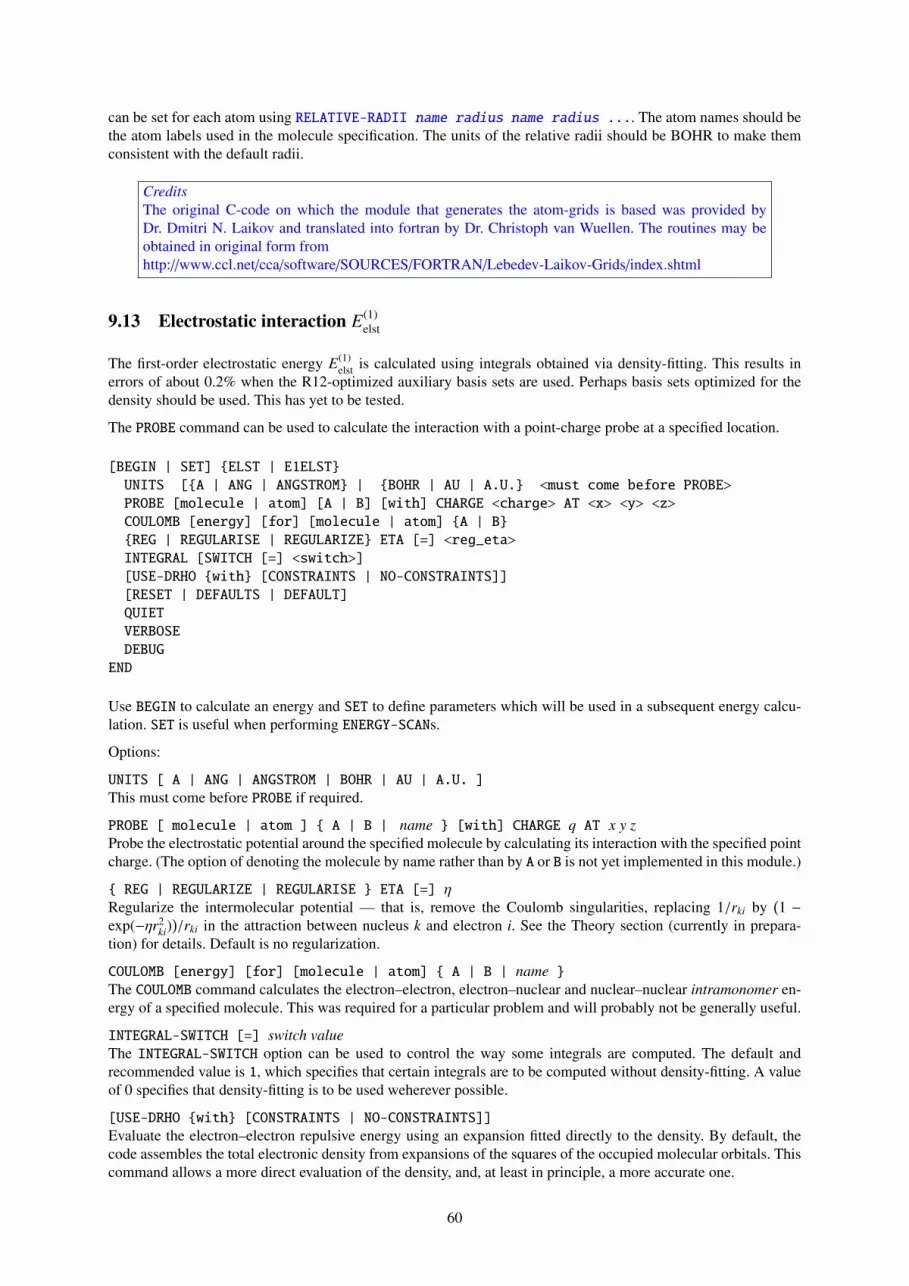
can be set for each atom using RELATIVE-RADII name radius name radius .... The atom names should bethe atom labels used in the molecule specification. The units of the relative radii should be BOHR to make themconsistent with the default radii.
CreditsThe original C-code on which the module that generates the atom-grids is based was provided byDr. Dmitri N. Laikov and translated into fortran by Dr. Christoph van Wuellen. The routines may beobtained in original form fromhttp://www.ccl.net/cca/software/SOURCES/FORTRAN/Lebedev-Laikov-Grids/index.shtml
9.13 Electrostatic interaction E(1)elst
The first-order electrostatic energy E(1)elst is calculated using integrals obtained via density-fitting. This results in
errors of about 0.2% when the R12-optimized auxiliary basis sets are used. Perhaps basis sets optimized for thedensity should be used. This has yet to be tested.
The PROBE command can be used to calculate the interaction with a point-charge probe at a specified location.
[BEGIN | SET] ELST | E1ELSTUNITS [A | ANG | ANGSTROM | BOHR | AU | A.U. <must come before PROBE>PROBE [molecule | atom] [A | B] [with] CHARGE <charge> AT <x> <y> <z>COULOMB [energy] [for] [molecule | atom] A | BREG | REGULARISE | REGULARIZE ETA [=] <reg_eta>INTEGRAL [SWITCH [=] <switch>][USE-DRHO with [CONSTRAINTS | NO-CONSTRAINTS]][RESET | DEFAULTS | DEFAULT]QUIETVERBOSEDEBUG
END
Use BEGIN to calculate an energy and SET to define parameters which will be used in a subsequent energy calcu-lation. SET is useful when performing ENERGY-SCANs.
Options:
UNITS [ A | ANG | ANGSTROM | BOHR | AU | A.U. ]This must come before PROBE if required.
PROBE [ molecule | atom ] A | B | name [with] CHARGE q AT x y zProbe the electrostatic potential around the specified molecule by calculating its interaction with the specified pointcharge. (The option of denoting the molecule by name rather than by A or B is not yet implemented in this module.)
REG | REGULARIZE | REGULARISE ETA [=] ηRegularize the intermolecular potential — that is, remove the Coulomb singularities, replacing 1/rki by
(1 −
exp(−ηr2ki)
)/rki in the attraction between nucleus k and electron i. See the Theory section (currently in prepara-
tion) for details. Default is no regularization.
COULOMB [energy] [for] [molecule | atom] A | B | name The COULOMB command calculates the electron–electron, electron–nuclear and nuclear–nuclear intramonomer en-ergy of a specified molecule. This was required for a particular problem and will probably not be generally useful.
INTEGRAL-SWITCH [=] switch valueThe INTEGRAL-SWITCH option can be used to control the way some integrals are computed. The default andrecommended value is 1, which specifies that certain integrals are to be computed without density-fitting. A valueof 0 specifies that density-fitting is to be used weherever possible.
[USE-DRHO with [CONSTRAINTS | NO-CONSTRAINTS]]Evaluate the electron–electron repulsive energy using an expansion fitted directly to the density. By default, thecode assembles the total electronic density from expansions of the squares of the occupied molecular orbitals. Thiscommand allows a more direct evaluation of the density, and, at least in principle, a more accurate one.
60

RESETParameter changes are normally saved. To reset to the default parameters, use this command.
9.14 First-order exchange (exchange-repulsion) E(1)exch
Calculate the first-order exchange energy between molecules A and B using the single-exhange (S 2) approximation.Integrals are obtained using density-fitting.
[BEGIN | SET] E1EXCHREG/REGULARISE/REGULARIZE [with] ETA [=] <reg_eta>OVERLAP [integrals] [ALGORITHM [DF [WITH | WITHOUT] [CONSTRAINTS]] [ISA | STOCKHOLDER]]INTEGRAL [SWITCH [=] <switch>]NO-E1EXCHQUIETVERBOSE[RESET | DEFAULTS | DEFAULT]DEBUG
END
Use BEGIN to calculate an energy and SET to define parameters which will be used in a subsequent energy calcu-lation. SET is useful when performing ENERGY-SCANs.
Options:
REGULARISE | REGULARIZE | REG [with] ETA [=] ηUse the regularized Coulomb potential. That is, remove the Coulomb singularities, replacing 1/rki by
(1−exp(−ηr2
ki))/rki
in the attraction between nucleus k and electron i. See the Theory section (currently in preparation) for details. De-fault is no regularization.
OVERLAP [integrals] [ALGORITHM [DF [WITH | WITHOUT] [CONSTRAINTS]] [ISA | STOCKHOLDER]]Calculate the overlap integrals. This can use the DF solution with or without constraints. Default is without con-straints. By default the overlap integrals are not calculated at all. The ISA algorithm is experimental and notaccessible in this version of the program.
INTEGRAL-SWITCH [=] switch valueThe INTEGRAL-SWITCH option can be used to control the way some integrals are computed. The default andrecommended value is 1, which specifies that certain integrals are to be computed without density-fitting. A valueof 0 specifies that density-fitting is to be used weherever possible.
NO-E1EXCHSkip the calculation of E(1)
exch. This only makes sense if OVERLAP is used to calculate the overlap integrals.
RESETParameter changes are normally saved. To reset to the default parameters, use this command.
9.15 Second-order induction energy E(2)ind,tot
The second-order induction energy E(2)ind,tot is calculated using the propagator defined in sec. 9.5. At present, only
the density-fitted expression can be calculated using this module (though the non-DF induction can be calculatedusing an older module). By default, the induction energy of molecules A and B is calculated. However, usingPROBE, the induction energy of a molecule with a point charge at a specified position can also be calculated.
If the second-order dispersion energy has been calculated before a call to this module, computational effort can bereduced by using the FORCE command to stop the initialisation of the J-integrals (JINT).
This module can use the R-SRS theory described by Patkowski et al. [2012] to evaluate the induction and exchange-induction energies. Here, the amplitudes are computed in the field from the regularized nuclear potentials of thepartners, but the energies evaluated using the full potential. Regularization is a convenient and robust way to definea basis-independent charge-transfer energy. Full details of how the regularized induction energy is defined aregiven by Misquitta [2013].
61
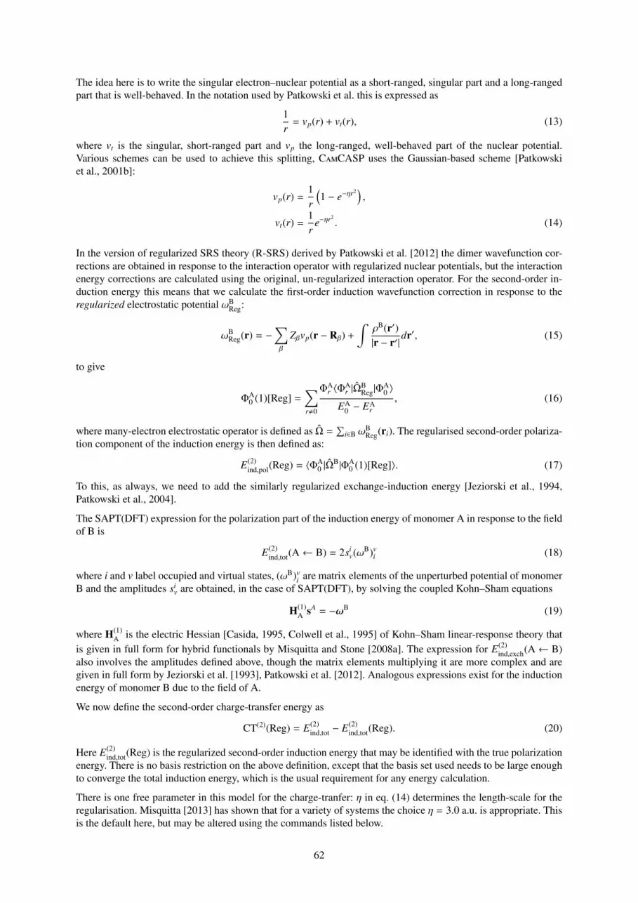
The idea here is to write the singular electron–nuclear potential as a short-ranged, singular part and a long-rangedpart that is well-behaved. In the notation used by Patkowski et al. this is expressed as
1r
= vp(r) + vt(r), (13)
where vt is the singular, short-ranged part and vp the long-ranged, well-behaved part of the nuclear potential.Various schemes can be used to achieve this splitting, CamCASP uses the Gaussian-based scheme [Patkowskiet al., 2001b]:
vp(r) =1r
(1 − e−ηr2)
,
vt(r) =1r
e−ηr2. (14)
In the version of regularized SRS theory (R-SRS) derived by Patkowski et al. [2012] the dimer wavefunction cor-rections are obtained in response to the interaction operator with regularized nuclear potentials, but the interactionenergy corrections are calculated using the original, un-regularized interaction operator. For the second-order in-duction energy this means that we calculate the first-order induction wavefunction correction in response to theregularized electrostatic potential ωB
Reg:
ωBReg(r) = −
∑β
Zβvp(r − Rβ) +
∫ρB(r′)|r − r′|
dr′, (15)
to give
ΦA0 (1)[Reg] =
∑r,0
ΦAr 〈Φ
Ar |Ω
BReg|Φ
A0 〉
EA0 − EA
r, (16)
where many-electron electrostatic operator is defined as Ω =∑
i∈B ωBReg(ri). The regularised second-order polariza-
tion component of the induction energy is then defined as:
E(2)ind,pol(Reg) = 〈ΦA
0 |ΩB|ΦA
0 (1)[Reg]〉. (17)
To this, as always, we need to add the similarly regularized exchange-induction energy [Jeziorski et al., 1994,Patkowski et al., 2004].
The SAPT(DFT) expression for the polarization part of the induction energy of monomer A in response to the fieldof B is
E(2)ind,tot(A← B) = 2si
v(ωB)vi (18)
where i and v label occupied and virtual states, (ωB)vi are matrix elements of the unperturbed potential of monomer
B and the amplitudes siv are obtained, in the case of SAPT(DFT), by solving the coupled Kohn–Sham equations
H(1)A sA = −ωB (19)
where H(1)A is the electric Hessian [Casida, 1995, Colwell et al., 1995] of Kohn–Sham linear-response theory that
is given in full form for hybrid functionals by Misquitta and Stone [2008a]. The expression for E(2)ind,exch(A← B)
also involves the amplitudes defined above, though the matrix elements multiplying it are more complex and aregiven in full form by Jeziorski et al. [1993], Patkowski et al. [2012]. Analogous expressions exist for the inductionenergy of monomer B due to the field of A.
We now define the second-order charge-transfer energy as
CT(2)(Reg) = E(2)ind,tot − E(2)
ind,tot(Reg). (20)
Here E(2)ind,tot(Reg) is the regularized second-order induction energy that may be identified with the true polarization
energy. There is no basis restriction on the above definition, except that the basis set used needs to be large enoughto converge the total induction energy, which is the usual requirement for any energy calculation.
There is one free parameter in this model for the charge-tranfer: η in eq. (14) determines the length-scale for theregularisation. Misquitta [2013] has shown that for a variety of systems the choice η = 3.0 a.u. is appropriate. Thisis the default here, but may be altered using the commands listed below.
62
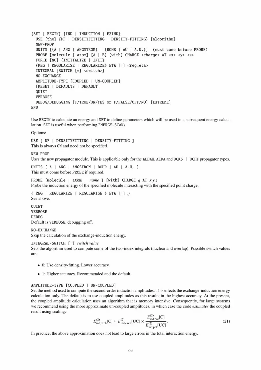
SET | BEGIN IND | INDUCTION | E2INDUSE [the] DF | DENSITYFITTING | DENSITY-FITTING [algorithm]NEW-PROPUNITS [A | ANG | ANGSTROM | BOHR | AU | A.U.] (must come before PROBE)PROBE [molecule | atom] [A | B] [with] CHARGE <charge> AT <x> <y> <z>FORCE [NO] INITIALIZE | INITREG | REGULARISE | REGULARIZE ETA [=] <reg_eta>INTEGRAL [SWITCH [=] <switch>]NO-EXCHANGEAMPLITUDE-TYPE [COUPLED | UN-COUPLED][RESET | DEFAULTS | DEFAULT]QUIETVERBOSEDEBUG/DEBUGGING [T/TRUE/ON/YES or F/FALSE/OFF/NO] [EXTREME]
END
Use BEGIN to calculate an energy and SET to define parameters which will be used in a subsequent energy calcu-lation. SET is useful when performing ENERGY-SCANs.
Options:
USE [ DF | DENSITYFITTING | DENSITY-FITTING ]This is always ON and need not be specified.
NEW-PROPUses the new propagator module. This is applicable only for the ALDAX, ALDA and UCKS | UCHF propagator types.
UNITS [ A | ANG | ANGSTROM | BOHR | AU | A.U. ]This must come before PROBE if required.
PROBE [molecule | atom | name [with] CHARGE q AT x y zProbe the induction energy of the specified molecule interacting with the specified point charge.
REG | REGULARIZE | REGULARISE ETA [=] ηSee above.
QUIETVERBOSEDEBUGDefault is VERBOSE, debugging off.
NO-EXCHANGESkip the calculation of the exchange-induction energy.
INTEGRAL-SWITCH [=] switch valueSets the algorithm used to compute some of the two-index integrals (nuclear and overlap). Possible switch valuesare:
• 0: Use density-fitting. Lower accuracy.
• 1: Higher accuracy. Recommended and the default.
AMPLITUDE-TYPE [COUPLED | UN-COUPLED]Set the method used to compute the second-order induction amplitudes. This effects the exchange-induction energycalculation only. The default is to use coupled amplitudes as this results in the highest accuracy. At the present,the coupled amplitude calculation uses an algorithm that is memory intensive. Consequently, for large systemswe recommend using the more approximate un-coupled amplitudes, in which case the code estimates the coupledresult using scaling:
E(2)ind,exch[C] ≈ E(2)
ind,exch[UC] ×E(2)
ind,pol[C]
E(2)ind,pol[UC]
. (21)
In practice, the above approximation does not lead to large errors in the total interaction energy.
63
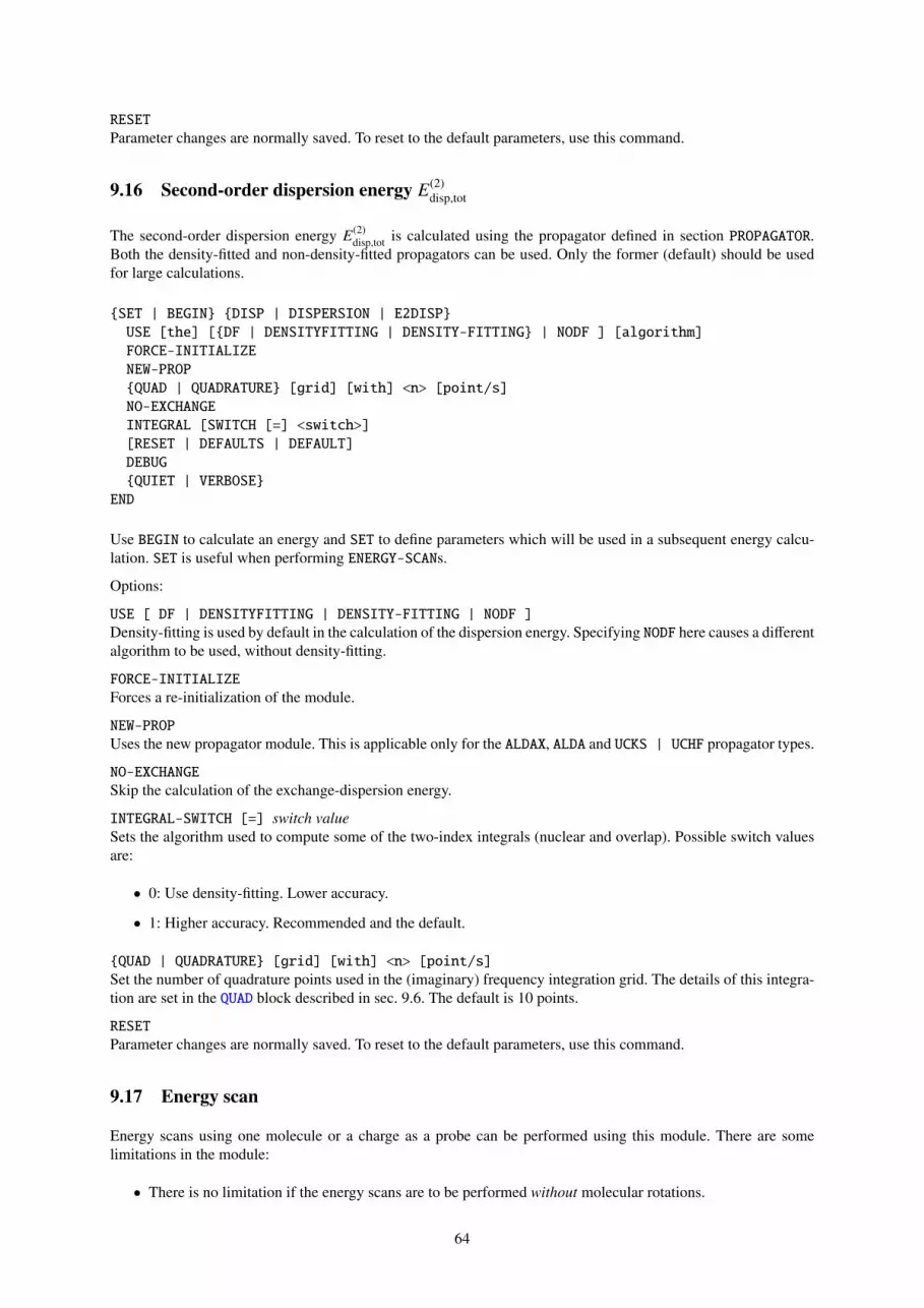
RESETParameter changes are normally saved. To reset to the default parameters, use this command.
9.16 Second-order dispersion energy E(2)disp,tot
The second-order dispersion energy E(2)disp,tot is calculated using the propagator defined in section PROPAGATOR.
Both the density-fitted and non-density-fitted propagators can be used. Only the former (default) should be usedfor large calculations.
SET | BEGIN DISP | DISPERSION | E2DISPUSE [the] [DF | DENSITYFITTING | DENSITY-FITTING | NODF ] [algorithm]FORCE-INITIALIZENEW-PROPQUAD | QUADRATURE [grid] [with] <n> [point/s]NO-EXCHANGEINTEGRAL [SWITCH [=] <switch>][RESET | DEFAULTS | DEFAULT]DEBUGQUIET | VERBOSE
END
Use BEGIN to calculate an energy and SET to define parameters which will be used in a subsequent energy calcu-lation. SET is useful when performing ENERGY-SCANs.
Options:
USE [ DF | DENSITYFITTING | DENSITY-FITTING | NODF ]Density-fitting is used by default in the calculation of the dispersion energy. Specifying NODF here causes a differentalgorithm to be used, without density-fitting.
FORCE-INITIALIZEForces a re-initialization of the module.
NEW-PROPUses the new propagator module. This is applicable only for the ALDAX, ALDA and UCKS | UCHF propagator types.
NO-EXCHANGESkip the calculation of the exchange-dispersion energy.
INTEGRAL-SWITCH [=] switch valueSets the algorithm used to compute some of the two-index integrals (nuclear and overlap). Possible switch valuesare:
• 0: Use density-fitting. Lower accuracy.
• 1: Higher accuracy. Recommended and the default.
QUAD | QUADRATURE [grid] [with] <n> [point/s]Set the number of quadrature points used in the (imaginary) frequency integration grid. The details of this integra-tion are set in the QUAD block described in sec. 9.6. The default is 10 points.
RESETParameter changes are normally saved. To reset to the default parameters, use this command.
9.17 Energy scan
Energy scans using one molecule or a charge as a probe can be performed using this module. There are somelimitations in the module:
• There is no limitation if the energy scans are to be performed without molecular rotations.
64

• If molecules are to be rotated, bear in mind the following:
For molecule...atom scans, if the molecule is kept fixed and only the atom moved around, there is noproblem at all.
For molecule...molecule scans, only the overlap integrals and first-order energies can be correctlyscanned at present. This is because the Hessians needed for the second-order energies are not yetrotated correctly. Also, such a scan limits you to use auxiliary basis sets with spherical GTOs. Bear inmind that this leads to lower accuracies in the density-fitting. We are working to resolve this problem.
The list of points at which the scan is to be performed will usually be read in from file (if USE POINTS is used) ordefined in the LATTICE module (if USE LATTICE is used).
The data generated by the energy scan module can be used by the Orientprogram to produce a graphical display of the energy over a molecularsurface. In this case the grid of points would be generated by Orient,exported to a file, and read into CamCASP using the POINTS option. TheFigure shows the map of dispersion energy between formamide and aneon atom, calculated in this way.
BEGIN SCAN/ENERGY_SCANPROBE | SCAN [molecule | atom] <molname> +++
WITH [<molname> [[and] CHARGE <charge>]]UNITS [A | ANG | ANGSTROM | BOHR | AU | A.U.] +++
[DEG | DEGREE | DEGREES | RAD | RADIAN | RADIANS]NOTE: UNITS must come before POINTS/RANDOM
CENTRE/CENTER PROBE [on] [COM]/[XYZ <x> <y> <z>]DC-AUX | DCAUXREGULARIZE [E1] [[and] E2] [with] ETA [=] <reg_eta>ENERGIES | ENERGY [DISP/DISPERSION/E2DISP] +++[&/and/,] [IND/INDUCTION/E2IND] [&/and/,] [ELST/E1ELST/ELECTROSTATICS] +++[&/and/,] [E1EXCH] [&/and/,] [E2EXIND] & [E2EXDISP] & [OVERLAP] [NOTHING]LATTICEPOINTS[TRANSLATIONS | TRANSLATIONS-ONLY][SKIP-FIRST-COLUMN]x1 y1 z1 [angle1 nx1 ny1 nz1]x2 y2 z2 [angle2 nx2 ny2 nz2]etc
--- <----end POINTS block with three hyphens.RANDOMPOINTS [=] <number of points>DRMIN [=] <dRmin>DRMAX [=] <dRmax>RADIAL [points] [=] <number of radial points per angular configuration>SKIP [=] <number to skip> [angular] [configurations]WRITE <filename> [APPEND]
---ENERGY-FILE [PREFIX] <file prefix> [[in | using] STYLE <style index>]OVERLAP-FILE [PREFIX] <file prefix> [[in | using] STYLE <style index>]DEBUGGING T/TRUE/ON or F/FALSE/OFFQUIET | VERBOSE
END
The options are:
PROBE | SCAN [ molecule | atom ] name +++[with] [ [ molecule | atom ] name ] [ [and] CHARGE q ]
Here the probe can be either a point charge or another molecule or both. Default is to use molecule B as the probe;that is, molecule A remains fixed while molecule B is moved so that its origin is successively at the positions
65
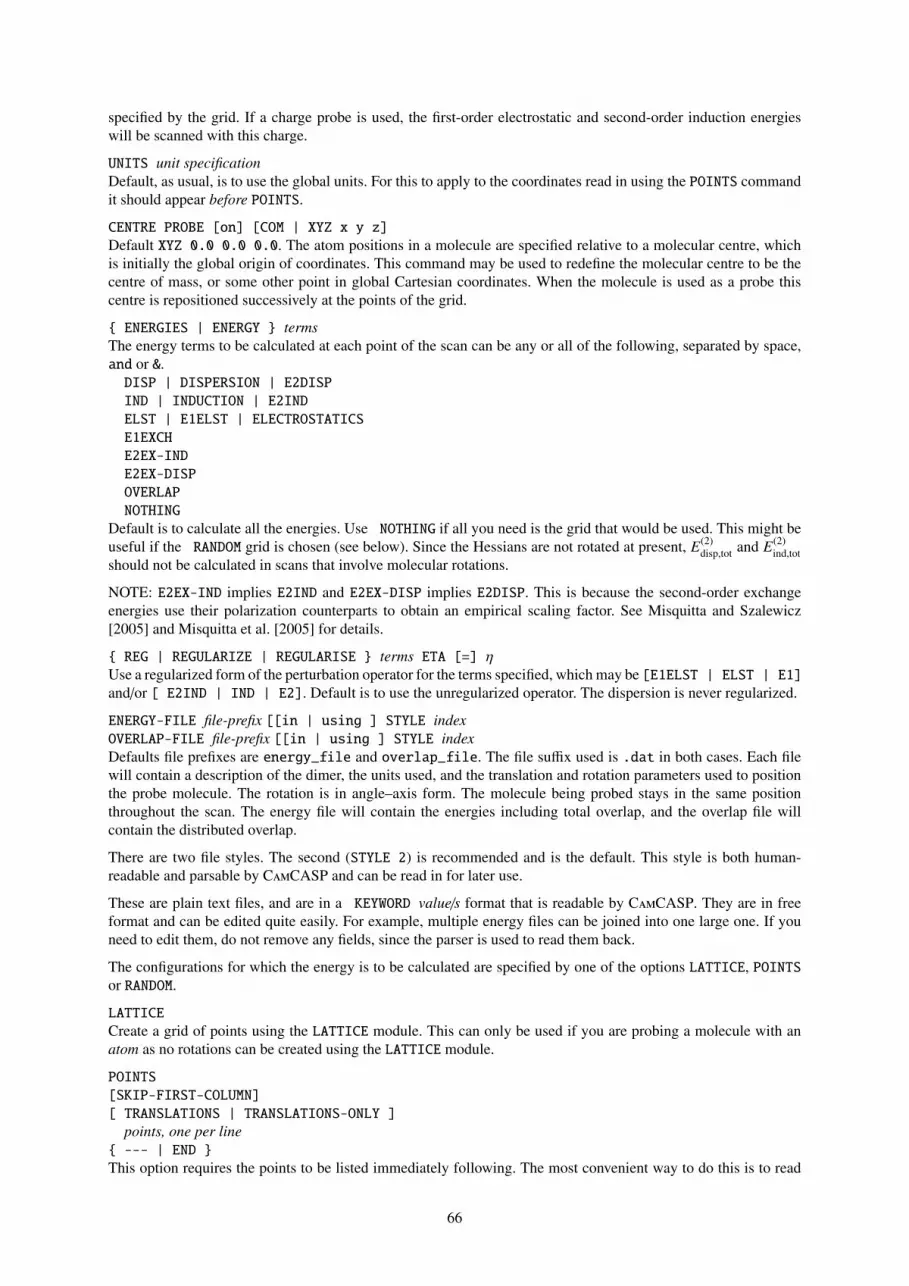
specified by the grid. If a charge probe is used, the first-order electrostatic and second-order induction energieswill be scanned with this charge.
UNITS unit specificationDefault, as usual, is to use the global units. For this to apply to the coordinates read in using the POINTS commandit should appear before POINTS.
CENTRE PROBE [on] [COM | XYZ x y z]Default XYZ 0.0 0.0 0.0. The atom positions in a molecule are specified relative to a molecular centre, whichis initially the global origin of coordinates. This command may be used to redefine the molecular centre to be thecentre of mass, or some other point in global Cartesian coordinates. When the molecule is used as a probe thiscentre is repositioned successively at the points of the grid.
ENERGIES | ENERGY termsThe energy terms to be calculated at each point of the scan can be any or all of the following, separated by space,and or &.
DISP | DISPERSION | E2DISPIND | INDUCTION | E2INDELST | E1ELST | ELECTROSTATICSE1EXCHE2EX-INDE2EX-DISPOVERLAPNOTHING
Default is to calculate all the energies. Use NOTHING if all you need is the grid that would be used. This might beuseful if the RANDOM grid is chosen (see below). Since the Hessians are not rotated at present, E(2)
disp,tot and E(2)ind,tot
should not be calculated in scans that involve molecular rotations.
NOTE: E2EX-IND implies E2IND and E2EX-DISP implies E2DISP. This is because the second-order exchangeenergies use their polarization counterparts to obtain an empirical scaling factor. See Misquitta and Szalewicz[2005] and Misquitta et al. [2005] for details.
REG | REGULARIZE | REGULARISE terms ETA [=] ηUse a regularized form of the perturbation operator for the terms specified, which may be [E1ELST | ELST | E1]and/or [ E2IND | IND | E2]. Default is to use the unregularized operator. The dispersion is never regularized.
ENERGY-FILE file-prefix [[in | using ] STYLE indexOVERLAP-FILE file-prefix [[in | using ] STYLE indexDefaults file prefixes are energy_file and overlap_file. The file suffix used is .dat in both cases. Each filewill contain a description of the dimer, the units used, and the translation and rotation parameters used to positionthe probe molecule. The rotation is in angle–axis form. The molecule being probed stays in the same positionthroughout the scan. The energy file will contain the energies including total overlap, and the overlap file willcontain the distributed overlap.
There are two file styles. The second (STYLE 2) is recommended and is the default. This style is both human-readable and parsable by CamCASP and can be read in for later use.
These are plain text files, and are in a KEYWORD value/s format that is readable by CamCASP. They are in freeformat and can be edited quite easily. For example, multiple energy files can be joined into one large one. If youneed to edit them, do not remove any fields, since the parser is used to read them back.
The configurations for which the energy is to be calculated are specified by one of the options LATTICE, POINTSor RANDOM.
LATTICECreate a grid of points using the LATTICE module. This can only be used if you are probing a molecule with anatom as no rotations can be created using the LATTICE module.
POINTS[SKIP-FIRST-COLUMN][ TRANSLATIONS | TRANSLATIONS-ONLY ]
points, one per line --- | END This option requires the points to be listed immediately following. The most convenient way to do this is to read
66
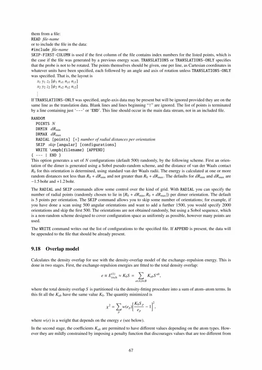
them from a file:READ file-nameor to include the file in the data:#include file-nameSKIP-FIRST-COLUMN is used if the first column of the file contains index numbers for the listed points, which isthe case if the file was generated by a previous energy scan. TRANSLATIONS or TRANSLATIONS-ONLY specifiesthat the probe is not to be rotated. The points themselves should be given, one per line, as Cartesian coordinates inwhatever units have been specified, each followed by an angle and axis of rotation unless TRANSLATIONS-ONLYwas specified. That is, the layout is
x1 y1 z1 [ψ1 nx1 ny1 nz1]x2 y2 z2 [ψ2 nx2 ny2 nz2]...
If TRANSLATIONS-ONLY was specified, angle-axis data may be present but will be ignored provided they are on thesame line as the translation data. Blank lines and lines beginning “!” are ignored. The list of points is terminatedby a line containing just ‘---’ or ‘END’. This line should occur in the main data stream, not in an included file.
RANDOMPOINTS NDRMIN dRminDRMAX dRmaxRADIAL [points] [=] number of radial distances per orientationSKIP skip [angular] [configurations]WRITE \emphfilename [APPEND]
--- | END This option generates a set of N configurations (default 500) randomly, by the following scheme. First an orien-tation of the dimer is generated using a Sobol pseudo-random scheme, and the distance of van der Waals contactR0 for this orientation is determined, using standard van der Waals radii. The energy is calculated at one or morerandom distances not less than R0 + dRmin and not greater than R0 + dRmax. The defaults for dRmin and dRmax are−1.5 bohr and +1.2 bohr.
The RADIAL and SKIP commands allow some control over the kind of grid. With RADIAL you can specify thenumber of radial points (randomly chosen to lie in [R0 + dRmin,R0 + dRmax]) per dimer orientation. The defaultis 5 points per orientation. The SKIP command allows you to skip some number of orientations; for example, ifyou have done a scan using 500 angular orientations and want to add a further 1500, you would specify 2000orientations and skip the first 500. The orientations are not obtained randomly, but using a Sobol sequence, whichis a non-random scheme designed to cover configuration space as uniformly as possible, however many points areused.
The WRITE command writes out the list of configurations to the specified file. If APPEND is present, the data willbe appended to the file that should be already present.
9.18 Overlap model
Calculates the density overlap for use with the density-overlap model of the exchange–repulsion energy. This isdone in two stages. First, the exchange-repulsion energies are fitted to the total density overlap:
e ≡ E(1)exch ≈ K0S =
∑a∈A,b∈B
KabS ab,
where the total density overlap S is partitioned via the density-fitting procedure into a sum of atom–atom terms. Inthis fit all the Kab have the same value K0. The quantity minimized is
χ2 =∑
p
w(ep)[K0S p
ep− 1
]2,
where w(e) is a weight that depends on the energy e (see below).
In the second stage, the coefficients Kab are permitted to have different values depending on the atom types. How-ever they are mildly constrained by imposing a penalty function that discourages values that are too different from
67

K0. The quantity minimized is nowχ2∑
p w(ep)+
∑ab
λ(Kab − K0)2,
with
χ2 =∑
p
w(ep)[∑
a∈A,b∈B KabS abp
ep− 1
]2.
The configurations and S abp values, and the fitted Kab values, are written to files suitable for input to Orient.
Molecules will often have symmetry. In CamCASP symmetry is handled using the TYPE specification (see Sec. 9.2)that sets the types of each site. The overlap matrix is symmetrized between site types within each molecule asfollows:
S abp =
∑i=a
∑j=b
S i jp (NoSymm) (22)
Here S i jp (NoSymm) is the matrix of overlap integrals for sites i in molecule A with type a and sites j in molecule
B with type j, and S abp is the symmetrized overlap matrix for types a and b.
Additionally, sites between molecules may have the same type. This would be the case for a symmetric dimerA...A, but it could also be that an approximate symmetry has been imposed to make, say, all hydrogen atoms havethe same type. If this is the case, an additional symmetrization of the overlap matrix may be performed using theSYMMETRIZE-BETWEEN-MOLECULES command described below.
The syntax for this module is
BEGIN OVERLAP-MODELUNITS [HARTREE | HARTREES] [KJMOL | KJ/MOL] [CM-1 | 1/CM]WEIGHT [NONE] [TYPE <number>] [and] [E0 | E_0 [=] <E_0>] +++
[and] [ALPHA [=] <alpha>]
ENERGY [=] [sign] <component> [ [sign] <component> ] ...wheresign = + or -andcomponent = E1ELST, E1ELST(AS), E1EXCH, E2IND, E2IND(AS), E2EXIND,
E2DISP, E2DISP(AS), E2EXDISP, DELTAor a composite energy such as
E1PEN = E1ELST - E1ELST(AS)E2PENIND = E2IND - E2IND(AS)E2PENDISP = E2DISP - E2DISP(AS)E2PEN = (E2IND - E2IND(AS)) + (E2DISP - E2DISP(AS))E2EXCH = E2EXIND + E2EXDISPE2INT = E1ELST + E1EXCH + E2IND + E2EXIND + E2DISP + E2EXDISP
ENERGY-OPTIONS [CHECK-ASYMP] [ABS-MAX-ENERGY [=] <value>]
EMAX | E-MAX [=] <maximum energy>EMIN | E-MIN [=] <minimum energy>ENERGY-FILE <full file name of energy file>OVERLAP-FILE <full file name of distributed overlap file>CONDITION [number] [=] <condition number for solver>CONSTRAINT [=] <lambda>[ SYMMETRIZE-BETWEEN-MOLECULES | SYMMETRIZE ]ORIENT [files] [YES | NO | TRUE | FALSE] [ISOTROPIC-SITES] [ANCHOR-LIST] +++
[SHAPE-SYMMETRY]ONLY-TOTAL-ORIENT [C6] [NO-WEIGHTS]DEBUGGING T/TRUE/ON or F/FALSE/OFFQUIETVERBOSE
68
[RESET | DEFAULTS | DEFAULT]END
The options are:
UNITS [HARTREE | HARTREES] [KJMOL | KJ/MOL] [CM-1 | 1/CM]Specify the units to be used for energies, if different from the global default.
WEIGHT [TYPE index ] [and] [E0 | E_0 [=] e0 ] [and] [ALPHA [=] α ]Specify the weighting scheme for the data points. The weight w(e) for a point with energy e is, according to theindex,
0: 1
1:(1 + (e/e0)
)−1
2:(1 + (e/e0)2)−1
3: (e0/e) + 1
4: exp[−α
(ln(e/e0)
)2]The last of these is the scheme used by Hodges and Wheatley [2000]. It is recommended and is the default. Thedefault parameters are e0 = 20.0 kJ mol−1 and α = 1/ ln 10.
EMIN EminEMAX EmaxEnergy values outside the range specified are ignored (given zero weight). Defaults: Emin = 0.01 kJ mol−1, Emax =
100 kJ mol−1.
ENERGY [=] E1EXCH [+ | -] E1PEN [+ | -] +++[+ | -] [E2EX-IND | E2EXIND] [+ | -] [E2EX-DISP | E2EXDISP] +++[+ | -] [E2PEN-IND | E2PENIND] [+ | -] [E2PEN-DISP | E2PENDISP] +++[+ | -] DELTA
The energy to be fitted to can be defined using this statement. By default, the energy used isE1EXCH + E2EXIND + E2EXDISP + E1PEN + E2PENIND + E2PENDISP + DELTA.These energies are:
• E1EXCH: The first-order exchange energy, E(1)exch.
• E2EX-IND: The second-order exchange-induction energy, E(2)ind,exch.
• E2EX-DISP: The second-order exchange-dispersion energy, E(2)disp,exch.
• E1PEN: The first-order penetration energy defined as E(1)elst − EAsymp
elst .
• E2PEN-IND: The induction contribution to the second-order penetration energy defined as E(2)ind,tot − EAsymp
ind .
• E2PEN-DISP: The dispersion contribution to the second-order penetration energy defined as E(2)disp,tot−EAsymp
disp .
• DELTA: A correction energy. This energy can be anything, and is left to the user. For example, it could bedefined to be the difference between SAPT(DFT) and CCSD(T) energies.
Alternatively, E2EXCH can be used as a synonym for E2EX-IND + E2EX-DISP and, likewise, E2PEN can be usedfor E2PEN-IND + E2PEN-DISP. These energies are all in the energy file (see below). We will usually use only +signs in the energy expression.
ENERGY-OPTIONS [CHECK-ASYMP] [ABS-MAX-ENERGY [=] value]The option CHECK-ASYMP will check the energies calculated with the multipole models (the asymptotic forms ofthe energy components) for missing values. If an energy is identically zero, that dimer is removed from the list.
The energy bounds set using EMIN and EMAX are useful for selecting configurations but these are not foolproof.There are instances where, because of energy cancellations with the multipole-expanded energies, repulsive con-figurations are included when they should not, to the detriment of the fit. This can be avoided using the option
69

ABS-MAX-ENERGY to set an upper limit to the absolute values of the individual interaction energy components. Bydefault this upper limit is set to be 100|Emax|.
SYMMETRIZE-BETWEEN-MOLECULESAs described above, the overlap matrix is symmetrized between site types within each molecule.If SYMMETRIZE-BETWEEN-MOLECULES is set, the site type information is used to symmetrize the overlap matrix,S ab
p , for site types between molecules A and B as follows:
S abp (symm) = S ab
p + S bap , if b ∈ A and a ∈ B (23)
where a and b are unique site types on molecules A and B, resp.
This command would be used for a dimer of the same molecule, or when you have assumed approximate symme-tries between molecules.
CONSTRAINT [=] λSpecifies the parameter to be used in the constrained fit. Default 10−8.
CONDITION [NUMBER] [=] cIf the least-squares problem leads to an ill-conditioned matrix, the problem is reduced to one with estimatedcondition number less than 1/c. The default value, c = 10−7, should be satisfactory.
ENERGY-FILE full file name of energy fileThe energy file will have been created from the ENERGY-SCAN module.
OVERLAP-FILE full file name of overlap fileThis is the file containing the distributed overlap. If the OVERLAP-MODEL block follows the ENERGY-SCAN block ina CamCASP run, then the file name need not be specified here as it will be passed internally.
The ENERGY-FILE and OVERLAP-FILE commands can appear as many times as needed. This is particularly usefulif data points from multiple runs are needed for an overlap model calculation. Make sure that the sequence of filesis the same for both of them. That is, if energies and overlaps have been computed in three runs, resulting in threesets of files, the sequence should be:
ENERGY-FILE energy_file_1.datENERGY-FILE energy_file_2.datENERGY-FILE energy_file_3.datOVERLAP-FILE overlap_file_1.datOVERLAP-FILE overlap_file_2.datOVERLAP-FILE overlap_file_3.dat
The recommended practice however is to generate the energy files using an MC basis but a DC auxiliary basis,while the overlap-mode calculation has to be done using an MC auxiliary basis and so requires a separate Cam-CASP job. This second job needs an energy-scan section just to read in the data points and to generate the overlapfile. The overlap-model section will then use this overlap file, which can be passed internally, and the energy filefrom the previous job.
ORIENT [files] [YES | NO ] [ISOTROPIC-SITES]By default, the results of the constrained overlap model will be used to construct input files for Orient. These inputfiles are needed to obtain the fit to the Born–Mayer term that describes the short-range interaction. It is done ina site–site form, so a file is generated for every pair of site types. Using this command the creation of these filescan be suppressed. Use ISOTROPIC-SITES to write out the Orient command files for a potential with all sitesisotropic.
The generated Orient files normally include separate data files for optimizing the individual site-site potentials, aswell as a data file for optimizing the total potential. The site–site fits should be carried out first, and the resultingparameters edited into the data file for the total potential fit. It will often be necessary to restrict the full optimizationby anchoring the parameters to their initial values by harmonic constraints, so that they don’t drift to physicallyunreasonable values. The anchor definition can be set up using the the anchors.pl script. Details of the procedurecan be found in the CamCASP Wiki at https://jasper.ph.qmul.ac.uk/wiki/ajm:camcasp:potentials.
ONLY-TOTAL-ORIENT [C6] [NO-WEIGHTS]Use the ONLY-TOTAL-ORIENT command to write out the Orient file for the entire potential. Use this when fine-tuning the potential fit by relaxing all or some parameters using anchors. By default we is assumed that the C6
70
coefficients will not be relaxed. Use the C6 option to generate an Orient file to relax these coefficients. Likewise,by default weights will be included in the Orient command file. The NO-WEIGHTS option will suppress this.
RESETParameter changes are normally saved. To reset to the default parameters, use this command.
9.19 Integrals
The integral routines are not meant to be accessed directly, but there may well be situations which demand it, soCamCASP allows direct control over the integrals. While almost all integrals are computed using density-fittingtechniques, some can be computed without this approximation.
BEGIN/SET DF-INT | DF-INTEGRALS | DF-INTS | INTEGRALS INT TYPE <type> DESC <description> +++
[and] [SWITCH [=] <switch>] [and] [PRINT] [and] [ROTATE]GEN-INT TYPE <type> DESC <description> +++
[and] [SWITCH [=] <switch>] [and] [PRINT] [and] [ROTATE][DF-CONSTRAINTS | CONSTRAINTS ] [ETA [=] <eta>] +++
[and] [LAMBDA [=] <lambda>] +++[and] [TYPE [=] [SITE | INTER-SITE] [repulsion | self-repulsion]]
DF-TYPE-DIMER [OO | OV | VO]DF-TYPE-MONOMER [OO | OV | VO | NN | FULL]QUIETVERBOSEDEBUG/DEBUGGING [T/TRUE/ON/YES or F/FALSE/OFF/NO]RESET
END
Options:
INT TYPE type DESC description +++[and] [SWITCH [=] switch] [and] [PRINT]
The INT command will cause a particular integral to be computed. Integrals are referenced by two four charactercodes: the integral type (TYPE) and the description (DESC).
The integral types describe which operators are used. At present, the following integral types are available (chem-ical notation is used for all integrals):
• 2-electron integral types: OVOV, VVOO, OOOOO refers to an occupied orbital and V to a virtual orbital.
• Nuclear integrals: NUCA, NUCBNUCA use the nuclei of molecule with label A and NUCB use nuclei from the molecule with label B.
• Integrals with a point-charge probe: PROBThese are a special case of the nuclear integrals where the ‘nucleus’ is a point charge.
• Overlap integrals: OVRL
• Miscellaneous integrals: See module df_integrals for details.
The integral description sets the kinds of basis functions or molecular orbitals that the operator operates on. Thereare too many of these to describe here, but the main ones are:
• 4-index descriptions: AAAA, BBBB, AABB, ABAB, ABBB, AAABThese are used for the 2-electron integrals only, though not all combintations are possible.
• 2-index descriptions: OOAA, OOBB, OOABThese are used for the nuclear, probe and overlap integral types.
71

• Integrals of the auxiliary bases: __XA, __XB, XAXB, _XABHere the X denotes an auxiliary basis function and A, B, AB denote molecule A, B and the dimer (AB).Once again, these are used mainly with the nuclear and probe integrals.
• Miscellaneous descriptions: See module df_integrals for details.
The SWITCH option allows us to control the method used to obtain particular integrals. Here SWITCH = 0 is thedefault, which uses density-fitting wherever possible. SWITCH = 1 results in some integrals being computed with-out density-fitting. This may seem a good idea at first sight, but since we frequently see a cancellation of errorsbetween integrals of different kinds, calculating some accurately could result in even larger errors in the end. Thisoption should therefore be used with caution.
However there is also an INTEGRAL-SWITCH option under each of the E1ELST, E1EXCH, E2IND and E2DISDPblocks, which allows the setting to be changed independently for each of these. Here the recommended value, andthe default, is 1, i.e. to use density-fitting wherever possible
At present, only the nuclear and overlap integrals can be computed without density-fitting.
The integrals are not printed unless the PRINT option is included in this line.
REG | REGULARIZE [with] ETA [=] regularization constantRegularize the intermolecular potential — that is, remove the Coulomb singularities, replacing 1/rki by
(1 −
exp(−ηr2ki)
)/rki in the attraction between nucleus k and electron i. See the Theory section (currently in prepara-
tion) for details. Default is no regularization.
GEN-INT TYPE type DESC description +++[and] [SWITCH [=] switch] [and] [PRINT]
The generalized 2-electron integrals can be computed using this command. These integrals are defined as (Chemi-cal notation):
v(i j|kl) = (i j|kl) +(i| j)(k|vA|l)
NA+
(i|vB| j)(k|l)NB
+(i| j)(k|l)NANB
Enn, (24)
where (i j|kl) is the standard 2-electron integral, (i| j) is the overlap integral, (k|vA|l) is the nuclear integral with thepotential vA of the nuclei of molecule A, Enn is the nuclear–nuclear Coulomb energy, and NA is the number ofelectrons of molecule A.
We assume canonical ortho-normal orbitals when calculating the generalized integrals.
DF-CONSTRAINTS | CONSTRAINTS [ETA [=] <eta>] +++[and] [LAMBDA [=] <lambda>] [and] [GAMMA [=] <gamma>] +++[and] [TYPE [=] [SITE | INTER-SITE] [repulsion | self-repulsion]]
By default, the integral routine uses the density-fitting solution without any constraints. If needed, the DF solutionwith constraints can be used. Use this with caution. See the Density-fitting section for details on the options.
QUIETVERBOSEDEBUG
The parameters used in evaluating the primitive integrals can be changed using:
SET INTEGRAL | INTEGRAL-PARAMETERSDUMMY-S <dummy S-exponent>CUTOFF <integral cutoff>KERNEL-CUTOFF <kernel integral cutoff>OVERLAP-CUTOFF <overlap integral cutoff>
END
Options:
CUTOFF integral cutoff
This sets the cutoff used in the pre-screening of the 2-electron integrals calculated for the density-fitting. Thedefault cutoff is 10−12.
72
DUMMY-S dummy S-exponentWe evaluate our 2-index and 3-index, 2-electron integrals using the GAMINT integral module which forms part ofthe Gamess(US) quantum chemistry code. This module computes 4-index integrals. So, in order to get the 2-indexand 3-index integrals, we use dummy functions in calls to gamint. The dummy functions are Gaussian orbitals ofs-symmetry and a very small exponent — ideally 0.0. The value of this exponent is set using this command. Thedefault value is 10−18. Values between 10−12 and 10−18 have been found to result in identical interaction energiesfor a variety of systems.
We do not recommend changing this value.
KERNEL-CUTOFF <kernel integral cutoff>This is the cutoff used to pre-screen the kernel integrals.
OVERLAP-CUTOFF <overlap integral cutoff>This cutoff is used in the overlap pre-screening of certain real-space two and three index integrals.
10 Process: Syntax
The Process program is used to read distributed polarizabilities from either CamCASP or Orient and processthem in some way. It can perform tasks such as calculating average polarizabilities and anisotropic polarizabilities,or writing local polarizabilities to file in LATEX table format, or writing an input file for the Pfit program witheither local or non-local polarizabilities. The program can also handle polarizabilities at multiple frequencies. TheINVERT command will apply the inversion operator on the distributed polarizabilities, to obtain the polarizabilitiesfor the enantiomorph of the current molecule. (This just involves some changes of sign, but it is easy to makemistakes when doing it by hand.)
The CASIMIR command will create the input file for the Casimir program. The SKIP option to CASIMIR tellsthe program to skip some of the initial frequencies. This is useful when the first frequency is 0.0 (i.e., staticpolarizabilities) as this one is not needed by Casimir.
The Pfit code can refine polarizabilities (as yet, only for one frequency at a time). An input file for such a refine-ment can be created using the PFIT...PENALTIES command. PENALTIES tells Process that the Pfit file shouldinclude the penalties section. This works for one molecule at a time so the second molecule (if defined) is ignored.Also, only local polarizabilities can be refined. If the polarizabilities have been computed with multiple frequen-cies, then a frequency can be chosen using the FREQ <index> sub-command. Thus, to create a Pfit input file forthe static polarizabilities, which are (typically) read in as the zeroth index in the polarizability file, use:
Molecule namemolecule specification
EndREAD LOCAL polarizabilities for molecule nameUSE BINARY file file-nameMAX rank maximum rank of polarizabilities on fileLIMIT rank to rank-limitFREQUENCIES STATIC + number of freqs
END
WRITE
PFIT file for name with CUTOFF cutoff +++
and FREQ 0 use PENALTIES with WEIGHT 4
End
The default is to use the static, i.e., 0th frequency, so the FREQ command could be omitted. The default number ofnon-zero frequencies is 10.
If the polarizability model needs to be simplified to include isotropic terms only, the following command can beused: WRITE
PFIT file for name with CUTOFF cutoff +++
and FREQ 0 use PENALTIES with WEIGHT 4 +++
and ISOTROPIC polarizabilities
End
The ISOTROPIC command does the following: from polarizabilities localized using the method of [Le Sueur and
73
Stone, 1994], isotropic polarizabilities are calculated for each site. The Pfit input file for the refinement step isthen constructed using these isotropic terms (limited to the specified rank). Pfit then refines the polarizabilities asin the standard WSM procedure. This option can be very useful in creating a polarizability and dispersion modelthat is suitable for use in most standard simulation programs.
If a rank-limit is given, polarizabilities of higher rank are ignored. The Pfit program adjusts the input polarizabil-ities to improve the agreement between the point-to-point polarizabilities given by the local polarizability modeland those calculated by CamCASP. The WEIGHT item specifies the weights attached to the input polarizabilities.A weight of zero means that the input polarizability value is ignored, so the fitted value is determined purely byleast-squares fit to the point-to-point polarizabilities. A non-zero value means that the least-squares function ismodified by a penalty that depends on the square of the difference between the fitted value and the input value, soit discourages excessive deviations from the input value. This is useful to prevent poorly-determined values frombecoming non-physical. This example uses WEIGHT 4, which is the default and the recommended weighting. Thepossible weighting schemes are as follows, where t and u label components of the polarizability tensor and αtu isits value in a.u.:
WEIGHT 0: w(t, u) = 0.0, ∀t, u.
WEIGHT 1: w(t, u) = 10−5, ∀t, u.
WEIGHT 2: w(t, u) = 10−5/(|αtu| + 1), ∀t, u.
WEIGHT 3: w(t, u) = 10−4/(α2tu + 1), ∀t, u.
WEIGHT 4: w(t, u) =
10−5 if t ∈ 10, 10c, 10s and u ∈ 10, 10c, 10s0.0 otherwise.
WEIGHT 5: w(t, u) =
10−5 if t ∈ 10, 10c, 10s and u ∈ 10, 10c, 10s10−8 otherwise.
WEIGHT 6: w(t, u) =
10−5 if t ∈ 10, 10c, 10s and u ∈ 10, 10c, 10s10−7 otherwise.
For frequency-dependent polarizabilities at frequency ω, the weight is modified to be
w(t, u)→w(t, u)
1 + |ω|2. (25)
It is often useful to limit the maximum rank of polarizabilities on some atoms, particularly H atoms. In order tolimit the rank of polarizabilities on non-H atoms to 2 and on H atoms to 1, use something like:...define global data and molecule...
READ LOCAL polarizabilities for mol nameUSE BINARY file file-nameMAX rank maximum rank of polarizabilities on fileLIMIT rank to 2
LIMIT rank to 1 for SITES H1 H2
FREQUENCIES STATIC + number of frequencies in fileEND
Here the first LIMIT limits all sites to rank 2, and the second limits just sites H1 and H2 to rank 1. At present, thiscan be done only for local polarizabilities.
If you wish to remove certain sites from the polarizability model altogether, use, for example:READ LOCAL polarizabilities for nameUSE BINARY file file-nameMAX rank maximum rank of polarizabilities on fileLIMIT rank to 0
LIMIT rank to 2 for SITES C N O
FREQUENCIES STATIC + number of frequencies in fileEND
Assuming there are no charge-flow polarizabilities (i.e., they are all zero), this will retain only sites C N O.
The local polarizabilities refined by the Pfit program are written in ASCII format. They can be read in using:READ LOCAL [polarizabilities] [for] [molecule] name
74

USE ASCII file file-nameMAX rank maximum rank of polarizabilities on fileFREQUENCIES STATIC + number of frequencies in file
END
This read (unlike the others) is done in a safe way. That is, the sites listed here can be in a different order from thesites used to create the polarizability file. They must all be present — this allows a cross-check and hence reducesthe chance for errors.
The refinement using Pfit is done one frequency at a time. This means you get as many polarizability files as youhave frequencies — typically 10. To get Process to read them all in, concatenate them into one file using the UNIXcat command. Just make sure you don’t mess up the order of the frequencies. Use the localize.py script to dothis (see sec. 8.3).
The point-to-point polarizabilities needed for the refinement will normally be calculated by CamCASP at 11 fre-quencies — static plus 10 non-zero frequencies. These polarizabilities will be written into one file, but when usedby Pfit in the refinement procedure, they are needed in separate files: one for each frequency. A simple splitcommand (Linux or Unix) will not work due to the format of the file. Process can be used for this using the fol-lowing commands: READ LOCAL [polarizabilities] [for] [molecule] name
FREQUENCIES STATIC + number of frequencies in fileP2P-POLS point-to-point polarizability file name [SPLIT]
END
The point-to-point polarizabilities will be put into files indexed by the frequency index. The localize.py scripttakes care of this (see sec. 8.3).
To calculate dispersion coefficients we need to use the Casimir program. To get Process to write out an input filefor the Casimir program use, for example:Write
Casimir file for molecule-1 and molecule-2 with cutoff cutoff skip n frequencies
End
This command will use polarizabilities for molecules 1 and 2 to create the input file for the Casimir program.(Molecules 1 and 2 may be the same.) Only polarizabilities greater in magnitude than the cutoff specified will beused; this helps to avoid what could be numerical noise and results in a smaller file. A suitable value for the cutoff
is 0.0001. The default is to skip the static (i.e., zeroth) frequency, so the SKIP command could be omitted. Thelocalize.py script takes care of this (see sec. 8.3).
Frequency-dependent polarizabilities are needed for the dispersion coefficient calculation. By default, the Processprogram assumes that it should use the polarizabilities it has read in. There are some assumptions here:
• The Casimir program assumes frequencies on a certain quadrature grid. The default is a 10 point Gauss–Legendre grid with β = 0.5a.u. (β is sometimes denoted ω0). The Process program assumes that you haveused this grid. As this is the default for CamCASP and Casimir, this should not be a problem. If you’ve usedanother grid, edit the Casimir input file by hand. See the commands in the section on Casimir below.
• By default, CamCASP will calculate static polarizabilities in addition to the frequency-dependent polariz-abilities. The static polarizabilities are put first in the polarizability file. The SKIP sub-command in the aboveexample can be used to tell the Process program to skip the first frequency, as follows:WRITE
CASIMIR file for molecule-1 and molecule-2 with cutoff 0.0001 skip 1 frequency
END
Process now uses symmetry when creating the command files for Casimir and Pfit. Symmetry is imposed usingthe TYPE command in the MOLECULE block. We highly recommend imposing symmetry, but bear in mind that sitesbecome equivalent only when the local axes are suitably oriented. The transformation to a local axis system arenot done by Process, but by the Pfit and Orient programs.
To write out a sub-set of the polarizability matrix use: WRITE
POLS for for molecule :: freq site1 site2 | : : comp1 comp2 | : :
END Where freq is the frequency index, site1,site2 are the site indices and comp1,comp2 are the componentindices. The first :: is needed. The optional colon-pairs : : are indicate that all indices will be used. So towrite out the static charge-flow terms for all pairs of sites use WRITE
POLS for for molecule :: 1 : : 1 1
75
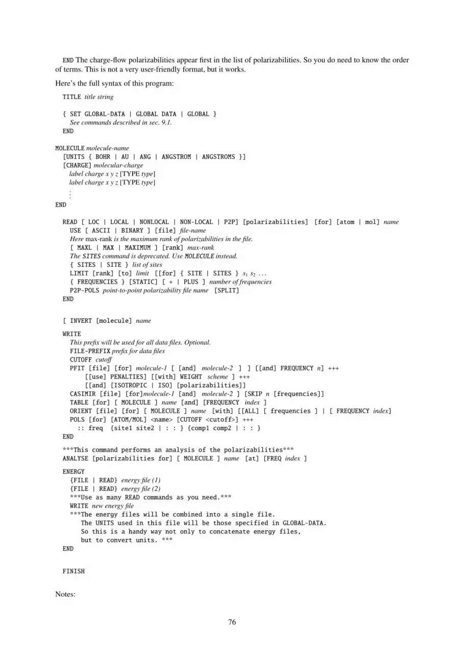
END The charge-flow polarizabilities appear first in the list of polarizabilities. So you do need to know the orderof terms. This is not a very user-friendly format, but it works.
Here’s the full syntax of this program:
TITLE title string
SET GLOBAL-DATA | GLOBAL DATA | GLOBAL See commands described in sec. 9.1.
END
MOLECULE molecule-name[UNITS BOHR | AU | ANG | ANGSTROM | ANGSTROMS ][CHARGE] molecular-charge
label charge x y z [TYPE type]label charge x y z [TYPE type]...
END
READ [ LOC | LOCAL | NONLOCAL | NON-LOCAL | P2P] [polarizabilities] [for] [atom | mol] nameUSE [ ASCII | BINARY ] [file] file-nameHere max-rank is the maximum rank of polarizabilities in the file.[ MAXL | MAX | MAXIMUM ] [rank] max-rankThe SITES command is deprecated. Use MOLECULE instead. SITES | SITE list of sitesLIMIT [rank] [to] limit [[for] SITE | SITES s1 s2 . . .
FREQUENCIES [STATIC] [ + | PLUS ] number of frequenciesP2P-POLS point-to-point polarizability file name [SPLIT]
END
[ INVERT [molecule] name
WRITEThis prefix will be used for all data files. Optional.FILE-PREFIX prefix for data filesCUTOFF cutoff
PFIT [file] [for] molecule-1 [ [and] molecule-2 ] ] [[and] FREQUENCY n] +++[[use] PENALTIES] [[with] WEIGHT scheme ] +++[[and] [ISOTROPIC | ISO] [polarizabilities]]
CASIMIR [file] [for]molecule-1 [and] molecule-2 ] [SKIP n [frequencies]]TABLE [for] [ MOLECULE ] name [and] [FREQUENCY index ]ORIENT [file] [for] [ MOLECULE ] name [with] [[ALL] [ frequencies ] | [ FREQUENCY index]POLS [for] [ATOM/MOL] <name> [CUTOFF <cutoff>] +++:: freq site1 site2 | : : comp1 comp2 | : :
END
***This command performs an analysis of the polarizabilities***ANALYSE [polarizabilities for] [ MOLECULE ] name [at] [FREQ index ]
ENERGYFILE | READ energy file (1)FILE | READ energy file (2)***Use as many READ commands as you need.***WRITE new energy file***The energy files will be combined into a single file.
The UNITS used in this file will be those specified in GLOBAL-DATA.So this is a handy way not only to concatenate energy files,but to convert units. ***
END
FINISH
Notes:
76

• Everything in the WRITE command is optional. The PFIT, CASIMIR and ORIENT options send data filessuitable for those programs to standard output. The TABLE option produces a tabular output suitable forprocessing with LATEX.
• When data for several frequencies are read in, they are numbered from 1 and can be referred to individuallyby this number, i.e. index in the syntax summaries above.
• The BINARY file comprises sections of the forms1 s2 rank sizeα(s1, s2, 1, 1:size)α(s1, s2, 2, 1:size)...
α(s1, s2,size, 1:size)
where s1 and s2 are site numbers, rank the maximum rank and size the dimension of the following polariz-ability matrix α(s1, s2), which is written one row to a record. If size is zero or no polarizability matrix existsfor a particular pair of sites, nothing is written for that pair. size= (rank+1)2 but is included in the file forconvenience.
11 Casimir
Author: Anthony J. Stone
The Casimir program reads uncoupled local polarizabilities (i.e. of the form αaatu ) for one or more molecules,
recouples them (i.e. to the form αav( j j′)), and computes dispersion coefficients up to C10. The code for C11 and C12
is included in the distribution, but is not activated as it hasn’t been adequately tested.
The input file for this program can be quite complicated for all but the smallest of molecules. This file will normallybe created by the Process program.
Input commands:
FREQUENCIES ω0 nfreqSpecify the base frequency and the number of frequencies to be used for the quadrature, in a.u. Defaults: 0.5 and10, respectively.
SKIP [ 0 | 1 ]By default, the static polarizability is not expected in the data file. If however it is present, SKIP or SKIP 1 willskip the first of each set of values, assuming it to be the static polarizability. SKIP 0 cancels a previous SKIP 1.
MOLECULE nameSubsequent polarizability data refers to the specified molecule. The end of the data for this molecule is specifiedby an END statement.
SITE nameIntroduces polarizability data for the site specified, in the current molecule. It comprises a number of sets of theformt u[α(0)] α(ω1) α(ω2) . . . α(ωn)terminated by “End” on a line by itself. Here t and u are spherical tensor indices (‘00’, ‘10’, ‘11c’, etc.). Thepolarizabilities, in a.u., follow on one or more lines. If the static polarizability is present, SKIP must be specified.(See above.)
PRINT ALL | NONZEROPrinting option for the recoupled polarizabilities. The default is to print only the nonzero ones.
CGDIR pathSpecify the directory where the coupling coefficients are to be found, if not in the current directory. These arecoupling coefficients for the real spherical tensor components. These coefficients are provided in $CAMCASP/data.
77

RECOUPLE [ALL | site site ...]Calculate recoupled polarizabilities for all sites, or for the sites specified. This is not needed if a DISPERSIONcommand follows.
DISPERSION n molecule-1 molecule-2Recouple the polarizabilities, if not already done, and calculate and print the dispersion coefficients to Cn, wheren is 6, 7, 8, 9, 10, 11 or 12. Coefficients up to C12 can be calculated, using (at present) only polarizabilities up tooctopole–octopole.
78
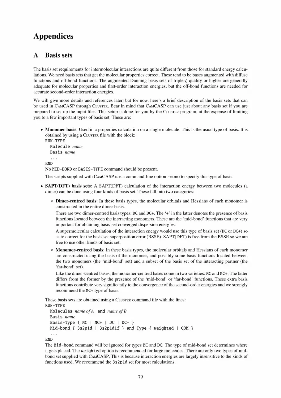
Appendices
A Basis sets
The basis set requirements for intermolecular interactions are quite different from those for standard energy calcu-lations. We need basis sets that get the molecular properties correct. These tend to be bases augmented with diffusefunctions and off-bond functions. The augmented Dunning basis sets of triple-ζ quality or higher are generallyadequate for molecular properties and first-order interaction energies, but the off-bond functions are needed foraccurate second-order interaction energies.
We will give more details and references later, but for now, here’s a brief description of the basis sets that canbe used in CamCASP through Cluster. Bear in mind that CamCASP can use just about any basis set if you areprepared to set up the input files. This setup is done for you by the Cluster program, at the expense of limitingyou to a few important types of basis set. These are:
• Monomer basis: Used in a properties calculation on a single molecule. This is the usual type of basis. It isobtained by using a Cluster file with the block:RUN-TYPEMolecule nameBasis name...
ENDNo MID-BOND or BASIS-TYPE command should be present.
The scripts supplied with CamCASP use a command-line option -mono to specify this type of basis.
• SAPT(DFT) basis sets: A SAPT(DFT) calculation of the interaction energy between two molecules (adimer) can be done using four kinds of basis set. These fall into two categories:
Dimer-centred basis: In these basis types, the molecular orbitals and Hessians of each monomer isconstructed in the entire dimer basis.There are two dimer-centred basis types: DC and DC+. The ‘+’ in the latter denotes the presence of basisfunctions located between the interacting monomers. These are the ‘mid-bond’ functions that are veryimportant for obtaining basis-set converged dispersion energies.A supermolecular calculation of the interaction energy would use this type of basis set (DC or DC+) soas to correct for the basis set superposition error (BSSE). SAPT(DFT) is free from the BSSE so we arefree to use other kinds of basis set.
Monomer-centred basis: In these basis types, the molecular orbitals and Hessians of each monomerare constructed using the basis of the monomer, and possibly some basis functions located betweenthe two monomers (the ‘mid-bond’ set) and a subset of the basis set of the interacting partner (the‘far-bond’ set).Like the dimer-centred bases, the monomer-centred bases come in two varieties: MC and MC+. The latterdiffers from the former by the presence of the ‘mid-bond’ or ‘far-bond’ functions. These extra basisfunctions contribute very significantly to the convergence of the second-order energies and we stronglyrecommend the MC+ type of basis.
These basis sets are obtained using a Cluster command file with the lines:RUN-TYPEMolecules name of A and name of BBasis nameBasis-Type MC | MC+ | DC | DC+ Mid-bond 3s2p1d | 3s2p1d1f and Type weighted | COM ...
ENDThe Mid-bond command will be ignored for types MC and DC. The type of mid-bond set determines whereit gets placed. The weighted option is recommended for large molecules. There are only two types of mid-bond set supplied with CamCASP. This is because interaction energies are largely insensitive to the kinds offunctions used. We recommend the 3s2p1d set for most calculations.
79

B Dispersion coefficients: in detail
The distributed C6, C7 and C8 dispersion coefficients can be obtained using the following steps. We have written afew simple scripts to perform some of the steps in this procedure, but you will still have to do some small tasks byhand.
Before getting to this, we will have had to perform a calculation of the non-local polarizabilities (say, ranks 0to 4) at 10 frequencies, and the point-to-point polarizabilities (on a grid of 1000 to 2000 points) at the same 10frequencies. These calculation are done in a standard properties calculation with the CamCASP program.
Let’s use C6Br2ClFH2 (XIII) as an example.
First of all we decide which axis system would be most appropriate for this molecule. The C2v symmetry of XIIImakes this an easy choice. Here is the local axis file for XIII:$ cat local_axesSites
! Units used: BOHRC1 2.27448932 -0.63093982 0.00000000C2 2.29369649 -3.26609468 0.00000000C3 0.00000000 0.74116754 0.00000000C4 -2.27526222 -0.62679565 0.00000000C5 -2.29946016 -3.26296530 0.00000000C6 -0.00413850 -4.52851101 0.00000000BR1 -5.43183783 1.06069375 0.00000000BR2 5.43383527 1.05079536 0.00000000CL 0.00318230 3.99305149 0.00000000F -0.00577500 -7.08124548 0.00000000H1 -4.05673525 -4.30060061 0.00000000H2 4.04880407 -4.30740551 0.00000000
End
AxesC1 z from C1 to BR2 x from C1 to C2BR2 z from C1 to BR2 x from C1 to C2C2 z from C2 to H2 x from C2 to C6H2 z from C2 to H2 x from C2 to C6C3 z from C3 to CL x from C3 to C4CL z from C3 to CL x from C3 to C4C4 z from C4 to BR1 x from C4 to C5BR1 z from C4 to BR1 x from C4 to C5C5 z from C5 to H1 x from C5 to C6H1 z from C5 to H1 x from C5 to C6C6 z from C6 to F x from C6 to C2F z from C6 to F x from C6 to C2
End
This choice of axes imposes the C2v symmetry. If we had wished to use the global axis system, the Axes...Endblock would not be needed.
First split the non-local polarizability file which contains polarizabilities at all computed frequencies (1+10 in thisexample) into 11 parts; one for each frequency. This can be done with a split command on a Linux system (seethe man page for split for details), or using Process with the following input file (at present, this file is createdby hand):
$ cat split_NL4.prss!! execute with: process < split_NL4.prss!
read non-local pols for XIIIUse ascii file XIII_0.0005_1000_f11_NL4.polMaximum rank 4! Use LIMIT to limit the rank, but it’s not essential here.! Limit rank to 2
80
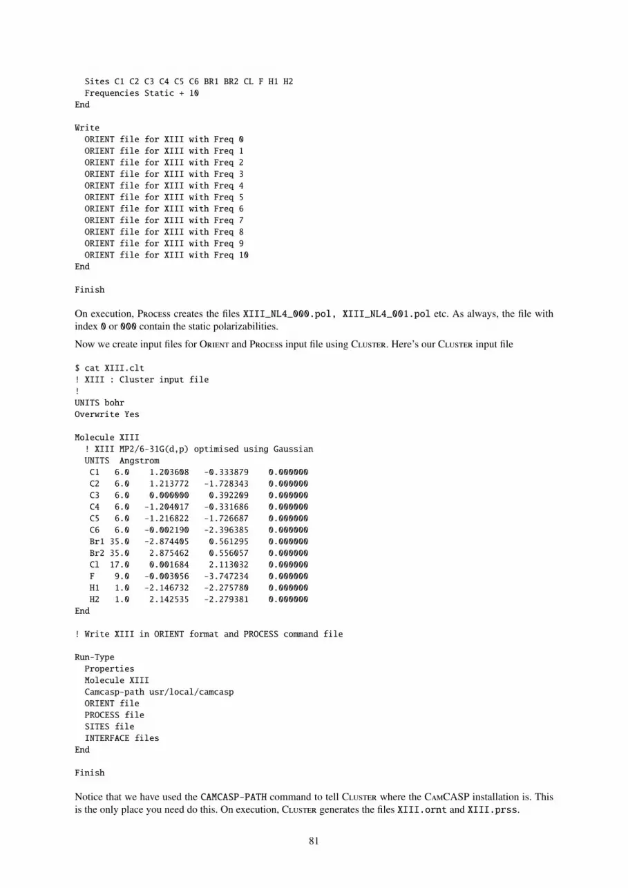
Sites C1 C2 C3 C4 C5 C6 BR1 BR2 CL F H1 H2Frequencies Static + 10
End
WriteORIENT file for XIII with Freq 0ORIENT file for XIII with Freq 1ORIENT file for XIII with Freq 2ORIENT file for XIII with Freq 3ORIENT file for XIII with Freq 4ORIENT file for XIII with Freq 5ORIENT file for XIII with Freq 6ORIENT file for XIII with Freq 7ORIENT file for XIII with Freq 8ORIENT file for XIII with Freq 9ORIENT file for XIII with Freq 10
End
Finish
On execution, Process creates the files XIII_NL4_000.pol, XIII_NL4_001.pol etc. As always, the file withindex 0 or 000 contain the static polarizabilities.
Now we create input files for Orient and Process input file using Cluster. Here’s our Cluster input file
$ cat XIII.clt! XIII : Cluster input file!UNITS bohrOverwrite Yes
Molecule XIII! XIII MP2/6-31G(d,p) optimised using GaussianUNITS AngstromC1 6.0 1.203608 -0.333879 0.000000C2 6.0 1.213772 -1.728343 0.000000C3 6.0 0.000000 0.392209 0.000000C4 6.0 -1.204017 -0.331686 0.000000C5 6.0 -1.216822 -1.726687 0.000000C6 6.0 -0.002190 -2.396385 0.000000Br1 35.0 -2.874405 0.561295 0.000000Br2 35.0 2.875462 0.556057 0.000000Cl 17.0 0.001684 2.113032 0.000000F 9.0 -0.003056 -3.747234 0.000000H1 1.0 -2.146732 -2.275780 0.000000H2 1.0 2.142535 -2.279381 0.000000
End
! Write XIII in ORIENT format and PROCESS command file
Run-TypePropertiesMolecule XIIICamcasp-path usr/local/camcaspORIENT filePROCESS fileSITES fileINTERFACE files
End
Finish
Notice that we have used the CAMCASP-PATH command to tell Cluster where the CamCASP installation is. Thisis the only place you need do this. On execution, Cluster generates the files XIII.ornt and XIII.prss.
81
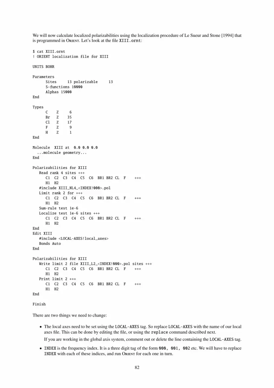
We will now calculate localized polarizabilities using the localization procedure of Le Sueur and Stone [1994] thatis programmed in Orient. Let’s look at the file XIII.ornt:
$ cat XIII.ornt! ORIENT localization file for XIII
UNITS BOHR
ParametersSites 13 polarizable 13S-functions 10000Alphas 15000
End
TypesC Z 6Br Z 35Cl Z 17F Z 9H Z 1
End
Molecule XIII at 0.0 0.0 0.0...molecule geometry...
End
Polarizabilities for XIIIRead rank 4 sites +++
C1 C2 C3 C4 C5 C6 BR1 BR2 CL F +++H1 H2
#include XIII_NL4_<INDEX!000>.polLimit rank 2 for +++
C1 C2 C3 C4 C5 C6 BR1 BR2 CL F +++H1 H2
Sum-rule test 1e-6Localize test 1e-6 sites +++
C1 C2 C3 C4 C5 C6 BR1 BR2 CL F +++H1 H2
EndEdit XIII
#include <LOCAL-AXES!local_axes>Bonds Auto
End
Polarizabilities for XIIIWrite limit 2 file XIII_L2_<INDEX!000>.pol sites +++
C1 C2 C3 C4 C5 C6 BR1 BR2 CL F +++H1 H2
Print limit 2 +++C1 C2 C3 C4 C5 C6 BR1 BR2 CL F +++H1 H2
End
Finish
There are two things we need to change:
• The local axes need to be set using the LOCAL-AXES tag. So replace LOCAL-AXES with the name of our localaxes file. This can be done by editing the file, or using the replace command described next.
If you are working in the global axis system, comment out or delete the line containing the LOCAL-AXES tag.
• INDEX is the frequency index. It is a three digit tag of the form 000, 001, 002 etc. We will have to replaceINDEX with each of these indices, and run Orient for each one in turn.
82
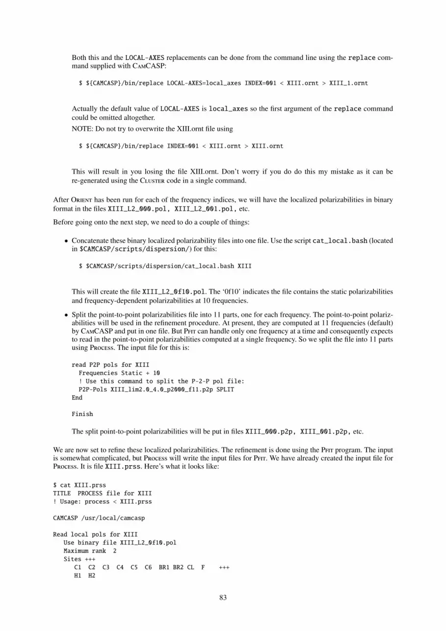
Both this and the LOCAL-AXES replacements can be done from the command line using the replace com-mand supplied with CamCASP:
$ $CAMCASP/bin/replace LOCAL-AXES=local_axes INDEX=001 < XIII.ornt > XIII_1.ornt
Actually the default value of LOCAL-AXES is local_axes so the first argument of the replace commandcould be omitted altogether.NOTE: Do not try to overwrite the XIII.ornt file using
$ $CAMCASP/bin/replace INDEX=001 < XIII.ornt > XIII.ornt
This will result in you losing the file XIII.ornt. Don’t worry if you do do this my mistake as it can bere-generated using the Cluster code in a single command.
After Orient has been run for each of the frequency indices, we will have the localized polarizabilities in binaryformat in the files XIII_L2_000.pol, XIII_L2_001.pol, etc.
Before going onto the next step, we need to do a couple of things:
• Concatenate these binary localized polarizability files into one file. Use the script cat_local.bash (locatedin $CAMCASP/scripts/dispersion/) for this:
$ $CAMCASP/scripts/dispersion/cat_local.bash XIII
This will create the file XIII_L2_0f10.pol. The ‘0f10’ indicates the file contains the static polarizabilitiesand frequency-dependent polarizabilities at 10 frequencies.
• Split the point-to-point polarizabilities file into 11 parts, one for each frequency. The point-to-point polariz-abilities will be used in the refinement procedure. At present, they are computed at 11 frequencies (default)by CamCASP and put in one file. But Pfit can handle only one frequency at a time and consequently expectsto read in the point-to-point polarizabilities computed at a single frequency. So we split the file into 11 partsusing Process. The input file for this is:
read P2P pols for XIIIFrequencies Static + 10! Use this command to split the P-2-P pol file:P2P-Pols XIII_lim2.0_4.0_p2000_f11.p2p SPLIT
End
Finish
The split point-to-point polarizabilities will be put in files XIII_000.p2p, XIII_001.p2p, etc.
We are now set to refine these localized polarizabilities. The refinement is done using the Pfit program. The inputis somewhat complicated, but Process will write the input files for Pfit. We have already created the input file forProcess. It is file XIII.prss. Here’s what it looks like:
$ cat XIII.prssTITLE PROCESS file for XIII! Usage: process < XIII.prss
CAMCASP /usr/local/camcasp
Read local pols for XIIIUse binary file XIII_L2_0f10.polMaximum rank 2Sites +++
C1 C2 C3 C4 C5 C6 BR1 BR2 CL F +++H1 H2
83
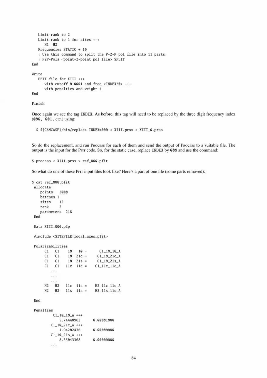
Limit rank to 2Limit rank to 1 for sites +++
H1 H2Frequencies STATIC + 10! Use this command to split the P-2-P pol file into 11 parts:! P2P-Pols <point-2-point pol file> SPLIT
End
WritePFIT file for XIII +++
with cutoff 0.0001 and freq <INDEX!0> +++with penalties and weight 4
End
Finish
Once again we see the tag INDEX. As before, this tag will need to be replaced by the three digit frequency index(000, 001, etc.) using:
$ $CAMCASP/bin/replace INDEX=000 < XIII.prss > XIII_0.prss
So do the replacement, and run Process for each of them and send the output of Process to a suitable file. Theoutput is the input for the Pfit code. So, for the static case, replace INDEX by 000 and use the command:
$ process < XIII.prss > ref_000.pfit
So what do one of these Pfit input files look like? Here’s a part of one file (some parts removed):
$ cat ref_000.pfitAllocate
points 2000batches 1sites 12rank 2parameters 218
End
Data XIII_000.p2p
#include <SITEFILE!local_axes_pfit>
PolarizabilitiesC1 C1 10 10 = C1_10_10_AC1 C1 10 21c = C1_10_21c_AC1 C1 10 21s = C1_10_21s_AC1 C1 11c 11c = C1_11c_11c_A
...
...
...H2 H2 11c 11s = H2_11c_11s_AH2 H2 11s 11s = H2_11s_11s_A
End
PenaltiesC1_10_10_A +++
5.74440962 0.00001000C1_10_21c_A +++
1.94202436 0.00000000C1_10_21s_A +++
8.35043368 0.00000000...
84
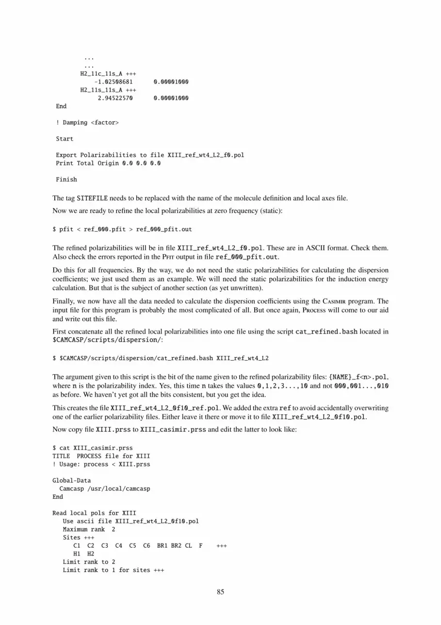
...
...H2_11c_11s_A +++
-1.02508681 0.00001000H2_11s_11s_A +++
2.94522570 0.00001000End
! Damping <factor>
Start
Export Polarizabilities to file XIII_ref_wt4_L2_f0.polPrint Total Origin 0.0 0.0 0.0
Finish
The tag SITEFILE needs to be replaced with the name of the molecule definition and local axes file.
Now we are ready to refine the local polarizabilities at zero frequency (static):
$ pfit < ref_000.pfit > ref_000_pfit.out
The refined polarizabilities will be in file XIII_ref_wt4_L2_f0.pol. These are in ASCII format. Check them.Also check the errors reported in the Pfit output in file ref_000_pfit.out.
Do this for all frequencies. By the way, we do not need the static polarizabilities for calculating the dispersioncoefficients; we just used them as an example. We will need the static polarizabilities for the induction energycalculation. But that is the subject of another section (as yet unwritten).
Finally, we now have all the data needed to calculate the dispersion coefficients using the Casimir program. Theinput file for this program is probably the most complicated of all. But once again, Process will come to our aidand write out this file.
First concatenate all the refined local polarizabilities into one file using the script cat_refined.bash located in$CAMCASP/scripts/dispersion/:
$ $CAMCASP/scripts/dispersion/cat_refined.bash XIII_ref_wt4_L2
The argument given to this script is the bit of the name given to the refined polarizability files: NAME_f<n>.pol,where n is the polarizability index. Yes, this time n takes the values 0,1,2,3...,10 and not 000,001...,010as before. We haven’t yet got all the bits consistent, but you get the idea.
This creates the file XIII_ref_wt4_L2_0f10_ref.pol. We added the extra ref to avoid accidentally overwritingone of the earlier polarizability files. Either leave it there or move it to file XIII_ref_wt4_L2_0f10.pol.
Now copy file XIII.prss to XIII_casimir.prss and edit the latter to look like:
$ cat XIII_casimir.prssTITLE PROCESS file for XIII! Usage: process < XIII.prss
Global-DataCamcasp /usr/local/camcasp
End
Read local pols for XIIIUse ascii file XIII_ref_wt4_L2_0f10.polMaximum rank 2Sites +++
C1 C2 C3 C4 C5 C6 BR1 BR2 CL F +++H1 H2
Limit rank to 2Limit rank to 1 for sites +++
85
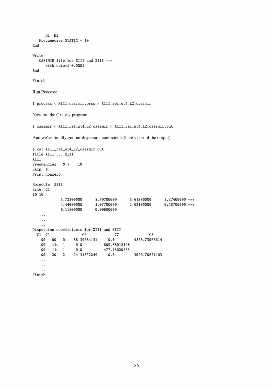
H1 H2Frequencies STATIC + 10
End
WriteCASIMIR file for XIII and XIII +++
with cutoff 0.0001End
Finish
Run Process:
$ process < XIII_casimir.prss > XIII_ref_wt4_L2.casimir
Now run the Casimir program:
$ casimir < XIII_ref_wt4_L2.casimir > XIII_ref_wt4_L2_casimir.out
And we’ve finially got our dispersion coefficients (here’s part of the output):
$ cat XIII_ref_wt4_L2_casimir.outTitle XIII ... XIIIXIIIFrequencies 0.5 10Skip 0Print nonzero
Molecule XIIISite C110 10
5.72200000 5.70700000 5.61200000 5.27400000 +++4.44000000 3.07700000 1.62100000 0.58700000 +++0.11800000 0.00600000
...
...
...Dispersion coefficients for XIII and XIII
C1 C1 C6 C7 C800 00 0 88.39684131 0.0 4820.7506661400 11c 1 0.0 809.8801219800 11s 1 0.0 477.1362055300 20 2 -24.31832249 0.0 -3056.70651103.........
Finish
86

C Older Scripts
These scripts are still present, but have been superseded by Python scripts. However they are still available in casethere are issues with Python installations.
For an up-to-date usage of these script use <script> --help.
C.1 High-level scripts
Most CamCASP calculations can be set up and run using the high-level scripts in conjunction with one simple datafile.
The following scripts are currently available. They can all be executed with the single argument --help to printbrief usage details and exit.
• runSAPTScript to run a complete SAPT(DFT) calculation to calculate the components of the interaction energybetween two molecules, or to calculate the properties (multipole moments and polarizabilities) of a singlemolecule. The command is justrunSAPT JOB -q queue -M memory
The ‘queue’ may be bg to run the calculation in the background, or none just to set up all the files andprepare a script for submitting the calculation. This allows you to modify any of the files if necessary. Youneed to provide one simple data file, JOB.clt, to define the system and specify the calculation. For details see§7 and the example in §8.1 below.
Because of an inconsistency in the site order used by these scripts and the newer Python scripts, yourCluster input file needs to have the line SITE-ORDER OLD in the RUN-TYPE block. If this is not present,the CamCASP interaction energy calculation will still proceed, but the results may be meaningless.
• search.plThe output of a SAPT(DFT) calculation can be analysed using the script search.pl. It picks out the energyterms from the CamCASP output file and displays them in a compact form.
• localizeUsing the polarizability files from a properties calculation, this script will generate local polarizabilities(static and dynamic). See §8.2.1 on p. 31 for details. The dynamic polarizabilities are then used to constructdispersion coefficients, if required.
C.2 Low-level scripts
Some of the scripts provided in the CamCASP package are low-level ones that just perform one step in setting upthe job, for example by generating further files that are needed for the calculations. If you need to do somethingunusual you may have to use the lower-level scripts directly, but for most purposes the high-level scripts willsuffice.
In all the following, JOB is the job-name, which identifies all the files belonging to the job — in particular, thecluster input file, usually called JOB.clt. Most jobs involve a large number of files, however, so it is not a goodidea to rely on the job-name to distinguish files for different jobs from each other. Recommended practice is to runevery job in its own private directory (folder).
The starting-point for all tasks is the ‘cluster’ file, conventionally given the .clt suffix, which contains informationabout the molecules involved, the basis sets to be used, and other details. Details are in §7. Once you have preparedthe input file for Cluster, called for example setup.clt, the cluster command is the first step in setting up thejob:cluster < setup.clt
(It will usually be called by a script rather than directly.) This will produce a file called JOB.template, whereJOB is the file prefix specified (or implied) in the Cluster data file. It will also produce a number of other files —for example JOB.cks and JOB_P.data — depending on the information in the .clt file.
87
Next, generate.pl is a low-level script that generates the input files for the Dalton 2013 ab initio calculation.These have names like A.mol, and MA.mol. Again, the particular files that are produced depend on the nature ofthe calculation.generate.pl options JOB
The options to this command are as follows:-monomer This is to be a properties calculation for a single molecule.-mc+, -mc This is a dimer interaction calculation, using monomer-centred basis sets, with or
without midbond functions. mc+ is the default calculation type.-dc+, -dc This is a dimer interaction calculation, using dimer-centred basis sets, with or without
midbond functions.-h, help Prints a help page to standard output.
Dalton 2013 also requires .dal files that describe the type of calculation to be done. Usually, these files do notdepend on the particular molecule or molecules for which the calculation is being done (they are described in the.mol files) but in the case of DFT calculations using the asymptotically-corrected PBE0 functional it is necessaryto specify the molecular ionization potential in order to set up the asymptotic correction properly. Accordingly thedal.pl command that sets up these files requires the ionization potentials:dal.pl options
where the options are[-j] JOB Specifies the jobname to be used as the file prefix-a moleculeA Alternatively, the molecule names can be specified, in which case the jobname will be
constructed from them.-b moleculeB For a dimer calculation, both molecules need to be specified.-ipa or -ip IP Vertical ionization potential for molecule A, or for a monomer (in Hartree).-ipb IP Vertical ionization potential for molecule B, if present.-monomer This is to be a properties calculation for a single molecule.-mc+, -mc This is a dimer interaction calculation, using monomer-centred basis sets, with or
without midbond functions.-dc+, -dc This is a dimer interaction calculation, using dimer-centred basis sets, with or without
midbond functions.The file CAMCASP/misc/IP.txt contains a list of ionization potentials for some small molecules; many others areavailable in the NIST Chemistry Webbook at webbook.nist.gov/chemistry/. If the IP cannot be found thereor elsewhere in the literature, it is necessary to calculate it.
88
ReferencesO. Akin-Ojo, R. Bukowski, and K. Szalewicz. Ab initio studies of He-HCCCN interaction. J. Chem. Phys., 119:
8379–8396, 2003.
R. Bukowski, R. Podeszwa, and K. Szalewicz. Efficient generation of the coupled Kohn–Sham dynamic suscepti-bility functions and dispersion energy with density fitting. Chem. Phys. Lett., 414:111–116, 2005.
M. E. Casida. Time-dependent density-functional response theory for molecules. In D. P. Chong, editor, RecentAdvances in Density-Functional Theory, page 155. World Scientific, 1995.
M. E. Casida and D. R. Salahub. Asymptotic correction approach to improving approximate exchange-correlationpotentials: Time-dependent density-functional theory calculations of molecular excitation spectra. J. Chem.Phys., 113:8918–8935, 2000.
S. M. Colwell, N. C. Handy, and A. M. Lee. Determination of frequency-dependent polarizabilities using currentdensity-functional theory. Phys. Rev. A, 53:1316–1322, 1995.
S. Grimme. Semiempirical GGA-type density functional constructed with a long-range dispersion correction. J.Comp. Chem, 27:1787 – 1799, 2006.
M. Gruning, O. V. Gritsenko, S. J. A. van Gisbergen, and E. J. Baerends. Shape corrections to exchange-correlationpotentials by gradient-regulated seamless connection of model potentials for inner and outer region. J. Chem.Phys., 114:652–660, 2001.
A. Hesselmann, G. Jansen, and M. Schütz. Density-functional theory-symmetry-adapted intermolecular perturba-tion theory with density fitting: A new efficient method to study intermolecular interaction energies. J. Chem.Phys., 122:014103, 2005.
M. P. Hodges and R. J. Wheatley. Flexible multipole models for hydrogen fluoride. Phys. Chem. Chem. Phys, 2:1631–1638, 2000.
B. Jeziorski, R. Moszynski, A. Ratkiewicz, S. Rybak, K. Szalewicz, and H.L. Williams. SAPT: A program formany-body symmetry-adapted perturbation theory calculations of intermolecular interaction energies, vol-ume B, page 79. STEF, Cagliari, 1993.
B. Jeziorski, R. Moszynski, and K. Szalewicz. Perturbation theory approach to intermolecular potential energysurfaces of van der waals complexes. Chem. Rev., 94:1887–1930, 1994.
C. R. Le Sueur and A. J. Stone. Localization methods for distributed polarizabilities. Molec. Phys., 83:293–308,1994.
T. C. Lillestolen and R. Wheatley. Atomic charge densities generated using an iterative stockholder approach.J. Chem. Phys., 131:144101, 2009.
T. C. Lillestolen and R. J. Wheatley. First-principles calculation of local atomic polarizabilities. J. Phys. Chem. A,111:11141–11146, 2007. doi: 10.1021/jp073151y.
A. J. Misquitta. Charge-transfer from regularized symmetry-adapted perturbation theory. J. Chem. Theory Com-put., 9:5313–5326, 2013. doi: 10.1021/ct400704a.
A. J. Misquitta and A. J. Stone. Distributed polarizabilities obtained using a constrained density-fitting algorithm.J. Chem. Phys., 124:024111, 2006.
A. J. Misquitta and A. J. Stone. Accurate induction energies for small organic molecules: I. Theory. J. Chem.Theory Comput., 4:7–18, 2008a.
A. J. Misquitta and A. J. Stone. Dispersion energies for small organic molecules: first row atoms. Molec. Phys.,106:1631 – 1643, 2008b.
A. J. Misquitta and K. Szalewicz. Intermolecular forces from asymptotically corrected density functional descrip-tion of monomers. Chem. Phys. Lett., 357:301–306, 2002.
A. J. Misquitta and K. Szalewicz. Symmetry-adapted perturbation-theory calculations of intermolecular forcesemploying density-functional description of monomers. J. Chem. Phys., 122:214109, 2005.
89
A. J. Misquitta, B. Jeziorski, and K. Szalewicz. Dispersion energy from density-functional theory description ofmonomers. Phys. Rev. Lett., 91:33201, 2003.
A. J. Misquitta, R. Podeszwa, B. Jeziorski, and K. Szalewicz. Intermolecular potentials based on symmetry-adapted perturbation theory with dispersion energies from time-dependent density-functional theory. J. Chem.Phys., 123:214103, 2005.
A. J. Misquitta, A. J. Stone, and S. L. Price. Accurate induction energies for small organic molecules. 2. Develop-ment and testing of distributed polarizability models against SAPT(DFT) energies. J. Chem. Theory Comput.,4:19–32, 2008a. doi: 10.1021/ct700105f.
A. J. Misquitta, G. W. A. Welch, A. J. Stone, and S. L. Price. A first principles prediction of the crystal structureof C6Br2ClFH2. Chem. Phys. Lett., 456:105–109, 2008b.
Alston J. Misquitta, Anthony J. Stone, and Farhang Fazeli. Distributed multipoles from a robust basis-spaceimplementation of the iterated stockholder atoms procedure. J. Chem. Theory Comput., 2014. doi: 10.1021/
ct5008444.
K. Patkowski, B. Jeziorski, and K. Szalewicz. Symmetry-adapted perturbation theory with regularized Coulombpotential. J. Mol. Struct. (TheoChem), 547:293–307, 2001a.
K. Patkowski, B. Jeziorski, and K. Szalewicz. Symmetry-adapted perturbation theory with regularized coulombpotential. J. Mol. Struct. (Theochem), 547:293–307, 2001b.
K. Patkowski, B. Jeziorski, and K. Szalewicz. Unified treatment of chemical and van der waals forces viasymmetry-adapted perturbation expansion. J. Chem. Phys., 120:6849–6862, 2004.
Konrad Patkowski, Krzysztof Szalewicz, and Bogumil Jeziorski. Induction and exchange-induction energy with aregularized coulomb potential. private communication, 2012.
R. Podeszwa, R. Bukowski, and K. Szalewicz. Density-fitting method in symmetry-adapted perturbation theorybased on kohn-sham description of monomers. J. Chem. Theory Comput., 2:400–412, 2006.
Fazle Rob and Krzysztof Szalewicz. Asymptotic dispersion energies from distributed polarizabilities. Chem. Phys.Lett., 572:146–149, 2013.
A. J. Stone. Distributed multipole analysis: Stability for large basis sets. J. Chem. Theory Comput., 1:1128–1132,2005.
A. J. Stone and A. J. Misquitta. Atom–atom potentials from ab initio calculations. Int. Rev. Phys. Chem., 26:193–222, 2007.
K. T. Tang and J. Peter Toennies. The damping function of the van der Waals attraction in the potential betweenrare gas atoms and metal surfaces. Surf. Sci. Lett., 279:203–206, 1992.
David J. Tozer and Nicholas C. Handy. Improving virtual Kohn–Sham orbitals and eigenvalues: Application toexcitation energies and static polarizabilities. J. Chem. Phys., 109:10180–10189, 1998.
H. L. Williams, E. M. Mas, K. Szalewicz, and B. Jeziorski. On the effectiveness of monomer-, dimer-, and bond-centered basis functions in calculations of intermolecular interaction energies. J. Chem. Phys., 103:7374–7391,1995.
90