by vivian yuen-chong tsang a thesis submitted in conformity
TRANSCRIPT
A NON-DUAL APPROACH TOMEASURING SEMANTIC DISTANCE
BY
INTEGRATING ONTOLOGICAL AND DISTRIBUTIONAL INFORMATION
WITHIN A NETWORK-FLOW FRAMEWORK
by
Vivian Yuen-Chong Tsang
A thesis submitted in conformity with the requirementsfor the degree of Doctor of Philosophy
Graduate Department of Computer ScienceUniversity of Toronto
Copyright c© 2008 by Vivian Yuen-Chong Tsang
I believe that much unseen is also here.
Walt Whitman, Song of the Open Road
On dit qu’a force d’ascese certains bouddhistes
parviennent a voir tout un paysage dans une feve.
Roland Barthes, S/Z
ii
Abstract
A Non-dual Approach to Measuring Semantic Distance
by
Integrating Ontological and Distributional Information within a Network-Flow Framework
Vivian Yuen-Chong Tsang
Doctor of Philosophy
Graduate Department of Computer Science
University of Toronto
2008
Text comparison is a key step in many natural language processing (NLP) applications in which
texts can be classified based on their semantic distance (howsimilar or different the texts are).
For example, comparing the local context of an ambiguous word with that of a known word can
help identify the sense of the ambiguous word. Typically, a distributional measure is used to
capture the implicit semantic distance between two pieces of text. In this thesis, we introduce
an alternative method of measuring the semantic distance between texts as a non-dual com-
bination of distributional information and ontological knowledge. We define non-dualism as
combining two distinct components such that they are seamless in the combination. We achieve
this non-dual combination by proposing a novel distance measure within a network-flow for-
malism. First, we represent each text as a collection of frequency-weighted concepts within
an ontology. Then, we make use of a network-flow method which provides an efficient way
of measuring the semantic distance between two texts by taking advantage of the ontological
structure. We evaluate our method in a variety of NLP tasks.
In our task-based evaluation, we find that our method performs well on two of three tasks.
We introduce a novel approach to analysing the sensitivity of our network-flow method to any
dataset (represented as a collection of frequency-weighted concepts). Given that the ontolog-
ical and the distributional components are intricately knitted together in our method, we find
iii

that a non-dual approach, rather than a purely distributional or graphical analysis, is more ap-
propriate and more effective in explaining the performanceinconsistency.
Finally, we address a complexity issue that arises from the overhead required to incorporate
more sophisticated concept-to-concept distances into thenetwork-flow framework. We propose
a graph transformation method which generates a pared-downnetwork that requires less time
to process. The new method achieves a significant speed improvement, and does not seriously
hamper performance as a result of the transformation, as indicated in our analysis.
iv

Acknowledgements
I would like to thank, first and foremost, my family for their emotional support. My apprecia-
tion can only be expressed with a Greek symbol,µ.
Much thanks to my advisor, Suzanne Stevenson, for planting the initial seed for thinking
about distance as moving dark soil. Digging and moving earthturned out to be rather strenuous.
Her patience and encouragements are much appreciated.
Much kudos to suzgrp for their support, emotional and otherwise. In particular, I would
like to thank Afsaneh Fazly, whose careful editing commentsare indispensible; and Afra Al-
ishahi, who borrowed a book by Michel Foucault and allowed itto sit on her desk for about
three hours. . . Though I never cared much for deconstructionism (still don’t), the book kept me
thinking about (mis)interpretations.
I would like to thank Prof. Derek Corneil and Frank Chu for their helpful discussions on
network-flow methods.
Finally, much thanks to my Sifu, Dorje Jidgral, and my Vajra comrades, who made me
realize meaning is one (integral piece) and not one or two or more.
v

vi
Contents
1 Introduction 1
1.1 Distributional Approaches . . . . . . . . . . . . . . . . . . . . . . . .. . . . 4
1.2 Ontological Approaches . . . . . . . . . . . . . . . . . . . . . . . . . . .. . 6
1.3 Graph-based Approaches in NLP . . . . . . . . . . . . . . . . . . . . . .. . . 8
1.4 Our Combined Approach to Semantic Distance . . . . . . . . . . .. . . . . . 9
2 The Network Flow Method 15
2.1 An Intuitive Overview . . . . . . . . . . . . . . . . . . . . . . . . . . . . .. 16
2.2 Minimum Cost Flow . . . . . . . . . . . . . . . . . . . . . . . . . . . . . . . 18
2.3 Semantic Distance as MCF . . . . . . . . . . . . . . . . . . . . . . . . . . .. 20
2.4 Ontological and Distributional Factors in MCF . . . . . . . .. . . . . . . . . 21
3 Task-based Evaluation 25
3.1 Task 1: Verb Alternation Detection . . . . . . . . . . . . . . . . . .. . . . . . 27
3.1.1 Experimental Setup . . . . . . . . . . . . . . . . . . . . . . . . . . . . 28
3.1.2 Results and Analysis . . . . . . . . . . . . . . . . . . . . . . . . . . . 30
3.2 Task 2: Name Disambiguation . . . . . . . . . . . . . . . . . . . . . . . .. . 35
3.2.1 Experimental Methodology . . . . . . . . . . . . . . . . . . . . . . .36
3.2.2 Results and Analysis . . . . . . . . . . . . . . . . . . . . . . . . . . . 39
3.3 Task 3: Document Classification . . . . . . . . . . . . . . . . . . . . .. . . . 44
3.3.1 Experimental Setup . . . . . . . . . . . . . . . . . . . . . . . . . . . . 45
vii
3.3.2 Results and Analysis . . . . . . . . . . . . . . . . . . . . . . . . . . . 47
3.4 Summary . . . . . . . . . . . . . . . . . . . . . . . . . . . . . . . . . . . . . 51
4 Measuring Coherence of Semantic Profiles 53
4.1 Profile Coherence . . . . . . . . . . . . . . . . . . . . . . . . . . . . . . . . .54
4.2 Separate Distributional and Ontological Approaches . .. . . . . . . . . . . . . 56
4.3 Integrating Distributional and Ontological Factors . .. . . . . . . . . . . . . . 58
4.3.1 Profile Density . . . . . . . . . . . . . . . . . . . . . . . . . . . . . . 58
4.3.2 Finding the Ancestor Set for Profile Density . . . . . . . . .. . . . . . 62
4.3.3 Results and Analysis . . . . . . . . . . . . . . . . . . . . . . . . . . . 63
4.3.4 The Impact of the Number of Ancestors . . . . . . . . . . . . . . .. . 65
4.4 Summary . . . . . . . . . . . . . . . . . . . . . . . . . . . . . . . . . . . . . 66
5 Graph Transformation 69
5.1 Solving the MCF Problem Using a Non-additive Distance . .. . . . . . . . . . 70
5.2 Network Transformation . . . . . . . . . . . . . . . . . . . . . . . . . . .. . 73
5.2.1 Path Shape in a Hierarchy . . . . . . . . . . . . . . . . . . . . . . . . 74
5.2.2 Network Reconstruction . . . . . . . . . . . . . . . . . . . . . . . . .75
5.3 Analysing the Transformed Network . . . . . . . . . . . . . . . . . .. . . . . 77
5.3.1 Distance Distortion . . . . . . . . . . . . . . . . . . . . . . . . . . . .77
5.3.2 Junction Selection . . . . . . . . . . . . . . . . . . . . . . . . . . . . 80
5.4 Evaluating the Transformed Network . . . . . . . . . . . . . . . . .. . . . . . 81
5.4.1 Junction Selection . . . . . . . . . . . . . . . . . . . . . . . . . . . . 82
5.4.2 Results and Analysis . . . . . . . . . . . . . . . . . . . . . . . . . . . 82
5.5 Summary . . . . . . . . . . . . . . . . . . . . . . . . . . . . . . . . . . . . . 85
6 Conclusions 87
6.1 Summary of Contributions . . . . . . . . . . . . . . . . . . . . . . . . . .. . 89
6.2 Short-term Improvements: Within the MCF Framework . . . .. . . . . . . . . 91
viii

6.3 Long-Term Research Directions . . . . . . . . . . . . . . . . . . . . .. . . . 92
Bibliography 95
ix

x
List of Tables
1.1 A representation of two texts as word frequency vectors.. . . . . . . . . . . . 4
1.2 Word frequency distributions of four different texts. Italicized frequencies in
each row reflect the difference between Text A and the corresponding text. . . . 6
1.3 Concept frequency distributions of the four texts in Table 1.2. . . . . . . . . . . 6
3.1 Accuracies on development data. . . . . . . . . . . . . . . . . . . . .. . . . . 31
3.2 Accuracies on test data. . . . . . . . . . . . . . . . . . . . . . . . . . . .. . . 32
3.3 Average accuracies on raw, Li and Abe, and Clark and Weir profiles. . . . . . . 33
3.4 Accuracies on development data on profiles generated using Clark and Weir’s
(2002) method. Best accuracies in each condition are shown in boldface. . . . . 34
3.5 Accuracies on test data on profiles generated using Clarkand Weir’s (2002)
method. Best accuracies in each condition are shown in boldface. . . . . . . . . 34
3.6 The pairs to be identified, the raw frequency, and the relative frequency of the
majority name. . . . . . . . . . . . . . . . . . . . . . . . . . . . . . . . . . . 37
3.7 Network-flow results (accuracy) using 200 training instances on the random
samples and their average performance. . . . . . . . . . . . . . . . . .. . . . 40
3.8 Performance results using 200 instances per gold standard profile. . . . . . . . 40
3.9 SVM results using 200 training instances. . . . . . . . . . . . .. . . . . . . . 41
3.10 Average classification results of the network flow method using 200, 100, and
50 training data per classification task. . . . . . . . . . . . . . . . .. . . . . . 41
xi
3.11 The performance results of of Pedersen et al. (2005) (Ped05), as well as net-
work flow (NF) and SVM using 100 training instances, ranked inthe order of
the JS divergence. . . . . . . . . . . . . . . . . . . . . . . . . . . . . . . . . . 43
3.12 Average classification results using 10 and 30 trainingdocuments per newsgroup. 47
3.13 Average classification results using 30 and 10 trainingdocuments per newsgroup. 50
4.1 Summary of task-based results. . . . . . . . . . . . . . . . . . . . . .. . . . . 54
4.2 The normalized profile density scores for each dataset atfive different values
of α, as well as the average scores across theα values. . . . . . . . . . . . . . 64
4.3 The normalized density scores at five different values ofα, as well as the aver-
age scores, calculated using Jiang and Conrath’s (1997) distance. . . . . . . . . 65
4.4 Thenorm density3 scores at five different values ofα, as well as the average
scores, calculated using edge distance. . . . . . . . . . . . . . . . .. . . . . . 66
4.5 Thenorm density3 scores at five different values ofα, as well as the average
scores, calculated using Jiang and Conrath’s (1997) distance. . . . . . . . . . . 66
5.1 Name disambiguation results (accuracy) at a glance. . . .. . . . . . . . . . . . 83
xii
List of Figures
1.1 The content of three texts. . . . . . . . . . . . . . . . . . . . . . . . . .. . . 2
1.2 An illustration of two profiles within an ontology. . . . . .. . . . . . . . . . . 10
1.3 Two variations of Figure 1.2. . . . . . . . . . . . . . . . . . . . . . . .. . . . 13
1.4 A path from S to D via their common ancestor A. . . . . . . . . . . .. . . . . 14
2.1 A small text represented as a collection of weighted nodes in a fragment of
WordNet. . . . . . . . . . . . . . . . . . . . . . . . . . . . . . . . . . . . . . 16
2.2 Two subgraphs with varying degrees of overlap. . . . . . . . .. . . . . . . . . 17
2.3 An illustration of flow entering and exiting nodei. . . . . . . . . . . . . . . . . 19
2.4 An example of transporting the weights at the square nodes (supply nodes) to
the triangle nodes (demand nodes). . . . . . . . . . . . . . . . . . . . . .. . . 22
3.1 Two noisy profiles, one represented by squares, the other, triangles. . . . . . . . 48
3.2 The same two profiles in Figure 3.1. The profile masses thatare “subtracted”
are shaded in grey. . . . . . . . . . . . . . . . . . . . . . . . . . . . . . . . . 50
4.1 Examples of two profiles . . . . . . . . . . . . . . . . . . . . . . . . . . . .. 55
4.2 Two examples of profile density within an ontology. . . . . .. . . . . . . . . . 59
4.3 Two profiles with equal density value. . . . . . . . . . . . . . . . .. . . . . . 60
4.4 Two profile examples with different number of ancestors but of equalnorm density
value. . . . . . . . . . . . . . . . . . . . . . . . . . . . . . . . . . . . . . . . 61
5.1 A bipartite network between the S and D profiles. . . . . . . . .. . . . . . . . 71
xiii

5.2 An example ontology with two profiles, S and D. . . . . . . . . . .. . . . . . 72
5.3 An example ontology with two profiles, S and D. Some commonancestors of
the profile nodes are highlighted (JS and JD nodes). . . . . . . . . . . . . . . . 75
5.4 Fragments of the transformed ontology with two profiles,S and D. The com-
mon ancestors of the profile nodes are labeled JS and JD. . . . . . . . . . . . . 76
5.5 The fully transformed ontology with two profiles, S and D.The common an-
cestors of the profile nodes are labeled JS and JD. . . . . . . . . . . . . . . . . 76
5.6 The original ontology, the bipartite graph and the fullytransformed graph with
two profiles, S and D. In the fully transformed graph, the common ancestors of
the profile nodes are labeled JS and JD. . . . . . . . . . . . . . . . . . . . . . . 78
5.7 Three clusters of concepts. . . . . . . . . . . . . . . . . . . . . . . . .. . . . 84
xiv
Chapter 1
Introduction
Rosencrantz: What are you playing at?
Guildenstern: Words. Words. They’re all we have to go on.
Tom Stoppard, Rosencrantz and Guildenstern are Dead
In this thesis, we address the problem of comparing the semantic content of natural language
texts. Given two texts, we measure their semantic distance by comparing the words in one
text with those in the other. Representing texts as bags of words, a simple way of measuring
the distance between two texts is to count the number of wordsthey have in common. Such
a measure, however, ignores the fact that the same notion maybe expressed using different,
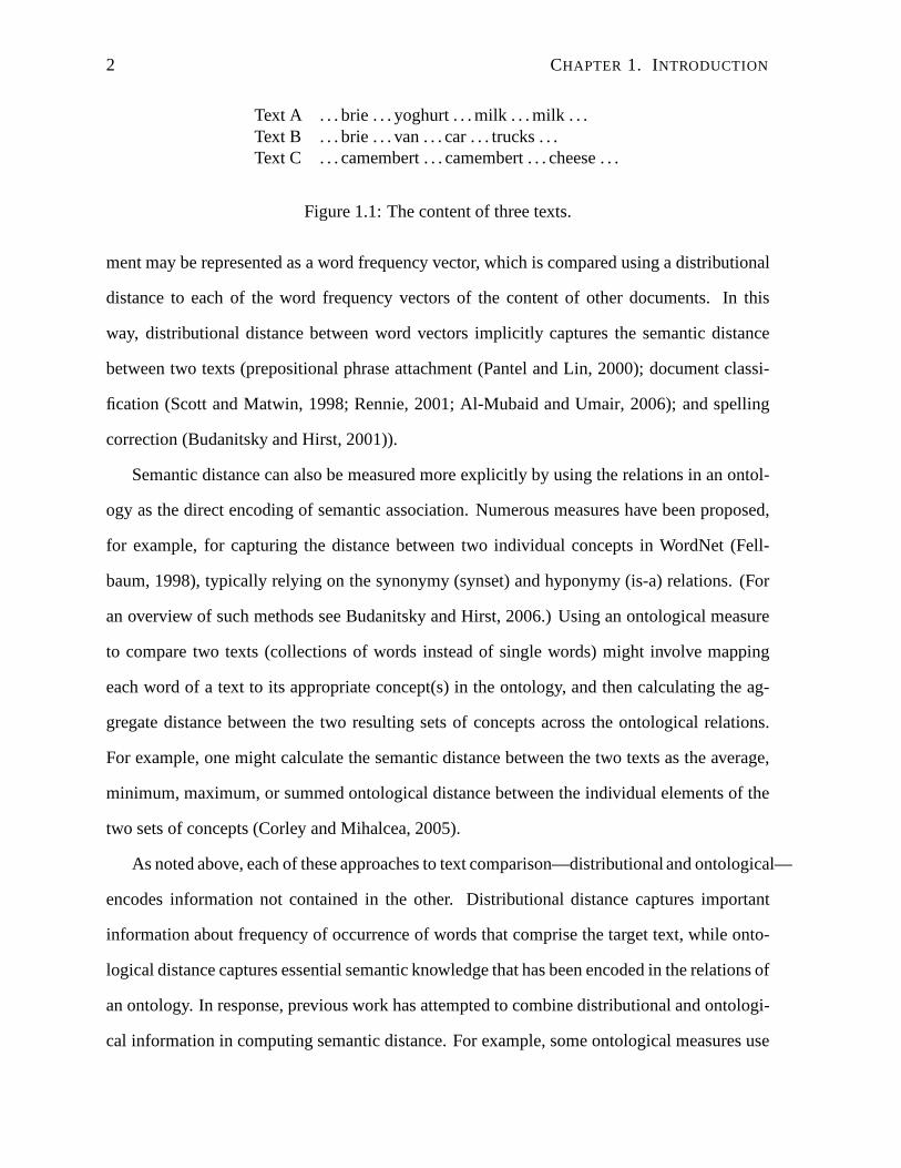
though semantically related, words. Consider the simple example in Figure 1.1. Text A and
Text B have more words in common than Text A and Text C have. Butbecause both Text A
and Text C contain semantically similar words (dairy products) whereas the content of Text B
mostly consists of words of another type (automobiles), we consider Text A to be less similar
to Text B than to Text C. It is thus important to take into account the contribution of each word
as well as groups of semantically related words to the overall semantic distance between text.
Distributional methods for semantic distance are successfully and widely used in compar-
ing texts that are represented as bags of words with associated frequencies of occurrence (e.g.,
Lee, 2001; Weeds et al., 2004). In document classification, for example, the content of a docu-
1
2 CHAPTER 1. INTRODUCTION
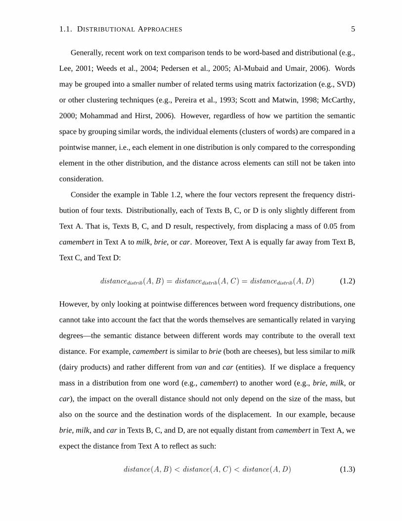
Text A . . . brie . . . yoghurt . . . milk . . . milk . . .Text B . . . brie . . . van . . . car . . . trucks . . .Text C . . . camembert . . . camembert . . . cheese . . .
Figure 1.1: The content of three texts.
ment may be represented as a word frequency vector, which is compared using a distributional
distance to each of the word frequency vectors of the contentof other documents. In this
way, distributional distance between word vectors implicitly captures the semantic distance
between two texts (prepositional phrase attachment (Pantel and Lin, 2000); document classi-
fication (Scott and Matwin, 1998; Rennie, 2001; Al-Mubaid and Umair, 2006); and spelling
correction (Budanitsky and Hirst, 2001)).
Semantic distance can also be measured more explicitly by using the relations in an ontol-
ogy as the direct encoding of semantic association. Numerous measures have been proposed,
for example, for capturing the distance between two individual concepts in WordNet (Fell-
baum, 1998), typically relying on the synonymy (synset) andhyponymy (is-a) relations. (For
an overview of such methods see Budanitsky and Hirst, 2006.)Using an ontological measure
to compare two texts (collections of words instead of singlewords) might involve mapping
each word of a text to its appropriate concept(s) in the ontology, and then calculating the ag-
gregate distance between the two resulting sets of conceptsacross the ontological relations.
For example, one might calculate the semantic distance between the two texts as the average,
minimum, maximum, or summed ontological distance between the individual elements of the
two sets of concepts (Corley and Mihalcea, 2005).
As noted above, each of these approaches to text comparison—distributional and ontological—
encodes information not contained in the other. Distributional distance captures important
information about frequency of occurrence of words that comprise the target text, while onto-
logical distance captures essential semantic knowledge that has been encoded in the relations of
an ontology. In response, previous work has attempted to combine distributional and ontologi-
cal information in computing semantic distance. For example, some ontological measures use
3
corpus frequencies of words to yield concept weights that are taken into account in measuring
the distance between two concepts (Resnik, 1995; Jiang and Conrath, 1997). However, these
methods are restricted to finding the distance between two individual concepts, not the aggre-
gate distance between the two sets of concepts corresponding to two texts. Other researchers
have developed measures of semantic distance between textsthat apply distributional distances
to concept vectors of frequencies rather than to word vectors (McCarthy, 2000; Mohammad
and Hirst, 2006). However, these approaches only make pointwise comparisions across the
concept vectors, and do not take into account the important ontological relations among the
concepts. What has been missing is an approach to semantic distance of text that can truly in-
tegrate the distributional and ontological (relational) information, drawing more fully on their
complementary advantages.
Given the complementary nature of distributional and ontological methods, our goal is to
develop a semantic distance method that achieves the advantages of the two. We thus propose
a novel graph-based method that seamlessly combines the distributional and the ontological
factors. In other words, we see distributional and ontological information as two distinct but
not separate (non-dual) parts of a semantic distance measure. The key is that both word fre-
quency (distributional information) and word meaning (ontological knowledge) contribute to
the underlying text meaning. Moreover, word meaning shouldnot serve only to partition the
semantic space, as is the case in a purely distributional approach. The relationship between
word meanings (ontological relations among concepts) should also be taken into account.
The rest of this chapter is organized as follows. In Section 1.1, we use an example to
explain in detail which aspects of semantic distance a distributional method captures. We
further elaborate on how existing distributional methods have tried to incorporate ontological
information, and argue that such an approach is not sufficient. In Section 1.2 , we present
how some of the existing ontological measures take into account distributional information
in their calculation. Again, we argue that such methods still lack an appropriate account of
distributional properties of texts. Our proposed method for seemlessly combining the two
4 CHAPTER 1. INTRODUCTION
words w1 w2 w3 . . . wn−1 wn
Text A a1 a2 a3 . . . an−1 an
Text B b1 b2 b3 . . . bn−1 bn
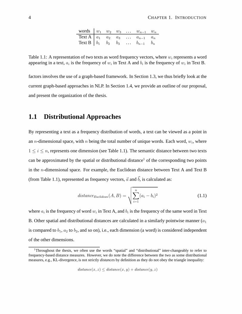
Table 1.1: A representation of two texts as word frequency vectors, wherewi represents a wordappearing in a text,ai is the frequency ofwi in Text A andbi is the frequency ofwi in Text B.
factors involves the use of a graph-based framework. In Section 1.3, we thus briefly look at the
current graph-based approaches in NLP. In Section 1.4, we provide an outline of our proposal,
and present the organization of the thesis.
1.1 Distributional Approaches
By representing a text as a frequency distribution of words,a text can be viewed as a point in
ann-dimensional space, withn being the total number of unique words. Each word,wi, where
1 ≤ i ≤ n, represents one dimension (see Table 1.1). The semantic distance between two texts
can be approximated by the spatial or distributional distance1 of the corresponding two points
in then-dimensional space. For example, the Euclidean distance between Text A and Text B
(from Table 1.1), represented as frequency vectors,~a and~b, is calculated as:
distanceEuclidean(A, B) =
√
√
√
√
n∑
i=1
(ai − bi)2 (1.1)
whereai is the frequency of wordwi in Text A, andbi is the frequency of the same word in Text
B. Other spatial and distributional distances are calculated in a similarly pointwise manner (a1
is compared tob1, a2 to b2, and so on), i.e., each dimension (a word) is considered independent
of the other dimensions.
1Throughout the thesis, we often use the words “spatial” and “distributional” inter-changeably to refer tofrequency-based distance measures. However, we do note thedifference between the two as some distributionalmeasures, e.g., KL-divergence, is not strictlydistancesby definition as they do not obey the triangle inequality:
distance(x , z ) ≤ distance(x , y) + distance(y, z )
1.1. DISTRIBUTIONAL APPROACHES 5
Generally, recent work on text comparison tends to be word-based and distributional (e.g.,
Lee, 2001; Weeds et al., 2004; Pedersen et al., 2005; Al-Mubaid and Umair, 2006). Words
may be grouped into a smaller number of related terms using matrix factorization (e.g., SVD)
or other clustering techniques (e.g., Pereira et al., 1993;Scott and Matwin, 1998; McCarthy,
2000; Mohammad and Hirst, 2006). However, regardless of howwe partition the semantic
space by grouping similar words, the individual elements (clusters of words) are compared in a
pointwise manner, i.e., each element in one distribution isonly compared to the corresponding
element in the other distribution, and the distance across elements can still not be taken into
consideration.
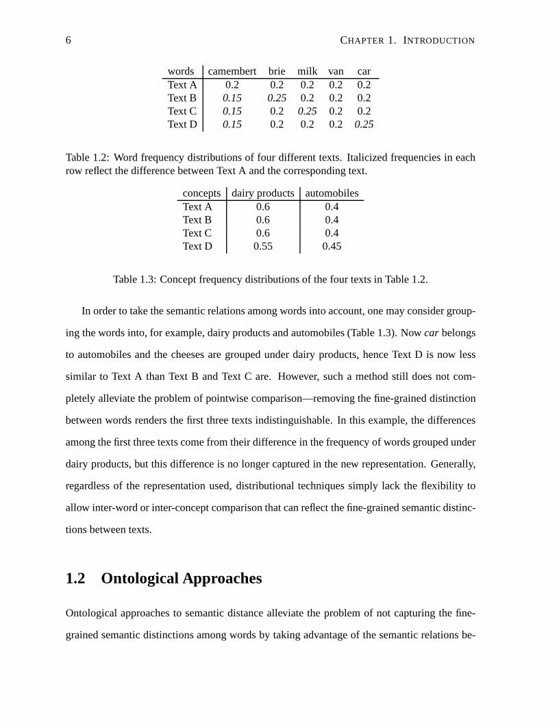
Consider the example in Table 1.2, where the four vectors represent the frequency distri-
bution of four texts. Distributionally, each of Texts B, C, or D is only slightly different from
Text A. That is, Texts B, C, and D result, respectively, from displacing a mass of 0.05 from
camembertin Text A to milk, brie, or car. Moreover, Text A is equally far away from Text B,
Text C, and Text D:
distancedistrib(A,B) = distancedistrib(A,C ) = distancedistrib(A,D) (1.2)
However, by only looking at pointwise differences between word frequency distributions, one
cannot take into account the fact that the words themselves are semantically related in varying
degrees—the semantic distance between different words maycontribute to the overall text
distance. For example,camembertis similar tobrie (both are cheeses), but less similar tomilk
(dairy products) and rather different fromvan andcar (entities). If we displace a frequency
mass in a distribution from one word (e.g.,camembert) to another word (e.g.,brie, milk, or
car), the impact on the overall distance should not only depend on the size of the mass, but
also on the source and the destination words of the displacement. In our example, because
brie, milk, andcar in Texts B, C, and D, are not equally distant fromcamembertin Text A, we
expect the distance from Text A to reflect as such:
distance(A,B) < distance(A,C ) < distance(A,D) (1.3)
6 CHAPTER 1. INTRODUCTION
words camembert brie milk van carText A 0.2 0.2 0.2 0.2 0.2Text B 0.15 0.25 0.2 0.2 0.2Text C 0.15 0.2 0.25 0.2 0.2Text D 0.15 0.2 0.2 0.2 0.25
Table 1.2: Word frequency distributions of four different texts. Italicized frequencies in eachrow reflect the difference between Text A and the corresponding text.
concepts dairy products automobilesText A 0.6 0.4Text B 0.6 0.4Text C 0.6 0.4Text D 0.55 0.45
Table 1.3: Concept frequency distributions of the four texts in Table 1.2.
In order to take the semantic relations among words into account, one may consider group-
ing the words into, for example, dairy products and automobiles (Table 1.3). Nowcar belongs
to automobiles and the cheeses are grouped under dairy products, hence Text D is now less
similar to Text A than Text B and Text C are. However, such a method still does not com-
pletely alleviate the problem of pointwise comparison—removing the fine-grained distinction
between words renders the first three texts indistinguishable. In this example, the differences
among the first three texts come from their difference in the frequency of words grouped under
dairy products, but this difference is no longer captured inthe new representation. Generally,
regardless of the representation used, distributional techniques simply lack the flexibility to
allow inter-word or inter-concept comparison that can reflect the fine-grained semantic distinc-
tions between texts.
1.2 Ontological Approaches
Ontological approaches to semantic distance alleviate theproblem of not capturing the fine-
grained semantic distinctions among words by taking advantage of the semantic relations be-
1.2. ONTOLOGICAL APPROACHES 7
tween concepts in an ontology. Since an ontology provides a graph structure, given that con-
cepts are connected via ontological relations, the semantic distance between two concepts can
be measured as the graphical distance within the ontology. The most straightforward way is to
count the number of edges on the shortest path connecting thetwo concepts. Alternatively, if
the ontology has a hierarchical structure (e.g., WordNet),one can consider a similarily mea-
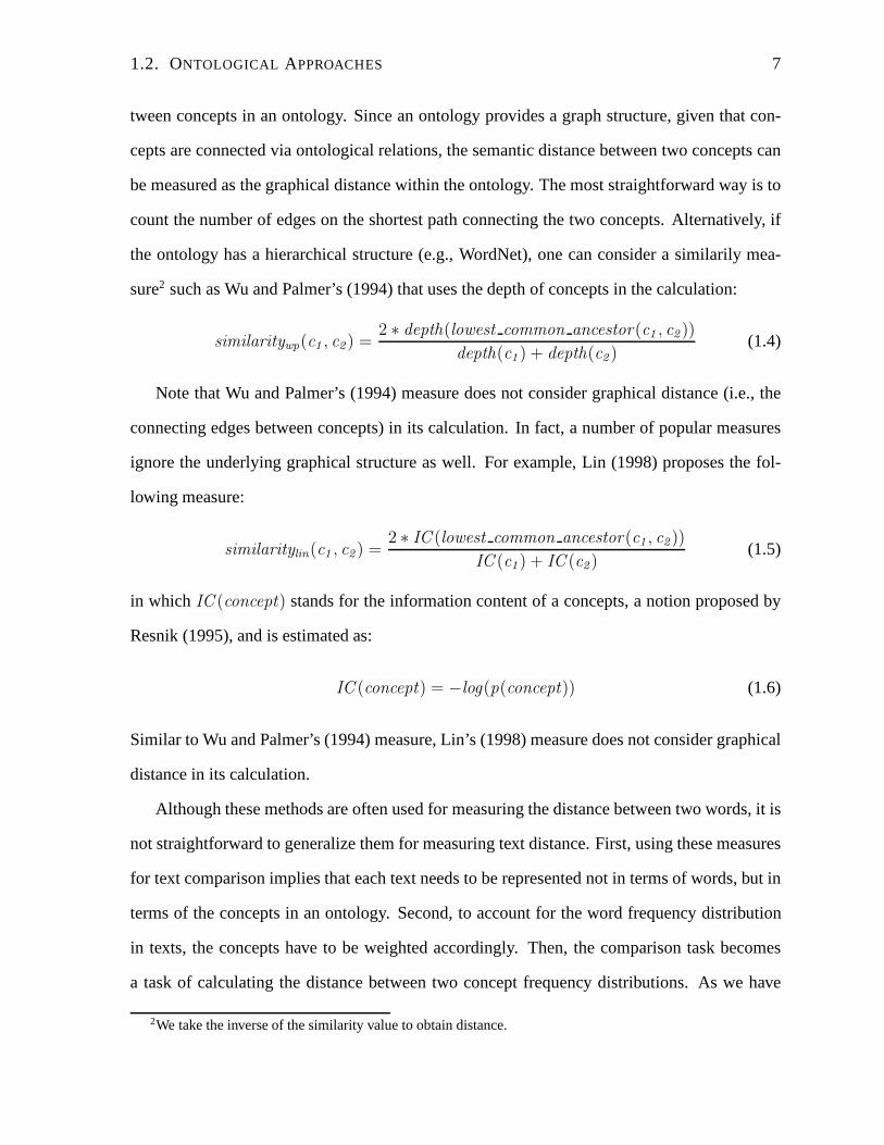
sure2 such as Wu and Palmer’s (1994) that uses the depth of conceptsin the calculation:
similaritywp(c1 , c2 ) =2 ∗ depth(lowest common ancestor(c1 , c2 ))
depth(c1 ) + depth(c2 )(1.4)
Note that Wu and Palmer’s (1994) measure does not consider graphical distance (i.e., the
connecting edges between concepts) in its calculation. In fact, a number of popular measures
ignore the underlying graphical structure as well. For example, Lin (1998) proposes the fol-
lowing measure:
similaritylin(c1 , c2 ) =2 ∗ IC (lowest common ancestor(c1 , c2 ))
IC (c1 ) + IC (c2 )(1.5)
in which IC (concept) stands for the information content of a concepts, a notion proposed by
Resnik (1995), and is estimated as:
IC (concept) = −log(p(concept)) (1.6)
Similar to Wu and Palmer’s (1994) measure, Lin’s (1998) measure does not consider graphical
distance in its calculation.
Although these methods are often used for measuring the distance between two words, it is
not straightforward to generalize them for measuring text distance. First, using these measures
for text comparison implies that each text needs to be represented not in terms of words, but in
terms of the concepts in an ontology. Second, to account for the word frequency distribution
in texts, the concepts have to be weighted accordingly. Then, the comparison task becomes
a task of calculating the distance between two concept frequency distributions. As we have
2We take the inverse of the similarity value to obtain distance.
8 CHAPTER 1. INTRODUCTION
emphasized earlier, by taking a purely distributional route, one can no longer take advantage of
the ontological structure to make finer-grained inter-wordor inter-concept distinctions between
texts.
One approach to comparing two texts might involve calculating the aggregate distance be-
tween the two resulting sets of concepts across the ontological relations. For example, we
mentioned Corley and Mihalcea’s (2005) work in which the semantic distance between the
two texts is calculated as the average, minimum, maximum, orsummed ontological distance
between the individual elements of the two sets of concepts.However, this approach ignores
distributional information of the texts, and hence treats all concepts as equally important in de-
termining the distance. Recall from Section 1.1 that the approaches which take the distribution
of concepts into account (e.g., McCarthy, 2001; Mohammad and Hirst, 2006) tend to ignore
the ontological relations among the concepts.
Our proposal is to capture both types of information with theaid of a graph-based method.
We will return to the details of our proposal in Section 1.4, after a brief description of current
uses of graph methods in NLP.
1.3 Graph-based Approaches in NLP
In recent years, we have seen an increasing use of graph-based methods in NLP (e.g., Pang
and Lee, 2004; Mihalcea, 2005; Navigli and Velardi, 2005). The graph-theoretic approach is
popular due to its elegance in representation, as well as theexistence of a large array of efficient
algorithms for graph processing. Graphs in general are a convenient mathematical formalism
to represent words or more complex semantic entities as nodes and the relationship between
them as edges.3 One of the most straightforward NLP examples is the use of WordNet as a
graph for measuring semantic relatedness (Rada et al., 1989; Wu and Palmer, 1994).
One popular graph method for NLP is the minimum-cut algorithm. For example, both
3The reverse is possible, though less intuitive, by using nodes to represent relations and edges for semanticentities. The choice of representation clearly depends on the NLP task itself.
1.4. OUR COMBINED APPROACH TOSEMANTIC DISTANCE 9
Pang and Lee (2004) and Barzilay and Lapata (2005) use minimum cut for two vastly differ-
ent applications, document polarity classification and content selection. In these works, the
sentences are represented as nodes in a graph and the edge connecting each pair of nodes is
weighted with an association score between the sentences (e.g., the distance between the sen-
tences in the text). The minimum-cut method partitions the nodes by finding the minimum cut
(the set of connecting edges with the minimum aggregate edgeweights). Thus, the sentences
are classified into different categories based on the node partition.
Another popular graph method is the random walk algorithm, which is successfully em-
ployed by the PageRank algorithm for ranking webpages (Brinand Page, 1998). The intuition
behind the algorithm is that the “popularity” (score) of a node depends on the “popularity” of
its neighbours. The more neighbours one has and/or the more popular the neighbours are, the
higher its popularity. This algorithm is useful when one wants to classify an item based on the
information contributed by related items. For example, Mihalcea (2006) uses random walk for
word sense disambiguation. In this work, each node represents an ambiguous (test) word, or a
(training) word labelled with one of its senses. Each edge indicates that the corresponding two
words co-occur in some context. The sense of an ambiguous word is determined by the sense
of its most relevant neighbour(s), by randomly traversing the graph until an equilibrium state
has been reached.
A graph-based method is necessary for us to take advantage ofthe intrinsic graph structure
of an ontology. More importantly, we need to choose an appropriate graph-based method which
calculates text distance that is simultaneously distribtional and ontological. In the next section,
we give an overview of our proposal which allows us to achievethis requirement.
1.4 Our Combined Approach to Semantic Distance
In our method, an ontology is treated as a graph in the usual manner, in which the concepts
are nodes and the relations are edges. A text can be represented as a collection of concepts in
10 CHAPTER 1. INTRODUCTION
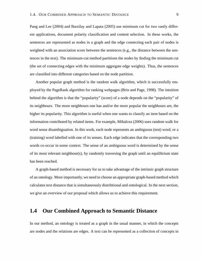
Figure 1.2: An illustration of two profiles within an ontology (the outer triangle). Each shaperepresents the nodes of one profile (representing a text) andthe size represents the mass (fre-quency) at a particular node in the ontology. Relations (edges) between concept nodes areomitted for simplicity.
the ontology, by mapping the words in the text into their corresponding concepts, which are
weighted according to the word frequencies. (We call the resulting set of frequency-weighted
concepts asemantic profile.) We can then use a graph-based method over the ontology to
calculate the frequency-weighted semantic distance between two profiles representing the two
texts to be compared.
Consider Figure 1.2, where we show a diagrammatic representation of an ontology (the
large open triangle) with two profiles representing two texts, one indicated with filled squares
and the other with filled triangles. The location of a filled shape indicates the location of a
profile concept in the ontology, and its size indicates its frequency within the profile. We
omit edges between the nodes for simplicity of the diagram, but note that we assume we have
a hierarchical, connected ontology (e.g., hyponymy links). Our proposal is to calculate the
distance between the two profiles by determining how much effort is required to transport,
along the ontological links, the frequency mass from all of the squares to “fill” the available
space in the triangles (or vice versa). The amount of mass to move and the amount of space
available are indicated by the size of the squares and triangles, respectively. Degree of effort to
transport one to the other indicates the degree of semantic distance.
Clearly, a graph-based method is necessary for us to take advantage of the intrinsic graph

1.4. OUR COMBINED APPROACH TOSEMANTIC DISTANCE 11
structure of an ontology. More importantly, it is crucial toselect an appropriate graph-based
method which achieves our goal to calculate text distance which is simultaneously distribu-
tional and ontological. As we have illustrated in Figure 1.2, to compare two texts, we calculate
the distance between the two corresponding profiles as the amount of “effort” required to trans-
form one profile to match the other graphically. To account for the ontological component of
the distance, observe that each profile can be viewed as a subgraph of the bigger graph repre-
senting the ontology. The edges that connect the two profilesare key to calculating the ontolog-
ical (graphical) distance between them. To account for the distributional component, observe
that each profile node is weighted according to the word-frequency distribution of a text. The
distributional difference can serve as a weighing factor tothe ontological distance. In short,
the weighted graphical distance is the desired distance. Ofall the existing graph formalisms,
network flow is the best formalism that best fits our specific set of requirements.
In this thesis, we explore a three-pronged approach in examining our non-dual framework
for text comparison. First, we demonstrate the usefulness of our method in three different
NLP tasks. Next, we examine the distributional and ontological sensitivity of our method to
the different types of texts involved in the task-based experiments. Finally, we look into the
method from an algorithmic perspective. Below, we present adetailed outline of the thesis, and
summarize the main contributions of our work.
In Chapter 2, we present our network-flow formalism for text comparison. Specifically,
we achieve our goal via a minimum-cost flow formulation. For our task, we have (i) a graph
structure based on the ontology; (ii) ontological distance(i.e., graphical distance) defined be-
tween concepts; and (iii) the profiles for each text (a concept frequency distribution). Given
this information, a minimum-cost flow problem definition allows us to (i) find a set of paths
connecting the two profiles such that (ii) the weighted sum ofthe paths’ distance, based on
the distributional difference of the two profiles, is minimum. Clearly, the resulting aggregate
distance is the desired text distance as it accounts for the ontological distance as well as the
distributional difference between texts.
12 CHAPTER 1. INTRODUCTION
Chapter 3 presents our task-based evaluation by testing ourmethod in three NLP tasks:
verb alternation detection (Section 3.1), name disambiguation (Section 3.2), and document
classification (Section 3.3). These applications are selected because they can be cast as a text
comparison task. However, they vary in how the set of words tobe compared is determined.
In the first task, the words have a particular syntactic relation to a target verb. In the second
task, the syntactic restriction is relaxed such that words appearing within a local window of an
ambiguous name are considered. Finally, in the last task, the window size restriction is also
relaxed such that words within a document are included.
Somewhat disappointingly, our method is not consistently successful across the three tasks.
Our network-flow method is found to be superior to state-of-the-art distributional methods in
verb alternation detection and name disambiguation but notso in the final task. To explain
the performance differential, we analyze various properties of the datasets in Chapter 4. We
begin with using simple distributional and graphical measures for our analysis, but they fail
to explain our method’s behaviour on the three datasets. This is unsurprising, given that there
are intricate interactions between the two types of knowledge within the network-flow method.
We propose a non-dually combined approach, calledprofile density, to measure the distribu-
tional and ontological coherence of a set of frequency-weighted concepts. Intuitively, profile
density within an ontology is analogous to the geographicalsense of population density. The
idea is based on the observation that data that is dispersed throughout the ontology are difficult
to separate into different distinct classes. In contrast, data that is concentrated within a number
of distinct regions of the ontology suggests a high semanticcoherence and therefore can be
classified more easily—distinct clusters of related concepts suggests a possible classification.
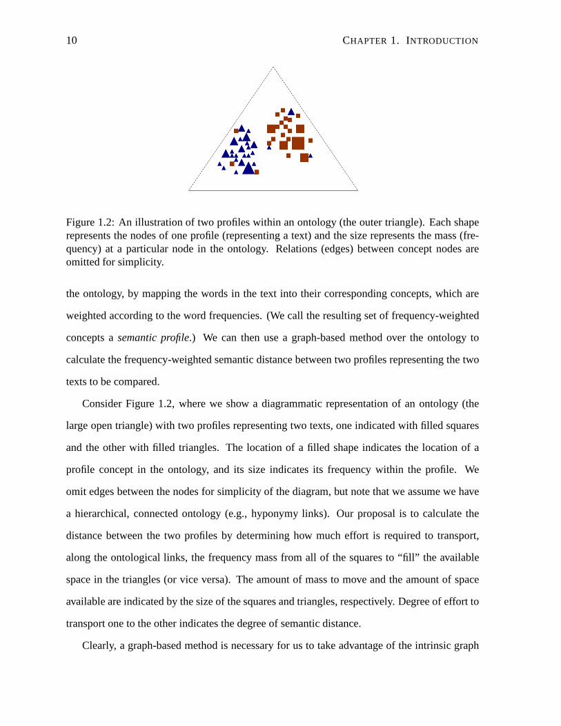
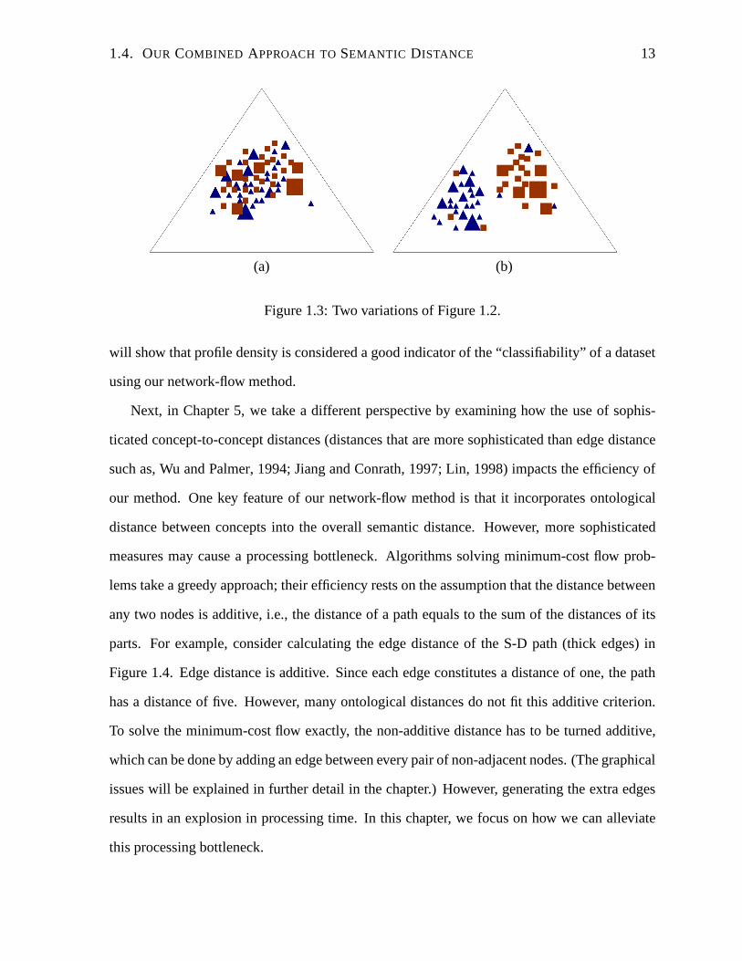
Consider two variations of Figure 1.2 in Figure 1.3. In comparison to diagram (a), the two
profiles in diagram (b) are clearly more easily recognized astwo separate clusters, which sug-
gests they may belong to two distinct classes. Similar to ournetwork-flow formulation for text
comparison, both the mass at the individual concept nodes and the distance between the masses
play a role in determining the density of a dataset. Indeed, by taking a combined approach, we
1.4. OUR COMBINED APPROACH TOSEMANTIC DISTANCE 13
(a) (b)
Figure 1.3: Two variations of Figure 1.2.
will show that profile density is considered a good indicatorof the “classifiability” of a dataset
using our network-flow method.
Next, in Chapter 5, we take a different perspective by examining how the use of sophis-
ticated concept-to-concept distances (distances that aremore sophisticated than edge distance
such as, Wu and Palmer, 1994; Jiang and Conrath, 1997; Lin, 1998) impacts the efficiency of
our method. One key feature of our network-flow method is thatit incorporates ontological
distance between concepts into the overall semantic distance. However, more sophisticated
measures may cause a processing bottleneck. Algorithms solving minimum-cost flow prob-
lems take a greedy approach; their efficiency rests on the assumption that the distance between
any two nodes is additive, i.e., the distance of a path equalsto the sum of the distances of its
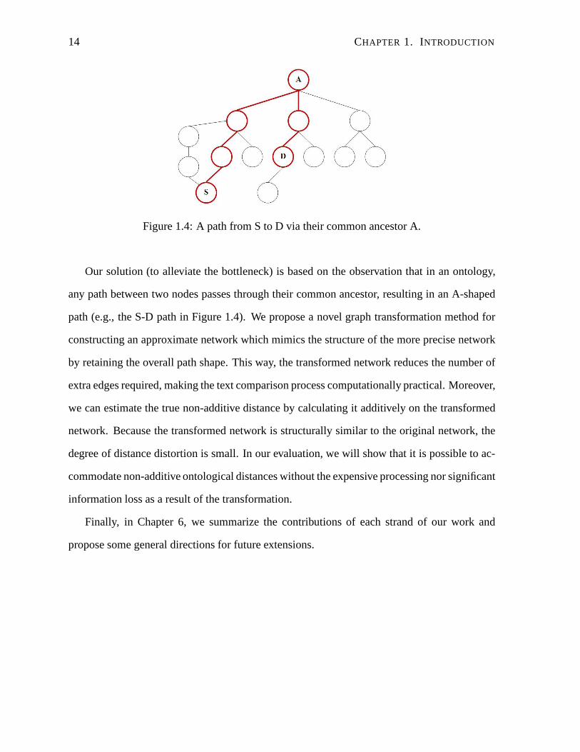
parts. For example, consider calculating the edge distanceof the S-D path (thick edges) in
Figure 1.4. Edge distance is additive. Since each edge constitutes a distance of one, the path
has a distance of five. However, many ontological distances do not fit this additive criterion.
To solve the minimum-cost flow exactly, the non-additive distance has to be turned additive,
which can be done by adding an edge between every pair of non-adjacent nodes. (The graphical
issues will be explained in further detail in the chapter.) However, generating the extra edges
results in an explosion in processing time. In this chapter,we focus on how we can alleviate
this processing bottleneck.
14 CHAPTER 1. INTRODUCTION
Figure 1.4: A path from S to D via their common ancestor A.
Our solution (to alleviate the bottleneck) is based on the observation that in an ontology,
any path between two nodes passes through their common ancestor, resulting in an A-shaped
path (e.g., the S-D path in Figure 1.4). We propose a novel graph transformation method for
constructing an approximate network which mimics the structure of the more precise network
by retaining the overall path shape. This way, the transformed network reduces the number of
extra edges required, making the text comparison process computationally practical. Moreover,
we can estimate the true non-additive distance by calculating it additively on the transformed
network. Because the transformed network is structurally similar to the original network, the
degree of distance distortion is small. In our evaluation, we will show that it is possible to ac-
commodate non-additive ontological distances without theexpensive processing nor significant
information loss as a result of the transformation.
Finally, in Chapter 6, we summarize the contributions of each strand of our work and
propose some general directions for future extensions.
Chapter 2
The Network Flow Method
Fred: – and one thing that keeps cropping up is this about “sub-
text.” Songs, novels, plays – they all have a subtext, which I take
to mean a hidden message or import of some kind.
Ted nods.
Fred: So subtext we know. But what do you call the meaning, or
message, that’s right there on the surface, completely open and
obvious? They never talk about that. What do you call what’s
above the subtext?
Ted: The text.
Fred: Okay. That’s right . . . But they never talk about that.
Whit Stillman, Barcelona
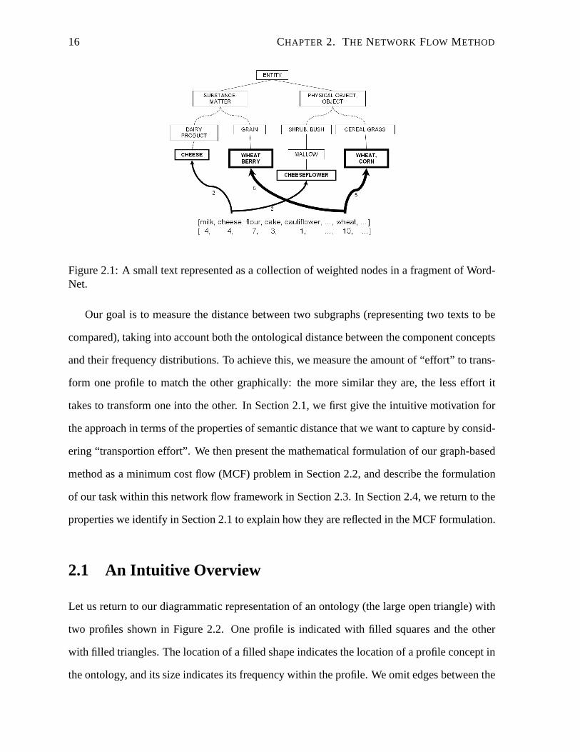
As noted in Chapter 1, we treat an ontology as a graph and represent a text as a semantic
profile—a collection of nodes in the graph (concepts in the ontology), each having a weight
(its frequency). For example, in Figure 2.1, a small text consisting of the wordscheeseand
wheat (among other words) with frequencies of 4 and 10, respectively, is represented as a
small weighted subgraph in an ontology by uniformly distributing the word frequencies among
the associated concepts. In this way, a text is a weighted subgraph within a larger graph (with
the thickness of the boxes in the figure indicating weight), and two such weighted subgraphs
are connected via a set of paths in the graph.
15
16 CHAPTER 2. THE NETWORK FLOW METHOD
Figure 2.1: A small text represented as a collection of weighted nodes in a fragment of Word-Net.
Our goal is to measure the distance between two subgraphs (representing two texts to be
compared), taking into account both the ontological distance between the component concepts
and their frequency distributions. To achieve this, we measure the amount of “effort” to trans-
form one profile to match the other graphically: the more similar they are, the less effort it
takes to transform one into the other. In Section 2.1, we firstgive the intuitive motivation for
the approach in terms of the properties of semantic distancethat we want to capture by consid-
ering “transportion effort”. We then present the mathematical formulation of our graph-based
method as a minimum cost flow (MCF) problem in Section 2.2, anddescribe the formulation
of our task within this network flow framework in Section 2.3.In Section 2.4, we return to the
properties we identify in Section 2.1 to explain how they arereflected in the MCF formulation.
2.1 An Intuitive Overview
Let us return to our diagrammatic representation of an ontology (the large open triangle) with
two profiles shown in Figure 2.2. One profile is indicated withfilled squares and the other
with filled triangles. The location of a filled shape indicates the location of a profile concept in
the ontology, and its size indicates its frequency within the profile. We omit edges between the
2.1. AN INTUITIVE OVERVIEW 17
(a)
(b) (c)
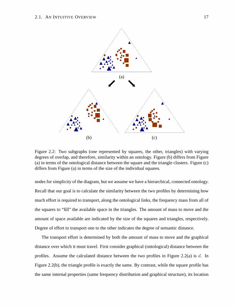
Figure 2.2: Two subgraphs (one represented by squares, the other, triangles) with varyingdegrees of overlap, and therefore, similarity within an ontology. Figure (b) differs from Figure(a) in terms of the ontological distance between the square and the triangle clusters. Figure (c)differs from Figure (a) in terms of the size of the individualsquares.
nodes for simplicity of the diagram, but we assume we have a hierarchical, connected ontology.
Recall that our goal is to calculate the similarity between the two profiles by determining how
much effort is required to transport, along the ontologicallinks, the frequency mass from all of
the squares to “fill” the available space in the triangles. The amount of mass to move and the
amount of space available are indicated by the size of the squares and triangles, respectively.
Degree of effort to transport one to the other indicates the degree of semantic distance.
The transport effort is determined by both the amount of massto move and the graphical
distance over which it must travel. First consider graphical (ontological) distance between the
profiles. Assume the calculated distance between the two profiles in Figure 2.2(a) isd. In
Figure 2.2(b), the triangle profile is exactly the same. By contrast, while the square profile has
the same internal properties (same frequency distributionand graphical structure), its location

18 CHAPTER 2. THE NETWORK FLOW METHOD
is further from the triangles. Since the two profiles occupy more distant portions of the on-
tological space, they are less semantically similar than inFigure 2.2(a). As desired, the extra
ontological distance over which the square frequency mass must be transported to the triangles
will cause the calculated distance in Figure 2.2(b) to be larger thand.
Next consider the effect of varying the frequency distribution over the profile nodes. Again,
in Figure 2.2(c), the triangle profile is exactly the same as in Figure 2.2(a). However, while the
nodes of the square profile in Figure 2.2(c) are in the same locations as in Figure 2.2(a), their
distributional properties are different. The bulk of the frequency distribution is now shifted
closer to the nodes of the triangle profile. Since the two profiles have more distributional
weight located closer within the ontology, this indicates that the semantic space they occupy
is more similar than in Figure 2.2(a). Correspondingly, since much of the mass of the square
profile needs to travel less far to fill the space of the triangle nodes, the calculated distance in
Figure 2.2(c) will be less thand.
These intuitive examples show that calculating semantic distance as “transport effort” cap-
tures in a well-motivated way both the ontological distancebetween the profiles and their
weighting by the distributional amounts of the concept nodes. Next we turn to a mathematical
formulation that captures these properties in a network flowframework.
2.2 Minimum Cost Flow
Our intuitive “transport effort” examples above can be viewed as a supply-demand problem,
in which we find the minimum cost flow (MCF) from the supply profile to the demand profile
to meet the requirements of the latter. Mathematically, letG = (N ,E ) be a connected graph
representing an ontology, whereN is the set of nodes representing the individual concepts, and
E is the set of edges representing the relations between the concepts.1 Each edge has a cost
c : E → R, which is the ontological distance of the edge. Each nodei ∈ N is associated
1Most ontologies are connected; in the case of a forest, adding an arbitrary root node yields a connected graph.
2.2. MINIMUM COST FLOW 19
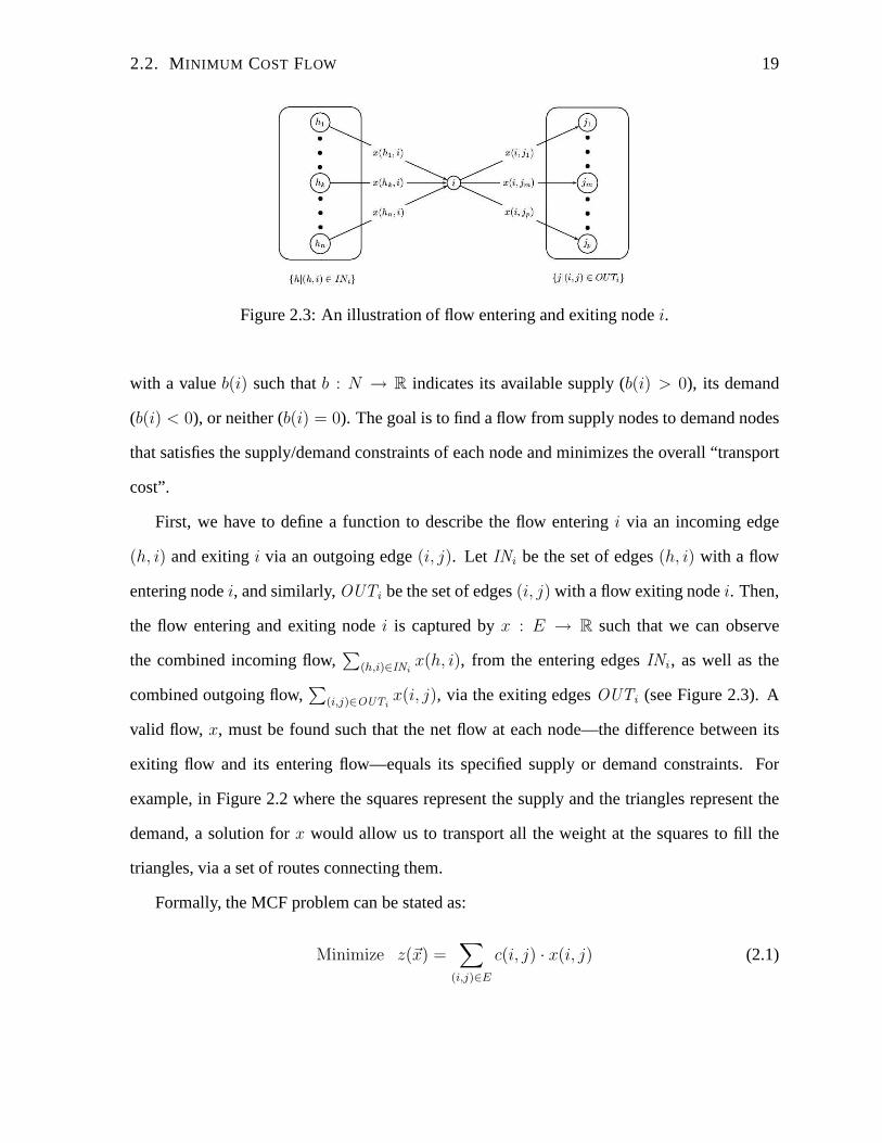
Figure 2.3: An illustration of flow entering and exiting nodei.
with a valueb(i) such thatb : N → R indicates its available supply (b(i) > 0), its demand
(b(i) < 0), or neither (b(i) = 0). The goal is to find a flow from supply nodes to demand nodes
that satisfies the supply/demand constraints of each node and minimizes the overall “transport
cost”.
First, we have to define a function to describe the flow entering i via an incoming edge
(h, i) and exitingi via an outgoing edge(i, j). Let INi be the set of edges(h, i) with a flow
entering nodei, and similarly,OUTi be the set of edges(i, j) with a flow exiting nodei. Then,
the flow entering and exiting nodei is captured byx : E → R such that we can observe
the combined incoming flow,∑
(h,i)∈INix(h, i), from the entering edgesINi , as well as the
combined outgoing flow,∑
(i,j)∈OUTix(i, j), via the exiting edgesOUTi (see Figure 2.3). A
valid flow, x, must be found such that the net flow at each node—the difference between its
exiting flow and its entering flow—equals its specified supplyor demand constraints. For
example, in Figure 2.2 where the squares represent the supply and the triangles represent the
demand, a solution forx would allow us to transport all the weight at the squares to fill the
triangles, via a set of routes connecting them.
Formally, the MCF problem can be stated as:
Minimize z(~x) =∑
(i,j)∈E
c(i, j) · x(i, j) (2.1)
20 CHAPTER 2. THE NETWORK FLOW METHOD
subject to∑
(i,j)∈OUTi
x(i, j) −∑
(h,i)∈INi
x(h, i) = b(i), ∀i ∈ N (2.2)
and x(i, j) ≥ 0, ∀(i, j) ∈ E (2.3)
The constraint specified by eqn. (2.2) ensures that the difference between the flow entering
and exiting each nodei matches its supply or demand (b(i)) exactly. The next constraint,
eqn. (2.3), ensures that the flow is transported from the supply to the demand but not in the
opposite direction. The calculation ofz in eqn. (2.1) (which is subject to these constraints)
multiplies the amount of flow travelling along each edge,x(i, j), by the transportation cost of
using that edge,c(i, j). Taking the summation over all edges of the productc(i, j) · x(i, j)
yields the desired “transport effort” of using the supply tofill the demand.
2.3 Semantic Distance as MCF
To cast our text comparison task into this framework, we firstrepresent each text as a semantic
profile in an ontology. The profile of one text is chosen as the supply (S) and the other as the
demand (D); our distance measure is symmetric, so this choice is arbitrary. In our examples in
Section 2.1, the square profile was seen as the supply and the triangle profile as the demand.
The concept frequencies of the profiles are normalized, so that the total supply equals the total
demand.
The cost of the routes between nodes is determined by a semantic distance measure defined
over the nodes in the ontology. A relation (such as hyponymy)between two conceptsi andj
is represented by an edge(i, j), and the costc on the edge(i, j) can be defined as the semantic
distance betweeni andj within the ontology. For simplicity in this paper, we use edge distance
as our semantic distance measurec; that is, each edge(i, j) has a cost of 1, and the distance
between any two concepts is the number of edges separating them.2
2Some semantic distances, such as those of Lin (1998) and Resnik (1995), do not take into account the under-
2.4. ONTOLOGICAL AND DISTRIBUTIONAL FACTORS IN MCF 21
Next, we must determine the value ofb(i) at each concept nodei. In the simple case,i
occurs in only one profile or the other. Ifi ∈ S, b(i) is set to the normalized supply frequency,
fS (i). If i ∈ D, b(i) is set to the negative of the normalized demand frequency, -fD(i), since
demand is indicated by a value less than zero. However,i may be part of both the supply and
demand profiles, and thenb(i) must be set to the net supply/demand at nodei. Thus we have:
b(i) = fS (i) − fD(i) (2.4)
For example, if the supply profile contains a nodecar with frequency of 0.25, and the same
node in the demand profile has a frequency of 0.7, thenb(car) is −0.45. In other words, the
nodecar has a net demand of 0.45.
Recall that our goal is to transport all the supply to meet thedemand—the key step is
to determine the optimal routes betweenS andD such that the constraints in eqn. (2.2) and
eqn. (2.3) are satisfied. The total distance of the routes, orthe MCF—z(~x) in eqn. (2.1)—is
the distance between the two semantic profiles.
2.4 Ontological and Distributional Factors in MCF
To see how the factors of ontological distance and frequencydistribution play out in the MCF
formulation, let’s return to our square and triangle profileexample. Consider a hypothetical
zoomed in area of the earlier diagram in Figure 2.2(a), shownin Figure 2.4. Here we assume
that the square nodes have a net supply (b(i) > 0) and the triangle nodes have a net demand
(b(i) < 0).3 The size of the square and triangle nodes in the figure indicates |b(i)|—i.e.,
the relative supply/demand, respectively. The circles indicate nodes with neither supply nor
demand constraints—i.e.,b(i) = 0. Each arrow from nodei to nodej indicates the source
lying graph structure of the ontology in calculating the distance between two concepts. Using this type of distancein our MCF framework requires an extra graph transformationstep; see Chapter 5 for more details.
3Earlier we made the simplifying assumption that square nodes were the supply profile and triangle nodes thedemand profile. We have now seen that a node can belong to both profiles, and its characterization more accuratelyis stated in terms ofnetsupply/demand. Thus, for example, a square node may belong to just the supply profileor to both the supply and demand profile; the defining factor isthat it has a net supply.
22 CHAPTER 2. THE NETWORK FLOW METHOD
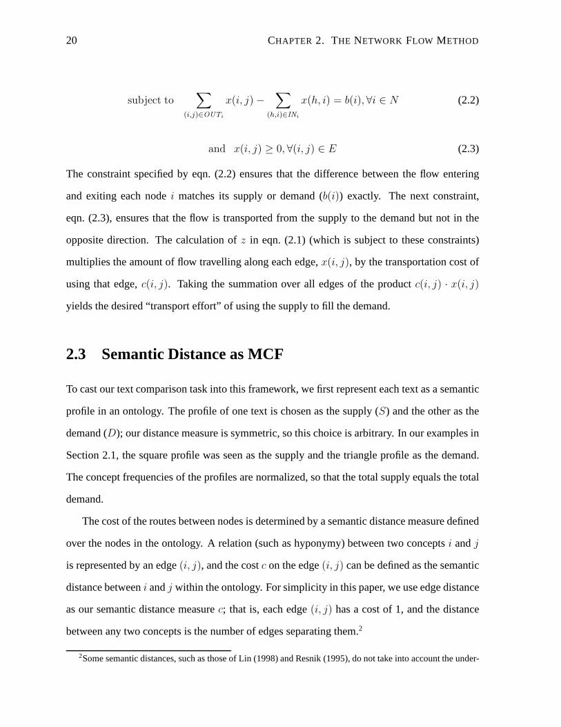
Figure 2.4: An example of transporting the weights at the square nodes (supply nodes) to thetriangle nodes (demand nodes). The circle nodes have zero supply/demand requirement.
and destination for transported flow from a square node to a triangle. The length of an arrow
represents the ontological distance,c(i, j), and the width indicates the amount of flow,x(i, j).
Note that both the ontological distance between nodes and the node weights are important in
determining the minimum cost flow. For example, the mass at the leftmost square is transported
over a path with one edge (as indicated by the arrow nearby) instead of a path with three edges
(with two circle nodes on the path). The mass at the rightmostsquare has to be distributed
over the two triangles, and the mass at the leftmost square istransported over a path with one
edge (as indicated by the arrow nearby) instead of a path withthree edges (with two circle
nodes on the path). The aggregated length and width of the three arrows corresponds to the
minimum cost flow, i.e, the semantic distance between the profiles represented by the squares
and triangles.
It is clear that ontological information plays a crucial role in the MCF formulation. If
the squares were further away from the triangles in the ontology in Figure 2.4—i.e., if more
edges separated the squares and the triangles—the sets of concepts they represent would be
less semantically similar. In other words, the length of thearrows (representingc(i, j)) would
be greater, and the resulting MCF would be larger, reflectingthe greater semantic distance
between the profiles. Distributional information in this method is equally critical to the distance
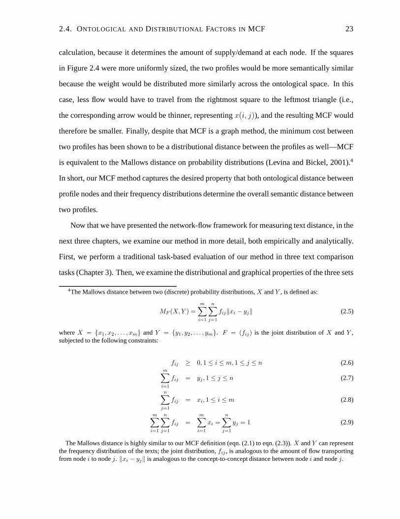
2.4. ONTOLOGICAL AND DISTRIBUTIONAL FACTORS IN MCF 23
calculation, because it determines the amount of supply/demand at each node. If the squares
in Figure 2.4 were more uniformly sized, the two profiles would be more semantically similar
because the weight would be distributed more similarly across the ontological space. In this
case, less flow would have to travel from the rightmost squareto the leftmost triangle (i.e.,
the corresponding arrow would be thinner, representingx(i, j)), and the resulting MCF would
therefore be smaller. Finally, despite that MCF is a graph method, the minimum cost between
two profiles has been shown to be a distributional distance between the profiles as well—MCF
is equivalent to the Mallows distance on probability distributions (Levina and Bickel, 2001).4
In short, our MCF method captures the desired property that both ontological distance between
profile nodes and their frequency distributions determine the overall semantic distance between
two profiles.
Now that we have presented the network-flow framework for measuring text distance, in the
next three chapters, we examine our method in more detail, both empirically and analytically.
First, we perform a traditional task-based evaluation of our method in three text comparison
tasks (Chapter 3). Then, we examine the distributional and graphical properties of the three sets
4The Mallows distance between two (discrete) probability distributions,X andY , is defined as:
MF (X, Y ) =
m∑
i=1
n∑
j=1
fij‖xi − yj‖ (2.5)
whereX = {x1, x2, . . . , xm} andY = {y1, y2, . . . , ym}. F = (fij) is the joint distribution ofX andY ,subjected to the following constraints:
fij ≥ 0, 1 ≤ i ≤ m, 1 ≤ j ≤ n (2.6)m
∑
i=1
fij = yj , 1 ≤ j ≤ n (2.7)
n∑
j=1
fij = xi, 1 ≤ i ≤ m (2.8)
m∑
i=1
n∑
j=1
fij =m
∑
i=1
xi =n
∑
j=1
yj = 1 (2.9)
The Mallows distance is highly similar to our MCF definition (eqn. (2.1) to eqn. (2.3)).X andY can representthe frequency distribution of the texts; the joint distribution, fij , is analogous to the amount of flow transportingfrom nodei to nodej. ‖xi − yj‖ is analogous to the concept-to-concept distance between nodei and nodej.

24 CHAPTER 2. THE NETWORK FLOW METHOD
of data in relation to our method’s performance (Chapter 4).Finally, we examine the method
from an algorithmic perspective (Chapter 5).
Chapter 3
Task-based Evaluation
In surfaces, perfection is less interesting. For instance, a page
with a poem on it is less attractive than a page with a poem on it
and some tea stains.
Anne Carson, “The Art of Poetry No. 88.” Interview with Will
Aitken. The Paris Review, Issue 171, Fall 2004.
We evaluate our network-flow method on three different NLP tasks that can be formulated as
text comparison problems based on semantic distance between the texts. In each case, the
texts to be compared are treated as bags of words with associated frequencies. The tasks are
chosen to reflect different types of relations used to extract the relevant words, to see if a
varying amount of constraint on the words comprising a text influences the performance of our
method.
In verb alternation detection (Section 3.1), we identify which verbs, out of a set of target
and filler verbs, allow a certain variation in the syntactic expression of their underlying ar-
gument structure. The task is achieved by comparing the set of head words that occur with
the verb in each of two different syntactic positions (e.g.,subject of intransitive and object of
transitive). In this task, the words that comprise the textsto be compared have a particular syn-
tactic relation to the verb under consideration. In proper name disambiguation (Section 3.2),
a variant of word sense disambiguation (WSD), we classify the sense of an ambiguous name
25
26 CHAPTER 3. TASK-BASED EVALUATION
according to its local context. We compare the text comprising the ambiguous instance to texts
representing each of the known referents of the name. Here, the words of a text are extracted
from a small window of occurrence around the target name token (25 words on each side), re-
gardless of syntactic relations among the words. For the known referents, the words from these
windows are aggregated across a small set of labelled instances. In document classification
(Section 3.3), a text is classified into one of a restricted number of topic categories. The text
to be classified consists of all the words in a document; for each topic, it is compared to a set
of words corresponding to a small set of known documents for that topic. The extracted words
are not constrained by syntactic relation (as in verb alternation) or even by distance to a target
element (as in name disambiguation).
In each case, the resulting bag of words for a text must be mapped into a semantic profile—
a frequency-weighted set of concepts in an ontology. Because all three of our tasks involve
general domain text, we use WordNet (Fellbaum, 1998). (A domain-restricted task may moti-
vate the use of a domain-specific ontology, such as UMLS for comparing medical texts as in
Bodenreider 2004.) Because the noun hierarchy of the WordNet ontology is most developed,
we restrict our semantic profiles to use only the nouns from the bag of words corresponding to
a text.
The bag of nouns with their associated frequencies must be mapped to the appropriate
concepts in WordNet. A simple method is to distribute the frequency of each word to its
corresponding concepts. For example, Ribas (1995) maps theword frequency to the most
specific concept(s) for the word, while Resnik (1993) distributes the word frequency across the
most specific concept(s) as well as their hypernyms. Other approaches estimate the appropriate
probability distribution over a set of concepts to represent a given bag of nouns as a whole,
rather than mapping each noun individually to its concepts (Li and Abe, 1998; Clark and Weir,
2002). For all three of our tasks, we map each noun individually to its most specific concepts,
uniformly dividing the word frequency among them. In verb alternation, we also experiment
with the possibility of finding the best set of frequency-weighted concepts for the full bag of
3.1. TASK 1: VERB ALTERNATION DETECTION 27
nouns, to see if this affects the performance of our method.
The precise classification experiment performed using these semantic profiles is described
in detail below in the section for each task. In each case, we compare the performance of our
MCF method on the semantic profiles to one or more purely distributional methods using the
original word frequencies.
3.1 Task 1: Verb Alternation Detection
Verb alternation refers to variations in the syntactic expression of verbal arguments. If a verb
participates in an alternation, the same underlying semantic argument may appear in varying
positions (slots) of the verb’s subcategorization frames.For example, the following sentences
show that the argument undergoing the melting action can appear as the subject of an intransi-
tive use ofmelt(1a) or as the object of a transitive use (1b).
1a. The chocolatemelted.
1b. The cook melted the chocolate.
This type of intransitive/transitive pairing is known as the causative alternation because of the
explicit expression of the causer (the cook) in the transitive alternant.
It has long been hypothesized that the semantics of a verb andits relations to its argu-
ments at least partially determine the syntactic expression of those arguments (see Pinker,
1989, among others). Influential work by Levin (1993) showedthat this relationship could be
exploited “in reverse” by using alternation behaviour as anindicator of the underlying seman-
tics of a verb—specifically, that verbs undergoing the same sets of alternations form classes
with similar semantics. Computational linguists have built on this work by demonstrating that
statistical cues to alternation behaviour can be used to automatically place verbs into semantic
classes (e.g., Merlo and Stevenson, 2001; Schulte im Walde,2006).
28 CHAPTER 3. TASK-BASED EVALUATION
Detection of verb alternation behaviour can be cast as a textcomparison problem (Merlo
and Stevenson, 2001; McCarthy, 2000). Consider an alternation, such as the causative illus-
trated in (1) above. The set of nouns appearing in the subjectof the intransitive (such as
chocolate) have the same relation to the verb as the set of nouns appearing in the object of the
transitive. Because the verb places constraints on what kinds of entities can be in that relation
(here, things that are meltable), the two sets of nouns should be similar. Hence, to identify a
particular alternation for a verb, the set of nouns in a certain slot of one of its subcategorization
frames is compared to the set of nouns in the alternating slotfor that semantic argument in
another subcategorization frame.
For example, Merlo and Stevenson (2001) devise a simple lemma overlap score that counts
the number of tokens appearing inboth of the relevant syntactic slots. McCarthy (2000) in-
stead compares two semantic profiles in WordNet that containthe concepts corresponding to
the nouns from the two argument positions. In McCarthy’s method, the profiles are first gen-
eralized to a set of higher level nodes in the hierarchy (starting with the method of Li and
Abe, 1998); next, skew divergence is used to find the distancebetween the resulting vectors
of concepts. Here we use our network flow method to directly compare the semantic profiles
corresponding to the noun sets. Our method allows us to compare sets of weighted concepts as
in McCarthy (2000), but using a distance method that applieswithin the ontology graph, rather
than simply using a distributional distance measure over concept vectors.
3.1.1 Experimental Setup
3.1.1.1 Experimental Verbs
We evaluate our method on the causative alternation. As noted above, in this alternation the
target syntactic slots for comparison are the subject of theintransitive (Subj-Intrans) and the
object of the transitive (Obj-Trans). (These are the positions ofthe chocolatein (1a) and (1b)
above, respectively.) To identify verbs undergoing this alternation, we randomly select verbs
3.1. TASK 1: VERB ALTERNATION DETECTION 29
from among Levin classes that are indicated to allow the causative alternation. This allows
us to test our method’s ability to detect alternation behaviour among verbs from a range of
semantic classes, which may differ in other respects.
We refer to the verbs that are expected to undergo the causative alternation as causative
verbs. For comparison, we randomly select an equal number offiller verbs, subject to the
constraint that their Levin classes do not allow a causativealternation. (Specifically, none of
the classes containing a filler verb allows an alternation inwhich the same underlying argument
appears in the Subj-Intrans slot as well as the Obj-Trans slot.) The full set of potential causative
and filler verbs are filtered according to corpus counts, as described next.
3.1.1.2 Corpus Data and Argument Extraction
We use a randomly selected 35M-word portion of the British National Corpus (BNC, Burnard,
2000). The text is parsed using the RASP parser of Briscoe andCarroll (2002), and subcate-
gorization frames are extracted using the system of Briscoeand Carroll (1997). Each subcate-
gorization frame entry for a verb includes a list of the observed argument heads per slot along
with their frequencies. For each verb/slot pair, we can thusextract the set of nouns used in that
slot along with their frequency of occurrence.
Verbs are filtered from the potential list of experimental items if they occur less than 10
times in our corpus in either the transitive or intransitiveframe. The verbs are then divided
into multiple frequency bands: high (at least 450 instances), medium (between 150 and 400
instances), and low (between 10 and 100 instances). An equalnumber of verbs of each type
(causative and filler) is randomly selected within each band, yielding a total of 120 experimen-
tal verbs in balanced datasets of 60 items for development and 60 items for testing. We evaluate
our method on the full set of 60 verbs in each of the datasets, as well as individually on the
three frequency bands of 20 verbs each.
30 CHAPTER 3. TASK-BASED EVALUATION
3.1.1.3 Comparing Semantic Profiles
For each verb, we create a semantic profile for each of the Subj-Intrans and Obj-Trans slots.
We map the argument head frequencies from the extracted subcategorization frame for the verb
to the corresponding nodes in WordNet, as described in the introduction of this chapter. (We
also consider here a different profile generation method, discussed later in Section 3.1.2.2.)
We then calculate the network flow distance between the two semantic profiles for each verb,
yielding a distance calculation for that verb. Recall that we expect verbs that participate in
the alternation to have more similar semantic profiles corresponding to the Subj-Intrans and
Obj-Trans nouns. We thus rank all the verbs by the distance calculation, and (as in McCarthy,
2000) set a threshold to divide the verbs into causative (smaller distance values) and non-
causative (larger distance values). Following McCarthy, we experimented with both the mean
and median values as the threshold, but found little difference. We report the results using the
median distance as the threshold, since this provided more consistent results with our method.
3.1.2 Results and Analysis
We present results on both development and test data, and also examine the effect of using
alternative profile generation methods. Because we label all verbs in our experiments, we use
accuracy as the performance measure; the random baseline (given our balanced datasets) is
50%. We compare our network-flow distance (NF) to a number of other distance measures
including probability distributional distances given by Jensen-Shannon divergence (JS) and
skew divergence (skew div) (Lee, 2001), as well as the general vector distances of cosine,
Manhattan distance, and Euclidean distance.
3.1.2.1 Development and Test Results
On the development data, our network flow distance performs better than or as well as all
other measures on the individual frequency bands. (See Table 3.1. Best performance in each
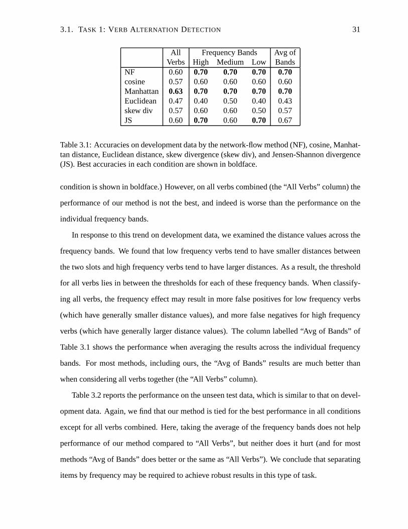
3.1. TASK 1: VERB ALTERNATION DETECTION 31
All Frequency Bands Avg ofVerbs High Medium Low Bands
NF 0.60 0.70 0.70 0.70 0.70cosine 0.57 0.60 0.60 0.60 0.60Manhattan 0.63 0.70 0.70 0.70 0.70Euclidean 0.47 0.40 0.50 0.40 0.43skew div 0.57 0.60 0.60 0.50 0.57JS 0.60 0.70 0.60 0.70 0.67
Table 3.1: Accuracies on development data by the network-flow method (NF), cosine, Manhat-tan distance, Euclidean distance, skew divergence (skew div), and Jensen-Shannon divergence(JS). Best accuracies in each condition are shown in boldface.
condition is shown in boldface.) However, on all verbs combined (the “All Verbs” column) the
performance of our method is not the best, and indeed is worsethan the performance on the
individual frequency bands.
In response to this trend on development data, we examined the distance values across the
frequency bands. We found that low frequency verbs tend to have smaller distances between
the two slots and high frequency verbs tend to have larger distances. As a result, the threshold
for all verbs lies in between the thresholds for each of thesefrequency bands. When classify-
ing all verbs, the frequency effect may result in more false positives for low frequency verbs
(which have generally smaller distance values), and more false negatives for high frequency
verbs (which have generally larger distance values). The column labelled “Avg of Bands” of
Table 3.1 shows the performance when averaging the results across the individual frequency
bands. For most methods, including ours, the “Avg of Bands” results are much better than
when considering all verbs together (the “All Verbs” column).
Table 3.2 reports the performance on the unseen test data, which is similar to that on devel-
opment data. Again, we find that our method is tied for the bestperformance in all conditions
except for all verbs combined. Here, taking the average of the frequency bands does not help
performance of our method compared to “All Verbs”, but neither does it hurt (and for most
methods “Avg of Bands” does better or the same as “All Verbs”). We conclude that separating
items by frequency may be required to achieve robust resultsin this type of task.
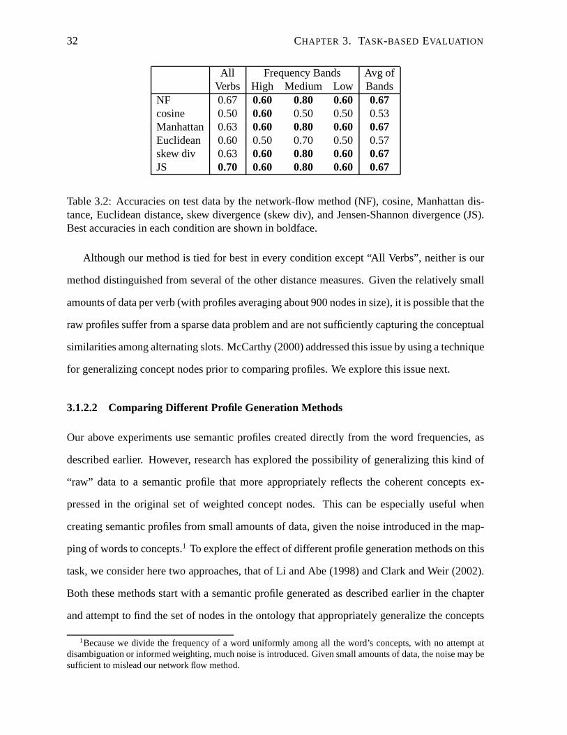
32 CHAPTER 3. TASK-BASED EVALUATION
All Frequency Bands Avg ofVerbs High Medium Low Bands
NF 0.67 0.60 0.80 0.60 0.67cosine 0.50 0.60 0.50 0.50 0.53Manhattan 0.63 0.60 0.80 0.60 0.67Euclidean 0.60 0.50 0.70 0.50 0.57skew div 0.63 0.60 0.80 0.60 0.67JS 0.70 0.60 0.80 0.60 0.67
Table 3.2: Accuracies on test data by the network-flow method(NF), cosine, Manhattan dis-tance, Euclidean distance, skew divergence (skew div), andJensen-Shannon divergence (JS).Best accuracies in each condition are shown in boldface.
Although our method is tied for best in every condition except “All Verbs”, neither is our
method distinguished from several of the other distance measures. Given the relatively small
amounts of data per verb (with profiles averaging about 900 nodes in size), it is possible that the
raw profiles suffer from a sparse data problem and are not sufficiently capturing the conceptual
similarities among alternating slots. McCarthy (2000) addressed this issue by using a technique
for generalizing concept nodes prior to comparing profiles.We explore this issue next.
3.1.2.2 Comparing Different Profile Generation Methods
Our above experiments use semantic profiles created directly from the word frequencies, as
described earlier. However, research has explored the possibility of generalizing this kind of
“raw” data to a semantic profile that more appropriately reflects the coherent concepts ex-
pressed in the original set of weighted concept nodes. This can be especially useful when
creating semantic profiles from small amounts of data, giventhe noise introduced in the map-
ping of words to concepts.1 To explore the effect of different profile generation methods on this
task, we consider here two approaches, that of Li and Abe (1998) and Clark and Weir (2002).
Both these methods start with a semantic profile generated asdescribed earlier in the chapter
and attempt to find the set of nodes in the ontology that appropriately generalize the concepts
1Because we divide the frequency of a word uniformly among allthe word’s concepts, with no attempt atdisambiguation or informed weighting, much noise is introduced. Given small amounts of data, the noise may besufficient to mislead our network flow method.
3.1. TASK 1: VERB ALTERNATION DETECTION 33
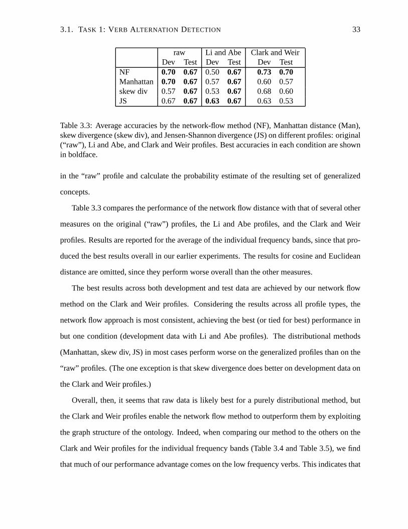
raw Li and Abe Clark and WeirDev Test Dev Test Dev Test
NF 0.70 0.67 0.50 0.67 0.73 0.70Manhattan 0.70 0.67 0.57 0.67 0.60 0.57skew div 0.57 0.67 0.53 0.67 0.68 0.60JS 0.67 0.67 0.63 0.67 0.63 0.53
Table 3.3: Average accuracies by the network-flow method (NF), Manhattan distance (Man),skew divergence (skew div), and Jensen-Shannon divergence(JS) on different profiles: original(“raw”), Li and Abe, and Clark and Weir profiles. Best accuracies in each condition are shownin boldface.
in the “raw” profile and calculate the probability estimate of the resulting set of generalized
concepts.
Table 3.3 compares the performance of the network flow distance with that of several other
measures on the original (“raw”) profiles, the Li and Abe profiles, and the Clark and Weir
profiles. Results are reported for the average of the individual frequency bands, since that pro-
duced the best results overall in our earlier experiments. The results for cosine and Euclidean
distance are omitted, since they perform worse overall thanthe other measures.
The best results across both development and test data are achieved by our network flow
method on the Clark and Weir profiles. Considering the results across all profile types, the
network flow approach is most consistent, achieving the best(or tied for best) performance in
but one condition (development data with Li and Abe profiles). The distributional methods
(Manhattan, skew div, JS) in most cases perform worse on the generalized profiles than on the
“raw” profiles. (The one exception is that skew divergence does better on development data on
the Clark and Weir profiles.)
Overall, then, it seems that raw data is likely best for a purely distributional method, but
the Clark and Weir profiles enable the network flow method to outperform them by exploiting
the graph structure of the ontology. Indeed, when comparingour method to the others on the
Clark and Weir profiles for the individual frequency bands (Table 3.4 and Table 3.5), we find
that much of our performance advantage comes on the low frequency verbs. This indicates that
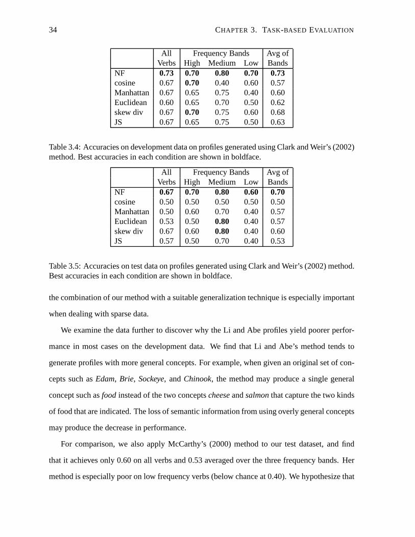
34 CHAPTER 3. TASK-BASED EVALUATION
All Frequency Bands Avg ofVerbs High Medium Low Bands
NF 0.73 0.70 0.80 0.70 0.73cosine 0.67 0.70 0.40 0.60 0.57Manhattan 0.67 0.65 0.75 0.40 0.60Euclidean 0.60 0.65 0.70 0.50 0.62skew div 0.67 0.70 0.75 0.60 0.68JS 0.67 0.65 0.75 0.50 0.63
Table 3.4: Accuracies on development data on profiles generated using Clark and Weir’s (2002)method. Best accuracies in each condition are shown in boldface.
All Frequency Bands Avg ofVerbs High Medium Low Bands
NF 0.67 0.70 0.80 0.60 0.70cosine 0.50 0.50 0.50 0.50 0.50Manhattan 0.50 0.60 0.70 0.40 0.57Euclidean 0.53 0.50 0.80 0.40 0.57skew div 0.67 0.60 0.80 0.40 0.60JS 0.57 0.50 0.70 0.40 0.53
Table 3.5: Accuracies on test data on profiles generated using Clark and Weir’s (2002) method.Best accuracies in each condition are shown in boldface.
the combination of our method with a suitable generalization technique is especially important
when dealing with sparse data.
We examine the data further to discover why the Li and Abe profiles yield poorer perfor-
mance in most cases on the development data. We find that Li andAbe’s method tends to
generate profiles with more general concepts. For example, when given an original set of con-
cepts such asEdam, Brie, Sockeye, andChinook, the method may produce a single general
concept such asfood instead of the two conceptscheeseandsalmonthat capture the two kinds
of food that are indicated. The loss of semantic informationfrom using overly general concepts
may produce the decrease in performance.
For comparison, we also apply McCarthy’s (2000) method to our test dataset, and find
that it achieves only 0.60 on all verbs and 0.53 averaged overthe three frequency bands. Her
method is especially poor on low frequency verbs (below chance at 0.40). We hypothesize that
3.2. TASK 2: NAME DISAMBIGUATION 35
her method is less robust to low frequency counts because it may overgeneralize the data by
first applying Li and Abe’s (1998)’s method, and then generalizing the nodes even further.
We see that while some amount of generalization of the semantic profiles is useful in this
task, overgeneralization may be harmful. We leave it to future work to explore the interaction
of our network flow method with different types of profile generation across various tasks.
Since the next two tasks we consider use larger amounts of data, we only experiment with raw
profiles in those cases.
3.2 Task 2: Name Disambiguation
Interest in the NLP problem of name disambiguation has increased as the growth of the World
Wide Web has led to large numbers of ambiguous name references in on-line text. For example,
websites or documents containing the nameJohn Edwardsmay refer to the U.S. presidential
candidate for 2008, an NBA basketball player, or a British medical geneticist. As in word
sense disambiguation, an ambiguous name may be resolved by comparing its local textual
context—the set of words it co-occurs with—with the local textual contexts of the name when
its reference is known. For example, the text surrounding the nameJohn Edwardsin its various
uses are very likely to include distinguishing words such aspolitician vs. gamevs. research.
Many approaches have been proposed for resolving name ambiguity by using distributional
methods over contextual information (e.g., Han et al., 2005; Pedersen et al., 2005; Xu et al.,
2003).
In this section, we present the application of our network flow distance measure to a name
disambiguation task, and demonstrate the benefits of combining ontological and distributional
knowledge in this task. The particular task we examine is oneof “pseudo name disambigua-
tion”, in which the texts containing matched pairs ofdifferentnames are extracted, and then the
two different names are replaced by a single symbol, leadingto an ambiguous “name” across
the two sets of texts. The goal is to recover the correct target name in each instance. For exam-
36 CHAPTER 3. TASK-BASED EVALUATION
ple, the names of two soccer players (Ronaldo and David Beckham) form one disambiguation
task, while the names of an ethnic group and a diplomat (Tajikand Rolf Ekeus) form another.
This task was established by Pedersen et al. (2005) to provide “annotated” experimental data
(with each text indicating the correct name), without the need for expensive manual annotation.
In Pedersen et al.’s (2005) work, an unsupervised method of name discrimination through
text clustering was used to address this task. This is infeasible for a method like ours, in
which each distance calculation requires access to an ontology. (The worst-case complexity of
clustering with our method is quadratic in the size of the ontology used; a detailed discussion
can be found in Chapter 5.) Instead, we use a supervised methodology, but experiment with
varying small amounts of data in a minimally supervised approach. Although our method
requires extra manual effort in the form of data annotation for training, we find that the amount
of annotated data required is modest.
3.2.1 Experimental Methodology
3.2.1.1 Corpus Data
We use Pedersen et al.’s (2005) dataset, which was taken fromthe Agence France Press English
Service portion of the GigaWord English corpus distributedby the Linguistic Data Consortium.
They extracted the local context of six pairs of names of varying confusability, including: the
names of two soccer players (Ronaldo and David Beckham); an ethnic group and a diplomat
(Tajik and Rolf Ekeus); two companies (Microsoft and IBM); two politicians (Shimon Peres
and Slobodan Milosevic); a nation and a nationality (Jordan and Egyptian); and two countries
(France and Japan). For each name instance, the extracted text consists of 50 words (25 words
to the left and to the right of the target name), with the target name obfuscated. For example,
for the task of distinguishing “David Beckham” and “Ronaldo”, the target name in each in-
stance becomes “DavidBeckhamRonaldo”. Each pair of names thus serves as one of sixname
disambiguation tasks. Table 3.6 shows the number of instances per task (name pair). The “Ma-
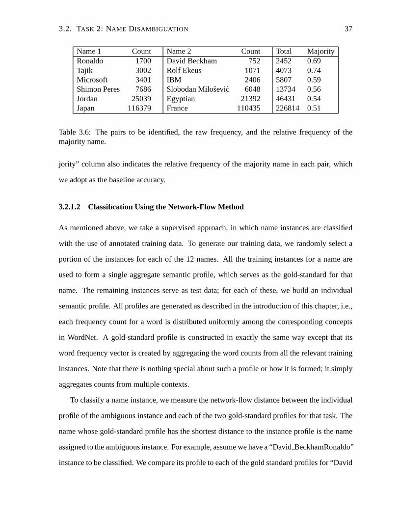
3.2. TASK 2: NAME DISAMBIGUATION 37
Name 1 Count Name 2 Count Total MajorityRonaldo 1700 David Beckham 752 2452 0.69Tajik 3002 Rolf Ekeus 1071 4073 0.74Microsoft 3401 IBM 2406 5807 0.59Shimon Peres 7686 Slobodan Milosevic 6048 13734 0.56Jordan 25039 Egyptian 21392 46431 0.54Japan 116379 France 110435 226814 0.51
Table 3.6: The pairs to be identified, the raw frequency, and the relative frequency of themajority name.
jority” column also indicates the relative frequency of themajority name in each pair, which
we adopt as the baseline accuracy.
3.2.1.2 Classification Using the Network-Flow Method
As mentioned above, we take a supervised approach, in which name instances are classified
with the use of annotated training data. To generate our training data, we randomly select a
portion of the instances for each of the 12 names. All the training instances for a name are
used to form a single aggregate semantic profile, which serves as the gold-standard for that
name. The remaining instances serve as test data; for each ofthese, we build an individual
semantic profile. All profiles are generated as described in the introduction of this chapter, i.e.,
each frequency count for a word is distributed uniformly among the corresponding concepts
in WordNet. A gold-standard profile is constructed in exactly the same way except that its
word frequency vector is created by aggregating the word counts from all the relevant training
instances. Note that there is nothing special about such a profile or how it is formed; it simply
aggregates counts from multiple contexts.
To classify a name instance, we measure the network-flow distance between the individual
profile of the ambiguous instance and each of the two gold-standard profiles for that task. The
name whose gold-standard profile has the shortest distance to the instance profile is the name
assigned to the ambiguous instance. For example, assume we have a “DavidBeckhamRonaldo”
instance to be classified. We compare its profile to each of thegold standard profiles for “David
38 CHAPTER 3. TASK-BASED EVALUATION
Beckham” and “Ronaldo” by measuring the distance between each of the two pairs of profiles.
If the instance profile has a shorter distance to the profile for “David Beckham” than to that of
“Ronaldo,” then it is classified as “David Beckham,” otherwise as “Ronaldo.”
3.2.1.3 Evaluation Methodology
We use the accuracy of labelling all instances as our evaluation measure. To compare to prior
results using F-measure, we report that in some tables. Since we label all instances, accuracy
and F-measure are equivalent, using2rp/(r + p) as the definition of F-measure.
The random baseline for our task is the accuracy of labellingall instances with the pre-
dominant name, as shown in the “Majority” column of Table 3.6. Since we use the dataset of
Pedersen et al. (2005), we compare our performance to their distributional method (reporting
their best results both with and without singular value decomposition). Because their method
is an unsupervised one, we also train and test a supervised learner using distributional data
(LIBSVM by Chang and Lin, 2001). For each set of training data, we remove stopwords and
use the remaining words as input features for the SVM. We thenobtain the optimal parameters
(i.e., optimal values for cost and gamma in LIBSVM) by using 10-fold cross-validation over
the training data. Finally, we perform classification on thetest data using those parameters.
This enables us to compare our results to a purely distributional method with access to the
same training data.
Because our method is supervised, it is important to minimize the amount of annotated
data required to build the gold-standard profiles.2 Since it is unclear a priori what amount of
training data is sufficient, we experiment with several quantities. We initially select 200 random
instances per pair of names, respecting the relative proportions of the two names overall. (200
instances constitute about 0.1–10% of the data per pair of names.) Subsequently, we decrease
the quantity further, to one-half and one-quarter the original amount (100 and 50 instances,
2Lengthy training time can also be an issue for a supervised method, but here “training” is the straightforwardtask of building an aggregate semantic profile.
3.2. TASK 2: NAME DISAMBIGUATION 39
respectively) to observe how the performance is influenced by the amount of data used to
construct the gold standard profiles.3 To reduce the impact of possible skewed sampling of
training data, we repeat the random sampling five times, withno overlap between the random
samples. We report the performance of each sample set as wellas the average over the five
samples.
3.2.2 Results and Analysis
3.2.2.1 Initial Experiments
Table 3.7 shows the performance of our method over five randomsamples of 200 training
instances per task. Observe that the performance over the five rounds varies very little (a
maximum difference of 0.08, and most are much closer). This shows the robustness of our
method to different make-ups of training data. Table 3.8 shows the average performance of
our method, in comparison to the chance (majority) baseline, as well as the results produced
by the unsupervised method of Pedersen et al. (2005) (with singular value decomposition—
SVD—reported as Ped05SVD, and without SVD as Ped05), and the supervised SVM on the
same training data as our method. Observe that our method notonly significantly outperforms
the random baseline, it is moreover the best performer amongst all the methods (paired t-test,
p < 0.05).
There are cases for which Pedersen et al.’s methods have at best chance performance (Mi-
crosoft/IBM and Japan/France). The authors suggest that these pairs of names arise in contexts
of news text in which there are “no consistently strong discriminating features” useful in the
clustering algorithm. (Interestingly, this is the case even with SVD, where words are grouped
into a small number of unnamed concepts.) Even the SVM has difficulty with these pairs, also
3We also experiment with 400 training instances to see whether increasing the amount of training data helps.The performance benefit is minimal: two tasks have the same average performance, three improve by 1%, andone by 2%, with an improvement in the average over all the tasks of 1.25%. A paired t-test between the results on400 and 200 training instances yields a highp value (p = 0.73), indicating that the differences between the twoare statistically insignificant.
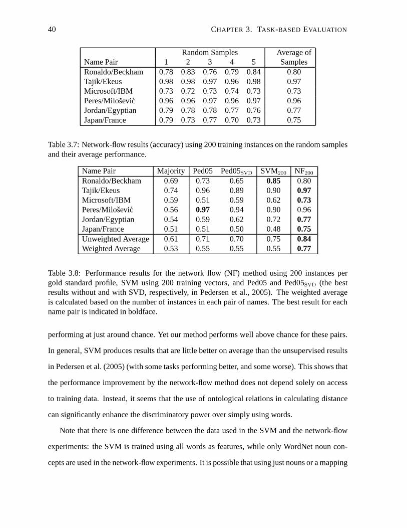
40 CHAPTER 3. TASK-BASED EVALUATION
Random Samples Average ofName Pair 1 2 3 4 5 SamplesRonaldo/Beckham 0.78 0.83 0.76 0.79 0.84 0.80Tajik/Ekeus 0.98 0.98 0.97 0.96 0.98 0.97Microsoft/IBM 0.73 0.72 0.73 0.74 0.73 0.73Peres/Milosevic 0.96 0.96 0.97 0.96 0.97 0.96Jordan/Egyptian 0.79 0.78 0.78 0.77 0.76 0.77Japan/France 0.79 0.73 0.77 0.70 0.73 0.75
Table 3.7: Network-flow results (accuracy) using 200 training instances on the random samplesand their average performance.
Name Pair Majority Ped05 Ped05SVD SVM200 NF200
Ronaldo/Beckham 0.69 0.73 0.65 0.85 0.80Tajik/Ekeus 0.74 0.96 0.89 0.90 0.97Microsoft/IBM 0.59 0.51 0.59 0.62 0.73Peres/Milosevic 0.56 0.97 0.94 0.90 0.96Jordan/Egyptian 0.54 0.59 0.62 0.72 0.77Japan/France 0.51 0.51 0.50 0.48 0.75Unweighted Average 0.61 0.71 0.70 0.75 0.84Weighted Average 0.53 0.55 0.55 0.55 0.77
Table 3.8: Performance results for the network flow (NF) method using 200 instances pergold standard profile, SVM using 200 training vectors, and Ped05 and Ped05SVD (the bestresults without and with SVD, respectively, in Pedersen et al., 2005). The weighted averageis calculated based on the number of instances in each pair ofnames. The best result for eachname pair is indicated in boldface.
performing at just around chance. Yet our method performs well above chance for these pairs.
In general, SVM produces results that are little better on average than the unsupervised results
in Pedersen et al. (2005) (with some tasks performing better, and some worse). This shows that
the performance improvement by the network-flow method doesnot depend solely on access
to training data. Instead, it seems that the use of ontological relations in calculating distance
can significantly enhance the discriminatory power over simply using words.
Note that there is one difference between the data used in theSVM and the network-flow
experiments: the SVM is trained using all words as features,while only WordNet noun con-
cepts are used in the network-flow experiments. It is possible that using just nouns or a mapping
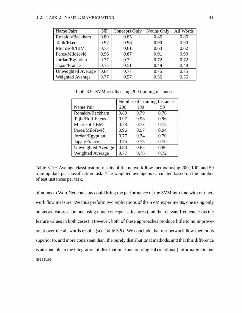
3.2. TASK 2: NAME DISAMBIGUATION 41
Name Pairs NF Concepts Only Nouns Only All WordsRonaldo/Beckham 0.80 0.85 0.86 0.85Tajik/Ekeus 0.97 0.96 0.90 0.90Microsoft/IBM 0.73 0.61 0.63 0.62Peres/Milosevic 0.96 0.87 0.91 0.90Jordan/Egyptian 0.77 0.72 0.72 0.72Japan/France 0.75 0.51 0.49 0.48Unweighted Average 0.84 0.77 0.75 0.75Weighted Average 0.77 0.57 0.56 0.55
Table 3.9: SVM results using 200 training instances.
Number of Training InstancesName Pair 200 100 50Ronaldo/Beckham 0.80 0.79 0.76Tajik/Rolf Ekeus 0.97 0.98 0.96Microsoft/IBM 0.73 0.73 0.72Peres/Milosevic 0.96 0.97 0.94Jordan/Egyptian 0.77 0.74 0.70Japan/France 0.75 0.75 0.70Unweighted Average 0.83 0.83 0.80Weighted Average 0.77 0.76 0.72
Table 3.10: Average classification results of the network flow method using 200, 100, and 50training data per classification task. The weighted averageis calculated based on the numberof test instances per task.
of nouns to WordNet concepts could bring the performance of the SVM into line with our net-
work flow measure. We thus perform two replications of the SVMexperiments, one using only
nouns as features and one using noun concepts as features (and the relevant frequencies as the
feature values in both cases). However, both of these approaches produce little to no improve-
ment over the all-words results (see Table 3.9). We concludethat our network-flow method is
superior to, and more consistent than, the purely distributional methods, and that this difference
is attributable to the integration of distributional and ontological (relational) information in our
measure.
42 CHAPTER 3. TASK-BASED EVALUATION
3.2.2.2 Reducing the Amount of Training Data
Because, in contrast to Pedersen et al. (2005), we use a supervised approach, we want to de-
termine whether we can reduce our dependence on training data. Here, we report experiments
using one-half (100 instances) and one-quarter (50 instances) of the training data used above.
As before, we repeat the random sampling of the training instances five times in each case, and
report the average performance here.
Table 3.10 shows the network flow performance for 200, 100, and 50 training instances.
Numerically, the results do not differ by much when the training data is reduced from 200 to
100 instances, and a paired t-test finds the difference to be non-significant. The performance
drop is more pronounced in the 50-instance experiment, where every pair of names shows
some drop in performance compared to 100 instances. Here, a paired t-test shows that the
performance drop in the 50-instance experiment is statistically significant (p = 0.04). Despite
this, we still outperform the other methods: our results using 50 training instances are much
better than those of Pedersen et al. (2005) in all but one task, and even better overall than the
SVM using 200 training instances (compare the SVM column of Table 3.8).
For comparison, we also train the SVM on 100 training instances, and find a decrease
of 3% on average from using 200 training instances. We conclude that our method is more
robust to minimal training conditions. To explore the leastamount of training data needed
for our measure, we further reduce the amount for producing gold-standard profiles to 20 and
5 instances per task, and observe a continual drop in performance. The performance of one
task (Ronaldo/David Beckham) drops below chance with 20 training instances and another
(Microsoft/IBM) drops below chance with 5. For this set of data, we conclude that a minimum
of 50 instances per task are required to provide enough discriminating power for our method.
Although unsupervised methods have the advantage of requiring no training data, in our
case, 50 to 100 training instances constitute only a very small portion of the data, as well as
a small amount of annotation effort in absolute terms. We conclude that the (small) labelling
effort is justified by the performance gain achieved using our minimally-supervised approach.
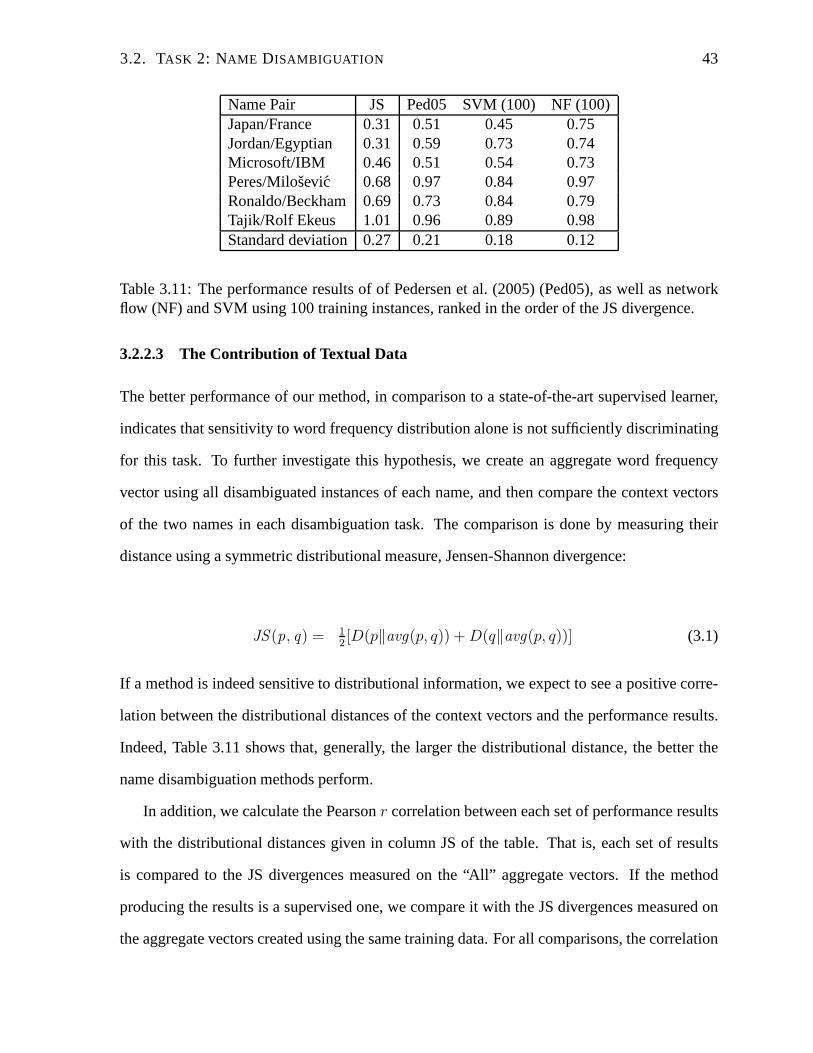
3.2. TASK 2: NAME DISAMBIGUATION 43
Name Pair JS Ped05 SVM (100) NF (100)Japan/France 0.31 0.51 0.45 0.75Jordan/Egyptian 0.31 0.59 0.73 0.74Microsoft/IBM 0.46 0.51 0.54 0.73Peres/Milosevic 0.68 0.97 0.84 0.97Ronaldo/Beckham 0.69 0.73 0.84 0.79Tajik/Rolf Ekeus 1.01 0.96 0.89 0.98Standard deviation 0.27 0.21 0.18 0.12
Table 3.11: The performance results of of Pedersen et al. (2005) (Ped05), as well as networkflow (NF) and SVM using 100 training instances, ranked in the order of the JS divergence.
3.2.2.3 The Contribution of Textual Data
The better performance of our method, in comparison to a state-of-the-art supervised learner,
indicates that sensitivity to word frequency distributionalone is not sufficiently discriminating
for this task. To further investigate this hypothesis, we create an aggregate word frequency
vector using all disambiguated instances of each name, and then compare the context vectors
of the two names in each disambiguation task. The comparisonis done by measuring their
distance using a symmetric distributional measure, Jensen-Shannon divergence:
JS (p, q) = 12[D(p‖avg(p, q)) + D(q‖avg(p, q))] (3.1)
If a method is indeed sensitive to distributional information, we expect to see a positive corre-
lation between the distributional distances of the contextvectors and the performance results.
Indeed, Table 3.11 shows that, generally, the larger the distributional distance, the better the
name disambiguation methods perform.
In addition, we calculate the Pearsonr correlation between each set of performance results
with the distributional distances given in column JS of the table. That is, each set of results
is compared to the JS divergences measured on the “All” aggregate vectors. If the method
producing the results is a supervised one, we compare it withthe JS divergences measured on
the aggregate vectors created using the same training data.For all comparisons, the correlation
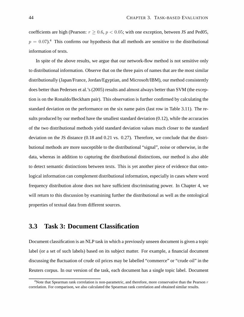
44 CHAPTER 3. TASK-BASED EVALUATION
coefficients are high (Pearson:r ≥ 0.6, p < 0.05; with one exception, between JS and Ped05,
p = 0.07).4 This confirms our hypothesis that all methods are sensitive to the distributional
information of texts.
In spite of the above results, we argue that our network-flow method is not sensitive only
to distributional information. Observe that on the three pairs of names that are the most similar
distributionally (Japan/France, Jordan/Egyptian, and Microsoft/IBM), our method consistently
does better than Pedersen et al.’s (2005) results and almostalways better than SVM (the excep-
tion is on the Ronaldo/Beckham pair). This observation is further confirmed by calculating the
standard deviation on the performance on the six name pairs (last row in Table 3.11). The re-
sults produced by our method have the smallest standard deviation (0.12), while the accuracies
of the two distributional methods yield standard deviationvalues much closer to the standard
deviation on the JS distance (0.18 and 0.21 vs. 0.27). Therefore, we conclude that the distri-
butional methods are more susceptible to the distributional “signal”, noise or otherwise, in the
data, whereas in addition to capturing the distributional distinctions, our method is also able
to detect semantic distinctions between texts. This is yet another piece of evidence that onto-
logical information can complement distributional information, especially in cases where word
frequency distribution alone does not have sufficient discriminating power. In Chapter 4, we
will return to this discussion by examining further the distributional as well as the ontological
properties of textual data from different sources.
3.3 Task 3: Document Classification
Document classification is an NLP task in which a previously unseen document is given a topic
label (or a set of such labels) based on its subject matter. For example, a financial document
discussing the fluctuation of crude oil prices may be labelled “commerce” or “crude oil” in the
Reuters corpus. In our version of the task, each document hasa single topic label. Document
4Note that Spearman rank correlation is non-parametric, andtherefore, more conservative than the Pearsonr
correlation. For comparison, we also calculated the Spearman rank correlation and obtained similar results.
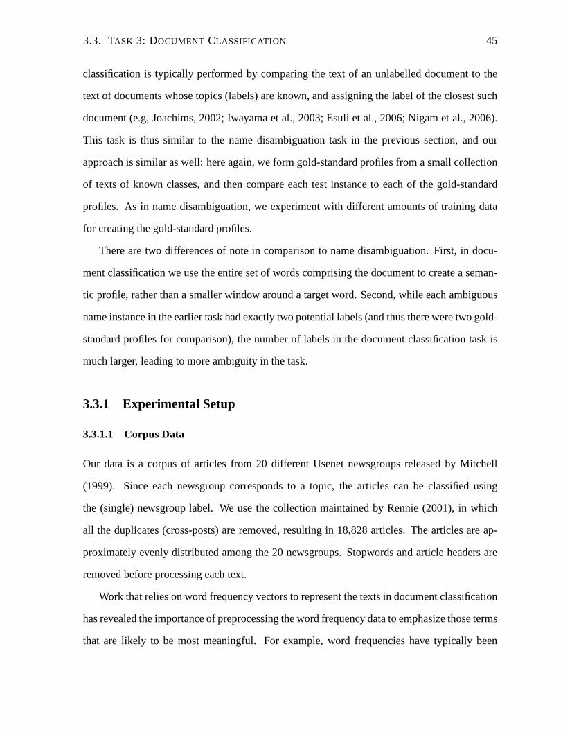
3.3. TASK 3: DOCUMENT CLASSIFICATION 45
classification is typically performed by comparing the textof an unlabelled document to the
text of documents whose topics (labels) are known, and assigning the label of the closest such
document (e.g, Joachims, 2002; Iwayama et al., 2003; Esuli et al., 2006; Nigam et al., 2006).
This task is thus similar to the name disambiguation task in the previous section, and our
approach is similar as well: here again, we form gold-standard profiles from a small collection
of texts of known classes, and then compare each test instance to each of the gold-standard
profiles. As in name disambiguation, we experiment with different amounts of training data
for creating the gold-standard profiles.
There are two differences of note in comparison to name disambiguation. First, in docu-
ment classification we use the entire set of words comprisingthe document to create a seman-
tic profile, rather than a smaller window around a target word. Second, while each ambiguous
name instance in the earlier task had exactly two potential labels (and thus there were two gold-
standard profiles for comparison), the number of labels in the document classification task is
much larger, leading to more ambiguity in the task.
3.3.1 Experimental Setup
3.3.1.1 Corpus Data
Our data is a corpus of articles from 20 different Usenet newsgroups released by Mitchell
(1999). Since each newsgroup corresponds to a topic, the articles can be classified using
the (single) newsgroup label. We use the collection maintained by Rennie (2001), in which
all the duplicates (cross-posts) are removed, resulting in18,828 articles. The articles are ap-
proximately evenly distributed among the 20 newsgroups. Stopwords and article headers are
removed before processing each text.
Work that relies on word frequency vectors to represent the texts in document classification
has revealed the importance of preprocessing the word frequency data to emphasize those terms
that are likely to be most meaningful. For example, word frequencies have typically been
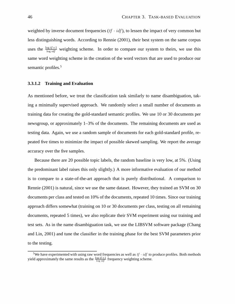
46 CHAPTER 3. TASK-BASED EVALUATION
weighted by inverse document frequencies (tf · idf ), to lessen the impact of very common but
less distinguishing words. According to Rennie (2001), their best system on the same corpus
uses thelog tf +1log idf
weighting scheme. In order to compare our system to theirs, we use this
same word weighting scheme in the creation of the word vectors that are used to produce our
semantic profiles.5
3.3.1.2 Training and Evaluation
As mentioned before, we treat the classification task similarly to name disambiguation, tak-
ing a minimally supervised approach. We randomly select a small number of documents as
training data for creating the gold-standard semantic profiles. We use 10 or 30 documents per
newsgroup, or approximately 1–3% of the documents. The remaining documents are used as
testing data. Again, we use a random sample of documents for each gold-standard profile, re-
peated five times to minimize the impact of possible skewed sampling. We report the average
accuracy over the five samples.
Because there are 20 possible topic labels, the random baseline is very low, at 5%. (Using
the predominant label raises this only slightly.) A more informative evaluation of our method
is to compare to a state-of-the-art approach that is purely distributional. A comparison to
Rennie (2001) is natural, since we use the same dataset. However, they trained an SVM on 30
documents per class and tested on 10% of the documents, repeated 10 times. Since our training
approach differs somewhat (training on 10 or 30 documents per class, testing on all remaining
documents, repeated 5 times), we also replicate their SVM experiment using our training and
test sets. As in the name disambiguation task, we use the LIBSVM software package (Chang
and Lin, 2001) and tune the classifier in the training phase for the best SVM parameters prior
to the testing.
5We have experimented with using raw word frequencies as wellastf · idf to produce profiles. Both methodsyield approximately the same results as thelog tf +1
log idffrequency weighting scheme.
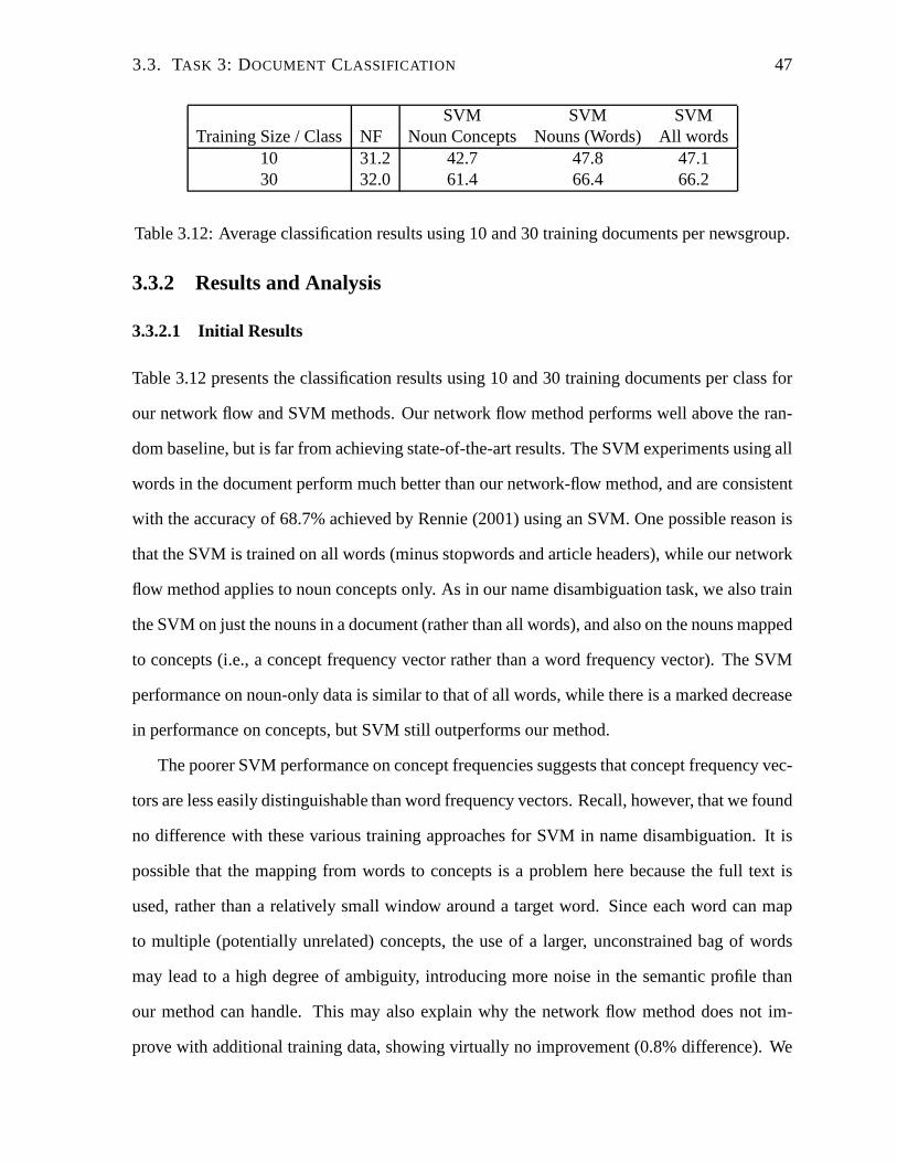
3.3. TASK 3: DOCUMENT CLASSIFICATION 47
SVM SVM SVMTraining Size / Class NF Noun Concepts Nouns (Words) All words
10 31.2 42.7 47.8 47.130 32.0 61.4 66.4 66.2
Table 3.12: Average classification results using 10 and 30 training documents per newsgroup.
3.3.2 Results and Analysis
3.3.2.1 Initial Results
Table 3.12 presents the classification results using 10 and 30 training documents per class for
our network flow and SVM methods. Our network flow method performs well above the ran-
dom baseline, but is far from achieving state-of-the-art results. The SVM experiments using all
words in the document perform much better than our network-flow method, and are consistent
with the accuracy of 68.7% achieved by Rennie (2001) using anSVM. One possible reason is
that the SVM is trained on all words (minus stopwords and article headers), while our network
flow method applies to noun concepts only. As in our name disambiguation task, we also train
the SVM on just the nouns in a document (rather than all words), and also on the nouns mapped
to concepts (i.e., a concept frequency vector rather than a word frequency vector). The SVM
performance on noun-only data is similar to that of all words, while there is a marked decrease
in performance on concepts, but SVM still outperforms our method.
The poorer SVM performance on concept frequencies suggeststhat concept frequency vec-
tors are less easily distinguishable than word frequency vectors. Recall, however, that we found
no difference with these various training approaches for SVM in name disambiguation. It is
possible that the mapping from words to concepts is a problemhere because the full text is
used, rather than a relatively small window around a target word. Since each word can map
to multiple (potentially unrelated) concepts, the use of a larger, unconstrained bag of words
may lead to a high degree of ambiguity, introducing more noise in the semantic profile than
our method can handle. This may also explain why the network flow method does not im-
prove with additional training data, showing virtually no improvement (0.8% difference). We
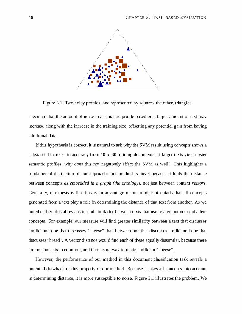
48 CHAPTER 3. TASK-BASED EVALUATION
Figure 3.1: Two noisy profiles, one represented by squares, the other, triangles.
speculate that the amount of noise in a semantic profile basedon a larger amount of text may
increase along with the increase in the training size, offsetting any potential gain from having
additional data.
If this hypothesis is correct, it is natural to ask why the SVMresult using concepts shows a
substantial increase in accuracy from 10 to 30 training documents. If larger texts yield nosier
semantic profiles, why does this not negatively affect the SVM as well? This highlights a
fundamental distinction of our approach: our method is novel because it finds the distance
between conceptsas embedded in a graph (the ontology), not just between contextvectors.
Generally, our thesis is that this is an advantage of our model: it entails that all concepts
generated from a text play a role in determining the distanceof that text from another. As we
noted earlier, this allows us to find similarity between texts that use related but not equivalent
concepts. For example, our measure will find greater similarity between a text that discusses
“milk” and one that discusses “cheese” than between one thatdiscusses “milk” and one that
discusses “bread”. A vector distance would find each of theseequally dissimilar, because there
are no concepts in common, and there is no way to relate “milk”to “cheese”.
However, the performance of our method in this document classification task reveals a
potential drawback of this property of our method. Because it takes all concepts into account
in determining distance, it is more susceptible to noise. Figure 3.1 illustrates the problem. We
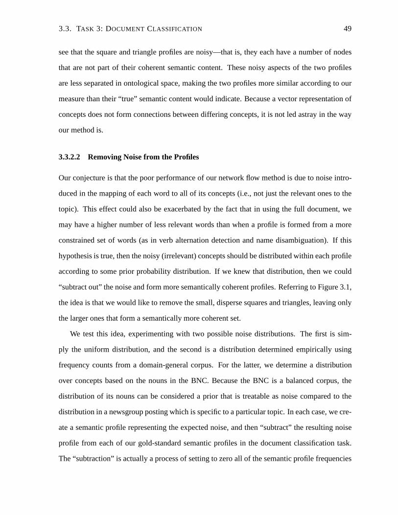
3.3. TASK 3: DOCUMENT CLASSIFICATION 49
see that the square and triangle profiles are noisy—that is, they each have a number of nodes
that are not part of their coherent semantic content. These noisy aspects of the two profiles
are less separated in ontological space, making the two profiles more similar according to our
measure than their “true” semantic content would indicate.Because a vector representation of
concepts does not form connections between differing concepts, it is not led astray in the way
our method is.
3.3.2.2 Removing Noise from the Profiles
Our conjecture is that the poor performance of our network flow method is due to noise intro-
duced in the mapping of each word to all of its concepts (i.e.,not just the relevant ones to the
topic). This effect could also be exacerbated by the fact that in using the full document, we
may have a higher number of less relevant words than when a profile is formed from a more
constrained set of words (as in verb alternation detection and name disambiguation). If this
hypothesis is true, then the noisy (irrelevant) concepts should be distributed within each profile
according to some prior probability distribution. If we knew that distribution, then we could
“subtract out” the noise and form more semantically coherent profiles. Referring to Figure 3.1,
the idea is that we would like to remove the small, disperse squares and triangles, leaving only
the larger ones that form a semantically more coherent set.
We test this idea, experimenting with two possible noise distributions. The first is sim-
ply the uniform distribution, and the second is a distribution determined empirically using
frequency counts from a domain-general corpus. For the latter, we determine a distribution
over concepts based on the nouns in the BNC. Because the BNC isa balanced corpus, the
distribution of its nouns can be considered a prior that is treatable as noise compared to the
distribution in a newsgroup posting which is specific to a particular topic. In each case, we cre-
ate a semantic profile representing the expected noise, and then “subtract” the resulting noise
profile from each of our gold-standard semantic profiles in the document classification task.
The “subtraction” is actually a process of setting to zero all of the semantic profile frequencies
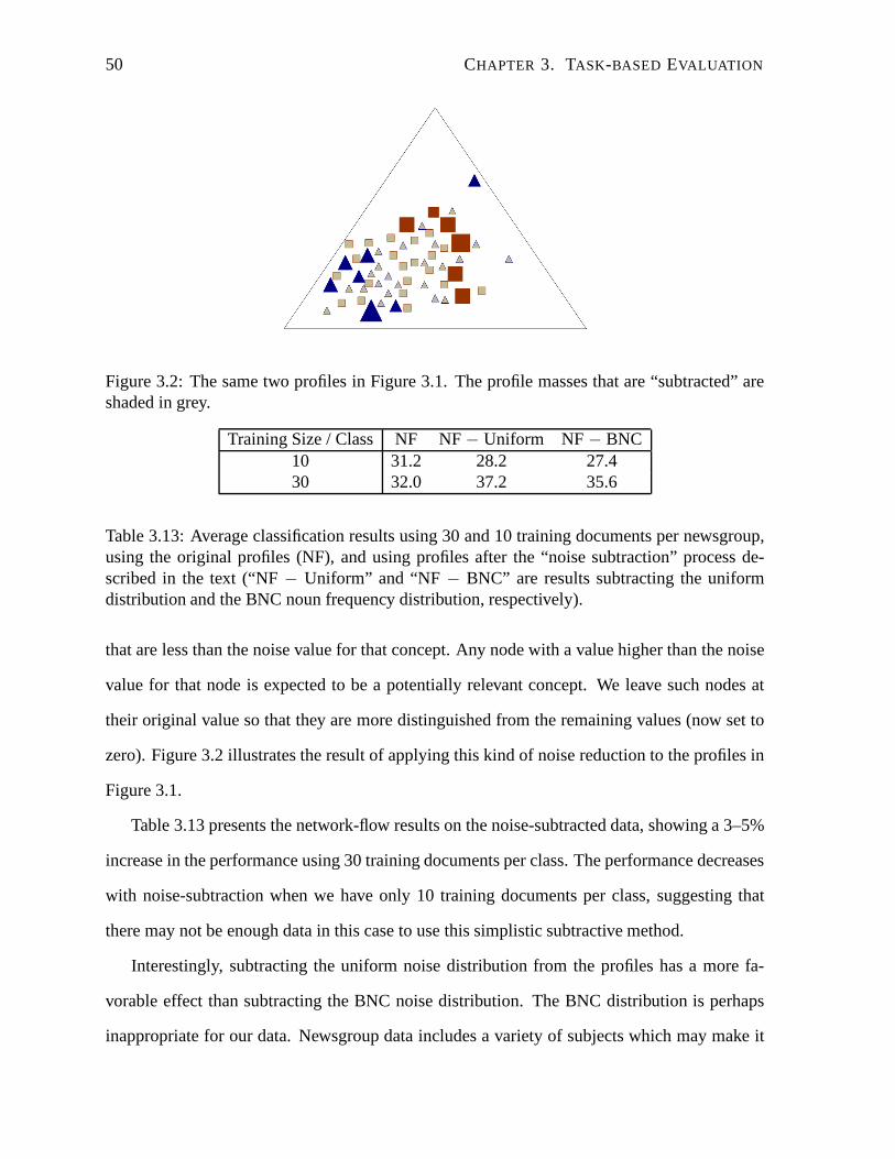
50 CHAPTER 3. TASK-BASED EVALUATION
Figure 3.2: The same two profiles in Figure 3.1. The profile masses that are “subtracted” areshaded in grey.
Training Size / Class NF NF− Uniform NF− BNC10 31.2 28.2 27.430 32.0 37.2 35.6
Table 3.13: Average classification results using 30 and 10 training documents per newsgroup,using the original profiles (NF), and using profiles after the“noise subtraction” process de-scribed in the text (“NF− Uniform” and “NF − BNC” are results subtracting the uniformdistribution and the BNC noun frequency distribution, respectively).
that are less than the noise value for that concept. Any node with a value higher than the noise
value for that node is expected to be a potentially relevant concept. We leave such nodes at
their original value so that they are more distinguished from the remaining values (now set to
zero). Figure 3.2 illustrates the result of applying this kind of noise reduction to the profiles in
Figure 3.1.
Table 3.13 presents the network-flow results on the noise-subtracted data, showing a 3–5%
increase in the performance using 30 training documents perclass. The performance decreases
with noise-subtraction when we have only 10 training documents per class, suggesting that
there may not be enough data in this case to use this simplistic subtractive method.
Interestingly, subtracting the uniform noise distribution from the profiles has a more fa-
vorable effect than subtracting the BNC noise distribution. The BNC distribution is perhaps
inappropriate for our data. Newsgroup data includes a variety of subjects which may make it
3.4. SUMMARY 51
more similar to a balanced corpus than we have originally anticipated, thus what we are treat-
ing as a “noise” distribution in this case may not actually represent noise. That said, there is
a small but notable increase even using the BNC noise distribution when we have sufficient
training data. The idea of subtracting out noise seems promising, but we leave the appropriate
representation of noise, and the mechanism for removing it effectively, as an area of future
research.
3.4 Summary
In this chapter, we have presented a task-based evaluation of our network-flow method for text
comparison. In comparison to a traditional distributionalapproach, we have demonstrated that
a non-dual approach to text comparison can add semantic sensitivity. What distinguishes our
approach from traditional distributional methods is that our method does not attempt to parti-
tion the semantic space (i.e., grouping words into related concepts), but rather it lets the onto-
logical structure as well as the frequency distribution of the target texts determine which words
are compared. As shown in the first two tasks, the non-dual combination is a strength in cases
where both types of knowledge offer discriminating power intext comparison. However, in the
last task, the semantic relation between words does not provide additional benefits—in fact,
frequency information is sufficient for classification. This suggests that either the ontological
relations provided by WordNet are inappropriate for this task, or the data is not semantically
coherent enough to take advantage of the ontological relations. In the next chapter, we will
examine the factors that contribute to the sensitivity of our method on a dataset.

52 CHAPTER 3. TASK-BASED EVALUATION
Chapter 4
Measuring Coherence of Semantic Profiles
(Nine on the Fourth. Because you are ready, there is much to
gain. Do not hesitate. Gather friends around you. As a hair clasp
holds hair together.)
Yao Text of Hexagram 16, Line 4, Yijing
We have seen a performance difference across the three taskswe used in evaluation: the
network-flow method outperforms purely distributional measures on verb alternation detection
and name disambiguation, but does poorly on document classification compared to a distri-
butional approach. (See Table 4.1 for a summary of the results.) We use the same ontology
(WordNet) and the same concept distance (number of edges) inour network-flow measure
across all three tasks, hence there must be some difference in the three datasets themselves that
impacts the ability of our method to distinguish the semantic profiles corresponding to one class
of data (one usage of an ambiguous name, for example) from theprofiles of a different class of
data (the other usage of the name). In this section, we develop a measure that can capture this
property and explain the performance differential we have observed for our method.
53

54 CHAPTER 4. MEASURING COHERENCE OFSEMANTIC PROFILES
Verb Alt’n Detection random Manhattan skew div JS NFDevelopment Avg 0.50 0.70 0.57 0.67 0.70Test Avg 0.50 0.67 0.67 0.67 0.67Name Disamb’n random SVM (100) SVM (200) NF (100) NF (200)Unweighted Avg 0.61 0.72 0.75 0.83 0.83Weighted Avg 0.53 0.52 0.55 0.76 0.77Document Class’n random SVM (10) SVM (30) NF (10) NF (30)20 newsgroups 0.05 0.43 0.61 0.31 0.32
Table 4.1: Summary of task-based results. The numbers in parentheses indicate the number oftraining instances used. The best result for each task is shown in bold.
4.1 Profile Coherence
Our goal is to find a property of individual semantic profiles that, when averaged across the
profiles in a dataset, indicates how well our method will be able to distinguish profiles of
different classes in that dataset. That is, we aim to learn about the overall separability of
the classes in a dataset by investigating the properties of individual profiles that comprise the
dataset. Our hypothesis is that the important factor for ourmethod is what we refer to as
profile coherence: the degree to which profile mass is concentrated within a constrained space
(or set of constrained spaces) of the ontology. The more spatially coherent the sets of weighted
concepts are for the profiles in a dataset, the more likely it is that our method will be able to
distinguish contrasting profiles. Conversely, less coherent profiles, whose frequency mass is
more distributed across a wider area of the ontology, will bemore difficult to separate into
classes.
For example, consider the square and triangle profiles in Figure 4.1. Coherent profiles
have their profile mass (the concept weights) focused withinsmall, distinct regions of the
ontology, as in Figure 4.1(a). These types of profiles tend tobe highly distinguishable from
each other. Less coherent profiles, whose mass is more dispersed through the ontology, such
as those in Figure 4.1(b), are likely to be less distinguishable. Note, however, that it is not
simply occupying greater or fewer nodes in the hierarchy that determines profile coherence
(and distinguishability). The profiles in Figure 4.1(c) are“spread out” as in (b), but are more
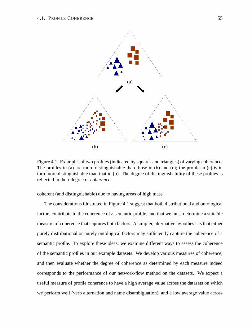
4.1. PROFILE COHERENCE 55
(a)
(b) (c)
Figure 4.1: Examples of two profiles (indicated by squares and triangles) of varying coherence.The profiles in (a) are more distinguishable than those in (b)and (c); the profile in (c) is inturn more distinguishable than that in (b). The degree of distinguishability of these profiles isreflected in their degree ofcoherence.
coherent (and distinguishable) due to having areas of high mass.
The considerations illustrated in Figure 4.1 suggest that both distributional and ontological
factors contribute to the coherence of a semantic profile, and that we must determine a suitable
measure of coherence that captures both factors. A simpler,alternative hypothesis is that either
purely distributional or purely ontological factors may sufficiently capture the coherence of a
semantic profile. To explore these ideas, we examine different ways to assess the coherence
of the semantic profiles in our example datasets. We develop various measures of coherence,
and then evaluate whether the degree of coherence as determined by each measure indeed
corresponds to the performance of our network-flow method onthe datasets. We expect a
useful measure of profile coherence to have a high average value across the datasets on which
we perform well (verb alternation and name disambiguation), and a low average value across
56 CHAPTER 4. MEASURING COHERENCE OFSEMANTIC PROFILES
the dataset on which we perform poorly (document classification).
In Section 4.2, we briefly review several measures intended to separately capture the dis-
tributional or ontological coherence of a semantic profile.We show that such measures are
insufficient for accounting for the performance differences of our method across the datasets.
In Section 4.3, we develop a novel measure to capture the coherence of our profiles in terms of
both distributional and ontological information. This measure, calledprofile density, expresses
the degree to which a semantic profile forms a coherent clustering of weighted concepts in an
ontology. We demonstrate that our profile density measure can account for the performance
differential across our datasets.
4.2 Separate Distributional and Ontological Approaches
We explored several (unsuccessful) means for capturing profile coherence with a purely distri-
butional or purely ontological measure. While we could not exhaustively investigate all pos-
sible measures of this kind, the underlying reasons for the lack of success of these measures
in explaining the differing performance of our method across the datasets convinced us of the
need for a measure that integrates distributional and ontological factors (which we present in
the following section). We mention the single-factor measures here for completeness.
Potential Distributional Coherence. Recall that Section 3.3.2.2 shows that removing the
“noise” distribution from each profile improves the document classification performance of
our method. In other words, subtracting the noise distribution from a profile makes it distri-
butionally more distinct from other profiles. Based on this observation, we hypothesize that
the less a profile resembles a noise distribution over the ontology, the more coherent it is—that
is, the more likely the frequency mass is situated in meaningful clusters of concepts. To test
this hypothesis, we calculate the average distance (using KL-divergence, Kullback and Leibler,
1951) of the profiles in a dataset from a profile created from a noise distribution (the uniform
distribution of words, or their distribution in the BNC, as in Section 3.3.2.2). Higher values of
4.2. SEPARATE DISTRIBUTIONAL AND ONTOLOGICAL APPROACHES 57
this measure indicate further distance from the uniform distribution.
Potential Ontological Coherence.Here we consider two observations. First, we hypoth-
esize that profiles with fewer concepts are more coherent, since a smaller number of concepts
is more likely to be less dispersed in the ontology. We simplyuse average profile size to cap-
ture this property (here, smaller values of profile size indicate greater coherence). Second, we
hypothesize that profiles whose concepts have greater specificity are more coherent, because
use of less specific concepts is indicative of vagueness and potential lack of coherence. Since
specificity corresponds well to depth in WordNet, we use a simple measure of average profile
depth to indicate the specificity of the set of concepts in a profile (here, greater values of depth
should indicate greater coherence).
Analysis of the Single-Factor Measures. For each task, we calculate the average of
each of the hypothesized distributional and ontological coherence measures over the profiles
in the dataset, and find that there is no consistent correspondence with the performance of our
network-flow method across the tasks. Despite the intuitions and observations presented above,
these results are not surprising. For example, the profiles of a dataset may all be distribution-
ally very similar overall to the noise profile, supposedly indicating low coherence, but they
may be quite coherent in the actual ontological space they occupy. Similarly, the profiles in a
dataset may all have a small average depth in the ontology or large size (again supposedly indi-
cating low coherence), but their distributional properties (the weights on the concepts that are
occupied) may yield coherent clusters of mass in the profile.This analysis then confirms our
hypothesis that, because distributional and ontological information are intertwined in the rep-
resentation of a semantic profile, a useful measure of profilecoherence must take into account
an integration of these two information sources.

58 CHAPTER 4. MEASURING COHERENCE OFSEMANTIC PROFILES
4.3 Integrating Distributional and Ontological Factors
As noted earlier, and tentatively confirmed by the above results, we assume that the interaction
of distributional and ontological factors determines the coherence of profiles—i.e., a coherent
profile has its frequency mass concentrated within a reasonably constrained space (or set of
constrained spaces) of the ontology. We observe that this issimilar to the geographical notion
of population density, which is determined by the population mass divided by the area occu-
pied. Here we extend the geographical definition of density within our network framework by
relating population mass to distributional weights on concepts, and occupied area to the spread
of the weighted concepts in the ontology. We call the resulting measure of profile coherence
profile density.
4.3.1 Profile Density
To adapt the definition of geographical density to our problem, we first need to determine
the analogs of population mass and occupied area in a semantic profile. The profile mass at
each concept node is directly analogous to the population mass. Defining the occupied area
within an ontology is not as straightforward, as there is no simple definition of area within a
graph.1 We develop a definition of area that captures the actual spatial spread of the profile
mass through the ontology.
To begin, we note that any subgraph of the WordNet hypernym hierarchy is hierarchical
itself. Thus, any region of the ontology that contains some profile mass is a hierarchy rooted
at some common ancestor of those profile nodes.2 As shown in Figure 4.2, the more dispersed
(less closely clustered together) a set of nodes is, the further away their common ancestor is.
That is, a highly related (and spatially constrained) set ofconcept nodes can be generalized
to a more specific ancestor concept (i.e., near the descendants, as in Figure 4.2(b)), while
1Agirre and Rigau (1996) use the number of nodes within a subgraph as its area, but this fails to take intoaccount how dispersed the nodes are throughout the ontology.
2Although WordNet contains instances of multiple inheritance, the rate is low. As a result, the likelihood of aset of profile nodes sharing multiple ancestors is low as well.
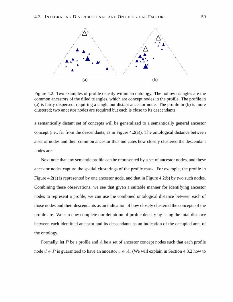
4.3. INTEGRATING DISTRIBUTIONAL AND ONTOLOGICAL FACTORS 59
(a) (b)
Figure 4.2: Two examples of profile density within an ontology. The hollow triangles are thecommon ancestors of the filled triangles, which are concept nodes in the profile. The profile in(a) is fairly dispersed, requiring a single but distant ancestor node. The profile in (b) is moreclustered; two ancestor nodes are required but each is closeto its descendants.
a semantically distant set of concepts will be generalized to a semantically general ancestor
concept (i.e., far from the descendants, as in Figure 4.2(a)). The ontological distance between
a set of nodes and their common ancestor thus indicates how closely clustered the descendant
nodes are.
Next note that any semantic profile can be represented by a setof ancestor nodes, and these
ancestor nodes capture the spatial clusterings of the profile mass. For example, the profile in
Figure 4.2(a) is represented by one ancestor node, and that in Figure 4.2(b) by two such nodes.
Combining these observations, we see that given a suitable manner for identifying ancestor
nodes to represent a profile, we can use the combined ontological distance between each of
those nodes and their descendants as an indication of how closely clustered the concepts of the
profile are. We can now complete our definition of profile density by using the total distance
between each identified ancestor and its descendants as an indication of the occupied area of
the ontology.
Formally, letP be a profile andA be a set of ancestor concept nodes such that each profile
noded ∈ P is guaranteed to have an ancestora ∈ A. (We will explain in Section 4.3.2 how to
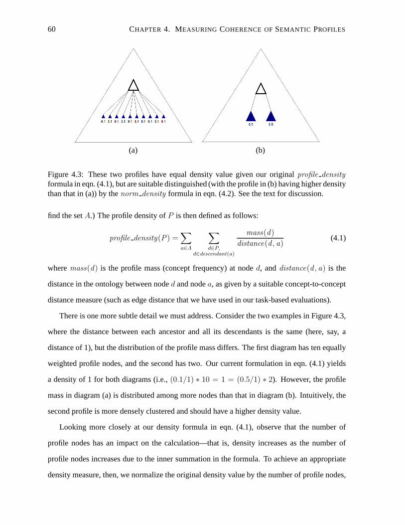
60 CHAPTER 4. MEASURING COHERENCE OFSEMANTIC PROFILES
(a) (b)
Figure 4.3: These two profiles have equal density value givenour originalprofile density
formula in eqn. (4.1), but are suitable distinguished (withthe profile in (b) having higher densitythan that in (a)) by thenorm density formula in eqn. (4.2). See the text for discussion.
find the setA.) The profile density ofP is then defined as follows:
profile density(P) =∑
a∈A
∑
d∈P,d∈descendant(a)
mass(d)
distance(d , a)(4.1)
wheremass(d) is the profile mass (concept frequency) at noded, anddistance(d , a) is the
distance in the ontology between noded and nodea, as given by a suitable concept-to-concept
distance measure (such as edge distance that we have used in our task-based evaluations).
There is one more subtle detail we must address. Consider thetwo examples in Figure 4.3,
where the distance between each ancestor and all its descendants is the same (here, say, a
distance of 1), but the distribution of the profile mass differs. The first diagram has ten equally
weighted profile nodes, and the second has two. Our current formulation in eqn. (4.1) yields
a density of 1 for both diagrams (i.e.,(0.1/1) ∗ 10 = 1 = (0.5/1) ∗ 2). However, the profile
mass in diagram (a) is distributed among more nodes than thatin diagram (b). Intuitively, the
second profile is more densely clustered and should have a higher density value.
Looking more closely at our density formula in eqn. (4.1), observe that the number of
profile nodes has an impact on the calculation—that is, density increases as the number of
profile nodes increases due to the inner summation in the formula. To achieve an appropriate
density measure, then, we normalize the original density value by the number of profile nodes,
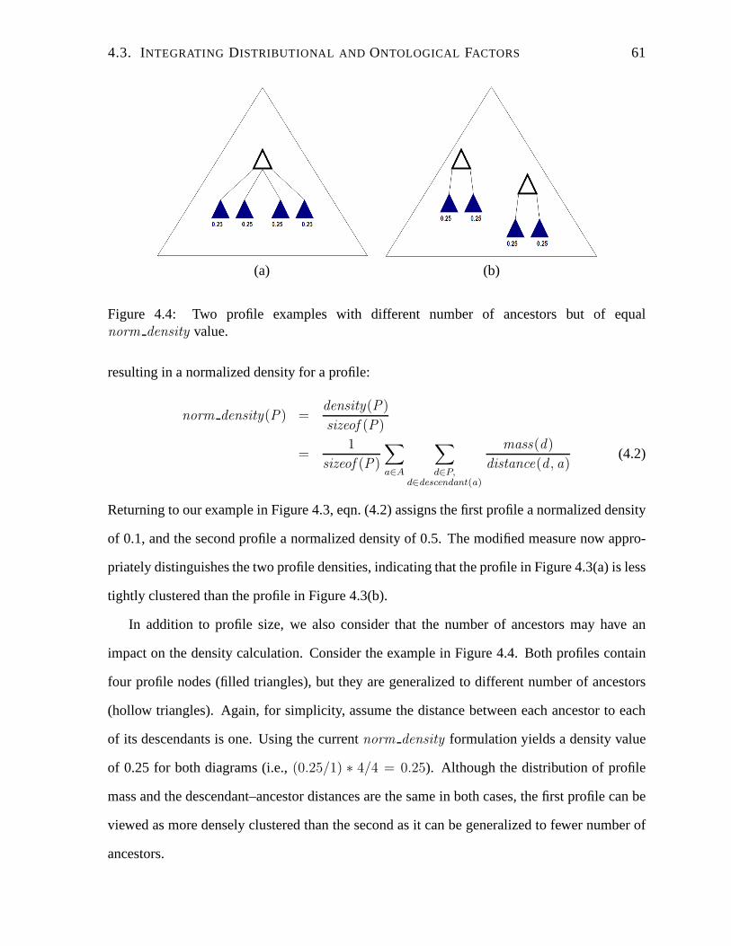
4.3. INTEGRATING DISTRIBUTIONAL AND ONTOLOGICAL FACTORS 61
(a) (b)
Figure 4.4: Two profile examples with different number of ancestors but of equalnorm density value.
resulting in a normalized density for a profile:
norm density(P) =density(P)
sizeof (P)
=1
sizeof (P)
∑
a∈A
∑
d∈P,d∈descendant(a)
mass(d)
distance(d , a)(4.2)
Returning to our example in Figure 4.3, eqn. (4.2) assigns the first profile a normalized density
of 0.1, and the second profile a normalized density of 0.5. Themodified measure now appro-
priately distinguishes the two profile densities, indicating that the profile in Figure 4.3(a) is less
tightly clustered than the profile in Figure 4.3(b).
In addition to profile size, we also consider that the number of ancestors may have an
impact on the density calculation. Consider the example in Figure 4.4. Both profiles contain
four profile nodes (filled triangles), but they are generalized to different number of ancestors
(hollow triangles). Again, for simplicity, assume the distance between each ancestor to each
of its descendants is one. Using the currentnorm density formulation yields a density value
of 0.25 for both diagrams (i.e.,(0.25/1) ∗ 4/4 = 0.25). Although the distribution of profile
mass and the descendant–ancestor distances are the same in both cases, the first profile can be
viewed as more densely clustered than the second as it can be generalized to fewer number of
ancestors.
62 CHAPTER 4. MEASURING COHERENCE OFSEMANTIC PROFILES
To account for the difference, similarly to the number of profile nodes, we observe that
the number of ancestors can have an influence on how densely clustered a profile is—more
ancestors result in a less densely clustered profile. To achieve the desired inversely proportional
relationship (between the number of ancestors and density), we explore two variations:
norm density2 (P) =density(P)
sizeof (P) ∗ sizeof (A)(4.3)
norm density3 (P) =density(P)
sizeof (P) + sizeof (A)(4.4)
In both cases, we increase the denominator in eqn. (4.2) by the number of ancestors,sizeof (A),
such that density decreases when the number of ancestors increases. In eqn. (4.3), we divide
density by the product of the number of profile nodes (sizeof (P)) and the number of ancestors
(sizeof (A)). In eqn. (4.4), we divide by their sum. Returning to our example in Figure 4.4, the
first diagram has anorm density2 of 0.25 andnorm density3 of 0.2; and the second diagram
has anorm density2 of 0.125 andnorm density3 of 0.167.
Note thatnorm density2 penalizes considerably more thannorm density3 because of the
multiplication (instead of addition) in the denominator. The size of the ancestor set depends
not only on how densely the profile nodes are clustered, but also on how conservative the
method that searches for the ancestor set is. In the extreme case, we may have an ancestor set
that is the same as the profile itself. Dividing bysizeof (A) over-penalizes density, hence we
opt for norm density3 for a less severe penalty. We will report results fornorm density and
norm density3 .
4.3.2 Finding the Ancestor Set for Profile Density
As noted earlier, our definition of profile density depends onidentifying a suitable set of ances-
tor nodes of the concept nodes in the profile: the distance of the ancestors to the profile nodes
indirectly indicates the degree to which the profile nodes are spatially clustered close together.
Thus, given a profileP , we need to findA, the set of nodes that are ancestors of the profile
nodesd ∈ P . (The nodesa ∈ A correspond to the hollow triangles indicated in Figure 4.2 and
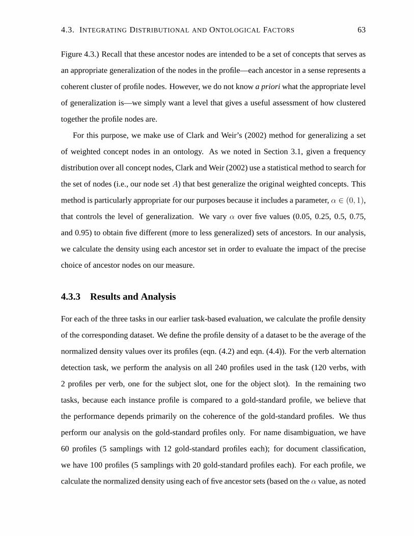
4.3. INTEGRATING DISTRIBUTIONAL AND ONTOLOGICAL FACTORS 63
Figure 4.3.) Recall that these ancestor nodes are intended to be a set of concepts that serves as
an appropriate generalization of the nodes in the profile—each ancestor in a sense represents a
coherent cluster of profile nodes. However, we do not knowa priori what the appropriate level
of generalization is—we simply want a level that gives a useful assessment of how clustered
together the profile nodes are.
For this purpose, we make use of Clark and Weir’s (2002) method for generalizing a set
of weighted concept nodes in an ontology. As we noted in Section 3.1, given a frequency
distribution over all concept nodes, Clark and Weir (2002) use a statistical method to search for
the set of nodes (i.e., our node setA) that best generalize the original weighted concepts. This
method is particularly appropriate for our purposes because it includes a parameter,α ∈ (0, 1),
that controls the level of generalization. We varyα over five values (0.05, 0.25, 0.5, 0.75,
and 0.95) to obtain five different (more to less generalized)sets of ancestors. In our analysis,
we calculate the density using each ancestor set in order to evaluate the impact of the precise
choice of ancestor nodes on our measure.
4.3.3 Results and Analysis
For each of the three tasks in our earlier task-based evaluation, we calculate the profile density
of the corresponding dataset. We define the profile density ofa dataset to be the average of the
normalized density values over its profiles (eqn. (4.2) and eqn. (4.4)). For the verb alternation
detection task, we perform the analysis on all 240 profiles used in the task (120 verbs, with
2 profiles per verb, one for the subject slot, one for the object slot). In the remaining two
tasks, because each instance profile is compared to a gold-standard profile, we believe that
the performance depends primarily on the coherence of the gold-standard profiles. We thus
perform our analysis on the gold-standard profiles only. Forname disambiguation, we have
60 profiles (5 samplings with 12 gold-standard profiles each); for document classification,
we have 100 profiles (5 samplings with 20 gold-standard profiles each). For each profile, we
calculate the normalized density using each of five ancestorsets (based on theα value, as noted
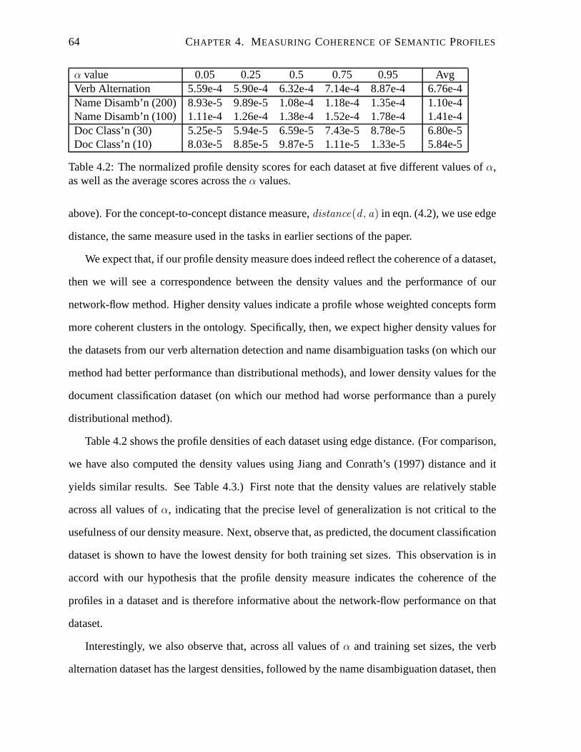
64 CHAPTER 4. MEASURING COHERENCE OFSEMANTIC PROFILES
α value 0.05 0.25 0.5 0.75 0.95 AvgVerb Alternation 5.59e-4 5.90e-4 6.32e-4 7.14e-4 8.87e-4 6.76e-4Name Disamb’n (200) 8.93e-5 9.89e-5 1.08e-4 1.18e-4 1.35e-4 1.10e-4Name Disamb’n (100) 1.11e-4 1.26e-4 1.38e-4 1.52e-4 1.78e-4 1.41e-4Doc Class’n (30) 5.25e-5 5.94e-5 6.59e-5 7.43e-5 8.78e-5 6.80e-5Doc Class’n (10) 8.03e-5 8.85e-5 9.87e-5 1.11e-5 1.33e-5 5.84e-5
Table 4.2: The normalized profile density scores for each dataset at five different values ofα,as well as the average scores across theα values.
above). For the concept-to-concept distance measure,distance(d , a) in eqn. (4.2), we use edge
distance, the same measure used in the tasks in earlier sections of the paper.
We expect that, if our profile density measure does indeed reflect the coherence of a dataset,
then we will see a correspondence between the density valuesand the performance of our
network-flow method. Higher density values indicate a profile whose weighted concepts form
more coherent clusters in the ontology. Specifically, then,we expect higher density values for
the datasets from our verb alternation detection and name disambiguation tasks (on which our
method had better performance than distributional methods), and lower density values for the
document classification dataset (on which our method had worse performance than a purely
distributional method).
Table 4.2 shows the profile densities of each dataset using edge distance. (For comparison,
we have also computed the density values using Jiang and Conrath’s (1997) distance and it
yields similar results. See Table 4.3.) First note that the density values are relatively stable
across all values ofα, indicating that the precise level of generalization is notcritical to the
usefulness of our density measure. Next, observe that, as predicted, the document classification
dataset is shown to have the lowest density for both trainingset sizes. This observation is in
accord with our hypothesis that the profile density measure indicates the coherence of the
profiles in a dataset and is therefore informative about the network-flow performance on that
dataset.
Interestingly, we also observe that, across all values ofα and training set sizes, the verb
alternation dataset has the largest densities, followed bythe name disambiguation dataset, then
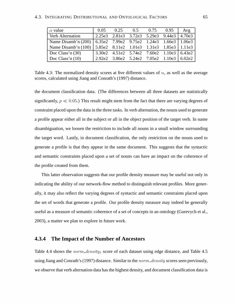
4.3. INTEGRATING DISTRIBUTIONAL AND ONTOLOGICAL FACTORS 65
α value 0.05 0.25 0.5 0.75 0.95 AvgVerb Alternation 2.25e3 2.81e3 3.72e3 5.29e3 9.44e34.70e3Name Disamb’n (200) 6.35e2 7.99e2 9.75e2 1.24e3 1.66e31.06e3Name Disamb’n (100) 5.85e2 8.11e2 1.01e3 1.31e3 1.85e31.11e3Doc Class’n (30) 3.30e2 4.51e2 5.74e2 7.60e2 1.10e36.43e2Doc Class’n (10) 2.92e2 3.86e2 5.24e2 7.05e2 1.10e36.02e2
Table 4.3: The normalized density scores at five different values ofα, as well as the averagescores, calculated using Jiang and Conrath’s (1997) distance.
the document classification data. (The differences betweenall three datasets are statistically
significantly,p ≪ 0.05.) This result might stem from the fact that there are varyingdegrees of
constraint placed upon the data in the three tasks. In verb alternation, the nouns used to generate
a profile appear either all in the subject or all in the object position of the target verb. In name
disambiguation, we loosen the restriction to include all nouns in a small window surrounding
the target word. Lastly, in document classification, the only restriction on the nouns used to
generate a profile is that they appear in the same document. This suggests that the syntactic
and semantic constraints placed upon a set of nouns can have an impact on the coherence of
the profile created from them.
This latter observation suggests that our profile density measure may be useful not only in
indicating the ability of our network-flow method to distinguish relevant profiles. More gener-
ally, it may also reflect the varying degrees of syntactic andsemantic constraints placed upon
the set of words that generate a profile. Our profile density measure may indeed be generally
useful as a measure of semantic coherence of a set of conceptsin an ontology (Gurevych et al.,
2003), a matter we plan to explore in future work.
4.3.4 The Impact of the Number of Ancestors
Table 4.4 shows thenorm density3 score of each dataset using edge distance, and Table 4.5
using Jiang and Conrath’s (1997) distance. Similar to thenorm density scores seen previously,
we observe that verb alternation data has the highest density, and document classification data is
66 CHAPTER 4. MEASURING COHERENCE OFSEMANTIC PROFILES
α value 0.05 0.25 0.5 0.75 0.95 AvgVerb Alternation 4.74e-4 4.97e-4 5.24e-4 5.70e-4 6.57e-45.44e-4Name Disamb’n (200) 8.29e-5 9.02e-5 9.65e-5 1.04e-4 1.15e-49.78e-5Name Disamb’n (100) 1.04e-4 1.16e-4 1.25e-4 1.35e-4 1.51e-41.26e-4Doc Class’n (30) 5.03e-5 5.61e-5 6.13e-5 6.78e-5 7.78e-56.27e-5Doc Class’n (10) 7.28e-5 7.86e-5 8.50e-5 9.12e-5 7.59e-58.07e-5
Table 4.4: Thenorm density3 scores at five different values ofα, as well as the average scores,calculated using edge distance.
α value 0.05 0.25 0.5 0.75 0.95 AvgVerb Alternation 1.91e3 2.37e3 3.07e3 4.20e3 6.93e33.69e3Name Disamb’n (200) 5.85e2 7.23e2 8.68e2 1.08e3 1.41e39.34e2Name Disamb’n (100) 5.46e2 7.42e2 9.10e2 1.15e3 1.57e39.84e2Doc Class’n (30) 3.14e2 4.24e2 5.32e2 6.93e2 9.75e25.88e2Doc Class’n (10) 2.80e2 3.64e2 4.87e2 6.41e2 9.68e25.48e2
Table 4.5: Thenorm density3 scores at five different values ofα, as well as the average scores,calculated using Jiang and Conrath’s (1997) distance.
the least dense. Althoughnorm density3 produces smaller density values thannorm density ,
the difference is small. For the data from the three tasks, the number of ancestors appears to
have negligible impact on the overall density.
4.4 Summary
In summary, our analysis in this section has shown that both distributional and ontological
properties contribute to the coherence of a profile, but neither alone is indicative of the network-
flow performance in a particular task. Our new measure of profile density serves as a tool for
analyzing profiles that integrates their distributional and ontological coherence, and provides a
post-hoc means for explaining the performance differential of our method across the different
tasks we performed here. The results also point to the possibility of devising a diagnostic tool
for the suitability of the network-flow method on novel data.An analysis of the data and results
across a larger set of tasks will allow us to investigate the possibility of determining a density

4.4. SUMMARY 67
threshold that would be indicative of expected positive results with our method.

68 CHAPTER 4. MEASURING COHERENCE OFSEMANTIC PROFILES
Chapter 5
Graph Transformation
(Gone, gone. Gone all the way. Everyone gone over to the other shore. Enlightenment!)
Prajnapamita Hr. daya Sutra
Thus far, for simplicity, we have only considered edge distance as the distance between each
pair of nodes (i.e.,c(i, j)). In other words, one edge constitutes a distance of one, andthe
distance of a path is the number of edges it has. This is an appropriate node-to-node (or
concept-to-concept) distance with the MCF framework, because the MCF problem definition
assumesc(i, j) to be additive (the distance of a path equals the sum of the distances of the
edges on the path). Note, however, that there exists a numberof non-additive distances widely
used to measure the semantic distance between two concepts in an ontology such as WordNet.
In this chapter, we first focus on the impact on accuracy and efficiency by using a non-additive
distance within our network-flow framework. Then we will present our novel solution that
allows us to maximize both accuracy and efficiency. Finally,we will present our evaluation
and analysis.
69

70 CHAPTER 5. GRAPH TRANSFORMATION
5.1 Solving the MCF Problem Using a Non-additive Distance
In this section, we will discuss the issues relevant to solving the MCF problem accurately and
efficiently. We will describe the impact of using non-additive distances and offer two possible
(but not ideal) solutions. The first solution allows us to calculate the final distance exactly but is
computationally expensive, while the opposite is true for the second solution (the final distance
is approximated but the method is efficient). Based on these two solutions, we propose a third
possibility: we trade off the exactness of the calculation with efficiency, a discussion we will
return to in Section 5.2.
Recall that a distance is additive if the distance between any two nodes is the sum of the
distances of the edges connecting them. Say, if the edges,(j0, j1), (j1, j2), . . . , (jn−1, jn),
wherei = j0, jn = k, lie along a path connecting nodei and nodek, then the additive distance
between them is:
distance(i , k) =
n−1∑
m=0
distance(jm , jm+1 ) (5.1)
Interestingly, the additivity issue arises from the MCF problem definition itself. Note that both
the objective function, eqn. (2.1), and the constraints, eqn. (2.2) and eqn. (2.3), are expressed
in terms of the flow and/or the cost of the individual edges. Ateach step of the search, to
consider an edge as part of the solution, not only does it haveto satisfy the constraints, it has
to be the cheapest (i.e., locally). Observe that the objective function, eqn. (2.1), in particular,
is expressed as a linear combination of edge costs. Thus, thelocally cheapest edges would
eventually lead to the cheapest route globally. Essentially, the problem is defined in a way that
additivity is assumed to hold (and therefore this greedy approach works). However, many ex-
isting concept-to-concept distances, such as those proposed by Resnik (1995) and Lin (1998),
are non-additive. Moreover, these measures have often beenshown to be superior to the simple
edge distance in comparing WordNet concepts (Jarmasz and Szpakowicz, 2003; Weeds, 2003).
Unfortunately, for these non-additive concept-to-concept distances, the cheapest set of edges
locally does not yield the cheapest set of edges globally, rendering the use of MCF without
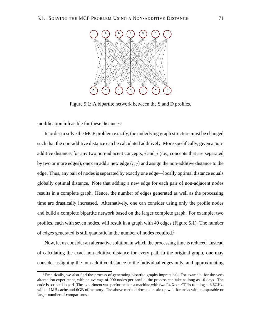
5.1. SOLVING THE MCF PROBLEM USING A NON-ADDITIVE DISTANCE 71
Figure 5.1: A bipartite network between the S and D profiles.
modification infeasible for these distances.
In order to solve the MCF problem exactly, the underlying graph structure must be changed
such that the non-additive distance can be calculated additively. More specifically, given a non-
additive distance, for any two non-adjacent concepts,i andj (i.e., concepts that are separated
by two or more edges), one can add a new edge(i, j) and assign the non-additive distance to the
edge. Thus, any pair of nodes is separated by exactly one edge—locally optimal distance equals
globally optimal distance. Note that adding a new edge for each pair of non-adjacent nodes
results in a complete graph. Hence, the number of edges generated as well as the processing
time are drastically increased. Alternatively, one can consider using only the profile nodes
and build a complete bipartite network based on the larger complete graph. For example, two
profiles, each with seven nodes, will result in a graph with 49edges (Figure 5.1). The number
of edges generated is still quadratic in the number of nodes required.1
Now, let us consider an alternative solution in which the processing time is reduced. Instead
of calculating the exact non-additive distance for every path in the original graph, one may
consider assigning the non-additive distance to the individual edges only, and approximating
1Empirically, we also find the process of generating bipartite graphs impractical. For example, for the verbalternation experiment, with an average of 900 nodes per profile, the process can take as long as 10 days. Thecode is scripted in perl. The experiment was performed on a machine with two P4 Xeon CPUs running at 3.6GHz,with a 1MB cache and 6GB of memory. The above method does not scale up well for tasks with comparable orlarger number of comparisons.
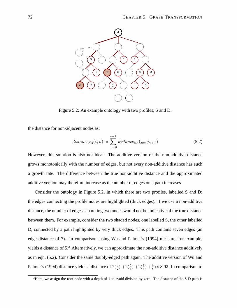
72 CHAPTER 5. GRAPH TRANSFORMATION
Figure 5.2: An example ontology with two profiles, S and D.
the distance for non-adjacent nodes as:
distanceNA(i , k) ≈
n−1∑
m=0
distanceNA(jm , jm+1 ) (5.2)
However, this solution is also not ideal. The additive version of the non-additive distance
grows monotonically with the number of edges, but not every non-additive distance has such
a growth rate. The difference between the true non-additivedistance and the approximated
additive version may therefore increase as the number of edges on a path increases.
Consider the ontology in Figure 5.2, in which there are two profiles, labelled S and D;
the edges connecting the profile nodes are highlighted (thick edges). If we use a non-additive
distance, the number of edges separating two nodes would notbe indicative of the true distance
between them. For example, consider the two shaded nodes, one labelled S, the other labelled
D, connected by a path highlighted by very thick edges. This path contains seven edges (an
edge distance of 7). In comparison, using Wu and Palmer’s (1994) measure, for example,
yields a distance of 5.2 Alternatively, we can approximate the non-additive distance additively
as in eqn. (5.2). Consider the same doubly-edged path again.The additive version of Wu and
Palmer’s (1994) distance yields a distance of2(32) +2(5
4) +2(7
6) +9
8≈ 8.93. In comparison to
2Here, we assign the root node with a depth of1 to avoid division by zero. The distance of the S-D path is
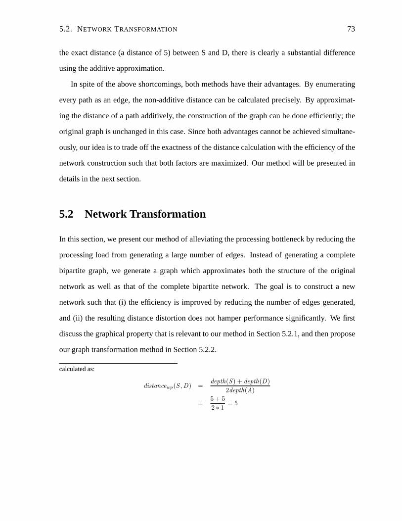
5.2. NETWORK TRANSFORMATION 73
the exact distance (a distance of 5) between S and D, there is clearly a substantial difference
using the additive approximation.
In spite of the above shortcomings, both methods have their advantages. By enumerating
every path as an edge, the non-additive distance can be calculated precisely. By approximat-
ing the distance of a path additively, the construction of the graph can be done efficiently; the
original graph is unchanged in this case. Since both advantages cannot be achieved simultane-
ously, our idea is to trade off the exactness of the distance calculation with the efficiency of the
network construction such that both factors are maximized.Our method will be presented in
details in the next section.
5.2 Network Transformation
In this section, we present our method of alleviating the processing bottleneck by reducing the
processing load from generating a large number of edges. Instead of generating a complete
bipartite graph, we generate a graph which approximates both the structure of the original
network as well as that of the complete bipartite network. The goal is to construct a new
network such that (i) the efficiency is improved by reducing the number of edges generated,
and (ii) the resulting distance distortion does not hamper performance significantly. We first
discuss the graphical property that is relevant to our method in Section 5.2.1, and then propose
our graph transformation method in Section 5.2.2.
calculated as:
distancewp(S ,D) =depth(S ) + depth(D)
2depth(A)
=5 + 5
2 ∗ 1= 5
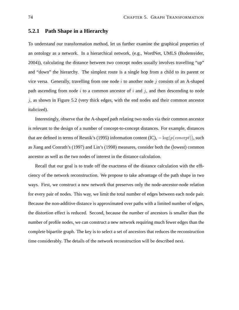
74 CHAPTER 5. GRAPH TRANSFORMATION
5.2.1 Path Shape in a Hierarchy
To understand our transformation method, let us further examine the graphical properties of
an ontology as a network. In a hierarchical network, (e.g., WordNet, UMLS (Bodenreider,
2004)), calculating the distance between two concept nodesusually involves travelling “up”
and “down” the hierarchy. The simplest route is a single hop from a child to its parent or
vice versa. Generally, travelling from one nodei to another nodej consists of an A-shaped
path ascending from nodei to a common ancestor ofi and j, and then descending to node
j, as shown in Figure 5.2 (very thick edges, with the end nodes and their common ancestor
italicized).
Interestingly, observe that the A-shaped path relating twonodes via their common ancestor
is relevant to the design of a number of concept-to-concept distances. For example, distances
that are defined in terms of Resnik’s (1995) information content (IC),− log(p(concept)), such
as Jiang and Conrath’s (1997) and Lin’s (1998) measures, consider both the (lowest) common
ancestor as well as the two nodes of interest in the distance calculation.
Recall that our goal is to trade off the exactness of the distance calculation with the effi-
ciency of the network reconstruction. We propose to take advantage of the path shape in two
ways. First, we construct a new network that preserves only the node-ancestor-node relation
for every pair of nodes. This way, we limit the total number ofedges between each node pair.
Because the non-additive distance is approximated over paths with a limited number of edges,
the distortion effect is reduced. Second, because the number of ancestors is smaller than the
number of profile nodes, we can construct a new network requiring much fewer edges than the
complete bipartite graph. The key is to select a set of ancestors that reduces the reconstruction
time considerably. The details of the network reconstruction will be described next.
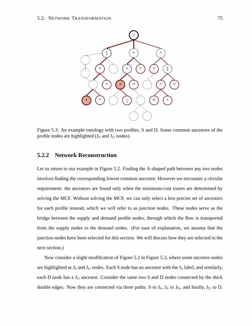
5.2. NETWORK TRANSFORMATION 75
Figure 5.3: An example ontology with two profiles, S and D. Some common ancestors of theprofile nodes are highlighted (JS and JD nodes).
5.2.2 Network Reconstruction
Let us return to our example in Figure 5.2. Finding the A-shaped path between any two nodes
involves finding the corresponding lowest common ancestor.However we encounter a circular
requirement: the ancestors are found only when the minimum-cost routes are determined by
solving the MCF. Without solving the MCF, we can only select aless precise set of ancestors
for each profile instead, which we will refer to asjunction nodes. These nodes serve as the
bridge between the supply and demand profile nodes, through which the flow is transported
from the supply nodes to the demand nodes. (For ease of explanation, we assume that the
junction nodes have been selected for this section. We will discuss how they are selected in the
next section.)
Now consider a slight modification of Figure 5.2 in Figure 5.3, where some ancestor nodes
are highlighted as JS and JD nodes. Each S node has an ancestor with the JS label, and similarly,
each D node has a JD ancestor. Consider the same two S and D nodes connected by thethick
double edges. Now they are connected via three paths: S to JS, JS to JD, and finally, JD to D.
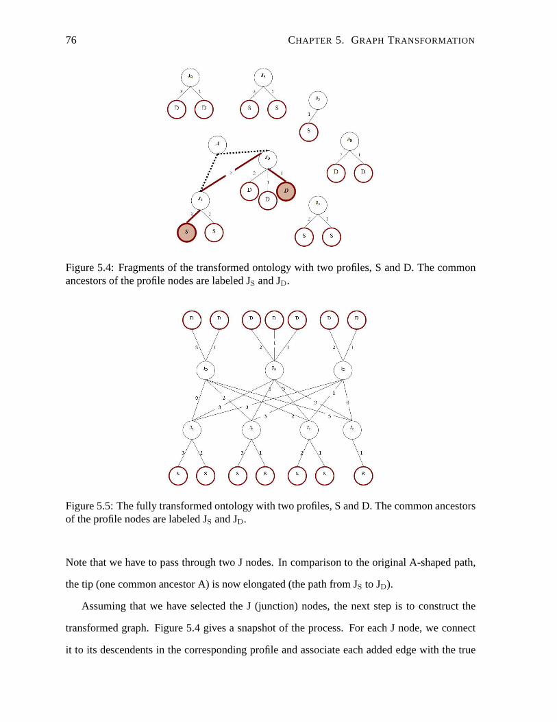
76 CHAPTER 5. GRAPH TRANSFORMATION
Figure 5.4: Fragments of the transformed ontology with two profiles, S and D. The commonancestors of the profile nodes are labeled JS and JD.
Figure 5.5: The fully transformed ontology with two profiles, S and D. The common ancestorsof the profile nodes are labeled JS and JD.
Note that we have to pass through two J nodes. In comparison tothe original A-shaped path,
the tip (one common ancestor A) is now elongated (the path from JS to JD).
Assuming that we have selected the J (junction) nodes, the next step is to construct the
transformed graph. Figure 5.4 gives a snapshot of the process. For each J node, we connect
it to its descendents in the corresponding profile and associate each added edge with the true
5.3. ANALYSING THE TRANSFORMED NETWORK 77
non-additive distance in the original graph. (For ease of understanding, we show edge distance
here.) Next, we connect each JS node to each JD node, and again, associate each edge with the
corresponding non-additive distance in the original network. For the two target S and D nodes
in the current example, they are now connected via an A-shaped path with an elongated JS-JD
tip (thick edges). The completely transformed graph is shown in Figure 5.5.
5.3 Analysing the Transformed Network
In summary, Figure 5.6 presents all three networks. Figure (a) is the original network and is
only feasible when the concept-to-concept distance is additive. In the case of non-additivity,
we can replace each A-shaped path (S-D path) in Figure (a) with an edge to create the bipartite
graph in Figure (b). Alternatively, we can select a set of junction nodes from the original
network, then replace each A-shaped S-D path from the original network with a S-JS-JD-D
path in Figure (c), such that the bipartite portion (betweenJS nodes and JD nodes) is shrunk
considerably. We refer to this graph as the transformed network.
Recall that we have two objectives for adapting the MCF framework for non-additive
concept-to-concept distances: (i) the adaptation should not severely compromise the exact-
ness of the distance calculation; (ii) in comparison to the algorithm using additive distances,
the resulting method should be relatively efficient. In Section 5.3.1, we will address the first
objective by analysing the distortion effect of the distance approximation. In Section 5.3.2, we
will address the second objective by examining how we can keep the overall processing cost
low in the junction selection.
5.3.1 Distance Distortion
To address the first objective of minimizing the distance distortion, let us first define the cost
function on the transformed network. For each supply-demand node pair,S andD, the precise
concept-to-concept distance is simplydistanceNA(S ,D) (both in the original network and the
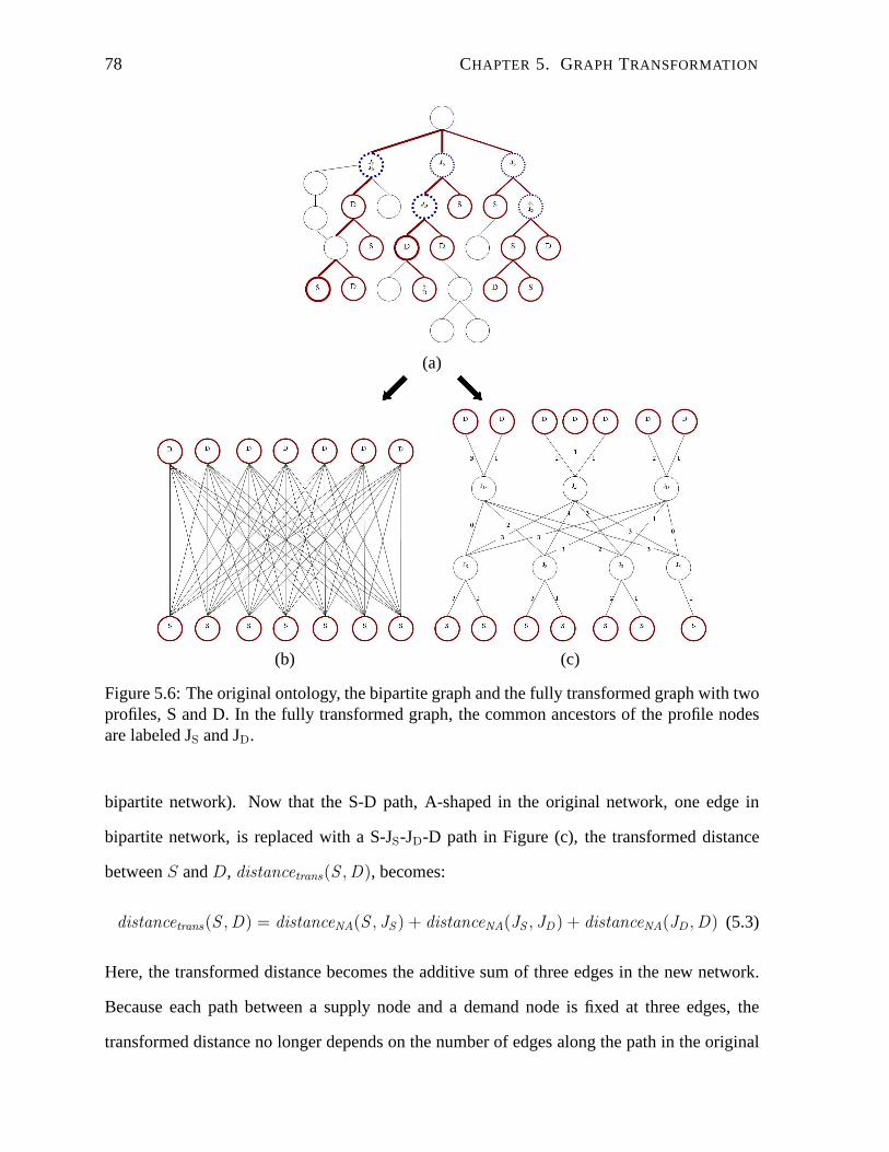
78 CHAPTER 5. GRAPH TRANSFORMATION
(a)
(b) (c)
Figure 5.6: The original ontology, the bipartite graph and the fully transformed graph with twoprofiles, S and D. In the fully transformed graph, the common ancestors of the profile nodesare labeled JS and JD.
bipartite network). Now that the S-D path, A-shaped in the original network, one edge in
bipartite network, is replaced with a S-JS-JD-D path in Figure (c), the transformed distance
betweenS andD, distancetrans(S ,D), becomes:
distancetrans(S ,D) = distanceNA(S , JS ) + distanceNA(JS , JD) + distanceNA(JD ,D) (5.3)
Here, the transformed distance becomes the additive sum of three edges in the new network.
Because each path between a supply node and a demand node is fixed at three edges, the
transformed distance no longer depends on the number of edges along the path in the original
5.3. ANALYSING THE TRANSFORMED NETWORK 79
network (cf. eqn. (5.2)). As a result, we reduce the distortion effect on the transformed distance.
Despite that each path has exactly three edges, there is still some distortion from approxi-
mating the concept-to-concept distance additively. To illustrate the distortion effect, consider
Jiang and Conrath’s (1997) distance, which measures the difference in information content
between two concepts and their lowest common ancestors, i.e.,
distancejc(S ,D) = IC (S ) + IC (D) − 2IC (LCA(S ,D)) (5.4)
After the transformation,distancejctrans(S ,D) becomes:
distancejctrans(S, D) = distancejc(S , JS) + distancejc(JS , JD) + distancejc(JD ,D)
= [IC (S ) + IC (JS) − 2IC (JS)] +
[IC (D) + IC (JD) − 2IC (JD)] +
[IC (JS) + IC (JD) − 2IC (LCA(JS , JD))]
= IC (S ) + IC (D) − 2IC (LCA(JS , JD)) (5.5)
whereJS andJD are the junction ancestors ofS andD, respectively. The transformation
replaces the lowest common ancestorLCA(S ,D) in eqn. (5.4) with some other common an-
cestor (LCA(JS , JD)). UnlessLCA(JS , JD) = LCA(S ,D), the distance is distorted by using
a less precise quantity,IC (LCA(JS , JD)).
Note that the degree of distortion depends on the distance and the choice of junction nodes.
In the current example, we use the information content of a concept as given by its maximum
likelihood estimate based on its frequency in a large corpus. An increment in the frequency
of a concept leads to an increment in the frequency of all its ancestors. Due to the frequency
percolation, concepts with a small depth tend to accumulatehigher counts than those deeper
in the hierarchy. Thus, we expect the information content ofa concept to be higher than its
ancestors, because a concept is more semantically specific than its ancestors (the notion of
semantic specificity is captured by the use of the negativelog function in the definition of IC).
The transformed distance is distorted accordingly, i.e.,IC (LCA(JS , JD)) ≤ IC (LCA(S ,D)),
80 CHAPTER 5. GRAPH TRANSFORMATION
as LCA(JS , JD) is an ancestor ofIC (LCA(S ,D)) and thus semantically less specific. In
the next section, we will discuss the impact of the choice of junction nodes in relation to the
distance distortion.
For other concept-to-concept distances, the analysis is similar. Given that these measures
are also defined in terms of the two concepts of interest and their common ancestor, our approx-
imation minimizes the distortion from the additive calculation by using two ancestors instead
of one, as in eqn. (5.3).
5.3.2 Junction Selection
Now we turn to our second objective. Returning to Figure 5.6 (c), observe that the middle bi-
partite portion between JS and JD nodes (in the transformed network) is considerably smallerin
size than the bipartite graph in Figure (b). Therefore, to significantly reduce the amount of time
generating the transformed network, we need to choose the junction set (or the set of ancestors)
that contains considerably fewer nodes than the supply and demand profiles do. Selection of
junction nodes is a key component of the network transformation. Trivially, a junction consist-
ing of profile nodes yields a network equivalent to the complete bipartite network. The key is
to select a junction that is considerably smaller in size than its corresponding profile, hence,
cutting down the number of edges generated, which results insignificant savings in complexity.
Note that there is a tradeoff between the overall computational efficiency and the similar-
ity between the transformed network and the complete bipartite network, and therefore, the
degree of distance distortion. The closer the junctions areto the corresponding profiles, the
closer the transformed network resembles the complete bipartite network. Though the distance
calculation is more accurate, such a network is also more expensive to process. On the other
hand, there are fewer nodes in a junction as it approaches theroot level, i.e., the transformed
network becomes more different from the complete bipartitenetwork, and thus there is more
distortion in the transformed concept-to-concept distance. Clearly, it is important to balance
the two factors.
5.4. EVALUATING THE TRANSFORMED NETWORK 81
Selecting junction nodes involves finding a small set of ancestor nodes representing the
profile nodes in a hierarchy. In other words, the junction canbe viewed as an alternative
representation of the profile which is also a generalizationof the profile nodes. Finding
a generalization of a profile is explored in the works of Clarkand Weir (2002) and Li and
Abe (1998). Unfortunately, the complexity of these algorithms is quadratic (the former) or
cubic (the latter) in the number of nodes in a network, which is unacceptably expensive for
our transformation method, given that generating the complete bipartite graph itself is just as
expensive. Note that to ensure every profile node has an ancestor node in the junction, the
selection process has a linear lower bound. To keep the cost low, it is best to keep a linear
complexity for the junction selection process. However, ifthis is not possible, it should be
significantly less expensive than a quadratic complexity inthe number of nodes. We will
empirically explore the process further in section 5.4.1.
5.4 Evaluating the Transformed Network
To demonstrate the change in processing time and performance, we choose to compare our
transformation method with the original MCF method in the name disambiguation task (Sec-
tion 3.2) given the large number of comparisons required (nearly 300,000 comparisons).
Recall that in our name disambiguation experiment, we use the data collected by Peder-
sen et al. (2005) for the same name disambiguation task. Thisdata is taken from the Agence
France Press English Service portion of the GigaWord English corpus distributed by the Lin-
guistic Data Consortium. It consists of the contexts of six pairs of names to reflect a range of
confusability between names. Each pair of names serves as one of six name disambiguation
tasks. Each name instance consists of a window of 50 words with the target name obfuscated.
The goal is to recover the correct target name in each instance. In Section 5.4.1, we describe
our experimental setup for junction selection. Our resultsare presented in Section 5.4.2.
82 CHAPTER 5. GRAPH TRANSFORMATION
5.4.1 Junction Selection
We reported earlier that a complete bipartite graph with 900nodes is too expensive to process.
Our first attempt is to select a junction on the basis of the number of nodes it contains. Here,
the junctions we select are simple to find by taking a top-downapproach. We start at the top
nine root nodes of WordNet (nodes of zero depth) and proceed downwards. We limit the search
within the top two levels because the second level consists of 158 nodes, while the following
level consists of 1307 nodes, which, clearly, exceeds 900 nodes. Here, we select the junction
which consists of eight of the top root nodes (siblings ofentity) and the children ofentity, given
thatentity is semantically more general than its siblings.3
In our current experiment, we use Jiang and Conrath’s distance for its ease of analysis. As
shown in section 5.3.1, only one term in the distance,IC (LCA(i , j )), is replaced because of
the use of the junction nodes. Any change in the performance (in comparison to our method
without the transformation) can be attributed to the distance distortion as a result of this term
being replaced. The analysis of experimental results (nextsection) is made easy because we can
assess the goodness of the transformation given the selected junction—a significant degradation
in performance is an indication that the junction nodes should be brought closer to the profile
nodes, yielding a more precise distance.
5.4.2 Results and Analysis
To compare the two variants of our method, we perform our namedisambiguation experiment
using 100 and 200 training instances per ambiguous name to create the gold standard profiles.
See Table 5.1 for the results. Comparing the results using the full network and the transformed
network, observe that there is very little performance degradation; in fact, in most cases, there
3The complexity of this selection process is linear in the number of profile nodes because all profile nodesmust be examined to ensure they have an ancestor in the junction, as it is possible that a profile node is an ancestorof a junction node. Thus, we have to add any such profile nodes to the junction. This process can only be avoidedby using root nodes as junction nodes exclusively.
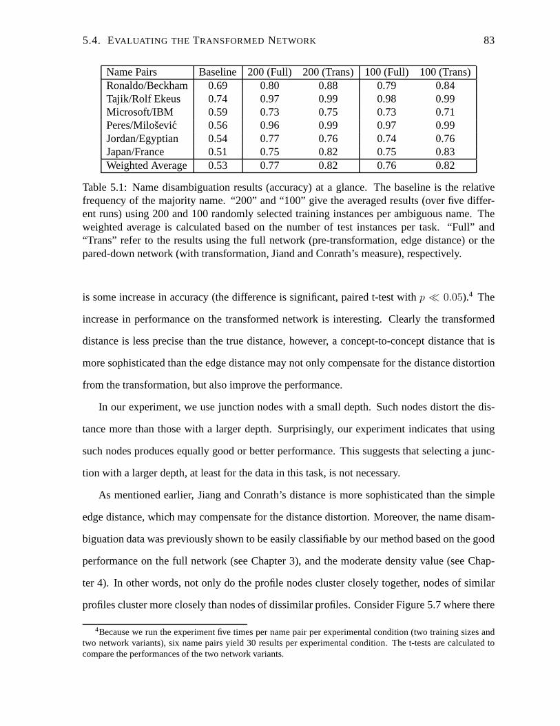
5.4. EVALUATING THE TRANSFORMED NETWORK 83
Name Pairs Baseline 200 (Full) 200 (Trans) 100 (Full) 100 (Trans)Ronaldo/Beckham 0.69 0.80 0.88 0.79 0.84Tajik/Rolf Ekeus 0.74 0.97 0.99 0.98 0.99Microsoft/IBM 0.59 0.73 0.75 0.73 0.71Peres/Milosevic 0.56 0.96 0.99 0.97 0.99Jordan/Egyptian 0.54 0.77 0.76 0.74 0.76Japan/France 0.51 0.75 0.82 0.75 0.83Weighted Average 0.53 0.77 0.82 0.76 0.82
Table 5.1: Name disambiguation results (accuracy) at a glance. The baseline is the relativefrequency of the majority name. “200” and “100” give the averaged results (over five differ-ent runs) using 200 and 100 randomly selected training instances per ambiguous name. Theweighted average is calculated based on the number of test instances per task. “Full” and“Trans” refer to the results using the full network (pre-transformation, edge distance) or thepared-down network (with transformation, Jiand and Conrath’s measure), respectively.
is some increase in accuracy (the difference is significant,paired t-test withp ≪ 0.05).4 The
increase in performance on the transformed network is interesting. Clearly the transformed
distance is less precise than the true distance, however, a concept-to-concept distance that is
more sophisticated than the edge distance may not only compensate for the distance distortion
from the transformation, but also improve the performance.
In our experiment, we use junction nodes with a small depth. Such nodes distort the dis-
tance more than those with a larger depth. Surprisingly, ourexperiment indicates that using
such nodes produces equally good or better performance. This suggests that selecting a junc-
tion with a larger depth, at least for the data in this task, isnot necessary.
As mentioned earlier, Jiang and Conrath’s distance is more sophisticated than the simple
edge distance, which may compensate for the distance distortion. Moreover, the name disam-
biguation data was previously shown to be easily classifiable by our method based on the good
performance on the full network (see Chapter 3), and the moderate density value (see Chap-
ter 4). In other words, not only do the profile nodes cluster closely together, nodes of similar
profiles cluster more closely than nodes of dissimilar profiles. Consider Figure 5.7 where there
4Because we run the experiment five times per name pair per experimental condition (two training sizes andtwo network variants), six name pairs yield 30 results per experimental condition. The t-tests are calculated tocompare the performances of the two network variants.
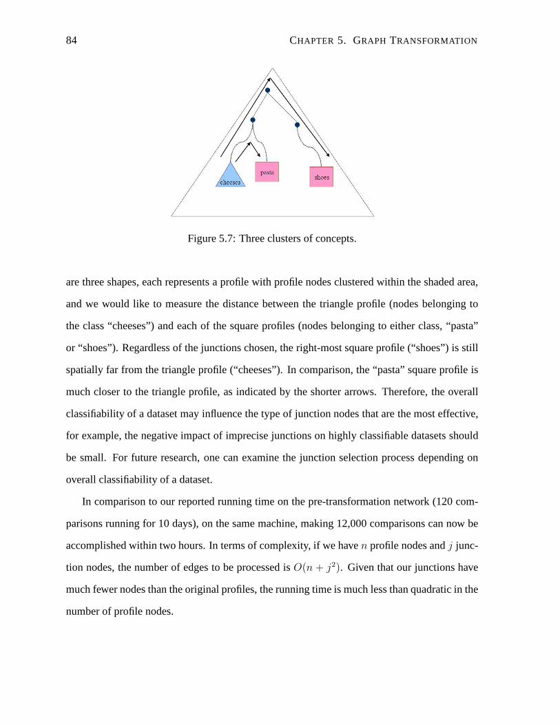
84 CHAPTER 5. GRAPH TRANSFORMATION
Figure 5.7: Three clusters of concepts.
are three shapes, each represents a profile with profile nodesclustered within the shaded area,
and we would like to measure the distance between the triangle profile (nodes belonging to
the class “cheeses”) and each of the square profiles (nodes belonging to either class, “pasta”
or “shoes”). Regardless of the junctions chosen, the right-most square profile (“shoes”) is still
spatially far from the triangle profile (“cheeses”). In comparison, the “pasta” square profile is
much closer to the triangle profile, as indicated by the shorter arrows. Therefore, the overall
classifiability of a dataset may influence the type of junction nodes that are the most effective,
for example, the negative impact of imprecise junctions on highly classifiable datasets should
be small. For future research, one can examine the junction selection process depending on
overall classifiability of a dataset.
In comparison to our reported running time on the pre-transformation network (120 com-
parisons running for 10 days), on the same machine, making 12,000 comparisons can now be
accomplished within two hours. In terms of complexity, if wehaven profile nodes andj junc-
tion nodes, the number of edges to be processed isO(n + j2). Given that our junctions have
much fewer nodes than the original profiles, the running timeis much less than quadratic in the
number of profile nodes.
5.5. SUMMARY 85
5.5 Summary
In this chapter, we have presented a method of incorporatingnon-additive concept-to-concept
distances by transforming the underlying ontological structure because the pre-transformation
network is inefficient to process. To remedy this, we proposea novel technique that mimics
the structure of the more computationally intensive network. Our evaluation shows that it is
possible to transform the structure of the original networkwithout hampering the network-flow
method’s ability to make fine-grained semantic distinctions, and the computational complexity
is drastically reduced as well. Our transformed network offers a competitive alternative to the
pre-transformation network.

86 CHAPTER 5. GRAPH TRANSFORMATION
Chapter 6
Conclusions
About six weeks ago Gertrude Stein said, it does not look to me
as if you were ever going to write that autobiography. You know
what I am going to do? I am going to write it for you. I am going
to write it as simply as Defoe did the autobiography of Robinson
Crusoe. And she has and this is it.
Gertrude Stein, The Autobiography of Alice B. Toklas
In this thesis, we have presented a graph-theoretic approach to calculating semantic distance
between two texts (collections of words). Our method takes advantage of the relational se-
mantic information among words provided by an ontology, andis simultaneously sensitive to
distributional information taken from a corpus. Given a suitable ontology, a word frequency
distribution for a text can be transformed into a frequency distribution over concept nodes.
Hence, each text is treated as a weighted and connected subgraph within a larger graph (the
ontology). By incorporating the semantic distance betweenindividual concepts, the ontology
becomes a metric space in which we calculate the distance between two texts as the minimum-
cost flow between the corresponding subgraphs.
We have explored a three-pronged approach in examining our graph-theoretic method for
text comparison. First, we have evaluated our network-flow approach in three different text
comparison tasks. We selected these tasks in a way that we cantest our method across texts
with varying degrees of constraint on the words comprising them. Second, in relation to
87
88 CHAPTER 6. CONCLUSIONS
the task-based evaluation, we have examined the classifiability of a dataset (a set of texts,
each represented as a collection of frequency-weighted concepts) with respect to our network-
flow method. Classifiability is defined as how well the data canbe clustered together within
the graphical structure of the ontology, or how semantically coherent the concepts are in the
dataset. Accordingly, we have devised a novel measure called profile densityto measure the se-
mantic coherence and by extension, as an indirect indication of classifiability. Finally, we have
examined a computational efficiency issue of our method thatstems from the need to general-
ize our network-flow method to using non-additive concept-to-concept distances such as those
by Wu and Palmer (1994) and Jiang and Conrath (1997). Incorporation of these concept-to-
concept distances requires an expensive pre-processing step if computed exactly. Instead, we
have developed a graph transformation method which allows us to reduce the computational
complexity without significant performance degradation.
We address the problem of text comparison in terms of the semantic distance between texts.
In particular, we are interested in examining how differences in word frequency and in word
meaning contribute to the overall text distance. Our methodis unique—we combine the two
factors via a network-flow framework. Via the intrinsic graphical structure of an ontology
and the formation of semantic profiles, a text can be thought of as a weighted collection of
concepts which are connected via ontology links. Then, the distance between two texts is their
ontological distance weighted by their difference in word frequency.
The idea of non-dualism can be traced back to the Sanskrit term, advaita, which refers
to things that are distinct while not being separate (Katz, 2007). This is an apt description
of our approach as the distributional and the ontological function as one integral piece (i.e.,
transporting frequency masses in a connected graph) instead of two (e.g., two separate features
fed into a machine learning method). The key connective tissue comes from the ontological
relations, which link two words or concepts via a path withinthe ontology. If we took a
purely distributional approach, each text would be treatedas a point in an n-dimensional space,
where each word would occupy one dimension, completely orthogonal (unrelated) to other
6.1. SUMMARY OF CONTRIBUTIONS 89
words/dimensions. For the purpose of measuring distance, our method has the flexibility to
allow inter-word or inter-concept comparison. Furthermore, MCF has been shown to measure
the distributional distance between two frequency distributions. Our method is the first to
introduce such a non-dual combination systematically.
6.1 Summary of Contributions
In this section, we will summarize our contributions with emphasis on our experimental results.
Applying Our Graph-Theoretic Model to Measuring Text Distance. In Chapter 3, we
evaluated our network-flow method in three different NLP tasks: verb alternation detection,
name disambiguation, and document classification. We selected these tasks to test our method
on data with varying degrees of syntactic and semantic constraints imposed on them. In the
first task, the words have a particular syntactic relation toa target verb. In the second task,
the syntactic restriction is relaxed such that words appearing within a local window of an
ambiguous name are considered. Finally, in the last task, the window size restriction is relaxed
further so that words within a document are included.
The results show that our method is superior to other distributional methods in the first two
tasks. In the verb alternation task, our method achieves an average accuracy of 0.67 on ran-
domly selected verbs and is the best method in most conditions. In the name disambiguation
task, where the syntactic restriction on the text is relaxed, our method achieves an average ac-
curacy of 0.83 (weighted) and 0.76 (unweighted). In contrast, purely distributional approaches
at best reach 0.72 and 0.52 of weighted and unweighted accuracies.
Our method is less successful in the document classificationtask, in which the window size
restriction is further removed. In this task, distributional methods reach an accuracy of 0.61 or
above, whereas our method achieves an accuracy only in the low 0.30s. Increasing the window
size clearly introduces more noise to the data. In an attemptto remove the noise from the data,
we created a noise frequency distribution of concepts and subtracted it from the data. The noise
90 CHAPTER 6. CONCLUSIONS
removal results in a slight increase in the performance but is not sufficient to improve it to be
on par with the best distributional results.
Measuring Semantic Coherence within an Ontology. Because of the network-flow frame-
work, there is intricate interaction between ontological and distributional information used in
the calculation of the minimum-cost flow. Therefore, in Chapter 4, we proposed a non-dual
approach to measuringprofile densityas an indicator of how well our network-flow method
can classify a dataset. Our analysis shows that profile density correlates very well with the per-
formance of our method: the datasets of verb alternation detection and name disambiguation
are denser, hence more easily classifiable, than document classification data.
In our task-based evaluation, our data has varying degrees of syntactic and semantic con-
straints. Interestingly, the degree of constraints influences the relatedness or the semantic co-
herence within the dataset. In the first task, the words have the most restrictions imposed on
them: in addition to syntactic constraints, because we selected verbs from a handful of se-
mantic classes, the verbs exert a high degree of selectionalrestriction on their arguments. Not
surprisingly, this dataset has the highest profile density and therefore semantic coherence. As
we relax the constraints further, the density values decrease. Name disambiguation data has
the next highest density. Document classification data has the least degree of restriction and,
indeed is the least dense.
Maximizing the Accuracy and Efficiency in the Calculation of Non-additive Distances.
In Chapter 5, we addressed the problem of incorporating non-additive distances into our net-
work-flow framework via a graph transformation method. Because the MCF problem defini-
tion assumes additivity to hold for the concept-to-conceptdistance, the use of a non-additive
distance becomes impractical without modification—the exactness of distance calculation and
efficiency cannot be simultaneously achieved. In this chapter, we introduced a graph transfor-
mation method that constructs a new graph in which we can balance the two factors. In our
evaluation, we compared the name disambiguation results onthe transformed graph vs. those
6.2. SHORT-TERM IMPROVEMENTS: WITHIN THE MCF FRAMEWORK 91
on the original graph. Not only have we improved the speed (120 comparisons in 10 days
vs. 12,000 comparisons in two hours), there is no major performance degradation; in fact, our
results on the transformed graph showed some performance improvement.
Our result suggests that there is a link between semantic distance and density. We have
shown that density is an indicator of classifiability using our text distance. Given moderate to
high density value and good performance on the full network,similar profiles nodes are closer
in distance than dissimilar profiles are, regardless of the precision of junction nodes selected.
Indeed, we have shown that this is indeed the case for the datadisambiguation data using high
imprecise junction nodes. We conclude that for a highly classifiable dataset, an approximate
network is sufficiently precise to yield comparable results.
6.2 Short-term Improvements: Within the MCF Framework
Text Representation. Currently, we have used a simple profile representation by uniformly
distributing word counts to relevant concepts. A more accurate frequency estimates of the
concepts would clearly result in more accurate classification, especially in the document clas-
sification task. There exist statistical methods such as those by Li and Abe (1998) and Clark
and Weir (2002), which produce probability estimates over acollection of concepts. However,
when applied to every profile, these methods are impracticalgiven their complexity. One low
complexity option is to pre-process the whole dataset once by pruning out concepts to which
low frequency and/or highly ambiguous words are mapped, then we can then form more “ac-
curate” profiles by considering only the remaining concepts. This way, we improve on the
frequency estimates of concepts with very little extra overhead attached to the profile genera-
tion.
The Use of Different Ontological Relations. Currently, we only use the hyponymy links
within the ontology to capture the semantic relations amongwords or concepts. It has been
shown that readers process the content of a text by relating the concepts in a variety of ways
92 CHAPTER 6. CONCLUSIONS
other then hyponymy (Morris, 2006). It is thus possible thatthe inclusion of other ontological
relations will be useful in some applications. As a result, the graphical representation would no
longer be hierarchical, which poses little problem as the MCF definition makes no assumption
on the graph structure. However, we may have to re-consider what a reasonable concept-to-
concept distance is. Many distance measures consider both the two target concepts as well
as their common ancestors. Given that there are many relations, there are potentially multi-
ple common ancestors. Hence, computing the distance between two concepts become more
complicated and computationally inefficient (e.g., Hirst and St-Onge, 1998, who consider all
ontological relations in WordNet). A new method of measuring concept-to-concept distance
may be necessary to account for the more complicated graph structure.
Classifiability within the Network-Flow Framework. We use profile density to analyse
the behaviour of our MCF method on three NLP tasks. One area worthy of exploration is the
use of profile density as an indicator of the overall classifiability of a dataset using the MCF
framework. Currently, we are able to rank the three datasetsin terms of their density values,
but further examination is needed to determine a reliable indicator of classifiability within our
network-flow framework. One straightforward method is to test on more variety of texts to
establish a meaningful threshold (range) to predict whether the MCF will be useful for a task.
6.3 Long-Term Research Directions
Semantic Coherence. We suggest that not only is our profile density useful in predicting the
performance of our network-flow method on unseen data, it canalso be useful for measuring
the semantic coherence of a text in general. Note that a text that is semantically coherent tends
to form profiles with highly frequent and highly related concepts within an ontology. Coin-
cidentally, our profile density formulation measures the overall coherence of a collection of
concepts by taking into account the distance between the concepts as well as their frequencies.
For example, if we relax the notion of a text to include a collection of verbal arguments (e.g.,
6.3. LONG-TERM RESEARCH DIRECTIONS 93
nouns appearing as the direct object of a verb), and not just the words appearing sequentially
in a document, semantic coherence of a text can be thought of as the selectional preference
strength a verb imposes on its arguments. As future work, we intend to investigate profile
density as an indicator of selectional preference strength.
Verb Alternation Discovery. Verb alternation discovery is a generalized version of verb
alternation detection. The idea is to discover possible alternation behaviour given a labelled
slot and an unlabelled slot, which is potentially useful in tasks such as semantic role labelling
and in detecting non-compositionality (McCarthy et al., 2007). The assumption here is that
given a verb, syntactic slots with the same role label would have similar selectional preference
strength. For example, theTHEME slots (subject of the intransitive and direct object of the
transitive) of the verbmeltare likely to be “meltable” things. Given that both slots would have
similar selectional preferences, the instances of their selectional preference strength (or profile
density as selectional preference strength) would also be similar. Then, the goal is to detect
new alternations if an unlabelled syntactic slot is shown tohave similar selectional strength as
that of a known slot.
Hot-spot Detection. Finally, profile density measures the graphical density of acollection
of weighted nodes. A useful extension ishot-spot detection. Given a collection of weighted
nodes, the idea is to detect clusters (“hot spots”) by measuring the density of subsets of nodes
in comparison to the overall graphical density. Since the current work assumes a hierarchical
graphical structure (e.g., hyponymy hierarchy in WordNet), subset partition is made possible
with the use of ancestors (lowest common ancestors) to the nodes. Hot-spot detection is useful
in applications such as verb sense detection. Consider the verbpour as in “I pour some milk
into the glass” vs. “The Bank of England poured£3M into Northern Rock”. Here, there are
two distinct senses of the verb: a liquid-displacement sense and a financial sense. Assuming
the corpus counts of the direct objects reflect the two senses, there would be two detectable hot
spots in the ontology. Generally, we believe profile densitymay offer a quantitative measure

94 CHAPTER 6. CONCLUSIONS
for semantic coherence and other related NLP applications.
Bibliography
Agirre, E. and Rigau, G. (1996). Word sense disambiguation using conceptual density. InIn
Proceedings of the 12th International Conference of Computational Linguistics (COLING-
1996), pages 16–22, Copenhagen, Denmark.
Al-Mubaid, H. and Umair, S. A. (2006). A new text categorization technique using distribu-
tional clustering and learning logic.IEEE Transaction on Knowledge and Data Engineering,
18(9).
Barzilay, R. and Lapata, M. (2005). Collective content selection for concept-to-text generation.
In Proceedings of the Joint Conference on Human Language Technology / Empirial Methods
in Natural Language Processing (HLT/EMNLP).
Bodenreider, O. (2004). The unified medical language system(UMLS): Integrating biomedical
terminology.Nucleic Acids Research, 32:D267–D270.
Brin, S. and Page, L. (1998). The anatomy of a large-scale hypertextual web search engine.
Computer Networks and ISDN Systems, 30(1–7):107–117.
Briscoe, T. and Carroll, J. (1997). Automatic extraction ofsubcategorization from corpora.
In Proceedings of the 5th Applied Natural Language ProcessingConference (ANLP), pages
356–363.
Briscoe, T. and Carroll, J. (2002). Robust accurate statistical annotation of general text. In
95
96 BIBLIOGRAPHY
Proceedings of the Third International Conference on Language Resources and Evaluation
(LREC 2002), pages 1499–1504.
Budanitsky, A. and Hirst, G. (2001). Semantic distance in wordnet: An experimental,
application-oriented evaluation of five measures. InProceedings of the Workshop on Word-
Net and Other Lexical Resources, in the North American Chapter of the Association for
Computational Linguistics (NAACL-2001), Pittsburgh, PA.
Budanitsky, A. and Hirst, G. (2006). Evaluating WordNet-based measures of semantic distance.
Computational Linguistics, 32(1):13–47.
Burnard, L. (2000).The British National Corpus Users Reference Guide. Oxford University
Computing Services, Oxford, UK.
Chang, C.-C. and Lin, C.-J. (2001).LIBSVM: a library for support vector machines. Software
available athttp://www.csie.ntu.edu.tw/∼cjlin/libsvm.
Clark, S. and Weir, D. (2002). Class-based probability estimation using a semantic hierarchy.
Computational Linguistics, 28(2):187–206.
Corley, C. and Mihalcea, R. (2005). Measuring the semantic similarity of texts. InProceedings
of the ACL Workshop on Empirical Modeling of Semantic Equivalence and Entailment.
Esuli, A., Fagni, T., and Sebastiani, F. (2006). TreeBoost.MH: A boosting algorithm for multi-
label hierarchical text categorization. InProceedings of the 13th International Symposium
on String Processing and Information Retrieval (SPIRE’06), pages 13–24, Glasgow, UK.
Fellbaum, C., editor (1998).WordNet: An Electronic Lexical Database. MIT Press.
Gurevych, I., Malaka, R., Porzel, R., and Zorn, H.-P. (2003). Semantic coherence scoring
using an ontology. InProceedings of the Joint Human Language Technology and Northern
Chapter of the Association for Computational Linguistics Conference (HLT-NAACL), pages
88–95, Edmonton, Canada.
BIBLIOGRAPHY 97
Han, H., Zha, H., and Giles, C. L. (2005). Name disambiguation in author citations using a
K-way spectral clustering method. InJoint Conference on Digital Libraries (JCDL’05).
Hirst, G. and St-Onge, D. (1998). Lexical chains as representations of context for the detection
and correction of malapropisms. In Fellbaum (1998), pages 305–332.
Iwayama, M., Fujii, A., Kando, N., and Marukawa, Y. (2003). An empirical study on retrieval
models for different document genres: Patents and newspaper articles. InProceedings of the
26th ACM SIGIR International Conference on Research and Development in Information
Retrieval, pages 251–258.
Jarmasz, M. and Szpakowicz, S. (2003). Rogets thesaurus andsemantic similarity. InProceed-
ings of Conference on Recent Advances in Natural Language Processing (RANLP 2003),
pages 212–219, Borovets, Bulgaria.
Jiang, J. and Conrath, D. (1997). Semantic similarity basedon corpus statistics and lexical
taxonomy. InProceedings on the International Conference on Research inComputational
Linguistics, pages 19–33.
Joachims, T. (2002).Learning to Classify Text Using Support Vector Machines – Methods,
Theory, and Algorithms. Kluwer/Springer.
Katz, J. (2007).One: Essential Writings on Nonduality. Sentient Publications.
Kullback, S. and Leibler, R. (1951). On information and sufficiency. Annals of Mathematical
Statistics, 22:79–86.
Lee, L. (2001). On the effectiveness of the skew divergence for statistical language analysis.
In Artificial Intelligence and Statistics, pages 65–72.
Levin, B. (1993). English Verb Classes and Alternations: A Preliminary Investigation. Uni-
versity of Chicago Press.
98 BIBLIOGRAPHY
Levina, E. and Bickel, P. (2001). The earth mover’s distanceis the mallows distance: Some
insights from statistics. InProceedings of the Eighth IEEE International Conference on
Computer Vision, volume 2, pages 251–256.
Li, H. and Abe, N. (1998). Word clustering and disambiguation based on co-occurrence data.
In Proceedings of COLING-ACL 1998, pages 749–755.
Lin, D. (1998). An information-theoretic definition of similarity. In Proceedings of Interna-
tional Conference on Machine Learning.
McCarthy, D. (2000). Using semantic preferences to identify verbal participation in role
switching alternations. InProceedings of Applied Natural Language Processing and North
American Chapter of the Association for Computational Linguistics (ANLP-NAACL 2000),
pages 256–263.
McCarthy, D. (2001).Lexical Acqusition at the Syntax-Semantics Interface: Diathesis Alter-
nations, Subcategorization Frames and Selectional Preferences. PhD thesis, University of
Sussex, Brighton, UK.
McCarthy, D., Venkatapathy, S., and Joshi, A. K. (2007). Detecting compositionality of verb-
object combinations using selectional preferences. InProceedings of the Conference on
Empirical Methods in Natural Language Processing (EMNLP 2007), Prague, Czech Repub-
lic.
Merlo, P. and Stevenson, S. (2001). Automatic verb classification based on statistical distribu-
tions of argument structure.Computational Linguistics, 27(3):393–408.
Mihalcea, R. (2005). Unsupervised large-vocabulary word sense disambiguation with graph-
based algorithms for sequence data labeling. InProceedings of the Joint Conference
on Human Language Technology / Empirial Methods in Natural Language Processing
(HLT/EMNLP).
BIBLIOGRAPHY 99
Mihalcea, R. (2006). Random walks on text structures. InProceedings of Computational Lin-
guistics and Intelligent Text Processing (CICLing) 2006, pages 249–262. Springer-Verlag.
Mitchell, T. (1999). 20 newsgroups usenet articles.http://kdd.ics.uci.edu/
/databases/20newsgroups/20newsgroups.data.html.
Mohammad, S. and Hirst, G. (2006). Distributional measuresof concept-distance: A task-
oriented evaluation. InProceedings of the 2006 Conference on Empirical Methods in Natural
Language Processing (EMNLP 2006), Sydney, Australia.
Morris, J. (2006). Readers’ subjective perceptions of lexical cohesion and implications for
computers’ interpretations of text meaning. InProceedings of CaSTA Conference on Breadth
of Text, University of New Brunswick, Canada.
Navigli, R. and Velardi, P. (2005). Structural semantic interconnections: A knowledge-based
approach to word sense disambiguation.IEEE Transactions on Pattern Analysis and Ma-
chine Intelligence, 27(7).
Nigam, K., McCallum, A., and Mitchell, T. (2006).Semi-supervised Text Classification Using
EM, pages 33–56. MIT Press, Boston, MA, USA.
Pang, B. and Lee, L. (2004). A sentimental education: Sentiment analysis using subjectivity
summarization based on minimum cuts. InProceedings of the 42nd ACL, pages 271–278.
Pantel, P. and Lin, D. (2000). An unsupervised approach to prepositional phrase attachment us-
ing contextually similar words. InProceedings of Association for Computational Linguistics
(ACL-00), pages 101–108, Hong Kong.
Pedersen, T., Purandare, A., and Kulkarni, A. (2005). Name discrimination by clustering
similar context. InProceedings of the Sixth International Conference on Intelligent Text
Processing and Computational Linguistics.
100 BIBLIOGRAPHY
Pereira, F., Tishby, N., and Lee, L. (1993). Distributionalclustering of english words. In
Proceedings of the 31st Annual Meeting of the Association for Computational Linguistics.
Pinker, S. (1989).Learnability and Cognition: The Acquisition of Argument Structure. MIT
Press, Cambridge, MA.
Rada, R., Mili, H., Bicknell, E., and Blettner, M. (1989). Development and application of a
metric on semantic nets.IEEE Transactions on Systems, Man and Cybernetics, 19:17–30.
Rennie, J. (2001). Improving multi-class text classification with naive bayes. Master’s thesis,
Massachusetts Institute of Technology.
Resnik, P. (1993).Selection and Information: A Class-Based Approach to Lexical Relation-
ships. PhD thesis, University of Pennsylvania, Philadelphia, PA, USA.
Resnik, P. (1995). Using information content to evaluate semantic similarity in a taxonomy. In
Proceedings of the 14th International Joint Conference on Artificial Intelligence.
Ribas, F. (1995). On learning more appropriate selectionalrestrictions. InProceedings of the
Seventh Conference of the European Chapter of the Association for Computation Linguistics,
pages 112–118, Dublin, Ireland.
Schulte im Walde, S. (2006). Experiments on the automatic induction of German semantic
verb classes.Computational Linguistics, 32(2):159–194.
Scott, S. and Matwin, S. (1998). Text classification using WordNet hypernyms. InProceed-
ings of the COLING-ACL Workshop on Usage of WordNet in Natural Language Processing
Systems, pages 45–51.
Weeds, J. (2003).Measures and Applications of Lexical Distributional Similarity. PhD thesis,
University of Sussex, Sussex, UK.
BIBLIOGRAPHY 101
Weeds, J., Weir, D., and McCarthy, D. (2004). Characterising measures of lexical distributional
similarity. InProceedings of the 20th International Conference of Computational Linguistics
(COLING-2004).
Wu, Z. and Palmer, M. (1994). Verb semantics and lexical selection. In Proceedings of the
32nd Annual Meeting of the Association for Computational Linguistics, pages 133–138.
Xu, W., Liu, X., and Gong, Y. (2003). Document clustering based on non-negative matrix
factorization. InProceedings of the 26th ACM SIGIR International Conferenceon Research
and Development in Information Retrieval.