Busy periods of a fractional

Brownian type Gaussian

storage

Tommi Sottinen

University of Helsinki

A joint work with

Yu. Kozachenko and O. Vasylyk

Kyiv National University.

1

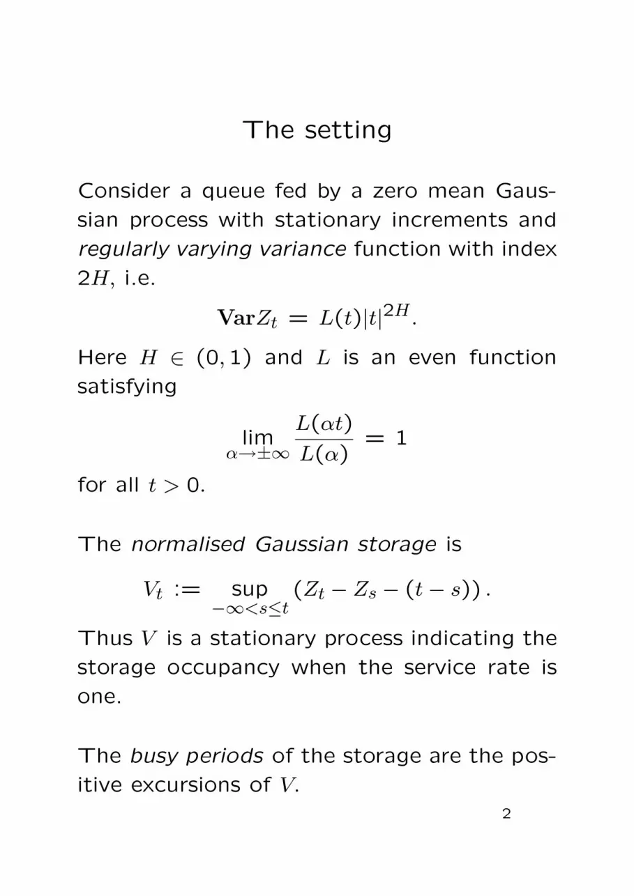
The setting

Consider a queue fed by a zero mean Gaus-

sian process with stationary increments and

regularly varying variance function with index

2H, i.e.

VarZt = L(t)|t|2H .

Here H ∈ (0,1) and L is an even function

satisfying

limα→±∞

L(αt)

L(α)= 1

for all t > 0.

The normalised Gaussian storage is

Vt := sup−∞<s≤t

(Zt − Zs − (t− s)) .

Thus V is a stationary process indicating the

storage occupancy when the service rate is

one.

The busy periods of the storage are the pos-

itive excursions of V.

2

The setting, cont.

Let C(R) be the space of continuous func-

tions over R. As the underlying probability

space take

Ω :=ω ∈ C(R) : ω(0) = 0, lim

t→±∞ω(t)

1 + |t|= 0

equipped with the norm

‖ω‖Ω := supt∈R

|ω(t)|1 + |t|

and the corresponding Borel σ-algebra. The

Probability measure P on Ω is such that

ω(t) = Zt(ω).

(we give later assumptions on L so that

Z(ω) ∈ Ω.)

3

The case of fractional Brownian

motion

If L ≡ 1 then Z is a fractional Brownian mo-

tion (fBm), i.e. a centred Gaussian process

with covariance function

R(t, s) =1

2

(|t|2H + |s|2H − |t− s|2H

).

Let H be the Reproducing Kernel Hilbert

Space (RKHS) of Z, i.e. the space of func-

tions f : R → R defined by letting

Zt 7→ R(t, ·)

span an isometry from the linear space of Z

onto H.

Remark H ⊂ Ω as a set and the topology in

H is finer that that of Ω.

4

The case of fBm, cont.

The generalised Shilder’s theorem states:

Theorem 1 The function

I(ω) =

12‖ω‖

2H, if ω ∈ H,∞, otherwise,

is a good rate function for Z and

lim supα→∞

α−1 lnP(α−12Z ∈ F ) ≤ − inf

ω∈FI(ω),

lim infα→∞ α−1 lnP(α−

12Z ∈ G) ≥ − inf

ω∈FI(ω),

for all F ⊂ Ω closed and G ⊂ Ω open, i.e.

(α−12Z, α)α≥1 satisfies the Large Deviations

Principle (LDP) on Ω with rate function I.

5

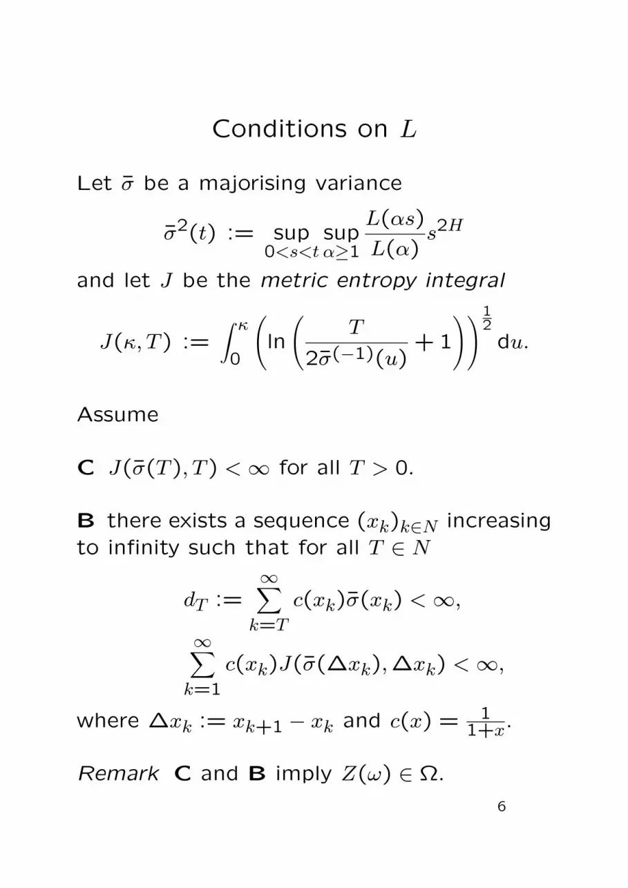
Conditions on L

Let σ be a majorising variance

σ2(t) := sup0<s<t

supα≥1

L(αs)

L(α)s2H

and let J be the metric entropy integral

J(κ, T ) :=∫ κ

0

(ln

(T

2σ(−1)(u)+ 1

))12du.

Assume

C J(σ(T ), T ) < ∞ for all T > 0.

B there exists a sequence (xk)k∈N increasingto infinity such that for all T ∈ N

dT :=∞∑

k=T

c(xk)σ(xk) < ∞,

∞∑k=1

c(xk)J(σ(∆xk),∆xk) < ∞,

where ∆xk := xk+1 − xk and c(x) = 11+x.

Remark C and B imply Z(ω) ∈ Ω.

6

Convergence and LDP of Z

Define a family (Z(α))α≥1 by

Z(α)t :=

1

αHL(α)12

Zαt.

Assumptions C and B yield

Theorem 2 The processes (Z(α))α≥1 con-

verge weakly in Ω to a fBm.

On the proof The finite dimensional conver-

gence is obvious. Assumptions C and B are

needed to prove that the family (Z(α))α≥1 is

tight in Ω.

7

Application to busy periods, cont.

Theorem 3 The scaled familyL(α)12

α1−HZ(α) ,

α2−2H

L(α)

α≥1

satisfies LDP on Ω with the rate function I

of a fBm.

On the proof Fix a vector t = (t1, . . . , td)

and denote

Z(α) :=(Z

(α)t1

, . . . , Z(α)td

).

Let Λ(α) be the logarithm of the moment

generating function of L(α)12αH−1Z(α) :

Λ(α)(u) := lnE exp

⟨u,

L(α)12

α1−HZ(α)

⟩.

8

Application to busy periods, cont,

cont.

It is easy to see that

α2−2H

L(α)Λ(α)(u) →

1

2〈Γu,u〉 ,

where Γ is the covariance of

B =(B

(α)t1

, . . . , B(α)td

)and B is a fBm with index H. Then, for theFenchel–Legendre tranform we have

Λ∗(x) = supu∈Rd

(ux− Λ(u))

=1

2

⟨Γ−1x,x

⟩=

1

2‖x‖2H.

The LDP in Ω equipped with projective limittopology follows now from the Gartner–Ellistheorem.

For the full LDP on Ω we need the so-calledexponential tightness which follows from as-sumption C and B.

9

Application to busy periods

Recall the storage process

Vt(ω) := sup−∞<s≤t

(ω(t)− ω(s)− (t− s)) .

The busy period containing 0 is the stochas-

tic interval

[A, B] :=

[supt ≤ 0 : Vt = 0 , inft ≥ 0 : Vt = 0] ,

if A < 0 < B. Otherwise the system is not

busy at time 0.

Denote by

KT := A < 0 < B, B −A > T

the set of paths for which the ongoing busy

period at 0 is strictly longer than T.

10

Application to busy periods, cont.

Lemma For any T ≥ 1

P (Z ∈ KT ) = P

L(T )12

T1−HZ(T ) ∈ K1

.

proof

P(Z ∈ KT

)= P

(∃a < 0, b > (a + T )+∀t ∈ (a, b) :

Zt − Za > t− a)

= P(∃a < 0, b > (a + 1)+∀t ∈ (a, b) :

ZTt − ZTa > Tt− Ta)

= P(∃a < 0, b > (a + 1)+∀t ∈ (a, b) :

T−1(ZTt − ZTa) > t− a)

= P(L(T )

12TH−1Z(T ) ∈ K1

).

11

Application to busy periods, cont.,

cont.

Theorem 4

limT→∞

L(T )

T2−2HlnP(Z ∈ KT ) = − inf

ω∈K1I(ω),

where infω∈K1I(ω) ∈ [12,

c2H2 ], and

c2H =1

H(2H − 1)(2− 2H)B(H − 12,2− 2H)

.

Remark One can numerically find arbitrar-ily good approximations to infω∈K1

I(ω) usingRKHS techniques.

Example Suppose the traffic is composedof independent fBm streams with differentHurst indices, i.e.

Z =n∑

k=1

akBHk.

Then assumptions C and B are satisfied and

L(T )

T2−2H=

n∑k=1

a2kT2Hk−2.

12

Literature

1. Buldygin, V. V. and Kozachenko, Yu. V.Metric Characterization of Random Variables andRandom Processes.American Mathematical Society, Providence, RI,2000.

2. Dembo, A. and Zeitouni, O.Large Deviations Techniques and Applications.Second Edition.Springer, 1998.

3. Yu. Kozachenko, T. Sottinen and O. Vasylyk.Path space large deviations of a large buffer withGaussian input traffic.Preprint 294, University of Helsinki, 2001, 12 p.(submitted to Queueing Systems.)

4. Norros, I.Busy Periods of Fractional Brownian Storage: ALarge Deviations Approach.Advances in Performance Analysis, Vol. 2(1), pp.1–19, 1999.

13