------------------------------------------------ * Correspondence to: Jing He, jhe@cs.odu.edu.

Building the Initial Chain of the Proteins through De Novo Modeling of the Cryo-Electron Microscopy Volume Data at

the Medium Resolutions Kamal Al Nasr, Lin Chen, Dong Si, Desh Ranjan, Mohammad Zubair, Jing He*

Department of Computer Science Old Dominion University, Norfolk, VA 23529, USA {kal, lchen, dsi, dranjan, zubair, jhe} @cs.odu.edu

ABSTRACT Cryo-electron Microscopy (cryoEM) is an advanced imaging technique that produces volume maps at different resolutions. This technique is capable of visualizing large molecular complexes such as viruses and ribosomes. At the medium resolutions, such as 5 to 10Å, the location and orientation of the secondary structure elements (SSEs) can be computationally identified. However, there is no registration between the detected SSEs and the protein sequence, and therefore it is challenging to derive the atomic structure from such volume data. We present, in this paper, the preliminary results of the full-atom protein chains using our de novo modeling framework. The framework has multiple components including the ranking of topologies, the construction of helices and loops along the density traces, and the energy evaluation of the structure. A test containing thirteen simulated density maps and two experimentally derived density maps show that the true topology was ranked among the top 35 of the huge topological space. The best atomic model of the true topology was ranked within the top 40 for twelve of the fifteen proteins tested. The average backbone RMSD100 of these models is about 4Å for the fifteen proteins.

General Terms Algorithms, Performance, Design, Experimentation, Theory, Verification.

Keywords Protein, Modeling, Shortest paths, Graph, , Structure, Electron Microscopy, Topology, Secondary Structure, Loop, Volume, Density.

1. INTRODUCTION Cryo-Electron Microscopy (cryoEM) is an attractive imaging technique that has great potential in deriving the three-dimensional structure of large protein complexes [1-4]. Unlike other experimental techniques (i.e. X-ray crystallography and nuclear magnetic resonance (NMR) cryoEM is capable of producing volume, or density maps, of large proteins. Using the current advances of cryoEM techniques, it is possible to produce volume maps of a proteins in the high resolution range, such as 3-5Å resolution [5, 6]. At this resolution, the connection between the secondary structures is mostly distinguishable and the backbone of the protein can be derived [5-7]. Due to various

experimental difficulties, many large protein complexes have been resolved to the medium resolution range between 5 and 10Å [8].

At the medium resolution range, the volume map is not resolved well enough to determine the atomic information of the protein. For example, the conformation of the loops and side chains is mostly not distinguishable. Recent work has shown that the volume maps can be used to distinguish between the models built by ab initio structure prediction and the comparative modeling [9-15]. However, the size of the proteins in the cryoEM maps often proposes challenges to the ab initio method. When a component of the protein has a known atomic structure, fitting is often used to derive the rest portion of the protein structure. When a template atomic structure is available, comparative modeling method can be used.

Permission to make digital or hard copies of all or part of this work for personal or classroom use is granted without fee provided that copies are not made or distributed for profit or commercial advantage and that copies bear this notice and the full citation on the first page. To copy otherwise, or republish, to post on servers or to redistribute to lists, requires prior specific permission and/or a fee. ACM-BCB ’12, October 7-10, 2012, Orlando, FL, USA. Copyright 2012 ACM 978-1-4503-1670-5/12/10 ...$15.00.

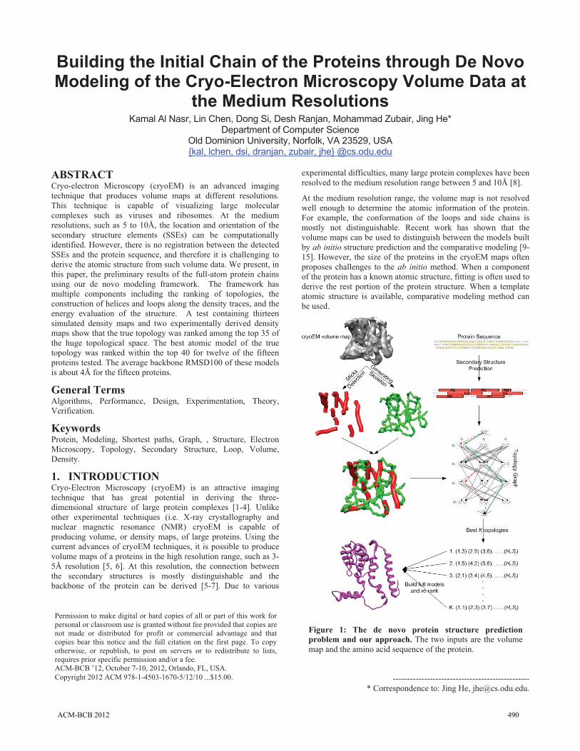
Figure 1: The de novo protein structure prediction problem and our approach. The two inputs are the volume map and the amino acid sequence of the protein.

ACM-BCB 2012 490

Contrary to the fitting and the template approach, de novo modeling aims to derive the atomic structure of the protein without a template. Gorgon is one of the de novo approaches. It uses a semi-automated approach to build the backbone of the protein. It has been shown successful in deriving the model if the resolution is high enough for visual distinction of the secondary structures and their major connections [16]. Lindert et al. [17, 18] proposed a de novo folding approach called EM-Fold. EM-Fold uses the Monte Carlo method to assemble the secondary structures. The loops and side chains are added by Rosetta in the refinement step.

We previously developed a fast graph method to rank the topologies of the SSEs [19]. We have also described a statistical multi-well energy function for structural evaluation using the reduced representation of the amino acids [20, 21]. This paper focuses on two additional steps to construct the initial atomic model of the protein. The first step involves building the backbone of a helix guided by the density trace. The second step aims to build a loop that follows density skeleton. We report the result of the initial structures that were built using our framework. The initial structures are expected to be refined by additional refinement programs in the future.

2. THE FRAMEWORK OF DE NOVO MODELING

Figure 1 illustrates the major steps in our de novo modeling method. There are two sources of inputs. One comes from the density map that can be obtained by cryoEM technique. The other is the amino acid sequence of the proteins involved. The framework includes multiple components: the detection of the secondary structure elements, the detection of the skeleton, the ranking of the topologies of the SSEs, the construction of the all-atom chain, and the energy evaluation of the structure. We describe the work for �-proteins in this paper, although the framework can be generally applied to those proteins with �-sheets.

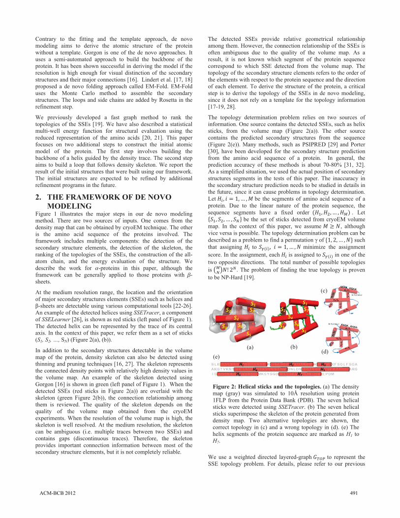
At the medium resolution range, the location and the orientation of major secondary structures elements (SSEs) such as helices and �-sheets are detectable using various computational tools [22-26]. An example of the detected helices using SSETracer, a component of SSELearner [26], is shown as red sticks (left panel of Figure 1). The detected helix can be represented by the trace of its central axis. In the context of this paper, we refer them as a set of sticks (S1, S2, …, SN) (Figure 2(a), (b)).

In addition to the secondary structures detectable in the volume map of the protein, density skeleton can also be detected using thinning and pruning techniques [16, 27]. The skeleton represents the connected density points with relatively high density values in the volume map. An example of the skeleton detected using Gorgon [16] is shown in green (left panel of Figure 1). When the detected SSEs (red sticks in Figure 2(a)) are overlaid with the skeleton (green Figure 2(b)), the connection relationship among them is reviewed. The quality of the skeleton depends on the quality of the volume map obtained from the cryoEM experiments. When the resolution of the volume map is high, the skeleton is well resolved. At the medium resolution, the skeleton can be ambiguous (i.e. multiple traces between two SSEs) and contains gaps (discontinuous traces). Therefore, the skeleton provides important connection information between most of the secondary structure elements, but it is not completely reliable.

The detected SSEs provide relative geometrical relationship among them. However, the connection relationship of the SSEs is often ambiguous due to the quality of the volume map. As a result, it is not known which segment of the protein sequence correspond to which SSE detected from the volume map. The topology of the secondary structure elements refers to the order of the elements with respect to the protein sequence and the direction of each element. To derive the structure of the protein, a critical step is to derive the topology of the SSEs in de novo modeling, since it does not rely on a template for the topology information [17-19, 28].

The topology determination problem relies on two sources of information. One source contains the detected SSEs, such as helix sticks, from the volume map (Figure 2(a)). The other source contains the predicted secondary structures from the sequence (Figure 2(e)). Many methods, such as PSIPRED [29] and Porter [30], have been developed for the secondary structure prediction from the amino acid sequence of a protein. In general, the prediction accuracy of these methods is about 70-80% [31, 32]. As a simplified situation, we used the actual position of secondary structures segments in the tests of this paper. The inaccuracy in the secondary structure prediction needs to be studied in details in the future, since it can cause problems in topology determination. Let ��� � � ��� � be the segments of amino acid sequence of a protein. Due to the linear nature of the protein sequence, the sequence segments have a fixed order ��� ���� � � � . Let ���� ��� � � ��� be the set of sticks detected from cryoEM volume map. In the context of this paper, we assume � �, although vice versa is possible. The topology determination problem can be described as a problem to find a permutation � of ��� �� � ��� such that assigning �� to ����� � � ��� � � minimize the assignment score. In the assignment, each �� is assigned to ���� in one of the two opposite directions. The total number of possible topologies is � ���� ��. The problem of finding the true topology is proven to be NP-Hard [19].

We use a weighted directed layered-graph ���� to represent the SSE topology problem. For details, please refer to our previous

Figure 2: Helical sticks and the topologies. (a) The density map (gray) was simulated to 10Å resolution using protein 1FLP from the Protein Data Bank (PDB). The seven helical sticks were detected using SSETracer. (b) The seven helical sticks superimpose the skeleton of the protein generated from density map. Two alternative topologies are shown, the correct topology in (c) and a wrong topology in (d). (e) The helix segments of the protein sequence are marked as H1 to H7.

(a) (b)

(c)

(d)(e)

ACM-BCB 2012 491

work in [19]. We briefly outline the main idea of our graph approach in this section. The number of regular nodes in the graph is � � � � , where is the number of SSE segments on sequence and � is the number of SSE sticks detected from density map. Each node represents one possible assignment between one SSE sequence segment and one SSE stick in a specific direction. For example, node �� �� � represents the assignment of segment �� to the stick �! in "direction. Two special nodes �#$%# and &�' are added. Most of the edge weights in the graph were assigned by tracing the skeleton. For any possible edge, the weight of the edge is the absolute difference between the virtual length of the loop and the virtual length of the trace detected on the skeleton. More details about the weight calculation will be included in a separate paper.

A path of ���� begins at �#$%# node and ends at &�' node. The problem of enumerating all valid topologies becomes the problem of enumerating all valid paths. Not every path is a valid path. For example, those paths that visited the same column more than once are not valid paths, since no stick can be assigned to multiple sequence segments. An example of a valid path is shown in green thick lines and a non-valid path is shown in red dashed lines (Figure 3). For clear viewing, only non-special edges and those with weights not equal to � are shown in Figure 3.

We have developed a dynamic programming algorithm to find the shortest valid path in the topology graph in (� ������� compared to the (� ���� ��� time in the naïve approach [19].

3. BUILDING THE ATOMIC MODEL The process of building the atomic model is divided into three major components. The task of the first component is to build the backbone model of the helices. For those helices detected to carry curvature, we bent the helices to align with the density spline. The task of the second component is to build the backbone model of the loops that connect the helices. In this task, the loops were built to align with the density skeleton. The task of the third component

is to simulate the translation and shift of the helices, to add the side chains and to evaluate the energy of the full-atom structure.

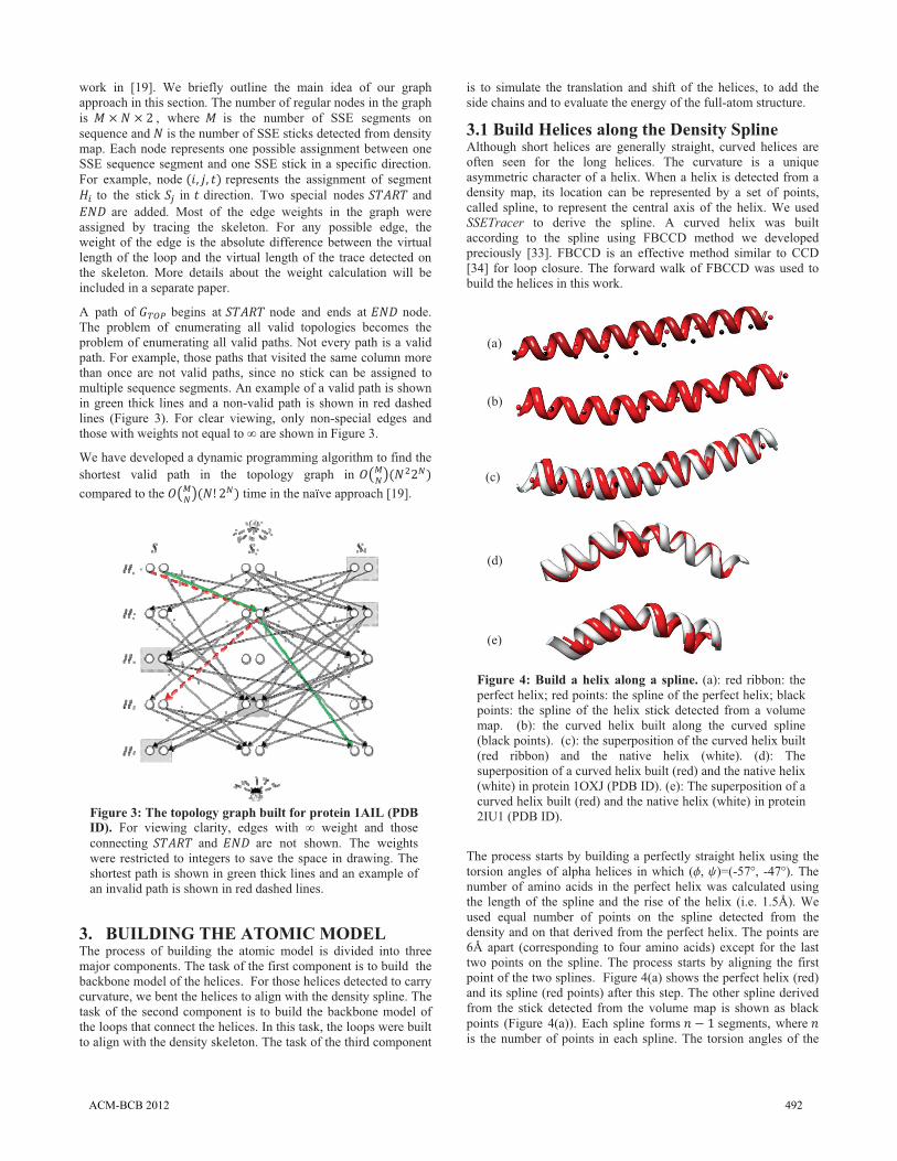
3.1 Build Helices along the Density Spline Although short helices are generally straight, curved helices are often seen for the long helices. The curvature is a unique asymmetric character of a helix. When a helix is detected from a density map, its location can be represented by a set of points, called spline, to represent the central axis of the helix. We used SSETracer to derive the spline. A curved helix was built according to the spline using FBCCD method we developed preciously [33]. FBCCD is an effective method similar to CCD [34] for loop closure. The forward walk of FBCCD was used to build the helices in this work.

The process starts by building a perfectly straight helix using the torsion angles of alpha helices in which (�, �)=(-57�, -47�). The number of amino acids in the perfect helix was calculated using the length of the spline and the rise of the helix (i.e. 1.5Å). We used equal number of points on the spline detected from the density and on that derived from the perfect helix. The points are 6Å apart (corresponding to four amino acids) except for the last two points on the spline. The process starts by aligning the first point of the two splines. Figure 4(a) shows the perfect helix (red) and its spline (red points) after this step. The other spline derived from the stick detected from the volume map is shown as black points (Figure 4(a)). Each spline forms ) * � segments, where ) is the number of points in each spline. The torsion angles of the

Figure 4: Build a helix along a spline. (a): red ribbon: the perfect helix; red points: the spline of the perfect helix; black points: the spline of the helix stick detected from a volume map. (b): the curved helix built along the curved spline (black points). (c): the superposition of the curved helix built (red ribbon) and the native helix (white). (d): The superposition of a curved helix built (red) and the native helix (white) in protein 1OXJ (PDB ID). (e): The superposition of a curved helix built (red) and the native helix (white) in protein 2IU1 (PDB ID).

(a)

(b)

(c)

(d)

(e)

Figure 3: The topology graph built for protein 1AIL (PDB ID). For viewing clarity, edges with � weight and those connecting �#$%# and &�' are not shown. The weights were restricted to integers to save the space in drawing. The shortest path is shown in green thick lines and an example of an invalid path is shown in red dashed lines.

ACM-BCB 2012 492

four amino acids on each segment were modified using FBCCD in order to align the corresponding segments from the two splines. After the first pair of segments was aligned, FBCCD works on the next pair of segments from the two splines respectively. To preserve the structure of the helix, the update was accepted if the new torsion angles are within the predefined range of a helix (i.e. �+ [-80�, -40�] and �+[-60�, 10�]). The process terminates either when the maximum number of cycles is reached or when the cutoff distance of the target is reached. In our current implementation, the maximum number of cycles is 100 and the cutoff distance is 0.1Å. Figure 4(b) shows the two splines after all segments were aligned. Note that the red points are aligned with the black points fairly well. Figure 4(c) shows superposition of the constructed curved helix and the native helix.

The process of building bent helices improves the RMSD of the model. In a previous study [28] we used straight helices in the modeling process. Table 1 shows the accuracy and time taken to build a curved helix. The RMSD was calculated for the backbone atoms (N, CA, C, and O). As an example, the RMSD calculated using the curved helix built in protein 3ODS is 0.88Å whereas that for the straight helix is 1.72Å. Although the difference in RMSD is small, it is expected to impact the potential energy of the final model because all the side chain and backbone atoms are displaced if a perfect helix were built for a curved helix in the protein. We want to mention that building a curved helix using FBCCD is fast. It takes less than 40 milliseconds to build one helix of 51 amino acids (Table 1 row 5) using a regular laptop computer. On average, it takes about 37.4 milliseconds to build a curved helix on a Lenovo X300 laptop (at 1.2 GHz).

Table 1: The performance of bending helices.

No IDa Helixb AAc RMSD straight

d

RMSDbente timef

1 1OXJ 644-669 26 2.61 1.26 55 2 1BZ4 90-123 34 1.32 0.81 30 3 2IU1 365-384 20 1.73 1.36 31 4 3ODS 124-146 23 1.72 0.88 31 5 2OEV 646-696 51 2.98 1.97 39

average 30.8 2.07 1.26 37.4 a: The PDB ID of the protein. b: The amino acid index of the helix c: The number of amino acids in the helix. d: The backbone RMSD between the perfect straight helix

built and the native helix. e: The backbone RMSD between the curved helix built and the

native helix. f: The time (in milliseconds) needed to build the curved helix.

3.2 Loop Building Using the Skeleton Loop closure problem arises in nearly all loop prediction problems. Loop closure is a problem of generating a loop whose N and C terminal residues satisfy the constrained locations. It has been proved that the loop closure problem with six degrees of freedom has at most sixteen possible solutions, whereas the number of possible solutions is infinite for the problem with more than six degrees of freedom [35-38]. Although analytical solutions have been proposed [35, 39-41], optimization methods are often adopted [36, 40].

The density skeleton obtained from the volume map provides a rough estimate of the shape of a loop. The goal of our task is to

build a loop that fit the skeleton trace. This is similar to the sample-based motion planning in robotics. Many methods have been developed to address this problem [42-46]. The problem of filling the gap in incomplete structure model is addressed in [47]. In their work, Lotan et al. aimed to fill the gap using the density map of X-ray crystallography. The algorithm proposed consists of two stages. In the first stage, a number of initial conformations were randomly generated. The Cyclic Coordinate Descent (CCD) [34] method was then used to close the loop. Additional constraints from the density map were used to avoid the collision. In the second stage, the initial conformations were ranked by their fit to the density map.

Although the problem addressed by [47] shares the similar nature with our loop problem, it differs by the precision in the density map. The density map obtained using X-ray crystallography often has much higher resolution than the medium resolution map in our problem. Therefore, the method in [47] aims at finding the specific loop that satisfies the density constrains in fine precision. Since the skeleton of the medium resolution map only provides rough trace of the loop, we aim to quickly find one of the many loops that align with the skeleton. As mentioned in [47], it may take 30 minutes to build short loops (with ~4 amino acids) and 178 minutes for longer loops (with ~15 amino acids). We describe a segment-wise loop-building method that can produce approximate loops efficiently. A typical collision-free loop of ten amino acids takes approximately three minutes to build.

The idea of building the loop is similar to that of building a curved helix in terms of partitioning the trace into segments. The main difference is that the length of the helix trace is the same as that for the perfect helix built initially, but the length of the skeleton trace may not be the same as that of the loop to be built. The entire initial helix was built at the beginning and then FBCCD was used to update the structure. The process starts by dividing the sequence of the loop into segments of four amino acids. Thus, the virtual length of each segment is about 15Å. In order to divide the skeleton trace into same number of segments, the length of the segments was chosen as (LengthTrace/nLoopSegments)Å, where LengthTrace is the length of the skeleton trace and nLoopSegments is the number of segments in the loop sequence. We used the length of four amino acids for the segment of loop sequence for the ease of building. If the

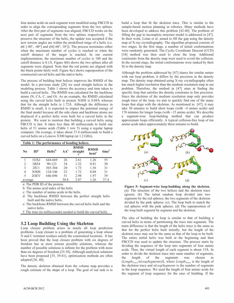
Figure 5: Segment-wise loop-building along the skeleton. (a): The structure of the two helices and the skeleton trace (green). (b) The initial random loop divided into two segments by the red spheres; the two segments of the skeleton divided by the pink spheres. (c): The loop built to match the red spheres with the pink spheres. (d) The superposition of the loop built segment by segment and the skeleton.

(a) (b)

(c) (d)

ACM-BCB 2012 493

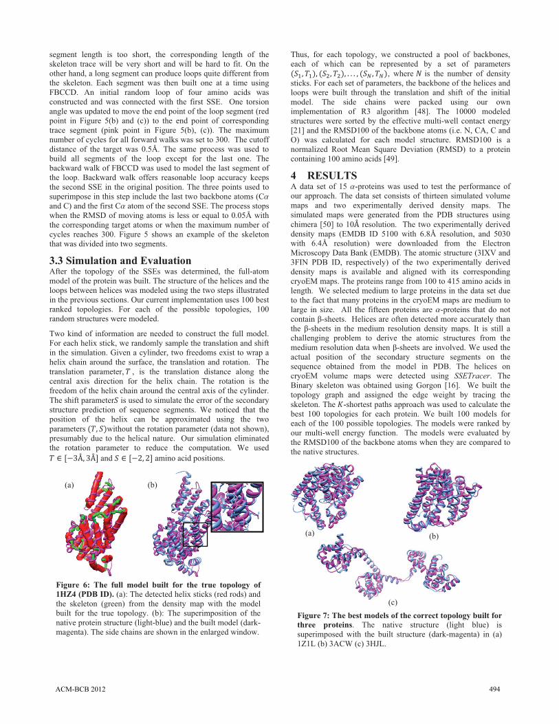
segment length is too short, the corresponding length of the skeleton trace will be very short and will be hard to fit. On the other hand, a long segment can produce loops quite different from the skeleton. Each segment was then built one at a time using FBCCD. An initial random loop of four amino acids was constructed and was connected with the first SSE. One torsion angle was updated to move the end point of the loop segment (red point in Figure 5(b) and (c)) to the end point of corresponding trace segment (pink point in Figure 5(b), (c)). The maximum number of cycles for all forward walks was set to 300. The cutoff distance of the target was 0.5Å. The same process was used to build all segments of the loop except for the last one. The backward walk of FBCCD was used to model the last segment of the loop. Backward walk offers reasonable loop accuracy keeps the second SSE in the original position. The three points used to superimpose in this step include the last two backbone atoms (C� and C) and the first C� atom of the second SSE. The process stops when the RMSD of moving atoms is less or equal to 0.05Å with the corresponding target atoms or when the maximum number of cycles reaches 300. Figure 5 shows an example of the skeleton that was divided into two segments.

3.3 Simulation and Evaluation After the topology of the SSEs was determined, the full-atom model of the protein was built. The structure of the helices and the loops between helices was modeled using the two steps illustrated in the previous sections. Our current implementation uses 100 best ranked topologies. For each of the possible topologies, 100 random structures were modeled.

Two kind of information are needed to construct the full model. For each helix stick, we randomly sample the translation and shift in the simulation. Given a cylinder, two freedoms exist to wrap a helix chain around the surface, the translation and rotation. The translation parameter, # , is the translation distance along the central axis direction for the helix chain. The rotation is the freedom of the helix chain around the central axis of the cylinder. The shift parameter� is used to simulate the error of the secondary structure prediction of sequence segments. We noticed that the position of the helix can be approximated using the two parameters #� ��without the rotation parameter (data not shown), presumably due to the helical nature. Our simulation eliminated the rotation parameter to reduce the computation. We used # + ,*-.� -./ and � + ,*�� �/ amino acid positions.

Thus, for each topology, we constructed a pool of backbones, each of which can be represented by a set of parameters ��� #��� ��� #��� 0 0 0 � ��� #��, where � is the number of density sticks. For each set of parameters, the backbone of the helices and loops were built through the translation and shift of the initial model. The side chains were packed using our own implementation of R3 algorithm [48]. The 10000 modeled structures were sorted by the effective multi-well contact energy [21] and the RMSD100 of the backbone atoms (i.e. N, CA, C and O) was calculated for each model structure. RMSD100 is a normalized Root Mean Square Deviation (RMSD) to a protein containing 100 amino acids [49].

4 RESULTS A data set of 15 �-proteins was used to test the performance of our approach. The data set consists of thirteen simulated volume maps and two experimentally derived density maps. The simulated maps were generated from the PDB structures using chimera [50] to 10. resolution. The two experimentally derived density maps (EMDB ID 5100 with 6.8Å resolution, and 5030 with 6.4Å resolution) were downloaded from the Electron Microscopy Data Bank (EMDB). The atomic structure (3IXV and 3FIN PDB ID, respectively) of the two experimentally derived density maps is available and aligned with its corresponding cryoEM maps. The proteins range from 100 to 415 amino acids in length. We selected medium to large proteins in the data set due to the fact that many proteins in the cryoEM maps are medium to large in size. All the fifteen proteins are �-proteins that do not contain �-sheets. Helices are often detected more accurately than the �-sheets in the medium resolution density maps. It is still a challenging problem to derive the atomic structures from the medium resolution data when �-sheets are involved. We used the actual position of the secondary structure segments on the sequence obtained from the model in PDB. The helices on cryoEM volume maps were detected using SSETracer. The Binary skeleton was obtained using Gorgon [16]. We built the topology graph and assigned the edge weight by tracing the skeleton. The 1-shortest paths approach was used to calculate the best 100 topologies for each protein. We built 100 models for each of the 100 possible topologies. The models were ranked by our multi-well energy function. The models were evaluated by the RMSD100 of the backbone atoms when they are compared to the native structures.

Figure 7: The best models of the correct topology built for three proteins. The native structure (light blue) is superimposed with the built structure (dark-magenta) in (a) 1Z1L (b) 3ACW (c) 3HJL.

(a) (b)

(c) Figure 6: The full model built for the true topology of 1HZ4 (PDB ID). (a): The detected helix sticks (red rods) and the skeleton (green) from the density map with the model built for the true topology. (b): The superimposition of the native protein structure (light-blue) and the built model (dark-magenta). The side chains are shown in the enlarged window.

(a) (b)

ACM-BCB 2012 494

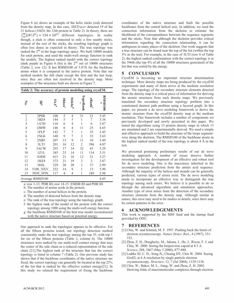
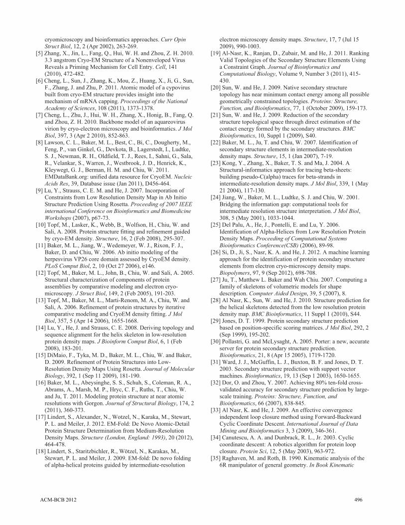
Figure 6 (a) shows an example of the helix sticks (red) detected from the density map. In this case, SSETracer detected 19 of the 21 helices (1HZ4, the 12th protein in Table 2). In theory, there are "� ���� ��� 2 �-3 � �4�5 different topologies. In reality though, a stick is often connected to only a few nearby sticks, instead of the rest of the sticks, the resulting topology graph is often less dense as expected in theory. The true topology was ranked the 2nd in the huge topology space. We built 10000 models for each protein, and used the multi-well energy function to rank the models. The highest ranked model with the correct topology (dark purple in Figure 6 (b)) is the 2nd out of 10000 structures (Table 2, row 12). It has RMSD100 of 3.87Šfor the backbone atoms when it is compared to the native protein. Note that our method models the full chain except the first and the last loop, since they are often not resolved in the density map. More examples of the structures built are shown in Figure 7.

Table 2: The accuracy of protein modeling using cryoEM.

No.

IDa

#AA

b

#hlces c

#sticks d

TopoR

anke

eRank

f

RM

SD100

g

1 2PSR 100 5 4 31 21 5.452 1BZ4 144 5 5 1 7 3.34 3 1A7D 118 6 4 1 6 3.87 4 1JMW 146 6 4 11 25 4.65 5 1FLP 142 7 7 1 35 3.45 6 1NG6 148 9 7 2 33 3.63 7 2XB5 207 13 9 11 10 3.49 8 3LTJ 201 16 12 2 396 4.07 9 3ACW 293 17 14 32 43 3.29

10 1Z1L 345 23 14 11 114 3.51 11 3ODS 415 21 16 12 31 3.27 12 1HZ4 373 21 19 2 2 3.87 13 3HJL 329 20 20 1 37 2.99 14 5100_3IXV_ 222 14 9 1 13 5.90 15 5030_3FIN_ 117 4 4 1 189 5.98

Average RMSD100 4.05 a: row 1-13: PDB ID;.row 14-15: EMDB ID and PDB ID.b: The number of amino acids in the protein. c: The number of actual helices in the protein. d: The number of detected helices from the density map. e: The rank of the true topology using the topology graph. f: the highest rank of the model of the protein with the correct

topology among 1000 using the multi-well energy function. g: the backbone RMSD100 of the best true model reconstructed

with the native structure based on potential energy.

Our approach to rank the topologies appears to be effective. For all the fifteen proteins tested, our topology detection method consistently ranks the true topology among the top 35, with top 1 for six of the fifteen proteins (Table 2, column 6). The 10000 structures were ranked by our multi-well contact energy that uses the center of the side chain as a reduced representation of the side chain [21].The highest rank of the structure that has the correct topology is listed in column 7 (Table 2). Our previous study has shown that if the backbone coordinates of the native structure are fixed, the correct topology can generally be located at the top 25% of the list that is ranked by the effective contact energy[21]. In this study we relaxed the requirement of fixing the backbone

coordinates of the native structure and built the possible backbones from the central helical axis. In addition, we used the connection information from the skeleton to estimate the likelihood of the correspondence between the sequence segments and the sticks. Note that although the skeleton provides critical information regarding the connection relationship, it can be ambiguous in many places of the skeleton. Our work suggests that a true structure can be found near the top of the list (within the top 5% in the test). For example, in the case of 3LTJ (row 8 of Table 2), the highest ranked conformation with the correct topology is at the 396th (the top 4% of all the 10000 structures generated) of the list that was sorted by the energy.

5 CONCLUSION CryoEM is becoming an important structure determination technique. More density maps are being produced by the cryoEM experiments and many of them arrive at the medium resolution range. The topology of the secondary structure elements detected from the density map is a critical piece of information for deriving the atomic structures from such density maps. We previously translated the secondary structure topology problem into a constrained shortest path problem using a layered graph. In this paper, we present a de novo modeling framework to derive the atomic structure from the cryoEM density map at the medium resolution. This framework includes a number of components we previously developed and newly presented in this paper. We tested the algorithms using 15 protein density maps in which 13 are simulated and 2 are experimentally derived. We used a simple and effective approach to build the structure of the loops segment-wise along the skeleton. The RMSD100 of the backbone atoms in the highest ranked model of the true topology is about 4 Å in the test.

We presented promising preliminary results of our de novo modeling approach. A number of issues deserve further investigation for the development of an effective and robust tool for de novo modeling. One is the inaccuracy inherited in the secondary structure prediction from the amino acid sequence. Although the majority of the helices and strands can be generally predicted, various types of errors exist. The de novo modeling needs to incorporate an effective way to distinguish the true topology among such errors. We believe it is possible to do so through the advanced algorithms and simulation approaches. Another type of error arises from the detection of the secondary structure elements from the density map. Although similar in nature, this error may need to be studies in details, since there may be certain patterns in the error.

6 ACKNOWLEDGEMENTS This work is supported by the MSF fund and the startup fund provided by ODU.

7 REFERENCES [1] Chiu, W. and Schmid, M. F. 1997. Pushing back the limits of

electron cryomicroscopy. Nature Struct. Biol., 4 (1997), 331-333.

[2] Zhou, Z. H., Dougherty, M., Jakana, J., He, J., Rixon, F. J. and Chiu, W. 2000. Seeing the herpesvirus capsid at 8.5 A. Science, 288, 5467 (May 5 2000), 877-880.

[3] Ludtke SJ, C. D., Song JL, Chuang DT, Chiu W. 2004. Seeing GroEL at 6 A resolution by single particle electron cryomicroscopy. Structure, 12, 7 (Jul 2004), 1129-1136.

[4] Chiu, W., Baker, M. L., Jiang, W. and Zhou, Z. H. 2002. Deriving folds of macromolecular complexes through electron

ACM-BCB 2012 495

cryomicroscopy and bioinformatics approaches. Curr Opin Struct Biol, 12, 2 (Apr 2002), 263-269.

[5] Zhang, X., Jin, L., Fang, Q., Hui, W. H. and Zhou, Z. H. 2010. 3.3 angstrom Cryo-EM Structure of a Nonenveloped Virus Reveals a Priming Mechanism for Cell Entry. Cell, 141 (2010), 472-482.

[6] Cheng, L., Sun, J., Zhang, K., Mou, Z., Huang, X., Ji, G., Sun, F., Zhang, J. and Zhu, P. 2011. Atomic model of a cypovirus built from cryo-EM structure provides insight into the mechanism of mRNA capping. Proceedings of the National Academy of Sciences, 108 (2011), 1373-1378.

[7] Cheng, L., Zhu, J., Hui, W. H., Zhang, X., Honig, B., Fang, Q. and Zhou, Z. H. 2010. Backbone model of an aquareovirus virion by cryo-electron microscopy and bioinformatics. J Mol Biol, 397, 3 (Apr 2 2010), 852-863.

[8] Lawson, C. L., Baker, M. L., Best, C., Bi, C., Dougherty, M., Feng, P., van Ginkel, G., Devkota, B., Lagerstedt, I., Ludtke, S. J., Newman, R. H., Oldfield, T. J., Rees, I., Sahni, G., Sala, R., Velankar, S., Warren, J., Westbrook, J. D., Henrick, K., Kleywegt, G. J., Berman, H. M. and Chiu, W. 2011. EMDataBank.org: unified data resource for CryoEM. Nucleic Acids Res, 39, Database issue (Jan 2011), D456-464.

[9] Lu, Y., Strauss, C. E. M. and He, J. 2007. Incorporation of Constraints from Low Resolution Density Map in Ab Initio Structure Prediction Using Rosetta. Proceeding of 2007 IEEE international Conference on Bioinformatics and Biomedicine Workshops (2007), p67-73.

[10] Topf, M., Lasker, K., Webb, B., Wolfson, H., Chiu, W. and Sali, A. 2008. Protein structure fitting and refinement guided by cryo-EM density. Structure, 16, 2 (Feb 2008), 295-307.

[11] Baker, M. L., Jiang, W., Wedemeyer, W. J., Rixon, F. J., Baker, D. and Chiu, W. 2006. Ab initio modeling of the herpesvirus VP26 core domain assessed by CryoEM density. PLoS Comput Biol, 2, 10 (Oct 27 2006), e146.

[12] Topf, M., Baker, M. L., John, B., Chiu, W. and Sali, A. 2005. Structural characterization of components of protein assemblies by comparative modeling and electron cryo-microscopy. J Struct Biol, 149, 2 (Feb 2005), 191-203.

[13] Topf, M., Baker, M. L., Marti-Renom, M. A., Chiu, W. and Sali, A. 2006. Refinement of protein structures by iterative comparative modeling and CryoEM density fitting. J Mol Biol, 357, 5 (Apr 14 2006), 1655-1668.

[14] Lu, Y., He, J. and Strauss, C. E. 2008. Deriving topology and sequence alignment for the helix skeleton in low-resolution protein density maps. J Bioinform Comput Biol, 6, 1 (Feb 2008), 183-201.

[15] DiMaio, F., Tyka, M. D., Baker, M. L., Chiu, W. and Baker, D. 2009. Refinement of Protein Structures into Low-Resolution Density Maps Using Rosetta. Journal of Molecular Biology, 392, 1 (Sep 11 2009), 181-190.

[16] Baker, M. L., Abeysinghe, S. S., Schuh, S., Coleman, R. A., Abrams, A., Marsh, M. P., Hryc, C. F., Ruths, T., Chiu, W. and Ju, T. 2011. Modeling protein structure at near atomic resolutions with Gorgon. Journal of Structural Biology, 174, 2 (2011), 360-373.

[17] Lindert, S., Alexander, N., Wotzel, N., Karaka, M., Stewart, P. L. and Meiler, J. 2012. EM-Fold: De Novo Atomic-Detail Protein Structure Determination from Medium-Resolution Density Maps. Structure (London, England: 1993), 20 (2012), 464-478.

[18] Lindert, S., Staritzbichler, R., Wötzel, N., Karakas, M., Stewart, P. L. and Meiler, J. 2009. EM-fold: De novo folding of alpha-helical proteins guided by intermediate-resolution

electron microscopy density maps. Structure, 17, 7 (Jul 15 2009), 990-1003.

[19] Al-Nasr, K., Ranjan, D., Zubair, M. and He, J. 2011. Ranking Valid Topologies of the Secondary Structure Elements Using a Constraint Graph. Journal of Bioinformatics and Computational Biology, Volume 9, Number 3 (2011), 415-430.

[20] Sun, W. and He, J. 2009. Native secondary structure topology has near minimum contact energy among all possible geometrically constrained topologies. Proteins: Structure, Function, and Bioinformatics, 77, 1 (October 2009), 159-173.

[21] Sun, W. and He, J. 2009. Reduction of the secondary structure topological space through direct estimation of the contact energy formed by the secondary structures. BMC Bioinformatics, 10, Suppl 1 (2009), S40.

[22] Baker, M. L., Ju, T. and Chiu, W. 2007. Identification of secondary structure elements in intermediate-resolution density maps. Structure, 15, 1 (Jan 2007), 7-19.

[23] Kong, Y., Zhang, X., Baker, T. S. and Ma, J. 2004. A Structural-informatics approach for tracing beta-sheets: building pseudo-C(alpha) traces for beta-strands in intermediate-resolution density maps. J Mol Biol, 339, 1 (May 21 2004), 117-130.

[24] Jiang, W., Baker, M. L., Ludtke, S. J. and Chiu, W. 2001. Bridging the information gap: computational tools for intermediate resolution structure interpretation. J Mol Biol, 308, 5 (May 2001), 1033-1044.

[25] Del Palu, A., He, J., Pontelli, E. and Lu, Y. 2006. Identification of Alpha-Helices from Low Resolution Protein Density Maps. Proceeding of Computational Systems Bioinformatics Conference(CSB) (2006), 89-98.

[26] Si, D., Ji, S., Nasr, K. A. and He, J. 2012. A machine learning approach for the identification of protein secondary structure elements from electron cryo-microscopy density maps. Biopolymers, 97, 9 (Sep 2012), 698-708.

[27] Ju, T., Matthew L. Baker and Wah Chiu. 2007. Computing a family of skeletons of volumetric models for shape description. Computer Aided Design, 39, 5 (2007), 8.

[28] Al Nasr, K., Sun, W. and He, J. 2010. Structure prediction for the helical skeletons detected from the low resolution protein density map. BMC Bioinformatics, 11 Suppl 1 (2010), S44.

[29] Jones, D. T. 1999. Protein secondary structure prediction based on position-specific scoring matrices. J Mol Biol, 292, 2 (Sep 1999), 195-202.

[30] Pollastri, G. and McLysaght, A. 2005. Porter: a new, accurate server for protein secondary structure prediction. Bioinformatics, 21, 8 (Apr 15 2005), 1719-1720.

[31] Ward, J. J., McGuffin, L. J., Buxton, B. F. and Jones, D. T. 2003. Secondary structure prediction with support vector machines. Bioinformatics, 19, 13 (Sep 1 2003), 1650-1655.

[32] Dor, O. and Zhou, Y. 2007. Achieving 80% ten-fold cross-validated accuracy for secondary structure prediction by large-scale training. Proteins: Structure, Function, and Bioinformatics, 66 (2007), 838-845.

[33] Al Nasr, K. and He, J. 2009. An effective convergence independent loop closure method using Forward-Backward Cyclic Coordinate Descent. International Journal of Data Mining and Bioinformatics 3, 3 (2009), 346-361.

[34] Canutescu, A. A. and Dunbrack, R. L., Jr. 2003. Cyclic coordinate descent: A robotics algorithm for protein loop closure. Protein Sci, 12, 5 (May 2003), 963-972.

[35] Raghaven, M. and Roth, B. 1990. Kinematic analysis of the 6R manipulator of general geometry. In Book Kinematic

ACM-BCB 2012 496

analysis of the 6R manipulator of general geometry 1990), 263-269.

[36] Go, N. and Scheraga, H. A. 1970. Ring closure and local conformational deformations of chain molecules. Macromolecules, 3 (1970), 178-186.

[37] Kolodny, R., Guibas, L., Levitt, M. and Koehl, P. 2005. Inverse kinematics in biology:The protein loop closure problem. International Journal of Robotics Research, 24, 23 (2005), 151.

[38] Manocha, D. and Canny, J. 1994. Efficient inverse kinematics for general 6R manipulator. IEEE Trans. Robot. Autom, 10, 5 (1994), 648-657.

[39] Wedemeyer, W. J. and Scheraga, H. A. 1999. Exact analytical loop closure in proteins using polynomial equations. J. Comput. Chem., 201999), 819-844.

[40] Coutsias, E. A., Seok, C., Jacobson, M. P. and Dill, K. A. 2004. A kinematic view of loop closure. J. Comput. Chem., 25 (2004), 510-528.

[41] Mandell, D. J., Coutsias, E. A. and Kortemme, T. 2009. Sub-angstrom accuracy in protein loop reconstruction by robotics-inspired conformational sampling. Nat Meth, 6 (2009), 551-552.

[42] Kavraki, L. E., Svestka, P., Latombe, J. C. and Overmars, M. H. 1996. Probabilistic roadmaps for path planning in high-dimensional configuration spaces. Robotics and Automation, IEEE Transactions on 1996, 12 (1996), 566-580.

[43] Dawen, X. and Amato, N. M. 2004. A kinematics-based probabilistic roadmap method for high DOF closed chain systems. In Robotics and Automation, 2004 Proceedings ICRA '04 2004 IEEE International Conference on; (16 April - 1 May 2004), 473-478.

[44] Cortés, J., Siméon, T. and Laumond, J. P. 2002. A random loop generator for planning the motions of closed kinematic chains using PRM methods. In Robotics and Automation, 2002 Proceedings ICRA '02 IEEE International Conference on;(2002), 2141-2146.

[45] Cortés, J., Siméon, T., Remaud-Simeon, M. and Tran, V. 2004. Geometric algorithms for the conformational analysis of long protein loops. Journal of Computational Chemistry, 25 (2004), 956-967.

[46] Yakey, J. H., LaValle, S. M. and Kavraki, L. E. 2001. Randomized path planning for linkages with closed kinematic chains. Robotics and Automatin, IEEE Transactions on 2001, 17 (2001), 951-958.

[47] Lotan, I., van den Bedem, H., Deacon, A. M. and Latombe, J. C. 2005. Computing Protein Structures form Electron Density Maps: The Missing Fragment Problem Algorithmic Foundations of Robotics VI. Springer Tracts in Advanced Robotics, 17 (2005), 345-360.

[48] Xie, W. and Sahinidis, N. V. 2006. Residue-rotamer-reduction algorithm for the protein side-chain conformation problem,. Bioinformatics, 22, 2 (2006), p188-194.

[49] Carugo, O. and Pongor, S. 2001. A normalized root-mean-square distance for comparing protein three-dimensional structure. Protein Science, 10 (2001), 1470-1473.

[50] Pettersen, E., Goddard, T., Huang, C., Couch, G., Greenblatt, D., Meng, E. and Ferrin, T. 2004. UCSF Chimera--a visualization system for exploratory research and analysis. J Comput Chem., 25, 13 (2004), 1605-1612.

ACM-BCB 2012 497